Non-White Noise in fMRI:Does modelling have an impact?

Torben E. Lund, !,a Kristoffer H. Madsen a,b Karam Sidaros a

Wen-Lin Luo c Thomas E. Nichols d

aDanish Research Centre for Magnetic Resonance, Copenhagen UniversityHospital, Hvidovre, Denmark

bInformatics and Mathematical Modelling, Technical University of Denmark,Lyngby, Denmark

cMerck & Co., Inc., Whitehouse Station, New Jersey, USAdDepartment of Biostatistics, University of Michigan, Ann Arbor, Michigan, USA

Abstract

The sources of non-white noise in Blood Oxygenation Level Dependent (BOLD)functional magnetic resonance imaging (fMRI) are many. Familiar sources includelow-frequency drift due to hardware imperfections, oscillatory noise due to respira-tion and cardiac pulsation, and residual movement artefacts not accounted for byrigid body registration. These contributions give rise to temporal autocorrelation inthe residuals of the fMRI signal and invalidate the statistical analysis as the errorsare no longer independent. The low-frequency drift is often removed by high-passfiltering, and other effects are typically modelled as an autoregressive (AR) process.In this paper we propose an alternative approach: Nuisance Variable Regression(NVR). By inclusion of confounding effects in a general linear model (GLM), wefirst confirm that the spatial distribution of the various fMRI noise sources is sim-ilar to what has already been described in the literature. Subsequently we demon-strate, using diagnostic statistics, that removal of these contributions reduces firstand higher order autocorrelation as well as non-normality in the residuals, therebyimproving the validity of the drawn inferences. In addition we also compare theperformance of the NVR method to the whitening approach implemented in SPM2.

Key words: Physiological noise, temporal autocorrelation, low-frequency drift.

Preprint submitted to Elsevier Science 1 July 2005

* Manuscript

Introduction

Non-white noise in fMRI has been a known issue ever since the earliest days offMRI. Weisskoff et al. (1993) presented power-spectra from different regions ofinterest acquired using fast (7Hz) imaging of a single slice in visual cortex. Thespectra showed white noise in white matter (WM), cardiac, respiratory andlow-frequency noise in grey matter (GM) and cardiac noise in cerebrospinalfluid (CSF). Since a convenient assumption when making statistical inferenceis to assume that errors in the measurement are independent and identicallynormally distributed (i.i.d.) this observation is important and has had largeimpact on paradigm design and data analyses.

With non-white noise, the i.i.d. assumption is no longer fulfilled, and if thisis ignored the estimated standard deviations will typically be negatively bi-ased, resulting in invalid (liberal) statistical inferences. Another consequenceis the difficulty in detecting signals when covered in noise. As we are normallyinterested in the GM signal it is problematic that this is the region wherestructured noise is most pronounced. With physiological noise increasing withfield strength (Kruger & Glover, 2001; Kruger et al., 2001), the full benefit insignal to noise ratio (SNR) by using high field scanners cannot be achievedwithout proper handling of physiological noise.

While it has been argued that the low-frequency oscillations or drifts arephysiological in nature they have also been observed in cadavers (Smith etal., 1999) and phantoms (Lund & Larsson, 1999). Noise contributions withthese frequencies can be avoided by a combination of a high-pass filter and astimulation paradigm fast enough to “escape” the region of the spectra wherelow-frequency noise is dominant. The system noise makes it difficult to studystates of neural activity with BOLD fMRI, if the state remains unchangedfor more than a minute. Being a differential, measurement arterial spinla-belling (ASL) experiments are less prone to these drift problems, and thuslow paradigm frequency can be used in ASL (Wang et al., 2003).

In typical whole brain acquisitions the physiological noise components are

! To whom correspondence should be addressed:Torben E. LundDanish Research Centre for Magnetic Resonance, Copenhagen University Hospital,HvidovreKettegaard Alle 30, 2650 Hvidovre, DenmarkPhone: +45 3632 3328Fax: +45 3647 0302

Email address: torbenl@magnet.drcmr.dk.URL: http://www.drcmr.dk.

2

heavily aliased and possibly non-stationary making it difficult to identify di-rectly. This is perhaps the reason why no commonly accepted model of noisein fMRI exists. Recent versions of most fMRI analysis software try to estimatethe covariance due to these effects (e.g. using an autoregressive model), anduse the estimated process to pre-whiten the errors. If the estimated covari-ance structure is correct this procedure is unbiased and efficient. However,the modelling is time consuming and often global and/or low-order modelsneed to be used in order to get a robust estimate. From the power spectraby Weisskoff et al. (1993) it is known that the noise in part consists of os-cillations at respiratory and cardiac frequencies and their higher harmonics.It is also known (Dagli et al., 1999) that the non-white noise is structuredin space. Nevertheless a first order process stationary in time and often inspace as well, is often assumed when the coefficients of the model are to beestimated (e.g. SPM2 (Friston et al., 2002)). As it takes two AR coefficientsto model a single oscillator the approach will, at best, only be valid when thenoise is heavily aliased and smeared due to long repetition times (TR) andnon-stationary heart and respiratory rates. Using a variational Bayesian ap-proach for AR model-order estimation, Penny et al. (2003) have demonstratedthat higher order processes are necessary to describe the auto-correlation inregions close to the vasculature e.g. medial cerebral artery (MCA), and cir-cle of Willis (CW). However, with current high-end computing power, thisestimation takes about 30 minutes per slice.

As an alternative to estimating the correlation in the errors, a number oftechniques have been suggested which try to predict the effect of various noisesources on the measured signal. While these methods were primarily intro-duced for noise reduction purposes, they could potentially serve as whiteningfilters too and substitute autoregressive modelling which is both difficult andtime consuming.

The first methods (Hu et al., 1995; Biswal et al., 1996) for removing cardiacand respiratory noise both used pulse-oximeter time-courses. The method byBiswal et al. (1996) uses the pulse-oximeter time-course to construct a band-stop filter, which is only appropriate when the noise is critically sampled orvery stationary. The method by Hu et al. (1995) conversely uses retrospec-tive gating of raw k-space data, and also works for long TR, and multi-shotsequences, as long as the noise is quasi-periodic. A drawback of this methodis that it performs best for data points with high SNR which would typicallymean mainly points in central k-space. Central k-space is where global effectslike movement (e.g. due to respiration) manifest themselves. Effects of pulsat-ing blood, on the other hand, are localised in real space to areas near vessels,and hence spread out over the entire k-space. This is perhaps the reason whyHu et al. (1995) find effects of respiration to be more dominant than effectsof cardiac pulsation. On the other hand, the method by Hu et al. (1995) wasused by Dagli et al. (1999) to show that cardiac noise is dominant near major

3

arteries e.g. MCA and CW. Josephs et al. (1997) and Glover et al. (2000)suggested performing retrospective correction in the reconstructed images ina way similar to that proposed by Hu et al. (1995). The two implementationsdiffer slightly. Josephs et al. (1997) implemented the correction as a part of thedesign matrix in a GLM whereas Glover et al. (2000) performed the correc-tion during the preprocessing. Both methods assume that physiological noiseis fixed during acquisition of a single slice. While this is a good approximationfor single-shot 2D echo planar imaging (EPI) it is not the case for multi-shotacquisitions in general 1 .

Using the property that respiration-induced noise is a global effect Frank etal. (2001) proposed estimating and correcting this effect from the k-space dataitself. As global effects (centre of k-space) are actually sampled for each slicein an EPI volume, the sampling rate for global effects equals the numberof slices per volume divided by TR instead of 1/TR, thereby making globalnoise-effects critically sampled. A similar approach is to use time-courses fromregions of no interest to regress out behaviour similar to that of major vesselsor CSF time-courses (Petersen et al., 1998; Lund & Hanson, 2001). This canbe achieved by identifying voxels located in CSF and vessels by inspecting avariance image of the fMRI time-course (Lund & Hanson, 2001). Buonocore& Maddock (1997) used time-courses from “truly inactive” and “truly active”voxels to construct a Wiener-filter and demonstrated how this approach is su-perior to notch filtering. This filter is, however, still stationary and will not beoptimal in the presence of variations in the heart and respiratory rates. Inde-pendent component analysis (ICA) has great potential for identifying patternsof structured noise in fMRI data. However, so far it has only been evaluated forTR’s short enough to critically sample the cardiac noise (Thomas et al., 2002)in which case, a simple low-pass filter is adequate for removing physiologicalnoise.

The purpose of this paper is to suggest a unified theory for physiological noisein fMRI. We will show how relevant nuisance regressors in a general linearmodel can be used to describe spatiotemporal behaviour of low-frequency,residual movement, respiratory and cardiac related effects. Using StatisticalParametric Mapping Diagnosis (SPMd) (Luo & Nichols, 2003) we hereafterdemonstrate the impact of physiological noise correction on the i.i.d. assump-tion and compare the performance of the suggested method to the whiteningapproach implemented in SPM2. Finally the findings of this paper are dis-cussed in relation to assumptions made during common fMRI preprocessingand analysis including slice-timing and functional connectivity analysis.

1 Glover et al. (2000) stated that the method is effective up to 3-shot spiral acqui-sitions.

4

Materials and methods

General Linear Models for non-white noise in fMRI images

In this section we describe how the effect of different of non-white noise sourcesin fMRI can be described in the GLM framework where the significance of eachnoise source can be tested using an F-test.

Low-frequency drift due to hardware instabilities

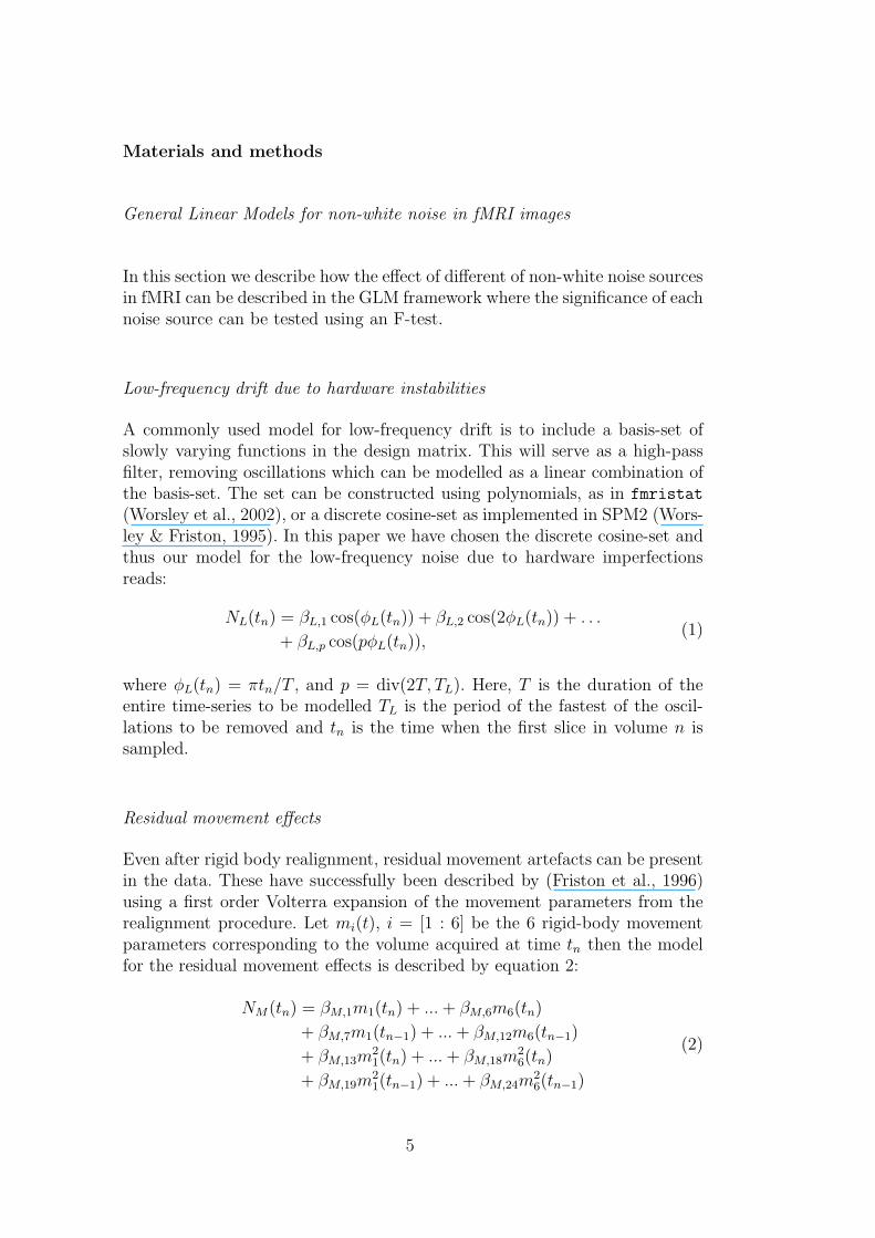
A commonly used model for low-frequency drift is to include a basis-set ofslowly varying functions in the design matrix. This will serve as a high-passfilter, removing oscillations which can be modelled as a linear combination ofthe basis-set. The set can be constructed using polynomials, as in fmristat(Worsley et al., 2002), or a discrete cosine-set as implemented in SPM2 (Wors-ley & Friston, 1995). In this paper we have chosen the discrete cosine-set andthus our model for the low-frequency noise due to hardware imperfectionsreads:

NL(tn) = βL,1 cos(φL(tn)) + βL,2 cos(2φL(tn)) + . . .

+ βL,p cos(pφL(tn)),(1)

where φL(tn) = πtn/T , and p = div(2T, TL). Here, T is the duration of theentire time-series to be modelled TL is the period of the fastest of the oscil-lations to be removed and tn is the time when the first slice in volume n issampled.

Residual movement effects

Even after rigid body realignment, residual movement artefacts can be presentin the data. These have successfully been described by (Friston et al., 1996)using a first order Volterra expansion of the movement parameters from therealignment procedure. Let mi(t), i = [1 : 6] be the 6 rigid-body movementparameters corresponding to the volume acquired at time tn then the modelfor the residual movement effects is described by equation 2:

NM(tn) = βM,1m1(tn) + ... + βM,6m6(tn)

+ βM,7m1(tn−1) + ... + βM,12m6(tn−1)

+ βM,13m21(tn) + ... + βM,18m

26(tn)

+ βM,19m21(tn−1) + ... + βM,24m

26(tn−1)

(2)

5

Modelling aliased physiological noise

From basic signal processing it is known that the modulus of the Fouriertransform of a real signal, S, sampled at the frequency, fs, is symmetric around0 and repeated with a period of fs. A signal containing frequencies larger thanthe Nyquist frequency fn = fs/2, is not critically sampled and will, therefore,be aliased i.e. folded into the frequency range [−fn, fn[. Contrary to what issometimes stated e.g. (Frackowiak et al., 2004, p795-796) or (Thomas et al.,2002; Li et al., 2000) there is in general no single frequency band into whichthe aliasing happens. If f = kfs/2+ν is the frequency of a signal, and k is thelargest integer to make 0 ≤ ν < fs/2 the aliased frequency, fa, will be givenby equation 3 (see e.g.(Franckowiak et al., 1997, p. 475 Fig.2)):

fa =

ν for k even

fs/2 − ν for k odd(3)

In the case of multislice fMRI a typical sampling frequency fs = 1/TR isaround 0.5Hz, and with fundamental frequencies of the cardiac noise fc in theinterval [0.6Hz, 1.5Hz] this gives 2 ≤ k ≤ 6 i.e. the cardiac noise is from 2 to6 times under-sampled. Correspondingly this interval of cardiac frequencies isfour times as large as the sampled bandwidth!

By using external measures of respiration and cardiac pulsation, e.g. respira-tory belt and pulse-oximeter, it is possible to assign a cardiac and respiratoryphase to each volume and thereby identify physiological noise even when itis aliased. One way of performing this retrospective image correction is theRETROICOR method described by Glover et al. (2000). The RETROICORmethod models the physiological noise as a basis set of sines and cosines rep-resenting the aliased frequencies of the cardiac and respiratory oscillationsand their higher harmonics. The method accounts for non-stationarity in thecardiac and respiratory time-series by letting the phase of the reference time-course be the phase of a quasiperiodic oscillation.

The respiratory noise has at least three different components, and two fun-damentally different phases are of potential interest in relation to modellingits effect. Part of the respiration-induced noise will manifest itself as rigidbody motion of the head, which, in part, is likely to also be reflected in themovement parameters. Ideally, by modelling respiratory effects, within volumemovements could also be accounted for. For TR values short enough to samplethe respiration critically alignment is expected to account for this. Other res-piratory effects include susceptibility changes in the brain due to movementof organs in the abdomen (Raj et al., 2000, 2001) and respiration-dependentvasodilation or oxygenation difference (Windischberger et al., 2002). With re-gard to the first two of the described phenomena the phase does not increaselinearly with time but changes dramatically around the time of inspiration and

6

expiration, and stays fairly constant in between. Conversely the phase of theeffects of oxygenation differences and vasodilation increases linearly with thetime since the last inspiration. Glover et al. (2000) the non-linearly increas-ing phase is used, but as we have used fairly short TR and comprehensivemodelling of residual movement effects we have chosen primarily to model theoxygenation dependent part of the respiration induced noise, and thus onlythe phase increasing linearly with time is used.

Each volume in an fMRI time-course is assigned a cardiac and respiratoryphase, φc and φr. The phases are the temporal distance from the first slicein the volume to the last peak in the cardiac or respiratory reference time-course, divided with the peak to peak interval at that timepoint, for eachreference time-course, at the time of the acquisition the first slice. Here it isassumed that the pulse rate is constant within the acquisition of a volume.Based on power-density spectra from low TR data, where the physiologicalnoise is critically sampled, we have chosen a model with 5 harmonics for thecardiac and 3 harmonics for the respiratory signal, leading to a total of 16physiological noise regressors as described in Equation 4:

Np(tn) = βp,1 sin(φc(tn)) + βp,2 cos(φc(tn)) + . . .

+ βp,15 sin(3φr(tn)) + βp,16 cos(3φr(tn)),(4)

where βp,1−10 are coefficients of sines and cosines describing the five harmon-ics of the cardiac noise and βp,11−16 are the coefficients of sines and cosinesdescribing the three harmonics of the respiratory noise. By calculating an F-test on the set, or a subset, of the βp-values it is possible to map the regionsin the brain showing a significant effect of one or more of the physiologicalnoise regressors e.g. the first harmonic of the cardiac noise or all harmonics ofthe respiratory noise. In the following we will use Nuisance Variable Regres-sion (NVR) as a generic term for models including different combinations ofmovement and RETROICOR regressors.

Datasets

To investigate the properties and performance of our nuisance models simu-lated, phantom and in vivo data were used.

Simulated data

The performance of the RETROICOR method as a whitening approach isexpected to depend critically on at least three factors: 1) the precision with

7

which the phase of the externally recorded physiological signal can be as-signed, 2) the white noise level and 3) The frequency of the underlying phys-iological noise source in question. In order to get a rough estimate of therequired precision we generated an artificial dataset containing white noiseand aliased harmonic oscillations. A total of 13 datasets each containing 381volumes of four slices were generated. The mean of each voxel timecoursewas set to 100 and added normal distributed white-noise with a datasetspecific white noise level. The standard deviation of the added white noisewas Wi = [0.01, 0.05, 0.1, 0.2, 0.3, 0.4, 0.5, 0.6, 0.7, 0.8, 0.9, 1.0]. Three oscilla-tory time-courses with frequencies f1 = 1Hz, f2 = 2Hz, f3 = 3Hz, were createdand sampled at TR=2.37s giving rise to aliased frequencies of fa

1 = 0.1561Hz,fa

2 = 0.1097Hz, fa3 = 0.0464Hz. These oscillations were now added to the

time-courses of selected voxels as illustrated in figure 1. In slice 1 voxels in apattern marking the digit “1” were added a single sine with frequency fa

1 , andsimilar for slice 2 and 3. In slice 4 the pattern of oscillatory behaviour wasconstructed by adding the patterns of the slices 1 to 3. Where two or morepatterns from these slices intersect the corresponding oscillations were addedto the time-course of the particular voxel. These datasets were then analysedwith a simple model: (mean+white noise) and several NVR models containingRETROICOR nuisance regressors corresponding to Equation 4 but with dif-ferent amounts of jitter introduced to the phase of the reference time-courses.The added phase jitter was normal distributed white noise with standard de-viations of: [0 1 2 3 ... 10 15 20 ... 40 50 60 ... 100 120 140 ... 200] ms. Theparameters of these models were estimated using Ordinary Least Squares.

Phantom data

In order to investigate the effects of system noise in the absence of physio-logical noise a phantom experiment was performed. A phantom consisting ofthree gel-filled bottles were positioned in the headcoil and scanned using thesame echo planar imaging (EPI) sequence as in the in vivo data describedbelow (but with slightly different parameters 500 volumes of 44 slices with aTR=2.61s). Gel-phantoms were selected to minimise convection effects whichwe have previously observed using other phantoms. The dataset was anal-ysed both with a simple model: (mean+white noise) and a model extended toinclude a high-pass filter as described in equation 1 with TL = 60 s.

In vivo data

Sixteen datasets (8 subjects and 2 paradigms) each consisting of 381 volumes offorty slices (matrix size 64x64) were acquired on a 3T scanner (Magnetom Trio,Siemens, Erlangen Germany) using a gradient echo EPI sequence: TE=30 ms,TR=2.37 s, in-plane resolution 3 mm× 3 mm, number of slices 40, flipangle:

8

90◦, slice thickness 3mm, interleaved acquisition without gaps. During thescans the subjects were stimulated visually using 8Hz reversing checkerboard(expanding ring (R) and rotating wedge (W)). Each rotation/expansion lasted30 seconds. Following rigid-body realignment using SPM2, each dataset wassubsequently analysed with eight different general linear models describedin Table 1. All models were estimated using SPM2. For all models except“SPM2-AR(1)” errors were assumed to be i.i.d. In the “SPM2-AR(1)” modelthe SPM2 “AR(1) + white noise” noise-model was used.

Testing assumptions in the general linear model

After the analyses, Statistical Parametric Mapping diagnosis (SPMd) was usedto test the whiteness and normality of the residuals. One test for dependentnoise (Dep) is based on the cumulative power spectrum of the BLUS residuals(Best Linear Unbiased residuals with a Scalar (diagonal) covariance matrix).The cumulative spectrum is tested for linearity, as it should be a straightline under whiteness. Instead of usual residals e = Y − Y , BLUS residualsare used because Var(e) = (I − (X ′X)−1X ′)σ2 $= σ2 even under whiteness.The BLUS residuals are a sequence of n − p residuals that are, under i.i.d.assumptions, white and have smallest expected distance to the unobservableerrors ε. Another test of dependence is the Durbin-Watson statistic, specificallydesigned to detect AR(1) autocorrelation (Corr). The Durbin-Watson is theuniformly most powerful test of Gaussian AR(1) noise versus an alternative ofwhite Gaussian noise. The Shapiro-Wilk test of normality (Norm) is essentiallythe square of the correlation between the ordered standardized residuals andtheir expected value. (See Luo & Nichols (2003) for complete references).

Results

Simulated data

In Figure 2 we show as a function of SNR, for different values of jitter inthe phase of the reference time-course, the result of the SPMd analysis asapplied to the residuals after model fitting. With regard to the whiteness ofthe errors (Dep and Corr) it is seen that for a range of white noise levels thenominal number of rejections is achieved with a phase precision around 30mswhereas 70ms will lead to 10 times more voxels being rejected. With regardto the normality of errors (Norm) it is noted that the test seems to lose powerwhen the noise level increases. In Figure 3 we show the corresponding outputfrom SPMd of the dataset with a standard deviation of the white noise of 0.5.

9

Three things are observed from the figure. The simple model does not givewhite errors (Dep and Corr) in the voxels where oscillations were added. Atjitter-values lower than 30ms the NVR method seems capable of removing thealiased noise of even the 3Hz oscillation, whilst with increased jitter valuesonly the slower oscillation can be removed. At this noise level the normalitytest (Norm) show problems in identifying the aliased 1 Hz oscillation as non-normal.

Phantom study

The results of the SPMd on the two analyses (with and without high-pass fil-ter) of the phantom dataset are shown in Figure 4 together with periodograms,of standardised residuals, averaged over all voxels in the phantom. It is seenfrom the figure that the use of the 60s high-pass filter adequately removesnon-white and non-normal noise.

In vivo data

The F-test maps of the different nuisance effects are shown in Figure 5 to Fig-ure 8. The maps are all from the same session for the expanding ring paradigmin subject 3 (R3), however maps from other sessions had similar structures.Both low-frequency noise (Figure 5) and residual movement artefacts (Fig-ure 6) are seen to be pronounced near the edges of the brain (F-test of re-spective nuisance regressors thresholded at p=0.05 corrected using GaussianRandom Fields (GRF)). The map of the respiratory noise (Figure 7) showssignificant effect in ventricles and veins as expected from previous studies, butthe effect was less pronounced and for display purposes the F-test of respi-ration regressors was thresholded at p=0.05 corrected using False DiscoveryRate (FDR). The cardiac induced noise is dominant near the major arteriesof the brain e.g. CW and MCA, in fact the map shown in Figure 8 has sim-ilarities with a coarse arterial angiogram. The corresponding activation map(F-test of the 6 sinosoidals describing the paradigm thresholded at p=0.05GRF corrected) is shown in Figure 9, where activation in the visual cortexand the laterale geniculate nuclei is seen.

The results of the SPMd of the eight different analyses of the 16 sessions aresummarized in Figure 10. The figure shows for the different analyses acrossthe different sessions the factor by which rejections of the null-hypothesisexceeded the expected number when the SPMd maps are thresholded at p-value of p=0.001. In Figure 11 the SPMd maps for selected representativesessions (R3, W3 and R6) are shown.

10

The first thing to notice in the maps in Figure 11 is that the lowpass filteris not sufficient to provide white normal noise in vivo. This is in agreementwith the histograms in Figure 12 showing that in our study almost all cardiacinduced noise is aliased down to frequencies escaping the high-pass filter. Nextthing to note is that the “SPM2-AR(1)” model fails to whiten the noise inthe regions where we have shown especially cardiac noise to be dominant e.g.MCA and CW. In fact while the “SPM2-AR(1)” method seems to reduce firstorder temporal correlation significantly it also seems to increase higher ordercorrelations.

The “NVR-ECG” and “NVR-ox” models have the best overall performanceand in general seem to be able to remove the cardiac-induced noise, but thereis virtually no difference between the performance of these two “NVR” models.“NVR-Phys” and “NVR-Motion” seem to have similar performance. Next tothe “Simple” model the “NVR-rp” model has the poorest overall performance,only the normality test seems to loose power when extra random regressors areincluded. Yet even when this drop in power of the normality test is taken intoconsideration no model performs as well as the “NVR-ECG” and “NVR-ox”models.

Discussion

Simulated data

Our simualations show that aliased physiological noise can give rise to non-white non-normal noise, suggesting that these can be modelled satisfacto-rily using RETROICOR or similar methods. The results show, as expected,that the necessary precision of the phase measurement provided by exter-nal recording (ECG, pulse-oximeter, respiratory belt) increases with the fre-quency of the oscillation in question. Correspondingly a longer TR will alsorequire higher precision. The results indicate that 1Hz oscillations sampled at1/(2.37s) should be almost completely removable with a phase precision of100ms. This can be matched by the quality of the time-courses provided byscanner vendors (e.g. on newer Siemens systems ECG is sampled at 400Hz andpulse-oximetry 50Hz). For higher frequencies, or longer TR’s, the results areless optimistic. Given the flat nature of the peaks observed with pulse oxime-try a better sampling rate is probably not going to help. The ECG is sampledat 400Hz, but is typically contaminated by the oscillating gradients of the EPIsequence. If filtering techniques known from simultaneous EEG-fMRI (Allenet al., 2000) were applied it should be possible to increase the precision of thephase estimated from the ECG time-courses.

11

Phantom study

From Figure 4 it is seen that the high-pass filter modelled as a discrete cosineset adequately removes non-normal and correlated noise. This allows us tosuggest that if high-pass filtering is not enough for ensuring white normaldistributed noise in the in vivo data, physiological sources are needed to modelthe remaining correlation.

In vivo data

Not only do the “NVR-ECG” and “NVR-ox” models seem to be capable ofremoving correlations and non-normality in the residual errors, they also havethe best overall performance in the SPMd tests. The “SPM2-AR(1)” modelis better at removing AR(1) type correlations but is not able to robustlyreduce the correlation in errors due to cardiac-induced noise. The observationthat the “NVR-ox” model gives almost similar results to the “NVR-ECG”model indicates that the phase of the cardiac cycle is not better determinedin the ECG than in the pulse-oximeter time-course. Two explanations existfor this phenomenon. The first explanation is that the poor ECG qualitydoes not allow for precise phase determination. If this is the case we couldin future expect the “NVR-ECG” to perform better if more precise phasedetermination can be made. Alternatively the phase of the pulse-wave is poorlydefined because of dispersion of the pulse-wave through the vasculature, andin this case there is little hope for improved performance. The “NVR-Phys”and “NVR-Motion” models perform similar, but both worse than the fullmodel indicating that all effects need to be modelled if the technique is tobe successful. The poor performance of the “NVR-rp” demonstrates that theperformance obtained by the “NVR-ECG” and “NVR-ox” models is not justan effect of the SPMd tests losing power when a large number of regressors isincluded in the design matrix.

Impact on fMRI techniques and data analysis

The findings in this paper are of special concern if areas such as hippocampus,amygdala, insula and thalamus are among the regions of interest. Howeversince cardiac induced noise is found in 27.5% of all grey matter voxels (Dagliet al., 1999) the problem of non-white noise is of general concern when validstatistics are required.

In addition to residual whitening the findings in this paper are relevant toother topics in fMRI including slice-timing and connectivity measurements in

12

fMRI.

The main assumption behind slice-timing is that the measured signal and noiseare critically sampled thereby making it possible to use sinc-interpolation topredict the signal between samples. While the signal itself is probably sampledat a high enough rate, the cardiac noise etc. is typically not. Therefore slice-timing is problematic in regions where we have shown cardiac and potentiallyrespiratory noise to contribute to the measured signal. In our study it waspossible to use a GLM which can account for differences in acquisition timewithout slice-timing. Based on the findings in this and other studies, thisis the recommended procedure, if possible. Alternatively methods should bedeveloped which account for physiological noise as a part of the slice-timingprocedure.

Functional connectivity mapping is an interesting technique for studying spon-taneous neural activity by correlating the time-course of a seed voxel to allother voxels in the brain. In its original version (Biswal et al., 1995) short TRwas used to assure critical sampling of cardiac and respiratory noise, makingit possible to eliminate these noise sources using simple high pass filtering. Forlong TR, however, connectivity mapping is complicated by aliasing of physio-logical noise (Lund, 2001) which could lead to vascular components (Lund etal., 2002) in what is interpreted as a map of functional connectivity. The F-testof the effect of the nuisance regressors described in this paper illustrates clearlythat several non-neural effects can give rise to structured “activity” patternsin fMRI time-courses. On the other hand, the suggested nuisance model (orsimilar models) could be used to study functional connectivity even in thecase where cardiac noise is not critically sampled. This approach is along thesame path as that used by Peltier & Noll (2002) who have used the methodproposed by Hu et al. (1995) to correct for physiological noise sources.

Conclusion

In the current paper we have shown that the NVR model composed of a com-prehensive set of nuisance regressors is sufficient to whiten otherwise correlatedresiduals. The NVR model is based on a number of effects which are known tocontribute to the non-white noise in fMRI (hardware drift, residual movementartefacts, respiration and cardiac pulsation). In fact the proposed NVR modelis only new in the sense that we for the first time have used a combination ofseveral already published models in the same analysis.

It was furthermore found that our approach, in general, was superior to thecovariance estimation currently implemented in SPM2. In particular, we foundthe global AR(1) model of SPM to be inadequate near larger arteries which

13

is not surprising given the inability of a first-order AR model to acount foroscillatory noise.

Acknowledgements

Mark Griffin, Montreal Neurological Institute, Canada and Gunnar Kruger,Siemens Medical, Germany, are acknowledged for their help with accessingthe physiological recordings from the scanner. The Simon Spies Foundation isacknowledged for donation of the Siemens Trio scanner.

References

Allen, P., Josephs, O., & Turner, R. (2000). A method for removing imagingartifact from continuous EEG recorded during functional MRI. NeuroImage,12(2), 230–9.

Biswal, B., Yetkin, F. Z., Haughton, V. M., & S., H. J. (1995). Functionalconnectivity in the motor cortex of resting human brain using echo-planarMRI. Magn Reson Med, 34(4), 537–41.

Biswal, B., Edgar, A., Yoe, D., & Hyde, J. S. (1996). Reduction of Physio-logical Fluctuations in fMRI Using Digital filters. Magn Reson Med, 35,107–113.

Buonocore, M. & Maddock, R. (1997). Noise suppression digital filter forfunctional magnetic resonance imaging based on image reference data. MagnReson Med, 38(3), 456–69.

Dagli, M. S., Ingeholm, J. E., & Haxby, J. V. (1999). Localization of cardiac-induced signal change in fMRI. NeuroImage, 9(4), 407–15.

Frackowiak, R., Friston, K., C.D., F., Dolan, R., Price, C., Zeki, S., Ashburner,J., & Penny, W. (2004). Human Brain Function. Elsevier Academic Press,London, second edition.

Franckowiak, R. S. J., Friston, K. J., Frith, C. D., Dolan, R. J., & Mazziotta,J. C. (1997). Human Brain Function. Academic Press, London.

Frank, L. R., Buxton, R. B., & Wong, E. C. (2001). Estimation of respiration-induced noise fluctuations from undersampled multislice fMRI data. MagnReson Med, 45, 635–44.

Friston, K. J., Williams, S., Howard, R., Franckowiak, R. S. J., & Turner, R.(1996). Movement-Relatet effects in fMRI time series. Magn Reson Med,35, 346–355.

Friston, K. J., Glaser, D. E., Henson, R. N., Kiebel, S., Phillips, C., & Ash-burner, J. (2002). Classical and Bayesian inference in neuroimaging: appli-cations. NeuroImage, 16, 484–512.

Glover, G. H., Li, T. Q., & Ress, D. (2000). Image-based method for retro-

14

spective correction of physiological motion effects in fMRI: RETROICOR.Magn Reson Med, 44, 162–7.

Hu, X., Le, T. H., Parrish, T., & Erhard, P. (1995). Retrospective Estimationand Correction of Physiological Fluctuation in Functional MRI. Magn ResonMed, 34, 201–212.

Josephs, O., Howseman, A., Friston, K., & Turner, R. (1997). Physiologicalnoise modelling for multi-slice EPI fMRI using SPM. In: Proceedings of the5th Annual Meeting of ISMRM, page 1682.

Kruger, G. & Glover, G. H. (2001). Physiological noise in oxygenation-sensitivemagnetic resonance imaging. Magn Reson Med, 46, 631–7.

Kruger, G., Kastrup, A., & Glover, G. H. (2001). Neuroimaging at 1.5 Tand 3.0 T: comparison of oxygenation-sensitive magnetic resonance imaging.Magn Reson Med, 45, 595–604.

Li, S., Biswal, B., Li, Z., Risinger, R., Rainey, C., Cho, J., Salmeron, B., &Stein, E. (2000). Cocaine administration decreases functional connectivityin human primary visual and motor cortex as detected by functional MRI.Magn Reson Med, 43(1), 45–51.

Lund, T. E. (2001). fcMRI -Mapping Functional Connectivity or CorrelatingCardiac Induced Noise. Magn Reson Med, 46, 628.

Lund, T. E. & Hanson, L. G. (2001). Physiological noise correction in fMRI us-ing vessel time-series as covariates in a general linear model. In: Proceedingsof the 9th Annual Meeting of ISMRM, page 22.

Lund, T. E. & Larsson, H. B. W. (1999). Spatial distribution of low-frequencynoise in fMRI. In: Proceedings of the 7th Annual Meeting of ISMRM, page1705.

Lund, T. E., Pagsberg, A. K., & Barre, W. (2002). Spatial distribution ofcardiac induced noise - implications for fMRI and functional connectivitymapping. In: Proceedings of the 10th Annual Meeting of ISMRM, page 304.

Luo, W. L. & Nichols, T. E. (2003). Diagnosis and exploration of massivelyunivariate neuroimaging models. NeuroImage, 19, 1014–32.

Peltier, S. J. & Noll, D. C. (2002). T2* dependence of low frequency functionalconnectivity. NeuroImage, 16, 985–92.

Penny, W., Kiebel, S., & Friston, K. (2003). Variational Bayesian inferencefor fMRI time series. NeuroImage, 19, 727–41.

Petersen, N. V., Jensen, J. L., Burchardt, J., & Stødkilde-Jørgensen, H. (1998).State space models for physiological noise in fMRI time series. NeuroImage,7(4), s592.

Raj, D., Paley, D. P., Anderson, A. W., Kennan, R. P., & Gore, J. C. (2000). Amodel for susceptibility artefacts from respiration in functional echo-planarmagnetic resonance imaging. Phys Med Biol, 45, 3809–20.

Raj, D., Anderson, A. W., & Gore, J. C. (2001). Respiratory effects in humanfunctional magnetic resonance imaging due to bulk susceptibility changes.Phys Med Biol, 46, 3331–40.

Smith, A. M., Lewis, B. K., Ruttimann, U. E., Ye, F. Q., Sinnwell, T. M., Yang,Y., Duyn, J. H., & Frank, J. A. (1999). Investigation of low frequency drift

15

in fMRI signal. NeuroImage, 9, 526–33.Thomas, C. G., Harshman, R. A., & Menon, R. S. (2002). Noise reduction in

BOLD-based fMRI using component analysis. NeuroImage, 17, 1521–37.Wang, J., Aguirre, G. K., Kimberg, D. Y., Roc, A. C., Li, L., & Detre, J. A.

(2003). Arterial spin labeling perfusion fMRI with very low task frequency.Magn Reson Med, 49, 796–802.

Weisskoff, R. M., Baker, J., Belliveau, J., Davis, T. L., Kwong, K. K., Cohen,M., & Rosen, B. R. (1993). Power spectrum analysis of functionally weigthedMR data: What’s in the noise. In Proc., SMRM, number 12, page 7, NewYork.

Windischberger, C., Langenberger, H., Sycha, T., Tschernko, E. M.,Fuchsjager-Mayerl, G., Schmetterer, L., & Moser, E. (2002). On the ori-gin of respiratory artifacts in bold-epi of the human brain. Magn ResonImaging, 20, 575–82.

Worsley, K. J. & Friston, K. J. (1995). Analysis of fMRI time-series revisited–again. NeuroImage, 2, 173–81.

Worsley, K. J., Liao, C. H., Aston, J., Petre, V., Duncan, G. H., Morales,F., & Evans, A. C. (2002). A general statistical analysis for fMRI data.NeuroImage, 15, 1–15.

16

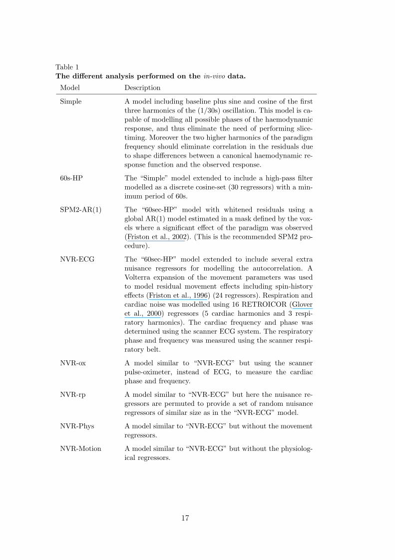
Table 1The different analysis performed on the in-vivo data.

Model Description

Simple A model including baseline plus sine and cosine of the firstthree harmonics of the (1/30s) oscillation. This model is ca-pable of modelling all possible phases of the haemodynamicresponse, and thus eliminate the need of performing slice-timing. Moreover the two higher harmonics of the paradigmfrequency should eliminate correlation in the residuals dueto shape differences between a canonical haemodynamic re-sponse function and the observed response.

60s-HP The “Simple” model extended to include a high-pass filtermodelled as a discrete cosine-set (30 regressors) with a min-imum period of 60s.

SPM2-AR(1) The “60sec-HP” model with whitened residuals using aglobal AR(1) model estimated in a mask defined by the vox-els where a significant effect of the paradigm was observed(Friston et al., 2002). (This is the recommended SPM2 pro-cedure).

NVR-ECG The “60sec-HP” model extended to include several extranuisance regressors for modelling the autocorrelation. AVolterra expansion of the movement parameters was usedto model residual movement effects including spin-historyeffects (Friston et al., 1996) (24 regressors). Respiration andcardiac noise was modelled using 16 RETROICOR (Gloveret al., 2000) regressors (5 cardiac harmonics and 3 respi-ratory harmonics). The cardiac frequency and phase wasdetermined using the scanner ECG system. The respiratoryphase and frequency was measured using the scanner respi-ratory belt.

NVR-ox A model similar to “NVR-ECG” but using the scannerpulse-oximeter, instead of ECG, to measure the cardiacphase and frequency.

NVR-rp A model similar to “NVR-ECG” but here the nuisance re-gressors are permuted to provide a set of random nuisanceregressors of similar size as in the “NVR-ECG” model.

NVR-Phys A model similar to “NVR-ECG” but without the movementregressors.

NVR-Motion A model similar to “NVR-ECG” but without the physiolog-ical regressors.

17

BG=100+Noise

BG+1Hz

BG+2Hz

BG+3Hz

BG+1Hz+2Hz

BG+2Hz+3Hz

BG+1Hz+2Hz+3Hz

0 5 10 15 20 25 30−1

0

1

time [s]

0 5 10 15 20 25 30−1

0

1

time [s]

0 5 10 15 20 25 30−1

0

1

time [s]

0 5 10 15 20 25−2

0

2

time [s]

Fig. 1. Generation of Simulated data. The figure shows how the data used in thesimulation were generated. Slice 1 contains an aliased 1Hz oscillation in all voxelslocated in a pattern showing the digit “1”, slice 2 contains an aliased 2Hz oscillationin all voxels located in a pattern showing the digit “2”, slice 3 contains an aliased3Hz oscillation in all voxels located in a pattern showing the digit “3”. In slice 4 thepattern of oscillatory behaviour was constructed by adding the patterns of the slices1 to 3. Where two or more patterns from these slices intersect the correspondingoscillations were added to the time-course of the particular voxel, as illustrated forthe voxels where all three digits intersect (red curve). In addition to the harmonicoscillations the time-course of all voxels were added a constant value of 100 andnormal-distributed white noise with standard deviation specific to each dataset.

18

100

102

Independence of errors (Dep)

100

102

First order correlation of errors (Corr)

Fact

or b

y wh

ich re

ject

ions

exc

eed

expe

cted

num

ber

0 0.2 0.4 0.6 0.8 1

100

102

Normality of errors (Norm)

Standard deviation of white, normal distributed noise

simple 0ms 1ms 2ms 3ms 4ms5ms 6ms 7ms 8ms 9ms 10ms15ms 20ms 25ms 30ms 35ms 40ms50ms 60ms 70ms 80ms 90ms 100ms120ms 140ms 160ms 180ms 200ms

Fig. 2. Non-white noise in simulated data. The figure shows for the threedifferent tests, as a function of increasing standard deviation of the white noise,the factor by which rejections exceed the expected number. The different curvescorrespond to a simple analysis and several analyses using an external referencetime-course to whiten the periodic behaviour. Different colours indicate the standarddeviation of the jitter introduced to the phase of the reference time-course. Thevertical dotted black line at 0.5 indicates the noise-level of the dataset used inFigure 3.

19

Dep

Corr

Norm

Standard deviation of phase−jitter [ms]

Standard deviation of white, normal distributed noise: 0.5

simple0 5 10 15 20 25 30 35 40 50 60 70 80 90 100 120 140 160 180 2001

0.1

0.01

0.001

0.0001

0.00001

0.000001

Fig. 3. Non-white noise in simulated data. The figure shows the output of theSPM-diagnosis from the simple analysis and from several analyses using an externalreference time-course to whiten the periodic behaviour. In the horizontal directionincreasing jitter has been introduced to the phase of the reference time-course. Thecolours correspond to the p-value at which the null hypothesis of the correspondingSPMd test (Dep, Corr or Norm) was rejected.

20

10−2 10−1

104

105

106

107

108

Frequency [Hz]

Powe

r den

sity

[a.u

.]

Simple60s High−Pass

Simple 60s High−Pass

Dep

Corr

Norm

1

0.1

0.01

0.001

0.0001

0.00001

0.000001

Fig. 4. Non-white noise in Phantom data. The figure shows (left) averagedperiodograms of the standardised residuals from all voxel inside the phantom and(right) SPM-diagnosis maps from analysis with and without high-pass filter in-cluded in the design matrix. The colours correspond to the p-value at which thenull hypothesis of the corresponding SPMd test (Dep, Corr or Norm) was rejected.It is seen from the spectrum and the image that non-white noise in phantom datacan be modelled adequately using a discrete cosine-set (with shortest period of 60s)as high-pass filter.

21

2

4

6

8

10

12

14

Fig. 5. Low-frequency noise in vivo. The figure shows (in colour) F-test valuesof the voxels showing significant (p=0.05 corrected using GRF) effect of a linearcombination of the discrete cosine-set constituting the high-pass filter (F-test). It isseen that the low-frequency noise is dominant near the edges of the brain.

22

2

4

6

8

10

12

14

Fig. 6. Residual movement effects. The figure shows (in colour) F-test valuesof the voxels showing significant (p=0.05 corrected using GRF) effect of a linearcombination of the regressors describing residual movement effects (F-test). It isseen that the residual movement effects are dominant near the edges of the brain.

23

2

4

6

8

10

12

14

Fig. 7. Respiratory induced noise.The figure shows (in colour) F-test valuesof the voxels showing significant (p=0.05 corrected using FDR) effect of a linearcombination of the regressors describing the aliased respiratory oscillation (F-test).It is seen that the respiratory induced noise is dominant near the edges of the brainas well as near in the larger veins and in the ventricles.

24

2

4

6

8

10

12

14

Fig. 8. Cardiac-induced noise. The figure shows (in colour) F-test values of thevoxels showing significant (p=0.05 corrected using GRF) effect of a linear combi-nation of the regressors describing the aliased cardiac oscillation (F-test). It is seenthat the cardiac-induced noise is dominant near larger vessels (e.g. medial cerebralartery and Circle of Willis).

25

2

4

6

8

10

12

14

Fig. 9. Visual activation. The figure shows (in colour) F-test values the voxelsshowing significant (p=0.05 corrected using GRF) effect of a linear combination ofthe regressors describing the stimulation with the expanding ring paradigm (F-test).Primary and higher order visual cortices are seen as well as Lateral GeniculateNuclei.

26

100

102

Independence of errors (Dep)

100

102

First order correlation (Corr)

Fact

or b

y wh

ich re

ject

ions

exc

eed

expe

cted

num

ber

R1 W1 R2 W2 R3 W3 R4 W4 R5 W5 R6 W6 R7 W7 R8 W8

100

102

Normality of errors (Norm)

Session #

Simple 60sec−HP SPM2−AR(1)NVR−ECG NVR−rp NVR−oxNVR−Phys NVR−Motion Nominal

Fig. 10. Non-white in vivo. The figure shows for the three different tests, for eachof the 16 sessions, the factor by which rejections exceed the expected number. Thedifferent curves correspond to various models. The maps corresponding to sessionR3, W3 and R8 are shown in Figure 11.

27

Simple 60sec−HP SPM2−AR(1) NVR−ox NVR−ECG NVR−rp

Dep

Corr

Norm

1

0.1

0.01

0.001

0.0001

0.00001

0.000001

R3

Simple 60sec−HP SPM2−AR(1) NVR−ox NVR−ECG NVR−rp

Dep

Corr

Norm

1

0.1

0.01

0.001

0.0001

0.00001

0.000001

W3

Simple 60sec−HP SPM2−AR(1) NVR−ox NVR−ECG NVR−rp

Dep

Corr

Norm

1

0.1

0.01

0.001

0.0001

0.00001

0.000001

R6

Fig. 11. Non-white noise in vivo. The figure shows SPM-diagnosis maps fromseveral different analyses of the data from 3 different sessions. The colours corre-spond to the p-value at which the null hypothesis of the corresponding SPMd test(Dep, Corr or Norm) was rejected. It is seen that white noise can be obtained bymodelling effects of cardiac, respiratory, motion and low-frequency drift (NVR-ECGor NVR-ox), but not using the standard SPM2 whitening approach (SPM2-AR(1)).

28

0

0.02

0.04

Aliased

0

0.1

0.2

Original

0

0.02

0.04

0

0.1

0.2

0

0.02

0.04

0

0.1

0.2

0.3

0

0.02

0.04

0

0.1

0.2

0.3

0

0.02

0.04

0

0.1

0.2

0.3

0

0.02

0.04

0

0.1

0.2

0.3

0

0.02

0.04

0

0.1

0.2

0.3

0 0.05 0.1 0.15 0.20

0.02

0.04

Frequency [Hz]0 0.5 1 1.5

0

0.1

0.2

0.3

Frequency [Hz]

Fig. 12. Aliasing of cardiac pulsation. The figure shows normalised histogramsof beat to beat frequencies, for the eight different subjects, before and after aliasing(aliased frequencies are calculated using Eaquation 3). The frequencies are calcu-lated as one divided by the beat to beat interval. It is seen from the histogramthat the aliased beat to beat frequencies are distributed across the entire sampledbandwidth.

29