INTERNATIONAL JOURNAL FOR NUMERICAL METHODS IN ENGINEERINGInt. J. Numer. Meth. Engng 2009; 78:1037–1075Published online 16 December 2008 in Wiley InterScience (www.interscience.wiley.com). DOI: 10.1002/nme.2516

Non-linear seismic analysis of RC structures withenergy-dissipating devices

P. Mata1,∗,†, A. H. Barbat1, S. Oller1 and R. Boroschek2

1Technical University of Catalonia, UPC, Jordi Girona 1-3, Modul C1, Campus Nord, 08034 Barcelona, Spain2Civil Engineering Department, University of Chile, Blanco Encalada 2002, Santiago, Chile

SUMMARY

The poor performance of some reinforced concrete (RC) structures during strong earthquakes has alertedabout the need of improving their seismic behavior, especially when they are designed according to obsoletecodes and show low structural damping, important second-order effects and low ductility, among otherdefects. These characteristics allow proposing the use of energy-dissipating devices for improving theirseismic behavior. In this work, the non-linear dynamic response of RC buildings with energy dissipatorsis studied using advanced computational techniques. A fully geometric and constitutive non-linear modelfor the description of the dynamic behavior of framed structures is developed. The model is based on thegeometrically exact formulation for beams in finite deformation. Points on the cross section are composedof several simple materials. The mixing theory is used to treat the resulting composite. A specific type ofelement is proposed for modeling the dissipators including the corresponding constitutive relations. Specialattention is paid to the development of local and global damage indices for describing the performance ofthe buildings. Finally, numerical tests are presented for validating the ability of the model for reproducingthe non-linear seismic response of buildings with dissipators. Copyright q 2008 John Wiley & Sons, Ltd.

Received 8 February 2008; Revised 7 October 2008; Accepted 28 October 2008

KEY WORDS: RC structures; beam model; non-linear analysis; composites; passive control

1. INTRODUCTION

Conventional seismic design practice permits designing reinforced concrete (RC) structures forforces lower than those expected from the elastic response, on the premise that the structural design

∗Correspondence to: P. Mata, Technical University of Catalonia, Jordi Girona 1-3, Modul C1, Campus Nord, 08034Barcelona, Spain.

†E-mail: pmata@cimne.upc.edu

Contract/grant sponsor: European Commission; contract/grant number: CEE–FP6 Project FP6-50544(GOCE)Contract/grant sponsor: Spanish Government (Ministerio de Educacion y Ciencia); contract/grant numbers: BIA2003-08700-C03-02, BIA2005-06952Contract/grant sponsor: CIMNE and AIRBUS; contract/grant number: PBSO-13-06

Copyright q 2008 John Wiley & Sons, Ltd.

1038 P. MATA ET AL.

assures significant structural ductility [1]. Frequently, the dissipative zones are located near thebeam–column joints and, due to cyclic inelastic incursions during earthquakes, structural elementscan suffer a great amount of damage [2]. This situation is generally considered economicallyacceptable if life safety and collapse prevention are achieved.

In the last decades, new techniques based on adding devices to the buildings with the mainobjective of dissipating the energy exerted by the earthquake and alleviating the ductility demandon primary structural elements have contributed to improve the seismic behavior of the structures[3, 4]. Their purpose is to control the seismic response of the buildings by means of a set ofdissipating devices that constitutes the control system, adequately located in the structure. In thecase of passive energy-dissipating devices (EDD), an important part of the energy input is absorbedand dissipated, therefore, concentrating the non-linear phenomenon in the devices without the needof an external energy supply.

Several works showing the ability of EDDs in controlling the seismic response of structuresare available; for example, in Reference [5] the responses of framed structures equipped withviscoelastic and viscous devices are compared; in Reference [6] a comparative study consideringmetallic and viscous devices is carried out. Aiken [7] presents the contribution of extra energydissipation due to EDDs as an equivalent damping added to the linear bare structure (the term bareis used to indicate the structure without EDDs or any type of stiffeners) and gives displacementreduction factors as a function of the added damping ratio. A critical review of reduction factorsand design force levels can be consulted in Reference [8]. A method for the preliminary designof passively controlled buildings is developed in Reference [9]. Lin and Copra [10] study theaccuracy of estimating the dynamic response of asymmetric buildings equipped with EDDs whenthey are replaced by their energetic equivalent viscous dampers. Other procedures for the analysisand design of structures with EDDs can be consulted in Reference [11].

Today, only a few countries have codes for designing RC buildings with EDDs. Particularly, inUnited States the US Federal Emergency Management Agency gives code provisions and standardsfor the design of EDDs devices to be used in buildings [12, 13]. In Europe, the efforts have beenfocused on developing codes for base isolation but not for the use of EDDs.

The design methods proposed for RC structures are mainly based on the assumption that thebehavior of the bare structure remains elastic, while the energy dissipation relies on the controlsystem. However, experimental and theoretical evidence shows that inelastic behavior can alsooccur in the structural elements of controlled building during severe earthquakes [14]. In orderto perform a precise dynamic non-linear analysis of passively controlled buildings, sophisticatednumerical tools become necessary for both academics and practitioners [15].

There is agreement that fully three-dimensional numerical technique constitute the most precisetools for the simulation of the seismic behavior of RC buildings. However, the computing timeusually required for real structures makes many applications unpractical. Considering that mostof the elements in RC buildings are columns and beams, one-dimensional formulations for structuralelements appear as a solution combining both numerical precision and reasonable computationalcosts [16]. Experimental evidence shows that inelasticity in beam elements can be formulatedin terms of cross-sectional quantities [17]. Some formulations of this type have been extendedfor considering geometric non-linearities [18, 19]. An additional refinement is obtained consid-ering inhomogeneous distributions of materials on arbitrarily shaped beam cross sections [20].In this case, the constitutive relationship at the cross-sectional level is deduced by integrationand, therefore, the mechanical behavior of beams with complex combinations of materials can besimulated.

Copyright q 2008 John Wiley & Sons, Ltd. Int. J. Numer. Meth. Engng 2009; 78:1037–1075DOI: 10.1002/nme

NON-LINEAR SEISMIC ANALYSIS OF RC STRUCTURES 1039

On the one hand, formulations for beams considering both constitutive and geometric non-linearity are rather scarce; most of the geometrically non-linear models are limited to the elasticcase [21, 22] and the inelastic behavior has been mainly restricted to plasticity [18]. Recently,Mata et al. [16, 23] have extended the geometrically exact formulation for beams due to Reissnerand Simo [22, 24, 25] to an arbitrary distribution of composite materials on the cross sections forthe static and dynamic cases.

On the other hand, from the numerical point of view, EDDs usually have been described ina global sense by means of force–displacement or moment–curvature relationships [4], whichattempt to capture appropriately the energy-dissipating capacity of the devices [26]. The inclusionof EDDs in software packages for the seismic analysis of RC structures is frequently done bylinking elements equipped with the mentioned non-linear relationships. The relative displacementand/or rotation between the anchorage points activates the dissipative mechanisms of the devices.

In summary, a modern numerical approach to the structural seismic analysis of RC buildingsshould take into account the following aspects:

(i) Geometric non-linearity due to the changes in the configuration experienced by flexiblestructures during earthquakes. Finite deformation models for beam structures, particularlythe geometrically exact ones, in most of the cases have been restricted to the elastic caseor, when they consider inelasticity, it corresponds to plasticity in the static range.

(ii) Constitutive non-linearity. Inhomogeneous distributions of inelastic materials can appearin many structures. The obtention of the resultant forces and moments as well as theestimation of the dissipated energy should be considered in a manner consistent with thethermodynamical basis of the constitutive theory. Most of the formulations consideringinelasticity in beam models have been developed under the small strain assumption; consti-tutive laws are valid for specific geometries of the cross sections or the thermodynamicalbasis of the constitutive theories are violated (e.g. treating the shear components of thestress elastically while the normal component presents inelastic behavior or providing anunlimited energy-dissipating capacity in plastic models).

(iii) Control techniques, which allow to improve the dynamic response of structures by means ofthe strategic incorporation of dissipating devices. Several research and commercial numer-ical codes have included special elements for EDDs; however, the obtained implementationsinherit the drawbacks of points (i) and (ii).

According to the authors’s knowledge the state of the art in seismic analysis provides a set ofpartial solutions to the above-mentioned requirements; however, there is not a unified approachcovering all these aspects in a manner consistent with the principles of the continuum mechanics(see (ii)).

In this work, a fully geometric and constitutive non-linear formulation for rod elements isextended to the case of flexible RC structures equipped with EDDs. A fiber-like approach is usedto represent arbitrary distributions of composite materials on the beam cross sections. EDDs areconsidered as bar elements linking two points in the structure. Thermodynamically consistentconstitutive laws are used for concrete and longitudinal and transversal steel reinforcements. Inparticular, a damage model able to treat the degradation associated with the tensile and compressivecomponents of stress in an independent manner is presented. The extension to the rate-dependentcase is obtained by means of a regularization of the evolution rules of the damage thresholds.The mixing rule is employed for the treatment of the resulting composite. A specific non-linearhysteretic force–displacement relationship is provided for describing the mechanical behavior of

Copyright q 2008 John Wiley & Sons, Ltd. Int. J. Numer. Meth. Engng 2009; 78:1037–1075DOI: 10.1002/nme

1040 P. MATA ET AL.

several types of EDDs. A description of the damage indices capable of estimating the remainingload-carrying capacity of the buildings is also given. Finally, numerical results from simulationsshowing the ability of the proposed formulation in simulating the static and dynamic inelasticresponse of RC buildings equipped with EDDs are provided. Examples cover several complexphenomena such as the inelastic P–� effect and inelastic dynamic structural torsion.

2. FINITE DEFORMATION FORMULATION FOR STRUCTURAL ELEMENTS

2.1. Beam model

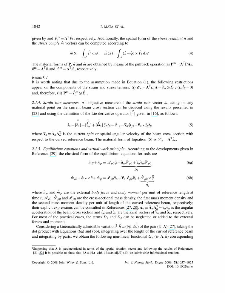
The original geometrically exact formulation for beams due to Reissner [24], Simo [22] and Simoand Vu Quoc [25, 27] is expanded for considering an intermediate curved reference configurationaccording to Ibrahimbegovic [21]. The main difficulty arises from the fact that the geometry andthe kinematics of the beams are developed in the non-linear differential manifold‡ R3×SO(3)and, therefore, a number of standard procedures, such as the computation of strain measures orthe linearization of the weak form of the balance equations become more complicated. In thissection a brief summary of results relevant for the development of constitutive laws able to beincorporated in the beam theory and the construction of a model for EDDs are presented.

2.1.1. Kinematics. Let {Ei } and {ei } be the spatially fixed material and spatial frames,§ respec-tively. The straight reference beam is defined by the curve �00= SE1, with S∈[0, L] its arch-lengthcoordinate. The beam cross sections are described by means of the coordinates �� directed along

{E�} and the position vector of any material point is X = SE1+�� E�.The case of a beam with initial curvature (and twist) is considered by means of a curved

reference beam defined by means of the spatially fixed curve �0=�0i (S)ei ∈R3. Each point onthis curve has rigidly attached an orthogonal local frame t0i (S)=K0 Ei ∈R3, where K0∈SO(3) isthe orientation tensor. The beam cross section A(S) is defined considering the local coordinatesystem �� but directed along {t0�}. The planes of the cross sections are normal to the vectortangent to the reference curve, i.e. �0,S = t01(S). The position vector of a material point on the

curved reference beam is x0= �0+K0�� E�. In this case, the straight beam is used as an auxiliaryreference frame for the construction of strain measures as it will be explained in following.

The motion displaces points on the curved reference beam from �0(S) to �(S, t) (at time t)adding a translational displacement u(S, t) and the local orientation frame is simultaneously rotated,together with the beam cross section, from K0(S) to K(S, t) by means of the incremental rotationtensor K=KnK0≡ ti ⊗ Ei ∈SO(3) (see Figure 1).

In general, the normal vector t1 �= �,S because of the shearing [22]. The position vector of amaterial point on the current beam is

x(S,��, t)= �(S, t)+�� t�(S, t)= �+K�� E� (1)

‡The symbol SO(3) is used to denote the finite rotation manifold [22, 27].§The indices i and � range over {1,2,3} and {2,3}, respectively, and summation convention hold. The symbol (·),xis used to denote partial differentiation of (·) with respect to x .

Copyright q 2008 John Wiley & Sons, Ltd. Int. J. Numer. Meth. Engng 2009; 78:1037–1075DOI: 10.1002/nme

NON-LINEAR SEISMIC ANALYSIS OF RC STRUCTURES 1041

Figure 1. Configurational description of the beam.

Equation (1) implies that the current beam configuration is completely determined by the pairs(�,K)∈R3×SO(3).

2.1.2. Strain measures. The deformation gradient is defined as the gradient of the deformationmapping of Equation (1) and determines the strain measures at any material point of the beamcross section [27]. The deformation gradients of the curved reference beam and of the currentbeam referred to the straight reference configuration are denoted by F0 and F, respectively. Thedeformation gradient (relative to the curved reference beam) Fn :=FF−1

0 is responsible for thedevelopment of strains and can be expressed as [28]

Fn =FF−10 =g−1

0 [�,S− t1+xn�� t�]⊗ t01+Kn (2)

where g0=Det[F0] and xn ≡Kn,SKTn is the spatial curvature tensor relative to the curved referencebeam. In Equation (2), the term defined as �n = �,S− t1 corresponds to the reduced spatial strain

measure of shearing and elongation [22, 28] with material description given by �=KT�. Thematerial representation of Fn is obtained as Fm

n =KTFnK0.Removing the rigid body component from Fn , it is possible to construct the spatial strain tensor

en =Fn−Kn . The corresponding spatial strain vector acting on the current beam cross section isobtained as

�n =en t01=g−10 [�n+xn�� t�] (3)

with material form given by En =KT�n .

2.1.3. Stress measures. en is (energetically) conjugated to the asymmetric First Piola Kirchhoff(FPK) stress tensor P= Pi ⊗ t0i [22] with Pi being the FPK stress vector acting on the deformedface in the current beam corresponding to the normal t0i in the curved reference configuration.Equivalently, �n is the energetically conjugated pair to P1. The corresponding material forms are

Copyright q 2008 John Wiley & Sons, Ltd. Int. J. Numer. Meth. Engng 2009; 78:1037–1075DOI: 10.1002/nme

1042 P. MATA ET AL.

given by and Pm1 =KT P1, respectively. Additionally, the spatial form of the stress resultant n and

the stress couple m vectors can be computed according to

n(S)=∫A

P1 dA, m(S)=∫A

(x−�)× P1 dA (4)

The material forms of P, n and m are obtained by means of the pullback operation as Pm=KTPK0,nm=KTn and mm=KTm, respectively.

Remark 1It is worth noting that due to the assumption made in Equation (1), the following restrictionsappear on the components of the strain and stress tensors: (i) En =KTenK= En⊗ E1, (en t� =0)

and, therefore, (ii) Pm= Pm1 ⊗ E1.

2.1.4. Strain rate measures. An objective measure of the strain rate vector sn acting on anymaterial point on the current beam cross section can be deduced using the results presented in

[23] and using the definition of the Lie derivative operator [�· ] given in [16], as follows:

sn =�

[˙�n]=�

[˙�n]+�

[ ˙xn]�� t� = ˙�,S− vn�,S+ vn,S�� t� (5)

where vn ≡ KnKTn is the current spin or spatial angular velocity of the beam cross section withrespect to the curved reference beam. The material form of Equation (5) is Sn =KTsn .

2.1.5. Equilibrium equations and virtual work principle. According to the developments given inReference [29], the classical form of the equilibrium equations for rods are

n,S+ n p =A�0¨�+ anS�0+ vn vnS�0︸ ︷︷ ︸

D1

(6a)

m,S+�,S× n+m p = I�0�n+ vnI�0vn+S�0× ¨�︸ ︷︷ ︸D2

(6b)

where n p and m p are the external body force and body moment per unit of reference length attime t , A�0, S�0 and I�0 are the cross-sectional mass density, the first mass moment density andthe second mass moment density per unit of length of the curved reference beam, respectively;their explicit expressions can be consulted in References [27, 28]. an ≡ KnKTn − vn vn is the angularacceleration of the beam cross section and vn and �n are the axial vectors of vn and an , respectively.For most of the practical cases, the terms D1 and D2 can be neglected or added to the externalforces and moments.

Considering a kinematically admissible variation¶ h≡(�,) of the pair (�,K) [27], taking thedot product with Equations (6a) and (6b), integrating over the length of the curved reference beamand integrating by parts, we obtain the following non-linear functional Gw(�,K, h) corresponding

¶Supposing that K is parameterized in terms of the spatial rotation vector and following the results of References[21, 22] it is possible to show that K=hK with =axial[h]∈R3 an admissible infinitesimal rotation.

Copyright q 2008 John Wiley & Sons, Ltd. Int. J. Numer. Meth. Engng 2009; 78:1037–1075DOI: 10.1002/nme

NON-LINEAR SEISMIC ANALYSIS OF RC STRUCTURES 1043

to the weak form of the balance equations [21, 27], which is another way of writing the virtualwork principle:

Gw(�,K, h) =∫ L

0[(�,S−×�,S) · n+,S ·m]dS

+∫ L

0[�·A�0

¨�+·(I�0 �n+ vnI�0 vn)]dS

−(∫ L

0[�· n p+·m p]dS+[�· n+ ·m]|L0

)= G int

w (�,K, h)+G inew (�,K, h)−Gext

w (�,K, �, h)=0 (7)

where �=[nTp, mTp] is the external loading vector,G int

w , andG inew andGext

w correspond to the internal,

inertial and external contributions of the virtual work principle. The terms (�,S−×�,S) and

,S appearing in Equation (7) correspond to the co-rotated variations of the reduced strain measures�n and �n in spatial description.

2.2. Energy-dissipating devices

The finite deformation model for EDDs is obtained from the previously described beam model,releasing the rotational degrees of freedom and supposing that the complete mechanical behaviorof the device is described in terms of the evolution of a unique material point located in themiddle of the resulting bar. This point is referred as the dissipative nucleus (see Figure 2). Thecurrent position of a point in the EDD bar is obtained from Equation (1), but considering that nocross-sectional description is required; thus, one can neglect �� and assume x= �(S, t).

The current orientation of the (straight) EDD bar of initial length L∗ is given by the tensorK∗(t). Assuming that the rotational degree of freedom are released one has: (i) K∗

,S =0 and (ii)

K∗ �=0. Therefore, the spatial position of the dissipative nuclei is obtained as �(L∗/2, t) where

L∗/2 is the arch-length coordinate of the middle point in the bar element.The only non-zero component of the strain vector is the axial one, denoted by Ed1 and computed

with the help of Equation (3) as

Ed1(t)= �n|(L∗/2) · E1=[(K∗T�,S) · E1]|(L∗/2)−1=[�,S · t1]|(L∗/2)−1 (8)

Figure 2. Energy-dissipating device.

Copyright q 2008 John Wiley & Sons, Ltd. Int. J. Numer. Meth. Engng 2009; 78:1037–1075DOI: 10.1002/nme

1044 P. MATA ET AL.

and the corresponding strain rate, Ed1 , is obtained as

Ed1(t)=d

dtEd1(t)

∣∣∣∣(L∗/2,t)

=[(K∗T( ˙�,S− vn�,S)) · E1]|(L∗/2,t) (9)

Note that the same expression can be deduced from Equation (5). Let Pmd be the value of the

stress measure in the EDD, which is energetically conjugated to Ed1 . The formulation of specificconstitutive relations Pm

d (Ed1, Ed1) is provided in Section 3.5.In spite of the fact that t1 can be calculated as t1=(�(L∗)−�(0))/‖�(L∗)−�(0)‖=KE1

one has that t1=KE1= hK �=0 although � can be zero for rigid body motions (however,(),S =0). Then, taking (�,) superposed onto (�,K) and considering that the linear partof Equation (8) is Ed1 =[�,S+u,S]· t1, one has that the contribution of the EDDs to thefunctional of Equation (7) written in the material description is

GEDD =∫ L∗

0Pmd Ed1 dS+(� ·Md

¨�)|(L∗/2,t)

=∫ L∗

0Pmd K

T[�,S+u,S]· E1 dS+(�·Md¨�)|(L∗/2,t) (10)

where it was assumed that I�0 ≈0, i.e. the contribution of the EDDs to the rotational mass of thesystem is neglected and Md =Diag[Md ,Md ,Md ] is the EDD’s translational inertia matrix, i.e.the mass of the control system; Md , is supposed to be concentrated in the middle point of the bar.

3. CONSTITUTIVE MODELS

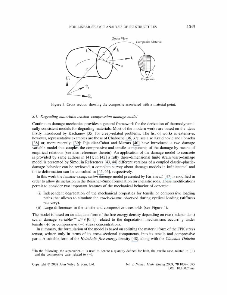
In this work, material points on the cross sections are considered as formed by a composite materialcorresponding to a homogeneous mixture of different simple‖ components, each of them with itsown constitutive law (see Figure 3). The resulting behavior is obtained by means of the mixingtheory (see e.g. [30] or more recently [31, 32] and references therein).

In the formulation of constitutive models, the kinematic assumptions of the present theory hasto be considered, which limit the number of known components of the strain and stress tensorsto those existing on the cross-sectional planes. Therefore, following the same reasonings as inprevious works of the authors [16, 23], the models are formulated in terms of the material formof the FPK stress, strain and strain rate vectors, Pm

1 , En and Sn , respectively.Although the present constitutive models constitute a dimensionally reduced form of the general

three-dimensional formulations, they allow to simulate the coupled non-linear behavior among thecomponents of the stress vector, respecting the thermodynamical basis of irreversible processes.In this sense, the present approach avoids the use of one-dimensional constitutive laws for theaxial component of the stress maintaining the behavior of shear components uncoupled, which isone of the most common assumptions in fiber-like models for rods (see e.g. [33, 34]). Two kindsof non-linear constitutive models for simple materials are used: the tension–compression damageand the plasticity models.

‖The term simple is used for referring to materials that are described by means of a single constitutive law.

Copyright q 2008 John Wiley & Sons, Ltd. Int. J. Numer. Meth. Engng 2009; 78:1037–1075DOI: 10.1002/nme

NON-LINEAR SEISMIC ANALYSIS OF RC STRUCTURES 1045

Figure 3. Cross section showing the composite associated with a material point.

3.1. Degrading materials: tension–compression damage model

Continuum damage mechanics provides a general framework for the derivation of thermodynami-cally consistent models for degrading materials. Most of the modern works are based on the ideasfirstly introduced by Kachanov [35] for creep-related problems. The list of works is extensive;however, representative examples are those of Chaboche [36, 37]; see also Krajcinovic and Fonseka[38] or, more recently, [39]; Pijaudier-Cabot and Mazars [40] have introduced a two damagevariable model that couples the compressive and tensile components of the damage by means ofempirical relations (see also references therein). An application of the damage model to concreteis provided by same authors in [41]; in [42] a fully three-dimensional finite strain visco-damagemodel is presented by Simo; in References [43, 44] different versions of a coupled elastic–plastic-damage behavior can be reviewed; a complete survey about damage models in infinitesimal andfinite deformation can be consulted in [45, 46], respectively.

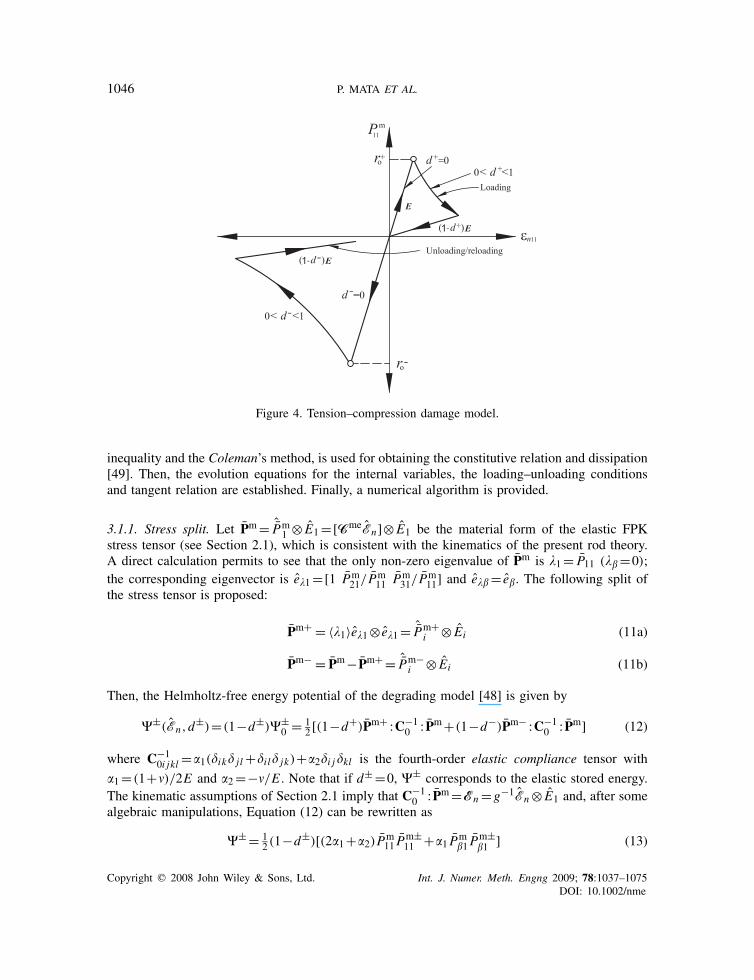
In this work the tension–compression damage model presented by Faria et al. [47] is modified inorder to allow its inclusion in the Reissner–Simo formulation for inelastic rods. These modificationspermit to consider two important features of the mechanical behavior of concrete:

(i) Independent degradation of the mechanical properties for tensile or compressive loadingpaths that allows to simulate the crack-closure observed during cyclical loading (stiffnessrecovery).

(ii) Large differences in the tensile and compressive thresholds (see Figure 4).

The model is based on an adequate form of the free energy density depending on two (independent)scalar damage variables∗∗ d± ∈[0,1], related to the degradation mechanisms occurring undertensile (+) or compressive (−) stress concentrations.

In summary, the formulation of the model is based on splitting the material form of the FPK stresstensor, written only in terms of its cross-sectional components, into its tensile and compressiveparts. A suitable form of the Helmholtz-free energy density [48], along with the Clausius–Duheim

∗∗In the following, the superscript ± is used to denote a quantity defined for both, the tensile case, related to (+)and the compressive case, related to (−).

Copyright q 2008 John Wiley & Sons, Ltd. Int. J. Numer. Meth. Engng 2009; 78:1037–1075DOI: 10.1002/nme

1046 P. MATA ET AL.

Figure 4. Tension–compression damage model.

inequality and the Coleman’s method, is used for obtaining the constitutive relation and dissipation[49]. Then, the evolution equations for the internal variables, the loading–unloading conditionsand tangent relation are established. Finally, a numerical algorithm is provided.

3.1.1. Stress split. Let Pm= ˆPm1 ⊗ E1=[CmeEn]⊗ E1 be the material form of the elastic FPK

stress tensor (see Section 2.1), which is consistent with the kinematics of the present rod theory.A direct calculation permits to see that the only non-zero eigenvalue of Pm is �1= P11 (�� =0);the corresponding eigenvector is e�1=[1 Pm

21/Pm11 Pm

31/Pm11] and e�� = e�. The following split of

the stress tensor is proposed:

Pm+ = 〈�1〉e�1⊗ e�1= ˆPm+i ⊗ Ei (11a)

Pm− = Pm−Pm+ = ˆPm−i ⊗ Ei (11b)

Then, the Helmholtz-free energy potential of the degrading model [48] is given by

�±(En,d±)=(1−d±)�±

0 = 12 [(1−d+)Pm+ :C−1

0 : Pm+(1−d−)Pm− :C−10 : Pm] (12)

where C−10i jkl =�1(ik jl +il jk)+�2i jkl is the fourth-order elastic compliance tensor with

�1=(1+ )/2E and �2=− /E . Note that if d± =0, �± corresponds to the elastic stored energy.The kinematic assumptions of Section 2.1 imply that C−1

0 : Pm=En =g−1En⊗ E1 and, after somealgebraic manipulations, Equation (12) can be rewritten as

�± = 12 (1−d±)[(2�1+�2)P

m11 P

m±11 +�1 P

m�1 P

m±�1 ] (13)

Copyright q 2008 John Wiley & Sons, Ltd. Int. J. Numer. Meth. Engng 2009; 78:1037–1075DOI: 10.1002/nme

NON-LINEAR SEISMIC ANALYSIS OF RC STRUCTURES 1047

In this manner, the free energy density is expressed only in terms of the cross-sectional stressvector and two situations can occur:

(i) Tensile axial behavior, �1= Pm11>0, then Pm+ �=0 (see Equation (11a)) and

ˆPm+i = Pm

i1

Pm11

ˆPm1 , ˆPm−

1 =0 (14a)

�+ = 1

2(1−d+)

[1−

2E�21+ 1+

2E‖Pm

1 ‖2]= 1

2(1−d+)�+

0 (14b)

Considering 0�d±�1, it is possible to see that �+>0. This case applies for zones in thecross section that are subjected to tension due to flexion or only tensile axial force.

(ii) Compressive axial behavior, �1= Pm11<0, then Pm+ =0, Pm− = ˆPm

1 ⊗ E1 (see Equation (11b))and �− = 1

2 (1−d−)�−0 >0. This case considers compressed zones in flexion or compressive

axial force. The case �1≈0 reduces to �− = 12 (1−d−)�1‖Pm

1 ‖2>0.

It is worth to note that −��/�d± =�±0 are the thermodynamical forces associated with d±.

Remark 2Owing to the kinematic assumptions, the evolution of shear stresses depends on the sign of �1 andnot on the their own sign. An additional sophistication can be obtained considering, for example,the stress tensor Pm∗ = 1

2 [Pm+PmT ]; however, in this case {��} �=0 and, therefore, more complicatedexpressions are obtained for Equations (11a)–(13).

3.1.2. Damage criteria. Two (scalar) equivalent stresses, which constitute norms for differentstress states [50], are defined as

�+ :=√Pm+ :C−1

0 : Pm+ =⎧⎨⎩

√�+

0 if �1>0

0 if �1�0(15a)

�− :=√√

3(K �−oct+ �−

oct)={0 if �1>0

≈K Pm11 if �1�0

(15b)

where �−oct= 1

3 Pm11, �−

oct=√23 Pm

11 are the octahedral normal and shear stresses obtained from Pm−and K ∈ [1.16–1.2] is a materials property, described in detail in Reference [47]. It is worth notingthat Equation (15a) is a measure of elastic stored energy in contrast with Equation (15b) whereequivalent stress is a measure involving information about specific components of the stress in thespace.

In the same way, two separated damage criteria [51, 52] are defined

g±(�±,r±)= �±−r±�0 (16)

where r± are the current damage thresholds that control the size of the damage surface. In thepresent damage theory, the linear-elastic domain depends on ‖Pm

1 ‖2 and, due to the kinematicassumptions, multi-dimensional representations in the �i planes are not possible.

Copyright q 2008 John Wiley & Sons, Ltd. Int. J. Numer. Meth. Engng 2009; 78:1037–1075DOI: 10.1002/nme

1048 P. MATA ET AL.

The initial values for r± are

r+0 = f +

0√E

, r−0 =K f −

0 (17)

where f ±0 are the elastic thresholds in one-dimensional tensile and compressive tests, respectively.

Then, from Equation (15b) it is possible to see that the boundary of the compressive elastic domainis defined for a value of r− K -times greater than the one-dimensional compressive elastic limit f −

0 .

3.1.3. Evolution equations. The following evolution laws are used for d± and r±

d± = ± �G±(r±)

�r± , r± = ±

(18)

where G± are monotonically increasing functions determined according with experimental dataand

±are the damage consistency parameters. The above rules have to be complemented with

the loading and unloading relations defined with the help of the standard Kuhn–Tucker relations:

(i) ±�0, (ii) G±�0, (iii)

±G± =0 (19)

The corresponding interpretation of these relations is standard and can be consulted, e.g. inReferences [47, 53].

In a generic instant t one has that r±t =max[r±

0 ,r±∗ ] with r±∗ =maxs∈[0,t]r±s . Finally, from

Equations (18) one obtains that d± = G±(r±)�0.

3.1.4. Constitutive relation and dissipation. Considering Equation (12) for the free energy densityand the fact that C−1

0 :En = E1⊗ E1 one has that Clausius–Duheim inequality [48]: �=−�+ Pm1 ·

˙En�0 can be expressed as

�=(Pm1 − ��

�En

)· ˙En+�±

0 d± (20)

which establish that entropy always grows leading to an irreversible process. Considering that bothP± are first degree homogeneous functions of En (see [47] for details) and applying Coleman’sprinciple, the following constitutive relation is obtained:

Pm1 =(1−d±)

��±0

�En=(1−d+) ˆPm+

1 +(1−d−) ˆPm−1 (21)

where ˆPm±1 = Pm± E1. Taking into account Equation (20) it is straightforward to see that dissipation

is given by �=�±0 d

±�0.The material form of the tangent stiffness tensor, Cmt, is obtained taking the material time

derivative of Equation (21) as

˙Pm

1 =(1−d±)˙Pm±1 − d± ˆPm±

1 =Cmt Sn (22)

where Sn is the material form of the strain rate vector as explained in Section 2.1.

Copyright q 2008 John Wiley & Sons, Ltd. Int. J. Numer. Meth. Engng 2009; 78:1037–1075DOI: 10.1002/nme

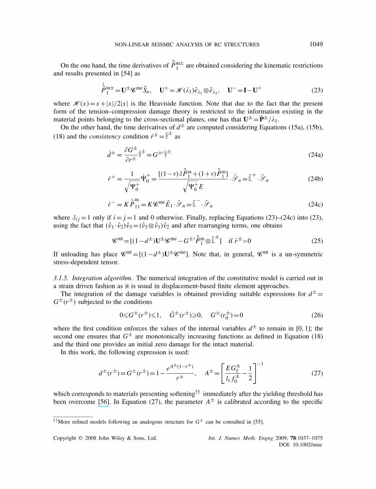
NON-LINEAR SEISMIC ANALYSIS OF RC STRUCTURES 1049

On the one hand, the time derivatives of ˆPm±1 are obtained considering the kinematic restrictions

and results presented in [54] as˙Pm±1 =U±Cme Sn, U+ =H(�1)e�1 ⊗ e�1, U− =I−U+ (23)

where H(x)= x+|x |/2|x | is the Heaviside function. Note that due to the fact that the presentform of the tension–compression damage theory is restricted to the information existing in thematerial points belonging to the cross-sectional planes, one has that U± = P±/�1.

On the other hand, the time derivatives of d± are computed considering Equations (15a), (15b),(18) and the consistency condition r± = ˙�±

as

d± = �G±

�r± ˙�± =G±′ ˙�±(24a)

r+ = 1√�+

0

�+0 = [(1− )J ˆPm

1 +(1+ ) ˆPm1 ]√

�+0 E

·Sn = L+ ·Sn (24b)

r− = K ˙Pm11=KCme E1 ·Sn = L

− ·Sn (24c)

where Ji j =1 only if i= j =1 and 0 otherwise. Finally, replacing Equations (23)–(24c) into (23),using the fact that (v1 · v2)v3=(v3⊗ v1)v2 and after rearranging terms, one obtains

Cmt=[(1−d±)U±Cme−G±′ ˆPm1 ⊗ L

±] if r±>0 (25)

If unloading has place Cmt=[(1−d±)U±Cme]. Note that, in general, Cmt is a un-symmetricstress-dependent tensor.

3.1.5. Integration algorithm. The numerical integration of the constitutive model is carried out ina strain driven fashion as it is usual in displacement-based finite element approaches.

The integration of the damage variables is obtained providing suitable expressions for d± =G±(r±) subjected to the conditions

0�G±(r±)�1, G±(r±)�0, G±(r±0 )=0 (26)

where the first condition enforces the values of the internal variables d± to remain in [0,1]; thesecond one ensures that G± are monotonically increasing functions as defined in Equation (18)and the third one provides an initial zero damage for the intact material.

In this work, the following expression is used:

d±(r±)=G±(r±)=1− eA±(1−r±)

r± , A± =[EG±

f

lc f±0

− 1

2

]−1

(27)

which corresponds to materials presenting softening†† immediately after the yielding threshold hasbeen overcome [56]. In Equation (27), the parameter A± is calibrated according to the specific

††More refined models following an analogous structure for G± can be consulted in [55].

Copyright q 2008 John Wiley & Sons, Ltd. Int. J. Numer. Meth. Engng 2009; 78:1037–1075DOI: 10.1002/nme

1050 P. MATA ET AL.

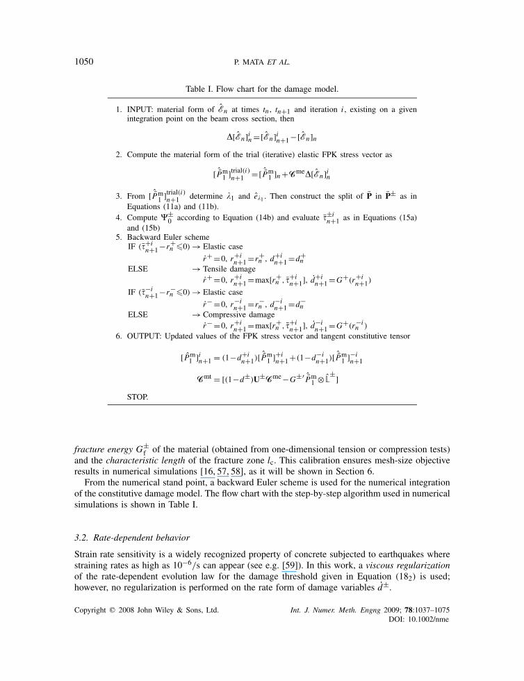
Table I. Flow chart for the damage model.

1. INPUT: material form of En at times tn , tn+1 and iteration i , existing on a givenintegration point on the beam cross section, then

�[En]in =[En]in+1−[En]n2. Compute the material form of the trial (iterative) elastic FPK stress vector as

[ ˆPm1 ]trial(i)n+1 =[ ˆPm

1 ]n+Cme�[En]in

3. From [ ˆPm1 ]trial(i)n+1 determine �1 and e�1 . Then construct the split of P in P± as in

Equations (11a) and (11b).4. Compute �±

0 according to Equation (14b) and evaluate �±in+1 as in Equations (15a)

and (15b)5. Backward Euler scheme

IF (�+in+1−r+

n �0) → Elastic case

r+ =0, r+in+1=r+

n , d+in+1=d+

nELSE → Tensile damage

r+ =0, r+in+1=max[r+

n , �+in+1], d+i

n+1=G+(r+in+1)

IF (�−in+1−r−

n �0) → Elastic case

r− =0, r−in+1=r−

n , d−in+1=d−

nELSE → Compressive damage

r− =0, r+in+1=max[r+

n , �+in+1], d−i

n+1=G+(r−in )

6. OUTPUT: Updated values of the FPK stress vector and tangent constitutive tensor

[Pm1 ]in+1 = (1−d+i

n+1)[ ˆPm1 ]+i

n+1+(1−d−in+1)[ ˆPm

1 ]−in+1

Cmt = [(1−d±)U±Cme−G±′ ˆPm1 ⊗L

±]STOP.

fracture energy G±f of the material (obtained from one-dimensional tension or compression tests)

and the characteristic length of the fracture zone lc. This calibration ensures mesh-size objectiveresults in numerical simulations [16, 57, 58], as it will be shown in Section 6.

From the numerical stand point, a backward Euler scheme is used for the numerical integrationof the constitutive damage model. The flow chart with the step-by-step algorithm used in numericalsimulations is shown in Table I.

3.2. Rate-dependent behavior

Strain rate sensitivity is a widely recognized property of concrete subjected to earthquakes wherestraining rates as high as 10−6/s can appear (see e.g. [59]). In this work, a viscous regularizationof the rate-dependent evolution law for the damage threshold given in Equation (182) is used;however, no regularization is performed on the rate form of damage variables d±.

Copyright q 2008 John Wiley & Sons, Ltd. Int. J. Numer. Meth. Engng 2009; 78:1037–1075DOI: 10.1002/nme

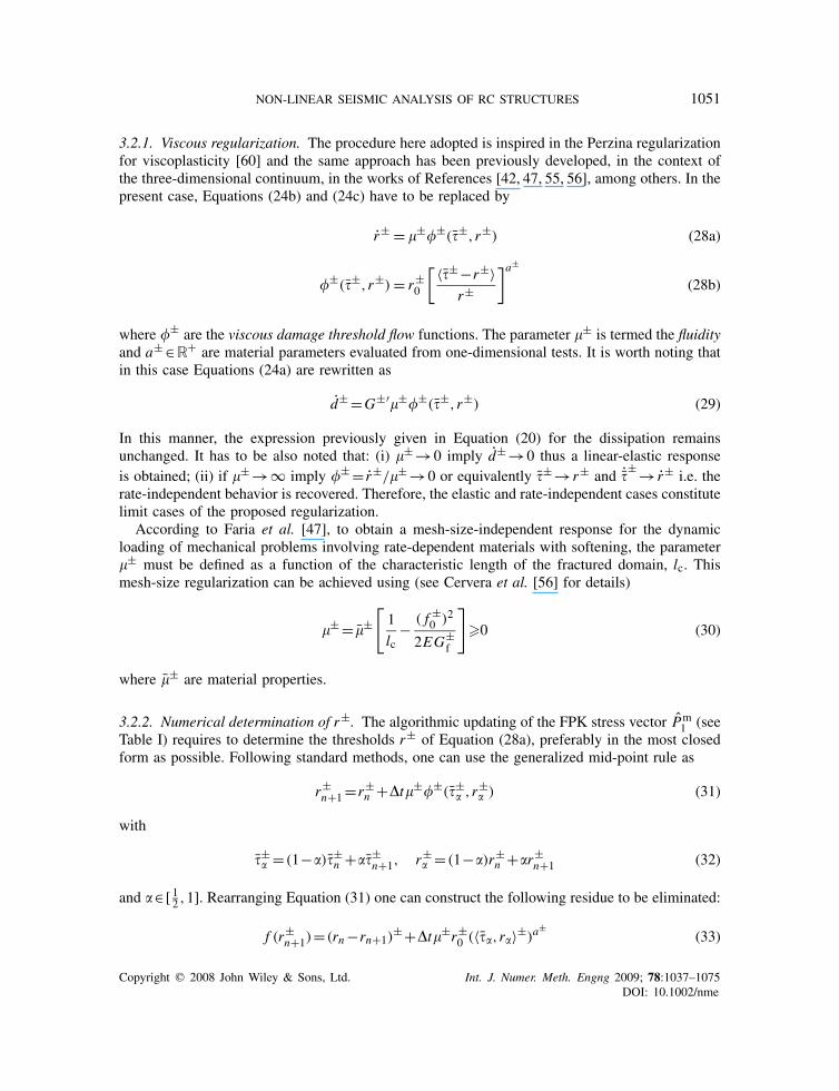
NON-LINEAR SEISMIC ANALYSIS OF RC STRUCTURES 1051

3.2.1. Viscous regularization. The procedure here adopted is inspired in the Perzina regularizationfor viscoplasticity [60] and the same approach has been previously developed, in the context ofthe three-dimensional continuum, in the works of References [42, 47, 55, 56], among others. In thepresent case, Equations (24b) and (24c) have to be replaced by

r± = �±�±(�±,r±) (28a)

�±(�±,r±) = r±0

[ 〈�±−r±〉r±

]a±

(28b)

where �± are the viscous damage threshold flow functions. The parameter �± is termed the fluidityand a± ∈R+ are material parameters evaluated from one-dimensional tests. It is worth noting thatin this case Equations (24a) are rewritten as

d± =G±′�±�±(�±,r±) (29)

In this manner, the expression previously given in Equation (20) for the dissipation remainsunchanged. It has to be also noted that: (i) �± →0 imply d± →0 thus a linear-elastic responseis obtained; (ii) if �± →∞ imply �± = r±/�± →0 or equivalently �± →r± and ˙�± → r± i.e. therate-independent behavior is recovered. Therefore, the elastic and rate-independent cases constitutelimit cases of the proposed regularization.

According to Faria et al. [47], to obtain a mesh-size-independent response for the dynamicloading of mechanical problems involving rate-dependent materials with softening, the parameter�± must be defined as a function of the characteristic length of the fractured domain, lc. Thismesh-size regularization can be achieved using (see Cervera et al. [56] for details)

�± = �±[1

lc− ( f ±

0 )2

2EG±f

]�0 (30)

where �± are material properties.

3.2.2. Numerical determination of r±. The algorithmic updating of the FPK stress vector Pm1 (see

Table I) requires to determine the thresholds r± of Equation (28a), preferably in the most closedform as possible. Following standard methods, one can use the generalized mid-point rule as

r±n+1=r±

n +�t�±�±(�±� ,r±

� ) (31)

with

�±� =(1−�)�±

n +��±n+1, r±

� =(1−�)r±n +�r±

n+1 (32)

and �∈[ 12 ,1]. Rearranging Equation (31) one can construct the following residue to be eliminated:

f (r±n+1)=(rn−rn+1)

±+�t�±r±0 (〈��,r�〉±)a

±(33)

Copyright q 2008 John Wiley & Sons, Ltd. Int. J. Numer. Meth. Engng 2009; 78:1037–1075DOI: 10.1002/nme

1052 P. MATA ET AL.

In general, one has: (i) if a± �=1 the problem defined in Equation (33) is non-linear; (ii) ifa± ∈{1,2,3,4} it admits an explicit solution; (iii) in the general case, a Newton–Raphson type ofiterative scheme is required to determine r±

n+1. In this work, an additional simplification has beenassumed: a± =1 by convenience.

In what regards to the algorithm presented in Table I, Point (5) has to be modified in thefollowing manner:

(i) having obtained �±(i)n+1 , compute �±(i)

� according to Equation (321).

(ii) Verify (�±(i)� −r±

n )<0; if YES then set: (ii.1) r±n+1=r±

n and go to (6) of Table I; (ii.2)

on the contrary, compute r±(i)n+1 using to (33). Evaluate r±

� according to (322). If (�±� <r±

� )

set r±n+1=r±

n ; update the damage d± =G±; on the contrary, d± =G± and go to (6) ofTable I.

3.2.3. Viscous tangent tensor. An advantage of the present viscous regularization is given by thefact that the expression for the tangent relation given in Equation (25) is maintained in the viscouscase. It should be noted that, in this case, there are not explicit expressions for r± as a linearfunction of Sn .

Remark 3Comparing the present formulation with that of [23], some comments can be made: (1) Owingto the fact that there is not a component of viscous stress, viscous secant constitutive tensors areavoided. (2) The linearized increment of the material and co-rotated forms of the FPK stress vector

are simply �Pm1 =Cmv�En and �

�[P1]=Csv�

�[�n]. Therefore, when linearizing the virtual work

principle, the viscous contribution of the tangential stiffness vanishes.

3.3. Plastic materials

For the case of materials that can undergo non-reversible deformations, the plasticity modelformulated in the material configuration is used for predicting their mechanical response. Assumingsmall elastic, finite plastic deformations, an adequate form of the free energy density, �, andanalogous procedures as those for the damage model, we have

Pm1 =�0

��(Een,kp)

�Een

=Cms(En−EPn )=CmeE

en (34)

where the Een is the elastic strain calculated subtracting the plastic strain E

Pn from the total strain

En , �0 is the density in the material configuration, kp is the plastic damage internal variable andthe material form of the secant constitutive tensor is such that Cms=Cme.

Both, the yield function, Fp, and plastic potential function, Gp, are formulated in terms of theFPK stress vector Pm

1 and the plastic damage internal variable kp as

Fp(Pm1 ,kp) =Pp(P

m1 )− f p(P

m1 ,kp)=0 (35a)

Gp(Pm1 ,kp) =K (35b)

Copyright q 2008 John Wiley & Sons, Ltd. Int. J. Numer. Meth. Engng 2009; 78:1037–1075DOI: 10.1002/nme

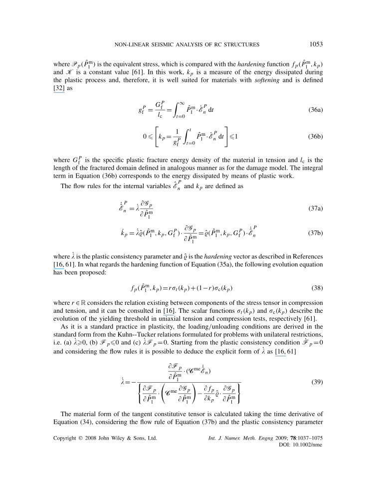
NON-LINEAR SEISMIC ANALYSIS OF RC STRUCTURES 1053

wherePp(Pm1 ) is the equivalent stress, which is compared with the hardening function f p(Pm

1 ,kp)and K is a constant value [61]. In this work, kp is a measure of the energy dissipated duringthe plastic process and, therefore, it is well suited for materials with softening and is defined[32] as

gPf = GP

f

lc=

∫ ∞

t=0Pm1 ·EP

n dt (36a)

0�[kp = 1

gPf

∫ t

t=0Pm1 ·EP

n dt

]�1 (36b)

where GPf is the specific plastic fracture energy density of the material in tension and lc is the

length of the fractured domain defined in analogous manner as for the damage model. The integralterm in Equation (36b) corresponds to the energy dissipated by means of plastic work.

The flow rules for the internal variables EPn and kp are defined as

˙EP

n = ��Gp

�Pm1

(37a)

k p = ��(Pm1 ,kp,G

Pf ) · �Gp

�Pm1

= �(Pm1 ,kp,G

Pf ) · ˙

EP

n (37b)

where � is the plastic consistency parameter and � is the hardening vector as described in References[16, 61]. In what regards the hardening function of Equation (35a), the following evolution equationhas been proposed:

f p(Pm1 ,kp)=r�t (kp)+(1−r)�c(kp) (38)

where r ∈R considers the relation existing between components of the stress tensor in compressionand tension, and it can be consulted in [16]. The scalar functions �t (kp) and �c(kp) describe theevolution of the yielding threshold in uniaxial tension and compression tests, respectively [61].

As it is a standard practice in plasticity, the loading/unloading conditions are derived in thestandard form from the Kuhn--Tucker relations formulated for problems with unilateral restrictions,i.e. (a) ��0, (b) Fp�0 and (c) �Fp =0. Starting from the plastic consistency condition Fp =0and considering the flow rules it is possible to deduce the explicit form of � as [16, 61]

�=−

�Fp

�Pm1

·(Cme ˙En){

�Fp

�Pm1

·(

Cme �Gp

�Pm1

)− � f p

�kp� · �Gp

�Pm1

} (39)

The material form of the tangent constitutive tensor is calculated taking the time derivative ofEquation (34), considering the flow rule of Equation (37b) and the plastic consistency parameter

Copyright q 2008 John Wiley & Sons, Ltd. Int. J. Numer. Meth. Engng 2009; 78:1037–1075DOI: 10.1002/nme

1054 P. MATA ET AL.

of Equation (39) as

Pm1 =CmtEn =

⎡⎢⎢⎢⎢⎣Cme−

(Cme �Gp

�Pm1

)⊗

(Cme �Fp

�Pm1

)�Fp

�Pm1

·(

Cme �Gp

�Pm1

)− �Fp

�kp�·

(�Gp

�Pm1

)⎤⎥⎥⎥⎥⎦En (40)

3.4. Mixing theory for composites

Each material point on the beam cross section is treated as a composite material according to themixing theory [31, 61]. This theory is based on the early works of Truesdell and Toupin [62] forbi-phasic materials and further exploited by a number of authors (see e.g. Ortiz and Popov [30]and references therein, among many others).

In this theory, the interaction between all the components defines the overall mechanical behaviorof the composite at material point level. Supposing N different components coexisting in a genericmaterial point subjected to the same material strain field En , we have the following closingequation: En ≡(En)1=·· ·=(En)q =·· ·=(En)N , which imposes the strain compatibility betweencomponents. The free energy density of the composite, �, is obtained as the weighted sum ofthe free energy densities of the N components. The weighting factors, kq , correspond to thequotient between the volume of the qth component, Vq , and the total volume, V , such that∑

q kq =1.

The material form of the FPK stress vector Pmt1 for the composite, including the participation

of rate-dependent effects, is obtained in analogous way as for simple materials i.e.

Pmt1 ≡

N∑qkq(P

m1 + Pmv

1 )q =N∑qkq

[(1−d)Cme

(En+ �

E0Sn

)]q

(41)

where (Pm1 )q and (Pmv

1 )q correspond to the rate-independent and -dependent stresses of each oneof the N components, respectively. The material form of the secant and tangent constitutive tensorsfor the composite, C

msand C

mt, is obtained as [16, 23, 61]

Cms≡

N∑q=1

kq(Cms)q , C

mt≡N∑

q=1kq(C

mt)q (42)

where (Cms)q and (Cmt)q are the material form of the secant and tangent constitutive tensors ofthe qth component.

3.5. Constitutive relations for EDDs

The constitutive law proposed for EDDs is based on a previous work of the authors [26] whichprovides a versatile strain–stress relationship with the following general form:

Pmd (Ed1, Ed1, t)= Pm

d1(Ed1, t)+Pmd2(Ed1, t) (43)

Copyright q 2008 John Wiley & Sons, Ltd. Int. J. Numer. Meth. Engng 2009; 78:1037–1075DOI: 10.1002/nme

NON-LINEAR SEISMIC ANALYSIS OF RC STRUCTURES 1055

where Pmd is the average stress in the EDD, Ed1 the strain level, t the time, Ed1 the strain rate

and, Pmd1

and Pmd2

are the strain-dependent and rate-dependent parts of the total stress in the device,respectively.

The model uncouples the total stress in viscous and non-viscous components, which correspond,in terms of rheological models, to a viscous dashpot device acting in parallel with a non-linearhysteretic spring. The purely viscous component does not requires to be a linear function of thestrain rate.

From the results obtained from experiments carried out on a large variety of different types ofdevices, it is possible to see that the function Pm

d1should have the following characteristics:

(i) Hardening for strain levels over 150%.(ii) Variable instantaneous stiffness.(iii) For elastomer-based devices, the initial slope of a given loading or unloading branch of

their characteristic force–displacement curves is a function of the point in the strain–stressspace where the velocity of deformation changes of sign (see [26]).

3.5.1. Rate-dependent part. The viscous component of the stress has the following form:

Pmd2(Ed1, t)=cd(Ed1)Ed1 (44)

where cd is the (non-linear) viscous coefficient function of the device that is obtained fitting apolynomial to experimental data. A method is proposed in Reference [26] for the case of elastomer-based devices; however, the same procedure can be applied to other base materials.

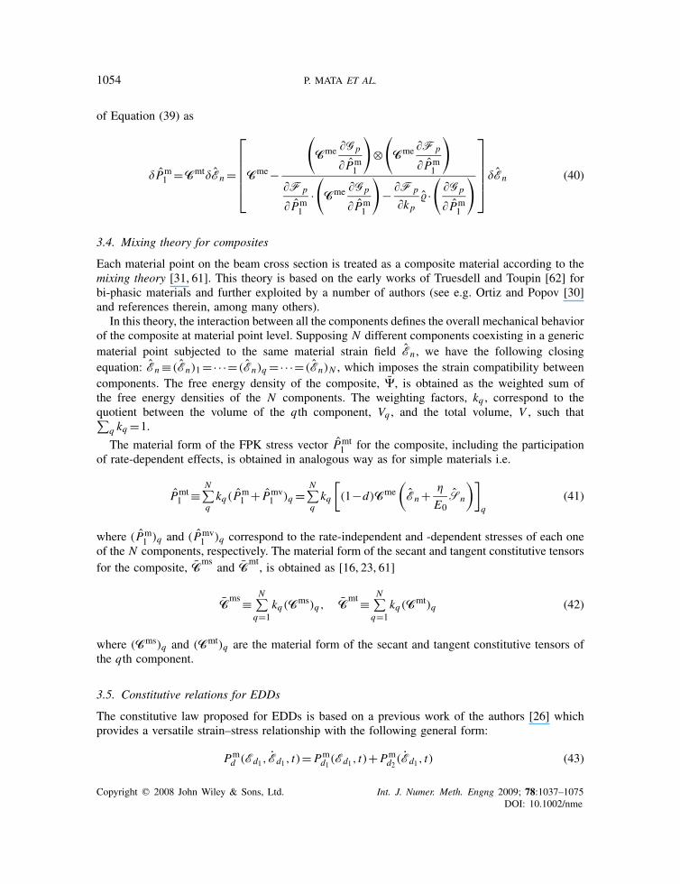
3.5.2. Rate-independent part. The capacity of the model for simulating hardening for strain levelsover 150% (e.g. in the case of elastomer-based devices) is given by an adequate non-linear-elasticbackbone added to the non-viscous hysteretic cycles, as it can be seen in the scheme of Figure 5. Theproposed backbone is defined numerically by means of a polynomial, whose coefficients are fittedto experimental data; for example, for the case of the high damping elastomer of Reference [26]

Figure 5. Non-linear elastic backbone added to the rate-independent part of the constitutive relation.

Copyright q 2008 John Wiley & Sons, Ltd. Int. J. Numer. Meth. Engng 2009; 78:1037–1075DOI: 10.1002/nme

1056 P. MATA ET AL.

the following formula is obtained: Pmhd1

=sgn[Ed1]A0(〈|Ed1 |−A1〉)A2 , where A0, A1 and A2 arescalars obtained from experimental tests.

The response of the non-linear hysteretic spring is obtained solving the following system ofnon-linear differential equations:

Pmd1(Ed1, t) = Ky(E

�d1

, Pm�d )Ed1 +[Ke(E

�d1

, Pm�d )−Ky(E

�d1

, Pm�d )]e (45a)

if Ed1e�0→ e =⎡⎣1−

∣∣∣∣∣ e

dy(E�d1

, Pm�d )

∣∣∣∣∣n(E

�d1

,Pm�d )

⎤⎦ Ed1 (45b)

else→ e = Ed1

where Ky is the post yielding stiffness, Ke the elastic stiffness, dy is the yielding strain of thematerial and e represents an internal variable of plastic (hysteretic) strain, which takes values in therange [−dy,dy]. The parameter n in the associated flow rule of Equation (45c) describes the degreeof smoothness exhibited by the transition zone between the pre and the post yielding branches ofthe hysteretic cycle. The solution procedure solves the system of equations taking into accountthat Ke, Ky, dy, and n are function of the point in the strain–stress space where the last change of

sign of the strain rate has occurred, which is denoted by (E�d1

, Pm�d ) in Equations (45a) and (45c).

Therefore, the proposed algorithm (see [26]) updates the parameters of the model for each changeof sign of the strain rate. If there is no change in the sign of the strain rate, the parameters of themodel are maintained constants. Hardening can be incorporated by means of adding the non-linearelastic backbone Pmh

d1to Equation (45a).

The parameters Ke, Ky, dy, n are non-linear functions of (E�d1

, Pm�d ), i.e.

Ke=℘1(E�d1

, Pm�d ), Ky=℘2(E

�d1

, Pm�d ), dy=℘3(E

�d1

, Pm�d ), n=℘4(E

�d1

, Pm�d ) (46)

Explicit expression for ℘k (k=1, . . . ,4) (in function of (E�d1

, Pm�d )) are determined from experi-

mental data. In any case, it is possible to simulate the mechanical behavior of a wide variety ofdevices, e.g.

• cd =0, ℘1=℘2=constant, ℘3∼∞ and ℘4=1: an elastic spring is obtained. This case corre-sponds to devices designed as re-centering‡‡ elements in structures.

• cd =constant, ℘1=℘2=0, ℘3∼∞ and ℘4=1: a viscous dashpot is obtained. This case canbe found in devices applied to control the effects of wind loads.

• cd =constant, ℘1=℘2=constant, ℘3∼∞ and ℘4=1: Maxwell’s model is obtained. This casecorresponds to a typical viscous device with re-centering mechanism. See Figure 6(a) wherethe loading was defined by sinusoidal path of imposed strains with increasing amplitude upto a maximum value of 2mm/mm (the same applies for the rest of the figures).

‡‡Re-centering forces are considered to be of importance in structures subjected to strong earthquakes. Re-centeringmechanisms help to recover the original configuration of the structure after the seismic action.

Copyright q 2008 John Wiley & Sons, Ltd. Int. J. Numer. Meth. Engng 2009; 78:1037–1075DOI: 10.1002/nme

NON-LINEAR SEISMIC ANALYSIS OF RC STRUCTURES 1057

0 1 2 0 1 2

0

10

20

0 1 2

0

10

20

Strain, mm/mm

0 1 2

Strain, mm/mm

0

20

40

60

Str

ess,

N/m

m2

0

20

40

60

Str

ess,

N/m

m2

(a) (b)

(c) (d)

Figure 6. Examples of EDD’s behaviors: (a) Maxwell model, cd =7, ℘1=℘2=25, ℘3∼∞and ℘4=1; (b) bilinear inviscid plastic model, cd =0, n=1, ℘1=25, ℘2=2.5 and Ey=0.5;(c) non-linear dashpot, cd =7, Kc=2.1, ℘1=℘2=25, ℘3∼∞ and ℘4=1; and (d) rubbermodel, ℘1=−34.9267+217.7Ed1 −530.1(Ed1)

2+655.1(Ed1)3−451.3(Ed1)

4+176.7(Ed1)5

−39.7(Ed1)6+26.6(Ed1)

7, ℘2=2.5, Pmhd1

=sign(E�d1

)∗8∗(|E�d1

|−1.25)5 (if E�d1

>1.35).

• cd =constant, ℘1�℘2>0, n∈[1,100] and Ey>0: a visco-plastic device can be simulated(assuming uncoupled Maxwell’s viscosity). Particularly, if cd =℘2=0 and n=1 a bilinearperfectly plastic model is obtained. See Figure 6(b).

• cd =(Ed1)Kc (0<Kc<1), ℘1=℘2=0, ℘3∼∞ and ℘4=1: a non-linear viscous dashpot is

obtained. Some modern viscous devices employ modern valves’s systems that produces thenon-linear force–velocity curve with a saturation level (see e.g. [4] Chapter 6 and Figure 6(c).

• In the case of devices made of high damping elastomers (such as those considered inReference [26]) it is possible to consider: cd =constant, ℘1=∑Nc

k=0 Ak(E�d1

)k , Ak =constant,∀k=(1 . . .Nc); the post-yielding stiffness function, ℘2, is maintained constant. The analyticalexpression of ℘3 is ℘3=(|Pm�

d |−|Pm�0 −Pm�

d |)/(℘2−℘1); where Pm�0 is a parameter calcu-

lated evaluating the line with slope ℘2 at zero strain level. The function ℘4 can be taken℘4≈1 (see Figure 6(d)).

More complex material behaviors, such as those of other types of rubber or smart-based devices,can be simulated by means of providing suitable functions for the parameters of the model (seeEquation (46)).

Copyright q 2008 John Wiley & Sons, Ltd. Int. J. Numer. Meth. Engng 2009; 78:1037–1075DOI: 10.1002/nme

1058 P. MATA ET AL.

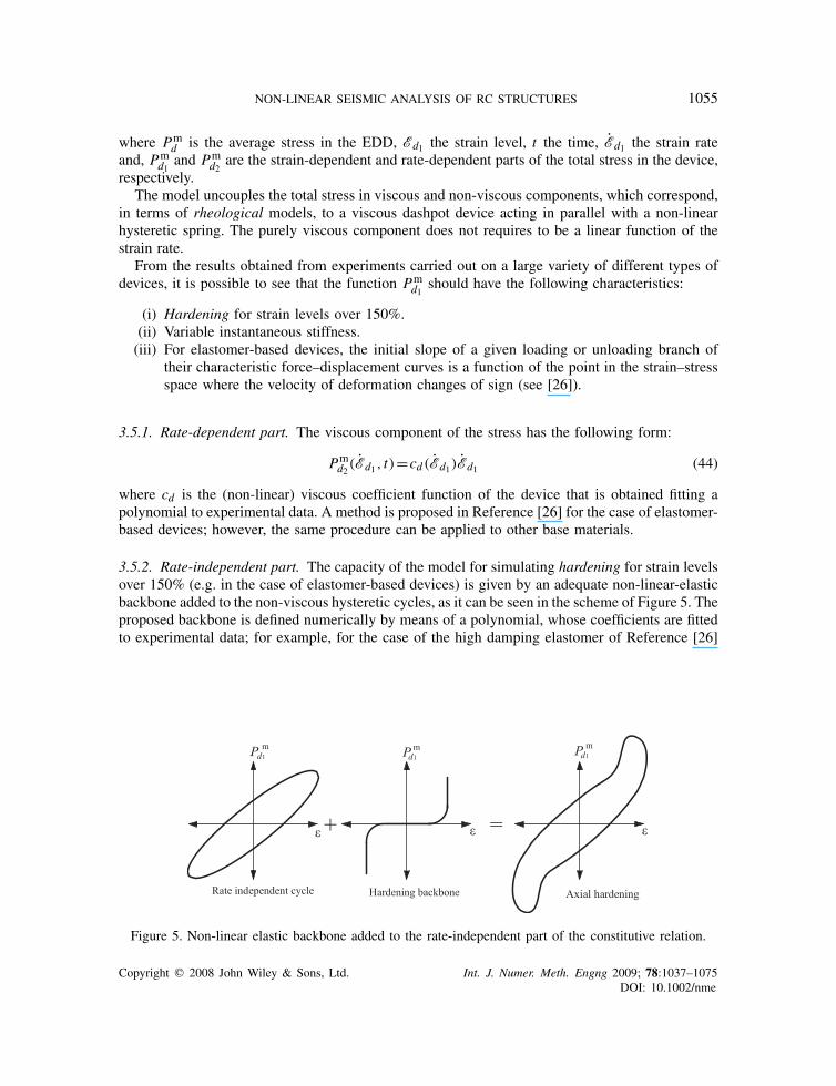
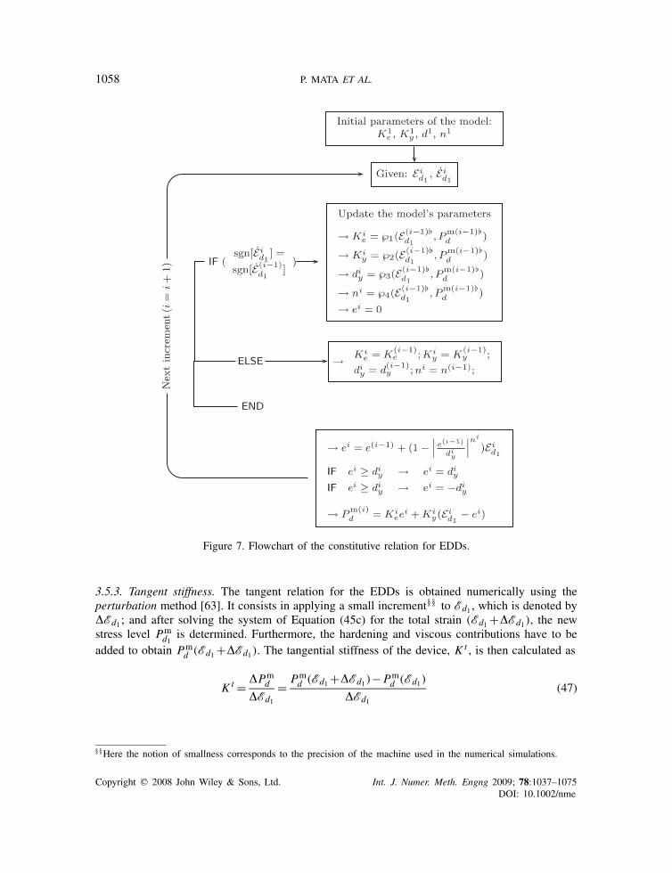
Figure 7. Flowchart of the constitutive relation for EDDs.

3.5.3. Tangent stiffness. The tangent relation for the EDDs is obtained numerically using theperturbation method [63]. It consists in applying a small increment§§ to Ed1 , which is denoted by�Ed1 ; and after solving the system of Equation (45c) for the total strain (Ed1 +�Ed1), the newstress level Pm

d1is determined. Furthermore, the hardening and viscous contributions have to be

added to obtain Pmd (Ed1 +�Ed1). The tangential stiffness of the device, K t , is then calculated as

K t = �Pmd

�Ed1= Pm

d (Ed1 +�Ed1)−Pmd (Ed1)

�Ed1(47)

§§Here the notion of smallness corresponds to the precision of the machine used in the numerical simulations.

Copyright q 2008 John Wiley & Sons, Ltd. Int. J. Numer. Meth. Engng 2009; 78:1037–1075DOI: 10.1002/nme

NON-LINEAR SEISMIC ANALYSIS OF RC STRUCTURES 1059

It is important to note that the sign of the perturbation has to be the same as Ed1 in order to obtaina tangential stiffness consistent with the sign of the loading process in the device, when cyclicactions are considered.

3.5.4. Integration algorithm. The numerical algorithm starts by assigning an initial values to theparameters of the model. For each strain level, Ei

d1, the algorithm verifies if the strain rate changes

of sign. If this is the case, an updating procedure for the parameters ℘k (k=1, . . . ,4) is carriedout. On the contrary, the parameters are maintained. Then, plastic strain, stress and the tangentialrelation are estimated. The flow-chart of the algorithm is shown in Figure 7.

4. NUMERICAL IMPLEMENTATION

In order to obtain a Newton-type numerical solution, the linearized part of the weak form ofEquation (7) is required, which can be written as

L[Gw(�∗,K∗, h)]=Gw(�∗,K∗, h)+DGw(�∗,K∗, h) · p (48)

where L[Gw(�∗,K∗, h)] is the linear part of the functional Gw(�,K, h) at the configurationdefined by (�,K)=(�∗,K∗) and p≡(��,�) is an admissible variation. The term Gw∗ suppliesthe unbalanced force vector obtained adding the contributions of the inertial, external and internalterms; and DGw∗ · p, gives the tangential stiffness [27].

On the one hand, the linearization of the inertial and external components, G inew and Gext

w , yieldsthe inertial and load-dependent parts of the tangential stiffness, KI∗ and KP∗, respectively; and theycan be consulted in [25, 27]. On the other hand, the linearization of the internal term is obtainedas [16, 23]

DG intw∗ · p=

∫ L

0hT(BT∗��−nS∗ p)dS (49)

where ��T=[�nT∗�mT∗ ], the operator nS∗ contributes to the geometric part of the tangent stiffnessand B∗ relates h and the co-rotated variation of the strain vectors. Explicit expression for B andnS∗ can be found in References [16, 27, 28], respectively.

The computation of �� appearing in Equation (49) requires taking into account the linearizedrelation between Pm

1 and En . After integrating over the beam cross section, the following resultis obtained:

��=(CsvB∗−F) p (50)

where Csv is the spatial form of the cross-sectional tangent constitutive tensor depending onthe material properties and F is the stress-dependent tensor (see [16, 23] for details). Finally,Equation (50) allows to rewrite Equation (49) as

DG intw · p=

∫ L

0hTBT∗Cst∗B∗ pdS+

∫ L

0hT(nS∗−BT∗ F∗) pdS=KM∗+KG∗ (51)

Copyright q 2008 John Wiley & Sons, Ltd. Int. J. Numer. Meth. Engng 2009; 78:1037–1075DOI: 10.1002/nme

1060 P. MATA ET AL.

where KG∗, KM∗, evaluated at (�∗,K∗), give the geometric and material parts of the tangentstiffness, which allows to rewrite Equation (48) as

L[G∗]=Gw∗+KI∗+KM∗+KV∗+KG∗+KP∗ (52)

The solution of the discrete form of Equation (51) by using the finite element method follows anidentical procedure as that described in [27] for an iterative Newton–Raphson integration schemeand it will not be discussed here.

Newmark’s implicit time-stepping algorithm has been chosen as integration method followingthe development originally proposed by Simo and Vu-Quoc [25]. For the rotational part, thetime-stepping procedure takes place in SO(3) and the basic steps, as well as the iterative updatealgorithm for the strain and strain rate vectors, are given in Reference [23].Remark 4Recently, the attention of the research community has been directed toward energy–momentum-conserving time-stepping schemes. Some algorithms has been developed for inelastic materialsinheriting conservative properties in the elastic range. In particular, Armero [64] presents an algo-rithm for multiplicative plasticity at finite strains that recovers the energy–momentum-conservingproperties in the elastic range. In Reference [65] Noels et al., propose a modification of the varia-tional updates framework to introduce numerical dissipation for high-frequency modes, leading to aenergy-dissipative momentum-conserving algorithm for elastoplasticity. In the case of elastic struc-tural elements with large rotations, it is possible to consult [66] and more recently [67]; however,in this last case, the conservative properties do not have been extended to the inelastic range.

5. CROSS-SECTIONAL ANALYSIS AND DAMAGE INDICES

5.1. Cross-sectional analysis

The cross-sectional analysis is carried out by expanding each integration point of the beam axisin a set of integration points located onto the cross section. Then, the cross sections are meshedinto a grid of quadrilaterals, each of them corresponding to a fiber oriented along the beam axis.The geometry of each quadrilateral is described by means of normalized bi-dimensional shapefunctions and several integration points can be specified according to a specific integration rule.The average value of a quantity, [·], for example the components of FPK stress vector or thetangential tensor existing on a quadrilateral, are

[·]= 1

Ac

∫[·]dAc= 1

Ac

Np∑p=1

Nq∑q=1

[·](yp, zq)JpqWpq (53)

where Ac is the area of the quadrilateral, Np and Nq are the number of integration points in thetwo directions of the normalized geometry, [·](yp, zq) is the value of the quantity [·] existing ona integration point with coordinates (yp, zq) with respect to the reference beam axis, Jpq is theJacobian of the transformation between normalized coordinates and cross-sectional coordinatesand Wpq are the weighting factors. Two additional integration loops are required. The first oneruns over the quadrilaterals and the second loop runs over each simple material associated withthe composite of the quadrilateral. More details can be consulted in [16, 23].

Copyright q 2008 John Wiley & Sons, Ltd. Int. J. Numer. Meth. Engng 2009; 78:1037–1075DOI: 10.1002/nme

NON-LINEAR SEISMIC ANALYSIS OF RC STRUCTURES 1061

5.2. Damage indices

A measure of the damage level of a material point can be obtained as the ratio of the existing stresslevel to its elastic counterpart. Following this idea, it is possible to define the fictitious damagevariable D as [51]

3∑i=1

|Pm1i |=(1− D)

3∑i=1

|Pm1i0|→ D=1−

∑3i=1 |Pm

1i |∑3i=1 |Pm

1i0|(54)

where |Pm1i | and |Pm

1i0| are the absolute values of the components of the existing and elastic stress

vectors, respectively. Initially, the material remains elastic and D=0, but when all the energyof the material has been dissipated |Pm

1i |→0 and D→1. Equation (54) can be extended toconsider elements or even the whole structure by means of integrating over a finite volume asfollows:

D=1−∫Vp

(∑i |Pm

1i |)dVp∫

Vp

(∑i |Pm

1i0|)dVp

(55)

where Vp is the volume of the part of the structure. Equation (55) is easily implemented in anstandard finite element method code without requiring large extra memory storage.

6. NUMERICAL EXAMPLES

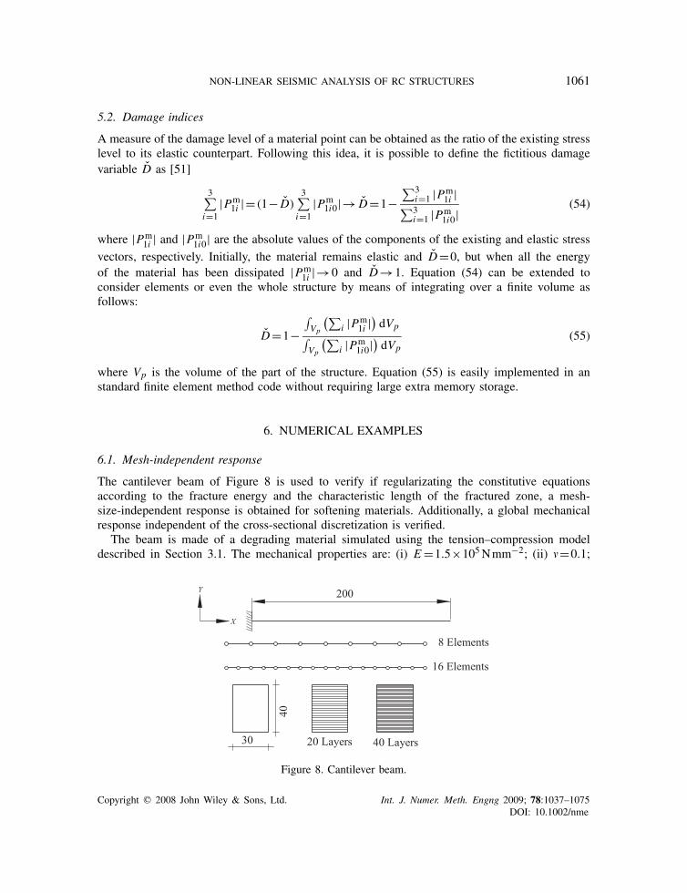
6.1. Mesh-independent response

The cantilever beam of Figure 8 is used to verify if regularizating the constitutive equationsaccording to the fracture energy and the characteristic length of the fractured zone, a mesh-size-independent response is obtained for softening materials. Additionally, a global mechanicalresponse independent of the cross-sectional discretization is verified.

The beam is made of a degrading material simulated using the tension–compression modeldescribed in Section 3.1. The mechanical properties are: (i) E=1.5×105Nmm−2; (ii) =0.1;

Figure 8. Cantilever beam.

Copyright q 2008 John Wiley & Sons, Ltd. Int. J. Numer. Meth. Engng 2009; 78:1037–1075DOI: 10.1002/nme

1062 P. MATA ET AL.

0 10 20

0

0.5

1

1.5

x 104

Displacement, mm

Ver

tical

rea

ctio

n, N

0 10

0

1

2

3

x 106

Displacement, mm

Mom

ent r

eact

ion,

N–

mm

8E40L8E20L16E40L16E20L

8E40L8E20L16E40L16E20L

(a) (b)

Stiffness recovery Stiffness recovery

Figure 9. Mesh-independent response: (a) vertical displacement versus vertical reaction and (b) verticaldisplacement versus moment reaction.

(iii) f −0 =500Nmm−2; (iv) f +

0 =250Nmm−2; (v) G−f =500Nmm−2 (G+

f =125Nmm−2);(vi) K =1. An imposed displacement was applied on the free end in the Y direction. The loadingpath was the following: 20 steps of 1mm and then 60 steps of the same magnitude in the oppositedirection.

Four discretizations were used: (1) Eight linear elements along the beam axis and 20 layers inthe cross section. This case is denoted as 8E20L; (2) Eight linear elements along the beam axis and40 layers in the cross section (case 8E40L); (3) Sixteen linear elements along the beam axis and 20layers in the cross section (case 16E20L); (4) Sixteen linear elements along the beam and 40 layersin the cross section (case 16E40L) (see Figure 8). The Gauss integration rule was considered in thesimulations. The length of the fractured zone corresponds to the characteristic length associatedwith the integration point.

Figures 9(a) and (b) show two capacity curves relating the vertical reaction and moment reactionwith the vertical displacement of the free end, respectively. It is possible to see that the numericalresponses are almost the same for the four cases considered, confirming thus the independencyof the global mechanical response with the number of elements and the specific discretizationof the cross section. It is possible to appreciate the fact that the independency between tensileand compressive degradations produces the stiffness recovery phenomenon in the global responsewhen reverse loading paths are applied.

Figures 10(a)–(c) show the time evolution of the strain–stress relations for three cases: (a) TheEn1–Pm

11 relation obtained from the upper layer of the cross-sectional discretization. (b) Idem asin (a) but obtained from the bottom cross-sectional layer. (c) The (shear) strain–stress relationEn3–Pm

13 obtained from the layer located immediately over the geometrical center of the crosssection. From these figures, it is clear that the obtained strain–stress relations strongly depend onthe size of elements (as expected), but that the number of layers of the cross-sectional discretizationhas a minor significance.

Therefore, it is possible to affirm that regularizing the strain–stress relation according to thespecific fracture energy and the characteristic length of the fractured zone (characteristic meshsize), the purpose of obtaining a mesh-independent response at global level is obtained, even whenthe post-yielding strain–stress relations become mesh dependent.

Copyright q 2008 John Wiley & Sons, Ltd. Int. J. Numer. Meth. Engng 2009; 78:1037–1075DOI: 10.1002/nme

NON-LINEAR SEISMIC ANALYSIS OF RC STRUCTURES 1063

0 0.1 0.2

0

100

200

Pm 11

, upp

er la

yer

Pm 11

, bot

tom

laye

r

Pm 11

, mid

dle

laye

r

0 0.2 0.4

0

100

200

0 0.1 0.2

0

50

100

150

200

250

εn3, middle layerεn1, upper layer εn1, bottom layer(a) (b) (c)

8E40L8E20L16E40L16E20L

8E40L8E20L16E40L16E20L

8E40L8E20L16E40L16E20L

Figure 10. (a) Evolution of the En1–Pm11 relation in the upper layer of the cross section; (b) evolution of

the En1–Pm11 relation in the bottom layer of the cross section; and (c) evolution of the En3–Pm

13 relationin the layer of the middle of the cross section.

6.2. Experimental–numerical comparative study of a scaled RC building model

This example corresponds to the comparison between the numerical simulation obtained by meansof the proposed formulation and the experimental data obtained by Lu [68] for the seismic analysisof a scaled model (1:5.5) of a regular bare frame. The structure was designed for a ductility classmedium in accordance with the Eurocode 8 [69] with a peak ground acceleration of 0.3g and soilprofile A.

The material properties are: (i) Concrete class C20 with an elastic modulus of Ec=2×104Nmm−2, Poisson coefficient c=0.2, characteristic compressive strength f −

c =20Nmm−2

( f +c =2Nmm−2 and K =1), fracture energy G−

c =10Nmm−2 (G+c =1Nmm−2), mass density

�c=2.4×10−9Kgmm−3 and fluidity �+ =1500s−1, �− =5×104 s−1 (a± =1) and (ii) Flexuralreinforcement Grade S400, Es=2.1×105Nmm−2, s=0.3, f ±

s =400Nmm−2 (K =1), G±s =

100Nmm−2, �s=7.8×10−9Kgmm−3 and �± =5000s−1 (a± =1). Other details such as loads,geometry and distribution of steel reinforcements can be consulted in the same publication. In theexperimental program, the structure was subjected to several scaled versions of the N–S componentof the El Centro 1940 earthquake record.

Four quadratic elements with two Gauss integration points were used for each beam and column.Cross sections where meshed into a grid of 20 equally spaced layers. Longitudinal steel reinforce-ments were included in the external layers as part of a composite material. The fracture energyof the damage model used for concrete was modified to take into account the confining effectof transversal stirrups [16]. In the numerical simulations, the model is subjected to a pushoveranalysis. Static forces derived from the inertial contribution of the masses are applied at the floorlevels considering an inverted triangular distribution.

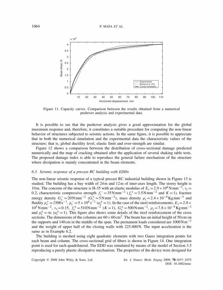
A relationship between the measured base shear and the top lateral displacement is given inReference [68] for each seismic record. This curve is compared in Figure 11 with the capacitycurve obtained by means of using the numerical pushover analysis. Additionally, the result obtainedfrom a numerical simulation presented by the authors in [70] using an alternative damage modelis given as well.

Copyright q 2008 John Wiley & Sons, Ltd. Int. J. Numer. Meth. Engng 2009; 78:1037–1075DOI: 10.1002/nme

1064 P. MATA ET AL.

10 20 30 40 50 60 70 80 90 100 1100

0.5

1

1.5

2

2.5

3

3.5

4

x 104

Horizontal displacement, mm

Bas

e sh

ear,

N

ExperimentalBarbat et al. [70]Current simulation

Figure 11. Capacity curves. Comparison between the results obtained from a numericalpushover analysis and experimental data.

It is possible to see that the pushover analysis gives a good approximation for the globalmaximum response and, therefore, it constitutes a suitable procedure for computing the non-linearbehavior of structures subjected to seismic actions. In the same figure, it is possible to appreciatethat in both the numerical simulation and the experimental data the characteristic values of thestructure; that is, global ductility level, elastic limit and over-strength are similar.

Figure 12 shows a comparison between the distribution of cross-sectional damage predictednumerically and the map of cracking obtained after the application of several shaking table tests.The proposed damage index is able to reproduce the general failure mechanism of the structurewhere dissipation is mainly concentrated in the beam elements.

6.3. Seismic response of a precast RC building with EDDs

The non-linear seismic response of a typical precast RC industrial building shown in Figure 13 isstudied. The building has a bay width of 24m and 12m of inter-axes length. The storey height is10m. The concrete of the structure is H-35 with an elastic modulus of Ec=2.9×104Nmm−2, c=0.2, characteristic compressive strength f −

c =35Nmm−2 ( f +c =3.5Nmm−2 and K =1), fracture

energy density G−c =20Nmm−2 (G+

c =5Nmm−2), mass density �c=2.4×10−9Kgmm−3 andfluidity �+

c =1500s−1, �−c =5×104 s−1 (a±

c =1). In the case of the steel reinforcements, Es=2.0×105Nmm−2, s=0.15, f ±

s =510Nmm−2 (K =1), G±s =500Nmm−2, �s=7.8×10−9Kgmm−3

and �±s =∞ (a±

s =1). This figure also shows some details of the steel reinforcement of the crosssections. The dimensions of the columns are 60×60cm2. The beam has an initial height of 50cm onthe supports and 140cm in the middle of the span. The permanent loads considered are 1000Nm−2

and the weight of upper half of the closing walls with 225.000N. The input acceleration is thesame as in Example 6.2.

The building is meshed using eight quadratic elements with two Gauss integration points foreach beam and column. The cross-sectional grid of fibers is shown in Figure 14. One integrationpoint is used for each quadrilateral. The EDD was simulated by means of the model of Section 3.5reproducing a purely plastic dissipative mechanism. The properties of the device were designed for

Copyright q 2008 John Wiley & Sons, Ltd. Int. J. Numer. Meth. Engng 2009; 78:1037–1075DOI: 10.1002/nme

NON-LINEAR SEISMIC ANALYSIS OF RC STRUCTURES 1065

(a) (b)

Figure 12. Damage: (a) map of fissures obtained from experimental dataand (b) numerical: cross-sectional damage index.

Figure 13. Description of the structure.

obtaining a yielding force of 200000N for a relative displacement between the two end nodes of1.2mm. Hardening or viscous effects were not considered. The length of the devices was of 3.1m.

First, a set of pushover analyses is performed considering the following cases: (i) The bare frameunder small displacements assumption; (ii) The bare frame in finite deformation; (iii) The framewith EDDs and small deformation; (iv) Idem as (iii) but with finite deformation. The purpose isto establish clearly the importance of considering second-order effect coupled with inelasticity inthe study of flexible structures.

Figure 15(a) shows the capacity curves obtained for the four mentioned cases. In this figure itis possible to see that for both, the passively controlled and uncontrolled cases, the small strain

Copyright q 2008 John Wiley & Sons, Ltd. Int. J. Numer. Meth. Engng 2009; 78:1037–1075DOI: 10.1002/nme

1066 P. MATA ET AL.

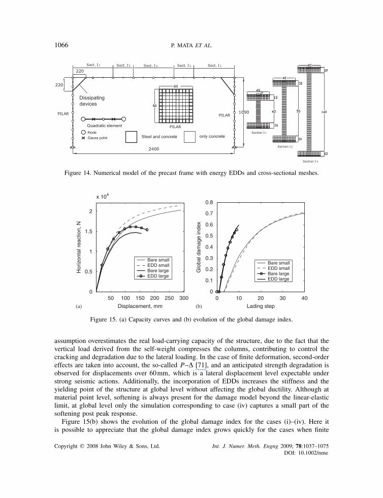
Figure 14. Numerical model of the precast frame with energy EDDs and cross-sectional meshes.

50 100 150 200 250 3000

0.5

1

1.5

2

x 104

Displacement, mm

Hor

izon

tal r

eact

ion,

N

Bare smallEDD smallBare largeEDD large

0 10 20 30 400

0.1

0.2

0.3

0.4

0.5

0.6

0.7

0.8

Lading step

Glo

bal d

amag

e in

dex

Bare smallEDD smallBare largeEDD large

(a) (b)

Figure 15. (a) Capacity curves and (b) evolution of the global damage index.

assumption overestimates the real load-carrying capacity of the structure, due to the fact that thevertical load derived from the self-weight compresses the columns, contributing to control thecracking and degradation due to the lateral loading. In the case of finite deformation, second-ordereffects are taken into account, the so-called P–� [71], and an anticipated strength degradation isobserved for displacements over 60mm, which is a lateral displacement level expectable understrong seismic actions. Additionally, the incorporation of EDDs increases the stiffness and theyielding point of the structure at global level without affecting the global ductility. Although atmaterial point level, softening is always present for the damage model beyond the linear-elasticlimit, at global level only the simulation corresponding to case (iv) captures a small part of thesoftening post peak response.

Figure 15(b) shows the evolution of the global damage index for the cases (i)–(iv). Here itis possible to appreciate that the global damage index grows quickly for the cases when finite

Copyright q 2008 John Wiley & Sons, Ltd. Int. J. Numer. Meth. Engng 2009; 78:1037–1075DOI: 10.1002/nme

NON-LINEAR SEISMIC ANALYSIS OF RC STRUCTURES 1067

1 2 3 4 5 6 7 8

050

100150

Dis

plac

emen

t, m

m

Bare frameEDDs

3 3.5 4 4.5 5 5.5

0

100

Bare frameEDDs

2.5 3 3.5 4 4.5

0

500

1000

Time, s

Acc

eler

atio

n, m

ms–

2V

eloc

ity, m

ms

–2

Bare frameEDDs

168.872.7

(a)

(b)

(c)

Figure 16. Time history responses of the top beam–column joint: (a) horizontaldisplacement; (b) velocity; and (c) acceleration.

deformation is considered and the benefits of adding EDDs are not visible due to the fact that thepushover analysis does not takes into account the effects of energy dissipation.

The results of the numerical simulations in the dynamic range allow seeing that the use of plasticEDDs contributes to improve the seismic behavior of the structure for the case of the employedacceleration record. Figure 16 shows the time history response of the horizontal displacement,velocity and acceleration of the upper beam–column joint for the uncontrolled and the controlledcases. A reduction of approximately 57.5% is obtained for the maximum lateral displacementwhen compared with the bare frame. Acceleration and velocity are controlled in the same way,but only 24.3 and 7.0% of reduction is obtained, respectively. A possible explanation for thelimited effectiveness of the EDD is that the devices only contribute to increase the ductility of thebeam–column joint without alleviating the base shear demand due to the dimensions of the deviceand its location in the structure.

Figure 17 shows the evolution of the global damage index. It is possible to see that the damageindex grows quickly and reaching higher values for the non-controlled case, confirming the benefitsobtained from the use of EDDs.

It is worth noting that with the present formulation the need of using specific cross-sectionalconstitutive laws depending on the cross-sectional shape and the distribution of steel reinforcementsis completely avoided (compare with [17, 19]). On the contrary, the constitutive relations arededuced using the cross-sectional integration procedure described in Section 5. Moreover, comparedwith other fiber models, [20], the coupling between stress components of thermodynamically

Copyright q 2008 John Wiley & Sons, Ltd. Int. J. Numer. Meth. Engng 2009; 78:1037–1075DOI: 10.1002/nme

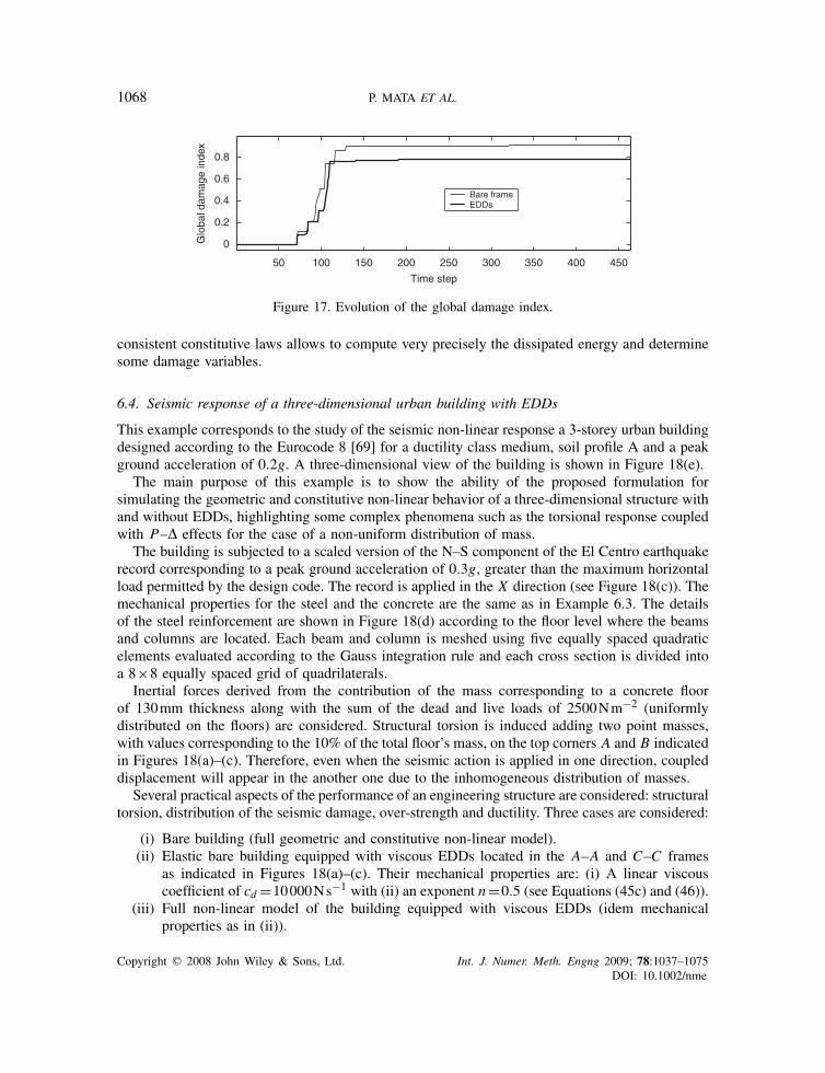
1068 P. MATA ET AL.

50 100 150 200 250 300 350 400 450

0

0.2

0.4

0.6

0.8

Time step

Glo

bal d

amag

e in

dex

Bare frameEDDs

Figure 17. Evolution of the global damage index.

consistent constitutive laws allows to compute very precisely the dissipated energy and determinesome damage variables.

6.4. Seismic response of a three-dimensional urban building with EDDs

This example corresponds to the study of the seismic non-linear response a 3-storey urban buildingdesigned according to the Eurocode 8 [69] for a ductility class medium, soil profile A and a peakground acceleration of 0.2g. A three-dimensional view of the building is shown in Figure 18(e).

The main purpose of this example is to show the ability of the proposed formulation forsimulating the geometric and constitutive non-linear behavior of a three-dimensional structure withand without EDDs, highlighting some complex phenomena such as the torsional response coupledwith P–� effects for the case of a non-uniform distribution of mass.

The building is subjected to a scaled version of the N–S component of the El Centro earthquakerecord corresponding to a peak ground acceleration of 0.3g, greater than the maximum horizontalload permitted by the design code. The record is applied in the X direction (see Figure 18(c)). Themechanical properties for the steel and the concrete are the same as in Example 6.3. The detailsof the steel reinforcement are shown in Figure 18(d) according to the floor level where the beamsand columns are located. Each beam and column is meshed using five equally spaced quadraticelements evaluated according to the Gauss integration rule and each cross section is divided intoa 8×8 equally spaced grid of quadrilaterals.

Inertial forces derived from the contribution of the mass corresponding to a concrete floorof 130mm thickness along with the sum of the dead and live loads of 2500Nm−2 (uniformlydistributed on the floors) are considered. Structural torsion is induced adding two point masses,with values corresponding to the 10% of the total floor’s mass, on the top corners A and B indicatedin Figures 18(a)–(c). Therefore, even when the seismic action is applied in one direction, coupleddisplacement will appear in the another one due to the inhomogeneous distribution of masses.

Several practical aspects of the performance of an engineering structure are considered: structuraltorsion, distribution of the seismic damage, over-strength and ductility. Three cases are considered:

(i) Bare building (full geometric and constitutive non-linear model).(ii) Elastic bare building equipped with viscous EDDs located in the A–A and C–C frames

as indicated in Figures 18(a)–(c). Their mechanical properties are: (i) A linear viscouscoefficient of cd =10000Ns−1 with (ii) an exponent n=0.5 (see Equations (45c) and (46)).

(iii) Full non-linear model of the building equipped with viscous EDDs (idem mechanicalproperties as in (ii)).

Copyright q 2008 John Wiley & Sons, Ltd. Int. J. Numer. Meth. Engng 2009; 78:1037–1075DOI: 10.1002/nme

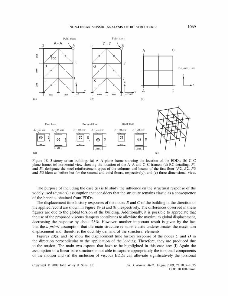
NON-LINEAR SEISMIC ANALYSIS OF RC STRUCTURES 1069

(a)

(d) (e)

(b) (c)

Figure 18. 3-storey urban building: (a) A–A plane frame showing the location of the EDDs; (b) C–Cplane frame; (c) horizontal view showing the location of the A–A and C–C frames; (d) RC detailing. P1and B1 designate the steel reinforcement types of the columns and beams of the first floor (P2, B2, P3and B3 idem as before but for the second and third floors, respectively); and (e) three-dimensional view.

The purpose of including the case (ii) is to study the influence on the structural response of thewidely used (a priori) assumption that considers that the structure remains elastic as a consequenceof the benefits obtained from EDDs.

The displacement time history responses of the nodes B and C of the building in the direction ofthe applied record are shown in Figure 19(a) and (b), respectively. The differences observed in thesefigures are due to the global torsion of the building. Additionally, it is possible to appreciate thatthe use of the proposed viscous dampers contributes to alleviate the maximum global displacement,decreasing the response by about 25%. However, another important result is given by the factthat the a priori assumption that the main structure remains elastic underestimates the maximumdisplacement and, therefore, the ductility demand of the structural elements.

Figures 20(a) and (b) show the displacement time history response of the nodes C and D inthe direction perpendicular to the application of the loading. Therefore, they are produced dueto the torsion. The main two aspects that have to be highlighted in this case are: (i) Again theassumption of a linear bare structure is not able to capture appropriately the torsional componentsof the motion and (ii) the inclusion of viscous EDDs can alleviate significatively the torsional

Copyright q 2008 John Wiley & Sons, Ltd. Int. J. Numer. Meth. Engng 2009; 78:1037–1075DOI: 10.1002/nme

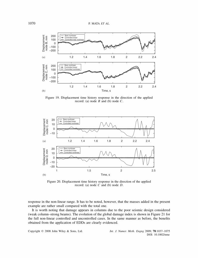
1070 P. MATA ET AL.

0100200

Dis

plac

emen

tno

de B

, mm

1.2 1.4 1.6 1.8 2 2.2 2.4

1.2 1.4 1.6 1.8 2 2.2 2.4

0100200

Time, s

Dis

plac

emen

t n

ode

C, m

m Bare nonlinearControlled linearControlled nonlinear

Bare nonlinearControlled linearControlled fully nonlinear

(a)

(b)

Figure 19. Displacement time history response in the direction of the appliedrecord: (a) node B and (b) node C .

1.2 1.4 1.6 1.8 2 2.2 2.4

0

10

20

Dis

plac

emen

t n

ode

C, m

m

Bare nonlinearControlled linearControlled nonlinear

1 1.5 2 2.5

0

10

20

Time, s

Dis

plac

emen

tno

de D

, mm

Bare nonlinearControlled linearControlled nonlinear

(a)

(b)

Figure 20. Displacement time history response in the direction of the appliedrecord: (a) node C and (b) node D.

response in the non-linear range. It has to be noted, however, that the masses added in the presentexample are rather small compared with the total one.

It is worth noting that damage appears in columns due to the poor seismic design considered(weak column–strong beams). The evolution of the global damage index is shown in Figure 21 forthe full non-linear controlled and uncontrolled cases. In the same manner as before, the benefitsobtained from the application of EDDs are clearly evidenced.

Copyright q 2008 John Wiley & Sons, Ltd. Int. J. Numer. Meth. Engng 2009; 78:1037–1075DOI: 10.1002/nme

NON-LINEAR SEISMIC ANALYSIS OF RC STRUCTURES 1071

0 0.5 1 1.5 2 2.5 30

0.1

0.2

0.3

0.4

0.5

0.6

0.7

Time, s

Glo

bal d

amag

e in

dex

BareViscous EDDs

Figure 21. Time history response of the global damage index.

7. CONCLUSIONS

In this work, a geometrically exact formulation for initially curved and twisted beams has beenextended for considering arbitrary distributions of rate-dependent inelastic composite materials onthe cross sections in the static and dynamic (even seismic) cases. The consistent linearization ofthe weak form of the momentum balance equations considers the constitutive non-linearity withrate-dependent effects. The resulting model is implemented in a displacement-based finite elementcode. An iterative Newton–Raphson scheme is used for the solution of the time-discrete versionof the linearized problem. A specific finite element for EDDs is developed based on the beammodel, but releasing the rotational degrees of freedom.

Each material point of a cross section is assumed to be composed of several simple materialswith their own constitutive laws. Thermodynamically consistent versions of the plasticity andthe tensile-compressive damage models are developed, which consider full interaction amongthe components of the FPK stress vector. The mixing rule is used for describing the resultingcomposite. Viscosity is included at constitutive level by means of an adequate regularization of theevolution equations of the damage thresholds, avoiding ad hoc formulations such as the so-calledRayleigh’s method (see [72]). A versatile model is proposed for the force–displacement relation ofthe EDDs. Calibrating the model’s parameters it is possible to simulate a wide variety of dissipativemechanisms.

From the numerical point of view, beam cross sections are meshed into a grid of quadrilateralscorresponding to fibers directed along the beam axis. Then, in each integration point, two additionalintegration loops are required to obtain the reduced cross-sectional forces, moments and tangentialtensors. The present approach avoids the formulation of constitutive laws in terms of cross-sectionalquantities, which in most of the cases are valid for specific geometries and the thermodynamicbasis of the constitutive laws are, in general, violated. Moreover, the shear components of the stressare determined from the inelastic constitutive laws and, therefore, they are not deduced from theelemental equilibrium as in the case of other fiber models [20]. Local and global damage indiceshave been developed based on the ratio between the non-linear stresses and their visco elasticcounterparts. They constitute a measure of the degradation level and, therefore, of the dissipatedenergy.

The present formulation is validated by means of a set of numerical examples, which includesthe comparison with existing experimental data and the study of the seismic response of precastand cast in place RC structures equipped with EDDs. Several rather complex phenomenon can

Copyright q 2008 John Wiley & Sons, Ltd. Int. J. Numer. Meth. Engng 2009; 78:1037–1075DOI: 10.1002/nme

1072 P. MATA ET AL.

be reproduced: (i) The coupling between geometric and constitutive non-linearity (P–� effects)in the static and dynamic ranges; (ii) The full non-linear dynamic torsional response for struc-tures presenting non-coincident elasticity and mass centers subjected to seismic loadings; (iii)The numerical simulation and evaluation (in terms of the evolution of damage indices) of theeffectiveness of using passive EDDs for improving the dynamic response of RC buildings.

The use of EDDs appears as a convenient technique for controlling the dynamic behavior ofRC structures subjected to earthquake loading; however, for strong seismic actions an appreciablelevel of damage can also be produced in the main structural elements; therefore, this aspect shouldbe considered when designing passively controlled structures.

ACKNOWLEDGEMENTS

This research was partially supported by the European Commission, CEE–FP6 Project FP6-50544(GOCE)‘Risk Mitigation for Earthquakes and Landslides (LESSLOSS)’; by the Spanish Government (Ministeriode Educacion y Ciencia), project BIA2003-08700-C03-02 ‘Numerical simulation of the seismic behaviorof structures with energy dissipation devices’, project BIA2005-06952 ‘Study of composite materials fordesign, reinforcement and retrofit of civil engineering structures (RECOMP)’; and by the collaborationframework between CIMNE and AIRBUS, project PBSO-13-06 ‘Innovative finite element methods fornon-linear analysis of composite structures (FEMCOM)’. All this support is gratefully acknowledged.

REFERENCES

1. Hanson RD, Aiken ID, Nims DK, Ritchter PJ, Batchman RE. State of the art and state of the practice in seismicengineering dissipation. Proceedings, ATC-17-1 Seminar on Seismic Isolation, Passive Energy Dissipation andActive Control, Applied Technology Council, San Francisco, CA, March 1993.

2. Pampanin S, Calvi GM, Moratti M. Seismic behavior of RC beam–column joints designed for gravity only.Twelfth European Conference on Earthquake Engineering, London, 9–13 September 2002. Paper Reference 726.

3. Reinhorn AM, Constantinou MC, Li C. Use of supplemental damping devices for seismic strengthening of lightlyreinforced concrete frames. Proceedings, Workshop on the Seismic Rehabilitation of Lightly Reinforced ConcreteFrames, Gaithersburg, MD, 12–13 June 1995.

4. Soong TT, Dargush GF. Passive Energy Dissipation Systems in Structural Engineering. Wiley: New York, 1997.5. Fu Y, Kasai K. Comparative study of frames using viscoelastic and viscous dampers. Journal of Structural

Engineering 1998; 124(5):513–522.6. Kasai K, Fu Y, Watanabe A. Passive control systems for seismic damage mitigation. Journal of Structural

Engineering 1998; 124(5):501–512.7. Aiken I. Passive energy dissipation hardware and applications. Proceedings, Los Angeles County and Seaosc

Symposium on Passive Energy Dissipation Systems for New and Existing Buildings, Los Angeles, July 1996.8. Lin YY, Chang KC. Study on damping reduction factors for buildings under earthquake ground motions. Journal

of Structural Engineering 2003; 129(2):206–214.9. Connor JJ, Wada A, Iwata M, Huang YH. Damage-controlled structures. I: preliminary design methodology for

seismically active regions. Journal of Structural Engineering 1997; 123(4):423–431.10. Lin WH, Chopra AK. Asymmetric one-storey elastic system with non-linear viscous and viscoelastic dampers:

earthquake response. Earthquake Engineering and Structural Dynamics 2003; 32:555–577.11. Clark P, Aiken I, Ko E, Kasai K, Kimura I. Design procedures for buildings incorporating hysteretic seismic

devices. Proceedings, 68th Annual Convention, Structural Engineering Association of California, Santa Barbara,CA, October 1999.

12. Federal Emergency Management Agency (FEMA). Prestandard and commentary for the seismic rehabilitation ofbuildings. Report 356, Washington, DC, FEMA, 2000.

13. Federal Emergency Management Agency (FEMA). NEHRP recommended provisions for seismic regulations fornew buildings and other structures. Report 368, Washington, DC, FEMA, 2000.

Copyright q 2008 John Wiley & Sons, Ltd. Int. J. Numer. Meth. Engng 2009; 78:1037–1075DOI: 10.1002/nme

NON-LINEAR SEISMIC ANALYSIS OF RC STRUCTURES 1073

14. Shen KL, Soong TT. Design of energy dissipation devices based on concept of damage control. Journal ofStructural Engineering 2005; 122(1):76–82.

15. Mata P, Barbat AH, Oller S, Boroschek R. Computational models for the seismic response of reinforced concretebuildings with energy dissipating devices. Archives of Computational Methods in Engineering 2008; 15:489–539.DOI: 10.1007/s11831-008-9024-z.

16. Mata P, Oller S, Barbat AH. Static analysis of beam structures under nonlinear geometric and constitutivebehavior. Computer Methods in Applied Mechanics and Engineering 2007; 196:4458–4478.

17. Bayrak O, Sheikh SA. Plastic hinge analysis. Journal of Structural Engineering 2001; 127(9):1092–1100.18. Simo JC, Hjelmstad KD, Taylor RL. Numerical formulations of elasto-viscoplastic response of beams accounting

for the effect of shear. Computer Methods in Applied Mechanics and Engineering 1984; 42:301–330.19. Sivaselvan MV, Reinhorn AM. Collapse analysis: large inelastic deformations analysis of planar frames. Journal

of Structural Engineering 2002; 128:1575–1583.20. Nukala PKVV, White DW. A mixed finite element for three-dimensional nonlinear analysis of steel frames.

Computer Methods in Applied Mechanics and Engineering 2004; 193(5):2507–2545.21. Ibrahimbegovic A. On finite element implementation of geometrically nonlinear Reissner’s beam theory: three-

dimensional curved beam elements. Computer Methods in Applied Mechanics and Engineering 1995; 122:11–26.22. Simo JC. A finite strain beam formulation. The three-dimensional dynamic problem. Part I. Computer Methods

in Applied Mechanics and Engineering 1985; 49:55–70.23. Mata P, Oller S, Barbat AH. Dynamic analysis of beam structures considering geometric and constitutive

nonlinearity. Computer Methods in Applied Mechanics and Engineering 2008; 197:857–878.24. Reissner E. On one-dimensional large-displacement finite-strain beam theory. Studies in Applied Mathematics

1973; LII 2:87–95.25. Simo JC, Vu-Quoc L. On the dynamics in space of rods undergoing large motions—a geometrically exact

approach. Computer Methods in Applied Mechanics and Engineering 1988; 66:125–161.26. Mata P, Boroschek R, Barbat AH, Oller S. High damping rubber model for energy dissipating devices. Journal

of Earthquake Engineering 2007; 11(2):231–256.27. Simo JC, Vu-Quoc L. A three-dimensional finite-strain rod model. Part II: computational aspects. Computer

Methods in Applied Mechanics and Engineering 1986; 58:79–116.28. Kapania RK, Li J. On a geometrically exact curved/twisted beam theory under rigid cross-section assumption.

Computational Mechanics 2003; 30:428–443.29. Antman SS. Nonlinear Problems of Elasticity. Springer: Berlin, 1991.30. Ortiz M, Popov E. Plain concrete as a composite material. Mechanics of Materials 1982; 1:139–150.31. Car E, Oller S, Onate E. An anisotropic elasto plastic constitutive model for large strain analysis of fiber

reinforced composite materials. Computer Methods in Applied Mechanics and Engineering 2000; 185:245–277.32. Oller S, Onate E, Miquel J. Mixing anisotropic formulation for the analysis of composites. Communications in

Numerical Methods in Engineering 1996; 12:471–482.33. Bratina S, Saje M, Planinc I. On materially and geometrically non-linear analysis of reinforced concrete planar

frames. International Journal of Solids and Structures 2004; 41:7181–7207.34. Davenne L, Ragueneau F, Mazar J, Ibrahimbegovic A. Efficient approaches to finite element analysis in earthquake

engineering. Computers and Structures 2003; 81:1223–1239.35. Kachanov L. Time of rupture process under creep conditions. Izvestia Akademii Nauk SSSR, Otdelenie

Tekhnicheskich Nauk 1958; 8:26–31.36. Chaboche J. Continuum damage mechanics. Part I: general concepts. Journal of Applied Mechanics (ASME)

1988; 55:59–64.37. Chaboche J. Continuum damage mechanics. Part II: damage growth, crack initiation, and crack growth. Journal

of Applied Mechanics (ASME) 1988; 55:65–72.38. Krajcinovic D, Fonseka G. The continuum damage theory of brittle materials. Part 1: general theory. Journal of

Applied Mechanics (ASME) 1981; 48:809–815.39. Krajcinovic D. Damage mechanics: accomplishments, trends and needs. International Journal of Solids and

Structures 2000; 37:267–277.40. Pijaudier-Cabot G, Mazars J. Damage models for concrete. In Handbook of Materials Behavior, Chapter 6,

Lemaitre J (ed.), vol. 2. Academic Press: New York, 2001; 500–512.41. Mazars J, Pijaudier-Cabot G. Continuum damage theory. Application to concrete. Journal of Engineering

Mechanics (ASCE) 1989; 115(2):345–365.42. Simo JC. On a fully three-dimensional finite-strain viscoelastic damage model: formulation and computational

aspects. Computer Methods in Applied Mechanics and Engineering 1987; 60:153–173.

Copyright q 2008 John Wiley & Sons, Ltd. Int. J. Numer. Meth. Engng 2009; 78:1037–1075DOI: 10.1002/nme

1074 P. MATA ET AL.

43. Lemaitre J. Coupled elasto-plasticity and damage constitutive equations. Computer Methods in Applied Mechanicsand Engineering 1985; 51:31–49.

44. Menzel A, Ekh M, Steinmann P, Runesson K. Anisotropic damage coupled to plasticity: modelling based on theeffective configuration concept. International Journal for Numerical Methods in Engineering 2002; 54:1409–1430.

45. Armero F, Oller S. A general framework for continuum damage models. I. Infinitesimal plastic damage modelsin stress space. International Journal of Solids and Structures 2000; 37:7409–7436.

46. De Souza Neto EA, Peric D, Owen DRJ. Continuum modelling and numerical simulation of material damage atfinite strains. Archives of Computational Methods in Engineering 1998; 5(4):311–384.

47. Faria R, Oliver J, Cervera M. A strain-based plastic viscous-damage model for massive concrete structures.International Journal of Solids and Structures 1998; 35(14):1533–1558.

48. Lubliner J. On the thermodynamic foundations of non-linear solid mechanics. International Journal of Non-LinearMechanics 1972; 7:237–254.

49. Lubliner J. Thermomechanics of Deformable Bodies. Department of Civil Engineering, University of CaliforniaPress: Berkeley, 1985.

50. Simo JC, Ju JW. Strain- and stress-based continuum damage models—II. Computational aspects. InternationalJournal of Solids and Structures 1987; 23(7):841–869.

51. Barbat AH, Oller S, Hanganu A, Onate E. Viscous damage model for Timoshenko beam structures. InternationalJournal for Solids and Structures 1997; 34(30):3953–3976.

52. Hanganu AD, Onate E, Barbat AH. Finite element methodology for local/global damage evaluation in civilengineering structures. Computers and Structures 2002; 80:1667–1687.

53. Simo JC, Ju JW. Strain- and stress-based continuum damage models—I. Formulation. International Journal ofSolids and Structures 1987; 23(7):821–840.

54. Cercera M. Viscoelasticity and rate-dependent continuum damage models. Pub. M79, International Center forNumerical Methods in Engineering, Barcelona, 2003.

55. Cervera M, Oliver J, Prato T. Thermo-chemo mechanical model of concrete. I: hydration and aging. Journal ofEngineering Mechanics (ASCE) 1999; 125:1018–1027.

56. Cervera M, Oliver J, Manzoli O. A rate-dependent isotropic damage model for the seismic analysis of concretedams. Earthquake Engineering and Structural Dynamics 1996; 25(9):987–1010.

57. Oliver J, Cervera M, Oller S, Lubliner J. Isotropic damage models and smeared crack analysis of concrete.Proceedings 2nd ICCAADCS, Zell Am See, vol. 2. Pineridge Press: Austria, 1990; 945–958.

58. Oliver J. A consistent characteristic length for smeared cracking models. International Journal for NumericalMethods in Engineering 1989; 28:461–474.

59. Perry SH, Al-Shaikh AH, Cheong HK. Influence of strain rate on laterally confined concrete columns subjectedto cyclic loading. Journal of Materials Research 1986; 1(2):382–388.

60. Simo JC, Hughes TJR. Computational Inelasticity, vol. 7. Springer: Berlin, 1997.61. Oller S, Onate E, Miquel J, Botello S. A plastic damage constitutive model for composites materials. International

Journal of Solids and Structures 1996; 33(17):2501–2518.62. Truesdell C, Toupin R. The Classical Field Theories. Handbuch der Physik III/I. Springer: Berlin, 1960.63. Car E. Modelo constitutivo continuo para el estudio del comportamiento mecanico de los materiales compuestos.

Ph.D. Thesis, Technical University of Catalonia, 2000.64. Armero F. Energy-dissipative momentum-conserving time-stepping algorithms for finite strain multiplicative

plasticity. Computer Methods in Applied Mechanics and Engineering 2006; 195:4862–4889.65. Noels L, Stainier L, Ponthot JP. A first-order energy-dissipative momentum-conserving scheme for elasto-plasticity

using the variational updates formulation. Computer Methods in Applied Mechanics and Engineering 2008;197:706–726.

66. Simo JC, Tarnow N, Doblare M. Non-linear dynamics of three-dimensional rods: exact energy and momentumconserving algorithms. International Journal for Numerical Methods in Engineering 1992; 34:117–164.

67. Romero I, Armero F. An objective finite element approximation of the kinematics and geometrically exact rodand its use in the formulation of an energy-momentum conserving scheme in dynamics. International Journalfor Numerical Methods in Engineering 2002; 54:1683–1716.

68. Lu Y. Comparative study of seismic behavior of multistory reinforced concrete framed structures. Journal ofStructural Engineering 2002; 128(2):169–178.

69. EC8, Eurocode No 8. Design of structures for earthquake resistance, 3rd Draft, prEN 1998-1-1:2001, EuropeanCommittee for Standardization, May 2001.

Copyright q 2008 John Wiley & Sons, Ltd. Int. J. Numer. Meth. Engng 2009; 78:1037–1075DOI: 10.1002/nme

NON-LINEAR SEISMIC ANALYSIS OF RC STRUCTURES 1075

70. Barbat AH, Mata P, Oller S, Vielma JC. Computational simulation of the seismic response of buildings withenergy dissipating devices. ECCOMAS, Thematic Conference on Computational Methods in Structural Dynamicsand Earthquake Engineering, Rethymno, Crete, Greece, 13–16 June 2007.

71. Williamson EB. Evaluation of damage and P–� effects for systems under earthquake excitation. Journal ofStructural Engineering 2003; 129(8):1036–1046.

72. Chopra AK. Dynamics of Structures: Theory and Applications to Earthquake Engineering. Prentice-Hall:Englewood Cliffs, NJ, 2000.

Copyright q 2008 John Wiley & Sons, Ltd. Int. J. Numer. Meth. Engng 2009; 78:1037–1075DOI: 10.1002/nme