1

Non linear imaging of biological structures by employing

femtosecond lasers

George Filippidis Institute of Electronic Structure and Laser, Foundation of Research and Technology-Hellas, P.O. Box 1385, 71110 Heraklion, Crete, Greece Tel: ++ 30 2810391320 Fax: ++ 30 2810 391318 e-mail address: filip@iesl.forth.gr

2

Summary The first part of this lecture presents an overview of the main medical imaging techniques (Ultrasound, MRI, X-rays, CT-scan, PET-scan). that are employed for the extraction of anatomic and physiologic information from the human body. The basic principles and informative images of these modalities are showed. In the second part, a short presentation of the basic principles of confocal microscopy is demonstrated. The main part of this lecture is focused on the non linear imaging microscopy modalities by employing ultrafast (femtosecond) lasers as excitation sources. The analytical describtion of the basic theory and the biological applications of Two photon Excited Fluorescence (TPEF), Second and Third Harmonic Generation (SHG, THG) and Coherent Anti-stokes Raman Scattering (CARS) imaging techinques are introduced. The axial and lateral resolution of these non linear modalities is mentioned. An overview of the femtosecond lasers that have been used as excitation source for THG microscopy measurements is depicted. Furthermore, the potential of these imaging microscopy techniques for obtaining complementary information about functions and processes of several biological systems in vivo is discussed. At the end a brief introduction to methodologies (FMT), which are used for the in vivo macroscopic imaging of biological samples is presented.

3

Introduction Structure visualisation and process monitoring in biological specimens are essential in biomedical sciences. The constant evolution of optical microscopy over the past century has been driven by the desire to improve the spatial resolution and image contrast with the goal to achieve a better characterization of smaller specimens. Being a pure imaging tool, conventional optical microscopy suffers from its low physical and chemical specificity. Further advances in the field of microscopy critically rely on the capability to image the complicated sub-cellular and tissue structures with higher contrast and higher 2-D, 3-D spatial and temporal resolution. This need has been addressed by the use of laser scanning confocal microscopy (CM). CM has been very successful due to its reliability, robustness and its applicability to living specimens. However, confocal microscopes can offer only few of the capabilities possible with the nonlinear imaging modalities. In the last few years, non-linear optical measurements used in conjunction with microscopy observations, have created new opportunities of research and technological achievements in the field of biology. Second-order nonlinear processes such as second-harmonic generation (SHG), and third-order processes such as third-harmonic generation (THG), coherent anti-Stokes Raman scattering (CARS), and two-photon excited fluorescence (TPEF) have been employed for the imaging and the understanding of biological systems and processes. The use of femtosecond (fs) lasers enables high peak powers for efficient nonlinear excitation, but at low enough energies so that biological specimens are not damaged. By employing these non linear modalities, in vivo cellular processes can be monitored with high spatial and axial resolution continuously for a long period of time, since the unwanted interactions (e.g., thermal, mechanical side-effects) are minimized. Furthermore, the combination of non linear image-contrast modes in a single instrument has the potential to provide complementary information about the structure and function of tissues and individual cells of live biological specimens. The non linear imaging techniques represent the forefront of research in cell biology. These modalities comprise a powerful tool for elucidating structural and anatomical changes of biological samples and for probing functions and developmental processes in vivo at the microscopic level. Consequently, the investigation of in vivo cellular and sub-cellular activities, by means of these non linear imaging techniques, can provide valuable and unique information related to fundamental biological problems, leading to the development of innovative methodologies for the early diagnosis and treatment of several diseases. An analytical description of the main non linear imaging microscopy techniques is presented in the next chapters. The basic characteristics of these methodologies are depicted. Their unique biological applications are discussed.

4

1. Medical Imaging Techniques

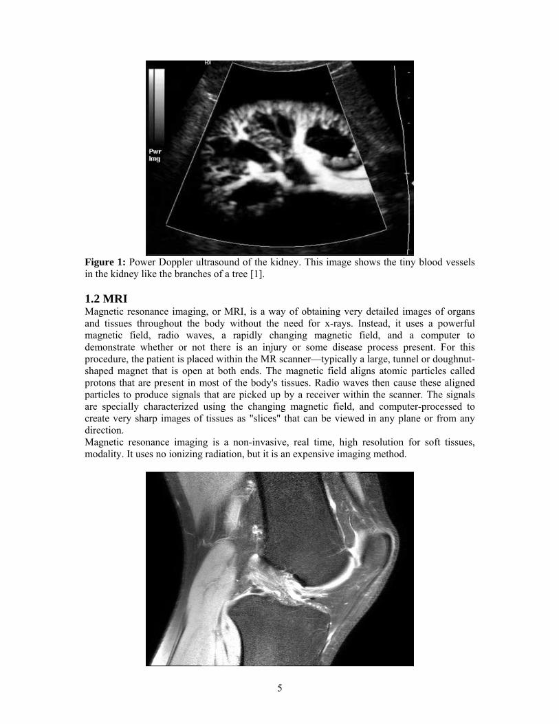
Medical imaging is the principal method for noninvasively obtaining anatomic and physiologic information about the human body. The main medical imaging techniques are ultrasounds, x-rays, computed tomography (CT); magnetic-resonance imaging (MRI) and positron emission tomography (PET). Images are important not only to the detection and diagnosis of disease and injury, but also to the design, delivery, and monitoring of treatment in order to reduce human disease and disability The evolution of medical imaging is the product of physicists working in collaboration with engineers and physicians. Following, the basic principles of these imaging modalities are depicted. 1.1 Ultrasound Ultrasound imaging is based on the same principles involved in the sonar used by bats, ships and fishermen. When a sound wave strikes an object, it bounces backward, or echoes. By measuring these echo waves it is possible to determine how far away the object is and its size, shape, consistency (whether the object is solid, filled with fluid, or both) and uniformity. In medicine, ultrasound imaging is used to detect changes in appearance and function of organs, tissues, or abnormal masses, such as tumors. A transducer both sends the sound waves and records the echoing waves. When the transducer is pressed against the skin, it directs a stream of inaudible, high-frequency sound waves into the body. As the sound waves bounce off of internal organs, fluids and tissues, the sensitive microphone in the transducer records tiny changes in the sound's pitch and direction. These signature waves are instantly measured and displayed by a computer, which in turn creates a real-time picture on the monitor. These live images are usually recorded on videotape and one or more frames of the moving pictures are typically captured as still images. Doppler ultrasound, a special application of ultrasound, measures the direction and speed of blood cells as they move through vessels. The movement of blood cells causes a change in pitch of the reflected sound waves (Doppler effect). A computer collects and processes the sounds and creates graphs or pictures that represent the flow of blood through the blood vessels. Ultrasound scanning is a noninvasive, painless, real-time imaging technique. Ultrasound is widely available, easy-to-use and less expensive than other imaging methods. Ultrasound scanning gives a clear picture of soft tissues that do not show up well on x-ray images. Moreover this kind of imaging uses no ionizing radiation. The main limitations of this imaging technique is that, ultrasound does not penetrate bone and air-filled organs (bladder, lungs, etc) are opaque to the sound waves.

5

Figure 1: Power Doppler ultrasound of the kidney. This image shows the tiny blood vessels in the kidney like the branches of a tree [1].

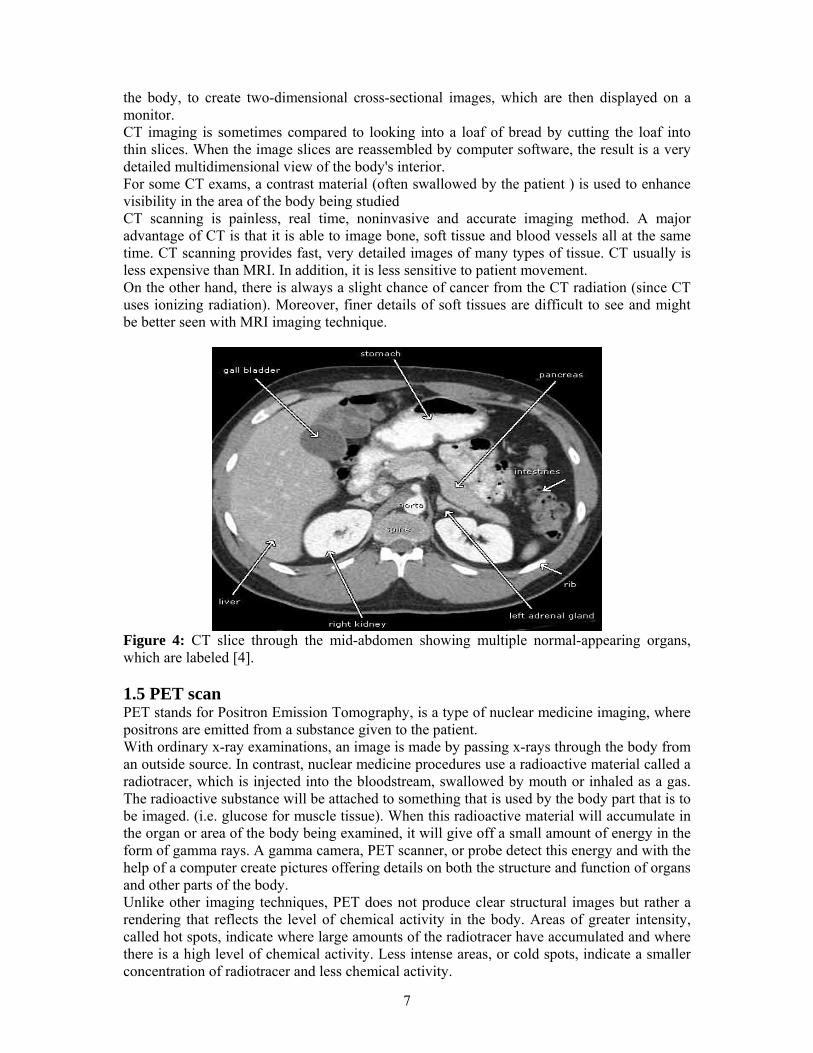
1.2 MRI Magnetic resonance imaging, or MRI, is a way of obtaining very detailed images of organs and tissues throughout the body without the need for x-rays. Instead, it uses a powerful magnetic field, radio waves, a rapidly changing magnetic field, and a computer to demonstrate whether or not there is an injury or some disease process present. For this procedure, the patient is placed within the MR scanner—typically a large, tunnel or doughnut-shaped magnet that is open at both ends. The magnetic field aligns atomic particles called protons that are present in most of the body's tissues. Radio waves then cause these aligned particles to produce signals that are picked up by a receiver within the scanner. The signals are specially characterized using the changing magnetic field, and computer-processed to create very sharp images of tissues as "slices" that can be viewed in any plane or from any direction. Magnetic resonance imaging is a non-invasive, real time, high resolution for soft tissues, modality. It uses no ionizing radiation, but it is an expensive imaging method.

6

Figure 2: Anatomic MRI of the Knee The used MRI scan shows high contrast between different structures of interest (e.g. bones, menisci, cruciate ligaments and cartilage) [2]. 1.3 X-rays X-rays are a form of radiation like light or radio waves. X-rays are small wavelength, high energy, electromagnetic rays that are emitted when inner orbital electrons are excited. X-rays pass through most objects, including the body. Once it is carefully aimed at the part of the body being examined, an x-ray machine produces a small burst of radiation that passes through the body, recording an image on photographic film or a special image recording plate. Different parts of the body absorb the x-rays in varying degrees. Dense bone absorbs much of the radiation while soft tissue, such as muscle, fat and organs, allow more of the x-rays to pass through them. As a result, bones appear white on the x-ray, soft tissue shows up in shades of gray and air appears black. It is the oldest and most frequently used imaging technique. It is fast, easy to use, relatively inexpensive and widely available method. It is particularly useful for emergency diagnosis purposes. X rays imaging involves the exposure of a part of the body to a small dose of ionizing radiation which is harmful. Additionally, soft tissue is not well shown with this technique.

Figure 3: X-ray showing frontal view of both hands [3].

1.4 CT scan CT stands for Computed Tomography. In many ways CT scanning works very much like other x-ray examinations. This technology uses X-rays to get multiple angled pictures to create a 3-D image. In a conventional x-ray exam, a small burst of radiation is aimed at and passes through the body, recording an image on photographic film or a special image recording plate. As we have already mentioned, bones appear white on the x-ray; soft tissue shows up in shades of gray and air appears black. With CT scanning, numerous x-ray beams and a set of electronic x-ray detectors rotate around the patient, measuring the amount of radiation being absorbed throughout the body. At the same time, the examination table is moving through the scanner, so that the x-ray beam follows a spiral path. A special computer program processes this series of pictures, or slices of

7

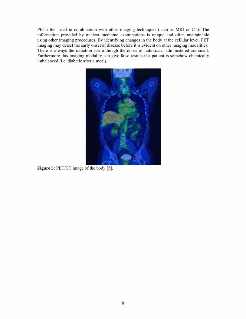
the body, to create two-dimensional cross-sectional images, which are then displayed on a monitor. CT imaging is sometimes compared to looking into a loaf of bread by cutting the loaf into thin slices. When the image slices are reassembled by computer software, the result is a very detailed multidimensional view of the body's interior. For some CT exams, a contrast material (often swallowed by the patient ) is used to enhance visibility in the area of the body being studied CT scanning is painless, real time, noninvasive and accurate imaging method. A major advantage of CT is that it is able to image bone, soft tissue and blood vessels all at the same time. CT scanning provides fast, very detailed images of many types of tissue. CT usually is less expensive than MRI. In addition, it is less sensitive to patient movement. On the other hand, there is always a slight chance of cancer from the CT radiation (since CT uses ionizing radiation). Moreover, finer details of soft tissues are difficult to see and might be better seen with MRI imaging technique.

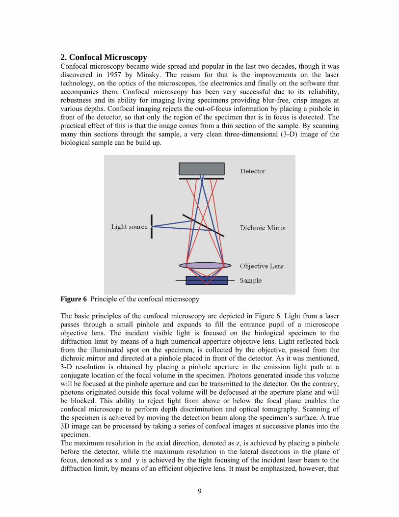
Figure 4: CT slice through the mid-abdomen showing multiple normal-appearing organs, which are labeled [4]. 1.5 PET scan PET stands for Positron Emission Tomography, is a type of nuclear medicine imaging, where positrons are emitted from a substance given to the patient. With ordinary x-ray examinations, an image is made by passing x-rays through the body from an outside source. In contrast, nuclear medicine procedures use a radioactive material called a radiotracer, which is injected into the bloodstream, swallowed by mouth or inhaled as a gas. The radioactive substance will be attached to something that is used by the body part that is to be imaged. (i.e. glucose for muscle tissue). When this radioactive material will accumulate in the organ or area of the body being examined, it will give off a small amount of energy in the form of gamma rays. A gamma camera, PET scanner, or probe detect this energy and with the help of a computer create pictures offering details on both the structure and function of organs and other parts of the body. Unlike other imaging techniques, PET does not produce clear structural images but rather a rendering that reflects the level of chemical activity in the body. Areas of greater intensity, called hot spots, indicate where large amounts of the radiotracer have accumulated and where there is a high level of chemical activity. Less intense areas, or cold spots, indicate a smaller concentration of radiotracer and less chemical activity.

8

PET often used in combination with other imaging techniques (such as MRI or CT). The information provided by nuclear medicine examinations is unique and often unattainable using other imaging procedures. By identifying changes in the body at the cellular level, PET imaging may detect the early onset of disease before it is evident on other imaging modalities. There is always the radiation risk although the doses of radiotracer administered are small. Furthermore this imaging modality can give false results if a patient is somehow chemically imbalanced (i.e. diabetic after a meal).

Figure 5: PET/CT image of the body [5].

9

2. Confocal Microscopy Confocal microscopy became wide spread and popular in the last two decades, though it was discovered in 1957 by Minsky. The reason for that is the improvements on the laser technology, on the optics of the microscopes, the electronics and finally on the software that accompanies them. Confocal microscopy has been very successful due to its reliability, robustness and its ability for imaging living specimens providing blur-free, crisp images at various depths. Confocal imaging rejects the out-of-focus information by placing a pinhole in front of the detector, so that only the region of the specimen that is in focus is detected. The practical effect of this is that the image comes from a thin section of the sample. By scanning many thin sections through the sample, a very clean three-dimensional (3-D) image of the biological sample can be build up.

Figure 6 Principle of the confocal microscopy The basic principles of the confocal microscopy are depicted in Figure 6. Light from a laser passes through a small pinhole and expands to fill the entrance pupil of a microscope objective lens. The incident visible light is focused on the biological specimen to the diffraction limit by means of a high numerical apperture objective lens. Light reflected back from the illuminated spot on the specimen, is collected by the objective, passed from the dichroic mirror and directed at a pinhole placed in front of the detector. As it was mentioned, 3-D resolution is obtained by placing a pinhole aperture in the emission light path at a conjugate location of the focal volume in the specimen. Photons generated inside this volume will be focused at the pinhole aperture and can be transmitted to the detector. On the contrary, photons originated outside this focal volume will be defocused at the aperture plane and will be blocked. This ability to reject light from above or below the focal plane enables the confocal microscope to perform depth discrimination and optical tomography. Scanning of the specimen is achieved by moving the detection beam along the specimen’s surface. A true 3D image can be processed by taking a series of confocal images at successive planes into the specimen. The maximum resolution in the axial direction, denoted as z, is achieved by placing a pinhole before the detector, while the maximum resolution in the lateral directions in the plane of focus, denoted as x and y is achieved by the tight focusing of the incident laser beam to the diffraction limit, by means of an efficient objective lens. It must be emphasized, however, that

10

3-D resolution (in the axial direction), is obtained by limitation of the region of observation, not of the region of excitation, as in the lateral directions.

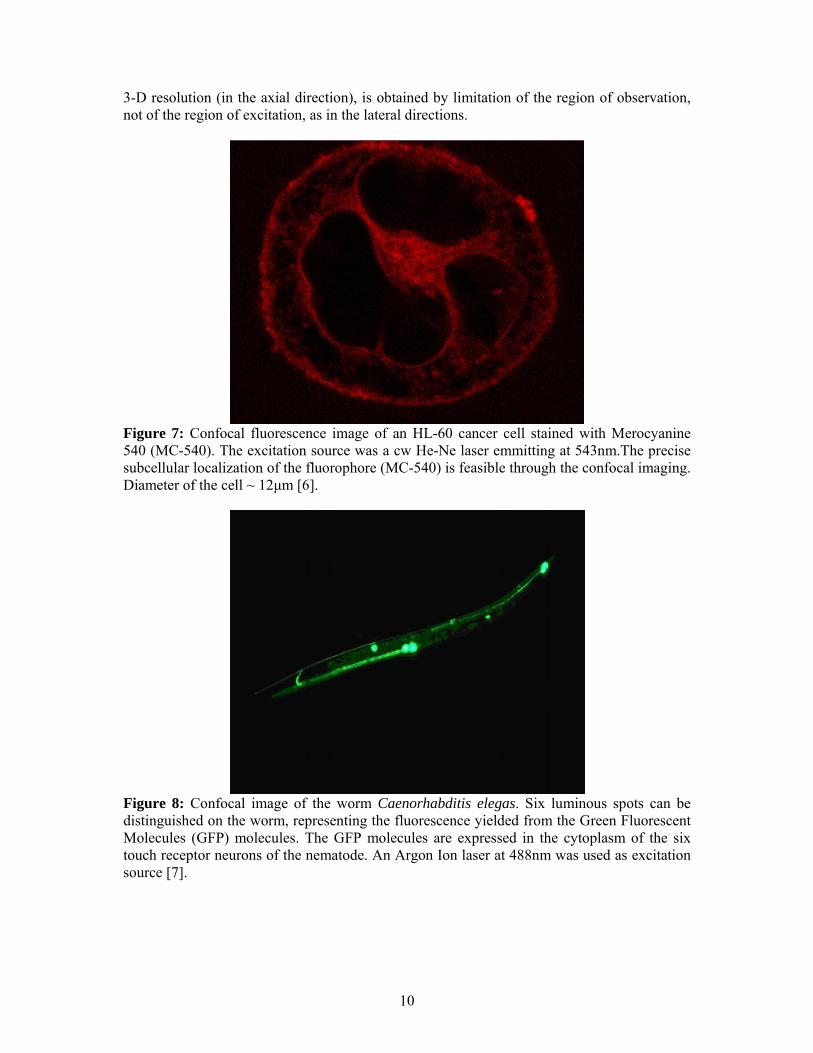
Figure 7: Confocal fluorescence image of an HL-60 cancer cell stained with Merocyanine 540 (MC-540). The excitation source was a cw He-Ne laser emmitting at 543nm.The precise subcellular localization of the fluorophore (MC-540) is feasible through the confocal imaging. Diameter of the cell ~ 12μm [6].

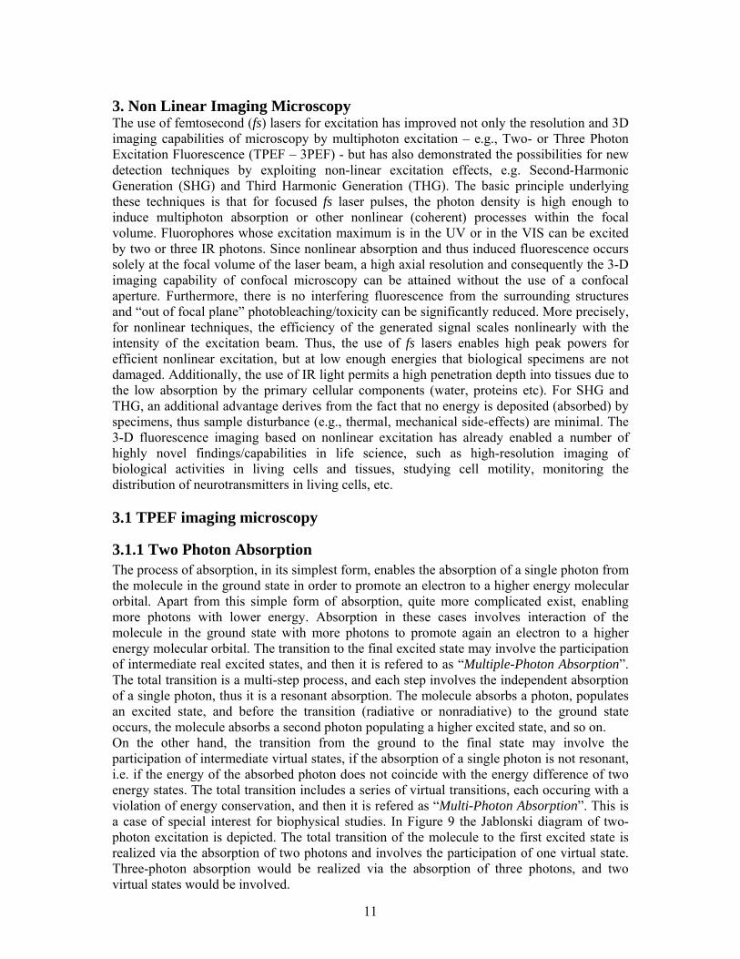
Figure 8: Confocal image of the worm Caenorhabditis elegas. Six luminous spots can be distinguished on the worm, representing the fluorescence yielded from the Green Fluorescent Molecules (GFP) molecules. The GFP molecules are expressed in the cytoplasm of the six touch receptor neurons of the nematode. An Argon Ion laser at 488nm was used as excitation source [7].

11

3. Non Linear Imaging Microscopy The use of femtosecond (fs) lasers for excitation has improved not only the resolution and 3D imaging capabilities of microscopy by multiphoton excitation – e.g., Two- or Three Photon Excitation Fluorescence (TPEF – 3PEF) - but has also demonstrated the possibilities for new detection techniques by exploiting non-linear excitation effects, e.g. Second-Harmonic Generation (SHG) and Third Harmonic Generation (THG). The basic principle underlying these techniques is that for focused fs laser pulses, the photon density is high enough to induce multiphoton absorption or other nonlinear (coherent) processes within the focal volume. Fluorophores whose excitation maximum is in the UV or in the VIS can be excited by two or three IR photons. Since nonlinear absorption and thus induced fluorescence occurs solely at the focal volume of the laser beam, a high axial resolution and consequently the 3-D imaging capability of confocal microscopy can be attained without the use of a confocal aperture. Furthermore, there is no interfering fluorescence from the surrounding structures and “out of focal plane” photobleaching/toxicity can be significantly reduced. More precisely, for nonlinear techniques, the efficiency of the generated signal scales nonlinearly with the intensity of the excitation beam. Thus, the use of fs lasers enables high peak powers for efficient nonlinear excitation, but at low enough energies that biological specimens are not damaged. Additionally, the use of IR light permits a high penetration depth into tissues due to the low absorption by the primary cellular components (water, proteins etc). For SHG and THG, an additional advantage derives from the fact that no energy is deposited (absorbed) by specimens, thus sample disturbance (e.g., thermal, mechanical side-effects) are minimal. The 3-D fluorescence imaging based on nonlinear excitation has already enabled a number of highly novel findings/capabilities in life science, such as high-resolution imaging of biological activities in living cells and tissues, studying cell motility, monitoring the distribution of neurotransmitters in living cells, etc. 3.1 TPEF imaging microscopy

3.1.1 Two Photon Absorption The process of absorption, in its simplest form, enables the absorption of a single photon from the molecule in the ground state in order to promote an electron to a higher energy molecular orbital. Apart from this simple form of absorption, quite more complicated exist, enabling more photons with lower energy. Absorption in these cases involves interaction of the molecule in the ground state with more photons to promote again an electron to a higher energy molecular orbital. The transition to the final excited state may involve the participation of intermediate real excited states, and then it is refered to as “Multiple-Photon Absorption”. The total transition is a multi-step process, and each step involves the independent absorption of a single photon, thus it is a resonant absorption. The molecule absorbs a photon, populates an excited state, and before the transition (radiative or nonradiative) to the ground state occurs, the molecule absorbs a second photon populating a higher excited state, and so on. On the other hand, the transition from the ground to the final state may involve the participation of intermediate virtual states, if the absorption of a single photon is not resonant, i.e. if the energy of the absorbed photon does not coincide with the energy difference of two energy states. The total transition includes a series of virtual transitions, each occuring with a violation of energy conservation, and then it is refered as “Multi-Photon Absorption”. This is a case of special interest for biophysical studies. In Figure 9 the Jablonski diagram of two-photon excitation is depicted. The total transition of the molecule to the first excited state is realized via the absorption of two photons and involves the participation of one virtual state. Three-photon absorption would be realized via the absorption of three photons, and two virtual states would be involved.

12

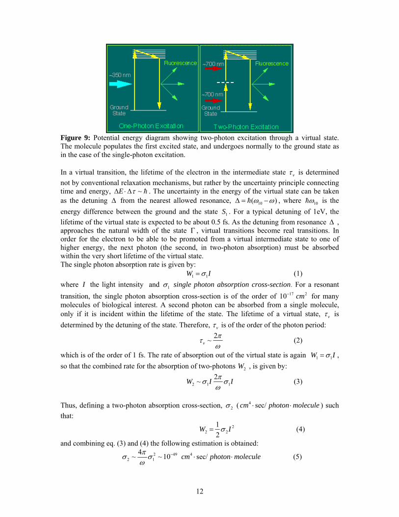
Figure 9: Potential energy diagram showing two-photon excitation through a virtual state. The molecule populates the first excited state, and undergoes normally to the ground state as in the case of the single-photon excitation. In a virtual transition, the lifetime of the electron in the intermediate state vτ is determined not by conventional relaxation mechanisms, but rather by the uncertainty principle connecting time and energy, ~E τΔ ⋅Δ h . The uncertainty in the energy of the virtual state can be taken as the detuning Δ from the nearest allowed resonance, 10( )ω ωΔ = −h , where 10ωh is the energy difference between the ground and the state 1S . For a typical detuning of 1eV, the lifetime of the virtual state is expected to be about 0.5 fs. As the detuning from resonance Δ , approaches the natural width of the state Γ , virtual transitions become real transitions. In order for the electron to be able to be promoted from a virtual intermediate state to one of higher energy, the next photon (the second, in two-photon absorption) must be absorbed within the very short lifetime of the virtual state. The single photon absorption rate is given by: 1 1W Iσ= (1) where I the light intensity and 1σ single photon absorption cross-section. For a resonant transition, the single photon absorption cross-section is of the order of 1710− 2cm for many molecules of biological interest. A second photon can be absorbed from a single molecule, only if it is incident within the lifetime of the state. The lifetime of a virtual state, vτ is determined by the detuning of the state. Therefore, vτ is of the order of the photon period:

2~vπτω

(2)

which is of the order of 1 fs. The rate of absorption out of the virtual state is again 1 1W Iσ= , so that the combined rate for the absorption of two-photons 2W , is given by:

2 1 12~W I Iπσ σω

(3)

Thus, defining a two-photon absorption cross-section, 2σ ( 4 sec/cm photon molecule⋅ ⋅ ) such that:

22 2

12

W Iσ= (4)

and combining eq. (3) and (4) the following estimation is obtained:

2 492 1

4~ ~ 10πσ σω

− 4 sec/cm photon molecule⋅ ⋅ (5)

13

The value obtained from this crude estimation is in rather good agreement with both theoretical and experimental data, since for common chromophores with excitation wavelength ranging from 690 nm to 1050 nm, 2σ is about 4810− to 5010−

4 sec/cm photon molecule⋅ ⋅ [8]. 3.1.2 Two Photon Excited Fluorescence In TPEF, the quantum yield of fluorescence 2 fΦ is defined as: 2

number of fluorescence emitted photonsnumber of pair of absorbed photonsfΦ = (6)

Eq. (4) gives the rate, 2W at which a molecule populates an excited state through two-photon absorption. This rate, when multiplied by the fluorescence quantum efficiency 2 fΦ , provides the rate at which a photon is emitted from the molecule, which undergoes from the excited to

the ground state. In other words, the power of the TPEF, TPEFP in sec

photons is given by:

22 2

12TPEF fP Iσ= Φ (7)

Finally, if we define 2 2TPEF fσ σ= Φ ⋅ as the two-photon fluorescence cross-section (or action cross-section), eq. (7), can be expressed as:

212TPEF TPEFP Iσ= (8)

Once an excited state has been populated through two-photon (or multi photon) absorption, a process of deactivation follows with the same characteristics as the one-photon excited fluorescence process (OPEF). OPEF and multi photon excited fluorescence lie their differences in the way that the excited state is reached, but not in the way that the excited state is deactivated to populate again the ground state 0S . Fluorescence in both cases is only one of the possible ways that the excited molecule can undergo to the ground state. As far as the polarization of the emitted photons through fluorescence is concerned, it is expected that when fluorescent molecules are illuminated with linear polarized light, the emitted photons have a specific polarization, related with the polarization of the incident photons and the specific transition moment between the excited and the ground state. This specific transition is directly related with the orientation of the molecules in the space. However, since the molecules are free to rotate during the time taken for the electronic transitions to occur, changing their orientation and the corresponding transition moment, the fluorescence emission is largely unpolarized. For small fluorescent molecules, the rotational correlation time is much shorter than the fluorescence lifetime. For example, fluorescein has a rotational correlation time of 120 ps , 40 times shorter than its fluorescence lifetime [9]. By contrast, when the fluorescent molecule is relatively large, its rotational correlational time is larger than its fluorescence lifetime, and the fluorescence emission is more polarized. Green Fluorescent Protein (GFP) is an example of such a fluorescent molecule [10]. 3.1.3 TPEF microscopy By far the most well known form of nonlinear microscopy is based on TPEF. It is a 3-D imaging technology, alternative to conventional confocal microscopy. It was firstly introduced by Denk, Webb and coworkers in 1990 [11], and since then has become a laboratory standard. As we already mentioned, the electronic transition of a fluorophore can be induced by the simultaneous absorption of two photons. These two photons, typically in the infrared spectral range, have energies approximately equal to half of the energetic

14

difference between the ground and excited electronic states. Since the two-photon excitation probability is significantly less than the one-photon probability, two-photon excitation occurs with appreciable rates only in regions of high temporal and spatial photon concentration. The high spatial concentration of photons can be achieved by focusing the laser beam with a high numerical aperture (NA) objective lens to a diffraction-limited focus. The high temporal concentration of photons is made possible by the availability of high peak power pulsing lasers, with pulse width of the order of hundreds of femtoseconds (10-15 sec). The most important feature of two-photon microscopy is its intrinsic depth discrimination. For one-photon excitation in a spatially uniform fluorescent sample, equal fluorescence intensities are generated from each z section above and below the focal plane assuming negligible attenuation of the laser beam. However, in the two-photon case almost the total fluorescence intensity comes from a 1μm thick region about the focal point for objectives with high NA. Thus, 3-D images can be constructed as in confocal microscopy, but without a confocal pinhole. This depth discrimination effect of the two-photon excitation arises from the quadratic dependence of two-photon fluorescence upon the excitation photon flux, which decreases rapidly away from the focal plane. The fact that the 3-D sectioning arises from the limitation of the excitation region, ensures that photobleaching and photodamage of the biological specimen are restricted only to the focal point. Since out-of-plane fluorophores are not excited, they are not subject neither to photodamage nor to photobleaching. The minimally invasive nature of two-photon imaging can be best appreciated in a number of embryology studies. At this point it is necessary to describe briefly the terms photobleaching and photodamage. Photobleaching occurs when, under illumination, the triplet state in the fluorophore reacts with molecular oxygen, forming a nonfluorescing molecule. Photobleaching tends to limit the

fluorescence emission to a maximum of ~105 sec

photonsmolecule ⋅

for some of the best fluorophores

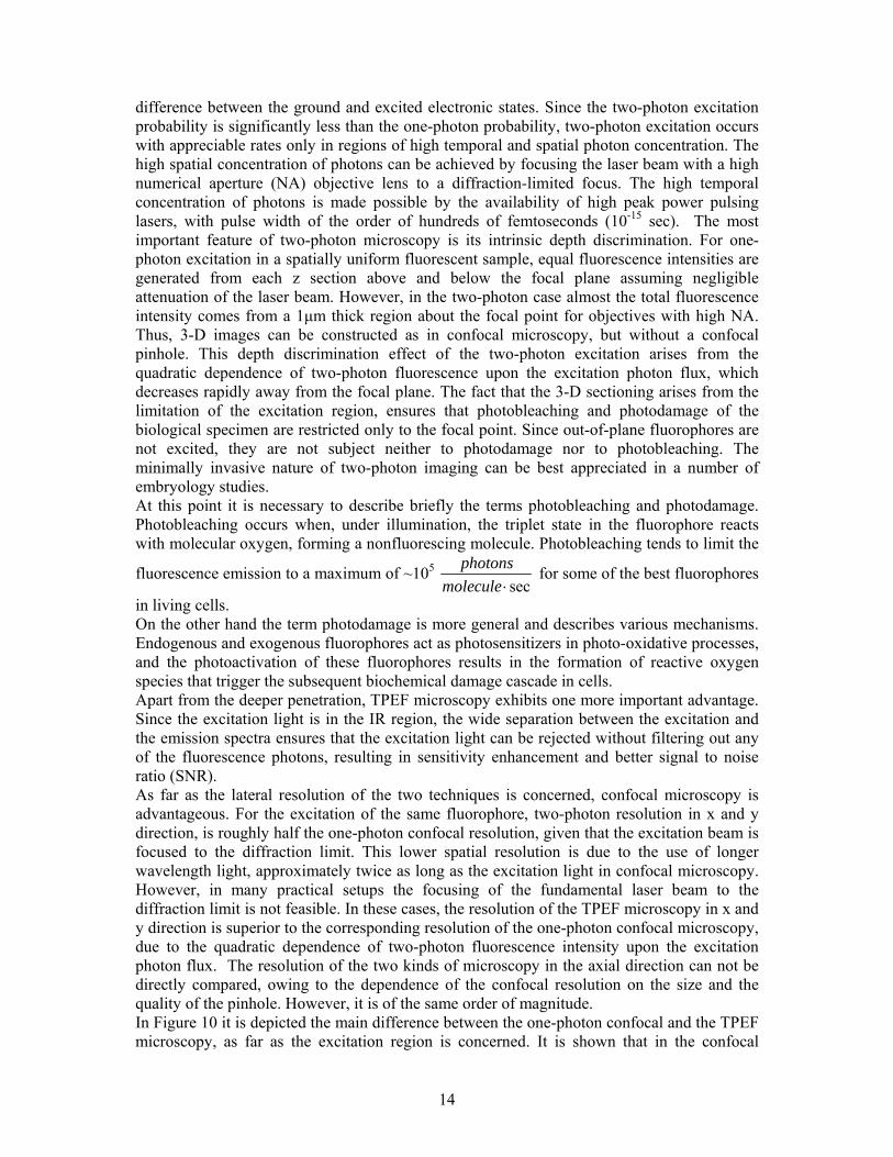
in living cells. On the other hand the term photodamage is more general and describes various mechanisms. Endogenous and exogenous fluorophores act as photosensitizers in photo-oxidative processes, and the photoactivation of these fluorophores results in the formation of reactive oxygen species that trigger the subsequent biochemical damage cascade in cells. Apart from the deeper penetration, TPEF microscopy exhibits one more important advantage. Since the excitation light is in the IR region, the wide separation between the excitation and the emission spectra ensures that the excitation light can be rejected without filtering out any of the fluorescence photons, resulting in sensitivity enhancement and better signal to noise ratio (SNR). As far as the lateral resolution of the two techniques is concerned, confocal microscopy is advantageous. For the excitation of the same fluorophore, two-photon resolution in x and y direction, is roughly half the one-photon confocal resolution, given that the excitation beam is focused to the diffraction limit. This lower spatial resolution is due to the use of longer wavelength light, approximately twice as long as the excitation light in confocal microscopy. However, in many practical setups the focusing of the fundamental laser beam to the diffraction limit is not feasible. In these cases, the resolution of the TPEF microscopy in x and y direction is superior to the corresponding resolution of the one-photon confocal microscopy, due to the quadratic dependence of two-photon fluorescence intensity upon the excitation photon flux. The resolution of the two kinds of microscopy in the axial direction can not be directly compared, owing to the dependence of the confocal resolution on the size and the quality of the pinhole. However, it is of the same order of magnitude. In Figure 10 it is depicted the main difference between the one-photon confocal and the TPEF microscopy, as far as the excitation region is concerned. It is shown that in the confocal

15

microscopy, the out-of-focus plane excitation is very intense, whereas in the TPEF microscopy is not. (a) (b)

Figure 10 a) The excitation region (pink colour) is limited in the focal plane for the two-photon case, while extends above and below in the one-photon excitation. b) The same characteristic is noted in the two comparative pictures Fluorophores utilized in two-photon tissue imaging are divided in two classes, endogenous and exogenous. Most proteins are fluorescent due to the presence of tryptophan and tyrosine. However, two-photon tissue imaging based on amino-acid fluorescence is uncommon, because these amino-acids have one-photon absorption in the UV spectral range (250-300nm). Two-photon excitation of these fluorophores requires femtosecond laser sources with emission in the range of 500-600nm, which is not easily available. Two-photon imaging of cellular structures is often based on the fluorescence of NAD(P)H and flavoproteins. NAD(P)H has a one-photon absorption spectrum at about 340nm, whereas flavoproteins around 450nm. Two-photon microscopy can also image extracellular matrix structures in tissues. Two of the key components in the extracellular matrix are collagen and elastin. Elastin has excitation wavelengths of 340-370nm, and can be readily imaged by two-photon excitation in the wavelength range of about 800nm. Similarly, many types of collagen have among others excitation wavelengths around 400nm, thus TPEF of collagen can be readily achieved and observed in many two-photon imaging systems. While autofluorescent tissue structures can be readily studied, the study of nonfluorescent components is difficult. However, many biochemical processes are based on nonfluorescent structures, and for their monitoring, compatible fluorescent exogenous probes should be developed and uniformly delivered into intact, in vivo tissues. For example, Green Fluorescent Protein (GFP) is one of the most important, genetically encoded, exogenous fluorophores, used in TPEF microscopy. Two-photon microscopy has found an increasingly wide range of applications in biology and medicine. The advantage of two-photon imaging has been well demonstrated in neurobiology, embryology, dermatology and pancreatic physiology. Especially, as far as the neurobiological studies are concerned, TPEF microscopy provide 3-D mapping of neuron organization and assays neuron communications by monitoring action potentials, calcium waves and neural

16

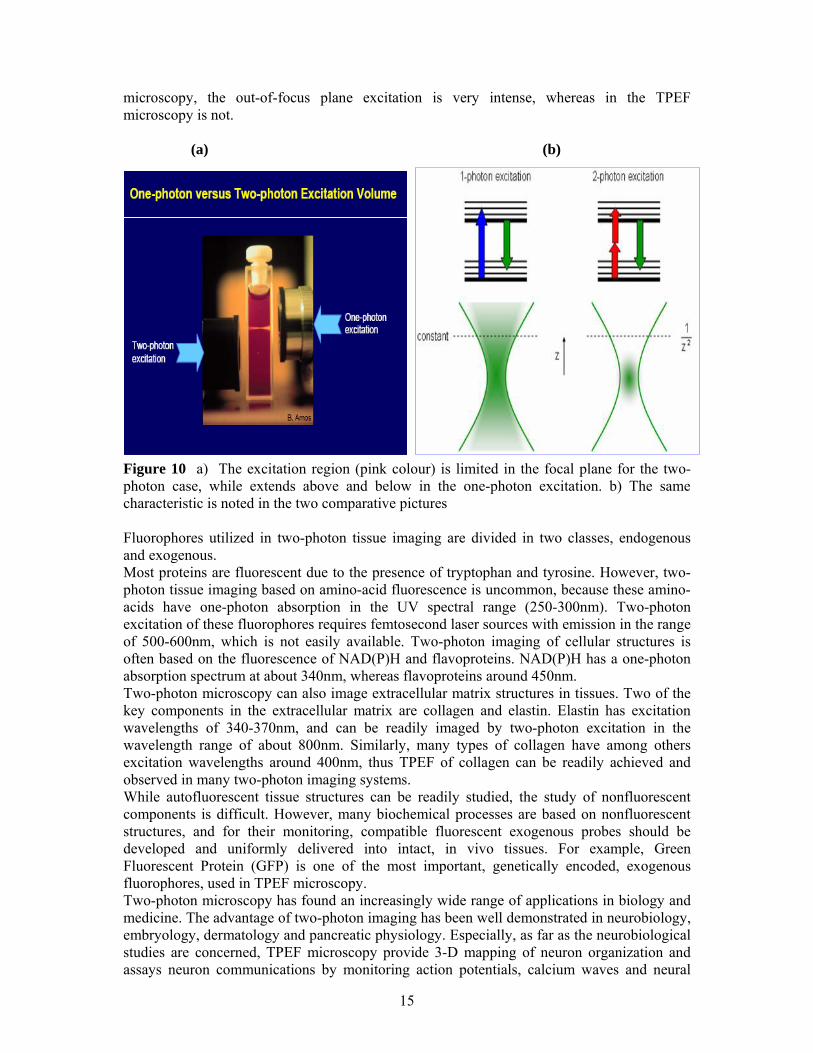
transmitters. Many two-photon neural biological studies have focused on the remodeling of neuronal dendritic spines or on the dynamics of calcium signal propagation [12]. Others focused on system level interactions of neurons [13], neuronal hemodynamics [14], or on the in vivo study of neuronal pathology [15]. In Figure 11 the precise localization of one touch receptor neuron and the neuron axon is feasible via TPEF measurements. The image was obtained from the tail of a worm expressing Green Fluorescence Protein (GFP) in the mechanoreceptor neurons.

Figure 11: TPEF signals generated at the tail of Caenorhabditis elegas expressing GFP in the mechanoreceptor neurons The neuronal cell body (~2μm) and the axon (~200nm) are detectable [16]. 3.2 SHG imaging microscopy Second Harmonic Generation (SHG) imaging microscopy was used several years prior to the invention of TPEF, based on the generation of second-harmonic light either from surfaces or from endogenous tissue structures such as rat-tail tendons. In SHG, light of the fundamental frequency ω is converted by the nonlinear material into light at exactly twice that frequency, 2ω. Because of difficulties in signal interpretations and because of its seemingly arcane utility, at least in biological imaging, SHG microscopy has gone by relatively unnoticed until very recently. The discovery that exogenous markers can lead to exceptionally high signal levels has been a leading cause for the revival of SHG microscopy. In particular, SHG markers, when properly designed and collectively organized, can produce signal levels easily comparable to those encounterd in standard TPEF microscopy. Apart from that, many intrinsic structures of biological systems produce strong SHG signal, so labeling with exogenous molecular probes is not always required. Molecular frequency doubling is caused by the non-linear dependence of the induced dipolar moment μ of the molecule on the incident optical electric field E . Thus μ can be expanded in a Taylor’s series about 0E = :

1 1 ...2 6o E E E E E Eμ μ α β γ= + ∗ + ∗ ∗ + ∗ ∗ ∗ + (9)

where oμ is the permanent dipolar moment of the molecule, α is the linear polarizability,β is the molecular first hyperpolarizability, which governs in the molecular level SHG, and γ is the second hyperpolarizability which governs among others multiphoton absorption and Third Harmonc Generation (THG) [17]. Macroscopically the optical response of materials to incident light, or generally electromagnetic radiation, is characterized by the optically induced polarization density, P , which can also be expanded in a Taylor’s series about 0E = : (1) (2) (3) ...P E E E E E Eχ χ χ= ∗ + ∗ ∗ + ∗ ∗ ∗ + (10) where P represents the polarization density vector, and ( )nχ are the nth order optical susceptibility tensors. The first term describes linear absorption and reflection of light, the second term describes SHG, sum and difference frequency generation, and the third term covers multiphoton absorption, third-harmonic generation and stimulated Raman processes.

17

The macroscopic second order susceptibility tensor (2)χ , which is responsible for SHG, is related to the molecular first hyperpolarizability, β , by: (2) Nχ β= ⟨ ⟩ (11) where N is the spatial density of molecules, and β⟨ ⟩ represents an orientational average [18]. Equation (11) implies that only non-centrosymmetric materials have a non-vanishing second order susceptibility (2)χ , and the coherent summation of their single molecules’ SHG radiation patterns are not cancelled out, resulting in a highly directional, detectable second-harmonic signal. The second-harmonic intensity in such media scale as [18]:

( )( )222sigSHG p τ χ∝ (12)

where p and τ are the laser pulse energy and pulse width, respectively. Combining equations (11) and (12), it is apparent that the second-harmonic intensity is proportional to

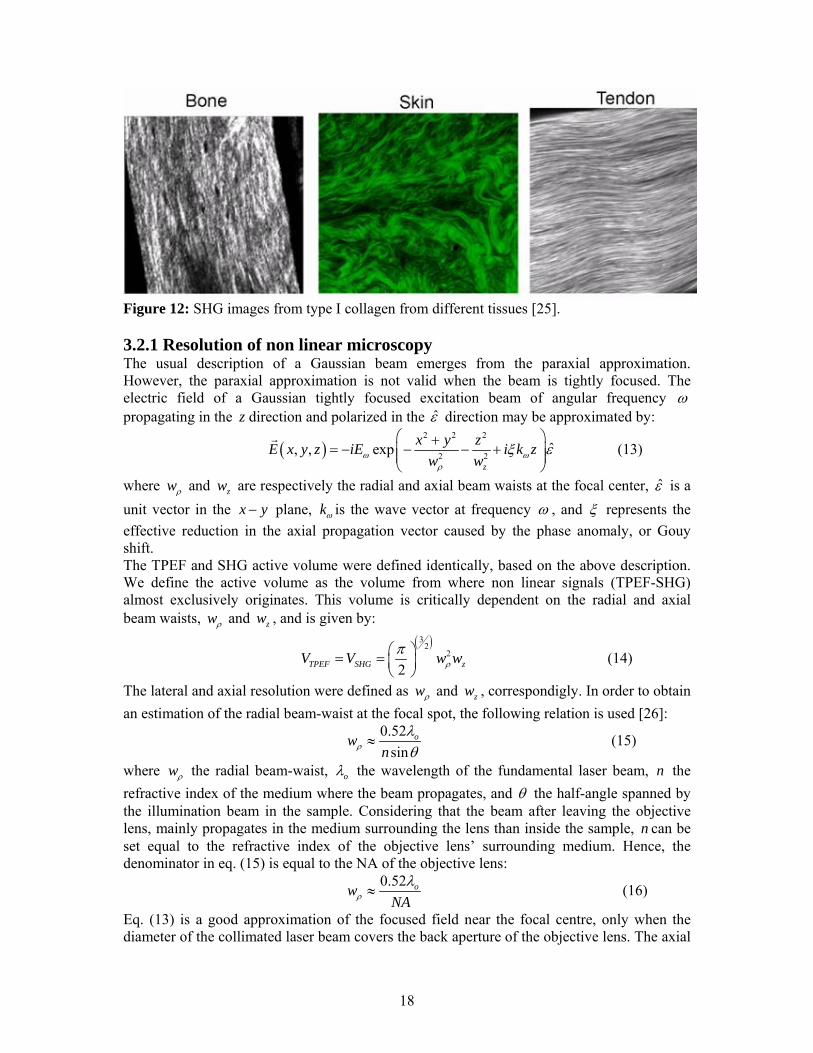
2N , whereas TPEF intensity is known to be proportional to N . The quadratic dependence of the second-harmonic intensity on the spatial density of molecules is somehow expected, since the single molecules act as dipole radiators and the total SHG signal arises from their constructive interference. By contrast the TPEF is a noncoherent phenomenon, and the radiation of each fluorescent molecule is independent from the emission of the neighboring molecules. Under this symmetry constraint it is obvious that SHG can be mainly produced from structures with high degree of orientation and organization but without inversion symmetry, such as crystalls or endogenous arrays of structural proteins (collagen, actomyosin complexes, tubulin) in biological systems [19]. It can be also produced from metal surfaces, where there is a huge change in the refractive indices, and generally from interfaces, where the symmetry breaks. Over the last two decades SHG has been widely used as a spectroscopic imaging tool in a variety of interfacial studies, including liquid-solid, liquid-air and liquid-liquid interfaces [20]. Because of the interfacial specificity of the process, SHG is an ideal approach to the study of biophysics in model membranes [21], and the membrane physiology of living cells [22]. Particurarly, one of the innovative applications of the SHG phenomenon is its usage as a highly sensitive monitor of membrane potential [23]. When a laser pulse is incident on a membrane, it induces dipoles in the fluorescent molecules that are membrane bound via transmembrane proteins, making them candidates for SHG. Alterations in the membrane potential alter the magnitude of the induced dipoles, thus affecting the magnitude of the observed SHG signal. Green Fluorescent Protein (GFP) has been used as SHG probe in this way [24], since it undergoes large electron redistribution in the presence of light, and the resulted induced dipole is affected by the characteristics of the transmembrane potential. The Figure 12 shows representative high resolution SHG images from type I collagen from different tissues. Type I collagen is the most abundant protein in our bodies and comprises the matrix in bone, skin, and tendon.

18

Figure 12: SHG images from type I collagen from different tissues [25]. 3.2.1 Resolution of non linear microscopy The usual description of a Gaussian beam emerges from the paraxial approximation. However, the paraxial approximation is not valid when the beam is tightly focused. The electric field of a Gaussian tightly focused excitation beam of angular frequency ω propagating in the z direction and polarized in the ε̂ direction may be approximated by:

( )2 2 2

2 2ˆ, , exp

z

x y zE x y z iE i k zw wω ω

ρ

ξ ε⎛ ⎞+

= − − − +⎜ ⎟⎜ ⎟⎝ ⎠

r (13)

where wρ and zw are respectively the radial and axial beam waists at the focal center, ε̂ is a unit vector in the x y− plane, kω is the wave vector at frequency ω , and ξ represents the effective reduction in the axial propagation vector caused by the phase anomaly, or Gouy shift. The TPEF and SHG active volume were defined identically, based on the above description. We define the active volume as the volume from where non linear signals (TPEF-SHG) almost exclusively originates. This volume is critically dependent on the radial and axial beam waists, wρ and zw , and is given by:

( )3

22

2TPEF SHG zV V w wρπ⎛ ⎞= = ⎜ ⎟⎝ ⎠

(14)

The lateral and axial resolution were defined as wρ and zw , correspondigly. In order to obtain an estimation of the radial beam-waist at the focal spot, the following relation is used [26]:

0.52sin

ownρ

λθ

≈ (15)

where wρ the radial beam-waist, oλ the wavelength of the fundamental laser beam, n the refractive index of the medium where the beam propagates, and θ the half-angle spanned by the illumination beam in the sample. Considering that the beam after leaving the objective lens, mainly propagates in the medium surrounding the lens than inside the sample, n can be set equal to the refractive index of the objective lens’ surrounding medium. Hence, the denominator in eq. (15) is equal to the NA of the objective lens:

0.52 owNAρλ

≈ (16)

Eq. (13) is a good approximation of the focused field near the focal centre, only when the diameter of the collimated laser beam covers the back aperture of the objective lens. The axial

19

resolution has been defined as zw . For a Gaussian ellipsoid illumination profile, as it is described by eq. (13), the axial beam-waist zw is estimated by [26]:

0.76(1 cos )

ozw

nλθ

≈−

(17)

We attribute again the value of the refractive index that surrounds the objective lens to the parameter n , using the same arguments as above. Expressing cosθ as a function of the NA, eq. (17) becomes:

1

0.76

(1 cos sin

ozw

NAnn

λ−

≈⎛ ⎞⎛ ⎞− ⎜ ⎟⎜ ⎟⎝ ⎠⎝ ⎠

(18)

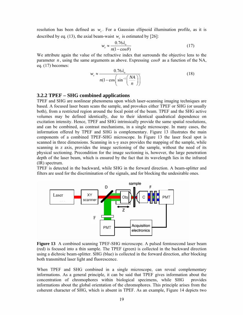
3.2.2 TPEF – SHG combined applications TPEF and SHG are nonlinear phenomena upon which laser-scanning imaging techniques are based. A focused laser beam scans the sample, and provokes either TPEF or SHG (or usually both), from a restricted region around the focal point of the beam. TPEF and the SHG active volumes may be defined identically, due to their identical quadratical dependence on excitation intensity. Hence, TPEF and SHG intrinsically provide the same spatial resolutions, and can be combined, as contrast mechanisms, in a single microscope. In many cases, the information offered by TPEF and SHG is complementary. Figure 13 illustrates the main components of a combined TPEF-SHG microscope. In Figure 13 the laser focal spot is scanned in three dimensions. Scanning in x-y axes provides the mapping of the sample, while scanning in z axis, provides the image sectioning of the sample, without the need of its physical sectioning. Precondition for the image sectioning is, however, the large penetration depth of the laser beam, which is ensured by the fact that its wavelength lies in the infrared (IR) spectrum. TPEF is detected in the backward, while SHG in the forward direction. A beam-splitter and filters are used for the discrimination of the signals, and for blocking the undesirable ones.

Figure 13 A combined scanning TPEF-SHG microscope. A pulsed femtosecond laser beam (red) is focused into a thin sample. The TPEF (green) is collected in the backward direction using a dichroic beam-splitter. SHG (blue) is collected in the forward direction, after blocking both transmitted laser light and fluorescence. When TPEF and SHG combined in a single microscope, can reveal complementary informations. As a general principle, it can be said that TPEF gives information about the concentration of chromophores within biological specimens, while SHG provides informations about the global orientation of the chromophores. This principle arises from the coherent character of SHG, which is absent in TPEF. As an example, Figure 14 depicts two

Laser

F

20

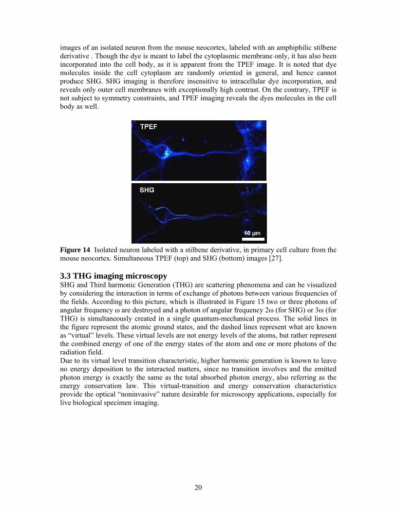
images of an isolated neuron from the mouse neocortex, labeled with an amphiphilic stilbene derivative . Though the dye is meant to label the cytoplasmic membrane only, it has also been incorporated into the cell body, as it is apparent from the TPEF image. It is noted that dye molecules inside the cell cytoplasm are randomly oriented in general, and hence cannot produce SHG. SHG imaging is therefore insensitive to intracellular dye incorporation, and reveals only outer cell membranes with exceptionally high contrast. On the contrary, TPEF is not subject to symmetry constraints, and TPEF imaging reveals the dyes molecules in the cell body as well.

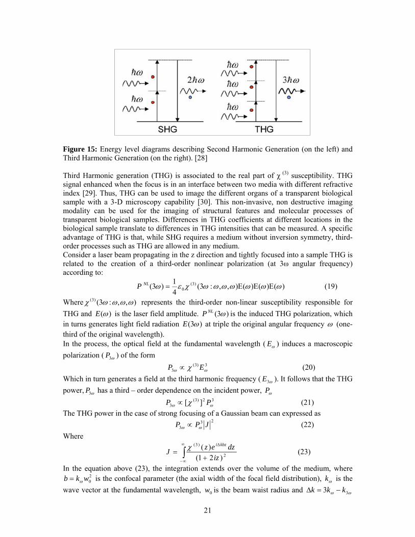
Figure 14 Isolated neuron labeled with a stilbene derivative, in primary cell culture from the mouse neocortex. Simultaneous TPEF (top) and SHG (bottom) images [27]. 3.3 THG imaging microscopy SHG and Third harmonic Generation (THG) are scattering phenomena and can be visualized by considering the interaction in terms of exchange of photons between various frequencies of the fields. According to this picture, which is illustrated in Figure 15 two or three photons of angular frequency ω are destroyed and a photon of angular frequency 2ω (for SHG) or 3ω (for THG) is simultaneously created in a single quantum-mechanical process. The solid lines in the figure represent the atomic ground states, and the dashed lines represent what are known as “virtual” levels. These virtual levels are not energy levels of the atoms, but rather represent the combined energy of one of the energy states of the atom and one or more photons of the radiation field. Due to its virtual level transition characteristic, higher harmonic generation is known to leave no energy deposition to the interacted matters, since no transition involves and the emitted photon energy is exactly the same as the total absorbed photon energy, also referring as the energy conservation law. This virtual-transition and energy conservation characteristics provide the optical “noninvasive” nature desirable for microscopy applications, especially for live biological specimen imaging.

21

Figure 15: Energy level diagrams describing Second Harmonic Generation (on the left) and Third Harmonic Generation (on the right). [28] Third Harmonic generation (THG) is associated to the real part of χ (3) susceptibility. THG signal enhanced when the focus is in an interface between two media with different refractive index [29]. Thus, THG can be used to image the different organs of a transparent biological sample with a 3-D microscopy capability [30]. This non-invasive, non destructive imaging modality can be used for the imaging of structural features and molecular processes of transparent biological samples. Differences in THG coefficients at different locations in the biological sample translate to differences in THG intensities that can be measured. A specific advantage of THG is that, while SHG requires a medium without inversion symmetry, third-order processes such as THG are allowed in any medium. Consider a laser beam propagating in the z direction and tightly focused into a sample THG is related to the creation of a third-order nonlinear polarization (at 3ω angular frequency) according to:

)()()(),,:3(41)3( )3(

0 ωωωωωωωχεω ΕΕΕ=NLP (19)

Where ),,:3()3( ωωωωχ represents the third-order non-linear susceptibility responsible for THG and )(ωE is the laser field amplitude. )3( ωNLP is the induced THG polarization, which in turns generates light field radiation )3( ωE at triple the original angular frequency ω (one-third of the original wavelength). In the process, the optical field at the fundamental wavelength ( ωE ) induces a macroscopic polarization ( ω3P ) of the form 3)3(

3 ωω χ EP ∝ (20) Which in turn generates a field at the third harmonic frequency ( ω3E ). It follows that the THG power, ω3P has a third – order dependence on the incident power, ωP 32)3(

3 ][ ωω χ PP ∝ (21) The THG power in the case of strong focusing of a Gaussian beam can expressed as 23

3 JPP ωω ∝ (22) Where

∫∞

∞−

Δ

+= 2

)3(

)21()(

izdzezJ

kbziχ (23)

In the equation above (23), the integration extends over the volume of the medium, where 20wkb ω= is the confocal parameter (the axial width of the focal field distribution), ωk is the

wave vector at the fundamental wavelength, 0w is the beam waist radius and ωω 33 kkk −=Δ

22

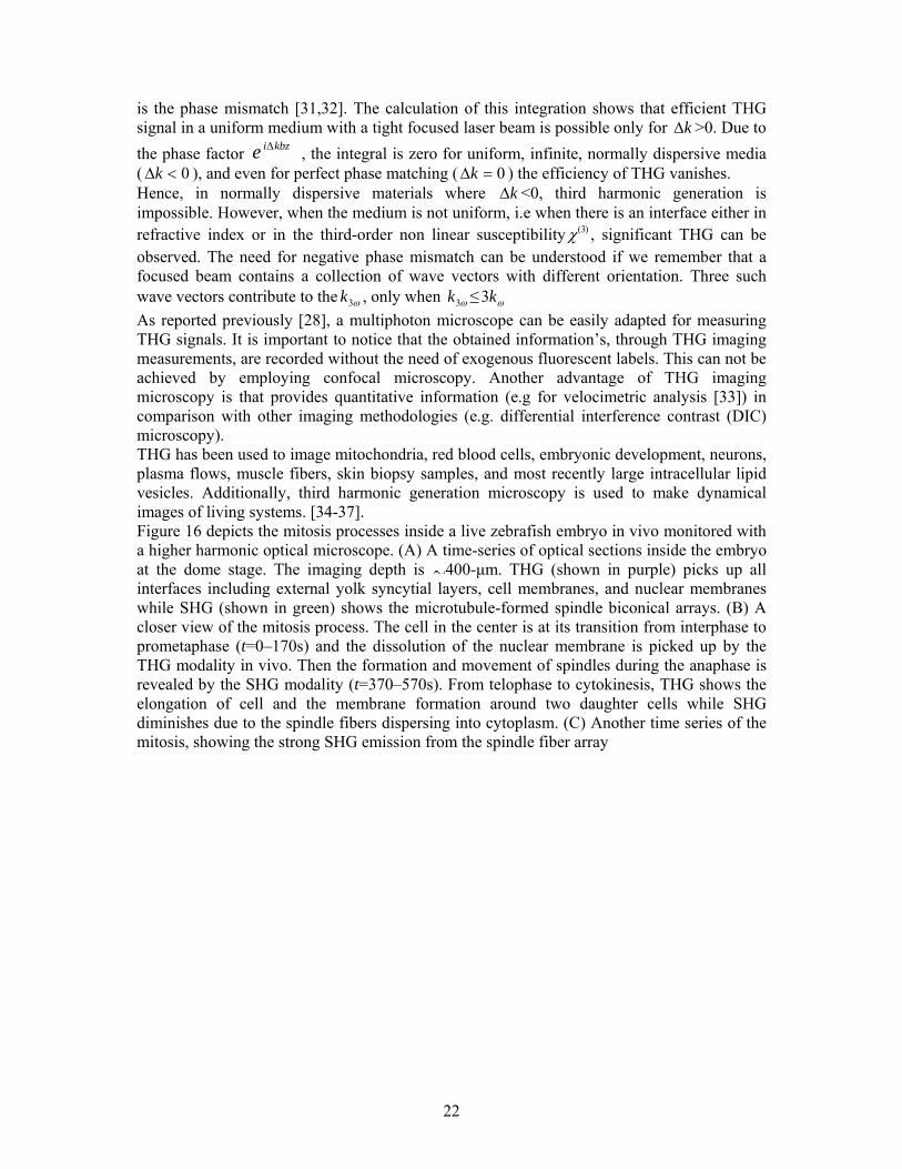
is the phase mismatch [31,32]. The calculation of this integration shows that efficient THG signal in a uniform medium with a tight focused laser beam is possible only for kΔ >0. Due to the phase factor kbzie Δ , the integral is zero for uniform, infinite, normally dispersive media ( 0<Δk ), and even for perfect phase matching ( 0=Δk ) the efficiency of THG vanishes. Hence, in normally dispersive materials where kΔ <0, third harmonic generation is impossible. However, when the medium is not uniform, i.e when there is an interface either in refractive index or in the third-order non linear susceptibility )3(χ , significant THG can be observed. The need for negative phase mismatch can be understood if we remember that a focused beam contains a collection of wave vectors with different orientation. Three such wave vectors contribute to the ω3k , only when ω3k ≤ ωk3 As reported previously [28], a multiphoton microscope can be easily adapted for measuring THG signals. It is important to notice that the obtained information’s, through THG imaging measurements, are recorded without the need of exogenous fluorescent labels. This can not be achieved by employing confocal microscopy. Another advantage of THG imaging microscopy is that provides quantitative information (e.g for velocimetric analysis [33]) in comparison with other imaging methodologies (e.g. differential interference contrast (DIC) microscopy). THG has been used to image mitochondria, red blood cells, embryonic development, neurons, plasma flows, muscle fibers, skin biopsy samples, and most recently large intracellular lipid vesicles. Additionally, third harmonic generation microscopy is used to make dynamical images of living systems. [34-37]. Figure 16 depicts the mitosis processes inside a live zebrafish embryo in vivo monitored with a higher harmonic optical microscope. (A) A time-series of optical sections inside the embryo at the dome stage. The imaging depth is 400-μm. THG (shown in purple) picks up all interfaces including external yolk syncytial layers, cell membranes, and nuclear membranes while SHG (shown in green) shows the microtubule-formed spindle biconical arrays. (B) A closer view of the mitosis process. The cell in the center is at its transition from interphase to prometaphase (t=0–170s) and the dissolution of the nuclear membrane is picked up by the THG modality in vivo. Then the formation and movement of spindles during the anaphase is revealed by the SHG modality (t=370–570s). From telophase to cytokinesis, THG shows the elongation of cell and the membrane formation around two daughter cells while SHG diminishes due to the spindle fibers dispersing into cytoplasm. (C) Another time series of the mitosis, showing the strong SHG emission from the spindle fiber array

23

Figure 16 : Mitosis processes inside a live zebrafish embryo in vivo monitored with THG and SHG imaging modalities (A) Image size: 235x235μm2. (B) and (C). Image size: 60x60 μm2 [28]. 3.3.1 Femtosecond laser sources for THG measurements Different femtosecond lasers have been used as excitation source for THG microscopy measurements. Systems emitting above 1200 nm, as synchronously pumped OPO emitting at 1500 nm [34], femtosecond fiber laser at 1560 nm [38] and Cr:Forsterite emitting at 1230 nm [28,39], have been employed due to the advantage that their third harmonic signals are in the visible range. However, absorption in water increases by employing these wavelengths as excitation sources leading to unwanted heating of the biological specimens (especially by using wavelengths above 1500 nm). In addition, the lateral and axial resolutions degrade with the increasing wavelength. On the other hand, THG microscopy measurements have been performed by using titanium-sapphire lasers (~800nm) [40]. The main limitation of a Ti:sapphire laser as an excitation source for THG measurements is the wavelength of the third harmonic which is located in the ultraviolet (UV) near 265nm. Therefore, condenser optics and deflecting mirrors with special coatings are needed for the collection of the THG signal. Moreover, the THG signal is completely absorbed by standard microscope slides or even from thin cover slips, imposing an inverted configuration of the microscope. THG measurements have also been performed by employing femtosecond lasers emitting around 1 μm [41,42]. The absorption coefficient of water for this wavelength is ~0.1 cm-1, avoiding unwanted thermal heating of the sample. The emitted THG signal lies in the near ultraviolet part of the spectrum (~350nm), thus the induced losses of the emitted THG signals, due to the thin cover slips which are used to mount the biological samples, are constrained. Moreover, by using a wavelength of ~1 μm as excitation source, photodamage effects onto the biological specimens are reduced (due to the lower power per photon) compared with the typical wavelength of around the 800nm (Ti sapphire laser).

24

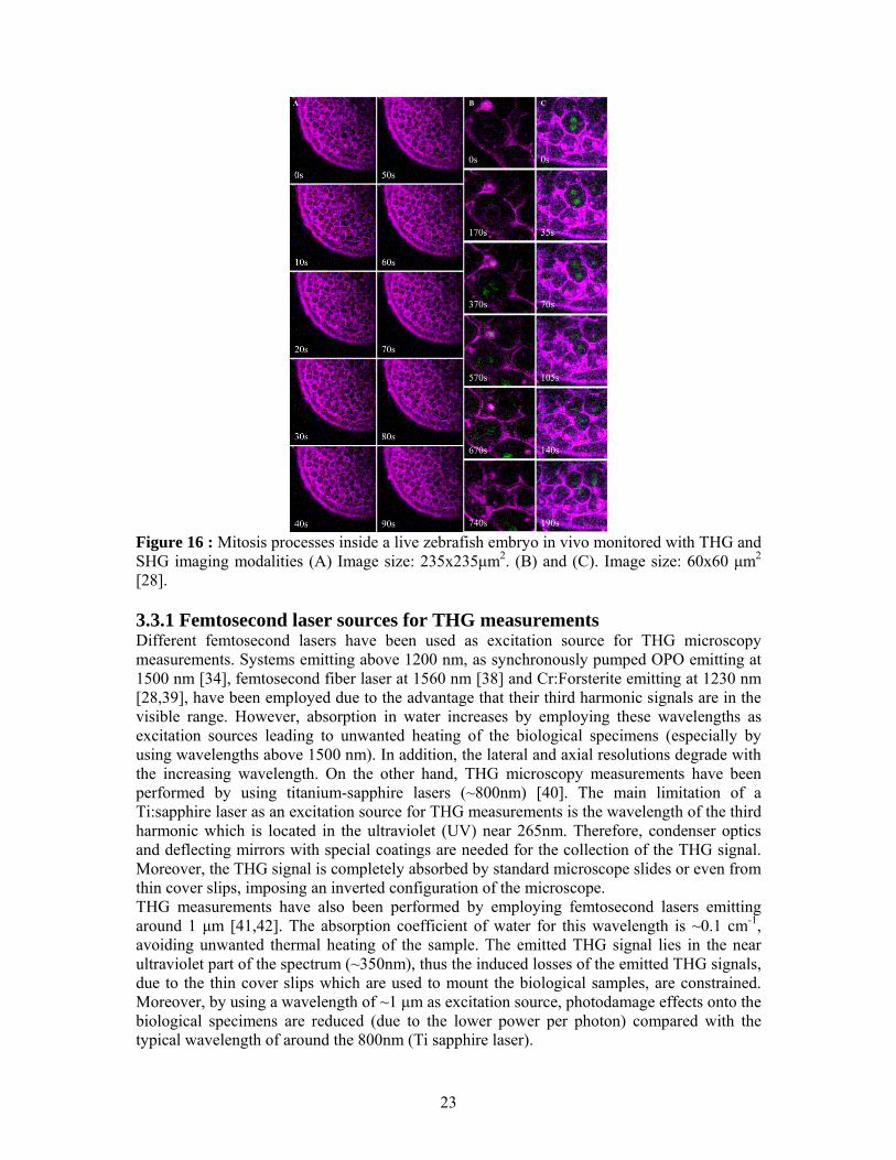
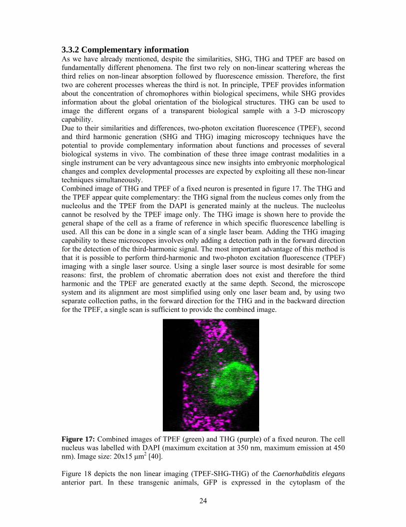
3.3.2 Complementary information As we have already mentioned, despite the similarities, SHG, THG and TPEF are based on fundamentally different phenomena. The first two rely on non-linear scattering whereas the third relies on non-linear absorption followed by fluorescence emission. Therefore, the first two are coherent processes whereas the third is not. In principle, TPEF provides information about the concentration of chromophores within biological specimens, while SHG provides information about the global orientation of the biological structures. THG can be used to image the different organs of a transparent biological sample with a 3-D microscopy capability. Due to their similarities and differences, two-photon excitation fluorescence (TPEF), second and third harmonic generation (SHG and THG) imaging microscopy techniques have the potential to provide complementary information about functions and processes of several biological systems in vivo. The combination of these three image contrast modalities in a single instrument can be very advantageous since new insights into embryonic morphological changes and complex developmental processes are expected by exploiting all these non-linear techniques simultaneously. Combined image of THG and TPEF of a fixed neuron is presented in figure 17. The THG and the TPEF appear quite complementary: the THG signal from the nucleus comes only from the nucleolus and the TPEF from the DAPI is generated mainly at the nucleus. The nucleolus cannot be resolved by the TPEF image only. The THG image is shown here to provide the general shape of the cell as a frame of reference in which specific fluorescence labelling is used. All this can be done in a single scan of a single laser beam. Adding the THG imaging capability to these microscopes involves only adding a detection path in the forward direction for the detection of the third-harmonic signal. The most important advantage of this method is that it is possible to perform third-harmonic and two-photon excitation fluorescence (TPEF) imaging with a single laser source. Using a single laser source is most desirable for some reasons: first, the problem of chromatic aberration does not exist and therefore the third harmonic and the TPEF are generated exactly at the same depth. Second, the microscope system and its alignment are most simplified using only one laser beam and, by using two separate collection paths, in the forward direction for the THG and in the backward direction for the TPEF, a single scan is sufficient to provide the combined image. Figure 17: Combined images of TPEF (green) and THG (purple) of a fixed neuron. The cell nucleus was labelled with DAPI (maximum excitation at 350 nm, maximum emission at 450 nm). Image size: 20x15 μm2 [40]. Figure 18 depicts the non linear imaging (TPEF-SHG-THG) of the Caenorhabditis elegans anterior part. In these transgenic animals, GFP is expressed in the cytoplasm of the

25

pharyngeal muscle cells. Figure 18(a) shows a TPEF image, obtained by backward detection, while figures 18(b) and 18(c) show the SHG and THG measurements respectively, detected in the forward direction. The combination of the three contributions is shown in figure 18(d). By TPEF imaging of the GFP molecules in pharyngeal muscles is feasible to visualize the inner part of the pharynx. The endogenous structures of well-ordered protein assemblies in the pharyngeal muscles, such as actomyosin complexes, are the main contributors to recorded SHG signals [19]. GFP molecules, due to their random orientation in the pharynx region do not contribute to the SHG signal. The contour and shape of the worm can be observed through THG measurements. Furthermore, high THG intensity signals are collected from the linings of the animal pseudocoelomic cavity. Consequently, the three non linear image modalities provide complementary information about the biological sample, as seen in figure 18. This is due to the fact that individual, induced signals come from different components. Diffuse GFP molecules are the main source of the detected TPEF signals. The endogenous oriented structural proteins are responsible for the observed SHG signals. Unique structural and functional information can be obtained by recording THG signals, given the sensitivity of these signals to changes of the refractive index of the medium.

Figure 18: Non-linear signals generated in the pharynx region of a worm expressing GFP in the pharyngeal muscles: (a) TPEF (b) SHG (c) THG and (d) multimodal image obtained by the combination of the previous three: TPEF (green), SHG (red) and THG (blue). The dimensions of the scanned region were 51 x 21 μm2 [42]. 3.4 Coherent Anti-stokes Raman scattering (CARS) Vibrational spectra of biological specimens contain a multitude of molecular signatures that can be used for identifying biochemical constituents in tissue. Conventional vibrational microscopy methods, however, lack the sensitivity required for rapid tissue examination. Infrared microscopy is limited by low spatial resolution due to the long wavelength of infrared light, as well as strong water absorption in biological specimens. Raman microspectroscopy, while capable of discriminating healthy from diseased tissue in vivo , is hampered by long integration times and/or high laser powers that are not desirable in biomedical applications. Much stronger vibrational signals can be attained with coherent anti-Stokes Raman scattering (CARS), a nonlinear Raman technique. CARS is a four-wave mixing process in which a

26

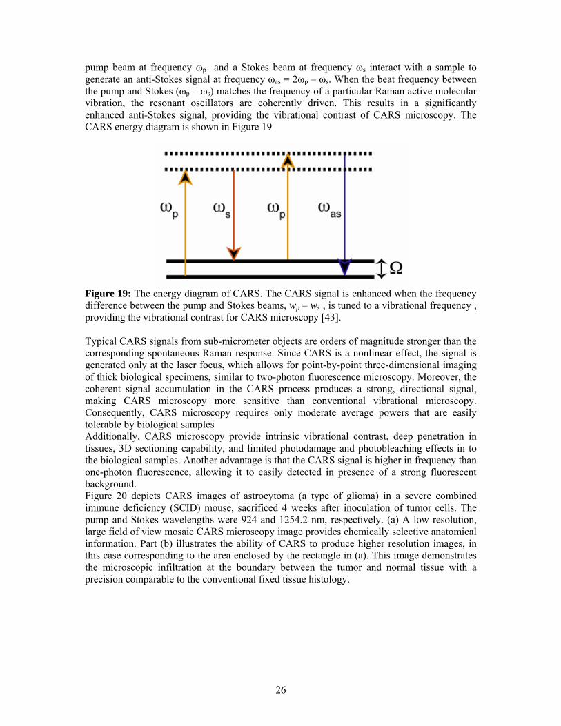
pump beam at frequency ωp and a Stokes beam at frequency ωs interact with a sample to generate an anti-Stokes signal at frequency ωas = 2ωp – ωs. When the beat frequency between the pump and Stokes (ωp – ωs) matches the frequency of a particular Raman active molecular vibration, the resonant oscillators are coherently driven. This results in a significantly enhanced anti-Stokes signal, providing the vibrational contrast of CARS microscopy. The CARS energy diagram is shown in Figure 19

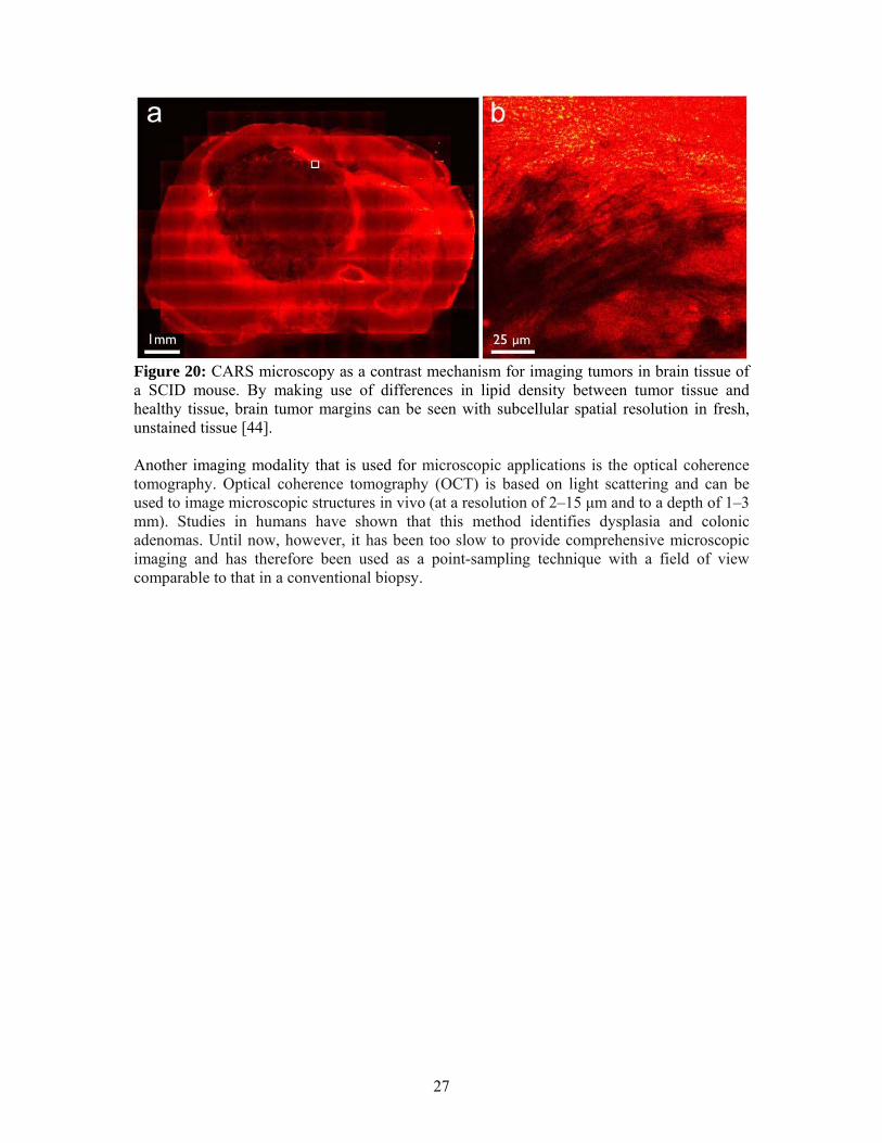
Figure 19: The energy diagram of CARS. The CARS signal is enhanced when the frequency difference between the pump and Stokes beams, wp – ws , is tuned to a vibrational frequency , providing the vibrational contrast for CARS microscopy [43]. Typical CARS signals from sub-micrometer objects are orders of magnitude stronger than the corresponding spontaneous Raman response. Since CARS is a nonlinear effect, the signal is generated only at the laser focus, which allows for point-by-point three-dimensional imaging of thick biological specimens, similar to two-photon fluorescence microscopy. Moreover, the coherent signal accumulation in the CARS process produces a strong, directional signal, making CARS microscopy more sensitive than conventional vibrational microscopy. Consequently, CARS microscopy requires only moderate average powers that are easily tolerable by biological samples Additionally, CARS microscopy provide intrinsic vibrational contrast, deep penetration in tissues, 3D sectioning capability, and limited photodamage and photobleaching effects in to the biological samples. Another advantage is that the CARS signal is higher in frequency than one-photon fluorescence, allowing it to easily detected in presence of a strong fluorescent background. Figure 20 depicts CARS images of astrocytoma (a type of glioma) in a severe combined immune deficiency (SCID) mouse, sacrificed 4 weeks after inoculation of tumor cells. The pump and Stokes wavelengths were 924 and 1254.2 nm, respectively. (a) A low resolution, large field of view mosaic CARS microscopy image provides chemically selective anatomical information. Part (b) illustrates the ability of CARS to produce higher resolution images, in this case corresponding to the area enclosed by the rectangle in (a). This image demonstrates the microscopic infiltration at the boundary between the tumor and normal tissue with a precision comparable to the conventional fixed tissue histology.

27

Figure 20: CARS microscopy as a contrast mechanism for imaging tumors in brain tissue of a SCID mouse. By making use of differences in lipid density between tumor tissue and healthy tissue, brain tumor margins can be seen with subcellular spatial resolution in fresh, unstained tissue [44]. Another imaging modality that is used for microscopic applications is the optical coherence tomography. Optical coherence tomography (OCT) is based on light scattering and can be used to image microscopic structures in vivo (at a resolution of 2–15 μm and to a depth of 1–3 mm). Studies in humans have shown that this method identifies dysplasia and colonic adenomas. Until now, however, it has been too slow to provide comprehensive microscopic imaging and has therefore been used as a point-sampling technique with a field of view comparable to that in a conventional biopsy.

28

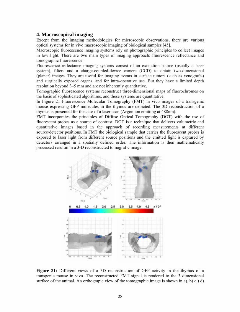
4. Macroscopical imaging Except from the imaging methodologies for microscopic observations, there are various optical systems for in vivo macroscopic imaging of biological samples [45]. Macroscopic fluorescence imaging systems rely on photographic principles to collect images in low light. There are two main types of imaging approach: fluorescence reflectance and tomographic fluorescence. Fluorescence reflectance imaging systems consist of an excitation source (usually a laser system), filters and a charge-coupled-device camera (CCD) to obtain two-dimensional (planar) images. They are useful for imaging events in surface tumors (such as xenografts) and surgically exposed organs, and for intra-operative use. But they have a limited depth resolution beyond 3–5 mm and are not inherently quantitative. Tomographic fluorescence systems reconstruct three-dimensional maps of fluorochromes on the basis of sophisticated algorithms, and these systems are quantitative. In Figure 21 Fluorescence Molecular Tomography (FMT) in vivo images of a transgenic mouse expressing GFP molecules in the thymus are depicted. The 3D reconstruction of a thymus is presented for the case of a laser scan (Argon ion emitting at 488nm). FMT incorporates the principles of Diffuse Optical Tomography (DOT) with the use of fluorescent probes as a source of contrast. DOT is a technique that delivers volumetric and quantitative images based in the approach of recording measurements at different source/detector positions. In FMT the biological sample that carries the fluorescent probes is exposed to laser light from different source positions and the emitted light is captured by detectors arranged in a spatially defined order. The information is then mathematically processed resultin in a 3-D reconstructed tomografic image.

Figure 21: Different views of a 3D reconstruction of GFP activity in the thymus of a transgenic mouse in vivo. The reconstructed FMT signal is rendered to the 3 dimensional surface of the animal. An orthograpic view of the tomographic image is shown in a). b) c ) d)

29

show the coronial, the axial and the sagittal view of the reconstructed thymus rendered to the 3D surface [46]. Furthermore, we have to mention that, several macroscopic optical imaging modalities that are not based on fluorescence have also been introduced (e.g. bioluminescence imaging). Bioluminescence imaging has emerged as a useful technique for imaging small experimental animals. The imaging signal depends on the expression levels of a luciferase enzyme, the presence of exogenously administered enzyme substrate (a luciferin), ATP, oxygen and depth. Numerous luciferase–luciferin pairs have been harnessed for in vivo imaging. In contrast to fluorescence techniques, there is no inherent background noise, which makes this technique highly sensitive. However, at present, this method does not allow absolute quantification of target signal instead, its primary uses is as an imaging tool to follow the same animal over time in identical conditions, including positioning of the body.

30

5. References [1] http://www.radiologyinfo.org/content/ultrasound-general.htm [2] http://www.mr-tip.com/serv1.php?type=isimg [3] http://www.radiologyinfo.org/content/bone_radiography.htm [4] http://www.radiologyinfo.org/content/ct_of_the_body.htm [5] http://www.radiologyinfo.org/content/petomography.htm [6] G. Filippidis, C. Kouloumentas, D. Kapsokalyvas, G. Voglis, N. Tavernarakis, T. G. Papazoglou, Journal of Physics D: Applied Physics 38 (2005) 2625 [7] P. Syntichaki, N. Tavernarakis, Physiological Reviews, 84 (2004) 1097 [8] C Xu W W. Webb, J. Opt. Soc. Am. B, 13, (1996) 481. [9] N. Billinton, A. W. Knight, Analytical Biochemistry, 291 (2001) 175. [10] R. Swaminathan, C. P. Hoang A. S. Verkman, Biophys. J., 72 (1997) 1900. [11] W. Denk, J. H. Strickler, W. W. Webb, Science 73, (1990) 248. [12] R. Yuste, W. Denk, Nature, 375, (1995) 682 [13] M. Maletic-Savatic, R. Malinow, K. Svoboda, ” Science, 283, (1999) 1923. [14] D. Kleinfeld, P. P. Mitra, F. Helmchen, W. Denk, Proc. Natl. Acad. Sci. USA, 95, (1998) 15741. [15] . B. J. Bacskai, S. T. Kajdasz, R. H. Christie, C. Carter, D. Games, P. Seubert, D. Schenk, B. T. Hyman, Nat. Med., 7, (2001) 369. [16] E.J. Gualda, G. Filippidis, G. Voglis, M. Mari, C. Fotakis, N. Tavernarakis SPIE, 6630, (2007) 663003. [17] L. Moreaux, O. Sandre, S. Charpak, M. Blanchard-Desce, J. Mertz, Biophysical Journal, 80, (2001) 1568. [18] P. J. Campagnola, L. M. Loew, Nature Biotechnology 21 (2003) 1356. [19] G. Filippidis, C. Kouloumentas, G. Voglis, F. Zacharopoulou, T. G. Papazoglou, N. Tavernarakis, Journal of Biomedical Optics 10, (2005) 024015. [20] Y. R. Shen Nature, 337, (1989) 519. [21] O. Bouevitch, A. Lewis, I. Pinevsky, J. P. Wuskell, L. M. Loew, Biophysical Journal, 65, (1993) 672. [22] G. Peleg, A. Lewis, M. Linial, L. M. Loew, Proc. Natl. Acad. Sci. USA, 96, (1999) 6700. [23] L. Moreaux, T. Pons, V. Dambrin, M. Blanchard-Desce, J. Mertz, Optics Letters, 28, (2003) 625. [24] A. Khatchatouriants, A. Lewis, Z. Rothman, L. Loew, M. Treinin, Biophysical Journal, 79, (2000) 2345. [25] http://www.ccam.uchc.edu/campagnola/Research/shg.html [26] J. Mertz, Eur. Phys. J. D, 3, (1998) 53. [27] J. Mertz, in A. Dixon (Ed), Second harmonic generation microscopy in: Multi-photon laser scanning microscopy, BIOS Press, Oxford, in press [28] C.K. Sun, S.W. Chu, S. Y. Chen, T. H. Tsai, T. M. Liu, C. Y. Lin H. J. Tsai, Journal of Structural Biology, 147, (2004) 19. [29] J. Squier, M. Muller, Rev. of Scientific. Instruments 72 (2001) 2855. [30] D. Debarre, W. Supatto, A. M. Pena, A. Fabre, T. Tordjmann, L. Combettes, M. C. Schanne-Klein, E. Beaurepaire, Nature Methods 3 (2006) 47. [31] Y. Barad, H. Eisenberg, M. Horowitz, Y. Silberberg, Applied Physics Letters, 70 (1997) 922 [32] G. Veres, S. Matsumoto, Y. Nabekawa, and K. Midorikawa, Applied Physics Letters, 81 (2002) 3714 [33] D. Debarre, W. Supatto, E. Farge, B. Moulia, M.C. Schanne-Klein, E. Beaurepaire, Opt. Letters 29 (2004) 2881 [34] D. Yelin, Y Silberberg, Opt. Express 5 (1999) 169

31

[35] W. Supatto, D. Debarre, E. Fargea, E. Beaurepaire, Med. Las. Application 20 (2005) 207 [36] M. Muller, J. Squier, K.R. Wilson , G.F. Brakenhoff , J. of Microscopy 191 (1998) 266 [37] E. J. Gualda, G. Filippidis, M. Mari, G. Voglis, M. Vlachos, C. Fotakis N. Tavernarakis in press Journal of Microscopy [38] A. C. Millard, P.W. Wiseman, D.N. Fittinghoff, K.R. Wilson, J.A. Squier, M. Muller, App. Optics, 38 (1999) 7393 [39] T.H. Tsai, S.P. Tai, W.J. Lee, H.Y. Huang, Y.H. Liao, C.K. Sun, Opt. Express 14 (2006) 749 [40] D. Yelin, D. Oron, E. Korkotian, M. Segal, Y. Silberberg, Appl. Phys. B 74 (2002) 97. [41] G.O. Clay, A.C. Millard, C.B. Schaffer, J. Aus-der-Au, P.S. Tsai, J.A. Squier, D. Kleinfeld, J. Opt. Soc. Am. B, 23 (2006) 932. [42] E.J. Gualda, G. Filippidis, G. Voglis, M. Mari, C. Fotakis, N. Tavernarakis Journal of Microscopy 229, (2008) 141. [43] http://bernstein.harvard.edu/research/cars.html [44] C.L. Evans, X. Xu, S. Kesari, X.S. Xie, S. T.C. Wong, G. S. Young, Optics Express 15, (2007) 12076. [45] R. Weissleder, M.J. Pittet, Nature 452 (2008) 06917 [46] A. Garofalakis, G. Zacharakis, H. Meyer, E.N. Economou, C. Mamalaki, J. Papamatheakis, D. Kioussis, V. Ntziachristos, J. Ripoll, Mol. Imaging, 6 (2007) 96

32

George Filippidis received the B.Sc. degree from the Physics Department of the University of Crete, Greece, in 1995. He received the Doctorate degree from the Medical School of the University of Crete, Greece, in 2000. His thesis was on the detection of atherosclerotic tissue using laser induced fluorescence spectroscopy (LIFS). He is associated researcher at the Laser & Application Division FORTH-IESL from 2002. His research interests include L.I.F.S. for medical diagnostics, optical characterization of tissue, photodynamic therapy, random lasers, TPEF, SHG and THG imaging microscopy. He has published 26 articles in international refereed journals and 18 full-length articles in edited and refereed proceedings volumes. He is scientific responsible of 2 European Union research projects.