
Noise Estimation in the Presence of BPSK Digital Burst ...
110
Air Force Institute of Technology Air Force Institute of Technology AFIT Scholar AFIT Scholar Theses and Dissertations Student Graduate Works 3-2005 Noise Estimation in the Presence of BPSK Digital Burst Noise Estimation in the Presence of BPSK Digital Burst Transmissions Transmissions Susan E. Bettison Follow this and additional works at: https://scholar.afit.edu/etd Part of the Applied Mathematics Commons, and the Signal Processing Commons Recommended Citation Recommended Citation Bettison, Susan E., "Noise Estimation in the Presence of BPSK Digital Burst Transmissions" (2005). Theses and Dissertations. 3715. https://scholar.afit.edu/etd/3715 This Thesis is brought to you for free and open access by the Student Graduate Works at AFIT Scholar. It has been accepted for inclusion in Theses and Dissertations by an authorized administrator of AFIT Scholar. For more information, please contact richard.mansfield@afit.edu.
-
Upload
khangminh22 -
Category
Documents
-
view
0 -
download
0
Transcript of Noise Estimation in the Presence of BPSK Digital Burst ...

Air Force Institute of Technology Air Force Institute of Technology
AFIT Scholar AFIT Scholar
Theses and Dissertations Student Graduate Works
3-2005
Noise Estimation in the Presence of BPSK Digital Burst Noise Estimation in the Presence of BPSK Digital Burst
Transmissions Transmissions
Susan E. Bettison
Follow this and additional works at: https://scholar.afit.edu/etd
Part of the Applied Mathematics Commons, and the Signal Processing Commons
Recommended Citation Recommended Citation Bettison, Susan E., "Noise Estimation in the Presence of BPSK Digital Burst Transmissions" (2005). Theses and Dissertations. 3715. https://scholar.afit.edu/etd/3715
This Thesis is brought to you for free and open access by the Student Graduate Works at AFIT Scholar. It has been accepted for inclusion in Theses and Dissertations by an authorized administrator of AFIT Scholar. For more information, please contact [email protected].

NOISE ESTIMATION IN THE PRESENCE OF BPSK DIGITAL BURST TRANSMISSIONS
THESIS
Susan Elizabeth Bettison, Second Lieutenant, USAF
AFIT/GAM/ENC/05-03
DEPARTMENT OF THE AIR FORCE
AIR UNIVERSITY
AIR FORCE INSTITUTE OF TECHNOLOGY
Wright-Patterson Air Force Base, Ohio
APPROVED FOR PUBLIC RELEASE; DISTRIBUTION UNLIMITED

The views expressed in this thesis are those of the author and do not re�ect the o¢ cial
policy or position of the Department of Defense or the United States Government.

AFIT/GAM/ENC/05-03
Noise Estimation in the Presence of BPSK Digital Burst Transmissions
THESIS
Presented to the Faculty of the School of Engineering
of the Air Force Institute of Technology
Air University
In Partial Ful�llment of the
Requirements for the Degree of
Master of Science in Applied Mathematics
Susan Elizabeth Bettison, B.S.
Second Lieutenant, USAF
March 2005
Approved for public release; distribution unlimited

AFIT/GAM/ENC/05-03
Noise Estimation in the Presence of BPSK Digital Burst Transmissions
Susan Elizabeth Bettison, B.S.
Second Lieutenant, USAF
Approved:
Lawrence K. Chilton (Chairman) Date
Jay E. Apisa (Member) Date
Richard K. Martin (Member) Date
AFIT/GAM/ENC/05-03
Abstract
This research explores noise estimation techniques in an attempt to improve upon a
previously developed digital burst transmission Binary Phase Shift Keyed (BPSK) demod-
ulator. The demodulator success is dependant on the accuracy of the estimate of Power
Spectral Density (PSD) of the unknown noise. Given a discrete time signal transformed
into the frequency domain, the research seeks to determine if it is possible to e¤ectively
estimate the PSD of the unknown noise. The demodulator was developed using a new sig-
nal model for digital burst transmissions based on linear spectral subspace theory. Using
this model and the redundancy properties of BPSK digital burst transmissions, �ve noise
estimation techniques will be presented and tested. The success of the methods will be
reported in two ways, �rst, the e¤ect the new noise PSD estimates have on the success of
the demodulator and second, a comparison to the actual PSD of the noise.
iii

Acknowledgements
I would sincerly like to thank my advisor, Dr. Chilton and my committee members Dr.
Martin and Mr. Apisa.
Susan Elizabeth Bettison
iv

Table of Contents
Page
Abstract . . . . . . . . . . . . . . . . . . . . . . . . . . . . . . . . . . . . . . . . iii
Acknowledgements . . . . . . . . . . . . . . . . . . . . . . . . . . . . . . . . . . iv
List of Figures . . . . . . . . . . . . . . . . . . . . . . . . . . . . . . . . . . . . viii
I. Introduction . . . . . . . . . . . . . . . . . . . . . . . . . . . . . . . . 1
1.1 Problem De�nition . . . . . . . . . . . . . . . . . . . . . . . . 1
1.2 Organization . . . . . . . . . . . . . . . . . . . . . . . . . . . 3
II. Background . . . . . . . . . . . . . . . . . . . . . . . . . . . . . . . . . 2-1
2.1 Burst Transmission Signals . . . . . . . . . . . . . . . . . . . 2-1
2.1.1 Pulse Amplitude Modulated Signal Model . . . . . . 2-2
2.1.2 Burst Transmission Subspace and BPSK Signal Model
Speci�cs . . . . . . . . . . . . . . . . . . . . . . . . . 2-4
2.1.3 The Distribution of a Burst Transmission Signal, x(t) 2-13
2.2 Existing Signal Processing Methods . . . . . . . . . . . . . . 2-16
2.2.1 Stationary approach . . . . . . . . . . . . . . . . . . 2-16
2.2.2 Cyclostationary . . . . . . . . . . . . . . . . . . . . . 2-17
2.3 A Better Signal Model for Burst Transmission Signals . . . . 2-19
2.4 Optimal Filtering . . . . . . . . . . . . . . . . . . . . . . . . 2-20
2.4.1 Matched Filtering . . . . . . . . . . . . . . . . . . . 2-21
2.4.2 Equalization . . . . . . . . . . . . . . . . . . . . . . 2-22
2.5 A Minimum Mean Square Error Filter for Burst Transmission
Signals . . . . . . . . . . . . . . . . . . . . . . . . . . . . . . 2-23
2.6 Preliminaries . . . . . . . . . . . . . . . . . . . . . . . . . . . 2-25
v

Page
III. Theoretical Development . . . . . . . . . . . . . . . . . . . . . . . . . 3-1
3.1 Method One: Subtract in Time . . . . . . . . . . . . . . . . . 3-1
3.2 Methods Using the Signal Redundancies . . . . . . . . . . . . 3-2
3.2.1 Subtraction of the Smallest Redundancy . . . . . . . 3-5
3.2.2 Subtraction of the Average Redundancy . . . . . . . 3-6
IV. Analysis by Simulation . . . . . . . . . . . . . . . . . . . . . . . . . . 4-1
4.1 Impact on Demodulation . . . . . . . . . . . . . . . . . . . . 4-1
4.1.1 Method One: Subtract in Time . . . . . . . . . . . . 4-1
4.1.2 Methods Using the Signal Redundancies . . . . . . . 4-2
4.2 Comparison to Actual Power Spectral Density of the Noise . 4-6
4.2.1 Method One: Subtract in Time . . . . . . . . . . . . 4-7
4.2.2 Methods Using Signal Redundancies . . . . . . . . . 4-7
V. Conclusions/Recommendations . . . . . . . . . . . . . . . . . . . . . . 5-1
5.1 Summary of Results . . . . . . . . . . . . . . . . . . . . . . . 5-1
5.2 Future Work . . . . . . . . . . . . . . . . . . . . . . . . . . . 5-2
5.3 Conclusion . . . . . . . . . . . . . . . . . . . . . . . . . . . . 5-2
VI. Appendix A Mathematica Notebooks . . . . . . . . . . . . . . . . . . 6-1
6.1 Data Generation . . . . . . . . . . . . . . . . . . . . . . . . . 6-1
6.2 Known Noise Scale . . . . . . . . . . . . . . . . . . . . . . . . 6-3
6.3 Known Noise Shape . . . . . . . . . . . . . . . . . . . . . . . 6-5
6.4 Unknown Shape and Scale . . . . . . . . . . . . . . . . . . . 6-8
6.5 Subtraction of the Minimum Redundancy . . . . . . . . . . . 6-11
6.5.1 Subtraction of the Minimum Redundancy Before Mul-
tiplication by Pulse Shape . . . . . . . . . . . . . . . 6-11
6.5.2 Subtraction of the Minimum Redundancy After Mul-
tiplication by Pulse Shape . . . . . . . . . . . . . . . 6-18
vi

Page
6.6 Subtraction of the Average Redundancy . . . . . . . . . . . . 6-24
6.6.1 Subtraction of the Average Redundancy Before Mul-
tiplication by Pulse Shape . . . . . . . . . . . . . . . 6-24
6.6.2 Subtraction of the Average Redundancy After Multi-
plication by Pulse Shape . . . . . . . . . . . . . . . . 6-29
6.7 Comparison . . . . . . . . . . . . . . . . . . . . . . . . . . . . 6-34
Bibliography . . . . . . . . . . . . . . . . . . . . . . . . . . . . . . . . . . . . . BIB-1
vii

List of Figures
Figure Page
1.1. Diagram of BPSK Signal Model Construction . . . . . . . . . . . . . . . 2
2.1. A Sum of Three BPSK Burst Transmissions . . . . . . . . . . . . . . . 2-4
2.2. Positioning of Redundancies in the Frequency Domain Vector . . . . . . 2-8
2.3. The Spectral Density Problem with Classical Burst Signal Analysis . . . 2-20
2.4. The Structure of an Optimal Filter . . . . . . . . . . . . . . . . . . . . 2-21
2.5. Bandpass MMSE (Gisselquist�s) System Diagram . . . . . . . . . . 2-24
2.6. A Sinc Function vs. Modi�ed Sinc . . . . . . . . . . . . . . . . . . . . 2-25
2.7. BPSK signal with Ns = 64 . . . . . . . . . . . . . . . . . . . . . . . 2-26
2.8. BER vs. Noisescale for Unknown Scale and Shape of the Noise PSD . . . 2-27
2.9. BER vs. SNR for Unknown Shape and Scale of the Noise PSD . . . . . . 2-27
2.10. BER vs. Noisescale for Known Scale and Unknown Shape of the Noise PSD 2-28
2.11. BER vs. SNR for Known Scale and Unknown Shape of the Noise PSD . . 2-28
2.12. BER vs. Noisescale for Known Shape and Unknown Scale of the Noise PSD 2-29
2.13. BER vs. SNR for Known Shape and Unknown Scale of the Noise PSD . . 2-29
3.1. Flow Diagram for Method One: Subtract in Time . . . . . . . . . . . . . 3-3
3.2. Diagram of Subtraction of Minimum Redundancy before Pulse Shape
Multiplication . . . . . . . . . . . . . . . . . . . . . . . . . . . . . . 3-6
3.3. Diagram of Subtraction of Minimum Redundancy after Pulse Shape
Multiplication . . . . . . . . . . . . . . . . . . . . . . . . . . . . . . 3-7
3.4. Diagram of Subtraction of the Redundancy Average before Pulse
Shape Multiplication . . . . . . . . . . . . . . . . . . . . . . . . . . 3-8
3.5. Diagram of Subtraction of the Redundancy Average after Pulse Shape Mul-
tiplication . . . . . . . . . . . . . . . . . . . . . . . . . . . . . . . . . 3-9
4.1. Method One: Subtract in Time BER vs. Iteration Number . . . . . . . 4-2
viii

Figure Page
4.2. BER vs. Noisescale, Subtraction of the Smallest Redundancy before Pulse
Shape Multiplication . . . . . . . . . . . . . . . . . . . . . . . . . . . 4-3
4.3. BER vs. SNR in dB, Subtraction of the Smallest Redundancy before Pulse
Shape Multiplication . . . . . . . . . . . . . . . . . . . . . . . . . . . 4-4
4.4. BER vs. SNR, Subtraction of the Smallest Redundancy after Pulse shape
Multiplication . . . . . . . . . . . . . . . . . . . . . . . . . . . . . . 4-4
4.5. BER vs. SNR, Subtraction of the Average Redundancy before Pulse Shape
Multiplication . . . . . . . . . . . . . . . . . . . . . . . . . . . . . . 4-5
4.6. BER vs. SNR, Subtraction of the Average Redundancy after Pulse Shape
Multiplication . . . . . . . . . . . . . . . . . . . . . . . . . . . . . . . 4-5
4.7. BER vs. SNR . . . . . . . . . . . . . . . . . . . . . . . . . . . . . . . 4-6
4.8. Results of Method One: Subtract in Time . . . . . . . . . . . . . . . . . 4-7
4.9. Estimated Noise PSD Using Subtraction of the Smallest Redundancy before
Mulitplication by Pulse Shape . . . . . . . . . . . . . . . . . . . . . . . 4-8
4.10. Zoomed in Estimated Noise PSD Using Subtraction of the Smallest Redun-
dancy before Mulitplication by Pulse Shape . . . . . . . . . . . . . . . . 4-8
4.11. Actual Noise PSD . . . . . . . . . . . . . . . . . . . . . . . . . . . . 4-9
4.12. MSE vs. SNR, Using Subtraction of the Smallest Redundancy before Mulit-
plication by Pulse Shape . . . . . . . . . . . . . . . . . . . . . . . . . 4-10
4.13. Estimated Noise PSD Using Subtraction of the Smallest Redundancy after
Mulitplication by Pulse Shape . . . . . . . . . . . . . . . . . . . . . . . 4-10
4.14. Zoomed in Estimated Noise PSD Using Subtraction of the Smallest Redun-
dancy after Mulitplication by Pulse Shape . . . . . . . . . . . . . . . . 4-11
4.15. Actual Noise PSD . . . . . . . . . . . . . . . . . . . . . . . . . . . . 4-11
4.16. MSE vs. SNR Using Subtraction of the Smallest Redundancy after Pulse
Shape Multiplication . . . . . . . . . . . . . . . . . . . . . . . . . . . 4-11
4.17. Estimated Noise PSD Using Subtraction of the Average Redundancy before
Pulse Shape Multiplication . . . . . . . . . . . . . . . . . . . . . . . . 4-12
4.18. Zoomed in Estimated Noise PSD Using Subtraction of the Average Redun-
dancy before Pulse Shape Multiplication . . . . . . . . . . . . . . . . . 4-12
ix

Figure Page
4.19. Actual PSD Using Subtraction of the Average Redundancy before Pulse
Shape Multiplication . . . . . . . . . . . . . . . . . . . . . . . . . . . 4-13
4.20. MSE vs. SNR Using Subtraction of the Average Redundancy before Pulse
Shape Multiplication . . . . . . . . . . . . . . . . . . . . . . . . . . . 4-13
4.21. Estimated Noise PSD Using Subtraction of the Average Redundancy after
Pulse Shape Multiplication . . . . . . . . . . . . . . . . . . . . . . . . 4-14
4.22. Zoomed in Estimated Noise PSD Using Subtraction of the Average Redun-
dancy after Pulse Shape Multiplication . . . . . . . . . . . . . . . . . . 4-14
4.23. Actual Noise PSD . . . . . . . . . . . . . . . . . . . . . . . . . . . . 4-14
4.24. MSE vs. SNR Using Subtraction of the Average Redundancy after Pulse
Shape Multiplication . . . . . . . . . . . . . . . . . . . . . . . . . . . 4-14
4.25. MSE vs. Noise Scale Subtraction Methods Compared . . . . . . . . . . . 4-15
x
Noise Estimation in the Presence of BPSK Digital Burst Transmissions
I. Introduction
Digital burst transmission signals are all around us, everyday. An example everyone
has seen is a digital cell phone. As communication techniques become increasingly secure,
exploitation di¢ culties increase. Not only do problems exist when trying to exploit non
friendly communications, but in cooperative communications. If successful, the application
of this research will be helpful in both scenarios.
1.1 Problem De�nition
A fundamental problem in all signal processing has always been the estimation of the
noise received with any transmitted signal. The more that is known about the noise, the
more e¤ective any signal processing algorithm will be. Using linear subspace theory, a new
demodulation algorithm was developed in (11). Existing signal processing techniques did
not fully apply to the digital burst transmission signal processing problem (11) thus a new
approach was needed. The linear subspace theory research resulted in a new demodulation
algorithm which outperformed all other existing demodulation techniques, for digital burst
transmissions, including Binary Phase Shift Keyed (BPSK) modulated signals (11). The
drawback of the technique is that it performs best when an a priori estimation of the noise
environment is known, and a colored noise environment increases the success even further
(11). This was the initial motivation for this research. However, to jump directly into the
colored noise problem is not feasible since colored noise environments are generally unpre-
dictable. Thus, the white noise estimation problem is a logical starting point. Although
the white noise estimation problem is unlikely to immediately improve the performance of
the demodulation technique, it provides a starting point for the colored noise estimation
problem or even adaptive noise estimation techniques.
The new demodulation algorithm provided a solution to a problem, but also presented
additional problems to be solved. The problem of note for this thesis is the estimation of
the Power Spectral Density (PSD) of the noise since the demodulation technique presented
1
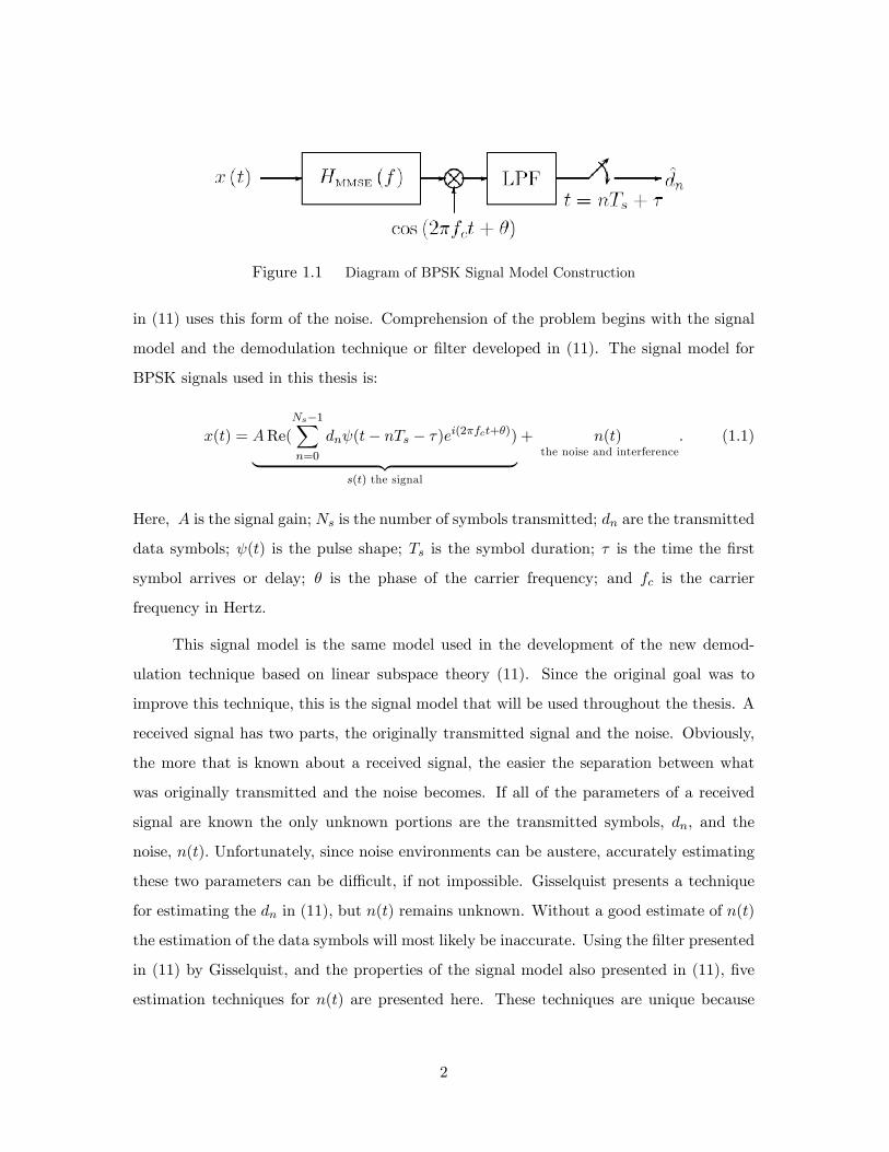
Figure 1.1 Diagram of BPSK Signal Model Construction
in (11) uses this form of the noise. Comprehension of the problem begins with the signal
model and the demodulation technique or �lter developed in (11). The signal model for
BPSK signals used in this thesis is:
x(t) = ARe(
Ns�1Xn=0
dn (t� nTs � �)ei(2�fct+�))| {z }s(t) the signal
+ n(t)the noise and interference
: (1.1)
Here, A is the signal gain; Ns is the number of symbols transmitted; dn are the transmitted
data symbols; (t) is the pulse shape; Ts is the symbol duration; � is the time the �rst
symbol arrives or delay; � is the phase of the carrier frequency; and fc is the carrier
frequency in Hertz.
This signal model is the same model used in the development of the new demod-
ulation technique based on linear subspace theory (11). Since the original goal was to
improve this technique, this is the signal model that will be used throughout the thesis. A
received signal has two parts, the originally transmitted signal and the noise. Obviously,
the more that is known about a received signal, the easier the separation between what
was originally transmitted and the noise becomes. If all of the parameters of a received
signal are known the only unknown portions are the transmitted symbols, dn, and the
noise, n(t): Unfortunately, since noise environments can be austere, accurately estimating
these two parameters can be di¢ cult, if not impossible. Gisselquist presents a technique
for estimating the dn in (11), but n(t) remains unknown. Without a good estimate of n(t)
the estimation of the data symbols will most likely be inaccurate. Using the �lter presented
in (11) by Gisselquist, and the properties of the signal model also presented in (11), �ve
estimation techniques for n(t) are presented here. These techniques are unique because
2

they are implemented using techniques based on Gisselquist�s linear subspace approach.
Prior to Gisselquist�s research, signal processing techniques for BPSK and other Pulse Am-
plitude Modulated (PAM) digital signals was based on stationary or cyclostationary signal
processing (11). Provided the techniques presented here are su¢ ciently robust, they will
be an excellent starting point for the larger colored noise estimation problem and for the
adaptive noise estimation problem. Even if not successful, they should provide direction
for future noise estimation techniques.
1.2 Organization
This thesis begins with an in depth explanation of the signal model, the properties
used in estimating the PSD of the noise, a description of relevant existing statistical signal
processing models and �nally an overview of the demodulation technique presented by
Gisselquist. Chapter III presents the methods used to estimate the PSD of the noise based
o¤ the explanations in Chapter II, and Chapter IV explains the results when tested in
simulations. The last chapter, Chapter V draws some conclusions regarding the success of
the noise estimation techniques.
3

II. Background
This chapter presents an explanation of digital burst transmission signals, a summary of
relevant statistical signal processing models, an optimal �ltering technique for the rele-
vant statistical signal processing models, and �nally presents the minimum mean square
error �lter that suggested the need for noise estimation in the presence of digital burst
transmission signals.
The working signal model is a signal with a general modulation type of Pulse Ampli-
tude Modulation (PAM), but more speci�cally, Binary Phase Shift Keyed (BPSK) modu-
lation. The received signal in time may be represented by equation 1.1. This signal model
has many properties that existing statistical signal processing models did not adequately
exploit (11). Because of this, Gisselquist established a statistical signal processing model
for burst transmission signals and then developed a Minimum Mean Square Error (MMSE)
�lter which exploits more of the characteristics than previous �lters. This �lter produced
the best symbol recovery results to date, given the noise estimate used in the construction
of the �lter was accurate in shape and scale (11). The relevant statistical signal processing
models will be presented, then the chapter will �nish with the derivation of Gisselquist�s
MMSE �lter, presenting some results obtained using his �lter on simulated BPSK signals.
2.1 Burst Transmission Signals
Burst transmission signals have many unique properties that distinguish them from
other types of signals. The �rst and most important, is that they are not in�nite in time.
In fact they are very time limited, and more uniquely, the times when the signal is active
may or may not be of all the same duration. This section presents a basic PAM signal
model, an explanation of the subspace that describes it, the speci�cs of a BPSK signal
model that exists in this subspace, and �nally the distribution of a burst transmission
signal is derived.
2-1

2.1.1 Pulse Amplitude Modulated Signal Model. The received signal in time may
be represented by (11),
x(t) = ARe(
Ns�1Xn=0
dn (t� nTs � �)ei(2�fct+�))| {z }s(t) the transmitted signal
+ n(t)the noise and interference
: (2.1)
The parameters in this signal model are de�ned in Section 1.1.
In this thesis, the signal is analyzed in the frequency domain for two reasons. First,
stationary signals which are correlated in time become uncorrelated in frequency for suf-
�ciently long observation times (11, 18). Second, the unknown terms in � and � become
constant multipliers in the frequency domain, making them easier to work with. When it
comes to signal processing in the frequency domain, there are two statistics of interest that
have been studied extensively by others; these statistics are the �rst and second moments
(11). The �rst moment is the expected value, or the mean, and is assumed to be zero for
both the signal and noise terms. The second moment, or the variance, is more interesting
and is where many of the di¤erentiating characteristics of signals are found. The variance
of a signal depends on how the signal is de�ned (11). If the signal is time-limited then the
in�nite time Fourier transform X(f) of the signal x(t);
X(f) ,Z 1
�1x(t)e�i2�ftdt; (2.2)
converges. With a time limited signal, both the signal and noise are assumed to have zero
mean and the variance of X(f) is1 EfjX(f)j2g: If the signal is of in�nite length, the Fourier
transform will not always converge (17, 11). Because of this, an alternate method must
be used to describe the variance of an in�nite time signal. This alternate method is the
Power Spectral Density (PSD), Sx(f), and is de�ned as (17):
Sx(f) , limT!1
1
TEfjXT (f)j2g (2.3)
where XT (f) is the time limited Fourier transform of x(t);
1The notation Ef�g is used throughout to refer to the expected value of its argument.
2-2

XT (f) ,Z T
2
�T2
x(t)e�i2�ftdt (2.4)
Thus the PSD can be used to describe the distribution of the power in a signal, as a
function of frequency (11). Additionally, a nice property of uncorrelated signals is that the
PSD of the received signal Sx(f) is the sum of the PSD of the transmitted signal, Ss(f),
and the PSD of the noise, Sn(f)(11, 23):
Sx(f) = Ss(f) + Sn(f): (2.5)
This is very useful in both Gisselquist�s algorithm development and the methods used in
this thesis to estimate the PSD of the noise. The PSD of a burst transmission signal or
more generally a pulse amplitude modulated (PAM) signal is2 (9):
Ss(f) =A2
4Tsj(f � fc)j2Efjdnj2g (2.6)
Here, (f) is the Fourier transform of the pulse function (t). Ts is the symbol duration.
fc is the carrier frequency in Hertz, and dn are the transmitted data symbols. A received
PAM transmission signal with a �nite number of symbols, Ns, is described by equation
2.1.
The noise and interference term represents a random process that is assumed to be
stationary, independent of the signal, and to have a PSD de�ned as Sn(f)(11). This thesis
focuses on developing an adequate method of estimating this PSD. Each of the terms in
equation 2.1 can be understood in the context of how the signal is created. As an example,
consider the signal example in Figure 2.1, an example of three transmissions created with
the model in equation 2.1 with the noise term set to zero. The bursts are created from a
sum of pulses, (t� nTs � �). The �gure is a sum of three bursts all of di¤erent lengths.
The pulses are separated by Ts, and scaled by a system gain, A = 1; from their original
amplitude. A time delay � ; has shifted the signal to the right, and the phase, �; and the
2The assumption that the transmitted data symbols are uncorrelated or that Efdnd�mg = 0, for n 6= mis made throughout this thesis.
2-3

Figure 2.1 A Sum of Three BPSK Burst Transmissions
carrier frequency fc; are both zero. Each burst is itself a sum of pulses, one pulse for each
data symbol transmitted. The �rst burst has two data symbols, the second has eight and
the third, four. Each burst is separated by a time of four seconds. This is obviously a
very elementary example but illustrates what burst transmission signals might look like.
Although this �gure has three bursts, within the scope of this thesis, we will only be
concerned with estimating the noise in one burst ignoring the time before and after, when
the signal is inactive.
2.1.2 Burst Transmission Subspace and BPSK Signal Model Speci�cs. Gisselquist
took the principles of other statistical signal processing techniques and extended them so
they would be applicable to time-limited burst transmission signals. Next we will describe
in detail Gisselquist�s development of the signal model and the associated subspace, as
it plays a major role in the development of the processing technique. Other statistical
signal processing techniques assume in�nite time length signals as in the case of stationary
signals, or that the cyclic spectral density function, also known as the Spectral Correlation
Function, de�ned in equation 2.32 is known, as in cyclostationary signals. Neither of
these apply to burst transmission signals. Burst transmissions do have correlation in the
frequency domain, however it is not usually known. Further explanation of the di¤erences
2-4

between burst transmission signals and these other statistical signal processing models will
be explained in Section 2.2.
In deriving a new statistical model for burst transmissions, Gisselquist �rst had to
establish the subspace that burst transmission signals exist in. Consider the set of all
functions de�ned over a �nite time containing the signal. This can be seen because the
signal is a linear combination of evenly spaced pulses weighted by the dn values. The pulses
then form the basis for the subspace where the signal resides. These two sets of vectors
span the subspace that contains PAM signals (11):
�ki = (t� kTs � �) cos(2�fct+ �), k 2 Is�kq = (t� kTs � �) sin(2�fct+ �), k 2 Is
(2.7)
where Is is some �nite set of consecutive integers. The problem with this subspace is
that these basis vectors depend on the unknown delay, � , and the carrier phase, �; making
them di¢ cult to use in practice (11). To continue with the development, the signal must
be transformed into the frequency domain with the Fourier transform.
Burst transmission signals are time limited and thus fall within a �nite observation
time, t 2 (�T2 ;
T2 ): Although here the time limited Fourier transform is identical to the
in�nite time Fourier transform, the time limited transform is required since the noise may
or may not be time-limited (11). The time-limited Fourier transform of the received signal
is then (11):
XT (f) ,Z T
2
�T2
x(t)e�i2�ftdt (2.8)
De�ne NT (f) to be the time-limited Fourier transform of the noise and interference thus
the Fourier transform of
x(t) = ARe(
Ns�1Xn=0
dn (t� nTs � �)ei(2�fct+�)) + n(t) (2.9)
2-5

becomes (11):
XT (f) = NT (f) +A2
Ns�1Pn=0
Re(dn)R1�1 (t� nTs � �)[ei2�fct+i��i2�ft + e�i2�fc�i��i2�ft]dt
+iA2
Ns�1Pn=0
Im(dn)R1�1 (t� nTs � �)[ei2�fct+i��i2�ft + e�i2�fc�i��i2�ft]dt
(2.10)
Since the scope of our problem is BPSK signals only, we can disregard the imaginary part
since the signal is purely real in the time domain. Now letting u = t�Ts� � ; and du = dt
we have (11):
XT (f) = NT (f)+A
2ei�
Ns�1Xn=0
cos(2�(f�fc)�)[dn cos(2�(f�fc)nTs)]Z 1
�1 (u) cos(2�(f�fc)u)du:
(2.11)
Continuing with substitutions, if we let the Fourier transform of (t) be
(f) ,R1�1 (t)e�i2�ftdt and the z-transform of the data symbols be
D(z) ,Ns�1Xn=0
dnz�n (2.12)
the function becomes (11):
XT (f) = NT (f) +A
2ei�e�i2�(f�fc)�(f � fc)D(ei2�(f�fc)Ts) (2.13)
Two redundancies can be seen here. It is important to note that these are not redundancies
in the sense that they are exactly the same, but redundant because they contain the
same information as other locations. Since the information contained is the same in each
redundancy, knowing how these locations di¤er is what allows the signal processor to
exploit the redundancies. The di¤erences between these �rst two locations come from the
fact that D(ei2�(f�fc)Ts) is periodic (11) and the second from the fact that it is conjugate
symmetric.
2-6

To see the redundancies, let Xs(f) , XT (f)� NT (f) and ignore the noise term for
now. The �rst redundancy is found between f and f + kTs
where k is any integer. For
two such frequencies (11),
24 Xs(f)
Xs(f +kTs)
35 = A
2ei�e�i2�(f�fc)�
24 (f � fc)
e�i2�k�Ts(f + k
Ts� fc)
35D(ei2�(f�fc)Ts) (2.14)
and the Fourier Transform of the data within the signal is completely redundant. This is
caused by the fact that the signal was created by linearly modulating an impulse stream
and thus D(ei2�(f�fc)Ts) is a periodic function of f (11). This was �rst noticed by Nyquist
(16) and later exploited by Berger and Tufts in their �lter development (11, 1, 26). The
implication, presented by Nyquist, is that any bandwidth larger than 1Tscontains redun-
dancies (11, 1). This is commonly referred to as the Nyquist Minimum Bandwidth of a
complex signal.
The second redundancy can be seen about the carrier frequency since the BPSK
signal is purely real, so the Z-Transform of a real sequence and the Fourier transform of a
real signal are both conjugate symmetric about zero (25). From this we have (11)
24 Xs(f)
X�s (2fc � f)
35 = A
2ei�e�i2�(f�fc)�
24 (f � fc)
e�i2��(f � fc)
35D(ei2�(f�fc)Ts) (2.15)
This redundancy was �rst noticed by Nyquist yet not exploited by Tufts (11). When
combined with equation 2.14, this equation implies that the minimum bandwidth
of an underlying communications signal having real symbols is 12Ts(11, 16) since a
smaller bandwidth would not completely contain these redundancies. From these
equations 2.15 ,2.14, a subspace can be described in frequency in which the under-
lying signal must lie (11). This subspace includes a periodic redundancy and, for
real-valued signals, a redundancy about the carrier as well (11). Consider a signal
constrained to lie within a baseband of jfcj � 1Ts, and having symbols in the BPSK
2-7

Figure 2.2 Positioning of Redundancies in the Frequency Domain Vector
symbol set, D= f�1g. In this case the spectral redundancies associated with the
frequency f , provided � 1Ts� f � 1
Tscan be written as (11)
26666664Xs(f)
Xs(f +1Ts)
X�s (2fc � f)
X�s (2fc � f � 1
Ts)
37777775 =Aei�e�i2�(f�fc)�
2
26666664(f � fc)
e�i2��Ts(f + 1
Ts� fc)
e�i2��(f � fc)
e�i2�e�i2��Ts�(f + 1
Ts� fc)
37777775D(ei2�(f�fc)Ts)
(2.16)
It is easier to see with fc = 0; � = 0; and � = 0:
26666664Xs(f)
Xs(f +1Ts)
X�s (�f)
X�s (�f � 1
Ts)
37777775 =A
2
26666664(f)
(f + 1Ts)
�(f)
�(f + 1Ts)
37777775D(ei2�fTs) (2.17)
It is important to remember that the Xs(f) refers to the portion of the received signal due
to signal alone (11). The actual received signal includes corresponding noise terms and we
will use these redundancies of the received signal to estimate the received noise.
2.1.2.1 Compact Representation. While these equations describe redun-
dancies associated with one particular frequency, many frequency components are needed
to describe a signal of interest. Gisselquist states that it is readily proved that a complete
basis for the subspace of the signal requires a minimum of Ns elements for a real signal
2-8

and not just the single vectors describing an arbitrary frequency f presented above (11).
The transition between a set of frequencies, instead of just one, is examined here. The
transition to vector notation is also explained.
In order to represent the whole frequency bandwidth containing the signal, we need
to sample the Fourier Transform of the signal across its bandwidth (11). If we let Nf be
the minimum number of samples required to span the Nyquist minimum bandwidth of
the signal, then for a real signal, i.e. D(ei2�(f�fc)Ts) when the dn are real, then Nf = Ns2
samples are required. From the redundancy equations presented in the previous section,
every value of D(ei2�(f�fc)Ts) directly determines the signal component of m frequencies,
where m is determined by the bandwidth of the signal and the redundancy equations (11).
For the BPSK redundancy given in equation 2.16, m = 4; frequency samples are required
for each D(ei2�(f�fc)Ts) sample (11). This means that 4Nf complex frequency samples
are su¢ cient to describe the received signal across its entire frequency band (11). This is
equivalent to describing four copies of the signal�s Nyquist minimum bandwidth (11).
As for which 4Nf frequencies need to be chosen, the simplest option is just to uni-
formly sample all of the frequencies (11). These 4Nf frequencies are equally spaced and cen-
tered about the carrier frequency fc. Figure 2.2 shows where the redundancies occur within
the vector. The �rst of the Nf frequencies shall be denoted fc � 1Ts< f1; f2; f3; :::; fNf <
fc� 12Ts
and starts at the left in Figure 2.2. The remaining 3Nf frequencies are linear com-
binations of the �rst Nf frequencies. Let XT (f) be the Fourier transform of the received
2-9

signal as in equation 2.13. The vector of these x , would look something like
x =
266666666666666666666666664
X(f1)...
X(fNf )
X(fNf +1Ts)
...
X(f1 +1Ts)
X�(2fc � f1)......
X�(2fc � f1 � 1Ts)
377777777777777777777777775
(2.18)
The second half of the signal is conjugated, this is due to the baseband redundancy given in
equation 2.15. The noise vector is de�ned identically, with the exception that it corresponds
to the noise and interference terms without the transmitted signal (11). Thus, both the
noise and signal vectors are of dimension 4Nf � 1 (11).
The data portion of the signal D(z) is organized into a similar vector d, with dimen-
sion Nf � 1 as follows (11):
d ,
26666664D(ei2�(f1�fc)Ts)
D(ei2�(f2�fc)Ts)...
D(ei2�(fNf�fc)Ts)
37777775 : (2.19)
This data vector is shaped by a pulse weight matrix formed from the (fi � fc) terms in
the redundancy equations (11). This shaping matrix shall be referred to as , which is
2-10

4Nf �Nf and is constructed as follows (11):
=
2666666666666666666666666666666666666666666664
(f1 � fc) 0 � � � 0
0 (f2 � fc) � � � 0...
.... . .
...
0 0 � � � (fNf � fc)
(f1 +1Ts� fc) 0 � � � 0
0 (f2 +1Ts� fc) � � � 0
......
. . ....
0 0 � � � (fNf +1Ts� fc)
�(fc � f1) 0 � � � 0
0 �(fc � f2) � � � 0...
.... . .
...
0 0 � � � �(fc � fNf )
�(fc � f1 � 1Ts) 0 � � � 0
0 �(fc � f2 � 1Ts) � � � 0
......
. . ....
0 0 � � � �(fc � fNf � 1Ts)
3777777777777777777777777777777777777777777775
(2.20)
The contributions of � and � are grouped into a unitary and diagonal matrix R�, where �
refer to these complex phase values (11). R� is 4Nf � 4Nf and contains all of the complex
exponentials in the subspace equations and is a diagonal matrix as follows (11):
R� =
26666664R11� 0 � � � 0
0 R22� � � � 0
0 � � � R33� 0
0 � � � � � � R44�
37777775 (2.21)
2-11

where R11� =
26664e�i2�(f1�fc)� 0 0
0. . . 0
0 0 e�i2�(fNf�fc)�
37775,
R22� =
26664e�i2�(f1�fc)�e�i2�
�Ts 0 0
0. . . 0
0 0 e�i2�(fNf�fc)�e�i2�
�Ts
37775,
R33� =
26664e�i2�e�i2�(f1�fc)� 0 0
0. . . 0
0 0 e�i2�e�i2�(fNf�fc)�
37775,
and R44� =
26664e�i2�e�i2�(f1�fc)�e�i2�
�Ts 0 0
.... . .
...
0 0 e�i2�e�i2�(fNf�fc)�e�i2�
�Ts
37775 :These exponentials depend on � and �, values which must be determined in order to
specify R�, but the utility of R� is that even without knowing these values the property
that3 Ry�R� = I exists, is quite useful and plays a role in Gisselquist�s algorithm (11).
Now we are only left with the amplitude scaling factor, A2 : Putting all these vectors and
matrices together the discrete Fourier transform of the received signal in vector form may
be expressed as (11):
x=A
2R�d+n (2.22)
The dimensions of these terms are:
x : 4Nf � 1,
n : 4Nf � 1;
d : Nf � 1;
: 4Nf �Nf ;
R� : 4Nf � 4Nf .
These expressions make it simpler to manipulate the underlying redundancies in the follow-
3The notation xy is used throughout to refer to the conjugate transpose of a matrix or vector.
2-12

ing sections (11). It should be stressed that R� is not fully speci�ed and so any algorithm
that uses this model must make assumptions or estimate the values of � and �.
2.1.3 The Distribution of a Burst Transmission Signal, x(t). In equation 2.22
there are three unknown quantities, n, �; and d: Proper statistical analysis will depend
on knowing whether each of these quantities is random or deterministic and if random,
what the distribution is (11). The goal of this research is to determine a way to estimate
PSD of the noise term. Gisselquist completed his estimate of x assuming the noise was
multi-variate Gaussian with zero mean and approximately diagonal covariance matrix Rn
(11),
(Rn)jj , E
8<:�����Z T
2
�T2
n(t)e�i2�ftdt
�����29=; � TSn(f): (2.23)
The approximation in equation 2.23 introduces a bias into Rn that comes from the noise
and is signi�cant when Sn(f) changes rapidly (11) in frequency. In his statistical model
he assumed this matrix was known. He assumed that T was large enough so that the bias
was negligible. This is where this research plays a role, in estimating this noise matrix
Rn: There is a constraint on the unknown parameter �; it is unknown, but must be a
deterministic parameter because if � were to be treated as random, x(t) would become a
stationary process and it is not because Ns is �nite. The remaining unknown quantity, d,
is usually determined by the modulation type. Prior to the z-transform, the probability
distribution of fdng is usually well speci�ed by the modulation type of interest, in this case
BPSK (11). In this scheme dn is chosen from a �nite set of elements, precisely f�1g: These
dns may be entirely independent, or they may have some known correlation (11) caused
by a repeating pattern within each burst transmission. They may be biased or uniformly
distributed (11). The correlation in this data sequence can be expressed spectrally as (11):
Sd(ei2�f ) , lim
Ns!1
1
NsE
8<:�����Ns�1Xn=0
dne�i2�Tsfn
�����29=; (2.24)
Many communications systems transmit uncorrelated symbols leaving this value constant
(11). Either way, the probability distribution of fdng is known from the modulation
2-13

parameters (11). The probability distribution of D(ei2�(f�fc)Ts), the z-transform of fdng,
is not so obvious (11). Since D(ei2�(f�fc)Ts) is constructed from a sum of random numbers,
it may actually be Gaussian for a large enough number of symbols, Ns, by the Central
Limit Theorem. If D(ei2�(f�fc)Ts) is truly Gaussian, all that is required to specify its
distribution is its mean, 0, for most modulation types of interest, and its variance, Rd = NsI
for statistically independent values of dn having unit magnitude (11). If the dn are not
statistically independent, an approximately diagonal matrix with elements
(Rd)jj � NsSd(ei2�(fj�fc)Ts) (2.25)
may be used instead (11). Gisselquist introduces and proves the following theorem to
demonstrate that the Central Limit Theorem does apply as Ns !1, and identi�es when
the assumption that d is Gaussian is valid.
Theorem 1 Consider a message composed of Ns symbols dn, where dn is drawn randomly
from some �nite set of symbols, D, each having �nite energy. Assume also that the dn
have zero mean. Then the discrete time Fourier transform of the data, examined from any
angle, �, and any radian frequency, ! = 2�(f � fc)Ts;
Refei�D(ei!)g , Refei�Ns�1Xn=0
dne�i!ng, (2.26)
is asymptotically Gaussian as Ns ! 1 as long as EnRe�dne
i�e�i!n2o
> 0 for each n
(11).
In the case of BPSK transmissions the theorem applies everywhere except when � =
�2 . The exception results in a discontinuity in the probability distribution of D(e
i2�(f�fc)Ts)
as Ns !1 (11). For this one exception, the probability distribution of D(ei2�(f�fc)Ts) will
be approximated as Gaussian and the discontinuity will be treated as if it were non-existent
(11). The approximation at this exception point does introduce bias, but it is minimal
enough not to cause concern, and so the approximation will be applied throughout this
thesis.
2-14

Putting all of these probability distributions together, and given that we are approx-
imating d as Gaussian, with variance Rd and mean 0, the probability density function of
a received BPSK signal can be written as4 (11):
f(x; d) = ( 12� )4Nf+Nf
2 det jRnj�12 det jRdj�
12
�ef� 12(x�A
2R�d)yR
�1n (x�A
2R�d)� 1
2dyR�1d dg
(2.27)
When x is known or measured, this probability density function is referred to as the
likelihood function (11, 3). For �nite-time signals, all the statistics of interest are contained
within the second moment, for any particular observation length T , the second moment is
(11):
Ex;dfxxyg = Edn�
A2R�d
� �A2R�d
�yo+ En
�nny
= A2
4 R�RdyRy� +Rn
(2.28)
Normalizing these components by the observation length T = NsTs, and assuming uncor-
related symbols, Rd = NsI; as explained in Section 2.1.3 (11),
1
TEfxxyg = A2
4TsR�Rd
yRy� +1
TRn (2.29)
produces the second moment. Since the signal contribution does not increase as time goes
to 1; taking the limit as T !1 is a trivial matter (11). Looking at the terms after such
a limit, the PSD of the transmitted signal is (11):
Ss(f) =A2
4Tsj(f � fc)j2 : (2.30)
This is part of the PSD of the received signal:
Sx(f) = Ss(f) + Sn(f) (2.31)
The relevance of these subspace formulas is that the subspace in which the signal of
interest resides is smaller than the subspace typically used (11, 28, 15). Because of this, for
4A complete derivation of this probability density function can be found in Appendix A.
2-15

knownR�, , andRn a projection operator can be created, P =R�(yR�1n )�1yRy�R
�1n ,
which will project the received waveform onto the signal�s subspace (11, 20). Likewise, an
alternate projection operator, I�P, will project the received waveform onto a noise only
subspace (11). Gisselquist showed that a �lter for symbol estimation similar to this projec-
tion operator achieved the minimum mean square error (11), and will be derived in Section
2.5.
The next section will explore the relevant statistical signal processing models that
Gisselquist used in the development of his burst transmission signal statistical model,
optimal �ltering techniques and then goes on to describe the single sensor minimum mean
square error �lter that Gisselquist developed for symbol estimation.
2.2 Existing Signal Processing Methods
Convention in signal processing is to classify a signal of interest depending on not
just the characteristics of the signal but also by which characteristics were to be exploited.
When Gisselquist started his research burst transmission signals, he discovered that none
of the existing models adequately accounted for all of the characteristics he was interested
in exploiting (11). Thus, using the existing methodologies as a springboard, he de�ned
a new working signal model so that he could create a better processing algorithm. This
section describes the stationary and cyclostationary approaches to signal processing and
describes why neither of these approaches is adequate for burst transmission signals.
2.2.1 Stationary approach. The stationary approach to signal processing assumes
that the signal is stationary, meaning that its probability distribution function is indepen-
dent of absolute time (23). Thus only signals that are in�nite in length are truly stationary.
Research in the past has been based on signals of �nite length using the assumption that
it has a multivariate Gaussian probability distribution. So the received signals are treated
as Gaussian random vectors with elements independent in the frequency domain (13). In
this manner, the �rst two moments of the distribution are used to completely specify the
probability distribution. The �rst moment is the expected value, assumed to be zero, and
the second is speci�ed with the PSD of the signal. Thus, all the descriptive statistics
2-16
(parameters) of the signal are contained in the power spectral density. If a PAM signal
were treated as stationary, the parameters � and � in equation 2.1 would not be of concern
since the statistics of stationary signals are independent of time and both of these para-
meters require a time reference (11). While this is a good thing, there still is the fact that
the exploitation methods associated with this model do not allow for the redundancies of
BPSK signals to be taken advantage of. So although there are bene�ts to modeling a PAM
or BPSK signal as stationary, it is not the best since much is lost when the redundancies
are ignored. Exploiting the redundancies and the fact that burst transmissions are time-
limited requires a di¤erent approach. Because of this, PAM signals cannot be truly be
modeled as stationary (22, 9).
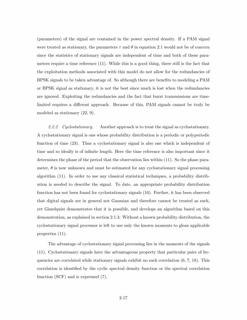
2.2.2 Cyclostationary. Another approach is to treat the signal as cyclostationary.
A cyclostationary signal is one whose probability distribution is a periodic or polyperiodic
function of time (23). Thus a cyclostationary signal is also one which is independent of
time and so ideally is of in�nite length. Here the time reference is also important since it
determines the phase of the period that the observation lies within (11). So the phase para-
meter, � is now unknown and must be estimated for any cyclostationary signal processing
algorithm (11). In order to use any classical statistical techniques, a probability distrib-
ution is needed to describe the signal. To date, an appropriate probability distribution
function has not been found for cyclostationary signals (10). Further, it has been observed
that digital signals are in general not Gaussian and therefore cannot be treated as such,
yet Gisselquist demonstrates that it is possible, and develops an algorithm based on this
demonstration, as explained in section 2.1.3. Without a known probability distribution, the
cyclostationary signal processor is left to use only the known moments to glean applicable
properties (11).
The advantage of cyclostationary signal processing lies in the moments of the signals
(11). Cyclostationary signals have the advantageous property that particular pairs of fre-
quencies are correlated while stationary signals exhibit no such correlation (6, 7, 18). This
correlation is identi�ed by the cyclic spectral density function or the spectral correlation
function (SCF) and is expressed (7),
2-17

S�x (f) , limt!1
1
TEfX�
T (f ��
2)XT (f +
�
2)g (2.32)
where � is the cycle frequency, or the separation in frequency between two correlated pairs.
It corresponds to one of the time periods found in the probability distribution function
(11). Only man-made signals have the non-zero spectral correlations when � 6= 0. Of these
man-made signals, only a �nite number of values for � yield non-zero spectral correlations
(11).
Typical values of � that produce non-zero spectral correlations are zero, integer
multiples of the symbol rate kTs, twice the carrier frequency 2fc, and linear combinations
of these (11, 9). For PAM signals, the cyclic spectral densities at integer multiples of the
baud rate, 1Ts; are known to be (11, 9),
SkTss (f) = e�i2�
k�TsA2
4Ts�(f � k
Ts� fc)(f +
k
Ts� fc)Efjdnj2g (2.33)
PAM signals with real valued dn, as in BPSK signals, have a correlation at twice their
carrier frequency as was discussed in Section 2.1.2,
S2fcs (f) = ei2�A2
4Tsj(f � fc)j2Efjdnj2g: (2.34)
When using these moments, one assumption must be made: only the signal of interest
is correlated at a particular value of �, implying that the chosen � is non-zero (11).
Then mathematically, the spectral density of the received signal, S�x (f), is identical to
the spectral density of the signal of interest, S�s (f) (11). This assumption justi�es the
philosophy that estimating this value will separate the signal of interest from the received
signal, and as such all the other noise and interference in the environment (11). This is
how signal selectivity is achieved and is the basis for cyclostationary signal processing. If
the estimate for � is non-zero, the signal is present (11, 8).
There are two big disadvantages when using this technique. The �rst is the noise, and
the second is that the cyclic correlation function is unknown and must be estimated (11).
The noise problem is that it increases the variance in any estimate of the cyclic correlation
2-18

function, S�x (f) (11). Thus, despite the assumption that only signal will contribute, noise
variations can easily create other apparent contributions (11). The extra variation can
be dealt with by averaging the statistic over longer and longer observation periods while
requiring some amount of smoothness in the estimated SCF (11, 6). This is appropriate for
working with signals of exceptionally long durations buried in noise, but is not applicable
for short duration signals of interest, which is the category that burst transmissions fall
into (11).
Treating a PAM signal as a cyclostationary signal allows the redundancy property
to be taken advantage of, but assumes complete correlation in the frequency domain. This
assumption then allows the PSD of the transmitted signal to be estimated, not taking
into consideration the bias caused by the noise, since the noise contribution is assumed
zero. This is not applicable to burst transmission signals, since the correlation in the
frequency domain for burst transmission signals is not completely correlated, especially so
when dealing with bursts of di¤erent lengths, or when dealing with bursts that do contain
some sort of correlation between the transmitted data symbols.
2.3 A Better Signal Model for Burst Transmission Signals
Although each of these previously mentioned techniques has merit, they also have
some obvious disadvantages. Since the spectral correlation functions are only de�ned for
in�nite length signals, (11) none of the discussed methods apply completely to burst signal
transmissions and thus the noise estimation for each is not valid.
The table in Figure 2.3 is helpful in understanding the di¤erences between station-
ary and cyclostationary approaches of signal processing. The PSD of the signal can be
measured if the signal is stationary, but the noise contribution cannot be separated from
the signal. When a signal is considered cyclostationary the techniques focus on the places
where only the signal contributes, that is where the values of � are non-zero (11). By
measuring these properties and averaging them over time an estimate for the signal can be
obtained that is theoretically free of noise. The key here is that neither of these techniques
works for burst transmission signals since the Spectral Correlation Functions (SCF) are
2-19

Figure 2.3 The Spectral Density Problem with Classical Burst Signal Analysis
only de�ned for in�nite length signals, making them inappropriate for time limited signals
(11).
The stationary approach is advantageous since some of the unknown parameters
disappear in the frequency domain, and since a probability distribution function is known.
Cyclostationary techniques account for more of the true characteristics of the
signal, making the methods that use them more accurate. The drawback lies in that cy-
clostationary techniques have no probability distribution function, making conventional
statistical methods di¢ cult to apply. The working signal model for burst transmission
signals allowed Gisselquist to apply classical statistical principles such as Maximum Like-
lihood Estimator (MLE) and likelihood ratios (11) in the development of a demodulator.
The next section brie�y discusses optimal �ltering techniques before presenting the deriva-
tion of Gisselquist�s Minimum Mean Square Error (MMSE) �lter.
2.4 Optimal Filtering
The application of Gisselquist�s research was focused on optimal �ltering. In the
development of Gisselquist�s �lter, the question of what �lter should be applied to get
the "best" results is answered (11). That is, he develops a �lter that obtains a reliable
estimate of the transmitted data symbols in the face of colored or white noise. Here we
are concerned with improving his �ltering process by obtaining a more reliable estimate of
the noise PSD since the PSD of the noise is an important part of the MMSE �lter. The
2-20

Figure 2.4 The Structure of an Optimal Filter
optimal �lter to obtain the "best" results is known to consist of a matched �lter for white
noise, followed by a Tapped Delay Line (TDL) equalizer (11) as shown in Figure 2.4.
This optimal �lter is applicable regardless of the criteria used to de�ne "best" (5).
Speci�c to our purposes, "best" means obtaining the most reliable estimate of the original
data symbols. In this �gure, xBB(t) represents a signal with zero carrier frequency, fc = 0,
t is the time the sample is taken, and dn is the estimated symbol at the output of the �lter
(11). This section will follow the form of the �lter, �rst discussing matched �ltering and
then the combination of a matched �lter with equalization.
2.4.1 Matched Filtering. A matched �lter is de�ned as a unique �lter that
maximizes the signal-to-noise ratio of a known input (11). Common developments of this
are presented in (11, 24, 25, 27). In each development, the signal is assumed to be known,
for example s(t) = A (t) with a constant gain factor A (11). The �lter that maximizes
the signal-to-noise ratio in white noise is (11, 19, 25)
hMF (t) = �(�t) (2.35)
in the frequency domain this �lter is
HMF (f) = �(f) (2.36)
There are other developments such as (4) which extend this �lter to a colored noise
environment (11). The matched �lter is obviously the optimum �lter when only one data
symbol is transmitted, but not when multiple pulses are transmitted in succession (11) as in
a burst transmission signal. When multiple pulses are transmitted, the pulses may interfere
2-21

with each other at the output of the �lter causing Intersymbol Interference (ISI)(11, 24).
Such interference is problematic when (f) has been designed and �xed in the transmitter,
prior to the estimation of Sn(f) (11).
2.4.2 Equalization. Removing the ISI is accomplished through the use of an
equalizer (11). Ericson proves, using the spectral redundancies inherent in a modulated
signal, that the optimal receiving �lter always consists of a matched �lter followed by a
Tapped Delay Line (TDL) equalizer (11, 5). This �lter can be implemented as a discrete
time �lter operating on the symbols that are sampled after the matched �lter (11). Using
this structure, there are two ways of applying a �lter, �xed and adaptive (11).
A �xed equalizer can be designed by minimizing the mean square error (MSE) be-
tween the output and the true symbols that were sent (11). Berger and Tufts present
one such Minimum Mean Square Error (MMSE) �lter for a PAM communication stream
(11, 1). First they modulated the communications signal as a sum of delayed pulses with
unknown weights (11),
s(t) =
1Xn=�1
dn (t� nTs): (2.37)
This is similar to the s(t) in equation 2.1 with the exception that burst transmission signals
have a limited number of data symbols, Ns. They derive their �lter from the PSD of the
noise, Sn(f), together with the PSD of the discrete pulse sequencefdng1n=�1; written as
Sd(ei2�fTs) (11). They point out that this �lter is comprised of both a periodic and non-
periodic component,
H(f)MMSEBerger and Tufts
0BB@ Sd(ei2�fTs)
1 + Sd(ei2�fTs)A2
Ts
P1n=�1
���(f� nTs)���2
Sn(f� nTs)
1CCA| {z }
TDL Equalizer
�(f)
Sn(f)| {z }Matched Filter
(2.38)
where the periodic portion is the TDL equalizer, and the non-periodic portion is the
matched �lter (11). The periodic portion has periodicity 1Ts; making it a TDL equalizer
and matching Ericson�s prediction (11, 5).
2-22

The second type of equalizer is an adaptive equalizer (11). These equalizers were
�rst demonstrated by Lucky (14) in 1966 and later studied by Haykin and many others
(11, 12, 2). The problem with these adaptive equalizers lies in their implementation, since
no knowledge of the noise PSD nor the true pulse shape is used (11). Without using the
noise PSD to �lter out narrow band interference, large amounts of interference may enter
into the system (11). Without using the true pulse shape, signal energy is arbitrarily lost
in the initial �lter (11). While the TDL equalizer may be able to reduce any resulting
distortion, it cannot fundamentally compensate for poor signal-to-noise conditions in the
received signal (11). Thus these systems are less than optimal, despite their practicality.
2.5 A Minimum Mean Square Error Filter for Burst Transmission Signals
The MMSE �lter has well known optimization properties, and is well de�ned when
the pulse shape and the noise PSD are de�ned (11). However, Berger and Tuft�s version of
the MMSE �lter does not exploit the extra spectral redundancies found in a BPSK signal
at bandpass frequencies discussed in Section 2.1.2 (11). Gisselquist created a MMSE �lter
that gives the "best" estimate of the dn provided the pulse shape is known and a reliable
estimate of the noise spectrum is available.
The �rst step for Gisselquist in the development of his MMSE �lter was to �nd the
d that satis�es:
d(x)MMSE , argmind(x)
E��d(x)� d
�y �d(x)� d
��: (2.39)
The statistical solution to this minimization is the expected value of the conditional prob-
ability distribution or d(x)MMSE = Efdjxg which is known to minimize the mean square
error when an a-priori probability distribution for d is known (11, 21). Since d and x are
Gaussian, or treated as Gaussian, as explained in Section 2.1.3 the conditional probability
distribution of d given x is also Gaussian with mean (11),
Efdjxg = A
2
�A2
2(yR�1n +R
�1d
��1yRy�R
�1n x, (2.40)
2-23

Figure 2.5 Bandpass MMSE (Gisselquist�s) System Diagram
and variance (11),
Efddyjxg =�A2
4(yR�1n +R
�1d
��1. (2.41)
So the MMSE estimate of d is (11),
d(x)MMSE =
"A
2
�A2
2(yR�1n +R
�1d
��1yRy�R
�1n
#x, (2.42)
which is an optimal �lter for recovering d. To see this we use the matrices provided in
Section 2.1.2.1 to calculate a new form of this �lter. This vector of data symbol estimates
will have dimension Nf � 1 and after simpli�cation and rearrangement look like (11),
D(ei2�(fj�fc)Ts) =
e�i�ei2�(fj�fc)�H(fj)XT (fj)
+e�i�ei2�(fj�fc)�ei2��TsH(fj +
1Ts)XT (fj +
1Ts)
+ei�ei2�(fj�fc)�H�(2fc � fj)X�T (2fc � fj)
+ei�ei2�(fj�fc)�ei2��TsH(2fc � fj � 1
Ts)XT (2fc � fj � 1
Ts)
(2.43)
Then, expanding equation 2.42 to solve for H(f), we see that the minimum mean square
error �lter for BPSK modulation is (11)
HMMSE(f) =
A2�(f�fc)TsSn(f)
1 + A2
4j(f�fc)j2TsSn(f)
+ A2
4
����f+ 1Ts�fc
����2TsSn
�f+ 1
Ts
� + A2
4j(fc�f)j2TsSn(2fc�f) +
A2
4
����fc�f� 1Ts
����2TsSn
�2fc�f� 1
Ts
�(2.44)
for f 2 (fc � 1Ts; fc). The implementation of this �lter is illustrated in Figure 2.5.
To implement the �lter an estimate of the PSD of the noise must be obtained. Since
the received signal has both the transmitted signal and the noise intertwined as explained in
2-24

Figure 2.6 A Sinc Function vs. Modi�ed Sinc
Section 2.1.1, methods to estimate the noise must be established. In Chapter III, methods
for estimating this noise are discussed and the success evaluated in Chapter IV.
2.6 Preliminaries
Gisselquist�s �lter is optimal in terms of mean square error when demodulating BPSK
burst transmissions (11), assuming a colored noise environment. This thesis is concerned
with estimating the PSD of white noise. The results will hopefully lead to e¤ective esti-
mation of colored noise. The �rst experiment generated a burst transmission signal as in
equation 2.1. The pulse shape used was a modi�ed Nyquist5 pulse shape, speci�cally a
modi�ed sinc:
(t) =1
Ts
�sinc(
2t
Ts� 12) + sinc(
2t
Ts+1
2)
�: (2.45)
Although the sinc pulse is in�nite as a function of time, the magnitude decreases as
jtj increases, as can be seen in Figure 2.6. The advantage of the modi�ed Nyquist pulse can
also be seen in Figure 2.6 because the magnitude decreases even faster than the unmodi�ed
sinc. Figure 2.7 shows a burst transmission signal using the following parameters: A = 1;
fc = 1; � = 0, � = 0, Ts = 1, Ns = 64, and (t) was as in equation 2.45. The equation
5For the purposes of this thesis sinc(t) = sin(�t)�t
:
2-25

Figure 2.7 BPSK signal with Ns = 64
plotted in Figure 2.7 is:
s(t) = Re(
63Xn=0
dn (t� n)ei(2�t)): (2.46)
This signal is then combined with white noise multiplied by a noise scale as follows:
x(t) = Re(
63Xn=0
dn (t� n)ei(2�t)) + (noise scale) n(t): (2.47)
The noise scale in the simulated received signal, x(t), was allowed to vary incrementally
from 10�1:5 to 101:5 while s(t) and n(t) remained the same. Thus the only variable allowed
to change was the noise scale. The noise PSD, Sn(f), used in the MMSE �lter was simply
white noise with a noise scale factor of 1: Thus the shape of the Sn(f) used in the �lter
di¤ered in both shape and scale from the actual Sn(f) in the simulated received signal.
For each noise scale increment, the received signal was processed using equation 2.43 and
symbol estimates, dn obtained. These dn were compared to the originally transmitted
symbols, dn; and the bit error rate (BER) recorded. The BER is de�ned as
BER =Number of Incorrectly Identi�ed SymbolsTotal Number of Transmitted Symbols
(2.48)
The success of the �lter is plotted as a function of the noise scale in Figure 2.8 and
BER, and in Figure 2.9 as a function of the Signal to Noise Ratio (SNR) in dB .
These �gures show two important results. First, as the noise scale increases, the
success of the �lter decreases. The second, when the noise scale used in the MMSE �lter
2-26

Figure 2.8 BER vs. Noisescale for Unknown Scale and Shape of the Noise PSD
Figure 2.9 BER vs. SNR for Unknown Shape and Scale of the Noise PSD
2-27

Figure 2.10 BER vs. Noisescale for Known Scale and Unknown Shape of the Noise PSD
Figure 2.11 BER vs. SNR for Known Scale and Unknown Shape of the Noise PSD
is close to the actual noise scale, the success increases. Likewise, the farther that the
noise scale used in the MMSE �lter is from the actual noise scale, the poorer the symbol
estimation results. This was further examined in a second experiment.
In the second experiment, the received signal was generated exactly as in the �rst
experiment. The di¤erence in the second experiment is that the PSD of the noise, Sn(f)
used in the MMSE �lter was constant, the constant being the noise scale used in the signal
generation. So the MMSE �lter has a correct estimate of the scale of Sn(f) but not of the
shape of Sn(f). The BER is low for noise scale values < 1, but then sharply increased as
the noise scale values increased as shown in Figures 2.10 and 2.11.
The important thing to note here is that the success drops o¤ rapidly when the noise
is much larger than the signal, most likely since the shape of the noise PSD, Sn(f) is
incorrect. This suggested the need for a third experiment.
2-28
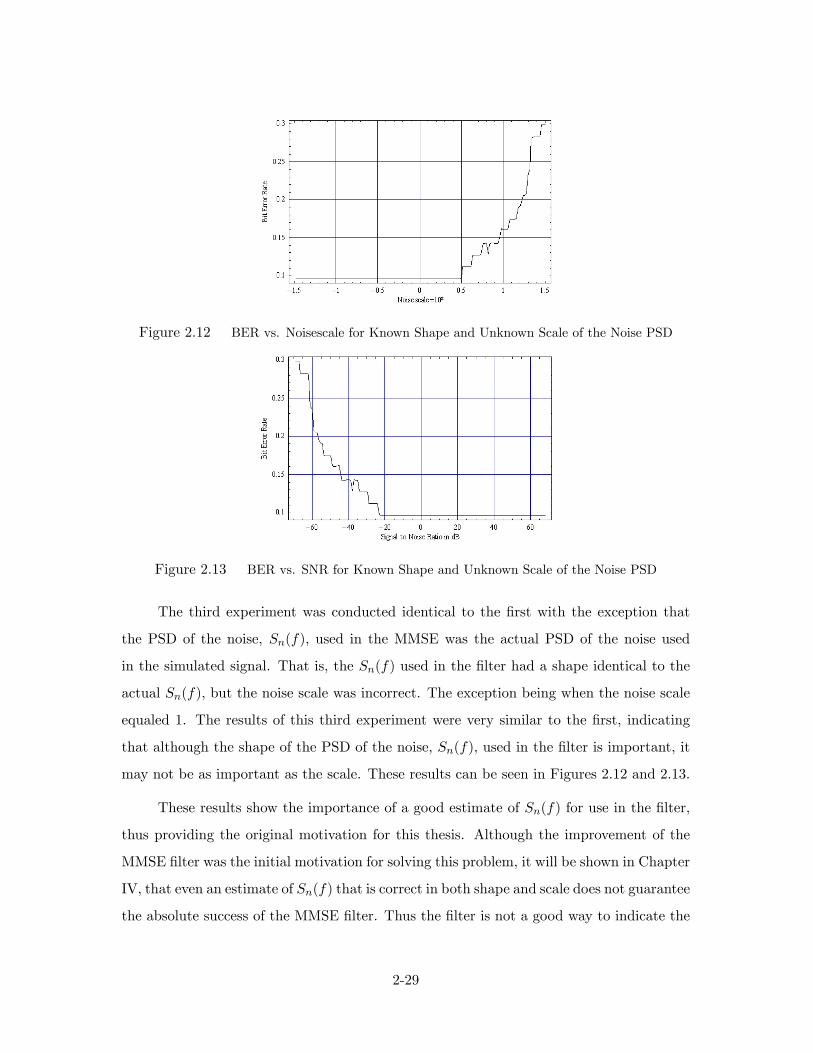
Figure 2.12 BER vs. Noisescale for Known Shape and Unknown Scale of the Noise PSD
Figure 2.13 BER vs. SNR for Known Shape and Unknown Scale of the Noise PSD
The third experiment was conducted identical to the �rst with the exception that
the PSD of the noise, Sn(f); used in the MMSE was the actual PSD of the noise used
in the simulated signal. That is, the Sn(f) used in the �lter had a shape identical to the
actual Sn(f), but the noise scale was incorrect. The exception being when the noise scale
equaled 1. The results of this third experiment were very similar to the �rst, indicating
that although the shape of the PSD of the noise, Sn(f); used in the �lter is important, it
may not be as important as the scale. These results can be seen in Figures 2.12 and 2.13.
These results show the importance of a good estimate of Sn(f) for use in the �lter,
thus providing the original motivation for this thesis. Although the improvement of the
MMSE �lter was the initial motivation for solving this problem, it will be shown in Chapter
IV, that even an estimate of Sn(f) that is correct in both shape and scale does not guarantee
the absolute success of the MMSE �lter. Thus the �lter is not a good way to indicate the
2-29

success of a particular noise estimation technique. Since the MMSE �lter is optimized for a
colored noise environment it is not expected to be the best measure for evaluating a white
noise estimation technique.
2-30

III. Theoretical Development
The noise estimation techniques presented in this thesis are based on two properties of
PAM signals. The �rst property is the fact that any received PAM signal can be expressed
in time as a sum of the transmitted signal and the noise as follows:
x(t) = s(t) + n(t) (3.1)
The problem is that the individual quantities of s(t) and n(t) are unknown. Since they are
unknown, exploitation becomes a problem that must be solved.
The noise estimation techniques are also based on the redundancies discussed in
Section 2.1.2. As stated these redundancies were discovered by Nyquist, exploited �rst by
Berger and Tufts, and then by Gisselquist in the development of his burst transmission
subspace theory (11). Gisselquist exploited these redundancies in the development of his
Minimum Mean Square Error (MMSE) �lter, which produced better results than any
previous work (11). It would seems that equation 3.1 would be the obvious choice to use
in combination with Gisselquist�s �lter, however, the results in Chapter 4 will show that
this is not the best approach to use, since the success of Gisselquist�s �lter depends on an
accurate a priori estimation of the Power Spectral Density (PSD) of the noise. Additionally,
it is not the best solution since Gisselquist�s �lter works best with colored noise, but gives
acceptable results with white noise when the noise scale is known (11). The �rst section in
this chapter explains the theory behind a method based on equation 3.1 and the following
sections provide better alternatives.
3.1 Method One: Subtract in Time
Equation 3.1 provides a seemingly simple solution to the noise estimation problem,
extract the transmitted signal from the received signal and only the noise will remain.
Gisselquist�s MMSE provides an estimate of the content of a BPSK signal which is described
in equations 2.43 and 2.44. This method proposes using this �lter on a received signal to
recover an initial estimate for the originally transmitted BPSK symbols. Since an a priori
estimate for the noise PSD is required, Sn(f), a small constant value is used, since the
3-1

expected value of Gaussian white noise over an in�nite amount of time is known to be
constant. The received signal is processed as in Figure 2.5, providing an estimate for the
originally transmitted signals, call it d1. The pulse shape, , gain, A, symbol length, Ts,
number of symbols, Ns; time of arrival, � ; and the phase of the carrier, �; are all assumed
to be known or previously recovered. dn is replaced with d1 in
s(t) = ARe(
Ns�1Xn=0
dn (t� nTs � �)ei(2�fct+�)) (3.2)
to create a new signal, s1(t). The signal is then sampled to create a discrete form of s1(t):
Then s1(t) is subtracted from equation 3.1 giving:
x(t)� s1(t) = s(t) + n(t)� s1(t) = n1(t) (3.3)
The power spectral density of n1(t) is calculated and used in the MMSE �lter to obtain an
second estimate of the data symbols, d2. This estimate of the originally transmitted data
symbols is then used to construct a new signal estimate in the time, s1(t), assuming the
pulse shape is known. Using the property presented in equation 3.1, s2(t) is subtracted
from x(t) leaving n2(t): The noise estimate is converted into the frequency domain using
the DFT, the PSD calculated, and then Sn2(f) is used in the MMSE �lter to recover a
third estimate for the data symbols, d3, the process continuing until the di converge. A
�ow chart for this method is illustrated in Figure 3.1.The method seems to be ideal, but
since the success of the original �ltering process depends on an accurate estimate of the
noise PSD, it will most likely not converge to the actual dn. Given that the �lter depends
on an accurate estimate of the noise PSD, it seems intuitive to use the received signal in
the noise estimation process. The remaining sections of this chapter do exactly that, and
combined with the redundancy property, seem to be better methods in the noise estimation
problem.
3.2 Methods Using the Signal Redundancies
Given that there are two properties discussed at length within this thesis, it seems
only natural that the ideal estimation techniques presented should take advantage of both.
3-2

Figure 3.1 Flow Diagram for Method One: Subtract in Time
In this section, four di¤erent methods will be presented. All exploit the redundancy prop-
erties, and all will hopefully provide promising results for use in the MMSE �lter and in the
larger non Gaussian noise estimation problem. First, the development of the redundancies
as they apply to the PSD will be presented, and then an in depth explanation of each
method will follow.
Since both the Fourier transform and the PSD are linear when dealing with burst
transmission signals, the sum property presented in Section 2.1.1 can be easily extended
into the frequency domain. It is known that the Fourier transform of equation 3.1 is:
XT (f) = NT (f) +A
2ei�
Ns�1Xn=0
e�i2�(f�fc)� [dne�i2�(f�fc)nTs ]
Z 1
�1 (u)e�i2�(f�fc)udu: (3.4)
As presented in Subsection 2.1.3 the PSD of the transmitted signal, Ss(f), is of the form:
A2
4Tsj(f � fc)j2Efjdnj2g: To simplify this equation, let Efjdnj2g = Sd(f) and k = A2
4Ts;
resulting in:
Ss(f) = kj(f � fc)j2Sd(f): (3.5)
Removing the carrier frequency by moving it to fc = 0 results in:
Ss(f) = k j(f)j2 Sd(f) (3.6)
3-3

This is summed with the PSD of the noise Sn(f) to give (11, 23):
Sx(f) = Ss(f) + Sn(f): (3.7)
Sx(f) has the same redundancy properties presented in Section 2.1.2 and its vector is of
the form:
Sx(f) =
266666666666666666666666664
Sx(f1)...
Sx(fNf )
Sx(f1 +1Ts)
...
Sx(fNf +1Ts)
S�x(2fc � f1)......
S�x(2fc � fNf + 1Ts)
377777777777777777777777775
(3.8)
The redundancies for a given frequency, fi 2 (fc � 1Ts; fc); occur at Sx(fi); Sx(fi + 1
Ts);
S�x(2fc � fi); and S�x(2fc � fi +1Ts): It is important to note that at these locations, the
information is the same, not the actual values. The PSD of the transmitted signal can be
further broken down into the PSD of the transmitted symbols and the magnitude of the
Fourier Transform of the pulse shape. Both are scaled by a constant, k = A2
4Ts, where A is
the gain of the received signal and Ts is the symbol duration. In this section the constant
value, k, and the pulse shape are assumed to be known. The �rst step in all the methods
will divide by the magnitude of the pulse shape and the constant, k, to give:
Sx(f)
k j(f)j2= Sd(f) +
Sn(f)
k j(f)j2(3.9)
That division occurs for each redundancy at a corresponding location in the pulse shape.
Also, keep in mind that each piece has the same data, thus the Sd(f) are all assumed to
be the same regardless of the frequency. The explanation will continue using the following
3-4

notation,
F(f) =Sx(f)
k j(f)j2= Sd(f) +
Sn(f)
k j(f)j2(3.10)
When referring to the redundancies, they will be called F (f j), where j = 1; 2; 3; 4: Specif-
ically f1 refers to the values having the form Sx(fi), f2 refers to the Sx(fi + 1Ts) values,
f3 the values at S�x(2fc � fi); and f4 the values at S�x(2fc � fi + 1Ts), i 2 [1; Nf ].
The redundancies and the sum in equation 3.1 are the two properties exploited in
this section when obtaining an estimate for Sn(f). The estimation techniques are similar,
but have important di¤erences that will hopefully produce distinct results. Thus, although
repetitive, each method will be explained starting from equation 3.10. Which method to
use should be based on the known and unknown parameters of the received signal and
what the estimate will be used for. The explanation of each method will begin at this
point.
3.2.1 Subtraction of the Smallest Redundancy. There are two methods that use
the smallest redundancy value to extract an estimate for Sn(f): Starting with equation
3.10, F (f) is evaluated at f1; f2; f3; and f4: The smallest F (f j) in absolute value is
selected. The smallest of the four values will have the smallest value for Sn(f) since the
Sd(f) are the same at each location. Call this new vector of smallest values: Sdsmall(f).
This vector of smallest values is used in the following two methods.
3.2.1.1 Subtraction Before Pulse Shape Multiplication. If we subtract this
vector, Sd(f); from the values in equation 3.9 we will get:
Sx(f)
k j(f)j2� Sdsmall(f) = Sd(f)� Sdsmall(f) +
Sn(f)
k j(f)j2(3.11)
At this point (Sd(f) � Sd(f)) is assumed to be small, so the remaining values are the
estimates for the PSD of the noise, divided by k j(f)j2. To obtain Sn(f), equation 3.11
is multiplied by k j(f)j2 resulting in:
Sx(f)� Sdsmall(f)k j(f)j2 = Sn(f) (3.12)
3-5

Figure 3.2 Diagram of Subtraction of Minimum Redundancy before Pulse Shape Multi-plication
The degree of correctness of this estimation will be demonstrated and measured in Chapter
IV.
3.2.1.2 Subtraction After Pulse Shape Multiplication. If we �rst multiply
this vector, Sd(f); by k j(f)j2, and then subtract this value from equation 3.7 we will get:
Sx(f)� k j(f)j2 Sdsmall(f) = Sn(f) (3.13)
The method di¤ers in where the subtraction occurs. Instead of subtracting in the manner of
equation 3.11, the vector of smallest values, Sdsmall(f); is multiplied by the magnitude of the
pulse shape, the scalar k, and then subtracted from equation 3.7. Again Sd(f)� Sdsmall(f)
is assumed to be small, so the remaining value, is Sn(f) is the estimate for the PSD of the
noise. Thus, subtracting before or after multiplication by the pulse shape produces the
same result, Sn(f):
3.2.2 Subtraction of the Average Redundancy. For the methods that subtract
the average redundancies, we start with equation 3.9. These methods take the four
redundancies: F(f) = Sx(f)
kj(f)j2 = Sd(f) +Sn(f)
kj(f)j2 ; called F (fj), where j = 1; 2; 3; 4 and
3-6

Figure 3.3 Diagram of Subtraction of Minimum Redundancy after Pulse Shape Multi-plication
averages them to obtain:
Faverage(f) =
14
�Sd(f
1) + Sn(f1)
kj(f1)j2 + Sd(f2) + Sn(f2)
kj(f2)j2 + Sd(f3) + S�n(f
3)
kj�(f3)j2 + Sd(f4) + S�n(f
4)
kj�(f4)j2�
(3.14)
The Sd(f) are the same so we can simplify this to:
Faverage(f) =1
4
�4Sd(f) +
Sn(f1)
k j(f1)j2+
Sn(f2)
k j(f2)j2+
S�n(f3)
k j�(f3)j2+
S�n(f4)
k j�(f4)j2
�(3.15)
Faverage(f) = Sd(f) +1
4
�Sn(f
1)
k j(f1)j2+
Sn(f2)
k j(f2)j2+
Sn(f3)
k j�(f3)j2+
Sn(f4)
k j�(f4)j2
�(3.16)
Faverage(f) = Sdaverage(f) +1
4
4Xk=1
Sn(fk)
k j(fk)j2(3.17)
From this point the average methods start.
3-7
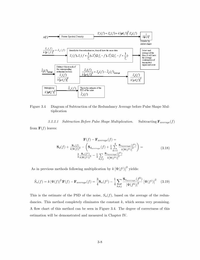
Figure 3.4 Diagram of Subtraction of the Redundancy Average before Pulse Shape Mul-tiplication
3.2.2.1 Subtraction Before Pulse Shape Multiplication. Subtracting Faverage(f)
from F(f) leaves:
F(f)� Faverage(f) =
Sd(f) +Sn(f)
kj(f)j2 ��Sdaverage(f) +
14
4Pk=1
Snaverage (fk)
kj(fk)j2�=
34Sn(fj)
kj(fj)j2 �14
Pk 6=j
Snaverage (fk)
kj(fk)j2
(3.18)
As in previous methods following multiplication by k��(f j)��2 yields:
Sn(f) = k j(f)j2F(f)� Faverage(f) =3
4Sn(f
j)� 14
Xk 6=j
Snaverage(fk)
j(fk)j2��(f j)��2 (3.19)
This is the estimate of the PSD of the noise, Sn(f), based on the average of the redun-
dancies. This method completely eliminates the constant k; which seems very promising.
A �ow chart of this method can be seen in Figure 3.4. The degree of correctness of this
estimation will be demonstrated and measured in Chapter IV.
3-8
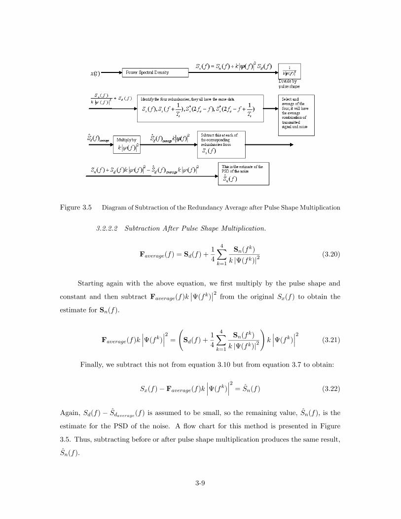
Figure 3.5 Diagram of Subtraction of the Redundancy Average after Pulse Shape Multiplication
3.2.2.2 Subtraction After Pulse Shape Multiplication.
Faverage(f) = Sd(f) +1
4
4Xk=1
Sn(fk)
k j(fk)j2(3.20)
Starting again with the above equation, we �rst multiply by the pulse shape and
constant and then subtract Faverage(f)k��(fk)��2 from the original Sx(f) to obtain the
estimate for Sn(f):
Faverage(f)k���(fk)���2 = Sd(f) + 1
4
4Xk=1
Sn(fk)
k j(fk)j2
!k���(fk)���2 (3.21)
Finally, we subtract this not from equation 3.10 but from equation 3.7 to obtain:
Sx(f)� Faverage(f)k���(fk)���2 = Sn(f) (3.22)
Again, Sd(f) � Sdaverage(f) is assumed to be small, so the remaining value, Sn(f); is the
estimate for the PSD of the noise. A �ow chart for this method is presented in Figure
3.5. Thus, subtracting before or after pulse shape multiplication produces the same result,
Sn(f).
3-9

IV. Analysis by Simulation
As observed at the end of Chapter II, the success of the �lter when no characteristics of
the noise are known decreases dramatically when the noise scale exceeds the scale of the
transmitted signal. Thus it seems logical that one method of testing should be to test the
success of the demodulator at various noise levels. The results in this chapter are presented
in two sections. The �rst section presents the e¤ect the noise PSD estimates have on the
demodulation success of the MMSE �lter, reviewed in Section 2.5. As noise levels increase,
the ability to accurately recover the originally transmitted data symbols is measured. The
second section presents a comparison between the actual and estimated PSDs of the noise.
As explained, the noise estimation problem has two important goals. First, can these
methods accurately measure the scale of the noise? Second, can they obtain an accurate
estimate of the noise shape? It is important to note that the noise estimates do not give
actual noise content as it exists in the time domain, but rather estimates of the PSD of the
noise, since this is the form of the noise that the �lter presented in Chapter II and other
signal processing methods use.
4.1 Impact on Demodulation
The demodulation technique, Gisselquist�s Minimum Mean Square Error �lter, can
serve not only for measuring noise estimation success, but as part of the algorithm to
estimate the noise. This section is organized into two subsections, the �rst presents the
results of Method One: Subtract in Time, and the second exploits the signal redundancies
in the estimation algorithms. The measure of success in this section is the Bit Error Rate
(BER) as the noise scale is incrementally increased or in the �rst method compared to
iterations.
4.1.1 Method One: Subtract in Time. This method seemed to be the most
obvious, and possibly the most �awed. There may be other ways to estimate the noise
in the time domain, but only Subtract in Time is evaluated here. This approach was not
e¤ective as Figure 4.1 shows. The BER in this experiment did not converge, even after
�fty iterations. The initial estimate of the data symbols obtained using an arbitrary value
4-1

Figure 4.1 Method One: Subtract in Time BER vs. Iteration Number
for the PSD of the noise, Sn(f), was the best estimate. The estimates seemed to �uctuate
wildly as the noise level increased. This is an indication that the method is not an adequate
solution to the PSD of the noise estimation problem. The formula used to calculate the
BER in this section and all following sections is:
BER =Number of Incorrectly Identi�ed SymbolsTotal Number of Transmitted Symbols
(4.1)
There are probably several reasons why this method is not successful. One reason may be
that the demodulation technique that the noise estimation is trying to improve is part of
the noise estimation algorithm. The next subsection implements algorithms that rely only
on information gleaned from the received signal. The next subsection also takes advantage
of more properties of the received signal and the processing occurs in the frequency domain,
for these reasons they hold more promise in accurately estimating the noise.
4.1.2 Methods Using the Signal Redundancies. The previous method did not
exploit the properties of the received signal to estimate the PSD of the noise and it is
likely that because of this, was not very successful. The results presented here use the
redundancies of the signal to estimate the noise PSD. An improvement in these techniques
is that they do not use the demodulation technique that they are trying to improve as part
of the noise estimation algorithms.
4-2

Figure 4.2 BER vs. Noisescale, Subtraction of the Smallest Redundancy before Pulse ShapeMultiplication
4.1.2.1 Subtraction of the Smallest Redundancy. As explained in Section
2.1.2, BPSK signals have redundancy properties that can be exploited. Unfortunately the
results using the smallest redundancy were not as successful as expected in the improvement
of data symbol recovery. Section 3.2.1 explains that subtraction of the smallest redundancy
can occur at two points in the estimation algorithm. The results of each are presented here.
Subtraction of the Smallest Redundancy Before Pulse Shape Multiplica-
tion. This method improved the data symbol estimation algorithm, as can be seen if
we compare the results in Chapter II, Figures 2.8 and 2.9 with Figures 4.2 and 4.3. These
results are slightly better than using an arbitrary value for the PSD of the noise in the
demodulation algorithm. As the noise scale increased, the BER increased to a level no
better than random. Here the results are plotted in two ways, against the noise scale and
against the SNR. Future results will only have the BER versus the SNR.
Subtraction of the Smallest Redundancy After Pulse Shape Multiplication.
This variation of the previous method produced identical results which can be seen in
Figure 4.4. Hopefully it will be more successful in predicting the noise scale, which is
explored in the following section.
Although the methods that subtract the smallest redundancy didn�t have the positive
impact on the demodulation technique as hoped, it should not be taken as an indication
that the methods are invalid. Since the demodulation technique, the MMSE �lter, uses
4-3

Figure 4.3 BER vs. SNR in dB, Subtraction of the Smallest Redundancy before Pulse ShapeMultiplication
Figure 4.4 BER vs. SNR, Subtraction of the Smallest Redundancy after Pulse shape Multipli-cation
only a small portion of the observed noise spectrum, it is possible that the methods are
not applicable in those particular portions of the observed noise spectrum.
4.1.2.2 Subtraction of the Average Redundancy. Subtracting the minimum
redundancy in the previous two methods, did not improve the demodulator performance
as much as hoped. Instead of subtracting the minimum, the next two methods subtract an
average of the four redundancies, since they all contain the same information. Hopefully
these methods will provide a more positive impact on the demodulation success of the
MMSE �lter. As when subtracting the minimum, the subtraction of the average can occur
at two di¤erent places in the algorithm. Both variations are presented here.
Subtraction of the Average Redundancy Before Pulse Shape Multiplica-
tion. The results when subtracting the average of the redundancies before multiplying
4-4

Figure 4.5 BER vs. SNR, Subtraction of the Average Redundancy before Pulse Shape Multi-plication
Figure 4.6 BER vs. SNR, Subtraction of the Average Redundancy after Pulse Shape Multipli-cation
by the pulse shape is shown in Figure 4.5. This produced an improvement over the method
that subtracted the minimum before multiplying by the pulse shape. Additionally these
results were better than using an unknown noise scale and unknown noise shape as can be
seen in Figure 2.9 in Chapter II.
This method improves the success of the demodulator, however the BER continues
to be high and �uctuate wildly when the SNR is high. The acceptable BER is system
dependent and so the measure of how well the methods work is dependent on the system.
Subtraction of the Average Redundancy After Pulse Shape Multiplication.
As seen in Figure 4.6 this method like the subtraction of the smallest redundancy meth-
ods provided identical results as subtracting before multiplication by the pulse shape.
The methods that subtract the average of the redundancies improved the success of
the demodulator which can be seen in Figure 4.7. The results using the methods that
4-5

Figure 4.7 BER vs. SNR
subtract the average redundancies improved the success of the demodulator even when
the SNR exceeded -30 dB. This is promising since SNRs rarely exceed -40 dB. In Figure
4.7 it can be seen that the subtraction of the average redundancies is the most successful
as compared to subtracting the minimum redundancies and using an arbitrary noise SNR
value in the demodulator, which are the results labeled "Unknown".
The next section measures the success of the methods over the entire observed noise
spectrum, rather than just in the one small portion that the �lter uses for demodulation,
using the Mean Square Error (MSE) between the actual noise PSD and the estimated noise
PSD.
4.2 Comparison to Actual Power Spectral Density of the Noise
Improvement of Gisselquist�s MMSE �lter was the initial motivation for this research,
and it yielded positive results when subtracting the average of the redundancies. This
section examines the whole observed noise spectrum in an attempt to measure the success
of the previously explained methods. The two important characteristics of the PSD of
the noise, scale and shape, are examined and then a measure of the mean square error
between the actual PSD of the noise and the estimated PSD of the noise is presented.
Each technique captured a part of the characteristics we desire to estimate. Although they
were not completely successful individually, perhaps a combination of these methods may
prove to be an improvement.
4-6

Figure 4.8 Results of Method One: Subtract in Time
4.2.1 Method One: Subtract in Time. Since this method uses the �lter in the
estimation process, the results are as expected, less than stellar. Not only did the method
fail to capture the correct noise scale, but the method did not obtain the correct shape
of the PSD of the noise. Figure 4.8 shows the estimated power spectral density of the
noise plotted next to the actual power spectral density of the noise. The �gure shows that
neither the scale nor shape of the noise is accurately estimated.
These results, like the results in the �lter improvement, probably stem from the
fact that the results we are looking for are in the frequency domain, while the processing
technique occurs in the time domain. Additionally, since the �lter is used in the estimation
algorithm, the estimate accuracy at best is only valid in the portions of the observed noise
spectrum that the demodulation algorithm uses. The following results do not rely on the
�lter, and thus may have more success in estimating the PSD of the noise, both in shape
and scale.
4.2.2 Methods Using Signal Redundancies. Although these methods were not all
successful in the improvement of the demodulation algorithm, they did show some promise
at least in some small portions of the observed noise spectrum. Perhaps this success can
be used to implement algorithms with a smaller observation period or algorithms that
combine one or more of the methods. Algorithms that use a smaller observation period
would use a portion of the burst transmission, instead of using the entire burst as these
methods do. These algorithms would account for rapid changes in the noise since the PSD
of the noise would be normalized over a smaller amount of time. These methods use the
4-7

Figure 4.9 Estimated Noise PSD Using Subtraction of the Smallest Redundancy before Mulit-plication by Pulse Shape
Figure 4.10 Zoomed in Estimated Noise PSD Using Subtraction of the Smallest Redundancybefore Mulitplication by Pulse Shape
entire burst to estimate the PSD of the noise, which tends to minimize the contribution of
the noise over the period. A smaller observation period would not do this.
4.2.2.1 Subtraction of the Smallest Redundancy. The hope for these meth-
ods was that the scale would be estimated accurately, which is in fact re�ected in the
results. A suggestion for improvement may be to use a smaller observation window as
previously suggested. The results can be seen in Figures 4.9, 4.10, and 4.11. Figure 4.9
shows the entire estimated noise spectrum, while Figure 4.10 shows a zoomed in picture.
When comparing Figure 4.10 with Figure 4.11 it can be seen that the methods accurately
estimated the shape and scale of the noise PSD in the center of the plot, but when com-
pared with Figure 4.11 examination of the outer edges shows that the method did not
accurately capture the scale of the actual noise PSD.
4-8

Figure 4.11 Actual Noise PSD
Subtraction of the Smallest Redundancy Before Multiplication by Pulse
Shape. This method did not estimate the shape of the actual PSD of the noise with
accuracy, but did capture the correct scale at least in a portion of the estimated noise
spectrum. Since it was not very successful in �lter improvement, it can be assumed that
the estimated shape was not correct in the portions of the spectrum that the �lter uses.
Figure 4.12 presents the mean square error between the actual power spectral density
of the noise and the estimated power spectral density of the noise. This mean square error
was calculated in the following manner:
MSE , 1
N
NXi=1
(pi � pi)2 (4.2)
where N is the number of points at which the noise was estimated, which equates to the
number of signal samples in both the time and frequency domains. The pi are the actual
values at each point in the noise spectrum and the pi are the estimated noise PSD values.
As expected, as the noise scale increases, the mean square error increases greatly. However
the MSE was very low when the noise scales were low.
Subtraction of the Smallest Redundancy After Multiplication by Pulse
Shape. For estimating the scale of the noise spectrum, this method is more promis-
ing than the previous method. These results can be seen in Figures 4.13, 4.14, and 4.15.
Although it produced BER results identical to the method that subtracts the smallest
redundancy before multiplication, it clearly does a better job of estimating the scale across
the entire observed noise spectrum. Again since this method did not improve the demodu-
4-9
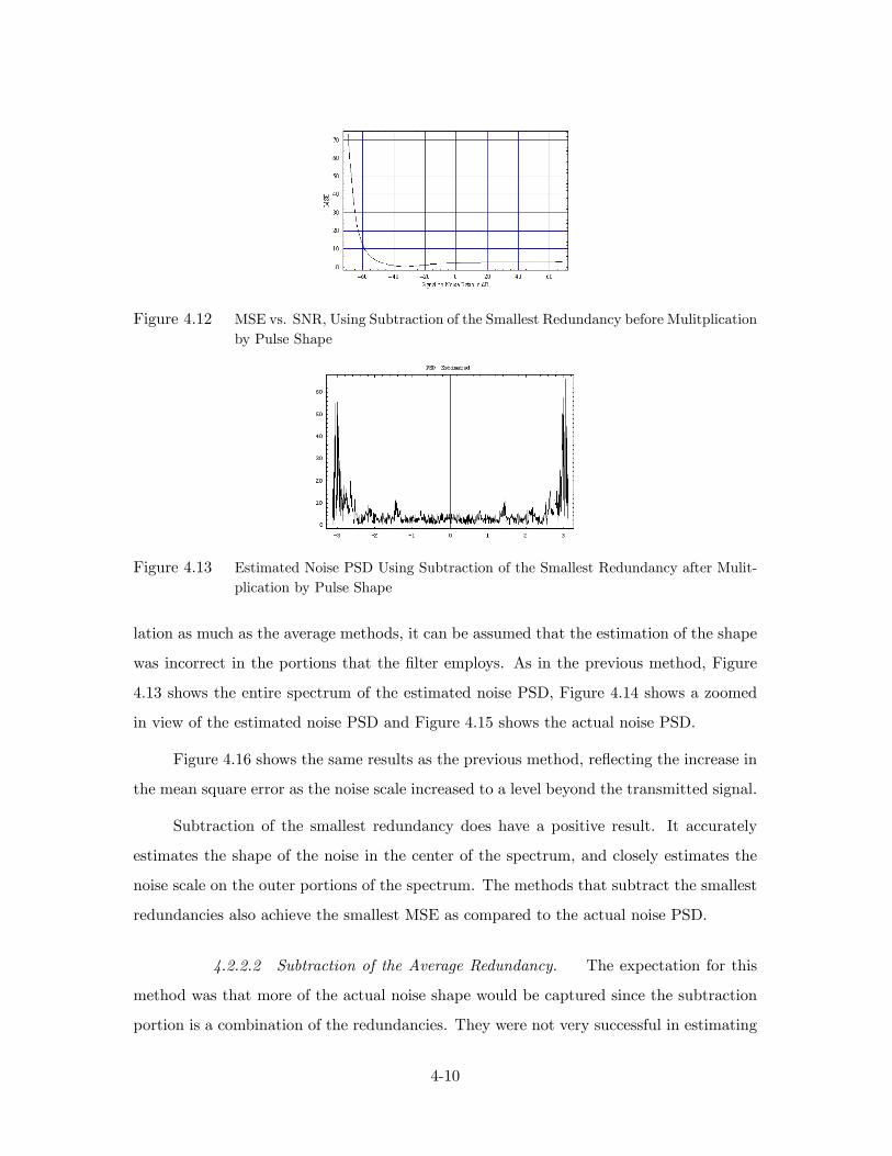
Figure 4.12 MSE vs. SNR, Using Subtraction of the Smallest Redundancy before Mulitplicationby Pulse Shape
Figure 4.13 Estimated Noise PSD Using Subtraction of the Smallest Redundancy after Mulit-plication by Pulse Shape
lation as much as the average methods, it can be assumed that the estimation of the shape
was incorrect in the portions that the �lter employs. As in the previous method, Figure
4.13 shows the entire spectrum of the estimated noise PSD, Figure 4.14 shows a zoomed
in view of the estimated noise PSD and Figure 4.15 shows the actual noise PSD.
Figure 4.16 shows the same results as the previous method, re�ecting the increase in
the mean square error as the noise scale increased to a level beyond the transmitted signal.
Subtraction of the smallest redundancy does have a positive result. It accurately
estimates the shape of the noise in the center of the spectrum, and closely estimates the
noise scale on the outer portions of the spectrum. The methods that subtract the smallest
redundancies also achieve the smallest MSE as compared to the actual noise PSD.
4.2.2.2 Subtraction of the Average Redundancy. The expectation for this
method was that more of the actual noise shape would be captured since the subtraction
portion is a combination of the redundancies. They were not very successful in estimating
4-10

Figure 4.14 Zoomed in Estimated Noise PSD Using Subtraction of the Smallest Redundancyafter Mulitplication by Pulse Shape
Figure 4.15 Actual Noise PSD
Figure 4.16 MSE vs. SNR Using Subtraction of the Smallest Redundancy after Pulse ShapeMultiplication
4-11

Figure 4.17 Estimated Noise PSD Using Subtraction of the Average Redundancy before PulseShape Multiplication
Figure 4.18 Zoomed in Estimated Noise PSD Using Subtraction of the Average Redundancybefore Pulse Shape Multiplication
the noise scale over the whole noise spectrum, but the shape resembles at least a portion
of the actual noise PSD.
Subtraction of the Average Redundancy Before Multiplication by Pulse
Shape. This method almost captured the scale and the shape in the center of the
observed noise spectrum. This portion can be seen best in Figure 4.18. Figure 4.17 shows
that the scale estimate on the outer portion, which the �lter uses, is completely wrong.
However incorrect the scale is in these portions, the shape must be accurately captured
since the demodulation results were so successful. Figure 4.20 shows the mean square error
between the estimated and actual PSDs of the noise. It is calculated as in equation 4.2.
As expected because of the horrible scale error in the higher frequencies, the mean
square error increased dramatically as the noise scale increased.
Subtraction of the Average Redundancy After Multiplication by Pulse
Shape. Like the previous method, this method accurately captured the scale and
4-12

Figure 4.19 Actual PSD Using Subtraction of the Average Redundancy before Pulse ShapeMultiplication
Figure 4.20 MSE vs. SNR Using Subtraction of the Average Redundancy before Pulse ShapeMultiplication
the shape in the center of the observed noise spectrum. Figures 4.21, 4.22, and 4.23 show
the results of this �nal method. Figure 4.21 shows that like the previous method, the scale
in the higher frequencies is completely of from the actual noise PSD. Figure 4.22 shows
that this method nearly captures the shape and scale in the center of the noise spectrum.
Like the previous method, subtraction of the average redundancy after multiplication by
the pulse shape is not very successful over the entire spectrum, this is re�ected in Figure
4.24.
The methods that subtract the average of the redundancies do not accurately capture
the scale of the actual noise PSD, but they did have the best success in improvement of
the demodulator success. Figure 4.25 shows a comparison of the MSE between all the
subtraction methods and the MSE using a noise PSD with unknown shape and scale. As
previously shown, the methods that subtract the average redundancies do not do a good
job of estimating the noise PSD over the whole noise spectrum. The methods that subtract
the minimum redundancies obtain a MSE about equal to using a noise PSD with unknown
4-13

Figure 4.21 Estimated Noise PSD Using Subtraction of the Average Redundancy after PulseShape Multiplication
Figure 4.22 Zoomed in Estimated Noise PSD Using Subtraction of the Average Redundancyafter Pulse Shape Multiplication
Figure 4.23 Actual Noise PSD
Figure 4.24 MSE vs. SNR Using Subtraction of the Average Redundancy after Pulse ShapeMultiplication
4-14

Figure 4.25 MSE vs. Noise Scale Subtraction Methods Compared
shape and scale. Thus the best methods for estimating the noise PSD over the entire
spectrum are the methods that subtract the smallest redundancies.
4-15

V. Conclusions/Recommendations
The initial goal of this research was to determine if an accurate estimate of the noise
power spectral density (PSD) could be obtained. The need for a solution to this problem
stemmed from research done by Gisselquist in (11). He created a minimum mean square
error (MMSE) �lter whose success depended on an accurate a priori estimate of the noise
PSD. His �lter is designed and works best in a colored noise environment (11). This
thesis tackled the white noise estimation problem, in the hopes of providing direction
for the colored noise problem. Five methods were developed and tested to determine if
they improved his �lter results. The methods were also measured against the entire noise
spectrum as well, since the �lter that Gisselquist created only employs a small part of the
noise PSD.
The estimation techniques can be improved and suggestions for further research are
included in this chapter following a summary of the results obtained. Overall the research
was a success as it provided a good starting point for further research.
5.1 Summary of Results
The methods tested included Subtraction in Time, and four other methods which
exploited the redundancies of the signal properties. The second group of methods included
the Subtraction of the Smallest Redundancy Before and After Pulse Shape Multiplication.
Finally the third group included Subtraction of the Average Redundancy Before and After
Pulse Shape Multiplication. The results of the Subtract in Time method were totally
unsuccessful. In fact, the results obtained using an arbitrary noise PSD in the �lter with
a random shape and scale provided better results than Subtract in Time. The methods
that used the smallest redundancy provided a slight improvement in the demodulator
performance, but were most successful in obtaining the most accurate estimate across
the entire noise PSD spectrum. The methods that subtracted the average redundancies
provided the best results. Not the best when compared to the actual entire noise PSD
spectrum, but in improvement of the MMSE �lter. This is a success since the most
important goal of this thesis was to improve the success of Gisselquist�s MMSE �lter.
5-1

5.2 Future Work
As stated previously, Gisselquist�s �lter is optimal in a colored noise environment.
Because of this it is obvious that a suggestion for further work is to extend these methods
to the colored noise environment. Another area for continued research is the exploration
of why the subtraction of the average redundancy methods do not capture the scale of the
noise PSD in the higher frequencies. Perhaps if a more accurate estimate of the scale can
be obtained in this region, the success of the method can be improved further. A third area
to explore is combining these methods which only use an active signal with methods that
use observations when the signal is not active. When the signal is not active, only noise is
present, thus a good estimate should be possible when combined with the estimates of the
noise when the signal is present.
Overall, the methods presented in this thesis provide a good ground work for sev-
eral future estimation methods in both the colored and white noise environments. One
last suggestion for future work is to employ a smaller observation window combined with
adaptive �ltering. This would allow the noise PSD used in the �lter to perhaps capture
more of the noise characteristics in a smaller region, improving the success incrementally
as the observation time moves along.
5.3 Conclusion
Gisselquist created an excellent and new signal model for burst transmission signals.
Additionally he created an excellent demodulation technique based on this model. The
results presented in this thesis can hopefully be implemented so that the MMSE �lter can
be improved. The results show that the methods employed are successful in the white
noise environment. Hopefully future research can extend the methods and combine them
with other methods to further the improvement of Gisselquist�s MMSE �lter.
5-2

VI. Appendix A Mathematica Notebooks
All the �gures in the thesis were generated using Mathematica. The notebooks are all
presented here. The �gures that each notebook produced are listed in the explanation
which precedes each notebook.
6.1 Data Generation
This notebook creates the variables needed for all subsequent experiments. It was not
used to generate any �gures. The �rst section creates the variables used in the signal gen-
eration process. The comments after each variable describe what the variable corresponds
to in the thesis.
This portion creates a random vector of white noise and calculates the PSD.
This portion generates the signal vector, adds the white noise and takes the discrete
Fourier Transform of the generated signal and noise combined.
6-1

This portion creates the Minimum Mean Square Error Filter.
This portion accomplishes the recovery of the originally transmitted data symbols.
6-2

6.2 Known Noise Scale
This �rst portion of the notebook creates the variables used throughout. Some are
recovered from data vectors created in the notebook "Data Generation." This notebook
was used to create Figures 2.10 and 2.11.
6-3

This section tests the BER using a known noise scale. Notice that the PSD used in
the �lter is a constant, equal to the noise scale.
This section plots the results.
6-4

6.3 Known Noise Shape
This �rst portion of the notebook creates the variables used throughout. Some are
recovered from data vectors created in the notebook "Data Generation." This notebook
was used to create Figures 2.12 and 2.13.
6-5

This section tests the recovery rate using a known noise shape. Notice that the PSD
used in the �lter is identical to the noise used in the signal. The scale is the only thing
that varies.
6-6

This section plots the results.
6-7

6.4 Unknown Shape and Scale
This �rst portion of the notebook creates the variables used throughout. Some are
recovered from data vectors created in the notebook "Data Generation." This notebook
was used to create Figures 2.8 and 2.9.
6-8
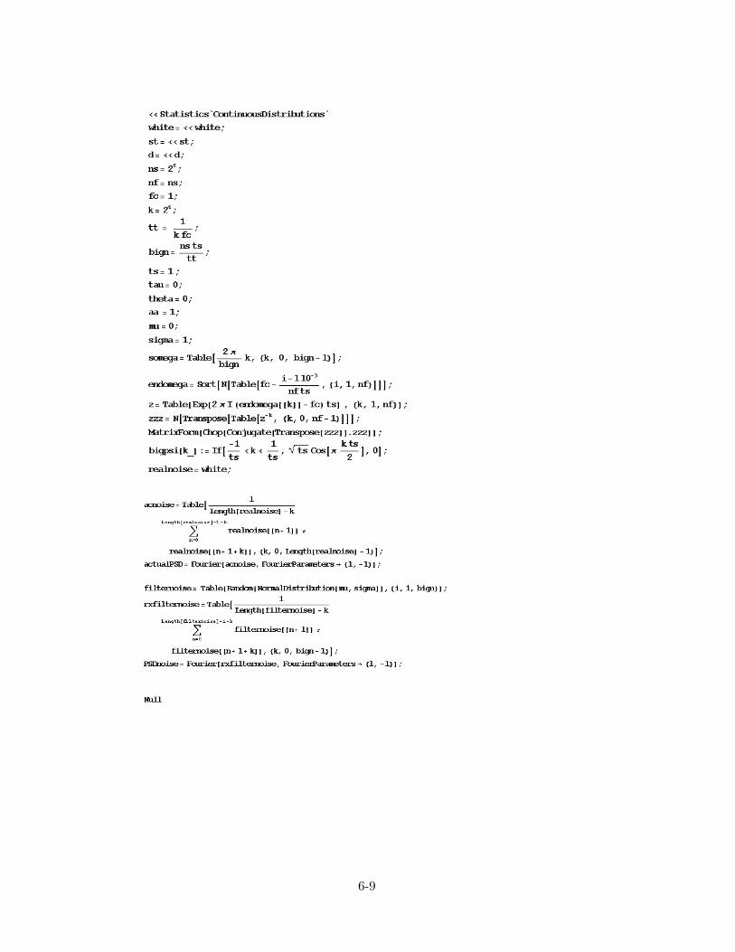
6-9

This section tests the recovery rate using an unknown noise shape and scale.
This section plots the results.
6-10

6.5 Subtraction of the Minimum Redundancy
6.5.1 Subtraction of the Minimum Redundancy Before Multiplication by Pulse Shape.
This portion of the Mathematica notebook creates the variables used throughout. Some
are recovered from data vectors created in the notebook "Data Generation." The vectors�
meaning is the same as in the �rst notebook. This notebook was used to create Figures
4.12 and 4.3.
6-11

This section is the loop that tests each of the various noise scales, recovers data
symbols at each noise scale, and compares the actual PSD to the estimated PSD using
MSE.
6-12

6-13

This section plots the results and stores them to be used in a comparison of all the
results.
6-14

This notebook plots the estimated PSD and the actual PSD, the noise scale here is
�xed as 1 to get a good comparison of the noise. All of the variables are the same as in
the notebook "Data Generation." This notebook was used to create Figures 4.9, 4.10, and
4.11.
6-15
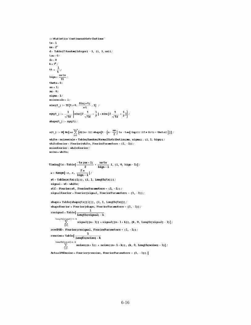
6-16

This section plots the results.
6-17

6.5.2 Subtraction of the Minimum Redundancy After Multiplication by Pulse Shape.
This portion of the Mathematica notebook creates the variables used throughout. Some
are recovered from data vectors created in the notebook "Data Generation." The vectors�
meaning is the same as in the �rst notebook. This notebook was used to create Figures
4.4 and 4.16.
6-18

This section is the loop that tests each of the various noise scales, recovers data
symbols at each noise scale, and compares the actual PSD to the estimated PSD using
MSE.
6-19

6-20

This section plots the results and stores them to be used in a comparison of all the
results.
6-21

This Mathematica notebook plots the estimated PSD and the actual PSD, the noise
scale here is �xed as 1. All of the variables are the same as in the notebook "Data
Generation."
It was used to create Figures 4.13, 4.14, and 4.15.
6-22

This section creates the estimated noise PSD, plots the estimated noise PSD zoomed
out and zoomed in, and plots the actual noise PSD.
6-23

6.6 Subtraction of the Average Redundancy
6.6.1 Subtraction of the Average Redundancy Before Multiplication by Pulse Shape.
This portion of the Mathematica notebook creates the variables used throughout. Some
6-24

are recovered from data vectors created in the notebook "Data Generation." Each of these
experiments uses the same vectors. This notebook was used to create Figures 4.5 and 4.20.
This section is the loop that tests each of the various noise scales, recovers data
symbols at each noise scale, and compares the actual PSD to the estimated PSD using
MSE.
6-25

6-26

This section plots the results and stores them to be used in a comparison of all the
results.
This Mathematica notebook plots the estimated PSD and the actual PSD, the noise
scale here is �xed as 1. All of the variables are the same as in the notebook "Data
Generation." This notebook creates Figures 4.17, 4.18, and 4.19.
6-27
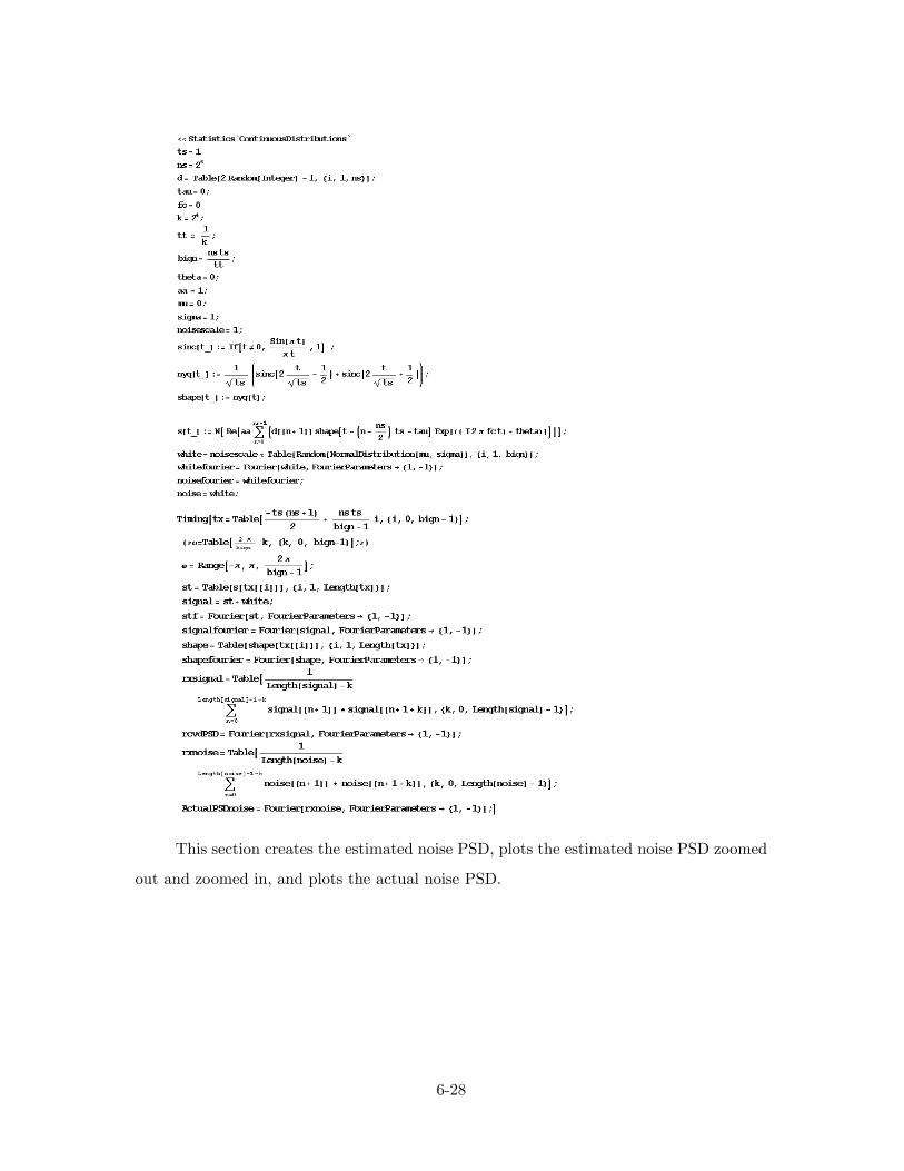
This section creates the estimated noise PSD, plots the estimated noise PSD zoomed
out and zoomed in, and plots the actual noise PSD.
6-28

6.6.2 Subtraction of the Average Redundancy After Multiplication by Pulse Shape.
This portion of the notebook creates the variables used throughout. Some are recovered
from data vectors created in the notebook "Data Generation." Each of these experiments
uses the same vectors. This notebook was used to create Figures 4.24 and 4.6.
6-29

This section is the loop that tests each of the various noise scales, recovers data
symbols at each noise scale, and compares the actual PSD to the estimated PSD using
MSE.
6-30

6-31

This section plots the results and stores them to be used in a comparison of all the
results.
This Mathematica notebook plots the estimated PSD and the actual PSD, the noise
scale here is �xed as 1. All of the variables are the same as in the notebook "Data
Generation." This notebook creates Figures 4.21, 4.22, and 4.23.
6-32

This section creates the estimated noise PSD, plots the estimated noise PSD zoomed
out and zoomed in, and plots the actual noise PSD.
6-33

6.7 Comparison
The �nal notebook combines the results from all the previous notebooks and plots
them together. This notebook was used to create Figures 4.7 and 4.25.
6-34

6-35

Bibliography
1. Berger, Toby and Donald W. Tufts. �Optimal Pulse Amplitude Modulation Part I:Transmitter Receiver Design and Bounds From Information Theory,� IEEE Transac-tions on Information Theory , 196�208 (April 1967).
2. Bernard Widrow, et Al. �Adaptive Noise Cancelling: Principles and Applications,�Proceedings of the IEEE , 1692�1716 (December 1975).
3. Casella, George and Roger L. Berger. Statistical Inference (Second Edition). Paci�cGrove CA: Duxbury, 2002.
4. Dwork, B. M. �Detection of a Pulse Superimposed on Fluctuation Noise,�Proceedingsof the IRE , 38 :771�774 (July 1950).
5. Ericson, Thomas. �Structure of Optimum Receiving Filters in Data TransmissionSystems,�IEEE Transactions on Information Theory , 352�353 (May 1971).
6. Gardner, William A. Statistical Spectral Analysis: A Nonprobabilistic Theory . Engle-wood Cli¤s NJ: Prentice Hall, 1988.
7. Gardner, William A. �Exploitation of Spectral Redundancy in Cyclostationary Sig-nals,�IEEE SP Magazine, 14�36 (April 1991).
8. Gardner, William A. �Signal Interception : A Unifying Theoretical Framework for Fea-ture Detection,�IEEE Transactions on Communications, 36:897�906 (August 1988).
9. Gardner, William A. �Spectral Correlation of Modulated Signals: Part II-Digital Mod-ulation,�IEEE Transactions on Communications, COM�35(6):595�601 (June 1987).
10. Gardner, William A. and Chih Kang Chen. �Signal-Selective Time-Di¤erence-of-Arrival Estimation for Passive Location of Man-Made Signal Sources in Highly Cor-ruptive Environments, Part I: Theory and Method,� IEEE Transactions on SignalProcessing , 40(5):1168�1184 (May 1992).
11. Gisselquist, Daniel E. A Linear Subspace Approach to Bust Communication SignalProcessing . AFIT/DS/ENG/04-02, Graduate School of Management and Engineering,Air Force Institute of Technology (AU), Wight Patterson AFB, OH, 2002.
12. Haykin, Simon. Adaptive Filter Theory . Upper Saddle River NJ: Prentice Hall, 1996.
13. Knapp, Charles H. and G. Cli¤ord Carter. �The Generalized Correlation Methodfor Estimation of Time Delay,� IEEE Transactions on Acoustics, Speech, and SignalProcessing , ASSP�24(4): 320�327 (August 1976).
14. Lucky, R. W. �Techniques for Adaptive Equalization of Digital Communication Sys-tems,�The Bell System Technical Journal , 45 (April 1966).
15. Mills, R. F. and G. E. Prescott. �A Comparison of Various Radiometer Detection Mod-els,� IEEE Transactions on Aerospace and Electronic Systems, 32 :467�473 (January1996).
BIB-1
16. Nyquist, H. �Certain Topics in Telegraph Transmission Theory,�Transactions of theAIEE(Communications and Electronics), 47 :617�644 (April, 1928).
17. Oppenheim, Alan V. and Ronald W. Schafer. Discrete-Time Signal Processing (SecondEdition). Englewood Cli¤s NJ: Prentice Hall, 1999.
18. Priestley, M. B. Spectral Analysis and Time Series. San Diego CA: Academic Press,1981.
19. Roberts, Richard A. and Cli¤ord T. Mullis. Digital Signal Processing . Reading MA:Addison-Wesley, 1987.
20. Scharf, Loius L. and Benjamin Friedlander. �Matched Subspace Detectors,� IEEETransactions on Signal Processing , 42(8):2146�2157 (August 1994).
21. Scharf, Louis L. Statistical Signal Processing: Detection, Estimation, and Time SeriesAnalysis. Reading MA: Addison�Wesley Publishing Company, 1991.
22. Shanmugan. �Spectral Correlation of Modulated Signals: Part I-Analog Modulation,�IEEE Transactions on Communications, COM�35(6):584�594 (June 1987).
23. Shanmugan, K. Sam and A.M. Breipohl. Random Signals: Detection, Estimation, andData Analysis. New York NY: John Wiley and Sons, 1988.
24. Sklar, Bernard. Digital Communications: Fundamentals and Applications (2nd Edi-tion). Upper Saddle River NJ: Prentice Hall, 2001.
25. Stremler, Ferrel G. Introduction to Communication Systems (3rd Edition). ReadingMA: Addison-Wesley Publishing, 1992.
26. Tufts, Donald W. �Nyquist�s Problem�The Joint Optimization of Transmitter andReciever in Pulse Amplitude Modulation,�Proceedings of the IEEE , 248�259 (March1965).
27. Turin, George L. �An Introduction to Matched Filters,� IRE Transactions on Infor-mation Theory , 311�329 (June 1960).
28. Urkowitz, Harry. �Energy Detection of Unknown Deterministic Signals,�Proceedingsof the IEEE , 55 (4):523�531 (April 1967).
BIB-2

REPORT DOCUMENTATION PAGE Form Approved OMB No. 074-0188
The public reporting burden for this collection of information is estimated to average 1 hour per response, including the time for reviewing instructions, searching existing data sources, gathering and maintaining the data needed, and completing and reviewing the collection of information. Send comments regarding this burden estimate or any other aspect of the collection of information, including suggestions for reducing this burden to Department of Defense, Washington Headquarters Services, Directorate for Information Operations and Reports (0704-0188), 1215 Jefferson Davis Highway, Suite 1204, Arlington, VA 22202-4302. Respondents should be aware that notwithstanding any other provision of law, no person shall be subject to an penalty for failing to comply with a collection of information if it does not display a currently valid OMB control number. PLEASE DO NOT RETURN YOUR FORM TO THE ABOVE ADDRESS. 1. REPORT DATE (DD-MM-YYYY)
21-03-2005 2. REPORT TYPE
Master’s Thesis 3. DATES COVERED (From – To)
August 2003 – March 2005 5a. CONTRACT NUMBER
5b. GRANT NUMBER
4. TITLE AND SUBTITLE Noise Estimation in the Presence of BPSK Digital Burst Transmissions 5c. PROGRAM ELEMENT NUMBER
5d. PROJECT NUMBER 5e. TASK NUMBER
6. AUTHOR(S) Bettison, Susan E., Second Lieutenant, USAF
5f. WORK UNIT NUMBER
7. PERFORMING ORGANIZATION NAMES(S) AND ADDRESS(S) Air Force Institute of Technology Graduate School of Engineering and Management (AFIT/EN) 2950 Hobson Way, Building 640 WPAFB OH 45433-8865
8. PERFORMING ORGANIZATION REPORT NUMBER AFIT/GAM/ENC/05-03
10. SPONSOR/MONITOR’S ACRONYM(S)
9. SPONSORING/MONITORING AGENCY NAME(S) AND ADDRESS(ES)
11. SPONSOR/MONITOR’S REPORT NUMBER(S)
12. DISTRIBUTION/AVAILABILITY STATEMENT APPROVED FOR PUBLIC RELEASE; DISTRIBUTION UNLIMITED.
13. SUPPLEMENTARY NOTES 14. ABSTRACT This research explores noise estimation techniques in an attempt to improve upon a previously developed digital burst transmission Binary Phase Shift Keyed (BPSK) demodulator. The demodulator success is dependant on the accuracy of the estimate of Power Spectral Density (PSD) of the unknown noise. Given a discrete time signal transformed into the frequency domain, the research seeks to determine if it is possible to effectively estimate the PSD of the unknown noise. The demodulator was developed using a new signal model for digital burst transmissions based on linear spectral subspace theory. Using this model and the redundancy properties of BPSK digital burst transmissions, five noise estimation techniques will be presented and tested. The success of the methods will be reported in two ways, first, the effect the new noise PSD estimates have on the success of the demodulator and second, a comparison to the actual PSD of the noise.
15. SUBJECT TERMS signal processing, digital communications, white noise, filters
16. SECURITY CLASSIFICATION OF:
19a. NAME OF RESPONSIBLE PERSON Lawrence K. Chilton, Ph.D. (AFIT/ENC)
a. REPORT
U
b. ABSTRACT
U
c. THIS PAGE
U
17. LIMITATION OF ABSTRACT
UU
18. NUMBER OF PAGES
109
19b. TELEPHONE NUMBER (Include area code) (937) 255-3636, ext 4523 ([email protected])
Standard Form 298 (Rev. 8-98) Prescribed by ANSI Std. Z39-18