NOAA Technical Memorandum NMFS
96
U.S. DEPARTMENT OF COMMERCE National Oceanic and Atmospheric Administration National Marine Fisheries Service Southwest Fisheries Science Center NOAA Technical Memorandum NMFS U A N C I I T R E E D M S A T A F T O E S O F T C N O E M M M T R E A R P C E E D NOAA-TM-NMFS-SWFSC-402 APRIL 2007 K. Kelly Hildner DATA SOURCES: CALIFORNIA HABITAT RESTORATION PROJECT COST ANALYSIS
-
Upload
khangminh22 -
Category
Documents
-
view
3 -
download
0
Transcript of NOAA Technical Memorandum NMFS

U.S. DEPARTMENT OF COMMERCENational Oceanic and Atmospheric AdministrationNational Marine Fisheries ServiceSouthwest Fisheries Science Center
NOAA Technical Memorandum NMFS
U
AN
CI IT
RE
EDMS ATA FT OE S
OFT CN OE MM MT
R E
A R
P C
E E
D
NOAA-TM-NMFS-SWFSC-402
APRIL 2007
K. Kelly Hildner
DATA SOURCES: CALIFORNIA HABITAT
RESTORATION PROJECT COST ANALYSIS

The National Oceanic and Atmospheric Administration (NOAA), organized in 1970, has evolved into an agency which establishes national policies and manages and conserves our oceanic, coastal, and atmospheric resources. An organizational element within NOAA, the Office of Fisheries is responsible for fisheries policy and the direction of the National Marine Fisheries Service (NMFS).
In addition to its formal publications, the NMFS uses the NOAA Technical Memorandum series to issue informal scientific and technical publications when complete formal review and editorial processing are not appropriate or feasible. Documents within this series, however, reflect sound professional work and may be referenced in the formal scientific and technical literature.

MOSTA PHD EN RA ICCI AN DA ME IC N
O IS
L T
A R
N ATOI IOT
A N
N
U
E.S C. RD EE MPA MR OT CM FENT O
NOAA Technical Memorandum NMFSThis TM series is used for documentation and timely communication of preliminary results, interim reports, or specialpurpose information. The TMs have not received complete formal review, editorial control, or detailed editing.
NOAA-TM-NMFS-SWFSC-402
APRIL 2007
National Marine Fisheries Service,NOAA
Southwest Fisheries Science Center
110 Shaffer Road
Santa Cruz, California 95060
U.S. DEPARTMENT OF COMMERCECarlos M. Gutierrez, SecretaryNational Oceanic and Atmospheric AdministrationVADM Conrad C. Lautenbacher, Jr., Undersecretary for Oceans and AtmosphereNational Marine Fisheries ServiceWilliam T. Hogarth, Assistant Administrator for Fisheries
K. Kelly Hildner
DATA SOURCES: CALIFORNIA HABITAT
RESTORATION PROJECT COST ANALYSIS

2
ACKNOWLEDGEMENTS I am grateful to Cindy Thomson (National Marine Fisheries Service, Southwest Fisheries Science Center), for helpful organizational suggestions and comments on earlier versions. Many thanks go to the GIS staff at the SWFSC, notably Rob Schick and Aditya Agrawal, for GIS support.

3
TABLE OF CONTENTS ACKNOWLEDGEMENTS ......................................................................................................... 2
ABSTRACT................................................................................................................................... 5
1 INTRODUCTION................................................................................................................. 6
2 WAGE DATA........................................................................................................................ 7
2.1 OVERVIEW ....................................................................................................................... 7 2.2 MAPS AND METADATA .................................................................................................... 8
2.2.1 Covered Employment and Wages (CEW) Wage Data for ‘Heavy Construction Excluding Building’ from RAND California (1990-2000).................................................... 10 2.2.2 Covered Employment and Wages (CEW) Wage Data for ‘Heavy and Civil Engineering Construction’ from RAND California (2001-2003) ......................................... 13
3 UNEMPLOYMENT DATA............................................................................................... 14
3.1 OVERVIEW ..................................................................................................................... 14 3.2 MAPS AND METADATA .................................................................................................. 15
3.2.1 Unemployment Rates – Labor Force Data from the Labor Market Information Division of the California Employment Development Department (1990-2004) ................. 17
4 POPULATION AND POPULATION DENSITY............................................................ 20
4.1 OVERVIEW ..................................................................................................................... 20 4.2 MAPS AND METADATA .................................................................................................. 22
4.2.1 Census 2000 Population Database for Counties, County Subdivisions, and Incorporated and Designated Places.................................................................................... 22 4.2.2 Census Incorporated Places and Balance of County Areas with Census 2000 Population and Population Density...................................................................................... 25 4.2.3 Census Incorporated and Designated Places and Balance of County Areas with Census 2000 Population and Population Density ................................................................ 29 4.2.4 Census County Subdivisions with Census 2000 Population and Population Density 33
5 CITIES / URBAN AREAS ................................................................................................. 34
5.1 OVERVIEW ..................................................................................................................... 34 5.2 MAPS AND METADATA .................................................................................................. 35
5.2.1 Point Locations of California Cities from Environmental Systems Research Institute 37 5.2.2 Census 2000 TIGER/Line Urban Area Boundaries .............................................. 40
6 LAND USE AND LAND COVER DATA......................................................................... 42
6.1 OVERVIEW ..................................................................................................................... 42
7 SOILS ................................................................................................................................... 43
7.1 OVERVIEW ..................................................................................................................... 43 7.2 MAPS AND METADATA .................................................................................................. 45
4
7.2.1 STATSGO Soils Data Base Containing Hydrology-Relevant Information for California .............................................................................................................................. 47
8 PRECIPITATION .............................................................................................................. 50
8.1 OVERVIEW ..................................................................................................................... 50 8.2 MAPS AND METADATA................................................................................................ 51
8.2.1 Average Annual Precipitation 1961-1990 - Spatial Climate Analysis Service, Oregon State University........................................................................................................ 52
9 ELEVATION / SLOPE ...................................................................................................... 53
9.1 OVERVIEW ..................................................................................................................... 53 9.2 MAPS AND METADATA .................................................................................................. 54
9.2.1 30 Meter Resolution Elevation Data Created from USGS National Elevation Dataset (NED) Data.............................................................................................................. 56 9.2.2 Slope Derived from 30 Meter USGS National Elevation Dataset (NED) Data ... 60
10 ROADS............................................................................................................................. 61
10.1 OVERVIEW ..................................................................................................................... 61 10.2 MAPS AND METADATA .................................................................................................. 61
10.2.1 U.S. Census 2000 TIGER/Line Road Data ................................................................ 63 10.2.2 U.S. Census 2000 TIGER/Line Highways.................................................................. 69 10.2.3 Road Density from U.S. Census 2000 TIGER/Line Road Data................................. 72
11 STREAMS ....................................................................................................................... 73
11.1 OVERVIEW ..................................................................................................................... 73 11.2 MAPS AND METADATA .................................................................................................. 73
11.2.1 Streams Data (CDFG & PSMFC, March 2003) ....................................................... 76
12 WATERSHEDS .............................................................................................................. 79
12.1 OVERVIEW ..................................................................................................................... 79 12.2 MAPS AND METADATA .................................................................................................. 79
12.2.1 California Interagency Watershed Map of 1999 (CalWater 2.2, updated May 2004, “calw221”) ........................................................................................................................... 81 12.2.2 CalWater 2.2.1 Hydrologic Units .............................................................................. 85 12.2.3 USGS Hydrologic Units............................................................................................. 88 12.2.4 NOAA Fisheries Salmonid Technical Recovery Team Watersheds ........................... 91
APPENDIX A: METADATA CATEGORY DEFINITIONS................................................. 93

5
ABSTRACT Landscape and socioeconomic factors that may affect salmonid habitat restoration costs in California are identified. Data sources for each factor are identified, and each data source and its relevant derivations are described in terms of maps and metadata. The documentation provided is intended to facilitate future research on habitat restoration costs.
6
1 INTRODUCTION
Ten California salmonid stocks are currently listed as threatened or endangered under the Endangered Species Act (ESA), and millions of dollars are spent annually on habitat restoration projects designed to benefit these fish. Although the ESA requires that recovery plans incorporate information on implementation costs, to date very little has been published on salmonid habitat restoration costs. To help fill this void, the California Habitat Restoration Project Database (CHRPD) was created by the Pacific States Marine Fisheries Commission, with funding originally provided by NOAA Fisheries and later by the California Department of Fish and Game. The California Habitat Restoration Project Database (CHRPD) contains information on salmonid habitat restoration projects in California from 1981 to the present and is being updated as new projects occur. The database includes detailed information on each restoration project, including the type of project, its cost, its spatial location, and various other project attributes. NOAA Fisheries hopes to use this database in conjunction with socio-economic and environmental variables to predict the costs of future restoration projects. To this end, NOAA Fisheries (Southwest Fisheries Science Center, Santa Cruz) is compiling spatial data on factors that may affect the costs of habitat restoration projects. The purpose of this document is to provide information on the selected data sources. Information about data sources examined but not selected is also provided.
The CHRPD contains restoration projects widely distributed in both space and time. Projects occur throughout California (with the majority, as of March 2005, clustered along the coast of the northern half of the state) and over a span of more than two decades. Most socio-economic variables also vary over space and time. Ideally, we would like to obtain spatial data on socio-economic and environmental variables that cover the entire state and are available in a time series, with data corresponding to each year for which we have restoration project data.
Finding such data is difficult, however, and in many cases impossible. Consistent spatial data for such a large geographic area are inherently difficult to produce and are concomitantly rare. For example, creating a land-use/land cover dataset for California is highly labor intensive and time consuming; consequently, such datasets are not updated yearly, but rather, are typically derived from data sources that span multiple years. Data that are available as time series, including some socio-economic variables (e.g. population size, unemployment rates, and wages) are not usually consistent through time. In some cases the methodology or classification system for collecting the information has changed part way through the time series, and in other cases, the geographic boundaries upon which the data are based have changed. These complexities are outlined in the relevant sections below. We did our best to find the most consistent time series of data available for each variable.
This document is organized into sections representing the data types examined for use in our analyses. Each section begins with an overview describing the data sources researched. Following the overview are maps and metadata (data about data) for each of the selected data sources and its relevant derivations. Metadata included in this document serve as a general guide to the data sources; more detailed metadata are generally stored with the actual data files. For definitions of the metadata categories used in this document, see Appendix A.

7
2 WAGE DATA
2.1 OVERVIEW
Several sources of wage data were researched in an attempt to find a time series of comprehensive statewide construction wages by county (or smaller geographic unit). Data sources explored include the Davis-Bacon Act Wage Determinations, Bureau of Labor Statistics (BLS), California Employment Development Department, California Department of Finance, Bureau of Economic Analysis, and RAND California. The Davis-Bacon Act requires payment of prevailing wage rates on federally funded construction projects and was anticipated to be a valuable source of construction wage data. The Davis-Bacon Act Wage Determinations were ruled out, however, as a source for comprehensive wage data because the data are not standardized, there is no classification system, and the classifications of jobs and their definitions vary by county and by state (Pam Lee, Wage and Hour Division, Department of Labor, personal communication 202-693-0597, [email protected]). The Bureau of Labor Statistics databases explored include the National Compensation Survey (NCS), Current Employment Statistics (CES) Survey, Occupational Employment Statistics (OES) program, and the Covered Employment and Wages (CEW) program. The NCS provides earnings data by worker characteristics and establishment characteristics for certain metropolitan areas. This survey does not provide complete data coverage of the state. Likewise, the CES Survey, a monthly survey of business establishments that provides estimates of employment, hours, and earnings data by industry, does not provide complete coverage of the state. These sources were, therefore, not explored further.
The OES program provides employment and wage estimates by occupation for 25 MSAs (metropolitan statistical areas and primary metropolitan statistical areas) in California. MSAs do not provide complete coverage of California, but OES data available for download from the California Employment Development Department includes 5 balance of state (BOS) regions that complete the coverage of the state. BOS regions data, however, are only available for selected years, and some BOS regions and MSA areas are quite large and therefore do not provide much spatial resolution in wage data. Additionally, the OES survey changed its method of classifying occupations from the OES classification system to the Standard Occupational Classification (SOC) system starting in 1999. The new classification system includes a Construction Laborers occupation (code 47-2061) that was not available in the previous classification system. This data source was rejected due to its lack of spatial resolution and lack of temporal consistency.
The CEW program is a cooperative program involving the BLS, the U.S. Department of Labor, and the State Employment Security Agencies (SESAs), which “publishes a quarterly count of employment and wages reported by employers covering 98 percent of U.S. jobs, available at the county, MSA, state and national levels by industry” (http://www.bls.gov/cew/home.htm#overview). From this program it is possible to retrieve employment and wages by industry and county for California; for some industry/county/year combinations, however, data are not available due to disclosure restrictions. CEW data do not include members of the armed forces, the self-employed, proprietors, domestic workers, unpaid family workers, and railroad workers covered by the railroad unemployment insurance system (http://www.bls.gov/cew/cewover.htm). In 2001 the BLS switched from the 1987 Standard

8
Industrial Classification (SIC) system to the 2002 version of the North American Industrial Classification System (NAICS) for classifying industries, so pre-2001 data are not directly comparable with data from 2001 and beyond. Annual CEW average industry wage data are compiled in user-friendly downloadable tables by RAND California (http://ca.rand.org/stats/statlist.html; a subscription is required).
The California Employment Development Department (CalEDD) and the California Department of Finance do not have any sources of wage data that are not also available from the BLS. The Bureau of Economic Analysis (BEA) has personal income and employment data by industry for counties and MSAs. These data are based on the ES-202 survey and are more comprehensive than CEW data (Kathy Albetski, BEA Personal Income Branch, personal communication). Dividing the personal income values on the BEA website by total employment provides average earnings per job instead of average wages, and the employment numbers are only provided for the construction industry as a whole, not the heavy construction industry. In order to acquire wage data for the heavy construction industry, we would need permission for the disclosure of suppressed data from the CalEDD Labor Market Information Division (LMID). Since permission for the disclosure of suppressed data is typically only granted for economic development purposes (Janyce Wong, CalEDD LMID Confidential Data Coordinator, personal communication), we abandoned this potential data source.
RAND California has average industry wage statistics for California Counties by industry and ownership type. As mentioned above, these data are from the BLS CEW program but are more readily accessible from the RAND California website. A comparison of the numbers available on the RAND website with those available on the BLS website indicated some minor differences for some counties for some years. RAND California was unable to explain these differences. Nonetheless, we decided to use these data because they are readily accessible, and, unlike the OES data, are available at the county level.
CEW data at the RAND website are broken down by ownership type (private sector, local government, state government, and federal government), but data for most counties are only available for the private sector; therefore, we only used data for the private sector. Because the classification of industries changed from SIC to NAICS in 2001, pre-2001 data are not directly comparable with data from 2001 and beyond. Data downloaded for 1990-2000 are for SIC category ‘Heavy Construction Ex. Building’ and data downloaded for 2001 to 2003 are for NAICS category ‘Heavy and Civil Engineering Construction’.
2.2 MAPS AND METADATA
9
Inyo
Kern
San Bernardino
Fresno
Riverside
Tulare
Siskiyou
Lassen
Modoc
Imperial
Mono
ShastaTrinity
San Diego
Humboldt
Tehama
Monterey
Plumas
Los Angeles
ButteMendocino
Madera
Lake
Merced
Kings
Placer
Ventura
Tuolumne
Yolo
Glenn
San Luis Obispo
Sonoma
El Dorado
Santa Barbara
Colusa
Sierra
Mariposa
Napa
Stanislaus
Solano
San Benito
Nevada
Yuba
Alpine
San Joaquin
Santa Clara
Orange
Del Norte
Calaver
as
Sutter
Marin
Alameda
Sacr
amen
to
Amador
Contra Costa
San Mateo
Santa Cruz
San Francisco
Figure 2.2.1a. 2000 Average Annual Wages Heavy Construction Excluding Building
(Private Industry)
Average Annual Wages
20,000 - 25,000
25,001 - 30,000
30,001 - 35,000
35,001 - 40,000
40,001 - 45,000
45,001 - 50,000
50,001 - 55,000
55,001 - 60,000
60,001 - 90,000
No Data
Created by Kelly Hildner, February 6, 2003 NOAA Fisheries, Santa Cruz, CA 95060
Data Source: RAND California, http://ca.rand.orgProjection: NAD27 UTM Zone 10
±0 200100
Kilometers
0 10050Miles

10
2.2.1 Covered Employment and Wages (CEW) Wage Data for ‘Heavy Construction Excluding Building’ from RAND California (1990-2000)
Type: Wages Name: Covered Employment and Wages (CEW) Wage Data 1990-2000 File Name: RANDWagebyIndustry.mdb Location: C:\Rest_Cost_Proj\GIS_data\Wages Description: Average Annual Wages for Standard Industrial Classification (SIC) category ‘Heavy Construction Excluding Building’ for 1990 thru 2000 from the Covered Employment and Wages (CEW) program of the Bureau of Labor Statistics. The CEW program provides wage and employment data by industry at the national, state and county levels. Data for the year 2000 were the last data using the 1987 SIC system. Data Source: Rand California, http://ca.rand.org. Data were downloaded from RAND California. The original data source is the Bureau of Labor Statistics, http://www.bls.gov Time Period: 1990-2000 Spatial Coverage: Data are by county for California. Spatial coverage varies by year. Data are not available for all counties for each year. The BLS withholds data from publication when necessary to protect the identity of employers. Limitations: With the release of the 2001 data, the program switched to the 2002 version of the North American Industry Classification System (NAICS) as the basis for tabulation of data by industry. Data for 2001 and later are not comparable to the SIC-based data for earlier years. Industry wages reflect the average wage for all employees in an industry regardless of occupation. “Employment data under the CEW program represent the number of covered workers who worked during, or received pay for, the pay period including the 12th of the month. Excluded are members of the armed forces, the self-employed, proprietors, domestic workers, unpaid family workers, and railroad workers covered by the railroad unemployment insurance system. Wages represent total compensation paid during the calendar quarter, regardless of when services were performed. Included in wages are pay for vacation and other paid leave, bonuses, stock options, tips, the cash value of meals and lodging, and in some States, contributions to deferred compensation plans (such as 401(k) plans). The CEW program does provide partial information on agricultural industries and employees in private households.” - http://stats.bls.gov/cew/cewover.htm “Average Annual Pay - The result of dividing the Total Annual Payroll by the Monthly Average Employment. CAUTION! Average annual pay is affected by the ratio of full-time to part-time

11
workers; the number of workers who worked for the full year; and the number of individuals in high-paying and low-paying occupations. When comparing average pay levels between geographic areas and industries, these factors should be taken into consideration. For example, industries characterized by high proportions of part-time workers will show average wage levels appreciably less than the pay levels of regular full- time employees in these industries. The opposite effect characterizes industries with low proportions of part-time workers, or industries that typically schedule heavy weekend and overtime work. Average wage data also may be influenced by work stoppages, labor turnover, retroactive payments, seasonal factors, bonus payments, and so on.” - http://www.calmis.ca.gov/file/es202/cew-readme.htm Original Format: Tab delimited Processing Steps: Downloaded tab delimited data from the website. Imported data into Excel. Created new Access database and imported excel tables. Renamed fields. Imported a table with county names and FIPS codes. Created a query combining FIPS codes with wage data for linking to county GIS layers. Field data types and sizes were changed to reflect the type and size of data stored. Data Format: Access Database (.mdb) Notes: Final table: zzAnnWageHvyConstPvt90to2000. For mapping, link to county GIS data using the CntyFIPS field.
“IMPORTANT NOTE: Federal quarterly wage data for the two-year period from the third quarter 1999 through the third quarter 2001 are currently under review for an underreporting issue involving a missing pay-period for some workers” (http://www.calmis.ca.gov/file/es202/CEW-About.htm; February 6, 2006).
Attributes/Data Dictionary: See table design view in Access

12
Inyo
Kern
San Bernardino
Fresno
Riverside
Tulare
Siskiyou
Lassen
Modoc
Imperial
Mono
ShastaTrinity
San Diego
Humboldt
Tehama
Monterey
Plumas
Los Angeles
ButteMendocino
Madera
Lake
Merced
Kings
Placer
Ventura
Tuolumne
Yolo
Glenn
San Luis Obispo
Sonoma
El Dorado
Santa Barbara
Colusa
Sierra
Mariposa
Napa
Stanislaus
Solano
San Benito
Nevada
Yuba
Alpine
San Joaquin
Santa Clara
Orange
Del Norte
Calaver
as
Sutter
Marin
Alameda
Sacra
men
to
Amador
Contra Costa
San Mateo
Santa Cruz
San Francisco
Figure 2.2.2a. 2001 Average Annual Wages Heavy and Civil Engineering Construction
(Private Industry)
Average Annual Wages
20,055 - 25,000
25,001 - 30,000
30,001 - 35,000
35,001 - 40,000
40,001 - 45,000
45,001 - 50,000
50,001 - 55,000
55,001 - 60,000
60,001 - 95,000
95,001 - 170,000
No Data
Created by Kelly Hildner, February 6, 2006 NOAA Fisheries, Santa Cruz, CA 95060
Data Source: RAND California, http://ca.rand.orgProjection: NAD27 UTM Zone 10
±0 200100
Kilometers
0 10050Miles

13
2.2.2 Covered Employment and Wages (CEW) Wage Data for ‘Heavy and Civil Engineering Construction’ from RAND California (2001-2003)
Type: Wages Name: Covered Employment and Wages (CEW) Wage Data 2001-2003 File Name: RANDWagebyIndustry01to03.mdb Location: C:\Rest_Cost_Proj\GIS_Data\Wages Description: Average Annual Wages for ‘Heavy and Civil Engineering Construction’ for 2001 to 2003 from the Covered Employment and Wages (CEW) program of the Bureau of Labor Statistics. The CEW program provides wage and employment data by industry at the national, state and county levels. Data for the year 2001 are the first data using the 2002 version of the North American Industrial Classification System (NAICS) for classifying industries. Data Source: Rand California, http://ca.rand.org. Data were downloaded from RAND California, http://ca.rand.org/stats/economics/avgwagenaicsUS.html. The original data source is the Bureau of Labor Statistics, http://www.bls.gov Time Period: 2001-2003 Spatial Coverage: Data are by county for California. Spatial coverage varies by year. Data are not available for all counties for each year. The BLS withholds data from publication when necessary to protect the identity of employers. Data for 2001 are available for 54 of the 58 counties in California and data for 2002 and 2003 are available for 53 counties each. The counties missing data differ in different years. Limitations: With the release of the 2001 data, the program switched to the 2002 version of the North American Industry Classification System (NAICS) as the basis for tabulation of data by industry. Data for 2001 and later are not comparable to the SIC-based data for earlier years. Industry wages reflect the average wage for all employees in an industry regardless of occupation. “Employment data under the CEW program represent the number of covered workers who worked during, or received pay for, the pay period including the 12th of the month. Excluded are members of the armed forces, the self-employed, proprietors, domestic workers, unpaid family workers, and railroad workers covered by the railroad unemployment insurance system. Wages represent total compensation paid during the calendar quarter, regardless of when services were performed. Included in wages are pay for vacation and other paid leave, bonuses, stock options, tips, the cash value of meals and lodging, and in some States, contributions to deferred compensation plans (such as 401(k) plans). The CEW program does provide partial information on agricultural industries and employees in private households.” - http://stats.bls.gov/cew/cewover.htm

14
“Average Annual Pay - The result of dividing the Total Annual Payroll by the Monthly Average Employment. CAUTION! Average annual pay is affected by the ratio of full-time to part-time workers; the number of workers who worked for the full year; and the number of individuals in high-paying and low-paying occupations. When comparing average pay levels between geographic areas and industries, these factors should be taken into consideration. For example, industries characterized by high proportions of part-time workers will show average wage levels appreciably less than the pay levels of regular full-time employees in these industries. The opposite effect characterizes industries with low proportions of part-time workers, or industries that typically schedule heavy weekend and overtime work. Average wage data also may be influenced by work stoppages, labor turnover, retroactive payments, seasonal factors, bonus payments, and so on.” - http://www.calmis.ca.gov/file/es202/cew-readme.htm Original Format: Tab delimited Processing Steps: Downloaded tab delimited data from the website. Imported data into Excel. Created new Access database and import excel table. Created an empty table with desired field definitions. Imported a table with county names and FIPS codes. Created a query combining FIPS codes with wage data and appended the data to the empty table. Data Format: Access Database (.mdb) Notes: Final table: AnnWageHvyCvlEngConstPvt01to03. For mapping, link to county GIS data using the CntyFIPS field.
“IMPORTANT NOTE: Federal quarterly wage data for the two-year period from the third quarter 1999 through the third quarter 2001 are currently under review for an underreporting issue involving a missing pay-period for some workers” (http://www.calmis.ca.gov/file/es202/CEW-About.htm; February 6, 2006).
Attributes/Data Dictionary: See table design view in Access
3 UNEMPLOYMENT DATA
3.1 OVERVIEW
Unemployment data are available by county from both the Bureau of Labor Statistics (BLS) Local Area Unemployment Statistics (LAUS) program
(http://www.bls.gov/lau/home.htm#tables) and the California Employment Development Department (CalEDD) Labor Force Data program (http://www.calmis.cahwnet.gov/htmlfile/subject/lftable.htm). CalEDD provides the data to the BLS, so CalEDD is the preferred data source. Labor force data represent employment by place of residence as opposed to by place of work. Beginning with estimates for January 1996, time series models became the basis for the estimates of labor force data (labor force, employment, unemployment, and the unemployment rate) for California and Los Angeles County instead of the Current Population Survey (CPS). The data were revised using this method back to 1980.

15
County level data are available from two places on the CalEDD website (http://www.calmis.ca.gov/htmlfile/subject/lftable.htm), and these have slightly different data. The first set is the 400C reports and the second set is the HLF.TXT files (available from the table at the bottom of the web page). According to Nancy Gemignani at CalEDD Labor Market Information, the later files are updated and should be used for creating time series.
In January 2005, labor force data for all areas were revised back to 1976 using new time series models.
In addition to county level data, CalEDD has data available at the sub-county level. These data are created by multiplying current estimates of county-wide employment and unemployment by the respective employment and unemployment shares (percentages) in each sub-county area at the time of the last decennial census. Sub-county labor force is then obtained by summing employment and unemployment, and the result is divided into unemployment to calculate the unemployment rate. This method assumes that the rates of change in employment and unemployment since the last census are exactly the same in each sub-county area as at the county level (i.e., that the shares are still accurate). If this assumption is not true for a specific sub-county area, then the estimates for that area may not be representative of the current economic conditions. Since this assumption is untested, caution should be employed when using the sub-county data. For this reason, we are using the county level data for our analyses.
3.2 MAPS AND METADATA

16
4.7%
5.5%
5.5%
7%
11.3%
3%
9.5%
3%
14.3%
8.5%
5.3%
15.5%
6.9%
26.3%
6.4%
6.6%
6%
9.6%
5.6%
6.9%
12.7%
8.4%
3.7%
7%
8%
2%
4.5%
4.1%
11.8%14.5%
2.6%
3.1%
12%
7.7%
8.9%
7.9%
10.5%
13.9%
3%
8%
6.7%
4.3%
8.7%
4.2%
7.8%
17.6%
4.2%
2.5%
3.6%
3.2%
2.7%
4.4%
1.6%
11.8%
13.1%
1.6%
5.7%
2.8%
Unemployment 2000
1.6% - 2%
2.1% - 3.2%
3.3% - 4.7%
4.8% - 6.7%
6.8% - 8.9%
9% - 12.7%
12.8% - 17.6%
17.7% - 26.3%
Figure 3.2.1a. 2000 Unemployment Rates by County
Created by Kelly Hildner, February 21, 2006 NOAA Fisheries, Santa Cruz, CA 95060
Data Source: California Employment Development Department, Labor Market Information Division
http://www.calmis.cahwnet.gov/htmlfile/subject/lftable.htmProjection: NAD27 UTM Zone 10
0 50 10025Miles
0 50 100 150 20025Kilometers
±

17
3.2.1 Unemployment Rates – Labor Force Data from the Labor Market Information Division of the California Employment Development Department (1990-2004)
Type: Unemployment Name: Labor Force Statistics, Unemployment 1990-2002 File Name: UnemploymentCalEDD.mdb Location: C:\Rest_Cost_Proj\GIS_data\Unemployment Description: Unemployment rates for counties in California for 1990 to 2004. These data are Labor Force Data from the Labor Market Information Division of the California Employment Development Department.
Methods for Labor Force Estimates (from http://www.labormarketinfo.edd.ca.gov/article.asp?ARTICLEID=179&PAGEID=94&SUBID=)
Definition of Terms:
Civilian Labor Force is the sum of civilian employment and civilian unemployment. Civilians, as defined, are age 16 years or older, not members of the Armed Services, and are not in institutions such as prisons, mental hospitals, or nursing homes.
Civilian Employment includes all individuals who worked at least one hour for a wage or salary, or were self-employed, or were working at least 15 unpaid hours in a family business or on a family farm, during the week including the 12th of the month. Those who were on vacation, on other kinds of leave, or involved in a labor dispute, were also counted as employed.
Civilian Unemployment includes those individuals who were not working but were able, available, and actively looking for work during the week including the 12th of the month. Individuals who were waiting to be recalled from a layoff, and individuals waiting to report to a new job within 30 days were also considered to be unemployed.
Unemployment Rate is the number of unemployed as a percentage of the labor force.
California and Los Angeles-Long Beach-Glendale Metropolitan Division - Time Series Models
In January 1996, time series models replaced the Current Population Survey (CPS) as the basis for the estimates of labor force data (labor force, employment, unemployment, and the unemployment rate) for California. In January 2005, the LMID revised data back to 1976 using the new time series models. The models cover two areas of the State: the Los Angeles-Long Beach-Glendale Metropolitan Division (MD) and the "Balance of California" (i.e., the rest of California). The results are added together to derive state- level data.
18
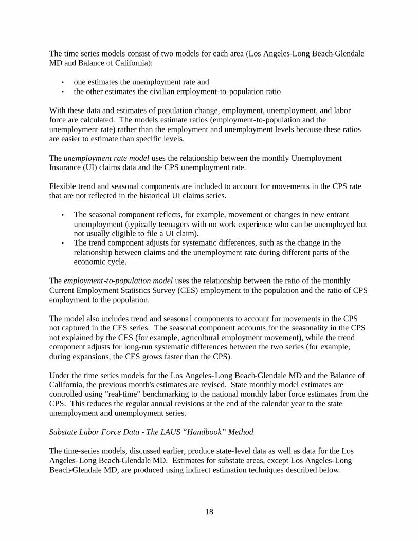
The time series models consist of two models for each area (Los Angeles-Long Beach-Glendale MD and Balance of California):
• one estimates the unemployment rate and • the other estimates the civilian employment-to-population ratio
With these data and estimates of population change, employment, unemployment, and labor force are calculated. The models estimate ratios (employment-to-population and the unemployment rate) rather than the employment and unemployment levels because these ratios are easier to estimate than specific levels.
The unemployment rate model uses the relationship between the monthly Unemployment Insurance (UI) claims data and the CPS unemployment rate.
Flexible trend and seasonal components are included to account for movements in the CPS rate that are not reflected in the historical UI claims series.
• The seasonal component reflects, for example, movement or changes in new entrant unemployment (typically teenagers with no work experience who can be unemployed but not usually eligible to file a UI claim).
• The trend component adjusts for systematic differences, such as the change in the relationship between claims and the unemployment rate during different parts of the economic cycle.
The employment-to-population model uses the relationship between the ratio of the monthly Current Employment Statistics Survey (CES) employment to the population and the ratio of CPS employment to the population.
The model also includes trend and seasona l components to account for movements in the CPS not captured in the CES series. The seasonal component accounts for the seasonality in the CPS not explained by the CES (for example, agricultural employment movement), while the trend component adjusts for long-run systematic differences between the two series (for example, during expansions, the CES grows faster than the CPS).
Under the time series models for the Los Angeles-Long Beach-Glendale MD and the Balance of California, the previous month's estimates are revised. State monthly model estimates are controlled using "real-time" benchmarking to the national monthly labor force estimates from the CPS. This reduces the regular annual revisions at the end of the calendar year to the state unemployment and unemployment series.
Substate Labor Force Data - The LAUS “Handbook” Method
The time-series models, discussed earlier, produce state- level data as well as data for the Los Angeles-Long Beach-Glendale MD. Estimates for substate areas, except Los Angeles-Long Beach-Glendale MD, are produced using indirect estimation techniques described below.
19
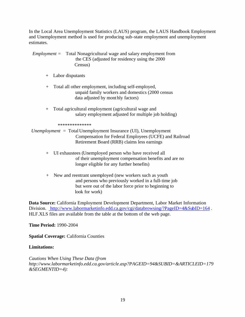
In the Local Area Unemployment Statistics (LAUS) program, the LAUS Handbook Employment and Unemployment method is used for producing sub-state employment and unemployment estimates.
Employment = Total Nonagricultural wage and salary employment from the CES (adjusted for residency using the 2000 Census) + Labor disputants + Total all other employment, including self-employed, unpaid family workers and domestics (2000 census data adjusted by monthly factors) + Total agricultural employment (agricultural wage and salary employment adjusted for multiple job holding) ************** Unemployment = Total Unemployment Insurance (UI), Unemployment Compensation for Federal Employees (UCFE) and Railroad Retirement Board (RRB) claims less earnings + UI exhaustees (Unemployed person who have received all of their unemployment compensation benefits and are no longer eligible for any further benefits) + New and reentrant unemployed (new workers such as youth and persons who previously worked in a full- time job but were out of the labor force prior to beginning to look for work)
Data Source: California Employment Development Department, Labor Market Information Division. http://www.labormarketinfo.edd.ca.gov/cgi/databrowsing/?PageID=4&SubID=164 . HLF.XLS files are available from the table at the bottom of the web page.
Time Period: 1990-2004 Spatial Coverage: California Counties Limitations:
Cautions When Using These Data (from http://www.labormarketinfo.edd.ca.gov/article.asp?PAGEID=94&SUBID=&ARTICLEID=179&SEGMENTID=4):

20
• The "Employment" which is shown under "Labor Force" is not directly comparable to the "Total, All Industries" employment. A complete description of the Employment by Industry Method is also available.
• County labor force data are not adjusted for seasonality. When doing a comparison with state and U.S. rates, it is important to use "Not Seasonally Adjusted" labor force data for the state and the nation.
• The unemployment rate usually gets the most attention, as it is a rough gauge of the area's labor market. It is best to consider the unemployment rate over a period of several months, or years. The employment and unemployment figures tend to vary from month to month for many reasons. Seasonal variation often may not reflect the economic conditions in all areas of the county. Seasonal factors may contribute to an area's high unemployment rate, but firms in some industries may have difficulty finding qualified employees. The labor market can vary greatly in different industries, in different occupations, and in different parts of the county.
• The annual average figures, over time, tend to be a better gauge of the labor force trends within the area.
• Month-to-month labor force data are a useful indicator to show the seasonal changes in an area including outdoor activities (such as construction), holiday hiring, school schedules, and agricultural activities.
Original Format: Excel files (HLF.XLS) Processing Steps: Data were downloaded from the website (http://www.calmis.cahwnet.gov/htmlfile/subject/lftable.htm) on 8/9/2005, and a VBA macro was written to extract the average annual unemployment rate for each year from each of the county files and put them into a single excel table (UnemploymentCalEDD2004.xls). The resulting excel table was then imported into Access (UnemploymentCalEDD.mdb). The word ‘County’ was removed from each county name in order to link to a table of county names and FIPS codes. Data Format: Access Database (.mdb) Notes: The query qryCntyUnemploy90to04Fips is a table of unemployment rates for each county for each year with FIPS county codes for linking to GIS maps. Attributes/Data Dictionary: See table design view in Access
4 POPULATION AND POPULATION DENSITY
4.1 OVERVIEW
Population data are available from the US Census Bureau, the California Department of Finance (DOF) and RAND California. In general, population estimates at the county level are

21
relatively easy to find, and data at finer spatial resolution are more difficult to find, especially in a time series. Generally the finer spatial resolution data that are available in annual estimates are data for incorporated places. Additionally, data at the county subdivision level are available from the decennial census.
The data available from RAND California are originally from the other two sources and are not discussed further. Data from the California Department of Finance include the official state estimates of population size for California Counties and Cities and are available at http://www.dof.ca.gov/HTML/DEMOGRAP/repndat.htm.
Population data from the DOF differ from Census population data in that the DOF data for each year are based on that year’s current geography, incorporating all boundary changes. Data from the Census Bureau, on the other hand, are based on a consistent reference geography for a given time series. Census population data are, therefore, more easily mapped because they are based on a single geography per time series, while the geographies for the DOF data can vary year by year and are not readily available in digital form. We, therefore, chose to use the Census population data for our analyses.
The US Census Bureau provides both decennial census population values and annual population estimates. Decennial census population data are available through the US Census American FactFinder website (http://factfinder.census.gov/servlet/BasicFactsServlet), under ‘2000 Summary File 1’, for many levels of geographic organization, including counties, county subdivisions, and places (incorporated and designated). Decennial Census population data are based on an actual census of the population, while population estimates for the intervening years are developed using an estimate methodology called the “Distributive Housing Unit Method”.
Annual population estimates are available through the Population Estimates Program (PEP). These estimates are revised, and previously released estimates are superseded, for years back to the last census with each new issue. Revisions are usually due to input data updates, changes in methodology, or legal boundary changes. Population estimates for the year 2000 from the 2000-2002 population estimates differ from the population data for the actual 2000 census (for some cities by as much as 100%). The discrepancies result largely from changes in geographic boundaries (due to annexations, etc.) and from differences in the time of year on which the estimates are based. According to Greg Harper of the Census Population Estimates Division (personal communication), estimates for 2000-2002 are based on geography reflecting boundary changes that occurred prior to January 1, 2002, whereas 2000 census data are based on census 2000 boundaries. The 2000 estimates also incorporate corrections of ‘group quarters’ errors in the 2000 census data (these changes are minor for California – see ‘Notes and Errata’ at http://www.census.gov/main/www/cen2000.html).
The census PEP also publishes intercensal estimates that correct the intervening census estimates based on the 1990 and 2000 census population values. It is not clear, however, on what geography these estimates are based, and they are currently available for counties but not cities.
Because the census estimates are updated each year based on a new geography, and the geographies are often not readily available in GIS form, we decided to use the 2000 census data for creating population density estimates rather than attempting to derive accurate estimates for each year for which we have restoration projects.

22
4.2 MAPS AND METADATA
4.2.1 Census 2000 Population Database for Counties, County Subdivisions, and Incorporated and Designated Places
Type: Population Name: Census 2000 Population Data File Name: PopCensus2000.mdb Location: C:\Rest_Cost_Proj\GIS_data\Population Description: Census 2000 population data for counties, county subdivisions, and incorporated and designated places. The data were downloaded from the US Census Bureau, American FactFinder (http://factfinder.census.gov/servlet/BasicFactsServlet) Summary File 1 and imported into an Access database. Summary File 1 presents counts and basic cross tabulations of information collected from all people and housing units. The population size of balance of county areas (both for all places and for incorporated places) was calculated by subtracting the sum of the population sizes of all places within a county from the county population size. Data Source: U.S. Census Bureau, American FactFinder (http://factfinder.census.gov/servlet/BasicFactsServlet) 2000 Summary File 1 Time Period: 2000, April 1 Spatial Coverage: California counties, county subdivisions, and incorporated and designated places. Limitations: NA Original Format: Data were downloaded from the Census website as comma delimited (.txt) files. Processing Steps: Data were downloaded from the American FactFinder website (http://factfinder.census.gov/servlet/BasicFactsServlet) and imported into Access. The county within which each place is located was brought in as a table from the Census 2000 TIGER/Line place boundaries shapefile created from data downloaded at the ESRI website (http://www.esri.com/data/download/census2000_tigerline/index.html). Place class codes, with place FIPS codes and places names, were downloaded from American FactFinder and imported into Access. These class codes were used to distinguish between incorporated places (C1) and designated places (U1 and U2). A query was created in Access to sum the population of each place by county and these values were then subtracted from the total population for each county to arrive at balance of county population estimates. A new field called NewID was created for

23
linking the population data to the geographic data. NewID values are the FIPS codes for places and the county codes plus the letter ‘B’ for balance of county areas. See the database for queries and resulting tables. Data Format: Access Database (.mdb) Notes: Shapefiles have been created containing these data. See section 4.2.2 thru 4.2.4. Tables in the database for linking to GIS layers are as follows: Table Description IncPlaceCntyPop00 Census 2000 population data for incorporated places and balance of
county areas PlaceCntyPop00 Census 2000 population data for incorporated and designated
places and balance of county areas SubCntyPop2000 Census 2000 population data for county subdivisions Attributes/Data Dictionary: See table design view in Access

24
Population Density (#/Sq Km)
1 - 628
629 - 1,420
1,421 - 2,391
2,392 - 4,120
4,121 - 9,185
Figure 4.2.2a. 2000 Population DensityIncorporated Places
and Balance of County Areas
Created by Kelly Hildner, September 10, 2003 NOAA Fisheries, Santa Cruz, CA 95060
Data Source: US Census BureauProjection: NAD27 UTM Zone 10
0 50 10025Miles
0 50 100 150 20025Kilometers
±
25
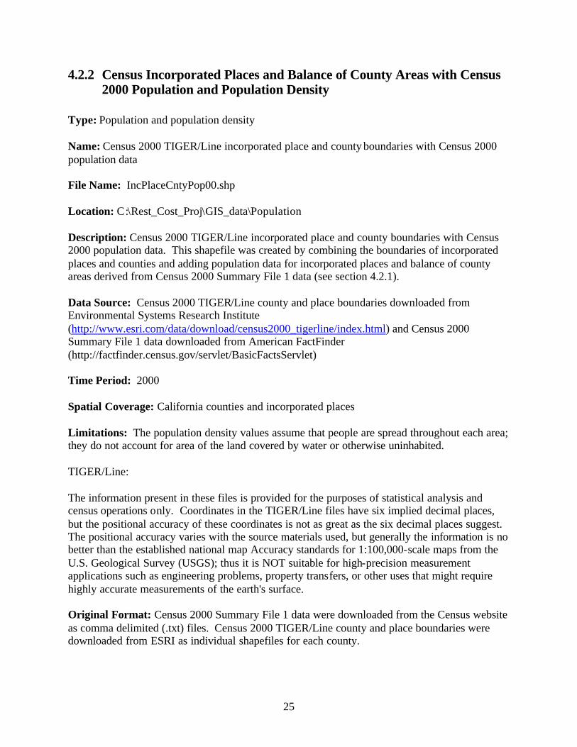
4.2.2 Census Incorporated Places and Balance of County Areas with Census 2000 Population and Population Density
Type: Population and population density Name: Census 2000 TIGER/Line incorporated place and county boundaries with Census 2000 population data File Name: IncPlaceCntyPop00.shp Location: C:\Rest_Cost_Proj\GIS_data\Population Description: Census 2000 TIGER/Line incorporated place and county boundaries with Census 2000 population data. This shapefile was created by combining the boundaries of incorporated places and counties and adding population data for incorporated places and balance of county areas derived from Census 2000 Summary File 1 data (see section 4.2.1). Data Source: Census 2000 TIGER/Line county and place boundaries downloaded from Environmental Systems Research Institute (http://www.esri.com/data/download/census2000_tigerline/index.html) and Census 2000 Summary File 1 data downloaded from American FactFinder (http://factfinder.census.gov/servlet/BasicFactsServlet) Time Period: 2000 Spatial Coverage: California counties and incorporated places Limitations: The population density values assume that people are spread throughout each area; they do not account for area of the land covered by water or otherwise uninhabited. TIGER/Line: The information present in these files is provided for the purposes of statistical analysis and census operations only. Coordinates in the TIGER/Line files have six implied decimal places, but the positional accuracy of these coordinates is not as great as the six decimal places suggest. The positional accuracy varies with the source materials used, but generally the information is no better than the established national map Accuracy standards for 1:100,000-scale maps from the U.S. Geological Survey (USGS); thus it is NOT suitable for high-precision measurement applications such as engineering problems, property transfers, or other uses that might require highly accurate measurements of the earth's surface. Original Format: Census 2000 Summary File 1 data were downloaded from the Census website as comma delimited (.txt) files. Census 2000 TIGER/Line county and place boundaries were downloaded from ESRI as individual shapefiles for each county.

26
Processing Steps: Incorporated Place Boundaries: The Census 2000 TIGER/Line Designated Places were downloaded from the ESRI data website by county. The individual county files were merged together in ArcMap. Data were reprojected to NAD27 UTM Zone 10. The shapefile was then clipped to the boundary of California using the 2000 Census cartographic boundary file for the state (state_ca00_cbf). A field was created (CntyPlcNam, String, 50) and calculated to contain the concatenated county code (COUNTY), place code (PLACE), and name (NAME). The resulting shapefile was then dissolved (ArcMap 8.2 Geoprocessing Wizard) on CntyPlcNam to create a new shapefile (place_ca00_tgr2.shp). Place Class Codes were downloaded from American Factfinder with Place FIPS codes and place names and imported into Access. This table was joined with the attribute table of place_ca00_tgr2.shp. ‘Select by Attributes’ was used to select only the polygons with a class code of 'C1' (Incorporated places), and these selected polygons were exported to a new shapefile. County Boundaries: The 2000 census County TIGER/Line data for all counties in California were downloaded as shapefiles from the ESRI data website: http://www.esri.com/data/download/census2000_tigerline/index.html. The individual county shapefiles were merged together in ArcMap 8.2. Data were reprojected to NAD27 UTM Zone 10. The shapefile was then clipped to the boundary of California (state_ca00_cbf) using the Geoprocessing Wizard in ArcMap 8.2. The clipped shapefile was then dissolved on County name using the Geoprocessing Wizard and new fields were created with the correct field names and definitions and the new fields were populated with the values from the old fields before those were deleted. Incorporated Places and Balance of County Areas: The Geoprocessing Wizard in ArcGIS 8.2 was used to create a Union of county boundaries (CNTY_CA00_tgr2.shp) and incorporated place boundaries (IncPlace_ca00_tgr.shp). The column NewID was added to the attribute table and calculated to equal the place FIPS codes for all of the places and to equal the county FIPS code plus the letter 'B' for the balance of county areas. Population data (IncPlaceCntyPop00 from the PopCensus2000 Access database) were joined to the attribute table of the incorporated places and balance of county areas shapefile (IncPlaceCnty_ca00_tgr.shp) based on NewID using the Join command in ArcMap 8.2. The attribute table was then dissolved on the name field from the joined table and NewID, County, Place, and the population field were included in the output.

27
The area of each place and balance of county area was computed in Acres and Hectares using the ‘Calculate Area, Perimeter, Length’ command in the XTools extension in ArcMap. New fields were added to the table to hold area in square kilometers (SqKm) and Density (DensSqKm) values. Both fields were defined as type Double. Area in square kilometers was calculated by dividing the Hectares field by 100, and density was calculated by dividing the population size by the area in square kilometers (using the field calculator). Data Format: shapefile Notes: This file was created for comparison with data from the Census Population Estimates Program, which produces estimates for incorporated places and balance of county areas. Population density was estimated by dividing the population size by the polygon area estimated using GIS. This estimate does not take into account water bodies, etc., so the population density is likely an underestimate. Note also that this is an estimate of the density for the polygon as a whole, but population density probably varies within each polygon. Attributes/Data Dictionary: Selected attributes: Field Description NAME Area name Min_County 5-digit FIPS county code Min_NewID Code for linking GIS and tabular data. Place FIPS codes for all places and county
FIPS code plus the letter 'B' for balance of county areas Min_Place FIPS place code DensSqKm Population density per square kilometer (assumes entire area is habitable – does
not account for water) Pop00 Census 2000 population

28
Population Density (#/Sq Km)
0 - 647
648 - 1,669
1,670 - 3,092
3,093 - 5,533
5,534 - 9,310
Figure 4.2.3a. 2000 Population DensityIncorporated and Designated Places
and Balance of County Areas
Created by Kelly Hildner, September 10, 2003 NOAA Fisheries, Santa Cruz, CA 95060
Data Source: US Census BureauProjection: NAD27 UTM Zone 10
0 50 10025Miles
0 50 100 150 20025Kilometers
±

29
4.2.3 Census Incorporated and Designated Places and Balance of County Areas with Census 2000 Population and Population Density
Type: Population and population density Name: Census 2000 TIGER/Line place and county boundaries with Census 2000 population data File Name: PlaceCntyPopEst00.shp Location: C:\Rest_Cost_Proj\GIS_data\Population Description: Census 2000 TIGER/Line place and county boundaries with Census 2000 population data. This shapefile was created by combining the boundaries of places and counties and adding population data for places and balance of county areas derived from Census 2000 Summary File 1 data (see section 4.2.1). Data Source: Census 2000 TIGER/Line county and place boundaries downloaded from Environmental Systems Research Institute (http://www.esri.com/data/download/census2000_tigerline/index.html) and Census 2000 Summary File 1 data downloaded from American FactFinder (http://factfinder.census.gov/servlet/BasicFactsServlet) Time Period: 2000 Spatial Coverage: California counties and places Limitations: The population density values assume that people are spread throughout each area; they do not account for area of the land covered by water or otherwise uninhabited. TIGER/Line: The information present in these files is provided for the purposes of statistical analysis and census operations only. Coordinates in the TIGER/Line files have six implied decimal places, but the positional accuracy of these coordinates is not as great as the six decimal places suggest. The positional accuracy varies with the source materials used, but generally the information is no better than the established national map Accuracy standards for 1:100,000-scale maps from the U.S. Geological Survey (USGS); thus it is NOT suitable for high-precision measurement applications such as engineering problems, property transfers, or other uses that might require highly accurate measurements of the earth's surface. Original Format: Census 2000 Summary File 1 data were downloaded from the Census website as comma delimited (.txt) files. Census 2000 TIGER/Line county and place boundaries were downloaded from ESRI as individual shapefiles for each county.

30
Processing Steps: Place Boundaries: The TIGER/Line 2000 Census Designated Places were downloaded from the ESRI data website by county. The individual county files were merged together in ArcMap. Data were reprojected to NAD27 UTM Zone 10. The shapefile was then clipped to the boundary of California using the 2000 Census cartographic boundary file for the state (state_ca00_cbf). The resulting shapefile was then dissolved (ArcMap 8.2 Geoprocessing Wizard) on Place. County Boundaries: The 2000 census County TIGER/Line data for all counties in California were downloaded as shapefiles from the ESRI data website http://www.esri.com/data/download/census2000_tigerline/index.html . The individual county shapefiles were merged together in ArcMap 8.2. Data were reprojected to NAD27 UTM Zone 10. The shapefile was then clipped to the boundary of California (state_ca00_cbf) using the Geoprocessing Wizard in ArcMap 8.2. The clipped shapefile was then dissolved on County name using the Geoprocessing Wizard and new fields were created with the correct field names and definitions and the new fields were populated with the values from the old fields before those were deleted. Places and Balance of County Areas. The Geoprocessing Wizard in ArcGIS 8.2 was used to create a Union of county boundaries (CNTY_CA00_tgr2.shp) and place boundaries (place_ca00_tgr2.shp). The column GeoID was added to the attribute table and calculated to equal the place FIPS codes for all of the places and to equal the county FIPS code plus the letter 'B' for the balance of county areas. Population data (PlaceCntyPop00 from the PopCensus2000 Access database) were joined to the attribute table of the places and balance of county areas shapefile (PlaceCnty00tgr.shp) based on NewID (GeoID) using the Join command in ArcMap 8.2. The attribute table was then dissolved on the name field from the joined table and NewID, County, Place, and the population field were included in the output. The area of each place and balance of county area was computed in Acres and Hectares using the ‘Calculate Area, Perimeter, Length’ command in the XTools extension in ArcMap. New fields were added to the table to hold area in square kilometers (SqKm) and Density (DensSqKm) values. Both fields were defined as type Double. Area in square kilometers was calculated by dividing the Hectares field by 100, and density was calculated by dividing the population size by the area in square kilometers (using the field calculator).

31
Data Format: shapefile Notes: This shapefile includes both incorporated and designated places. Balance of county areas are smaller, therefore, then those in IncPlaceCntyPop00.shp, and balance of county population sizes are concomitantly reduced. Population density was estimated by dividing the population size by the polygon area estimated using GIS. This estimate does not take into account water bodies, etc., so the population density is likely an underestimate. Note also that this is an estimate of the density for the polygon as a whole, but population density probably varies within each polygon. Attributes/Data Dictionary: Selected attributes: Field Description Name Area name County 5-digit FIPS county code NewID Code for linking GIS and tabular data. Place FIPS codes for all places and county
FIPS codes plus the letter 'B' for balance of county areas Place FIPS place code DensSqKm Population density per square kilometer (assumes entire area is habitable – does
not account for water) Pop00 Census 2000 population
32
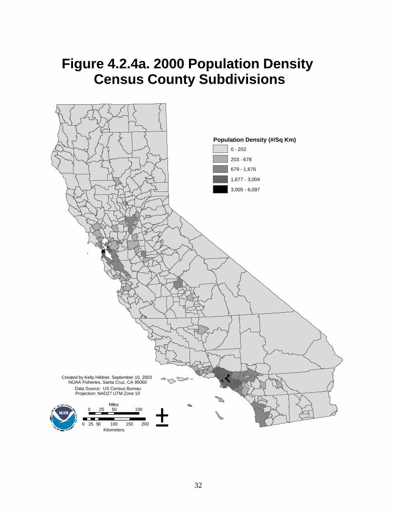
Population Density (#/Sq Km)
0 - 202
203 - 678
679 - 1,676
1,677 - 3,004
3,005 - 6,097
Figure 4.2.4a. 2000 Population Density Census County Subdivisions
Created by Kelly Hildner, September 10, 2003 NOAA Fisheries, Santa Cruz, CA 95060
Data Source: US Census BureauProjection: NAD27 UTM Zone 10
0 50 10025Miles
0 50 100 150 20025Kilometers
±

33
4.2.4 Census County Subdivisions with Census 2000 Population and Population Density
Type: Population and population density Name: Census 2000 TIGER/Line county subdivision boundaries with Census 2000 population data File Name: SubCntyPopEst00tgr.shp Location: C:\Rest_Cost_Proj\GIS_data\Population Description: Census 2000 TIGER/Line county subdivision boundaries with Census 2000 population data. This shapefile was created by adding population data for county subdivisions derived from Census 2000 Summary File 1 data to the Census TIGER/Line county subdivision polygon data. Data Source: Census 2000 TIGER/Line county subdivision boundaries downloaded from Environmental Systems Research Institute (http://www.esri.com/data/download/census2000_tigerline/index.html) and Census 2000 Summary File 1 data downloaded from American FactFinder (http://factfinder.census.gov/servlet/BasicFactsServlet) Time Period: 2000 Spatial Coverage: California county subdivisions Limitations: The population density values assume that people are spread throughout each area, they do not account for area of the land covered by water or otherwise uninhabited. TIGER/Line: The information present in these files is provided for the purposes of statistical analysis and census operations only. Coordinates in the TIGER/Line files have six implied decimal places, but the positional accuracy of these coordinates is not as great as the six decimal places suggest. The positional accuracy varies with the source materials used, but generally the information is no better than the established national map Accuracy standards for 1:100,000-scale maps from the U.S. Geological Survey (USGS); thus it is NOT suitable for high-precision measurement applications such as engineering problems, property transfers, or other uses that might require highly accurate measurements of the earth's surface. Original Format: Census 2000 Summary File 1 data were downloaded from the Census website as comma delimited (.txt) files. Census 2000 TIGER/Line county subdivision boundaries were downloaded from ESRI as individual shapefiles for each county.

34
Processing Steps: The 2000 County Census Divisions (County Subdivisions) TIGER/Line data for all counties in California were downloaded as shapefiles from the ESRI data website http://www.esri.com/data/download/census2000_tigerline/index.html. The individual county shapefiles were merged together in ArcMap 8.2. The merged file was then clipped to the 2000 cartographic boundary file California state boundary (state_ca00_cbf). The clipping process both clipped the shapefile and reprojected it to NAD27 UTM Zone 10 (the projection of the dataframe). The resulting file was dissolved based on the Subdivision FIPS code (MCD2000) and the original attributes were added back by joining the original merged shapefile to the dissolved shapefile based on MCD2000 and then exporting the data to a new shapefile SubCnty_ca00_tgr.shp. The XTools extension in ArcMap was used to calculate perimeter and area (acres and hectares). A column was added in ArcMap to contain the area in SqKm, and the field was populated by using ‘Calculate’ to divide area in Hectares by 100. The table was linked to the Census population data (PopCensus2000.mdb/SubCntyPop2000) based on the MCD2000_1 FIPS codes and a new field was created (DensSqKm00) to hold population density. This field was populated by dividing the Pop2000 field by the SqKm field. 2000 population (Pop2000) was also added to the attribute table. Data Format: shapefile Notes: Population density was estimated by dividing the population size by the polygon area estimated using GIS. This estimate does not take into account water bodies, etc., so the population density is likely an underestimate. Note also that this is an estimate of the density for the polygon as a whole, but population density probably varies within each polygon. Attributes/Data Dictionary: Selected attributes: Field Description NAME Area name COUNTY 5-digit FIPS county code MCD2000_1 FIPS code for county subdivisions DensSqKm00 Population density per square kilometer (assumes entire area is habitable – does
not account for water) Pop2000 Census 2000 population
5 CITIES / URBAN AREAS
5.1 OVERVIEW
Geographic data on cities and urban areas were acquired from Environmental Systems Research Institute (ESRI) and the US Census Bureau. Data from ESRI are the point locations of
35
cities in California with a population of 10,000 or greater. The points roughly correspond to the centroids of incorporated and designated places from the 2000 census.
Data from the US Census Bureau include 1) boundaries and population data for incorporated and designated places and counties (see section 4, Population and Population Density above) and 2) 2000 census urban areas, which consist of densely settled territory that contains 50,000 or more people (see http://www.census.gov/geo/www/cob/ua_metadata.html for more information).
5.2 MAPS AND METADATA

36
!(
!(
!(!(!(
!(
!(
!(
!(
!(
!(
!(
!(
!(
!(
!(
!(
!(
!(
!(
!(
!(
!(
!(
!(!(
!(
!(!(
!(
!(
!(
!(!(!(
!(
!(
!(
!(
!(
!(
!(
!(
!(!(
!(
!(
!(
!(
!(
!(
!(
!(
!(
!(
!(
!(
!(
!(
!(
!(
!(
!(
!(
!(
!(
!(
!(
!(!(
!(
!(
!(
!(
!(
!(
!(
!(
!(
!(
!(!(
!(
!(
!(
!(
!(
!( !(
!(
!(
!(!(
!(
!(
!(
!(
!(
!(
!(
!(!(
!(
!(
!(
!(
!(
!(
!(
!(
!(
!( !(
!(
!(
!(
!(
!(
!(
!(
!(!(
!(
!(
!(
!(
!(
!(
!(
!(
!(
!(
!(
!(
!(
!(
!(
!(
!(
!(
!(!(
!(
!(!( !(
!(
!(
!(
!(
!(
!(
!(
!(
!(
!(!(
!(
!(
!(
!(
!(
!(
!(
!(
!(
!(
!(
!(
!(!(
!(
!(
!(
!(!(
!(
!(
!( !(!(!(
!(
!(!(
!(
!(
!(
!(
!(
!(
!(
!(
!(
!(
!(
!(
!(!(
!(
!(
!(
!(
!(
!(
!(
!(
!(
!(
!(
!(
!(
!(
!(
!( !(
!(
!(
!(!(
!(
!(
!(
!(
!(!(
!(
!(
!(
!(
!(
!(!(
!(
!(
!(
!(
!(
!(
!( !(!(
!(
!(
!(
!(
!(
!(
!(
!(
!(
!(
!(
!(
!(
!(
!(
!(
!(
!(
!(
!(
!(
!(!(
!(
!(
!(
!(
!(
!(
!(
!(
!(
!(
!(
!(
!(
!(
!(!(
!(
!(
!(
!(
!(
!(
!(
!(
!(!(
!(
!(
!(!( !(
!(
!(
!(
!(
!(
!(
!(
!(
!(
!(
!(
!(!(
!(
!(
!(
!(
!(
!(
!(
!(
!(
!(
!(
!(
!( !(
!(
!(
!(
!(
!(
!(
!(
!(
!( !(
!(
!(
!(
!(
!(
!(
!(
!(
!(
!(
!(!(
!(
!(
!(
!(
!(
!(
!(!(
!(
!(
!(
!(
!(!(
!(
!(
!(
!(
!(
!(
!(
!(
!(
!(
!(
!(
!(
!(
!(
!( !(
!(
!(!(
!(
!(
!(!(
!(
!(
!(
!(!(
!(
!(
!(
!(
!(
!(
!(
!(
!(
!(
!(
!(
!(!(
!(
!(
!(
!(
!(
!(!(
!(
!(
!(
!(
!(
!(
!(
!(
!(
!(!(
!(
!(
!(
!(
!(
!(
!(
!(
!(
!(!(
!(
!(!(
!(
!(!(
!(
!(
!(
!(
!(
!(
!(
!(!(
Figure 5.2.1a. Cities in California (2000)with Population of at least 10,000
Created by Kelly Hildner, September 10, 2003 NOAA Fisheries, Santa Cruz, CA 95060Data Source: ESRI Data & Maps 2002
Projection: NAD27 UTM Zone 10
0 50 10025Miles
0 50 100 150 20025Kilometers
±

37
5.2.1 Point Locations of California Cities from Environmental Systems Research Institute
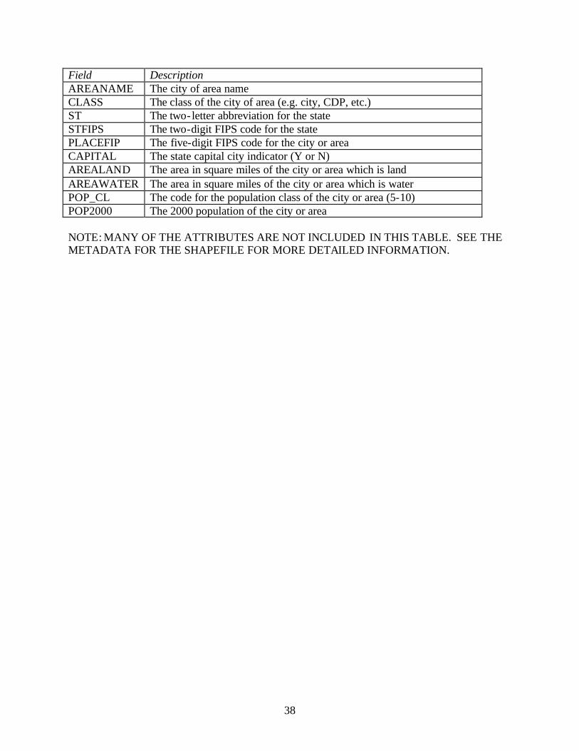
Type: Cities Name: California Cities - Environmental Systems Research Institute File Name: Cities_ca00_esri.shp Location: C:\Rest_Cost_Proj\GIS_data\Cities Description: Point locations of California cities with a population of 10,000 or greater. Data Source: Environment Systems Research Institute (ESRI). ESRI Data & Maps 2002 CD-ROM Set is available only as part of ESRI software. The data are provided by multiple, third party data vendors under license to ESRI. Original source for data: US Census Bureau, Census 2000 Time Period: April 2000 Spatial Coverage: California Limitations: Largest scale when displaying the data: 1:250,000. The redistribution rights for this data set: Public domain data from U.S. government is freely redistributable with proper metadata and source attribution. Original Format: Shapefile Processing Steps: Data were downloaded from the ESRI data CD and reprojected to NAD27 UTM Zone 10 using ArcToolbox 9.0 and the NAD_1927_ To_NAD_1983_NADCON datum conversion. The data were clipped to the boundary of CA (state_ca00_cbf.shp) using the Clip tool in ArcToolbox 9.0. Data Format: Shapefile Notes: NA Attributes/Data Dictionary: There are many demographic variables included in this dataset (e.g. number of people by race, sex, and age group). Detailed descriptions of the fields and domains are available in the metadata file for the shapefile. Some of the general attributes are:
38
Field Description AREANAME The city of area name CLASS The class of the city of area (e.g. city, CDP, etc.) ST The two-letter abbreviation for the state STFIPS The two-digit FIPS code for the state PLACEFIP The five-digit FIPS code for the city or area CAPITAL The state capital city indicator (Y or N) AREALAND The area in square miles of the city or area which is land AREAWATER The area in square miles of the city or area which is water POP_CL The code for the population class of the city or area (5-10) POP2000 The 2000 population of the city or area NOTE: MANY OF THE ATTRIBUTES ARE NOT INCLUDED IN THIS TABLE. SEE THE METADATA FOR THE SHAPEFILE FOR MORE DETAILED INFORMATION.

39
Urban Areas
Rural Areas
Figure 5.2.2a. Urban Areas2000 Census TIGER/Line Files
Created by Kelly Hildner, September 10, 2003 NOAA Fisheries, Santa Cruz, CA 95060
Data Source: US Census BureauProjection: NAD27 UTM Zone 10
0 50 10025Miles
0 50 100 150 20025Kilometers
±

40
5.2.2 Census 2000 TIGER/Line Urban Area Boundaries Type: Urban Areas Name: Census 2000 TIGER/Line Urban Areas File Name: urban_ca00_tgr.shp Location: C:\Rest_Cost_Proj\GIS_data\boundaries\Urban Description: Census 2000 TIGER/Line Urban Areas. http://www.census.gov/geo/www/ua/ua_2k.html Urban and Rural Classification For Census 2000, the Census Bureau classifies as "urban" all territory, population, and housing units located within an urbanized area (UA) or an urban cluster (UC). It delineates UA and UC boundaries to encompass densely settled territory, which consists of:
• core census block groups or blocks that have a population density of at least 1,000 people per square mile and
• surrounding census blocks that have an overall density of at least 500 people per square mile
In addition, under certain conditions, less densely settled territory may be part of each UA or UC.
The Census Bureau's classification of "rural" consists of all territory, population, and housing units located outside of UAs and UCs. The rural component contains both place and nonplace territory. Geographic entities, such as census tracts, counties, metropolitan areas, and the territory outside metropolitan areas, often are "split" between urban and rural territory, and the population and housing units they contain often are partly classified as urban and partly classified as rural. http://www.census.gov/geo/www/cob/ua_metadata.html “An urbanized area (UA) consists of densely settled territory that contains 50,000 or more people. A UA may contain both place and nonplace territory. The U.S. Census Bureau delineates UAs to provide a better separation of urban and rural territory, population, and housing in the vicinity of large places. At least 35,000 people in a UA must live in an area that is not part of a military reservation. For Census 2000, UA delineations constitute a "zero-based" approach that requires no "grandfathering" of UA boundaries from the 1990 census. Because of the more stringent density requirements (and the less restrictive extended place criteria), some territory that was classified

41
as urbanized for the 1990 census has been reclassified as rural. In addition, some areas that were identified as UAs for the 1990 census have been reclassified as urban clusters. The title of a UA may contain up to three incorporated place names, and will include the two-letter U.S. Postal Service abbreviation for each state into which the UA extends. However, if the UA does not contain an incorporated place, the UA title will include the single name of the geographic entity that occurs first from the following list: census designated place, minor civil division, or populated place recognized by the U.S. Geological Survey. Each UA is assigned a five-digit census code in alphabetical sequence on a nationwide basis, interspersed with the codes for urban clusters (UCs), also in alphabetical sequence. For the 1990 census, the U.S. Census Bureau assigned a four-digit UA code based on the MA codes. For Census 2000, a separate flag is included in data tabulation files to differentiate between UAs and UCs. In printed reports, this differentiation is included in the name.” Data Source: downloaded from the ESRI website: http://www.esri.com/data/download/census2000_tigerline/index.html. Original data source: US Census Bureau, Census 2000 TIGER/Line. Time Period: 2000 Spatial Coverage: California Limitations: The information present in these files is provided for the purposes of statistical analysis and census operations only. Coordinates in the TIGER/Line files have six implied decimal places, but the positional accuracy of these coordinates is not as great as the six decimal places suggest. The positional accuracy varies with the source materials used, but generally the information is no better than the established national map Accuracy standards for 1:100,000-scale maps from the U.S. Geological Survey (USGS); thus it is NOT suitable for high-precision measurement applications such as engineering problems, property transfers, or other uses that might require highly accurate measurements of the earth's surface. ‘The Census Bureau identifies and tabulates data for the urban and rural populations and their associated areas solely for the presentation and comparison of census statistical data. If a federal, state, local, or tribal agency uses these urban and rural criteria in a nonstatistical program, it is that agency's responsibility to ensure that the results are appropriate for such use. It also is that agency's responsibility to ensure that it has provided the necessary tools for use in that agency's programs.’ - http://www.census.gov/geo/www/ua/ua_2k.html Original Format: Downloaded as shapefiles from ESRI. Original data format: TIGER/Line. Processing Steps: The data were downloaded as separate shapefiles for each county and then merged using the geoprocessing wizard in ArcMap. Data were reprojected to UTM NAD27 Zone 10 using ArcToolbox and the NAD_1927_ To_NAD_1983_NADCON datum conversion.

42
Data Format: Shapefile Notes: NA Attributes/Data Dictionary: Selected attributes: Field Description ID Urban area ID code NAME Name of Geographic Area LSADC Legal/Statistical Area Description Code LSADC_DESC Legal/Statistical Area Description COUNTY County name FIPSSTCO Five-digit state county FIPS code AREA_MI Area in square miles
6 LAND USE AND LAND COVER DATA
6.1 OVERVIEW
Land use data in GIS form are difficult to find. Most datasets combine land use information with land cover information. Our primary need for land use data is to distinguish urban areas from rural areas. We are currently planning to use the Census 2000 TIGER/Line Urban Areas data rather than land use data for this purpose. Nonetheless, we outline several sources of land use and/or land cover data for California briefly below, as a need for more detailed land use data may arise in the future.
CALIFORNIA DEPARTMENT OF WATER RESOURCES: The California Department of Water Resources has a land use program that has conducted over 250 land use surveys of all or parts of California’s 58 counties since 1950 (see http://www.waterplan.water.ca.gov/landwateruse/landuse/luindex.htm) with the primary purpose of monitoring water use. Land use data are available as shapefiles on the DWR website for certain counties in certain years. Complete coverage of the state is not available. Land use polygons contain detailed agricultural land uses and less detailed urban and native vegetation land uses. CALIFORNIA GAP ANALYSIS LAND-COVER/LAND USE DATA: Gap analysis Land Cover data consists of land cover polygons divided into 62 Wildlife Habitat Relationships (WHR) habitat types, 222 California Natural Diversity Database (CNDDB) types, and 431 species types. The land cover types mainly describe vegetation types but also include some agricultural and urban types. Source data are from approximately 1980-1995. Minimum mapping unit is 40-100 ha. File Name: lulc_CA.mdb, lulc_ca_gap; File Type: Geodatabase

43
TEALE GIS SOLUTIONS GROUP VEGETATION DATA – USFS: This vegetation layer is a polygon layer containing 41 WHR types and 72 dominant vegetation types for California. All types are vegetation types except one category for Urban-Agriculture and one for Water. The source data are from 1979-1981. Minimum mapping unit is 400 acres (162 ha). File Name: lulc_CA.mdb - veg_ca_usfs; File Type: Geodatabase CALIFORNIA DEPARTMENT OF FORESTRY (CDF) LAND COVER MAPPING AND MONITORING PROGRAM (LCMMP) VEGETATION MAP: Data consist of vegetation polygons derived from LANDSAT TM imagery from 1991 - 2001. The dataset contains 65 WHR types, 12 cover types, and 191 vegetation types. The minimum mapping unit is 2.5 acres. Complete coverage of the state is not available. CALIFORNIA DEPARTMENT OF FORESTRY (CDF) MULTI-SOURCE LAND COVER DATA (2002 V2): This is a raster compilation of “best available” data from multiple sources. The dataset contains 59 WHR types, 10 WHR “Major Land cover” classes, 13 WHR “Land cover Subclasses”, and 8 WHR “Life Form Classes”. Size and density classes are also available. Non-vegetation classes available are Barren/Other, Urban, and Water. Source data dates vary but are mostly from the 1990s. Grid size is 100 meters. File Name: lc_ca_cdf; File Type: Raster USGS NATIONAL LAND COVER DATA (NLCD) 1992: This raster land cover dataset contains 21 land cover classifications using a modified Anderson land-use and land-cover classification system. This dataset includes three levels of development intensity for developed areas (Low Intensity Residential, High Intensity Residential, and Commercial/Industrial/Transportation). The source data are from 1987-1993. Grid size is 30 meters. File Name: lc_nca_usgs and lc_sca_usgs; File Type: Raster
Should we decide to use land use/land cover data in the future, we will most likely choose the NLCD dataset because it contains multiple categories for developed areas. The CDF Multi-source land cover data might also prove useful because it is at a coarser resolution that may be easier to work with, and it has fields with varying levels of category detail.
7 SOILS
7.1 OVERVIEW The Natural Resources Conservation Service (NRCS) has created a State Soil Geographic (STATSGO) Database that contains general soil map unit data compiled and digitized from 1:250,000-scale maps. Each map unit consists of up to 21 soil components that are used to apportion different characteristics of a map unit but are not represented spatially. Each soil component is further apportioned into a maximum of 6 layers corresponding to distinct soil layers (Figure 7.1a). Soil characteristics recorded for a particular layer usually include a high and low value describing the range for that characteristic within that layer. The data were designed primarily for small-scale (regional, multi-county, multi-state, etc.) planning.

44
More detailed soils digital data are available for portions of California through the Soil Survey Geographic (SSURGO) Database also created by NRCS; mapping scales for SSURGO generally range from 1:12,000 to 1:63,360. For the status of available digitized maps through this program, see http://www.ncgc.nrcs.usda.gov/products/datasets/ssurgo/. Complete SSURGO coverage of California is not available. For our analyses, we are interested in the erodibility of the soil, as this may affect the cost of restoration projects. Attributes in the STATSGO soils data that indicate soil erodibility include kffact and kfact. According to the STATSGO documentation1, kffact is “An erodibility factor which quantifies the susceptibility of soil particles to detachment and movement by water. This factor is used in the Universal Soil Loss Equation to calculate soil loss by water”, and kfact is “An erodibility factor which is adjusted for the effect of rock fragments.” These attributes are associated with soil layers (not map units) in the STATSGO database. Two sources were found that have processed the STATSGO attribute data into more useable forms – the United States Geological Survey (USGS) Water Resources Section and the Pennsylvannia State Earth System Science Center (ESSC). These sources each used a different approach for creating map unit level soil attributes. Attributes in the USGS soil data were created by first creating a simple average of the high and low values of the attribute for each soil layer, then creating, for each component, a weighted average across all layers using the relative layer thickness as the weight, and finally, to obtain map unit level information, creating a weighted average across all components using the component percentages as weights. The USGS soils data include kffact but not kfact. ESSC soils data (http://www.essc.psu.edu/soil_info/index.cgi?index.html), on the other hand contain both kffact and kfact, but these attributes are created by taking a weighted average across all components of attribute values from the surface layer only. We predict that there will be many situations (e.g. road cuts and stream banks) where more than just the surface layer will be susceptible to erosion, so we decided to use the USGS attribute data for our analyses.
1 State Soil Geographic (STATSGO) Data Base: Data use information. July 1994. United Sates Department of Agriculture.
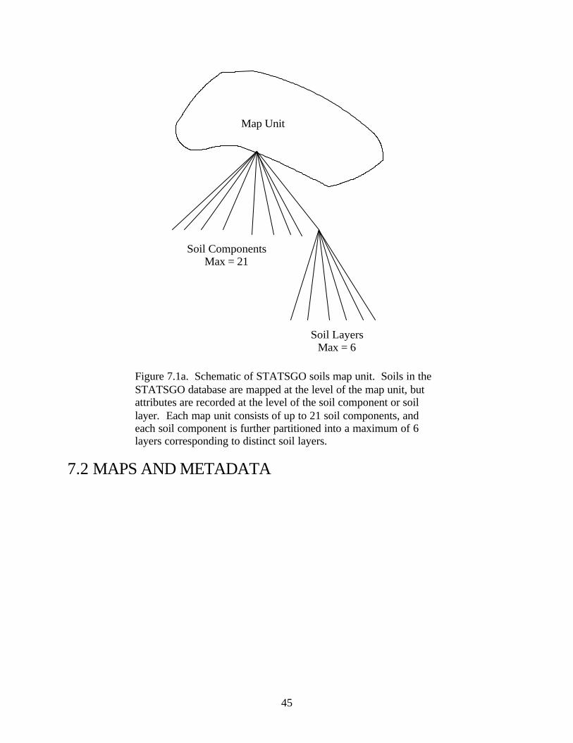
45
Map Unit
Soil ComponentsMax = 21
Soil LayersMax = 6
Figure 7.1a. Schematic of STATSGO soils map unit. Soils in the STATSGO database are mapped at the level of the map unit, but attributes are recorded at the level of the soil component or soil layer. Each map unit consists of up to 21 soil components, and each soil component is further partitioned into a maximum of 6 layers corresponding to distinct soil layers.
7.2 MAPS AND METADATA
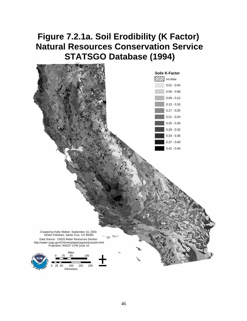
46
Soils K-Factor
no data
0.01 - 0.04
0.05 - 0.08
0.09 - 0.12
0.13 - 0.16
0.17 - 0.20
0.21 - 0.24
0.25 - 0.28
0.29 - 0.32
0.33 - 0.36
0.37 - 0.40
0.41 - 0.44
Figure 7.2.1a. Soil Erodibility (K Factor) Natural Resources Conservation Service
STATSGO Database (1994)
Created by Kelly Hildner, September 10, 2003 NOAA Fisheries, Santa Cruz, CA 95060
Data Source: USGS Water Resources Section http://water.usgs.gov/GIS/metadata/usgswrd/ussoils.html
Projection: NAD27 UTM Zone 10
0 50 10025Miles
0 50 100 150 20025Kilometers
±

47
7.2.1 STATSGO Soils Data Base Containing Hydrology-Relevant Information for California
Type: Soils Name: State Soil Geographic (STATSGO) Data Base Containing Hydrology-Relevant Information for California File Name: soils_ca_usgs2.shp Location: C:\Rest_Cost_Proj\GIS_data\soils Description: Soils shapefile containing hydrology-relevant information for California. The data for California were extracted from the National database created by USGS from individual State coverages contained in the October 1994 State Soil Geographic (STATSGO) Data Base produced on CD-ROM. Original USGS Abstract: “USSOILS is an Arc 7.0 coverage containing hydrology-relevant information for 10,498 map units covering the entire conterminous United States. The coverage was compiled from individual State coverages contained in the October 1994 State Soil Geographic (STATSGO) Data Base produced on CD-ROM. The geo-dataset USSOILS.PAT relates (on the basis of a map unit identifier) the 10,498 map units to 78,518 polygons. The scale of the geo-dataset is 1:250,000. The INFO attribute table USSOILS.MUID_ATTS contains selected variables from the STATSGO data set for 10,501 map units (an extra 3 map units are contained in the attribute table that are not in the geo-dataset - see the 'Procedures' section below), including: the map unit identifier, a 2-character state abbreviation, available water capacity of the soil, percent clay in the soil, the actual k-factor used in the water erosion component of the universal soil loss equation, the organic material in soil, soil permeability, cumulative thickness of all soil layers, hydrologic characteristics of the soil, quality of drainage, surface slope, liquid limit of the soil, share of a map unit having hydric soils, and the annual frequency of flooding. To facilitate mapping the attribute data, the narrative section below contains instructions for transferring the information contained in the attribute table USSOILS.MUID_ATTS to the polygon attribute table USSOILS.PAT. Excerpt from original USGS metadata, Supplemental_Information: “Procedures_Used: The individual State coverages are from the State Soil Geographic (STATSGO) CD-ROM data base, issued by U.S. Department of Agriculture, NRCS National Cartography and GIS Center, P.O. Box 6567, Fort Worth, Texas 76115-0567, 1-800-672-5559 (U.S. Department of Agriculture, 1991). The CD-ROM coverage for New Mexico was defective and was not used. A corrected copy of the New Mexico coverage was obtained from Norman Bliss of the EROS Data Center ((605) 594-6034). The STATSGO State-based coverages were merged together into a national coverage using the Arc MAPJOIN command. All nodes along merged boundaries were checked and edited to remove any superfluous nodes created during the
48
mapjoin process, and to ensure arcs properly merged along and across State boundaries. The joining process preserved all State boundaries. To understand the procedures used to create the attribute table USSOILS.MUID_ATTS, it helps to have an understanding of the STATSGO data structure. The smallest spatial entity mapped within the STATSGO dataset is called a map unit, of which there are 10,498 broken out into 78,518 polygons within the conterminous United States. Each map unit consists of up to 21 components. Components are used to apportion different characteristics of a map unit and do not represent a separate spatial entity. To help understand this, consider a map unit that has only two components. Suppose 30 percent of this map unit contains soil of type A and the remaining 70 percent contains soil of type B. Thus, component 1 of the map unit would have soil type A and component 2 would have soil type B. The data base would record the soil type for each component, along with the percentage of the map unit represented by each component (in this example, 30 percent for component 1 and 70 percent for component 2). The specific locations of soil types A and B are not spatially defined in the data base. Each component is further delineated into a maximum of 6 layers, corresponding to distinct soil layers. Soil characteristics recorded for a layer typically consist of a high and low value, which describes a range for that characteristic within that layer. Included among the characteristics of the soil layer is the thickness of the layer. In developing the USSOILS.MUID_ATTS table, it is necessary to aggregate the layer and component information up to the level of a map unit. To aggregate layer information to the component level, we first construct a simple average of the high and low values of a characteristic for each layer. We then construct a weighted average across all layers of the layer-specific characteristic averages, the weights being the thickness of the layer relative to the total thickness of all layers. For component-level information that is expressed as a range, we construct a simple average of the high and low values defining the range. These steps reduce layer-specific information and ranges of component-specific information into a single datum of component-specific information for each characteristic in the data base. Finally, to obtain map unit information, we construct a weighted average across all components of the component-specific information, the weights being the component percentages given for the map unit.” Data Source: United States Geological Survey (USGS) Water Resources Section (http://water.usgs.gov/GIS/metadata/usgswrd/XML/ussoils.xml), based on State coverages from the October 1994 State Soil Geographic (STATSGO) CD-ROM data base, issued by U.S. Department of Agriculture, NRCS National Cartography and GIS Center, P.O. Box 6567, Fort Worth, Texas 76115-0567, 1-800-672-5559 Time Period: Original data published 1994 Spatial Coverage: California Limitations: (Source: Original STATSGO metadata)
“The U.S. Department of Agriculture, Soil Conservation Service should be acknowledged as the data source in products derived from these data. STATSGO was designed
49
primarily for regional, multicounty, river basin, State, and multistate resource planning, management, and monitoring. STATSGO data are not detailed enough to make interpretations at a county level. This soil survey product is not designed for use as a primary regulatory tool in permitting or citing decisions, but may be used as a reference source. When STATSGO data are overlayed with other data layers, such as land use data, caution must be used in generating statistics on the co-occurence of the land use data with the soil data. The composition of the STATSGO map unit can be characterized independently for the land use and for the soil component, but there are no data on their joint occurrence at a more detailed level. Analysis of the overlayed data should be on a map polygon basis. Additional political, watershed, or other boundaries may be intersected with the soil data. Although the composition of each political and watershed unit may be described in terms of the STATSGO map units, information is not available to assign the components to the boundary units with full accuracy. As with the land use categories, the analysis should be restricted to the classified components. The approximate minimum area delineated is 625 hectares (1,544 acres), which is represented on a 1:250,000-scale map by an area approximately 1 cm by 1 cm (0.4 inch by 0.4 inch). Linear delineations are not less than 0.5 cm (0.2 inch) in width. The number of delineations per 1:250,000 quadrangle typically is 100 to 200, but may range up to 400. Delineations depict the dominant soils making up the landscape. Other dissimilar soils, too small to be delineated, are present within a delineation. Digital enlargements of these maps to scales greater than that at which they were originally mapped can cause misinterpretation of the data. If enlarged, maps do not show the small areas of contrasting soils that could have been shown at a larger scale. The depicted soil boundaries, interpretations, and analysis derived from them do not eliminate the need for onsite sampling, testing, and detailed study of specific sites for intensive uses. Thus, these data and their interpretations are intended for planning purposes only. Some attribute data for some data elements may be incomplete or missing. Where data are unavailable, a mask should be used to exclude the area from analysis. Digital data files are periodically updated. Files are dated, and users are responsible for obtaining the latest version of the data.”
Original Format: ArcInfo Coverage Processing Steps: The data were downloaded from http://water.usgs.gov/GIS/metadata/usgswrd/ussoils.html as multiple coverages. The coverages were merged together (mapjoin), the boundaries were dissolved (dissolve), the resulting coverage was reprojected (project), and polygon topology was rebuilt (build). The related table ussoils.muid_atts was joined to the attribute table of the coverage, and the polygons for California were selected using the query: "MUID" LIKE 'CA___' OR "MUID" LIKE 'CA_', and the selected polygons were exported to a shapefile in ArcMap 8.2. Data Format: Shapefile Notes: NA Attributes/Data Dictionary: Selected attributes. See the metadata associated with the shapefile for additional and more detailed attribute information. Field Description
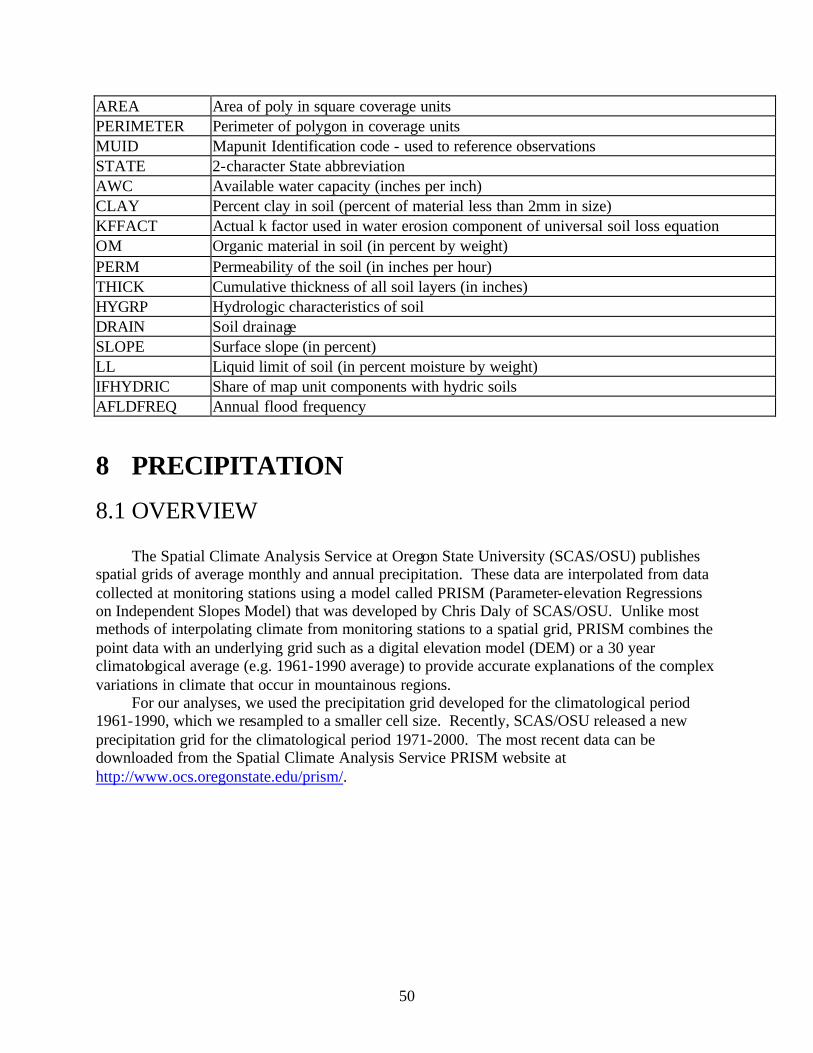
50
AREA Area of poly in square coverage units PERIMETER Perimeter of polygon in coverage units MUID Mapunit Identification code - used to reference observations STATE 2-character State abbreviation AWC Available water capacity (inches per inch) CLAY Percent clay in soil (percent of material less than 2mm in size) KFFACT Actual k factor used in water erosion component of universal soil loss equation OM Organic material in soil (in percent by weight) PERM Permeability of the soil (in inches per hour) THICK Cumulative thickness of all soil layers (in inches) HYGRP Hydrologic characteristics of soil DRAIN Soil drainage SLOPE Surface slope (in percent) LL Liquid limit of soil (in percent moisture by weight) IFHYDRIC Share of map unit components with hydric soils AFLDFREQ Annual flood frequency
8 PRECIPITATION
8.1 OVERVIEW
The Spatial Climate Analysis Service at Oregon State University (SCAS/OSU) publishes spatial grids of average monthly and annual precipitation. These data are interpolated from data collected at monitoring stations using a model called PRISM (Parameter-elevation Regressions on Independent Slopes Model) that was developed by Chris Daly of SCAS/OSU. Unlike most methods of interpolating climate from monitoring stations to a spatial grid, PRISM combines the point data with an underlying grid such as a digital elevation model (DEM) or a 30 year climatological average (e.g. 1961-1990 average) to provide accurate explanations of the complex variations in climate that occur in mountainous regions.
For our analyses, we used the precipitation grid developed for the climatological period 1961-1990, which we resampled to a smaller cell size. Recently, SCAS/OSU released a new precipitation grid for the climatological period 1971-2000. The most recent data can be downloaded from the Spatial Climate Analysis Service PRISM website at http://www.ocs.oregonstate.edu/prism/.

51
8.2 MAPS AND METADATA
Figure 8.2.1a. Average Annual Precipitation 1961-1990 Spatial Climate Analysis Service,
Oregon State University
Created by Kelly Hildner, February 23, 2006 NOAA Fisheries, Santa Cruz, CA 95060
Data Source: Spatial Climate Analysis Service, Oregon State University,
http://www.ocs.oregonstate.edu/prism/Projection: NAD27 UTM Zone 10
0 50 10025Miles
0 50 100 150 20025Kilometers
±
Average Annual Precipitationmillimeters
High : 6778
Low : 48
52
8.2.1 Average Annual Precipitation 1961-1990 - Spatial Climate Analysis Service, Oregon State University
Type: Precipitation Name: Average Annual Precipitation 1961-1990 File Name: wc_precip13rs Location: C:\Rest_Cost_Proj\GIS_data\precip \wc_precip13rs Description: This data set contains spatially gridded precipitation of average annual precipitation for the climatological period 1961-90. Distribution of the point measurements to a spatial grid was accomplished using the PRISM model, developed by Chris Daly of SCAS/OSU. Units are in millimeters (mm). These data have been resampled to a grid cell size of 30.579902 meters. There are many methods of interpolating climate from monitoring stations to grid points. Some provide estimates of acceptable accuracy in flat terrain, but few have been able to adequately explain the extreme, complex variations in climate that occur in mountainous regions. Significant progress in this area has been achieved through the development of PRISM (Parameter-elevation Regressions on Independent Slopes Model). PRISM is an analytical model that uses point data and a digital elevation model (DEM) to generate gridded estimates of monthly and annual maximum temperature (as well as other climatic parameters). PRISM is well suited to regions with mountainous terrain, because it incorporates a conceptual framework that addresses the spatial scale and pattern of orographic processes. A Gaussian filter was applied to increase the resolution of the grids from the base resolution 2.5 arc-minutes (~4 km) to 1.25 arc-minutes (~2 km). This filter is a modification of the Barnes filter (Barnes, 1964), originally adapted by Dr. Stephen Esbensen of Oregon State University, and later modified for use here by Wayne P. Gibson, also of Oregon State University. Data Source: Spatial Climate Analysis Service, Oregon State University, http://www.ocs.oregonstate.edu/prism/ Time Period: 1961-1990 Spatial Coverage: Washington, Oregon, and California Limitations: The precipitation data was prepared by the Spatial Climate Analysis Service (SCAS). “Neither the SCAS nor any agency thereof, nor any of their employees, make any warranty, expressed or implied, or assumes any legal liability or responsibility for the accuracy, completeness, or misuse of the data, or for damage, transmission of viruses or computer contamination through the distribution of these data sets or for the usefulness of any information, apparatus, product, or process disclosed in this report, or represents that its use would not infringe privately owned rights. Reference therein to any specific commercial product, process, or service by trade name, trademark, manufacturer, or otherwise does not necessarily constitute

53
or imply its endorsement, recommendation, or favoring by the SCAS or any agency thereof. Any views and opinions of authors expressed herein do not necessarily state or reflect those of the SCAS or any agency thereof.” – from original metadata. Accuracy of this data set is based on the original specification of the Defense Mapping Agency (DMA) 1 degree digital elevation models (DEM). The stated accuracy of the original DEMs are 130 m circular error with 90% probability. Original Format: Raster Dataset Processing Steps: The raster data file was originally acquired as a national grid by the Salmon Population Analysis Team at NOAA Fisheries in Santa Cruz. Data for the west coast were extracted by buffering a west coast layer by one grid cell width and then using the buffered west coast layer to clip the precipitation grid. This clipped grid was copied from J:\GIS_DATA_READ\X_BOUNDARY\precip \buffered\us_precip13uc and renamed wc_precip13uc. The grid was resampled to a cell size of 30.579902 using Spatial Analyst 8.3 and the nearest neighbor algorithm.
Options: Analysis extent - same as wc_precip13uc Snap grid - wc_precip13uc Cell size - same as wc_precip13uc Raster Calculator: wc_precip13rs = resample(C:\Rest_Cost_Proj\GIS_data\precip\wc_precip13uc, 30.5799020263, nearest)
Data Format: Raster Dataset Notes: An updated version of the PRISM precipitation data for 1971-2000 is available for download from the PRISM website http://www.ocs.oregonstate.edu/prism/. Attributes/Data Dictionary: Raster cell values are average annual precipitation in millimeters.
9 ELEVATION / SLOPE
9.1 OVERVIEW
The US Geological Survey (USGS) National Elevation Dataset (NED) is a 1 arc-second (approximately 30-meter) resolution elevation dataset for the conterminous United States. According to the metadata provided by the USGS EROS Data Center, the NED is a seamless mosaic of best-available elevation data. The 7.5-minute elevation data for the conterminous

54
United States are the primary initial source data. USGS developed efficient processing methods to filter production artifacts in the existing data, convert to the NAD83 datum, edge-match, and fill slivers of missing data at quadrangle seams. One of the effects of the NED processing steps is a much-improved base of elevation data for calculating slope and hydrologic derivatives.
Data were acquired on CD by NOAA Fisheries Technical Recovery Team staff for the
areas of California that are included in salmonid study areas. The original data files for the study areas are in 17 pieces. The data were reprojected to UTM coordinates, converted to a cell size of 30 meters, and small imperfections were removed using the Fill command (with the Sink option) in the Grid module of ArcInfo. The DEMs were then converted to integer grids by rounding the elevation values, and the Mosaic command in Grid was used to combine the separate DEMs into a single grid. The resulting mosaic was used as our elevation dataset.
Slope data (measured in degrees) were created from the elevation data (based on the
individual floating point elevation grids) using the Slope command in the Grid module of ArcInfo. The slope command identifies the rate of maximum change in elevation value from each cell. The slope grids were converted to integer grids by rounding the slope values and were combined into a single grid using the Mosaic command in ArcInfo Grid.
9.2 MAPS AND METADATA

55
56
9.2.1 30 Meter Resolution Elevation Data Created from USGS National Elevation Dataset (NED) Data
Type: Elevation Name: USGS National Elevation Dataset (NED) File Name: sa_mos_dem, dem_ca_i Location: C:\Rest_Cost_Proj\GIS_data\DEM Description: 30 meter resolution integer elevation data for salmonid study areas in California and Southern Oregon created from USGS NED data. Abstract from NED metadata:
The U.S. Geological Survey has developed a National Elevation Dataset (NED). The NED is a seamless mosaic of best-available elevation data. The 7.5-minute elevation data for the conterminous United States are the primary initial source data. In addition to the availability of complete 7.5-minute data, efficient processing methods were developed to filter production artifacts in the existing data, convert to the NAD83 datum, edge-match, and fill slivers of missing data at quadrangle seams. One of the effects of the NED processing steps is a much- improved base of elevation data for calculating slope and hydrologic derivatives.
Data Source: USGS National Elevation Dataset (http://gisdata.usgs.net/ned/default.asp) Time Period: Published 1999; time period of data is unknown Spatial Coverage: Most of California and parts of Southern Oregon (areas covered by salmonid study areas) Limitations: The source data quality and resolution vary, and artifacts exist in some areas. Original Format: Grid Processing Steps: Original NED data were reprojected to NAD27 UTM Zone 10, converted to a cell size of 30 meters, and small imperfections were removed using the Fill command (with the Sink option) in the Grid module of ArcInfo. The digital elevation models (DEMs) were then converted to integer grids by rounding the elevation values, and the Mosaic command in the Grid module of ArcInfo was used to combine the separate DEMs into a single grid. Data Format: Grid Notes: For analysis, use sa_mos_dem. For display, dem_ca_i was created by clipping sa_mos_dem to the boundary of California using a grid based on the 2000 Census cartographic boundary file for California as a mask grid.
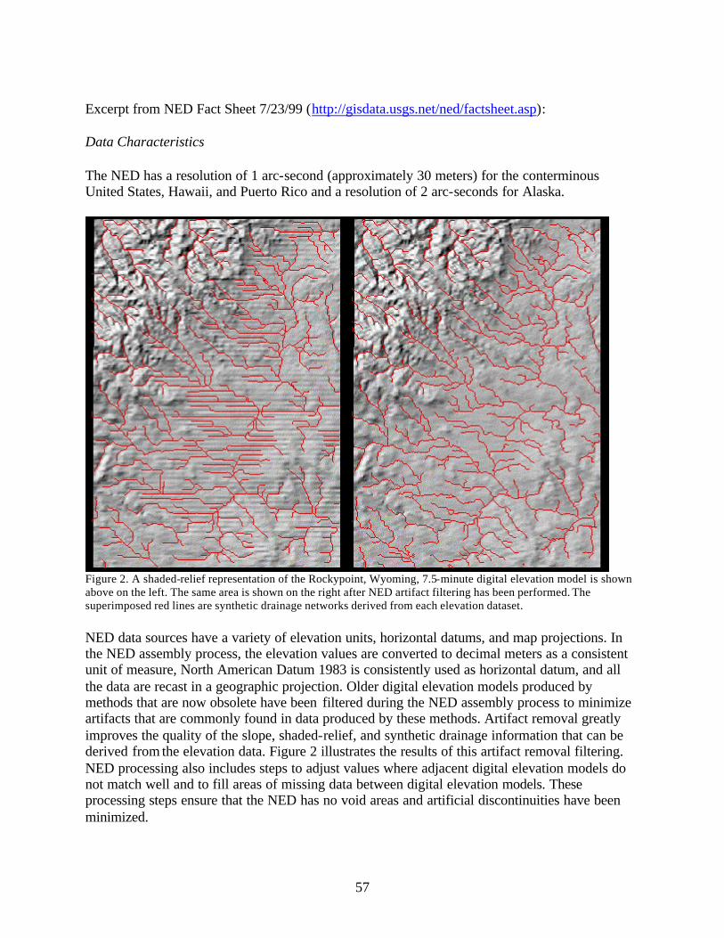
57
Excerpt from NED Fact Sheet 7/23/99 (http://gisdata.usgs.net/ned/factsheet.asp): Data Characteristics
The NED has a resolution of 1 arc-second (approximately 30 meters) for the conterminous United States, Hawaii, and Puerto Rico and a resolution of 2 arc-seconds for Alaska.
Figure 2. A shaded-relief representation of the Rockypoint, Wyoming, 7.5-minute digital elevation model is shown above on the left. The same area is shown on the right after NED artifact filtering has been performed. The superimposed red lines are synthetic drainage networks derived from each elevation dataset.
NED data sources have a variety of elevation units, horizontal datums, and map projections. In the NED assembly process, the elevation values are converted to decimal meters as a consistent unit of measure, North American Datum 1983 is consistently used as horizontal datum, and all the data are recast in a geographic projection. Older digital elevation models produced by methods that are now obsolete have been filtered during the NED assembly process to minimize artifacts that are commonly found in data produced by these methods. Artifact removal greatly improves the quality of the slope, shaded-relief, and synthetic drainage information that can be derived from the elevation data. Figure 2 illustrates the results of this artifact removal filtering. NED processing also includes steps to adjust values where adjacent digital elevation models do not match well and to fill areas of missing data between digital elevation models. These processing steps ensure that the NED has no void areas and artificial discontinuities have been minimized.
58
As higher resolution or higher quality data become available, the NED is updated to incorporate the best available coverage. As the USGS’s 7.5-minute and 15-minute digital elevation products near completion for the conterminous United States and Alaska respectively, NED data will soon incorporate these sources. For the small areas that are not yet covered, the lower resolution 30-minute and 1-degree USGS digital elevation model products were interpolated to obtain values used in NED. These original elevation files are currently available at http://edcwww.cr.usgs.gov/doc/edchome/ndcdb/ndcdb.html. In cases where 7.5-minute digital elevation models have 10-meter resolution, the original source data will be at a higher resolution than the NED. As more data become available at a finer resolution than that of the NED, the feasibility of developing a finer resolution NED will be investigated.
Attributes/Data Dictionary: Cell values are elevation in meters rounded to the nearest whole number.
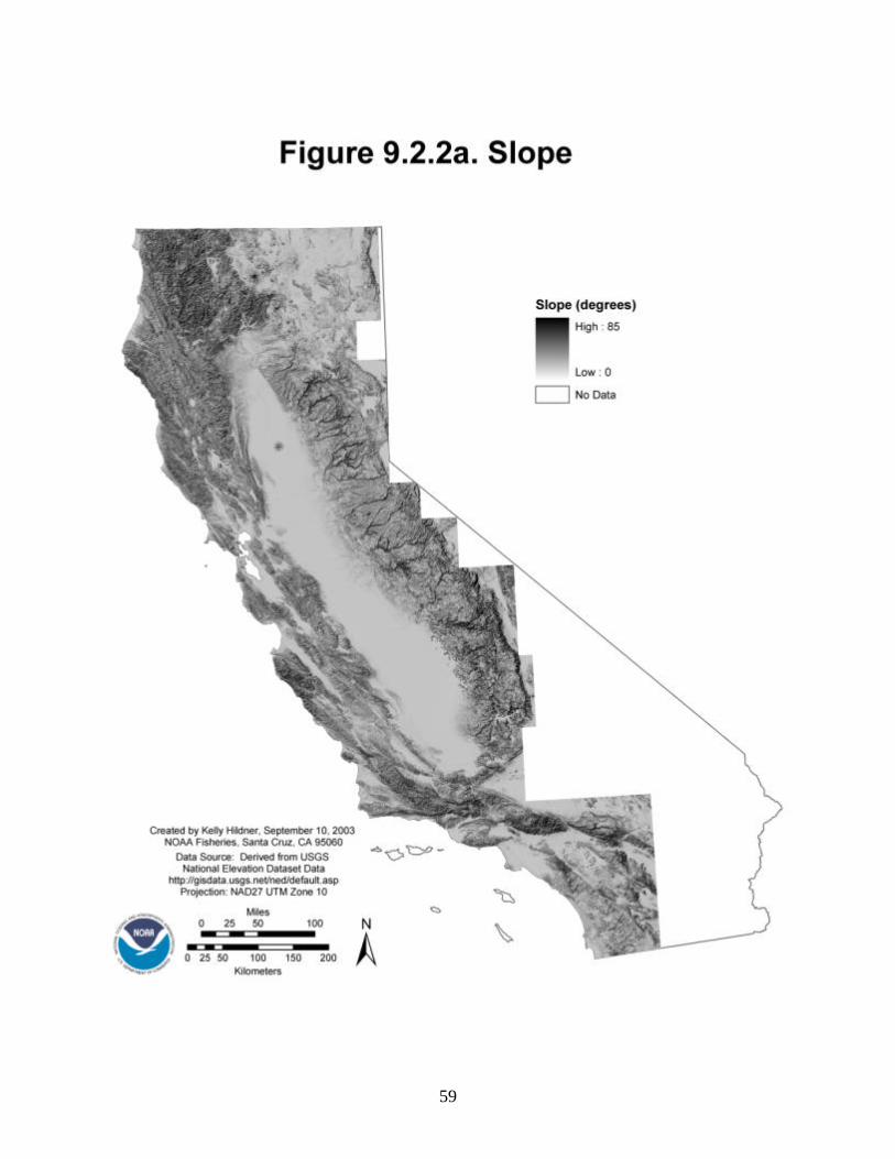
59

60
9.2.2 Slope Derived from 30 Meter USGS National Elevation Dataset (NED) Data
Type: Slope Name: Slope derived from USGS National Elevation Dataset (NED) Data File Name: slpmosaic_i, slp_ca_i Location: C:\Rest_Cost_Proj\GIS_data\DEM Description: 30 meter resolution integer slope data for salmonid study areas in California and Southern Oregon created from USGS NED data. Note that while the cell size is 30 meters, the data were created from 30 meter NED data using the Slope command in ArcInfo GRID which uses the cells in a 3x3 neighborhood to calculate the slope of each cell, so the actual data resolution is less than 30 meters. Abstract from NED metadata:
The U.S. Geological Survey has developed a National Elevation Dataset (NED). The NED is a seamless mosaic of best-available elevation data. The 7.5-minute elevation data for the conterminous United States are the primary initial source data. In addition to the availability of complete 7.5-minute data, efficient processing methods were developed to filter production artifacts in the existing data, convert to the NAD83 datum, edge-match, and fill slivers of missing data at quadrangle seams. One of the effects of the NED processing steps is a much- improved base of elevation data for calculating slope and hydrologic derivatives.
Data Source: USGS National Elevation Dataset (http://gisdata.usgs.net/ned/default.asp) Time Period: Published 1999; time period of data is unknown Spatial Coverage: Most of California and parts of Southern Oregon (areas covered by salmonid study areas) Limitations: The source data quality and resolution vary, and artifacts exist in some areas. Original Format: Grid Processing Steps: Original NED data were reprojected to NAD27 UTM Zone 10, converted to a cell size of 30 meters, and small imperfections were removed using the Fill command (with the Sink option) in the Grid module of ArcInfo. The Slope command was then used to convert the filled DEMs to slope grids. The slope grids were then converted from floating point to integer using the Int function in GRID: slp##_i = int(slp_##utm_f + .5). The integer slope grids were then combined using the Mosaic command in GRID to create slpmosaic_i. The mosaic was clipped to the boundary of California using the ca00cbfgrid (based on 2000 Census cartographic boundary file for California) as a mask:

61
Setwindow ca00cbfgrid Setmask ca00cbfgrid Slp_ca_i = slpmosaic_i Data Format: Grid Notes: For analysis, use slpmosaic_i. For display use slp_ca_i. See Notes in section 9.2.1 for more information on the source data. Attributes/Data Dictionary: Cell values are slope in degrees rounded to the nearest whole number.
10 ROADS
10.1 OVERVIEW
We examined several sources for geographic data on roads including Environmental Systems Research Institute (ESRI), the California Department of Forestry and Fire Protection, and the US Census Bureau. ESRI produces a layer of California’s major roads on their data and maps CD provided to software users, but these data do not include minor roads.
The California Department of Forestry and Fire Protection has detailed road data for some
areas where there are active timber harvest plans (THP). We explored these data because they include logging roads. Roads data were downloaded from the CDF ftp site: ftp://ftp.fire.ca.gov/forest/ForestPracticeGIS. According to Suzanne Lang (CDF, 707-576-2955) these data are based on 1:24k Digital Line Graphs (DLG); the different road layers overlap with each other and often contain different data; and edge matching to create a single layer is problematic. Also the maps are only complete where there is an active THP, so there is not statewide coverage.
The US Census Bureau creates road and other geographic data for US. We chose to use the
Census 2000 TIGER/Line road data because they provide a consistent statewide roads layer that is freely available. The data was acquired from Environmental Systems Research Institute (ESRI) as shapefiles that were created from the Topologically Integrated Geographic Encoding and Referencing (TIGER) database of the United States Census Bureau.
10.2 MAPS AND METADATA

62
63
10.2.1 U.S. Census 2000 TIGER/Line Road Data Type: Roads Name: U.S. Census 2000 TIGER/Line Road Data File Name: road_ca00_tgr.shp Location: C:\Rest_Cost_Proj\GIS_data\roads Description: The Redistricting Census 2000 TIGER/Line files of roads for the state of California. Environmental Systems Research Institute (ESRI) converted these data to shapefile format by using the TGRR2SHP Translator available from GIS Tools, Inc. The data were downloaded from the ESRI data website at http://www.esri.com/data/download/census2000_tigerline/index.html. Data Source: ESRI is the distributor of the data in shapefile format (http://www.esri.com/data/download/census2000_tigerline/index.html). The data originally come from the U.S. Bureau of the Census. Time Period: 2000 Spatial Coverage: California Limitations: [From U.S. Bureau of the Census Metadata] The Redistricting Census 2000 TIGER/Line files do NOT contain the ZIP Code Tabulation Areas (ZCTAs) and the address ranges are of approximately the same vintage as those appearing in the 1999 TIGER/Line files. That is, the Census Bureau is producing the Redistricting Census 2000 TIGER/Line files in advance of the computer processing that will ensure that the address ranges in the TIGER/Line files agree with the final Master Address File (MAF) used for tabulating Census 2000. The information present in these files is provided for the purposes of statistical analysis and census operations only. Coordinates in the TIGER/Line files have six implied decimal places, but the positional accuracy of these coordinates is not as great as the six decimal places suggest. The positional accuracy varies with the source materials used, but generally the information is no better than the established national map accuracy standards for 1:100,000-scale maps from the U.S. Geological Survey (USGS); thus it is NOT suitable for high-precision measurement applications such as engineering problems, property transfers, or other uses that might require highly accurate measurements of the earth's surface. The USGS 1:100,000-scale maps met national map accuracy standards and use coordinates defined by the North American Datum, 1983. For the contiguous 48 States, the cartographic fidelity of most of the Redistricting Census 2000 TIGER/Line files, in areas outside the 1980 census Geographic Base File/Dual Independent map Encoding (GBF/DIME) file coverage and selected other large metropolitan areas, compare favorably with the USGS 1:100,000-scale maps. The Census Bureau cannot specify the accuracy of features inside of what was the 1980 GBF/DIME-File coverage or selected metropolitan areas. The Census Bureau added updates to the TIGER/Line files that enumerators
64
annotated on maps sheets prepared from the Census TIGER data base as they attempted to traverse every street feature shown on the Census 2000 map sheets; the Census Bureau also made other corrections from updated map sheets supplied by local participants for Census Bureau programs. The locational accuracy of these updates is of unknown quality. In addition to the Federal, State, and local sources, portions of the files may contain information obtained in part from maps and other materials prepared by private companies. Despite the fact the TIGER/Line data positional accuracy is not as high as the coordinate values imply, the six-decimal place precision is useful when producing maps. The precision allows features that are next to each other on the ground to be placed in the correct position, on the map, relative to each other, without overlap. Original Format: Downloaded as shapefiles from ESRI. Original data format: TIGER/Line. Processing Steps: The data were downloaded as separate shapefiles for each county and then merged using the geoprocessing wizard in ArcMap. Data were reprojected to UTM NAD27 Zone 10 using ArcToolbox and the NAD_1927_ To_NAD_1983_NADCON datum conversion. Data Format: Shapefile Notes: NA Attributes/Data Dictionary: Census Feature (Line) Class Codes (CFCCs) A census feature class code (CFCC) is used to identify the most noticeable characteristic of a feature. The CFCC is applied only once to a chain or landmark with preference given to classifications that cover features that are visible to an observer and a part of the ground transportation network. Thus, a road that also is the boundary of a town would have a CFCC describing its road characteristics, not its boundary characteristics. The CFCC, as used in the TIGER/Line(r) files, is a three-character code. The first character is a letter describing the feature class; the second character is a number describing the major category; and the third character is a number describing the minor category. Some street features in the Census 2000 TIGER/Line(r) files that normally would be classified as "A" class features may now be coded with a "P' instead of the "A" to indicate that the feature is a "provisional" feature. The numeric portion of the CFCC still classifies the street as if an "A" were preceding it. Attributes of Geographic Objects 3-27 Provisional features are those streets that were added from reference sources or other programs in preparation for Census 2000, but were not field verified by census staff during field operations or through the use of aerial photography or imagery. As these features are verified in future operations, the provisional flag will be removed for subsequent TIGER/ Line(r) file releases. Features that still have the provisional flag at the time the U.S. Census Bureau assigned the Census 2000 tabulation block numbers were not held as Census 2000 tabulation block boundaries.

65
Feature Class A, Road The U.S. Census Bureau uses the term “divided” to refer to a road with opposing traffic lanes separated by any size median, and “separated” to refer to lanes that are represented in the Census TIGER(r) data base as two distinct complete chains. The term “rail line in center” indicates that a rail line shares the road right-of- way. The rail line may follow the center of the road or be directly next to the road; representation is dependent upon the available source used during the update. The rail line can represent a railroad, a streetcar line, or other carline. Primary Highway With Limited Access - Interstate highways and some toll highways are in this category (A1) and are distinguished by the presence of interchanges. These highways are accessed by way of ramps and have multiple lanes of traffic. The opposing traffic lanes are divided by a median strip. The TIGER/Line(r) files may depict these opposing traffic lanes as two distinct lines in which case, the road is called separated. CFCC Description
A11 Primary road with limited access or interstate highway, unseparated A12 Primary road with limited access or interstate highway, unseparated, in tunnel A13 Primary road with limited access or interstate highway, unseparated, underpassing A14 Primary road with limited access or interstate highway, unseparated, with rail line in center A15 Primary road with limited access or interstate highway, separated A16 Primary road with limited access or interstate highway, separated, in tunnel A17 Primary road with limited access or interstate highway, separated, underpassing A18 Primary road with limited access or interstate highway, separated, with rail line in center Primary Road Without Limited Access - This category (A2) includes nationally and regionally important highways that do not have limited access as required by category A1. It consists mainly of US highways, but may include some state highways and county highways that connect cities and larger towns. A road in this category must be hard-surface (concrete or asphalt). It has intersections with other roads, may be divided or undivided, and have multi- lane or single-lane characteristics. CFCC Description
A21 Primary road without limited access, US highways, unseparated A22 Primary road without limited access, US highways, unseparated, in tunnel A23 Primary road without limited access, US highways, unseparated, underpassing A24 Primary road without limited access, US highways, unseparated, with rail line in center A25 Primary road without limited access, US highways, separated A26 Primary road without limited access, US highways, separated, in tunnel A27 Primary road without limited access, US highways, separated, underpassing A28 Primary road without limited access, US highways, separated, with rail line in center

66
Secondary and Connecting Road - This category (A3) includes mostly state highways, but may include some county highways that connect smaller towns, subdivisions, and neighborhoods. The roads in this category generally are smaller than roads in Category A2, must be hardsurface (concrete or asphalt), and are usually undivided with single- lane characteristics. These roads usually have a local name along with a route number and intersect with many other roads and driveways. CFCC Description
A31 Secondary and connecting road, state highways, unseparated A32 Secondary and connecting road, state highways, unseparated, in tunnel A33 Secondary and connecting road, state highways, unseparated, underpassing A34 Secondary and connecting road, state highways, unseparated, with rail line in center A35 Secondary and connecting road, state highways, separated A36 Secondary and connecting road, state highways, separated, in tunnel A37 Secondary and connecting road, state and county highways, separated, underpassing A38 Secondary and connecting road, state and county highway, separated, with rail line in center Local, Neighborhood, and Rural Road - A road in this category (A4) is used for local traffic and usually has a single lane of traffic in each direction. In an urban area, this is a neighborhood road and street that is not a thoroughfare belonging in categories A2 or A3. In a rural area, this is a short-distance road connecting the smallest towns; the road may or may not have a state or county route number. Scenic park roads, unimproved or unpaved roads, and industrial roads are included in this category. Most roads in the Nation are classified as A4 roads. CFCC Description
A41 Local, neighborhood, and rural road, city street, unseparated A42 Local, neighborhood, and rural road, city street, unseparated, in tunnel A43 Local, neighborhood, and rural road, city street, unseparated, underpassing A44 Local, neighborhood, and rural road, city street, unseparated, with rail line in center A45 Local, neighborhood, and rural road, city street, separated A46 Local, neighborhood, and rural road, city street, separated, in tunnel A47 Local, neighborhood, and rural road, city street, separated, underpassing A48 Local, neighborhood, and rural road, city street, separated, with rail line in center Vehicular Trail - A road in this category (A5) is usable only by four-wheel drive vehicles, is usually a one- lane dirt trail, and is found almost exclusively in very rural areas. Sometimes the road is called a fire road or logging road and may include an abandoned railroad grade where the tracks have been removed. Minor, unpaved roads usable by ordinary cars and trucks belong in category A4, not A5. CFCC Description
A51 Vehicular trail, road passable only by 4WD vehicle, unseparated A52 Vehicular trail, road passable only by 4WD vehicle, unseparated, in tunnel

67
A53 Vehicular trail, road passable only by 4WD vehicle, unseparated, underpassing Road with Special Characteristics - This category (A6) includes roads, portions of a road, intersections of a road, or the ends of a road that are parts of the vehicular highway system and have separately identifiable characteristics. CFCC Description
A60 Special road feature, major category used when the minor category could not be determined A61 Cul-de-sac, the closed end of a road that forms a loop or turn-around A62 Traffic circle, the portion of a road or intersection of roads forming a roundabout A63 Access ramp, the portion of a road that forms a cloverleaf or limited access interchange A64 Service drive, the road or portion of a road that provides access to businesses, facilities, and rest areas along a limited-access highway; this frontage road may intersect other roads and be named A65 Ferry crossing, the representation of a route over water that connects roads on opposite shores; used by ships carrying automobiles or people Road as Other Thoroughfare - A road in this category (A7) is not part of the vehicular highway system. It is used by bicyclists or pedestrians, and is typically inaccessible to mainstream motor traffic except for private-owner and service vehicles. This category includes foot and hiking trails located on park and forest land, as well as stairs or walkways that follow a road right-ofway and have names similar to road names. CFCC Description
A70 Other thoroughfare, major category used when the minor category could not be determined A71 Walkway or trail for pedestrians, usually unnamed A72 Stairway, stepped road for pedestrians, usually unnamed A73 Alley, road for service vehicles, usually unnamed, located at the rear of buildings and property A74 Driveway or service road, usually privately owned and unnamed, used as access to residences, trailer parks, and apartment complexes, or as access to logging areas, oil rigs, ranches, farms, and park lands
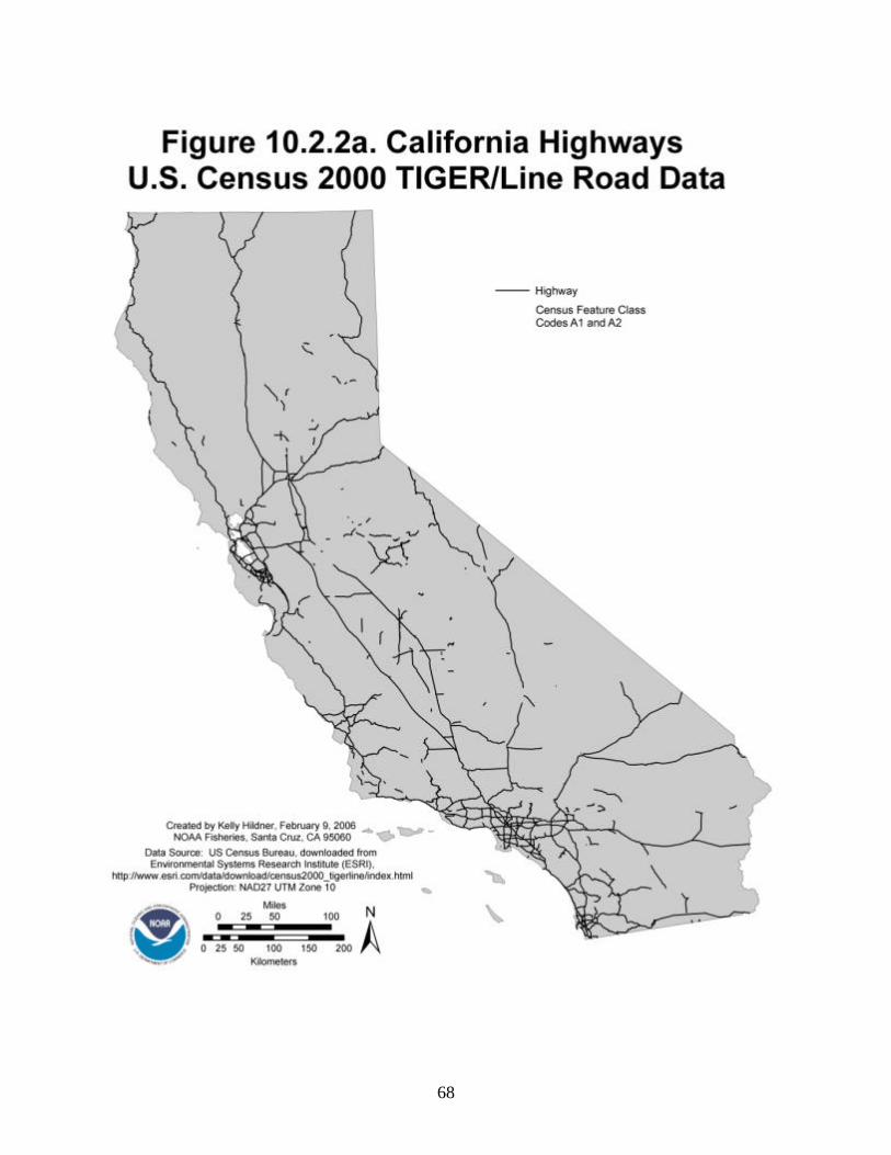
68

69
10.2.2 U.S. Census 2000 TIGER/Line Highways Type: Highways Name: Highway Data from U.S. Census 2000 TIGER/Line Road Data File Name: Highway_ca00_tgr.shp Location: C:\Rest_Cost_Proj\GIS_data\roads Description: Highways data from the Redistricting Census 2000 TIGER/Line files of roads for the state of California. Environmental Systems Research Institute (ESRI) converted the Census road data to shapefile format by using the TGRR2SHP Translator available from GIS Tools, Inc. The data were downloaded from the ESRI data website at http://www.esri.com/data/download/census2000_tigerline/index.html, and the highways (Census Feature Class Codes A1 and A2) were selected and exported to a new shapefile. Data Source: ESRI is the distributor of the data in shapefile format (http://www.esri.com/data/download/census2000_tigerline/index.html). The data originally come from the U.S. Bureau of the Census. Time Period: 2000 Spatial Coverage: California Limitations: This dataset does not include interchanges, ramps and connector roads. [From U.S. Bureau of the Census Metadata] The Redistricting Census 2000 TIGER/Line files do NOT contain the ZIP Code Tabulation Areas (ZCTAs) and the address ranges are of approximately the same vintage as those appearing in the 1999 TIGER/Line files. That is, the Census Bureau is producing the Redistricting Census 2000 TIGER/Line files in advance of the computer processing that will ensure that the address ranges in the TIGER/Line files agree with the final Master Address File (MAF) used for tabulating Census 2000. The information present in these files is provided for the purposes of statistical analysis and census operations only. Coordinates in the TIGER/Line files have six implied decimal places, but the positional accuracy of these coordinates is not as great as the six decimal places suggest. The positional accuracy varies with the source materials used, but generally the information is no better than the established national map accuracy standards for 1:100,000-scale maps from the U.S. Geological Survey (USGS); thus it is NOT suitable for high-precision measurement applications such as engineering problems, property transfers, or other uses that might require highly accurate measurements of the earth's surface. The USGS 1:100,000-scale maps met national map accuracy standards and use coordinates defined by the North American Datum, 1983. For the contiguous 48 States, the cartographic fidelity of most of the Redistricting Census 2000 TIGER/Line files, in areas outside the 1980 census Geographic Base File/Dual Independent map Encoding (GBF/DIME) file coverage and selected other large metropolitan areas, compare

70
favorably with the USGS 1:100,000-scale maps. The Census Bureau cannot specify the accuracy of features inside of what was the 1980 GBF/DIME-File coverage or selected metropolitan areas. The Census Bureau added updates to the TIGER/Line files that enumerators annotated on maps sheets prepared from the Census TIGER data base as they attempted to traverse every street feature shown on the Census 2000 map sheets; the Census Bureau also made other corrections from updated map sheets supplied by local participants for Census Bureau programs. The locational accuracy of these updates is of unknown quality. In addition to the Federal, State, and local sources, portions of the files may contain information obtained in part from maps and other materials prepared by private companies. Despite the fact the TIGER/Line data positional accuracy is not as high as the coordinate values imply, the six-decimal place precision is useful when producing maps. The precision allows features that are next to each other on the ground to be placed in the correct position, on the map, relative to each other, without overlap. Original Format: Downloaded as shapefiles from ESRI. Original data format: TIGER/Line. Processing Steps: The data were downloaded as separate shapefiles for each county and then merged using the geoprocessing wizard in ArcMap. Data were reprojected to UTM NAD27 Zone 10 using ArcToolbox and the NAD_1927_ To_NAD_1983_NADCON datum conversion. California highways were extracted from the complete road layer (road_ca00_tgr.shp) by selecting roads with CFCC (Census Feature Class Code) A1_ and A2_ (CFCC Like 'A1_' or CFCC Like 'A2_') and exporting to a new shapefile. Data Format: Shapefile Notes: NA Attributes/Data Dictionary: See attributes information for U.S. Census 2000 TIGER/Line Road Data (section 10.2.1).
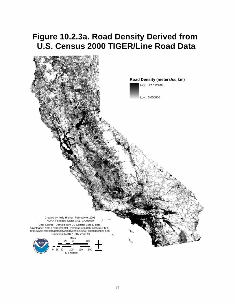
71
Figure 10.2.3a. Road Density Derived from U.S. Census 2000 TIGER/Line Road Data
Created by Kelly Hildner, February 9, 2006 NOAA Fisheries, Santa Cruz, CA 95060
Data Source: Derived from US Census Bureau data, downloaded from Environmental Systems Research Institute (ESRI),http://www.esri.com/data/download/census2000_tigerline/index.html
Projection: NAD27 UTM Zone 10
0 50 10025Miles
0 50 100 150 20025Kilometers
±
Road Density (meters/sq km)High : 27.012266
Low : 0.000000

72
10.2.3 Road Density from U.S. Census 2000 TIGER/Line Road Data Type: Road Density Name: Road Density from U.S. Census 2000 TIGER/Line Road Data File Name: lineden_1km Location: C:\Rest_Cost_Proj\GIS_data\roads Description: Road density from Census 2000 TIGER/Line roads data for the state of California. Environmental Systems Research Institute (ESRI) converted the Census road data to shapefile format by using the TGRR2SHP Translator available from GIS Tools, Inc. The data were downloaded from the ESRI data website at http://www.esri.com/data/download/census2000_tigerline/index.html, and a raster layer of road density was created using the ‘Line Density’ command in ArcGIS 9.1. The raster cell size is 30 meters, and the search radius for which the density is calculated is 1 kilometer. Data Source: ESRI is the distributor of the data in shapefile format (http://www.esri.com/data/download/census2000_tigerline/index.html). The U.S. Bureau of the Census originally produced the data. Time Period: 2000 Spatial Coverage: California Limitations: [From U.S. Bureau of the Census Metadata] The positional accuracy varies with the source materials used, but generally the information is no better than the established national map accuracy standards for 1:100,000-scale maps from the U.S. Geological Survey (USGS); thus it is NOT suitable for high-precision measurement applications such as engineering problems, property transfers, or other uses that might require highly accurate measurements of the earth's surface. Original Format: Downloaded as shapefiles from ESRI. Original data format: TIGER/Line. Processing Steps: The data were downloaded as separate shapefiles for each county and then merged using the geoprocessing wizard in ArcMap. Data were reprojected to UTM NAD27 Zone 10 using ArcToolbox and the NAD_1927_ To_NAD_1983_NADCON datum conversion. A road density grid was created using the Line Density command in ArcToolbox 9.1 with a cell size of 30 meters and a search radius 1000 meters (1 km). Resulting units are meters/square km. Data Format: Raster Dataset Notes: NA
73
Attributes/Data Dictionary: Each raster cell contains the road density in a circular area with a radius of 1 kilometer around the cell.
11 STREAMS
11.1 OVERVIEW For our analyses, we used a version of the routed hydrography created by the California
Department of Fish and Game (CDFG) and the Pacific States Marine Fisheries Commission (PSMFC). This dataset was based on the USGS 1:100k National Hydrographic Dataset (NHD), and the current version is available for download on the CalFish website http://www.calfish.org/. This dataset combines established streams (Geographic Names Information System - GNIS) and calculated stream levels (relating flow with spatial attributes) to create a stream layer more complete and compatible with fisheries applications.
The NHD is the national standard for hydrography data and is being used by multiple federal, state, and local agencies and organizations. The NHD is a comprehensive set of digital spatial data that contains information about surface water features such as lakes, ponds, streams, rivers, springs, and wells that is the culmination of cooperative efforts of the U.S. Environmental Protection Agency (USEPA) and the U.S. Geological Survey (USGS). For more information about the NHD, go to http://nhd.usgs.gov/. Stream flow data and other data on stream characteristics were acquired from the Salmon Population Analysis Team (SPAT) at NOAA Fisheries in Santa Cruz. These data were created as part of a project to measure the intrinsic potential of streams as salmonid habitat and were derived from a USGS Digital Elevation Model (DEM) of California using programs written by Daniel Miller at Earth Systems Institute. Contact the SPAT for further information. Because these data are derived from a DEM, they lack stream identifiers such as names. In order to associate data with streams of interest, it is necessary to compare the streams from the DEM derived data with an established hydrography layer and transfer the data to the appropriate named stream.
11.2 MAPS AND METADATA

74
Figure 11.2.1a. Streams DataCDFG & PSMFC, March 2003
Created by Kelly Hildner, February 21, 2006 NOAA Fisheries, Santa Cruz, CA 95060
Data Source: California Department of Fish and Game (CDFG) & Pacific States Marine
Fisheries Commission (PSMFC): www.calfish.orgProjection: NAD27 UTM Zone 10
0 50 10025Miles
0 50 100 150 20025Kilometers
±

75
Figure 11.2.1a. Streams DataCDFG & PSMFC, March 2003
Created by Kelly Hildner, February 21, 2006 NOAA Fisheries, Santa Cruz, CA 95060
Data Source: California Department of Fish and Game (CDFG) & Pacific States Marine
Fisheries Commission (PSMFC): www.calfish.orgProjection: NAD27 UTM Zone 10
0 50 10025Miles
0 50 100 150 20025Kilometers
±
76
11.2.1 Streams Data (CDFG & PSMFC, March 2003) Type: Streams Name: 100k Hydrography; Bigroutes File Name: cdfg100kutm2_arc; cdfg100kutm2_route_streams Location: C:\Rest_Cost_Proj\GIS_data\hydrography\ cdfg100kutm2.mdb\streams Description: (From original metadata) 1:100,000 scale stream based routed hydrography covering the area of California currently known by California Department of Fish & Game (CDFG) and Pacific States Marine Fisheries Commission (PSMFC) to contain anadromous fishes plus a large portion of northern and central California. The coverage utilizes existing National Hydrography Database (NHD) 1:100,000 linework and attributes as well as Geographic Names Information System (GNIS) identifiers as guidelines to determine the stream networks that were combined into routes. Utilizing both automatic routines developed by CDFG/PSMFC staff as well as manual (on screen) networking techniques, a series of line segments from the NHD were networked into a stream first by the existence of a GNIS ID. If no GNIS ID was present for a series of segments, the NHD "Level" attribute was used to determine the network. The resulting routes represent what are commonly referred to as streams under the aforementioned guidelines. Streams are identified with the unique LLID identifier. Although derived from Latitude/Longitude coordinates, the LLID should be used as a stream identifier only and not as a spatial identifier. cdfg100kutm2_arc contains all streams and artificial or broken waterways from the NHD in the covered geographic area; cdfg100kutm2_route_streams contains only routed streams. Data Source: California Department of Fish and Game (CDFG), Pacific States Marine Fisheries Commission (PSMFC). Current version can be downloaded from the CalFish website: http://www.calfish.org/DesktopDefault.aspx?tabId=76 Time Period: Published March 2003 Spatial Coverage: Parts of California. The area of California currently known by California Department of Fish & Game (CDFG) and Pacific States Marine Fisheries Commission (PSMFC) to contain anadromous fishes plus a large portion of northern and central California. The current version of the file, available from the CalFish website, contains only routed hydrography and covers all of California. Limitations: For the complete routed hydrography for California, go to the CalFish website (http://www.calfish.org/), and for the complete hydrography of California including artificial waterways and disconnected stream segments, go to the NHD website (http://nhd.usgs.gov/). Original Format: ArcInfo coverage Processing Steps: Data were imported to a geodatabase projected in NAD 27 UTM Zone 10N.

77
Data Format: Geodatabase feature class Notes: None Attributes/Data Dictionary: For complete entity and attribute information see U.S. Geological Survey, 1999, Standards for National Hydrography Dataset: Reston, Virginia, U.S. Geological Survey at http://nhd.usgs.gov/chapter1/index.html. Selected attributes for cdfg100kutm2_arc: Field Description COM_ID
The common identifier is a 10-digit integer value that uniquely identifies the occurrence of each feature. Each value occurs only once throughout the Nation. Once assigned, the value is associated permanently with its feature. When a feature is deleted, the value for its identifier is retired.
LEVEL
Stream level (see description below). The special value "-9998" means that a value can be applied to the transport reach but has not been specified. This value usually occurs where flow relations cannot be determined or have not been encoded. Without this information, main paths cannot be identified and stream level cannot be assigned. This value is also assigned to coastline reaches.
GNIS_ID The eight-digit identifier for a name in the Geographic Names Information System NAME Geographic names from the Geographic Names Information System FTYPE Feature types encoded with a character string (for example, "Stream/River") HUC
An 8-digit hydrologic unit code that uniquely identifies each of the four levels of classification within four 2-digit fields. The first 2 digits identify regions, the first 4 digits identify subregions, the first 6 digits identify accounting units, and the full 8 digits identify subbasins.
NETWORKID Network identifier Shape_Length Length of arc in meters Selected attributes for cdfg100kutm2_route_streams: Field Description LLID
Unique Stream Identifier derived from Latitude/Longitude coordinates of mouth of stream. Once established, LLID of a stream does not change regardless of changes to stream network. LLID is not to be used as a location identifier.
NAME Geographic Names Information System (GNIS from USGS) Name LENGTH_FT Length of stream network in feet NETWORKID Network identifier UPX Teale-Albers X coordinate at headwater of stream UPY Teale-Albers Y coordinate at headwater of stream DOWNX Teale-Albers X coordinate at mouth of stream

78
DOWNY Teale-Albers Y coordinate at mouth of stream DOWN_LLID LLID of stream directly downstream of stream DOWN_NAME GNIS Name of stream directly downstream of stream DOWN_MEAS Measured location on downstream stream of mouth of stream MOUTH Explanation of occurence on stream of no downstream LLID Shape_Length Length of arc in meters
Stream level (from http://nhd.usgs.gov/chapter1/index.html#_Toc474479764)
“The stream level is a numeric code that identifies each main path of water flow through a drainage network. Stream level is assigned by identifying the terminus of a drainage network (see Figure 11). The lowest value6 for stream level is assigned to a transport reach at the end of a flow and to upstream transport reaches that trace the main path of flow back to the head. The stream level value is incremented by one and is assigned to all transport reaches that terminate at this path (that is, all tributaries to the path) and to all transport reaches that trace the main path of the flow along each tributary back to its head. The stream level value is incremented again and is assigned to transport reaches that trace the main path of the tributaries to to their heads. This process is continued until all transport reaches for which flow is encoded are assigned a stream level.
Figure 11. Stream level assignment for a simple drainage network.
6The lowest value for stream level is: "1" for transport reaches that terminate at the Atlantic, Pacific, or Arctic Oceans, the Gulf of Mexico, or the Caribbean Sea. "2" for transport reaches that terminate at the Great Lakes or the Great Salt Lake. "3" for transport reaches that terminate at the boundary of the United States with Canada or Mexico. "4" for transport reaches that terminate at any other place (isolated drainage).”

79
12 WATERSHEDS
12.1 OVERVIEW
CalWater 2.2 is the official California watershed map and is the “best available data” for most uses. It does not, however, meet Federal Geographic Data Committee (FGDC) Watershed Boundary Dataset mapping standards. CalWater delineations are primarily designed to be administrative reporting units, and the boundaries should not be used to define authoritative drainage area above a given point. Some watershed boundary definitions in the CalWater database include non-physical boundaries such as administrative and political boundaries, particularly in valley floor and urbanized coastal areas. There are 6 watershed designation levels in the CalWater database that consist of six levels of increasing specificity (see Table 1). CalWater watersheds do not correspond directly to USGS Hydrologic Unit Codes (HUCs). According to the CalWater FAQ (http://cain.nbii.gov/calwater/calwfaq.html) the state HSA (Hydrologic Sub-Area) approximates the USGS 4th field, 8 digit HUC “Cataloguing Unit”.
Table1. CalWater 2.2 hierarchy of watershed designations
Watershed Designation Level Sq Miles / Acres # in CalWater 2.2 Hydrologic Region (HR) 12,735 sq miles / 8,150,000 acres 10 Hydrologic Unit (HU) 672 sq miles / 430,000 acres 190 Hydrologic Area (HA) 244 sq miles / 156,000 acres 522 Hydrologic Sub-Area (HSA) 195 sq miles / 125,000 acres 655 Super Planning Watershed (SPWS) 78 sq miles / 50,000 acres 1623 Planning Watershed (PWS) 5-15 sq miles / 3,000-10,000 acres 6271
Watersheds are also delineated by the USGS using a nationwide system based on surface
hydrologic features. This system divides the country into 21 regions (2-digit), 222 subregions (4-digit), 352 accounting units (6-digit), and 2,262 (154 in California) cataloguing units (8-digit). A hierarchical hydrologic unit code (HUC), consisting of 2 digits for each level in the hydrologic unit system, is used to identify any hydrologic area.
NOAA Fisheries Technical Recovery Team staff has delineated biologically relevant
watershed boundaries using Digital Elevation Model (DEM) data and the USGS 4th field HUCs as a guide.
12.2 MAPS AND METADATA
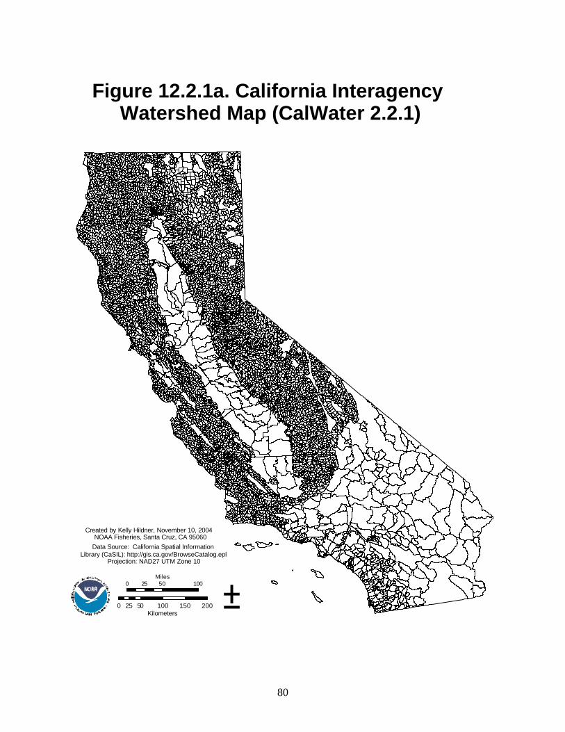
80
Figure 12.2.1a. California Interagency Watershed Map (CalWater 2.2.1)
Created by Kelly Hildner, November 10, 2004 NOAA Fisheries, Santa Cruz, CA 95060
Data Source: California Spatial Information Library (CaSIL): http://gis.ca.gov/BrowseCatalog.epl
Projection: NAD27 UTM Zone 10
0 50 10025Miles
0 50 100 150 20025Kilometers
±

81
12.2.1 California Interagency Watershed Map of 1999 (CalWater 2.2, updated May 2004, “calw221”)
Type: Watersheds Name: CalWater 2.2.1 planning watersheds File Name: calw221.shp Location: C:\Rest_Cost_Proj\GIS_data\boundaries\Watersheds Description: The California Interagency Watershed Map of 1999 (Calwater 2.2, updated May 2004, "calw221") is the State of California's working definition of watershed boundaries. Previous Calwater versions (1.2 and 2.2) described California watersheds, beginning with the division of the State's 101 million acres into ten Hydrologic Regions (HR). Each HR is progressively subdivided into six smaller, nested levels: the Hydrologic Unit (HU, major rivers), Hydrologic Area (HA, major tributaries), Hydrologic Sub-Area (HSA), Super Planning Watershed (SPWS), and Planning Watershed (PWS). Data Source: The California Spatial Information Library (CaSIL) is the current distributor of the coverage in the Teale Albers Conical Equal-Area projection, North American Datum of 1983. http://gis.ca.gov/BrowseCatalog.epl Time Period: The California Resources Agency (CRA) Department of Forestry and Fire Protection (CDF) contracted with Tierra Data Systems for the original digital production in 1993, based on Hydrologic Basin Planning Maps published in hardcopy (SWRCB, 1986). The State of California Stephen P. Teale Data Center GIS Solutions Group (Teale) under the direction of the California Department of Water Resrouces (DWR) and CDF, finalized the current version in ESRI ArcInfo coverage format in 1999 with USDA Forest Service and RWQCB/SWRCB inputs. Spatial Coverage: California Limitations: Calwater 2.2.1 most accurately delineates true watersheds in mountainous terrain. However, neither Calwater 2.2.1 nor any of its predecessors is a "pure" watershed map because administrative boundaries such as the State border were used to delineate watershed areas. Some of the boundaries, particularly in developed valley areas, also have legal and administrative purposes other than the representation of actual drainage divides. Examples include the so-called "Legal Delta" (California Water Code, Chapter 2, the Delta, Sec. 12220) and other district boundaries. Neither is Calwater a legal map document, as it does not represent State of California Regional Water Quality Control Board (RWQCB) jurisdictions, officiated by the State Water Resources Control Board (SWRCB) under California Water Code Section 13200. Calwater is a hybrid, a spatial cross-reference for use in local, State, and federal information communities.

82
Original Format: ArcInfo export file (.e00) Processing Steps: Data were imported to an ArcInfo coverage in ArcGIS 9.0 using the Import From Interchange File Tool, and the coverage was exported as a shapefile, which was then reprojected to NAD27 UTM Zone 10 using the Project Tool and the NAD_1927_To_NAD_1983_NADCON transformation. Data Format: shapefile Notes: None Attributes/Data Dictionary: COL ITEM NAME WIDTH OUTPUT TYPE DEC DESCRIPTION
1AREA 8 18 F 5Area of Polygon (square meters) 9PERIMETER 8 18 F 5Perimeter of Polygon (meters)
17CALW221# 4 5 B - ArcInfo internal record number 21CALW221-ID 4 5 B - ArcInfo user id (not used) 25CALWNUM 12 12 C - Calwater Watershed ID Number (Interagency) 37SWRCBNUM21 6 6 C - Watershed ID Number (SWRCB at Calwater v2.1) 43HRC 2 2 C - Hydrologic Region Code (DWR) 45HBPA 2 2 C - Hydrologic Basin Planning Area (RWQCB) 47RBU 5 5 I - Concatenates HR,RB,HU into a single integer 52RBUA 6 6 I - Concatenates HR,RB,HU,HA 58RBUAS 7 7 I - Concatenates HR,RB,HU,HA,HSA 65RBUASP 9 9 I - Concatenates HR,RB,HU,HA,HSA,SPWS 74RBUASPW 11 11 I - Concatenates HR,RB,HU,HA,HSA,SPWS,PWS 85HR 2 2 I - Hydrologic Region (1->10)(DWR) 87RB 1 1 I - Regional Water Qual. Cont. Board (1->9)(RWQCB) 88HU 2 2 I - Hydrologic Unit (00->~80)(SWRCB) 90HA 1 1 I - Hydrologic Area (0->9)(SWRCB) 91HAS 1 1 I - Hydrologic Sub-Area (0->9)(SWRCB) 92SPWS 2 2 I - Super Planning Watershed (00->~30)(CDF) 94PWS 2 2 I - Planning Watershed (00->~13)(CDF) 96HRNAME 35 35 C - Hydrologic Region Name (DWR)
131RBNAME 35 35 C - Regional Water Qual. Cont. Board Name 166HBPANAME 35 35 C - Hydrologic Basin Planning Area Name 201HUNAME 35 35 C - Hydrologic Unit Name 236HANAME 35 35 C - Hydrologic Area Name 271HSANAME 35 35 C - Hydrologic Sub-Area Name 306CDFSPWNAME 35 35 C - Super-Planning Watershed Name 341CDFPWSNAME 35 35 C - Planning Watershed Name 376ACRES 4 12 F 0Acreage of watershed polygon 380HUC_8 8 8 I - Federal 8-digit Hydrologic Unit Code (HUC) 388HUC_8_NAME 48 48 C - Name of Federal 8-digit HUC 436HUC_8_ALT2 8 8 I - Second Overlapping HUC

83
444HUC_8_ALT3 8 8 I - Third Overlapping HUC 452DWRNUM20 12 12 C - DWR watershed identifier (Calwater v2.0 MOU) 464DWRHUNAME 35 35 C - DWR Hydrologic Unit Name (Calwater v2.0) 499DWRHANAME 35 35 C - DWR Hydrologic Area Name (Calwater v2.0) 534DWRHSANAME 35 35 C - DWR Hydrologic Sub-Area Name (Calwater v2.0) 569CDFNUM22 12 12 C - CDF Watershed ID Number (at Calwater v2.2)

84
MOJAVE
PIT RIVER
AMARGOSA
KLAMATH RIVER
SALINAS
OWENS
EEL RIVER
IMPERIAL
ANTELOPE
FEATHER RIVER
TRIN
ITY R
IVER
KE
RN
RIV
ER
WA
RD
SUSANVILLE
SO
UTH
VA
LLE
Y F
LOO
R
BALLARAT
CO
LUS
A B
AS
IN
CHUCKWALLA
KINGS RIVER
SANTA MARIA
WHITEWATER
ROUT
E SIXT
Y SIX
TEHAMA
HOMER
DALE
YUBA RIVER
AMERICAN RIVER
SANTA ANA RIVER
MONO
SALINE
TRO
NA
CA
DIZ
RU
SSIAN R
IVER
MIDDLE SIERRA
FREMONT
SAN PABLO
TUOLUMNE RIVER
PAJARO RIVER
SU
ISU
N
IND
IAN
WE
LLS
MEN
DO
CIN
O C
OAST
WHITMORE
SANTA YNEZ
EU
RE
KA
MERCED RIVER
SHAS
TA B
ALLY
REDD
ING
RIC
EFigure 12.2.2a. California Interagency
Watershed Map (CalWater 2.2.1)Hydrologic Units
Created by Kelly Hildner, November 10, 2004 NOAA Fisheries, Santa Cruz, CA 95060
Data Source: California Spatial Information Library (CaSIL): http://gis.ca.gov/BrowseCatalog.epl
Projection: NAD27 UTM Zone 10
0 50 10025Miles
0 50 100 150 20025Kilometers
±

85
12.2.2 CalWater 2.2.1 Hydrologic Units Type: Watersheds Name: CalWater 2.2.1 hydrologic unit boundaries File Name: calw221HU.shp Location: C:\Rest_Cost_Proj\GIS_data\boundaries\Watersheds\calw221HU.shp Description: The California Interagency Watershed Map of 1999 (Calwater 2.2, updated May 2004, "calw221") is the State of California's working definition of watershed boundaries. Previous Calwater versions (1.2 and 2.2) described California watersheds, beginning with the division of the State's 101 million acres into ten Hydrologic Regions (HR). Each HR is progressively subdivided into six smaller, nested levels: the Hydrologic Unit (HU, major rivers), Hydrologic Area (HA, major tributaries), Hydrologic Sub-Area (HSA), Super Planning Watershed (SPWS), and Planning Watershed (PWS). This dataset represents the Hydrologic Units. Data Source: The California Spatial Information Library (CaSIL) is the current distributor of the coverage in the Teale Albers Conical Equal-Area projection, North American Datum of 1983. http://gis.ca.gov/BrowseCatalog.epl Time Period: The California Resources Agency (CRA) Department of Forestry and Fire Protection (CDF) contracted with Tierra Data Systems for the original digital production in 1993, based on Hydrologic Basin Planning Maps published in hardcopy (SWRCB, 1986). The State of California Stephen P. Teale Data Center GIS Solutions Group (Teale) under the direction of the California Department of Water Resources (DWR) and CDF, finalized the current version in ESRI ArcInfo coverage format in 1999 with USDA Forest Service and RWQCB/SWRCB inputs. Spatial Coverage: California, hydrologic units Limitations: Calwater 2.2.1 most accurately delineates true watersheds in mountainous terrain. However, neither Calwater 2.2.1 nor any of its predecessors is a "pure" watershed map because administrative boundaries such as the State border were used to delineate watershed areas. Some of the boundaries, particularly in developed valley areas, also have legal and administrative purposes other than the representation of actual drainage divides. Examples include the so-called "Legal Delta" (California Water Code, Chapter 2, the Delta, Sec. 12220) and other district boundaries. Neither is Calwater a legal map document, as it does not represent State of California Regional Water Quality Control Board (RWQCB) jurisdictions, officiated by the State Water Resources Control Board (SWRCB) under California Water Code Section 13200. Calwater is a hybrid, a spatial cross-reference for use in local, State, and federal information communities.

86
Original Format: ArcInfo export file (.e00) Processing Steps: Data were imported to an ArcInfo coverage in ArcGIS 9.0 using the Import From Interchange File Tool, and the coverage was exported as a shapefile, which was then reprojected to NAD27 UTM Zone 10 using the Project Tool and the NAD_1927_To_NAD_1983_NADCON transformation. The data were then dissolved on the hydrologic unit code (RBU) using the Dissolve tool in ArcToolbox 9.0. Data Format: shapefile Notes: None Attributes/Data Dictionary: Attributes are retained in the original shapefile (calw221.shp) and can be joined to this shapefile using the RBU codes. See section 12.2.1 for attribute data.

87
Lost
Salton Sea
Mojave
Southern Mojave
Salinas
Trinity
Tulare-Buena Vista Lakes
Lower Pit
Upper PitU
pper Amargosa
Pajaro
Impe
rial R
eser
voir
Russian
Death Valley-Lower Amargosa
Santa Ana
Scott
Illinois
Lower Eel
Truckee
Crowley Lake
Honey-Eagle Lakes
Sm
ith
Upper King
War
ner L
akes
Cuyama
Santa Clara
San D
iego
Ant
elop
e-F
rem
ont V
alle
ysEstrella
Havasu-M
ohave Lakes
Coyote
Sm
oke
Cre
ek D
eser
t
Butte
Ivanpah-Pahrump Valleys
Shasta
Upper Yuba
Owens Lake
Lowe
r Klam
ath
Panamint Valley
Middle San Joaquin-Lower
Salmon
Mono Lake
Upper Tuolumne
Upp
er K
ern
Upper Klamath
Piute Wash
Fish Lake-Soda S
pring Valleys
Goose Lake
East
Walk
er
Upper San
Joaquin
Chetco
Mas
sacr
e La
ke
San P
ablo Bay
Mcc
loud
Wes
t Wal
ker
Santa Ynez
Upper Merced
Applegate
Eureka-Saline Valleys
Sacramento-Stone C
orral
Upper Cache
Upper Eel
Mattole
Upper C
arson
San Jacinto
Big-N
avarro-Garcia
Nor
th F
ork F
eath
er
San
Gab
riel
Sou
th F
ork
Ker
n
Surprise V
alley
Upper S
tony
Suisun B
ay
Madeline Plains
Low
er B
utte
South Fork Eel
Upper Mokelumne
Calleguas
Figure 12.2.3a. USGS Hydrologic Units
Created by Kelly Hildner, November 12, 2004 NOAA Fisheries, Santa Cruz, CA 95060Data Source: USGS Water Resources:
http://water.usgs.gov/GIS/huc.htmlProjection: NAD27 UTM Zone 10
0 50 10025Miles
0 50 100 150 20025Kilometers
±

88
12.2.3 USGS Hydrologic Units Type: Hydrologic Units (“Watersheds”)
Name: 1:250,000-scale Hydrologic Units (huc250k) File Name: huc250_ca_USGS.shp Location: C:\Rest_Cost_Proj\GIS_data\boundaries\Watersheds Description: The Geographic Information Retrieval and Analysis System (GIRAS) was developed in the mid 70s to put into digital form a number of data layers which were of interest to the USGS. One of these data layers was the Hydrologic Units. The map is based on the Hydrologic Unit Maps published by the U.S. Geological Survey Office of Water Data Coordination, together with the list descriptions and name of region, subregion, accounting units, and cataloging unit. The hydrologic units are encoded with an eight- digit number that indicates the hydrologic region (first two digits), hydrologic subregion (second two digits), accounting unit (third two digits), and cataloging unit (fourth two digits). The data produced by GIRAS was originally collected at a scale of 1:250K. Some areas, notably major cities in the west, were recompiled at a scale of 1:100K. In order to join the data together and use the data in a geographic information system (GIS), the data were processed in the ARC/INFO GIS software package. Within the GIS, the data were edgematched and the neatline boundaries between maps were removed to create a single data set for the conterminous United States. Data Source: USGS Water Resources, http://water.usgs.gov/GIS/huc.html Time Period: 1994 Spatial Coverage: California, hydrologic units Limitations: This data set was compiled originally to provide the National Water Quality Assessment (NAWQA) study units with an intermediate-scale river basin boundary for extracting other GIS data layers. The data can also be used for illustration purposes at intermediate or small scales (1:250,000 to 1:2 million). Original Format: ArcInfo export file (.e00) Processing Steps: USGS hydrologic units were downloaded from http://water.usgs.gov/GIS/dsdl/huc250.e00.gz, unzipped, and imported to an ArcInfo coverage using the Import From Interchange File tool in ArcToolbox 9.0. Polygons that intersect the state of California were selected and exported to a shapefile which was then reprojected to NAD27 UTM Zone 10 using the Project tool in ArcToolbox 9.0. Basin names were added from the text-formatted list of hydrologic units names and numbers from USGS Water-Supply Paper 2294
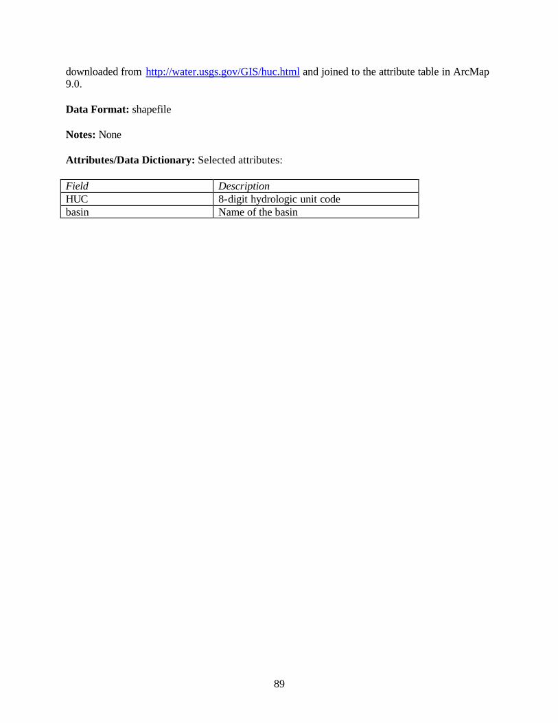
89
downloaded from http://water.usgs.gov/GIS/huc.html and joined to the attribute table in ArcMap 9.0. Data Format: shapefile Notes: None Attributes/Data Dictionary: Selected attributes: Field Description HUC 8-digit hydrologic unit code basin Name of the basin
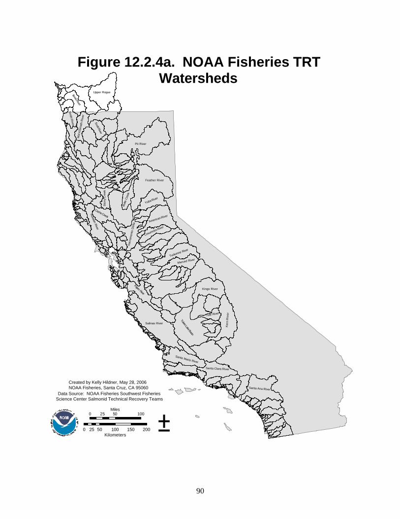
90
Pit River
Salinas River
Feather River
Ker
n R
iver
Tulare Lake Basin
Upper Rogue
Kings River
Santa Ana River
American River
Yuba River
Tuolumne River
Russian R
iver
Pajaro River
Santa Maria River
Merced River
Santa Clara River
Cache Creek
Ilinois River
Sac
ram
ento
Del
ta
Scott River
Butte
Cre
ek
Sm
ith River
Sto
ny C
reek
Mid
Kla
mat
h R
iver
Cosumnes River
Tule River
Figure 12.2.4a. NOAA Fisheries TRTWatersheds
Created by Kelly Hildner, May 28, 2006 NOAA Fisheries, Santa Cruz, CA 95060
Data Source: NOAA Fisheries Southwest FisheriesScience Center Salmonid Technical Recovery Teams
0 50 10025Miles
0 50 100 150 20025Kilometers
±

91
12.2.4 NOAA Fisheries Salmonid Technical Recovery Team Watersheds Type: Watersheds
Name: Salmonid TRT Watersheds File Name: TRTWatersheds1.shp Location: C:\Rest_Cost_Proj\GIS_data\boundaries\Watersheds Description: Watersheds delineated to facilitate the identification of independent anadromous fish populations and characterize the geographic areas where those independent populations occur. Watershed sizes are not uniform and do not correspond to any specific order of hydrologic units, but rather, they vary with the area drained by each river. All watersheds were delineated to follow natural features rather than political boundaries or other man-made features. This file was created by essentially merging the watershed coverages created by NOAA Fisheries Technical Recovery Team staff (cv_wsheds, noceca_wshds4, scaco_wsheds2, and sonc_indpop5). Details about the watersheds can be found in the metadata for the source files. Data Source: NOAA Fisheries Southwest Fisheries Science Center Time Period: Varies Spatial Coverage: California anadromous fish watersheds Limitations: Delineating watershed boundaries in areas of minimal topographic relief involved some subjectivity. Original Format: ArcInfo coverages Processing Steps: This file was created by essentially merging the watershed coverages created by NOAA Fisheries Technical Recovery Team staff (cv_wsheds, noceca_wshds4, scaco_wsheds2, and sonc_indpop5). The following changes were made prior to merging: 1) Field names were changed to be consistent among the four files. 2) A field named StArea was added to each shapefile to hold the study area names. This was calculated to equal the study area name or "NOCECA and SONC" for the area of overlap 3) All NOCECA watersheds except Walnut Creek were saved into a separate shapefile in order to exclude this watershed because it is a subset of the South Suisun Bay watershed in the Central Valley study area. 4) SONC watersheds excluding those that overlap with NOCECA watersheds were saved to a separate shapefile (sonc_only_indpop5) NOTE: 3 watersheds in the SONC study area are broken up into smaller units in the NOCECA, so NOCECA watersheds were used. Data Format: shapefile

92
Notes: None Attributes/Data Dictionary: Selected attributes: Field Description NAME Watershed name STAREA Study area

93
APPENDIX A: METADATA CATEGORY DEFINITIONS Type: General data type Name: A descriptive name for the data including, where appropriate the time period spanned File Name: The name of the digital file storing the data Location: Pathname to file location Description: A narrative summary of the dataset Data Source: The source agency for the dataset and, if possible, a link to where the data can be downloaded Time Period: Time period information for the dataset. Where possible, the time period for which the data reflect the ground condition. Spatial Coverage: Geographic area and, where relevant, type of geographic division (e.g. county, incorporated place, etc.) covered by the data. Limitations: Limitations or complexities relevant to using the data Original Format: Format of the original source file Processing Steps: Processing steps used to convert the original data file into its current format Data Format: Current data format (e.g. shapefile, access database, etc.) Notes: Other relevant information that doesn’t fit into other metadata categories Attributes/Data Dictionary: Description of relevant or selected attributes in the database.

RECENT TECHNICAL MEMORANDUMSCopies of this and other NOAA Technical Memorandums are available from the National Technical Information Service, 5285 Port Royal Road, Springfield, VA 22167. Paper copies vary in price. Microfiche copies cost $9.00. Recent issues of NOAA Technical Memorandums from the NMFS Southwest Fisheries Science Center are listed below:
NOAA-TM-NMFS-SWFSC-392 Ichthyoplankton and station data for surface (manta) and oblique (bongo) plankton tows for California Cooperative Oceanic Fisheries Investigations survey cruises in 2005. D.A. AMBROSE, R.L. CHARTER, and S.M. MANION
393 Ichthyoplankton, paralarval cephalopod, and station data for oblique (bongo) plankton tows from the Oregon, California, and Washington line-transect expedition (ORCAWALE) in 2001. S.R. CHARTER, B.S. MacCALL, R.L. CHARTER, S.M. MANION, W. WATSON, and L.T. BALLANCE
394 Steelhead of the South-Central/Southern California Coast: Population characterization for recovery planning. D.A. BOUGHTON, P.B. ADAMS, E. ANDERSON, C. FUSARO, E. KELLER, E. KELLEY, L. LENTSCH, J. NIELSEN, K. PERRY, H. REGAN, J. SMITH, C. SWIFT, L. THOMPSON, and F. WATSON (September 2006)
395 The physical oceanography off the central California coast during May- June 2001: A summary of CTD and other hydrographic data from young of the year juvenile rockfish surveys. K.A. BALTZ, K.M. SAKUMA, and S. RALSTON (September 2006)
396 Assessment of the Pacific sardine (Sardinops sagax caerulea) population for U.S. Management in 2007. K.T. HILL, N.C.H. LO, B.J. MACEWICZ, and R. FELIX-URAGA (November 2006)
397 AMLR 2005/2006 field season report: Objectives, Accomplishments, and Tentative Conclusions. J.D. LIPSKY, Editor (December 2006) 398 U.S. Pacific marine mammal stock assessments: 2006. J.V. CARRETTA, K.A. FORNEY, M.M. MUTO, J. BARLOW, J. BAKER, B. HANSON, and M.S. LOWRY (January 2007)
399 Monitoring and research needed to manage the recovery of threatened and endangered Chinook and steelhead in the Sacramento-San Joaquin basin. J.G. WILLIAMS, J.J. ANDERSON, S. GREENE, C. HANSON, S.T. LINDLEY, A. LOW, B.P. MAY, D. McEWAN, M.S. MOHR, R.B. MacFARLANE, and S. SWANSON (February 2007)
400 Extraction of DNA from formalin-fixed cetacean tissues. K.M. ROBERTSON, C.A. LeDUC, R.G. LeDUC, and P.A. MORIN (February 2007)
401 Spawning biomass of Pacific sardine (Sardinops sagax) off U.S. and Canada in 2006. N.C.H. LO, B.J. MACEWICZ, D.A. GRIFFITH, and R.L. CHARTER (February 2007)