New method for predicting the ultimate bearing capacity of driven piles by using Flap number

KSCE Journal of Civil Engineering (2015) 19(3):611-620 Copyright ⓒ2014 Korean Society of Civil Engineers DOI 10.1007/s12205-013-0315-z

− 611−

pISSN 1226-7988, eISSN 1976-3808

www.springer.com/12205

Geotechnical Engineering

New Method for Predicting the Ultimate Bearing Capacity

of Driven Piles by using Flap Number

Fatehnia Milad*, Tawfiq Kamal**, Hataf Nader***, and Ozguven Eren Erman****

Received June 3, 2013/Revised January 14, 2014/Accepted April 9, 2014/Published Online October 3, 2014

··································································································································································································································

Abstract

A new method was proposed to predict the compressive bearing capacity of driven piles based on the number of hammer strikes inthe last one meter of pile penetration (known here as Flap number). To collect the data, a literature review was done on technicalpublications and pile driving record reports that were accessible to the authors at the time of publication. The data of a hundred drivenpiles including Flap number, basic properties of the surrounding soil, pile geometry, and pile-soil friction angle was collected. Thesedata were initially used in the artificial neural network to establish a relation for predicting pile capacity. Subsequently, by usinggenetic programing and linear regression, equations for determining pile bearing capacity with respect to the Flap number, soilparameters, and pile geometries were proposed. Finally, the performance of all applied methods in predicting the pile bearingcapacity were compared. The utmost importance was given to the comparison of the accuracy of the three models as well as the errorestimation.

Keywords: driven pile, Flap number, bearing capacity, neural network, genetic programming

··································································································································································································································

1. Introduction

Finding the unique bearing capacity of each driven pile is a

concern in foundation design. Although it is a common procedure

to use the same bearing capacity equation for different piles

installed in similar geotechnical settings, such a practice should

be dealt with caution. On the other side, since the pile-soil

interaction is ambiguous and not entirely understood, most of the

proposed procedures have achieved limited success in terms of

providing accurate prediction of pile capacity. This limitation can

be attributed to the assumptions and simplifications on which the

procedures have based their interpretation of pile behavior.

Using one of the available static methods to determine base

resistance may result in the same capacity for different piles of a

project. On the other hand, dynamic equations and dynamic

methods, which mostly use pile and hammer information and

pile set to predict the pile capacity, over-simplify the pile driving

problem. These methods do not take the characteristics of the

soil into account. Finally, the static tests, which are the most

reliable of all methods, have their own restrictions. In addition to

the high cost of these tests, if pile loading is stopped before the

pile fails, interpreting the test results is difficult and if loading is

continued until the pile’s failure, the test piles will be impaired

and the test can be only performed on a small percentage of all

piles. Therefore, an inexpensive method which can easily

suggest an accurate value for the compressive bearing capacity

of every driven pile is needed.

Based on the number of effective parameters in pile capacity, it

is needed to employ efficient computational algorithms that are

capable of incorporating the interdependence of several parameters.

In this respect, the methods that do not require prior assumptions

such as artificial intelligence techniques would provide better

solutions. Neural Network and Genetic Programming methods

had been widely used by professions for pile capacity predictions.

Researchers adopted different input parameters in their modeling

and tried to make the best estimation of the pile bearing capacity

from the proposed input parameters. Nawari et al. (1999) used

Back-Propagation, and Generalized Regression Neural Network

models to predict the pile capacity from N-SPT value and pile

geometrical properties (pile length, cross-sectional area,

circumference and the amount of steel reinforcement). They

used a database consisting of 83 full-scale loaded drilled shafts

TECHNICAL NOTE

*Ph.D. Candidate, Dept. of Civil and Environmental Engineering, FAMU-FSU College of Engineering, Tallahassee, FL 32310, United States (Corre-

sponding Author, E-mail: [email protected])

**Professor and Chair, Dept. of Civil and Environmental Engineering, FAMU-FSU College of Engineering, Tallahassee, FL 32310, United States (E-mail:

[email protected])

***Professor, Dept. of Civil and Environmental Engineering, Shiraz University, Shiraz 71345, Iran (E-mail: [email protected])

****Assistant Professor, Dept. of Civil and Environmental Engineering, FAMU-FSU College of Engineering, Tallahassee, FL 32310, United States (E-mail:

[email protected])

Fatehnia Milad, Tawfiq Kamal, Hataf Nader, and Ozguven Eren Erman

− 612− KSCE Journal of Civil Engineering

for their modeling and determined the real behavior of the piles

from comprehensive lateral and axial load tests in different

projects. Chan et al. (1995) trained a three-layer Back-Propagation

Neural Network to determine the bearing capacity of driven piles

using the same parameters listed in the simplified Hiley formula.

The parameters adopted were: Elastic compression of pile and soil,

pile set, and driving energy transferred to pile (evaluated from

the strain and acceleration measurements at the pile head in a

dynamic test). The pile capacity evaluated from CAPWAP or

CASE method was taken as the desired output value in training.

Lee and Lee (1996) adopted Neural Network to simulate the

results of modeled and some full scale pile load tests obtained

from a literature survey. They assumed that ultimate bearing

capacities were affected by penetration depth ratio, average

standard penetration number along the pile shaft, average

standard penetration number near the pile end, pile set (final

penetration depth/blow), and Hammer energy. Abu Kiefa (1998)

introduced a General Regression Neural Network for predicting

the capacity of a driven pile in non-cohesive soil. Four variables

were selected as input data: angle of friction of soil, effective

overburden pressure, pile length, and pile’s cross sectional area.

Ardalan et al. (2009) used Group Method of Data Handling type

Neural Networks optimized using Genetic Algorithms to model

the effects of effective cone point resistance and cone sleeve

friction as input parameters on pile unit shaft resistance. They

employed a database of 33 full-scale pile loading tests with

information of soil types and CPT soundings performed close to

the piles’ locations. Mahnesh (2011) employed a dataset consisting

94 pile driving records in cohesion-less soil. He used Generalized

Regression Neural Network based modeling approach to estimate

the pile bearing capacity from elastic modulus of pile, length,

cross-sectional area, weight, hammer drop, hammer weight, pile

set, and hammer type. Alkroosh and Nikraz (2012) utilized Gene

Expression Programming technique to predict axial capacity of

pile foundations driven into cohesive soils from the equivalent

pile diameter, pile embedment length, weighted average cone

point resistance over pile tip failure zone, weighted average

sleeve friction along shaft, weighted average cone point

resistance over shaft length, pile elastic modulus, E, and pile

Material. The data used for the development of the GEP model

was collected from the literature and comprised a series of in-situ

driven pile load tests as well as Cone Penetration Test (CPT)

results. Their model’s single target output was the interpreted

failure load. Wardani et al. (2013) used the Artificial Neural

Network to predict the ultimate bearing capacity of single pile

from pile diameter, length of the pile embedded, the N60 (shaft)

value, and the N60 (tip) value. They used the full-scale pile load

test as a reference for measuring the precision and accuracy of

modeling results. Maizer and Kassim (2013) applied the Artificial

Neural Network for prediction of axial capacity of a driven pile

from high strain dynamic testing, i.e.., Pile Driving Analyzer

(PDA) data by adopting 300 data from several projects in

Indonesia and Malaysia. The parameters they used as input for

their networks were pile equivalent diameter, embedment length,

compression stress, tension stress, vertical displacement, ram

weight, drop height, and energy. Axial bearing capacity of the

single pile was selected as the single target output variable for

their study.

In all of the stated researches, the main parameter adopted for

pile capacity modeling were either pile set, cone point resistance,

or N SPT value. In the current research, Flap number was

adopted as the main parameter in measurement of the ultimate

bearing capacity of driven pile. Flap number was defined as the

number of hammer blows needed to drive the last one meter of

pile length into the soil. This number is unique for each pile and

depicts the soil condition and pile- soil interaction. Since the Flap

number is highly dependent on the hammer type, we multiplied

the number of blows by the relative energy of the hammer to be

able to compare the number of blows that each pile has received.

On the other side, in previous studies, physical parameters of the

soil were not assumed to be effective in pile capacity, while here,

besides the Flap number, a soil’s basic parameters, a pile’s

geometric parameters, and the soil-pile friction angle were

assumed effective.

For conducting the research, data of a hundred concrete and

steel piles, including the soil condition, driving records, and

static load test results were collected. The collected data included

different steel and concrete piles ranging in length from 15 meter

concrete piles embedded in sand to 98 meter steel offshore piles.

The samples had cross sectional areas ranging from 0.1 m2 to

1.59 m2. Artificial Neural Network was used as the first method

of this research to estimate the pile ultimate bearing capacity.

Subsequently, the second method used Genetic Programming to

find the equation of pile bearing capacity prediction from pile’s

Flap number and other principal pile and soil characteristics.

Finally by using the Linear Regression techniques, the best linear

fit to predict the pile capacity was obtained. The precision of the

results in all applied methods were checked by root mean square

error and coefficient of multiple determinations that all certified

the satisfactory performance of the results.

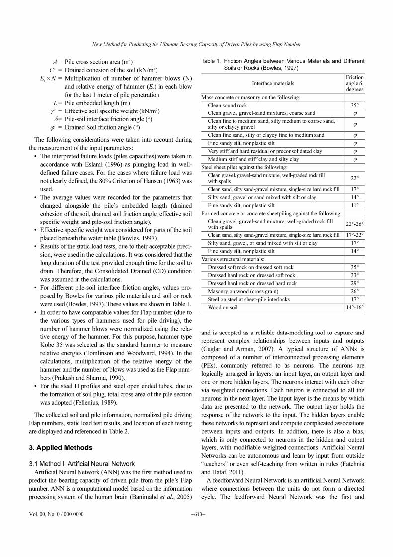
2. Pile and Soil Information

The information of a hundred concrete and steel piles was

collected. The geometrical characteristics of the pile, physical

properties of the soil, Flap numbers and their respective

hammer strike energies, and static pile load test results were

compiled for all 100 piles. We assumed that drained cohesion

of the soil, drained friction angle of the soil, and effective

specific weight were the parameters that described soil

condition; pile cross section and embedded length were the

parameters that described pile geometric size; and pile-soil

friction angle was the parameter that described pile material.

Besides the selected parameters, Flap number was assumed to

represent all other unseen effective factors in measurement of

pile bearing capacity.

The seven parameters selected for the pile bearing capacity

estimations were

New Method for Predicting the Ultimate Bearing Capacity of Driven Piles by using Flap Number

Vol. 00, No. 0 / 000 0000 −613−

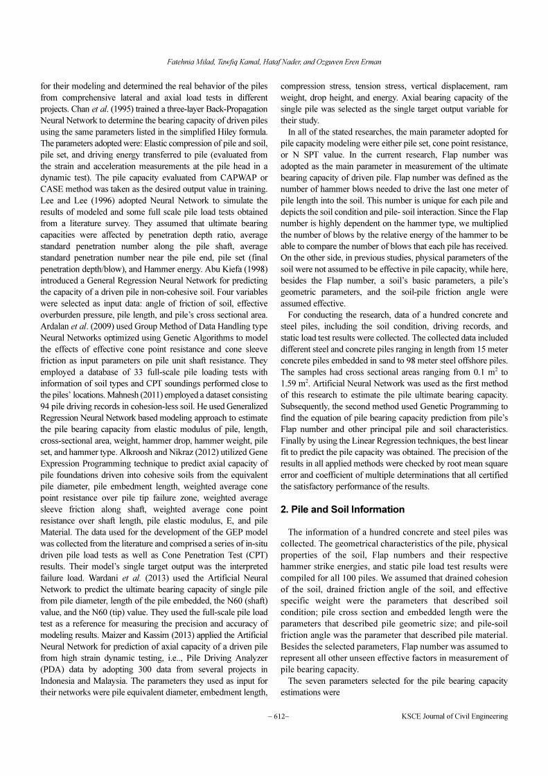
A = Pile cross section area (m2)

= Drained cohesion of the soil (kN/m2)

= Multiplication of number of hammer blows (N)

and relative energy of hammer (Er) in each blow

for the last 1 meter of pile penetration

L = Pile embedded length (m)

= Effective soil specific weight (kN/m3)

δ= Pile-soil interface friction angle (°)

= Drained Soil friction angle (°)

The following considerations were taken into account during

the measurement of the input parameters:

• The interpreted failure loads (piles capacities) were taken in

accordance with Eslami (1996) as plunging load in well-

defined failure cases. For the cases where failure load was

not clearly defined, the 80% Criterion of Hansen (1963) was

used.

• The average values were recorded for the parameters that

changed alongside the pile’s embedded length (drained

cohesion of the soil, drained soil friction angle, effective soil

specific weight, and pile-soil friction angle).

• Effective specific weight was considered for parts of the soil

placed beneath the water table (Bowles, 1997).

• Results of the static load tests, due to their acceptable preci-

sion, were used in the calculations. It was considered that the

long duration of the test provided enough time for the soil to

drain. Therefore, the Consolidated Drained (CD) condition

was assumed in the calculations.

• For different pile-soil interface friction angles, values pro-

posed by Bowles for various pile materials and soil or rock

were used (Bowles, 1997). These values are shown in Table 1.

• In order to have comparable values for Flap number (due to

the various types of hammers used for pile driving), the

number of hammer blows were normalized using the rela-

tive energy of the hammer. For this purpose, hammer type

Kobe 35 was selected as the standard hammer to measure

relative energies (Tomlinson and Woodward, 1994). In the

calculations, multiplication of the relative energy of the

hammer and the number of blows was used as the Flap num-

bers (Prakash and Sharma, 1990).

• For the steel H profiles and steel open ended tubes, due to

the formation of soil plug, total cross area of the pile section

was adopted (Fellenius, 1989).

The collected soil and pile information, normalized pile driving

Flap numbers, static load test results, and location of each testing

are displayed and referenced in Table 2.

3. Applied Methods

3.1 Method I: Artificial Neural Network

Artificial Neural Network (ANN) was the first method used to

predict the bearing capacity of driven pile from the pile’s Flap

number. ANN is a computational model based on the information

processing system of the human brain (Banimahd et al., 2005)

and is accepted as a reliable data-modeling tool to capture and

represent complex relationships between inputs and outputs

(Caglar and Arman, 2007). A typical structure of ANNs is

composed of a number of interconnected processing elements

(PEs), commonly referred to as neurons. The neurons are

logically arranged in layers: an input layer, an output layer and

one or more hidden layers. The neurons interact with each other

via weighted connections. Each neuron is connected to all the

neurons in the next layer. The input layer is the means by which

data are presented to the network. The output layer holds the

response of the network to the input. The hidden layers enable

these networks to represent and compute complicated associations

between inputs and outputs. In addition, there is also a bias,

which is only connected to neurons in the hidden and output

layers, with modifiable weighted connections. Artificial Neural

Networks can be autonomous and learn by input from outside

“teachers” or even self-teaching from written in rules (Fatehnia

and Hataf, 2011).

A feedforward Neural Network is an artificial Neural Network

where connections between the units do not form a directed

cycle. The feedforward Neural Network was the first and

C′

Er N×

γ ′

ϕ′

Table 1. Friction Angles between Various Materials and Different

Soils or Rocks (Bowles, 1997)

Interface materialsFriction angle δ, degrees

Mass concrete or masonry on the following:

Clean sound rock 35°

Clean gravel, gravel-sand mixtures, coarse sand ϕ

Clean fine to medium sand, silty medium to coarse sand,silty or clayey gravel

ϕ

Clean fine sand, silty or clayey fine to medium sand ϕ

Fine sandy silt, nonplastic silt ϕ

Very stiff and hard residual or preconsolidated clay ϕ

Medium stiff and stiff clay and silty clay ϕ

Steel sheet piles against the following:

Clean gravel, gravel-sand mixture, well-graded rock fill with spalls

22°

Clean sand, silty sand-gravel mixture, single-size hard rock fill 17°

Silty sand, gravel or sand mixed with silt or clay 14°

Fine sandy silt, nonplastic silt 11°

Formed concrete or concrete sheetpiling against the following:

Clean gravel, gravel-sand mixture, well-graded rock fillwith spalls

22°-26°

Clean sand, silty sand-gravel mixture, single-size hard rock fill 17°-22°

Silty sand, gravel, or sand mixed with silt or clay 17°

Fine sandy silt, nonplastic silt 14°

Various structural materials:

Dressed soft rock on dressed soft rock 35°

Dressed hard rock on dressed soft rock 33°

Dressed hard rock on dressed hard rock 29°

Masonry on wood (cross grain) 26°

Steel on steel at sheet-pile interlocks 17°

Wood on soil 14°-16°


−614− KSCE Journal of Civil Engineering

Table 2. 100 Pile Capacities for Different Flap Numbers, Soil Properties, and Pile Information

Pile No.

LocationPile

Material

Average Cohesion (kN/m2)

Average Friction angle (°)

Average soil Specific weight

(kN/m3)

Average Pile-Soil friction

angle (°)

Flap Number

Pile Area (m2)

Pile Length (m)

Pile Capacity

(kN)

1

Haraz-Iran

Steel 033 28.85 09.82 12.49 20.1 0.1 19.5 1040

2 Steel 033 29.89 09.73 12.41 27 0.1 23.5 1400

3 Steel 033 28.81 09.82 12.49 20 0.1 19.4 990

4 Steel 00 28 09.57 12.27 21 0.1 19.5 960

5 Steel 00 28 09.69 12.22 24 0.1 23.5 1330

6 Steel 63 05 09.69 11.2 40 0.1 19.4 1230

7

Mahshahr-Iran

Concrete 06.37 29.84 09.7 14 177 0.16 25.3 3335

8 Concrete 06.8 29.3 09.92 14 61 0.16 21.5 2000

9 Concrete 06.4 29.78 09.73 14 180 0.16 24.9 3142

10 Concrete 07 29 10.03 14 80 0.16 19.9 2520

11 Concrete 06.64 29.48 09.84 14 115 0.16 22.7 2840

12 Concrete 06.4 29.8 09.72 14 250 0.16 25 3867

13 Concrete 06.34 29.87 09.69 14 202 0.16 25.6 4012

14 Concrete 06.65 29.46 09.85 14 69 0.16 22.6 2278

15 Concrete 07 29 10.34 14 50 0.16 15.2 1900

16

Mahshahr-Iran

Concrete 138 4.23 07.52 14 246 0.16 22.9 2500

17 Concrete 142 4.14 07.55 14 210 0.16 23.4 2250

18 Concrete 148 4.03 07.58 14 306 0.16 24 2700

19 Gulf of Mexico(Stockard, 1979)

Steel 08.7 24 08.55 11.75 790 0.89 61 19000

20 Steel 07.72 26.04 09.54 12.84 632 0.89 82 24900

21

India(Stockard, 1986)

Steel 01.4 29.39 09.1 13.75 1360 1.59 98 48470

22 Steel 01.58 27.67 08.66 12.68 1300 1.17 98 36250

23 Steel 04.87 26.77 08.81 12.1 2130 1.59 98 52100

24 Steel 02.76 28.39 08.93 13.12 1750 1.59 90 49350

25

Alton-Illinois(Larry, 1988)

Steel 07.47 35.99 12.91 16.68 178 0.1 18 5900

26 Steel 06.59 35.64 12.92 16.13 178 0.1 20.4 6200

27 Steel 06.71 35.69 12.92 16.2 180 0.1 20 6120

28 Steel 07.78 36.62 13.19 17 86 0.1 16.1 4280

29 Steel 07.78 36.62 13.15 17 70 0.1 16.4 3130

30 Steel 07.83 36.56 13.49 17 29 0.07 14.2 1321

31 Steel 07.83 36.57 13.46 17 63 0.1 14.4 1300

32 Steel 07.79 36.6 13.27 17 49 0.13 15.6 1830

33 Illinois(Fellenius, 1989)

Steel 14.6 32.22 09.89 13.75 16 0.16 15.2 1043

34 Steel 14.6 32.22 09.89 13.75 15 0.1 15.2 987

35

Bandar Imam-Iran

Concrete 51.4 00 11.19 14 361 0.16 24.5 2030

36 Concrete 26 00 11.68 14 110 0.16 16 1145

37 Concrete 54.8 00 11.15 14 482 0.16 25.9 2250

38 Concrete 0.07 22.43 11.33 15.45 328 0.16 25.5 2600

39 Concrete 0.06 23.79 11.26 15.51 202 0.16 28.5 2200

40

Bandar Imam-Iran

Concrete 51.8 11.81 07.3 14.88 234 0.16 26.5 2920

41 Concrete 51 12.24 07.36 15.02 263 0.16 27.2 2880

42 Concrete 58.6 11.43 08.34 14.59 112 0.16 14.5 680

43 Concrete 58.5 11.38 08.29 14.58 78 0.16 14.7 540

44

Shiraz-Iran

Concrete 136 27.82 08.94 14 167 0.16 18.2 2100

45 Concrete 137 27.1 08.84 14 94 0.16 19.5 1700

46 Concrete 138 29.3 09.21 14 98 0.16 15.9 2200

47 Ontario(Fellenius and Altaee, 2002)

Steel 18.2 20 05.45 13.75 78 0.09 60 2750

48 Steel 17.9 19.76 05.43 13.82 87 0.09 62 2870

49 Steel 17 18.93 05.38 14.07 96 0.09 70 3050


Vol. 00, No. 0 / 000 0000 −615−

Table 2. continued

Pile No.

LocationPile

Material

Average Cohesion (kN/m2)

Average Friction angle (°)

Average soil Specific weight

(kN/m3)

Average Pile-Soil friction

angle (°)

Flap Number

Pile Area (m2)

Pile Length (m)

Pile Capacity

(kN)

50

Bandar Abbas-Iran

Steel 45.8 31.11 11.23 10.14 406 0.78 20.5 2670

51 Steel 49.8 31.01 11.2 12.47 670 1.16 22.5 3350

52 Steel 45.8 31.11 11.23 10.14 730 0.78 20.5 3750

53 Steel 45.8 31.11 11.23 10.14 1236 0.78 20.5 4100

54 Steel 45.8 31.11 11.23 10.14 710 0.78 20.5 3450

55 Steel 45.2 31.12 11.23 12.63 756 0.78 20.2 3570

56 Steel 48.8 31.03 11.21 12.5 1030 1.16 22 3570

57 Steel 44.7 31.14 11.24 12.65 1463 1.16 20 4936

58 Steel 51.5 30.97 11.2 12.4 1448 1.16 23.5 4900

59 Steel 49.8 31.01 11.2 12.47 1298 1.16 22.5 4650

60 Steel 41.1 31.23 11.25 12.78 1610 1.16 18.5 2150

61 Steel 42.4 31.2 11.24 12.74 1590 1.16 19 4150

62 Steel 45.8 31.11 11.23 10.14 701 0.89 20.5 3600

63 Steel 44.7 31.14 11.24 12.65 1112 0.89 20 4000

64 Steel 49.8 31.01 11.2 12.47 990 1.16 22.5 3870

65

Bandar Imam-Iran

Concrete 08.21 25.02 09.045 12.295 510 0.89 71.5 21965

66 Concrete 06.58 29.57 09.81 14 65 0.16 23.4 2682.5

67 Concrete 06.7 29.39 09.88 14 72 0.16 22.4 2846

68 Concrete 06.52 29.64 09.78 14 97 0.16 23.8 3368.5

69 Concrete 07.03 35.815 12.915 16.405 423 0.1 19.2 6065

70 Concrete 06.49 29.665 09.77 14 70 0.16 24.1 3160

71 Concrete 08.59 16.615 08.93 14 113 0.16 19 2215

72 Concrete 09.2 4.083 07.565 14 186 0.16 23.7 2490

73 Concrete 07.24 36.155 13.055 16.6 321 0.1 18.1 5215

74 Concrete 07.8 36.59 13.32 17 116 0.08 15.3 2240.5

75 Concrete 07.81 36.585 13.365 17 132 0.11 15 1580

76

Mahshahr-Iran

Steel 24.6 32.22 09.89 13.75 56 0.13 15.2 1030

77 Steel 33.7 0 11.432 14 306 0.16 20.2 1602.5

78 Steel 27.4 11.215 11.24 14.725 505 0.16 25.7 2440

79 Steel 21.49 28.53 08.88 13.215 1106 1.38 32.2 4275

80 Steel 23.81 27.58 08.8715 12.61 1323 1.59 36.5 5740

81 Steel 25.9 17.8 09.28 15.195 196 0.16 27.5 2575

82 Steel 27.4 19.6 08.615 14.29 153 0.16 16.4 1335

83

Isfahan-Iran

Concrete 38 28.2 09.025 14 196 0.16 23.7 1965

84 Concrete 28.1 19.88 05.44 13.785 70 0.09 27 2825

85 Concrete 31.4 25.02 08.305 12.105 725 0.44 25 2875

86 Concrete 45.8 31.11 11.23 10.14 2291 0.78 35.5 3790

87 Concrete 54.8 11.835 07.85 14.805 123 0.16 37.8 1795

88

Bandar Abbas-Iran

Steel 47.8 31.06 11.215 11.305 1631 0.97 21.5 3565

89 Steel 47 31.075 11.22 12.565 2078 0.97 21.1 3585

90 Steel 48.1 31.055 11.217 12.525 2147 1.16 21.7 3870

91 Steel 45.4 31.12 10.967 12.625 2243 1.16 20.5 3415

92 Steel 44.1 31.155 11.235 11.44 1009 1.02 19.7 5465

93 Steel 49.8 31.01 11.2 12.47 849 1.16 22.5 4275

94 Steel 31.1 34.42 11.54 15.375 131 0.1 15.7 2648.5

95 Steel 29.6 18.31 12.17 15.5 291 0.13 20.4 2595

96

Isfahan-Iran

Concrete 33 29.37 09.775 12.45 14 0.1 21.5 1235

97 Concrete 28.5 28.405 09.695 12.38 14 0.1 19.4 1145

98 Concrete 31.5 16.5 09.69 11.71 22 0.1 21.4 1295

99 Concrete 26.9 18.28 12.582 15.5 131 0.11 15.1 1248

100 Concrete 31.3 18.285 12.305 15.5 320 0.13 20.1 1790



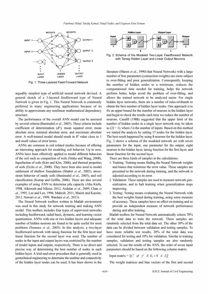
arguably simplest type of artificial neural network devised. A

general sketch of a 3-layered feedforward type of Neural

Network is given in Fig. 1. This Neural Network is commonly

preferred in many engineering applications because of its

ability to approximate any nonlinear mathematical dependency

structure.

The performance of the overall ANN model can be assessed

by several criteria (Banimahd et al., 2005). These criteria include

coefficient of determination (R2), mean squared error, mean

absolute error, minimal absolute error, and maximum absolute

error. A well-trained model should result in R2 value close to 1

and small values of error terms.

ANNs are common in soil related studies because of offering

an interesting approach for modeling soil behavior. Up to now,

ANNs have been effectively applied to model different behaviors

of the soil such as compaction of soils (Sinha and Wang, 2008),

liquefaction of soils (Kim and Kim, 2006), and thermal properties

of soils (Erzin et al., 2008). They have been also used to model

settlement of shallow foundations (Shahin et al., 2002), stress-

strain behavior of sandy soils (Banimahd et al., 2005), and soil

classification (Kurup and Griffin, 2006). There are also several

examples of using ANN to determine pile capacity (Abu Kiefa,

1998, Alkroosh and Nikraz, 2012, Ardalan et al., 2009, Chan et

al., 1995, Lee and Lee, 1996, Mahesh, 2011, Maizir and Kassim,

2013, Nawari et al., 1999, Wardani et al., 2013).

The Neural Network toolbox written in Matlab environment

was used in this study for network training and making ANN

model. This toolbox includes four types of supervised networks

including feedforward, radial basis, dynamic, and learning vector

quantization. ANNs with one or two hidden layers and adequate

number of hidden neurons are found to be quite useful for most

problems (Sonmez et al., 2005). In this analysis, a two-layer

feedforward network with tansig function for the first layer and

linear function for the second layer was used. The number of

nodes in the input and output layers was restricted by the number

of model inputs and outputs, respectively. There is no direct and

precise way of determining the best number of nodes in each

hidden layer. A trial-and-error procedure that is generally used in

geotechnical engineering to determine the number and connectivity

of the hidden layer nodes can be used. It has been shown in the

literature (Maren et al., 1990) that Neural Networks with a large

number of free parameters (connection weights) are more subject

to over-fitting and poor generalization. Consequently, keeping

the number of hidden nodes to a minimum, reduces the

computational time needed for training, helps the network

perform better, helps avoid the problem of over-fitting, and

allows the trained network to be analyzed easier. For single

hidden layer networks, there are a number of rules-of-thumb to

obtain the best number of hidden layer nodes. One approach is to

fix an upper bound for the number of neurons in the hidden layer

and begin to check the results each time we reduce the number of

neurons. Caudill (1988) suggested that the upper limit of the

number of hidden nodes in a single layer network may be taken

as (2I + 1), where I is the number of inputs. Based on this method

we started the analysis by setting 15 nodes for the hidden layer.

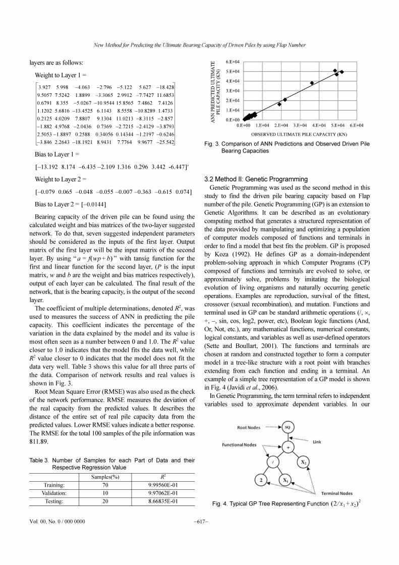
The best result happened by using 8 neurons for the hidden layer.

Fig. 2 shows a schema of the modeled network set with seven

parameters for the input, one parameter for the output, eight

neurons in the hidden layer, tansig function for the first layer, and

linear function for the second layer.

There are three kinds of samples in the calculations:

1. Training: Training means finding the Neural Network weights

and biases that minimize the error value. These samples are

presented to the network during training, and the network is

adjusted according to its error.

2. Validation: These samples are used to measure network gen-

eralization, and to halt training when generalization stops

improving.

3. Testing: Testing means evaluating the Neural Network with

the best weights found during training, using some measure

of accuracy. These samples have no effect on training and so

provide an independent measure of network performance

during and after training.

Matlab toolbox for Neural Network automatically selects 70%

of the total data to train the network. These samples are

randomly selected from the total data set. The other 30% of the

data can be divided between validation and testing samples. To

have more reliable test results, 20% of the total data was

considered for testing and 10% for validation. Similar to training

samples, validation and testing samples are also randomly

selected. To use the results of the ANN, the order of seven input

parameters should be based on the following column matrix:

Input matrix =

The weight matrices and bias vectors of the first and second

C′ ϕ′ γ ′ δ Er N × A L[ ]′

Fig. 1. Three-Layered Feed-Forward Network

Fig. 2. Schema of the Modeled Two-Layer Feedforward Network

with Tansig Hidden Layer and Linear Output Neurons


Vol. 00, No. 0 / 000 0000 −617−

layers are as follows:

Weight to Layer 1 =

Bias to Layer 1 =

Weight to Layer 2 =

Bias to Layer 2 =

Bearing capacity of the driven pile can be found using the

calculated weight and bias matrices of the two-layer suggested

network. To do that, seven suggested independent parameters

should be considered as the inputs of the first layer. Output

matrix of the first layer will be the input matrix of the second

layer. By using “ ” with tansig function for the

first and linear function for the second layer, (P is the input

matrix, w and b are the weight and bias matrices respectively),

output of each layer can be calculated. The final result of the

network, that is the bearing capacity, is the output of the second

layer.

The coefficient of multiple determinations, denoted R2, was

used to measures the success of ANN in predicting the pile

capacity. This coefficient indicates the percentage of the

variation in the data explained by the model and its value is

most often seen as a number between 0 and 1.0. The R2 value

closer to 1.0 indicates that the model fits the data well, while

R2 value closer to 0 indicates that the model does not fit the

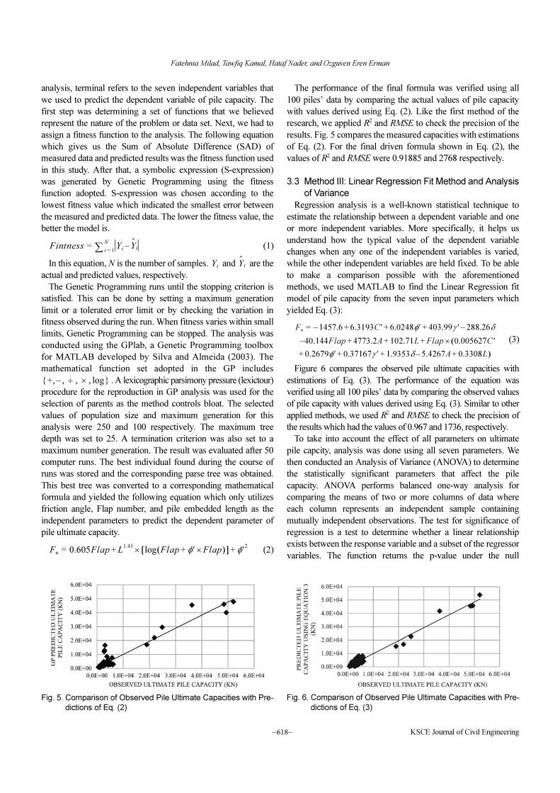
data very well. Table 3 shows this value for all three parts of

the data. Comparison of network results and real values is

shown in Fig. 3.

Root Mean Square Error (RMSE) was also used as the check

of the network performance. RMSE measures the deviation of

the real capacity from the predicted values. It describes the

distance of the entire set of real pile capacity data from the

predicted values. Lower RMSE values indicate a better response.

The RMSE for the total 100 samples of the pile information was

811.89.

3.2 Method II: Genetic Programming

Genetic Programming was used as the second method in this

study to find the driven pile bearing capacity based on Flap

number of the pile. Genetic Programming (GP) is an extension to

Genetic Algorithms. It can be described as an evolutionary

computing method that generates a structured representation of

the data provided by manipulating and optimizing a population

of computer models composed of functions and terminals in

order to find a model that best fits the problem. GP is proposed

by Koza (1992). He defines GP as a domain-independent

problem-solving approach in which Computer Programs (CP)

composed of functions and terminals are evolved to solve, or

approximately solve, problems by imitating the biological

evolution of living organisms and naturally occurring genetic

operations. Examples are reproduction, survival of the fittest,

crossover (sexual recombination), and mutation. Functions and

terminal used in GP can be standard arithmetic operations (/, ×,

+, −, sin, cos, log2, power, etc), Boolean logic functions (And,

Or, Not, etc.), any mathematical functions, numerical constants,

logical constants, and variables as well as user-defined operators

(Sette and Boullart, 2001). The functions and terminals are

chosen at random and constructed together to form a computer

model in a tree-like structure with a root point with branches

extending from each function and ending in a terminal. An

example of a simple tree representation of a GP model is shown

in Fig. 4 (Javidi et al., 2006).

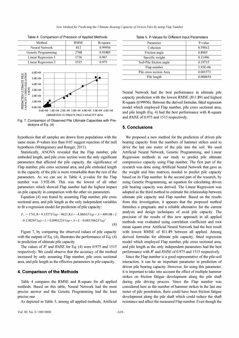
In Genetic Programming, the term terminal refers to independent

variables used to approximate dependent variables. In our

3.927 5.998 4.063– 2.796– 5.122– 5.627 18.428–

9.5057 7.5242 1.8899 3.3065– 2.9912 7.7427– 11.6853

0.6791 8.355 5.0267– 10.9544– 15.8565 7.4862 7.4126

1.1202 5.6816 13.4525– 6.1143 8.5558 10.8289– 1.4733

0.2125 4.0209 7.8807 9.1304 11.0213 8.3115– 2.857–

1.882– 4.9768 2.0436– 0.7369 2.7215– 2.4129– 3.8793–

2.5053 1.8897– 0.2588 0.34056 0.14344 1.2197– 0.6246–

3.846– 2.2643 18.1921– 8.9431 7.7764 9.9677 25.542–

13.192 – 8.174 6.435 – 2.109 – 1.316 0.296 3.442 -6.447[ ]′

0.079– 0.065 0.048 – 0.055 – 0.007 – 0.363 – 0.615 – 0.074[ ]

0.0144–[ ]

a f wp b+( )=

Table 3. Number of Samples for each Part of Data and their

Respective Regression Value

Samples(%) R2

Training: 70 9.99560E-01

Validation: 10 9.97062E-01

Testing: 20 8.66835E-01

Fig. 3. Comparison of ANN Predictions and Observed Driven Pile

Bearing Capacities

Fig. 4. Typical GP Tree Representing Function 2 x1⁄ x2+( )2



analysis, terminal refers to the seven independent variables that

we used to predict the dependent variable of pile capacity. The

first step was determining a set of functions that we believed

represent the nature of the problem or data set. Next, we had to

assign a fitness function to the analysis. The following equation

which gives us the Sum of Absolute Difference (SAD) of

measured data and predicted results was the fitness function used

in this study. After that, a symbolic expression (S-expression)

was generated by Genetic Programming using the fitness

function adopted. S-expression was chosen according to the

lowest fitness value which indicated the smallest error between

the measured and predicted data. The lower the fitness value, the

better the model is.

(1)

In this equation, N is the number of samples. and are the

actual and predicted values, respectively.

The Genetic Programming runs until the stopping criterion is

satisfied. This can be done by setting a maximum generation

limit or a tolerated error limit or by checking the variation in

fitness observed during the run. When fitness varies within small

limits, Genetic Programming can be stopped. The analysis was

conducted using the GPlab, a Genetic Programming toolbox

for MATLAB developed by Silva and Almeida (2003). The

mathematical function set adopted in the GP includes

. A lexicographic parsimony pressure (lexictour)

procedure for the reproduction in GP analysis was used for the

selection of parents as the method controls bloat. The selected

values of population size and maximum generation for this

analysis were 250 and 100 respectively. The maximum tree

depth was set to 25. A termination criterion was also set to a

maximum number generation. The result was evaluated after 50

computer runs. The best individual found during the course of

runs was stored and the corresponding parse tree was obtained.

This best tree was converted to a corresponding mathematical

formula and yielded the following equation which only utilizes

friction angle, Flap number, and pile embedded length as the

independent parameters to predict the dependent parameter of

pile ultimate capacity.

(2)

The performance of the final formula was verified using all

100 piles’ data by comparing the actual values of pile capacity

with values derived using Eq. (2). Like the first method of the

research, we applied R2 and RMSE to check the precision of the

results. Fig. 5 compares the measured capacities with estimations

of Eq. (2). For the final driven formula shown in Eq. (2), the

values of R2 and RMSE were 0.91885 and 2768 respectively.

3.3 Method III: Linear Regression Fit Method and Analysis

of Variance

Regression analysis is a well-known statistical technique to

estimate the relationship between a dependent variable and one

or more independent variables. More specifically, it helps us

understand how the typical value of the dependent variable

changes when any one of the independent variables is varied,

while the other independent variables are held fixed. To be able

to make a comparison possible with the aforementioned

methods, we used MATLAB to find the Linear Regression fit

model of pile capacity from the seven input parameters which

yielded Eq. (3):

(3)

Figure 6 compares the observed pile ultimate capacities with

estimations of Eq. (3). The performance of the equation was

verified using all 100 piles’ data by comparing the observed values

of pile capacity with values derived using Eq. (3). Similar to other

applied methods, we used R2 and RMSE to check the precision of

the results which had the values of 0.967 and 1736, respectively.

To take into account the effect of all parameters on ultimate

pile capcity, analysis was done using all seven parameters. We

then conducted an Analysis of Variance (ANOVA) to determine

the statistically significant parameters that affect the pile

capacity. ANOVA performs balanced one-way analysis for

comparing the means of two or more columns of data where

each column represents an independent sample containing

mutually independent observations. The test for significance of

regression is a test to determine whether a linear relationship

exists between the response variable and a subset of the regressor

variables. The function returns the p-value under the null

Fintnessi 1=

NYi Yi–∑=

Yi Yi

+ – ÷ × log, , , ,{ }

Fu 0.605Flap L1.43

log Flap φ′ Flap×+( )[ ] φ′2

+×+=

Fu

1457.6– 6.3193C′ 6.0248φ′ 403.99γ ′ 288.26δ–+ + +=

40.144Flap 4773.2A 102.71L Flap 0.005627C( ′×+ + +–

0.2679φ′ 0.37167γ ′ 1.9353δ 5.4267A– 0.3308L)+ + + +

Fig. 5. Comparison of Observed Pile Ultimate Capacities with Pre-

dictions of Eq. (2)


dictions of Eq. (3)


Vol. 00, No. 0 / 000 0000 −619−

hypothesis that all samples are drawn from populations with the

same mean. P-values less than 0.05 suggest rejection of the null

hypothesis (Montgomery and Runger, 2011).

Statistically, ANOVA revealed that the Flap number, pile

embeded length, and pile cross section were the only significant

parameters that affected the pile capacity. the significance of

Flap number, pile cross sectional area, and pile embeded length

in the capacity of the pile is more remarkable than the rest of the

parameters. As we can see in Table 4, p-value for the Flap

number was 3.93E-06. This was the lowest of all other

parameters which showed Flap number had the highest impact

on pile capacity in comparison with the other six parameters.

Equation (4) was found by assuming Flap number, pile cross

sectional area, and pile length as the only independent variables

to fit a regression model for prediction of pile capacity:

(4)

Figure 7, by comparing the observed values of pile capacity

with the outputs of Eq. (4), illustrates the performance of Eq. (4)

in prediction of ultimate pile capacity.

The values of R2 and RMSE for Eq. (4) were 0.975 and 1515

respectively. We could observe that the accuracy of the method

increased by only assuming Flap number, pile cross sectional

area, and pile length as the effective parameters in pile capacity.

4. Comparison of the Methods

Table 4 compares the RMSE and R-square for all applied

methods. Based on this table, Neural Network had the most

precise answer and the Genetic Programming had the least

precise one.

As depicted in Table 5, among all applied methods, Artificial

Neural Network had the best performance in ultimate pile

capacity prediction with the lowest RMSE (811.89) and highest

R-square (0.99956). Between the derived formulas, fitted regression

model which employed Flap number, pile cross sectional area,

and pile length (Eq. 4) had the best performance with R-square

and RMSE of 0.975 and 1515 respectively.

5. Conclusions

We proposed a new method for the prediction of driven pile

bearing capacity from the numbers of hammer strikes used to

drive the last one meter of the pile into the soil. We used

Artificial Neural Network, Genetic Programming, and Linear

Regression methods in our study to predict pile ultimate

compressive capacity using Flap number. The first part of the

research was done using Artificial Neural Network that gave us

the weight and bias matrices needed to predict pile capacity

based on its Flap number. In the second part of the research, by

using Genetic Programming, an equation for calculating driven

pile bearing capacity was derived. The Linear Regression was

adopted as the third method to estimate the relationship between

ultimate pile capacity and Flap number. Based on the results

from this investigation, it appears that the proposed method

furnishes a pragmatic and a reliable alternative for the current

analysis and design techniques of axial pile capacity. The

precision of the results of this new approach in all applied

methods was evaluated using correlation coefficient and root

mean square error. Artificial Neural Network had the best result

with lowest RMSE of 811.89 between all applied. Among

derived formulas for ultimate pile capacity, fitted regression

model which employed Flap number, pile cross sectional area,

and pile length as the only independent parameters had the best

performance with R2 and RMSE of 0.975 and 1515 respectively.

Since the Flap number is a good representative of the pile-soil

interaction, it can be an important parameter in prediction of

driven pile bearing capacity. However, for using this parameter,

it is important to take into account the effect of multiple hammer

strikes on friction fatigue development along the pile shaft

during pile driving process. Since the Flap number was

considered here as the number of hammer strikes in the last one

meter of pile penetration, there could have been friction fatigue

development along the pile shaft which could reduce the shaft

resistance and affect the measured Flap number. Even though the

Fu

1741.8 9.1557Flap 9623.8A– 4.0601Flap– A× 409.08 L×+ + +=

0.13829Flap L× 0.090122Flap A L 0.0013062Flap2

–××+–

Table 4. Comparison of Precision of Applied Methods

Method RMSE R-square

Neural Network 812 0.99956

Genetic Programming 2768 0.91885

Linear Regression 1 1736 0.967

Linear Regression 2 1515 0.975


dictions of Eq. (4)

Table 5. P-Values for Different Input Parameters

Parameter P-value

Cohesion 0.59012

Friction angle 0.8905

Specific weight 0.11496

Soil-Pile friction angle 0.19715

Flap number 3.93E-06

Pile cross section Area 0.001571

Pile length 0.000654


−620 KSCE Journal of Civil Engineering

pile capacity derived from the static load tests was used as the

output of the utilized networks and modeling’s of this study,

there is still a need to do more studies on applicability of using

Flap number for friction piles capacity modeling.

References

Abu Kiefa, M. A. (1998). “General regression neural networks for

driven piles in cohessionless soils.” Journal of Geotechnical and

Geoenvironmental Engineering, Vol. 124, No. 12, pp. 1177-1185.

Alkroosh, I. and Nikraz, H. (2012). “Predicting axial capacity of driven

piles in cohesive soils using intelligent computing.” Journal of

Engineering Applications of Artificial Intelligence, Vol. 25, pp. 618-

627.

Ardalan, H., Eslami, A., and Nariman-Zadeh, N. (2009). “Piles shaft

capacity from CPT and CPTu data by polynomial neural networks

and genetic algorithms.” Computers and Geotechnics, Vol. 36, pp.

616-625.

Banimahd, M., Yasrobi, S. S., and Woodward P. (2005). “Artificial

neural network for stress-strain behavior of sandy soils: Knowledge

based verification.” Computers and Geotechnics, Vol. 32, No. 5, pp.

377-386.

Bowles, J. E. (1997). Foundation analysis and design, McGraw-Hill,

Peoria, IL.

Caglar, N. and Arman, H. (2007). “The applicability of neural networks

in the determination of soil properties.” Bulletin of Engineering

Geology and the Environment, Vol. 66, No. 1, pp. 295-301.

Caudill, M. (1988). “Neural networks primer: Part III.” AI Expert, pp.

52-59.

Chan, W. T., Chow, Y. K., and Liu, L. F. (1995). “Neural network: An

alternative to pile driving formulas.” Computers and Geotechnics,

Vol. 17, pp. 135-156.

Erzin, Y., Rao, B. H., and Singh, D. N. (2008). “Artificial neural networks

for predicting soil thermal resistivity.” International Journal of

Thermal Sciences, Vol. 47, No. 10, pp. 1347-1358.

Eslami, A. (1996). Bearing capacity of piles from cone penetration data,

PhD Thesis, University of Ottawa, Ottawa, Canada.

Fatehnia, M. and Hataf, N. (2011). “Determination of the compressive

capacity of driven piles using flap number.” Proc., Int. Conf. on

Advances in Geotechnical Engineering, Curtin University, Perth,

Australia, pp. 1027-1032.

Fellenius, B. H. (1989). “Predicted and observed axial behavior of

piles.” Proc., Symp. on Driven Pile Bearing Capacity Prediction,

American Society of Civil Engineers, New York, pp. 75-115.

Fellenius, B. H. and Altaee, A. (2002). “Pile dynamics in geotechnical

practice - six case histories.” Proc., Int. Deep Foundation Cong.,

Down to Earth Technology, American Society of Civil Engineers,

Orlando, Florida, pp. 619-633.

Hansen, B. J. (1963). “Discussion on hyperbolic stress-strain response,

cohesive soils.” Soil Mechanics and Foundation Engineering, Vol.

89, No. 4, pp. 241-242.

Javidi, A. A., Rezania, M., and Mousavi Nezhad, M. (2006). “Evaluation

of liquefaction induced lateral displacements using genetic

programming.” Computers and Geotechnics, Vol. 33, Nos. 4-5, pp.

222-233.

Kim, Y. S. and Kim, B. T. (2006). “Use of artificial neural networks in

the prediction of liquefaction resistance of sands.” Journal of

Geotechnical and Geoenvironmental Engineering, Vol. 132, No. 11,

pp. 1502-1504.

Koza, J. R. (1992). Genetic programming: On the programming of

computers by means of natural selection, MIT press, Cambridge,

MA.

Kurup, P. U. and Griffin, E. P. (2006). “Prediction of soil composition

from CPT data using general regression neural network.” Journal of

Computing in Civil Engineering, Vol. 20, No. 4, pp. 281-289.

Larry, M. (1988). Analysis of the pile load test at the lock and dam 26

replacement project, Research Report 4690F, Texas A&M University,

Texas, pp. 15-33.

Lee, I. M. and Lee, J. H. (1996). “Prediction of pile bearing capacity

using artificial neural networks.” Computers and Geotechnic, Vol.

18, No. 3, pp. 189-200.

Mahesh, P. (2011). “Modeling pile capacity using generalized regression

neural network.” Proc., Indian Geotechnical Conference, Kochi,

India, No. N-027, pp. 811-814.

Maizir, H. and Kassim, K. A. (2013). “Neural network application in

prediction of axial bearing capacity of driven piles.” Proc., International

MultiConference of Engineers and Computer Scientists, IMECS,

Hong Kong, Vol. 1.

Maren, A., Harston, C., and Pap, R. (1990). Handbook of neural

computing applications, Academic Press, San Diego, CA.

Montgomery, D. C. and Runger, G. C. (2011). Applied statistics and

probability for engineers, John Wiley & Sons, Hoboken, N. J.

Nawari, N. O., Liang, R., and Nusairat, J. (1999). “Artificial intelligence

techniques for the design and analysis of deep foundations.” The

Electronic Journal of Geotechnical Engineering, Vol. 4.

Prakash, S. and Sharma, H. D. (1990). Pile foundation in engineering

practice, John Wiley & Sons, New York, NY.

Sette, S. and Boullart, L. (2001). “Genetic programming: Principles and

applications.” Journal of Engineering Application and Artificial

Intelligence, Vol. 14, No. 6, pp. 727-736.

Shahin, M. A., Maier, H. R., and Jaksa, M. B. (2002). “Predicting

settlement of shallow foundations using neural networks.” Journal

of Geotechnical and Geoenvironmental Engineering, Vol. 128, No.

9, pp. 785-793.

Silva, S. and Almeida, J. (2003). “GPLAB: A genetic programming

toolbox for MATLAB.” Proc., Nordic MATLAB Conference,

Copenhagen, Denmark, pp. 273-278.

Sinha, S. K. and Wang, M. C. (2008). “Artificial neural network prediction

models for soil compaction and permeability.” Journal of Geotechnical

and Geological Engineering, Vol. 26, pp. 47-64.

Sonmez, H., Gokceoglu, C., Nefeslioglu, H. A., and Kayabasi, A. (2005).

“Estimation of rock modulus: For intact rocks with an artificial

neural network and for rock masses with a new empirical equation.”

International Journal of Rock Mechannics and Mining Science, Vol.

43, No. 2, pp. 224-235.

Stockard, D. M. (1979). “Case histories-pile driving in the gulf of

mexico.” Proc., 11th Annual OTC, Houston, Texas, pp. 737-747.

Stockard, D.M. (1986). “Case histories-pile driving offshore india.”

Proc., 18th Annual OTC, Houston, Texas, pp. 56-68.

Tomlinson, M. J. and Woodward, J. (1994). Pile design and construction

practice, Chapman and Hall, London, England.

Wardani, S. P. R., Surjandari, N. S., and Jajaputra, A. A. (2013).

“Analysis of ultimate bearing capacity of single pile using the

artificial neural networks approach: A case study.” Proc., 18th Int.

Conf. on Soil Mechanics and Geotechnical Engrg., Paris, France,

pp. 837-840.

−

New method for predicting the ultimate bearing capacity of driven piles by using Flap number

Documents

Transcript of New method for predicting the ultimate bearing capacity of driven piles by using Flap number