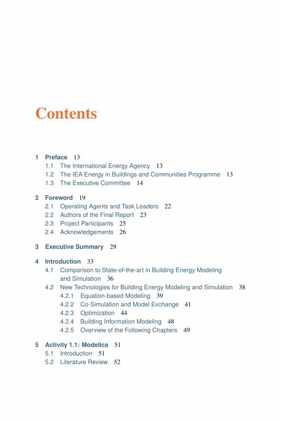
EBC is a programme of the International Energy Agency (IEA)

International Energy Agency

New Generation Computational Tools

for Building & Community Energy Systems

Annex 60 Final Report

September 2017

Cooling and ventilation

Wall

Heating

Weather

wa

lCa

p

V=V_zone

zone

V=V_zone

zone

co

nvR

es

rad

bouAir

T

bouWat

weaDat

wallResTout

heaWat

Q=QHea_nominal

u Q_flow

pump

Pm_flow

K

senTemZonAir

vavDam

M

fan

P

dp_in

dp

window

hexRec

eps=0.85

hysRad

273.15 + 20273.15 + 22

booleanToReal1

BR

not1

not

const_dp

k=A_win*g_win

gaiWin

booleanToInt

BI

conDam

PTSetRoo

cooAir

T Q_flow

TSupAirCoo

weaBus

ISBN 978-0-692-89748-5

Michael Wetter and Christoph van Treeck

International Energy Agency

New Generation Computational Tools

for Building & Community Energy Systems

Annex 60 Final Report

September 2017

Edited by

Michael WetterBuilding Technology and Urban Systems DepartmentEnergy Technologies AreaLawrence Berkeley National Laboratory, USA

Christoph van TreeckChair in Energy Efficiency and Sustainable Building (E3D)RWTH Aachen University, Germany

4

(c) Copyright The Regents of the University of California (through Lawrence BerkeleyNational Laboratory), subject to receipt of any required approvals from U.S. Departmentof Energy, and RWTH Aachen University, Germany, 2017.

All property rights, including copyright, are vested in The Regents of the University of Cali-fornia (through Lawrence Berkeley National Laboratory), subject to receipt of any requiredapprovals from U.S. Department of Energy, and RWTH Aachen University, Germany, Op-erating Agent for EBC Annex 60, on behalf of the Contracting Parties of the InternationalEnergy Agency Implementing Agreement for a Programme of Research and Developmenton Energy in Buildings and Communities.

Published by The Regents of the University of California (through Lawrence BerkeleyNational Laboratory) and RWTH Aachen University, Germany.

Disclaimer Notice: This publication has been compiled with reasonable skill and care.However, neither The Regents of the University of California (through Lawrence BerkeleyNational Laboratory) and RWTH Aachen University, Germany, nor the Contracting Partiesof the International Energy Agency Implementing Agreement for a Programme of Researchand Development on Energy in Buildings and Communities make any representation as tothe adequacy or accuracy of the information contained herein, or as to its suitability for anyparticular application, and accept no responsibility or liability arising out of the use of thispublication. The information contained herein does not supersede the requirements givenin any national codes, regulations or standards, and should not be regarded as a substitutefor the need to obtain specific professional advice for any particular application.

ISBN: 978-0-692-89748-5

Participating countries in EBC: Australia, Austria, Belgium, Canada, P.R. China, CzechRepublic, Denmark, France, Germany, Ireland, Italy, Japan, Republic of Korea, the Nether-lands, New Zealand, Norway, Portugal, Spain, Sweden, Switzerland, United Kingdom andthe United States of America.

Additional copies of this report may be obtained from:

EBC BookshopC/o AECOM LtdThe Colmore BuildingColmore Circus QueenswayBirmingham B4 6ATUnited KingdomWeb: www.iea-ebc.orgEmail: essu@iea-ebc.org

Contents

1 Preface 131.1 The International Energy Agency 131.2 The IEA Energy in Buildings and Communities Programme 131.3 The Executive Committee 14

2 Foreword 192.1 Operating Agents and Task Leaders 222.2 Authors of the Final Report 232.3 Project Participants 252.4 Acknowledgements 26

3 Executive Summary 29

4 Introduction 334.1 Comparison to State-of-the-art in Building Energy Modeling

and Simulation 364.2 New Technologies for Building Energy Modeling and Simulation 38

4.2.1 Equation-based Modeling 394.2.2 Co-Simulation and Model Exchange 414.2.3 Optimization 444.2.4 Building Information Modeling 484.2.5 Overview of the Following Chapters 49

5 Activity 1.1: Modelica 515.1 Introduction 515.2 Literature Review 52

6 CONTENTS

5.3 What is Modelica 555.3.1 Acausal Modeling 575.3.2 Separation of Concerns 675.3.3 Example Model 695.3.4 Model Translation 695.3.5 Use of External Code 735.3.6 Debugging 74

5.4 Annex 60 Library 755.4.1 Approach 765.4.2 Libraries That Use the Annex 60 Library as Their Core 765.4.3 Functional Requirements 775.4.4 Mathematical Requirements 785.4.5 Process for Quality Control 795.4.6 Requirements for Adding Classes 805.4.7 Design Decisions 825.4.8 Main Classes of the Library 855.4.9 Merging with other Libraries 88

5.5 Getting Started 885.5.1 Literature for Users 885.5.2 Literature for Developers 89

5.6 Conclusions 89

6 Activity 1.2: Co-simulation and Model Exchange Using the FMI

Standard 916.1 Introduction 91

6.1.1 Motivation for Coupled Simulation 916.1.2 Need for a Tool Coupling Standard 936.1.3 Overview of the FMI Standard 946.1.4 Mathematical Aspects of Model Exchange and

Co-Simulation 956.1.5 Functional Mockup Interface for Model Exchange 956.1.6 Functional Mockup Interface for Co-Simulation 976.1.7 Master Algorithms 1006.1.8 Exporting and Importing of Functional Mockup Units 103

6.2 Use Cases and Applications 1036.2.1 Simulation-Based Building Operation 103

CONTENTS 7

6.2.2 Design and Operational Analysis of Energy, Controland Communication Grids 104

6.2.3 Co-Simulation via Domus with Modelica, EnergyPlusand ANSYS CFX 106

6.3 FMI-Compliant Tools for Buildings and District Simulation 1076.4 FMU Export Facilities 109

6.4.1 THERAKLES (Room Model) 1096.4.2 NANDRAD (Building Energy Simulation/Multizone) 1106.4.3 EnergyplusToFMU 1116.4.4 FMI++ TRNSYS FMU Export Utility 1116.4.5 FMI++ PowerFactory FMU Export Utility 112

6.5 Simulation Environments and Master Algorithms for FMI 1136.5.1 Building Controls Virtual Test Bed 1136.5.2 EnergyPlus 1146.5.3 DACCOSIM 1156.5.4 Ptolemy II and Quantized State Systems (QSS) 1166.5.5 FUMOLA - The Functional Mock-Up Laboratory 1176.5.6 WRM (Waveform Relaxation Method) as a Proposition

of a Simple Master Algorithm 1186.5.7 Domus 1196.5.8 MasterSim 119

6.6 Desired FMI Features and Proposal of Evolutions of theStandard 120

6.7 Best-Practice Recommendations 1236.7.1 Climate Data Export 1236.7.2 FMI Interfaces for Room and HVAC Systems 123

6.8 Conclusions 125

7 Activity 1.3: BPS Code Generation from Building Information

Models 1277.1 Introduction 1277.2 Building Information Modeling (BIM) 129

7.2.1 What is BIM? 1307.2.2 Changes Within the Planning/Design Process 1337.2.3 Relevant BIM Standards and Implementation

Agreements 136

8 CONTENTS

7.2.4 Review of Existing BIM Tools for Visualization andModel Checking 139

7.3 Importing BIM Data to BPS 1437.3.1 Overall Transformation Process 1437.3.2 Requirements for BPS Models Across Different Stages

of the Building Design Process Based on Uncertainty 1457.3.3 Building Geometry Generation and Processing 1527.3.4 Energy Modeling Using IFC 1537.3.5 Model View Definition (MVD) for Energy Related BIM

Support 1547.3.6 SimModel: A Data Model for BPS 1637.3.7 Formal Transformation Process 167

7.4 Open Framework for Modelica Code Generation from BIM 1727.4.1 Conversion from BIM to BPS 1747.4.2 Data Transformation 1777.4.3 IFC to SimModel 1797.4.4 libSimModel C++ library 1887.4.5 Mapping Rules 1947.4.6 Python Tools for Modelica Code Generation 1987.4.7 Topology Mapping 205

7.5 Use Cases and Demonstration 2127.5.1 Use Case 1.1: Boiler with Radiator 2147.5.2 Use Case 1.2: Boiler with Radiator and Domestic Hot

Water 2177.5.3 Use Case 2.1: Heat Pump with Radiator 2197.5.4 Use Case 2.2: Heat Pump with Underfloor Heating 2207.5.5 Use Case 3: Combined Heat and Power (CHP) Unit 2217.5.6 Use Case 4.1: Air handling Unit for Heating (AHU

Heating) 2227.5.7 Use Case 4.2: Air Handling Unit for Cooling (AHU

Cooling) 2247.5.8 Use Case 5: Multi Zone Model 2267.5.9 Use Case 6: Rooftop Building 230

7.6 Limitations of the Framework and Future Work 2337.6.1 Limitations 2347.6.2 Future Work 234

CONTENTS 9

8 Activity 1.4: Workflow Automation Tools 2378.1 Introduction and Motivation 2378.2 Tools and Methodology 240

8.2.1 Functional Requirements 2408.2.2 Associated Packages 2448.2.3 Third-Party Packages 244

8.3 Examples of Application 2458.3.1 Single Simulation of a Building using BuildingsPy 2468.3.2 Parametric Study using BuildingsPy and ModelicaRes 2538.3.3 Parametric Study of a Boiler FMU from Dymola using

PyFMI 2588.3.4 Import Data to Co-Simulation FMU using PyFMI and

Pandas 2608.4 Summary 266

9 Activity 2.1: Design of Building Systems 2679.1 Introduction 2679.2 Case Studies 268

9.2.1 Development of PV Cooling Systems for ResidentialBuildings in the MENA Region 269

9.2.2 Control Optimization of Geothermal Heat PumpSystems Combined with Thermally Activated BuildingSystems 272

9.2.3 Investigation of the Role of Buildings in an EuropeanGreenhouse Gas Emission Free Energy System 275

9.2.4 Implementation of Model Predictive Control for theHVAC System of a Belgian Thermally Activated OfficeBuilding 278

9.2.5 Modeling for the Design of an Energy and WaterEfficient Hotel 281

9.2.6 Design of an Innovative Two-Pipe Chilled BeamSystem for Simultaneous Heating and Cooling of OfficeBuildings 282

9.2.7 Integrated Optimal Design and Control of OfficeBuildings Using Renewable Energy Sources 286

9.2.8 Development of a Virtual Computational Test-Bed forBuilding Integrated Renewable Energy Solutions 287

10 CONTENTS

9.2.9 Influence of German Energy Saving Ordinances onHeat Demand of a Residential Building 291

9.2.10 Comparative Analysis of all Case Studies 2939.2.11 Reasons for the Use of Modelica 2959.2.12 Drawbacks of Using Modelica 296

9.3 Model Analysis 2989.4 OD/OC Method Analysis 300

9.4.1 Multi-Criteria Optimization of PV-Cooling Systems forResidential Buildings 300

9.4.2 Model Predictive Control Framework 3049.4.3 Optimal Control of Room-Level HVAC and Facade

Control 3069.4.4 Building simulation scenario for optimal design 317

9.5 Summary 326

10 Activity 2.2: Design of District Energy Systems 32910.1 Introduction 32910.2 Description of District Energy Systems 330

10.2.1 Electrical Versus Thermal Energy 33110.2.2 State-Of-The-Art in District Energy Networks 33310.2.3 Components Typically Encountered in District Energy

Systems 33510.2.4 Energy Demand 336

10.3 Modeling of District Heating and Cooling Systems 33810.3.1 Introduction 33810.3.2 Modeling Methodology 33910.3.3 Data Acquisition 34010.3.4 Problems and Challenges 34110.3.5 District Heating and Cooling Modeling Approaches 34210.3.6 Applications of Modelica in District Energy System

Modeling 34610.4 DESTEST 352

10.4.1 Framework 35210.4.2 Definition of Common Exercise: Reference Annex 60

Neighborhood Case 35410.4.3 Annex 60 Neighborhood Case: a Comparative Study 363

CONTENTS 11

10.4.4 Examples of the Use of the Annex 60 NeighborhoodCase 370

10.5 Multi-Physics Simulation of DES in Modelica 38210.6 Co-Simulation of DES 385

10.6.1 Modeling for FMU-Based Co-Simulation 38610.6.2 Computational Experiments 39010.6.3 Conclusion and Perspective on Co-Simulation of DES 394

10.7 Conclusions and Outlook 39510.7.1 Conclusion 39510.7.2 Outlook 397

11 Activity 2.3: Model use During Operation 39911.1 Introduction 399

11.1.1 Model Predictive Control 39911.1.2 Fault Detection and Diagnosis 40011.1.3 Hardware in the Loop 40011.1.4 Overview of Projects that Contributed to the Annex 60

Activity 2.3 40011.2 Background on Areas for Model Use During Operations 404

11.2.1 Model Predictive Control 40411.2.2 Fault Detection and Diagnosis 40511.2.3 Hardware in the Loop 40711.2.4 Modelica Interfacing Options 407

11.3 General Overview on Modeling Approaches for Buildings 40911.4 Application Areas and Case Studies 410

11.4.1 Model Predictive Control 41011.4.2 Fault Detection and Diagnosis 41511.4.3 Hardware in the Loop 428

11.5 Discussion and Conclusions 432

12 Management and Dissemination 43512.1 Coordination and Meetings 435

12.1.1 Semi-Annual Expert Meetings 43512.1.2 Coordination Meetings 43612.1.3 Shared Content Management System 436

12.2 Publications and Outreach 43612.2.1 Annex 60 Joint Publications 436

12 CONTENTS

12.2.2 Outreach 43712.2.3 Annex 60 Web Site 438

13 Conclusions 43913.1 Technology Development 43913.2 Governance and Dissemination 44413.3 Continuation Framework 444

14 Glossary 445

15 References 449

Chapter 1

Preface

1.1 The International Energy Agency

The International Energy Agency (IEA) was established in 1974 within theframework of the Organisation for Economic Co-operation and Development(OECD) to implement an international energy programme. A basic aim ofthe IEA is to foster international co-operation among the 29 IEA participatingcountries and to increase energy security through energy research, develop-ment and demonstration in the fields of technologies for energy efficiency andrenewable energy sources.

1.2 The IEA Energy in Buildings and Communities

Programme

The IEA co-ordinates international energy research and development (R&D)activities through a comprehensive portfolio of Technology Collaboration Pro-grammes. The mission of the Energy in Buildings and Communities (EBC)Programme is to develop and facilitate the integration of technologies and pro-cesses for energy efficiency and conservation into healthy, low emission, and

14 Preface

sustainable buildings and communities, through innovation and research. (Un-til March 2013, the IEA-EBC Programme was known as the Energy in Build-ings and Community Systems Programme, ECBCS.)

The research and development strategies of the IEA-EBC Programme are de-rived from research drivers, national programmes within IEA countries, and theIEA Future Buildings Forum Think Tank Workshops. The research and devel-opment (R&D) strategies of IEA-EBC aim to exploit technological opportunitiesto save energy in the buildings sector, and to remove technical obstacles tomarket penetration of new energy efficient technologies. The R&D strategiesapply to residential, commercial, office buildings and community systems, andwill impact the building industry in five focus areas for R&D activities:

• Integrated planning and building design• Building energy systems• Building envelope• Community scale methods• Real building energy use

1.3 The Executive Committee

Overall control of the IEA-EBC Programme is maintained by an ExecutiveCommittee, which not only monitors existing projects, but also identifies newstrategic areas in which collaborative efforts may be beneficial. As the Pro-gramme is based on a contract with the IEA, the projects are legally estab-lished as Annexes to the IEA-EBC Implementing Agreement. At the presenttime, the following projects have been initiated by the IEA-EBC Executive Com-mittee, with completed projects identified by (*):

Annex 1 Load Energy Determination of Buildings (*)Annex 2 Ekistics and Advanced Community Energy Sys-

tems (*)Annex 3 Energy Conservation in Residential Buildings (*)Annex 4 Glasgow Commercial Building Monitoring (*)Annex 5 Air Infiltration and Ventilation CentreAnnex 6 Energy Systems and Design of Communities (*)

Continued on next page

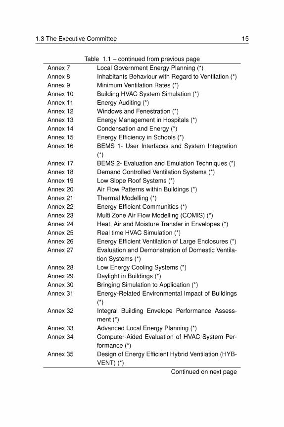
1.3 The Executive Committee 15

Table 1.1 – continued from previous pageAnnex 7 Local Government Energy Planning (*)Annex 8 Inhabitants Behaviour with Regard to Ventilation (*)Annex 9 Minimum Ventilation Rates (*)Annex 10 Building HVAC System Simulation (*)Annex 11 Energy Auditing (*)Annex 12 Windows and Fenestration (*)Annex 13 Energy Management in Hospitals (*)Annex 14 Condensation and Energy (*)Annex 15 Energy Efficiency in Schools (*)Annex 16 BEMS 1- User Interfaces and System Integration

(*)Annex 17 BEMS 2- Evaluation and Emulation Techniques (*)Annex 18 Demand Controlled Ventilation Systems (*)Annex 19 Low Slope Roof Systems (*)Annex 20 Air Flow Patterns within Buildings (*)Annex 21 Thermal Modelling (*)Annex 22 Energy Efficient Communities (*)Annex 23 Multi Zone Air Flow Modelling (COMIS) (*)Annex 24 Heat, Air and Moisture Transfer in Envelopes (*)Annex 25 Real time HVAC Simulation (*)Annex 26 Energy Efficient Ventilation of Large Enclosures (*)Annex 27 Evaluation and Demonstration of Domestic Ventila-

tion Systems (*)Annex 28 Low Energy Cooling Systems (*)Annex 29 Daylight in Buildings (*)Annex 30 Bringing Simulation to Application (*)Annex 31 Energy-Related Environmental Impact of Buildings

(*)Annex 32 Integral Building Envelope Performance Assess-

ment (*)Annex 33 Advanced Local Energy Planning (*)Annex 34 Computer-Aided Evaluation of HVAC System Per-

formance (*)Annex 35 Design of Energy Efficient Hybrid Ventilation (HYB-

VENT) (*)Continued on next page

16 Preface

Table 1.1 – continued from previous pageAnnex 36 Retrofitting of Educational Buildings (*)Annex 37 Low Exergy Systems for Heating and Cooling of

Buildings (LowEx) (*)Annex 38 Solar Sustainable Housing (*)Annex 39 High Performance Insulation Systems (*)Annex 40 Building Commissioning to Improve Energy Perfor-

mance (*)Annex 41 Whole Building Heat, Air and Moisture Response

(MOIST-ENG) (*)Annex 42 The Simulation of Building-Integrated Fuel Cell and

Other Cogeneration Systems (FC+COGEN-SIM)(*)

Annex 43 Testing and Validation of Building Energy Simula-tion Tools (*)

Annex 44 Integrating Environmentally Responsive Elementsin Buildings (*)

Annex 45 Energy Efficient Electric Lighting for Buildings (*)Annex 46 Holistic Assessment Tool-kit on Energy Efficient

Retrofit Measures for Government Buildings (En-ERGo) (*)

Annex 47 Cost-Effective Commissioning for Existing and LowEnergy Buildings (*)

Annex 48 Heat Pumping and Reversible Air Conditioning (*)Annex 49 Low Exergy Systems for High Performance Build-

ings and Communities (*)Annex 50 Prefabricated Systems for Low Energy Renovation

of Residential Buildings (*)Annex 51 Energy Efficient Communities (*)Annex 52 Towards Net Zero Energy Solar Buildings (*)Annex 53 Total Energy Use in Buildings: Analysis & Evalua-

tion Methods (*)Annex 54 Integration of Micro-Generation & Related Energy

Technologies in Buildings (*)Continued on next page

1.3 The Executive Committee 17

Table 1.1 – continued from previous pageAnnex 55 Reliability of Energy Efficient Building Retrofitting

- Probability Assessment of Performance & Cost(RAP-RETRO) (*)

Annex 56 Cost Effective Energy & CO2 Emissions Optimiza-tion in Building Renovation

Annex 57 Evaluation of Embodied Energy & CO2 EquivalentEmissions for Building Construction

Annex 58 Reliable Building Energy Performance Character-isation Based on Full Scale Dynamic Measure-ments (*)

Annex 59 High Temperature Cooling & Low TemperatureHeating in Buildings

Annex 60 New Generation Computational Tools for Building &Community Energy Systems

Annex 61 Business and Technical Concepts for Deep EnergyRetrofit of Public Buildings

Annex 62 Ventilative CoolingAnnex 63 Implementation of Energy Strategies in Communi-

tiesAnnex 64 LowEx Communities - Optimised Performance of

Energy Supply Systems with Exergy PrinciplesAnnex 65 Long-Term Performance of Super-Insulating Mate-

rials in Building Components and SystemsAnnex 66 Definition and Simulation of Occupant Behavior in

BuildingsAnnex 67 Energy Flexible BuildingsAnnex 68 Indoor Air Quality Design and Control in Low En-

ergy Residential BuildingsAnnex 69 Strategy and Practice of Adaptive Thermal Comfort

in Low Energy BuildingsAnnex 70 Energy Epidemiology: Analysis of Real Building

Energy Use at ScaleAnnex 71 Building Energy Performance Assessment Based

on In-situ MeasurementsWorking Group Energy Efficiency in Educational Buildings (*)

Continued on next page

18 Preface

Table 1.1 – continued from previous pageWorking Group Indicators of Energy Efficiency in Cold Climate

Buildings (*)Working Group Annex 36 Extension: The Energy Concept Adviser

(*)Working Group Survey on HVAC Energy Calculation Methodolo-

gies for Non-residential Buildings

Chapter 2

Foreword

This publication is the official report of IEA EBC Annex 60, which was con-ducted from 2012 to 2017 through a collaboration among 42 institutes from16 countries. Annex 60 developed and demonstrated new generation compu-tational tools for the design and operation of building and community energysystems. The report is aimed at users of simulation, HVAC and urban energysystem designers as well as researchers in the field of energy systems for thebuilt environment.

A key driver for this work are the trends towards zero energy and electrifica-tion of the energy infrastructure that demands that buildings and district energysystems become increasingly integrated to reduce energy use, power densityand to shift load. Typical measures include high-performance facades, en-ergy storage, waste heat utilization within and among buildings through nearambient-temperature networks, and heat pumps that boost waste heat and re-newable sources to usable temperatures. Advanced controls need to orches-trate this operation while providing electrical load shifting and load sheddingcapabilities, and bidding these capabilities into a dynamic electricity market.What are the implications on building simulation and associated computingand the digitalization of the entire planning process including BIM tools?

Clearly, building simulation programs face new challenges to support suchsystems throughout the building life cycle. They must become a modular ser-

20 Foreword

vice that integrates seamlessly with other tools, sometimes at small time-stepsand below the level of a whole building, during design and operation. Thisrepresents a radical structural shift from conventional building simulation pro-grams, which provide little workflow automation for design, analysis and opti-mization and no facilities for runtime integration. This situation leads to newfunctional requirements which are not addressed by existing building simula-tion programs, which are often load-based, assume ideal and non-integratedsteady-state control of each individual subsystem, and are hard to extend fromdesign to operation, and from buildings to districts.

In the meantime, other engineering sectors have been making large invest-ments and substantial progress in next generation computing tools for the de-sign and operation of complex, dynamic, engineered systems based on theopen standards Modelica, a modeling language, and Functional Mockup Inter-face (FMI), a standard for exchanging models.

Annex 60 transfers and adapts these technologies to the buildings industriesthrough the collaborative development of Modelica libraries, FMI-technologies,and translators from Building Information Models (BIM) to Modelica.

Due to this large ecosystem of technology that can be adapted for the build-ings industry, due to the evolving requirements that demand new approachesfor modeling, simulation and optimization that are a shift from todays practicein building performance simulation, and to have a means to collaboratively de-velop software, all work in Annex 60 was based on the following three openstandards:

• The equation-based, object-oriented Modelica language which allowsgraphical composition of models for simulation, operation and optimiza-tion. The models may be multi-physics system models, such as energysystems that couple thermodynamics, heat transfer, fluid dynamics, andelectrical systems. These physics-based models can be combined withdata-driven models and with models of continuous-time, discrete-time,and event-driven feedback control systems.

• The Functional Mockup Interface (FMI) Standard, a specification thatdescribes how to encapsulate and exchange models or simulators, in-dependent of the authoring tool or application domain. The FMI standardis currently supported by more than 80 tools.

• The Industry Foundation Classes (IFC), the only life cycle model of build-

21

ings that is an open international standard, governed by ISO 16739. BIMmodels described by IFC may be HVAC components or entire buildingenergy systems. A building services-related BIM model originating fromthe digital planning process cannot serve as basis for simulation withoutfurther knowledge-based transformation.

Using these standards, the core research problem that has been solved withinAnnex 60 was the coordinated development, application and demonstration ofnew generation computational tools for building and community energy sys-tems that are based on open standards and that allow buildings and energygrids to be designed and operated as integrated, robust, and performancebased systems.

In hindsight, embracing these standards was instrumental for collaborative re-search and development, as there was a clear specification of the technology,formalized through standards, that served as the basis of the collaborative de-velopment. Probably most important, working through these standards allowsthe building simulation community to collaborate with experts from other fields,such as experts in multi-physics modeling, hybrid systems, numerical meth-ods, computer algebra, compiler technology or language design, that are im-portant for the new requirements that the building simulation community faces,but that are generally not present in our community.

Software development is an investment in foundational tools that encapsu-lates sophisticated, complex methods to make them accessible to non-expertsthrough easy-to-use interfaces. By committing to standards rather than a par-ticular tool provider’s implementation, the software developed in Annex 60 thatdoes not rely on, and hence locks customers into the use of tools provided byany single vendor.

22 Foreword

2.1 Operating Agents and Task Leaders

The operating agents were

Michael Wetter

Building Technology and Urban Systems Department

Energy Technologies Area

Lawrence Berkeley National Laboratory, USA

and

Christoph van Treeck

Chair in Energy Efficiency and Sustainable Building (E3D)

RWTH Aachen University, Germany

Annex 60 was structured into the following subtasks and activities.

Subtask 1: Technology Development

Led by Michael Wetter, LBNL, Berkeley, CA

Activity 1.1: Modelica model libraries

Led by Michael Wetter, LBNL, Berkeley, CA

Activity 1.2: Co-simulation and model exchange through Functional MockupUnits

Led by Frederic Wurtz, Grenoble University, Grenoble, France

Activity 1.3: Building Information Model

Led by Christoph van Treeck, RWTH Aachen University, Germany

Activity 1.4: Workflow automation tools

2.2 Authors of the Final Report 23

Led by Sebastian Stratbuecker, Fraunhofer IBP, Holzkirchen, Ger-many

Subtask 2: Validation and Demonstration

Led by Lieve Helsen, KU Leuven, Leuven, Belgium

Activity 2.1: Design of building systems

Led by Christoph Nytsch-Geusen, Berlin University of the Arts,Berlin, Germany

Activity 2.2: Design of district energy systems

Led by Dirk Saelens, KU Leuven, Leuven, Belgium

Activity 2.3: Model use during operation

Led by Ignacio Torrens, Eindhoven University of Technology, TheNetherlands

Subtask 3: Dissemination

Led by Christoph van Treeck and Michael Wetter

2.2 Authors of the Final Report

The final report was co-authored by the participants listed below, and editedby the operating agents Michael Wetter and Christoph van Treeck.

24 Foreword

Name AffiliationBaetens, Ruben KU Leuven, BelgiumBazjanac, Vladimir Standford University, CA, USABlum, David Lawrence Berkeley National Laboratory, Berkeley,

CA, USACao, Jun RWTH Aachen University, Aachen, GermanyFuchs, Marcus RWTH Aachen University, Aachen, GermanyJorissen, Filip KU Leuven, Leuven, BelgiumKeane, Marcus M. National University of Ireland, Galway, IrelandLauster, Moritz RWTH Aachen University, Aachen, GermanyMaile, Tobias Maile Consulting, Fellbach, GermanyMitterhofer,Matthias

Fraunhofer Institute for Building Physics IBP,Holzkirchen, Germany

Nouidui, Thierry S. Lawrence Berkeley National Laboratory, Berkeley,CA, USA

Nytsch-Geusen,Christoph

Berlin University of the Arts, Berlin, Germany

O’Donnel, James University College Dublin, DublinPicard, Damien KU Leuven, Leuven, BelgiumPinheiro, Sergio University College Dublin, DublinProtopapadaki,Christina

KU Leuven/EnergyVille, Belgium

Reinbold, Vincent KU Leuven/EnergyVille, BelgiumSaelens, Dirk KU Leuven/EnergyVille, BelgiumSterling, Raymond National University of Ireland, Galway, IrelandStratbuecker,Sebastian

Fraunhofer Institute for Building Physics IBP,Holzkirchen, Germany

Thorade, Matthis Berlin University of the Arts, Berlin, GermanyTugores, CarlesRibas

Berlin University of the Arts, Berlin, Germany

van der Heijde,Bram

KU Leuven/EnergyVille, Belgium

van Treeck,Christoph

RWTH Aachen University, Aachen, Germany

Wetter, Michael Lawrence Berkeley National Laboratory, Berkeley,CA, USA

Wimmer, Reinhard RWTH Aachen University, Aachen, Germany

2.3 Project Participants 25

2.3 Project Participants

The following 42 institutes from 16 countries participate in Annex 60:

Institute CountryLawrence Berkeley National Laboratory USAMassachusetts Institute of Technology USAPurdue University USAStanford University USATexas A&M University USAUCI Engineering, Inc. USAUniversity of Alabama USAUniversity of Miami USAUniversity of Texas, San Antonio USARWTH Aachen University GermanyMaile Consulting GermanyTU Dresden GermanyKIT Karlsruher Institut of Technology GermanyFraunhofer ISE GermanyBerlin University of the Arts (UDK) GermanyFraunhofer IBP GermanyAEC3 GermanyAustrian Institute of Technology AustriaAEE-Intec AustriaKU Leuven BelgiumCenaero BelgiumUniversity of Liège BelgiumPontifícia Universidade Católica do Paraná BrazilChongqing University ChinaAalborg University DenmarkUniversity of Southern Denmark DenmarkLGCgE, Université d’Artois FranceGrenoble University FranceCEA INES France

Continued on next page

26 Foreword

Table 2.1 – continued from previous pageInstitute CountryI2M University of Bordeaux FranceCSTB FranceEDF FranceNational University of Ireland, Galway IrelandUniversity College Dublin IrelandUniversità Politecnica delle Marche ItalyEindhoven University of Technology The NetherlandsExergy Studios SlovakiaIK4-TEKNIKER SpainSwegon AB SwedenEQUA Simulation AB SwedenEMPA SwitzerlandMasdar Institute United Arab Emirates

2.4 Acknowledgements

This research was supported by the Assistant Secretary for Energy Efficiencyand Renewable Energy, Office of Building Technologies of the U.S. Depart-ment of Energy, under Contract No. DE-AC02-05CH11231.

This research was supported by the European Union through the SeventhFramework Programme (FP7/2007-2013) under grant agreement nº 285408.

This research was supported by the European Union through the SeventhFramework Programme (FP7/2007-2013) under grant agreement nº 284920.

This research was supported by the International Energy Research Centre andEnterprise Ireland under project n. CC-2011-4005B and by the Irish ResearchCouncil - D’Appolonia enterprise partnership scheme.

This research was supported by the German Federal Ministry of Economic Af-fairs and Energy (BMWi), national research project EnTool:EnEff-BIM (EnOB),promotional references 03ET1177A, 03ET1177B, 03ET1177C, 03ET1177D,03ET1177E.

2.4 Acknowledgements 27

This research was supported by the German Federal Ministry of EconomicAffairs and Energy (BMWi), national research project EnTool:CoSim (EnOB),promotional references 03ET1215A, 03ET1215B, 03ET1215C, 03ET1215D.

This research was supported by a Marie Curie FP7 Integration Grant withinthe 7th European Union Framework Programme project title SuPerB, projectnº 631617 and Conselho Nacional de Desenvolvimento Científico and Tec-nológico (CNPq) under the Programme Science without Borders in Brazil.

Research participants collaboratively worked together under the umbrella ofthe IEA EBC framework. Duplications of work were avoided and participantsbenefitted from collaboration and synergies which became possible due to thestrong organizational Annex 60 framework.

28 Foreword

Chapter 3

Executive Summary

The IEA EBC project Annex 60: New Generation Computational Tools for

Building & Community Energy Systems led to open-source, freely avail-able, documented, validated and verified new generation computational tools.These tools allow buildings and community energy grids to be designed andoperated as integrated, robust, performance based systems with low energyuse and low peak power demand. The developed tools are all based on threenon-proprietary, open standards:

• The Modelica modeling language for implemeting models (https://www.modelica.org/),

• the Functional Mockup Interface (FMI) standards to couple simulators(https://www.fmi-standard.org/), and

• the Industry Foundation Classes (IFC) for building information modeling(http://www.buildingsmart-tech.org/) as well as other BIM-related stan-dards such as Information Delivery Manual (IDM) and Model View Defi-nitions (MVD).

Thus, Annex 60 committed to, leveraged and contributed to open standardsthat can be used with a variety of tools, rather than developed software tech-nology that depends on the implementation of a single tool provider. Thisavoids vendor lock-in and provides to industry a stable basis, governed bystandards, to invest in.

30 Executive Summary

The target audience of Annex 60 is the building energy research community,design firms and energy service companies, equipment and tool manufactur-ers, as well as students in building energy-related sciences. Through Annex60, fragmented duplicative activities in modeling, simulation and optimizationof building and community energy systems that are based on the Modelica andFMI standards were coordinated. Tool-chains were created, often by adaptingand extending technologies from other industry sectors, to link Building In-

formation Models (BIM) to energy modeling, building simulation to controlsdesign tools, and design tools to operational tools. These tools were demon-strated for building design, district energy system design, and for use of modelsduring operation to support fault detection and diagnostics algorithms, modelpredictive control, and hardware-in-the-loop experimentation.

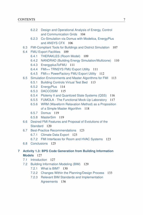
Activity 1.1

Modelica model libraries

Activity 1.2

Functional Mockup Units

Subtask 1:

Technology

development

Subtask 2:

Validation &

demonstration

Subtask 3:

Dissemination

Activity 1.3

Building Information Models

Activity 1.4

Workflow automation tools

Activity 2.1

Design of

building systems

Activity 2.2

Design of

district energy systems

Activity 2.3

Model use

during operation

Fig. 3.1: Structure and organization of Annex 60.

Annex 60 was organized in the subtasks and activities shown in Fig. 3.1. Sub-tasks 1 developed and implemented the software technology required by theapplications. Subtask 2 was focused on validation, verification and demonstra-

31

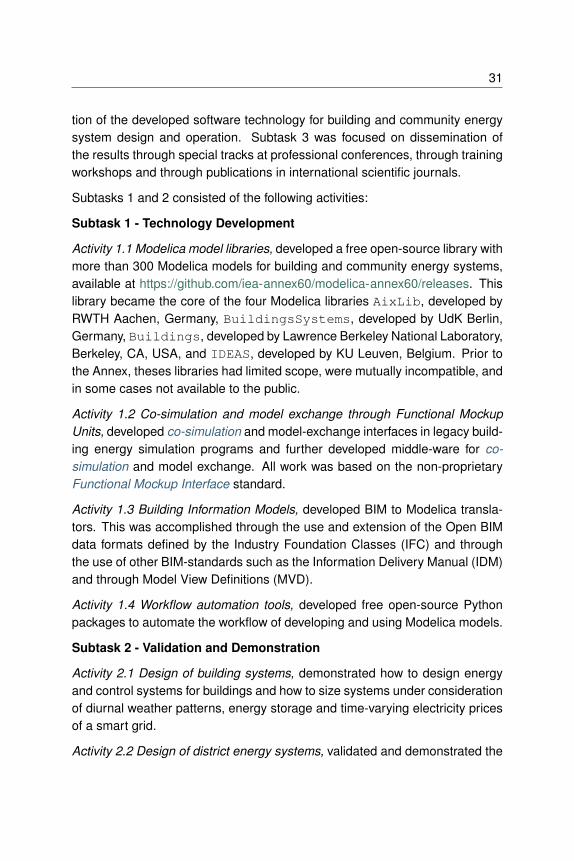
tion of the developed software technology for building and community energysystem design and operation. Subtask 3 was focused on dissemination ofthe results through special tracks at professional conferences, through trainingworkshops and through publications in international scientific journals.

Subtasks 1 and 2 consisted of the following activities:

Subtask 1 - Technology Development

Activity 1.1 Modelica model libraries, developed a free open-source library withmore than 300 Modelica models for building and community energy systems,available at https://github.com/iea-annex60/modelica-annex60/releases. Thislibrary became the core of the four Modelica libraries AixLib, developed byRWTH Aachen, Germany, BuildingsSystems, developed by UdK Berlin,Germany, Buildings, developed by Lawrence Berkeley National Laboratory,Berkeley, CA, USA, and IDEAS, developed by KU Leuven, Belgium. Prior tothe Annex, theses libraries had limited scope, were mutually incompatible, andin some cases not available to the public.

Activity 1.2 Co-simulation and model exchange through Functional Mockup

Units, developed co-simulation and model-exchange interfaces in legacy build-ing energy simulation programs and further developed middle-ware for co-

simulation and model exchange. All work was based on the non-proprietaryFunctional Mockup Interface standard.

Activity 1.3 Building Information Models, developed BIM to Modelica transla-tors. This was accomplished through the use and extension of the Open BIMdata formats defined by the Industry Foundation Classes (IFC) and throughthe use of other BIM-standards such as the Information Delivery Manual (IDM)and through Model View Definitions (MVD).

Activity 1.4 Workflow automation tools, developed free open-source Pythonpackages to automate the workflow of developing and using Modelica models.

Subtask 2 - Validation and Demonstration

Activity 2.1 Design of building systems, demonstrated how to design energyand control systems for buildings and how to size systems under considerationof diurnal weather patterns, energy storage and time-varying electricity pricesof a smart grid.

Activity 2.2 Design of district energy systems, validated and demonstrated the

32 Executive Summary

tools from Subtask 1, applied to district energy systems and smart grid inte-gration at the scale of the district energy system.

Activity 2.3 Model use during operation, used control models from Activity 1.1and FMI export programs from Activity 1.2 during the operation of buildingenergy systems, and during hardware-in-the-loop experimentation.

Subtask 3 - Dissemination

Subtask 3, which is not described in this report, focused on the disseminationof the results through special sessions at scientific conferences and throughworkshops that trained users in the technology developed in Annex 60. Re-sults have further been disseminated through publication in international sci-entific journals.

Annex 60 was conducted from June 2012 to June 2017. The core of theteam will continue key developments and disseminations of Annex 60 underthe umbrella of the International Building Performance Simulation Association(IBPSA). This will be the first research project formally conducted under theumbrella of IBPSA, executed as “Project 1: BIM/GIS and Modelica Frameworkfor building and community energy system design and operation.”

Chapter 4

Introduction

To meet increasingly stringent energy performance targets and challengesposed by distributed renewable energy generation on the electrical and ther-mal distribution grid, recent attention has been given to system-level integra-tion, part-load operation and operational optimization of buildings. The in-tent is to design and operate a building or a neighborhood optimally as aperformance-based, robust system. This requires taking into account system-level interactions between building storage, HVAC systems and electrical andthermal grid. Such a system-level analysis requires multi-physics simulationand optimization using coupled thermal, electrical and control models. Op-timal operation also requires closing the gap between designed and actualperformance through commissioning, energy monitoring and fault detectionand diagnostics. All of these activities can benefit from using models that rep-resent the design intent. These models can then be used to verify responsesof installed equipment and control sequences, and to compute optimal controlsequences in a Model Predictive Controller (MPC), the latter of which possiblyrequiring simplified models.

Furthermore, in the AEC domain the processes of designing, constructing andcommissioning buildings and engergy systems are rapidly changing towarddigitalization. Building Information Modeling (BIM) is an enabler as collabora-tive method and tool to consistently gather, manage and exchange building-related data on a digital basis over the entire life cycle of a facility. BIM is

34 Introduction

not a specific software, it is rather a method as part of, but not limited to, theintegral design. A truly added value is expected for the near future when de-sign and commissioning in the sense of computer aided facility managementcomes together. The above mentioned issues of commissioning, energy mon-itoring and fault detection and diagnostics can therefore highly benefit from athorough digital planning when location and function of technical systems aretogether referenced in a digital model, when the as-built state is harmonizedwith and well documented in a model and when home and building automationbecomes integrally linked with BIM.

This shift in focus will require an increased use of models throughout the build-ing delivery stages and continuing into the operational phase. Consider, forexample, the development and use of an HVAC system model:

1. During design, a mechanical engineer will construct a model that rep-resents the design intent, such as system layout, equipment selection,and control sequences. The basis of such a model could be from a BIMin the case of a building, or from a GIS in the case of a district.

2. During construction, to reduce cost for implementation of the control se-quence, and to ensure that the control intent is properly implemented,a control model could be used to generate code that can be uploadedto supervisory building automation systems, thereby executing the samesequence as was used during design [NW14] .

3. During commissioning, the design model will be used to verify properinstallation.

4. During operation, the model will be used for comparing actual with ex-pected energy use [PWBH11] , and for fault detection and diagnostics[BSG+14] . Furthermore, the model may be converted to a form thatallows its use during operation as part of an MPC algorithm.

In addition to the focus on closing the performance gap between design andoperation, another recent focus is on system integration. Here, the challengelies in the co-design and operation of building dynamics, HVAC, thermal andelectrical storage, renewable energy generation, and grid responsive control inorder to maintain the power quality of the electrical grid. Commonly, to supportsystem integration, models from different engineering domains need to be cou-pled during run-time. For example, for active facade control, it may be neces-sary to couple a ray-tracing tool such as Radiance with a building energy simu-

35

lation tool to asses the impact of daylighting controls on reducing glare, energy,and peak cooling demand. Similarly, for building to electrical grid integration,building HVAC and domestic hot water control can be designed such that build-ings present themselves as a flexible load to the electrical grid, which can in-crease the amount of renewable energy integrated into the grid. Such couplingof domain-specific models may be done within Modelica, an equation-based,object-oriented modeling language, or through tool coupling that involves co-simulation, a technique in which simulators exchange data as the simulation-time advances. See [Wet11a][BDCVR+12][BWN14][WBN16][CH15] for ex-ample applications.

For a larger discussion of functionalities that future building modeling tools willneed to provide to address the needs for low energy building and communityenergy grid design and operation, we refer to [Wet11b] and [Cla15] .

The aforementioned new foci give rise to new requirements for building simu-lation tools, including the following:

1. Mechanical engineers should be able to design, assess the performanceand verify the correctness of local and, in particular, supervisory controlsequences in simulation. They should then use such a verified, non-ambiguous specification to communicate their design intent to the con-trol provider. Moreover, the specification should be used during com-missioning to verify that the control contractor implemented the designintent.

2. Controls engineers should be able to extract subsystem models frommodels used during the building design in order to use them within build-ing control systems for commissioning, model-based controls, fault de-tection and diagnostics.

3. Urban planners and researchers should be able to combine models ofbuildings, electrical grids and controls in order to improve the design andoperation of such systems to ensure low greenhouse gas emissions orcosts, and high quality power delivery [BDCVR+12][WBN16][BWN14] .

4. Mechanical engineers should be able to convert design models to a formthat allows the efficient and robust solution of optimal control problemsas part of MPC [SOCP11] . Such models may then be combined withstate estimation techniques that adapt the model to the actual building[BSG+14] .

36 Introduction

The first item requires modeling and simulation of actual control sequences,including proper handling of hybrid systems, i.e., systems in which the stateevolves in time based on continuous time semantics that arises from physics,and discrete time and discrete event semantics that arises from digital con-trol [Wet09][WZNP14] . This poses computing challenges for the deterministicsynchronization of these domains [BGL+15] . The second item requires extrac-tion of a subsystem model and exporting this model in a self-contained formthat can readily be executed as part of a building automation system as shownin [NW14] . The third item requires models of different physical domains andmodels of control systems to be combined for a dynamic, multi-physics simu-lation that involves electrical systems, thermal systems, controls and possiblycommunication systems, which may evolve at vastly different time scales. Thefourth item greatly benefits if model equations are accessible to perform modelorder reduction and to solve optimal control problems.

4.1 Comparison to State-of-the-art in Building En-

ergy Modeling and Simulation

Today’s whole-building simulation programs formulate models using impera-tive programming languages. Imperative programming languages assign val-ues to functions, declare the sequence of execution of these functions andchange the state of the program, as is done for example in C/C++, Fortran orMATLAB/Simulink. In such programs, model equations are tightly intertwinedwith numerical solution methods, often by making the numerical solution pro-cedure part of the actual model equations. This approach has its origin inthe seventies when neither modular software approaches were implementednor powerful computer algebra tools were available. These programs havebeen developed for the use case of building energy performance assessmentto support building design and energy policy development. Other use casessuch as control design and verification, model use in support of operation,and multi-physics dynamic analysis that combines building, HVAC, electricaland control models were not priorities, nor even considered [CLW+96] . How-ever, the position paper of IBPSA shows that they recently gained importance[Cla15] .

4.1 Comparison to State-of-the-art in Building Energy Modeling andSimulation 37

Tight coupling of numerical solution methods with model equations and in-put/output routines makes it difficult to extend these programs to support newuse cases. The reason is that this coupling imposes rules that determinefor example where inputs to functions that compute HVAC, building or controlequipment are received from the internal data structure of the program, whenthese inputs are updated, when these functions are evaluated to produce newoutput, and what output values may be lagged in time to avoid algebraic loops.Such rules have made it increasingly difficult for developers to add new func-tionalities to software without inadvertently introducing an error in other partsof the program. They also make it difficult for users to understand how com-ponent models interact with other parts of the system model, in particular theirinteraction with, and assumptions of, control sequences. Furthermore, theyalso have shown to make it difficult to use such tools for optimization [WW04] .

The tight coupling of numerical solution methods with model equations alsomakes it difficult to efficiently simulate models for the various use cases. Nu-merical methods in today’s building energy simulation programs are tailored tothe use case of energy analysis during design. However, other use cases,such as controls design and verification, coupled modeling of thermal andelectrical systems, and model use during operation require different numeri-cal methods. To see why different numerical methods are required, considerthese applications:

• Stiff systems: The simulation of feedback control with time constants ofseconds coupled to building energy models with time constants of hoursleads to stiff ordinary differential equations. Their efficient numericalsolution requires implicit solvers [HW96] .

• Non-stiff systems: In EnergyPlus [CLP+99] and in many TRNSYS[KDB76] component models, the dynamics of HVAC equipment andcontrollers, which is fast compared to the dynamics of the building heattransfer, is generally approximated using steady-state models. Hence,the resulting system model is not stiff as the only dynamics is from thebuilding model. In this situation, explicit time integration algorithms aregenerally more efficient. Such an approximation of the fast dynamicscan also be done with dynamic Modelica HVAC models, see [JWH15] .

• Hybrid systems: Hybrid systems require proper simulation of coupledcontinuous time, discrete time and discrete event dynamics. This in turnrequires solution methods with variable time steps and event handling.

38 Introduction

For example, when a temperature sensor crosses a setpoint or a batteryreaches its state of charge, a state event takes place that may switcha controller, necessitating solving for the time instant when the switchhappens and reducing accordingly the integration time step. Standardordinary differential equation solvers require an iteration in time to solvefor the time instant of the event, and reinitializing integrators after theevent, which both are computationally expensive. A new class of ordi-nary differential equation solvers called Quantized State System (QSS)integration [ZL98][KJ01][CK06][Kof03][MBKC13] are promising for theefficient simulation of such systems as they do not require iteration forstate event detection. However, their efficient use requires knowledgeof the dependency graph of the state equations, which generally is notavailable in legacy building simulators, but readily available in equation-based languages.

It follows from this discussion that for models to be applicable to a wide rangeof applications, it should be possible to use them with different numericalsolvers. Therefore, models for building energy systems and their numericalsolution methods should be separated where possible. Exceptions are equa-tions for which special tailored solution methods and parallel programmingpatterns allow humans to better exploit the structure of the equations than iscurrently supported by code generators, often arising from partial differentialequations or from light distributions. Examples include solvers for computa-tional fluid dynamics, heat transfer in borehole heat exchangers [PH14] , andray-tracing for daylighting. Work, however, is ongoing to remedy this situation[Cas15][SWF+15][BBCK15] .

4.2 New Technologies for Building Energy Model-

ing and Simulation

This section describes new technologies which can be applied to building en-ergy modeling in support of the different use cases.

4.2 New Technologies for Building Energy Modeling and Simulation 39

4.2.1 Equation-based Modeling

As explained above, the use of imperative programming languages limits theapplicability and extensibility of models. Furthermore, in building simulationprograms, numerical solution algorithms are often tightly integrated into themodels and thereby can mandate the use of supervisory control logic that isfar removed from how control sequences are implemented in reality. For ex-ample, in EnergyPlus, a cooling coil may request from the supervisory controla certain air mass flow rate in order to meet the load computed in the predic-tor step of the thermal zone heat balance. In actuality, the air mass flow ratewould be determined by the position of dampers in combination with the speedof a supply fan, each of which could be controlled by zone temperature andduct static pressure feedback controllers.

A key difference between imperative programming languages and equation-based languages is that the latter do not require a specification of the se-quence of computer assignments required to simulate a model. Rather, amodel developer can specify the mathematical equations, package them intographically represented components and store them in a hierarchical library. Amodel user then assembles these components in a schematic editor to form asystem model. A simulation environment analyses these equations, optimallyrearranges them using computer algebra, translates them to executable code,typically C, and links them with numerical solvers.

Specifically, the translation of equations to executable code involves determin-ing which variables can be replaced by so-called alias variables, for example,in the case of a mass flow rate that may be the same for all components thatare used to compose an air handler unit. It also involves reducing the dimen-sion of coupled linear and nonlinear system of equations through symbolicinverting equations and through Block Lower Triangularization and Tearing[CK06][EO94] , which often significantly reduces the dimension of the coupledsystems of equations. See also Section 5.3.4. Furthermore, during transla-tion, zero-crossing functions are generated, for example, to indicate when athermostat crosses a set-point, and high-order differential algebraic systemsof equations are reduced to index 1 [MS93] : Some Modelica translators alsogenerate code for specific solvers. The benefit of this has been demonstratedby Fernandez and Kofman who showed for QSS methods more than an or-der of magnitude simulation speed improvements when code is generated in a

40 Introduction

form that is specifically designed for the QSS methods [FK14] , as opposes tousing QSS methods with a conventional discrete event simulation solver. Sym-bolic manipulations also allow to partition the model automatically for parallelcomputing [EMO14] .

Loosely speaking, while simulation models implemented using imperative pro-gramming languages require numerical solvers to select numerical inputs andcompare the function values for these inputs to infer what equations they solve,equation-based modeling languages such as Modelica allow for the under-stand of equation structure, and making use of this understanding to gen-erate efficient code for computation. Examples of structures include whichvariables are connected to each other through algebraic constraints or dif-ferential equations, which equations can be differentiated, which equationscan be inverted, and which equations trigger an event that can instantlychange a control signal. For a more detailed discussion, see [Elm78] , [CK06] ,[EO94] and [EOC95] . To make these technologies accessible to a widerange of users in building simulation, research and development is requiredand ongoing to advance translators and solvers to better handle large models[Wet09][Zim13][WZNP14][JWH15][Cas15][SWF+15][BBCK15] .

A promising aspect of Modelica is that it is an open-source language that issupported internationally by various industries. As these industry sectors usethe same modeling language, modeling environments, simulation and opti-mization code generators and solvers, the investement in these technologiescan be shared. Consequently, large international projects that further advanceModelica have been conducted, such as

• MODELISAR (https://itea3.org/project/modelisar.html, 29 partners, Euro26.6M, 2008-2011) which initiated the FMI standard,

• EUROSYSLIB (http://www.eurosyslib.com/, 19 partners, Euro 16M,2007-2010) which developed Modelica libraries for embedded systemmodeling and simulation, and

• MODRIO (https://www.modelica.org/external-projects/modrio, Euro21M, 2012-2015) which extended Modelica and FMI to support proper-ty/requirement modelling, state estimation, multi-mode modelling, e.g.,systems with multiple operating modes and varying number of states,and nonlinear model predictive control.

4.2 New Technologies for Building Energy Modeling and Simulation 41

4.2.2 Co-Simulation and Model Exchange

In 2008, a European project called MODELISAR started with the objectiveto facilitate interoperability between simulation models and simulation toolsthrough a standardized application programming interface (API). This projectresulted in the Functional Mockup Interface (FMI) standard, which is a tool-independent, open-source standard which supports exporting, exchangingand importing simulation models or simulation tools [MC14] .

A simulation model or a complete simulator that is exported in the format spec-ified by the FMI standard is called a Functional Mockup Unit (FMU). The FMIstandard defines a set of C-functions (FMI functions) to interact with the modelor the simulator. It also defines an xml schema that is used to declare prop-erties of the exported model or simulator. In addition, it standardizes how topackage as a zip file the xml file, the C-functions, possibly as compiled bi-naries, and resources required by the model or simulator, such as files withweather data.

The FMI standard distinguishes between model-exchange and co-simulation.In FMI for model-exchange, a system of differential, algebraic and discrete-time equations can be exported, and the host simulator that executes the FMUneeds to provide an algorithm that integrates the equations in time. In contrast,in FMI for co-simulation, the host simulator requests the FMU to integrate itsequations in time. See for example [BBG+13] for such an algorithm.

Version 2.0 of FMI standard was released in 2014, and it adds features thatwill facilitate the use of FMU models to support the design and operation ofbuildings. Some of the important features are as follows:

Saving and restoring the state The complete FMU state can besaved, restored, and serialized to a byte vector. As a result, asimulation can be restarted from a saved FMU state. This is avery important feature for model-based fault detection as theone in [BSG+14] or model predictive controls applications asboth of them require state initialization.

Input and state dependencies In the xml file, it can be declaredwhich state variables and which output variables have a di-

rect dependency on the input variables, and which outputvariables have a direct dependency on the state variables.

42 Introduction

This allows1. determining the sparsity pattern for Jacobians, and2. to use sparse matrix methods in numerical solvers to

simulate stiff FMUs.The information about dependency also opens the doorto the implementation of efficient asynchronuous numericaltime integration algorithms such as QSS.Furthermore, for FMUs that are connected to form a cyclicgraph, the dependency information of outputs on inputs isrequired for the deterministic execution [BBG+13] , and thedetection of algebraic loops. Once those algebraic loopsare detected, nonlinear equation solvers such as a Newton-Raphson solver can be used to solve them.The following example, which is borrowed from [BBG+13] ,illustrates why exposing such dependencies is important.Consider the FMU that comprises the system shown in Fig.4.1. If this FMU is imported in a simulator and y1 is connectedto u, possibly using an algebraic function f : R → R, then amaster algorithm can output the state y1, assign u = f (y1),output y2 = −5 u and integrate the state. If however u wereconnected to f (y2) rather than f (y1), then a master algorithmcan output y1, next it needs to solve u = f (y2) = −5 f (u),in general using numerical iterations, and then it can inte-grate the state. This illustrates that input-output dependencyis important as it allows a simulator to detect whether cyclicgraphs, formed by connecting inputs and outputs amongFMUs, lead to an algebraic system of equations that may re-quire an iterative solution. See [BBG+13] for a more detaileddiscussion.

Directional derivatives Directional derivatives can be computedfor derivatives of continuous-time states and for outputs. Thisis useful when connecting FMUs and the partial derivativesof the connected FMU shall be computed, for example bya stiff ordinary differential equation solver, an algebraic loopsolver, an extended Kalman filter, or for model linearization.If the exported FMU performs this computation analytically,then all numerical algorithms based on these partial deriva-

4.2 New Technologies for Building Energy Modeling and Simulation 43

Fig. 4.1: FMU for which output y1 does not have a direct dependency on input u but

output y2 does.

tives are more efficient and more reliable [MC14] . Direc-tional derivatives are also required by second-order QSS al-gorithms [Kof03] . This is illustrated with the following exam-ple. Consider an FMU which implements dx(t)/dt = f (x , u, t)for some differentiable function f : R × R × R → R. If theFMU provides directional derivatives, then the second timederivative can be computed exactly because

df (x , u, t)dt

=∂f (x , u, t)

∂x

dx(t)dt

+∂f (x , u, t)

∂u

du(t)dt

,

where ∂f (x , u, t)/∂x and ∂f (x , u, t)/∂u are the directionalderivatives with respect to state and input, which are pro-vided by the FMU.

In summary, there are various benefits in using equation-based languages,such as Modelica, for system simulation. First, they allow for sufficient se-mantics for a code generator to identify the state variables in a model, whichsupports saving and restoring states for initializing simulations. Second, theyallow for the discovery of input-output and input-state dependencies, whichsupports master algorithm development. Lastly, they allow for automatic dif-ferentiation of model equations, which supports in providing directional deriva-tives to solvers. While these pieces of information could in principle also bespecified by a model developer in models that are written using imperative lan-guages, the size of models typically encountered in building simulation wouldmake such a manual declaration a tedious, expensive and error-prone propo-sition.

44 Introduction

The relevance of these properties for the building simulation community hasbeen illustrated in the following examples. Broman et al. [BBG+13] developeda master algorithm for the deterministic composition of FMUs for co-simulation,which is only possible if input/output dependencies are provided for FMUs thatare connected in a cyclic graph. Wetter et al. [WNL+15] simulated a buildingwith radiant heating system using a collection of FMUs for model exchangethat are asynchronously integrated in time using QSS methods. The input-state dependencies were required to determine which state variables need tobe updated. Bonvini et al. [BWS14] have developed and applied an FMU-based state and parameter estimator that has been used as part of a faultdetection algorithm which is capable of identifying faults in a valve. This algo-rithm required saving and restoring states.

The capabilities of FMI and the aforementioned use cases indicate its appli-cability to support building simulation for design and operation. At the time ofwriting, there are more than 70 tools which support import or export of simula-tion models or tools as FMUs. This indicates the adoption of the standard andits relevance for the building simulation community.

4.2.3 Optimization

Equation-based modeling languages allow code generators to convert modelequations to a form that is well suited to solve large scale nonlinear optimiza-tion problems [AAG+10] . This section describes a state of the art method thatconverts an infinite dimensional optimal control problem into a finite dimen-sional approximation that standard nonlinear programming (NLP) solvers cansolve. Equation-based modeling languages allow automating this conversion.

Equation-based modeling languages allow to describe systems of differentialalgebraic equations (DAE) in the general form

F (t , x(t), x(t), u(t), y (t), Θ) = 0,

Y (t , x(t), u(t), y (t), Θ) = 0,

F0(x(t0), x(t0), u(t0), y(t0),Θ) = 0,

(4.1)

where F (·, ·, ·, ·, ·, ·) describes the time rate of change, Y (·, ·, ·, ·, ·) are algebraicconstraints, F0(·, ·, ·, ·, ·) implicitly defines initial conditions, t ∈ [t0, tf ] is time for

4.2 New Technologies for Building Energy Modeling and Simulation 45

some initial and final time t0 and tf , x : R → Rnx is the state vector, u : R → R

nu

is the control function, y : R → Rny is the vector of algebraic variables, and

Θ ∈ Rp is the vector of parameters. Such a DAE system can be used to

model a building, its HVAC systems and controllers. Necessary and sufficientconditions for existence, uniqueness and differentiability of a solution to (4.1)can be found in [Wet05] .

Once the model is available, we can add constraints and a cost function todefine an optimal control problem that minimizes energy consumption or cost.An example optimal control problem for (4.1) is

minimizeu(·)∈� , Θ∈Rp

f (x(t), u(t), y (t), Θ),

subject to F (t , x(t), x(t), u(t), y (t), Θ) = 0,

Y (t , x(t), u(t), y (t), Θ) = 0,

F0(x(t0), x(t0), u(t0), y (t0), Θ) = 0,

H(t , x(t), x(t), u(t), y (t), Θ) = 0,

G(t , x(t), x(t), u(t), y (t), Θ) ≤ 0,

(4.2)

for all t ∈ [t0, tf ], where f (·, ·, ·, ·) is the cost function and U is the set of ad-missible control functions. The solution to (4.2) is the optimal control functionand the optimal design parameter that minimizes f (·, ·, ·, ·) while satisfying thesystem dynamics F (·, ·, ·, ·, ·, ·) = 0, and Y (·, ·, ·, ·, ·) = 0, the initial conditionsF0(·, ·, ·, ·, ·) = 0 and the constraints H(·, ·, ·, ·, ·, ·) = 0 and G(·, ·, ·, ·, ·, ·) ≤ 0.For generality, we assume (4.2) to be nonlinear and twice continuously differ-entiable [Pol97] .

The problem (4.2) is infinite dimensional because its solution is a functionalthat has to be valid for all t ∈ [t0, tf ]. Directly solving an infinite dimen-sional optimal control problem for a general nonlinear system is not possibleand it therefore needs to be converted into a finite dimensional approximation[Pol97] . Biegler [Bie10] presents multiple methods for such a conversion intothe form

minimizez∈Rnz

c(z),

subject to z l ≤ z ≤ zu ,

g(z) = 0,

h(z) ≤ 0,

46 Introduction

where z is the finite dimensional optimization variable, z l and zu are the lowerand upper bounds, c(·) is the cost function, and g(·) and h(·) are the equalityand inequality constraints.

Among the available techniques, we describe direct collocation methods be-cause they are well suited for equation-based modeling languages [AAG+10] .Direct collocation methods use polynomials to approximate the trajectories ofthe variables of a DAE system. The polynomials are defined on a finite num-ber of support points that are called collocation points. By optimizing thesefinite number of control points, they convert the infinite to a finite dimensionaloptimization problem, which can be solved by a NLP solver such as IPOPT[WB06] .

The method starts by dividing the time horizon [t0, tf ] into ne elements, eachelement containing the same number of collocation points nc . For example,the JModelica software [AGT09] uses the Radau collocation method to placethese points. The Radau collocation method places a collocation point at thestart and end of each element to ensure continuity of the state trajectories, andplaces the others to maximize accuracy. In each element, time is normalizedas ti (τ ) = ti−1+hi (tf−t0) τ , for τ ∈ [0, 1] and i ∈ {1, ... , ne}, where ti is the timeat the end of element i , τ ∈ [0, 1] is the normalized time within the element,and hi is the length of element i . The time dependent variables x(·), x(·), u(·),and y (·) are approximated using collocation polynomials in each element. Thecollocation polynomials use the Lagrange basis polynomials, and they use thecollocation points as the interpolation points. The collocation polynomials are

xi (τ ) =nc

k=0

xi ,k lk (τ ),

ui (τ ) =nc

k=1

ui ,k lk (τ ),

yi (τ ) =nc

k=1

yi ,k lk (τ ),

(4.3)

where xi ,k , ui ,k , and yi ,k are the values of the variable x(·), u(·) and y (·) atthe collocation point k in element i , lk (·) is the Lagrange basis polynomial andlk (·) is the Lagrange basis polynomial that includes the first point to ensurecontinuity of the state variables. The Lagrange bases are, with i ∈ {1, ... , ne},

4.2 New Technologies for Building Energy Modeling and Simulation 47

lk (τ ) =

j∈{0, ..., nc}∖{k}

τ − τj

τk − τj

,

lk (τ ) =

j∈{1, ..., nc}∖{k}

τ − τj

τk − τj

.(4.4)

As τ is normalized, the basis polynomials are the same for all elements. Thepolynomial approximation of the derivative xi (·) in (4.3) is

xi (τ ) =1

hi (tf − t0)

nc

k=0

xi ,kdlk (τ )

dτ. (4.5)

The collocation method defines the approximations (4.3) and (4.5) of the vari-ables in (4.2). Equation-based modeling languages allow accessing the modelequations, thereby allowing to automatically generate the finite dimensionalapproximations defined by the collocation methods.

JModelica employs a collocation method to transcribe the problem (4.2) intoan NLP problem. A local optimum to the finite dimensional approximationof (4.2) will be found by solving the first-order Karush-Kuhn-Tucker (KKT)conditions, using iterative techniques based on Newton’s method. This re-quires first- and second-order derivatives of the cost and constraint func-tions with respect to the NLP variables. JModelica uses CasADi [And13] ,a software for automatic differentiation that is tailored for dynamic optimiza-tion. Equation-based modeling languages allow for automatically providingthe information required by CasADi to build a symbolic representation of theoptimization problem. Using the symbolic representation of the NLP prob-lem, CasADi can efficiently compute the required derivatives and exploit thesparsity pattern of the problem. NLP solvers such as IPOPT are then usedto find a piecewise polynomial approximation of the solution to the origi-nal problem (4.2). The number of variables in the approximated problem isnz = (1+ne nc)(2nx +nu +ny )+ (ne −1)nx +np +2. For a more detailed overviewsee [MA12] .

In summary, equation-based modeling languages provide three main advan-tages for optimization: First, they support the automatic conversion of simula-tion models into optimization problems, reducing engineering costs and time.Second, they can provide analytic expressions for gradients to be used by NLP

48 Introduction

solvers. Third, they allow for automatic generation of the finite dimensional ap-proximations defined by the collocation methods.

Section 9.4.3 shows how this improves computing performance relative tosimulation-based optimization.

4.2.4 Building Information Modeling

Building Information Modeling (BIM) provides methods, interfaces and toolsfor the integral design, construction, commissioning and operation of build-ings. It is furthermore an enabler for quality assurance and digital documenta-tion of the as-built state and to manage other building life cycle-relevant data[ETSL11] . Managing projects with BIM promises major improvements in theadherence of schedules, in transparency and in cost control [VIB15] , if a BIMproject is properly set-up and run. Digital planning methods are a key elementfor the design, commissioning and operation of energy efficient buildings, en-ergy systems and city quarters at the interface between building envelope,building systems, distribution network, automation and control.

BIM-related processes may comprise the coordination of different models ofthe architecture, engineering and construction (AEC) domains, for example in-volving advanced rule-based model checker software. On the other hand, BIMmay be applied for domain-specific planning tasks within the building servicesand HVAC domains. Thereby, a CAD model can serve as basis for layout anddimensioning, for engineering and code compliance testing, clash detection,or static and dynamic heat and cooling load calculations, for example.

Today, powerful CAD tools exist for the AEC domain which can be used fordesign and construction of HVAC systems. Some of these tools provide built-in and proprietary solutions for static or dynamic calculations building on theirinternal core and data model.

However,

• the lack of open-source solutions to support a tool-chain for BPS modeltransformation from BIM using open data formats such as the Industry

Foundation Classes (IFC) makes it difficult to make BIM models avail-able for BPS.

4.2 New Technologies for Building Energy Modeling and Simulation 49

• Other BPS-related data formats such as gbXML are mainly restrictedto geometrical issues and disregard parameter which are relevant fordescribing properties of HVAC components or control sequences.

• Current BIM formats lack the objects and semantics needed to expresscontrol logic, e.g., the algorithms that turn measured signals and set-points into actuator signals.

• Defining and generating an integrated building performance simula-tion model representing the building geometry and topology as well asits energy systems can be a cumbersome and error-prone procedure[BMOD+11] .

• Furthermore, a CAD or BIM model cannot be readily transformed intoan object-oriented simulation model, as the structure of both prevailingmodeling worlds differ significantly [vTR06] . Models may be hamperedby diverse inconsistencies due to modeling failures or inconsistenciesor simply due to conceptual differences between the AEC domains andtheir modeling hierarchy, especially from a geometrical and topologicalpoint of view concerning the issue of space boundaries [BK07] .

• The representation of CAD objects and its parameters in the HVAC do-main itself differs from the representation which is needed in an object-oriented BPS model such as Modelica. In BIM, objects may not be prop-erly linked with each other, or the way, how these objects are mutuallyconnected may not be eligible for a model transformation into Modelicacode which assumes objects are connected as in the real world throughfluid ports.

These constraints often make it necessary to manually re-generate a BPSmodel from scratch instead of converting an existing CAD model to a BPS-likerepresentation.

4.2.5 Overview of the Following Chapters

The next chapters describe the activities conducted in Annex 60.

Activities 1.1 to 1.4 were focused on the development of technologies for mod-eling, co-simulation, BIM to Modelica translations and workflow automationdeveloped in Subtask 1. Activity 1.1, described in Section 5, gives an overviewabout Modelica and the Modelica Annex 60 library developed in this project.

50 Introduction

Activity 1.2, described in Section 6, introduces co-simulation using the FMIstandard and presents FMI compliant tools and FMI capabilities of buildingenergy simulators. Activity 1.3, described in Section 7, introduces BIM andpresents an open framework for Modelica code generation from BIM. Lastly,Activity 1.4, described in Section 8, presents tools and examples for workflowautomation in building and district energy simulation.

Activities 2.1 to 2.3 were focused on the validation and demonstration of thetechnologies developed in Subtask 2. Activity 2.1, described in Section 9,presents case studies that involve Modelica-based simulation and optimiza-tion at the building scale. Activity 2.2, described in Section 10, provides anoverview about district energy systems. It then introduces first efforts to de-velop a validation test procedure for district energy system simulations calledDESTEST, and it closes with examples of district energy simulation usingmono-simulation and co-simulation. Activity 2.3, described in Section 11, de-scribes use of Modelica and FMI for Fault Detection and Diagnostics, for ModelPredictive Control, and for Hardware-in-the-Loop experimentation.

Concluding remarks can be found in Section 13, and a glossary for technicalterms can be found in Section 14.

Chapter 5

Activity 1.1: Modelica

This chapter provides an overview of Modelica, gives an introduction withpointers to further literature about its capabilities, and presents the ModelicaAnnex60 library that has been developed within the IEA EBC Annex 60. Thelibrary is available from http://www.iea-annex60.org/releases/modelica/1.0.0/Annex60-v1.0.0.zip. The models are documented at http://www.iea-annex60.org/releases/modelica/1.0.0/help/Annex60.html. They will be further devel-oped within the IBPSA Project 1 at https://github.com/ibpsa/modelica-ibpsa.

5.1 Introduction

Modelica is an object-oriented equation-based modeling language. The lan-guage has been developed to support design and operation of complex engi-neered systems that are governed by differential equations, algebraic equa-tions, time- and state events. It is now used in various industrial sectors suchas automotive, aerospace, electrical engineering, power plants, robotics, build-ings and district energy systems.

At the time of this writing, more than 70 free open-source and commer-cial Modelica libraries were available, see for example https://modelica.org/libraries and http://impact.github.io/#/all. The Modelica Standard Library ver-

52 Activity 1.1: Modelica

sion 3.2.1, which is the official library of the Modelica Association, containsabout 1500 models, blocks and functions, covering most engineering domains.

The goal of the Annex 60 library development is to provide well documented,vetted and validated open-source Modelica models that will serve as the coreof future building and district energy simulation programs.

5.2 Literature Review

Modelica origins in the PhD thesis of Hilding Elmqvist in 1978 at the Depart-ment of Control, Lund University, under the supervision of Karl Johan Åström[Elm78] . In [Elm14] , Elmqvist gives a perspective on the Modelica evolutionwhich is summarized as follows: In his PhD thesis, Elmqvist designed the DY-namic MOdeling LAnguage Dymola, which contained a class object for object-oriented modeling and a structured feature to describe interaction betweensubmodels. In Spring 1996, discussions started to unify the modeling lan-guages Dymola, Omola, NMF and Allan. In Fall 1996, the first design meetingwas held as Elmqvist realized that it was time for a global unified language de-sign initiative. The primary reason was that modeling requires reuse of storedknowledge and hence a standard language, rather than the various tool ven-dors inventing their own language and a new language being created for everyPhD thesis on modeling. In 1997, after one year of design, Modelica 1.0 wasreleased. The first version of Dymola that supported Modelica was releasedin 1999 and three years later the first open-source implementation OpenMod-elica followed [FAB+02b] .

In the buildings community, the use of equation-based languages has its originin the energy simulation program ENET [LS82][STLL84] , which provided thefoundation of the SPANK or SPARK program [SBEW86][SBN89][BEWS93] .In 1989, Sahlin and Sowell [SS89] introduced an equation-based languagecalled Neutral Model Format (NMF) which is used in the commercial softwareIDA/ICE [BBE+99] . In 1993, Klein introduced the equation-based EngineeringEquation Solver EES [Kle93] .

Felgner et al. [FAB+02a] reported in 2002 the earliest applications of Mod-elica for building energy simulation [Mer02] , which led to the ATPlus library[FAB+02a] which no longer seems to be developed. In 2005, Nytsch-Geusen

5.2 Literature Review 53

et al. presented a hygrothermal building model [NGNHH05] . In 2004, devel-opment of a proprietary Modelica library for building and HVAC system sim-ulation started at the United Technology Research Center [Wet06b][Wet06a] .In 2007, Wetter started at LBNL the development of the open-source ModelicaBuildings library [WHMS08][Wet09][WZNP14] . Also in 2007, Müller startedto develop the model library AixLib for building and urban energy systemsat RWTH Aachen University [BM10][FCL+15] . This work was based on hisfirst activities at TU Berlin to model active building components in Model-ica [HHTM05] . In 2010, Baetens et al. started at KU Leuven the develop-ment of IDEAS, a library for Integrated District Energy Assessment Simula-tions [BDCVR+12][BDCJ+15] . In 2012, Nytsch et al. presented the ModelicaBuildingSystems library developed at UdK Berlin [NGHLR12] .

Between 2012 to 2014, the AixLib, BuildingSystems and IDEAS libraries weremade open-source to facilitate collaboration within the IEA EBC Annex 60.With the AixLib, Buildings, BuildingSystems and IDEAS libraries, four open-source libraries for building and district energy systems became available;however, due to different design choices and modeling principles, combin-ing models from these libraries was cumbersome if not impossible for mostusers. Furthermore, because the libraries used different conventions and im-plementations, sharing development effort was not possible prior to the An-nex 60, thereby wasting development resources. Therefore, within Annex 60,the design choices of these libraries were harmonized, models were madecompatible, and a common core of a Modelica library, the Annex60 library,has been developed [WFG+15] . All four of these libraries are now based onthe collaboratively developed Annex60 library whose goal is to provide a well-documented, vetted and validated open source Modelica library that serves asthe core of future building simulation programs.

In addition to these open-source libraries, various commercial and proprietarylibraries have been developed. In 2005, Modelon presented the AirCondition-

ing library [TEP05] for detailed steady-state and dynamic modeling of vaporcompression cycles, and TLK Thermo presented a similar library as part ofthe TIL suite [GKRT10] . Since 2009, XRG develops and distributes the HVAC

library and HumanComfort libraries [ME09] . In 2012, ITI, EA Systems, Hondaand TU Dresden introduced the GreenBuilding library [USM+12] . In 2014,Électricité de France presented the BuildSysPro library [PKL14] .

54 Activity 1.1: Modelica

Various literature compares equation-based and procedural modeling lan-guages. Sahlin [Sah96] reports that developing a simulation model in theequation-based modeling language NMF [SS89] was about three times fasterthan it was in the BRIS simulation program [Bro90] , but the computation timein BRIS was three times faster. Sahlin et al. [SEG+04] compared the computa-tion time of IDA ICE with EnergyPlus. In their numerical experiments, IDA ICErequired approximately half the computation time that was required by Energy-Plus for a three zone building with natural ventilation and twice the computationtime in an initial experiment for a 53 zone building without natural ventilation.In the latter experiments, the COMIS airflow program was not included in Ener-gyPlus. Sowell and Haves [SH01] compared the computation time of SPARKand HVACSIM+ for a variable air volume flow system that serves six thermalzones. They report that SPARK computes about 15 to 20 times faster thanHVACSIM+ and attribute the faster computation to SPARK’s graph decompo-sition and cut set reduction. Wetter et al. [WHMS08] compared the SPARKsolver with Dymola for a variable air volume flow system with five zones andconcluded that they have comparable computing time. Wetter and Haugstetter[WH06] compared computing time in TRNSYS and the Modelica environmentDymola. TRNSYS simulated about three to four times faster, which most likelywas due to the time series representation used in TRNSYS for the conduc-tion heat transfer calculation. Jorissen et al. [JWH15] show how model andsolver knowledge can lead to simulation times that are two orders of magni-tude lower for large Modelica models when using explicit solvers instead ofimplicit solvers.

Also, decreasing the computing time for large Modelica mod-els through changes in the Modelica translators and numeri-cal methods is an active area of development, see for example[MBKC13][FBC+14][Cas15][BBCK15][BRC16][CR16][OE17][BCB17][JHB17] .

To compare the labor time for model development, Wetter [Wet11b] comparedthe development time and, as development time often scales with code size,he also compared for cross comparison the code size for models in Fortran,C/C++ and Modelica. Their development time comparison indicates a five toten times faster development through use of Modelica rather than C++ for theC++ multizone building model of BuildOpt [Wet05] . This translated to aboutone year of labor savings. The Modelica implementation required 6,000 linesof code while the C++ implementation required 24,000 lines. A similar re-

5.3 What is Modelica 55

duction in labor time was observed for a small heat transfer problem that wasindependently implemented in Fortran and in Modelica by three engineers whowere familiar with both languages. See Fig. 5.1.

Fig. 5.1: Comparison of relative reduction in labor time and code size for equation-

based vs. procedural programming languages.

5.3 What is Modelica

This section gives an overview about the main capabilities of Modelica. Theintent is to familiarize the reader with the ideas of the Modelica language andexplain how Modelica models are converted to simulation code. While mostusers will use existing Modelica component models from a library, this sectionalso gives some background information that helps understanding the princi-ples of the language.

Modelica is an equation-based, acausal, object-oriented modeling languagethat is designed for component-oriented modeling of dynamic systems. Mod-els are described by differential equations, algebraic equations and discreteequations. Using standardized interfaces, the mathematical relations of aproblem between its interface variables are encapsulated in a model, whichcan be represented graphically by an icon. The interface variables of multiplemodels can be graphically connected with each other in a graphical model ed-itor, without requiring any notion of what is input and what is output of a model.

56 Activity 1.1: Modelica

This encapsulation together with the standardized acausal model interface fa-cilitates model reuse and model exchange. Since Modelica is a standardizedlanguage, models can be shared and exchanged by a large user community.

To realize such a flexible modeling environment, the Modelica language em-bodies the object-oriented modeling paradigm, a term that was coined byElmqvist [Elm78] and summarized by Cellier et al. [CEO95] as follows:

Encapsulation of knowledge The modeler must be able to en-code all knowledge related to a particular object in a compactfashion in one place with well-defined interface points to theoutside.

Topological interconnection capability The modeler should beable to interconnect objects in a topological fashion, plug-ging together component models in the same way as an ex-perimenter would plug together real equipment in a labora-tory. This requirement entails that the equations describingthe models must be declarative in nature, i.e., they must beacausal.

Hierarchical modeling The modeler should be able to declare in-terconnected models as new objects, making them indistin-guishable from the outside from the basic equation models.Models can then be built up in a hierarchical fashion.

Object instantiation The modeler should have the possibility todescribe generic object classes, and instantiate actual ob-jects from these class definitions by a mechanism of modelinvocation.

Class inheritance A useful feature is class inheritance, since itallows encapsulation of knowledge even below the level of aphysical object. The so encapsulated knowledge can thenbe distributed through the model by an inheritance mecha-nism, which ensures that the same knowledge will not haveto be encoded several times in different places of the modelseparately.

Generalized Networking Capability A useful feature of a mod-eling environment is the capability to interconnect modelsthrough nodes. Nodes are different from regular models (ob-jects) in that they offer a variable number of connections to

5.3 What is Modelica 57

them. This feature mandates the availability of across andthrough variables, so that power continuity across the nodescan be guaranteed.

The following subsections describe the approaches that are used in Modelicato realize this object-oriented modeling paradigm.

5.3.1 Acausal Modeling

5.3.1.1 Physical Connectors and Balanced Models

A tenet of Modelica is that each component should represent a physical de-vice with physical interface ports called connectors. To accomplish this, Mod-elica requires models to be balanced. Casually expressed, a model is bal-anced when the number of its equations equals the number of its variables. Amore rigorous definition can be found in [OOME08] . Models interact with othermodels through connectors. The connectors of a model contain all variablesrequired to uniquely define the boundary conditions of the model.

The Modelica Standard Library implements connectors for various domains,such as heat transfer, fluid flow, electrical and translational systems. Theseconnectors declare the interfaces of the models. Table 5.1 shows differentconnectors and their variables, which are either potential, flow or stream vari-ables. Potential variables are the driving force for a flow, and hence examplesare voltage V , position x , temperature T , and pressure p. The associated flowvariables are current I, force F , heat flow rate Q and mass flow rate m. Ther-mofluid flow systems are a special case because the mass flow rate carriesproperties such as specific enthalpy h, mass fractions X and trace substanceconcentrations C. These properties therefore change depending on the flowdirection. Hence, these are stream variables, and are, for numerical perfor-mance, treated in Modelica in a unique way [FCO+09a] .

When connectors are connected with each other, Modelica automatically gen-erates equations that equate the potential variables. For example, connectingn connectors of heat flow components ci , for i ∈ {1, ... , n}, results in all ci

having the same temperatures at the connection points, e.g., c1 T = ci T , forall i ∈ {1, ... , n}. Furthermore, for the electrical, translational and heat flow do-

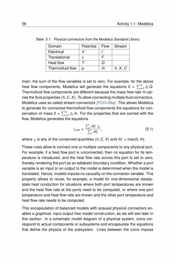
58 Activity 1.1: Modelica

Table 5.1: Physical connectors from the Modelica Standard Library.

Domain Potential Flow StreamElectrical V I

Translational x F

Heat flow T Q

Thermofluid flow p m h, X , C

main, the sum of the flow variables is set to zero. For example, for the aboveheat flow components, Modelica will generate the equations 0 =

n

i=1 ci Q.Thermofluid flow components are different because the mass flow rate m car-ries the fluid properties (h, C, X ). To allow connecting multiple fluid connectors,Modelica uses so called stream-connectors [FCO+09a] . This allows Modelicato generate for connected thermofluid flow components the equations for con-servation of mass 0 =

n

i=1 ci m. For the properties that are carried with theflow, Modelica generates the equations

χmix =

i m+i χi

i m+i

, (5.1)

where χ is any of the conserved quantities (h, C, X ) and m+i = max(0, m).

These rules allow to connect one or multiple components to any physical port.For example, if a heat flow port is unconnected, then no equation for its tem-perature is introduced, and the heat flow rate across this port is set to zero,thereby rendering the port as an adiabatic boundary condition. Whether a portvariable is an input or an output to the model is determined when the model istranslated. Hence, models impose no causality on the connector variable. Thisproperty allows to reuse, for example, a model for one-dimensional steady-state heat conduction for situations where both port temperatures are knownand the heat flow rate at the ports need to be computed, or where one porttemperature and heat flow rate are known and the other port temperature andheat flow rate needs to be computed.

This encapsulation of balanced models with acausal physical connectors en-ables a graphical, input-output free model construction, as we will see later inthis section. In a schematic model diagram of a physical system, icons cor-respond to actual components or subsystems and encapsulate the equationsthat define the physics of the subsystem. Lines between the icons impose

5.3 What is Modelica 59

the port equations to conserve flow and to equate state variables, or they maypropagate signals in a control system. Because these connectors are stan-dardized, models from different libraries can be connected with each other,thereby allowing users to use models from various domains and libraries withinone system model.

5.3.1.2 Illustration of a Simple Model

We will now illustrate how a simple heat flow component is built using theheat flow connector of the Modelica Standard Library. This connector is imple-mented by the following lines of Modelica code:

1 partial connector HeatPort

2 "Thermal port for 1-D heat transfer";

3 SI.Temperature T "Port temperature";

4 flow SI.HeatFlowRate Q_flow "Heat flow rate";

5 end HeatPort;

On line 4, the type prefix flow declares that Q_flow is a flow variable andhence need to be summed to zero as explained above. This connector canthen be instantiated to define the interface with the outside of the model in aone-dimensional heat transfer element with no energy storage. In Modelica’sthermal library, such a heat transfer element is implemented as follows:

1 partial model Element1D

2 "Partial heat transfer element with two HeatPorts"

3 SI.HeatFlowRate Q_flow

4 "Heat flow rate from port_a->port_b";

5 SI.TemperatureDifference dT "port_a.T-port_b.T";

6 public

7 HeatPort port_a "Heat port a";

8 HeatPort port_b "Heat port b";

9 equation

10 dT = port_a.T - port_b.T;

11 port_a.Q_flow = Q_flow;

12 port_b.Q_flow = -Q_flow;

13 end Element1D;

60 Activity 1.1: Modelica

Lines 3 to 5 contain the declaration of the variables Q and ∆T that are typicallycomputed in a one dimensional heat transfer element. Lines 7 and 8 instanti-ate the HeatPort connector to expose to the outside of this model the porttemperatures port_a.T and port_b.T, as well as the port heat flow ratesport_a.Q_flow and port_b.Q_flow. The equations on line 10 to 12 de-fine the relationships among the variables of the two HeatPort connectorsand the variables of the partial model Element1D. Note that Element1Ddoes not declare a relation between the heat flow rate and the temperatures,as this relation is different for conduction, convection or radiation. Because thisrelation is not specified, the model is declared partial to indicate that it canbe extended by other models to refine its implementation, but that it cannot beinstantiated directly as it does not define how temperature and heat flow rateare related. To implement a thermal conductor, the above partial model canbe extended as follows:

1 model ThermalConductor

2 "Lumped thermal element

3 transporting heat without storing it"

4 extends Interfaces.Element1D;

5 parameter SI.ThermalConductance G

6 "Constant thermal conductance";

7 equation

8 Q_flow = G*dT;

9 end ThermalConductor;

This thermal conductor model can then be encapsulated in a graphical iconusing drawing elements that are part of the Modelica language standard, andhence, can be interpreted by different Modelica modeling environments. Byusing a different parameter declaration on line 5 and a different equation online 8, the semantics can be changed to represent other one-dimensional heattransfer elements such as a model for long-wave radiation between two sur-faces. Note that the above code is not pseudo-code, but rather a completeimplementation of a heat conductor in the Modelica language, except for theoptional graphical annotations that will be explained in the next section. Notethat in the implementation above, the model developer only declared the vari-ables and the constraints between heat flow rate and temperatures. Whetherthe model will solve for the heat flow rate or for a port temperature will bedetermined by a code generator that analyzes the overall simulation model in

5.3 What is Modelica 61

order to determine a numerically efficient sequence of computations, as wewill show in Section 5.3.4.

5.3.1.3 Graphical Encapsulation

Creating, changing and understanding reasonably large system models with-out a graphical model editor would be very cumbersome if not impossible. Tobe able to use models in different graphical model editors, Modelica also stan-dardizes graphical elements such as lines, circles and colors that can be usedto graphically render an icon which encapsulates the model. In graphical edi-tors, these icons can be opened to see the actual model implementation, andthe icons can be used to graphically assemble components to build systemmodels. Fig. 5.2 shows how the above heat conductor can be used to com-pute the heat flow rate for a time-varying and a constant temperature boundarycondition on the left and right, respectively.

conductor

G=1

TBou2

T=T

KK

TBou1ramp

duration=1

Fig. 5.2: Thermal conductor with varying temperature boundary conditions.

5.3.1.4 Object-Oriented Modeling

Object-oriented modeling allows reusing common functionalities across differ-ent models. Duplication of code which would make it difficult to correct codingerrors throughout a large library of models when code is copied to differentmodels. In the Annex60 library, object-orientation is extensively used to imple-ment heat and mass balances of thermofluid flow components. It is also used,for example, to implement two-way control valves, which we will use here toexplain the principle of object-oriented modeling.

Two-way valves can be characterized by an opening function

ϕ(y ) =k(y )Kv

, (5.2)

62 Activity 1.1: Modelica

where y ∈ [0, 1] is the control input, k : [0, 1] → R is the flow rate divided bythe square root of the pressure drop and Kv = k (1) characterizes that flow ratefor a fully open valve. For a valve with linear opening characteristic, ϕ(y ) =l + y (1 − l), where l is the leakage of the closed valve, whereas for an equalpercentage valve, the function ϕ(·) is more complicated. To share code that iscommon among these valves, we can implement a base class such as

1 partial model PartialTwoWayValveKv

2 "Partial model for a two way valve using Kv"

3 extends BaseClasses.PartialTwoWayValve;

4

5 equation

6 k = phi*Kv_SI;

7 m_flow=BaseClasses.FlowModels.basicFlowFunction_dp(

8 dp=dp, k=k, m_flow_turbulent=m_flow_turbulent);

9 // ... (other code omitted for brevity)

Now, we can implement the valve with linear opening characteristics by ex-tending this base class and assigning the function ϕ(·) as follows:

1 model TwoWayLinear

2 "Two way valve with linear flow characteristics"

3 extends BaseClasses.PartialTwoWayValveKv(

4 phi=l + y * (1 - l));

5 // ... (other code omitted for brevity)

6 end TwoWayLinear;

Similarly, the valve with equal percentage opening characteristics can be im-plemented as

1 model TwoWayEqualPercentage

2 "Equal-percentage two-way valve"

3 extends BaseClasses.PartialTwoWayValveKv(

4 phi=BaseClasses.equalPercentage(y, R, l, delta0));

5 parameter Real R=50

6 "Rangeability, R=50...100 typically";

7 // ... (other code omitted for brevity)

8 end TwoWayEqualPercentage;

where the function BaseClasses.equalPercentage implements the

5.3 What is Modelica 63

opening characteristics.

This object-inheritance has various benefits. For users, if they understandwhat physics is implemented in the base class, for example that the valvelinearizes the pressure drop calculations at very small flow rates, then theyknow that this applies to both valves. For a developer, if a new capability needto be implemented, such as a heat loss of the valve, then this can be donein the base class and will be automatically propagated to both valves models.This is also useful for users that build system models from existing componentmodels. For example, in a variable air volume (VAV) flow system, each VAVdamper likely has the same controller. Hence, the user can implement thecontroller in one object and instantiate it for each VAV damper. Should thecontrol law require changes, then this can be done at a central place and thechange be propagated to all instances of this controller.

5.3.1.5 Hierarchical Modeling

Hierarchical modeling supports keeping a well-defined and visually accessiblemodel structure and helps manage complexity. This is aligned with the factthat physical problems are often analyzed by disaggregating them into sev-eral parts. Using hierarchical modeling allows having the same view withinsimulation models.

Consider for example modeling the thermal mass of a building. Standard work-flow encompasses disaggregating the building into several thermal zones. Inour fictive case, we consider two thermal zones (Fig. 5.3). Each of these ther-mal zones encompasses a number of wall elements representing e.g. exteriorwalls, interior walls and floor plates. These wall elements interact with eachother by radiative heat exchange and via convective heat exchange throughthe indoor air volume. Each wall element in turn encompasses the descriptionof heat transfer and heat storage effects, in our case described by thermalresistances and capacities.

Using hierarchical modeling approaches in Modelica, each level of thermalmass modeling can be created by connecting sub-models that represent lowerlevels. In this way, each level takes care of modeling the interactions betweenthe sub-models.

64 Activity 1.1: Modelica

Building

BuiOne

Thermal Zone

One

Thermal Zone

Two

Floor Plate

FloPla

Exterior Wall

ExtWal

Interior Wall

IntWal

Exterior Wall

ExtWal

Floor Plate

FloPla

Interior Wall

IntWal

RC-Element

RC-Element

RC-Element

RC-Element

RC-Element

RC-Element

Fig. 5.3: Hierarchical structure of a thermal building model with levels for building,

thermal zones, wall elements and RC-elements.

Refering to the system given in Fig. 5.3, the uppermost level is the buildingitself. At this level, we instantiate two thermal zones, using reduced ordermodels for thermal zones with three wall elements:

1 model Building

2 "Illustrates the use of hierarchical modeling"

3

4 RC.ThreeElements thermalZoneOne(...)

5 "Thermal zone one";

6 RC.ThreeElements thermalZoneTwo(...)

7 "Thermal zone two";

The visualization in the schematic diagram editor shows at the building levelboth thermal zones as simple icons without revealing any insights such as theirsub-models. These insights become only visible on the thermal zone level asshown in Fig. 5.4. This level implements the interactions of the walls, e.g., theradiative heat exchange. It also instantiates wall elements for exterior walls,interior walls and a floor plate.

Looking into BaseClasses.InteriorWall, as shown in Fig. 5.5, revealsthe actual implementation of resistances and capacities. These are connectedin series using vectors of models to create a finite difference heat transfermodel.

5.3 What is Modelica 65

SolargRadiation

ExteriorgWalls

Windows

IndoorgAir

V=VAir

volAir

V=VAir

volAir

resWin

R=RWin

convHeatSol

radHeatSolradHeatSol

ThermSplitter

ThermSplitter

extWallRC convExtWall

Gc

alp

Ext

k=

k

convWin

Gc

alp

Win

k=

k

k=g

eRadSol

k=g

eRadSol

k=g

eConvSol

resE

xtW

allW

in

G=

G

K

senTAir

Kse

nT

Ra

d

sumSolsumSol

InteriorgWalls

intWallRCconvIntWall

Gc

alp

Int

k=

k

resExtWallIntWall

G=G

resIntWallWin

G=G

FloorgPlate

floo

rRC

co

nvF

loo

r

Gc

alpFlo

k=K

resE

xtW

allF

loo

r

G=

G

resIntWallFloor

G=G

resF

loo

rWin

G=

G

solRad

TAir

TRad

ports

extWall

window intGainsConv

intGainsRad

windowIndSur extWallIndSur intWallIndSur floorfloorIndSur

Fig. 5.4: Diagram view of a thermal zone model with three wall elements (exterior

walls, interior walls and floor plate), windows and indoor air volume.

CInt

thermCapInt

CInt

thermResInt

R=RInt

thermResInt

R=RInt

port_a

Fig. 5.5: Diagram view of a thermal network for interior walls, consisting of an array

of thermal resistances and capacities.

66 Activity 1.1: Modelica

5.3.1.6 Architecture-Driven Modeling

When evaluating different building systems, it is convenient to implement asystem model of a base line, and then only declare how design variants differfrom the base line. Modelica supports such modeling through architecture-driven modeling, which enables declaration of which models can be replacedwith a different implementation. For illustration, consider a simple example inwhich we are interested in evaluating two different valves for a heat exchanger.One valve has linear opening characteristics, whereas the other valve has ex-ponential opening characteristics. This can be accomplished by implement-ing a system model of the base case, which contains the valve with the linearopening characteristics. We can declare this, using the TwoWayLinear valvedescribed above with the following code:

1 replaceable TwoWayLinear valve

2 constrainedby BaseClasses.PartialTwoWayValveKv(

3 redeclare package Medium = Medium,

4 CvData=Buildings.Fluid.Types.CvTypes.Kv,

5 Kv=0.65,

6 m_flow_nominal=0.04)

7 "Replaceable valve model”;

Here, we declared that the valve is of type TwoWayLinear (a two-way valvewith linear opening characteristics) and it can be replaced by any other valvethat uses (extends) the base class PartialTwoWayValveKv. The valveuses Kv data for the flow coefficient, with Kv = 0.65 and a design mass flowrate of m = 0.04 kg/s. These values are also applied to any valve that re-places this TwoWayLinear valve. Typically, such a model is part of a largersystem model as shown in Fig. 5.6 in which the replaceable valve is graphicallyrendered by a gray box.

With the few lines of code below, which can be either entered in a textualeditor or created from a graphical model editor, we can create a new modelthat is identical to the previous model except for the valve. The correspondingdeclaration is:

1 model EqualPercentageValve

2 "Model with equal percentage valve"

5.3 What is Modelica 67

sin_2 sou_2

sin_1sou_1

temSen

T

val

M

TSet

offset=0

hex

con

PIPI

Fig. 5.6: Model with heat exchanger, feedback control and replaceable valve. The

gray background rendered around the valve indicates visually that this model can be

replaced by another implementation.

3 extends DryCoilCounterFlowPControl(

4 redeclare Actuators.Valves.TwoWayEqualPercentage

5 valve);

6 end EqualPercentageValve;

This allowed us to change the architecture of the system by replacing a model,while reusing everything else in the base case. In large systems that may havehundreds of models, such modeling is very convenient as it shows only whathas changed from one version to another. Note that the replaced model canbe another hierarchical system model, for example one can replace in a wholebuilding simulation a heating plant with a gas furnace by a plant that uses aheat pump with a borehole heat exchanger.

5.3.2 Separation of Concerns

When implementing a model, a model developer typically writes computercode that implements functions, variable assignments, computing procedures,

68 Activity 1.1: Modelica

numerical methods and routines to obtain input. With Modelica, this is nolonger needed, as it suffices to simply state the physical laws and the controlalgorithm that a model should obey. Therefore, Modelica requires only declara-tion of the physics and dynamics of a model. How to solve the equations, whichvariables to assign first, when to read input and update outputs etc. need notbe specified. Thus, it is a modeling language, as opposed to an imperativeprogramming language such as C/C++. The underlying design philosophy isto separate the concerns between modeling, simulation and other applicationssuch as optimization or real-time simulation. In Modelica it suffices to imple-ment a mathematical model of the system without having to specify how tosolve the equations. The simulation program is automatically generated fromthe mathematical model using a Modelica translator that employs computer al-gebra as explained in Section 5.3.4. This allows for various target applications:For example, from a Modelica model, code can be generated for the following:

A conventional time-domain simulator that uses a classical or-dinary differential equation solver, and optionally generatecode for sequential or parallel computing [EMO14] .

A discrete-event simulator that can handle order of magnitudesbigger models than classical ordinary differential equationsolver [MBKC13] .

A building automation system that imports control code in astandardized format [NW14] .

An embedded real-time controller that may not have any harddisk for file input and output.

A web application in which the model is translated to JavaScriptso it can run native in a web-browser [Fra14] .

An optimization program that symbolically converts the modelto a form that allows computing optimal control functionssignificantly faster than conventional optimization methods[WBN16] .

Such a separation between mathematical model and executable applicationcode is a critical underlying principle for a future modeling and simulation en-vironment for building systems. By following this principle, it is possible tostructure the problem more naturally in the way a human thinks, and not howone computes a solution.

5.3 What is Modelica 69

5.3.3 Example Model

Fig. 5.7 demonstrates how a simple model can be constructed using compo-nents from the Annex 60 library. The model is available in the Annex60 libraryas Annex60.Fluid.Examples.SimpleHouse. It consists of a simplebuilding, a heating system and a ventilation system, with both systems includ-ing a controller. The building model consists of a wall, an air volume and awindow. The wall is represented using a simple model consisting of a singleheat capacitor and a heat conductor. The zone air is modeled using a controlvolume with mixed air, which is connected to the wall using a thermal resistorwhich represent the convective heat transfer. The window is modeled using acomponent that injects heat onto the wall. Boundary conditions are the outsidetemperature of the wall and the solar irradiation on the window.

The heating system consists of a radiator, a pump and a heater as illustrated inthe bottom of the figure. The heater thermal power is controlled using an on/offcontroller with hysteresis that tracks a set point for the zone air temperature.

To ventilate or cool the room, a ventilation system is modeled that consists ofa heat recovery unit, a fan, a cooling device and a damper. The fan appliesa constant pressure difference over the damper. The damper position is mod-ulated by a proportional controller to provide more air if there is a need forcooling.

To build the model, each individual component model was dragged from thecomponent library, placed on the schematic editor window, and connected toother components much like physical components. Model parameters like thepump mass flow rate were set by double-clicking on the respective component,which opened a parameter window. More detailed building models may beimplemented using one of the libraries that extend the Annex60 library andare listed at Section 5.4.2.

5.3.4 Model Translation

The translation of a Modelica model into a simulation program is a fully auto-mated process. When translating a model, symbolic processing is important toreduce computing time since many building system simulation problems lead

70 Activity 1.1: Modelica

Cooling and ventilation

Wall

Heating

Weather

walC

ap

V=V_zone

zone

V=V_zone

zone

convR

es

rad

bouAir

T

bouWat

weaDat

wallResTout

heaWat

Q=QHea_nominal

u Q_flow

pump

Pm_flow

K

senTemZonAir

vavDam

M

fan

P

dp_in

dp

window

hexRec

eps=0.85

hysRad

273.15 + 20273.15 + 22

booleanToReal1

BR

not1

not

const_dp

k=A_win*g_win

gaiWin

booleanToInt

BI

conDam

PTSetRoo

cooAir

T Q_flow

TSupAirCoo

weaBus

Fig. 5.7 : Modelica system model SimpleHouse as rendered by a Modelica graphical

model editor.

5.3 What is Modelica 71

Table 5.2: Incidence matrix prior to block lower triangularization.

Equation T1(t) T2(t) Q(t)1 x x x2 x3 x x

to large, sparse differential algebraic equation systems (DAE systems). Sym-bolic processing is typically used to reduce the index of the DAE system andto exploit sparsity. The following methods are typically used in Modelica simu-lation environments. To solve a DAE system with ordinary differential equationsolvers, the index of the DAE is reduced using the algorithm of Pantelides[Pan88] . Next, to exploit the sparsity of the model, Modelica translators gen-erally convert the coupled system of equations to block lower triangular form,by changing the equation order. This process is called block lower triangular-ization and is discussed in detail by Duff [DER89] . A simple example is asfollows: Consider the system of equations

Q(t) = T1(t)4 − T2(t)4,

f1(t) = T1(t)4,

f2(t) = T1(t)4 + T2(t)4,

(5.3)

where f1, f2 : R → R are known functions of time and T1, T2, Q are unknowns.A naive implementation would solve directly a three-dimensional non-linearsystem of equations using a Newton solver. However, we can consider theincidence matrix whose columns are the independent variables and rows arethe equations, as shown on the left of Table 5.2. In the incidence matrix, cell(i,j) contains an x if the independent variable i depends on the equation j.

For this system, we can permute the rows so that all cells with an x are belowthe diagonal, as shown in Table 5.3.

This shows that by rearranging the equations, we can solve sequentially

f1(t) = T1(t)4,

f2(t) = T1(t)4 + T2(t)4,

Q(t) = T1(t)4 − T2(t)4.

(5.4)

72 Activity 1.1: Modelica

Table 5.3: Incidence matrix after block lower triangularization.

Equation T1(t) T2(t) Q(t)2 x3 x x1 x x x

Finally, using computer algebra, these equations can be converted into theexplicit assignment

T1(t) = (f1(t))1/4,

T2(t) = (f2(t) − T1(t)4)1/4

Q(t) = T1(t)4 − T2(t)4,

(5.5)

and hence no iterative solution is required.

After block lower triangularization, there may still be sets of equations that re-quire a coupled iterative solution. In this situation, tearing can be used to breakthe dependency graph of equations and variables to further reduce the dimen-sionality of the coupled system of equations. The resulting coupled systemsof equations are typically small but dense. Tearing can be done automaticallyor it can be guided by using physical insight with language constructs that canbe embedded in a model library [EO94] . A simple example of tearing is asfollows: Suppose we have an equation of the form

0 = f (x), (5.6)

for some x ∈ Rn, with n > 1, that can be written in the form

L x1 = f1(x2),

0 = f2(x1, x2),(5.7)

where L is a lower triangular matrix with constant non-zero diagonals. If this isthe case, we can pick a guess value for x2, solve the first equation for x1, com-pute a new value for x2 from the second equation and iterate until x2 converges.As f1(·) has fewer equations than f (·), this often results in faster computationas the computing time of many numerical algorithms grows proportional to n3.

5.3 What is Modelica 73

Fig. 5.8 from the Dymola 2016 user manual shows for a mechanical modelwith kinematic loops that consist of 1, 200 equations how symbolic processingsignificantly reduces the dimension of the coupled systems of equations.

0 200 400 600 800 1000 1200

0

200

400

600

800

1000

1200

nz = 3995

0 50 100 150 200 250 300

0

50

100

150

200

250

300

nz = 1017

0 50 100 150 200 250

0

50

100

150

200

250

nz = 895

0 50 100 150 200 250

0

50

100

150

200

250

nz = 916

Incidence matrix of the original problem

(dimension 1200x1200)

Incidence matrix after elimination of alias

variables (dimension 330x330)

After simplifications

and BLT

(dimension

250x250)

Tearing reduces

dimension of nonlinear system of equations from 12x12 to 2x2,

and the dimension of one linear system from 11x11 to 2x2 and

for another linear system from linear 57x57 to 5x5

Fig. 5.8: Reduction of the dimension of the system of equations for the case of a

mechanical model during the symbolic processing.

Finally, a further reduction in computation time can be obtained by symbolicallyinserting the discretization formula that represents the numerical integrationalgorithm into the differential-algebraic equation model, a process called inlineintegration that was introduced by Elmqvist et al. [EOC95] .

5.3.5 Use of External Code

While the above model translation is powerful, there are situations where a hu-man programmer can generate more efficient code. In the buildings domain,a typical example is the solution for partial differential equations for compu-tational fluid dynamics. Partial differential equations often lead to repeatingstructures, such as a band-diagonal matrix, for which efficient solution algo-

74 Activity 1.1: Modelica

rithms or parallelization methods can be devised or that can simulate fasterwhen parts of the computation is done on a graphical processing unit, see forexample [ZC10] . For such situations, the Modelica language allows for thecalling of C or FORTRAN 77 code, as well as compiled code. Using C codeis for example used in the Buildings library to connect Modelica with Python,and compiled code is used to link code for computational fluid flow dynamicsfor indoor air simulation to the building model in [ZWT+16] .

5.3.6 Debugging

When talking about debugging, users typically mean instruction-by-instructionexecution of a program code. This makes sense for imperative programminglanguages such as C/C++, or for signal flow diagrams such as in Simulink, orin actor-based modeling such as in Ptolemy II. However, Modelica, except forthe body of Modelica functions, has no notion for line-by-line execution.The equations are declarative. A tool can rearrange equations, invert them bychanging variables on the left- and right-hand side or by doing other computeralgebra before it generates code. Hence, the process of “simulating” a Model-ica model is fundamentally different from simulating a model that is expressedin code such as C/C++, Java or Python. Consequently, debugging needs tobe approached differently.

To explain how to debug declarative Modelica models, let us first stipulate thatthe code is translated correctly from Modelica to an executable language suchas C/C++, but that the trajectories of the simulation are unexpected. There-fore, one debugs to verify what equations, not what variable assignment, maybe wrong. This is often easiest by breaking up large models into small compo-nent models and test them individually. Through this process, wrong equationsare often easy to detect by looking at the results of a simulation and comparingthem to an analytical solution. This is also the reason why good model devel-opment should always include the implementation of small unit tests, prefer-ably for different input signals for which the correct solution is known a-priori.Then, assembling models to form larger systems seldom introduces an errordue to Modelica’s implementation of physical connectors and its requirementsof models to be balanced, as described in the Section 5.3.1.1.

Debugging can also consist of understanding why a system model has large

5.4 Annex 60 Library 75

linear or nonlinear algebraic loops. In this situation, Modelica translators typi-cally allow for the inspection of intermediate formats that are human-readablemodel representations after the symbolic manipulation but before generatingC code. For example, an intermediate format can show which equations relatethe inputs to the outputs and which equations require use of a linear solver oruse of a nonlinear iterative solver.

Another purpose of debugging may be to reduce computing time. For thispurpose, some simulation environments allow for running diagnostics on themodel to see in what equations most of the computing time is spent, whatvariables dominate the error and the time step size control, and what logicaltests produce events that can increase the computing time.

Furthermore, tools typically have intermediate formats and/or debuggers thatshow what Modelica variable appears in what part of the generated code.

5.4 Annex 60 Library

This section describes the open-source, free Modelica Annex60 library thathas been developed since 2012 and is now used as the core of the Model-ica libraries of RWTH Aachen, from LBNL Berkeley, CA, UdK Berlin and KULeuven.

The goal of the development of the Annex60 library is to create an open-source, freely available, well documented, validated and verified Modelica li-brary that serves as the core of other Modelica libraries for building and districtenergy systems, and for whole building simulation programs. Hence, the li-brary should set a foundation for the development of models and whole modellibraries that serves the building simulation community over the next decades.

This effort is also expected to support realizing various propositions of JoeClarke’s position paper that he wrote on behalf of the IBPSA Board [Cla15] .That position paper calls for a consolidation of models for HVAC and controlsthat can be used for testing, as a review framework and as a library (Proposi-tions 1, 3, 4, 5, 6, 7, 9, 11 and 12). The stated opportunity is

1. to standardize the approach for how such component and system mod-els are represented, both as data-model and as mathematical models

76 Activity 1.1: Modelica

that formalize the physics, dynamics and control algorithms,2. to agree upon the physics that should be included in such components

for specific use cases, and3. to share resources for development, validation and distribution of such

component and system models

Specifically, proposition 6 states:

IBPSA will encourage manufacturers to provide more fundamen-tal descriptions of components and make these available within astandard library.

We believe that the Annex60 Modelica library could serve as the basis ofsuch a standard library.

5.4.1 Approach

The approach of the library distribution is modeled after Linux, which has akernel that is used by different distributions (e.g., Ubuntu, RedHat etc.), whichthen provide installation packages, user support and detailed documentation.In a similar fashion, the Annex60 library provides reliable base classes forbuilding and HVAC component models. Developers of the different modellibraries then integrate this library into their Modelica library, add additionalmodels, provide documentation and user support. Through this process, thedifferent model libraries of participating institutions can be further developed,each with their specific focus, while compatibility among the libraries is en-sured by the use of the common base classes from the Annex60 library. Inaddition to the advantages of having a reliable and well-tested common foun-dation for model development, further benefits include increased compatibility,exchange and collaboration as opposed to the previously fragmented develop-ment of mutually incompatible libraries.

5.4.2 Libraries That Use the Annex 60 Library as Their Core

At the start of Annex 60, four institutes developed their own library in a mannerthat made models among these libraries incompatible. This led to duplicative

5.4 Annex 60 Library 77

effort in model development and validation, and limited the scope of each li-bray. Within Annex 60, the following institutes worked together, which resultedin their libraries to be all based on the Annex60 library, thereby allowing usersto combine models from these libraries, and reducing development effort:

• RWTH Aachen, Germany, which develops AixLib, available from https://github.com/RWTH-EBC/AixLib

• UdK Berlin, Germany„ which develops BuildingsSystems, availablefrom http://modelica-buildingsystems.de

• Lawrence Berkeley National Laboratory, Berkeley, CA, USA, whichdevelops Buildings, available from http://simulationresearch.lbl.gov/modelica

• KU Leuven, Belgium, which develops IDEAS, available from https://github.com/open-ideas/IDEAS

5.4.3 Functional Requirements

The Annex60 library needs to fulfill several functional requirements that origi-nate from typical use cases in building performance simulation. The use casesinclude design and analysis of warm water heating and distribution systems,cooling systems, ventilation systems, heat demand calculations of multiplebuildings, controls design, co-simulation and export of models for use in othersimulators or in building automation systems. The use cases aim at optimaldesign and operation of thermal energy systems as well as district energy sys-tems and model use during operation. Thus, the Annex60 library focuses onannual whole building simulation, on single as well as on multiple buildings.

Regarding physical resolution, various effects are modeled to ensure suitabil-ity for typical use cases. For example, all mass flow rates are pressure drivento allow simulations of duct and piping networks. Optionally, all equations forpressure drop calculations can be removed from the models through a param-eter assignment. Transport delays can be added to fluid flow networks. Themedia models are compatible with models from Modelica.Media to ensurecompatibility with other libraries. For air, water vapor and trace substancessuch as CO2 or VOC concentrations are tracked as to account for moisturetransfer and for simulation of indoor air quality. For cooling devices, no de-tailed modeling of the state and distribution of refrigerants is conducted as this

78 Activity 1.1: Modelica

would lead to computing time that is too large for annual building simulation.1

Regarding dynamic system behavior, models with different idealizations areimplemented. Where applicable, it is possible to approximate the dynamic re-sponse of models using a first or higher order response, and optionally disablethe model dynamics to conduct a quasi steady-state simulation. For example,the dynamics of sensors can be approximated by a first order response. Thiscan be disabled to obtain a steady-state sensor, or to add a more detailedsensor response to the output signal of the sensor.

It is also possible to export as a Functional Mockup Unit (FMU) thermofluidcomponents, as described in [WFN15] . All models use SI units.

5.4.4 Mathematical Requirements

Component models from this library are typically assembled to form systemmodels that lead to systems of ordinary differential equations, which are cou-pled to algebraic systems of linear, nonlinear and discrete equations. To en-sure that these systems of equations can be solved efficiently, they need tosatisfy certain mathematical properties. In this section, we describe the mainrequirements that have been followed during the development and are satis-fied by the Annex60 library.

For equations that describe the physics, the following mathematical propertiesneed to be satisfied:

1. Equations must be differentiable and have a continuous first derivativethat is bounded on compact sets, i.e., they need to be once continu-ously differentiable on compact sets. This is not only needed for nu-merical efficiency, but also to establish existence of a unique solutionto the system of differential equations [CL55] , and it provides a keyrequirement for the solution of optimal control problems in which thecost function is defined on numerical approximations to the solutions ofthe differential equations [Pol97][PW06] . For example, instead of us-ing y (x) = sign(x)

|x |, this equation needs to be approximated bya differentiable function that has a finite derivative near zero because

1 For such applications, the AC library from Modelon or the TIL library from TLK-Thermo GmbHmay be used.

5.4 Annex 60 Library 79

limx→0 y ′(x) = limx→0 1/(2

|x |) = ∞. Otherwise, Newton-Raphsonsolvers may fail if x is close to zero, as the Newton step length is propor-tional to the inverse of the derivative of the residual function.

2. Equations where the first derivative with respect to another variable iszero must be avoided. For example, let x , y ∈ R and x = f (y ). Anequation such as y = 0 for x < 0 and y = x2 is not allowed. The reasonis that if a simulator tries to solve 0 = f (x), then any value of x ≤ 0 is asolution, which can cause instability in the solver. An example of sucha situation is a valve. If it were to have no leakage flow, then any valueof the pressure drop would cause zero mass flow rate, which may leadto ill-conditioned equations for some flow networks. More formally, theconditions for the Implicit Function Theorem [Pol97] need to be satisfiedas this guarantees existence and differentiability of an inverse of thefunction.

3. Equations that cause divisions by zero should be avoided.

Clearly, models for controls require discrete variables that can only take oncertain values, such as for switching equipment on or off. This certainly isallowed, but must be implemented using a hysteresis to avoid chattering. Forexample, an equation such as y = 0 if T > 20∘C and y = 1 otherwise is notallowed as this can lead to chattering in continuous time solvers.

5.4.5 Process for Quality Control

The Annex60 library is used as a foundation on which different libraries forend users are developed. It therefore needs to provide reliable models and re-sults. Thus, a strict process for quality control was implemented from the startof the library development. This process includes open source code develop-ment in a version control system on GitHub, automated regression testing ofthe entire library, and a review process before authorizing any code changes.This process is supervised by a core development team. However, contribu-tions from the community are encouraged, given that they meet the qualitystandards and requirements of the library.

Using git for version control of the source code and documentation of thelibrary allows for keeping a record of all development stages and changesof the library. Stable models are kept in the so-called master branch. Ad-

80 Activity 1.1: Modelica

ditions and code changes are restricted to dedicated branches for featuredevelopment that are documented in a corresponding issue tracker. In or-der to prevent any unintended effects of code changes to existing models,the translation statistics and reference results for each model are automati-cally created, stored, and managed by using the Python package BuildingsPy(https://github.com/lbl-srg/BuildingsPy). This package includes functions forunit testing. The implemented process for quality control requires contributorsto provide a scripted test for every model, so that these tests can be run au-tomatically for the whole library. When introducing a model and its test, thesimulation results are saved by the unit testing routine. The unit testing is runbefore accepting any changes to the master branch. Differences in the transla-tion statistics and simulation results between reference results and the testedmodel are automatically plotted and need to be accepted or rejected manu-ally, thus guarding against introducing unwanted effects on any of the existingmodels.

Once code changes have been documented and evaluated by unit testing, theyneed to be reviewed by a second developer. Thus, the author of the changesissues a pull request to suggest moving the new code into the master branch.Only after all comments from the reviewer have been addressed by the orig-inal author of the changes is the new code merged to the master branch. Atthe time of writing, this process has been applied to over 400 issues and 1000changes to the code base. Finally, the underlying version control system canserve as a safety net if changes need to be reverted despite the describedquality control process. As each step of code change as well as the responsi-ble author is documented at all times, such corrections require little effort.

5.4.6 Requirements for Adding Classes

The Annex60 library aims at following a coherent set of conventions and re-quirements to ease maintenance and further development. The library followsand extends the conventions of the Modelica Standard library. In addition, thenames of models, blocks and packages must start with an upper-case and bea combination of adjectives and nouns using camel-case to combine multiplewords, whereas instances of these models, blocks and packages start with alower case letter. The names of each Modelica function must start with a

5.4 Annex 60 Library 81

lower-case character. Instance names are usually a character, such as T fortemperature and p for pressure, or a combination of the first three charactersof a word, such as TSet for temperature setpoint or higPreSetPoi for highpressure set point.

New components of fluid flow systems must extend the partial classes definedin the package Annex60.Fluid.Interfaces. If the new class is partialor if it is not intended for the end-user, it must be added to a BaseClasses

package. Each new model must be used in at least one model containedin the Examples or Validation package, which illustrates or validates itsbehavior and is included in the unit tests.

Each class needs to be documented. Every variable and parameter must havea documentation string. The documentation section of the model providesa more comprehensive documentation describing the main equations, modelassumptions and limitations, typical use, options, validation, implementationand references. Some of these sections are optional as they are not appli-cable to all models. Each class also contains a list of revisions made by thedevelopers to keep track of the changes and their rationale.

The robustness of the models is also a key requirement, and the guidanceexplained in Section 5.4.4 needs to be followed. Fluid flow models must bestable near zero mass flow rate even under the assumption that flow rates orheat input are approximate solutions obtained using an iterative solver. Fluidflow models must be well-behaved if the mass flow reverses direction.2 Fur-thermore, fluid flow models use the Annex60.Media models, which havephysical constraints such as the valid temperature range or relative humiditybounds outside which they are not valid. These bounds need to be takeninto account by the models in order to avoid non-physical situations or con-vergence problems. Parameters and variables should whenever possible useunits from Modelica.SIunits and they should declare bounds for minimaland maximal values. Default values for parameters, which can be adapted bythe end-user, should be declared using the start attribute so that the user getsa warning if no other value has been provided.

2 By well-behaved, we do not mean, for example, that a performance-curve based model of adirect expansion cooling coil computes the right physical results if there is a slight backward flow,but rather that the model is robust. For example, it suffices to add no energy to the air if there isslight backward flow.

82 Activity 1.1: Modelica

Each model must be validated using either measurement data, cross validationwith other simulators or with analytical solutions. Validation models need to beadded to the Validation package and be included in the unit tests.

Finally, new models should be in line with the scope of the library as describedin the functional requirements.

5.4.7 Design Decisions

This section describes the main design decisions for the Annex60 library.

5.4.7.1 Media

In Modelica, component models typically call functions to obtain thermody-namic properties such as the specific enthalpy.

We experimented with two implementations. One approach calledMediaFunctions was using functions for the thermodynamic proper-ties of a medium, with an enumeration as a function argument that de-clares the medium type such as air or water. The other approach calledMediaPackages was using a separate package for each medium type, as isdone in Modelica.Media.

The main differences between these two implementations are as follows:

1. For MediaFunctions, models of HVAC equipment require parame-ters for the medium type and for the default values of pressure, tempera-ture, mass concentration and trace substances. The medium type needsto be propagated to the functions that compute the thermodynamic prop-erties.

2. For MediaPackages, there is one package for each media type, asin Modelica.Media. Models of HVAC equipment contain a replace-able parameter for the medium package that needs to be set to mediumtype. Prior to the model translation, the medium type such as water, airor glycol must be declared, but its concentration can be changed aftertranslation.

5.4 Annex 60 Library 83

Based on these implementations, we decided to organize media in packagesas is done in Modelica.Media. The benefits are:

1. Full compatibility with Modelica.Media.2. Default values for the medium, such as the default pressure and mass

concentration, can be propagated through its declaration because pack-ages can contain constants.

3. Modelica translators can verify that connected fluid ports contain thesame medium, and refuse to translate the model if this is not satisfied.

The advantage of using MediaFunctions would be that only two sets ofFMUs need to be generated, one for the single species medium water, andone for the dual-species media such as air and glycol. However, the cost ofseparately compiling FMUs for air and for glycol is small as this can be fullyautomated and be done as part of a simulation engine development.

While the implementation of Annex60.Media is compatible withModelica.Media, we generally use simpler implementations. For ex-ample, in Annex60.Media.Air, water is only present in vapor form even ifthe water vapor pressure is above the saturation pressure. This allows for thecomputation of temperature from specific enthalpy and mass concentrationwithout requiring iterations, thereby leading to more efficient models.

5.4.7.2 Fluid Connectors

We decided to use the same fluid connectors as defined in Modelica.

Fluid. These connectors declare the medium package (used to assert thatonly models with the same medium are connected), the mass flow rate as theconserved quantity, the absolute pressure as the potential variable, and thefollowing variables that are carried by the mass flow: the specific enthalpy, op-tionally the mass fraction such as to declare the mass concentration for watervapor in air, and optionally trace substances. Trace substances are concentra-tions that can be neglected for the thermodynamic calculations such as CO2

or VOC concentrations.

We also explored using temperature instead of specific enthalpy in the con-nector. Modelica’s concept of flow and stream variables allows connecting

84 Activity 1.1: Modelica

multiple fluid ports. It then automatically generates the conservation equation

χmix =

i m+i χi

i m+i

, (5.8)

where χ is the conserved quantity, m+i = max(0, m) is the mass flow rate if it is

positive and the subscripts mix stands for the mixture and i for the connectedports. If χ = h is the specific enthalpy, then hmix is always correct. If χ = T

were temperature, then Tmix is wrong if the specific heat capacity cp dependson temperature. We therefore selected the specific enthalpy to be in the fluidconnector, as is also used in Modelica.Fluid.

5.4.7.3 Package Structure

In Modelica, classes can be collected and organized hierarchically into pack-ages. This section describes how the Annex 60 library organizes classes intothe following main packages:

BoundaryConditions contains models for weather datareader, solar radiation and sky temperature.

Controls contains models for continuous time and discrete timecontrollers and for set point scheduling.

Fluid is the main package that contains thermofluid flow com-ponents such as heat exchangers, pumps, valves, airdampers and boilers. We considered introducing subpack-ages Fluid.{Air,Water,Glycol} but have not doneso yet as this would lead to duplication of code and docu-mentation. Consequently, users always need to assign themedia.

Utilities contains the major packages Psychrometrics,which implement blocks and functions for psychrometricproperties, and Math, which provides blocks and functionsthat are once continuously differentiable approximations tofunctions such as min : R×R → R, abs : R → R, the Heav-iside step function or cubic spline interpolation. The functionsin the Math package are used to satisfy the earlier discusseddifferentiability requirements.

5.4 Annex 60 Library 85

Major packages contain user guides, and all packages contain an Examplesor a Validation package that demonstrates how to use the models, andthat are used for validation and regression testing.

5.4.8 Main Classes of the Library

The Annex60 library provides models for simulating HVAC systems in build-ings, containing both hydronic and air flow models. These systems combinedifferent types of components such as energy and mass transfer models, me-dia models for air and water, control models and supporting utilities. Thesetypes are grouped in separate packages. This section gives the highlights ofthese packages.

5.4.8.1 Fluid Component Models

A typical HVAC system contains components such as valves, pumps, dampersand heat exchangers. Essentially these are all components that transfer massand/or energy. These models are therefore grouped in the Fluid package.The most important parts of this package are now discussed.

Conservation of Energy and Mass Since all of these models need to con-serve mass and energy, the Fluid package heavily relies on the modelConservationEquation that implements these conservation laws. Themodel is implemented in a generic way such that it can be used for dif-ferent types of media: compressible and incompressible and media withor without moisture or trace substances. The energy and mass conserva-tion laws can be configured to be a steady state or dynamic balance. TheConservationEquation model is instantiated by the MixingVolume

model, which is used by most equipment models.

Flow Networks Since the physics of fans and pumps is similar, they are im-plemented using the same models in the Movers subpackage. This packagecontains four mover models, each using a different control signal:

86 Activity 1.1: Modelica

FlowControlled_m_flow This model directly sets the massflow rate, independent of the head pressure that results fromthe duct or pipe network simulation.

FlowControlled_dp This model directly sets a pressurehead, independent of the mass flow rate that results fromthe duct or pipe network simulation.

SpeedControlled_Nrpm This model sets the speed. Massflow rate and pressures are calculated from similarity laws,from a user-provided pump curve and the duct or pipe net-work simulation.

SpeedControlled_y This model is identical toSpeedControlled_Nrpm, except that the input sig-nal is normalized by the nominal speed.

Various types of flow resistance are implemented. For example,FixedResistanceDpM implements a pressure curve according to Kv =mnom/

√∆pnom = m/

√∆p, where mnom is the nominal mass flow rate, ∆pnom

is the nominal pressure drop, and m and ∆p are the actual mass flow rate andpressure drop. In a neighborhood around zero, this function is regularized. Invalves and dampers, the Kv value is a function of the actuator input y . Thelibrary implements models in the Actuators subpackage where the relationbetween Kv and y is expressed using a linear, quick opening or an equal per-centage characteristic. Custom opening characteristics using a table can alsobe used, as well as a pressure independent characteristic. Various dampers,two-way and three-way valves of these types are implemented.

Energy Transfer The library provides the model HeaterCooler_T, whichis a heater or cooler that maintains an outlet temperature, subject to optionalcapacity limits. The outlet temperature is obtained from an input signal. Themodel HeaterCooler_u is a variant of this model that takes as an inputa control signal that is proportional to the heat to be added to or removedfrom the fluid. A heat exchanger with constant effectiveness can be usedto transfer energy between different fluid streams. A similar model exists fora mass exchanger that transfers moisture. The model RadiatorEN442_2implements a radiator model based on the EN 442-2 norm.

5.4 Annex 60 Library 87

Other Models Various models are available for integrating fluid componentsin larger models. Models from the Sensors package can be used for integrat-ing control components and for performing analysis. The Sources subpack-age implements components for enforcing boundary conditions on fluid ports.The user can configure the model to obtain the mass flow rate or pressurefrom a parameter or from an input signal.

5.4.8.2 Media

The library contains media implementations for water and air. Water is con-sidered to be incompressible with constant thermal properties. Air con-tains moisture, has a pressure-dependent density and constant thermal prop-erties. More detailed implementations are available in the subpackagesSpecialized.{Air,Water}.

5.4.8.3 Control Models

The Controls package contains basic control components such as PID con-trollers and blocks for set point resets. Our intention is to expand this packageto provide control blocks and template control sequences that are commonlyused in building control systems.

5.4.8.4 Utilities

The Utilities package contains models that simplify the consistent im-plementation of other components. The Psychrometrics subpackage, forexample, contains functions and models for relating the vapor fraction and par-tial pressure to the humidity and wet bulb temperature. The Math subpackagecontains commonly needed once continuously differentiable approximations tomathematical functions.

88 Activity 1.1: Modelica

5.4.9 Merging with other Libraries

To automatically merge the Annex60 library with libraries that are basedon it, such as the libraries AixLib, Buildings, BuildingSystems andIDEAS, developers of these libraries use the Python package BuildingsPyand execute the following commands:

1 import buildingspy.development.merger as m

2 src="/home/joe/modelica-annex60/Annex60"

3 des="/home/joe/modelica-buildings/Buildings"

4 mer=m.Annex60(src, des)

5 mer.merge()

These commands copy all Annex60 library models from the directory /

home/joe/modelica-annex60/Annex60 into the library Buildings

in the directory /home/joe/modelica-buildings/Buildings. Themerge() command updates all hyperlinks, references to package names andfile names that contain the Annex60 string. Therefore, users will only see therespective library and do not have to combine models from different libraries.

5.5 Getting Started

To get started with Modelica, we suggest the following literature for those whowant to use Modelica or want to develop Modelica models.

5.5.1 Literature for Users

The following books are useful for new users to get started:

• The online book with interactive examples of Michael Tiller at http://book.xogeny.com/.

• The books by Michael Tiller [Til01] and Peter Fritzson [Fri11][Fri15] .• The tutorials that are listed at https://www.modelica.org/publications.

Although the Modelica Language Tutorial at https://www.modelica.org/documents/ModelicaTutorial14.pdf is for an older version (Modelica 1.4), it is

5.6 Conclusions 89

still instructive and relevant to understand the concepts of the language.

The Annex60 library as well as the libraries that use it as their core containshundreds of examples of varying complexity that can be simulated and modi-fied to get accustomed to using Modelica.

5.5.2 Literature for Developers

For users who develop new thermofluid models, it is essential to under-stand the concept of stream connectors. Stream connectors are explainedin the Modelica language definition, available at https://www.modelica.org/documents, and in [FCO+09a] . Furthermore, developers should have a properunderstanding of the implications of flow reversal and know when what typesof algebraic loops are generated. This is discussed in [JWH15] .

The Annex60 library uses similar modeling principles, as the Modelica.

Fluid library. Hence, we also recommend reading the paper about thestandardization of thermofluid models in Modelica.Fluid as described in[FCO+09b] .

Xogeny’s Modelica Web Reference at http://modref.xogeny.com/ gives a con-cise overview, explanation and further links about the Modelica language.

5.6 Conclusions

Using Modelica allowed using and contributing to an open standard for modelrepresentation, which is supported by a large ecosystem of tools, has an activedevelopment and user community, and enjoys significant investment from var-ious industrial sectors. Using a multi-disciplinary modeling language allowedfor interdisciplinary collaboration among communities in engineering, appliedmathematics and computing. Collaboration between these research commu-nities that have deeper knowledge of their respective fields has shown to becritical in addressing increasingly challenging demands on computational toolsthat support the design and operation of high performance buildings and com-munities.

90 Activity 1.1: Modelica

At the first expert meeting of the planning phase of Annex 60, in March 2013at RWTH Aachen, Germany, participants were hesitant to open up their pro-prietary development, open-source their code and embark on a joint develop-ment of an open-source library that should become the core of their respectivelibraries. However, as the collaborations slowly took shape, participants sawthe value in avoiding duplicative work, in conducting collaborative researchand in jointly developing a core library. Hence, participants ended up investinga considerable amount of work in scrutinizing different implementations, refac-toring their respective libraries and sharing previously proprietary code. As aresult, the four major Modelica libraries for building and district energy systemsnow all share the same set of core models, they became more robust, bettervalidated and compatible with each other. With this shared development, An-nex 60 created a robust, open-source basis for a model library for the buildingsperformance simulation community. As of this writing, the further developmentof this code is being transferred from the umbrella of the IEA EBC Programmeto the International Building Performance Simulation Association IBPSA.

Chapter 6

Activity 1.2: Co-simulation

and Model Exchange Using

the FMI Standard

6.1 Introduction

6.1.1 Motivation for Coupled Simulation

Currently, there is a significant number of sophisticated simulation models andtools available for use in building energy simulation. Models and parametriza-tion are provided by different specialists, with some models being the outcomeof many years of development. Hence, different programming languages andmodeling approaches are used.

Often, a tool misses functionality provided by others. For many applications itis desirable to use several simulation tools concurrently and make use of re-sults generated by the different models. Consequently, tools running transientsimulations often need results generated by other models at runtime. For ex-ample, a building energy simulation model computing room air temperaturesmay require heating loads from an HVAC supply system, with the latter coming

92 Activity 1.2: Co-simulation and Model Exchange Using the FMI Standard

from a simulation model external to the building simulation tool.

Pure integration of several existing models into a single simulation tool is tech-nically very difficult, in particular since many tools include their own numericalsolver engines and calculation algorithms. Moreover, different simulation toolsmanage their internal data differently, which further complicates their integra-tion. Also, given different authors, domain experts, copyright limitations, etc.an integration into a single tool may not be meaningful or possible at all. Lastly,future development and maintenance of such an integral model may be difficultto organize. It is also difficult to ensure lasting financial support for develop-ment and maintenance of a complex integral simulation tool authored by manyindividual developers.

Translating existing models into modular equation-based languages such asModelica could be considered as an alternative, and could benefit from mod-ern Modelica features. Modular, hierarchical design could be used and Model-ica tools would be able to optimize the system of resulting equations for perfor-mance. However, this approach may not be economically feasible regardingthe expected overhead of translating a large number of existing models, andtheir documentation. Also, copyright and intellectual property protection maynot permit integrating their existing model code.

As an alternative, new and existing code of complex systems can be decom-posed into sub-systems, the subsystems simulated with the simulator whichsuits best the specific domain, and interface variables exchanged as the sim-ulation progresses.

Co-simulation is a technique in which simulators are executed simultaneouslywhile exchanging data during run-time. In this context we refer to simulators,also called slaves, as individual component models described by differentialalgebraic or discrete equations.

The simulators typically embed systems with differential-algebraic equations.Each simulator may implement different numerical techniques tailored to aspecific physical or mathematical problem. This includes the possibility thatthrough usage of special programming language features, memory layout,parallelization or other specific optimization, the specialized implementationfor model equations may perform better than an equivalent model in a genericsimulation environment.

6.1 Introduction 93

6.1.2 Need for a Tool Coupling Standard

When considering coupled simulation of different tools, several options areavailable:

1. When access to source code is possible, or tool developers can workactively together, tools may interface directly. Simulation tool develop-ers may even incorporate calculation capability from another tool intotheir own code. Such a procedure depends on many prerequisites, suchas compatible programming languages, proper license agreements,data and calculation structure compatibility and sufficient developer re-sources. In many cases the resulting code can be considered as a newintegrated tool and not really a coupled tool.

2. In the one-to-one approach, two tools implement a specific protocol thatregulates exchange of data during runtime. This approach is the mostflexible and can support any kind of numerical solution method and alsotake into account peculiarities of the tools involved. However, the imple-mentation may need to be continuously updated when one of the toolsevolves. Also, if tools are developed independently, testing and checkingof correct functionality may become time-consuming. Furthermore, in-terfacing with a third tool typically requires reformulation or adaptation ofthe protocol and effectively implementing another coupling mechanismtailored to the new tool. Lastly, the development of a clear applicationprogramming interface (API) specification and the semantics of the toolcoupling is difficult, and subsequent revisions to this API may incur largedevelopment costs.

3. To overcome the need for, potentially many, one-to-one exchange pro-tocol implementations a middleware could be used. This acts as a hubfor several tools that interface with it and relays communicated data toother connected tools. This approach is less flexible than the one-to-oneapproach, since a common ground on interface capability needs to beagreed upon. When interfacing domain-specific tools, the middlewarecan be fitted to the specifics of the problem types and applied numericalmethods. Tools need to implement only a single interface and commu-nication protocol and only need to revise code when the middleware isupgraded. However, the same problem regarding the API specificationas for the one-to-one approach remains.

94 Activity 1.2: Co-simulation and Model Exchange Using the FMI Standard

In the past, many tool coupling technologies have been developed and ap-plied, with different mathematical concepts and programming interfaces. Manyhave been tool-specific proprietary interfaces that may change frequently asthe original tool developers see fit. Further, the details of interfaces are of-ten restricted to certain applications and lack functionality needed in otherphysical domains. This is particularly true for domain-specific middleware ap-proaches. In addition, closed-source middleware implementation details maychange from version to version, thus potentially render previously connectedtools incompatible.

To overcome these limitations it was necessary to develop an open-sourceand community driven standard for coupled simulation. In 2008 the Mod-elisar project started to develop such a standard, named the FunctionalMockup Interface (FMI, https://www.fmi-standard.org/). Finally, with the ini-tial 1.0 release, a standard for interfacing simulation tools has become avail-able. See [BOA+11] for an introductory paper and https://www.fmi-standard.org/literature for various literature about FMI.

6.1.3 Overview of the FMI Standard

The FMI standard describes the mathematical concept for coupled simulationof several simulators, called Functional Mockup Units (FMU). The FMI stan-dard defines the following:

1. A set of C-functions (FMI functions) that allow exchange of data betweenFMUs. The standard defines the signature of these function, their re-quired behavior, e.g., the semantics, and it also prescribes during whatstate of the simulation these functions can or must be called.

2. An XML scheme that is used by each FMU to publish meta-data ofthe model and the simulator. These data are stored in a file calledmodelDescription.xml. It contains meta-data such as the numberand type of variables to be exchanged and integrated, the capabilities ofthe simulator, and the mathematical structure the FMU.

3. A zip file with extension fmu that is used to package the XML file, thecompiled binaries with the implemented FMI functions, optionally theoriginal source code, as well as resources (databases, project parame-ters, etc.) required to execute the model.

6.1 Introduction 95

The FMI standard allows two modes of encapsulating a model: model-exchange and co-simulation. The next sections describe these modes.

6.1.4 Mathematical Aspects of Model Exchange and Co-

Simulation

With respect to solving the coupled system of equations arising from all FMUswithin one simulation system, two different approaches are standardized. Thefirst, called model exchange, requires a central time integration algorithm thatsolves collectively the system of differential-algebraic equations defined withinthe FMUs.

The second approach, called co-simulation, defines a methodology for inter-connecting different encapsulated models and numerical solution methods.The individual FMUs incorporate their own integration method that may be tai-lored towards the physical problem to solve. Also, existing simulator enginescan be re-used by implementing a co-simulation interface. The co-simulation

master algorithm needs to ensure agreement of all exchanged variables, i.e.that variables computed by one FMU and used by another are correctly syn-chronized among the tools.

The next sections describe FMI for model exchange and co-simulation, thendescribe how to synchronize FMUs with a master algorithm, and finally how togenerate or export FMUs.

6.1.5 Functional Mockup Interface for Model Exchange

The mathematical concept behind FMI for Model Exchange is based on theidea that a model can be formulated as a function whose output depends onparameters, input variables, state variables and time. Parameters are valuesthat do not change with time. They are assigned at the start of the simulation.Inputs are values that can change with time.

Consider the example illustrated in Fig. 6.1.

The corresponding Modelica code illustrates the functionality of the model:

96 Activity 1.2: Co-simulation and Model Exchange Using the FMI Standard

TOut

P

Q_flow

der(T)

C KParametersInputs Outputs

C * der(T) = Q_flow + P

Q_flow = K * (TOut - T)

Fig. 6.1: Simple room model with air change model and externally defined heat

source.

1 model RoomModel

2 parameter Real C "Room heat capacity in J/K";

3 parameter Real K "Heat loss coefficient in W/K";

4 input Real TOut "Outdoor air temperature in K";

5 input Real P "Heat added to the room in W";

6 output Real Q_flow "Heat exchange with the ambient in W";

7 Real T(start=293.15) "Room air temperature in K";

8 equation

9 Q_flow = K * ( TOut - T);

10 C * der(T) = Q_flow + P;

11 end RoomModel;

Suppose now a user wants to incorporate this model into a Model ExchangeFMU. The inputs to the model are u = (Tout , P), the state is T , the state deriva-tive is dT/dt , and the requested output is the heat exchange with the ambientQ = K (Tout − T ). The actual calculation code looks like:

1 // We have cached the state variable T and

2 // inputs TOut and P.

3

4 // Compute the output.

5 Q_flow = K * ( TOut - T);

6 // Compute the time derivative.

7 dT_dt = (Q_flow + P) / C;

The implementation of the physics of such a model is fairly simple. The model

6.1 Introduction 97

obtains input, caches the state variable and computes the output and timederivative. The time integration will be managed by the simulation masterand is not a task of the model. Therefore, no solver to integrate the ordinarydifferential equation through time needs to be implemented. However, modeldevelopers must bear in mind that there is no notion of time step size. Also,the model implementation must not make the assumption that time is alwaysincreasing, since the simulation master may request the model to be evaluatedseveral times at the same time, or even requested to go back to a past timeinstant. See Section 6.1.7 for more detail.

The FMI standard defines a state-machine approach for evaluation of the func-tions that set inputs, update states, compute outputs, etc. This means, that themodel is not evaluated through a single function call passing the complete setof input variables and expecting all outputs and states at once. Instead, themodel is treated as an object with a state.

The state of an FMU is only modified when input variables or the time arechanged by invoking the FMI functions. While the FMI standard prescribeswhen the state of the object and outputs are updated, the model can makeuse of efficient implementation. For example, in our implementation above,if the input P is updated but TOut and T remains unchanged, then Q_flow

= K * ( TOut - T) need not be recomputed, saving unnecessary modelcomputation time.

In the model implemented above, all outputs can readily be evaluated withoutany iteration. However, some FMUs may involve equations that form an alge-braic loop. For example, an FMU may implement a hydraulic network whichrequires an iterative solution to compute pressures and mass flow rate. Inthis situation, the numerical algorithm to solve such an algebraic loop, typicallya Newton-Raphson method, needs to be part of the FMU. Alternatively, themodel can be split into two FMUs, and the task of resolving algebraic loopsmay be delegated to the master algorithm (see Section 6.1.7).

6.1.6 Functional Mockup Interface for Co-Simulation

Co-Simulation describes a calculation method that requires each simulator tointegrate its own model equations over a time interval requested by the mas-

98 Activity 1.2: Co-simulation and Model Exchange Using the FMI Standard

ter algorithm, and exchange outputs only at certain time instants called thecommunication points. At these communication points, the master algorithmretrieves output variables, and distributes them to other FMUs that use theseoutputs as inputs. Once the inputs have been updated, the master requestseach FMU to integrate to the next communication point. If a simulator cannotadvance time to the next communication point, for example because its errorwould be too large, or because an event happened inside the simulator, it canreport this to the master algorithm, which then may request other FMUs toredo their time integration over a shorter time interval.

Co-simulation slaves are, similar to Model Exchange simulators, state objects.The key difference is that for model-exchange, FMUs output the time deriva-tives of their continuous-time state variables, whereas for co-simulation, FMUsneed to integrated this states themselves and output the new values of thestate variables.

If the room model example from the previous section is implemented as anFMU for co-simulation, the time integration needs to be performed manually.In the example code below, a simple explicit Euler Integration is implemented:

1 // We are requested to integrate over the communication

2 // interval with length h beginning at current time t.

3

4 // The FMU state T is stored at time t.

5 // We have cached the inputs TOut and P at time t

6 // which are treated constant over the interval t...t+h.

7

8 steps = h/dt; // number of integration steps

9

10 for (unsigned int i=0; i < steps; ++i) {

11 // compute time derivative

12 Q_flow = K * ( TOut - T);

13 // Update the state

14 T = T + dt * ((Q_flow + P) / C);

15 }

Note that the explicit Euler integration algorithm with fixed time step size maybe inefficient. During the time integration from one communication time stepto the next, the FMU assumes its inputs to be constant, while in actuality, they

6.1 Introduction 99

may vary more frequently through time. Hence, large communication timesteps can incur large errors of the co-simulation.

For example, consider again the thermal room model example above. Sup-pose the heat added to the room P is computed by a heating system in an-other FMU. The heater may be controlled by the room temperature and re-duce heating power when the set point temperature is approached. The roommodel provides the room temperature as output. At the beginning of the com-munication interval, this temperature is passed as input to the heating model,and being below the set point temperature, a heating power is computed. Thisheating power is then passed to the room model. During the time integrationof the room model, this heating power remains constant, and may eventuallylead to a room temperature above the set point temperature, as illustrated inFig. 6.21.

Time

T

P

t+ht Communication Interval

TsetT(t)

T(t+h)

P(t) = const

P(t+1)

Fig. 6.2: Illustration of room air temperature exceeding the set point temperature due

to delayed variable exchange.

While the co-simulation method is a flexible tool coupling approach, it is impor-tant to control communication interval sizes and implement suitable algorithmsthat handle events and control the numerical error of the coupled equations.

1 To allow larger communication time steps, the FMI standard also allows for providing timederivatives of the continuous real inputs.

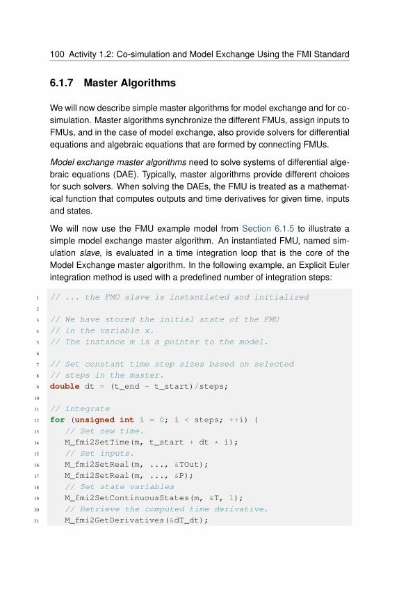
100 Activity 1.2: Co-simulation and Model Exchange Using the FMI Standard

6.1.7 Master Algorithms

We will now describe simple master algorithms for model exchange and for co-simulation. Master algorithms synchronize the different FMUs, assign inputs toFMUs, and in the case of model exchange, also provide solvers for differentialequations and algebraic equations that are formed by connecting FMUs.

Model exchange master algorithms need to solve systems of differential alge-braic equations (DAE). Typically, master algorithms provide different choicesfor such solvers. When solving the DAEs, the FMU is treated as a mathemat-ical function that computes outputs and time derivatives for given time, inputsand states.

We will now use the FMU example model from Section 6.1.5 to illustrate asimple model exchange master algorithm. An instantiated FMU, named sim-ulation slave, is evaluated in a time integration loop that is the core of theModel Exchange master algorithm. In the following example, an Explicit Eulerintegration method is used with a predefined number of integration steps:

1 // ... the FMU slave is instantiated and initialized

2

3 // We have stored the initial state of the FMU

4 // in the variable x.

5 // The instance m is a pointer to the model.

6

7 // Set constant time step sizes based on selected

8 // steps in the master.

9 double dt = (t_end - t_start)/steps;

10

11 // integrate

12 for (unsigned int i = 0; i < steps; ++i) {

13 // Set new time.

14 M_fmi2SetTime(m, t_start + dt * i);

15 // Set inputs.

16 M_fmi2SetReal(m, ..., &TOut);

17 M_fmi2SetReal(m, ..., &P);

18 // Set state variables

19 M_fmi2SetContinuousStates(m, &T, 1);

20 // Retrieve the computed time derivative.

21 M_fmi2GetDerivatives(&dT_dt);

6.1 Introduction 101

22 // Integrate in time.

23 T = T + dt * dT_dt;

24 }

In general, a more sophisticated integration algorithm is needed to ensurethat the integration error remains below a user-prescribed tolerance, to handletime events and state events, and to integrate the equations more efficiently.Typically, an adaptive time step method is used that adapts the integration timestep based on an estimate of the integration error and events. Furthermore,if algebraic loops are present, the master algorithm needs to provide a linearor nonlinear solver. Such algebraic loops are formed if the outputs and inputsof an FMU have direct dependency , and the inputs and outputs with directdependency are connected with each other.

Implicit time integration methods and nonlinear equation solvers typically usea Newton-Raphson algorithm. Since the Newton-Raphson algorithm buildsa Jacobian matrix that has the same dimension as the number of variables,this operation can be computationally expensive. The use of sparse Jaco-bian matrices is helpful, but requires information on dependencies of individ-ual variables on others. The ability for an FMU to publish such dependencyinformation has been added to the FMI standard in version 2.0. The informa-tion about dependency also allows usage of efficient asynchronous numericaltime integration algorithms such as Quantized State Systems (QSS) methods[ZL98][Kof03][FK14] .

Co-simulation master algorithms assign inputs to outputs of other FMUs, as-sign the requested time step to FMUs, and advance time of the co-simulation.Hence, each FMU is responsible for integrating in time its continuous-timestate variables from the current time to the next communication time point.

Next, we illustrate a basic co-simulation master algorithm with a simple ex-ample. Suppose, the room model example above was complemented by acontrolled heating model which takes the room air temperature as input andcomputes the required power of the heating unit based on a temperature set-point. The heating model and the room model both hold a state at a certaintime point. Advancing from this time point to the next communication point canbe managed by the co-simulation master algorithm as follows:

102 Activity 1.2: Co-simulation and Model Exchange Using the FMI Standard

1 // The FMU slaves are instantiated and initialized.

2 // s1 is the room model, and s2 is the heater model

3

4 // Both FMU slaves are at time t and the master algorithm

5 // has cached the output variables of both slaves.

6

7 t = startTime;

8 h = communicationTimeStep;

9 // Loop over all slaves.

10 while(tc < stopTime &&

11 status1 == fmi2OK &&

12 status2 == fmi2OK)

13 // Retrieve outputs.

14 s1_fmi2GetReal(s1, ..., 1, &T);

15 s2_fmi2GetReal(s2, ..., 1, &P);

16 // Set inputs.

17 s1_fmi2SetReal(s1, ..., 1, &P);

18 s2_fmi2SetReal(s2, ..., 1, &T);

19 // Advance time.

20 status1 = s1_fmi2DoStep(s1, t, h, fmi2True);

21 status2 = s2_fmi2DoStep(s2, t, h, fmi2True);

22 // Increment master time.

23 t += h;

24 }

In this example, the master algorithm retrieves outputs, assigns them as inputsto the other FMU, and then requests the FMUs to advance time. Not shownin this example is error handling, as well as handling the situation in which anFMU may reject to advance time to t+h.

The choice of the co-simulation master algorithm can have a great impact onoverall performance, as well as on the correctness of the result, in particularin the presence of an event. To ensure that the results of co-simulations ofhybrid systems are deterministic and, hence, equal regardless of the tool thatimplements the master algorithm, [BGL+15] provides requirements and a testsuite with expected results that can be used to verify correctness of masteralgorithms.

6.2 Use Cases and Applications 103

6.1.8 Exporting and Importing of Functional Mockup Units

Simulation programs may generate and export FMUs. During FMU export, thesimulation model is exposed in such a way that it can be used with the FMIfunctions for model exchange or co-simulation. The result of the FMU exportis a zip file, called the FMU file, as described in Section 6.1.3.

A simulation master or a simulation environment needs to import FMUs in or-der to use them. Importing FMUs consist of extracting the FMU file, parsingthe modelDescription.xml file, and connecting the internal data struc-ture with the FMI functions provided by the FMU. Through these FMI functions,the master or the simulation environment will interact with the model that wasprovided inside the FMU.

6.2 Use Cases and Applications

Having explained the FMI standard and its philosophy of use, we will nowpresent typical use cases and applications in the design and operation of build-ing and district energy systems in which utilizing FMI offers interesting and in-novative perspectives. We will present typical and generic use cases, as wellas specific applications that were developed by participants of this activity.

6.2.1 Simulation-Based Building Operation

This use case describes how FMI can be applied to monitor the actual perfor-mance of a building relative to the design intent during operation.

During the design, an HVAC designer creates a simulation model of a building,including its HVAC system and controls. The designer then exports the modelas an FMU for co-simulation and imports it into a building management system(BMS) such as NiagaraAX. In the BMS, the designer links the model input tomeasured data. The design model can then be used to compute expectedroom air temperature or energy consumption, which in turn can be used tocompare measured with expected performance. Details of these steps are asfollows:

104 Activity 1.2: Co-simulation and Model Exchange Using the FMI Standard

• As a first step, the HVAC engineer develops a model of the building andits HVAC and control system in a modeling language such as Modelica.

• As a second step, the HVAC engineer simulates the building model alongwith its HVAC and control system to ensure correctness of the controlsequence.Optionally, to verify the control sequence, the HVAC response and thebuilding response, the model could be decomposed into these three sub-systems: Measured data could be fed into the control model to verifyactual versus expected control actions; the control signals of the ac-tual system, together with measured outdoor and room conditions couldbe sent to the HVAC model to verify actual versus expected HVAC effi-ciency; and the measured HVAC supply conditions and outdoor condi-tions could be sent to the building model to verify actual versus expectedenergy provided to the rooms.

• As a third step, the model of the building with its HVAC and control se-quence is exported as an FMU for co-simulation and imported into thebuilding management system. The exported system model can then runin real-time to compute the expected performance of the building.

For more information, see [NW14] .

6.2.2 Design and Operational Analysis of Energy, Control

and Communication Grids

Buildings as components of an energy system consume, store and produceenergy. In order to provide more global energy efficient solutions and to facil-itate the integration of intermittent energy resources, one should consider theinteraction of clusters of buildings with the electrical, gas and, if district heatingor cooling is present, thermal networks. Such energy grids may have overlyingcentralized or distributed control, coupled through communication networks.

Such networks are complex systems composed of multi-disciplinary, multi-physics components that can be difficult to handle by any one functional do-main: energy assets, information and communication technology and busi-ness processes. Energy assets (electrical components, buildings and HVACsystems, industrial processes, thermodynamics) are conveniently describedby differential algebraic equations. In other domains, typically for information

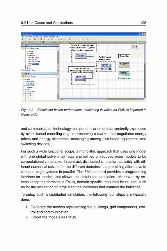
6.2 Use Cases and Applications 105

Fig. 6.3: Simulation-based performance monitoring in which an FMU is imported in

NiagaraAX.

and communication technology, components are more conveniently expressedby event-based modeling (e.g. representing a market that negotiates energyprices and energy allotments, messaging among distributed equipment, andswitching devices).

For such a wide functional scope, a monolithic approach that uses one modelwith one global solver may require simplified or reduced order models to becomputationally tractable. In contrast, distributed simulation, possibly with dif-ferent numerical solvers for the different domains, is a promising alternative tosimulate large systems in parallel. The FMI standard provides a programminginterface for models that allows this distributed simulation. Moreover, by en-capsulating the domains in FMUs, domain-specific tools may be reused, suchas for the simulation of large electrical networks that connect the buildings.

To setup such a distributed simulation, the following four steps are typicallydone:

1. Generate the models representing the buildings, grid components, con-trol and communication.

2. Export the models as FMUs.

106 Activity 1.2: Co-simulation and Model Exchange Using the FMI Standard

3. Connected the FMUs in a master algorithm, possibly using distributedcomputing.

4. Control the simulation with a master algorithm.

See also [CBM+16][RGCJ+16] for applications.

6.2.3 Co-Simulation via Domus with Modelica, EnergyPlus

and ANSYS CFX

During the IEA Annex 60 project, the research version of Domus, Domus-r, de-scribed in Section 6.5.7, has been improved for co-simulation. For EnergyPlusand Modelica, an FMI for co-simulation import interface has been added, whilefor ANSYS-CFX a script-based interface has been added. In a tool-couplingtest case with EnergyPlus, a pure conductive heat transfer envelope modelwas encapsulated as an FMU for co-simulation and imported into Domus, withthe objective to validate the Domus FMI interface.

The Domus pixel counting technique (Fig. 6.4 a) has been used for accurateand fast evaluation of complex shading at internal and external surfaces. Theintention of this use case was to simulate the effect that complex shading hason building energy use, with the latter being computed in EnergyPlus.

As a first step of a Domus co-simulation with CFD, Domus has been usedto co-simulate with ANSYS-CFX a hollowed block (Fig. 6.4 b) wall. The re-sults are promising and demonstrate a functional integration between Domusand CFX that can expand the current limits of both simulation tools and al-low 3-D simulation of building elements.The introduction of the co-simulationin Domus enables detailed, combined consideration of the three heat trans-fer modes calculated by CFX and integration of this with different tools suchas EnergyPlus and Modelica. This would allow for assessment of indoor airquality and building energy efficiency under asymmetric indoor and outdoorboundary conditions. Nevertheless, the high computer run time for CFD is stilla considerable constraint so that further research is needed to make it viable.

6.3 FMI-Compliant Tools for Buildings and District Simulation 107

Fig. 6.4: The use of pixel counting technique for accurate and fast evaluation of

complex shading (a) at an external surface due to a non-planar tree. (b) The hollowed

block used in the wall ANSYS CFX co-simulation and (c) the preliminary results.

6.3 FMI-Compliant Tools for Buildings and District

Simulation

This section provides an overview of FMI-compliant simulation tools that areeither specifically developed for, or useful for, building simulation. Whilethe majority of these tools have been developed outside of Annex 60, theyare listed here to guide new users. A more comprehensive list of thosethat support the FMI standard can be found on the FMI-Standard website(https://www.fmi-standard.org/tools).

Dymola (http://www.3ds.com/products-services/catia/products/dymola/) is anenvironment that supports modeling and simulation of multi-physics systemsimplemented in the Modelica language. Dymola can be used to import andexport models as FMUs for both co-simulation and model exchange.

JModelica (http://www.jmodelica.org/) is a Modelica-based open source plat-form for optimization, simulation and analysis of complex dynamic systems.JModelica has been used by the building simulation community for the simu-lation and optimization of building energy systems. It supports the export andimport for FMUs for model exchange and for co-simulation using the PyFMIPython package.

108 Activity 1.2: Co-simulation and Model Exchange Using the FMI Standard

OpenModelica (https://openmodelica.org/) is an open-source Modelica-basedmodeling and simulation environment. It has been used in the building com-munity for the modeling and simulation of building energy systems. It supportsthe export and import for FMUs for both model exchange and co-simulation.

SimulationX (https://www.simulationx.com/) is a modeling and simulation toolwhich can be used for energy efficiency and HVAC systems modeling andsimulation. It supports the export and import of FMUs for both co-simulationand model exchange.

MATLAB/Simulink (http://mathworks.com/products/simulink/) also supportFMI import and export using the Modelon FMI toolbox (http://www.modelon.com/products/fmi-toolbox-for-matlab/). A building application case and someimplementation comparisons can be found in [WJEP15] .

Ptolemy II is an open-source software framework [Pto14] supporting exper-imentation with actor-oriented design. Actors are software components thatexecute concurrently and communicate through messages sent via intercon-nected ports. Ptolemy II has been used to create the Building Controls VirtualTest Bed (BCVTB) [Wet11a] . Ptolemy II supports the import of FMUs whichimplement FMI 1.0 and 2.0 for co-simulation and model exchange. A largedistrict energy system co-simulation has been implemented in [ZJB+16] .

PyFMI (https://pypi.python.org/pypi/PyFMI) is a python package for loadingand interfacing with FMUs for co-simulation and model exchange. PyFMI isavailable as a stand-alone package or as part of the JModelica.org distribu-tion. PyFMI has been used by the building simulation community for appli-cations such as fault detection and diagnostics, and model predictive con-trols. A building co-simulation example using Dymola models can be found in[RRDW15] .

MasterSim (http://mastersim.sourceforge.net) is a co-simulation master algo-rithm implementation and graphical user interface written in C/C++ (Windows/-Mac/Unix) for coupled simulation of FMUs using FMI 2.0. It supports errorcontrolled co-simulation and iterative master algorithms that set and get thestate variables.

EnergyPlus (https://energyplus.net/) is a whole building energy simulation pro-gram that engineers, architects, and researchers use to model energy con-sumption for heating, cooling, ventilation, lighting and plug and process loads,

6.4 FMU Export Facilities 109

as well as water use in buildings. Import and export of model FMUs are avail-able for co-simulation [NWZ14] . Numerous applications can be found in theliterature, see for example [DEP16][ZJB+16] .

WUFI+ (https://wufi.de/en/software/wufi-plus/) is a hygrothermal whole build-ing simulation program which supports the import of FMUs for co-simulation[PBR+12] . The FMU import functionality was added to integrate ModelicaHVAC system models to WUFI.

TRNSYS (http://www.trnsys.com/) is a graphically-based software environ-ment used to simulate the behavior of transient systems. Even though TRN-SYS itself does not officially provide FMI support, there is a dedicated FMI-based tool coupling solution openly available at http://trnsys-fmu.sourceforge.net. Furthermore, the feasibility of importing FMUs in TRNSYS through aTRNSYS Type has been demonstrated in [EWP+13][EAWP13] .

DIgSILENT PowerFactory (http://www.digsilent.com/) is a state-of-the-artindustrial-grade modeling and simulation tool for electrical networks. Eventhough PowerFactory itself does not officially provide FMI support, it pro-vides several APIs for co-simulation and there is a dedicated FMI-based tool-coupling solution openly available (see http://powerfactory-fmu.sourceforge.net) that utilizes these APIs in an FMI-compliant way.

6.4 FMU Export Facilities

This section describes software packages that can be used to export FMUsand were developed by participants of the Annex 60.

6.4.1 THERAKLES (Room Model)

THERAKLES (http://www.bauklimatik-dresden.de/therakles) is a single-zonehygrothermal model with detailed construction models developed at the Insti-tute for Building Climate Control of the TU Dresden. It includes basic equip-ment component models. It provides modeling of the thermal storage of thewall by use of spatial discretization techniques. Focusing on deployment inengineering practice, it also provides a user-friendly graphical user interface.

110 Activity 1.2: Co-simulation and Model Exchange Using the FMI Standard

For simulation with more advanced equipment and control logic, the THERAK-LES model can be exported as an FMU for model exchange and co-simulationaccording to the FMI 2.0 standard. A graphical dialog is provided to lead theuser through the export process. The generated FMUs provide reset func-tionality for state variables. Thus, all exported FMUs support error-controlledco-simulation.

THERAKLES has its own climate data base and exports calculated climaticdata during simulation. The climate model is encapsulated in the CCM-librarywhich supports an internal binary data format but also reads and converts datafrom *.epw file format.

6.4.2 NANDRAD (Building Energy Simulation/Multizone)

NANDRAD (http://www.bauklimatik-dresden.de/nandrad) is a building energysimulation framework developed at the Institute for Building Climate Controlat TU Dresden. The NANDRAD tool is a command line application designedfor the efficient simulation of complex buildings, including detailed wall models.The resulting large differential equation system is solved by state-of-the-art nu-merical methods, such as Newton-Krylov-iteration methods and sparse matrixalgorithms.

NANDRAD supports FMU export for FMI 2.0 co-simulation and model ex-change by a script-based automated procedure. The provided input and outputinterfaces allow the coupling between the NANDRAD building simulation andan external HVAC model, for example a heating or a hydraulic cycle Modelicamodel. The import of the FMU into a Modelica environment is directly sup-ported by an automatically generated wrapper model. This wrapper encapsu-lates the NANDRAD FMU, connects all inputs and outputs with vector valuedports and generates a graphical representation. Additionally, NANDRAD pre-calculates heating and cooling design data and publishes it in a report file.

Similar to THERAKLES, the NANDRAD FMUs support getting and setting ofstate variables and climate data export.

6.4 FMU Export Facilities 111

6.4.3 EnergyplusToFMU

EnergyPlusToFMU (https://github.com/lbl-srg/EnergyplusToFMU) is a soft-ware package written in Python that allows users to export the building simu-lation program EnergyPlus version 8.0 or higher as an FMU for co-simulationusing the FMI standard version 1.0. This FMU can then be imported into avariety of simulation programs that can import a FMU for co-simulation. Thiscapability allows, for instance, for modeling the envelope of a building in En-ergyPlus, exporting the model as an FMU, and then importing and linking themodel with an HVAC system model developed in a system simulation tool suchas the Modelica environment Dymola. EnergyPlusToFMU is released under anopen-source BSD-license.

Fig. 6.5: An EnergyPlus room model has been exported as an FMU. This FMU is

coupled to a controller implemented in a Modelica simulation environment.

6.4.4 FMI++ TRNSYS FMU Export Utility

Even though TRNSYS itself does not officially provide FMI support, there is adedicated FMI-based tool coupling solution openly available, called the FMI++TRNSYS FMU Export Utility. It has been developed using the FMI++ library(see http://fmipp.sourceforge.net/) and enables the export of a TRNSYS modelwith a Python script as an FMU for co-simulation, using FMI 1.0.

The export tool provides to modelers a special TRNSYS block calledType6139. This type provides external data sent to TRNSYS as inputs to

112 Activity 1.2: Co-simulation and Model Exchange Using the FMI Standard

the model and also allows for sending data as external outputs. Apart from theadditional input and output block of this type, TRNSYS models are constructedin the usual way as shown in Fig. 6.6.

The FMI++ TRNSYS FMU Export Utility is released under an open-sourceBSD-license and is available at http://trnsys-fmu.sourceforge.net

Fig. 6.6: Example of a TRNSYS model containing blocks of Type6139 for FMU export.

6.4.5 FMI++ PowerFactory FMU Export Utility

The FMI++ PowerFactory FMU Export Utility is a stand-alone tool for export-ing FMUs for Co-Simulation (FMI Version 1.0) from DIgSILENT PowerFactorymodels, based on code from the FMI++ library (see http://fmipp.sourceforge.net/). It provides a Python script that creates FMUs from certain PowerFactorymodels, including the XML model description and shared libraries. Additionalfiles (e.g., time series files) and start values for exported variables can be spec-ified. Currently only steady-state simulations are supported, where the systemevolution with respect to time comprises a series of load flow snapshots.

The FMI++ PowerFactory FMU Export Utility is released under an open-sourceBSD-license, available at http://powerfactory-fmu.sourceforge.net

6.5 Simulation Environments and Master Algorithms for FMI 113

6.5 Simulation Environments and Master Algo-

rithms for FMI

This section describes simulation environments with FMU import facilities andmaster algorithms that have been developed by Annex 60 participants. It alsodescribes numerical methods that have been implemented to integrate in timeFMUs for model exchange.

6.5.1 Building Controls Virtual Test Bed

The Building Controls Virtual Test Bed (BCVTB) is a free, open-source middle-ware based on Ptolemy II (http://ptolemy.eecs.berkeley.edu/). It allows usersto couple different simulation tools for data exchange during run-time and forreal-time simulation. Programs that are linked to the BCVTB are

1. EnergyPlus, the whole building energy simulation program,2. Dymola, the Modelica modeling and simulation environment,3. Functional Mock-up Units (FMU) for co-simulation and model-exchange

for the Functional Mock-up Interface (FMI) 1.0 and 2.0,4. MATLAB and Simulink tools for scientific computing,5. Radiance, the ray-tracing software for lighting analysis,6. ESP-r, the integrated building energy modeling program,7. TRNSYS, the system simulation program,8. BACnet stack, which allows exchanging data with BACnet compliant

Building Automation System (BAS),9. USB-1208LS, the analog/digital interface from Measurement Computing

Corporation that can be connected to a USB port.

Fig. 6.7 shows its graphical user interface with a co-simulation model.

The BCVTB has been used in several applications such as agent-based sim-ulation, real-time simulation, control of networked sensors and actuators, andperformance prediction of HVAC systems. The BCVTB is released underan open-source BSD license and available at http://simulationresearch.lbl.gov/bcvtb. For more information, see [Wet11a] .

114 Activity 1.2: Co-simulation and Model Exchange Using the FMI Standard

Fig. 6.7 : The BCVTB is used to couple a controller implemented in Ptolemy II with a

room model implemented in Dymola and exported as an FMU.

6.5.2 EnergyPlus

EnergyPlus (https://energyplus.net/) is a whole building energy simulation pro-gram that engineers, architects, and researchers use to model both energyconsumption and water use in buildings. To extend the capability of Energy-Plus for building simulation, EnergyPlus has been linked through co-simulationto various programs using direct coupling of tools through custom interfacesand through master algorithms in which EnergyPlus acts as a client.

To address the limitation of these custom coupling mechanisms, an FMI forco-simulation 1.0 import interface has been added to EnergyPlus to supportthe import of FMUs. Also, a facility has been developed to export EnergyPlusas an FMU for co-simulation 1.0. This interface allows users to link the build-ing envelope of EnergyPlus with an HVAC system modeled in Modelica, or inanother simulation tool and language. EnergyPlus is released under an open-source BSD license, and available at https://github.com/NREL/EnergyPlus.For more information, see http://simulationresearch.lbl.gov/fmu/EnergyPlus/export and [NWZ14] .

6.5 Simulation Environments and Master Algorithms for FMI 115

6.5.3 DACCOSIM

DACCOSIM lets you design and execute a simulation composed of multipleFMUs on multi-core computation nodes or distributed on clusters.

Fig. 6.8: Co-simulation architecture components in DACCOSIM.

A framework is provided to graphically define how the FMUs are connectedto each others and on which computation nodes they should be distributed.DACCOSIM automatically generates the associated code and the DACCOSIMlibrary is then used to execute the multi-simulation on the distributed compu-tation nodes. It could be either Java or C++ code.

The main functionalities provided by DACCOSIM are

1. co-initialization with the Newton-Raphson method,2. inputs extrapolation,3. support for both constant and variable step size with rollback ,4. various error estimation methods that automatically adjust the step size

(Euler, Richardson and Adams-Bashforth),

It runs on Windows and Linux, 32-bits and 64-bits and uses FMI-CS. It isdeveloped by the Supelec IDMaD research team and the EDF R&D MIREdepartment in the RISEGrid Institute (http://www.supelec.fr/342_p_38091/risegrid-en.html).

DACCOSIM is released under the AGPL open-source license and available athttp://daccosim.foundry.supelec.fr/.

116 Activity 1.2: Co-simulation and Model Exchange Using the FMI Standard

6.5.4 Ptolemy II and Quantized State Systems (QSS)

Ptolemy II provides a master algorithm for FMUs for model-exchange and co-simulation, which implements the FMI 2.0 specification.

The master algorithm is implemented in the discrete event domain of PtolemyII. Additionally, a family of Quantized State System (QSS) integrators is pro-vided to integrate state variables of FMUs for model exchange 2.0. Detailsabout the master algorithm and the QSS integrator can be found in [WNL+15] .The algorithm is release as part of Ptolemy II, and also in the cyber-physicalsystem simulator CyPhySim [LNNW15][BLL+15] , which is a subset of PtolemyII. Both are available under a BSD-license from http://ptolemy.eecs.berkeley.edu/ptolemyII/ and https://chess.eecs.berkeley.edu/cyphysim/.

The CyPhySim simulator supports classical (Runge-Kutta) and quantized-state simulation of ordinary differential equations, modal models (hybrid sys-tems), discrete-event models, the Functional Mockup Interface (FMI) formodel-exchange and co-simulation, discrete-time systems, and algebraic loopsolvers. CyPhySim provides a graphical editor, an XML file syntax for models,and an open API for programmatic construction of models. It includes an inno-vation called smooth tokens, which allow for a blend of numerical and symboliccomputation, and for certain kinds of system models, dramatically reducing thecomputation required for simulation. For example, Fig. 6.9 shows a model ofa bouncing ball implemented in the CyPhySim simulator. For this problem,a Runge-Kutta 2-3 solver required 14,072 time steps and 3.3 seconds, whileQSS required only 46 points in time and completed in 0.085 seconds, or 38times faster. Furthermore, the QSS solvers have the interesting property thatif certain assumptions about the integrator inputs are satisfied, then rollbackis never required. If these assumptions are valid, then there is no error due tonumerical approximation of the integration, and events such as zero crossingsare predictable in advance. For certain cyber-physical systems, such assump-tions are indeed valid, and hence computationally exact simulation is possible,where the only source of errors is numerical round-off errors. There is no errordue to numerical integration. See [LNNW15] for more details.

6.5 Simulation Environments and Master Algorithms for FMI 117

Fig. 6.9: CyPhySim model of a bouncing ball with QSS integration.

6.5.5 FUMOLA - The Functional Mock-Up Laboratory

FUMOLA is a co-simulation framework specifically designed to support thefeatures offered by the FMI specification. FUMOLA is developed on top of thePtolemy II framework (http://ptolemy.eecs.berkeley.edu/) and the FMI++ library(http://fmipp.sourceforge.net/), mapping Ptolemy II’s functions to the function-ality provided by the FMI++ library. Therefore, it provides a flexible platform toinvestigate the full range of possibilities offered by the FMI specification basedon advanced simulation concepts. This allows for implementation of varioussimulation approaches, including discrete event-based simulations [MW15] ,simulations of coupled physical systems [WMB+15] and simulations of closed-loop control systems models [WJEP15] .

FUMOLA is available at http://fumola.sourceforge.net.

118 Activity 1.2: Co-simulation and Model Exchange Using the FMI Standard

6.5.6 WRM (Waveform Relaxation Method) as a Proposition

of a Simple Master Algorithm

The Waveform Relaxation Method [Lel82][LRSV82] has existed since 1982and was developed and used to solve large systems of ordinary nonlineardifferential equations [IC90] , in particular for integrated circuit simulations. Themethod was adapted to be able to be used as a master algorithm for couplingdifferent black box software components such as FMUs [RRDW15] .

The idea is to combine several heterogeneous systems that may have differentdynamics, and couple them using an iterative method on the waveforms (Fig.6.10). Each system is solved in time throughout the considered time domain,and its solution, e.g., the entire waveform, is used as an input of the othersystems. The procedure can be done for the whole time domain, or for asequence of sub-domains. This approach is like a strong coupling, and insteadof exchanging simple values at a given time, it exchanges the waveform.

Fig. 6.10: Waveform relaxation algorithm for co-simulation.

WRM has many advantages. The master algorithm is simple and easy toimplement. It can be used to couple different components without having toknow the internal dynamics and simulation step sizes. In situations where timeexchange data between components is important, such as for a web service,the WRM reduces the computation time by reducing the number of calls of thedifferent sub-models. As the simulation time gets longer, the efficiency of thewaveform relaxation method increases [RRDW15] .

Limitations and disadvantages include less efficient simulations for models thathave events. See the application in [RRDW15] .

6.5 Simulation Environments and Master Algorithms for FMI 119

6.5.7 Domus

Domus is a building simulation software written in C++. It has an OpenGL-based graphical interface that has been improved to allow importing modelsfrom EnergyPlus 8.0 or higher as a FMU for co-simulation 1.0. Domus hasalso been improved for

1. shading and sunlit area calculation using a pixel counting technique,2. reading and writing of EnergyPlus IDF files, and3. co-simulation with ANSYS-CFD.

This last capability can allow for instance the co-simulation for performanceassessment of whole-buildings with 3-D ventilated walls combined with indoorand outdoor air flow under heterogeneous surface boundary conditions. Do-mus is available from http://www.domus.pucpr.br/. See [MOG03][MBZF08] formore information.

6.5.8 MasterSim

MasterSim is an open-source co-simulation master implementation that sup-ports FMI 1.0 and 2.0.

The simulation master was developed specifically for application in buildingenergy simulation, i.e, interfacing of building simulation models with HVACsystem models and control systems, or specialized sub-system models. Themaster employs several algorithms for obtaining stable, efficient and error con-trolled solutions. It contains

• different master algorithms/iteration methods, such as non-iterativeGauss-Jacobi, and iterative Gauss-Seidel and Newton methods,

• variable communication step sizes with local error control,• serialization/deserialization for stop-and-restart of the master.

MasterSim is developed in C++ and runs on Windows, Mac OS X and Linux.Also, the master supports a feature that disables automatic unzipping of FMUarchives, which allows for using persistent DLL/shared library files, which isimportant for FMU developers.

120 Activity 1.2: Co-simulation and Model Exchange Using the FMI Standard

MasterSim is available from http://mastersim.sourceforge.net under a GPLv3.0 license.

6.6 Desired FMI Features and Proposal of Evolu-

tions of the Standard

While the FMI standard is well-suited for our classes of problems, as with anyother standard that covers such a complex use case, there are certain limita-tions encountered and improvements that the Annex 60 participants would liketo see in future versions of FMI. As a result of Annex 60, some changes havebeen proposed to the standards committee. For this cases, we list below theticket number of the FMI development site. This section provides an overviewof the key challenges encountered while using FMI version 1.0 and 2.0, withactions undertaken to address some of the limitations.

Change of array size during initialization: The size of arrays used for inputs,outputs and state variables is fixed once the FMU is generated. It would bedesirable to allow defining array variables as quantities where the array sizeis being controlled by a parameter given during the instantiation of an FMU.This would allow pre-compiling FMUs in which array sizes vary for differentapplications, such as for CFD, ray-tracing, or heat conduction through solidsand through windows.

For this item, the FMI committee has a working group.

FMU time unit: The FMI standard does not specify the unit of the time passedto the FMUs. This can result in synchronization problems if slaves assume adifferent unit for time. Thus it would be desirable to extend the standard tospecify the unit of the time passed to the FMU slaves, or conversely, state inthe specification that time is in seconds, which seems to be the implicit as-sumption and corresponds to what most, if not all, tools implement. Currently,FMU exporters have to agree on a time unit and specify this in the interfacedescription.

A ticket has been filed on the FMI issue tracker (ticket #307).

Handling of FMU-specific output and log files: While FMI 2.0 provides apath to a read-only resource location, such as for data files to be read by

6.6 Desired FMI Features and Proposal of Evolutions of the Standard 121

the model, it does not provide a path to a writable location where output andlog files shall be written. Knowledge of such a writable location is important,for example, when the same FMU is instantiated several times within a co-simulation scenario. Then, each FMU instance needs to use a different rootdirectory for its written files in order to avoid overwriting each other’s files. Thesame applies when multiple co-simulation runs are executed in parallel usingthe same FMU files. Hard-coding writable paths inside the FMU does not workin this situation. Use of the current working directory as basis does not workon the Windows platform, since several Windows API function related to fileand directory handling change the working directory. The outcome dependson the order in which the FMUs are instantiated and initialized, and on theirinternal operation. Therefore, it would be meaningful to pass such a directory,if available on the given platform, during instantiation of the FMU. Without aformal method, FMUs must agree on a specific name of the output directory,and the master algorithm must set this before entering the initialization modeof an FMU.

A ticket has been filed on the FMI issue tracker (ticket #299).

Support for structured variables: FMI 2.0 only defines scalar variables inthe ModelVariables subsection of fmiModelDescription at the root-level of the schema file modelDescription.xml. Various domains (e.g. fluid,heat transfer, electrical, magnetic, mechanics) would benefit from support-ing structured variables of fixed size, especially one-dimensional arrays, in-stead of only scalar variables. This would also require new fmi2GetXXX andfmi2SetXXX functions.

For this item, the FMI committee has a working group.

Event handling in co-simulation: In FMI for co-simulation 2.0, an FMU can-not announce to the master algorithm an upper bound for the step it can sim-ulate. Rather, an FMU will have to reject a step size requested by the masterif it is too long. [BGL+15] suggests a new function fmiGetMaxStepSize

that would allow an FMU to announce how long a step it can take. A similarsuggestion is also made by [TCT+16] , who propose to add the next event timeto a new function fmi21DoStep. Announcing the maximum step size wouldbe useful, for example, if a model knows its next time event and hence canask the master to step no further than that time point. With the current imple-mentation, a master algorithm may step over this time instant, then get notified

122 Activity 1.2: Co-simulation and Model Exchange Using the FMI Standard

by the FMU that it went too far, and then ask the FMUs to rollback and do asmaller step.

This item is in discussion within the FMI committee.

Efficient mechanism for output writing in FMI for model exchange: Cur-rently it is unclear how to handle FMU-specific outputs efficiently in FMI 2.0for model exchange. For example, in a building simulation FMU, at certaintime points, usually hourly or every 15 minutes, a lot of output data needs tobe stored in output files. Passing that amount of output data through the FMIinterface seems not practical.

The integrator within the master algorithm may use a higher-order integrationmethod with variable time steps, such as CVODE. Therefore, integration stepsand output steps in the FMU generally do not match.

Currently the only means for the ModelExchange FMU to identify a suitabletime point for writing past outputs is the fmi2CompletedIntegratorStepfunction. The FMU may than write outputs within the last step at the scheduledtime point. However, the FMU does not have information about the higher-order integration method of the integrator. Therefore, backward interpolationwill likely give different results compared to those computed by the integrator.

A ticket has been filed on the FMI issue tracker (ticket #326).

Master shall be required to set fixed parameters even if unchanged Cur-rently, when specifying fixed parameters in the modelDescription.xml

file, the standard does not require that the master calls fmi2SetXXX func-tions for such parameters. Most master implementations currently set the pa-rameters, even if the values have not been changed by the user.

In order to ensure consistency between the default parameter values set dur-ing the export of the FMU and the values in the modelDescription.xml

file, it would be useful to require the master to always set the values during theinitialization of the FMU.

A ticket has been filed on the FMI issue tracker (ticket #366).

6.7 Best-Practice Recommendations 123

6.7 Best-Practice Recommendations

This section summarizes best practices proposed by Annex 60 participants forbuilding or district-level simulations using the FMI standard.

6.7.1 Climate Data Export

While simulating coupled FMUs, redundant calculations of the same physicalpart should be avoided because of the risk of inconsistency. Typically, thisproblem occurs when climate data calculation are performed by different FMUssimultaneously. An example is a system with two FMUs, one for a buildingmodel, and one for an HVAC system, which both require outdoor conditions.

As climate data only depend on time, using a common FMU for climate datawill not create cyclic dependencies among FMUs.

Since there are different possibilities for defining climate parameters (units,naming conventions, sun coordinate system, etc.) standardizing an interfacefor climate data would be beneficial.

6.7.2 FMI Interfaces for Room and HVAC Systems

Different variables could be exposed at the interface of rooms and HVAC sys-tems. In order to make different FMUs compatible, an FMI package has beenadded to the Annex60 library which allows for exporting HVAC models, HVACsystems, and thermal zones as FMUs. This package contains connectors thatcan be exposed to retrieve and to output HVAC system variables. The pack-age also contains FMI adaptors, which have been added to facilitate the ex-port of HVAC systems. See http://www.iea-annex60.org/releases/modelica/1.0.0/help/Annex60_Fluid_FMI.html for documentation. The rationale for the se-lection of variables that are used as inputs and outputs of the HVAC FMU arediscussed in [WFN15] . Fig. 6.11 shows a model of a heater with the FMI inter-faces. The instances bou* convert between causal input and output signalsand the acausal fluid ports.

124 Activity 1.2: Co-simulation and Model Exchange Using the FMI Standard

com

T Q_flow

com.port_a.p - com.port_b.p

dpCom

bouIn

m

inlet

p

bouOut

outlet

p

-

pOut

inlet outlet

inlet outlet

TSetQ_flow

Fig. 6.11: Modelica block that can be used to export a heater that has acausal fluid

ports as an FMU.

6.8 Conclusions 125

6.8 Conclusions

This chapter demonstrates that having a standard for exchanging models be-tween different simulators and for linking simulators during run-time is an im-portant topic for building and district energy system simulation. As buildingand district energy simulation typically involve large models and long simula-tion periods, having efficient master algorithms is important. The participantsof Activity 1.2 demonstrated that FMI is useful for various applications. Theyalso demonstrated the capability of tools to export, import, and co-simulatemodels encapsulated as FMUs. They showed that the FMI approach is suitedfor solving the multi-physics, multi-component systems encountered in the sim-ulation of buildings, and they contributed to proposals for further improving theFMI standard. Simulation coupling with open-source standards is potentially akey for tackling the scalability issues that will be encountered for district-levelsimulations. This is one of the big challenges that building and district energysimulations will encounter in the years to come.

126 Activity 1.2: Co-simulation and Model Exchange Using the FMI Standard

Chapter 7

Activity 1.3: BPS Code

Generation from Building

Information Models

7.1 Introduction

Activity 1.3 of the Annex 60 is dedicated to the complex issue of transforming adigital model of a building and its energy systems into Modelica code that canbe readily used for advanced building performance simulation (BPS). It is theconceptual idea and vision of this activity to thoroughly address the prevail-ing tedious, cumbersome and error-prone process of manual data conversionand model generation and to provide a methodology for automatically, or atleast semi-automatically, transforming a digital model into an object-orientedacausal model.

The transformation is hampered by several constrains such as

• models contain inconsistencies and modeling errors and are typicallynot built by a person skilled in energy performance simulation,

• models originate in the design process from other domains such as thearchitecture or structural domain,

128 Activity 1.3: BPS Code Generation from Building Information Models

• objects and parameters in a CAD model significantly differ from the rep-resentation needed in Modelica,

• input models are lacking information relevant for BPS,• a conversion process needs to support multiple Modelica libraries with

different model topologies and varying syntax at the same time,• the object-oriented data schema of the digital building model is contin-

uously updated and subject to changes which need to be dynamicallyreflected by the tool.

Consequently, several complex requirements form the specification of a soft-ware framework that is capable to deal with these constraints. Furthermore, aflexible methodology is required to take expert knowledge into account whenit comes to object and parameter mapping. The software framework shallprovide interfaces to Open BIM data formats such as the Industry Founda-tion Classes (IFC). And, as well, the framework must be modularly structuredin order to allow for further and distributed developments on an open sourcebasis by an international community. Its structure shall allow to maintain theframework or even most parts of it in due time.

In order to carefully consider these settings, the activity followed the followingapproach:

• As BIM data format, the Annex supports the Open BIM format IndustryFoundation Classes (IFC). Before processing BIM models, these modelsare checked for integrity concerning two aspects. First, the geometricconsistency is accounted for by an advanced model checking processwhich includes the definition of space boundaries. Secondly, the HVACmodel is checked by another model checking toolbox developed in thisproject.

• Models are then transformed into an intermediate data format calledSimXML. Therefore, a flexible module for schema parsing was devel-oped. Relevant data which are missing in the BIM can be added to theSimXML data model.

• In order to manage these SimXML data, a dynamic schema parser wasdeveloped in C++. This offers the flexibility to dynamically account forchanges and updates of the SimXML schema (and, thus, for changesof the IFC data model as well). An application programming interface(API) between C++ and Python was implemented to efficiently interact

7.2 Building Information Modeling (BIM) 129

with the data model.• An object and parameter mapping mechanism as well as respective

mapping rules were developed in order to formulate engineering knowl-edge in a rule-based methodology. These rules are processed by theframework.

• An IFC model view definition (MVD) was developed in order to specifythe subset of IFC data relevant to BPS.

• In order to dynamically support multiple Modelica libraries at the sametime, a template-based approach was selected as solution and imple-mented in Python.

• All transformation tools and methods are provided as open sourceframework for further developments in the community. Researchers areinvited to collaborate and to further extend the framework.

The following sections briefly introduce what BIM is, explain the BIM data im-port process and detail the developed open Annex 60 framework for Modelicacode generation from BIM. At the end of the chapter, the use cases applied fortesting and development are introduced as well. It shall be noted at this point,that the activity followed a bottom-up approach which was based on these usecases. Therefore, the framework is currently limited to support these cases.As the activity focused on a subset of IFC data, on the other hand, with theresources on hand it was possible to finalize the overall framework as such inthe Annex and to provide a modular framework for further development anddissemination.

7.2 Building Information Modeling (BIM)

This subchapter starts by introducing the term BIM and by explaining thechanges required when BIM is used in a project. For the evaluation of the de-veloped model transformation and BPS code generation concept and toolchainthe use cases and case study are described next. The authors detail currentstate-of-the-art toolboxes and tools that are relevant for our prototype develop-ment. Finally, in this subchapter we summary relevant standards and agree-ments that are needed for development of BIM based data exchange.

130 Activity 1.3: BPS Code Generation from Building Information Models

7.2.1 What is BIM?

The acronym BIM stands for Building Information Model or Modeling. It in-volves buildings and building designs, information about given buildings and/ordesigns, and to how that information is modeled. Searching the term BIM onthe web one will find many industry definitions such as: BIM and Sustainabil-ity, Green BIM, 4D BIM, BIM and the Bottom Line, BIM for Risk Management,BIM BOP, BIM CON!FAB, BIM Symposia, BIM Consulting, BIM Surveys, andmany more. It seems that anybody who is asked to define BIM has their owndefinition which reflects their own needs, expectations and uses of BIM.

According to Bazjanac [Baz04] , the BIM acronym can have two meanings:noun or verb. The science definition of BIM-the-noun is straight forward:

A Building Information Model (BIM) is an instance of a populated

data model of buildings that contains multi-disciplinary data spe-

cific to a particular building which they describe unambiguously.

The science definition of BIM-the-verb is even simpler:

Building Information Modeling (BIM) is the act or process of creat-

ing a Building Information Model (BIM-the-noun).

Charles Eastman and colleagues offer a more elaborate and practical workingdefinition of BIM for the buildings industry [ETSL11] :

BIM is a modeling technology and associated set of processes toproduce, communicate, and analyze building models character-ized by

• Building components that are represented with intelligent digital repre-sentations and can be associated with computable attributes and para-metric rules.

• Components that include data that describe how they behave.• Consistent and non-redundant data.• Coordinated data such that all views of the model are represented in a

coordinated way.

Similarly, definitions of BIM by buildingSMART International [bSI15a] , the U.S.National Institute for Building Sciences [NIB16] and the U.S. National BIMStandard Project [NIB13] are in full concordance with this definition.

7.2 Building Information Modeling (BIM) 131

Eastman and colleagues also define what causes a data agglomeration not tobe a BIM, disqualifying building “models” which some industry members callBIM:

• Building models that contain 3D data only and no object attributes.• Building models with no support of behavior (i.e. models that do not

utilize parametric intelligence).• Building models that are composed of multiple 2D CAD reference files

that must be combined to define the building.• Building models that allow changes in one view that are not automatically

reflected in other views.

Accordingly, a Building Information Collection (BIC) is also not a BIM. A BICis characterized by an ad-hoc database to which information is supplied as aparticipant recognizes the need for it, with no systematically rules for databasecreation. As a result, the database is used indiscriminately from one buildingto another, and when viewing a datum in the database one cannot be confidentwhat the datum actually represents without examining why and how the datumhas been entered in the database.

In order to create a proper BIM, three conditions must be satisfied: (1) validbuilding data must be available and verifiable; (2) a specific data model ofbuildings must be used in the instantiation of data; and (3) software capable ofproperly populating the data model must be available and used in all instancesof entering data in the data model. BIM data used in this research project arevalid and verifiable for the purposes of the project. The most common datamodel format used with BIM is Industry Foundation Classes (IFC). The latestIFC version 4 Addendum 2 (IFC4 Add 2) [bSI15b] release is the data modelused as basis for the BIM applications to share information across multiplessoftware. All software used to populate the BIM is directly or indirectly IFCcompatible.

IFC is fully object-oriented and is fully extensible. It is absolutely “neutral” (i.e.does not favor any software environment, platform, market, endeavor or suiteof tools). IFC is also the only life cycle model of buildings that is an “open”International Standard Organization (ISO) Standard (no. 16739), and can beused free of charge.

The main purpose of the IFC data model is the enabling and support of soft-

132 Activity 1.3: BPS Code Generation from Building Information Models

ware interoperability in the buildings industry. Software interoperability – es-sential to collaborative design – is the common name of technologies that allowsoftware to communicate to one another and seamlessly share and exchangedata. Some advantages of interoperability are detailed below:

• Allows automatic and flawless exchange of relevant common projectdata between one software application and another.

• Supports automatic data conversion between software that use partiallyoverlapping data.

• Offers consistency management of the various ways that are used tomodel a building.

• Provides the tracking and management of information consistent withbest practices required for security, provenance, etc. in support of con-tractual and legal frameworks.

Interoperable applications enable the work of multiple disciplines with variedexpertise, and automatically translate data to support the different data struc-turing and viewing needs for different decision-making industry domains.

Any complete BIM of a sizeable commercial building will contain much moredata than any single software application can read and manipulate. The mainreason for that is not necessarily the size of the building – it is the multi-disciplinary nature of the data in a complete BIM. In most cases only disciplinesoftware can populate the BIM with all relevant discipline data, and only disci-pline software can read such data. To avoid having to deal with data in the BIMthat are irrelevant to the discipline, relevant data are grouped and agglomer-ated in a “view” of the particular BIM [Hie06] and such views are defined asModel View Definitions (MVD).

Data included in Model View Definitions (MVD) are subsets of the IFC datamodel. The subsets specify all discipline (or project type) definitions in theIFC data model that need to be shared or exchanged among multiple softwareapplications in support of work of a given discipline, project type or any othergiven purpose. bSI certifies software applications’ compliance with a givenMVD if the application can demonstrate that all data exchange requirementsof the given MVD (object/attribute/relationship sets, as well as their form andformat) have been implemented by the application.

The BIM Collaboration Format (BCF) is an open XML file format that supports

7.2 Building Information Modeling (BIM) 133

workflow communication and messaging among different software applica-tions engaged in BIM processes [bSI14] . It boosts collaboration in BIM work-flows by exchanging only the lean machine-readable BCF-topics with attachedBIM-snippets (and not the entire BIM) among participating applications. TheRESTful API enables seamless automated exchanges of BCF-topics amongsoftware that has implemented this Application Protocol Interface [bSI15c] .

7.2.2 Changes Within the Planning/Design Process

The adoption of BIM (as a verb) constitutes a paradigm shift in the Archi-tectural, Engineering, Construction and Facilities Management (AEC/FM) in-dustry. BIM based collaboration is a different way of working as opposed tocomplementing the traditional 3D CAD approach. The key difference is theopportunity for collaboration over the entire building life-cycle: from concep-tion to design, construction and operation and up to the final demolition. Thedeployment of BIM in construction can make the industry more efficient, ef-fective, flexible and innovative [THN13] . However, the use and adoption of anew technology begins with a series of decisions that ends in appropriate andeffective use of such technologies.

In some countries such as USA, UK, Norway, Finland, Denmark, Singaporeand South Korea the use of BIM in projects is obligatory. Despite the industry’sawareness of the potential of BIM, construction organizations are yet to use iteffectively. Fig. 7.1 shows that BIM is leading a change in resource allocationand associated costs from the later to the earlier stages of the project. Bycomparing the traditional 3D CAD approach with BIM, BIM is considered moreefficient and less-time consuming, therefore less costly.

The use of BIM concentrates stakeholder collaboration throughout the entirebuilding life-cycle. In doing so it provides a central repository of informationthat can be accessed by any stakeholder, when needed, in order to makethe best and most effective use of available information. The major benefitsfrom this approach are design consistency and visualization, cost estimates,clash detection and implementation of lean construction [VSS14] . This digitaltransformation cannot happen unless there are appropriately skilled personnelto support BIM implementation.

134 Activity 1.3: BPS Code Generation from Building Information Models

Fig. 7.1: Comparison between BIM-based workflow and traditional workflow (Adapted

from [EHLP13]).

7.2.2.1 Roles and Responsibilities in the BIM-Based Process

It is expected that the demand for BIM will required new organizational struc-ture and changes of responsibilities within defined roles. [GT14] on their studyreviewed over 300 jobs description to determine responsibilities and skills re-quired in BIM related roles. They identified three core roles: BIM Manager, BIMCoordinator and BIM Modeler. Others researches also mentioned different ter-minologies for these roles but with the same responsibilities of management,coordination and modeling [BS10][PH13][SML13] .

A BIM Manager is a person familiar with the building and design process fromstart to finish. This role does not require a domain identifier as this is an over-arching role within the organization covering all aspects such as collaborativeinformation management, standards management and process planning. Thisperson can work directly with BIM Coordinators and BIM Modelers and withmanagement designing processes. The BIM Coordinator is the person re-sponsible for facilitating the transition into BIM based work practices and sub-sequently enhance the performance of BIM based activities. This person’s keyrole is to help with the model and other BIM related issues. Lastly the BIM

7.2 Building Information Modeling (BIM) 135

Modeler requires a domain identifier and skillset in their respective. This per-son focuses on a specific performance aspect of the project. Therefore, thesuccess of a project depends on meaningful integration of the roles involved,through an efficient and sustainable use of BIM.

7.2.2.2 Agreements in the BIM Process

Different national and international BIM guidelines and standards are avail-able today to help organizations to implement BIM in their processes[EHLP13][AECUKC15][BIMGW12] . The benefits of using BIM depends onthe manner in which information will be created, maintained and shared withinproject stakeholders. People involved in the BIM project are expected to havethe ability to produce, manage and share any information required in a stan-dard format. According to Egger [EHLP13] , the success of a project in thebuilding industry depends on four factors: people, processes, guidelines andtechnology (Fig. 7.2). With the exception of technologies that are well estab-lished in the construction industry, the remaining three factors present prob-lems that need to be overcome, especially the lack of professional training andguidelines.

Fig. 7.2: Main factors of influence on the use of BIM method [EHLP13].

Within BIM projects all information is coordinated in a common data envi-ronment and it is very important that all objectives and deliverables are de-fined within this environment at the beginning of the project. In this manner,BIM servers provide a multi-disciplinary collaboration platform that maintains

136 Activity 1.3: BPS Code Generation from Building Information Models

a repository of the building data, and allows applications to import and exportfiles from the database for viewing, checking, updating and modifying the data.The information contained in the common environment will form the basis ofthe BIM Execution Plan. The execution plan is a crucial document that reflectsthe employer information requirements to ensure that design is developed inaccordance with their needs. As a consequence of this new process, a higherquality and consistency is provided and administered in BIM projects.

7.2.3 Relevant BIM Standards and Implementation Agree-

ments

In context of building energy performance of buildings two types of standardsexist: data exchange standards and energy code standards. The data ex-change formats most relevant are gbXML, IFC and SimModel, which we de-scribe in the next subsection below. Energy code standards have a local char-acter and can generally be further divided into standards that are based onstatic calculations and standards that are more detailed and based on sim-ulation. For example, the German energy code (EnEV) is a static calcula-tion whereas the US energy code (ASHRAE 90.1) is using simulation models.For further details on those energy standards we refer to van Treeck et al([vTWM15]). Since this project is focusing on Modelica simulation, which is amore detailed approach, energy standards could become a byproduct in thefuture with additional development.

7.2.3.1 Data Exchange Formats

In the traditional approach, the majority of information is exchanged via 2Ddrawings that consist of lines, but with the introduction of BIM-based exchangethere is a possibility to link or embed data into BIM objects. Several dataexchange formats are available today for BIM applications to share informationamong each other. The most common are:

• Green Building XML schema (gbXML) facilitates the exchange of dataamong CAD tools and energy analysis software;

• IFC is the most used data format in the AEC/FM industry, mainly be-cause of its ability to represent elements of a building as objects with

7.2 Building Information Modeling (BIM) 137

properties and references to others objects [ARHZ15] . The latest re-lease IFC4 contains many improvements in the HVAC domain and someenhancements for space boundaries.

• SimModel is a simulation domain specific data model. It combines con-tent from both IFC and gbXML as well as other relevant data models.As a simulation domain specific data model it also contains data that arerelevant to simulation only.

With IFC4, energy-related data of a building and its systems can be ex-changed. This includes space boundary information for representing thermalzones. Compared to previous versions it also contains new and more detailedHVAC components. A data format for the exchange of vendor-specific productdata is the ISO Standard 16757. The standard provides a data format for thedescription of manufacturer product data and can be seen as a supplement tothe IFC data model.

All three data models can be also represented in XML format (IFC is mostlydefined in the STEP format, whereas SimModel has also a binary represen-tation) and are object oriented data models. Thus, they include classes, at-tributes and references. The IFC data model contains many relational objectsthat link two different objects together. For example, the IfcRelAggregates ob-ject can link the IfcSite and IfcBuilding object. Since some of these relationalobjects are very generic, there exists a large number of possibilities to link ob-jects. SimModel simplifies this by combining these relational objects into themain objects. For the example above, the SimSite object contains a propertythat directly links to the SimBuilding object. While SimModel is still very closein its structure and hierarchy to the IFC model, this adds another level of detailfor the definition of objects. In IFC classes can be further specified by usingan ObjectType, SimModel uses the additional ObjectSubType to further spec-ify objects. gbXML does not provide the necessary level of detail of HVACcomponents and was thus not further considered in this project.

While IFC is seen as the right data format to retrieve building data from thearchitect and other domain experts it does not cover special requirements forsimulation purposes. For that reason, the simulation domain specific datamodel SimModel (see Section 7.3.6) is used as an intermediate step towardsthe Modelica simulation. Due to the mentioned flexibility to define and linkobjects in an IFC model as well as it large scope, the mechanism to limit scope

138 Activity 1.3: BPS Code Generation from Building Information Models

is needed and discussed in the next subsection.

7.2.3.2 Implementation Agreements

BIM standards like IFC need further implementation agreements to limit thetheoretically possible representation options within the data model to a practi-cal subset. BuildingSMART has introduced the concept of Model View Defini-tions (MVD) that identifies a subset of IFC that is needed to support a selectedset (partial model) of use cases. The definition of an MVD is described in Sec-tion 7.3.5. Other domains, such as the structural domain are not relevant inthe simulation context and can be excluded from the scope via an MVD. Geo-metric representations with corresponding material properties, internal loads,thermal zones, HVAC systems and HVAC components are topics that wouldbe entailed in a simulation MVD. Besides the data itself, the MVD also de-fines so-called concepts that show how objects should be connected to forman interconnected data model. For example, a concept to define topology con-nections or a concept to place HVAC components in a system. As shown inSection 7.3 MVDs can be formalized using the mvdXML format so that auto-matic checking for required objects and properties is possible. This checkingwill be introduced with the software certification for IFC4 to enable more andbetter quality checks of IFC implementations. If a software passes all testcases defined for an MVD, then it will be certified by buildingSMART to meetdefined quality criteria. The MVD concept and corresponding tools have beenfurther developed for this latest IFC4 version and now cover a wider range offeatures. In previous versions, so-called implementer agreements were es-sential to define concepts in a more loose manner, but to properly documentthem for software implementers. For example, detailed space boundary defini-tions were specified in special add-on of implementers agreements in IFC2x3.Since the IFC4 version is quite new as well as the improved MVD, time willtell if implementers agreements will still be an important aspect in addition toMVDs or if they will be mostly replaced by MVDs.

7.2 Building Information Modeling (BIM) 139

7.2.4 Review of Existing BIM Tools for Visualization and

Model Checking

For the development of software prototypes based on the IFC data model, itwas important to reuse existing tools, resources and technologies to optimizethe project output. Due to the large number of existing IFC tools a proper re-view was needed and conducted within this project. We illustrate this reviewin context of the development of the model checking and conversion compo-nents. Here, two major feature areas were of particular interest:

• Free and open source IFC-based viewing components• BIM Model Checking Tools including their analysis features

The following tools have been selected and analyzed:

Open source IFC-based viewing components

• xBIM Explorer (sample application from xBIM Toolkit), V 2.4.1.28• IfcPlusPlus Viewer (sample application from IFC++ Toolkit)

Free IFC-based viewing components

• Constructivity Viewer, V 0.9.7.0• DDS-CAD-OpenBIM-Viewer, V 8.0.2012.101• FZKViewer 4.1, V 4.1• IFC JAVA VIEWER (Part of IFC-Tools Project) V 2.0 ,• IFC Engine DLL: Sample Viewer, V 1.0.0.1• Solibri Model Viewer, V 8.1.0.80• Tekla BIMsight, V 1.8.5002.18178 ,

Free BIM-Model checking tools

• DDS-CAD-OpenBIM-Viewer, V 8.0.2012.101• FZKViewer 4.1, V 4.1• Tekla BIMsight, V 1.8.5002.18178

We evaluated the available tools and components in terms of their capabilitiesto represent, model and appropriately describe specific aspects as describedbelow with respect to:

• support of IFC2x3• support of IFC4

140 Activity 1.3: BPS Code Generation from Building Information Models

• support of the STEP IFC base syntax• support of the XML IFC base syntax• reliability and performance of IFC import• platform independence• capability to validate IFC files• visualization features• selection of attributes• clash detection

Since the ifcXML syntax was essential to a subset of our tools, it was an impor-tant criterion for our review. In addition, the reliability and performance of theIFC import is obviously an important criterion. But the evaluation of the IFC4 import was difficult due to the early stage of the related tool developmentefforts. Thus our review of this functionality is limited. Since a basic validationof IFC files is essential before any conversion process is meaningful, we alsoinvestigated if tools can validate the IFC file against the schema. If it supportsrule-based validation where the rules can be predefined within the tool, poten-tial users can apply those to their IFC files. In addition, some tools support therecalculation of surface areas and volumes to verify those properties with theIFC file content. The tools were also assessed on their visualization features.We investigated view and render options as well as support for transparency.Object selection and filtering based on attributes is also a common featureamong those tools and was added as criterion.

The free model checking tools such as FZKViewer and Solibri Viewer do sup-port basic checking features such as clash detection or quantity takeoff. How-ever, we could not identify a free model checking tool for the required HVACconsistency check of the IFC model (Section 7.4.3.3). This is why we reusedour previously developed components for this model checking implementa-tion. In context of the ifcXML support only the RDF Viewer based on theIFCEngine.DLL and the FZKViewer do currently support import and export ofthe ifcXML file. Only the former is also available as open source.

Based on these criteria, two toolkits can be identified as the most promisingones to serve basic functionalities: the open source XBIM tool kit (Fig. 7.3)and the IFC Engine DLL toolkit (Fig. 7.4).

For the development of the Annex 60 model checking tool (ref Section 7.4.3)the second tool was selected due to its simpler enhancement possibilities.

7.2 Building Information Modeling (BIM) 141

Fig. 7.3: Brief technical description of the XBIM tool

142 Activity 1.3: BPS Code Generation from Building Information Models

Fig. 7.4: Brief technical description of the IFC Engine DLL Toolkit

7.3 Importing BIM Data to BPS 143

7.3 Importing BIM Data to BPS

This section describes the transformation from Building Information Modelingto Building Performance Simulation in Modelica. Starting with a first and initialdraft of the data transformation process adopted in this Annex, requirementsfor BPS in different stages of the building design are described. We detail thepossibilities and requirements to generate Building Information Models witha focus on BPS in this section. The section further illustrates how to extractrelated information from a BIM and transforming it to be used as basis for BPS,respectively.

The use of Building Information Modeling implies interoperability between soft-ware applications and the collaboration of different disciplines. Fig. 7.5 illus-trates the process how to derive Modelica models for different Modelica li-braries from BIM. Each step requires different actors and software. The ar-chitect and HVAC engineer use domain specific BIM-based CAD software andmay export their models to an Industrial Foundation Classes (IFC) file (leftside). This file is converted into SimXML which is the file format for SimModel,a data model for the simulation domain. SimModel extends information pro-vided by IFC with simulation specific parameters. The SimXML file is thenconverted to a valid Modelica model with the software framework developed inthis Annex. This framework is setup to support multiple Modelica libraries aswell.

This section puts energy modeling into the context of Building InformationModeling, including IFC, SimModel and tools to check the BIM for integrity.

7.3.1 Overall Transformation Process

For the task of converting BIM into Modelica models (as outlined in Section7.1), we used a case study approach for the development of the tool chain(Section 7.4).

Fig. 7.6 illustrates the data transformation process within the developedmethodology, in which the IFC data model is instantiated in the BIM Platformand exported as an IFC4 file. In order to read and operate with these data, the

144 Activity 1.3: BPS Code Generation from Building Information Models

SimModel+

informationmodel

CAD/BIM

informationmodel

Modelica

simulationmodel

*.ifcXML

Building

HVAC

*.mo

HVAC

Building

*.mo

HVAC

Building

*.mo

HVAC

Building

*.simXML

Building

HVAC

Architect

Engineer

Fig. 7.5: Overview of the transformation process from IFC to Modelica models using

different Modelica libraries.

Fig. 7.6: Data transformation from BIM to Modelica

7.3 Importing BIM Data to BPS 145

model is converted into a specific exchange model for BPS. SimModel is sucha data exchange model specifically developed for BPS and thus serves as theintermediate format to support the exchange of data from BIM to Modelica inthis Annex. SimModel offers a flexible data model allowing enhancements andadditions as described in Section 7.3.6. The final process in the tool chaingenerates a Modelica file.

The conceptual and software development of this methodology was driven bya set of simple use cases (described in Section 7.5).

7.3.2 Requirements for BPS Models Across Different

Stages of the Building Design Process Based on Un-

certainty

BPS models can be used at different stages of the design process, for exampleto investigate the thermal comfort and energy consumption of a building orto support the planning of the HVAC configuration and controls. Dependingon the respective application of a BPS model and the corresponding designphase, different requirements must be satisfied in terms of the nature of themodel and the associated input data.

It is important to know the level of detail which is required at each design stage.This allows for the BPS engineer to generate reliable results. Here, it has tobe taken into account that simulation results always comprise some extent ofuncertainty. This uncertainty arises due to unknowns within the inputs of thesimulation model. Certain input uncertainties decrease in the course of thedesign process, particularly as detailed planning proceeds and available infor-mation is increasing. Other input uncertainties are more or less constant overthe entire planning process, for example: climate conditions or user behavior.The challenge is to identify which level of detail, represented by subsets of datacontained in the BIM, is necessary for a BPS model at a specific stage of thedesign, which is a crucial consideration given the corresponding uncertaintiesat that stage.

To provide answers to this challenge, methods for uncertainty and sensitivityanalysis can be used. In [BJH10] a methodology is described which allowsfor consideration and evaluation of uncertainties in BPS models using Model-

146 Activity 1.3: BPS Code Generation from Building Information Models

Table 7.1: Overview of the uncertain input parameters and their respective distribu-

tions.

Parameter Unit Minimum Maximum DistributionzoneParam.RRest K/W 0.03 0.05 uniformzoneParam.R1o K/W 0.0003 0.005 uniformzoneParam.C1o J/K 1.0e06 2.0e06 uniformzoneParam.Aw m2 5 9 uniformzoneParam.g 0.5 0.7 uniformpipe.dp Pa 5000 20000 uniformvalve.dp Pa 5000 20000 uniformflow.temperature °C 70 90 uniform

ica. Additionally, the methodology can be used to determine the impact of theuncertain inputs on the output uncertainty (sensitivity analysis) and, thus pro-vides a means to rank model inputs according to their relative importance interms of the simulation result. The most sensitive inputs are highly relevant forproviding valuable simulation results while less sensitive inputs (lowest rank-ing) have little influence on the simulation results.

Accordingly, one can argue that a simulation model should account for themost sensitive inputs (even if the respective inputs are not exactly known) withrespect to the output of interest. Less sensitive inputs can be initialized withdefault values or ignored in the model.

In the following, the procedure for uncertainty and sensitivity analysis is brieflyexplained and illustrated using the example of use case 1.1 (Section 7.5.1)(standard office building modeled as a simple zone with radiators and a boiler).From the results of this type of analysis one can estimate the output uncertain-ties and deduce BPS model requirements for different design stages.

The first step is to identify the uncertain model input parameters and estimatetheir respective distributions. Here, we assume that building parameters arenot fully known, which leads to uncertainties in the heat demand, and the exactHVAC layout has not been specified yet. This situation can, for example, ap-pear in the outline planning when first simulations are run, in order to supportcode compliance or later certifications, while significant uncertainties have tobe considered.

7.3 Importing BIM Data to BPS 147

The assumed input parameter distributions are shown in Table 7.1. Here, thefirst five lines correspond to building (zone) parameters, while the last threelines correspond to HVAC parameters. RRest, R1o and C1o describe ther-mal resistances and a thermal capacity in the reduced order building modelaccording to VD16020. These parameters cannot be directly related to physi-cal quantities in the building, but represent aggregates. Aw and g denote thearea and the solar transmittance of the windows, respectively. The parame-ters valve.dp and pipe.dp are associated with the pressure losses of valvesand pipes.

Fig. 7.7 : Distribution of the fuel consumption over all simulation runs. White bars

correspond to a varied heat demand according to the building parameter distributions

given in Table 7.1. Gray bars correspond to a fixed heat demand and only HVAC

parameters are varied according to Table 7.1.

Then, Monte Carlo Simulations are performed, where for each uncertain in-put parameter 4096 random samples from the given range are chosen. Thesimulation period is six weeks, starting from 1st of January. The consideredoutput is the total energy consumption of the HVAC system which consists ofthe fuel consumption of the boiler and the electricity consumption of the pump,summed over the simulation period.

Fig. 7.7 and Fig. 7.8 show the resulting distributions of the outputs, fuel con-

148 Activity 1.3: BPS Code Generation from Building Information Models

sumption and pump power, when the input parameters are varied accordingto Table 7.1 (white bars). For comparison, the corresponding distributions areshown when the heat demand is assumed to be known (associated with fixedbuilding parameters) and only the HVAC parameters are varied (gray bars).It can be seen that the uncertainty in heat demand has major influence onthe total energy consumption: the estimate of the total energy consumption ismuch more precise when the heat demand is known. The remaining, relativelysmall, uncertainty if the heat demand is fixed results from the uncertainties inthe HVAC layout. In comparison to the building parameters, the HVAC layoutplays a negligible role for the overall output uncertainty.

Fig. 7.8: Distribution of the pump power over all simulation runs. White bars corre-

spond to a varied heat demand according to the building parameter distributions given

in Table 7.1. Gray bars correspond to a fixed heat demand and only HVAC parameters

are varied according to Table 7.1.

This effect can be quantified via the calculation of sensitivity indices. Thevariance-based first order sensitivity indices for all varied input parameters withrespect to fuel consumption and pump power are shown in Fig. 7.9. A higherindex indicates a greater influence on the observed output uncertainty. Alsofrom this figure, it becomes clear that, in this setting, the building parametershave a greater impact on the energy consumption than the HVAC layout. Inparticular, the thermal resistance parameter of the simplified zone model and

7.3 Importing BIM Data to BPS 149

the window area turn out to be most influential.

So, one can deduce from these results that for a reliable estimate of the energyconsumption the heat demand should be known relatively well, while a roughpicture of the HVAC system configuration is sufficient at this stage. Whenit comes to optimizing the operation of the HVAC system, having eliminatedother uncertainties to large extent, the exact HVAC layout becomes important.

Fig. 7.9: Sensitivity indices for the outputs fuel consumption and pump power with

respect to the varied input parameters. The variation of the building parameters has

much more effect on the outputs than the variation of the parameters concerning the

HVAC layout.

In a similar way, one can identify the following model requirements, based onthe simple use case 1.1 (Section 7.5.1), for four different design stages:

7.3.2.1 Preliminary Planning

A simple building simulation model is used to estimate the energy demand ofthe designed building. Uncertainties in weather conditions, internal loads andbuilding parameters (e.g. materials, areas) have to be taken into account. Theresulting energy demand yields a probability distribution.

The resulting energy demand distribution from the building simulation is usedto perform an HVAC simulation and to support the HVAC planning. Therefore,a simple HVAC model is used which only comprises the boiler and radiator,

150 Activity 1.3: BPS Code Generation from Building Information Models

and yet uses the uncertain energy demand as input. If applicable, severaldifferent HVAC concepts with alternative heat sources or heat exchangers arecompared. A first estimate of the energy consumption in terms of a probabilitydistribution is provided.

7.3.2.2 Outline Planning

As more details concerning the building geometry and the materials areknown, a corresponding building simulation yields a more precise heat de-mand, which, however, still comprises some uncertainty due to unknown inter-nal loads and weather conditions.

An HVAC simulation is used to determine the optimal dimensions for the boilerand radiator. Uncertain heat demand, unknown set values and controls haveto be taken into account. A model-based optimization of set values (e.g. flowtemperatures) and controls (e.g. night set-back) could be pursued. As a resultof the HVAC simulation, the estimated energy consumption is obtained andserves as a basis for code compliance and certification.

7.3.2.3 Detailed Planning

A detailed HVAC simulation is used to optimize the HVAC configuration andcontrols. Pipes and valves are included in the model. Uncertain heat de-mand, unknown pressure and heat losses are taken into account. As a resultof the HVAC simulation a more precise distribution of energy consumption isobtained and serves as a baseline for building operation.

7.3.2.4 Operation Phase

A detailed as-built building and HVAC simulation model is calibrated with mea-surement data. The calibrated model is used for model-based on-line faultdetection and optimization or model-based control.

The BPS model requirements for this simple example arise from a sensitivityanalysis. For more elaborated systems with storage and renewable energyusage the picture could change slightly. In particular, controls would have a

7.3 Importing BIM Data to BPS 151

more important role to play during the early design as they tend to have a largeimpact on the energy consumption of innovative or low energy systems.

design stage

application of simulation models

available input data (from BIM)/uncertainties

model requirements

preliminary planning

building simulation:- energy demand estimate

HVAC simulation:- analysis of different supply concepts- cost estimate - functional description

available:- rough building geometry - location

uncertainties:- internal loads- weather- building materials

simple building model:- uncertain building parameters- uncertain inner loads- uncertain weather

simple HVAC model:- heat sources- heat exchangers- uncertain demand- uncertain yields

outline planning

HVAC simulation:- system components dimensioning- rough control scheme - rough energy consumption estimate (code-compliance, certification)- cost calculation

available: - HVAC components- demand estimate

uncertainties:- controls- exact HVAC layout- internal loads- weather

HVAC model:- efficiencies- specified components- uncertain demand- uncertain yields

detailed planning

HVAC simulation:- support layout planning- detailed control scheme- precise energy consumption estimate

uncertainties:- internal loads- weather

detailed HVAC model:- pipes, ducts, valves (incl. heat and pressure losses)- controls- uncertain demand- uncertain yields

commis-sioning/operation

building and HVAC simulation:- performance evaluation- control optimization- fault detection and diagnosis

measurements:- energy consumption- room temperatures- occupancy- weather- yields

detailed (calibrated) building and HVAC model

Fig. 7.10: Overview of the usage and requirements of simulation models in different

design stages.

An overview of the use of simulation models in different design stages is givenin Fig. 7.10, as is the availability of relevant input data for each respectivephase and the data requirements for the BPS model. Although this representa-tion is not exhaustive and can certainly not be applied to all building processes,the image indicates typical dependencies between available information andtargeted BPS results. As a result, this information can serve as a basis forInformation Delivery Manuals (IDM) as described in sub:numref:sec_IDM.

152 Activity 1.3: BPS Code Generation from Building Information Models

7.3.3 Building Geometry Generation and Processing

Building geometry definitions for use in Building Energy Performance (BEP)simulation modeling usually originate in CAD software. They are defined byCAD in 2D, 2.5D or 3D, and are delivered in electronic form or on paper.

Geometry information on paper (drawing prints) generated by 2D CAD tools,such as AutoCAD [Aut16] , must be manually transcribed into electronic ge-ometry definitions that can be read by BEP simulation programs and engines.This is a very tedious, time-consuming, frustrating and extremely error-proneprocess that can, depending on the size and complexity of the modeled build-ing, consume more than a half of the total simulation project budget.

If the 2D building geometry is available in electronic format (DWG or DXF)which contains scalable dimension information, the transcription into geome-try definitions readable by BEP simulation programs and engines can be a bitfaster (using copy-and-past) and somewhat more efficient. Still, the transcrip-tion requires heavy human modeler involvement.

State-of-the-art 2D CAD software, such as AutoCAD, can provide the thirddimension by extruding the information defined in 2D plans vertically. Suchgeometry is called 2.5D, as it is not true 3D geometry. While 2.5D geometrycan further expedite the geometry transcription for use in BEP simulation, itcan have the opposite effect when different adjacent buildings have differentextrusion length.

“Model-based” architectural CAD tools, such as Revit [Aut15] , ArchiCAD[Gra16] , Allplan [Nem16] and MicroStation [Ben15] , offer definition of buildinggeometry in true 3D formats – geometry definitions that are object-oriented.Each of these CAD tools exports geometry in its own proprietary file format,but also includes utilities for export and import of geometry in IFC format.Third party software, such as the Space Boundary Tool [RB13] and Simergy[Alc16] , can automatically or semi- automatically transcribe geometry definedin IFC format into input for EnergyPlus. Bentley’s AECOsim Building Designer[Ben15] , transcribes building geometry originally created by MicroStation forseamless use in EnergyPlus. The OpenStudio platform can import buildinggeometry defined by SketchUp (not a “model-based” CAD tool) or other CADtools that export geometry in gbXML format [GbX16] and use it directly in En-ergyPlus without any additional transcription.

7.3 Importing BIM Data to BPS 153

Most CAD tools allow the modeler to define “center-line” building geometrymodels in which walls, floor slabs, ceiling slabs, roof slabs, windows and doorsare represented by flat surfaces parallel to the sides and placed in the cen-ter of each particular object; “center-line” representations have no thickness.While “center-line” modeling simplifies the modeling process and may savetime, “center-line” geometry definitions result in BEP simulation results thatsignificantly overestimate building energy consumption [BMNG16] .

Building geometry definitions as required for use in detailed Modelica geome-try algorithms should be as precise as possible. Any current high-end “model-based” CAD tool can facilitate the necessary modeling precision; it is up to

the modelers to define building geometry precisely [BMNG16] . Thus it isparamount to always verify the correctness and precision of any generatedbuilding geometry.

7.3.4 Energy Modeling Using IFC

IFC based BIM has the potential to provide significant other inputsfor BPS modeling, thus reducing the time, effort and expense associ-ated with model creation [RB13][vTR06] . To date the majority of workin the area of BIM to BPS has focused on geometry transformations[Sim15][GLG+15][Gra11][JKC+16][JS16][OMR+13] . Commercial BPS toolssuch as RIUSKA [Gra11][LOK10] , Simergy [SHS+11] , IDA-ICE [Sim15] andTRNSYS [CRR+11] focus mainly on the import of geometrical information.Section 7.3.3 describes geometry transformations in detail but such transfor-mations require high quality IFC models which are typically not delivered inpractice. Previous efforts such as the Design BIM 2010 ([BDA12]) MVD de-velopment did go beyond just geometry data, in adding internal loads data aswell as high level data on space requirements and HVAC systems (CDB2010is supported by Simergy).

In addition to geometric information, HVAC, controls, operating schedules andsimulation parameters should be contained within a BIM. However, when map-ping HVAC systems to BPS tools, a number of complex and interrelated issuesarise. Primarily, the broad variation in representation of HVAC systems withinsoftware tools results in bespoke mapping solutions from BIM to each targetBPS engine. As an example, HVAC duct designers typically use a supply

154 Activity 1.3: BPS Code Generation from Building Information Models

and return convention for loop structure while EnergyPlus uses a supply anddemand loop structure. Modelica on the other hand, only requires systemtopology information and a different parameter set compared to parameterstypically entered by HVAC system designers.

At the data level, many of the objects required for BPS are not contained withinIFC based BIM or are not inserted into IFC by appropriate BIM based CADtools. This shortcoming is particularly noticeable in the HVAC controls domainwhere the object and property definitions required by simulation are not yet rig-orously defined and have not been in focus of data exchange developments.As a result a formal definition of the data requirements for BPS would signifi-cantly assist data transfer to the BPS domain and MVD is an ideal platform toservice this need.

7.3.5 Model View Definition (MVD) for Energy Related BIM

Support

In order to facilitate data exchange between applications using the IFCschema, an MVD was developed to meet the requirements needed by BPStools. The MVD focuses on the definition of IFC entities, attributes, relationsand properties that satisfy this specific exchange scenario. This defines asubset of the building product model schema that provides a complete repre-sentation of the information concepts needed for a particular use case in anAEC/FM workflow [PWM+16] .

The MVD also defines the business rules and agreements necessary to assistthe implementation of import and export functions by BIM applications. Thus,a first quality assurance can be done by checking for mandatory entities andproperty sets. In cases where information is not currently represented in theIFC specification, properties can be defined to extend the IFC schema.

7.3.5.1 Available MVDs and Current Status

In 2016, buildingSMART published the IFC4 Addendum 2 (IFC4 Add 2), to-gether with two new MVDs to support IFC4 implementation: Reference View(RV) and Design Transfer View (DTV). The main purpose of the first one is

7.3 Importing BIM Data to BPS 155

to define a standardized subset of the schema that supports exchange in onedirection only. The RV is characterized by the ability to provide workflow for thewidest array of software applications. The second MVD proposed is an exten-sion of the Reference View. Contrary to the RV, the DTV enables model editingby design software platforms. DTV is considered the successor of the formerIFC2x3 Coordination View and is compatible with IFC2x3 import [Bui16] .

Since the introduction of the MVD concept, organizations started develop-ing their own MVDs to support internal processes based on the IFC2x3schema. There are some related to energy performance such as: Holistic En-ergy Efficiency Simulation and Management of Public Use Facilities HESMOS[LSW+13] and Concept Design BIM 2010 (CDB) [BDA12] . Fig. 7.11 showsa short comparison of the energy related MVDs. The HESMOS project didactually not define an MVD, the project focused on the definition of exchangerequirements (ER) only. HESMOS and CDB focused on the building envelope,but added some additional HVAC related data as a first step towards a simula-tion MVD. CDB MVD requires 2nd level space boundaries, whereas HESMOSonly demands first level space boundaries. The HESMOS project developed aconversion tool that transforms from 1st into 2nd level space boundaries. Bothprojects attached the internal loads to a space. HESMOS covers most of therelevant data for a static simulation, whereas CDB’s focus lays on a more gen-eral definition of the energy analysis zone. HVAC systems are only describedas existing flags or with basic parameters. HVAC components itself are com-pletely missing. In addition to that, renewables like photovoltaic componentsare part of the simplified definitions.

7.3.5.2 Identification of Data Requirements and Mapping to IFC

As shown in Section 7.3.2, the exchange requirements for energy simulationcan be different at different stages of the building life cycle. Within this project,several use cases were defined using different levels of complexity from a sin-gle room to a large commercial building. The main purpose of creating theseuse cases is to analyze several HVAC systems that are used in the buildingsector. Based on these use cases, it is possible to identify the scope of infor-mation needed by BPS tools and subsequently map it to the IFC schema. Thisprocess involves the IDM methodology (Section 7.4.1), which is a standardizedmethodology to create information exchange requirements [WK10] .

156 Activity 1.3: BPS Code Generation from Building Information Models

Concept Design BIM 2010 MVDHESMOS Exchange Requirements

Building Elements

SpacesInternal Loads (more details)

Design + Lighting Requirements

Space Boundary1st Level

SystemBasic parameters

Container for Spaces

RenewablesExistence flags

Building Elements

Energy Analysis ZoneInfiltration

Daylighting

HVAC TypeContainer for Spaces

SpacesInternal Loads

Design Requirements

Space Boundary2nd Level

SystemContainer for Spaces

Renewables

PV’s

Fig. 7.11: Contrasting juxtaposition of existing energy related ER/ MVDs.

7.3 Importing BIM Data to BPS 157

Working with proprietary software to generate IFC files we were bound to thecontent it offers. In this project, we used mainly the IFC4 version due to itsadded content in the HVAC component area. During the runtime of the Annex60 project, only limited IFC functionality existed since official buildingSMARTcertification of IFC4 was not yet available. Through our cooperation with soft-ware vendors during the project significant effort is put into the support of IFC4export. Over time better support for IFC4 will become available. Besides thesedescribed difficulties originating in the early stage of the implementation of theIFC4 data model, this also provides an opportunity for feedback and possibleinfluence on further development.

In general, new versions of the IFC schema provide new entities to cover thewider scope and support additional areas of the AEC industry. Along with newentities, existing entities can change and in special cases even be deprecated.These changes have to be incorporated into the import and export function-alities of software which is then submitted for certification. Additionally, IFCsupports property sets for the export of product characteristics. Some toolssupport these property sets with corresponding library objects, while othertools may only provide the properties through manual input. Once certified, adetailed certification report can be found on the buildingSMART website listingthe level of support for individual entities.

7.3.5.3 Specification of the MVD

An MVD is composed of the following elements: ModelView, ConceptRoots,ExchangeRequirements, ConceptTemplates and Concepts. The ModelView isthe description of an MVD and is specific to an IFC schema release. It groupszero-to-many ExchangeRequirements and ConceptRoots thereby defining thescope of the MVD. The ExchangeRequirements define the information neces-sary for a particular exchange scenario and may add additional constraints tothe use of Concepts. The ConceptRoot is represented by a collection of avail-able Concepts, each of which references a specific IFC entity, e.g. IfcSpace.Each Concept describes rules for common subsets of information (e.g. spaceattributes) within the context of the particular root. The Concept is backed bya ConceptTemplate describing a graph of object instances, relationships andconstraints. The information contained inside of the ConceptTemplate enablesthe generation of instance diagrams of the MVD [CLW13] . The MVD is de-

158 Activity 1.3: BPS Code Generation from Building Information Models

fined by using the open source tool ‘IFC Documentation Generator’, providedby buildingSMART ([bib]). The information defined in the existing energy re-lated MVDs are integrated in the creating of the new MVD.

HierarchyGeometry

IfcRelSpaceBoundaries

(2nd

level)

IfcSpace IfcZone

IfcSystem

HVAC Components

IfcBoiler

IfcPipe

...

IfcPump

Topology

IfcDistributionPort

IfcRelConnectsPorts

IfcRelConnectsPortToElement

Schedules Performance CurvesInternal Loads

IfcBuildingElements

IfcPropertySet(Pset_SpaceThermalLoad)

0

5

10

15

20

25

30

35

5 10 15 20 25

Fig. 7.12: Overview of the main topics to define the energy related MVD.

The fundamental elements for an energy related MVD are shown in Fig. 7.12.

Geometry : The Geometry defines the basis of the model. Second level spaceboundaries link spaces to building elements and are used as basic surfacesfor the heat transfer between spaces internally and between spaces and theoutdoor. These should be well defined and correct (see also Section 7.4.3.1).

Internal loads: Space contains the definition of the internal loads as propertysets. IFC4 already has designated properties for internal loads as follows:

• Maximum/Minimum temperature of the space• Maximal number of people• The total sensible heat or energy gained• Lighting loads• Percent of sensible load to radiant heat

These simplified properties originate from earlier MVDs. Most importantly

7.3 Importing BIM Data to BPS 159

the dynamic nature of schedules is hereby missing which is crucial for BPS.Schedules in general are discussed next.

Schedules: The ability to define complex schedules in combination with thealready defined properties allows for example the definition of detailed internalloads. BPS defines this schedule requirement that has not been introduced byother disciplines. Currently in IFC, schedules can be defined in three differentways:

• IfcWorkCalendar: On/off status through the year with predefined pat-terns

• IfcRegularTimeSeries: A regular time series that defines values basedon a regular time interval (e.g., hourly).

• IfcIrregularTimeSeries: A time series that defines values on a irregulartime series.

Typically, schedules for BPS follow a regular pattern, mostly daily, weekly andseasonal patterns are used. The ability to define patterns would simplify andreduce the data representation of schedule significantly. The IfcWorkCalenderuses the IfcRecurrancePattern that is able to define such patterns, but canonly contain an on/off signal and no values. For example, the presence of acertain number of people in the thermal zone on a weekday, which changesover the course of the day, or the opening range of a valve on a national holidaycannot be described with a Boolean flag. This is a significant limitation of theIFC model and creates the need for a workaround solution.

In order to enable the definition of these schedules, it is necessary to define anew concept. The IFC Documentation Generator (IfcDoc tool) is used to definethe new concepts, based on the newest IFC4 data model. The top level of theconcepts hierarchy is IfcObject. IfcObject is best suited for applying schedulesto each possible spatial and non spatial element, such as a zone, space orHVAC component. The object is assigned via a relating control to the IfcPer-formanceHistory. IfcPerformanceHistory offers the recurrence patterns, usingthe entity IfcWorkCalender. IfcPerformanceHistory is also defined by proper-ties, which in turn allow the definition of complex properties and ir/regular timeseries. If IFC 4 allows the definition of recurrence patterns for time series, theapplication of detailed schedules on an hour basis over the course of a day ispossible. To improve this limitation, we suggested changes for the coming ver-sion of the IFC data model. The application of this concept allows for dynamic

160 Activity 1.3: BPS Code Generation from Building Information Models

simulation using detailed schedules of the typically complex properties for athermal zone.

Hierarchy : The hierarchy for the thermal zones is defined using the composi-tion concept, provided by buildingSMART. IfcSpace is the lowest level, com-posed to IfcBuildingStorey, which is in turn composed of IfcBuilding. IfcZoneis used as a grouping mechanism, which allows for a definition of the thermalzones in combination with the space boundaries. The HVAC system is definedusing IfcSystem as a top hierarchy entity. The system can be separated intosubsystems. For a single loop heating system, the distribution system wouldbe defined as supply and return pipe systems in which the radiators representa thermal sink and the boiler a thermal source, which are also part of the sub-systems. No previous agreements exist on the hierarchy of systems that iswhy we are proposing a simple hierarchy with one parent system for each loopthat contains a supply and demand subsystem. For simulation purposes thisdifferentiation can be useful to know which components are supplying a loopand which are demanding cooling or heating needs.

HVAC components: In the latest IFC4 version, several enhancements to theHVAC component were made. In particular, components definitions becamemore detailed. E.g., an IfcBoiler used to be a generic IfcEnergyConversionDe-vice. This great enhancement makes the representation of HVAC componentmore explicit. However, there are a number of HVAC component that did notget a more detailed class, such as heat pumps and combined heat and powerunits. Those need to be represented with a more generic class IfcUnitaryE-quipment.

Topology : Since most HVAC systems are based on some kind of fluid flow,topology connections are one of the key concepts to consider. In IFC this isdone by defining an IfcDistributionPort, which is connected to a IfcDistribu-tionElement. The IfcRelConnectsPorts relationship connects two ports andforms the basis for the topology.

Performance curves: Another aspect of HVAC components are performancecurves. Typically, performance curves are used to describe specific behaviorof a component at varying conditions. E.g., a boiler efficiency curve that de-pends on the water return temperature. In IFC4 this concept does not exist.We did realize the definition of performance curves with the use of IfcComplex-Properties which in turn is a list of IfcProperties. This list of properties then

7.3 Importing BIM Data to BPS 161

defines the coefficients of the curve, minimum and maximum values as well asother relevant properties.

Ob

ject T

yp

e D

efin

ition

s

Pro

ject U

nits

Pro

ject R

ep

rese

nta

tion

Co

nte

xt 2

D

Pro

ject G

lob

al P

ositio

nin

g

Pro

ject D

ocu

me

nt In

form

atio

n

Ob

ject T

yp

ing

Pro

pe

rty S

ets

for O

bje

cts

Pro

pe

rty S

ets

for T

yp

es

Qu

an

tity S

ets

So

ftwa

re Id

en

tity

Re

vis

ion

Co

ntro

l

Use

r Ide

ntity

Site

Attrib

ute

s

Bu

ildin

g A

ttribu

tes

Sto

rey A

ttribu

tes

Sp

ace

Attrib

ute

s

Do

or A

ttribu

tes

Win

do

ws A

ttribu

tes

Ele

me

nt T

yp

e P

red

efin

ed

Typ

e

Ma

teria

l Sin

gle

Ma

teria

l La

ye

r Se

t

Ma

teria

l La

ye

r Se

t Usa

ge

Ma

teria

l Pro

file S

et

Ma

teria

l Co

nstitu

en

ts

Sp

atia

l Co

mp

ositio

n

Sp

atia

l De

co

mp

ositio

n

Po

rt Ne

stin

g

Typ

e P

ort N

estin

g

Ele

me

nt V

oid

ing

Dis

tribu

tion

Syste

m A

ssig

nm

en

t

Zo

ne

Assih

nm

en

t

Sp

atia

l Co

nta

ine

r

Sp

atia

l Co

nta

inm

en

t

Sp

ace

Bo

un

da

ries 2

nd

Le

ve

l

Pa

th C

on

ne

ctiv

ity

Po

rt Co

nn

ectiv

ity

Pro

du

ct S

ha

pe

Pro

du

ct L

oca

l Pla

ce

me

nt

Pro

du

ct T

yp

e G

eo

me

tric R

ep

rese

nta

tion

Inte

rna

l Lo

ad

s-S

ch

ed

ule

s

IfcBoiler

IfcBuilding

IfcBuildingStorey

IfcDistributionElement

IfcDistributionElementType

IfcDistributionPort

IfcDistributionSystem

IfcDoor

IfcElement

IfcElementType

IfcMaterial

IfcOpeningElement

IfcPipeFitting

IfcPipeSegment

IfcProduct

IfcProject

IfcPump

IfcRoot

IfcSite

IfcSlab

IfcSpace

IfcSpaceHeater

IfcSpatialElement

IfcSpatialZone

IfcSystem

IfcTank

IfcValve

IfcWall

IfcWallStandardCase

IfcWindow

IfcZone

Fig. 7.13: Overview of the concepts used to define the MVD for use case 1.1.

The developed MVD is based on well-defined ConceptTemplates provided bybuildingSMART [bia] . For instance, the definition of properties and connec-tions of HVAC components were defined using ConceptTemplates such as“Port Nesting” and “Property Sets for Objects”. Fig. 7.13 shows the conceptsapplied to a subset of the MVD. On the left hand side are the objects listedthat are used for the use case 1.1. The top shows a list of the used con-cepts for the MVD. The white boxes show that the concepts can be appliedto the object and the grey boxes show that the concepts are not applicable.

162 Activity 1.3: BPS Code Generation from Building Information Models

As already mentioned the 2nd level space boundaries are mandatory for theMVD and this concept is assigned to IfcSpace. The concepts “Port Connec-tivity” and “Port Nesting” are necessary to connect the Ports on distributionelements and to define placement, indicating the position and outward orien-tation. The different materials of the numerous entities are also defined usingthe given concepts, such as “Material Layer Set” or “Material Constituent”. Ifsomething is undefinable using this method, an Implementer Agreement canbe used (see Section 7.2.3).

It is important to notice that the process of certification is done on the basisof MVDs and not the general IFC schema. This process requires time anddepends on buildingSMART as well as software developers. However, there isalready some work being done to provide IFC4 support within 2016.

7.3.5.4 Outlook

The MVD developed in the Annex 60 project applies the methodology frombuildingSMART, and uses the recommended ifcDoc tool for its formal and de-scriptive definition. IfcDoc enables the export of HTML documentation in themvdXML format (official BSI format) for software certification and the genera-tion of a subset schema containing all relevant entities and properties of ourMVD.

Available ConceptTemplates are re-used as far as possible. While it covers allrequirements identified by the various use cases, the MVD has been designedto be a general purpose view for thermal simulations, i.e. it is not restricted tothe Modelica simulation package. Since the MVD is developed based on ourset of use cases it has a limited scope in terms of HVAC objects, but it containsall key concepts related to BPS. Feedback on what is missing in the IFC4 datamodel from a BPS perspective as well as a description and discussion of keyconcepts and issues form important steps towards a first BPS MVD.

Besides the MVD itself, we also discovered a number of inconsistencies ormissing concepts in the IFC data model.

• Missing pattern definition for schedules• Missing explicit classes for heat pumps and CHPs• Missing performance curve concept

7.3 Importing BIM Data to BPS 163

• Missing agreement on system hierarchy

The next step will be to submit the MVD proposal to buildingSMART for furtherreview by the community as well as to extend its scope to cover all relevantHVAC objects. As the current proposal already includes definitions from pre-vious work, in particular the space boundary add-on view to fill the currentgeneric simulation MVD gap. In parallel to the review period the software cer-tification process can be prepared, which means to specify test cases andexpected quality criteria. For this, the developed use cases and prepared ex-ample data can be used as a starting point. They already cover the main as-pects of our use cases, but may need to be extended to check further aspectsof the MVD.

7.3.6 SimModel: A Data Model for BPS

SimModel is primarily used as an internal data model by the Simergy softwaredeveloped at LBNL and continued by Digital Alchemy [LBN13][SHS+11] . Thistool was first conceived as a platform that facilitates data flow to and from BPSsimulation tools to and from potentially any building modeling tool [BMR+11] .Bi-directional data flow is possible to and from IFC BIM, DOE-2 software ortools that use the DOE-2 engine, EnergyPlus, and tools with gbXML export(Fig. 7.14). These tools are typically used for BPS simulations. Data from anyof these environments can be mapped to and from the SimModel data modelusing the Simergy software [LBN13] .

SimModel is an object-oriented data model which defines all object /at-tribute/relationship sets used for BPS. The primary objective of SimModel isto accommodate the existing input data requirement of EnergyPlus, while al-lowing mapping from/to other domain data models and easy incorporation ofnew definitions [BMOD+11] . At its core, SimModel is represented using theXML markup language [OSM+11] . This representation is closely aligned tothe IFC data model, in order to link to incoming or outgoing IFC information(Fig. 7.14), a motivating factor for using SimModel in this project. In this con-text, SimModel also reduces some of the complexity of the IFC data model bysimplifying relationship objects though direct object references.

164 Activity 1.3: BPS Code Generation from Building Information Models

CAD

Tools

MEP

Tools

Other

Tools

Other

Adapter

OS to

SimModel

gbXML to

SimModel

IFC to

SImModel

Other

Format

Open

Studio

gbXML

IFC

SimModel

Other

Adapter

SimModel

to IDF

Other Sim

Tools

EnergyPlus

Other

IDF

Source

Applcation

Exchanged

DataAdapter

Target

Application

Exchanged

DataAdapter

Exchanged

Data

Data

Software

Data Transfer

Future Addition

Fig. 7.14: Interoperable data exchange enabled by SimModel. This solution enables

re-use of original project data as contained in IFC based BIM (bi-directional mapping)

and data from other sources (import only)

7.3 Importing BIM Data to BPS 165

7.3.6.1 SimModel Design

SimModel incorporates a number of features that address current domainweaknesses (as detailed in [OSM+11]), a set of requirements for a sharedsimulations model and is easily extensible to account for future domain ad-vances. This data model ensures interoperable exchange of simulation datawithin the simulation domain and most importantly across an entire buildingproject. The unique design enables interoperable data exchange and uses anumber of features to do so, these include: mappings to/from existing domainmodels; structured yet flexible class definitions; property set definitions; ob-ject type definitions; model ontology; templates and resources. The followingsubsections detail only the key features.

7.3.6.2 Data Model Mappings

The data model should facilitate seamless data exchange for the extendedbuilding-simulation domain and even for the entire AECOO industry [NRE10] .Version 1.0 supports BIM concepts from IFC, gbXML, IDF, and OpenStudio[NRE10] . Version 2.0 adds support for SDD (Standards Data Dictionary) toenable the foundation for code compliance analysis (here California Title 24)([MHS15]). The quality of data varies with each file format so customizedadapters enable single or bi-directional mappings on a case-by-case basis.SimModel can also accommodate bi-directional mapping to other data modelsas the need arises, e.g. IDA-ICE or IES-VE.

7.3.6.3 Class Definitions

Data element/entity ontologies vary greatly between SimModel, the Energy-Plus schema called Input Data Dictionary (IDD) and gbXML. The EnergyPlusIDD contains ~650 element types and other relevant data model schemascontain several hundred classes. SimModel uses approximately 120 datamodel classes to represent the merger of the EnergyPlus IDD and other modelschemas. This approach results in fewer software classes, less code to main-tain and simplified model evolution.

166 Activity 1.3: BPS Code Generation from Building Information Models

The streamlined approach uses a type/subtype hierarchy for each data modelclass. An example best illustrates this concept. SimMaterial is a data modelclass that represents material types. However opaque and transparent aretypes within that class, where each type then contains the relevant subtypes,e.g. class = SimMaterial, type = OpaqueMaterial, subtype = NoMass.

The type/subtype approach also acts as a filter for data on an object instanceto ensure that only properties relevant to the subtype are used. This approachenables schema evolution and application specific schema variants. This prop-erty filtering is a key feature that is not supported by most other data models.

7.3.6.4 Model Ontology

The SimModel ontology introduces two concepts that were previously un-defined in simulation data models: 1) projects and 2) design alternatives.These new concepts enable an efficient re-use of existing data and minimizethe overhead associated with tracking changes between design alternatives.Other features include geometric entities, HVAC systems, HVAC components,groups, controls, simulation parameters, and outputs. The concept of model-ing systems and zones as groups is unique when compared with other datamodels in the simulation domain. This feature aligns with the definition ofThermal Blocks as contained in COMNET (a set of rules and procedures forenergy modeling) [RES10] . Explicitly defined properties enable collections ofgroup members. SimModel also surpasses IFC with respect to loosely definedbuilding element assemblies by formalizing definitions for curtain walls, ramps,roofs, stairs, transportation systems, site assemblies, day-lighting assembliesand ventilation assemblies.

7.3.6.5 Resources

SimModel takes advantage of a number of resource objects that are absentfrom other simulation domain data models. These include actors in a project,which can include people, organizations, or people in organizations (as in IFC).Examples that have come into SimModel from CDB-2010 ([BDA12]) includethe building owner, the architect, and building occupants. Actors are also usedto support the fact that simulation tools require not only heat generated by

7.3 Importing BIM Data to BPS 167

occupants but also their behavior and presence. For the purposes of collab-oration, applications may also associate an actor with the ownership of eachindividual object instance (called the OwnerHistory as in IFC). Other new re-sources include templates and library object entries that support the reuseof library and template content. With this model in place we now describe atransformation process from SimModel to Modelica.

7.3.6.6 Extensions

Due to the nature of SimModel, the majority of concepts, objects and param-eters did already exist and could be used in this project. The project initiatedthe addition of a small number of parameters as well as a couple of new ob-ject subtypes. In particular, controller representations are simple in SimModel(originating in the simple representation in EnergyPlus) and needed some ofthese extensions. In addition, we added a couple of parameters such as areaand normal direction to the space boundary object. This addition eliminatedthe need for 3D geometric processing for our conversion from SimModel toModelica.

7.3.7 Formal Transformation Process

This subchapter formally describes the data transformation process mathe-matically.

7.3.7.1 Overall Definitions

In order to map SimModel objects and properties to relevant Modelica objectsand properties, in the Annex 60 project a set of generic mapping rules wasdeveloped. This mapping of objects and parameters consists of four mappingrules using a formal mathematical description (Fig. 7.15). To illustrate themapping appropriately, the rules are defined by using set theory [PD00] :

Let U be a universal set. U contains the input data for SimModel (representedby the subset S) and Modelica (represented by the subset M), where S is a

168 Activity 1.3: BPS Code Generation from Building Information Models

Fig. 7.15: Venn diagram for the mapping details between SimModel and Modelica

subset of U. It represents the SimModel objects with corresponding parame-ters (7.1).

S = S1, S2, ... , Sn (7.1)

Se represents the extension of parameters and objects beyond the data set ofSimModel (S). This is necessary for representing the required additional datawithin the targeted Modelica libraries (7.2),

Se = Sn+1, ... (7.2)

Si(i = 1 ... n) is a subset of elements of S, where Si contains objects andparameters as relevant input data for the targeted Mi (7.3) + (7.4),

Si = z1, z2, ... , zm (7.3)

z is an element of the set U and represents a single parameter.

Si ⊂ S (7.4)

ML(L = AixLib, Buildings, BuildingSystem, IDEAS) is a subset of U. ML repre-sents the objects and parameters necessary for a specific library in Modelica(7.5),

ML = M1, M2, ... , Mn (7.5)

7.3 Importing BIM Data to BPS 169

S ∪ ML ⊂ Se = U (7.6)

Mi(i = 1 ... n) is a subset of ML. It represents a set of objects and parameters(7.7) + (7.8),

Mi = z1, z2, ... , zm (7.7)

Mi ⊂ ML (7.8)

For an optimal communication between the two data models, the interface rep-resents a minimum data flow. To meet this requirement, the following boundarycondition needs to be fulfilled (7.9).

|Si| → min (7.9)

The following two sections define the formal transformation rules. Thereby,two different kinds of mappings are distinguished. The first section considersthe so-called object mappings while the second section focuses on parametermappings.

7.3.7.2 Object Mapping

The object mapping defines how a mapping between objects of the two do-mains essentially takes place. The type of mapping thereby depends on theissue if objects can be mapped directly (i.e., one to one), if a single objectneeds to be mapped to more than a single object or vice versa (referred to asmany to one or one to many mapping), or if such a mapping is not possible atall (gap) which requires to extend the model, respectively.

One to One Mapping The One to One mapping formally represents an in-tersection of ML and S (7.10) and identical subsets (7.11):

ML ∩ S (7.10)

170 Activity 1.3: BPS Code Generation from Building Information Models

Mi = Si (7.11)

Example: Identical fans in SimModel and Modelica.

Many to One (7.12) / One to Many Mapping (7.13) Several different subsetsSi represent the necessary elements for a single Mi or vice versa

S ⊇ (S1 ∪ · · · ∪ Sn) = Mi ⊆ ML (7.12)

S ⊇ Si = (M1 ∪ · · · ∪ Mn) ⊆ ML (7.13)

Example: A valve is part of the radiator object in SimModel whereas in theused Modelica library models the valve and radiator are separate objects.

Gap The SimModel project instance does not contain the targeted object(7.14) and needs an extension by Se (7.15) or this missing object needs to beadded to the corresponding instance of the data model.

S ∩ Mi = ∅ (7.14)

|Mi ∩ (S ∪ Se)| > 0 (7.15)

Example: A SimModel project instance does not contain an expansion vesselfor hot water systems.

Combination Possible combination of the above rules.

7.3.7.3 Parameter Mapping

Similar to the object mapping, model parameter need to be mapped betweenthe two models. We formally distinguish between the following situations.

7.3 Importing BIM Data to BPS 171

One to One mapping Intersection of a subset Si and Mi (7.16) with identicalparameters (7.17)

Mi ∩ Si (7.16)

Mi = z1, ... , zm = Si (7.17)

Example: Power of a radiator (W).

Gap The specific data model defined in SimModel does not contain the pa-rameter (7.14), so that it needs to be extended by Se (7.15) or added to thisspecific data model instance.

Example: A SimModel project instance does not contain the maximum pres-sure for a tempering valve.

Transformation Rule The transformation rule represents a special case.Technically, it describes a gap, as there is no corresponding parameter in Sim-Model (7.14). However, with a transformation of a subset it is possible to createthe required data. With this rule, a new subset σ is accordingly defined.

σ represents a set of parameters which are similar to the definition of parame-ters in Mi (7.18)

σ ∼ Mi (7.18)

To accomplish the mapping with a union of Mi with σ, it is necessary to trans-form the elements in σ via an algorithm (7.19)

f : σ → Mi (7.19)

To combine several parameters, it is necessary to define transformation algo-rithms (7.20) + (7.21)

f (σi = z1, ... , zm) = Mi = z1 (7.20)

172 Activity 1.3: BPS Code Generation from Building Information Models

f (σi = z1) = Mi = z1, ... , zm (7.21)

The transformation rule covers a conversion of parameters as well.

For example, a simple unit conversion or a more complex conversion of onefunction to another function needs to be handled by a certain algorithm.

Combination Possible combination of the rules above.

Fig. 7.15 exemplarly conceptualizes the mapping rules for the object mappingwith the universal set U, the corresponding subsets S, ML and Se, and thesub-subsets. The figure specifically illustrates the parameter mapping. S1 andM1 contain identical parameters and represent the first rule. M2 represents thegap, which is closed by embedding the missing information in the SimModeldata model via Se. σ3 and M3 represent a transformation from many param-eters in the SimModel set to a single parameter on the Modelica side. At thispoint, it is necessary to use the transformation rule, as the user needs to im-plement algorithms (illustrated by the function f) to combine the parameters.The outcome of this algorithm is a single parameter on the Modelica side. Thelink between σ4 and M4 demonstrates the use of a single parameter at theSimModel side to define multiple parameters on the Modelica side.

7.4 Open Framework for Modelica Code Genera-

tion from BIM

This subchapter presents and describes tools developed in this Annex 60project required for the conversion from Building Information Models to Build-ing Performance Simulation using different Modelica libraries. The tools resultin a tool-chain which is highly modular and supports the reuse of different partsin follow on projects. We identify three necessary steps:

• Data model generation• Information selection, enrichment and verification• Simulation model generation

7.4 Open Framework for Modelica Code Generation from BIM 173

CoTeTo

MV

D

*.ifc

Building

HVAC

*.simXML

HVAC

Building

AP

I

HVAC

Building*.mo

HVAC

Building

libSimModel

Parse

Validate

Mapping

SBT/Simergy

XLST Translation

Checker Converter

Topology Mapping

Data Processing

Process Control

Fig. 7.16: Overview of the transformation tool-chain from IFC to SimXML and Model-

ica model

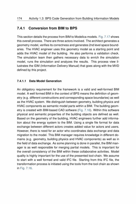
174 Activity 1.3: BPS Code Generation from Building Information Models

7.4.1 Conversion from BIM to BPS

This section details the process from BIM to Modelica models. Fig. 7.17 showsthis overall process. There are three actors involved. The architect generates ageometry model, verifies its correctness and generates 2nd level space bound-aries. The HVAC engineer uses this geometry model as a starting point andadds the HVAC model of the building. He also performs a validation check.The simulation team then gathers necessary data to enrich the simulationmodel, runs the simulation and analyzes the results. This process view il-lustrates the IDM (Information Delivery Manual) that goes along with the MVDdefined by this project.

7.4.1.1 Data Model Generation

An obligatory requirement for the framework is a valid and well-formed BIMmodel. A well formed BIM in the context of BPS means the definition of geom-etry (e.g. different constructions and corresponding space boundaries) as wellas the HVAC system. We distinguish between geometry, building physics andHVAC components as semantic model parts within a BIM. The building geom-etry is created with BIM-based CAD software (Fig. 7.16). Within this softwarephysical and semantic properties of the building objects are defined as well.Based on the geometry of the building, HVAC engineers further add informa-tion about the energy system to the BIM. Using a single file format for dataexchange between different actors creates added value for actors and users.However, there is need for an actor who coordinates data exchange and datamigration to the model. This BIM manager requires knowledge in different do-mains (e.g. geometry, building physics and HVAC components) as well as inthe field of data exchange. As some planning is done in parallel, the BIM man-ager is as well responsible for merging partial models. This is important forthe overall consistency of the BIM within these collaborative activities. Modelquality is highly important for the use of the presented tool-chain. We assumeto start with a well formed and valid IFC file. Starting from this IFC file, thetransformation process is initiated using the tools from the tool chain as shownin Fig. 7.16.

7.4 Open Framework for Modelica Code Generation from BIM 175

Project: IEA Annex 60 (Task 1.3)

BIM Coordinator

(Architect)

Data

Exchange

BIM Coordinator

(HVAC Engineer)

Data

Exchange

BIM Modeller

(Simulation Team)

Data

Exchange

Precheck building model

(Model Viewer)

Model

enrichment

Simulation

(Modelica/EnergyPlus)

Analysis of the

simulation results

Adjust data model,

depending on the

targeted simulation tool

Activity and

Schedule

Specific

parameters for

EnergyPlus

Prepare geometry model

(BIM authoring tool)

Generate 2nd

level

space boundaries

(SBT)

Model check for Space

Boundary Tool

(Solibri)

BIM HVAC

ModelPrepare HVAC model

(BIM Authoring tool)

HVAC Model Check

(KIT Tool HVAC

Model Check)

BIM Geometry

Model

Geometry

Energy

Model

Results

Report

Gather information

for the purpose of

data enrichment

Weather

Data

Internal

Loads

Economical

Data

Fig. 7.17 : Overall process diagram (IDM)

176 Activity 1.3: BPS Code Generation from Building Information Models

7.4.1.2 Information Selection, Enrichment and Verification

The IFC format is able to store detailed information about various disciplines,for example, fire protection. Not all of the exchanged data is needed for BPS,therefore the energy consultant uses a specific Model View Definition, whichis described in Section 7.3.5, to read the relevant data for BPS in Modelica(middle part in Fig. 7.16). An MVD is a subset of the IFC-schema that de-fines discipline-specific exchange requirements. As an example the energyconsultant needs spatial surface geometry defined in the MVD as a basis forthermal zones. On the other hand, the simulation of HVAC equipment mightneed further information that is not part of the information model of IFC. Tostore and exchange this additional information, the energy consultant migratesthe collected data from the MVD to the intermediate file format SimXML. Thetransformation is done by using Space Boundary Tool and Simergy for the ge-ometry part of the IFC mode, see Section 7.4.3.1 and Section 7.4.3.2. TheHVAC related objects are transformed with a tool developed as part of thisproject. It uses the XSLT language to translate the model into SimXML (Sec-tion 7.4.3.4). The information model behind SimXML is called SimModel (seeSection 7.3.6) which is a simulation domain specific data model. Both toolsadd further, missing information to the SimXML file. This particularly refers tospace boundary and semantic information, needed for dynamic building sim-ulation. The resulting file is automatically verified against the XML schemadefinition. Section 7.4.3 describes technical details of the transformation fromIFC to SimModel.

7.4.1.3 Simulation Model Generation

The last step is the generation of valid Modelica code. This task divides intothe parsing and validating of the SimXML file, mapping from SimModel to aspecific Modelica library (e.g. BuildingSystems or AixLib) and textual outputof the code itself. For parsing and validating the SimXML file we developed aC++ framework, called libSimModel (Section 7.4.4). In addition the code mapsobjects and parameters defined by mapping rules from SimModel to Modelicalibrary. Furthermore, individual processing and the mapping of object topolo-gies (as these differ in different libraries) need to be considered. Throughan API we expose relevant data available in libSimModel to the Python pro-

7.4 Open Framework for Modelica Code Generation from BIM 177

gramming language and perform these individual steps in a tool called CodeTemplating Tool (CoTeTo). Both object and parameter as well as the topologymapping needs to be defined by a simulation expert, who has fundamentalknowledge of the considered library and SimModel. CoTeTo collects now allinformation and prints out Modelica code with regard to a correct Modelicasyntax. The process is described in detail in Section 7.4.6.3.

7.4.2 Data Transformation

The primary role of a Building Information Model (BIM) is to serve as a com-prehensive repository of data that are retrievable by multiple software applica-tions which participate in the same AECO industry project. Data placed in aBIM by one software application are retrieved and used by other applications.Retrieved data are at times not useable by the recipient application in exactlythe same form and/or format as received; in such cases the received data aremanipulated and/or transformed before they can be used [BK07] .

A software application is entering new data in a BIM, it is authoring thosedata. Such data constitute the original BIM data that can then be used byother, usually downstream, software applications. Downstream applicationsmay, and often do, support different disciplines and have implemented differentmodel views than the authoring application.

CAD applications generate building geometry and, in the process of docu-menting it, are usually the first to create original data. Additional data aresubsequently authored by downstream applications. Because the need to ex-change data among CAD applications is relatively infrequent, the real pay-off from software interoperability is seamless data exchange with and amongdownstream applications. But that data exchange is not always automatic orstraight forward.

A software application imports or generates itself all data it manipulates. Toobtain valid results, data imported by an application must not only be in a formand format that is readable by the application, but also must represent valueswithin the range the application expects to import. For example, if a down-stream application expects to import a value for floor-to-floor space height,the imported value must represent floor-to-floor and not floor-to-ceiling space

178 Activity 1.3: BPS Code Generation from Building Information Models

height. Because of the diversity of applications (and their internal data struc-tures) that may participate in a given data exchange, “original” data must oftenbe transformed before they can be used by a downstream application – datasets must be reduced and/or simplified, or data must be translated and/or in-terpreted.

In general, data transformation can be classified in four types:

1. Data set simplification. An original data set can be too “rich” to importby a downstream application. For example, the original definition of afloor structure may include the precise geometry of all material layers inthe floor, while a downstream application can only import a generalized“sandwich” definition of the floor. The redefinition of the floor “sandwich”that loses some geometry detail but still accounts for all material layersamounts to a simplification of the original geometry. Geometry approxi-mation usually falls in this category.

2. Data set reduction. If the “rich” original geometry data set contains def-initions that cannot be used by the downstream application, these areomitted from the exchange set. This is the case when, for example, acolumn in its original is partially embedded in a wall, but the downstreamapplication cannot import column definitions; the column definition is ex-cluded from the exchange set and the wall of the original definition isextended over the space previously occupied by the column.

3. Data set translation. Most of this type of data transformation involvesunits of measurement, such as conversion of metric to imperial units.Another type of translation is the textual definition of surface orientationwhich in the original definition is expressed by the “normal” vector, andthe downstream application requires textual identification of the orienta-tion (e.g. “exterior”).

4. Data set interpretation. When data required by downstream applicationshave not been explicitly defined before, it may be possible to derive themfrom original data which themselves may not be needed by these appli-

cations. The interpretation of original information that yields derived datathen becomes a process that can involve recognition, extraction, sorting,and calculation. This process can be relatively simple, as in deriving thefloor-to-wall area ratio not included in the original BIM data, or fairly com-plicated, as in deriving the proper “net” building area as specified by localcode.

7.4 Open Framework for Modelica Code Generation from BIM 179

Legitimate data transformation is performed following rules which are agreedupon and standardized. These rules cannot be arbitrary and should be em-bedded in data transformation software to be executed faithfully. Manual datatransformation is acceptable only if it follows applicable rules.

7.4.3 IFC to SimModel

The process of converting the IFC data model into SimModel consists of var-ious tools that convert both the geometry as well as the HVAC data. For thegeometry, the Space Boundary Tool generates 2nd level space boundaries.Simergy will transform the geometry data from IFC to SimXML. For the HVACdata, we first describe the checking tool and then the converter.

7.4.3.1 Space Boundary Tool (SBT)

SBT is a tool that calculates all levels of space boundaries that define surfacegeometry which constitutes the building geometry model in BEP simulationusing EnergyPlus and other simulation engines with similar internal geome-try models [Baz10] . The main SBT algorithm is based on graph theory toconvert a three-dimensional architectural building model without defined ther-mal space boundaries into geometry suitable for import into a whole-buildingenergy performance simulation engine such as EnergyPlus [RB13] . The algo-rithm expects input specified as an Industry Foundation Classes (IFC) model,accepts a wide variety of input geometry, and is capable of accounting for abuilding’s construction material configuration as well as its geometry. The de-scribed approach is limited to solid-to-solid heat exchange; solid-to-fluid andfluid-to-fluid heat exchange is not considered.

In addition, SBT performs two other functions: It (a) automatically performsdata transformation that is necessary so that EnergyPlus- like simulation en-gines can read and use information contained in SBT export files without fur-ther data transformation, and (b) it automatically corrects modeling errors thatcan be automatically corrected. All data transformation is performed accord-ing to rules embedded in SBT. The following is the list of 16 geometry datatransformation rules embedded in SBT:

180 Activity 1.3: BPS Code Generation from Building Information Models

• Skipping of internal wall objects when walls are entirely contained withinthe same thermal zone;

• Reversal of the order of construction material layers for ”other side”second-level space boundaries for walls and slabs which have asym-metric construction;

• Redefinition of embedded columns as separate wall objects;• Definition of the remaining wall construction parts when columns are

only partially embedded in walls;• Recognition of exterior building shade types;• Positioning of exterior building shades right outside the exterior space

boundaries of exterior walls;• Detection and redefinition of virtual walls and slabs;• Assignment of “virtual constructions” to virtual walls and slabs;• Identification of floor and ceiling surfaces of a slab;• Subdivision of slabs with voids into “void-free” segments;• Redefinition of “exterior ceilings” as roofs;• Connection of slab-on-grade objects to the ground object;• Creation of the parent wall’s space boundaries for windows (if missing);• Adjustment of window area to effective glass area;• Linking of glazing definitions to Window 6.2 tool;• Linking of material and construction objects to the EnergyPlus library of

materials’ thermal properties.

SBT’s automatic model correction is limited to surface connecting errors typi-cally prevalent in BIM geometry models generated by industry modelers: sur-faces not connecting when connection is intended and/or necessary, and sur-faces penetrating each other when such penetration is not intended. In model-ing cases where not connecting surfaces is intentional (but SBT detects a gapbetween surfaces as defined in the IFC input file), SBT allows its user to settolerance that identifies the intended gap and does not treat such instances aserrors.

In addition to flat planar geometry, SBT can generate geometry models ofcurved surfaces and spaces. It calculates the geometry of single flat seg-ment connections between end points of curved surfaces, but overrides sur-face area and space volume data associated with flat surfaces with actual val-ues of curved surfaces and spaces. Since IFC definitions of curved surfaces islimited to 2D curves, SBT can itself only accept 2D curves. The tool can also

7.4 Open Framework for Modelica Code Generation from BIM 181

interactively map thermal properties of construction materials from ASHRAEspecifications to construction materials identified in the imported IFC geome-try.

The tool generates two export files: an updated IFC file (with added spaceboundary definitions) and an IDF file that delineates the building’s geometry fordirect input and execution in EnergyPlus. The latter exports a 3D wire-frameview of the building geometry imported into EnergyPlus, which facilitates visualinspection of correctness of the imported geometry. Section 7.5.9 shows anexample of this transformation.

7.4.3.2 Simergy

Simergy is a simulation front end that currently supports EnergyPlus simula-tions and analysis for the California Energy Code (Title24). With its data modelSimModel (Section 7.3.6) aligns closely to the IFC data model and this sup-ports import and export of IFC files as well as other data formats (e.g., gbXMLor EnergyPlus input data format (IDF)). The promise of Simergy is to alloweasy reuse of data in form of library object entries as well as data and systemtemplates. This enables quick setup of detailed simulation models that caneasily be adjusted and optimized.

In context of this project and its tool chain, Simergy provides mainly two func-tions. The first one is the import of IFC data files and the export of SimXMLfiles containing geometry data. For this function it can either use space bound-aries generated by SBT or generate them internally. The second feature is theaddition of internal loads data. While previous efforts (such as Concept De-sign BIM 2010, [BDA12]) tried to enable the definition of internal loads in CADapplications, currently support is only partial. Especially scheduling data is notsupported by CAD applications. Since schedules are a major part of internalloads definition, we add them for this project within Simergy. Besides the ge-ometry and internal load data, HVAC data is an important part of the simulationmodel and the relevant data transformation and checking is illustrated in thenext subsections.

182 Activity 1.3: BPS Code Generation from Building Information Models

7.4.3.3 IFC Model Checking

Quality assurance of the initial BIM model has been identified as an impor-tant precondition for a qualified simulation process. Thus, the objective wasto provide a coherency check of the IFC data to ensure that data enteringthe overall tool-chain passes quality requirements. The conception of the toolbuilds on existing generic software components and packages that were usedto implement the tool.

Requirements Section 7.3.5 highlights general requirements for quality as-surance within the BIM-based processes. In the context of the BIM to Model-ica conversion process the required data quality was examined in a scenario-based requirements analysis. Based on these results specific rules were de-rived which specify model quality and IFC contents. For example, all pipe partsof a pipe circuit have to be correctly connected (referenced). The rules aim todetect inconsistencies within the designated source data of the simulation, be-fore they are transformed to the intermediate format SimModel.

Concept The tools core architecture is based on concepts and generic com-ponents of the BLM collaboration toolKIT. There are two main underlying con-cepts, such as the workflow based conception of the user interface, and theconcept of independant rules written in XML files to define the domain-specificmodel checking aspects. In order to support non-experts the UI was designedas a four-step procedure to check a model file against given rules. These rulesare formalized in [EvB13] and are stored in different XML files. The rule-basedmethod builds a base to depict the simulation-related data quality demandsand enables to check whether a designated model complies with them. Pri-marily the defined rules in natural language have to be formalized in order tobuild the logical (domain-specific) base for the machine-interpretable businesslogic (rule code). Methodically the first step of formalizing the rules takes nec-essary elements of the specified IFC4 syntax on a binary level into account(e.g. paths to respective object classes). These first rule parts or elementsbuild the base for deriving collections, resolving relations etc. as needed toformalize the overall natural language content (rule logic) into rule code. Theother developed components which adopt the reused concepts, together with

7.4 Open Framework for Modelica Code Generation from BIM 183

the new developed viewing component are finally integrated into a standalonetool. This application together with the separated rule base is available athttps://download.building-lifecycle-management.de for free. The application isused to support the designated users of the projects tool-chain with respectivequality measures to examine their potential IFC-based input data.

Implementation The model checking tool is released using the component-based-development approach based on the .NET framework. The developedrules are either required or optional and following rules were developed for thecontext of the project.

Obligatory rules:

• building context information, e.g. proper hierarchy, location information• building elements have material (layers) connected• space entities have space boundaries connected• all (HVAC) IFC components have to be connected to a IfcSystem (or

derivate)• air systems are connected to a thermal zone• mechanical air systems contain at least one fan component

Optional rules:

• mechanical air systems are either fresh air or are closed loop systems• controlled water systems contain at least one pump component

Fig. 7.18 shows the current development stage of the user interface of the stan-dalone software tool “KIT EnEff-BIM Model Check”. The workflow of modelchecking is presented in four steps:

1. load model file2. select rules3. execute model check4. summarize results

The workflow is displayed in a corresponding four tab view to the user. Besidesthe possibility to export a respective (error-) report to a spreadsheet file in tab4, as well a call to the conversion tool has been implemented. In case of afault free model check the already loaded and checked ifcXML model file is

184 Activity 1.3: BPS Code Generation from Building Information Models

passed as an argument to the standalone console application Section 7.4.3.4.This converter is described in the next subsection.

Fig. 7.18: Screenshot “KIT EnEff-BIM Model Check” Version 0.9 rule selection tab.

7.4.3.4 XSLT-Based IFC to SimXML Converter for HVAC Elements

The main objective of this tool is to provide a mechanism that converts theHVAC partial model in IFC4 to the SimModel format.

Requirements For the development of the converter tool, the Annex 60use cases define the requirements and build accordingly the logical base forthe transformation of the IFC4 HVAC partial model to SimModel. The web-based BIM*Q platform ([316]) was used to collect and specify the requirementsneeded for the translation. The IFC entities related to the use cases and theirparameters form the mapping information of the respective SimModel objects.

Concept The concept of the conversion tool is based on the existing (techni-cal) World Wide Web Consortium (W3C) approach that specifies the eXtensi-

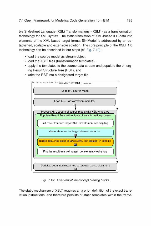
7.4 Open Framework for Modelica Code Generation from BIM 185

ble Stylesheet Language (XSL) Transformations - XSLT - as a transformationtechnology for XML syntax. The static translation of XML-based IFC data intoelements of the XML-based target format SimModel is addressed by an es-tablished, scalable and extensible solution. The core principle of the XSLT 1.0technology can be described in four steps (cf. Fig. 7.19):

• load the source model as stream object,• load the XSLT files (transformation templates),• apply the templates to the source data stream and populate the emerg-

ing Result Structure Tree (RST), and• write the RST into a designated target file.

Fig. 7.19: Overview of the concept building blocks.

The static mechanism of XSLT requires an a priori definition of the exact trans-lation instructions, and therefore persists of static templates within the frame-

186 Activity 1.3: BPS Code Generation from Building Information Models

work of the XSLT application. Due to the joint development of the mappingrequirements, the static approach of XSLT was supplemented with generic so-lutions. These are specified in the following four concept blocks that define thecore architecture of the tool:

1. Prefilter the relevant IFC model entities from the source model datastream. Several “Traversing Templates” (for processing the IFC topol-ogy) are used on side of the technical development to optimize theoverall conversion procedure (in the subsection “Implementation” we de-scribe how this concept block is realised and how to bypass it)

2. Dynamic injection of the externally defined translation instructions be-tween source and target model (the used concept of a simple syntax forthe mapping logic is introduced in the following sub-section)

3. Trigger the (element-wise) generation of the target model contents bystarting the conversion procedure through applying exactly one framing(main) XSLT template and loosely coupled “Production Templates”. ThisXSLT core principle (cf. Fig. 7.19) builds the base for further thematicalextensions of the conversion tool.

4. Final assembly of the output (SimModel file) supported by the targetmodel schema.

Referring to the “Divide and Conquer” principle these four concept buildingblocks were consolidated into a comprehensive transformation process (cf.concept building block 3; see Fig. 7.21).

Concept of Machine-Readable Mapping Table Entries In order to trans-fer the mapping logic into the tool a syntactic machine-readable structurewas defined that refers to the contents of the table-based BIM*Q platform.This structured information is then handed off to the conversion mechanismby exporting it to the Comma-Seperated Values (CSV) format. Conceptuallythe two columns of the mapping-tuple - IFC column and SimModel column -were extended by a third column that defines an initial condition for conver-sion of the respective tuple. Following mapping case example (IfcBoiler toSimFlowPlant_Boiler_BoilerHotWater) exemplarily depict the simplified modelinstances:

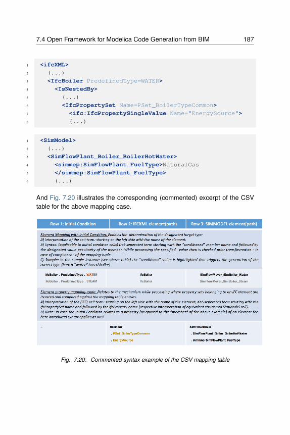
7.4 Open Framework for Modelica Code Generation from BIM 187

1 <ifcXML>

2 (...)

3 <IfcBoiler PredefinedType=WATER>

4 <IsNestedBy>

5 (...)

6 <IfcPropertySet Name=PSet_BoilerTypeCommon>

7 <ifc:IfcPropertySingleValue Name="EnergySource">

8 (...)

1 <SimModel>

2 (...)

3 <SimFlowPlant_Boiler_BoilerHotWater>

4 <simmep:SimFlowPlant_FuelType>NaturalGas

5 </simmep:SimFlowPlant_FuelType>

6 (...)

And Fig. 7.20 illustrates the corresponding (commented) excerpt of the CSVtable for the above mapping case.

Fig. 7.20: Commented syntax example of the CSV mapping table

188 Activity 1.3: BPS Code Generation from Building Information Models

The simple “point-syntax” of the term further enables e.g. the specificationof mappings between nested elements, and completes the machine readablemapping concept. Based on this mapping syntax definition and without havingthe mapping table fully formulated in detail, a (dynamic) requirement basis forthe implementation of the designated conversion tool is given.

Implementation For realizing the converter with XSLT 1.0, the above intro-duced concept blocks one, two and four were integrated into an XSLT trans-formation procedure which is described in the third concept block. Fig. 7.21shows the overall procedure where the green templates - ifcXML root elementand Production Templates for respective IFC elements - realize the overarch-ing main procedure.

Thereby recursively nested templates of the first (blue) and second (yellow)concept block extend the static procedure with mechanisms to

1. a priori collect all relevant IFC entities from the source model stream and2. inject the conversion instructions from a CSV table that is delivered by

the BIM*Q platform.

Fig. 7.21 depicts the generation of the target root element “SimModel”. Withinthe green box “MATCHED production templates” a recursive sub-procedurehandles the generation of the target elements and their content. For furtherreading we refer to [EvB16] . In summary, a demand-led, dynamic and scal-able solution was realized. Future developments (or other configurations) aresupported by providing the full implementation of the tool as open source (ac-cess via https://download.building-lifecycle-management.de).

7.4.4 libSimModel C++ library

This section describes the transformation system developed for linking BIMwith different Modelica libraries. In the system, SimModel acts as the BIMcontainer to save BIM data generated from IFC, for example, HVAC, geometry,property data of HVAC systems and equipment, simulation configurations, etc.

7.4 Open Framework for Modelica Code Generation from BIM 189

Fig. 7.21: Recursively superimposed concept blocks of final tool specification

190 Activity 1.3: BPS Code Generation from Building Information Models

7.4.4.1 SimXML Data Binding and Syntax Validation

The data file of SimModel is an XML-based file named SimXML. It saves all theSimModel data as a structured XML document that is in accordance with thesyntax defined by the SimModel schema. Thus, this sub-section introducesthe XML data binding technique for accessing SimXML and validating its syn-tax. XML data binding is the process of extracting data from a structure rep-resentation of XML documents and presenting it as a hierarchy of objects thatcorrespond to a document vocabulary. This allows us to manipulate SimXMLdata in a more direct and efficient way. We selected the open source, cross-platform CodeSythesis XSD [Cod14] as our system XML binding parser. Itis an efficient framework whose parser can be adjusted for custom applica-tions. The automated XML data binding of CodeSythesis XSD will generatea C++ API for accessing the data stored in SimXML after parsing the Sim-Model schema. For the SimModel schema version 2.2, 2611 C++ classesrepresenting different SimModel objects are generated for the data manipula-tion in a given SimXML file. The XML syntax validation performs a numberof checks on the XML document to prevent the construction of an inconsis-tent object model, such as an object model with missing required attributes orelements. Our SimXML validation relies on the underlying Xerces-C++ XMLparser embed in CodeSythesis XSD. It checks the SimXML data against thegiven SimModel schema, and outputs the errors found into a log file. The syn-tax validation is enabled by default and is very useful during the developmentstage to detect problems with the data model at an early stage. For a user ofthe framework, this validation does not play a significant role anymore, sincethe changes to the SimModel model are finalized.

7.4.4.2 SimModel Hierarchy Parsing and Visualization

A model hierarchy is an arrangement of the model elements, e.g., objects,names, values, categories, etc., in which the elements are represented as be-ing “above,” “below,” or “at the same level as” one another. Consequently, theSimModel consists of a hierarchical tree structure saving such relationshipsbetween different SimModel data elements (see Fig. 7.22).

As illustrated in Fig. 7.22, a SimProject class object is normally the root node ofthis hierarchy tree representing a unique simulation project. This root node can

7.4 Open Framework for Modelica Code Generation from BIM 191

Fig. 7.22: SimModel hierarchy tree structure.

192 Activity 1.3: BPS Code Generation from Building Information Models

store multiple links that refer to different building design alternatives. Each de-sign alternative also refers to a set of building elements, zones, HVAC systemsdistributed inside the building, etc. Therefore, the SimModel hierarchy savesa set of different SimModel elements as well as the links between them in atree-based structure. At the bottom of the SimSystem sub-tree, different typesof SimDistributionElement nodes are created to save different HVAC compo-nents located at different sides of the SimSystem, e.g., a hot water boiler will besaved as a child SimDistributionElement node of the SimSystem water supplyside. At each SimDistributionElement node, a list of child nodes are createdfor saving different physical connections between these HVAC components,e.g., the pipe connections within a hot water looping system for connectingthe boiler and pump. The physical connections saved by these child nodesrepresent the SimModel topology.

In SimXML, each model element is given a unique long type ID that distin-guishes it from all other elements. Each parent element of the SimModel hi-erarchy links to a child element by saving its ID. As a result, “parse SimModelhierarchy” is a recursive algorithm that detects each SimModel element, lo-cates its position in the hierarchical tree and creates a tree node with a link toits data. After that, we can also recursively iterate each node of this hierarchy,retrieve the link to the SimXML data element and print out the element data forvisualizing the created hierarchy.

7.4.4.3 SimModel to Modelica Mapping Rule Schema and Rule Filter

The mapping rule concept was first introduced in mathematics, representinga particular transformation. This transformation describes the conversion ofa source model data into a target model data under the constraints speci-fied by a given equation system. As SimModel is significantly different fromthe data model of a specific Modelica library [CMO+14] , e.g., AixLib or Build-ingSystems, we also need to define a set of mapping rules that can handlethe difference between these two different data models. [WCR+15][WMO+14]

proposed a set of different mapping rules that can convert the SimModel datainto the Modelica model data defined by a specific BPS library AixLib [EBC14] .Based on this work, we developed a mapping rule schema in XML SchemaDefinition (XSD), containing the data model of the mapping rules betweenSimModel and different Modelica libraries [CWT+15] . We can thus efficiently

7.4 Open Framework for Modelica Code Generation from BIM 193

re-use this mapping rule schema, originally developed for our transformationsystem, to define different sets of mapping rule instances for different targetModelica libraries. Mapping rules are classified according to three differentlevels in the schema:

• The first level is library mapping, which is designed to link different map-ping rule instances for different Modelica libraries.

• The second level is component mapping, which is responsible for map-ping SimModel components, e.g., a boiler of the HVAC system, into thecorresponding component of the Modelica library specified by the firstlevel mapping.

• The third level deals with the internal properties mapping of the compo-nents defined by the upper-level mapping rules.

Czarnecki and Helsen [CH06][CH03] discussed fundamental work on datamodel transformation. In context of their work we can view transforming Sim-Model data model to Modelica code as a special case of model-to-model trans-formations. We only need to provide the meta-models for the source modeland the target programming language as well as the transformation definedwith respect to the meta-models. A transformation engine transfers the sourcemodel data into the target programming language model. In our case, thesource model is SimModel and the target language is Modelica. The transfor-mation is an instance of the mapping rule schema saved as XML file formatand the transformation engine contains a set of filters translating the modeldata by filtering the mapping rule instance. The source model data is storedin SimXML file and the target programming language model is the Modelicacode, based on a specific BPS library.

7.4.4.4 SimModel Python API for Modelica Code Generation

The main parts of the transformation system are implemented in the C++ pro-gramming language, in order to satisfy the requirements of model transforma-tion speed and the access to low-level system features, such as virtual mem-ory allocation. Script programming languages, like Python, are heavily usedfor pre- and post-processing of Modelica. They are more flexible and easier touse for controlling the procedure of Modelica code generation based on tech-niques like pre-defined code templates and interpretation engines. Therefore,

194 Activity 1.3: BPS Code Generation from Building Information Models

this sub-section introduces a generic API developed for interfacing SimModelC++ library and the script programming language Python, in order to bettercontrol the Modelica code generation by separating the translation logic fromcode generation.

We developed our prototype for this generic API based on a technique namedlanguage binding. In computer science, a binding from a programming lan-guage to a library is an API providing the glue code to use that library in aparticular programming language. In the context of our generic API, bindingsare wrapper libraries that bridge the C++ and Python programming languagesin order to re-use the SimModel API generated for C++ in Python.

According to the testing on different binding libraries, e.g., ctypes, Cython,Boost.Python, we use SWIG [SWI15] as the binding libraries to wrap the Sim-Model API for data access out of Python. Compared to other binding libraries,SWIG is easier to port the interface of a large C/C++ library to other languages,like Python. It is an open-source and battle-tested binding software used bylarge companies, e.g., Google. It keeps both the C++ and Python code clean,i.e. not altering Python itself such as Cython is doing. SWIG provides C++compatible data types, and allows calling functions in the Dynamic Link Li-brary (DLL) or the other types of shared libraries from Python. In the systemprototype, we exposed the mapped or translated SimModel components andtheir internal properties into a Python-based Modelica code generator via theSWIG wrapper. In order to provide Python with full controls on SimModel in-ternal data, we also exposed more data objects from the SimModel hierarchyas well as the topology into Python via the generic API. Fig. 7.22 illustratesSimModel hierarchy exposed for Python.

7.4.5 Mapping Rules

Several steps need to be considered to complete the mapping between theSimModel data model and the Modelica libraries. Fig. 7.23 and Fig. 7.24shows two BPMN (Business Process Model and Notation) process diagramsto illustrate the decisions and steps needed for a successful mapping.

As indicated in Section 7.3.7, in the formal mapping process we distinguishbetween object and parameter mapping.

7.4 Open Framework for Modelica Code Generation from BIM 195

Object represented

on Simmodel side?

Analysis of the

parameter

Al l relevant

information

represented?

Extended analysis of

the SimModel objects

Needed

information

represtented?

Many to One mappingOne to One mapping Gap

Yes

Yes

NoYes

No

No

Fig. 7.23: BPMN process diagram for the object mapping

196 Activity 1.3: BPS Code Generation from Building Information Models

Parameters

identical?

One to One

mapping

Gap

Definition of

transformation

algorithm

Adding additional

information

No

Yes

Yes

Al l relevant

information

represented?

Extended analysis of

SimModel

parameters

No

Parameters

represented

completely?

No

Transformation

Yes

Fig. 7.24: BPMN process diagram for the parameter mapping

7.4 Open Framework for Modelica Code Generation from BIM 197

The object mapping is performed as a first step in order to find all the relevantobjects to represent the data needed in the specific Modelica library. Fig. 7.23shows the sequence of the object mapping. Checking if the object neededfor Modelica is represented in the SimModel data schema is the first step. Tounderstand the objects of each side, the SimModel and the Modelica librarydocumentations should be considered. If an object is not defined in SimModel,either the missing object needs to be added to the existing data schema or theGap mapping rule needs to be applied. If it is represented, the next step is tocheck if all parameters in the SimModel object are sufficient for the targetedModelica object. One to One mapping can be applied, if all relevant data areavailable. If further information are needed, other SimModel objects need tobe considered in addition. In case several objects are needed to provide therelevant information, the Many to One mapping rule defines those. If still someinformation is lacking, the data schema of SimModel needs to be extendedagain by applying the Gap rule.

Fig. 7.24 illustrates the next steps to complete the mapping between the Sim-Model data schema and the Modelica libraries. If the parameters on both sidesare defined identically, a simple One to One mapping rule can be applied. Ifadditional information is needed, further parameters should be considered.Several SimModel parameters can be combined to define a single parameteron the Modelica side. To perform a combination of parameters, the trans-formation mapping rule needs to be applied. For defining the transformationalgorithm, it can be necessary to add external data.

A specific example of the transformation rule is demonstrated below. The valueof the set temperature for a gas boiler on the SimModel side is defined usingthe unit Celsius, whereas the unit for the Modelica side needs to be defined inKelvin.

The transformation algorithm for this mapping process is

f = a + 273.15

where a is the temperature setpoint of a gas boiler in the SimModel datamodel.

As shown, the algorithm transforms the set temperature from Celsius to Kelvin,adding 273.15. Thus, the SimModel value is transformed and describes therelevant data for the Modelica side.

198 Activity 1.3: BPS Code Generation from Building Information Models

7.4.6 Python Tools for Modelica Code Generation

Python as an interpreted language is used widely in the Modelica communityfor scripting, workflow automation, pre- and post-processing and as a gluelanguage. Using the wrapper for the libSimModel library generated by SWIG,most functions from the C++ library can be called from Python. The Pythontools using the libSimModel API so far are a Qt based viewer and editor forthe SimModel object tree, a high-level API that adds further functionality andimplements the topology mapping and the code templating tool CoTeTo, thatis used for generating Modelica code.

7.4.6.1 SimModelTreeView

Based on the API generated by SWIG, a simple viewer for the SimModel objecttree has been implemented as a PyQt widget. It uses QTreeView and readsdata from the API on demand when unfolding the tree. A second widget isimplemented for viewing and editing the attributes of objects. Both widgetscan be called on their own or be embedded in another GUI or be imported asa module.

7.4.6.2 High-Level API

The API as generated by SWIG reflects the functions defined in C++. For userconvenience, a set of Python classes that can be loaded as a module has beenimplemented on top of that API. A UML diagram for these classes is shown inFig. 7.25.

The classes each have attributes that are accessible using the dot notation.One attribute is, where applicable, an iterable list of child objects. The Pythonclasses as well implement the topology mapping which is described in thefollowing paragraph.

7.4 Open Framework for Modelica Code Generation from BIM 199

MapSpaceBoundaries

Collects construction

element attributes

MapProject

Handles all

Components and

connections

MapBuilding

Handles zones and

components (Full

System)

MapThermalZone

Collects zone

attributes

MapComponent

Generic class for

HVAC component in

SimModel

MapConnector

Class for Modelica

connector

information

MapConnection

Class for Connection

of two Connectors

MapProperty

Class for Modelica

Property

21

MapRecord

Class for Modelica

Record

1 *

1*1

*

1*

1

*

1*

MapControl

Class for generic

control strategy1 1

1 *

1

*

1*

1*

Fig. 7.25: UML diagram for the high-level API.

200 Activity 1.3: BPS Code Generation from Building Information Models

7.4.6.3 CoTeTo: Code Templating Tool

The actual Modelica code generation is implemented as a tool named CoTeTo,which stands for Code Templating Tool [TRR+15] . Although designed for thisproject, this tool was implemented in a way that it can be used standaloneand in other software environments. CoTeTo is released under the MIT open-source license at https://github.com/UdK-VPT/CoTeTo .

In this project, Modelica models for a set of different model libraries have to begenerated using a common data source. Each library needs separate filteringand output of data because of different modeling approaches. These librariesare currently under development and are likely to change in the future as well.This requires a flexible and generic data conversion framework to allow forfuture changes. Thus, the framework should allow flexible output componentsfor different libraries in multiple versions as well as flexible input components,both should be easy to maintain even for non-programmers.

The workflow of CoTeTo and the coupling to other tools within the toolchain isshown in Fig. 7.16.

We designed CoTeTo to be used by graphical, command line and library levelinterfaces. The multiple access possibilities open the framework to be used bya larger community.

The fact that Python does not require extensive compilation cycles helps withrapid development. The following section will give an overview of the compo-nents and their functionality. We divided CoTeTo into input components (Data

APIs) and output components (Generators). A Generator depends on a spe-cific Data API (defined by its name and version).

The Template Approach There are two general concepts for the genera-tion of textual output within a computer program. One approach is to embedprint()-statements for text strings and data in the structure of a program.This is useful for nearly static, well-defined structures of the data set and ofthe textual output.

The other approach is template-based, where placeholders for the content areembedded in a text file (a template for the output). Besides placeholders tem-plates also offer control structures. Thus, template-based model generation al-

7.4 Open Framework for Modelica Code Generation from BIM 201

lows complying with fixed Modelica language syntax and adding flexible modelcontent in the same file. One advantage is the flexibility for the end user, whodoes not necessarily need to dive into the programs’ internal structure, but canenrich the template file with placeholders and simple programming constructs,whenever the used Modelica models change. This workflow is much like theform letter function in office software, which fills some variable address fieldsin a text document from a database.

The template approach fits well into the flexible structure of the CoTeTo frame-work, as it is independently usable for different information sources. From thelist of available template engines Mako [Bay14] and Jinja2 [Ron14] seem to fitbest into CoTeTo. At this point support for both is implemented.

Input - Data APIs A Data API is a Python module that defines a prescribedway to fetch data sets from a data source. Although we use the Python lan-guage to write the CoTeTo, Data API functions can interface with other lan-guages.

Different Data APIs and different versions can be used in parallel. Samplemodules for reading JSON, XML and CSV files exist in CoTeTo. This allowsflexible processes during development and testing. There is no definition forthe structure of the returned data items, since different data sources containdifferent types of data (tree, table, graph, map). It is the job of the correspond-ing output Generator to understand the data delivered by the related Data API.

The most important Data API in the Annex 60 context is the interface to theC++ library libSimModel, which handles the SimModel parsing and the map-ping to Modelica. Seen from the Python framework and from CoTeTo it definesthe data source used to fill the placeholders in the output templates.

Output - Generators Once all relevant data have been loaded into CoTeTo,it is passed to the output component, called Generator. We designed the Gen-

erator to contain all items needed to generate the code for a specific Modelicalibrary. This includes

• filter functions,• the meta model structure,• text templates,

202 Activity 1.3: BPS Code Generation from Building Information Models

• additional configuration and information and• additional files.

The filter functions, meta model structure and text templates are used andapplied by CoTeTo. Additional files like the mapping rules XML file can bestored inside the Generator.

Some data need manipulation that may not fit well into the mapping rule mech-anism. For this purpose, Generators can include filter functions (Python code)that we call between the data API and the templates. The filters are custom-built to the used library. In our case, they may include simplification of ge-ometric relationships and calculation of model specific parameters. Anotherapplication of filters would be the creation of annotations for the graphical ap-pearance and placement of model components in the Modelica code.

One major challenge in the automated generation of Modelica models is theflexibility of Modelica. Generally said, setting up useful models needs theknowledge of an experienced user. We are following the approach to encap-sulate this knowledge in library specific meta-models and templates. One es-sential task is the appropriate connection of components. The API returns theconnection information corresponding to the SimModel ontology, which differsfrom the one in a Modelica library. The meta model checks if the connection isapplicable, if not, it manipulates it.

The text templates are the last step in the process chain. The template enginecombines the data structures returned by the Data API and possibly manip-ulated by filters with the text templates to files with valid Modelica code. Thetemplates in a Generator can be split into several files to ease maintenance.

Generators can be easily exchanged between different installations, as theyare simple folders or even zip-files with a defined structure. Generators canbe maintained and edited with standard system tools like a file manager and atext editor. Creating a new Generator is as simple as copying a folder with anexisting Generator and changing the name or version number in a text file.

One example for a Generator template using Mako template engine is given infollowing listing. Static elements can easily be implemented as plain text in thetemplate (e.g. within line 1). A Dollar symbol, followed by curly brackets markthe placeholder, e.g. MapData.used_library in line 1 is replaced by the Pythonclass attribute used_library in the complied template. Control elements, like

7.4 Open Framework for Modelica Code Generation from BIM 203

for loops, are identified by a percentage symbol and follow the Python syntax,with the exception that indentation is not supported and the control elementhas to be closed (e.g. %endfor, line 6). This example template generates asimple model, by printing the library location (target_location) and individualname (target_name) in the first loop from line 4 to 6 and their correspondingconnections in line 9 to 13.

1 within ${MapData.used_library};

2 model ${MapData.name}

3

4 %for comp in MapData.hvac_components:

5 ${comp.target_location} ${comp.target_name}();

6 %endfor

7

8 equation

9 %for con in MapData.connections:

10 connect(

11 ${con.con_a.parent.target_name}.${con.con_a.name},

12 ${con.con_a.parent.target_name}.${con.con_a.name});

13 %endfor

14

15 end ${MapData.name};

User Interface and Handling There are currently three ways to use CoTeTo:

• CoTeTo can be imported in Python software as a module library. CoTeToworks both with Python 2.7 and 3.3+. All functions are usable via themodules API.

• A command line interface can be used interactively or called from othersoftware. It allows listing the available Data APIs and Generators andexecuting a Generator with a data source URI to produce the text output.

• The graphical user interface (GUI) is implemented using PyQt4. It al-lows flexible browsing and editing of all components and included filesand the execution of selected Generators. The GUI can be used as astandalone tool (see Fig. 7.26) or embedded in PyQt4-based applica-tions as a widget.

204 Activity 1.3: BPS Code Generation from Building Information Models

Fig. 7.26: Screenshot of the CoTeTo user interface

7.4 Open Framework for Modelica Code Generation from BIM 205

7.4.7 Topology Mapping

As already stated in the introduction of this section, the Mapping Rules (Sec-tion 7.4.5) deal with objects and parameters from SimModel to a specific Mod-elica library. In addition to the Mapping Rules in its current status we needinformation about model topology (e.g. number, type and name of Modelicaconnectors attached to the model) to generate valid Modelica models.

We define model topology as the way that the model in a certain object ori-ented language or information model is described in terms of connection toother models. In addition it offers the possibility to characterize which partsof the model are included in the object and which additional objects need tobe connected in order to work appropriate (e.g. different control elements).This topology differs from SimModel to Modelica libraries. One advantage ofthe presented work is that the transformation process complies and adaptswith the BIM and the specific model topology in Modelica libraries. Neither thetopology of the BIM model nor the topology of the Modelica library need to bechanged.

Furthermore the topology of models in different Modelica libraries may differ,even if the models describe the same behavior/object. To extend the informa-tion provided by the BIM with these Modelica and library specific informationwe developed a set of Python classes. This section describes the differenttopologies of SimModel and Modelica in more detail, taken the AixLib as anexample. Furthermore, the Python classes and the usage for other librariesare demonstrated.

In SimModel as well as in Modelica different objects are connected by con-

nections with different connectors. However, the type of connections differsfor these languages. For the given use cases and with a special focus onBPS we identified four connector types in Modelica to be significantly moreimportant. Table 7.2 lists these Modelica and the corresponding SimModelconnector types. In addition, Fig. 7.27 show the different connectors in Model-ica, the left column shows the connectors dedicated for design input, the rightfor design output respectively. However, for Fluid and thermal connectors thisis just a guideline as these connectors are acausal. The Fluid connector canbe used for various media (e.g. water or air) by changing the Medium attributeinside the connector.

206 Activity 1.3: BPS Code Generation from Building Information Models

Fluid_a Fluid_b

Thermal_a Thermal_b

Real_aReal_b

Boolean_aBoolean_b

Fig. 7.27 : Different connector types in Modelica (graphical representation).

Table 7.2: Comparison of Modelica and SimModel connector types.

MSL SimModelFluid connector (Medium: water) Water connector (cold, hot)Fluid connector (Medium: air) Air connectorThermal connector Air connectorReal connector Control connectorBoolean connector Control connector

7.4 Open Framework for Modelica Code Generation from BIM 207

As Table 7.2 shows one connector type in Modelica may correspond to severalconnector types in SimModel and vice versa. The topology mapping needs toconsider the different connectors and in the code generation distinguish be-tween them. This may be done by setting the correct parameters in the model,for example in the case of a water connection in SimModel, the correspondingmedia of the fluid is also set to water, by an mechanism in the Python topologyclasses.

Not only the type of connections differs from SimModel to Modelica but alsothe number of connectors per specific model and in particular the function andname of the connectors can differ from library to library (e.g. in the case ofdifferent Pumps). Thus, it has an effect on the topology of the models in thislibrary and the library itself. As the transformation process was designed tobe flexible enough, the library developers do not have to change their library,but adapt the transformation process. This is advantageous as the librarycan be developed for different purposes, without delimiting the developmentbecause of BIM required restrictions. Other pre- and post-processing tools ofthe individual library do not need to be changed.

In the following we present three examples and compare the topology andconnections of the Modelica objects from AixLib (the topology may differ inother libraries) and SimModel. The considered objects are:

1. Pump2. Radiator in a thermal zone3. Temperature controlled valve

7.4.7.1 Pump

The first example considers a pump. In SimModel the specific object is calledSimFlowMover_Pump_VariableSpeedReturn. It has three different connectortypes:

• SimNode_HotWaterFlowPort_Water_In

• SimNode_HotWaterFlowPort_Water_Out

• SimNode_DigitalControl_HWLoop_DigitalSignal_In

Water_In and Water_Out illustrate the causal approach of SimModel andare used to connect the pump within a hydraulic loop. The Digital-

208 Activity 1.3: BPS Code Generation from Building Information Models

Fig. 7.28: Connector types in Simergy shown on a pump (graphical representation)

Control input is used to attach a certain control object to the model.The AixLib holds five different implementations that could be used as apump. We take AixLib.Fluid.Movers.Pump, which is AixLib specific, andAixLib.Fluid.Movers.FlowControlled_dp, which is inherited from an Annex60library example to point out differences (see Fig. 7.29). Both models havetwo Fluid connectors to connect them within a hydraulic loop. This conceptaligns with the topology in SimModel. Further, both Modelica models have in-puts to control the pump. AixLib.Fluid.Movers.FlowControlled_dp uses a realinput named dp_in to imprint the pressure difference of the pump, which maycome from arbitrary control strategies. In contrast to that the developers ofAixLib.Fluid.Movers.Pump implemented a control strategy in the model itself,to use the model for specific applications. The control strategy uses a booleansignal to switch between two different operational characteristics. This input iscalled IsNight. Both the type and the name of all three connectors need to beadded within the topology mapping. In addition, the control strategies of thepumps need additional model objects (e.g. a boolean pulse), the instantiationand correct connection of these additional objects can also be assured in thetopology mapping.

Annex60_Pump

MP

Realdp

AixLib_Pump

Bool

Fig. 7.29: Comparison between AixLib.Fluid.Movers.Pump and

AixLib.Fluid.Movers.FlowControlled_dp

7.4 Open Framework for Modelica Code Generation from BIM 209

7.4.7.2 Radiator in a Thermal Zone

To distribute thermal energy into a thermal zone, radiators can be used. Theintegration into a hydraulic loop is very similar to the procedure described inthe above example and thus not part of this section. To semantically connecta radiator and the thermal zone, the concepts of SimModel and the approachused in AixLib differ, see Fig. 7.30. In SimModel the radiator is attached (by ref-erencing it with an ID) to a ZoneHvacGroup, which is a collection of all HVACequipment used or aligned to that certain zone. In AixLib the distribution ofthermal energy is done by thermal connectors, that calculate the heat flux forconvective and radiative heat transfer respectively. Therefore both, the radia-tor and the thermal zone hold each two thermal connectors. Between theseconnectors the topology mapping needs to instantiate the correct connec-tions [connect(Radiator.heatPortCon, ThermalZone.internalGainsConv) andconnect(Radiator.heatPortRad, ThermalZone.internalGainsRad)]. It is worth-while mentioning that the names of the connectors and models are againmodel and library specific. Further standardization would simplify the con-version process in the future.

7.4.7.3 Temperature Controlled Valve

This example illustrates the different handling of controls in SimModel andAixLib. We consider a PID controlled valve for flow regulation in a hy-draulic loop. The measured variable in this case is the air tempera-ture in the thermal zone, set point is a constant value and the manipu-lated variable is the opening of the valve. SimModel has no such con-trol, the radiator is controlled by an ideal controller that is connected withSimNode_DigitalControl_HWLoop_DigitalSignal connectors to the thermalzone and the ZoneHvacGroup, respectively. For AixLib we need to instanti-ate a PID controller, a constant block and a temperature sensor (see Fig. 7.31,all taken from MSL) and connect them in the correct manner with the valveand the thermal zone air node.

210 Activity 1.3: BPS Code Generation from Building Information Models

Fig. 7.30: Connection between a radiator and a thermal zone in SimModel and AixLib

7.4 Open Framework for Modelica Code Generation from BIM 211

valve

M

flowPipe1

dp_nom inal=1e4m0=5

radiatorPipe

dp_nom inal=1e4m0=5

K

sensor

P ID

PID

setTemp

k=293.15

Fig. 7.31: Temperature controlled valve in SimModel and AixLib.

212 Activity 1.3: BPS Code Generation from Building Information Models

7.4.7.4 Python Classes for Topology Mapping

The set of python classes used for topology mapping can be obtained fromFig. 7.32. The idea is to provide highly reusable classes with general func-tions for the transformation of SimModel and Modelica, including the pro-cessing of data from libSimModel API and providing functions for topologymapping. Individual library can directly use the classes (e.g. MapProjector MapBuilding) or inherit them and extend it with library specific informa-tion (e.g. MapThermalZone and MapComponent). The Python classes andan example implementation for the AixLib models can be found at https://github.com/EnEff-BIM/EnEffBIM-Framework.

1

MapProject

MapBuilding

MapThermalZone

MapConnection

MapConnector

MapComponent

MapControl

MapProperty

MapRecord

1

*

1

*

1

2

1

*

Associated with

*

1

*

*

*

*

1

11

*

1

Fig. 7.32: Simplified UML diagram of the Python classes used for applying information

from libSimModel API and topology mapping.

7.5 Use Cases and Demonstration

To test the tool chain and to analyze the different data models, in the Annex 60,a set of nine use cases was defined. Each use case is applied in the differentsteps of the tool chain. By modeling each of these use cases in IFC, SimXMLand Modelica each (where possible, see more at the end of this section) itwas possible to compare data structures and to determine requirements for

7.5 Use Cases and Demonstration 213

Table 7.3: Overview of the use cases for transformation from BIM to Modelica.

Identifier andname:

HVAC System (generation + distribution)

1.1 Boiler gas boiler + radiator1.2 Boiler gas boiler, buffer storage for domestic hot water +

radiator2.1 Heat Pump heat pump, buffer storage + radiator2.2 Heat Pump heat pump + floor heating3 CHP combined heat and power unit + radiator4.1 AHU air handling unit heating4.2 AHU air handling unit cooling5 Multi Zone combination (Boiler 1.1, AHU 4.1, AHU 4.2)6 Rooftop Building test case for geometry processing

the transformation from BIM to Modelica. While the information structure inIFC and SimModel will not change, the structure of Modelica libraries differs,as already described. Table 7.3 provides an overview of the use cases. Alluse cases contain different HVAC-systems, to ensure that different compo-nents with multiple model topologies are considered. For the sake of betterreadability, this list does not include other necessary components like pipes,ducts, pumps or control elements, however, these components are part of theuse cases as well.

The transformation of BIM to Modelica in this project focusses on HVAC com-ponents. Thus, we use the same thermal zone for the first seven use casesto calculate the thermal losses. This test room is parameterized according toGerman guideline VDI 6007-1 (Fig. 7.33). Basic characteristics of the roomare:

• One room with a window, on the second floor of a three story-building• Floor area: 17.5 m2

• Outer wall area: 3.5 m2

• Window area: 7 m2

• Adiabatic (no heat transfer through) internal walls and slabs. Heat trans-fer only through the outer wall and the window

• internal loads: occupancy, plug loads, lighting

214 Activity 1.3: BPS Code Generation from Building Information Models

• Weather-data: TRY dataset for Germany, zone 5 (Aachen)

Fig. 7.33: The single room architecture for the use cases 1.1 - 4.2.

For weather boundary conditions we are using a Test Reference Year (TRY)from Aachen, Germany. Internal loads for persons, plug loads and lights aretaken from DIN 18599 and SIA 2024.

Use case eight was defined as multi-zone test case. Use case nine is dedi-cated to geometry processing and testing.

7.5.1 Use Case 1.1: Boiler with Radiator

Short identification

HVAC-system of Use Case 1.1 (Fig. 7.34) consists of the following items:

• gas fired boiler• pump• expansion vessel• radiator with P-controlled valve• pipes to connect components

Gas fired boiler

The gas boiler has a maximum heat output of 1300 W. The flow temperatureis set to a constant value of 340 K. The volume of the water inside the heatexchanger is 0.01 m3. The efficiency is indicated in the form of Table Table 7.4as function of part load ration.

Pump with night set back

7.5 Use Cases and Demonstration 215

Boiler

TC

Gas

Valve

Expansion

vesselRadiator

Pump

Burner

Fig. 7.34: Use case 1.1.

Table 7.4: Efficiency of gas fired boiler as function of part load ratio.

Part load ratio Efficiency0.0 0.780.2 0.780.4 0.820.6 0.840.8 0.861.0 0.88

216 Activity 1.3: BPS Code Generation from Building Information Models

Table 7.5: Head of pump as function of volume flow.

Flow [m3/h] min head [m] max head [m]0.0 0.6 5.00.5 0.4 4.50.75 0.3 3.01.3 0.0 2.51.5 0.0 1.52.5 0.0 1.03.0 0.0 0.53.5 0.0 0.0

The pump has a maximum head of 5 m and a maximum flow of 3 m3/h (ifthe control strategy requires a maximum flow). The flow characteristics of thepump are given in Table 7.5 as dependence of the flow (in m3/h). During 6pm and 5 am the night signal is turned on and the minimal characteristics areused.

Radiator

The radiator type is a single-row radiator with one convector and cladding. Thecharacteristics of the radiator can be taken out of Table 7.6. These character-istics follow the description of the European standard ISO EN 442 .

Control valve of radiator

The valve is connected to a P-Controller. The gain is 0.1, lower and upperlimits are 0 and 1, respectively. The set temperature for the controller is set to20 °C.

Pipes

All pipes used to connect components have the same properties. They are 3m long, have a diameter of 0.03 m and a roughness of 2 ∗ 10−5m .

Expansion vessel

The expansion vessel ensures a constant pressure of 1 bar on the suction sideof the pump.

7.5 Use Cases and Demonstration 217

Table 7.6: Radiator characteristics according to ISO EN 442

Parameter ValueNominal power 979 WNominal flow Temperature 75 °CNominal return Temperature 65 °CNominal room Temperature 20 °CVolume 3.15 lMass of steel 19.58 kgPercent of radiative heat 0.35length 1 mheight 0.6 mExponent for heat transfer 0.35

7.5.2 Use Case 1.2: Boiler with Radiator and Domestic Hot

Water

Boiler

TC

hot

water

tankGas

sink

potable

water

Fig. 7.35: Use case 1.2.

Short identification

HVAC-system of use case 1.2 (Fig. 7.35) consists of following items:

• gas fired boiler (see Section 7.5.1)• pump (see Section 7.5.1)

218 Activity 1.3: BPS Code Generation from Building Information Models

Table 7.7 : Buffer storage characteristics.

Parameter Valuediameter 0.72 mstorage height 1 mvolume of heat exchanger inside storage 0.05 m3

heat exchanger heat transfer coefficient 1500 W/(m2 K)heat exchanger area 20 m2

thermal conductivity of insulation 0.04 W/(m K)thickness of insulation 0.2 minternal heat transfer coefficient 1500 W/(m2 K)external heat transfer coefficient 15 W/(m2 K)

• expansion vessel (see Section 7.5.1)• buffer storage for domestic hot water• three way valve for switching loading/unloading of buffer storage• radiator with P-controlled valve (see Section 7.5.1)• pipes to connect components (see Section 7.5.1)

Gas fired boiler

The domestic hot water system and the water for the heating system is seper-ated. The potable water has a seperate port connected to the public watersystem.

Hot water tank

The hot water tank is only used for domestic hot water. The usage of domestichot water is triggered by a simple time table to indicate when hot water is used.The set value of the flow temperature is 70 °C. The buffer storage has followingparameters:

Three way valve

The three way valve is used to control loading of the buffer storage, with a sim-ple on/off strategy. The storage is supplied with hot water (valve fully opened)when the room temperature is warm enough and the temperature on the toplevel of the storage is too cold. In any case the valve opening to the bufferstorage is set to zero.

7.5 Use Cases and Demonstration 219

Table 7.8: Electric power as function of sink and source temperature

Sink/source temp. [K] 273.15 283.15 288.15308.15 203 W 212 W 217 W328.15 295 W 323 W 337 W

7.5.3 Use Case 2.1: Heat Pump with Radiator

Heat pump

TC

Radiator/

Floor

heating

Fig. 7.36: Use case 2.1 & 2.2.

Short identification

HVAC-system of use case 2.1 (Fig. 7.36) consists of following items:

• heat pump with fixed source temperature• pump (see Section 7.5.1)• expansion vessel (see Section 7.5.1)• radiator with P-controlled valve (see Section 7.5.1)• pipes to connect components (see Section 7.5.1)

Heat pump

The heat pump characteristics are given in Table 7.8 and Table 7.9. Basedon these tables the electric power and the heat flows of the condenser can becalculated as a function of source and sink temperatures.

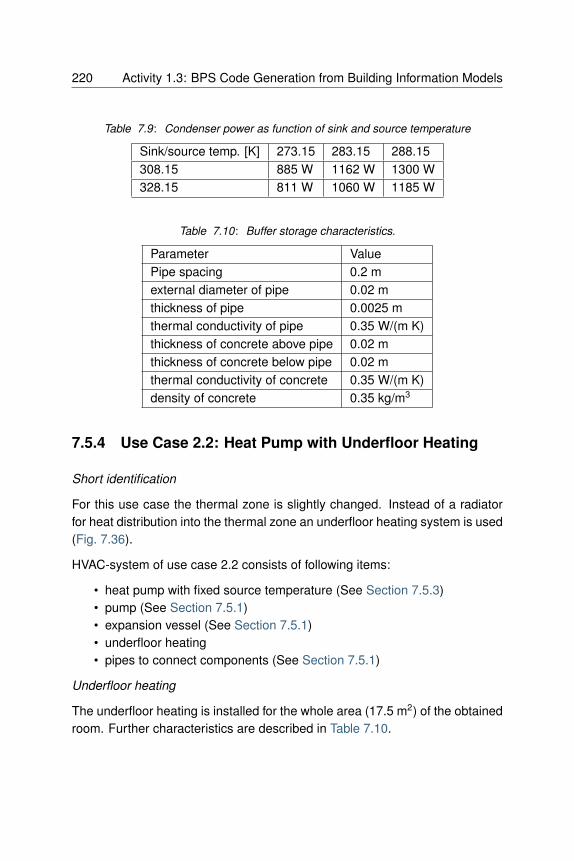
220 Activity 1.3: BPS Code Generation from Building Information Models

Table 7.9: Condenser power as function of sink and source temperature

Sink/source temp. [K] 273.15 283.15 288.15308.15 885 W 1162 W 1300 W328.15 811 W 1060 W 1185 W

Table 7.10: Buffer storage characteristics.

Parameter ValuePipe spacing 0.2 mexternal diameter of pipe 0.02 mthickness of pipe 0.0025 mthermal conductivity of pipe 0.35 W/(m K)thickness of concrete above pipe 0.02 mthickness of concrete below pipe 0.02 mthermal conductivity of concrete 0.35 W/(m K)density of concrete 0.35 kg/m3

7.5.4 Use Case 2.2: Heat Pump with Underfloor Heating

Short identification

For this use case the thermal zone is slightly changed. Instead of a radiatorfor heat distribution into the thermal zone an underfloor heating system is used(Fig. 7.36).

HVAC-system of use case 2.2 consists of following items:

• heat pump with fixed source temperature (See Section 7.5.3)• pump (See Section 7.5.1)• expansion vessel (See Section 7.5.1)• underfloor heating• pipes to connect components (See Section 7.5.1)

Underfloor heating

The underfloor heating is installed for the whole area (17.5 m2) of the obtainedroom. Further characteristics are described in Table 7.10.

7.5 Use Cases and Demonstration 221

7.5.5 Use Case 3: Combined Heat and Power (CHP) Unit

Boiler

micro

CHP

TC

Fig. 7.37 : Use case 3.

Short identification

HVAC-system of use case 3 (Fig. 7.37) consists of following items:

• CHP unit• pump (See Section 7.5.1)• expansion vessel (See Section 7.5.1)• radiator with P-controlled valve (See Section 7.5.1)• pipes to connect components (See Section 7.5.1)• buffer storage (See Section 7.5.2)• three way valve for loading and unloading

Combined Heat and Power unit

The boiler is replaced by a Combined Heat and Power unit with following char-acteristics:

Three way valve

The three way valve is used to control unloading and loading of the buffer stor-age. If the thermal zone requires thermal energy, first the buffer storage iscompletely unloaded, until it is not able to satisfy the flow temperature. The

222 Activity 1.3: BPS Code Generation from Building Information Models

Table 7.11: CHP characteristics.

Parameter ValueElectrical output 1000 WThermal output 2500 WElectrical efficiency 0.27Thermal efficiency 0.67Fuel utilization rate 0.92Modularity 0.5 - 1.0

storage is loaded if the temperature in the thermal zone is above the set tem-perature and the buffer storage temperature reached the flow temperature plusa additional temperature difference of 5 K.

7.5.6 Use Case 4.1: Air handling Unit for Heating (AHU

Heating)

Short identification

HVAC-system of use case 4.1 (Fig. 7.38) consists of following items:

• Air ducts• supply/ return air damper• silencer• pressure controlled fans for supply/ return air (radial/ axial)• air filter for supply/ return• electric device for heating

Damper

The dampers for supply and exhaust air are set to a constant opening fractionof 0.7. The face area of the dampers are 0.1 m2.

Fan

The fan is pressure controlled to supply the zone with heated air. The pressuredifference is controlled with a PID-Controller PID (gain = 100, time constantintegrator = 20 s, time constant deriative = 4 s). Lower and upper limits for

7.5 Use Cases and Demonstration 223

Thermal Zone

Damper

Silencer

Filter

Fan

Heating

device

Fig. 7.38: Use case 4.1.

224 Activity 1.3: BPS Code Generation from Building Information Models

pressure difference are set to 18 Pa and 550 Pa, respectively. The heat addedby the fan is negligible.

Filter, silencers, ducts

Several components like the filter, the silencer or the ducts introduce pressurelosses into the system. These pressure losses are combined and set to 300Pa.

Heater

The heater increases the supply air temperature to reach the room set tem-perature (20 °C). The maximum temperature of the supply air is set to 40 °C.The power of the heater is set 1300 W and controlled with a P-Controller, thepressure loss is 200 Pa.

7.5.7 Use Case 4.2: Air Handling Unit for Cooling (AHU

Cooling)

Short identification

HVAC-system of use case 4.2 (Fig. 7.39) consists of following items:

• Air ducts (see Section 7.5.6)• supply/ return air damper (see Section 7.5.6)• silencer (see Section 7.5.6)• pressure controlled fans for supply/ return air (radial/ axial) (see Section

7.5.6)• air filter for supply/ return (see Section 7.5.6)• Evaporative, adiabatic cooling device

Evaporative, adiabatic cooling device

The cooler reduces the supply air temperature to reach the rooms set tem-perature, by adding moisture the air stream. The temperature of water that isadded to the fluid stream is set to 8 °C. The added water is controlled with aP-controller using the zone set temperature of 20 °C.

7.5 Use Cases and Demonstration 225

Thermal Zone

Cooling

device

Fig. 7.39: Use case 4.2.

226 Activity 1.3: BPS Code Generation from Building Information Models

7.5.8 Use Case 5: Multi Zone Model

Short identification

This case study building represents a three story office building, located inAachen.

Fig. 7.40: Case study building, address: Mathieustraße 30, 52074 Aachen, Germany.

The building primarily comprises office spaces but also contains kitchens,washrooms, corridors, mechanical rooms and a server room. The heatingsystem consists of a gas boiler and radiators (see Section 7.5.1). The BIMmodel developed in Revit Architecture is shown on the right and a picture ofthe building is shown on the left of Fig. 7.40. The heating systems, also mod-elled with revit is shown in Fig. 7.41

The thermal zones are defined, according to the DIN V 18599. It defines thethermal conditions for the room type. The office type rooms should have anair temperature of 21°C. The presence of persons is between 7:00 and 17:30.The metabolic rate is equal to a sitting person, emitting 80 Watt per squaremeter skin surface. The light switches on at 17:00 and other equipment, likecomputers and screens are activated the whole time people are present. Be-cause the offices are heading in different directions the operations of the zonesto guarantee the thermal comfort is different. One side of the building is head-ing mostly to to the west and the other side is heading mostly to the east. The

7.5 Use Cases and Demonstration 227

Fig. 7.41: Whole heating system of use case five, modelled with Revit 2016.

Table 7.12: Multi zone use case characteristics.

Parameter ValueThermal zones 2 on each floorThermal output 80490 WPump performance 9068 PaVolume flow 2.22 l/sNumber of radiators 96

differences in the solar radiation requires different operations for the heatingsystems. The corridor should have an air temperature of at least 15°C and thelight is turned on at 16:30. Nearly no solar radiation hits the corridor directly.The different thermal zones are shown in Fig. 7.42, differently coloured.

Use Case 5 modeled in Modelica, using the AixLib library is shown in Fig. 7.40.The six thermal zones are represented on the top. To improve the simulationperformance, the thermal zones were simplified in an additional step. Thenine thermal zones have been comprised to six thermal zones. The corridoris separated, so that one half of the corridors’s thermal zone is part of theeastern and the other part belongs to the western thermal zone. The heatingsystem is modeled below the zones. All 96 radiators are represented, to servethe building.

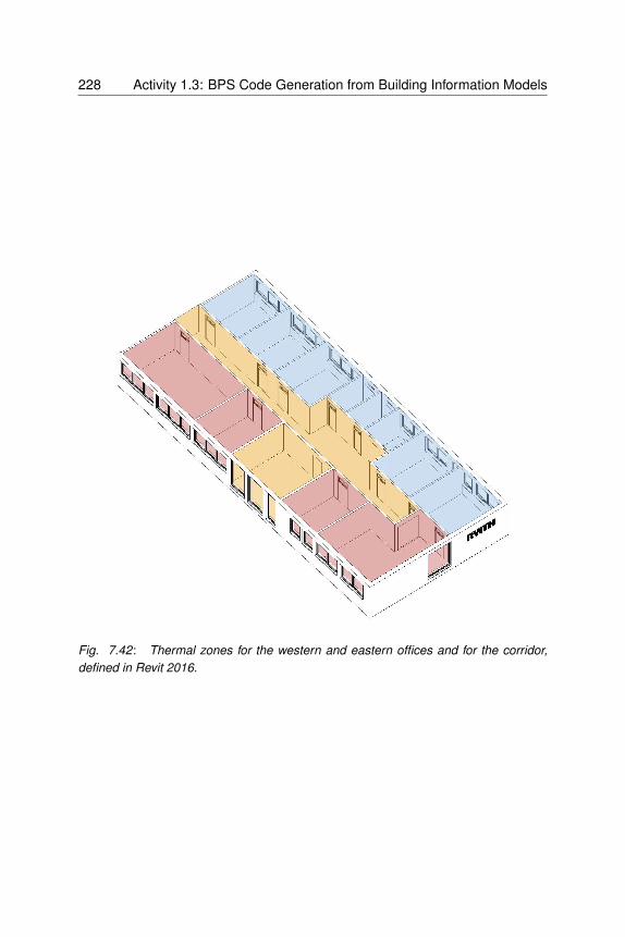
228 Activity 1.3: BPS Code Generation from Building Information Models

Fig. 7.42: Thermal zones for the western and eastern offices and for the corridor,

defined in Revit 2016.

7.5 Use Cases and Demonstration 229

Fig. 7.43: Use Case 5 modeled with the AixLib Modelica library.

230 Activity 1.3: BPS Code Generation from Building Information Models

7.5.9 Use Case 6: Rooftop Building

Building geometry modeling for use with Modelica algorithms must be preciseand must include all relevant detail, must be “clean” (i.e. error-free) and mustbe thoroughly checked and validated. If not, Modelica algorithms can lose theireffectiveness. As virtually all major model-based CAD tools have the ability togenerate building geometry models that are precise, it is always the modeler’stask to create models precise enough to meet the geometry definition needsof Modelica algorithms, and to assure that these models are technically error-free and verifiable [BMNG16] . Technically error-free models do not containmodeling errors and pass all tests with model checking tools. An exampleof such a model checker 3D view after successful validation is shown in Fig.7.44. Yet, such models may still not be verifiable because buildings data usedin the modeling process may be incorrect. Even the most competent modelercannot create an error-free and verifiable model without access to trustworthydata about the building.

Fig. 7.44: Geometry model of the Rooftop building in Solibri Model Checker.

7.5 Use Cases and Demonstration 231

In the cases of modeling existing buildings, ideally the modeler has access to“as-built” documentation that provides reliable data about building construc-tion. Unfortunately, “as-built” documentation seldom defines what was ac-tually built – it does not document last-moment construction and installationchanges. This inevitably results in “as-built” model inaccuracies, which con-tribute to the gap between simulated and measured building performance.

Fig. 7.45: Geometry model of the Rooftop building in passive state as imported

into EnergyPlus, showing space boundaries, PV panels and shutters in their original

position.

The Rooftop Building is a good example of “best-practices” modeling for BEPsimulation (Fig. 7.45). Its geometry model was built specifically to provideprecise geometry data for use in the execution of Modelica algorithms thatmodel energy systems installed in the building. As shown in Fig. 7.45, thebuilding features an elaborate system of fixed and movable PV panels; panelsdirectly above the building are fixed, while those projecting over the buildingsides are movable to optimize solar incidence angles during the day, as wellas provide needed shading and shuttering. The building was an entry in theSolar Decathlon Europe 2014 [UBTB14] . The Decathlon entry was as welldocumented as one can expect at the end of design. Yet, some of the criticalmodeling data are missing in the documentation; other critical data contradicteach other.

232 Activity 1.3: BPS Code Generation from Building Information Models

Fig. 7.46: Computer generated perspective image of the Rooftop building placed in

Berlin city-scape (source [GFMAE14]).

Fig. 7.47 : Orthogonal projection of the Rooftop building’s geometry model in active

state as imported into EnergyPlus, reflecting PV and shutter positioning shown in Fig.

7.46.

7.6 Limitations of the Framework and Future Work 233

Fig. 7.46 is a computer generated “artist’s view” of the building, copied fromthe project documentation. Fig. 7.47 shows the building geometry model, gen-erated using best available information from the same project documentationthat mimics the positioning of movable PV panels and shutter shown in Fig.7.46. The modeler had to improvise and guess some of the missing informa-tion and, in the case of conflicting data, to subjectively decide which data touse. Visual comparison of Fig. 7.46 and Fig. 7.47 shows what was expected(Fig. 7.46) and want appears to have been built (Fig. 7.47). Finally the result-ing Modelica model is shown in Fig. 7.48. Fortunately, the Rooftop Buildingis being reconstructed and instrumented at the UDK- Berlin campus. Thisis providing a unique opportunity to record true “as-built” data, re-model thebuilding geometry and see how closely simulation results can match energyperformance measurements in the building.

Fig. 7.48: Screenshot of the Modelica model of the roof top building.

7.6 Limitations of the Framework and Future Work

This subchapter describes the limitations of the framework focusing on genericlimitations rather then today’s technical limitations which are improving overtime. Furthermore, we discuss future work that is enabled by this development.

234 Activity 1.3: BPS Code Generation from Building Information Models

7.6.1 Limitations

The basic limitations of this framework or tool chain lies in the fact that variousdata models and tools are used. The tool chain is restricted to the functionalityof each tool and data model. For example, HVAC components that are notavailable in Modelica libraries reduce the list of supported components. Thesame is true if any other tool or data model is not supporting a particular HVACobject. The distributed development in small tools also makes changes that in-fluence multiple tools time consuming and sometimes difficult. E.g., changinga parameter in SimModel does create the need for updated mapping rulesfrom IFC to SimModel as well as from SimModel to Modelica. In that context,the implementation of control objects turned out to be quite cumbersome sinceno tools exist that define controls and have a relevant IFC export and/or importfunctionality. In this area we developed a so-called workaround and attachrelevant properties to the object that is controlled. This was necessary sincecontroller objects are not available in the MEP CAD applications. One of thebiggest challenges in this subtask was the flexible nature of Modelica and itslibraries as well as their continuous development. While significant progresstowards a standardized Modelica library development has been made throughthe Annex 60 base library, there still exists potential to standardize more as-pects of the Modelica libraries. From a data model and mapping perspectiveadditional standardization and library creator agreements would simplify futuremapping and conversion efforts. E.g., currently connector names of compo-nents can be any arbitrary string. Yet another limitation is the quality of BIMs.While model checking tools exist and are further developed, the understandingof providing data models of high quality is not present in practice yet. Anotheraspect is that the generated Modelica models are just a starting point andneed further fine tuning at the instance level of the Modelica models.

7.6.2 Future Work

While the developed tool chain is limited in scope and is a first prototype, thefollowing developments could be based on it:

• Further specification of the MVD to include further relevant HVAC com-ponents

7.6 Limitations of the Framework and Future Work 235

• Officially certified MVD that is implemented by various software applica-tions.

• Extensions of the IFC data model for missing concepts that we identifiedwithin this project (see Section 7.3.5.3)

• Further development of the prototype tools to cover more HVAC compo-nents.

• Further development of the Modelica libraries to include missing compo-nents.

In order to allow for international collaboration and further developments, allin this project developed code and models related to the transformation pro-cess are made available as open source. The Annex 60 framework thereforeprovides a solid and well-documented base for further developments.

236 Activity 1.3: BPS Code Generation from Building Information Models

Chapter 8

Activity 1.4: Workflow

Automation Tools

8.1 Introduction and Motivation

Today, workflow automation tools play an important role in the scope of buildingand community energy performance simulation as models, tools and engineer-ing tasks become incleasingly complex. Running a script in order to start toolsin batch mode and to preprocess variables is common practize in simulation.This is especially true if, for example, multiple domains are coupled, differ-ent scenarios shall be investigated, if input parameters are frequently varied,if multiple times a similar task shall be performed or if a conversion of inputparameters or data formats becomes necessary. Another issue is that com-putational capabilities are increasing steadily following Moore’s law. Hence,dealing with simulation models becomes more complex for both, users anddevelopers. Challenges for practitioners in the field of building energy simu-lations therefore include the handling of bigger amounts of input/output data(many or huge data files) [SN14] . Furthermore, a greater number of simula-tions will need to be run in order to perform sensitivity or uncertainty analysisof single or multiple parameters [HH11][BJH10] . Analysis of the resulting databy means of visualization or statistical figures [RK11] as well as mathematical

238 Activity 1.4: Workflow Automation Tools

operations on the inputs and outputs will increase in importance. The variousdata formats involved in simulation need to be converted and adjusted in orderto allow comparisons and communication between models.

These tasks do not require scientific expertise or any specific engineeringskills, rather they are often very time consuming and repeating. If performedmultiple times manually, not only valuable time will be wasted, it is also con-ceived to be error prone and tedious. As a consequence, building simulationresearchers should be able to use scripting languages or other automation en-vironments to gain more efficiency while ensuring the quality of their results.According to [SN14] the iterative nature of the building simulation workflow canbe leveraged by every step in the process which is automated using Pythonscripting. Fig. 8.1 is exemplifying the whole simulation process in this contextstarting from Modelica models based on the Annex 60 Library.

The importance of workflow automation is also identfied by [SN14] when work-ing with big data. It is recommended to write scripts that automate largebatch processes for simulation tasks. Thus, building simulation researchersand practitioners benefit from basic parsing and scripting knowledge.

This chapter provides an overview of associacted Python packages and rec-ommended third party packages. Several Python tools and packages are avail-able for developers and for model users. Those Python tools and packages en-hance the workflows for developing and using Modelica and FMI-based mod-els.

They will assist developers in unit tests and checking libraries with confor-mance to coding guidelines. Furthermore, users will be able to pre-process,run and post-process batches of simulations, such as for parametric studies orfor uncertainty propagation, including post-processing of different data formatscreated by FMUs. It will additionally be possible to integrate Modelica or FMIbased models with optimization packages for design optimization and ModelPredictive Control.

8.1 Introduction and Motivation 239

.hdf

Design of Experiments

Pre-processing & Simulation

Post-processing & Analysis

.csv .mat .xls .txt

AixLib BuildingsBuilding Systems

IDEAS

Fig. 8.1: Schematic of typical building simulation workflow to demonstrate use cases

for Python based process automation

240 Activity 1.4: Workflow Automation Tools

8.2 Tools and Methodology

This section provides an overview of existing tools and Python packages forautomation of building simulation workflows. In the Annex, the necessary ca-pabilities of such tools have been identified and compiled into a common work-ing document. After discussions within the expert groups, a set of mature andutile Python packages was selected, under consideration of their capabilities,license type and implementation language. From the analysis of existing soft-ware and features for building simulation automation, a structured list of usecases was derived which reflects the high level requirements for workflow au-tomation tools.

8.2.1 Functional Requirements

The main focus of automation tools lies in the possibility to execute simulationsfrom a script. This is a precondition to efficiently apply pre- and postprocessingfunctions. These functions are then able to generate the desired efficiencygain for repeatedly used operations. The following paragraph concludes thedesired functional requirements of automation tools.

8.2.1.1 Running Simulations

In order to provide a broad foundation for working with simulation inputs andresults, the tools should help the user to run different simulation engines likeDymola, OpenModelica, JModelica, FMUs, etc. Simulations of similar typesshould be processed in parallel. Execution of simulations, especially paramet-ric studies should be done in automated batch setups. An efficient allocationof ressources will be a valuable advantage in this regard. Furthermore, alsointeraction with external programs in order to couple different simulators is de-sired. This can also be realized by supporting co-simulation interfaces like theFMI standard.

8.2 Tools and Methodology 241

8.2.1.2 Preprocessing Operations

The initial treatment of simulation input data can be relevant when usingchanging data sources on the same simulation model, investigating parametervariations or preparing external data for the simulation. In order to supportthese processes, commonly used scripts should support the transformation ofinput data (e.g. from BIM data). Also, automated preparation of input datafrom a database (e.g. product catalogues) is to be considered. This can alsobe realized based on templates for the simulation model. Parameters for themodel can therefore be set instantly. Furthermore, simulation settings, likepaths for input data or result files as well as specific simulation parameters(start/end time, verbosity, logging) and solver settings (type, tolerance, inte-gration method) should be handled. Besides the instantiation of parameters,functionality for importing dynamic inputs serving as boundary conditions tothe simulation, like specific profiles as data from .xls or .csv files needs to beincluded. Common data-readers in the Annex60 or other Modelica libraries aswell as standardized weather data (TRY, TMY) are only a few valuable inputsources to be considered.

8.2.1.3 Postprocessing Operations

Increasing amounts of computational resources, modeling capabilities andmemory has led to enormous amounts of data that can be generated fromsimulations. Automated processing of result files has therefore become a timeintensive task. In order to reduce this effort, postprocessing of a set of simi-lar result files, e.g. from a parametric study, must be possible. Furthermore,filtering of result data based on different criteria helps to reduce the data ca-pacity that needs to be handled. However, a suitable way for storing data inlarger files or database systems is still necessary, especially when differentdata sources are to be merged. In addition, computation of typical result crite-ria like thermal comfort or annual energy consumption needs to be supported.

242 Activity 1.4: Workflow Automation Tools

8.2.1.4 Data Analysis

Gathering parameter sets or patterns of simulation data is often only a firstpostprocessing step. Various analysis methods, e.g. statistical functions likecomputing the mean, maximum, minimum or standard deviation of a resultvariable, can be very useful when analyzing the computed values. More ad-vanced statistical methods involve the computation of a moving average, auto-correlation-functions and ARMA-models. Postprocessing scripts should alsobe able to compare results with a baseline design option and perform regres-sion analysis such as a linear least square method, trend estimation or curvefitting. The computation of the R2 goodness of fit enables fast comparisonsbetween two data series. The ASHRAE Guideline 14 [ASH02] states furthervalues for result interpretation. Besides statistical analysis, frequently usedbase functionalities for timeseries, like integration, arithmetic or logical oper-ations, as well as frequency analysis, event counting or discarding irreleventdata from a timeseries, can help a user to interpretate and work with simulateddata.

8.2.1.5 Data Visualization

Graphical representation of simulation results is a valuable measure topresent, compare and analize simulations. Post-processing scripts shouldtherefore inherit typically used options including

• multiple graph plots,• plot subsets of simulations for comparison,• various plotting routines for time series, parameter values, box plots, bar

charts, carpet plots, scatter plots, histograms, Sankey diagrams, Bodeplots or Nyquist plots.

8.2.1.6 Parametrization

Once provided with the opportunity to automatically instantiate and initializea simulation, methods to execute studies on a single simulation model arenecessary. This includes the automated parametrization of models in order tooptimize the design. During such a study, often a vast amount of input data

8.2 Tools and Methodology 243

is generated and needs to be organized. Sampling methods (e.g. Latin Hy-percube Sampling) help to design the experiment (DoE) in order to decreasethe data space. A limited number of input parameters are thereby sampledthrough a probability density function within the design space. The results al-low to perform sensitivity analysis and compute uncertainty propagations ofthe results.

8.2.1.7 Data Conversion

Multiple simulation environments and various data sources lead to the require-ment of converting data between different formats. Useful script tools shouldtherefore provide functionalities to handle the container format HDF5, .mosfiles, tables from .csv and .xls files, .mat files and figures, diagrams as imagesin .png or .jpg format.

8.2.1.8 Verification

Simulations often serve as supporting measures to better understand a sys-tems behaviour. However, previous verification of such models is important toprevent errors. Automated model check algorithms are therefore a valuabletool to increase productivity. Their functionality should include the verifica-tion of model correctness and completeness as well as compliance and modelcompatibility checking. Furthermore, unit testing can prevent time intensiveand cumbersome search for smaller errors in the model. Erroneous input datacan be eliminated with fault detection algorithms based on an isolated view ofthe data itself or in conjunction with test runs of the model.

8.2.1.9 Optimization

After previous simulation generation and analysis, further algorithms can helpto support optimization of a system. These incorporate

• derivative-free optimization that evaluates a model for different parame-ter values; these can be heuristic such as genetic algorithms or particle

244 Activity 1.4: Workflow Automation Tools

swarm optimization, or deterministic such as generalized pattern searchmethods [WW04][PW06] ,

• gradient based parameter optimization that either numerically approxi-mate derivatives, or that use computer algebra to obtain analytic expres-sions for derivatives [AGT09] .

8.2.2 Associated Packages

The requirements for Activity 1.4 were mapped to existing tools and packagesand the missing functionalities and capabilities needed for building simulationtasks (i.e. validation and demonstration) within the scope of Annex 60 wereidentified. In order to illustrate the advantages arising from these packages,the following ones are highlighted in the example applications.

• BuildingsPy (http://simulationresearch.lbl.gov/modelica/buildingspy/)from LBNL allows for running Modelica simulations in Dymola andinherits functionality to process result files. It furthermore enables unittests and the refactoring of Modelia libraries.

• awesim from KU Leuven (https://github.com/saroele/awesim) providesfunctionality to pre- and postprocess Modelica models. It is possible tocompile models, set parameters and solver options. Simulations can berun in parallel. Plots based on the result files can be created and filteringof results based on filenames and parameter sets is possible.

• ModelicaRes (http://kdavies4.github.com/ModelicaRes/) is a package togenerate simulation scripts for Dymola. Result data can be loaded, ana-lyzed and plotted. The package interacts with the popular pandas pack-age for Python, allowing for numerous statistical analysis.

8.2.3 Third-Party Packages

Other third-party Python packages exist which provide additional capabilitieswhich are useful for the purposes of building performance simulation such as

• DyMat (http://www.j-raedler.de/projects/dymat/), which is a package forhandling Dymola’s or OpenModelica’s .mat output files. Browsing forvariables and exporting their content to various formats is supported.

8.3 Examples of Application 245

• PyFMI (https://pypi.python.org/pypi/PyFMI) is a framework to incorpo-rate the Functional Mockup Interface (FMI) in the Python environment.Functional Mockup Units can be loaded, instantiated, simulated andmodified or queried using the provided functions by the standard.

• matplotlib (http://matplotlib.org/) serves to plot and visualize data of var-ious kind. Several graph types can be generated and saved in differentformats like .png or .jpg.

• scipy (http://www.scipy.org/) is a package for scientific computing (basedon numpy). It includes functionalities imitating Matlab-like treatment ofdata in the Python environment.

• pandas (http://pandas.pydata.org) is a package for data and time seriesanalysis (similar to the statistics tool ‘R’). Huge amounts of data can beefficiently stored, queried and analyzed in data frames.

• StatsModels (http://statsmodels.sourceforge.net/) includes statisticalmethods (similar to ‘R’) that allow for statistical tests, intensive data ex-ploration and the generation of statistical models in Python.

• pyTables (http://www.pytables.org) serves to manage hierarchicaldatasets. Huge amounts of data can be handled efficiently and easily.The package is based on the HDF5 library.

• pysimulator (https://github.com/PySimulator (LGPL)) is a simulation andanalysis environment for Functional Mockup Units and Modelica modelsin Python.

8.3 Examples of Application

The following examples cover some of the previously stated requirementsthrough self-explaining Python code. The IPython Notebook was chosen toserve as the implementation platform of these examples. A Notebook is an in-teractive Python computing environment that enables users to author workflowautomation scripts that include executable code, interactive graphs and plots,textual comments, images and governing equations.

While executing a Notebook it generates output from the executed Pyhton ker-nel that is running in the background. The multi-media output is fully em-bedded in the notebook giving a complete and comprehensible record of acomputation.

246 Activity 1.4: Workflow Automation Tools

The sequential reading, executing and verifying of computation results in astep-by-step walkthrough facilitates productive and re-usable code for either,model developers and users.

These Notebooks can as well be published as interactive web application (seehttp://jupyter.readthedocs.io). Notebook documents available from a publicURL (e.g. on GitHub) can be shared via nbviewer. A web service ist loadingit from the URL and displays the Notebook as static web page to be sharedwith others.

The Notebooks created for the Annex 60 project start with a short descriptionof their purpose, the used packages and the used simulation model as faras it is relevant to fully understand the Notebook. The simulation models areidentical or slightly adapted examples from the Dymola libraries involved inthe project scope. Within the Notebooks, code cells are bundled to executespecific tasks. Short text descriptions before and comments in the code helpto get a clear picture of these fragments. Some of the cells produce output likegraphs, dataframes or pure text. These are shown directly beneath the codecells. The requirements for the notebooks to work are the following:

• all used Python packages must be installed. These include the following:numpy, os, BuildingsPy, pandas, pyDOE, ModelicaRes, pyFMI, csv anddatetime;

• the FMI library must be installed and set as a system environment vari-able in order for pyFMI to be able to call FMI functions;

• the path to the executable of the used Dymola version needs to be in-cluded in the path system environment variables.

8.3.1 Single Simulation of a Building using BuildingsPy

Running simulations from script can proof beneficial when applying identicalpre- and postprocessing patterns to a single simulation. Especially the effortfor statistical and graphical evaluation of the results can be significantly re-duced. In this IPython Notebook, a framework including relevant function callsto adress these issues for a single simulation in Dymola is provided. In partic-ular, the Python library BuildingsPy is used, supplemented with elements frompandas and NumPy. The model serving as an example in this case is a slightly

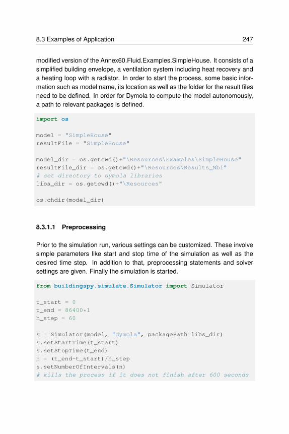
8.3 Examples of Application 247

modified version of the Annex60.Fluid.Examples.SimpleHouse. It consists of asimplified building envelope, a ventilation system including heat recovery anda heating loop with a radiator. In order to start the process, some basic infor-mation such as model name, its location as well as the folder for the result filesneed to be defined. In order for Dymola to compute the model autonomously,a path to relevant packages is defined.

import os

model = "SimpleHouse"

resultFile = "SimpleHouse"

model_dir = os.getcwd()+"\Resources\Examples\SimpleHouse"

resultFile_dir = os.getcwd()+"\Resources\Results_Nb1"

# set directory to dymola libraries

libs_dir = os.getcwd()+"\Resources"

os.chdir(model_dir)

8.3.1.1 Preprocessing

Prior to the simulation run, various settings can be customized. These involvesimple parameters like start and stop time of the simulation as well as thedesired time step. In addition to that, preprocessing statements and solversettings are given. Finally the simulation is started.

from buildingspy.simulate.Simulator import Simulator

t_start = 0

t_end = 86400*1

h_step = 60

s = Simulator(model, "dymola", packagePath=libs_dir)

s.setStartTime(t_start)

s.setStopTime(t_end)

n = (t_end-t_start)/h_step

s.setNumberOfIntervals(n)

# kills the process if it does not finish after 600 seconds

248 Activity 1.4: Workflow Automation Tools

s.setTimeOut(600)

s.setSolver('dassl')

s.addPreProcessingStatement("Evaluate:=true;")

s.printModelAndTime()

s.setResultFile(resultFile)

s.setOutputDirectory(resultFile_dir)

s.simulate()

Model name = SimpleHouse

Output directory = .

Time = Thu Jun 02 12:08:13 2016

8.3.1.2 Postprocessing

A reader object from BuildingsPy serves to retrieve the values of defined resultvariables and saves them into the IPython workspace as a pandas dataframe.Since the Dymola simulation yields an irregular time grid, an interpolation isperformed to match the result values to the above defined timestep. Finally, theresults are exported to a .csv file to ensure the possibility of further, individualanalysis.

from buildingspy.io.outputfile import Reader

from buildingspy.io.postprocess import Plotter

import pandas as pd

import numpy as np

# variable names to be extracted from the result file are

# determined

variables = ['zone.T','Q_heating']

r = Reader(resultFile_dir+"\"+resultFile, "dymola")

# the original time grid is defined

tSup = np.linspace(t_start, t_end, h_step)

ResultValues = pd.DataFrame(columns=['time']+variables)

for var in variables:

(time,temp) = r.values(var)

# results are reduced to the original time grid

8.3 Examples of Application 249

ResultValues[var] = Plotter.interpolate(tSup,

time,

temp)

ResultValues['time'] = tSup

ResultValues.to_csv(resultFile_dir+"\"+resultFile+".csv")

print ResultValues.head()

time zone.T Q_heating

0 0.000000 293.149994 0.000000

1 1464.406780 293.889343 1380.513502

2 2928.813559 294.936695 1840.707414

3 4393.220339 295.025860 702.443914

4 5857.627119 294.288450 241.524324

The above defined variable outputs are visualized in two ways using plottingfunctions from BuildingsPy. The first plot is a boxplot. To execute the function,a time interval needs to be provided over which the boxplot is to be computed.Furthermore, the number of evaluations of the boxplot must be stated. Theresult is a figure consisting of various boxplots, each representing the giventime intervall in sequential order. A second graph produces a simple line plotwith the result values represented over the simulation time. Formatting func-tions provided by the matplotlib can be used within the BuildingsPy packageto customize the appearance of the graphs.

for var in variables:

# 12 statistical evaluations for 600s time intervals.

# In this case, one hour is divided into 5 minute

# intervals. For each interval the statistics

# to create a boxplot are computed.

plt=Plotter.boxplot(t=list(ResultValues['time']),

y=list(ResultValues[var]),

increment=600,

nIncrement=12)

plt.xlabel('Time')

plt.ylabel(var)

plt.grid()

plt.savefig(resultFile_dir+"\"+var+"_boxplot.png",

dpi=300)

250 Activity 1.4: Workflow Automation Tools

plt.show()

# a line plot over the simulation time

plt.plot(list(ResultValues['time']),

list(ResultValues[var]))

plt.xlabel('Time')

plt.ylabel(var)

plt.grid()

plt.savefig(resultFile_dir+"\"+var+"_lineplot.png",

dpi=300)

plt.show()

0 1 2 3 4 5 6 7 8 9 10 11Time

293.0

293.5

294.0

294.5

295.0

295.5

zone.T

The NumPy package provides several useful functions for simple statistics.The following cell computes various measures of descriptional statistics andsaves them to a pandas dataframe. The above applied command can be usedagain to export the dataframe effortlessly to a .csv file.

ResultStatistics=pd.DataFrame(columns=variables)

for var in variables:

ResultStatistics.loc['Minimum',var] =

np.min(ResultValues[var])

ResultStatistics.loc['Maximum',var] =

8.3 Examples of Application 251

0 10000 20000 30000 40000 50000 60000 70000 80000 90000Time

293.0

293.5

294.0

294.5

295.0

295.5

zone.T

0 1 2 3 4 5 6 7 8 9 10 11Time

0

500

1000

1500

2000

Q_heating

252 Activity 1.4: Workflow Automation Tools

0 10000 20000 30000 40000 50000 60000 70000 80000 90000Time

0

500

1000

1500

2000Q_heating

np.max(ResultValues[var])

ResultStatistics.loc['Mean',var] =

np.mean(ResultValues[var])

ResultStatistics.loc['Median',var] =

np.median(ResultValues[var])

ResultStatistics.loc['25th percentile',var] =

np.percentile(ResultValues[var], 25)

ResultStatistics.loc['50th percentile',var] =

np.percentile(ResultValues[var], 50)

ResultStatistics.loc['Standard Deviation',var] =

np.std(ResultValues[var])

ResultStatistics.loc['Variance',var] =

np.var(ResultValues[var])

ResultStatistics.to_csv(resultFile_dir+"\"+resultFile+

"_statistics.csv")

print ResultStatistics

zone.T Q_heating

Minimum 293.1131 0

Maximum 295.1935 1972.613

Mean 294.0912 941.9056

8.3 Examples of Application 253

Median 294.052 881.5341

25th percentile 293.4302 232.922

50th percentile 294.052 881.5341

Standard Deviation 0.6809249 708.8307

Variance 0.4636587 502440.9

Some useful BuildingsPy functions can also help to quickly assess certainperformance indicators. In this case, an integral function is applied to therequired heating power. As a result, the cumulative heating energy over thesimulated time period can be evaluated.

print "Total heating energy sums up to" ,

r.integral('Q_heating')

Total heating energy sums up to 81547626.5705

8.3.2 Parametric Study using BuildingsPy and ModelicaRes

Single simulations can assist practitioners to better understand and assess asystem. However, knowing the influence of parameter variation on the sys-tem’s behaviour is crucial for system optimization and provides valuable addi-tional insights. The following script serves to automatically run such a param-eter study in Dymola based on a Latin Hypercube Sampling (LHS) of chosenvariables. The package pyDOE is used to generate the sample for the study.The setup and start of the simulation is executed with BuildingsPy. Modeli-caRes is used to label and compare the simulation runs graphically. The mod-ified version of the Annex60.Fluid.Examples.SimpleHouse example is againtaken to demonstrate the procedure. Parameters under investigation are theoutside wall area of the building, its mean U-value as well as the nominal heat-ing power. The study is performed with the purpose to find suitable combina-tions of the three parameters in oder to ensure comfortable temperatures inthe building. In a first step, the usual settings for model name, directories etc.must be defined. Again, the directory containing relevant Modelica libraries forthe model needs to be provided.

254 Activity 1.4: Workflow Automation Tools

import os

model = "SimpleHouse"

model_dir = os.getcwd()+"\Resources\Examples\SimpleHouse"

result_dir = os.getcwd()+"\Resources\Results_Nb2"

# set directory to dymola libraries

libs_dir = os.getcwd()+"\Resources"

os.chdir(model_dir)

8.3.2.1 Parameter Sampling

In order to get a set of simulations, each based on different parameter values,the variables in question need to be determined. A minimum and maximumvalue for each parameter ensures that the samples are amongst the definedrange. These values can represent certain constraints or requirements thatmight occur during planning. To create the sample, the Latin Hypercube Sam-pling method, implemented in the pyDOE package, is applied. It creates amultidimensional set of parameter values for the batch simulation. Besidesthe minimum and maximum values of the variables, the number of total simu-lation runs must be determined. The output of the following code cell showsthe created samples in a pandas dataframe.

from pyDOE import *

import numpy as np

import pandas as pd

# Varying parameters in the study

varList = ['A_wall', 'U_wall', 'Q_RadNominal']

MinMax = [(200,300), (0.4,0.8), (1000,3000)]

# Number of simulation runs

n_simulations = 5

# generation of samples with latin hypercube sampling (lhs)

design = lhs(len(varList), samples=n_simulations)

diff = []

mins = []

# the normalized design values are mapped to the parameter

8.3 Examples of Application 255

# ranges

for pair in MinMax:

diff.append(pair[1]-pair[0])

mins.append(pair[0])

Sample = pd.DataFrame(design*np.array(diff)+np.array(mins),

columns=varList)

print Sample

A_wall U_wall Q_RadNominal

0 270.708852 0.730839 2151.677135

1 289.948056 0.700511 2313.956082

2 252.777500 0.548079 1369.952720

3 220.802008 0.587404 2900.892276

4 213.898259 0.437846 1661.255155

8.3.2.2 Batch Simulation

To run the created parameter sets in batch mode, the BuildingsPy package isused. It creates a folder for every run in the result directory. Naming follows theenumeration corresponding to the parameter set number. After defining startand end time as well as the timestep, simulations with the updated parametersets are executed in a loop and saved to the corresponding folders.

from buildingspy.simulate.Simulator import Simulator

t_start = 0

t_end = 86400*15

h_step = 60

for i in range(0, n_simulations):

parameters = {}

for var in varList:

parameters[var] = Sample[var][i]

s = Simulator(model, 'dymola', packagePath=libs_dir)

s.setOutputDirectory(result_dir+'\run'+str(i))

s.addParameters(parameters)

256 Activity 1.4: Workflow Automation Tools

s.setSolver('dassl')

s.addPreProcessingStatement("Evaluate:=true;")

s.setStartTime(t_start)

s.setStopTime(t_end)

n = (t_end-t_start)/h_step

s.setNumberOfIntervals(n)

s.simulate()

del s, parameters

8.3.2.3 Batch Postprocessing

In order to retrieve the results from the individual folders, ModelicaRes is used.Every simulation run receives a label. This label can later on be used to differ-entiate between the result values e.g. in a graph.

from modelicares import SimResList

sims = SimResList(result_dir+"//*//*.mat")

# labelling

i = 0

for sim in sims:

label = 'run'+str(i)

i+=1

sim.label = label

In the following cell, defined outputs of the simulation are compared. Modeli-caRes therefore collects the values of each result variable from each simula-tion run and plots them in one graph. Start and end time of the graph canbe provided within the simulation period. The graphs are finally saved to theresults directory. Possibilities to customize the graph representation can againbe found in the matplotlib documentation.

# define result variables for comparison.

variables = ['zone.T', 'Q_heating']

t_start_plot = 86400*5

8.3 Examples of Application 257

t_end_plot = 86400*15

for var in variables:

fig_temp = sims.plot(ynames1=var, ylabel1=var,

title="Parameter Study")

fig = fig_temp[0]

fig.set_xbound(lower=t_start_plot, upper=t_end_plot)

labels = fig.get_xticklabels()

labels_h = []

for i in range(0, len(labels)):

labels_h.append((t_start_plot+(t_end_plot-

t_start_plot)/(len(labels)-1)*i)/3600)

fig.set_xlabel('Time / h')

fig.set_xticklabels(labels_h)

fig.figure.savefig(result_dir+"\"+var+".png", dpi=300)

146 173 200 226 253 280 306 333Time / h

290

291

292

293

294

295

296

zone.T/K

Parameter Study

zone.T (run0)zone.T (run1)zone.T (run2)zone.T (run3)zone.T (run4)

258 Activity 1.4: Workflow Automation Tools

146 173 200 226 253 280 306 333Time / h

500

0

500

1000

1500

2000

2500

3000

3500

4000Q

_heati

ng/W

Parameter Study

Q_heating (run0)

Q_heating (run1)

Q_heating (run2)

Q_heating (run3)

Q_heating (run4)

8.3.3 Parametric Study of a Boiler FMU from Dymola using

PyFMI

In certain cases, planners might interact by exchanging simulation modelsas FMUs for immediate testing of models from other disciplines on designchanges. This tutorial on hand shows how to load and run a parametric studyof a single FMU exported from Dymola using PyFMI. In this case, the boilersimulation model from the AixLib library is considered as an example. It is asingle thermal zone heated by a radiator. The valve between the boiler and theradiator is controlled by a proportional controller. It is the intention to observethe influence of the temperature set point on the total energy consumption ofthe boiler over a year. To do so, the model is run a few times with differentvalues for the set point.

In order to extract the FMU, this model has been previously compiled in theDymola environment in the Windows operating system. It is available as theAixLib_Boiler_DymolaWin.fmu file. The PyFMI python package will be usedto call the solver and run the simulations. Since the FMU has been exportedwith Dymola, a Dymola license is needed to run this as well as the followingexample. Just like in the previous examples, folders and model name must bedefined to start with the tutorial.

8.3 Examples of Application 259

8.3.3.1 Loading an FMU

from pyfmi import load_fmu

import os

model = 'AixLib_Boiler_DymolaWin.fmu'

model_dir = os.curdir + "//Resources//Examples//Boiler"

result_dir = os.getcwd()+"//Resources//Results_Nb3"

boiler = load_fmu(fmu=model, path=model_dir)

os.chdir(model_dir)

8.3.3.2 Execute Parametric Study in Loop

In the following, parameter values to be applied in the study need to be defined.A loop executes the simulation several times providing the current parametervalue as an input signal to the FMU. For each simulation run, the cumulativeheating energy is computed in an integral function and saved to a growing list.

from scipy.integrate import trapz

import numpy as np

t_start = 0

t_end = 3.1536e7

T = [291.15, 292.15, 293.15, 294.15, 295.15, 296.15]

Q = []

for TAirSet in T:

boiler.reset()

boiler.set('setTemp.k', TAirSet)

try:

res = boiler.simulate(start_time=t_start,

final_time=t_end)

except:

print "One of the simulation cases has failed."

260 Activity 1.4: Workflow Automation Tools

# The heat flow from the boiler is recovered from the

# simulation results

res_time = res['time'] # s

res_Q = res['boiler.heatDemand.Q_flow_out'] # W

Q.append(trapz(res_Q, res_time) / 3600 / 1000)

8.3.3.3 Postprocessing

After finishing all simulations, a graphical postprocessing can be started. Inthis case, a simple point plot is created to demonstrate the dependency ofheating energy demand on the temperature setpoint.

import matplotlib.pyplot as plt

plt.figure()

plt.plot([x-273.15 for x in T], Q, 'ok')

plt.xlabel('Temperature set point (C)')

plt.ylabel('Total heat consumption (kWh)')

plt.savefig(result_dir+'\Total heat consumption.png',

dpi=300)

8.3.4 Import Data to Co-Simulation FMU using PyFMI and

Pandas

Input data for simulations can often come from measurements, other simu-lation results or any external data sources. In order to consider this data inFMU simulations, co-simulation FMUs can be used. Co-simulations offer astep-wise execution of the simulation. After every time step the simulation canbe stopped and input values are updated. The package pyFMI offers the nec-essary function calls to fulfil this purpose. In the following, the SimpleHouseexample from above serves as the FMU. In contrary to the original model,weather data is missing in the FMU. Instead, temperature and solar irradiation

8.3 Examples of Application 261

18 19 20 21 22 23Temperature set point (C)

250

300

350

400

450

500

550

600Tota

l heat

consu

mpti

on (

kWh)

are read from a .csv file. To start with the notebook the FMU name and itsdirectory must be defined.

import os

from pyfmi import load_fmu

model = "SimpleHouse.fmu"

model_dir = os.getcwd()+"\Resources\Examples\SimpleHouse"

FMU = load_fmu(fmu=model, path=model_dir)

Input and output variables of the FMU can be determined with the followingfunction calls. Later in this script, the found variable names serve as connectorto the exchanged weather data.

input_vars = FMU.get_input_list()

print input_vars.keys()

output_vars = FMU.get_output_list()

print output_vars.keys()

['T_amb', 'Irr_HGloHor']

262 Activity 1.4: Workflow Automation Tools

['T_air']

8.3.4.1 Import Tabular Data

A .csv file is imported to IPython in the following cell. The column called “time[s]” is used as a time index. The start date for the time series is chosen in thevariable “date”. These formatting measures are necessary in order to be ableto map a possibly different time grid of the input data to the time grid of thesimulation.

import csv

import numpy as np

import pandas as pd

from datetime import datetime

# Definition of Input .csv file

weatherFile = "Weather.csv"

weatherFile_dir = model_dir

# Data is formated with a time index

date = datetime(2015,1,1)

InputFile = pd.read_csv(weatherFile_dir+'\'+weatherFile)

InputFile.set_index(date+pd.to_timedelta

(InputFile['time [s]'], unit='s'), inplace=True)

time [h] time [min] time [s] T_amb

→˓[K] T_amb [C] \

time [s]

2015-01-01 00:00:00 0 0 0 278.

→˓15 5

2015-01-01 01:00:00 1 60 3600 277.

→˓15 4

2015-01-01 02:00:00 2 120 7200 276.

→˓15 3

2015-01-01 03:00:00 3 180 10800 275.

→˓15 2

2015-01-01 04:00:00 4 240 14400 275.

→˓15 2

8.3 Examples of Application 263

2015-01-01 05:00:00 5 300 18000 275.

→˓15 2

2015-01-01 06:00:00 6 360 21600 274.

→˓15 1

2015-01-01 07:00:00 7 420 25200 274.

→˓15 1

2015-01-01 08:00:00 8 480 28800 274.

→˓15 1

2015-01-01 09:00:00 9 540 32400 274.

→˓15 1

Irr_HGloHor [W/m2]

time [s]

2015-01-01 00:00:00 0

2015-01-01 01:00:00 0

2015-01-01 02:00:00 0

2015-01-01 03:00:00 0

2015-01-01 04:00:00 0

2015-01-01 05:00:00 0

2015-01-01 06:00:00 150

2015-01-01 07:00:00 250

2015-01-01 08:00:00 300

2015-01-01 09:00:00 400

After definition of the simulation time grid, the input data can be edited to thegiven time base. Therefore, the relevant columns of the input file are chosen,resampled and interpolated using pandas. The time indexing within this pack-age is especially practical for this purpose. After preparation of the input data,the FMU co-simulation algorithm can be initialized.

import pandas as pd

from pandas.tseries.offsets import Second

SimInputs = ['T_amb [K]','Irr_HGloHor [W/m2]']

# simulation time grid

t_start = 0

t_end = 86400*1

h_step = 60

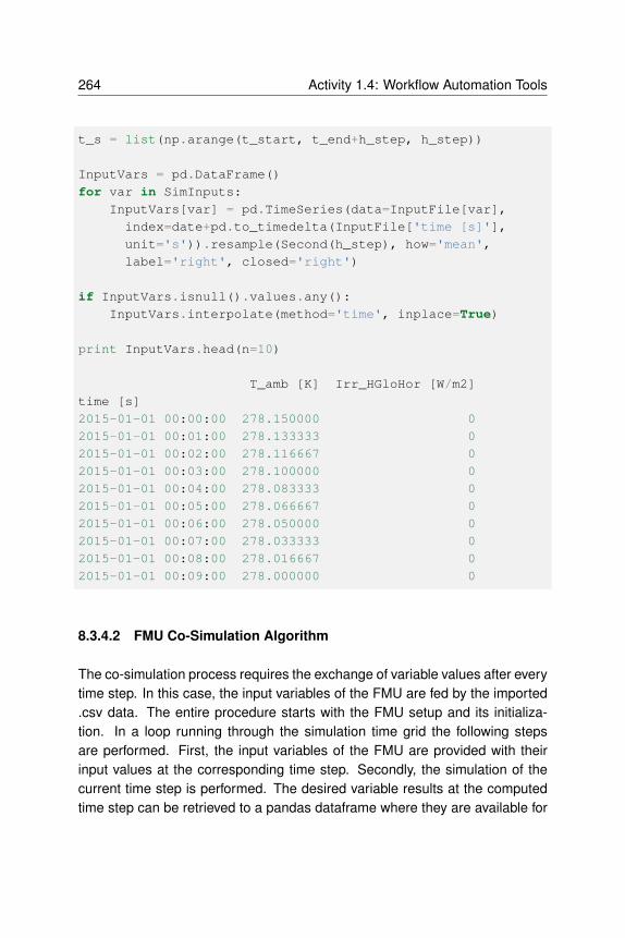
264 Activity 1.4: Workflow Automation Tools

t_s = list(np.arange(t_start, t_end+h_step, h_step))

InputVars = pd.DataFrame()

for var in SimInputs:

InputVars[var] = pd.TimeSeries(data=InputFile[var],

index=date+pd.to_timedelta(InputFile['time [s]'],

unit='s')).resample(Second(h_step), how='mean',

label='right', closed='right')

if InputVars.isnull().values.any():

InputVars.interpolate(method='time', inplace=True)

print InputVars.head(n=10)

T_amb [K] Irr_HGloHor [W/m2]

time [s]

2015-01-01 00:00:00 278.150000 0

2015-01-01 00:01:00 278.133333 0

2015-01-01 00:02:00 278.116667 0

2015-01-01 00:03:00 278.100000 0

2015-01-01 00:04:00 278.083333 0

2015-01-01 00:05:00 278.066667 0

2015-01-01 00:06:00 278.050000 0

2015-01-01 00:07:00 278.033333 0

2015-01-01 00:08:00 278.016667 0

2015-01-01 00:09:00 278.000000 0

8.3.4.2 FMU Co-Simulation Algorithm

The co-simulation process requires the exchange of variable values after everytime step. In this case, the input variables of the FMU are fed by the imported.csv data. The entire procedure starts with the FMU setup and its initializa-tion. In a loop running through the simulation time grid the following stepsare performed. First, the input variables of the FMU are provided with theirinput values at the corresponding time step. Secondly, the simulation of thecurrent time step is performed. The desired variable results at the computedtime step can be retrieved to a pandas dataframe where they are available for

8.3 Examples of Application 265

postprocessing.

# variable names to retrieve result values from FMU after

# each time step

variables = ['zone.T','Q_heating']

FMU.setup_experiment(start_time=t_start, stop_time=t_end)

FMU.initialize()

ResultValues = pd.DataFrame(columns=variables,

index=date +

pd.to_timedelta(t_s, unit='s'))

# while loop through simulation steps with i as running

# variable

i=0

while i <= len(t_s)-1:

# current input values are taken from prepared input

# file

T_amb = InputVars['T_amb [K]'][date+

pd.to_timedelta(t_s[i], unit='s')]

Irr_HGloHor = InputVars['Irr_HGloHor [W/m2]'][date+

pd.to_timedelta(t_s[i], unit='s')]

# Input values from data file are written to FMU inputs

FMU.set('T_amb', T_amb)

FMU.set('Irr_HGloHor', Irr_HGloHor)

try:

res = FMU.do_step(current_t= t_s[i],

step_size=h_step, new_step=True)

if res != 0:

print "Failed to do step", t_s[i]

except ValueError:

raw_input("Error...")

# variable names defined earlier serve for extracting

266 Activity 1.4: Workflow Automation Tools

# variable values

for var in variables:

ResultValues[var][date+pd.to_timedelta(t_s[i],

unit='s')] = float(FMU.get(var))

i+=1

8.4 Summary

Workflow automation is a key tool to automize pre- and postprocessing pro-cesses and simulation control in order to perform perform efficient and reliablebuilding performance simulations. Workflow automation is an enabler for mas-sive parameter studies and a precondition as tool for uncertainty and sensi-tivity analysis and the like. The complexity of systems and associated com-putational models imposes additional requirements to building researches andsimulation engineers. Handling sophisticated building simulations requires ba-sic skills in programming, data processing and statistical analysis. Beginningwith a thorough investigation of already existing resources to start from, Ac-tivitiy 1.4 compiled and presented useful methods, tools and packages for theaforementioned tasks.

As Python is already established as quasi-standard in the scientific world, itwas chosen to be the core scripting language. IPython Notebooks were usedas means to present some of the features of existing Python packages in orderto assist building simulation engineers and researchers to achieve a higherlevel of workflow automation.

Chapter 9

Activity 2.1: Design of

Building Systems

This chapter gives an overview about energy-efficient design and optimiza-tion of building systems based on the application of Modelica building energysimulation libraries and corresponding optimization methods.

9.1 Introduction

In Activity 2.1, we mean by a building system the combination of the buildingconstruction and the corresponding HVAC system. One important advantageof the modeling approach of Modelica is that complex technical systems canbe configured in one overall system model. Hence, in the case of the designof building systems, all interdependencies between the thermal building mod-els and the models of the HVAC system can be considered in one couplednumerical problem.

This section is structured as follows:

First, nine case studies are presented in which building energy simulation anal-ysis and building energy designs were performed based on existent Modelicalibraries. Second, component models commonly used in these case studies,

268 Activity 2.1: Design of Building Systems

such as buildings, ducts, pumps and solar collectors, were analyzed to figureout the relevance of the base models of the Annex 60 library. Third, methodsfor optimal design (OD) and optimal control (OC) for building systems are de-scribed and applied in three case studies. Fourth, a Modelica-based buildingsimulation scenario for the exemplary evaluation of OD- and OC-methods isspecified. For this purpose, a system model for a solar heating building wasdeveloped, which is largely based on the Annex 60 library of Activity 1.1.

9.2 Case Studies

This section describes several case studies, in which Modelica was used to de-sign, analyze and optimize building energy and control systems. Ten differentsystems of residential and non-residential buildings and their correspondingenergy, HVAC and control technologies were modeled by different researchinstitutes.

The description of the different case studies also demonstrates which advan-tages Modelica offers for building and plant simulation in comparison to othersimulation tools and approaches.

The locations of the case studies are distributed over seven countries, namelyGermany, Belgium, the Netherlands, Denmark, Iran, Egypt and the USA.Therefore, building energy supply systems both for moderate and for hot cli-mate were evaluated.

The case studies are:

• Development of PV-cooling systems for residential buildings in theMENA region (Section 9.2.1, TU Berlin, UdK Berlin, Germany),

• Control optimization of geothermal heat pump systems combined withthermally activated building systems (Section 9.2.2, Fraunhofer ISE,Germany),

• Investigation of the role of buildings in an European greenhouse gasemission free energy system (Section 9.2.3, KU Leuven, Belgium),

• Implementation of Model Predictive Control for the HVAC system of aBelgian thermally activated office building (Section 9.2.4, KU Leuven,Belgium),

9.2 Case Studies 269

• Modeling for the design of an energy and water efficient hotel (Section9.2.5, University of Miami, UCI Engineering, USA),

• Design of an innovative two-pipe chilled beam system for both heatingand cooling of office buildings (Section 9.2.6, Aalborg University, Den-mark and LBNL, USA),

• Integrated optimal design and control of office buildings using renewableenergy sources (Section 9.2.7, KU Leuven, Belgium),

• Development of a Virtual Computational Test-bed for Building IntegratedRenewable Energy Solutions (Section 9.2.8, TU/e, Netherlands)

• Influence of German energy saving ordinances on heat demand of aresidential building (Section 9.2.9, RWTH Aachen, Germany)

9.2.1 Development of PV Cooling Systems for Residential

Buildings in the MENA Region

This case study deals with the simulation-based development of PV-coolingsystems for residential buildings, located in different countries within the Mid-dle East and North Africa (MENA) region. The hot climate in the MENA regionleads to a relevant cooling demand in the summer in residential buildings.The standard used active air-conditioning technologies in the MENA regionare water evaporation coolers, often used for dry climate conditions, and alsoelectric-driven small vapor-compression chillers (mostly split units), in particu-lar in regions where natural drinking water resources are scarce (see Fig. 9.1):

Fig. 9.1: Locations of the case study in Iran and Egypt (left) and typical residential

building in El Gouna with room-wise installed split unit devices in the facade (right).

270 Activity 2.1: Design of Building Systems

As an alternative, the available high solar irradiation potential in the MENAregion, for example 1,900 kWh/(m2a) in Hasthgerd New Town (located in thenorthern part of Iran, 100 km west of Tehran) or 2,400 kWh/(m2a) in El Gouna(located at the coast of the Red Sea, 500 km south of Cairo) can be usedto minimize the CO2-emissions by fossil building air-conditioning (see bothlocations in Fig. 9.1). Within the Young Cities project, different energy conceptsfor residential building cooling were developed for a new planned 35 ha districtin Hashtgerd [HNG11] . One of the proposed technical solutions was a PV-based cooling system, which can store the produced electricity in an electricbattery and the cooling energy from the compression chiller in a cold watertank, before it is used for room cooling purposes in a multi-family house with278 m2net floor area.

Fig. 9.2 illustrates the principle of a PV cooling system for air-conditioning ofresidential buildings:

Fig. 9.2: PV cooling system, which supports direct air cooling and indirect surface

cooling

The new developed PV cooling system was modeled in Modelica as a basefor different simulation analyses for the locations Hashtgerd (North-Iran) andEl Gouna (Red Sea, Egypt). The main objectives were the optimization of theenergy system design and its most important system parameters, namely the

9.2 Case Studies 271

size of the PV-generator, the capacity of the electric battery, the volume of thecold water tank and nominal power of the compression chiller. Furthermore,suited control strategies for the energy management were considered.

A corresponding simulation system model in Modelica is shown in Fig. 9.3:

Fig. 9.3: Plant diagram of the PV cooling system, based on the Modelica BuildingSys-

tems library

The model diagram illustrates the different energy transformation steps fromthe solar irradiation to the generated and stored electricity (PV generator withbattery), the cold water production with a compression chiller (cold water loop),the storage in a cold water tank and the use of the cooling energy by thebuilding (cooling load loop).

The system models for the simulation analysis were configured with the com-ponent models of the BuildingSystems library [NGHLR12] .

The whole energy system was modeled in Modelica and simulated with Dy-mola. A simplified thermal building model with one zone was used. In a moredetailed analysis, a thermal multi-zone building model, modeled in Energy-Plus, was combined with the energy plant model in Modelica. Both sub-modelswere integrated in a co-simulation, realized with the BCVTB [Wet11a] . For theoptimization of the system parameters such as the nominal power of the PV

272 Activity 2.1: Design of Building Systems

generator or the capacity of the electrical battery, the GenOpt optimizationprogram (http://simulationresearch.lbl.gov/GO/) was used.

9.2.2 Control Optimization of Geothermal Heat Pump Sys-

tems Combined with Thermally Activated Building

Systems

The simulation analysis focuses on the control optimization of space heatingand cooling concepts that utilize environmental energy as heat source andsink. In this study a simulation-based analysis was performed for the inHaus2located in Duisburg, Germany, as shown in Fig. 9.4. The inHaus2 is a buildingowned by the Fraunhofer-Gesellschaft for the demonstration and evaluationof building related technologies (http://www.inhaus.fraunhofer.de/en.html). Itconsists of 3 building segments with a total net useful area of 3,700 m2for lab-oratory, research, conference and office areas. The heating and cooling en-ergy demand of the building is approximately 60 kWh/(m2a) and 14 kWh/(m2a)respectively.

Fig. 9.4: The inHaus2 Building and the orientation of the 3 segments

The space heating and cooling is mainly realized by a heat pump system usingnear surface geothermal energy with 12 borehole heat exchangers, each witha depth of 120 m. The nominal heating power of the heat pump is 75 kW with aCOP of 4.4 at the operating point B0/W35. Mostly thermally activated buildingsystems (TABS) in terms of concrete core activation are used for the heating

9.2 Case Studies 273

and cooling of the rooms. Cooling of the building is by means of passivecooling with the borehole heat exchangers and by active cooling using theheat pump as a chiller with a nominal cooling power of 69 kW and an EERof 6.0 at the operating point B35/W18. A monitoring system is installed in theenergy supply system for the evaluation of the system performance. The datacan also be used for the validation of the simulation models.

Fig. 9.5 shows the HVAC components that are integrated in the energy supplysystem for heating and cooling of the inHaus2.

Fig. 9.5: HVAC Schematic of inHaus2: AR-Adsorption Refrigeration, MV-Mechanical

Ventilation, BHEX-Borehole Heat Exchanger

The objective of the study was to develop optimized control strategies for thethermal as well as the hydraulic system of the geothermal heat pump system.The thermally activated building systems have a high thermal mass and there-fore cause controls difficulties for the room temperature which can lead to over-or under-supply of the thermal zones. Furthermore, the hydraulic heat distri-bution system causes high energy consumption for the circulating pumps dueto the long pipe network and high volume flow rates in the hydraulic circuits forthe TABS, as well as the borehole heat exchangers.

It has been observed that the auxiliary energy in such systems can amountup to 30 percent of the total end energy consumption of the building [KH09] .Therefore, this study aimed at a thermo-hydraulic optimization of the control

274 Activity 2.1: Design of Building Systems

of the whole system concerning minimized end energy consumption underconsideration of the thermal comfort requirements of the building.

Fig. 9.6: Representation of the geothermal heat pump system of inHaus2 in Modelica

Fig. 9.6 shows the representation of the geothermal heat pump system of theinHaus2 HVAC system in Modelica. The system model for the simulation anal-ysis is built using component models of the Buildings library [WZNP14] ,the Modelica Standard Library (MSL) and models that are developed at Fraun-hofer ISE.

For the optimization analysis, an executable dymosim file and an input filewith the initial states and parameter values were generated from the system

9.2 Case Studies 275

model in Dymola. Using these files, the optimization was realized with theoptimization tool GenOpt (http://simulationresearch.lbl.gov/GO/). The systemcontrol optimization also had to take into account predictions for weather andinternal heat gains. Therefore, a Python-framework for the realization of amodel-based predictive control (MPC) was built, which coupled the systemmodel and the optimization tool GenOpt.

9.2.3 Investigation of the Role of Buildings in an European

Greenhouse Gas Emission Free Energy System

This case study was part of a project called “A fundamental study of a green-house gas emission free energy system” which studies the European energysystem in 2050 assuming that the energy system would be all-electrical. Animportant part of this project was on the potential of demand-side response ofelectric vehicles, appliances and heating and cooling of buildings, as shown inFig. 9.7.

The study focuses on residential buildings. A large range of technologies wasconsidered, namely these which use local renewable energy sources (such asbiomass, solar thermal, PV and geothermal) or electricity (such as heat pumpsand electrical resistance heaters), eventually combined with thermal grids.

This study followed a back casting approach. The aim was to determine whichcombinations of energy technologies in 2050 make it possible to have a green-house gas (GHG) emission free energy system. For this purpose, a number ofscenarios were simulated. The building stock was represented by a set of sim-plified models from which the energy demand and the flexibility of this demandwere extracted (see Fig. 9.8).

The validity of these simple models was checked against detailed models inModelica. In a later step, optimizations were performed, determining for eachscenario what the optimal combination of HVAC systems is. The study ranfrom October 2011 to October 2015. Fig. 9.9 shows an exemplary systemmodel for the above described approach.

The IDEAS library [BDCVR+12] was used for the verification of the simplemodels used in the operational model. The operational model was imple-mented in GAMS, using Matlab for pre- and post-processing. The verification

276 Activity 2.1: Design of Building Systems

Fig. 9.7 : Europe’s building stock will be studied, taking the different climates and

current building stock into account. (Source: http:// drmrenfrew.files.wordpress.com/

2013/ 08/ europe_climate-map-western-europe-atlas.gif )

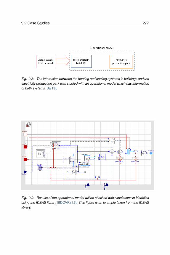
9.2 Case Studies 277

Fig. 9.8: The interaction between the heating and cooling systems in buildings and the

electricity production park was studied with an operational model which has information

of both systems [Bal13].

Fig. 9.9: Results of the operational model will be checked with simulations in Modelica

using the IDEAS library [BDCVR+12]. This figure is an example taken from the IDEAS

library.

278 Activity 2.1: Design of Building Systems

of the results were done by performing more detailed simulations in Modelicausing Dymola. The second part of the work, namely the optimization of theheating and cooling systems in different scenarios was performed in Matlabby using the yalmip toolbox [Lof04] .

9.2.4 Implementation of Model Predictive Control for the

HVAC System of a Belgian Thermally Activated Office

Building

The case study building, called “Hollandsch Huys” and shown in Fig. 9.10, islocated in Hasselt, Belgium. Its construction was finished in 2007. Designed tobe a low-energy, innovative office building, it makes use of thermally activatedbuilding systems (TABS), in which the thermal mass of the concrete floorsis activated by a water piping circuit for both heating and cooling. The heatand cold are produced by a ground-coupled heat pump (22 single-U-tube boreholes of 75 m) and with a gas-fired boiler of 60 kW as back-up for the airhandling unit.

Fig. 9.10: Hollandsch Huys building (Hasselt, Belgium)

The building and its systems are monitored by a large set of built-in sensors.Historical data of these measurements since 2007 are stored, allowing a de-tailed analysis of the technical performance. The main difficulty in interpre-tation of these data lies in the fact that the building has not been fully rentedand occupied by the time this study started. In 2007, about 75 percent of thesecond floor and the roof apartment was still vacant. From 2010, the second

9.2 Case Studies 279

floor was used. The systems commissioning phase was not fully completedyet, resulting in control set points being tuned during the measurement period.

Since January 2013, the building is controlled intermittently during the heatingseason using model predictive control (MPC) instead of the traditional rule-based control (RBC). The MPC has been developed by the University of WestBohemia, Czech Republic (Jan Siroky) and the Czech Technical University inPrague, Czech Republic [Cig13] in collaboration with KU Leuven. The project(SMART GEOTHERM) aimed at analyzing the improvements obtained by thereduced-model-based MPC strategy, generalizing the results for different typesof thermally activated building offices using geothermal energy and extractinga new RBC algorithm based on the MPC results. The analysis was done by acombination of simulations and experiments.

Fig. 9.11 shows the components of the thermally activated building.

Fig. 9.11: Scheme of the thermally activated building components (floor heating: red,

TABS: yellow)

The production unit in heating mode and the general layout of the simulationmodel are shown in Fig. 9.12 and Fig. 9.13, respectively.

The building was simulated using the IDEAS-library developed by KU Leu-ven. The whole energy system was modeled in Modelica and simulated withDymola.

280 Activity 2.1: Design of Building Systems

Fig. 9.12: Production unit in heating mode

Fig. 9.13: General layout of the Modelica system simulation model, using the IDEAS-

library. Left: building structure. Top: air handling unit. Center: heating/cooling produc-

tion system. Bottom: internal gains due to occupancy. Right: electrical grid.

9.2 Case Studies 281

9.2.5 Modeling for the Design of an Energy and Water Effi-

cient Hotel

The case study deals with the HVAC, non-portable water and domestic hotwater system of the newly constructed Grand Beach Hotel at Surfside, Florida,USA [MHB+15] (see Fig. 9.14).

Fig. 9.14: Grand Beach Hotel at Surfside, Florida

To achieve the efficiency in energy and water, the HVAC, non-portable waterand domestic systems are highly coupled. The collected rain water is usedfor non-portable water usage, such as flushing the toilet, and used as makeupwater for the cooling tower. When condition allows, the domestic water will bepre-heated using the waste heat from the heat pump, and it will be used toreduce the cooling energy that is to be provided by the chilled water.

282 Activity 2.1: Design of Building Systems

The simulation analysis was used for the system design and optimization. Ithelped the engineers decide the potential energy saving, balance the waterpressure in the pipe system, and evaluate the control sequence.

Fig. 9.15 and Fig. 9.16 show the schematic HVAC and domestic water systemand the corresponding Modelica models.

Fig. 9.15: Schematic of the HVAC and domestic water system

The system models for the simulation analysis were configured with the com-ponent models of the LBNL’s Buildings library [WZNP14] . The whole energyand hydraulic system was modeled in Modelica and simulated with Dymola.

9.2.6 Design of an Innovative Two-Pipe Chilled Beam Sys-

tem for Simultaneous Heating and Cooling of Office

Buildings

This case study aims to design and evaluate energy performance of an inno-vative two-pipe system in active chilled beam application. The system enablessimultaneous heating and cooling of office buildings by transferring energy be-tween zones, using one hydronic circuit only. The system is designed to havethe same inlet water temperature on the entire circuit. This temperature is con-trolled between 20∘C to 23∘C, depending on the room air temperatures. Outlethot and cold water is mixed together and as a result the system only needs to

9.2 Case Studies 283

Fig. 9.16: Modelica system model of the same system

cool or heat the water to reach the inlet temperature again. By only having tocool or heat the water, no energy is wasted by doing both at the same time.

The possibility to design such a system was explored through a preliminarysimulation-based research at the Danish Building Research Institute, in col-laboration with Lindab A/S [ANHB13] . The system was modeled with BSim,a Danish building energy simulation tool, and integrated into a typical officebuilding model. Standard internal gains for offices were set and thermal prop-erties for the building envelope elements were selected according to Danishregulations. The building is located in Copenhagen (Denmark) and the corre-spondent weather file was used for the simulation. Results showed that thetwo-pipe configuration uses 3 percent less energy than a conventional four-pipe system.

However, BSim does not offer all the necessary features for a detailed designof the two-pipe system and some assumptions in the model were made. Inorder to be able to represent and control each single component of the systemModelica was chosen for more detailed studies.

Fig. 9.17 illustrates the principle of the two-pipe active chilled beam system.In this particular example, the inlet water temperature in the circuit is 22∘C.

284 Activity 2.1: Design of Building Systems

The room located on the north facade needs heating and the outlet water tem-perature is 20∘C. Conversely, the space located on the south facade needscooling and the outlet water temperature is 23∘C. As a result, the outlet watertemperature in the circuit was 21.5∘C. The system only needs to provide en-ergy to reach 22∘C. Fig. 9.18 shows the system model in Modelica used forthe preliminary analysis.

Fig. 9.17 : Two-pipe active chilled beam system for simultaneous heating and cooling

After the preliminary study, a more detailed study was conducted, using a typ-ical office building model. Simulations were run for two construction sets ofthe building envelope and two conditions related to inter-zone air flows. Tocalculate energy savings, a conventional four-pipe system was modelled andused for comparison. The conventional system presented two separated wa-ter loops for heating and cooling with supply temperatures of 45∘C and 14∘C,respectively. Simulation results showed that the two-pipe system was ableto use less energy than the four-pipe system thanks to three effects: use-ful heat transfer from warm to cold zones, higher free cooling potential andhigher efficiency of the heat pump. In particular, the two-pipe system used ap-proximately between 12% and 18% less total annual primary energy than thefour-pipe system, depending on the simulation case considered [MWA+17] .

The Buildings library from LBNL ([WZNP14]) was used for the system model-ing, the energy analsysis and the controls design.

9.2 Case Studies 285

Fig. 9.18: Modelica model of the building system

286 Activity 2.1: Design of Building Systems

9.2.7 Integrated Optimal Design and Control of Office Build-

ings Using Renewable Energy Sources

This case study was performed in the PhD project “Integrated optimal designand control of office buildings using renewable energy sources” at the KU Leu-ven. The aim of this PhD project was to find a methodology for integratingoptimal control and design of office buildings (compare with Fig. 9.19).

Fig. 9.19: General outline of the case

Usually, optimal control and design are solved as two independent problems.Optimal control is performed on a fixed design and optimal design is performedby assuming a simplified control sequence. However, technologies such asConcrete Core Activation (CCA) typically operate in a transient regime due totheir large time constants. Furthermore the added value of renewable energysources is difficult to assess without considering the entire system. This PhDproject aimed to assess the potential of optimal control and optimal design us-ing an integrated approach and dynamic simulations. This research proposeda methodology that optimally exploits this potential in practice so that the totalcosts (investment and running costs) are minimized. Modelica was used tocreate a parameterized emulator model of the building that needs to be opti-

9.2 Case Studies 287

mized. A Model Predictive Controller (MPC) performed the optimal control ofthe building’s HVAC-system. A controller model (RC model) was used to limitthe computational effort. The performance of this controller was evaluated us-ing the Modelica emulator model. This control optimization was nested in astochastic optimization that optimizes the design of the building with respectto building parameters, different HVAC-components, etc.

The IDEAS library [BDCVR+12] and the Buildings library [WZNP14] was usedfor this research in combination with Dymola.

9.2.8 Development of a Virtual Computational Test-Bed for

Building Integrated Renewable Energy Solutions

In this case study, a virtual computational test-bed for building integrated re-newable energy solutions was developed using Modelica. This test-bed helpsassessing the full scale performance potential of existing products based onpilot scale testing results from the Eindhoven University of Technology (TU/e)campus and simulations which are calibrated using the pilot scale testing mea-surements. The pilot scale testing facility is a cooperation known as SolarBEAT(http://www.seac.cc/projects/solar-beat) which has been established betweenthe TU/e and the Solar Energy Application Centre (SEAC), an independent re-search organization. This facility is being constructed on the roof of the Vertigobuilding, home of the Department of the Built Environment at TU/e. It consistsof dummy buildings with building-integrated photovoltaic/thermal (BIPVT) solarcollectors.

The end product of this work will be a complete building system simulatingphotovoltaic modules, solar thermal collectors, occupancy, ventilation, infiltra-tion, heating system, domestic hot water demand and heat storage, as shownin Fig. 9.20. The virtual computational test-bed helps assessing the perfor-mance of different technologies. Those technologies will consist of BIPVTsystems from different companies which are interested in testing their prod-ucts and assessing their performance.

The building is a single family house for 4 occupants. It is assumed that thehouse has 10 thermal zones: 3 zones at the ground floor including the kitchen,living room and the entrance, 5 zones in the second floor including 3 bedrooms

288 Activity 2.1: Design of Building Systems

Fig. 9.20: Full home system schematic

and the second floor/attic which is divided into 2 rooms. The different zonesare connected to each other thermally through the common walls and throughthe doors which can be controlled to be open or closed. However, the airconnection between the different floors was not modeled.

The Modelica model consists of three major parts: the PV model, the solarthermal model and the house model. The house model was used to modelthe heating demand of the home. The first two models were used to modelthe generation of renewable energy for the given location of interest. Usingthe combined simulation, it was possible to analyze the dynamic interactionbetween the renewable generation systems and the energy demand of thehome. The house is heated using typical radiators which are connected to thewater heating system.

A complete heating system was modeled in this case study. The schematicin Fig. 9.21 illustrates a more detailed depiction of the solar thermal, spaceheating and domestic water heating system.

This system contains a heat storage tank connected by a heat exchanger toan array of solar collectors. This tank is also connected to a boiler whichheats the water to a specific temperature required by the heating system. Theheating is provided by radiators in each of the thermal zones. Each of the

9.2 Case Studies 289

Fig. 9.21: Heating system schematic

radiators is controlled by a valve according to the set-point temperature. Apump in the collector circuit and another pump in the heating circuit ensurehot water circulation. Moreover, the domestic hot water circuit contains anotherboiler to ensure sufficient hot water temperature, and it contains a pump for thewater circulation. All the components are controlled depending on the requiredtemperature for the day, night and the outside temperature.

The electrical model should consist of an electrical network, representing thedwellings distribution system to which the PV and all power consuming equip-ment are connected. However, modeling different components inside thehouse and their energy consumption is a complicated task which requires theavailability a well determined usage and occupancy profile. In the case of thiswork, the decision was made to represent the electrical demand using averagemeasured data varying throughout the year.

The electrical power demand can vary according to the user behavior, thenumber of occupants and the resolution of the data available. For instance, aset of electric power demand data with a resolution of 5 minutes is more accu-rate than one with a resolution of 15 minutes. The 15 minutes data has flatterpeaks of power demand due to its temporal averaging. Therefore, the higher

290 Activity 2.1: Design of Building Systems

the resolution, the more representative is the data [SHK14] . That being said,it is difficult to get access to detailed specific data from power companies dueto privacy issues. The most complete data available for this application is anaverage consumption data for one house with a resolution of 15 minutes. Theelectrical network contains also a resistor representing losses and a voltagesource to set the operating voltage as shown in Fig. 9.22.

Fig. 9.22: Electric model containing the weather data, PV and the load profile

Fig. 9.23 represents the implementation of the model in Modelica. The blockon the left contains the BIPVT and the heating system, while the block on theright represents the single family Dutch house. The top block is the weatherdata input.

The system models for the simulation analysis were configured with the com-ponent models of the Buildings library from LBNL [WZNP14] . The whole en-ergy system was modeled in Modelica and simulated with Dymola.

9.2 Case Studies 291

Fig. 9.23: Model implementation in Modelica

9.2.9 Influence of German Energy Saving Ordinances on

Heat Demand of a Residential Building

This case study investigated the influence of different German energy savingordinances on the heat demand of a residential building. In the past, Germangovernment had issued several energy saving ordinances, which define limitsfor the properties of building envelopes in order to reduce heat demands innew building construction. As these properties define the minimum require-ment for all buildings built in a certain time period, they can help estimating abuilding’s properties given only its year of construction. Therefore, referencesimulations of buildings with these standard properties can serve as bench-marks for a large share of Germany’s building stock and as the foundation forfurther investigations of the system or its parts.

As a reference building for this case study, a one family dwelling with an areaof 150 m2over two floors (see Fig. 9.24) was used. In order to only quan-tify the influence of the building envelope, each room is equipped with anideal heater. For the location of this reference building, central Germany with

292 Activity 2.1: Design of Building Systems

Fig. 9.24: Floor plan for the reference building

weather input from the German test reference year region 12 was selected.The same building setup and weather input was used for building instanceswith envelope properties of energy saving ordinances from 1984, 1995, 2002,and 2009. Because this case study shall serve as a foundation for furtherstudies, it was included as a demonstration example in the Modelica libraryAixLib [BM10][FCL+15] . Further details can be found in [CSM14] .

The Modelica system model was built in a modular way, starting with wall el-ements including windows and doors. Several wall elements were groupedtogether to form a room model. The room models were connected to modela single floor. The floors can be connected to the outside environment and toheating system models to form a model of the entire building. In order to testthe influence of different building envelope properties, upper-level parametersspecify the wall constructions according to a chosen energy saving ordinance.Further parameters can be used to specify a light, medium or heavy buildingconstruction and air exchange rates. Thus, there is little manual effort neededto compare different building setups in a certain context. Through the modu-larity of the modeling approach, the building model could also be connected

9.2 Case Studies 293

to a more elaborate heating system model with a prototype controller to testthe control performance subject to different building properties. This allowsengineers to quickly test their developments with a variety of typical Germanbuilding setups.

The Modelica model of this building setup is shown in Fig. 9.25. The wholeenergy system was modeled in Modelica and simulated with Dymola.

Fig. 9.25: This case study is an illustrative example of the library AixLib. It uses

components from AixLib’s Building package as well as basic models from the Modelica

Standard Library

9.2.10 Comparative Analysis of all Case Studies

A comparison of all nine case studies regarding the used Modelica libraries,the type of the component models and the used Modelica tools provides fol-

294 Activity 2.1: Design of Building Systems

lowing information:

Used Modelica libraries: Different Modelica libraries were used for the casestudies, 3 times the Buildings library from LBNL, 3 times the IDEAS libraryfrom KU Leuven, once the BuildingSystems library from UdK Berlin. Furtherspecialized Modelica models were used by the Fraunhofer institute ISE, whichare not part of the publicly available Modelica libraries.

Used Modelica component models: A wide range of energy plant modelsand thermal building models were used in the case studies:

• Auxiliary models:– Controllers (Two point-controller, PI controller)– Data reader & interpolation (e.g. weather data, user behavior)– Radiation calculation on tilted surfaces

• Energy transformation models:– PV module and generator with maximum power point tracking– Solar thermal collector– Electric driven heat pump and chiller– Borehole heat exchanger for ground coupled heat pumps– Cooling tower– Boiler (e.g. condensing gas, wood pellet)– HVAC: adiabatic cooling, mechanical cooling

• Energy storages Models:– Electric battery– Thermal water storage (cold water, hot water)– Bore-field

• Energy transport models:– Thermo-hydraulic components: pipe, branch, two-way and three

way valves, constant and variable speed pump– HVAC components: ducts, ventilators, heat recovery components– Heat emission systems such as radiators and floor heating– Heat exchangers– Heat emission components: TABS, radiators, active beams

• Building models:– Simplified thermal building model (one zone)– Detailed building model (multiple zones)

Used Simulation Tools: In all of the case studies, Dymola was used as the

9.2 Case Studies 295

Modelica simulation tool. (When the case studies were conducted, Dymolawas the only tool that could simulate all used models. However, as of Spring2017, JModelica fully supports the Annex 60 library and the Buildings library.)In two cases, EnergyPlus was used in addition by co-simulation, based onBCVTB (https://simulationresearch.lbl.gov/bcvtb). In one case study GAMS(http://www.gams.com) was used for an operational model.

In two of the case studies, optimization analysis with GenOpt(https://simulationresearch.lbl.gov/GO/) were done. One case study used a Python-framework for the realization of a model-based predictive control (MPC). Onecase study used the MATLAB toolbox YALMIP (http://users.isy.liu.se/johanl/yalmip/pmwiki.php?n=Main.HomePage) for optimization.

9.2.11 Reasons for the Use of Modelica

The reasons for the use of Modelica as stated by the case study participantscan be clustered into the following groups:

Flexible and extensible object-oriented modeling approach: The object-oriented modeling approach leads to a high working efficiency and supportsa transparent and clear understanding of component and system models.Hereby, an easy manipulation, re-use and/or adaption of existing componentmodels is possible and missing component models can be easily implemented.The graphical and hierarchical modeling approach enables a well-structuredand clear modeling process and supports system models with different levelsof detail in the sub-models (e.g. a detailed plant model in combination with asimplified thermal building model). The combined use of existing large Mod-elica libraries enables new system models, which are normally not present inexisting simulation tools.

Acausal equation-based modeling approach: The equation based approachleads to an easy understanding of the physical modeling of existing modelsand newly implemented models. It also gives a good physical insight in theproblem and the components. The result is a clear understanding of the under-lying physical-technical equation system at the component and system level.Especially the non-causal approach of Modelica supports necessary featuresin energy plant simulation domain such as the bi-directional mass flow within

296 Activity 2.1: Design of Building Systems

thermo-hydraulic networks.

Multi-domain approach: The multi-physical modeling approach of Modelica in-cluding the domain specific common interface definitions supports the integra-tion of domain specific sub-models into a common system model (e.g. buildingphysics, hydraulics and electrical grids).

Numerical reasons: The automatically translation of the textual Modelicamodel into a running simulation model with time integration allows the modelera clear separation between the physical-technical model itself and its numeri-cal solution.

External interfaces to Modelica: Modelica-models can be easily coupled withexternal optimization software (e.g. GenOpt and GAMS). The scripting lan-guage Python can control Modelica simulation tools and can serve for pre-andpost-processing steps. Co-simulations of Modelica with other simulation toolsare possible, e.g. with BCVTB and/or FMI. One typical example is the co-simulation of a HVAC system, modeled in Modelica and a multi-zone buildingmodel in EnergyPlus.

Collaborative development : The modular approach of Modelica supports com-mon software development within single teams, and also within a broader dis-tributed model development such as done for the Annex 60 library that wasdeveloped in Activity 1.1 and is used in major Modelica libraries for buildingenergy applications.

9.2.12 Drawbacks of Using Modelica

The authors of the case studies have stated the following most important draw-backs by using the Modelica language, Modelica libraries, or Modelica tools inthe context of building energy simulation:

Long simulation times for detailed whole building simulation: Whole buildingsimulations are often slower than with dedicated building energy simulationprograms, in particular if detailed HVAC models are combined with multi-zonebuilding envelop models. This has several reasons: First, Modelica modelsoften include more detail than for example an EnergyPlus or TRNSYS simu-lation. Typical examples include modeling of realistic control sequences andpressure-driven mass flow distribution in pipe and duct networks. Second,

9.2 Case Studies 297

numerical solvers in the tools use the same time step for all equations.However, for building envelope heat conduction, much larger time steps couldbe used than what is required for control loops. Here, the use of multi-ratesolvers with error control is promising. Third, if an event is triggered by amodel, then the whole time integration is stopped, and the integration isrestarted, typically with a low order integration method. However, manyevents could be treated in a subsystem, in particular if they affect other partsof the model through integrators, as integrators smoothen discontinuities.Fourth, Modelica translators typically convert the models to a dense system ofequations rather than preserving the sparsity, which then could be exploitedusing sparse solvers. Fifth, ordinary differential equation solvers for stiffequations that scale cubic in the number of state variables are often used.This can lead to large computing time if the building envelope model, withmany slow evolving states, and the HVAC model, with few but fast evolvingstates, are coupled. However, research and development is ongoing on all ofthese issues, and they are not an inherent problem of the Modelica languagewhich for simulation is converted to efficient C-code, as described in Section5.3.4. Rather, it is a problem of the solvers that are currently in use and needto be improved as users simulate larger Modelica models than they did in thepast. At the time of this writing, various research in such model translationsand numerical methods that allow faster simulation is ongoing, see for example[MBKC13][FBC+14][Cas15][BBCK15][BRC16][CR16][OE17][BCB17][JHB17] .As Modelica separates declarative model formulations from solution methods,these methods can be made available in simulation environments with little tono changes to the underlying model libraries.

Reliance on one commercial Modelica tool : During the research phase of thisproject (2013 to 2016), only Dymola supported the entire Modelica languagespecification. Hence, complex Modelica system model run only partly withother commercial or open Source Modelica tools. Since Spring 2017, the situ-ation is improving as the open source Modelica tool JModelica works with theAnnex 60 library and the Buildings libary, and other tool providers stated thatthey are working on increasing the support of models that are used for buildingenergy simulation.

Connector types were not standardized : At the start of the Annex, someModelica libraries used connectors and function that compute enthalpy as afunction of temperature that were different from the ones standardized in the

298 Activity 2.1: Design of Building Systems

Modelica Standard Library. This made combining existing models difficult asadapters had to be implemented. In the meantime, the Annex60, AixLib, Build-ingSystems, Buildings and IDEAS libraries all use the same adapters and me-dia functions, making their models compatible.

Fewer validated models than established building simulation programs: Mod-elica offers fewer models than for example EnergyPlus or TRNSYS, and sincethe libraries are new compared to these established tools, the range of vali-dated models is smaller. However, Modelica libraries are more transparent incomparison to EnergPlus, in particular regarding how components and sys-tems are controlled. Also increasing the scope of models and their level ofvalidation was a key motivation for the development of the Annex 60 library asa common base for different Modelica libraries. See also Section 5.4.5 for thequality control in the Annex 60 library.

9.3 Model Analysis

Outgoing from the described case studies, an analysis about the used Model-ica models of the four libraries for building energy and plant simulation AIXLib,BuildingSystems, Buildings, and IDEAS was performed. Because the quantityof all of the used Modelica component models was large, only models used inone or several of the case studies were considered in the analysis.

In the second step, a comparison between the spectrum of the used mod-els and the present models of the Annex 60 library (version during Fall 2014)were conducted. In this manner, commonly used models were identified. Thisserved as a basis to prioritize which new component models to add to the An-nex 60 library. This fits with the idea of the Annex 60 project of providing acore Modelica library, while allowing individual libraries to differ in the special-ized models that they provide.

The following ranking was obtained by the statistics of how often a Modelicamodel was used in all of the case studies and was not present during Fall 2014in the Annex 60 library:

1. Compression chiller/heat pump; Thermal zone models or building mod-els: 6 x

9.3 Model Analysis 299

2. Radiation calculation for tilted surfaces: 5 x3. Thermal water storage (hot water/cold water): 4 x4. Data reader / interpolator: 3 x5. Borehole heat exchanger; Cooling ceiling / radiant slab; Photovoltaic

model: 2 x6. Solar thermal collector model; thermally activated building systems;

electric battery model; Cooling tower: 1 x

Starting from this case, the following five most used models should be inte-grated in the future versions of the Annex 60 library:

A simplified thermal building model: In the majority of case studies, thebuilding energy and plant simulations were coupled, with the focus of the anal-ysis being on the plant. The building model delivered the dynamically calcu-lated heating and cooling demand, typically in yearly simulations. Hence, asimplified thermal building model is needed.

A thermal water storage model: Many thermal energy concepts used a ther-mal storage tank to store hot or cold water. They are integrated in hydraulicconcepts in different manners (e.g. internal/external heat exchangers) andalso often the thermal stratification is important (e.g. for solar thermal sys-tems). Hence, a thermal horizontal 1D-discritized tank model with flexible in-puts and outputs should be part of the Annex 60 library.

A compression chiller/heat pump model: Many energy concepts are basedon (reversible) heat pumps and/or compression chillers. Hence, a simplifiedmodel should be included in the library, which uses characteristic curves forfast system simulation analysis.

A solar radiation calculation model: One basic feature consists in the trans-formation of horizontal solar radiation as obtained from the weather data intothe incident irradiation on tilted surfaces (e.g. building envelope, solar thermalcollectors, photovoltaic modules).

A data reader model: All building and plant system models have to readdiscrete, typically hourly, weather data, which have to be transformed into con-tinuous boundary conditions for the building and its HVAC system. Hence, adata reader model which supports different types of interpolation should bepart of the Annex 60 library.

300 Activity 2.1: Design of Building Systems

9.4 OD/OC Method Analysis

Methods for optimal design and optimal control were used in following of thecase studies:

• Multi-criteria optimization of PV-cooling systems for residential buildings(Section 9.4.1, TU Berlin, UdK Berlin, Germany), and

• Model predictive control framework (Section 9.4.2, KU Leuven, Bel-gium).

9.4.1 Multi-Criteria Optimization of PV-Cooling Systems for

Residential Buildings

Optimization problem: A residential building in a hot climate region with spacefor two families (net floor area of 278 m2) is air-conditioned by a solar PV cool-ing system. The optimization problem was analyzed for two different climate lo-cations in the MENA region: The city Hashtgerd in Iran and the city El Gouna inEgypt [NGHN13] . The maximum air temperatures in Hashtgerd and El Gounaare nearly the same (41°C), but the mean temperature during the summerperiod in El Gouna (30.4°C) is much higher than in Hashtgerd (26.0°C). Theyearly horizontal global solar radiation is about 1, 800 kWh/(m2 a) in Hasht-gerd and 2, 400 kWh/(m2 a) in El Gouna.

The mean U-value of the thermal envelope of the considered building was0.593 W/(m2 K) for walls, windows and roof, and 0.350 W/(m2K) for the floor.The potential surface for PV modules on the roof was about 135 m2.

The study aims to solve a multi-criteria optimization of the PV cooling system.Furthermore, the PV cooling system has to supply 100 percent of the coolingdemand by solar energy without any use of additional electricity from the grid.

For this purpose a cost-function with three different design criteria was defined:

1. Over temperature: The first criteria was to avoid overheating for an opti-mal thermal comfort. If the indoor air temperature exceeds the set tem-perature of 26°C, then the difference TAir-TSet (over temperature) wasintegrated over time.

9.4 OD/OC Method Analysis 301

2. Investment costs: The second criteria was the minimization of the in-vestment costs. The following assumptions to the specific investmentcosts were made: (PV generator: 0.7 Euro/Wpeak ; Battery: 600 Eu-ro/kWh; Compression chiller: 0.4Euro/Wel ; Cold water storage: costs inEuro = 1649.81 V−0.464 where V is the storage volume.

3. Durability of the components: The third criteria was the reduction ofswitching on/off events of the compression chiller.

These three criteria were weighted with the factors f1 = 1, f2 = 1 and f3 = 2.Electricity costs were not considered, because the PV cooling system worksgrid-independently.

These chosen optimization parameters and the possible parameter spans forthe optimization algorithm were as follows:

1. Number of PV modules: 1 to 83,2. Capacity of the electric battery: 1 to 80 kWh,3. Nominal power of the compression chiller: 0.1 to 5.0 kW and4. Volume of the cold water storage: 0.1 m3 to 10.0 m3.

Used Modelica system model for optimization: The PV cooling system wasmodeled in Modelica by the use of the BuildingSystems library. It consists ofthe following seven main sub-models which are also shown in Fig. 9.26:

1. A weather data reader and its conversion to different surfaces (PV sur-faces and building facades),

2. a PV generator system model,3. an electrical battery model,4. a model of a compression chiller with its recooling unit,5. a cold water storage model,6. a simplified thermal building model,7. controller models.

Several controllers were implemented within this system model. The first con-troller manages the cooling load pump. This pump switches on if the roomair temperature reaches the set temperature with an offset of 2 K. The sec-ond controller measures the water temperature in the top of the cold waterstorage. If the temperature rises above 7°C, the compression chiller, the re-cooling pump and the cold water loop pump turns on, but only if the batteryload state is not lower than 20% (discharge protection).

302 Activity 2.1: Design of Building Systems

Fig. 9.26: Modelica system model of the PV cooling system and its sub-models

Used method and tools for optimization: The GenOpt framework (http://simulationresearch.lbl.gov/GO/) was used for the parameter optimization prob-lem. GenOpt varies predefined parameter sets within the admissible param-eter bounds, dependent on the selected optimization algorithm. It then startsthe Dymola simulation for one year, and the simulation model writes the costfunction value to a file that will be read by GenOpt. Dependent on the progressof the optimization, Genopt varies the parameter set again for the next simu-lation run until a convergence criterion is satisfied. The GPSHookeJeevesalgorithm was used for the optimization problem.

Results of the optimization: GenOpt was started at both climate locations withthe same parameter set:

• Number of PV modules: 70,• capacity of the electric battery: 40 kWh,• nominal power of the chiller: 1.0 kW,• volume of the cold water storage: 5.0 m3.

After 120 simulations, the cost-function for both locations has converged, as

9.4 OD/OC Method Analysis 303

shown in Fig. 9.27.

Fig. 9.27 : Final cost-function value and its composition for the locations El Gouna and

Hashtgerd

The cooling load in Hashtgerd leads to higher peak values. However, theyearly cooling energy in El Gouna is higher than in Hashtgerd, because of itshigher mean temperature. The maximum temperature during the summer isnearly the same at both locations.

For these reasons, the optimization algorithm has found for Hashtgerd thesame number of PV modules (83). This is maximum value of possible moduleson the roof area. The location El Gouna with a higher mean temperature andcooling demand needs greater storage capacities for cooling energy. The dailyand yearly timeline of the solar irradiation is more balanced in comparison toHastgerd. Consequently, the optimization algorithm calculated for El Gouna alarger and cheaper cold water storage (6.1 m3 instead of 5.5 m3) and reducedthe capacity of the electric battery (40 kWh instead of 55 kWh) in comparisonto Hashtgerd.

Fig. 9.28 shows the detailed investment costs for both locations. The maincosts are from the battery and the PV generator. The costs of the cold waterstorage and the chiller are less significant.

The PV cooling system causes in Hashtgerd a higher overheating time (16.9hours) as in El Gouna (10.8 hours) caused by the higher cooling load peaks.Because of the higher alternating external temperature, the compression

304 Activity 2.1: Design of Building Systems

Fig. 9.28: Investment costs in Euro for both locations

chiller switches on more often in Hashtgerd (355 times) than in El Gouna (270times).

9.4.2 Model Predictive Control Framework

Model Predictive Control (MPC) is a control strategy that can be applied tobuilding applications. The idea of MPC is to create an optimization problemthat optimizes the control variables (valve positions, heat flow rates) such thatthe operation point with the lowest cost is obtained that still satisfies com-fort constraints and other constraints that may be imposed. An MPC problemestimates future energy use under consideration of weather and occupancyforecasts. Hence, it anticipates future solar gains, thereby possibly reducingthe heating power or pre-cooling the building at night when cooling is typ-ically cheaper. Comfort constraints are typically formulated based on zoneoperative temperatures. Depending on the complexity of the model that isused to estimate energy use, the optimization problem may be categorizedinto different problem classes such as a Linear Programming (LP), QuadraticProgramming (QP), Nonlinear Programming (NLP) etc. Efficient specializedoptimization solvers exist depending on the problem class. LP’s can for in-stance be solved very quickly. Each of these solvers however requires that theequalities, inequalities, cost function and input data defining the problem areprovided to the solver in a certain format. Obtaining these equations and data

9.4 OD/OC Method Analysis 305

requires knowledge of specialists, especially for large problems.

Classical building simulation tools typically do not allow the automated extrac-tion of these model equations or input data. The model equations of individualcomponent models may be publicly available, but using these directly wouldagain require the equations to be recombined manually when individual com-ponent models are coupled. Modelica offers some interesting advantages inthis respect, which may greatly simplify extracting models for use in MPC. First,open source libraries exist where the users has control over the type of equa-tions, meaning that component models may be simplified to match a certainproblem class. For instance, a library of linear building component modelsmay be constructed if the user wants to obtain a LP controller model. Sec-ond, Modelica simulation environments allow any variable to be stored in anoutput file, and therefore the required input data can be exported. Third, Mod-elica simulation environments typically allow to linearize a model and extract alinear state space formulation of the problem in the form

x = A x + B u,

y = C x + D u,(9.1)

where x are the problem states, x is the time derivative of x , u are model in-puts and A, B, C, D are constant matrices. When linearizing a model, thesematrices are computed. Fourth, specialized Modelica solvers such as JModel-ica and OpenModelica allow to directly optimize the model equations withoutneeding to export them first. At the time of this writing, their solvers, however,conservatively assume that the problem is a non-linear programming (NLP)problem, which increases the computation time compared to using a solver forlinear programming (LP) problem.

Using these properties of the Modelica language and their solvers, an auto-mated way for creating and exporting linear controller models with matchinginput data may be set up. A first step would be to create a building model inModelica using a library that contains only linear equations. Second, a statespace model of the form (9.1) needs to be extracted. Third, an input data fileneeds to be generated that matches the inputs u of the state space model.Then, these data can be used by an efficient LP optimization algorithm tocompute optimal control results. Note that an interesting feature of Modelicais that the optimization algorithm, which is not implemented in Modelica, maybe compiled into C-code that may be called from Modelica. This way, an MPC

306 Activity 2.1: Design of Building Systems

controller may be embedded into a Modelica model, which removes the needfor co-simulation techniques.

This approach was used at the KU Leuven to set up an automated ModelPredictive Framework using the IDEAS library. In [PJH15] the linearizationapproach is outlined. In [JH16] the framework is explained and applied to anoffice building. In [PSJ16] the framework’s performance is compared to a greybox approach.

9.4.3 Optimal Control of Room-Level HVAC and Facade

Control

This example demonstrates the use of collocation methods to solve a con-strained nonlinear optimal control problem, and compares its computing per-formance to a gradient free optimization method. The example demonstratesthe benefits obtained through the problem manipulation that the Modelica lan-guage allows due to its declarative nature.

9.4.3.1 Optimization Problem

The example minimizes sensible cooling, heating and fan energy demand fora thermal zone of a variable air volume flow (VAV) system by adjusting thetime profiles of the supply air mass flow rate, the shading device control signaland the reheat power at the terminal box, subject to comfort constraints. Ourapplication requirements are that the optimizations of individual zones are de-coupled from each other, and that the central HVAC system can have its owncontrol. For our example, the central HVAC system will supply air at 18∘C andat a relative humidity required for humidity control.

Fig. 9.29 shows the simplified thermal model of the zone. Separate modelsexist for exterior constructions, partitions to adjacent zones and internal mass.These constructions are characterized by thermal capacitors and thermal con-ductance that account for heat conduction and convection. There is also athermal conductor for infiltration.

The windows were modeled with a thermal conductance Gwin and a powersource Qwin

sol (t) = Srad (t) Awin SHGC χ(uwin(t)), where Srad (t) is the total so-

9.4 OD/OC Method Analysis 307

Window

Zone air

Cair

Qihg(t) Phvac(t)

Internal mass

Qim(t)

Cim

Exterior

constructions

Cconext

Ginfext

Gconvext Gin

ext

Qsolwin(t)

Gwin

Gim

GCondext

Interior

constructions

Cconint

Ginfint

GoutintGin

int

Tairadj(t)Tout(t)

Qsolext(t)

Tout(t)

Fig. 9.29: Simplified model of a thermal zone.

lar radiation per unit area towards the window normal direction, Awin is theglass area, SHGC is the solar heat gain coefficient of the window, uwin(t) ∈[0, 1] is the position of the blind, and χ : R → R is a function that mod-els the impact of the blinds on the fraction of solar radiation that enters thezone. The contribution due to solar radiation on the external constructionsis Qext

sol (t) = Srad (t) Aext α, where Aext is its area, and α is the solar absorp-tion coefficient of the exterior surface. The thermal conductance Gim mod-els the heat transfer between the air and the internal mass. The powersources Qihg(t) and Qim(t), respectively, model the internal heat gains thatcontribute to the zone air and internal mass. The internal heat gain is definedas Qihg(t) = Pocc(t) + Plights(t) + Pplug(t), where Pocc(t) is the internal heat gaindue to occupancy, Plights(t) is the internal heat gains due to lights, and Pplug(t)is the internal heat gains due to the plug loads. The power delivered by theHVAC system is Phvac(t) = Phea(t) + Psup(t) + Pfan(t), where Phea(t) is the powerreleased by the reheating coil in the VAV box, Pfan(t) is the fan power, andPsup(t) is the cooling power provided by the supply air from the central HVACsystem through the VAV box.

The latter is Psup(t) = mair (t) cp (Tsup(t)−Tair (t)), where mair (t) is the mass flowrate of air passing through the VAV box, cp is the air specific heat capacity,Tsup(t) is the temperature of the supply air entering the VAV box and Tair (t)is the temperature of the air in the zone.footnote{Note that the computationof Psup(t) is approximate to decouple the individual optimizations of multiple

308 Activity 2.1: Design of Building Systems

zones from each other. This was done to reduce the dimensionality of theoptimization and to allow them to be solved in a distributed way.

The actual sensible cooling provided by a cooling coil in a system with econ-omizer is Pc(t) = mair (t) cp (Tsup(t) − (Tmix (t) + ∆Tfan(t))), where Tmix (t) is themixed air temperature after the economizer and ∆Tfan(t) is the temperatureraise over the fan. If yout (t) ∈ [0, 1] is the outside air fraction, this becomesPc(t) = mair (t) cp (Tsup(t)−Tair (t)+yout (t) (Tair (t)−Tout (t))−∆Tfan(t)). As yout (t)and ∆Tfan(t) (through the fan efficiency) depends on the mass flow rates andreturn air temperatures of other zones, these terms have been neglected in or-der to decouple the individual zone-level optimizations.} The power of the fan isPfan(t) = Pnom

fan (mair (t)/mnomair )3, where mnom

air is the nominal supply air mass flowrate, and Pnom

fan is the fan power required to supply mnomair to the zone. Weather

data for Sacramento, CA, have been used.

The described model was implemented in Modelica. The model can be de-scribed as an initial-value ordinary differential equation. Thus, it is a spe-cial case of the generalized DAE system, in which the algebraic constraintsY (·, ·, ·, ·, ·) are absent. Therefore, the state variables, control functions andparameter are

x(t) = [Tair (t), Tim(t), T intcon(t), T ext

con(t)],

u(t) = [mair (t), uwin(t), Phea(t)],

Θ = [Tair (t0)].

The energy consumption of the HVAC system is

E(tf ) = tf

t0

(−Psup(t) ηcoo + Phea(t) ηhea + Pfan(t)) dt ,

where ηcoo and ηhea are coefficients that represents the efficiency of the HVACsystem to provide cooling and heating. These typically include the coefficientof performance of chillers or heat pumps, or the efficiency of the furnace, aswell as the effect of free-cooling by the economizer. The optimization variablesare the time profiles for the control signals of the supply air mass flow ratemair (·), the blind position uwin(·), the reheat power Phea(·), as well as the initialzone temperature Tair (t0). We modified the equation for E(tf ) to balance theweights of all its terms, obtaining

Eγ(tf ) = tf

t0

(−γ1Psup(t)ηcoo + γ2Phea(t)ηhea + γ3Pfan(t)) dt ,

9.4 OD/OC Method Analysis 309

where γ ∈ R3, with γ i > 0 for all i ∈ {1, 2, 3}, are constants.

The optimal control problem is formulated as

minimizeu(·)∈�

Eγ(tf ) + tf

t0

κ uwin(t)2 dt ,

subject to F (t , x(t), x(t), u(t), y (t), Θ) = 0,

F0(x(t0), x(t0), u(t0), y (t0), Θ) = 0,

T lair (t) ≤ Tair (t) ≤ T u

air (t),

0 ≤ uwin(t) ≤ uuwin(t),

mlair ≤ mair (t) ≤ mu

air ,

Phea(t) ≥ 0,

Tair (t0) = Tair (tf ),

for all t ∈ [t0, tf ], where U is the set of admissible control functions u(·), κ ∈ R+

is a constant, T lair (t) and T u

air (t) are the lower and upper bounds of the comfortregion of the air temperature, uu

win(t) is the maximum admissible value for thecontrol signal of the blind, and ml

air and muair are the minimum and maximum

supply air mass flow rates for the zone.

The cost function includes an additional term that penalizes excessive controlactions of the windows. For example it penalizes deploying the blinds at night.The equality constraint imposes that the temperature of the air at the start andat the end of the optimization period are the same.

9.4.3.2 Used Method and Tools for Optimization

The optimization problem was solved using JModelica [AGT09] , using the col-location method described in Section 4.2.3 and solved the finite dimensionalNLP problem with IPOPT version 3.11.9, and with the linear solver mumps.

For comparison of the computation time, the optimization problem was alsosolved using the Nelder-Mead algorithm, a derivative-free algorithm that isimplemented in JModelica. For the solution with the collocation method, ne =48 elements was used, each being 30 minutes long. For each element, threecollocation points were used. The optimization ran for a summer day.

310 Activity 2.1: Design of Building Systems

To assess the performances of the collocation-based method, it was comparedwith the simulation-based Nelder-Mead optimization algorithm. The Nelder-Mead algorithm can be applied to nonlinear optimization problems wherederivatives are not available, as is the case with conventional building simu-lation programs. See [WW04] for a comparison among the Nelder-Mead andother derivative free methods. The optimization variables in the Nelder-Meadoptimization problem are the initial temperature of the air in the zone, the con-trol signal for the blinds, and the supply air mass flow rate. To reduce the sizeof the optimization problem, it was simplified for the Nelder-Mead optimizationas follows: The heating power was set to Phea(t) = 0 for all t ∈ [t0, tf ], and boththe supply air mass flow rate mair (t) and the blind control signal uwin(t) wasdiscretized using one-hour rather than 30 minutes intervals. The decision tochoose no heating is appropriate for this hot day. Therefore, the optimizationvariables are

z = [Tair (t0), mhvac(t0), mhvac(t0 + ∆t), ... , mhvac(t0 + 24∆t),

uwin(t0), uwin(t0 + ∆t), ... , uwin(t0 + 24∆t)].

Hence, the total number of variables to optimize is nz = 51. Let τ = {t0 +i ∆t}24

i=0. The cost function minimized by the Nelder-Mead algorithm is

fNM (z) = Eγ(tf ) + µj (∆Terr + ∆Tinit ) ,

∆Terr = maxt∈τ

(0, Tair (t) − T uair (t), T l

air (t) − Tair (t)),

∆Tinit = (Tair (t0) − Tair (tf ))2,

where µj = 1.5j/10, for the iteration counter j ∈ N, are penalty function multi-pliers, ∆Terr penalizes thermal comfort constraint violations, and ∆Tinit forcesinitial and final zone air temperature to be equal. The Nelder-Mead algo-rithm accepts upper and lower limits for the optimization variables. The limitsTair (t0) ∈ [20, 26]∘C, and mair (t) ∈ [ml

air , muair ] and uwin(t) ∈ [0, uu

win(t)] for allt ∈ τ were used.

9.4.3.3 Results of the Optimization

Both algorithms were run on Ubuntu 14.04 64 bits hosted on a Virtual Boxvirtual machine with 2 GB of memory and four processors. Both algorithmswere initialized with a sub-optimal feasible solution computed by a PI controller

9.4 OD/OC Method Analysis 311

that maintains the temperature of the zone at a fixed value of 24∘C. Theselection of initial conditions of the optimization problem play an important role,in particular for collocation based methods [MA12] because the trajectories ofthe state, input, output and algebraic variables are used to create the initialpolynomial approximations and to place the collocation points. Hence, theinitial conditions have to be feasible.

Collocation method : Fig. 9.30 to Fig. 9.33 show the results of the collocationmethod. The optimal cooling power delivered by the HVAC system maintainsthe temperature of the zone inside the thermal comfort zone. The constrainton the minimum air change causes the temperature to not quite reach theupper comfort bound at night. The optimal blind position follows the maximumadmissible value in order to reduce the solar heat gain during the afternoon,when the supply mass flow rate reaches its maximum capacity of seven airchanges per hour. Fig. 9.32 shows that the additional term in the cost functionthat penalizes excessive control actions causes the blinds to be closed at night.The red line in Fig. 9.31 shows that the VAV box does not reheat the air tomaintain comfort in the zone. This result is consistent with the high outside airtemperatures.

0 6 12 18 24Time [hours]

18202224262830323436

Tem

pera

ture

[◦ C

]

Tair(t)

Tout(t)

Tsup(t)

Fig. 9.30: Optimal room air temperature (black line), thermal discomfort zone (red

area), outside temperature (red dotted) and supply air temperature (blue dashed).

Nelder-Mead algorithm: The blue lines in Fig. 9.35 show the optimal cool-ing load computed during successive iterations of the Nelder-Mead algorithm.Each line corresponds to a different penalty function multiplier µi , with the bold

312 Activity 2.1: Design of Building Systems

0 6 12 18 24Time [hours]

0

15

30

45

Pow

er d

ensi

ty [W

/m2]

Psup(t)

Phea(t)

Fig. 9.31: Optimal cooling and heating power provided by the HVAC system through

the VAV box.

0 6 12 18 24Time [hours]

0.0

0.2

0.4

Win

dow

con

trol

sig

nal [

1]

Fig. 9.32: Optimal control signal for the blind (black line).

9.4 OD/OC Method Analysis 313

0 6 12 18 24Time [hours]

0.0

0.2

0.4

0.6

0.8

Air m

ass

flow

rate

[kg/s]

Fig. 9.33: Optimal supply air mass flow rate. The red areas indicate the infeasible

regions.

line being the final optimal solution. Fig. 9.34 shows a similar plot for the re-sulting optimal zone air temperature. As µi increases, the solutions convergetowards an optimal trajectory that satisfy the constraints.

Comparison: Both algorithms converge to solutions that minimize the energyconsumption with a similar strategy. The strategy is to maintain the zone tem-perature close to the upper boundary of the thermal comfort zone during thepeak hours. Both algorithms compute an optimal solution that reaches a max-imum cooling power density of approximately 45 W/m2 around 4 PM. The tra-jectories computed by the two algorithms are different because of the differentdiscretization mechanisms, implementations of the cost and constraint func-tions, and the numerical methods. The optimized total energy consumptionE(tf ) is 15.721 kWh/day and 16.543 kWh/day for the optimization with the col-location and Nelder-Mead method, respectively. Hence, the collocation meth-ods reduces the cost by an additional 5.2%.

Table 9.1 and Table 9.2 show the statistics of the two optimization meth-ods. Despite the fact that the optimization problem solved with the collocationmethod is larger and has a finer temporal resolution, it was solved approxi-mately 2, 200 times faster than the problem solved using Nelder-Mead.

314 Activity 2.1: Design of Building Systems

0 6 12 18 24Time [hours]

18202224262830323436

Tem

pera

ture

[◦ C

]

Tair(t)

Tout(t)

Tsup(t)

Fig. 9.34: Resulting optimal zone air temperature (black line) and its successive

approximations for different values of the penalty function multiplier µi (gray lines).

0 6 12 18 24Time [hours]

0

15

30

45Pow

er d

ensi

ty [W

/m2]

Psup(t)

Phea(t)

Fig. 9.35: Optimal cooling power provided by the HVAC system through the VAV box

(blue line) and its successive approximations for different values of µi (light blue lines),

and optimal heating power provided by the VAV box (red line).

9.4 OD/OC Method Analysis 315

0 6 12 18 24Time [hours]

0.0

0.2

0.4

Win

dow

con

trol

sig

nal [

1]

Fig. 9.36: Optimal control signal for the blind (black line) and its successive approxi-

mations for different values of µi (gray lines).

0 6 12 18 24Time [hours]

0.0

0.2

0.4

0.6

0.8

Air m

ass

flow

rate

[kg/s]

Fig. 9.37 : Optimal supply air mass flow rate (black line) and its successive approx-

imations for different values of µi (gray lines). The red areas indicate the infeasible

regions.

316 Activity 2.1: Design of Building Systems

Table 9.1: Statistics of the collocation-based optimization method.

Number of variables 10385Number of equality constraints 9953Number of inequality constraints 1160Number of Iterations 72Initialization time 0.93 sSolution time 6.79 sPost-processing time 0.04 sTotal computing time 7.75 s

Table 9.2: Statistics of the simulation-based optimization method for different values

of the penalty multiplier ui and for the cumulative time of the whole optimization.

µi Computing time in [s] Function evaluations Iterations0.150 2673 25033 4470.225 1461 13605 2420.337 1877 16853 3000.506 2829 25033 4470.759 2276 20773 3701.139 1768 16517 2941.709 1498 13829 2462.563 1793 15957 2843.844 1222 10805 192Total 17401 15840 2822

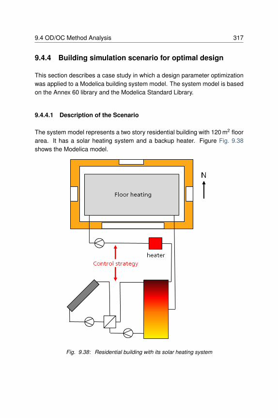
9.4 OD/OC Method Analysis 317

9.4.4 Building simulation scenario for optimal design

This section describes a case study in which a design parameter optimizationwas applied to a Modelica building system model. The system model is basedon the Annex 60 library and the Modelica Standard Library.

9.4.4.1 Description of the Scenario

The system model represents a two story residential building with 120 m2 floorarea. It has a solar heating system and a backup heater. Figure Fig. 9.38shows the Modelica model.

Fig. 9.38: Residential building with its solar heating system

318 Activity 2.1: Design of Building Systems

The simulation model has to be fast because the parameter optimization canrequire hundreds of simulations.

The scenario is specified with following aspects:

9.4.4.2 Climate Locations

Two locations are used, San Francisco (relative warm climate during the heat-ing period) and Chicago (very cold climate during the heating period).

9.4.4.3 User Behavior

A mean air change rate of 0.5 1/h is assumed. The air temperature setpointprofile for heating is 20°C. Internal heat sources are considered with a specificmean value of 3 W/m2. 50 percent is convective, and 50 percent is radiative.

9.4.4.4 Building Geometry and Thermal Properties

The building is a single family house with 120 m2 floor space. It has two iden-tical stories and a flat roof as shown in Fig. 9.39.

The total thickness of the external walls in the reference case is 0.3 m, also forthe base plate and the ceiling between the two stories. All inner walls have athickness of 0.2 m. The roof thickness is 0.4 m.

The windows in the south façade have a width of 3 m and a height of 1.4 m. Allthe other facades (east, west, north) have windows with a smaller size of 1 mwidth and 1.4 m height. The height of the sill of all windows is 0.6 m. Becauseit is a theoretical model, doors are neglected. All rooms have the same size of15 m2.

The materials listed in Table 9.3 were used for the specification of the opaquebuilding elements.

This leads to the U-values shown in Table 9.4.

For the windows, the mean U-value of the panes and frame of the window is1.0 W/(m2K) and the g-value for perpendicular irradiation is 0.6.

9.4 OD/OC Method Analysis 319

Fig. 9.39: Geometry of the two stories residential building

Table 9.3: Materials of the opaque building elements.

Material ρ [kg/m3] c [J/(kg K)] λ [W/(m K)]Concrete 2,000 1,000 1.35Insulation 30,0 1,000 0.04Gravel 1,800 1,000 0.7

320 Activity 2.1: Design of Building Systems

Table 9.4: U-values of the opaque building elements.

Construction U [W/(m2 K)] LayersExternal walls 0.35 20 cm concrete, 10 cm insulationFloor 0.35 20 cm concrete, 10 cm insulationRoof 0.34 20 cm concrete, 10 cm insulation, 10 cm

gravelInnerconstructions

3.14 20 cm concrete

9.4.4.5 Energy Supply System

The energy supply system consists of a warm water heating system with floorheating. An additional solar thermal plant with a fixed azimuth angle of 0°andtilt angle of 30° generates thermal energy, which is fed into a solar storage.The specific mass flow rate through the solar collector field is 40 kg/(m2 h).

The return flow of the heating loop is warmed up by the solar storage. If nec-essary, the backup system (heater) adds thermal energy to obtain the supplywater temperature set point of 45°C.

9.4.4.6 Control System

The solar loop is controlled by a simple on/off controller. If the output temper-ature of the collector is 4 K above the temperature in the lowest layer of thesolar storage, and the temperature is under 100 °C (in order to avoid boiling),then the solar pump is switched on until the temperature difference falls under1 K. For the space heating, a two-way valve adjusts the water flow rate.

9.4.4.7 Implementation and Parametrization of the Scenario in Modelica

An implementation of the scenario, based on the Annex 60 library, the Model-ica standard library and two models of the BuildingSystems library (a collectormodel and storage model, which are not present in the Annex 60 library) wasrealized. Fig. 9.40 shows the system model.

9.4 OD/OC Method Analysis 321

Fig. 9.40: Modelica model of the scenario.

322 Activity 2.1: Design of Building Systems

The parameterization of the low-order building model was performed using theTEASER tool (https://github.com/RWTH-EBC/TEASER).

9.4.4.8 Optimization Problem

The following parameters were varied during the optimization:

• The thickness of the insulation of the exterior walls (from 6 cm to 30 cm),• the volume of the solar storage (from 1 m3 to 40 m3), and• the collector area (from 1 m2 to 40 m2).

The cost function consisted of components for labor and material costs forthe insulation Cins, component and installment costs for the thermal collectorsCcol , component cost for the solar storage Csol and energy cost for the neededbackup energy Cbac . An additional penalty factor Cpen considers a desiredsolar covering rate of the solar heating system:

Cf = Ccol + Csto + Cins + Chea + Cpen,

where

Ccol =200 Acol

τcol,

Csto =1649.81 V−0.464

sto Vsto

τsto

,

Cins =Aext (2.431 dins 100.0 + 87.35)

τins

,

Cbac = r Qbac ,

and

Cpen = p (SFset − SF ),

where τ is the expected life time. Parameter optimizations with a energy pricesr of 8 Euro cent per kWh and a penalty factor p of 0 Euro and 1,500 Euro wereperformed. A desired solar covering rate of SFse = 0.5 was assumed. The lifetime was assumed to be 20 years for the solar collector τcol , 20 years for thesolar storage τsto and 30 years for the insulation τins.

9.4 OD/OC Method Analysis 323

Because the optimization of the solar heating system has to be considered asa seasonal problem, each simulation run was performed over 2 years simula-tion time, where only the second year was evaluated for the cost function. Thesimulation starts from 1st of July with a start temperature for the solar storageof 60°C for the entire water volume. All optimization runs were initialized withan insulation thickness of 0.1 m, a solar collector area of 20 m2 and a volumeof the solar storage of 10 m3.

The optimization problem was solved with GenOpt, using the Particle Swarmalgorithm in combination with the General Pattern Search algorithm. Dymola2017 was used to evaluate the cost function.

9.4.4.9 Optimization Results

The colder climate of Chicago leads to a larger insulation thickness of 15 to 20cm in comparison to San Francisco, where 6 to 7 cm insulation are optimal.If the penalty factor is set to 1,500 Euro, then the thickness of the insulationis increasing at the colder location and decreasing at the warmer location, asshown in Fig. 9.41.

Fig. 9.41: Optimized insulation thickness for Chicago and San Francisco

A pure economic optimization (penalty factor = 0 Euro) leads to a solar cov-erage rate of 8.5 percent for Chicago and 19.6 percent for San Francisco, asshown in Fig. 9.42. With a penalty factor of 1,500 Euro, for both locations thesolar coverage rate is about 50 percent, which minimizes the penalty term.

324 Activity 2.1: Design of Building Systems

Fig. 9.42: Optimized solar coverage rate for Chicago and San Francisco.

The colder climate of Chicago causes a larger collector area than in San Fran-cisco. If the penalty factor set to 1,500 Euro, then the collector area is drasti-cally increased to reach the desired solar coverage rate, as shown in Fig. 9.43.

Fig. 9.43: Optimized volume solar storage for Chicago and San Francisco.

The optimized volume of the solar storage is 1 m3, except for Chicago (about30 m3) if the penalty factor of 1,500 Euro is applied. A seasonal storage of solarenergy from the summer for the heating period with a large storage volume isa precondition to reach the desired solar coverage rate, as shown in Fig. 9.44.

Fig. 9.45 shows that the required backup energy in Chicago is 6 to 8 timeshigher than in San Francisco.

9.4 OD/OC Method Analysis 325

Fig. 9.44: Optimized volume solar storage for Chicago and San Francisco

Fig. 9.45: Optimized thermal energies for Chicago and San Francisco

326 Activity 2.1: Design of Building Systems

9.4.4.10 Computation Time

A single simulation run over two years took 33 seconds. GenOpt requiredbetween 25 minutes and 50 minutes.

9.5 Summary

The nine case studies from seven countries of Activity 2.1 have illustrated thatModelica building libraries are able to cover a wide range of building designand building optimization problems.

The authors of the case studies mentioned the following main advantages ofModelica: First, the modular approach of Modelica enabled them to modelbuilding systems at various levels of detail. Temporal and spatial resolutioncould be increased where needed to address a particular design questionwhile abstracting other parts of the model using simplified equations. Second,Modelica’s object-orientation and encapsulation through standardized connec-tors for heat flow and fluid flow allowed collaborative development in whichsub-models of complex building systems were configured by different mod-elers and subsequently combined to form a system model. Third, missingmodels could be added quickly, either through new implementations, throughcombinations of existing models, or through use of base classes that imple-ment conservation equations. Fourth, models of different domains such asheat transfer, fluid flow, electrical systems and control systems could be com-bined graphically to form an integrated model. The main reported drawback ofModelica was that annual simulations can be time-consuming if detailed HVACmodels are combined with multi-zone building envelop models. This is largelydue to the solvers that are currently implemented in the Modelica simulators.As Modelica is translated to efficient C-code (see Section 5.3.4), this is not aninherent problem of Modelica, but rather a questions of what solvers to useas users simulate ever larger models. To obtain fast simulations, componentparameters have to be adjusted and the right solver and its tolerance haveto be chosen in the Modelica simulation tools [JWH15] . Moreover, detailedcontrol algorithms can slow down the simulations performance, in particular ifthey generate many events. Addressing these problems is an active field ofresearch, see for example Section 5.2.

9.5 Summary 327

Two examples could demonstrate the application of optimal design and opti-mal control problems based on Modelica libraries: A multi-criteria parameteroptimization of PV cooling systems for residential buildings and a non-linearoptimal control problem for the HVAC and facade control in a thermal zone.For the latter, the computer algebra conducted by the Modelica tool when itconstructed the optimization problem, based on the declarative model formu-lation, led to 2,200 times faster optimization compared to a derivative freeoptimization method that simply evaluated the cost function iteratively.

A final building simulation scenario for optimal design summarizes the workof Activity 2.1: A parameter optimization method was exemplary applied to aModelica building system model that couples a solar thermal system to a sim-plified building model. This building system model is almost entirely composedof components from the Annex 60 library and the Modelica standard library. Atwo-year simulation of this model took half a minute. Two optimization variantsthat optimize life cycle cost using weather data for a moderate climate and avery cold climate were performed.

328 Activity 2.1: Design of Building Systems

Chapter 10

Activity 2.2: Design of

District Energy Systems

10.1 Introduction

Recent developments to reduce the energy use of buildings focus on the inte-gration of renewables and on energy efficiency. European legislation enforcesthat by 2020 all new buildings are nearly Zero-Energy Buildings (ZEBs) andit requires the deployment of a European Smart Grid. The shift in the energyinfrastructure leads to new requirements and technical challenges as the inter-action of buildings becomes increasingly important. To quantify the requiredinteraction among buildings and the grid, as well as the restrictions causedby the existing neighborhood topologies and grid configurations, an integratedmodeling environment is needed. This activity focuses on the use, verificationand demonstration of Modelica libraries from Activity 1.1 and co-simulationtools for multi-scale simulation from Activity 1.2 to assess District Energy Sys-tems (DES). The focus of this activity extends the traditional focus on individualbuilding performance to DES. The analysis of these systems requires an in-tegrated simulation platform that is capable of simulating simultaneously theenergy demand of multiple buildings, the thermal and electrical energy distri-bution grids and the control systems.

330 Activity 2.2: Design of District Energy Systems

The work that was carried out in this activity consisted of three main parts:

1. A literature study focusing on the modeling of DES2. The development of a common exercise to model DES within Modelica

environments3. The use of co-simulation techniques to model DES

Section 10.2 presents a description of the main components typically found inDES. Section 10.3 addresses the modeling of multi-scale energy flows in dis-tricts and presents an overview of simulation tools and environments to modelthese systems. The overview discusses both Modelica and non-Modelica im-plementations. Section 10.4 reports on the common exercise that has beenset up to analyze the capabilities of the current Modelica libraries of the Annex60 participants and provides a first step to develop a comparative model valida-tion test for district energy simulations: a DESTEST. In this exercise, a relevantsimulation case (including building definition, occupant behavior, grid definitionetc.) is developed for two purposes. Firstly, the set can be used to analyze rel-evant research problems such as how to design district heating systems andhow to integrate renewables in districts. Secondly, the information and chal-lenges gathered during the development will be used for setting up a frame-work to test District Energy System simulation tools. Although the simulationof DES within one software environment has many advantages and makes it adesired solution, scalability of the numerical methods to large models are stilla challenge if one solver is used for the whole system of equations. Therefore,in Section 10.6, the opportunities and threads for co-simulation techniquesrelated to DES simulation are analyzed. Finally, Section 10.7 presents conclu-sions and perspectives.

10.2 Description of District Energy Systems

A DES comprises all components that enable the delivery of energy servicesin a district. This typically includes electricity, gas, heat or cool, possibly at cas-cading temperature levels. However, in this section, modeling of gas networksare not discussed.

10.2 Description of District Energy Systems 331

10.2.1 Electrical Versus Thermal Energy

Although the generation of electrical and thermal power have always beenclosely related, at least in power plants relying on combustion, their respec-tive carrier grids have experienced a separate evolution. Fig. 10.1 shows anoverview of commonly used technologies and their respective energy sources.

Fig. 10.1: Overview of heating technologies and their respective energy sources.

Source [Com16b].

The International Energy Agency reports [Age14] that worldwide, electricityhas the largest final energy consumption by far. Fig. 10.2 shows the producedand consumed annual electric energy and heat worldwide in 2014. However,note that a substantial part of electric energy is also used to meet heatingand cooling demands by use of electric heaters and boilers, heat pumps andchillers. With a trend towards installation of more heat pumps, it can be ex-pected that the electric energy fraction for the building sector will increasecompared to the heat fraction.

The previous section considers all end uses of electricity and heat. When look-ing at the categories of energy use, it can be seen that both forms of energyhave approximately the same fraction of energy use in buildings (consideringresidential and community and public services to correspond to the energydemand of buildings), as can be seen in Fig. 10.3.

332 Activity 2.2: Design of District Energy Systems

Fig. 10.2: Worldwide electricity and heat production and consumption in 2014.

Source: [Age14]

Fig. 10.3: End use fraction of electric and heat energy for different sectors in 2014.

Source [Age14]

10.2 Description of District Energy Systems 333

In the European Union in 2012, 50% of the primary energy use originated frombuilding heating and cooling demand [Com16a] , making it the largest energysector. 18% of the primary energy comes from renewable energy sources.Biomass holds the largest share for heating only, namely 90% of renewableenergy sources. [Com16b] further illustrates the end uses and sources ofheating.

Part of this heating demand is provided through district heating and coolingnetworks. The share of district heating in the residential sector in the EUwas 9% in 2012, and 8% for the industrial sector [Com16b] . For some EUcountries, almost half of the national heat consumption is provided throughdistrict heating (Sweden, Denmark, Lithuania, Estonia and Finland).

On the other hand, district cooling systems are mostly used for office buildings.However, district cooling has not gained the same attention as district heating.This can be derived from the projected potential of both concepts in the EUStrategy for Heating and Cooling [Com16b] and the absence of district coolingin the Heat Roadmap for Europe 2050 [CNP13] . The installed capacity is lessthan 1% of that of district heating systems [Com16b] .

There are more than 150,000 km of pipes in the district heating systems inthe European Union [Com16b] . Denmark and Sweden have the most ex-tended network, followed by Poland and Germany. However, the average sys-tem length varies greatly, signifying a large variation in the number of thermalnetworks in each country versus its size. Looking at the percentage of thepopulation served by district heating systems, the lead is taken by Denmarkand the Baltic states. On the other hand, the final energy use in district heatingis by far, with twice as much energy as the runner-up, the largest in Germany.On a European average, almost half of the demand in district heating systemsis met by dedicated boilers, while 42% comes from CHP installations. Only 5%is currently provided by directly recycling waste heat. Hence, the list of primaryenergy sources is still dominated by natural gas (40%) and coal (29%).

10.2.2 State-Of-The-Art in District Energy Networks

In the 1880s, the first district heating systems were installed, powered bysteam [LWW+14] . In the meantime, district energy technology has evolved

334 Activity 2.2: Design of District Energy Systems

and matured. Three trends can be identified:

• a decreasing supply temperature for heating, and increasing supply tem-perature for cooling,

• a decreasing size and amount of material used for its components, and• an increased share of standardization and prefabricated components.

Extending these evolutions, Lund et al. reason that after three generations ofdistrict heating systems, the next step must be the fourth generation with evenlower heating supply temperatures and an increased focus towards the inte-gration of renewable energy sources. Examples of mainly solar powered DEScan be found a.o. in Canada (Drake Landing Solar Community [SMD+12]) andDenmark (Marstal district heating system [PS13])

The Swiss Competence Center for Energy Research is exploring an even fur-ther step forward with bi-directional thermal networks [SKS15] . Much like theelectrical grid can convey energy both from a centralized generator to a con-sumer and back from a rooftop PV into the grid, a bi-directional thermal net-work uses a single circuit for both heating and cooling. When in net morecooling is needed than heating, the system circulates from a central plant inone direction. When more heating is needed, the system circulates in the op-posite direction. In the case of a balanced system, no water flows through thecentral plant. Thus, in bi-directional systems, buildings can recover heat fromeach other directly.

12°C-20°C (54 F-68 F)

heatpump chiller

building

heatpump chiller

building

heatpump chiller

building

heatpump chiller

building

heatpump chiller

building

heatpump chiller

distributed plant

8°C-16°C (46 F-61 F)

optional modular extension

Flow direction in main pipe

Heating dominated Cooling dominated

distributedplant orstorage

optionalstorage

Fig. 10.4: Bi-directional thermal network.

10.2 Description of District Energy Systems 335

Fig. 10.4 shows an example schematic of a bi-directional thermal network.The plant guarantees that the hot side is kept between 12∘C to 20∘C, whilethe cold side is kept between 8∘C to 16∘C. The system uses near-ambienttemperatures to maximize the efficiency of heat pumps. Unlike earlier gen-erations of district heating, the bi-directional system need not be operated toserve the lowest and highest temperature needs. Rather, each individual build-ing is equipped with heat pumps, allowing to locally boost the temperature upor down to the temperature required by the building. The system has the ben-efit of being modular extensible, allowing adding buildings, heat sources, heatsinks and storage without having to oversize the initial system.

Regarding electrical energy network at the district level, distributed generationby means of PV panels or micro CHP units is becoming more prevalent. How-ever, in the low voltage grid, care must be taken that the voltage stays withinan acceptable range. This becomes increasingly difficult with more distributedgeneration. On the other hand, electrical demand is also expected to go up inthe very near future, with increasingly more air conditioning units, heat pumpsand electric vehicles.

The integration of all these new technologies necessitate smart control strate-gies such as demand response, transactive controls or curtailing PV produc-tion in case of overproduction, in order to guarantee adequate system opera-tion.

10.2.3 Components Typically Encountered in District En-

ergy Systems

Next, we will describe the components that are typically encountered in ther-mal and electrical district energy systems

A general overview of thermal components typically encountered in districtheating and cooling systems is given in [FW13] . Below, a short summary ofcomponents is provided. Models for these components must be available in adistrict energy simulation library.

Pipes transport heat (or cold) from production sites to consumersin the grid.

336 Activity 2.2: Design of District Energy Systems

Substations separate the primary (high pressure) network fromthe secondary (customer) side hydraulically. This is usuallydone by using heat exchangers to contain the consequenceof leakages at the customer side.

Control valves regulate mass flows in different parts of the net-work. They regulate the flow that each customer receivesand the bypass from the supply to the return pipe. The goalis to maintain the correct temperature in all parts of the net-work: high enough supply temperature, and a return temper-ature that is as low as possible [GW14] .

Buffer tanks store hot or chilled water for later use and hencelimit peak power.

Long term storage allows shifting energy for a long-time, usuallyseasonally. They include borehole fields or acquifers.

Pumps and pressurization provide a pressure difference suchthat the water flows from the supply to the return side. Forhigh temperature networks, they also prevent the water fromboiling.

At the heat and cold production side, boilers, combined heat and power units,heat pumps or chillers are encountered. Furthermore, solar thermal boilerscan be used to directly incorporate solar thermal energy.

For the simulation of electrical consumption in DES, typically only the low volt-age grid is considered. Power from the high voltage grid is usually assumedto be available, but local power injection from decentralized production suchas photovoltaics is possible. Hence, the components needed for electricalsimulations are distribution lines (3-phases and neutral), transformers, powerconverters such as rectifiers, inverters and DC/DC converters, batteries, andPV panels.

10.2.4 Energy Demand

We will now characterize the thermal and electical energy demand.

The thermal energy demand consists of the demand for domestic hot water(DHW), space heating, process heat and cooling. The conditioning of indoor

10.2 Description of District Energy Systems 337

spaces can be provided with a large variety of systems, such as convectors,radiators, variable or constant air volume units, radiant ceilings and floors. Thechoice of the emission system determines the temperature at which the heator cold is required.

The energy demand is largely determined by three aspects: the occupants,the weather conditions and the building characteristics.

Occupants influence the energy demand in the following ways:

• Desired temperature set point or comfort band in the heated and cooledspaces.

• Internal gains directly from occupants.• Internal gains from appliances used by occupants (e.g., cooking, light-

ing, electronic devices).• Domestic hot water demand.

These processes are characterized by high levels of uncertainty. One wayto cope with this uncertainty is to model the energy demand stochastically.A software tool to calculate these uncertainties is presented by Baetens andSaelens [BS15] .

The weather conditions outside of the modeled buildings determine the heat-ing or cooling demand. Here, mostly solar irradiation and ambient tempera-tures are prevalent influence factors.

Related to this, the building characteristics such as the level of insulation, as-pect ratio and building orientation determine how large the influence from theaforementioned weather conditions on the indoor climate is.

Electricity is needed for lighting and for powering home appliances. It can alsobe used to power thermal systems, such as heat pumps, cooling machines (airconditioning) or electric heating. Furthermore, electricity is needed to powerpumps in the different parts of a thermal network and fans in the ventilationsystems. Moreover, electrical cars cause an additional load but also an oppor-tunity for electrical storage.

338 Activity 2.2: Design of District Energy Systems

10.3 Modeling of District Heating and Cooling Sys-

tems

10.3.1 Introduction

DES models can be distinguished between physical domains, geographicscales and time scales.

Various modeling tools for DES exist. Many of the existing tools have limitedsupport for modeling integrated energy systems. In tools that have detailedbuilding and HVAC models, the study of electricity systems is idealized, oftennot allowing to assess the impact of renewable generation on the voltage sta-bility. Other tools focus on medium or high voltage grids, but use simplifiedbuilding and HVAC models for a very high number of households, sometimesnot allowing to determine the required temperature levels.

Fig. 10.5 compares time scales and simulation objectives for district heatingand cooling systems. Simulation can be used for time range of seconds forassessing water hammer effects to years for network design and investmentplanning.

Fig. 10.5: Time considerations depending on the focus of the study.

10.3 Modeling of District Heating and Cooling Systems 339

10.3.2 Modeling Methodology

Modeling and simulation of district energy systems must cover different lev-els of detail and a large application range from components sizing to networktopology design. In this section, a generic methodology for modeling a largescale system is presented in order to assess performances of DES, such asenergy demand or efficiency as well as operational and control strategies.Three main steps can be highlight:

Grid and network modeling. The grid topology provided by the operatoris aggregated and modeled into the simulation tool. The dynamic thermo-hydraulic behavior of a grid model is carried out with numerical models of thesimplified and/or aggregated DES. Grid models include the implementation ofthe grid topology and pipe models.

Occupancy modeling. In the residential sector, customers needs consist ofa combination of space heating or cooling, domestic hot water and electricaldemand. Space heating or cooling can be based on models parametrizedwith physical properties of the buildings or regression functions on the basis ofmonitoring data. Electrical and domestic hot water demand are usually derivedfrom statistical models.

More details on the determination of typical load profiles can be found in Sec-tion 10.2.4. Internal heat gains are deduced from occupancy profiles and ac-tivity probability functions. Process heat demand for industrial usage and/orfor absorption chillers can be considered, but is not covered in this section.

Supply modeling. Heat plants and decentralized production are identifiedbased on data provided by the grid operator and technical specifications. Op-erational strategies and control need to be implemented to balance energyand meet specifications.

Fig. 10.6 shows a schematic of all components to be modeled and how theyinteract.

In order to facilitate both the process of modeling and the post-processing ofsimulation results, geographic information system (GIS) tools are commonlyused. Detailed descriptions of the single components are reported in the fol-lowing sections.

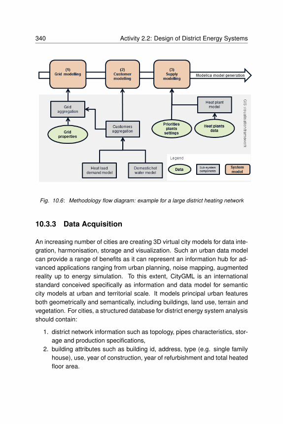
340 Activity 2.2: Design of District Energy Systems

Fig. 10.6: Methodology flow diagram: example for a large district heating network

10.3.3 Data Acquisition

An increasing number of cities are creating 3D virtual city models for data inte-gration, harmonisation, storage and visualization. Such an urban data modelcan provide a range of benefits as it can represent an information hub for ad-vanced applications ranging from urban planning, noise mapping, augmentedreality up to energy simulation. To this extent, CityGML is an internationalstandard conceived specifically as information and data model for semanticcity models at urban and territorial scale. It models principal urban featuresboth geometrically and semantically, including buildings, land use, terrain andvegetation. For cities, a structured database for district energy system analysisshould contain:

1. district network information such as topology, pipes characteristics, stor-age and production specifications,

2. building attributes such as building id, address, type (e.g. single familyhouse), use, year of construction, year of refurbishment and total heatedfloor area.

10.3 Modeling of District Heating and Cooling Systems 341

Relevant parameters therefore can be extracted from the city model and ag-gregated to construct a district energy model.

10.3.4 Problems and Challenges

As part of any modeling work, challenges and problems might be encounteredin the whole process, from the digitalization to the final assessment of networkperformance. The following list is the result of an Annex 60 survey in terms ofproblems encountered from the participants in their activities.

One of the main interests in modeling district heating networks is to simulatethe rate of energy transport through the system. This transport is not onlydependent on the water flow through the system, but also on the temperaturelevels in the network. Variations in temperature in a district heating system aremostly due to three phenomena [Pal00] :

• Changes in supply temperature, controlled by a system operator. Thesevariations can be large and fast.

• Return temperature changes due to heat or cold transfer at customersubstations. These variations are usually rather slow, but fast variationsdue to domestic hot water preparation are possible.

• Heat transfer between the pipes and their environment.

Temperature drops due to heat loss or infiltration in pipes are quite stable.However, the changes in supply and return temperatures affect the transientheat losses and the heat storage in the pipes. Heat losses represent the mainsource of energy losses in high temperature district heating systems. For thelatest generation of district heating systems, due to the low supply tempera-tures, friction losses gain an increasing importance in the overall energy losses[LS12] .

There is an important difference between flow and temperature dynamics[FW13] . Changes in the flow are quickly transferred to the whole networkin form of pressure waves, typically in matter of seconds. Changes in temper-ature, however, are transferred relatively slowly, in relation to changes in theflow. Thus, the response time from a production plant to a consumer station,with respect to temperature changes, can be up to several hours.

342 Activity 2.2: Design of District Energy Systems

Bi-directional thermal networks require a higher level of physics modeling ca-pability than previous generations of district heating and cooling systems. Be-cause the fluid flow direction can, and likely will, reverse, the associated dy-namics need to be captured. This is difficult to accomplish in existing buildingsimulation programs as they are not designed to handle situations where theflow direction changes [KK12][KKG+14][KSS15] . In contrast, the Modelicastream connector [FCO+09a] is designed to handle flow reversal, and doesso in a numerically efficient way. Also, the thermal capacity and location ofpipes should be accounted for, in particular if the flow reverses for a few hoursdaily in which case energy storage in the pipes can become important. Also,the accuracy of modeled system temperatures is more important when heatexchangers are designed to operate over changes of only a few Kelvin. Aninaccuracy of 1-2 K could result in a different flow direction and large error inanalysing the potential for waste heat recuperation or free cooling potential.The decentralized controls associated with directing flow at junctions, choos-ing temperature set points, and turning distributed generators on/off are muchmore intricate than with centralized, uni-directional systems. Furthermore, be-cause the thermal distribution losses are low and the energy input for the heatpumps is low compared to that for a natural gas-fired boiler, the relative impor-tance of flow friction and associated energy use of pumps and fans are moresignificant.

10.3.5 District Heating and Cooling Modeling Approaches

10.3.5.1 State of the Art

There are two basis methods used for dynamic modeling of district heatingnetworks [LPBhmR02] :

1. Physical models that model the physical structure and behavior of thesystem, and

2. statistical models that use a statistical black-box approach.

Typically, only the energy equations are modeled dynamically, while the pres-sure and momentum equations are simplified as steady-state.

10.3 Modeling of District Heating and Cooling Systems 343

10.3.5.2 Physical Models for District Heating and Cooling Systems

Physical models represent the physical relations among subsystems. All theimportant components in a district heating network are explicitly modeled, andthe whole structure of the system is taken into account. It is easy to changeand add components to an existing model.

Based on the physical approach, Zhao [Zha95] and Benonysson [Ben91] com-pared methods for quasi- dynamic modeling of district heating networks, whichare referred to as the element method and the node method. The elementmethod was found to be inferior to the node method, both with respect to ac-curacy and computational cost. On the other hand, the node method doesnot exhibit difficulties due to numerical diffusion. Although the node methodhas been found to be faster and more accurate in some cases, the elementmethod seems to be more frequently applied in practice [BhmHK+02] .

Next, we will describe the element method and the node method.

In the element method, computations are based on a temperature profile alongthe pipe. The pipe is divided into a number of elements in the axial direction.Each element is typically divided into four sections for the water, the steel pipe,the insulation materials and the cylinder of ground surrounding the buried pipe.Radial heat transfer is computed by assuming a single uniform temperature inthe water and the steel, and uniform temperatures are assumed in the insula-tion and the a cylinder of soil that surrounds the pipe. In this case, the temper-ature at each time step is determined only from the time step before. Whenusing this method, it is necessary to take the Courant number into account:

Cou =∆T u

∆x

where ∆T is the time step, ∆x is the element length and u is the flow velocity.The Courant number should be less than or equal to one for accurate results.Usually, when the Courant number is equal to one, the model gives the exactresult. Large numerical diffusion occurs as the Courant number approacheszero. Numerical diffusion is an artifact of the discretization, and the effect isas if the medium had a higher diffusivity. The temperature of the steel pipe isassumed to be equal to the water temperature since the thermal conductivityof both materials is relatively large compared to the thermal conductivity of

344 Activity 2.2: Design of District Energy Systems

the insulation and surroundings. Heat conduction in axial direction is usuallyneglected.

In the node method [Ben91] , only the inlet and outlet of the pipe are takeninto account, as opposed to the discretisation in the element method. Theoverall heat transfer coefficient is based on the method of thermal resistances,but the heat transfer between neighbouring pipes is not taken into account.Computations are based on a time history of temperatures and flows, takinginto acount the propagation delay between inlet and outlet for the whole pipe.The thermal capacity of the pipe wall is modelled in an aggregated way foreach pipe segment, while that of the insulation and the surrounding groundis not taken into account. This assumption is justified by the lower thermalcapacity in these regions and the limited temperature variations as a result ofthe lower conductivity of the insulation.

10.3.5.3 Statistical Models for District Heating and Cooling Systems

Statistical models based on time-series or neural networks tend to be com-putationally simpler, but their main drawback is that they have low degree ofaccuracy and many non-physical relationships. In addition, they require theavailability of large amounts of measurements for model estimation and vali-dation [Pal93] .

The classical time-series method depends on the assumption of linearity andstationarity, either in the raw data or as a result of some well defined andinvertible transformation of the raw data. While those assumptions simplifymodeling and enable a coherent use of statistical measures, they also limitthe applicability and place demand on proper pre-processing of data. Further-more, methods based on artificial neural networks can also be used.

10.3.5.4 Modeling of District Electrical Network

An electricity grid consists of different nodes connecting the different gener-ators and loads through cables. For district network application, low-voltage(LV) distribution grids have mostly a radial topology. Thus, there is one feeding

10.3 Modeling of District Heating and Cooling Systems 345

transformer for each set of distribution feeders. In the presence of distributedenergy resources, bi-directional electricity flows are possible.

Redundancy is possible through particular grid topologies, such as ring andmesh topologies. In these topologies, the loads are supplied by more thanone medium voltage distribution grid. In Europe, most LV distribution grids(230/400V) are radial, three-phase grids. In case of a ring or meshed grid, allLV grids are operated in radial configuration.

Different types of grid simulations exist, ranging from electromagnetic toquasy-stationary and steady-state modeling. Electromagnetic effects occurduring events such as when a switch opens or closes or lighting strikes thenetwork. In quasi-stationary models, the frequency is modeled as quasi-stationary, assuming a perfect sine wave with no higher harmonics. Volt-ages and currents are considered as sine waves and just their amplitudesand phase shifts are taken into account during the analysis. With such an as-sumption, electric quantities can be represented with a phasor, i.e., a vector inthe complex plane. A variation to the quasi-stationary models are models withso-called dynamic phasorial representation. The basic idea of the dynamicphasorial representation is to account for dynamic variations of the amplitudeand the angle of the phasors. With such an approach, it is possible to analyzefaster dynamics without directly representing all the electromagnetic effectsand high-order harmonics. For more details, see [SLA99] , [SA00] . In steady-state models, the time derivatives are eliminated.

In electricity grids, the power flow analysis is performed for each node and linebased on the Kirchhoff laws:

1. Kirchhoff’s node rule: the sum of currents flowing into a node is zero.2. Kirchhoff’s loop rule: the directed sum of the potential differences in any

closed loop is zero.

For fully balanced systems, no current flows in the neutral conductor. There-fore, an equivalent single-phase grid can be used to simulate the balancedthree-phase grid.

346 Activity 2.2: Design of District Energy Systems

10.3.6 Applications of Modelica in District Energy System

Modeling

As illustrated in previous chapters, Modelica has often been used for modelingDES, in particular for district heating networks. In this chapter, publicationsare presented which have integrated thermal, electrical and control Modelicamodels for simulation and/or optimization of DES. The use cases demonstratethe capabilities of Modelica for this purpose, while weaknesses are tackled byusing a combination of tools and co-simulation approaches. The majority ofModelica libraries employed in these studies have been introduced in Section5.2.

10.3.6.1 Buildings

Simulation of a DES usually involves numerous buildings that consist of het-erogeneous structures, heating systems, occupancy behavior, etc. First, itintroduces modeling difficulties linked to the data availability, the large numberof sub-components, bias and validity of the final model. Secondly, it introducesscalability issues, related to the simulation time with respect to the number ofbuildings. In that sense, component-based and oriented-object modeling lan-guages such as Modelica offer significant possibilities as the model fidelity canrapidly be changed and the symbolic processor can simplify equations and canprovide analytic derivatives for the numerical solvers.

Several papers propose the use of simplified building models for simulationand optimization of district energy demand, as they can significantly reducethe computation time. Kim et al. [KPHR14] used physical simplifications andmodel order reduction based on detailed Modelica building models to cre-ate simple models for urban energy simulations. The performance of the re-duced models was evaluated for annual and hourly heating and cooling loads,showing satisfactory results. Nytsch-Geusen and Kaul [NGK15] describeda method to simulate district heating and cooling demand for residentialbuildings, combining low-order thermal models from the BuildingSystemsModelica library [NGHLR12] with statistical distribution functions for the build-ing stock characteristics. Lauster et al. [LFT+13] also presented a tool chainfor district heating demand simulation. Typical office building data sets based

10.3 Modeling of District Heating and Cooling Systems 347

on statistical data were used to automatically parametrize simplified dynamicbuilding models implemented in Modelica. The method has been applied tosimulate the energy demand of a research campus, performing well at an ag-gregate scale for annual demand, as compared to measurements. For thispurpose, they later developed adaptive low order building models, to be usedin different levels of required discretization, from single building to districts[LFH+15] . These are also automatically generated making use of statisticaldata. City information models (CIM) and geographical information systems(GIS) have been used to support district energy simulation and optimization.The TEASER tool for automated building heat demand simulations based onGIS-extracted data was developed in RWTH Aachen University. Schiefelbeinet al. [SJL+15] described the development of a CIM, based on TEASER andthe AixLib Modelica library [BM10][FCL+15][RE15] . Fuchs et al. [FTL+16]

presented a tool called uesmodels to automate district energy simulations us-ing Modelica and Python as a workflow automation tool. Previously, a similarapproach was used in [SJD+14] , where a city district database was designedand linked to GIS to enable energy optimization of city districts. An inter-face then automatically generated building models for a simulation environ-ment with Modelica and NEPLAN. The planning tool was verified with GermanSynthetic Load Profiles (SLP) and measurement data. Nouvel et al. [NBK+15]

presented the work of an international collaboration, developing the energyApplication Domain Extension (ADE) for the CityGML information model. ThisADE is used to manage and store data in 3D city models that are related tobuilding energy flows, such as building envelope and energy systems charac-teristics and occupancy. Coccolo et al. [CMK15] showed the connection ofthe CitySim simulation tool to the CityGML urban information model with theEnergy ADE, applied to the EPFL campus.

10.3.6.2 District Heating and Cooling

As explained in Section 10.3.4, the Modelica language allows a higher levelof physics modeling capability, especially for bi-directional thermal network.Moreover, a multi-domain language allows considering flow friction and asso-ciated energy use of pumps and fans, which are important in networks withsmall temperature differences.

In that context, many studies employed Modelica to simulate and analyze dis-

348 Activity 2.2: Design of District Energy Systems

trict heating systems. Basciotti et al. [BSKD14] presented a decision supportmethodology, where substations with different hot water preparation principlesare compared based on several performance indicators. In [BS14] , they in-vestigated demand and supply-side measures to reduce peak loads in thenetwork. They found large consumer load shifting and utilization of the net-work as storage to be the most economic feasible measures. Köfinger et al.[KBS+16] evaluated the feasibility of low-temperature district heating imple-mentations in Austria using four case studies in which the ecological, eco-nomic and energetic performances were assessed. Models based on theModelica.Fluid [COP+06] , Buildings [WHMS08][Wet09][WZNP14] ,and the DisHeatLib [BP11] libraries were used in the above studies.

Giraud et al. [GBP+15] assessed control strategies to reduce distributionlosses in a virtual district heating network for which they developed and vali-dated Modelica models. A 10% loss reduction was achieved using a dynamicsupply temperature algorithm instead of a fixed heating curve. Based on low-order AixLib building models and the Modelica Standard Library (MSL) pipemodels, Fuchs et al. [FDT+13] evaluated the impact of building retrofit onsupply and return flows of a small network branch. They argue that benefitsfrom building retrofit should be evaluated taking into account also the posi-tive impact at the district level. In [RTFC+15] , Modelica was used to simu-late and assess potential benefits of seasonal aquifer thermal energy storagein the district heating system of a university campus in Germany, showingpromising results. Low-order building models from BuildingSystems li-brary, Annex60 library, Buildings, MSL and own models were used. Ljubi-jankic et al. [LNGU09] described the application of the FluidFlow Modelicalibrary to design a heating and cooling energy supply system in a newly builtresidential area in Iran. This library was specifically developed to simulate thethermo-hydraulic behavior of complex energy systems. Giraud et al. presenta comparison of Modelica with TRNSYS for a solar district heating system[GPB15] .

The advantage of Modelica as a modeling language has been illustratedin several applications. Burhenne et al. [BWE+13] reviewed Modelica li-braries and demonstrated their capabilities for building performance simulationthrough examples. Simulations of the building envelope, HVAC system or anentire district heating system were shown, and also co-simulation cases wereexplored. In the district heating simulation example, the authors compared

10.3 Modeling of District Heating and Cooling Systems 349

heat losses for different supply strategies. Schwan et al. [SULK14] demon-strated the use of the Modelica GreenBuildings library [USM+12] for dis-trict energy system simulations, in an example historical town center. Soonset al. [STHS14] modeled a biogas-powered low-temperature district heatingsystem with and without thermal energy storage for the university campus inEindhoven, illustrating the improved accuracy and level of detail offered byModelica. On a slightly different topic, Casetta et al. [CNB+15] developedmodels for district cooling systems in Modelica, using Buildings, MSL andown models. They performed a scenario analysis varying the secondary returntemperature of the substations in a simple district cooling network.

Modelica tools also allow the export of models using the FMI standard for sub-sequent co-simulation with other tools, as described in Section 6. Huber andNytsch-Geusen [HNG11] described the different possible approaches in mod-eling urban districts. They presented a use case in which a large urban areais modeled, combining EnergyPlus for thermal building simulations with a de-tailed plant and distribution network in Modelica, coupled within the BuildingControls Virtual Test Bed (BCVTB) [Wet11a] . Elci et al. [ENKH13] also com-bined Modelica with other software. They presented a district heating casestudy in which the influence of demand change due to refurbishment is inves-tigated. The study employed simplified building and district heating models inModelica, and the statistical modeling environment GNU R for heat generationand storage models.

10.3.6.3 Electrical Network

Modelica also provides the possibility to simulate electrical networks. TheIDEAS library [BDCJ+15][Ope15] has been used to study the integration ofheat pumps (HP) and photovoltaic (PV) systems in Belgian residential low-voltage feeders. Baetens et al. [BDCVR+12] simulated the IEEE 34-Node TestFeeder with net zero-energy dwellings, in order to assess electrical challengesat the neighborhood level. It was shown that the dwelling’s self-consumptiondepended significantly on the grid capacity, as PV generation curtailmentwould occur due to voltage rise. For the same feeder, the potential of rule-based Demand Side Management (DSM) on domestic hot water productionwith HP was evaluated, showing promising results [DCBS+14] . To analyzethe impact of low-energy dwellings on a range of feeders, several grid impact

350 Activity 2.2: Design of District Energy Systems

criteria were studied in [BS13][Bae15] , evaluating in particular the requiredgrid reinforcements resulting from grid constraint violations. Protopapadakiet al. [PBS15] further analyzed correlations between grid impact criteria andbuilding and neighborhood properties, finding significant relationships. Fur-thermore, IDEAS was employed in [VR15] , where strategies are evaluated toalleviate the impact of electric vehicles on the distribution grid. For all abovestudies, buildings, thermal systems, electric vehicles and grid were all simu-lated within the Dymola environment.

Bonvini et al. [BWN14] validated the electrical models of the Buildings

library using the IEEE four nodes test feeder, and subsequently applied themodels to demonstrate how to study the integration and control of renew-able energy sources in an electric distribution grid. Bonvini et al. [BW15]

demonstrated the use of Modelica models for gradient-based optimal controlof batteries and HVAC in an electrical district energy system. Wetter et al.[WBN16] coupled models from the Buildings library for the electrical grid,multiple buildings, HVAC systems and controllers to test a controller that ad-justs building room temperatures and PV inverter reactive power to maintainvoltage quality in the distribution grid. Chatzivasileiadis et al. [CBM+16] ex-ported reduced order building and HVAC models from Modelica as FMUs forco-simulation with the DigSILENT PowerFactory simulator for the low voltagegrid and the OMNeT++ simulator for the communication network.

Several other studies also investigated the interaction of low-carbon tech-nologies with the electrical grid at district level. For example, Schlosser etal. [SSMM14] analyzed the impact of home energy systems including heatpumps, combined heat and power (CHP) and PV, on a typical German low-voltage grid. This study employed models from the AixLib Modelica libraryto determine thermal loads, and network simulations were performed in MAT-POWER. Further, in [SSP+15] they assess the potential of control strategiesin reducing this impact. Even though a small improvement is achieved, addi-tional measures are needed to eliminate the problems. Baggi et al. [BRM+14]

modeled a residential neighborhood to assess voltage instabilities and self-consumption for different penetration levels of photovoltaic and storage systeminto the low voltage grid. They show battery systems can significantly improvegrid stability and self-consumption. In this work, few Modelica libraries werecombined, namely the AC [Hau08] and the ElectricEnergyStorage li-braries [ECK+11] . Elci et al. [EOH+15] demonstrated that a decentralized so-

10.3 Modeling of District Heating and Cooling Systems 351

lar CHP district heating system has better grid-interactivity compared to a con-ventional one, based on a simulation with components from the Buildings

and the internal Modelica library ISELib of Fraunhofer ISE.

10.3.6.4 Control and Optimization

Aertgeerts et al. [ACDCH15] explored co-simulation methods coupling Model-ica with Python to allow optimal control of district energy systems, with promis-ing results showing Model Predictive Control (MPC) outperforming rule-basedcontrol methods. Focusing on optimal control involving both thermal andelectrical domains, Bonvini and Wetter [BW15] presented a tool chain basedon JModelica that allows reusing simulation models from the Buildings

Modelica library to solve optimization problems. They demonstrated that aJModelica-based toolchain is efficient for optimization of optimal control prob-lems with more than 10,000s of variables and that involve both thermal andelectrical domains, nonlinear dynamics and constraints. Velut et al. [VLW+14]

and Runvik et al. [RLV+15] used Modelica models to formulate the eco-nomic dispatch problem for production optimization of district heating systems.Python and JModelica were employed to solve the optimization problems. Withthis method they were able to add physical constraints, which significantly af-fected the optimal control function.

To perform optimization, other approaches utilized co-simulation based on theFunctional Mock-up Interface (FMI) specification, but using simulation toolsother than Modelica. For instance, Zucker et al. [ZJB+16] optimized the op-eration of a district heating plant towards minimization of CO2 emissions byoptimizing the temperature set points of the building. They used a previouslydeveloped co-simulation platform for modeling and simulation of district en-ergy systems with FMI [WMB+15] , and automatically generated EnergyPlusbuilding models from GIS data.

10.3.6.5 Advantages of Using Modelica for District Energy System Sim-

ulation and Optimization

Numerous use cases are available in the literature, some of which are sum-marized above, that use the Modelica language. They cover a large range of

352 Activity 2.2: Design of District Energy Systems

applications and multiple domains, such as building physics, district heatingand cooling, electrical network and control.

The first advantage of using Modelica is the large number of available andwell-tested or validated models or sub-components. This allows a quick andfast aggregation of component-oriented models to build large district energysystem models. Numerous uses cases also highlight Modelica’s potentialto integrate multi-physics models, such as hydraulic, thermal and electricalsub-components. It thus allows testing control strategies and optimization ofa large district energy systems. Moreover, bi-directional fluid flow is one ofthe major advantage of the Modelica language for district heating and coolingsystems, allowing the analysis of complex inter-meshed networks [FCO+09a]

[BP11] . The above literature review also highlighted numerous examples thatinclude analysis and development of controllers. These can readily be im-plemented using formulations based on optimal control, finite state machines,discrete time or continuous time control.

Modelica modeling and simulation environments are compatible with numer-ous external environments. All major Modelica modeling and simulation en-vironments support import and export of FMUs, and they contain applicationprogramming interfaces that allow interaction with the model as the simula-tion progresses. This can be used to tackle scalability issues of large districtenergy systems. In that perspective, a use-case and preliminary results arepresented in the Section 10.6 to assess the potential of co-simulation usingModelica models and FMI export.

10.4 DESTEST

10.4.1 Framework

The modeling exercises in the scope of Activity 2.2 have identified the need fora testing framework for district energy simulation models: a DESTEST. ThisDESTEST aims at providing the structure for a common reference frameworkfor testing models in a district energy simulation context, just like the BESTEST[JN95] does for building simulation models. It also aims to become a bench-mark for academic exercises for technological solutions, modeling or method

10.4 DESTEST 353

assessment. The latter is reflected in the development of the Annex 60 Neigh-

borhood Case that was used to define common exercises for the Activity 2.2participants. This DESTEST framework will encompass a range of tests thatwill need to be completed in order to validate models for district energy sys-tems.

The concept of the framework is based on the ASHRAE 140 standard [JN06]

for building simulation models. Three types of validation are proposed here:

1. Empirical,2. analytic and3. comparative validation,

each of which have their specific advantages and disadvantages. Empiricalvalidation requires measurement data, analytic validation requires test casesfor which an analytic solution can be found, and comparative validation fo-cuses on the relative differences between the results from different models ormodel libraries without knowledge of the true solution. The reason for this divi-sion is the (un)availability of measurement data and validated model equationsdepending for different cases.

The testing starts at the component level, e.g. simple tests of pipes, electricitygrid elements etc. The tests are executed in increasing level of complexity anddetail, building up from static to dynamic cases and from component level tofull system integration.

Focusing on heating and cooling distribution networks, the framework wouldbuild up from component tests such as a pipe. Starting with pressure drop val-idation for a pipe in steady state, levels of complexity can gradually be added,such as temperature drop, changes in mass flow, periods of zero mass flowand mass flow reversal, changes in inlet temperature and thermal capacity ofpipe walls and insulation. In a next step, these components are added in atest grid set-up. At first, this is a purely branching network in a steady state(laminar or turbulent flow), thereafter meshed grids can be considered as wellas dynamic operation. This case would correspond to the Annex 60 Neigh-

borhood Case, which is described in the following section. Lastly, a databasewith measurements from a real district heating (and/or cooling) network couldbe built in order to simulate a realistic case and compare the outcome of thesimulation with real measurements.

354 Activity 2.2: Design of District Energy Systems

Static

simulation

Static thermo-

hydraulic 3

customers

tree network

Static thermo-

hydraulic 3

customers

meshed

network

Laminar flow

test

dp, Tout

Turbulent flow

test

dp, Tout

Laminar flow

test

dp, Tout

Turbulent flow

test

dp, Tout

Dynamic test

Annex 60

Neighborhood

Case

Pipe test

Real case study

test

(Analytical)

(Comparative)

(Empirical)

Simplified

operation

Complex

operational

setting

(90-60) & (50-

30)

From activity

1.1

Linked to

activity 1.1

Complex

operational

setting

(20-10)

Fig. 10.7 : Envisioned testing structure of the DESTEST Framework.

Finally, a range of key performance indicators has to be defined. These can bedivided in different categories. First and foremost, the difference between theresults from different models must be considered. Furthermore, the compu-tational speed and memory needed for initialization and simulation are impor-tant. For the specific case of Modelica, other numerical parameters such asnumber of Jacobian evaluations, eigenvalues, number of states, size of non-linear systems etc. can be compared. It is important that for every test, alimited number of relevant key performance indicators is selected in order notto overcomplicate testing.

10.4.2 Definition of Common Exercise: Reference Annex 60

Neighborhood Case

10.4.2.1 Introduction

Activity 2.2 primarily focuses on evaluating, testing and demonstrating model-ing and simulation approaches developed in Subtask 1. Therefore, the aim ofthis common exercise is to define a reference Annex 60 Neighborhood Case

10.4 DESTEST 355

on which various of these models can be tested. The test case provides anenvironment enabling the analysis of aspects such as the following:

• Interconnection of electrical and thermal grids• Hydraulic balancing• Change from consumers to prosumers: influence of distributed energy

generation• Control strategies: their benefits, impact on consumers, modeling op-

tions• Demand Side Management (DSM): how to use flexibility provided by

thermal networks and storage

The development of the Annex 60 Neighborhood Case, comprises three stepsdescribed below. These steps aim at gradually incorporating features whichare necessary to analyze the identified issues. During the course of Annex 60not all steps were completed. Nevertheless this outline will serve as a guidefor further development of the DESTEST.

In the first step, the description of the Annex 60 Neighborhood Case is elab-orated. Considering the aims of this common exercise, a small neighborhoodis defined, with typical configuration and providing possibilities to implement adistrict heating and electrical network. Buildings include residential dwellingsand an office building, producing various demand profiles resulting from differ-ent use, size, insulation quality and occupancy. Description of a district heat-ing network and an electricity network connecting all buildings is generated aswell. The level of complexity of the simulated energy systems is progressivelyincreased, from individual to collective complex systems.

The second step consists of modeling the behavior of buildings and their in-stallations in the defined neighborhood, where buildings are treated as stand-alone (not coupled). Participants were asked to individually perform this task,freely selecting a building modeling approach, however, within the Modelicaenvironment. Comparison of predefined performance indicators representa-tive for the building energy demand is then carried out. While the main aimof this step is to identify a common library with building models, an additionalaim is to demonstrate the consequences of modeling decisions and to illus-trate the effect of different levels of complexity. By analyzing the results, thelevel of understanding in modeling buildings of all participants levels out, whilecorrections were performed to the developed models.

356 Activity 2.2: Design of District Energy Systems

In the third step, district heating networks were investigated. Participants wereasked to individually model the network, using models and simulation meth-ods developed in other activities. For example, direct integration in Modelicamay be chosen, or use of FMI and co-simulation. Reporting on the differentapproaches taken and modeling difficulties encountered, feedback is given toother activities, while knowledge is shared among participants.

10.4.2.2 Description of the Reference Annex 60 Neighborhood Case

This section provides an overview of the Annex 60 neighborhood case. Adetailed description is available from the reference document at http://www.iea-annex60.org/downloads/Annex60_2_2_ReferenceCaseStudy-v1.0.pdf.

A typical neighborhood is defined including residential buildings and an of-fice building. Mixing of end uses allows studying the potential heat exchangeamong buildings. Since the simultaneity of heating, cooling and electrical de-mand is a determining factor in the design and operation of district energysystems, additionally various insulation levels and stochastic user behaviorare foreseen.

Neighborhood

The reference neighborhood is based on a small set of reference buildingswhich are combined to describe a street section. Five typologies are madefor the building layouts, i.e. a detached (D), a semi-detached (S) and a ter-raced (T) dwelling, an apartment block (A) and an office building (O). Two sub-typologies are made to distinguish between the levels of thermal insulation.The five dwelling typologies and two levels of thermal insulation are combinedinto a street design of 24 buildings as shown in Fig. 10.8. All required pipingand wiring of district systems (for heating, cooling or electricity) are foreseenon a single side of the street as shown in Fig. 10.8, resulting in asymmetricconnections.

Building typology

Detailed plans of all five building typologies are given in the reference docu-ment describing all dimensions and interior subdivisions of the buildings. Suchdetail allows participants to select the number of simulated zones per building.Nonetheless, a minimum of two zones per building is required. Table 10.1

10.4 DESTEST 357

Fig. 10.8: Street layout of the neighborhood with the selected building typologies.

summarizes the main geometric parameters of the reference buildings. Eachof the single-family residential building comprises two sub-topologies to dis-tinguish between two levels of thermal insulation, the first one referring to therequirements of the EPBD 2010 in Flanders, and the second one representingtypical Flemish buildings of the period 1946-1970, both based on the IEE TAB-ULA project typologies. All construction elements are described in detail in thereference document, including material properties, angle-dependent glazingproperties, and airtightness.

Occupancy

Initially, a constant set point temperature of 21∘C for heating is assumed forall zones. There are no internal gains and no requirements for cooling. Thissimplification allows for an easier comparison between models and brings thefocus on the implemented physics. In a next step, it is proposed to refinethis assumption by introducing stochastic user profiles for internal gains, tem-perature set-points, electricity use, etc. All these are provided as input filesfor each building, based on generated profiles from the StROBe package of

358 Activity 2.2: Design of District Energy Systems

Table 10.1: Summary of the main building parameters (entire building for the dwellings

and typical floor for the apartment block and office building, which have a total of 5

floors).

De-tacheddwelling(D)

Semi-detacheddwelling (S)

Terraceddwelling(T)

Apart-mentblock(A)

Officebuild-ing(O)

Usable

floor

area

102.7 100.9 107.5 107.5 107.5 m2

Total

floor

area

185.5 187.8 161.0 161.0 161.0 m2

Heat

loss

area

371.1 3051 219.1 104.6 104.6 m2

Air vol-

ume

451.5 455.1 446.5 435.9 435.9 m3

10.4 DESTEST 359

openIDEAS [BDCJ+15] .

Space heating, hot water and ventilation systems

For the second step of this exercise, the energy demand is compared. Individ-ual and ideal heating systems are assumed. State #1 residential buildings areheated by an air-to-water heat pump, while state #2 buildings are heated bya condensing gas boiler. There are no cooling systems installed in residentialbuildings. In the office building, the cooling load is covered by an air-cooledchiller and the heating load by a condensing gas boiler. The same simulationmodel of the condensing boiler is used for both residential and office buildings.Initially, the distribution and emission systems are not simulated. The con-densing boiler, the heat pumps and the chiller are assumed to provide waterat respectively 50∘C, 40∘C and 7∘C. Nominal operation conditions for thesesystems are provided in the reference document, together with look-up tablesfor boiler efficiencies for the initial stages.

Reference district heating network

The district heating network topology considers the pipes for supply and returnon a single side of the street, as shown in Fig. 10.8, buried at a depth of 1 m.The pipes are buried directly in the ground. Three different scenarios havebeen considered, using different supply/return temperatures, namely:

• Scenario 90-60 has 90∘C supply temperature and 60∘C return temper-ature.

• Scenario 50-30 has 50∘C supply temperature and 30∘C return temper-ature.

• Scenario 20-10 has 20∘C supply temperature and 10∘C return temper-ature.

The pipeline distances between two nodes and the nominal diameter per sce-nario are specified, as are the insulation properties of the pipeline. The posi-tion of the main heat plant has to be considered at node 0. The temperaturelevel of the different scenarios refers to the supply temperature at node 0 andthe return temperatures at the costumers’ nodes. The DH design takes intoaccount the maximum heat load requirements based on the space heating de-mand simulated in the previous steps, assuming a maximum velocity in thepipes of 1.1 m/s.

360 Activity 2.2: Design of District Energy Systems

The supply model can be initially considered as an ideal source supplyingunlimited mass flow rate at 90/50/20∘C respectively for the three scenarios.Therefore, an ideal pump is supposed to be installed, providing at any timestep the required mass flow rate (no worst-point control on the pressure dropis considered).

Ground properties

The pipeline is assumed to be buried directly in the ground at 1 m depth. Inorder to calculate the ground temperature for the heat distribution losses of thepipe model, any ground model can be used. Ground properties and relatedassumptions are provided for uniform results among participants.

Substation design

Each substation contains a valve to control the water flow from the DH networkand a heat exchanger between the primary loop (DH side) and the secondaryloop (building side). The valve is controlled in order to meet the heat demandof the building and to maintain a low return temperature on the DH networkside. The latter is the most important criterion in limiting the water flow andambient heat losses in the DH network.

To model the heat exchanger, it is proposed to impose a constant heat transfervalue (UA), to neglect the thermal inertia of the heat exchanger and to neglectthe heat losses of the heat exchanger to the ambient. A set of equations todescribe the substations is given in the reference document, resulting from theprevious assumptions, as well as a proposed method to identify the parame-ters of each substation.

Demand

Participants not modeling the buildings in detail may use the provided heatingdemand profiles for the district heating simulation. The profiles were generatedfrom detailed building simulations implemented at the KU Leuven, using thispresent description and the IDEAS Modelica library [BDCJ+15] .

Model performance criteria

The developed models should be able to simulate a typical annual behaviorof the buildings or district heating network. Depending on the models andsimulators, not all performance criteria may be available. As a common base,we define the hourly data as the actual value at the beginning of the hour, and

10.4 DESTEST 361

the hourly maximum (or minimum) as the maximum value of the above hourlydata. The following model performance criteria should be evaluated.

Energy demand and energy use

The energy demand is the energy required by the building to achieve the setpoints regardless of the heating or cooling system. The energy use of thebuilding takes into account the efficiency of the heating cooling system includ-ing conversion efficiency, control efficiency, emission efficiency and distribu-tion efficiency. Initially, predefined system efficiencies are used for calculationof the energy use. The following information is required for model comparison,ideally at an hourly basis:

• Total and peak heating and cooling energy requirements of individualbuildings and aggregated.

• Overall average system efficiency for each building.

Thermal behavior

The buildings are simulated in two ways: free floating temperature and withheating and cooling system. For both simulations, peak (maximum and min-imum) and average temperatures are compared per dwelling. Ideally, hourlytemperature profiles of each building for the free floating case will be available,to allow an additional analysis of the temperature rise and decrease.

District heating network

The following information should be provided:

• Minimum and maximum heat distribution losses• Total energy for the heat distribution losses• Minimum and maximum pressure drop• Total ideal pumping energy

Production plant

The following information should be provided:

• Minimum, maximum and average mass flow rate• Minimum, maximum and average return temperature• Peak production• Total energy production

362 Activity 2.2: Design of District Energy Systems

LV distribution grid

Grid cable parameters

Three different grid strengths will be examined, denoted by strong feeder, mod-erate feeder and weak feeder. The nominal cross-section area of the cables isgiven in the reference document for all lines and each grid strength. For strongfeeders 120 mm2 cable is proposed for the entire grid; for the moderate 120mm2 for line 0-16 and 95 mm2 for the branch J-24; and for the weak grid 95mm2 for 0-16 and 70 mm2 for J-24 (see diagram Fig. 10.8). In practice, cablessmaller than 70 mm2 are rarely used.

The lengths of the cables between the LV distribution grid and buildings areshown in Fig. 10.8. The size of these cables is as follows:

• Single-family building (D/S/T): 16 mm2;• Apartment building (A): 35 mm2;• Office building (O): 50 mm2.

The cable parameters are based upon the IDEAS library [BDCJ+15] and aregiven in the reference document.

Transformer parameters

Transformers are modeled with identical phase impedances for all threephases. The parameters are given in the reference document. For the strongand moderate feeders, a 250 kVA transformer is chosen, while for the weakfeeder, a 160 kVA transformer is selected. This choice may vary depending onthe load profile of the office building, and/or total grid load.

Single/three-phase connection

Buildings may have a single or three-phase connection to the LV distributiongrid. Two options can be assessed:

• All buildings have a three-phase connection leading to balanced condi-tions.

• Buildings have a single or three-phase connection, depending on thepower rating of loads in the building.

In the latter case, all buildings are single-phase connected to the LV distributiongrid, except when the power rating of at least one load (e.g., heat pump or

10.4 DESTEST 363

photovoltaic system) is larger than 5 kVA. This philosophy is taken from theconnection requirements for PV systems in Flanders.

10.4.3 Annex 60 Neighborhood Case: a Comparative Study

10.4.3.1 Introduction

This section presents a comparison of the energy performance results ob-tained from the different approaches taken by activity 2.2 participants to modelthe common district case-study described in Section 10.4.2. The modelers(KUL, TUe, EDF, ULg) used the Modelica language and were given flexibilityto choose their preferred modeling approach regarding model complexity, usedlibraries and components, etc. The aim of the exercise was to first predict theannual heating demand (peak and average) of the district, and then to analyzethe differences in the results obtained by the different participants, evaluatingthe potential influence of their selected modeling approach.

10.4.3.2 Case Description

The Annex 60 Neighborhood Case was defined in Definition of Section 10.4.2.The main information is presented here for reader’s convenience. The neigh-borhood contains five typologies of building, i.e. detached (D), semi-detached(S), terraced dwelling (T), apartment (A) and office (O) building. Two levels ofthermal insulation are taken into account. Level #1 represents the insulationlevel required by the EPB 2010 in Flanders and level #2 represents Flem-ish buildings in 1946-1970 based on the IEE TABULA report [CRHV11] . Fig.10.8 depicts the street layout of the reference neighborhood. Detailed descrip-tion about building layout, dimensions, thermal properties of building envelopeplease refer to case definition.

10.4.3.3 Modeling Approaches using Modelica

The models that constitute the district are based on different Modelica compo-nents libraries. The level of abstraction used to model the buildings and their

364 Activity 2.2: Design of District Energy Systems

sub-division in thermal zones as well as the heat transfer to adjacent buildingswas left up to each of the participants. A constant heating set point of 21∘C

was used for all the buildings and no internal gains or shading were modeled.The assumptions and modeling approach adopted by the participants is sum-marized in Table 10.2.

10.4.3.4 Results and Discussions

Figures 10.9 to 10.15 show the heating demand simulated by the participantsfor the different building typologies in the reference neighborhood. To betterpresent heating demand for each building typology, we divided the results intoa cold and warm season according to the outdoor air temperature from theweather file and the heating set point used. The warm season was definedfrom the first day when the outdoor air temperature was greater than the heat-ing set point to the first day when every hour was lower than the set point. Inthis case, this period goes from the 19th of May to the 10th of October. Thecold season was assumed to be the remaining time of the year.

Figures 10.9 to 10.15 present a comparison of the thermal performance of thedifferent building typologies for the cold season. The apartment block (Fig.10.9) and office building (Fig. 10.10) appear to have similar performance. Thedifferences are only 1.4% on average demand and 0.1% on maximum demandfor the results from TUe. This is mainly due to the similar geometry and ther-mal properties used for both building envelops. Note that internal gains werenot included in the model. The different modeling approaches by the partic-ipants in terms of the number of thermal zones modeled and the heat flowbetween adjacent buildings (Table 10.2) did not create significant differences.However, for other building typologies, significant differences can be observed,especially for the poorly insulated buildings.

One of the reasons for these differences could be the approaches taken tomodel the heating system. Fig. 10.16 shows indoor air temperature in thesemi- detached dwelling S1_1 from ULg and TUe. The results from ULg showroom temperatures varying from 20.4 to 21∘C, with an average of 20.6∘C.From the TUe results, we can observe that room temperature was most of thetime at 21∘C, due to the idealized heating control modeled.

Figures 10.17 and 10.18 show annual heating demand and peak demand per

10.4 DESTEST 365

Table 10.2: Summary of Modeling Approaches

Partici-

pant

TUe EDFR&D

KUL ULg RWTHAACHEN

Li-braries& Ver-sions

Modelica3.2.1Buildings1.6

Modelica3.2.1;BuildSysPro2015.12b

Modelica3.2.1;IDEAS v0.2

Modelica3.2.1;Buildings1.5; Ther-mocycle

Model-ica3.2.1;AixLibv0.3.2

Nb. ofZones

1 per floor(D, T, S); 2per floor(O); 3 perfloor (A)

Mono-zone

1 / floor(unheatedattic ) (D, T,S); 3 perfloor (A,O)

6 (D, T); 5(S); 5 perfloor (A,O)

4 (D, T,S, A,O)

Shad-ing

N N N N N

Heat transfer through adjacent surface

Floor to

Ground

Y Y Y Y Y

to adja-

cent

zones

Y Y Y Y N

to adja-

cent

build-

ing

Y Y N N N

GroundFloorTem-pera-ture(oC)

10.3 10 9+periodiceffect (ISO13370)

10.0 10

WeatherLoca-tion

Uccle, Belgium

366 Activity 2.2: Design of District Energy Systems

Fig. 10.9: Simulated daily heating demand apartments

building of the district. Significant differences can be observed in poorly in-sulated buildings such as buildings 4, 6, 7, 9, 15, 20, 21, 23 and 24. Theseresults are much more sensitive to the complexity and assumptions adopted inthe modeling approach. We can also observe different results for two buildingsof the same typology, as for numbers 17 and 18. The difference in heating de-mand is caused by the way the heat transfer to adjacent buildings is modeled.

Figure 10.19 shows the overall heating demand and peak load from the dif-ferent participants. As for the building analysis on figures 10.17 and 10.18,we can see that KUL and TUe may have underestimated energy needs withrespect to other participants. The results show significant deviations for theoverall yearly heating demand up to 20% from the average and 15% for thepeak heating demand.

In order to further compare the simulated results from different participants,energy signatures for one building representative of each building typology aregenerated and shown in Figures 10.21 to 10.24. The energy signature shows

10.4 DESTEST 367

Fig. 10.10: Simulated daily heating demand for offices

the relationship between the outside air temperature and heating demand fora given building. A linear regression of daily average values was performed forevery building typology.

Taking the energy signature of the detached dwelling (Fig. 10.20) as an exam-ple, the relationship between daily heating demand and daily average outdoortemperature can be observed. This relationship consists of two parts, onewhere it is approximately constant (flat) for all temperatures above the balancetemperature (when the set-point is reached without the need for heating) anda part with certain slope for outdoor temperatures when heating is required.A linear regression for these temperatures above the balance temperature isshown in Fig. 10.21. R-squared for the three regression curves range from0.72 to 0.78.

The energy signatures for all other building types of thermal insulation level 1#are shown in figures 10.22 to 10.24. As depicted from figures 10.9 and 10.10,heating demands in the apartments building (A) and office building (O) havesimilar distributions. As stated before, this is mainly due to not including inter-

368 Activity 2.2: Design of District Energy Systems

Fig. 10.11: Simulated daily heating demand for detached dwellings

nal gains and a similar set point schedule. For this reason, only the energy sig-nature of the apartments building is shown (Fig. 10.22). Only one building pertypology is illustrated, in this case, terraced house no.11 and semi-detachedhouse no.1. The terraced dwellings have the largest observed difference be-tween participants. Both slopes and balanced temperatures vary significantly.This could be explained by the way heat transferred is modeled across adja-cent buildings, since terraced house no.11 has a larger heat transfer surfaceto adjacent buildings compared to its own volume.

In addition, Figures 10.25 to 10.28 show the energy signature generated fromthe simulated data obtained by the participants for buildings with thermal insu-lation level #2. Compared to Fig. 10.20, the linear relationship between dailyheating demand and daily average outdoor temperature is more obvious and,as expected, the balance temperature of poorly insulated buildings is signifi-cantly higher, as shown in Fig. 10.25. The energy signature of each buildingtypology with thermal insulation level #2 are shown in figures 10.26 to 10.28.

10.4 DESTEST 369

Fig. 10.12: Simulated daily heating demand for semi-detached dwellings S1_1

10.4.3.5 Summary and Discussion of the Common Results

Five participants from different institutions modeled and simulated the An-nex 60 Neighborhood Case using different approaches and Modelica libraries.As illustrated and discussed in previous sections, the largest relative differ-ences on heating demand among the participants occurred in poor insulatedbuildings. A preliminary analysis has been conducted to explore the possiblecauses, which can be concluded as follows:

• Relative to the selected modeling approaches, e.g. zoning methods,heat storage for internal partitions, heat transfer through surfaces (fromadjacent zones and buildings), soil temperature, thermal models;

• Relative to the parameters selected, e.g., geometrical dimensions wereprovided as detailed floor plan with thickness of walls. However, model-ers may have used different measuring approaches regarding outside/in-side/center of the walls;

• Undefined inputs, e.g. infiltration rate for non-conditioned zones, thick-

370 Activity 2.2: Design of District Energy Systems

Fig. 10.13: Simulated daily heating demand for semi-detached dwellings S2_7

ness of glass pane and air space.

However, within this project, we could not conclusively determine where thediscrepancies origin from. Therefore, one suggestion for further research is toconduct a systematic evaluation, e.g., a one-at-a-time analysis. It would be in-teresting to additionally perform a sensitivity analysis with respect to the men-tioned parameters. Further evolution of the DESTEST to compare the energyperformance results obtained from different modeling approaches will requirethat the case descriptions avoid ambiguous specification of parameters.

10.4.4 Examples of the Use of the Annex 60 Neighborhood

Case

In this section, we briefly present two examples of the use of Annex 60 Neigh-borhood Case that extends the above performance studies. They were di-rected toward bioclimatic design and retrofit solutions for DHS extension re-

10.4 DESTEST 371

Fig. 10.14: Simulated daily heating demand for terraced dwellings T1_3

spectively. The following results are mainly preliminary and will be furtherdescribed and analyzed in future work.

10.4.4.1 Towards Urban and Bioclimatic Design: Taking the Building

Surroundings into Account

The ANR VALERIE collaborative project (2009-2012) adopted a bioclimaticapproach of building analysis to understand the possible energy exchanges(like infra-red radiation) of the building with its neighbors, shading effects orurban heat island effects [Duf12] . Results showed that current design meth-ods under-use these available resources. Thus, the source of performancebrought by the use of free renewable energy available in the environment ismore significant than “more insulation” for new buildings [CDRR12] . Urbandensification is also a major factor of urban micro climate degradation, andspecialists of urban issues seek more information on the influence of build-ings. In order to study these new research questions, the ANR MERUBBI

372 Activity 2.2: Design of District Energy Systems

Fig. 10.15: Simulated daily heating demand for terraced dwellings T2_4

project (2014-2018) is developing a methodology that takes the urban aspectinto consideration by dealing with the integration of a new building into an ex-isting district.

The new tool chain developed in order to answer these research questions hasbeen applied to the Annex 60 Neighborhood Case. Starting from the commonneighborhood description, the district was modeled using SketchUp. Then, the3D architectural model is transformed into an energy model in two steps. Thefirst one consists of a transformation of the 3D architecture model into a pivotXML file. Then, a Python tool has been developed to translate the gbXML fileinto a building energy model based on the BuildSysPro open-source Modelicalibrary [PKL14] . Raytracing calculations, based on the open-source Embreelibrary [WWB+14] , are used to calculate the form factors in the district, and theamount of direct, diffuse and reflected solar radiation for each surface, as wellas the ground albedo.

At the time of this writing, only preliminary results could be established andanalyzed. These show that, for instance, that certain houses are negatively

10.4 DESTEST 373

Fig. 10.16: Simulated room temperature for semi-detached dwelling S1_1

374 Activity 2.2: Design of District Energy Systems

Fig. 10.17 : Simulated annual heating demand for each building from the different

participants

Fig. 10.18: Simulated annual heating peak load for each building from the different

participants

10.4 DESTEST 375

Fig. 10.19: Overall yearly annual heating demand and peak load on the Annex 60

Neighborhood Case

Fig. 10.20: Relationship of simulated daily heating demand for D1 and outdoor tem-

perature by different participants

376 Activity 2.2: Design of District Energy Systems

Fig. 10.21: Energy signature for building type D1

Fig. 10.22: Energy signature for building type A

10.4 DESTEST 377

Fig. 10.23: Energy signature for building type T1

Fig. 10.24: Energy signature for building type S1

378 Activity 2.2: Design of District Energy Systems

Fig. 10.25: Relationship of simulated daily heating demand for D2 and outdoor tem-

perature by different participants

Fig. 10.26: Energy signature for building type D2

10.4 DESTEST 379

Fig. 10.27 : Energy signature for building type T2

Fig. 10.28: Energy signature for building type S2

380 Activity 2.2: Design of District Energy Systems

impacted by the presence of nearby apartment blocks, showing an increaseof 20% of their heating energy consumption. This preliminary work will bedetailed further when the tool chain of the ANR MERUBBI project is fully vali-dated.

The impact of shadow effects is small for the configuration of the Annex 60Neighborhood Case. Hence, it is not necessarily the best test case to assessthe effect of local micro climate effects. Nevertheless, it was found useful toperform preliminary tests. It however demonstrates that in order to developa meaningful DESTEST, different use cases should be carefully analyzed tomake sure that the developed DESTEST is suitable to assess the analyzedproblem. This example showed that it the development of more than oneneighborhood case description may be necessary to cover the variety of prob-lems that may be encountered and assessed in district energy simulations.

10.4.4.2 Model-Based Assessment of Cost-Effective Retrofit Solutions

for a District Heating System Extension

Numerous research has been conducted on DHS, early examples go as faras the 14th century. However, few studies can be found on the evolution andthe adaptation of older DHS in today’s world. Therefore, the present studyadopted the Annex 60 Neighborhood Case to define a fictional neighborhoodfor the investigation of the long-term adaptability of such an existing DHS. Inparticular, we considered reusing the return water of the existing network toheat a new branch of the DHS, as shown in Fig. 10.29.

The upper part indicates the initial DHS (red and orange pipes), which is di-rectly fed by the heat source. The lower part shows the extension branch to beadded to the initial DHS (orange and blue pipes), which will be fed by the re-turn water of the initial DHS. In this study, some promising retrofit opportunitieswere evaluated on an extended DHS. In particular, the following stand-aloneretrofit measures were applied in the original study :

0. No retrofit measure.1. Retrofit of the envelope of the municipality buildings.2. Decentralized storage in each of the new buildings.3. Centralized storage on the municipality buildings.4. Limitation of the internal set point temperature.

10.4 DESTEST 381

Fig. 10.29: Diagram of the studied district based on the Annex 60 Neighborhood Case.

Red lines represent the supply flow, orange lines the intermediate flow, and blue lines

the return flow. Buildings A2 and O2, in red, are assumed to belong to the municipality.

The curves connecting supply and return lines represent the bypass valves.

382 Activity 2.2: Design of District Energy Systems

Studies were done to compare the results to the new DHS without any retrofitmeasures (solution #0) during the coldest week. Solution #1 allows significantenergy savings, and thus presents better results to extend the network up toa certain point. Installing individual and centralized water tanks (retrofits #2and #3) present a global increase of the energy demand of the DHS. Prelimi-nary results show that, during the peak demand, the DHS is unable to supplyenough heat to the customers, regardless of the retrofit measure. As a conse-quence, during the peak laod, we observe a maximum deviation of 1.12 Kelvinwith respect to the set point temperature.

This study is an example of how the Annex 60 Neighborhood Case has beenused as a case to analyze possibilities for retrofitting of an existing DHS.

10.5 Multi-Physics Simulation of DES in Modelica

This example demonstrates how Modelica allows to couple models of differ-ent physical domains for voltage stabilization of the distribution grid throughdemand response and PV inverter control. The example analyzes both thethermal and electrical dynamics of a small neighborhood with a high PV pene-tration. It requires the coupling of models for building energy simulation, elec-trical system simulation and feedback control loops. The models interact witheach other through the electrical load imposed by the building on the grid, andthe feedback control that adjusts the building room temperature set point andthat increases the reactive power of the PV inverter in case of violation of thepower quality.

Fig. 10.30 shows a net zero energy (NZE) neighborhood. By coupling modelsof buildings, HVAC, electrical systems and controls we can assess the effectof building load onto the electrical grid and assess the efficacy of control mea-sures. The neighborhood contains seven small office buildings. Each buildingrepresents a small office that is part of the EnergyPlus commercial referencebuilding models [DFS+11] . Each model has one floor and is divided into fivethermal zones plus one attic. The floor area of each building is about 500 m2.

The building model comprises four different components, the thermal part,the schedules, the HVAC system and the electrical models. The thermal partaccounts for the heat transfer through the envelope and energy storage in

10.5 Multi-Physics Simulation of DES in Modelica 383

gri

line1line1

line2line2 line3line3 line4line4

line5line5 line6line6 line7line7

vP

line8line8

sen1V

theta

sen7V

theta

sen8V

theta

EWin

I

k=1

ESol

I

k=1

PLoa

ELoa

I

k=1

EProEPro

+

+1

+1

ERatERat

bui1 bui3 bui5 bui7bui2 bui4 bui6

PSol

winSpe

weaDat

weaBus

Σj=1...7 buij.PSol

Σj=1...7 buij.PHvac+buij.PLight+buij.PPlug

sen6V

theta

Fig. 10.30: Neighborhood model with renewable energy sources. The yellow lines

are weather data, green lines are electrical lines, and dashed blue lines are for post-

processing.

building constructions. The schedules represent the building internal loadsdue to occupants, as well as plug loads and lighting systems. The HVACmodel represents the mechanical system and the control loops that maintainthe thermal comfort in the building. The electrical models represent the in-teraction between the building and the electric network. They include an in-ductive load model that represents the electric load of the building and PVpanels. All models are implemented in Modelica using the Buildings li-brary [WZNP14][BWN14] . The thermal model was available as an Energy-Plus model. To integrate it with the rest of the building model, it was automati-cally converted to Modelica. The automatic conversion program leverages theOpenStudio API to identify the thermal zones and the components of the build-ing fabrics. The conversion program converts the models by instantiating andconnecting components of the Modelica Buildings library.

The building electricity consumption is modeled using the inductive load

Pbui (t) = Phvac(t) + Pplug(t) + Plight (t),

Qbui (t) = Pbui (t) tan(φ),

where Pbui (·) is the total active power, Qbui (·) is the total reactive power, φ is thephase angle of the apparent power for the power factor pf , with φ = arccos(pf ),Phvac(·) is the power consumed by the HVAC system, Pplug(·) are the plug loadsand Plight (·) is the lighting power. In addition, the neighborhood has a windturbine that supplements the energy provided by the PVs. TMY3 weather datafor San Francisco, CA, were used. For more information about the electrical

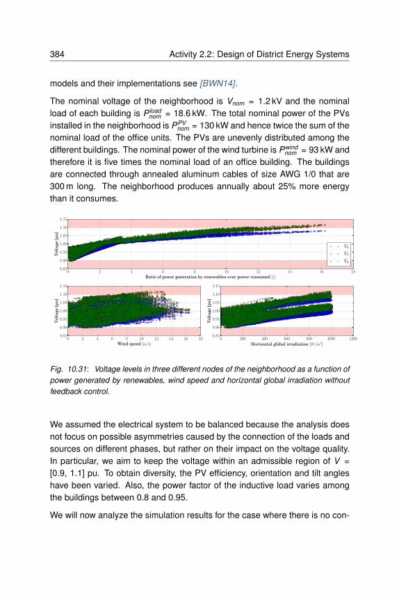
384 Activity 2.2: Design of District Energy Systems

models and their implementations see [BWN14] .

The nominal voltage of the neighborhood is Vnom = 1.2 kV and the nominalload of each building is P load

nom = 18.6 kW. The total nominal power of the PVsinstalled in the neighborhood is PPV

nom = 130 kW and hence twice the sum of thenominal load of the office units. The PVs are unevenly distributed among thedifferent buildings. The nominal power of the wind turbine is Pwind

nom = 93 kW andtherefore it is five times the nominal load of an office building. The buildingsare connected through annealed aluminum cables of size AWG 1/0 that are300 m long. The neighborhood produces annually about 25% more energythan it consumes.

0 2 4 6 8 10 12 14 16 18Ratio of power generation by renewables over power consumed [1]

0.85

0.90

0.95

1.00

1.05

1.10

1.15

Volt

age

[pu

]

V6

V7

V8

0 2 4 6 8 10 12 14 16 18Wind speed [m/s]

0.85

0.90

0.95

1.00

1.05

1.10

1.15

Volt

age

[pu

]

0 200 400 600 800 1000 1200

Horizontal global irradiation [W/m2]

0.85

0.90

0.95

1.00

1.05

1.10

1.15

Volt

age

[pu

]

Fig. 10.31: Voltage levels in three different nodes of the neighborhood as a function of

power generated by renewables, wind speed and horizontal global irradiation without

feedback control.

We assumed the electrical system to be balanced because the analysis doesnot focus on possible asymmetries caused by the connection of the loads andsources on different phases, but rather on their impact on the voltage quality.In particular, we aim to keep the voltage within an admissible region of V =[0.9, 1.1] pu. To obtain diversity, the PV efficiency, orientation and tilt angleshave been varied. Also, the power factor of the inductive load varies amongthe buildings between 0.8 and 0.95.

We will now analyze the simulation results for the case where there is no con-

10.6 Co-Simulation of DES 385

0 2 4 6 8 10 12 14 16 18Ratio of power generation by renewables over power consumed [1]

0.85

0.90

0.95

1.00

1.05

1.10

1.15

Volt

age

[pu

]

V6

V7

V8

Fig. 10.32: Voltage levels in three different nodes of the neighborhood as a function of

power generated by renewables with feedback control that adjust room air temperature

setback and reactive power control at all PV inverters.

trol to ensure that the voltage remains within the admissible region. Fig. 10.31shows how the voltages in three different nodes of the neighborhood vary withrespect to the power generated by the renewables over the power consumed.The lower two plots show the voltage at the three nodes as a function of windspeed and horizontal global irradiation. As expected, the voltage increasesas the power generated by the renewables increases. The highest voltage isV8, measured by the sensor sen8 in Fig. 10.30, which is at the end of theline where the concentration of PVs is higher and where the wind turbine islocated. During 17 hours of the year, the voltage is above or below the admis-sible region of V = [0.9, 1.1] pu.

To keep voltages within the admissible region, we will now add two controlmeasures to the above example. During low voltages, we increase the setpoint temperature of the buildings by 2 Kelvin. During high voltages, we addreactive power at the PV converters [TSBC11] . Fig. 10.33 shows the section ofthe Modelica model that comprises of the building load, the PV, and a reactiveload. Based on the voltage at the PV connection, a feedback controller injectsreactive load in order to not exceed a voltage set point of 1.09 pu. Fig. 10.32shows that this control measure keeps the voltage within the admissible region.

10.6 Co-Simulation of DES

Co-simulation defines a technique that allows simulators to be executed si-multaneously while exchanging data during run-time. It allows a coherentintegration of a decomposed system by assigning a specific solver to each

386 Activity 2.2: Design of District Energy Systems

pv

P

senV

theta

reaPowconPID

PI

gainpuMax

k=1.09

weaBus

term

Voltage sensor

Gain for reactive

power

Control

set point

PI controller Reactive load

PV panel

loaloa

Building load

Connector for

electrical lines

Connector for

weather data

Fig. 10.33: Electrical circuit with reactive power control at the PV inverter.

sub-component. Thus, co-simulation methods can provide a solution to ad-dress performance limitations that may be encountered when simulating theoverall system in one tool. Furthermore, co-simulation allows reuse of domain-specific tools.

In this section, we propose a practical application of co-simulation and toolsdescribed in Section 6, by applying it to a simple DES test case using a limitednumber of dwellings. The model has been implemented using Dymola and theOpenIDEAS library. Neither the electrical grid, the heating systems nor thebuilding envelop as been simplified. The main purpose of this section is thusto propose a proof of concept of co-simulation and highlight advantages, goodpractices and the main drawbacks of such approach for DES.

10.6.1 Modeling for FMU-Based Co-Simulation

To focus on scalability for district energy system simulation, a simple districtmodel using a changing number of buildings has been implemented in Mod-elica and acts as a reference to compare the co-simulation results against.This comparative study involves 3 and 6 dwellings, connected to a low voltage

10.6 Co-Simulation of DES 387

distribution grid. For each dwelling, we consider 2 thermal zones (day andnight zones) and one heat-pump (HP) connected to a 3-phase linear feeder.Occupancy profiles, such as temperature set points, electrical and hot-waterdemands are heterogeneous and derived from a stochastic model [BS15] . Weconsider complex quasi-stationary equations of the grid in order to study theinfluence of the HP demand on the voltage fluctuation [PBS15] . Therefore, weused an output time step of 300 s. An example of 3 grid-connected buildingswith scalar time-dependent connections is presented in Fig. 10.34.

Fig. 10.34: Full simulation test case for 3 grid-connected buildings in Dymola.

Decomposition and graph dependence

Decomposing the model into sub-model for co-simulation is an important ques-tion, but it would be far beyond the subject to discuss theoretical aspects.However, in the scope of DES co-simulation through FMI and Modelica mod-els, some good practices and advice can be highlighted. For more details, seealso Section 6.7. The model decomposition is usually a trade-off between:

• exchange of quantities that vary slowly in order to use a large communi-cation time step,

• decouple equations to make sub-models simpler to solve,• create equivalent-size sub-systems to optimize the CPU usage in case

of parallel computing.

The Modelica language usually make the decomposition straightforward since

388 Activity 2.2: Design of District Energy Systems

it is a component-oriented modeling language that explicitly declares decom-position, inputs and outputs of each sub-components. Moreover, DES typi-cally consist of many similar components that are repeated and linked to eachother. As a consequence, one could consider creating communications be-tween clusters of buildings, buildings or, deeper, between heating systems,thermal envelope, and the network. As a starting point, we consider dwellingsas several FMUs, and the electrical network as another one.

In our case, on the building side, we consider steady state complex voltageas inputs (supplied by the grid) and current as outputs. After defining thedecomposition, one may need to add adapters to convert acausal ports tocausal ports such as shown in the code snippet below. This adapter is thenused to connect buildings to the grid as shown in Fig. 10.34.

model Pin2FMI_current

"Adapts an acausal connector to input/output signals"

import QS = Modelica.Electrical.QuasiStationary;

Modelica.ComplexBlocks.Interfaces.ComplexOutput i;

Modelica.ComplexBlocks.Interfaces.ComplexInput v;

Modelica.Blocks.Interfaces.RealInput freq(start=50);

QS.SinglePhase.Interfaces.PositivePin positivePin;

protected

QS.SinglePhase.Basic.Ground ground;

QS.SinglePhase.Sensors.CurrentSensor iSensor;

QS.SinglePhase.Sources.VariableVoltageSource vSource;

equation

connect(iSensor.y, i);

connect(v, vSource.V);

connect(vSource.f, freq);

connect(vSource.pin_n, ground.pin);

connect(iSensor.pin_n, positivePin);

connect(iSensor.pin_p, vSource.pin_p);

end Pin2FMI_current;

Concerning external resources, on the one hand, weather data should be del-

10.6 Co-Simulation of DES 389

egated to a single FMU because of inconsistency risks. On the other hand,occupancy, hot water demand, and all the dwelling-related data could be im-plemented in the FMU of the associated house. Indeed, those data usuallycome from stochastic modeling [BS15] and logically differs among dwellings.Three possibilities are available:

1. create one FMU data-reader for all the dwellings,2. create one FMU data-reader for each dwelling,3. embed data reading into each FMU-dwellings.

The first solution is straightforward but introduces numerous communicationsthat could affect computation time. Solutions 1 and 2 are not compliant withthe boundary condition management of the used IDEAS library in which theinformation manager is embedded in each building. Therefore, those solutionswould have introduced a lot of structural modifications. Embedded data read-ing in each dwellings implies a specific management of the resources. First,the declaration of all the possible data profiles as resources for each FMUmay lead to increased memory requirements. This solution would lead to loadall available profiles for each dwelling. Secondly, exporting each dwelling us-ing its own data profile path would be a tedious work, and we thus loose thepossibility to change the data profile after the compilation. The solution we de-veloped is to automatically change the resource path during the instantiationof the FMU by casting an integer parameter to the resources’ path as follows:

model GenBui_grid

"General 2-zone building standalone with dynamic resource

→˓path"

[...]

parameter Integer idOcc = 36

"id-number for occupant behavior on external data references

→˓";

inner IDEAS.Occupants.Extern.StrobeInfoManager strobe(

FilNam_P="P/P_"+String(idOcc)+".txt",

filDir = Modelica.Utilities.Files.fullPathName("C:/Data/

→˓Inputs/"));

[...]

390 Activity 2.2: Design of District Energy Systems

In this example, the resource path points to C:/data/Inputs/P/P_36.txt. Thisway, the resulting FMU is still generic, i.e. we can change the data profile bychanging the tunable parameter idOcc and the instantiation of the FMU wouldload only one data profile, limiting the memory usage.

The final model dedicated to co-simulation is then a simple combination ofFMUs. The dependency graph for 3-connected building is shown on Fig.10.35.

Fig. 10.35: Dependency graph of the 3 grid-connected dwellings.

10.6.2 Computational Experiments

We compared six different simulations for 3 and 6 grid-connected dwellings.This gives us an understanding of the scalability of the simulation. The six

10.6 Co-Simulation of DES 391

Table 10.3: Simulations information

Sim. Environment Solver tolerance

‘ref’ Dymola 1 × 10−8

1 Dymola 1 × 10−6

Table 10.4: Co-simulations information

Co-

sim.

Environ-

ment

Solver

tol.

Master

tol.

Communication Time

Step (s)

2 Dymola 1× 10−6 1 × 10−6 603 Dymola 1× 10−6 1 × 10−6 1204 Dymola 1× 10−6 1 × 10−6 3005 Daccosim 1× 10−6 1 × 10−6 120

simulations reflect changing the solver tolerance, the master algorithm toler-ance and the communication time-step in the case of co-simulation. Detailedcharacteristics of all simulations can be found in Tables 10.3 and 10.4.

Note that the simulation number 6 uses the Daccosim environment and parallelcomputing [GVD+15] (see Section 6.5.3). Parallel computing using Dymola forsimulation and co-simulation shows irrelevant results in term of CPU time andis not reported in this analysis. Only fixed time-step communication was usedin the master algorithm.

Table 10.5 shows the results for the 3 grid-connected buildings, including theCPU time, in absolute format for one year simulation (hour/minutes), in relativeformat with respect to the reference simulation and the Mean Absolute Error(MAE) of main physical quantities.

One can see that all the co-simulation results are worse in terms of computa-tion time with respect to the complete simulation with the same tolerance (i.e.simulation no. 1). Moreover, MAE for the current might not be acceptable for300s communication time-step (i.e. simulation no. 4) since it is higher than2%. We noted that the delay on the voltage is determined by the communi-cation time-step, whereas no delay is noted in the output of the current. Thisis due to the master-algorithm itself and might be an issue in the context offast-control and safety, but has no impact on peak or mean values.

392 Activity 2.2: Design of District Energy Systems

Table 10.5: Simulations results for 3 buildings

Sim. CPU Time MAE

(h, min) / ratio Ire Vre

‘ref’ (7, 28)1 0.56 3.12 × 10−3 1.35 × 10−5

2 2.18 5.37 × 10−3 4.10 × 10−5

3 1.28 5.31 × 10−3 6.36 × 10−5

4 0.74 2.04 × 10−2 1.39 × 10−4

5 0.78 5.30 × 10−3 1.01 × 10−4

Note the good accuracy between simulation no. 1 and co-simulation no. 3 and5 on Fig. 10.36.

The results of the 6 grid-connected dwellings are summarized in Table 10.6.Concerning accuracy, the same analysis as the 3-dwellings simulations can bemaid, delay on the voltage and a good accuracy for communication time-stepssmaller than 300s can be observed. As a result in this case, we consider acommunication step higher than 120s not adapted for grid-connected buildingsimulation. However, this value could increase for district heating systems withsmoother dynamics.

In terms of computation time, we observe three main results :

1. Without parallel computing, we note lower simulation times due to theco-simualtion itself. The relative computation time decrease from 1.28 (3grid-connected dwellings) to 0.72 (6 grid-connected dwellings) for simu-lation no. 3. That means that the gain in computation time increases ifthe number of buildings is higher. Although, co-simulation no. 3 still isslower than the equivalent simulation, but the gap is decreasing.

2. Doubling the number of connected dwellings increases the simulationtime by a factor of 3.45 (i.e. simulations no. 1 and 2), whereas for co-simulation, this factor is about 1.9. This indicates that co-simulation ismore scalable and potentially allows increasing the number of buildingsin an easier way.

3. Simulation no. 6, using parallel computing, shows the best result witha relative computation time of 0.37, which is even faster than simulationno. 1 using comparable tolerance. Parallel computing on a two physical

10.6 Co-Simulation of DES 393

Fig. 10.36: Comparison between simulations no. 1, 3 and 5 : Inner temperature,

current and voltage of the building no. 1 for one day.

394 Activity 2.2: Design of District Energy Systems

Table 10.6: Simulations results for 6 buildings

Sim. CPU Time MAE

(d, h, min) / ratio Ire Vre

‘ref’ (1, 1, 49)1 0.56 2.97 × 10−5 5.62 × 10−7

2 1.21 2.84 × 10−3 5.13 × 10−5

3 0.72 3.33 × 10−4 9.26 × 10−5

4 0.41 1.35 × 10−2 2.72 × 10−4

5 0.37 2.72 × 10−4 1.23 × 10−4

core CPU divides the computation time by 1.65 to 1.94 compared to anequivalent co-simulation.

10.6.3 Conclusion and Perspective on Co-Simulation of

DES

Conclusion

This section tackled practical aspect of co-simulation of District Energy Sys-tem using Modelica and FMI decomposition. It involved decomposition andadapting methods for future FMUs and introduced a method to deal with exter-nal data inputs using casting to generate heterogeneous occupancy data andsave memory during the FMU instantiation. To analyze the possibilities thatco-simulation offers, a comparative study involving 3 and 6 grid-connecteddwellings, heterogeneous input data, different communication step-size andtwo environments has been performed. This comparison takes into accountthe quality of the main outputs, to ensure a good accuracy of results, andthe CPU usage. Co-simulation shows a better scalability comparing simula-tions for 3 and 6 buildings since the computation time was proportional to thenumber of buildings if used with a fixed time-step communication master algo-rithm. Moreover, we note a significant time saving using parallel computing.In our experiments, the CPU time was 1.9 faster using a dual-core CPU. Al-though the speed-up cannot be attributed to the co-simulation methods itself,co-simulation generally facilitates the implementation of parallel computing.

10.7 Conclusions and Outlook 395

Perspectives

Co-simulation for DES offers many perspectives. From a methodological pointof view, one could improve the time simulation considering adaptive commu-nication time-steps. In this case, the scalability of the approach might be de-creased. Considering the implementation, parallel computing and an FMUcontaining inner co-simulation and parallel computing schemes, offers goodperspectives in terms of CPU usage and interoperability. From the applicationpoint of view, test case using a higher number of buildings could be consid-ered to assess those results for a larger number of dwellings. The effect ofthe heterogeneity of the structure and the occupancy data profile on the co-simulation performances could be also analyzed for grid-connected dwellingsor other DES.

10.7 Conclusions and Outlook

10.7.1 Conclusion

Activity 2.2 “Design of district energy systems” looked into the use of Modelicaand co-simulation techniques to analyze DES. The activity consisted of mainlythree parts. A first part looked into the existing simulation tools to analyze thebehavior of DES. In the second part a common exercise was set-up to de-velop and test a simple District Energy System and to initiate a framework todevelop a validation test called DESTEST. Finally, in the third part of this ac-tivity, a preliminary assessment of co-simulation techniques for District EnergySimulations was performed.

Section 10.2 gives a description of all components that enable the deliveryof energy services in DES. Because of the research interest of this activity,the focus lies on the modeling of electrical, heating and cooling networks atthe neighborhood scale. The literature review of District Energy Simulationmodels (Section 10.3) focused on Modelica and non-Modelica implementa-tions. It revealed that already many models and tools have been developedfor building and district simulations. These models cover a large range, suchas building physics, district heating and cooling, electrical network and control.As the analysis of DES requires an integrated whole system approach, often

396 Activity 2.2: Design of District Energy Systems

these tools have some drawbacks and shortcomings towards integrated en-ergy system modeling. In many simulation environments, not all domains canbe treated at the required level of detail. The many use cases demonstrate thesuitability of the Modelica approach to model DES. The following advantageshighlight this: numerous available and well-tried models or sub-componentscan be used to build large scale DES models including multi-physics optionsthat are able to take into account specific phenomena such as bi-directionalflows in thermal networks. Modelica is compatible with numerous external sim-ulation environments through FMI exports. The created models can be usedas testbed for controllers and as basis to optimize the design and operation ofDES.

Section 10.4 reports on the common exercise that has been set up to analyzethe capabilities of the Modelica libraries of the Annex 60 participants. It pro-vides a first step to develop a test environment for District Energy Simulations:a DESTEST. A generic Annex 60 Neighborhood Case with 24 buildings wasdeveloped. It includes a mix of residential buildings and an office building. Thedescription includes a full description of the building geometry, properties andoccupant behavior and defined a heating network and an electricity networkconnecting all the buildings in the neighborhood. Five Annex 60 participantsfrom different institutions modeled and simulated the heating demand of theneighborhood, using different approaches and Modelica libraries. Surprisingly,the results of the different participants showed deviations for the overall yearlyheating demand up to 20% from the average and 15% for the peak heating de-mand. Exact identification of the cause of the discrepancies was not possiblewithin the time frame of this project. This demonstrates that the many pos-sible modeling approaches and the implementation by different users, eachwith their own interpretation of the data, indeed may easily result in importantdeviations.

The purpose of the Annex 60 Neighborhood Case is twofold.

1. It serves as a reference case to analyze relevant research problemssuch as how to design district heating systems and how to integraterenewables in districts. This was illustrated with two case studies. A firststudy analyzes to what extent the inclusion of the surroundings in DESsimulations influence the result. For the Annex 60 Neighborhood Case,preliminary results showed that taking into account shadowing effects

10.7 Conclusions and Outlook 397

increased the heating demand of buildings with up to 20%. A secondstudy assessed cost-effective retrofit solutions for a DES extension. Inboth cases, the Annex 60 Neighborhood Case proofed to be useful toexecute the analysis.

2. The information and challenges gathered during the development of theDESTEST will be used for setting up a framework to test District En-ergy System simulation tools. This framework will focus on developingdifferent tests for testing models in a DES context. It also aims to pro-vide benchmarks for academic and industrial analysis for technologicalsolutions, modeling or method assessment.

As an alternative for full Modelica simulations, Section 10.6 analyzed the pos-sibilities that co-simulation of DES using Modelica and FMI decomposition of-fers. It involved model decomposition and introduced a method to deal withexternal data inputs using casting to generate heterogeneous occupancy dataand save memory during the FMU instantiation. By performing a comparativestudy involving 3 and 6 grid-connected dwellings, heterogeneous input data,different communication step-size and two environments, it was shown thatco-simulation shows better scalability. Furthermore, for the tools used, theco-simulation techniques facilitated the implementation of parallel computing,further decreasing the computation time. Finally, the co-simulation case wasan interesting example demonstrating the benefits of the interaction betweenActivities 1.2 and 2.2 of this Annex.

10.7.2 Outlook

The transition towards zero energy buildings and neighborhoods requires aconstant evolution of the tools to design and assess the opportunities andchallenge. Already many simulation environments and models exist to simu-late the system behavior of the different components that DES consist of. Itis expected that this number will rapidly increase and form a comprehensiveframework that can be used to design and assess existing and upcoming DES-technologies in a fully integrated and systematic manner. The massive integra-tion of renewable energy sources and reuse of excess energy from buildingsand industrial processes demands flexibility in terms of supply and demand.Furthermore, different storage technologies should be added to future intelli-

398 Activity 2.2: Design of District Energy Systems

gent energy systems. In order to adequately apply demand side managementtechniques and make use of different energy storage options, state-of-the artcontrollers and algorithms are needed. Future research should look into howto implement these controllers more easily in the simulation environment totest and improve them. Lastly, multi-critria optimization tools should be furtherimproved to facilitate the automated design of DES.

The implementation of data into DES simulation software is often a very elabo-rate and error-prone process. Moreover, the necessary data are often hard tofind or even completely lacking. In short, there is a need for methods to eas-ily implement existing data and reliable data to construct models of existingneighborhoods and to construct representative data sets for a generic anal-ysis. To easily implement real neighborhoods, existing technologies such asBIM and GIS applications have to be further exploited and transformed intoa toolchain capable of an automated generation of neighborhoods models.Especially challenging is finding reliable manners to implement missing data.Once such an automated toolchain is developed, it can be used to statisti-cally analyze many different neighborhoods and even cities to create relevantreference neighborhood cases with statistically realistic behavior which is oneof the aims of the DESTEST framework continuation in IBPSA Project 1. Thequestion however remains how to verify the results of such neighborhood mod-els. Still, only a limited amount of high quality measurement data are availableto perform validation tests. The availability of such a toolchain will facilitatethe development of neighborhood models, but will inevitably further increasethe computation time and raise scalability issues. This emphasizes the impor-tance of further analysis and development of numerical solvers, co-simulationtechniques and parallel computing algorithms.

Chapter 11

Activity 2.3: Model use

During Operation

11.1 Introduction

This chapter provides insights into using Modelica models to solve real-worldproblems in real-time. Three applications are presented in this chapter: Modelpredictive control (MPC); Fault detection and diagnosis (FDD) and Hardware-in-the-Loop (HIL).

11.1.1 Model Predictive Control

Model Predictive Control (MPC) uses a model of a studied system to pre-dict its future evolution. This eliminates many drawbacks of traditional controlapproaches, such as laborious control gain tuning, weak prediction capabil-ity, difficult implementation of supervisory control, and need for re-tuning afteroperating conditions have changed. In addition, MPC is also able to handleconstraints on control inputs and system states [MBH+12] .

400 Activity 2.3: Model use During Operation

11.1.2 Fault Detection and Diagnosis

In general terms, a fault is considered as any issue or state that causes adegradation of performance [RWF05] , even if it is not perceived immediatelyby humans. Detecting a fault is the process by which, using available informa-tion, there is a realization of this degradation of performance. Diagnosing afault is determining the root cause of the degradation of performance [Str08] .Fault Detection and Diagnosis (FDD) is the field within control engineering thatstudies the automated detection and diagnosis of faults [Ise97] .

11.1.3 Hardware in the Loop

Testing and evaluating controller hardware performance is crucial for scalabledeployment of control logics such as load controls and distributed control so-lutions. A Hardware-in-the-loop (HIL) method connects the controller hard-ware with a system model in lieu of the actual system. Therefore, controllerhardware and control strategies (e.g., load control algorithms) can be testedand optimized in conjunction with a real-time emulator that is connected tothe a real controller. Models running on the real-time emulator would repre-sent building or grid energy equipment and systems. This method enables aclosed control loop in a partially virtual system with real controllers.

11.1.4 Overview of Projects that Contributed to the Annex

60 Activity 2.3

Activity 2.3 focuses on the use of Modelica models to augment monitoring,control and fault detection and diagnostics methods. This section presents anoverview of the case studies that contributed to the activity.

11.1 Introduction 401

Table 11.1: Overview of projects participating in Activity 2.3

Area Title Brief description

MPCMPC for energycontrol of un-derground publicspaces - UniversitaPolitecnica DelleMarche, Italy

This case study concerns the SEAM4USEU FP7 project pilot that has been de-ployed in the Passeig de Gracia (PdG)Line 3 metro Station in Barcelona, Spain.The pilot is currently operating, and isaimed at demonstrating the effectivenessof MPC applied to the ventilation, light-ing and passenger movement systemsin underground subway stations. Thedevelopment of the MPC component re-quired modeling the energy dynamics ofthe underground stations. The modelingof the environmental dynamics includedthe passenger flow, ventilation, lightingsystems, and outdoor and indoor ther-mal, fluid and pollutant dynamics.

MPC for heat pumps- KU Leuven, Bel-gium

In this case study, an MPC approach wasdeveloped to optimize the heat produc-tion of two identical heat pumps and agas boiler. The MPC was implementedand tested using the Modelica environ-ment at the headquarters office buildingof 3E, which is located in the center ofBrussels, Belgium.

Continued on next page

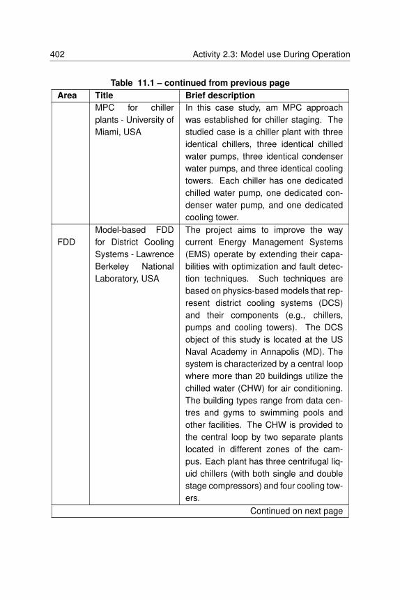
402 Activity 2.3: Model use During Operation

Table 11.1 – continued from previous page

Area Title Brief description

MPC for chillerplants - University ofMiami, USA

In this case study, am MPC approachwas established for chiller staging. Thestudied case is a chiller plant with threeidentical chillers, three identical chilledwater pumps, three identical condenserwater pumps, and three identical coolingtowers. Each chiller has one dedicatedchilled water pump, one dedicated con-denser water pump, and one dedicatedcooling tower.

FDDModel-based FDDfor District CoolingSystems - LawrenceBerkeley NationalLaboratory, USA

The project aims to improve the waycurrent Energy Management Systems(EMS) operate by extending their capa-bilities with optimization and fault detec-tion techniques. Such techniques arebased on physics-based models that rep-resent district cooling systems (DCS)and their components (e.g., chillers,pumps and cooling towers). The DCSobject of this study is located at the USNaval Academy in Annapolis (MD). Thesystem is characterized by a central loopwhere more than 20 buildings utilize thechilled water (CHW) for air conditioning.The building types range from data cen-tres and gyms to swimming pools andother facilities. The CHW is provided tothe central loop by two separate plantslocated in different zones of the cam-pus. Each plant has three centrifugal liq-uid chillers (with both single and doublestage compressors) and four cooling tow-ers.

Continued on next page

11.1 Introduction 403

Table 11.1 – continued from previous page

Area Title Brief description

Fault detectionthrough qualitativemodels of air han-dling unit compo-nents - FraunhoferISE, Germany

For demonstrating fault detection withqualitative models, different faults havebeen simulated with the Modelica faulttriggering library, developed by the Ger-man Aerospace Center. An applica-tion example of a heat exchanger of aHVAC&R system shows the applicabilityof the qualitative modeling approach.

Fault diagnosis us-ing qualitative mod-els of air handlingunits - National Uni-versity of Ireland,Galway, Ireland

This case study, comprises a constant airvolume air handling unit (AHU). The AHUserves a facility consisting of an audiolaboratory of around 50 m2. In this au-dio laboratory, strict conditions of temper-ature and humidity should be maintained.The building is located in Cork city in theRepublic of Ireland.

Quantitiative model-based diagnosis ofAHUs - KU Leuven,Belgium

This case study focuses on the applica-tion of an open and easy to replicate faultdetection and diagnosis method. Themethod was used for component fail-ure detection in an AHU, focusing on aprospective malfunction of the dampers,the heat recovery system and the fans.

Continued on next page

404 Activity 2.3: Model use During Operation

Table 11.1 – continued from previous page

Area Title Brief description

HIL Hardware in-the-loop - University ofAlabama, USA

The study was performed at the inte-grated building energy and control lab-oratory at The University of Alabama,Tuscaloosa, AL, USA. A room servedby a VAV terminal unit is the study ob-ject, where the room and VAV terminalunit are modeled in Modelica and down-loaded to the HIL machine that is con-nected to a real VAV box controller. Theobjective of this case study is to researchdifferent control algorithms including faulttolerant controls for VAV boxes.

11.2 Background on Areas for Model Use During

Operations

11.2.1 Model Predictive Control

A recent review of control for HVAC systems with an emphasis on MPC can befound in [AJS14] . MPC eliminates many drawbacks of conventional control inlarge-scale applications, including difficult parameter tuning, limited predictioncapability, difficult implementation of supervisory control and limited adaptabil-ity to varying operating conditions. From the operational point of view, thefollowing aspects are relevant in the engineering of MPC for energy efficiencyapplications [MBH+12] :

• The selection of the cost function: MPC can minimize for operating cost,energy use, peak demand, greenhouse gas emission, discomfort, etc.

• The decision whether uncertainty should be part of the cost function,which leads to a stochastic MPC problem.

• The handling of thermal comfort: various metrics for thermal comfortmay be used in the cost function, such as the predicted mean vote in[Fan73] , [BKC+12] , [HK14] . Otherwise, other descriptive comfort met-

11.2 Background on Areas for Model Use During Operations 405

rics might be used in a set of linear constraints, such as zone tempera-tures, COtextsubscript{2} concentrations, and relative humidity [ASH04] ,[FOM08] , [KMB11] , [OPJ+10] , [MBH+12] .

• The modeling technology: the three main approaches are detailed mod-eling [HKLF05] , [CHMK10] ; simplified modeling and grey-box models[Bra90] , [KMB11] , [OPJ+10] , [AMH00] , [BM11] [RDS14] , and black boxmodels [CJL06] , [CPV+12] , [LH06a][LH06b] .

• The implementation of the control actions: two major implementationmethods can be found, either computing the control signals in real-time[KMB11] , [OPJ+10] , or using look-up tables for accessing solutions pre-computed off-line [AB09] , [Cof11] , [BKC+12] , [DZMJ11] .

• The implementation technology and, consequently, the development anddeployment framework of the MPC solution. TRNSYS, MATLAB andModelica appear at present time to be the most used tools for developingscalable and site-specific solutions for optimized control. The Modelicalanguage has some key features that provides substantial advantagesover the TRNSYS environments facing the complexity of large non-linearMPC applications [WBN16] , [BWE+13] . A specific MPC library for linearproblems provide integrated control system design in Modelica [HA09] .Modelica models can be directly used in the main MPC loop [IKS08]

unless the size of the model makes it computationally impractical. Inthose cases, they can be used as the data source for model reductionprocesses [BWE+13] .

The design of building models for MPC is not a trivial task. MPC models mustprovide sufficiently accurate predictions of future states, while also being com-putationally efficient for on-site deployment using cost-effective computationalresources. At the same time, MPC models must provide results in a time framecompatible with operational time constraints. Furthermore, MPC models mustbe embedded in systems that, for cost reasons, will not include all of the sens-ing/actuating capabilities desired.

11.2.2 Fault Detection and Diagnosis

Fault detection and diagnosis in building operations can be seen as part ofthe building optimization process. A large amount of energy is wasted be-

406 Activity 2.3: Model use During Operation

cause many HVAC&R systems do not operate as designed [KB05b] , [KB05a] ,[BRK+14] . Malfunctioning or faults are often not detected or only detectedwhen they manifest themselves at the system level, such as when occupantscomplain [BRK+14] . It is estimated that FDD methodologies can reduce en-ergy waste by 5% to 40% [PKH01] , [WRB03] , [RLW+05] , [BRA+12] , [LKH05] ,in particular when faulty operations are timely rectified for the most frequentand high-impact faults types [Age06] , [Hei12] , [LY10] . Apart from leading toenergy waste and reduction of equipment life, faults can also lead to healthproblems for the building’s occupants [MI03] . However, the building sector islagging behind other industrial sectors regarding development and applicationof FDD since operational optimisation of building operations has received lit-tle attention. In current practice faults are mostly identified manually duringroutine inspections, due to persistent alarms, or as a result of a noticeabledegradation of performance. The problem with this approach is that manyfaults can be undetected for long periods of time, thus leading to considerableenergy and monetary waste [HDN+09] . Automated FDD can help with thisproblem by providing timely indications of the existence and root cause of thefault, and possibly also suggest correctives actions.

Automated FDD requires a-priori knowledge of the normal and faulty behaviorof the systems to be embedded in the methodology. In this sense, FDD tech-niques can be classified as rule-based or model-free methodologies [Don10] ,model-based methodologies and history-based methodologies [Ste15] . In theAnnex 60 project, the focus lies specifically in using Modelica and FMI for auto-mated FDD in order to test and demonstrate the applicability of this technology.

Modelica models can be used for FDD in two different aspects: directly, byusing simulation results as a reference for the monitored data, and indirectly,by using simulation data as training data for black box models. In the lattercase, the results of the black box model are then used as a reference for themonitored data. The direct use of Modelica models for FDD, based on faultmodels, has been reported in [BIFM09] , [LLM06] , [CMZ11] . However, in thebuilding sector, Modelica models have been rarely used for FDD, partly dueto the effort that is typically involved in the development and calibration of abuilding and HVAC&R model. In the past few years, a step forward has beenmade with respect to the development of standardized building and HVAC&Rlibraries with the publication of the various Modelica libraries specifically forbuilding energy modeling, which facilitates the setup of simulation models.

11.2 Background on Areas for Model Use During Operations 407

The possibility to import and export Modelica models as Functional Mock-upUnits (FMUs) enables the integration of models using a standardized, tool-independent API into existing FDD routines. This allows coupling tools fordata analysis, simulation, FDD and optimization in one single environment. Anintegral solution can be realized, for example, using the Building Controls Vir-tual Test Bed (BCVTB) [Wet11a] or JModelica with the Python module PyFMI[AAG+10] .

11.2.3 Hardware in the Loop

HIL is a process used for product development and testing in industries suchas automotive and aerospace. Example applications can be found in [WG06]

and [ECP07] where Modelica models were used for the development of hy-brid electric vehicles. Specifically, implementations of a HIL test platform wereused for simulations of drive cycles during testing of battery and fuel cell en-ergy storage systems respectively. In [ZLD+09] , a HIL simulation system ofa civil aircraft thrust reverser using a Modelica-based simulation platform waspresented.

Although HIL with Modelica is a common process in different industries, it hasnot yet found wide applicability in the buildings community. In [KRD13] , theauthors present HIL-based design and validation approaches of a home en-ergy system using Modelica. In [NKWM12] , HIL was used for the developmentof a model-based controller of a window blind. In this process, Modelica mod-els from the Buildings library were used to construct a model of a physicaltest cell with a controllable window blind. This model was used in real-time,together with Radiance and the BCVTB, to determine the blind position thatminimized the energy consumption of the test cell. This blind position wasthen converted into an actuation signal that was used to control the blind ofthe physical test cell.

11.2.4 Modelica Interfacing Options

Modelica models can either be interfaced directly, or exported as a FunctionalMockup Unit. Next, we describe these two approaches.

408 Activity 2.3: Model use During Operation

11.2.4.1 Direct Interfacing of Modelica

The Modelica standard does not specify the application programming interface(API) of compiled models. However, some Modelica simulation environmentcompile the model and generate a text file that contains parameters of themodels that may be changed prior to simulating the model. This, however, istool-dependent, and the format of the text file may vary as tools are updated.

Furthermore, different Modelica modeling environments provide their own APIto manipulate models, such as setting parameter values, simulate the model,and obtain outputs. For example, Modelica has been integrated in the scien-tific computing environments Maple and Mathematica so that models can bemanipulated and used directly from these high-level languages. Furthermore,JModelica and Dymola both have a Python interface. Dymola contains specifictools to couple Dymola and Matlab/Simulink.

The BCVTB is another free tool for interfacing Modelica models with differentsoftware and hardware tools specially oriented at building simulation applica-tions.

Since tools and interfacing options are tool dependent and can change withtime, we refer the interested reader to the documentation of the particular Mod-elica modeling environment.

11.2.4.2 Functional Mock-Up Interface

The Functional Mock-up Interface (FMI) is used to exchange models betweendifferent simulation tools by encapsulating tool-specific models in FunctionalMockup Units (FMU). See also Section 6. Recent years witnessed importantdevelopments and adoption of the FMI technology. Now, over 90 tools supportthe standard, including all Modelica simulation environments. The use of FMIhas the advantage that the FDD application can be developed independent ofa specific simulation tool choice, and, conversely, the user can provide modelsfor use in the application from a variety of model development environments.Moreover, the API is defined by a standard, rather than determined by a on-off-a-kind project that may not likely be supported through the life cycle of thebuilding.

11.3 General Overview on Modeling Approaches for Buildings 409

11.3 General Overview on Modeling Approaches

for Buildings

Building energy modeling encompases the modeling of several interrelatedprocesses such as building physics, energy systems, electrical elements, con-trols, occupancy, etc. The performance of the models during operation islinked not only with the quality of the model used, but also with its developmentand implementation costs and its reliability. Such aspects remain the largestbottleneck for efficient implementation of models in real-life scenarios. To date,a comprehensive overview of approaches for building energy modeling can befound in [HL12] .

The value of building energy modeling during operations is determined by theavailability of real data that can be used either to develop a model or to cali-brate a model. Three modeling approaches can be defined for building energymodeling:

• Whitebox models model a building by considering as much of the under-lying physics as reasonably possible. Advantages of these models arethe generalization capabilities, and the ability to directly relate physicalphenomena to model equations. The disadvantages of this approachare the time and effort it takes to construct such a model and the com-plexities associated with calibrating the model with measurement data.

• Blackbox models are the complete opposite of whitebox models and ne-glect all physical insights by solely using the information of measurementdata. The biggest advantage of this approach is that the model is con-figured automatically based on data. The disadvantages are that a goodmodel needs a large amount of data and the resulting model might notbe valid outside the range of the data that was used to build it. Fur-thermore, if used for FDD applications, if a black-box model is trainedagainst faulty data, it cannot be used to identify operational faults.

• Greybox models use a predefined model structure which relies on phys-ical insights. Measurement data are used to determine unknown param-eter values. Compared to blackbox models, these models can have awider range of applicable results and require less data. However, theycan suffer from poorly chosen model structures for different buildingsand systems. Compared to whitebox models, the calibration procedure

410 Activity 2.3: Model use During Operation

can be easier to implement due to the reduced set of parameters, whilestill representing the physical behavior in the structure.

11.4 Application Areas and Case Studies

In the following sections, an overview of how Modelica was integrated in theprocesses of the three application areas concerned in this chapter is pre-sented. For MPC, applications to heat pumps, chiller plants, and energy con-trol of underground public spaces will be discussed. For FDD, applications todistrict cooling systems and air-handling unit components will be discussed.For hardware in the loop, an application to a VAV system will be discussed.

11.4.1 Model Predictive Control

In the design of MPC, the structure of the system model is critical. The mod-els should be able to provide reasonably accurate predictions of future states,while also having low computational demand, so that they are compatible withcost-effective computational resources for on-site deployment. These compet-ing requirements for the system modeling can be fulfilled by Modelica. Ad-vantages of Modelica for MPC include the ability to model multiple physicalphenomena (such as heat transfer, fluid distribution, and electrical systems)[HZS16] with different system dynamics (continuous, discrete, or hybrid timeand discrete event) [WZNP14] and different system sizes, ranging from sin-gle equipment to a building to communities with district energy systems andelectrical grids [WBN16] .

The following examples demonstrate these benefits of using Modelica forMPC.

11.4.1.1 MPC for Heat Pumps

This case study presents the development of an MPC approach to optimizethe heat production of two identical heat pumps and a gas boiler. The MPC

11.4 Application Areas and Case Studies 411

has been implemented and tested [DCH16] at the headquarters office buildingof 3E, which is located in the center of Brussels, Belgium.

The MPC ensures thermal comfort while trying to minimize the heating costs.Comfortable temperatures in the conditioned zones lie between 20∘C and24∘C during office hours. The heating system operates from Septemberthrough May. The produced heat is distributed by three parallel hydraulic cir-cuits through fan coil units (FCU), radiators and an air handling unit (AHU) todirectly or indirectly transfer the heat to the zones.

Fig. 11.1: MPC architecture.

The MPC runs online repeatedly through the loop presented in Fig. 11.1. Witha system model and predictions of weather and internal load, an optimal con-trol problem is solved to find the control variables which minimize the objectivefunction over the prediction horizon. Since neither the model nor the predic-tions are perfect, a feedback loop is implemented. The heating system watertemperature and the zone air temperature measurements from the buildingmonitoring system are used to correct erroneous predictions through a sim-ple moving horizon state estimation algorithm, which updates the states of themodel based on measurements. With the new model state the next optimiza-tion loop starts.

The optimal control problem in the MPC is solved using JModelica [AAG+10] ,based on a toolbox written in Python to implement optimization problems us-ing Modelica models. The reason for using Modelica and JModelica in theapproach of MPC is twofold. First, the models implemented to represent thethermal behavior of the building and heating system are constructed in Mod-

412 Activity 2.3: Model use During Operation

elica. The object-oriented implementation allowed constructing a library oflow order resistance-capacitance models to represent the thermal system. Apython toolbox implemented in JModelica allows for identification of model pa-rameter values by solving an optimization problem that fits the model buildingtemperature outputs to real measurements [DCMAH15] . Parameters of sev-eral model structures were identified, and from these, the best fitted model wasselected. Secondly, JModelica was used to set up the optimal control problem.Since JModelica uses gradient-based methods for solving an optimal controlproblem, the equation based Modelica models are particularly well-suited asthey allow symbolic differentiation and analysis of the model structure.

11.4.1.2 MPC for Chiller Plants

This case study presents the implementation of MPC for a chiller plant in orderto improve the operating efficiency of the plant. To facilitate the implementationof the MPC, a software environment was developed consisting of three mod-ules as shown in Fig. 11.2: Dynamic Optimization, Pre-processing and Post-processing. As the core of the framework, the Dynamic Optimization moduleis composed of an optimization engine and a system model. Raw measureddata from the plant is processed in the Pre-processing module, which cleansit for input into the Dynamic Optimization module. The optimization results arethen processed in the Post-processing module. Modelica is used to build thesystem model for the entire chiller plant (the primary chilled water loop and thecondenser water loop).

In Fig. 11.2, the Dynamic Optimization module is designed to perform the opti-mization of the control inputs for the chiller plant. The objective function of theoptimization is the energy consumption of the chiller plant during the optimiza-tion period. The optimized control inputs are the condenser water set pointand the thresholds for chiller staging. The input variables for the optimizationare the cooling load, the outdoor wet bulb temperature and the state of thecontroller. The Pre-processing module contains two components: Initializerand Input File Generator. The Initializer generates the Initial Data based onthe Final Data from the previous optimization period. The Input File Generatorconverts the raw data, such as cooling load and weather data, into the InputData, which can be directly read by the System Model. In the Post-processingmodule, the System Model reads the Optimization Output Data and generates

11.4 Application Areas and Case Studies 413

Load &

Weather

Predictor

Input File

Generator

InitializerOptimization

Engine

System

Model

Dynamic Optimization

Optimization

Output Data

Output File

Generator

Initial Data

Input Data

Pre-processing

System

Model

Post-processing

Final Data

Optimal

Values

Measurement

Fig. 11.2: MPC for chiller plants workflow.

the Final Data, which is then used for the next optimization period. The FinalData module includes the state vector. In addition, a component called OutputFile Generator processes the raw data in the Optimization Output Data andexports the data for later use, such as for plotting the results and generatingthe control signals.

For our experiments, we used the Dymola simulation environment. Dymola,as other Modelica environments, allow easy reseting of state variables whichis needed when solving the optimal control problem, and when advancing timeduring the MPC algorithm. Of further benefit was the adaptive time step solver,which adjusted the time step automatically, selecting smaller time steps intimes when the system changes rapidly. This lead to fast simulation time,while properly representing the dynamics of the process.

11.4.1.3 MPC for Energy Control of Underground Public Spaces

This case study describes the MPC implementation on the forced ventilationsystem in the Passeig De Gracia Metro Station in Barcelona (Spain). Giventhe complexity of the environment and the safety requirements specified, anMPC engineering framework was designed to minimize the impact of the sys-tem development on the station operation. Within this framework, Modelicawas used to develop the whole building metro station model, including thermaland fluid dynamics, ventilation and lighting systems, and train and passenger

414 Activity 2.3: Model use During Operation

flows. This system model was then used as an emulator to train a BayesianNetwork that was used inside the MPC. Despite the size of the resulting model,amounting to about 77,000 unknowns, the adopted Modelica development en-vironment, Dymola, still provided manageable simulation times with respect tothe overall MPC engineering requirements.

Fig. 11.3: MPC for energy control of underground public spaces workflow.

The MPC engineering workflow is depicted in Fig. 11.3. Context Analysis wasaimed at surveying the site geometry, the plants technology and at assessingthe original design. The characterization of the outdoor environment was ac-complished through Finite Element modeling (FEM). It aimed at establishingthe boundary conditions that influence the indoor dynamics. FEM was used todevelop a preliminary model of the indoor environment as well, which informeda preliminary sensor network design. At this point, three tasks were startedconcurrently: on-site survey, the preliminary sensor network design and thedevelopment of the Modelica multi-physics station model. Despite the FEMmodeling phase providing a number of insights regarding the behavior of theenvironment airflow and pollutants under different environmental conditions, itwas limited to steady state analysis because of the size of the environment.This strongly limited its applicability to the development of complex MPC algo-rithms in the following phases, where optimality is achieved through accuratemanagement of the transitory conditions. To this aim, Modelica provided agood compromise between expressiveness and computational efficiency. It

11.4 Application Areas and Case Studies 415

endowed the abstraction and modularization that are required to manage themodeling complexity of such large domains. Knowledge encapsulation, topo-logical interconnection, hierarchical modeling, and object orientation, as wellas the availability of validated libraries granted operational effectiveness, and,at the same time, reduced the development effort. As soon as the first setof the monitoring data was available, the Modelica model was calibrated ac-cording to ASHRAE guidelines [ASH02] . This was a complex task and thecomputational stability and efficiency of the Modelica solvers were major fac-tors in the success of this phase. Once calibrated, the Modelica station modelwas used to generate the data-set to train the Bayesian Network that was em-bedded in the deployed MPC loop and to fine tune the algorithms of the MPCsystems without affecting the real station (Model Reduction). The flexibility ofthe Modelica environment was a major successful factor in this stage. Thelarge station model was embedded as an FMU component in the MATLAB en-vironment, and allowed for the development of optimal control algorithms in anemulated environment, without affecting the real station at all.

In this case study, Modelica proved effective as a fundamental part of a largerMPC engineering process. Modelica allows for the development of multi-physics domains made of thousands of components and evolving in a mixedcontinuous-discrete time model. Modelica is also an efficient language, as thesolver speeds are adequate and the possibility of exporting FMUs opens pos-sibilities of system integration. From an engineering perspective, the majorlimitations were associated with lack of a native support for model calibration,for which we used sensitivity and cluster analysis.

11.4.2 Fault Detection and Diagnosis

In building applications, the implementation of fault detection and diagnosissystems is usually programmed by experts for each specific plant, exploitingknowledge about the structure of the plant and the behavior of its componentsduring correct and, if necessary, faulty conditions. These implementations,traditionally called expert systems, are typically structured as a set of rules thatlink potential symptoms and the faults possibly causing them, and an algorithmthat applies the rules to given observations about the behavior of the system.The problem with this approach is not so much a technical one, but lies in

416 Activity 2.3: Model use During Operation

the inevitably high efforts required to adapt or re-write the diagnostic programfor a new plant or to reflect changes in an existing plant. The code (or theset of rules) has to be inspected in order to determine which part still appliesand which must be modified or newly produced. The reason why these, oftenprohibitive, efforts are inevitable is that such programs capture the applicationof expert knowledge to a specific plant and, hence, leave both the structure ofthe plant and the knowledge about the physics of its components implicit in thecode. A further drawback is that the set of rules is limited to symptoms andfaults that have been experienced previously [Ste15] .

Model-based fault detection and diagnosis overcomes these limitations by us-ing models that provide an explicit representation of the knowledge about thecomponents and the information about the plant structure, which determineshow the components interact with each other. Based on a library of genericcomponent models and the representation of the HVAC system topology, asystem model (possibly covering both the nominal and faulty behaviors) canbe obtained. The context-free component models allow for their re-use, theautomated generation of system models, and, hence, cost-effective creationof new applications and easy adaptation to variants and modifications [Ste15] .The following examples demonstrate these benefits of using Modelica for FDD.

11.4.2.1 FDD for District Cooling Systems

The goal of this case study was to provide FDD and fault identification for achilled water plant, including the increase in energy use or operational costsdue to the fault. This data is provided to the operator in order to prioritize theurgency of correcting a fault. The project was conducted at the US NavalAcademy in Annapolis (MD), which has a district cooling system with twoplants that serve 20 buildings.

Fig. 11.4 visualizes the approach used to implement the fault detection al-gorithm in the district cooling plant. The FDD algorithm is based on a stateand parameter estimation algorithm that uses an Unscented Kalman Filter[BSG+14] . This requires repeated simulation of the model, subject to differ-ent parameters, initial states and input trajectories. The cooling plant andits components have been modeled using the Modelica Buildings library[WZNP14] and calibrated to measured data. The models were exported as

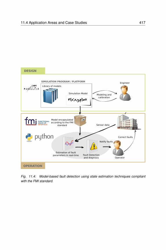
11.4 Application Areas and Case Studies 417

FMUModel encapsulated

according to the FMI

standard

Fault Detection

and diagnosis

Sensor data

Correct faults

Estimation of fault

parameters in real-time

Notify faults

Operator

DESIGN

OPERATION

Library of models

Modeling and

calibrationF(x',x,y,p)=0

Simulation Model

SIMULATION PROGRAM / PLATFORMEngineer

Fig. 11.4: Model-based fault detection using state estimation techniques compliant

with the FMI standard.

418 Activity 2.3: Model use During Operation

an FMU for co-simulation and used during the operation of the plant within theFDD module, for representing the expected operation, and for computing thedifferences in energy and cost between faulty and correct operation. Pythonwas used for the workflow automation, which consists of reading measureddata from a data base, executing the state and parameter identification, whichin turn executes the FMU for different inputs, initial states and parameters, andwriting the results to a database for display to the operator in a web-based GUI.Fig. 11.5 shows parts of the GUI with monitored and estimated Coefficient ofPerformance (COP) of the chiller. The results of the state and parameter esti-mation algorithm are compared to the COP of the calibrated model. One of theadvantages of this approach is that it provides a statistical description of theperformance, and hence it allows to set fault thresholds based on a probability.

Fig. 11.5: Outputs of the fault identification algorithm, with costs caused by the fault

(top graph) and comparison between measured and expected COP (bottom graph).

The red rectangles are time intervals that have been identified as faulty periods in

which the performance of the chiller was outside the tolerance.

Using Modelica allowed reusing a variety of component models from the Mod-elica Buildings library to build subsystem models of the chilled water plant,such as for the chillers and the cooling towers, which were then calibratedwith measured data. After the calibration, these models were exported asFMUs in order to provide a model for the FDD algorithm. The use of FMUs

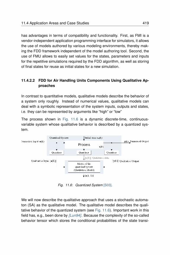
11.4 Application Areas and Case Studies 419

has advantages in terms of compatibility and functionality. First, as FMI is avendor-independent application programming interface for simulators, it allowsthe use of models authored by various modeling environments, thereby mak-ing the FDD framework independent of the model authoring tool. Second, theuse of FMU allows to easily set values for the states, parameters and inputsfor the repetitive simulations required by the FDD algorithm, as well as storingof final states for reuse as initial states for a new simulation.

11.4.2.2 FDD for Air Handling Units Components Using Qualitative Ap-

proaches

In contrast to quantitative models, qualitative models describe the behavior ofa system only roughly. Instead of numerical values, qualitative models candeal with a symbolic representation of the system inputs, outputs and states,i.e. they can be represented by arguments like “high” or “low”

The process shown in Fig. 11.6 is a dynamic discrete-time, continuous-variable system whose qualitative behavior is described by a quantized sys-tem.

Fig. 11.6: Quantized System [S03].

We will now describe the qualitative approach that uses a stochastic automa-ton (SA) as the qualitative model. The qualitative model describes the quali-tative behavior of the quantized system (see Fig. 11.6). Important work in thisfield has, e.g., been done by [Lun94] . Because the complexity of the so-calledbehavior tensor which stores the conditional probabilities of the state transi-

420 Activity 2.3: Model use During Operation

tions of the automaton increases rapidly with a rising number of inputs, outputsand state signals, solutions for reducing the computational efforts and storageamounts are required. As shown in [MKLR15] , the complexity of the behaviortensor of the SA can be reduced by exploiting the underlying tensor structureof the behavior relation. Therefore, a non-negative canonical polyadic (CP)tensor decomposition can be used to make qualitative models applicable tolarge discrete-time systems. Usually, qualitative models can be generated byan abstraction from a quantitative model or by stochastic qualitative identifica-tion. In our application, we will focus on the latter which has been developedby [Lic98] . The stochastic qualitative identification allows the generation ofa qualitative model directly from measurement data or from simulation data.For both cases, for Fault Detection (FD) nominal data of the faultless systembehavior is needed. Fault Detection and Diagnosis (FDD) requires also faultmodels or faulty measurement data. [LS96] used a qualitative observer forfault detection and diagnosis. Qualitative observation means the prediction ofthe possible system states at discrete time k + 1 based on the measured inputand output combination at time k . In general, the qualitative observer is thequalitative equivalent of e.g. the Luenberger observer known from continuous-time systems. The algorithm yields for each time step a probability vectordescribing the possible behavior of the system states for a given input.

If the probability vector contains only zeros, the measured input-output com-bination is inconsistent with the qualitative model and a fault can be struc-turally detected, [Lic98] . For demonstrating FD with qualitative models, differ-ent faults have been simulated with the Modelica fault triggering library, de-veloped by the German Aerospace Center (DLR), [vdL14] . In the following,an application example of a heat exchanger of a HVAC&R system shows theapplicability of the qualitative modeling approach.

We will now present an example. The considered system is a Heat Exchanger(HX) that cools air. It has been simulated with Modelica for the input signalsshown in Fig. 11.7 for nominal and faulty conditions.

The simulated fault describes a malfunction of the pump that leads to the prob-lem of a fully opened valve, because the controller tries to track the set point ofthe air outlet temperature. Fig. 11.8 shows the faulty behavior during the timeinterval 2420 ≤ t ≤ 2708. As the figure shows, the air outlet temperature ofthe HX equals the air inlet temperature because no water circulates.

11.4 Application Areas and Case Studies 421

Fig. 11.7 : Generic HX scheme.

Fig. 11.8: Simulation Data.

422 Activity 2.3: Model use During Operation

Next, the qualitative model was trained using the nominal behavior of the HXas produced by the simulation model. Fig. 11.9 illustrates the qualitative statetrajectory of the state variable Tair ,out for a selected time range.

The state trajectory computed by the qualitative observation algorithm andit shows the probability distribution of the state signal for each discrete timestep k. The different grey shades of the bars denote the probabilities. In theexample, the state signal Tair ,out was quantized into five intervals that can beseen by the horizontal separation of the black and grey bars.

Fig. 11.9: Qualitative state trajectory of the air outlet temperature Tair ,out (nominal

condition).

Fig. 11.10 shows the qualitative state trajectory for the faulty condition. Duringthe faulty operation, the measured input-output pair is inconsistent with thequalitative model, leading to components of the probability vector being closeto zero. This is visualized by the white space in the figure for 2420 ≤ k ≤ 2708.

For a better visualization, Fig. 11.11 displays 1 for non-faulty conditions and 0for faulty conditions.

While this example shows how fault detection with qualitative models can berealized, fault diagnosis is also possible. To achieve this, a set of qualitativemodels, where each model is trained with a different faulty condition has to begenerated. Note that even for this simple example, the behavior relation of theSA contains over 3.9 · 106 values, leading to a significant calculations for each

11.4 Application Areas and Case Studies 423

Fig. 11.10: Qualitative state trajectory of the air outlet temperature Tair ,out (faulty

condition).

Fig. 11.11: Probability of the air outlet temperature x_2 (faulty condition).

424 Activity 2.3: Model use During Operation

discrete time step k . For building automation systems (BAS), such high com-puting demands may not be possible. We therefore used a CP-decomposition,which reduced the size of the behavior relation by a factor of 3200 from 3.9106

to 1200. This met the computing capabilities of the BAS for real-time applica-tion.

We will now turn the discussion to another case study. This case study demon-strates the use of Modelica to support a qualitative model-based fault detec-tion and diagnosis approach based on first-order logic and a generic diagno-sis algorithms. Model-based diagnosis is based on an explicit representationof the knowledge about the components and the information about the plantstructure, which determines how the components interact with each other.Based on a Modelica library of generic component models representing first-principles of energy and mass transfer between components of the AHU andthe representation of the AHU topology, a system model, possibly coveringboth the nominal and faulty behaviors, can be obtained. This model is thenused by a generic diagnosis algorithm, which is neither plant- nor domain-specific. The diagnosis models used in qualitative model-based diagnosis areobtained by using the Modelica model to capture acceptable deviations of vari-ables from their respective nominal behavior. Instead of using a stochastic au-tomata, this method uses an inferencing system based on first-order logics togenerate the diagnosis.

In Fig. 11.12, a complete workflow and system modules are presented thatare required to build a diagnostic solution for a class of plants, such as HVACsystems, and to deploy and run it for a single plant. This process is referredto as qualitative model-based diagnosis. Here, we give an overview of thesteps and modules. The steps are described in detail in [SPF+14] and aresummarized as follows:

• Producing the general solution (top row) involves:

• The production of a library of Modelica models of the components (e.g.first principle models) [FSTK13] and

• its transformation into a qualitative diagnostic model library.

• Producing an application system (middle-row), based on the general so-lution, which requires:

• The configuration and calibration of the Modelica models of the correct

11.4 Application Areas and Case Studies 425

Modelica Component

Library

Model Transformation

Diagnosis Component

Library

Modelica OK Model

Plant TopologyExtraction

AutomatedModel

Composition

Diagnosis Model

Sensor Data

Deviation Generation

Diagnosis Engine Diagnoses

Fig. 11.12: Fault Detection of Air Handling Unit Components in a Qualitative Approach

Workflow.

behavior [FSK15] , and• the composition of the diagnostic model based on the diagnostic library

and the topology of the plant, which can be extracted from the Modelicasystem model.

• For on-line diagnosis (bottom row):

• Computing the difference between the real data and the predictions gen-erated by the Modelica model of the plant, and comparing the differencewith given thresholds [SPF+14] , and

• diagnosing the differences, using a runtime diagnosis engine such asRaz’r [OCCM14] , which is an implementation of consistency-based di-agnosis [MS96] . The output of the consistency-based diagnosis engineis a minimum set of combinations of component faults.

In this example, models were developed and applied to support model-baseddiagnosis. Use of Modelica led to a clear understanding of the underlyingphysical equation system since the equations within the component model andalso on the level of the system model (connect equations) are clearly definedand can be easily reconstructed by the user of the model.

426 Activity 2.3: Model use During Operation

The main drawback of Modelica tools for this case study was the lack of nativetools to interact with simulations during run-time. A python-Modelica interfaceneeded to be developed. However, this need can nowadays be overcome bythe use of FMI, for which Python interfaces are available.

11.4.2.3 FDD for Air Handling Unit Systems Using a Quantitative Ap-

proach

This case study focuses on the application of an open and replicable FDDmethod. The method consists of a combination of a Modelica model-basedfault detection and a classifier-based diagnosis. It analyzes the monitoreddata on a real-time basis where a calibrated Modelica model evaluates theoutputs from the outdoor conditions and the control signal and compares theestimation against the measurement to detect errors.

The method was used for component failure detection in an AHU, focusing ona prospective malfunction of the dampers, the heat recovery system and thefans. The AHU is part of a comprehensive test facility located on the KU Leu-ven Technology Ghent campus in Belgium. The facility is equipped with its ownweather station measuring global solar irradiation, relative humidity, tempera-ture, precipitation, wind speed and wind direction. A set of embedded sensorskeep track of the AHU parameters such as the air volume flow, air temperatureand relative humidity in the supply air and in the return air. The damper po-sition signals are monitored as well. The monitored data are centralized andstored with a one minute frequency in a Soft-PLC based monitoring systemwhere the BMS and the FDD algorithm is integrated on the same industry PChardware.

As depicted in Fig. 11.13, a semi-automated BIM based process has beenutilized to generate the Modelica model used for fault detection. It relies on aPython framework to extract and convert BIM data into a Modelica componentcompatible format. In this context, the BIM-based modeling approach is facili-tated by the component-oriented feature of Modelica, which in turn allows aneasy mapping between BIM objects and Modelica components. Data from thebuilding delivery manual are used as input for the remaining parameter valuesnot available in the BIM. An optimization-based calibration process is used tocalibrate the Modelica model where a data set obtained throughout the initial

11.4 Application Areas and Case Studies 427

Delivery

manual

Modelica

Model

Calibrated

Modelica

Model

FMU

ClassifiersBIM

BMS

Python based

BIM data collection

framework

Optimization

Initial commissioning data

Fault

Detection

Real time data

Fault

Diagnosis

Synthetic data

Training data set

Online

FDD

Test facility

Real time data

BMS error notification

Building manager

error notification

Fig. 11.13: Fault Detection of Air Handling Unit Systems in a Quantitative Approach

Workflow.

428 Activity 2.3: Model use During Operation

commissioning process and assumed as fault free is utilized.

The Modelica model is exported as an FMU to be integrated into the BMS fora near-real time estimation of the outputs (e.g. supply air temperature). Adiscrepancy between the model estimation and the measurements superiorto a predefined threshold is a sign of a likely issue on the system. To diag-nose the error cause, the classifiers estimate the set of control signals whichcould provide the current output value as outcome. The cause of an error isisolated in a component if a discrepancy between the estimated and the ac-tual control signal within this specific component is detected. In addition tothe fault-free initial commissioning data, the classifiers are trained using syn-thetic data which represent several operating scenarios generated from thecalibrated Modelica model.

An error notification is sent to the BMS if the algorithm detects the fault and itsroot cause is determined. An error notification is sent to the building managerif the occurrence of the error spans over a predefined period of time (e.g. 2days). A BIM based error notification has been developed where the errorlocation is pinpointed within the virtual representation of the building.

In this project, the use of Modelica was motivated by its ability to model thedynamic behavior of the components of the AHU. In addition, as an openlanguage and considering the availability of open-source and validated li-braries dedicated to buildings, Modelica fits well with developing an open FDDmethod.

11.4.3 Hardware in the Loop

Lastly, this section describes a hardware in the loop system. In this study, theModelica Buildings library [WZNP14] is utilized to model an HVAC systemthat was used in a HIL setup to test the performance of closed loop controlalgorithms. During this project, the interface used to run Dymola models on thedSpace HIL simulator was still in development and not yet sufficiently reliablefor utilization in this project. This was circumvented by importing the Dymola-generated code for the model in Simulink, and then using Simulink’s codegeneration functionality.

The pieces of equipment chosen to complete the loop in this study include a

11.4 Application Areas and Case Studies 429

Fig. 11.14: Hardware in the loop workflow.

dSpace processor to execute models and a set of programmable VAV terminalcontrollers from Automated Logic Corporation (ALC). Additionally, digital-to-analog (D/A) and analog-to-digital (A/D) boards are used to establish commu-nications between the dSpace and the controllers.

The model workflow shown in Fig. 11.14 mimics a room served by a VAVbox with a reheat valve and a damper. This study focuses only on sensibleheat transfer in buildings. Therefore, there is no humidity control and the airis assumed to be dry air. An AHU provides simple dry air at a prescribedtemperature and sufficient pressure to overcome losses due to the damperand heat exchanger. The air is given a nominal flow rate, which serves as theflow rate of air with the damper fully open. From the AHU, the supply air flowsthrough a heat exchanger block (i.e., reheat coil) with a constant effectiveness.Reheat is provided using a water-to-air heating coil, controlled by a linear two-way valve. Finally, the VAV damper is modeled using an exponential dampermodule from the Modelica Buildings library. The nominal supply airflowrate is set inside this module, and varies exponentially down to zero as thedamper is closed. External signals are used to control both valve position onthe reheat water loop and supply air damper position, as these signals willbe received from the ALC controllers in the HIL simulation through an A/Dboard. Ideal flow and temperature sensors are placed throughout the model tomonitor properties and ensure correct performance. Such sensor information

430 Activity 2.3: Model use During Operation

was sent to ALC controllers through a D/A board. Finally, parameters that arenot yet defined are set as inputs to the system. These will be declared later inSimulink, allowing them to be changed during real-time testing.

The room model in Fig. 11.14 describes a room using a thermal resistance-capacitance (RC) model and is modified from a RC model in the ModelicaAnnex60 library [WvTH13] . A capacitor for each surface represents thermalenergy storage, followed by conduction and internal convection resistors. Theambient temperature is an input to the system, while the ground temperature isheld at a constant value. Fluid ports allow the air from the VAV box to enter theroom and return the air to an exit, maintaining the mass balance. Therefore, afixed volume of air is maintained in the room at all times. There are a varietyof assumptions made in this model, including the neglecting of infiltration andhandling of outdoor convection as constant.

The combined thermal zone and VAV box model was downloaded to dSpacefor the real-time execution. As previously mentioned, the model was first im-ported in Simulink for the code generation. This is possible using a Dymola-to-Simulink interface called DymolaBlock. This feature allows the model to beinserted into Simulink as a functional block whose outputs are calculated fromdefined inputs. In order to complete the loop, some parameters must be as-sociated with D/A and A/D boards, and therefore either read from or sent tothe real controllers. In this study, the room temperature is sent to the controllerand the reheat valve position is returned for the heating model simulation. AdSpace blockset allows these communications to be defined in Simulink. Be-fore building the model to code, a fixed step integrating method was selected.The model is then compiled to C code using Matlab, and the variable descrip-tion files are downloaded onto dSpace for the real-time testing.

This HIL setup was used to test a conventional VAV box control called singlemaximum logic [TSPC12] . The outdoor air temperature was set to be verycold and the VAV box always stayed in the heating loop. Therefore only reheatvalve position had to be controlled. The control was accomplished by usinga PI block. Zone temperature and setpoint were compared to determine anappropriate reheat valve position, which was then sent to the Modelica model.The VAV box changed the model accordingly and solved for zone temperatureat each time step, writing this value (sensor information) to the controllers tocomplete the loop. Both zone air temperature and reheat value position were

11.4 Application Areas and Case Studies 431

Fig. 11.15: Hardware in the loop results.

trended and recorded in the BEMS (Fig. 11.15).

As can be seen in Fig. 11.15, the desired setpoint of the room was 72 Fahren-heit. The simulation was stopped around 1 pm and later resumed, with dif-ferent PI loop tuning to illustrate the difference this can make. Before there-tuning, wild fluctuations in the reheat valve were experienced. If this controlwere implemented in a real system, the constant opening and closing of thevalve would lead to noise, wasted energy, discomfort, mechanical wear andeventually failure.

After a more optimal tuning was applied to the PI block, a classic underdampedoscillator curve can be seen. The reheat valve position ceases to undergooscillatory changes, and finds a steady value to maintain room temperatureat the setpoint. Reversals in signal can still be seen, but they are minimalcompared to the prior tuning and are practically unavoidable.

During this study, sometimes compatibility issues have been encountered be-tween the building code for dSpace and the Dymola-to-Simulink interface.This only occured with certain models, such as MixedAir from the ModelicaBuildings library, and we have not yet located the root cause of these is-sues. These models work fine in Simulink but return a Simstruct Mex errorduring code generation. FMI usage should avoid such issues in future imple-mentations.

432 Activity 2.3: Model use During Operation

11.5 Discussion and Conclusions

The use of Modelica to support the operation of building energy systems ispromising as buildings involve multiple physical phenomena (e.g., heat trans-fer, fluid dynamics, electricity, etc.) and are complex in terms of their dynamics(e.g., coupling of continuous time physics with discrete time and discrete eventcontrol). Some clear advantages in the use of Modelica for supporting modeluse during operations include:

• The open source characteristic combined with the existence of severalfreely available Modelica libraries [BDCVR+12] , [LTF+14] , [NGHLR13] ,[WZNP14] allows for models to be modified and extended depending onthe application requirements;

• Object-orientation not only enhances modularity and reusability of themodels but also allows models to be developed following the physicalsystem structure, which makes them easier to understand. The object-orientation enables extension and reuse of components and the use ofstandardized interfaces enables collaboration across physical domainsand disparate developer groups.

• The Modelica object-oriented approach also allows for the developmentand the management of large and complex models. In such large-scaleapplications, the translators, the modeling language and environmentare significantly stressed, and their robustness proved an enabling factorof the overall modeling process. This makes the Modelica toolchain wellsuited for handling highly complex models from the end user and theengineering perspective.

• The possibility to import and export Modelica models as FunctionalMock-up Units (FMUs) enables the integration of models using a stan-dardized, tool-independent API into existing FDD routines or the devel-opment of integral solutions that couple tools for data analysis, simu-lation, FDD and optimization in one single environment. An integralsolution can be realized, for example, using the Building Controls Vir-tual Test Bed (BCVTB) [Wet11a] or JModelica with the Python modulePyFMI [AAG+10] .

• Modelica allows for a seamless use of the models developed in the de-sign phase during the operational phase, for example, by exporting mod-els as FMUs.

11.5 Discussion and Conclusions 433

Finally, it is important to note that the advantages of Modelica can turn againstthe unexperienced developer. For example, because of the object-orientationemployed in many libraries, it can be difficult to predict the depth to whicha change in one component can have an effect in other components in thelibrary. However, regression tests as are setup for the Modelica Annex60

library can detect such unintended side effects. In addition, the current capa-bilities of Modelica IDEs are still developing means to provide better debugginginformation. Also, training is highly recommended for novice users as the typeof model verification and debugging done in equation-based languages differsfrom what users may be accustomed to when writing procedural code.

434 Activity 2.3: Model use During Operation

Chapter 12

Management and

Dissemination

The IEA EBC Annex 60 was conducted from 2012 to 2017 through the col-laboration of 42 institutes from 16 countries. The research phase of Annex60 started on July 1, 2013. The Annex benefited from a strong organizationalframework in order to coordinate work between the various researchers world-wide.

12.1 Coordination and Meetings

12.1.1 Semi-Annual Expert Meetings

During the research phase, eight international, semi-annual expert meetingswere successfully held and most of the expert meetings were followed by tech-nical workshops over multiple days:

• on March 11-12, 2013 at RWTH Aachen, Germany, during the planningphase (50 attendees),

• on August 23-24, 2013, in Aix-les-Bains, France (54 attendees),• on March 8-9, 2013, in Lund, Sweden (50 attendees),

436 Management and Dissemination

• on September 15, 16 and 17, 2014, in Berkeley, USA (50 attendees),• on April 21 and 22, 2015, in Galway, Ireland (50 attendees),• on September 16-18, 2015, in Leuven, Belgium (50 attendees),• on May 9-11, 2016, in Miami, USA (30 attendees),• on October 22-23, 2016, in Porticcio, France (65 attendees).

12.1.2 Coordination Meetings

In order to synchronize work packages and activities, more than 120 coor-dination meetings and web conferences were conducted within the activitiesand among the leaders since the start of Annex 60. Minutes of these activitiesand meetings were continuously organized and disseminated using the Annex-internal bitbucket repository system. The repository system, which included awiki, was a key resource for organizing collaboration.

12.1.3 Shared Content Management System

In order to support joint collaboration, documentation, report and code man-agement, a cross-platform, cloud-based repository system, called Bitbucket,was utilized and maintained by the operating agents. The system provides ver-sion control using git and is recommended for managing future Annex projects.

12.2 Publications and Outreach

12.2.1 Annex 60 Joint Publications

Besides this final report, Annex 60 published 11 journal articles, 38 confer-ence papers and a Modelica library, which are all accessible at http://www.iea-annex60.org/pubs.html.

12.2 Publications and Outreach 437

12.2.2 Outreach

Several special scientific tracks at national and international conferences wereorganized to disseminate and promote results of the entire project. In order torepresent the Annex in a consistent manner, a common text for the acknowl-edgement section of papers was formulated and distributed to all participants.The Annex 60 project gained a high international visibility through, among oth-ers, the following outreach activities:

• multiple announcements in the Newsletters of the International BuildingPerformance Simulation Association (IBPSA),

• announcements in the Newsletter of its US-Affiliate IBPSA-USA,• announcements in the Newsletter of the Modelica Association,• presentation at the SimBuild 2012 conference in Madison, WI, USA,• presentation of the Annex at the International Symposium “EnTool 2013

Symposium, Workshop & Summer School” in Dresden, Germany,• presentation at the Modelica North-America User Meeting in Ann Arbor,

Michigan, in May 2013,• presentation at the IBPSA-USA meeting in Dallas, TX, in January 2013,• presentation at a special conference track at the international Building

Simulation conference in August 2013 in France,• implementation of a special conference track at the BauSIM 2014 con-

ference in Aachen, Germany,• receiving the Best Paper Award for an Annex 60 paper out of 100 pre-

sentations at BauSIM 2014,• implementation of a special conference track at the ASHRAE/IBPSA-

USA Building Simulation Conference in 2014,• presentations at the SIAM Annual Meeting in the USA in 2014,• organization of special tracks at the Building Simulation 2015 conference

in Hyderabad, India, where 28 joint papers were presented from theAnnex 60 framework,

• presentations at a public workshop sponsored by the Netherlands andFlanders chapter of the IBPSA,

• presentations in 2016 at a public Annex 60 workshop with hands-ontraining by IBPSA-France,

• presentations at the Clima 2016 conference in Aalborg, Denmark,• presentations at the ASHRAE and IBPSA-USA SimBuild 2016 confer-

438 Management and Dissemination

ence in Salt Lake City, Utah, USA,• presentations within a special track at the BauSIM 2016 conference in

Dresden, Germany,• invited presentation about Annex 60 and IBPSA Project 1 at the IBPSA-

England BSO 2016 conference in Newcastle, England,• presentation at the Modelica North America Users’ Group meeting in

Troy, Michigan in 2016,• invited presentation at the international conference of the European En-

ergy Research Alliance (EERA) in 2016,• presentations at the Modelica conference in Prague in 2017, and• presentation of the Annex 60 / IBPSA Project 1 continuation framework

at the Building Simulation 2017 conference in San Francisco, USA.

Furthermore, progress of the Annex 60 framework was disseminated in a num-ber of issues of the IEA EBC News.

12.2.3 Annex 60 Web Site

The public Annex 60 web site is accessible at http://www.iea-annex60.org.This page also host papers that resulted from the Annex 60 collaboration, listsparticipants and their respective contact information.

Chapter 13

Conclusions

13.1 Technology Development

The technology development in Annex 60 was organized around three stan-dards:

1. IFC for data modeling,2. Modelica for multi-domain, multi-physics modeling, and3. FMI for run-time interoperability of simulators.

Basing the work on these standards was critically important to enable jointtechnology development among multiple participants, many of whom broughtinto Annex 60 their existing code, further developed it within the project, andthen integrated it back into their tools. A prime example of technology devel-oped around these standards is the Modelica Annex60 library developed inActivity 1.1. In this work, multiple institutes started a collaborative develop-ment of a free, open-source Modelica library for building and district energysystems. This work harmonized the previously fragmented and duplicative de-velopment of libraries, and resulted in a jointly developed library that is nowused by four major Modelica libraries for building systems. As part of this pro-cess, the four libraries not only grew in their functionality, but also improvedtheir robustness, validation and documentation. Getting to this point requiredthe developers of previous libraries, each having a considerable code base, to

440 Conclusions

mutually agree upon common processes for development and quality control.These processes needed to allow for rapid experimentation, as is often donein University settings, as well as ensure robust and stable development, whichis more important for commercial software companies and government labo-ratories. The joint development also required the developers to agree uponvarious design decisions and conventions for coding, documentation and val-idation, to jointly work on implementation and vetting of a core of a library, torefactor their existing libraries, and to open-source previously proprietary code.This is the first international collaboration for a library with free, open-sourcemodels for buildings and district energy systems that are built using an open-standard modeling language. It initiated a larger open-source developmentthat will be further supported though IBPSA, whose vision includes providinga standard library with fundamental model descriptions that will be supportedby manufacturers and integrated in various building performance simulators.

A second example of technology developed using the previously mentionedstandards is the development of building and district energy simulation toolsbased on the FMI standard. A key advantage of using the FMI interface isthat it decouples the model authoring from the simulation run-time environ-ment, allowing quite different approaches to be used to integrate the mod-els in time. Over the course of the project, different FMI simulators not onlyemerged from within Annex 60, but also from within the significantly largerFMI community. Within Annex 60, using the FMI standard as an ApplicationProgramming Interface (API) to different simulators allowed run-time couplingof various simulators, prototyping of an interface that allows energy and con-trol models authored in FMI for co-simulation to be integrated with a commer-cial building automation system for real-time control or real-time energy mon-itoring, and hardware-in-the-loop testing of building control sequences. Fromthe technology development point of view, such a decoupling between modelauthoring and simulation, and work with an open standard, has the key ad-vantage of being able to develop, prototype, and test different simulators oncommon models, while keeping the time and cost to adapt a new simulatorlow. This is compared to what is done in most modeling and simulation tools,which have a tight integration of models and solvers. While it has been shownthat the FMI standard is well-suited for the classes of problems encountered inbuilding and district energy simulation, certain limitations were encountered,as is common with any standard that covers such a complex use case, and

13.1 Technology Development 441

improvements have been recommended. Some of these recommendationshave already been addressed by the FMI standards committee. Overall, usingthe well-developed FMI standard, together with its development process thatensures stability, gave rise to the ecosystem of building and district energysimulation tools developed as part of this project.

A third example of technology development using these open standards is thatwhich was done to support processes that transform digital planning and de-sign to simulation. In Annex 60, a mechanism was developed to transform adigital model of a building and its energy systems to Modelica code, which canthen be readily used for advanced building performance simulation. This wasaccomplished through the use and extension of the Open BIM data formatsdefined by the Industry Foundation Classes (IFC) as well as through the useof other BIM-standards, such as the Information Delivery Manual (IDM) andModel View Definitions (MVD). Annex 60 thoroughly addressed the prevail-ing tedious, cumbersome and error-prone process of manual data conversionand model generation by providing a methodology and software framework forautomatically, or at least semi-automatically, transforming a digital model intoan object-oriented acausal model. The software framework developed in An-nex 60 supports the Open BIM format IFC. Models are checked for integrityin terms of geometric consistency and HVAC definition. Using a flexible mod-ule for schema parsing, models are transformed into the intermediate dataformat SimXML. To manage these SimXML data, a dynamic schema parserin C++ with an API between C++ and Python was developed to interact withthe data model. An object and parameter mapping mechanism as well as re-spective mapping rules were defined to formulate engineering knowledge in arule-based methodology. These rules are processed by the framework. Fur-thermore, an IFC MVD was published in order to specify the subset of IFCdata relevant to building performance simulation. To support multiple Model-ica libraries, we selected a template-based approach and implemented it inPython. As a result, the software framework of the translator from BIM to Mod-elica can generate models using the four different Modelica libraries, usingthe same software stack with small adaptations. The developed methodologywas tested for a set of use cases. Annex 60 thereby followed a bottom-upapproach which was based on these use cases. The framework supports thewhole model checking and model transformation process but is currently lim-ited to these use cases. The result is a modular framework which is open for

442 Conclusions

further development and dissemination.

In addition to the use of open standards, workflow automation also played animportant role in technology development, both for model development andalso for case studies. Due to the large ecosystem of free, open-source Pythonpackages, Python-based tools were further developed and used in the casestudies, and documentation and workshops for novice users were developed.An example for workflow automation during model development is the regres-sion testing that we setup for the Annex60 Modelica library. This library con-sists of 2, 400 files. During any change to a model, more than 120, 000 resultpoints are compared to verify that they are either identical to or expectedly dif-ferent from results computed with an earlier version, within a tolerance of 10−3.Furthermore, daily tests are run to compare all of these points among the twosimulators Dymola and JModelica to make sure that the library produces thesame result with different simulators. Regarding workflow automation for casestudies, many case studies used optimization, stochastic simulations, or cou-pled multiple simulation tools. For such applications, automating the workflowwas critical to produce reliable and repeatable results.

Subtask 2 demonstrated how these technologies can be used for the designand operation of building and district energy systems. In many of these appli-cations, models from Activity 1.1 were combined with FMI-tools from Activity1.2 and workflow automation scripts from Activity 1.4, and with open-sourceand commercial software that has been developed outside of Annex 60, tosolve problems related to the design and operation of building and district en-ergy systems. The case studies showed that very low energy systems andincreased grid integration imposes structural changes to building and commu-nity energy modeling and simulation tools and processes. For example,

• Models of different physical domains, control systems, occupant behav-ior, and occupancy need to be combined for dynamic, multi-physics sim-ulations that involve electrical systems, thermal systems, flow distribu-tion, controls and possibly communication systems. Such models typi-cally evolve at vastly different time scales.

• Tools need to properly handle control sequences and hybrid systems inwhich the states evolve in time based on both continuous and discretetime semantics that arise from physics and digital control, respectively.

• Subsystem models need to be extractable in order to export and execute

13.1 Technology Development 443

models in a self-contained form in a building automation system, or ahardware-in-the-loop setup.

• Model equations need to be accessible in order to perform model orderreduction, model linearization, extraction of a linear model in state-spacerepresentation, and to solve optimal control problems.

The case studies showed Modelica is well-suited to address the above prob-lems. Various case studies combined thermal, electrical and control modelsfor projects at the building and district scales. While Modelica tools gener-ate very efficient C-code for simulation, simulating large systems can still bea challenge. Research in translation of large models and in multi-rate solverswith adaptive time step control is ongoing and needed to apply this technologyto large systems.

As part of analyzing thermal district energy systems, it becomes evident that astandardized validation test, similar to ANSI/ASHRAE BESTEST 140, but fordistrict systems, would be immensely valuable. Currently, there is neither atest, nor a common understanding of what is meant by a district energy simu-lation. Approaches in industry range from simple spread-sheet based analysisthat disregard temperature levels, energy storage and pressure drops, to fullycoupled simulation of buildings, thermal distribution networks, flow friction andfeedback control. In absence of a test procedure for district models, it is hardto judge how credible the tool and approach that was selected by the modeleris. A first start for such a test was done in Annex 60, and it is planned tocontinue this effort within the IBPSA Project 1.

Annex 60 participants who worked on model use during operation reportedthat the object-orientation of Modelica not only enhances reusability of themodels, but also allowed models to be developed following the physical sys-tem structure, which makes them easier to understand. Moreover, the possi-bility to import and export Modelica models as FMUs enabled the integration ofmodels using a standardized, tool-independent API into independent or com-bined solutions for data analysis, simulation, fault detection and diagnosis, andoptimization now and in the future.

In summary, had our work not been based on such open standards, such atight collaboration and integration of software among widely ranging use caseswould not have been possible. Moreover, analyzing multi-physics problemssuch as the integration of thermal and electrical systems, overlaid with controls

444 Conclusions

that coordinates the two, would have been very difficult without Modelica’ssupport for multi-physics modeling, and FMI’s support for co-simulation usingdomain-specific tools.

13.2 Governance and Dissemination

The Annex 60 benefited from a strong organizational framework to coordinatework between the various researchers world-wide. Eight semi-annual inter-national expert meetings were conducted, most of them followed by technicalworkshops over multiple days. To synchronize work packages and activities,more than 120 online coordination meetings and web-conferences were heldwithin the activities and among activity leaders. A Bitbucket repository systemwas used, including a wiki, as a key resource to organize collaboration andmanage shared documents. Several special scientific tracks at national andinternational conferences were organized to disseminate and promote resultsof the entire project, which helped to gain a high international visibility. Annex60 published 11 journal articles, 38 conference papers, a Modelica library anddiverse source code packages, all managed through a Git code repository.

13.3 Continuation Framework

Although the Annex has delivered a solid basis of tools and demonstrated theirapplication, tool development is a continuous effort. It continuously needs toprovide support, respond to new system technologies and apply advancesin computer science and applied mathematics. Upcoming research and de-velopment issues that remain to be solved after completion of the Annex willtherefore be coordinated under the umbrella of the network of the InternationalBuilding Performance Simulation Association (IBPSA) as a living and support-ing dissemination framework.

Chapter 14

Glossary

This section defines various technical terms that are used throughout the re-port.

Building Information Model (BIM) A Building Information Model (BIM usedas a noun) is an instance of a data model that describes a building andits components unambiguously, e.g. a digital footprint of a building andits properties, represented over its entire life cycle.

Building Information Modeling (BIM) Building Information Modeling (BIMused as a verb) is a collaboration method to consistently acquire, man-age, exchange and hand-over information of a building which are rele-vant over its entire life cycle, using digital models and targeting a consis-tent communication between parties.

Business Process Modeling Notation (BPMN) Graphical notation to struc-ture and display processes to formally and descriptively describe tasks,responsibilities and informations within IDM. So-called swim-lanes areused to graphically group elements, which belong to an actor respec-tively.

Industry Foundation Classes (IFC) Object oriented data format for digitaldescription of building information models. Open BIM data exchangestandard developed by buildingSMART published as ISO 16739. Physi-cal data exchange as Step (Express) or ifcXML data file.

Information Delivery Manual (IDM) Method standardized as ISO 29481 to

446 Glossary

capture and specify processes and to define information exchange re-quirements in BIM. Usually as formal description of planning processesusing Busines Process Modeling Notation (BPMN).

Model View Definition (MVD) Part or subset of the IFC scheme which isdefined in order to fulfil a single or multiple domain-specific exchangerequirements. Typically, IDM serves as method to define these exchangerequirements.

package In Modelica, a package is a collection of models, functions, or otherpackages that are used to hierarchically structure a Modelica library.

class In Modelica, a class is a term that includes models, blocks, functionsand packages.

connector In Modelica, a connector is an instance of a class that is usedto connect models and blocsk with each other. Connectors can containconstants, parameters and variables, but no equations.

co-simulation Co-simulation refers to a simulation in which different simu-lation programs exchange run-time data at certain synchronization timepoints. A master algorithm sets the current time, input and states, andrequest the simulator to advance time, after which the master will retrievethe new values for the state. Each simulator is responsible for integratingin time its differential equation. See also model-exchange.

block In Modelica, a block is a special case of a model in which all connectorsare either inputs or outputs.

events An event is either a time event if time triggers the change, or a state

event if a test on the state triggers the change.model In Modelica, a model is a special class in which the causality of its

connector need not be specified.model-exchange Model-exchange refers to a simulation in which different

simulation programs exchange run-time data. A master algorithm setstime, inputs and states, and requests from the simulator the time deriva-tive. The master algorithm integrates the differential equations in time.See also co-simulation.

zero-crossing function A zero crossing function is a function that is usedby solvers to indicate when variables cross a threshold. For example,suppose a thermostat should switch off a heater when the room tem-perature Tr (t) crosses a set point Ts(t). For this case, a zero crossingfunction is f (t) = Tr (t) − Ts(t).Zero-crossing functions are used by numerical solvers to detect where

447

such discrete changes in a model occur. Specifically, at t = t1, theysearch for τ ∈ arg min{t > t1 | f (t) = 0}.

direct dependency A variable is said to directly depend on another variableif there is an algebraic constraint between these variables. For example,consider the model shown in Fig. 14.1. If the input u changes, then theoutput y3 immediately changes, whereas y1 and y2 only change aftertime is advanced. Hence, the output y3 is said to have a direct depen-dency on u. Similarly, the state derivative x1 directly depends on theinput u, and x2 directly depends on the state x1. The outputs y1 and y2

directly depend on the states x1 and x2, respectively. Hence, unless timeis advanced, if u is updated, only y3 needs to be updated, whereas if y1

and y2 need not be updated. Such information is useful to detect theexistence of algebraic loops, and to implement certain numerical timeintegration methods such as the QSS methods.

Fig. 14.1: Signal flow diagram that illustrates direct dependency.

Functional Mockup Interface The Functional Mockup Interface (FMI) stan-dard defines an open interface to be implemented by an executablecalled Functional Mockup Unit (FMU). The FMI functions are called bya simulator to create one or more instances of the FMU, called models,and to run these models, typically together with other models. An FMUmay either be self-integrating (co-simulation) or require the simulator toperform the numerical integration.

Functional Mockup Unit Compiled code or source code that can be exe-cuted using the application programming interface defined in the Func-

448 Glossary

tional Mockup Interface standard.rollback We say that a simulator is doing a rollback if its model time is set to

a previous time instant, and all its state variables are set to the valuesthey had at that previous time instant.

time event We say that a simulation has a time event if its model changesbased on a test that only depends on time. For example,

y =

0, if t < 1,

1, otherwise,

has a time event at t = 1.state event We say that a simulation has a state event if its model changes

based on a test that depends on a state variable. For example, for someinitial condition x(0) = x0,

dx

dt=

1, if x < 1,

0, otherwise,

has a state event when x = 1.

Chapter 15

References

[316] AEC 3. BIM*Q. 2016. URL: http://aec3.de/kompetenzen/BIM-Q-Database.htm.

[ACDCH15] Arnout Aertgeerts, Bert Claessens, Roel De Coninck, and LieveHelsen. Agent-based control of a neighborhood: a generic approach bycoupling Modelica with Python. In BS2015, 14th Conference of Interna-

tional Building Performance Simulation Association. 2015.

[AJS14] Abdul Afram and Farrokh Janabi-Sharifi. Theory and applications ofHVAC control systems - a review of model predictive control (MPC).Building and Environment, 2014. doi:10.1016/j.buildenv.2013.11.016.

[ANHB13] A. Afshari, G. R. Norouzi, G. Hultmark, and C. N. Bergsoe. Two-pipechilled beam system for both cooling and heating of office buildings. InProceedings of CLIMA 2013: 11th REHVA World Congress and the 8th

International Conference on Indoor Air Quality, Ventilation and Energy

Conservation in Buildings. Prague, Czech Republic, June 2013.

[Age06] International Energy Agency. Iea annex 34: computer aided evaluationof HVAC sytem performance. Technical Report, International EnergyAgency, Hertfordshire, UK, 2006.

450 BIBLIOGRAPHY

[Age14] International Energy Agency. World Electricity and Heat for2014. 2014. URL: http://www.iea.org/statistics/statisticssearch/report/?country=WORLD&product=electricityandheat&year=2014.

[Alc16] Digital Alchemy. Digital Alchemy - Simergy Pro. 2016. URL: http://www.digitalalchemypro.com/html/products/DAProducts_Simergy.html.

[AB09] Alessandro Alessio and Alberto Bemporad. A survey on explicit modelpredictive control. In Lalo Magni, DavideMartino Raimondo, and FrankAllgöwer, editors, Nonlinear Model Predictive Control, volume 384 ofLecture Notes in Control and Information Sciences, pages 345–369.Springer Berlin Heidelberg, 2009. doi:10.1007/978-3-642-01094-1_29.

[AMH00] Klaus Kaae Andersen, Henrik Madsen, and Lars H. Hansen. Mod-elling the heat dynamics of a building using stochastic differential equa-tions. Energy and Buildings, 31(1):13–24, 2000. doi:10.1016/S0378-7788(98)00069-3.

[And13] Joel Andersson. A general-purpose software framework for dynamic

optimization. PhD thesis, KU Leuven, Leuven, Belgium, October2013. URL: https://lirias.kuleuven.be/bitstream/123456789/418048/1/thesis_final2.pdf.

[ASH02] ASHRAE. Ashrae guideline 14. measurement of energy and demandsavings. Technical Report, ASHRAE, 2002.

[ASH04] ASHRAE. ASHRAE 90.1 - 2004 Energy Standard for Buildings Except

Low-Rise Residential Buildings. American Society of Heating, Refriger-ating and Air-conditioning Engineers, si edition edition, 2004.

[ARHZ15] Emira El Asmi, Sylvain Robert, Benjamen Hass, and Khaldoun Zreik.A standardized approach to BIM and energy simulation connection. In-

ternational Journal of Design Sciences and Technology, 21(1):59–82,2015.

[Aut15] Autodesk. Revit Family - Overview. 2015. URL: http://www.autodesk.com/products/revit-family/overview.

[Aut16] Autodesk. AutoCAD - Overview. 2016. URL: http://www.autodesk.com/products/autocad/overview.

BIBLIOGRAPHY 451

[BM11] Peder Bacher and Henrik Madsen. Identifying suitable models for theheat dynamics of buildings. Energy and Buildings, 43(7):1511–1522,2011. doi:10.1016/j.enbuild.2011.02.005.

[BM10] Azadeh Badakhshani and Dirk Müller. Dynamische exergetische Anal-yse von Gebäuden anhand der Gesamtsystemsimulation in der objekt-orientierten Programmiersprache Modelica. In BauSIM 2010 - 3rd

German-Austrian IBPSA Conference, 409–413. International BuildingPerformance Simulation Association, 2010. URL: http://www.ibpsa.org/proceedings/bausimPapers/2010/409.pdf.

[BDCVR+12] R. Baetens, R. De Coninck, J. Van Roy, B. Verbruggen,J. Driesen, L. Helsen, and D. Saelens. Assessing electrical bot-tlenecks at feeder level for residential net zero-energy buildingsby integrated system simulation. Applied Energy, 96:74–83, 2012.doi:10.1016/j.apenergy.2011.12.098.

[Bae15] Ruben Baetens. On Externalities of Heat Pump-Based Low-Energy

Dwellings at the Low-Voltage Distribution Grid. PhD thesis, KU Leu-ven, 2015.

[BDCJ+15] Ruben Baetens, Roel De Coninck, Filip Jorissen, Damien Picard,Lieve Helsen, and Dirk Saelens. OPENIDEAS - An Open Frameworkfor Integrated District Energy Simulations. In Proceedings of Building

Simulation 2015. Hyderabad, India, 2015.

[BS13] Ruben Baetens and Dirk Saelens. Multi-criteria grid impact evaluationof heat pump and photovoltaic based zero-energy dwellings. In BS2013,

13th Conference of International Building Performance Simulation As-

sociation, 3529–3536. 2013.

[BS15] Ruben Baetens and Dirk Saelens. Modelling uncertainty in district en-ergy simulations by stochastic residential occupant behaviour. Jour-

nal of Building Performance Simulation, 1493(September):1–17, 2015.doi:10.1080/19401493.2015.1070203.

[BRM+14] Shalako Baggi, Davide Rivola, Vasco Medici, Gianluca Corbellini,Davide Strepparava, and Roman Rudel. Modeling and simulation of aresidential neighborhood with photovoltaic systems coupled to energy

452 BIBLIOGRAPHY

storage systems. In EU PVSEC 2014, 29th European Photovoltaic Solar

Energy Conference and Exhibition. 2014.

[BS10] Maria Bernardete Barison and Eduardo Toledo Santos. An overviewof BIM specialists. In Proceedings of the International Con-

ference on Computing in Civil and Building Engineering icc-

cbe2010, 141. 2010. URL: http://www.engineering.nottingham.ac.uk/icccbe/proceedings/pdf/pf71.pdf.

[BP11] Daniele Basciotti and Olivier Pol. A theoretical study of the impact ofusing small scale thermo chemical storage units in district heating net-works. In International Sustainable Energy Conference. 2011.

[BS14] Daniele Basciotti and R R Schmidt. Peak reduction in district heatingnetworks: a comparison study and practical considerations. In 14th In-

ternational Symposium on District Heating and Cooling. 2014.

[BSKD14] Daniele Basciotti, R R Schmidt, M Köfinger, and C Doczekal.Simulation-based analysis and evaluation of domestic hot water prepa-ration principles for low-temperature district heating networks. In 14th

International Symposium on District Heating and Cooling. 2014.

[Bay14] Michael Bayer. Mako Templates for Python.http://www.makotemplates.org/, 2014. Accessed: 2015-05-13.

[Baz04] Vladimir Bazjanac. Virtual building environments - Applying informa-tion modeling to buildings. In 5th European Conference on Product and

Process Modelling in the Building and Construction Industry - ECPPM

2004, 41–48. Istanbul, Turkey, August 2004. Attila Dikbas and RaimarScherer, Taylor & Francis 2004. doi:10.1201/9780203023426.ch7.

[Baz10] Vladimir Bazjanac. Space boundary requirements for modeling of build-ing geometry for energy and other performance simulation. In 27th CIB-

W78 Conference. Cairo, Egypt, 2010.

[BK07] Vladimir Bazjanac and Arto Kiviniemi. Reduction, Sim-plification, Translation and Interpretation in the Exchangeof Model Data. In 24th CIB_W78, 163–168. University ofMaribor, CIB W78, 2007. URL: http://cic.vtt.fi/projects/vbe-net/data/2007_Data_Simplification_@_CIB-W78_Maribor.pdf.

BIBLIOGRAPHY 453

[BMNG16] Vladimir Bazjanac, Tobias Maile, and Christoph Nytsch-Geusen.Generation of building geometry for energy performance simulation us-ing Modelica. In CESBP/ BauSIM 2016 conference. Dresden, Germany,2016.

[BMOD+11] Vladimir Bazjanac, Tobias Maile, James O’Donnell, Cody Rose,and Natasa Mrazovic. Data environments and processing in semi-automated simulation with EnergyPlus. In CIB W078-W102: 28th In-

ternational Conference. Sophia Antipolis, France, 2011. CIB.

[BMR+11] Vladimir Bazjanac, Tobias Maile, Cody Rose, James O’Donnell,Natasa Mrazovic, Elmer Morrissey, and Benjamin Welle. An assessmentof the use of building energy performance simulation in early design. InIBPSA Building Simulation 2011. Sydney, Australia. Sydney, Australia,2011. IBPSA.

[Ben91] A. Bennonysson. Dynamic Modelling and Operation Optimization of

District Heating Systems. PhD thesis, Technical University of Denmark(DTU), 1991.

[Ben15] Bentley. Modeling, Documentation and Visualization Software.2015. URL: https://www.bentley.com/en/products/product-line/modeling-and-visualization-software/microstation.

[BBCK15] Federico Bergero, Mariano Botta, Esteban Campostrini, and ErnestoKofman. Efficient compilation of large scale dynamical systems. In Pe-ter Fritzson and Hilding Elmqvist, editors, 11-th International Modelica

Conference, 449–458. Paris, France, September 2015. Modelica Associ-ation. doi:10.3384/ecp15118449.

[BRC16] Federico Bergero, Akshay Ranade, and Francesco Casella. QSS andmulti-rate simulation of object-oriented models. In Proceedings of the

7th International Workshop on Equation-Based Object-Oriented Mod-

eling Languages and Tools, EOOLT ‘16, 69–77. New York, NY, USA,2016. ACM. doi:10.1145/2904081.2904091.

[Bie10] Lorenz T. Biegler. Nonlinear programming: concepts, algorithms,

and applications to chemical processes. volume 10. SIAM, 2010.doi:10.1137/1.9780898719383.

454 BIBLIOGRAPHY

[BBE+99] Niclas Björsell, Axel Bring, Lars Eriksson, Pavel Grozman, MagnusLindgren, Per Sahlin, Alexander Shapovalov, and Mika Vuolle. IDAindoor climate and energy. In N. Nakahara, H. Yoshida, M. Udagawa,and J. Hensen, editors, Proc. of the 6-th IBPSA Conference, 1035–1042.Kyoto, Japan, September 1999. URL: http://www.ibpsa.org/conferences.htm.

[BOA+11] T. Blochwitz, M. Otter, M. Arnold, C. Bausch, C. Clauß, H. Elmqvist,A. Junghanns, J. Mauss, M. Monteiro, T. Neidhold, D. Neumerkel,H. Olsson, J.-V. Peetz, and S. Wolf. The functional mockup interfacefor tool independent exchange of simulation models. In Proc. of the 8-

th International Modelica Conference. Dresden, Germany, March 2011.Modelica Association. doi:10.3384/ecp11063105.

[BSG+14] Marco Bonvini, Michael D. Sohn, Jessica Granderson, MichaelWetter, and Mary Ann Piette. Robust on-line fault detection di-agnosis for HVAC components based on nonlinear state esti-mation techniques. Applied Energy, 124(0):156 – 166, 2014.doi:10.1016/j.apenergy.2014.03.009.

[BW15] Marco Bonvini and Michael Wetter. Gradient-based optimal control ofbatteries and HVAC in district energy systems. In BS2015, 14th Con-

ference of International Building Performance Simulation Association.2015.

[BWN14] Marco Bonvini, Michael Wetter, and Thierry Stephane Nouidui.A Modelica package for building-to-electical grid integration. In5th BauSim Conference, 6–13. Aachen, Germany, September2014. IBPSA-Germany. URL: http://simulationresearch.lbl.gov/wetter/download/2014-BauSim-BonviniWetterNouidui.pdf.

[BWS14] Marco Bonvini, Michael Wetter, and Michael D Sohn. An FMI-basedframework for state and parameter estimation. In 10th International

Modelica Conference, Lund, Sweden. 2014. doi:10.3384/ECP14096647.

[BKC+12] James E Braun, Donghun Kim, Eugene Cliff, John a Burns, andBill Henshaw. Whole building control system design and evaluation :simulation-based assessment. Technical Report, GPIC Energy EfficientBuildings Hub, February 2012.

BIBLIOGRAPHY 455

[Bra90] JE Braun. Reducing energy costs and peak electrical demand through op-timal control of building thermal storage. ASHRAE transactions, 1990.

[BCB17] Willi Braun, Francesco Casella, and Bernhard Bachmann. Solvinglarge-scale Modelica models: new approaches and experimental resultsusing OpenModelica. In Proc. of the 12-th International Modelica Con-

ference, 557–563. Prague, Czech Republic, May 2017. Modelica Asso-ciation. doi:10.3384/ecp17132557.

[BBG+13] David Broman, Christopher Brooks, Lev Greenberg, Edward A. Lee,Michael Masin, Stavros Tripakis, and Michael Wetter. Determinatecomposition of FMUs for co-simulation. In Embedded Software (EM-

SOFT), 2013 Proceedings of the International Conference on, 1–12.2013. doi:10.1109/EMSOFT.2013.6658580.

[BGL+15] David Broman, Lev Greenberg, Edward A. Lee, Michael Massin,Stavros Tripakis, and Michael Wetter. Requirements for hybridcosimulation standards. In 18th International Conference on Hybrid

Systems: Computation and Control. ACM Press, April 2015. URL:http://simulationresearch.lbl.gov/wetter/download/2015-BromanEtAl_HybridCosimulation_HSCC.pdf.

[BLL+15] Christopher Brooks, Edward A. Lee, David Lorenzetti, Thierry S.Nouidui, and Michael Wetter. Demo: CyPhySim – a cyber-physicalsystems simulator. In 18th International Conference on Hybrid Sys-

tems: Computation and Control. ACM Press, April 2015. URL:http://simulationresearch.lbl.gov/wetter/download/2015-BrooksEtAl_CyPhySimDemo.pdf.

[Bro90] Gösta Brown. The BRIS simulation program for thermal design of build-ings and their services. Energy and Buildings, 14(4):385–400, 1990.doi:10.1016/0378-7788(90)90100-W.

[Bal13] K. Brunix and al. Short-term demand response of flexible electric heatingsystems: the need for integrated simulations. In Proceedings of the 10th

international Conference on the European Energy Market. 2013.

[BRA+12] Ken Bruton, Paul Raftery, Niall Aughney, Marcus M. Keane., andDominic O’Sullivan. Development of an automated fault detection and

456 BIBLIOGRAPHY

diagnosis tool for AHU‘s. In Proceedings of the Twelfth International

Conference for Enhanced Building Operations. Manchester, UK, 2012.

[BRK+14] Ken Bruton, Paul Raftery, Barry Kennedy, Marcus M. Keane, andD. T. J. O’Sullivan. Review of automated fault detection and diagnostictools in air handling units. Energy Efficiency, 7(2):335–351, November2014. doi:10.1007/s12053-013-9238-2.

[bSI14] bSI. Open BIM Collaboration Format (BCF). 2014. URL: http://www.buildingsmart-tech.org/specifications/bcf-releases/bcf-intro.

[bSI15a] bSI. Core Purpose. 2015. URL: http://buildingsmart.org/about/vision-mission/core-purpose/.

[bSI15b] bSI. IFC4 Add1 Release - Welcome to buildingSMART-Tech.org. 2015.URL: http://www.buildingsmart-tech.org/specifications/ifc-releases/ifc4-add1-release.

[bSI15c] bSI. Web service specification for BIM Collaboration Format. 2015.URL: https://github.com/BuildingSMART/BCF-API.

[BEWS93] W.F. Buhl, A.E. Erdem, F.C. Winkelmann, and E.F. Sowell. Recentimprovements in SPARK: strong component decomposition, multival-ued objects,and graphical interface. In Proc. of the 3-rd IBPSA Confer-

ence, 283–291. Adelaide, Australia, August 1993.

[Bui16] BuildingSMART. Model View Definition Releases. 2016. URL: http://www.buildingsmart-tech.org/specifications/ifc-view-definition.

[bia] buildingSMART international. Concepts for the MVDs. online. URL:http://www.buildingsmart-tech.org/ifc/IFC4/Add2/html/link/chapter-4.htm.

[bib] buildingSMART international. IfcDOCTool summary page. on-line. URL: http://www.buildingsmart-tech.org/specifications/specification-tools/ifcdoc-tool.

[BIFM09] Peter Bunus, Olle Isaksson, Beate Frey, and Burkhard Münker.RODON - a model-based diagnosis approach for the DX diagnostic com-petition. Proc. DX‘09, pages 423–430, 2009.

BIBLIOGRAPHY 457

[BJH10] Sebastian Burhenne, Dirk Jacob, and Gregor P. Henze. Uncertainty anal-ysis in building simulation with monte carlo techniques. In SimBuild

2010 Fourth National Conference of IBPSA-USA. 2010.

[BWE+13] Sebastian Burhenne, Dominik Wystrcil, Mehmet Elci, Sattaya Narm-sara, and Sebastian Herkel. Building performance simulation using Mod-elica: analysis of the current state and application areas. In BS2013, 13th

Conference of International Building Performance Simulation Associa-

tion. 2013.

[BhmHK+02] Benny Bøhm, Seung-kyu Ha, W Kim, Bong-kyun Kim, T Koljo-nen, Helge V. Larsen, Michael Lucht, Yong-soon Park, Kari Sipilä,Michael Wigbels, and Magnus Wistbacka. Simple models for opera-tional optimisation. Technical Report, Technical University of Denmark,2002.

[CMO+14] Jun Cao, Tobias Maile, James O’Donnell, Reinhard Wimmer, andChristoph van Treeck. Model transformation from SimModel to Model-ica for building energy performance simulation. In 5th BauSim Confer-

ence, 22–24. Aachen, Germany, September 2014. IBPSA-Germany.

[CWT+15] Jun Cao, Reinhard Wimmer, Matthis Thorade, Tobias Maile, JamesO’Donnel, Jörg Rädler, Jérôme Frisch, and Christoph van Treeck. A flex-ible model transformation to link bim with different modelica librariesfor building energy performance simulation. In Proceedings of the 14th

IBPSA Conference. 2015.

[Cas15] Francesco Casella. Simulation of large-scale models in modelica:state of the art and future perspectives. In Peter Fritzson andHilding Elmqvist, editors, 11-th International Modelica Conference,459–468. Paris, France, September 2015. Modelica Association.doi:10.3384/ecp15118459.

[COP+06] Francesco Casella, Martin Otter, Katrin Proelss, Christoph Richter,and Hubertus Tummescheit. The Modelica Fluid and Media library formodeling of incompressible and compressible thermo-fluid pipe net-works. In 5th International Modelica Conference, 631–640. 2006.

[CR16] Francesco Casella and Akshay Ranade. Efficient modelling and simu-lation of multi-domain smart grids using Modelica and multi-rate in-

458 BIBLIOGRAPHY

tegration algorithms. In IECON 2016 - 42nd Annual Conference of

the IEEE Industrial Electronics Society, 6285–6291. October 2016.doi:10.1109/IECON.2016.7794050.

[CNB+15] Damien Casetta, Cynthia Nerbollier, Guillaume Brecq, Pascal Sta-bat, and Dominique Marchio. Dynamic modelling of a district coolingnetwork with Modelica. In BS2015, 14th Conference of International

Building Performance Simulation Association. 2015.

[CEO95] François E. Cellier, Hilding Elmqvist, and Martin Otter. The Control

Handbook., chapter Modeling from Physical Principles, pages 99–108.CRC Press, Boca Raton, FL, 1995.

[CK06] François E. Cellier and Ernesto Kofman. Continuous System Simulation.Springer, 2006. doi:10.1007/0-387-30260-3.

[CBM+16] Spyros Chatzivasileiadis, Marco Bonvini, Javier Matanza, RongxinYin, Thierry S. Nouidui, Emre C. Kara, Rajiv Parmar, David Loren-zetti, Michael Wetter, and Sila Kiliccote. Cyber-physical modeling ofdistributed resources for distribution system operations. Proceedings of

the IEEE, 104(4):789–806, 2016. doi:10.1109/JPROC.2016.2520738.

[CJL06] Kuentai Chen, Yue Jiao, and E. Stanley Lee. Fuzzy adaptive networksin thermal comfort. Applied Mathematics Letters, 19(5):420–426, 2006.doi:10.1016/j.aml.2005.06.013.

[CDRR12] Lou Chesné, Thierry Duforestel, Jean-Jacques Roux, and GillesRusaouën. Energy saving and environmental resources potentials: to-ward new methods of building design. Building and Environment,58:199–207, 2012. doi:10.1016/j.buildenv.2012.07.013.

[CLW13] Tim Chipman, Thomas Liebich, and Matthias Weise. mvdXML -Specification of Standardized format to define and exchange ModelView Definitions with Exchange Requirements and Validation Rules.Technical Report, Model Support Group (MSG) of buildingSMARTInternational Ltd., 2013. URL: http://www.buildingsmart-tech.org/downloads/accompanying-documents/formats/mvdxml-documentation/mvdxml-schema-documentation-v1-1-draft.

[Cig13] Jir Cigler. Model Predictive Control for Buildings. PhD thesis,Czech Technical University in Prague, Faculty of Electrical Engineer-

BIBLIOGRAPHY 459

ing, 2013. URL: https://support.dce.felk.cvut.cz/mediawiki/images/5/5f/Diz_2013_cigler_jiri.pdf.

[CPV+12] Jirí Cigler, Samuel Prívara, Zdenek Vána, Eva Žáceková, and LukášFerkl. Optimization of predicted mean vote index within model predic-tive control framework: computationally tractable solution. Energy and

Buildings, 52:39–49, 2012. doi:10.1016/j.enbuild.2012.05.022.

[CH15] J. A. Clarke and J. L. M. Hensen. Integrated building performance simu-lation: progress, prospects and requirements. Building and Environment,91(0):294 – 306, 2015. Fifty Year Anniversary for Building and Envi-ronment. doi:10.1016/j.buildenv.2015.04.002.

[Cla15] Joe Clarke. A vision for building performance simulation: aposition paper prepared on behalf of the IBPSA Board. Jour-

nal of Building Performance Simulation, 8(2):39–43, 2015.doi:10.1080/19401493.2015.1007699.

[CMK15] Silvia Coccolo, D Mauree, and Jérôme Kämpf. Urban energy simu-lation based on a new data model paradigm: the CityGML applicationdomain extension energy. a case study in the EPFL campus of Lausanne.In CISBAT2015, International Conference on Future Buildings & Dis-

tricts Sustainability from Nano to Urban Scale. 2015.

[CL55] Earl A. Coddington and Norman Levinson. Theory of ordinary differen-

tial equations. McGraw-Hill Book Company, Inc., New York-Toronto-London, 1955.

[Cod14] CodeSynthesis. Xsd: XML data binding for C++ [Computer Software].In Retrieved from http://www.codesynthesis.com/products/xsd/. 2014.

[Cof11] Brian Coffey. Using Building Simulation and Optimization to Calculate

Lookup Tables for Control. PhD thesis, University of California at Berke-ley, 2011. URL: http://escholarship.org/uc/item/1202p562.

[CHMK10] Brian Coffey, Fariborz Haghighat, Edward Morofsky, and Ed-ward Kutrowski. A software framework for model predictive con-trol with GenOpt. Energy and Buildings, 42(7):1084–1092, July 2010.doi:10.1016/j.enbuild.2010.01.022.

[Com16a] European Commission. Communication from the commission to theeuropean parliament, the council, the european economic and social

460 BIBLIOGRAPHY

committee and the committee of the regions on an eu strategy forheating and cooling. Technical Report, European Commission, Brus-sels, 2016. URL: https://ec.europa.eu/energy/sites/ener/files/documents/1_EN_ACT_part1_v14.pdf.

[Com16b] European Commission. Communication from the Commission tothe European Parliament, the Council, the European Economicand Social Committee and the Committee of the Regions onan EU Strategy for Heating and Cooling - Review of avail-able information. Technical Report, European Commission, Brus-sels, 2016. URL: https://ec.europa.eu/energy/sites/ener/files/documents/1_EN_autre_document_travail_service_part1_v6_0.pdf.

[CNP13] David Connolly, Steffen Nielsen, and Urban Persson. Heat Roadmap

Europe 2050. Department of Development and Planning, Aalborg Uni-versity, Aalborg, 2013. ISBN 9788791404481.

[CSM14] A. Constantin, R. Streblow, and D. Mueller. The Modelica House-Models library: Presentation and evaluation of a room model with theASHRAE Standard 140. In Proceedings of the 10th International Mod-

elica Conference, 293–299. Lund, Sweden, March 2014. Modelica As-sociation. doi:10.3384/ECP14096293.

[CRR+11] Anthony Cormier, Sylvain Robert, Pierrick Roger, Louis Stephan, andEtienne Wurtz. Towards a BIM-based service oriented platform: appli-cation to building energy performance simulation. In Proceedings of the

12th International IBPSA Conference. Sydney, Australia, 2011. URL:http://www.ibpsa.org/proceedings/BS2011/P_1930.pdf.

[CLP+99] Drury B. Crawley, Linda K. Lawrie, Curtis O. Pedersen, Richard J.Liesen, Daniel E. Fisher, Richard K. Strand, Russell D. Taylor, Freder-ick C. Winkelmann, W. F. Buhl, A. E. Erdem, and Y. J. Huang. Energy-Plus, a new-generation building energy simulation program. In Proc. of

Renewable and Advanced Energy Systems for the 21st Century. Lahaina,Maui, Hawaii, April 1999.

[CLW+96] Drury B. Crawley, Linda K. Lawrie, Frederick C. Winkelmann, Cur-tis Pedersen, Richard Liesen, and Dan Fisher. Next-generation build-ing energy simulation tools – a vision of the future. In Proceedings

of the ACEEE 1996 Summer Study on Energy Efficiency in Buildings,

BIBLIOGRAPHY 461

volume 4 of Commercial Buildings: Technologies, Design, and Perfor-mance Analysis, 4.69–4.75. Asilomar, Pacific Grove, CA, August 1996.ACEEE.

[CMZ11] Xiaolong Cui, Jiming Ma, and Shengkui Zeng. The fault modelingmethodology of actuator system based on Modelica. In Reliability, Main-

tainability and Safety (ICRMS), 2011 9th International Conference on,997–1002. IEEE, 2011.

[CRHV11] W. Cyx, N. Renders, M. Van Holm, and S. Verbek. Ee tabula -typology approach for building stock energy assessment. Technical Re-port, VITO - Vision on technology, 2011.

[CH03] Krzysztof Czarnecki and Simon Helsen. Classification of model trans-formation approaches. In Proceedings of the 2nd OOPSLA Workshop on

Generative Techniques in the Context of the Model Driven Architecture,volume 45, 1–17. USA, 2003.

[CH06] Krzysztof Czarnecki and Simon Helsen. Feature-based survey of modeltransformation approaches. IBM Systems Journal, 45(3):621–645, 2006.doi:10.1147/sj.453.0621.

[DCBS+14] Roel De Coninck, Ruben Baetens, Dirk Saelens, A Woyte,and Lieve Helsen. Rule-based demand-side management of domes-tic hot water production with heat pumps in zero energy neighbour-hoods. Journal of Building Performance Simulation, 7:271–288, 2014.doi:10.1080/19401493.2013.801518.

[DCH16] Roel De Coninck and Lieve Helsen. Practical implementationand evaluation of model predictive control for an office build-ing in Brussels. Energy and Buildings, 111:290–298, 2016.doi:10.1016/j.enbuild.2015.11.014.

[DCMAH15] Roel De Coninck, Fredrik Magnusson, Johan Åkesson, and LieveHelsen. Toolbox for development and validation of grey-box buildingmodels for forecasting and control. Journal of Building Performance

Simulation, pages 1–16, 2015. doi:10.1080/19401493.2015.1046933.

[DFS+11] Michael Deru, Kristin Field, Daniel Studer, Kyle Benne, BrentGriffith, Paul Torcellini, Bing Liu, Mark Halverson, Dave Winiarski,Michael Rosenberg, Mehry Yazdanian, Joe Huang, and Drury Craw-

462 BIBLIOGRAPHY

ley. U.S. Department of Energy commercial reference building modelsof the national building stock. Technical Report NREL/TP-5500-46861,National Renewables Energy Laboratory, 1617 Cole Boulevard, Golden,Colorado 80401, February 2011.

[DEP16] W Stuart Dols, Steven J Emmerich, and Brian J Polidoro. Coupling themultizone airflow and contaminant transport software contam with ener-gyplus using co-simulation. In Building simulation, volume 9, 469–479.Springer, 2016. doi:10.1007/s12273-016-0279-2.

[DZMJ11] Alexander Domahidi, Melanie N. Zeilinger, Manfred Morari, andColin N. Jones. Learning a feasible and stabilizing explicit model pre-dictive control law by robust optimization. Proceedings of the 50IEEE

Conference on Decision and Control and European Control Conference,pages 513–519, 2011. doi:10.1109/CDC.2011.6161258.

[Don10] Gheorghe Donca. Modelling and simulation fault detection and diagnos-tics of HVAC systems. Analele Universitaatii din Oradea, Fascicula:

Ecotoxicologie, Zootehnie si Tehnologii de Industrie Alimentara 2010,pages 381–387, 2010.

[DER89] Iain S. Duff, Albert M. Erisman, and John K. Reid. Direct Methods for

Sparse Matrices. Monographs on Numerical Analysis. Oxford SciencePublications, Oxford, 1989.

[Duf12] Thierry Duforestel. Le projet habisol-valerie. Technical Report, ANR,2012.

[ETSL11] Chuck Eastman, Paul Teicholz, Rafael Sacks, and Kathleen Liston.BIM Handbook: A Guide to Building Information Modeling for Owners,

Managers, Designers, Engineers and Contractors. John Wiley & Sons,second edition, 2011. ISBN 978-0-470-54137-7.

[EBC14] EBC. Modelica AixLib library]. In Retrieved from

https://github.com/RWTH-EBC/AixLib. Institute for Energy Effi-cient Buildings and Indoor Climate EBC, Energy Research CenterE.ON, RWTH Aachen University, Germany, 2014.

[EvB13] Sebastian Ebertshäuser and Petra von Both. Ifcmodelcheck - a tool forconfigurable rule-based model checking. In eCAADa 2013: Computa-

tion and Performance Vol.2., Delft. 2013.

BIBLIOGRAPHY 463

[EvB16] Sebastian Ebertshäuser and Petra von Both. Prüfung und Konvertierungvon TGA IfcXML-Modellen zu SimModel. In IBPSA BauSIM 2016 pro-

ceedings, Dresden. 2016.

[ECP07] Arno Ebner, Fiorentino Valerio Conte, and Franz Pirker. Rapid valida-tion of battery management system with a Dymola hardware-in-the-loopsimulation energy storage test bench. The World Electric Vehicle Associ-

ation Journal, 1:205–207, 2007.

[EHLP13] Martin Egger, Kerstin Hausknecht, Thomas Liebich, and Jakob Przy-bylo. BIM-Guide for Germany Information und guidebook BIM guidefor Germany. Technical Report, Federal Ministry for Transport, 2013.

[ECK+11] M Einhorn, F V Conte, C Kral, C Niklas, H Popp, and J Fleig. A Mod-elica library for simulation of elecric energy storages. In 8th Interna-

tional Modelica Conference, 436–445. 2011. doi:10.3384/ecp11063436.

[ENKH13] Mehmet Elci, Sattaya Narmsara, Florian Kagerer, and SebastianHerkel. Simulation of energy conservation measures and its implicationson a combined heat and power district heating system : a case study.Proceedings of BS2013:13th Conference of Building Performance Sim-

ulation Association, pages 104–111, 2013.

[EOH+15] Mehmet Elci, Axel Oliva, Sebastian Herkel, Konstantin Klein, andAlexander Ripka. Grid-interactivity of a solar combined heat andpower district heating system. Energy Procedia, 70:560–567, 2015.doi:10.1016/j.egypro.2015.02.161.

[EOC95] H. Elmqvist, M. Otter, and F. Cellier. Inline integration: a newmixed symbolic/numeric approach for solving differential– algebraicequation systems. In Keynote Address, Proc. ESM‘95, xxiii–xxxiv”.Prague, Czech Republic, June 1995. European Simulation Multicon-ference. URL: http://citeseerx.ist.psu.edu/viewdoc/summary?doi=10.1.1.127.3787.

[Elm78] Hilding Elmqvist. A structured model language for large continuous sys-

tems. PhD thesis, Lund Institute of Technology, Lund, Sweden, 1978.URL: http://lup.lub.lu.se/record/8524888.

464 BIBLIOGRAPHY

[Elm14] Hilding Elmqvist. Modelica evolution – from my perspective. In 10-th

International Modelica Conference, 17–26. Lund, Sweden, March 2014.Modelica Association. doi:10.3384/ECP1409617.

[EMO14] Hilding Elmqvist, Sven Erik Mattsson, and Hans Olsson. Parallelmodel execution on many cores. In 10-th International Modelica Con-

ference, 363–370. Lund, Sweden, March 2014. Modelica Association.doi:10.3384/ECP14096363.

[EO94] Hilding Elmqvist and Martin Otter. Methods for tearing systems of equa-tions in object-oriented modelling. In European Simulation Multiconfer-

ence, 326–332. Barcelona, Spain, June 1994. URL: http://www.robotic.de/fileadmin/control/shared/publications/1994/elmqvist_esm.ps.gz.

[EAWP13] Atiyah Elsheikh, Muhammad Usman Awais, Edmund Widl, and PeterPalensky. Modelica-enabled rapid prototyping of cyber-physical energysystems via the functional mockup interface. In Modeling and Simula-

tion of Cyber-Physical Energy Systems (MSCPES), 2013 Workshop on,1–6. IEEE, 2013.

[EWP+13] Atiyah Elsheikh, Edmund Widl, Peter Pensky, Florian Dubisch,Markus Brychta, Daniele Basciotti, and Wolfgang Müller. Modelica-enabled rapid prototyping via TRNSYS. In The 13th International Con-

ference of the International Building Performance Simulation Associa-

tion. 2013.

[Fan73] P. O. Fanger. Thermal Comfort. McGraw-Hill, 1973. ISBN 8757103410.

[FSK15] Jesús Febres, Raymond Sterling, and Marcus Keane. Automated cal-ibration of air handling unit models using a modified Preisach model.In Proceedings of BS2015: 14th Conference of International Building

Performance Simulation Association, 1547 – 1554. 2015.

[FSTK13] Jesús Febres, Raymond Sterling, Ignacio Torrens, and Marcus M.Keane. Heat ventilation and air conditioning modelling for model-basedfault detection and diagnosis. In Building Simulation 2013, 3513 – 3520.2013.

[FAB+02a] F. Felgner, S. Agustina, R. Cladera Bohigas, R. Merz, and L. Litz.Simulation of thermal building behaviour in Modelica. In Martin Otter,editor, Proceedings of the 2nd Modelica conference, 147–154. Oberpfaf-

BIBLIOGRAPHY 465

fenhofen, Germany, March 2002. Modelica Association and DeutschesZentrum fur Luft- und Raumfahrt. URL: https://modelica.org/events/Conference2002/papers/p19_Felgner.pdf.

[FK14] Joaquín Fernández and Ernesto Kofman. A stand-alone quantizedstate system solver for continuous system simulation. SIMULATION,90(7):782–799, 2014. doi:10.1177/0037549714536255.

[FBC+14] X. Floros, F. Bergero, N. Ceriani, F. Casella, E. Kofman, andF. E. Cellier. Simulation of smart-grid models using quantization-based integration methods. In 10-th International Modelica Confer-

ence, 787–797. Lund, Sweden, March 2014. Modelica Association.doi:10.3384/ECP14096787.

[FCO+09a] Rüdiger Franke, Francesco Casella, Martin Otter, Michael Siele-mann, Hilding Elmqvist, Sven Erik Mattsson, and Hans Olsson. Streamconnectors – an extension of Modelica for device-oriented modeling ofconvective transport phenomena. In Francesco Casella, editor, Proc. of

the 7-th International Modelica Conference. Como, Italy, September2009. Modelica Association. doi:10.3384/ecp09430078.

[Fra14] Rüdiger Franke. Client-side Modelica powered by Python or JavaScript.In 10-th International Modelica Conference, 1105–1112. Lund, Sweden,March 2014. Modelica Association. doi:10.3384/ECP140961105.

[FCO+09b] Rüdiger Franke, Francesco Casella, Martin Otter, Katrin Proelss,Michael Sielemann, and Michael Wetter. Standardization of thermo-fluidmodeling in Modelica.Fluid. In Francesco Casella, editor, Proc. of the

7-th International Modelica Conference. Como, Italy, September 2009.Modelica Association. doi:10.3384/ecp09430077.

[FW13] Svend Frederiksen and Sven Werner. District heating and cooling. Stu-dentlitteratur AB, Lund, first edition, 2013.

[FOM08] Roberto Z. Freire, Gustavo H C Oliveira, and Nathan Mendes.Predictive controllers for thermal comfort optimization and en-ergy savings. Energy and Buildings, 40(7):1353–1365, 2008.doi:10.1016/j.enbuild.2007.12.007.

466 BIBLIOGRAPHY

[Fri11] Peter Fritzson. Introduction to Modeling and Simulation of Technical

and Physical Systems with Modelica. Wiley-IEEE Press, September2011. ISBN 978-1-1180-1068-6. doi:10.1002/9781118094259.

[Fri15] Peter Fritzson. Principles of Object-Oriented Modeling and

Simulation with Modelica 3.3. John Wiley & Sons, 2015.doi:10.1002/9781118989166.

[FAB+02b] Peter Fritzson, Peter Aronsson, Peter Bunus, Vadim Engelson,Levon Saldamli, Henrik Johansson, and Andreas Karström. The opensource Modelica project. In Martin Otter, editor, Proceedings of the

2nd Modelica conference, 297–306. Oberpfaffenhofen, Germany, March2002. Modelica Association and Deutsches Zentrum fur Luft- undRaumfahrt. URL: https://modelica.org/events/Conference2002/papers/p37_Fritzson2.pdf.

[FCL+15] Marcus Fuchs, Ana Constantin, Moritz Lauster, Peter Remmen, RitaStreblow, and Dirk Müller. Structuring the building performance model-ica library AixLib for open collaborative development. In 14-th IBPSA

Conference, 331–338. International Building Performance SimulationAssociation, December 2015. URL: http://www.ibpsa.org/proceedings/BS2015/p2202.pdf.

[FDT+13] Marcus Fuchs, Thomas Dixius, Jens Teichmann, Moritz Lauster, RitaStreblow, and Dirk Müller. Evaluation of interactions between buildingsand district heating networks. In BS2013, 13th Conference of Interna-

tional Building Performance Simulation Association. 2013.

[FTL+16] Marcus Fuchs, Jens Teichmann, Moritz Lauster, Peter Remmen,Rita Streblow, and Dirk Müller. Workflow automation for combinedmodeling of buildings and district energy systems. Energy, 2016.doi:10.1016/j.energy.2016.04.023.

[VIB15] BMVi Bundesministerium für Verkehr und digitale Infrastruk-tur (BMVi). Stufenplan Digitales Planen und Bauen. 2015.

[GW14] Henrik Gadd and Sven Werner. Achieving low return temperaturesfrom district heating substations. Applied Energy, 136:59–67, 2014.doi:10.1016/j.apenergy.2014.09.022.

BIBLIOGRAPHY 467

[GVD+15] Virginie Galtier, Stephane Vialle, Cherifa Dad, Jean-Philippe Tavella,Jean-Philippe Lam-Yee-Mui, and Gilles Plessis. FMI-based distributedmulti-simulation with DACCOSIM. In Proceedings of the Symposium on

Theory of Modeling & Simulation: DEVS Integrative M&S Symposium,39–46. Society for Computer Simulation International, 2015.

[GT14] Mike Gathercole and Niraj Thurairajah. The influence of BIM on the re-sponsibilities and skills of a project delivery team. In International Con-

ference on Construction in a Changing World. Heritance Kandalama, SriLanka, 2014. Birmingham School of the Built Environment.

[GbX16] GbXML. About Green Building XML Schema. 2016. URL:http://www.gbxml.org/About_GreenBuildingXML_gbXML.

[GLG+15] Georgios I. Giannakis, Georgios N. Lilis, Miguel Angel Garcia, Gior-gos D Kontes, Cesar Valmaseda, and Dimitrios V. Rovas. A Methodol-ogy to Automatically Generate Geometry And Material Inputs for En-ergy Performance Simulation from Ifc Bim Models. In 14th Interna-

tional Conference of the International Building Performance Simulation

Association. Hyderabad, India, 2015. IBPSA.

[GPB15] Loic Giraud, Cedric Paulus, and Roland Baviere. Modeling of so-lar district heating: a comparison between TRNSYS and Modelica.Proceedings of the EuroSun 2014 Conference, pages 1–11, 2015.doi:10.18086/eurosun.2014.19.06.

[GBP+15] Loïc Giraud, Roland Bavière, Cédric Paulus, Mathieu Vallée, andJean-François Robin. Dynamic modelling , experimental validation andsimulation of a virtual district heating network. In Proceedings of ECOS

2015 - The 28th international conference on Efficiency, Cost, Optimiza-

tion, Simulation and the Environmental Impact of Energy Systems. Pau,2015.

[Gra11] Granlund. BSPro Homepage. 2011.

[Gra16] Graphisoft. About ARCHICAD - A 3D architectural BIM software fordesign & modeling. 2016. URL: http://www.graphisoft.com/archicad/.

[GKRT10] M. Gräber, K. Kosowski, C. Richter, and W. Tegethoff. Modellingof heat pumps with an object-oriented model library for thermodynamic

468 BIBLIOGRAPHY

systems. Mathematical and Computer Modelling of Dynamical Systems,16(3):195–209, 2010. doi:10.1080/13873954.2010.506799.

[HW96] E. Hairer and G. Wanner. Solving ordinary differential equations. II.Springer series in computational mathematics. Springer-Verlag, Berlin,second edition, 1996. ISBN 3-540-60452-9. doi:10.1007/978-3-642-05221-7.

[Hau08] Anton Haumer. Quasi-Stationary Modeling and Simulation of ElectricalCircuits using Complex Phasors. In 6th International Modelica Confer-

ence, 229–236. 2008.

[HDN+09] Philip Haves, Joseph J. Deringer, Massieh Najafi, Brian Coffey, andDaniel McQuillan. Automated rooftop air conditioning fault detection inretail stores and extension of Learn HVAC. Technical Report, LawrenceBerkeley National Laboratory, Berkeley, 2009.

[Hei12] Kristin Heinemeier. Rooftop HVAC fault detection and diagnostics:technology and market review energy and demand savings estimates.Technical Report October, Western Cooling Efficiency Center, Califor-nia, USA, 2012.

[HL12] J L M Hensen and R Lamberts. Building Performance Sim-

ulation for Design and Operation. Taylor & Francis, 2012.doi:10.4324/9780203891612.

[HKLF05] Gregor P Henze, Doreen E Kalz, Simeng Liu, and Clemens Felsmann.Experimental analysis of model-based predictive optimal control for ac-tive and passive building thermal storage inventory. HVAC&R Research,11(2):189–213, 2005. doi:10.1080/10789669.2005.10391134.

[Hie06] Jiri Hietanen. IDM/MVD - ITM Summit #34 WashingtonDC. Technical Report, Tampere University of Technology,2006. URL: http://cic.vtt.fi/projects/vbe-net/data/20061030_IDM-MVD_@_Washington_DC.pdf.

[HHTM05] Alexander Hoh, Timo Haase, Thomas Tschirner, and Dirk Müller.A combined thermo-hydraulic approach to simulation of active build-ing components applying modelica. In Gerhard Schmitz, editor, 4-th In-

ternational Modelica Conference. Hamburg, Germany, 2005. ModelicaAssociation.

BIBLIOGRAPHY 469

[HH11] Christina J. Hopfe and Jan L. M. Hensen. Uncertainty analysis in build-ing performance simulation for design support. Energy and Buildings,43(10):2798–2805, 2011. doi:10.1016/j.enbuild.2011.06.034.

[HK14] Jianjun Hu and Panagiota Karava. Model predictive control strategiesfor buildings with mixed-mode cooling. Building and Environment,71:233–244, 2014. doi:10.1016/j.buildenv.2013.09.005.

[HZS16] Sen Huang, Wangda Zuo, and Michael D. Sohn. Amelioration ofthe cooling load based chiller sequencing control. Applied Energy,168:204–215, 2016. doi:10.1016/j.apenergy.2016.01.035.

[HNG11] Jörg Huber and Christoph Nytsch-Geusen. Development of Modelingand Simulation Strategies for Large-Scale Urban Districts. In Building

Simulation 2011, 1753–1760. IBPSA, 2011.

[HA09] Sebastian Hölemann and Dirk Abel. Modelica predictive control - anMPC library for Modelica. In Automatisierungstechnik, volume 57,187–194. 2009. doi:10.1524/auto.2009.0766.

[IC90] M. D. Ilic and M. Crow. The waveform relaxation method forsystems of differential/algebraic equations. In Proceedings of the

29th IEEE Conference on Decision and Control. IEEE, 1990.doi:10.1109/CDC.1990.203640.

[IKS08] L. Imsland, P. Kittilsen, and T. S. Schei. Model-based optimizing controland estimation using Modelica models. In Proceedings of the Modelica

Conference 2008, 301–310. 2008. doi:10.4173/mic.2010.3.3.

[Ise97] R. Isermann. Supervision, fault-detection and fault-diagnosis methods- an introduction. Control Engineering Practice, 5(5):639–652, 1997.doi:10.1016/S0967-0661(97)00046-4.

[JHB17] Lennart Ochel Jan Hagemann, Patrick Täuber and Bernhard Bach-mann. Smart processing of function calls to achieve efficient simula-tion code. In Proc. of the 12-th International Modelica Conference,581–588. Prague, Czech Republic, May 2017. Modelica Association.doi:10.3384/ecp17132581.

[JKC+16] WoonSeong Jeong, Jong Bum Kim, Mark J. Clayton, Jeff S. Haberl,and Wei Yan. A framework to integrate object-oriented physical mod-elling with building information modelling for building thermal simula-

470 BIBLIOGRAPHY

tion. Journal of Building Performance Simulation, 9(1):50–69, January2016. doi:10.1080/19401493.2014.993709.

[JS16] WoonSeong Jeong and JeongWook Son. An algorithm to translate build-ing topology in Building Information Modeling into object-orientedphysical modeling-based building energy modeling. Energies, 9(1):50,January 2016. doi:10.3390/en9010050.

[JH16] Filip Jorissen and Lieve Helsen. Towards an Automated ToolChain forMPC in Multi-zone Buildings. In International High Performance Build-

ings Conference, number 4. West-Lafayette, Indiana, 2016.

[JWH15] Filip Jorissen, Michael Wetter, and Lieve Helsen. Simulation speedanalysis and improvements of Modelica models for building energy sim-ulation. In Peter Fritzson and Hilding Elmqvist, editors, 11-th Inter-

national Modelica Conference, 59–69. Paris, France, September 2015.Modelica Association. doi:10.3384/ecp1511859.

[JN95] R. Judkoff and J. Neymark. International Energy Agency building energy

simulation test (BESTEST) and diagnostic method. National RenewableEnergy Laboratory (NREL), February 1995. URL: http://www.osti.gov/scitech/servlets/purl/90674, doi:10.2172/90674.

[JN06] Ron Judkoff and Joel Neymark. Model validation and testing: Themethodological foundation of ASHRAE Standard 140. ASHRAE Trans-

actions, 112 PART 2:367–376, 2006.

[KH09] D. E. Kalz and S. Herkel. The impact of auxiliary energy on theefficiency of the heating and cooling system: monitoring of low-energy buildings. Energy and Buildings, 41(10):1019–1030, 2009.doi:10.1016/j.enbuild.2009.05.004.

[KRD13] Chen Kan, Streblow Rita, and Mueller Dirk. Simulation based designand validation of home energy system. In 13th Conference of Interna-

tional Building Performance Simulation Association. 2013.

[KB05a] Srinivas Katipamula and Michael R Brambley. Methods forfault detection, diagnostics, and prognostics for building sys-tems - a review, part ii. HVAC&R Research, 11(2):169–187, 2005.doi:10.1080/10789669.2005.10391133.

BIBLIOGRAPHY 471

[KB05b] Srinivas Katipamula and Michael R Brambley. Methods forfault detection, diagnostics, and prognostics for building sys-tems - a review, part i. HVAC&R Research, 11(1):3–25, 2005.doi:10.1080/10789669.2005.10391123.

[KMB11] Anthony Kelman, Yudong Ma, and Francesco Borrelli. Analy-sis of local optima in predictive control for energy efficient build-ings. In Proceedings of the 50th IEEE Conference on Decision

and Control and European Control Conference, 5125–5130. 2011.doi:10.1109/CDC.2011.6161498.

[KPHR14] Eui-Jong Kim, Gilles Plessis, Jean-Luc Hubert, and Jean-JacquesRoux. Urban energy simulation: Simplification and reduction ofbuilding envelope models. Energy and Buildings, 84:193–202, 2014.doi:10.1016/j.enbuild.2014.07.066.

[Kle93] S. A. Klein. Development and integration of an equation-solvingprogram for engineering thermodynamics courses. Computer

Applications in Engineering Education, 1(3):265–275, 1993.doi:10.1002/cae.6180010310.

[KDB76] S. A. Klein, J. A. Duffie, and W. A. Beckman. TRNSYS – A transientsimulation program. ASHRAE Transactions, 82(1):623–633, 1976.

[Kof03] Ernesto Kofman. Quantization-based simulation of differential al-gebraic equation systems. SIMULATION, 79(7):363–376, 2003.doi:10.1177/0037549703038881.

[KJ01] Ernesto Kofman and Sergio Junco. Quantized-state systems: a DEVSapproach for continuous system simulation. Transactions of The Society

for Modeling and Simulation International, 18(1):2–8, 2001.

[KKG+14] Philipp Kräuchi, M. Kolb, Thomas Gautschi, Urs-Peter Menti, andMatthias Sulzer. Modellbildung für thermische Arealvernetzung mitIDA-ICE. In BauSIM 2014. Aachen, Germany, September 2014. URL:http://www.ibpsa.org/proceedings/bausimPapers/2014/p1130_final.pdf.

[KK12] Philipp Kräuchi and Matthias Kolb. Simulation thermischer Arealver-netzung mit IDA-ICE. In BauSIM 2012. Berlin, Germany, Septem-ber 2012. URL: http://www.ibpsa.org/proceedings/bausimPapers/2012/BauSIM2012_139.pdf.

472 BIBLIOGRAPHY

[KSS15] Philipp Kräuchi, Thomas Schluck, and Matthias Sulzer. Modelling oflow temperature heating networks with ida-ice. In Proceedings of Inter-

national Conference CISBAT, 827–832. Lausanne, Switzerland, Septem-ber 2015. doi:10.5075/epfl-cisbat2015-827-832.

[KBS+16] M Köfinger, Daniele Basciotti, R.R. Schmidt, E. Meissner,C. Doczekal, and A. Giovannini. Low temperature district heating inAustria: Energetic, ecologic and economic comparison of four case stud-ies. Energy, 2016. doi:10.1016/j.energy.2015.12.103.

[LOK10] Tuomas Laine, Olof Granlund Oy, and Antti Karola. Energy and ther-mal performance management through utilisation of building informa-tion models. 2010.

[LPBhmR02] Helge V. Larsen, Halldór Pálsson, Benny Bøhm, and Hans F.Ravn. Aggregated dynamic simulation model of district heating net-works. Energy Conversion and Management, 43(8):995–1019, 2002.doi:10.1016/S0196-8904(01)00093-0.

[LTF+14] M. Lauster, J. Teichmann, M. Fuchs, R. Streblow, and D. Mueller.Low order thermal network models for dynamic simulations of build-ings on city district scale. Building and Environment, 73:223–231, 2014.doi:10.1016/j.buildenv.2013.12.016.

[LFH+15] Moritz Lauster, Marcus Fuchs, Max Huber, Peter Remmen, Rita Stre-blow, and Dirk Müller. Adaptive thermal building models and meth-ods for scalable simulations of multiple buildings using Modelica. InBS2015, 14th Conference of International Building Performance Simu-

lation Association. 2015.

[LFT+13] Moritz Lauster, Marcus Fuchs, Jens Teichmann, Rita Streblow, andDirk Müller. Energy simulation of a research campus with typical build-ing setups. In BS2013, 13th Conference of International Building Per-

formance Simulation Association. 2013.

[LBN13] LBNL. Simergy: Simergy Homepage. October 2013. URL: https://simergy-beta.lbl.gov/.

[LKH05] Thoi H Le, Gottfried Knabe, and Gregor P Henze. Fault detection anddiagnosis of control strategies for air-handling units. In Building Simu-

lation, 609–616. Montréal, 2005.

BIBLIOGRAPHY 473

[LNNW15] Edward A. Lee, Mehrdad Niknami, Thierry S. Nouidui, and MichaelWetter. Modeling and simulating cyber-physical systems using Cy-PhySim. In EMSOFT. October 2015. URL: http://simulationresearch.lbl.gov/wetter/download/2015-LeeEtAl_CyPhySim_EMSOFT.pdf,doi:10.1109/EMSOFT.2015.7318266.

[LY10] S.H. Lee and F.W.H. Yik. A study on the energy penalty of various air-side system faults in buildings. Energy and Buildings, 42(1):2–10, Jan-uary 2010. doi:10.1016/j.enbuild.2009.07.004.

[LRSV82] E. Lelarasmee, A. E. Ruehli, and A. L. Sangiovanni-Vincentelli. Thewaveform relaxation method for time-domain analysis of large scale in-tegrated circuits. 1982. doi:10.1109/TCAD.1982.1270004.

[Lel82] Ekachai Lelarasmee. The waveform relaxation method for time domainanalysis of large scale integrated circuits: theory and applications, mem-orandum no. ucb/erl m82/40. 1982.

[LS12] Hongwei Li and Svend Svendsen. Energy and exergy analysis of lowtemperature district heating network. Energy, 45(1):237–246, 2012.doi:10.1016/j.energy.2012.03.056.

[Lic98] Gerwald Lichtenberg. Theorie und Anwendung der qualitativen Model-

lierung zeitdiskreter dynamischer Systeme durch nichtdeterministische

Automaten. volume 686 of Fortschrittberichte VDI, Reihe 8: Mess-,Steuerungs- und Regelungstechnik. VDI Verlag GmbH, 1998. ISBN 3-18-368608-2. URL: http://d-nb.info/953082466/about/html.

[LS96] Gerwald Lichtenberg and Andrew Steele. An Approach to Fault Diag-nosis using parallel qualitative Observers. In International Workshop on

Discrete Event Systems, 290 – 295. Institution of Electrical Engineers,1996.

[LSW+13] Thomas Liebich, Konrad Stuhlmacher, Matthias Weise, RomyGuruz, Peter Katranuschkov, and Raimar J Scherer. HESMOS D+Additional Deliverable: Information Delivery Manual Work withinHESMOS. Technical Report, © HESMOS Consortium, Brussels,Belgium, 2013. URL: http://hesmos.eu/downloads/hesmos_additional-del_idm_final.pdf.

474 BIBLIOGRAPHY

[LH06a] Simeng Liu and Gregor P. Henze. Experimental analysis of simulatedreinforcement learning control for active and passive building thermalstorage inventory: part 1. theoretical foundation. Energy and Buildings,38(2):142–147, 2006. doi:10.1016/j.enbuild.2005.06.002.

[LH06b] Simeng Liu and Gregor P. Henze. Experimental analysis of simulatedreinforcement learning control for active and passive building thermalstorage inventory: part 2: results and analysis. Energy and Buildings,38(2):148–161, 2006. doi:10.1016/j.enbuild.2005.06.001.

[LNGU09] Manuel Ljubijankic, Christoph Nytsch-Geusen, and Steffen Unger.Modelling of complex thermal energy supply systems based on theModelica-Library FluidFlow. 7th Modelica Conference, pages 335–340,2009. doi:10.3384/ecp09430070.

[Lof04] J. Lofberg. Yalmip: a toolbox for modeling and optimization in matlab.In Computer Aided Control Systems Design, 2004 IEEE International

Symposium. IEEE, 2004.

[LS82] D.W. Low and E.F. Sowell. ENET, a PC-based building energy sim-ulation system. In Energy Programs Conference, 2–7. Austin, Texas,September 1982. IBM Real Estate and Construction Division.

[LWW+14] Henrik Lund, Sven Werner, Robin Wiltshire, Svend Svendsen,Jan Eric Thorsen, Frede Hvelplund, and Brian Vad Mathiesen.4th Generation District Heating (4GDH). Integrating smart thermalgrids into future sustainable energy systems. Energy, 68:1–11, 2014.doi:10.1016/j.energy.2014.02.089.

[LLM06] Karin Lunde, Rüdiger Lunde, and Burkhard Münker. Model-basedfailure analysis with RODON. In Proceedings of the 2006 conference

on ECAI 2006: 17th European Conference on Artificial Intelligence,647–651. IOS Press, 2006.

[Lun94] J. Lunze. Qualitative modelling of linear dynamical systems withquantized state measurements. Automatica, 30(3):417–431, 1994.doi:10.1016/0005-1098(94)90119-8.

[MBH+12] Y Ma, F Borrelli, B Hencey, B Coffey, S Bengea, and P Haves. Modelpredictive control for the operation of building cooling systems. IEEE

BIBLIOGRAPHY 475

Transactions on Control Systems Technology, 20(3):796–803, 2012.doi:10.1109/TCST.2011.2124461.

[MWA+17] Alessandro Maccarini, Michael Wetter, Alireza Afshari, GöranHultmark, Niels C. Bergsøe, and Anders Vorre. Energy saving po-tential of a two-pipe system for simultaneous heating and coolingof office buildings. Energy and Buildings, 134:234 – 247, 2017.doi:10.1016/j.enbuild.2016.10.051.

[MA12] Fredrik Magnusson and Johan Åkesson. Collocation methods for opti-mization in a Modelica environment. In Proceedings of the 9th Interna-

tional Modelica Conference, 649–658. 2012. doi:10.3384/ecp12076649.

[MHS15] Tobias Maile, Philip Haves, and Richard See. Integrating a rule basedcode compliance software platform into a building simulation front end.In 14-th IBPSA Conference, 1909–1915. International Building Per-formance Simulation Association, December 2015. URL: http://www.ibpsa.org/proceedings/BS2015/p2914.pdf.

[MS96] Andreas Malik and Peter Struss. Diagnosis of dynamic systems does notnecessarily require simulation. In 7th Int. Workshop on Principles of Di-

agnosis. 1996.

[MS93] Sven Erik Mattsson and Gustaf Söderlind. Index reduction indifferential-algebraic equations using dummy derivatives. SIAM Journal

on Scientific Computing, 14(3):677–692, 1993. doi:10.1137/0914043.

[MBZF08] N. Mendes, Rogerio Marcos Barbosa, Freire Roberto Zanetti,and Oliveira R. C. L. F. A Simulation Environment for Perfor-

mance Analysis of HVAC Systems. Building Simulation Springer, 2008.doi:10.1007/s12273-008-8216-7.

[MOG03] N. Mendes, R.C.L.F. Oliveira, and Henrique G. Domus 2.0: a whole-building hygrothermal simulation program. In Eighth IBPSA Interna-

tional Building Performance Simulation Association, 863–870. Eind-hoven, Netherlands, 2003. IBPSA International Building PerformanceSimulation Association.

[Mer02] Rolf Mathias Merz. Objektorientierte Modellierung thermischen

Gebäudeverhaltens. PhD thesis, Universität Kaiserslautern, Kaiser-

476 BIBLIOGRAPHY

slautern, Germany, September 2002. URL: https://kluedo.ub.uni-kl.de/files/1345/kluedo-1500.pdf.

[ME09] Boris Michaelsen and Joerg Eiden. HumanComfort modelica-librarythermal comfort in buildings and mobile applications. In FrancescoCasella, editor, Proc. of the 7-th International Modelica Confer-

ence, 403–412. Como, Italy, September 2009. Modelica Association.doi:10.3384/ecp09430082.

[MBKC13] Gustavo Migoni, Mario Bortolotto, Ernesto Kofman, and François E.Cellier. Linearly implicit quantization-based integration methods for stiffordinary differential equations. Simulation Modelling Practice and The-

ory, 35(0):118 – 136, 2013. doi:10.1016/j.simpat.2013.03.004.

[MHB+15] R.J. Miranda, S. Huang, G.A., Barrios, D. Li, and W. Zuo. Energyefficient design for hotels in the tropical climate using modelica. InProceedings of the 11th International Modelica Conference. Versailles,France, 2015. doi:10.3384/ecp1511871.

[MI03] SA Mumma and Application Issues. Detecting system degradation.ASHRAE IAQ Applications, pages 14–15, 2003.

[MKLR15] Thorsten Müller, Kai Kruppa, Gerwald Lichtenberg, and NicolasRéhault. Fault detection with qualitative models reduced by tensordecomposition methods. IFAC-PapersOnLine, 48(21):416–421, 2015.doi:10.1016/j.ifacol.2015.09.562.

[MW15] W. Müller and E. Widl. Using FMI components in discreteevent systems. In Modeling and Simulation of Cyber-Physical En-

ergy Systems (MSCPES), 2015 Workshop on, 1–6. April 2015.doi:10.1109/MSCPES.2015.7115397.

[Nem16] Nemetschek. Allplan Architecture Neuerungen 2016. 2016. URL: https://www.allplan.com/en/software/architecture/allplan-architecture-2017.html.

[NIB13] NIBS. National BIM Standard-United State - V2 eBook. National In-stitute of Building Science and buildingSMARTalliance, second edition,2013. URL: https://www.nibs.org/store/ViewProduct.aspx?id=2038899.

[NIB16] NIBS. About the National BIM Standard-United States. 2016. URL:https://www.nationalbimstandard.org/about.

BIBLIOGRAPHY 477

[NKWM12] Thierry Stephane Nouidui, Phalak Kaustubh, Zuo Wangda, and Wet-ter Michael. Validation and application of the room model of the Model-ica Buildings library. In Proc. of the 9th International Modelica Confer-

ence. 2012. doi:10.3384/ecp12076727.

[NW14] Thierry Stephane Nouidui and Michael Wetter. Linking simulation pro-grams, advanced control and FDD algorithms with a building manage-ment system based on the Functional Mock-Up Interface and the build-ing automation Java architecture standards. In ASHRAE/IBPSA-USA

Building Simulation Conference, 49–55. Atlanta, GA, September 2014.IBPSA-USA. URL: http://simulationresearch.lbl.gov/wetter/download/2014-IBPSA-USA-NouiduiWetter.pdf.

[NWZ14] Thierry Stephane Nouidui, Michael Wetter, and Wangda Zuo.Functional mock-up unit for co-simulation import in EnergyPlus.Journal of Building Performance Simulation, 7(3):192–202, 2014.doi:10.1080/19401493.2013.808265.

[NBK+15] Romain Nouvel, Jean-Marie Bahu, Robert Kaden, Jérôme Kämpf,Piergiorgio Cipriano, Moritz Lauster, Karl-Hainz Haefele, EstebanMunoz, Olivier Tournaire, and Egbert Casper. Development of theCityGML application domain extension energy for urban energy simula-tion. In BS2015, 14th Conference of International Building Performance

Simulation Association, 560–564. 2015.

[NRE10] NREL. NREL: OpenStudio. 2010. URL: http://openstudio.nrel.gov/.

[NGHLR12] Christoph Nytsch-Geusen, Jörg Huber, Manuel Ljubijankic, andJörg Rädler. Modelica BuildingSystems - Eine Modellbibliothek zurSimulation komplexer energietechnischer Gebäudesysteme. In Proceed-

ings of the BAUSIM 2012 Conference. Berlin, Germany, September2012. URL: http://www.ibpsa.org/conferences.htm.

[NGHLR13] Christoph Nytsch-Geusen, Jörg Huber, Manuel Ljubijankic, andJörg Rädler. Modelica BuildingSystems - eine Modellbibliothek zurSimulation komplexer energietechnischer Gebäudesysteme. Bauphysik,35(1):21–29, 2013. doi:10.1002/bapi.201310045.

[NGHN13] Christoph Nytsch-Geusen, Jörg Huber, and Yue Nie. Simulation-based design of pv cooling systems for residential buildings in hot and

478 BIBLIOGRAPHY

dry climates. In Proceedings of the 13th International IBPSA Confer-

ence. Aix-les-Bains, France, August 2013. International Building Per-formance Simulation Association.

[NGK15] Christoph Nytsch-Geusen and Werner Kaul. Generation of dynamicenergetic district models from statistical relationships. In BS2015, 14th

Conference of International Building Performance Simulation Associa-

tion, 324–330. 2015.

[NGNHH05] Christoph Nytsch-Geusen, Thierry Nouidui, Andreas Holm, andWolfram Haupt. A hygrothermal building model based on the object-oriented modeling language Modelica. In Ian Beausoleil-Morrison andMichel Bernier, editors, Proceedings of the Ninth International IBPSA

Conference, volume 1, 867–876. Montreal, Canada, August 2005. Inter-national Building Performance Simulation Association and Ecole Poly-technique de Montreal.

[OMR+13] James O’Donnell, T. Maile, C Rose, N Mrazovic, E. Morrissey, Kris-ten Parrish, C Regnier, and V. Bazjanac. Transforming BIM to BEM:Generation of Building Geometry for the NASA Ames SustainabilityBase BIM. Technical Report LBNL-6033E, Lawrence Berkeley NationalLaboratory, Berkeley, CA, January 2013. URL: http://buildings.lbl.gov/sites/all/files/LBNL-6033E.pdf.

[OSM+11] James T. O’Donnell, Richard See, Tobias Maile, Vladimir Bazjanac,and Philip Haves. SimModel: A domain data model for whole build-ing energy simulation. In IBPSA Building Simulation 2011. Sydney, Aus-

tralia. Sydney, Australia, 2011. IBPSA.

[OCCM14] OCC’M. Raz’r. 2014.

[OPJ+10] Frauke Oldewurtel, Alessandra Parisio, Colin N Jones, ManfredMorari, Dimitrios Gyalistras, Markus Gwerder, Vanessa Stauch, BeatLehmann, and Katharina Wirth. Energy efficient building climate con-trol using stochastic model predictive control and weather predictions.In Proceedings of the American Control Conference (ACC), 2010,5100–5105. 2010. doi:10.1109/ACC.2010.5530680.

[OOME08] Hans Olsson, Martin Otter, Sven Erik Mattsson, and HildingElmqvist. Balanced models in Modelica 3.0 for increased model qual-

BIBLIOGRAPHY 479

ity. In Bernhard Bachmann, editor, Proc. of the 6-th International

Modelica Conference, volume 1, 21–33. Bielefeld, Germany, March2008. Modelica Association and University of Applied Sciences Biele-feld. URL: http://www.modelica.org/events/modelica2008/Proceedings/sessions/session1a3.pdf.

[Ope15] OpenIDEAS. Integrated District Energy Assessment Simulations. 2015.URL: https://github.com/open-ideas.

[OE17] Martin Otter and Hilding Elmqvist. Transformation of differential al-gebraic array equations to index one form. In Proc. of the 12-th Inter-

national Modelica Conference, 565–579. Prague, Czech Republic, May2017. Modelica Association. doi:10.3384/ecp17132565.

[PD00] Peter Jan Pahl and Rudolf Damrath. Mathematische Grundlagen

der Ingenieurinformatik. Springer-Verlag Berlin Heidelberg, 2000.doi:10.1007/978-3-642-57013-1.

[Pal93] Olafur Petur Palsson. Stochastic modeling, control and optimization of

district heating systems. PhD thesis, Ph. D. thesis, IMSOR, DTU, 1993.

[PWBH11] Xiufeng Pang, Michael Wetter, Prajesh Bhattacharya, and PhilipHaves. A framework for simulation-based real-time whole building per-formance assessment. Building and Environment, 54(54):100–108, Au-gust 2011. doi:10.1016/j.buildenv.2012.02.003.

[Pan88] Constantinos C. Pantelides. The consistent initialization of differential-algebraic systems. SIAM Journal on Scientific and Statistical Comput-

ing, 9(2):213–231, March 1988. doi:10.1137/0909014.

[PS13] Thomas Pauschinger and Thomas Schmidt. Solar unterstützte Kraft-Wärme-Kopplung mit saisonalem Wärmespeicher. Euro Heat & Power,2013.

[PBR+12] Matthias Pazold, Sebastian Burhenne, Jan Radon, Sebastian Herkel,and Florian Antretter. Integration of Modelica models into an existingsimulation software using FMI for co-simulation. In 9th International

Modelica Conference. 2012. doi:10.3384/ecp12076949.

[PH14] Damien Picard and Lieve Helsen. A new hybrid model for borefieldheat exchangers performance evaluation. In ASHRAE Annual Confer-

ence, volume 120, 1–8. Seattle, WA, 2014. ASHRAE.

480 BIBLIOGRAPHY

[PJH15] Damien Picard, Filip Jorissen, and Lieve Helsen. Methodology for Ob-taining Linear State Space Building Energy Simulation Models. In 11th

International Modelica Conference, 51–58. Versailles, France, 2015.doi:10.3384/ecp1511851.

[PSJ16] Damien Picard, Maarten Sourbron, and Filip Jorissen. Comparison ofModel Predictive Control Performance Using Grey-Box and White-BoxController Models of a Multi-zone Office Building. In International

High Performance Buildings Conference, 4. West-Lafayette, Indiana,2016.

[PKH01] Mary Ann Piette, Sat Kartar Kinney, and Philip Haves. Analy-sis of an information monitoring and diagnostic system to improvebuilding operations. Energy and Buildings, 33 (8):783–791, 2001.doi:10.1016/S0378-7788(01)00068-8.

[PWM+16] Sergio Pinheiro, Reinhard Wimmer, Sergej Muhic, Tobias Maile,James O’Donnell, Vladimir Bazjanac, Jérôme Frisch, and Christoph vanTreeck. Model View Defintion for Advanced Building Energy Perfor-mance Simulation. In BauSim Conference. Dresden, Germany, 2016.

[PKL14] Gilles Plessis, Aurélie Kaemmerlen, and Amy Lindsay. BuildSysPro: aModelica library for modelling buildings and energy systems. In 10-th

International Modelica Conference, 1161–1169. Lund, Sweden, March2014. Modelica Association. doi:10.3384/ECP140961161.

[Pol97] Elijah Polak. Optimization – Algorithms and Consistent Approximations.volume 124 of Applied Mathematical Sciences. Springer Verlag, 1997.doi:10.1007/978-1-4612-0663-7.

[PW06] Elijah Polak and Michael Wetter. Precision control for general-ized pattern search algorithms with adaptive precision functionevaluations. SIAM Journal on Optimization, 16(3):650–669, 2006.doi:10.1137/040605527.

[PH13] Atul Porwal and Kasun N. Hewage. Building InformationModeling (BIM) partnering framework for public constructionprojects. Automation in Construction, 31:204–214, May 2013.doi:10.1016/j.autcon.2012.12.004.

BIBLIOGRAPHY 481

[PBS15] Christina Protopapadaki, Ruben Baetens, and Dirk Saelens. Exploringthe impact of heat pump-based dwelling design on the low-voltage distri-bution grid. In BS2015, 14th Conference of International Building Per-

formance Simulation Association, 1–8. 2015.

[Pto14] Claudius Ptolemaeus, editor. System Design, Modeling, and Simulation

using Ptolemy II. Ptolemy.org, 2014. URL: http://ptolemy.org/books/Systems.

[Pal00] Hálldór Pálsson. Methods for planning and operating decentralized com-

bined heat and power plants. Risø & DTU-Department of Energy Engi-neering (ET), 2000.

[RRDW15] Abbass Raad, Vincent Reinbold, B. Delinchant, and F. Wurtz. En-ergy building co-simulation based on the WRM algorithm for efficientsimulation over FMU components of web service. In Proceedings of

Building Simulation 2015. IBPSA, 2015. URL: http://www.ibpsa.org/proceedings/BS2015/p2387.pdf.

[RK11] Paul Raftery and Marcus Keane. Visualizing patterns in building perfor-mance data. In IBPSA International Building Performance SimulationAssociation, editor, Proceedings of 12th Building Simulation Confer-

ence. 2011.

[RES10] RESNET. Commercial Buildings Energy Modeling Guidelines and Pro-cedures. August 2010. URL: http://www.comnet.org.

[RDS14] G. Reynders, J. Diriken, and D. Saelens. Quality of grey-box mod-els and identified parameters as function of the accuracy of inputand observation signals. Energy and Buildings, 82:263–274, 2014.doi:10.1016/j.enbuild.2014.07.025.

[RTFC+15] Carles Ribas Tugores, Henning Francke, Falk Cudok, Alexander In-derfurth, Stefan Kranz, and Christoph Nytsch-Geusen. Coupled model-ing of a District Heating System with Aquifer Thermal Energy Storageand Absorption Heat Transformer. In 11th International Modelica Con-

ference. 2015. doi:10.3384/ecp15118197.

[Ron14] Armin Ronacher. Jinja2 Templates for Python. http://jinja.pocoo.org/,2014. Accessed: 2015-05-13.

482 BIBLIOGRAPHY

[RB13] Cody M. Rose and Vladimir Bazjanac. An algorithm to generate spaceboundaries for building energy simulation. Engineering with Computers,29(4):1–10, 2013. doi:10.1007/s00366-013-0347-5.

[RGCJ+16] Sergi Rotger-Griful, Spyros Chatzivasileiadis, Rune Hylsberg Jacob-sen, Emma M. Stewart, Javier Matanza Domingo, and Michael Wetter.Hardware-in-the-loop co-simulation of distribution grid for demand re-sponse. In Proc. of the 19th Power Systems Computation Conference

(PSCC). Genoa, Italy, June 2016. doi:10.1109/PSCC.2016.7540828.

[RLW+05] Kurt Roth, Patricia Llana, Detlef Wetphalen, James Brodrick, Energy-savings Potential, and Market Factors. Automated whole building diag-nostics. ASHRAE journal, 47(5):82–84, 2005.

[RWF05] KW Roth, D Westphalen, and MY Feng. Energy impact of commer-

cial building controls and performance diagnostics: market character-

ization, energy impact of building faults and energy savings. NationalTechnical Information Service, U.S. Department of Commerce, Spring-field, VA, 2005.

[RLV+15] Håkan Runvik, Per-Ola Larsson, Stéphane Velut, Jonas Funquist,Markus Bohlin, Andreas Nilsson, and Sara Modarrez Razavi. Produc-tion planning for distributed district heating networks with JModel-ica.org. In 11th International Modelica Conference, 217–223. 2015.doi:10.3384/ecp15118217.

[RE15] RWTH-EBC. Aixlib - a Modelica model library for building per-formance simulations. 2015. URL: https://github.com/RWTH-EBC/AixLib.

[Sah96] Per Sahlin. Modelling and Simulation Methods for Modular Continuous

Systems in Buildings. PhD thesis, KTH, Stockholm, Sweden, May 1996.URL: http://www.equa.se/dncenter/thesis.pdf.

[SEG+04] Per Sahlin, Lars Eriksson, Pavel Grozman, Hans Johnsson, AlexanderShapovalov, and Mika Vuolle. Whole-building simulation with symbolicDAE equations and general purpose solvers. Building and Environment,39(8):949–958, August 2004. doi:10.1016/j.buildenv.2004.01.019.

[SS89] Per Sahlin and Edward F. Sowell. A neutral format for building simula-tion models. In Proceedings of the Second International IBPSA Confer-

BIBLIOGRAPHY 483

ence, 147–154. Vancouver, BC, Canada, June 1989. URL: http://www.ibpsa.org/conferences.htm.

[SHK14] A. Samuel, J. Hand, and N. Kelly. High resolution modelling for per-formance assessment of future dwellings. In Proceedings of the Second

National IBPSA-England Conference. London, UK, June 2014.

[SN14] Jibonananda Sanyal and Joshua New. Building simulation modelers –are we big data ready? September 2014.

[SJD+14] J Schiefelbein, A Javadi, M Diekerhof, R Streblow, D Müller, andA Monti. GIS supported city district energy system modeling. In 9th

International Conference on System Simulation in Buildings, number 1,1–17. Liège, 2014.

[SJL+15] Jan Schiefelbein, Amir Javadi, Moritz Lauster, Peter Remmen, RitaStreblow, and Dirk Müller. Development of a city information model tosupport data management and analysis of building energy systems withincomplex city districts. In CISBAT2015, International Conference on Fu-

ture Buildings & Districts- Sustainability from Nano to Urban Scale.2015.

[SKS15] Thomas Schluck, Philipp Kräuchi, and Matthias Sulzer. Non-linear ther-mal networks - how can a meshed network improve energy efficiency? InProceedings of International Conference CISBAT, 779–785. Lausanne,Switzerland, September 2015. doi:10.5075/epfl-cisbat2015-779-784.

[SSMM14] Tim Schlösser, Sebastian Stinner, Antonello Monti, and Dirk Müller.Analyzing the impact of home energy systems on the electrical grid.In 2014 Power Systems Computation Conference, 1–7. IEEE, 2014.doi:10.1109/PSCC.2014.7038378.

[SSP+15] Tim Schlösser, Sebastian Stinner, Ferdinanda Ponci, Rita Streblow,Antonello Monti, and Dirk Müller. Impact of control approaches forbuilding energy systems on distribution grid state. 2015 IEEE Eindhoven

PowerTech, pages 1–6, 2015. doi:10.1109/PTC.2015.7232791.

[S03] Jochen Schröder. Modelling, State Observation and Diagnosis of Quan-

tised Systems. volume 282 of Lecture Notes in Control and Informa-tion Sciences. Springer-Verlag, 2003. ISBN ISBN 978-3-540-44075-8.doi:10.1007/3-540-46086-1.

484 BIBLIOGRAPHY

[SWF+15] Joseph Schuchart, Volker Waurich, Martin Flehmig, Marcus Walther,Wolfgang E. Nagel, and Ines Gubsch. Exploiting repeated structures andvectorization in Modelica. In Peter Fritzson and Hilding Elmqvist, edi-tors, 11-th International Modelica Conference, 265–272. Paris, France,September 2015. Modelica Association. doi:10.3384/ecp15118265.

[SULK14] Torsten Schwan, René Unger, Christian Lerche, and Christian Kehrer.Model-based design of integrative energy concepts for building quartersusing Modelica. In Proceedings of the 10th International Modelica Con-

ference, 97–106. March 2014. doi:10.3384/ecp1409697.

[SHS+11] Richard See, Philip Haves, Pramod Sreekanthan, Mangesh Basarkar,James O’Donnell, and Kevin Settlemyre. Development of a user inter-face for the EnergyPlus whole building energy simulation program. InIBPSA Building Simulation 2011. Sydney, Australia. Sydney, Australia,2011. IBPSA.

[SML13] Muhammad Tariq Shafiq, Jane Matthews, and Steve Lockley. A studyof BIM collaboration requirements and available features in existingmodel collaboration systems. Journal of Information Technology in Con-

struction (ITcon), 18:148–161, April 2013. URL: http://www.itcon.org/2013/8.

[SMD+12] Bruce Sibbitt, Doug McClenahan, Reda Djebbar, Jeff Thornton,Bill Wong, Jarrett Carriere, and John Kokko. The performance ofa high solar fraction seasonal storage district heating system - fiveyears of operation. Energy Procedia, 30:856–865, January 2012.doi:10.1016/j.egypro.2012.11.097.

[Sim15] EQUA Simulation. IDA-ICE. March 2015. URL: http://www.equa.se/.

[STHS14] F F M Soons, J Ignacio Torrens, J L M Hensen, and R A M DeSchrevel. A Modelica based computational model for evaluating a re-newable district heating system. 9th International Conference on System

Simulations in Buildings, 2(1):1–16, 2014.

[STLL84] E.F. Sowell, K. Taghavi, H. Levy, and D.W. Low. Generation of build-ing energy system models. ASHRAE Transactions, 90(1B):573–586,1984.

BIBLIOGRAPHY 485

[SBN89] Edward F. Sowell, W. Fred Buhl, and Jean-Michel Nataf. Object-oriented programming, equation-based submodels, and system reduc-tion in SPANK. In Proceedings of the Second International IBPSA

Conference, 141–146. Vancouver, BC, Canada, June 1989. URL: http://www.ibpsa.org/conferences.htm.

[SBEW86] Edward F. Sowell, Walter F. Buhl, Ahmet E. Erdem, and Frederick C.Winkelmann. A prototype object-based system for HVAC simulation.Technical Report LBL-22106, Lawrence Berkeley National Laboratory,September 1986.

[SH01] Edward F. Sowell and Philip Haves. Efficient solution strate-gies for building energy system simulation. Energy and Buildings,33(4):309–317, 2001. doi:10.1016/S0378-7788(00)00113-4.

[SA00] Aleksandar M. Stankovic and Timur Aydin. Analysis of asymmetricalfaults in power systems using dynamic phasors. Power Systems, IEEE

Transactions on, 15(3):1062–1068, 2000. doi:10.1109/59.871734.

[SLA99] Alex M. Stankovic, Bernard C. Lesieutre, and Timur Aydin. Mod-eling and analysis of single-phase induction machines with dynamicphasors. Power Systems, IEEE Transactions on, 14(1):9–14, 1999.doi:10.1109/59.744460.

[Ste15] Raymond Sterling. Self-aware buildings: an evaluation framework and

implementation technologies for improving building operations. PhDthesis, National University of Ireland, Galway, 2015.

[SPF+14] Raymond Sterling, Gregory Provan, Jesús Febres, Dominic O Sullivan,Peter Struss, and M Keane. Model-based fault detection and diagnosisof air handling units : a comparison of methodologies. Energy Procedia,62(0):686–693, 2014. doi:10.1016/j.egypro.2014.12.432.

[Str08] Peter Struss. Model-based problem solving. In V. Lifschitz F. vanHarmelen and B. Porter, editors, Handbook of Knowledge Represen-

tation, Elsevier, volume 6526, pages 395 – 465. Elsevier B.V., 2008.doi:10.1016/S1574-6526(07)03010-6.

[SWI15] SWIG. SWIG: simplified wrapper and interface generator [ComputerSoftware]. In Retrieved from http://www.swig.org. 2015.

486 BIBLIOGRAPHY

[THN13] Roshana Takim, Mohd Harris, and Abdul Hadi Nawawi. Building In-formation Modeling (BIM): a new paradigm for quality of life withinArchitectural, Engineering and Construction (AEC) industry. Proce-

dia - Social and Behavioral Sciences, 101:23–32, November 2013.doi:10.1016/j.sbspro.2013.07.175.

[TCT+16] Jean-Philippe Tavella, Mathieu Caujolle, Charles Tan, Gilles Plessis,Mathieu Schumann, Stéphane Vialle, Cherifa Dad, Arnaud Cuc-curu, and Revol Sébastien. Toward an hybrid co-simulation with theFMI-CS standard. Technical Report, EDFLab Paris-Saclay, Saclay,France, RISEGRID Institute, Saclay, France, EDFLab Les Renardières,Moret, France, Centrale Supélec, Saclay, France, CEA LIST, Saclay,France, April 2016. URL: https://hal-centralesupelec.archives-ouvertes.fr/hal-01301183/document.

[TSPC12] Steven T. Taylor, Jeff Stein, Gwelen Paliaga, and Hwakong Cheng.Dual maximum VAV box control logic. ASHRAE Journal, 54(12):16–24,2012.

[TRR+15] Matthis Thorade, Jörg Rädler, Peter Remmen, Tobias Maile, Rein-hard Wimmer, Jun Cao, Moritz Lauster, Christoph Nytsch-Geusen, DirkMüller, and Christoph van Treeck. An open toolchain for generatingModelica code from building information models. In Peter Fritzsonand Hilding Elmqvist, editors, 11-th International Modelica Confer-

ence, 383–391. Paris, France, September 2015. Modelica Association.doi:10.3384/ecp15118383.

[Til01] Michael M. Tiller. Introduction to Physical Modeling with Modelica.Kluwer Academic Publisher, 2001. doi:10.1007/978-1-4615-1561-6.

[TEP05] Hubertus Tummescheit, Jonas Eborn, and Katrin Prölss. AirCondi-tioning - a Modelica library for dynamic simulation of AC systems.In Gerhard Schmitz, editor, Proceedings of the 4th Modelica confer-

ence, 185–192. Hamburg, Germany, March 2005. Modelica Associationand Hamburg University of Technology. URL: http://www.modelica.org/events/Conference2005/online_proceedings/Session3/Session3a1.pdf.

[TSBC11] Konstantin Turitsyn, P. Sulc, Scott Backhaus, and Michael Chertkov.Options for control of reactive power by distributed photovoltaic

BIBLIOGRAPHY 487

generators. Proceedings of the IEEE, 99(6):1063–1073, June 2011.doi:10.1109/JPROC.2011.2116750.

[UBTB14] UDK-Berlin and TU-Berlin. Solar Dechatlon 2014. Technical Report,University of Arts Berlin and Technical University Berlin, German Fed-eral Ministry for economic Affairs and Energy, 2014.

[USM+12] René Unger, Torsten Schwan, B. Mikoleit, Bernard Bäker, Chris-tian Kehrer, and Tobias Rodemann. “green building” – modelling re-newable building energy systems and electric mobility concepts us-ing Modelica. In Proc. of the 9-th International Modelica Conference,897–906. Munich, Germany, September 2012. Modelica Association.doi:10.3384/ecp12076897.

[vdL14] FLJ van der Linden. General fault triggering architecture to triggermodel faults in Modelica using a standardized blockset. In 10th In-

ternational Modelica Conference, number Section 5, 427–436. 2014.doi:10.3384/ECP14096427.

[VR15] Juan Van Roy. Electric vehicle charging integration in buildings Local

charging coordination and DC grids. PhD thesis, KU Leuven, 2015.

[vTR06] Christoph van Treeck and Ernst Rank. Dimensional reduction of 3Dbuilding models using graph theory and its application in building en-ergy simulation. 2006. doi:10.1007/s00366-006-0053-7.

[vTWM15] Christoph van Treeck, Reinhard Wimmer, and Tobias Maile. BIM

für die Energiebedarfsermittlung und Gebäudesimulation., chapter 18,pages 293–303. VDI Buch, Springer Verlag, 2015. doi:10.1007/978-3-658-05606-3_18.

[VLW+14] Stéphane Velut, Per-Ola Larsson, Johan Windahl, Linn Saarinen, andKatarina Boman. Short-term production planning for district heating net-works with JModelica.org. In 10th International Modelica Conference.2014. doi:10.3384/ECP14096959.

[VSS14] Rebekka Volk, Julian Stengel, and Frank Schultmann. Building Infor-mation Modeling (BIM) for existing buildings – literature review andfuture needs. Automation in Construction, 38:109–127, March 2014.doi:10.1016/j.autcon.2013.10.023.

488 BIBLIOGRAPHY

[WWB+14] Ingo Wald, Sven Woop, Carsten Benthin, Gregory S Johnson,and Manfred Ernst. Embree: a kernel framework for efficient cpuray tracing. ACM Transactions on Graphics (TOG), 33(4):143, 2014.doi:10.1145/2601097.2601199.

[WRB03] Detlef Westphalen, Kurt W Roth, and James Brodrick. System & com-ponent diagnostics. ASHRAE Journal, pages 58–59, 2003.

[Wet05] Michael Wetter. BuildOpt – a new building energy simulation pro-gram that is built on smooth models. Building and Environment,40(8):1085–1092, August 2005. doi:10.1016/j.buildenv.2004.10.003.

[Wet06a] Michael Wetter. Multizone airflow model in Modelica. In Chris-tian Kral and Anton Haumer, editors, Proc. of the 5-th Interna-

tional Modelica Conference, volume 2, 431–440. Vienna, Austria,September 2006. Modelica Association and Arsenal Research. URL:http://www.modelica.org/events/modelica2006/Proceedings/sessions/Session413.pdf.

[Wet06b] Michael Wetter. Multizone building model for thermal building simu-lation in Modelica. In Christian Kral and Anton Haumer, editors, Proc.

of the 5-th International Modelica Conference, volume 2, 517–526.Vienna, Austria, September 2006. Modelica Association and Ar-senal Research. URL: http://www.modelica.org/events/modelica2006/Proceedings/sessions/Session5b4.pdf.

[Wet09] Michael Wetter. Modelica-based modeling and simulation to support re-search and development in building energy and control systems. Jour-

nal of Building Performance Simulation, 2(2):143–161, June 2009.doi:10.1080/19401490902818259.

[Wet11a] Michael Wetter. Co-simulation of building energy and con-trol systems with the building controls virtual test bed. Jour-

nal of Building Performance Simulation, 3(4):185–203, 2011.doi:10.1080/19401493.2010.518631.

[Wet11b] Michael Wetter. The future of building system modeling and simula-tion. In Jan L. M. Hensen and Roberto Lamberts, editors, Building Per-

formance Simulation for Design and Automation, pages 481–504. Taylor& Francis, Oxon, OX, 2011.

BIBLIOGRAPHY 489

[WBN16] Michael Wetter, Marco Bonvini, and Thierry S. Nouidui. Equation-based languages - a new paradigm for building energy model-ing, simulation and optimization. Energy and Buildings, 2016.doi:10.1016/j.enbuild.2015.10.017.

[WFG+15] Michael Wetter, Marcus Fuchs, Pavel Grozman, Lieve Helsen,Filip Jorissen, Moritz Lauster, Dirk Müller, Christoph Nytsch-Geusen,Damien Picard, Per Sahlin, and Matthis Thorade. IEA EBC Annex60 Modelica library – an international collaboration to develop a freeopen-source model library for buildings and community energy sys-tems. In 14-th IBPSA Conference, 395–402. International Building Per-formance Simulation Association, December 2015. URL: http://www.iea-annex60.org/downloads/p2414.pdf.

[WFN15] Michael Wetter, Marcus Fuchs, and Thierry Stephane Nouidui. Designchoices for thermofluid flow component and systems that are exportedas Functional Mockup Units. In Peter Fritzson and Hilding Elmqvist,editors, 11-th International Modelica Conference, 31–41. Paris, France,September 2015. Modelica Association. doi:10.3384/ecp1511831.

[WH06] Michael Wetter and Christoph Haugstetter. Modelica versus TRNSYS– A comparison between an equation-based and a procedural model-ing language for building energy simulation. In Proc. of SimBuild. Cam-bridge, MA, August 2006. IBPSA-USA. URL: http://ceae.colorado.edu/ibpsa/ocs/viewpaper.php?id=162&cf=2.

[WHMS08] Michael Wetter, Philip Haves, Michael A. Moshier, and Edward F.Sowell. Using SPARK as a solver for Modelica. In Proc. of Sim-

Build. Berkeley, CA, August 2008. IBPSA-USA. URL: http://ibpsa.us/simbuild2008/technical_sessions/SB08-DOC-TS03-1-Wetter.pdf.

[WNL+15] Michael Wetter, Thierry S. Nouidui, David Lorenzetti, Edward A.Lee, and Amir Roth. Prototyping the next generation energyplus simula-tion engine. In 14-th IBPSA Conference, 403–410. International Build-ing Performance Simulation Association, December 2015. URL: http://www.iea-annex60.org/downloads/p2419.pdf.

[WvTH13] Michael Wetter, Christoph van Treeck, and Jan Hensen. New gener-ation computational tools for building and community energy systems.Technical Report, International Energy Agency, 2013.

490 BIBLIOGRAPHY

[WW04] Michael Wetter and Jonathan Wright. A comparison of determinis-tic and probabilistic optimization algorithms for nonsmooth simulation-based optimization. Building and Environment, 39(8):989–999, August2004. doi:10.1016/j.buildenv.2004.01.022.

[WZNP14] Michael Wetter, Wangda Zuo, Thierry S. Nouidui, and Xiufeng Pang.Modelica Buildings library. Journal of Building Performance Simula-

tion, 7(4):253–270, 2014. doi:10.1080/19401493.2013.765506.

[WMB+15] E. Widl, W. Müller, D. Basciotti, S. Henein, S. Hauer, and K. Eder.Simulation of multi-domain energy systems based on the FunctionalMock-up Interface specification. In Smart Electric Distribution Systems

and Technologies (EDST), 2015 International Symposium on, 510–515.September 2015. doi:10.1109/SEDST.2015.7315261.

[WJEP15] Edmund Widl, Florian Judex, Katharina Eder, and PeterPalensky. Fmi-based co-simulation of hybrid closed-loop con-trol system models. In Complex Systems Engineering (ICCSE),

2015 International Conference on, 1–6. IEEE, November 2015.doi:10.1109/ComplexSys.2015.7385981.

[WCR+15] Reinhard Wimmer, Jun Cao, Peter Remmen, Tobias Maile, JamesO’Donnell, Jérôme Frisch, Rita Streblow, Dirk Müller, and Christophvan Treeck. Implementation of advanced BIM-based mapping rules forautomated conversion to Modelica. In Proceedings of the 14th IBPSA

Conference. 2015.

[WMO+14] Reinhard Wimmer, Tobias Maile, James O’Donnell, Jun Cao, andChristoph van Treeck. Data-requirements specification to support BIM-based HVAC-definitions in Modelica. In BauSIM 2014, Aachen, Ger-

many, September, 2014. 2014.

[WG06] Dietmar Winkler and Clemens Gühmann. Hardware-in-the-loop simu-lation of a hybrid electric vehicle using Modelica/Dymola. In The 22nd

International Battery, Hybrid and Fuel Cell Electric Vehicle Symposium

and Exposition. 2006.

[WK10] Jeffrey Wix and Jan Karlshoej. Information Delivery Man-ual - Guide to Components and Development Methods.Technical Report, BuildingSMART International, 2010.

BIBLIOGRAPHY 491

URL: http://web.stanford.edu/group/narratives/classes/08-09/CEE215/ReferenceLibrary/Industry Foundation Classes(IFC)/IDM/IDM2_Methodology.pdf.

[WB06] Andreas Wächter and Lorenz T. Biegler. On the implementation ofan interior-point filter line-search algorithm for large-scale nonlin-ear programming. Mathematical Programming, 106(1):25–57, 2006.doi:10.1007/s10107-004-0559-y.

[ZL98] Bernard Zeigler and Jong Sik Lee. Theory of quantized systems: formalbasis for DEVS/HLA distributed simulation environment. In SPIE Con-

ference on Enabling Technology for Simulation Science, volume SPIEVol. 3369, 49–58. Orlando, 1998. doi:10.1117/12.319354.

[Zha95] Hongping Zhao. Analysis, Modelling and Operational Optimization of

District Heating Systems. Centre for District Heating Technology, Tech-nical University of Denmark, 1995.

[ZLD+09] Jianjun Zhao, Ziqiang Li, Jianwan Ding, Liping Chen, Qifu Wang,Qing Lu, WangHongxin, and Shuang Wu. HIL simulation of aircraftthrust reverser hydraulic system in Modelica. In 7th International Mod-

elica Conference. 2009. doi:10.3384/ecp09430040.

[Zim13] Dirk Zimmer. Using artificial states in modeling dynamic systems: Turn-ing malpractice into good practice. In Proceedings of the 5th Inter-

national Workshop on Equation-Based Object-Oriented Modeling Lan-

guages and Tools, 77–85. 2013. URL: http://www.ep.liu.se/ecp/084/009/ecp13084009.pdf.

[ZJB+16] Gerhard Zucker, Florian Judex, Max Blöchle, Mario Köstl, Ed-mund Widl, Stefan Hauer, Aurelien Bres, and Jyoti Zeilinger. A newmethod for optimizing operation of large neighborhoods of buildingsusing thermal simulation. Energy and Buildings, 125:153 – 160, 2016.doi:10.1016/j.enbuild.2016.04.081.

[ZC10] Wangda Zuo and Qingyan Chen. Simulations of air distributions inbuildings by FFD on GPU. HVAC&R Research, pages 785–798, 2010.doi:10.1080/10789669.2010.10390934.

[ZWT+16] Wangda Zuo, Michael Wetter, Wei Tian, Dan Li, MingangJin, and Qingyan Chen. Coupling indoor airflow, HVAC, control

492 BIBLIOGRAPHY

and building envelope heat transfer in the Modelica Buildings li-brary. Journal of Building Performance Simulation, 9:366–381, 2016.doi:10.1080/19401493.2015.1062557.

[AECUKC15] AEC (UK) Committee. AEC (UK) BIM Technology Protocolv2.1 - Practical implementation of BIM for the UK Architectural, En-gineering and Construction (AEC) industry. Technical Report, AEC(UK) Inititative, 2015. URL: https://aecuk.files.wordpress.com/2015/06/aecukbimtechnologyprotocol-v2-1-1-201506022.pdf.

[BIMGW12] BIM Guide Workgroup. Singapore BIM Guide Version 2. TechnicalReport, Building and Construction Authority, 2012.

[BDA12] BLIS Consortium and Digital Alchemy. IFC Solutions Factory - TheModel View Definition site. 2012. URL: http://www.blis-project.org/IAI-MVD/.

[GFMAE14] German Federal Ministry for economic Affairs and Energy. RooftopProject Manual - Project Drawings. In Solar Decathlon Europe 2014.Team Rooftop, Universität der Künste Berlin and Technische UniversitätBerlin, 2014.

[MC14] MODELISAR Consortium. Functional Mock-up Interface for Model-

Exchange and Co-Simulation version 2.0. 2014. URL: https://www.fmi-standard.org/downloads.

[SOCP11] Jan Široký, Frauke Oldewurtel, Jirí Cigler, and Samuel Prívara. Ex-perimental analysis of model predictive control for an energy effi-cient building heating system. Applied Energy, 88(9):3079–3087, 2011.doi:10.1016/j.apenergy.2011.03.009.

[AGT09] Johan Åkesson, Magnus Gäfvert, and Hubertus Tummescheit. JModel-ica – an open source platform for optimization of modelica models. InProceedings of MATHMOD 2009 - 6th Vienna International Conference

on Mathematical Modelling. Vienna, Austria, February 2009. TU Wien.

[AAG+10] Johan Åkesson, Karl-Erik Årzén, Magnus Gäfvert, ToveBergdahl, and Hubertus Tummescheit. Modeling and optimiza-tion with Optimica and JModelica.org - languages and toolsfor solving large-scale dynamic optimization problem. Comput-

BIBLIOGRAPHY 493

ers and Chemical Engineering, 34(11):1737–1749, January 2010.doi:10.1016/j.compchemeng.2009.11.011.

Index

Bblock, 446

Building Information Model (BIM),445

Building Information Modeling (BIM),445

Business Process Modeling Notation(BPMN), 445

Cclass, 446

co-simulation, 446

connector, 446

Ddirect dependency, 447

Eevents, 446

FFunctional Mockup Interface, 447

Functional Mockup Unit, 447

IIndustry Foundation Classes (IFC), 445

Information Delivery Manual (IDM),445

Mmodel, 446

Model View Definition (MVD), 446

model-exchange, 446

Ppackage, 446

Rrollback, 448

Sstate event, 448

Ttime event, 448

Zzero-crossing function, 446

EBC is a programme of the International Energy Agency (IEA)

www.iea-ebc.org