ISSN 2347-1921

1635 | P a g e M a y 2 3 , 2 0 1 4

New Generalized Definitions of Rough Membership Relations and Functions from Topological Point of View M. E. Abd El-Monsef, A.M. Kozae and M. K. El-Bably

Department of Mathematics, Faculty of Science,

Tanta University, EGYPT.

E-mail: monsef@dr.com, akozae55@yahoo.com and mkamel_bably@yahoo.com

Abstract

In this paper, we shall integrate some ideas in terms of concepts in topology. In fact, we introduce two different views to define generalized membership relations and functions as mathematical tools to classify the sets and help for measuring exactness and roughness of sets. Moreover, we define several types of fuzzy sets. Comparisons between the induced operations were discussed. Finally, many results, examples and counter examples to indicate connections are investigated.

AMS Subject Classifications: 54A05, 54C10.

Keywords: 𝑗 -Neighborhood Space; Topology; Near Operators; Membership Relations; Rough Set; Membership

Functions and Fuzzy Set.

Council for Innovative Research

Peer Review Research Publishing System

Journal: Journal of Advances in Mathematics

Vol 8, No 3

editor@cirjam.org

www.cirjam.com, www.cirworld.com

ISSN 2347-1921

1636 | P a g e M a y 2 3 , 2 0 1 4

1 Introduction.

In order to extract useful information hidden in voluminous data, many methods in addition to classical logic have been proposed. These include fuzzy set theory [16], rough set theory [35, 36], computing with words [17-19] and computational theory for linguistic dynamic systems [12]. Rough set theory, proposed by Pawlak [35], is a new mathematical approach to deal with imprecision, vagueness and uncertainty in data analysis and information system. Rough set theory has many applications in several fields (see [2-13, 19-27]). The classical rough set theory is based on equivalence relations. However, the requirement of equivalence relations as the indiscernibility relation is too restrictive for many applications. In light of this, many authors introduced some extensions (generalizations) on Pawlak’s original concept (see [1-12, 19-27 and 29-34]). But most of them could not apply the properties of original rough set theory and thus they put some conditions and restrictions.

In our work [20], we have introduced frame work to generalize Pawlak’s original concept. In fact, we have

introduced the generalized neighborhood space 𝑗 − 𝑵𝑺 as a generalization to neighborhood space. Moreover, in our

approaches 𝑗 − 𝑵𝑺, we have introduced different approximations that satisfy all properties of original rough set theory

without any conditions or restrictions. In addition, we have introduced an important result as a new method to generate general topology from any neighborhood space and then from any binary relation. This technique opens the way for more topological applications in rough context and help in formalizing many applications from real-life data. Accordingly, our work [21] introduced some of the important topological applications named “Near concepts” as easy tools to classify the

sets and help for measuring near exactness and near roughness of sets.

In the present paper, we introduce some new notions in 𝑗 − 𝑵𝑺 such as “𝑗-rough membership relations, 𝑗-rough

membership functions and 𝑗-fuzzy sets”. In addition, we apply near concepts on the above notions to define different tools for modification the original operations. Many results, examples and counter examples are provided to illustrate the properties and the connections of the introduced approaches.

Moreover, the introduced 𝑗-rough membership functions are more accurate than other rough member function

such as Lin [28]; Lemma 4.2 & 4.3, prove this result. For first time, we use the new topological application named “𝑗-near

concepts” to define new different tools namely “𝑗 -near rough membership relations and 𝑗 -near rough membership

functions” to classify the sets and help for measuring near exactness and near roughness of sets. Considering the 𝑗-near

rough membership functions, we introduce new different fuzzy sets in 𝑗 − 𝑵𝑺 . The introduced techniques are very

interesting since it is give new connection between four important theories namely “rough set theory, fuzzy set theory and the general topology”.

2 Preliminaries.

In this section, we introduce the fundamental concepts that were used through this paper.

Definition 2.1"Topological Space"[18]

A topological space is the pair 𝑈, 𝜏 consisting of a set 𝑈 and family 𝜏 of subsets of 𝑈 satisfying the following

conditions:

(T1) ∅ ∈ 𝜏 and 𝑈 ∈ 𝜏 .

(T2) 𝜏 is closed under finite intersection.

(T3) 𝜏 is closed under arbitrary union.

The pair 𝑈, 𝜏 is called "space", the elements of 𝑈 are called "points" of the space, the subsets of 𝑈 that belonging to 𝜏

are called "open" sets in the space and the complement of the subsets of 𝑈 belonging to 𝜏 are called "closed" sets in the

space; the family 𝜏 of open subsets of 𝑈 is also called a "topology" for 𝑈.

Definition 2.2 "Pawlak Approximation Space"[36, 37]

Let 𝑈 be a finite set, the universe of discourse, and 𝑅 be an equivalence relation on 𝑈, called an indiscernibility relation.

The pair 𝒜 = 𝑈, 𝑅 is called Pawlak approximation space. The relation 𝑅 will generate a partition 𝑈 𝑅 = [𝑥]𝑅: 𝑥 ∈ 𝑈 on 𝑈, where[𝑥]𝑅 is the equivalence class with respect to 𝑅 containing x.

For any, 𝑋 ⊆ 𝑈 the upper approximation 𝐴𝑝𝑟 𝑋 and the lower approximation 𝐴𝑝𝑟 𝑋 of a subset X are defined

respectively as follow [36, 37]:

𝐴𝑝𝑟 𝑋 =∩ 𝑌 ⊆ 𝑈 𝑅: 𝑌 ∩ 𝑋 ≠ ∅ and 𝐴𝑝𝑟 𝑋 =∪ 𝑌 ⊆ 𝑈 𝑅: 𝑌 ⊆ 𝑋 .

Let ∅ be the empty set, 𝑋𝑐 is the complement of 𝑋 in 𝑈, we have the following properties of the Pawlak’s rough sets [36,

37]:

(L1) 𝐴𝑝𝑟 𝑋 = 𝐴𝑝𝑟 𝑋𝑐 𝑐. (U1) 𝐴𝑝𝑟 𝑋 = 𝐴𝑝𝑟 𝑋𝑐

𝑐

.

(L2) 𝐴𝑝𝑟 𝑈 = 𝑈. (U2) 𝐴𝑝𝑟 𝑈 = 𝑈.

ISSN 2347-1921

1637 | P a g e M a y 2 3 , 2 0 1 4

(L3)𝐴𝑝𝑟 𝑋 ∩ 𝑌 = 𝐴𝑝𝑟 𝑋 ∩ 𝐴𝑝𝑟 𝑌 . (U3) 𝐴𝑝𝑟 𝑋 ∪ 𝑌 = 𝐴𝑝𝑟 𝑋 ∪ 𝐴𝑝𝑟 𝑌 .

(L4) 𝐴𝑝𝑟 𝑋 ∪ 𝑌 ⊇ 𝐴𝑝𝑟 𝑋 ∪ 𝐴𝑝𝑟 𝑌 . (U4) 𝐴𝑝𝑟 𝑋 ∩ 𝑌 ⊆ 𝐴𝑝𝑟 𝑋 ∩ 𝐴𝑝𝑟 𝑌 .

(L5) If 𝑋 ⊆ 𝑌, then 𝐴𝑝𝑟 𝑋 ⊆ 𝐴𝑝𝑟 𝑌 . (U5) If 𝑋 ⊆ 𝑌, then 𝐴𝑝𝑟 𝑋 ⊆ 𝐴𝑝𝑟 𝑌 .

(L6) 𝐴𝑝𝑟 ∅ = ∅. (U6) 𝐴𝑝𝑟 ∅ = ∅.

(L7) 𝐴𝑝𝑟 𝑋 ⊆ 𝑋. (U7) 𝑋 ⊆ 𝐴𝑝𝑟 𝑋 .

(L8) 𝐴𝑝𝑟 (𝐴𝑝𝑟 𝑋 ) = 𝐴𝑝𝑟 𝑋 . (U8) 𝐴𝑝𝑟(𝐴𝑝𝑟 𝑋 ) = 𝐴𝑝𝑟(𝑋).

(L9)𝐴𝑝𝑟 ( 𝐴𝑝𝑟 𝑋 ) = 𝐴𝑝𝑟 𝑋 . (U9) 𝐴𝑝𝑟(𝐴𝑝𝑟 𝑋 ) = 𝐴𝑝𝑟(𝑋).

Definition 2.3[37] ”Pawlak Membership function”

Rough sets can be also defined employing, instead of approximations, rough membership function as follow: 𝜇𝑋

𝑅: 𝑈 ⟶ 0,1 , where

𝜇𝑋𝑅 𝑥 =

[𝑥]𝑅∩𝑋

[𝑥]𝑅 , and 𝑋 denotes the cardinality of 𝑋.

Lin [28] have defined new rough membership function in the case of R is a general binary relation as the following definition illustrates.

Definition 2.4[28] ”Lin Membership function”

Rough sets can be also defined employing, instead of approximations, rough membership function as follow: 𝜇𝑋𝑅 : 𝑈 ⟶

0,1 , 𝑤ℎ𝑒𝑟𝑒

𝜇𝑋𝑅 𝑥 =

𝑥𝑅∩𝑋

𝑥𝑅

, and 𝑥𝑅 indicates to the after set of element 𝑥 ∈ 𝑈.

3 Generalized Neighborhood Space and Near Concepts in Rough Sets.

In this section, we introduce the main ideas about the new j-neighborhood space (briefly j − NS) which represents

a generalized type of neighborhood spaces; that was given in [20]. Moreover, we introduce a comprehensive survey

about the near concepts in j − 𝑵𝑺 that were introduced in [21]. Different pairs of dual approximation operators were

investigated and their properties being discussed. Comparisons between different operators were discussed. Many results, examples and counter examples were provided.

Definition 3.1 Let 𝑅 be an arbitrary binary relation on a non-empty finite set 𝑈 .The 𝑗 -neighborhood of 𝑥 ∈

𝑈 𝑁𝑗 𝑥 , ∀ 𝑗 ∈ {𝑟, 𝑙, 𝑟 , 𝑙 , 𝑢, 𝑖, 𝑢 , 𝑖 }, can be defined as follows:

(i) 𝑟-neighborhood: 𝑁𝑟 𝑥 = 𝑦 ∈ 𝑈 | 𝑥𝑅𝑦 ,

(ii) 𝑙-neighborhood: 𝑁𝑙 𝑥 = 𝑦 ∈ 𝑈 | 𝑦𝑅𝑥 ,

(iii) 𝑟 -neighborhood: 𝑁 𝑟 𝑥 = 𝑁𝑟 𝑦 𝑥∈𝑁𝑟 𝑦 ,

(iv) 𝑙 -neighborhood : 𝑁 𝑙 𝑥 = 𝑁𝑙 𝑦 𝑥∈𝑁𝑙 𝑦 ,

(v) 𝑖-neighborhood: 𝑁𝑖 𝑥 = 𝑁𝑟 𝑥 ∩ 𝑁𝑙 𝑥 ,

(vi) 𝑢-neighborhood: 𝑁𝑢 𝑥 = 𝑁𝑟 𝑥 ∪ 𝑁𝑙 𝑥 ,

(vii) 𝑖 -neighborhood: 𝑁 𝑖 𝑥 = 𝑁 𝑟 𝑥 ∩ 𝑁 𝑙 𝑥 ,

(viii) 𝑢 -neighborhood: 𝑁 𝑢 𝑥 = 𝑁 𝑟 𝑥 ∪ 𝑁 𝑙 𝑥 .

Definition 3.2 Let 𝑅 be an arbitrary binary relation on a non-empty finite set 𝑈 and 𝜉𝑗 : 𝑈 ⟶ 𝑃 𝑈 be a mapping

which assigns for each 𝑥 in 𝑈 its 𝑗-neighborhood in 𝑃 𝑈 . The triple 𝑈, 𝑅, 𝜉𝑗 is called 𝑗-neighborhood space, in

briefly 𝑗 − 𝑵𝑺.

The following theorem is interesting since by using it we can generate eight different topologies.

Theorem 3.1 If 𝑈, 𝑅, 𝜉𝑗 is 𝑗 − 𝑵𝑺, then the collection

𝜏𝑗 = 𝐴 ⊆ 𝑈| ∀ 𝑝 ∈ 𝐴, 𝑁𝑗 𝑝 ⊆ 𝐴 ,

∀ 𝑗 ∈ {𝑟, 𝑙, 𝑟 , 𝑙 , 𝑢, 𝑖, 𝑢 , 𝑖 }, is a topology on 𝑈.

ISSN 2347-1921

1638 | P a g e M a y 2 3 , 2 0 1 4

Proof

𝑇1 Clearly, 𝑈 and ∅ belong to 𝜏𝑗 .

𝑇2 Let 𝐴𝑖 | 𝑖 ∈ 𝐼 be a family of elements in 𝜏𝑗 and 𝑝 ∈ 𝐴𝑖𝑖 . Then there exists 𝑖0 ∈ 𝐼 such that 𝑝 ∈ 𝐴𝑖0. Thus

𝑁𝑗 𝑝 ⊆ 𝐴𝑖0 this implies 𝑁𝑗 𝑝 ⊆ 𝐴𝑖𝑖 and so 𝐴𝑖𝑖 ∈ 𝜏𝑗 .

𝑇3 Let 𝐴1 , 𝐴2 ∈ 𝜏𝑗 and 𝑝 ∈ 𝐴1 ∩ 𝐴2. Then 𝑝 ∈ 𝐴1 and 𝑝 ∈ 𝐴2 which implies 𝑁𝑗 𝑝 ⊆ 𝐴1 and 𝑁𝑗 𝑝 ⊆ 𝐴2 . Thus

𝑁𝑗 𝑝 ⊆ 𝐴1 ∩ 𝐴2 and then 𝐴1 ∩ 𝐴2 ∈ 𝜏𝑗 .

Accordingly 𝜏𝑗 is a topology on 𝑈. ∎

Example 3.1 Let 𝑈 = 𝑎, 𝑏, 𝑐, 𝑑 and

𝑅 = 𝑎, 𝑎 , 𝑎, 𝑑 , 𝑏, 𝑎 , 𝑏, 𝑐 , 𝑐, 𝑐 , 𝑐, 𝑑 , 𝑑, 𝑎 . Thus we get

𝑁𝑟 𝑎 = 𝑎, 𝑑 , 𝑁𝑙 𝑎 = 𝑎, 𝑏, 𝑑 , 𝑁𝑖 𝑎 = 𝑎, 𝑑 𝑎𝑛𝑑 𝑁𝑢 𝑎 = 𝑎, 𝑏, 𝑑 .

𝑁𝑟 𝑏 = 𝑎, 𝑐 , 𝑁𝑙 𝑏 = ∅, 𝑁𝑖 𝑏 = ∅ 𝑎𝑛𝑑 𝑁𝑢 𝑏 = 𝑎, 𝑐 .

𝑁𝑟 𝑐 = 𝑐, 𝑑 , 𝑁𝑙 𝑐 = 𝑏, 𝑐 , 𝑁𝑖 𝑐 = 𝑐 𝑎𝑛𝑑 𝑁𝑢 𝑐 = 𝑏, 𝑐, 𝑑 .

𝑁𝑟 𝑑 = 𝑎 , 𝑁𝑙 𝑑 = 𝑎, 𝑐 , 𝑁𝑖 𝑑 = 𝑎 𝑎𝑛𝑑 𝑁𝑢 𝑑 = 𝑎, 𝑐 .

𝑁 𝑟 𝑎 = 𝑎 , 𝑁 𝑙 𝑎 = 𝑎 , 𝑁 𝑖 𝑎 = 𝑎 𝑎𝑛𝑑 𝑁 𝑢 𝑎 = 𝑎 .

𝑁 𝑟 𝑏 = ∅, 𝑁 𝑙 𝑏 = 𝑏 , 𝑁 𝑖 𝑏 = ∅ 𝑎𝑛𝑑 𝑁 𝑢 𝑏 = 𝑏 .

𝑁 𝑟 𝑐 = 𝑐 , 𝑁 𝑙 𝑐 = 𝑐 , 𝑁 𝑖 𝑐 = 𝑐 𝑎𝑛𝑑 𝑁 𝑢 𝑐 = 𝑐 .

𝑁 𝑟 𝑑 = 𝑑 , 𝑁 𝑙 𝑑 = 𝑎, 𝑏, 𝑑 , 𝑁 𝑖 𝑑 = 𝑑 𝑎𝑛𝑑𝑁 𝑢 𝑑 = 𝑎, 𝑏, 𝑑 .

Thus we get

𝜏𝑟 = 𝑈, ∅, 𝑎, 𝑑 , 𝑎, 𝑐, 𝑑 , 𝜏𝑙 = 𝑈, ∅, 𝑏 , 𝑏, 𝑐 , 𝜏𝑢 = 𝑈, ∅ ,

𝜏𝑖 = 𝑈, ∅, 𝑏 , 𝑐 , 𝑎, 𝑑 , 𝑏, 𝑐 , 𝑎, 𝑏, 𝑑 , 𝑎, 𝑐, 𝑑 , 𝜏 𝑟 = 𝜏 𝑖 = ℘(𝑈),

𝜏 𝑙 = 𝑈, ∅, 𝑎 , 𝑏 , 𝑐 , 𝑎, 𝑏 , 𝑎, 𝑐 , 𝑏, 𝑐 , 𝑎, 𝑏, 𝑐 , 𝑎, 𝑏, 𝑑 = 𝜏 𝑢 .

Remark 3.1 From the results that were given in [20], the implications between different topologies τj are given in the

following diagram (where ⟶ means ⊆).

Diagram 3.1

By using the above topologies, we introduce eight methods for approximation rough sets using the interior and closure of

the topologies 𝜏𝑗 , ∀𝑗 ∈ {𝑟, 𝑙, 𝑟 , 𝑙 , 𝑢, 𝑖, 𝑢 , 𝑖 } .

Definition 3.4 Let 𝑈, 𝑅, 𝜉𝑗 be 𝑗 − 𝑵𝑺. The subset 𝐴 ⊆ 𝑈 is said to be 𝑗-open set if 𝐴 ∈ 𝜏𝑗 , the complement of 𝑗-open

set is called 𝑗-closed set. The family Γ𝑗 of all 𝑗-closed sets of a j-neighborhood space is defined by

Γ𝑗 = 𝐹 ⊆ 𝑈 | 𝐹𝑐 ∈ 𝜏𝑗 .

Definition 3.5 Let 𝑈, 𝑅, 𝜉𝑗 be 𝑗 − 𝑵𝑺 and 𝐴 ⊆ 𝑈 . The 𝑗 -lower and 𝑗 -upper approximations of 𝐴 are defined

respectively by

𝑅𝑗 𝐴 =∪ 𝐺 ∈ 𝜏𝑗 : 𝐺 ⊆ 𝐴 = 𝑗-interior of 𝐴,

𝝉𝒖

𝝉𝒓

𝝉𝒊

𝝉𝒍

𝝉 𝒖

𝝉 𝒓

𝝉 𝒊

𝝉 𝓵

ISSN 2347-1921

1639 | P a g e M a y 2 3 , 2 0 1 4

𝑅𝑗 𝐴 =∩ 𝐻 ∈ Γ𝑗 : 𝐴 ⊆ 𝐻 = 𝑗-closure of 𝐴.

Definition 3.6 Let 𝑈, 𝑅, 𝜉𝑗 be 𝑗 − 𝑵𝑺 and 𝐴 ⊆ 𝑈 . The 𝑗-boundary, 𝑗-positive and 𝑗-negative regions of 𝐴 are

defined respectively by

𝐵𝑗 𝐴 = 𝑅𝑗 𝐴 − 𝑅𝑗 𝐴 ,

𝑃𝑂𝑆𝑗 𝐴 = 𝑅𝑗 𝐴 , and

𝑁𝐸𝐺𝑗 𝐴 = 𝑈 − 𝑅𝑗 𝐴 .

Definition 3.7 Let 𝑈, 𝑅, 𝜉𝑗 be 𝑗 − 𝑵𝑺 . Then subset 𝐴 is called 𝑗 -definable (exact) set if 𝑅𝑗 𝐴 = 𝑅𝑗 𝐴 = 𝐴 .

Otherwise, it is called 𝑗-rough.

Definition 3.8 Let 𝑈, 𝑅, 𝜉𝑗 be𝑗 − 𝑵𝑺. The 𝑗-accuracy of the approximations of 𝐴 ⊆ 𝑈 is defined by

𝛿𝑗 𝐴 = 𝑅𝑗 𝐴

𝑅𝑗 𝐴 , 𝑤ℎ𝑒𝑟𝑒 𝑅𝑗 𝐴 ≠ 0.

Remarks 3.2 It is clear that 0 ≤ 𝛿𝑗 𝐴 ≤ 1 and 𝐴 is 𝑗-exact if ℬ𝑗 𝐴 = ∅ and 𝛿𝑗 𝐴 = 1. Otherwise, 𝐴 is 𝑗-rough.

Remark 3.3 According to the above results, we can conclude that the using of τi in constructing the approximations of

sets is accurate than 𝜏𝑟 , 𝜏𝑙 and 𝜏𝑢 . Also, the using of 𝜏 𝑖 in constructing the approximations of sets is accurate than

𝜏 𝑟 , 𝜏 𝑙 and 𝜏 𝑢 . Moreover, the topologies 𝜏𝑖 and 𝜏 𝑖 are not necessarily comparable and consequently so are 𝛼𝑖 𝐴

and 𝛼 𝑖 𝐴 .

Some properties of the approximation operators 𝑅𝑗 𝐴 and 𝑅𝑗 𝐴 are imposed in the following proposition.

Proposition 3.1 Let 𝑈, 𝑅, 𝜉𝑗 be 𝑗 − 𝑵𝑺 and 𝐴, 𝐵 ⊆ 𝑈 . Then

1 𝑅𝑗 𝐴 ⊆ 𝐴 ⊆ 𝑅𝑗 𝐴 .

2 𝑅𝑗 𝑈 = 𝑅𝑗 𝑈 = 𝑈 ,

𝑅𝑗 ∅ = 𝑅𝑗 ∅ = ∅.

3 𝑅𝑗 𝐴 ∪ 𝐵 = 𝑅𝑗 𝐴 ∪ 𝑅𝑗 𝐵 .

4 𝑅𝑗 𝐴 ∩ 𝐵 = 𝑅𝑗 𝐴 ∩ 𝑅𝑗 𝐵 .

5 𝐼𝑓 𝐴 ⊆ 𝐵 𝑡ℎ𝑒𝑛 𝑅𝑗 𝐴 ⊆ 𝑅𝑗 𝐵 .

6 𝐼𝑓 𝐴 ⊆ 𝐵 𝑡ℎ𝑒𝑛 𝑅𝑗 𝐴 ⊆ 𝑅𝑗 𝐵 .

7 𝑅𝑗 𝐴 ∪ 𝐵 ⊇ 𝑅𝑗 𝐴 ∪ 𝑅𝑗 𝐵 .

8 𝑅𝑗 𝐴 ∩ 𝐵 ⊆ 𝑅𝑗 𝐴 ∩ 𝑅𝑗 𝐵 .

9 𝑅𝑗 𝐴 = 𝑅𝑗 𝐴𝑐

𝑐,

𝑤ℎ𝑒𝑟𝑒 𝐴𝑐 𝑖𝑠 𝑡ℎ𝑒 𝑐𝑜𝑚𝑝𝑙𝑒𝑚𝑒𝑛𝑡 𝑜𝑓 𝐴.

10 𝑅𝑗 𝐴 = 𝑅𝑗 𝐴𝑐

𝑐

11 𝑅𝑗 𝑅𝑗 𝐴 = 𝑅𝑗 𝐴

12 𝑅𝑗 𝑅𝑗 𝐴 = 𝑅𝑗 𝐴 .

Proof By using properties of interior and closure, the proof is obvious. ∎

Remark 3.4 The above proposition can be considered as one of the differences between our approaches and other

generalizations such as [12, 18, 21, 25, and 27]. Although they used general binary relation but they added some conditions to satisfy the properties of Pawlak approximation operators. Our approaches satisfied most of the properties of Pawlak approximations. So, we can say that our approaches are the actual generalizations of Pawlak approximation space [36] and the other generalizations in [1, 4, 7, 9, 14, 16, 17, 27, 28 and 30-37].

The following table shows the comparisons between our approaches and some of other generalizations which used general relation.

ISSN 2347-1921

1640 | P a g e M a y 2 3 , 2 0 1 4

Properties of

Pawlak approximations

Yao [35] and others [1, 4, 7, 9, 14, and 30]

𝒋 − 𝑵𝑺

(L1) * *

(L2) * *

(L3) * *

(L4) * *

(L5) * *

(L6) *

(L7) *

(L8) *

(L9) *

(U1) * *

(U2) *

(U3) * *

(U4) * *

(U5) * *

(U6) *

(U7) *

(U8) *

(U9) *

Table 3.1

The following example illustrates the comparison between our approaches and Yao's method [34].

Example 3.2 Let 𝑈, 𝑅, 𝜉𝑗 is a 𝑗 − 𝑵𝑺 where 𝑈 = 𝑎, 𝑏, 𝑐, 𝑑 and

𝑅 = 𝑎, 𝑐 , 𝑏, 𝑏 , 𝑐, 𝑎 , 𝑑, 𝑎 .

Then we compute the approximations of all subsets of 𝑈 according to Yao method as follows:

Yao [35] defines the approximations of any subset 𝑋 ⊆ 𝑈 as follow:

𝑎𝑝𝑟 𝑋 = 𝑥 ∈ 𝑈: 𝑥𝑅 ⊆ 𝑋 and 𝑎𝑝𝑟 𝑋 = 𝑥 ∈ 𝑈: 𝑥𝑅 ∩ 𝑋 ≠ ∅ .

The following table gives the comparison between Yao approach and our approaches 𝑗 − 𝑵𝑺, in case of 𝑗 = 𝑟 , 𝑙 , and

the other cases similarly.

ISSN 2347-1921

1641 | P a g e M a y 2 3 , 2 0 1 4

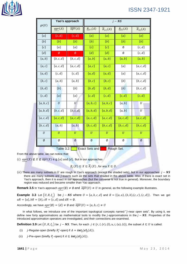
℘ 𝑈

Yao's approach 𝑗 − 𝑵𝑺

𝑎𝑝𝑟 𝐴 𝑎𝑝𝑟 𝐴 𝑅 𝑟 𝐴 𝑅 𝑟 𝐴 𝑅 𝑙 𝐴 𝑅 𝑙 𝐴

𝑎 𝑐, 𝑑 𝑐, 𝑑 𝑎 𝑎 𝑎 𝑎

𝑏 𝑏 𝑏 𝑏 𝑏 𝑏 𝑏

𝑐 𝑎 𝑎 𝑐 𝑐 ∅ 𝑐, 𝑑

𝑑 ∅ ∅ 𝑑 𝑑 ∅ 𝑐, 𝑑

𝑎, 𝑏 𝑏, 𝑐, 𝑑 𝑏, 𝑐, 𝑑 𝑎, 𝑏 𝑎, 𝑏 𝑎, 𝑏 𝑎, 𝑏

𝑎, 𝑐 𝑎, 𝑐, 𝑑 𝑎, 𝑐, 𝑑 𝑎, 𝑐 𝑎, 𝑐 𝑎 𝑎, 𝑐, 𝑑

𝑎, 𝑑 𝑐, 𝑑 𝑐, 𝑑 𝑎, 𝑑 𝑎, 𝑑 𝑎 𝑎, 𝑐, 𝑑

𝑏, 𝑐 𝑎, 𝑏 𝑎, 𝑏 𝑏, 𝑐 𝑏, 𝑐 𝑏 𝑏, 𝑐, 𝑑

𝑏, 𝑑 𝑏 𝑏 𝑏, 𝑑 𝑏, 𝑑 𝑏 𝑏, 𝑐, 𝑑

𝑐, 𝑑 𝑎 𝑎 𝑐, 𝑑 𝑐, 𝑑 𝑐, 𝑑 𝑐, 𝑑

𝑎, 𝑏, 𝑐 𝑈 𝑈 𝑎, 𝑏, 𝑐 𝑎, 𝑏, 𝑐 𝑎, 𝑏 𝑈

𝑎, 𝑏, 𝑑 𝑏, 𝑐, 𝑑 𝑏, 𝑐, 𝑑 𝑎, 𝑏, 𝑑 𝑎, 𝑏, 𝑑 𝑎, 𝑏 𝑈

𝑎, 𝑐, 𝑑 𝑎, 𝑐, 𝑑 𝑎, 𝑐, 𝑑 𝑎, 𝑐, 𝑑 𝑎, 𝑐, 𝑑 𝑎, 𝑐, 𝑑 𝑎, 𝑐, 𝑑

𝑏, 𝑐, 𝑑 𝑎, 𝑏 𝑎, 𝑏 𝑏, 𝑐, 𝑑 𝑏, 𝑐, 𝑑 𝑏, 𝑐, 𝑑 𝑏, 𝑐, 𝑑

𝑈 𝑈 𝑈 𝑈 𝑈 𝑈 𝑈

∅ ∅ ∅ ∅ ∅ ∅ ∅

Table 3.2: Exact Sets and Rough Set.

From the above table, we can notice that:

𝑖 𝑎𝑝𝑟 𝑋 ⊈ 𝑋 ⊈ 𝑎𝑝𝑟 𝑋 e.g. 𝑎 and {𝑑}. But in our approaches

𝑅𝑗 𝑋 ⊆ 𝑋 ⊆ 𝑅𝑗 𝑋 , for any 𝑋 ⊆ 𝑈.

𝑖𝑖 There are many subsets in 𝑈 are rough in Yao's approach (except the shaded sets), but in our approaches 𝑗 − 𝑵𝑺

there are many subsets are 𝑗-exacts such as the sets that shaded in the above table. Also, if there is exact set in

Yao's approach, then it is exact in our approaches (but the converse is not true in general). Moreover, the boundary region was reduced and became smaller than Yao approach.

Remark 3.5 In Yao's approach 𝑎𝑝𝑟 ∅ ≠ ∅ and 𝑎𝑝𝑟 𝑈 ≠ 𝑈 in general, as the following example illustrates.

Example 3.3 Let 𝑈, 𝑅, 𝜉𝑗 be 𝑗 − 𝑵𝑺 where 𝑈 = 𝑎, 𝑏, 𝑐, 𝑑 and 𝑅 = 𝑎, 𝑎 , 𝑏, 𝑏 , 𝑐, 𝑐 , 𝑐, 𝑑 . Then we get

𝑎𝑅 = 𝑎 , 𝑏𝑅 = 𝑏 , 𝑐𝑅 = 𝑐, 𝑑 and 𝑑𝑅 = ∅.

Accordingly, we have 𝑎𝑝𝑟 ∅ = 𝑑 ≠ ∅ and 𝑎𝑝𝑟 𝑈 = {𝑎, 𝑏, 𝑐} ≠ 𝑈

In what follows, we introduce one of the important topological concepts named “𝑗-near open sets”. By using it, we

define new forty approximations as mathematical tools to modify the 𝑗-approximations in the 𝑗 − 𝑵𝑺. Properties of the

introduced approximation operators are investigated, and their connections are examined.

Definition 3.9 Let 𝑈, 𝑅, 𝜉𝑗 be 𝑗 − 𝑵𝑺. Then, for each 𝑗 ∈ {𝑟, 𝑙, 𝑟 , 𝑙 , 𝑢, 𝑖, 𝑢 , 𝑖 }, the subset 𝐴 ⊆ 𝑈 is called:

(i) 𝑗-Regular-open (briefly 𝑅𝑗∗-open) if 𝐴 = 𝒊𝒏𝒕𝒋(𝒄𝒍𝒋 𝐴 ).

(ii) 𝑗-Pre-open (briefly 𝑃𝑗 -open) if 𝐴 ⊆ 𝒊𝒏𝒕𝒋(𝒄𝒍𝒋 𝐴 ).

ISSN 2347-1921

1642 | P a g e M a y 2 3 , 2 0 1 4

(iii) 𝑗-Semi-open (briefly 𝑆𝑗 -open) if 𝐴 ⊆ 𝒄𝒍𝒋(𝒊𝒏𝒕𝒋 𝐴 ).

(iv) 𝛾𝑗 -open if 𝐴 ⊆ 𝒊𝒏𝒕𝒋(𝒄𝒍𝒋 𝐴 ) ∪ 𝒄𝒍𝒋(𝒊𝒏𝒕𝒋 𝐴 ).

(v) 𝛼𝑗 -open if 𝐴 ⊆ 𝒊𝒏𝒕𝒋[𝒄𝒍𝒋(𝒊𝒏𝒕𝒋 𝐴 )].

(vi) 𝛽𝑗 -open (semi-pre-open) if 𝐴 ⊆ 𝒄𝒍𝒋[𝒊𝒏𝒕𝒋(𝒄𝒍𝒋 𝐴 )].

Remarks 3.6

(i) The above sets are called 𝑗-near open sets and the families of 𝑗-near open sets of 𝑈 denoted by 𝐾𝑗 𝑂 𝑈 , for

each 𝐾 = 𝑅∗, 𝑃, 𝑆, 𝛾, 𝛼 and 𝛽.

(ii) The complements of the 𝑗 − 𝑛𝑒𝑎𝑟 open sets are called 𝑗-near closed sets and the families of 𝑗-near closed sets

of 𝑈 denoted by 𝐾𝑗 𝐶 𝑈 , for each

𝐾 = 𝑅∗, 𝑃, 𝑆, 𝛾, 𝛼 and 𝛽.

(iii) According to [21], 𝛼𝑗𝑂 𝑈 represent a topology on 𝑈, and then the 𝑗-near interior (resp. the 𝑗-near closure)

represent the 𝑗-interior (resp. the 𝑗-closure).

Remark 3.7 According to the results in [21], the implications between the topologies 𝜏𝑗 and the above families of 𝑗-near

open sets (resp. 𝑗-near closed sets) are given in the following diagram (where ⟶ means ⊆).

Diagram 3.2

By using the 𝑗-near open set, we can introduce new methods for approximation rough sets using the 𝑗-near

interior and the 𝑗-near closure for each topology of 𝜏𝑗 as the following definitions illustrate.

Definition 3.10 Let 𝑈, 𝑅, 𝜉𝑗 be 𝑗 − 𝑵𝑺 and 𝐴 ⊆ 𝑈 . Then, for each 𝑗 ∈ {𝑟, 𝑙, 𝑟 , 𝑙 , 𝑢, 𝑖, 𝑢 , 𝑖 } and 𝑘 ∈

{𝑅∗, 𝑝, 𝑠, 𝛾, 𝛼, 𝛽}, the 𝑗-near lower and 𝑗-near upper approximations of A are defined respectively by

𝑅𝑗𝑘 𝐴 =∪ 𝐺 ∈ 𝑘𝑗 𝑂(𝑈): 𝐺 ⊆ 𝐴 = 𝑗-near interior of 𝐴,

𝑅𝑗

𝑘 𝐴 =∩ 𝐻 ∈ 𝑘𝑗 𝐶 𝑈 : 𝐴 ⊆ 𝐻 = 𝑗-near closure of 𝐴.

Definition 3.11 Let 𝑈, 𝑅, 𝜉𝑗 be 𝑗 − 𝑵𝑺 and 𝐴 ⊆ 𝑈. Then, for each

𝑗 ∈ 𝑟, 𝑙, 𝑟 , 𝑙 , 𝑢, 𝑖, 𝑢 , 𝑖 and 𝑘 ∈ 𝑅∗, 𝑝, 𝑠, 𝛾, 𝛼, 𝛽 , the𝑗-near boundary, 𝑗-near positive and 𝑗-near negative regions

of A are defined respectively by

𝐵𝑗𝑘 𝐴 = 𝑅𝑗

𝑘 𝐴 − 𝑅𝑗

𝑘 𝐴 ,

𝑃𝑂𝑆𝑗𝑘 𝐴 = 𝑅𝑗

𝑘 𝐴 and

𝑁𝐸𝐺𝑗𝑘 𝐴 = 𝑈 − 𝑅𝑗

𝑘 𝐴 .

Definition 3.12 Let 𝑈, 𝑅, 𝜉𝑗 be 𝑗 − 𝑵𝑺 and 𝐴 ⊆ 𝑈. Then, for each

𝑗 ∈ {𝑟, 𝑙, 𝑟 , 𝑙 , 𝑢, 𝑖, 𝑢 , 𝑖 } and 𝑘 ∈ 𝑅∗, 𝑝, 𝑠, 𝛾, 𝛼, 𝛽 , the 𝑗-near accuracy of the 𝑗-near approximations of 𝐴 ⊆ 𝑈 is

defined by

𝑅𝑗∗𝑂(𝑅𝑗

∗𝐶)

𝜏𝑗 𝑂(Γ𝑗 𝐶)

𝛼𝑗 𝑂(𝛼𝑗𝐶)

𝛾𝑗 𝑂(𝛾𝑗 𝐶)

𝛽𝑗 𝑂(𝛽𝑗 𝐶)

𝑃𝑗 𝑂(𝑃𝑗 𝐶)

𝑆𝑗 𝑂(𝑆𝑗 𝐶)

ISSN 2347-1921

1643 | P a g e M a y 2 3 , 2 0 1 4

𝛿𝑗𝑘 𝐴 =

𝑅𝑗𝑘 𝐴

𝑅𝑗

𝑘 𝐴

, 𝑤ℎ𝑒𝑟𝑒 𝑅𝑗

𝑘 𝐴 ≠ 0.

It is clear that 0 ≤ 𝛿𝑗𝑘 𝐴 ≤ 1.

The following propositions give the fundamental properties of the 𝑗-near approximations.

Proposition 3.2 Let 𝑈, 𝑅, 𝜉𝑗 be 𝑗 − 𝑵𝑺 and 𝐴 ⊆ 𝑈. Then, for each

𝑗 ∈ {𝑟, 𝑙, 𝑟 , 𝑙 , 𝑢, 𝑖, 𝑢 , 𝑖 } and 𝑘 = 𝑟∗, 𝑝, 𝑠, 𝛾, 𝛼, 𝛽

8 𝐴 ⊆ 𝑅𝑗

𝑘 𝐴 .

(9) 𝑅𝑗𝑘 ∅ = 𝑅𝑗

𝑘 ∅ = ∅.

10 If 𝐴 ⊆ 𝐵 then 𝑅𝑗

𝑘 𝐴 ⊆ 𝑅𝑗

𝑘 𝐵 .

11 𝑅𝑗

𝑘 𝐴 ∩ 𝐵 ⊆ 𝑅𝑗

𝑘 𝐴 ∩ 𝑅𝑗

𝑘 𝐵 .

12 𝑅𝑗

𝑘(𝐴 ∪ 𝐵) ⊇ 𝑅𝑗

𝑘 𝐴 ∪ 𝑅𝑗

𝑘 𝐵 .

(13) 𝑅𝑗

𝑘 𝐴 = 𝑅𝑗

𝑘 𝐴𝑐 𝑐, where Ac

is the complement of 𝐴.

14 𝑅𝑗

𝑘(𝑅𝑗

𝑘 𝐴 ) = 𝑅𝑗

𝑘 𝐴 .

1 𝑅𝑗𝑘 𝐴 ⊆ 𝐴.

2 𝑅𝑗𝑘 𝑈 = 𝑅𝑗

𝑘 𝑈 = 𝑈

3 If 𝐴 ⊆ 𝐵 then 𝑅𝑗𝑘 𝐴 ⊆ 𝑅𝑗

𝑘 𝐵 .

4 𝑅𝑗𝑘 𝐴 ∩ 𝐵 ⊆ 𝑅𝑗

𝑘 𝐴 ∩ 𝑅𝑗𝑘 𝐵 .

5 𝑅𝑗𝑘 𝐴 ∪ 𝐵 ⊇ 𝑅𝑗

𝑘 𝐴 ∪ 𝑅𝑗𝑘 𝐵 .

6 𝑅𝑗𝑘 𝐴 = 𝑅𝑗

𝑘 𝐴𝑐

𝑐

, where Ac

is the complement of 𝐴.

7 𝑅𝑗𝑘( 𝑅𝑗

𝑘 𝐴 ) = 𝑅𝑗𝑘 𝐴 .

Remark 3.8 Since the topologies 𝜏𝑗 are larger than the families of all regular open sets of 𝑈, 𝑅𝑗∗𝑂 𝑈 , (that

is, 𝑅𝑗∗𝑂 𝑈 represents a special case of the topologies 𝜏𝑗 ) then we will not using it in our approaches.

The 𝑗-near approximations are very interesting in rough context since the use of the 𝑗-near structures can help for further

developments in the theoretical and applications of rough sets. Moreover, the 𝑗-near approximations can help in the

discovery of hidden information in data collected from real-life applications, since the boundary regions will decreased or cancelled by increasing the lower and decreasing the upper approximations, as the following results illustrate.

Proposition 3.3 Let 𝑈, 𝑅, 𝜉𝑗 be 𝑗 − 𝑵𝑺 and 𝐴 ⊆ 𝑈. Then, for each

𝑗 ∈ 𝑟, 𝑙, 𝑟 , 𝑙 , 𝑢, 𝑖, 𝑢 , 𝑖 and 𝑘 ∈ 𝑅∗, 𝑝, 𝑠, 𝛾, 𝛼, 𝛽 such that 𝑘 ≠ 𝑅∗:

𝑅𝑗 𝐴 ⊆ 𝑅𝑗𝑘 𝐴 ⊆ 𝐴 ⊆ 𝑅𝑗

𝑘 𝐴 ⊆ 𝑅𝑗 𝐴

Proof Since the families of 𝑗-near open sets 𝑘𝑗 𝑂(𝑈) (resp. 𝑗-near closed sets 𝑘𝑗 𝐶(𝑈)) are larger than the topologies 𝜏𝑗

(resp. the families of 𝑗-closed sets Γ𝑗 ). Then we have

𝑅𝑗 𝐴 =∪ 𝐺 ∈ 𝜏𝑗 : 𝐺 ⊆ 𝐴 ⊆∪ 𝐺 ∈ 𝑘𝑗𝑂(𝑈): 𝐺 ⊆ 𝐴 = 𝑅𝑗𝑘 𝐴 .

By similar way, we can prove 𝑅𝑗

𝑘 𝐴 ⊆ 𝑅𝑗 𝐴 .∎

Corollary 3.1 Let 𝑈, 𝑅, 𝜉𝑗 be 𝑗 − 𝑵𝑺 and 𝐴 ⊆ 𝑈. Then, for each

𝑗 ∈ 𝑟, 𝑙, 𝑟 , 𝑙 , 𝑢, 𝑖, 𝑢 , 𝑖 and 𝑘 ∈ 𝑅∗, 𝑝, 𝑠, 𝛾, 𝛼, 𝛽 such that 𝑘 ≠ 𝑅∗:

1 𝐵𝑗𝑘 𝐴 ⊆ 𝐵𝑗 𝐴 . 2 𝛿𝑗 𝐴 ≤ 𝛿𝑗

𝑘 𝐴 .

The aim of the following example is to show that, the above results and to illustrate the importance of using 𝑗-near

concepts in rough context.

Example 3.4 Let the 𝑗 − 𝑵𝑺 𝑈, 𝑅, 𝜉𝑗 , where 𝑈 = 𝑎, 𝑏, 𝑐, 𝑑 and

𝑅 = 𝑎, 𝑎 , 𝑎, 𝑏 , 𝑏, 𝑎 , 𝑏, 𝑏 , 𝑐, 𝑎 , 𝑐, 𝑎 , 𝑐, 𝑏 , 𝑐, 𝑐 , 𝑐, 𝑑 , 𝑑, 𝑑 .

Then, we get 𝑁𝑟 𝑎 = 𝑎, 𝑏 , 𝑁𝑟 𝑏 = 𝑎, 𝑏 , 𝑁𝑟 𝑐 = 𝑈, 𝑁𝑟 𝑑 = 𝑑 this implies

𝜏𝑟 = 𝑈, ∅, 𝑑 , 𝑎, 𝑏 , 𝑎, 𝑏, 𝑑 and Γ𝑟 = 𝑈, ∅, 𝑐 , 𝑐, 𝑑 , 𝑎, 𝑏, 𝑐 .

We shall compute the 𝑗-near approximations for 𝑗 = 𝑟 and 𝑘 = 𝑝, 𝛾, 𝛽 and the other cases similarly as follow:

𝑃𝑟𝑂 𝑈 = 𝑈, ∅, 𝑎 , 𝑏 , 𝑑 , 𝑎, 𝑏 , 𝑎, 𝑑 , 𝑏, 𝑑 , 𝑎, 𝑏, 𝑑 , 𝑎, 𝑐, 𝑑 , 𝑏, 𝑐, 𝑑 ,

ISSN 2347-1921

1644 | P a g e M a y 2 3 , 2 0 1 4

𝑃𝑟𝐶 𝑈 = 𝑈, ∅, 𝑎 , 𝑏 , 𝑐 , 𝑎, 𝑐 , 𝑏, 𝑐 , 𝑐, 𝑑 , 𝑎, 𝑏, 𝑐 , 𝑎, 𝑐, 𝑑 , 𝑏, 𝑐, 𝑑 ,

𝛾𝑟𝑂 𝑈 = 𝑈, ∅, 𝑎 , 𝑏 , 𝑑 , 𝑎, 𝑏 , 𝑎, 𝑑 , 𝑏, 𝑑 , 𝑐, 𝑑 , 𝑎, 𝑏, 𝑐 , 𝑎, 𝑏, 𝑑 , 𝑎, 𝑐, 𝑑 , 𝑏, 𝑐, 𝑑 ,

𝛾𝑟𝐶 𝑈 = 𝑈, ∅, 𝑎 , 𝑏 , 𝑐 , 𝑑 , 𝑎, 𝑏 , 𝑎, 𝑐 , 𝑏, 𝑐 , 𝑐, 𝑑 , 𝑎, 𝑏, 𝑐 , 𝑎, 𝑐, 𝑑 , 𝑏, 𝑐, 𝑑 ,

𝛽𝑟𝑂(𝑈) = 𝑈, ∅, 𝑎 , 𝑏 , 𝑑 , 𝑎, 𝑏 , 𝑎, 𝑐 , 𝑎, 𝑑 , 𝑏, 𝑐 , 𝑏, 𝑑 , 𝑐, 𝑑 , 𝑎, 𝑏, 𝑐 , 𝑎, 𝑏, 𝑑 ,

𝑎, 𝑐, 𝑑 , 𝑏, 𝑐, 𝑑 and

𝛽𝑟𝐶(𝑈) = 𝑈, ∅, 𝑎 , 𝑏 , 𝑐 , 𝑑 , 𝑎, 𝑏 , 𝑎, 𝑐 , 𝑎, 𝑑 , 𝑏, 𝑐 , 𝑏, 𝑑 , 𝑐, 𝑑 , 𝑎, 𝑏, 𝑐 , 𝑎, 𝑐, 𝑑 ,

𝑏, 𝑐, 𝑑 .

The following table introduces comparisons between the 𝑗-approximations and the 𝑗 -near approximations of the all

subsets of 𝑈 as follow:

℘ 𝑈

𝜏𝑟 𝑃𝑟 𝛾𝑟 𝛽𝑟

𝑅𝑟 𝐴 𝑅𝑟 𝐴 𝑅𝑟𝑝 𝐴 𝑅𝑟

𝑝 𝐴 𝑅𝑟

𝛾 𝐴 𝑅𝑟

𝛾 𝐴 𝑅𝑟

𝛽 𝐴 𝑅𝑟

𝛽 𝐴

𝑎 ∅ 𝑎, 𝑏, 𝑐 𝑎 𝑎 𝑎 𝑎 𝑎 𝑎

𝑏 ∅ 𝑎, 𝑏, 𝑐 𝑏 𝑏 𝑏 𝑏 𝑏 𝑏

𝑐 ∅ 𝑐 ∅ 𝑐 ∅ 𝑐 ∅ 𝑐

𝑑 𝑑 𝑐, 𝑑 𝑑 𝑐, 𝑑 𝑑 𝑑 𝑑 𝑑

𝑎, 𝑏 𝑎, 𝑏 𝑎, 𝑏, 𝑐 𝑎, 𝑏 𝑎, 𝑏, 𝑐 𝑎, 𝑏 𝑎, 𝑏 𝑎, 𝑏 𝑎, 𝑏

𝑎, 𝑐 ∅ 𝑎, 𝑏, 𝑐 𝑎 𝑎, 𝑐 𝑎 𝑎, 𝑐 𝑎, 𝑐 𝑎, 𝑐

𝑎, 𝑑 𝑑 𝑈 𝑎, 𝑑 𝑎, 𝑐, 𝑑 𝑎, 𝑑 𝑎, 𝑐, 𝑑 𝑎, 𝑑 𝑎, 𝑑

𝑏, 𝑐 ∅ 𝑎, 𝑏, 𝑐 𝑏 𝑏, 𝑐 𝑏 𝑏, 𝑐 𝑏, 𝑐 𝑏, 𝑐

𝑏, 𝑑 𝑑 𝑈 𝑏, 𝑑 𝑏, 𝑐, 𝑑 𝑏, 𝑑 𝑏, 𝑐, 𝑑 𝑏, 𝑑 𝑏, 𝑑

𝑐, 𝑑 ∅ 𝑐, 𝑑 𝑑 𝑐, 𝑑 𝑐, 𝑑 𝑐, 𝑑 𝑐, 𝑑 𝑐, 𝑑

𝑎, 𝑏, 𝑐 𝑎, 𝑏 𝑎, 𝑏, 𝑐 𝑎, 𝑏 𝑎, 𝑏, 𝑐 𝑎, 𝑏, 𝑐 𝑎, 𝑏, 𝑐 𝑎, 𝑏, 𝑐 𝑎, 𝑏, 𝑐

𝑎, 𝑏, 𝑑 𝑎, 𝑏, 𝑑 𝑈 𝑎, 𝑏, 𝑑 𝑈 𝑎, 𝑏, 𝑑 𝑈 𝑎, 𝑏, 𝑑 𝑈

𝑎, 𝑐, 𝑑 𝑑 𝑈 𝑎, 𝑐, 𝑑 𝑎, 𝑐, 𝑑 𝑎, 𝑐, 𝑑 𝑎, 𝑐, 𝑑 𝑎, 𝑐, 𝑑 𝑎, 𝑐, 𝑑

𝑏, 𝑐, 𝑑 𝑑 𝑈 𝑏, 𝑐, 𝑑 𝑏, 𝑐, 𝑑 𝑏, 𝑐, 𝑑 𝑏, 𝑐, 𝑑 𝑏, 𝑐, 𝑑 𝑏, 𝑐, 𝑑

𝑈 𝑈 𝑈 𝑈 𝑈 𝑈 𝑈 𝑈 𝑈

∅ ∅ ∅ ∅ ∅ ∅ ∅ ∅ ∅

Table 3.3: Exact Set

From the above table, we can notice that:

(i) Applying the j-near approximations is very interesting for removing the vagueness of rough sets, and this would helps

to extract and discovery of hidden information in data collected from real-life applications.

(ii) The best 𝑗-near approach is 𝛽𝑗 (since 𝛽𝑗 is more accurate than the other types of 𝑗-near open sets).

(iii) There are many rough sets in 𝜏𝑟 , but it is𝑗-near exact such as the shaded sets.

4 𝑗-Rough Membership Relations, 𝑗-Rough Membership Functions and 𝑗-Fuzzy Sets.

The present section is provided to introduce new definitions of “rough membership relations, rough membership

functions and fuzzy sets” in 𝑗 − 𝑵𝑺. Moreover, we introduce some differences between our approaches and some others

approaches such as Lin [28]. In addition, we give some solutions to accurate the approximations and exactness of rough sets. In the last of the section we give some connections between rough set theory, fuzzy set theory and topology.

Definition 4.1 Let 𝑈, 𝑅, 𝜉𝑗 be 𝑗 − 𝑵𝑺 and 𝐴 ⊆ 𝑈. Then we say that:

(i) x is " 𝑗-surely" belongs to 𝐴, written 𝑥 ∈𝑗 𝐴, if 𝑥 ∈ 𝑅𝑗 𝐴 .

ISSN 2347-1921

1645 | P a g e M a y 2 3 , 2 0 1 4

(ii) x is " 𝑗-possibly" belongs to X, written 𝑥 ∈𝑗 𝐴, if 𝑥 ∈ 𝑅𝑗 𝐴 .

These two membership relations are called " 𝑗 -strong" and " 𝑗 -weak" membership relations respectively , ∀ 𝑗 ∈{𝑟, 𝑙, 𝑟 , 𝑙 , 𝑢, 𝑖, 𝑢 , 𝑖 }.

Lemma 4.1 Let the triple 𝑈, 𝑅, 𝜉𝑗 be 𝑗 − 𝑵𝑺 and 𝐴 ⊆ 𝑈 . Then the following statements are true in general:

(i) If 𝑥 ∈𝑗𝐴 implies to 𝑥 ∈ 𝐴. (ii) If 𝑥 ∈ 𝐴 implies to 𝑥 ∈𝑗 𝐴.

Proof Straight forward. ∎

Remark 4.1 The converse of the above lemma is not true in general, as the following example illustrates:

Example 4.1 Consider the triple 𝑈, 𝑅, 𝜉𝑗 be 𝑗 − 𝑵𝑺 , where 𝑈 = 𝑎, 𝑏, 𝑐, 𝑑 and = 𝑎, 𝑎 ,

𝑏, 𝑏 , 𝑐, 𝑐 , 𝑐, 𝑏 , 𝑐, 𝑑 , 𝑑, 𝑎 . Then we get

𝜏𝑟 = {𝑈, ∅, 𝑎 , 𝑏 , 𝑎, 𝑏 , 𝑎, 𝑑 , {𝑎, 𝑏, 𝑑}and

Γ𝑟 = {𝑈, ∅, 𝑐 , 𝑏, 𝑐 , 𝑐, 𝑑 , 𝑎, 𝑐, 𝑑 , {𝑏, 𝑐, 𝑑}.

We show the above remark in case of 𝑗 = 𝑟 and the other cases similarly. Suppose that 𝐴 = 𝑎, 𝑏, 𝑐 , then we

get

𝑅𝑟 𝐴 = 𝑎, 𝑏 and 𝑅𝑟 𝐴 = 𝑈.

Clearly 𝑐 ∈ 𝐴 but 𝑐 ∉𝑗 𝐴 and 𝑑 ∈𝑟 𝐴 but 𝑑 ∉ 𝐴.

Proposition 4.1 Let 𝑈, 𝑅, 𝜉𝑗 be 𝑗 − 𝑵𝑺 and 𝐴, 𝐵 ⊆ 𝑈. Then by using the properties of the 𝑗-approximations we can

prove the following properties:

(i) If 𝐴 ⊆ 𝐵, then (𝑥 ∈𝑗 𝐴 ⟹ 𝑥 ∈𝑗 𝐵 and 𝑥 ∈𝑗 𝐴 ⟹ 𝑥 ∈𝑗 𝐵).

(ii) 𝑥 ∈𝑗 𝐴 ∪ 𝐵 ⟺ 𝑥 ∈𝑗 𝐴 or 𝑥 ∈𝑗 𝐵.

(iii) 𝑥 ∈𝑗 𝐴 ∪ 𝐵 ⟺ 𝑥 ∈𝑗 𝐴 and 𝑥 ∈𝑗 𝐵.

(iv) If 𝑥 ∈𝑗 𝐴 or 𝑥 ∈𝑗 𝐵, then 𝑥 ∈𝑗 𝐴 ∪ 𝐵 .

(v) If 𝑥 ∈𝑗 𝐴 ∪ 𝐵 , then 𝑥 ∈𝑗 𝐴 and 𝑥 ∈𝑗 𝐵.

(vi) 𝑥 ∈𝑗 𝐴𝑐 ⟺ non 𝑥 ∈𝑗 𝐴.

(vii) 𝑥 ∈𝑗 𝐴𝑐 ⟺ non 𝑥 ∈𝑗 𝐴.

Remarks 4.2 We can redefine the 𝑗-approximations by using ∈𝑗 and ∈𝑗 as follows, for any 𝐴, 𝐵 ⊆ 𝑈:

𝑅𝑗 𝐴 = {𝑥 ∈ 𝑈|𝑥 ∈𝑗 𝐴}and 𝑅𝑗 𝐴 = {𝑥 ∈ 𝑈|𝑥 ∈𝑗 𝐴}.

The following proposition is very interesting since it is give the relations between different types of 𝑗-rough

membership relations ∈𝑗 and ∈𝑗 . Accordingly, we will illustrate the importance of using these different types of

membership relations.

Proposition 4.2 Let 𝑈, 𝑅, 𝜉𝑗 be 𝑗 − 𝑵𝑺 and 𝐴 ⊆ 𝑈. Then

𝑖 If 𝑥 ∈𝑖 𝐴 ⟹ 𝑥 ∈𝑟 𝐴 ⟹ 𝑥 ∈𝑢 𝐴.

𝑖𝑖 If 𝑥 ∈𝑖𝐴 ⟹ 𝑥 ∈

𝑙𝐴 ⟹ 𝑥 ∈

𝑢𝐴.

𝑖𝑖𝑖 If 𝑥 ∈𝑢 𝐴 ⟹ 𝑥 ∈𝑟 𝐴 ⟹ 𝑥 ∈𝑖 𝐴.

𝑖𝑣 If 𝑥 ∈𝑢 𝐴 ⟹ 𝑥 ∈𝑙 𝐴 ⟹ 𝑥 ∈𝑖 𝐴.

𝑣 If 𝑥 ∈ 𝑖 𝐴 ⟹ 𝑥 ∈ 𝑟 𝐴 ⟹ 𝑥 ∈ 𝑢 𝐴.

𝑣𝑖 If 𝑥 ∈ 𝑖

𝐴 ⟹ 𝑥 ∈ 𝑙

𝐴 ⟹ 𝑥 ∈ 𝑢

𝐴.

𝑣𝑖𝑖 If 𝑥 ∈ 𝑢 𝐴 ⟹ 𝑥 ∈ 𝑟 𝐴 ⟹ 𝑥 ∈ 𝑖 𝐴.

𝑣𝑖𝑖𝑖 If 𝑥 ∈ 𝑢 𝐴 ⟹ 𝑥 ∈ 𝑙 𝐴 ⟹ 𝑥 ∈ 𝑖 𝐴.

Proof We will prove first statement and the others similarly:

ISSN 2347-1921

1646 | P a g e M a y 2 3 , 2 0 1 4

𝑖 If 𝑥 ∈𝑖 𝐴 ⟹ 𝑥 ∈ 𝑅𝑖 𝐴 ⟹ 𝑥 ∈ 𝑅𝑟 𝐴 ⟹ 𝑥 ∈𝑟 𝐴.

Also, if 𝑥 ∈𝑟 𝐴 ⟹ 𝑥 ∈ 𝑅𝑟 𝐴 ⟹ 𝑥 ∈ 𝑅𝑢 𝐴 ⟹ 𝑥 ∈𝑢 𝐴. ∎

Remark 4.3 The converse of the above proposition is not true in general as the following example illustrates.

Example 4.2 Let the triple 𝑈, 𝑅, 𝜉𝑗 be −𝑵𝑺 , where 𝑈 = 𝑎, 𝑏, 𝑐, 𝑑 and

𝑅 = 𝑎, 𝑎 , 𝑎, 𝑏 , 𝑏, 𝑐 , 𝑏, 𝑑 , 𝑐, 𝑎 , 𝑑, 𝑎 . Then we get

𝜏 𝑟 = {𝑈, ∅, 𝑎 , 𝑎, 𝑏 , 𝑐, 𝑑 , 𝑎, 𝑐, 𝑑 }and Γ 𝑟 = {𝑈, ∅, 𝑏 , 𝑎, 𝑏 , 𝑐, 𝑑 , 𝑏, 𝑐, 𝑑 }.

𝜏 𝑙 = {𝑈, ∅, 𝑎 , 𝑏 , 𝑎, 𝑏 , 𝑎, 𝑐, 𝑑 }and Γ 𝑙 = {𝑈, ∅, 𝑏 , 𝑐, 𝑑 , 𝑎, 𝑐, 𝑑 , 𝑏, 𝑐, 𝑑 }.

𝜏 𝑖 = 𝑈, ∅, 𝑎 , 𝑏 , 𝑎, 𝑏 , 𝑐, 𝑑 , 𝑎, 𝑐, 𝑑 , 𝑏, 𝑐, 𝑑 = Γ 𝑖 .

𝜏 𝑢 = {𝑈, ∅, 𝑎 , 𝑎, 𝑏 , 𝑎, 𝑐, 𝑑 }and Γ 𝑢 = {𝑈, ∅, 𝑏 , 𝑐, 𝑑 , 𝑏, 𝑐, 𝑑 }.

Suppose that 𝐴 = 𝑏, 𝑐, 𝑑 . Thus we get

𝑅 𝑢 𝐴 = ∅, 𝑅 𝑟 𝐴 = 𝑐, 𝑑 , 𝑅 𝑙 𝐴 = 𝑏 and𝑅 𝑖 𝐴 = 𝑏, 𝑐, 𝑑 .

Accordingly, 𝑐 ∈ 𝑟 𝐴 and 𝑏 ∈ 𝑙 𝐴 but 𝑏 ∉ 𝑢 𝐴 and 𝑐 ∉ 𝑢 𝐴 .

Also 𝑏 ∈ 𝑖 𝐴 and 𝑐 ∈𝑖𝐴 but 𝑏 ∉𝑟 𝐴 and 𝑐 ∉𝑙 𝐴.

By similar way, we can illustrate the others cases.

Definition 4.2 Let 𝑈, 𝑅, 𝜉𝑗 be 𝑗 − 𝑵𝑺 and 𝐴 ⊆ 𝑈. Then ∀ 𝑗 ∈ {𝑟, 𝑙, 𝑟 , 𝑙 , 𝑢, 𝑖, 𝑢 , 𝑖 } and 𝑥 ∈ 𝑈 we define the 𝑗-

rough membership functions of 𝑗 − 𝑵𝑺 as follows:

The 𝑗- rough membership functions on Ufor subset 𝐴 are 𝜇𝐴𝑗

: 𝑈 → [0,1], where

𝜇𝐴𝑗 𝑥 =

{∩ 𝑁𝑗 𝑥 } ∩ 𝐴

∩ 𝑁𝑗 𝑥

and 𝐴 denotes the cardinality of 𝐴.

The rough 𝑗-membership function expresses conditional probability that 𝑥 belongs to 𝐴 given 𝑅 and can be

interpreted as a degree that 𝑥 belongs to A in view of information about 𝑥 expressed by 𝑅. Moreover, in case of infinite

universe, the above membership function 𝜇𝐴𝑗

can be use for spaces having locally finite minimal neighborhoods for each

point.

Remark 4.4 The rough 𝑗-membership functions can be used to define 𝑗-approximations of a set 𝐴, as shown below:

𝑅𝑗 𝐴 = 𝑥 ∈ 𝑈 𝜇𝐴𝑗 𝑥 = 1} and

𝑅𝑗 𝐴 = 𝑥 ∈ 𝑈 𝜇𝐴𝑗 𝑥 > 0}.

The following results give the fundamental properties of the above 𝑗- rough membership functions.

Proposition 4.3 Let 𝑈, 𝑅, 𝜉𝑗 be 𝑗 − 𝑵𝑺 and 𝐴, 𝐵 ⊆ 𝑈. Then

(i) 𝜇𝐴𝑗 𝑥 = 1 ⟺ 𝑥 ∈𝑗 𝐴.

(ii) 𝜇𝐴𝑗 𝑥 = 0 ⟺ 𝑥 ∈ 𝑈 − 𝑅𝑗 𝐴 .

(iii) 0 < 𝜇𝐴𝑗 𝑥 < 1 ⟺ 𝑥 ∈ ℬ𝑗 𝐴 .

(iv) 𝜇𝑈−𝐴𝑗 𝑥 = 1 − 𝜇𝐴

𝑗 𝑥 for any 𝑥 ∈ 𝑈.

(v) 𝜇𝐴∪𝐵𝑗 𝑥 ≥ max(𝜇𝐴

𝑗 𝑥 , 𝜇𝐵𝑗 𝑥 )𝑓𝑜𝑟 𝑎𝑛𝑦 𝑥 ∈ 𝑈.

(vi) 𝜇𝐴∩𝐵𝑗 𝑥 ≤ min(𝜇𝐴

𝑗 𝑥 , 𝜇𝐵𝑗 𝑥 )𝑓𝑜𝑟 𝑎𝑛𝑦 𝑥 ∈ 𝑈.

Proof We will prove (i), and the others similarly.

𝑥 ∈𝑗 𝐴 ⟺ 𝑥 ∈ 𝑅𝑗 𝐴 ⟺ 𝑥 ∈ 𝐴, 𝑁𝑗 𝑥 ⊆ 𝐴 ⟺ 𝜇𝐴𝑗 𝑥 = 1. ∎

Remark 4.5 The rough 𝑗-membership functions divides the universe 𝑈 by using the 𝑗-boundary, 𝑗-positive and 𝑗-negative regions of 𝐴 ⊆ 𝑈, respectively as follow:

ISSN 2347-1921

1647 | P a g e M a y 2 3 , 2 0 1 4

ℬ𝑗 𝐴 = 𝑥 ∈ 𝑈 0 < 𝜇𝐴𝑗 𝑥 < 1},

𝑃𝑂𝑆𝑗 𝐴 = 𝑥 ∈ 𝑈 𝜇𝐴𝑗 𝑥 = 1} and

𝑁𝐸𝐺𝑗 𝐴 = 𝑥 ∈ 𝑈 𝜇𝐴𝑗 𝑥 = 0}.

Lemma 4.2 Let 𝑈, 𝑅, 𝜉𝑗 be 𝑗 − 𝑵𝑺 and 𝐴 ⊆ 𝑈. Then for every 𝑥 ∈ 𝑈

(i) 𝜇𝐴𝑢 𝑥 = 1 ⟹ 𝜇𝐴

𝑟 𝑥 = 1 ⟹ 𝜇𝐴𝑖 𝑥 = 1 .

(ii) 𝜇𝐴𝑢 𝑥 = 1 ⟹ 𝜇𝐴

𝑙 𝑥 = 1 ⟹ 𝜇𝐴𝑖 𝑥 = 1 .

(iii) 𝜇𝐴 𝑢 𝑥 = 1 ⟹ 𝜇𝐴

𝑟 𝑥 = 1 ⟹ 𝜇𝐴 𝑖 𝑥 = 1 .

(iv) 𝜇𝐴 𝑢 𝑥 = 1 ⟹ 𝜇𝐴

𝑙 𝑥 = 1 ⟹ 𝜇𝐴 𝑖 𝑥 = 1 .

Proof

(i) If 𝜇𝐴𝑢 𝑥 = 1 ⟹ 𝑥 ∈𝑢 𝐴 ⟹ 𝑥 ∈𝑟 𝐴 ⟹ 𝜇𝐴

𝑟 𝑥 = 1 .

Also, if 𝜇𝐴𝑟 𝑥 = 1 ⟹ 𝑥 ∈𝑟 𝐴 ⟹ 𝑥 ∈𝑖 𝐴 ⟹ 𝜇𝐴

𝑖 𝑥 = 1.

(ii) , (iii) and (iv) Similarly as (i).∎

Lemma 4.3 Let 𝑈, 𝑅, 𝜉𝑗 be 𝑗 − 𝑵𝑺 and 𝐴 ⊆ 𝑈. Then for every 𝑥 ∈ 𝑈

(i) 𝜇𝐴𝑢 𝑥 = 0 ⟹ 𝜇𝐴

𝑟 𝑥 = 0 ⟹ 𝜇𝐴𝑖 𝑥 = 0 .

(ii) 𝜇𝐴𝑢 𝑥 = 0 ⟹ 𝜇𝐴

𝑙 𝑥 = 0 ⟹ 𝜇𝐴𝑖 𝑥 = 0 .

(iii) 𝜇𝐴 𝑢 𝑥 = 0 ⟹ 𝜇𝐴

𝑟 𝑥 = 0 ⟹ 𝜇𝐴 𝑖 𝑥 = 0 .

(iv) 𝜇𝐴 𝑢 𝑥 = 0 ⟹ 𝜇𝐴

𝑙 𝑥 = 0 ⟹ 𝜇𝐴 𝑖 𝑥 = 0 .

Proof

(i) If 𝜇𝐴𝑢 𝑥 = 1 ⟹ 𝑁𝑢 𝑥 ∩ 𝐴 = ∅ ⟹ 𝑁𝑟 𝑥 ∩ 𝐴 = ∅

⟹ 𝜇𝐴𝑟 𝑥 = 0 .

Also, if 𝜇𝐴𝑟 𝑥 = 0 ⟹ 𝑁𝑟 𝑥 ∩ 𝐴 = ∅ ⟹ 𝑁𝑖 𝑥 ∩ 𝐴 = ∅

⟹ 𝜇𝐴𝑖 𝑥 = 0.

(ii) , (iii) and (iv) Similarly as (i).∎

Remarks 4.6

(i) According to the above results and by using Proposition 4.2, we can prove that 𝜇𝐴𝑖 is more accurate than the

others types, this means that:

1 If 𝑥 ∈ 𝐴 ⟹ 𝜇𝐴𝑢 𝑥 ≤ 𝜇𝐴

𝑟 𝑥 ≤ 𝜇𝐴𝑖 𝑥 and

if 𝑥 ∈ 𝐴 ⟹ 𝜇𝐴𝑢 𝑥 ≤ 𝜇𝐴

𝑙 𝑥 ≤ 𝜇𝐴𝑖 𝑥 .

2 If 𝑥 ∉ 𝐴 ⟹ 𝜇𝐴𝑖 𝑥 ≤ 𝜇𝐴

𝑟 𝑥 ≤ 𝜇𝐴𝑢 𝑥 and

if 𝑥 ∉ 𝐴 ⟹ 𝜇𝐴𝑖 𝑥 ≤ 𝜇𝐴

𝑙 𝑥 ≤ 𝜇𝐴𝑢 𝑥 .

3 If 𝑥 ∈ 𝐴 ⟹ 𝜇𝐴 𝑢 𝑥 ≤ 𝜇𝐴

𝑟 𝑥 ≤ 𝜇𝐴 𝑖 𝑥 and

if 𝑥 ∈ 𝐴 ⟹ 𝜇𝐴 𝑢 𝑥 ≤ 𝜇𝐴

𝑙 𝑥 ≤ 𝜇𝐴 𝑖 𝑥 .

4 If 𝑥 ∉ 𝐴 ⟹ 𝜇𝐴 𝑖 𝑥 ≤ 𝜇𝐴

𝑟 𝑥 ≤ 𝜇𝐴 𝑢 𝑥 and

if 𝑥 ∉ 𝐴 ⟹ 𝜇𝐴 𝑖 𝑥 ≤ 𝜇𝐴

𝑙 𝑥 ≤ 𝜇𝐴 𝑢 𝑥 .

(ii) The converse of the above lemmas is not true in general.

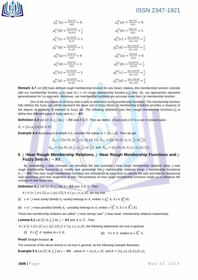
The following example illustrates Remarks 4.6.

Example 4.3 According to Example 4.2, consider the subset 𝐴 = 𝑏, 𝑐, 𝑑 . Then we get

ISSN 2347-1921

1648 | P a g e M a y 2 3 , 2 0 1 4

𝜇𝐴 𝑟 𝑎 =

{𝑎}∩𝐴

{𝑎} = 0.

𝜇𝐴 𝑟 𝑏 =

{𝑎 ,𝑏}∩𝐴

{𝑎 ,𝑏} =

1

2.

𝜇𝐴 𝑟 𝑐 =

{𝑐 ,𝑑}∩𝐴

{𝑐 ,𝑑 = 1.

𝜇𝐴 𝑟 𝑑 =

{𝑐 ,𝑑}∩𝐴

{𝑐 ,𝑑} = 1.

𝜇𝐴 𝑙 𝑎 =

{𝑎}∩𝐴

{𝑎} = 0.

𝜇𝐴 𝑙 𝑏 =

{𝑏}∩𝐴

{𝑏} = 1.

𝜇𝐴 𝑙 𝑐 =

{𝑎 ,𝑐 ,𝑑}∩𝐴

{𝑎 ,𝑐 ,𝑑} =

2

3.

𝜇𝐴 𝑙 𝑑 =

{𝑎 ,𝑐 ,𝑑}∩𝐴

{𝑎 ,𝑐 ,𝑑} =

2

3.

𝜇𝐴 𝑖 𝑎 =

{𝑎}∩𝐴

{𝑎} = 0.

𝜇𝐴 𝑖 𝑏 =

{𝑏}∩𝐴

{𝑏} = 1.

𝜇𝐴 𝑖 𝑐 =

{𝑐 ,𝑑}∩𝐴

{𝑐 ,𝑑} = 1.

𝜇𝐴 𝑖 𝑑 =

{𝑐 ,𝑑}∩𝐴

{𝑐 ,𝑑} = 1.

𝜇𝐴 𝑢 𝑎 =

{𝑎}∩𝐴

{𝑎} = 0.

𝜇𝐴 𝑢 𝑏 =

{𝑎 ,𝑏}∩𝐴

{𝑎 ,𝑏} =

1

2.

𝜇𝐴 𝑢 𝑐 =

{𝑎 ,𝑐 ,𝑑}∩𝐴

{𝑎 ,𝑐 ,𝑑} =

2

3.

𝜇𝐴 𝑢 𝑑 =

{𝑎 ,𝑐 ,𝑑}∩𝐴

{𝑎 ,𝑐 ,𝑑} =

2

3.

Remark 4.7 Lin [28] have defined rough membership function for any binary relation, this membership function coincide

with our membership function 𝜇𝐴𝑗in case of 𝑗 = 𝑟(𝑟-rough membership function 𝜇𝐴

𝑟 ) only. So, our approaches represent

generalization for Lin approach. Moreover, our membership functions are accurate more than Lin membership function.

One of the key issues in all fuzzy sets is how to determine fuzzy membership functions. The membership function fully defines the fuzzy set, which represent the basic tool in fuzzy theory. A membership functions provides a measure of

the degree of similarity of element to fuzzy set. The following definition uses the 𝑗-rough membership functions 𝜇𝐴𝑗 to

define four different types of fuzzy sets in 𝑗 − 𝑵𝑺.

Definition 4.3 Let 𝑈, 𝑅, 𝜉𝑗 be 𝑗 − 𝑵𝑺 and 𝐴 ⊆ 𝑈. Then we define 𝑗-fuzzy sets in 𝑈 is a set of ordered pairs:

𝐴 𝑗 = {(𝑥, 𝜇𝐴𝑗 𝑥 )|𝑥 ∈ 𝑈}.

Example 4.4 According to Example 4.2, consider the subset 𝐴 = 𝑏, 𝑐, 𝑑 . Then we get

𝐴 𝑟 = { 𝑎, 0 , (𝑏,1

2), (𝑐, 1), (𝑑, 1)}, 𝐴 𝑙 = { 𝑎, 0 , (𝑏, 1), (𝑐,

2

3), (𝑑,

2

3)},

𝐴 𝑢 = { 𝑎, 0 , (𝑏,1

2), (𝑐,

2

3), (𝑑,

2

3)}, and 𝐴 𝑖 = { 𝑎, 0 , (𝑏, 1), (𝑐, 1), (𝑑, 1)}.

5 𝑗 -Near Rough Membership Relations, 𝑗 -Near Rough Membership Functions and 𝑗-Fuzzy Sets in 𝑗 − 𝑵𝑺 .

By considering 𝑗-near concepts, we introduce the new concepts 𝑗-near rough membership relations (resp. 𝑗-near

rough membership functions) to modify and generalize the 𝑗 -membership relations (resp. 𝑗 -membership functions)

in 𝑗 − 𝑵𝑺. The near rough membership functions are considered as easy tools to classify the sets and help for measuring

near exactness and near roughness of sets. The existence of near rough membership functions made us to introduce the concept of near fuzzy sets.

Definition 5.1 Let 𝑈, 𝑅, 𝜉𝑗 be 𝑗 − 𝑵𝑺 and 𝐴 ⊆ 𝑈. Then

∀ 𝑗 ∈ 𝑟, 𝑙, 𝑟 , 𝑙 , 𝑢, 𝑖, 𝑢 , 𝑖 , 𝑘 ∈ 𝑝, 𝑠, 𝛾, 𝛼, 𝛽 , we say that:

(i) 𝑥 is " 𝑗-near surely"(briefly 𝑘𝑗 -surely) belongs to 𝐴, written 𝑥 ∈𝑗𝑘 𝐴, if 𝑥 ∈ 𝑅

𝑗

𝑘 𝐴 .

(ii) 𝑥 is " 𝑗-near possibly"(briefly 𝑘𝑗 - possibly) belongs to 𝐴, written 𝑥 ∈𝑗𝑘

𝐴, if 𝑥 ∈ 𝑅𝑗

𝑘 𝐴 .

These two membership relations are called " 𝑗-near strong" and " 𝑗-near weak" membership relations respectively.

Lemma 5.1 Let 𝑈, 𝑅, 𝜉𝑗 be 𝑗 − 𝑵𝑺 and 𝐴 ⊆ 𝑈 . Then

∀ 𝑗 ∈ 𝑟, 𝑙, 𝑟 , 𝑙 , 𝑢, 𝑖, 𝑢 , 𝑖 , 𝑘 ∈ 𝑝, 𝑠, 𝛾, 𝛼, 𝛽 , the following statements are true in general:

(i) If 𝑥 ∈𝑗𝑘 𝐴 implies to 𝑥 ∈ 𝐴. (ii) If 𝑥 ∈ 𝐴 implies to 𝑥 ∈𝑗

𝑘𝐴.

Proof Straight forward. ∎

The converse of the above lemma is not true in general, as the following example illustrates:

Example 5.1 Let 𝑈, 𝑅, 𝜉𝑗 be 𝑗 − 𝑵𝑺 , where 𝑈 = 𝑎, 𝑏, 𝑐, 𝑑 and 𝑅 = 𝑎, 𝑎 , 𝑏, 𝑏 , 𝑏, 𝑎 ,

ISSN 2347-1921

1649 | P a g e M a y 2 3 , 2 0 1 4

𝑐, 𝑎 , 𝑐, 𝑑 , 𝑑, 𝑎 , 𝑑, 𝑐 , 𝑑, 𝑑 .Thus we get

𝑁 𝑟 𝑎 = 𝑎 , 𝑁 𝑟 𝑏 = 𝑎, 𝑏 , 𝑁 𝑟 𝑐 = 𝑎, 𝑐, 𝑑 , 𝑁 𝑟 𝑑 = 𝑑 .

We will show the above remark in case of ( 𝑗 = 𝑟 𝑎𝑛𝑑 𝑘 = 𝑝) and the other cases similarly.

𝑃 𝑟 𝑂 𝑈 = {𝑈, ∅, 𝑎 , 𝑑 , 𝑎, 𝑏 , 𝑎, 𝑑 , 𝑎, 𝑏, 𝑑 , 𝑎, 𝑐, 𝑑 } and

𝑃 𝑟 𝐶 𝑈 = {𝑈, ∅, 𝑏 , 𝑐 , 𝑏, 𝑐 , 𝑐, 𝑑 , 𝑎, 𝑏, 𝑐 , 𝑏, 𝑐, 𝑑 }

Suppose that 𝐴 = 𝑏, 𝑑 , then we get

𝑅 𝑟 𝑝 𝐴 = 𝑑 and 𝑅 𝑟

𝑝 𝐴 = {𝑏, 𝑐, 𝑑}. Clearly 𝑏 ∈ 𝐴 , but 𝑏 ∉ 𝑟

𝑝𝐴 and 𝑐 ∈ 𝑟

𝑝𝐴 but 𝑐 ∉ 𝐴.

Remarks 5.1 We can redefine the 𝑗-near approximations by using ∈𝑗𝑘 and ∈𝑗

𝑘 as follows:

For any 𝐴, 𝐵 ⊆ 𝑈

𝑅𝑗𝑘 𝐴 = 𝑥 ∈ 𝑈 𝑥 ∈𝑗

𝑘 𝐴 and 𝑅𝑗

𝑘 𝐴 = {𝑥 ∈ 𝑈|𝑥 ∈𝑗

𝑘𝐴}.

The following proposition is very interesting since it is give the relations between the 𝑗- rough membership

relations and 𝑗-near rough membership relations. Accordingly, we will illustrate the importance of using these different

types of 𝑗-near rough membership relations.

Proposition 5.1 Let 𝑈, 𝑅, 𝜉𝑗 be 𝑗 − 𝑵𝑺 and 𝐴 ⊆ 𝑈. Then∀ 𝑗 ∈ 𝑟, 𝑙, 𝑟 , 𝑙 , 𝑢, 𝑖, 𝑢 , 𝑖 ,

𝑘 ∈ 𝑝, 𝑠, 𝛾, 𝛼, 𝛽 , the following statements are true in general:

𝑖 If 𝑥 ∈𝑗 𝐴 ⟹ 𝑥 ∈𝑗𝑘 𝐴. 𝑖𝑖 If 𝑥 ∈𝑗

𝑘𝐴 ⟹ 𝑥 ∈𝑗 𝐴.

Proof We will prove first statement and the other similarly:

𝑖 If 𝑥 ∈𝑗 𝐴 ⟹ 𝑥 ∈ 𝑅𝑗 𝐴 ⟹ 𝑥 ∈ 𝑅𝑗𝑘 𝐴 ⟹ 𝑥 ∈𝑗

𝑘 𝐴. ∎

Remark 5.2 The converse of the above proposition is not true in general as the following example illustrates.

Example 5.2 Consider Example 5.1, where 𝑈 = 𝑎, 𝑏, 𝑐, 𝑑 and

𝑅 = 𝑎, 𝑎 , 𝑏, 𝑏 , 𝑏, 𝑎 , 𝑐, 𝑎 , 𝑐, 𝑑 , 𝑑, 𝑎 , 𝑑, 𝑐 , 𝑑, 𝑑 . Thus we get

𝑁 𝑟 𝑎 = 𝑎 , 𝑁 𝑟 𝑏 = 𝑎, 𝑏 , 𝑁 𝑟 𝑐 = 𝑎, 𝑐, 𝑑 , 𝑁 𝑟 𝑑 = 𝑑 .

We will show the above remark in case of ( 𝑗 = 𝑟 𝑎𝑛𝑑 𝑘 = 𝑠) and the other cases similarly.

𝑆 𝑟 𝑂 𝑈 = {𝑈, ∅, 𝑎 , 𝑑 , 𝑎, 𝑏 , 𝑎, 𝑑 , 𝑎, 𝑐 , 𝑐, 𝑑 , 𝑎, 𝑏, 𝑐 , 𝑎, 𝑏, 𝑑 , 𝑎, 𝑐, 𝑑 } and

𝑆 𝑟 𝐶 𝑈 = {𝑈, ∅, 𝑏 , 𝑐 , 𝑑 , 𝑎, 𝑏 , 𝑏, 𝑐 , 𝑏, 𝑑 , 𝑐, 𝑑 , 𝑎, 𝑏, 𝑐 , 𝑏, 𝑐, 𝑑 }

Suppose that 𝐴 = 𝑎, 𝑐 𝑎𝑛𝑑 𝐵 = {𝑎, 𝑏}, then we get 𝑅 𝑟

𝐴 = 𝑎 and 𝑅 𝑟 𝑠 𝐴 = {𝑎, 𝑐}. Clearly 𝑐 ∈ 𝑟

𝑠 𝐴 , but 𝑐 ∉ 𝑟 𝐴

although 𝑐 ∈ 𝐴.

Also 𝑅𝑟 𝐵 = 𝑎, 𝑏, 𝑐 and 𝑅𝑟

𝑠 𝐵 = 𝑎, 𝑏 . Clearly 𝑐 ∉ 𝑟

𝑠𝐵, but 𝑐 ∈ 𝑟 𝐵

although 𝑐 ∉ 𝐵.

Definition 5.2 Let 𝑈, 𝑅, 𝜉𝑗 be 𝑗 − 𝑵𝑺 and 𝐴 ⊆ 𝑈 . Then we define the j -near rough membership functions for

𝑗 − NS as follows:

For each 𝑗 ∈ 𝑟, 𝑙, 𝑟 , 𝑙 , 𝑢, 𝑖, 𝑢 , 𝑖 , 𝑘 ∈ 𝑝, 𝑠, 𝛾, 𝛼, 𝛽 and 𝑥 ∈ 𝑈:

The 𝑗-near rough membership functions on 𝑈 for subset 𝐴 are 𝜇𝐴

𝑘𝑗: 𝑈 → 0,1 where

𝜇𝐴

𝑘𝑗 𝑥 = 1 𝑖𝑓 1 ∈ Ψ𝐴

𝑘𝑗 𝑥 .

𝒎𝒊𝒏 Ψ𝐴

𝑘𝑗 𝑥 𝑂𝑡ℎ𝑒𝑟𝑤𝑖𝑠𝑒.

And Ψ𝐴

𝑘𝑗 𝑥 = 𝑘𝑗 𝑥 ∩𝐴

𝑘𝑗 𝑥 𝑥 ∈ 𝑘𝑗 𝑥 such that 𝑘𝑗 𝑥 is a 𝑗-near open set in 𝑈.

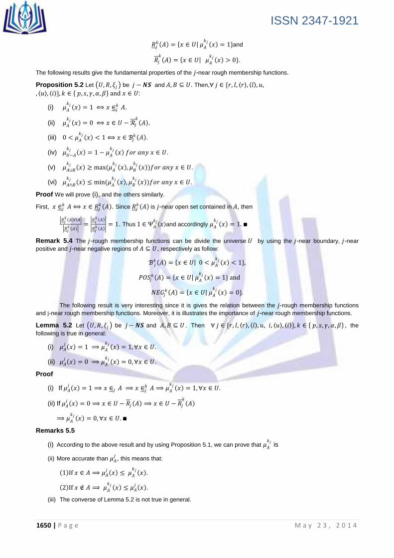
Remark 5.3 The 𝑗-near rough membership functions can be used to define 𝑗-near approximations as shown below:

ISSN 2347-1921

1650 | P a g e M a y 2 3 , 2 0 1 4

𝑅𝑗𝑘 𝐴 = 𝑥 ∈ 𝑈 𝜇𝐴

𝑘𝑗 𝑥 = 1}and

𝑅𝑗

𝑘 𝐴 = 𝑥 ∈ 𝑈 𝜇𝐴

𝑘𝑗 𝑥 > 0}.

The following results give the fundamental properties of the 𝑗-near rough membership functions.

Proposition 5.2 Let 𝑈, 𝑅, 𝜉𝑗 be 𝑗 − 𝑵𝑺 and 𝐴, 𝐵 ⊆ 𝑈. Then,∀ 𝑗 ∈ {𝑟, 𝑙, 𝑟 , 𝑙 , 𝑢,

, 𝑢 , 𝑖 }, 𝑘 ∈ 𝑝, 𝑠, 𝛾, 𝛼, 𝛽 and 𝑥 ∈ 𝑈:

(i) 𝜇𝐴

𝑘𝑗 𝑥 = 1 ⟺ 𝑥 ∈𝑗𝑘 𝐴.

(ii) 𝜇𝐴

𝑘𝑗 𝑥 = 0 ⟺ 𝑥 ∈ 𝑈 − ℛ𝑗

𝑘 𝐴 .

(iii) 0 < 𝜇𝐴

𝑘𝑗 𝑥 < 1 ⟺ 𝑥 ∈ ℬ𝑗𝑘 𝐴 .

(iv) 𝜇𝑈−𝐴

𝑘𝑗 𝑥 = 1 − 𝜇𝐴

𝑘𝑗 𝑥 𝑓𝑜𝑟 𝑎𝑛𝑦 𝑥 ∈ 𝑈.

(v) 𝜇𝐴∪𝐵

𝑘𝑗 𝑥 ≥ max(𝜇𝐴

𝑘𝑗 𝑥 , 𝜇𝐵

𝑘𝑗 𝑥 )𝑓𝑜𝑟 𝑎𝑛𝑦 𝑥 ∈ 𝑈.

(vi) 𝜇𝐴∩𝐵

𝑘𝑗 𝑥 ≤ min(𝜇𝐴

𝑘𝑗 𝑥 , 𝜇𝐵

𝑘𝑗 𝑥 )𝑓𝑜𝑟 𝑎𝑛𝑦 𝑥 ∈ 𝑈.

Proof We will prove (i), and the others similarly.

First, 𝑥 ∈𝑗𝑘 𝐴 ⟺ 𝑥 ∈ 𝑅𝑗

𝑘 𝐴 . Since 𝑅𝑗𝑘 𝐴 is 𝑗-near open set contained in 𝐴, then

𝑅𝑗𝑘 𝐴 ∩𝐴

𝑅𝑗𝑘 𝐴

= 𝑅𝑗

𝑘 𝐴

𝑅𝑗𝑘 𝐴

= 1. Thus 1 ∈ Ψ𝐴

𝑘𝑗 𝑥 and accordingly 𝜇𝐴

𝑘𝑗 𝑥 = 1. ∎

Remark 5.4 The 𝑗-rough membership functions can be divide the universe 𝑈 by using the 𝑗-near boundary, 𝑗-near

positive and 𝑗-near negative regions of 𝐴 ⊆ 𝑈, respectively as follow:

ℬ 𝑗𝑘 𝐴 = 𝑥 ∈ 𝑈 0 < 𝜇𝐴

𝑘𝑗 𝑥 < 1},

𝑃𝑂𝑆𝑗𝑘 𝐴 = 𝑥 ∈ 𝑈 𝜇𝐴

𝑘𝑗 𝑥 = 1} and

𝑁𝐸𝐺𝑗𝑘 𝐴 = 𝑥 ∈ 𝑈 𝜇𝐴

𝑘𝑗 𝑥 = 0}.

The following result is very interesting since it is gives the relation between the 𝑗-rough membership functions

and j-near rough membership functions. Moreover, it is illustrates the importance of 𝑗-near rough membership functions.

Lemma 5.2 Let 𝑈, 𝑅, 𝜉𝑗 be 𝑗 − 𝑵𝑺 and 𝐴, 𝐵 ⊆ 𝑈 . Then ∀ 𝑗 ∈ {𝑟, 𝑙, 𝑟 , 𝑙 , 𝑢, 𝑖, 𝑢 , 𝑖 }, 𝑘 ∈ 𝑝, 𝑠, 𝛾, 𝛼, 𝛽 , the

following is true in general:

(i) 𝜇𝐴𝑗 𝑥 = 1 ⟹ 𝜇𝐴

𝑘𝑗 𝑥 = 1, ∀𝑥 ∈ 𝑈.

(ii) 𝜇𝐴𝑗 𝑥 = 0 ⟹ 𝜇𝐴

𝑘𝑗 𝑥 = 0, ∀𝑥 ∈ 𝑈.

Proof

(i) If 𝜇𝐴𝑗 𝑥 = 1 ⟹ 𝑥 ∈𝑗 𝐴 ⟹ 𝑥 ∈𝑗

𝑘 𝐴 ⟹ 𝜇𝐴

𝑘𝑗 𝑥 = 1, ∀𝑥 ∈ 𝑈.

(ii) If 𝜇𝐴𝑗 𝑥 = 0 ⟹ 𝑥 ∈ 𝑈 − 𝑅𝑗 𝐴 ⟹ 𝑥 ∈ 𝑈 − 𝑅𝑗

𝑘 𝐴

⟹ 𝜇𝐴

𝑘𝑗 𝑥 = 0, ∀𝑥 ∈ 𝑈. ∎

Remarks 5.5

(i) According to the above result and by using Proposition 5.1, we can prove that 𝜇𝐴

𝑘𝑗 is

(ii) More accurate than 𝜇𝐴𝑗, this means that:

1 If 𝑥 ∈ 𝐴 ⟹ 𝜇𝐴𝑗 𝑥 ≤ 𝜇𝐴

𝑘𝑗 𝑥 .

2 If 𝑥 ∉ 𝐴 ⟹ 𝜇𝐴

𝑘𝑗 𝑥 ≤ 𝜇𝐴𝑗 𝑥 .

(iii) The converse of Lemma 5.2 is not true in general.

ISSN 2347-1921

1651 | P a g e M a y 2 3 , 2 0 1 4

The following example illustrates Remarks 5.5.

Example 5.3 Let 𝑈, 𝑅, 𝜉𝑗 be 𝑗 − 𝑵𝑺 , where 𝑈 = 𝑎, 𝑏, 𝑐, 𝑑 and

𝑅 = 𝑎, 𝑎 , 𝑎, 𝑏 , 𝑏, 𝑎 , 𝑏, 𝑏 , 𝑐, 𝑎 , 𝑐, 𝑏 , 𝑐, 𝑐 , 𝑐, 𝑑 , 𝑑, 𝑑 .

We will show the above result in case of 𝑗 = 𝑟 and 𝑘 = 𝑠 the other cases similarly as follow:

The family of 𝑟-semi open sets is:

𝑆𝑟𝑂 𝑈 = {𝑈, ∅, 𝑎 , 𝑑 , 𝑎, 𝑏 , 𝑎, 𝑑 , 𝑎, 𝑐 , 𝑐, 𝑑 , 𝑎, 𝑏, 𝑐 , 𝑎, 𝑏, 𝑑 , 𝑎, 𝑐, 𝑑 }and

𝑆𝑟𝐶 𝑈 = {𝑈, ∅, 𝑏 , 𝑐 , 𝑑 , 𝑎, 𝑏 , 𝑏, 𝑑 , 𝑏, 𝑐 , 𝑐, 𝑑 , 𝑎, 𝑏, 𝑐 , 𝑏, 𝑐, 𝑑 }.

Now consider the subset 𝐴 = {𝑎, 𝑐}, then the 𝑟-rough membership functions of 𝐴, 𝑥 ∈ 𝑈 are

𝜇𝐴𝑟 𝑎 =

{𝑎 ,𝑏}∩𝐴

{𝑎 ,𝑏} =

1

2.

𝜇𝐴𝑟 𝑏 =

{𝑎 ,𝑏}∩𝐴

{𝑎 ,𝑏} =

1

2.

𝜇𝐴𝑟 𝑐 =

𝑈∩𝐴

𝑈 =

1

2.

𝜇𝐴𝑟 𝑑 =

{𝑑}∩𝐴

{𝑑} = 0.

But the 𝑟-semi rough membership functions of 𝐴, 𝑥 ∈ 𝑈 are

Ψ𝐴𝑠𝑟 𝑎 =

{𝑎}∩𝐴

{𝑎} = 1,

{𝑎 ,𝑏}∩𝐴

{𝑎 ,𝑏} =

1

2, … ⟹ 𝜇𝐴

𝑠𝑟 𝑎 = 1.

Ψ𝐴𝑠𝑟 𝑏 =

{𝑎 ,𝑏}∩𝐴

{𝑎 ,𝑏} =

1

2, {𝑎 ,𝑏 ,𝑐}∩𝐴

{𝑎 ,𝑏 ,𝑐} =

2

3, {𝑎 ,𝑏 ,𝑑}∩𝐴

{𝑎 ,𝑏 ,𝑑} =

1

3 ⟹ 𝜇𝐴

𝑠𝑟 𝑏 =1

3.

Ψ𝐴𝑠𝑟 𝑐 =

{𝑎 ,𝑐}∩𝐴

{𝑎 ,𝑐} = 1,

{𝑐 ,𝑑}∩𝐴

{𝑐 ,𝑑} =

1

2, … ⟹ 𝜇𝐴

𝑠𝑟 𝑐 = 1.

Ψ𝐴𝑠𝑟 𝑑 =

{𝑑}∩𝐴

{𝑑} = 0,

{𝑎 ,𝑑}∩𝐴

{𝑎 ,𝑑} =

1

2, … ⟹ 𝜇𝐴

𝑠𝑟 𝑎 = 0.

The 𝑗-near rough membership functions 𝜇𝐴

𝑘𝑗 allow us to define forty different types of fuzzy sets in 𝑗 − NS as the

following definition illustrates.

Definition 5.3 Let 𝑈, 𝑅, 𝜉𝑗 be 𝑗 − 𝑵𝑺 and 𝐴 ⊆ 𝑈. Then ∀ 𝑗 ∈ {𝑟, 𝑙, 𝑟 , 𝑙 , 𝑢, 𝑖, 𝑢 , 𝑖 } and 𝑘 ∈ 𝑝, 𝑠, 𝛾, 𝛼, 𝛽 , the 𝑗-

near fuzzy set in 𝑈 is a set of ordered pairs:

𝐴 𝑗𝑘 = {(𝑥, 𝜇𝐴

𝑘𝑗 𝑥 )|𝑥 ∈ 𝑈}

Example 5.4 According to Example 5.3, the 𝑟-semi fuzzy set of a subset 𝐴 = {𝑎, 𝑐} is

𝐴 𝑟𝑠 = { 𝑎, 1 , 𝑏,

1

3 , 𝑐, 1 , 𝑑, 0 }. But the 𝑟-fuzzy set of a subset 𝐴 = {𝑎, 𝑐} is

𝐴 𝑟 = { 𝑎,1

2 , 𝑏,

1

2 , 𝑐,

1

2 , 𝑑, 0 }.

Conclusion

In this paper, we have integrated some ideas in terms of concepts in topology. Topology is a branch of mathematics, whose concepts exist not only in almost all branches of mathematics, but also in many real life applications. We believe that topological structure will be an important base for modification of knowledge extraction and processing.

We have introduced some the important topological applications named “Near concepts” as easy tools to classify the sets and help for measuring near exactness and near roughness of sets. Near rough membership functions allowed us to introduce different types of near fuzzy sets. Accordingly, we introduced a useful connection between four important theories namely “rough set theory, fuzzy set theory and the general topology” that will be useful in applications.

Finally, we introduced an important application to illustrate the importance of using near concepts. So, we can say that the introduced structures are useful in the applications and thus these techniques open the way for more topological applications in rough context and help in formalizing many applications from real-life data.

References

[1] A. A., Allam , M. Y., Bakeir and E. A., Abo-Tabl: New approach for basic rough set concepts. in: Rough Sets, Fuzzy Sets, Data Mining, and Granular Computing, Lecture Notes in Artificial Intelligence 3641, D. Slezak, G. Wang, M. Szczuka, I. Dntsch, Y. Yao (Eds.), Springer Verlag GmbH ,Regina, (2005), 64-73.

[2] A. S., Salama: Some Topological Properties of Rough Sets with Tools for Data Mining, IJCSI, International Journal of Computer Science Issues, Vol. 8, Issue 3, No. 2, (2011), 588-595.

[3] A. Skowron: On topology in information system, Bulletin of Polish Academic Science and Mathematics 36 (1988) 477–480.

ISSN 2347-1921

1652 | P a g e M a y 2 3 , 2 0 1 4

[4] B., Chen and J., Li: On topological covering-based rough spaces, International Journal of the Physical Sciences Vol. 6(17), (2011), pp. 4195-4202.

[5] B.K., Tripathy, A., Mitra: Some topological properties of rough sets and their applications, Int. J. Granular Computing, Rough Sets and Intelligent Systems, Vol. 1, No. 4,( 2010 )355-375.

[6] B.K., Tripathy, M. Nagaraju: On Some Topological Properties of Pessimistic Multi-granular Rough Sets, I.J. Intelligent Systems and Applications, 8, (2012), 10-17.

[7] B.M.R., Stadler; P.F., Stadler: Generalized topological spaces in evolutionary theory and combinatorial chemistry, J. Chem. Inf. Comp. Sci. 42 (2002), 577–585.

[8] B.M.R., Stadler; P.F., Stadler: The topology of evolutionary Biology, Ciobanu, G., and Rozenberg, G. (Eds.): Modeling in Molecular Biology, Springer Verlag, Natural Computing Series, (2004), 267-286.

[9] E. Lashin, A. Kozae, A.A. Khadra, T. Medhat Rough set theory for topological spaces, International Journal of Approximate Reasoning 40 (1–2) (2005) 35–43.

[10] F.Y. Wang: On the abstraction of conventional dynamic systems: from numerical analysis to linguistic analysis, Information Sciences 171 (2005) 233–259.

[11] G., Liu; Y., Sai: A comparison of two types of rough sets induced by coverings, International Journal of Approximate Reasoning 50 (2009), 521-528.

[12] J.J., Li: Topological Methods on the Theory of Covering Generalized Rough Sets, Patt. Recogn. Artificial Intelligence, 17(1),(2004), pp.7-10.

[13] J., Slapal: A Jordan Curve Theorem with respect to certain closure operations on the digital plane. Electronic Notes in Theoretical Computer Science 46, (2001), 1-20.

[14] L. Zadeh: Fuzzy sets, Information and Control 8 (1965) 338–353. [15] L. Zadeh: The concept of a linguistic variable and its application to approximate reasoning – I, Information

Sciences 8 (1975) 199–249. [16] L. Zadeh: The concept of a linguistic variable and its application to approximate reasoning – II, Information

Sciences 8 (1975) 301–357. [17] L. Zadeh: The concept of a linguistic variable and its application to approximate reasoning – III, Information

Sciences 9 (1975) 43–80. [18] L. Zadeh: Fuzzy logic = computing with words, IEEE Transactions on Fuzzy Systems 4 (1996) 103–111. [19] M.E. Abd El-Monsef, O.A. Embaby and M.K. El-Bably: New Approach to covering rough sets via relations,

International Journal of Pure and Applied Mathematics, Volume 91 No. 3 (2014), 329-347. [20] M.E. Abd El-Monsef, O.A. Embaby and M.K. El-Bably: Comparison between new rough set approximations

based on different topologies, International Journal of Granular Computing, Rough Sets and Intelligent Systems (IJGCRSIS), (to appear).

[21] M.E. Abd El-Monsef, O.A. Embaby and M.K. El-Bably: On Generalizing Pawlak Approximation Space and j −Near Concepts in Rough Sets (Submitted).

[22] M. K. El-Bably: Generalized Approximation Spaces, M.Sc. Thesis, Tanta Univ., Egypt, (2008). [23] M. Kryszkiewicz: Rough set approach to incomplete information systems, Information Sciences 112 (1998) 39–

49. [24] M. Kryszkiewicz: Rule in incomplete information systems, Information Sciences 113 (1998) 271–292. [25] N. D., Thuan: Covering Rough Sets from a Topological Point of View, Int. Journal of Computer Theory and

Engineering, Vol. 1, No. 5, (2009), pp 606-609. [26] P., Zhu: Covering rough sets based on neighborhoods: An approach without using neighborhoods, Int. J. of

Approximate Reasoning, 52(3), (2011), pp. 461-472. [27] R. Slowinski, D. Vanderpooten: A generalized definition of rough approximations based on similarity, IEEE

Transactions on Knowledge and Data Engineering 12 (2) (2000) 331–336. [28] T.Y. Lin: Granular computing on binary relation I: Data mining and neighborhood systems, in: Rough Sets in

Knowledge Discovery, Physica-Verlag, (1998), pp. 107-121. [29] U., Wybraniec-Skardowska: On a generalization of approximation space, Bulletin of the Polish Academy of

Sciences: Mathematics 37, (1989), pp. 51–61. [30] W.J. Liu: Topological space properties of rough sets, in: Proceedings of the Third International Conference on

Machine Learning and Cybernetics, 2004, pp. 26–29. [31] W., Zhu and F., Wang (Eds.): Axiomatic Systems of Generalized Rough Sets, RSKT 2006, LNAI 4062, (2006),

pp. 216–221. [32] W., Zhu: Topological approaches to covering rough sets, International Journal of Computer and Information

Sciences 177(2007), 1499-1508. [33] X., Ge: An Application of Covering Approximation Spaces on Network Security. Comp. Math. Appl., 60, (2010),

pp. 1191-1199. [34] Yao, Y.Y. and Lin, T.Y.: "Generalization of rough sets using modal logic, Intelligent Automation and Soft

Computing, an Int. J. 2, (1996), pp. 103–120. [35] Z. Pawlak: Rough sets, International Journal of Computer and Information Sciences 11 (1982) 341–356. [36] Z. Pawlak: Rough Sets, Theoretical Aspects of Reasoning about Data, Kluwer Academic Publishers, Boston,

1991.