Potential improvements in global carbon flux estimates from a ...
Upload
univ-rennes1Category
view
2download
0
New Estimates of Variations in Water Flux and Storage over Europe Based onRegional (Re)Analyses and Multisensor Observations
ANNE SPRINGER
Institute of Geodesy and Geoinformation, Bonn University, and Centre for High-Performance Scientific
Computing in Terrestrial Systems, Geoverbund ABC/J, Bonn, Germany
JÜRGEN KUSCHE
Institute of Geodesy and Geoinformation, Bonn University, Bonn, Germany
KERSTIN HARTUNG
Meteorological Institute, Stockholm University, Stockholm, Sweden
CHRISTAN OHLWEIN
Hans-Ertel Centre for Weather Research, Climate Monitoring Branch, Meteorological Institute,
Bonn University, Bonn, Germany
LAURENT LONGUEVERGNE
CNRS, UMR 6118, Geosciences Rennes, Rennes, France
(Manuscript received 7 March 2014, in final form 10 July 2014)
ABSTRACT
Precipitation minus evapotranspiration, the net flux of water between the atmosphere and Earth’s surface,
links atmospheric and terrestrial water budgets and thus represents an important boundary condition for both
climatemodeling and hydrological studies. However, the atmospheric–terrestrial flux is poorly constrained by
direct observations because of a lack of unbiased measurements. Thus, it is usually reconstructed from at-
mospheric reanalyses. Via the terrestrial water budget equation, water storage estimates from the Gravity
Recovery and Climate Experiment (GRACE) combined with measured river discharge can be used to assess
the realism of the atmospheric–terrestrial flux in models. In this contribution, the closure of the terrestrial
water budget is assessed over a number of European river basins using the recently reprocessed GRACE
release 05 data, together with precipitation and evapotranspiration from the operational analyses of the high-
resolution, limited-area NWP models [Consortium for Small-Scale Modelling, German version (COSMO-
DE) and European version (COSMO-EU)] and the new COSMO 6-km reanalysisAU1 (COSMO-REA6) for the
European Coordinated Regional Climate Downscaling Experiment (CORDEX) domain. These closures are
compared to those obtained with global reanalyses, land surface models, and observation-based datasets. The
spatial resolution achieved with the recent GRACE data allows for better evaluation of the water budget in
smaller river basins than before and for the identification of biases up to 25mmmonth21 in the different
products. Variations of deseasoned and detrended atmospheric–terrestrial flux are found to agree notably
well with GRACE/AU2 discharge-derived flux with correlations up to 0.75. Finally, bias-corrected fluxes are de-
rived from various data combinations, and from this, a 20-yr time series of catchment-integratedwater storage
variations is reconstructed.
1. Introduction
Redistribution and phase changes of water have a
strong impact on Earth’s climate. The hydrological cycle
is linked to the energy cycle via fluxes, such as evapo-
transpiration E and precipitation P. Water evaporates
Corresponding author address: Anne Springer, Astronomical,
Physical and Mathematical Geodesy Group, Institute of Geodesy
and Geoinformation (IGG), Bonn University, Nußallee 17, 53115Bonn, Germany.E-mail: [email protected]
JOBNAME: JHM 00#00 2014 PAGE: 1 SESS: 8 OUTPUT: Wed Aug 27 13:09:51 2014 Total No. of Pages: 21/ams/jhm/0/jhmD140050
MONTH 2014 S PR INGER ET AL . 1
DOI: 10.1175/JHM-D-14-0050.1
� 2014 American Meteorological Society
Jour
nal o
f Hyd
rom
eteo
rolo
gy (
Proo
f Onl
y)
from the oceans and the land surface because of solar
radiation, thereby cooling them, and is transported
through the atmosphere, released as precipitation, and
finally returns to the oceans via surface runoff and river
discharge R.
An ‘‘intensification’’ of the water cycle (Huntington
2006) should be associated with observable positive
rates of continental P and E. In fact, an increase of land
precipitation has been observed in the higher latitudes,
that is, over North America and Eurasia (Trenberth
2011). For these regions, changes in P usually implicate
an increase of extreme precipitation events (Coumou
and Rahmstorf 2012) leading to more frequent and se-
vere flooding (Hall et al. 2013). On the other hand, ob-
served positive trends inE have been attributed to rising
temperatures and radiation and are found to be con-
strained by moisture supply (Jung et al. 2010). Pre-
cipitation minus evapotranspiration (P 2 E) controls
the amount of water stored in soils, groundwater, and
surface water bodies. With freshwater representing a
major natural resource, monitoring systems are indis-
pensable in order to manage the various components of
water consumption. Quantifying spatiotemporal varia-
tions in fluxes and storages is thus a necessity in order to
assess their impact on local and global climatic, eco-
logical, and environmental conditions. For all these
reasons, long, unbiased, and consistent time series of
fluxes P, E, R, and of total water storage (TWS) are
required.
At all spatial scales (i.e., grid cell, catchment, and
continent) water storage changes DS are linked to P, E,
and R via the terrestrial water budget equation:
DS5P2E2R . (1)
The four terms in Eq. (1) can be evaluated from differ-
ent datasets. Since 2002, the Gravity Recovery and
Climate Experiment (GRACE) twin-satellite mission
enables the direct observation of total water storage
variations from space. At catchment scale, river dis-
charge is usually derived from gauging stations, and P
and E are either obtained from observation-based data-
sets or from numerical weather prediction (NWP) model
analyses or reanalyses. However, the representation of P
andE in global reanalyses is subject to large uncertainties
(e.g., Lorenz and Kunstmann 2012).
At the core of this study is the closure of the water
budget at river basin scale, in order to assess the realism
of the representation of theP andEfluxes inNWPmodels.
In particular, high-resolution output fields from the Con-
sortium for Small-Scale Modelling, German version
(COSMO-DE) and European version (COSMO-EU),
which are analysis runs of the nonhydrostatic regional
atmospheric COSMO model developed by the Deutscher
Wetterdienst (DWD), are evaluatedand compared to global
models and observation-based datasets. Our study area
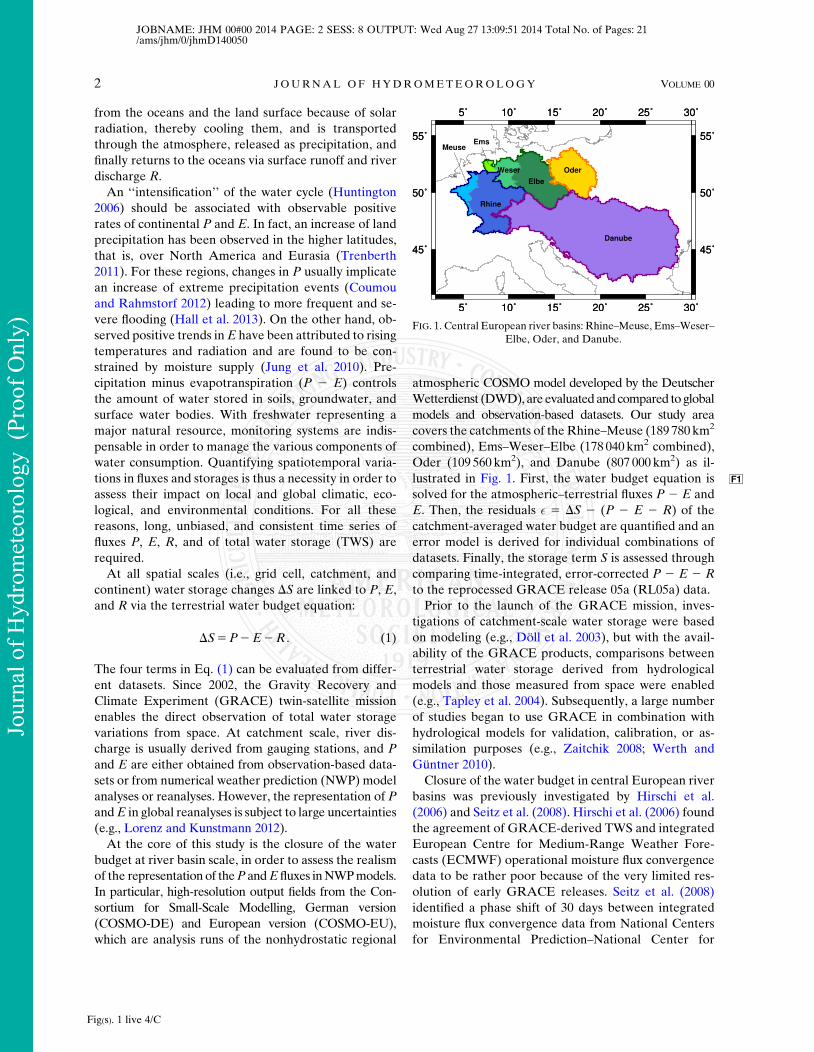
covers the catchments of the Rhine–Meuse (189 780 km2
combined), Ems–Weser–Elbe (178 040 km2 combined),
Oder (109 560 km2), and Danube (807 000 km2) as il-
lustrated in F F1ig. 1. First, the water budget equation is
solved for the atmospheric–terrestrial fluxes P 2 E and
E. Then, the residuals � 5 DS 2 (P 2 E 2 R) of the
catchment-averaged water budget are quantified and an
error model is derived for individual combinations of
datasets. Finally, the storage term S is assessed through
comparing time-integrated, error-corrected P 2 E 2 R
to the reprocessed GRACE release 05a (RL05a) data.
Prior to the launch of the GRACE mission, inves-
tigations of catchment-scale water storage were based
on modeling (e.g., Döll et al. 2003), but with the avail-
ability of the GRACE products, comparisons between
terrestrial water storage derived from hydrological
models and those measured from space were enabled
(e.g., Tapley et al. 2004). Subsequently, a large number
of studies began to use GRACE in combination with
hydrological models for validation, calibration, or as-
similation purposes (e.g., Zaitchik 2008; Werth and
Güntner 2010).Closure of the water budget in central European river
basins was previously investigated by Hirschi et al.
(2006) and Seitz et al. (2008). Hirschi et al. (2006) found
the agreement of GRACE-derived TWS and integrated
European Centre for Medium-Range Weather Fore-
casts (ECMWF) operational moisture flux convergence
data to be rather poor because of the very limited res-
olution of early GRACE releases. Seitz et al. (2008)
identified a phase shift of 30 days between integrated
moisture flux convergence data from National Centers
for Environmental Prediction–National Center for
FIG. 1. Central European river basins: Rhine–Meuse, Ems–Weser–
Elbe, Oder, and Danube.
Fig(s). 1 live 4/C
2 JOURNAL OF HYDROMETEOROLOGY VOLUME 00
JOBNAME: JHM 00#00 2014 PAGE: 2 SESS: 8 OUTPUT: Wed Aug 27 13:09:51 2014 Total No. of Pages: 21/ams/jhm/0/jhmD140050
Jour
nal o
f Hyd
rom
eteo
rolo
gy (
Proo
f Onl
y)
AtmosphericResearch (NCEP–NCAR) andGRACE for
the years after 2006. Compared to Hirschi et al. (2006),
they obtained better agreements between GRACE and
model data because of reprocessed GRACE solutions
and a larger study area. In particular, the Danube, the
largest of theEuropean river basins, was subject to several
investigations in the context of water budget studies: for
example, Ramilien et al. (2006) and Rodell et al. (2011)
used GRACE data in conjunction with observed P and R
in order to estimateE, whichwas then compared to results
from different atmospheric and land surface models.
Rodell et al. (2011) confirmed the benefit of GRACE-
based E estimates for the assessment of the phase and
amplitude of the annual cycle, especially for regions
where model-derived E estimates disagree.
The global NWP models and observation-based
datasets, which we employ as a reference for compari-
son and validation purposes in this study, have been
widely used in the context of water budget studies. For
example, Hirschi et al. (2006), Rodell et al. (2011), and
Syed et al. (2009) worked with the ECMWF reanalysis
and the Modern-Era Retrospective Analysis for Re-
search and Applications (MERRA). In addition, Fersch
et al. (2012) included high-resolution regional atmo-
spheric simulations produced with the Weather Re-
search and Forecasting (WRF) Model for six different
climatic regions. They found dynamic downscaling of
global atmospheric fields generally useful for reducing
the bias in these fields, but time series of basin-averaged
TWS change estimates did not improve with respect to
the global models. Outputs of different models and ob-
servational datasets were merged using assimilation
techniques by Pan et al. (2012) to derive trend and an-
nual water budget terms over 32 major river basins.
Furthermore, the quality of observation-based P and E
datasets has been assessed in several studies. For in-
stance, the Global Precipitation Climatology Centre
(GPCC) dataset and the European daily high-resolution
gridded dataset (E-OBS) are discussed in detail by
Roebeling et al. (2012). Acquisition of evapotranspira-
tion fields on an observational basis is considered more
challenging (Wang and Dickinson 2012). An overview
and evaluation of recently derived global evapotrans-
piration datasets can be found, for example, in Mueller
et al. (2011) and Jiménez et al. (2011), including a data-
set of upscaled Flux Network (FLUXNETAU3 ) data derived
by Jung et al. (2011), which is also used in our study.
Furthermore, Long et al. (2014) used the three-cornered
hat method in order to compute uncertainties of evapo-
transpiration from three different methods, including the
water budget approach.
Continental-scale atmospheric fluxes ofP,E, andP2E
produced by three global reanalyses, including MERRA
and Interim ECMWF Re-Analysis (ERA-Interim), were
assessed by Lorenz and Kunstmann (2012). They de-
termined inconsistent continental and oceanic P 2 E for
MERRA, whereas ERA-Interim showed a good closure
of the water balance. Miralles et al. (2011) provide P, E,
andP2E estimates froma combination of remote sensing
observations.
In this contribution, we focus on the atmospheric part
of the water cycle. However, we found moisture flux
convergence derived from the high-resolution COSMO
models as being very noisy; therefore, we directly eval-
uate P and E fields. We will demonstrate that the
COSMO model shows superior skills in closing the wa-
ter budget over Europe compared to the global models.
Until now, most water budget studies have concentrated
on large river basins and/or the annual cycle ofE,P2E,
or S only; here, we will include month-to-month vari-
ability and trends. Moreover, we will evaluate the wa-
ter budget equation for smaller European river basins.
We find this possible now thanks to the increased ac-
curacy of the reprocessed GRACE RL05a data and to
a consistent and thorough postprocessing of GRACE
and flux deficit data. This contribution is organized as
follows. In section 2, we introduce the investigated
datasets and the methods. The results are presented in
section 3. First, the characteristics of the four compo-
nents of the water budget equation are assessed. Then,
the water budget equation is solved for P 2 E and
compared to the independent GRACE and discharge
observations. As the observation and modeling of E is
particularly challenging, the derivation of E via the
water budget equation is evaluated. In the next step,
the residuals of the water budget are quantified and
error models for the individual datasets of P 2 E are
derived. Finally, error-corrected fluxes are computed
and used in order to extend the GRACE-derived time
series of TWS change and TWS (since 2002) backward
in time (to 1990).
2. Data and methods
a. Data
Assessing the closure of the terrestrial water budget
requires that datasets of P, E, R, and DS are combined.
Evapotranspiration is related to latent heat flux QL via
the relation
E5 l21QL , (2)
with the latent heat of vaporization for water l 5 2.5 3103 kJ kg21. T T1able 1 provides an overview of the datasets
that are described in the following.
MONTH 2014 S PR INGER ET AL . 3
JOBNAME: JHM 00#00 2014 PAGE: 3 SESS: 8 OUTPUT: Wed Aug 27 13:09:51 2014 Total No. of Pages: 21/ams/jhm/0/jhmD140050
Jour
nal o
f Hyd
rom
eteo
rolo
gy (
Proo
f Onl
y)
1) GRACE
The primary objective of the National Aeronautics
and Space Administration (NASA)–German Aero-
space Center (DLR) GRACE mission, launched in
2002, is the measurement of Earth’s time-variable
gravity field. In a seminal paper, Wahr et al. (1998) an-
ticipated the benefits and limitations of the mission for
resolving water storage variations from space; this was
later confirmed by a great number of applications in
large-scale hydrology as described, for example, in the
review by Güntner (2008). With GRACE, a dual one-
way K-band microwave ranging system measures the
distance and its rate between two satellites in coplanar
orbit, with accuracy of a few micrometers. From the
distance change and from complementary tracking of
the individual spacecraft positions with GPS, Earth’s
changing gravity field is inferred on a monthly basis.
Many users are interested in the temporal variations due
to changes in Earth’s terrestrial hydrosphere, which are
obtained in a straightforward way since other gravity
signals like Earth and ocean tides, nontidal ocean mass
variability, and atmospheric pressure changes have al-
ready been removed in the gravity recovery processing
by using so-called background models.
With release 05 (Dahle et al. 2013), the Geo-
ForschungsZentrum (GFZ) Helmholtz-Zentrum in Pots-
dam provides improved (Chambers and Bonin 2012)
monthly gravity solutions in the form of spherical har-
monic coefficients starting in January 2003. Release 05was
recently reprocessed because of some shortcomings in the
satellite orbit determination, and the new dataset, which is
applied in this contribution, has been distributed as release
05a.Wewill compare theGFZ solution to those generated
at the Jet Propulsion Laboratory (JPL), California In-
stitute of Technology, and the Center for Space Research
(CSR), The University of Texas at Austin. In addition, we
willmake use of error estimates forGFZ coefficients in the
form of so-called calibrated errors; these do account for
measurement and processing errors, but they neglect error
correlations and cannot account for errors introduced by
background model imperfections.
The same postprocessing is performed for each of the
threeGRACE solutions. First, the gravity effect resulting
from ongoing isostatic adjustment of Earth’s crust and
mantle, in response to past ice age deglaciation, is re-
moved from the harmonic coefficients using the model of
Klemann andMartinec (2011). Then, since coefficients of
degree 1 AU4cannot be measured by GRACE, these are
substituted from a time series of geocenter motion pro-
vided by Rietbroek et al. (2012). Furthermore, the zonal
c2,0 coefficient, related to the flattening of Earth, is known
to be not well determined by GRACE. Therefore, it is
replaced using a time series derived from satellite laser
ranging (SLR) by Cheng and Tapley (2004).
2) WGHM
As an alternative to GRACE, the Water—a Global
Assessment and Prognosis (WaterGAP) Global Hy-
drology Model (WGHM; Döll et al. 2003) is used to
obtain TWS anomalies. WGHM represents a global
conceptual model of the terrestrial water cycle, with the
objective of providing indicators of freshwater avail-
ability worldwide. All storage compartments relevant
for calculating TWS are modeled, including surface
water and groundwater. InWGHM, the water balance is
solved at daily time steps with a spatial resolution of 0.58.Monthly precipitation forcing data from GPCC are
disaggregated to daily rain rates. The computation of
daily potential evapotranspiration is based on Priestley
and Taylor (1972). The model has been calibrated
against long-term discharge. Special emphasis is paid to
anthropogenic effects like water consumption.
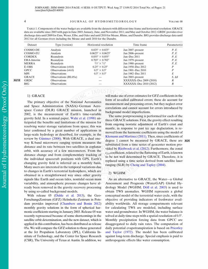
TABLE 1. Components
AU18
of the water budget are available from the datasets with different time frame and horizontal resolution. GRACE
data are available since 2003with gaps in June 2003; January, June, andNovember 2011; andMay andOctober 2012.GRDCprovides river
discharge data until 2009 for Ems,Weser, Elbe, andOder and until 2010 forMeuse, Rhine, andDanube. BfG provides discharge data until
2012 for all German rivers including the Meuse and until 2010 for the Danube.
Dataset Type (version) Horizontal resolution Time frame Parameter(s)
COSMO-DE Analysis 0.0258 3 0.0258 Jan 2007–present P, E
COSMO-EU Analysis 0.06258 3 0.06258 Jan 2006–present P, E
CORDEX Reanalysis 0.0558 3 0.0558 Jan–Dec 2011 P, E
ERA-Interim Reanalysis 0.7038 3 0.7028 Jan 1979–present P, E
MERRA Reanalysis 2/38 3 1/28 Jan 1980–present P, E
E-OBS Observations (v8.0) 0.258 3 0.258 Jan 1950–Dec 2012 P
GPCC Observations (v6.0) 0.58 3 0.58 Jan 1901–Dec 2010 P
MPI Observations 0.58 3 0.58 Jan 1982–Dec 2011 E
GRACE Observations (RL05a) — Jan 2003–present S, DSGRDC Observations — XXXXXX–Dec 2009 (2010) R
BfG Observations — XXXXXX–Dec 2010 (2012) R
4 JOURNAL OF HYDROMETEOROLOGY VOLUME 00
JOBNAME: JHM 00#00 2014 PAGE: 4 SESS: 8 OUTPUT: Wed Aug 27 13:09:52 2014 Total No. of Pages: 21/ams/jhm/0/jhmD140050
Jour
nal o
f Hyd
rom
eteo
rolo
gy (
Proo
f Onl
y)
3) TWS CHANGE FROM PAN ET AL. (2012)
A reference dataset for TWS change was provided
to us by Ming Pan. Pan et al. (2012) evaluated the
components of the water budget by merging a number
of different datasets using a data assimilation tech-
nique to enforce the water balance. As a prerequisite,
they had performed a thorough error investigation.
Thus, the estimation of the water budget components
is optimized and includes error information derived
from confronting independent datasets. Pan et al.
(2012) utilized in situ observations, remote sensing
retrievals, and model outputs, among other datasets.
For TWS change, GRACE data and outputs from the
Variable Infiltration Capacity (VIC) model were ap-
plied. The study was performed for 32 river basins and
for the time span 1984–2006. In our contribution, we
use the TWS change estimate provided for the Danube
basin.
4) REGIONAL ANALYSES AND REANALYSES
The COSMO-EU and -DE analyses and the COSMO
6-km reanalysis (COSMO-REA6) are based on the
COSMONWPmodel developed by theDWD.COSMO
represents a nonhydrostatic regional atmospheric model,
where atmosphere–surface coupling is realized with the
soil and vegetation model TERRA_MLAU5 . Lateral bound-
ary conditions are obtained for COSMO-EU from the
global weather prediction model GME (developed by the
DWD) and for COSMO-DE from the COSMO-EU
model. Continuous data assimilation is performed based
on observation nudging (Schraff 1997) with hourly model
outputs. COSMO-EU output fields are available to us
from 2006, and COSMO-DE outputs are available from
2007 onward.
COSMO-EU covers the eastern Atlantic and Europe
with a grid resolution of 0.06258 (;7 km) and 40 vertical
layers. COSMO-DE has a higher resolution of 0.0258(;2.8 km) and 50 vertical layers and covers Germany,
Switzerland, Austria, and parts of neighboring countries
with a total area of about 1300 3 1200 km2. The major
differences to COSMO-EU are that COSMO-DE re-
solves deep convection and assimilates surface pre-
cipitation rates from the German radar network.
Additionally, we investigate the COSMO-based re-
analysis COSMO-REA6 for the European Coordinated
Regional Climate Downscaling Experiment (CORDEX)
0.118 resolution (EUR-11) domain with 0.0558 (6.2 km)
resolution (Bollmeyer et al. 2014, manuscript submitted
to Quart. J. Roy. Meteor. Soc.). It is currently being
developed and processed within the Hans-Ertel Centre
for Weather Research and has been completed for the
year 2011AU6 .
5) GLOBAL REANALYSES
For comparison and validation, we use the global
ERA-Interim andMERRA. ERA-Interim was initiated
in 2006 and covers the period since 1979. It is the suc-
cessor of the 40-yr ECMWFRe-Analysis (ERA-40) and
was designed to improve, for instance, the representa-
tion of the hydrological cycle, the quality of the strato-
spheric circulation and the handling of biases and
changes in the observing system (Berrisford et al. 2011).
A sequential data assimilation scheme with 12-hourly
analysis cycles is performed, and every 3 h output fields
of the 2D variables are produced (Dee et al. 2011). In the
vertical dimension, 37 levels are considered. Synoptic
monthly means of precipitation and latent heat flux
evaluated in this study have a resolution of 1.58 3 1.58.MERRA is from NASA’s Global Modeling and As-
similation Office (GMAO) and covers the period from
1979 until today. TheGoddard EarthObserving System,
version 5 (GEOS-5), is applied for data assimilation,
with special attention paid to improving the hydrological
cycle (Rienecker et al. 2011). Uncertainties in precip-
itation and high-frequency variability are reduced
(Lucchesi 2012), rendering themodel more adequate for
climate studies. We use monthly output products that
are archived and distributed by the Goddard Earth
Sciences Data and Information Services Center (DISC).
The horizontal grid resolution is dl 5 2/38 in longitude
and df 5 1/28 in latitude; 72 vertical levels are con-
sidered.
6) OFFLINE LAND SURFACE MODEL
Since MERRA’s land surface fluxes are known to
contain errors, we also consider its land component from
the revised, land-only, offline version, MERRA-Land
(Reichle et al. 2011). MERRA is prone to errors in the
intensity of precipitation, resulting from the atmospheric
general circulation model and the land surface model it-
self (Reichle et al. 2011). MERRA-Land is driven with
hourly atmospheric fields from MERRA, with the pre-
cipitation forcings corrected using an observation-based
product of the Global Precipitation Climatology Project
(GPCP). Furthermore, MERRA-Land contains an up-
dated catchment land surface model with revised model
parameters. These changes were shown to lead to im-
proved land surface fluxes (Reichle et al. 2011).
7) OBSERVATIONAL DATASETS
In this study, we compare analysis and reanalysis re-
sults to three gridded, observation-based datasets.
Global monthly latent heat flux grids are provided by
Jung et al. (2011) at a resolution of 0.58 3 0.58. They useda machine learning approach to upscale observations
MONTH 2014 S PR INGER ET AL . 5
JOBNAME: JHM 00#00 2014 PAGE: 5 SESS: 8 OUTPUT: Wed Aug 27 13:09:52 2014 Total No. of Pages: 21/ams/jhm/0/jhmD140050
Jour
nal o
f Hyd
rom
eteo
rolo
gy (
Proo
f Onl
y)
from FLUXNET together with meteorological and re-
mote sensing observations. FLUXNET is a global net-
work of more than 570 tower sites (200 stations in
Europe) where the eddy covariancemethod is applied to
assess atmospheric variables such as latent heat flux.
Second, we use a precipitation product from the
GPCC, established in 1989 at the DWD. It is based on
67 200 rain gauge stations worldwide. Monthly total
precipitation on 0.58 3 0.58 grids was downloaded from
the GPCC website. We use the GPCC Full Data Re-
analysis, version 6.0, the most accurate GPCC in situ
precipitation reanalysis dataset (Schneider et al. 2011) that
covers the period 1901–2010. Using GPCC data for as-
sessing the global water cycle is discussed in Schneider
et al. (2014). Finally, we consider the European gridded
rain gauge dataset E-OBS from the European Union 6th
Framework Programme (EU-FP6) project ENSEMBLESAU7
(http://ensembles-eu.metoffice.com) and from the data
providers in the European Climate Assessment & Data-
set (ECA&D) project (www.ecad.eu). Daily gridded
observational precipitation data cover the European land
surface and are available at different resolutions. We use
version 7.0 with a grid resolution of 0.258 3 0.258, whichcontains data from January 1950 to December 2012,
collected from 2316 stations.
8) RIVER DISCHARGE DATA
Here we use monthly discharge data measured at the
gauging stations located at the most downstream part of
each river provided by the Global Runoff Data Centre
(GRDC) and Bundesanstalt für Gewässerkunde (BfG).The BfG time series agree with the GRDC time seriesbut provide more complete and recent information forGerman rivers. In a few cases, missing data have beeninferred from upstream gauging stations. Data areavailable up to 2012 for Rhine–Meuse, Ems–Weser–
Elbe, and Oder and up to 2010 for the Danube.
b. Methods
1) THE WATER BUDGET EQUATION
At all spatial scales, DS within a given region is bal-
anced by inflow (P) and outflow (E and R):
DS5P2E2R . (3)
While Eq. (3) describes the
AU8
terrestrial water budget, the
atmospheric water balance can be expressed by ap-
proximating P 2 E through atmospheric water storage
and vertically integrated moisture flux convergence
(e.g., Fersch et al. 2012). However, fields of horizontal
moisture flux represented in high-resolution atmo-
spheric models such as COSMO are relatively noisy. We
found that computing the divergence amplifies noise and
leads to results that are contaminated with large errors.
Therefore, in this contribution, we use the flux deficit
P 2 E as represented in Eq. (3).
The GRACE solutions determine the temporal res-
olution with which we evaluate the water budget equa-
tion at catchment scale. Monthly mean, spatially
averaged TWS from GRACE has to be numerically
differentiated in order to approximate DS. Performing
this in a way consistent with the flux terms involves some
subtle issues that are often overlooked in the literature;
therefore, we will provide a full account here.Moreover,
as an alternative, we will discuss an approach that seeks
to consistently time integrate the spatially averaged
fluxes.
Monthly averaged DS within an arbitrary (catchment)
area is related to the monthly accumulated P, E, and R
according to
DS5 �ni
i51
P(ti)2 �nj
j51
E(tj)2 �nk
k51
R(tk) , (4)
where AU9t is discretized with daily or subdaily time steps
and t1 and tn denote the first and the last value of one
particular month. The monthly water budget of a catch-
ment can then be represented as in Eq. (3). Monthly
accumulated fluxes are obtained from the data providers
or calculated through Eq. (4).
In Eq. (3), DS is usually obtained by numerically dif-
ferentiating GRACE-derived S. Instead, the integral of
the right side of the water budget equation can be
equated at time t, after discretizing according to
SF(t)5 �m
i51
[P(t0i)2E(t0i)2R(t0i)] , (5)
where t0i represents monthly
AU10
intervals; P(t0i), E(t0i), and
R(t0i) represent the monthly sums; and SF TWS is in-
ferred from fluxes. Variable SF(t) equates to TWS, de-
rived from integrating fluxes, at time t with respect to
(unknown) TWS at time t1. However, as we will show,
spatially averaged P 2 E is usually contaminated with
nonnegligible errors. Thus, we prefer to use error-
corrected precipitation minus evapotranspiration
(gP� E). The estimation and modeling of this error will
be described in section 2b(3). TWS from error-corrected
fluxes fSF is then defined as
fSF(t)5 �m
i51
[(gP� E)(t0i)2R(t0i)] . (6)
In the following, we will limit our deliberations to error-
corrected TWS estimates; therefore, the tilde will be
omitted and the left-hand side ofEq. (6)will be abbreviated
6 JOURNAL OF HYDROMETEOROLOGY VOLUME 00
JOBNAME: JHM 00#00 2014 PAGE: 6 SESS: 8 OUTPUT: Wed Aug 27 13:09:52 2014 Total No. of Pages: 21/ams/jhm/0/jhmD140050
Jour
nal o
f Hyd
rom
eteo
rolo
gy (
Proo
f Onl
y)
by SF(t). Flux-integrated TWS anomalies SaF(t) are ob-
tained by removing the long-termmean over a time span
from ta to te, for example, the GRACE period, ac-
cording to
SaF(t)5SF(t)21
te 2 ta�e
i5aSF(t
0i) . (7)
Correspondingly, GRACE-derived TWS anomalies Sa(t)
for the same time frame are obtained from
Sa(t)5S(t)21
te 2 ta�e
i5aS(t0i) . (8)
To be consistent, the long-term mean removed in both
approaches must refer to the same time period. Apart
from observation errors and incorrect representation of
analysis and reanalysis fields, TWS anomalies obtained
from integrating fluxes [Eq. (7)] and fromGRACE [Eq.
(8)] should match. In section 3e, these two approaches
are compared.
Both direct and time-integrated evaluations of the
water budget equation have advantages and drawbacks.
Because of the integration of fluxes in Eq. (5), errors
in P, E, and R accumulate. While white noise leads to
random walk–type patterns, constant biases introduce
trends into SaF . Therefore, for evaluating primarily the
fluxes, the approach of Eq. (3) is well suited as it employs
flux information directly. On the other hand, storage
change exhibits much variability, whereas storage
evolves at longer time scales. Short-term variations are
easier to interpret analyzing TWS instead of TWS
change. Furthermore, the GRACE signal-to-noise ratio
is better when TWS is evaluated and not its derivative.
We will show that, despite unfavorable error propaga-
tion, fluxes from NWPmodels enable us to infer storage
change. This is the key to reconstructing realistic spa-
tially averaged TWS prior to the GRACE period, which
may be then spatially disaggregated through land sur-
face models. However, this requires a well-determined
error model for the fluxes from storage data collected
within the GRACE period. Yet we found that, espe-
cially in global reanalyses, biases in P 2 E may change
with time.
2) GENERATING CONSISTENT TIME SERIES
Assessing closure of the water budget, that is, studying
the residuals �5 DS2 (P2 E2 R), requires consistent
time series of TWS change,P,E, andR. Spatial averages
of P and E are simply accumulated over all output grid
cells of the target region, defined as the catchment area
down to the gauging station where river discharge is
measured.
For deriving TWS from the GRACE data products, it
is possible to accumulate over gridded TWS maps, as
provided online through the NASA Tellus, GFZ In-
ternational Centre for Global Earth Models (ICGEM),
or Groupe de Recherche de Géodésie Spatiale (GRGS)GRACE Plotter websites, in a similar way as with thefluxes. However, it is more consistent to map the originalspherical harmonic coefficients into spatial averages fora number of reasons: (i) TWSmaps have to be filtered tosuppress ‘‘striping,’’ but less filtering is required to de-
rive catchment averages, so using gridded products
usually involves a loss of information; (ii) filtering re-
duces amplitude, but counteracting this effect for TWS
maps is more difficult than for region averages; and
(iii) for TWSmaps, usually no consistent error information
is provided.
First, the GRACE potential coefficients cn,m and sn,m,
postprocessed as described in section 2a(1), are reduced
by a long-term mean field corresponding to the period
ta, te to Dcn,m and Dsn,m, and converted to coefficients of
surface densityDcsn,m andDssn,m (Wahr et al. 1998) via the
relations
�Dcsn,mDssn,m
�5
M
4pR2E
2n1 1
11k0n
(Dcn,mDsn,m
). (9)
In Eq. (9), M is Earth’s mass, RE is its
AU11
radius, and
(2n1 1)/(11 k0n) accounts for the elastic deformation of
the solid Earth under a changing water storage load
through applying the load Love numbers k0n [we use
LLNs from Gegout (2014)]. The total mass variation
over a given area—which corresponds to TWS since
atmospheric mass variations have been removed
already—is calculated directly from the coefficients of
surface density according to
S5 4pR2E �
nmax
n51�n
m50
f cn,m �
n
n051�n0
m050
wfc,cg,n0 ,m0n,m Dcsn0 ,m0 1wfc,sg,n0 ,m0
n,m Dssn0 ,m0 1 f sn,m �n
n051�n0
m050
wfs,cg,n0 ,m0n,m Dcsn0 ,m0 1wfs,sg,n0 ,m0
n,m Dssn0 ,m0
!.
(10)
MONTH 2014 S PR INGER ET AL . 7
JOBNAME: JHM 00#00 2014 PAGE: 7 SESS: 8 OUTPUT: Wed Aug 27 13:09:54 2014 Total No. of Pages: 21/ams/jhm/0/jhmD140050
Jour
nal o
f Hyd
rom
eteo
rolo
gy (
Proo
f Onl
y)
The geographical extent of the target region is repre-
sented by the shape coefficients f cn,m and f sn,m (Wahr et al.
1998). Applying filter coefficients wf.,.g,n0,m0n,m is generally
deemed necessary to reduce correlated noise contained
in the potential coefficients of high degree. In this contri-
bution, we use the nonisotropic DDK4AU12 filter (Kusche
2007) that seeks to decorrelate and smooth the GRACE
solutions simultaneously. Finally, mass variations are
converted to equivalent water height by dividing Eq. (10)
by a reference density of water.
Spatially averaged TWS from maps or from Eq. (10)
includes an error due to the limited spectral bandwidth
recovered by GRACE and the necessity to smooth the
solutions through filtering. The resulting amplitude
underestimation, or in some cases, overestimation, has
been termed the leakage effect (Klees et al. 2007;
Longuevergne et al. 2010). Depending on the mass
distribution inside and outside of the basin (i.e., water
storage variability and, in coastal regions, ocean mass
change), the filter averaging width, and the extent of
the region, the signal is either transported out of the
target area (leakage out) or leaks into it (leakage in).
Therefore, it is imperative to rescale water storage
signals derived from GRACE. Rescaling factors are
derived as multiplicative corrections separately for
every river catchment and for each month through as-
suming the spatial distribution of P 2 E as ‘‘true TWS
change’’ and monitoring the effect of the truncation of
the spherical harmonic expansion and the damping
effect of GRACE filtering. Magnitudes of the rescaling
factors and the associated TWS variability are dis-
cussed in section 3a(4).
The time derivative of storageDS(t) for themonth t is
obtained from central differences using storage of the
following month St11 and the previous month St21 as
DS(t)51
2(St112 St21) . (11)
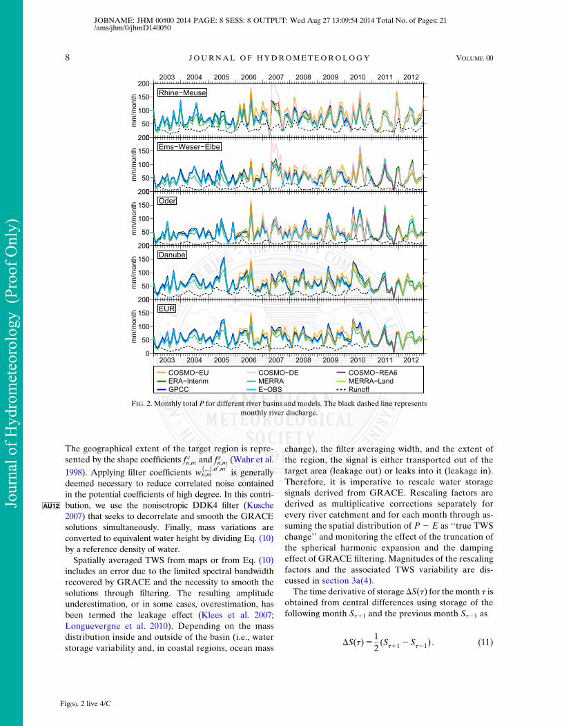
FIG. 2. Monthly total P for different river basins and models. The black dashed line represents
monthly river discharge.
Fig(s). 2 live 4/C
8 JOURNAL OF HYDROMETEOROLOGY VOLUME 00
JOBNAME: JHM 00#00 2014 PAGE: 8 SESS: 8 OUTPUT: Wed Aug 27 13:09:54 2014 Total No. of Pages: 21/ams/jhm/0/jhmD140050
Jour
nal o
f Hyd
rom
eteo
rolo
gy (
Proo
f Onl
y)
Unlike with backward or forward difference operators,
central difference schemes avoid introducing a phase
shift in GRACE storage change time series.
3) ERROR MODEL OF THE FLUX DEFICIT
We find that the residuals of the water budget equa-
tion differ most notably for every set of model output
fields and for every catchment. Since R is small, � can
thus be safely assumed to be associated with errors in
P 2 E, which means that we will use DS 1 R as a refer-
ence for fitting an error model to the catchment re-
siduals for each model output.
First, differentmodels for representing the residuals were
assessed. We observe that the difference of monthly P
datasets appears to be characterized primarily by an offset,
and E is generally smoother, mainly characterized by an
annual signal. Sincewebelieve that both errors inP and inE
contribute to the residual of the water budget, these char-
acteristics suggest the consideration of an offset and the
modeling of an annual and a semiannual signal. The offset
can be considered using an additive model according to
�5 (P2E)2 (DS1R)1 a1 b sin
�2p
Tt
�1 c cos
�2p
Tt
�1d sin
�2p
T/2t
�1 e cos
�2p
T/2t
�,
(12)
or a multiplicative model according to
�5 a(P2E)2 (DS1R)1b sin
�2p
Tt
�1 c cos
�2p
Tt
�1d sin
�2p
T/2t
�1 e cos
�2p
T/2t
�,
(13)
whereT is the annual period. The estimated error model
� is applied toP2E of Eqs. (4) and (5) in order to obtain
error-corrected TWS change and TWS estimates.
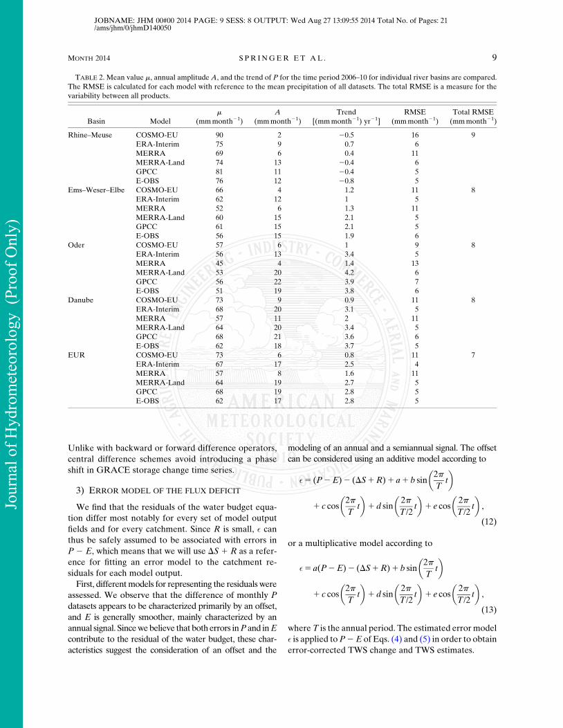
TABLE 2. Mean value m, annual amplitude A, and the trend of P for the time period 2006–10 for individual river basins are compared.
The RMSE is calculated for each model with reference to the mean precipitation of all datasets. The total RMSE is a measure for the
variability between all products.
Basin Model
m
(mmmonth21)
A
(mmmonth21)
Trend
[(mmmonth21) yr21]
RMSE
(mmmonth21)
Total RMSE
(mmmonth21)
Rhine–Meuse COSMO-EU 90 2 20.5 16 9
ERA-Interim 75 9 0.7 6
MERRA 69 6 0.4 11
MERRA-Land 74 13 20.4 6
GPCC 81 11 20.4 5
E-OBS 76 12 20.8 5
Ems–Weser–Elbe COSMO-EU 66 4 1.2 11 8
ERA-Interim 62 12 1 5
MERRA 52 6 1.3 11
MERRA-Land 60 15 2.1 5
GPCC 61 15 2.1 5
E-OBS 56 15 1.9 6
Oder COSMO-EU 57 6 1 9 8
ERA-Interim 56 13 3.4 5
MERRA 45 4 1.4 13
MERRA-Land 53 20 4.2 6
GPCC 56 22 3.9 7
E-OBS 51 19 3.8 6
Danube COSMO-EU 73 9 0.9 11 8
ERA-Interim 68 20 3.1 5
MERRA 57 11 2 11
MERRA-Land 64 20 3.4 5
GPCC 68 21 3.6 6
E-OBS 62 18 3.7 5
EUR COSMO-EU 73 6 0.8 11 7
ERA-Interim 67 17 2.5 4
MERRA 57 8 1.6 11
MERRA-Land 64 19 2.7 5
GPCC 68 19 2.8 5
E-OBS 62 17 2.8 5
MONTH 2014 S PR INGER ET AL . 9
JOBNAME: JHM 00#00 2014 PAGE: 9 SESS: 8 OUTPUT: Wed Aug 27 13:09:55 2014 Total No. of Pages: 21/ams/jhm/0/jhmD140050
Jour
nal o
f Hyd
rom
eteo
rolo
gy (
Proo
f Onl
y)
4) ERROR ASSESSMENT
The GFZ provides calibrated errors [assessed, for ex-
ample, by Wahr et al. (2006)] for the monthly spherical
harmonic coefficients that are mapped to error estimates
for spatially averagedTWS change. These error estimates
include the effects of noise in the distance measurement
between the satellites as well as those of the precise orbit
determination, while they disregard noise of some other
relevant instruments such as accelerometers and errors in
the background models. However, since spatial correla-
tions (i.e., correlations between different coefficients) are
not provided, the result is expected to somewhat un-
derestimate the real error. Besides, the standard de-
viation of discharge is assumed to be 15%of the discharge
value itself. We believe this is a conservative assumption,
compared to the relative uncertainties between 5% and
10% assumed by Rodell et al. (2011) and Pan et al.
(2012). Finally, uncertainties of P and E fields are in-
ferred from the spreading of these datasets around the
mean of the various products.
3. Results
First, in section 3a, we describe the variability of the
fluxes and storages and the contributionof each component
to the water budget. In section 3b, the atmospheric–
terrestrial flux as represented by the models and obser-
vational datasets is evaluated using GRACE and river
discharge data as an independent reference. The obser-
vation andmodeling ofE is particularly challenging; this is
whywe assess the approach of solving thewater budget for
E in section 3c. Next, in section 3d, the residuals of the
water budget are analyzed and an errormodel forP2E is
established. Finally, in section 3e, this error model is used
to correct the flux P 2 E in order to reconstruct TWS
change and TWS prior to the GRACE period.
All results are presented for the combined river basins
Rhine–Meuse, Ems–Weser–Elbe, the Oder and Danube
catchments, and the total catchment area of these four
regions, referred to here as EUR. The statistics we provide
refer to the time period 2006–10. COSMO-DE (available
from 2007 to 2010) and COSMO-REA6 (available for
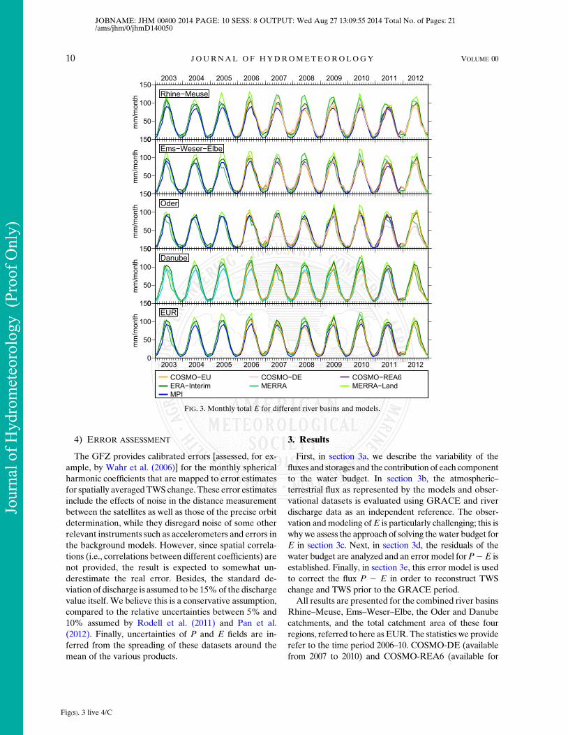
FIG. 3. Monthly total E for different river basins and models.
Fig(s). 3 live 4/C
10 JOURNAL OF HYDROMETEOROLOGY VOLUME 00
JOBNAME: JHM 00#00 2014 PAGE: 10 SESS: 8 OUTPUT: Wed Aug 27 13:09:55 2014 Total No. of Pages: 21/ams/jhm/0/jhmD140050
Jour
nal o
f Hyd
rom
eteo
rolo
gy (
Proo
f Onl
y)
2011) do not cover the entire time span, and therefore,
these results will only be illustrated in the figures.
Throughout the analysis we pay particular attention to the
high-resolution COSMO-EUmodel, as this relatively new
model has not been discussedmuch in the literature so far.
a. Fluxes and storages: The components of theterrestrial water budget
1) PRECIPITATION
Monthly total precipitation over Europe is highly vari-
able (FF2 ig. 2). Spatial averaging causes smaller variability in
large target areas (e.g., EUR) than in small target areas
(e.g., Rhine–Meuse). The P time series are controlled by
the intensity of individual precipitation events and not by
the annual cycle. TT2 able 2 details similarities and differences
between the individual basins and precipitation products.
Over EUR, Danube, and Ems–Weser–Elbe, average
P amounts to about 65mmmonth21. In contrast, meanP
is significantly smaller in the Oder basin, with about
55mmmonth21, and higher in the Rhine–Meuse basin,
with about 80mmmonth21. While over the catchment of
Rhine–Meuse no significant precipitation trend canbe seen
during 2006–10, for the other basins we do find positive
trends between 2 and 4mmmonth21. As already men-
tioned, the annual cycle is rather small, with amplitudes
between 10 and 20mmmonth21 for the individual basins.
Differences among the individual P datasets are
mainly characterized by an offset (Fig. 2). Generally,
mean P from the different datasets has a similar order
in every basin (Table 2). Most of the time, COSMO-
EU exhibits the highest values followed by GPCC,
ERA-Interim, MERRA-Land, E-OBS, and MERRA.
As a gridded dataset, which is based on spatial in-
terpolation of observed precipitation, GPCC is natu-
rally less prone to a model-induced bias. This is
complemented by thorough quality control as de-
scribed by Schneider et al. (2014). GPCC and E-OBS
differ by an offset of 5–6mmmonth21. ERA-Interim
and MERRA-Land tend to underestimate P, yet
amplitudes and trends are consistent with the
observation-based datasets. In agreement with Lorenz
and Kunstmann (2012), we find that MERRA gener-
ally predicts significantly less P than the other datasets.
Furthermore, compared to the other models, the an-
nual amplitude ofMERRA is only half as large and the
trend also appears to be notably smaller.
In total, COSMO-EU overestimates P by about
5mmmonth21 compared to GPCC. This is mainly be-
cause of high precipitation rates in the first years of the
model run, which also lead to a large root-mean-square
error (RMSE). However, the agreement of COSMO-
EU with the observation-based datasets improves with
time, which is likely because of ongoing changes in the
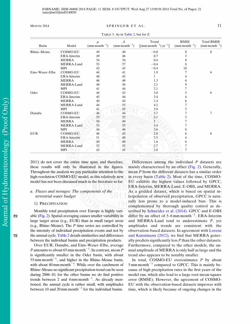
TABLE 3. As in Table 2, but for E.
Basin Model
m
(mmmonth21)
A
(mmmonth21)
Trend
[(mmmonth21) yr21]
RMSE
(mmmonth21)
Total RMSE
(mmmonth21)
Rhine–Meuse COSMO-EU 49 40 20.8 8 8
ERA-Interim 49 46 0.7 3
MERRA 54 54 0.4 8
MERRA-Land 53 57 20.4 8
MPI 42 43 20.4 10
Ems–Weser–Elbe COSMO-EU 44 41 1.9 7 6
ERA-Interim 48 45 1 4
MERRA 46 48 1.3 6
MERRA-Land 48 56 2.1 9
MPI 41 44 2.1 7
Oder COSMO-EU 44 43 3.8 5 6
ERA-Interim 45 44 3.4 4
MERRA 40 44 1.4 6
MERRA-Land 44 53 4.2 7
MPI 41 45 3.9 5
Danube COSMO-EU 46 44 3.7 7 7
ERA-Interim 53 52 3.1 5
MERRA 50 49 2 7
MERRA-Land 53 55 3.4 7
MPI 44 46 3.6 8
EUR COSMO-EU 46 43 2.8 6 6
ERA-Interim 51 49 2.5 4
MERRA 49 49 1.6 6
MERRA-Land 52 55 2.7 7
MPI 43 45 2.8 7
MONTH 2014 S PR INGER ET AL . 11
JOBNAME: JHM 00#00 2014 PAGE: 11 SESS: 8 OUTPUT: Wed Aug 27 13:09:56 2014 Total No. of Pages: 21/ams/jhm/0/jhmD140050
Jour
nal o
f Hyd
rom
eteo
rolo
gy (
Proo
f Onl
y)
data assimilation scheme. We find that one year of re-
analysis data from COSMO-REA6 in 2011 closely re-
sembles COSMO-EU. We further note that in 2007,
COSMO-DE differs significantly with respect to the
other models in the catchments of Rhine–Meuse and
Ems–Weser–Elbe. We speculate that this effect is likely
due to the introduction of radar-derived rain rates via
latent heat nudging.
2) EVAPOTRANSPIRATION
Evapotranspiration variability over EUR is rather
smooth, with a clear annual cycle with large values in
summer and limited signal in winter (FF3 ig. 3). Mean
values and amplitudes are similar in all river basins
(TT3 able 3). TheE trend is nearly zero in the catchment of
Rhine–Meuse, whereas the other basins have clear
positive trends.
Especially in summer, large biases of up to
45mmmonth21 between themodels persist (Fig. 3). The
only observational dataset, Max Planck Institute (MPI AU13),
indicates the smallest mean E, followed by E from
COSMO-EU (Table 3). ERA-Interim, MERRA, and
MERRA-Land predict larger meanE in equal measure.
The characteristic seasonal cycle has amplitudes of
about 50mmmonth21, which differ largely for the in-
dividual models. MERRA-Land, in particular, over-
estimates the annual cycle in comparison to MPI with
amplitude differences of up to 13mmmonth21, that is,
more than 20%of the amplitude. This spread reflects the
large uncertainties of E datasets.
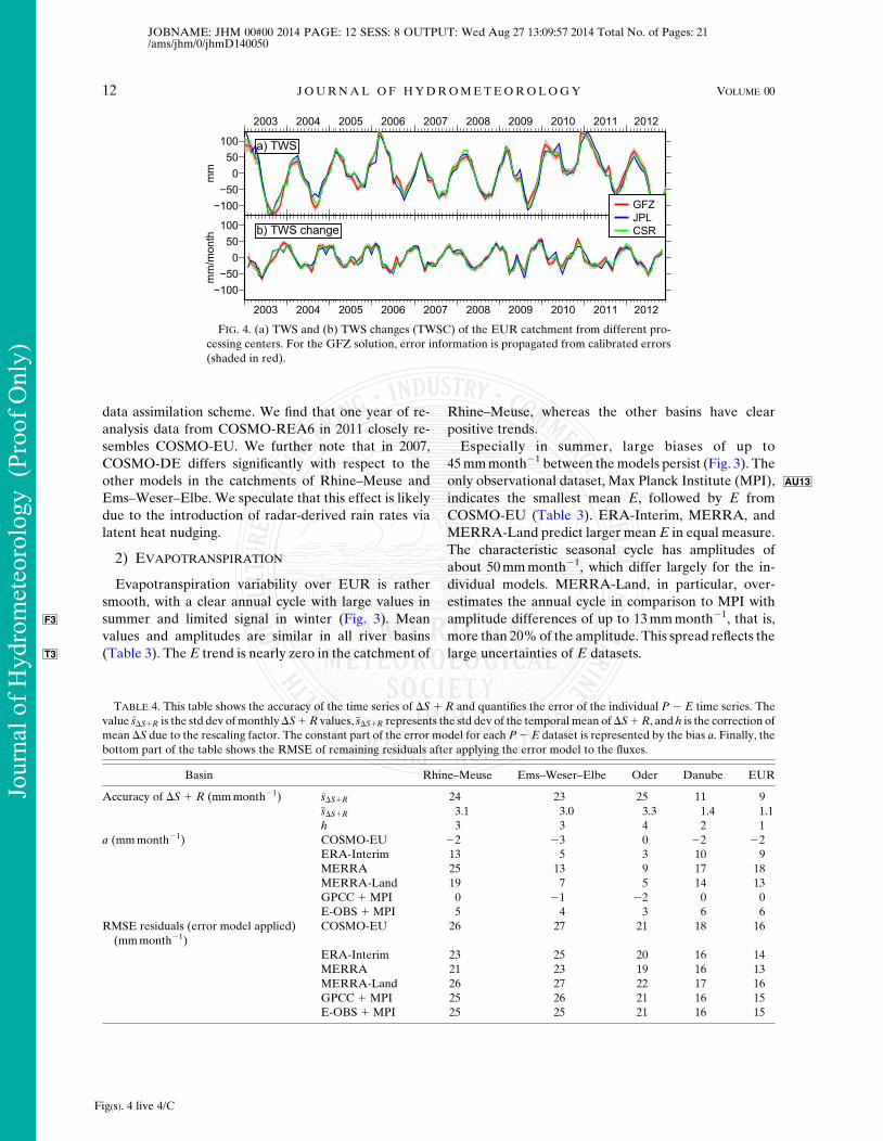
FIG. 4. (a) TWS and (b) TWS changes (TWSC) of the EUR catchment from different pro-
cessing centers. For the GFZ solution, error information is propagated from calibrated errors
(shaded in red).
TABLE 4. This table shows the accuracy of the time series of DS 1 R and quantifies the error of the individual P 2 E time series. The
value sDS1R is the std dev ofmonthlyDS1R values, sDS1R represents the std dev of the temporal mean ofDS1R, and h is the correction of
mean DS due to the rescaling factor. The constant part of the error model for each P2 E dataset is represented by the bias a. Finally, the
bottom part of the table shows the RMSE of remaining residuals after applying the error model to the fluxes.
Basin Rhine–Meuse Ems–Weser–Elbe Oder Danube EUR
Accuracy of DS 1 R (mmmonth21) sDS1R 24 23 25 11 9
sDS1R 3.1 3.0 3.3 1.4 1.1
h 3 3 4 2 1
a (mmmonth21) COSMO-EU 22 23 0 22 22
ERA-Interim 13 5 3 10 9
MERRA 25 13 9 17 18
MERRA-Land 19 7 5 14 13
GPCC 1 MPI 0 21 22 0 0
E-OBS 1 MPI 5 4 3 6 6
RMSE residuals (error model applied)
(mmmonth21)
COSMO-EU 26 27 21 18 16
ERA-Interim 23 25 20 16 14
MERRA 21 23 19 16 13
MERRA-Land 26 27 22 17 16
GPCC 1 MPI 25 26 21 16 15
E-OBS 1 MPI 25 25 21 16 15
Fig(s). 4 live 4/C
12 JOURNAL OF HYDROMETEOROLOGY VOLUME 00
JOBNAME: JHM 00#00 2014 PAGE: 12 SESS: 8 OUTPUT: Wed Aug 27 13:09:57 2014 Total No. of Pages: 21/ams/jhm/0/jhmD140050
Jour
nal o
f Hyd
rom
eteo
rolo
gy (
Proo
f Onl
y)
3) RIVER DISCHARGE
Measured river discharge was obtained from the
GRDC and the BfG. Monthly discharge amounts to
about one-third of precipitation (Fig. 2). The monthly
values lead to a rather smooth time series with strong
annual signal with its maximum in winter or spring.
4) TOTAL WATER STORAGE CHANGE
Three GRACE solutions are compared for the EUR
study area in FF4 ig. 4. We find that the reprocessed
GFZ release 05a fits much better to the JPL and CSR so-
lutions than the previous GFZ release 05 (not shown).
Figure 4a shows TWS and Fig. 4b shows TWS change,
derived using central differences. We find that the com-
putation of backward derivatives instead (not shown)
would introduce a phase shift of at least 8 days.
TT4 able 4 provides, in the first three rows, information
about the error budget of themodel-independent part of
the water budget, DS 1 R. Depending on the basin size,
discharge contributes 4–20 times less to the error budget
as compared to GRACE; that is, its effect is small or
even negligible in the error budget. Also, we find that
the rescaling procedure has a small influence of only
1–4mmmonth21 on the TWS change estimate. We es-
timate that in the EURbasin,DS1R exhibits a standard
deviation of 9mmmonth21, and that for the smaller
basins the error of DS 1 R amounts to about
24mmmonth21. In comparison, for EUR AU14the time series
of P 2 E have a standard deviation of about
23mmmonth21.
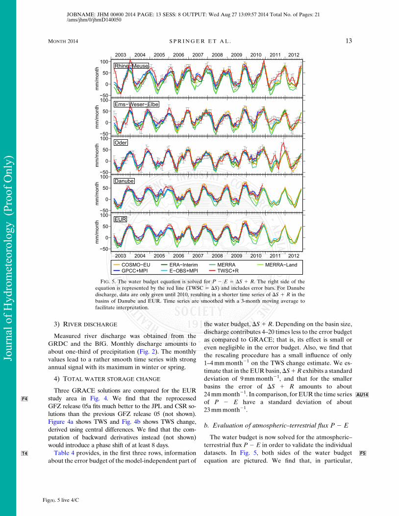
b. Evaluation of atmospheric–terrestrial flux P 2 E
The water budget is now solved for the atmospheric–
terrestrial flux P 2 E in order to validate the individual
datasets. In F F5ig. 5, both sides of the water budget
equation are pictured. We find that, in particular,
FIG. 5. The water budget equation is solved for P 2 E 5 DS 1 R. The right side of the
equation is represented by the red line (TWSC 5 DS) and includes error bars. For Danube
discharge, data are only given until 2010, resulting in a shorter time series of DS 1 R in the
basins of Danube and EUR. Time series are smoothed with a 3-month moving average to
facilitate interpretation.
Fig(s). 5 live 4/C
MONTH 2014 S PR INGER ET AL . 13
JOBNAME: JHM 00#00 2014 PAGE: 13 SESS: 8 OUTPUT: Wed Aug 27 13:09:57 2014 Total No. of Pages: 21/ams/jhm/0/jhmD140050
Jour
nal o
f Hyd
rom
eteo
rolo
gy (
Proo
f Onl
y)
COSMO-EU and the observational datasets are in good
agreement with DS 1 R, even for smaller basins. Also,
ERA-Interim performs quite well, whereas both
MERRA models drift, that is, they systematically un-
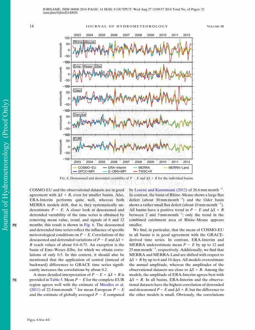
derestimate P 2 E. A closer look at deseasoned and
detrended variability of the time series is obtained by
removing mean value, trend, and signals of 6 and 12
months; this result is shown in FF6 ig. 6. The deseasoned
and detrended time series reflect the influence of specific
meteorological conditions on P2E. Correlations of the
deseasoned and detrended variations ofP2E andDS1R reach values of about 0.6–0.75. An exception is the
basin of Ems–Weser–Elbe, for which we obtain corre-
lations of only 0.5. In this context, it should also be
mentioned that the application of central (instead of
backward) differences to GRACE time series signifi-
cantly increases the correlations by about 0.2.
A more detailed interpretation of P 2 E 5 DS 1 R is
provided in TT5 able 5. Mean P2E for the complete EUR
region agrees well with the estimate of Miralles et al.
(2011) of 22.4mmmonth21 for mean European P 2 E
and the estimate of globally averaged P 2 E computed
by Lorenz and Kunstmann (2012) of 26.6mmmonth21.
In contrast, the basin of Rhine–Meuse shows a large flux
deficit (about 30mmmonth21) and the Oder basin
shows a rather small flux deficit (about 10mmmonth21).
All basins have a positive trend in P 2 E and DS 1 R
between 2 and 5mmmonth21; only the trend in the
combined catchment area of Rhine–Meuse appears
smaller.
We find, in particular, that the mean of COSMO-EU
in all basins is in good agreement with the GRACE-
derived time series. In contrast, ERA-Interim and
MERRA underestimate mean P 2 E by up to 12 and
25mmmonth21, respectively. Additionally, we find that
MERRA andMERRA-Land are shifted with respect to
DS1 R by up to 6 and 10 days. All models overestimate
the annual amplitude, whereas the amplitudes of the
observational datasets are close to DS 1 R. Among the
models, the amplitude of ERA-Interim agrees best with
DS 1 R. In all basins, ERA-Interim and the observa-
tional datasets have the highest correlation of detrended
and deseasoned P2E and DS1R, but the difference to
the other models is small. Obviously, the correlations
FIG. 6. Deseasoned and detrended variability of P 2 E and DS 1 R for the individual basins.
Fig(s). 6 live 4/C
14 JOURNAL OF HYDROMETEOROLOGY VOLUME 00
JOBNAME: JHM 00#00 2014 PAGE: 14 SESS: 8 OUTPUT: Wed Aug 27 13:09:57 2014 Total No. of Pages: 21/ams/jhm/0/jhmD140050
Jour
nal o
f Hyd
rom
eteo
rolo
gy (
Proo
f Onl
y)
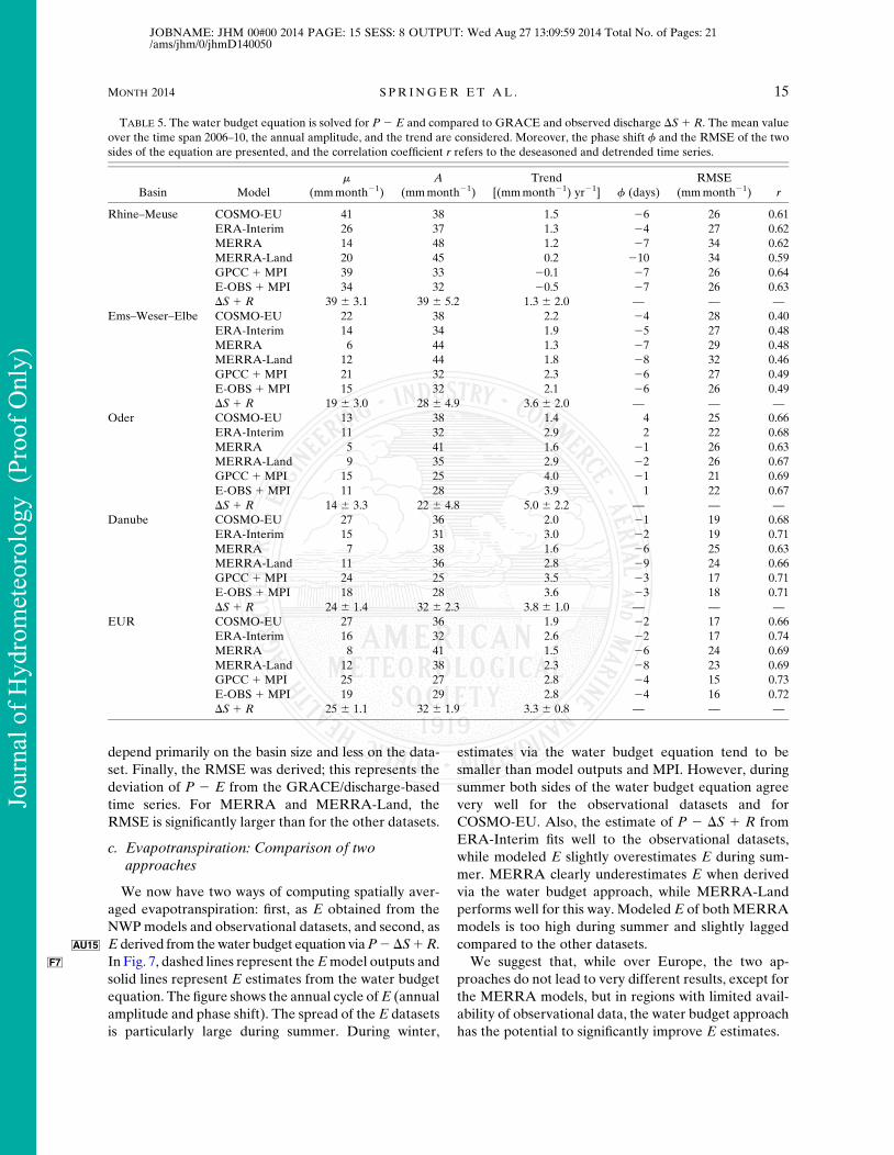
depend primarily on the basin size and less on the data-
set. Finally, the RMSE was derived; this represents the
deviation of P 2 E from the GRACE/discharge-based
time series. For MERRA and MERRA-Land, the
RMSE is significantly larger than for the other datasets.
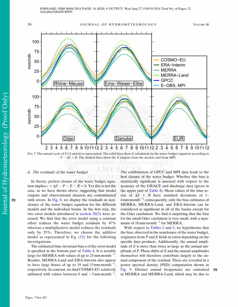
c. Evapotranspiration: Comparison of twoapproaches
We now have two ways of computing spatially aver-
aged evapotranspiration: first, as E obtained from the
NWPmodels and observational datasets, and second, as
E derived from thewater budget equation viaP2DS1AU15 R.
In FF7 ig. 7, dashed lines represent theEmodel outputs and
solid lines represent E estimates from the water budget
equation. The figure shows the annual cycle ofE (annual
amplitude and phase shift). The spread of theE datasets
is particularly large during summer. During winter,
estimates via the water budget equation tend to be
smaller than model outputs and MPI. However, during
summer both sides of the water budget equation agree
very well for the observational datasets and for
COSMO-EU. Also, the estimate of P 2 DS 1 R from
ERA-Interim fits well to the observational datasets,
while modeled E slightly overestimates E during sum-
mer. MERRA clearly underestimates E when derived
via the water budget approach, while MERRA-Land
performs well for this way. Modeled E of bothMERRA
models is too high during summer and slightly lagged
compared to the other datasets.
We suggest that, while over Europe, the two ap-
proaches do not lead to very different results, except for
the MERRA models, but in regions with limited avail-
ability of observational data, the water budget approach
has the potential to significantly improve E estimates.
TABLE 5. The water budget equation is solved for P 2 E and compared to GRACE and observed discharge DS 1 R. The mean value
over the time span 2006–10, the annual amplitude, and the trend are considered. Moreover, the phase shift f and the RMSE of the two
sides of the equation are presented, and the correlation coefficient r refers to the deseasoned and detrended time series.
Basin Model
m
(mmmonth21)
A
(mmmonth21)
Trend
[(mmmonth21) yr21] f (days)
RMSE
(mmmonth21) r
Rhine–Meuse COSMO-EU 41 38 1.5 26 26 0.61
ERA-Interim 26 37 1.3 24 27 0.62
MERRA 14 48 1.2 27 34 0.62
MERRA-Land 20 45 0.2 210 34 0.59
GPCC 1 MPI 39 33 20.1 27 26 0.64
E-OBS 1 MPI 34 32 20.5 27 26 0.63
DS 1 R 39 6 3.1 39 6 5.2 1.3 6 2.0 — — —
Ems–Weser–Elbe COSMO-EU 22 38 2.2 24 28 0.40
ERA-Interim 14 34 1.9 25 27 0.48
MERRA 6 44 1.3 27 29 0.48
MERRA-Land 12 44 1.8 28 32 0.46
GPCC 1 MPI 21 32 2.3 26 27 0.49
E-OBS 1 MPI 15 32 2.1 26 26 0.49
DS 1 R 19 6 3.0 28 6 4.9 3.6 6 2.0 — — —
Oder COSMO-EU 13 38 1.4 4 25 0.66
ERA-Interim 11 32 2.9 2 22 0.68
MERRA 5 41 1.6 21 26 0.63
MERRA-Land 9 35 2.9 22 26 0.67
GPCC 1 MPI 15 25 4.0 21 21 0.69
E-OBS 1 MPI 11 28 3.9 1 22 0.67
DS 1 R 14 6 3.3 22 6 4.8 5.0 6 2.2 — — —
Danube COSMO-EU 27 36 2.0 21 19 0.68
ERA-Interim 15 31 3.0 22 19 0.71
MERRA 7 38 1.6 26 25 0.63
MERRA-Land 11 36 2.8 29 24 0.66
GPCC 1 MPI 24 25 3.5 23 17 0.71
E-OBS 1 MPI 18 28 3.6 23 18 0.71
DS 1 R 24 6 1.4 32 6 2.3 3.8 6 1.0 — — —
EUR COSMO-EU 27 36 1.9 22 17 0.66
ERA-Interim 16 32 2.6 22 17 0.74
MERRA 8 41 1.5 26 24 0.69
MERRA-Land 12 38 2.3 28 23 0.69
GPCC 1 MPI 25 27 2.8 24 15 0.73
E-OBS 1 MPI 19 29 2.8 24 16 0.72
DS 1 R 25 6 1.1 32 6 1.9 3.3 6 0.8 — — —
MONTH 2014 S PR INGER ET AL . 15
JOBNAME: JHM 00#00 2014 PAGE: 15 SESS: 8 OUTPUT: Wed Aug 27 13:09:59 2014 Total No. of Pages: 21/ams/jhm/0/jhmD140050
Jour
nal o
f Hyd
rom
eteo
rolo
gy (
Proo
f Onl
y)
d. The residuals of the water budget
In theory, perfect closure of the water budget equa-
tion implies �5 DS2 P2 E2 R5 0. Yet this is not the
case, as we have shown above, suggesting that model
outputs and observational datasets are contaminated
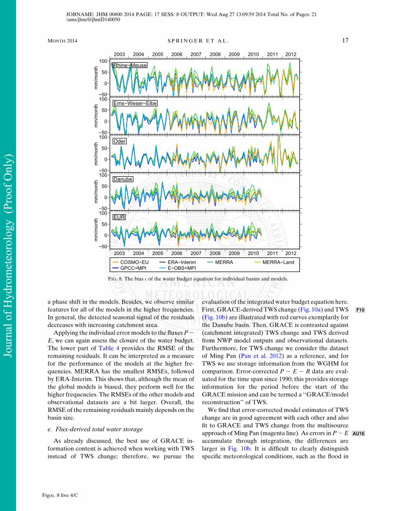
with errors. In FF8 ig. 8, we display the residuals or non-
closure of the water budget equation for the different
models and the individual basins. In the first step, the
two error models introduced in section 2b(3) were as-
sessed. We find that the error model using a constant
offset reduces the water budget residuals by 47%
whereas a multiplicative model reduces the residuals
only by 35%. Therefore, we choose the additive
model as represented in Eq. (12) for the following
investigations.
The estimated time-invariant bias a of the errormodel
is specified in the bottom part of Table 4. It is notably
large for MERRA with values of up to 25mmmonth21.
Besides, MERRA-Land and ERA-Interim also appear
to have large biases of up to 19 and 13mmmonth21,
respectively. In contrast, we find COSMO-EU relatively
unbiased with values between 0 and 23mmmonth21.
The combination of GPCC and MPI data leads to the
best closure of the water budget. Whether this bias is
statistically significant is assessed with respect to the
accuracy of the GRACE and discharge data (given in
the upper part of Table 4). Mean values of the time se-
ries of DS 1 R have standard deviations of 1–
4mmmonth21; consequently, only the bias estimates of
MERRA, MERRA-Land, and ERA-Interim can be
considered as significant in all of the basins except for
the Oder catchment. We find it surprising that the bias
for the small Oder catchment is very small, with a max-
imum of 10mmmonth21 for MERRA.
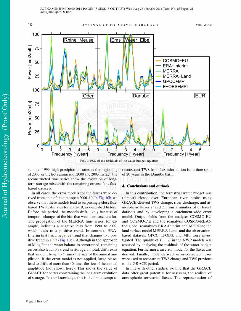
With respect to Tables 2 and 3, we hypothesize that
the bias, observed in the nonclosure of the water budget,
originates from P andE fields in ratios depending on the
specific data products. Additionally, the annual ampli-
tude of E is more than twice as large as the annual am-
plitude of P. Phase shifts ofE and the annual amplitudes
themselves will therefore contribute largely to the an-
nual component of the residual. These are revealed in a
power spectral density (PSD) computation shown in
F F9ig. 9. Distinct annual frequencies are contained
in MERRA and MERRA-Land, which may be due to
FIG. 7. The annual cycle of E (A and f) is represented. The solid lines show E calculated via the water budget equation according to
P 2 DS 1 R. The dashed lines show the E outputs from the models and from MPI.
Fig(s). 7 live 4/C
16 JOURNAL OF HYDROMETEOROLOGY VOLUME 00
JOBNAME: JHM 00#00 2014 PAGE: 16 SESS: 8 OUTPUT: Wed Aug 27 13:09:59 2014 Total No. of Pages: 21/ams/jhm/0/jhmD140050
Jour
nal o
f Hyd
rom
eteo
rolo
gy (
Proo
f Onl
y)
a phase shift in the models. Besides, we observe similar
features for all of the models in the higher frequencies.
In general, the detected seasonal signal of the residuals
decreases with increasing catchment area.
Applying the individual errormodels to the fluxesP2E, we can again assess the closure of the water budget.
The lower part of Table 4 provides the RMSE of the
remaining residuals. It can be interpreted as a measure
for the performance of the models at the higher fre-
quencies. MERRA has the smallest RMSEs, followed
by ERA-Interim. This shows that, although the mean of
the global models is biased, they perform well for the
higher frequencies. The RMSEs of the other models and
observational datasets are a bit larger. Overall, the
RMSE of the remaining residuals mainly depends on the
basin size.
e. Flux-derived total water storage
As already discussed, the best use of GRACE in-
formation content is achieved when working with TWS
instead of TWS change; therefore, we pursue the
evaluation of the integrated water budget equation here.
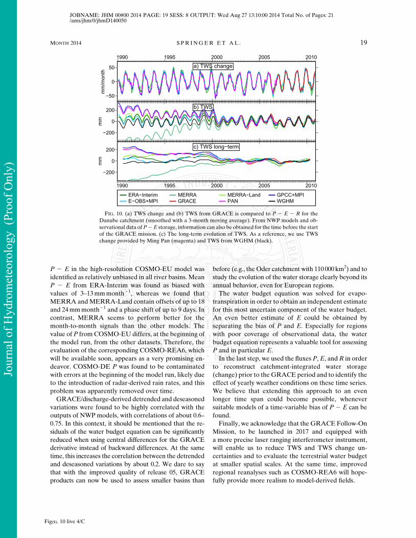
First, GRACE-derived TWS change (F F10ig. 10a) and TWS
(Fig. 10b) are illustrated with red curves exemplarily for
the Danube basin. Then, GRACE is contrasted against
(catchment integrated) TWS change and TWS derived
from NWP model outputs and observational datasets.
Furthermore, for TWS change we consider the dataset
of Ming Pan (Pan et al. 2012) as a reference, and for
TWS we use storage information from the WGHM for
comparison. Error-corrected P 2 E 2 R data are eval-
uated for the time span since 1990; this provides storage
information for the period before the start of the
GRACE mission and can be termed a ‘‘GRACE/model
reconstruction’’ of TWS.
We find that error-corrected model estimates of TWS
change are in good agreement with each other and also
fit to GRACE and TWS change from the multisource
approach ofMing Pan AU16(magenta line). As errors inP2E
accumulate through integration, the differences are
larger in Fig. 10b. It is difficult to clearly distinguish
specific meteorological conditions, such as the flood in
FIG. 8. The bias � of the water budget equation for individual basins and models.
Fig(s). 8 live 4/C
MONTH 2014 S PR INGER ET AL . 17
JOBNAME: JHM 00#00 2014 PAGE: 17 SESS: 8 OUTPUT: Wed Aug 27 13:09:59 2014 Total No. of Pages: 21/ams/jhm/0/jhmD140050
Jour
nal o
f Hyd
rom
eteo
rolo
gy (
Proo
f Onl
y)
summer 1999, high precipitation rates at the beginning
of 2000, or the hot summers of 2000 and 2003. In fact, the
reconstructed time series show the evolution of long-
term storagemixedwith the remaining errors of the flux-
based datasets.
In all cases, the error models for the fluxes were de-
rived from data of the time span 2006–10. In Fig. 10b, we
observe that these models lead to surprisingly close flux-
based TWS estimates for 2002–10, as described before.
Before this period, the models drift, likely because of
temporal changes of the bias that we did not account for.
The propagation of the MERRA time series, for ex-
ample, indicates a negative bias from 1990 to 2002,
which leads to a positive trend. In contrast, ERA-
Interim first has a negative trend that changes to a pos-
itive trend in 1995 (Fig. 10c). Although in the approach
of Ming Pan the water balance is constrained, remaining
errors also lead to a trend in storage. In total, drifts exist
that amount to up to 5 times the size of the annual am-
plitude. If the error model is not applied, large biases
lead to drifts of more than 40 times the size of the annual
amplitude (not shown here). This shows the value of
GRACE for better constraining the long-term evolution
of storage. To our knowledge, this is the first attempt to
reconstruct TWS from flux information for a time span
of 20 years in the Danube basin.
4. Conclusions and outlook
In this contribution, the terrestrial water budget was
(almost) closed over European river basins using
GRACE-derived TWS change, river discharge, and at-
mospheric fluxes P and E from a number of different
datasets and by developing a catchment-wide error
model. Output fields from the analyses COSMO-EU
and COSMO-DE and the reanalysis COSMO-REA6;
the global reanalyses ERA-Interim and MERRA; the
land surface model MERRA-Land; and the observation-
based datasets GPCC, E-OBS, and MPI were inves-
tigated. The quality of P 2 E in the NWP models was
assessed by analyzing the residuals of the water budget
equation. Furthermore, an error model for the fluxes was
derived. Finally, model-derived, error-corrected fluxes
were used to reconstruct TWS change and TWS previous
to the GRACE period.
In line with other studies, we find that the GRACE
data offer great potential for assessing the realism of
atmospheric–terrestrial fluxes. The representation of
FIG. 9. PSD of the residuals of the water budget equation.
Fig(s). 9 live 4/C
18 JOURNAL OF HYDROMETEOROLOGY VOLUME 00
JOBNAME: JHM 00#00 2014 PAGE: 18 SESS: 8 OUTPUT: Wed Aug 27 13:10:00 2014 Total No. of Pages: 21/ams/jhm/0/jhmD140050
Jour
nal o
f Hyd
rom
eteo
rolo
gy (
Proo
f Onl
y)
P 2 E in the high-resolution COSMO-EU model was
identified as relatively unbiased in all river basins. Mean
P 2 E from ERA-Interim was found as biased with
values of 3–13mmmonth21, whereas we found that
MERRA andMERRA-Land contain offsets of up to 18
and 24mmmonth21 and a phase shift of up to 9 days. In
contrast, MERRA seems to perform better for the
month-to-month signals than the other models. The
value of P from COSMO-EU differs, at the beginning of
the model run, from the other datasets. Therefore, the
evaluation of the corresponding COSMO-REA6, which
will be available soon, appears as a very promising en-
deavor. COSMO-DE P was found to be contaminated
with errors at the beginning of the model run, likely due
to the introduction of radar-derived rain rates, and this
problem was apparently removed over time.
GRACE/discharge-derived detrended and deseasoned
variations were found to be highly correlated with the
outputs of NWP models, with correlations of about 0.6–
0.75. In this context, it should be mentioned that the re-
siduals of the water budget equation can be significantly
reduced when using central differences for the GRACE
derivative instead of backward differences. At the same
time, this increases the correlation between the detrended
and deseasoned variations by about 0.2. We dare to say
that with the improved quality of release 05, GRACE
products can now be used to assess smaller basins than
before (e.g., the Oder catchment with 110 000km2) and to
study the evolution of the water storage clearly beyond its
annual behavior, even for European regions.
The water budget equation was solved for evapo-
transpiration in order to obtain an independent estimate
for this most uncertain component of the water budget.
An even better estimate of E could be obtained by
separating the bias of P and E. Especially for regions
with poor coverage of observational data, the water
budget equation represents a valuable tool for assessing
P and in particular E.
In the last step, we used the fluxes P,E, andR in order
to reconstruct catchment-integrated water storage
(change) prior to the GRACE period and to identify the
effect of yearly weather conditions on these time series.
We believe that extending this approach to an even
longer time span could become possible, whenever
suitable models of a time-variable bias of P 2 E can be
found.
Finally, we acknowledge that the GRACE Follow-On
Mission, to be launched in 2017 and equipped with
a more precise laser ranging interferometer instrument,
will enable us to reduce TWS and TWS change un-
certainties and to evaluate the terrestrial water budget
at smaller spatial scales. At the same time, improved
regional reanalyses such as COSMO-REA6 will hope-
fully provide more realism to model-derived fields.
FIG. 10. (a) TWS change and (b) TWS from GRACE is compared to P 2 E 2 R for the
Danube catchment (smoothed with a 3-month moving average). From NWP models and ob-
servational data ofP2E storage, information can also be obtained for the time before the start
of the GRACE mission. (c) The long-term evolution of TWS. As a reference, we use TWS
change provided by Ming Pan (magenta) and TWS from WGHM (black).
Fig(s). 10 live 4/C
MONTH 2014 S PR INGER ET AL . 19
JOBNAME: JHM 00#00 2014 PAGE: 19 SESS: 8 OUTPUT: Wed Aug 27 13:10:00 2014 Total No. of Pages: 21/ams/jhm/0/jhmD140050
Jour
nal o
f Hyd
rom
eteo
rolo
gy (
Proo
f Onl
y)
Acknowledgments.We thank the Global Runoff Data
Centre, 56068 Koblenz, Germany for providing river
discharge data and watershed boundaries, and we ac-
knowledge discharge data obtained from the Bunde-
sanstalt für Gewässerkunde. We are grateful to MingPan for providing the reference dataset applied inFig. 10, as well as for his useful comments. Moreover,
part of this research was carried out in the Hans-Ertel
Centre for Weather Research, a research network of
universities, research institutes, and the Deutscher
Wetterdienst funded by the BMVBS (Federal Ministry
of Transport, Building and Urban Development). Fi-
nally, the authors thank editor Ruby Leung and the re-
viewers for their helpful comments.
REFERENCES
Berrisford, P., and Coauthors, 2011: The ERA-Interim archive,
version 2.0. ERARep. Series 1, European Centre for Medium
Range Weather Forecasts, 23 pp.
Bollmeyer, C., and Coauthors, 2014: Towards a high-resolution
regional reanalysis for the European CORDEX domain.
Quart. J. Roy. Meteor. Soc., submittedAU17 .
Chambers, D. P., and J. A. Bonin, 2012: Evaluation of Release-05
GRACE time-variable gravity coefficients over the ocean.
Ocean Sci., 9, 2187–2214, doi:10.5194/os-8-859-2012.Cheng, M., and B. D. Tapley, 2004: Variations in the Earth’s ob-
lateness during the past 28 years. J. Geophys. Res., 109,
B09402, doi:10.1029/2004JB003028.
Coumou, D., and S. Rahmstorf, 2012: A decade of weather extremes.
Nat. Climate Change, 2, 491–496, doi:10.1038/nclimate1452.
Dahle, C., F. Flechtner, C. Gruber, D. König, R. König, G. Michalak,
and K.-H. Neumayer, 2013: GFZ GRACE level-2 processing
standards document for level-2 product release 0005: Revised
edition. Scientific Tech. Rep. STR12/02, 21 pp., doi:10.2312/
GFZ.b103-1202-25.
Dee, D. P., and Coauthors, 2011: The ERA-Interim reanalysis:
Configuration and performance of the data assimilation sys-
tem. Quart. J. Roy. Meteor. Soc., 137, 553–597, doi:10.1002/
qj.828.
Döll, P., F. Kaspar, and B. Lehner, 2003: A global hydrological
model for deriving water availability indicators: model tun-
ing and validation. J. Hydrol., 270, 105–134, doi:10.1016/
S0022-1694(02)00283-4.
Fersch, B., H. Kunstmann, A. Bárdossy, B. Devaraju, and
N. Sneeuw, 2012: Continental-scale basin water storage vari-
ation from global and dynamically downscaled atmospheric wa-
ter budgets in comparison with GRACE-derived observations.
J. Hydrometeor., 13, 1589–1603, doi:10.1175/JHM-D-11-0143.1.
Gegout, P., cited 2014: Load Love numbers. [Available online at
http://gemini.gsfc.nasa.gov/aplo/Load_Love2_CM.dat.]
Güntner, A., 2008: Improvement of global hydrological models
using GRACE data. Surv. Geophys., 29, 375–397, doi:10.1007/
s10712-008-9038-y.
Hall, J., and Coauthors, 2013: Understanding flood regime changes
in Europe: A state of the art assessment. Hydrol. Earth Syst.
Sci., 10, 15 525–15 624, doi:10.5194/hessd-10-15525-2013.Hirschi, M., P. Viterbo, and S. I. Seneviratne, 2006: Basin-scale
water-balance estimates of terrestrial water storage variations
from ECMWF operational forecast analysis. Geophys. Res.
Lett., 33, L21401, doi:10.1029/2006GL027659.
Huntington, T. G., 2006: Evidence for intensification of the global
water cycle: Review and synthesis. J. Hydrol., 319, 83–95,
doi:10.1016/j.jhydrol.2005.07.003.
Jiménez, C., and Coauthors, 2011: Global intercomparison of 12
land surface heat flux estimates. J. Geophys. Res., 116,D02102,
doi:10.1029/2010JD014545.
Jung, M., and Coauthors, 2010: Recent decline in the global land
evapotranspiration trend due to limited moisture supply. Na-
ture, 467, 951–954, doi:10.1038/nature09396.
——, and Coauthors, 2011: Global patterns of land–atmosphere
fluxes of carbon dioxide, latent heat, and sensible heat de-
rived from eddy covariance, satellite, and meteorological
observations. J. Geophys. Res., 116, G00J07, doi:10.1029/
2010JG001566.
Klees, R., E. A. Zapreeva, H. C.Winsemius, andH.H.G. Savenije,
2007: The bias in GRACE estimates of continental water
storage variations. Hydrol. Earth Syst. Sci., 11, 1227–1241,
doi:10.5194/hess-11-1227-2007.
Klemann, V., and Z. Martinec, 2011: Contribution of glacial-
isostatic adjustment to the geocenter motion. Tectonophy-
sics, 511, 99–108, doi:10.1016/j.tecto.2009.08.031.
Kusche, J., 2007: Approximate decorrelation and non-isotropic
smoothing of time-variable GRACE-type gravity field models.
J. Geod., 81, 733–749, doi:10.1007/s00190-007-0143-3.
Long, D., L. Longuevergne, and B. R. Scanlon, 2014: Uncertainty
in evapotranspiration from land surface modeling, remote
sensing, and GRACE satellites.Water Resour. Res., 50, 1131–
1151, doi:10.1002/2013WR014581.
Longuevergne, L., B. Scanlon, and C. R. Wilson, 2010: GRACE
hydrological estimates for small basins: Evaluating processing
approaches on the High Plains Aquifer, USA. Water Resour.
Res., 46, W11517, doi:10.1029/2009WR008564.
Lorenz, C., and H. Kunstmann, 2012: The hydrological cycle in
three state-of-the-art reanalyses: Intercomparison and perfor-
mance analysis. J. Hydrometeor., 13, 1397–1420, doi:10.1175/
JHM-D-11-088.1.
Lucchesi, R., 2012: File specification for MERRA products.
GMAOOffice Note No. 1 (version 2.3), Global Modeling and
Assimilation Office, 83 pp. [Available online at http://gmao.
gsfc.nasa.gov/pubs/docs/Lucchesi528.pdf.]
Miralles, D. G., R. A. M. De Jeu, J. H. Gash, T. R. H. Holmes, and
A. J. Dolman, 2011: Magnitude and variability of land evap-
oration and its components at the global scale. Hydrol. Earth
Syst. Sci., 15, 967–981, doi:10.5194/hess-15-967-2011.Mueller, B., and Coauthors, 2011: Evaluation of global
observations-based evapotranspiration datasets and IPCC
AR4 simulations.Geophys. Res. Lett., 38,L06402, doi:10.1029/
2010GL046230.
Pan, M., A. K. Sahoo, T. J. Troy, R. K. Vinukollu, J. Sheffield, and
E. F. Wood, 2012: Multisource estimation of long-term ter-
restrial water budget for major global river basins. J. Climate,
25, 3191–3206, doi:10.1175/JCLI-D-11-00300.1.
Priestley, C., and R. Taylor, 1972: On the assessment of surface
heat flux and evaporation using large-scale parameters. Mon.
Wea. Rev., 100, 81–92, doi:10.1175/1520-0493(1972)100,0081:
OTAOSH.2.3.CO;2.
Ramilien, G., F. Frappart, A. Günter, T. Ngo-Duc, A. Cazenave,
and K. Laval, 2006: Time variations of the regional evapo-
transpiration rate from Gravity Recovery and Climate Ex-
periment (GRACE) satellite gravimetry. Water Resour. Res.,
42, W10403, doi:10.1029/2005WR004331.
20 JOURNAL OF HYDROMETEOROLOGY VOLUME 00
JOBNAME: JHM 00#00 2014 PAGE: 20 SESS: 8 OUTPUT: Wed Aug 27 13:10:00 2014 Total No. of Pages: 21/ams/jhm/0/jhmD140050
Jour
nal o
f Hyd
rom
eteo
rolo
gy (
Proo
f Onl
y)
Reichle, R. H., R. D. Koster, G. J. M. D. Lannoy, B. A. Forman,
Q. Liu, S. P. P. Mahanama, and A. Tourè, 2011: Assessment
and enhancement ofMERRA land surface hydrology estimates.
J. Climate, 24, 6322–6338, doi:10.1175/JCLI-D-10-05033.1.
Rienecker, M. M., and Coauthors, 2011: MERRA: NASAs
Modern-Era Retrospective Analysis for Research and Applica-
tions. J. Climate, 24, 3624–3648, doi:10.1175/JCLI-D-11-00015.1.
Rietbroek, R., M. Fritsche, S.-E. Brunnabend, I. Daras, J. Kusche,
J. Schröter, F. Flechtner, and R. Dietrich, 2012: Global surface
mass from a new combination of GRACE, modelled OBP
and reprocessedGPS data. J. Geodyn., 59–60, 64–71, doi:10.1016/
j.jog.2011.02.003.
Rodell, M., E. B. McWilliams, J. S. Famiglietti, H. K. Beaudoing,
and J. Nigro, 2011: Estimating evapotranspiration using an
observation based terrestrial water budget.Hydrol. Processes,
25, 4082–4092, doi:10.1002/hyp.8369.
Roebeling, R. A., E. L. A. Wolters, J. F. Meirink, and H. Leinse,
2012: Triple collocation of summer precipitation retrievals
from SEVIRI over Europe with gridded rain gauge and
weather radar data. J. Hydrometeor., 13, 1552–1566, doi:10.1175/
JHM-D-11-089.1.
Schneider, U., A. Becker, P. Finger, A. Meyer-Christoffer,
B. Rudolf, and M. Ziese, 2011: GPCC full data reanalysis
version 6.0 at 0.58: Monthly land-surface precipitation from
rain-gauges built on GTS-based and historic data. Global
Precipitation Climatology Centre, Offenbach, Germany,
doi:10.5676/DWD_GPCC/FD_M_V6_050.
——,——,——,——,M. Ziese, and B. Rudolf, 2014: GPCC’s new
land surface precipitation climatology based on quality-
controlled in situ data and its role in quantifying the global
water cycle. Theor. Appl. Climatol., 115, 15–40, doi:10.1007/
s00704-013-0860-x.
Schraff, C. H., 1997: Mesoscale data assimilation and prediction of
low stratus in the Alpine region.Meteor. Atmos. Phys., 64, 21–50, doi:10.1007/BF01044128.
Seitz, F., M. Schmidt, and C. K. Shum, 2008: Signals of extreme
weather conditions in Central Europe in GRACE 4-D hy-
drological mass variations. Earth Planet. Sci. Lett., 268, 165–
170, doi:10.1016/j.epsl.2008.01.001.
Syed, T. H., J. S. Famiglietti, and D. P. Chambers, 2009: GRACE-
based estimates of terrestrial freshwater discharge from basin
to continental scales. J. Hydrometeor., 10, 22–40, doi:10.1175/
2008JHM993.1.
Tapley, B. D., S. Bettadpur, J. C. Ries, P. F. Thompson, and M. M.
Watkins, 2004: GRACE measurements of mass variability in
the earth system. Science, 305, 503–505, doi:10.1126/
science.1099192.
Trenberth, K. E., 2011: Changes in precipitation with climatic
change. Climate Res., 47, 123–138, doi:10.3354/cr00953.
Wahr, J., M. Molenaar, and F. Bryan, 1998: Time variability of the
Earth’s gravity field: Hydrological and oceanic effects and
their possible detection using GRACE. J. Geophys. Res., 103,
30 205–30 229, doi:10.1029/98JB02844.
——, S. Swenson, and I. Velicogna, 2006: Accuracy of grace mass
estimates. Geophys. Res. Lett., 33, L06401, doi:10.1029/
2005GL025305.
Wang, K., and R. E. Dickinson, 2012: A review of global terrestrial
evapotranspiration: Observation, modeling, climatology, and
climatic variability. Rev. Geophys., 50, RG2050, doi:10.1029/
2011RG000373.
Werth, S., and A. Güntner, 2010: Calibration analysis for
water storage variability of the global hydrological model
WGHM. Hydrol. Earth Syst. Sci., 14, 59–78, doi:10.5194/
hess-14-59-2010.
Zaitchik, B. F., 2008: Assimilation of GRACE terrestrial water
storage data into a land surface model: Results for the Mis-
sissippi river basin. J. Hydrometeor., 9, 535–548, doi:10.1175/
2007JHM951.1.
MONTH 2014 S PR INGER ET AL . 21
JOBNAME: JHM 00#00 2014 PAGE: 21 SESS: 8 OUTPUT: Wed Aug 27 13:10:01 2014 Total No. of Pages: 21/ams/jhm/0/jhmD140050
Jour
nal o
f Hyd
rom
eteo
rolo
gy (
Proo
f Onl
y)
Copyright © 2022 FDOKUMEN