STEPHEN OLINER

GLENN RUDEBUSCH

DANIEL SICHEL

New and Old Models of Business Investment: A Comparison of Forecasting Performance

RECENT EMPIRICAL RESEARCH on investment has focused on the estimation of the stochastic first-order conditions, or Euler equations, from dy- namic models derived under rational expectations. Because these models have an explicit structural interpretation, they are theoretically more appealing than tradi- tional models of investment. However, the empirical performance of Euler-equation models has not been tested against the traditional models. This paper performs such a test by adding two Euler equations to the usual group of traditional investment models examined in previous studies namely, the accelerator, neoclassical, mod- ified neoclassical, and Q-theory models. 1

The first of our two Euler equations is a "canonical'7 model that typifies the equa- tions estimated in recent years.2 Despite its popularity, this canonical model has a restrictive dynamic structure that is unlikely to capture the time lags inherent in the investment process. In contrast, our second Euler equation explicitly accounts for

The authors thank two anonymous referees for helpful comments and Tom Brennan, Greg Brown, Sam Coffin, and Gretchen Weinbach for excellent research assistance. This paper is a condensed version of Oliner, Rudebusch, and Sichel (1993). The views expressed are those of the authors and are not neces- sarily shared bv the Board of Governors of the Federal Reserve System, the Federal Reserve Bank of San Francisco, or the Brookings Institution.

1. Earlier evaluations of investment models include Bernanke, Bohn, and Reiss (1988), Kopcke (1985, 1993), Clark (1979), Elliott (1973), BischoS (1971), Jorgenson, Hunter, and Nadiri (1970a, b), and Jorgenson and Siebert (1968).

2. To our knowledge, Abel (1980) was the first to estimate an investment Euler equation under ratio- nal expectations. For later work within this literature, see Pindyck and Rotemberg (1983), Shapiro (1986a, b), Gilchrist (1990), Gertler, Hubbard, and Kashyap (1991), Hubbard and Kashyap (1992), Whited (1992), Carpenter (1992), and Ng and Schaller (1993).

STEPHEN OLINER is chief of the Capital Markets section at the Board of Governors of the Federal Reserve System. GLENN RUDEBUSCH is research oWcer at the Federal Reserve Bank of San Francisco. DANIEL SICHEL is research associate at the Brookings Institution. Journal of Money, Credit, and Banking, Vol. 27, No. 3 (August 1995) This article was written by the authors in their capacity as government officials. It is totally in the public domain.

STEPHEN OLINER, GLENN RUDEBUSCH, AND DANIEL SICHEL : 807

the lag between the start of an investment project and the later date at which the new capital begins to contribute to the firm's production. By embedding such "time-to- buildS' lags, which were emphasized by Kydland and Prescott (1982), this equation has a richer structure than most previous investment Euler equations.3

This paper focuses on the ability of the various models to forecast investment in equipment and in nonresidential structures. From a practical standpoint, such out- of-sample tests are needed to determine which models have the most value as fore- casting tools. Moreover, beyond this practical objective, out-of-sample performance is a powerful test of model specification (see, for example, Hendry 1979). We con- duct two sets of tests. The first set of tests examines the size, bias, and serial correla- tion of the modelsS one-step-ahead forecast errors, similar to the out-of-sample tests performed by Kopcke (1985) and Clark (1979). In addition, we compare the infor- mation content of model forecasts by regressing actual investment on predictions from pairs of modelss Fair and Shiller (1990) have argued that such regressions pro- vide a powerful test of alternative models.

To summarize the results, we find that the Euler equations produce extremely poor forecasts of investment for both equipment and nonresidential structures. The time-to-build version of the Euler equation outperforms the basic Euler equation in our tests, but the improvement is modest. All the Euler equations have mean squared forecast errors many times larger than those of the traditional models. Moreover, the Fair-Shiller tests suggest that, as a group, the traditional models for equipment dominate the Euler equations; for nonresidential structures, the Fair- Shiller tests show that neither the Euler equations nor the traditional models have any forecasting ability.

The paper is organized as follows. The next section describes the models in our horse race, while section 2 briefly discusses our data set. Section 3 presents full- sample estimates of each model, in order to gain some initial information on their relative fit. Section 4 documents that the Euler equations produce relatively poor forecasts, and section 5 attempts to explain why this is so, arguing that the standard assumptions that underlie these equations could be to blame. Section 6 concludes the paper and suggests areas for future research.

l. THE INVESTMENT MODELS

A. Two Investment Euler Equatzons To derive our Euler equations of investment spending, we adopt several assump-

tions that are fairly standard in the literature: * The firm's production function is Cobb-Douglas with constant returns to scale

Yt = F(Kt_ 1 aLt) = AKto- ILt 1 - o) , ( 1 )

3. Relatively few researchers have estimated structural time-to-build models of investment. This work appears to be limited to Chirinko and Schiantarelli (l991), Altug (1989), Rossi (1988), and Park (1984). For recent theoretical work on time-to-build models, see Altug (1993).

808 MONEY, CREDIT, AND BANKING

where Yt and Lt are output and employment during period t, and Kt_ 1 is the capital

stock at the end of period t-1. The marginal product of capital is

FK,-AYt+ l/8Kt = OYt+ 1/Kt (2)

* Capital is a quasi-fixed factor subject to the usual quadratic adjustment costs,

while employment is assumed to be a variable factor. Let It denote gross investment

during period t. Then, the adjustment cost function is

C(It Kt_ 1 ) = [oto(ItlSt- 1 ) + (°t112)(ItlSt_ 1 )2]Kt_ 1 .4 (3)

The partial derivatives of C(It, Kt_ 1) are

Cl, = otO + °tlIKt and CK, l =-((xl12)IKt2, (4)

where IKt-ItlSt_ 1. For the firm's investment decision to be well defined, CZ must

be increasing with the level of investment; that is, ACZ I AIt = ° l lSt_ 1 must be great-

er than zero, implying that (xl > O. We have no prior on the sign of (xO.

* All markets are perfectly competitive, implying that the price of output, the

price of capital goods, and the wage rate are exogenous. We normalize both input

prices by the price of output (Pt) and denote the resulting real price of capital goods

and real wage by pl and wt, respectively.5

* The firm's discount rate is exogenous, so that financing decisions are irrelevant

for the optimal investment path. We denote the firm's time-varying discount rate by

rt and the corresponding discount factor by St = 1/(1 + rt).

* There is only one type of capital, with a constant depreciation rate of b. As

discussed below, we relax this assumption in our empirical work by estimating sepa-

rate equations for equipment and nonresidential structures.6

* Investment projects are subject to time-to-build lags, where our specification of

these lags follows Taylor (1982). Let St denote the value of projects started in period

t. All projects take X periods to complete, so that additions to the capital stock in

period t equal project starts in period t-v. The equation of motion for the capital

stock is then

Kt=(l -a)Kt-l +St-T- ( )

4. If, instead, we were to specify a more general adjustment cost function that included interactions

between fixed capital and employment, the investment Euler equations would include terms for the

change in employment. However, these terms would introduce information into the Euler equations that

IS absent from the traditional models, undercutting our aim to compare limited-information models of

nvestment.

5. The assumption of perfect competition in output markets could be relaxed and indeed has been in

other work on investment Euler equations. However, because the neoclassical and Q models that we

estimate assume perfect competition, we make this assumption when deriving the Euler equation to en-

force a degree of consistency across models.

6. To simplify the notation, we also ignore the role of taxes in this section. However, corporate tax

provisions are incorporated in our empirical measure of the price of capital goods.

STEPHEN OLINER, GLENN RUDEBUSCH, AND DANIEL SICHEL : 809

Further, let 'ti denote the proportion of the project's total value that is put in place i periods after the start, with ¢0, . . ., XT ' O and Li=o Xi = 1. Thus, It equals the value put in place during period t from all projects underway at that time:

It = 2> XiSt- i (6) i=o

Given this setup, we assume that the firm maximizes the expected present value of real future profits,

G

Vt = Et t E 13tts rrs (7) s =t

where t*s = rl/5=t+ 1 g8j iS the discount factor from period s back to period t and

79 = F(K, ,, Ls)-C ( E XiSs i Ks , ) -WsLs-P' ( E iSs i) (8)

(using equation (6) to represent Is) Real profits equal revenue minus adjustment costs, labor costs, and the cost of purchasing new capital. Firms maximize (7) by choosing Ssv Ksv and Ls for all s ' t, subject to equation (5), the capital-stock con- straint. To carry out this maximization, we define the Lagrangian

50

-E 0 E * ( -A (K -(1 -8)K -S )) 1 (9) t t L t,s gS S S S-] S-T

s=t

Setting @ttl@A:s = for all s, with xs = (SsS Ks Ls)v yields a set of first-order condi- tions for each value of s. The two conditions needed to derive the Euler equation are

T

St: E XiEt(t t+i(Pt+i + CI,; i)) Et(t t+TAt+T) (10) i=o

Kt+T Et(tet+T+ }(FK,t T CKt+T)) Et(t t+TAt+ (1 8)t t+T+ 1 At+T+ I ) * (1 1)

At the optimal level of starts, equation (10) says that the expected cost of acquir- ing and installing capital goods over the next X periods (PZt+i + C/t+is for i = O, . . ., v) equals the expected shadow value of the marginal addition to the capital stock when the project comes on line (At+T). Both the cost of the project and its shadow value are discounted back to period t in this comparison. Equation (11) re- lates the shadow value of capital to its expected marginal return net of adjustment costs (FK CK )

To derive the Euler equation, combine equations (10) and (11) to eliminate the terms in A:

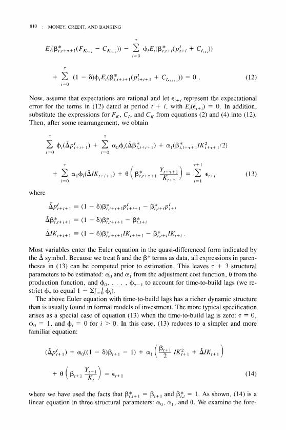
810 MONEY, CREDIT, AND BANKING

Et(t t+T+ I (FK,+T CK,+X)) E XiEt(tst+i(Pt+i + C,,+i)) i-o

+ E (1 -8)+iEt(l3t*t+i+l(pt+i+l + C',+f+,)) ° (12) i=o

Now, assume that expectations are rational and let et+i represent the expectational

error for the terms in (12) dated at period t + i, with Et(et+i) = O. In additionb

substitute the expressions for FK, CI, and CK from equations (2) and (4) into (12).

Then, after some rearrangement, we obtain

E i(Pt+i+l) + E tofi(At,t+i+l) + al(t,t+T+llKt+T+l/2) i=O i=O

E Ct|(>if IK,+;+ I ) f) ( t,t+T+ I K ) E e,+E (] 3)

where

APt+i+, (1 8)t,t+i+ lPt+i+, tot+iPt+i

t*t+i+l-(1-8)t*t+i+l-t*t+i

i\IKt+i+ l-( 1-a)13t*t+i+ lIKt+i+ 1-t*t+iIKt+i

Most variables enter the Euler equation in the quasi-differenced form indicated by

the A symbol. Because we treat 8 and the * terms as data, all expressions in paren-

theses in (13) can be computed prior to estitnation. This leaves X + 3 structural

parameters to be estimated: (xO and (xl from the adjustment cost function, 0 from the

production function, and +0, . . . , XT- l to account for time-to-build lags (we re-

strict XT to equal 1-EiT-o Xi) The above Euler equation with time-to-build lags has a richer dynamic structure

than is usually found in formal models of investment. The more typical specification

arises as a special case of equation (13) when the time-to-build lag is zero: X = O,

+0 = 1, and Xi = O for i > O. In this case, (13) reduces to a simpler and more

familiar equation:

(i\Pt+l) + Cto((l -8)13t+l - 1) + (xl (t2 ' IKt2+l + lSIKt+l )

+ 0 ( t+I K I ) = e+ l (14)

where we have used the facts that t*t+l = t+l and t*t = 1. As shown, (14) is a

linear equation in three structural parameters: (xOv (xl, and 0. We examine the fore-

STEPHEN OLINERs GLENN RUDEBUSCH, AND DANIEL SICHEL : 811

cast performance of both the Euler equation with time-to-build lags [equation (13)] and the simpler version that omits time-to-build [equation (14)].

B. Four Traditional Modets of Investment Several well-known models of investment predate the Euler-equation approach:

The Q model, the accelerator model7 Jorgenson's neoclassical model, and the mod- ified neoclassical model. Each of these models was analyzed in the comparative studies done by Clark (1979) and Bernanke, Bohn, and Reiss (1988). Our specifica- tion of each model is the same as in Clark (1979), except that we scale investment by the capital stock rather than by potential output.

Our traditional Q model takes the form:

N

IKt= dJ + E (sQt-sJ (l5) s-O

where QA is average Q, the ratio of the hrm's market value to the replacement cost of its capital stock. Equation ( 15), although often estimated in the literature, is not a structural model. If we ignore time-to-build lags, the structural Q equation implied by our framework is

IKt=-°t0lal + (l/°tl)(^t-pt) =-(xO/(xl + (1/xl)Qt n (16)

where the second equality replaces marginal Q(At - p') with average Q.7 As can be seen from (16), the structural Q equation from a standard dynamic framework ad- mits no role for lags of QA. These lags have been included by empirical researchers simply to improve the fit of the equation. The structural Q equation that emerges when we take into account time-to-build bears even less resemblance to equation (15) 8 Thus, we regard (15) as a reduced-form equation relating investment to prices in financial markets.

For both the accelerator model and Jorgenson's neoclassical model, the invest- ment equation has the form:

N

It= 4s + 22 (R)s/\ff*-s + aKt-l, (17) s=O

where K* is the firm's desired capital stock. In the accelerator model, the desired capital stock K* is assumed proportional to output Yt, so that /\Kt = 4Z\Yt. If we make this substitution for l\K* in equation (17), scale both sides of (17) by Kt_l, and add the random error ut, we obtain:

7. To derive the first equality in (16), set X = O and 40 = 1 in equation (10) and use (4) to substitute for C,. The second equality follows from Hayashi (1982), who showed that average Q equals marginal Q under constant returns to scale and competitive markets.

8. See Oliner, Rudebusch, and Sichel (1993) for details.

812 : MONEY. CREDIT, AND BANKING,

N

IKt = 8 + + E @ks /_$ + Ut . (18)

Kt- I '5'=° Kt- I

In contrast, Jorgenson's neoclassical model sets the marginal product of capital in a Cobb-Douglas technology equal to its real one-period rental price (c), so that K* = 0(YI(')t, and

N

IKt= 8 + + + E @ A(Y/C)t-s + U (19) t-I s = O t-- I

Finally, the modified neoclassical model, originated by Bischoff (1971), relaxes the symmetric treatment of output and the rental price in the neoclassical model. Bischoff assumed that capital is "putty-clay": Firms can choose the factor propor- tions for each new vintage of capital, but this choice is irreversible once the vintage has been installed. As discussed more fully in Oliner, Rudebusch, and Sichel (1993), the putty-clay assumption implies the following investment equation:

IK, = K + E 0@ls Kst t--9 + @2s ( )las I ] + Ut @ (20)

The @2s coefficients in equation (20) are expected to be negative, while Ct) ,. and the distributed lag coefficients for the other traditional models are expected to be

. .

posltlve.

2. DATA

We estimate equations (13), (14), (15), (18), (19), and (20) with quarterly data for the aggregate private business sector in the United States. These data cover the peri- od 1952:1 to 1992:4. To estimate the traditional models, we require series for gross investment (I), capital stock (K), output (Y), the real user cost of capital (c), and average Q (Q). To estimate the Euler equations, we employ the same constant- dollar series for l, K, and Y, along with series for the real after-tax price of invest- ment goods (p') and the discount factor (A), and an assumed value for the deprecia- tion rate (8). Here, we briefly describe the data, while the appendix in Oliner, Rudebusch, and Sichel (1993) fully documents each series.

Our constant-dollar series for output and gross investment are from the National Income and Product Accounts; because we estimate separate equations for pro- ducers' durable equipment and nonresidential structures, the investment data are disaggregated into these two categories. For each investment series, the correspond- ing capital stock is the annual constant-dollar net stock from the Bureau of Econom- ic Analysis, which we interpolate to a quarterly frequency. To construct the real user cost of capital (c) and the real after-tax purchase price of investment goods (pl), we follow the methodology in the Federal Reserve Board's Quarterly Econometric

STEPL-IEN OLINER CLENN RUDEBUSCH AND DANIEL SICHEL : 8]3

Model. Our measure of average Q is based on the tax-adjusted formulation in Ber- nanke, BohnS and Reiss (1988). The quarterly discount factor for the Euler equa- tions is d = 1/(1 + r), where r is an unweighted average of the real interest rate on three-month Treasury bills and the real return on equity; we use a short-term interest rate to conform with the definition of @ as a discount factor between adjacent quar- ters. Finally, to estimate the Euler equations and to construct the user cost of capital for the traditional modelsS we set the quarterly depreciation rate (8) to 0.03784 for equiprnent and 0.01412 for nonresidential structures, the values employed by Ber- nanke, Bohn, and Reiss (1988).

3. FULL-SAMPLE ESTIMATES OF THE INVESTMENT MODELS

A. The TraditzonaZ Models Table 1 shows full-sample parameter estimates for the traditional investment

models described in section 1. Each equation is estimated by ordinary least squares over the period 1955:2 to 1992:4, with all distributed lags allowed to be twelve quarters in length; we estimate these lags without constraints.9

Except for the Q modelS the coefficients on the distributed lag terms in the equip- ment equations are strongly signiScant and of the expected sign, tracing out a hump- shaped distribution with a modal lag of three to four quarters. In contrast7 in the Q model, the only significant coefficient on the lags of QA is negative, contrary to our expectation. More generally, the Durbin-Watson statistic in each equipment equa- tion is below 0.5, a sign of highly autocorrelated errors. Clearly, these models all fail to capture some persistent determinants of equipment investment.

For nonresidential structures, the performance of the traditional models is even less satisfactory. Although the coefficients in the accelerator and modified neoclassi- cal models have the expected signs, fewer of the lags are significant than was the case for equipment. Moreover, the distributed lags in the neoclassical and Q models are uniformly insignificant, and the Durbin-Watson statistic for each model is even smaller than its counterpart for equiprnent. The structures models may perform rela- tively poorly for a simple reason: Roughly half of the structures aggregate consists of public utilities oil and gas wells, private schools, churches, and hospitals, which have a diverse set of determinants excluded from our models.

B. The Eule^ Eqmations We estimate the Euler equations using the Generalized Method of Moments

(GMM) procedure described by Hansen and Singleton (1982). As with the tradition-

9. Our use of OLS departs from the usual method of estimating the traditional investment models with a correction for AR(1) errors. If these models actually captured the dynamics driving investment, the errors would be white noise and an AR(1) correction would not be needed. The AR(1) correction, there- fore, should be viewed as a "fix-up" for these models, which should be omitted from a fair horserace with the Euler equations. Given our use of OLS, we calculate standard errors by the Newey-West (1987) pro- cedure that is robust to heteroskedasticity and autocorrelation of unknown form.

(panu?luoJ)

(bSI ) bZZ-

(S£I ) ObZ-

(811 ) **9Z£-

(OZI ) **81£-

(SlI ) **16Z -

(ZlI )

.

**666 -

(Ll1 ) **99Z -

(9bl ) LSZ-

(011 ) Ibl -

(Z91 ) OZO -

(OSI ) (861 ) 81Z 60£

(ZZI ) (691 ) 5ZZ S9Z'

(101') (bSI ) **SZ£ **16b (Lll ) (L81 )

**£1£ **bZ9 (911 ) (Z61 )

**8LZ **££9 (SOI ) (S81 )

**80Z' **LZS (bll ) (OIZ )

**9LZ **S£L (6£1) (SbZ) 6SZ **£b9

(ZOI ) (Z61') 6£1' **SIS'

(££1') (IOZ') 6ZO'- 990'-

(O'S61) (b'£6) **Z'809 **Z'S8S-

(S9Z') (ZSZ') **S6'1 *00'£

SHN HAd le!sselDoaN P3!J!P°MI

£60' 00£ lOb £ZL (9L £) (Sb £ SZ S **ZI £

(S6 Z) (b£ z L8£ *8101

(b6 Z) (bl £ £b£ **II L

(8£ £) (9L' SS'b **LO'9

(80'£) (6£'Z **b8'L **ZI'Z

(Sl'£) (IS'Z **L6'9 **ZI't

(86'Z) (Z6'1 **L9'L **II'S

(Z6'Z) (Z6'1 8£'S **bb'£

(LL'Z) (b9'Z **Z£'9 **IL'L

(01'£) (bZ Z L6'£ **L6'S

(86'Z) (bO'Z ZL'I **L6'0

(£9'b) (£L'Z - 1£'£- 69' 8) (£'L8). (1'6 Z£- **S'16£ **b'L

(£ZI') (ZLO') **£9'1 **bO'b b

g SHN Hdt

(zoz-) 61S -

(bLI ) b5Z -

(8LI ) **bZS - (S81 )

**619 - (60Z-)

**L19 - (S81 )

**99S - (IfZ )

**6L9 - (ICZ )

**S99 - (OIZ )

**81b - (ILZ ) 080

6-%

S-%

L - JAA

(9 - iM

i_%

t_,

f_%

z AA

I -XX

JAA

solqelleA

6-'x

8 -X

L - JX

9 'X

S-}X

b-xX

X

Z X

I X

'X

l -X/ l

XUP}SUOD

salqetJ8A

a ZX

11 X

01 -}X

6-'x

8 -X

L - XX

9 'X

X

X

£ - XX

Z X

I X

'X

I -'/1

XUBlSUOD

salqelJ8A

SXN HAd

leo!ssel3°2bl P2!SIP°N

190 bf l ZbO 111 (£01 ) (bOZ S61- ZSO-

(6LO ) (SS I LZO 660

(9LO ) (9b1 100- 9£0

(LLO ) (ISI 6f0 IZO-

(990 ) (091 £ZO- 8f0

(b90 ) (OSI 090 CZO-

(b90 ) (Z91 090 bOO

(b90 ) (6SI £bO 88 1

(690 ) (CLI 111 60Z

(090 ) (981 1 60 L6Z

(OLO ) (LIZ LOO- 91Z

(601 ) (SbZ ZZI- *69

6LO 81Z

(8ZO ) 900 -

(6ZO ) SOO

(6ZO ) 110

(ZfO ) 600

(8ZO ) TOO

(8ZO ) 500 -

(LZO ) f00

(LZO ) f00

(0f0 ) S10 -

(8ZO ) bSO-

(6ZO ) 6f0 -

(ZVO ) 8bO-

(6 9f1) **l SLb

(bOI ) **ZL I

SHN

bOZ 9Sb'

(LLO **6bZ'

(090 **f61 '

(990 **OIZ'

(ILO') **961 '

(Z90 _F, _7 '

**G /G

(b90 ' ) **b5Z '

(Z80') **9LZ'

(iLO ) **f6Z'

(9LO ' ) **SbZ'

(690') **061 '

(690') OLO'

(b90 ' ) 890' -

(Z'S' **8 Z

(101 ) **81 b

gad

£)

£1 Z)

11

£) L Z)

9

Z)

Zl Z)

bl I)

Sl I)

£1 Z)

Ll Z)

1

)

1

)

5L) L6b-

Id

(ILO ) **96 1

SXN

(Zl1 ) **16 f

Had

8;5!sselDo3N JO}BJ2t333

SrIAaOW lNNlS]ANI rlYNOIllaVMX AH1 0 SGlYWllSg SiO

I H1SVA

STEPHEN OLINER, GLENN RUDEBUSCH, AND DANIEL SICHEL : 815

TABLE 1 (Continued) Modified Neoclassical Modified Neoclassical

Variables PDE NRS Variables PDE NRS

X,_ lO 559** .245 W,_ lO - .545** - .269 (.168) (.131) (.190) (.140)

xt- l l .532** .256 W,_ l l - .508** - .185 (.243) (.173) (.188) (.144)

R2 .815 .480 DW .436 .174

NOTES: All models were estimated over 1955:2-1992:4, with ltlKt_, as the dependent variable. To reduce the number of leading zeroes, all reported coefficients and standard errors have been multiplied by 100. The standard elTors were calculated with the Newey-West (1987) colTection for heteroskedasticity and autocolTelation and are in parentheses.

AY,_jlK,_, for accelerator model A(Ylc),_jlK,_l for neoclassical model

t i ^ ( I l c)t_ j_ l Yt_ jlKt_, for modified neoclassical model QA i for Q model.

For the modified neoclassical model, Wt_j-(Ylc) _ _tIK _ PDE = Producers' durable equipment. NRS = Nonresidential structures. DW = Durbin-Watson statistic. ** = significant at the 5 percent level.

al models, we use the Newey-West (1987) method to obtain a covariance matrix for the GMM parameter estimates that is robust to heteroskedasticity and serial correlation.

For GMM to yield consistent parameter estimates, the instruments must be uncor- related with the error term, e. If the error term were purely an expectational error, rational expectations implies that any variable in the firm's information set during period t would be uncorrelated with Et+i (i = 1, . . ., T). In this case, all variables dated t-1 and earlier would be valid instruments, as would endogenous variables chosen in period t. We take a more conservative stance, restricting our instruments to variables dated t-2 and earlier. This decision reflects our concern about the potential for measurement error among the variables in the Euler equations.l° Be- cause our Euler equations include variables dated as early as t-1 (lKt-ltlSt l), et - l could well include the error component of t- 1 dated variables. If so, any endogenous variable would have to be dated t-2 or earlier to be a valid instrument. Accordingly, the instrument set for the basic Euler equation includes a constant and the second and third lags of pl, IKt, IKt2, YtlSt_ 1, and [3tS while the instrument set for the Euler equation with time-to-build also includes the fourth and fifth lags of these variables. l l

10. In particular, measurement error almost certainly afflicts the price series p' given the problem of measuring quality change in capital goods. This error then contaminates the series for real investment and capital stock that BEA constructs from p'.

11. As a test of robustness, we also estimated the Euler equations with an instrument set that included the first lag of each instrument. The results were not materially different from those reported below. We should note that the exclusion of instruments dated t-1 will not ensure consistent estimates if the mea- surement errors are autocorrelated. In that case, all lagged endogenous variables will be correlated with the Euler equation's error term. Implicitly, we are assuming that any measurement errors are not strongly autocorrelated .

816 : MONEY CREDIT, AND BANKING

TABLE 2

GMM ESTIMATES OF INVESTMENT EUL.ER EQUAT10NS

ERqzlipment Structurcs Basic Model Titue-to-Build Basic Model Tinie-to-Build Parameteis ( I ) (2) (3) (4)

_ .

.

Ptoductios] fUElUtiOEl 0 .020 .021 - .193S S - .151 *X

( .017) ( .015) ( .048) ( .033) Adjustment costs (XO -.962 ! 4' -1.006 u -4.235 BE -3.537S *

(.185) (.163) (.822) (.558) (Xl I .590 3.965 B B - 18.334** -20.735X u

(1.469) ( I .560) (8.926) (05.353) Time-to-bllild

¢() .278 d $' .174* * (.090) (.040)

+ I .066 .242** (.092) ( .044) ¢D2 . 3034' B .27084' (.114) (.052)

¢3 .353>"S' .315*4' ( 094) (.059)

J Statistic 10.33 15.84 7.78 11.46 p-value .24 .39 .46 .72 NOIES: Basic model was esthilated over 1955:2-1992:3. while the time-to-build model was estimated over 1955:2-1')91:4. The standard CrTors are in parentheses and were calculated with the Newey-West ( 1987) colTection for heteroskedasticity and autocol-relation. Estimation of the time-to-build model was done subject to thc restl-iction that ¢() + +1 + ¢, X ¢, = 1. 8 -- significalit at the 5 percent Ievel.

To estimate the time-to-build equation, we must specify T, the length of time be- tween project starts and completions. The previous estimates of structural time-to- build models with quarterly data, Park (1984) and Altug (1989), set T to be three and four quarters, respectively. These values of T likely are appropriate for equipment investment, but are too small to encompass some construction projects. However, with a time-to-build lag much longer than four quarters, the large number of free parameters (the Xs) probably cannot be estimated with any precision. Therefore, we opted to follow the earlier work and set T = 3, which allows the investment project to be spread over four quarters. We estimate (+0, Xl, 42, ¢3), restricting the Xis to sum to one.

The basic Euler equation without time-to-build is estimated from 1955:2 to 1992:3 (the final period in the sample, 1992:4, provides data for the variables dated t + 1). Similarly, the Euler equation with time-to-build is estimated from 1955:2 to 1991:4. The estimates for both equations are shown in Table 2. As can be seen in column 1, the signs of 0 and (xl in the basic model for equipment are positive, con- sistent with our expectation. However, neither coefficient is significantly different from zero, and 0 is quite small given its interpretation in our model as the share of income accruing to equipment. In addition, the omission of time-to-build from the basic equation appears inconsistent with the data. As shown by the estimates for the time-to-build model in column 2, ¢0 = 0.278, indicating that only 27.8 percent of equipment spending occurs during the quarter of the project start; the bulk of invest- ment is estimated to take place two and three quarters after the start. Thus, the Euler

STEPHEN OLINER. GLENN RUDEBUSCH, AND DANIEL SICHEL : 817

equation with time-to-build captures the dynamics of equipment investment better than does the basic equation. Moreover, the addition of time-to-build increases ctl by enough to make that coefficient significantly greater than zero. Still, the time-to- build model does not alleviate all the problems with the basic equation, as 0 is still very low.

The results for the Euler equations for structures are worse than those for equip- ment, paralleling our results for the traditional models. As shown in columns 3 and 4, 0 and (xl are significantly negative for both Euler equations, violating our theoret- ical priors. Given these nonsensical parameter estimates, the time-to-build model for structures cannot be viewed as a success, even though the s are uniformly posi- tive and significant.

Despite the problems with the Euler equation estimates, the only specification test typically reported for Euler equations the J statistic does not reject any of the models at even the 20 percent level. 12 This result illustrates the weakness of the J statistic as an overall test of model specification. Further evidence of the inadequacy of the J statistic can be found in Oliner, Rudebusch, and Sichel (1995), where we show that the estimated parameters of an investment Euler equation appear to be unstable even though the J statistic fails to reject the model.

4. OUT-OF-SAMPLE PERFORMANCE OF THE INVESTMENT MODELS

A. Geslerating Out-of-Sample Forecasts For each traditional model, the forecast of IKt+ t is ztZt+ l, where zt denotes the

vector of OLS parameter estimates based on data through period t and Zt + l denotes the vector of actual values for the explanatory variables in period t + 1. We generate a sequence of these one-step-ahead forecasts by extending the sample one period at a time and recalculating YtZt+l for each sample. These forecasts are "out-of- sample" in that all coefficients are estimated from data prior to the forecast date. The forecasts, however, are "ex post" because they use the actual values of the explana- tory variables at time t + 1 in the forecast of investment at time t + 1. In real-time forecasting, such values are not available and must be replaced by projections. We analyze ex post forecasts because our interest centers on the adequacy of the invest- ment equations themselves, not the ease of forecasting the explanatory variables. 13

We apply an analogous procedure to the Euler equations to generate one-step- ahead, ex post forecasts of IK. The specifics of our procedure can be described most easily for the basic Euler equation that omits time-to-build Lequation (14)]. First,

12. The J statistic tests the null hypothesis that the instruments are orthogonal to the error term, as required for consistent estimation. This statistic equals the number of observations multiplied by the min- imized value of the objective function used in GMM estimation. It is asymptotically distributed X2(df) with df equal to the number of instruments minus the number of parameters.

13. However, we did compute ex ante forecasts from the traditional models using univariate auto- regressions to generate one-step-ahead forecasts for the explanatory variables. The ex ante forecast errors were almost the same as the ex post errors, as one might expect given the generally small coefficients reported in Table 1 for the contemporaneous explanatory variables.

818 : MONEY, CREDIT, AND BANKING

equation (14) is estimated by GMM using data through period t. Next, we solve the Euler equation for IKt+l. Given the parameter estimates (&0 &1, 0), the assumed value for 8, and the actual values for all variables in the equation other than IKt+ 1, equation ( 14) defines a quadratic equation in IKt+ 1:

( & 1 t+ 1 ) IKt2+ 1 + (& 1 ( 1 -8)t+ 1 )IKt+ 1 + Wt+ 1 ° (21 )

Where wt+l = (5pzt+l) + &0((l-8)t+l- t)-&lKt + 0 (t+ K ) and we have set the expectational error >,+ 1 to zero. Solving equation (21 ) yields

IKt+ 1 =-( 1-b) + (( 1-b)2-2 Wt+ 1 /(& 1 t+ 1 )) 1/2 ' (22)

as the forecasting equation for IKt+ 1 . We use the positive branch of equation (22). By extending the sample one period at a time and then repeating this procedure, we obtain the desired sequence of one-step-ahead, ex post forecasts.

The same method yields a forecasting rule for the Euler equation with time-to- build, equation (13). Given GMM estimates of a0, al17 0, and the Xs, equation (13) can be written as a quadratic in IKt+T+ 1:

(&lit2+T+ 1 ) IKt2+T+ 1 + (&14T(l-b)13t*,+T+ 1 )IK,+T+ 1 + Wt+r+ 1 = O, (23)

where Wt+T+1 = E i(APt+i+ 1) + &o E i(5tt+i+1) + 0 (tt+T+1 K ) =o i=o t+T

T-1

+ &1 E Xi(AIKt+i+ 1 )-&l+Tt*,+IK,+ . i=o

To make the time subscripts consistent with those in the basic Euler equation, we lag each term in equation (23) by X periods and then solve (23) for IKt+ 1:

IK,+1 = -+T(1 -b) + (+2(1 -a)2-2W,+l/(&l* ,+l))l'2 . (24)

The positive branch of equation (24) generates our ex post forecast of IKt+ 1 for the time-to-build model, based on the actual values for the right-hand side variables and GMM estimates of the parameters computed with data through period t. 14

14. Equations (22) and (24) are nonlinear functions of estimated parameters. Following Kennedy (1983), we also computed forecasts from equation (22) with a correction for the possible bias from this nonlinearity. The correction made virtually no difference and is not used below. We tried one other sensi- tivity test for the Euler equation forecasts from equation (22). Rather than using the actual values for right-hand-side variables dated at period t + 1, we used the projections of these variables on our instru- ment set. Strictly speaking, this procedure is more congruent with the rational expectations assumption built into the Euler equations. However, the use of projections rather than actual period t + 1 values had no material effect on the Euler equation forecasts.

STEPHEN OLINER, GLENN RUDEBUSCH, AND DANIEL SICHEL : 819

TABLE 3

SUMMARY STATISTICS FOR EQUIPMENT FORECAST ERRORS

100*(Forecast Error) Regressed on a Constant

Model 100*RMSE Bias DW N

Accelerator .228 - .022 .234 116 (.51)

Neoclassical .336 .045 .233 116 (.73)

Modified Neoclassical .227 - .105** .431 116 (2.92)

Q .396 - .231** .137 116 (3.75)

Basic Euler Equation 9.720 -.078 2.431 116 (.13)

Time-to-Build Euler Eqn. 1 2.224 .376 .676 113 (1.18)

NOTES: As described in the text, errors are calculated from rolling, one-quarter-ahead forecasts for 1964;1 to 1992:4. All forecasts are out- of-sample, ex post forecasts. Absolute value of t statistics are in parentheses and are calculated from Newey-West (1987) standard errors. 1. Excludes forecasts for three periods for which the model failed to generate a real-valued solution. RMSE = Root mean square elTor. DW = Durbin-Watson statistic. N = Number of forecast elTors. ** significant at the S percent level.

B. Out-of-Sample Forecast Errors

Table 3 summarizes the out-of-sample forecast performance of the equipment

models over the period 1964:1 through 1992:4. The first column shows the root

mean squared error (RMSE) of the one-step-ahead forecasts, multiplied by 100 to

remove leading zeroes. The next two columns present statistics derived from a re-

gression of the forecast errors on a constant. Column 2 shows the estimated coeffi-

cient from this regression, which equals the mean forecast error, a measure of the

forecast's bias. The Durbin-Watson statistic from the regression, shown in the third

column, characterizes the extent of first-order autocorrelation in the forecast errors.

Column 1 shows that both Euler equations produce far less accurate forecasts of

equipment investment than do the traditional models. The RMSE of the basic Euler

equation is roughly twenty-five times larger than that of the worst traditional model,

the Q equation. The addition of time-to-build lags markedly improves the forecast

performance of the Euler equation, but the RMSE of the time-to-build equation is

still well above those of the traditional models. The RMSEs of the traditional mod-

els as a group lie in a fairly narrow range, with the accelerator and modified neo-

classical models at the low end.

The relatively small RMSEs of the traditional models should not be interpreted as

an endorsement of their forecasting ability. The low Durbin-Watson (DW) statistics

indicate that the traditional models all make persistent forecast errors. Moreover,

the forecasts from the modified neoclassical and Q models have a significant down-

ward bias. The traditional models look good only relative to the performance of the

Euler equations.

Table 4 documents the forecast performance of the structures models. As in Table

3, the RMSEs for both Euler equations are many times larger than those of the tradi-

820 : MONEY, CREDIT, AND BANKING

TABLE 4

SUMMARY STATISTICS FOR STRUCTURES FORECAST ERRORS

100-8(Forecast Error) Regressed on a Constant

Model 100*RMSE Bias DW N

Accelerator . 2 13 .039 . OS 1 1 16 (.94)

Neoclassical .24 1 .077 .079 116 (1 .73)

Modified Neoclassical .205 .008 . 1 17 1 16 (.21)

Q .258 .067 .065 1 16 ( 1 .37)

Basic Euler Equation 8.735 .525 2.331 1 16 (.72)

Tirne-to-Build Eultr Eqn. 1 7.244 1.161 .871 1 12 ( I .78)

NOTES: See Table 3.

1. Excludes forecasts for four periods for which the Illodel failed to generate a real-valued solution. RMSE = Root mean s4uare error. DW = Durbin-Watson statistic. N= Number of forecast elTors.

tional models. However, in contrast to the results for equipment, the inclusion of time-to-build lags does not greatly reduce the RMSE of the Euler equation. Another difference from Table 3 is the absence of bias in the forecasts from the traditional models. Still, the forecast errors from these models are highly autocorrelated, with the largest DW statistic at 0.117, suggesting the omission of important explanatory variables.

C. Pairwise Forecast Comparisons The inability of the Euler equations to forecast out of sample also is evident in

pairwise model comparisons. These comparisons are made, following Fair and Shil- ler (1990), in regressions of the form

IKt+ l-IKt = a + QE(IKfE t+l-IKt) + QT(IKfrt+l-IKt) + ut (25)

where IKfE t+ I and IKfT t+ I are the one-step-ahead forecasts of IKt+ l from an Euler equation and a traditional model. Equation (25) regresses the actual change in IK on the predicted change from the two models. If QE = O, the forecasts from the Euler equation contain no predictive information beyond that in the constant or the tradi- tional model. Conversely, if QT = O, the forecasts from the traditional model con- tain no relevant information beyond that in the constant or the Euler equation. If neither model can predict changes in IK, the estimates of both QE and QT should be zero; if both models have predictive power, both QE and QT should be nonzero.

Table 5 displays the pairwise forecast comparisons for the models of equipment investment. The estimates of QE and QT appear in the first two columns, along with t statistics calculated from Newey-West standard errors. The top part of the table

STEPHEN OLINER, GLENN RUDEBUSCH, AND DANIEL SICHEL : 821

TABLE 5

FAIR_SHII LER REGRESSIONS FOR EQUIPMENT

SlE S27 Traditional Model R2 N

Basic Euler Equcltion 1. - .0006 .187* * AcceleratOr . 132 116

(.74) (2.64) 2. - .0007 .068 Neoclassical .021 116

(.94) (1.49) 3. - .0004 .233** Modified Neoclassical .175 116

(.62) (3.64) 4. -*0007 .069 Q .019 116

(.88) (1.45) Tiwze-to-Build Eules Equation 5. .011 *t .200** Accelerator . 170 113

(4.04) (2.80) 6. .009** .065 Neoclassical 037 113

(3.03) (1.40) 7. .009** .235** Modified Neoclassical .200 113

(3.77) (3.69) 8. .0088* .073 Q .043 113

(2.37) (1.48) NO1ES: Each row reports the OLS estimate.s of Qr and QT from the regression

IK, - IK,_l = a + QE (IK/E,-IK,_|) + S1T (IKfT,-IK,_|) + U,,

estimated over 1964:1- I992:4. IK/F, and IKfT, are the one-step-ahead forecasts of IK, from an Euler equation and a traditional model respectively. Absolute values of t statistics are in parentheses and are calculated from Newey-West (1987) standard errors.

** = significant at the 5 percent level.

compares the basic Euler equation to the traditional models. As shown, the esti- mates of QE are uniformly insignificant. That is, forecasts from the basic Euler equation have no significant information over and above that provided by the tradi- tional models. In contrast, two of the traditional models the accelerator and the modified neoclassical models- do have information not conveyed by the Euler equation. However, the relatively low values for R2 caution against relying too heavily on any of the models.

The bottom part of Table S compares the Euler equation with time-to-build lags to the traditional models. The accelerator and the modified neoclassical models pro- vide information not in the time-to-build Euler equation, similar to the results in the top panel. However, QE is now statistically significant in the comparison with each traditional model. Apparently, the addition of time-to-build lags yields an Euler equation forecast with information not found in the traditional models. Nonetheless, we do not interpret this result as particularly favorable to the Euler equation. First, QE is estimated to be extremely small, suggesting that the Euler equation should get little weight when pooled with the traditional models. Second, despite the signifi- cance of QE, the predictive power of the Euler equation is extremely limited. If we omit the traditional model from the Fair-Shiller regression, the R2 drops to 0.013. Thus, the Euler equation with time-to-build lags explains only 1.3 percent of the variation in IKt I-IKf over the full sample.

Table 6 presents the analogous pairwise comparisons for the models of structures investment. As can be seen, none of the structures models can predict changes in

822 : MONEY, CREDIT, AND BANKING

TABLE 6

FAIR-SHILLER REGRESSIONS FOR STRUCTURES

QE QT

Basic Euler Equation 1. - .0009 .022

(1.62) (.65) 2. - .001 - .0004

(1.52) (.01) 3. - .0009 .013

(1.59) (.42) 4. - .001 - .012

(1.46) (.50) Time-to-Build Euler Equation 5. .0009 .047

(1.61) (1.30) 6. .0007 .009

(1.41) (.28) 7. .0009 .036

(1.53) (1.08) 8. .0007 - .005

(1.35) (.17)

Traditional Model N

Accelerator

Neoclassical

Modified Neoclassical

.010 116

.004 1 16

.006 1 16

Q .007 1 16

Accelerator

Neoclassical .016

112

-.009 1 12

Modified Neoclassical .OO5 1 12

Q - oo9 112

NOTES: See Table 5.

IK. The estimates Of QE and QT are uniformly insignificant at the 5 percent level. Moreover, the values of R2 cluster around zero, with the largest value being only 0.016.

5. WHY DO THE EULER EQUATIONS PERFORM SO BADLY?

Several factors could account for the Euler equations' inaccurate forecasts of in- vestment spending. One possibility is that the GMM estimator has poor finite- sample properties [see West and Wilcox (1994) and Fuhrer, Moore, and Schuh (1995) for discussions of this problem in the context of inventory models]. Another possible shortcoming is the use of aggregate data to estimate Euler equations that apply at the firm level. In this section, however, we argue that the Euler equations may well forecast poorly because they impose an invalid dynamic structure on the data.

Consider equation (22), which generates the forecasts of IKt+ 1 for the basic Euler equation, expressed (after some algebra) in the form:

IKt+1 = -(1 -8) + L (1 -a)2 + 2 ( IKt _ MPKt-Ct) ] 1/2 (26)

where MPKt = HYt+l/Kt is the marginal product of capital, and ct represents the discrete-time version of Jorgenson's user cost of capital. 15 Equation (26) shows that the forecast of IKt+l depends on its own value in period t and on the difference between the marginal product and the cost of capital. The relative importance of

15. Specifically, ct = (Pt/ + (xO)(rt+ + 8) - (1 - 8)(PIt+l - Pt')

STEPHEN OLINER, GLENN RUDEBUSCH, AND DANIEL SICHEL : 823

each factor reflects the magnitude of marginal adjustment costs, (xl. If (xl is large, then adjusting the rate of investment is quite costlyS and 1Kt+ l will deviate relatively little from IKt, regardless of the difference between MPKt and ct. In contrast, as (xl approaches zero, MPKt-Ct becomes the dominant influence on IKt+ 1 Intuitively, when marginal adjustment costs are very small, the firm quickly adjusts the capital stock to arbitrage away differences between the marginal product of capital and the user cost. 16 Accordingly, the Euler equation will forecast IKt+ l to deviate sharply from IKt whenever (MPKt-ct)/xl is large. Given the smoothness of the actual data for IK, the forecasts in such cases will be inaccurate.

The previous section showed that adding time-to-build lags does not remedy the problems with the basic Euler equation, and equation (26) provides the key for un- derstanding this result. In particular, the version of equation (26) for the time-to- build model would replace IKt and MPKt-ct with four-quarter moving averages of these variables that run from period t-3 to period t. Thus, whenever a 1 is small or a wide gap exists between MPK and c for several quarters, the time-to-build model vvlll forecast big changes in investment. In 1986, for example, the time-to-build model for equipment produced terrible forecasts. The collapse in oil prices that year sharply reduced the price deflator for aggregate output relative to the deflator for equipment alone, driving up real equipment prices (p'). The resulting capital gain for owners of equipment lowered the user cost, Ct, relative to MPKt. Accordingly, the time-to-build Euler equation expected equipment outlays to be accelerated in order to take advantage of the low user cost, implying a dramatic decline in IKt+ l from its level in period t. In reality, no such intertemporal shift occurred.

As a general matter, the actual series for IK does not display the high degree of time shifting expected by either Euler equation in response to changes in relative prices and interest rates. This problem could well reflect some unrealistic assump- tions that underlie both Euler equations. First, the equations embed the "putty- putty" technology of the original neoclassical model. That is, the Euler equations do not distinguish between already-installed capital and capital still to be purchased. These equations expect the capital-output ratio for the entire installed capital stock to adjust to a change in relative prices or interest rates. Such an adjustment, even if done slowly, could induce a large shift in investment outlays. In contrast, a putty- clay model would not allow firms to alter the capital intensity of their existing pro- duction facilities.

In addition, the Euler equations assume that investment is fully reversible. Under the more reasonable assumption of irreversibility, Pindyck (1991) and others have shown that investment spending will adjust sluggishly to price changes that generate increased uncertainty about the economic environment.

Finally, the maintained assumption of convex adjustment costs-which generates the investment dynamics in our Euler equations may be unfounded. Although

16. Note that IKt+ l is negcztilely related to MPKt-ct. That is MPKt > ct implies a low value of IKt+ 0 relative to IK. The intuition is simply that the firm shifts investment from period t + 1 to period t to capture the profits from the high marginal product of capital.

824 MONEYz CREDIT, AND BANKING

convex adjustment costs are a convenient assumption, the case for convexity is weak, especially when the adjustments costs are internal to the firm. Convexity im- plies that the installation of new capital goods should be progressively less costly when dragged out over longer and longer periods. There is no inherent reason why this should be so, a point made originally by Rothschild (1971) and forcefully res- tated by Nlckell (1978), but ignored in most empirical models of investment.

6. CONCLUSION

This paper extends earlier "horse race" comparisons of empirical investment models by adding two Euler equations to the usual stable of traditional but largely nonstructural models and by focusing on out-of-sample performance. The basic Euler equation used in the comparisons is a "canonical" Euler equation representa- tive of those found in the applied investment literature. In addition, we use a richer Euler equation with time-to-build lags. Our results indicate that the forecast perfor- mance of both Euler equations is substantially worse than that of the traditional models. Although the time-to-build equation performs slightly better than the basic Euler equation, both Euler equations produce forecasts of investment spending that are much too volatile. Our results have the following implications. First, and most important, the inabil- ity of the Euler equations to forecast investment spending even one quarter ahead suggests that these models are misspecified. 17 Investment Euler equations based on simple adjustment cost functions have become a fixture in applied work, but re- searchers should not assume that these equations are valid structural models. We argued that better models of investment might be provided by Euler equations that embed irreversibility or a putty-clay technology, in order to produce more sluggish

.

. .

adJustments ln lnvestment. Second, none of the models we evaluated could forecast investment in nonresi- dential structures. This aggregate has a very diverse set of components, and no sin- gle model is likely to capture the determinants for all these types of structures. It would be interesting to know whether the traditional models or Euler equations can forecast investment for a single component of the aggregate, such as industrial or commercial buildings.

LITERATURE CITED

Abel, Andrew B. "Empirical Investment Equations: An Integrative Framework." In On the State of Macroeconomics, edited by Karl Brunner and Allan H. Meltzer, pp. 39-91. Carnegie-Rochester Conference Series on Public Policy 12, Spring 1980. Altug, Sumru. "Time-to-Build and Aggregate Fluctuations: Some New Evidence." Interna- tional Economic Review 30 (November 1989), 889-920. 17. See Oliner, Rudebusch, and Sichel ( 1995) for further evidence of misspecification. In that paper, we formally test for parameter constancy in an investment Euler equation similar to those estimated here. We find significant evidence of instability in each parameter.

STEPHEN OLINER, GLENN RUDEBUSCH, AND DANIEL SICHEL : 825

. "Time-to-Build, Delivery Lags, and the Equilibrium Pricing of Capital Goods." Journal of Money, Credit, and Banking 25 (August 1993, Part 1), 301-19.

Bernanke, Ben, Henning Bohn, and Peter C. Reiss. "Alternative Non-Nested Specification Tests of Time-Series Investment Models." Journal of Econometrics 37 (March 1988), 293- 326.

Bischoff, Charles W. "The Effect of Alternative Lag Distributions." In Tax Incentives and Capital Spending, edited by Gary Fromm, pp. 61-130. Washington, D.C.: Brookings In- stitution, 1971.

Carpenter, Robert E. "An Empirical Investigation of the Financial Hierarchy Hypothesis: Ev- idence from Panel Data.^' Washington University Working Paper Series, no. 164, 1992.

Chirinko, Robert S., and Fabio Schiantarelli. "Delivery Lags, Adjustment Costs, and Econo- metric Investment Models." New York University, C.V. Starr Center for Applied Econom- ics, Research Report no. 91-41, August 1991.

Clark, Peter K. "Investment in the 1970s: Theory, Performance, and Prediction." Brookings Papers on Economic Activity ( 1979: 1), 73- 113.

Elliott, J. W. "Theories of Corporate Investment Behavior Revisited." American Economic Review 63 (March 1973), 195-207.

Fair, Ray C., and Robert J. Shiller. "Comparing Information in Forecasts from Econometric Models." American Economic Review 80 (June 1990), 375-89.

Fuhrer, Jeffrey, George Moore, and Scott Schuh. "Estimating the Linear-Quadratic Inventory Model: Maximum Likelihood versus Generalized Method of Moments." Journal of Mone- tary Economics 35 (February 1995), 115-58.

Gertler, Mark, R. Glenn Hubbard, and Anil K. Kashyap. "Interest Rate Spreads, Credit Con- straints, and Investment Fluctuations: An Empirical Investigation." In Financial Markets and Financial Crises, edited by R. Glenn Hubbard, pp. 11-31. Chicago: University of Chicago Press, 1991.

Gilchrist, Simon. "An Empirical Analysis of Corporate Investment and Financing Hier- archies Using Firm Level Panel Data." Mimeo, 1990.

Hansen, Lars P., and Kenneth J. Singleton. "Generalized Instrumental Variables Estimation of Nonlinear Rational Expectations Models." Econometrica 50 (September 1982), 1269- 86.

Hayashi, Fumio. "Tobin's Marginal q and Average q: A Neoclassical Interpretation." Econo- metrica 50 ( January 1982), 213-24.

Hendry, D. F. "Predictive Failure and Econometric Modelling in Macroeconomics: The Transactions Demand for Money." In Economic Modelling, edited by P. Ormerod, pp. 217-42. London: Heimann Education Books, 1979.

Hubbard, R. Glenn, and Anil K. Kashyap. "Internal Net Worth and the Investment Process: An Application to U.S. Agriculture." Journal of Political Economy 100 (June 1992), 506- 34.

Jorgenson, Dale W., Jerald Hunter, and M. Ishaq Nadiri. "A Comparison of Alternative Econometric Models of Quarterly Investment Behavior." Econometrica 38 (March 1970), 187-212 (a).

. "The Predictive Performance of Econometric Models of Quarterly Investment Be- havior." Econometrica 38 (March 1970), 213-24 (b).

Jorgenson, Dale W., and Calvin D. Siebert. "A Comparison of Alternative Theories of Cor- porate Investment Behavior. " American Economic Keview 58 (September 1968), 681 -712.

Kennedy, Peter E. "Logarithmic Dependent Variables and Prediction Bias." Oxford Bulletin of Economics and Statistics 45 (1983), 389-92.

Kopcke, Richard W. "The Determinants of Investment Spending." New England Economic Review ( July/August 1985), 19-35.

826 : MONEY, CREDIT, AND BANKING

. "The Determinants of Business Investment: Has Capital Spending Been Surprisingly Low?" New England Economic Review ( January/February 1993), 3-31.

Kydland, Finn E., and Edward C. Prescott. "Time to Build and Aggregate Fluctuations." Econometrica 50 (November 1982), 1345-70.

Newey, Whitney K., and Kenneth West. "A Simple, Positive Semi-Definite, Hetero- skedasticity and Autocorrelation Consistent Covariance Matrix." Econometrica 55 (May 1987), 703-8.

Nickell, S . J. The Investment Decisions of Firms. Welwyn, England: James Nisbet and Com- pany, Ltd. and Cambridge University Press, 1978.

Ng, Serena, and Huntley Schaller. "The Risky Spread, Investment, and Monetary Policy Transmission: Evidence on the Role of Asymmetric Information." Carleton University, Economics Papers no. 93-07, 1993.

Oliner, Stephen, Glenn Rudebusch, and Daniel Sichel. "New and Old Models of Business Investment: A Comparison of Forecasting Performance." Economic Activity Section Working Paper no. 141, Board of Governors of the Federal Reserve System, 1993.

. "The Lucas Critique Revisited: Assessing the Stability of Empirical Euler Equations for Investment." forthcoming in Journal of Econometrics, 1995.

Park, Jong Ahn. "Gestation Lags with Variable Plans: An Empirical Study of Aggregate In- vestment." Ph.D. dissertation, Carnegie-Mellon University, Graduate School of Industrial Administration, 1984.

Pindyck, Robert S . "Irreversibility, Uncertainty, and Investment." Journal of Economic Liter- ature 29 (September 1991), 1110-48.

Pindyck, Robert S., and Julio Rotemberg. "Dynamic Factor Demands under Rational Expec- tations." Scandinavian Journal of Economics 85, no. 2 (1983), 223-38.

Rossi, Peter E. "Comparison of Dynamic Factor Demand Models." In Dynamic Econometric Modeling, edited by William A. Barnett, Ernst R. Berndt, and Halbert White, pp. 357-76. Cambridge, England: Cambridge University Press, 1988.

Rothschild, Michael. "On the Cost of Adjustment." Quarterly Journal of Economics 85 (November 1971), 605-22.

Shapiro, Matthew D. "The Dynamic Demand for Capital and Labor." Quarterly Journal of Economics 103 (August 1986), 513-42 (a).

. "Capital Utilization and Capital Accumulation: Theory and Evidence." Journal of Applied Econometrics 1 (1986), 211 -34 (b).

Taylor, John B. "The Swedish Investment Funds System as a Stabilization Policy Rule." Brookings Papers on Economic Activity ( 1982.1), 57-99.

West, Kenneth D., and David W. Wilcox. "Some Evidence on Finite Sample Distributions of Instrumental Variables Estimators of the Linear Quadratic Inventory Model." In Inventory Cycles and Monetary Policy, edited by Ricardo Fiorito, pp. 253-82. New York: Springer- Verlag, 1994.

Whited, Toni. "Debt, Liquidity Constraints, and Corporate Investment: Evidence from Panel Data." Journal of Finance 47 (September 1992), 1425-60.