Neuronal spatiotemporal pattern discrimination: The dynamical evolution of seizures

www.elsevier.com/locate/ynimg

NeuroImage 28 (2005) 1043 – 1055

Neuronal spatiotemporal pattern discrimination: The dynamical

evolution of seizures

Steven J. Schiff,a,* Tim Sauer,b Rohit Kumar,c and Steven L. Weinstein d

aKrasnow Institute, Program in Neuroscience and Department of Psychology, George Mason University, MSN 2A1,

Fairfax, VA 22030, USAbDepartment of Mathematics, George Mason University, Fairfax, VA 22030, USAcThomas Jefferson High School for Science and Technology, Fairfax, VA 22312, USAdDepartment of Neurology, Children’s National Medical Center and the George Washington University,

Washington DC 20010, USA

Received 26 April 2005; revised 12 June 2005; accepted 23 June 2005

Available online 28 September 2005

We developed a modern numerical approach to the multivariate linear

discrimination of Fisher from 1936 based upon singular value

decomposition that is sufficiently stable to permit widespread applica-

tion to spatiotemporal neuronal patterns. We demonstrate this

approach on an old problem in neuroscience—whether seizures have

distinct dynamical states as they evolve with time. A practical result

was the first demonstration that human seizures have distinct initiation

and termination dynamics, an important characterization as we seek to

better understand how seizures start and stop. Our approach is

broadly applicable to a wide variety of neuronal data, from multi-

channel EEG or MEG, to sequentially acquired optical imaging data or

fMRI.

D 2005 Elsevier Inc. All rights reserved.

Keywords: Epilepsy; Discrimination; Correlation; Synchrony; Dynamics;

Multivariate

Introduction

Multivariate canonical discrimination was invented by Fisher

in 1936 in order to quantify the static taxonomic classification

of plant species (Fisher, 1936). The method seeks to discrim-

inate between species based on weighting different measure-

ments (such as petal length and width) such that the aggregate

data from different species are maximally separated. Modern

implementations of this technique (Flury, 1997) can be numeri-

cally unstable when applied to dynamical measures of EEG

data, when common measures of signal frequency or correlation

may at times have very small absolute numerical values further

1053-8119/$ - see front matter D 2005 Elsevier Inc. All rights reserved.

doi:10.1016/j.neuroimage.2005.06.059

* Corresponding author. Fax: +1 703 993 4440.

E-mail address: [email protected] (S.J. Schiff).

Available online on ScienceDirect (www.sciencedirect.com).

confounded by noise and measurement error. We invent a novel

approach to the numerical solution of multivariate discrimina-

tion, which is consistent with Fisher’s original results, yet

permits an application to the analysis of neuronal electrical

activity. Our approach can be used in many other settings

(EEG, MEG, Optical Imaging, fMRI).

Although we frequently define seizures as monolithically

distinct dynamical entities – ictal as opposed to interictal – it

has long been clear that the characteristics of seizures can

change distinctively during an event. Many seizures behaviorally

change from focal to generalized activity, or from tonic to

clonic muscle contractions, and there are characteristic EEG

changes that accompany such transitions. Early work by Kandel

and Spencer (1961) revealed at least 3 stages of hippocampal

seizures in fornix deafferented cats. Studying EEG, extracellular

local field potentials, and single intracellular recordings from

untyped cells from cat cortex following topical penicillin

application, Matsumoto and Marsan (1964) suggested qualitative

segmentation of seizures into Fonset, development course and

end_. Ayala et al. (1970) recorded from similar seizures and

demonstrated (see their Fig. 1) an onset phase of seizures

distinct from a middle tonic and terminal clonic phase. Previous

work quantifying the segmentation of seizures focused on the

symbolic similarities (or dissimilarities) between seizures (Wen-

dling et al., 1996, 1999; Wu and Gotman, 1998), yet their

findings illustrated that EEG signals, from single channels and in

aggregate, changed during the course of a seizure. Today, we have

still never defined dynamically a seizure Fonset_ stage, and such a

characterization is essential if we are to distinguish a pre-ictal state

from the start of a seizure with better accuracy (Litt et al., 2001).

Similarly, identifying a distinct terminal phase of a seizure would

be useful in understanding why seizures stop, and how to hasten

such termination.

We here apply to our knowledge the first canonical discrim-

ination analysis to search for dynamically distinct stages of

http://www.sciencedirect.com

Fig. 1. Schematic of EEG data analysis. Simulated EEG data voltages are

shown above for 3 channels with 4 time points each. Following Hilbert

transformation and assignment of a phase angle h i for each data point,

shown as blue vectors, the order parameters of average amplitude, r(ti)

and phase angle h(ti) are determined at each time point ti. In addition,

the differences between average amplitude Dr(ti) and angle Dh(ti) withina data window (200 points for each second of data) are used to calculate

the variance of the Dr(ti) and Dh(ti) that create a measure of phase

dispersion. As a multichannel system synchronizes, the average

amplitude r(ti) within a window will increase towards unity, while its

amplitude differences Dr(ti) go to zero. Similarly, synchronization among

channels will make average angle differences Dh(ti) constant. Thus, the

variance of both the amplitude differences Dr(ti) and average angle

differences Dh(ti) will decrease towards zero in the synchronous state. At

the bottom of the figure is shown a schematic of our scheme for

surrogate data construction for 2 channels of data within a data window

(200 points, only 4 shown). For each channel with amplitude data, the

time series is cut at a random location within each data window, and the

2 segments created are swapped in location. This cutting and swapping is

performed at a different random location for each channel, and the

resultant data set subjected to the same correlation analysis as the

original data. The randomization and swapping is repeated, and thus an

ensemble of results obtained for which local correlations are largely

destroyed. For phase data as shown above, the Hilbert transformation

was performed on the entire data set. For phase data, the randomizations

are performed for phase angle time series within each data window,

choosing random times to cut each 200 point time series of phases, and

swapping the 2 segments. Again, these surrogate phase ensembles are

used to generate new order parameters of average amplitude, r(ti) and

phase angle h(ti) at each time point, as well as their differences Dr(ti)

and Dh(ti), which are used for comparison with the original data set.

Note that these block shufflings used to destroy short term correlations in

amplitude and phase data are distinct from the random permutations used

to re-label the multivariate points in Figs. 4F and 5F.

S.J. Schiff et al. / NeuroImage 28 (2005) 1043–10551044

epileptic seizures in humans. Applying these techniques to human

seizures recorded both from the scalp and intracranially, we find in

almost all cases the identification of unique initiation and

termination stage dynamics, distinct from the persistent middle

phase of seizures.

Methods

Human seizures

All human research was carried out on archived data

stripped of patient identifiers. This work was approved as

Category 4 Exempt research by the Institutional Review Boards

of both the Children’s National Medical Center and George

Mason University.

Seizure start and stop times were chosen using customary

clinical EEG inspection by a Board Certified Neurologist (SLW)

and Neurosurgeon (SJS). To fully contain the seizure, the nearest

integer second before the seizure onset, and the nearest integer after

seizure offset, were selected. We as others (Wu and Gotman, 1998)

were extremely reluctant to pre-select which electrodes should be

employed for analysis. Our only criteria for exclusion were the

presence of significant artifact in the recording channel. For scalp

data, 23 channels were used according to the standard 10–20

system. For intracranial recordings, the 4 subjects had 28, 63, 63,

and 64 usable channels, respectively.

All data were recorded following analog high pass filtering

between 0.1 and 0.3 Hz, and low pass filtering at 100 Hz, prior to

digitization at 200 Hz. Before signal processing, data were passed

through a 9th order low pass Butterworth filter with a cutoff

frequency of 55 Hz in order to prevent 60 Hz power line

contamination from affecting our correlation measures. The mean

voltage offset of each channel was similarly removed prior to

analysis.

Dynamical measures

Six dynamical measures were calculated within each non-

overlapping 1 s window of data: total power, total correlation at

both zero and arbitrary time lag, phase amplitude coherence, and

phase angle and amplitude dispersion. The choice of these six

Ffeatures_ is rather arbitrary, but our goals were to reflect measures

of synchronization from several semi-independent approaches, and

in addition the signal power, which is intimately related to changes

in epileptic EEG.

Total power was calculated by summing the squared value of

each voltage value.

Two measures reflecting total correlation were calculated. Each

electrodes’ time series, xi(t), where i indicates channel number,

was first-order detrended within each T = 1 s window, and then the

normalized crosscorrelation function, ci ,j(t), was calculated with up

to 1/2 s of lag

ci;j sð Þ ¼

XT=2t ¼ �T=2

xi tð Þxj t þ sð Þ

Xt ¼ T=2

t ¼ �T=2

xi tð Þð Þ21A

0@

1=2 Xt ¼ T=2

t ¼ �T=2

xj tð Þ� �21A

0@

1=2

This was performed for all unique channel pairs (i,j), and either

the values at zero lag (s = 0),

S0 ¼Xni;j ¼ 1i m j

jci; j s ¼ 0ð Þj

S.J. Schiff et al. / NeuroImage 28 (2005) 1043–1055 1045

or the values larger than twice the estimator of standard deviation

(Bartlett, 1946; Box and Jenkins, 1976), rij2(s),

r2ij sð Þ ¼ j XT=2

s ¼ �T=2

ci; i sð Þcj; j sð Þ

T þ 1� sð Þ j;Ss ¼

Xni; j ¼ 1i m j

XT=2s ¼ �T=2

��Ci; j sð Þ��hð��Ci; j sð Þ

�� 2rij sð ÞÞ

were summed to yield values S0 or Ss, respectively (h is the

Heaviside function). Such measures S reflect the total amount of

correlation between all channel pairs within the window. Examples

of such correlation values are seen in Fig. 3C, where the correlation

value at zero lag is the value in the center of the plots, and the

values of correlation exceeding twice the standard deviation of the

confidence limit are the values exceeding the red error bars at

arbitrary lags. Such arbitrary lags will turn out to be crucial to

consider when propagation delays are present in a system.

Phase was calculated in broad-band from Hilbert transformation

of each full time series from each electrode (at this stage without

regard to the smaller 1 s windows). The Hilbert transform is

defined as h tð Þ ¼ 1p lime Y 0 X

t � e�V

x sð Þt � s ds þ X

þV

t þ ex sð Þt � s dt

on; where

x(t) is the original signal (Bendat and Piersol, 1986). The Gabor

analytic signal Z(t) is defined as Z(t) = x(t) + ih(t) = a(t)eiu(t),

and the phase of the signal was obtained as u tð Þ ¼ tan�1 h tð Þx tð Þ (using

a four-quadrant inverse tangent). A schematic of such an analysis for

3 channels of data is shown in Fig. 1. For each time ti in the data, the

sum of the cosine,Pn

j ¼ 1 cos uj tið Þ� �

, and sine,Pn

j ¼ 1 sin uj tið Þ� �

,

of the phases over all n electrodes was taken, and the average phase

amplitude r(ti) and average angle h(ti) were calculated as

r tið Þ ¼ 1

n

ffiffiffiffiffiffiffiffiffiffiffiffiffiffiffiffiffiffiffiffiffiffiffiffiffiffiffiffiffiffiffiffiffiffiffiffiffiffiffiffiffiffiffiffiffiffiffiffiffiffiffiffiffiffiffiffiffiffiffiffiffiffiffiffiffiffiffiffiffiffiffiffiffiffiffiffiffiffiffiffiffiffiffiffiXnj ¼ 1

cos uj tið Þ� �! 2

þXnj ¼ 1

sin uj tið Þ� �! 2

vuut

h tið Þ ¼ tan�1Xnj ¼ 1

cos uj tið Þ� �!

þ iXnj ¼ 1

sin uj tið Þ� �! #"

as illustrated in Fig. 1. The variable r(ti) is also known asmean phase

coherence (Mormann et al., 2000), and is equivalent to (1 minus the)

circular variance (Fisher, 1993). The sequential average angle

h(ti)was unwrapped by adding 2p whenever mod[h(ti)] = 0.

The average phase amplitude within each 1 s window k ,

rk ¼ 1200

P200i ¼ 1 ri, was calculated in aggregate from all electrodes.

The differences of the average r and h, Dri = (r(ti + 1)) � r(ti)) and

Dhi = h(ti + 1)� h(ti), were calculated within each 1 s window (199

differences from 200 points). The phase amplitude and angle

dispersions are the variance of the differences, var[Dr] and var[Dh],within each window. Changes in phase amplitude dispersion have

been noted to appear to change during peri-ictal recordings

(Mormann et al., 2000). As signals become more coherent in phase,

both phase amplitude and angle dispersion should decrease.

Discrimination numerical analysis

Discrimination was performed on the sequence of the above

measurements, assembled into amatrixYwhere the rows are in units

of time (1 s intervals) and the columns represent the 6 multivariate

measurements of power, total correlation at zero lag, total correlation

at arbitrary lag, phase amplitude average, and phase amplitude and

angle dispersion averaged over each second. These values give us

different measures of the interaction between channels, reflecting

linear, non-linear, and time lagged interactions due to propagation

delays. Since with the approach that follows, adding additional

measures should improve rather than impair our ability to discrim-

inate, we have not sought to extract which measures contribute most

significantly to the discrimination strength. Instead, following

discrimination, we have examined which measures best character-

ized the difference between the different stages of the seizures.

Since we do not know the best way of partitioning each seizure into

a beginning, middle, and end, we examined all possible combinations

by letting the beginning period range from the first 2 s of the seizure up

to the first half of the entire seizure duration, while letting the

termination period range from the entire second half of the seizure to

the final 2 s. Two seconds was imposed as the minimum duration of a

partition, and was the minimum discretization for adjusting partitions.

Such an extensive Fbrute force_ sweep of partitions would permit us to

find the optimal partitioning—the one which most separated the

seizure dynamically into beginning, middle, and end.

For each partitioning, we separated the data matrix Y into

corresponding upper, middle, and lower matrices Y1, Y2, and Y3.

The multivariate means of these matrices were computed as

yj ¼ 1Nj

PNi

i ¼ 1 yji, where yji are i rows (seconds) from the matrix

Yj for groups j = 1,2,3. The corresponding covariance matrices are

8i ¼ 1Nj

PNj

i ¼ 1 yji � yj

� �T

yji � yj

� �where T indicates transpose,

and the full covariance matrix for the entire data set is

8total ¼ N�1N2

PNi ¼ 1 yi � yð ÞT yi � yð Þ. Pooled covariance within

groups, 8within was calculated as

8within ¼1

N1 þ N2 þ N3

½ N1 � 1ð Þ81þ N2�1ð Þ82þ N3 � 1ð ÞW3�

and the between group variance is thus

8between ¼ 8total �8within

Fisher (1936) recognized that for any linear combination z =

Yb, where b is a column vector of coefficients, that the variance

var z½ � ¼ bT8totalb ¼ bT8withinbþ bT8betweenb

and that separate groups j implies that 8total >> 8within.

Our goal is to find the discrimination function Z(c) that bestemphasizes the between with respect to the within covariances, or

in other words to maximize the ratio

bT8totalb

bT8withinb¼ 1þ bT8betweenb

bT8withinb¼ 1þ a

over all vectors of coefficients b. Then Z(c) = Yb will be the

optimal discriminator, and the maximum a will quantify the excess

between covariance.

Fisher’s insight (Flury, 1997) was that this maximization can be

achieved with a simultaneous spectral decomposition of bT8betweenb

bT8withinb

maxbT8betweenb

bT8withinb

��`

bTHLHTb

bTHHTb¼ bTLb

bTb¼ a

Maximizing a leads to k = 1,. . .,m orthogonal linear

combinations zk = Yck, where ck are the columns of (HT)�1. �is a diagonal matrix, whose values k1 . . . km > 0 = km + 1 =

. . . = kp, where p are the number of variables, in our case 6. Thus,

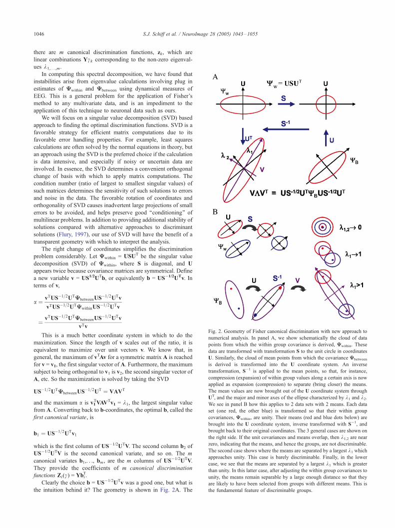
Fig. 2. Geometry of Fisher canonical discrimination with new approach to

numerical analysis. In panel A, we show schematically the cloud of data

points from which the within group covariance is derived, 8within. These

data are transformed with transformation S to the unit circle in coordinates

U. Similarly, the cloud of mean points from which the covariance 8between

is derived is transformed into the U coordinate system. An inverse

transformation, S�1 is applied to the mean points, so that, for instance,

compression (expansion) of within group values along a certain axis is now

applied as expansion (compression) to separate (bring closer) the means.

The mean values are now brought out of the U coordinate system through

UT, and the major and minor axes of the ellipse characterized by k1 and k2.

We see in panel B how this applies to 2 data sets with 2 means. Each data

set (one red, the other blue) is transformed so that their within group

covariances, 8within, are unity. Their means (red and blue dots below) are

brought into the U coordinate system, inverse transformed with S�1, and

brought back to their original coordinates. The 3 general cases are shown on

the right side. If the unit covariances and means overlap, then k1,2 are near

zero, indicating that the means, and hence the groups, are not discriminable.

The second case shows where the means are separated by a largest k1 which

approaches unity. This case is barely discriminable. Finally, in the lower

case, we see that the means are separated by a largest k1 which is greater

than unity. In this latter case, after adjusting the within group covariances to

unity, the means remain separable by a large enough distance so that they

are likely to have been selected from groups with different means. This is

the fundamental feature of discriminable groups.


there are m canonical discrimination functions, zk, which are

linear combinations Yck corresponding to the non-zero eigenval-

ues k1,. . .,m.

In computing this spectral decomposition, we have found that

instabilities arise from eigenvalue calculations involving plug in

estimates of 8within and 8between using dynamical measures of

EEG. This is a general problem for the application of Fisher’s

method to any multivariate data, and is an impediment to the

application of this technique to neuronal data such as ours.

We will focus on a singular value decomposition (SVD) based

approach to finding the optimal discrimination functions. SVD is a

favorable strategy for efficient matrix computations due to its

favorable error handling properties. For example, least squares

calculations are often solved by the normal equations in theory, but

an approach using the SVD is the preferred choice if the calculation

is data intensive, and especially if noisy or uncertain data are

involved. In essence, the SVD determines a convenient orthogonal

change of basis with which to apply matrix computations. The

condition number (ratio of largest to smallest singular values) of

such matrices determines the sensitivity of such solutions to errors

and noise in the data. The favorable rotation of coordinates and

orthogonality of SVD causes inadvertent large projections of small

errors to be avoided, and helps preserve good ‘‘conditioning’’ of

multilinear problems. In addition to providing additional stability of

solutions compared with alternative approaches to discriminant

solutions (Flury, 1997), our use of SVD will have the benefit of a

transparent geometry with which to interpret the analysis.

The right change of coordinates simplifies the discrimination

problem considerably. Let 8within = USUT be the singular value

decomposition (SVD) of 8within, where S is diagonal, and U

appears twice because covariance matrices are symmetrical. Define

a new variable v = US1/2UTb, or equivalently b = US�1/2UTv. In

terms of v,

a ¼ vTUS�1=2UT8betweenUS�1=2UTv

vTUS�1=2UT8withinUS�1=2UTv

¼ vTUS�1=2UT8betweenUS�1=2UTv

vTv

This is a much better coordinate system in which to do the

maximization. Since the length of v scales out of the ratio, it is

equivalent to maximize over unit vectors v. We know that, in

general, the maximum of vTAv for a symmetric matrix A is reached

for v = v1, the first singular vector of A. Furthermore, the maximum

subject to being orthogonal to v1 is v2, the second singular vector of

A, etc. So the maximization is solved by taking the SVD

US�1=2UT8betweenUS�1=2UT ¼ VAVT

and the maximum a is v1TVAVTv1 = k1, the largest singular value

from A. Converting back to b-coordinates, the optimal b, called the

first canonical variate, is

b1 ¼ US�1=2UTv1

which is the first column of US�1/2UTV. The second column b2 of

US�1/2UTV is the second canonical variate, and so on. The m

canonical variates b1,. . ., bm, are the m columns of US�1/2UTV.

They provide the coefficients of m canonical discrimination

functions Zi(c) = YbiT.

Clearly the choice b = US�1/2UTv was a good one, but what is

the intuition behind it? The geometry is shown in Fig. 2A. The


transformation simply scales linearly along the principal axes of

the within covariance ellipsoid, so as to make the within ellipsoid

the unit sphere. The magnitude of the principal axes of the resulting

between ellipsoid are the optimal ki.

To see this, note that the coordinate change consists of three

transformations. First, use UT to change to the coordinate system

where the covariance matrix8within is a diagonal matrix (where the

corresponding 8between covariance ellipsoid is aligned with the

coordinate axes). Second, shrink the ith coordinate axis by a factor

offfiffiffiffisi

p� �2 ¼ si. Third, change back to the original coordinate

system. After these three transformations, the 8within covariance

ellipsoid was squeezed to the unit ball, normalizing the within

covariance to better evaluate the size of the 8between covariance

ellipsoid. The magnitude of the principal axes of the resulting

8between covariance ellipsoid are now the ki, and the semi-major

axes are in the direction of the bi.

Fig. 2B illustrates the 3 general cases from this geometrical

transformation. All within group covariances are transformed into

unit spheres. The means of each group are stretched or shrunk by

an amount that is the inverse of the transform required to create the

unit spheres. On the right hand side, the first case is that the

eigenvalues ki approach zero. There is no discrimination possible

because the means and covariances of the groups overlap nearly

completely. The second case is where the eigenvalue k1 approaches

1. Here, the unit spheres are just touching, which is the threshold

for discriminating 2 groups. In the final case, k1 > 1, and the means

of the two groups are separated by more than the within group

covariances, implying that these data are discriminable into two

separate groups.

Testing discrimination quality

For each multivariate data vector Y (sample of power, average

phase amplitude, 2 correlation measures, and 2 phase dispersions),

the transformed vectors z have means u and normal p-variate

distributions f(z). Prior probabilities pj are determined from the

fraction of total samples within group j, pj = Nj / N. The posterior

probability pjz is the probability that for a given value of z, that the

data came from group j of n groups

pjz ¼pj f j zð ÞXn

k ¼ 1

pk f k zð Þ;k ¼ 1;N ;n

A suitable approximation to pj fj(z) is given by exp[ q(z)] where

q zð Þ ¼ uTj z� 12uTj uj þ lnpj (Flury, 1997). The highest posterior

probability among all possible groups is the predicted group

membership used in our calculations.

A robust method of testing the quality of classification is to

leave one multivariate data point out of the calculation of the

discriminant function, and then test for predicted group classi-

fication given its posterior probability.

A normal theory method to test for the significance of

discrimination is to examine the magnitude of the eigenvalues of

� above. We make use of Wilks’ statistic, W. After calculating the

log likelihood ratio as LLRS ¼ NPm

i ¼ 1 ln 1þ kið Þ, where ki are

the diagonal entries of �, W ¼ exp � 1NLLRS

��. A poor discrim-

ination yields small eigenvalues ki, and W approaches 1. Good

discrimination yields large eigenvalues, and W becomes small.

Since W is chi-squared distributed, we can calculate confidence

limits that the discrimination is significant (Flury, 1997).

We have compared our new numerical approach with more

standard numerical analysis (Flury, 1997) for the original Fisher

data set of morphometric measurements from 3 different iris flower

species. The canonical discrimination functions are, up to an

arbitrary sign, identical, and the W calculated by both methods is

identical (and highly significant).

Since we derive W from assumptions of normal distribution of

data variables with equal covariances, which our real data will

deviate from, an alternative means of testing the quality of

discrimination is to randomly permute the labeling of each

multivariate data point (to beginning, middle, or end of seizure

groups), and re-test the goodness of fit. Although there are

theoretically N!/N1N2N3 possible combinations for each of the

three groups (where N is the total number of measurements, and Ni

are the number within each partition), we will limit our

permutations to 1000.

In summary, we will present three different measures of the

substantiality of discrimination: leave one out error rate, W and its

normal theory confidence limits, and a bootstrapped confidence

limit that is robust against deviations from normality in the data

structure.

A full copy of working source code (written in Matlab) along

with a data sample (Scalp subject B, from Fig. 4) is archived as

Supplementary data).

Models of coupled systems

In order to help interpret our findings, we will also build

sequentially more complex linear autoregressive (AR) models of

coupled systems. These systems and resulting analysis are

illustrated in Fig. 3. We started with a 4 channel AR system, and

by brute force progressively increased the complexity in order to

create the simplest linear systems capable of replicating our

findings. The simplest AR model is

x1 tð Þ ¼ ax1 t � 1ð Þ þ n1 tð Þ




where for 4 channels of simulated data, x(t)1. . . x(t)4, each value

at time t is coupled to the previous value within the channel at

time t � 1, with the addition of an independent Gaussian

distributed random value n(t). The model is seeded with random

initial conditions. This model generates a data set without

coupling between the 4 channels.

Our next AR model of interest will be

x1 tð Þ ¼ ax1 t � 1ð Þ þ bx2 t � 1ð Þ þ n1 tð Þ


x3 tð Þ ¼ ax3 t � 1ð Þ þ bx4 t � 1ð Þ þ n3 tð Þ


where the first channel is coupled to the second, and the third

channel is coupled to the fourth, but there is no coupling between

channels 1 and 2 with channels 3 and 4.


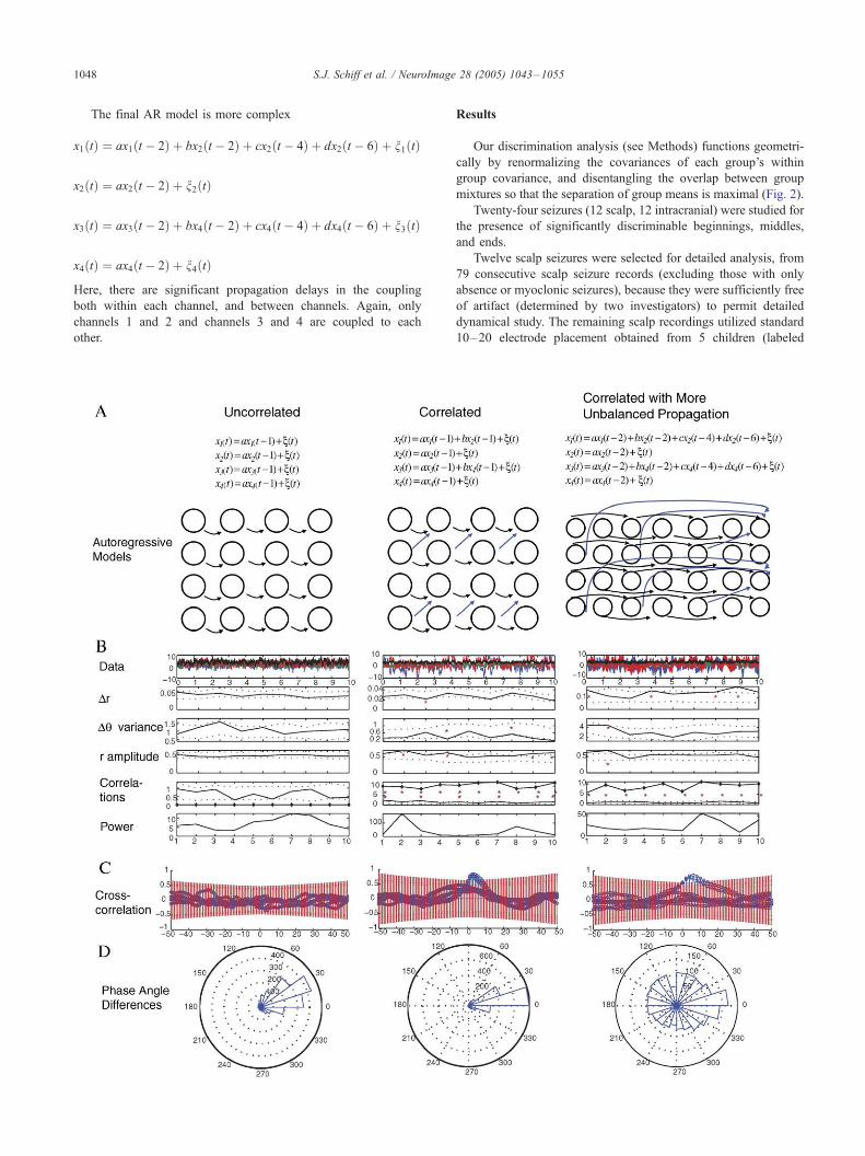
The final AR model is more complex

x1 tð Þ ¼ ax1 t � 2ð Þ þ bx2 t � 2ð Þ þ cx2 t � 4ð Þ þ dx2 t � 6ð Þ þ n1 tð Þ


x3 tð Þ ¼ ax3 t � 2ð Þ þ bx4 t � 2ð Þ þ cx4 t � 4ð Þ þ dx4 t � 6ð Þ þ n3 tð Þ


Here, there are significant propagation delays in the coupling

both within each channel, and between channels. Again, only

channels 1 and 2 and channels 3 and 4 are coupled to each

other.

Results

Our discrimination analysis (see Methods) functions geometri-

cally by renormalizing the covariances of each group’s within

group covariance, and disentangling the overlap between group

mixtures so that the separation of group means is maximal (Fig. 2).

Twenty-four seizures (12 scalp, 12 intracranial) were studied for

the presence of significantly discriminable beginnings, middles,

and ends.

Twelve scalp seizures were selected for detailed analysis, from

79 consecutive scalp seizure records (excluding those with only

absence or myoclonic seizures), because they were sufficiently free

of artifact (determined by two investigators) to permit detailed

dynamical study. The remaining scalp recordings utilized standard

10–20 electrode placement obtained from 5 children (labeled


subjects A through E) 2.3 to 12 years of age. One child had

cryptogenic generalized seizures not being treated at the time of the

recording and the others were receiving 2–3 anticonvulsants. The

symptomatic seizures were a consequence of bi-occipital gliosis,

cerebellar atrophy with history of prior hemiparesis, bi-parietal

encephalomalacia and ventriculomegaly, and cortical laminar

disorganization with dysgenic hippocampus. Each child had 1–5

partial seizures with or without secondary generalization analyzed.

The montage and an example from one subject (scalp subject B)

are shown in Figs. 4A and B.

Twelve intracranial seizure records from 4 patients (labeled A

through D) with disparate seizure types and etiologies were

without significant electrical artifact (from 16 consecutive records)

and were selected for further study. Subject A had a dysplastic

posterior temporo-parietal cortex, subject B had frontal gliosis,

subject C had a small cortical low grade astrocytoma with highly

focal seizures confined to a several square centimeter region near

the tumor, and subject D had both a dysplastic occipital lobe and

mesial temporal sclerosis (Fig. 5A). An example of a seizure from

subject D is shown in Fig. 5B. Of 16 consecutive intracranial

seizures for these patients, 12 were selected as free from artifact

after no more than 1 bad channel was eliminated from analysis. In

all, 3 seizures were selected for each of the 4 intracranial subjects.

Examples of the dynamical data calculations without regard to

discrimination are shown in Figs. 4E and 5E. We examined all

possible partitions of such data to divide the seizure into beginning,

middle, and terminal segments. This is done by letting the

beginning period vary from 2 s to up to half of the seizure in

length, and similarly letting the terminal period vary from the last 2

s to the last half of the seizure in length. All possible combinations

(in units of 2 seconds) of partitioning into beginning, middle, and

end are then tested for quality of discrimination using Wilks’

statistic, W (see Methods, note that optimizing on error rates would

have been an alternative), and the optimal partition combination

chosen.

Fig. 3. Autoregressive simulations and data analysis. Three progressively more co

uncorrelated model (first column, panel A), each of the 4 simulated channels is equ

a random shock n(t), which is independently applied to each channel 1–4 at each tithat the phase dispersion of these channels within each 200 point data window l

variance from 100 sets of surrogates for each data window as outlined in the legen

systems. The average r amplitude shows no evidence of coupling, and both the zero

lag correlation sums (diamonds, compared with the Bartlett, 1946 estimator as det

several pairs of crosscorrelation plots for different channels within the first data w

(T two times the absolute value of the Bartlett estimator of standard error). No v

distribution of phase angle differences within a data window are plotted on the c

constant) within each channel produces a distribution of phase angle changes which

a set of uncoupled processes which have well defined autocorrelation. In the midd

short propagation delays. Note in the data analysis in panel B that both Dr and Dhsurrogate data, which reflects the coupling present. The average r amplitude is now

(solid line) and non-zero (diamonds) lagged crosscorrelations are higher than exp

panel C, some channel pairs are not correlated-channels 1 to 3 or 1 to 4 for instanc

which is higher than expected by the Bartlett estimator, and although they show

significant. Note that the distribution of angle differences in panel D is now more ti

complex correlated model with more unbalanced propagation delays. Here, we hav

propagation delays greater than 1 time step (2 to 6 time steps). Again, the system

and 3 to 4, which only communicate within each pair. Now in panel B, we see tha

differences are now scattered uniformly over the unit circle. The Dh variance is

elevated. The zero lag crosscorrelation no longer reflects a coupled system (values

sum of crosscorrelation values (diamonds) easily pick up that this system has sign

force, searching for the simplest linear model which would reflect our experimen

setting of increased non-zero lagged crosscorrelation, simulates our main finding

An example of the result of such partition optimization for a

scalp seizure is shown in Fig. 4C. The minimal value of W was

0.12, which is much less than the value of 0.75 expected by the

chi-squared distribution for W (df = 12, p = 0.01, see Fig. 4D).

Since W assumes normally distributed variables, we checked the

integrity of our discrimination by randomly reassigning the

original measurements (6 measures combined) to different

assignments within this optimal partition (beginning, middle,

and end), and then repeated the calculation of W. For 1000

iterations of this reassignment, this bootstrap shows that the

partition is highly unlikely to have been seen by chance, with a

probability of less than 0.001 (Fig. 4F). The plot of the first

and second discriminants (linear combinations of original

variables) of this optimal partition, z1 and z2, are shown in

Fig. 4D. We find that the leave one out error rate for this

optimal discrimination is 11%.

Note the seizure partitions expanded in more detail at the top of

Fig. 4E. The optimization segmented the seizure into 3 stages that

contain, respectively, a rhythmic partial onset, tonic middle, and

clonic terminal activity to visual inspection.

Discrimination into 3 groups was possible for all 12 scalp

seizures, with significance by W (p < 0.01) and bootstrap (p <

0.001) for all seizures.

Similar analysis for an intracranial seizure from subject D is

shown in Fig. 5. The minimal value of optimized W was 0.16 (Fig.

5C), which is much less than the value of 0.88 expected by the chi-

squared distribution forW (df = 12, p = 0.01), and a plot of the first

and second discriminants is shown in Fig. 5D. One thousand

bootstrap permutations show that this partitioning is highly

unlikely to have been seen by chance, with a probability of less

than 0.001 (Fig. 5F). We find that the leave one out error rate for

this optimal discrimination is 16%.

Note the seizure partitions expanded in more detail at the top of

Fig. 5E. The optimization segmented the seizure into 3 stages that

contain substantially different patterns evident by visual inspection.

mplex autoregressive models, and their data analysis, are illustrated. In the

al to a constant, a < 1, multiplied by the previous data value (xi(t � 1)), plus

me t. The channels are uncoupled to each other. In B, the Dr variance shows

ies within the 98% confidence limits (dotted lines) set by recalculating Dr

d from Fig. 1. Similarly, Dh variance is within that expected for uncoupled

lag (solid line, compared with surrogates, dotted line) and the arbitrary (all)

ailed in Methods) show no evidence of correlation. In panel C, examples of

indow are shown, and the red error bars show twice the standard deviation

alues of crosscorrelation exceed the confidence limits. Lastly, plots of the

ircle. Note that, in this uncoupled case, the similar spectral frequency (a is

are clustered about a well defined mean change. All of this is the picture of

le column, the correlated model, we couple channels 1 to 2, and 3 to 4, with

variances now have some values which are smaller than expected from the

consistently higher than expected for an uncoupled system, and both zero

ected for uncoupled systems. Note that, in the plots of crosscorrelation in

e. Other channel pairs which are correlated reveal a peak in crosscorrelation

a time lag reflecting the lag in coupling, the values at zero lag remain

ghtly clustered, reflecting the coupling. In the right column, we show a more

e introduced propagation delays both within and between channels, and used

is compartmentalized in order to unbalance the system into channels 1 to 2

t the Dr variance is higher than expected. Note in panel D that the Dh angle

no longer decreased as in the middle column, and the r amplitude is less

at 0 lag are no longer above the confidence limit). However, the arbitrary lag

ificant crosscorrelation. We built up these autoregressive systems by brute

tal findings. This latter case, with prominently increased Dr variance in the

s well.


Discrimination into 3 groups was significant by W (p < 0.01)

for 12 of 12 seizures, but confirmed by bootstrap for 9 of 12 (p <

0.002). No more than 1 seizure per patient failed to be confirmed

by bootstrap.

We then normalized and averaged the results across all

partitions from all subjects: pre-seizure, beginning, middle, end,

and post-seizure periods. The grand average results for Scalp

seizures are shown in Fig. 6. Analysis of variance (ANOVA)

demonstrated that the phase dispersion (df = 59, F = 8.49, p <

0.00001) was significantly elevated during the middle phase of the

seizures. Tukey’s multiple comparison testing (Hogg and Ledolter,

1992) revealed that this increase in phase dispersion was

significant in comparison with both pre- and post-seizure periods.

Since seizures were unevenly divided among 5 subjects (1, 1, 1, 3,

and 6 seizures, respectively), we checked all possible combina-

tions of choosing 1 seizure from each subject, and recalculated the

grand averages: all 18 combinations of 5 seizures revealed

significant (p < 0.05) increases in phase dispersion during the

middle phase of seizures. Correlation sums at arbitrary lag were

similarly significantly elevated during the middle phase of seizures

(df = 59, F = 11.52, p < 0.000001). Again, checking all possible

combinations of choosing 1 seizure from each subject, and

recalculating the grand averages, all 18 combinations of 5 seizures

revealed significant (p < 0.05) increases in correlations during the

middle phase of seizures.

We next examined intracranial grand averages (Fig. 6). Phase

dispersion (df = 59, F = 3.4, p < 0.02) revealed elevated values

during the beginning of seizures, and multiple comparison testing

(Tukey test) revealed that this elevation was predominantly in

relation to post-seizure dispersions. Similar to the scalp seizures,

correlation sums at arbitrary lag were similarly significantly

elevated during the middle phase of seizures (df = 59, F = 4.9,

p < 0.002). Again, checking all possible combinations of choosing

1 seizure from each subject and recalculating the grand averages,

all 81 combinations of 4 seizures revealed significant (p < 0.05)

increases in correlations during the middle phase of seizures.

The issue of propagation critically affects the observation of

correlation in these data. If only the correlations at zero lag were

considered, one would have identified significant amplitude

correlations in only 3 scalp (2 subjects) and 4 intracranial (3

subjects) seizures, and the aggregate would not have revealed

significant correlations.

The most common pattern of dynamics which underlay our

findings was the simultaneous increase in synchronization (cross-

Fig. 4. Scalp electrode analysis. In panel A are shown the electrode positions for

electrode tracing of a scalp seizure from subject B contained within a 5 min record

C illustrates the optimization of Wilks’ Lambda for all possible partitions (second

plot of the first 2 canonical linear discriminants, z1 and z2, color coding the beginn

green asterisks, and red � marks. The means of these transformed groups are sho

that these groups are discriminable by visual inspection, and shown are the relev

analysis, and the low value of W, all consistent with a highly discriminable optima

that went into this analysis, along with relevant confidence limits. The top plot s

patterns (alternate channels have different colors), and the optimal partition indica

seizure partitions are further expanded to show detail above. Note that the Dr varia

the 99% confidence intervals based on surrogate data (2 dotted lines). Note that the

amplitude increases most prominently during the middle and end of the seizure, as

standard deviations of the 2 correlation measures, Dr variance, and r amplitude

correlation values, and the phase amplitudes. The non-zero correlation sums and D

seizure. In panel F are shown the bootstrap results for 1000 random permutations o

plot in panel D), and calculating W. Note that the small significant value for our

result, indicating that our partitioning is highly unlikely to be due to chance.

correlation sum at arbitrary lag) during the middle phase of

seizures, accompanied by an increase in phase dispersion. How can

we attempt to account for what appears at first to be a rather

counterintuitive set of findings—the increasing phase dispersion

would be expected to characterize asynchronous coupled systems?

To provide a possible explanation, we have constructed a series of

progressively more complex linear autoregressive model systems.

In Fig. 3A, we show a simulated 4 channel system where each

channel is made up of independent systems whose values depend

on the most recent previous values. Such a system appears

uncorrelated in all measures of amplitude or phase applied (Fig.

3B), but note that the phase angle differences are rather narrowly

confined (Fig. 3D). Given more time, such a system would

demonstrate increasing phase dispersion, but for such finite data

sets with similar native frequencies, one would be mislead without

appropriate bootstrap statistics as used here (Fig. 3B). In the

second column, we show data from coupling channels 1 to 2, and

channels 3 to 4, with the shortest possible propagation delays.

Phase coherence (r amplitude) now shows significant coupling, as

does both zero and arbitrary lagged correlation sums. Note that the

phase angle dispersion is decreased in Figs. 3B and D. Lastly, note

the more unbalanced state in column 3 with substantial propagation

delays in coupling. Now, although the arbitrary lag correlations are

significant, the zero lag correlations are not. Note that in the

correlation plots (Fig. 3C), one can see that the propagation delays

prevent the zero lagged correlations from being significant, while

longer lag correlations are significant. Most importantly, note that

the phase angle dispersions are now dramatically and highly

significantly increased (Figs. 3B and D).

We built up these autoregressive systems by brute force,

searching for the simplest (4 channel) linear model that would

reflect our experimental findings. The final pattern, seen by

progressively unbalancing an autoregressive system and introduc-

ing significant propagation delays, mimics the actual EEG results

closely.

Discussion

We have constructed a novel interpretation of the geometry of

R.A. Fisher’s 1936 method of canonical multivariate discrim-

ination analysis. A remarkable intellectual feat in the 1930s, Fisher

never wrote down a geometrical interpretation of his analysis.

Instead, the original report was more of a recipe for others to apply

the 10–20 electrode montage, and in panel B is illustrated a complete 23

ing. Note that the start and stop times are chosen by visual inspection. Panel

s) of the seizure time into beginning, middle, and end. Panel D illustrates a

ing (SzStart), middle (SzMid), and end (SzEnd) of the seizure into blue dots,

wn as colored open circles. The variances about these means clearly shows

ant leave one out error rates, 99% confidence limit for W by Chi-squared

l partitioning of this seizure. In panel E is shown the time course of all data

hows each raw data channel, color coded to bring out contrast in changing

ted by inverted triangles (r) into beginning, middle, and end periods. The

nce increases during the seizure buildup, and is prominently elevated above

Dh variance does not show changes outside of the confidence limits. The r

do arbitrary (all) lagged correlations. At the bottom are shown the means and

. Note that there are no significant changes in mean for the zero lagged

r variance show very significant elevations during the middle phase of this

f the group assignments of these data (equivalent to randomly recoloring the

optimum partition (red asterisk) is much lower than any other permutation

Fig. 5. Intracranial electrode analysis. Similar to Fig. 4, except that the electrode montages are now indicated for subdural, and in the case D, mixed subdural

and depth electrode assemblies. Note that for intracranial data, that the increase in Dr variance is more prominent during the beginning of the seizure, while the

non-zero lagged correlations are not prominent until late in the seizure.


Fig. 6. Grand average results for scalp and intracranial recordings. The results of all data were normalized and averaged within groups as pre-seizure, initiation,

middle, termination, and post-seizure periods. Four variables are shown to highlight the results of interest in phase dispersion and correlation. ANOVA for

Scalp seizures indicated significant changes in arbitrary (all) lag correlations (df = 59, F = 11.52, p = 7.3� 10�7) and Dr variance (df = 59, F = 8.49, p = 2.1 �10�5), and multiple comparison Tukey tests confirmed that the peak values of non-zero lag correlations and Dr variances were significantly higher than the pre-

and post-seizure values, accounting for these ANOVA results. Intracranial seizures again showed significant ANOVA differences in aggregate mean for

arbitrary lag correlations (df = 59, F = 4.86, p = 0.002) and Dr variances (df = 59, F = 3.36, p = 0.02), the peak in the arbitrary lag correlations significantly

higher than the post-seizure period (Tukey test), and the Dr variance was most prominently elevated during the beginning of the seizure (compared with post-

seizure by Tukey test).


this technique to mophometric data. Such data did not envision the

data structures created from a signal processing analysis of

neuronal signals, nor the developments in applied mathematics

and numerical analysis that accompanied the advent of digital

computers. We have shown a stable approach with a clear

geometrical interpretation to solving his original linear analysis

for the examination of data such as used in this report. Our

approach can be used in many other settings (EEG, MEG, Optical

Imaging, fMRI), and we offer our algorithms for others to make

use of in the Supplementary data.

Using this method, we report the first canonical discrimination

analysis to search for dynamically distinct stages of epileptic

seizures in humans. We found significant extraction of unique

initial and terminal phases from 21 of 24 scalp and intracranial

recordings. These results argue for an evolution of seizure patterns

that can be consistently partitioned based on dynamical measures.

Nonlinear methods to compute Fisher discriminants have

been developed in recent years using kernel-based approaches

(Muller et al., 2001). Similarly, one might ask whether using

non-linear dynamical EEG measures instead of our linear ones

might have improved the results of our linear or an alternative

non-linear discrimination method. Notwithstanding that we

anticipate that neuronal dynamics are fundamentally non-linear,

our robust results with linear methods here may reflect a more

general phenomenon seen with detecting coupling in the

presence of significant amounts of noise and non-linearity

(Netoff et al., 2004).

There has been surprisingly little previous work quantifying the

dynamical stages of seizures. In experimental kindled seizures,

Racine (1972) described progressive changes in electrical seizure

patterns corresponding to behavioral manifestations. In the tetanus

toxin model of experimental seizures, a staging system has been

devised for different segments of seizures (Finnerty and Jefferys,

2000). For the particular case of human status epilepticus, Treiman

et al. (1990) defined a staging system. In all of the above, the

classification of seizure stages was based upon qualitative assess-

ments following visual inspection of EEG. The most quantitative

approaches to segmentation of seizures that we are aware of

(Wendling et al., 1996; Wu and Gotman, 1998) focused upon

comparing the similarities (or dissimilarities) between different

seizures.

Although seizures have for over half a century been charac-

terized as synchronous or Fhypersynchronous_ (Penfield and

Jasper, 1954), the measurements to support such conclusions have

been sparse (for review see Netoff and Schiff, 2002). In our

analysis, no consistent evidence of increased synchronization was

evident within the initial or terminal phases of these seizures—

synchronization was a prominent feature only once the seizure had

passed through its initiation phase, and was a variable feature of

seizure termination depending on subject. The other consistent

dynamical feature of these seizures was the consistent increase in

phase dispersion, which tended to be reflected during the initial

stage of seizure formation intracranially, or during the middle

phase of seizures recorded at the scalp. Although the scales of

observation are vastly different, we note that observing intra-

cellular currents during experimental seizures similarly shows a

lack of synchronization during the initiation of such events (Netoff

and Schiff, 2002).


We still lack a dynamical definition of a seizure. Although we

customarily assign seizure onsets, as done in this study, by

applying subjective visual inspection to EEG records, such a

procedure is unsound for more definitive study of these phenom-

ena. We require a description of the dynamics of seizure onset that

is clearly discriminable from the preceding non-seizure dynamics.

Our study is a first attempt to prove that the initial phase of a

seizure bears unique dynamical signatures. A logical future step

will be to attempt such discrimination between pre-seizure and

seizure onset in an effort to objectively delineate seizure from non-

seizure.

There has been intense interest in whether there exists a pre-

seizure state (Ebersole, 2005, Lehnertz and Litt, 2005). Such a

state, if physiologically distinct from seizure onset, would

provide a means of predicting the imminent onset of a seizure.

If a pre-seizure state existed for a given subject, and

importantly, if the dynamics within this pre-seizure state were

discriminable from seizure onset, the methodology we have

described are a powerful means of delineating these states. Note

that if what we think is a pre-seizure state was actually a small

version of the seizure, that is a highly localized form of the

seizure whose dynamics were the same as the seizure onset,

then our approach would group such dynamics as part of the

seizure onset.

Our findings also point to the question of how is synchrony in

neural systems to be measured and observed. Although we

customarily infer the presence of synchrony by observing the

presence of correlations (in either signal amplitude or phase), such

findings ignore the stability constraints that must be present when

physical systems synchronize (Pecora and Carroll, 1998). We also

customarily ignore propagation delays in synchrony measures,

although such delays are inherent in all neural systems. Although

we cannot use perturbations (Francis et al., 2003) to test for

synchrony stability in human seizure recordings, we can compare

measures of synchronization that take propagation delays into

account. In our human seizure data, we found little evidence for

synchronization using phase or amplitude correlations measured

without permitting a time lag, but significant evidence for

synchrony during the middle stages of seizures when arbitrary

time lags were permitted. We also showed how an autoregressive

system with significant compartmentalization and propagation

delays within and between such compartments could generate

evidence of increased phase dispersion in the presence of

significantly increased amplitude correlations—mimicking closely

the general findings of our human seizure data. Although such

simulations in no way are a unique means to account for our

human findings, they point to one of the simplest models capable

of imitating these dynamics. Brains have compartments separated

by conduction delays, and such features need to be taken into

account when analyzing seizures for the presence of apparent

synchronization.

Why do seizures stop? Most human subjects with epilepsy have

self-limited transient seizures. Subjects with seizures that do not

limit their intensity and terminate are at substantially higher risk of

death. Unfortunately, we know little about the dynamical changes

that terminate seizures. If seizures have a terminal phase distinct

from earlier phases, then understanding how to induce such

terminal dynamics may offer a unique strategy for suppressing

seizures through deep brain stimulation.

Finally, how many dynamical stages constitute typical seizure

evolution? Although we searched for three stages, we were most

interested in whether seizures had distinct onsets and offsets.

Significant findings of discrimination into 3 separable groups is

possible given more than 3 true groups, and we did not attempt to

perform an optimization analysis searching for the most likely

number of stages present in our evolving seizures. In addition, for

a dynamical process that changes continuously (monotonically

and noiselessly), the separation into a finite number of groups

might be significant despite a theoretically infinite number of

stages. These issues make us cautious over placing too much

emphasis on a precise number of stages within these seizures.

Nevertheless, despite the very different means of observation

(intracranial depth and subdural versus scalp electrodes), we

found consistent patterns in phase and amplitude correlation

within our stages that were consistent across many subjects as

seizures evolved. These findings underscore the fundamental

results from applying our discrimination analysis—that seizures

dynamically evolve and display distinctive initiation and termi-

nation dynamics.

Acknowledgments

We are grateful for time in residence at a Pattern Formation

Workshop at the Institute for Theoretical Physics, University of

California at Santa Barbara (SJS), for helpful discussions from

G.A. Stolovitzky, E. Barreto, P. So, J.R. Cressman, and B.J.

Gluckman, and to E. Ben-Jacob for helpful comments on the

manuscript. Supported by NIH R01MH50006 and K02MH01493

(SJS).

Appendix A. Supplementary data

Supplementary data associated with this article can be found, in

the online version, at doi:10.1016/j.neuroimage.2005.06.059.

References

Ayala, G.F., Matsumoto, H., Gumnit, J., 1970. Excitability changes and

inhibitory mechanisms in neocortical neurons during seizures. J. Neuro-

physiol. 33, 70–85.

Bartlett, M.S., 1946. On the theoretical specification and sampling proper-

ties of autocorrelated time-series. J. R. Stat. Soc. B8, 27–41.

Bendat, J.S., Piersol, A.G., 1986. Random Data. J. Wiley and Sons, New

York, pp. 484–516.

Box, G.E.P., Jenkins, G.M., 1976. Time Series Analysis, Forecast-

ing and Control, (Rev edition). Holden-Day, San Francisco, FL,

pp. 376–377.

Ebersole, J.S., 2005. In search of seizure prediction, a critique. Clin.

Neurophysiol. 116, 489–492.

Finnerty, G.T., Jefferys, J.G.R., 2000. 9–16 Hz oscillation precedes

secondary generalization of seizures in the rat tetanus toxin model of

epilepsy. J. Neurophysiol. 83, 2217–2226.

Fisher, R.A., 1936. The use of multiple measurements in taxonomic

problems. Ann. Eugen. 7, 179–188.

Fisher, N.I., 1993. Statistical Analysis of Circular Data. Cambridge,

Cambridge, UK, pp. 30–35.

Flury, B., 1997. A First Course in Multivariate Statistics. Springer, New

York.

Francis, J.T., Gluckman, B.J., Schiff, S.J., 2003. Sensitivity of neurons to

weak electric fields. J. Neurosci. 120 (23), 7255–7261.

http:\\dx.doi.org\doi:10.1016\j.neuroimage.2005.06.059


Hogg, V.H., Ledolter, J., 1992. Applied Statistics for Engineers and

Physical Scientists. Macmillan, New York, pp. 271–272.

Kandel, E.R., Spencer, W.A., 1961. Excitation and inhibition of single

pyramidal cells during hippocampal seizure. Exp. Neurol. 4, 162–179.

Litt, B., Esteller, R., Echauz, J., D’Alessandro, M., Shor, R., Henry, T.,

Pennell, P., Epstein, C., Bakay, R., Dichter, M., Vachtsevanos, G., 2001.

Epileptic seizures may begin hours in advance of clinical onset: a report

of five patients. Neuron. 30, 51–64.

Lehnertz, K., Litt, B., 2005. The first international collaborative workshop

on seizure prediction, summary and data description. Clin. Neurophys.

116, 493–505.

Matsumoto, H., Marsan, C.A., 1964. Cortical cellular phenomena

in experimental epilepsy, Ictal manifestations. Exp. Neurol. 9,

305–326.

Mormann, F., Lehnertz, K., David, P., Elger, C.E., 2000. Mean phase

coherence as a measure for phase synchronization and its application to

the EEG of epilepsy patients. Physica D 144, 358–369.

Muller, K.-R., Mika, S., Ratsch, G., Tsuda, K., Scholkopf, B., 2001. An

introduction to kernel-based learning algorithms. IEEE Trans. Neural

Netw. 12, 181–202.

Netoff, T.I., Schiff, S.J., 2002. Decreased neuronal synchronization during

experimental seizures. J. Neurosci. 22, 7297–7307.

Netoff, T.I., Pecora, L.M., Schiff, S.J., 2004. Analytical coupling detection

in the presence of noise and nonlinearity. Phys. Rev., E 69, 017201.

Pecora, L.M., Carroll, T.L., 1998. Master stability functions for synchron-

ized coupled systems. Phys. Rev. Lett. 80, 2109–2112.

Penfield, W., Jasper, H., 1954. Epilepsy and The Functional Anatomy of the

Human Brain. Little-Brown, Boston, MA.

Racine, R.J., 1972. Modification of seizure activity by electrical stimula-

tion: II. Motor seizure. Electroencephalogr. Clin. Neurophysiol. 32,

281–294.

Treiman, D.M., Walton, N.Y., Kendrick, C., 1990. A progressive sequence

of electroencephalographic changes during generalized convulsive

status epilepticus. Epilepsy Res. 5, 49–60.

Wendling, F., Bellanger, J.J., Badier, J.M., Coatrieux, J.L., 1996. Extraction

of spatio-temporal signatures from depth EEG seizure signals based on

objective matching in warped vectorial observations. IEEE Trans.

Biomed. Eng. 43, 990–1000.

Wendling, F., Shamsollahi, M.B., Badier, J.M., Bellanger, J.J., 1999. Time-

frequency matching of warped depth-EEG seizure observations. IEEE

Trans. Biomed. Eng. 46, 601–605.

Wu, L., Gotman, J., 1998. Segmentation and classification of EEG

during epileptic seizures. Electroencephalogr. Clin. Neurophysiol. 106,

344–356.

Neuronal spatiotemporal pattern discrimination: The dynamical evolution of seizures

Documents

Transcript of Neuronal spatiotemporal pattern discrimination: The dynamical evolution of seizures