NAVIGATION PERFORMANCEPREDICTIONS FOR THE ORIONFORMATION FLYING MISSION

Philip FERGUSON, Franz BUSSE, and Jonathan P. HOW

Space Systems LaboratoryMassachusetts Institute of Technology

philf@mit.edu, teancum@stanford.edu, jhow@mit.edu

ABSTRACT - This paper presents hardware-in-the-loop results that exper-imentally demonstrate precise relative navigation for true formation flyingspacecraft applications. The approach is based on carrier-phase differentialGPS, which is an ideal navigation sensor for these missions because it pro-vides a direct measure of the relative positions and velocities of the vehicles inthe fleet. In preparation for Orion, a planned microsatellite formation flyingmission, four modified GPS receivers were used in the NASA GSFC Forma-tion Flying Testbed to demonstrate relative navigation. The results in thispaper show unprecedented levels of accuracy (»2cm position and <0.5mm/svelocity) which validate the use of a decentralized estimation architecture andoffer high confidence in the success of Orion.

1 - INTRODUCTION

Autonomous formation flying of satellite clusters has been identified as an enabling technologyfor many future NASA and the DoD missions [1, 2]. The use of fleets of smaller satellitesinstead of one monolithic satellite should improve the science return through longer baselineobservations, enable faster ground track repeats, and provide a high degree of redundancy andreconfigurability in the event of a single vehicle failure. If the ground operations can also bereplaced with autonomous onboard control, this fleet approach should also decrease the missioncost at the same time. However, there are many control, navigation, and autonomy technologiesthat must be developed and demonstrated before these advanced science missions can be flown.The Orion microsatellite mission was designed to address many of these concerns for formationflying in LEO [3, 4]. This paper discusses the current spacecraft design and recent results onthe decentralized relative navigation using differential GPS that has been developed for Orion.

The Orion mission will consist of two identical cube satellites that have been designed tobe launched from the Shuttle cargo bay (although other options are possible) and performexperiments for 50 to 90 days. There will be three primary operational stages [4]:

² Formation Stabilization: During this stage, the vehicles will be de-tumbled and theOrion vehicles will be maneuvered into their first formation (100m in-track separation).

² In-Track Experiments: In this stage, the two Orion spacecraft demonstrate tight for-mation flying with one vehicle following the other. The goal is to demonstrate a preciseformation with one Orion remaining within a 5m£10m£5m error box centered at a point100m (in-track) from the other Orion.

² Elliptical Formation Experiments: In this final stage, the spacecraft will be controlledto stay within error boxes that traverse passive apertures (closed-form ellipses) in theLVLH frame (e.g., as governed by Hills equations).

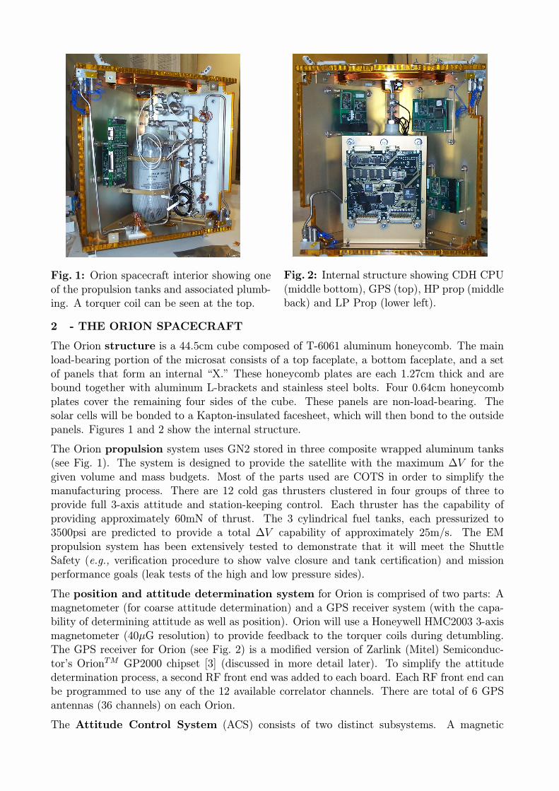
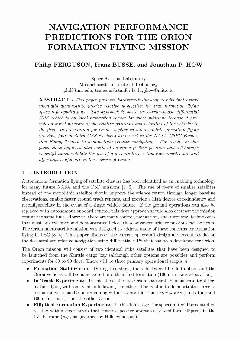
Fig. 1: Orion spacecraft interior showing oneof the propulsion tanks and associated plumb-ing. A torquer coil can be seen at the top.

Fig. 2: Internal structure showing CDH CPU(middle bottom), GPS (top), HP prop (middleback) and LP Prop (lower left).

2 - THE ORION SPACECRAFT

The Orion structure is a 44.5cm cube composed of T-6061 aluminum honeycomb. The mainload-bearing portion of the microsat consists of a top faceplate, a bottom faceplate, and a setof panels that form an internal “X.” These honeycomb plates are each 1.27cm thick and arebound together with aluminum L-brackets and stainless steel bolts. Four 0.64cm honeycombplates cover the remaining four sides of the cube. These panels are non-load-bearing. Thesolar cells will be bonded to a Kapton-insulated facesheet, which will then bond to the outsidepanels. Figures 1 and 2 show the internal structure.

The Orion propulsion system uses GN2 stored in three composite wrapped aluminum tanks(see Fig. 1). The system is designed to provide the satellite with the maximum ∆V for thegiven volume and mass budgets. Most of the parts used are COTS in order to simplify themanufacturing process. There are 12 cold gas thrusters clustered in four groups of three toprovide full 3-axis attitude and station-keeping control. Each thruster has the capability ofproviding approximately 60mN of thrust. The 3 cylindrical fuel tanks, each pressurized to3500psi are predicted to provide a total ∆V capability of approximately 25m/s. The EMpropulsion system has been extensively tested to demonstrate that it will meet the ShuttleSafety (e.g., verification procedure to show valve closure and tank certification) and missionperformance goals (leak tests of the high and low pressure sides).

The position and attitude determination system for Orion is comprised of two parts: Amagnetometer (for coarse attitude determination) and a GPS receiver system (with the capa-bility of determining attitude as well as position). Orion will use a Honeywell HMC2003 3-axismagnetometer (40µG resolution) to provide feedback to the torquer coils during detumbling.The GPS receiver for Orion (see Fig. 2) is a modified version of Zarlink (Mitel) Semiconduc-tor’s OrionTM GP2000 chipset [3] (discussed in more detail later). To simplify the attitudedetermination process, a second RF front end was added to each board. Each RF front end canbe programmed to use any of the 12 available correlator channels. There are total of 6 GPSantennas (36 channels) on each Orion.

The Attitude Control System (ACS) consists of two distinct subsystems. A magnetic

damping controller is included to slow the spacecraft rotation sufficiently for GPS signals tobe acquired. Dedicated hardware, consisting of a three-axis magnetometer and torquer coils,allows the detumbling to be performed without GPS information. The torquer coils can beseen at the top of Fig. 1 and 2. The second attitude controller uses the GPS attitude solutionand the thrusters. It is designed to keep the top face (with three GPS antennas) pointing “up”for the best GPS sky coverage. A Kalman filter is used to estimate the full attitude state.

The Command and Data Handling (C&DH) system is responsible for all low-level tasksonboard the spacecraft. These tasks include decoding ground and inter-satellite communication,forwarding commands to distributed subsystems, controlling power switching for subsystemsand experiments and gathering health and telemetry data. The CPU is a SpaceQuest NEC V53with a 10MHz processor and 1MB of EDAC Ram, and it will run the Space Craft OperatingSystem (SCOS) by BekTek. Both the CPU hardware and operating system have spaceflightheritage. Fig. 2 shows the C&DH integrated into Orion.

The Communications subsystem must handle all data transfer between the ground and Orionas well as between each Orion vehicle. Crosslink between spacecraft will operate in half-duplexwhile the down/uplink will operate in full-duplex mode. Both crosslink and up/downlinkcommunications will be conducted at 9600 baud. The modems for Orion are manufactured bySpaceQuest and have been used successfully on past spaceflights. The communications systemmakes use of an omni directional antenna pattern with circular polarization.

The Science Computer is a 200MHz StrongARM 1110 RISC based microprocessor called the“nanoEngine” (built by Brightstar Engineering). The nanoEngine has three RS-232 communi-cation ports and 20 general purpose IO pins for controlling other hardware. A CompactFlashmemory disk will be used for mass storage. At full usage, the entire nanoEngine board drawsless than 2W (»1700 MIPS/W). The nanoEngine weighs only 76g (without an interface card)and is smaller than a credit card. The operating system for the Science Computer is embeddedLinux. The Science Computer will perform the navigation computation and fleet coordination.

With the hardware design essentially complete, the goal of recent work on the Orion missionhas been to develop a simple, decentralized, real-time GPS filter that meets the performancetargets, as specified by the control analysis [6]. As discussed in the following, the capabilitiesof this filter have been demonstrated on a 4-vehicle, hardware-in-the-loop simulation.

3 - STATE DEFINITIONS

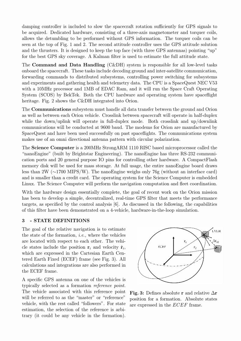
Fig. 3: Defines absolute r and relative ∆rposition for a formation. Absolute statesare expressed in the ECEF frame.

The goal of the relative navigation is to estimatethe state of the formation, i.e., where the vehiclesare located with respect to each other. The vehi-cle states include the position ri and velocity ri,which are expressed in the Cartesian Earth Cen-tered Earth Fixed (ECEF) frame (see Fig. 3). Allcalculations and integrations are also performed inthe ECEF frame.

A specific GPS antenna on one of the vehicles istypically selected as a formation reference point.The vehicle associated with this reference pointwill be referred to as the “master” or “reference”vehicle, with the rest called “followers”. For stateestimation, the selection of the reference is arbi-trary (it could be any vehicle in the formation).

Subscripts denote the user vehicles, where the reference vehicle will be indicated with the sub-script “1”; superscripts are used to denote the GPS NAVSTAR satellites. For example, theabsolute position of the master user is r1, and the absolute velocity of GPS satellite m is rm.

The formation state can be expressed equivalently in absolute states (relative to the center ofthe earth) or in relative states (relative to the reference point in the formation). The relativestates (∆X12 = X2¡X1) between the vehicles are of much greater interest for formation flying,leading to a basic formation state of the form (n vehicles)£

XT1 ∆XT

12 ¢ ¢ ¢ ∆XT1(n−1)

¤T(1)

3.1 - Measurement Model

Each vehicle has a GPS receiver, which collects its own independent set of measurements ateach time step. The GPS receiver provides three measurements: Code phase, carrier phase,and the Doppler shift on the carrier phase. Absolute navigation uses the code and Dopplermeasurements, but for orbital relative navigation, only the carrier phase measurement is needed.The carrier phase measurement, φ, for each visible GPS satellite by the receiver is

φmi = krmi ¡ rik+ bi +Bmi + βmi ¡ Imi + νφ (2)

where krmi ¡ rik = range between user i at measurement time and GPS satellite m at timeof signal transmission

bi = clock offset for user iBmi = clock offset for GPS satellite m at time of transmissionImi = ionospheric delayβmi = carrier phase bias for user iνφ = other noises (including receiver noise and multipath)

This measurement is a function of the user state, the GPS satellite state, the ionosphere, andother noise sources. Besides the user estimate, all of these terms have errors associated withthem. (For absolute state estimation, the biases also present some difficulty, and are generallydetermined by combining carrier phase with code phase). As an alternative, measurementsbetween two receivers from the same NAVSTAR satellite can be subtracted, which is referredto as the single difference measurement, ∆φmij = φ

mj ¡ φmi . In the case of relative navigation,

these measurement sets would be from receivers on different vehicles, and the single differenceprovides a direct measurement of the relative state between the two vehicles. More specifically,the single difference is

∆φmij = krmi ¡ rik ¡ krmj ¡ (ri +∆rij) k+∆βmij +∆bij +∆Bmij ¡∆Imij + ν∆φ (3)

where ∆rij = differential position between users i and j∆bij = differential clock offset between users i and j∆Bmij = differential clock offset for GPS satellite m, between the transmitting

states for users i and j∆Imij = differential ionospheric delay∆βmij = differential carrier phase bias between users i and j, on signal from mν∆φ = remaining differential noises

Note that the errors in these differential terms are typically much smaller than in the corre-sponding absolute terms. These single differences provide a direct measure of the relative statebetween vehicles, but do not provide an absolute state estimate.

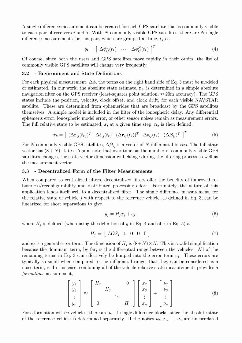
A single difference measurement can be created for each GPS satellite that is commonly visibleto each pair of receivers i and j. With N commonly visible GPS satellites, there are N singledifference measurements for this pair, which are grouped at time, tk as

yk =£∆φ1ij(tk) ¢ ¢ ¢ ∆φNij (tk)

¤T(4)

Of course, since both the users and GPS satellites move rapidly in their orbits, the list ofcommonly visible GPS satellites will change very frequently.

3.2 - Environment and State Definitions

For each physical measurement, ∆φ, the terms on the right hand side of Eq. 3 must be modeledor estimated. In our work, the absolute state estimate, r1, is determined in a simple absolutenavigation filter on the GPS receiver (least-squares point solution, ¼ 20m accuracy). The GPSstates include the position, velocity, clock offset, and clock drift, for each visible NAVSTARsatellite. These are determined from ephemerides that are broadcast by the GPS satellitesthemselves. A simple model is included in the filter of the ionospheric delay. Any differentialephemeris error, ionospheric model error, or other sensor noises remain as measurement errors.The full relative state to be estimated, x, at a given time step, tk, is then defined,

xk =£(∆rij(tk))

T ∆bij(tk) (∆rij(tk))T ∆bij(tk) (∆βij)

T¤T

(5)

For N commonly visible GPS satellites, ∆βij is a vector of N differential biases. The full statevector has (8+N) states. Again, note that over time, as the number of commonly visible GPSsatellites changes, the state vector dimension will change during the filtering process as well asthe measurement vector.

3.3 - Decentralized Form of the Filter Measurements

When compared to centralized filters, decentralized filters offer the benefits of improved ro-bustness/reconfigurability and distributed processing effort. Fortunately, the nature of thisapplication lends itself well to a decentralized filter. The single difference measurement, forthe relative state of vehicle j with respect to the reference vehicle, as defined in Eq. 3, can belinearized for short separations to give

yj = Hjxj + ej (6)

where Hj is defined (when using the definition of y in Eq. 4 and of x in Eq. 5) as

Hj =£LOSj 1 0 0 I

¤(7)

and ej is a general error term. The dimension of Hj is (8+N)£N . This is a valid simplificationbecause the dominant term, by far, is the differential range between the vehicles. All of theremaining terms in Eq. 3 can effectively be lumped into the error term ej. These errors aretypically so small when compared to the differential range, that they can be considered as anoise term, ν. In this case, combining all of the vehicle relative state measurements provides aformation measurement,

y2y3...yn

¼H2 0

H3. . .

0 Hn

x2x3...xn

+ν2ν3...νn

(8)

For a formation with n vehicles, there are n¡1 single difference blocks, since the absolute stateof the reference vehicle is determined separately. If the noises ν2, ν3, . . . , νn are uncorrelated

and independent, the noise covariance matrix for a centralized filter would be block diagonal.In this case, because of the block diagonal nature of the observation matrix, H, the filter couldbe decentralized without any loss of accuracy, and a centralized and decentralized filter wouldprovide exactly the same results. However, a decentralized filter is an approximation for thisapplication because the noise terms are correlated:

1. Since each vehicle forms single differences with respect to the same reference, these sin-gle differences will be correlated. However ground testing has shown that this level ofcorrelation is relatively small (carrier phase noise level ¼ 2-5mm); and

2. Recall that all other measurement errors in the remainder terms of Eq. 6 are lumped intothe noise term, νj . Although forming a single difference cancels out many of the commonmode errors, any residual errors will be correlated between vehicles.

However, if these correlations are relatively small, they can be ignored, resulting in decoupledmeasurements that can be used to form a decentralized estimator. As discussed, decentraliza-tion offers many benefits and a key aspect of this work was to investigate whether a decentralizedestimator could be used to meet the relative navigation goals set by the fuel usage [6].

The discussion presented in this section was based on a linearized version of the measurementequations. Linear filters are useful for formations with small separations, but, in general, anonlinear measurement update is required [7]. However, this decoupling in the measurementsthat leads to a decentralization estimator also holds for the nonlinear extended Kalman filter.

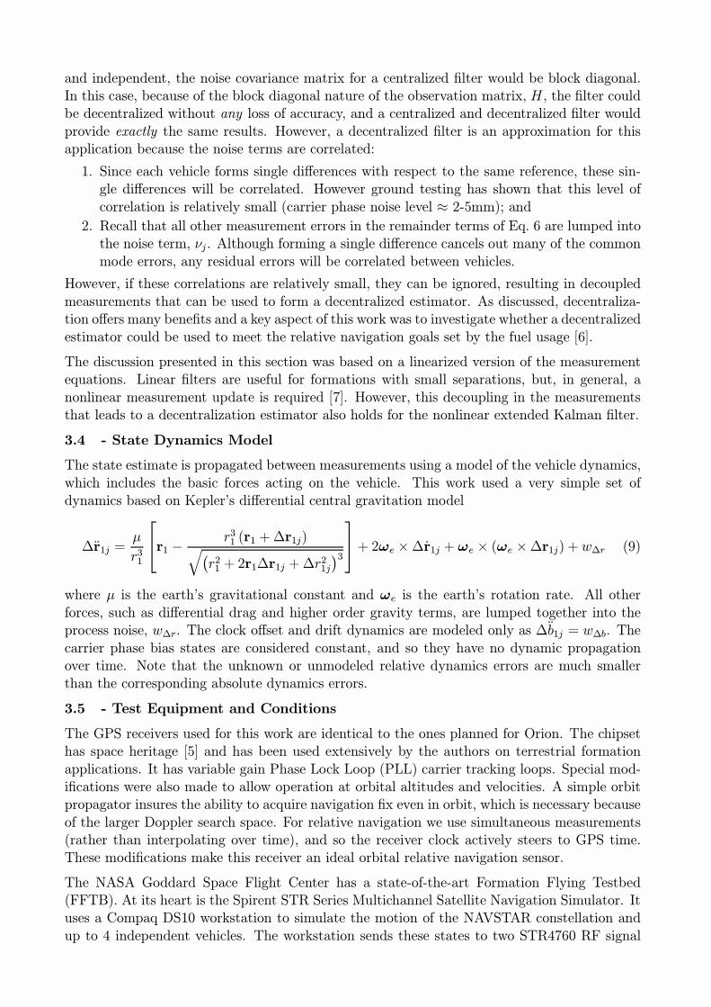
3.4 - State Dynamics Model

The state estimate is propagated between measurements using a model of the vehicle dynamics,which includes the basic forces acting on the vehicle. This work used a very simple set ofdynamics based on Kepler’s differential central gravitation model

∆r1j =µ

r31

r1 ¡ r31 (r1 +∆r1j)q¡r21 + 2r1∆r1j +∆r

21j

¢3+ 2ωe £∆r1j + ωe £ (ωe £∆r1j) + w∆r (9)

where µ is the earth’s gravitational constant and ωe is the earth’s rotation rate. All otherforces, such as differential drag and higher order gravity terms, are lumped together into theprocess noise, w∆r. The clock offset and drift dynamics are modeled only as ∆b1j = w∆b. Thecarrier phase bias states are considered constant, and so they have no dynamic propagationover time. Note that the unknown or unmodeled relative dynamics errors are much smallerthan the corresponding absolute dynamics errors.

3.5 - Test Equipment and Conditions

The GPS receivers used for this work are identical to the ones planned for Orion. The chipsethas space heritage [5] and has been used extensively by the authors on terrestrial formationapplications. It has variable gain Phase Lock Loop (PLL) carrier tracking loops. Special mod-ifications were also made to allow operation at orbital altitudes and velocities. A simple orbitpropagator insures the ability to acquire navigation fix even in orbit, which is necessary becauseof the larger Doppler search space. For relative navigation we use simultaneous measurements(rather than interpolating over time), and so the receiver clock actively steers to GPS time.These modifications make this receiver an ideal orbital relative navigation sensor.

The NASA Goddard Space Flight Center has a state-of-the-art Formation Flying Testbed(FFTB). At its heart is the Spirent STR Series Multichannel Satellite Navigation Simulator. Ituses a Compaq DS10 workstation to simulate the motion of the NAVSTAR constellation andup to 4 independent vehicles. The workstation sends these states to two STR4760 RF signal

generators. These signal generators create the GPS signals that would be observed by the fouruser receivers (with two RF outputs per generator).

Many scenarios have been run using this simulator (base orbit has altitude of »450km, ec-centricity of 0.005, and 28.5◦ inclination). The simulations use a tenth-order gravity modeland an atmospheric drag model (Lear’s). For the measurements, a diverging ephemeris andclock model was used and a standard orbital ionospheric model, as specified in NATO StandardAgreement STANAG 4294 Issue 1. There is no multipath noise in the simulation, but this isnot expected to be a significant error source for microsatellites. All vehicle models are identical,with a surface area of 1m2, drag coefficient of 2, and 0.1 metric tonne (the smallest mass inthe simulator). The antenna is at the center of gravity, and the vehicle maintained a nadirearth-pointing attitude. A standard hemispherical antenna gain pattern was used.

The decentralized filter for these demonstrations used the nonlinear update and propagationmodels [7]. Only carrier-phase single differences measurements were used. The update rate was1Hz. Several formations were considered:

1. 100m and 10km In-track. Here the vehicles were in the same orbital path, all separatedfrom one another by the prescribed amount in-track.

2. 1km and 10km In-plane ellipses. This formation is considered our baseline demonstrationfor meeting our performance targets. One vehicle followed the reference orbit. The otherthree vehicles moved about the master vehicle in an evenly spaced ellipse, staying withinthe orbital plane. The elliptical path in the local frame was 1km £ 2km.

3. 1km Out-plane ellipse. Similar motion, but now the relative motion ellipse is oriented outof the orbital plane, leading to greater differential J2 disturbances (larger process noise).

4 - RESULTS

This section presents the results from real-time hardware-in-the-loop experiments using theGSFC FFTB facility. For all experiments, data storage of the raw measurements began afterall four of the receivers achieved navigation fixes. The receivers performed “warm” starts,where they were provided almanac information for the NAVSTAR constellation, a rough currentposition guess (often wrong by several hundred kilometers) and a rough current time guess (offby up to fifteen seconds). The receivers can reliably and repeatedly lock on (accomplishedhundreds of time during the course of development). A navigation fix was usually obtained,and active tracking began, in less than two minutes after the simulation began.

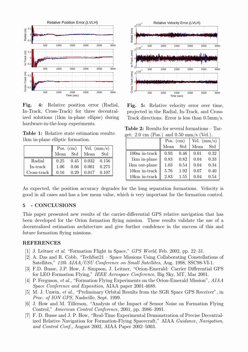
Figures 4 and 5 show the position and velocity errors for the three relative solutions (shown asprojections of the error into the Radial (R), In-Track (I), and Cross-Track (C) directions). Thesimulations start with large errors (¼ 2-5m) that result from the initial carrier phase bias errors.However, these biases are observable over time, and the position solution quickly converges.After the initial convergence, the biases on new measurements coming on-line are predicted fromthe current state estimate, but the results show that this initialization process does not disturbthe position or velocity estimates [7]. To quantify the performance, the standard deviation andmean of the error was computed over the last half of the simulation in each dimension. Table 1gives the root-mean-square of these means and standard deviations of the errors across thefleet’s three solutions. As shown, the position error has a mean of 0.2—1.1cm, and a standarddeviation of 0.3—0.7cm. The velocity error has a mean of 0.03mm/s and a standard deviationof »0.3mm/s.Table 2 shows a list of results for different formations that were compiled in the same way.First, it is clear that for the close formations (1km or less), the performance is better than thetarget precision (performance approaches the noise floor as determined in the error analysis).

500 1000 1500 2000 2500 3000

-0.1

0

0.1R

adia

l (m

)Relative Position Error,(LVLH)

500 1000 1500 2000 2500 3000

-0.1

0

0.1

In-T

rack

(m

)

500 1000 1500 2000 2500 3000

-0.1

0

0.1

Cro

ss-T

rack

(m

)

Time (sec)

Fig. 4: Relative position error (Radial,In-Track, Cross-Track) for three decentral-ized solutions (1km in-plane ellipse) duringhardware-in-the-loop experiments.

500 1000 1500 2000 2500 3000-2

0

2x 10

-3

Rad

ial (

m/s

)

Relative Velocity Error,(LVLH)

500 1000 1500 2000 2500 3000-2

0

2x 10

-3

In-T

rack

(m

/s)

500 1000 1500 2000 2500 3000-2

0

2x 10

-3

Cro

ss-T

rack

(m

/s)

Time (sec)

Fig. 5: Relative velocity error over time,projected in the Radial, In-Track, and Cross-Track directions. Error is less than 0.5mm/s.

Table 1: Relative state estimation results:1km in-plane elliptic formation.

Pos. (cm) Vel. (mm/s)

Mean Std Mean Std

Radial 0.25 0.45 0.032 0.156

In-track 1.06 0.66 0.001 0.275

Cross-track 0.16 0.29 0.017 0.107

Table 2: Results for several formations — Tar-get: 2.0 cm (Pos.) and 0.50 mm/s (Vel.).

Pos. (cm) Vel. (mm/s)

Mean Std Mean Std

100m in-track 0.93 0.46 0.01 0.32

1km in-plane 0.83 0.82 0.04 0.33

1km out-plane 1.03 0.54 0.04 0.34

10km in-track 5.76 1.92 0.07 0.40

10km in-track 2.83 1.55 0.04 0.54

As expected, the position accuracy degrades for the long separation formations. Velocity isgood in all cases and has a low mean value, which is very important for the formation control.

5 - CONCLUSIONS

This paper presented new results of the carrier-differential GPS relative navigation that hasbeen developed for the Orion formation flying mission. These results validate the use of adecentralized estimation architecture and give further confidence in the success of this andfuture formation flying missions.

REFERENCES

[1] J. Leitner et al. “Formation Flight in Space,” GPS World, Feb. 2002, pp. 22—31.[2] A. Das and R. Cobb, “TechSat21 — Space Missions Using Collaborating Constellations of

Satellites,” 12th AIAA/USU Conference on Small Satellites, Aug. 1998, SSC98-VI-1.[3] F.D. Busse, J.P. How, J. Simpson, J. Leitner, “Orion-Emerald: Carrier Differential GPS

for LEO Formation Flying,” IEEE Aerospace Conference, Big Sky, MT, Mar 2001.[4] P. Ferguson, et al., “Formation Flying Experiments on the Orion-Emerald Mission”, AIAA

Space Conference and Exposition, AIAA paper 2001-4688.[5] M. J. Unwin, et al., “Preliminary Orbital Results from the SGR Space GPS Receiver”, in

Proc. of ION GPS, Nashville, Sept. 1999.[6] J. How and M. Tillerson, “Analysis of the Impact of Sensor Noise on Formation Flying

Control,” American Control Conference, 2001, pp. 3986—3991.[7] F. D. Busse and J. P. How, “Real-Time Experimental Demonstration of Precise Decentral-

ized Relative Navigation for Formation-Flying Spacecraft,” AIAA Guidance, Navigation,and Control Conf., August 2002, AIAA Paper 2002—5003.