G.G. Nasr · N.E. Connor

Natural Gas Engineering and Safety ChallengesDownstream Process, Analysis, Utilization and Safety

Natural Gas Engineering and Safety Challenges

G.G. Nasr · N.E. Connor

1 3

Natural Gas Engineering and Safety ChallengesDownstream Process, Analysis, Utilization and Safety

G.G. NasrPetroleum and Gas Engineering DivisionUniversity of Salford SalfordUK

Springer Cham Heidelberg New York Dordrecht London

© Springer International Publishing Switzerland 2014This work is subject to copyright. All rights are reserved by the Publisher, whether the whole or part of the material is concerned, specifically the rights of translation, reprinting, reuse of illustrations, recitation, broadcasting, reproduction on microfilms or in any other physical way, and transmission or information storage and retrieval, electronic adaptation, computer software, or by similar or dissimilar methodology now known or hereafter developed. Exempted from this legal reservation are brief excerpts in connection with reviews or scholarly analysis or material supplied specifically for the purpose of being entered and executed on a computer system, for exclusive use by the purchaser of the work. Duplication of this publication or parts thereof is permitted only under the provisions of the Copyright Law of the Publisher’s location, in its current version, and permission for use must always be obtained from Springer. Permissions for use may be obtained through RightsLink at the Copyright Clearance Center. Violations are liable to prosecution under the respective Copyright Law.The use of general descriptive names, registered names, trademarks, service marks, etc. in this publication does not imply, even in the absence of a specific statement, that such names are exempt from the relevant protective laws and regulations and therefore free for general use.While the advice and information in this book are believed to be true and accurate at the date of publication, neither the authors nor the editors nor the publisher can accept any legal responsibility for any errors or omissions that may be made. The publisher makes no warranty, express or implied, with respect to the material contained herein.

Printed on acid-free paper

Springer is part of Springer Science+Business Media (www.springer.com)

ISBN 978-3-319-08947-8 ISBN 978-3-319-08948-5 (eBook)DOI 10.1007/978-3-319-08948-5

Library of Congress Control Number: 2014945355

N.E. ConnorColwyn BayUK

v

Preface

Natural gas has been a valuable energy commodity for many centuries. According to Encyclopaedia Britannica, the ancient Chinese were the first to observe the seeps and the use of natural gas in 600 BC with the first utilisation of it in the home during the great empire of Persia, now Iran, in 100 AD. It was not until 1803–1812 when the first gas lighting was patented in London by Frederick Winsor and the first company was then founded in London, England. It was dur-ing this century (19th) that natural gas for home lighting was also used directly from the wellhead in Fredonia, New York. Although natural gas was unpopular prior to the eighteenth century due to the use of manufactured gas such as ‘coal gas’, it was towards the latter part of the nineteenth century that most industrial countries started using natural gas and thus large transmission and distribution pipelines were constructed in transferring the gas to the required areas. The steady utilisation of natural gas grew to the peak during the 1960s to mid-1970s when the shortage of crude oil enforced most industrial nations to find alternative ways of harnessing energy and natural gas has since become one of the main fossil fuel energy sources. Natural gas is colourless with high flammability and energy value and together with its convenience has resulted in a rapid rise to extensive use as a fuel today.

As the utilisation of natural gas became more frequent as one of the main alternative choice of energy source it enabled rapid technological advancement and attainment of knowledge and understanding in various related disciplines of natural gas. Particularly over the last decades, there has been constant progress in research and innovation with regard to the production of natural gas, transmission, distribution, utilisation, safety and management in both upstream and downstream processes. The authors, whose backgrounds are outlined below, independently rec-ognised that whilst there are numerous academically orientated books as well as conference publications and standards available that address the upstream process of natural gas and certain specialised texts addressing narrower areas of applica-tion, there is an absence of an academically and industrially oriented book that covers, as far as possible, the downstream process, that is, after the wellhead to gas processing plants and finally to consumers.

Prefacevi

The book starts in a logical manner with the opening Chap. 1 describing the fundamentals of natural gas. Subsequent to the wellhead the gas must be transmit-ted and distributed to its final destination, that is, the consumers. These transmis-sion and distribution processes require thorough understanding of their systems and design which are described in Chap. 2. The gas should also be stored or trans-ported for later use as Liquefied Natural Gas (LNG), this is exposed in Chap. 3. Natural gas which contains certain physical characteristics should flow through various transmission and distribution designed network systems as is described in Chap. 4. No matter where the gas is being transferred to, the accurate control of it together with understanding its quality are pertinent which could eventually reflect on the overall capital expenditures of the gas. It is thus with this in mind that a comprehensive understanding of instrumentation and measurement sys-tems have been provided in Chap. 5. Although natural gas has become one of the main energy sources, the accidental release and subsequent ignition of flammable gas and vapour clouds has led to a number of incidents with catastrophic conse-quences on oil and gas platforms. Chapter 6 therefore provides inclusive under-standing of fire and explosion and safety aspects, where appropriate, of the natural gas. The utilisation of natural gas, including an overview of the heat transfer and heat exchangers, has also been given in Chap. 7. Within almost all the downstream processes the viability of the natural gas is dependent on how the gas business and the related projects should be managed and sustained, which is the subject mat-ter of Chap. 8. In the last Chap. 9, the authors have provided various innovation management models from their own experience and borrowed from various disci-plines, with a few case studies which over the last decade have become vital ingre-dients in the future sustainability of the gas industry.

Prior to commencing their cooperation on this book, GGN and NEC cooper-ated for many years as committee members of Institution of Gas and Mangers (IGEM) in Continuous Professional Development (CPD) and organized various conferences and short courses in gas safety and technology. Also, GGN and NEC had cooperated in research and consultancy projects, particularly involving gas processing and metering systems. The incentive to cooperate and write the book came from frequent requests from those in academia and industry for a text that was suited to their applications-oriented needs in the downstream process and yet which covered a wide breadth of knowledge. Although, together, the authors have experience in a wide range of gas engineering and safety applications, the very large number of concerns that exist in industry has meant that expertise has been sought from specialist companies and individuals, where appropriate. These spe-cialists are thanked in a later section of this introduction.

Ghasem G. Nasr is Professor of Mechanical Engineering and Innovation at University of Salford, Manchester, England and he is the head of Petroleum and Gas Engineering in the School of Computing, Science and Engineering (CSE) and Director of sprays and petroleum technology research groups. Graduating in Mechanical Engineering, Fuel Technology (PgDip) and Energy Science (MSc) from the University of Middlesex and Sussex University, respectively, and Heat Transfer and Fluid Mechanics (Ph.D.) from the University of Swansea, he moved

Preface vii

into project engineering management and energy utilization between 1988 and 1995 to Tata Steel, Wales, and subsequently acted as a Senior Consultant in Europe and the Middle East before moving to the University College of Manchester (now Stockport College) managing the engineering department. He then joined the University of Salford in 2001 as a leader of Gas Engineering and Management. He has over 25 years’ experience in innovation and research in many areas of spray production and gas utilisation and has been consultant to over 120 companies in New Product Development (NPD), innovation and research. He was a founder of ‘Spray Research Group’ and has authored 130 papers, including editorship of books and journals, and acquired 7 patents and was a lead author of the book Industrial Sprays and Atomisation (SV, 2001). He has also held a num-ber of executive appointments in various academic, professional and steering com-mittees. Currently, he is a member of PDC of IGEM and Executive Member of steering committee of Praxis-Global. He has also been guest speaker on many international platforms and delivered over 100 advanced short courses in various related subjects. He is a Chartered Engineer, a Fellow of the Institution of Gas Engineers and Managers (FIGEM) and of the Institute of Mechanical Engineers (FIMechE) and Member of FEANI EurIng and Institute of Liquid Atomisation and Spraying Systems (ILASS). Recently, he has been appointed as a director of Technology and Innovation at the Salvalco Ltd.

Norman E. Conner joined the North Western Gas Board as a student engi-neer in 1950 and began studying Mechanical Engineering at Warrington and St. Helens Technical Colleges. In 1953 he was awarded a Whitworth Society prize and a Technical State Scholarship to study Gas Engineering at the University of Leeds, graduating in 1957 with an Honors B.Sc., Degree. He returned to the North Western Gas Board as a production engineer in the South Lancashire group and was appointed Chief Chemist at the Warrington Production Station in 1958. In 1964 he left to take up an appointment as a Lecturer in Gas Engineering at the Royal College of Advanced Technology, Salford. He is a Chartered Engineer, a Fellow of the Institution of Gas Engineers and Managers and of the Energy Institute. He represented the University on the IGEM Education, Training and Academic Committees for many years and has been Chairman of the North Western Section of E.I., and the Manchester Gas Association. He received an M.Sc., Degree and Senior Lectureship in 1977. During his career he was actively involved in running Conferences/Symposia in gas engineering, fuel utilisation and chemical engineering at the University. He is also a co-author of: Industrial Gas Utilisation Engineering Principles and Practice Bowker 1977. He was involved in setting up and teaching on the M.Sc., course in Gas Engineering and Management with colleagues (A.L. Bowler and Dr. R. Pritchard) in the late 1980s, later becom-ing Course Director. He is still actively involved in the Gas and Petroleum Engineering programme at the University.

ix

Acknowledgments

This book reflects a total of some 80 years’ experience of the authors in gas engineering and utilisation in both industry and academia. The successful completion of the book, however, must be shared with those who provided the authors with invaluable advice and material. These are from a number of key companies involved in the field of gas engineering. The authors are very grate-ful for the willing cooperation of these companies and individuals within them. Specifically these include the following, where the sections of the book particu-larly relevant to each company are given in brackets:

• Scotia Gas and Network, Mr. David Macleod (Sect. 4.2)• Prakash Bhikaji Morje, Engineering Officer, Shell Trading and Shipping

Company, (Chap. 3)• Dr. R. Pritchard, Previous Senior lecturer University of Salford (Sect. 6.1)• Abubakar Abbas, Lecturer, Ahmadu Bello University, (Chaps. 1 and 2)• Dr. Salah Ibrahim, Senior Lecturer, University of Loughborough (Chap. 7)

Where illustrations have been reproduced with permission from other sources, this is acknowledged in the titles of the figures. Again, the authors express their thanks for kind agreement of the copyright holders. A number of individual indus-trial and academic colleagues are also greatly thanked, who kindly used their expert knowledge in the final manuscript of various chapters. In addition, all our past and present students in the field whose comments and supports are gratefully acknowledged. They include Mr. David Macleod, Late Charles Hazel Dean, Lewis Mather, Mr. Steve Johnson and Andy Bowler (Chap. 5). Also, Dr. R. Pritchard for his encouragement and supports together with academic colleagues who made valuable contributions to various chapters. Particularly Dr. Salah Ibrahim from the University Loughborough who brought expertise and focal contribution to the Fire and Explosion Chap. 7, Mr. Alan Wells to Chap. 8 and Dr. Godpower Chimagwu Enyi to Chap. 9 from the University Salford. The authors are also grateful to the senior research assistant Mr. Abubakar Abbas (Ahmadu Bello University, Zaria, Nigeria) who brought a wealth of experience into Chaps. 1 and 2. The contribu-tion of Dr. Amir Nourian of the University of Salford in the preparation of CAD

Acknowledgmentsx

drawings and Chap. 4 is also greatly acknowledged, also to Mr. Ali Kadir for his materials used in Chap. 2. Recognition and thanks are provided by the authors to Ms. Atoosa Sadeghian for her sustained effort in editing the drafts and preparing the final files for this book, over a period of two years. Finally, we would also like to thank our families for coping with us during the long hours put into this time-consuming but rewarding task. This is particularly the case for the long and enjoy-able hours working at home by GGN, who dedicates his efforts and this book to Tara, Elica and Sophia for their constant supports.

G.G. NasrN.E. Connor

January 2014

Salford, ManchesterEngland

xi

Contents

1 Fundamentals of Natural Gas . . . . . . . . . . . . . . . . . . . . . . . . . . . . . . . . . 11.1 Background to Natural Gas . . . . . . . . . . . . . . . . . . . . . . . . . . . . . . . . 1

1.1.1 Introduction . . . . . . . . . . . . . . . . . . . . . . . . . . . . . . . . . . . . . 11.1.2 Natural Gas Composition and Characteristics . . . . . . . . . . . 21.1.3 Natural Gas Specifications . . . . . . . . . . . . . . . . . . . . . . . . . . 81.1.4 Classification of Gas Families . . . . . . . . . . . . . . . . . . . . . . . 11

1.2 Combustion Properties . . . . . . . . . . . . . . . . . . . . . . . . . . . . . . . . . . . . 121.2.1 Calorific Value . . . . . . . . . . . . . . . . . . . . . . . . . . . . . . . . . . . 121.2.2 Wobbe Number . . . . . . . . . . . . . . . . . . . . . . . . . . . . . . . . . . . 13

References . . . . . . . . . . . . . . . . . . . . . . . . . . . . . . . . . . . . . . . . . . . . . . . . . . 15

2 Transmission and Distribution Systems and Design . . . . . . . . . . . . . . . 172.1 Transmission Pipelines . . . . . . . . . . . . . . . . . . . . . . . . . . . . . . . . . . . . 17

2.1.1 Introduction . . . . . . . . . . . . . . . . . . . . . . . . . . . . . . . . . . . . . 172.1.2 Gas Transmission Pipeline Design . . . . . . . . . . . . . . . . . . . . 182.1.3 Natural Gas Compression . . . . . . . . . . . . . . . . . . . . . . . . . . . 272.1.4 Testing and Commissioning . . . . . . . . . . . . . . . . . . . . . . . . . 282.1.5 Safety in Pipelines Design and Operations . . . . . . . . . . . . . 33

2.2 Natural Gas Distribution Networks . . . . . . . . . . . . . . . . . . . . . . . . . . 352.2.1 Distribution Network Design Consideration . . . . . . . . . . . . 372.2.2 Computer-Aided Design . . . . . . . . . . . . . . . . . . . . . . . . . . . . 42

References . . . . . . . . . . . . . . . . . . . . . . . . . . . . . . . . . . . . . . . . . . . . . . . . . . 42

3 Liquefied Natural Gas. . . . . . . . . . . . . . . . . . . . . . . . . . . . . . . . . . . . . . . . 453.1 Liquefied Natural Gas . . . . . . . . . . . . . . . . . . . . . . . . . . . . . . . . . . . . 45

3.1.1 Introduction . . . . . . . . . . . . . . . . . . . . . . . . . . . . . . . . . . . . . 453.1.2 Physical Properties and Composition of LNG . . . . . . . . . . . 46

3.2 Characteristics of LNG . . . . . . . . . . . . . . . . . . . . . . . . . . . . . . . . . . . . 503.2.1 Flammability of Methane, Oxygen and Nitrogen Mixtures . . . 503.2.2 Supplementary Characteristics . . . . . . . . . . . . . . . . . . . . . . . 52

Contentsxii

3.3 Natural Gas Liquefaction Plants . . . . . . . . . . . . . . . . . . . . . . . . . . . . . 543.3.1 Introduction . . . . . . . . . . . . . . . . . . . . . . . . . . . . . . . . . . . . . 543.3.2 LNG Purification . . . . . . . . . . . . . . . . . . . . . . . . . . . . . . . . . 54

3.4 LNG Liquefaction Processes . . . . . . . . . . . . . . . . . . . . . . . . . . . . . . . 563.4.1 Classical Cascade . . . . . . . . . . . . . . . . . . . . . . . . . . . . . . . . . 573.4.2 Modified Cascade Cycles (Mixed Refrigerant Cycles) . . . . 583.4.3 Pre-cooled Mixed Refrigerant Cycle (C3 = MR Cycle) . . . 59

3.5 LNG Import Terminal Storage Tanks and Regasifaction . . . . . . . . . . 603.5.1 Largest Above-Ground Full Containment LNG

Storage Tanks . . . . . . . . . . . . . . . . . . . . . . . . . . . . . . . . . . . . 613.5.2 Self-Supporting Classification . . . . . . . . . . . . . . . . . . . . . . . 613.5.3 Tank Design . . . . . . . . . . . . . . . . . . . . . . . . . . . . . . . . . . . . . 65

3.6 Regasification of LNG . . . . . . . . . . . . . . . . . . . . . . . . . . . . . . . . . . . . 783.6.1 LNG Terminal Regasification Technology . . . . . . . . . . . . . . 78

3.7 Safety on LNG Carriers . . . . . . . . . . . . . . . . . . . . . . . . . . . . . . . . . . . 893.7.1 Hazards on LNG Ships . . . . . . . . . . . . . . . . . . . . . . . . . . . . . 89

3.8 First Aid Action . . . . . . . . . . . . . . . . . . . . . . . . . . . . . . . . . . . . . . . . . 923.8.1 Skin Contact . . . . . . . . . . . . . . . . . . . . . . . . . . . . . . . . . . . . . 923.8.2 Inhalation . . . . . . . . . . . . . . . . . . . . . . . . . . . . . . . . . . . . . . . 933.8.3 Ingestion . . . . . . . . . . . . . . . . . . . . . . . . . . . . . . . . . . . . . . . . 933.8.4 LNG Fire Fighting Techniques and Equipment . . . . . . . . . . 93

References . . . . . . . . . . . . . . . . . . . . . . . . . . . . . . . . . . . . . . . . . . . . . . . . . . 99

4 Gas Flow and Network Analysis . . . . . . . . . . . . . . . . . . . . . . . . . . . . . . . 1014.1 Gas Flow in Circular Pipes . . . . . . . . . . . . . . . . . . . . . . . . . . . . . . . . . 101

4.1.1 Introduction . . . . . . . . . . . . . . . . . . . . . . . . . . . . . . . . . . . . . 1014.1.2 Pressure Drop Along the Pipeline . . . . . . . . . . . . . . . . . . . . 1024.1.3 Properties of Flowing Fluid . . . . . . . . . . . . . . . . . . . . . . . . . 1034.1.4 Pressure and Altitude . . . . . . . . . . . . . . . . . . . . . . . . . . . . . . 1044.1.5 Laminar and Turbulent Flow . . . . . . . . . . . . . . . . . . . . . . . . 1084.1.6 Predicting Flow Types . . . . . . . . . . . . . . . . . . . . . . . . . . . . . 1114.1.7 The Effects of Friction on Flow . . . . . . . . . . . . . . . . . . . . . . 1124.1.8 Frictional Head Loss in Laminar and Turbulent Flow . . . . . 1144.1.9 Friction in Turbulent Flow . . . . . . . . . . . . . . . . . . . . . . . . . . 1154.1.10 General Flow Equation . . . . . . . . . . . . . . . . . . . . . . . . . . . . . 1174.1.11 Friction and Smooth Pipe Law . . . . . . . . . . . . . . . . . . . . . . . 1194.1.12 Other Flow Equations . . . . . . . . . . . . . . . . . . . . . . . . . . . . . . 1204.1.13 Gas Velocity . . . . . . . . . . . . . . . . . . . . . . . . . . . . . . . . . . . . . 121

4.2 Network Analysis . . . . . . . . . . . . . . . . . . . . . . . . . . . . . . . . . . . . . . . . 1234.2.1 Introduction . . . . . . . . . . . . . . . . . . . . . . . . . . . . . . . . . . . . . 1234.2.2 General and Industrial Applications . . . . . . . . . . . . . . . . . . . 1254.2.3 Objectives and Input and Output Requirements

of Network Analysis . . . . . . . . . . . . . . . . . . . . . . . . . . . . . . . 1274.2.4 Rules that Underpin All Network Analysis Methods . . . . . . 131

Contents xiii

4.3 Principles of Transient Flow . . . . . . . . . . . . . . . . . . . . . . . . . . . . . . . . 1414.3.1 Calculation of Line-pack Storage . . . . . . . . . . . . . . . . . . . . . 1434.3.2 Dynamics of Pipelines . . . . . . . . . . . . . . . . . . . . . . . . . . . . . 145

4.4 Concluding Remarks . . . . . . . . . . . . . . . . . . . . . . . . . . . . . . . . . . . . . 149References . . . . . . . . . . . . . . . . . . . . . . . . . . . . . . . . . . . . . . . . . . . . . . . . . . 150

5 Natural Gas Measurement Systems . . . . . . . . . . . . . . . . . . . . . . . . . . . . 1515.1 Temperature and Heat Flux . . . . . . . . . . . . . . . . . . . . . . . . . . . . . . . . 151

5.1.1 Introduction . . . . . . . . . . . . . . . . . . . . . . . . . . . . . . . . . . . . . 1515.1.2 Thermometry Types . . . . . . . . . . . . . . . . . . . . . . . . . . . . . . . 1525.1.3 Radiation and Optical Pyrometry . . . . . . . . . . . . . . . . . . . . . 1605.1.4 Measurement of the Bulk Temperature of Solids

and Liquids . . . . . . . . . . . . . . . . . . . . . . . . . . . . . . . . . . . . . . 1635.1.5 Measurement of the Surface Temperature of Solids

and Liquids . . . . . . . . . . . . . . . . . . . . . . . . . . . . . . . . . . . . . . 1645.1.6 Gas Temperature Measurement . . . . . . . . . . . . . . . . . . . . . . 1645.1.7 Heat Flux Measurement . . . . . . . . . . . . . . . . . . . . . . . . . . . . 164

5.2 Pressure . . . . . . . . . . . . . . . . . . . . . . . . . . . . . . . . . . . . . . . . . . . . . . . 1675.2.1 Introduction . . . . . . . . . . . . . . . . . . . . . . . . . . . . . . . . . . . . . 1675.2.2 Liquid-Column Pressure Gauges (Manometer) . . . . . . . . . . 1695.2.3 Force-Balanced Pressure Gauges . . . . . . . . . . . . . . . . . . . . . 1695.2.4 Pressure Transducers . . . . . . . . . . . . . . . . . . . . . . . . . . . . . . 1725.2.5 Mechanical Pressure Transducer . . . . . . . . . . . . . . . . . . . . . 1725.2.6 Electrical Pressure Transducer . . . . . . . . . . . . . . . . . . . . . . . 180

5.3 Gas Flow Measurement . . . . . . . . . . . . . . . . . . . . . . . . . . . . . . . . . . . 1815.3.1 Introduction . . . . . . . . . . . . . . . . . . . . . . . . . . . . . . . . . . . . . 1815.3.2 Pressure Differential Devices . . . . . . . . . . . . . . . . . . . . . . . . 1815.3.3 Venturi Meter . . . . . . . . . . . . . . . . . . . . . . . . . . . . . . . . . . . . 1825.3.4 Nozzle Meters. . . . . . . . . . . . . . . . . . . . . . . . . . . . . . . . . . . . 1825.3.5 Pitot Tube . . . . . . . . . . . . . . . . . . . . . . . . . . . . . . . . . . . . . . . 1845.3.6 Elbow Meter . . . . . . . . . . . . . . . . . . . . . . . . . . . . . . . . . . . . . 1885.3.7 Variable Area Meters (Rotameters) . . . . . . . . . . . . . . . . . . . 1885.3.8 Positive Displacement Meters . . . . . . . . . . . . . . . . . . . . . . . 1885.3.9 Rotary Inferential Meters . . . . . . . . . . . . . . . . . . . . . . . . . . . 1945.3.10 Fluid Oscillatory Types . . . . . . . . . . . . . . . . . . . . . . . . . . . . 1985.3.11 Ultrasonic Meters . . . . . . . . . . . . . . . . . . . . . . . . . . . . . . . . . 2005.3.12 Direct Mass Type . . . . . . . . . . . . . . . . . . . . . . . . . . . . . . . . . 2045.3.13 Thermal Types . . . . . . . . . . . . . . . . . . . . . . . . . . . . . . . . . . . 2055.3.14 Miscellaneous Techniques . . . . . . . . . . . . . . . . . . . . . . . . . . 2075.3.15 Flow Meter Systems . . . . . . . . . . . . . . . . . . . . . . . . . . . . . . . 208

5.4 Gas Quality . . . . . . . . . . . . . . . . . . . . . . . . . . . . . . . . . . . . . . . . . . . . . 2185.4.1 Introduction . . . . . . . . . . . . . . . . . . . . . . . . . . . . . . . . . . . . . 2185.4.2 Methanol Determination. . . . . . . . . . . . . . . . . . . . . . . . . . . . 2195.4.3 Water and Hydrocarbon Dew point Measurement . . . . . . . . 2205.4.4 Oil–Fog Concentration Measurement . . . . . . . . . . . . . . . . . 220

Contentsxiv

5.4.5 Odorimetry and Leak Detection Measurement . . . . . . . . . . 2245.4.6 Sulphur and Hydrogen Sulphide Concentration

Measurement . . . . . . . . . . . . . . . . . . . . . . . . . . . . . . . . . . . . 2255.4.7 Component Analysis (Chromatography) . . . . . . . . . . . . . . . 2275.4.8 Calorific Value Measurement . . . . . . . . . . . . . . . . . . . . . . . . 2305.4.9 Density Measurement . . . . . . . . . . . . . . . . . . . . . . . . . . . . . . 2325.4.10 Wobbe Number Measurement . . . . . . . . . . . . . . . . . . . . . . . 2325.4.11 Aeration Number Measurement . . . . . . . . . . . . . . . . . . . . . . 235

5.5 Concluding Remarks . . . . . . . . . . . . . . . . . . . . . . . . . . . . . . . . . . . . . 235References . . . . . . . . . . . . . . . . . . . . . . . . . . . . . . . . . . . . . . . . . . . . . . . . . . 237

6 Industrial Utilisation of Natural Gas. . . . . . . . . . . . . . . . . . . . . . . . . . . . 2396.1 Burners . . . . . . . . . . . . . . . . . . . . . . . . . . . . . . . . . . . . . . . . . . . . . . . . 239

6.1.1 Introduction . . . . . . . . . . . . . . . . . . . . . . . . . . . . . . . . . . . . . 2396.2 Heat Transfer and Heat Exchangers . . . . . . . . . . . . . . . . . . . . . . . . . . 254

6.2.1 Introduction . . . . . . . . . . . . . . . . . . . . . . . . . . . . . . . . . . . . . 2546.2.2 Heat Exchangers . . . . . . . . . . . . . . . . . . . . . . . . . . . . . . . . . . 266

6.3 Overview of Combined Heat Power Using Natural Gas . . . . . . . . . . 2756.3.1 Introduction . . . . . . . . . . . . . . . . . . . . . . . . . . . . . . . . . . . . . 2756.3.2 Combined Gas and Steam Cycles . . . . . . . . . . . . . . . . . . . . 2766.3.3 Back-pressure Turbine/Pass-out or Extraction

Turbine Plant . . . . . . . . . . . . . . . . . . . . . . . . . . . . . . . . . . . . 277References . . . . . . . . . . . . . . . . . . . . . . . . . . . . . . . . . . . . . . . . . . . . . . . . . . 280

7 Fire and Explosion . . . . . . . . . . . . . . . . . . . . . . . . . . . . . . . . . . . . . . . . . . 2817.1 Introduction . . . . . . . . . . . . . . . . . . . . . . . . . . . . . . . . . . . . . . . . . . . . 2817.2 Examples of Actual Incidents of Vapour Cloud Explosions . . . . . . . 2827.3 Combustion and Flammability Characteristics of Gases . . . . . . . . . . 286

7.3.1 Combustion Chemistry . . . . . . . . . . . . . . . . . . . . . . . . . . . . . . 2867.3.2 Flammability Characteristics . . . . . . . . . . . . . . . . . . . . . . . . . 2877.3.3 Flame Speed and Burning Velocity . . . . . . . . . . . . . . . . . . . . 290

7.4 Deflagration and Detonation . . . . . . . . . . . . . . . . . . . . . . . . . . . . . . . 2937.5 Confined and Vapour Cloud Gas . . . . . . . . . . . . . . . . . . . . . . . . . . . . 294

7.5.1 Introduction . . . . . . . . . . . . . . . . . . . . . . . . . . . . . . . . . . . . . 2947.5.2 Confined Gas Explosions . . . . . . . . . . . . . . . . . . . . . . . . . . . 2957.5.3 Vapour Cloud Explosions . . . . . . . . . . . . . . . . . . . . . . . . . . . 298

7.6 Explosion Blast Loading on Structure . . . . . . . . . . . . . . . . . . . . . . . . 2997.7 Mitigation . . . . . . . . . . . . . . . . . . . . . . . . . . . . . . . . . . . . . . . . . . . . . . 301

7.7.1 Mitigation by Design . . . . . . . . . . . . . . . . . . . . . . . . . . . . . . 3017.7.2 Mitigation by Water Spray . . . . . . . . . . . . . . . . . . . . . . . . . . 301

7.8 Mathematical Modelling of Explosions . . . . . . . . . . . . . . . . . . . . . . . 3027.8.1 Empirical Models . . . . . . . . . . . . . . . . . . . . . . . . . . . . . . . . . 3037.8.2 Phenomenological Models . . . . . . . . . . . . . . . . . . . . . . . . . . 3067.8.3 Computational Fluid Dynamics Models . . . . . . . . . . . . . . . 307

References . . . . . . . . . . . . . . . . . . . . . . . . . . . . . . . . . . . . . . . . . . . . . . . . . . 308

Contents xv

8 Business and Project Management of Natural Gas . . . . . . . . . . . . . . . . 3098.1 Business and Project Management . . . . . . . . . . . . . . . . . . . . . . . . . . . 309

8.1.1 Introduction . . . . . . . . . . . . . . . . . . . . . . . . . . . . . . . . . . . . . . 3098.1.2 The Project Team . . . . . . . . . . . . . . . . . . . . . . . . . . . . . . . . . . 341

References . . . . . . . . . . . . . . . . . . . . . . . . . . . . . . . . . . . . . . . . . . . . . . . . . . 353

9 Innovation and Research . . . . . . . . . . . . . . . . . . . . . . . . . . . . . . . . . . . . . 3559.1 Introduction . . . . . . . . . . . . . . . . . . . . . . . . . . . . . . . . . . . . . . . . . . . . 355

9.1.1 Definition . . . . . . . . . . . . . . . . . . . . . . . . . . . . . . . . . . . . . . . 3559.1.2 Phases of Innovation for a Gas Company . . . . . . . . . . . . . . 357

9.2 Gas Company Innovation Strategy (Step-1) . . . . . . . . . . . . . . . . . . . . 3619.3 Ideas and Engagement (Step-2) . . . . . . . . . . . . . . . . . . . . . . . . . . . . . 3629.4 Portfolio Management Office: Evolve and Priorities (Step-3) . . . . . . 364

9.4.1 Introduction . . . . . . . . . . . . . . . . . . . . . . . . . . . . . . . . . . . . . 3649.4.2 Project Portfolio Management . . . . . . . . . . . . . . . . . . . . . . . 366

9.5 Implementation of Innovation Project (Step-4) . . . . . . . . . . . . . . . . . 3679.5.1 Implementation and PMO . . . . . . . . . . . . . . . . . . . . . . . . . . 3689.5.2 Post-Project Review . . . . . . . . . . . . . . . . . . . . . . . . . . . . . . . 369

9.6 Creating a Culture of Innovation Within Gas Company (Step-5) . . . 3709.7 Proposed Innovation Process for Gas Industry . . . . . . . . . . . . . . . . . 370

9.7.1 Performance Assessment . . . . . . . . . . . . . . . . . . . . . . . . . . . 3719.7.2 Performance Improvement Plan for Supplier

Gas Industry . . . . . . . . . . . . . . . . . . . . . . . . . . . . . . . . . . . . . 3769.7.3 Boost Performance and Key Projects . . . . . . . . . . . . . . . . . . 377

9.8 Innovations in Gas Industries: Case Studies . . . . . . . . . . . . . . . . . . . 3779.8.1 Carbon Nanotube Production: Case Study-1 . . . . . . . . . . . . 3779.8.2 GTL Plant Effluent Treatment: Case Study-2 . . . . . . . . . . . 3809.8.3 Scale Removal in Oil and Gas Production Tubing:

Case Study-3 . . . . . . . . . . . . . . . . . . . . . . . . . . . . . . . . . . . . 3859.8.4 Offshore LNG Unloading—Composite Hoses

and BOG Analysis: Case Study-4 . . . . . . . . . . . . . . . . . . . . 391References . . . . . . . . . . . . . . . . . . . . . . . . . . . . . . . . . . . . . . . . . . . . . . . . . . 396

Index . . . . . . . . . . . . . . . . . . . . . . . . . . . . . . . . . . . . . . . . . . . . . . . . . . . . . . . . . 399

xvii

Nomenclature

A Cross sectional area (m2)Ap Burner port area (mm)BPL Burner Port Loading (MW/m2)c Constant (–) Eq. 2.1CV Calorific value (MJ/m3)C Overall design coefficient (–)Cd Discharge coefficient (–)cP Centipoise (–)D Diameter (m)d Diameter (m)E Efficiency factor (–)F Force (kgm/s2)f Friction factor (–)g Gravity (m/s2)hf Frictional head lossh Height of gas column (m) Eq. 4.5IGU International Gas Union (–)K Constant (–)kv Velocity coefficient (–)L Length (m)NTS National Transmission Systems (–)P Pressure (Pa)psig Pound per square inch gauge (–)ppm Parts per million (–)Q Flow rate (m3 (st)/hr)q Heat transfer rate (W/m2)Re Reynolds number (–)r Air/gas ratio (–)R Molar gas constant (J/kg.K)s Specific gravity (–) Eq. 4.7Su Burning velocity (m/s)

Nomenclaturexviii

T Temperature (K)t Thickness (s)vg Gas rate (m3/hr)ve Erosional velocity (m/s)x Coordinate (m)Z Compressibility factor (m)

xix

Greek Alphabets

δ0 Film thickness (m)ε Emissivity (–)� Delta (–)λ Wave length (m)μ Dynamic viscosity (kg/ms)ν Kinematic viscosity (m2/s)ρ Density (kg/m3)�θ Temperature difference (K)σ Stress (N/m2)τ Shear stress (N/m2)

xxi

Subscripts

a Airc Coldg Gash Hoti Inletj JetL Liquidm Massm, 0.5 Refers to mass median valuemax Maximum valuep and q Subscript in generalized mean diameter relationshipR Refers to Rosin Rammler size distributionst Standards Atmosphericsp Smooth pipev Volumeo Initial value

xxiii

Note on Units

Unless stated in the text all equations are presented in SI units, that is, kg, m, s, K and derived units; J, N, Pa and W. In figures, tables and text more convenient or commonly used units may be used and these units are always clear, for example: μm, mm and kJ.

It is, however, normal practice in oil and gas industries that measurements are made using imperial units. This book adopted the SI units of measurement and where it was absolutely necessary, the imperial units were used. The following list provides some of the conversion factors of the units that were used in the respective text.

xxv

Length; 106 μm (microns) = 1 km = 0.62137 mile = 3281 ft = 1000 mArea; 1 m2 = 10.76387 ft2 = 1550 in2

Volume/Capacity; 1 m3 = 1000 litres = 6.28983 bbl = 1bbl/day = 0.1589873 m3/dayMass; 1t = 1000 kg = 2204.6223 Ib = 1 kg = 1000 gDensity; 1kg/m3 = 62.428 Ib/ft3 = 8.3304 Ib/galViscosity Dynamic (μ); 1 kgm−1s−1 = 1 Pas = 10 Poise = 103cP (centipoise)Viscosity Kinematic (ν = μ/ρ); 1 m2s−1 = 104 Stokes (St) = 106cStPressure 1 bar = 105Pa = 14.50 lb f inch−2 = 750 mmHg = 10.2 m H2O;

1Pa = 1 Nm−2; Standard Atmospheric Pressure = 1 atm = 1.0132 barForce 1N = 1 kgms−2 = 105 = dynes = 0.2248 lb fFlowrate; 1 litre/s = 2.119093 ft3/min1 MMscf/day = 28316.847 m3/dayTime; 1day = 24 hr = 86400 sVelocity; 1 m/s = 3.2808399 ft/sPower 1 kW = 1 kJs−1 = 1.341 HP (UK)Energy; 1 kJ = 0.0002777 kWh = 0.947817 BTUTemperature; K = °C + 273oC = [(oF – 32)/1.8]

Some Relationships

xxvii

Acronyms

ACQ Annual Contract QuantityALARP As Low As Reasonably PossibleANSI Association National Standard InstituteAPI American Petroleum InstituteASME American Society of Mechanical EngineersBAT Best Available TechniqueBPL Burner Port LoadingCEO Chief Executive OfficerDEA Diethanol AmineGIP Gas Innovative PortalGS(M)R Gas Safety Management RegulationsHAZID Hazard IdentificationHAZOP Hazard and Operability StudiesICO Innovative Centre OfficeID Innovation DirectorIGEM Institution of Gas Engineers and ManagersIGU International Gas UnionIM Innovation ManagerLFL Lower Flammability LimitsLNG Liquefied Natural GasLP Low PressureLPG Liquefied Petroleum GasMAPD Major Accident Prevention DocumentMEA Mono Ethanol AmineMSC Metric Standard ConditionsMW Molecular WeightNTS National Transmission SystemNTU Number of Transfer UnitsORV Open Rack VaporizersPE Poly Ethylene

Acronymsxxviii

PMO Portfolio Management OfficePRS Pressure Reduction StationTEA Triethanol amineUFL Upper Flammability LimitUK United KingdomW Wobbe Number

1

1.1 Background to Natural Gas

1.1.1 Introduction

At the present time, the gas industry in the UK and many other countries is based on the direct supply of natural gas. However, government and energy agencies are already planning for the major changes in energy supply which will be neces-sary in the medium-term future. It is clear that natural gas is a finite and depleting resource, but the rapid growth of the world’s natural gas supply industries in recent years has proved beyond doubt the acceptability on economic and environmental grounds of gas transmission in pipelines over long distances, especially for high-pressure supplies of high calorific value (HCV) of the range 31–52 MJ/m3 natu-ral gas. Such gas can be stored in a variety of ways: as liquid natural gas (LNG), underground in depleted natural gas reservoirs, aquifers or salt cavities and by compression in the transmission system.

The foregoing means that there is every incentive to maintain gas industries by reverting to a manufacturing base, producing a substitute gas from the dirtier and less convenient fossil fuels, particularly coal because of its relative abun-dance, but also from crude oils, residual fractions and tar sands. Once the decision to manufacture a substitute gas has been made, the composition of that gas must be decided. It would be easier from a process standpoint to produce a gas with a Lower Calorific Value (LCV), nearer in composition to the town gases previ-ously manufactured. However, apart from the need for appliance conversion, such a change would greatly reduce the capacity of the distribution system. A substitute natural gas consisting mainly of methane would therefore be preferred. This would allow maximum use of substitute gas to·be made in peak or seasonal load.

Chapter 1Fundamentals of Natural Gas

© Springer International Publishing Switzerland 2014 G.G. Nasr and N.E. Connor, Natural Gas Engineering and Safety Challenges, DOI 10.1007/978-3-319-08948-5_1

2 1 Fundamentals of Natural Gas

1.1.2 Natural Gas Composition and Characteristics

1.1.2.1 Natural Gas Composition

Natural gas, as the name implies, can be defined as any gaseous material, usually combustible, and normally emerging from the ground either without outside assis-tance, purely under its own pressure, or from a bore hole drilled from the surface into an underground reservoir. Combustible gases are not very numerous and nat-ural gas, therefore, invariably contains methane, usually ethane, sometimes pro-pane and butanes. Figure 1.1 shows an approximate composition by volume. Other occasional combustible components are the unsaturated analogues of ethane, pro-pane and butane, ethylene, propylene and the butylenes, hydrogen and carbon monoxide, hydrogen sulphide, ammonia which can be present in trace quantities.

Apart from combustibles, certain natural gases also contain inert gases, such as nitrogen, carbon dioxide and trace amounts of the inert gases such as helium, argon and xenon. Natural gas composition, to a considerable extent, depends on whether the gas, or condensate, is dry or produced in association with crude oil. In the former case, the main component will be methane and higher hydrocarbons heavier than ethane will only be present in traces; in the latter case, there will be a gradual transition from “permanently” gaseous (methane, ethane) to liquefiable under pressure (propane, butane) and to permanently liquid (pentane and heavier) hydrocarbons. Intermediate hydrocarbons such as propane and butane will thus generally be present in larger concentration in associated gas than in dry gas.

Fig. 1.1 Components of natural gas [1]

Heptane

Hexane

Pentane

Butane

Ethane

Propane

Methane

3

The presence of inerts such as nitrogen and carbon dioxide is unpredictable and depends on local geological and geophysical conditions. A number of typical natu-ral gas compositions are produced, i.e. before any possible treatment to remove impurities. A schematic diagram indicating the gas reserves and the drilling rig is shown in Fig. 1.2, with profile of different regions of earth crust.

Clearly, in order to arrive at a composition as close to uniformity as possible, removal of components other than methane and ethane would appear to be a rea-sonable approach. Unfortunately, this is not always possible, since, e.g. the separa-tion of nitrogen from the remaining gases would require cooling to extremely low (−180 °C) temperatures. Other components such as carbon dioxide and hydrogen sulphide, which are acidic gases, can be removed by scrubbing the gas with an alkaline solution, preferably one which can be regenerated and reused. Heavier hydrocarbons, from propane upwards, can be condensed by compressing and cool-ing the gas and separating the uncondensed part, which is now mainly methane with some ethane, from the liquid components, largely propane/butane with some higher hydrocarbons

1.1.2.2 Natural Gas Characteristics

The importance of a well-defined and unchanging composition of natural gas is not unrelated to the fact that each component has certain chemical physical, physi-ological and performance characteristics which, in the case of a widely used fuel such as natural gas, should vary as little as possible. However, before we con-sider the numerical values of the different characteristics of the various compo-nents, let us consider for a moment which aspects of gas technology depend on

Fig. 1.2 Natural gas production and reserves profile [2]

1.1 Background to Natural Gas

4 1 Fundamentals of Natural Gas

each characteristic. Natural gases are produced, purified, compressed, shipped and stored—in compressed or liquefied form distributed and eventually burned or con-verted into chemicals. Natural gas characteristics that are of particular significance for each operation are usually obtained from the gas well and then processed to meet the process requirements as shown in Fig. 1.3.

Combustion propertiesIn order to ensure regular and complete combustion of the gas, it is essential that those characteristics which have been grouped together under the heading of “combustion properties” should be both constant and within an acceptable range (which will depend on the combustion equipment used). The more important prop-erties and the flame characteristics which they control are the following:

• Calorific value• Wobbe index• Flame speed• Flammability range

The importance of constant gas composition can be demonstrated by listing cer-tain properties and especially the combustion characteristics of the more usual nat-ural gas components as shown in Table 1.1.

Liquefaction gas characteristicsAnother important set of gas characteristics are those which have a bearing on nat-ural gas liquefaction. Since the volume of methane can be reduced by a factor of about 600 by cooling and compressing the gas until it turns into a liquid, there is considerable incentive to ship, store and possibly even distribute it in the liquid

Oil and gas well

Gas well

Separation

Oil

WaterVented

and flared

Gas processing plant

Compressor station

Main line sales

Natural gas Company

Odorant

Compressor station

Underground storage reservoir

Products removedNonhydrocarbon gases removed

Return to field

Vented and flared

LNG storage

Consumers

Consumers

Consumers

Consumers

Fig. 1.3 Natural gas supply networks [3]

5

Tabl

e 1.

1 C

ompo

sitio

n of

nat

ural

gas

[6]

Fuel

com

posi

tion

and

prop

ertie

sN

atur

al g

asE

nerg

y cr

op (

switc

h gr

ass)

Typi

cal w

ood

gas

Agr

icul

tura

l was

tes

Met

hane

(C

H4)

93.7

74.

504.

004.

40

Eth

ane

(C2H

6)2.

600.

000.

000.

00

Prop

ane

(C3H

8)0.

370.

000.

000.

00

But

ane

(C4H

10)

0.10

0.00

0.00

0.00

Hig

her

hydr

ocar

bons

0.00

1.89

0.00

2.80

Car

bon

mon

oxid

e (C

O)

0.00

15.2

518

.00

10.2

0

Car

bon

diox

ide

(CO

2)1.

0217

.77

10.0

014

.80

Hyd

roge

n (H

2)0.

004.

1819

.50

11.7

0

Wat

er v

apou

r0.

000.

004.

005.

70

Nitr

ogen

(N

2)2.

1456

.41

44.5

050

.40

Wet

fue

l mol

ecul

ar w

eigh

t (kg

/km

ol)

17.1

29.2

23.7

Low

er h

eatin

g va

lue

(kJ/

kg)

46,7

873,

913

5,62

25,

094

Low

er h

eatin

g va

lue

(kJ/

Nm

3 )35

,679

5,10

35,

977

6,05

3

Stoi

ch a

ir/f

uel r

atio

(vo

lum

e ba

sed)

9.51

1.16

1.31

1.41

Ene

rgy

cont

ent o

f st

oich

mix

ture

(kJ

/Nm

3 )3,

396

2,35

82,

583

2,51

4

App

roxi

mat

e te

mpe

ratu

re r

ise

of s

toic

h m

ixtu

re (

K)

2,41

11,

669

1,88

21,

788

1.1 Background to Natural Gas

6 1 Fundamentals of Natural Gas

form; however, this is not an easy matter; the boiling point of methane is −162 °C and such low temperatures are difficult to achieve clearly.

Liquefaction of ethane, propane and butane is far easier. Importantly, also the critical temperature of methane, i.e. the temperature above which one cannot liq-uefy it simply by compression of the gas, is low (−83 °C), and methane must be pre-cooled to that level before the ultimate liquefaction pressure is applied.

Pipe Transmission characteristicsA different set of characteristics have a bearing on natural gas transport by pipe-line at elevated pressures (50–100 bar). Under these conditions, problems can arise in sections of a transmission system, due to the presence of water and, or, con-densable hydrocarbons. The gas supplied from the gas company’s fields or termi-nals is treated to meet a rigid specification for water and hydrocarbon dew point, so that ideally, it cannot deposit any water or hydrocarbon liquids in transmission lines or at pressure-reducing stations. However, appreciating that problems with gas treatment plant at terminals may occur and that the decision to accept gas with water and/or hydrocarbon dew points above the specified limit becomes necessary, systems are normally set up to monitor water and hydrocarbon dew points together with the methanol content of the gas. Responsibility for carrying out these deter-minations usually rests with company research or scientific sections and liaison with the terminals, producers and regulatory bodies.

It is also necessary to carry out the above-mentioned determinations when new transmission lines are being commissioned. A new line is first tested hydraulically and then swabbed with pigs to remove most of the residual water. To prevent the water still remaining in the line from forming gas hydrates, the pigging procedure is repeated using a large slug of methanol. This removes some more residual water and leaves a film of aqueous methanol which will not form hydrate so readily. From the volume of methanol used, the volume of liquid pigged out and the per-centage of methanol in this liquid, estimates can be made of the volume of water still in the main, how long it will take to become dry and whether the methanol content of the aqueous film is high enough to prevent hydrate formation. Decisions can then be taken to either gas the line up or pig again with methanol. After com-missioning, the concentration of methanol in the aqueous film must be maintained until the main is dry. This can be achieved by either adding enough methanol to the gas to achieve this or adding more methanol at intervals to the line.

The foregoing paragraphs have shown why instruments for measuring methanol concentration in gas and the water dew point of gas now play an important role in assessments of gas quality. Hydrocarbon dew point measurement is another impor-tant criterion of quality, because of the phenomenon of retrograde condensation. For example, at the terminals of the UK gas transmission system, the gas has its hydro-carbon dew point depressed by refrigeration to about −l5 °C at 70 bar, which ensures that no hydrocarbon condensation can occur in any part of the national transmission or distribution system. Any failure to treat in this way results in the hydrocarbon dew

7

point rising to a temperature in the range of 5–l5 °C at 70 bar and the occurrence of retrograde condensation when the pressure is reduced. Similarly, the presence of water must be strictly controlled in order to ensure satisfactory high-pressure trans-mission. Most hydrocarbons, higher hydrocarbons more so than methane, form solid hydrates which are stable below a given temperature and above a given pressure. Such hydrates that have the consistency of snow or ice can block valves and small diam-eter pipes. Their formation can be inhibited by the addition of methanol or glycol; however, the total absence of water, shown by a very low water dew point, is clearly the most effective means of preventing hydrate formation. The next criterion of qual-ity to be considered is odorosity which is extremely important. The main problem is usually to find an odorant or odorant mix which can be applied to all the natural gases encountered in the supply mix to a particular gas company and give satisfactory odor-isation control in all its aspects. This is only relevant for gas distributed below 7 bar.

Moving to the quality criteria of interest to utilisation engineers and gas con-sumers, it is again necessary to point out that these criteria may differ between gas industries due to natural gas composition, regulations and control legislation or may be changed after the introduction of natural gas into a system previously carrying manufactured gas. For example, in the UK, the specified upper limit for hydrogen sulphide in the gas was raised to 3.3 ppm which meant the development of analytical methods and instruments to measure to the new limit for official test-ing purposes. The measurement of total sulphur concentration also received a lot of attention.

The field of component analysis is also extremely important, and methods of analysis must be agreed on by the producers and the gas company as the analyses have an important bearing on the price structure for the natural gas. Problems may also be experienced in the measurement of CV which is again very important to the producers, the gas company and the consumers. The remaining quality criteria that are of interest are density and relative density (which are important also in meter-ing), Wobbe number, in complete combustion factor (ICF) and soot index (SI).

Compression Gas CharacteristicsThe need to compress natural gas arises where the latter is transmitted by pipe-line, re-injected into underground or above-ground reservoirs for storage under pressure, or where the gas is to be liquefied. Compression on a large scale usually implies the use of fast running centrifugal fans, and the blades of the latter can easily be damaged by solid particles of liquid droplets.

It is, therefore, essential that natural gas that is to be compressed should be free of solid or liquid contaminants, and in this context, its dust, water and higher hydrocarbon content are significant. Especially water, which can be converted into solid ice or hydrocarbon hydrates, must be carefully measured, and both hydrocar-bon and water dew point of the incoming gas must be established. Performance of compressors obviously also depends on gas relative density and to a lesser extent on compressibility and viscosity. It is also necessary to design these machines for a given inlet temperature and inlet pressure range.

1.1 Background to Natural Gas

8 1 Fundamentals of Natural Gas

1.1.3 Natural Gas Specifications

Specification relating to the transmission and distribution of natural gas must have items relating to the integrity of both the pipeline and the flow of gas. The compo-sition of gas entering the pipeline must be such that the pipeline is not damaged. Corrosion, stressing and abrasion must be avoided. The composition must also ensure that, under all temperature and pressure conditions of distribution, the flow of gas can occur. Accumulation of liquid in the pipeline will reduce the capacity of the pipeline and interfere with instrumentation and control equipment. Such inter-ference can lead to erroneous measurements and instrument failure.

The specification has aspects covering:-

i Safe use of domestic appliancesii Transmission and distribution needsiii Statutory requirements, e.g. hydrogen sulphide content

There is also a requirement that gas delivered shall be free from materials/dust. Solids or liquids might interfere with the operation of lines, metres or regula-tors. Such gas shall be free from objectionable odours so that a distinctive “gas odour” can be added to meet the requirements of the Gas Safety (Management) Regulations.

This transmission specification is the primary criterion in considering whether a gas needs processing. If the gas lies outside the specification, an evaluation is made of the possibility of mixing with other supplies, although this can have an effect on the security of supplies.

1.1.3.1 Hydrocarbon Dew Point

A temperature that is low enough to ensure that hydrocarbon liquid does not form under all temperature and pressure conditions of distribution must be specified. The dew point temperature specified will be governed by the lowest ambient tem-perature that the gas will experience while the gas is at pressures between 24 and 38 bar g (350 and 550 psig). This is the pressure range at which retrograde con-densation can occur. This phenomenon must be avoided in the transmission and distribution system. If too high a hydrocarbon dew point is allowed, a gas that is single phase at high pressure can become two phase (gas and liquid) at lower pres-sure even though the gas is not cooled. The extent of the two phase region within temperature and pressure coordinates depends on the gas composition. In particu-lar, the amounts of heavy hydrocarbons can give rise to retrograde condensation. The amount of the various heavy hydrocarbons allowed in the gas in inversely pro-portional to the carbon number of the hydrocarbon, i.e. in the series C6, C7, Cs, C9, C10, very much less C10 can give rise to retrograde condensation than that of C6. For most natural gas, after separation of the gas and condensate, the gas phase will contain too much C6+ component. This must be removed by gas processing and a chillers plant is usually employed.

9

1.1.3.2 Water Dew Point

The presence of liquid water in the transmission system must be avoided other-wise hydrate formation and pipeline corrosion can occur. Hydrates are a physical combination of the lower hydrocarbons and water and once formed are stable. A reduction in the pipeline diameter can result causing the flow capacity of the line to reduce. In the extreme, blockage of the line can occur. Hydrates will also inter-fere with the correct operation of instrumentation, and it is more likely that block-age of supply lines to instruments would occur. Hydrates can only occur if free water is present, i.e. the gas is at 100 % relative humidity. Corrosion, however, can occur at levels below 100 % RH. Protection against corrosion is ensured by oper-ating at not more than 50 % RH. The RH of gas is often conveniently expressed as a water dew point.

1.1.3.3 Carbon Dioxide Content

In early UK gas purchase contracts, it was considered necessary to specify a maxi-mum carbon dioxide content of 2 %. This was to ensure that acid gas corrosion of the 70 bar (1,000 psig) transmission system was avoided. Later, it became appar-ent that protection against corrosion was being secured with the water dew point limit. It remains necessary to have gas supplies of low carbon dioxide content due to requirements at the LNG plants.

1.1.3.4 Oxygen

The figure of 0.1 mol% was adopted rather than zero, which in practice is the oxy-gen content of natural gas, to overcome measurement difficulties and false read-ings which can occur when endeavouring to determine a zero concentration. This 0.1 mol% limit was sufficiently low to cause air ballasting by gas sellers to be generally uneconomic. However, as the molecular sieve purification units at LNG plants can be damaged by small oxygen concentrations, the current NTS (IOYS) specification has been altered to quote a preferred limit of 10 ppm oxygen; how-ever, it should be noted that the GS(M)R limit is 0.2 mol%.

1.1.3.5 Hydrogen Sulphide

A statutory obligation under the Gas Quality Regulations of the numerous Gas Acts required that gas shall contain a maximum of 3.3 ppm (volume/volume) hydrogen sulphide when distributed to customers. However, 3.3 ppm is seen as the limit and not the level for normal operation. Supplies are usually purchased with a much lower level.

1.1 Background to Natural Gas

10 1 Fundamentals of Natural Gas

1.1.3.6 Sulphur Content

This category is comprised of mercaptans, organic, sulphides and hydrogen sul-phide. The UK (NTS) has adopted a limit of 15 ppm (by volume) to control the amount of corrosion which could occur in domestic appliances following gas combustion. In practice, the level of total sulphur in gas delivered to the NTS is governed by the requirement that the gas is free from objectionable odour. The standard odorisation of a smell-free gas introduces 5 ppm (by volume) of total sulphur.

1.1.3.7 Temperature

Too low a delivery temperature may lead to freezing of the soil around a buried pipeline and damage to other pipelines and services can result. Conversely, a tem-perature too high can be injurious to pipeline wrappings and coatings. The tem-perature range of the transmission specification reflects these requirements.

1.1.3.8 Natural Gas Interchangeability

When formulating a gas specification, it is essential to take account of how the gas will burn on domestic appliances and the compatibility of the gas and the range of appliances. The international gas union (IGU) recognised the need to categorise gases according to their properties (See Sect. 1.1.4). Within each group, gases that have Wobbe numbers within +5 % and −5 % of the reference gas Wobbe number should be fully interchangeable, i.e. burn safely, cleanly and efficiently without a need for appliance adjustment. Figure 1.4 indicates the flame profile for a given characteristics.

This 5 % guideline holds good while gases have compositions not markedly different from the Reference gas. However, BG has found that for Group H gas the methane content of the gas must not be <80–85 % for the Wobbe index alone to be

Fig. 1.4 Typical flame [4]

11

a reliable guide to combustion characteristics. Also, a normal distribution limit of +3 % of reference Wobbe number was adopted. However, this aspect is now cov-ered by other standards such as the GS(M)R.

1.1.3.9 Natural Gas Composition Uncertainties

When a gas company such as British Gas negotiates the purchase of a new gas supply, it is necessary to establish “how much and what it is”, i.e. quantity and quality. Aspects that require clarification include the following:-

i Is the composition the same for the entire gas field? ii How reliable is the given composition? What variations are expected? iii Are any other natural gas supplies possible? If so, when? What is known

about the composition? iv What processing is the seller intending? In particular hydrocarbon dew point. v What requirements for gas composition does the seller have? vi What restriction on gas composition is placed by the seller’s transmission and

compression requirements? vii Which pressure does the seller intend for the delivery viii Can the supply be guaranteed for 365 days/year? ix Can maintenance schedules of the seller influence the availability of gas? x What plans does the seller have for supplying gas to other markets? What

requirements do these markets place on gas composition? xi If hydrogen sulphide content is quoted as zero is the statement reliable? How,

and for how long, was hydrogen sulphide tested for? xii What is the total sulphur content of the gas?

Answers to these questions give the company confidence that the chemical and physical properties of the gas will conform to the transmission specification and gas quality statutory obligations.

1.1.4 Classification of Gas Families

Natural gas and liquefied petroleum gases are two examples of fuel gases in large scale use in many countries. Gas industries have been in existence since the early 1800s often based on gases produced (manufactured) from fossil fuels such as coal and later petroleum-based feedstock.

The composition, physical and combustion properties such as relative density and CV of the gases were often very different depending on the feedstock, the process and the process conditions. Similarly, natural gases and liquefied petro-leum gases also have a range of Wobbe numbers as a consequence of differences in composition and hence CV and relative density. Wobbe number is an impor-tant criterion in the interchange ability of gases and in burner design. The Wobbe

1.1 Background to Natural Gas

12 1 Fundamentals of Natural Gas

numbers of gases that can be distributed in the UK fall into a very narrow range equal to 49.7 MJm−3(st) (1,335 Btu ft−3 (dry)) with a +3/−5 % variation.

The international gas union (IGU) recognised the need to categorise gases according to their properties. Three “Families” of gases were identified:

Family 1: gases having a Wobbe number in the range 22.4–30.0 MJ/m3(st) (dry). This family embraces the manufactured town gases of various types and lique-fied petroleum gases (LPG)/air mixtures within the same Wobbe number range.

Family 2: gases having a Wobbe number in the range 39–55 MJ/m3(st) (dry). This family was intended to include all the various natural gases, including synthetic gases and some LPG/air mixtures.

Family 3: gases having a Wobbe number in the range 73–88 MJ/m3(st) (dry). This family consists of the LPG’s, i.e. essentially propane and butane. The variety of gases within each family is too great; however, for all the gases to be fully interchangeable without appliance adjustment, it has been necessary to subdi-vide each family into “Groups”. For natural gases, the “Second Family” was divided into two “Groups”, Group L (based on the Dutch natural gas) consist-ing of gases in the lower part of the Wobbe number range (39–45) and Group H consisting of gases of higher Wobbe number (45.7–55 British natural gas). For each group, a “reference” or “adjustment” gas was defined, together with limit gases, for use in the testing of appliances (see interchangeability).

1.2 Combustion Properties

1.2.1 Calorific Value

The most important property a fuel gas possesses is the energy liberated when it is burned. This may be expressed as the heats of formation of its combustion prod-ucts on a molar basis. In the fuel industries, however, this property is much more commonly expressed as the CV which is the quantity of heat released by complete combustion under isothermal conditions at a constant pressure of one atmosphere, and at a specified reference temperature, of unit quantity of the fuel, the water formed during the combustion being in the liquid state, any sulphur in the fuel being converted to sulphur dioxide and any nitrogen remaining as such.

Complete combustion is possible with gaseous fuels at atmospheric pressure, and the CV is measured at constant pressure in a calorimeter. Solid and liquid fuels on the other hand require higher pressure, and determinations of CV are made under constant volume conditions in a bomb calorimeter.

Fuel gases that contain hydrogen or hydrocarbons possess two CV’s, the supe-rior (gross) CV and the inferior (net) CV depending upon whether the water formed in combustion is in the liquid or vapour phase.

The superior (gross) CV of the gas (relative to the volume of the dry gas) is defined as the amount of heat given out by the complete combustion of the gas with air, at a constant pressure of 1.01325 bar and at a constant temperature tH of a

13

specific volume (V) under specified conditions (tv, Pv), all the water that is formed during the combustion being condensed at the temperature tH(6). The superior CV is designated as:

The inferior (net) CV of the gas (relative to the volume of dry gas) is defined as the amount of heat given out by the complete combustion of the gas with air, at a constant pressure of 1.01325 bar and at a constant temperature tH of a specific vol-ume (V) under specified conditions (tv, Pv), all the water that is formed during the combustion remaining in the gaseous phase at the temperature tH. The inferior CV is designated as:

The gross CV provides the basis on which charges are made by the gas indus-try on their consumers, and the British Gas Industry for example is required by law to declare and maintain (within specific tolerances) this value. The specified conditions referred to above on the international system of units are known as “standard reference conditions” (src) or “metric standard conditions” (MSC) viz. a temperature of 15 °C and pressure of 101,325 Pa (dry). On this system, the (gross) CV is expressed in MJ m−3(st). These are the prime units used by British Gas to “declare” the CV; however, they are now converted for billing purposes. For impe-rial units, the conditions for gas volume measurement are 60 °F, a pressure of 30 in Hg (at 0 °C and subject to standard gravity 1015.92 mb).Using these units, the conversion from S.I. to imperial is given by 1 MJ/m3(st) (dry). The adoption of the “dry” cubic foot is a departure from previous gas industry practice resulting from the fact that natural gas, as transmitted at high pressure, is essentially dry.

1.2.2 Wobbe Number

This is termed the Wobbe index or Wobbe number, and it gives a measure of the relative heat input to a burner at a fixed gas pressure of any fuel gas. Consider the flow of a gas through an orifice (which may be the injector orifice of an aerated burner or the burner port of a postaerated burner).

Although details of burner design and sizing can be found in Sect. 6.1, when a gas conforms to the specified Wobbe number and CV ranges and the impurity levels, it is suitable for supply to customers. A typical aerated gas burner is shown sche-matically in Fig. 1.5 indicating the various components of an aerated burner.

This is basically the same design as a BW1Sen burner, but there is no collar to adjust the air supply. Gas enters the burner throat via a jet.

(1.1)HS{tH , V(tν , pν)}.

(1.2)Hi{tH , V(tν , pν)}

(1.3)W=CV√

ρ

1.2 Combustion Properties

14 1 Fundamentals of Natural Gas

The gas stream entrains air into the burner throat to give a gas/air mixture. Entrainment is by momentum sharing. The momentum of the gas jet is a function of only injector size and gas supply pressure and is independent of gas properties. Therefore, the burner will entrain a fixed amount of air. Typical burners entrain between 40 and 80 % of the air required for complete combustion (referred to as the percentage primary aeration). The gas/air mixture passes from a divergent tube which slows the mixture (the kinetic energy being converted to potential energy in the form of pressure). The gas/air mixture issues at the flame ports at the burner head. Combustion takes place firstly as a premixed (inner cone) and then as a dif-fusion flame (outer cone). Air diffuses into the partially burnt fuel gas to complete this second-stage combustion.

Heat input is directly proportional to gas CV. The flow of gas into a burner is inversely proportional to the square root of the relative density (RD). Hence, the heat input is dictated by the CV of the gas and the flow characteristic. Extensive research from that time has shown the Wobbe number to be a very good measure of burning character.

What are the combustion consequences if the Wobbe number changes? Consider a gas supply which has high methane content and gives satisfactory combustion, i.e. keen flames and a low carbon monoxide output. Then increase the ethane and propane content in the gas and hence increase the Wobbe number. The primary air entrained remains the same, but the air requirement for complete combustion has now increased, i.e. the percentage primary aeration achieved has fallen. This results in more air being required through diffusion at the flame to complete the combustion. The flame therefore lengthens and is more likely to impinge on cold heat exchanger surfaces. Laboratory work has shown a direct relationship between Wobbe number and CO production.

Raising the Wobbe number by 1.5 MJ/m3 (40 Btu/ft3) will double the CO out-put. Too great a reduction in Wobbe number will lead firstly to a loss of heat ser-vice and further reduction will lead to flame stability problems, i.e. the flame can lift away from the burner.

ab

c

d

e f

g h

i

j

k

Fig. 1.5 Section through an aerated burner [5]. a Injector b Primary airport c Aeration control shutter (primary air adjustment) d Venturi e Venturi throat f Throat restrictor (alternative primary air adjustment) g Mixing tube (burner tube) h Burner head (burner body) i Alternative flame retention ring j Burner ports (flame ports) k Retention ports (retention flame ports)

15

References

1. Petronas Gas (2013) http://www.petronasgas.com/Pages/WhatisNaturalGas.aspx (Accessed 17th December, 2012).

2. TutorVista (2013) http://www.tutorvista.com/content/physics/physics-ii/fission-and-fusion/petroleum.php# (Accessed as at 17th December, 2012)

3. Industry Canada (2013) http://www.ic.gc.ca/eic/site/mc-mc.nsf/eng/lm00334.html (Accessed 17th December, 2012)

4. GL-Noble Denton (2013) http://www.gl-nobledenton.com/en/consulting/592.php (Accessed 17th December, 2012)

5. Upper Plumbers (2013) http://www.upperplumbers.co.uk/Contacts.html (Accessed as at 30th May, 2013)

6. http://www.wtz.de/sites/05_gmk/Vortraege_5_DGMK/GMK_0505-0117-A.html (Accessed 17th December, 2012).

References

17

2.1 Transmission Pipelines

2.1.1 Introduction

Once natural gas is first extracted from corresponding well, this is followed by gas treatment plant (downstream process), then via transmission pipeline to dis-tribution network systems, and to the consumers. Through this transmission gas delivery, the concept of pipeline design is established through its location, the type of fluid being carried and its operating pressure and temperature are also of prime importance within this process. Unusual examples of severe location are the trans-Alaska pipeline where long sections are laid above ground to pro-tect the permafrost and the Middle East, where long pipelines are laid both above and below ground and can be subjected to large temperature changes that bring complex design concepts. The operating pressure will determine the grade and wall thickness of the material, and temperature will also affect the requirements for pipe coatings, insulation, expansion joints, anchor blocks, etc. Gas pipelines require special attention over and above the normal design requirements for liq-uids because of the vast quantity of stored energy in the pipeline steel due to the compressibility of gas. The design should therefore take account of the probable consequences of failure and the parameters that can be adjusted to minimise the possibility of failure in pipeline systems. This chapter therefore attempts to pro-vide the wide guidelines related to issues with the design and integrity of the trans-mission and distribution pipelines together with safety aspects of the systems.

Chapter 2Transmission and Distribution Systems and Design

© Springer International Publishing Switzerland 2014 G.G. Nasr and N.E. Connor, Natural Gas Engineering and Safety Challenges, DOI 10.1007/978-3-319-08948-5_2

18 2 Transmission and Distribution Systems and Design

2.1.2 Gas Transmission Pipeline Design

The design of gas transmission and distribution systems involves a series of tasks with their interdependencies to one another as shown in Fig. 2.1 below.

2.1.2.1 Design Criteria

Natural gas transmission systems design philosophy has survived revisions of guidelines that specify the detailed criteria for all components design. While standards used in different countries and regions differ, still there is wide over-lap of the fundamental guides between them. The major criteria considered below include pressure and temperature ratings, gas specifications, gas velocity, pipeline sizing, stress analysis and location class.

Pressure and Temperature RatingsTypically, new onshore and offshore gas transmission pipelines are designed and constructed to operate in the pressure range 40–94 barg, although IGEM/TD 1—Edition 5 allows for a maximum operating pressure of 100 barg. The maximum operating pressure of existing onshore pipelines is limited based on a periodic risk assessment of proximity to buildings, crossings and pipe condi-tion. Offshore subsea pipelines are operated at much higher pressures—typically 150 barg or higher—due to the lower consequential impacts of pipeline failure. Normal operating temperatures are relatively constant for buried pipelines, except in extreme conditions, and are generally taken to be 5 °C. IGEM/TD/1 stipu-lates a design temperature of 0 °C, with some exceptions such as at the exit from

LTS pressure reducing

(>7barg inlet pressure)

NTSEntry terminal

NTScompressor

NTSOff-take station

Pressure reducing station

(<7barg inlet pressure)

District governor(<7barg inlet

pressure)

HP storage LP storage

LTS pipelines IPS pipelines MPS pipelines LPS pipelines

NTS/GDNboundary

NTS/GDNboundary

Dom

estic consumers

Fig. 2.1 Transmission and distribution system network [21]

19

a pressure-reducing installation lower temperatures, at the exit from a compres-sor station—higher temperatures, at exposed bridge or other overhead pipeline crossings—lower or higher temperatures [1–3]. All pipeline materials should have adequate “fracture toughness” at or below the minimum design temperature. The pipeline must be designed for all possible operating temperatures; extreme examples are the above ground expansion/contraction loops on the trans-Alaska pipeline and similar loops incorporated into above ground desert pipelines in the Middle East. Exceptions to the normally assumed 5 °C operating temperature in the United Kingdom are:

• Low temperatures on the outlet of pressure-reducing regulators• Above ground pipework affected by ambient temperatures• High temperatures on the outlet of compressor stations, which can persist for

up to 50 km.

Gas SpecificationsAll pipeline materials should have adequate “fracture toughness” at or below the minimum design temperature. Although Fig. 2.2 has indicated the water dew point, in most cases, the gas that is conveyed in onshore gas transmission pipelines is dry, “sweet” methane, and the key gas quality parameters that are monitored and controlled are:

• Gross Calorific Value• Relative Density• Water Dew point• Hydrocarbon Dew point• Total Inerts• Oxygen Content• Hydrogen Sulphide• Total Sulphur Content• Impurities—dust, oil and contaminants

Fig. 2.2 Hydrocarbon dew pointing [21]

80

60

40

20

0-40 -30 -20 -10 0 10

Temperature °C

Pres

sure

(ba

r)

Water dew point

H20 and HC liquids present in gas

HC liquids present in gas

Wholly gaseous

Hydrocarbon dew point

2.1 Transmission Pipelines

20 2 Transmission and Distribution Systems and Design

Gas VelocityTheoretically, there is no velocity limit but dust, which is always present in pipe-line gas, produces an abrasive effect when carried in the gas stream. A maximum velocity of about 20 m/s is therefore recommended to avoid erosion of the pipe. Particularly at bends, very high flow rates can induce “dust storms” ,and these are often induced during the commissioning of pipelines or equipment resulting in blockages and malfunctions of A.G.I. equipment. With appropriate control of gas quality and suitable gas-filtering arrangements at pipeline entry point, there is generally no need to limit the gas velocity. However, where dust is a particular problem, internal abrasion of the pipe can take place and velocities should be lim-ited accordingly, typically up to 20 m/s. The fundamental equation involves [16] expressed as:

where Ve is the erosional velocity (m/s), N is 1.22 for metric system, c is a constant ranging between 100 and 250 [16], and d is the gas density (kg/m3).

Pipeline SizingThe required diameter will depend on economics as well as on the minimum pres-sures and required flow capacity. The requirement for compressors, which is of strategic and economic importance, will also affect the pipeline size. However, for basic sizing purposes, the steady state general flow equation can be used as described in Sect. 4.3 on Gas Flow in Pipelines. Consideration should always be given to transient analysis (unsteady state) to test the capability of the pipeline to meet emergency conditions and in the case of liquid pipelines to ensure that the pipeline is designed to meet surge conditions.

Pipeline Stress AnalysisMaximum Allowable Stress—Pressure and temperature as well as other operat-ing conditions such as bending can create expansion and flexibility problems, and therefore, stress criteria are specified in all codes, limiting the level of combined stresses allowed in a pipeline. The design factor relates only to hoop stress if other stresses are significant, then these could contribute to the pipeline steel exceed-ing its yield stress. Design codes vary in the way they calculate the combined or equivalent stress but the following equation is typical:

where, σeq = von Mises (equivalent) stress, σc = circumferential stress, σl = lon-gitudinal stress, τ = shear stress in plane of pipe cross.

(2.1)Ve = Nc

√ρ

(2.2)σeq =√

σ 2c + σ

21 − σcσ1 + 3τ 2

21

Pipeline FatigueThe fatigue life of a pipeline is usually defined in terms of the allowable pres-sure (stress) ranges and the associated numbers of pressure cycles. Normally, a 40-year life is assumed, but this could be longer or shorter depending on circum-stances. Pressure cycling (i.e hoop stress) can cause small weld defects to grow in time to a critical size and is therefore the major factor in determining the fatigue life of welded steel gas pipelines, particularly those pipelines that are designed to utilise line-pack storage. Fatigue life is not greatly influenced by tempera-ture, providing that the fracture toughness properties are met, because tempera-ture effects are small in comparison with those produced by hoop stress. When a new pipeline is high-level hydrostatically tested, any existing defects will grow under the influence of the high stress level and any that reach a critical length will fail resulting in pipe rupture. Normally, pipelines do not fail and any remaining defects are therefore non-critical. Pressure cycling, however, causes a gradual growth in the remaining defects such that one or more could become critical in time. Restrictions on pressure cycling are required to prevent this, particularly on pipelines operating under line-pack conditions. British Gas has determined that a pipeline life of 40 years, assuming 1 cycle/day, is equivalent to 15,000 cycles of 125 N/mm2 magnitude. There are two common approaches:

• Constant daily pressure cycling where the magnitude of daily pres-sure cycling is constant, the fatigue life should be determined from: S3 N = 2.93 × 1,010 where S = constant amplitude stress range (N/mm2), N = number of cycles.

• Pressure cycling where the magnitude of daily pressure cycling is not con-stant, the fatigue life is normally evaluated on the basis of converting the recorded variable cycles to an equivalent spectrum of constant amplitude stress cycles and the following condition for the damage fraction should be satisfied to obtain an acceptable fatigue life: DF = Σ ni ≤ 1.0 Ni

where ni = the actual number of cycles accumulated at stress range Si, DF = dam-age fraction, Si = stress range (Ni and ni), Ni = number of stress cycles allowed at stress range Si. 15,000 cycles at 125 N/mm2 has therefore been set as the maxi-mum permissible fatigue life in IGE TD/1. According to Fig. 2.3, if any cycles are <125 N/mm2, they are multiplied by a factor based on the number of stress cycles at the lower level, as shown in Fig. 2.3, which will be required to cause the same damage as 15,000 cycles at 125 N/mm2.

Location classFor gaseous fuel such as natural gas in pipelines and other toxic and flammable gas pipelines, the design codes use a system of area classification in order to have an objective view for allocation of design factors and other elements such as mini-mum proximity. The rationale behind this type of classification is that concentra-tion of people represents an increase in both risk to that population and also an

2.1 Transmission Pipelines

22 2 Transmission and Distribution Systems and Design

increased chance of third-party interference, i.e. digging up the pipeline, caused by that population. The manner in which the design codes perform this analysis is to establish a corridor centred on the pipeline. For a given length of corridor, the designer counts either the number of “people normally present” or “dwell-ing units” dependant on the code. The average number of people or dwellings is then calculated for the particular strip and the resultant design factor applied. The codes, however, make the highest classification subjective,—“central areas of towns and cities”—resulting in some confusion from time to time as to exactly what this constitutes.

It should be noted that only ASME B31.8 dictates a regarding of the pipeline on a continuous basis to take account of new developments built near to gas pipe-lines. Replacement of sections of the pipeline or restrictions in the MAOP can be necessary if a large development is built close to an existing pipeline. It is unlikely in the United Kingdom to occur due to the involvement of the HSE in planning application close to existing high-pressure gas pipelines. Other countries also have a form of building control within certain distances from hazardous installa-tions or pipelines. Design codes BS 8010 and TD/1 also incorporate minimum dis-tance requirements variable on MOP, pipe size, design factor and wall thickness, depicted on a graph.

The different ways of calculating area classification make direct comparison a little complicated; however, if an average of 3 persons/building is used (which is a common assumption used when counting people in the absence of detailed information), then a comparison can be made in the table below. There is a com-mon trend. The general design factor for each area is also given in Table 2.1, to

Fig. 2.3 Stress range versus number of cycles [21]

125

165

1,000 10,000 15,000 1,000,000

35

Table 2.1 Design factor for various standards [16]

ASME B 31.8 ISO 13623 PD8010/IGE TD/1

No. of build-ings in area

No. of people/km (approx) l km2

DF No. of people/km

DF No. of people/km

DF

1.1 <10 <46 0.8 0–1 0.83 1/R– <250 0.72

1.2 <10 <46 0.72 2– <50 0.77 1/R– <250 0.72

2 10–46 46–215 0.6 3–50 to 250 0.67 1/R– <250 0.72

3 >46 >215 0.5 4– >250 0.55 2/S– >250 0.3

4 Subjective Subjective 0.4 5–Subjective 0.45 3/T–Subj <16 bar

23

show the effect on design factor. There are often exceptions to particular features, e.g. schools and hospitals, which commonly down grade the area by one or more groups.

There are also specific design factors allocated to road, rail and river crossings and other such items. These are too numerous to list here, but are generally one classification lower than the adjacent pipeline.

Material gradeMaterial type considered as line pipe material specification until relatively recently was limited to American Petroleum Institute (API 5L). This specification provided the basic building blocks but was normally supplemented by additional company standards or specific project ones. In conjunction with the EN and ISO pipeline design codes, ISO line pipe specifications, ISO 3183, have also been issued, which have been incorporated into the EN system as EN 0208. The ISO and EN codes require use of their own line pipe specifications and requirements when the code is used (as well as a number of other “normative” codes listed in each code).

The ISO/EN line pipe specifications are split into three classes, A, B and C. A is essentially a rewrite of API 5L, B adds some general amendments varying such items as the under tolerance and offering numerous additional requirements sub-ject to choice by the designers, and C is for sour service and special pipes. Class B is the one most anticipated to be used for pipelines. The specifications also round up the SMYS in terms of kN/m2 varying the standard API SMYS ratings by a few per cent. The standard under tolerance for wall thickness for class 8 line pipe is reduced to 5 % from 10–12.5 % on the basic API 5L specification. Pipeline speci-fications list “standard” thicknesses of pipe that are usually used in order to gross up to the next available thickness. However, for pipelines longer than 50–60 km, there is a growing tendency to obtain pipe of exactly the required thickness at min-imal additional cost. This is especially true for pipe of increased thickness where the standard sizes can be several mm apart. For long trunklines, several pipelines are now installed with the 0 D non-standard, with a constant ID, regardless of wall thickness. There are considerable savings to be made by this approach, but it needs to be looked at for each design and is not applicable for all projects, usually those where a fixed throughput is specified and where the distance is long (>100 km).Other non-standard items that have occurred include purchasing line pipe in 18 m lengths. The cost of non-standard trucks to transport them can outweigh the reduc-tion in welds of 50 %. Logistics play an important part in this option as these loads are significantly longer than standard trailers. Line pipe grade is another area where changes in the “standard” have occurred in recent years. The most com-mon grade of line pipe seen is now X60 or X65, certainly for larger diameter and higher pressure pipelines. Pipelines using X70, X80 and X100 are now being assessed or built. They do require greater care during welding, and there are issues related to the narrowing between SMYS and UTS. A minimum ratio of 90 % of UTS to SMYS is commonly applied.

2.1 Transmission Pipelines

24 2 Transmission and Distribution Systems and Design

Wall thicknessWall Thickness (t)—Pipeline steels have standard values of nominal wall thickness with tolerances to allow for the manufacturing process. Acceptable tolerances vary depending on the requirements of the pipeline owner, but a typical tolerance for under thickness is 5 % for submerged arc welded (SAW) pipe. The nominal wall thickness therefore is not necessarily the actual wall thickness. In ANSI B31.8 pipelines can be designed using the nominal wall thickness but BS 8010 and IGE/TD/1 require the pipelines to be designed on the basis of “minimum wall thick-ness”, i.e. the nominal wall thickness less the maximum tolerance for under thick-ness. The minimum wall thickness should be equal to or greater than the design thickness t as in Eq. 2.3 where:

t = design thickness, d pipe diameter, p = internal pressure, S = specified mini-mum yield stress of the pipe material, f = design factor <1.0.

From the Eq. 2.1, it is clear that the design thickness is dependent on other parameters that will be determined by the required operating conditions. The pres-sure and diameter will be determined by the required transmission capacity, and the design factor will be dependent on the pipeline route; therefore, it remains to select a material grade that will give a suitable design thickness or vice versa.

An important consideration in the selection of pipe wall thickness, particularly for gas pipelines, is to know what wall thickness is required to resist penetration by mechanical equipment and what depth of defect will result from the different types of machinery likely to be encountered.

Figure 2.4 shows the results of tests carried out by British Gas to find the force required to produce a 0.5 lmm (0.2 inches) dent in X60 pipeline steel of different wall thicknesses. It will be observed that a wall thickness of 12.7 mm (0.5 inches)

(2.3)t =P · d

2fs

Fig. 2.4 Denting force versus wall thickness [21]

20,000

40,000

60,000

0 0.2 0.4 0.6 0.8

15,000 lbf

23,000 lbf

JCB 7C

JCB 3C

Quarry and heavy pipeline trenching machinery

Den

ting

forc

e (l

bf)

Wall thickness (inches)

25

will resist impact by the lighter types of machinery encountered in quarrying and pipeline trenching; however, during normal operations, it is unlikely that such equipment will be in use without the pipeline operator being aware of it. A wall thickness of 12.7 mm (0.5 inches) will resist impact by any of the commercially available excavators likely to be used during normal construction activities and is therefore suitable for use in high-risk areas, and a 9.52 mm (0.375 inch) wall thick-ness will resist an impact of 15,000 lbf that makes it suitable for use in the more remote areas. The choice of material grade should therefore reflect the require-ment for a wall thickness appropriate to the risk category of the pipeline route. Additionally, the requirement for thicker walled pipe should not be taken as an opportunity to reduce the material grade in any area below that being used on the remainder of the pipeline. High-risk areas require a combination of impact resist-ance and low operating stress level, which is provided by using a combination of appropriate wall thickness and grade of steel.

Material Properties of the pipe must have sufficient fracture toughness proper-ties to prevent propagating brittle or ductile fractures at the minimum operating temperature of the pipeline. In the United Kingdom, the normal operating tem-perature is taken as 5 °C and it is required by IGE/TDI that fracture toughness properties are demonstrated at 0 °C to give a margin of safety. In the case of brittle fracture, the requirement is for a minimum of 75 % shear area when subject to a Drop Weight Tear Test (D.W.T.T), i.e. <25 % brittle fracture. However, if the pipe-line is to operate permanently at a level below 30 % SMYS, then a D.W.T.T. is not required because propagating fractures do not occur below this level.

For existing pipelines operating above 30 % specified minimum yield stress (SMYS), the maximum design factor should be that corresponding to the Drop Weight Tear Test (D.W.T.T) transition temperature. As previously described, the arrest/propagate boundary is a function of the level of hoop stress and the transi-tion temperature. Samples of the pipeline steel are therefore required for D.W.T. testing. Ductile fracture is avoided by ensuring that the pipeline steel has sufficient energy absorption properties to prevent fracture occurring. The Charpy V-notch impact test is used as previously described, and the energy level required will depend on the grade of steel and diameter of pipe (Fig. 2.5 and Table 2.2).

Fig. 2.5 Pipeline trenching system [21] Pipe trenching

bargeLay barge

Pipeline StingerAnchors

Trenching system

2.1 Transmission Pipelines

26 2 Transmission and Distribution Systems and Design

For existing pipelines operating above 30 % SMYS, the maximum design fac-tor should be that corresponding to the D.W.T.T. transition temperature. As previ-ously described, the arrest/propagate boundary is a function of the level of hoop stress and the transition temperature. Samples of the pipeline steel are therefore required for D.W.T. testing before Fig. 2.6 can be used.

High-Density Routes—the pipeline must use pipe with a minimum wall thick-ness of 11.91 mrn, and the design factor must be <0.3. The thick-wall pipe should extend to a distance equal to the proximity distance on either side of the crossing, i.e. it is treated as though it were a type S area.

Other Routes—the pipeline must use a minimum of 9.52 mm wall thickness and have design factor of <0.3. In all locations where a pipe wall thickness of 19.1 mm or more is used, the design factor can be raised to 50 % SMYS because risk assessment has shown the risk of failure to negligible.

Parallel Routes—Pipeline routes parallel to traffic routes of any sort should be avoided. Any pipeline that is parallel and within the proximity distance (from the

Table 2.2 Tabulated steel grades [19]

Steel grade (I.S. EN 10208–2)

Minimum yield strength (N/mm2)

Corresponding steel grade (API 5L)

L 245 245 B

L 290 290 X42

L 360 360 X52

L 415 415 X60

L 450 450 X65

L 485 485 X70

L 555 555 X80

0 10 16 20 30 40 50 60 70 80 90 100

Maximum operating pressure (bar)

0

20

40

60

80

100

120

140

Min

imum

dis

tanc

e (m

)

A – Exceeding 1066.8mm but not exceeding 1219.2mmB – Exceeding 914.4mm but not exceeding 1066.8mmC – Exceeding 762.0mm but not exceeding 914.4mmD – Exceeding 609.6mm but not exceeding 762.0mmE – Exceeding 457.2mm but not exceeding 609.6mmF – Exceeding 323.3mm but not exceeding 457.2mmG – Exceeding 168.3mm but not exceeding 323.8mmH – Not exceeding 168.3mm

A

B

C

D

E

F

G

H

Fig. 2.6 Operating pressure versus minimum distance chart [21]

27

carriageway edge or rail running track) must conform to the traffic route require-ments for the whole length of the infringement. Under-exemplified UK codes sleeves are avoided wherever possible, however, ANSI B31.8 still recommends sleeves at crossings as per Table 2.3.

The introduction of “thick-wall” pipe has considerably reduced the need for sleeves, and they should be avoided wherever possible, but may be needed for con-struction reasons in certain locations. In such cases, the pipeline design require-ments should still conform to the appropriate crossing classification. Some existing pipelines were constructed using sleeves and therefore continue to operate under the original design conditions. Sleeves are classed according to their operational use:

Class 1—Sleeves required for (a) protection against external interference and (b) protect the public and property against a failure of the carrier pipe.This applies where the carrier pipe is operating above 30 % SMYS or has a wall thickness <11.91 mm, i.e. a Class 1 sleeve must contain the line pressure in the event of a carrier pipe failure.

Class 2—Sleeves required for impact protection only, i.e. pipelines operating below 30 % SMYS but where the pipe wall is not thick enough to prevent serious impact damage

Class 3—Sleeves installed for construction purposes only. This class of sleeve can be (a) concrete (b) steel. If a construction sleeve is required, then concrete is better since concrete does not create a shield against CP currents.

2.1.3 Natural Gas Compression

Compressors are used to increase the flow capacity in the system between two points. They increase pressure to help overcome flow-related pressure losses but they also increase flow capacity by making the gas denser as shown in the cross section of Fig. 2.7; denser gas occupies less space and it moves with lower veloc-ity so it loses less pressure along the way. Issues with legacy compressors are as follows: requirements of the industrial emission directive for emission limit values on Nox and CO, best available technique (BAT), low-efficiency operation, NTS reconfiguration requirements for changing flow patterns. Electric variable speed

Table 2.3 Tabulated nominal thickness [19]

Outside diameter (mm) Least nominal wall thickness (mm)

Exceeding Not exceeding

168.3 4.78

168.3 457.2 6.35

457.2 608.6 7.92

609.6 914.4 9.52

914.4 1066.8 11.91

1066.8 1219.2 12.70

2.1 Transmission Pipelines

28 2 Transmission and Distribution Systems and Design

motor drives and compressors are gradually replacing gas turbines and gas engines because of the following reasons: (i) There are no “local” air quality emissions, (ii) the electric motor has a high efficiency at its rated power, i.e. the full speed range of the compressor can be used without being compromised by adverse com-pressor drive issues, (iii) the GB transmission system operator has installed elec-tric variable speed drive units on about six sites nationally.

2.1.4 Testing and Commissioning

Hydrostatic testing is carried out for all transmission pipelines operating at a design factor ≥0.3, and the required test pressure is calculated from the expression in Eq. 2.3 and can be expressed as [3–6]:

(2.4)Pt = 20tnfsD−1

Fig. 2.7 Compressor units [22]

Advanced aerodynamic

design for NGVs

New turbine casings

Latest design root fixing for turbine blades

Advanced aerodynamic design for turbine blades

29

where Pt = test pressure (bar), tn = nominal wall thickness (mm), s = specified minimum yield strength (N/mm2), f = design factor, D = outside diameter of the pipe (mm)

In order to provide some test that the final completed pipeline with its various components and variations possible in materials, jointing, construction and back-filling are fit-for-purpose, a pressure test with or using a harmless fluid prior to commissioning is required in most design codes and safety legislation as being necessary. The accepted means is for a hydrostatic pressure test, whereby the pipeline is filled . completely with water, pressurised up to a set pressure and the pressure held for a minimum period of time, commonly 24 h, but sometimes Jess. Some of the design codes allow pneumatic testing, but this is generally limited to low pressure and low design factors due to the vastly increased energy in a pneu-matic test versus hydrostatic (>300 times) and the fact that any small leak takes much longer to be apparent on a pneumatic test versus hydrostatic.

Pressure testing is designed to achieve the following considerations: (i) dem-onstrate the integrity of the pipeline, (ii) locate the presence of small leaks and pinholes, (iii) remove defects, (iv) work-hardening small defects increasing fatigue life. The setting of the pressure test level needs to follow the methodology of the design code, but care also needs to be taken not to overstress the pipeline either at its lowest point or, when design calculations have used the empty weight of the pipe, as in gas pipes, and not the temporary weight of the hydrotest water. There have been occasions, often not publicised, where supports, pipe bridges and other spans have failed when a gas pipe is hydrostatically tested because insufficient thought had been given to the weight of the pipe when full of water instead of gas. The case for high-level or yield testing of pipelines relates to fracture mechanics, fatigue analysis and crack growth. The testing procedure normally recognises that if the pressure I volume graph for the water being used as the pressurising medium starts to get to a slope half of that found during the elastic portion of the test or that the pressure increase per unit volume is half that previously encountered, pressuri-sation should cease, regardless of the pressure as the pipeline has started to yield.

Acceptance criteria for pressure tests are normally blithely stated as “no pres-sure drop that cannot be accounted for by variations of temperature or other fac-tor”. It is very rare for a pressure test to achieve the test pressure and to remain unchanged within the limits of accuracy of the test instruments. The pipeline tem-perature is critical to understanding and computing the variations in pressure that will occur. Temperature . probes should be buried alongside the pipeline in at least three locations along the pipeline route. BS 8010 Sect. 8.6 and associated graphs provide a practical guide to computing the variations due to temperature. In the end, a decision is made based on observations, calculations and acceptance by one of the parties, usually the client or the testing company that the pipeline is free from defects. The pipeline is filled with water using pipeline “pigs” and pressur-ised to the required test pressure as a test of mechanical strength and integrity. The hydrostatic test also “work-hardens” and stress relieves the pipeline. A pressure–volume (PV) plot in Fig. 2.8, of the water added during the pressurisation pro-cess, is constructed, and this allows for the calculation of air content, which must be <0.2 % of the fill volume under test (or 0.5 % for short pipeline lengths).

2.1 Transmission Pipelines

30 2 Transmission and Distribution Systems and Design

Commissioning of pipelines is carried out in the following order of preference:

(i) Super-dry air/nitrogen followed by gas—an air-drying unit and compressors are used to propel foam pigs through the pipeline, which absorb liquid water and distribute residual water as a thin film on the internal pipe wall to facili-tate faster evaporation.

(ii) Vacuum drying followed by purging and gassing up—by reducing the pres-sure of air to 10 mbar, water will evaporate at 70 °C (the “saturation vapour temperature”) and the vapour is extracted via the vacuum. Methanol swabbing using a commissioning pig train is also conducted to ensure drying the pipe for water condensates, and it follows a sequence as outlined in Fig. 2.9 below.

In general, the key threats/risks to a gas transmission pipeline during its operating life arise from the following considerations (i) third-party interference, (ii) corro-sion, (iii) ground movement, (iv) flooding, (v) internal/external stress corrosion cracking, (vi) fatigue and (vii) human error. A suitable, risk-based approach to Operations and Maintenance (O&M) is required to ensure that the pipeline has ade-quate integrity and remains fit-for-purpose. This involves assessing pipeline threats and risks and mitigating these risks through appropriate O&M and training [7].

(i) Third-party interference: Typical O&M measures that are used to mitigate these risks include, pipeline surveillance in the form of dial-before-you-dig programmes, foot surveys, aerial surveys and landowner liaison, increased depth of cover

Fig. 2.8 Typical PV representations

Half slope

Elastic line

Extrapolation

Volume of water addedAir Volume

Atmospheric

Pres

sure

PIG 1 PIG 2 PIG 3 PIG 4 PIG 5

Direction of flow

N2

(1)Methanol

(2)Nitrogen

(3)Methanol

(2) Gas

Fig. 2.9 Methanol swabbing process

31

This has historically been not only the most common loss of integrity as exempli-fied in Fig. 2.10, but also provides the largest loss of integrity and the highest level of damage. The root cause of many incidents is lack of knowledge of a pipelines existence or depth. The most obvious place to start with in terms of information is visual markers on the ground. However, operating companies often find them-selves in a dilemma as to whether increased knowledge of the location of the pipe-lines makes them vulnerable to deliberate attack and whether this out weighs the decrease in third-party activity. Marker posts also require constant maintenance to keep up to date telephone numbers, etc., and to repair damage. Marker tape below ground has been shown to be of little effect unless combined with some other form of protection. Regular contact and notification with the landowner and occupier usually reap large dividends in preventing damage. Many pipelines have a right to walk I inspect the pipeline annually, which affords time to contact each land-owner. Loss of this right through inactivity and not keeping on up to date list of owners and occupiers has often been shown to be a false economy for the pipeline operator. A further means of preventing damage that has received much attention in the USA is the use of a “one-call” system whereby a contractor can phone one (free) number giving the location of where he is planning to excavate and a central record provides details on any pipeline or cable buried in the vicinity. This nor-mally requires legislation to require all operators to provide the information and contribute towards the running costs. The incorporation in the United Kingdom of the New Roads and Street Works Act may perform a similar function, but the reg-ister of services is still limited and may take some time to build up to a compre-hensive record. The majority of pipeline companies utilise an aerial observation of their pipelines, which can provide warning of works being undertaken on or close to the pipeline. The normal frequency adopted is bi-weekly, although this can have the effect of activities being kept on hold until the helicopter or plane has been over with the knowledge that there is two weeks grace before another inspection.

As in most activities, the hardest information to gather is near misses or in the case of pipelines dents or gouges. There is a human tendency not to report damage

Fig. 2.10 Typical third-party interferences [21]

2.1 Transmission Pipelines

32 2 Transmission and Distribution Systems and Design

to someone else’s property if it is not apparent and forget about it. Pipelines are vulnerable to this type of damage, especially gouges that concentrate stress levels and accelerate corrosion at the locality. The only practical way to get information about these types of incidents is for the pipeline operator to accept that repair costs will not fall onto the person inflicting the damage. In the long run, this will pro-duce effective results, but is sometimes difficult to accept.

(ii) Ground movement

The concept of ground movement as shown in Fig. 2.11 due to movement of ground occurring as a result of sand displacement due to ground movement

(iii) Corrosion

There are very few pipelines that are buried without some form of corrosion pro-tection incorporated on them in the form of coating(s) and cathodic protection as shown in Fig. 2.12. The various types of coatings and their advantages are covered in depth elsewhere, but two main points can be highlighted.

The first is that the long-term success of a coating has been shown many times to be related to the surface preparation. There is no real substitute for grit blasting to an acceptable standard. The second is that a cathodic protection system needs regular inspection and monitoring to ensure its continued success. Too low a volt-age does not provide protection and too high a voltage can damage coatings quite severely [8]. Internal corrosion can be prevented by the use of either the correct material to resist attack, internal coating or additives to prevent corrosion. Internal coatings have not had a good track record in the past, but advances in applica-tion technologies now mean that they should be at least as good as external coat-ings now are. Corrosion inhibitors have a good track record when used correctly, but require constant injection, albeit of concentrations in the order of 10 parts per

Ground movement point

Fig. 2.11 Ground movement [21]

33

million. The inclusion of water within oil and product pipelines can cause con-siderable problems when a pipeline is left dormant for long periods of time when full or partly full of product. The only satisfactory way to mothball a pipeline is to clear the contents and replace them with an inert dry liquid or gas. This is, how-ever, often not feasible for short durations, which over a period of a few years, can lead to substantial internal corrosion, commonly located about the 6 o’clock position.

(iv) Flooding

Flooding is one of the serious issues along the route of gas transmissions as shown in Fig. 2.13 typical scenario of flooding.

2.1.5 Safety in Pipelines Design and Operations

Safety is of paramount importance and in terms of protection of the asset a pipe-line with a low risk also has a low probability of failure, thus keeping it in ser-vice for longer. Any design cannot make a pipeline absolutely safe and will not reduce the inherent risk involved in transporting a hazardous fluid. What it can do is make that risk sufficiently low so that it meets legal and project requirements. It also provides the basis for any assessment made as to the effort and cost involved in reducing a risk even further than the initial design. Most UK safety legisla-tion and general practice world wide is for the risk to be to as low as reasonably practicable (ALARP). This means that items that would only contribute margin-ally to the overall risk level but cost a significant quantity of money to install (e.g.

Pitting corrosionGeneral corrosion

Fig. 2.12 Corrosion [21]

2.1 Transmission Pipelines

34 2 Transmission and Distribution Systems and Design

block valves every 500 m) can be discounted in a rational and reasoned manner. Quantified risk assessments, structural reliability assessments and the data used to make such calculations are covered elsewhere in the text. Activities that design needs to cover includes (i) identification of all the possible failure modes and actions taken to eliminate or minimise their effect (HAZID), (ii) identification of hazards during construction (HAZCON), (iii) discussion of potential hazards and all modes of operating safely (HAZOP), (iv) compilation of potential hazards and reports relating to construction, operation and maintenance under the COM reg-ulations [9], (v) production of the major accident prevention document (MAPD) required under the PSR 1996 regulations. Having introduced very briefly the envi-ronments in which gas pipes are laid, the materials and fittings used, the influ-ence of pressure on the mode of failure, it is important now to consider how all of these elements can be drawn together to provide a general framework whereby safe operation of gas systems can be established. This has been done in Britain. The documents described as IGE/TD/1 and IGE/TD/3 are a result of lengthy delib-erations on the assessment of safety with regard to operation of piping systems at pressures above and below 7 barg. Some of the steps, based on data presented so far and other items that describe the industry’s experience, are now discussed in relation to distribution systems operating at pressures below 7 barg and will affirm the approach used in IGE/TD/3. Whichever guideline is being used, it must be seen to be logical and consistent with the objective of realising safe, cost effective, gas systems.

The separation between transmission and distribution is not just a division conveniently created for reasons of operational responsibility but because of the difference in the initial premise from which hazard is assessed. For transmission systems, it is implicit in IGE/TD/1 that the objective of transmission decisions

Fig. 2.13 Typical Flooding in transmission pipeline [21]

35

is to prevent incidents which involve the public. As the majority of transmission pipelines pass through environments with population densities of <2.5 persons/ha, this is a technically reasonable and economically realisable objective. This is not so for distribution pipes. The majority are in environments with population densi-ties well above 50 persons/ha. Also, there is a difference in historical development. Many distribution systems have a long history, and it would seem unreasonable to develop standards for new pipes that did not take into account some of this herit-age (like the patterns, loading, strain and consequences of failure). The first prior-ity, therefore, is to establish from the history of these older mains a level of risk acceptable to the public.

Over the past 15 years, an average of 15 incidents/annum, involving damage to property or injury to people, occurred in Britain as a result of leaks from the distribution system. (Incidents are normally described as events that incur a severe explosion, i.e. fire, damage to property of an extent > £100, personal injury or death.) The incidents are not uniformly distributed. It is known that 80 % have occurred on 20 % of the older cast iron and PE system. Accordingly, the policy is now to give this section priority for replacement. The rest it has been determined, is operating at an acceptable level of safety. It is reasonable, therefore, to use this level as the base level for the design and construction of new pipelines operating at pressures below 7 barg.

At this stage, for the purposes of analysis, the distribution mains are divided into two sets: higher risk and lower (acceptable) risk. There is a variation in risk level within these sets but a useful general guide for comparison can be estab-lished by considering the difference in the average risk levels within these sets. As indicated, the more hazardous set comprising 20 % of mains covers 80 % of inci-dents, then conveniently the reverse is true of the rest of the mains that comprise the other set. This gives a difference in relative average risk between the sets of mains of 160. To continue this approach, it is now important to define a further set of attributes that help to resolve each of the above sets of mains into subsets. This will then enable the examination of the relative risks of these mains and, as a result of this information, to suggest the improvement in the performance of the materi-als, which is required to achieve a level of risk equivalent to the remaining 80 % of the cast-iron system.

2.2 Natural Gas Distribution Networks

The planning and design of gas distribution systems is an iterative process; there is no single absolute solution. The ideal design will minimise cost while at the same time retain sufficient flexibility to allow for future changes in the pattern of gas consumption. Figure 2.14 exemplifies the UK distribution system, although it var-ies from country to country around the world.

Systems should be designed to meet the maximum demands placed upon them. In low-pressure systems, experience has shown that this is likely to be the

2.1 Transmission Pipelines

36 2 Transmission and Distribution Systems and Design

maximum demand that will occur in any period of not <6 min, expressed as an hourly rate. However, it should be noted that flow rates may exceed this level for shorter durations and that instantaneous values could be up to 12.5 % higher. Where pressure differentials in excess of 25 mbar are to be used across a system; the design should be reassessed to ensure that, under peak instantaneous condi-tions, the minimum pressure in the system will ensure the continued safe operation of gas appliances.

For supplies to domestic estates, the design flow rate should be estimated from predicted and annual consumption. The estimate should be based upon the expected space-heating load and the rated load of any other appliances, tak-ing into account the size and type of property. For supplies to groups of domestic consumers, diversity can be taken into account and diversity curves, which relate the peak flow for groups of consumers to the annual consumption of individual consumers within the group, are useful for this purpose. For supplies to individual industrial or commercial consumers, the design flow rate should be assessed. In the absence of specific information, it may be possible to estimate the design flow rate from the predicted annual consumption, appliance details or floor area. For supplies to groups of commercial and industrial premises and buildings and for the purposes of designing the overall system, allowance should be made for the

Fig. 2.14 UK distribution network [23]

37

effects of diversity if such information is available. In the absence of information on diversity, it should be assumed that the maximum flow will occur at the peak of the system design flow rate. For systems where interruptible supplies are included, special consideration should be given to the effect of these supplies on the system design flow rate. Where a system contains a significant proportion of interruptible load, the maximum system demand may not occur under the peak 6-min condi-tions with interruptible supplies off, but rather at the point just prior to interrup-tion when firm demands will be at a lower level. Under these circumstances, this higher demand level should be used as a basis for the system design flow rate. Any system designed using this revised criteria should be tested for robustness against the theoretical peak.

2.2.1 Distribution Network Design Consideration

The size of pipework and associated equipment should be determined, either by applying a suitable flow equation to a simple pipe system, or by using a sophisti-cated network analysis computer programme to model a more complex integrated system. Some computer programmes have cost functions, which allow the design to be optimised for least cost as well as capacity

2.2.1.1 Gas Demand

Gas demand will depend upon: (i) season (outside ambient temps); (ii) day of the week; (iii) time of day; and (iv) the nature of gas use (heating and/or cooking)—and must take into account “diversity of demand”. The peak gas demand for one consumer is always less than the aggregate of all consumers’ individual demands because as the number of consumers in a group increases, the probability of the coincident use of gas burning appliances decreases. In simple terms, diversity of demand (D) is defined as:

Historical design diversity curves have been developed for various categories of consumer for a maximum 6-min demand period [10].

2.2.1.2 Source Pressure

Systems should, generally, be designed to operate with the optimum pressure dif-ferential in order to make the best use of the available pressure without creating such a large pressure loss that the system is vulnerable to increases in gas demand. Where a suitable source of pressure is available, consideration should be given to

(2.5)D =Maximum potential gas demand

Maximum actual gas demand

2.2 Natural Gas Distribution Networks

38 2 Transmission and Distribution Systems and Design

designing an intermediate-/medium-pressure supply system. In general, the same steps and principles apply as are used for low-pressure system design. Maximum use should be made of the pressure available, but due regard should be given to any effect on the upstream supply system. For example, its capacity to meet exist-ing and future commitments (including interruptible loads), operating constraints, ongoing repair and maintenance requirements and possible abandonment as a result of a replacement policy [17, 18]. For demands taken from medium- and intermediate-pressure systems, source pressure will depend upon the available out-let pressure from the regulator supplying that part of the system concerned when operating at the system design flow rate. In such cases, the source pressure sup-plying a low-pressure system should not exceed the maximum normal operating pressure of the system. Source pressure should be based on the highest available pressure to optimise pipe sizing but subject to proximity and routing constraints. For discrete, new PE networks, the source pressure can be 75 mbar (or 2 barg for medium-pressure networks), however, where new PE networks are intercon-nected with older, leaking metallic pipes, the source pressure is normally limited to around 50 mbar or less [11].

2.2.1.3 System Pressure and Installations

The minimum design pressure for a gas distribution system should be that pres-sure, at the extremity of the system, which will provide the minimum pressure for the safe operation of customer appliances, allowing also for the pressure loss in the customer’s plant pipework. This requirement also applies particularly to the operation of service pressure regulators. Supplies to consumers from a medium-pressure distribution main should provide adequate pressure to ensure proper con-trol by the service regulator which should, normally, be located outside of any building. The pressure at which gas is supplied inside domestic buildings should not, normally, exceed 75 mbar but [12], where a higher pressure is considered, account should be taken of any risks involved. Where it is known that a gas com-pressor or booster is to be used, to increase pressure at a customer’s premises, protection of the gas distribution system may be required by way of antifluctua-tors or valves. Pressure-regulating installations should normally be designed to pass the anticipated peak flow rate at the minimum expected inlet pressure and the maximum likely outlet pressure. The design should be based upon the peak flow rate likely to be experienced under normal supply conditions. However, the effects of any instantaneous flow rates that could be imposed by the downstream configuration should be considered. The design of installations should use a medium-term planning horizon, 10 years, based on network analysis predictions. Consideration should be given to any peculiarities of the system, for example the presence of interruptible consumers where the local load before interruption may be higher than at peak, or the effect of nearby non-domestic consumers on the nor-mal load pattern. If any regulator installation is expected to provide security for another installation, adequate capacity should be provided within the installation.

39

Such additional capacity will, normally, be contained within the standby stream of a dual stream installation. The configuration of equipment within a regulator installation will affect the pressure loss across the station and therefore the capac-ity. Manufacturer’s data apply only to their individual items of equipment, it is the responsibility of the design engineer to ensure that combinations of equipment will still deliver the required quantities of gas.

2.2.1.4 Distribution Velocity

Gas Velocity should be limited to 20 m/s [20] in systems where there is a dust problem, particularly where the new network is interconnected to an older, metal-lic system. Otherwise, gas velocities up to 40 ms−1 are acceptable. The veloc-ity equations used for low-pressure and higher (than LP)-pressure pipelines are described in Sect. 4.1 [13].

2.2.1.5 Pipe Materials

Pipe material is invariably polyethylene (PE) for new pipelines and may be PE80 or PE100 grades of pipe. Long-term testing using linear regression analysis has established that PE pipes will have a lifetime of at least 50 years when subject to a constant hoop stress of 80 bar for PE80 and 100 bar for PE100 as shown typically in Fig. 2.15, at a constant temperature of 20 °C. PE100 pipes can operate at sig-nificantly higher operating pressures than PE80 pipes for the same wall thickness. Similar calculations are performed for other type of pipe materials.

The relationship between hoop stress and internal operating pressure is expressed in terms of hoop stress and thickness as

(2.6)Hoop stress

Actual test data

Predicted data

50 years minimum required strength (MRS)

• PE80 8 MPa

• PE100 10 MPa

1 10 100 1,000 10,000 100,000 1,000,000

Time (hours)

Stre

ss (

MPa

)

Fig. 2.15 Stress per hourly distribution [21]

2.2 Natural Gas Distribution Networks

40 2 Transmission and Distribution Systems and Design

The maximum operating pressure (MOP) for the PE pipe is then made on the basis that it does not exceed 10 barg and that the overall design coefficient (“C”) shall be greater than or equal to 2, such that [14, 15]:

where MRS is the minimum required strength (long-term hydrostatic strength) and Df is a de-rating factor to allow for the influence of increased operating tempera-tures—i.e. 1.1 at 30 °C and 1.3 at 40 °C. The MOP in GB has typically been lim-ited to 4 barg for PE80 (5.5 barg for pipes of diameter ≤140 mm) and to 7 barg for PE100 within the temperature range. PE pipe has good “rapid crack propagation” (RCP). The critical RCP level is the pressure at which a crack can rapidly propa-gate through a pipeline (at a reference temp. of 0 °C). Sinusoidal crack at speed of sound over long distances.

Pipeline failure may result in catastrophic explosion of pipeline due to wrong pipe thickness or overpressure as shown in Fig. 2.16 for a typical failed section prior to pipe laying process (Fig. 2.17) from the stock PE pipes shown in Fig. 2.18.

(2.7)C =20 × MRS

MOP × (SDR − 1) × Df

Fig. 2.16 Typified pipeline failure in PE pipes [21]

41

Fig. 2.17 Typical PE pipeline used in construction [21]

Fig. 2.18 Computer-aided network design [24]

2.2 Natural Gas Distribution Networks

42 2 Transmission and Distribution Systems and Design

2.2.2 Computer-Aided Design

There are a variety of computer programmes available that can be used to cal-culate pipe diameters for a specific pipe or system configuration. Any com-puter-aided system design should be checked by a competent person, before implementation, to ensure its practicability. In some cases, special features are incorporated, including, (i) fixing certain pipe sizes, for example to specify the route of distribution mains supplying a new housing development or industrial estate, (ii) restricting regulator and/or other source flows where one limited capac-ity is available, (iii) security runs to determine whether looping 1 s necessary and/or to test the effect of regulator failure, and (iv) diversity runs, where the number of consumers supplied from each node is used in a diversity model to calculate the varying diversified flow throughout the system. Specifying pressures at par-ticular points to allow for future extensions, further analysis of simulation-aided design is discussed in Sect. 4.2. Figure 2.18 shows a typical computer-aided net-work design.

Modern, sophisticated network design and modelling tools can develop a distri-bution network design very easily. They also allow simulation analysis and valida-tion from actual pressure data in the field.

References

1. Anon., Code of Practice for pipelines, BS 8010 Part 2.8 Pipelines on land: design, construc-tion and installation, Steel for oil and gas, British Standards institute, 1992

2. Anon., Pipeline Transportation Systems for Liquid Hydrocarbons and Other Liquids, American National Standard, ASME 831.4-2002

3. Anon., Gas Transmission and Distribution Piping Systems, American National Standard, ASME 831.8-2003

4. Anon., Gas supply systems—Pipelines—Maximum operating pressure over 16 bar- Functional requirements, EN1594:2000

5. Anon., Petroleum and natural gas industries—Pipeline transportation systems, International Standard, ISO 13623 Ref no ISO 13623:2000(E)

6. Anon., Steel pipelines for High pressure Gas Transmission, IGE/TD/1 Edition4: communica-tion 1670, The institution of Gas Engineers, 2001

7. Anon., The Pipeline Safety Regulations 1996 (SI 1996 No.825), HMSO, UK, 1996 8. I·Corder, the application of risk techniques to the design and operation of pipelines, confer-

ence on Pressure Systems: Operation & Risk Management, Paper C502/016/95, I Mech E, London, October 1995

9. M Stafford, N Williams, Pipeline Leak Detection Study, 0 TH94 431, Health and Safety Executive, HMSO 1996 ISBN 0-7176-1167-1

10. Hopkins, P., Hopkins, H.F., I Corder, the design and location of Gas Transmission pipelines using risk analysis techniques, Risk and reliability and limit states conference, Aberdeen, May 1996

11. Posakony, G.J et al, assuring the integrity of natural gas pipelines. Topical report. GRI-91/0366, Chicago, 1993

12. Kirkwood, M, M Karam, A Scheme for Setting Pipeline Inspection, Maintenance and Inspection Priorities, Pipeline and Pigging Integrity Conference, Amsterdam, April 1994

43

13. Argent, C J R Greenwood, a Systems Approach to Pipeline Maintenance and Corrosion Control, 3rd Pipeline Rehabilitation Seminar, Houston, Texas, January 1991

14. Keifner, J F et al, Methods for Prioritising Pipeline Maintenance and Rehabilitation, AGA Report PR 3-919, September 1990

15. IGM/TD/1 High Pressure Pipelines 16. ASME B31.8-2003: Gas Transmission and Distribution Piping System 17. ASME B31.4-2006: Pipeline Transportation System for Liquid Hydrocarbons and other

Liquids 18. ASME B31.3-2004: Process Piping. 19. API SPECIFICATION 5L: Specification for Line Pipe, 43rd edition. 2004 20. API RP 14E-1991: Recommended Practice for Design and Installation of Offshore 21. Tomlin G. et al: Natural Gas Technology Short Course, Manchester, 2012 22. Rollsroyce.com (accessed as at 17th July, 2013) 23. Nationalgrid.com (accesses as at 3rd October, 2013) 24. Networkdesign.com (accessed ast at 3rd October, 2013)

References

45

3.1 Liquefied Natural Gas

3.1.1 Introduction

In the late 1920s, transportation of liquefied gases in bulk started. In the very beginning, it was transportation of propane and butane in fully pressurised tanks. When the steel quality became better and the knowledge about propane and butane was better, they started to carry those liquefied gases under temperature control. From the mid-1960s, we have carried fully refrigerated liquefied gases, and now the biggest gas carriers are more than 125,000 m3. The biggest gas carriers in the world are Q-max of Cargo capacity: 265,977.7 m3 at 100 %. Liquefied gas is divided into different groups based on boiling point, chemical bindings, toxicity and flammability. The different groups of gases have led to different types of gas carriers and cargo containment systems for gas carriers.

Economical pipeline supply is limited to around 2,500 km. Methane gas vol-ume is reduced by 600 times and can be stockpiled, and therefore, longer distances make delivery by the liquefied natural gas (LNG) carriers economical. The LNG value chain represents $7–$14 billion dollars of investment from start to finish. It begins with natural gas extracted from underground reservoirs and is sent through a pipeline to a liquefaction facility.

At the liquefaction facility, impurities are removed from the gas, and it is sent through three cooling processes until it reaches a final temperature of −160 °C.

The chilled gas, now LNG, is then loaded onto specially designed tanker ships where it will be kept chilled for the duration of the voyage, which may last any-where from 4 to 30 days, depending on the destination port. Once the ship arrives at a regasification terminal, the LNG is offloaded into large storage tanks, built with full-containment walls and systems to keep the LNG cold until it is turned

Chapter 3Liquefied Natural Gas

© Springer International Publishing Switzerland 2014 G.G. Nasr and N.E. Connor, Natural Gas Engineering and Safety Challenges, DOI 10.1007/978-3-319-08948-5_3

46 3 Liquefied Natural Gas

back into a gaseous state. A schematic pattern of natural gas processing trends is shown in Fig. 3.1 as typical example for most gas treatment and delivery processes.

3.1.2 Physical Properties and Composition of LNG

LNG results from a liquefaction process which consists in removing, by means of a condensation–vaporisation cycle, the sensible and latent heats of natural gas. Compared to natural gas, the volume of LNG is reduced by a factor of approxi-mately 600. Except for nitrogen, the components of LNG are hydrocarbons whose molecules contain only hydrogen and carbon atoms. Their general formula is CnH2n+2; they are “saturated” since the hydrogen atoms are singly united with car-bon atoms.

LNG is chemically non-reactive. It does not present compatibility problems with air, water and materials commonly used in the cargo tanks and handling installa-tions. In the presence of moisture, however, LNG can form hydrates. Liquefied natural gas (LNG) is a clear, colourless and odourless liquid. The LNG is usually transported and stored at a temperature very close to its boiling point at atmospheric pressure which is approximately −160 °C. Its density (less than half as dense as water), the heating value and other properties depend on its composition.

The main concern is accordingly with the properties of methane. The properties of the other constituents must not be neglected, however, particularly with regard to possible increases in concentration of higher hydrocarbons after evaporation of LNG from insulated containers.

Some of the combustion properties that determine the likelihood of a flam-mable gas or liquid catching fire are given in Table 3.1. It is seen that methane diffuses more rapidly and is more buoyant than all other gaseous fuels except hydrogen.

The actual composition of the LNG will vary depending on its source and on the liquefaction process, but the main constituent will always be methane. Other

Gas production

Liquefication plant

Shipping

Regasification terminal

Pipeline delivery

LNG value chain

Fig. 3.1 LNG value chain [1]

47

Tabl

e 3.

1 P

hysi

cal p

rope

rtie

s of

LN

G [

1]

Met

hane

CH

4E

than

e C

2H6

Prop

ane

C3H

8B

utan

e C

4H10

Pent

ane

C5H

12N

itrog

en N

2

Mol

ecul

ar w

eigh

t16

.042

30.0

6844

.096

58.1

2072

.150

28.0

16

Boi

ling

poin

t at 1

bar

abs

olut

e (°

C)

−16

1−

88.6

−42

.1−

0.5

36.1

−19

5.8

Liq

uid

dens

ity a

t boi

ling

poin

t (kg

/m3 )

426

544.

158

0.7

601.

861

0.2

808.

6

Vap

our

RD

at 1

5 C

and

1 b

ar a

bsol

ute

0.55

31.

041.

552.

002.

490.

97

Gas

vol

ume

liqui

d ra

tio a

t boi

ling

poin

t and

1

bar

abs.

619

431

311

222

205

694

Flam

mab

le li

mits

in a

ir b

y vo

lum

e (%

)5.

3–14

3.1–

12.5

2.1–

9.5

1.8–

8.5

3–12

.4N

on-fl

amm

able

Aut

o-ig

nitio

n te

mpe

ratu

re (

o C)

595

510

468

365,

500

--

Gro

ss h

eatin

g va

lue

at 1

5 ° C

(kJ

/kg)

55,5

5051

,870

50,3

6049

,520

49,0

10

3.1 Liquefied Natural Gas

48 3 Liquefied Natural Gas

constituents will be small percentages of heavier hydrocarbons such as ethane, propane, butane, pentane and possibly a small percentage of nitrogen. The physi-cal properties of the major constituent gases are given in Table 3.1. During a normal sea voyage, heat is transferred to the LNG cargo through the cargo tank insulation, causing part of the cargo to vaporise, i.e. “boil-off”. The composition of the LNG is changed by this boil-off because the lighter components which have lower boiling points at atmospheric pressure vaporise first. The discharged LNG therefore has a lower percentage content of nitrogen and methane than the LNG that was loaded and a slightly higher percentage of ethane, propane and butane, due to methane and nitrogen boiling off in preference to the heavier gases.

The flammability range of methane in air (21 % oxygen) is approximately 5.3–14 % (by volume). To reduce this range, the oxygen content is reduced to 2 %, using inert gas from the inert gas generators, prior to loading after dry dock. In theory, an explosion cannot occur if the O2 content of the mixture is below 13 % regardless of the percentage of methane, but for practical safety reasons, purg-ing is continued until the O2 content is below 2 %. This safety aspect is explained in detail later in this section. The boil-off vapour from LNG is lighter than air at vapour temperatures above −100 °C or higher depending on the LNG composi-tion; therefore, when vapour is vented to atmosphere, the vapour will tend to rise above the vent outlet and will be rapidly dispersed. When cold vapour is mixed with ambient air, the vapour air mixture will appear as a readily visible white cloud due to the condensation of the moisture in the air. It is normally safe to assume that the flammable range of vapour–air mixture does not extend signifi-cantly beyond the perimeter of the white cloud. The auto-ignition temperature of methane, i.e. the lowest temperature to which the gas needs to be heated to cause self-sustained combustion without ignition by a spark or flame is 595 °C.

At atmospheric pressure, LNG, depending on its composition, will boil at a temperature in the range −157 to −166 °C. At an absolute pressure of 13.8 bar, LNG can be stored at temperatures up to −ll8 °C. The presence of nitrogen in LNG depresses the boiling point by about 2.5 °C per volume per cent of nitrogen. The density of LNG is determined by its composition, temperature and pressure. Nitrogen increases the density by 5 kg/m3 per volume per cent. If the tempera-ture rises such that the vapour pressure increases by about 70 mbar. The density decreases by about 1.3 kg/m3.

3.1.2.1 Evaporation of Liquefied Natural Gas

When LNG is poured on to the ground, there is an initial period of film boiling, after which the rate of evaporation slows rapidly at a rate determined by the char-acteristics of the ground and the liquid. Rates of evaporation are of the order of 1.5 m3 (st) of gas per m2 of liquefied surface per minute after the first few minutes. This must be related to the rates of mixing and pocketing of the gas produced. If a combustible mixture is ignited, the flame will travel through the flammable zone and will tend to heat the liquid by radiation. This will increase the rate of

49

evaporation and hence the burning rate to values that could be as high as 8 m3 (st)/m2 surface per min.

The volumes of gas in m3 produced per tonne of LNG vaporised for the gases are Algerian 1,260, Libyan 1,030 and North Sea 1,440. The gross C.V of LNG is approximately 24 MJ/m3, and about 610 KJ are required to vaporise enough LNG to form 1 m3 of gas at ambient conditions. Immediately after evaporation, the nat-ural gas vapour is heavier than air and remains so until the temperature has risen above −ll3 °C. As the cold natural gas mixes with the warmer air and the tempera-ture rises towards ambient, its natural buoyancy and rapid dispersion ensure that the flammable zone extends only a few pool diameters from the edge of a pool of liquid once the initial rush of cold gas has passed. Experiments with an open flame near ground level have failed to ignite the vapour cloud from a 6-m (20 ft) pool of LNG at a distance greater than 2.1 m (7 ft) when a fairly strong breeze was blow-ing. The visible cloud formed by the condensation of water vapour usually extends beyond the boundaries of the flammable zone.

3.1.2.2 Variation of Boiling Point of Methane with Pressure

The Fig. 3.2 shows the vapour pressure diagram of liquid cargoes. The boiling point of methane increases with pressure, and this variation is shown in the dia-gram for pure methane over the normal range of pressures on board the vessel. The presence of the heavier components in LNG increases the boiling point of the cargo for a given pressure. The relationship between boiling point and pressure of LNG will approximately follow a line parallel to that shown for 100 % methane.

+20

0

-20

-40

-60

-80

-100

-120

-140

-160

-180

Lighter than air

Heavier than air

1.5 1.4 1.3 1.2 1.1 1.0 0.9 0.8 0.7 0.6 0.5

Fig. 3.2 Dependency of density on temperature for LNG [1]

3.1 Liquefied Natural Gas

50 3 Liquefied Natural Gas

3.2 Characteristics of LNG

3.2.1 Flammability of Methane, Oxygen and Nitrogen Mixtures

The ship must be operated in such a way that a flammable mixture of methane and air is avoided at all times. The relationship between the gas/air composition and flammability for all possible mixtures of methane, air and nitrogen are shown in Fig. 3.3. The vertical axis A–B represents oxygen–nitrogen mixtures with no methane present, ranging from 0 % oxygen (100 % nitrogen) at point A to 21 % oxygen (79 % nitrogen) at point B. The latter point represents the composition of atmospheric air. The horizontal axis A–C represents methane–nitrogen mixtures with no oxygen present, ranging from 0 % methane (100 % nitrogen) at point A to 100 % methane (0 % nitrogen) at point C. Any single point on the diagram within the triangle ABC represents a mixture of all three components, methane, oxygen and nitrogen, each present in specific proportion of the total volume. The propor-tions of the three components represented by a single point can be read off the diagram. For example, at point D: methane: 6.0 % (read on axis A–C), oxygen: 12.2 % (read on axis A–B) and nitrogen: 81.8 % (remainder).

2

4

6

8

10

12

14

16

18

20

Y

X

Z

MN

D

BE

F

C

A H

G

10 20 30 40 50 60 70 80 90 100

Methane %

Oxy

gen

%

Area EDFEflammable

Mixture of air and methane cannot be produced above

line BEFC

Area HDFCHCapable of forming flammable

mixtures with air, but containing too much methane to explode by itself

Area ABEDHANot capable of forming

flammable mixture with air

Fig. 3.3 Flammability of methane, oxygen and nitrogen mixtures [1]

51

The diagram consists of three major sectors as shown in Fig. 3.3:

1. The Flammable Zone Area EDF. Any mixture whose composition is repre-sented by a point which lies within this area is flammable.

2. Area HDFC. Any mixture whose composition is represented by a point which lies within this area is capable of forming a flammable mixture when mixed with air, but contains too much methane to ignite.

3. Area ABEDH. Any mixture whose composition is represented by a point which lies within this area is not capable of forming a flammable mixture when mixed with air.

Assume that point Y on the oxygen–nitrogen axis is joined by a straight line to point Z on the methane–nitrogen axis. If an oxygen–nitrogen mixture of composi-tion Y is mixed with a methane–nitrogen mixture of composition Z, the composi-tion of the resulting mixture will, at all times, be represented by point X, which will move from Y to Z as increasing quantities of mixture Z are added. In this example, point X, representing changing composition, passes through the flam-mable zone EDF, that is, when the methane content of the mixture is between 5.5 % at point M and 9.0 % at point N. Applying this to the process of inerting a cargo tank prior to cool down, assume that the tank is initially full of air at point B. Nitrogen is added until the oxygen content is reduced to 13 % at point G. The addition of methane will cause the mixture composition to change along the line GDC which, it will be noted, does not pass through the flammable zone, but is tangential to it at point D. If the oxygen content is reduced further, before the addi-tion of methane, to any point between 0 and 13 %, that is, between points A and G, the change in composition with the addition of methane will not pass through the flammable zone.

Theoretically, therefore, it is only necessary to add nitrogen to air when inert-ing until the oxygen content is reduced to 13 %. However, the oxygen content is reduced to 2 % during inerting because, in practice, complete mixing of air and nitrogen may not occur. When a tank full of methane gas is to be inerted with nitrogen prior to aeration, a similar procedure is followed. Assume that nitrogen is added to the tank containing methane at point C until the methane content is reduced to about 14 % at point H. As air is added, the mixture composition will change along line HDB, which, as before, is tangential at D to the flammable zone, but does not pass through it. For the same reasons as when inerting from a tank containing air, when inerting a tank full of methane, it is necessary to go well below the theoretical figure to a methane content of 5 % because complete mixing of methane and nitrogen may not occur in practice.

The procedures for avoiding flammable mixtures in cargo tanks and piping are summarised as follows:

1. In practice, the tanks and piping containing air are to be inerted with inert gas provided by the inert gas generator, as the nitrogen generator capacity is far too small to inert the cargo tanks, before admitting methane until all sampling points indicate 5 % or less oxygen content.

3.2 Characteristics of LNG

52 3 Liquefied Natural Gas

2. Tanks and piping containing methane are to be inerted with inert gas provided by the inert gas generator before admitting air until all sampling points indicate 5 % methane. It should be noted that some portable instruments for measur-ing methane content are based on oxidising the sample over a heated platinum wire and measuring the increased temperature from this combustion. This type of analyser will not work with methane–nitrogen mixtures that do not contain oxygen. For this reason, special portable instruments of the infrared type have been developed and are supplied to the ship for this purpose.

3.2.2 Supplementary Characteristics

3.2.2.1 When Spilt on Water

1. The boiling of LNG is rapid due to the large temperature difference between the product and the water.

2. LNG continuously spreads over an indefinitely large area, and it results in a magnification of its rate of evaporation until vaporisation is complete.

3. No coherent ice layer forms on the water.4. Under particular circumstances, with a methane concentration below 40 %,

flameless explosions are possible when the LNG strikes the water. It results from an interfacial phenomenon in which LNG becomes locally superheated at a maximum limit until a rapid boiling occurs. However, commercial LNG is far richer in methane than 40 % and would require lengthy storage before ageing to that concentration.

5. The flammable cloud of LNG and air may extend for large distances downwind (only methane when warmer than −100 °C is lighter than air) because of the absence of topographic features which normally promote turbulent mixing.

3.2.2.2 When Agitated By Water

When a flange drip tray becomes filled with LNG as a result of a leaking flange, under no circumstances should a water jet be directed into the drip tray. Such action will cause a severe eruption and a rapid expansion/boiling of the LNG within the tray, resulting in LNG and ice particles being blasted outwards. The LNG should be allowed to boil-off naturally or the drip tray warmed with water spray on the sides or base.

3.2.2.3 Vapour Clouds

1. If there is no immediate ignition of an LNG spill, a vapour cloud may form. The vapour cloud is long, thin and cigar shaped and, under certain

53

meteorological conditions, may travel a considerable distance before its con-centration falls below the lower flammable limit. This concentration is impor-tant, for the cloud could ignite and burn, with the flame travelling back towards the originating pool. The cold vapour has a higher density than air and thus, at least initially, hugs the surface. Weather conditions largely determine the cloud dilution rate, with a thermal inversion greatly lengthening the distance travelled before the cloud becomes non-flammable.

2. The major danger from an LNG vapour cloud occurs when it is ignited. The heat from such a fire is a major problem. A deflagration (simple burning) is probably fatal to those within the cloud and outside buildings but is not a major threat to those beyond the cloud, though there will be burns from thermal radiation.

3.2.2.4 Reactivity

Methane is an asphyxiant in high concentrations because it dilutes the amount of oxygen in the air below that necessary to support life. Due to its inactivity, meth-ane is not a significant air pollutant, and due to its insolubility, inactivity and vola-tility, it is not considered to be a water pollutant.

3.2.2.5 Cryogenic Temperatures

Contact with LNG or with materials chilled to its temperature of about −160 °C will damage living tissue. Most metals lose their ductility at these temperatures; LNG may cause the brittle fracture of many materials. In the case of LNG spillage onto the ship’s deck, the high thermal stresses generated from the restricted possi-bilities of contraction of the plating will result in the fracture of the steel.

3.2.2.6 Behaviour of LNG in the Cargo Tanks

When loaded into the cargo tanks, the pressure of the vapour phase is maintained substantially constant at slightly above atmospheric pressure. The external heat passing through the tank insulation helps generate convection currents within the LNG tank causing warmer LNG to rise to the surface where it then boils-off. The heat necessary for vaporisation comes from the LNG. As long as the vapour is con-tinuously removed by maintaining the pressure as substantially constant, the LNG remains at its boiling temperature. If the vapour pressure is reduced by removing more vapour than is generated, the LNG temperature will decrease. In order to make up the equilibrium pressure corresponding to its temperature, the vaporisation of LNG is accelerated, resulting in an increased heat transfer from LNG to vapour.

LNG is a mixture of several components with different physical properties, par-ticularly the vaporisation rates; the more volatile fraction of the cargo vaporises at

3.2 Characteristics of LNG

54 3 Liquefied Natural Gas

a greater rate than the less volatile fraction. The vapour generated by the boiling of the cargo contains a higher concentration of the more volatile fraction than the LNG. The properties of the LNG, i.e. the boiling point and density, have a ten-dency to increase during the voyage.

Nitrogen is used on board for the pressurisation of the cargo tank wedge and insulation spaces, the purging of cargo pipelines and heaters, boiler gas lines and Whessoe gauges and for the sealing of the LNG compressors. It is produced by the nitrogen generators whose principle is based on hollow fibre membranes to sepa-rate air into nitrogen and oxygen.

3.3 Natural Gas Liquefaction Plants

3.3.1 Introduction

The refrigeration and liquefaction sections of any LNG project are very costly items of equipment. A number of cycles have been developed to achieve the low temperatures required. Brief descriptions of a small number of process routes will be given; fuller details can be obtained from Sect. 3.4.

Some twelve countries were operating by 2003. The cycles employed are the classical cascade, the mixed refrigerant and the propane pre-cooled mixed refrig-erant. The process selected must ensure high onstream factors, reliability of equipment, flexibility and ease of operations and guaranteed capacities. Small dif-ferences in projected thermodynamic efficiencies are usually less than the uncer-tainties in equipment performance. A proper choice must be made between the use of well-proven technology and the acceptance of innovations designed to improve efficiencies and reliabilities.

In addition to the liquefaction equipment, a facility must have extensive gas purification equipment, designed to operate at high pressure, together with large compression machinery, special materials of construction, complex heat exchang-ers and large tankage.

3.3.2 LNG Purification

Gas piped to a liquefaction plant from fields around 100 miles away is usually only given the minimum purification necessary at the well head. The feed gas may therefore contain water, carbon dioxide, hydrogen sulphide, higher hydrocarbons and other impurities. The line must be pigged regularly to prevent blockage and irregularities due to two-phase flow. The first-stage treatment will therefore com-prises traps and facilities to collect liquids. Depending on ambient temperature, water content and pressure drop, glycol or methanol can be injected to prevent hydrate formation. In this case, glycol/methanol recovery involving fractionation will be required on the aqueous layer in the gas/liquid separator.

55

After reduction of liquid water, glycol and heavier hydrocarbons by simple gas/liquid separation, the gas is cooled by heat exchange to a few degrees below freez-ing. At pipeline pressure, this results in further condensation, and more water and heavy hydrocarbons separate out in a knockout drum.

The next stage, gas sweetening, removes H2S and CO2. The reagents used can operate either by a reversible chemical reaction between the acid gas and the sol-vent or by the acid gas dissolving in the absorber liquid in preference to the other gas components.

In the case of physical absorption, equilibrium concentrations of H2S and CO2 in the liquid are strictly proportional to the partial pressures of the gases. Reactive solvents, however, have absorption equilibria independent of the gas partial pressure.

Most solvents used for absorption of acid gases are non-or only partially selec-tive. CO2, H2S and mercaptans are removed roughly in proportion to their original concentration in the gas. Typical chemically reactive solvents include aqueous solu-tions of most alkanolamines such as monoethanolamine (MEA), diethanolamine (DEA), diglycolamine (DGA), di-isopropanolamine (Adip), triethanolamine (TEA) and anthraquinone disulphonic acid (Stretford solution). Apart from the latter, the acid gases are absorbed at near ambient temperature by the alkaline compound and are released by heating to near its boiling point. The Stretford solution, which also contains sodium vanadate, sodium carbonate and a trace of chelated iron, when blown with air, oxidises HS to elemental S which can be removed by filtration.

Another series of absorption solvents are based on potassium carbonate and act similarly to the alkanolamines. In the Benfield, Vetrocoke and Catacarb processes, the C02 reacts to form bicarbonate, which decomposes at elevated temperatures. A similar reaction occurs with H2S, and here, various additives, often arsenates, assist H2S removal by forming thioarsenates which decompose into arsenates and elemental sulphur as in the Giammarco Vetrocoke process.

Physical absorbents for acid gases include anhydrous propylene carbonate (Fluor solvent), N-methyl-2-pyrrolidone (Purisol), the dimethyl ether of polyeth-ylene glycol (Trigol). A disadvantage compared with chemical absorbents is a tendency to remove higher hydrocarbons from the gas. This can cause problems in Claus plant. The main disadvantage is the corrosive nature of absorbents and absorbent–acid compounds. Hybrid processes have been developed to alleviate the problem. An example is the sulfinol process which uses a mixture of the physical solvent sulpholane and chemical absorbents of the alkanolamine type.

The choice of process for a particular application depends on:

1. The original pressure of the gas—high pressure assists physical absorbtion2. The original concentration of the acid gases—in general, chemical absorbents

have a higher absorption capacity3. The relative concentrations of the acid impurities—some solvents are more

selective than others4. The permissible residual concentration of the impurities5. The presence or absence of COS and CS2.

3.3 Natural Gas Liquefaction Plants

56 3 Liquefied Natural Gas

After sweetening, the gas is generally saturated with water which obviously has to be removed before liquefaction. Drying can be carried out by

1. Simple refrigeration: for instance in a turbo expander.2. Glycol dehydration: in a counter-current scrubber using di-, tri- or tetraethyl-

ene glycol at gas temperatures from 15 to 65 °C. The saturated glycol is con-tinuously regenerated by stripping at 200 °C. Gas dew points of −70 °C can be achieved. Higher hydrocarbons are removed separately.

3. Solid desiccant adsorption: using desiccants such as silica gel, alumina or molecular sieves. The gas is passed at pressure through a packed adsorption vessel usually in a two-tower system where both hydrocarbons and water are removed. The towers are switched for regeneration by hot gas flow through the bed. The water and hydrocarbons can be recovered by cooling and condensa-tion. Hydrocarbon and water dew points of −50 to −70 °C can be achieved.

The use of certain molecular sieves permits selective separation of water, hydro-carbons sulphur compounds and carbon dioxide. However, the adsorption capaci-ties of the sieves limit these processes to final gas clean-up.

The level of impurity that can be tolerated in liquefaction plants depends on the actual process chosen. Generally, the water content should be less than 1 ppm, carbon dioxide concentration 50–150 ppm, hydrogen sulphide could be as high as 30–50 ppm, but considerations of odour, corrosion and toxicity restrict it to a maximum of 3 ppm. Higher hydrocarbons could be removed by separation facili-ties in the liquefaction section of the plant, but removal prior to liquefaction is better.

3.4 LNG Liquefaction Processes

Refrigeration is based on the conversion of internal energy of a fluid into external work, and the second law of thermodynamics imposes a limit on the efficiency with which such a conversion can be carried out. To operate between two tempera-tures, e.g. the boiling point of a fluid at compressor exits pressure TB and ambi-ent temperature TA. A fluid undergoing a closed cycle would absorb a minimum amount of mechanical energy as expressed as:

In order to transfer energy equivalent to Q from TB to TA, the efficiency term (TA − TB)/TB defines the ideal (reversible) energy required for refrigeration. In practice, the efficiency of actual processes falls seriously short of such values. To convert the internal heat of refrigeration into mechanical energy, the compressed gas can be expanded through an orifice and its temperature lowered by the Joule–Thompson effect, or energy can be recovered by extracting work from the expand-ing gas in an engine.

(3.1)W = Q =TA − TB

TB

57

To liquefy a boiling gas, it has to be cooled below its dew point (the tempera-ture at which condensation starts taking place at a given pressure). Table 3.2 lists dew points for a number of gas pressures. To cool a gas, heat energy has to be removed from the compressed gas either by means of cooling water, if this is pos-sible, or by means of an evaporating refrigerant if the temperature of heat removal is lower than ambient. Table 3.2 shows that only propane can be liquefied by heat exchange with cooling water at moderately high pressure. All lower boiling gases require refrigeration by means of a refrigerant prior to a final compression step which results in liquefaction.

Since sensible heats of gases are lower than their latent heats, latent heats are used to transfer the bulk of the refrigeration energy. Any intermediate refrigerants will boil at atmospheric or slightly lower pressures, at some intermediate tempera-ture between the boiling point of the gas which is to be liquefied and ambient tem-perature. A single refrigerant will as a rule permit cooling by 60–90 °C; if an even lower temperature is required, a number of refrigerants may be needed to act as intermediaries in the overall transfer of heat from the cold gas to cooling water or air.

3.4.1 Classical Cascade

This cycle uses three separate refrigerants, propane, ethylene and methane, in three compression refrigeration cycles operating at successively lower tempera-tures with the lower temperature cycles each rejecting heat to the next warmer cycle, i.e. cascading on to it. Operating conditions for a cascade process are there-fore largely defined once the number and type of refrigerants have been selected. Appropriate temperatures and pressures are given to Fig. 3.4 which slows a simpli-fied flow sheet for the process. Since cooling water or ambient air is the cheap-est means of refrigeration, each gas is first cooled to ambient temperature before being heat exchanged with the condensed refrigerant. Also, each of the refriger-ants is cooled by heat exchanger with its own vapour (not shown) before expan-sion through the throttling valve. Finally, each of the higher boiling refrigerants can be expanded at more than one pressure, e.g. propane liquid at medium pres-sure pre-cools both ethylene and methane; this is followed by a second expansion at lower pressure to cool methane only. Ethylene is also used at two pressures to

Table 3.2 Approximate dew points °C

Pressure (bar)

1.0 3.4 6.85 17.1 34.2

Methane −159 −144 −133 −92 −71

Ethane −91 −63 −44 −15.8

Propane −46 −12 +12 –

Ethylene −104 −80 −62 –

Propylene −49 −18 −5.6 −8.3

Nitrogen – – – –

3.4 LNG Liquefaction Processes

58 3 Liquefied Natural Gas

cool the methane in two stages before its final expansion (not shown). The first two base load plants built in Algeria and Alaska used cycles of this type.

3.4.2 Modified Cascade Cycles (Mixed Refrigerant Cycles)

In these cycles, refrigerant circulation is confined to a single stream, and by operat-ing a number of stages of heat exchange at different pressures, the mixed refrigerant produced using the heavier hydrocarbons from the natural gas itself can be pumped as a single fluid. Figure 3.5 shows a simplified flow diagram for a closed cycle mixed refrigerant cycle plant. The refrigerant stream consists of methane, ethane, propane and butane compressed to about 40 bar in a two stage compressor, cooled with cooling water and split in a knockout drum into a condensed propane/butane

Air fin heat exchanger

Air fin heat exchanger

Air fin heat exchanger

Propane surge

Propane comp.

Ethylene comp.

Methane comp.

Ethylene surge

Heat exchangers

Heat exchangers

Heat exchangers

Methane vaporiser

Storage tanks vapors

-161 °C

LNG to storage tanks

-105 °C-42 °C-35 °C

NGL (C2+)

Fuel gas

NGL removal column

Ethylene vaporizer

Propane vaporizer

Treated and pre-cooled fedd gas

Fig. 3.4 Modified cascade [2]

Ethylene circuit

Natural gas feed

Expansion valves

Propane circuit

Natural gas to liquefication

Expansion valves

Expansion valves

NGL to fractionation

LNG to storage tank

Fig. 3.5 Modified cascade [2]

59

stream and an overhead consisting of the lighter components. Both streams, together with the natural gas feed, pass to the first heat exchanger (E.l) at the inlet the heavy stream is expanded to compressor inlet pressure and returned through the third passage of the exchanger. The overhead after pre-cooling in E.l is split in a second knockout vessel, the ethane separator into condensate which is expanded at the inlet of the second exchanger (E.2) through which it passes in counter-current with the light overhead, which also passes through E.2 and goes into E.3. After expansion to compressor inlet pressure, it joins the low-pressure propane/butane vapour from E.l having first exchanged its cold with the liquid ethane and gaseous feed streams in E.2. E.3 serves to further cool the natural gas feed and the uncon-densed methane, which is expanded at its outlet to compressor inlet pressure, its flow is reversed, and it is mixed with the other expanded gases after heat exchange in E.3. Liquefaction of the natural gas feed is effected by passing it as a separate medium pressure stream through the three heat exchangers in series and expanding the gas through a throttling valve after the last exchanger.

The main advantages of such modified cycles are the smaller number of com-pressors and heat exchangers required; they also require less space, are simpler to operate and cost less to build. There is no need for a supply of or storage for refrigerant, and losses are easily made up. By careful selection of operating pres-sure, refrigerant composition and heat exchanger arrangement, efficient processes can be designed. The first base load plant of this type entered service in Libya in 1970.

3.4.3 Pre-cooled Mixed Refrigerant Cycle (C3 = MR Cycle)

This process was developed later and has been selected for all the most recent LNG plants. It combines the simplicity of a mixed refrigerant cycle with the effi-ciency of the cascade cycle and is now used at more than one half of the base load LNG plants. The process is now the preferred choice in terms of costs flex-ibility and efficiency; it consists of a mixed liquefaction refrigerant cycle and a separate cycle for pre-cooling the natural gas feed and the liquefaction refriger-ant. The mixed refrigerant consisting of nitrogen, methane, ethane, propane and possibly some butane is compressed and cooled against an ambient temperature cooling medium and pre-cooling refrigerant. The mixture that is split into a light and heavy stream is liquefied in the bundles of a spool-wound heat exchanger and subsequently expanded into the exchanger shell to serve as refrigerant.

The refrigerant is gradually vaporised and warmed up against natural gas and high-pressure refrigerant in the bundles (auto-cooling). Refrigerant vapour from the bottom of the exchanger shell is recompressed and the loop is closed. A sim-plified flow diagram is shown in Fig. 3.6. Normally, pre-cooling of liquefaction refrigerant and natural gas is provided by a propane cycle consisting of kettle-type heat exchangers and three or four pressure stages. The plant built years ago in Nigeria is a double mixed type.

3.4 LNG Liquefaction Processes

60 3 Liquefied Natural Gas

3.5 LNG Import Terminal Storage Tanks and Regasifaction

An LNG import terminal must have good port access to locate the dedicated facili-ties to unload LNG carriers. For example, a 265,977 m3 LNG tanker would need a water depth of at least 13 m. Each unloading berth is equipped with several unloading arms that connect the LNG tanker’s manifolds with the unloading line. They incorporate articulated joints to allow for different sizes of LNG tankers and for the LNG tanker’s movements as the tide rises and falls. The arms are often equipped with automatic emergency release couplings, which ensure rapid discon-nection in the event of an emergency situation. Unloading line(s) runs from the arms to the storage tanks, where the LNG is stored until it is needed for vaporisa-tion. These dedicated lines are usually made of stainless steel or some other mate-rial, such as aluminium, that can safely withstand the extremely low temperatures of LNG. They are insulated to reduce heat transfer from the atmosphere to the LNG as much as possible. Unloading lines also include expansion loops, which permit the lines to expand and contract as they warm up and cool down without overstressing the lines.

Most terminals have more than one unloading line, so that the lines can be kept cold between cargo deliveries by continuously circulating LNG through the unloading lines from storage to the berth and back again. If only one unloading line is installed, then a separate circulation line is required to feed LNG into the unloading line to keep it cold. LNG vapour is carried back to the LNG tanker’s cargo system by separate vapour return line(s), to ensure that the vapour pressure

Drier

Fuel gas

LNG rundownEndflash system

PMR cycleGE-7EA

MR cycle

GE-7EA

LPG

To/from fractionation

Treated gas

LMR

HMR

M

M

M

NG circuitMR circuitPMR circuit

Fig. 3.6 Pre-cooled mixed refrigerant cycle [2]

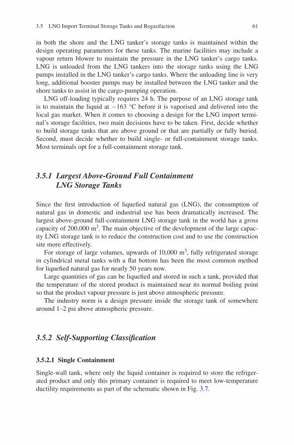
61

in both the shore and the LNG tanker’s storage tanks is maintained within the design operating parameters for these tanks. The marine facilities may include a vapour return blower to maintain the pressure in the LNG tanker’s cargo tanks. LNG is unloaded from the LNG tankers into the storage tanks using the LNG pumps installed in the LNG tanker’s cargo tanks. Where the unloading line is very long, additional booster pumps may be installed between the LNG tanker and the shore tanks to assist in the cargo-pumping operation.

LNG off-loading typically requires 24 h. The purpose of an LNG storage tank is to maintain the liquid at −163 °C before it is vaporised and delivered into the local gas market. When it comes to choosing a design for the LNG import termi-nal’s storage facilities, two main decisions have to be taken. First, decide whether to build storage tanks that are above ground or that are partially or fully buried. Second, must decide whether to build single- or full-containment storage tanks. Most terminals opt for a full-containment storage tank.

3.5.1 Largest Above-Ground Full Containment LNG Storage Tanks

Since the first introduction of liquefied natural gas (LNG), the consumption of natural gas in domestic and industrial use has been dramatically increased. The largest above-ground full-containment LNG storage tank in the world has a gross capacity of 200,000 m3. The main objective of the development of the large capac-ity LNG storage tank is to reduce the construction cost and to use the construction site more effectively.

For storage of large volumes, upwards of 10,000 m3, fully refrigerated storage in cylindrical metal tanks with a flat bottom has been the most common method for liquefied natural gas for nearly 50 years now.

Large quantities of gas can be liquefied and stored in such a tank, provided that the temperature of the stored product is maintained near its normal boiling point so that the product vapour pressure is just above atmospheric pressure.

The industry norm is a design pressure inside the storage tank of somewhere around 1–2 psi above atmospheric pressure.

3.5.2 Self-Supporting Classification

3.5.2.1 Single Containment

Single-wall tank, where only the liquid container is required to store the refriger-ated product and only this primary container is required to meet low-temperature ductility requirements as part of the schematic shown in Fig. 3.7.

3.5 LNG Import Terminal Storage Tanks and Regasifaction

62 3 Liquefied Natural Gas

3.5.2.2 Full Containment

Double-wall tank designed and constructed so that both inner and outer containers are capable of independently containing the stored refrigerated product as shown in Fig. 3.8 and additionally allowing for controlled release of product vapour resulting from a product leakage from the primary (inner) container resulting from a credible event.

There are two standards normally used to build LNG facilities in the world: the North American standard of NFPA 59A (Incorporates an LNG tank standard of API 620) and the European standard of EN 1473 (Incorporates an LNG tank standard of BS 7777).

According to BS7777, LNG tanks are classified into three different types. Single-containment tank is either a single tank or a tank comprising an inner tank and outer container designed and constructed so that only the inner tank is required to meet the low-temperature ductility requirements for storage of the product. Full-containment tank (Fig. 3.8) is described as a double tank designed and constructed so that both the inner tank and the outer tank are capable of independently contain-ing the refrigerated liquid stored. The difference between the double containment and full containment is that the outer tank of a full-containment tank is intended to be capable of both containing the refrigerated liquid and of controlled venting of the vapour resulting from product leakage after a credible event.

Among these three types of LNG tanks, the full-containment type is regarded as the most advanced type. The tanks are also classified by the elevations from the ground level: above-ground type, in-ground type and under-ground type.

Suspended deck Glasswool

Carbon steel tank

9% Ni steel tank

Perlite

Resilient blanket

Foamglas

Dyke

NG

NG

NGLNG-162 °C

Fig. 3.7 Single containment [1]

63

The largest tank developed in the world is an above-ground, full-containment type diagrammatically shown in Fig. 3.9, which consists of inner and outer tank. The inner tank is manufactured with 9 % nickel steel and the outer tank is com-posed of reinforced concrete and pre-stressed concrete. The 9 % nickel steel is widely used as a material for the inner tank since it has the strength and toughness enough for the cryogenic uses. The inner tank also has a function of preventing the LNG from leakage. Meanwhile, the concrete outer tank is designed to resist all the external loads including seismic load. Insulating materials are placed between the inner and outer tank to preserve the stored LNG.

The tank is of an above-ground, 9 % nickel steel full-containment type with a pre-stressed concrete outer tank and a corner protection system of 9 % nickel steel as a secondary barrier. The base of the tank has a bottom heating system (BHS) using ethylene glycol as brine fluid. The roof has a suspended ceiling deck and a steel-lined concrete dome.

First of all, different hydraulic calculations and process simulations from ship to tanks were carried out for determining the maximum elevation of the tank top. With the results of the calculations and simulations and the technical requirements above, the size of the tank to be developed was determined. Typical cross section of the full containment is shown in Fig. 3.10 indicating the different layers of the tank.

The LNG is stored in the 9 % nickel steel inner tank. The steel liner installed on the inside surface of the outer concrete tank provides the gas tightness. The boil-off rate is determined by the insulation system.

FoamglasSecondary 9% Ni steel bottom

Suspended deck Glasswool Carbon steel + concrete roof

9% Ni steel inner tank

Post-tensioned concrete shell

Perlite

Resilent blanket

9% Ni thermal corner protection

NG

NG

NGLNG-162 °C

Fig. 3.8 Full containment [1]

3.5 LNG Import Terminal Storage Tanks and Regasifaction

64 3 Liquefied Natural Gas

Fig. 3.9 Full-containment LNG storage tank [1]

Fig. 3.10 Sectional view of the 200,000 m3 full-containment LNG storage tank [1]

65

In case of an LNG leakage, liquid may impact on the outer tank. Accordingly, the liquid tightness must be guaranteed by the corner protection system as well as the polyurethane foam coating installed on the inside surface of the concrete wall. The concrete outer tank protects the inner tank in case of an emergency coming from the outside. The BHS is installed in order to avoid frost heave.

The roof liner consisting of a 5-mm-thick steel membrane stiffened with rafters in radial and tangential directions acts as formwork for the concrete sphere. The steel structure is fabricated on the bottom slab and lifted by air pressure to its final position. Rafters and roof liner plates are connected with a steel compression ring anchored in the concrete roof ring beam by welding.

3.5.3 Tank Design

The principal design codes applied to the design of the inner tank are API 620 and NFPA 59A. Figure 3.11 shows a general procedure for the design of 9 % nickel steel inner tank and the basic design data applied in the design.

3.5.3.1 Static Design

The inner tank is sized to contain 200,000 m3 of LNG at a specific gravity of 0.48 in cold condition. An additional dead space for the in-tank pump NPSH of 2.0 m has been given at the bottom of the inner tank, and the allowance for seismic slosh plus free board has been made above the design liquid level to determine the height of the inner tank. Figure 3.11 shows stages involved in the design.

The thickness of 9 % nickel steel plates of the inner tank shell is designed:

• For the full head of LNG corresponding to the design liquid level• For a partial hydrostatic test load corresponding to 1.25 times the full head of

LNG.

The operating vapour pressure is equalised on both sides of the tank shell since the inner tank has an open top.

3.5.3.2 Seismic Design

The inner tank is designed as an unanchored and unstrained tank to resist the OBE and SSE level design accelerations given in basic design data.

3.5 LNG Import Terminal Storage Tanks and Regasifaction

66 3 Liquefied Natural Gas

Hoop LoadingsThe hoop forces on the inner tank shell are a combination of the static pressure due to the product liquid, the impulsive pressure due to the action of the impulsive component of the liquid, the convective pressure due to the action of the convec-tive component of the liquid, and the vertical (or barrelling) pressure caused by the vertical component of the seismic loading.

Resistance to OverturningThe calculation of the resistance to overturning caused by contained liquid action on the annular plate and the width and thickness of the annular plate are based on the requirements of API 620.

Design condition Design condition

Working volumeNPSH

Plate dimensionAllowable stress

Filling height

BOR calculation resultsAnnular space

Insulation properties

Diameter of inner tank Shell insulation Bottom insulation

Shell height Material selection Material selection

Shell courses Calculation of inner tank movement

Arrangement of insulation

Static calculation

Dynamic calculation

Calculation of perlite pressure

Seismic shell hoop tensionShell thickness

Moment on baseStress & stability check

Sliding force

Blanket material and thickness

Calculation of seismic test load

Choose material

Shell thickness Annular plate Stiffener ring Bottom plate

Shell thicknessAnnular plateStiffener ring

Calculation of total weight on insulation

Fig. 3.11 General design procedure for 9 % nickel inner tank [1]

67

Shell CompressionThe shell compression is calculated using the procedure in API 620 for unan-chored tanks. The maximum allowable shell compression is in accordance with API.

Seismic SloshingThe seismic slosh height is calculated using the formula from API 620 L.8. An addition for shell run-up is made in accordance with the requirement of API 620 paragraph L.8.1.

Secondary BottomIf the secondary bottom is located at the top of the base insulation, it will be almost at the same temperature as the inner tank bottom in service. In the event of an inner bottom leak, no thermal shock to the secondary bottom will be given.If the secondary bottom is located at the middle of the base insulation, it will be at a higher temperature than the inner tank bottom in service. Leakage from the inner tank bottom will give a local thermal shock to the secondary bottom. More severe considerations than the code requirements for allowable stress and joint fac-tors must be taken in this circumstance.

Corner Protection SystemIn case of a leakage from the inner tank, LNG may accumulate in the annular space between the inner and outer tanks and cool the wall/bottom corner. In order to prevent the LNG from cracking of the lower concrete wall section, a liquid tight protection system thermally isolated with cellular glass insulation and shielded with 9 % nickel steel plates will be provided as shown on Fig. 3.12. The design will be carried out using finite element analysis taking into account pressure loads and thermal stresses/movements.The outer tank shall be capable of containing the full inner tank contents. Minor and major leak cases shall be checked by finite element analyses and combined with the maximum pressure in the analyses.

Suspended DeckThe suspended deck is designed to resist the loadings of self-weight, insulation weight, differential vapour pressure, construction traffic and seismic loadings. The design code applied in the design is British Standard Code of Practice CP 118.An aluminium-suspended deck with concentric ring stiffeners is used, and the thickness of the deck plate is 5 mm. The deck plate is thermally isolated by glass fibre blankets of six layers as shown in Fig. 3.13 for the top corner arrangement.

Roof SheetingRoof sheeting design is in accordance with the rules of API 620 or RPLAS. The design pressure for the roof sheeting will be maximum air pressure for either air-lift or during concreting of the roof.

Roof FittingsThe reinforcement of the roof plates for the roof fittings is designed in accord-ance with the rules of API 620. If heat breaks are fitted, they shall be designed

3.5 LNG Import Terminal Storage Tanks and Regasifaction

68 3 Liquefied Natural Gas

in accordance with BS5500. The loadings to be considered include self-weight, product weight, seismic loadings, loadings arising from the action of seismically induced liquid motions and wind loading on associated external and internal pipe work.

3.5.3.3 Thermal Design

The thermal insulation system of the tank is designed to have a boil-off rate less than 0.05 % of the full tank contents per day due to atmospheric heat leakage. The heat leak calculation is based on a maximum ambient air temperature and the product design metal temperature of −170 °C. The concrete base slab temperature is assumed to be +10 °C due to the bottom heating, and solar radiation effect is taken into consideration.

3.5.3.4 Design of Outer Tank

The outer container consists of an entirely closed monolithic concrete structure—bottom slab, wall ring beam and roof. The concrete containment is designed for

86400 inside dia of outer tank concrete wall

1200 84000 inside dia of inner tank

Polyurethane foam

Aluminium foil

Inner tank

Resilent glass fiber blanket

Perlite concrete Inner tank annular plate

9% Ni secondary bottom - 5 THK.

3 x 150mmt cellular glass

cellular glass

9% Ni corner protection

Loose fill expanded perlite

Fig. 3.12 Insulation and corner protection system [1]

69

all possible combinations of normal and emergency loads which may occur dur-ing construction, testing, commissioning, operating and maintenance of the tank. Design load combinations include the most severe combinations of loads. The general procedure for the design of outer tank is shown in Fig. 3.14, and the prin-cipal design code applied in this design is the British Standard BS8110: Structural use of concrete.

Design CriteriaThe concrete containment is designed for the conditions of four stages: construction, operation, test and emergency as shown in Fig. 3.14. The con-crete structure is designed on the ultimate limit state (ULS) and the ser-viceability limit state (SLS) for all normal situations and for the emergency situations of liquid spill in order to ensure containment for the liquid. For all other emergency situations, the concrete structure is designed on the ULS. The design was carried out according to the partial safety-factored design method of BS 8110. For the reasons of durability, the cracks at the concrete surface are limited.

Perlite fill nozzle

Radial roof rafter

Loose fill expanded perlite

Glass fiber

Suspended deck

Inner tank top stiffener

Support

Inner tank

Resilent glass fiber blanket

Puf

Outer tank wall

Roof anchor

Fig. 3.13 Top corner arrangements [1]

3.5 LNG Import Terminal Storage Tanks and Regasifaction

70 3 Liquefied Natural Gas

Loadings Considered in DesignThe loadings to be considered in the design of outer tank are as follows:For operation and test:

• Dead weight of the tank structure: concrete, inner steel tank, steel liners, sus-pended deck

• Pre-stressing including creep and shrinkage• LNG filling inner tank• Operating design gas pressure• Hydrostatic test of inner tank• Pneumatic test pressure• Piping and installation on roof• Live load on the dome• Wind• Snow• Temperature operation• Temperature difference slab–wall–roof

Inner tank dimensions

Outer tank dimensions

Determine springs for piles

Initial design of concrete section

(base, wall, ringbeam, roof)

Preliminary pre-stress calculation

Static analysis(Axi-symmetric shell model)

Seismic analysis(Full 3D shell model)

Stress resultant(Inplane axial force, inplane moment, inplane shear, hoop

force, hoop monent )

Determine concrete section

Fig. 3.14 Design procedure for concrete outer tank [1]

71

For emergency:

• Earthquake OBE• Earthquake SSE• LNG leakage• Temperature leakage• Increased overpressure• Thermal radiation from an adjacent area• Missile impact• Cold spot

Static AnalysisFor the static analysis of linear sectional forces, the main concrete tank structure is modelled using a semi-finite element computer program for axis-symmetric systems. The model comprises the bottom slab, the wall, the roof ring beam and roof. Spring elements were used to model the pile foundation in order to take into account the interaction between the tank structure and the subsoil.

Nonlinear AnalysisIn emergency cases in which the concrete is exposed to extreme temperatures due to heat radiation, nonlinear effects of the concrete behaviour caused by the reduced stiffness due to crack formation are taken into account. The linear analy-sis where the individual single load cases can be superposed, a nonlinear analysis must be carried out for load combinations determined previously.For nonlinear calculations, the reinforcement is an input data.

Dynamic AnalysisThe seismic calculations for OBE and SSE were done in two stages:

• Tank structure: modal analysis of an axis-symmetric model using acceleration response spectra as excitation input. The whole system is required to remain in the elastic limit; no physical or geometrical nonlinearities shall occur.

• Roof: additional modal analysis of a three-dimensional finite element model (roof) using response spectra as excitation input.

Figure 3.15 shows an example of full seismic analysis model including the outer tank, internal structures and liquid.Modelling of a burnout scenario involves 2D axisymmetric solid field elements and transient thermal analyses of the LNG tank outer walls. The tank roof and insulation layers (except any PUF layer) are assumed to have been destroyed and are not included in the analysis. Steady state conditions are initially applied for a specified time. To model the burnout situation, a temperature load of a specified peak temperature reducing to −170 °C over a distance of 1.5 m is moved down the inside of the tank at a constant speed for the burnout time under consideration. The constructed full containment is shown in Fig. 3.16 indicating the resulted structure.

3.5 LNG Import Terminal Storage Tanks and Regasifaction

72 3 Liquefied Natural Gas

Relief Valve Heat Flux ModellingWith relief valve heat flux modelling, the tank bases are normally excluded from an analysis because they are considered to be remote from the heat flux loading. 3D solid field and continuum elements are used for semi-coupled transient thermal analyses of a segment of an LNG tank. An initial stress-free temperature is applied to all elements, and steady state conditions are established for an internal tempera-ture of −170 °C and a specified mean annual external temperature. A heat flux is then be applied to a specified region on the top of the roof for the number of time steps under consideration.

Over The Top Piping and Tank Internal PumpsCodes require that shell/bottom penetrations be avoided, so all piping has to be over the top of the tank.Withdrawal is through in-tank pumps located in pump columns. Pump col-umns are provided with foot valves. In-tank pump systems require consider-able tank top piping plus provision for removing the pump out of the tank for maintenance.

AnchorsSingle-containment tanks need to be anchored to the foundation to resist uplifting loads due to tank internal pressure. This may not be necessary in

Fig. 3.15 Full model for 3D seismic analysis [1]

73

full-containment tanks, due to the weight of the concrete wall. This must be reviewed in high seismic locations.

Construction SequencesThese are shown in Figs. 3.17, 3.18, 3.19, 3.20, 3.21 and 3.22. The roof that has been built inside the tank is slowly lifted as shown in Fig. 3.23 using a shift in air pressure to raise the roof from floor to ceiling, when it reaches the top a team of welders secure the roof to the rim of the tank. The tank roof raising requires a focused effort to ensure that the work is completed safely. The wall profile is shown in Fig. 3.24.Roof air raising and then welding to compression ring, erection of outer concrete wall liner. The roof that has been built inside the tank is slowly lifted using a shift in air pressure to raise the roof from floor to the ceiling, when it reaches the top, a team of welders secures the roof to the rim of the tank. The tank roof raising requires a focused effort to ensure that the work is completed safely and that the all the people involved in this important task go home safely at the end of the day. The constructed wall profile is shown in Fig. 3.24.

Fig. 3.16 200,000 m3 full-containment LNG storage tank [1]

3.5 LNG Import Terminal Storage Tanks and Regasifaction

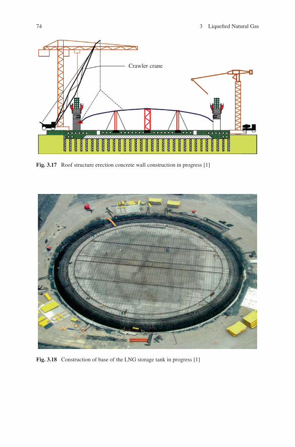
74 3 Liquefied Natural Gas

Crawler crane

Fig. 3.17 Roof structure erection concrete wall construction in progress [1]

Fig. 3.18 Construction of base of the LNG storage tank in progress [1]

75

Fig. 3.19 Roof structure erection concrete wall construction in progress [1]

Fig. 3.20 Construction of LNG storage tank side wall in progress [1]

3.5 LNG Import Terminal Storage Tanks and Regasifaction

76 3 Liquefied Natural Gas

Fig. 3.21 Construction of roof of LNG storage tank in progress [1]

Fig. 3.22 Completion of roof construction [1]

77

Fig. 3.23 Roof air raising in progress [1]

Fig. 3.24 Wall profile [1]

3.5 LNG Import Terminal Storage Tanks and Regasifaction

78 3 Liquefied Natural Gas

3.6 Regasification of LNG

The vaporisers at an LNG receiving facility transform LNG back into its gaseous state by warming the liquid so that the gas is at or above 5 °C (41 °F). There are several types of vaporisers in common use, but they all employ the same general principle—extracting heat from water to warm the LNG.

To return LNG to a gaseous state, it is fed into a regasification plant as shown in Fig. 3.25. On arrival at the receiving terminal in its liquid state, LNG is first pumped to a storage tank. When it is required for consumption, it is pumped at high pressure through various terminal components where it is warmed by passing it through pipes heated by direct-fired heaters, sea water or through pipes that are in heated water.

This illustration represents the process of taking liquefied natural gas (LNG) off of the ship as shown previously in Fig. 3.25, moving it into cold storage tanks and then regasifying it back into natural gas to send to market. The grey lines represent natural gas, and the yellow lines represent LNG. Naturally, there is a small amount of LNG which vaporises through contact with warmer air in the top of the ship containers and in the LNG storage tanks. This natural gas is syphoned out of the tanks and moved into the pipeline.

3.6.1 LNG Terminal Regasification Technology

The process of returning LNG to a gaseous state requires the introduction of heat energy.

Boil-off Compressor

Pipeline Compressor

VaporisersLNG storage

tank Pipeline

Condenser drum

Desuperheater

GasLiquid

Fig. 3.25 LNG import terminal gas flow [1]

79

The various vaporisation technologies considered include the following:

• Open rack vaporisers (ORVs)• Submerged combustion vaporisers (SCVs),• Shell and tube heat exchanger with heat transfer fluid (HTF)• Ambient air vaporisation systems, including:• Heat Integrated Ambient Air Vaporiser (HIAAV)• Direct Ambient Air Vaporisers (AAVs),

– Direct Natural Draft Ambient Air Vaporiser– Direct Forced Draft Ambient Air Vaporiser

• Indirect Ambient Air Vaporisers (IAAVs)

– Ambient Air Heat Exchanger with Heat Transfer Fluid (AAV-HTF)The following describes each vaporisation system in greater detail.

3.6.1.1 Open Rack Vaporisers (ORV)

The ORV is commonly considered in the design of LNG import terminals as shown in Figs. 3.26, 3.27, 3.28 and 3.29. The relatively low mechanical, electrical and process complexity and reduced air emissions present good engineering arguments in its favour. However, life cycle operating costs must also be considered. The ORV uses sea water as the sole heat source to vapor-ise LNG. The vaporiser consists of a heat conductor panel with multiple tubes through which the LNG passes. A typical ORV arrangement is illustrated in Fig. 3.26.

Sea water header

VaporiserOV

Natural gas

Sea water pump

Sea water intake

Drain channel LNG pumpLNG tank

Fig. 3.26 Open rack vaporiser (ORV) [1]

3.6 Regasification of LNG

80 3 Liquefied Natural Gas

Natural gas outlet

Sea water inlet manifold

LNG inlet

Cooled sea water discharge

Ambient sea water trough

Heat exchange panel block

Fig. 3.27 A typical open rack vaporiser (ORV) arrangement [1]

NG header

NG manifoldSeawater distributor

Concrete structure

Panel (heat exchange tubes)

LNG header

LNG

Seawater manifold

LNG manifold

Seawater distributing pipe

Fig. 3.28 A typical open rack vaporiser (ORV) arrangement [1]

81

LNG enters at the bottom of the vaporiser through a distribution header and moves up through the tubes while sea water flows down along the outer surface of the tube panels. Vaporised natural gas is removed from the top of the vaporiser and is sent to the distribution pipeline. The cooled sea water collects in a trough at the bottom of the vaporiser and is discharged to an outfall.

Chlorination of the sea water is used to prevent bio-fouling. Typically, sodium hypochlorite would be injected continuously to maintain a concentration of 0.2 ppm. In order to shock the system, elevated concentrations of 2.0 ppm would be injected for 20 min every 8 h, during ORV operation. De-chlorination of the effluent may also be required to meet environmental standards.

Further examples of open reach vapouriser arrangements and details are shown in Figs. 3.27, 3.28 and 3.29.

3.6.1.2 Submerged Combustion Vaporiser (SCV)

SCV systems are also commonly considered in the design of LNG import termi-nals as shown in Figs. 3.30 and 3.31. Study has shown the operational history, low capital cost, simplicity in design and operational flexibility combine to make this an attractive option. The SCV system uses natural gas as its heat source and requires electrical power to operate combustion air blowers and circulating water pumps. LNG is routed to a stainless steel tube bundle that is submerged in a water bath heated with flue gases generated by a submerged combustion burner. A sche-matic of typical SCV operation is presented in Fig. 3.30.

The forced air draft combustion burner is fuelled by low-pressure gas from either the boil-off gas (BOG) header or the natural gas send out pipeline. Hot

Fig. 3.29 Typical open rack vaporisation arrangement [1]

3.6 Regasification of LNG

82 3 Liquefied Natural Gas

exhaust gases from combustion are sparged into the water bath and create a rela-tively low-temperature (typically in the range of 12.8–32.2 °C) thermally stable heat source for the vaporisation of LNG flowing through the coil bundle. Natural gas exits the coils at pipeline pressure and temperature for pipeline distribution.

Since the SCV system does not use sea water, there is no impact on marine sys-tems. However, since the heat source is natural gas, consideration has to be given to emissions to the atmosphere from combustion. The capital cost of an SCV sys-tem is low when compared to other vaporisation systems. Since the SCV system uses natural gas as its heat source, operating costs are comparatively high. This reduces the attractiveness of SCVs as a sole means of vaporisation at the terminal. Figure 3.31 shows a typical SCV installation.

3.6.1.3 Shell and Tube Vaporiser with HTF

There are many configurations of shell and tube vaporiser technologies that are available for LNG applications. One such system uses a closed-loop heated water–glycol system to provide heat to vaporise the LNG using U-tube heat exchangers and a superheater. This is shown typically in Fig. 3.32. The HTF is warmed from an external heat source, such as a fired heater.

Since these types of vaporisers can be stacked, this arrangement requires rela-tively small amounts of space when compared to other available vaporisation tech-nologies. However, the inclusion of fired heaters requires additional space that can

Pilot gas inlets Exhaust stack Exhaust stackProcess fluid

InOutTube bundle

WeirCombustion air

Cooling water jacket

Water tank

Combustion air

Main gas inletDistributor duct with sparge tubes

Water recirculation

Fig. 3.30 Schematic of submerged combustion vaporiser [1]

83

negate the effects of any space saving advantages of this technology. The capital cost of the shell and tube arrangement with fired heaters is similar to that for SCV units.

3.6.1.4 Heat Integrated Ambient Air Vaporisation System with Waste Heat Recovery

This technology utilises the heat available in ambient air to vaporise LNG in a shell and tube heat exchanger as shown typically in Fig. 3.33. The design is gener-ally such that the required outlet temperature of the natural gas cannot be achieved from ambient heating alone, and therefore, supplementary heating is required. Supplementary heating is usually obtained from the transfer of heat from the exhaust of power generation prime movers such as gas engines or turbines to the natural gas, using a recirculating quench water system. Provisions for additional heat for vaporisation, should it be needed, can be made by trim heating the natural gas through a supplementary duct burner. The trim heater can be a conventional shell and tube exchanger or a printed circuit heat exchanger (PCHE).

Exhaust gases from the power generation gas turbine/engine are cooled in the waste heat recovery unit prior to entering the quench column, from where they are released to the atmosphere at approximately 90 °F. The quench column condenses water vapour from the flue gas, which results in a small blowdown stream that

Fig. 3.31 SCV installation [1]

3.6 Regasification of LNG

84 3 Liquefied Natural Gas

must be disposed of after treatment. Condensing the combustion products results in a high overall thermal efficiency of the system.

3.6.1.5 Direct Ambient Air Vaporisers (AAVs)

Direct AAVs transfer heat from the ambient air directly into the LNG through a heat exchanger heat transfer surface. In typical direct AAVs shown in Fig. 3.34, the LNG is passed through a manifold that divides the flow into a number of vaporiser units where a series of smaller flows are directed through individual heat transfer tubes. Each tube has aluminium fins for increased heat exchange area and is in direct contact with the ambient air.

HTF 36°F

Nat.Gas 40°F

HTF 54°F

LNG -240°F

36°F

-19°F54°F

36°F

54°F

36°F

-80°F

-80°F

-19°F

Fig. 3.32 Shell and tube vaporiser arrangement [1]

85

Although there is no significant operational experience for direct AAVs in high-volume LNG applications, Direct AAVs have been used in liquid nitrogen service (a fluid colder than LNG) for over 50 years.

While Direct AAVs are in operation, frost and/or ice will build up on the units due to the proximity of the LNG to the ambient air. The longer a unit runs, the

Quench column

Waste heat recovery unit

Natural gastrim exchangerVaporised fluid

Air

AirVaporisation service

Open

Closed

Cold air

Ice / water / cold air

Regenration service

Cryogenic fluid

Water catch basin

Condensed water to disposal

Air

Combustion air

Quench water circulation pumps

Power generation

Gas turbine / power generation

Fuel gas

Selective catalytic reduction

(if required)

Supplimental duct firing

(if required)

Fig. 3.33 Heat integrated ambient air vaporisation [1]

Fig. 3.34 Schematic of direct ambient air vaporiser [1]

Warm ambient air

Natural draft or fan assisted

Natural gas

Cool ambient air

Cold liquid LNG

3.6 Regasification of LNG

86 3 Liquefied Natural Gas

more frost and/or ice builds, which gradually reduces the performance of the unit due to a reduction in the heat transfer surface. Hence, Direct AAV units need to be periodically shut down and de-iced.

1. Direct Natural Draft Ambient Air Vaporisers

Direct Natural Draft AAVs shown in Fig. 3.35 rely on wind and natural convec-tive currents to move air over the tubes and fins of the vaporiser unit. As warm air contacts the tubes containing LNG, the air cools and becomes dense, caus-ing it to flow downwards to the bottom of the vaporiser unit. This causes warm ambient air from the surroundings to be drawn through the top of the unit.

The outlet gas temperature of a Direct AAV is dependent not only on ambient conditions but also on other factors such as run-time and number of units in operation. Consider a single AAV unit, at the onset of operation, the temperature of the outlet stream is nearly the same as the ambient temperature. As the run-time increases, the unit begins to frost and/or ice up, thus reduc-ing the amount of heat being transferred to the LNG. A significant amount of heat transfer is still achieved, but the temperature of the outlet stream reduces as time passes and ice accumulates.

2. Direct Forced Draft Ambient Air Vaporisers

In Direct Forced Draft AAVs shown typically in Figs. 3.36 and 3.37, airflow into the unit is controlled by fans installed on top of the vaporiser. Each unit can be equipped with shrouds on each side to direct airflow through the vapor-iser. Direct Forced Draft Vaporisers are approximately 1.7 times more effective than Natural Draft AAVs.

Fig. 3.35 Direct natural draft ambient air vaporiser in operation [1]

87

3.6.1.6 Indirect Ambient Air Heat Exchanger with Heat Transfer Fluid (AAVHTF)

This type of vaporisation system consists of shell and tube heat exchangers, fin-fan air heaters or reverse cooling towers and a heat transfer fluid (HTF)

Fig. 3.36 Direct forced draft ambient air vaporisers without shrouds [1]

Fig. 3.37 Direct forced draft ambient air vaporisers with shrouds [1]

3.6 Regasification of LNG

88 3 Liquefied Natural Gas

loop. Fin-fan air heaters are used to transfer heat from ambient air into the HTF, which is then sent to the LNG shell and tube vaporiser. The cooled HTF flows into a surge tank and is then pumped back to the air heaters as specified in Fig. 3.38.

The vaporised gas is then regulated for pressure and enters a pipeline system as natural gas. Once the LNG is regasified and leaves the regasifica-tion terminal, it ceases to be “LNG” and is indistinguishable from the conven-tional piped natural gas. Finally, residential and commercial consumers receive natural gas for daily use from local gas utilities or in the form of gas-powered electricity.

Although the main heat source for this vaporisation arrangement is the heat contained in the warm ambient air, supplemental heating is also required to main-tain capacity and delivery temperature when the ambient air temperature drops below a nominal value.

3.6.1.7 Supplementary Heating

When the ambient temperature is not warm enough to raise the temperature of the vaporised LNG to 4.4 °C, supplementary heating must be provided to provide natural gas to the pipeline at the required 4.4 °C. The minimum amount of heat needed from the supplemental system has been determined to be 133 MMBtu/h. To be conservative, the supplemental vaporisation system will be sized for 180 MMBtu/h which provides 35 % extra capacity. Figure 3.39 shows the sche-matic of vaporisation system.

Warm air

Cold air

Air heaters

Warm HTF

HTF pump

Cold HTF HTF surge tank

Shell and tube vaporiser

LNG

Pipeline gas

Fig. 3.38 Schematic of AAV-HTF system using air heat exchangers [1]

89

3.7 Safety on LNG Carriers

3.7.1 Hazards on LNG Ships

3.7.1.1 Cryogenic Hazard

Since liquefied gases are carried at very low temperatures, they pose a very seri-ous threat in terms of cold burns, frost bite and damage to structures by making them brittle and susceptible to fracture. For temperature below −55°, fully killed fine grain carbon manganese steels are required. For temperature below 104°, high nickel content steels, stainless steel or aluminium may be used.

Due to the thermal stresses caused by changes in temperatures, the cryogenic property of LNG makes it necessary to carry out operations such as cooling down at a very regulated and controlled rate.

3.7.1.2 Flammability Hazard

LNG is a flammable substance. Methane vapour is easily ignited. Much effort is put into ship design to ensure effective cargo containment so as to limit vapour escaping to atmosphere and adjacent spaces. In addition, ships and terminals have design specifications for electrical equipment so as to ensure that, within well-defined operating zones, such sources of ignition are eliminated. Furthermore, in ship and terminal working environments, stringent operational procedures apply that limit other possible sources of ignition. Because of the very rapid vaporisa-tion of spilled liquefied gases, the spread of flammable vapour will be far more

Vaporised LNG @ < 40°F

Natural gas@ 40°F Sendout

station

Vaporised LNG @ > 40°F

Supplimental gas fired vaporiser

Ambient air

vaporiser

Cold LNG from tank

Fig. 3.39 Schematic of vaporisation system [1]

3.7 Safety on LNG Carriers

90 3 Liquefied Natural Gas

extensive than in the case of a similar spillage of oil. The chances of ignition fol-lowing a spill of liquefied gas are, therefore, much greater.

The amount of vapour produced depends upon the volatility of the liquid.Volatility can be defined as the tendency of a liquid to evaporate. Volatility of a

liquid is measured using the following:

• Flashpoint• Vapour pressure• Boiling Temperature at atmospheric pressure.

3.7.1.3 Oxygen Deficiency Hazard

Oxygen deficiency in an enclosed space can occur due to any of the following conditions:

• When large quantities of cargo vapour are present.• When large quantities of inert gas or nitrogen are present and• Where rusting of internal tanks surfaces has taken place leading to oxygen

depletion below 21 %

In the case of LNG cargoes, the presence of large quantities of LNG vapour would act as an asphyxiant and hence cause oxygen deficiency.

Normal content of oxygen in the atmosphere for survival is 21 %. Susceptibility of persons to reduced oxygen levels varies, but at levels below 19 %, impaired mobility and mental confusion rapidly occur. At levels below 16 %, unconsciousness takes place rapidly and may lead to permanent brain dam-age and will result in death.

3.7.1.4 Reactivity Hazard

Hydrate Formation: with moisture and water, the cargo can form ice and slushy material which can lead to clogging of pipes and impellers etc. Since CO2 also forms dry ice at temperatures below −70°, this would also manifest as a powder in the tanks.

Self-Reaction: this risk does not exist in the case of LNG Reactions with other materials: for LNG, this hazard is not significant; however, due the vary-ing composition of the gas, the specific material safety data sheets should be referred to.

3.7.1.5 Hazard Due to Low Flashpoint

The lowest temperature at which a liquid gives off sufficient vapour to form a flammable mixture with air near the surface of the liquid.

91

Flashpoints of some gases are given below in degrees celsius:

• Methane: −175 °C• Propane: −105 °C• Butane: −60 °C

3.7.1.6 Auto-Ignition Hazard

The auto-ignition temperature of a substance is the temperature to which its vapour-in-air mixture must be heated to ignite spontaneously. The auto-ignition temperature is not related to the vapour pressure or to the flashpoint of the substance, and since the most likely ignition sources are external flames or sparks, it is the flashpoint rather than the auto-ignition temperature which is used for the flammability classifi-cation of the hazardous materials. Nevertheless, when vapour escapes are considered in relation to the adjacent steam pipes or other hot surfaces, the auto-ignition tem-perature is worthy of note. Listed below is auto-ignition temperature of some gases:

• Methane: 595 °C• Propane: 468 °C• Butane: 365 °C

3.7.1.7 Rollover Hazard

This is more common in shore tanks and is primarily caused by the layering caused by density differences. When lighter fractions evaporate from the surface, the heav-ier fractions that remain form a dense layer at the top of the tank trapping the less dense layer below. As the cargo continues to warm, the layers at the bottom get less dense, and at a certain stage, this becomes unstable and the dense layer rolls over to the bottom causing the lighter fractions to rise to the top with a heavy release of vapour. This phenomenon is less likely to occur on ships due to the constant motion of the vessel which would not allow the layering process to occur.

To summarise the hazards that can be associated with LNG, ships would fall under one of the following categories.

• LNG—hazards associated are frost bite, asphyxiation and flammability• Inert gas—toxic, skin irritation• Nitrogen—asphyxiant

3.7.1.8 Pressure Hazard

Due to the high evaporation rate of liquefied natural gases, there is a tendency to produce very high pressures in closed containment systems. Hence, all cargo sys-tems are provided with relief valve arrangements so as to mitigate the risk of dam-age to the containment systems.

3.7 Safety on LNG Carriers

92 3 Liquefied Natural Gas

Pressure surges also can cause significant damage to pipelines which are caused by static and dynamic forces. Hence, to deal with this risk, it is neces-sary to regulate the flow in manner so as to avoid the kinetic energy being con-verted into a strain energy that traverses the length of the pipeline at the speed of sound.

The size of the pressure surge is dependent upon the density of the liquid, the rate of deceleration and the length of the pipe. Pressure surges commonly can occur when filing a dead segment of a pipeline too fast, slamming of valves or even opening and closing a pipe segment to relieve pressure which would cause a sudden acceleration followed by a rapid deceleration.

3.8 First Aid Action

In the event of accidental leakage, or during maintenance tasks, personnel may be exposed to liquid or gaseous products being carried. The overall approach in the avoidance of hazards to personnel should always be prioritized as follows:

• Hazard removal• Hazard control, and then only on• Reliance on personal protection

3.8.1 Skin Contact

Since liquefied gases are carried at cryogenic temperatures, they constitute a sig-nificant hazard in terms of sustaining frost bite. If the skin is exposed to severe cold, the tissue becomes frozen. The symptoms of frostbite are extreme pain in the affected area (after thawing), confusion, agitation and possibly fainting. If the affected area is large, severe shock will develop initial symptoms are the skin ini-tially becomes red, but then turns white

• The affected area is usually painless and• The affected area is hard to touch if the area is left untreated, and the tissue will

die and gangrene may occur.

Treatment

• Warm the area quickly by placing in warm water (~42 °C) until it is thawed.• Keep the patient in a warm room.• Do not massage the affected area• Severe pain may occur on thawing: give pain killer or morphine if serious• Blisters should never be cut or clothing removed if it is adhering firmly• Dress the area with sterile dry gauze• If the area does not regain normal colour and sensation, obtain medical advice.

93

3.8.2 Inhalation

The hazard with LNG inhalation is asphyxiation as the LNG vapour can result in the deprivation of oxygen supply to the blood. Although no toxic properties are present, a condition of asphyxia can lead to unconsciousness and can be fatal if the condition is not reversed.

Some cargoes are toxic because their chemical composition/properties can result in temporary or permanent health hazards causing symptoms such as irrita-tion, tissue damage or impairment of faculties.

Other gases may effect the nervous system (state of anaesthesia). The uncon-scious person may react to sensory stimuli, but can only be roused with great difficulty.

3.8.3 Ingestion

Cases of ingestion on board will be very rare. MFAG and MSDS for the concerned cargo to be referred for the exact procedure to be followed.

3.8.4 LNG Fire Fighting Techniques and Equipment

Fire fighting on-board ships is an inherently hazardous and dangerous operation. The effects of smoke and heat are magnified by the steel structure which confines and controls the direction of the spreading fire. The steel structure, with ventilation shafts and multiple openings, also gives a fire an opportunity to spread in a three-dimensional fashion which requires ship’s staff to have an intimate knowledge of both the ship’s structure and fire fighting techniques and procedures.

In the case of a fire, it is vital that the response time is minimised as specifically in the case of LNG, spillage would result in the formation of a large flammable vapour cloud which could spread to other areas/sources of ignition.

Any LNG spillage would immediately start to boil-off as mentioned above. If the escaping liquid has a temperature below ambient, then the gas will form a vis-ible white cloud since it condenses the water vapour in the atmosphere. Should ignition take place the cloud will be rapidly consumed and flash back to the area above the leak. The rate of vaporisation will be increased by the heat generation.

The most effective way of stopping such fire is by cutting off the source and extinguishing the fire by starvation. The emergency shutdown system should be activated immediately and as many cargo system valves as possible closed. This will isolate most of the cargo system. In taking this action, it is important to know that suitable arrangements should be made to relieve the pressure in the pipelines as warmed up LNG inside these lines may expand and cause further leaks and damage to the system.

3.8 First Aid Action

94 3 Liquefied Natural Gas

3.8.4.1 Use of Dry Powder

The chemical reaction of the small particles of the extinguishing material when exposed to flame extinguishes the flame. Various types of powders are marketed; potassium-based powders are more effective than the sodium-based or multi-pur-pose powders.

When using the dry powder, the following points are worth noting:

• Because of the danger of reignition, dry powder should not normally be used unless the source of gas can be isolated.

• Maximum possible rate of application is desirable and as many high velocity jets as are available should be brought to bear at once so that reserves are not wasted and successful extinguishment obtained.

• Coordinated simultaneous attacks with all available applicators, if possible from windward, will have maximum effect.

• Jets should be aimed with the objective of reducing boil-off rate by sweeping the whole fire area, but on no account must the pool be agitated.

The powder jets should be slightly depressed below the horizontal sweeping rap-idly back and forth over the entire fire area. Direct impact of the powder jets on the liquid pools should be avoided. The application should be such that the entire surface area of the burning pool is covered. LNG ships are provided with dry powder hose stations along the cargo decks. The hoses are 15–20 m long and are located along the cargo deck so that they can cover the cargo tanks, manifolds and the machinery spaces. Figure 3.40 summarises the several steps taken to contain such incidents.

Process Isolation and DrainingIsolating valves and pipelines also require careful consideration as trapped LNG in a pipeline would expand rapidly when heated and can result in ruptures in the pipelines causing new leaks and extensive damage. This could cause a greater spread of the fire. Hence, when isolating, it is essential to drain the contents back into the tank or safely depressurize the system. Relief via the vent masts is pro-vided with nitrogen snuffing systems while draining back to tanks would have to be done with great care to prevent flash back to the source.

Water Spray ProtectionWater spray systems are designed to apply water at a predetermined application rate to protect specific equipment or areas. Water is cheap and at sea is readily available. It is non-toxic and does not give rise to toxic products. It has high heat absorption capability in terms of its specific heat and latent heat of vaporisation. When water turns to steam, the volume increase is in the ratio of 1:1,700.Steam forms a protective cover around the fire cutting off the supply of air, so that the combustion cannot be supported. Water spray system can be used to protect tanks, ship structure and fire fighters from radiated heat. Fixed water curtains and spray systems should be backed up by portable spray hoses. Fire fighters should

95

1 2 3 4

5

Water Fire Extinguishers Foam Fire Extinguishers

Powder Fire Extinguishers CO2 Fire Extinguishers

Solid Stream Wide Stream Water Wall

Fig. 3.40 Ideal use of water hoses [1]

3.8 First Aid Action

96 3 Liquefied Natural Gas

approach from windward protected from possible flash burns by water sprays and/or protective clothing.Water can also be used to prevent contact of liquid LNG with deck and metallic structures thereby reducing the chances of brittle fracture.

Use of High-ex Foam (Limited Use Only in Machinery Spaces)Application of foam would result in forming a barrier which would prevent the radiation from the flame to the liquid below and will thereby reduce the vapori-sation rate and consequently the extent and radiation of the fire. Foam should be continuously applied and a depth of 1–2 m should be achieved. High expansion foam of about 500 to 1 expansion ratio has been found to be the most rapidly effective for this purpose. Portable foam tanks would generally be found in the E/R and other machinery spaces; however, their use in the cargo spaces is limited.

Action to be Taken in the Event of LNG Vapour ReleaseIn the event of unintentional vapour release, the following actions should be taken: Spaces and areas where leakages or spillages have occurred should be evacuated upwind immediately. Take care as flames may be invisible. Leaking gas may be extremely cold.Measures should be taken to prevent leaking gases from penetrating into any other part of the ship. Bear in mind that some gas are heavier than air or may otherwise accumulate in lower or non-ventilated parts of the ship. Particular attention should be taken in order to prevent gases drifting into occupied areas of the ship, e.g. liv-ing quarters, machinery spaces and working areas.Wear protective clothing suitable for gas protection and self-contained breathing apparatus.Avoid all sources of ignition (e.g. naked lights, unprotected light bulbs, electric hand tools, friction). Wear non-sparking footwear.Even short inhalation of small quantities of gas can cause breathing difficulties.Keep clear of evolving gases. Avoid all skin contact.Let spilt liquefied gas evaporate. When in contact with cold liquefied gases, most materials become brittle and are likely to break without warning. Avoid all contact even when wearing protective clothing. If practicable, protect ships superstructure with copious quantities of water. Do not direct water jet into the centre of the spill.

Spillage On DeckSmall spillage: Let gas dissipate. Keep clear.Large spillage: Let gas dissipate. Keep bridge and living quarters upwind. Otherwise, protect crew and living quarters against flammable or toxic gases using water spray to drive gases away (water curtain). Spilt liquefied gas: Use water jets from as far as practicable to accelerate evaporation, not directing them straight onto the spill.

Spillage Under DeckSmall Spillage: Do not enter space. Provide adequate ventilation. Where a ventila-tion system is used, particular attention should be taken in order to prevent gas penetrating into other areas of the ship. Let gas evaporate. Keep clear.

97

Check atmosphere before entering (toxicity and explosion hazard). Do not enter space without self-contained breathing apparatus.Large spillage: Do not enter space. Provide adequate ventilation. Where a ven-tilation system is used, particular attention should be taken in order to prevent gas drifting into other areas of the ship. Bridge and living quarters must be kept upwind. Otherwise, protect crew and living quarters against flammable or toxic gases using water spray to drive gases away (water curtain). If practicable, use water spray to avoid ignition of flammable gases in the space. Check atmosphere before entering (toxicity and explosion hazard). Do not enter without self-con-tained breathing apparatus.

LNG JettisonThere are occasions where it is necessary to jettison cargo from a cargo tank.A containment or insulation failure in one or more of the cargo tanks may neces-sitate the jettisoning of cargo from that particular cargo tank to the sea.Jettisoning of cargo from a particular cargo tank to the sea is carried out using a single main cargo pump, discharging LNG through a portable nozzle fitted at the ship’s manifold. The jettison pipe is stored on the deck forward of the compressor house.As jettisoning of LNG will create hazardous conditions:

• All relevant fire fighting equipment must be manned and maintained in a state of readiness during the entire operation.

• All accommodation vents, other openings and all vent fans must be secured with the exception of that ventilation to the engine room necessary to maintain it in an operational status.

• The NO SMOKING rule must be rigidly enforced.• The fixed installation water curtain is to be placed in operation on the side of the

jettison to protect the ship’s structure.

The portable nozzle is approximately 6.5 m long and when connected extends 1.5 m from the ship’s side. Weather conditions, and the heading and speed of the vessel relative to the wind, must be considered so that the jettisoned liquid and resultant vapour cloud will be carried away from the vessel. In addition, if pos-sible, avoid blanketing the vapour with exhaust gases from the funnel as shown in Fig. 3.41. The discharge rate must be limited to the capacity of one cargo pump only and, if necessary, reduced to allow acceptable dispersal within the limits of the prevailing weather conditions.

Too rapid a flow of LNG will result in rapid phase transfer (RPT) when the liquid hits the sea water. Violent increase in gas vapour as liquid hits the sea water, producing a very cold cloud of vapour which does not dissipate readily from the immediate vicinity of the vessel.

Vent Mast on FireIt is likely that occasionally one of the four LNG vent masts will light-off when the ship is travelling through a thunder and lightning storm.

3.8 First Aid Action

98 3 Liquefied Natural Gas

The possible causes of the fire are as follows:

• Cargo tank pressure above 19kPa can result in one or more of the cargo tank safety valves temporarily lifting off their seats due to the surging motion of the ship in extremely rough sea conditions

• Leaking vapour header forward vent control valve CG702• Leaking cargo tank safety valve• Manually controlled venting through control valve CG702

The fire should be extinguished, but there is not any real danger to the ship or its personnel while the fire is burning because all of the LNG vent masts incorpo-rate the following safety features:

• Hood is located 12 m above the trunk deck• Hood and vent mast are 316 grade stainless steel• Hood is fitted with a regulatory body approved flame screen to prevent any

flame from passing across the screen and down into the vent mast• A nitrogen fire smothering valve is piped to each LNG vent mast

3000 3500

Securing bracket8" nozzle for cargo

6" end nozzle for

cargo

Manifold ship side

rail

16" flange

Manifold deck

Water curtain header

Upper deck

Fig. 3.41 LNG jettison [1]

99

Corrective Action to Extinguish the Fire on the Top of the LNG Vent MastIf carrying out controlled venting from No.1 LNG vent mast:

1. Stop venting by closing the control valve CG702.2. Manually open the nitrogen fire smothering valve piped to No.1 LNG vent

mast.

If non-controlled venting:

1. Manually open the nitrogen fire smothering valve piped to the LNG vent mast that has the flame.

2. If that does not extinguish, the flame and other means of reducing the cargo tank pressure fail:

• Insert a 1-mm-thick blank flange into the outlet flange of the cargo tank relief valve that is suspected of leaking and reopen the nitrogen fire smothering valve.

• If that does not extinguish the fire, remove the blank flange from the first tank relief valve and place it in the outlet flange of the other tank relief valve protect-ing the tank.

Reopen the fire smothering valve on the vent mast. If that extinguishes the flame, leave the fire smothering valve partially open to that mast and remove the 1-mm-thick blank from the outlet flange on the cargo relief valve.

Boil-Off Rate Measurement PurposeThe purpose of this note is to define the method of boil-off rate (BOR) measure-ment on-board G.T.T. membrane-type LNG carriers designed for QGTC and hav-ing a total cargo capacity of 266,000 m3 each.The design daily BOR of cargo during laden voyage shall be less than 0.135 % of the full loaded cargo when assuming the following conditions:

• Ambient air temperature = +45 °C• Sea water temperature = +32 °C• Cofferdams temperature maintained at +5 °C• Cargo considered as pure methane (density 425 kg/m3, latent heat of vaporisa-

tion 511 kJ/kg)• Cargo piping empty.

References

1. Morje, Prakash, (2011) “LNG Reliquefaction plants with economical techniques of transport-ing LNG by ships” University of Salford, UK.

2. http://www.worldoil.com/February-2006-Process-selection-is-critical-to-onshore-LNG-economics.html (05/03/2013).

3.8 First Aid Action

101

4.1 Gas Flow in Circular Pipes

4.1.1 Introduction

Since natural gas almost always flows through circular pipes, it is thus important to understand how the gas behaves in the pipes. What are the flow parameters and the properties of the flowing fluids and what are the gas flow governing equations in distribution and transmission systems? For gas flow in pipes, the parameters such as velocity, pressure and density, which describe the behaviour and state of a fluid, are not constant. They vary from one point in the pipe to another and from one instant in time to another. The concepts of steady and unsteady state flow in the context of some fundamental flow parameters should assist in better under-standing of how gas behaves in practice. In order to simplify many of the practi-cal problems encountered in the gas industry, we make a distinction between flow where the parameters vary with time (unsteady or transient flow) and flow that can be considered steady (although strictly speaking no gas flow is truly steady).

Transient flow is dealt with later in this module; for the time being we will only consider steady state

Flow Not surprisingly, steady state flow is much simpler to analyse than tran-sient flow, and fortunately, it can be applied widely in gas transportation, particu-larly for low-pressure distribution.

Steady state flow is defined as that in which the various parameters at any point do not change with time. Uniform flow is defined as that in which the various parameters at any particular instant do not change with position.

Often, we can assume steady state uniform flow, for example flow at a constant rate through a long straight pipe of constant cross section. However, the assump-tion of uniform flow is not valid near to the solid boundaries along which the fluid is flowing. This is because all fluids have viscosity, (a property that determines the

Chapter 4Gas Flow and Network Analysis

© Springer International Publishing Switzerland 2014 G.G. Nasr and N.E. Connor, Natural Gas Engineering and Safety Challenges, DOI 10.1007/978-3-319-08948-5_4

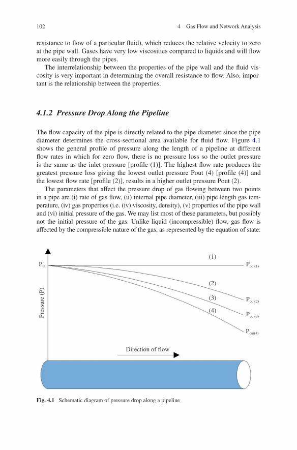
102 4 Gas Flow and Network Analysis

resistance to flow of a particular fluid), which reduces the relative velocity to zero at the pipe wall. Gases have very low viscosities compared to liquids and will flow more easily through the pipes.

The interrelationship between the properties of the pipe wall and the fluid vis-cosity is very important in determining the overall resistance to flow. Also, impor-tant is the relationship between the properties.

4.1.2 Pressure Drop Along the Pipeline

The flow capacity of the pipe is directly related to the pipe diameter since the pipe diameter determines the cross-sectional area available for fluid flow. Figure 4.1 shows the general profile of pressure along the length of a pipeline at different flow rates in which for zero flow, there is no pressure loss so the outlet pressure is the same as the inlet pressure [profile (1)]. The highest flow rate produces the greatest pressure loss giving the lowest outlet pressure Pout (4) [profile (4)] and the lowest flow rate [profile (2)], results in a higher outlet pressure Pout (2).

The parameters that affect the pressure drop of gas flowing between two points in a pipe are (i) rate of gas flow, (ii) internal pipe diameter, (iii) pipe length gas tem-perature, (iv) gas properties (i.e. (iv) viscosity, density), (v) properties of the pipe wall and (vi) initial pressure of the gas. We may list most of these parameters, but possibly not the initial pressure of the gas. Unlike liquid (incompressible) flow, gas flow is affected by the compressible nature of the gas, as represented by the equation of state:

Pin Pout(1)

Pout(2)

Pout(3)

Pout(4)

(1)

(2)

(3)

(4)

Direction of flow

Pre

ssur

e (P

)

Fig. 4.1 Schematic diagram of pressure drop along a pipeline

103

where P is the gas gauge pressure (N/m2), V is the volume of gas (m3), Z is the compressibility factor of gas, m is mass of the gas (kg), R is the universal gas con-stant (J/m2 K) and T is the gas temperature (K).

4.1.3 Properties of Flowing Fluid

4.1.3.1 Viscosity: Dynamic and Kinematic

All fluids will resist any force tending to cause one layer to move relative to another layer. However, this resistance is offered only while the movement is taking place. As a result, as soon as the external force is removed, the flow subsides due to the resisting forces. There is no tendency for the fluid particles to revert to their original positions when the fluid motion ceases. This resistance to movement of one fluid layer adjacent to another is said to be due to the viscosity of the fluid. The forces resisting the relative movement of fluid particles are called viscous forces and are dependent not only on external forces, but on the nature of the fluid itself.

“Thick” fluids such as treacle or tar are said to be very viscous; they do not flow very easily because the forces resisting relative movement between the fluid particles are strong. “Thin” fluids such as water flow more readily and gases even more so. If the viscous forces resisting the overall motion of a fluid exist between layers of individual fluid particles, then these layers must be moving at different velocities. The force opposing the motion of the fluid is the result of a stress being set up within the fluid between each layer, where the stress (T) is equal to the force (F) divided by the area over which the force acts (A). For the straight and parallel motion of a given fluid, the tangential stress between two adjacent layers is proportional to the velocity gradient (δu/δy) in a direction perpendicular to the layers. Thus:

Assuming that the velocity varies only perpendicularly to the flow, then in the limit as δy tends to zero then:

The constant of proportionality µ is called the coefficient of dynamic (absolute) viscosity of the fluid.

The value of µ is a function of the temperature of the fluid. In the case of a gas, µ is a function of pressure, although only at extremely high or low pressures (both of which are outside the normal pipeline operating pressures). The unit of dynamic viscosity is kg/ms or Pa s. There is no name given to this unit, which for practical purposes is too large. More commonly used is the centipoise (cP), which is 1,000 times smaller than the Pa s. Table 4.1 provides the value of µ at metric standard condition (MSC).

(4.1)PV = ZmRT

(4.2)τ =F

A∝

δu

δy

(4.3)F = µAdu

dy

4.1 Gas Flow in Circular Pipes

104 4 Gas Flow and Network Analysis

As we have seen, the viscous forces are proportional to the viscosity (μ), and since the forces of inertia are proportional to the density (ρ), the ratio µ/ρ, known as the kinematic viscosity (v), is a useful concept. The SI unit of kinematic viscosity (m2/s) is too large for most practical purposes. A more commonly used unit is the centistoke (mm2/s). Table 4.2 shows typical values of kinematic viscosity at MSC.

The magnitudes of the numerical values are reversed. For example, the absolute viscosity of air is about 1/70 that of water. The kinematic viscosity is about 12 times that of water. This is because the density of air is much lower than the den-sity of water.

Because the viscosities of gases are generally of the same order of magnitude, it is possible to use correlations to calculate the viscosity of a gas mixture from the known viscosities of the individual gases that make up the mixture. Such a correlation is:

where Mm is the absolute viscosity of the mixture, µi is the absolute viscosity of gas i, xi is the mole fraction of gas i in the mixture and MWi is the molecular weight of component i.

4.1.4 Pressure and Altitude

4.1.4.1 Pressure Head

The pressure at any point in a liquid is determined only by the vertical distance of the point of measurement below the free surface of the liquid. Pascal’s law tells us that this pressure will be the same in any horizontal direction and is unaffected by

(4.4)µm =∑

µixi

√MWi

∑

xi

√MWi

Table 4.1 Typical value of dynamic viscosity for different gases

Gas Dynamic viscosity (Pa.s)

Hydrogen 8.4 × 10−6

Methane 10.7 × 10−6

Air 17.0 × 10−6

Water 1,150.0 × 10−6

Table 4.2 Typical value of Kinematic viscosity for different gases

Gas Kinematic viscosity (mm2/s)

Hydrogen 105.0

Methane 15.4

Air 14.0

Water 12

105

the shape or size of the vessel containing the liquid. In Fig. 4.2a, the absolute pres-sure of the liquid at point X is equal to the atmospheric pressure (Pa) plus the addi-tional pressure resulting from the height of the liquid (h). This concept can also be applied to physically enclosed liquids where, for example, the pressure in a pipe containing water could be represented by a column of water extending upwards to a height h above the pipe as shown in Fig. 4.2b.

In each case, the pressure is given by:

where h is the pressure head in metres of water, p is the density, and g is the accel-eration due to gravity (9.81 m/s2). Clearly, trying to measure the pressure of gas in metres of gas is impractical, but we can measure it as an equivalent height of another fluid, for example water, by using a water-filled manometer.

4.1.4.2 Effect of Altitude

Equation 4.3 is only valid because the density of a liquid is assumed to remain constant over the height h. Gases are compressible, thus to determine the pressure at one point in a static column of gas relative to another point at a different eleva-tion: first consider that the gas at any point to be in equilibrium; this must be so since the gas is not moving. Then, we consider a thin element (δh) over which the density can be considered sensibly constant, as shown in Fig. 4.3.

For the element to be in equilibrium, the forces on δh must balance (force on bottom surface = force on top surface + weight of gas in element). Thus, the pres-sure between the bottom and top can be expressed as:

(4.5)P = ρgh

(a)

(b)

h

Pa

X

h

Fig. 4.2 Pressure at a point X in a fluid column (a) and the pressure head concept (b)

4.1 Gas Flow in Circular Pipes

106 4 Gas Flow and Network Analysis

Or by substituting for R = 287/S, Eq. 4.6 becomes:

where S is the relative density (air/gas), Pb is the bottom pressure (N/m2) and Pt is the top pressure (N/m2).

It should be clear from the results above that large elevation changes are required to produce even moderate corrections to the absolute pressure. As a rule of thumb, a static column of natural gas produces a pressure “head” equivalent to 1 % of the gas pressure for every 150 m of elevation. This may not appear to be very significant, but accuracy of pressure data is important for the effective uti-lisation of line pack and for modelling the operation of the transmission system on a daily basis. The equilibrium of the gas assumes that the pressure below the thin element (p + δp) is greater than the pressure above it (p). The pressure for

(4.6)Pb = exp

(

gH

ZRT

)

Pt

(4.7)Pb = exp

(

0.03417SH

ZT

)

Pt

Fig. 4.3 The element δh in equilibrium

0

H

h

P

P

Pt

Pb

A

H

107

natural gas with no buoyancy effect is when the atmospheric conditions are the same as MSC, the density of the gas would need to be the same, assuming the den-sity of air is 1.225 kg/m3, with relative density of natural gas being typically 0.5 at a range of pressure. Therefore, using ideal gas law:

And for natural gas of relative density 0.59, this gives p 171,742 Pa or approxi-mately 700 mbar (gauge). So, above 700 mbar, there is no buoyancy effect and Eq. 4.7 can be used, although as we have seen the effect is negligible unless large elevations are involved. The elevation differences within medium or intermediate pressure distribution systems are not great enough for Eq. 4.7 to have any effect so its use is restricted to transmission systems that traverse mountainous terrain. Below 700-mbar (gauge) natural gas is buoyant, relative to atmospheric air, so we must approach the problem from a different direction. Consider the vertical pipe, shown in Fig. 4.3, which is holding a static column of natural gas. There are effec-tively two columns of gas in equilibrium, one of natural gas inside the pipe, and one of atmospheric air outside. Because we are considering very low pressures, the density of each can be considered constant over the height h.

As can be seen from Fig. 4.4, if the gas gauge pressure was measured at the base of the column, it would be:

There is therefore an increase in the gauge pressure reading due to the difference in the densities of gas and air. This “increase” in gauge pressure would be nega-tive if the gas density was greater than that of air (as with propane or butane, for example). This effect is only apparent because the density of low-pressure natural gas is of the same order of magnitude as atmospheric air. It is not apparent when measuring the pressure of a liquid, because the density difference is too great for variations in the density of air to be noticed. Of course, there is no change in the absolute pressure of the gas, so before carrying out any flow calculations, we must always correct any gauge pressure readings to a common datum. The gauge pressure correction factor, (pa − Pg)gh, can be simplified for general use by introducing the relative density and converting the pressure units to mbar, which leads to:

This simplified version of the gauge pressure correction factor is restricted to low-pressure use only—up to 75 mbar (gauge). The restriction applies because the use of the relative density requires that the gas is at or near MSC. As the pressure increases, the density increases, and as we have seen, natural gas has approximately the same density as air at 700 mbar (gauge). If accurate corrections are required to gauge readings above 75 mbar, they should be made using (ρa − ρg) gh.

(4.8)P = ρgRgTg = 1.225 ×287.06

S× 288.15

(4.9)Pg +(

ρa − ρg

)

gh

(4.10)Low pressure gauge correction = 0.12(1−S)h

4.1 Gas Flow in Circular Pipes

108 4 Gas Flow and Network Analysis

4.1.5 Laminar and Turbulent Flow

4.1.5.1 Boundary Layer

Physical examination of a fluid flowing in a pipe shows that there is a thin layer of fluid adhering to the pipe wall and that the velocity of this layer relative to the pipe wall is zero. This zero-velocity layer affects the successive layers of flowing fluid. The normal distance from the pipe wall at which the flowing fluid ceases to be affected by the stationary layer is called the boundary layer thick-ness. The idea of a stationary layer of fluid, particularly gas, may seem surpris-ing but it is true even for the smoothest of pipe materials. It is in the boundary layer that the fluid velocity changes with distance from the boundary, from zero at the pipe wall to the velocity of the main flow stream, approaching this veloc-ity asymptotically as shown in Fig. 4.5. In the boundary layer, the velocity gradi-ent normal to the pipe wall, du/dy, is large, so even a low value of viscosity is very significant and may not be disregarded even though its effect on the main flow may be negligible.

Beyond the boundary layer thickness, the free flow is affected much less by the fluid viscosity and in many practical applications may be treated independently as though the boundary layer did not exist

Fig. 4.4 Vertical pipe with static column of natural gas column of natural gas

h

Pa

Pa - agh

Atmosphere Gas

Pa + Pg - gh

Pa + Pg

109

Fluid flow may be conveniently divided into two types of flow:

(i) laminar flow where the viscous forces tending to resist fluid movement pre-dominates, creating a boundary layer that effectively extends to the centre of the pipe from the pipe wall.

(ii) turbulent flow where the viscous forces are restricted to a thin layer that extends only a short distance in from the pipe wall. The characteristics of tur-bulent flow will be described in Sect. 4.1.5.3.

4.1.5.2 Laminar Flow

In laminar flow (sometimes called viscous flow), the viscous forces predominate and the entire flow could be defined as a boundary layer. This usually occurs at low velocities. It is the viscosity of a fluid that determines the resistance to move-ment of fluid particles between parallel layers of the fluid. If the viscous forces are predominant, then the flow of that fluid will occur in layers. For a circular pipe, these layers must consist of concentric “tubes” of fluid. The resulting velocity pro-file is parabolic where the velocity of the fluid layers increases from zero at the pipe wall to a maximum value at the centre. In most pipe flow problems, it is not

Fig. 4.5 Changes in fluid velocity with distance from the boundary surface

u = 0 at the boundary surface

u1

u2

u3

u4 Asymptoteu4 = Umax

Incr

easi

ng v

eloc

ity

4.1 Gas Flow in Circular Pipes

110 4 Gas Flow and Network Analysis

the velocity of the gas that is of interest but the quantity being transported. Thus, the volume flow rate (Q) is given by the continuity equation as:

where u is the velocity and A is the flow area, i.e. the cross-sectional area of the pipe. However, we cannot use the maximum velocity since this is not representa-tive of the velocity profile, nor can we use the minimum, since this is zero. The actual volume flow rate is given by:

where Ua is the average velocity. In the case of the velocity profile for laminar flow, Ua = 0.5 Umax. The use of the average velocity (Ua) is valid provided the flow is steady and continuous. Laminar flow can be mathematically analysed with-out the use of any additional coefficients or experimental data. This analysis leads to Eq. 4.13, which is known as the Hagen-Poiseuille equation:

where Q is the volume flow rate, d is the diameter of the pipe, µ is fluid viscos-ity, ΔP is pressure loss over the length of the pipe and L is the length of the pipe. The two important features of laminar flow are: (i) the volume flow rate (Q) is inversely proportional to fluid viscosity (µ) and (ii) the pressure loss ΔP is directly proportional to Q.

4.1.5.3 Turbulent Flow

Turbulent flow can be described as flow where any of the fluid particles are not travelling in straight parallel lines; they begin to take on random and irregular flow patterns, although the principal motion of the fluid along a pipe is still maintained leading to fluid mixing. Figure 4.6 shows the transition of the flow from laminar to turbulent regime.

The laminar layer adjacent to the pipe wall is known as the laminar sub-layer, and the flow is described as being partially turbulent.

The boundary layer, remember, is the distance from the pipe wall at which the flowing fluid ceases to be affected by the stationery layer, so in Fig. 4.6c, it is defined by the distance at which the velocity profile no longer changes with dis-tance from the pipe wall. So within the boundary layer, we have two types of flow occurring, the laminar sub-layer and an outer turbulent region. Further increases in flow rate (and hence velocity) cause the laminar sub-layer to become thinner. Theoretically, the layer would continue to decrease in width indefinitely as the fluid velocity increases. However, in practice, the laminar sub-layer becomes—so thin that it no longer covers the surface roughness of the pipe. In this situation, elements of the internal surface of the pipe are in contact with areas of turbulent flow. When this occurs, the fluid flow is described as fully developed turbulent flow.

(4.11)Q = U.A

(4.12)Q = Ua.A

(4.13)Qπd4

∆P

128 µL

111

4.1.6 Predicting Flow Types

Osborne Reynolds in the late nineteenth century argued that any general law gov-erning the flow of fluids must be concerned with the criteria that make the behav-iour of the fluid similar to the behaviour of that fluid, or any other fluid, when similar conditions are imposed on it. For fluid to be similar, the shape of the con-duits in which they are flowing must be similar, and the forces causing the fluid to move must also be similar, that is when the forces acting on a particle in one flow are in the same ratio of magnitudes as the forces acting on a particle at the corre-sponding point in another flow. For natural gas flow, the first condition is usually satisfied since the gas is transported in circular pipes.

Reynolds reasoned that the ratio of the inertial force to the viscous force (see previous Sect. 4.1.3) would not only determine similarity of flow but would also indicate the change of flow regime between laminar and turbulent flow. This is providing of course that the shape of the conduit is similar in all cases. So, for a circular pipe of diameter d, Reynolds Number (Re) is given by:

It represents the ratio of the forces of inertia to the viscous forces and hence is dimensionless. A high value of ρ, d or U− or a small value of µ gives a high value of Re, and of course, the converse is also true. Natural gas has a low value of vis-cosity and a low value of density, but do you remember. The kinematic viscosity (see Sect. 4.1.3) for natural gas is large, compared with water for example, so this tends to lead to high Re values. When this is combined with a large diameter, as

(4.14)Re =ρUd

µ

Boundary layer

Turbulent core

Pipe boundary Pipe wall

Laminar sub-layer

(a)

(b)

(c)

Fig. 4.6 The transition of flow from laminar to turbulent

4.1 Gas Flow in Circular Pipes

112 4 Gas Flow and Network Analysis

with some transmission pipelines, the Reynolds number under these circumstances would be very high. Re cannot change if the pipe dimensions and gas viscosity remain constant because Reynolds number is an indication of fluid flow similar-ity. If the quantity of gas flowing in at one end is the same as the quantity leaving at the other and then the flow is not just similar, it is the same. For steady state flow, the mass flow rate remains constant along the length of the pipe, so as the pressure (and density) decreases the volume flow rate (Q) must increase and since U− = Q/A, the velocity also increases. It is this increase in velocity that compen-sates for the fall in density and maintains a constant value of Re.

For natural gas, since both density and velocity change with falling pressure, we usually calculate Re as though all the flow occurred at MSC. Of course, the flow cannot actually occur at MSC, but this does not matter because the value of Re is determined by complementary values of ρ and U−, so MSC are just as valid as any other set of conditions.

For steady state gas flow, the mass flow rate of gas entering a pipe is equal to the mass flow of gas leaving the pipe, so the continuity equation is:

This is valid not only for the continuity of mass flow in the pipe but also for expressing the mass flow rate of the same gas at MSC. Thus, by using Eq. (4.14) and substituting Eq. (4.15), therefore, the Re for natural gas can be expressed as:

Assuming Qs to be in m3 (st)/h and d to be in mm and ρa = 1.225 kg/m3, µ = 10. 38 × l06 kg/m s and relative density S = 0.6.

A high value of Re indicates that the forces of inertia dominate the flow, so it is likely to be turbulent. When Re is small the viscous forces are the most significant so the flow will probably be laminar. As a general rule, the following types of flow can be expected for the given ranges of Re. These are: Re < 2,000 laminar, Re 4,000 > partially turbulent and Re > 107 fully turbulent.

The region between Re = 2,000 and Re = 4,000 is known as the critical zone. It is so called because the flow cannot easily be defined as either laminar or tur-bulent; it is the point at which the inertia forces are approximately equal to the viscous forces.

4.1.7 The Effects of Friction on Flow

Friction in fluid flow, as with any other process, results in a loss of energy, but in order to be able to lose energy, the fluid must first possess it! The idea that flu-ids possess energy was first postulated by Euler in the eighteenth century. Euler describes the total energy possessed by a moving fluid as follows:

(4.15)ρ1A1U1 = ρ2A2U2 = ρsAsUs

(4.16)Re = 25, 043Q

d

113

where x is the elevation above some arbitrary datum, P is absolute pressure, u is fluid velocity, ρ is the fluid density and g is gravitational acceleration.

The density of natural gas ρ varies with pressure. So, it would be necessary to relate ρ and p using the equation of state. For now, let us consider an incom-pressible fluid, but we will return to the question of a compressible fluid in a later section.

This is generally known as Bernoulli’s equation.Each of the terms in Eq. 4.18 possesses the unit of length, and so the equation

describes the total energy head of a given fluid. The quantity x is the elevation above some arbitrarily chosen horizontal datum and represents potential energy. The quantity u2/2 g is known as the velocity head and represents kinetic energy. The quantity p/ρg is known as the pressure head and represents the energy avail-able from pressure forces. This energy is not stored, in the sense of a compressed fluid. It is only available if there is a pressure difference in the fluid system that will allow the transmission of this pressure energy. In fact, none of the terms in Bernoulli’s equation represent stored energy, but together they represent the total mechanical energy to be transmitted by the fluid.

Let us return to fluids in an ideal fluid system in which there are no transmis-sion losses, so the total energy head will remain constant between any two points in the system. However, including the transmission losses, which is caused mainly by friction that can be denoted by hf, Eq. (4.18) at any two points in the fluid can be expressed as:

In laminar flow, the fluid moves in layers with a stationary layer of fluid at the pipe wall, so all the pressure loss is due to the properties of the fluid [refer to Eq. (4.13)]. There is no contact between the pipe wall and the flowing fluid.

In fully turbulent flow, the surface roughness of the pipe wall is in contact with the flowing fluid, all traces of laminar flow have disappeared and the pressure losses are due entirely to the friction caused by the fluid flowing over the pipe wall surface.

For partial turbulence, where there is a laminar sub-layer adjacent to the pipe wall, the losses are due to a combination of pipe wall properties and fluid prop-erties. Let us now consider frictional head loss in laminar and turbulent flow regime.

(4.17)dx +dp

ρ.g+

u.du

g= 0

(4.18)x +P

ρ.g+

u2

2g= Constant

(4.19)x1 +P1

ρ1.g+

u21

2g= x2 +

P2

ρ2.g+

u22

2g+ hf

4.1 Gas Flow in Circular Pipes

114 4 Gas Flow and Network Analysis

4.1.8 Frictional Head Loss in Laminar and Turbulent Flow

4.1.8.1 Frictional Head Loss in Laminar Flow

By using the Hagen-Poiseuille equation for laminar flow (4.13), the continuity Eqs. (4.12) and (4.19), the frictional head loss in laminar flow (due to friction between layers of fluid) is seen to be inversely proportional to Re and the frictional effects can be represented directly by 16/Re, which can be expressed as:

4.1.8.2 Frictional Head Loss in Turbulent Flow

Turbulent flow is highly complex due to the random movements of fluid particles superimposed on the main flow, since these random movements are unpredictable, there is, unlike laminar flow, no complete analytical solution for turbulent flow. However, if we look at the result of the above activity, we see that of the parame-ters involved, only 16/Re contains the value of the fluid viscosity, which is the root cause of the head loss in laminar flow. In a general equation for head loss, includ-ing turbulent flow, we might expect an expression of the form:

where f is a general friction factor.As early as 1841, Weisbach had developed a resistance equation using a dimen-

sionless coefficient to describe the energy lost by a fluid in motion. At around the same time, the French engineer Darcy was working on similar ideas, as expressed in Eq. (4.21).

This is commonly called the Darcy–Weisbach equation, but you may see it referred to simply as the Darcy equation. It is identical to that suggested by the extension of the laminar flow equation where 16/Re is replaced by an empirical friction coefficient (f). Because f is an empirical coefficient, the method of evaluat-ing it is not universal and various methods have been developed for this purpose. In particular, you should be aware that equations presented in other texts might use a value of f that is a multiple of the Darcy friction factor.

In North America, it is common to use a friction factor that is four times that defined by Eq. 4.20; this does not matter as long as the numerical coefficient in the equation is adjusted accordingly. In Britain, Transco uses both u−/2 g and L/d as performance criteria in the specifications for the supply of fittings to be used in their gas distribution system.

(4.20)hf =4LU

2

d.2g×

16

Re

(4.21)hf =4fLU

2

d.2g

115

4.1.9 Friction in Turbulent Flow

The parameters that affect the friction losses are represented in Fig. 4.7. Figure 4.7a represents the theoretical concept of a pipe with a perfectly smooth internal surface. If such a pipe existed, the laminar sub-layer would always com-pletely cover the pipe wall even though it would become very thin at high veloci-ties. In such circumstances, the main body of turbulent flow would never come into contact with the pipe wall so it is reasonable to assume that the wall plays no part in the resistance to flow. In fact, as with laminar flow, only the value of Re would be important.

(a)

(b)

(c)

(d)

Incr

easi

ng v

eloc

ity

Velocity profile

Velocity profile

Velocity profile

Velocity profile

Laminar sub-layer

Laminar sub-layer

Laminar sub-layer

Laminar sub-layer destroyed by edges

Perfectly smooth pipe

Rough pipe surface

Fig. 4.7 Effect of friction losses

4.1 Gas Flow in Circular Pipes

116 4 Gas Flow and Network Analysis

Figure 4.7b represents a real pipe with an internal surface, which consists of small particles, creating a certain amount of roughness. In this case the laminar sub-layer is thick enough to completely cover the surface roughness, so, as with a theoretically smooth pipe, the turbulent fluid flow does not come into contact with the internal pipe surface. It behaves as though it were a smooth pipe and so only the value of Re is significant.

In Fig. 4.7c, the laminar sub-layer has become thinner due to increasing veloc-ity and now some of the roughness peaks are just protruding through the sub-layer and into the turbulent flow. The flow is no longer independent of the internal pipe surface, but it is still partly dependent on Re since there is still a laminar sub-layer.

Finally, in Fig. 4.7d, increased velocity has caused the laminar sub-layer to shrink even more, allowing the pipe roughness to protrude further into the turbulent flow stream causing eddies to form around each particle that destroys the remains of the sub-layer. Since there is no laminar sub-layer, the influence of fluid viscosity disappears and the flow is no longer dependent on Re, only the surface roughness of the pipe.

4.1.9.1 Relative Roughness

The progression from smooth pipe flow to rough pipe flow is obviously dependent on the surface roughness. However, the description of fully developed turbulent flow as rough pipe flow does not indicate that the pipe is actually very rough, only that the roughness is totally responsible for the friction losses. The degree of pipe roughness is described by its relative roughness.

It is not easy to express the internal roughness of pipes in a quantitative man-ner, because we all have a different idea of what “rough” is. All surfaces, no mat-ter how well polished, are to some extent rough, in so much as there are minute particles making up the surface of the material. The irregularities created by these minute particles vary greatly in shape, size and spacing, making an absolute meas-ure of roughness very difficult. If we could make measurements of the height of these surface particles, we could arrive at a value for the mean height, which over a considerable area, could be expected to influence the frictional resistance to flow. Extending Reynolds’ reasoning on the similarity of flows would indicate that a relative roughness rather than an absolute roughness would be significant in deter-mining the characteristics of the flow. In the case of circular pipe, this is:

Relative roughness = Mean height of surface particles (Σ)/Internal pipe diameter (d)

This is also shown diagrammatically in Fig. 4.8.

4.1.9.2 Smooth and Rough Pipe Laws

Figure 4.7 represents the perfectly smooth pipe shown in Fig. 4.7a, but it also rep-resents the situation shown in Fig. 4.7b where the laminar sub-layer completely covers the surface roughness. You should note that the smooth pipe friction factor (fsp) is dependent only on Re.

117

The rough pipe friction factor (frf) is dependent only on the values of d and Σ (the relative roughness), and since these are constants for a given pipe, the friction factor is also constant.

The inverse of the relative roughness appears in the rough pipe law. In some textbooks, particularly, those published in the USA, the inverse is used instead of the relative roughness. The ratio d/M is known as the roughness factor.

4.1.9.3 The Moody Diagram

The American engineer Lewis F. Moody, in a synthesis of earlier work, presented his concept of fluid flow behaviour in the form of a diagram, which now bears his name—the Moody diagram. Figure 4.9 is a Moody diagram based on the Darcy friction factor (for laminar flow f = 16/Re). Remember, you may see other dia-grams based on multiples of this, for example f = 64/Re, for laminar flow. Friction factor should always be checked using the diagram to identify the following:

i. the laminar flow regionii. the smooth pipecurveiii. a series of lines representing values of relative roughnessiv. the critical zone between laminar and turbulent flow (B)v. the region of complete turbulence where the rough pipe law applies (D)vi. the transition zone between the smooth pipe and rough pipe regions (C).

In Moody’s diagram (Fig. 4.9), the curves representing the transition from smooth pipe to rough pipe are based on Colebrook’s equation and his experimental data using commercial grade pipes. These curves are used widely for predicting friction factor values in general pipe work systems

4.1.10 General Flow Equation

In order to develop the general flow equation, it is necessary to make some assumptions about the pipe system and the flow through it. As we will see, the assumptions do not place any excessive restrictions on the use of the equation. The

d

Relative roughness = d

Fig. 4.8 Relative roughness of the internal surface of a pipe

4.1 Gas Flow in Circular Pipes

118 4 Gas Flow and Network Analysis

flow process is isothermal, changes in the kinetic energy of the gas are negligi-ble, the pipeline is horizontal, no mechanical work is done by or on the gas, the energy loss due to friction is given by the Darcy–Weisbach Eq. (4.21) and the flow is steady state. Using Eqs. 4.17–4.21, the gas velocity at standard conditions for a given pressure drop can be expressed as:

The actual gas velocity varies along the pipe. It does not occur at standard condi-tions, but this is a convenient way of expressing it because it allows us to solve Euler’s equation for gas flow and can be converted to a volume flow rate at stand-ard conditions. Thus, the general flow equation can be written as:

In this equation, all the units are self-consistent, but for general use, it is conveni-ent to express it in terms of the units that are normally used:

• Pipe length (L) m Gas pressure (p) bar

• Pipe diameter (d) mm Gas flow rate (Q) m3 (st)/h

• Gas temperature (T) K

(4.22)Us =Ts

Ps

√

(

P21 − P2

2

)

d.Rg

2f .L.Z .T

(4.23)Q =7.574 × 10−4

√f

Ts

Ps

√

(

P21−P2

2

)

d5

S.L.Z .T

Fig. 4.9 Moody diagram

119

This equation applies over all pressure ranges and is the basis for many of the flow equations used in the analysis of transmission and distribution networks.

In summary, the general flow equation, using gas industry units, is given by:

The general flow equation can be simplified, for use in MP systems, to the following:

For use in LP systems, the general flow equation can be simplified further to

4.1.11 Friction and Smooth Pipe Law

As we are now familiar with the flow equations used for gas transmission and dis-tribution systems, let us consider the practical implications of using the smooth pipe law. In particular, let us examine the use of an efficiency factor for modelling the energy loss more accurately.

The transition from smooth pipe flow to fully turbulent (rough pipe) flow is shown as a series of curves in the Moody diagram. The curves are asymptotic to the smooth pipe and rough pipe curves and represent Colebrook’s data. So far, gas flow has been described as following the smooth pipe law, but no real system can follow it exactly because real systems are not perfectly smooth. Therefore, some significant factors such as actual pipe roughness, pipe joints, welds, bends, tees, fittings, valves, dust and debris.

In the case of gas transmission pipelines, these factors are uniformly distributed throughout the system and form a very small proportion of the overall pipeline length. The US Bureau of Mines’ tests indicate that the deviation from the smooth pipe law could be represented by a fixed percentage of the smooth pipe flow. This leads us to the idea of an efficiency factor that could correct the smooth pipe law to actual conditions which can be expressed as:

where E is an efficiency factor that converts the smooth pipe transmission factor into an actual transmission factor.

Taking the general flow equation as an example, this could be written as

(4.24)Q =7.574 × 10−4

√f

Ts

Ps

√

(

P21−P2

2

)

d5

S.L.Z .T

(4.25)Q =1.269 × 0−2

√f

√

(

P21−P2

2

)

d5

S.L

(4.26)Q =5.712 × 10−4

√f

√

(P1−P2)d5

S.L

(4.27)E =Qactual

Qsmooth pipe

4.1 Gas Flow in Circular Pipes

120 4 Gas Flow and Network Analysis

A typical value of E is 0.95 for a new pipeline and is constant for a wide range of Re. However, for distribution systems, this must be treated somewhat differently because of the higher incidence of drag-inducing elements. These elements induce energy losses, which can be expressed as a number of velocity heads (u2/2 g).

The total energy loss is obtained by adding together the velocity head losses of all the elements. Since there are a significant number of elements, the overall energy loss is sufficient to create a deviation from the smooth pipe law, which is dependent on the gas velocity. This deviation from smooth pipe conditions is not great enough to be considered as a Colebrook-type transition (for new pipes at least), but is sufficient to cause a deviation that increases with velocity. So for low-pressure distribution systems, we have:

Values of e at two velocities are given in the Table 4.3 for polyethylene pipe. Values of e selected from the Table 4.3 with the nearest velocity to that required are usually adequate for general calculations.

4.1.12 Other Flow Equations

The general flow equation developed in Sect. 4.1.10 is the basis for all gas flow equations and is valid for all pressure and flow conditions found in practice. One could come across other flow equations with other names, but these are all varia-tions of the general flow equation. Usually, it is the method chosen for the deter-mination of the transmission factor that gives its name to the flow equation. In this section, we will look briefly at some of these and comment on their usefulness.

Before the introduction of computers, the need to solve the general flow equa-tion by hand led to the development of some empirical but explicit friction factor relationships. Here are some of them

Blasius was the first to suggest a relationship of this kind, so equations of this kind are known as “Biasius-type” equations. Polyflo and Panhandle “A” are perhaps the best known, but they are all approximations to the smooth pipe law. Other friction

(4.28)factual =fsp

E2

(4.29)factual =fsp

e2

Blasius 1√f= 3.558 Re0.125

Meuller 1√f= 3.350 Re0.130

Fritsche 1√f= 5.145(Re.d)0.125

Polyflo 1√f= 5.350 Re0.076

Panhandle “A” 1√f= 6.87 Re0.07305

121

factor relationships that depend only on the pipe diameter, such as Unwin, Pole, Weymouth and Spitzglass, are crude approximations and should not be used.

The Panhandle equation is typical of gas flow equations that use a transmis-sion factor relationship of the Blasius type. Since it represents gas flow reasonably accurately, albeit within restricted ranges of Re, we can adopt the general form as a basis for describing gas flow in pipe networks.

Take another look at the Panhandle “A” flow in Sect. 4.1.12. All equations of this type may be represented by:

where n is the flow exponent and K is the resistance factor and are chosen accord-ing to the type of fluid and pipe system

The LP gas flow equation has the general form

At 75 mbar, the absolute pressure is 1.08825 bar, so the maximum pressure loss that can be accommodated using the LP equation is 2 % of this, i.e. 22 mbar.

4.1.13 Gas Velocity

We mentioned earlier about the effect of velocity on Reynolds Number and the compensating effect of density, which results in a constant value of Re along the length of a pipeline for a fixed mass flow of gas. We also extended this concept using the continuity Eq. (4.14) to allow us to use the volume flow of gas expressed at MSC in the general flow equation.

This is a very convenient way of expressing the flow; however, the actual con-ditions in the pipe are affected by the change in velocity (u) and density (ρ), for example dust migration is caused by high gas velocity [2].

(4.30)∆P2 = K .Qn

(4.31)∆P = K .Qn

Table 4.3 Typical pipe-sizing criteria

e6 represents 6 m between butt welds ande12 represents 12 m between butt welds

Nominal pipe size (mm)

SDR Maximum internal bead height (mm)

Velocity = 1.5 m/s efficiency factor

Velocity = 4.7 m/s efficiency factor

e6 e12 e6 e12

90 11 5.0 0.91 0.95 0.87 0.93

125 11 5.0 0.92 0.96 0.89 0.94

180 17 5.0 0.94 0.97 0.92 0.96

250 17 6.3 0.92 0.96 0.89 0.94

315 17 7.9 0.90 0.95 0.87 0.93

355 17 8.9 0.89 0.94 0.86 0.92

400 17 10.0 0.87 0.93 0.83 0.90

500 17 12.5 0.84 0.91 0.91 0.88

4.1 Gas Flow in Circular Pipes

122 4 Gas Flow and Network Analysis

The highest velocity occurs at the end of a pipeline where the pressure (and hence the density) of the gas is lowest. In order to maintain the same mass flow as the density falls, the velocity must increase. The Institution of Gas Engineers codes of practice recommends that the maximum velocity in a pipeline should not exceed 20 m/s. This is a practical constraint based on the damage that could be inflicted by gasborne dust, not a theoretical velocity limit. Because of the impor-tance of gas velocity in the management of dust, it is often necessary to know what the gas velocity is likely to be at a particular point in the system. The average velocity is given by u = Q/A, but we cannot use the flow rate calculated from the flow equations directly to obtain the velocity. The flow equations give the gas flow rate in m3(st)/h, so the velocity calculated from u = Q/A, would not be the actual gas velocity. The actual gas velocity is lower because the gas is under pressure. We must correct the flow rate to actual m3/h before calculating the velocity.

From the ideal gas law, we get:

where Ps, is the pressure at MSC and p is the actual gas pressure at the point of interest.

Remember, the gas velocity increases in the direction of flow as the pressure decreases, so at any particular point in the system where we need to know the velocity, we may not know the actual pressure. Usually, it is only convenient to measure the gas pressure at locations where the system is above ground, but the point at which we need to know the velocity may be some distance away. Take a look at Fig. 4.10. This shows a pipe where the value of velocity is required a dis-tance L from the point at which the gas pressure is measured. Using the following equation enables us to calculate gas velocity in any distribution main operating at pressures up to 7 bar (gauge):

The speed at which any gas can travel is limited to the speed at which sound can travel in the same gas. The speed of sound in Methane gas is 396 m/s. In gas pipe-lines, this very high velocity is not a practical constraint because the gas normally f1ows at less than 20 m/s. However, when gas escapes in an uncontrolled manner from a hole or pipe break, it will escape at the speed of sound provided that the pressure ratio of the internal pressure to the atmospheric pressure is more than the Critical Pressure Ratio. This ratio varies according to the gas composition but for a typical natural gas, it is approximately 2:1. For the critical pressure ratio to be 2:1, then the absolute pressure of the gas in the pipe must be twice the absolute atmospheric pressure. Taking the atmospheric pressure to be approximately 1 bar abs, then the internal pipe pressure would need to be 2 bar abs, or approximately l bar(gauge). Therefore, in all gas supply systems, except low-pressure distribu-tion systems, escaping gas will travel at the speed of sound. The speed of sound

(4.32)U =Q.Ps

A.P

(4.33)u2 = 353.68Q.Ps

√

d

d5.P21 − 6211.2Q2f .S.L

123

is a physical property of a gas, and it has important implications for the design and operation of pipeline systems operating under transient flow conditions as dis-cussed in the next section.

4.2 Network Analysis

4.2.1 Introduction

Natural gas is one of the world’s largest sources of primary energy supply. For many years, this type of gas was flared in the production of crude oil, but gradu-ally it began to replace town gas, mainly from coal. Over the years, gas reserves have grown at a substantial rate and natural gas has developed into a necessity across the world.

For the efficient, safe and reliable exploitation of natural gas resources, trans-portation of natural gas from various locations to consumers is of prime impor-tance. The gas industry is a very capital intensive industry. It can be suggested that the economics of its transportation may well be as important as the safety aspects. Therefore, design engineering and economic judgment are very important in the viability of any gas project.

In gas transmission systems, the gas flows are constant, and most operate 24 h a day, 7 days a week, 365 days a year. However, particularly in long-dis-tance pipelines, time-varying processes do exist in the systems due to the starting

Direction of flow (Q)

Vel

ocit

y

l 0 L

U1

P1

U1 + U

P1 - dP

U2

P2

Fig. 4.10 Change of velocity with pressure and distance

4.1 Gas Flow in Circular Pipes

124 4 Gas Flow and Network Analysis

and stopping of compressors or the sudden increase and decrease in consumer’s demands. Therefore, because of these variations, unsteady state and transient con-ditions have to be considered in the design of gas transportation systems. These systems are known as “networks”. In simple terms, it is the simulation of flow and pressure in pipes and the process of ensuring that a gas network can meet the spe-cific operational duties required of it and/or the design criteria under consideration.

Gas flow in pipes is a complex process and the parameters associated, such as velocity, pressure and density that aim to illustrate the behaviour and state of a fluid are not always constant. They vary from one point in the pipe to another, and thus, it can be suggested that problems involving the flow of gas can occur.

It is apparent that modelling a network is a complex task. In this report, the important concepts of unsteady and transient analysis will be examined along with highlighting the electronic calculating equipment and equations that are used in network analysis systems. The advantages and disadvantages of using such sys-tems in the gas industry today will also be elaborated on and a typical industry calculation will be provided to present how the maximum and minimum operating pressures of a network can be calculated. Every effort has been made to provide a comprehensive examination of network analysis and the reasons why it is such a popular choice in the gas industry. In order to support the descriptive investi-gation of network analysis, several workplace examples have been used through-out this report. These examples have been taken from scotia gas networks (SGN), one of the major gas distribution and transmission networks currently operating in the United Kingdom (UK), predominately in Scotland and the southern regions of England.

Before the introduction of network analysis techniques, the only solution in solving gas transmission and distribution networks was by trial and error. Estimating the flow of natural gas through each individual pipe and then mak-ing subjective judgments until a balance was achieved and a solution obtained. Obviously, this was a long and difficult process to undertake and the margin of error was high.

In 1936, a method known as the “Hardy Cross” was introduced into the indus-try. This method attracted a lot of attention across the world; however, it still required a large number of calculations to be made and thus was only practical when addressing small networks. It was not until 1965 that the first pipeline net-work analysis solution was solved on a computer and ever since; this method has taken off and has been widely adopted across the world. There are now several methods of network analysis systems introduced in the gas industry and most of them adopt the Hardy Cross solution in order to sufficiently manage the network and control the parameters associated with transient flow.

Transient flow in natural gas systems is flow where the flow velocity and pres-sure are changing with time. When changes occur to a fluid systems such as the starting or stopping of a compressor, closing or opening a valve, a pipeline failure or large demand surge then transient flow conditions arise; otherwise, the system is steady state. Often, transient flow conditions persist as oscillating pressure and velocity waves for some time after the initial event that caused it.

125

Transient flow can result in significant transient pressures that may exceed the design limit of the pipes and fittings. Therefore, a detailed understanding of tran-sient flow analysis is very important. Transient analysis deals with the dynamic nature of pressure and flow in gas transmission systems. The behaviour of the gas flow in the pipeline is derived from the mass balance, momentum balance and the energy balance equations. These problems are commonly solved using a finite dif-ference method known as the method of characteristics. The equations generated by this method can only readily be solved with a computer, which relates pressure, flow and their derivatives. Hence, network analysis exists.

4.2.2 General and Industrial Applications

4.2.2.1 General Application

The general application of network analysis is described as an influential system that is used across many industries. These industries include electricity, petro-chemical, water and gas. Network analysis is also frequently used in the process pipework design and power station cooling water systems. Inevitably, it is appar-ent that network analysis is a well-used system in a whole variety of industries across the world.

Gas distribution companies model their low-pressure networks in the same way that water companies make use of network analysis. Each of them adopts the basic steady state equations shown in Sect. 4.1.12. Furthermore, electricity companies across the world also use the same techniques for modelling their urban supply net-works. In recent years, the derivation from methods used to analyse large electrical networks has been introduced and used in the gas, petrochemical and water net-works. These basic electrical circuits can be analysed using Ohm’s law: V = IR, where, V = voltage drop (volts), I = current (amps) and R = electrical resistance (Ohm). The terms in a basic steady state Eq. 3.30 (Δp = KQn) are analogous to each of the terms in Ohm’s law. Voltage drop (V) is analogous to the fluid pres-sure loss (Δp); electrical resistance (R) is analogous to the resistance factor in fluid systems (K) and current (I) is analogous to the flow rate (Q). From analysing this theory, it is apparent that fluid networks are analogous to electrical networks, with the main difference between the equations being that the fluid flow equation is non-linear and this affects the way in which we approach the solution of gas networks.

4.2.2.2 Application to Gas Systems

As recalled by Babonneau et al. [1], “problems dealing with the design and the oper-ations of gas transmission networks are challenging”. However, the introduction of network analysis has had a significant role to play in easing the difficulties and prob-lems that can arise and has provided gas networks with more success when designing

4.2 Network Analysis

126 4 Gas Flow and Network Analysis

and operating either simple single delivery lines or large complex networks. In the UK gas industry, network analysis is carried out in accordance with the guidelines set out in industry standard documents; IGE/GL/1: Planning of Gas Distribution Systems Operating at Pressures Not Exceeding 7 bar and IGE/GL/2: Planning of Transmission and Storage Systems Operating at Pressures Exceeding 7 bar.

Network planning and operational analysis are supported by the creation of network models using network analysis software systems, to simulate network performance under various criteria. Network analysis simulates the performance of gas networks to enable the effects of physical changes to be anticipated and understood. It provides a mean of determining the dynamic interface requirements of gas infrastructure systems, and it delivers essential information to support business cases for the operation of and investment in safe, economic and efficient networks, pursuant to the obligations under the Gas Act 1986 applicable to gas transporters in the United Kingdom.

Once the basic network analysis model has been established, it can then be adopted over a large array of application uses. Network analysis is used for a num-ber of purposes including pipeline design; hydraulic analysis; the development of operation plans; and analysis of alternative scenarios. During the design stage, it can:

• Calculate the maximum/minimum throughput of gas through any particular pipeline system.

• Optimise pipe dimensions and pressures in the network.• Calculate compressor requirements.• Determine the optimal location of various equipments as shown in Fig. 4.11

contained within the network, such as compressors, valves, regulators and the operating envelopes and discharge temperatures they can withstand.

For existing pipelines, network analysis can be introduced to:

• Assess the ability of the existing network to meet specific demand conditions as may be specified by the appropriate Gas Transporters Licence obligations.

• Calculate the optimum flow distribution/transmission requirements.• Track the composition of gases (e.g. calorific value).• Identify and remove bottlenecks.• Provide a receipt of delivery volumes and support the provision of quotations

for new loads.• Provide the analytical capability to help understand and plan for the complex

dynamics between pipeline operation and pipeline economics.

Additional applications include the analysis of “what if” scenarios, commonly referred to in the industry as “scenario planning”. This investigates the implica-tions of loss of input supply or damage to equipment, such as loss of compres-sor power, i.e. emergency procedures. It also allows the feasibility of new contract requirements to be investigated, for example planning network reinforcement or replacement of a particular area; if reinforcement or mains replacement was required, it would be necessary to satisfy that load data and load growth rates are accurate and that there are no interruptible loads on the system. Various solutions for reinforcement or mains replacement would be considered and the least cost

127

solution likely selected, whether it be through increasing the size of a pipeline on the network or some other factors.

This process was carried out with the click of two buttons, which illustrates why network analysis is such a popular choice across various industries. Further advantages will be highlighted later in this section.

4.2.3 Objectives and Input and Output Requirements of Network Analysis

4.2.3.1 Objectives of Network Analysis

When looking to apply network analysis systems to the gas industry, there are sev-eral objectives that aim to be met. These can be summarised as:

• Determine current and future network capacity requirements, i.e. flow in all pipes.

• Determine current and future physical network capacity limitations, i.e. pres-sures at all pipe junctions.

• Ensure that the networks are capable of meeting maximum demand that will occur, on average, in not more than 1 winter out of 20 years.

• Determine and assess network enhancement options.• Record the processes.

Fertilizer plants

Manage transmission pipelines Manage compression and regulation

Manage model delivery point

Manage storage facilities

Manage distribution assets

Gas wells

Gas processing stations

Compressor stations

Houses

Residential supply

Distribution pipelines

Power plant

Regulator station

Regulator stations

Commercial supply

Farm supply

Above ground storage

Industrial supply

Fig. 4.11 Determination of optimal location of equipment [11]

4.2 Network Analysis

128 4 Gas Flow and Network Analysis

In most gas distribution companies, there is a network analysis suite of documents that highlights the policies and procedures that must be followed, such that these activities can be carried out in a defensible and consistent manner throughout the company and also the industry.

However, it is not applicable to only state that these are the main objectives of network analysis; it is also essential to fully appreciate that in order to satisfy these objectives gas distribution networks are required to know some necessary information:

• The fixed pressures at the supply points.• The loads or off-takes from the system.• Maximum/minimum pressures at various points in the network.

4.2.3.2 Input Requirements

Network analysis models must be developed, which represent the physical parameters of the network. These physical parameters are referred to as the input requirements of the system and comprise of pipe length, pipe diameter/condition, source and pressure regulation equipment operating characteristics and load data. Expanding on each of these parameters individually, it will allow a comprehen-sive representation of the input requirements of the network to be drawn. However, firstly, it is essential to touch upon the flow equation. Although this is not strictly input data, as it is already built into the network, it is still essential to comply with the network conditions. It is recognised that the form of the equation used varies depending on the preferred method of calculating the friction factor. The method chosen will undoubtedly affect the values of the constant (K) and exponent (n).

Pipe Length

From the low-pressure flow equation shown earlier, it is apparent that the pipe length (L) is directly proportional to the pressure loss, and therefore, any error will be directly reflected upon the value of K.

Since the input data are taken from the information recorded at the time of con-struction, for example off a transmission pipeline greater than 7 bar, then it is vital that this information is extremely accurate, as this reflects upon the information being applied to the network system.

Pipe Diameter

Standard theory concurs that the internal diameter of the constant K is proportional to 1/d5. Hence, this implies that if the input data for pipe diameter is inaccurate by 1 %, this will result in a 5 % error in the value of K and a 2.5 % error in the

129

flow calculation determined by the network analysis system. For this fundamental reason, it is vitally important that the information input is accurate. However, this is not easy and there are several difficulties that can arise that result in not so accu-rate information being applied.

Nominal diameters of pipes are not a good indication of the true internal diameter, significantly due to the manufacturing process. In some cases, pipeline diameters are measured to their external size and not internal, thus generating abnormalities. Therefore, in order to achieve the most accurate results, the wall thickness value must be used. Not only is the pipe diameter determined by its size but also the quality of the pipe; especially, internally is important. The inter-nal layers of the pipe will play an imperative role in the flow of gas through a pipeline.

Source Pressure

The term “source pressure” is defined as any point where gas enters the network as shown typically in. This is generally associated with pressure reduction sta-tions (PRS). At these points, accurate readings can be determined and related to the network analysis generated. In transmission networks, the source pressure is associated with supply terminals, compressors or regulator installations for steady state analysis. However, for unsteady and transient flow, it cannot be assumed that parameters will stay the same.

Load Data

This type of input data can only be assumed, due to the difficulty of establishing what the expected demands on the systems under peak conditions are. Gas net-works look to collate metre readings on a quarterly basis from all their custom-ers supplied from the network. This then allows them to analyse the peak flows and determine the times of year when loads are high, as previously shown in this chapter in relation to annual load factor and seasonality load demand. Moreover, to illustrate the load here Fig. 4.12 is the typical daily load factor. For example, in the winter of 2010 in the United Kingdom, especially in Scotland, a vast amount of snow has fallen and temperatures had dropped below what was anticipated, this has resulted in the gas distribution network in the United Kingdom operating at a sufficiently high load demand. This is essentially due to more and more people having to work from home, due to difficult travelling conditions and thus, heating, cooking, etc., is used more frequently throughout the day.

It is difficult for the gas distribution networks to anticipate these increases in demand; therefore, they aim to design their networks to meet the 1:20 peak 6-min demand expressed as an hourly rate. This means that the system will be designed to cope with a maximum demand that could occur, on average, in not more than 1 winter out of 20 years.

4.2 Network Analysis

130 4 Gas Flow and Network Analysis

Other load data information that the gas transporters will need to assess is by the loads taken from large industrial customers. These loads tend to be consist-ent throughout the year and are therefore required to be accurately controlled to ensure that sufficient supply has been established to provide a constant flow under the peak demand forecasts. However, care has to be taken when allocating such loads to these customers to ensure that these high loads do not have a disrupting effect on various other aspects of the network.

Additionally, another problem with assessing the peak demand is the rate of growth and the positioning of different rates of growth accurately within the network. Some areas are declining due to depopulation; some are saturated and can be considered negligible, whereas major cities are currently undergoing rapid development and con-siderable rates of growth. In most cases, the gas networks make estimates and closely analyse trends in the load growth; however, as the density of these cities becomes more and more of a significant concern, this scenario will soon become unachievable and in the years to come other adequate solutions will need to be developed.

4.2.3.3 Output Requirements

The primary requirements of the output from any network analysis programme are that it should precisely signify the actual network. In order to achieve this, it is necessary to ensure that four main aspects are effectively carried out.

• Ensuring input accuracy.• Load monitoring.• Pressure surveys.• Use data from pressure and flow surveys.

Expanding on each of these aspects briefly; starting with ensuring that the input is as accurate as possible. It is essential that the input information is accurately applied, in

In the winter months the peak flow rate tends to span over a longer time period throughout the day.

Daily load factor Peak hourly flow-rate

Average hourly flow-rate

Time of day

06:00 09:00 12:00 15:00 18:00 21:00 24:00 03:00 06:00

150

100

50

125

75

Daily load factor = Average hour flow-ratePeak hour flow-rate

Fig. 4.12 Typical daily load factor [4, 5]

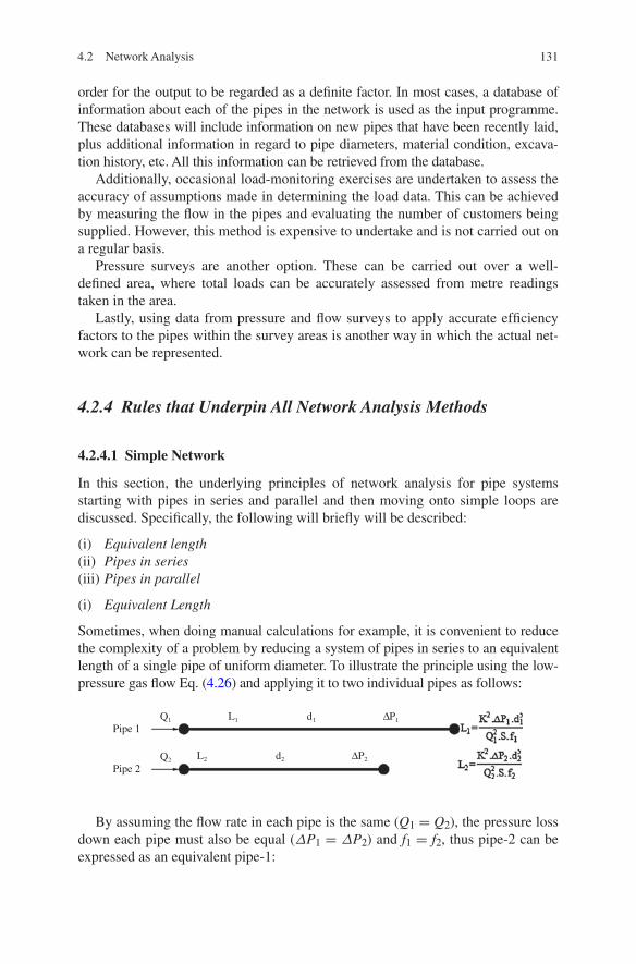
131

order for the output to be regarded as a definite factor. In most cases, a database of information about each of the pipes in the network is used as the input programme. These databases will include information on new pipes that have been recently laid, plus additional information in regard to pipe diameters, material condition, excava-tion history, etc. All this information can be retrieved from the database.

Additionally, occasional load-monitoring exercises are undertaken to assess the accuracy of assumptions made in determining the load data. This can be achieved by measuring the flow in the pipes and evaluating the number of customers being supplied. However, this method is expensive to undertake and is not carried out on a regular basis.

Pressure surveys are another option. These can be carried out over a well-defined area, where total loads can be accurately assessed from metre readings taken in the area.

Lastly, using data from pressure and flow surveys to apply accurate efficiency factors to the pipes within the survey areas is another way in which the actual net-work can be represented.

4.2.4 Rules that Underpin All Network Analysis Methods

4.2.4.1 Simple Network

In this section, the underlying principles of network analysis for pipe systems starting with pipes in series and parallel and then moving onto simple loops are discussed. Specifically, the following will briefly will be described:

(i) Equivalent length(ii) Pipes in series(iii) Pipes in parallel

(i) Equivalent Length

Sometimes, when doing manual calculations for example, it is convenient to reduce the complexity of a problem by reducing a system of pipes in series to an equivalent length of a single pipe of uniform diameter. To illustrate the principle using the low-pressure gas flow Eq. (4.26) and applying it to two individual pipes as follows:

Pipe 1

Pipe 2

Q1

Q2

L1 d1 ∆P1

L2 d2 ∆P2

By assuming the flow rate in each pipe is the same (Q1 = Q2), the pressure loss down each pipe must also be equal (ΔP1 = ΔP2) and f1 = f2, thus pipe-2 can be expressed as an equivalent pipe-1:

4.2 Network Analysis

132 4 Gas Flow and Network Analysis

(ii) Pipe in Series

Apply the principle of equivalent length to pipes in series, that is, end to end this is the simplest type of network. Pipes in series can be expressed in terms of one pipe of uniform diameter by using equivalent lengths. Take the following system:

A B CLAB

dAB

LBC

dBC

to express this system as one pipe of diameter dAB, convert section BC into an equivalent length of diameter dAB. For this to be valid, the flow rate in section BC must be the same as the flow rate in section AB, that is no off-take at B, and the overall pressure loss must remain unchanged. Thus, the total length of the system expressed in terms of dAB is:

(iii) Pipes in Parallel

Although still simple in concept, parallel pipes are more difficult to analyse than pipes in series. We often need to know the ratio of flows in each pipe, and these may have different lengths or diameters. But first, let us consider simplifying the network to a single pipe of an equivalent diameter. This must be able to pass the same quantity of gas as the two parallel pipes with the same overall pressure loss. Consider the following example:

Q

A B

Q

∆P1

Q2 , L2 , d2

∆P2

Applying again the LP Eq. (4.26) to the network and the two parallel pipes are joined at A and B, the pressures at these two points are common to both pipes which means that ΔP1 = ΔP2. Similarly, L1 = L2 = L and f1 = f2 = f. Furthermore, the flow into the network Q must be equal to the sum of the flows in each of the parallel pipes, thus if we replace the two parallel pipes with an equiva-lent single pipe, the low-pressure equation for this pipe is:

(4.34)L2 =(

d2

d1

)5

× L1

(4.35)Equivalent Length = LAB +(

dAB

dBC

)5

× LBC

133

where de is the equivalent diameter that allows the total flow Q to flow from A to B with the same overall pressure loss as the original system. Since this new pipe is equivalent to the original parallel pipe system then:

We can extend Eq. 4.38 to account for any number of parallel pipes as follows:

where

de equivalent diameter of a single piped1 diameter of the first parallel piped2 diameter of the second parallel pipedn diameter of the nth parallel pipe

4.2.4.2 Network Structures

Before the underpinning rules of network analysis can be discussed, it is necessary to generate a level of understanding into the structure of a gas network. Typically, industry networks consist of numerous combinations of trees and loops:

The term “tree” can be defined as a series of pipes in which each pipe is con-nected to a source by only one route. All the pipes can be solved analytically as a series of individual pipes. Figure 4.13 illustrates a typical tree network that would supply each pipe or node in the network.

(4.36)Q = K

√

�p · d5e

f · S · L

(4.37)Q = K

√

�p · d5e

f · S · L= K

√

�p

f · S · L

(

√

d51

)

+

(

√

d52

)

(4.38)de = (d2.51 + d2.5

2 + d2.53 + · · · d2.5

n )0.4

Fig. 4.13 Simple tree network

1 Source

2 3 4

4.2 Network Analysis

134 4 Gas Flow and Network Analysis

A “loop” can be defined as a closed path that begins and ends at the same point and therefore has a pressure drop of zero. Figure 4.14 presents a basic loop net-work structure.

Some network analysis techniques require the network loops to be defined before the analysis can proceed. Hence, it is important to know where the loops are in the network structure. Figure 4.14 shows three loops; 1–2–3–1, 1–3–4–1 and 1–2–3–4–1. Any two of these loops would identify all the pipes in the net-work, such a set of loops is known as an independent set.

Essentially, networks that have no loops can be considered tree networks and are relatively easy to deal with. However, in most cases, loops are present and the network solution can be very complicated. Some network analysis techniques, such as the Hardy Cross method, requires the network loops to be determined prior to conducting the analysis. Therefore, it is important to know where the loops are in the network structure.

Whether it is a tree or loop network, they both have an essential role to play in the success of network analysis.

4.2.4.3 Kirchhoff’s Laws

As previously mentioned, loops and nodes have an important role to play in net-work analysis. The flow of gas through nodes and loops is governed by a set of rules known as Kirchhoff’s Laws. Gustav Robert Kirchhoff, a Prussian physicist, first stated the analogous rules for electricity networks.

Kirchhoff’s First Law

The first law states that:

• The volume flow entering a given node is equal to volume of flow leaving that node in a specified period of time.

Fig. 4.14 Simple network consisting entirely of loops

1 Source

2 3 4

135

From this, we can state that the algebraic sum of all flows entering and leaving a given node is equal to zero as shown:

This law is the basis for all nodal equations. From Fig. 4.14, it is evident that a network consists of nodes and flows. Using Fig. 4.15 below, it is possible to pro-duce a set of equations that conveys Kirchhoff’s first law which states the alge-braic sum of flows entering and leaving a given node is equal to zero.

From the simple network above, the following equations can be derived for each node, as shown in Table 4.4.

There is one other additional equation based on the first law. The rule that the sum of the inflows must equal the sum of the outflows also applies to the complete network as well as individual nodes. Therefore,

In summary of the first law, it has been established that five equations exist and along with these, five unknown pipe flows arise. Unfortunately, these five equa-tions are not independent, which means it is not possible to solve the entire net-work using Kirchhoff’s first law; therefore, it is necessary that the second law is also used.

(4.39)∑

Q = 0

(4.40)Source Flow = L2 + L3 + L4

Fig. 4.15 Simple network with load nodes and pipe flows

2 3 4

1 Source

L2 L3 L4

Q23 Q34

Q12 Q13Q14

a b

Table 4.4 Nodal equations using simple network

Node 1 Source flow =Q12 + Q13 + Q14

Node 2 Q12 =L2 + Q23

Node 3 Q23 + Q13 =L3 + Q34

Node 4 Q34 + Q14 =L4

4.2 Network Analysis

136 4 Gas Flow and Network Analysis

Kirchhoff’s Second Law

The basis of the loop equation is Kirchhoff’s second law. This law states that:

• At any given instance in time, the pressure difference between any two nodes in a network is fixed and is the same for every flow path between those two nodes.

From this equation, we can state that the algebraic sum of the pressure drops around any given loop is equal to zero:

Therefore, because only one pressure value can exist at a given node in a network, this law also applies to the difference in pressures squared, as shown:

Unless both laws are satisfied, a network will not be balanced.

Underpinning Rules

In review of the foregoing sections, it is evident that two simple rules underpin all net-work analysis systems. These are: (i) what goes in must come out and (ii) the pressure loss between any two nodes provides the same value whatever way the flow travels.

4.2.4.4 Comparison of Methods

Hardy Cross (Mesh) Method

Network analysis based on the Hardy Cross Method uses Kirchhoff’s first and second law (Eqs. 4.41 and 4.42, respectively) for obtaining the value of flow rate and pressure in each segment. If the equations have not satisfied Kirchhoff’s law, a series of iterations will be done using. Use Newton’s method (for non-linear equa-tions) until the values for pipe flows within the required tolerance are reached. Computer solutions using the Hardy Cross method were developed originally because of the simplicity and convenience of the method, particularly when deal-ing with large steady state networks such as low-pressure distribution systems. Because each loop is considered individually, only the information relevant to one particular loop need be resident in the computer’s memory at any time. For early computer systems, this was a considerable advantage compared to the sub-stantial memory requirements for simultaneous solution techniques. The Hardy Cross method cannot be used for transient analysis because Kirchhoff’s laws, on

(4.41)∑

�P = 0

(4.42)∑

�P2 = 0.

137

which Hardy Cross is based, are not applicable. Transient problems are solved by a direct solution of the simultaneous equations arising from the dynamic models for pipelines, compressors and other network components. Transmission systems, although physically larger than distribution systems, do not contain very many pipes or loops; therefore, the memory requirements for the network are not as great, but the computational requirements are more complex.

The advantages of the Hardy Cross method are:

• Convergence is achieved rapidly because of the quadratic equation• The convergence is insensitive to the starting value• The disadvantages of the method, however, are:• A set of loops is required to be defined• Time consuming because each loop must be considered individually and

sequentially

The Nodal Method

Generally, the nodal method is similar to the Hardy Cross method except this method does not require the network loops to be defined, a process which can take up a significant proportion of the overall solution time of a computer. However, the disadvantage of this method is the convergence heavily depends on the initial estimate for the nodal pressures.

The advantages of the method are:

• The method does not rely on interconnected loops within the network and can be applied to any network where the requirements for fixed pressure nodes and load nodes are met.

Moreover, the disadvantages are:

• Square root function requires a large number of iterations to reach a practical solution. In addition, the divergence and oscillation are the risk of using this method.

• Time consuming because each node is considered individually and sequentially throughout the network.

Newton–Raphson Mesh Method

Unlike one Hardy Cross method in which each iteration on a loop takes no account of the effect of that loop on the other loops in the network and conse-quently contains flow correction for loops, Newton–Raphson Mesh method has a simultaneous solution that interacts one loop with another to be modelled. The advantages of using this method are the reduction of iterations required to solve the network.

4.2 Network Analysis

138 4 Gas Flow and Network Analysis

Newton–Raphson Nodal Method

The Newton–Raphson method enables the simultaneous solution of all the equa-tions derived from the application of Kirchhoff’s first law at each load node (pressure defined nodes, such as sources, are not included). The matrix equa-tion is constructed from an equation where n is the number of load nodes in the network. As a result, the matrix contains many more zero elements, allowing a greater degree of compaction. The advantages, as with the Newton–Raphson mesh method, are the improvement of solution speed by reducing the number of itera-tions required for convergence of the network.

Hybrid Method

This is a combination of Newton–Raphson mesh and nodal methods to get the advantages of the mesh and nodal methods for achieving a solution. Unlike Hardy Cross method, this method can only be achieved by using matrix methods.

In fact, the hybrid method is a variant of the Newton Nodal method. In the orig-inal Newton Nodal method, flow variables were eliminated before the equations were linearised; while in the hybrid method, the equations are linearised before the flow variables are eliminated and the problems are avoided.

4.2.4.5 Advantages and Disadvantages of Using Simulation Modelling

This section of the report examines the various simulation modelling software sys-tems that are commonly used throughout the gas industry to analyse a network. There are numerous advantages of using network analysis to simulate gas flow and pressure within a natural gas network. However, with these advantages fall several disadvan-tages. In this particular section, a flavour of the advantages and disadvantages that are associated with the various network analysis systems shall be determined. This will allow a comprehensive understanding into why network analysis is so popular not only in the gas industry but also in many other industries across the world.

In the United Kingdom, SGN adopts the SynerGee system for network pressures below 7 bar and uses Graphical Falcon for networks operating above 7 bar (Fig. 4.16).

Advantages of Simulation Modelling

There are many reasons why, industries, especially gas are attracted to simula-tion modelling on their networks. The biggest of these advantages is likely cost. Designing, building, testing, redesigning, rebuilding, retesting of a gas pipe-line network is an unrealistic option and would also be extremely expensive. Simulation modelling allows the building and rebuilding phases to be removed from the loop, therefore generating faster solutions.

139

These solutions will also significantly benefit the capital costs associated with operating the network. The modelling will allow an accurate assessment of the pipe diameter requirements necessary to cope with the pressure criteria of the pipe to be easily established. This is a huge advantage and will reduce material costs when constructing the necessary pipeline.

Another evident benefit is the reduction in time that the engineer will spend designing the network [6, 7]. This is significantly due to the vast array of detail that a network analysis system can provide the engineer with. For example, if the equations and calculations mentioned previously were to be determined manually, this would take days, however with simulation modelling an engineer can produce a whole network in a matter of hours because the system can generate all the nec-essary results at the click of a button.

“What If” scenarios as mentioned in Sect. 4.2 are also easily resolved using simulation modelling, which is another massive advantage for a gas distribution network. This allows them to assess the effectiveness of the network in the event of an occurrence happening. The example presented provides a brief insight into what happens to the existing network when a pipe is removed. From this example, it allows the advantages of simulation modelling to be demonstrated further.

Disadvantages of Simulation Modelling

Due to the nature of some of the underlying concepts of pipeline modelling, net-work analysis can never be absolutely accurate. The relationship between flow and

Gas works

Graphical falcon

Small network calculator

SNAP

GBNA

LINAS

Service calculator

SynerGEE®

Fig. 4.16 Common network analysis systems [3]

4.2 Network Analysis

140 4 Gas Flow and Network Analysis

pressure can be encapsulated in an equation. However, various other parameters that are less obvious tend to be forgotten about, such as:

• Internal roughness and/or efficiency of the pipeline.• Temperature of the gas.• Compressibility of the gas.• Altitude of the pipeline system.• Thermal properties of the burial material.• Burial depth of the pipeline, as shown in Fig. 4.17.

Most of these elements cannot be reasonably or accurately known. For example, the thermal properties of the burial material might rely on knowing the sand con-tent and water content of the soil: the former of these can vary greatly over a short distance, and the latter may need correction for seasonal variation [8, 9].

Additionally, there is no guarantee that all the data and input received are cor-rect, for example the pipe may not be PE 80; in fact, it may be PE 100 as shown typically in Fig. 4.18. Also the quality of workmanship may not be sufficient or the positioning of the pipeline may be incorrect; however, when using network analysis, it implies that the network is to the highest standard and runs a model regardless of pipe conditions, extra bends, etc.

• Altitude of the pipeline system.• Thermal properties of the burial material.• Burial depth of the pipeline, as shown in Figure 4.17

Anode

Fill

Bedding

Padding

Pipe

Fig. 4.17 Burial depth and materials used [10]

141

Hence, this means that all flow equations must be derived empirically, which conveys that any particular flow equation will be accurate only within a special context (e.g. a range of pressures). Thus, stating that network analysis is not a 100 % accurate method, although many gas networks make use of the information in this way.

4.3 Principles of Transient Flow

Previous sections were concerned with steady state flow. However, because gas is compressible, to model accurately the flows that take place in gas pipelines or during a pipe break, the concept of unsteady state or transient flow should be applied. The difference between steady state and unsteady state flow is where the flow parameters, such as pressure and mass flow rate, vary with time; so transient analysis is the analysis of the time-dependent variations in these parameters (the transients). For example, in a pipe break, the pressurised gas is released into the atmosphere in an uncontrolled manner and the pipeline will not empty rapidly because of the much larger quantity of compressed gas in the pipe. Clearly, steady state equations are inappropriate for the analysis of pipe breaks and they should not be used to determine the rate of gas leakage. The quantity of gas escaping depends mainly on the absolute pressure of the gas in the pipe and the resistance to flow created by the shape and size of the fracture area. If the gas supply into the pipe is maintained, the gas will escape at a rate determined by the gas pressure. If it is possible to isolate the fractured section, the pressure will decline exponen-tially with the consequent reduction in the rate of gas escaping.

Fig. 4.18 Differences between PE pipes [12]

4.2 Network Analysis

142 4 Gas Flow and Network Analysis

Unlike a water pipeline for example, where a fracture results in an immediate loss of pressure, a gas pipeline contains compressed gas, so the dynamics of the decompression are much slower; this fact has important consequences for pipe-line design, which are embodied in IGE/TD/1, the Institution of Gas Engineers recommendations for gas pipelines. The main difference between unsteady state flow and steady state flow is the time period between input and extraction of fluid from a system. The time difference between the input and extraction of fluid intro-duces the concept of storage, and in gas pipeline systems, this storage is used to smooth out variations in the flow at the demand end of the pipeline so that the inlet flow does not change significantly. The time difference allows gas to be extracted from the pipeline by reducing the pressure (rather than introducing more gas at the input) in the same way that water was drawn off from a barrel. This feature allows pipeline operators to manage the daily demand variations without the need to alter the rate at which they buy gas from the offshore producers. Let us have a look at this feature in more detail.

Figure 4.19 shows two steady state pressure profiles for a pipeline. Profile (1) represents the conditions for a steady state flow rate Q1 and profile (2) represents the conditions for a new steady flow state flow rate Q2.

The area under curve (2) is less than the area under curve (1) and since these areas are representative of the volume of gas in the pipeline, the line-pack vol-ume, it follows that a volume of gas, represented by the hatched area, has been

Pout(1)

Pout(2)

(1)

(2)

Direction of flow

Pres

sure

(P)

Pin

Pipe length

Fig. 4.19 Line-pack storage resulting from two steady state pressure profiles in a pipeline designed for gas transmission only

143

withdrawn from the pipeline, the line-pack storage volume. This gas has been used by the customers at the end of the pipeline causing the outlet pressure to fall from Pout(l) to Pout(2), this means that a finite period of time has elapsed between profile (1) and profile (2). The customers have effectively been using stored gas between time (1) and time (2). In fact, between these times, the rate of demand could have been higher than Q2 for a limited period because the higher demand does not need to be transmitted along the pipeline, it is only drawn off at the downstream end.

The line-pack storage volume, represented by the hatched area, is much larger than that shown in Fig. 4.19. Taking the line-pack storage a stage further is by designing the pipeline specifically for this purpose. To do this, the pipeline should be designed and constructed to withstand a higher pressure than that required purely for gas transmission.

Profiles (1) and (2) in Fig. 4.19 are exactly the same as those in Fig. 4.18. But what is the main difference between the two diagrams?

The difference is that Pin(l) is higher than the original Pin creating more storage between the two profiles. To release this storage at the required time, the inlet flow rate can be restricted to force the inlet pressure lower, but in practice, it is more effective to set a constant flow rate at the inlet (the daily average) and allow the variations in demand at the outlet to absorb the stored gas. The principle of line-pack storage has been introduced, but how is the storage volume calculated? This is described in the next section.

4.3.1 Calculation of Line-pack Storage

To calculate the volume of usable line-pack storage, the gas volume should be found which is represented by the areas under each of the profiles shown in Fig. 4.20 and subtract one from the other. Figure 4.21 shows a pipeline operating under steady state conditions. By considering an elemental volume of gas, we can integrate the pressure profile along the length of the pipeline to find the total vol-ume of gas under the profile.

The volume of the incremental section is A.dl so, from the real gas equation of state, the volume of gas in the section at standard conditions (dVs) is given by:

The pressure gradient in the pipe is Ap2/L, so the pressure (p) at array point dis-tance 1 from the start of the pipeline is given by:

(4.43)dVs =A · dl · p · Ts

Z · ps · T

(4.44)p =(

p21 −

1

L∆p2

)0.5

4.3 Principles of Transient Flow

144 4 Gas Flow and Network Analysis

Substituting for p in Eq. 4.47 which, when integrated and rearranged, gives

The volume of gas in the pipeline (Vs) is the physical volume of the pipeline (A.L) corrected to standard conditions using the average pressure (Pm). This is the same value of Pm for dealing with the compressibility factor. Thus:

(4.45)Vs =A · L · Ts

Z · T · ps

2

3

(

p31 − p3

2

p21 − p2

2

)

(4.46)A · L · Ts · pm

T · ps · Zm

Pout(1)

Pout(2)

(1)

(2)

Direction of flow

Pre

ssur

e (P

)

Pin(1)

Pipe length

Pin(2)

Fig. 4.20 Line-pack storage resulting from two steady state pressure profiles in a pipeline designed for gas transmission and storage

Area (A)l

dl

L

P2

P1

Fig. 4.21 Pipeline operating under steady state condition

145

Or in terms of diameter, with d expressed in mm, the difference between the volumes at the maximum and minimum conditions can be expressed for profiles (1) and (2) as:

where AVs is the volume of line-pack storage expressed at the standard condition Ts and Ps and Zm (1 and 2) are the maximum and minimum flow rates.

4.3.2 Dynamics of Pipelines

In a water pipeline, the dynamics are very fast because the fluid is incompress-ible and so changes in flowrate result in very rapid changes throughout the system, often resulting in “water hammer”. The equivalent of water hammer is not notice-able in HP gas pipelines because the gas, being compressible, absorbs the changes in p over a period of time. However, it can be seen in some LP situations because the gas behaves more like an incompressible fluid, e.g. where large load changes occur in a small volume of pipe.

Now look again at Fig. 4.18. This represents a pipeline where the inlet pres-sure is controlled at a constant value (say, 70 bar abs), so changes in pressure at the outlet, caused by changes in the flow rate, do not affect the value of the pres-sure at the inlet. All the pressure variations have been absorbed by the gas over the pipeline length. However, a change in the demand flow rate from one steady state condition (Qmm) to another steady state condition (Qmax) would lead to a change in the inlet flow rate from Qmm to Qmax, the time taken for this change to be appar-ent at the inlet is determined by the rate at which the change can be propagated through the gas from the outlet to the inlet. This, of course, is the dependent on the volume of line pack that must be used up. The length of time that it takes for flow rate change to propagate through the pipeline can be estimated by the difference in the flow rates using the following equation:

Figure 4.20 represents a pipeline designed for line-pack storage as well as transmission where the inlet flow rate is held at a constant value while the down-stream outflow varies according to the demand. In this case, we are interested in the pressure transients, that is the time taken for a change in pressure at one end to be observed at the other end and as with flow rate changes, we are dealing with quite long transient times.

Since both pressure and flow transients take a finite length of time to propagate along the pipeline they must travel with a certain velocity, so we can think in terms of a “wave” travelling through the gas.

(4.47)∆Vs =0.7854

106

Ts

ps

L · d2

T

[(

pm

Zm

)

1

−(

pm

Zm

)

2

]

(4.48)Approximate transient time =Volume of linepack storage (�Vs)

Change in flowrate (�Qs)

4.3 Principles of Transient Flow

146 4 Gas Flow and Network Analysis

Figure 4.22 illustrates the difference in concept between steady and unsteady state flow resulting from the inclusion of the time dimension. The steady state case is two dimensional in pressure and distance or flow and distance. The curve rep-resenting the pressure loss along the pipeline length can be described by n values and the flow, being constant, is described by one value along the whole length.

In the unsteady flow situation, Fig. 4.22, each of the n pressure values requires a further m values to describe the change in pressure with time; therefore, a total of m × n pressure values is required and since the flow also varies with time, m × n flow values are also required. This represents a great increase in complexity and so careful consideration must be given to the problem to be solved.

The disturbances introduced into the gas at one end of a pipeline will take a finite length of time to reach the other end; the length of time depends on the velocity at which the “wave” travels, which in turn depends on the type of distur-bance, the gas pressure and the characteristics of the pipeline t1.

Here is an example of how a pressure transient might travel along a pipeline. The response of a pipeline to a step change in pressure at its inlet is shown in Fig. 4.23. At the inlet conditions (t = 0), the flow is steady state and is represented by the pressure profile from P (0, 0) to P (0, L) at the outlet. At time t1, the inlet pressure rises from P (0, 0) to P (1, 0) but the pressure at the outlet P (1, L) is still at the original outlet pressure. At each increase in time, a higher pressure is seen at increasing distances along the pipe until at time t10 the pressure transient has reached the outlet of the pipeline, after which time the flow settles back to steady

Steady stateP

ress

ure

(P)

Distance (L)0 1 2 n-1 n

Flo

w (

Q)

Distance (L)

Distance (L)

0 1 2 n

Distance (L)

20 1 n

m

m

t t

P Q

Fig. 4.22 Comparisons of steady state and unsteady state flow

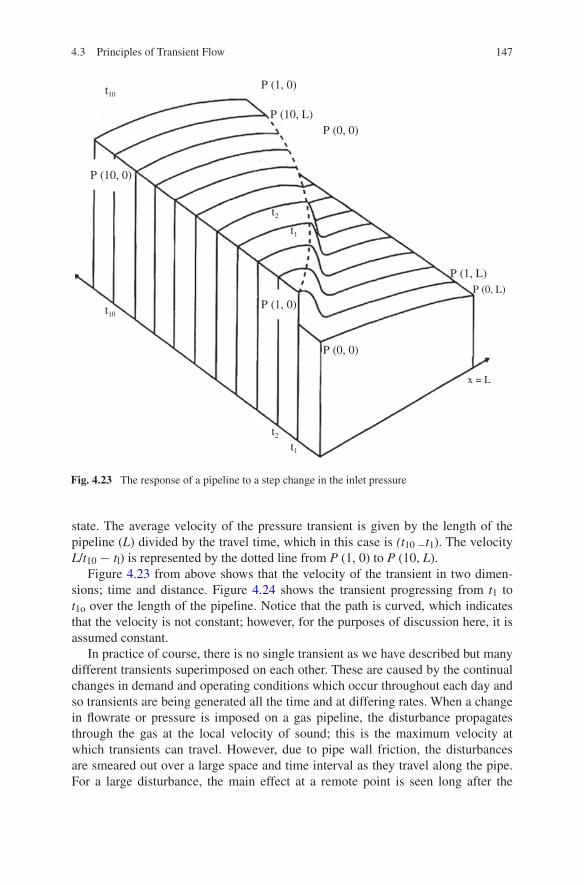
147

state. The average velocity of the pressure transient is given by the length of the pipeline (L) divided by the travel time, which in this case is (t10 −t1). The velocity L/t10 − tl) is represented by the dotted line from P (1, 0) to P (10, L).

Figure 4.23 from above shows that the velocity of the transient in two dimen-sions; time and distance. Figure 4.24 shows the transient progressing from t1 to t1o over the length of the pipeline. Notice that the path is curved, which indicates that the velocity is not constant; however, for the purposes of discussion here, it is assumed constant.

In practice of course, there is no single transient as we have described but many different transients superimposed on each other. These are caused by the continual changes in demand and operating conditions which occur throughout each day and so transients are being generated all the time and at differing rates. When a change in flowrate or pressure is imposed on a gas pipeline, the disturbance propagates through the gas at the local velocity of sound; this is the maximum velocity at which transients can travel. However, due to pipe wall friction, the disturbances are smeared out over a large space and time interval as they travel along the pipe. For a large disturbance, the main effect at a remote point is seen long after the

P (1, 0)

P (0, 0)

t1

t2

t10

P (1, 0)

P (0, 0)

t1

t2

t10

P (10, 0)

P (10, L)

x = L

P (0, L)

P (1, L)

Fig. 4.23 The response of a pipeline to a step change in the inlet pressure

4.3 Principles of Transient Flow

148 4 Gas Flow and Network Analysis

original wave front has passed. This delayed effect is referred to as a “slow tran-sient” and is the main interest for modelling pipelines. Figure 4.25 shows the range of velocities to be considered.

Because unsteady state flow problems are so complex, we need to optimise the method of solution; this means selecting a solution procedure which only deals

Fig. 4.24 Progress of transient between t1 and t10

l

t

l = L0

t0

t10

Fig. 4.25 Velocities associated with transient

t

0 1=L1

149

with the transients of interest. So transient analysis programmes are designed to model the pressure and flow transients that result from the action of friction rather than the disturbances moving at sonic velocity.

Here are some examples that are not suitable for analysis using a pipeline model.

• The velocity of gas escaping from a pipe break is equal to the sonic veloc-ity, which is outside the range of transients covered by a pipeline model. Pipe breaks must therefore be modelled using a programme specifically designed for this purpose.

• The dynamics of control valves are determined by the valve characteristics, the method of valve control and the pressure of the gas. In order to achieve accurate control of the gas pressure or flow rate the valves are designed to have a fast response time, this allows the valve to move quickly to correct any variation in the measured pressure or flow rate. The dynamics of control valves are therefore much faster than pipeline dynamics and outside the range of pipeline models. Special modules using different solution techniques must be built into a tran-sient analysis programme if required to simulate the interaction of valves and pipelines.

• As with control valves the dynamics of compressor stations are much faster than pipelines, they are also very complex, so special solution techniques must also be used to model the performance of compressors and their interaction with pipelines.

Because the dynamics of control valves and compressors are so fast compared to those of pipelines, a reasonable approximation can be made by assuming that the output from these devices is calculated on steady state basis. This simplifies the modelling considerably, but you should be aware of the limitations of such an approach.

4.4 Concluding Remarks

In the preceding chapter, a thorough evaluation of the principles of steady and unsteady state gas flow and network analysis were provided. Understanding gas flow and network analysis that are the most comprehensive system available today provides various industries such as the gas industry with a suitable simulation model of their ever evolving and continuously functional distribution and trans-mission network. There are a significant number of application uses for network analysis along with a whole list of advantages as to why the gas industry adopt such a system, one of the main ones being to determine safe operational flow and pressure through their pipes.

The mathematics behind all systems appears to be well specified and docu-mented and allows various sets of calculations to be established with several clicks of a mouse. However, it is worth mentioning that network analysis cannot

4.3 Principles of Transient Flow

150 4 Gas Flow and Network Analysis

be deemed to be 100 % accurate; however, it is the best solution available and provides numerous valuable pieces of information. To conclude, network analysis is a fundamental aspect in the success of transporting gas to millions of custom-ers worldwide. Network analysis systems will continually be improved and this will only assist the gas industry in providing a consistent supply of natural gas throughout the United Kingdom and across the world for many years to come.

References

1. Babonneau, F., Nesterov, Y. and Vial, J.P., Design Operations of Gas Transmission Networks. Ecore Discussion Paper, 2009.

2. Paxton, A. Network Modelling Software Review, Poyry Energy, 2009. 3. Scotia Gas Network (2006) Gas Requirements Manual. Section 15 (Formally Transco), 2006. 4. Scotia Gas Network (2010) Network Planning Policy Document (Formally Transco), 2010. 5. http://www.igem.org.uk/Technical/standards.asp, Online 21st November. 6. http://www.fluidmechanic.co.uk/transient.htm December 2nd and 3rd. 7. http://www.see.ed.ac.uk/~mzaiser/4thyear/websites05/MacRonald/Website/3-1.html

December 2nd. 8. http://www.sdcwa.org/nob-hill-pipeline-improvements (accessed as at 20th September, 2013). 9. http://www.trec-uk.org.uk/csp/transport.htm (accessed as at 20th September, 2013). 10. http://www.earthlyissues.com/transalaska.htm (24 oct 2013). 11. https://www.gedigitalenergy.com/geospatial/catalog/smallworld_gaspipeline.htm (25 oct 2013). 12. http://rajacorporation.wordpress.com/category/hdpe/ (24 oct 2013).

151

5.1 Temperature and Heat Flux

5.1.1 Introduction

Throughout the years, the gas industry has witnessed numerous different measurement techniques and experimental investigations relating to natural gas engineering, conse-quently making it extremely difficult to keep up to speed with the evolving technology that is being implemented across the world.

In the gas industry, the measurements of temperature, pressure, gas flow and gas quality are some of the key parameters that are considered. However, due to the copious amount of measurement techniques that are available, it is impractical to detail each of these in this chapter. For this reason, the rationale is to capture the key points from the vast array of measurement techniques being used across the gas industry and present them in a clear and concise manner. In this chapter, attempt has been made to provide the knowledge necessary to understand the operational principles of instruments that are available in the gas industry to moni-tor parameters such as temperature, pressure, gas flow and gas quality. Contained within each of these sections will be a brief overview of the parameter being meas-ured, the various types of instruments that are available to use for each param-eter, along with the specific options which exist. At the end of each related section, all the instruments that have been highlighted are then shown in tabulated format which includes a brief operations of feature of the instrument, the range, the accu-racy, advantages and disadvantages and application of each of the devices. This will provide the reader with sufficient data on the various instruments that can be used to measure the parameter being discussed. The conclusions drawn from each of the sections will then be presented at the end of the chapter. References are also provided with regard to design features of each instrument for further consultation.

Chapter 5Natural Gas Measurement Systems

© Springer International Publishing Switzerland 2014 G.G. Nasr and N.E. Connor, Natural Gas Engineering and Safety Challenges, DOI 10.1007/978-3-319-08948-5_5

152 5 Natural Gas Measurement Systems

Starting with temperature and heat flux in this section, one can see that, in general, it is not easy to define temperature in a practical way; therefore, it tends to be expressed using words, such as hot and cold. When any such object has a low temperature, it is referred to as cold and when a particular temperature is higher, it is referred to as hot. However, it is not practical to use sensations and notions as a means of measuring temperature, this is not scientifically correct. Fortunately, several properties of materials act in a consistent manner with temperature, hence forming the basis for accurate measurement of temperature.

When a hot body is brought into contact with a cold body, heat is transferred from the hot body to the cold body until both these bodies have equal temperature. At this point, it is referred to as thermal equilibrium. The zeroth law of thermody-namics states that if two bodies are in thermal equilibrium with a third body, they are in thermal equilibrium with each other. This zeroth law serves as a basis for the validity of temperature measurement.

Temperature scales aim at using a common basis for temperature measurement. Throughout the world, there are many scales that can be used; the most common is known as Celsius. However, the Kelvin scale is the temperature standard most commonly used in engineering principles and has the same incremental scaling as the Celsius scale, but fixes its origin at absolute zero (0 K = −273.15 °C). All temperature scales are based on some easily reproducible states, such as the freez-ing and boiling points of water. The Celsius scale adopts 0 °C as the freezing point of water and 100 °C as boiling point, whereas the Fahrenheit scale makes use of a historical scale at which water freezes at 32 °F and boils at 212 °F. It is also nec-essary to understand the relationship between temperature and absolute tempera-ture, shown below. In this case, there are no negative temperatures, and the lowest attainable temperature is absolute zero. The absolute temperature scale in the SI system is the Kelvin scale as shown in Fig. 5.1 and can be expressed as:

When zero is read on a temperature scale, it does not mean the point at which no heat is contained in the body being measured for Fahrenheit and Celsius scales. The presence of heat in any mass causes the molecules to vibrate. The more heat there is, the greater the oscillation becomes. When all molecular motion ceases in a body, this is the point at which there is no heat remaining in that body. This occurs at −273.4° on the Celsius scale and −460.16° on the Fahrenheit scale.

5.1.2 Thermometry Types

5.1.2.1 Expansion Thermometer

In most forms of temperature measurement, the variation of a substance with tem-perature tends to be the method commonly used. Expansion thermometers are divided into four expansion classes: solids, liquids, gases and change of state. In each of

Temperature (Kelvin) = Temperature (Celsius) + 273.15

153

these cases, the substances have a constant recognisable change when temperature is applied to them. In this particular section, each of the classes being discussed either increase or decrease in size, this is known as expansion or contraction. Therefore, tak-ing this into consideration, it is important to gain a thorough understanding of each of the expansion thermometer instruments that can be used under each particular class.

Solid Expansion

When two metallic strips with different expansion coefficients are applied under the same temperature, a differential expansion will occur on the strips. The increase in length of any side of a solid will depend on its original length, the rise in temperature and the coefficient of linear expansion.

The most practical instrument that is used for this particular class of expansion thermometer is known as bimetal strip. Figure 5.2 shows the process of two metals bonded together with different coefficients of expansion.

Liquid Expansion

In this class of expansion thermometers, an instrument referred to as liquid in metal thermometers tends to be used; however, liquid in glass thermometers is also extremely popular. See previous Table 5.1 for further information on this

Fig. 5.1 The temperature scale in SI unit

400 °K373 °K 350 °K

300 °K 273 °K 250 °K

200 °K 195 °K

150 °K

100 °K 82 °K 50 °K

0 °K

100 °C

50 °C

0 °C

-40 °C -50 °C -78 °C

-100 °C

-150 °C

-191 °C -200 °C

-250 °C-273 °C

Water boils

Water freezes

Dry ice(solid CO2)

Liquid air

Absolute zero

5.1 Temperature and Heat Flux

154 5 Natural Gas Measurement Systems

thermometer and other instruments related to expansion of liquids. Table 5.2 also indicates the related temperature ranges of thermometers (Fig. 5.3).

Change of State

There are two different instruments that can be used for measuring the change of state class. These instruments are known as vapour pressure thermometers and Pyrometric Cones, Bars and Rings and are described in more detail in Table 5.3.

5.1.2.2 Electrical Methods

Temperature measurement based on the changes of electrical resistance of a metal with temperature has become popular because they are very convenient tech-niques and they furnish a signal that is easily detected. The measurement can be amplified and or used for control purposes. Furthermore, they are generally quite

Room temperature

∆T ∆ε

x

δ

CooperIron

Unbonded

Bonded

Clamped

Fig. 5.2 Coefficients of expansion of bimetal strips

Table 5.1 Temperature ranges of thermometers

Liquid Temperature range

Mercury −38 to +600

Helium −55 to +600

Alcohol −80 to +50

Toluene −90 to +30

Pentane −200 to +30

155

Table 5.2 Expansion thermometer

Instrument Description, range and accuracy

Advantages (A) and disadvantages (D)

Application

Bimetal strip (solid)

Two strips of metals are bonded together. When heated, one side will expand more than the other, and the result in bending is translated into a temperature reading by mechanical linkage to a pointer. Range: −35 to 550 °C, Accuarcy: ±0.5 to 1 % Narrow operat-ing temperature range. Cannot be remotely indicated. Operation is dependent on external factors

A: Not expensive. Provide direct reading. Portable and do not require outside power

Used to operate thermo-stats and steam traps. As a switch in a heater circuit. Used to drive a pointer on an instrumentIt provides compensation for changes in atmos-pheric temperature

D: Not as accurate as thermocouples and RTDs

Liquid in glass ther-mometer (liquid)

This is the most common type of thermometer. It consists of a glass tube known as the capillary tube that has a bulb at one end, a capillary hole down the axis connected to a reservoir in the bulb filled with a liquid. Usually filled with mer-cury and when heat is applied, the liquid level will rise and, respec-tively, if cooled will fall. Range: −80 to 450 °C, Accuracy: ±0.5 %

A: Has good expansion Airplanes to measure the atmospheric icing conditionsMeasure temperatures of swimming pools and saunas. Used in medicinal examination

D: The glass can melt if exposed to high temperatures

Liquid in metal ther-mometer (Liquid)

The bulb and capillary are completely filled with liquid. The change in vol-ume on thermal expansion is indicated by a Bourbon tube. Range: −50 to 60 °C, Accuracy: ±1 %

A: Very accurate read-ings. Durable long stem are practical in industrial use

Air-conditioning units, burners, boilers, cookers, heat exchangers, water works tanks

D: The liquid in the thermometer may need to be shaken down prior to use

Gas ther-mometer (Gas)

The effect of tempera-ture on gas changes the pressure that is indicated by the movement of the Bourdon tube. If the change in volume of the tube as it curls can be neglected a fairly linear scale is produced. Range: −100 to 800 °C

A: Response is more rapid than liquid types. Can measure a wide range of temperatures

Process systems

D: Has to be calibrated before being used. Handling this thermom-eter is comparatively difficult

5.1 Temperature and Heat Flux

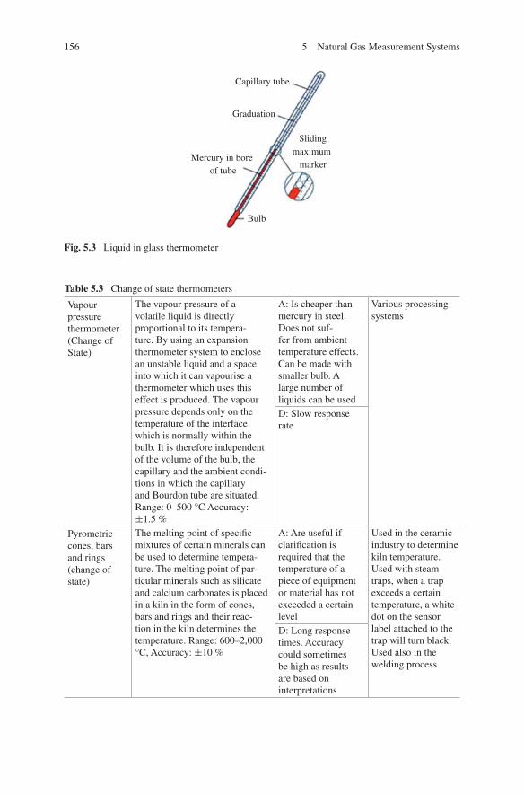
156 5 Natural Gas Measurement Systems

Table 5.3 Change of state thermometers

Vapour pressure thermometer (Change of State)

The vapour pressure of a volatile liquid is directly proportional to its tempera-ture. By using an expansion thermometer system to enclose an unstable liquid and a space into which it can vapourise a thermometer which uses this effect is produced. The vapour pressure depends only on the temperature of the interface which is normally within the bulb. It is therefore independent of the volume of the bulb, the capillary and the ambient condi-tions in which the capillary and Bourdon tube are situated. Range: 0–500 °C Accuracy: ±1.5 %

A: Is cheaper than mercury in steel. Does not suf-fer from ambient temperature effects. Can be made with smaller bulb. A large number of liquids can be used

Various processing systems

D: Slow response rate

Pyrometric cones, bars and rings (change of state)

The melting point of specific mixtures of certain minerals can be used to determine tempera-ture. The melting point of par-ticular minerals such as silicate and calcium carbonates is placed in a kiln in the form of cones, bars and rings and their reac-tion in the kiln determines the temperature. Range: 600–2,000 °C, Accuracy: ±10 %

A: Are useful if clarification is required that the temperature of a piece of equipment or material has not exceeded a certain level

Used in the ceramic industry to determine kiln temperature. Used with steam traps, when a trap exceeds a certain temperature, a white dot on the sensor label attached to the trap will turn black. Used also in the welding process

D: Long response times. Accuracy could sometimes be high as results are based on interpretations

Fig. 5.3 Liquid in glass thermometer

Capillary tube

Graduation

Mercury in bore of tube

Sliding maximum

marker

Bulb

157

accurate when calibrated properly. Table 5.4 provides details of a thermoelectric thermometer, also known as a thermocouple including other electrical methods for measuring temperatures. However, a number of factors govern the type of thermo-electric thermometer that can be used. In this section, these are briefly described.

Thermoelectric Thermometers (Thermocouples)

One of the most common industrial thermometers used today are the thermoelec-tric thermometers or thermocouples as they are generally referred too. The choice of

Table 5.4 Electrical methods of measuring temperature

Instrument Description, range, accuracy

Advantages (A) and disadvantages (D)

Application

Resistance thermometer

Resistance ther-mometers also called resistance temperature detectors (RTD’s) are temperature sensors that capitalise on the fact that the electri-cal resistance of a material changes as the temperature changes. They consist of spirals of fine wire wound on insulating formers. The variation of electrical resistance of the metal when heat is applied provides an accurate temperature measure-ment. Range: up to 1,000 °C, Accuracy: ±0.05 %

A: High Accuracy, can read up to 1,000 °C and above. Require no cold-junction measure-ment. Suitable for precision applications

Various process industries

D: Rarely used above 650 °C, as it becomes difficult to prevent con-tamination by impuri-ties of the metal sheath. Response speeds tend to be slower due to bulb size

Thermistors These are based on resistance change in a ceramic or polymer. This generates a higher precision with a limited temperature range. Can be classified into two types: positive temperature coefficient (PTC) and negative temperature coefficient (NTC). The resist-ance drops nonlinearly with temperature rise. Range: −100 to 300 °C , Accuracy: ±0.001 %

A: Have a high resis-tivity. Can respond quickly to temperature change

PTC thermistors are used as current-limiting devices for circuit protection

D: May de-calibration at high temperatures. Use is limited to a few hundred degrees. Fragile and care must be taken

NTC thermistors can be used to provide high ini-tial resistance to power supply circuits

(continued)

5.1 Temperature and Heat Flux

158 5 Natural Gas Measurement Systems

materials for a thermocouple is governed by a number of factors. They must develop a relatively large emf that does not fluctuate from the calibrated value when in use. The material must also be able to withstand the maximum temperature of use. Usually, the thermocouple is rugged and easy to install, and if properly connected, it provides an accurate temperature of its junction. However, care must be taken to ensure that the correct compensating cable is used and the correction for the temperature of the cold junction is made as typified in Fig. 5.4. As a result, there are four types of thermocou-ples commonly used for industrial application, which are described here.

Instrument Description, range, accuracy

Advantages (A) and disadvantages (D)

Application

Thermoelectric thermometers (thermocouple)

Consists of two dis-similar metals, joined together at one end. Changes in the tem-perature at the junction induce a change in electromagnetic force (emf) between the other ends. As temperature goes up, the output emf of the thermocouple rises, though not neces-sarily linearly. The current flowing in the loop can be detected by a galvanometer, which can also be used to convert heat into electric power. Range: 200–2,600 °C , Accuracy: ±0.1 %

A: Provides stable response. Capable of measuring a wide range of temperatures, up to 2,600 °C. The thermocouple junction may be grounded and brought into direct contact with the mate-rial being measured. Less expensive than other temperature sen-sors and can be easily installed

Thermocouples are widely used in sci-ence and the industry; applications include temperature measure-ment for kilns, gas tur-bine exhaust and diesel engines

D: Two temperatures need to be measured. Are usually complex and generates room for error

Measurement of electri-cal variable (Wheatstone Bridge)

In resistance ther-mometers, Wheatstone Bridge circuits are most commonly used. The current flows through the resistance in the bridge and also through the thermometer bulb. As a result, this generates heat in the thermometer produc-ing an indication of change. To achieve the most accurate readings, it is important to reduce the current through the thermometer to as low as possible

A: High accuracy and sensitivity. Can be used to measure numerous quantities, such as capacitance, impedance

Various

D: Requires calibration with the leads attached

Table 5.4 (continued)

159

Base-metal Thermocouples

Base-metal thermocouples range from −200 to 1,200 °C. The different types that are available are listed below.Note that

1. Copper/constantan elements are usually only used for laboratory measurement.2. Iron/constantan elements are used up to 800 °C under reducing conditions.

They deteriorate rapidly under oxidising conditions or in the presence of acids.3. Chrome/aluminium alloys are suitable for up to 1,000–2,000 °C under oxidising

conditions.

These thermocouples can be obtained in a mineral-packed type of construction which gives strong, small diameter-flexible thermocouples.

Rare-Metal Thermocouples

Rare-metal thermocouples are those based on platinum metals. They have rela-tively low thermoelectric power when the material is measured in response to a temperature difference across that material. This allows them to produce a good accurate measurement and is the preferred types for standard or reference thermocouples. It is advised that all rare-metal thermocouples should be used along with a good-quality sheath (protective cover) that is resistant to the tem-perature and conditions of use, as they are vulnerable to contamination by dirt and grease. The sheaths come in many different materials, such as mild steel, stainless steel, and chrome/iron and are all receptive to varying temperatures and conditions as well as oxidation and mechanical damage. The three types of ther-mocouples listed below are used in relation to rare-metal thermocouples and can be used in oxidising and inert atmospheres continuously at temperatures up to 1,600 °C.

Voltmeter

Reference junction (cold)

Measuring junction (hot)

Heat source

Dissimilar metal wires

Fig. 5.4 The basic principle of a thermocouple

5.1 Temperature and Heat Flux

160 5 Natural Gas Measurement Systems

Type Range (°C) Accuracy (%)

1 S (Pt/Pt10 %Rh) 0–1,600 ±1

2 R (Pt/Pt13 %Rh) 0–1,600 ±1

3 B (Pt6 %Rh/Pt13 %Rh) 0–1,600 ±1

Electrical Variable Measurement

In Table 5.4, the Wheatstone Bridge circuit is described. This method is one way in which to obtain a resistance and temperature from current flowing through a circuit. This method generates heat in the thermometer and causes its temperature indication to change.

5.1.3 Radiation and Optical Pyrometry

Radiation pyrmometry typically shown in Fig. 5.5 is the type used when the tem-perature is too high or at the point in which it is difficult to put radiant energy onto the junction of a thermocouple at which temperature is required.

Furnace shell

Heat rays

Lens

Thermocouple

Control box

(a)

(b)

Fig. 5.5 Radiation pyrometer. a Design features. b Typical instrument in continuous catching operation [1]

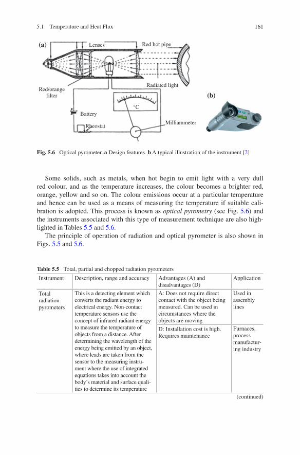
161

Some solids, such as metals, when hot begin to emit light with a very dull red colour, and as the temperature increases, the colour becomes a brighter red, orange, yellow and so on. The colour emissions occur at a particular temperature and hence can be used as a means of measuring the temperature if suitable cali-bration is adopted. This process is known as optical pyrometry (see Fig. 5.6) and the instruments associated with this type of measurement technique are also high-lighted in Tables 5.5 and 5.6.

The principle of operation of radiation and optical pyrometer is also shown in Figs. 5.5 and 5.6.

Lenses

Red/orange filter

Red hot pipe

Radiated light

Battery

RheostatMilliammeter

°C

(a)

(b)

Fig. 5.6 Optical pyrometer. a Design features. b A typical illustration of the instrument [2]

Table 5.5 Total, partial and chopped radiation pyrometers

Instrument Description, range and accuracy Advantages (A) and disadvantages (D)

Application

Total radiation pyrometers

This is a detecting element which converts the radiant energy to electrical energy. Non-contact temperature sensors use the concept of infrared radiant energy to measure the temperature of objects from a distance. After determining the wavelength of the energy being emitted by an object, where leads are taken from the sensor to the measuring instru-ment where the use of integrated equations takes into account the body’s material and surface quali-ties to determine its temperature

A: Does not require direct contact with the object being measured. Can be used in circumstances where the objects are moving

Used in assembly lines

D: Installation cost is high. Requires maintenance

Furnaces, process manufactur-ing industry

(continued)

5.1 Temperature and Heat Flux

162 5 Natural Gas Measurement Systems

Table 5.6 Ratio, reflecting and optical pyrometers

Instrument Description, range and accuracy

Advantages (A) and disadvantages (D)

Application

Ratio (two colour) pyrometers

An amplifier and recorder or indicator which measures and displays the output of the detector. Basically two partial-radiation pyrometers built into one. The two halves are sensitive to different wavebands and the tem-perature is obtained from the ratio of the outputs. Range: 700–1,800 °C

A: Reading is inde-pendent of the target paragraph emissivity provided emissivity is the same in both wavebands. The reading is independent of target size, provided the target surroundings are at least 300 °C colder than the target. The reading is in depended of partial obscuration of the target and of atmospheric absorption

Used in cement kilns and for the measure-ment of the tempera-ture of liquid metals

D: More expensive than single-waveband partial-radiation pyrometers

Instrument Description, range and accuracy Advantages (A) and disadvantages (D)

Application

Partial-radiation pyrometers

An optical system which ensures that radiation from the target either falls or is focused on the detecting element. It is most likely that the waveband is determined by the detector itself. Detectors in use are photo-electric, photoconductive and photoemissive types

A: There is the possibility to select a sensitive waveband to suit particular requirements

Food processing engineering

D: Installation cost is high. Requires maintenance

Chopped radiation pyrometers

An optical system which selects only radiation in the required waveband for detection. The radiation entering is periodi-cally interrupted by a mechani-cal device, which is usually a rotating disc with alternate open and opaque segments. It is possible to use AC amplifica-tion and sensitive detectors. The waveband can then be chosen to suit particular applications. Accuracy: ±1 %

D: Installation cost is high. Requires maintenance

Various

Table 5.5 (continued)

(continued)

163

5.1.4 Measurement of the Bulk Temperature of Solids and Liquids

This is described as one of the easier temperature-measuring problems encountered in industry. Provided that the sensor is completely surrounded by the medium and immersed to an adequate depth, no corrections are required for transient mass or heat transfer effects, conduction effects, radiation or velocity effects. The most common methods of measuring industrial bulk temperatures are by using thermocouples and resistance thermometers, which are referred to in Sect. 5.1.2.

Table 5.6 (continued)

Instrument Description, range and accuracy

Advantages (A) and disadvantages (D)

Application

Reflecting hemisphere pyrometers

The radiation detector is mounted at the top of the gold-plated reflecting cup, which is placed on the hot surface. The temperature is determined without knowing the emissivity of the surface, since it is measured essen-tially in black body condi-tions. A silicon cell would be the preferred detector option. Up to 1,300

Using a solar cell detec-tor is faster and better able to withstand high temperatures

Molten metals, forg-ing, ceramics, invest-ment casting and calibration procedures

It is less sensitive to emissivity errors and is more expensive

Optical pyrometers

This has some form of telescope, through which the high temperature object is observed. Usually, the telescope will have a light filter installed, to reduce dam-age to eyes. The telescope is focused on the object whose temperature is required. Colour filters can be intro-duced to the side of the object and the colour of the filter is matched with the colour of the object. There is a calibrated scale on the side of the object, which records the temperature. Range: Ranges: 700–1,400 °C, Accuracy: ±0.5

A: Accurate, robust VariousD: Expertise

5.1 Temperature and Heat Flux

164 5 Natural Gas Measurement Systems

5.1.5 Measurement of the Surface Temperature of Solids and Liquids

When heat transfer is of interest, it is essential to note that the surface is the only portion of the system that is accessible for measurement of temperature. In this case where the surface is accessible, measurement can be made with surface pyrometers such as the radiation and optical methods discussed in Sect. 5.1.3. Each of these instruments is easy to use and is suitable for discontinuous measurements.

Where the surface may not be accessible, for example in industrial environ-ments, it is necessary to fix the detecting element in place prior to heating the surface (the elements used are thermocouples). This option is simple; how-ever, precautions must be taken to avoid errors that can be introduced through changes in local transfer conditions, uncertainty about the positioning of the hot junction and heat loss by conduction along the thermocouples. In order to reduce this occurring, couples should have smaller diameters and be well insulated.

5.1.6 Gas Temperature Measurement

Measuring gas temperature is very difficult as a gas is rarely in thermal equi-librium with its surroundings and in furnaces, its spectral characteristics are unknown.

As a result of this, there are only three instruments, shown in Table 5.7 that are suitable for the measurement of gas temperature for industrial furnace applications:

1. The suction pyrometer, i.e. metal and water-cooled metal (See also Fig. 5.7).2. The Venturi Pneumatic Pyrometer.3. The Schmidt radiation method

5.1.7 Heat Flux Measurement

On some occasions, it is necessary to make a direct measurement of the heat flux incident upon a point in a furnace wall. The three instruments used to measure heat flux are: plug type, radial disc and ellipsoidal (see Figs. 5.8, 5.9 and 5.10, respectively). Each of these are available commercially, but are usually made spe-cially to suit a particular application. See Table 5.8 for particulars on each of these instruments.

165

Tabl

e 5.

7 M

easu

rem

ent o

f ga

s te

mpe

ratu

re

Inst

rum

ent

Des

crip

tion,

ran

ge a

nd a

ccur

acy

Adv

anta

ges

(A)

and

disa

dvan

tage

s (D

)A

pplic

atio

n

The

met

al

suct

ion

pyro

met

er

Thi

s in

stru

men

t mea

sure

s th

e tr

ue te

mpe

ratu

re o

f a

gas.

The

sen

sor

used

is

a ty

pe S

A: I

nstr

umen

t can

be

wid

ely

used

. Has

a h

igh

resp

onse

rat

e. I

s po

rtab

le a

nd r

obus

t and

onl

y re

quir

es A

C p

ower

sup

ply.

Pro

tect

s th

e th

er-

moc

oupl

e fr

om r

adia

tion

erro

rs b

y sh

ield

ing

Man

ufac

turi

ng

indu

stry

The

rmoc

oupl

e is

shi

elde

d by

3 c

once

ntri

c ce

ram

ic tu

bes

to m

inim

ise

the

radi

ativ

e ex

chan

ge f

rom

the

surr

ound

ing

surf

ace

or fl

ames

. The

gas

that

is

draw

n is

thro

ugh

the

stai

nles

s st

eel t

ube

and

then

pas

ses

out o

f th

e in

stru

-m

ent t

hrou

gh th

e T-

piec

e to

the

suct

ion

line.

The

em

f ge

nera

ted

by th

e th

erm

ocou

ple

is f

ed to

a s

ocke

t hou

sed

in th

e as

sem

bly

at th

e re

ar o

f th

e T-

piec

e. C

ompe

nsat

ing

cabl

e is

then

use

d to

con

nect

the

pyro

met

er to

the

mea

suri

ng in

stru

men

t. R

ange

: 0–1

100

°C, A

ccur

acy:

±2.

5 %

D: S

hiel

d ca

n be

blo

cked

by

dirt

y ga

ses,

th

eref

ore

caus

ing

dete

rior

atio

n of

the

ther

-m

ocou

ple

and

a sl

ow r

espo

nse

spee

d in

som

e ca

ses

Wat

er-

cool

ed m

etal

su

ctio

n py

rom

eter

It w

as d

evel

oped

to b

e us

ed a

s a

high

-tem

pera

ture

acc

esso

ry f

or u

se

with

por

tabl

e su

ctio

n py

rom

eter

des

crib

ed a

bove

. Ran

ge: 0

–1,6

00 °

C,

Acc

urac

y: ±

2.5

%

A: C

an b

e ex

tend

ed to

rea

d up

to 1

,800

°C

. H

as a

rap

id s

peed

of

resp

onse

Hea

t ex

chan

ger

D: R

equi

res

a su

ffici

ent fl

ow o

f w

ater

to a

void

in

stru

men

t dam

age

The

Ven

turi

pn

eum

atic

py

rom

eter

Mea

sure

s bo

th g

as a

nd fl

ame

tem

pera

ture

s. T

he g

as te

mpe

ratu

re is

mea

sure

d by

com

pari

ng th

e ga

s de

nsity

at t

he u

nkno

wn

tem

pera

ture

with

its

dens

ity a

t a

low

er te

mpe

ratu

re. T

he d

ensi

ty m

easu

rem

ents

are

ach

ieve

d by

ven

turi

rest

ric-

tions

, whi

ch s

tate

that

if Δ

P h a

nd Δ

P c a

re th

e pr

essu

re d

rops

acr

oss

the

hot

and

cold

ven

turi

es, r

espe

ctiv

ely,

and

if g

as te

mpe

ratu

res

at th

ese

poin

ts a

re T

h K

and

Tc K

, the

n T

h α

(ΔPh

/ΔPc

) Tc.

Ran

ge: 0

–2,5

00 °

C, A

ccur

acy:

±2

%

A: H

as a

ver

y ra

pid

rate

of

resp

onse

Man

ufac

turi

ng

indu

stry

D: T

hey

are

big

and

bulk

y

The

Sch

mid

t ra

diat

ion

pyro

met

er

Thi

s te

chni

que

prov

ides

a m

easu

rem

ent o

f th

e ef

fect

ive

tem

pera

ture

and

em

issi

vity

of

the

gas.

Tw

o re

adin

gs a

re ta

ken

thro

ugh

the

gas

with

a to

tal

radi

atio

n py

rom

eter

, one

with

a c

old

back

grou

nd th

e ot

her

with

a h

ot

back

grou

nd a

t a k

now

n ra

diat

ion

tem

pera

ture

. Alte

rnat

ivel

y, a

twin

-bea

m

pyro

met

er c

an b

e us

ed, o

ne b

eam

sig

hted

on

a ho

le in

the

furn

ace

and

the

othe

r on

a h

ot r

egio

n of

the

linin

g w

hich

con

tain

s a

ther

moc

oupl

e.

The

tem

pera

ture

obt

aine

d is

a m

ean

valu

e al

ong

the

optic

al p

ath

thro

ugh

the

gas

and

this

can

be

unac

cept

able

if la

rge

tem

pera

ture

gra

dien

ts a

re

invo

lved

. The

acc

urac

y al

so d

epen

ds o

n th

e em

issi

vity

of

the

gas

D: T

hey

give

non

linea

rly

wei

ghte

d av

erag

es

of u

nkno

wn

quan

titie

s ac

ross

the

com

bust

orC

ombu

stio

n ch

ambe

r m

easu

rem

ents

Taki

ng g

as s

ampl

es is

dif

ficul

t with

out d

is-

turb

ing

the

com

bust

ion

proc

ess

5.1 Temperature and Heat Flux

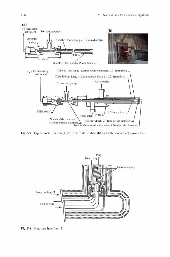
166 5 Natural Gas Measurement Systems

To suction pumpTo measuring

instrument

Asbestos spring

Sheathed thermocouple 1.59mm diameter

c. 125mmc. 900mm

Stainless steel hood 6.35mm diameter

To suction pump

To measuring instrument

PTFE swarf

Water inlet

Water outlet

‘O’ rings

Sheathed thermocouple 1.59mm outside diameter

Tube 321mm long, 11.1mm outside diameter, 0.711mm thick

Tube 305mm long, 14.3mm outside diameter, 0.711mm thick

6.35mm spider

6.35mm chock, 2.44mm inside diameter

Tube 6.35mm outside diameter, 4.5mm inside diameter

(a)

(b)

(c)

Fig. 5.7 Typical metal suction (a) [2, 3] with illustration (b) and water-cooled (c) pyrometers

PlugGuard ring

Thermocouples

Probe cooling

Plug cooling

Fig. 5.8 Plug-type heat flux [4]

167

5.2 Pressure

5.2.1 Introduction

Pressure can simply be defined as a measure of force per unit area, and the units of pressure are measured in either Pascal (1 N/m2), bar (105 Pa) or pound per square inch, gauge/absolute and mmHg. This section will go on to discuss various pres-sure terms and measurements commonly associated with the gas industry.

Connecting wires (e.g. copper)

Foil disc(e.g. constantan)

Instrument body (e.g. copper)

Water-cooled probe or housing

Fig. 5.9 Disc-type heat flux [4]

Cooling water

Cooling water

Copper

Stainless steel 20-25

∆V

Constantan wires

Thermocouple junctions

Nitrogen

Ellipsoid e = 0.5

F

Fig. 5.10 Ellipsodial heat flux [5]

5.2 Pressure

168 5 Natural Gas Measurement Systems

Absolute pressure refers to the absolute value of the force per unit area exerted on the surface of the fluid. Absolute pressure is defined as the difference between pressure at given point in a fluid and absolute zero or perfect vacuum.

Gauge pressure is the pressure difference between the absolute pressure and the local atmospheric pressure. It can also be referred to as differential-pressure.

The local atmospheric pressure varies from one place to another depending on the temperature, altitude and local weather conditions.

Differential-pressure refers to the measurement of the difference between any two pressures. Pressure may be measured directly in two ways:

Table 5.8 Plug, Radial disc and ellipsoidal heat flux measurement of heat flux

Instrument Description, range and accuracy Advantages (A) and dis-advantages (D)

Application

Plug-type heat flux meter

The heat incident upon the plug face is con-ducted through the plug to the water cooling at the rear. A guard ring system ensures the laminar flow of heat through the plug and the whole assembly is mounted in a water-cooled probe. The measurement of the heat flux is made by two thermocouples mounted with their hot junc-tions a distance apart on the axis of the plug, the heat flow through the plug, and hence, the heat flux incident on the plug face can be determined using the formula: Q = Aƛm (T2 − T1) /l

A: Accurate VariousD: Not simple in construction

Radial disc heat flux meter

Also measures the total heat flux. Here, the heat flux incident on the disc is conducted away radially to the instrument body which is water-cooled. The output is obtained from the differen-tial thermocouple formed by the junction of the disc circumference with the instrument body and the wire attached to the disc

A: Simple in construction and can be used in posi-tions inacces-sible to the plug type

Various

D: Less accurate and less robust. Each instru-ment requires individual calibration

Ellipsoidal radiometer

Has been designed to measure the total radiation from a solid angle. Radiation that passes through the instrument apertures is focused by the ellip-soidal mirror onto the blackened hemispherical detector, which is effectively the front surface of a very simple heat flow plug. The output is obtained from thermocouple junctions on the plug axis. A nitrogen purge is fed to the ellipsoid through small holes around its mirror diameter to prevent entry of furnace gases and particles

D: Slow response time. Not sensitive to convectional heat transfer effects

Used in fire testing. Furnace and flame radia-tion measure-ment since the sensing element is not exposed to hot gases

169

1. Pressure due to a fluid may be balanced by the pressure produced by a column of liquid of known density.

2. Pressure due to a fluid may be allowed to act over a known area, producing a force whose magnitude depends on the pressure.

5.2.2 Liquid-Column Pressure Gauges (Manometer)

There are various types of manometers used, which have different ranges and accuracies depending of the manometric fluid and configuration. The basic type is the U-tube manometer, which is a measuring device that measures pressure near atmospheric pressure. They are usually simple in construction containing mono-metric fluid, which is usually mercury due to its high density and low vapour pres-sure, as shown schematically in Fig. 5.11.

Liquid-column manometers have highly linear calibration with poor dynamic response. When measuring a vacuum pressure, the manometric fluid may evapo-rate and contaminates the vacuum if its vapour pressure is too high.

5.2.3 Force-Balanced Pressure Gauges

The force produced by a pressure can be measured by balancing it against a known weight or by the strain or deformation it produces in an elastic medium.

Measurement by balance against a known weight: In this kind of instrument, the force produced on a piston of known area is measured directly by the weight it will support. The pressure gauges operating on this principle are: (a) the pis-ton type, (b) the ring-balance type and (c) the bell type as shown in Fig. 5.12. Table 5.9 (A) and (B) provides more details of these gauges.

P0

Ambient fluid(atmospheric pressure in most cases)

Reference fluid with density of ρ

(Liquid, e.g. water or mercury)

Unknown pressure

P

Fluid of interest(Gas in most cases)

h

Gas pressure (∆P) = P – P0 = ρgh

(a) (b)

Fig. 5.11 Schematic diagram of U-tube manometer (a) and illustration of the device (b)

5.2 Pressure

170 5 Natural Gas Measurement Systems

PI

Weight (G)

Piston area (A, m2)Relief valve

Priming pump and reservoir

Valve opens only when priming

Screw press

P2

P1

Sealing liquid

Control weight

Range spring

High pressure

Low pressure

Bell

Restrictor

Overload valve

Fine restrictor

(a)

(b)

(c)

Fig. 5.12 Different types of pressure gauges. a The piston-type. b The ring-balanced. c Typical bell-type differential meter for a very low range (thin wall)

171

Table 5.9 Liquid-column pressure gauges

Instrument Description, range and accuracy Advantages (A) and disadvantages (D)

Application

(A)

U-tube manometer

U-tube manometer is a simple manometer which consists of a glass U-tube containing liquid. The difference in heights of the liquid in the two arms can be used as an indication of the pressure if the fluid is specified

A: It is used for measurement of differential-pressure

Simple in construction. Low cost hence easy to buy. Very accurate and sensitive. It can be used to meas-ure other process variables

D: Fragile in construction. Very sensitive to tempera-ture changes. Error can happen while measuring the height

Well-type manometer

The well has a cross section larger than that of the indicating tube rises appreciably. A direct reading of height can be taken from the scale which is designed to correct for the error introduced by the fall of level in the well. The nature of the fluid whose pressure is being measured and the pressure required would determine the kind of fluid used in the gauge

A: Used for standard cali-bration of other pressure-measuring elements. Used for more direct reading instrument than the U-tube manometer

They have no mechani-cally mov-ing parts. They are not expensive. They are simple

Up to 800 mmHg. In most cases, the uncertainty of a manometer reading is +0.5 of the smallest scale graduation

D: The higher pressure source being measured must always be connected to the well connection

Inclined-tube manometer

The inclined tube may be straight or curved, in each case the gauge can be calibrated to give a flow measurement directly. Inclined-tube manometer is used to measure small differential-pressure. Up to 40 mm H2O. Can read up to 2 mm. Accuracy: +3 %

Used to measure small differential-pressure

It is used for measuring pressure above or below atmospheric pressure. It is not expen-sive. It is simple and compact

(B)

Differential liquid manometer

Differential liquid manometer uti-lises the movement of an interface between two liquids which have different relative densities (specific gravities), different colours and do not mix. The cross-sectional areas of the wells are usually ten times larger than that of the U-tube

Used to measure the flow dynamics of gas flow in pipe

Various

(continued)

5.2 Pressure

172 5 Natural Gas Measurement Systems

Measurement of strain or deformation: These pressure elements are mechanical devices that are deformed by the applied pressure. They possess elasticity, and when deformed, the stresses establish equilibrium with the applied pressure. The choice and design of the type of element used depends on the magnitude of the pressure to be measured. These are, namely (a) the bourdon-tube, the diaphragm type and (c) the bellows type. Figure 5.14 shows schematically typical force-balanced pressure gauges types. Table 5.10 (A) and (B) also provides further details of these pressure gauges (Fig. 5.13).

5.2.4 Pressure Transducers

Pressure Transducers are devices that use an electrical system in conjunction with mechanical gauges to convert the deflection, due to pressure changes into electri-cal signals. They are useful for measuring pressures continuously, such that the electrical signal supplied to a control system can be used to monitor the pressure variations. Figure 5.14 shows the schematic diagram of strain gauge pressure cell.

There are two major types of pressure transducers: mechanical and electrical as described briefly in the following with further details in Tables 5.10 and 5.11, respectively.

5.2.5 Mechanical Pressure Transducer

The pressure-sensing element in a mechanical transducer shown in Fig. 5.15 is composed of a metal diaphragm capsule which translates the applied pressure into mechanical displacement. The tiny movement is detected by a sensitive flapper

Instrument Description, range and accuracy Advantages (A) and disadvantages (D)

Application

Micro-manometer

Micro-manometer consists of a shallow U-tube system, the left-hand limb being in the form of an inclined sight tube. The right-hand limb consists of a reservoir which may be raised or lowered. The height of the reservoir in relation to the sight tube is adjusted by means of a verti-cal micrometre screw. The gauge is constructed so that the opposing effect of temperature change on the surface tension and density of the gauge liquid largely cancel out. 0–3 bar and 0–50 mbar

Can measure small differential-pressures accurately

Various

Table 5.9 (continued)

173

Tabl

e 5.

10

Mec

hani

cal p

ress

ure

tran

sduc

ers

Inst

rum

ent

Des

crip

tion,

ran

ge a

nd a

ccur

acy

Adv

anta

ges

(A)

and

disa

dvan

tage

s (D

)A

pplic

atio

n

(A)

Pist

on p

ress

ure

Gau

geT

he f

orce

pro

duce

d on

a p

isto

n of

kno

wn

area

is m

easu

red

dire

ctly

by

the

wei

ght i

t will

sup

port

. If

the

pres

sure

act

ing

on th

e pi

ston

is p

Pa

and

the

area

ove

r w

hich

it a

cts

is A

m2 ,

the

forc

e pr

oduc

ed w

ill b

e Px

A(N

). I

f th

ere

is n

o fr

ictio

n th

en P

A =

F, t

he

wei

ght s

uppo

rted

by

the

pist

on. T

he s

yste

m s

how

n is

dea

dwei

ght

pres

sure

test

er w

hich

is u

sed

as a

sta

ndar

d of

pre

ssur

e m

easu

re-

men

t for

test

ing

othe

r ty

pes

of in

stru

men

t. U

p to

55

MPa

The

y ar

e w

idel

y us

ed f

or m

aint

aini

ng

calc

ulab

le p

ress

ures

in a

ran

ge e

xten

d-in

g fr

om a

bout

3 k

Pa (

gas

med

ia,

abso

lute

or

gaug

e m

ode)

to 1

GPa

(h

ydra

ulic

, gau

ge m

ode)

. Thi

s in

stru

-m

ent c

an b

e us

ed to

cal

ibra

te v

irtu

ally

an

y pr

essu

re d

evic

e

Eas

y to

han

dle.

It i

s us

ually

com

pact

and

sp

ace-

savi

ng. P

isto

n/cy

linde

r as

sem

blie

s ar

e si

mpl

e in

con

figur

a-tio

n, a

nd th

ere

are

no

mou

ntin

g fla

nges

or

othe

r ge

omet

ric

irre

gu-

lari

ties

that

can

res

ult i

n co

mpl

icat

ed s

tres

ses

in

the

cylin

der.

It c

anno

t be

use

d to

mea

sure

the

pres

sure

of

a flo

win

g flu

id

Rin

g pr

essu

re

gaug

eT

he o

pera

ting

forc

e de

pend

s on

the

diff

eren

ce b

etw

een

the

pres

sure

s on

the

two

side

s of

the

part

ition

. The

con

trol

wei

ght

atta

ched

to th

e in

stru

men

t is

used

for

the

calib

ratio

n. T

he r

ange

is

fixed

by

the

natu

re a

nd th

ickn

ess

of th

e m

ater

ial o

f co

nstr

uctio

n an

d th

e pr

essu

re w

hich

the

flexi

ble

conn

ectio

ns w

ill s

tand

. The

ra

nge

of d

iffe

rent

ial i

s fix

ed b

y th

e si

ze o

f th

e si

ze o

f th

e ri

ng a

nd

the

natu

re a

nd q

uant

ity o

f se

alin

g liq

uid

Use

d to

mea

sure

the

low

pre

ssur

e di

ffer

entia

l of

the

orde

r of

100

Pa

(1 m

bar)

Gas

indu

stry

and

va

riou

s

(con

tinue

d)

5.2 Pressure

174 5 Natural Gas Measurement Systems

Inst

rum

ent

Des

crip

tion,

ran

ge a

nd a

ccur

acy

Adv

anta

ges

(A)

and

disa

dvan

tage

s (D

)A

pplic

atio

n

Bel

l pre

ssur

e G

auge

In th

e be

ll ty

pe o

f ga

uge,

the

forc

e pr

oduc

ed b

y th

e di

ffer

ence

of

pres

sure

on

the

insi

de a

nd o

utsi

de o

f th

e be

ll is

bal

ance

d ag

ains

t a

wei

ght o

r fo

rce

prod

uced

by

the

com

pres

sion

of

a sp

ring

. The

re

are

two

type

s th

e th

ick-

wal

l and

thin

-wal

l. In

thic

k-w

all i

nstr

u-m

ent,

the

resu

ltant

for

ce c

ause

s th

e be

ll to

ris

e un

til e

quili

briu

m

is r

each

ed. T

he th

ickn

ess,

den

sity

, cro

ss-s

ectio

nal a

rea

and

the

dens

ity o

f th

e se

alin

g liq

uid

are

dete

rmin

ed b

y ra

nge

for

whi

ch

the

inst

rum

ent i

s to

be

used

. In

the

thin

-wal

l ins

trum

ent,

the

cont

rolli

ng f

orce

is o

btai

ned

by a

spr

ing.

The

trav

el o

f th

e be

ll is

pro

port

iona

l to

the

diff

eren

tial-

pres

sure

to b

e m

easu

red.

Thi

s ty

pe o

f in

stru

men

t nee

ds n

o ov

erlo

ad d

evic

e. T

he r

ange

will

be

dete

rmin

ed b

y th

e m

odul

us o

f el

astic

ity o

f th

e sp

ring

and

by

the

dens

ity o

f th

e se

alin

g liq

uid.

Ran

ge: 0

–250

Pa

and

0–3

kPa

Use

d to

mea

sure

low

sta

tic p

ress

ures

Gas

indu

stry

and

va

riou

s

(B)

Bou

rdon

-tub

e Pr

essu

re G

auge

It c

onsi

sts

of a

nar

row

-bor

e tu

be o

f el

liptic

al c

ross

sec

tion

seal

ed

at o

ne e

nd. W

hen

the

pres

sure

to b

e m

easu

red

is a

pplie

d, th

e ef

fect

of

the

forc

es in

tube

is to

str

aigh

ten

it so

that

the

clos

ed

end

is d

ispl

aced

. Thi

s di

spla

cem

ent i

s m

agni

fied

and

indi

cate

d on

th

e ci

rcul

ar d

ial b

y m

eans

of

mec

hani

cal l

inka

ges.

The

pre

ssur

e ch

ange

s m

ust n

ot p

rodu

ce f

orce

s w

hich

exc

eed

the

elas

tic li

mits

of

the

tube

so

that

it a

lway

s re

turn

s to

its

orig

inal

‘C

’ sha

pe w

hen

the

pres

sure

is r

elea

sed.

The

tube

s ar

e m

ade

from

a v

arie

ty o

f m

ater

ials

in a

var

iety

of

thic

knes

s. T

he m

ater

ial o

f co

nstr

uctio

n de

pend

s on

the

natu

re o

f th

e flu

id w

hose

pre

ssur

e is

bei

ng m

eas-

ured

and

the

thic

knes

s on

the

rang

e of

mea

sure

men

t req

uire

d.

Nor

mal

wor

king

pre

ssur

e sh

ould

not

be

grea

ter

than

60

% o

f th

e m

axim

um p

ress

ure

indi

cate

d. R

ange

: 0.1

–130

MPa

Acc

urac

y:

+1

%

Indu

stri

al-t

ype

gaug

e de

sign

for

flui

d m

ediu

m w

hich

doe

s no

t clo

g co

nnec

-tio

n or

cor

rode

316

sta

inle

ss s

teel

type

The

y ha

ve v

ibra

tion

and

shoc

k re

sist

ant.

It h

as

resi

stan

t to

corr

osio

n be

caus

e it

mad

e of

st

ainl

ess

stee

lT

he fi

lled

fluid

dep

ends

on

the

proc

ess

and

pres

sure

med

ium

to

mea

sure

esp

ecia

lly f

or

food

app

licat

ion

Tabl

e 5.

10

(con

tinue

d)

(con

tinue

d)

175

Inst

rum

ent

Des

crip

tion,

ran

ge a

nd a

ccur

acy

Adv

anta

ges

(A)

and

disa

dvan

tage

s (D

)A

pplic

atio

n

Dia

phra

gm

Pres

sure

Gau

geT

he m

ovem

ent o

f a

diap

hrag

m is

a c

onve

nien

t way

of

sens

ing

a pr

essu

re d

iffe

rent

ial;

this

is u

sed

in d

iaph

ragm

pre

ssur

e ga

uges

. T

he u

nkno

wn

pres

sure

is a

pplie

d to

one

sid

e of

the

diap

hrag

m

who

se e

dge

is r

igid

ly fi

xed

and

the

disp

lace

men

t of

the

cent

re o

f th

e di

aphr

agm

is tr

ansm

itted

via

a s

uita

ble

join

t and

mag

nific

a-tio

n lin

kage

to th

e po

inte

r of

the

inst

rum

ent.

In p

rinc

iple

, the

co

rrug

ated

dis

cs g

ive

a la

rger

dis

plac

emen

t and

can

be

com

bine

d to

for

m a

cap

sule

. The

inst

rum

ents

are

usu

ally

use

d ab

ove

or

belo

w a

tmos

pher

ic p

ress

ure,

and

the

mat

eria

l of

cons

truc

tion

is

chos

en to

sui

t a p

artic

ular

app

licat

ion.

Ran

ge: 2

.5 m

bar–

0.4

MPa

; A

ccur

acy:

1–2

.5 %

Dia

phra

gm p

ress

ure

gaug

es a

re u

sed

in th

e ch

emic

al in

dust

ry, c

hem

ical

fib

re, s

ynth

etic

fibr

e, o

il, d

yes,

alk

ali

and

othe

r in

dust

ries

. It i

s us

ed w

hen

med

ium

cou

ld b

e ha

rmfu

l to

the

pres

-su

re g

auge

It m

easu

res

fluct

uat-

ing

pres

sure

bet

ter

than

bou

rdon

gau

ge.

Dia

phra

gm s

eal p

re-

vent

s m

ediu

m e

nter

ing

the

gaug

eIt

can

not b

e us

ed in

a

corr

osiv

e en

viro

nmen

t

Bel

low

s Pr

essu

re

Gau

geA

n al

tern

ativ

e to

the

diap

hrag

m s

tack

is th

e be

llow

s el

emen

t w

hich

can

be

put i

nto

inst

rum

ents

to m

easu

re d

iffe

rent

ial,

abso

-lu

te a

nd g

auge

pre

ssur

e. T

he m

ater

ial o

f co

nstr

uctio

n in

clud

es

bery

llium

, cop

per,

bron

ze a

nd s

tain

less

ste

el. T

he ‘

flexi

bilit

y’

of a

bel

low

s is

pro

port

iona

l to

the

num

ber

of c

onvo

lutio

ns a

nd

inve

rsel

y pr

opor

tiona

l to

the

wal

l thi

ckne

ss a

nd m

odul

us o

f el

astic

ity o

f th

e be

llow

s m

ater

ial.

The

‘co

mpr

essi

on m

odul

us’

of a

bel

low

s va

ries

dir

ectly

as

the

mod

ulus

of

elas

ticity

of

the

bello

ws

mat

eria

l and

the

cube

of

the

wal

l thi

ckne

ss. I

t is

also

in

vers

ely

prop

ortio

nal t

o th

e nu

mbe

r of

con

volu

tions

and

to th

e sq

uare

of

the

outs

ide

diam

eter

of

the

bello

ws.

The

spr

ing

rate

can

be

incr

ease

d by

fitti

ng a

n in

tern

al s

prin

g to

opp

ose

the

forc

e co

m-

pres

sing

the

bello

ws.

Mea

suri

ng p

ress

ures

up

to 5

Mpa

, tho

ugh

desi

gn f

or lo

w p

ress

ure,

Acc

urac

y: ±

1.00

%

Bel

low

ele

men

ts a

re u

sed

in v

ario

us

appl

icat

ions

whe

re th

e pr

essu

re-s

ensi

-tiv

e de

vice

mus

t be

pow

erfu

l eno

ugh

to

oper

ate

not o

nly

the

indi

catin

g po

inte

r bu

t als

o so

me

type

of

reco

rdin

g de

vice

whi

ch c

onve

rts

the

diff

eren

tial-

pres

sure

in

to a

rot

ary

mov

emen

t by

way

of

a to

rsio

n tu

be

asse

mbl

y an

d m

echa

ni-

cal l

inka

ges

Tabl

e 5.

10

(con

tinue

d)

5.2 Pressure

176 5 Natural Gas Measurement Systems

Process pressure

A

A

C-Bourdon

Process pressure

Spiral

Process pressure Moving tip

Helical C-Bourdon

(a)

(b)

Fig. 5.13 Bourdon-tube (a) and diaphragm (b) strain type gauges

177

Low pressure diaphragms

Overload plug

Silicone fluid (low pressure)

High pressure diaphragms

P2

(low pressure)P1

(high pressure)

Sensor Output to transducer electronics

Silicone fluid (high pressure)

Fig. 5.14 Strain gauge pressure cell

Table 5.11 Electrical pressure transducers

Instrument Description, range and accuracy Advantages (A) and disadvantages (D)

Application

Strain gauge

In strain gauge pressure trans-ducer, the round platform at the top could be a diaphragm which is pushed down by a rising pressure. In a weighing device, it would be part where the unknown weight is applied. When a downward force is applied to the platform (diaphragm), it pushes down on the cross-shaped spring. There are rods of insulating material extending above and below the cross and thin wire winding is arranged around these rods. When the centre of the cross is pushed down, all the rods will tilt inwards at the top and outwards at the bottom. Therefore, the resistance of the windings under the cross will increase, while the upper resistance will decrease due to the slight relaxation of tension in these wires. The Wheatstone Bridge uses full difference between these windings to give a good deflection of the meter for only small changes in force, 0.1– 0.25 % of full scale

They have fast speed of response Simple to maintain

Gas industry and various

Small and easy to installIt can only measure narrow-span pressure

(continued)

5.2 Pressure

178 5 Natural Gas Measurement Systems

and nozzle device that regulates the air output from the transmitting section of the cell. The output pressure operates a remote recorder (in a control room), and it provides a feedback force so that the output is directly proportional to the differen-tial-pressure across the diaphragm.

Instrument Description, range and accuracy Advantages (A) and disadvantages (D)

Application

Load cell Load cells operate on the same principle and are used mainly for weight measurement. This is basically a spring metal cylinder with a flanged base-plate. Four resistances are securely bonded on to the side of the cylinder. Two are arranged horizontally and vertically, they are constructed from long-track carbon-film resis-tors printed on flexible insulating sheets or they may be thin metal foil tracks. When a force—such as a weight—is applied to the top of the load cell, the walls of the cylinder becomes barrel-shaped under the load, only a very tiny movement occurs but it is sufficient to slightly stretch the horizontal resistors and slightly contract the vertical ones. Accuracy: 0.03–0.25 % full scale

A: The hydraulic type takes high impacts, insensitive to tem-perature. Pneumatic load cells intrinsically safe. Contains no fluids

Pneumatic load cells are some-times used where intrinsic safety and hygiene are desired, and hydraulic load cells are consid-ered in remote locations, as they do not require a power supply

D: The hydraulic type is expensive and complex, while the pneumatic type has slow response and requires clean, dry air

Capacitor micro-phone

Capacitor microphones are suit-able for measuring fluctuating pressures. Voltage is supplied from high-impedance source so that the charge on the capacitor remains constant .The fluctuat-ing capacitance shows as a fluctuating voltage which can be amplified directly. The capacitor microphone is used due to the fact that small transducers essential to ensure adequate frequency response and also enable sitting close to the pressure-sensing element so avoiding long leads. Pressure transducers have to be calibrated since they are affected ambient temperature changes. Ranges: micron range to (70 MPa). Accuracy: within 0.1 % of reading or 0.01 % of full scale

A: Accuracy in reading Used to measure larger pressure differences than liquid manom-eters and other gauge types. In industry, it is used as a remote con-trol transducer

D: Calibration required

Table 5.11 (continued)

179

They are available for temperatures as high as 300 °C without external cooling or up to 1,000 °C when fitted with special adaptors. The main advantages of these gauges in comparison with liquid manometers and other gauges are as follows:

1. Capable of transmitting results over a reasonable distance.2. They can withstand high pressures and only react to the difference between the

two applied pressures.3. The air output can be fed directly into a control system, thereby automatically

updating the controller.

See also Table 5.10 for further details.

Fig. 5.15 Schematic diagram of mechanical transducer

20 p.s.i.Restrictor

Nozzle

Supply

Pilot relay

Relay output

To control room recorder

High

Measuring diaphragm

Low

Pivot diaphragm

Signal forceFeedback

force

Heavy beam

Signal force

Flapper

5.2 Pressure

180 5 Natural Gas Measurement Systems

5.2.6 Electrical Pressure Transducer

Electrical transducers convert responses from a pressure-sensing element into an electrical output and are much better than other gauges and mechanical transduc-ers for remote reading, automatic recording or other signal processing require-ments. The delays in response due to long pressure leads are eliminated. There are three types of electrical pressure transducers which are as follows: strain gauge put from El Kamki project, load cell and capacitor microphone, as shown sche-matically in Figs. 5.16, 5.17 and 5.18. Table 5.11 also provides for further details.

Fig. 5.17 Typical load cell transducer

Diaphragm

Force rod Strain-gauge windings (1 and 2)

Mounting ring

Sapphire posts

Spring element

Strain-gauge windings (3 and 4)

(a) (b)

Fig. 5.16 Schematic strain gauge tranducer (a) and illustration (b)

181

5.3 Gas Flow Measurement

5.3.1 Introduction

Measuring gas flow is a necessity. Gas suppliers need to know how much gas they are selling and thus how much they earn on the other hand, the gas consumer needs to know how much gas they consume and if the charges reflect that quantity prior to determining what meters to adopt. Part of meeting demand and supply gas measurement also answers other issues such as leakages. As the gas supply chain involves different stages such as transmission and distribution, the same is true with gas metering as domestic and non-domestic meters are required. The aim of this section is to present gas flow measurement devices from all stages; from labo-ratory instruments, domestic type of meters to those in high-pressure transmission lines used by producers and suppliers. At each stage, different meter specifica-tions are required, and therefore, knowledge and experience are required in order to select the best meter suited for the task. The meters are presented in families according to their operating principle. They can all fall into two categories: those that extract energy from flow and those that add energy during measuring.

5.3.2 Pressure Differential Devices

When pressure differential devices are inserted into a pipe which carries a fluid, the device can cause a flow obstruction creating a pressure difference on either side of the device. Thus, the meters belonging to this family are known also as obstruction-type meters. These meters consist of a primary element that cre-ate a pressure change. The devices then sense the differences in pressure and transmit them by analogue or digital means in which the flow rate is estimated using Bernoulli’s equation that is proportional to the square root of the pressure

Fig. 5.18 Schematic diagram of capacitor microphone transducer

Process pressure

Gauge wires to a.c. bridge

circuit

5.3 Gas Flow Measurement

182 5 Natural Gas Measurement Systems

difference across the obstruction. Obstruction of flow also means pressure loss, which is characterised by the discharge coefficient (Cd) a specification found in all differential-pressure meters. This family of meters is well documented in stand-ards and codes of practice such as the BS 1042 [6].

5.3.2.1 Orifice Plates

The orifice plate shown schematically in Fig. 5.18, is a metal disc with a concen-tric hole that is placed into the pipe carrying the Flid being metered. They are sim-ple and cheap and are available in a wide range of sizes. Thus, they are popular among gas industries worldwide since all natural gas that is bought and the largest sales are made using this type of meter. Table 5.12 provides further details with respect to this instrument (Fig. 5.19).

Figure 5.20 also shows the illustration of the orifice plate on a gas transmission line and the typical plate used in the laboratory.

5.3.3 Venturi Meter

The venturi meter is another obstruction device that is designed to minimise the pressure drop. It has a precision-engineered machining as seen from its shape as shown in Fig. 5.21 that accounts for the cost and accuracy. In addition, it has a smooth internal surface; thus, no sticking of particles from liquids or bubbles from gas could occur. The key point is the machining of the radius between the upstream cone and the throat where separation effects may be caused on the throat tapping being in the highest velocity region. A vital feature is the down-stream diffuser which decelerates the flow and gives maximum pressure recovery. Thus, lower pressure loss but larger size. The size of the downstream diffuser can be reduced by up to 35 % without affecting the characteristics of the device, thus reducing costs. Figure 5.20 is a diagram that illustrates the principles of a venturi meter, and Fig. 5.22 is the examples of venturi at a construction site and one in a gas flow laboratory. Table 5.12 also provides more details for this flow measuring device.

5.3.4 Nozzle Meters

The nozzle meter is the result of the effort to reduce the size and cost of the clas-sical venturi meter. Therefore, it is simple in construction but has higher pressure loss on flowing fluid. Figure 5.23 shows an schematic of a standard design of flow nozzle. Table 5.13 also gives more details specification of the instrument.

183

Tabl

e 5.

12

Ori

fice

plat

e an

d ve

ntur

i met

er

Inst

rum

ent

Des

crip

tion,

ran

ge a

nd a

ccur

acy

Adv

anta

ges

(A)

and

disa

dvan

tage

s (D

)A

pplic

atio

n

Ori

fice

plat

eA

n or

ifice

pla

te is

a th

in p

late

whi

ch h

as a

hol

e in

the

mid

dle

with

a b

ev-

elle

d do

wns

trea

m e

dge

so th

at fl

uid

or g

as r

each

ing

it, is

for

ced

to c

onve

rge

as it

goe

s th

roug

h. V

ena

cont

ract

a is

the

poin

t of

max

imum

con

verg

ence

an

d is

loca

ted

just

dow

nstr

eam

of

the

orifi

ce. T

hus,

vel

ocity

and

pre

ssur

e ch

ange

. Aft

er th

e ve

na c

ontr

acta

poi

nt, t

he fl

ow p

rofil

e re

take

s its

ori

gina

l fo

rm. B

y m

easu

ring

the

diff

eren

ce in

flui

d pr

essu

re b

efor

e th

e or

ifice

pla

te

and

at th

e ve

na c

ontr

acta

(m

inim

um p

ress

ure)

, the

vol

umet

ric

and

mas

s flo

w r

ates

can

be

calc

ulat

ed f

rom

Ber

noul

li’s

equa

tion.

The

pla

te m

ust

with

stan

d bu

cklin

g; th

us, i

t req

uire

s a

suffi

cien

t thi

ckne

ss a

nd is

usu

ally

m

ade

of s

tain

less

ste

el. .

For

gas

flow

mea

sure

men

t, th

e or

ifice

is p

lace

d co

ncen

tric

ally

with

in th

e pi

pelin

e. K

ey f

eatu

res:

A: S

impl

e an

d ro

bust

. Wel

l doc

umen

ted

by s

tand

ards

[6]

.Sta

ndar

d de

sign

s do

no

t nee

d ca

libra

tion.

Pla

te lo

w p

urch

ase-

pric

ed m

easu

res

liqui

ds a

nd g

ases

Hig

h-pr

essu

re

gas

met

erin

g on

the

larg

e flo

ws

betw

een

supp

liers

and

tr

ansm

issi

on

com

pani

es.

Fisc

al m

eter

ing

D: N

ot a

vaila

ble

in m

any

rang

es.

Perf

orm

ance

cha

nges

with

dam

aged

pl

ate

mai

nly

due

to e

rosi

on w

hich

can

pr

oduc

e ch

ange

s in

rou

ghne

ss a

nd g

ive

an

erro

r up

to 5

%. V

ulne

rabl

e to

poo

r flo

w

profi

les

and

swir

l pro

duce

d by

gov

erno

rs,

com

pres

sors

, ben

ds (

up to

15

% e

rror

at

40o

angl

e). N

ot li

near

to fl

ow r

ate

outp

ut

rela

tion.

Dif

ficul

t to

acco

unt a

ccur

acie

s w

hich

dep

ends

on

com

plet

e in

stal

latio

n an

d co

nditi

on o

f flo

ws.

For

hig

h ac

cura

cy

gene

rate

s hi

gh s

econ

dary

cos

ts to

geth

er

with

ful

l ins

talla

tion.

Col

lect

ion

of d

ust

or d

ebri

s be

fore

the

orifi

ce p

late

. A fi

lter

and

flow

str

aigh

tene

r an

d re

gula

r pl

ate’

s sh

arpn

ess

chec

king

may

red

uce

occu

rrin

g pr

oble

ms

Squa

re u

pstr

eam

edg

e w

hich

set

s th

e se

para

tion

poin

t thu

s co

ntra

ctio

nT

he c

onic

al e

ntra

nce

type

has

cha

mfe

red

upst

ream

edg

e an

d sq

uare

do

wns

trea

m e

dge

and

is u

sed

on v

isco

us fl

uids

. It i

s de

sign

ed to

kee

p C

d co

nsta

nt to

low

er R

eyno

lds

num

bers

Dis

char

ge c

oeffi

cien

t Cd =

0.6

con

stan

t at n

umbe

rs g

reat

er th

an 5

× 1

0−5

Re

Ran

ge: 3

to 4

:1 d

iffic

ult t

o ac

coun

t, de

pend

s on

com

plet

e in

stal

latio

n an

d co

nditi

on o

f flo

ws.

Acc

urac

y: 0

.6 to

±0.

75 %

Ven

turi

m

eter

sV

entu

ri is

a tu

bula

r se

t-up

whe

re fl

uid

flow

s th

roug

h a

vary

ing

diam

eter

pi

pe. A

ven

turi

tube

typi

cally

has

an

entr

y co

ne o

f 30

deg

rees

and

an

exit

cone

of

5 de

gree

s. T

his

geom

etry

allo

ws

the

vent

uri t

o m

aint

ain

a pr

acti-

cally

con

stan

t coe

ffici

ent o

f di

scha

rge

whe

n th

e R

eyno

lds

num

ber

(Re)

is

gre

ater

that

3 ×

105

at th

e th

roat

of

the

tube

. The

geo

met

ry e

xclu

des

curv

atur

e ef

fect

s at

the

tapp

ings

hav

ing

alm

ost o

ne-d

imen

sion

al fl

ow in

the

thro

at b

ecau

se o

f th

e ac

cele

ratio

n. D

isch

arge

coe

ffici

ent C

d ≈

1, c

onst

ant a

t nu

mbe

rs g

reat

er th

an 3

× 1

0−5

Re.

Mea

sure

men

t unc

erta

inty

of

only

±1

%

10–1

5 %

of

the

pres

sure

dif

fere

nce

acro

ss

A: C

ompa

red

to o

rific

e: H

ighe

r ef

ficie

ncy

and

pres

sure

rec

over

y. G

ood

perf

orm

ance

at

hig

h β

-rat

ios.

Mor

e ro

bust

and

less

af

fect

ed b

y in

tern

al e

rosi

on. L

ess

sens

itive

to

ups

trea

m d

istu

rban

ces

Use

d in

wat

er

dist

ribu

tion

sys-

tem

. Lab

orat

ory

mea

sure

men

ts.

Not

com

mon

fo

r us

e in

gas

m

eter

ing

D: O

ccup

ies

muc

h lo

nger

leng

th in

line

. M

ore

expe

nsiv

e to

man

ufac

ture

and

in

stal

l. L

arge

r si

ze d

iffic

ult t

o ha

ndle

. Not

pr

efer

able

in g

as I

ndus

try

5.3 Gas Flow Measurement

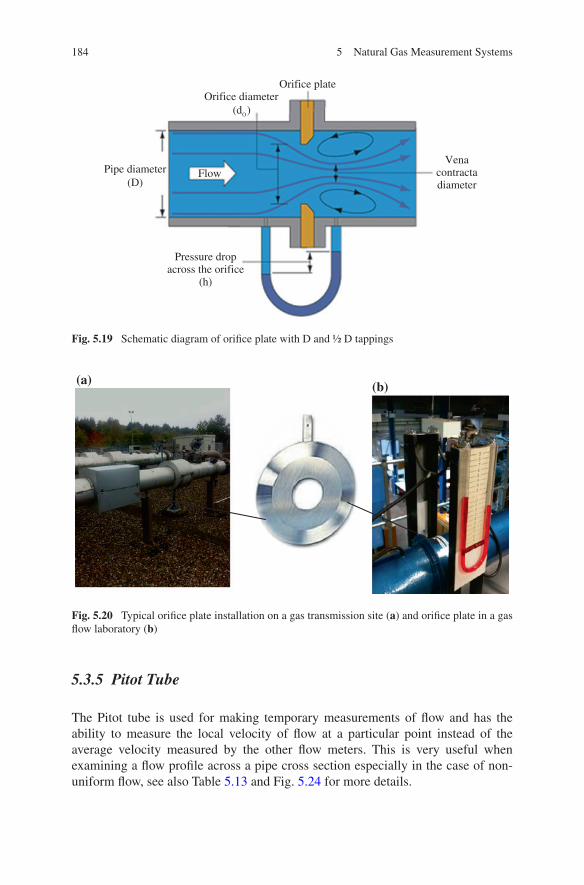
184 5 Natural Gas Measurement Systems

5.3.5 Pitot Tube

The Pitot tube is used for making temporary measurements of flow and has the ability to measure the local velocity of flow at a particular point instead of the average velocity measured by the other flow meters. This is very useful when examining a flow profile across a pipe cross section especially in the case of non-uniform flow, see also Table 5.13 and Fig. 5.24 for more details.

Orifice plateOrifice diameter

(dO)

Pipe diameter (D)

Pressure drop across the orifice

(h)

Vena contracta diameter

Flow

Fig. 5.19 Schematic diagram of orifice plate with D and ½ D tappings

(a) (b)

Fig. 5.20 Typical orifice plate installation on a gas transmission site (a) and orifice plate in a gas flow laboratory (b)

185

≤ 0.1D

≥ 0.03d

d

≤ 0.03d

Cylindrical0.3d

0.6041d

d/30.2d

D Flow

Fig. 5.23 Standard design of flow nozzle

Venturi meter

A2

V2

A1 V1

A2

V2

LO

P1

HI

P2

Fig. 5.21 Principles of a venturi meter

Fig. 5.22 Venturi meter on a construction site [7] (a) and in gas flow laboratory (b)

5.3 Gas Flow Measurement

186 5 Natural Gas Measurement Systems

Tabl

e 5.

13

Noz

zle

met

ers,

pito

t tub

e, e

lbow

and

var

iabl

e ar

ea m

eter

s

Inst

rum

ent

Des

crip

tion,

ran

ge a

nd a

ccur

acy

Adv

anta

ges

(A)

and

disa

dvan

tage

s (D

)A

pplic

atio

n

Noz

zle

met

ers

The

noz

zle

met

er is

a c

ompr

omis

e be

twee

n th

e or

ifice

and

the

vent

uri m

eter

. The

noz

zle

rese

mbl

es th

e co

mpa

ct o

rific

e pl

ate

sinc

e th

e ve

ntur

i’s u

pstr

eam

con

e is

rep

lace

d by

a n

ozzl

e an

d th

e di

ffus

er is

bei

ng d

isca

rded

but

yet

kee

ps th

e fa

vour

able

pr

essu

re lo

ss c

hara

cter

istic

s of

the

vent

uri.

The

Dal

l tub

e is

a

nozz

le v

aria

nt a

nd ta

kes

adva

ntag

e of

the

stre

amlin

e cu

rvat

ure

at th

e th

roat

tap

prod

ucin

g hi

gher

dif

fere

ntia

l-pr

essu

re f

or th

e sa

me

thro

at a

rea.

The

Dal

l tub

e is

use

d on

wat

er d

istr

ibut

ion

syst

ems.

The

cri

tical

(so

nic)

noz

zles

and

son

ic v

entu

ri n

ozzl

es

have

an

accu

rate

ly m

achi

ned

vent

uri t

ube

so th

at a

t a c

erta

in

flow

rat

e th

e pr

essu

re a

t the

thro

at is

abo

ut h

alf

the

upst

ream

pr

essu

re. P

ress

ure

at th

e th

roat

bec

omes

son

ic a

nd a

sho

ck

wav

e is

for

med

as

the

flow

exp

ands

aft

er th

e th

roat

, lim

iting

th

e flo

w to

a m

axim

um v

alue

of

Qm

(ca

lcul

atio

n fo

rmul

a to

be

inse

rted

). D

isch

arge

coe

ffici

ent C

d =

0.9

–0.9

9. C

ompa

rabl

e to

ven

turi

es

A: S

mal

l and

sim

ple

to u

se. W

ear

and

eros

ion

resi

stan

t. N

o sh

arp

edge

s,

high

er C

d

Use

d as

dif

fere

ntia

l-pr

essu

re

met

ers

on g

as fl

ow s

yste

ms.

C

ritic

al (

soni

c) n

ozzl

es a

nd

soni

c ve

ntur

i noz

zles

in th

e ca

libra

tion

and

test

ing

of o

ther

ty

pes

of g

as m

eter

. Can

per

-m

anen

tly c

heck

the

accu

racy

of

the

orifi

ce p

late

met

er a

t si

te. C

an p

rove

turb

ine

met

ers

whi

ch a

re u

sed

in p

rovi

ng

met

ers

unde

r te

st. I

n ne

twor

ks,

criti

cal n

ozzl

es c

an b

e us

ed a

s flo

w li

mite

rs s

ince

onc

e so

nic

flow

is e

stab

lishe

d on

ly a

lter-

ing

upst

ream

pre

ssur

e P u

can

ch

ange

the

flow

rat

e

D: F

or v

ery

larg

e flo

w r

ates

, sev

eral

de

vice

s m

ust b

e us

ed in

par

alle

l sin

ce

the

flow

is li

mite

d by

thro

at

Pito

t tub

esT

he p

itot t

ube

empl

oys

the

prin

cipl

e th

at if

it is

pla

ced

face

d in

to a

str

eam

of

fluid

, the

n th

e im

ping

ing

fluid

will

com

e to

re

st; t

hus,

its

kine

tic e

nerg

y w

ill b

e co

nver

ted

into

pre

ssur

e.

The

pre

ssur

e bu

ilt u

p in

the

tube

will

be

grea

ter

than

in f

ree

stre

am b

y th

e ‘i

mpa

ct p

ress

ure’

due

to th

e sq

uare

d ve

loci

ty in

th

e st

ream

. Thu

s, a

dif

fere

nce

is m

easu

red

betw

een

pres

sure

in

the

tube

and

sta

tic p

ress

ure

of th

e st

ream

. Sta

tic p

ress

ure

is

eith

er m

easu

red

by a

tapp

ing

in th

e w

all o

r by

tapp

ings

in th

e Pi

tot-

stat

ic tu

be. A

pre

ssur

e di

ffer

ence

is o

btai

ned

whi

ch is

a

mea

sure

of

the

‘im

pact

pre

ssur

e’ a

nd th

eref

ore

of th

e ve

loci

ty

if th

e flu

id a

t tha

t poi

nt ±

5 %

[8]

A: I

ntro

duce

neg

ligib

le fl

ow p

ress

ure

loss

. Che

ap a

nd e

asy

to in

stal

lN

ot p

erm

anen

tly u

sed

in

indu

stry

. Use

d fo

r ve

loci

ty

and

dire

ctio

n m

easu

rem

ents

in

com

bust

ion

stud

ies

and

heat

tr

ansf

er w

ork.

The

com

mer

-ci

al 5

-hol

e pi

tot t

ube

is u

sed

grea

tly w

ith f

urna

ce s

tudi

es

whe

re r

ecir

cula

tion

and

tur-

bule

nt z

ones

are

pre

sent

; thu

s,

gas

flow

is u

nkno

wn.

With

the

5-ho

le P

itot t

ube,

bot

h m

agni

-tu

de a

nd d

irec

tion

of th

e ga

s ve

loci

ty c

an b

e ob

tain

ed

D: I

nstr

umen

t for

mak

ing

tem

pora

ry

mea

sure

men

ts o

f flo

w

(con

tinue

d)

187

Inst

rum

ent

Des

crip

tion,

ran

ge a

nd a

ccur

acy

Adv

anta

ges

(A)

and

disa

dvan

tage

s (D

)A

pplic

atio

n

Elb

ow m

eter

sD

ue to

the

elbo

w b

end

and

cons

eque

ntly

to th

e ce

ntri

fuga

l fo

rces

dif

fere

ntia

l-pr

essu

re is

gen

erat

ed b

etw

een

the

inne

r an

d ou

ter

radi

i of

the

bend

. In

the

case

of

gase

s be

caus

e th

e di

ffer

entia

l-pr

essu

re is

ver

y lo

w a

nd a

ven

turi

can

ass

ist t

o in

crea

se it

. Les

s ac

cura

te

A: S

pace

sav

er. P

ress

ure

loss

is s

igni

fi-ca

ntly

less

than

ori

fice

plat

esC

ompr

essi

on s

tatio

n w

ith

spac

e lim

itatio

nD

: Acc

urac

y. N

oise

. Sen

sitiv

e to

up

stre

am c

ondi

tions

Rot

amet

ers

(var

iabl

e ar

ea

met

ers)

In it

s si

mpl

e ve

rsio

n, th

e de

vice

con

sist

s of

a v

ertic

al tu

be

with

a b

ore

tape

red

wid

er a

t the

top

cont

aini

ng a

fre

e pi

ston

(fl

oat)

. The

flow

in th

e in

stru

men

t is

vert

ical

ly u

pwar

ds a

nd

as th

e flo

w in

crea

ses,

the

pist

on r

ises

in th

e tu

be u

ntil

a po

int

of e

quili

briu

m is

rea

ched

. In

othe

r w

ords

, the

upw

ard

thru

st

of th

e pi

ston

gen

erat

ed b

y th

e di

ffer

entia

l-pr

essu

re o

f th

e m

eter

ed fl

uid

pass

ing

thro

ugh

the

annu

lar

spac

e ba

lanc

es th

e w

eigh

t of

the

pist

on. R

ange

: 10:

1 si

zes

up to

gla

ss: 4

kg/

s fo

r liq

uids

. Air

flow

: 0.0

5 m

3 /s.

Acc

urac

y: u

p to

±0.

5 %

A: H

igh-

accu

racy

met

erin

g-co

rros

ive

liqui

ds a

nd g

ases

. Eas

ily in

stal

led

deliv

ered

cal

ibra

ted

from

man

ufac

ture

r fo

r th

eir

inte

nded

use

Use

d in

labo

rato

ry, d

evel

op-

men

t and

indu

stri

al a

pplic

a-tio

ns f

or m

onito

ring

flow

ra

te o

f ga

s an

d ai

r su

pply

to

burn

ers

D: I

f us

ed f

or m

eter

ing

fluid

s w

ith d

if-

fere

nt d

ensi

ties,

they

mus

t be

corr

ecte

d

Tabl

e 5.

13

(con

tinue

d)

5.3 Gas Flow Measurement

188 5 Natural Gas Measurement Systems

5.3.6 Elbow Meter

Flow rate in this meter is measured by determining the differential-pressure devel-oped between the inner and outer radii of the bend by means of two pressure taps located midway on the bend as shown schematically in Fig. 5.25. See also Table 5.13 for more details.

5.3.7 Variable Area Meters (Rotameters)

Employ the principle that the differential-pressure is maintained constant and the magnitude of the variation of the cross-sectional area of the flow is a measure of the flow rate as shown in Fig. 5.26 (see also Table 5.13).

5.3.8 Positive Displacement Meters

5.3.8.1 The Impeller (Lobe)-Type (Roots Meter) and the Rotary Vane-Type (Rotor-Seal Meter)

BS1179 defines a rotary displacement meter as ‘a positive displacement meter in which the measuring compartment is formed between the walls of a stationary

PO

PS PS PO

B

B

(a)

(c)

(b)

Fig. 5.24 Schematic of pitot tube (a) and illustration of pitot-static tube (b) and laboratory gas flow measurement (c)

189

chamber and a rotating element or elements making substantially gas-tight contact with the walls’. They have been used in the industry for more than 70 years and account nearly 10 % [8] of the total number of flow meters in service. Positive dis-placement meters use mechanical parts to displace the fluid at measure in discrete known volumes. The impeller (lobe)-type (roots meter) and the rotary vane-type (roto-seal meter) meters are suitable for metering gas as shown schematically in Fig. 5.27.

Float

Equilibrium

Gravity

Flow

Tapered metering

tube

(a) (b)

Fig. 5.26 Schematic digram of variable area meters (a) and a typical instrument (b) [9]

Fig. 5.25 Schematic diagram of typical elbow meter (venturi type)

High pressure drop and good signal to noise ratio

22.5°

5.3 Gas Flow Measurement

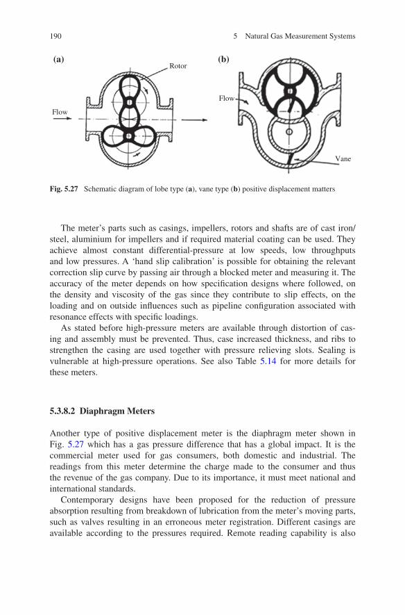
190 5 Natural Gas Measurement Systems

The meter’s parts such as casings, impellers, rotors and shafts are of cast iron/steel, aluminium for impellers and if required material coating can be used. They achieve almost constant differential-pressure at low speeds, low throughputs and low pressures. A ‘hand slip calibration’ is possible for obtaining the relevant correction slip curve by passing air through a blocked meter and measuring it. The accuracy of the meter depends on how specification designs where followed, on the density and viscosity of the gas since they contribute to slip effects, on the loading and on outside influences such as pipeline configuration associated with resonance effects with specific loadings.

As stated before high-pressure meters are available through distortion of cas-ing and assembly must be prevented. Thus, case increased thickness, and ribs to strengthen the casing are used together with pressure relieving slots. Sealing is vulnerable at high-pressure operations. See also Table 5.14 for more details for these meters.

5.3.8.2 Diaphragm Meters

Another type of positive displacement meter is the diaphragm meter shown in Fig. 5.27 which has a gas pressure difference that has a global impact. It is the commercial meter used for gas consumers, both domestic and industrial. The readings from this meter determine the charge made to the consumer and thus the revenue of the gas company. Due to its importance, it must meet national and international standards.

Contemporary designs have been proposed for the reduction of pressure absorption resulting from breakdown of lubrication from the meter’s moving parts, such as valves resulting in an erroneous meter registration. Different casings are available according to the pressures required. Remote reading capability is also

Flow

Rotor

Flow

Vane

(a) (b)

Fig. 5.27 Schematic diagram of lobe type (a), vane type (b) positive displacement matters

191

Tabl

e 5.

14

Rot

ary

impe

ller,

diap

hrag

m a

nd w

et g

as m

eter

s

Inst

rum

ent

Des

crip

tion,

ran

ge a

nd a

ccur

acy

Adv

anta

ges

(A)

and

disa

dvan

tage

s (D

)A

pplic

atio

n

Rot

ary

impe

ller

(lob

ed)

type

(ro

ots

met

er)

Two

impe

llers

con

tra

rota

te a

t the

sam

e tim

e, in

term

eshi

ng c

lose

ly a

t all

times

, and

th

us g

as is

pas

sed

forw

ard

from

the

inle

t to

the

outle

t thr

ough

the

mea

suri

ng c

ham

bers

. T

he im

pelle

rs a

re d

rive

n ro

und

by th

e ga

s du

e to

the

unba

lanc

ed lo

ad o

n on

e or

the

othe

r im

pelle

r w

hen

pres

sure

is a

pplie

d at

in

let.

The

tim

ing

gear

s en

sure

that

the

othe

r im

pelle

r w

ill tu

rn in

the

oppo

site

dir

ectio

n an

d th

us b

ecom

e ou

t of

bala

nce.

In

this

way

, th

e cy

cle

is c

ontin

uous

Ran

ge: U

p to

30:

1.

And

up

to 1

00 b

ar p

ress

ure.

Acc

urac

y: ±

1 %

fr

om. 1

0 to

100

% o

f m

axim

um fl

ow

A: A

ccur

ate

and

relia

ble.

Bud

get a

ffor

dabl

e.

Acc

urac

y m

aint

aine

d th

roug

hout

the

rang

es.

Doc

umen

ted

EE

C 7

1/31

8 an

d B

S117

9.

Puls

e co

unt m

etho

d su

itabl

e fo

r re

mot

e da

ta

proc

essi

ng. N

o is

sues

with

gas

sup

ply

secu

-ri

ty a

nd s

afet

y. P

robl

ems

may

be

redu

ced

by

regu

lar

insp

ectio

n, s

pin

test

s an

d by

the

use

of fl

ow s

trai

ghte

ners

Use

d in

oil

and

gas

indu

stry

for

man

y ye

ars

for

mea

suri

ng fl

ow d

ue to

thei

r ac

cura

cy a

nd

relia

bilit

y. T

he a

vaila

ble

rang

e co

vers

the

gas

oper

atin

g pr

essu

res

with

con

stan

t acc

urac

y ev

en w

ith lo

w fl

ows

and

low

pre

ssur

es w

hich

is

the

case

in d

omes

tic m

eter

ing.

Ext

ensi

vely

us

ed f

or lo

w-p

ress

ure

mea

sure

men

t

D: M

ovin

g pa

rts

thus

fri

ctio

n. V

isco

us d

rag

at c

lear

ance

s. P

ress

ure

loss

sin

ce e

nerg

y is

nee

ded

to r

otat

e th

e im

pelle

rs. R

equi

res

calib

ratio

n fo

r ha

ndlin

g sl

ip. N

oise

and

wea

r on

gea

rs a

nd b

lade

dam

age

mai

nly

from

de

bris

. Jam

min

g: w

hen

debr

is is

trap

ped

betw

een

impe

llers

cau

sing

flow

res

tric

tion,

A

filte

r in

inle

t and

an

auto

mat

ic m

eter

byp

ass

can

prov

ide

rem

edy.

Con

trol

equ

ipm

ent

such

as

gove

rnor

s an

d pi

lot s

uppl

ies

may

be

aff

ecte

d, p

ulsa

tion

and

impe

ller

iner

tia

caus

ing

slow

er im

pelle

rs r

espo

nse

time

whe

n ha

ving

rap

id v

aria

ble

load

s. T

his

may

als

o le

ad to

hig

her

met

er r

eadi

ngs.

Pip

e (a

cous

-tic

) re

sona

nce

with

pip

e w

ork

reso

nant

fre

-qu

ency

may

occ

ur. C

aref

ul d

esig

n el

imin

ates

th

is p

ossi

bilit

y. S

wir

l whi

ch p

rodu

ces

an

erro

r de

pend

ent o

n sw

irl a

ngle

(con

tinue

d)

5.3 Gas Flow Measurement

192 5 Natural Gas Measurement Systems

Inst

rum

ent

Des

crip

tion,

ran

ge a

nd a

ccur

acy

Adv

anta

ges

(A)

and

disa

dvan

tage

s (D

)A

pplic

atio

n

Dia

phra

gm

met

ers

The

re a

re f

our

cham

bers

in th

e m

eter

whi

ch

empt

y an

d fil

l in

sequ

ence

. Sin

ce th

e ex

act

volu

me

of th

e ch

ambe

rs is

kno

wn,

by

coun

ting

the

num

ber

of d

ispl

acem

ents

, the

vo

lum

e of

the

gas

is m

easu

red.

Ent

ranc

e an

d ex

it of

the

gas

to th

e co

mpa

rtm

ents

are

co

ntro

lled

by s

lidin

g va

lves

. Com

part

men

ts

2–3

are

enca

sed

by b

ello

ws

whi

ch e

xpan

d an

d co

ntra

ct

A: A

vaila

ble

in r

ange

s an

d hi

gh r

elia

bilit

y.

Can

be

adju

sted

for

rem

ote

data

tran

sfer

s or

pr

e-pa

y m

etho

ds. D

ocum

ente

d an

d ap

prov

ed

rate

d un

der

natio

nal a

nd in

tern

atio

nal s

tand

-ar

ds: B

S416

1 pa

rts

1–5

for

spec

ifica

tions

, B

SCP

part

2 f

or in

stal

latio

n, I

GE

M a

lso

prod

uces

rec

omm

enda

tions

For

dom

estic

and

com

mer

cial

sel

ling

of g

as

due

to th

e w

ide

rang

e av

aila

ble

that

sui

ts th

e na

ture

of

diff

eren

t cus

tom

ers

and

also

due

to

the

stre

ngth

and

dur

abili

ty o

f th

e m

eter

D: P

ress

ure

abso

rptio

n ca

usin

g di

aphr

agm

to

ballo

on o

utR

: Tin

plat

e: p

ress

ure:

up

to 5

kPa

and

up

to

35 k

Pa s

peci

al r

ange

(w

ith u

p to

170

m3 /

h ca

paci

ty).

Ste

el c

ase:

Pre

ssur

e: u

p to

25

kPa.

C

apac

ity: u

p to

160

m3 /

h. A

lum

iniu

m d

ie

cast

: Pre

ssur

e up

to 7

bar

Cap

acity

: up

to

280

m3 /

h

Wet

gas

m

eter

It c

onsi

sts

of a

rot

atin

g dr

um s

emi-

bath

ed

in a

flui

d su

ch a

s w

ater

or

oil.

The

dru

m is

di

vide

d in

to c

ham

bers

of

know

n vo

lum

e,

and

thus

, as

the

drum

rot

ates

, the

gas

is

char

ged

and

disc

harg

ed f

rom

inle

t to

outle

t fo

llow

ing

the

desi

gned

rou

te th

roug

h th

e ch

ambe

rs a

nd th

e liq

uid.

In

orde

r to

ach

ieve

th

e sp

ecifi

ed a

ccur

acy,

the

spee

d of

the

rota

t-in

g dr

um m

ust b

e ke

pt lo

w in

ord

er n

ot to

di

stur

b th

e w

ater

leve

l whi

ch is

cri

tical

. The

m

eter

alw

ays

mus

t sta

nd le

vel.

Ran

ge: 1

0:1.

C

apac

ity: 0

.5 m

3 /h.

Acc

urac

y: u

p to

0.2

5 %

Hig

h ac

cura

cy. N

o pr

oble

ms

with

sea

ling

mov

ing

part

s. lo

w c

apac

ity m

eter

. Vul

nera

ble

to h

umid

ity. I

f dr

y ai

r or

gas

pas

ses

thro

ugh

met

er, t

hey

will

bec

ome

satu

rate

d an

d in

or

der

to a

void

this

sui

tabl

e oi

l ins

tead

of

wat

er is

use

d

Use

d as

a r

efer

ence

sta

ndar

d fo

r ca

libra

ting

othe

r ty

pes

of m

eter

, for

labo

rato

ry u

se

Tabl

e 5.

14

(con

tinue

d)

193

available in the present days if any remote reading is required. Also the latest feature is the meter can accept prepaid electronic tokens such as the British Gas Quantum System that accepts a reusable gas card (see also Table 5.14 for more details) (Fig. 5.28).

inlet Outlet inlet Outlet

inlet Outlet inlet Outlet

(a) (b)

(c) (d)

Fig. 5.28 Schematic operative features of diaphragm meter [10]. a Chamber 1 is emptying, 2 is filling, 3 is empty and 4 has just filled. b Chamber 1 is now empty, 2 is full, 3 is filling and 4 is emptying. c Chamber 1 is filling, 2 is emptying, 3 has filled and 4 has emptied. d Chamber 1 is now completely filled, 2 is empty, 3 is emptying and 4 is filling

5.3 Gas Flow Measurement

194 5 Natural Gas Measurement Systems

5.3.8.3 Wet Gas Meters

The last member of the positive displacement meters is the wet gas meters, which solves the sealing of the moving parts through its principle of operation. Figure 5.29 and Table 5.14 provide more details for these meters.

5.3.9 Rotary Inferential Meters

5.3.9.1 Axial (In-Line) Turbine

An axial turbine is a velocity device for measuring volume as shown in Fig. 5.30. The direction of flow is parallel to the rotation axis of the rotor and the speed of

1

2

3

4

567

(a) (b)

Fig. 5.30 Schematic diagram of axial turbine (a) and typical-type illustration of the meter (b) [11]. 1 Pickoff, 2 Bearings, 3 End connections, 4 Supports, 5 Rotor blade, 6 Rotor hub, 7 Meter housing

Outlet

Direction of drum rotation

Sigh glass

Inlet

Rotatingdrum

Drum axis

Plumpline

Water Cha

rgin

g

Charged

Gas discharging

(a) (b)

Fig. 5.29 Schematic view of wet gas meter (a) and typical illustration of the meter (b)

195

rotation is proportional to the flow rate. For gas measurement, the meter must have low non-fluid retarding torques so that rotor percentage slip is acceptable. Retarding torque is due to: (a) non-fluid forces such as bearing friction and mechanical loading from various instruments used whose contribution in the torque can be assumed constant, (b) friction drag due to turbulence can generate a constant percentage slip on the flow range of the meter (see also Table 5.15).

Table 5.15 Axial, insertion turbine and roating-vane meters

Instrument Description, range and accuracy

Advantages (A) and disadvantages (D)

Application

Axial (in-line) turbine

A meter consists of a body, a rotor mechanism with inlet and outlet diffusers, a mechanical index and a mag-netic drive or pulse counter. The flow of gas causes the multi-blade wheel to rotate at a rate that is proportional to the volume flow. Thus, the meter’s driving energy from the kinetic energy from the gas that is caused to increase as it passes through the meter by reducing the cross-sectional area of the flow stream through diffusers. The rotor is constructed with the maximum effective radius to create the highest torque for a given force. Bearing friction is an important parameter; thus, meters for gases are less linear than liquid ones. Flow rate, bearing design, blade edge sharpness, roughness and nature of the flow have different effects on linearity; thus, calibration is needed for establishing meter fac-tors. The maximum capacity rating is established through the pressure across the meter, the end thrust of the rotor shaft and bearing caused by the differential-pressure and the rotational frequency of the rotor assembly. Capacity: 50 mm /14–113 m3/h. Up to 1015 mm /45–300 m3/h. Pressure: 2.5–100 bar. Accuracy: Up to ±1 %

A: They have small size, large volume capacity and range ability suit-able for measuring large flows. Compact and light in weight; thus, movable do not need large foundations. They can be supplied with correcting devices. Self-adjusting models such as the Rockwell type where effects of bearing wear are compensated through self-correcting and self-checking

Their advantages make them suitable for transmission dis-tribution or industrial applicationsThe self-adjusting Rockwell type is attractive for offshore applications where flow-metering space is limited. This is because it is less affected by flow disturbances such as swirl

D: Greatly affected by any debris or matter in the metering gas or fluid. Bearing wear causes pressure loss Large errors in case of two-phase flow

(continued)

5.3 Gas Flow Measurement

196 5 Natural Gas Measurement Systems

5.3.9.2 Insertion Turbine

It was developed to measure directly the rate and direction of gas flow in individ-ual mains as shown in Fig. 5.31.

Instrument Description, range and accuracy

Advantages (A) and disadvantages (D)

Application

Insertion turbine

The main parts of this type of meter are the rotor cage that is subject to the application with the leg. The insertion tube with the pressure relief chamber and at the top the M 700 connection with the wiring that runs all over the length of the meter. Sizes of rotor cages must be compat-ible with 100-mm-diameter pipe assembly. The calibra-tion must be unaffected by the range of operating densi-ties and insensitive to small misalignment. Required velocity range: 0.3–15 m/s

Ease of insertion Portability and robust-ness. Simple to use and operate. Meter gives direct reading or signal output for a wide range of mains

Used to measure directly the rate and direction of gas flow in individual mains. Used to validate net-work analysis modelsUsed to establish boundary conditions, Used to identify blocked or uncon-nected mains

Rotating-vane gas meter

The meter consists of cast iron housing with an alumin-ium anemometer fan. As it rotates, it transmits the drive to a counter-mechanism that integrates the flow. Capacity: 4–200 m3/h. Pressure: up to 1.7 bar About ±2 % over 10:1 range

It is a rugged construction

Suitable for most non-corrosive gases

Rotating-vane air meter (anemom-eter)

In this type of instrument, the vanes must be light or have a large surface area. The rotor may be of two kinds: In the cup anemometer, it consists of three light conical-shaped cups made of aluminium attached to arms on a vertical spindle geared to a count-ing mechanism. In the air meter type, the rotor has a multi-vane assembly made of aluminium alloy carried on a shaft with its other end attached to a count-ing mechanism. Velocity: 0.13–30, 0.3–25 m/s

Used in meteorology. Moving parts

Various

Table 5.15 (continued)

197

5.3.9.3 Rotating-Vane Gas Meter and Air Meter (Anemometer)

The rotating-vane gas metre is shown schematically in Fig. 5.32, which is basi-cally an aluminium anemometer fan rotates on a vertical shaft as fluid flows and

Connection to M700

Collet clamp nut

Pressure-relief nipple

Pressure chamber

Insertion tube

Pickup coil

Leg

Pickup unit

Collet

‘O’ ring seal

End fitting to suit 1½ in gate valve

Signal wire from pickup coil

Rotor cage (type to suit application)

(a)

(b)

Fig. 5.31 Schematic of insertion meter (a) and typical illustration of the meter (b)

Fig. 5.32 Schematic diagram of rotating-vane gas meter

Multipointer index

Rotor vaneGuide ports

5.3 Gas Flow Measurement

198 5 Natural Gas Measurement Systems

a counter-mechanism subsequently integrates the flow. Table 5.15 also provides more information on this instrument.

The rotating-vane air meter (see also Fig. 5.33) is an instrument which can meas-ure velocity, but it can also be designed to measure flow rate of air and gases directly. This can be done by attaching a capacitance transducer on the outer ring of the ane-mometer where as the vane rotates an electrical pulse output will be taken up by the indicator unit producing a direct reading. The rotor and the whole assembly must be balanced and the bearing selection must minimise friction as much as possible. The vanes of the assembly must be light or have large surface area (see also Table 5.15).

5.3.10 Fluid Oscillatory Types

5.3.10.1 Fluidic Meters

This instrument detects flow from the oscillatory movement of a jet of a gas within the meter. The instrument produces the oscillatory movement by design since it is a fluidic feedback oscillator based on the Coanda effect, i.e. the tendency of the fluid to be attracted to a nearby surface as shown schematically in Fig. 5.34. The stream is guided to oscillate from side to side at a frequency proportional to the flow rate. Table 5.16 provides more detail of the various types of fluid oscillatory meters. These meters are also summarised in the following sections.

5.3.10.2 Vortex Type

The phenomenon of vortex shedding provides the operating principle of this rela-tively new type of instrument, as shown schematically in Fig. 5.35 together with Table 5.16 which provides further details for the meter.

5.3.10.3 Swirl Meters

This type of meter produces swirl, and with a combination of a venturi and a diffuser, a flow rate relationship can be established as shown in Fig. 5.36 (see also Table 5.16).

Fig. 5.33 Typical rotating-vane air meter

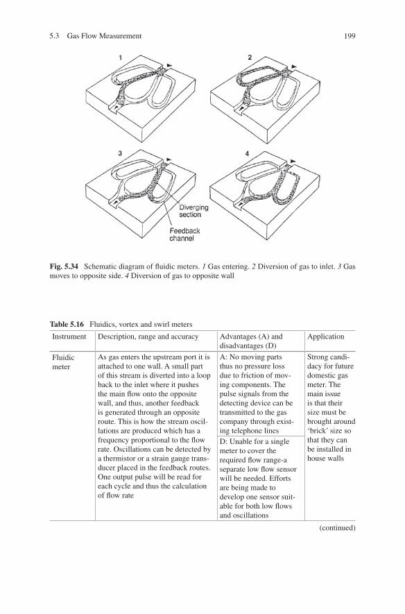
199

Fig. 5.34 Schematic diagram of fluidic meters. 1 Gas entering. 2 Diversion of gas to inlet. 3 Gas moves to opposite side. 4 Diversion of gas to opposite wall

Table 5.16 Fluidics, vortex and swirl meters

Instrument Description, range and accuracy Advantages (A) and disadvantages (D)

Application

Fluidic meter

As gas enters the upstream port it is attached to one wall. A small part of this stream is diverted into a loop back to the inlet where it pushes the main flow onto the opposite wall, and thus, another feedback is generated through an opposite route. This is how the stream oscil-lations are produced which has a frequency proportional to the flow rate. Oscillations can be detected by a thermistor or a strain gauge trans-ducer placed in the feedback routes. One output pulse will be read for each cycle and thus the calculation of flow rate

A: No moving parts thus no pressure loss due to friction of mov-ing components. The pulse signals from the detecting device can be transmitted to the gas company through exist-ing telephone lines

Strong candi-dacy for future domestic gas meter. The main issue is that their size must be brought around ‘brick’ size so that they can be installed in house walls

D: Unable for a single meter to cover the required flow range-a separate low flow sensor will be needed. Efforts are being made to develop one sensor suit-able for both low flows and oscillations

(continued)

5.3 Gas Flow Measurement

200 5 Natural Gas Measurement Systems

5.3.11 Ultrasonic Meters

5.3.11.1 Doppler Type

If a sound of a known frequency is reflected from a moving object, the frequency of the reflected beam is altered by an amount that is proportional to the velocity of the moving object. Thus, the flow rate is calculated through the Doppler shift frequency. Figure 5.37 shows the principle of operation of the industrial ultrasonic meter. Table 5.17 also provides more details with regard to this instrument.

Instrument Description, range and accuracy Advantages (A) and disadvantages (D)

Application

Vortex meters

A bluff body is placed in the flow. At very low flows the streamlines pass smoothly round the object but as the fluid velocity increases the fluid separates from the body forming vortices in the low-pres-sure region behind the body. The frequency at which these vortices are shed is proportional to fluid velocity, and thus, the flow rate can be calculated. In gas flows sensitive thermistors are used to detect vortex frequency. Range: 50:1, Accuracy ±1 %

A: No moving parts thus high reliability. No maintenance ire required and their cost is similar to an orifice plate [8]. Frequency is almost independent of the fluid used so calibra-tion to establish meter factor can be done using water. Less sensitive to dirty gas and upstream disturbances than orifice plates

An alternative to pressure differen-tial meters. Retrofix vortex meter under development by British Gas allows an orifice to be converted into vortex shed-ding improving flow capacity of the systemInsertion meters version can be used as a single point velocity tester through a small hole cut in the pipeline

D: Interaction of vortices with acoustic waves which have negative impact on accuracy. Dependent on bluff body size limitation

Swirl meters

Fixed inlet guide vanes force the entering gas into a swirling motion. Then the gas accelerates through a Venturi and then decelerated through a diffuser. This sequence causes the axis of the swirling gas to process about the pipe centre line. The frequency of precession is proportional to the gas flow rate. A thermistor in the throat casing detects the passage of the coils of the helix. As it leaves the meter the flow is expanded and diswirled by a set of vanes

A: Insensitive to upstream conditions.D: Quite high pressure loss thus not suitable for low-pressure metering

Table 5.16 (continued)

201

Fig. 5.36 schematic diagram of swirl meter (a) and a typical illustration (b)

Strouhal number (S) = fd/V = constant Frequency of vortex shedding (l)

Gas velocity (V) d

Gas velocity = fd/S

Bluff body

Sensor

Vortex steel

(a)

(b)

Fig. 5.35 Schematic of flow characteristic of (a) and typical diagram of the vortex meter (b)

5.3 Gas Flow Measurement

202 5 Natural Gas Measurement Systems

Receiver

Flow

Transmitter

(a) (b)

Fig. 5.37 a Principle of operative. b Typical industrial ultrasonic meter

Table 5.17 Ultrasonic meters

Instrument Description, range and accuracy Advantages (A) and disadvantages (D)

Application

Doppler type

The instrument consists of a transmit-ter and a receiver of ultrasonic waves. The scattering elements which in the case of gas can be either gas particles or eddies deflect the ultrasonic energy from the transmitter. This provides a frequency shift between the deflected energy and the energy from the transmitter; thus, the velocity of the fluid can be calculated. Since velocity profiles are present, the received signal will be a range of frequencies propor-tional to the prevailing flow profile conditions; thus, meters are designed to process the strongest signal through conditioned amplitude modulation and demodulation in order to give an output proportional to flow [8]

A: High reliability and low maintenance costs. Can be attached easily and externally without disturbing the pipeline flow opera-tion; thus, personnel do not come into con-tact with the flowing medium that can be hazardous. In modern days, ultrasonic trans-mitters and receivers are cheap, and thus, the meter is relatively inexpensive

Useful or measuring the flow of corro-sive fluids and slurries

D: The flow profile pipe-wall thickness constancy number, size and distribution of the particles in the flow. Thus, there is great accuracy vari-ance and to avoid it a carefully and rigorous calibration must be carried out

(continued)

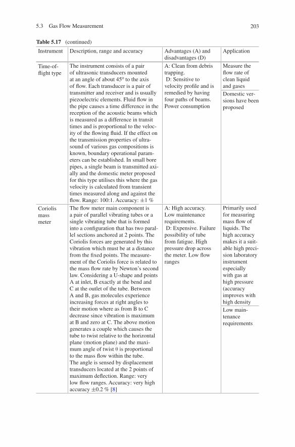
203

Instrument Description, range and accuracy Advantages (A) and disadvantages (D)

Application

Time-of-flight type

The instrument consists of a pair of ultrasonic transducers mounted at an angle of about 45o to the axis of flow. Each transducer is a pair of transmitter and receiver and is usually piezoelectric elements. Fluid flow in the pipe causes a time difference in the reception of the acoustic beams which is measured as a difference in transit times and is proportional to the veloc-ity of the flowing fluid. If the effect on the transmission properties of ultra-sound of various gas compositions is known, boundary operational param-eters can be established. In small bore pipes, a single beam is transmitted axi-ally and the domestic meter proposed for this type utilises this where the gas velocity is calculated from transient times measured along and against the flow. Range: 100:1. Accuracy: ±1 %

A: Clean from debris trapping. D: Sensitive to velocity profile and is remedied by having four paths of beams. Power consumption

Measure the flow rate of clean liquid and gasesDomestic ver-sions have been proposed

Coriolis mass meter

The flow meter main component is a pair of parallel vibrating tubes or a single vibrating tube that is formed into a configuration that has two paral-lel sections anchored at 2 points. The Coriolis forces are generated by this vibration which must be at a distance from the fixed points. The measure-ment of the Coriolis force is related to the mass flow rate by Newton’s second law. Considering a U-shape and points A at inlet, B exactly at the bend and C at the outlet of the tube. Between A and B, gas molecules experience increasing forces at right angles to their motion where as from B to C decrease since vibration is maximum at B and zero at C. The above motion generates a couple which causes the tube to twist relative to the horizontal plane (motion plane) and the maxi-mum angle of twist θ is proportional to the mass flow within the tube. The angle is sensed by displacement transducers located at the 2 points of maximum deflection. Range: very low flow ranges. Accuracy: very high accuracy ±0.2 % [8]

A: High accuracy. Low maintenance requirements. D: Expensive. Failure possibility of tube from fatigue. High pressure drop across the meter. Low flow ranges

Primarily used for measuring mass flow of liquids. The high accuracy makes it a suit-able high preci-sion laboratory instrument especially with gas at high pressure (accuracy improves with high densityLow main-tenance requirements

Table 5.17 (continued)

5.3 Gas Flow Measurement

204 5 Natural Gas Measurement Systems

Figure 5.38 also shows an illustration of a domestic ultrasonic meter. A pair of transducers are mounted at opposite ends of a length of tube carrying the gas flow. The gas velocity can be calculated from a pair of transit times measured with and against the flow together with some geometrical constants. The accuracy of this cal-culation is not significantly affected by changes in gas properties or temperature. Almost all these types of meters incorporate sophisticated hardware and software.

5.3.11.2 Time-of-flight Type

This type relies on the measurement of the time difference between an ultrasonic pulse travelling with and against the flow in a pipe as shown in Fig. 5.39 (see also Table 5.17 for further details).

5.3.12 Direct Mass Type

5.3.12.1 Coriolis Mass Meter

Coriolis mass meter is the only representative from the direct mass-type family. The principle behind this instrument is Coriolis force. Such forces are generated

Transducer 2

Transducer 1

Flow

velocity (v)

Speed of sound

in medium (c)

dθ

(a) (b)

Fig. 5.39 Principle of time-of-flight flow meter (a) and illustration of the meter (b) [12]

Ultrasonic transdicure(emitters and receivers)

L

C.VC.V

Flow velocity (V)

Outer chamber

Stiffering plate Flow tube

Transducer holder

Inlet chamber

Inlet portOutlet port

(a) (b)

Fig. 5.38 Ultrasonic meter a and b

205

whenever a body, which is rotated about a fixed point, undergoes a change of posi-tion relative to the fixed point as shown in Fig. 5.40 (see also Table 5.17).

5.3.13 Thermal Types

5.3.13.1 Hot-Wire Anemometer

The physical principle behind this type of meter is that when a fluid flows over a heated surface, there is heat transfer from the surface and a consequential reduc-tion in temperature, which is related to the rate of flow. Figure 5.41 shows the principle of the operation the hot-wire anemometer with further details provided in Table 5.18.

5.3.13.2 Probe Type

This type of meter senses changes in flow and associates them with a change in DC output. Figure 5.42 shows the typical illustration of instrument and Table 5.18 provides further details.

FlowFlow

Fluid force

Fluid force

Fluid forces reacting to vibration of flow tube

Vibrating flow tube

Twist angle

Twist angle

End view of flow tube showing twist

Fig. 5.40 Features and principle operative of coriolis mass meter

Fig. 5.41 Schematic diagram of hot-wire anemometer

5.3 Gas Flow Measurement

206 5 Natural Gas Measurement Systems

Table 5.18 Thermal-type flow meters

Instrument Description, range and accuracy Advantages (A) and disadvantages (D)

Application

Hot-wire anemom-eter

Heat is supplied electrically to a wire placed in the flow stream. The temperature of the wire is obtained by measurement of its resistance using a Wheatstone Bridge. Current adjustment is required so that temperature remains constant and measur-ing the heating current so that the bridge remains balanced. A potentiometer is used to measure the potential difference across a standard resistance in the appropriate arm of the bridge. At equilibrium, heat supplied equals heat lost, and thus, if resistance and temperature of the wire are kept constant, a relation is established with the velocity of flow and the fourth power of the current. Wide range ±2 % [8]

Low flow rates Suitable to measure air or gas flowUseful for laboratory and research applications

Probe type The instrument consists of a small hand held probe made of stainless steel and containing the two sensing elements, the thermocouples. Alternative current is used to heat the elements and a change in flow results in a change in direct current (DC) output. A third unheated thermocouple (identical to the other two) is added to the dc output and this is to compensate the transient heat generated when ambient temperature changes. Range: Up to 30 m/s

A: Measuring low velocity flows 0.05–0.5 m/s due to its dense spaced scale at lower velocities

Measurement of air veloci-ties through supply grills and ceiling diffusers in air-condi-tioning and ventilating systems

Fig. 5.42 Typical probe-type flow meter

207

5.3.14 Miscellaneous Techniques

5.3.14.1 Laser Doppler Meter

Measures the Doppler shift of laser radiation scattered from particles moving within the gas stream. Figure 5.43 shows the principle operation of the instrument, and Table 5.19 gives further details.

5.3.14.2 Cross-Correlation Meter

An ultrasonic arrangement that correlates data from two pairs of transmitters and receivers as shown schematically in Fig. 4.44 (see also Table 5.19) (Fig. 5.44).

5.3.14.3 Tracers

They inject a substance into the pipeline gas stream and then a characteristic related to the flow rate is measured. For the application of this technique, two methods are available. The first one is the dilution method where the flow rate is determined by injecting a known quantity of tracer into the pipe and measur-ing the dilution ratio at a downstream point. The second one is the transit-time method where a pulse of tracer is injected and a measure is taken for the time for the tracer to travel over a known volume section. Figure 5.45 shows schemati-cally the operation features of the meter. Table 5.20 also gives more details of the instrument.

He-Ne laser

Beam splitter

Probe beam

Neutral density filter

ApertureNarrow band

filter

Reference beam20

Photomultiplies

Amplifier

Spectrum analyser

Recorder

Oscillator

Frequency counter

Fig. 5.43 Schematic diagram of laser doppler flow meter

5.3 Gas Flow Measurement

208 5 Natural Gas Measurement Systems

5.3.15 Flow Meter Systems

5.3.15.1 Metering Large Industrial and Commercial Loads

Since gas industries have developed, there is an increase in large measurement systems (>300 m3/h volumetric flow rate) as well as having an increase in meas-urement at high pressure. Concerning statutory requirements and standards, these are covered by national standards organisations, officially recognised and backed by the government such as the British Standards (BS) or the German Din, and in addition, industry-orientated national bodies also exist such as the Institution of

Table 5.19 Miscellaneous flow meters

Instrument Description, range and accuracy Advantages (A) and disadvan-tages (D)

Application

Laser Doppler meter

The main instruments of the meter are a laser source, beam splitter, filters, an optical system and a series of photomultiplier, amplifier, analyser and recording devices

A: Needs no cal-ibration. Linear frequency/veloc-ity relationship over high range. High accuracy, reproducibility and does not disturb the flow, thus no pressure loss due to the meter device D: Expensive and fragile complex and a need for skilled operation. High performance is subjected to ‘clear windows’ in pipeline

Fluid and combustion researchDetect water vapour in gas flow or other debrisA standard on which other meter-ing devices can be calibrated

The laser beam is split into two components, and using an optical system, they are focused to intersect the gas stream. Any particle in the gas will be trapped between the two beams, and a phase shift will be recorded in frequency which is associated with the particle’s velocity. Small enough particles are selected in order to follow gas flow with great accuracy. The opti-cal system is designed to allow velocity profile across pipes to be obtained, and thus, the total flow can be calculated. Frequencies output linear with velocities from 0.1 mm–3 Mach. Accuracy: ±0.5 %

Cross-correlation meter

Two transverse beams of ultrasound are sent across the pipe diameter. If no flow occurs, the beam’s signals are the same as the ones transmitted. In the case that flow exists, the signals received will be modulated because of the existence of particles in the flow stream or eddies in the case of turbulent flow. These modulated signals will be fed into a data processor called a cross-correlator where by comparing the two signals, the transit time will be obtained and hence the velocity. In reality, meters are designed to give the average veloc-ity across the diameter

Very expensive by industrial standards

Two-phase and flare gas applications

209

Gas Engineers and Managers (IGEM). At international level, the following organi-sations issue standards relating to gas metering:

OIML The International Organization of Legal MetrologyISO The International Standards OrganizationIEC The International Electro-technical CommissionEEC European Economic Community

In the UK, legal requirements exist for metering systems concerning safety and accuracy. The safety aspect is covered by Gas Safety Management Regulations 1996 (GS(M)R), whereas the accuracy is covered aspect by the relevant Gas Act and the Gas (Meter) Regulations. Meters used for charging must be stamped or ‘Badged’ except when special terms are agreed between supplier and customer. Stamped

2nd detector 1st detector Injection point

Flow

185 diameters 80 diameters

6in reference Venturi meter

6in pipe line

Fig. 5.45 Schematic features of tracer flow meter

Fig. 5.44 Schematic diagram of cross-correlation flow meter

TransmitterUnmodulated

modulated Receiver

Cross correlator

x(t) y(t)

L

5.3 Gas Flow Measurement

210 5 Natural Gas Measurement Systems

Tabl

e 5.

20

Tra

ces

flow

met

er

Inst

rum

ent

Des

crip

tion,

ran

ge a

nd a

ccur

acy

Adv

anta

ges

(A)

and

disa

dvan

tage

s (D

)A

pplic

atio

n

Tra

cers

Con

stan

t rat

e in

ject

ion

met

hod

Mob

ile s

yste

ms

and

accu

rate

Suita

ble

for

dete

ctin

g si

g-ni

fican

t dev

ia-

tions

in m

eter

ac

cura

cy

Dilu

tion

tech

niqu

esA

trac

er o

f kn

own

volu

me

is in

ject

ed in

to th

e st

ream

at

cons

tant

rat

e, a

nd a

fter

str

eam

and

trac

er c

once

ntra

tion

is f

airl

y m

ixed

, a m

easu

rem

ent i

s ta

ken

at a

dow

n-st

ream

poi

nt. T

he v

olum

etri

c flo

w r

ate

is d

eter

min

ed

by r

elat

ing

back

grou

nd, i

njec

tion

and

mix

ed fl

ow tr

acer

co

ncen

trat

ions

Als

o ca

n be

use

d fo

r ca

libra

tion

and

prov

ing

Pul

se in

ject

ion

met

hod

The

dif

fere

nce

is th

at th

e tr

acer

is s

udde

nly

inje

cted

into

th

e ga

s st

ream

. Aft

er c

ompl

ete

mix

ing,

the

conc

entr

atio

n pr

ofile

for

the

tota

l clo

ud o

f in

ject

ant i

s m

easu

red

dow

n-st

ream

. The

vol

ume

flow

rat

e is

obt

aine

d by

inte

grat

ing

on th

e co

ncen

trat

ion

profi

le. A

ccur

acy:

± 1

%

Tra

nsit-

time

tech

niqu

esG

as is

sud

denl

y in

ject

ed in

to th

e ga

s st

ream

and

the

time

for

trac

er c

loud

to p

ass

betw

een

two

dete

ctor

s is

mea

s-ur

ed. D

ue to

turb

ulen

t flow

, the

tran

sit t

ime

is th

e sa

me

as

the

mea

n re

side

nce

time

of th

e tr

acer

in th

e pi

pe v

olum

e be

twee

n de

tect

ors.

The

trac

er g

as c

an b

e ra

dioa

ctiv

e or

ch

emic

al (

Eth

yl b

rom

ide

and

Arg

on 4

1). M

ulti-

chan

nel

UV

rec

orde

rs w

ith c

ryst

al o

scill

ator

tim

ing

puls

es a

re

used

to ti

me

the

trac

er p

ulse

trav

ellin

g th

e kn

own

dist

ance

be

twee

n de

tect

or p

oint

s. T

he v

olum

e of

the

mea

sur-

ing

sect

ion

is a

ver

y im

port

ant p

aram

eter

and

BS5

857

reco

mm

ends

its

dete

rmin

atio

n be

fore

ass

embl

y, e

xter

nal

mea

sure

men

ts o

f th

e pi

pe g

eom

etry

suc

h as

wal

l thi

ck-

ness

with

X-r

ay o

r ul

tras

onic

met

hods

can

be

depl

oyed

in

dete

rmin

ing

the

volu

me.

Acc

urac

y: ±

0.5

%

Thr

ee s

mal

l dia

met

er ta

ppin

gs a

re r

equi

red,

and

the

expo

sed

leng

th is

the

leas

t for

any

trac

er m

etho

d. S

hort

hal

f-lif

e is

otop

es a

nd th

e gr

eat d

ilutio

n of

the

trac

er g

as in

the

pipe

line

ensu

re n

eglig

ible

rad

ioac

tive

haza

rds

tow

ards

con

sum

ers.

Sc

intil

latio

n co

unte

rs c

an b

e st

rapp

ed to

the

pipe

ext

erna

lly,

and

ther

efor

e, p

ipe

need

s no

mod

ifica

tion.

Use

of

grap

hica

l ou

tput

fro

m c

ount

ers

in a

dditi

on w

ith o

ptim

ised

sta

tistic

al

anal

ysis

to a

chie

ve m

axim

um a

ccur

acy.

Use

of

sym

met

rica

l ar

ray

may

red

uce

need

for

com

plet

e m

ixin

g si

nce

sens

ing

is p

rese

nt to

all

part

s of

the

pipe

’s c

ross

sec

tion.

Als

o le

ngth

be

twee

n in

ject

ion

poin

t and

firs

t det

ecto

r ca

n be

red

uced

. D

iffic

ultie

s w

hen

usin

g ra

dioa

ctiv

e flu

ores

cent

or

chem

ical

as

trac

er g

as s

ince

fluo

resc

ent r

equi

res,

a tr

ansp

aren

t win

dow

in

the

pipe

and

che

mic

al tr

acer

s re

quir

e id

entic

al s

ampl

ing

poin

ts

in o

rder

to h

ave

iden

tical

res

pons

e tim

es. I

soto

pes

need

to h

ave

pow

erfu

l γ r

ays

to p

enet

rate

the

stee

l pip

e, s

o de

tect

ion

can

be

feas

ible

Gas

indu

stry

an

d ov

er e

ach

labo

rato

ry

211

meters must be accurate within ±2 % and maximum pressure drop is specified for diaphragms meters, whereas no statutory pressure drop is cited for rotary displace-ment meters. International and national bodies cover meter specification as follows:

OIML Produces standards for most types of gas meterBS4161 Diaphragm, rotary displacement, turbine meters and also

mechanical volume correctorsBS1042 and ISO 5167 Orifice plates

For gas supplied under the terms of published tariffs, the following must be met:

1. Compulsory use of stamped meter either by the relevant authority or examiner2. Meter register serves as evidence of quantity supplied (where supply is done

through meter)3. ±2 % meter deviation from actual quantity supplied.

Special agreements between suppliers and consumers are permitted by the Gas Act. Also in the agreement, quantity supplied may be determined other than by the meter register by recording agreed parameters often in remote mode such as:

1. The maximum hourly or daily demand rate2. The total demand each day during a charging period3. The hourly demand, to permit the use of tariff terms for charging for differently

priced blocks of gas through a single meter4. The period of interruption and its proof.5. Gas pressure and/or temperature at the meter.

Recommendations based upon metering pressure are available for metering system design:

• BSCP 331 and IGE Comm.750: if metering pressure does not exceed 7.5 kPa (75 mbar)

• IGE GM/1: if inlet pressure is between 7.5 kPa (75 mbar) and 7 MPa (70 bar)• IGE/TD/9: if inlet pressure at installation exceeds 700 kPa (7 bar)

The above recommendations cover installation of gas meters in industrial and commercial facilities for all distributed gaseous fuel where the gas temperature at the meter is between −5 and 40 °C. For other gases or outside the previous lim-its, recommendations must be consulted which are limited to the following type of meter: positive displacement diaphragm, rotary displacement, turbine, orifice.

5.3.15.2 System Specification

The meter’s design specifications include the following:

1. Performance targets

• Continuity of measurement• Security of gas supplied being monitored

5.3 Gas Flow Measurement

212 5 Natural Gas Measurement Systems

• Flow rate accuracy• Integrated flow accuracy

2. Maximum flow capacity 3. Operating load profile 4. Upstream and downstream control equipment 5. Maximum allowable pressure drop 6. Operating gas pressure and temperature ranges 7. Gas composition limits 8. Read-out requirements, including time data for interruptible loads 9. Available power supplies for their specifications 10. Space available.

5.3.15.3 Measurement and Correction of Gas Flow Parameters

Only the orifice meter from the three types considered requires a secondary instru-ment for a flow reading. Secondary devices can also be used as correctors to reduce the measured volume to the base volume. For this purpose, the following instrument classes are available:

• Differential-pressure/pressure transmitters• Temperature transmitters• Density meters• Correctors.

5.3.15.4 Differential-Pressure/Pressure Transmitters

These are pressure sensors measuring pressure of gases or liquids. They can also indirectly be used to measure other variables such as fluid/gas flow, speed water level and altitude. Different technologies are available with different design and cost; thus, selection is made according to the intended application and budget.

The accuracy is usually specified as a percentage of output. Careful selection is needed and ranging since uncertainty proportion to output increases as the out-put decreases. Recommendations are provided by BS6174 where calibration is also cited which is affected by long periods of operations at high differential-pressures. Figure 5.46 shows a typical instrument for a differential-pressure/pressure transmitter.

To minimise uncertainty down to 1 %, the range of an individual PPT should be limited to about 10:1 on DP (3:1 on flow). With a computer controlling switch-ing, two or more DPTs can be used to increase single meter range ability keeping the uncertainty down to 1 % over 4:1 flow ratio. Also the switching point between DP ranges has an effect on error, but if flow rate variation is known, it can be com-pensated. Also temperature can cause a zero shift and span change of 0.1 % and a 0.2 % in the basic accuracy; therefore, temperature-controlled applications may be required on some applications.

213

When using the pTZ method of density determination, the selection of the trans-mitter should reflect the effect on pressure measurement uncertainty on the total flow measurement uncertainty. Narrow-span transmitters with elevated zero values can be sued, or at relatively low pressure, absolute-pressure transmitters may be necessary.

Pressure transmitters with electrical output signals and with an overall meas-urement uncertainty of 0.25 % are recommended. (BS6447, 0.2A classification). The preferred location is upstream of the meter, and they should be as feasibly close to the tapping and protected against vibrations and environmental effects. They must be calibrated before commissioning and periodically afterwards using a dead-weight tester.

5.3.15.5 Temperature Transmitters

Accurate temperature measurement is essential for:

• Computation of flowing gas quantities when using the pTZ correction method of density determination

Fig. 5.46 Typical differential-pressure/pressure transmitter

5.3 Gas Flow Measurement

214 5 Natural Gas Measurement Systems

• In cases where operational variations in the flowing temperature will have a sig-nificant effect on orifice meter bore dimensions.

• Checking gas temperature in density meters.

Electrical resistance thermometry in accordance with BS1041 pt.3 and BS1904 is recommended. A platinum 100 Ω BS1904 class A tolerance is preferred when pTZ method is used. Class B tolerance is adequate for orifice bore and density meter calibration corrections. The calibration of the resistance thermometer should be done according to national standards. Figure 5.47 shows a typical temperature transmitter.

5.3.15.6 Density Meters

The measurement of density/relative density in gas flow measurement is required:

• For the calculation of volume flow at reference conditions from volume meas-ured at line conditions (e.g. at orifice)

• For the calculation of volume flow at reference conditions from mass flow using relative density

• For mass flow measurement using density at line conditions of temperature and pressure

• For quality determination using relative density.

Fig. 5.47 Typical transmitter

215

The gas density at line conditions can be directly determined by:

• A continuous on-line density meter• Measurement of relative density near reference conditions• Application of pTZ method and by calculation from gas composition

For an accurate gas density measurement, the vibrating element, buoyancy or inertia types of density meter can be used. In the UK, the vibrating element is used for fiscal measurement and has an uncertainty as low as 0.2 % if installed prop-erly. A reference chamber of pipeline gas controls the pressure of the supply to the density cell. A good thermal equilibrium exists between the reference cell and the pipeline gas. The electrical output of the density is related to the relative density of the pipeline gas after suitable calibration.

Continuous density meters contribute significantly to the cost of the system. There cost and benefit analyses for such a need should be made. They are pre-ferred at high gas pressures and approaching critical point conditions because pTZ method will have greater uncertainty, but their use must be avoided when gas is dirty or at dew point conditions.

Density meters are calibrated by the manufacturer on a range of gases that have certified component analysis such as nitrogen or argon. Their primary objective is that the gas pressure and temperature at the point of density measurement must be as close as possible to those at the flow meter its self.

The density meter is fitted in the line using a pocket at a specified point accord-ing to standards. There must be access to the meter for maintenance and testing without interrupting the gas flow. The density meter bears the advantage that it can be externally placed.

The pTZ method can be used when it is impossible to measure the density directly at line conditions, but the density reference conditions are known. The pTZ method should be considered as an alternative to the direct on-line method where

• uncertainties in compressibility factor are small (low-pressure case)• gas is near dew point conditions and contains liquid droplets and dirt; thus, a

direct sample cannot be obtained• pressure and temperature and other operating conditions are beyond the density

meters’ available ranges.• benefit of accuracy is overturned by cost, and pTZ method gives adequate accu-

racy at lower cost than a density meter.

Figure 5.47 shows schematically the features of the density meter with a typical illustration (Fig. 5.48).

5.3.15.7 Correctors

Automatic correctors can achieve pressure temperature and compressibility cor-rection. They all require an output drive from the meter either by means of direct

5.3 Gas Flow Measurement

216 5 Natural Gas Measurement Systems

mechanical linkage or by indirect electromechanical/electronic means. They are available in mechanical type with accuracy ±1 % and electronic type with accu-racy ±0.25 %. They utilise the gas law correction where flow rate Q is a function of the ratio of pressure, temperature and compressibility at reference condition and

Gas line

Isolation valve

Vent and input for calibration gases

Valve B

Valve A

Pressure regulator

Orifice

Filter

Inlet

Temperature stabiliser

Diaphragm Density

transducer

Pressure relief valve

Outlet

Valve C

Thermal insulating cover

Reference chamber

Reference chamber valve

Pressure control valve

Control pressure indicator

To vent

(a)

(b)

Fig. 5.48 Schematic features (a) of density meter with typical illustration (b)

217

at line condition. Figure 5.49 shows a typical corrector. There also two types of automatic pressure/temperature/compressibility correctors:

1. The trapped sample which operates by trapping a specific mass of gas in a flex-ible container and measures its deflection when subjected to gas-line pressure and temperature giving correction accuracies of ±1 %.

2. The density cell which utilises a density transducer mounted in a small gas sampling line giving an accuracy of 0.2 %.

5.3.15.8 The Flow Computer

The flow computer encompasses the development of correctors. It is used in high-pressure metering, custody transfers and of course in offshore installations. The signals from the two elements (primary, secondary) are transmitted to the computing system. There the signals are processed into engineering quantities such as flow rate, and they are presented in graphical displays together with a systems diagnostic reports such as warnings or operational data such as valve position.

Possible system configuration for digital computers may include:

1. A number of meter stream computers associated with one meter task connected to a bank which concentrates information from the peripheral meters to produce the station’s operational status.

2. A master computer system which receives all transmitted signals from the stations and processes them into engineering data. For fiscal measurement, a backup in case of system failure must be provided, such as a dual master com-puter configuration.

3. For simple fiscal systems, a single computer can be used in conjunction with an independent device displaying flow rate.

2 3 4 5 6 7 8 9

Electronic flow correctore

Pressure transducer

Flow transducer Temperature transducer

Flow

(a)(b)

Fig. 5.49 Schematic diagram of corrector (a) with typical illustration of the meter (b)

5.3 Gas Flow Measurement

218 5 Natural Gas Measurement Systems

The computer system must meet the specifications and performance for real-time flow rate measurement giving accuracies of the order of 0.01 %. The Petroleum Measurement Manual, Part XV, Sect. 2 covers the specifications concerning com-puter system components and data integrity and security.

Meter stream computers may perform the following functions:

1. Process digital or analogue signals and convert them into engineering data and specific readings (density signals are transformed into density readings) for computation purposes.

2. Monitor these signals for any system deviations and provide alarms if limits are violated.

3. Communicating with the supervising meter bank computer for several issues including both computer’s and system’s health.

A meter bank computer may perform the following tasks:

1. Sum flow rates from stream computers and give totals for the connected stations.

2. Handle signals not already processed by stream computers.3. Transmit alarm signals received from stream computers to the data logging

system.4. Calculate gas properties such as calorific value from data entered manually or

acquired from an on-line chromatograph.

5.4 Gas Quality

5.4.1 Introduction

Gas quality is the key parameter which must be constantly monitored and meas-ured. Broadly speaking, gas quality measurement is important for four main reasons:

1. To ensure the safe and efficient transportation of gas through the transmission system as the systems are designed to operate to a particular gas specification.

2. To certify that gas appliances receive the correct gas specifications as they are unable to safely and efficiently consume gases that are not correct.

3. To guarantee that consumers receive the quality of gas that they pay for.4. To ensure that any gas that is injected into the natural gas grid (e.g. liquefied

natural gas, imported gases or bio-methane) matches the quality of gas that already exists in the transportation system.

Natural gas consists of a number of different hydrocarbon gases along with some non-hydrocarbon gases and other contaminants. To put it simply, gas qual-ity specifications define the mixtures of these gases that can be transported and conveyed to consumers. In the UK, the gas quality specifications are laid out in the GS(M)R. It is important that gas producers, suppliers and transporters adhere to

219

these specifications in order to avoid financial penalties and/or even criminal pros-ecutions (not conforming to them could jeopardise public safety). The Table 5.21 provides the GS(M)R Gas Quality Specification for the UK.

GS(M)R also goes on to specify that all gas with a pressure below 7 barg should be treated with a suitable stenching agent (odorant) to ensure that it has a distinctive and characteristic odour which should remain distinctive and charac-teristic when the gas is mixed with gas which has not been so treated (for further details on odorimetry see Sect. 4.5.1).

It is clear from the GS(M)R Specification that gas quality specification relat-ing to the distribution and transmission of natural gas must have items relating to the integrity of both the pipeline and the flow of gas. The composition of the gas entering the network must be such that the pipeline is not damaged or affected in any way. Corrosion stressing and abrasion must be avoided.

The following sections in this chapter will discuss the various parameters that must be measured in order to accurately analyse gas quality.

5.4.2 Methanol Determination

As part of the commissioning of a new transmission pipeline, the line must be hydrostatically tested to prove that the line can withstand the operation pressures it was designed for. Subsequent to this, the residual water must be removed in order to prevent the formation of gas hydrates (white crystalline compound that looks like ice that forms when water mixes with natural gas at high pressure). Water removal is achieved by swabbing the line with pigs (pipeline inspection gauge).

Table 5.21 GS(M)R Gas quality specification for the UK

Content or characteristic Value

Hydrogen sulphide content

≤5 mg/m3

Total sulphur content (including H2S)

≤50 mg/m3

Hydrogen content ≤0.1 % (molar)

Oxygen content ≤0.2 % (molar)

Impurities shall not contain solid or liquid material which may interfere with the integrity or operation of pipes or any gas appliance which a consumer could reasonably be expected to operate

Hydrocarbon dew point and water dew point

shall be at such levels that they do not interfere with the integrity or operation of pipes or any gas appliance (within the meaning of regulation 2(1) of the 1994 Regulations) which a consumer could reasonably be expected to operate

Wobbe Index (i) ≤51.41 MJ/m3 and

(ii) ≥47.20 MJ/m3

ICF ≤0.48

SI ≤0.60

5.4 Gas Quality

220 5 Natural Gas Measurement Systems

However, this will not remove all the water. The next step is to lower the hydrate formation temperature below ambient temperatures using a hydrate inhibitor. Either methanol or glycol can be used (or both), which will lower the formation temperature significantly. To get the methanol (or glycol) into the pipeline, the pigging procedure is repeated with a large slug of methanol.

The foregoing paragraph has explained why methanol is introduced into the pipeline, and from this, we can accept why instruments for measuring methanol concentration in the gas and the water dew point have an important role to play in the assessment of gas quality. Figure 5.50 shows a typical methanol instrument, and Table 5.21 provides more details.

5.4.3 Water and Hydrocarbon Dew point Measurement

Due to the phenomenon of retrograde condensation, water and hydrocarbon dew point measurement is another important criterion of gas quality measurement. For example at the terminals of the UK gas transmission system, the gas has its hydrocarbon dew point depressed to about −15 °C at 70 bar which ensures that no hydrocarbon condensation can occur. If the dew point was not depressed, then the hydrocarbon dew point would rise to a temperature in the range 5–15 °C at 70 bar with the occurrence of retrograde condensation when the pressure is reduced. Refer to Dew Point section in Table 5.22 for specific instrument details

5.4.4 Oil–Fog Concentration Measurement

Along with the use of dry natural gas in distribution systems comes the prob-lem of the shrinkage of rubber sealing rings in jointed mains. Methods for

Fig. 5.50 Schematic diagram of methanol determination (a) and typical illustration (b)

221

Tabl

e 5.

22

Met

hona

l and

dew

poi

nt d

eter

min

atio

n

Inst

rum

ent

Des

crip

tion,

ran

ge a

nd a

ccur

acy

Adv

anta

ges

(A)

and

disa

dvan

tage

s (D

)A

pplic

atio

n

Bri

tish

Gas

M

etha

nol

Det

erm

inat

ion

Met

hod

The

re a

re tw

o st

ages

invo

lved

in th

is m

etho

d:A

: Onl

y on

e co

mpo

nent

is

dete

rmin

ed w

ithou

t int

erfe

r-en

ce f

rom

hyd

roca

rbon

s, a

nd

stan

dard

isat

ion

is s

impl

e

Use

d in

the

gas

indu

stry

to

mea

sure

met

hano

l in

a p

ipel

ine

afte

r th

e lin

e ha

s be

en

pigg

ed w

ith a

larg

e sl

ug o

f m

etha

nol

1st s

tage

—0.

5 ft

³ of

gas

is p

asse

d th

roug

h 20

mls

of

wat

er a

t a r

ate

not

grea

ter

than

1.5

ft³

/h. T

he a

ppar

atus

is u

sual

ly c

onne

cted

to th

e m

ain

unde

r te

st b

y m

eans

of

a hi

gh-p

ress

ure

need

le v

alve

fitte

d in

to a

n ex

istin

g va

lve,

or

a p

ress

ure

gaug

e ca

n be

tem

pora

rily

rem

oved

. One

end

of

a sh

ort p

iece

of

PVC

tubi

ng is

atta

ched

to th

e ne

edle

val

ve a

nd is

pur

ged

with

gas

; the

oth

er

end

is th

en c

onne

cted

to th

e bu

bble

r, th

e ou

tlet o

f w

hich

is c

onne

cted

to a

su

itabl

e m

eter

(w

et m

eter

)2n

d st

age—

Inje

ctio

n of

1 m

icro

litre

of

the

was

h w

ater

into

a c

hrom

ato-

grap

h. C

alib

ratio

n is

don

e w

ith 1

mic

rolit

re o

f a

stan

dard

sol

utio

n co

ntai

n-in

g 1

ml (

0.8

g) o

f m

etha

nol p

er li

tre.

The

col

umn

is o

f st

ainl

ess

stee

l or

alum

iniu

m 3

m lo

ng a

nd 2

.5 m

m w

ide

pack

ed w

ith c

hrom

asor

b 10

2 or

por

a pa

k q,

60/

80 o

r 80

/100

mes

h. T

he c

olum

n te

mpe

ratu

re is

at 1

50 °

C a

nd th

e in

ject

ion

port

is a

t 150

–200

°C

. The

car

rier

gas

is h

eliu

m o

r ni

trog

en, a

t 28

ml/m

in. A

flam

e io

nisa

tion

dete

ctor

is u

sed

to g

ive

the

requ

ired

sen

sitiv

-ity

. The

con

cent

ratio

n of

met

hano

l in

the

gas

in g

allo

ns/m

illio

n sf

t³ is

giv

en

by:

(

5.6

×h

1×

ch

L×

V

)

} w

here

h1 =

pea

k he

ight

fro

m s

ampl

e,

h 2 =

pea

k he

ight

fro

m s

tand

ard

C =

con

cent

ratio

n of

the

stan

dard

(g/

lt)

V =

vol

ume

of g

as p

asse

d, f

t³. R

ange

: 0.0

1–10

gal

lons

of

met

hano

l per

mil-

lion

scf

of g

as. A

ccur

acy:

the

slip

is a

bout

1 %

UG

C D

ewsc

ope

Det

erm

ined

at m

ains

pre

ssur

e, th

e hy

droc

arbo

n de

w p

oint

can

be

mea

sure

d in

the

form

of

a liq

uid

film

that

app

ears

on

the

mir

ror

com

pone

nt o

f th

e in

stru

men

t. T

his

is a

chie

ved

by g

ently

coo

ling

the

tem

pera

ture

unt

il de

w

appe

ars,

the

dew

poi

nt is

oft

en n

ot v

isib

le u

ntil

the

tem

pera

ture

is s

ever

al

degr

ees

belo

w th

e de

w p

oint

. The

tem

pera

ture

is th

en in

crea

sed

grad

u-al

ly a

nd th

e de

w p

oint

is ta

ken

as th

e te

mpe

ratu

re a

t whi

ch th

e de

posi

t jus

t di

sapp

ears

Port

able

can

be

used

dir

ectly

at

pres

sure

s up

to 3

,000

psi

Gas

indu

stry

and

la

bora

tory

(Hyd

roca

rbon

dew

po

int)

(con

tinue

d)

5.4 Gas Quality

222 5 Natural Gas Measurement Systems

Inst

rum

ent

Des

crip

tion,

ran

ge a

nd a

ccur

acy

Adv

anta

ges

(A)

and

disa

dvan

tage

s (D

)A

pplic

atio

n

Para

ffin

was

her

(Wat

er D

ew p

oint

)T

he p

araf

fin w

ashe

r is

use

d to

rem

ove

the

hydr

ocar

bon

as w

ater

dew

poi

nt

is m

uch

low

er th

an a

hyd

roca

rbon

dew

poi

nt. T

he in

stru

men

t is

conn

ecte

d to

the

mai

n, a

nd th

e ga

s is

pur

ged

at a

rat

e of

5 f

t/h f

or a

min

imum

of

10 m

in. T

he r

ate

is th

en r

educ

ed to

2 f

t/h in

ord

er to

obt

ain

read

ings

. Wat

er

dew

poi

nt is

det

erm

ined

at m

ains

pre

ssur

e. O

ptic

s of

the

dew

scop

e ar

e ar

rang

ed s

o th

at th

e de

w a

ppea

rs o

n th

e m

irro

r as

a w

hite

dep

osit

agai

nst a

da

rk b

ackg

roun

d. T

o ca

rry

out a

t tes

t, th

e in

stru

men

ts a

re c

oole

d at

a s

low

pa

ce u

ntil

a m

ist a

ppea

rs. T

he te

mpe

ratu

re is

then

allo

wed

to r

ise

agai

n un

til

the

dew

eva

pora

tes

and

then

slo

wly

red

uced

aga

in. B

y ca

refu

l adj

ustm

ent o

f th

e co

olan

t, ei

ther

the

tem

pera

ture

s ar

e no

ted

at w

hich

the

dew

app

ears

and

di

sapp

ears

and

then

the

valu

es a

vera

ge ta

ken,

or

the

dew

poi

nt is

the

tem

-pe

ratu

re a

t whi

ch a

sm

all d

epos

it do

es n

ot in

crea

se o

r de

crea

se in

am

ount

As

abov

e

Oil

impi

ngem

ent

appa

ratu

sR

ough

ly b

etw

een

2 an

d 20

ft³

of

gas

is p

asse

d fo

r th

is te

st, a

nd it

is m

eter

ed

at th

e ou

tlet.

The

sam

ple

is o

btai

ned

in a

gla

ss-w

eigh

ing

bottl

e an

d se

nt to

a

lab

for

anal

ysis

whe

re th

e co

nten

ts o

f th

e gl

ass

are

diss

olve

d in

spe

ctro

sol

cycl

ohex

ane.

The

abs

orba

nce

of th

e cy

cloh

exan

e ex

trac

t is

mea

sure

d an

d co

mpa

red

with

a c

alib

ratio

n cu

rve.

The

n, r

equi

site

dilu

tions

of

the

oil a

re

mad

e an

d m

easu

rem

ents

take

n ag

ain.

Can

det

ect o

il qu

antit

ies

of a

s lo

w a

s 5–

10 m

g

As

abov

e

Tab

le 5.

22

(con

tinue

d)

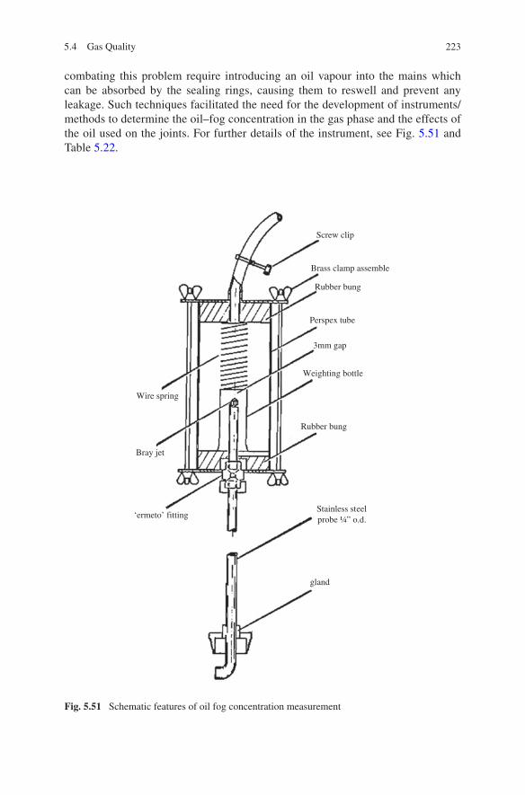
223

combating this problem require introducing an oil vapour into the mains which can be absorbed by the sealing rings, causing them to reswell and prevent any leakage. Such techniques facilitated the need for the development of instruments/methods to determine the oil–fog concentration in the gas phase and the effects of the oil used on the joints. For further details of the instrument, see Fig. 5.51 and Table 5.22.

Fig. 5.51 Schematic features of oil fog concentration measurement

Screw clip

Brass clamp assemble

Rubber bung

Perspex tube

3mm gap

Weighting bottle

Rubber bung

Wire spring

Bray jet

‘ermeto’ fitting Stainless steel probe ¼” o.d.

gland

5.4 Gas Quality

224 5 Natural Gas Measurement Systems

5.4.5 Odorimetry and Leak Detection Measurement

This section has been split into two parts: odorimetry and leak detection. Firstly, odorimetry explains why odour is added to the gas and why accurate measure-ment of odour concentration is essential. Secondly leak detection, leading on from odorimetry, explains why measurements of the leak are carried out.

5.4.5.1 Odorimetry

Odorosity is an extremely important criterion of gas quality. The smell in gas is man-made since raw natural gas is odourless. It is added during the gas-manufacturing/gas-refining process so as to be able to detect it. The chemical is a mercaptan. It is important that the concentration levels of the odorant are correct and consistent across the country. If the odour is too weak, then gas leaks may go undetected, and if too strong, then even the minutest of leaks will be detected miles away. One drop of mercaptan can be detected up to three miles away. For this reason, it is crucial that accurate measurements of odori-sation are made. Figure 5.52 shows the schematic features of an odorisation chambers.

Odour can be measured using either subjective or analytical methods. Analytical methods work by tracing the sulphur compounds contained in odorants. They use the instruments and techniques designed for measuring total sulphur and hydrogen sulphide to assess odorant concentration.

Subjective measurement of odour is carried out by trained personnel known as rhino-analysts. Rhino-analysts smell the gas and assess the odour concentration depending on the intensity of the smell and the odour assessment scale which they are using. There are various scales of odour assessment which are used within the global gas industry: the odorisity scale, the odour level and the odour intensity scale.

The instruments used for the analytical and subjective measurement of odour are detailed in the Odorimetry section of Table 5.23. Figure 5.53 also shows the typical British Gas odorimetry.

5.4.5.2 Leak Detection

Subsequent to the detection of a gas leak, measurements of the intensity of the gas leak must be made. Broadly speaking, this is carried out in order to track down the exact location of the leak and to assess the immediate danger pre-sented by the leak. Leak detection instruments are listed and detailed within the Odorimetry section in Table 5.23. Figure 5.53 also shows the Gasco Seeker, the typical flame ionisation and electron capture detection for gas leak detection (Fig. 5.54).

225

5.4.6 Sulphur and Hydrogen Sulphide Concentration Measurement

In addition to water and oil removal, one of the most important parts of gas pro-cessing involves the removal of sulphur. Natural gas from some wells contains sig-nificant amounts of sulphur. Natural gas with a high sulphur content is commonly called ‘sour gas’ because of the rotten smell caused by the sulphur.

Sulphur exists in natural gas as hydrogen sulphide (H2S), and the gas is usually considered sour if the hydrogen sulphide content exceeds 5.7 mg of H2S per cubic metre of natural gas. The process for removing hydrogen sulphide from sour gas is commonly referred to as ‘sweetening’ the gas. Sour gas is undesirable because the sulphur compounds it contains can be extremely harmful, even lethal, to breathe. Sour gas can also be extremely corrosive. It is therefore essential that it is meas-ured and controlled. Please refer to the relevant section in Table 5.23 for details on sulphur and hydrogen sulphide concentration measurement devices. Figure 5.55

To silencer and extractor fan

To separate extractor fan

Slide valve inside chamber

C

A

B

Light

Light

E

F

D

Fig. 5.52 Ordorisation chamber. A Test room. B Air lock. C 4 mixing fans. D Carbon air filter. E Sample injection chamber. F Electric fan switches. G Odorant injection point

5.4 Gas Quality

226 5 Natural Gas Measurement Systems

Table 5.23 Various gas quality instruments

Instrument Description, range and accuracy Advantages (A) and disadvantages (D)

Application

The Watson House Odorimeter (Odorimetry)

This is a subjective method whereby the measurements are made by rhino-analysts. Gas is introduced to a stream of pure air, which then passes through a funnel into the atmosphere. The observer smells the effluent from the funnel and then records his/her analysis which is recorded in accordance with the odorisity scale. Range: Flow range of 0.002–1.5 ft³/h and pressure range of 0.5–6 in water gauge

Cost, static nature of the system and training required for rhino-analysts

Gas industry and laboratory

British Gas Odorant Chromatograph (Odorometry)

This method is an analytical method. Sulphur contents are separated and passed into a hydrogen/oxygen flame, burning in a hydrogen atmosphere at the tip of a burner in a silica tube, any sulphur compound present forms species which emit a characteristic radiation in the violet and UV regions. Can determine individual sulphur compounds down to con-centrations of 0.01 ppm

Extremely accurate costly

Used in offtakes and pressure reduc-tion stations (PRS)

Gasco seeker (leak detection)

Portable device for measuring methane concentrations in gas /air mixture atmospheres. It uses a pellister (VQ3 Pellister) and Thermal conductivity detector as the second filament. A hand-operated aspirator is used to draw the test atmosphere. Range: +1 % LEL scale +1 % Gas scale +3 % reading

Gas detector is a reliable means of detecting flammable gas, and of measur-ing the percentage of lower explosive limit and the percentage by volume

Emergency gas engineers use this device on a daily basis to detect gas leaks

Must be regularly calibratedDoes not pinpoint the exact location of the leak

Flame ionisa-tion monitor (leak detection)

Effluent gas is passed into hydrogen/air flame in which two electrodes are placed with a poten-tial difference between them. The detector current passes through the high resistance creating a potential difference which appears across the output of the impedance converter and after suitable attenu-ation is measured by the recorder. Max leak sensitivity of 6

Extremely sensitive. Must handle with care

Used to detect high-risk main leakage in win-ter surveys

(continued)

227

also typifies a gas pipe exposed to excessive sulphide gas concentration which led to drastic deterioration of the corresponding pipe over a period of time.

5.4.7 Component Analysis (Chromatography)

The field of component analysis is also very significant as the analyses have a bearing on the pricing structure for the natural gas. Component analysis or gas chromatography as it is often referred to is a physical method of separating the

Instrument Description, range and accuracy Advantages (A) and disadvantages (D)

Application

Electron cap-ture detector (leak detection)

Consists of an irradiation chamber and a pair of electrode. Eluted molecules with a strong electron affinity will capture electrons to form heavy, slow moving negative ions. The resulting decrease in the current flowing between the electrodes is measured. Range in ‘sniffing’ mode is 1 × 10*-8 mls. when sampling 1 × 10*-9 mls

High sensitivity Used for leak testing new mains on air and pressure testing of vessels

The British Gas Sulphur Selective Detector

(Same as BG Gas chromatograph) sulphur contents are separated and passed into a hydrogen/oxy-gen flame, burning in a hydrogen atmosphere at the tip of a burner in a silica tube, any sulphur compound present forms species which emit a characteristic radia-tion in the violet and UV regions

A: good and accurate Gas industry and laboratoryD: Sensitive

The Barton sulphur titrator

Consists of three basic units, a titration cell, an electronic control circuit and a recorder. Bromine is generated by passing an electri-cal current through a suitable electrolyte solution. Compounds bubbled through the solution react with the reagent. The net generating current is thus directly proportional to the concentration of the compounds titrated and is continuously recorded. Range: 0–1,000 in 7 steps, Hydrogen sulphide (0.08 ppm H2S by vol), organic sulphides (0.16 ppm) and sulphur dioxide (0.16 ppm)

Sensitive Gas industry and laboratory

Table 5.23 (continued)

5.4 Gas Quality

228 5 Natural Gas Measurement Systems

various components that constitute the natural gas mix (see also chromatography section in Table 5.24). Figure 5.56 shows a combination of three illustrations, two of which show the gas chromatograph recording equipment (in this case a Daniels 500) and the third illustration the sampling pointing on the pipeline:

Column identification element

Heatingelement

(a)

(b)

(c)

Fig. 5.54 Typical Gasco Seeker (a) flame ionisation detector (b) and electron capture detector (c) [13]

Aluminium reflector

Chimney

Injection port

Heat filter UV filter

Detector

PM tube

300 x 2.5 i.d. packed flow resistor

Tricresyl phosphate

Celite support

Recorder

Attenuator and zero shift

D.C power supply

Transparent silica envelope

Fig. 5.53 British gas odorant chromatograph

229

Fig. 5.55 Typical gas pipe subjected to sulphide gas concentration

Table 5.24 Various gas quality instruments

Instrument Description, range and accuracy Advantages (A) and disadvantages (D)

Application

Gas chroma-tograph(e.g. Daniels 500)

Physical method of separation. Materials are separated and partitioned into two phases. The first is stationary and the second is mobile and percolates through the stationary phase. The mobile phase is gaseous and the stationary phase solid or a solid supporting material impregnated with liquid. Depending on the affinity, the substances are retained to a greater or lesser extent by the stationary phase and issue as separated frac-tions at the end of the column. The gases in the flowing carrier gas stream are detected by measuring a chemical or physical property

A: Superior to any other procedures formerly employed in terms of time-consumed, separa-tion of multi-component systems and amount of sample required D: Costly

Commonly found on offtakes or any network injection points

Perkin Elemer 8700

Same as above Gives a full report via a computer

The Cambridge Thomas Gas Calorimeter

This calorimeter is a modified form of the classic Rossini-style instrument in which heat liber-ated by the complete combustion of a discrete sample of gas is measured thermometrically in a constant pressure enclosed vessel. Accuracy: ±0.03 MJ/m3

Gas industry and laboratory

The British Gas Reference Calorimeter

Range: CVs in the range 30–45 MJ/m3. High accuracy

Gives direct determina-tion of gross CV, density and relative density. The length of time required to obtain a result can be from 2 days to a week

As above

(continued)

5.4 Gas Quality

230 5 Natural Gas Measurement Systems

5.4.8 Calorific Value Measurement

Calorific value (CV) is a measure of heating power and is dependent upon the composition of the gas. The CV refers to the amount of energy released when a known volume of gas is completely combusted under specified conditions. The CV of gas, which is dry and measured at standard conditions of temperature and pressure, is usually quoted in mega joules per cubic metre (MJ/m3). Figure 5.57 shows a typical Boys non-recording calorimeter.

Gas passing through the UK National Grid pipeline system has a CV of 37.5–43.0 MJ/m3, with the exception of Stornoway which receives liquid petroleum gas (LPG). CV information is provided daily to gas shippers and suppliers, which is then used to bill gas consumers. These data are also used by gas transportation companies

Instrument Description, range and accuracy Advantages (A) and disadvantages (D)

Application

The honey-well heating value trans-mitter (HVT)

This instrument uses the relation-ship between the air to fuel ratio and the CV at stoichiometric conditions. The rotary valve motor speed is required to produce stoi-chiometric combustion and is then used as a basis for computing the CV of the gas being burned

HVT is insensitive to ambient temperature changes

As above

‘Simmance’ specific gravity bell (specific gravity)

The ‘Simmance’ Specific Gravity Bell consists of a small water tank in which a bell is suspended from a beam carrying a pointer. The pointer moves over a scale plate which has two lines engraved on it. These lines relate to the upper and lower heights of the bell between which the effusion time is measured. A balanced weight is fitted at the end of the beam opposite the pointer; this weight controls the rate of effusion. An orifice (0.75–0.8 mm in diameter) is mounted on the nipple at the top of the bell. A dust cap covers the orifice to protect from any dirt. The bell is connected via a cord to the beam, which rests on a quad-rant arm to ensure the bell remains in the centre of the tank. Gas or air is introduced into the bell through either of two cocks which are attached to a connecting tube to a standpipe located inside the bell

Accurate and used for many substances but not in use constantly

Used in the gas industry to calculate relative density

Table 5.24 (continued)

231

to determine transportation charges for gas shippers and suppliers. The CV of natu-ral gas is measured continually using process gas chromatographs. Process gas chro-matographs separate natural gas into its constituent compounds (i.e. methane, ethane, carbon dioxide) and measure the amount of each in the gas. The physical character-istics of each component, as defined by ISO 6976 in the UK, are programmed into the chromatograph and an overall CV is derived from the measured composition. The determination of the CV of gas is carried out in accordance with international stand-ards and the Gas (Calculation of Thermal Energy) Regulations, as amended in 1997. These regulations stipulate when and where the CV of gas is measured and the type of instrument to be used. In the UK, the regulations are enforced by Ofgem, who also perform audit checks on the primary data. CV measurement instruments are detailed in the CV section of Table 5.24.

Needle valve

Injection site

Recorder

Detector

Thermostat

Column

Gas outlet

Gas outlet

Collection device

3-waycock

Flow meter

Manometer Gas

cylinder

(a)

(b) (c)

Fig. 5.56 Schematic features of chromatography (a) with illustration of Daniels 500 instrument (b) and the sampling pointing on the pipeline (c)

5.4 Gas Quality

232 5 Natural Gas Measurement Systems

5.4.9 Density Measurement

From the gas flow equations, it is clear that if density is measured directly, then the compressibility of gas is automatically accounted for. This helps explain the reason why British Gas adopted density correction over pressure and temperature correction. To put it simply, measuring density helps measure gas flow more pre-cisely (for further details on density measurement instruments see also the density section of Tables 5.24 and 5.25. Figure 5.58 shows a typical ‘Simmance’ Specific Gravity Bell used for a simple laboratory spot test.

5.4.10 Wobbe Number Measurement

The maintenance of the combustion performance of gases with regard to heating output and air requirement of burners is influenced essentially by Wobbe number. Wobbe number is simply an indicator of the quality of a fuel gas, measured from the heat produced by burning through a defined orifice under standard tempera-ture and pressure conditions, quantitatively defined as the ratio of Btu per cubic foot to the square root of the specific gravity of the gas. Most gas bills involve a heat-value factor to correct for variations in quality; measured centrally to repre-sent average quality fed into the distribution network, this is applied to the meas-ured volume consumed by each customer to establish the energy charge. The factor could be the Wobbe index, but may be in common energy units or the ratio of current heat energy content to the reference value used in setting the tariff.

Fig. 5.57 Boys non-recording calorimeter

233

Table 5.25 Various industry meters

Instrument Description, range and accuracy

Advantages (A) and disadvantages (D)

Application Range Column

Spinner type

In this instrument, an open-ended tube full of gas is rotated and a measurement is made of the differential-pressure between the centre and the ends of the tube which is directly proportional to the gas density. Accuracy: 0.2–0.5 %

Accurate Gas indus-try and research laboratory

Vibrating element

Gas is located in a cylinder inside the device, and the vibrating element is driven at a natural frequency. The resulting displacement is detected and converted to an electrical signal which is recorded. Errors are less than 0.1 %, with accuracies quoted between 0.02 and 0.1 %

A: With non-corrosive, filtered gases, the stability of the cylinder is excellent

As above

D: The necessity of having to measure the differential-pressure and maintaining thefrequency stability of the electrical supply to drive the motor are major limitations

Buoyant beam

This is the most fundamen-tal of all methods. A sealed globe of glass or stainless steel is immersed in the gas and balanced by a force-balanced system. The electri-cal output from this system forms the transmitted reading

As above

British Gas Density Balance

The principle is to measure the apparent mass of 10-cm-diameter constant-volume glass globe suspended in an atmospheric sample of gas at an accurately known pressure. By making similar measurements using pure gas (methane) at several known densities at around atmospheric pressure, the instrument may be calibrated and the unknown density inferred. Can handle objects up to 100 g high accuracy, high precision

A: The large thermal mass of the aluminium cylinders help to damp out detri-mental effects of small temperature fluctuations D: Extremely sensitive to ambi-ent temperature changes

As above

(continued)

5.4 Gas Quality

234 5 Natural Gas Measurement Systems

The above statements help to explain the role of Wobbe number in natural gas. From this, it is clear to see that in the use of gas and gas–air mixtures, it is neces-sary to monitor and control the Wobbe number as by doing so the quality of the gas being supplied will be restricted be to only minor variations.

Instrument Description, range and accuracy

Advantages (A) and disadvantages (D)

Application Range Column

Ac-Me Balance (relative density)

This is a pressure balance type of instrument. The relative density is calculated from the ratio of the absolute pressures. This is obtained from a beam carrying a bulb and a counter-weight which is brought to balance suc-cessively in air and in gas by adjusting the balance case pressure. Accuracy: ±3 %

Reliable As above

Debro recorder (relative density)

Operates on the principle that output pressure of a fan is proportional to the density of the gas being pumped. It comprises of two bells sus-pended from a balance beam sealed in an oil bath. Dry air and gas are introduced to the bells, and the difference in pressure between air and gas is recorded by taking the deflection of the balance beam

As above

The aeration test burner (Sigma ATB model)

This instrument gives an immediate indication of the combustion characteristics of the gas under test. It consists of a Bunsen-type burner with a fixed gas nipple operat-ing at a standard pressure. The primary air shutter is then adjusted to manually to provide an inner flame cone to a specific height and the degree of opening the shutter is indicated on a scale, cali-brated in units, which can be read of the calibration chart as ATB numbers. 0–400 ATB number

Gives an immedi-ate indication of the combustion characteristics of the gas under test. Readings are taken by individuals; therefore, there is possibility of human error

The burner can be used in gas-mix-ing quality control and in appliance approval tests

Table 5.25 (continued)

235

5.4.11 Aeration Number Measurement

The aeration number simply gives an indication of the combustion characteris-tics of the gas under test. Figure 5.59 shows a typical aeration number instrument. Measuring the aeration number helps control the quality of gas entering the net-work, ensuring the gas is adequate for use in the various types of gas appliances. Refer to Aeration section in Table 5.25 for further details.

5.5 Concluding Remarks

Natural gas has established itself as a primary fuel choice in the twenty-first cen-tury. This is due to the fact that it is environmentally friendly and cleaner than oil and coal, hence, greater demand from consumers, i.e. industrial and residential. Throughout the years, the gas industry has witnessed numerous different meas-urement techniques and experimental investigations relating to natural gas engi-neering, consequently making it extremely difficult to keep up to speed with the evolving technology that is being implemented across the world.

Fig. 5.58 Typical ‘Simmance’ Specific Gravity Bell

5.4 Gas Quality

236 5 Natural Gas Measurement Systems

Contractual obligations require that the distribution and transmission compa-nies supply gas of certain specifications in accordance with regulatory standards and the consumers ensure that the fuel supply from meets the demand require-ments. Therefore, there is a need to measure the volume and determine the quality of gas supplied by the operator.

Accurate measurement of gas is influenced by the temperature and pressure of the flow. Actual volume measurement is taken by gas flow instruments, such as orifice plate, venturi meter and pitot tubes. Experimental measurements are carried out to determine the quality of gas by measuring the quantity of impurities such as hydrogen sulphide, carbon dioxide and water present in the gas. It is necessary to remove these impurities as it both poses environmental concern and affects the combustion quality.

In the light of the foregoing, this chapter has presented a comprehensive review of each of the instruments used for measurement of temperature, pressure, gas flow and also the devices used for determination of the quality of natural gas. The chapter evaluated each device in terms of range, accuracy, application and advan-tages and disadvantages relevant for making engineering decisions. It has also provided a framework for engineers, scientists and managers to familiarise them-selves with the instruments and together with the related standards can aid their decision-making in practice.

Fig. 5.59 Typical sigma aeration test burner

237

References

1. British Standard Institution, BS 1041-4: Section 2.1: 1992 Code for temperature measurement.

2. Atkinson, P.G., GC33; Trans. Inst. Gas Eng.,106-441, 1956. 3. www.instrumenttoday.com (accesssed as at 20th July, 2013. 4. Dingle, M.G.W., Instruments for the fuel technologist, Ind. Process Heat II, 6th edition,

1971. 5. Rathakrishnan, E (2007) Instrumentation, Measurement and Experiments in Fluids. Taylor

and Francis Group Brand Katastrophen, Tosa Verlag Wien, 1999. 6. British Standard Institution, BS 1042-1-1.2:1989 Measurement of fluid flow in closed

conduits. 7. http://trade.indiamart.com/details.mp?offer=2021251788 (accessed as at 24th July, 2013). 8. Morris, A.S. (2001) Measurement and Instrumentation Principles. Butterworth Heinemann. 9. http://www.rotameters.co.in/product.html. 10. Nasr, G.G. (2010) Experimental Measurement Method Lecture Notes. The University of

Salford. 11. https://www.ftihttpmeters.com/tech_library/modern_electronics_turbine_flowmeters.html. 12. Retrieved From: http://www.sz-wholesaler.com/p/1068/1083-1/multi-path-ultrasonic-flowmeter-

ur-1000plus-529703.html. 13. http://www.wfu.edu/chemistry/courses/organic/GC/index.html (accessed as at 24th July,

2013).

References

239

6.1 Burners

6.1.1 Introduction

The design and applications of the burners using natural gas have extensively been covered previously by Nasr et al. [1] and Connor et al. [2]. In the following sec-tion, however, a brief overview of various burners together with theoretical con-siderations, where appropriate, will be provided. This can also complement the subsequent sections in this chapter in terms of utilisation of natural gas relating to heat recovery, furnaces and elsewhere in the previous chapters.

The primary role of burners is to provide flame stabilisation, as well as other operations such as air or gas entrainment or mixing in producing the required flow pattern. On the proviso that combustion is complete, the heat released by com-bustion of unit quantity of gas is the same no matter how the gas is burned. The optimum performance of any industrial, commercial or domestic burner using gas stipulates a range of requirements such as flame temperature, shape, size and aera-tion. Burners could, arguably, be classified under six broad headings, which are controlled by mixing gas and oxidant [2]. The categories are as follows:

1. Postaerated or diffusion-flame burners.2. Air-blast burners.3. Machine-premix burner systems4. Gas oxygen burners.

Other burner systems: the four mentioned above are used mostly in domestic industrial and commercial gas usage. Other systems include surface-combustion burners, pulsating combustors and catalytic combustors. Also there are special applications of types (i)–(iv), for example, radiant tubes, packaged burners and dual-fuel burners.

Chapter 6Industrial Utilisation of Natural Gas

© Springer International Publishing Switzerland 2014 G.G. Nasr and N.E. Connor, Natural Gas Engineering and Safety Challenges, DOI 10.1007/978-3-319-08948-5_6

240 6 Industrial Utilisation of Natural Gas

6.1.1.1 Postaerated Burners

In these types of burners, all the air for combustion is obtained from the surround-ing atmosphere; thus, there is no primary process. In laminar postaerated flames, with laminar diffusion, the mixing process is essentially molecular diffusion with freedom from lightback and consequently high turndown ratio, and extremely low noise levels. In turbulent postaerated flames, however, diffusion is the governing process. Moreover, compared with aerated burners, laminar postareated burners have their freedom from linting and port blockage, their compactness, the well-defined flame they produce and their relative insensitivity to changes in combus-tion characteristics. These advantages have enabled the postaerated burners to be the leader in the design of most domestic, commercial and low-temperature indus-trial appliances, particularly in the times of manufactured town gas in the UK. However, these burners give unacceptable performance on natural gas and on con-version have been replaced by aerated burners. As also noted by Pritchard et al. [2], soft flames of fluctuating shape are formed with much decreased stability due primarily to the lower burning velocity and narrower range of flammability.

There are two versions of radically different design that are capable of burning natural gas satisfactorily. These are (i) pinhole burners and (ii) matrix burners.

6.1.1.2 Pinhole Burners

Early design of pinhole burners were developed by the VEG Gas Institute in the Netherlands [2]. These consist essentially of a centre-fed pressed-steel flat-topped box with a row of small holes, typically 0.3–0.4 mm diameter which form the main flame ports. The vertical cylindrical main flames are stabilised by adjacent small auxiliary flames as shown in Fig. 6.1.

Fig. 6.1 Schematic of postaerated burner [2]

Fuel Air

Air

Fuel gas

241

6.1.1.3 Matrix Burners

The principle of matrix burners was originally developed at the British Petroleum Research Centre, and the first version of a matrix burner comprised of a symmetri-cal array of short hexagonal-ended tubes. Gas fed into the free space between the tubes emerges through the very small interconnected slots formed between hex-agonal tube ends on the burner top, the bottom ends being sealed. The exit flow resistance is higher than in the transverse direction so that a uniform gas distribu-tion at the burner face is achieved. Air flow takes place through the tubes under the influence of flue draught or from a low-pressure axial-flow fan similar to that shown previously in Fig. 6.1. These burners burn satisfactorily with any fuel gas ranging from propane to hydrogen with a flame height of only a few millimetres.

Gases with low burning velocity, such as natural gas, have the separation between flame base and burner top which allows some time for gas/air inter- mixing and the resultant flame is blue without yellow-tipping. The pinhole burner also suffers from burn-back sooting. This problem has prevented the development of both matrix and pinhole types. Furthermore, as with other postaerated burn-ers, matrix burners have turndown of about 40 % due to the low-gas-orifice pres-sure drop, although placing a restrictor upstream of the burner could significantly reduce this effect.

6.1.1.4 Atmospheric Aerated Burners

The operation of atmospheric burners is based on the primary air which is entrained by momentum sharing between the gas jet and the surrounding air in which the induced air is some 50–70 % of the stoichiometric air requirement. Two types of atmospheric burners may be distinguished: those in which the gas is used at normal supply pressures of 6.25–20 mbar equivalent to 0.064–0.204 mm of water (i.e. Bunsen burner) and those in which the gas is supplied from a compres-sor or high-pressure supply. Low-pressure atmospheric burners are used on nearly all domestic appliances and have very many low-temperature industrial applica-tions, whereas high-pressure atmospheric burners are restricted more to industrial utilisation. Figure 6.2 shows the essential features of an atmospheric burner.

Air Entrainment

Referring to Fig. 6.2, at (1) gas emerges at high velocity (60) m/s (say) into sta-tionary air. Shear forces between jet and air causes air entrainment into the jet of gas which increases in diameter until it reaches the wall at point (2), with small pressure change between (1) and (2), close to atmospheric pressure. For the mix-ture to overcome flow resistance in the burner, it is necessary to develop a positive pressure in the burner by slowing down the mixture in a divergent diffuser. Here, part of the kinetic energy of the mixture stream is converted to pressure energy.

6.1 Burners

242 6 Industrial Utilisation of Natural Gas

A homogeneous mixture forms in the diffuser and mixing tube, and this is distrib-uted evenly to the flame ports (or burner ports).

Mathematical analysis is complex since throughout the burner, there are flow resistances that are dependent on flow rate, aeration level and on the local velocity profile. Rigorous treatment is outside the scope of this section, but the analyses of Jones [3] derived from Prigg [4] resolve in their simplest form to:-

where r is the air/gas ratio, a function of the relative density of gas, d, the flame-port area Ap and the injector orifice area Aj. Constant K accounts for the friction losses and discharge coefficients in the burner, K, are usually 0.6–0.7. For maxi-mum entrainment, the throat area, At, should be about 0.7 Ap. The diffuser should have an included angle of 5°–8° and should be about 12 × throat diameters in length. Often, practical constraints result in shorter mixing arrangements with some loss of primary aeration.

The Gas Jet or Injector Orifice

The integrated form of the Bernoulli equation governs the discharge of gas through the injector orifice. This may be written:

where Vg is gas rate (m3/h), Aj is orifice area (mm2), Cd is discharge coefficient, p is static pressure at orifice (mbar) and RD is relative density of gas (air = 1).

Multi-hole injectors are widely used in the UK to reduce injector “hiss”. Primary air ports are large to minimise resistance. May have form of aeration

(6.1)r =√

RD

[√

KAP

Aj

− 1

]

(6.2)Vg = AjCd

√

P

RD

Mixture tube

Flame ports or burner ports

Burner bar or head

Gas jet or injector orifice

Primary airport

Primary air control

Throat

Diffuser

Gas

1 2

Fig. 6.2 Schematic diagram of atmospheric burner [2]

243

control but increasingly in the UK they are non-adjustable to give “fixed aeration”. Any dimensional changes likely to affect aeration in particular injector/throat mis-alignment, e.g. for cooker burners on natural gas about 4 % reduction in aeration % for each 1 mm off centre and about 2 % for each 1 % of yaw. Injector jet diam-eter tolerances are important, e.g. 6 % change for each 0.1 mm departure from design value. Burner pressure for different gases are normally town gas 6.25 mbar, natural gas 20 mbar, propane 35 mbar and butane 27.5 mbar. For conversion from one gas to another, gas pressure is decided on the basis of the gas modulus, as defined in the following section.

Gas Modulus

For the same heat input and the same primary aeration, virtually the same volume of primary air needs to be entrained whatever the fuel gas. Volume of gas which does the entrainment, however, is proportional to 1/Cg, where Cg is the gross calo-rific value of the gas. Thus, on conversion from town gas to natural gas, about half of the natural gas needs to entrain the same amount of air. So this smaller flow must be given the same momentum by using a higher pressure. The gas modu-lus (√P/Wobbe No.) thus ensures a constant equal momentum. So to convert from town gas of Wobbe No. 27.8 MJ/m3 and gas pressure 6.25 mbar to natural gas at 50.7 MJ/m3 for equal gas modulus, the required pressure is 21 mbar. This is the basis on which conversion pressures in the UK were calculated, and service regu-lators are all set to give this pressure.

Effect of Gas Pressure and Burner-port Loading

For a given gas, the aeration equation shows no dependence on gas rate and hence gas pressure. Thus, a plot of primary air–gas ratio versus gas pressure would be expected to be like curve (a) in Fig. 6.3. In practice, the form of the graph is as shown in (b), the decrease in aeration at low flow rates being caused by changes in friction factor and the discharge coefficient of the flame ports at low Reynolds number.

The degree of primary aeration is determined by the total area of the flame ports for a particular duty, air/gas ratio increases with values Ap/Ao. The burner-port area for a particular gas rate is conveniently expressed as the burner-port load-ing or flame-port loading, which is the heat input to the burner divided by the total flame-port area (V × Cg/Ap (MW m2)).

where BPL is in MW/m2, V is the theoretical gas rate (m3/h) and Cg is the gross calorific value (CV) of the gas (J/m3).

Also, altering the burner-port loading will also have an effect on flame sta-bility. As also noted by Pritchard et al. [2], reducing the burner-port loading

(6.3)BPL =Heat input

Total flame port area=

VCG

AP

6.1 Burners

244 6 Industrial Utilisation of Natural Gas

(i.e. reducing the mixture velocity at the flame ports) will, in principle, increase the resistance of a burner to blowoff and decrease its resistance to lightback par-ticularly if the reduction in burner-port loading is achieved by providing larger burner ports. Atmospheric burners designed for town gas normally operated at 40–60 % of primary aeration (r = 2–2.5), and this is achieved with burner-port loading of 18–32 MW/m2 with Ap/Ao = 25–30. Thus, if the flames set to light-back with high aerations and large flame ports, say, on turndown, then the required flame stability is achievable. Natural gas blowoff occurs at these high BPLs which need to be reduced to 9–13.5 MW/rn2. Burners with low BPLs widely used in USA, but in the UK, high BPLs are retained and flame prevented from blowoff by an added flame stabilisation device. This can be done by flame-port design and flame retention. For flame-port design, either low efflux velocities resulting from large flame-port areas are used or some external means of flame retention must be provided. Figure 6.4 shows various port configurations. Gauzes are also fitted behind flame ports to provide flow smoothing and to flameproof burners, i.e. prevent them from lighting back. The problem is build up of fluff or “lint” which reduces effective, A, and therefore aeration. Most burners now produced are also multi-gas or “universal” burners. They can burn Family 1, 2 or 3 gases if the injector orifice is changed and the operating pressure is in accordance with gas modulus [1, 2].

6.1.1.5 Air-Blast Burners

There are basically three types of air-blast burners (i) premix (ii) Nozzle-mixing and (iii) tunnel-mixing burners.

Fig. 6.3 Variation of air/gas ratio with pressure for typical aerated burner [2]

100

90

80

70

60

50

40

30

20

10

02.5 5 7.5 10 12.5 15 17.5

(a)

(b)P

rim

ary

aera

tion

(%

)

245

1. Premix types

Figure 6.5 shows schematically a forced-draught premix burner, which should fol-low a set of criteria that have been adopted widely in industrial practice. These criteria are as follows:

• Attainment of Stoichiometric proportions.• Precise control of air–gas ratio.• Comprised of an inherent self-proportioning facility, if the gas is entrained from

a supply at atmospheric (or combustion chamber) pressure.• Use a single control valve on the air supply for varying throughput.• Achieve high mixture pressures using air-supply pressures resulting in high

turndown ratios.

Main flame ports

Retention plates

Main flame ports

Retention platesMain flame ports

Auxiliary flame

Metering orifice

Retention platesMain flame ports

Auxiliary flame

Metering orifice

Retention platesMain flame ports

Auxiliary flame

Metering orifice

Retention plates

Main flame portsAuxiliary flame

Metering orifice

Main flame portsSlotted flame ports

Burner bar

Ribbon ports

Slotted main flame portsAuxiliary flame

Metering orifice

(a) (b) (c)

(d) (e) (f)

(g)(h)

(f)(k)

Fig. 6.4 Burner-port configurations [11]

6.1 Burners

246 6 Industrial Utilisation of Natural Gas

• High burner-port loadings may be obtained.• Positive hot-gas distribution in the combustion chamber should be produced by

giving the combustion products sufficient momentum. Thus less reliance on nat-ural draught than low-pressure systems.

• Produce good air–gas mixing which minimises flame length and combustion-space requirements.

• Interchangeability of fuel gases should be achievable.

If Pg = Pf (see Fig. 6.5), then radius, r, is independent of theoretical gas flow rate Va (= r × Vgas). There is an inherent self-proportioning action, a constant air–gas ratio is given for all throughputs and throughput is controlled very simply by a sin-gle control valve on the air supply. Furnace pressure Pf is commonly atmospheric, and if air–gas ratio control is required, Pg is reduced to atmospheric via a zero-pressure governor.

2. Nozzle-mixing and Tunnel-mixing Burners

With these types of burners, air and gas are simultaneously mixed turbulently during the combustion process at the burner nozzle (burner head). If a tunnel is used, mixing and combustion occur simultaneously in the tunnel and thus the name tunnel-mixing burner. Figure 6.6 shows a typical illustration of this type of burner. The advantages these burners possessed over premix air-blast systems are as follows:

• Lightback is eliminated.• Utilisation of lower air pressure.• Preheated air may be employed.• With lift, flame stability is improved and burners are capable of operating at

high excess air levels.• Capable of conversion from burning town gas to natural gas by changing the air/

gas ratio.

A0

PgZero Govemor

Air

Burner head (typical)

Furnace pressure (PF)

Injector

Gas at supply pressure

Fig. 6.5 Schematic diagram of a premix burner

247

The popular variant integrates the burner with throughput, ratio, ignition and flame-detection controls into a packaged system which are termed packaged burn-ers; these will be described in Sect. 6.1.1.8.

Nozzle-mixing burners can operate on preheated air. These burners provide good combustion, if the mixing is rapid, that is by means of a high relative veloc-ity between the air and gas streams. Alternatively, provision of a large surface area for mixing can also provide satisfactory combustion for the burners. This can be carried out by discharging the air through an annulus or a series of jets. One major drawback with these types of burners is that they are not inherently self-propor-tioning and control schemes of varying complexity are necessary to provide con-trol of air/gas ratio on turndown. Such control is important since deviation from stoichiometric proportions leads to serious fuel wastage.

6.1.1.6 Machine-Premix Systems

In these, air and gas at atmospheric pressure are drawn in through a propor-tioning valve to the inlet of a positive displacement compressor or less com-monly a fan. The mixture is then compressed and distributed to the burners. Their widest applications are found in supplying precisely controlled mixtures to controlled atmosphere generation plant or to large numbers of small burn-ers in, for example, glass-working machinery. Because stoichiometric mix-tures are distributed the safety requirements are severe, and for this reason, the system is not widely used. A recent low-pressure variant is the fully aer-ated domestic burner, which will be considered in Other Burner Systems in Sect. 6.1.1.8.

(a) (b)Burner housing

Gas

AirDistribution plate

Refractory block

Fig. 6.6 Schematic diagram of nozzle-mixing burner (a) [1] and a typical illustration (b) [2]

6.1 Burners

248 6 Industrial Utilisation of Natural Gas

6.1.1.7 Gas and Oxygen Burners

If oxygen is used instead of air, high flame temperatures and rates of heat transfer are obtained. The maximum theoretical flame temperature for oxygen/natural gas flames is around 2700 °C or more, compared with about 1950 for natural gas/air flames and heat transfer rates are typically about twice as great. Premixed gas and oxygen are used in small-scale burners below about 30 kW and are used for weld-ing, glass working, etc., but since the burning velocity is very high (four to five times as great as gas/air flames), lightback is the limiting consideration. Larger oxy/gas burners are nozzle-mixing and are increasingly used in high-temperature industrial processes. The cost of oxygen limits the application of gas/oxygen burn-ers, but recent developments in on-site oxygen generation using pressure-swing adsorption or membrane air-separation techniques are likely to widen considerably the applications of gas/oxygen flames.

6.1.1.8 Other Burner Systems

Radiant (Surface-combustion) BurnersIn these, a high proportion of the energy supplied in the fuel is converted into radi-ant energy. Such burners normally consist of a radiant refractory plaque either of a porous material or of a dense material with a large number of small (approxi-mately 1.5 mm) perforations fed either from a premix air-blast mixer or from a low-pressure atmospheric injector. Combustion takes place at or just below the surface and the plaque quickly becomes incandescent. Very low burner-port load-ings are possible without lightback. Surface temperatures range from about 800 °C to around 1350 °C. Figure 6.7 shows typical arrangements. Common applications are in space heating (the familiar free-standing LPG heater) and in industrial dry-ing processes. The low flame temperatures in radiant burners result in much lower emissions of oxides of nitrogen (NOx).

Catalytic Radiant BurnersGases can be burnt without visible flame at the surface of a catalyst at very low temperatures (about 450 °C for natural gas). Space heaters working on

Air

Gas

Fig. 6.7 Typical surface-combustion burners

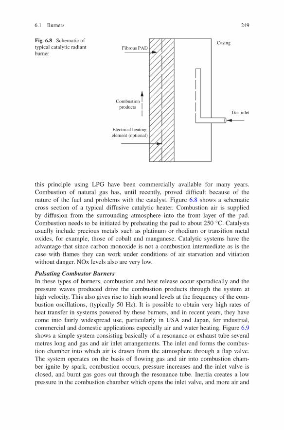
249

this principle using LPG have been commercially available for many years. Combustion of natural gas has, until recently, proved difficult because of the nature of the fuel and problems with the catalyst. Figure 6.8 shows a schematic cross section of a typical diffusive catalytic heater. Combustion air is supplied by diffusion from the surrounding atmosphere into the front layer of the pad. Combustion needs to be initiated by preheating the pad to about 250 °C. Catalysts usually include precious metals such as platinum or rhodium or transition metal oxides, for example, those of cobalt and manganese. Catalytic systems have the advantage that since carbon monoxide is not a combustion intermediate as is the case with flames they can work under conditions of air starvation and vitiation without danger. NOx levels also are very low.

Pulsating Combustor BurnersIn these types of burners, combustion and heat release occur sporadically and the pressure waves produced drive the combustion products through the system at high velocity. This also gives rise to high sound levels at the frequency of the com-bustion oscillations, (typically 50 Hz). It is possible to obtain very high rates of heat transfer in systems powered by these burners, and in recent years, they have come into fairly widespread use, particularly in USA and Japan, for industrial, commercial and domestic applications especially air and water heating. Figure 6.9 shows a simple system consisting basically of a resonance or exhaust tube several metres long and gas and air inlet arrangements. The inlet end forms the combus-tion chamber into which air is drawn from the atmosphere through a flap valve. The system operates on the basis of flowing gas and air into combustion cham-ber ignite by spark, combustion occurs, pressure increases and the inlet valve is closed, and burnt gas goes out through the resonance tube. Inertia creates a low pressure in the combustion chamber which opens the inlet valve, and more air and

Fig. 6.8 Schematic of typical catalytic radiant burner

Fibrous PAD

Electrical heating element (optional)

Combustion products

Casing

Gas inlet

6.1 Burners

250 6 Industrial Utilisation of Natural Gas

gas enter and ignition occurs from the previous cycle and the process continues. The ignition spark is not required after this stage. Noise is the fundamental disad-vantage of pulse combustors, but modern silencer systems have reduced noise to acceptable levels for all but the most demanding requirements. Pulse combustors produce lower NOx levels than conventional burners.

Fully Aerated Domestic BurnersRecent developments in compact high-efficiency boilers in which the combus-tion products are cooled down below their dew point have focused attention on the need for burners which produce short intense flames and which can be fired down-wards or sideways as well as upwards . Fully aerated burners in which air from a low-pressure fan is premixed with gas are coming into use for this type of appli-cation. Such burners may be formed of rows of corrugated steel ribbons or may be ceramic plaques operating either in radiant or in lifted mode. Downward fir-ing is popular since this avoids problems of condensate dropping onto the burner. The burners typically operate at 20 % excess air levels, and boilers operating at 90–95 % thermal efficiency are feasible.

Packaged BurnersIn the firing of boilers and other low-temperature plants, a wide range of forced-draught automatic packaged burners have been utilised since the 1980s and are still evolving, in terms of design and or efficiency. The burner, fan, throughput and air–gas ratio controls and ignition and safety systems are integrated into a single unit. Ratings range from around 0.5 to 18 MW or more. Packaged burners are almost exclusively of the nozzle-mixing type and use metallic burner heads incor-porating a wide variety of stabilising and mixing arrangements as shown typically in Fig. 6.10.

Dual-Fuel BurnersInterruptible gas allows the gas industry to optimise the operation of its transmis-sion and distribution system. Provision for interruptible operation may be made by the installation of separate burners for the two fuels but is much more commonly achieved by the use of dual-fuel burners, i.e. burners designed to burn gas or oil

Gas Igniter

Flame stabiliser Air inlet

Air

Air

Gas inlet Combustion chamber

Exhaust tube

Fig. 6.9 Schematic of typical pulsating combustor burner [2]

251

Air inlet

Atomized oil

Secondary airdischarge

Gas inlet

Rotary atomizer

Atomizer drivemotor

Oil inlet

Fig. 6.10 Typical package burner [1]

6.1 Burners

252 6 Industrial Utilisation of Natural Gas

(or less commonly gas or coal) separately, the equipment being capable of rapid and efficient switchover to the alternative fuel. Dual-fuel burners have found their widest application in industrial boiler firing.

The common components for both systems include the air-supply duct which in the case of packaged burners is attached to the burner body, vanes or plates to control the air direction, an air manifold or windbox and a refractory tunnel or quarl. In addition, a pilot burner or burners must be provided and carefully located so as to ignite both oil and gas reliably. The pilot burner will be integrated into the control programme of both fuel systems when automatic control is used. Flame detectors also need to be particularly carefully located so that the pilot, main gas and oil flames are detected. The fact that the two fuel supply systems are incorpo-rated into one burner housing leads to some degree of mutual interference. The gas system is much more tolerant with regard to mixing and combustion than the alter-native system and the effect of introducing a small oil atomiser on the centre line of the gas supply system presents few problems. Conversely, the introduction of a relatively much larger gas supply into an oil burner may interfere with the mixing pattern and the solution has generally been to dispose the gas inlets out towards the periphery of the burner. Figure 6.11 shows a typical dual-fuel burner.

Heat Recovery BurnersIn high-temperature processes, a very large proportion (often over 50 %) of the energy entering the process is wasted in the sensible heat content of the hot waste gases. Some of this waste heat may be recovered by using it to preheat the load

Swirler

Gas inlet

Gas nozzle

Oil/steam inlet

Fig. 6.11 Typical dual-fuel burner [1]

253

(restricted to continuous processes) or by preheating the combustion air in some form of heat exchanger. Commonly, nowadays this heat exchange is incorporated in the burners themselves to provide high-efficiency compact units. Two types are available: recuperative burners shown in Fig. 6.12 and regenerative burners shown in Fig. 6.13. In the former, the combustion products are drawn counter-current to the incoming air and heat is transferred through a metallic tube. Air preheats of up to 600 °C are feasible.

Regenerative burners on the other hand are cyclical and operate in pairs. Burner “A” fires and its combustion products are drawn through burner “B” heat-ing up the bed of ceramic spheres in its body. The system then reverses, and air is passed through burner “B” where it is preheated. Gas enters and combustion takes place, the waste gases being drawn through burner “A”. The upper part of Fig. 6.13 shows the principle of regenerative firing and the lower part the applica-tion of regenerative burner to a steel coil annealing furnace. Regenerative burners can be used at very high temperatures (1,600 °C or more) since there is no metallic interface between combustion product and air. Both recuperative and regenerative systems are capable of providing enormous energy savings in high-temperature process.

Low-Nox BurnersThis is a relatively new burner classification resulting from recent intense interest, particularly in Japan, USA and Germany in the reduction of emissions of nitrogen oxide from fuel-burning equipment. Nitric oxide (NO) is formed by nitrogen fixa-tion in high-temperature flames. In the atmosphere, it converts to nitrogen dioxide (NO2) by a photochemical reaction. NO2 is a major contributor to smog formation.

Furnace gases inlet Cast refractory block Furnace gases oulet

Fuel gas

Combustion airNozzle

Furnace wall

Fig. 6.12 Schematic diagram of recuperative burner [2]

6.1 Burners

254 6 Industrial Utilisation of Natural Gas

NO and NO2 are normally lumped together as Knox and considered as a single pollutant. Unfortunately, NOx formation is favoured by those combustion condi-tions generally regarded as ideal from other viewpoints, i.e. near-stoichiometric, intense, high-temperature combustion. Various techniques are employed in low-NOx burners to reduce emissions including:-

• Recirculation of cooled flue gases into the combustion zone• Two-stage combustion (fuel-rich primary combustion followed by secondary

combustion after heat exchange or with dilution).

Figure 6.14 shows a Japanese low-NOx burner incorporating both these principles.

6.2 Heat Transfer and Heat Exchangers

6.2.1 Introduction

There are many published books and articles dealing with heat transfer and heat exchangers [5–10]. However, throughout downstream gas processing, and as high-lighted throughout this book, heat exchangers are regularly utilised and they play an important role. It is beyond the scope of this book to give detailed analysis of these subject areas since they can be treated as stand-alone. To this end, an over-view of the modes of heat transfer and the conceptual design of heat exchangers has been provided. The intention here is thus to provide an appreciation of the

Fuel burners

Furnace

air Reversing valve

Combustion gases to stack

a b

1 2

Fig. 6.13 Schematic diagram of regenerative burner

255

subject matter, which in turn formulates a better understanding when dealing with heat exchangers in the gas processing and production environment. Readers are also advised to consult various publications, some of which have been given in the reference section of this chapter.

6.2.1.1 Modes of Heat Transfer

There are basically three modes of heat transfer, namely conduction, convection and radiation.

i. Conduction: this is primarily concerned with heat transfer in solids and takes place by one molecule transferring heat to adjacent molecules.

ii. Convection: this is primarily concerned with liquids and gases and occurs due to the movement of molecules. There are generally two types of convection: the first being natural convection and the other being forced convection.

iii. Radiation: radiation heat transfer takes place via wavelength and is transmit-ted by waves, in a similar way to radio waves using but different wavelengths.

For heat transfer, of any kind to take place there must be a temperature difference.

Conduction

Fourier’s law of conduction states that the heat flux through a solid is proportional to the infinitesimal temperature gradient per unit length or more formally for one dimension:

(6.4)q = −kθT

θx

Recirculation gas

Secondary air

Primary air

gas

Fig. 6.14 Schematic diagram of low-Nox burner

6.2 Heat Transfer and Heat Exchangers

256 6 Industrial Utilisation of Natural Gas

where k is a constant of proportionality called the thermal conductivity W/

mK, q is the rate of heat transfer (W

/

m2), θT is temperature difference ( ◦

K

)

and ϑx is the thickness (m).

Heat Transfer Through a Flat PlateFourier’s law can be exploited to evaluate the heat transfer through a plate. If it is assumed that the heat transfer is steady, the temperature distribution is a func-tion of x only and the conductivity is temperature independent, then by integration Eq. (6.4) reduces to:

where .

Q is the heat transfer per unit time (W).

Heat Transfer Through a Composite Flat PlateIt should be noted that the term kA

x in Eq. 6.5 is a constant for a material of known

thickness. Furthermore, since the heat flow is steady, the value of Q will not change over any linear distance x. So writing Eq. (6.5) in a more convenient form gives ∆T = x

kA

.

Q or ∆T = Rth

.

Q, where Rth can be expressed as:

Equation (6.5) is analogous with Ohm’s law and can be used to calculate the temperature drops across many plates with different thermal conductivity. Equation (6.5) is termed the thermal resistance for a flat plate.

Consider the heat transfer through a number of flat plates shown schematically in Fig. 6.15. The concept of thermal resistance can be exploited here to calculate the total temperature drop across the plates. That is, since the heat flow is con-stant across each of the plates, (Q = Qa = Qb = Qc). Furthermore, the total tem-perature change is equal to the sum of the individual temperature changes; thus, (∆T = (∆T)a + (∆T)b + (∆T)c).

Applying Eq. (9.5) to each of the plates gives:

(6.5).

Q =kA(∆T)

x

(6.6)Rth =x

kA

Fig. 6.15 Heat transfer through a number of plates KbKa Kc

XbXa Xc

T4T3T2T1

257

Hence,

where RthT is termed the total thermal resistance. Application of Eq. (6.6) to the

figure will give:

Substitution of this into Eq. (9.9) renders:

Note the main assumption here is that the values of ki are independent of tempera-ture. If this is not the case, then methods of integration should be employed. Note also that so far we have only considered the heat transfer through solid wall sur-faces. It is possible to exploit the thermal resistance concept to consider heat trans-fer in a fluid system. This is achieved by considering heat transfer from the solid wall to a thin boundary layer of the fluid through which there is a temperature change. These regions are often referred to as films of fluid and we must consider the film heat transfer coefficients.

Heat Transfer Through a Composite Flat Plate (Including Film Coefficients)The diagram shows a typical steady heat transfer system from the hot fluid through a composite wall to a cold fluid. In the regions adjacent to the wall, the fluid tem-perature changes through the film. Newton’s law of cooling states that the heat flux through a film is proportional to the temperature difference that is,

where Tw and Tf are the wall and fluid temperatures, respectively, (K) and “�” or “h” is the heat transfer coefficient

(

W/

m2K)

.

Figure 6.16 shows schematically the composite flat plates, and then in terms, thermal resistance is,

Hence, the heat transfer through the fluid can just be looked on as another resist-ance term for this particular system which can be expressed as:

(6.7)RthT

.

Q = Rtha

.

Q + Rthb

.

Q + Rthc

.

Q

(6.8)RthT=

n∑

i

Rthi

(6.9)RthT=

xa

kaA+

xb

kbA+

xc

kcA

(6.10).

Q =A∆T

xa

ka+ xb

kb+ xb

kb

(6.11).

Q = A�(

Tw − Tf

)

(6.12)Rthf=

1

A�

(6.13)RthT=

1

A�1

+xa

kaA+

xb

kbA

1

A�2

6.2 Heat Transfer and Heat Exchangers

258 6 Industrial Utilisation of Natural Gas

Therefore, application of Eq. (9.13) renders:

Radial Steady-state Conduction Through the Wall of a Tube and a Composite Thick

Radial Steady Flow Through the Wall of a TubeHeat flows radially through the wall of a tube at steady-state and at a constant tem-perature with direction of the heat flowing normal to the axis of the tube. The rate of conduction at the steady-state condition through the wall can be estimated at a unit length rather than a surface area which makes it more expedient. The increase of area for consecutive layers with radius implies that the temperature gradient decreases with the radius. Figure 6.17 shows schematically the temperature distri-bution and the possible flow patterns.

If the thickness of an elemental cylindrical tube is dr and the area of flow per unit length of the tube is 2πr, with the temperature gradient normal to the tube dT

dr,

then using Fourier’s law, the heat flow is .

Q = 2πkr dTdr

. Also by integration, with the proviso that

.

Q is independent of, r, the temperature difference can be expressed as:

Or in terms of thermal resistance, Eq. 6.15 can be written as:

(6.14).

Q =A∆T

1A�1

+ xa

kaA+ xb

kbA+ 1

A�2

(6.15)∆T =

loge

{

r2r1

}

2πk

.

Q

(6.16)Rth =loge

{

r2r1

}

2πk

Fig. 6.16 Heat transfer from a solid to a fluid KbKa

XbXa

T3T2T1

T1f

T3f

1

2

Hot

Cold

259

Radial Steady Conduction Through the Wall of a Composite Thick CylinderConsider a thick composite cylinder as shown in the diagram for the fluid inside and outside the tube, Newton’s law of cooling still applies, and hence, this can be considered as an extra resistance term, per unit length, thus in terms of thermal resistance, the radial conduction through the wall of a composite thick cylinder can be written as (Fig. 6.18):

(6.17)RthT=

1

2π

1

r1�1

+n

�

i=1

loge

�

r1+1ri

�

ki

+1

rn�n

Temperature profile

Cylindrical isothermal surfaces Lines of heat flow

T1

T2

T

dT

r1r2

Fig. 6.17 Radial temperature profile of a tube [5]

Fig. 6.18 Composite tube

T1

T2

T3

R1

R2

R3

6.2 Heat Transfer and Heat Exchangers

260 6 Industrial Utilisation of Natural Gas

Overall Heat Transfer CoefficientWhere pipes are concerned, it is also useful to show the heat transfer in terms of an overall heat transfer coefficient U

(

W/

m2K)

; thus,

Hence, using Eq. (6.17) and combining with (6.18), the overall heat transfer coef-ficient can be expressed as

This overall heat transfer coefficient can be envisaged as an overall heat conduc-tion term. Furthermore, since A is an area of contact with the fluid, as far as pipes are concerned, this area may be calculated with respect to an inner or outer diam-eter. Since the area of contact per unit length is given by A = 2πr, this leads to the following definitions.

where Ai = the inner area; hence,

Likewise for the outer diameter

General Equation of Heat Conduction (With Internal Heat Generation)Consider the volumetric element of the typical conducting material shown in Fig. 6.19 as follows:Heat transfer rate into the cube in the x direction.

at (x + δx), the heat transfer rate has changed.

Therefore, the difference between the entering and leaving value:

(6.18).

Q = AU∆T

(6.19)∆T

RthT

= AU∆T

Ui =1

AiRthT

(6.20)Ui =1

2πriRthT

(6.21)Uo =1

2πroRthT

δQx = −kx∂t

∂x· δy · δz

δQ(x + δx) = δQx +∂

∂x(δQx) · δx.

= δQx +∂

∂x

(

−kx∂t

∂x· δy · δz

)

δx.

δQx − δQ(x+δx) =∂

∂x

(

kx∂t

∂x

)

· δy · δz · δx

261

A similar expression can be obtained for the y and z directions.Hence, the net heat transfer inflow rate is,

Assume there is an internal heat generation Qi/unit-time and volume, e.g. elec-trical resistance heating.

Therefore,

where Cp is the specific heat capacity (J/KgK), ρ is the density (kg/m3) and T is time (s).For k constant in directions x, y and z, then Eq. (9.23) can be expressed as,

where the thermal diffusivity, α, is:

=[

∂

∂x

(

kx∂t

∂x

)

+∂

∂y

(

ky∂t

∂y

)

+∂

∂z

(

kz∂t

∂z

)]

δy · δz · δx·

Rate of heat generation + influx = rate of increased energy

(6.22)

Qiδy · δzδx +[

∂

∂x

(

kx∂t

∂x

)

+∂

∂y

(

ky∂t

∂y

)

+∂

∂z

(

kz∂t

∂z

)]

δyδzδx = ρCρδyδzδx∂t

∂T

(6.23)∂t

∂T=

Qi

ρCp+

k

ρCp

[

∂2t

∂x2+

∂2t

∂y2+

∂2t

∂z2

]

(6.24)α =k

ρCp

(

m2

hor

m2

s

)

Fig. 6.19 Typical volumetric element (cartesian coordinates)

Y

X

Z

x

x (x

6.2 Heat Transfer and Heat Exchangers

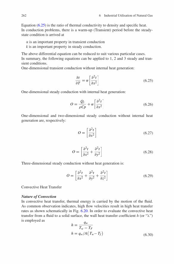
262 6 Industrial Utilisation of Natural Gas

Equation (6.25) is the ratio of thermal conductivity to density and specific heat.In conduction problems, there is a warm-up (Transient) period before the steady-state condition is arrived at

α is an important property in transient conductionk is an important property in steady conduction.

The above differential equation can be reduced to suit various particular cases.In summary, the following equations can be applied to 1, 2 and 3 steady and tran-sient conditions.One-dimensional transient conduction without internal heat generation:

One-dimensional steady conduction with internal heat generation:

One-dimensional and two-dimensional steady conduction without internal heat generation are, respectively:

Three-dimensional steady conduction without heat generation is:

Convective Heat Transfer

Nature of ConvectionIn convective heat transfer, thermal energy is carried by the motion of the fluid. As common observation indicates, high flow velocities result in high heat transfer rates as shown schematically in Fig. 6.20. In order to evaluate the convective heat transfer from a fluid to a solid surface, the wall heat transfer coefficient h (or “λ”) is employed as

(6.25)∂t

∂T= α

[

∂2t

∂x2

]

(6.26)O =Qi

ρCp+ α

[

∂2t

∂x2

]

(6.27)O =[

∂2t

∂x2

]

(6.28)O =[

∂2t

∂x2+

∂2t

∂y2

]

(6.29)O =[

∂2t

∂x2+

∂2t

∂y2+

∂2t

∂z2

]

(6.30)

h =qw

Tw − TF

h = qw/A(

Tw− Tf

)

263

where qw is heat transfer rate per unit area (W/m2), A is surface area (m2), Tw = wall temperature (K) and TF = a representative (e.g. ambient) fluid tempera-ture away from the wall (K).

In engineering calculations, the use of the heat transfer coefficient h provides a general method for the evaluation of convective heat transfer from a fluid to a solid.

In the case of external flows, TF is T, the temperature of the fluid far enough from the wall to be unaffected by its presence. In the case of internal flows (e.g. pipe flow), TF is taken as the average or bulk temperature of the fluid TB. The precise calculation of h (or “λ”) requires the solution of the full heat transport equation containing convection. The convection equation can be constructed by considering the energy balance for an infinitesimally small control volume within the fluid. Readers, if required, should refer to an appropriate book on heat trans-fer or consult the Refs. [5, 6] given at the end of this chapter, for a derivation of convection equation as well as other related areas including dimensional analysis. A more widely used (and simpler) approach to evaluate h (or “λ”) is from experi-mental correlations which are generalised using dimensional analysis.It is, however, useful here to provide a brief explanation of two different convec-tion heat transfers. Convection can be subdivided into two types: (i) forced con-vection and (ii) natural convection

(i) Forced ConvectionIn forced convection, the motion of the fluid is caused by external factors; the fluid is “forced” to move, e.g. by a pressure difference as shown in Fig. 6.21. The pres-ence of fluid flow then also assists heat transfer. The pressure gradient drives the fluid. The fluid carries thermal energy which is transmitted to the solid wall.

(ii) Natural (or Free) ConvectionIn the absence of external forces, the temperature gradients in the fluid lead to density differences which cause buoyancy-induced motion. This motion then car-ries thermal energy either to or away from the solid surface, as shown schemati-cally previously in Fig. 6.20. Under the circumstances for the heat transfer from hot surface to cold stationary air, the near-wall fluid is at a higher temperature than the fluid further away from the wall. The near-wall fluid has, therefore, a lower density than the fluid further away.

U Boundary layerqw

Actual temperature

Temperature in motionless fluid

Y

Tw

TF

Fig. 6.20 Velocity and temperature profiles in a fluid boundary layer

6.2 Heat Transfer and Heat Exchangers

264 6 Industrial Utilisation of Natural Gas

Radiation Heat Transfer

Thermal RadiationIf a heated body is completely isolated from any contacting medium, i.e. placed in a vacuum, then its temperature is observed to decrease with time, again showing a loss of energy. This mode of heat transfer is evidently quite different from conduc-tion and convection, where heat transfer relies on contact between the heated body and a contacting medium. Thermal radiation is the transfer of energy by virtue of electromagnetic wave motion. The electromagnetic wave spectrum is wide, and common types of E-M waves are classified by their wave length (Fig. 6.22).

Thermal radiation is carried by those waves which fall within the infrared band. The infrared waves themselves result from electron transitions between electron shells within the atoms of the radiating body.

Absorptivity, Reflectivity and TransmissivityWhen radiant energy falls upon a body, part or all of it may be absorbed, part or all of it may be reflected, and part or all of it may be transmitted (passed through the body). This can be shown schematically in Fig. 6.23.

Black Body RadiationRadiation striking a body can be absorbed by the body, reflected from the body or transmitted through the body. The fractions of the radiation absorbed, reflected and

U

P

qw T

Fig. 6.21 Velocity profile in a tube

X-rays, -rays Ultra-violet Light

Infra-red radio waves

10-12 10-8 10-6 10-3 1 102 104

Fig. 6.22 The E–M spectrum

265

transmitted are called the absorptivity, α, the reflectivity ρ, and the transmissivity, τ, respectively. Then, we haveα + ρ + τ = 1. For most solids and liquids encoun-tered in engineering, the amount of radiation transmitted through a substance is negligible. Therefore, α + ρ = 1. An ideal black body absorbs all the radiation which falls upon it. For a black body, α = 1and ρ = 0. It should be noted that the term black does not necessarily mean black to the eye. Kirchoff’s law states that the emissivity of a body radiating energy at a temperature T is equal to the absorp-tivity of the body when receiving energy from a source at a temperature T.

The Grey BodyIn considering radiation so far, it has been assumed that the energy emitted by thermal radiation is the same for all wavelengths of radiation. This is not the case. Surfaces in practice are very often assumed to have a constant emissivity over all wavelengths and for all temperatures such an ideal surface is called a grey body. Then, for a grey body, α = ε at all temperatures where αand ε are the total absorp-tivity and the total emissivity, respectively, over all wavelengths. In practice, although a suitable total value of the emissivity may be taken for a large num-ber of industrial surfaces (i.e. furnaces, metal making) over a wide range of wave-lengths, there is still a variation of total emissivity with temperature [5].

The Stefan–Boltzman LawIt was found experimentally by Stefan and proved theoretically by Boltzmann that the emissive power of a black body is directly proportional to the fourth power of its absolute temperature. If the emissivity of the body at T1 is largely different from the emissivity of the body at T2, then the approximate of the grey body may not be suf-ficiently accurate. In that case, it is a good approximation to make the absorptivity of the body (1) when receiving radiation from a source at T2 as being equal to the emis-sivity of body (1) when emitting radiation at T2 as shown schematically in Fig. 6.24.Thus, heat transfer by radiation can be defined as:

(6.31)Q = εσA(T41 − T4

) (W)

Fig. 6.23 Different radiant energy

6.2 Heat Transfer and Heat Exchangers

266 6 Industrial Utilisation of Natural Gas

where ε is the emissivity, σ is Setfan–Boltzman constant (56.7 × 10−12 kW/m2 K4),

A is the surface area (m2) and T is absolute temperature (K).The absorptivity, while depending mainly on the temperature of the source of

radiation, also depends on the temperature of the surface itself. For most metals, this factor can be important and it has been shown that the absorptivity of two metal sur-faces at T1 for radiation from a source at T2 is approximately equal to the emissivity of the surface when at temperature T3 given by T3 =

√T1T2. Further information on

radiation heat transfer is also given in [5, 6, 11] and various published works.It should be also noted that radiation from gases and flames are complex and

need to be separately treated. Readers are advised to consult the appropriate publi-cations. Generally speaking, gases play an important role in transferring heat, are extremely selective emitters and cannot be considered as grey [5]. The radiation from flame, however, can be estimated subject to knowing the density and distri-bution of the suspended solid particles and thus assume the flame is of the black nature. In the Chap. (7), the concept of combustion, luminous (yellow) and non-luminous (blue) flame is described. Effectively the yellow flame could transfer its energy to other bodies by radiation more readily than the blue flame. The anal-ogy of this concept is gas fires for space heating in which the blue flames are sur-rounded by refractory materials. When these refractory materials are subjected to the corresponding heat, it enables the radiation from the fire to be more efficiently transmitted (e.g. see also previous preceding sections in this chapter).

6.2.2 Heat Exchangers

6.2.2.1 Introduction

The three modes of heat transfer that were briefly described in Sect. 6.2.2.1 can be combined and treated concurrently by considering an overall heat transfer coefficient. As the name implies, a heat exchanger is a device that aims to promote exchange

T1

T2

Body

Black surrounding

For a gray body

T1 > T2

Fig. 6.24 Black body and heat transfer radiation

267

of thermal energy between two fluids. Every day experience alone (car-radiator, domestic heating radiators, and refrigerators) is sufficient to illustrate the important role of such components. There is a variety of different types of heat exchanger avail-able. The need for different designs partly arises from the different types of fluid involved (gas-to-gas, gas-to-liquid and liquid-to-liquid) and partly because of the dif-ferent applications to which heat exchangers are used. In an aeronautical application, weight and size may be the limiting factor, whereas in other situations, thermal effec-tiveness and capital costs may be the main considerations. In the following analysis, different types of heat exchangers are described, mainly, from atheoretical point view which can therefore be utilised in natural gas processing plant as appropriate.

Types of Heat Exchangers

1. Double-pipe Heat Exchanger

This is the simplest heat exchanger type. When the pipe and annulus flows are in the same direction, then we have a parallel-flow situation as shown schematically in Fig. 6.25. When Fluid A flows in the opposite direction from Fluid B, then we use the term counter-flow heat exchanger.

The thermal resistance between the two fluids is given by:

Therefore, overall heat transfer coefficient Uol based on our radius is

where hi and ho can be determined from correlations.In a parallel-flow situation, there is a maximum temperature difference at the

entrance and a minimum temperature difference at the exit (between the hot and cold fluid). In counter-flow situations, the temperature differences between the hot and cold fluids remain more uniform (Fig. 6.26).

2. Shell-and-Tube Heat Exchanger

Such heat exchangers are widely used in chemical-process industries. One fluid flows inside the tubes, and the other fluid is forced over and outside the tubes through the shell. The baffles force the shell-side fluid to flow across the tubes and thus promote heat transfer. A variety of baffles can be used in practice. A multiple number of tube passes (4, 6, 8, etc.) can also be present. A two-shell arrangement is also possible as shown in Fig. 6.27.

3. Cross-flow Heat Exchangers

Cross-flow heat exchangers are commonly used in gas cooling and heating appli-cations. The fluid inside the tubes would normally be a liquid and the outside fluid a gas as depicted in Fig. 6.28.

Rth =l

hiAc+

ℓh(ro/ri)

2πkL+

1

hoA6

(6.32)Uo = 1/

{

Ao

Al

l

hl+

Aoln(ro/ri)

2πkL+

1

ho

}

6.2 Heat Transfer and Heat Exchangers

268 6 Industrial Utilisation of Natural Gas

4. Compact Heat Exchangers

These are basically gas-to-gas heat exchangers. Because of the lower overall heat transfer coefficient (associated with gases), gas-to-gas heat exchangers have a higher surface area per unit volume than other types.

Their examination is beyond the scope of this book. Readers should consult appropriate Refs. [7–9].

The Log-Mean Temperature Difference (LMDT)

This is one of the available calculation methods for heat exchanger design. There are a set of objectives for this method. Given a heat exchanger of known surface

Fluid B

Fluid Ain

Pipe

Fluid Aout

Fluid Bout

1 2

in

Fig. 6.25 Schematic diagram of double-pipe heat exchanger

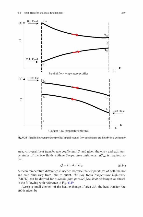
269

area, A, overall heat transfer rate coefficient, U, and given the entry and exit tem-peratures of the two fluids a Mean Temperature difference, ΔTm, is required so that

A mean temperature difference is needed because the temperatures of both the hot and cold fluid vary from inlet to outlet. The Log-Mean Temperature Difference (LMTD) can be derived for a double-pipe parallel-flow heat exchanger as shown in the following with reference to Fig. 6.29.

Across a small element of the heat exchange of area ΔA, the heat transfer rate ΔQ is given by

(6.34)Q = U · A · ∆Tm

Cold Fluid

Hot Fluid

TC1

TH1

TC2

TH2

1 2

Cold Fluid

Hot Fluid

TC1

TH1

TC2

TH2

1 2

T

T

L

L

(a)

(b)

Parallel flow temperature profiles

Counter flow temperature profiles

Fig. 6.26 Parallel flow temperature profiles (a) and counter flow temperature profiles (b) heat exchanger

6.2 Heat Transfer and Heat Exchangers

270 6 Industrial Utilisation of Natural Gas

From the energy balance,

where m is mass flow rate (kg/s), c is specific heat capacity (J/kgK).Combining 6.35 and 6.36 and by integration and when x = x1, Th = Th1,

Tc = Tc1, Ax = 0 and Constant = ln(Th1 − Tc1), then LMTD can be expressed as:

(6.35)∆Qx = U · ∆Ax(Th − Tc)x

(6.36)∆Q = −mhCh∆Th = mcc · ∆Tc

∆Tm =(Th2 − Tc2) − (Th1 − Tc1)

ℓn[(Th2 − Tc2)/(Th1 − Tc1)]

Baffle

(a)

(b)

Fig. 6.27 Shell-and-tube heat exchanger a one tube pass and b two tube passes

271

or∆Tm is called LMDT

Equation (9.37) is also applicable to a counter-flow double-pipe heat exchanger as shown in Fig. 6.30.

Thus, the LMDT for parallel flow can be expressed as

(6.37)∆Tm =∆T2 − ∆T1

ℓn(∆T2/∆T1)

(6.38)∆Tm =

∆T2 − ∆T1

ℓn(∆T2/∆T1)

Heating or cooling fluid

Gas flow

Gas flow

Heating or cooling fluid

Cross -flow heat exchanger, one fluid mixed and one unmixed

Cross -flow heat exchanger, both fluids unmixed

Fig. 6.28 Cross-flow heat exchangers

6.2 Heat Transfer and Heat Exchangers

272 6 Industrial Utilisation of Natural Gas

For other types of heat exchangers, if T1 and t1 are the two fluid inlet temperatures, then T2 and t2 are the corresponding exit temperatures as typified in Fig. 6.31.

The corresponding LMTD can thus be written as

where F is a correction factor.The value of F depends on the type of heat exchanger used and also on the

temperature ratios P and R. The correction factor F allows for the fact that flow may not be true parallel flow or true counter-flow. These correction factors are

(6.39)∆Tm =F{(T1 − t2) − (T2 − t1)}ℓn[(T1 − t2)/(T2 − t1)]

TH1

TC1

TH2

TC2

12

TH

TC

1 2

1

2

T

L

Fig. 6.29 Parallel-flow heat exchanger

TH1

TC1

TH2

TC2

1

2

1 2

TH1

TC1

TH2

TC2

12T

L

Fig. 6.30 Counter-flow heat exchanger

273

functions of both flow and temperatures and temperature differences between shell-and-tube fluids and are presented as graphs (see Fig. 6.32). These graphs are in various standards and publications such as Tubular Exchanger Manufacturers Associations (i.e. TEMA) [10], readers should refer to the standards appropriate to their respective exchangers. Note that P = t2−t1

T1−t1 and R = T1−T2

t2−t1.

The values of F for shell-and-tube and also for cross-flow heat exchangers are given in Fig. 6.31a–c.

Effectiveness and Number of Transfer Unit Method

The LMTD method discussed in the previous section is not easy to apply when all inlet and outlet temperatures are not known. An iterative solution procedure would have to be employed. A more generally applicable method for heat exchanger analysis is the effectiveness NTU method. The objective is to determine the heat exchanger effectiveness ε, where ε can be defined as

The actual heat transfer Q is either the energy lost by the hot fluid or the energy gained by the cold fluid.

The maximum possible heat transfer for the heat exchanger could be attained if the fluid with the minimum mC value was to under go a temperature change equal to the maximum temperature difference. The maximum temperature difference is the difference between the hot and cold fluid inlet temperatures Th1 and Tc1.

It is necessary to use the minimum mC fluid because it is physically impossible for the fluid with the maximum mC value to undergo the maximum temperature change. Therefore,

Having defined ε, the problem is how to determine its value for a given situation. If C = .

m c, it will be shown that ε is a function of Cmin/Cmax and of UA/Cmin.

ε =Actual Heat Transfer

Maximum Possible Heat Transfer

(6.40)Q = m .

hch(Th1 − Th2) = m .

hch(Tc2 − Tc1)

Qmax = (.

m c)min(Th1 − Tc1)

ε =∆T(minimum fluid)

(Th1 − Tc1)

Fig. 6.31 Heat exchanger with two fluid inlet temperature

T1 T2

t2 t1

Heat Exchanger

6.2 Heat Transfer and Heat Exchangers

274 6 Industrial Utilisation of Natural Gas

Fig. 6.32 Typical correction factor plot from TEMA for various heat exchanger configurations a T on the tube side, T′ on the shell side. i = input, o = output. One pass on shell side, any multiple of two passes on tube side. b Correction factor plot for exchanger with two-shell passes and four, eight or any multiples of tube passes. c Correction factor plot for cross-flow exchanger with both fluids unmixed, laterally

275

(Note that C ≤ 1). C is known as the capacity rate and UA/cmin is called the num-ber of transfer units (NTU). The NTU is a measure of heat exchanger size. This is useful since one of the restrictions of the LMTD method of analysis is that the configuration of hot and cold inlet and outlet temperatures is needed before the design can be done. If not a “guestimation” of the outlet temperatures is made, then an iterative calculation is carried out to “home in” on the final solution.

and

Effectiveness in a parallel-flow double-pipe can be expressed as

And for a counter-flow double-pipe heat exchanged, it can be shown that

Readers should consult various references for derivations of these equations [7–10]. For heat exchangers of different types, similar expressions can also be derived (either exact or approximate). The value of N(= UA/cmin) in terms of the ε and cmax and cmin values for various types are also provided in different related pub-lications. In boilers, condensers, and furnaces where the temperature of one of the fluids remains constant, cmin/cmax is effectively zero because cmax tends to infinity. The effectiveness of parallel and counter-flow heat exchangers can also be found in [7–9] for example.

6.3 Overview of Combined Heat Power Using Natural Gas

6.3.1 Introduction

On a large scale, the application of combined heat and power (CHP) systems has been slow to take off, mainly due to economic considerations rather than environ-mental considerations. In mainland Europe, many such schemes are in operation for the supply of district heating. Combined heat and power on a smaller scale has been taken up more readily and systems up to a maximum of 150 kW heat-ing load are commonly referred to as micro-CHP systems. Typical applications of these systems are in hotels, leisure complexes, water treatment plants, etc. Standard packages comprising engines, heat exchangers and control systems are

NTU =UA

mcCpc

when mnCpn > mcCpc

NTU =UA

mhCph

when mhCph < mcCpc

(6.41)ε =1 − EXP[C − N)(1 + cmin/cmax)]

1 + cmin/cmax

(6.42)ε =1 − EXP[C − N)(1 + cmin/cmax)]

1 − (cmin/cmax)EXP[(−N)(1 − cmin/cmax)]

6.2 Heat Transfer and Heat Exchangers

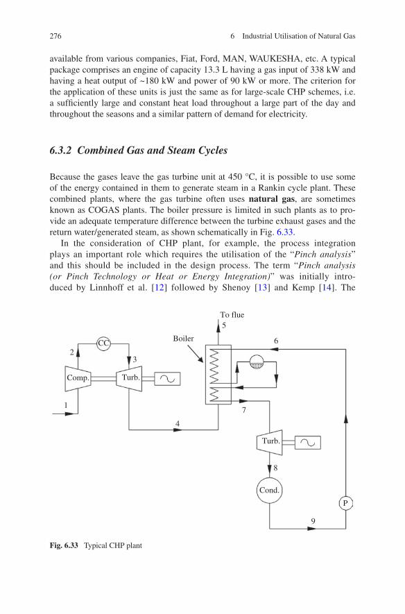
276 6 Industrial Utilisation of Natural Gas

available from various companies, Fiat, Ford, MAN, WAUKESHA, etc. A typical package comprises an engine of capacity 13.3 L having a gas input of 338 kW and having a heat output of ~180 kW and power of 90 kW or more. The criterion for the application of these units is just the same as for large-scale CHP schemes, i.e. a sufficiently large and constant heat load throughout a large part of the day and throughout the seasons and a similar pattern of demand for electricity.

6.3.2 Combined Gas and Steam Cycles

Because the gases leave the gas turbine unit at 450 °C, it is possible to use some of the energy contained in them to generate steam in a Rankin cycle plant. These combined plants, where the gas turbine often uses natural gas, are sometimes known as COGAS plants. The boiler pressure is limited in such plants as to pro-vide an adequate temperature difference between the turbine exhaust gases and the return water/generated steam, as shown schematically in Fig. 6.33.

In the consideration of CHP plant, for example, the process integration plays an important role which requires the utilisation of the “Pinch analysis” and this should be included in the design process. The term “Pinch analysis (or Pinch Technology or Heat or Energy Integration)” was initially intro-duced by Linnhoff et al. [12] followed by Shenoy [13] and Kemp [14]. The

1

23

4

5

6

7

8

9

Comp. Turb.

Turb.

Cond.

CC

P

Boiler

To flue

Fig. 6.33 Typical CHP plant

277

technique is for designing a process to minimise energy consumption and max-imise heat recovery. The process integration is not constrained to the design of new plants; it can also be applied to retrofit design and the operation of cur-rent systems. Pinch analysis uses a systematic analysis relating to chemical processes and the surrounding utility systems by applying the first and second laws of thermodynamics. The first law of thermodynamics enables the enthalpy changes (ΔH) to be estimated using the energy equation whereas the second law (entropy (S)) identifies the direction of heat flow (hot to cold). A key to the technique is the Pinch temperature, which is effectively the most constrained point in the process. The application of Pinch technology is not limited to the thermal Pinch analysis; it can be equally applicable to mass-exchangers net-work as well as water minimisation and materials recycle. A simple explana-tion within a system shown in Fig. 6.33, for example, is where minimum flow rate occurs at the minimum temperature difference. Thus, for this particular plant shown in Fig. 6.33, the flow rate of steam generated in the boiler is lim-ited by the amount of exhaust gas available, and an energy balance is thus nec-essary on the boiler; hence,

where h is the specific enthalpy of steam (J/kg). Note also that the thermal effi-ciency (ή) of such a plant will be greater than that of the gas turbine plant or the steam plant alone.

Again, referring to the plant shown in Fig. 6.33, the heat transfer across the pinch can be illustrated as in Figs. 6.34 and 6.35 by using temperature (T) and enthalpy (S) cycle diagram.

6.3.3 Back-pressure Turbine/Pass-out or Extraction Turbine Plant

In many industries, there is a dual requirement for power and heat, and many systems have been devised to meet this need. These systems can include back- pressure turbine plants, pass-out or extraction steam turbine plants, and large-scale Combined Heat and Power plants (CHP) and micro-CHP plants. Diagrams illus-trating the first two examples are shown in Figs. 6.36 and 6.37.

Figure 6.36 may be used when the power and heating loads are matched and steady, and this arrangement could replace two systems. A disadvantage of this plant is that there will be a lower thermal efficiency for the power plant compared with a conventional steam power plant.

(6.44)mgasCpgas(t4 − t5) = msteam(h7 − h6)

(6.45)ZTh =

.

W34 + W78.

Q23

6.3 Overview of Combined Heat Power Using Natural Gas

278 6 Industrial Utilisation of Natural Gas

QH-min

QC-min

Possible

Not allowedmin

min

T

S

Fig. 6.34 Typical illustration of heat transfer across the pinch [note that minimum temperature difference, ΔTmin, occurs when TPinch (Hot) > TPinch (Cold)]

Fig. 6.35 T–H diagrams for CHP plant (Fig. 6.33)

7

5

4

TP

h

279

Figure 6.37 shows a development of this where some of the steam is expanded “down” to a low pressure corresponding to a temperature of ~29 °C; the remainder is extracted at a pressure appropriate to the process heat requirements. This system can respond to a certain extent to changes in demand for process heat by extract-ing a variable amount of steam.

12

3

4

5

6

Q23

Q34

Q45W56

W12

Q61

Boiler

Process heat

exchanger 1

2

34

5

6Process

temperature

29°C

T

S

(a)(b)

Fig. 6.36 Typical CHP plant (back-pressure turbine) (a) temperature (T)–entropy (S) cycle diagram (b)

8

9

W

5

W

W

Q

Q

Q

Q 83Proc

4

Sup

2

1

3

4

6

8

7 9

S

TQ Q

Q

W

4

3

T

S

(a) (b)

Fig. 6.37 Typical CHP plant pass-out or extraction turbine (a) with temperature (T)–entropy (S) cycle (b) [15]

6.3 Overview of Combined Heat Power Using Natural Gas

280 6 Industrial Utilisation of Natural Gas

References

1. Nasr G.G., Yule A. J., and Bendig L., Industrial sprays and atomisation, Springer Verlag, 2001.

2. Pritchard R., Guy J.J., Connor N.E., Industrial gas utilization, Engineering Principles and Practices, Bowker, British Gas Corporation, 1977.

3. H.R.N. Jones, The application of combustion principles to domestic gas burner design, Taylor and Francis, 1989.

4. Prigg J. A., British Junior Gas Asso. Jt, Proc., 38 (1954-5), 165, 1954. 5. Rogers, G.C.F & Mayhew, Y.R. (1996) Engineering thermodynamics, Prentice Hall, 1996 6. K.S.N. Raju, Fluid Mechanics, Heat transfer and mass transfer, wily pub., 2010 7. Ramesh K. Shah, Dusen P. Sekluic, Fundamentals of Heat Exchanger Design, Wiley pub.,

2003 8. Kaka c, H. Liu, Heat Exchanger Selection, Rating, thermal Design, 2nd edition, Taylor and

Francis, 2002 9. T. Kappen, Heat Exchanger Design handbook, CRC Press, Technology and Engineering,

2000 10. TEMA Standards, 11th Edition, 2011 11. Goodwin C.J., Hogarth M.L., and Reay D., Gas council res. commum., GC165 (1965), J.

Inst. Gas Eng., 10 (1970), 324, 1970. 12. Linnhoff, B., D.W. Townsend, D. Boland, G.F. Hewitt, B.E.A. Thomas, A.R. Guy and R.H.

Marsland, A User Guide on Process integration for the efficient use of energy, IChemE, UK, 1982.

13. Shenoy, U.V., Heat Exchanger Network Synthesis: Process Optimization by Energy and Resource Analysis, Gulf Publishing Company, Houston, TX, USA. ISBN 0-88415-391-6, 1995.

14. Kemp, I.C., Pinch analysis and process Integration: A user guide on process integration for the efficient use of energy, 2nd edition, Butterworth-Heinemann, ISBN 0-7506-8260-4, includes downloadable spreadsheet software, 2006.

15. Horlock, J.H., (1996) Cogeneration-combined heat and power: Thermodynamics and eco-nomics, Krieger Publishing Company.

281

7.1 Introduction

Compliance with new UK and EU gas safety legislation for chemical processing plants is today a major factor influencing its design and operation. The activities of exploration and production of natural gas are associated with gas transportation, distribution and storage. In industrial, commercial and domestic markets, there are innumerable combusting flows as gas is burned as an end product by customers. In all these activities, accurate assessment of what would happen in the event of an operational or accidental release of gas, particularly where gas dispersion, fire or explosion might be involved, is an essential part of ensuring safe operations.

Accidental release of a flammable mixture can result in a drifting vapour cloud. If ignited, damaging pressures may be generated due to interactions of the cloud with repeated obstacles contained within highly congested regions of chemical processing plants. Liquefied natural gas (LNG) is being transported in large carri-ers at essentially atmospheric pressure and a temperature of about −160 °C. These carriers deliver the liquid to terminals where it is off-loaded into insulated stor-age tanks. Should a spill from a carrier tank occur then, if the release were not ignited immediately, the heat absorbed from the water or the surface of the dike would result in the rapid evaporation of the LNG and the formation of a vapour cloud. The resultant hazard to the environment would then be realised upon the ignition and combustion of this vapour cloud. When ignition occurs, a flame will travel through the cloud, releasing and transferring energy, and thus leading to thermal damage. If the speed at which the flame travels is sufficiently high, then the combustion process can also lead to mechanical damage through the genera-tion of pressure waves of significant amplitude. Such an event has become known as a “vapour cloud explosion”. Figure 7.1 shows typical consequences of combus-tible gas into the atmosphere. These events can occur inside equipment or pipes, in building, in onshore or offshore chemical processing plants.

Chapter 7Fire and Explosion

© Springer International Publishing Switzerland 2014 G.G. Nasr and N.E. Connor, Natural Gas Engineering and Safety Challenges, DOI 10.1007/978-3-319-08948-5_7

282 7 Fire and Explosion

Three elements are necessarily for fires or explosions to occur. These are:

• Fuel• Oxidiser• Ignition source

When these three elements are present at the relevant level, combustion will occur. In fires, energy released due to the combustion process will be released slowly, while in explosions, energy release is very rapid. It should be noted that fires can result from explosion and explosion can result from fire.

7.2 Examples of Actual Incidents of Vapour Cloud Explosions

Losses in the oil/gas process industry are mostly caused by vapour cloud explo-sions. Details of the individual accidental explosions show a large variety in size of the explosion and loss experience. It was learned that gas explosions have a ten-dency to repeat themselves in similar conditions. Example of such explosion inci-dents includes the Flixborough onshore plant and Piper Alpha offshore module.

Release of combustible gas

Delayed ignitionFire

Gas explosion

Fire No damageDamage to personnel and materials

Immediate ignitionFormation of

combustible fuel/air cloud

No ignition

Fig. 7.1 Typical consequences of accidental release of combustible gas into atmosphere

283

Nipro Plant, Flixborough, U.K., June 1974In the Flixborough, UK, incident, about 40 tonnes of cyclohexane vapour was released at high pressure due to the failure of a temporary pipe connection between 2 vessels. A large cloud was formed over the plant, some reactor vessels, a pipe rack and a large region of open site. The flammable cloud was ignited about one minute or so after the release. Following ignition, an explosion took place, which is estimated, from the blast damage as equivalent to about 16 tonnes of TNT. Figure 7.2 shows the aftermath of the explosion at Flixborough in the UK on June 1974.The damage recorded that the congested region of the plant and 2 adjacent sec-tions of the plant were almost entirely responsible for the blast. The plant was totally destroyed, and 28 persons were killed, and 36 others were injured on site. Outside the plant, 53 persons were reported injured and many houses and shops suffered damage.

Piper Alpha, North Sea, July 1988At Piper Alpha’s offshore module, a rather small gas explosion in a compressor module caused fires. The main part of the platform burned down killing 167 peo-ple. From the Piper Alpha incident, we can learn that a gas explosion can easily result in domino effects and loss of control. Installations should be designed to avoid domino effects. Figure 7.3 shows the aftermath of the explosion in the Piper Alpha offshore module plant at North Sea in the UK.

Fig. 7.2 Flixborough (UK) explosion, June 1974. (Paphoses.co.uk)

7.2 Examples of Actual Incidents of Vapour Cloud Explosions

284 7 Fire and Explosion

Buncefield Oil Storage Depot, England, December 2005On Sunday 11 December 2005, a large explosion occurred at the Buncefield Oil Storage Depot (Figs. 7.4 and 7.5). The explosion destroyed a significant section of the depot and caused widespread damage to homes and businesses surround-ing the site. Overfilling of one of the storage tanks caused a release of 300 tons of unleaded gasoline and created a very large vapour cloud (>120,000 m2).

Fig. 7.3 Piper Alpha (UK) explosion, July 1988. (News.bbc.co.uk)

Fig. 7.4 Explosion ensuing fire at the 2005 Buncefield oil and gasoline terminal

285

The ignition source of the cloud was likely an emergency pump house. The explo-sion resulted in very large overpressures (>2 bar), which caused significant dam-age to neighbouring commercial and residential structures.Reviews of actual vapour cloud explosion incidents suggest that their occurrence is linked to:

1. Chemical and physical properties of the fuel. Historical evidence suggests that the probability of an explosion is higher with more reactive fuels such as propane and ethylene.

2. The way in which the fuel is stored.3. The environment into which the release occurs. A common feature of vapour

cloud explosions is that they have all involved ignitions of clouds which have engulfed sections of plant with a high degree of congestion.

Following the Piper Alpha disaster in July 1988, a group of concerned individual companies together with the UK and Norwegian regulators (UKHSE and NPD), set about organising a joint industry Project on Fire and Explosion for topside structures (“JIP Phase 1” [1]). The project ran from May 1990 to February 1991; the aim was to identify the best available knowledge worldwide and to identify significant gaps in that knowledge base leading to uncertainty in design, as well as to devise future programmes aimed at reducing the uncer-tainty level. The output of that project now comprises 26 reports and a “1991” guidance document [2].

Fig. 7.5 Pre-accident view of Buncefield oil storage depot

7.2 Examples of Actual Incidents of Vapour Cloud Explosions

286 7 Fire and Explosion

7.3 Combustion and Flammability Characteristics of Gases

Fire and explosions are basically rapid chemical reactions or combustion. Good understanding of the basic chemical reactions and thermodynamics principles is essential for the assessments of the fire or explosion processes. This understand-ing will help improving the safety issues related to the damaging effects resulting from a fire and/or explosion incidents. When an incident involves the release of flammable gas, the gas reacts with the oxygen in air. Following ignition, heat and light are given off and products of combustion are generated.

7.3.1 Combustion Chemistry

The following example shows the oxidation of methane with oxygen in air:

In this chemical reaction processes, one molecule of methane is completely oxi-dised by two oxygen molecules and heat of combustion is generated as a result of the rearrangements of chemical structures from reactants to products. The result-ing products are one molecule of carbon dioxide and two molecules of water vapour. It is important to note that the number and kind of atoms on the reactants side (left-hand side) are algebraically equal to the number and kind of atoms on the products side (right-hand side); in all sorts of chemical reactions, mass must be conserved, i.e. the total mass of materials before the reaction must be equal to total mass of the materials after the reaction. This can be checked as follows:

When air is used instead of pure oxygen for the oxidation of methane, the chemi-cal equation becomes:

The products of combustion are mixed with a large amount of inert nitrogen which heats up along with the rest of the combustion products.

The fuel-to-air ratio of the above reaction can be calculated from:

whereni moles of species iMi molecular weight of species i

(7.1)(Reactants)1CH4 + 2O2 → (Products)1CO2 + 2H2O + heat of combustion

Mass of materials “before”reaction = (12 + 4 × 11) + 2(2 × 16) = 80

Mass of materials “after”reaction = (12 + 2 × 16) + 2(2 + 16) = 80

(7.2)1CH4 + 2(O2 + 3.76N2) → 1CO2 + 2H2O + 2(3.76)N2

(7.3)Mass fuel

Mass air=

∑

Fuels niMi∑

air niMi

287

In this example,

The air-to-fuel ratio is calculated from:AFR = Air-to-fuel ratio = 1/ FAR = 17.2A useful parameter often used in combustion chemistry is the fuel–air equiva-

lence ratio, Φ;

where

ϕ < 1 excess air (lean mixture)ϕ = 1 stoichiometricϕ > 1 excess fuel (rich mixture)

In stoichiometric combustion, all the fuel is burned and all products are fully oxi-dised. While controlled combustion in practical engineering devices such as boilers, gas turbine or homogenous-charged spark ignition engines may get very close to stoichiometric combustion, non-stoichiometric combustion usually occurs in fires. That is, where not enough air is available through natural convective effects to fully oxidise available fuel. In such cases, partial oxidisation of the fuel will occur, rich mixture combustion condition. The product of combustion will then be a combina-tion of carbon dioxide, carbon monoxide, unburned fuel and oxides of nitrogen.

7.3.2 Flammability Characteristics

The main parameters that describe the ability of a flammable mixture to burn are its flammability limits, flashpoints and auto-ignition temperatures. The flamma-ble limits (FL) specify the range of a concentration of a flammable mixture that will burn (or explode) if an ignition source is introduced. The limits are commonly called the “lower flammability limit” (LFL) and the “upper flammability limit” (UFL). Below the LFL, the mixture is too lean to burn, and above the UFL, the mixture is too rich to burn. Figure 7.6 shows a schematic drawing for the variation of explosion pressure with concentration of flammable mixture of fuel and air.

The flashpoint is the lowest temperature, at which a liquid gives off enough flammable vapour to ignite when mixed with air. Substances with a flashpoint below 55 °C are considered flammable. Figure 7.7 shows a schematic drawing for the flashpoint curve.

The auto-ignition temperature is the lowest temperature at which a flammable mixture will self-ignite. Table 7.1 shows values for flammability limits, flashpoints and auto-ignition temperatures for several common substances.

(7.4)AFR =1 mole CH4 × 16

gmol

CH4(

2 mole O2 × 32g

molO2

)

+(

3.76 mol N2 × 28g

molN2

) = 0.058

(7.5)ϕ =AFR (mixture)

AFR (stoichiometric)

7.3 Combustion and Flammability Characteristics of Gases

288 7 Fire and Explosion

Fig. 7.6 Schematic drawing for the variation of explosion pressure with concentration of flam-mable mixture of fuel and air

Flammable range

LFL UFLVapour/gas concentration in air (%)

Exp

losi

on p

ress

ure

Fig. 7.7 Flashpoint curves

Vap

our

pres

sure

% in

air

Flash point

Too lean

LEL

Too richHEL

Temperature

Table 7.1 Characteristic values for the LFL, UFL, flashpoint and auto-ignition temperature for common gases

Substance Lower flammable limit %v/v in air

Upper flammable limit %v/v in air

Flashpoint °C Auto-ignition temperature °C

Acetic acid 5 16 43 427

Acetone 3 13 −19 538

Acetylene 2 83 − 305

Benzene 1 8 −11 560

Butyl acetate 1 8 22 421

Butane 2 9 − 365

Butyl alcohol 1 11 29 345

Butyl methyl ketone 1 8 25 423

Carbon disulphide 1 44 −30 90

Cyclohexane 1 8 −18 260

Cyclohexanol 1 9 68 300

Cyclohexanone 1 9 44 420

o-Dichlorobenzene 2 9 65 648

1,1-Dichloroethane 6 11 14 458

1,2-Dichloroethane 6 16 13 413

Dichloromethane 16 66 − 600

Diethanolamine 2 13 12 662

(continued)

289

Table 7.1 (continued)

Substance Lower flammable limit %v/v in air

Upper flammable limit %v/v in air

Flashpoint °C Auto-ignition temperature °C

Diethylamine 2 3. 10 −26 312

Diethylether 2 48 −45 160

Diisobutyl ketone 1 6 49 396

Diisopropyl ether 1 21 −28 443

Dimethyl sulphoxide 3 42 88 215

1,4-Dioxane 2 22 12 180

Epichlorohydrin 4 21 31 416

Ethane 3 12 − 515

Ethanol 3 19 12 363

Ethyl acetate 2 12 −4 410

Ethylene glycol 3 22 111 400

2-Ethoxyethanol 3 18 43 235

2-Ethoxyethyl acetate 2 8 56 379

Ethylene 3 34 − 305

Furan 2 14 −36 −Furfural 2 19 60 316

Glycerol 3 19 199 370

Heptane 1 7 −4 204

Hexane 1 8 −22 223

Hydrogen 4 76 − −Isobutyl alcohol 2 11 28 426

Isophorone 1 4 84 460

Isopropyl alcohol 2 12 12 399

Methanol 6 37 11 385

Methyl acetate 3 16 −10 455

Methyl ethyl ketone 2 11 −6 516

Nitrobenzene 2 9 88 482

Octane 1 7 13 206

Pentane 1 8 −40 285

Propane 3 12 − 515

Propyl acetate 2 8 13 450

Propylene 2 11 −108 460

Pyridine 2 12 20 482

Styrene 1 6 31 490

Tetrahydrofuran 2 12 −14 321

Toluene 1 7 4 530

1,1,1-Trichloroethane 8 11 −1 537

Trichloroethylene 13 90 32 420

o-Xylene 1 6 17 464

m-Xylene 1 7 25 528

p-Xylene 1 7 25 529

7.3 Combustion and Flammability Characteristics of Gases

290 7 Fire and Explosion

The limits indicated are for gas and air at 20 °C and atmospheric pressure. (Data extracted from Gas Data Book, 7th edition, copyright 2001 by Matheson Gas Products)

LFL can be estimated from the flashpoint as:

For mixtures, the following empirically derived Le Chatelier’s (H. Le Chatelier, Ann. Mines, vol. 19, ser 8) equations may be used

where

LFLi, UFLi Lower and upper flammability limits for component i in the mixtureyi the mole fraction of in the number of combustible species

7.3.3 Flame Speed and Burning Velocity

In order for fire or explosion to take place, two conditions must be present; suf-ficient quantities of flammable fuel and air and an ignition source. These two com-ponents are necessary to initiate fire or explosion. Once the flammable fuel or gas is ignited, a flame front is generated, which separates the burned from unburned mixtures. Chemical reactions will take place at the flame front, and the heat released during combustion causes the flame to propagate and the gas to expand and pushed away from the ignition source due to convection effects.

The definition of the burning velocity is the speed at which the flame front propagates through the flammable mixture relative to the unburned mixture ahead of the flame. It should be noted that the burning velocity does not take in account the flame expansion relative to a stationary object, such as a wall. When such expansion is taken into account, the term “flame speed” is used. Flame speed is the velocity by which the flame travels relative to a stationary object. The flame speed associated with deflagration is much higher than the burning velocity.

In general, the flame speed is related to the burning velocity as follows:

where

Sf flame speedSu burning velocityug gas velocity relative to a stationary object

LFL = vapour pressure at flash point/(7500 mm Hg)

(7.6)LFLmix =1

∑ni = 1

yi

LFLi

(7.7)UFLmix =1

∑ni = 1

yi

UFLi

(7.8)Sf = Su + ug

291

Rates of flame propagation are characterised by the burning velocity (Su), i.e. the velocity of a plane flame normal to itself and relative to the unburned reac-tants. Tabulated burning velocities are those measured under laminar or static flow conditions and represent the lowest possible intrinsic flame propagation rates.

Examples:

• 0.43 m/s for methane• 0.80 m/s for ethylene• 3.50 m/s for hydrogen

In general, the rate of generation of mass of products can be calculated from:

This enables the calculation of the flame spread in any system with product con-finement, at constant pressure.

Turbulence may enhance burning velocities well above the laminar value. It is usually present in explosions and may be generated by the flow of unburned gas ahead of the flame over obstacles within an enclosure. Turbulent burning velocity, St, should exceed the laminar value by the intensity of turbulence. A better corre-lation of experimental data, which also allows for the burning velocity tending to zero at the limits of flammability, gives:

where

U′ the turbulence intensityTb the final flame temperatureTb,L final flame temperature at the limit of flammability

The increased transport of heat and mass in the flame front causes increased burning rates. Quantifying the effects of turbulence is difficult, and some subjec-tivity is unavoidable. Two factors in addition to turbulence Reynolds number, Re, have to be introduced to fully describe flow behaviour—intensity and scale of tur-bulence. Small-scale turbulence increases local heat and mass transfer rates to give higher Su and Pmax. Large-scale turbulence generated by obstructions can increase in flame area, thus higher Pmax. Turbulence may typically enhance burning veloc-ity by a factor up to 10.

Flame speeds can become high, particularly in the tube situation where dis-placement of the gas ahead of the flame creates pipe-flow turbulence. Flame speed without turbulence for hydrogen would be about 24 m/s but turbulence could lead to “normal” flame speeds of 240 m/s or more even at this flame speed; however, deflagrations are still “normal” flames. It is only when the flame speed exceeds the velocity of sound in the unburned gas that the flame becomes “abnormal” (See the following section). Detonation is an abnormal flame process which occurs at

(7.9)dmb

dt= SuAf ρu

(7.10)St

Su

= 1 +

[

(

Tb − Tb,I

)

2Tu

]

.u′

Su

7.3 Combustion and Flammability Characteristics of Gases

292 7 Fire and Explosion

many times the speed of sound in the unburned gas. For hydrocarbon–air mix-tures, the detonation velocity is 2,000–3,000 m/s (NB velocity of sound in air is about = 330 m/s).

It can be shown that in the general case,

i.e.

where E = expansion factor.The expansion factor, E is a measure of the increase in volume produced by

combustion and may be expressed as

where:Nu and Nb: the number of moles before and after combustion.For most hydrocarbons mixture with air, E ≈ 8 [3], main combustion properties

are given in Tables 7.2 and 7.3.

Sf =(

ρu

ρb

)

Su

(7.11)Sf = E.Su

(7.12)E =(

Tf

Ti

)(

Nb

Nu

)

Table 7.2 Main combustion properties of hydrogen and hydrocarbon mixtures with air [3]

Fuel Molecular weight

A flammability %v/v gas

% gas at stoichiometric ratio

B

LFL UFL % gas at maximum burning velocity

Maximum laminar burning velocity Su (m/s)

Hydrogen H2 2 4 75 30 54 3.5

Methane CH4 16 5 15 9.5 10 0.45

Ethane C2H6 30 3 12.5 5.6 6.3 0.63

Propane C3H8 44 2.2 9.5 4.0 4.5 0.52

Butane C4H10 58 1.9 8.5 3.1 3.5 0.50

Pentane C8H12 72 1.5 7.8 2.6 2.9 0.52

Hexane C6H14 86 1.2 7.5 2.2 2.5 0.52

Heptane C7H16 100 1.2 6.7 1.9 2.3 0.52

Acetylene C2H2 26 2.5 80 7.7 9.3 1.58

Ethylene C2H4 28 3.1 32 6.5 7.4 0.83

Propylene 42 2.4 10.3 4.4 5.0 0.66

Butylene 56 1.7 9.5 3.4 3.9 0.57

Benzene C6H6 78 1.4 7.1 2.7 3.3 0.62

Cyclohexane C6H12

84 1.3 8.0 2.3 2.7 0.52

293

7.4 Deflagration and Detonation

Following ignition, explosions from combustion of flammable gas can produce two different types of flames:

i. Deflagration (flame propagation)ii. Detonation

The difference depends on the speed of the shock wave generated from the combustion process. In the deflagration mode, the most common mode, the flam-mable mixture burns relatively slowly and the generated flame propagates at subsonic speed relative to the unburned gas. For hydrocarbon–air mixtures, the deflagration velocity is typically far below 100 m/s and relatively modest over-pressure. The main mechanism of flame propagation is of a flame front that moves forward through the gas mixture, i.e the reaction zone (flame front) progresses through the medium by processes of diffusion of heat and mass. The flame prop-agation speed and explosion-generated pressure will strongly depend on the gas cloud and the geometrical conditions within the cloud (i.e. process equipment, piping, etc.) or geometries confining the cloud (i.e. buildings etc.). A deflagrating flame may turn into detonation (deflagration to detonation transition, DDT), par-ticularly when travelling down a long pipe but unlikely when travelling in vessels or open spaces. Acceleration to detonation appears to be unlikely or impossible in three-dimensional systems unless powerful initiators, e.g. explosive detonators, have been used (Fig. 7.8).

Table 7.3 Properties of hydrocarbons

Fuel Net calorific value (W/m2) (288 K, 1atm)

Minimum ignition energy

Auto-ignition temperature (K)

Maximum laminar flame speed (m/s)

Expansion ratio Tf/Ti Ti = 288 K

Adiabatic flame temperature (K)

Hydrogen 10.2 0.02 847 28.0 8.0 2,318

Methane 34 0.29 813 3.5 7.4 2,148

Ethane 60.5 0.24 788 4.0 7.5 2,168

Propane 86.4 0.25 4.0 7.6 2,198

Butane 111.4 0.25 678 3.7 7.5 2,168

Pentane 138.1 0.25 533 4.0 7.7 2,232

Hexane 164.4 0.25 498 4.0 7.7 2,221

Heptane 190.4 0.25 488 4.0 7.6 2,196

Acetylene 51 0.02 578 14.2 9.0 2,598

Ethylene 56 0.12 763 6.5 7.8 2,248

Propylene 81.5 0.28 733 5.1 7.7 2,208

Butylene 107.1 0.28 658 4.3 7.6 2,203

Benzene 134.0 0.22 833 4.9 7.9 2,287

Cyclohexane 167.3 0.24 518 4.1 7.8 2,232

7.4 Deflagration and Detonation

294 7 Fire and Explosion

In the detonation mode, the flame front travels as a shock wave followed closely by a combustion wave or flame, which releases the energy to sustain the shock wave. The detonation front reaches and exceeds the velocity of sound (330 m/s) typically of the order of 2,000–3,000 m/s. A detonation generates greater pressures and is more destructive than a deflagration explosion flame. Whereas the peak pressure caused by the deflagration of a hydrocarbon–air mix-ture in a closed vessel is of the order of 8 bar, a detonation may give a peak pres-sure of the order of 20 bar (Fig. 7.9).

7.5 Confined and Vapour Cloud Gas

7.5.1 Introduction

A basic distinction may be drawn between explosions which occur in some sort of containment (confined explosion) and those which occur in unconfined vapour or gas clouds (unconfined vapour cloud explosion). In general, the term “unconfined” is a misnomer. It is more accurate to call this type of explosion simply a “vapour cloud explosion (VCE)”.

A confined explosion occurs in a confined space, such as a vessel or a build-ing. On the other hand, VCE occurs in the open. This type of explosion is usually the result of a flammable gas spill. The gas is dispersed and mixed with until it

Fig. 7.8 Characteristics of deflagrating and detonating pressures

Detonation

Vapour cloud deflagration

Time

Ove

r pr

essu

re

Fig. 7.9 Schematic diagram of a detonation wave: (A) shock wave front. The arrow shows the direction of propagation of the wave

Pressure distribution in wave

Zone of chemical reaction

Products of chemical reaction

Explosive

A

295

comes in contact with an ignition source. VCE are rarer than confined explosions since the explosive material is frequently diluted below the LFL by wind disper-sion. These explosions are very destructive since large quantities of gas and large areas are frequently involved.

7.5.2 Confined Gas Explosions

The two most common confined explosion scenarios involve explosive vapours and explosive dusts. The nature of an explosion is a function of several character-istics that can be determined experimentally. These characteristics are dependent on the explosive material used and include flammability or explosion limits, max-imum rate of pressure rise and maximum explosion pressure after ignition. The limits of flammability or explosively are used to determine the safe concentrations for operation or the quantity of inert required to control the concentration within safe regions. In general, explosions that occur in buildings or plant are initially confined but due to failure of part or whole of the structure become at an early stage vented explosions.

The level of generated explosion pressure depends on the rate at which the energy is released.

Two basic types of energy released in an explosion:

i. Physical energy: includes pressure energy in gases, strain energy in metals, etc.ii. Chemical energy: derives from a chemical reaction usually combustion.

A completely confined gas explosion can generate a pressure higher than 8 bar. This is much greater than most structures can withstand, and normally a weaker section will fail and allow the gases to be vented at a much lower pressure. Once venting begins, the rate of pressure rise will depend on the balance between the rate of increase of volume due to combustion and the rate at which the unburned and/or burned gases are vented. If the latter is small, the pressure will continue to rise but at a lower rate. However, internal gas explosions rarely cause complete destruction because either by design or fortuitously the pressure is relieved at an early stage of the explosion by failure of weak components. Such explosions are termed vented confined explosions.

The maximum rate of pressure rise is indicative of the flame front propagation rate and thus the magnitude of the explosion. Thus, the explosive behaviour of dif-ferent materials can be compared on a relative basis. It is also used in to design of relief system (rupture discs, explosion door, etc) for a vessel during an explosion before the pressure ruptures the vessel, or to establish the time interval for adding an explosion suppressant (water, carbon dioxide, or Halon) to stop the combustion process.

The maximum pressure generated in a totally confined explosion in which the mixture completely fill the enclosure depends on the energy content (calorific value, CV) and is independent of the volume of the enclosures. Although calorific

7.5 Confined and Vapour Cloud Gas

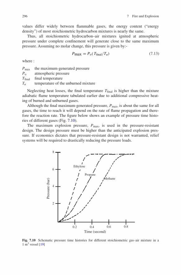
296 7 Fire and Explosion

values differ widely between flammable gases, the energy content (“energy density”) of most stoichiometric hydrocarbon mixtures is nearly the same.

Thus, all stoichiometric hydrocarbon–air mixtures ignited at atmospheric pressure under complete confinement will generate close to the same maximum pressure. Assuming no molar change, this pressure is given by:-

where :

Pmax the maximum-generated pressurePo atmospheric pressureTfinal final temperatureTu temperature of the unburned mixture

Neglecting heat losses, the final temperature Tfinal is higher than the mixture adiabatic flame temperature tabulated earlier due to additional compressive heat-ing of burned and unburned gases.

Although the final maximum-generated pressure, Pmax, is about the same for all gases, the time to reach it will depend on the rate of flame propagation and there-fore the reaction rate. The figure below shows an example of pressure time histo-ries of different gases (Fig. 7.10).

The maximum explosion pressure, Pmax, is used in the pressure-resistant design. The design pressure must be higher than the anticipated explosion pres-sure. If economics dictates that pressure-resistant design is not warranted, relief systems will be required to drastically reducing the pressure loads.

(7.13)Pmax = Po( Tfinal/Tu)

Fig. 7.10 Schematic pressure time histories for different stoichiometric gas–air mixture in a 1 m3 vessel [19]

2

4

6

8

Pres

sure

(ba

r)

0.2 0.4 0.6 0.8

Time (second)

Ethylene

PropaneMethane

297

Throughout totally confined explosion, the pressure generated always acts uniformly on the enclosure because pressure equalises at the speed of sound (2 orders higher than flame speed). In spherical vessels starting with an initially quiescent gas mixture, and centrally ignited, it has been reported [4] that the maximum rate of pressure rise is inversely proportional to the cube root of the volume. The constant of proportionality is termed the KG value and has the units of bar m/s:

where:

KG is a flame deflagration indexV the vessel volume

This relationship is called the “Cubic Law” and has been used to scale data from laboratory-sized vessels to plant-scale equipment. As the strength of an explosion increases, the deflagration index increases. The table below gives values of KG for some gases (Table 7.4).

Pressure development in a vented explosion depends on:

• Mixture distribution• Enclosure Geometry• Point of ignition

Pressure developed in a vented explosion when mixture does not fill enclo-sure can be as high as when it does despite the fact that energy release is less. Because maximum pressure attainable often depends on maximum flame area achieved, maximum pressure normally occurs when flame reaches its maximum surface area. Non-central ignition reduces maximum flame area possible which may affect pressure/time profile through effect on volume of unburned mixture expelled prior to burnt gas venting. Location of the point of ignition relative to the relief vent is also important. The closer the relief vent to the point of igni-tion, the lower the maximum-generated pressure. Higher pressure is possible if two ignition sources present. This is due to flame kernels coalesce and increase flame area.

Figure 7.11 shows a pressure–time history in vented explosions. Following ignition, early flame propagation (stage A) is associated with a low-pressure gradi-ent until the vent opens at P1 before flame reaches it. This is followed with a faster flame acceleration (stage C) until maximum pressure P2 is reached. Decay in pres-sure will follow (stage D) during flame venting from the vessel.

(7.14)KG = (dP/dt)maxV1/3

Table 7.4 Average KG values for selected gases [4]. NB. Values at ambient conditions and ignition energy of 10 J

Gas KG (bar m/s)

Methane 55

Propane 75

Hydrogen 550

7.5 Confined and Vapour Cloud Gas

298 7 Fire and Explosion

7.5.3 Vapour Cloud Explosions

A VCE is the result of a release of flammable material in the atmosphere, a subse-quent dispersion phase, and, after some delay, an ignition of the vapour cloud. A flame must propagate at a considerable speed to generate blast, especially for 2D (double-plane configurations) and 3D (dense obstacle) environments. In order to reach these speeds, either the flame has to accelerate or the cloud has to be ignited very strongly, thereby producing direct initiation of a detonation.

Flame acceleration is only possible in the presence of:

• outdoor obstacles, for example congestion due to pipe racks,• weather canopies, tanks, process columns and multi-level process structures;• high momentum release causing turbulence, for example an explosively• dispersed cloud or jet release;

Several factors influence the strength of VCE if the cloud ignites:

• degree of confinements, turbulence and cloud composition• strength of ignition source• cloud configuration• reactivity of the mixture.

The major blast source of VCE is the presence of obstruction or confinement. Reactivity of the mixture has only a secondary effect on the explosion strength. Turbulence increases the strength of the blast. It can be generated by the type of release prior ignition or by the flame propagation itself in the cloud especially when many obstructions are present down the path of flame propagation.

Large-scale release of fuel vapour followed by ignition, usually result in fire balls which produce much radiation, due to the high emissivity of pyrolysing fuel, but no blast. However, premixing with air occurs because of fast jet entrains, VCE can occur. VCE can cause devastating damage and have two unexpected features:

Fig. 7.11 A pressure–time history in vented explosion

A

C D

P1

P2

Pres

sure

Time

299

i. They correspond to flame speeds in excess of 100 m/s, without involving detonation.

ii. The damage is often caused at sites remote from the location of the explosion where the devastation may be much less.

VCEs have increased in number due to an increase in the use of flammable materials in chemical processing plants and operation in more severe conditions. Some of the worst disasters in the history of the process industries have been VCEs. Some examples include:

• June 1974, Flixborough, England (28 fatalities)• October 1989, Houston, Texas, USA (23 fatalities)• March 2005, Texas City, Texas, USA (15 fatalities)• December 2005, Buncefield, England (no fatalities but 43 injuries and major

damage)• October 2009, Jaipur, India (12 fatalities)

Lees [5] has shown that:

i. Vapour cloud fires are more common than explosion ii. The ignition probability increases as the size of the vapour cloud increasesiii. Ignition of the cloud at a point remote from the release increases the severity

of the explosioniv. The explosion efficiency, defined as the percentage of the combustion energy

that is converted into a blast wave, is usually small—about 2 %.

It is difficult to cope with a potential VCE once an accidental release has occurred. Consequently, the best procedure to guard against a VCE is to prevent the release in the first place. Safe piping is essential to protect against VCEs. Forty per cent of all major plant losses are due to piping failures, and corrosion is one of the largest single causes of plant and equipment breakdown. Moreover, mistakenly open valves that caused mammoth emissions of hydrocarbons have resulted in two major VCEs with a total of 29 deaths in those two instances. Thus, close scrutiny regarding piping and valves is mandatory to help prevent VCEs. Commonly used methods to prevent VCE include:

• Use leak detector for leaks at low concentration• Keep low amount of volatile, flammable materials• Install automated block valves to shut systems down at the early stages of a spill.

7.6 Explosion Blast Loading on Structure

In VCE, the generating deflagrating flame produces a pressure/blast waves caus-ing loading on structures which lies in its path causing destructive effects. The pressure waves move at subsonic speed and retain its destructive force longer as it moves away from the ignition source. This force increases as the distances from

7.5 Confined and Vapour Cloud Gas

300 7 Fire and Explosion

the ignition force increases. This is due to an increase in the flame front area due to volume expansion. Therefore, the area of most destruction will be at some dis-tance away from the ignition source. The turbulence generated as the flame moves around solid obstructions, such as vessels, pipes, buildings, etc, can dramatically increases the surface area of the deflagrating flame and therefore increases its destructive damage due to higher generated peak pressure (Table 7.5).

Different pressure/time profiles of gas explosions result in different levels and types of damage. Therefore, the structure response to an explosion blast is time-dependent.

Structure response depends on relative ratio between the duration of the imposed load, Td, and the natural period of vibration, Tn, of the structure. Three basic types of response have been identified by Harris [19]:

i. Td > Tn: here the loading experienced will effectively be equivalent to a static load equal to the peak explosion overpressure.

ii. Td ≈ Tn: here the loading experienced will effectively be equivalent to a static loading of a magnitude greater than the peak overpressure. The equivalent static overpressure can be up to 1T 12 times the incident overpressure

iii. Td < Tn: here the pressure is effectively partially absorbed and the loading experienced will be equivalent to a static loading lower than the explosion peak overpressure, i.e. a structure can withstand a higher dynamic pressure than the static load necessary to cause failure.

Thus, gas explosions can be considered approximately as static loadings equal to the peak overpressure.

In detonation, generated pressure waves move at supersonic speeds but dissi-pate very quickly which make its destructive effects localised on nearby objects. At large distance, low-energy shock will be present. The blast produced by detona-tion usually pulverise nearby surfaces, creating a crater whose size reflect the size of and magnitude of the detonation blast.

Table 7.5 Provides typical blast effects

Pressure (psi) Damage

0.15 Typical pressure for glass

0.4 Limited minor structural damage

0.5–1 Breakage of window glass

0.7 Minor damage to house structure

1–2 Corrugated asbestos shattered

3 Near total destruction to light industrial buildings of rigid steel framing; corrugated steel structures less severely damaged

3–4 Frameless, self-framing steel panel buildings demolished

5–7 Nearly complete destruction of houses

7 Loaded railroad cars overturned

7–8 Brick panels, 8–12 inches thick, not reinforced fail by shearing or flexure

9 Complete destruction of railroad boxcars

10 Probable total destruction of buildings

301

7.7 Mitigation

7.7.1 Mitigation by Design

Mitigation by design is one of the important and cost-effective ways of reduc-ing explosion damaging overpressure [6] gave a concise account of the best advice that current platform ventilation and explosion understanding could then give. This work has not been overtaken by subsequent research although much more experience has now been gained. A “classic” case of mitiga-tion by design optimisation has been illustrated [7]. In the design of the BP ETAP platform against explosion, they showed how in one instance a layout with pig launchers in a north–south direction gave a computed (CFD) over-pressure of over 4 bar, with the equipment in east–west direction maximum pressures of 0.5 bar were attained. The paper appears to be a good illustration of how design optimisation for explosion at an early stage results in low or no cost optimisation and can also bring design simplification. The authors also correctly draw attention to the pitfalls of failing to take into account vendors skids, cable racks, etc. Even explosion mitigation by design optimisation was not universal practice at that time work on water spray methods had been used in similar geometries.

7.7.2 Mitigation by Water Spray

The optimisation process for system design with water spray mitigation com-prises getting a water spray of sufficient loading density in the right place with a droplet size amenable to forming micro-droplets by the stripping process. While many studies and most implementations have concentrated on the use of area deluge methods as implemented for fire protection, the delivery of water drops already in the fine mist format necessary for flame reduction is an obvious alter-native. Over the years, a number of fine mist devices have been developed and tested. One device uses stored thermal energy in superheated water at 180 °C, svp 10 bar. On discharge, immediate flashing occurs and many droplets formed are in the 10 micron range with a tail of non-flashed material as large as 100 µ. One of these devices, Micromist [1, 8] has been tested in a medium-scaled replica of an offshore module. Tam et al. [8] used 4 devices, two on the roof discharging downwards and two discharging horizontally in a range of directions. Different ignition to discharge times (50, 100, 150 ms) were used and both central and end ignition were tried. The tests demonstrated that such devices could arrest a propa-gating flame and totally suppressed an explosion within a confined module. The results showed that the performance of the mist curtain lies somewhere between that of a diluent and a perfect suppressant. If the mist curtain was deployed over only the upper half of the module, then the effect was negative. There remain a number of questions to be answered, especially those concerned with the number

7.7 Mitigation

302 7 Fire and Explosion

and position of devices to be deployed, reliability of device and trigger system, maintenance required, etc. Nevertheless, the idea of a device with localised intel-ligence is appealing [20–23].

7.8 Mathematical Modelling of Explosions

Following the Piper Alpha disaster and the subsequent Cullen enquiry, offshore oper-ators now have to define the risks associated with their operations and convince the HSE that these risks are as low as reasonably practicable (ALARP). This approach embodies a vast array of design methodologies for structures, process engineering, construction, human factors and safety. Many of these procedures are well docu-mented in standards which have been tested over time. However, when consider-ing safety issues, it is necessary to ascribe probabilities to failures and events which may lead to a loss of flammable material and subsequently may lead to a fire or an explosion. The probability of an explosion has major implications on the safety of personnel on a platform both in terms of potential loss of life and the possibility of escalation of the process which could lead to a domino effect and more serious con-sequences. An understanding of the possible severity of an explosion is therefore a critical factor in establishing the satisfactory demonstration of ALARP. The mecha-nisms that enhance explosion overpressures, therefore, need to be established with some certainty in order to ensure that all aspects of safe design (structures and pro-cesses), and the safe protection of personnel are taken into account. Builders and operators of process plant require design criteria to ensure that the risks associated with an explosion from an accidental release of flammable material satisfy ALARP.

In recent years, considerable effort has been devoted to the development of reli-able means of assessing the vulnerability of industrial plant to fire and explosion. Examples include the Commission of European Communities (CEC) co-sponsored project MERGE—Modelling and Experimental Research into Gas Explosions and the Steel Construction Institute’s Joint Industry Project (JIP) on blast and fire engi-neering. Current explosion models are either empirical or based on phenomenological computational fluid dynamics (CFD) models and are very often tuned to particular experiments which thereby limit their range of applicability. Moreover, the effect of obstacles in the generation of turbulence and its effect on the rate of chemical reac-tion are inadequately treated. Since explosions are characterised by the interaction between a compressible fluid flow and rapid chemical reactions, any realistic predic-tive computer model must be able to deal with both of these aspects of the problem.

There is a wide range of explosion models that are frequently used in support of facility layout and risk. They range from simple empirical to phenomenological to complete CFD models. Moving from one to another means more physical rep-resentation can be simulated. The common practice is to use a model to generate solution to a defined explosion incident. Once the model is constructed, the pro-duced results are validated against a series of experimental tests, to examine how well the model recreates the actual explosion phenomena.

303

Results that are often used for model validation are the profile and magnitude of the generated explosion pressure. These data are used to assess the damage that might be expected at various locations. For VCE, the gaseous fuel and its proper-ties and concentration must be identified together with the areas of congestion and confinements.

In the following sections, brief overview of models that are used in explosion modelling is presented and discussed together with their shortcoming.

7.8.1 Empirical Models

Empirical models are related to experimental data. They represent little or no physics. Among these models are the TNT equivalency and multi-energy models.

7.8.1.1 The TNT Model

The trinitrotoluene (TNT) equivalency model relates the explosion to that equiva-lent of TNT. There are some essential differences between gas explosion and TNT. Among those are that the local pressure of the gas explosion is much less than that of TNT. The pressure decay from TNT is much more rapid than that of the gas explosion. The TNT equivalency model uses pressure–distance curves to yield the peak pressure. The model was extended [3] to take geometry effects in account.

The model calculates the TNT equivalent mass WTNT, which is the mass of TNT that would produce the same effects as the amount involved in the explo-sion. The TNT equivalent mass describes the effect of the explosive at a certain space when it blasts and can be calculated from the explosive amount Wexp and the equivalency/yield factor f (kg TNT/kg explosive substance):

The yield factor, f, comes from experience and not universal. It also does not suit gas explosions since the behaviour is different than solid explosions. More specifi-cally, it does not work for weak gas explosions. It must be taken into account that TNT equivalences often vary with distance. To determine the distance at which peak pressure occurs, the following formulae is used:

where:

R the distance to peak overpressure,Z the scaled distance (from Fig. 7.12)WTNT the equivalent weight of TNT.

It should be noted that the TNT method does not take into account the vapour cloud size or the obstacles and congestion in the region of the vapour cloud.

(7.15)WTNT = f · Wexp

(7.16)R = Z(WTNT)1/3

7.8 Mathematical Modelling of Explosions

304 7 Fire and Explosion

Nevertheless, the model has been used extensively to predict peak pressures from gas explosions due to its relative simplicity and the vast amount of data that exists from experiments.

7.8.1.2 The Multi-energy Model (MEM)

Berg [9] proposed another model based on multi-energy concept, which assumes that only the volume of gas that is within a confined or obstructed area contrib-utes to the overpressure generated in a gas explosion. The fuel in the unconfined regions is treated as a fireball with small-generated overpressure. The model appears inaccurate when modelling a weak explosion as only small parts are con-fined. It also cannot model complex geometry properly. Its performance is unclear when many confined parts exist.

A hemispherical flame shape is assumed at the point of ignition with a con-stant flame speed. It is also assumes that the mixture within the confined region to be homogeneous and stoichiometric. The generated overpressure is calculated as a function of the combustion energy and a scaled distance from the ignition point.

The following equations are used to determine the overpressure:

(7.17)R = R(PO/E)1/3, PS = PS/PO

1,000

100

10

1

0.10.1 1 10 100 1,000

Lethality threshold (lung damage)

Eardrum rupture threshold

Probable total destruction of buildings

Nearly complete destruction of houses

Lower limit of serious structural damage

Minor damage to house structures

Typical pressure for glass breakage

Sonic boom glass breakage

Scaled distance (Z), m/kg1/3

Ove

r pr

essu

re, k

Pa

Fig. 7.12 Peak side–on overpressure versus scaled distance [11]

305

where:

R combustion energy-scaled distance,R distance from the ignition point (m)Po ambient pressure (pa),E the combustion energy per volume times Vcloud, where Vcloud is the volume

of vapour cloud in the congested areaPS dimensionless “side-on” peak overpressurePS the “side-on” peak overpressure.

Considering that the combustion energy vary little with different hydrocarbon–air mixture, the combustion energy can be estimated from

where Vcloud is measured in m3.The strength of the explosion can be estimated by taking into account the lay-

out of the explosion source. The charge strength is given a number between one and 10, where 10 represent a detonation. Figure 7.13 shows the variation of PS with R, at different blast strength values from 1 to 10.

A development of the MEM is the Baker–Strehlow methodology [10] and extended [11]. The model uses essentially the same method, however instead of specifying an explosion strength, the user can specify a flame speed, and the curves are represented as a function of the flame speed. The model takes into account several parameters such as dimension of the confined areas and potential

(7.18)E ≈ 3.5 Vcloud, [MJ]

Fig. 7.13 Dimensionless overpressure versus energy-scaled distance [9]

100

10

1

0.1

0.01 1 10 100

0.01

0.0010.001

1

2

4

3

5

6

8

7

9

10

R(m)

P S(k

Pa)

P

Time

tT

7.8 Mathematical Modelling of Explosions

306 7 Fire and Explosion

explosion locations. It then calculates flame speed and fuel reactivity. The model is attractive since it takes into account geometry and hazardous areas and because of being easy to perform. However, it can be overconservative.

Since the models are based on experimental finding rather than on real physics, they are limited in their applicability and give only little description of the flow field.

7.8.2 Phenomenological Models

Phenomenological models are regarded as simplified physical models. They rep-resent the main physics of the explosion. The models simplify the geometry and replace it by a vented chamber that contains several turbulence-generating grids. Simplifying geometry leads to uncertainty in the model setting as well as the sim-ulated results. These models fall between empirical models and CFD models in terms of complexity.

Among codes that implement phenomenological model is the SCOPE [12] which is developed further [13]. The model is one-dimensional and is based on the idealised geometry of a vented vessel containing a series of obstacle grids. The code can handle vented and external explosions. However, unlike CFD-based models, it cannot describe details of the flow field. Puttock et al. [13] developed model takes into account the effects of obstacle complexity—phenomena not previously realised in earlier versions. At the same time, the authors have taken into account a revised turbulent burning velocity formulation, allowed for vents at rear walls, treatment of gas mixtures and of temperatures and humidity vari-ations. After validation against over 300 experiments, the prediction of the data sets and the predictability in blind tests are not significantly inferior to the much more complex CFD calculations—but this type of model is so simple to run that batch running permits large numbers of combinations of ignition position geom-etry, etc—to be assessed.

Based on the applications to vented vessels explosions, Fairweather and Vasey [14] and Chippett [15] developed phenomenological models. The models see the confined explosions in buildings as several combustion chambers linked together. This is the case of a typical process plan congested with piping net-works. The model parameters are determined from the obstacles-flow interac-tion. A combustion model is based on the local flow properties to determine the laminar and turbulent burning velocities. In this model, it is assumed that flow conservation equation apply on each chamber as a whole. Thus, the flame shape is predicted empirically and the ignition point can be anywhere within the cham-ber. The turbulent burning velocity is based on the laminar flamelet concept [16] and [17] which has been calibrated against measurements made [18]. This model can handle external explosions and can generate physics description from the geometry.

307

Phenomenological models, however, do not provide the same wealth of information about the flow field as CFD models as they contain less geometrical details than CFD models. Moreover, they can only deal with single enclosures.

7.8.3 Computational Fluid Dynamics Models

CFD models solve the partial differential equations, Navier–Stokes equations gov-erning the fluid flow in the explosion process over thousands or millions of com-putational cells. The numerical solutions are generated by discretising the solution domain (in both space and time). The conservation equations are applied to each of the sub-domains formed by the discretisation process, generating a number of coupled algebraic equations that are normally solved by an iterative procedure.

Most models use a porosity distributed resistance (PDR) to model small-scale objects. A gas dispersion model is used to simulate the gas flow through the com-putational domain in and around the structures that exist. This then produces a cloud that is varied in concentration. In order to accurately model an explosion, the gas dispersion model must be able to simulate the release and flow of gas tak-ing into account the obstacles, structures and the ambient conditions. After the cloud has dispersed, an ignition source is introduced. Turbulence is modelled using a turbulence model while the combustion chemistry is modelled using a reaction rate model.

Solutions obtained with CFD codes contain detailed information about the flow field, i.e. velocities, pressure, density, species concentrations, etc. Surface pressure data can be used for structural analysis. The data results from a CFD model are usually validated against well-controlled, well-defined and repeatable experiments in order to gain confidence in the results obtained, CFD models are powerful and useful tools. However, accuracy of the results will depend on the correct imple-mentation of the geometry, initial and boundary conditions, turbulence and com-bustion sub-models.

Examples of CFD-based codes for explosion modelling include:

• EXSIM: a purpose-built explosion code developed by the Telemark Technological R&D Centre (Tel-Tek) in Norway and Shell Global Solutions in UK.

• FLACS (FLame ACceleration Simulator) code has been developed at the Christian Michelsen Research Institute in Norway, now CMR-GEXCON

• AutoReaGas: developed as a joint venture, between Century Dynamics Ltd. and TNO.

• CFX: a general purpose, commercially available CFD code, developed by AEA– Technology Engineering Software at Harwell.

• REACFLOW: a CFD code developed at the Joint Research Centre of– the European Union in Ispra, Italy [24].

7.8 Mathematical Modelling of Explosions

308 7 Fire and Explosion

References

1. HSE, Health and Safety Executive reports OTI 92 585-610 (1992) 2. Bimson, B.J., Bull, D.C., Cresswell, T.M., Marks, P.R., Masters, A.P., Prothero, A., Puttock,

J.S., Rowson, J.J. and Samuels, B. “An experimental study of the physics of gaseous defla-grations in a very large vented enclosure” 14th ICDERS Coimbra Portugal, 1993

3. Harris, R. J. and Wickens, M. J., “Understanding vapour cloud explosions-an experimental study”. 55th Autumn Meeting, The Institution of Engineering, 1989.

4. Bartknech W., Explosions, Springer-Verlag, New York, 1981. 5. Lees F.P. Loss prevention in the process industries, Butterworths, London 1986. 6. Bakke, J.R. and van Wingerden, K. “Guidance for designing offshore modules evolving from

gas explosion research”, SPE paper 24617 763-770 (1992) 7. Paterson, K., Tam, V.H.Y., Moros, T. and Ward-Gittos, D. “The design of BP ETAP platform

against gas explosions” Jnl Loss Prevn Proc Ind 13, 73–79 (2000) 8. Tam, V., O’Connell, M.,Pedersen, G. and Renwick, P. “Testing of the Micromist device: An

active soft barrier for explosion control”, ERA Conference Major Hazards Offshore 4.4.1–4.4.11, 2000

9. Berg, A. C. van den, “The Multi-Energy Method—A Framework for Vapour Cloud Explosion Blast Prediction”, Journal Hazardous Materials 12:1–10, 1985

10. Baker, Q. A., Tang, M. J., Scheier, E. A. and Silva, G. J., Vapor cloud explosion analysis, AIChE Loss Prevention Symposium, Atlanta, Georgia, U.S.A., 1994.

11. Baker, Q. A., Doolittle, C. M., Fitzgerald, G. A. and Tang, M. J., Recent developments in the Baker-Strehlow VCE Analysis Methodology, Process Safety Progress 17(4):297−301, 1998.

12. Cates, A. T., and Samuels, B., A simple assessment methodology for vented explosions, Journal of Loss Prevention in the Process Industries 4:287-296, 1991.

13. Puttock, J. S., Yardley, M. R. and Cresswell, T. M., Prediction of vapour cloud explosions using the SCOPE model, Journal of Loss Prevention in the Process Industries 13:419−430, 2000.

14. Fairweather, M. and Vasey, M. W., A mathematical model for the prediction of overpres-sures generated in totally confined and vented explosions, 19th Symposium (International) on Combustion, The Combustion Institute, Pittsburgh, Pennsylvania, U.S.A., pp. 645−653, 1982.

15. Chippett, S., Modeling of Vented Deflagrations, Combustion and Flame 55:127−140, 1984. 16. Bray, K. N. C., Complex chemical reaction systems (J. Warnatz, W. Jager, Eds.), p. 356,

Springer series in Chemical Physics, 47, Springer-Verlag, Berlin, 1987. 17. Bray, K. N. C., Champion, M. and Libby, P. A., Combust. Sci. Technol., 55, p. 139, 1987. 18. Abdel-Gayed, R.G., Bradely D. and Lawes, M., Turbulent burning velocities: a general cor-

relation in terms of straining rates, Proc. R. Soc. London, Ser. A, 414, p. 389, 1987. 19. Harris, R.J. “The investigation and control of gas explosions in buildings and heating plant”,

London, E & F N Spon Ltd, 1983 20. Berg, A.C., van den and Wingerden, C.J.M., “Vapour Cloud Explosion Blast Modelling”, 6th

International Symposium on Loss Prevention and Safety in The Process Industrious, Oslo, Norway, June 1989

21. Clancey, V.J., “Explosion damage”, 6th International Meeting of Forensic Science, Edingurgh, 1972.

22. HSE Book “The assessment of pressure hot water explosion sub pressure in system”, OTH 93 406, 1993

23. Nasr, G.,G., Yule, A.J., Bendig, L. Industrial spray and atomisation, Spring Verlag, 2001. 24. Nasr G.G., Yule A.J., and Hughes T., Utilisation of spill-return atomizer in health care,

Journal of Mechanical Engineering Science, Proceedings of Institution of Mechanical Engineers, Part C, 225 (part-c), pp 897−908, April 2011

309

8.1 Business and Project Management

8.1.1 Introduction

No matter where the gas is supplied from and where its destination is, the entire process, within the context of the natural gas business, should be managed in a coherent manner. This chapter thus starts by giving an overview of natural gas and its place as a viable source of future energy as well as providing information on the business elements of it. Moreover, the related legal framework of gas contract intends to give a better insight and knowledge when it comes to contract nego-tiation. After all we have to sell the gas once it has been produced. The chapter continues to give information on project evaluation, investment appraisal, team-working, economic efficiency, gas chain and pricing of the gas [1].

The basics of project management can be applied to any product. This is also true in the framework of the natural gas business. What differs from project to pro-ject is the product uses, its application and the associated business. There is a need to understand the product history since this is what has shaped the product and in the case of gas how its use has developed resulting in it being regarded as the fuel of the future. There are many reasons why gas is so unusual. The high cost of gas stor-age and consequent need of continuity all the way from production to point of use this of course can be turned into an advantage as continuity of supply can be a fac-tor and offered to the customer when justifying change from existing fuels, e.g. coal and oil. The fact that natural gas comes out of the ground apparently “free” and that gas operations, at times, can be very profitable. This has resulted in piped gas sys-tems being built throughout Europe and elsewhere. The relatively risky way of han-dling gas at high pressure, or, after liquefaction is also another reason for peculiarity of natural gas. In addition, the frequent contact with natural gas of complete lay-men, or more exactly, and more frequently, laywomen, with the resultant need for safety and high standard of work, including quality, characteristics and behaviour.

Chapter 8Business and Project Management of Natural Gas

© Springer International Publishing Switzerland 2014 G.G. Nasr and N.E. Connor, Natural Gas Engineering and Safety Challenges, DOI 10.1007/978-3-319-08948-5_8

310 8 Business and Project Management of Natural Gas

It is interesting to compare gas industry development in Europe and Japan, on the one hand, with that in the USA, on the other. In the USA, manufactured gas never made a particular impact because of (i) the wide availability and low cost of liquid fuels, (ii) the absence of gas lighting and (iii) US cities largely managed without illumination until the arrival of electricity, the civil war and its conse-quences during the period of town gas development in Europe and, most impor-tantly, the availability of associated natural gas from oil production all over the country which established a price standard difficult to meet for gas manufacturers. In Europe, Japan and a number of less important gas-consuming areas, the non-availability of natural gas had become an accepted fact. The Netherlands enabled the gas industries in Germany, France and Belgium, and to some extent Italy and Switzerland to use it as their main source of supply.

Gas transmission lines from Texas to New England, Canada to California, across Canada and from Mexico into the US, became the ancestors of major European supply mains from Russia, the Norwegian North Sea and Algeria into central and Western Europe including the UK, in addition to the new lines which had already been laid for the transport of Dutch gas. Obviously, the new transmis-sion mains do not all supply gas across national frontiers, and large diameter high-pressure distribution grids apart from the US have also been laid in most major European countries, in the Arabian peninsula, India, South America and Australia. Interestingly, few Japanese gas utilities are interconnected by high-pressure mains, a fact which can be explained in terms of their reliance on LNG for a gas supply.

8.1.1.1 The Business of Natural Gas

Natural gas and its place in the world as the fuel of the future are becoming increasingly evident in recent years. There are constant references to the demand, customers, investors and profit in the business of natural gas. It is thus appropriate we should understand the business elements which can influence these areas and the need to ensure the right level of profit so that the future business developments can take place as well as the level of return on investment to the financial industry.

It is not easy sometimes to see how, as individuals we can support the business, after all, we are usually recruited and employed for our, hopefully, high individual skills and expertise in engineering, geology, finance, etc., but it is essential that all understand and appreciate how we can support the business of producing and sell-ing natural gas at a profit. Figure 8.1 typified the concept of the “Gas Chain” as a model.

The gas chain concept assumes that a complete chain exists between the source of natural gas and the point of use. There are also problems of security of supply and unit fuel cost, as compared to other fuels, as customers are interested in the comparative cost of heat at the burner tip. This is further complicated by high-volume users, speciality industries, low-volume users and chemical users, where natural gas may provide part of the feedstock for the manufacture of the product.

311

Let us start to build-up a business model from this as typically shown in Fig. 8.2 and by taking each element in turn raise our awareness of its affect on the business of producing natural gas. The key factors of the gas chain model are as follows:

• There must be a complete process chain from wellhead to the customer.• Each link in the chain must be correctly designed and sized so that there are

no weaknesses (production and maintenance) so that continuous operation and availability may be achieved.

Production - Gathering - TreatmentTransmission Power generation

Industry

Commercial

Domestic and Residential

Export

Fig. 8.1 Typical gas chain concept

Production - Gathering - Treatment

Transmission

Power generation

Industry

Commercial

Domestic and Residential

Export

FinanceExploration

Environ-ment

Restoration

Technology

Ind. relations

Operations

MarketingContracts

Legal system

Exports

Imports

Markets

Governm-ents

Enginee-ring

Planning

Legislation

Fig. 8.2 Typical business model

8.1 Business and Project Management

312 8 Business and Project Management of Natural Gas

• There should be close co-operation of all participating parties, preferentially with investment participation and interest.

• All elements of the chain should be appraised and understood.

Also the key elements of the gas chain are as follows:

• The market prospects and potential value of gas in the market.• The competitiveness of other projects and competing energy supplies.• Transportation costs throughout the chain.• The commitment of all organisations involved in the chain to invest and develop

their part of the chain.

The process and associated technology of natural gas can be found elsewhere in the preceding chapters, what is important however is that at the end of this phase, large amount of capital has been used and there is no product to sell. Hence, the business demands sourcing the finance against predictions and estimations of vol-ume and quality. At this stage, even with today’s technology, finance is a gamble and may be sourced by governments or companies, from within their own funds. Capital funding from elsewhere will demand high level of return on the invest-ment. However, when gas is found and sampled, then the picture changes and with volumes now predicted and quality assured the investment becomes more clear and at a lower level of risk delivery now takes over and planning of finance, con-struction and especially marketing become crucial to the business to ensure the necessary funding. While accurate estimates of costs of construction, operation and ongoing maintenance are crucial it is the market potential and realisation and the projected profit after taxes, royalties, license cost, etc., which will make the business viable.

In addition the market for natural gas can be segmented according to its char-acteristics of volume of gas to be supplied, achievable selling price, quality and end use. Users demanding high volumes and comparable heat at the burner tip will expect a lower unit price than say a chemical producer who uses gas as both source of energy and part of the feedstock for the product who may be prepared to pay a higher unit price while taking large volumes of gas.

Other customers/users may demand a clean fuel, e.g. the ceramics manufac-turer, in addition to fuel economy with the resulting negotiated unit price. Ease of use and convenience may be the priority of the commercial and domestic sector which although demanding low volumes are prepared to pay a higher unit price.

All the above will require a clean, high-quality fuel and security of supply in addition to a comparable Net Cost of heat at the burner tip.

To provide an example of Net Cost, it may be worthwhile to refer this to the power industry in moving to natural gas. The power industry has depended on the use of coal, and conversion to a more environmentally friendly fuel is desirable. Processes for the scrubbing of exhaust gases from power stations, to eliminate sul-phur products and particulate matter, exist but are not without their problems of high-operational and maintenance costs along with the production of gypsum as a waste product. The latter has, of course, decimated the production of gypsum from

313

natural sources, and there is an oversupply of material to the subsequent manu-facturing industry which results in a low-price product. In addition to this, the use of coal produces fly ash, which although has some use, e g as an additive in the production of cement and some building products, still results in waste which is not part of the core business of producing electricity. This cost of course can be avoided if the power station converts to natural gas. In addition, the cost of the operation and maintenance of coal, limestone and fly ash processing and handling plant can be eliminated along with the corresponding reduction of staff. These costs should be taken into account when making the case for conversion to, and using natural gas to replace coal. The increased efficiency of the process is also attrac-tive. All these must be factored into the calculation of the net cost of heat delivered at the burner tip and comparing fuel cost. Natural gas may cost more but can be cheaper, and more environmentally friendly, than using coal and oil. Similarly, it is possible to carry out an analysis of other fuels which makes the use of natural gas more attractive in terms of an overall model for a respective business. The natural gas business has more a flexible pricing mechanism, and an individual customer can bargain for its own price, unlike oil and coal, which have a fixed market price. Furthermore, the natural gas supply can be flexible, firm or interruptible, and a lower price may be possible depending on the process requirements.

Within the natural gas business model considered, the ideal supply profile should also be considerable. Figure 8.3 shows an ideal total supply profile from a suppliers point of view, where the agreed total maximum daily supply profile closely follows the daily contract quantity thus utilising the pipeline capacity to the full. In practice, this is difficult to achieve due to the vagaries of climate and activity of the customer, and careful estimation and aggregation of a large num-ber of supply profiles is required for maximum sales of gas and the calculation of

Pipeline capacity = max. daily quantity (min)

Dai

ly s

uppl

y ra

te

Time (Days)

Contract period

365 days (ACQ)

Dai

ly c

ontr

act

quan

tity

Max

imum

dai

ly

quan

tity

Swing factor =Max.daily quantity

Daily contract quantity

Fig. 8.3 Ideal total supply

8.1 Business and Project Management

314 8 Business and Project Management of Natural Gas

minimum production costs. The production of LNG can be utilised to some extent to modulate the profile as can the production of compressed natural gas. Both of these can be seen as storage.

Further complications can arise from climatic conditions and the work/usage requirements of customers who are willing to pay varying amounts for their gas depending on volume, and timing and duration of demand periods. All will require quality and security of supply at the lowest price. These areas of influence are depicted generally in Figs. 8.4 and 8.5 and can be further compounded by inter-ruptible supply profiles, resulting from dual-fuel usage. Nevertheless, the market must be understood and estimated with each contract agreed to suit, as described in the next section.

Periodic variations in aggregate demand

Upper band

Lower band

WinterSummer Summer

Fig. 8.4 Variation in demand profiles

Gas demand above the average

Average hourly flow rate

Gas demand below the average

06:00 06:0009:00 12:00 15:00 18:00 21:00 24:00 03:00

100

75

50

125

150

Flow

rat

e -%

of

aver

age

hour

rat

e

Time of day

Fig. 8.5 Diurnal variations in natural gas

315

8.1.1.2 Natural Gas and Market Sectors

The Power Generation MarketThis market is characterised by the use of very large volumes of gas which may vary between winter and summer, and periods of transformation between those periods. This effect can be dramatic in countries where there is a variation in day-light hours and climatic conditions as, for example, in areas of Northern Europe and the UK. The resulting Diurnal variation (as shown previously in Fig. 8.5) can further affect the daily demand profile. The implications of this are as follows: while they demand high volumes of gas, they result in a poor daily load factor and can be further complicated by the influence of interruptible contracts. While all of this contributes to a low transportation cost and places the customer/buyer in a good position to bargain for a low price for the gas, it puts the supplier in a good position to agree “take or pay” contracts. This is good for the overall business in that the producer gets an agreed annual income which satisfies his production and the demands of repaying loan capital and satisfying shareholders.A load factor measures the ratio of gas consumption at times of peak demand compared with average consumption. A declining load factor means that peak demand is growing more quickly than average consumption. A declining load factor presents issues such as increased spending on network infrastructure which is used for small periods of the year; increased requirements for peak load power stations that can be switched on and off quickly; and greater variation (or volatility) in demand [2–4].

The Chemical Feedstock MarketThis market is characterised by the use of very large volumes of gas without the affects of seasonality and diurnal variations. Processes require a predictable chem-ical quality at a high-delivery pressure. This results in high-throughput rates and a high-load factor and a more efficient use of the pipeline and low-unit transport cost. There is also the possibility of dual use where natural gas may be used as a fuel as well as a chemical feedstock.

The Industrial MarketIn this market, a large number of locations can be geographically spread and utilise large volumes of gas which are only partially affected by seasonality. Throughput is reasonable, but load factors can be variable. Conversions can be affected by high cost of installing a pipeline feed from the gas main supply.

The Commercial Industry MarketThis market can utilise a wide range of volumes and be affected by diurnal varia-tions and seasonality. They can be even more geographically spread. The implica-tion to the gas company is the supply profile can be the result of the aggregation of volumes supplied by a number distribution companies and provide poor daily and annual load factors and high-investment costs.

The Domestic MarketThis market is geographically spread and utilises comparably very small volumes of gas which are subject to diurnal and seasonal variations.

8.1 Business and Project Management

316 8 Business and Project Management of Natural Gas

The implication to the gas company is the supply profile can be the result of the aggregation of volumes supplied by a number of distribution companies and pro-vide very poor daily and annual load factors and very high-investment costs.

Other Market Issues

Future Load GrowthWhile the existing real market should be the basis for the case for investment in the project, any perceived growth should be recognised, quantified and factored into the overall case as sensitivity in the financial analysis. This provides an indi-cation of the overall business potential and financial security, and of course will satisfy and encourage investment agencies to invest in the project. Future load growth should be real and not a fanciful look into the future and should be sup-ported by facts and logic. The finance industry does not like to gamble and will seek a substantial basis for the predicted growth.

Inter-fuel CompetitionThis is when other fuels seek to be used as alternatives. Natural gas of course, unlike oil (possibly its main competitor), does not have an international price base and is free to compete in all markets. It is fast becoming the fuel of choice for all industries due to it being environmentally friendly, controllable and with security of supply due to large reserves. However, it would be a mistake to take inter-fuel competition for granted as suppliers of other fuels seek to solve the environmental problems associated with their use and compete on the basis of comparing the net cost of providing heat at the burner tip. One area yet to be developed, certainly in the UK, is the use of natural gas to power transport. While the use of gases to power vehicles goes back to the wartime years, it has never been developed due to the dominance of oil and the lack of an infrastructure. Petrol stations are owned by the oil companies and are now selling LPG mostly in parts of Europe. However, less developed countries, where the infrastructure for the sales of fuels to vehicles are being developed, are building service stations for the delivery of natural gas at the pump and the population seeing the resulting economies. Natural gas is now being offered in the USA but has yet to be exploited in the UK and Europe and a number of car and heavy vehicle manufacturers are offering dual fuel and gas powering as an option. This will provide much needed competition of pricing and affect the world’s dominance and reliance on petrol and oil. The use of natural gas in transport could be the next great influence on economies, resulting in cheaper transport costs.

The Development of New FuelsThe world has now become increasingly environmentally aware due to the increased domination of oil and its perceived dwindling of recoverable reserves.

While the use of natural gas is increasing, and backed by huge reserves, it remains a fact that the reserves of coal significantly exceed those of gas, and of course gas can be produced from coal. Other fuels such as nuclear and hydrogen are in differing stages of use, and development, and provide a constant threat to the business of providing power and heat. Large amount of capital is in the process

317

of being invested in wind power in the USA, Europe and UK, and projects exist to examine the ways of producing power from the large tidal flows which exist, cer-tainly around Europe and the UK.

However, these methods of utilising natural resources are not without their obvious problems. At this stage, natural gas seems to be the most available source of energy.

GovernmentsGovernments are under constant pressure to reduce the cost of living and in par-ticular in the areas of heating and transport. They prioritise these in their mani-festos along with refining the country’s economies, and the fact that they may be up for election/re-election may produce changes in government pressure. This can manifest itself in many other ways which are in their control such as import and export duty, royalties, purchase tax, duties of fuels, etc. It is possible that a gov-ernment of a country can change a number of times in the life of a gas project, and therefore, political awareness is important, and working closely with govern-ments is paramount. The fact that gas pipelines now cross many borders, means that the supply of gas can become internationally political and it must be recog-nised, and be a major factor in trying to solve conflict. There have already been instances where the gas supplier has switched off its supply to other countries for political reasons. The supply of energy and ownership and control of reserves has in the past been a major factor in declaration of war between countries, and it is logical to conclude that this could still happen as fuels become less abundant. This of course can result in higher risk of investment capital, and investors will seek a higher financial return commensurate with that risk.

While supply by pipeline presents the lowest delivered price for natural gas along with security of supply, it does in itself present its own problems. The fact that pipe-lines cross-borders make the delivery politically sensitive. This is further exacerbated by ownership issues and pipeline charges, which may affect the cost of delivery. Indeed, there have been instances where gas supplies have arguably been more effec-tive than military action in resolving disagreements between governments. This of course does not mean that selling and control of gas supplies are a deciding factor but one cannot rule out that they may in turn be the cause of military action as have the issues associated with the supply of oil. All need to be assessed and taken into account at the exploration stage and prior to seeking and procuring investment capital.

8.1.1.3 Gas Pricing

When seeking to negotiate a price for the sale of gas, it is important to recog-nise and distinguish between mature and immature markets. In immature mar-kets, monopolies may exist where gas is purchased from the producer by a single organisation and sold directly to the end-user, effectively dictating prices and con-tractual terms. State-regulated price structures may exist for producer and con-sumer, which may be politically directed to the extent that some industries may

8.1 Business and Project Management

318 8 Business and Project Management of Natural Gas

be excluded from supply. For example, a government of a country rich in coal reserves may exclude the use of gas as a fuel for the supply of electrical power. This market of course is characterised by a take it or leave it attitude and an absence of inter-fuel competition.

The industry may be state owned, with field production sold under depletion contracts where the whole field capacity is sold by joint venture. Pricing may be a composition of base price, further affected by price indexation formulae and provisions for price revision. Any short-term contracts will be characterised by a published tariff system of pricing and contracts which are standard. The market is divided into tariff sectors by the seller of the gas to market sectors. The whole market being characterised by a lack of competition on price and volume and a take it or leave it principle. On the other hand, mature markets may have long-term contracts agreed but these are decreasing in number and volume with time as com-petition develops within the industry. Medium-term contracts may exist for sales by producer direct to end-user similar to a large number of short-term contracts where the duration may vary to satisfy the end-user.

Contract provision and complexity may depend on contract duration, and consideration of alternative suppliers may take place as gas is offered at vary-ing prices. Contracts may take a standard form of agreement and offer an agreed price for the contract period. This has been developed to such an extent in the UK that gas supply companies have now turned into energy supply companies offer-ing financial inducements for home owners to buy electricity and gas from them as a package. However, the base price of the gas must be competitive with other fuels and based on a comparison of the NET COST OF USEFUL HEAT AT THE BURNER TIP.

The determination of base price should take into account cost (economic) sav-ings arising from the use of natural gas, i.e. higher efficiencies, reduced pollution, no storage requirement, improved product quality, environment costs and reduced maintenance costs

The Buyers ObjectiveThe agreed price from the buyer’s point of view must cover the cost of conver-sion from an existing fuel and any capital and operational cost associated with the business of selling gas and then remain competitive with the alternative fuel price. This should include any business taxes which of course can be variable depending on government policy. A cost/benefit margin, for example, profit which should be included and that will at least permit the price to remain competitive in its markets.

The Sellers ObjectiveIn real terms, the seller’s price must permit recovery of investment, operating and finance costs. Care should be taken to include all associated costs and the relative cost of inflation over the life of the project. Money has a value which varies in relation to time which is difficult to calculate.

In business terms, 5 years can be almost regarded as geological time, as world economies, finance and governments change. However, the affects have to be estimated and sensitivities analysis carried out on the business case. In addition,

319

a profit element is required commensurate with risk, shareholders dividend, and finance company expectations.The aim of pricing mechanisms must maintain the division of economic bene-fit between buyer and seller and is vital to the success of the business, hence the importance of price revision and review clauses. They are not a gamble on future trends. Gas price revision formulae can be simply multiplicative or additive or more complex and has restraints incorporated within them (e.g. top and bottom limits)

Contracts agree a base period, a review period and frequency of any agreed price revisions. Frequent price revisions will result in the price staying close to the market values whereas infrequent revision, if indices rise will be good for buyer and bad for seller.

The Base Period and Review PeriodThe base period is the starting point and is the period prior to the period to which the base price applies and published data must be available during the base period. The review period is the period for which price is calculated, and base period/review period relationships must be consistent. Base period values may affect price.

Price Break ClausesThe advantage of including a price break clause is to provide protection against unforeseen risks. The disadvantages, of course, are they are very difficult to nego-tiate and may lead to prolonged disputes if used.

The pricing clause should be reviewed at regular intervals. If market conditions change, the price changes. The price break clause may be included by the buyer or the seller, and arbitration should be sought if no agreement is reached. Clauses may be simple where the buyer takes a fixed margin and the balance goes to the gas producers. Prices could be revised if competing fuels indexation components change. Complex revisions may reflect major changes in circumstances and rela-tive values to parties, and the base price may also be changed.

NegotiationThe negotiation of a contract can, if not managed properly, result in confrontation where each side is trying to maximise its own benefits. The need to win, or to be seen to win, at the others cost can override the main objective which should be that each side should have a financially viable business at the end of the negotiation. It is essential to appreciate that a contract is an agreement between the parties and all should be comfortable with the outcome. If this is not so, the management of the contract may become confrontational and difficult to manage. The following are some areas where negotiation can become difficult and result in a situation where both parties are unable or unwilling to negotiate and take an immovable stand on their conditions, .i.e. Deadlock

• The determination of the base price: this is the initial price which will be subject to review.

• The buyer will want to ensure the price covers the cost of conversion from existing fuel and then remain competitive with alternative fuel price. One requires also a cost/benefit margin that will at least permit the buyer to remain competitive in its markets.

8.1 Business and Project Management

320 8 Business and Project Management of Natural Gas

• The seller would like to get a price in real terms that will permit recovery of investment, operating and financial costs of the gas project and a profit element commensurate with risk, shareholders dividend and finance company expectations.

These conflicting objectives of buyer and seller may lead to a situation where discussions cannot continue and may eventually end up in a deadlock.

• The price revision gas formula would be used to review the gas price time after time during the life of the contract. It will contain all the parameters considered relevant to the value of the gas with respect to time, by the buyer, and the seller. The aim of pricing mechanisms is to maintain the division of economic benefit between buyer and seller and not to gamble on future trends.

• Gas price revision indices and review periods are potential areas of misunder-standing and disagreement, which may lead to Deadlock if not properly man-aged. Terms such as “frequency of price revision, base period and review period” should be well understood by both parties and the base period/review period relationship must be consistent.

The “take or pay” provision is the quantity of gas, when supplied by the seller to the buyer in accordance with the contract terms, must be paid, whether taken by the buyer or not. This quantity can be taken in the future as “make up” gas, at no cost within the period specified in the contract. It is usually expressed as percent-age of Annual Contract Quantity (ACQ). This is an essential component of most long-term gas contracts. The seller would like to have guaranteed revenue to jus-tify investment and obtain finance.

The “swing factor” is the measure of degree of fluctuation of quantity of gas, required by the buyer, which the seller, would be obliged to provide when the buyer nominates. The buyer would like to have flexible off-take to match the seasonal, daily or hourly fluctuations, while the seller, would like have constant rate of production because off-take flexibility costs money in terms of investment and operational costs.

Quantity provisions need effective and understanding communications during negotiations and if they are not properly managed can lead to deadlock.

A Strategy for BreakingFirst reframe and represent your position on the issue. Let it be clear, concise and adequate to avoid wrong interpretation. It is possible that the other party misun-derstood your position, which caused the deadlock. One may then soften your position and offer an exchange of concessions. For example, lower take or pay quantity for lower swing factor. Make sure the costs and benefits of these con-cessions are well understood. This might make a lot of difference to the opposing party and resolve the deadlock. Suggest that both negotiating teams should consult their management with a common proposal on the issue at stake to resolve the deadlock. Call off the meeting during which the negotiation came to a deadlock to get time to analyse and evaluate issues already discussed and agreed upon. Make necessary consultations and prepare for a new proposal for the next meeting.

Suggest the formation of a small committee comprising people from both par-ties to work out an acceptable common position on the issue, which both parties would present to their management for consideration.

321

Recommend possible concessions that can be offered during the next meeting to break the deadlock to your management for consideration highlighting the costs and benefits of these concessions. Identify the other party’s concern on the issue at stake and appreciate their concern and give assurance that their concern will be respected as much as it is feasible during the next meeting. Call for the next meet-ing to resolve the deadlock and move forward.

8.1.1.4 The Legal Framework of Gas Contracts

The upsurge of interest in natural gas as an environmentally friendly fuel makes it more necessary than ever for gas contract negotiators to have an understanding of the important role of the law in relation to gas contracts. The main reason for the need to structure gas contracts on a sound legal basis and to draft them with great care is the long duration of the contracts, often 15–25 years [6]. During such a long period, there will almost certainly be significant economic, commercial and technological changes, which have a bearing on the contracts. Contracts must be structured and drafted in such a way that they will be able to survive such changes.

The difference between oil and gas sale contractsOil sale contracts are generally of short duration, rarely more than 1 year. Gas con-tracts have a totally different time scale, normally 15–25 years. The reason for the difference of duration is physical. It stems from the relative ease of transportation of oil as compared with gas. Oil may be relatively easily transported by sea or on land, and this fact has been an important element in the creation of an international market in oil.

Speaking in general terms, it is not a matter of concern to an oil producer on the UK Shelf, or in the Gulf, or Nigeria, where in the world its production is mar-keted. There is a worldwide market, and, in normal market conditions, there is no reason for the producer to fear that its production will not be sold at a profit. In contrast, gas is not so easily transported. Transportation of LNG is of course prac-ticable but liquefaction and reconversion of gas makes this gas expensive in com-parison with pipeline gas.

In consequence, the majority of gas supplies are transported in the gaseous state in pipelines to the specific market where they are to be sold. Because of the very large capital cost of developing major gas fields, it is very important to a gas pro-ducer to ensure that, before developing a new gas field, it has entered into long-term contracts for the sale of a large part of the production of the field. The buyer, because of its normal concern for security of supply over a long period of time, will also in most cases seek a long-term contract.

The Contents of a Typical Gas ContractThe contract will contain provisions dealing with the following matters:

i. The obligation of the seller to sell, and of the buyer to buy over the contract period, a quantity of gas and also provisions dealing with the daily quantities to be delivered

8.1 Business and Project Management

322 8 Business and Project Management of Natural Gas

ii. The contract duration and start-up dateiii. Warranties by the seller relating to title of the gas and to taxesiv. In the case of depletion contracts, reservations by the seller for its own use of

a part of the gas from the fieldv. Take or pay obligation, and rights of the buyer associated with that obligation,

such as rights relating to make up and carry forward amounts of gas.vi. Base price, price review provisions and, sometimes, price reopener provisionsvii. Billing and paymentviii. Force majeureix. Default (and damages)x. Expert determinationsxi. Delivery point, quality and pressurexii. Assignment

It is the contractual provisions dealing with these matters which constitute the essential framework of a gas contract.

The Main Areas of Law Which May Be Applicable to Gas ContractsSome are more relevant to the interests of one party rather than the other and not all of them will be applicable to every gas contract. However, all of them should be considered before entering into a gas contract. As we go through each of these areas, we will look at their relevance to gas contracts in general, and then describe their relevance under UK law and in some instances comment on their relevance under other systems of law. There are nine main areas of relevant law. They are as follows:

(a) The Law Dealing with the Granting of Rights to Produce Oil and Gas

Relevant matters will include the duration of production licences and the terms relating to royalties, including royalties in kind and production consents.

The UK law is contained in the Petroleum Production Act, 1934. The regime set-up under this legislation provides for grants of exploration licenses and pro-duction licenses for a specified area. The production licences grant a right for licensees to search for, bore, and get hydrocarbons from, the specified areas for a specified period.

It is important for the buyer of gas to know who the licence holders are and that the parties who intend to sell the gas do in fact have title to the gas which they propose to sell. It does not always follow that the licence holder will have title to the gas, for example, for tax reasons, the licensee may have arranged that the gas should be sold by one of its subsidiary or associated companies. The duration of the licence is clearly a fundamental element to bear in mind in considering the duration of the contract. It is worth noting that under the UK law there is no auto-matic right to an extension of a licence if at the end of the licence period there are unrecovered reserves still in the ground.

(b) The Law Relating Specifically to Sale of Goods (as Distinct from Land)

Relevant matters dealt with in this area of law will include the time at which the ownership and risk in the goods passes to the buyer. In the UK, the relevant

323

statute is the Sale of Goods Act, 1979. This contains general rules about sale and the rules relating to the warranties which are deemed to be given by the seller (e.g. title to goods and quality). The law relating to contracts in general are as follows:

Relevant matters under this heading are the law relating to mistake and misrepresentation.

(i) In the UK, this law is mainly to be found in the common law which is a body of uncodified customary law. However, the Misrepresentation Act, 1967, and the Unfair Contract Term Act, 1977, are also relevant.

(ii) In contrast to the position in the UK, the general contract law is, in most countries, codified. For example, France has the Commercial Code and the USA has the Uniform Commercial Code which applies in almost all states.

(c) The Law Relating to Force Majeure

Force majeure provisions are common in all types of commercial contracts. They have a particular importance in gas contracts largely because the contracts are of such long duration. They are particularly important for the seller because of the hazards of production and transportation of gas. Under English law, and the law of most countries whose legal system is based upon English law, there is no statutory definition of force majeure. In the case of contracts which are subject to English law, or the law of such other countries, a specific force majeure clause should be drafted which meets the needs of the individual contract. In contrast, in France, and in most other countries whose system of law is based upon French law, there is a statutory definition of force majeure.

The definition in French law is limited and not satisfactory for gas contracts.The definition of force majeure requires that, in order to qualify for force

majeure relief, the event which caused the failure must satisfy two tests:

(i) It must be one which could not have been prevented, and(ii) It must be one which was not foreseeable.

Many events which may not be capable of being prevented are foreseeable. For example, the possibility that a submarine might collide with a platform may not be capable of being prevented but it is foreseeable. A producer would properly require force majeure protection for such an event. The legal solution is to extend the statutory definition of force majeure in the contract so that the event is covered.

(d) Special Legislation Relating to the Buyer

Where the buyer is granted by the state a licence to carry on an activity as a gas distributor, which is the case for most utilities, it is important for both buyer and seller to consider the terms of that licence. In the UK, there is special legislation relating to British Gas PLC. British Gas is a public gas supplier under the Gas Act 1986 and under that Act it has an authorisation to supply gas for an unspecified period. There are no special statutes governing the activities of the principal UK electricity power producers (National Power and PowerGen).

8.1 Business and Project Management

324 8 Business and Project Management of Natural Gas

(e) Tax Law Relating to Production and Sale of Hydrocarbons

Production taxes may be a factor to take into account in evaluating the profitability of a project and may have contractual implications particularly in relation to the termination of depletion contracts. In the UK, there are special laws limiting the right of producers to set off expenditure on one hydrocarbon project against the profits made on another such project, the ring fence concept. Also petroleum rev-enue tax (“PRT”), a tax on hydrocarbon revenues and not on profits, is a relevant factor in determining profitability. The impact of sales taxes may be relevant and should be considered because they may give rise to disputes about whether they are to be borne by the seller or passed through to the buyer.

(f) Competition Law

The competition law relating to joint activities may have an impact on a group of sellers or buyers in relation to how they should contract, as production licences are often held by more than one party this area of law can often apply to sellers. The competition law relating to monopolies may be applicable to the buyer.

For example, in the UK, the statute which deals with joint activities is the Restrictive Trade Practices Act, 1976, which may apply to the activities of produc-ers in joint developments and also to joint buying consortia. The Fair Trading Act, 1973, and the Competition Act, 1981, are relevant to monopolistic behaviour. Also the competition provisions of the Treaty of Rome can be relevant to gas contracts.

As a single European gas market develops the importance of the competition provisions of the Treaty of Rome (Articles 85 and 86) will increase not only in relation to gas contracts but also in relation to gas transportation.

In relation to US-based companies and their UK subsidiaries, the provisions of US anti-trust legislation are also relevant.

(g) Arbitration law

This is normally only relevant in international contracts. Those were the seller and buyer carrying on business in different jurisdictions. In the case of contracts for the supply of gas from the UK shelf to the UK, the parties normally accept for set-tlement of disputes the jurisdiction of the ordinary English courts in preference to arbitration. The reason for this is that arbitration is perceived by most companies to be more expensive than proceedings before the ordinary courts. That factor is con-sidered to outweigh the benefit of the secrecy which accompanies arbitration pro-ceedings. The relevant provisions of English law are contained in the Arbitration Acts 1975–1979. In the case of international contracts, an agreement to settle dis-putes by arbitration is often desirable as neither party will agree to submit to the jurisdiction of the courts of the other country. It is important in these cases to agree at the time of entering into the contract procedures for appointing the arbitrator(s) and for conducting the arbitration. Frequently, parties agree to be bound by the arbitration rules of international arbitration bodies such as the International Chamber of Commerce (based in Paris) or the Stockholm Chamber of Commerce. There are other similar bodies in the Middle East and Asia.

325

(h) The Governing Law of the Contract

If the parties are incorporated in the same state, then it is not normally necessary to specify that the law of the state of incorporation applies. However, it is neces-sary to deal with the matter where the parties are incorporated in different states. This choice of governing law is important as it establishes which state’s law is to apply to the contract. In practice, the choice is between the law of the state of the buyer and that of the seller. There are legal dangers in selecting the law of a state which has no connection with the contract.

It is important to remember that the choice of law determines the rules which will apply to interpretation of the contract. These rules differ considerably from one legal system to another. This is well illustrated by the differences between English and Norwegian law. Under English law, it is not permitted, when interpreting the contract, to refer to any document other than the contract itself. Also under English law, the intentions of a party are established by a strict interpretation of the language used in the contract. Under Norwegian Law, the position is quite different, it is pos-sible when interpreting the contract under that law to refer not only to the contract but also to working drafts of the contract and Minutes of Meetings. Also the inter-pretation of the language used is not so strict. This difference must be borne in mind by anyone proposing to purchase gas from Norway as it is likely that Norwegian sellers will insist that Norwegian Law is the governing law of the contract.

(i) The Language of the Contract

It is customary in the gas industry for contracts to be in the English language. However, one party may insist upon a text in another language. In such a case, it is important to agree on provisions to cover the case where there is a conflict between the two texts.

(j) The Differences Between the Depletion Contract and the Supply Contract

There are essentially two types of gas contract:

(i) The Depletion Contract

This contract, is one in which, the producer agrees to sell the whole of the economi-cally recoverable reserve (“ERR”) of a field. All the gas in the field is dedicated to the buyer except for such quantities reserved for the seller’s own use. The economi-cally recoverable reserves are those reserves which a reasonable and prudent operator might reasonably be expected to recover from the field under the terms of the con-tract. The ERR which is actually recovered from a field will depend on such unpre-dictable factors as reservoir performance and the fluctuations of the contract price. It follows that the quantity to be sold under a depletion contract is uncertain and that the contract duration is uncertain. It should be noted that it is the buyer who bears the risk of this uncertainty; the seller bears the risk that the development which has been put in place may not be profitable. It should also be noted that it is possible for a producer to terminate a depletion contract before any gas has been produced if it can show that there are in fact no economically recoverable gas reserves in the field.

8.1 Business and Project Management

326 8 Business and Project Management of Natural Gas

(ii) The Supply Contract

This contract is one in which the producer agrees to supply a specific quantity of gas over a specific period of years. In contrast to the depletion contract, it is the producer who takes the responsibility, and therefore the risk, of ensuring that the supply of gas contracted to be sold is made available to the buyer.

Under the provisions of a supply contract, the producer cannot claim force majeure relief on grounds of unexpectedly poor reservoir behaviour. If the gas is not made available, the producer will be in breach of contract and liable to dam-ages unless force majeure relief is available. The distinctions drawn between a depletion contract and a supply contract have been put very starkly.

Depletion contracts are negotiated which contain some elements of a supply contract, and supply contracts are negotiated which contain some elements of a depletion contract. For example, some depletion contracts contain what is known as a minimum plateau period, which is a period in which the producer guaran-tees a specific level of deliveries thereby providing the buyer, during this limited period, with the level of security of supply obtained under a supply contract. In the case of supply contracts, there are instances where the contract provides for force majeure relief for reservoir failure and thereby gives the producer a level of risk which is comparable with that of a depletion contract.

In the UK, supply contracts have come into use as a result of the privatisation of British Gas, the Monopolies and Mergers Commission report already men-tioned, and the emergence of the new market of gas supply to power stations. Prior to that time, gas bought by British Gas was bought under depletion contracts. However, supply contracts have been for some years the normal method by which Norwegian and Russian gas has been sold into continental Europe.

It is interesting to note that although the essence of a supply contract is an obligation to supply a specific quantity of gas over a period of years, the con-tract must accommodate the wishes of the buyer to take different volumes from day to day.

The buyer’s need for variation in quantities will depend upon a number of fac-tors including weather variations. The duration of the contract should therefore be sufficiently flexible to permit early termination, if the total contract quantity agreed to be bought has been bought by the buyer before the end of the originally envisaged termination date, and to permit an extension of the contract if the quan-tity has not been taken by that date.

(k) Contractual Terms

The following is an explanation of some of the contractual terms which are used in connection with take or pay.

The Take or Pay ObligationThis is an obligation on the buyer to take delivery of a specific quantity of gas over a specific period (normally a year but it may be quarterly or half yearly), or if it does not take delivery of that quantity pay the seller for a quantity of gas equiva-lent to that which it fails to take.

327

Minimum Bill QuantityThis is the quantity of gas which the buyer undertakes to take or pay under its take or pay obligation. This quantity is derived from the Annual Contract Quantity. In order to compute the Minimum Bill Quantity, it is necessary to deduct from the annual contract quantity the quantities which the buyer failed to take in the con-tract year for reasons of force majeure, and the quantities which the seller failed to deliver for any reason in that contract year.

This figure is known as the Adjusted Annual Contract Quantity. From that adjusted annual contract quantity, a deduction is negotiated and the figure resulting from such deduction is the Minimum Bill Quantity.

Daily Contract QuantityThis is an agreed daily quantity by reference to which the buyer makes its nomina-tions for the deliveries of gas on each day.

TheAnnual Contract QuantityThis is the quantity of gas which the buyer expects to take in a contract year. It is equal to the product of multiplying the Daily Contract Quantity, applicable for the relevant contract year, by the number of days in the contract year.

Make Up RightThis is a right of the buyer in any contract year, after it has made a take or pay payment and has taken delivery of the Annual Contract Quantity for that contract year, to take delivery free of charge of a quantity of gas up to an amount equal to the quantity in respect of which it has previously made a take or pay payment.

TheCarry Forward RightThis is a right of the buyer to reduce the Minimum Bill Quantity in a contract year, where in previous contract years the buyer has taken a quantity in excess of the adjusted Annual Contract Quantity.

The Take or Pay ProvisionThe important legal point to bear in mind in connection with the take or pay provi-sion is that the payment made by the buyer if it fails in the relevant period to take delivery of the minimum bill quantity required under the take or pay provision is not a damages payment. It is a payment made in order to meet an obligation to maintain a minimum cash flow. By contrast, a payment by the seller under the default clause is a damage payment. The damages will be determined in accord-ance with the law if not agreed in advance by the parties.

Price Review and Price Reopener ClausesGenerally, it is important to appreciate the different functions of the price review clause and the price reopener clause. The price review clause is automatically applied at stated intervals say 3, 6, or 12 months.

It is intended to cause the contract price to move upwards or downwards against certain defined indices and thereby ensure that both from the buyer’s point of view and the seller’s point of view, the gas price in normal circumstances will over the life of the contract remain in line with the commercial aspirations of the

8.1 Business and Project Management

328 8 Business and Project Management of Natural Gas

parties when they entered into the contract. By contrast, the price reopener clause does not apply automatically; it cannot operate unless invoked by either party. It may only be invoked at stated intervals, normally not more frequently than 3 years. If the parties do not agree that the circumstances in which it is expressed to be capable of being invoked have arisen then, unless the person called upon to adjudicate upon the dispute, decide that they have arisen the clause cannot be invoked.

The clause is designed to deal with those instances where, as a result of the occurrence of events which were outside the control of the parties, the operation of the price review mechanism has not proved capable of maintaining the original commercial balance of the contract.

The commercial balance will have been upset if, in the case of the buyer, the buyer is no longer able to make an adequate level of profit on the resale of the gas, and in the case of the seller, if the contract price which is payable is not in line with the then current prices payable in respect of gas supplied under similar contracts. If the parties cannot agree on the revised price, the dispute is referred to an agreed third party whose discussion as to the revised price is binding on the parties.

The Price Review ClauseThe commercial considerations involved in choice of indices and percentages to be attributed to competing fuels will no doubt take most of your time in the com-ing week. From a legal point of view, there are two important elements in a price review clause.

The first is that the indices required for the operation of the clause should be derived from reliable and readily available published statistics. In the case of the UK contracts, it is usual to take statistics from the government publication “energy trends” but in some cases industry publications such as Platt’s are used.

The second relates to the continuity of the contract. In this connection, in order to ensure that at all times a price can be established, it is important to include in the contract provisions to cover non-availability of, and change of indices.

The Price Reopener ClauseFrom a strictly legal point of view, such clauses have their dangers. The reasons for this are that, inevitably, they must be drafted in general terms and that general drafting always brings with it a danger of dispute as to the meaning of the clause. I say “inevitably” because the parties cannot foresee the precise situations for which they are trying to legislate (e.g. the reconstitution of the OPEC Cartel), if they could do so the lawyers could draft precise provisions to cover them.

The experience of the operation of price reopener clauses in the Norwegian and Russian supply contracts seemed to be “satisfactory”. The reason for this seems to be mutual self-interest. The parties tend to agree on the revised price, as they are both fearful of putting the determination of the contract price into the hands of a third party, in addition, as parties to long-term sale contracts are in practice almost inextri-cably linked to each other, it is not in the interest of either party to allow the balance of the contract to be permanently upset by insisting on unreasonable price terms.

329

It is, of course, possible to draft price reopener clauses which do not put the determination of the price in the hands of a third party. For example, the parties may agree to meet and discuss if they consider that the gas prices which they are receiving or paying have fallen out of line with the underlying understand-ing between the parties about profitability of the contract at the time when it was entered into. Such clauses have no legal “teeth” but they can be useful if the parties genuinely wish to make their long-term contract work in changing circumstances.

The Importance of Clear DraftingThe clear drafting of gas contracts is of paramount importance. The contracts are normally of such long duration, and involve such important commercial interest, that it is unrealistic to draft them in the belief that the parties will be able to “put them in a drawer and never look at them again”. Points will arise and because of the nature of the contracts, the sums will be almost always significant. It is rare to come across a dispute with a value of less than £5 million and some claims are far in excess of that amount. If the drafting is ambiguous, much management time will be taken up in dispute and the relationship between seller and buyer may well be damaged. In most cases, the parties will reach a compromise, but the balance of that compromise will be determined by the words employed in the contract, with reference to the different methods of contractual interpretation under different sys-tems of law e.g. under English and Norwegian law. This difference will have an effect on the drafting style. A “broader” brush approach will be applied in a con-tract which is subject to Norwegian law than a contract which is subject to English law. However, it would be highly dangerous to adopt the broader brush Norwegian approach to a contract which is subject to English law because of the strict rules of interpretation of the contract under English law and the fact that references to working drafts and minutes is not permitted.

8.1.1.5 Principles of Project Evaluation

Although the careful evaluation of any project both ahead of its realisation, and also after, to assess the degree of accuracy of the methods used. Assessment dis-cussion is mainly concerned with the technical and economic evaluation carried out by a financier before he agrees to underwrite a project. There are broadly speaking three reasons for this:

(i) Most projects depend at some stage on external finance, and it is, therefore, important to know which aspects will be considered critical by a financier.

(ii) Economic success is, clearly, of equal importance to both financier and owner/operator of a project.

(iii) Any form of feasibility study ahead of realisation is invariably much cheaper than continuing with a mistaken project or, even if the basic concept is cor-rect, moving in the wrong direction.

It may also be worth mentioning that not all financiers and investors seem to insist on carrying out project assessments of their own. Clearly, they have the alternative

8.1 Business and Project Management

330 8 Business and Project Management of Natural Gas

of using external consultants, often paid for by the promoter of the project. They may also be content with feasibility studies carried out by, or for the borrower. But in either of these cases, they will generally insist on replies to certain questions, on a number of predictions of certain “business ratios”, and on direct contact with operational staff and, if applicable, outside contractors. It is proposed to discuss now in somewhat greater detail, the type of information required to make a mean-ingful financing decision.

Project BackgroundProjects are not developed in a vacuum and, obviously, any financial organisation will want to know the political and economic circumstances which have given life to and will regulate the operability and economics of the project. Such information will include, particularly in the case of gas and oil projects, the political facts of life both as far as the location of the project itself is concerned and also in its marketing and raw material supplies area. Is it likely that there will be political changes in the foreseeable future? Are there any ethnic or religious problems? Are there territorial claims which could affect the project, its source of supplies, its markets and its staff?

Little need be said at this stage about the contractual, legal and regulatory back-ground to the project, beyond saying that detailed information about the status of the project in all these respects must be available. It will, clearly, be critical for any assessment that all legal and regulatory requirements have been met before embarking on the project and that the promoter’s proposals are within the legal framework of the country in question.

An important aspect of any project is taxation of profits, of turnover, of raw materials and of products. Personal taxes on local and expatriate staff income can also affect project operability. Arrangements must be made regarding royalties payable on raw materials and duties on products. While it may not always be pos-sible to guarantee that duties, royalties and taxes will remain the same through-out the project life, some information can be gained from past experience; there should be information on all major changes in the past.

In addition, an important aspect of any project will be the economic climate of the project country and, if they are different, its markets and its suppliers. Information should be provided on inflation, unemployment, trade balances in the project location and, if these are different, in the countries supplying raw materials and in the prospective markets. Both present situation as well as past experience and forecasts of the future will be required.

Other areas in which background information ought to be provided are pop-ulation, population growth, level of schooling, linguistic abilities, availability of education labour, skilled labour, trained staff, graduates, restrictions on expatriate staff, labour laws, employment cost and social charges, quality of social services and need for company contributions in kind or in cash are similarly significant and religious and cultural taboos, dietary rules, tribal and national customs which might have a bearing on employment or staff training should also be reported.

Although all the above-mentioned aspects of project background are important in regard to all industrial and mining and some infrastructural developments, there

331

are certain project-related points which are of particular importance where natural gas is to be produced, liquefied or exported. Essentially, it is the openness of the authorities to accept outside investment and the absence of blocking powers by individuals, organisations, government departments, etc. Strict adherence to con-tracts, even if conditions change, is very important, and an honest administration with little or no corruption is desirable.

MarketsAgain intensive studies of available outlets for the output of a project are an essen-tial prerequisite for valid decisions about finance for all projects. However, the low degree of flexibility of natural gas projects and the close links, both physical and commercial, which exist between producer and consumer make it even more important for gas project financiers to be informed in some detail about intended sales, year by year, and if there are substantial variations, season by season for both the initial or build-up, phase, the plateau phase and sometimes even the run-down of the project.

Since natural gas markets do not stand on their own but depend on climatic conditions, industrial progress, general energy use, living standards and political decisions such as acceptance or otherwise of nuclear energy and energy import policies, any useful market study must deal with these aspects. It will further address itself, in the case of industrial sales, to the prospects for consumers’ prod-ucts such as electricity, fertilisers, chemicals, non-ferrous metals, etc. Admittedly, a detailed follow-up of all downstream activities would be quite impracticable; but there should be at least qualitative indications whether non-contract customers are likely to succeed and will continue purchasing natural gas. Especially, where the entire production of a plant or production train is earmarked for export, or destined for a limited number of customers, it will be desirable to have detailed information on customers’ markets and their likely development.

Since it is hardly ever possible to tie-up all production by long-term contracts and most contracts will have to have at least some, sometimes a great deal of flex-ibility, to allow for changes in the economic climate, etc., a good market study should also provide information on alternative outlets to those envisaged and indi-cations on how these would affect profitability.

PricingAny assessment of the success or otherwise of a project will always be based on price forecasts. These may be underpinned by contracts, provisional or definitive, by studies of energy availability and future energy prices, and by assessments of our own and competitive production costs. Nevertheless, this is the area in which most project evaluations by producers, consultants and financiers have gone wrong, the main reason being the unsatisfactory nature of energy and especially of natural gas supply and demand balances both locally and worldwide. The familiar scenario is the OPEC story and the inability of this group of producers to match world energy demand with production by acting as swing producers, and the con-sequent fluctuations in energy prices. Inevitably, these have affected gas prices in the past and will no doubt do so in future. A basic assumption which, I believe,

8.1 Business and Project Management

332 8 Business and Project Management of Natural Gas

must be fed into any price forecast is that there will be no shortage of natural gas in any of the major consumption areas of the world in the near- and medium-term future.

Minimum price forecasts must therefore be based on the cost of supply of the cheapest competitor: not an easy thing to do since much of the international gas trade is politically inspired and the FSU, for example, until quite recently, had no equivalent of a cost of supply as perceived by the capitalist world. Fortunately, this situation is now changing and it may be more meaningful in future to talk of the cost of piping FSU (Former Soviet Union) gas to Europe or moving FSU LNG to Japan.

There are, however, other problems associated with gas pricing: most interna-tional gas prices are denominated in US$, and the US currency has been fluctuat-ing widely in the recent past. If a gas producer has large outgoings in currencies other than the US$, e.g. to repay Yen denominated loans, he may find this difficult if his customers settle in US$. Information on the currencies involved in a project is therefore essential.

TechnologyAll financiers, promoters and consultants connected with any project will wish to be reassured concerning the technical feasibility and future performance of the equipment installed. While they generally do not have in-house expertise to assess submissions by consultants or promoters they will often resort to cross-check-ing using more than one expert. In the case of natural gas and oil projects, there will be need for further information on field geology, geophysics and oil and gas producibility.

The most common controversy appears to arise over fundamental technology. Clearly, it is important that the new project should be at least as cost-effective as its nearest competitor. Equally clearly the technology used should be reliable and, therefore, tested in other projects. How one can reconcile these contradictions appear to be the great problem.

Normally, all major projects are tendered for competitively by a number of con-tractors; one way of dealing with this situation is to give the contractors submit-ting tenders, who should know more about project technology than anyone else involved, a free hand to propose whatever technology they feel they can guarantee as to reliability and lowest operating cost. Comparative feasibility studies by con-sultants can help and should be referred to, or submitted together, with requests for finance.

Since construction has to be paid for all along the line, time spent building is important and must be reduced to a minimum. One can offer premiums for early completion and/or penalise a contractor; but since the promoter almost invariably has to provide certain services, or else co-ordinate the work of several contractors, it is not always easy to allocate blame for delays. The alternative of employing a managing contractor with full responsibility can be expensive.

In any case, information about technology, tendering procedures, type of con-tract chosen, reasons, premiums and penalties, anticipated time of construction

333

and first production, etc., should be submitted. Financiers for obvious reasons will also want to know about the site and its ownership, size of buildings and type and capacity of machinery, utilities and of sites, storage tanks, control equipment, road and rail links, jetties, harbours and other transport infrastructure, office and staff facilities, and unused land surrounding the plant.

Staff and ManagementAlthough it is difficult to assess the quality of staff and management for a pro-spective project, especially since recruiting may only proceed apace with con-struction, it is one of the essential tasks of consultants and project evaluation staff to report on training and ability of future operators and management. This may involve forming a judgement on company culture and employee relations, in over-seas locations on the need for expatriate experts or management, pre-completion and in-house training, and regarding the involvement of future managers with the construction phase of the plant. All this is much easier if the project in question only involves expansion of existing facilities, and most of the operators and man-agers of the new plant will be selected from existing staff. Speed of expansion and experience gained in the old plant by staff to be transferred, as well as their involvement in the planning and construction of the new facilities will have to be assessed, in addition to their training, capability, character, etc.

Operating CostsUltimate economic performance of the plant will depend on input cost, output realisation and operating costs of the new facility. Only the latter is under the direct control of the operator and information must, therefore, be provided on how it can be contained.

It is generally possible to reduce manning by increasing investment in con-trol and automation; however, there is a limit beyond which it might be unsafe to operate the plant without human supervision. Proposals for plant manning should originate with the contractor, and information should be provided on numbers, responsibility and quality of operators. Together with salary levels and adding in the necessary overheads, this should result in total personnel costs for the plant.

Other operating costs, such as purchased utilities—cost of utilities produced in the plant must be treated the same as production costs—are more accurately predictable in the short term, but they can change over the lifetime of the plant. Nonetheless, the best possible forecasts of the consumption and cost of power, fresh water, cooling water, high and low pressure steam, chemicals catalysts, lubri-cants and process fuel must be made.

If plant depreciation is considered part of the operating cost, this should be spe-cifically mentioned and it must be subtracted for in the calculation of some of the performance ratios which shall be discussed later.

The Finance PlanAny assessment of a project would be incomplete if it did not provide detailed information on how the entire plant expenditure is to be provided. A com-plete finance plan will take into account both prospective dates of payments to

8.1 Business and Project Management

334 8 Business and Project Management of Natural Gas

contractors and equipment suppliers, salaries of staff connected with the project, and initial supplies of raw materials, utilities and other project requirements, i.e. the working capital. Financial charges, such as interest and capital repayments, must also be provided for. Any production during the initial phase should be credited.

Financial coverage must be assured at any moment in the form of promoter’s equality, government subsidies, suppliers’ credits, loans from financial institutions including international bodies such as the World Bank, the Regional Investment Banks, Government Agencies, etc., and finally grants from governments and oth-ers. Since it is generally uneconomic to pay interest on loans before the money is required, it will be ideal, though not always practicable, to accept loan disburse-ments precisely on the date when the funds are required.

While financiers of a project are of course familiar with the cash flow (disburse-ments of loan instalments, repayment of capital and interest) of their own contri-bution, they will wish to know about other loans and other means of financing the project. They will want to check that cash availability at any moment during con-struction and initial running of the project matches cash calls; in other words that the project realisation will not run into liquidity problems.

Project ProfitabilityIt could be argued that once all the qualitative and numerical information men-tioned above has been collected, it should be left to outside assessors of the project to form their own opinion. In actual fact, it is normal practice to evaluate the data further in the form, first of all, of an overall cash balance over the life of the project.

As mentioned before, cash flow analysis is required during construction and initial operation; it is quite easy to extend our cash flow forecast further, given suf-ficient accurate information on raw material costs, product prices, sales volumes and changes in operating cost. The remaining items of information such as inter-est and loan repayments are known; they are part and parcel of loan conditions, and while some of the grants received may be conditional, it is not too difficult to make more than one forecast, one with the other without the grant.

Obviously, there will always be some degree of uncertainty about forecasts, par-ticularly in the long term, and it is advisable to allow for such variations in the evalu-ation. Almost inevitably, there will be more than one “case”, usually three, i.e. a best, a worst and a most probable case. To take away from the subjectivity of such assess-ments, it is common practice to introduce variations at a lower level, e.g. regard-ing future gas prices, royalties, salary levels and to rely on computer programmes to integrate these into the forecast. Further refinement calls for a probability analysis of the variants which have been introduced, with the result that one obtains not one or three but a whole range of profitability. Little can be gained by such sophistication.

A further item of information which must be fed into the cash flow forecast is taxation. This may be a simple income or corporation tax percentage of net reve-nue; it may be a graded tax or it may start at some given level of income, through-put or return on the promoter’s investment. Again this should be clearly visible at the time of the evaluation.

Having established inward and outward cash flows for each year, or shorter period, it remains to estimate the active life of the project; this can be a function of

335

available reserves of raw materials, particularly for oil and gas projects, or it may be the result of obsolescence. Obsolescence may be due to wear and tear and the increasingly uneconomic nature of maintenance and repairs; it may also be due to technical changes and the arrival on the scene of more advanced and more eco-nomic processes. The residual value of the project will vary accordingly. But it should be evaluated and inserted as a cash inward flow item in the last year of the project.

One of the most common criteria of profitability is the internal return on invest-ment (IRI), and it is customary to calculate it as the interest rate at which the sum of the discounted cash flows for all the periods equals zero. Initial cash flows, dur-ing construction and before plateau operation of the project, will inevitably be negative and only at a later stage will there be positive net cash flows; it follows that there must always be an IRR value which equals zero.

A mathematically simpler correlation is the average net income of the project expressed as a percentage of the total investment on completion of the project. In this instance, but not in the case of the other ratios, it is common practice to allow for annual depreciation and/or depletion. This is often referred to as the classical rate of return (ROR).

Other correlations such as break-even time can be based on either straight or discounted cash flows and are the number of periods—years, half years, months—which have to elapse before the sum of the cash flows, initially negative, later pos-itive, equals zero.

One can assess a project on the basis of its overall net cash flow, sometimes over and above a basic return. In other words, all cash flows are first discounted to a standard interest rate, and only the excess over and above this income is consid-ered a net profit. The sum of these residual values or the total residual cash flows can be discounted forward so as to obtain a net final value, or backward to produce a net present value.

While the above ratios are the most common correlations used to compare pro-jects—they can be refined to distinguish between financial and economic profit-ability, returns before and after tax—there are numerous other measures of the success or otherwise of a project. While it is merely advisable to compare alter-native proposals using several different ratios—they do not always tell the same story, it is absolutely essential to compare like with like, and to be quite sure that published data or results of somebody else’s calculations are based not only on the same basic information but that the method of calculation is also the same.

The principles discussed are illustrated by means of the example below. It will be noted that the calculations of cash flows and returns were carried out by means of a PC; this has been done to avoid arithmetical errors but, for a short-lived pro-ject as the one treated here, it is not at all essential. In fact, the calculation will only take very slightly longer if performed on a pocket calculator with facilities for evaluating financial data.

Investment for the project is spread over years 1 and 2; subsequently, it has been assumed production rate will be uniform over years 3–9, and at the end of that year, the project will be wound up, the site recovered, and the equipment assigned a scrap value.

8.1 Business and Project Management

336 8 Business and Project Management of Natural Gas

Finance for the project was to be in the shape of equity, supplier credits, bank loans and grants. Interest rates were assumed to be 10 % throughout, and repay-ments were spread evenly over 5 years. A substantial grant or subsidy towards the investment was to be provided, on the one hand, while normal tax and royalty pay-ments were to be made to the host government, on the other.

The promoter’s cash flow consists of: Sales Proceeds + Loans + Credits + Grants + Tax Credits—Loan Repayments—Credit Repayments—Interest—Overheads—Operating Cost—Raw Materials—Royalties—Taxes—Investment—Equity

Project cash flow, on the other hand, is made up of: Sales Proceeds + Grants + Tax Credits—Overheads—Operating Cost—Royalties—Taxes—Investment. In other words, the promoter’s cash flow is less than all financial terms.

A further difference between “project” and “promoter” cash flows is that the promoter contributes the equity, i.e. for him it is an outflow. As far as the project is concerned, equity is just one of the sources of finance, the same as any other.

The difference between economic and financial terms is that the former disre-gards taxes, tax repayments and grants.

Finally, to calculate a classical average return over the life of the project, we consider only total investment, and set against it total net income (not deducting interest and loan repayments), deducting however capital depreciation.

It will be noted that quite different returns result underlining the need for a precise definition of the parameter applied. The second set of returns is based on economic rather than financial evaluation. As discussed in the text previously, pay-ments such as grants, royalties, taxes and other direct government contributions by a project have little bearing on its inherent profitability; an evaluation which does not take them into account is, therefore, more informative in regard to its desirabil-ity for the community as a whole.

The evaluation of project proposals, in the realm of natural gas and petroleum, is basically no different from that of other projects, although project background is generally of much greater importance. This is mainly due to the essentially politi-cal nature of most projects, to their location in sensitive areas, frequently in less developed countries, and to the large investments involved, which often require action by non-nationals both as promoters and as financiers.

It is also essential in the case of many gas and oil projects to take geological data, and especially field information, into account since in many instances these will be the critical factors which determine ultimate profitability. It has frequently been argued that this additional degree of uncertainty of oil and gas investments justifies a higher return and establishes a higher cut-off point for project feasibility.

8.1.1.6 Investment Appraisal

The objective of Investment AppraisalCompanies do not stand still but continually make changes. Most changes involve new capital expenditure on fixed assets. Such capital expenditure may be for replacement assets or for more efficient assets or in connection with new products,

337

production methods, factories, branches, etc. The acquisition of an entire busi-ness or company takeover situations can also be regarded as capital expenditure. Clearly, decisions on such capital expenditure should not be made without thought and the processes by which possible capital expenditure is considered is called capital budgeting or capital investment appraisal. There are various techniques for considering such capital expenditure.

Capital ExpenditureCapital expenditure is expenditure on fixed assets. Fixed assets are long-lived items such as land, buildings, plant and machinery and vehicles. These are called tangible assets. In this, the acquisition of intangible assets such as goodwill, pat-ents and trademarks will be included. Fixed assets can be acquired singly as in the purchase of a replacement lorry or lathe or the construction of a factory exten-sion. They can also be acquired as a set as in the setting up of a new branch, a new production line or a whole business. Capital expenditure often involves very large sums and is non-routine, so it is very important to have a system to deal with pro-jected capital expenditure. Such systems are called investment appraisal or capital budgeting. The important thing is to distinguish between capital expenditure and revenue expenditure.

Revenue ExpenditureRevenue expenditure is spending on the supply and manufacture of goods and the provision of services charged in the profit and loss account in the accounting period in which they are consumed. In most companies, this is controlled by sys-tems of budgetary control perhaps with standard costing and variance analysis. Methods of appraising capital expenditure

Payback PeriodA simple way of appraising projected capital investment is to use payback. This is simply considering the length of time, which is required for a stream of cash receipts flowing from the investment to recover the initial investment. Suppose a replacement machine was being considered. The cost (after deducting the proceeds of the sale of the old machine) will be say £5,000. The new machine will cost less to run, and the annual savings are estimated at £1,500 a year. Thus:

For management, knowing the payback period is useful in deciding whether or not to go ahead with an investment and deciding between possible alternatives. Some companies have a hurdle such that investments are not accepted unless the pay-back period is say less than 3 or 4 years. Points about payback period include:

• Cash flows are considered, not accounting flows.• Future cash flows are not equivalent to current cash flows as current cash can be

invested to earn interest. £1,000 today can be invested at say 10 % so that in one year’s time, it is equivalent to £1,100. This important idea is not recognised by payback.

The payback period is 31

3years (3 × £1, 500 + 1/3 × £1, 500).

8.1 Business and Project Management

338 8 Business and Project Management of Natural Gas

• Payback period prefers short-term investments rather than investments which take a long time to pay off. Short termism is a criticism that has often been lev-elled at British management

• In a time of rapid technological change, payback period has some obvious benefit• Projects that payback quickly may present less risk, and payback is sometimes

used as a proxy for the riskiness of the project.

Discounted cash flow and Profitability IndexThis is a more sophisticated approach to capital investment appraisal but is not so simple to understand. The important concept is that money has a time value, for example if you have £1,000 today (the present time), then it can be invested to earn say 10 % interest. This means that its value grows as shown in Table 8.1.

Table 8.1 is easy to understand. However, we can see the process in a differ-ent way. Table 8.1 can say that the £1,210 after 2 years is equivalent in value to the £1,000 now. Also say that the present (=now) value of £1,210 receivable in 2 years time is £1,000. If the interest rate was say 15 % the figures could be illus-trated differently as typified in Table 8.2.

So, the present value of £1,322.50 2 years in the future at 15 % rate of interest is £1,000. It is possible to calculate the present value of any future sum, given its date and a rate of interest. Using the following relationship:

The formula can also be applied to estimate the net present value (NPV)

where r is the rate of interest.This has to be expressed as a percentage, i.e. if the rate is 16 %, then r = 0.16,

and n = the number of years. If the figures already calculated and taken as £1,322.50 at 15 % 2 years in the future. Therefore, the NPV can be:

NPV = future sum

= (1 + r)n

NPY =13, 225

(1.15)2= £10, 000

Table 8.1 Example of cash flow

£

Now 1,000

Interest year 1 100 1,100

Value after 1 year interest year 2 (10 % of £1,100) 1,200

Value after 2 years 1,210

Table 8.2 Example of interest rate

£

Interest year-1 1,000

Value after 1 year 1,150

Interest year-2 172.50

Value after 2 years 1,322.50

339

Alternatively, tabulated form which is shown in Table 8.3.From Table 8.3, the discount factor for a sum 3 years away at 14 % is 0.67.So if we need the present value of £4,800 3 years away at 14 % needed, then

the answer is £4,800 × 0.67 = £3,216 or as 0.67 is a rounded figure which should be, perhaps, specified as £3,200. Using the related formula for present value gives £3,239.86.

Internal Rate of ReturnThis is a similar but more difficult alternative to NPV. It actually presents a num-ber of conceptual and practical problems not addressed here. As a result, it is not very commonly used in business. The objective of this approach is to see what rate of interest a proposed project will return. Suppose that a company is considering a joint venture project abroad, which will involve an outlay now (year 0) of £65,000 and the expected returns over the 3-year life of the project are: Year 1 = £20,000, Year 2 = £30,000 and year 3 = £40,000. Thus, what rate of return is given by this project? An alternative statement of the problem is:

What rate of discount will discount the cash flows in years 1, 2 and 3 back to the outlay in year zero?

This can only be found by trial and error. Starting with 14 % interest rate, therefore the internal rate of return will be shown in Table 8.4.

Present values in total are £68,000. This is more than the outlay, so we can say the project pays more than 14 %. Lets try 15 %, this gives figures of £17,000 + £23,000 + £26,000 = £66,000 (= £17,000 + £23,000 +£26,000). This is approx-imately correct and we can say the project will pay about 15 %. The company may have a rule that all projects, which pay above the cost of capital of 12 %, are acceptable and then this project would be considered to be acceptable. Some points about internal rate of return are:

• Most textbooks calculate the rate exactly (e.g. 14.63 %). However, the forecast cash flows are estimates with a large margin for error, and it is not really pos-sible to specify the rate of return accurately. In fact, it may give management a spurious confidence in the accuracy of the forecasts.

Table 8.3 Tabulated form of calculating discount factor

Year Interest rate

1 10 % 12 % 14 % 16 %

2 0.91 0.89 0.88 0.86

3 0.83 0.80 0.77 0.74

4 0.68 0.64 0.59 0.55

Table 8.4 Example of internal rate of interest

Year 1 2 3

£’000 £’000 £’000

Cash flows 20 30 40

Discount factor at 14 % 0.88 0.40 0.27

Present values 18 23 27

8.1 Business and Project Management

340 8 Business and Project Management of Natural Gas

• The calculations can be tedious and in practice are carried out on a computer.• The higher the internal rate of return in relation to the cost of capital, the less

risky the project appears to be.

Accounting Rate of ReturnThe net present value and internal rate of return approaches use cash flows. A dis-advantage of this approach is that measurements of cash flows are not made or are reported so there is often no feedback on the success of the forecasts made. As measurement and reporting are done of accounting flows, some advocate appraising projects by using the accounting rate of return. Suppose the company is proposing to open a new branch and expected initial outlays are £30,000. Thus, expected returns are as shown in Table 8.5.

The returns shown in Table 8.5 are after depreciation, thus the average return is £30,000/5 = £6,000. Also, the accounting rate of return is £6,000

£3,000× 100 = 20 %

An alternative is to take the average capital employed which, assuming that the investment will be steadily depreciated to nil over the 5 years is

In this case, the accounting rate of return will be:

Points about this method include:

• It is in effect a rate of return on capital employed.• The accounting flows are subject to the vagaries of accounting measurement

including different depreciation methods.• The method is not intellectually rigorous, and there are no universally accepted

methods of applying it.• Its use is not recommended.

Practical Investment AppraisalIn practise, there is agreement that some approach to formal capital investment appraisal is desirable if only to clarify thinking. For example, management may decide that they fancy a company aeroplane but to do so without careful esti-mates of costs, revenues, savings, alternatives, etc., may well lead to a bad deci-sion. However, the intellectually rigorous methods of appraisal (net present value against internal rate of return) do have drawbacks including the fact that manage-ment do not always understand them.

The simple methods (payback and accounting rate of return) are easier to understand but lack rigour. Many companies adopt a combination of methods.

£30, 000

2= £15, 000

£6, 000

£15, 000× 100 = 40 %

Table 8.5 Example of expected return

Year 1 2 3 4 5

(in £0.000) 5 6 8 6 5

341

This may mean net present value as a first hurdle and payback as a second hurdle. Also in practice proposals may pass the tests and be rejected by management and many fail the tests but are adopted anyway.

8.1.2 The Project Team

Roles and Responsibilities and the need for teamworkThe project manager is responsible for the organisation of the management team and ensuring that all aspects of the project are considered in the business and oper-ational sense. A project team should of course be lead by the most experienced person and he/she should organise the team and its reporting regime in achieving the overall objective. The team should include heads of functions responsible for exploration, design, procurement, construction, commissioning, legal and finance, Sales and marketing, personnel and safety all working in a coordinated manner to their own plans which should be coordinated into a macro-project plan all to an agreed timescale. Specifications should be written which include all details of exploration including estimated expenditure associated with the exploration for gas along with a detailed plan.Engineering functions to provide design, details and estimates of the process and plant design, construction, commissioning and training of personnel, process and maintenance, and procurement of all plant required to supply gas to a sales out-let. Value analysis and hazard and operability analysis should be carried out along with the provision of a reinstatement plan.

The legal and financial sections should bring together all aspects of finance associated with the project and presented within the total financial plan. Estimates and records of cash flow are required for the whole project up to, and including, the stage when the project runs into profit. This may also be responsible for estab-lishing and securing the supply of capital funding for the project. It will provide advice on, and draw up, all legal documents and contracts associated with the pro-ject and agree the legal basis of the project.

MarketingThe Sales and marketing team should be formed and be active as the soon as the source of gas is discovered, and quantity and quality of the source gas are known. This is essential for the analysis of the business case for sourcing capital finance for the project. It should provide all market analysis, strategy and planning includ-ing analysis of risk associated with the sale of the gas

Human resources should research and advise on all aspects of government, social and educational influences including requirements for training, staffing and personnel management including the labour laws of the countries associated with the project.

The preceding paragraph covers a huge amount of ground and is not aimed at being definitive but merely to provide a structured example and to argue the case for planning of all functions as a basis for the business of natural gas.

8.1 Business and Project Management

342 8 Business and Project Management of Natural Gas

Project PlanningGas projects have to be successful because we live in a highly competitive, mini-mum capital environment where there is no world price for natural gas. Therefore, we have to be totally capital productive and natural gas and other associated capi-tal projects have to be completed within time and budget. To achieve this, the project must be well managed, organised and controlled. Planning is an essential component of project control and offers to the business and project manager the perfect mechanism for coordination and communication within the project. For example: a natural gas production plant, whether large or small needs a variety of parts, vessels, pumps, pipework, valves, instruments, steelwork, etc., to be in the right place at the right time. This means that the various pieces of equipment must be designed, ordered, manufactured and delivered in the correct sequence to enable the plant to be constructed in an orderly way and within budget. Planning, therefore, is about the work and the ways in which it is done. We need to know when various jobs and activities can or must be performed.

The start and completion dates of each activity in the project should be accu-rately forecasted and managed to achieve them. Materials and equipment should be delivered to site just in time, and the money made available to pay for them. These and many other such activities involve an analysis of both the durations of individual activities and manpower and equipment involved. It follows then that project planning is essential to the provision of capital money so that a successful project can be completed to time and specification.

The investor will want to know the amount of risk involved and consequently will expect a return on invested capital commensurate with that level of risk. This of course coupled with the fact that gas projects are often in third world coun-tries, which may have volatile governments, and borders, and not a penny of the returns on capital invested will be realised, until the project is complete, and gas is sold to a complete market, at its optimum planned rate and price. Therefore, planning of the market demand rates and pricing of the gas forms a fundamental of the financial plan and projected production date become crucial to the case for investment.

One of today’s problems is that there are a number of huge sources of gas which are in various stages of development to supply a world market which is dominated by oil. Therefore, whereas governments know that there is an increas-ing demand for gas as an alternative supply of energy, there is an oversupply potential in the world and due to the absence of a world price for gas, each project has to compete with other fuels in its own market.

Planning Philosophy CommitmentIf planning is to be successful, it must have the basic ingredient, commitment. All parties that contribute to the plan must have complete commitment to it at all times. Commitment has to come from a senior level, and in the case of capital projects, from the project manager. He must set the scene and ensure that at pro-gress review meetings, all members of the project team can demonstrate, they are working to the plan.

343

All members of the project team must be encouraged to identify precise activi-ties of work, nothing airy fairy can be entertained and realistic estimates of dura-tions of jobs and manpower must be made.

Everyone involved must resist at all costs the optimistic and equally the pes-simistic. Although both are bad practice, the pessimistic estimate is possibly the lesser of the two evils, inasmuch as the completion date for the project will prob-ably be nearer the mark when you consider that slippages will always occur during the lifetime of the project. All information must always be issued to the planner, be it good or bad, so that the effect on the project can be assessed and corrective actions taken if necessary.

Finally, commitment to plans can never be realised if the plans themselves are too complex. Plans can be made to be as large and as comprehensive as the project to be undertaken. Logic networks can cope with as many or as few activities as the degree of control requires. Plans can be drawn to cover even nuts, bolts, joint rings and every small item you think are essential to the building of the plant. However, be aware that production of vast amounts of activities requires a large amount of updating and there is also the risk of introducing spurious logic. This will lead to the plan having to be modified regularly in an attempt to reflect apparent change. People can quickly lose confidence in plans that change too regularly. Once pri-orities are set, it is unproductive to change them often. It is also unrealistic, for effort cannot be transferred backwards and forwards from jobs. The continuity of the project will inevitably suffer. Also people will not understand the plans and as a consequence will not use them. Gone is the commitment. Only the necessary amount of detail in the plan consistent with control is needed. Concentrate on fun-damental activities which experience has taught are usually the one’s which will cause problems.

The Elements of the Natural Gas Project PlanThe overall plan may be made up of a number of planned activities: the explo-ration and analysis, the financial, the sales and marketing, the engineering and design, the construction, the commissioning, the future development, the decom-missioning, the production and the safety and operational and any other plans which may contribute to the success of the project. These in turn will have many sub-plans which may make up the overall master plan. Therefore, in order for planning to be effective, the environment must be correct. The project team must be set up as early as possible. And the project procedures must exist for all dis-ciplines and must be clearly understood. Planning will be of little help in an ill-disciplined environment. All parties must understand their commitments to the project plan. Key components which effect project organisation, and hence, pro-gress must also be established as soon as is practicable. Key dates for things, such as information flow, are obvious early contenders, but perhaps the most impor-tant element of project organisation is the definition of the physical components of the project. Once a detailed plan is established, and individual jobs specified and timed, job methods for each event can be written and associated risk assessed. These can be timed to suite progress, and there is learning from successive jobs

8.1 Business and Project Management

344 8 Business and Project Management of Natural Gas

which can be applied to later events. This highlights where events can impinge or affect access and equipment and eliminate any risks resulting from jobs being carried out in parallel. One such example is where large pressure vessels have to be installed within a structure and structural members may have to be left out to permit access for the installation of the vessel. Frequently, this is overlooked and will result in having to remove structural items from a building which could put the structural integrity of the building at risk. Not only does this compromise the safety of the building but it can add cost to the project. Hence, it is critical to the success of a project to employ planning engineers.

The Involvement of the Planning EngineerUsually, the need for planning on a capital project is identified by the project man-ager. However, sometimes, if the project is of high-strategic importance, the need for planning may be initiated by the Board of Directors. To obtain maximum ben-efit from planning, the planning engineer must be appointed at the earliest moment in the projects life. The degree of influence which can be brought to bear upon the direction in which effort should be exerted is highest when the project is at its birth. The point at which the planning engineer can be meaningfully involved var-ies, but in general, the earlier the better.

An example of early involvement of planning was where the planning engineer was involved during the research stage of the project when R&D requested help in determining which avenues of research should and could be pursued within the constraints of the project timetable. This involvement may start anything from around 2/3 years before capital sanction and could well involve laboratory or pilot plant effort to decide the final route for the process.

Planning OpinionUnfortunately, planning can be viewed as a waste of time and effort. Especially when employing smaller contractors on smaller jobs. But large jobs and pro-jects are made up of a larger number of smaller jobs and can utilise thousands of smaller contractors. Some will argue that plans can go wrong, and job duration, and manpower times, are almost impossible to estimate. They are costly to pro-duce and result in a plan that may be inaccurate and raise expectation.

The counter argument is, of course, that planning is a fundamental discipline, and an organisational tool which can aid decision-making. It is a system of moni-toring and, yes, will raise expectation that the project will be completed on time. Planning is the key to successful Business and Project Management.

A project should have an overall macro-plan which is fed by a number of detailed plans. It will provide a base for costing, scheduling, estimation of person-nel requirements, and forecasting cash flow. Target setting and management are key to its achievement and the reporting of progress fundamental to the business case.

The critical path method (CPM) is a project modelling technique developed in the late 1950s by Morgan R. Walker of DuPont and James E. Kelley, Jr. of Remington Rand [5].

CPM is commonly used with all forms of projects, including construc-tion, aerospace and defence, software development, research projects, product

345

development, engineering, and plant maintenance, among others. Any project with interdependent activities can apply this method of mathematical analysis. Although the original CPM programme and approach is no longer used, the term is generally applied to any approach used to analyse a project network logic dia-gram. The essential technique for using CPM is to construct a model of the project that includes the following:

(i) A list of all activities required to complete the project (typically categorised within a work breakdown structure),

(ii) The time (duration) that each activity will take to completion, and(iii) The dependencies between the activities.

Using these values, CPM calculates the longest path of planned activities to the end of the project, and the earliest and latest that each activity can start and finish without making the project longer. This process determines which activities are “critical” (i.e. on the longest path) and which have “total float” (i.e. can be delayed without making the project longer). In Project Management, a critical path is the sequence of project network activities which add up to the longest overall dura-tion. This determines the shortest time possible to complete the project. Any delay of an activity on the critical path directly impacts the planned project completion date (i.e. there is no float on the critical path). A project can have several, parallel, near critical paths. An additional parallel path through the network with the total duration shorter than the critical path is called a sub-critical or non-critical path.

Originally, the CPM considered only logical dependencies between terminal elements. Since then, it has been expanded to allow for the inclusion of resources related to each activity, through processes called activity-based resource assign-ments and resource levelling. A resource-levelled schedule may include delays due to resource bottlenecks (i.e. unavailability of a resource at the required time) and may cause a previously shorter path to become the longest or most “resource criti-cal” path.

A related concept is called the critical chain, which attempts to protect activ-ity and project durations from unforeseen delays due to resource constraints. Since project schedules change on a regular basis, CPM allows continuous monitoring of the schedule, allows the project manager to track the critical activities and alerts the project manager to the possibility that non-critical activities may be delayed beyond their total float, thus creating a new critical path and delaying project com-pletion. In addition, the method can easily incorporate the concepts of stochastic predictions, using the programme evaluation and review technique (PERT) and event chain methodology. Currently, there are several software solutions available in industry that uses the CPM method of scheduling. A schedule generated using critical path techniques often is not realised precisely, as estimations are used to calculate times. If one mistake is made, the results of the analysis may change. This could cause an upset in the implementation of a project if the estimates are blindly believed, and if changes are not addressed promptly. However, the structure of critical path analysis is such that the variance from the original schedule caused by any change can be measured, and its impact either ameliorated or adjusted for.

8.1 Business and Project Management

346 8 Business and Project Management of Natural Gas

Indeed, an important element of project post-mortem analysis is the as built critical path, which analyses the specific causes and impacts of changes between the planned schedule and eventual schedule as actually implemented. Whereas the original critical path diagrams were produced manually and may have taken days to rework, computerised systems are easy to change and the affects of changes observed immediately. The resulting scheduling systems can be invaluable in com-puting cost advantages, etc.

Sales and Market PlanningIt is essential that the market for a new gas field be established so that the business case can be made. This is fundamental to estimating the return on capital employed and involving business partners in funding the project. Therefore, a sales and mar-keting plan should be produced as soon as the volume of recoverable reserves and quality of gas are known. The plan must define the potential markets and magni-tude of possible sales of gas and the opportunity to compete with and replace alter-native fuels. This might be an existing gas market with potential growth in sales represented by conversion from existing fuels. The location of potential gas sales must be defined along with the cost of utilising alternative fuels. Unlike oil, gas has no world price structure and so any new business will require to compete in each individual market. The cost of delivery and marketing of natural gas must be esti-mated along with any marketing and distribution costs. SWOT analysis should be carried out for all market sectors and competing fuels and supply companies. Any other factors arising should be included in producing the marketing plan.

Definition ofPotential MarketsThe market must be defined in terms of load factor and volume characteristics for gas use. The affects of the geographical location and climate should be assessed along with types of customer, e.g. domestic, power, industrial, etc.

The magnitude of sales of existing and alternative fuels should be quantified. Total energy demand should be assessed identifying which fuel is used and why for each market and subsequently the potential for market penetration/substitution by gas. Potential growth in sales should be identified by:

• An analysis of potential customer’s business and markets• Price/volume relationships• Government policy (e.g. environmental)• Development/construction projects• Location of potential “gas sales”

Existing and future sales must identify

• location of ownership transfer (who is responsible?).• Location of metres• Identification of “the customer”• Location of potential sale relative to the existing supply system.• Compatibility of supply and demand characteristics.• Cost of alternative fuels.• The delivered cost to customer’s site.

347

• Take into account all associated costs.• A comparison of energy cost at burner tip.• Premium uses or added value for natural gas.

Cost of delivery and marketing

• Cost of field, transmission and distribution facilities.• Sales, billing, customer service costs (can be very high).• General marketing and market entry costs.

SWOT analysis carried out identifying

• Strengths• Weaknesses• Opportunities• Threats

For the product, own company and competitors, other factors to be addressed are as follows:

• Effect of government/international action/policy.• Privatisation/introduction of competition• Effect of changes of ownership of any transmission and distribution structure.

The Market Planning Process

• Define start point (Where are we now?)• Where do we want to be and when? (define objectives).• How do we get there? (strategy and tactics)• Compare actual with target. (Are we where we expected to be?)• Measure, reformulate objectives, and incorporate experience into new plan.

The market plan should taken into account (see Fig. 8.6)

• Sales forecasts• Budgets (investment, Sales and promotion, customer service, operations, etc.).• Cash flow forecasts.• Finance

8.1.2.1 Economic Efficiency

There are with 3 types or areas where efficiency can be measured from a business aspect. They are referred to as productive,allocative and dynamic efficiency.

Productive efficiency requires that production of an output be undertaken using the least cost technology. It is the method or technique of producing goods or ser-vices, which provides the least cost of production. The implication of productive efficiency to pipeline is that the productive system has to be working at full capac-ity, and consequently, the energy per unit cost transported will be low. Therefore,

8.1 Business and Project Management

348 8 Business and Project Management of Natural Gas

productive efficiency can easily be achieved in open access or common carriage pipeline access systems because both systems permit and encourage competition.

Allocative efficiency requires that the market price for a product is equal to the cost of marginal unit of production. It is to ensure that the prices match the cost of supplying a product or service. The implication of allocative efficiency to a pipe-line is that the price of gas should be able to match the landed cost of gas at any location. This can only be achieved if the gas market is liberalised and competition is allowed in trading of gas and the pipeline operates a free access or common car-riage system.

Dynamic efficiency requires that new investment should be made when the cost of producing from the original marginal source of production exceeds the cost of making the new investment. This means that lower priced producers/service pro-viders replacing higher priced producers/service providers over time. There is no dynamic efficiency in a pipeline business because if you can make investment in

Fig. 8.6 Steps in marketing planning process

Your market position

Environmental analysis

Market analysis

Resource analysis

Competitive analysis

Marketing objectives

Marketing strategy

Implementation plan

Monitor changes and progress

Revise marketing plan and correct

1 2

3

5 4

6

7

8

9

10

349

pipeline infrastructure, the pipeline will remain in good condition underground operating without requiring any huge operating/maintenance cost that will justify any further investment. There will be no time within the useful life of the pipe-line where the maintenance/operational costs of the pipeline would be higher than the costs of replacing the entire pipeline with a new one. An energy regulator will optimise overall economic efficiency of a gas pipeline company operating in a mature gas market by assessing the competitive capacity utilisation of the pipeline that will result in a low tariff, which will be reflected in the end-user price of the gas.

8.1.2.2 LNG and the Gas Chain

The gas chain in the context of natural gas delivered to user by pipeline was dis-cussed earlier in this chapter. However, let us consider whether this model is appropriate for the LNG gas chain.

The key factors of the gas chain model described in Sect. 8.1.1.1 can be applied here to LNG. Figure 8.7 shows the gas chain modified to produce LNG as an end product.

From Fig. 8.7, this can be seen that the pipeline is replaced by the liquefaction process with transport by ship to a receiving terminal where it goes through the process of regasification and then into the distribution system.

If we now compare the LNG model shown in Fig. 8.8 with the requirements/definition of the gas chain as we delivered by pipeline, this complies with the key factors and elements except that it is necessary to have a complete process from wellhead to the customer. Both the liquefaction and regasification plants can be designed and operated for continuous operation which leaves the business implica-tion of transporting the LNG by ship.

SellerBuyer

Gas production

Liquefaction

Shipping

Receiving terminal

Distribution

End user

Fig. 8.7 Typical mode of “gas chain” for LNG production

8.1 Business and Project Management

350 8 Business and Project Management of Natural Gas

Therefore to determine the number of carriers needed, the following list should be considered:

The capacity of each shipThe average service speedThe distance between LNG plant and receiving terminals.LNG plant production rates.Number of berthsPriorities at the receiving terminalsRisk of delays to carriers.Numbers of ships available/required

Also added to the following key parameters defining the market are as follows:

Plateau volumesPriceWhat build-up is requiredTake or pay levelsAnnual and or seasonal flexibilityDuration of contractsTiming of start-upQuality of gas required

Fig. 8.8 LNG and the gas chain [6]

351

From this data, one can ensure parity with pipeline operation. Furthermore, one must also ensure that operation and maintenance regimes are in place for continu-ous operation so that the chain becomes complete. This in practise is achievable, and therefore, it could be argued that the gas chain model is suitable for the LNG chain. The strongest argument is of course its use as a business model in making the case for securing capital investment.

8.1.2.3 Interfuel Competition and Pricing to Industrial Consumers

Although most industrial consumers in Europe, the Far East and North America can now expect to pay a price for gas which is more or less related to the value of crude oil, heavy fuel oil (particularly for interruptible supplies), gasoil, LPG or coal, the extent of such “linkage” varies widely, as the following examples will show:

• In Australia, prices are determined by competing fuels (off-peak electricity in some cases) and varying widely by state.

• Austria: built up from import prices (Russia, Germany and Norway); close to gasoil parity for small industry and to low sulphur fuel oil (LSFO) for large industry, with few interruptible contracts.

• Belgium: government-controlled firm prices escalated monthly against the aver-age frontier price of gas and a proportion of changes in indices of wages and prices; large interruptible linked to LSFO. Some coal links in power station contracts.

• Canada: because of more production than export capacity, prices in Alberta were historically below US levels. Now, the situation has been reversed, and Canadian prices have risen to American levels.

• Denmark: gas prices changed monthly and linked to local and Rotterdam oil quotations (gasoil and/or LSFO).

• Finland: no interruptible and related to price of gas imported from Russia, which tracks Dutch export price; generally below LSFO parity, partly because of high-oil taxes.

• France: firm prices changed quarterly and reflecting oil price movements as well as Gaz de France’s purchase prices and distribution costs; interruptible is linked either to fuel oil (mostly 2 % sulphur) or to a discount from firm price.

• Germany: standard contracts for smaller users and freely negotiated prices for larger consumers reflecting competing fuels, a convenience premium for gas, the investment needed to switch from gas and, for smaller consumers, the budget needs of municipally owned distributors; increasing proportion of gasoil prices in indexation formulae, allegedly for environmental reasons; less inter-ruptible than in other European countries.

• Italy: monthly indexation (for firm) of the commodity charge against a vary-ing basket (depending on volume) of high-sulphur fuel oil (HSFO), LSFO and gasoil in Rotterdam and Italy over the previous 12 months, with six-monthly

8.1 Business and Project Management

352 8 Business and Project Management of Natural Gas

indexation of the demand charge against a proportion of changes in indices of wages and prices; interruptible linked to LSFO in Mediterranean and changed monthly.

• Japan: because of the link between import prices of LNG and crude oil, gas sales to industrial consumers other than power stations are mainly for direct heat rather than steam-raising, with prices more or less reflecting market levels for gasoil, kerosene or liquefied petroleum gases, plus a premium for conveni-ence, etc. Now increasing use of coal in power stations in addition to LNG, fuel oil and nuclear.

• Netherlands: quarterly link with LSFO at Rotterdam for all but the first 170,000 m3/year (gasoil-linked), with decreasing supplements by volume tranche. Transportation tariffs above 10 million m3/year.

• Spain: monthly links with LSFO and HSFO (firm and interruptible).• Sweden: related to prices of competing fuels (usually 0.4 % sulphur fuel oil or

gasoil and sometimes coal).• Switzerland: largely interruptible and usually related to gasoil for environmental

reasons.• U.K.: complete gas-to-gas competition: British gas trading (now part of

Centrica) has lost over 90 % of firm market over 2,500 MMBTU/year, over 80 % of interruptible sector (including power stations) and about 60 % of mar-ket between 250 and 2,500 MMBTU per year. Prices are averages, while those for new contracts are 40–50 % higher, i.e. now similar to levels on the conti-nent. Prices are now ultimately determined by spot market levels, which are however now influenced by trade through the interconnector, thus re-establish-ing a link with oil.

• U.S.: the most direct link is with spot gas prices offered by producers rather than competing fuels, although some power station contracts are tied to coal and heavy fuel oil, if dual- or triple-firing alternatives are in place. Gas prices to industrial consumers are normally changed less frequently than those of oil, with the result that the former can sometimes be out of line for several weeks if oil markets are in a volatile state. Gas shortages have, in the past caused spot and city-gate prices to rise well above fuel oil, particularly in Los Angeles. Coal prices are still well below those of fuel oil and interruptible gas.

• Interruptible gas prices (where available) are once again broadly in line with those of heavy fuel oil; in the UK., this is true for new gas contracts, mainly because of the interconnector’s link with pricing on the continent.

• Consumers of firm gas normally pay prices which are above those of heavy fuel oil but which are now well below gasoil parity, partly through time-lags and partly because of high-excise duties on oil.

• Coal remains cheaper than either gas or fuel oil.

It should however be remembered that market comparisons reflect only the gross calorific values of the fuel and do not take account of:

• The generally greater convenience of gas• Its lower sulphur content

353

• Preheating costs for heavy fuel oil• Storage costs for fuel oil and gasoil• Investment required to switch from one fuel to another

As liberalisation on the continent of Europe approaches, some oil–gas links may break, as was the case until 1999 in Great Britain, but this will take time. Governments and government policies change in a world which is now more environmentally aware and against a background of reducing availability of oil at the right price. This will affect the business of natural gas throughout the world and introduce much needed competition in the business of energy supply. Those involved in the gas business should use the information in this section as a base for exploring the effect of changes in government policies and involvement in gas projects.

References

1. Wells, A. and Nasr, G.G., Lecture note series, Gas Engineering and Management, 2010.2. Badiru, B.A, and Osisanya, S.O, Project Management for the Oil and Gas Industry, CRC

Press, 2013.3. Inkpan, A., and Moffet, M.H., The global oil and gas industry: Management, Strategy and

finance, Pennwell, 2011.4. Peters, S., The mind management, Vermillion, 2012.5. Walker, S., Wave theory for alternative investments: Riding the wave with hedge funds, com-

modities, and venture capital, Kindle edition, 2010.6. Mullins, L.J., Management and organisational behaviour, 5th edition, Pitman publishing, 1999.

8.1 Business and Project Management

355

• Introduction of a good to consumer or new consumer with better quality• New methods of production in industry, maybe used in other sector too• The opening of new market• The use of new source of supply• New forms of competition, leading to the restructuring of the sector

9.1 Introduction

The subject of innovation was firstly realised by the economist Joseph Schumpeter [1] in the 1930s. He classified the concept of innovation into five distinct catego-ries which were also summarised by Goffin and Mitchell [2] as follows:

Chapter 9Innovation and Research

© Springer International Publishing Switzerland 2014 G.G. Nasr and N.E. Connor, Natural Gas Engineering and Safety Challenges, DOI 10.1007/978-3-319-08948-5_9

9.1.1 Definition

Today, nearly 1,000 hardcover listed books by Amazon alone cover the topic of management. There are so many conferences and technology-based platforms that they have regularly become the conduit of the promises to capture the innovations. The subject also eternally captivates the business leaders in inspiring innovation through improving and changing products, process, services, technologies and/or business models into the corresponding organisations.

In spite of numerous theories, tools and approaches in innovation management, there is no clear and available methodology that can assist the business leaders in improving innovation performance. It should also be noted that R/D is the source of the innovation and driver of many generated ideas. Organisations must NOT fall into the trap that produces sophisticated products without understanding the

356 9 Innovation and Research

Hence, innovation generally refers to renewing, changing or creating processes that are more effective products or ways of doing things. An innovative process should answer the three basic questions as typified in Fig. 9.1.

“Collation of knowledge, experience and ideas converted into new or improved products processes, business models and services in gaining competitive advantage or strategic leverage in the market”.

requirement of the market. The effectiveness of the innovation can ONLY be via-ble when every functional area of the organisation contributes to innovation. These areas are as follows:

• Marketing: Identifying customer needs• R/D: source of innovation leading to new products and services• Operations: Key roles in innovation• Finance and accounting: Essential support for RoI• HR Management: Hiring, developing and motivating people• Outside Resources: Open innovation—Industry or universities or consultants.

In the context of what was explained above, organisations should consider the def-inition of innovation [3] in its broadest sense as follows:

What is desirable to users ?

What is possible with technology ?

What is viable in the market place ?

Innovation

Fig. 9.1 Typical innovation matrix

357

9.1.2 Phases of Innovation for a Gas Company

The authors throughout have endeavoured to reclaim a suitable innovation model which can suit the organisational structure and the activities of a given gas com-pany. The authors believe that the 5-Steps Innovation Framework model that was originated by Goffin and Mitchel [2] can fit well within a given gas company ecosystem, bearing in mind that Goffin and Mitchell named this model as “The Innovation Pentathlon Framework”.

9.1.2.1 Gas Company 5-Steps Innovation Framework

Most projects either start from an initial idea from a potential customer or are gen-erated inside the organisation. Such ideas usually exceed the available resources or funding for them to turn into active projects. An initial screening process is essen-tial to avoid overcommitting resources and failure to deliver the desired results. Moreover, the business case is a key controlling document as the fundamental charter for the project and must be subject to regular revision and updating. The question should also be asked, i.e.

How often do organisations put effort and money into a project to find at the end that no one needs the outcome? Selection is the decision of the senior manage-ment who need to be given enough data to make the decision.

Two approaches are used:

(i) qualitative method(ii) quantitative method

For the qualitative method, any project selection process requires the manager to ask some basic questions:

• Will the proposed project maximise profits• Will the proposed project open new markets, consolidate market position• Will the project maximise utilisation of existing resources (i.e. people)• Will the project maximise the utilisation of existing manufacturing capacity• Will it boost company image• Will it increase risk faced by the company• Is it within the company’s current skill and experience

The quantitative method focuses on financial data to support the case. The infor-mation needed includes the following:

• Payback period• Return on investment• Rate of return

Innovation should progress through a number of phases before it becomes com-mercially viable. In 1988, “the creative gap” by Majaro [4] was proposed as an

9.1 Introduction

358 9 Innovation and Research

acceptable process for an innovation. It was initially developed for the pharmaceu-tical industry, and afterwards used by many other organisations. Figure 9.2 shows the typical phases of innovation with a funnel of ideas generated with some ideas filtered out, if not viable, whereas others progress further and are developed into concepts.

As can be seen in Fig. 9.2a, certain concepts can be rejected or recycled. Furthermore, the project may be cancelled or modified during implementation. It has been experienced that the funnel model could lead to the overlapping of the different phases and with common problems which necessitates an iteration pro-cess. The 5-Steps (or Pentathlon) innovation framework, shown in Fig. 9.3, how-ever, provides the essential linkage between the innovation strategy, people and the organisation. This is fundamentally the two additional elements which should

Engagement

ideas

Evolve and prioritise

proof of concept

Implement

projectMarket

Ideas 'filtered out'

Rejected concept Project terminated ('killed')

Recycled 'ideas'

Ideas from open innovation(Industry, consultant, university)

• New products• New services• New processes• New business processes

Primary screening Secondary screening

Resource needs(people / funding)Strategic alignment

Ideas and opportunities

for projectsProject business case

Project approved to enter definition

Drive initial business case or proposal

Go decision

Go decision

Customer needs and expectations

Ideas confined to trash/wait bin

Ideas confined totrash/wait bin

(a)

(b)

Fig. 9.2 a Typical phases of an innovation using the development of funnel model and b alterna-tive illustration of the funnel model for project selection

359

be built onto the funnel model. All the related elements of the 5-Steps Innovation have been echoed onto it in order to provide a better insight into the proposed model.

A further proposed innovation model in which gas company can adopt is typi-fied in Fig. 9.4.

9.1.2.2 Proposed Model for Gas Company Innovation Strategy

However, an alternative model shown in Fig. 9.4 can also be adopted while main-taining the philosophy of the 5-steps innovation framework. Each step is num-bered from 1 to 5 to signify the 5-step. Human resources play an active part in a gas industry’s innovation process. Human beings perform the technology and implementation processes. They ask the following questions:

• Are ideas quickly developed into new products/service concepts?• Are creativity techniques and workshops used?• Do human resource policies support a “culture of innovation” through stimulat-

ing a creative, problem-solving working environment?

• Market• Products• Processes• Services

• Culture• Rewards and recognition• Appraisal

Innovation strategy (1)

People & organisation (5)

Ideas&engagement (2)

Evolve&prioritise (3)

Implement (4)

• Goals• Communication• Measure• Technology

Fig. 9.3 Proposed gas company 5-steps innovation framework (option-I)

9.1 Introduction

360 9 Innovation and Research

Humans provide the answers to these questions. Hence, this model introduced the human factor into the innovative process.

In the following Sections, the 5-Steps Innovation Framework shown in Fig. 9.3 will be utilised and described in formulating an innovation management ecosys-tem within a given gas company.

It is important to realise that each area of “5-Steps” SHOULD NOT inde-pendently be chosen to improve the performance of the company. Each area is complex in its own right with complex interaction between them and some-times difficult to predict. Gas companies must continue analysing the benefits that the companies can offer to their customers/stakeholders and maintain them. Companies should also ask how their value is to be maintained and enhanced into the future. The typical example of this analysis could be using the current TQM tools in linking the product features to customer satisfaction. Kano [5] sug-gested three categories in linking to customer satisfaction (i) basic feature (must be there), (ii) performance features (creating concept, using market advantage) and (iii) excitement feature (provides unexpected value to customer). It is also the responsibility of the management to ensure that the contribution of Continuous

Communication&

Customer portals(5)

Sustainability&

Reinstatement(1)

Key account management

(1)

Gas tech&

Renewable energy(1)

R/D & Network optimisation

(2)

Stakeholders&

Consumers’ satisfaction

(2)

Market knowledge

(2)

Rewards, recognition, symbols and

narratives(5)

Gas innovation

portal (GIP)(5)

HR(5)

Efficient&

Safe work delivery

(4)Minimise gas loss

(4)

Construction&

Pipe inspection(4)

NPD(4)

Legislation&

Environment(3)

Financial strategy

(3)Enhanced

frameworks&

Commercial services

(3)

Evolve&

Prioritise(3)

Gas industry

innovation centre

People and culture

Innovation strategy

Idea

s an

d en

gage

men

t

Implementation Evolve and prioritise

Fig. 9.4 Proposed gas industry model (option-II)

361

“Innovation is a multidisciplinary group process which must be supported top-down and driven bottom-up” [3].

Improvement (or as expressed by Japanese “Kaizen”) is fully communicated to the entire workforce of the gas company.

9.2 Gas Company Innovation Strategy (Step-1)

On the passage of building strategy within the gas company, some major steps are worthy of note:

1. Identification of where innovation is needed;2. Determination of the strand of the business that requires the innovation (i.e.

products, processes, systems, services and company and culture);3. The extent to which the change is necessary;4. Uncovering the best way to protect the innovation from competition by

management.

The critical success factors are a leadership-defined strategy for growing and sustaining the innovation ecosystem. Moreover, there should be a commitment to making innovation a core strategy for the gas company growth and renewal, a pledge of long-term funding and a time horizon that accommodates learning and adjustment to processes.

In developing an innovation strategy, a gas company must do the following:

• Treat the innovation strategy as a continuous process event NOT as a single-point improvement.

• Have a full understanding of the limits of their existing products, services, sys-tems, processes and company and culture and to fully realise her competences.

• Fully realise the gap between what is desired for now is a requirement of the future projections.

• Have a clear understanding that the limitations do not put the organisation at a competitive disadvantage.

• Protect your innovation using intellectual property rights (IPR) tools.• Choose and time the innovations with care.• Use proper road mapping and prepare participation of all involved.• Recognise as competencies in innovation within the gas company mature,

the company is ready to move from products, processes, services to business process.

• Provide efficient training and recruitment together with HR planning.

9.1 Introduction

362 9 Innovation and Research

The workforce must be encouraged to participate in their innovation efforts, develop innovation portal, make the progress transparent, demon-strate that their input is valued, review ideas regularly and reward people for successful efforts.

9.3 Ideas and Engagement (Step-2)

In the engagement state, it is important that the gas company senior leadership team inspire the innovation vision and set an expectation on the structure and mission of the innovation intended. It is also essential that in this process gas company engages employers, and partners as well as customer requirements. Furthermore, innovation requires creativity, the application of knowledge and protection of the resulting ideas and engagement. It should be borne in mind that creativity is NOT simply for totally new ideas, it is also solving known problems as well as the resulting creativity from substantial research, either individual or group works. This is a second element of the 5-steps innovation framework (see Fig. 9.3). This element should not simply be based on critical market research which relies mainly on direct questioning rather than more market intelligence techniques which involves observation and indirect questioning that enable the company to identify breakthrough in order to revitalise existing markets or create new ones. According to Goffin and Mitchell, the “hidden needs” of the customer are difficult to capture through traditional market research.

The gas company must continue in creating a culture of creativity and innova-tion in which innovation project teams can progress, which in fact is people man-agement. Employees of a company must feel empowered and recognised by their company for doing great things and motivate others to do great work.

There are various techniques available for innovation, such as the classic brain-storming in which a group of people are asked to describe any ideas that come to mind as solutions to a problem or as opportunities for new products, services of business and then by recording the ideas and reflecting these back to the group to simulate further discussion. For example, why certain customers are happy with a product and some are satisfied.

Another technique could be “left–right brain alterations” [2], as the left side of the brain is capturing analytical aspects and the right side controls our abili-ties for intuition, art and visualisation. For example, the improvement of a service product which can be from left side of the brain asking a question such as what is the core product? How quickly is delivered, what are the key performance indica-tors. By contrast, the right side lead us to ask, how does the customer perceive our service, how do they feel about the service, etc.

Gas companies should give close consideration in developing an ideation portal, the site invites ideas from everyone with some set parameters, depending

363

on the product, and each time a new challenge is issued, the site is refreshed. Otherwise, it becomes like the old suggestion box in a corporate lobby and the usage tends to decline. Moreover, every idea has to undergo top-management scru-tiny and if approved, seed funding is available, resources are quickly identified, and high-level priorities are set.

It is also worthwhile to note that a high percentage of new product develop-ments do not fully reach their business objectives. It is thus pertinent that company products, services, systems and process innovation are aligned to the customer input through effective market research.

There are a number approaches to identify the customer problems and their requirements. Goffin and Mitchell [2] proposed a suggested approach which is summarised below. Although it seems to be generic in places, a gas company could align this to their needs.

• Survey research: direct and open questions may have low response rate, and also questionnaires should not be designed poorly

• Focus groups: two-way mirror research with market researches; hidden needs could surface. Particular individual can dominate the discussion and prevent inexperience moderators.

• Structured interview: users and customers undergo a structured interview; powerful, hidden needs could emerge. Experience interviewees needed with 5-6 different products and services

• Empathic design: putting product designers in shoes of users with systematic observation. Need an expert to conduct this. Vast amount of qualitative data may be generated which needs effective analysis.

• Lead users: extreme user needs in the current market. Workshop could be set up for creative discussions. Difficult to identify the lead users, time-consuming and outside the normal working hours.

• Tester session: customers presented with the prototype of the product. Observe the reaction of the customers. May require expensive virtual prototyping equipment.

• Co-joint analysis: customer chooses their preferences of the products or ser-vice. Enable pricing model, product identification. Limitation on accuracy of the findings due to having artificial nature.

Protection of ideas also enables companies to protect and exploit their knowledge. There are many kinds of intellectual property rights (IPR) such as patents, copy-rights, trademarks and design right. Gas companies should continue to establish who is responsible for filing costs and maintenance fees if licensing patent or start-ing a joint venture.

In summary, for Ideas and Engagement step, gas company should do the following:

• Must create environment that stimulates creativity and generation of ideas.

9.3 Ideas and Engagement (Step-2)

364 9 Innovation and Research

• Develop ideation portal, encourage and recognise and actively collect ideas such as gas innovative portal (GIP).

• Devise an effective customer input through market research• Protect ideas from competitors.

Fig. 9.5 Gas company PMOCEO or

Managing director (MD)

Directors

Managers and all

Innovation director (ID)or

Innovation Manager (IM)

Portfolio Management Office (PMO)or

Innovation Centre Office (ICO)

Other innovation inputs

9.4 Portfolio Management Office: Evolve and Priorities (Step-3)

9.4.1 Introduction

For a gas company to create a viable solution for effectively prioritising and selecting projects, it must first define a framework within which it will oper-ate. This framework should be created within the concept of PMOPortfolio Management Office [3]. The office is responsible for dealing with all of the com-pany’s projects as a single portfolio. Figure 9.5 typifies when the PMO could be placed within the gas industry management structure. While the projects within the portfolio are still managed as individual initiatives, from the senior manage-ment perspective, the office must be viewed as a collective means of establish-ing the company’s goal. It may be for many projects that they never see the light of day, but choosing the right project allows the company to succeed and thrive, while the wrong project can take the company into a wrong path without recovery. Figure 9.6 shows a typical gas company management and PMO.

365

PMO enables gas companies to address some fundamental questions like the following:

(i) Are we doing the right projects(ii) Are we confident about the chosen projects and will they be delivered on time

and meet the company goals and(iii) Last but not least, for the projects that we have completed, are we consciously

changing how the organisation operates in order to realise the value the com-pany expected.

Established and operational PMO will also provide the gas company with the following:

(i) Maximum value strategically and on ROI;(ii) Improved visibility in terms of strategic goals of the company, less political

decision-making and a shared understanding of what the company is doing and why;

(iii) Improved effectiveness with regard to an ongoing project performance, ben-efits and achievement of the company change;

(iv) Reduced execution risk in terms of investment risk, project with high success, allocation of resources and prioritisation of initiatives, control and monitoring at portfolio level and suitability of environment for successful delivery of the project;

MD / CEO

Directors

Innovation director

PMO

Manager

All workforces

Innovation Committee

Review

Innovation director (manager), team or

individual, HR, marketing, finance and external consultant (if

appropriate)

Fig. 9.6 Proposed innovation management organogram with innovation director (or manager) and PMO

9.4 Portfolio Management Office: Evolve and Priorities (Step-3)

366 9 Innovation and Research

(v) Improved governance and control;(vi) Improved integration between portfolio, programmes and project

management;(vii) Enhanced stakeholder and/or customer engagement;

PMO main responsibilities are categorised as follows:

i. Assess current state and requirements of gas company in achieving their inno-vation objectives.

ii. Develop vision and outline to support, guide and enable gas company to achieve their innovation objectives.

iii. Develop roadmap and business case for implementation.

9.4.2 Project Portfolio Management

Project portfolio management (PPM) is not only making the right decision, it is also about reviewing those decisions regularly, changing them if appropriate and assisting staff and colleagues to understand and accept the changes. There are financial methods and non-financial methods by which projects can be valued. Gas companies should continue to improve their process by reviewing the adopted methodology that is currently in place which can be aligned to PPM. In the follow-ing, selecting the right project and ranking the project for selection and managing a portfolio is briefly described.

In general, financial method can include the net present value (NPV), sensitiv-ity analysis, decision tree analysis for multistage projects or Monte Carlo simulation. The financial method, however, could sometimes be misleading and takes a lot of effort, and since the projects are at the conceptual stage, it could result in a number of uncertainties which could make it cumbersome to develop a detailed business plan.

Non-financial method is based on a project scoring system and the method is well documented [6] and at the moment is the best technique that is available. It is better to use so-called anchoring statements in ensuring that all participants use the scales in a similar manner. Scoring system enables the team to think about all aspects of the project and not just the cost and technical feasibility. If the infor-mation is shared in an open way, the group will reach a consensus on each fac-tor. Although one must avoid the dominance of an individual or senior members influence on the process. An example of anchoring statements is proposed by Goffin and Mitchell [2] which is interesting to consider. This is based on a scor-ing method (rating 1–10) based on criteria such as sales increase over 3 years, cost reduction, pricing, efficiency, customer impact and technology platform for growth. Although some are generic statements, it is, however, possible for a gas company to consider and revise the contents to suit their related project scoring. Similarly, scoring systems can be used in design processes and R/D projects but in a different fashion, relating more to the specifications and under the “wish” and “demand” category. It is important that the information is circulated to all not

367

In summary, it is important, as mentioned previously, that the selection pro-cess is as open and as objective as possible with no official timetable, just as required and leave no one with any disappointment when the project is can-celled; otherwise, it can create disillusionment. It is after this process that the project is presented to senior management team.Innovation is risky, but the risk must be borne by the company not an indi-vidual. Furthermore, unsuccessful innovators should be rewarded for their efforts. The final stages of this assessment process, scoring, NPV and risk and reward is a fully evaluated business plan.

“only a few” managers and when a meeting commences, everyone starts knowing all the facts.

Furthermore, in choosing and managing a portfolio, this should also be consid-ered with respect to the following:

(a) Strategic alignment: if a gas company’s long-term aim, for example, is to move into a new technology or enter into a market or percentage of innovation investment directed towards the project or include strategic priorities as fac-tors in the project scoring system.

(b) Time and resources: completion time and resources allocated to projects should be realistically balanced against the number of projects to be delivered at any one time since the company has a limit to manage change at one time. On the other hand, there may be a good reason to launch some innovations together to maximise their impact.

(c) The risk/reward profile: There are varieties of methods to assess risk. Data may be taken from NPV analysis or from a project scoring system. In assess-ing project risk, for example, by scoring (1–10), a gas company could con-sider dividing the project as follows:(i) Technical: consider the novelty of the project, uncertainties of the techni-

cal issues, has feasibility demonstrated and knowledge of market for the product available.

(ii) Commercial: is the market ready to enter and do we have capability/experience and expertise in our structure.

9.5 Implementation of Innovation Project (Step-4)

Gas company should create a viable solution for effectively prioritising and select-ing projects which can define a framework within which it will operate. This framework should be created within the concept of PMO. The portfolio manage-ment office could be structured in a number of ways depending on its type and the organisation’s requirement.

This is a final stage of the innovation funnel on the 5-steps innovation frame-work (see also Fig. 9.3) and should not be treated as a separate activity. After this,

9.4 Portfolio Management Office: Evolve and Priorities (Step-3)

368 9 Innovation and Research

ideas are collected and prioritisation decision made. Implementation of an idea into innovation must be treated as a project and building the project team, and exe-cuting the project is something of a unique experience while taking into account design, market potential and legal evaluation. After review is finalised, design documentation is prepared and project team collaboration workspace provided; given that final funding is approved, the project then commences. Good project management is an essential ingredient as well as people skills. The project man-ager assigned to an innovation project must also manage the reactions of custom-ers and whoever has been affected. NPD is an obvious innovation project which demands learning and experimentation on the route to a novel result. Common sense prevails in which any innovation project, even at implementation stage, faces high levels of uncertainty and risks. It is thus important that risk management tech-niques are used as well as constant project reviews. What seems to be needed is project risk analysis in a more coherent manner:

(i) Incorporating failure mode and effect analysis [7], which are used for prod-ucts and processes, could be used for projects. This can be done by scoring method from 1 to 10. This will provide better insight into the risk manage-ment processes which can lead to a reduction in costs and lead times in R and D projects for example.

(ii) Similarly, the project links to customer needs in which all elements of the design contribute satisfactorily to them. Again, use the approaches to identify the customer problems and their requirements and score them and link them to customer needs from 1 to 10. Other method is quality function deployment (QFD) as described by Don Clausing [8].

(iii) In terms of services, [2] is to get full understanding in terms of the following:

• The value of the services the company provides (customers pay and gain, needs, time spent by consumers to receive the value)

• The form and function of services (delivery, added value)• The nature of the service experience (how competitor’s service is per-

ceived, what is negatively perceived with current services or otherwise)• The outcomes from services (tangible and intangible, clarity, additional

outcomes appreciated).

9.5.1 Implementation and PMO

Implementation of the innovation project should be managed through the PMO as previously described. Innovation must not be treated as a “one-off” event; it is rather a continuing need for PMO to manage the processes and project individu-ally or a stream of projects which could occur simultaneously. Managers should also install a specific process for managing innovation projects in terms of, say, progress, prioritisation, project review with improve a communication and as a conduit for learning and improvement. There are various adopted methods, for example for NPD or managing R/D function, such as stagegate [9]. Basically, the

369

stagegate is based on giving final approval to move the project to the next phase and if not, the project is stopped or delayed until deficiencies are corrected; this is called a phase review of stage gate.

It should be noted that if during the phase-gate process project experienced delay and moving forward, then one should consider peer review or design review stage. This can be done by the design team through PMO by inviting a group of colleagues from outside of the project and asking them to carry out an in-depth review with the aim of picking up any problems that the team may have missed. The reviewing team do not take over the project or even share responsibility for the work. They only offer advice to the team which also creates a better teamwork-ing environment.

Innovation could also require collaboration with other companies through joint projects or strategic partnership (i.e. university) and could provide a gateway for major investments in implementation which is the part of 5-steps innovation framework.

9.5.2 Post-Project Review

Post-Project Review (PPR) is also another important element in the implemen-tation process after the innovation project via PMO. The core purposes of PPR detailed by Rajegopal [3] are summarised in the following:

• Timing: PPR immediately after the completion of the innovation project• Scope and moderation: no blame culture must be adhered to here and also led

by moderator with experience who could be from PMO.• Learning from success and failure. This provides mechanisms in “lesson

learnt”.• Review all aspects of the projects, technical, problem-solving, process adopted

and running project.• Dissemination of the results on intranet under “lesson learnt” is meant to bring

the problems faced at the start of any new project to remind people of the prob-lems to avoid.

• Linking the learning into action through PMO to avoid repeating mistakes between each project.

• Efficiency and effectiveness of people working on a number of projects with graphical representation (efficiency against number of projects).

In summary, gas company must ensure that robust innovation management processes are in place through Innovation Manager or Director and PMO. Appraise and manage risk as well as managing the process through cus-tomer-focused and install control processes such as stagegate or improve and

9.5 Implementation of Innovation Project (Step-4)

370 9 Innovation and Research

align their current system to innovation projects. Avoid delays and queues in managing innovation projects and develop a competence in managing col-laboration and closely conduct PPR while not jeopardising the gas company strategic position.

9.6 Creating a Culture of Innovation Within Gas Company (Step-5)

People and organisation is the fifth element of the “5-steps innovation frame-work”. Great innovations come from people at gas company, and to create an effective innovation culture, the company should generally consider the following points as also noted by Rajegopal [3]:

1. Growth and strategy is aligned: Ensure growth platform is pursued and innova-tion strategy is fully determined in all areas of gas company activities (ideas and engagement, evolve and prioritise and implementation).

2. Creating a close cross-functional process through PMO for transparent deci-sion criteria for assessment, decision-making, governance and balancing a mix-ture of projects

3. Letting market help gas company innovate: reduce market research, release more products and let the market dictate which ones are worth major invest-ment (although it is important to have full understanding of market and R/D leading to technology which subsequently leads to consumers and customers).

4. Inspire innovation as an organisational discipline.

There are a numerous collated articles and publications currently available that relate to building an innovation culture in organisations. Readers should consult these articles or similar for further details for example [10–12].

9.7 Proposed Innovation Process for Gas Industry

The gas industry should consider adopting a simple innovation management pro-cess. This could include the input and output innovation process in which the cor-responding inputs comprised of resources, time and investment with allocation of measured revenue to innovation (i.e. 5 %) and with output (process, product ser-vices, etc.) measured against commercial impact of innovations as indicators.

In recent years, the present authors applied the 5-steps (or Pentathlon) to gas industry suppliers inspired by Goffin and Mitchell model with some additions in order to suit the business operation of the company. Figure 9.7 shows the model that was followed in embedding the innovation management with supplier gas industry (SGI).

371

9.7.1 Performance Assessment

To assess the performance of a SGI, an intangible audit is conducted with respect to the 5-steps innovation framework. Note that tangential (or financial) auditing could also be carried out using the past performance. In assessing the perfor-mance, qualitative methods were used rather than quantitative (financial) measure

Managing director (MD) /

CEO

DirectorsManagers and all

Innovation director (ID)or

Innovation manager (IM)

Portfolio management office (PMO)

SGIPerformance assessment

SGIPerformance improvement

plan

SGIBoost

performance

SGIKey project

Audit (qualitative)or

Measure (quantitative:

financial)

5 steps innovation

management eco-system

Change management and

innovation

SGIStarts with low risk and high

impact project

Strength and weakness of innovation ideas

collected improvementacted upon

Leadership type driving innovation

DVP > Cost(dissatisfied, vision

and process for Change > Cost)

SGIIdentified areas of the

5-steps innovation management eco-

system

And make improvement (i.e. products,

processes, services, servicing, and systems)

GIP(Gas Innovation

Portal)In generating ideas and

create networks

Manage changes for SGI innovation

Fig. 9.7 Process for improving innovation performance for the SGI

9.7 Proposed Innovation Process for Gas Industry

372 9 Innovation and Research

since it would be sometimes difficult to provide accurate financial forecasts in the rapidly changing energy environment.

In summary, the company is divided into various tiers in terms of their job description and the corresponding working activities as typified in Table 9.1.

The performance assessment intended to measure and improve assessment is grouped into the following subheadings:

• Products/Service and Servicing: final end-user products and services.• Processes/Systems: the tools, methodologies and ways of working to deliver the

products.• Company: corporate development and company strategy.• Culture: the company’s culture and the workforce’s ability to implement inno-

vative ideas, people and investors in people.

9.7.1.1 Methodology, Results and Analysis of Innovation Audit

Three questionnaires outlined in this document are to be used to establish a bench-mark of the level of innovation within a supplier gas industry. The question-naires have been designed to encompass the five areas of the 5-steps innovation framework (ideas and engagement, evolve and prioritise, implementation, people and organisation and innovations strategy). The subsequent findings of the audit will be used to aid in the development of an innovation strategy throughout the organisation. The audit is to provide a comprehensive analysis of the level (and perceived level) of innovation throughout the company. As mentioned before, the target groups that will take part in the innovation audit are divided into five tiers (as shown in Table 9.1) and will cover all departments within the company. The

Table 9.1 Target group activities

Job specification Number Questionnaire

Tier 1 (MD) Managing director/CEO 1 Generic, performance, process and technical

Tier 2 (Senior Managers)

Operations, sales finance 3 Generic, performance, process and technical

Tier 3 (Managers)

Production/works, logistics/job expediting purchasing/MRP quality/human resources marketing UK sales export sales gas sales service financial IT

11 Generic, process and technical

Tier 4 (Team Leaders)

Assembly dept. stores/goods in premium dept. design/research gas and utilities dept. service engineer fabrication etc.

11 Generic, process and technical

Tier 5 (Operators)

Gas operators 26 Generic

373

depth of questioning will be determined from the individual’s position within the company. This strategy of questioning will provide both a hierarchical and role perspective of innovation throughout the organisation. Some of the questions high-lighted in Table 9.1 are proposed by Rajegopal [3], but modified here to suit activi-ties of the company.

Questionnaire OverviewThe three questionnaires consist of the following:

(i) Generic questionnaire that will be applicable to all employees of the company and will be completed by the entire workforce (all tiers). The rationale of this questionnaire is to obtain the entire workforce’s perspective of innovation within the company and to assess the feeling of innovation across departments (see Table 9.2).

(ii) Performance audit questionnaire this is a more searching questionnaire that quantifies financially innovation within the company. This will be completed by only Tier 1 and Tier 2 Management (see Company Organogram) (see Table 9.3).

(iii) Process and Technical audit questionnaire this will establish how the process of innovation is undertaken within the company, both at a hierarchical level and across the departments. The questionnaire will be completed by Tiers 1, 2, 3 and 4. The interviews for the process and technical audit will take the form of a structured interview following a set of clearly defined questions (see Table 9.4).

It should be noted that innovation covers the whole spectrum of operations within the company. For the purpose of this audit, these are defined as follows:

• Products/Service and Servicing: final end-user products and services as shown in Table 9.2.

• Processes/Systems: the tools, methodologies and ways of working to deliver the products.

• Company: corporate development and strategy of the company.• Culture: the company’s culture and the workforce’s ability to implement inno-

vative ideas, people and investors in people.

9.7.1.2 Analysis of the Company Audit: Performance Assessment

This section provides the SGI with an analysis of the data that were obtained through the innovation audit. The findings are to be used to aid in the formulation of an innovation strategy and to devise an action plan to improve the performance of the company (through “senior and middle managers”).

The Generic Questionnaire was completed by 120 employees and covered all operations within the company (sales and marketing, engineering and R&D, oper-ations, servicing, finance and IT) and across all tiers.

Table 9.5 provides an overview of the total respondents’ answers to the survey to the five areas of innovation. The feedback is further broken down into the indi-vidual departments.

9.7 Proposed Innovation Process for Gas Industry

374 9 Innovation and Research

Tabl

e 9.

2 G

ener

ic q

uest

ion

(all

tiers

)

NO

Whe

re a

ppro

pria

te a

nsw

er a

s fo

llow

s: (Y

es o

r N

o) a

nd/o

r ei

ther

(Poo

r, Sa

tisfa

ctor

y or

Goo

d)Y

esN

oPo

orSa

t.G

ood

(1)

Idea

s an

d E

ngag

emen

t.1

Are

idea

s co

llect

ed o

n a

regu

lar

basi

s?

2A

re id

eas

quic

kly

deve

lope

d in

to n

ew: p

rodu

cts/

proc

esse

s/sy

stem

s/se

rvic

es (

way

s of

wor

king

)?

3A

re c

reat

ivity

tech

niqu

es a

nd w

orks

hops

use

d to

gen

erat

e id

eas?

(2)

Evo

lve

and

Pri

oriti

se4

Are

mee

tings

reg

ular

ly h

eld

(for

mal

and

info

rmal

) to

dis

cuss

Com

pany

pro

gres

s w

ith r

egar

d to

ne

w id

eas

that

will

aff

ect y

ou?

5A

re y

ou a

war

e of

how

the

perf

orm

ance

of

the

prod

uct/p

roce

sses

/sys

tem

s/cu

lture

/ser

vice

(w

ays

of

wor

king

) af

fect

s C

ompa

ny p

erfo

rman

ce?

6C

an y

ou s

ee a

mor

e ef

ficie

nt w

ay o

f st

ream

linin

g de

cisi

on-m

akin

g?

7D

oes

the

resp

onsi

bilit

y of

scr

eeni

ng d

ecis

ions

lie

too

high

with

in th

e or

gani

satio

n hi

erar

chy?

(3)

Impl

emen

tati

on8

Are

new

pro

duct

s/pr

oces

ses/

syst

ems

impl

emen

ted

rela

tivel

y qu

ickl

y an

d ef

ficie

ntly

?

9D

o yo

u se

e in

you

r ar

ea o

f w

ork

a bo

ttlen

eck?

10Is

this

a b

ottle

neck

bec

ause

too

man

y in

nova

tions

are

atte

mpt

ed?

11A

re te

am m

eetin

gs e

ffec

tivel

y us

ed?

(4)

Peo

ple

and

Inno

vati

on12

Are

you

aw

are

of a

ll th

e as

pect

s of

inno

vatio

n (n

ot ju

st p

rodu

ct d

esig

n), i

.e. (

prod

ucts

, pro

cess

es,

syst

ems,

cor

pora

te d

evel

opm

ent,

cultu

re, s

ervi

ces,

ser

vici

ng?)

13D

o yo

u fe

el th

at th

e C

ompa

ny is

inno

vativ

e? (

i.e.,

deve

lopm

ent o

f ne

w p

rodu

cts/

serv

ices

/pr

oces

ses/

syst

ems/

cultu

re)

14D

o yo

u fe

el th

at y

ou u

nder

stan

d th

e im

port

ance

of

inno

vatio

n?

15D

o yo

u fe

el th

at y

ou c

an b

ecom

e m

ore

invo

lved

in in

nova

tion?

16Is

ther

e a

blam

e cu

lture

if th

ings

go

wro

ng?

17Is

inno

vatio

n co

vere

d in

you

r an

nual

per

sona

l app

rais

al w

ith y

our

Lin

e M

anag

er?

(5)

Inno

vati

on

Stra

tegy

18A

re y

ou a

war

e of

an

inno

vatio

n ph

iloso

phy

with

in th

e C

ompa

ny?

19A

re y

ou a

war

e of

you

r ro

le w

ithin

the

inno

vatio

n st

rate

gy o

f th

e C

ompa

ny?

20D

oes

top

Man

agem

ent s

pend

suf

ficie

nt ti

me

supp

ortin

g al

l sta

ges

of in

nova

tion?

21D

o pe

rfor

man

ce m

easu

res

refle

ct th

e in

nova

tion

stra

tegy

?

22A

re p

erfo

rman

ce m

easu

res:

sim

ple,

app

ropr

iate

and

val

id?

23Is

ther

e a

Com

pany

fra

mew

ork

to r

ewar

d an

d re

cogn

ise

indi

vidu

al a

chie

vem

ent i

n de

velo

ping

in

nova

tive

idea

s?

375

NO

Whe

re a

ppro

pria

te a

nsw

er a

s fo

llow

s: (Y

es o

r N

o) a

nd/o

r ei

ther

(Poo

r, Sa

tisfa

ctor

y or

Goo

d)Y

esN

oPo

orSa

t.G

ood

(1)

Idea

s an

d E

ngag

emen

t.1

Are

idea

s co

llect

ed o

n a

regu

lar

basi

s?

2A

re id

eas

quic

kly

deve

lope

d in

to n

ew: p

rodu

cts/

proc

esse

s/sy

stem

s/se

rvic

es (

way

s of

wor

king

)?

3A

re c

reat

ivity

tech

niqu

es a

nd w

orks

hops

use

d to

gen

erat

e id

eas?

(2)

Evo

lve

and

Pri

oriti

se4

Are

mee

tings

reg

ular

ly h

eld

(for

mal

and

info

rmal

) to

dis

cuss

Com

pany

pro

gres

s w

ith r

egar

d to

ne

w id

eas

that

will

aff

ect y

ou?

5A

re y

ou a

war

e of

how

the

perf

orm

ance

of

the

prod

uct/p

roce

sses

/sys

tem

s/cu

lture

/ser

vice

(w

ays

of

wor

king

) af

fect

s C

ompa

ny p

erfo

rman

ce?

6C

an y

ou s

ee a

mor

e ef

ficie

nt w

ay o

f st

ream

linin

g de

cisi

on-m

akin

g?

7D

oes

the

resp

onsi

bilit

y of

scr

eeni

ng d

ecis

ions

lie

too

high

with

in th

e or

gani

satio

n hi

erar

chy?

(3)

Impl

emen

tati

on8

Are

new

pro

duct

s/pr

oces

ses/

syst

ems

impl

emen

ted

rela

tivel

y qu

ickl

y an

d ef

ficie

ntly

?

9D

o yo

u se

e in

you

r ar

ea o

f w

ork

a bo

ttlen

eck?

10Is

this

a b

ottle

neck

bec

ause

too

man

y in

nova

tions

are

atte

mpt

ed?

11A

re te

am m

eetin

gs e

ffec

tivel

y us

ed?

(4)

Peo

ple

and

Inno

vati

on12

Are

you

aw

are

of a

ll th

e as

pect

s of

inno

vatio

n (n

ot ju

st p

rodu

ct d

esig

n), i

.e. (

prod

ucts

, pro

cess

es,

syst

ems,

cor

pora

te d

evel

opm

ent,

cultu

re, s

ervi

ces,

ser

vici

ng?)

13D

o yo

u fe

el th

at th

e C

ompa

ny is

inno

vativ

e? (

i.e.,

deve

lopm

ent o

f ne

w p

rodu

cts/

serv

ices

/pr

oces

ses/

syst

ems/

cultu

re)

14D

o yo

u fe

el th

at y

ou u

nder

stan

d th

e im

port

ance

of

inno

vatio

n?

15D

o yo

u fe

el th

at y

ou c

an b

ecom

e m

ore

invo

lved

in in

nova

tion?

16Is

ther

e a

blam

e cu

lture

if th

ings

go

wro

ng?

17Is

inno

vatio

n co

vere

d in

you

r an

nual

per

sona

l app

rais

al w

ith y

our

Lin

e M

anag

er?

(5)

Inno

vati

on

Stra

tegy

18A

re y

ou a

war

e of

an

inno

vatio

n ph

iloso

phy

with

in th

e C

ompa

ny?

19A

re y

ou a

war

e of

you

r ro

le w

ithin

the

inno

vatio

n st

rate

gy o

f th

e C

ompa

ny?

20D

oes

top

Man

agem

ent s

pend

suf

ficie

nt ti

me

supp

ortin

g al

l sta

ges

of in

nova

tion?

21D

o pe

rfor

man

ce m

easu

res

refle

ct th

e in

nova

tion

stra

tegy

?

22A

re p

erfo

rman

ce m

easu

res:

sim

ple,

app

ropr

iate

and

val

id?

23Is

ther

e a

Com

pany

fra

mew

ork

to r

ewar

d an

d re

cogn

ise

indi

vidu

al a

chie

vem

ent i

n de

velo

ping

in

nova

tive

idea

s?

Table 9.3 Performance audit questionnaire (Tiers 1 and 2)

(1) What percentage of your revenue was spent on R&D?

(2) How many new innovative products and services did your Company launch last year?(i.e.: Product/Processes/Systems/Company Development/Culture)(3) How many innovative products have you got in the pipeline?(i.e.: Product/Processes/Systems/Company Development/Culture)(4) How many innovative ideas were submitted within the last 12 months and how many of these were approved and completed?(5) What proportion of your revenue comes from innovative products or services launched in the last two years?(6) What savings were made from innovative ways of working (i.e. from changes to pro-cesses, systems, etc.) in the last two years?(7) Do departments openly collaborate on innovative projects (please provide any evidence)?

Table 9.4 Process and technical audit questionnaire (Tiers 1,2,3 and 4)

(1) Describe how ideas are collected within the Company?

For example: (Where do the ideas originate?/Are any techniques used to create ideas?)(2) Describe how these ideas are prioritised?For example: (Are regular meetings held on the ideas going forward? What methods do you have in place to check progress and viability?)(3) Describe the implementation process for new ideas?(i.e.: Product/Processes/Systems/Company Development/Culture (dependent upon the department))(4) How does the workforce regard innovation within the company?For example: (Is the innovation process understood by all employees and are there initiatives to promote innovation within the Company?)(5) Explain the innovation structure within the companyFor example: (Is there an innovation philosophy, goals etc.? Does senior management spend time supporting it? Are performance measures in place to reflect that strategy?)

Table 9.5 Generic questionnaire overview

Key (Positive Rating)39 ≥ Weak 40 ≤ Average ≤ 59 60 ≤ Strong

Positive rati rating (%)

(1–3) Ideas (4–7) Prioritisation

(8–11) Implementation

(12–17) People and innovation

(18–23) Innovation strategy

Total average Weak (22.7) Average (47.8) Average (40.1) Average (48.2)

Weak (25.7)

Engineering and R&D

Weak (33.3) Average (45.8) Average (41.7) Average (55.5)

Average (45.7)

Operations Weak (17.5) Average (45.6) Weak (38.7) Average (45.0)

Weak (22.3)

Servicing Weak (33.3) Average (58.3) Average (45.8) Average (50.8)

Weak (22.3)

Finance and IT

Average (55.8)

Average (58.7) Average (53.6) Average (56.9)

Average (45.7)

9.7 Proposed Innovation Process for Gas Industry

376 9 Innovation and Research

The table provides a “Positive Rating” for the individual departments and a “Total average” for all the departments. The rating was obtained by calculating the percentage of positive responses to the generic questionnaire. It should be noted that the figure is based upon the assumption that each question has an equal rating

From the table, it is apparent that the workforce does recognise that the com-pany is innovative and that they see the value of innovation and do want to get involved. This is significant, as the workforce across all departments is open to developing innovation within the company.

Further investigation is required with regard to the response of a blame culture, as a significant number of respondents highlight that there was a blame culture within the company. This can be a potential obstacle to innovation as employees will be less likely to suggest and try new ideas in fear of failure and getting the blame for it.

The survey highlights that even though innovation is clearly occurring within the company, the process has been organic and lacking in clear systems across all five areas. It is normal that out of five steps, a company could be weak on 2 or 3 areas. This was not clearly the case here. The questionnaire indicates that a clear and coherent innovation policy and strategy for the company has to be developed and processes put in place to formalise and embed innovation. This initiative has to be clearly communicated to the entire workforce to ensure a culture of open innovation throughout the company.

9.7.2 Performance Improvement Plan for Supplier Gas Industry

In order for the senior management to take the lead and transform all the weakness to strength through the SGI 5-steps innovation framework, a workshop was arranged as an “away day” to improve and agree innovation strategy, as typified in Fig. 9.8. This included both senior and middle managers to ensure a united front is exposed in identifying and building an effective improvement plan within the organisation (Fig. 9.7). Subsequently, all tiers within SGI should undergo “in-house” training prior to full rolling out of the SGI Innovation Management Ecosystem.

SGIWorkshop innovation

management facilitators

Directors and managers plus acting innovation

director/manager(if possible)‘Away day’

‘In-house’Innovation

workshop for all tiers

Purpose:Define priorities for

improvement and generate effective improvement

plan

Innovation training for

SGI eco-system

SGI innovation management eco-system:ROLL OUT

Fig. 9.8 SGI workshop for setting innovation improvement plan strategy

377

9.7.3 Boost Performance and Key Projects

As shown previously in Fig. 9.7, ‘boost performance’ is the next stage of improve-ment in innovation management ecosystem of SGI. This methodology is far from reach and is subject to more fundamental research. However, SGI has been attempt-ing to implement this through the suggested ingredients as shown in Fig. 9.7 with various “key projects” with low-risk and high-impact projects. The duration of the entire process could take 18 months or more before any real outcome is to be evi-dent. Patience and perseverance are virtues in innovation management.

9.8 Innovations in Gas Industries: Case Studies

The following four exemplified case studies have been provided which were driven through research and innovation process, leading to commercialisation. These examples could be related to both upstream and downstream areas of the gas and oil industry.

9.8.1 Carbon Nanotube Production: Case Study-1

9.8.1.1 Introduction

Natural gas (NG) is composed of methane, but it is typically mixed with varying amounts of heavier hydrocarbons such as ethane, propane, butane and pentane and non-hydrocarbon gases such as water vapour, hydrogen sulphide, carbon dioxide, helium, nitrogen and other compounds. NG processing essentially depends on the gas composition [13, 14].

In this study, the utilisation of NG that was previously flared was investigated experimentally using spraying and atomisation techniques for the production of single-wall carbon nanotubes (SNCNTs). These materials (SWCNTs) are mainly made up of 96.3 % of carbon, 2.91 % of carbon monoxide, while other metal and non-metal additives form the remaining 0.79 %.

9.8.1.2 Design Procedures and the Set-up

This section is discussed in two phases. The first phase describes the design of the atomiser used for the production of SWCNTs which was designed by the Spray Research Group (SRG) at the University of Salford, while the second phase describes the experimental procedure for the production of SWCNTs using the atomiser that was designed in the first phase. The second phase was realised in collaboration with the University of Oxford.

9.7 Proposed Innovation Process for Gas Industry

378 9 Innovation and Research

The atomiser device was designed to operate at low pressure and consisted of a confinement tube with a cover for each open end, which were screwed onto the tube and a manifold of a hollow cone commercial swirl atomiser that interacted with a baffle plate (or impactor) as shown in Fig. 9.9. This baffle plate was used to separate the larger droplets and to produce a fine spray in the aerosol tube of the device Fig. 9.10. This is a novel method of producing fine spray droplets of ≤5 µm using standard pressure atomisers. The confinement tube was constructed from Perspex with dimensions: 250 mm length, 180 mm inside diameter and 3 mm wall thickness. On the centre of the top cover, an atomiser holding block of 50 mm diameter was fixed, for mounting the manifold of the four atomisers.

Hollow cone atomiser

Fig. 9.9 Liquid spraying atomisers and holding block. a Manifold with 4 atomisers. b Manifold with 8 atomisers

Fig. 9.10 Optimum baffle plate arrangement and atomiser assembly

379

The designed atomiser device assembly was mounted on a furnace (Carbolite type, STF 16/450 model). The furnace was heated to 1,200 °C, and methane was blown over aqueous solution of powdered metallic catalyst as shown in Fig. 9.11. The reaction products are as shown in Eqs. 9.1 and 9.2.

The carbon produced in Eq. 9.2 combines with the carbon monoxide in Eq. 9.1 to form carbon nanotubes.

Figure 9.12 shows the typical transmission electronic microscopy (TEM) images obtained during this preliminary test run. SWCNT particles were depos-ited as products and were studied using TEM. These limited results provide further

(9.1)CH4 + H2O → CO + 3H2

(9.2)CH4 → 2H2 + C (SWCNTs)

Fig. 9.11 Schematic set-up of the rig

Heat shield

Fine spray distribution

Aqueoussolution

Methane in

Heat shield

SWCNTparticles

SWCNTparticles

SWCNTproducts

Fig. 9.12 TEM images of the produced SWCNT

9.8 Innovations in Gas Industries: Case Studies

380 9 Innovation and Research

assurance that flare gas can be utilised to produce SWCNT using the novel design for the atomiser device. A number of further trials have been conducted and pro-cessed at the University of Oxford which will be published in due course.

9.8.1.3 Final Remarks

The preliminary results showed that it is possible to produce SWCNTs from NG (mainly CH4) that would have been flared by preliminary utilising the designed “atomiser device assembly”. The utilisation of flared NG for SWCNTs production will reduce the CO2 emissions into the atmosphere.

9.8.2 GTL Plant Effluent Treatment: Case Study-2

9.8.2.1 Overview of GTL Technology

The gas-to-liquid (GTL) technology consists of a chemical conversion of NG into a stable liquid by means of the Fischer–Tropsch (F–T) process. This conversion makes it possible to obtain products that can be consumed directly as fuel (diesel, kerosene and gasoline) or special products such as lubricants.

The conversion of NG to liquid is achieved by using two different routes: the direct and indirect routes [15]. The direct route involves an attempt to convert NG (methane) directly to liquid hydrocarbon. The difficulty of activating methane chem-ically makes this route complex and expensive. The indirect route involves the pro-duction of synthesis gas (or syngas) which is a mixture of H and carbon monoxide. It has a major advantage over the direct route. However, it requires a four-step pro-cess and elaborate separation and processing operations which are as follows:

• Desulphurisation of NG• Conversion of NG to synthesis gas• Conversion of synthesis gas to crude liquid products• Upgrade of the crude products to finished products

Desulphurisation of NG 4 The NG feed should be free of water and sulphur to avoid catalyst poisoning. The desulphurisation step consists of passing sulphur (S) containing NG feed at about 300–400 °C over cobalt molybdenum (CoMo) cata-lyst in presence of H, to convert organic sulphur compounds to hydrogen sulphide (H2S). This is then followed by adsorption of the hydrogen sulphide on zinc oxide (ZnO) in a guard chamber to form zinc sulphide (ZnS). This reaction reduces the sulphur level in the NG to less than 0.1 ppm wt which is the level that the oxida-tion and F–T catalysts can tolerate.

Conversion of NG to synthesis gas The conversion of desulphurised NG to syn-thesis gas (syngas) is accomplished by using any of the four commercially proven

381

reforming technologies [16]. Irrespective of the type of reformer used, the prod-ucts of the reaction are the same; only the composition will change.

Steam Methane Reforming (SMR) Steam reforming is currently the widely practiced technology for syngas production. It is used for both large- and small-capacity GTL plants. Economic evaluation of GTL recommends it for smaller pro-duction capacities of under 5,000 barrel per day [17].

It involves reacting steam with NG over a bed of nickel oxide catalyst as shown in reaction 9.3. In complete combustion reaction, pure methane (CH4) molecule with two molecules of oxygen produces one CO2 gas molecule, two water (H2O) molecules in vapour form and heat. In practice, the combustion process is not always perfect, and when the air supply is inadequate, carbon monoxide (CO) and particulate matter (soot) are also produced.

A mixture of steam and desulphurised NG is converted to synthesis gas in one processing step in a steam reformer. The produced synthesis gas releases heat to boiler feed water to produce high-pressure steam. Typical operating temperature and pressure of a steam reformer are 870 °C and 400 psia at the outlet.

The disadvantages of conventional long tube steam methane reformers are their large size and high cost due to materials of construction [18].

Conversion of synthesis gas to crude liquid products The conversion of produced synthesis gas (CO and H2) to liquid hydrocarbon is a chain growth reaction of carbon monoxide and H on the surface of a heterogeneous catalyst. The catalyst is either iron based or cobalt based, and the reaction is highly exothermic. The basic reaction is expressed as follows:

In the above equation, the –CH2– assembles to form hydrocarbon chains.

Upgrade the crude products (Hydro-cracking) In the upgrading step, the waxy paraffinic product is cracked in the presence of H to any required molecular weight product. After the hydrogenation, the product is fractionated in a conven-tional distillation section, to produce, diesel, kerosene, gasoline and waxes with a small proportions of gaseous products.

Figure 9.13 shows the emissions associated with various oil and gas processes including conventional oil, heavy oil and gas to liquids (GTL). As can be seen in Fig. 9.13, approximately 1,150 kg of CO2 is produced by a tonne (7.52 barrels) of GTL product and based on over 20 GTL projects around the world, each produc-ing about 34,000 barrels per day of GTL products; the volume of produced carbon dioxide calls for capture to avoid environmental emissions. These large volumes of carbon dioxide are available in GTL plant from the following sources.

(i) The NG supply(ii) The reformer product and(iii) The F–T reaction

(9.3)CH4 + H2O → CO + 3H2

(9.4)nCO + 2nH2 → n (−CH2−) + nH2O

9.8 Innovations in Gas Industries: Case Studies

382 9 Innovation and Research

9.8.2.2 Effluent Quality and Treatment

All industrial operations produce wastewaters which must be returned to the envi-ronment. Effluent from the GTL plant is a source of environmental pollution. To exemplify, Table 9.6 shows typical effluent parameters from a NG synthesis plant in Nigeria.

Many NG conversion plants such as GTL use sulphuric acid to control the wastewater pH in the effluent treatment unit of the plant. The acid is purchased and stored in a storage tank within the utilities/offsite area. Late delivery of the acid will inevitably result in plant shutdown. Apart from this, the acid poses maintenance problems and it is very corrosive. Finally, accurate pH control using H2SO4 is difficult to achieve due to sudden pH increase at the end point (neutral

0

200

400

600

800

1000

1200

Conventionaloil production

Refining LNG Heavy oil Hydrocarbonupgrade

GTL

Am

ount

of C

O2(k

g)

Fig. 9.13 Emissions associated with oil and gas operations

Table 9.6 Effluent quality before and after treatment

*Federal Environmental Protection Agency (Nigeria)

Parameter FEPA* limit Before treatment After treatment

Temperature (oC) 40 35 27.57

pH 6–9 10.1 7.56

Conductivity (mhos/cm) 4,000 3,400 1,300

TDS (ppm) 2,000 3,100 515.15

TSS (ppm) 30 45 32

BOD at 20 °C (ppm) 20 25 22

DO (ppm) 5 7.3 5

Oil and grease (mg/l) 50 10 Traces

Heavy metals (ppm) (Fe, Ni, Cr, Zn) 3 1.73 1.49

383

point) at a drop of small quantity of the acid. Hence, the replacement of H2SO4 by carbon dioxide which is produced within the plant complex as wastewater pH control can not only reduce the operating cost of the plant but also reduce carbon dioxide emissions from GTL plant to the atmosphere.

The advantages of carbon dioxide over mineral acids are as follows:

• The production of CO2 could be within the plant which is readily available• Due to its natural buffering action that cannot cause the pH to be reduced below

5, even if overdosing occurs

The effluent treatment unit receives the gas plant wastewater, GTL plant wastewa-ter and reaction water from the F–T reaction. Other sources of wastewater to the treatment plant and their various flow rates are shown in Fig. 9.14.

9.8.2.3 Description of the Set-up

A laboratory-scale effluent system was designed and built to demonstrate the fea-sibility of utilising carbon dioxide produced as a result of reforming and F–T reac-tions for pH control in the effluent treatment unit of a GTL facility. The schematic of the system is shown in Fig. 9.15.

CO2 unit

P = 0.7 kg/cm2

T = 38 °C Q = 14733 kg/hr

Blow down / ReactionWater from F-T unit

Q1 = 5216 kg/hr

Waste / Reaction water from Hydrogen production unit

Q2 = 566 kg/hr

Waste / Reaction water from Synthesis gas unit

Q3 = 5891 kg/hr

Effluent treatment unit

(Design volume = 380 m3)

Waste water from Caustic and Sulphuric acid storage units & raw water treatment

Q4 = 53185 kg/hr

Blow down from cooling towers

Q5 = 83142 kg/hr

Waste water fromsteam leaks and blow down

Q6 = 2787 kg/hr

Treated water to users/disposal

QT = 149868 kg/hr

CO2 recycle to Synthesis gas unit

CO

2ef

flue

nt u

nit

Fig. 9.14 Sources and quantities of effluent to the treatment unit

9.8 Innovations in Gas Industries: Case Studies

384 9 Innovation and Research

Effects of effluent volume on CO2 consumption Six sets of experiments were conducted for six effluent volumes between 30 and 100 l. The dispose carbon dioxide was fed into the tank containing the effluent water at a constant flow rate of 25 l/min. When the target pH of the solution dropped to ≤6.6, it was assumed the effluent was neutralised. The total volume of carbon dioxide and the change in pH with time for each volume was recorded.

9.8.2.4 Final Remarks

The experiments were carried out as described above and the values of the total volume of carbon dioxide required to neutralise a given volume of effluent water obtained. By plotting the graphs of carbon dioxide volumes versus pHs and volumes of the effluent, deductions could be made on total carbon dioxide requirements of any GTL plant, given the size and volume of the plant wastewater treatment unit. It will also help us to determine whether the carbon dioxide produced from the plant will be enough for the operation or, if too much, ways to handle the excess.

Figure 9.13 shows that to produce one tonne (7.52 barrels) of GTL product, an equivalent of 1,150 kg of CO2 is produced in one day. Hence, a typical 34,000 barrels per day GTL plant will produce about 216,670 kg/h of CO2. Figure 9.16 shows the consumption of carbon dioxide at different effluent volumes. As can be seen in Fig. 9.16, carbon dioxide consumption increases with increased effluent volume. From the experimental results, 100 litres (0.10 m3) of the effluent volume

Water inlet

Gas valve

Metal struts Perspex

tank

pH/temperature recorder

Agitator shaft

Electric motor Pressure

regulator valve

CO2inlet

Flow meter

Stainless steel tank

Electric heaters

CO2cylinder

Fig. 9.15 Schematic laboratory set-up

385

consumed a total of 338 l/min (0.338 m3/min) of carbon dioxide. Assuming that the effluent volume is operating at a capacity of 350 m3, it will thus consume a total of 139,120 kg/hr of carbon dioxide. This shows that about 64 % of the total carbon dioxide produced in a typical GTL plant could be utilised within the plant.

About 64 % of the daily carbon dioxide production from the process reactions, which would have been emitted to the atmosphere, could be used in the treatment process. The consumption of carbon dioxide increased with increase in effluent volume; hence, more carbon dioxide will be captured and utilised as the effluent volume increases.

9.8.3 Scale Removal in Oil and Gas Production Tubing: Case Study-3

9.8.3.1 Introduction

One of the major problems facing the oil and gas industry is that of the mineral growth forming in hydrocarbon producing wellbore. Scale is a mineral deposit usually formed on surfaces in contact with water. Some common scales associated with oil field brines are calcium sulphate, barium sulphate and calcium carbonate. Scale deposition can be attributed to such factors as pressure drops, mixture of incompatible waters, changes in physical or chemical environment, or temperature changes that the well fluids encounter.

The primary effect of mineral growth in the tubing is to lower the produc-tion rate by increasing the surface roughness of the pipe and reducing the flow-ing area. The pressure therefore increases and production decreases. If the mineral growth increases, the access to lower sections of the well becomes impossible and ultimately the tubing itself will block completely. Treatment of scale down the

Fig. 9.16 Variation of effluent volume with volume of CO2 utilised for neutralisation

9.8 Innovations in Gas Industries: Case Studies

386 9 Innovation and Research

tubing-casing annulus protects down-hole equipment but may not be effective at the face of the formation.

9.8.3.2 Apparatus and Assembly

The schematic arrangement shown in Fig. 9.17 was designed to experimentally dem-onstrate oilfield scale removal through the use of flat fan atomisers to generate over-lapping sprays from high-pressure water. It consists of a pump (1), unloading valve (2), safety valve (3), gauge pressure (4), three atomisers spray head (5), tubing sam-ple (6), water reservoir (7) and water tank (8). The Speck Kolben pump (1) delivers high-pressure water at about 6 MPa and flow rate of 23 l/min to the “spray head”. The purpose of this pump was to increase the pressure of the water to guarantee the desired high impact force which is necessary to remove the scale. The water pres-sure is regulated through the pressure gauge (4) to the spray head. A pressure relief valve (3) was provided within the pump circulation loop to protect the entire assem-bly from excessive pressure. As a further safety measure, an unloader valve (2) was installed within the pump as a regulator when the water pressure reaches the adjust-ment limit. Three pieces of Perspex tube were fixed together by means of flanges and aluminium bars. The top Perspex tube contains the scale sample tubular with

Unloading valve

Safety valve Pressure gauge

Three overlapped flat spray atomisers

Scale sample

Perspex tank

Base clamp aluminium

Water reservoir

Water tank

Pump

(1)

(2)

(3)(4)

(5)

(6)(7)

(8)

Fig. 9.17 Liquid spraying atomisers and holding block. 1 Water circulation pump. 2 Unloading valve. 3 Safety valve. 4 Pressure gauge. 5 Atomiser. 6 Perspex tank. 7 Water reservoir. 8 Water tank

387

the middle one carrying the sieves. The bottom tube fixed below the bench returns the water to the reservoir tank. The water tank is made of high-density polyethylene (HDPE). This HDPE material is anti-rust, making it the best choice for the experi-mental work because of non-interference with the results. It was fitted with an outlet valve which was connected to the pump inlet line and an outlet valve for the return of water to the pump, thus maintaining a steady and continuous flow. A flat fan spray atomiser was used to provide the necessary water spraying stream to remove the cor-responding scales easily (Fig. 9.18).

The aluminium clamp was fixed to the base of the Perspex tank and was pushed downwards to provide suction between the rubber seating and the bottom of the rectangular Perspex box. This arrangement allowed the scale sample to be rigidly clamped to the base of the tank, thus preventing it from any form of movement during the entire period of descaling.

The sieve was placed on top of the tank under the transparent rectangular Perspex box to collect scale removed from the sample during spraying operations. The mesh size employed for the collection of the removed scale has an aperture of (180 mm). It is made of stainless steel which conforms to BS410-2:200 British Standard Institution specifications.

9.8.3.3 Procedures for Scale Removal

The volume scale removal trials used the actual oilfield soft and hard scale sam-ples, as well as a laboratory-made soft scale using candle wax as a means of

Fig. 9.18 Dense overlapping region

9.8 Innovations in Gas Industries: Case Studies

388 9 Innovation and Research

comparison with the results obtained from the actual oilfield scale samples. The scale samples from Sirte Oil Company, in Libya shown in Fig. 9.19, and wax scales prepared from our research laboratory were used in this investigation.

The scale samples were placed on the aluminium base flange and secured in position. The spray head is lowered vertically downwards to carefully select a pre-determined height to coincide with the radial axis of each sample, thus ensuring that the spray impacts the scale at the correct angle, at the right target, at different pressure, flow rate, height and precise timing, respectively.

The water pump was switched on to start the descaling operations at an initial water flow rate of 8 l/min. and a pressure of 3.7 MPa, and then adjusted to obtain the desired flow rate and pressure of 23 l/min and 6 MPa, respectively, for three overlapping flat fan atomisers. The overlapping spray jets from the atomisers were directed axially on to the scale sample to be removed as shown in Fig. 9.20. The experiment was performed on totally plugged pipe; hence, the jet was directed axi-ally onto the scale. For partially plugged pipes, the jet will impinge tangentially on the scale.

After 15 min of spray operation, the water pump was switched off and the scale particles collected by the sieve were dried and weighed with a weighing scale. The procedure above was repeated for desired pressure of 4.8 MPa and at desired flow rate of 14 l/min using two overlapping flat fan spray atomisers for 10 and 15 min.

The snapshot of scale samples removed from soft and hard scales sam-ples using three nozzles (3 N) placed at downstream position of 25 mm and

Fig. 9.19 Types of scale samples

389

after 10 min (3 N@25 mm@10 min) of operation is shown in Fig. 9.21a and b, respectively.

9.8.3.4 Final Remarks

Experimental tests were performed for one, two and three atomisers at different downstream distances, flow rates and spraying time. Here, most of the results dis-cussed centred on three overlapping flat fan atomiser arrangements at a pressure of 6 MPa and flow rate of 23 l/min though mention was made of one and two atomis-ers for comparisons.

Scale removal tests were carried out on oil scale samples using one, two and three atomisers at three different downstream distances of 25, 50 and 75 mm.

Fig. 9.20 Snapshot of descaling operation using three atomisers

Fig. 9.21 Scale samples removed by high-pressure spray a soft scale samples and b hard scale sample

9.8 Innovations in Gas Industries: Case Studies

390 9 Innovation and Research

Figure 9.22 represents the volume of soft gas scale sample removed by using a combination of three flat fan spray atomisers at different downstream distances. The maximum volume of scales sheared off from the sample surface at 75 mm downstream, spray cone angle of 30° and at spraying time of 15 min was 11.688 cm3. Applying the same experimental conditions on an oil wax scale, a total volume of 13.750 cm3 was removed, while for hard scale samples as shown in Fig. 9.23, the volume of scale removed was approximately 0.989 cm3.

It is interesting to note that with the application of one atomiser to three atom-isers, there is a steady increase in the volume of scale removed, whereas for the three atomisers overlapping combinations, there is a significant increase in VSR compared with one- or two-atomiser applications. This confirms the dependency of VSR on spraying at high water supply pressure (≤6 MPa) with high impact force (≤0.657 MPa) and with overlapping configurations. As can be seen from Fig. 9.23, the most effective way of removing scale appeared to be with three-atomiser combinations particularly for downstream of the exit orifice. At 75 mm downstream, there are regions of highly dense overlapping sprays as shown in

Fig. 9.22 Scale removals of soft gas scale sample (SGSS)

Fig. 9.23 Scale removals of hard oil scale sample (HOSS)

391

Fig. 9.18 which was due to high applied pressure which could provide substantial impact force in breaking up the hard oil scale.

From the results, it is evident that removing various volumes of scale depends on the selection of atomiser type (i.e. flat fan spray), number of atomisers, spray distance and time, supply water pressure and impact force of the spray.

It should be noted that all trials in this investigation were conducted under ambient conditions, at water pressures of 3.7, 4.8 and 6 MPa, flow rates of 8.0, 14.0 and 23 l/min and impact force of ≤0.657 MPa for one-, two- and three-atom-iser configurations, respectively. Further investigations using a simulated pressure vessel (≤20 MPa) to remove the deposited scale under realistic condition as well as the gradual increase of supply water pressure are ongoing. The results and anal-ysis presented here, from the current research, have provided an in-depth knowl-edge database which will greatly assist future investigators into this important and problematic area that currently exists in the petroleum industry.

9.8.4 Offshore LNG Unloading—Composite Hoses and BOG Analysis: Case Study-4

9.8.4.1 Introduction

Consistent growth of the liquefied natural gas (LNG) market due to increased world’s energy demand has moved the industry towards exploration and produc-tion (E&P) of offshore gas reservoirs. The transfer system is widely regarded as the weakest component of the LNG chain [19]. While in mild conditions the system comprises rigid arms with swivels, in harsh environments this design no longer represents a reliable solution. Instead, flexible hoses have the ability to withstand tension loads and twist. Actually, these hoses are manufactured in diam-eters smaller than those required to obtain reasonable pressure drop through the system at typically 10,000 m3/h. Thus, unloading a standard 150,000 m3 LNG ship in approximately 12 h, two lines of 16″ are required. However, deployment of large-bore cryogenic hoses with diameters up to 20″ and 24″ reducing the system down to a single line is seen as a potential cost reduction.

These hoses are essentially a sequence of fabric sheets wrapped over an inner helical wire resulting in a periodically corrugated inner profile as shown in Fig. 9.24. This profile encourages turbulence, flow separation, and high shear stresses and induces the flow to swirl.

During unloading, LNG remains close to its boiling point, as a result, any energy or heat influx from the surroundings might cause a fraction of the LNG to vapor-ise. This boil-off gas (BOG) results from the energy added by the LNG pumps, fric-tion losses, turbulence effects, heat transfer and flash vaporisation due to differential pressure between vessels [20]. The total BOG is estimated as follows:

BOGTotal = BOGpipe + BOGhose + BOGfalsh vap + BOGvap retrn + BOGLNG pumps

9.8 Innovations in Gas Industries: Case Studies

392 9 Innovation and Research

If the amount BOG exceeds the capacity of the receiving terminal, flaring or vent-ing methane into the atmosphere might occurs. In 2007, over 3.3 mtpa of BOG (nearly the annual capacity of a large LNG train) was lost during marine transpor-tation. Its associated cost exceeded 1.275 billion USD [20]. Hence, research and development (R&D) of large-bore cryogenic hoses towards generation of BOG represents an important cost saving in regasification terminals.

A typical LNG unloading procedure is shown in Fig. 9.25. During unloading, some of the BOG is sent back to the ship tanks to keep a constant operating pres-sure within the vessels; the remaining fraction is diverted into the BOG compres-sor and the recondenser where the subcooled LNG condenses this extra BOG. Thereby, flaring or venting methane is avoided.

LNG unloading involves a large number of variables that are constantly chang-ing throughout the entire process and making it difficult to obtain a unique solu-tion. Thus, the novelty of this work relies not only on analysis of the interaction between components of a regasification terminal but also on estimation of BOG considering the entire range of values that each variable may reach during an unloading procedure.

To evaluate the consistency of our calculations, simulations in Aspen HYSYS were carried out and a comparison is presented in Table 9.7.

External wire helixInner lining fabric

Intermediate lining fabricExternal lining fabric

Internal wire helixHose head

Fig. 9.24 Lightweight flexible composite cryogenic hose

393

9.8.4.2 CFD Analysis of Boil-off Gas

The Sparlat-Allmaras turbulent model was used to simulate the steady-state effects of pressure drop in isothermal and incompressible LNG flow. The fluid domain comprises a 16″ hose with helical corrugations and pitch of 30 mm, and the heights of the first and secondary corrugations are 7 and 1.5 mm, respectively.

Fig. 9.25 A typical LNG transfer system a showing different transfer units and b hose/pipe con-nection to ship

Table 9.7 Accuracy of results predicted by Aspen Hysys and the new software

Energy consumption HYSYS Model Units Ref. err (%)

Compressor consumption 507.50 562.83 BHP −10.90

Ship pump power 28.78 29.58 BHP −2.80

Send-out pumps power 3,394.95 3,397.11 BHP −0.06

Heat leak through unloading line

HYSYS Model Units Ref. err (%)

Ship pipelines 114.86 109.34 kW 4.80

RT pipelines 142.30 135.67 kW 4.66

Hose transfer 262.91 251.52 kW 4.33

Boll-off through unloading line

HYSYS Model Units Ref. err (%)

Ship pipelines 712.54 719.62 kg/hr −0.99

RT pipelines 791.61 892.87 kg/hr −12.79

Hose transfer 1,610.51 1,655.33 kg/hr −2.78

9.8 Innovations in Gas Industries: Case Studies

394 9 Innovation and Research

A fluid domain length of 5D based on previous DNS works [21] ensures that the streamwise velocity is uncorrelated; thus, periodic boundary conditions can be imposed. In this approach, the velocity and eddy viscosity profiles at the exit are repeatedly reported at the entrance of the fluid domain; thereby, the entrance length is no longer needed to be computed. Due to our computational limita-tions, treatment near the wall consisted in a wall function. However, the height of the first layer was set to 200 wall units matching the results obtained in [22]. Figure 9.26 typifies the mesh of the cross section of the hose.

The average streamwise velocity solution detaches at the top of the primary corrugation, and recirculation vortices exist between consecutive corrugations. Moreover, the helical nature of these corrugations generates an angular component of the velocity-inducing swirl. A high-pressure zone occurs at 45º upstream of the corrugation, while low-pressure zones are expected at the top of the corrugation. This behaviour indicates that the flow periodically detaches at the top of each cor-rugation and reattaches at 45º upstream the next one.

The CFD result validates reasonably the Riley’s correlation with a relative error of 9.5 %. The BOG reduces when a hose of 24″ is selected. Although the heat transfer is similar to the one obtained for 20 inches, the friction losses are approxi-mately 60 % lower.

9.8.4.3 Effects of Hose Diameters on BOG

BOG as function of the LNG unloading rate at different hose diameters is pre-sented in Fig. 9.27. It is evident that less heat transfer and pressure drop in a 24″ hose generates far less BOG than those obtained with a 16″ or 20″. Although the pressure losses in a 20″ ID hose are higher than those losses in a two lines of 16″, its associated BOG is smaller at unloading rates lower than 10,500 m3/h. This tendency is expected as one single line reduces the area exposed to heat transfer.

Fig. 9.26 Tetrahedral mesh of the cross section of the hose

395

However, at higher flow rates, the substantial increase in pressure losses in a 20″ hose becomes more significant. This result favours 16″ hoses at low unloading rates despite its higher pressure losses. In other words, the cost of running the compression station with lower BOG seems to be more important than the cost associated with the power consumption by the LNG pumps.

BOG can be controlled by the unloading rate. The higher the unloading rate, the higher the BOG sent to the ship tanks; as a result, the portion of BOG going to the recondenser is reduced. Nevertheless, as the unloading rate increases, the total BOG increases.

9.8.4.4 Annual Operating and Shipping Costs

Six target functions were forecast using Monte Carlo simulations at 95 % confi-dence level. These functions were as follows: energy consumption by LNG pumps and BOG compressors, BOG associated with the hose, total BOG, annual shipping costs and annual operating costs. Five thousand trials combining the upper and lower bounds of each decision variable allowed us to estimate their envelope and probability distribution. Energy consumption plus shipping costs were estimated using a triangular distribution of the energy prices and uncertainties of the friction factor obtained from CFD.

The benefits of large-bore hoses are seen by optimising annual costs. A con-straint function which minimises both annual costs and BOG given by the hose was imposed. Results plotted in Fig. 9.28 have shown that low percentages of BOG can be achieved with a 24″ hose; however, a trade-off between BOG and annual costs needs to be considered due to the effects of the unloading rate. Thereby, low rates reduce the pressure losses and BOG at the expense of longer transfer time. The effect of diameter of the hose is quite interesting. Although a single 20″ line increases the energy cost, however, increasing the diameter further to 24″ leads to savings of the order of 35 %.

010002000300040005000600070008000

8000 9000 10000 11000 12000 13000 14000

BO

G r

ate(

kg/h

r)

Unloading rate(m3/hr)

2x16 1x20 1x24

Fig. 9.27 Effects of hose diameter on BOG

9.8 Innovations in Gas Industries: Case Studies

396 9 Innovation and Research

High vapour return temperatures generate large amounts of BOG and conse-quently higher power consumption by the compression station. However, these temperatures occur only during a few hours at the beginning of the unloading procedure.

9.8.4.5 Final Remarks

R&D of large-bore composite cryogenic hoses seems to be an optimistic solution looking towards BOG cost reduction in offshore LNG unloading. Although BOG is mostly affected by the hose diameter instead of the friction factor of the hose, 70 % of the total pressure drop comes from cryogenic hoses regardless of the hose diameter. Thus, reduction of friction factor by using liners is still an important area of research.

References

1. Schumpeter, J.A., The theory of economic development, Boston, MA: Harvard university press, 1934.

2. Goffin, K., and Mitchell, R., Innovation management: Strategy and implementation using the pentathlon framework, Palgrave Macmillan, 2nd edition, 2010.

3. Rajegopal, S., Portfolio management, Palgrave Macmillian, 2013. 4. Majaro, S., The creative gap, Longman, 1988. 5. Kano, N., Saraku, N., Takahashi, F., and Tsuji, S., Attractive quality and must-be quality, in

Hromi, J., The best on quality, Vol 7, Ch. 10, 1996. 6. Cooper, R.G., Edgett, S.J., and KleinSchmidth, E.J., Portfolio management for new products,

Perseus Books Press, 2nd edition, 2001. 7. Baxter, M., Product design: practical methods for the systematic development of new prod-

ucts, Nelson Thornes, 1999. 8. Clausing, D., Total quality management, ASME press, 1994.

Fig. 9.28 Effect of BOG by the hose in annual costs

397

9. Cooper, R.G., Stage gate systems for new product success, marketing management, Vol.1, No. 4, 1992.

10. Jamrog, J., Vickers, M., and Bear, D., Building and sustaining a culture that supports innova-tion, Human Resource Planning, Vol. 29, No. 3, 2006.

11. Schein, E.H., Coming to a new awareness of organisational culture, Sloan Management Review, Vol. 25, No. 4, 1984.

12. De Boentani, U., and KleinSchmidt, E., Corporate culture and commitment: Impact on per-formance of international new product development programs, Journal of Product Innovation Management, Vol. 2, No. 5, 2004.

13. Devold, H., Oil and gas production handbook: an introduction to oil and gas production, 2nd edition, ABB oil and gas, 2009.

14. Hughes, R., Processing of natural gas offshore, A paper presented in a symposium on pro-duction and processing of natural gas, Kinh Saud University, 1992.

15. Rojey, A., Durand, B., Jaffret, C., Jullian, S., and Valais, M., Natural gas production, process-ing and transport, Edition Technip, Paris, 1996.

16. Dybkjaer, I., Christensen, T.S., Hansen, V.L., and Rostrup-Nielsen, J.R., Synthesis Gas Production by Steam Reforming. US Patent No 7060118, 1998.

17. Christensen, T.S., and Primdahl, I.I., Improve Syngas Production Using Autothermal Reforming. Hydrocarbon Processing. March, 1994.

18. Ogden, J., Kreutz, T., Karlha, S., and Iwan, L., Assessment of Technology for Producing Hydrogen from Natural Gas at Small-Scale. Princeton University Center for Energy and Environmental Studies Draft Report, Nov. 26. 1996.

19. McDonald, D., Chiu, C-H., and Adkin, D., Comprehensive Evaluation of LNG Transfer Technology for Offshore LNG Development. Qatar : ChevronTexaco, 2004.

20. Hasan, M.M., Faruque, Z., Alfred, M., and Karimi, I. A., Minimizing Boil-Off Losses in Liquefied Natural Gas Transportation, Industrial & Engineering Chemistry Research, 2009 p. 10.

21. Eggels, J. G. M., et al. Fully developed turbulent pipe flow: a comparison between direct numerical simulation and experiment, Journal of Fluid Mechanic, UK: Cambridge University Press, Vol. 268. 1994.

22. Pisarenco, M., Friction Factor Estimation for Turbulent Flows in Corrugated Pipes with Rough Walls. Department of Mathematics and Computer Science. Eindhoven, 2007.

References

399399

Index

AA.G.I, 20Air, 104Air-blast burners, 239Air heaters, 87ALARP, 33Annual Contract Quantity, 320, 327API 5L, 23, 26API 620, 62, 65–67Arbitration law, 324Area classification, 21, 22ASME B31.8, 22Atmospheric burners, 241Auto ignition temperature, 91Axial, 194, 195Axial turbine, 194

BBell pressure, 174Bernoulli’s, 113Bimetal strip, 155Blasius, 120, 121Blowoff, 244Boil-off, 48, 52, 63, 68, 99Boiling point, 45–49, 54–57, 61Boltzmann, 265Boundary layer thickness, 108Bourdon-tube, 176Boys non-recording calorimeter, 230Brainstorming, 362British gas, 11, 13British Gas Methanol Determination Method,

221British standard, 67, 69Bulk temperatures, 163

CCapacitor microphone, 178Cargo, 45, 53, 98, 99Carriers, 45, 60, 99Carry forward right, 327Catalytic radiant burner, 249CFD, 393–395Characteristics, 50, 52CHP, 275–279Circumferential, 20Classical cascade, 57, 58Closed monolithic concrete structure, 68Column of natural gas, 106, 107Combined heat and power plants, 277Composite tube, 259Compressors, 7, 20, 27, 30Computer programmes, 42Condensation, 46, 48, 49, 55–57Conduction, 255, 258–260, 262, 264Constant daily pressure cycling, 21Convection, 255, 263, 264Coriolis mass meter, 203Corresponding steel grade, 26Corrosion, 30, 33, 32Cost of delivery, 347Critical Pressure Ratio, 122Customer needs, 356, 368

DD.W.T.T, 25, 26Daily contract quantity, 327Deadlock, 319, 320Density, 46, 48, 49, 53, 54, 91, 92, 99Design criteria, 124Dew point, 57, 220–222

© Springer International Publishing Switzerland 2014 G.G. Nasr and N.E. Connor, Natural Gas Engineering and Safety Challenges, DOI 10.1007/978-3-319-08948-5

Index400400

Gas pressure, 106, 122Gas treatment plant, 17Gross calorific value, 19Ground movement, 30, 32

HHAZCON, 34HAZID, 34Hagen-Poiseuille, 110, 114Hardy Cross, 124Heat flux, 152, 164, 166–168Heat transfer, 256, 260Hot-wire anemometer, 205Hydrocarbon dew point, 19, 219Hydrogen, 104Hydrogen content, 219Hydrogen sulphide, 2, 3, 7–11, 19, 219, 227

IIGEM/TD/1, 18IGU, 10, 12ISO 13623, 22Impurities, 19In-tank pumps, 72Inertia forces, 112Innovation, 355–363, 365–377Insertion turbine, 195Interchangeability, 246Interruptible loads, 38Isothermal, 12

JJETTISON, 97

KKinematic viscosity, 104Kirchhoff’s laws, 134

LLaminar, 109–117Language of the contract, 325Law of the contract, 325Lightback, 246Line-pack storage, 143, 145Line-pack volume, 142Liquefaction, 45, 46, 54, 56, 57, 59Liquid in gas thermometer, 156Liquid in metal thermometer, 155Liquid-Column, 169

Di-isopropanolamine, 55Differential liquid manometer, 171Diffusion-flame, 239Diglycolamine, 55Discharge coefficient, 182Displacement meter, 188, 190Distribution, 17, 18, 34, 35, 38, 39, 42Diurnal variation, 315Double pipe, 268, 269, 271, 275Double wall tank, 61, 62Downstream, 17, 38Dynamic viscosity, 103, 104

EEconomic efficiency, 347Effluent, 380, 382–385Elbow meter, 189Ellipsoidal radiometer, 168Equivalent length, 131Excavators, 25

FFailure, 17, 18, 26, 27, 33, 35, 40, 42Family 1, 12Family 2, 12Family 3, 12Fibre membranes, 54Financial method, 366Flame, 4, 14Flame retention, 244Flammability of methane, 50Flammability range, 48Flammable limits, 47Flooding, 30, 33, 34Fluidic meter, 199Forced convection, 255, 263Friction factor, 128Full containment, 61–63, 73

GGas chain, 310Gas contract, 321Gas demand, 37Gas flow, 20Gas pricing, 317Gas thermometer, 155Gas velocity, 20, 39Gas distribution, 125Gas modulus, 243, 244Gas oxygen burners, 239Gas pipelines, 17

Index 401401

LNG, 1, 9, 45–50, 52–54, 56, 59–65, 67, 70–76, 78, 79, 81–86, 88–91, 93, 94, 96–99

Load cell, 178Location class, 21Log-Mean Temperature Difference, 268, 269,

271

MMachine-premix burner, 239Make up right, 327MAOP, 22Market planning, 346, 347Material grade, 23Material properties, 25Matrix, 356Maximum operating pressure, 18, 40Mean temperature difference, 269Mercaptan, 10, 224Methane, 46, 48–53, 57–59, 99, 104, 122Meuller, 120Micro-manometer, 172Middle East, 17Minimum Bill Quantity, 327Minimum required strength, 40Minimum pressures, 20Minimum yield strength, 26Mixed refrigerant, 58–60Modified cascade, 58Molecular weight, 47Moody’s diagram, 117

NNegotiation, 319, 320NPSH, 65Natural gas, 2, 4, 7, 11Net cost, 312Network, 4, 17, 18, 36–39, 41, 42Network planning, 126Newton–Raphson, 137, 138Newton’s law of cooling, 257, 259Nozzle meter, 182, 186Nozzle mixing, 244

OOdorisation, 7, 10, 224Open rack vaporiser, 79, 80Operating conditions, 20, 24Optical pyrometer, 161Orifice plate, 182–184, 186, 200Osborne Reynolds, 111Oxygen content, 19, 219

PPanhandle, 120, 121Partial-radiation pyrometers, 162Parts per million, 32PD8010/IGE TD/1, 22Petrochemical, 125Pinch technology, 276Pipe diameter, 102, 116, 118, 121Pipe length, 102, 118Pipeline, 1, 10, 102, 103, 118–123Pipes in parallel, 131, 132Pipes in series, 131Pitot tube, 184, 186Plug type heat flux meter, 168Plug type, 164, 168Polyflo, 120Portfolio management office, 364, 367Postaerated burner, 240Postaerator, 239Potential markets, 346Premix, 239, 244–246, 248Pressure, 101–107, 110, 112, 113, 118–123,

154, 156, 167–169, 172–175, 178, 180Pressure cycling, 21Project evaluation, 329Project management, 309, 345

QQualitative method, 357Quality specification, 219Quantitative method, 357

RRadiation pyrmometry, 160Radiation, 255, 264–266Reactivity, 53, 90Regasifaction, 60Relative density, 7, 11, 14, 19Resistance, 157Reynolds number, 111, 112, 121Roating-vane meters, 195Roof sheeting, 67Rotary impller, 191Rotating-vane gas metre, 197

SSales, 336, 341, 346, 347Saturation vapour, 30Scale removal, 386, 387Schmidt radiation method, 164Serviceability limit state, 69

Index402402

VValue chain, 45, 46Vaporise, 48Vapour pressure thermometer, 156Variable area meters, 186, 189Venturi pneumatic pyrometer, 164, 165Venturi meter, 182, 185, 186Vertical pipe, 108Viscous forces, 103, 104, 109, 111, 112Volatility, 90Volume flow rate, 110, 112, 118Vortex meters, 200

WWall thickness, 24Water dew point, 19Water, 104Watson House Odorimeter, 226Wave length, 264Weisbach, 114, 118Wet gas meters, 194Wheatstone bridge, 158, 160Wobbe index, 219Wobbe number, 7, 10–14Water hammer, 145

XX60, 23, 24, 26

ZZeroth law, 152

Simulation, 42SMYS, 23, 25–27Steady state, 101, 112Steel grade, 26Stefan–Boltzman Law, 265Stoichiometric proportions, 245Storage tanks, 60, 61Strain gauge, 177Strain gauge pressure cell, 177Strategic alignment, 367Stress, 18, 20, 21, 24–26, 32, 39Suction pyrometer, 164, 165Suppliers gas industry, 371Surface-combustion burners, 248Suspended deck, 67, 70

TTemperature, 151–165, 168, 171, 172, 178Temperature detectors, 157Temperature changes, 256, 257Testing and commissioning, 28The risk/reward profile, 367Thermal insulation, 68Thermocouple, 155, 157, 158, 163–165, 168Thermometers, 154, 157, 158Third-party interference, 30Total inerts, 19Total radiation pyrometers, 161Total sulphur content, 19, 219Traces flow meter, 210Transient, 101, 123Transmission, 17–19, 24, 28, 30, 34Trunklines, 23Tunnel-mixing burners, 244Turbulent flow, 109, 110, 113–117

UUTS, 23Ultimate limit state, 69Unsteady, 101