National Library - Bibliothèque et Archives Canada

..... National Libraryof Canada

Acquisitions andBibliographie Services Branch

395 Wellington StreetOttawa. OntarioK1AON4

NOTICE

Bibliothèque nationaledu Canada

Direction des acquisitions eldes services bibliographiques

395. rue WeŒnglonOttawa (Ontario)K1AON4

AVIS

The quality of this microform isheavily dependent upon thequality of the original thesissubmitted for microfilming.Every effort has been made toensure the highest quality ofreproduction possible.

If pages are missing, contact theuniversity which granted thedegree.

Sorne pages may have indistinctprint especially if the originalpages were type::l with a poortypewriter ribbon or if theuniversity sent us an inferiorphotocopy.

Reproduction in full or in part ofthis microform is governed bythe Canadian Copyright Act,R.S.C. 1970, c. C-30, andsubsequent amendments.

Canada

La qualité de cette microformedépend grandement de la qualitéde la thèse soumise aumicrofilmage. Nous avons toutfait pour assurer une qualitésupérieure de reproduction.

S'il manque des pages, veuillezcommuniquer avec l'universitéqui a conféré le grade.

La qualité d'impression decertaines pages peut laisser àdésirer, surtout si les pagesoriginales ont étédactylographiées à l'aide d'unruban usé ou si l'université nousa fait parvenir une photocopie dequalité inférieure.

La reproduction, même partielle,de cette microforme est soumiseà la Loi canadienne sur le droitd'auteur, SRC 1970, c. C-30, etses amendements subséquents.

•

•

Immobilization of Heavy Metals in Lime-Fly Ash

Cementitious Binders

by

Shahé Shnorhokian

B.Sc.

A thesis submitted to the Faculty of Graduate Studies and

Research in partial fulfillment of the requirements

for the degree ofMaster of Science

Department of Mining and Metallurgical Engineering

McGill University

Montréal, Canada

March 1996

© Shahé Shnorhokian, 1996

1+1 National Libraryof Canada

Bibliothèque nationaledu Canada

Acquisitions and Direction des acquisitions etBibliographie Services Branch des services bibliographiques

395 Wellington StreetOttawa, OntarioK1AON4

395. rue WellingtonOnawa (Ontario)K1AON4

YOUf frle Votre ro'éftHlCO

OUr file NoIre ,é'érencfJ

The author has granted anirrevocable non·exclusive licenceallowing the National Library ofCanada to reproduce, loan,distribute or sell copies ofhis/her thesis by any means andin any form or format, makingthis thesis available to interestedpersons.

The author retains ownership ofthe copyright in his/her thesis.Neither the thesis nor substantialextracts from it may be printed orotherwise reproduced withouthis/her permission.

L'auteur a accordé une licenceirrévocable et non exclusivepermettant à la Bibliothèquenationale du Canada dereproduire, prêter, distribuer ouvendre des copies de sa thèsede quelque manière et sousquelque forme que ce soit pourmettre des exemplaires de cettethèse à la disposition despersonnes intéressées.

L'auteur conserve la propriété dudroit d'auteur qui protège sathèse. Ni la thèse ni des extraitssubstantiels de celle·ci nedoivent être imprimés ouautrement reproduits sans sonautorisation.

ISBN 0-612-12272-7

Canada

•

•

•

!loûmUl6" u/1p/iz/1 6"ûnrzll/1u 1

u/1pmf. /il q.ûUlfiUlU1Ulûllmf.

Dedicated to my parents,

with love and appreciation

•

•

•

ABSTRACT

Acid mine drainage (AMD) is one of the largest problems facing the mining of

base metals in Canada today. Tt results in the leaching of toxic heavy metals from waste

rocks and tailings into the environment. Solidificationlstabilization is a process whereby

hazardous wastes are chemical1y stabilized and their handling properties improved. The

objective of the project was to stabilize two tailings obtained from base metal mines in

Quebec by adding varying proportions of lime and fly ash to them. The fixing capabilities

of the two additives were tested by a modified Toxicity Char :>'.:istic Leaching Procedure

(TCLP) test after 1, 14 and 35 days of curing. Mineralogical changes were monitored by

the x-ray diffraction (XRD) analysis of6 selected samples.

Results indicated the capability of lime-fly ash binders in the immobilization of

heavy metals. XRD ana1ysis showed the formation of gypsum and the graduaI decline in

pyrite content in most of the sampJes. The mineraI ettringite was not detected, probably

due to the relatively low pH of the samples and a deficiency in reactive a1uminum. Hence,

the results suggest the existence of other phases, possibly amorphous calcium silicates,

which were responsible for the reduction in leachability.

•

•

•

SOMMAIRE

Le drainage minier acide est le plus important problème environmental auquel doit

faire face, aujourd'hui, l'industrie minière canadienne. Il en résulte une lixiviation dans

l'environment de métaux lourds provenant des stériles et des rejets. La solidification!

stabilisation est un procédé par lequel les résidus dangereux sont chimiquement stabilisés

et leurs propriétés de manutention grandement améliorées. Utilisant des rejets provenant

de deux mines de minéraux métalliques situées au Québec, le projet avait pour but de

stabiliser les rejets en y ajoutant des proportions variables de chaux et de cendres volantes.

Les capacités de fixation des deux additifs furent vérifiées en utilisant une version modifiée

d'un test de procédures de caractérisation de la toxicité par lixiviation après 1, 14 et 35

jours de traitement. A l'aide d'analyses par diffraction X, les changements minéralogiques

furent suivis sur six échantillons indicateurs.

Les résultats indiquent une capacité au-dessus de la moyenne des liants à

immobiliser les métaux lourds. Dans la plupart des échantillons, la diffraction X identifie la

formation de la gypse et le remplacement graduel de la pyrite. Le minéral ettringite n'était

pas présent, probablement à cause du bas niveau de pH dans la plupart des échantillons.

D'ici, les résultats suggère l'existence des autres produits de réactions pouzzolaniques,

probablement des silicates de calcium, qui seraient responsables de la réduction lors de la

lixiviation.

ii

•

•

•

ACKNOWLEDGMENTS

1 would like to express my gratitude 1.0 my supervisor, Dr. Ferri Hassani, for hi~

guidance and constant support throughout th,; project. Thanks are also due to Dr. A.M.O.

Mohammed of the Geotechnical Research Center (GRC) for his thoughtful inputs and

suggestions regarding the experimentation phase.

The experiments performed would not have proceeded as weil as they did had il

not been for the assistance ofMr. Frank Caporuscio, Mrs. Sangeeta Khanna (GRC), Mrs.

Monique Riendeau (Department of Metallurgical Engineering), Ms. Glenna Keating

(Geochernical Laboratories) and Mr. Salah Shalta (Department of Earth and Planetary

Sciences), to ail ofwhom 1 owe many thanks.

Last but not least, 1would like to thank Mr Mohsen Hossein with whom l worked

and without whose guidance and help, this project would not have been possible.

iii

• TABLE OF CONTENTS

CHAPTER 1 INTRODUCTION 1

1.1 Background 1

1.2 Objective

1.3 Experimental Methodology 2

1.4 Results and Conclusions 2

CHAPTER2 ACID MINE DRAINAGE 3

2.1 Introduction 3

2.2 Processes of AMD Generation 3

2.2.1 Reactions 1nvolved in AMD Production 3• 2.2.2 Factors Affecting AMD Production 5

2.3 Characteristics and Scope of AMD 6

2.3.1 Characteristics ofAMD 6

2.3.2 ScopeofAMD 7

2.4 Prevention and Treatment of AMD 7

2.4.1 Prevention ofAMD 7

2.4.2 Treatment ofAMD la

•

CHAPTER 3 SOLIDIFICATION 1STABILIZATION

3.1 Introduction

3.2 Properties of SIS

3.2.1 Leachability

3.2.2 Fixation ofMetals

3.2.3 Factors Affecting SIS

iv

17

17

18

18

19

21

• 3.3 Categories of SIS Processes 22

3.3.1 Portland Cement Based Systems 2-1

3.3.2 Portland Cement/Soluble Silicate Proeesses 27

3.4 Applications 27

CHAPTER4 LIME - FLY ASH BINDERS 34

4.1 Introduction 34

4.2 Materials 34

4.2.1 Lime 3-1

4.2.2 FlyAsh 35

4.2.2.1 Composition 35

4.2.2.2 Types 35

4.2.2.3 Pozzolanie Properties 36

• 43 Reactions 37

4.4 Applications 38

4.5 Ettringite Formation 41

CHAPTERS SOLIDIFICATION/STABILIZATION PROJECT 47

•

5.1 Objective and Scope

5.2 Materials

5.3 Preliminary Experiments

5.3.1 Physieal Charaeteristies

5.3.2 Chemieal Charaeteristies

5.4 Project Related Experiments

5.5 Lime/Fly Ash Binder

5.6 TCLP Leaching of the Treated Wastes

5.7 Elemental Analysis and Sulfate Measurement

v

47

47

48

48

50

52

54

56

57

• 5.8 X-Ray Diffraction 58

CHAPTER6 RESULTS AND DISCUSSION 84

6.1 Introduction 84

6.2 Preliminary Tests 84

6.2.1 Physical Properlies 84

6.2.2 Chemical Properlies 85

6.3 Project Related Experiments 85

6.4 Leaching and Elemental Analysis 87

6.4.1 Wasle #1 88

6.4.2 Wasle #2 93

6.5 Sulfate Analysis 98

6.6 X-Ray Analysis 99

• CHAPTER 7 CONCLUSIONS AND RECOMMENDATIONS 114

7.1 Conclusions 114

7.2 Recommendations Ils

•vi

• LIST OF TABLES

2.1 Characteristics of Seepage Water from a Tailings Pile in Elliott Lake, ON 13

2.2 Classification of Mine Drainages 13

2.3 Concentration of the Main Components in Acid Mine Drainage with Water

Quality Guidelines

2.4 Concentration ofthe Trace Elements in Acid Mine Drainage with Water

Quality Guidelines

14

14

3.1 Comparison of Regulatory Limits for Various Test Procedures 30

3.2 Comparison ofHydroxide and Sulfide Solubilities 30

3.3 Summary ofTCLP Results for Metals for SARM Type III 30

• 3.4 Cost of Reagents in US Dollars 31

3.5 Typical Compositions of Portland Cements: Chemical Composition (%) 31

3.6 Typical Compositions ofPortland Cements: Mineral Composition (%) 32

3.7 Composition of the Cements and Fly Ash 32

4.1

4.2

4.3

Properties of Commercial Limes

Approximate Limits in Ash Composition of Sorne US Coals

Characterization of Fly Ashes

43

43

44

5.1 Composition ofFly Ashes Type C and F 60

5.2 Moisture Content ofWastes 60

5.3 Specifie Gravity Values 61

5.4 Cone Penetrometer Results 61• 5.5-a Sieve Analysis for Waste #1 62

vii

•

•

•

5.5-b Sieve Analysis for Waste #2

5.6 pH Values ofWastes

5.7 Redox Values for Wastes

5.8 X-Ray Fluorescence Analysis ofWastes

5.9 Elemental Analysis ofWastes-Acid Digestion

5.10 Optimum Lime Content-Waste #1

5.11 Optimum Lime Content-Waste #2

5.12 Optimum Lime Content for Fly Ashes-Results

5.13 Optimum Fly Ash Content for Waste #1

5.14 Optimum Fly Ash Content for Waste #2

5.15 Waste #I-Sample Mixes

5.16 Waste #2-Sample Mixes

5.17-a Waste #I-Results After 1 Day ofCuring

5.18-a Waste #I-Results After 14 Days ofCuring

5.19-a Waste #1-Results After 35 Days of Curing

5.17-b Waste #I-Results ofBatch Test After 1 Day ofCuring

5.18-b Waste #I-Results ofBatch Test After 14 Days ofCuring

5.J9-b Waste #I-Results ofBatch Test After 35 Days ofCuring

5.20-a Waste #2-Results After 1 Day ofCuring

5.21-a Waste #2-Results After 14 Days ofCuring

5.22-~ Waste #2-Results After 35 Days ofCuring

5.20-b Waste #2-Results ofBatch Test After 1 Day ofCuring

5.21-b Waste #2-Results ofBatch Test After 14 Days ofCuring

5.22-b Waste #2-Results ofBatch Test After 35 Days ofCuring

5.23 Comparison of the Effect ofTCLP Solutions on the Control Sample

6.1-a Elements Leached with TCLP #2 - In 40 ml. Leachate

viii

62

62

63

63

63

64

64

64

65

65

66

67

68

69

70

71

71

72

73

74

75

76

76

77

77

102

• 6.1-.b Elements Leached with TCLP #2 - In Material 102

6.2 Percentage of Elements Leached - Waste # 1 - 1 Day 103

6.3 Percentage of Elements Leached - Waste #1 - 14 Days 103

6.4 Percentage of Elements Leached - Waste # 1 - 35 Days 104

6.5 Percentage of Elements Leached - Waste #2 - 1 Day 104

6.6 Percentage of Elements Leached .. Waste #2 - 14 Days lOS

6.7 Percentage of Elements Leached - Waste #2 - 35 Days 105

6.8 Percentage of Sulfate Leached - Waste #1 106

6.9 Percentage of Sulfate Leached - ':/aste #2 106

•

•ix

4.2 Etfects of Curing Temp~rature and Curing Time on the Compressive Strength

•

•

LIST OF FIGURES

2.1 Potential Acid Drainage Sites in Canada

2.2 Metal Hydroxide Solubilities

3.1 Solubilities of Metal Hydroxides as a Function of pH

3.2 Solubilities of Metal Hydroxides and Sulfides

4.1 Compositions of Fly Ash, Natural Pozzolans and Portland Cements in the

System CaO-Si02-Al203

Development of an LFA Mixture

4.3 pH vs. Time for Water Extract

15

16

33

33

45

45

46

5.1 Waste #1 - Liquid Limit Test 78

5.2 Waste #2 - Liquid Limit Test 78

5.3 XRD Analysis for Waste #1 - Sample #7 79


5.5 XRD Analysis for Waste #1 - Sample # 18 80






• 5.11 XRD Analysis for Waste #2 - Sample #23 83


x

• 6.1 Optimum Lime Content - Waste #1 107

6.2 Optimum Lime Content - Waste #2 107

6.3 Calcium Release from Waste #1 108

6.4 Iron Release from Waste #1 108

6.5 Aluminum Release from Waste #1 108

6.6 Magnesium Release from Waste #1 109

6.7 Copper Release from Waste #1 109

6.8 Zinc Release from Waste # 1 109

6.9 Waste #1 - Waste pH Comparison 110

6.10 Sulfate Release from Waste #1 110

6.11 Calcium Release from Waste #2 II 1

6.12 Iron Release from Waste #2 II 1

• 6.13 Aluminum Release from Waste #2 II 1

6.14 Magnesium Release from Waste #2 112

6.15 Copper Release from Waste #2 112

6.16 Zinc Release from Waste #2 112

6.17 Lead Release from Waste #2 113

6,18 Waste #2 - Waste pH Comparison 113

6.19 Sulfate Release from Waste #2 113

•xi

• 1.0 INTRODUCTION

•

•

1.1 Background

Acid mine drainage (AMD) is a negative phenomenon associated with the mining

of base metals. It results in the contamination of soil and groundwater and poses a serious

threat to animal and plant life. As such, mining companies resort to prevent or treat acid

mine drainage in the best and economically most feasible manner.

As far as prevention is concemed, sorne existing methods include the use of

wetlands, revegetation or impoundment. When it cornes to treatment, by far the most

widely used method is lime neutralization, whereby the toxic metals are precipitated as

hydroxides.

On the other hand, solidification/stabilization (SiS) has been used extensively for

the treatment of hazardous and radioactive wastes. Sorne of these wastes have included

.industrial sludges, containing toxic heavy metals. A few of the SIS methods include the

use of Portland cement, lime, fly ash and other additives. The exact mechanisms

responsible for the immobilization of the heavy metals are not clearly understood yet.

Microencapsulation and confinement within the chemical matrix of newly formed minerals

are sorne ofthe methods hailed for the reduction in the leachability of the toxic metals.

1.2 Objective

The main objective of this project was to use a lime/fly ash binder to chemically

stabilize two tailings obtained from base metal mines. Other goals included studying the

effect ofusing two types of fly ashes in different quantities with the same amount of lime.

Special attention was given to understanding the mechanisms inhibiting the leaching of

heavy metals from the treated samples. The monitoring of physical properties was not

within the scope of this study. Hence, experimental procedures did not take specifie

requh'errlents pertaining to these properties into account.

1

1.3 Experimental Methodology

Two types of tailings were obtained from base metal mines and were tested for

basic physical and chemical properties. This formed the background against which the

treatment details were cast. The main part of the project was combining the wastes with

different proportions of lime and two types of fly ash (type C and F). The amounts of

these additives were determined according to the chemical tests performed in the initial

part of the study. The samples were analyzed after 1, 14 and 35 days of curing in a 100%

relative humidity environment. Tests included leaching with an acetic acid solution of pH

2.85 and the subsequent analysis of the fol1owing elements by flame atomic absorption;

aluminum, calcium, chromium, copper, iron, lead, magnesium and zinc. Sulfate (S04-2)

was also analyzed using ion chromatography. The minerai phases in the treated samples

were studied by x-ray diffraction (XRD).

•

• 1.4 Results and Conclusions

•

It was seen that lime-fly ash combinations without any excess of either additive

gave the best results. In waste # 1, which was the less acidic of the two, type C fly ash

(FAC) and lime gave very good results in reducing heavy metal leachability. As much as

98% of the soluble iron, 70% of the soluble copper, 55% of the soluble zinc, as weil as

20% of the soluble sulfate were immobilized. In the case of waste #2, combinations of

type F fly ash (FAF) and lower lime contents produced significant decreases in iron

leachability, while FAC and lime performed better in reducing copper (30%) and zinc

(20%) solubilities.

XRD analysis indicated the formation of gypsum, specially in the FAF samples,

due to their high sulfate content. Since pH values were lower than Il.5, no ettringite

could be formed in the treated samples. Furthermore, the absence of any calcium

aluminates suggested the possibility of amorphous calcium silicates having been formed .

These would then be responsible for the immobilization of heavy metals.

2

• 2.0 ACID MINE DRAINAGE

•

2.1 Introduction

The potential for acid mine drainage (AMD) has existed ever since man discovered

and started using metals and coal. Metals were probably found in their native forro by

early man and used as such. An important step in history was reached when man leamt to

mix two metals to forro an alloy. Bronze was such an alloy, combining copper and tin, and

served as an important weapon for the Romans [1]. These tirst experiments in metallurgy,

as weil as the extraction of the metals, would not have posed a serious threat to the

environrnent in terros of AMD, due to the geographical limitation of such operations.

Their quantity was also of no major significance, taking into account nature's ability to

absorb the impact.

A common feature between coal and metais today is the production of AMD by

mines engaged in the extraction of either of these resources. In his famous work De Re

Metallica, Agricola, in 1554, observed contaminated waters resulting from ore washing,

thus providing the tirst record ofthe impact ofAMD on the environrnent [1].

In today's world of heavy industry and mining, the threat of AMD to the

environrnent is much greater than ever. It is considered as the single greatest concern

associated with the reclamatioll of sultidic mine tailings and waste rocks in Canada [2], as

weil as being the largest single environrnental problem facing the mining industry [3]. As

such, governrnental, industrial and academic institutions are seen working to better

understand the problem so as to provide sound prevention and treatment technologies.

2.2 Processes of AMD Generation

2.2.1 Reactions Involved in AMD Production

The processes involved in the production of AMD from wastes are complicated

and the object of intense study. They can be summarized by stating that AMD is the result

3

•

•

•

of sulfide oxidation in the presence of oxygen and water and the production of sulfuric

acid. This acid, in turn, lowers the pH of its immediate environment, thus mobilizing the

heavy metals within the waste. If untreated or uncollected, drainage results in the

contamination of groundwater, plants, wildlife and fish [3]. The process resembles a

vicious circle in that when acid is produced and the pH drops, the rate of oxidation

increases dramatically and thus pushes the reaction further on. The main requirements for

the production of AM]) are [1]:

- Sulfide minerais

- Oxygen

- Water

- Catalysts in the form of bacteria

The main chemical equations that occur during the oxidation of sulfide are [Z]:

ZFeSZ + 70Z + ZHZO ~ ZFeS04 + ZHZS04 (1)

ZFeS04 + 0.50Z + HZS04 ~ FeZ(S04h + HZO (Za)

FeS04 + Ca(OH)z ~ Fe(OH)z + CaS04 (Zb)

Fe(OH)z +-OZ ~ Fe(OHh (Zc)

FeZ(S04h + 6HZO ~ ZFe(OHh + 3HZS04 (3)

FeSZ + 7FeZ(S04h + 8HZO ~ 15FeS04 + 8HZS04 (4)

ZFeSZ + 7.50Z + 7HZO ~ ZFe(OHh + 4HZS04 (5)

Ofthese, equation 5 is the most important one as it summarizes the oxidation of pyrite and

the production of sulfuric acid. Note that for each mole of pyrite oxidized, Z moles of acid

are produced. Other authors [4] claim that although correct, this equation presents the

worst-case scenario. At the other end of the scale, they put forward another equation:

6FeSZ + ZZ.50Z + 15HZO~ ZHFe3(S04)z(0H)6 + 8HZS04

In this case, 1.33 moles of acid are produced for every mole of pyrite oxidized. One thing

is c\ear, however; the amount of acid produced from 1 mole of pyrite varies between 1.33

4

•

•

•

and Z moles, depending on the specific conditions prevailing. Williams [5] divides pyrite

oxidation a!ong other lines; reactions occurring in either dry or wet environments:

FeSz + 30Z ~ FeS04 + SOZ (dry)

ZFeSz +ZHZO + 70Z ~ ZFeS04 + ZHZS04 (wet #1)

4FeS04 + ZHZS04 + Oz ~ ZFeZ(S04)) + ZHZO (wet #Z)

FeZ(S04)) + 6HZO ~ ZFe(OH)) + 3HZS04 (wet #3)

Il can be seen that in dry conditions, ferrous sulfate and sulfur dioxide are produced. In

wet conditions, however, sulfuric acid is produced and converts the ferrous iron into ferric

iron. The latter precipitates as ferric hydroxide and releases more sulfuric acid in the

process. According to the same author [5], the ferric iron produced reacts with pyrite and

results in more sulfuric acid production. The equation is:

7Fez(S04b + FeSZ + 8HZO ~ 15FeS04 + 8HZS04

Workers have defined two separate mechanisms respcnsible for the production of

AMD; chemical and biologica! [4]. In 1947, Colmer and Hink1e first showed that the

bacteria Thiobacillus ferrooxidans was present in the drainage from coal mines [6].

Thiobacillus ferrooxidans gets its energy from the oxidation of reduced sulfur compounds

and ferrous iron and requires water, oxygen, and carbon dioxide, as weIl as arnmonia and

phosphorus in small amounts [4]. Under a!ka!ine conditions, chemical oxidation dominates

and its rate is slow. However, in an acidic environment, biologica! oxidation takes over

and the ferrous to ferric iron transformation is greatly accelerated [Z]. Since most mine

tailings are usually acidic in nature, it is easy to see why AMD is such a great concern and

can be produced at an alarming rate.

2.2.2 Factors AtTecting AMD Production

There are severa! factors that affect the production of AMD. Natura!ly, these

factors are directly linked to the chemical or biologica! mechanisms involved in acid

generation. The main ones are listed below [Z].

5

•

•

•

1. Temperature: It has been observed that the ambient temperature for acid generation is

in the range of 33°C - 40°C [7, 8, 9]. It is witmn tms range that the bacteria Thjobacillus

ferrooxidans reaches the pinnacle of its activity in the oxidation of iron.

2. pH: Another major factor is the pH of the environment in wmch AMD is produced. It

has been seen that between a pH of 1.5 and 5.0, Thiobacillus ferrooxidans has its optimum

growth rate.

3. Oxvgen: The chemical oxidation of sulfides is directly proportional to the oxygen

concentration.

Rate = K * p(OZ)n

where, K =rate constant

P(OZ) = partial pressure of oxygen

n = order of the reaction, with suggested values of 0.8, 0.67 and 0.5 [\0].

4. Carbon dioxide: Il has been seen that an increase in the amount of carbon dioxide

witmn the system increases the growth rate ofthe Tmobacillus ferrooxidans bacteria [II J.

5. Nutrients: Small amounts of nitrogen and phosphorus are required for the bacteria to

exist [IZ].

6. Water content: The presence ofwater usually helps the biological oxidation process. An

excess ofwater, though, could inlùbit the oxygen supply to the system.

7. Inhibitors: Organic acids, such as acetate and butyrate, could inmbit the growth of the

bacteria even at small concentrations [13].

8. Surface area: The larger the surface area of the sulfidic tailings, the more acid is

produced as oxygen is supplied to a larger number of pyrite particles.

2.3 Characteristics and Scope of AMD

2.3.1 Characteristics of AMD

The characteristics of AMD are quite obvious; the production of sulfuric acid, a

decrease in the pH and the solubility of heavy metals such as cadmium, chromium, copper,

6

•

•

•

lead and zinc, in addition to aluminum and iron. Table 2.1 provides typical characteristics

of seepage water from a tailings piles [14], while table 2.2 provides a classification of

drainages [15]. Tables 2.3 and 2.4 compare the main and trace element concentrations,

respectively, to water quality guidelines (modified from [1]). It can be clearly seen that it is

not merely the presence of heavy metals in AMD that pose a threat, but also the high

concentration ofthese metals.

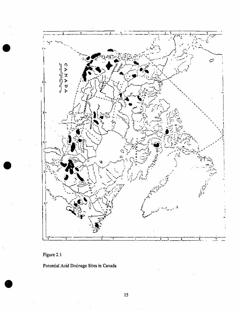
2.3.2 Scope of AMD

Acid mine drainage is the result of sulfide oxidation. Hence, it is usually found to

occur in the tailings of base metal and coal mines. These wastes invariably contain pyrite

and/or pyrrhotite, which is the more reactive of the iron sulfides. This does not mean that

ail mines fitting the above description will have AMD problems. Since acid generation

requires a number of conditions as outlined in the previous section, the absence of any of

these will prevent il. However, more often than not, these conditions do prevail and acid is

generated. In Canada, 4% of the total acid generating tailings, amounting to 72 million

tons, is found in British Columbia, while 80% of the acid generating waste rock (250

million tons) is found in the same province [3]. The main sources of AMD in Canada are

coal mines (New Brunswick, Nova Scotia, Saskatchewan, Alberta and British Columbia),

base metal mines (producing sulfidic tailings) and uranium mines (Ontario, Saskatchewan),

as can be seen in figure 2.1 [1].

In the United States, AMD originated in the Appalachian region with the

expansion of coal mining [5]. This region is still known to produce 75% of coal mine

drainage in the US, due to the high pyrite content ofthe coal [1].

2.4 Prevention and Treatment of AMD

2.4.1 Prevention ofAMD

The seriousness of the threat posed by AMD has initiated a series of research

7

•

•

•

initiatives aimed at curbing the problem by prevention and treatment. Two such groups

have been active in Canada and a summary of their work appears below [3]:

1. Mine Environment Neutral Drainage (]vfEND): This is a national body working with

provincial environrnental agencies and industry. For two decades, research done by the

governrnent ha~ focused on the use of vegetative covers to prevent AMD and good

methods were put forward. However, with the passage of time, it became obvious that

although the aesthetic aspect had improved, no improvement had been evident in the

quality of drainage from the treated sites. This group has identified AMD potential sites

and with the inevitable mining of low-grade deposits in the future, it can only be

speculated that the number of these sites is likely to increase. As such, MEND is focusing

research on several aspects of AMD. These are:

- Prediction

- Prevention and control

- Treatment

- Monitoring

- Technology transfer

- International liaison

2. Be AMD: This group is a provincial one and focuses on the problems of AMD in

British Columbia. Seeing that 80% of the acid generating waste rock in Canada is in that

province [3], it should come as no surprise to have a provincial group working towards

AMD prevention and treatment.

Having seen the requirements, as weil as the factors affecting the production of

AMD, prevention techniques should also be reviewed. One such method is the inhibition

of the oxidation ofsulfidic minerais. Several ways to achieve this end are Iisted below [4]:

- Restricting the oxygen supply by revegetation, flooding or sealants

- Restricting water

- Isolating the sulfide components

8

•

•

•

- Reducing the ferric iron

- Controlling pH

- Using bactericides

- Limiting the area of the reactive surface

- Controlling the temperature, as below SoC, the reactions proceed very slowly

Wet barriers preventing the supply of oxygen have been the popular method in

prevention techniques. Dave et al. [16] report on the deployment of such a barrier on

pyritic uranium tailings in Elliot! Lake, Ontario. They maintain that these barriers produce

anoxie conditions that support the growth of anaerobic heterotrophes (such as sulfate

reducers). These, in turn, will produce hydrogen sulfide and precipitate any dissolved

metals as sulfides. A complete review of the prevention measures taken against AMD has

been done by McCready [17]. He classifies the different methods along the following lines:

1. Physical Methods:

- Direct surface revegetation: He estimates that the cost would be around $4000 - $6000

per hectare and points out that although it improves soil erosion control, it does not raise

the quality of drainage.

- Surface amendment and revegetation: This method incorporates a crushed rock layer

between the tailings surface and the upper layer of overburden. The rock layer would act

as an impermeable boundary and prevent any acid migration from the tailings into the

overburden.

- Impervious capping: Il is achieved by using plastic films to coyer the waste rock and

tailings pile. Howevo::r, variations in temperature (freeze and thaw) may cause the rupture

of these films and renùer the whole treatment useless.

- Surface application of organic residues: This technique involves the use of organic

compounds like sewage sludge or compost to coyer the waste rock. These have the

quality of absorbing oxygen and preventing this essential element for AMD from reaching

the wastes. However, it would work only ifthe tailings are completely saturated.

9

•

•

•

- Underwater disposai: Preventing the supply of oxygen from contacting the wastes is

accomplished by underwater disposai, which renders them completely inactive.

- Clay capping and revegetation: This is yet another technique in the revegetation series.

However, a serious flaw is that as the trees grow and their roots sink into the overburden,

they might fracture the clay caps and the system wou1.d lose its effectiveness.

2. Chemical methods:

- Bactericidal agents: Using these chemicals to attack the bacteria Thiobacillus

ferrooxidans can prove to be effective. However, they stand the risk of being le~ched into

the environment with drainage.

- Surfactants: Although preferable to the bactericides, these chemicals have limited

applicability and have to be renewed ail the time.

3. Biolozjcal methods:

- Predators: The use of certain organisms to consume Thiobacillus ferrooxidans has been

tried, with limited success.

- In situ wetland vegetation: This involves the use of special plant populations that can

grow in acidic environments. They stabilize the surface and create an organic layer to

absorb oxygen.

2.4.2 Treatment of AMD

Waü:rs resulting from acid mine drahlage are invariably charged with high

concentrations of heavy metaIs that pose a threat to animai and plant life. By far the most

popular method for trea!.ing drainage with heavy metaI ions is neutraIization. It involves

the addition of aIkaIi compounds to raise the pH of sludges, neutraIize their acidity and

precipitate metaIs. Sorne of the compounds used are lime (CaO, Ca(OHh), limestone

(CaC03) and caustic soda (NaOH). Lime is the reagent most relied upon as it is widely

available, highly reactive and relatively cheap. The equation for neutralization is [18]:

4Ca(OHh + Fe2(S04)] + H2S04 =4CaS04 + 2Fe(OH)3 + 2H20

10

•

•

•

Other heavy metals generally tend to follow a similar trend as ferric iron in precipitation.

The other alkali compounds are not used as widely as lime for several ieasons. Limestone,

for example, although cheaper than lime, does not react fast enough and cannot raise the

pH above 6.0 [18]. The same source admits that using lime has its own problems, such as

gypsum formation. Using caustic soda will eliminate that problem, but is a much more

expensive operation. Another drawback for this alkali is that sodium sulfates are highly

soluble and thus, no reduction in sulfate content is achieved [5]. Sulfide precipitation has

also been tried, but has been limited due to high cost and the potential for toxic sulfides to

come out with the effluent [18].

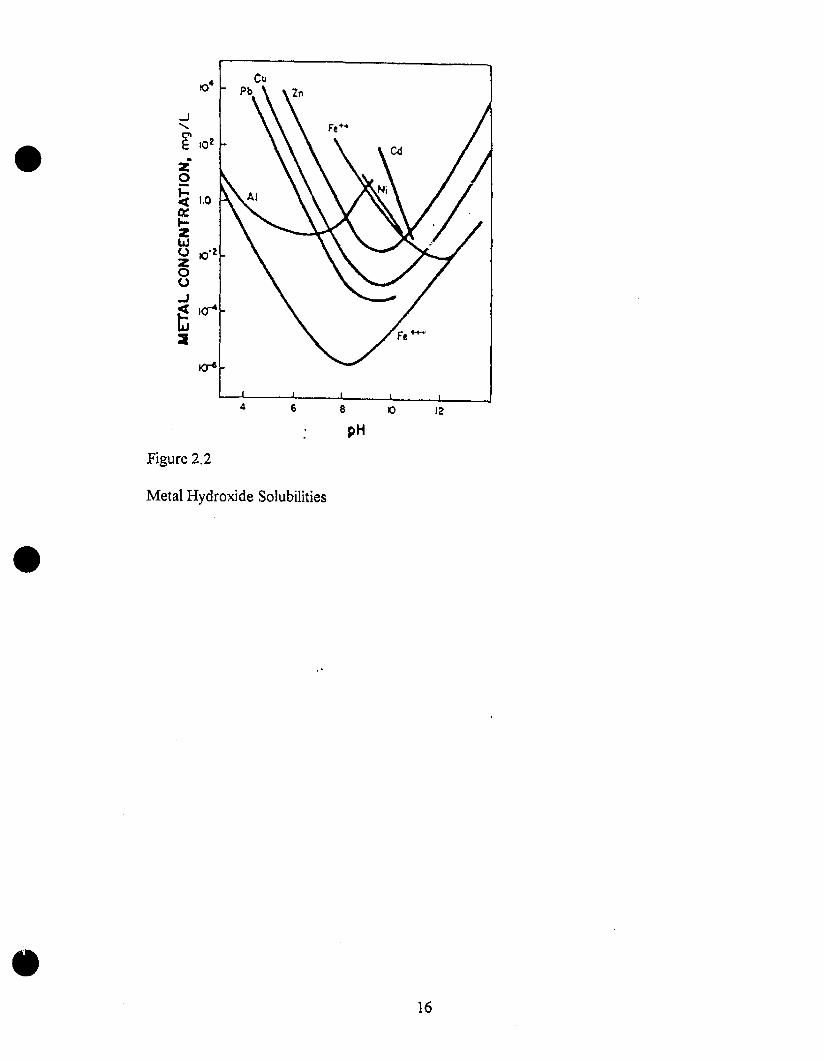
The process oflime neutralization is weil known in ttoe mining industry. The pH is

raised to about 9.5 and the metals are precipitated as hydroxides. Where aluminum and

ferric iron are abundant, a two stage process is applied; an initial raise to pH 6.0 to remove

Al+3 and Fe+3, then a subsequent raise to pH 9.5 for the other metals [18]. The whole

process requires a good knowledge of the precipitation values of the metals at different

pHs. The curves for different metal hydroxides are clearly presented in figure 2.2 [18]. It

can be seen from the curves that ferric iron precipitates earlier than its ferrous counterpart;

thus, it might be advantageous to oxidize the ferrous iron according to the following

equation [4]:

4FeS04 + 2H2S04 + 02 = 2Fe2(S04b + 2H20

A1though popular, lime neutralization is by no means the only method of treatment

for acid mine drainage. Some other processes have been tested and are still being studied.

A short list is given below:

1. Reverse osmosis: In this process, suspended solids are first removed. The effluent is

then fed to a reverse osmosis unit where it is exposed to membrane cells in a pressure

vesse!. The concentrated brine that results is either injected into a deep weil or treated [5].

Other authors report a 75% recovery of clean water by this method [18]. However, the

high cost associated with this process limits its extensive use.

11

•

•

•

2. Silicate treatment: In this complex methoà, the drainage water is tirst neutralized with a

dilute sodium silicate solution. Two gels are allowed to develop at the second stage; one

on the surface of the refuse pile to seal it from runoffwater, and another within the pile (a

silica-alumina gel) to prevent water percolation through the pile. However, it was found

that the results are no better than those obtained by conventional methods.

3. Activated carbon treatment: A method has been developed whereby activated carbon is

used to almost completely remove ferrous iron from acid mine drainage [19]. The

resuiting water can then be neutralized by limestone. The problem is that activated carbon

soon loses ils reactivity as it absorbs the iron and has to be replaced, thus creating a high

cost for treatment. In connection to this method, peat has been seen to remove metais

from wastewater effectively, a method that is of low cost and needs minimal maintenance

[20].

4. Sulfide precipitation: This method, also expensive in cost, has found sorne measure of

success. Mahemer et al [21] report that in a specially constructed wetland, sultide

precipitation accounted for most of the metal removal. Sultide/lime treatments have been

proven to be more effective than caustic soda treat"llents [22]. Metal sultide precipitates

have also been the resuit of biological sulfate reduction, which is the reduction of sulfate

to sultide under anaerobic conditions [23]. As was mentioned before, sultide treatment has

the disadvantage of introducing harmful compounds to the environment.

As a conclusion, the traditional method of lime neutralization has been the process

most used in AMD treatment. Although cheaper than other more sophisticated processes,

it still creates the problem ofultimate sludge disposai.

12

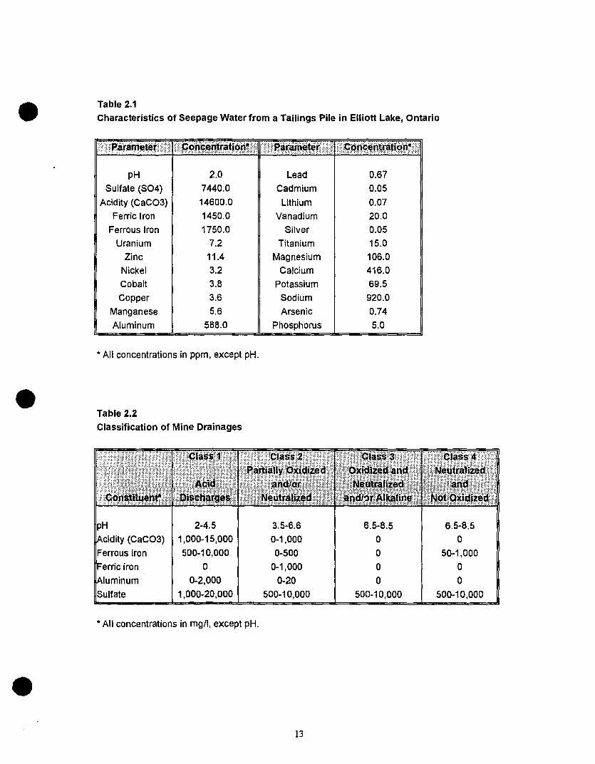
• Table 2.1Characteristics of Seepage Water from a Tailings Pile in Elliott Lake, Ontario

pH

Sulfate (S04)

Acidity (CaC03)

Ferric Iron

Ferrous Iron

Uranium

Zinc

Nickel

Cobalt

Copper

Manganese

Aluminum

2.07440.014600.01450.01750.0

7.211.43.23.83.65.6

588.0

Lead

Cadmium

Lithium

Vanadium

Silver

Titanium

Magnesium

Calcium

Potassium

Sodium

Arsenic

Phosphorus

0.670.05

0.0720.00.0515.0106.0416.069.5920.00.745.0

•* Ali concentrations in ppm, except pH.

Table 2.2Classification of Mine Drainages

pH

Acidity (CaC03)

Ferrous iran

Ferrie iran

luminum

Sulfate

2-4.51,000-15,000500-10,000

a0-2,000

1,000-20,000

3.5-6.60-1,0000-5000~1,OOO

0-20500-10,000

6.5-8.5oooo

500-10,000

6.5-8.5o

50-1,000

°o500-10,000

•* Ali concentrations in mg/l, except pH.

13

•

•

•

Table 2.3

Concentration of the Main Components in Acid Mine Drainage with Water QualityGuidelines

Aluminum 1~2,000 0.1

Iron 1-10,000 0.3

Calcium 1-500 None

Magnesium 1-200 None

Sulfate 1-20,000 None

pH 1.4-7.0 6.5-9.5

Table 2.4

Concentration of Trace Elements in Acid Mine Drainage with Water Quality

Guidelines

Manganese ta 50 0.02

Nickel ta 5 0.025

Vanadium ta 2

Zinc ta 10 0.03

Strontium to 5

Barium ta 5 0.5

Titanium ta 5

* Ali concentrations in mg/l, except pH.

2 [24]

3 [25]

14

•

•

•

{

Figure 2.1

Potential Acid D .ramage Sites in Canada

---' •. --

15

104

..J

......C"• E 102

z·Q

ti 1.00:1-Zl.lJUZ0(,)

..J

~:1

Figure 2.2

4 6 B

pH12

•

•

Metal Hydroxjde Solubilities

16

• 3.0 SOLIDIFICATION 1STABILIZATION

•

•

3.1 Introduction

Solidificationlstabilization (SIS) is a technology whereby a treated waste material

is rendered more acceptable in terms of physical and chemical properties. It is usually

applied to hazardous and radioactive wastes. Solidification refers to that part of the

process which is responsible for improving the physical properties of the material and

making it easier to handle the end product. Stabilization refers to the chemical stability and

decrease in the hazard potential of a waste. The EPA (Environmental Protection Agency)

[1] has defined the terms as follows:

- Solidification: Techniques that encapsulate the waste in a monolithic solid of high

structural integrity. It does not necessarily involve a chemical interaction between the

waste and solidifYing agents.

- Stabilization: Techniques that reduce the hazard potential of a waste by converting the

contaminants into their least soluble, mobile or toxic form. This does not necessarily

change the physical handling of properties. Stabilization is also referred to by the term

chemical fixation.

This introductory section on SIS (3.1) and the sections on SIS properties (3.2) and

the categories of SIS technologies used (3.3) are heavi!y based on the monumental work

by Conner [2]. The interested reader is strongly referred to it for a thorough and

exhaustive review of all aspects of solidificationlstabilization. Hence, unless otherwise

stated, all figures, tables and subdivisions in the aforementioned sections are those of

Conner and have been Sü!T'marized here in a compact lilanner.

Chemical fixation and solidification (CfS) systems date to the 1970's. The

materials used then were generally Portland cement, fly ash, sodium silicate and lime. It is

a known fact that for decades, mines in Canada and the US have been using cement alone,

with a combination of fly ash or solid mine wast.:: to produce cemented backfill.

17

•

•

•

International Utilities Conversion Systems (now Conversion Systems, Inc.) is known to

have used lime-fly ash combinations to incorporate sulfates [4].

Today, solidificaticnlstabilization is a widely practiced technique for the treatment

of hazardous w?sttlS. Many methods and components are used, with a wide range of

applications, depending on the specific characteristics of the waste, a subject that will be

covered in the coming sections.

3.2 Properties of SIS

Solidification/stabilization is a process involving chemical reactions and results in

notable changes in the physical and chemical properties of the treated sample. As such,

certain properties whereby the success or failure of the process is evaluated are of great

interest. These can be c1assified uncter four topics; leachability of toxic elements, fixation

of metals, factors affecting SIS and the characteristic types of SIS processes.

3.2.1 Leachability

Leaching can be defined as the process whereby water, or any other liquid,

contacts and dissolves part of a waste. The liquid is called the leachant and the

contaminated liquid coming out of the waste is termed the leachate. In such cases,

leaching and a leaching rate are said to have been established. In the United States, the

environmental acceptability of a hazardous waste is based on the US EPA Exuaction

Procedure Toxicity (EPT) test [3] and more recently, on the Toxicity Characteristic

Leaching Procedure (TCLP) [4]. Other leaching procedures inc1ude the Multiple

Extraction Procedure (MEP) [5] and the Oily Waste Extraction Procedure (OWEP) [6].

AU ofthese tests create worst case scenarios, as their strength to leach out contaminants is

much more than what could occur in nature. Most leach tests use a leachant to waste ratio

of20:1. Therefore, the maximum concentration of the constituent elements or compounds

that can be attained in the leachate is only 5% of their concentration in the solid waste.

18

•

•

•-.::...::.-

One of the most important controlling factors in metal leaching is the final pH of the

leachate, The TCLP test, for example, is designed to simulate a scenario in which a

hazardous waste is disposed of in a regular municipallandfilL Table 3,1 (modified from

[2]) gives the regulatory levels allowable in different tests for a certain contaminant The

different values for different tests represent a reflection of the changes in regulation over a

period of years,

The leachability of a waste is a function of dlfferent variables and may give

different results if one or more ofthese variables is changed, A list of the important factors

that affect leachability are presented below:

- Surface area of the waste

- Extraction vessel

- Agitation technique and equipment

- Nature ofleachant

- Ratio of leachant to waste

- Number of elutions

- rime of contact

- Temperature

- pH adjustment

- Separation of extract

- Analysis

3.2.2 Fixation of Metals

Indeed, one of the most important properties of SIS technology is its ability to

immobilize heavy metals, which are toxic to various life foriil'ô, Each metal species has its

own range of solubility, However, most metals are insoluble in alkaline conditions, Le"

relatively high pH values, The solubilities of various metal hydroxides vs, pH are given in

figure 3,1 [7]. Another diagram showing the solubility curves of metal hydroxides and

19

•

•

•

sulfides vs. pH is given in figure 3.2 [7]. As can be clearly seen, hydroxides oflead (Pb),

zinc (Zn) and chromium (Cr) exhibit minimum solubility in the range ofpH 7.5-\0.0, their

solubilities increasing beyond the ends of this range. Based on this knowledge, several

fixation mechanisms have been developed, a brief overview ofwhich is given below:

1. pH control: The above mentioned diagrams have clearly demonstrated the close

relationship of the pH to the solubility of the metal ions. To raise the pH of the system

above the neutral threshold requires the use of alkali compounds, such as lime (CaO), soda

ash (Na2C03) and sodium hydroxide (NaOH). This rise in the pH results in the

precipitation of the metals as hydroxides. Of the three compounds mentioned, lime is the

most commonly used and could be in either calcitic (CaO) or dolomitic (CaO, MgO) form.

2. Redox potential control: The basic reason behind this method of fixation is the fact that

sometimes the reduced forro of a certain metal can be more insoluble. Hence, special

reducing agents are employed, such as ferrous sulfate, sodium metabisulfitelbisulfite and

sulfides. Oxidation is much less common as a step in SIS, due to its limited applicability

and high cost.

3. Precipitation: This is by far the most popular way of metal fixation in SIS technologies.

A1though the common forms of insoluble metal species are hydroxides, sulfides and

silicates, others such as carbonates and phosphates are also used. Sulfide precipitation has

sorne advantages over its hydroxide counterpart. One point is the fact that sulfides are less

sensitive to pH changes and thus are easier to manage [8]. Another advantage is the

extremely low solubilities of the sulfides oftoxic metals. Table 3.2 gives a comparison of

hydroxide and sulfide solubilities for different metals. The major drawback in sulfide

precipitation is that they may resolubilize under oxidizing conditions [9].

4. Bonding to insoluble substrates: Another method of metal fixation is to react it with the

surface of an insoluble substrate.

5. SOqJtion: Sorption can be achieved on a variety of materials, four of which have been

listed below:

20

•

•

•

a. C/ays

b. Active oxides

c. Synthetic sorbents

d. Activated carbon

6. Ion exchange: Ion exchange is a phenomenon that is likely to occur in all SIS processes

iovolving metal removal. Although this reaction is helpful for metal fixation, it could also

prove to be disturbing for pozzolanic reactions as it tends to remove calcium from the

system.

7. Miscellaneous systems: Other less frequently used methods of metal fixation include

cementation, hydrophobizing (waterproofing) the agents in question to prevent leaching,

biological methods (using microorganisms to remove metals by absorbing them in their

cellular structures) and electrochemical methods.

3.2.3 Factors AfTecting SIS

No review of solidificationlstabilization processes would be complete without a

look at the various factors that influence them. For purposes of clarity, they can be divided

into two broad categories; physical and chemical.

1. Physical factors:

a. Partide size and shape: It has been seen that the smaller the size of the

particles, the more resistant the solidified product is to leaching [10, Il].

b. Water content: The important part of the water content of a waste is what is

termed "free water", which is the portion that is free to react with the additives and is not

interlocked in the matrix of compounds.

c. SoUds content: It influences the physical properties of the end product, such that

the higher the solids content, the better these properties will be.

d. Specific gravity/density: The point worth mentioning in this case is that a large

21

•

•

•

difference between the specific gravities ofwaste (usually 1.0-1.5) and additives (usually

>2.0) could result in a phase separation in the end product.

e. Viscosity

f Wetting: It is very important that the reagents added for solidification purposes

be properly wetted.

g. Mixing: It is a crucial step in the solidification process. Care must be taken to

do it properly, as each case will need a certain manner of mixing.

h. Temperature and humidity: As with ail reactions, the rate of those involved in

solidification rises with a rise in the temperature of the system. As for humidity, the

procedure is usually to cure the samples in a 95% relative humidity (RH) environment.

2. Chemical factors:

The chemical factors affecting SIS processes are varied and many. Most are due to

the presence of certain reagents, but chemical processes also have their effects. For

example, ion exchange may retard or accelerate the reactions involved in an SIS system.

An example of a study done on these kinds of differences is by Cullinane et al [12]; sorne

oftheir conclusions were that:

- The same chemical did not have the same effect on all the systems.

- The same chemical increased strength at low concentrations, but decreased it at high

percentages.

3.3 Categorietl of SIS Processes

The different processes of SIS can be divided generically into two broad

categories: inorganic and organic, based on the characteristics of the reagents used. They

will be discussed separately and two important types of inorganic processes will be given

separate discussions in this section. A third inorganic binder, Iime-flyash, will be discussed

in the next chapter, due to its high relevance to the project upon which this thesis is based.

22

•

•

•

1. Inorganic processes: The inorganic processes of SIS can be subdivided a10ng two lines;

those that use bulking agents, such as type F fly ash, and those that do not. It should be

remembered that the function of a bulking agent is to increase the total solids content in a

system and by increasing the viscosity, prevent an early phase separation before setting can

take place. Examples of these two categories are; cement/fly ash and lime/fly ash that use

bulking agents and cement-based and cement/soluble silicate systems that do not employ

such agents. The basic difference in the two subdivisions is that those processes that use

bulking agents often cost less, as these agents are cheaper replacements for more

expensive materials such as cement.

The main types ofinorganic processes are:

- Portland cement

- Portland cement/lime

- Portland cement/fly ash

- Portland cement/soluble silicate

- Lime/fly ash

- Kiln dust

Some characteristics of the inorganic processes of SIS are given below:

- Low cost

- Long term physical and chemical stability

- Documentation for the past 10 years

- Availability of chemical reagents

- Non toxicity of chemical reagents

- Ease in processing

• Wide range of volume increase

- Inertness to ultraviolet radiation

• High resistance to biodegradation

• Low water solubility

23

•

•

•

- Low water permeability

- Good mechanical and structural characteristics

2. Organic processes: They are also subdivided into two categories; thermoplastic and

polymerization systems. The former use bitumen with either water-base or solvent/oil-base

wastes, while the latter are usually used with water-based wastes. Sorne of the

characteristics of organic systems are their high cost, potential of using one system with a

variety of waste types, unproved long term stability, limited commercial use except for

radioactive wastes and sorne of its components being hazardous.

Il would be very he1pful to be able to compare the different systems of SIS as they

apply to the same waste. A recent study by Weizman et al [13] evaluated several processes

on four synthetic analytic reference matrices (SARMs). The one that is ofreJevance to this

project is SARM #3, which had low organic and high metal concentartions, with a 19.3%

water content. The different SIS processes used were Portland cement, kiln dust and

lime/fly ash binders. Chemically, the samples were subjected to TCLP leaching, the results

ofwhich are presented in table 3.3 (modified from [13]), and show that Portland cement

gave the best values. To have an idea about the price of the different reagents used in SIS

processes, table 3.4 gives the delivered cost of sorne materials in northern industrial areas

in the US [14].

3.3.1 Portland Cement Based Systems

Sorne of the reasons for the importance of this type of process today are that:

- The compositions of the reagents are constant from source to source.

- A lot is known about the reactions involved due to the wide range of applications of

cement in various industries.

Typical weight proportions for ordinary cement are:

- 50% tricalcium silicate (C3S in cement shorthand)

·25% dicalcium silicate (C2S)

24

•

•

•

- 10% tricalcium aluminate (C3A)

- 10% calcium aluminoferrite (C4AF)

- 5% modes.

Note that C, S, A and F represent the modes of the elements calcium, silicon, aluminum

and iron. Portland cement requires a certain amount of water to obtain workability; the

minimum amount is usually a 0.40 water:cement ratio.

1. Chemical and Physical Properties of Cement:

a. Cement types and compositions:

- ASTM type 1: this is the type used in typical SIS applications.

- ASTM type I(A): this type has an improved resistance to freeze-thaw and scaling.

- ASTM type II: it resists moderate sulfate attack.

- ASTM type II(A): it is the same as II(A), but also contains air-entraining agents.

- ASTM type III: it develops a high early strength and is suitable for coId weather.

• ASTM type III(A): it is the same as III(A), but also contains air-entraining agents.

- ASTM type IV: it is used where temperature rise must be controlled, as it has a low heat

of hydration.

- ASTM type V: it is used primarily for high sulfate content soils and groundwater

environments.

Tables 3.5 and 3.6 depict the chemical and minerai compositions, respectively, ofvarious

types of Portland cement.

b. Chemistry ofcement setting: Although the production and the chemical composition of

cement seem simple enough, there is still disagreement among scientists as to how water

and cement react together. In the case of normal Portland cement, it is believed that

tricalcium aluminate and sulfates react first and form hydrates. As for strength

development, it is attributed mainly to C3S and ~-C2S formation.

c. Inhibitors: A variety of substances can inhibit setting or alter the properties of cement,

when present in sufficient quantities.

25

•

•

•

d. Accelera/ors: There are also other compounds known as accelerators that counteract

the effect of inhibitors or accelerate cement setting if the latter are not present.

2. Physical Properties ofWastes Stabilized with Portland Cement:

Sorne of the important properties ofwastes treated with Portland cement are listed below:

- They are usually strong and exhibit load-bearing capacity.

- The permeability of the end product is comparable to that of clay.

- One of the crucial factors is the water:cement ratio, which cannot be controlled as it

depends on the moisture content of the original sludge.

• Sometimes additives like f1y ash are used as partial replacement for cement to minimize

~osts.

- A smaller volume ofwaste has to be disposed of since low mix ratios are used.

3. Chemical Properties ofWastes Stabilized with Portland Cement:

- The heavy metal compounds are usually fixed chemically or physically In the

microstructure.

• Bhatty [15] has pointed out 4 mechanisms which are involved in the fixation of heavy

metals by C3S:

- Addition: CSH + M ~ MCSH

- Substitution: CSH + M ~ MSCH + Ca

- Formation ofnew compounds

• Multiple mechanisms

where M is the metal ion.

- A study by Bishop [10] on a cadmium, chromium and lead sludge showed the following

characteristics:

- Rate of metalleaching decreases with decreasing particle size.

- Metals were first leached and then reprecipitated or sorbed onto particles where

alkaline conditions still prevailed.

26

•

•

•

- Chromium and lead were bound into the silica matrix and were thus immobilized

as long as the matrix remained intact.

3.3.2 Portland Cement/Soluble Silicate Processes

Sodium silicates have been used for the production of special cements. The

presence of calcium or magnesium ions can reduce the solubility of the silica matrix by

several orders of magnitude, a property that is essential in any SIS technology. Soluble

silicates can form insoluble metal oxides/silicates and reduce toxic metalleachability.

Chemical and Physical Properties:

- A rapid reaction between soluble silicates and metal ions produces low-solubility metal

silicates which are non-toxic and cannot be easily resolubilized at a later stage.

- The gel produced by Portland cement/soluble silicate interaction can hoId a lot of water

while itself acting as a solid.

- Gelation and solidification: Since cost considerations are always important in designing

an SIS system, the most commercially used one has been type 1 Portland cement and a

38% solution of sodium silicate (silica:sodium oxide ratio of3.22), which is also known as

water glass. The main purpose behind using this process of SIS is to quickly gel wastes

with low solids content and aid in the cement hardening process. Another function of the

sodium silicate is to reduce the permeability of the resulting monolith.

3.4 Applications

Solidificatic,lIstabilization technologies have found a wide range of applications. A

number of workers have tested the different techniques and processes on a variety of

industrial and synthetic wastes. An excellent report by Bishop [la] shows the physical and

chemical characteristics of synthetic heavy meta! sludges treated by type II Portland

cement. Sorne of the observations and conclusions that the author reached are given

below:

27

•

•

•

- During hydration, a calcium-silicate-hydrate gel formed and metals were precipitated as

hydroxides, having been trapped in the cement matrix.

- Maximum compressive strength was reached within 28 to 48 day:. and metals leaching

remained the same from 42 days onward.

- Metal leaching rates decreased with a decrease in particle size. The author speculates

that this might be the result of the metals binding to particles by sorption.

- Little metalleaching occurred until the pH dropped below 6.0. Cadmium was found to

be more soluble than chromium and lead.

- Chromium and lead were believed to be bound within the silica matrix itself If this were

the case, they would not be expected to leach until the matrix broke down.

A similar project of sludge solidification was done using a mixture of Portland

cement and fly ash [16]. The project involved the preparation of a synthetic sludge by

adding the nitrates of nickel, chromium, cadmium and mercury to water. Lime was also

added to induce hydroxide precipitation. X-ray diffraction analysis revealed the formation

of the mineral ettringite on the fly ash particles, although not in abundance. Another

conclusion reached was that the heavy metals retarded the hydration of calcium silicates.

The authors admit that the design of SIS systems cannot be derived from first principles

yet, but has to rely on empirical tests such as TCLP and unconfined compressive strength.

Heimann et al [17] did a similar test with heavy metal sludges. The fly ash and

cement compositions used in their test are given in table 3.7. It was seen that cadmium

was retained in all cements and was not dependent on leachate pH. They also concluded

that metal leaching from solidified/stabilized wastes is controlled by various complex

factors, such as speciation and type of the metal, leachant type and particle size.

While sorne workers have studied the applicability of different combinations of

reagents in SIS technology, others have tried to understand the mech~:sms of the

reactions involved. One such study was done by Tseng [18], using Portland cement on

28

•

•

•

hazardous metal-Iaden sludges. In the report, the author set out the equations for strength

gain in cement:

C3S + HZO ~ C-S-H + nCH [19]

C3A + 3CSHZ + Z6H ~ C3A.3CS.H32 (ettringite)

C3A.3CS.H32 + ZC3A + 4H ~ 3C3A.CS.H1Z (monosulfate)

where C=CaO, A=AlZ03, S=SiOZ, S=S03 and H=HZO. Tseng ascribed waste

immobilization to one or both ofZ mechanisms:

- Encapsulation (either micro- or macro-), with the metals being trapped inside matrices.

- Chemical fixation, with the metals being chemically bound to compounds.

Sorne of the conclusions the author reached were that:

- The leachability of the heavy metals was reduced to such an extent so as to classify ail

the sludges except one as non-hazardous by EPA standards.

- The leachability decreased with an increase in curing time and strength.

The effect of certain factors on SIS processes have also been the target of study.

Roy et al [ZO] studied the effect of sodium sulfate on several types of SiS processes. Three

different binders were used, with the following binder to sludge ratios:

- Type 1Portland cement, with PC:S = 0.3:1.

- Type 1Portland cement and type F fly ash, with PC:FA:S = 0.Z:0.5:1

- Type C fly ash and lime, with lime:FA:S = 0.3 :0.5:1

A few of the observations made by the authors were:

- In ail the three binders, ettringite formation was observed.

- The method ofwaste immobilizatioll was physical encapsulation.

• Fly ash was seen to exchange material with the sludge.

A final important factor effecting SIS applications, which has rare1y been studied,

is the redox potential. A group of workers [ZI] looked at this factor and found that

chromium leaching increased significantly under highly oxidizing conditions and that

arsenic, vanadium, iron and lead leached more under reducing conditions.

29

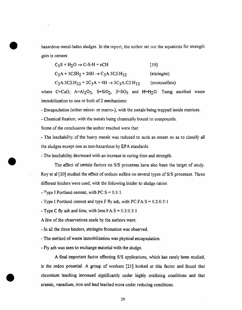
•Table 3.1Comparison of Regulatory Limits for Various Test Procedures

'{,Câriacliari')';',::;ÇPSB ','

rsenicCadmiumChromium (+3)Chromium (+6)CopperLeadMercuryNickelZinc

5.0001.0005.0005.000

5.0000.200

5.0001.0005.0005.000

5.0000.200

5.000.505.005.00

5.000.10

Values expressed as concentration of constituent in leachate or waste, mg!!.

'rable 3.2Comparison of Hydroxide and Sulfide Solubilities

Iron 5" iD' 1 .. 10-4 5" 103

Cadmium 3" 100 1 .. 10~8 3" 108

Chromium 1 .. 10~3 None None• Copper 2"10·:2 2" 10-13 1 .. 1011

Lead 2" 10 6 .. 10-9 3 "108Mercury 6" 10-4 1 .. 10-21 6" 1017

Nickel 7 "'10-1 6 * 10.8 1 * 107

Silver 2 "iD 4*10-12 5" 1012

Zinc 3 * 102 1 * 10-6 3" 108

Difference Factor == hydroxide solubility ! sulfide solubility.Source: Adapted from Permutit Company, Suljex™ Heavy Metals Waste Trealment Process, Tech. Bull. XI1l, No,6, Paramus, NJ.

Table 3.3Summary of TCLP Results for Matais for SARM Type III

BIlI,:;'i!!j;~l~'1.~:}: ::'~::':'~~f:~:~,t~~:~J1:':::: :,:':,~~r~:~:,:;~,,',>~, :,.:::~~p,~~r;'~ ":'> '<:'":~~~d,, "'b'::,,. ',::'a~,i~C"'.b: ,',.

•

1II RAW 6.39 ND + 80.7 19.9 3597 PC(14) ND 0.07 + 0.15 100 0.63 95 0.58 100

21 KD(14) ND 0.22 + 1.02 96 13.3 + 4.38 9533 LF(14) 0.81 52 0.03 + 2.96 87 51 + 3.81 967 PC(28) ND 0.07 + 0.09 100 ND 100 0.69 10021 KO(28) 0.21 98 0.12 + 0.85 96 18.3 + 4.07 9533 LF(28) 0.79 51 0.07 + 2.59 87 51 + 3.97 96

a = TCLP results in ppm. b =Percent reduction. corrected for dilution.Note: ND =below detection Iimit, + =increase over raw SARM.

30

Table 3.4Cost of Reagents in US' Dollars

e······.··Fleâ~iéijt··· .... ········.·:P:lÎcê/Tôn·

Portland cement 70Flyash 15Lime 50Kiln dust (cement or lime) 20Clay (regional) 70Sodium silicate 140

Table 3.5Typical Compositions of Portland Cements: Chemical Composition (%)

1 Normal Portland-general use 0;6

II Moderate heatevolution

III High early strengthIV Low heat evolutionV Sulfate resistance

Rapid hardening 0.9Super rapidhardening 0.9Jet cement 0.6

0.1

0.2

0.10.1

22

21

19.713.8

5.1

4.9

5.111.4

2.9

2.71.5

65

66

6559

1.4

2.52.01.81.91.1

2.00.9

1.6

2.5

3.010

... CllA7CaF2.2 Specifie surface area is the Blaine value in cm2/g.

31

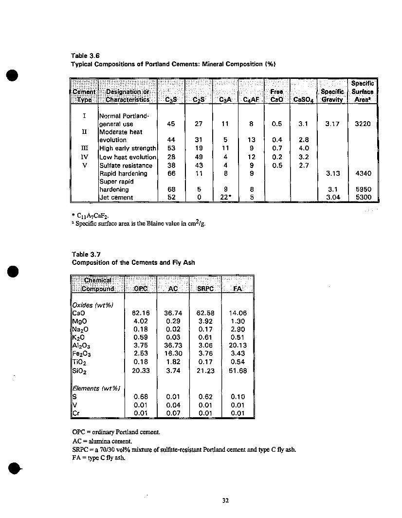
Table 3.6Typical Compositions of Portland Cements: Mineral Composition (%)

l Normal Portland-general use 45 27 11 8 0.5 3.1 3.17 3220

n Moderate heatevolution 44 31 5 13 0.4 2.8

ID High early strength 53 19 11 9 0.7 4.0IV Law heat evolution 28 49 4 12 0.2 3.2V Sulfate resistance 38 43 4 9 0.5 2.7

Rapid hardening 66 11 8 9 3.13 4340Super rapidhardening 68 5 9 8 3.1 5950Jet cement 52 0 22· 5 3.04 5300

* CllA7CaF2·Z Specifie surface area is the Blaine value in cm2/g.

Table 3.7Composition of the Cements and Fly Ash

'.·•..• ·..···1 .

.AC·SEtPC·I.' .>FA

Oxides (wt%)CaOMgONa20K20Al20SFe20STi02

Si02

62.16 36.74 62.58 14.064.02 0.29 3.92 1.300.18 0.02 0.17 2.900.59 0.03 0.61 0.513.75 36.73 3.06 20.132.53 16.30 3.76 3.430.18 1.82 0.17 0.54

20.33 3.74 21.23 51.68

Elements (wt%)SVCr

0.680.010.01

0.010.040.07

0.620.010.01

0.100.010.01

oPC =ordinary Portland cement.AC =alumina cement.SRPC = a 70/30 vol% mixture of sulfate-resistant Portland cement and type C fly ash.FA =type C fly ash.

32

o., I---+--\--+---*,~~-,-+-_-+ __~~

~

, 0 t----'r-+---":+--Ir-\--I\---\+--+-~_-+--~<.•:......~

1.0 t---T---i--+-'r-~-~r1-~':"_+-_~-1

100 r----r----r---r-...,......---r----,...,-_._-,

0.0 1 t----i----fr----+--~*__,A-_1_-,L,,"'___l

•

1110•pH

•70.000' L..---.l..---3.-.J-.-_..L.__....L-__-J-__-J

•Figure 3.1Metal Hydroxide Solubilities YS. pH•

Figure 3.2 PH.

Solubilities ofMetal Hydroxides and Metal Sulfides

12.10

~ ICi',Cd(C>-lh<r

{-...~ LO"..r

"Il3 10'·

*ci..0 10'Z0ç~1- '0"1.IIIUZ0lJ

Iv'"

•33

• 4.0 LIME - FLY ASH BIND1i;RS

•

•

4.1 Introduction

Lime and fly ash have been used together, successfully, in many

solidification/stabilization projects. They have had the advantage of providing cheaper

alternatives to waste treatment than, say, Portland cement. The reason that lime-fly ash

binders (LFA) are being covered in a separate section is their high relevance to the project

upon which this thesis is based.

4.2 Materials

4.2.1 Lime

Lime is usually taken to mean the oxides and hydroxides of calcium and

magnesium, but not their carbonates [1]. According to the same source, the controlled

addition of water to calcitic (CaO) and dolomitic (CaO+MgO) quicklimes produces three

types of hydrated lime:

- Ca(OH)z : high calcium

- Ca(OH)z + MgO : monohydrated dolomitic

- Ca(OH)z + Mg(OH)z : dihydrated dolomitic

The usual practice in LFA stabilization is to use the first two types of hydrates.

Some properties of commercially available lime are given in table 4.1 (modified from [1 D.

Although sorne authors have claimed that monohydrated dolomitic lime is the more

effective one in LFA stabilization [2, 3], other studies have shown that high-calcium lime,

at low percentages, gives higher strengths [4, 5]. However, it seems that the quality of the

fly ash used in LFA systems has a much greater influence on the reactions involved than

the type of lime [1).

34

•

•

•

4.2.2 Fly Ash

Fly ash is the fine residue that resutts from the combustion of coal. It is usually

collected by mechanical or electrostatic precipitators. It is considered a waste itself,

although it is increasingly being used in the concrete industry as a partial replacement for

cement. The annual US production of fly ash is 50 million tons, 70% of which is land

disposed [6].

4.2.2.1 Composition

Physically, fly ash is composed of particles that are predominantly amorphous and

spherical, whether solid or hollow [1]. They range in diameter from 1-150 !-lm with surface

areas of 4000-7000 cmZ/g [7]. The same source stipulates that the size of the particles

depends largely on the collection mechanism used. Thus, electrostatic precipitators collect

an ash that has much more fine particles than one collected by a cyclone.

Mineralogically, fly ash is mainly composed of quartz, mullite, hematite, magnetite,

carbon and an amorphous component [7].

Chemically, it is a mixture of amorphous and crystatline phases of SiOZ, AlZO]

and FezO], largely determined by the composition of the inorganic portion of the coal

burnt [7]. A cornpositional range of US fly ashes from different coal sources is given in

table 4.Z [8]. Another diagram showing average fly ash composition with respect ta SiOZ,

AlZO] and CaO is given in figure 4.1 [7]. Rapid cooling of the ashes usually results in

non-crystalline (glassy) or amorphous compounds, white gradual cooling may produce

sorne crystallization [9].

4.2.2.2 Types

Two types offly ash have been identified, the classification being largely based on

the type of coal from which it has been derived and the calcium content. Ashes derived

from sub-biturninous coals are generally rich in calcium (type C), while those from

35

•

•

•

bituminous ones are calcium-poor (type F) [9]. Table 4.3 lists type C (FAC) and type F

(FAF) compositions (modified from [10]). The difference in calcium content plays an

important role in the pozzolanic properties of a fly ash, as is explained in the next section.

4.2.2.3 Pozzolanic Properties

By far the most important of the characteristics of fly ash is its pozzolanic

properties. A pozzolan is defined as "a siliceous and aluminous material, which in itself

possesses little or no cementitious value but which will, in finely divided form and i;:) the

presence of moisture, chemically react with calcium hydroxide at ûrdinary temperatures to

form compounds possessing cementitious properties" (ASTM C219-74a*). Minnick has

done considerable work on this subject and has proposed that the amorphous components

of fly ash are responsible for the main pozzolanic reactions in LFA mixtures [II]. Sorne

authors have pointed out several factors indicatmg good reactivity:

- An increase in the percentage ofa fly ash passing the 45 J.lm sieve [12].

- Increase in Si02 [12] and Si02 + Al203 contents [13].

- Low carbon content [12] and loss on ignition [14].

- Increased alkali contents [14].

The main feature of fly ash is that it reacts with Ca(OHh to form new

cementitious material, which improves the strength of the mix. Workers in concrete

research have observed the formation of calcium sulfo-aluminates at the early stages of

curing, in addition to the expected calcium silicate hydrates [II, 15, 16, 17, 18]. This

might be due to the presence of S03 in fly ashes, which usually exists as CaSO4 [19].

Unfortunately, it is very difficult to determine a reliable method to measure the reactivity

offly ash accurately [7].

Another classification of fly ashes is possible along the lines of reactivity. FAC,

which is rich in calcium, exhibits self-cementing properties, eliminating the need to add

lime or Portland cemeilt. FAF, being poor in calcium, does not show these properties on

36

1.

Z.

3.• 4.

5.

6.

7.

where

•

•

its own, but does so when mixed with lime [9]. Therefore, adding FAC to a soil does not

only eliminate the need for lime or calcium, but provides a mechanism by which the

moisture content can be reduced by 10-ZO% [9]. This occurs when the calcium in fly ash

hydrates to produce Ca(OHh.

4.3 Reactions

Lime-fly ash binders have been used to treat the largest volume of waste in the

United States [ZO]. The reactions involved in these mixes are complex, to say the least,

and not weil understood. Minnick [11] has given out a list of reactions that involve these

two additives:

RO ~ R(OHh in the presence ofHZO

RO ~ RC03 + HZO in the presence ofHZO and COZ

R(OHh ~ RC03 + HZO in the presence ofHZO

R(OHh + 5iOZ ~ xRO.ySiOZ.zHZO in the presence ofHZO

R(OHh + AlZ03 ~ xRO.yAlZ03.zHZO in the presence ofHZO

R(OHh + AlZ03 + SiOZ ~ xRO.yAlZ03.z5iOZ.wHZO in the presence ofHZO

R(OHh + 503-Z + AlZ03 ~ xRO.yAlZ03.zRS04.wHZO in the presence ofHZO

R = Ca+Z or Mg+Z or a combination ofboth.

Based on his own studies as weil as those of others, Minnick maintains that the

major cementing products resulting from lime-fly ash reactions are calcium silicate

hydrates, and possibly the minerai ettringite [11]. Conner [ZO] also mentions the formation

of ettringite and attributes it to the presence of sulfates and sulfites in the wastes being

treated.

Sorne factors aifecting these reactions include temperature, curing time, materials

used and proportions. It has been observed that for a given LFA combination, increased

quantities of pozzolanic materials are produced by extending the curing time and

increasing the temperature. This is graphically presented in figure 4.Z [Zl]. Taking into

37

•

•

•

account all these factors, two stages of reactivity are understood in the case of pozzolanic

reactions [7]:

1. After the irnmediate mixing of fly ash with cement and water, the reaction seems to be

controlled by the percentage of the amorphous particles present in the ash, as weil as the

reactive surfaces available for reaction with the Ca(OH)z liberated.

2. After long curing periods, the reactivity becomes a function of the total Si02 and

Al203 available in the ash.

In the end, the quality of the stabilized material by these two additives is largely

dependent on the material itself. Strength development is an essential part of a

solidification process, specially if the end product will be used for construction purposes.

Smith [10] states that water is essential for this purpose and attributes strength gain to 3

mechanisms:

- Pozzolanic: This occurs when reactive silica and alumina compounds interact with lime

and water and gain strength. The classical combination is FAF and lime.

- Ettringite formation: It occurs in FAC and is responsible for early strength gain.

- Cement hydration: In cases where Portland cement is used, its hydration results III

significant strength gains due to the interaction of calcium silicate hydrates and lime.

Since lime and fly ash interactions are responsible for strength gain and a decrease

in contaminant mobility, it is essential to maximize their reactivity. A study by Sivapullaiah

et al [22] suggests a few simple tests to determine the optimum lime content for fly ashes.

These include a pH test, liquid limit test and free swell index.

4.4 Applications

Lime/fly ash combinations have been studied for some time. There seem to be two

reasons behind mixing these two additives. The first one is to stabilize the fly ash itself, as

it is considered a hazardous by-product of coal burning. The second one is to provide a

binder within which other hazardous sludges and wastes could be stabilized. The range of

38

•

•

•

applications of lime/fly ash extends from waste and soil stabilization to pavement

construction. An example of the former case is the use of fly ash in the stabilization of

tropical soils [23]. A study was conducted on Hawaiian soils with high percentages ofiron

and aiuminum. The stabilization process was attributed to two basic sets of reactions:

- Short-term: This set included flocculation and agglomeration of clay particles due to ion

exchange. The result was a reduction in swelling, shrinkage and plasticity.

- Long-term: This set of reactions resulted in the binding of the soil particles together due

to the formation of cementitious materials. The main factor behind these reactions was the

presence of pozzolans provided by the fly ash.

It was seen that the lime/fly ash treated soils gave higher strength vaiues. The

authors conclude that this method may provide a more cost effective treatment than one

with lime alone.

Not ooly soils, but wastes have aiso been stabilized using a lime/fly ash binder.

Smith [10J has done a comprehensive study on the utilization of these additives in

industrial waste treatment. He states that fly ash and kiln dusts are the less expensive

additives in stabilization, unlike Portland cement and lime. As a conclusion, the author

presents curves depicting the pH of aqueous extracts as a function of time for a metal

hydroxide sludge stabilized by severai common agents (figure 4.3). He then makes the

following observations:

- In the case of cement, the pH rises with time due to lime generation.

- For FAC aione, the pH remains constant.

- Where FAF/lime has been used, the pH decreases with time, since lime is consumed in

ettringite formation and pozzolanic reactions.

Work in recent years has focused maioly on the application of lime/fly ash as a

binder within which wastes and sludges have been solidified and stabilized. The main

criterion for the success of the binder has been the amount of metals that could be leached

from the end product. One such example has been the reduced leachability of metals from

39

•

•

•

a combination ofwastes [24]. The authors concluded that the reduction in leachability was

due to the formation of solid hydrated phases incorporating the trace metals and not just

due to the rise in pH. Synthetic sludges have also been used with limelfly ash binders. Roy

and Eaton [25] made such a sludge with the metals nickel, chromium, cadmium and

mercury, which were precipitated by lime addition. X-ray diffraction showed the formation

of calcium hydroxide and calcium carbonate phases. The heavy metais were found to be in

complex forms and were also seen on fly ash surfaces by energy dispersive x-ray

spectroscopy (EDX). Another attempt with synthetic sludges was made by DebRoy and

Dara [26], where three solidification procedures were followed:

- Fixation: The lime and fly ash were mixed and the sludge added to il. After the water

was added, the samples were compacted.

• Coating: Cubes were prepared according to the above procedure, then dipped into a 5%

sodium silicate solution.

• Encapsulation: Cavities were made in the LFA molds, and filled with hydroxide sludge.

After the leaching test, it was seen that the methods rated as follows from most to least

effective:

Encapsulation> Coating > Fixation

Other workers have compared the performance of lime/fly ash to that of cement

and other binders. Akhter et al [27] concluded that type 1 Portland cement exceeded

combinations of FAF, lime, blast fumace slag and silica fume in immobilizing arsenic and

chromium in contarninated soils. Metal sludges are by no means the only type of waste to

which lime/fly ash binders can be applied. Martin et al [28] were able to apply it to a

hydrocarbon sludge in a silty matrix. The binder was seen to effectively retard leachability

due to physical microencapsulation.

Joshi et al [29] studied the properties of Alberta fly ash, concentrating mainly on

ils physical characteristics. They reached the conclusion that the addition of lime

decreased the conductivity of the mix, increased its strength and decreased the leaching of

40

•

•

•

metals from the fly ash. The improvement of the physical properties of lime/fly ash treated

samples has not been ignored by soil scientists. The two additives were used by Inraratna

et al [30] to stabilize a soft clay, giving it a compressive strength 2-3 times its original

value.

4.5 Ettringite Formation

The minerai ettringite is a calcium-aluminum-sulfate-hydrate and has been studied

extensively in the cement industry. As was mentioned earlier in this chapter, it is

responsible for early strength gain in concrete, but could lead to swelling and failure later

on. The crystal structure of ettringite is quite complex and is discussed by sorne workers in

detail [31]. Ettringite formation is usually triggered by the exposure of concrete to sulfate

bearing waters [32]. Sorne authors have proposed the use of FAF to improve the sulfate

resistance of cement [33]. Factors such as temperature and water:cement ratio have been

studied to provide clues to understanding ettringite formation [34, 35].

Although an undesirable event in the concrete industry, ettringite formation has

been hailed as a possible mechanism of heavy metal immobilization in lime/fly ash binders.

This should not come as a surprise, as the essential elements for its formation are provided

adequately in these mixes. Calcium is provided by lime, aluminum can come from fly ash,

and almost ail metal sludges are rich in sulfate content. Hassett and Hassett [24] attribute

the decrease in the leachability of toxic elements in several wastes to the formation of

ettringite. Solem·Tishmack et al [36] state that the reason FAC shows cementitious

properties is due to the same minerai. Their experiments have shown that due to its

formation, boron and selenium ions were immobilized. Not only metals, but sulfate from a

fly ash has also been seen to be fixed due to the formation of ettringite [37]. Kamon and

Nontananandh [38] explain this phenomenon of making use of the components of the

wastes themselves. They contend that most industrial waste sludges are aiready rich in

41

•

•

•

CaO, AIZ03, SiOZ and Fez03. They then put forward the reaction for ettringite

formation:

- C3A (tricalcium aluminate) + 3CSHZ (gypsum) + Z6H (water) ~ C6AS3H32 (ettringite)

Due to its unique ability to trap metals and reduce their leachability, the factors

affecting the formation of ettringite have also been extensively studied. Mattias et al [39)

found out sorne interesting features in their study, which are summarized as follows:

- Maximum strength was obtained with a 30% water content by weight.

- The best ratio oflime:ash was seen to be 30:70.

Although it has its advantages, ettringite also shows sorne major drawbacks. It is

vulnerable to calcium dioxide attack, which can cause it to disintegrate. It can also expand,

causing serious problems, whether it be in concrete or in a binder for heavy metal sludges.

This feature has also been seen in soil stabilization, where c1ays were stabilized by

gypsum-lime (3Ca(OH)z + ZCaS04.Y2HZO) [40). A major study of ettringite expansion in

soils has been carried out by Mitchell and Dermatas [41). The authors state that a non

expansive monosulfate calcium-aluminum-hydrate forms at first, then converts gradually

to ettringite, which is a trisulfate. The rate and amount of alumina release into the solution

is held to be the main factor controlling the amount ofheave.

Work is currently being done to understand the mechanisms of ettringite

formation. Two have been proposed so far; through solution and topochemical reaction

[4Z, 43). It is hoped that once its formation process is well understood, the reasons for its

expansion will also be known.

42

Table 4.1Properties of Commercial Limes·

1 Constituenf(%)' HighCâlCiùm . Dolol11itic .......

CaO 92.25-98.00 55.70-57.50MgO 0.30-2.50 37.60-40.80C02 0.40-1.50 0.40-1.50Si02 0.20-1.50 0.10-1.50Fe20 3 0.10-0.40 0.05-0.40AI203 0.10-0.50 0.05-0.50H20 0.10-0.90 0.10-0.90Specifie Gravity 3.2-3.4 3.2-3.4

... Data taken from "Chemical Lime Facts", Bulletin 214 (3 rd. ed.), National Lime Association, (1973).

Table 4.2Approximate Umits in Ash Composition of Some US Coals

1 Caer' ..••........ Chernical,Analys,s (p~r. cent by wei~~t)·of Ash' ,'., ··<·,.:·::·::.';:/'ii:~

ClalisHiC:atic:iJ'l..:\§iQ?( :~~2g3:·:.g~#9~?:::P~P?:':M~9:!.'.:\",,~?g:.: ::·:JS~q,::::·:·:$Q:~:·:·::::::·!IR~!:·::·f~g~:j:t

AnthraciteBituminousSub-bituminousLignite

47-687-6817-586-45

25-434-394-356-23

2-102-443-191-18

0.2-40.7-362-4515-44

43

0.2-1.20.1-4.20.5-83-12

0.2-3

0.2-11

0.2-4

0.1-2

0.1-1.10.1-322.7-166.2-30

1-20.5-40.6-20.1-1

0.08-40.05-30.02-3

0-1

Table 4.3Characterization of Fly Ashes

Silicon Dioxide, Si02 51.86 30.97 16.95Aluminum Oxide, AI203 24.16 17.08 7.51Titanium Dioxide, Ti02 1.16 1.00 0.43Iron Oxide, Fe203 13.85 5.27 10.21Calcium Oxide, CaO 3.04 30.07 40.89Magnesium Oxide, MgO 1..53 4.14 2.10Potassium Oxide, K20 3.13 0.18 0.82Sodium Oxide, Na20 0.62 2.68 0.52Sulfur Trioxide, S03 0.06 3.37 19.01Phosphorus Pentoxide, P20S 0.24 1.06 0.26Strontium Oxide, SrO 0.12 0.52 0.05Barium Oxide, BaO 0.15 0.62 0.00Manganese Dioxide, Mn02 0.06 0.05 0.11

DensityAmount Retained on #325 Sieve

2.2814.5

2.7715.4

2.8354.0

Anhydrite, CaS04 - 2Lime, CaO - 1Quartz, Si02 8 6Hematite, Fe203 2 -Calcite, CaC03 . -Calcined clays - -Mullite, AIsSi2013 12 6Ferrite Spinel, (Mg,Fe)(Fe,AI)204 2 2Melilite, Ca2(Mg,AI)(AI,SiI20, - 2Tricalcium aluminate, Ca3AI20S - 3Merwinite, Ca3Mg(Si04h - 7Periclase, MgO - 3

...

30156122010

Source ofmineralogical data for Class F and Class C fly ashes was Dr. Greg McCarthy ofNorth DakotaState University.

44

•

CoO

Naturol pozzolans

~I..---- Fly ashes

•

•

Portlandcements

Figure 4.1Compositions ofFly Ash, Natural Pozzolans and Portland Cements in the System CaOSi02-A1203

Figure 4.2Effects ofCuring Temperature and Curing Time on the Compressive StrengthDevelopment of an LFA Mixture ,,' . ,

4S

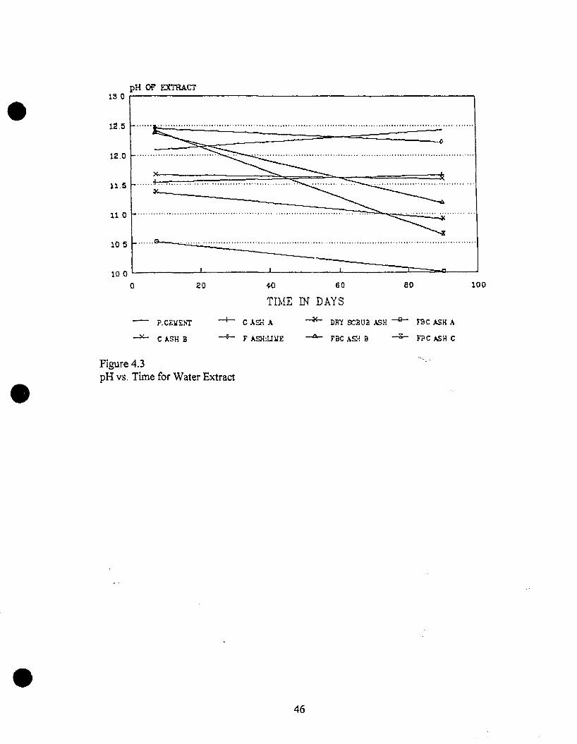
•pH OF EX'!'RAcr

150 ,...-----------------------------.

12.~ .. ~ , .

12.0

11.5

110

100ao6020

105r-=:·~:====~~~=~..lOOL

o

TIME IN DAYS

~ DR't S:;WB .AS11 -0- me,t,SH A?CEVEhi

C .'.SH B

-+- C.'.Si-! A

F .'.SH:UllE rlle .\SH B ~ flle ASH C

•Figure 4.3pH vs. Time for Water Extract

•46

• 5.0 SOLIDIFICATION 1STABILIZATION PROJECT

•

•

5.1 Objective and Scope

The objective of the solidificationlstabilization project was to immobilize metal

ions in mine tailings using a limelfly ash cementitious binder. The tailings were known to

contain large amounts ofheavy metals and sulfate, conditions that could easily lead to acid

mine drainage. As these additives have been seen to immobilize and reduce metal

leachability in industrial waste sludges, the project was designed to reveal the effect of

different types of additives, as weil as sorne of the mechanisms by which this reduction

took place.

As for the scope of the project, it was restricted to the chemical aspect of SIS and

the analyses were performed as such. Physical properties such as unconfined compressive

strength and permeability were not within the domain ofthis project. Two types offly ash,

type C (FAC) and type F (FAF), were used in the study to evaluate their effects on the

final products. The main chemical analysis for the treated tailings was a modified TCLP

(Toxicity Characteristic Leaching Procedure) leach test, in addition to batch tests with

water as the leachant and pH measurements. These were complimented by an x-ray

diffraction of selected samples to verify any mineralogical variations.

5.2 Materials

Two representative samples of sulfate-rich mine tailings were obtained from mine

sites in Quebec. They were labeled as waste #1 and #2 and kept in sealed plastic buckets

with their original moisture contents. Portions were taken out, spread in aluminum foil

dishes and put under a fume hood for air-drying. After 3-4 days, the dry samples were

gently crushed with a mortar and pest1e and put in sealed glass containers. The wastes

used for ail the experiments were obtained from these containers.

47

•

•

•

The lime used was commercial quicklime (CaO) with no major impurities. Two

types of fly ash (calcium-rich FAC and calcium-poor FAF) were also obtained and used

with lime for solidificationlstabilization. Table 5.1 gives the composition of the two fly

ashes. Deionized water was used in all the experiments and unless otherwise stated, it has

been referred to by the term "water" in this chapter. A basic assumption made to simpliry

matters, after verification, was that 1 ml. ofwater weighed 1 g. at room temperature.

5.3 Preliminary Experiments

5.3.1 Physical Characteristics

Although the physical aspect of solidificationlstabilization was not the main object

of study in the project, sorne basic tests were done to evaluate a few of the physical

properties of the tailings.

1. Moisture content:

This was the orny experiment where original samples from the buckets were used

as the natural moisture of the tailings was to be determined. The moisture content is the

ratio of the mass of fluid in the sample to the mass ofthe solid particles:

• Moisture content (%) = Weight of pore fluid (g) * 100 / Weight of solid particles (g)

Representative samples were taken from both wastes and put in pre-weighed aluminum

dishes. They were then weighed and put in an oven at a constant temperature of 110°C for

24 hours. After this period, the dishes were taken out, allowed to cool and weighed again.

Table 5.2 lists the results of the test.

2. Specifie gravity:

The specifie gravity of a soil is defined as "the ratio of a unit volume ofthe soi! at a

stated tempe,ature to the mass, in air, of the same volume of distilled water at a stated

temperature" (ASTM D854-83*). Since the samples at hand were mine tailings, it was

necessary to find Ol!t if their specifie gravities differed significantly from those of ordinary

soi!s, which are in the range of2. 60-2.75.

48

•

•

•

A volumetrie flask of 100 ml. capacity was cleaned and dried and its weight

determined. It was then filled to the mark with distilled water and weighed, the

temperature of the water also being measured. The water was transferred to a clean

beaker and approximately 25 g. of oyen dried waste was put into the empty flask. Then,

using water from the beaker, the flask was filled to 2/3 its capacity. Using vacuum suction

for approximately 20 minutes, air was removed from the soil-water mixture. The flask was

filled to the marker with additional distilled water and weighed. The temperature of the

solution was read but not used in the equation, as the difference was less than a degree.

Specifie gravity = Gt * Ws / {Ws + W2 - WI}

where, G( specifie gravity ofwater at T oC

Ws: dry weight of soil (g)

W2: weight of bottle and water

W1: weight ofbottle and water and soil

The results of the experiment are given in table 5.3.

3. Liquid limit and plastic limit:

The liquid limit and the plastic limit together constitute the Atterberg limits of a

soil. There are two popular methods for determining the liquid limit of a soil and both

were considered for testing the wastes. However, the method proposed by ASTM D4318

84* involving the use of the Casagrande apparatus proved to be a difficult one, since the

sarnples were rather silty in nature. This property did not allow cutting a clean groove in

the paste as is outlined in the method. Therefore, the cone-penetrometer method (British

Standard BS 1377:part 2:1990:4:3) [1] was employed. It involved the use of a polished

stainless steel cone, 80 g. in weight, which falls freely for 5 seconds and penetrates the seil

contained in a special cylindrical cup. The wastes were mixed with varying arnounts of

distilled water, put in the steel cup and tested with the cone. At least 4 readings between

15 and 25 mm. of penetration were taken for each one. The numbers were plotted against

the respective moisture contents of that sarnple. The liquid limits of the wastes were

49

•

•

•

determined by reading tbe moisture content for a penetration of 20 mm. The resu1ts are

given iD table 5.4, with figures 5.1 and 5.2 providing the plots. The plastic limits of the

wastes were analyzed by rolling sarnples witb different moisture contents to a thread about

3.2 mm. thick, without breaking it (ASTM D4318-84*). However, it was found that the

plastic limits for both soils were very close to their liquid limits and thus could not be

determined.

4. Sieve analysis:

Sieve analysis is probably tbe most common of all physical soil tests. Its main

purpose is to determine the relative abundance of certain ranges of particle size in a

sarnple, which plays an important role in the geotechnical properties of the soil. For Ihis

test, approximately 300 g. of each waste was used. The sarnples were first washed by tap

water over a #200 sieve (0.075 mm.), with the soil-water mixture that passed through

being collected in a clean bucket. This latter portion was then filtered using positive

pressure. The resu1ting cake and the portion retained on the sieve were both oven-dried at

110°C for 24 hours. The latter was then slightly ground and subjected to sieve analysis

with a mechanical shaker for 15 minutes. Table 5.5 lists the different sieve sizes used, as

well as the data obtained.

5.3.2 Cbemical Cbaracteristics

The chemical experiments performed on the waste sampies were part of the

preliminary tests needed to characterize their properties. Due to the focus of the project

on tbe chemical aspects of solidification/stabilization, these tests attempted to gain as

much information as possible.

1. pH measurement:

By far the simplest of all the chemical tests, this one was nevertheless crucial in

assessing the acidity of the wastes. The subsequent design of the treatment procedure was

largely based on these pH readings. The procedure followed ASTM D4972-89* and a

50

•

•

•

second method suggested by Head [1). Approximate1y 1 g. of each waste was taken and

put into plastic test-tubes, to which 10 ml. of distilled water was added. The tubes were

then agitated for 3 minutes on a mechanical shaker and allowed to sit for 1 hour before the

pH was measured. The meter used was an electronic Cole-Parmer model with an Orion

Sure-Flow electrode. Table 5.6 provides the results of the test.

2. Oxidation-reduction potential:

It is known that the oxidation-reduction (redox) potential readings of a solution

are directly related to its pH. The instrument used for the measurements was a combined

pH meter/redox potential meter with three electrodes; one for temperature reading, one

for reference and the indicator electrode. The reading taken was the potential difference

between the reference and indicator electrodes, which, in tum, depended on the activity of

hydrogen ion in the solution. Note that the redox potential of a solution is inversely

proportional to its pH. Samples of 3 g. were taken from each waste and 30 ml. of distilled

water was added to them in clean centrifuge tubes. They were placed on a mechanical

shaker for 1.5 hours, then poured into clean containers and their redox potentials read.

The results are presented in table 5.7 and show good inverse relationships with the pH

readings of the same samples. According to Benefield et al. [2], the readings do not

"indicate the presence or absence of a particular ion but, rather, indicate the activity ratio

of total oxidizing species present to that oftotal reducing species present".

3. X-ray fluorescence analysis:

XRF is a useful technique in determining the total composition of a sample. Hence,

the two wastes were analyzed by this method at the Geochemical Laboratories of the

university, the results ofwhich appear in table 5.8.

4. Acid digestion and elemental analysis:

The method of acid digestion involved the use of nitric (HN03) and hydrochloric

(HCl) acids as the main reagents. The use of hydrogen peroxide (H202), although

recommended, was intentionally limited as the wastes were known to contain no organic

51

•

•

•

matter. Samples of 2 g. were taken from each waste and transferred to a conical beaker.

To this was added 10 ml. of 1: 1 nitric acid:water solution and the beaker covered with a

watch glass. The slurry was heated to 95°C and refluxed for 20 minutes. After this period,

a 5 ml. dose of concentrate,} nitric acid was added to each beaker and allowed to reflux

for another 30 minutes, this last step being repeated one more time. The solution was then

allowed to evaporate until the soil was barely covered with liquid. The samples were

allowed to cool, after which 2 ml. of distilled wat~r and 3 ml. of 30% hydrogen peroxide

were added to each beaker. They were returned to the hot plates for warming and to begin

the peroxide reaction. No more th;'ü1 the initial 3 ml. of peroxide was used in the digestion,

as no organics were present for the reagent to digest. After this last step, 5 ml. of

concentrated hydrocWoric acid and 10 ml. of distilled water were added to the beakers and

allowed to reflux for another 15 minutes. The slurries were then allowed to cool and

diluted to 100 ml. with distilled water. The new solutions were allowed to sit for 30

minutes before 30 ml. of each was transferred to a tube and centrifuged at 8000 rpm for

10 minutes to separate the supernatant from the solid particles The former was analyzed

for different elements by flam~ atomic absorption (FLAA). The standards for the FLAA

were prepared from 1000 ppm liquid concentrates tor each element using distilled water

for dilution. The results of the analyses are given in table 5.9.


This set of experiments, although preliminary in time sequence, was distinct in the

sense that it forrned a prelu de to the actual project experiments. A series of tests was

needed to assess the different properties of the materials involved, including the wastes,

lime and the !WO types of fly ash. As was mentioned before, the pH of a treated sample

was crucial for the outcome of the project and was the single most important factor to be

monitored. Therefore, an accurate picture of the effect of lime on the wastes and the fly

ashes, as well as the effects of the ashes on the wastes, was needed. The set of

52

•

•

•

experiments carried out for this purpose was made up of optimum lime content (OLC) for

the wastes, optimum lime content for the fly ashes, and optimum fly ash content for the

wastes.. By the term "optimum", it should be understood the maximum pH attained by

using a relatively small percentage of the additive.

1. Optimum Lime Content:

The optimum lime content of the wastes was important in two ways: it would give

an idea as to the degree of acidity of the wastes, and would also reveal the effectiveness of

lime in raising their pH. A 1 g. sample of the waste was weighed accurately into a 50 ml.

centrifuge tube. Depending on the percentage, lime was also added to the tube and the

two were dry mixed by vigorous sha.1cing. To this mix, water was added in the ratio of

waste:water 1:5 by weight. The tubes were then put on a mechanical shaker for 1 hour.

After this step, they were allowed to sit for la minutes berore the pH was measured. The

percentages were determined arbitrarily at first, and were then narrowed down around

tbose numbers that gave the maximum pH for the minimum amount of lime. The results of

this test are given in table 5.10 for waste #1 and table 5.11 for waste #2.

2. Optimum Lime Content for the Fly Ashes:

This was a similar experiment to the one described above, except that the material

tested was fly ash, one of the additives in the projecl. Since lime and fly ash were the

binders used, it was very interesting to see the effects of their combination on the pH of

their end producl. It would also give an idea about the characteristics of the two types of

fly ash, as weil as a comparison between them. As before, a certain weight of fly ash (5 g.)

was placed in a centrifuge tube, with an appropriate amount of lime added to il. After dry

mixing, a fly ash:water ratio of 1:5 was added (25 ml.) to the mix and it was shaken for 1

hour. After 10 minutes of settling, the pH was measured and recorded. In table 5 12, the

results of the test are presented for both fly ashes.

3. Optimum Fly Ash Content:

The purpose ofthis experiment was to determine the effect of adding fly ash alone

53

•

•

•

to the waste samples. It was expected that the pH of the mix would increase, although not

as dramatically as with lime. Anc'h~r reason was to study the differences between the two

types of fly ash used, so as to have an idea about their capabilities. During the course of

the experiment, an upper limit for fly ash added was set at 35% by weight to the wastes. A

1 g. sample from each waste was placed in a centrifuge tube and fly ash was added

according to certain percentages. The ratio of waste:water was 1:5 and the mixtures were

shaken for 1 hour on the mechanical shaker. They were then allowed to sit for 10 minutes

before measuring the pH. Just as in the previous experiment, optimum lime content for fly

ash, it was seen that FAF produced a lower pH than FAC. After testing waste # l, it was

seen that no significant pHs were reached by adding 2%-10% of FAC. Therefore, for

waste #2, the starting point was taken at 10% FAC. By the term "significant", it is meant a

pH of at least 7.0. The results for waste #1 are given in table 5.13, while table 5.14

presents those for waste #2.

5.5 LimelFly Ash Binder

After completing the preliminary experiments, sorne early results had been

obtained. The general physical and chemical characteristics of both wastes had been

established, giving an important insight as to the presence of different heavy metals and

their relative abundance. Based on these results, a lime/fly ash binder with appropriate

proportions could be designed for the treatment of the wastes. Since most metals

precipitate at a pH around 11.0, it was decided that the maximum amount oflime added

should be equivalent to the least percentage oflime needed to obtain a pH of 12.0. This

amount varied depending on the waste, and was known from the optimum lime content

tests. The reason behind this logic was that if a certain amount of lime could raise the pH

to that level, there would be no reason to add more. Although one of the main purposes of

the projE:ct was to study the mechanisms of heavy metal immobilization in a lime/fly ash

binder, another object of study was the difference between two types of fly ash and the

54

•

•

•

extent 1.0 which they could replace lime in the binder. Hence, the binder was designed such

that:

- The minimum amount oflime needed 1.0 raise the pH 1.0 12.0 would be the upper limit of

lime addition. Accordingly, one sample from each waste would have this amount of lime

without any fly asi: in il., as the lime would be enough 1.0 obtain the required pH.

- Another set of samples from each waste would next receive lime in an amount that

would be 1% less than the optimum lime content of the waste. This decrease in lime

content would be compensated by the addition of 0, 10, 20, 30, 40 and 50% by weight

(relative 1.0 waste) of each type of fly ash. In this manner, il. would be apparent as 1.0 how

the fly ash affected the treated waste and if il. made up for the decrease in lime.

- A third set of samples would receive an amount of lime which would be 2% less than the

optimum lime content. The fly ash would again be in the amount of 0, 10, 20, 30, 40 and

50% by weight of the waste.

- One sample from each waste would receive no additives al. ail and be the control sample.

- Thus, a total of 24 samples would be prepared from each waste.

One of the most important parameters in the treatment of the wastes was the

amount of water that would be added 1.0 the mix. Based on several sources in the literature

[3, 4, 5, 6], and from cornmon practice in the cement industry, il. was decided that this

amount would be in the ratio of water:binder =0.30 by weight. By the term "binder" il. is

meant the sum of the weights of fly ash and lime. However, this was c1early a very small

amount if il. were 1.0 be added 1.0 the dry waste, lime and fly ash mix by itself, and would be

absorbed by the waste before the hydration of lime could take place. In the Iiterature, the

usual practice seemed 1.0 be the addition oflime or other additives 1.0 a sludge [7, 8, 9, 10,

Il], which would eliminate the problem of water. Therefore, il. wan decided 1.0 add the

minimum arriount of water that would saturate the wastes completely and render them

incapable ofp.bsorbing the hydration water. After performing a surface saturation test on

the wastes act.ording 1.0 ASTM C-128*, it was obvious that the m":.;ture needed 1.0 just

55

•

•

•

fully saturate the waste was very close to its liquid limit value. Hence, it was decided to

add water in the following manner:

Total amount ofwater added to a sample = Liquid !imit value of the waste +

Water:binder ratio of 0.30 for lime hydration Equation 1

The next question that arose was the manner in which the different components would be

mixed. At first, it was considered to add the liquid limit part of the water to the waste and

let it stand for 24 hours in sealed containers. The lime, fly ash and hydration water would

then be added to the slurry on the following day. However, this would inhibit a thorough

mixing of the lime, which would form lumps as 50on as it came in contact with the moist

waste. The best option available, as seen from sorne initial test mixes, was to dry mix the

waste, lime and fly ash and achieve a homogeneous mix. The total amount of water

needed would then be gradually added and thoroushly mixed until a paste was obtained.

As such, the latter method was followed with 40 g. of waste per sample forming

the basis for mix preparation. The number of different mixes for each waste amounted to

24 samples. The lime and fly ash percentages were ail based on the 40 g. ofwaste used for

each sample. The amount ofwater to be added was calculated as indicated in Equation J.

After the paste was thoroughly mixed, the containers were tapped gently 50 as to

settle the mixture in a compact manner. They were then sealed, and put in a 100% relative

humidity environment for curing. The weights and percentages of ail the components are

given in tables 5.15 and 5.16 for wastes #1 and #2, respectively.

5.6 TCLP Leaching of the Treated Wastes

The major indication as to the success of a certain binder in immobilizing heavy

metals is the amount leached under certain conditions. In recent years, the Toxicity

Characteristic Leaching Procedure (TCLP) put forward by the EPA has been a popular

method of leaching among researchers [12, 13]. A detailed summary of the method can be

found in a special US EPA publication [14]. Owing to the wide usage ofthis test, it was

56

•

•

•

decided to adopt a modified version of the TCLP for the project. The reason for the

modification was the unavailability of certain equipment, such as a rotary tumbler and a

pressure filter apparatus. The solutions used for the test were the same ones indicated in

the guidelines. The control sample for each waste, being free of any additives, maintained

a pH below 5.0, requiring the use of TCLP solution #1, with a pH of 4.85. Ali the other

sampies had pHs higher than 5.0, thus requiring TCLP solution #2, with a pH of2.85.

The samples were leached after l, 14 and 35 days of curing. A 2 g. portion of each

treated sample was taken and placed in a small plastic bottle, to which 40 ml. ofthr:: proper

TCLP solution was added. The bottles were then capped and placed on a mechanical

shaker, moving horizontally, for 15 hours. The length of time was decided upon after a

series of initial tests on identical samples, indicating that after 15 hours on the sh'lker, the

am01!nt of the elements leached from a certain sample remained constant. After the

agitation period, the sampies were vacuum filtered using 0.45 ~m tilter papers and their

pHs recorded. To compare results, 6 selected samples were also leached with water.

These samples have been indicated in tables 5.15 and 5.16. After the pH measurement, the

samples were acidified with a few drops of concentrated nitric acid. AlI of the samples also

underwent a soil pH measurement. A gram oftreated waste was put in a sealed tube, with

10 ml. of water. The mixtures were agitated for 1 hour, let to sit for 10 minutes and their

pH was then measured and recorded.

5.7 Elemental Analysis and Sulfate Measurement

The leachates, after being tested for the pH, were prepared for elemental analysis.

This was done by flame atomic absorption (FLAA) using a Parkin-Elmer 3500 machine. It

was decided to 3.l.'1alyze the leachates for 8 elements; aluminum (Al), calcium (Ca),

chromium (Cr), copper (Cu), iron (Fe), magnesium (Mg), lead (Pb) and zinc (Zn).

Chromium, copper, iron, lead and zinc were metals that needed to be immobilized due to

their abundance in the wastes and their high toxicity. Calcium and aluminum were

57

•

•

•

monitored as they constitute two of the major elements involved in pozzolanic reactions.

Magnesium was monitored as a control element, as weil as a possible exchangeable cation

between the waste and the binder. Dilutions of 1/10, 1/100 and 111000 were prepared

from the leachates, using TCLP #1, #2 or water as the dilutant, depending on the solution

the sample had been leached with. Standards for the various elements were made from

1000 ppm concentrates, using TCLP #2 as the dilutant, as explained in Appendix 1. After

these preparations, the samples were analyzed for the various elements.

Another important measurement was th~' sulfate (S04-2) content of the samples.

This was done by using a Dionex DX-IOO Ion Chromatograph (IC). Standards were

prepared for the IC and injected into it for analysis. The leachate of a given sample, or one

of its dilutions, would then be injected into the IC and the result compared to the

standards and read accordingly. The importance of the sulfate component cannot be

overemphasized. Since it constitutes one of the primary reasons for the production of acid

mine drainage, the ability of a binder to reduce sulfate leachability is almost as important

as its ability to immobilize heavy metal ions. The samples were tested after l, 14 and 35

days of curing and showed sorne very interesting results. Tables 5.17, 5.18 and 5.19

present the results of elemental analysis for waste # l, as weil as the pH values for the

leachates and the wastes. The results for waste #2 are given in tables 5.20, 5.21 and 5.22.

Since sample #1 was leached with TCLP #l, it was thought that leaching it with TCLP #2

as well would prove to be useful in making comparisons between the two solutions. This

was done for both wastes and the results compared in table 5.23.

5.8 X-Ray Diffraction

Pozzolanic reactions take place whenever lime and fly ash are mixed together and

hydrated. It was expected that new minerais would form in these reactions and old ones

would disappear. The best way to study these mineralogical changes was by x-ray

diffraction (XRD). For this purpose, a Rigaku DIMAX 2400 x-ray diffractometer was

58

•

•

•

employed. Six sampies were chosen to be analyzed after 1, 14 and 35 days of cur:r::g. The

reason these particulr..r samples were chosen was that each one had the maximum ::.mount

of fly ash for a certain lime percentage and would thus show maximum reactivity. After

the indicated curing period, samples were removed from the containers and placed in

aluminum dishes. These were then placed in a conventional oyen at 40°C for 20 minutes to

obtain a relatively dry chunk. The dried samples were lightly ground and the powder

analyzed by XRD. Mineralogical analysis was performed using the JADE Search/Match

software. The graphs are presented as follows for waste #1:

- Figures 5.3 through 5.7 are for samples #7, #12, #18, #2.3, #24, respective1y. The

lowermost graph belongs to the control sample, with the 1 day, 14 days and 35 days old

samples shown from bottom to top, respectively. This has been done to facilitate

comparisons of the same sample over the curing period.

As for waste #2, the analyses is presented in the following manner:

- Figures 5.8 through 5.12 are for samples #7, #12, #18, #23, #24, respectively. The same

procedure as the one above has been adopted, with the lowermost graph being that of the

control sample.

59

Table 5.1Composition of Ry Ashes Type C and F

Si02AI203Ti02P20SFe203CaOSrOMgONa20K20

S03Loss on Ignition (LOI)Total~

MoistureLOI at 750°CIrotal Carbon

Available Na20

Available K20

53.3023.630.710.124.4012.450.221.153.030.420.200.71

100.34

0.060.370.631.140.29

40.7117.930.850.17

29.862.800.151.090.731.561.271.95

99.07

0.060.250.481.360.26

*All constituents are expressed in percentages.

Table 5.2Moisture Content of Wastes

1 1 1.72 39.01 35.952 1.66 55.36 50.463 1.67 48.91 44.90

t 2

4 1.71 48.83 45.12

1 1.75 31.64 29.322 1.68 23.11 21.55-

AIl weights are expressed in grams.

60

3.06 34.23 8.944.90 48.80 10.044.01 43.23 9.283.71 43.41 8.55 9.20

2.32 27.57 8.411.56 19.87 7.85 8.13

• Table 5.3Specifie Gravity Values

Wt of soil 25.01 24.99

Wt of s+w+b (Tx) 692.64 694.45

Wt of b+w (Ty) 676.12 676.28

Temperature Tx 20.60 21.35

Temperature Ty 21.00 21.40

Specifie gravity 2.94 3.66

Pu: weights are expressed in grams. s:soil (waste), b: bonle, w:water. .

•Table 5.4Cone Penetrometer Results

1

2

1 17.24 4 1.73 12.60 10.88 18.802 18.07 TM 1.62 12.82 11.04 18.903 17.92 SM 1.62 14.36 12.34 18.844 25.03 TI 1.60 11.64 9.99 19.675 23.12 R 1.60 14.92 12.77 19.25

1 14.28 1 1.71 12.36 10.94 15.382 19.43 SH1 1.55 12.19 10.71 16.163 20.57 H1 1.55 11.52 10.08 16.884 22.42 H2 1.56 16.86 14.65 16.88

19.06

16.50

•

Ali weights are expressed in grams.

61

100.00100.00100.0099.3776.4862.1836.934.410.00

•

•

Table 5.5 (a)Sieve Analysis for Waste #1

lid 295.40 295.40 0.00 0.00 0.00 100.0010 2.000 466.27 466.32 0.05 0.04 0.04 99.9620 0.840 423.70 423.78 0.08 0.07 0.11 99.8940 0.425 477.63 485.26 7.63 S 52 6.73 93.2780 0.180 343.28 403.55 60.27 li2.28 59.01 40.99

100 0.150 355.94 370.89 14.95 12.97 71.98 28.02140 0.106 248.75 264.85 16.10 13.96 85.94 14.06200 0.075 328.27 340.45 12.18 10.56 96.50 3.50pan 355.94 359.97 4.03 3.50 100.00 0.00

Total 115.29 100.00

Table 5.5 (b)Sieve Analysis for Waste #2

.1L~'.~.II'.'111.I~l~~~I~r\~'~~~~~(p~r~:;l!id 295.40 295.40 0.00 0.00 0.00

Il 10 2.000 466.32 466.32 0.00 0.00 0.00,20 0.840 423.70 423.70 0.00 0.00 0.00

40 0.425 477.63 478.26 0.63 0.63 0.6380 "U80 343.23 366.00 22.77 22.88 23.52

100 0.150 355.87 370.10 14.23 14.30 37.82140 0.106 248.95 274.08 25.13 25.25 63.07200 0.075 328.85 361.21 32.36 32.52 95.59pan 356.04 360.43 4.39 4.41 100.00

Total

AlI weights are expressed in grams.

Table 5.6pH Values of Wastes

99.51 100.00

•1

2

1212

3.233.292.46

2.45

3.26

2.46

62

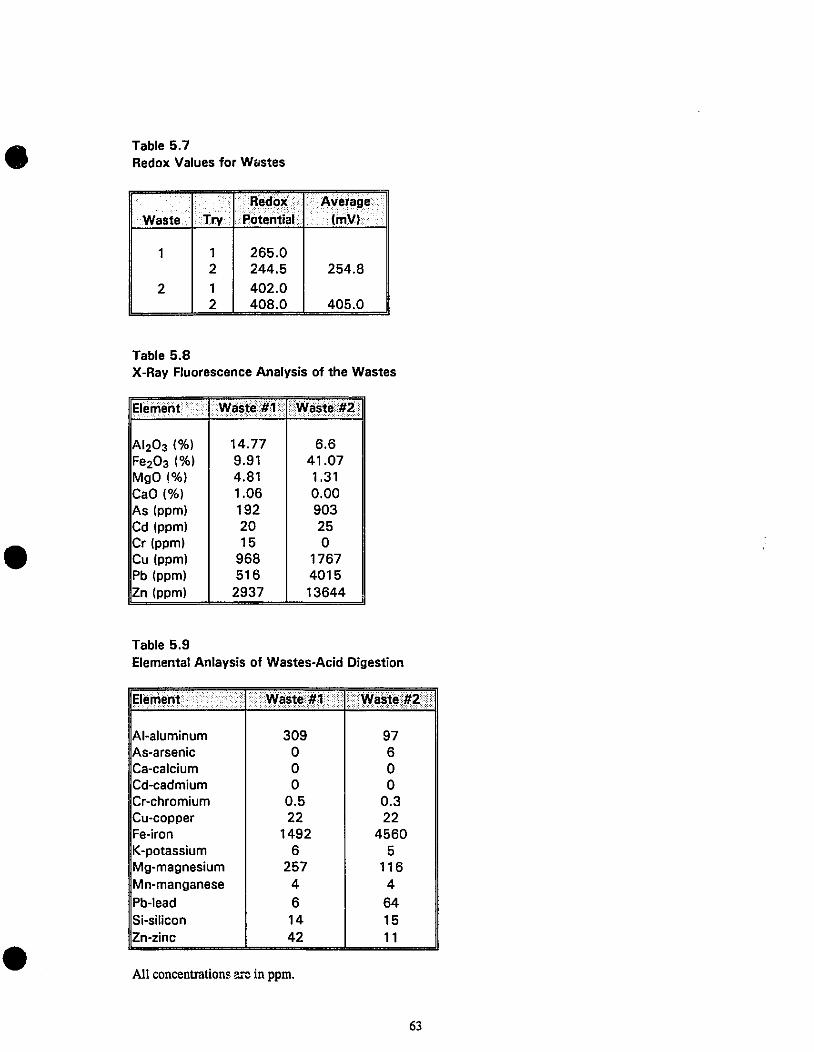
• Table 5.7Redox Values for WlIstes

_. Redox AveiageWaste 1rv Potential (mV)

2

1212

265.0244.5

402.0408.0

254.8

405.0

Table 5.8X-Ray Fluorescence Analysis of the Wastes

Element· Wliste#1 Wliste#2

•

AI20a (%)

Fe20a (%)MgO (%)

CaO (%)As (ppm)Cd (ppm)Cr (ppm)Cu (ppm)Pb (ppm)Zn (ppm)

14.779.914.811.061922015

968516

2937

6.641.071.310.0090325o

1767401513644

Table 5.9Elemental Anlaysis of Wastes-Acid Digestion

''''CIUC,",· .... . Wliste#1· .....·Wàste#2 .•.•.

AIl concentrations a.-c in ppm.•

AI-aluminumAs-arsenicCa-calciumCd-cadmiumCr-chromiumCu-copperFe-ironK-potassiumMg-magnesiumMn-manganesePb-leadSi-siliconZn-zinc

309ooo

0.522

14926

257461442

976oo

0.322

45605

1164

641511

63

• Table 5.10Optimum Lime Content-Waste #1

0.99970.99971.00001.0000

AlI weights are in grams.

0.00980.01960.02950.0398

0.981.962.953.98

7.4411.8012.8512.37

•

Table f;.11Optimum Lime Content-Waste #2

0.9998 0.0199 1.99 7.010.9996 0.0298 2.98 10.531.0001 0.0402 4.02 12.250.9~39 0.0700 7.00 12.441.0002 0.0896 8.96 13+0.9995 0.1000 10.01 13+1.0003 0.1108 11.08 NIA1.0004 0.1304 13.03 NIA

AU weights are in grarns.

Table 5.12O.,i~mum Lime Content for Fly Ashes-Results

•

C (Sundance)

F (Tupper Point)

0.001.002.053.034.035.000.001.042.013.033.99

5.01

12.1612.2611.7411.9312.1711.838.5311.7611.9912.0311.72

12.13

64

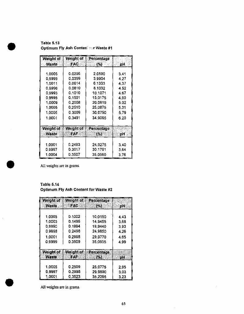
• Table 5.13Optimum Fly Ash Conter.~ ".If Waste #1

1.0005 0.0206 2.0590 3.410.9999 0.0399 3.9904 4.271.0011 0.0614 6.1333 4.370.9996 0.0810 8.1032 4.520.9993 0.1010 10.1071 4.670.9995 0.1501 15.0175 4.901.0009 0.2008 20.0619 5.021.0005 0.2510 25.0875 5.311.0005 0.3009 30.0750 5.791.0001 0.3491 34.9065 6.20

AlI weights are in grams.•1.00010.99971.0004

0.24930.30170.3507

24.927530.179135.0560

3.403.643.76

Table 5.14Optimum Fly Ash Content for Waste #2

1.00051.00030.999C0.9998

1.00010.9999

0.10020.14950.19940.24980.29980.3509

10.015014.945519.944024.9850

29.977035.0935

4.433.683.934.26

4.654.99

Alt weights are in grams.•1.00050.99971.0001

0.25090.29980.3523

25.077529.989035.2265

2.953.033.23

65

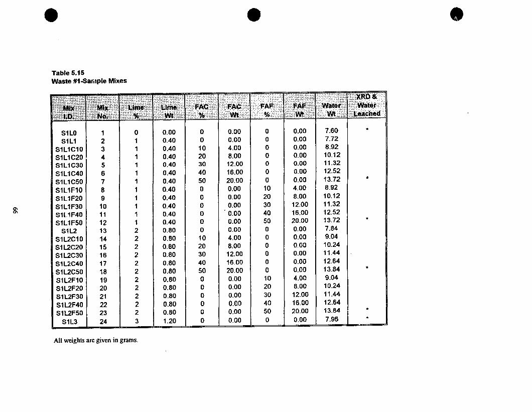
•Table 5.15Waste #1-Sarilple Mixes

• •

S1LO 1 0 0.00 a 0.00 0 0.00 7.60

S1L1 2 1 0.40 0 0.00 a 0.00 7.72

S1L1C10 3 1 0.40 10 4.00 0 0.00 8.92

S1L1C20. 4 1 0.40 20 8.00 0 0.00 10.12

S1L1C30 5 1 0.40 30 12.00 a 0.00 11.32

S1L1C40 6 1 0.40 40 16.00 0 0.00 12.52

S1L1C50 7 1 0.40 50 20.00 0 0.00 13.72

S1L1F10 8 1 0.40 0 0.00 10 4.00 8.92

S1L1F20 9 1 0.40 0 0.00 20 8.00 10.12

0- S1L1F30 10 1 0.40 0 0.00 30 12.00 11.320- S1L1F40 11 1 0.40 0 0.00 40 16.00 12.52

S1L1F5D 12 1 0.40 a 0.00 50 20.00 13.72

S1L2 13 2 0.80 0 0.00 a 0.00 7.84

S1L2C10 14 2 0.80 10 4.00 a 0.00 9.04

S1l2C20 15 2 0.80 20 8.00 0 0.00 10.24

S1L2C30 16 2 0.80 30 12.00 0 0.00 11.44

S1L2C40 17 2 0.80 40 16.00 a 0.00 12.64

S1l2CSO 18 2 0.80 50 20.00 0 0.00 13.84

S1L2F10 19 2 0.80 0 0.00 10 4.00 9.04

S1L2F20 20 2 0.80 0 0.00 20 8.00 10.24

S1L2F30 21 2 0.80 a 0.00 30 12.00 11.44

S1L2F40 22 2 0.80 a 0.00 40 16.00 12.64

S1L2F50 23 2 0.80 a 0.00 50 20.00 13.84

S1L3 24 3 1.20 0 0.00 0 0.00 7.96

Ail weights are given in grams.

..

Ir

Ir

..

..

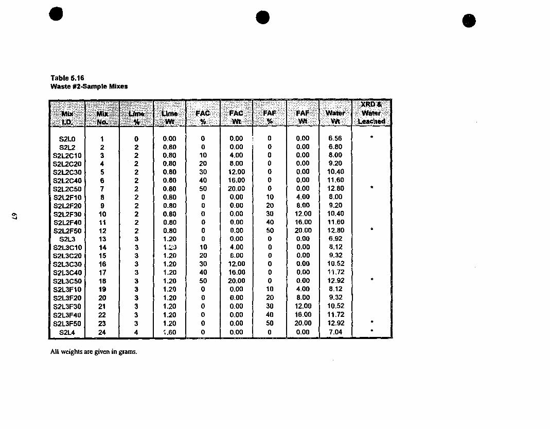
•Table 5.16Waste #2-Sample Mixes

• •

S2LO 1 0 0.00 a 0.00 a 0.00 6.56S2L2 2 2 0.80 0 0.00 0 0.00 6.80

S2L2C10 3 2 0.80 10 4.00 a 0.00 8.00S2L2C20 4 2 0.80 20 8.00 a 0.00 9.20S212C30 5 2 0.80 30 12.00 0 0.00 10.40S2L2C40 6 2 0.80 40 16.00 0 0.00 11.60S212C50 7 2 0.80 50 20.00 0 0.00 12.80S2L2F10 8 2 0.80 a 0.00 10 4.00 8.00S2L2F20 9 2 0.80 a 0.00 20 8.00 9.20

0- S2L2F30 10 2 0.80 a 0.00 30 12.00 10.40....S2L2F40 11 2 0.80 a 0.00 40 16.00 11.60S2L2F50 12 2 0.80 0 0.00 50 20.00 12.80

S2L3 13 3 1.20 a 0.00 a 0.00 6.92S2L3C10 14 3 1.:::J 10 4.00 0 0.00 8.12S2l3C20 15 3 1.20 20 8.00 0 0.00 9.32S2L3C30 16 3 1.20 30 12.00 0 0.00 10.52S2L3C40 17 3 1.20 40 16.00 0 0.00 11.72S2L3C50 18 3 1.20 50 20.00 a 0.00 12.92S2L3F10 19 3 1.20 0 0.00 10 4.00 8.12S2L3F20 20 3 1.20 0 0.00 20 8.00 9.3252L3F30 21 3 1.20 0 0.00 30 12.00 10.52S2L3F40 22 3 1.20 0 0.00 40 16.00 11.72S2L3F50 23 3 1.20 0 0.00 50 20.00 12.92

S2L4 24 4 ~.60 a 0.00 0 0.00 7.04

AU weights are given in grams.

..

..

..

..

..

..

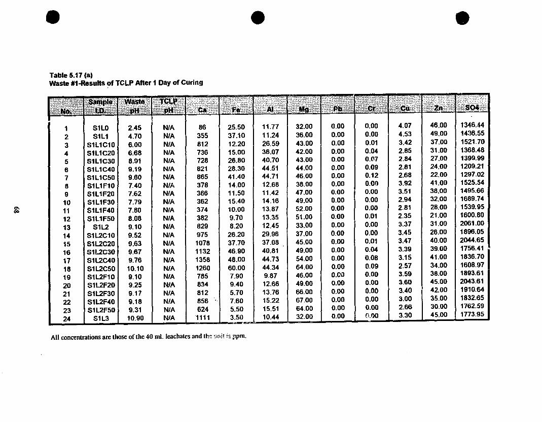
•Table 5.17 (a.Waste #1-Results ~f TClP After 1 Day of Curing

• •

1 S1LO 2.45 NIA 86 25.50 11.71 32.00 0.00 0.00 4.07 46.00 1346.44

2 S1L1 4.70 NIA 355 37.10 11.24 36.00 0.00 0.00 4.53 49.00 1436.55

3 S1L1C10 6.00 NIA 812 12.20 26.59 43.00 0.00 0.01 3.42 37.00 1521.70

4 SiLi C20 6.68 NIA 736 15.00 36.07 42.00 0.00 0.04 2.85 31.00 1368.48

5 S1L1C30 8.91 NIA 728 26.80 40.70 43.00 0.00 0.07 2.84 27.00 1399.99

6 S1L1C40 9.19 NIA 821 28.30 44.51 44.00 0.00 0.09 2.81 24.00 1209.21

7 S1L1CSO 9.60 NIA 865 41.40 44.71 46.00 0.00 0.12 2.68 22.00 1297.02

8 51L1F10 7.40 NIA 378 14.00 12.68 38.00 0.00 0.00 3.92 41.00 1525.54

9 S1L1F20 7.62 NIA 366 11.50 11.42 47.00 0.00 0.00 3.51 38.00 1495.66

10 51L1F30 7.79 NIA 362 15.40 14.16 49.00 0.00 0.00 2.94 32.00 1689.74CI\ 11 S1L1F40 7.80 NIA 374 10.00 13.87 52.00 0.00 0.00 2.81 28.00 1539.9500

12 S1l1F50 8.08 NIA 382 9.70 13.35 51.00 0.00 0.01 2.35 21.00 1600.80

13 51L2 9.10 NIA 829 8.20 12.45 33.00 0.00 0.00 3.37 31.00 2061.00

14 51L2C10 9.52 NIA 975 26.20 29.96 37.00 0.00 0.00 3.45 26.00 1896.05

15 51L2C20 9.63 NIA 1078 37.70 37.08 45.00 0.00 0.01 3.47 40.00 2044.65

16 51l2C30 9.67 NIA 1132 46.90 40.81 49.00 0.00 0.04 3.39 39.00 1756.41

17 51L2C40 9.76 NIA 1358 48.00 44.73 54.00 0.00 0.08 3.15 41.00 1836.70

18 S1L2CSO 10.10 NIA 1260 60.00 44.34 64.00 0.00 0.09 2.57 34.00 1608.97

19 51L2F10 9.10 NIA 785 7.90 9.87 46.00 0.00 0.00 3.59 38.00 1893.61

20 51L2F20 9.25 NIA 834 9.40 12.66 49.00 0.00 0.00 3.60 45.00 2043.61

21 51L2F30 9.17 NIA 812 5.70 13.76 66.00 0.00 0.00 3.40 42.00 1910.64

22 S1L2F40 9.18 NIA 856 " 7.60 15.22 67.00 0.00 0.00 3.00 35.00 1832.65

23 S1L2F50 9.31 NIA 624 5.50 15.51 64.00 0.00 0.00 2.66 30.00 1762.59

24 S1L3 10.90 NIA 1111 3.50 10.44 32.00 0.00 0.00 3.30 45.00 1773.95

Ali concentrations are those of the 40 ml. leachates and th~ 'wit !S :Jpm.

•Table 5.18 (a)Waste *1-Results of Tell» Mer 14 Days of Curing

• •

123456789101112131415161718192021222324

S1l0S1l1

S1l1C10S1L1C20S1L1C30S1l1C40S1l1C50S1l1F10S1l1F20S1l1F30Sll1F40S1l1F50

S1L2S112C10S1L2C20S1L2C30S1L2C40S112C50S1l2F10S112F20S112F30S1L2F40S1L2F50

S1l3

2.564.118.449.229.569.679.907.087.298.328.808.969.909.899.809.9110.1510.458.969.068.879.419.3410.41

4.282.703.323.593.743.723.792.862.973.073.143.223.283.563.653.703.173.853.273.233.263.303.303.55

8131944~

526705803807343362352386394743821886

1092107010786436246146346061110

8.6023.707.9010.209.60

10.2012.0014.1010.108.707.307.309.80

10.3011.9014.6036.6046.3010.006.206.204.907.103.63

5.4614.9243.4364.4673.8576.9979.5515.6216.1716.4219.9121.3315.7846.4159.6466.3782.9086.7419.2518.7620.4423.3024.528.17

32.0036.0047.0044.0041.0044.0041.0044.0048.0040.0047.0053.0029.0036.0040.0043.0048.0047.0038.0043.0050.0053.0059.0034.00

0.100.000.000.000.000.000.000.000.000.000.000.000.360.000.000.000.000.000.000.000.000.000.000.00

0.000.000.000.000.000.000.020.000.000.000.000.000.000.000.000.010.040.060.000.000.000.000.000.00

3.253.482.772.592.322.201.923.353.202.842.622.323.382.932.842.622.542.443.663.233.112.882.633.52

50.0050.0028.0028.0020.0020.0016.0039.0040.0035.0023.0018.0022.0021.0035.0041.0038.0037.0044.0044.00311.0033.0039.0059.00

1313.001401.221299.751170.621039.701006.55925.231379.241314.791122.931092.641098.881448.191426.831389.841339.561277.951223.541654.191550.651537.961408.751468.821192.44

AU concentrations are tho~·: of the 40 ml. leachates and the unit is ppm.

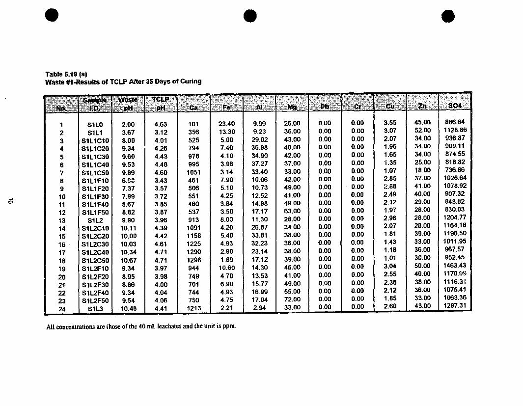
•Table 5.19 (a)Waste #1-Results of TCLP After 35 Days of Curing

• •

1 SilO 2.00 4.63 101 23.40 9.99 26.00 0.00 0.00 3.55 45.00 886.64

2 S1L1 3.67 3.12 356 13.30 9.23 36.00 0.00 0.00 3.07 52.00 1128.86

3 S1L1C10 8.00 4.01 525 5.00 29.02 43.00 0.00 0.00 2.07 34.00 936.87

4 S1L1C20 9.34 4.26 794 7.40 36.98 40.00 0.00 0.00 1.96 34.00 909.11

5 S1L1C3D 9.60 4.43 978 4.10 34.90 42.00 0.00 0.00 1.65 34.00 874.55

6 S1l1C4D 9.53 4.48 995 3.96 37.27 37.00 0.00 0.00 1.35 25.00 818.82

7 S1L1C50 9.89 4.60 1051 3.14 33.40 33.00 0.00 0.00 1.07 18.00 736.86

8 S1L1F1D 6.se 3.43 461 7.90 10.06 42.00 0.00 0.00 2.85 37.00 1026.64

9 S1L1F20 7.37 3.57 506 5.10 10.73 49.00 0.00 0.00 ~!.ô8 41.00 1078.92

.... 10 S1L1F30 7.99 3.72 551 4.25 12.52 41.00 0.00 0.00 2.49 40.00 907.320 11 S1L1F40 8.67 3.85 460 3.84 14.98 49.00 0.00 0.00 2.12 29.00 843.82

12 S1L1F50 8.82 3.87 537 3.50 17.17 63.00 0.00 0.00 1.97 28.00 830.03

13 S1L2 9.90 3.96 913 8.00 11.30 28.00 0.00 0.00 2.96 28.00 1204.77

14 S1L2C1D 10.11 4.39 1091 4.20 26.87 34.00 0.00 0.00 2.07 28.00 1164.18

15 S1L2C20 10.00 4.42 1158 5.40 33.81 38.00 0.00 0.00 1.81 39.00 1196.50

16 . S1L2C30 10.03 4.61 1225 4.93 32.23 36.00 0.00 0.00 1.43 33.00 1011.95

17 S1L2C40 10.34 4.71 1290 2.90 23.14 38.00 0.00 0.00 1.18 36.00 967.57

18 S1L2C50 10.67 4.71 1298 1.89 17.12 39.00 0.00 0.00 1.01 30.00 952.45

19 S1L2F10 9.34 3.97 944 10.60 14.30 46.00 0.00 0.00 3.04 50.00 1463.43

20 S1L2F20 8.95 3.98 749 4.70 13.53 41.00 0.00 0.00 2.55 40.00 1170.0~ ,

21 S1L2F30 8.86 4.00 701 6.90 15.77 49.00 0.00 0.00 2.36 38.00 1116.31

22 S1L2F40 9.34 4.04 744 4.93 16.99 55.00 0.00 0.00 2.12 36.00 1075.41

23 S1L2F50 9.54 4.06 750 4.75 17.04 72.00 0.00 0.00 1.85 33.00 1063.36

24 S1L3 10.48 4.41 1213 2.21 2.94 33.00 0.00 0.00 2.60 43.00 1297.31

Ail concentrations are ,hose of the 40 ml. leachates and the unît is ppm.

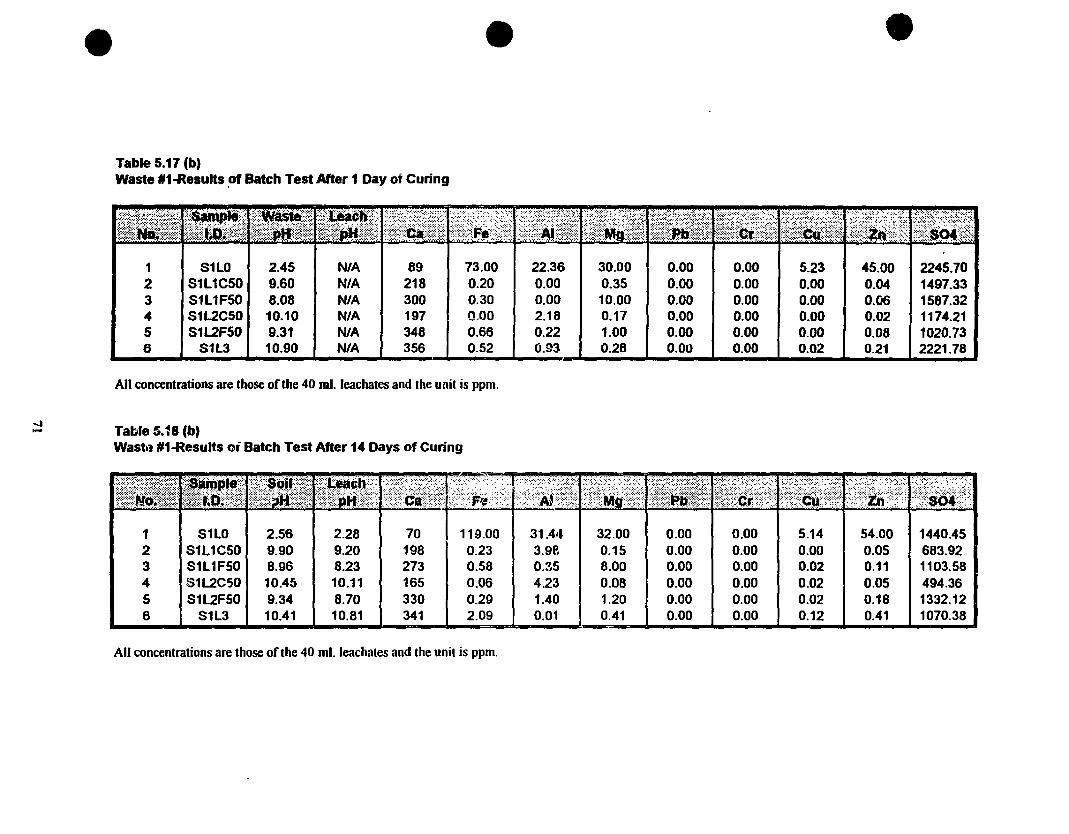
• • •Table 5.17 (b)Waste 1Il1-Results ~f Batch Test After 1 Day oi Curing

1 S1LO 2.45 NIA 892 S1L1CSO 9.60 NIA 2183 S1L1FSO 8.08 NIA 300.. S1L2C50 10.10 NIA 1975 S1L2F50 9.31 NIA 3486 S1l3 10.90 NIA 356

73.00 22.36 30.00 0.00 0.00 5.23 45.00 2245.700.20 0.00 0.35 0.00 0.00 0.00 0.04 1497.330.30 0.00 10.00 0.00 0.00 0.00 0.06 1587.32<tOO 2.18 0.17 0.00 0.00 0.00 0.02 1174.210.66 0.22 1.00 0.00 0.00 0.00 0.08 1020.730.52 0.93 0.28 0.00 0.00 0.02 0.21 2221.78

Ali concentrations are those of the 40 ml. Jeachates and the unit is ppm.

...- Table S.18 (b)

Wast\! #1-Results oi Batch Test After 14 Days of Curing

31.4•• 32.00 0.00 0.003.ge 0.15 0.00 0.000.35 8.00 0.00 0.004.23 0.06 0.00 0.001.40 1.20 0.00 0.000.01 0.41 0.00 0.00

"1r1l.L~Diiliïi~il(';~""~"~1!IWN/;/'1If_1~~I.~il~>~··:;,;..[:/::],·.~~..::;:~:~~)·:·;i:<~:;;:~.~:'1 S1LO 2.56 2.28 70 119.00 5.14 54.00 1440.452 S1L1CSO 9.90 9.20 198 0.23 0.00 0.05 683.923 S1L1F50 8.96 8.23 273 0.58 0.02 0.11 1103.584 S1L2CSO 10.45 10.11 165 0.06 0.02 0.05 494.365 S1l2FSO 9.34 8.70 330 0.29 0.02 0.18 1332.126 S1L3 10.41 10.81 341 2.09 0.12 0.41 1070.38

Ali concentrations are those of the 40 ml. leachales and the unÎt is ppm.

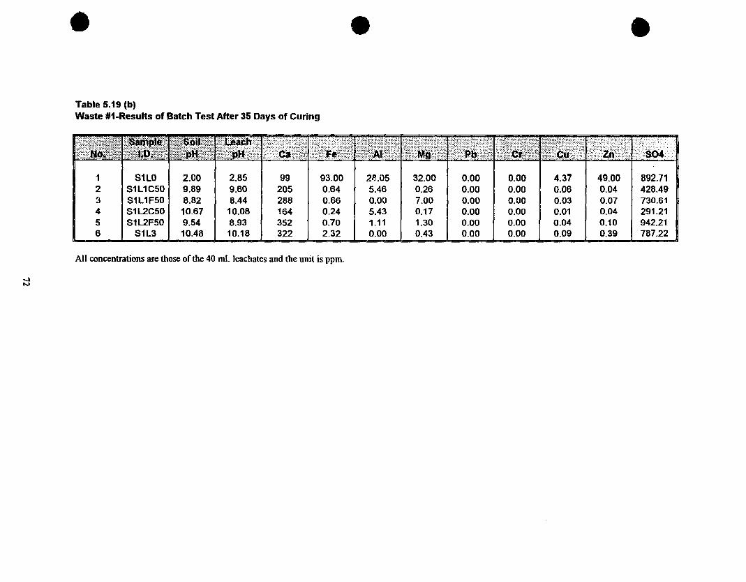
•Table 5.19 (b)Waste #1-Results of Batch Test After 35 Days of Curing

• •

1 S1LO 2.00 2.852 S1L1CSO 9.89 9.603 S1L1FSO 8.82 8.444 S1L2CSO 10.67 10.085 S1L2F50 9.54 8.936 S1L3 10.48 10.18

99205288164352322

93.00 2e.05 32.00 0.000.64 5.46 0.26 0.000.66 0.00 7.00 0.000.24 5.43 0.17 0.000.70 1.11 1.30 0.002.32 0.00 0.43 0.00

0.00 4.37 49.00 892.710.00 0.06 0.04 428.490.00 0.03 0.07 730.610.00 0.01 0.04 291.210.00 0.04 0.10 942.210.00 0.09 0.39 787.22

Ali concentrations are those of the 40 ml. Jeachates and the unit is ppm.

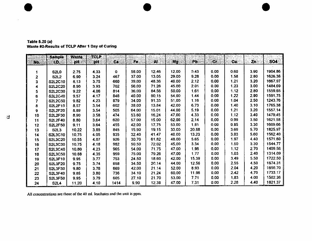
•Table 5.20 (a)Waste #2-Results of TCLP After 1 Day of Curing

• •

123456789

101112131415161718192021222324

S2LOS2l2

S2L2C10S2l2C20S2L2C30S2L2C"~O

S2L2c!SOS2L2F10S2L2F20S2L2F30S2L2F40S2L2F50

S2L3S2L3C10S2L3C20S2L3C30S2L3C40S2L3C50S2L3F10S2l3F20S2l3F30S2l3F40S2l3F50

S2l4

2.756.908.138.909.229.579.828.578.898.908.809.11

10.2210.7510.5510.7510.8010.889.959.759.809.859.9511.20

4.333.243.753.934.064.174.233.543.543.583.643.643.854.054.074.184.234.353.773.743.763.803.794.10

o46766Q7028148488796025054746204558459359269829659597536586697366051414

58.0037.0039.0056.0036.0040.0034.0038.0064.0053.6057.0042.0015.9032.4030.7050.5054.0075.0024.5034.5042.0034.1027.109.90

12.4613.0548.3671.2684.5690.1591.3313.8415.0116.2415.0017.7519.1541.4761.8272.0271.7579.2618.6020.1421.1421.2421.7012.39

12.0029.0046.0045.0050.0054.0051.0042.0044.0047.0062.0053.0033.0040.0048.0045.0047.0047.0042.0044.0052.0060.0053.0047.00

0.439.282.122.011.611.441.166.735.194.332.141.81

20.8813.235.653.341.961.77

15.3912.568.93

11.967.717.31

0.000.000.000.000.000.000.000.000.000.000.000.000.000.000.000.000.000.000.000.000.000.000.000.00

0.601.581.211.231.121.221.041.401.211.120.990.853.693.031.971.501.121.033.492.552.042.421.832.28

3.902.803.203.002.802.902.503.103.203.403.503.305.705.604.403.302.702.405.504.504.204.704.004.40

1904.861626.361667.971484.691559.651591.751243.761765.381557.141479.451621.581609.661825.971562.401571.601544.771409.561314.091722.501674.311656.701733.171502.361821.37

Ali concentrations are those of the 40 ml. leachates and the unit is ppm.

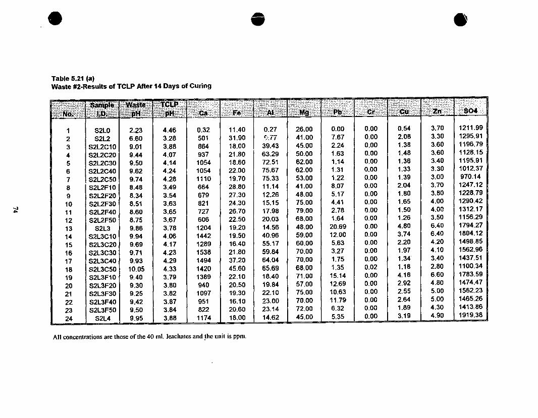
• • •Table 5.21 (a)Waste #2-Results of TCLP After 14 Days of Curing

~~~t1!;~;~;I~~'~·!:I!;:ilf~l"îll;:~:' ~1~·[I.i!II!::l!:i;,~il~i'!~~i~: ; ~ '.~.~-,;:,:;:,:: :-~' ;-:- .:,'. :' - - ... ::/~:~:;.:-~: ::-::'.:.o::i:S04.:..

1 S2LO 2.23 4.46 0.32 11.40 0.27 26.00 0.00 0.00 0.54 3.70 1211.99

2 S2L2 6.60 3.28 501 31.90 r:.ï7 41.00 7.67 0.00 2.0B 3.30 1295.91

3 S2L2C10 9.01 3.88 864 18.00 39.43 45.00 2.24 0.00 1.38 3.60 1196.79

4 S2L2C20 9.44 4.07 937 21.80 63.29 50.00 1.63 0.00 1.48 3.60 1128.15

5 S2L2C30 9.50 4.14 1054 18.60 72.51 62.00 1.14 0.00 1.36 3.40 1195.91

6 S2L2C40 9.62 4.24 1054 22.00 75.67 62.00 1.31 0.00 1.33 3.30 1012.37

7 , S2L2C50 9.74 4.28 1110 19.70 75.33 53.00 1.22 0.00 1.39 3.00 970.14

8 S2L2F10 8.48 3.49 664 28.80 11.14 41.00 8.07 0.00 2.04 3.70 1247.12

9 S212F20 8.34 3.54 679 27.30 12.26 48.00 5.17 0.00 1.80 3.80 1228.79

...:110 S2L2F30 8.51 3.63 821 24.30 15.15 75.00 4.41 0.00 1.65 4.00 1290.42

.... 11 S2L2F40 8.60 3.65 727 26.70 17.98 79.00 2.78 0.00 1.50 4.00 1312.17

12 S2L2F50 8.75 3.67 606 22.50 20.03 68.00 1.64 0.00 1.26 3.50 1156.29

13 S2L3 9.86 3.78 1204 19.20 14.56 48.00 20.69 0.00 4.80 6.40 1794.27

14 S2L3C10 9.94 4.06 1442 19.50 40.96 59.00 12.00 0.00 3.74 6.40 1804.12

15 S2L3C20 9.69 4.17 1289 16.40 55.17 60.00 5.63 0.00 2.20 4.20 1498.85

16 S2L3C30 9.71 4.23 1538 21.80 59.84 70.00 3.27 0.00 1.97 4.10 1562.96

17 S2L3C40 9.93 4.29 1494 37.20 64.04 70.00 1.75 0.00 1.34 3.40 1437.51

18 S2L3C50 10.05 4.33 1420 45.60 65.69 68.00 1.35 0.02 1.18 2.80 1100.34

19 S2L3F10 9.40 3.79 1389 22.10 18.40 71.00 15.14 0.00 4.16 6.60 1783.59

20 S2L3F20 9.30 3.80 940 20.50 19.84 57.00 12.69 0.00 2.92 4.80 1474.47

21 S2L3F30 9.25 3.82 1097 19.30 22.10 75.00 10.63 0.00 2.55 5.00 1562.23

22 S2L3F40 9.42 3.87 951 16.10 23.00 70.00 11.79 0.00 2.64 5.00 1465.26

23 S2L3FSO 9.50 3.84 822 20.60 23.14 72.00 6.32 0.00 1.89 4.30 1413.86

24 S2L4 9.95 3.88 1174 18.00 14.62 45.00 5.35 0.00 3.19 4.90 1919.38

Ali concentrations are those of the 40 ml. leachates and ~he unit is ppm.

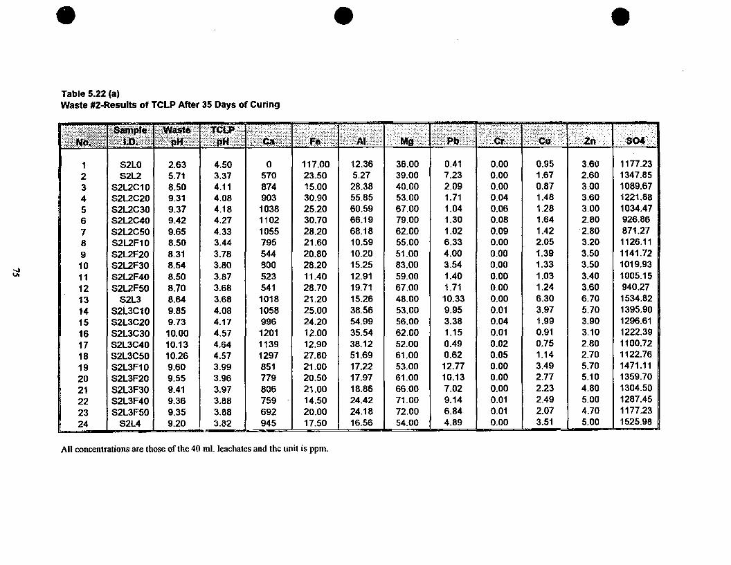
•Table 5.22 (a)Waste #2-Results of TCLP After 35 Days of Curing

• •

123456789101112131415161718192021222324

S2LO52L2

S2L2C10S2L2C20S2L2C3052L2C40S2L2C50S2L2F10S2L2F20S2L2F30S2L2F40S2L2F50

S2L3s2L3C10S2L3C20S2L3C30S2L3C40S2L3C50S2L3F10S2L3F20S2L3F30S2L3F40S2L3F50

S2L4

2.635.718.509.319.379.429.658.508.318.548.508.708.649.859.7310.0010.1310.269.609.559.419.369.359.20

4.503.374.114.084.184.274.333.443.783.803.873.683.684.084.174.574.644.573.993.963.973.883.883.8-2

117.0023.5015.0030.9025.2030.7028.2021.6020.8028.2011.4028.7021.2025.0024.2012.0012.9027.8021.0020.5021.0014.5020.0017.50

12.365.2728.3855.8560.5966.1968.1810.5910.2015.2512.9119.7115.2638.5654.9935.5438.1251.6917.2217.9718.8624.4224.1816.56

36.0039.0040.0053.0067.0079.0062.0055.0051.0083.0059.0067.0048.0053.0056.0062.0052.0061.0053.0061.0066.0071.0072.0054.00

0.417.232.091.711.041.301.026.334.003.541.401.71

10.339.953.381.150.490.6212.7710.137.029.146.844.89

0.000.000.000.040.060.080.090.000.000.000.000.000.000.010.040.010.020.050.000.000.000.010.010.00

0.951.670.871.481.281.641.422.051.391.331.031.246.303.971.990.910.751.143.492.772.232.492.073.51

3.602.603.003.603.002.802.803.203.503.503.403.606.705.703.903.102.802.705.705.104.805.004.705.00

1177.231347.851089.671221.881034.47926.86871.271126.111141.721019.931005.15940.271534.821395.901296.611222.391100.721122.761471.111359.701304.501287.451177.231525.98


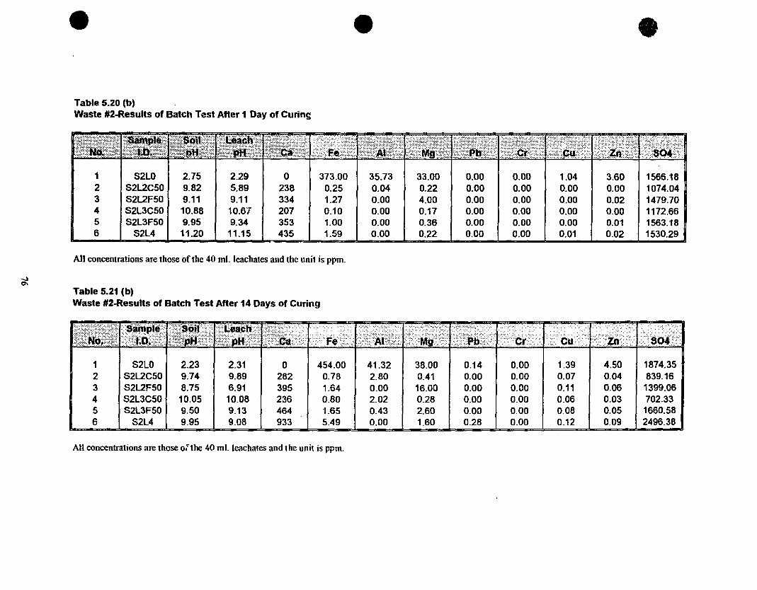
•Table 5.20 (b)Waste #2-Results of Batch Test After 1 Day of Curing

• •, , ,.,'..•.. '_." ..,.>::::;:;.~..;.:.:,;:: ..,.'..:

1 S2LO 2.75 2.292 S2L2C50 9.82 5.893 S2L2F50 9.11 9.114 S2L3C50 10.88 10.6'15 S2L3F50 9.95 9.346 52L4 11.20 11.15

0 373.00 35.73 33.00238 0.25 0.04 0.22334 1.27 0.00 4.00207 0.10 0.00 0.17353 1.00 0.00 0.36435 1.59 0.00 0.22

0.000.000.000.000.000.00

0.000.000.000.000.000.00

1.040.000.000.000.000.01

3.600.000.020.000.010.02

1566.181074.041479.701172.661563.181530.29

Ali concentrations are those of the 40 ml. leachates and the unît is ppm.

Table 5.21 (b)Waste #2-Results of Batch Test After 14 Days of Curing

1 S2LO 2.23 2.31 0 454.00 41.32 38.00 0.14 0.00 1.39 4.50 1874.352 52L2C50 9.74 9.89 282 0.78 2.80 0.41 0.00 0.00 0.07 0.04 839.163 S2L2F50 8.75 6.91 395 1.64 0.00 16.00 0.00 0.00 0.11 0.06 1399.064 S2L3C50 10.05 10.08 236 0.80 2.02 0.28 0.00 0.00 0.06 0.03 702.335 S2L3F50 9.50 9.13 464 1.65 0.43 2.60 0.00 0.00 0.08 0.05 1660.586 S2L4 9.95 9.08 933 5.49 0.00 1.60 0.28 0.00 0.12 0.09 2496.38

AH concentrations are those ofthe 40 ml. leachates and the unit is ppm.

•Table 5.22 (b)Waste #2-Results of Batch Test After 35 Days of Curing

• •

1 S2LO 2.63 2.48 a 430.00 30.16 39.00 0.01 0.00 1.25 4.202 S2L2C50 9.65 8.45 292 1.02 2.21 0.80 0.00 0.00 0.03 0.043 S2L2F50 8.70 7.59 434 1.14 0.00 13.00 0.00 0.00 0.01 0.044 S2L3C50 10.26 8.65 249 0.90 1.27 0.39 0.00 0.00 0.00 0.025 S2L3F50 9.35 8.17 466 1.63 0.00 2.20 0.00 0.00 0.01 0.056 S2L4 9.20 8.04 686 3.49 0.00 1.40 0.24 0.00 0.04 0.07

Ali conl;':aiJ'ations are those ofthe 40 ml. leachates and the unit is ppm.

Table 5.t3Compar~sonof the Effect of TCLP Solutions on the Control Sampie

Aluminum 11.77 33.96 12.46 37.06Calcium 86 356 0 0Chromium 0.00 0.00 0.00 0.00Copper 4.07 5.41 0.60 1.42Iron 25.50 180.00 58.00 696.00Lead 0.00 0.00 0.43 0.38Magnesium 32.00 39.00 12.00 39.00Zinc 46.00 61.00 3.90 45.00Sulfate 1346.44 1116.10 1904.86 1405.11


1405.234628.571107.88492.551238.241720.10

• Waste #1-Liquid Limit Test

10.00 15.00 20.00 25.00 30.QO

Penetration (mm)

5.00

20.20

S? 20.00-_ 19.80c! 19.60c8 19.40

~ 19.20::J

~ 19.00o~ 18.80

18.60 +---+----t---~--__f_--__+--___j0.00

Figure 5.1

•Waste #2-Liquid Limit Test

25.0020.0015.0010.005.00

17.50-ë 17.00-! 16.50

5 16.00uQ) 15.50...oS 15.00VIo-c 14.50:1

14.00 +---..........j----+-----+----+-------j

0.00

Penetration (mm)

• Figure 5.2

78

• l5000 -

XRD Analysis for Waste #1 - Sample #7 - 1% Lime + 50% FAC

II1l0000 ..-c:::Jo

U

5000 -

0- 0

10

Figure 5.3

•lSOOO -

1

20o

30

2-Theta

,~O

,50 GO

2-TtletaXRD Analysis for Waste #1 - Sample #12 - 1% Lime + 50% FAF•

11110000 -...,C::JoU

5000 -

Figure 5.4

la 20 ~o 50 GO

79

• 15000 -

\fi J0000 -....C::lo

U

5000 -

10 20 30

2-The ta40 50

•

•

Figure 5.5

15000 -

IIll0000 -....C::lo

U

5000 -

Figure 5.6

10

XRD Analysis for Waste #1 - Sample #18 - 2% Lime + 50% FAC

33 days

14 da)'s

1 da>,

Control umplc

20. 2-Theta

XRD Analysis for Waste #1 - Sample #23 - 2% Lime + 50% PAf

80

2- TM t a

XR.D Analysis for Waste #1 - Sample #24 - 3% Lime

•

•

15000 -

Ifll0000 -.uc::JoU

5000 -

lO

Figure 5.7

SOOO -

20 50 50

•

111.uc::JoU

Figure 5.8"" T .............

XRD Analysis for Waste #2 - Sarnple #7 - 2% Lime + 50% FAC

81

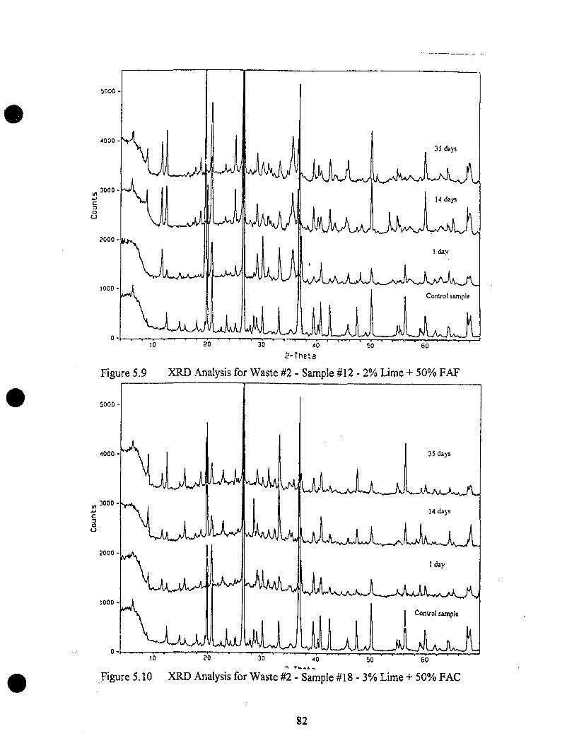
XRD Analysis for Waste #2 - Sample #12 - 2% Lime + 50% FAF

figure 5.10 XRD Analysis for Waste #2 - Sample #18 - 3% Lime + 50% FAC

•

•

•

~ooo •

~ooo -

III 3000 •...C;:lo

U

?OOO·

1000 -

Figure 5.9

5000 -

4000 -

III 3000 -...c;:lo

U

2000 -

1000 -

AD

2-Theta

""' ...............

50

50

60

35 da)'s

60

82

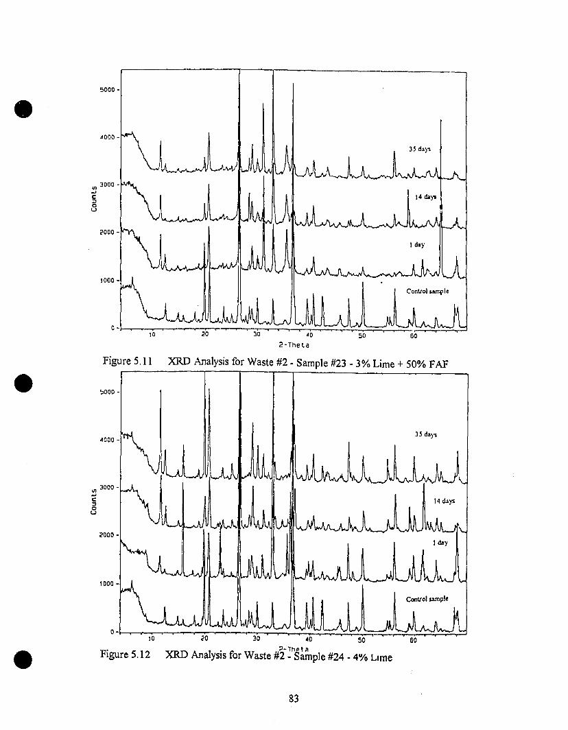
•5000 -

•

~ooo ~

ln :l000 -.,c:;,ou

2000 ~

1000 -

C·L-.-,.......,I0,.......,-=...:..::,.:.::2:':O~:..;~~~3;0:":::':::;:~:;:;~0~'::;~:::;~5:';0:::;:=::~~~6~0~~~~=:12-Theta

Figure 5.11 )(RD Analysis for Waste #2 - Sample #23 ~ 3% Lime + 50% FAF

~OOO •

3S da)"

10o-h.........-...........--..........--r-"T-:o:-......--...........-......-:':"..........--r--.-~~..;..:;;--.:.;;...;;;.~:::;=:::;.-..,...;..;r-::~-.;;,.:...;..,..:--...---'

20 30 ~o 50;:J. Thp t;\

XRD Analysis for Waste #2 - Sample #24 - 4% LImeFigure 5.12

~OOO -

2000 -

1000 -

ln 3000 -.,c;)ou

•83

• 6.0 RESULTS AND DISCUSSION

•

•

6.1 Introduction

The experiments that were conducted during the course of the project went

relatively weil. Although sorne hindrances were encountered in the form of occasional

equipment malfunctions, these were quickly overcome and bore no negative effects on the

outcome of the project or the results.

6.2 Preliminary Tests

6.2.1 Physical Properties

The moisture content test gave a general idea as to the state the wastes would be

found in. Although this parameter was not a natural one, as tailings are not natural soils, it

was nevertheless a starting point for tests involving the addition of water, such as liquid

and plastic limits. Waste #1 had an average moisture content of 9.20%, while waste #2

was at 8.13%. The values were relatively close, as was evident from the texture of the

wastes.

Most soils have specific gravities in the 2.60-2.75 range. Il was expected that the

wastes would exhibit slightly higher values, as they were mine tailings and would contain

large amounts of metals. This prediction was confirmed with a value of 2.94 for waste #1

and 3.66 for waste #2.

The Atterberg limits of a soil can give ample information about its texture and

behavior. Those of the wastes were found to be of a particular nature. The plastic limit

could not be obtained for either waste, indicating very low plasticity indices. Waste #1 was

of a silty texture, more so than waste #2, with a liquid limit of 19.06%. Waste #2 had a

lower value for the same property at 16.40%.

The sieve analysis gave an idea about the relative size of the particles and their

abundance. As can be seen, the majority ofparticles in waste #1 were between O. 180 mm.

84

•

•

•

and 0.425 mm. in size, which qualifies them as medium sand. The silty part, which passes

the #200 sieve, was rather scarce, making up only 3.50% of the total weight. As for waste

#2, its largest portions was between 0.075 mm. and 0.150 mm., which can be called

medium silt-fine sand. The fine silt-clay component was very low, at only 4.41%.

6.2.2 Chemical Properties

The most important of these was undoubtedly the pH of the tailings. It would

indicate the degree of their acidity and hint at the solubility levels of the toxic metal ions

present in them. A quick glance at figures 3.1 and 3.2 shows that most metal ions are

higWy soluble at lower pH ranges, particularly below 7.0. With pHs of 3.26 and 2.46 for

wastes #1 and #2, respectively, it would not be surprising to get a large amount of metals

dissolved in any leachant passing through them. The redox potential for the two wastes

were +254.8 and +405.0, respectively. It can be seen that a lower pH resulted in a higher

redox potential, indicating a high ratio of activity between oxidizing and reducing agents.

An acid digestion and subsequent elemental analysis indicated the concentration of

different elements, including heavy metals, within each waste. The resuIts obtained showed

concentrations much higher thim could ever be obtained by leaching the wastes with

natural leachants such as groundwater. As can be seen trom the tables, waste #1 was

found to be rich in a1uminum, iron and magnesium, while waste #2 had an extremely high

concentration of iron and appreciable amounts of magnesium and lead. It is important to

point out the lack of significant amounts of calcium in both wastes, thus accounting for

their low pH values. The resuIts trom the acid digestion can be compared to those

obtained by x-ray fluorescence (XRF). It should be kept in mind that the XRF results

indicate the total amount of elements present within each waste.


The most important of these experiments was the optimum lime content of the

8S

•

•

•

wastes. One percent of lime increased the pH of waste #1 from an extremely acidic value

00.26 to an almost neutral 7.44. As can be seen from figure 6.1, consequent additions of

1% lime iricreased the pH only slightly. An almost 3% lime content gave the first pH value

above 12.00. It was therefore decided to adopt this number as the maximum amount of

lime to be added to waste #1. Other samples were prepared with 2% and 1% lime

contents, each set including two types of fly ash ranging in content from 0-50% in 10%

increments. A control sample without additives was also prepared for comparison.

The same procedure was followed for waste #2. Being more acidic in nature, with

a pH of only 2.46, it required a larger amount of lime to raise the pH above 12.00. The

general trend of lime addition is graphically presented in figure 6.2. A 4% lime addition

was enough to achieve the required pH, and the same methodology outlined above was

followed for preparing the samples, with sets having 3% and 2% lime contents and varying

fly ash proportions.

Overall, the optimum lime content set out the basis for lime requirement for both

wastes and defined the boundaries within which the treatment would take place. Although

relatively simple in procedure and logic, it nevertheless offered a solid foundation for a

treatment procedure that relies heavily on the pH of the system for its efficacy.

The optimum lime content for the fly ashes was an interesting experiment designed

to study pH changes within mixtures involving the two additives. As can be seen from the

results in table 5.12, type C fly ash (FAC) showed a remarkably high pH by itse1f, with no

lime addition. Subsequent additions actually decreased the pH slightly, with further

fluctuations occurring with increasing lime content. With almost 10% more CaO than class

F fly ash (FAF), FAC was expected to have a higher pH. FAF gave a pH of 8.53 without

lime, but the value quickly rose to about 12.00 with small dosages. The slight fluctuations

might be either attributed to errors in readings or a slight variation in reactivity due to the

initial dry mixing. As a final note in this section, it should be remembered that a recent

study indicated a simple pH test as one of the methods to assess the optimum lime content

86

•

•

•

for a fly ash, the term "optimum" meaning œaximum reactivity [1]. The optimum content

was defined by the authors as the point beyond which the pH remained constant with

subsequent lime additions.

The final one of the project related experiments was the optimum fly ash content

for the wastes. Although not of direct relevance, it was quite singular in the demonstration

of pH variations induced by different additives. One has only to look at tables 5.13 and

5.14 to see that the pH rise in both cases was not even close to those induced by lime.

These relatively Mediocre results were achieved at a concentration of no less than 35%.

When it is kept in mind that lime achieved a pH of above 12.00 with only 3% and 4%

additions, the difference in the strengths between the two additives becomes quite

obvious. However, several useful observations were made:

- The relative acidity of the two wastes was demonstrated once again, as 35% of FAC

raised the pH ofthe system to 6.20 in the first case, but only to 4.99 in the second one.

- It was clear that FAF did not have a significant result on the pHs ofthe wastes. Even at a

35% rate, the wastes did not even exhibit a \.00 unit rise in their pHs.

As a concluding statement, the general, as wel1 as project related experiments gave

very satisfactory results. With the exception of a few minor irregularities, a clear picture

was obtained as to the major physical and chemical characteristics of the wastes and the

additives.

6.4 Leaching and Elemental Analysis

The TCLP method stipulates the use of solution #1 for soils with a pH lower than

5.0, and solution #2 for those with a pH higher than 5.0. This meant the use of TCLP #1

for the control samples in both wastes and TCLP #2 for the rest. However, due to the

different pH values of these solutions, elements sometimes showed a higher concentration

in the treated samples than in the control sample. Furthermore, the concentration of

elements varied with curing time in the control samples, as can be seen from tables 5.17 to

87

•

•

•

5.22. Although no immobilization was taking place there, the variation might have been

due to the fact that the solution used for the control samples was not freshly prepared

every time. For this reason, 2 g. from the control samples were also leached with TCLP #2

and the results obtained were taken to represent the true concentration of leachable

elements from both wastes. It should be noted that 2 g. of each type of fly ash "i~re also

put in centrifuge tubes and leached with TCLP #2, much like the treated and control

samples, and were subjected to elemental analysis. The reason for this was to assess the

leachability of different elements from them. The results of this initial leach tests are

presented in table 6.1.

The outcome of this project rested heavily on the amount of different elements

leached out from the samples by TCLP #2. Hence, it was very important to compare the

amount of an element leached to the total leachable amount available in a sample when

reviewing the results. For example, to assess the success of the lime/fly ash binder in

immobilizing iron in waste #1, consider sample #8. Table 5.15 shows that it is a mixture of

40 g. waste #1, 0.4 g. lime and 4 g. FAF. The proportion leached from the mix itself is

compared to the proportion of iron that would have been released from the various

components had they been leached separately. It can be seen in table 6.2 that the amount

leached from sample #8 after 1 day of curing was only 8.54% of the totalleachable iron

available in the mix. The method of calculation is based on the results from the control

samples leached with TCLP #2 and is explained in detail in Appendix 2. Thus, for both

wastes, this method of comparison was adopted except for lead in waste #2, where the

basis of comparison was not the amount of leachable lead but the total amount of lead

present in the samples. The reason for this step was that larger amounts of lead were

released from the treated samples than the control sample.

6.4.1 Waste #1

Tables 6.2 to 6.4 present the percentage of each element leached from the samples

88

•

•

•

for waste #1, with figures 6.3 to 6.10 comparing the effect of curing periCld for each

element.

1. Calcium:

The least proportion of calcium leached is seen to occur, strangely enough, in the

control sarnple. Two explanations could account for this phenomenon. It could be that

TCLP #1, due to its higher pH, has leached a lesser arnount of calcium than the TCLP #2

used on the other sarnples. The other reason could be that calcium in the control sample

cornes only from the waste itself. Il is possible, therefore, that it exists there in a less

soluble form than in lime and fly ash, components which are present in the other 23

sarnples. There does not seem to be a particular trend in the different sets, except that the

least arnounts leached are from the set with 1% lime and FAF. Not surprisingly, this is the

set with the least arnount of calcium after sarnples #1 and #2. A comparison along the

curing time line shows a decrease in calcium leachability after 14 days, followed by an

increase after 35 days. The numbers in table 6.4 indicate that the sets with FAC show a

very high release rate, in contrast to the ones with FAF. Taking into account the

proportions of soluble calcium in FAC and FAF, it seems that the reason for this is an

excess of unreacted calcium which is rendered available for leaching. Another observation

to fit this hypothesis is that with increasing FAC or FAF content within a given set, the

percentage of calcium released generally increases.

2. Iron:

Table 6.1 shows that waste #1 provides a high proportion of leachable iron

compared to FAC and FAF. Il is also c1ear from tables 6.2 to 6.4 that the sets with FAF

have exceeded others in terms of immobilizing iron after 1 day of curing. As ferrous iron

solubility is at its lowest at a pH of 10.0, and FAC sarnples demonstrate such a range,it

must be deduced that the release ofiron is not a function ofpH after 1 day of curing. After

14 days, most sarnples show a decrease in iron leachability. With 35 days of curing, a

sharp decline occurs in the percentages of iron released from FAC samples. So much so,

89

•

•

•

that overall, they fare better than the FAF ones. Although the pH range of FAC sampies is

closer to the 10.0 mark, it was seen that the pH of the mix had !ittle effeet in the solubility

of iron in the mixes. Another important observation is that samples with higher fly ash

content show lower proportions of iron released. AIl this leads to the conclusion that iron

immobilization takes place due to the pozzolanic reactions between lime and fly ash, and is

thus affeeted more by the amount of bind~r present and curing time than by pH variations.

It is interesting to observe the relatively small amount of iron leaehed from the control

sample by TCLP #1 compared to TCLP #2. In the samples with only lime as the additive,

it can be seen that iron release is primarily controIled by the pH of the mix, as no

pozzolanic activity occurs.

3. Aluminum:

The waste and FAF showed a higher release of a1uminum when leaehed separately

as compared to FAC. However, the leaehability of a1uminum was seen to be erratic at

times, with sorne samples releasing more than 100%. It should be remembered that the

basis of eomparison is the total amount released from the different components had they

been leached separately. Henee, those percentages above 100% merely indicate that the

waste, lime and fly ash have released more a1uminum when combined than was

anticipated. The pattern seems to be that FAF samples release much less a1uminum than

the FAC ones after only 1 day of curing. After 14 days, ail samples show a general

increase in the proportions released, with the aforementioned pattern being still evident.

Curiously, the leachability increases with increasing fly ash content. The best resu1t cornes

from sample #8, with a 1% lime and 10% FAF content. It would appear that the reactions

between lime and FAF are more effective in immobilizing a1urninum than those between

lime and FAC. Among the lime-only samples, #24 with 3% lime shows the most prornising

result. However, pH a10ne cannot eXt,lain this phenomenon, as other samples have similar

pHs to sample #24. The only explanation can be that lime has precipitated a1urninum and

90

•

•

•

rendered it insoluble; hence, the bigher the lime content, the lower the proportion of

aluminum leached,

4, Magnesium:

The re1ease of magnesium was monitored mainly for comparison purposes and the

possibility of cation exchange, The main source of leachable magnesium was seen to be

FAF when leached with TCLP #2, It is quite interesting, therefore, to observe that the

samples with FAF have released lower percentages of Mg than their FAC counterparts

after 1 day of leacbing, The set with 2% lime and FAC shows a definite trend of

leachability increase with bigher fly ash contents, After 14 days of curing, most samples

show a decrease in Mg solubility, One explanation could be the incorporation of

magnesium cations in the matrices of new minerais formed by lime-fly ash interactions,

Note that tbis decrease is not evident in the lime-only samples, The 35 days oid samples

continue to show the drop in solubility with a few exceptions, The best results still come

from FAF samples; tbis could suggest that a lack of calcium induces magnesium ions to

perform most of the cation exchange and thus be less vulnerable to leaching,

5, Copper:

Although rich in total copper content, waste #1 released only a small fraction of

the metal when leached with TCI,P #2 (tables 5,8 and 6.1), The resuits after 1 day of

curing show no distinctive trend among the sampies, The proportions released after 14

days r,f curing register a definite decrease, with more predominant results in the FAC

samples, Copper hydroxide is least soluble at a pH of9,0, Since those of the FAC samples

are closer to that value, il would be expected that they give the better resuits, However,

tbis is not so obvious after 1 day or 14 days of curing, Il does not appear that pH plays an

important part in the immobilization of copper in the samples, After 35 days, although the

general trend is a reduction in the proportions of copper released, the FAC samples show

the more dramatic drops, The bigher the fly ash content in a sample, the lower the

percentage of copper released becomes, Once again, the pozzolanic reactions of lime and

91

•

•

•

FAC can be held responsible for the immobilization of copper. The lime-only samples

demonstrate the trend of low metal release with a high CaO content, thus confirming the

occurrence of hydroxide precipitation. It is worth mentioning that lime-fly ash

combinations give a better rate of copper immobilization than precipitation.

6. Zinc:

After 1 day of curing orùy, the trend in zinc solubility seems to be that sarnples

with 1% lime have lower leachability percentages than the ones with 2% lime. The pH

ranges of the different sets are too irregular to suggest a possible link to solubility. The

trend continues on after 14 days of curing, with a regular decrease in release rates within

the lower lime sets. The pattern within a given set is an initial increase in leachability with

increasing fly ash content, fol1owed by a final decrease towards the end. After 35 days of

curing, the best result cornes from the sample with 1% lime and 50% FAC, although a

general increase in solubility can be seen. This might suggest that additional calcium might

interfere with the immobilization of zinc. Therefore, care should be taken in such cases to

avoid an excess of either lime or fly ash within the treated sample.

As a conclusion, it seems that the immobilization of metals (iron, copper and zinc)

in waste #1 was best achieved with FAC and lime combinations. Aluminum was the

exception, in that FAF and lime achieved better results in its stabilization. However,

hydroxide precipitation was seen te be the most effective way of decreasing aluminum

solubility. Calcium became more abundant with increasing fly ash content and its solubility

was merely an indication ofthe reactivity rate between the two additives.

The samples leached with water proved to be useful assets. As the tables indicate,

water leached lesser amounts of ail the elements than the TCLP solutions. In reality, the

only elements leached in significant quantities iTom the treated samples were calcium and

magnesium. AIl of the heavier metals showed only minor solubility levels.

92

•

•

•

6.4.2 Waste #2

Waste #2 differed in several ways from waste #1; it was more acidic and had

higher concentrations of iron, lead, copper and zinc (table 5.8). However, when leached

with TCLP #2, it released lesser amounts of copper and zinc (table 6.1). Once again, the

values obtained in this test fonned the basis for comparison between the treated sanlples.

The importance for this basis is obvious; a1though richer in total metal content, waste #2

released lesser amounts of these metals when compared to waste # 1. An analysis based on

the total metal content would therefore have proven misleading in tenns of the degree of

immobilization. Tables 6.5 to 6.7 give the percentages of the elements leached from the

samples, while figures 6.11 to 6.19 present the graphical comparison of the samples

throughout the period of curing.

1. Calcium:

Calcium was completely absent from waste #2 and as such, its only source in the

samples were the lime and f1y ash added. After a day of curing, the results seem erratic and

with no particular pattern. Even within sets, no trends can be seen with increasing f1y ash

content. Not even the higher percentage of lime in the second half of the samples seems to

correspond to proportional increases in calcium release. After 14 days, the samples show a

general increase in the percentage of calcium leached, sorne even surpassing the 100%

mark. As was the case with waste #1, this merely indicates a higher release rate for

calcium and not an error in the method of calculation. Once again, no c1ear trend can be

seen in the leachability rates of the samples. The erratic behavior continues in the 35 days

old samples, where a slight decrease from the previous rates is the only c1ear change. ln

general, however, the samples with a higher lime percentage show lower calcium

leachability proportions, specially the FAF ones. Strangely enough, the lowest calcium

leachability rate cornes from sample #24', which has the highest lime content. This could he

the result of hydroxide precipitation, the rate of which could be higher in lime-f1y ash

samples. The only trend visible in the leachability of calcium is that FAC samples show

93

•

•

•

higher pHs than the FAF ones, and those with 3% lime are in a similar position when

compared to the 2% lime ones.

2. Iron:

Waste #2 had a very high total iron content, with a 41.07% ferrous made

concentration. This translated into an equal1y high release of iron when leached with

TCLP #2. The results after 1 day of leaching (table 6.5) indicate that a higher percentage

of lime, when added alone, results in a dramatic decrease in iron release from the waste,

with only 1.48% of the leachable iron removed from sample #24. In the samples with lime

and f1y ash, the ones with a lower lime content show better results with FAC, while the

reverse is true for the ones with a higher lime content. Another feature is that within each

set, the best result cornes from the sample with the lowest f1y ash content. Lime

neutralizatîon could explain this phenomenon, as with an increase in excess calcium, this

process becomes more effective. The pH range is also important, as the samples showing

the best results have values close to 10.0, the range of minimum iron hydroxide solubility.

After 14 days of curing, ail samples show a decrease in leachability, with a continuation of

the aforementioned pattern. Slight increases are seen after 35 days of curing in the samples

with a lower lime content, while the rates of iron release continue to go down in the ones

with a higher lime content. The best results within the FAF samples come from those with

a 40% f1y ash content. This might indicate the ideal combination between lime and FAF in

terms of reactivity. On the whole hydroxide precipitation gave the lowest iron leachability

results, fol1owed closely by several limelFAF and IimelFAC samples. Tt means that the

mechanism for immobilization is different within each waste.

3. A1uminum:

In terms of the rate of aluminum leached from the treated samples, waste #2 did

not differ significant1y from waste #1. A very clear pattern is immediately seen after 1 day

of curing. Those samples with an FAC content show incredibly high aluminum leachability

rates. These increase dramatically with increasing f1y ash content and are higher for

94

•

•

•

samples with a lower lime percentage. The percentages exceed the 100% mark by quite a

margin. It seems that combining the various components in these samples has resulted in a

higher rate of aluminum leachability than the sum of the rates from each component.

Among the FAF ones, the best results are observed in sarnples with only 10% fly ash.

Furtherrnoœ, the excellent results from the lime-oruy samples indicate that hydroxide

precipitation is the best way of immobiiizing aluminum at this stage. A general decrease in

aluminum release is evident after 14 and 35 days of curing. At the end, sample #2 with

oruy 2% lime shows the lowest aluminum leachability, followed by sample #8 with 2%

lime and 10% FAF. It does seem obvious that a minimum amount of calcium in the sample

gives the most desirable result. This might be an indication that an excess of calcium ions

triggers aluminum release from the system, possibly by cation exchange.

4. Magnesium:

In the case ofwaste #2, the conditions were almost the same as with waste #1. The

reason for this was that an equal amount of magnesium was leached from both wastes

with TCLP #2, and equal proportions of fly ash were used. The only difference was the

percentage of lime in the samples, with 1%, 2%, 3% for waste #1 and 2%, 3%, 4% for

waste #2. Once again, FAF sarnples show a better performance overall than the others

after a day of curing. After 14 days, a systematic increase is seen in almost aIl sampies.

The 100% mark is surpassed most notably by the 3% lime samples, indicating one more

time the important role played by an excess of calcium cations. The situation becomes

more unpredictable after 35 days of curing. Not oruy most sarnples show a further increase

in Mg solubility, but the best result coming from sarnple #11 shows that not much of this

element has been taken up into the matrix. It is therefore logical to conclude that

magnesium release is directly linked to the arnount of calcium present in the sample.

5. COlmer:

The arnount of copper released from waste #2 by TCLP #2 is minimal compared to

the total amount of copper present. Other than the waste, the only other source of the

95

•

•

•

metal is FAF (table 6.1). Table 6.5 indicates that after 1 day of curing, many samples have

released percentages of copper that are much higher than the 100% mark. Among the

samples that have immobilized copper in a more efficient way are those with a low lime

content and a high FAF percentage. On the whole, samples with lower lime contents are

seen to have performed better than the others. Furthermore, among the latter, an increase

in f1y ash content results in a decrease in copper solubility. The pH values of the different

sets are quite different; hence, no simple pH variatiol; ::'culd account for this phenomenon,

although, admittedly, the set with 2% lime and FAF has the lowest pH range at about 8.0.

Once again, an increase in calcium content seems to be directly proportional to an increase

in copper solubility, lIldicating a possible replacement of the metal by unreacted calcium

cations. Most of the samples indicate a more abundant release of copper after 14 days of

curing, with a su\:-sequent decrease in leachability after 35 days. The general trend

continues to be a decrease in copper solubility with a lower lime content. It is difficult to

say which one of the f1y ashes has done better in immobilizing the metal as the results are

quite similar. The lime-only samples do not seem to have accomplished much, thus further

supporting the connection between unreacted calcium cations and copper solubility.

6. Zinc:

Like copper, soluble zinc in waste #2 is a mere fraction of the total zinc content.

FAF was seen to release an equal amount of zinc as waste #2 (table 6.1). AJJ table 6.5

indicates, after 1 day of curing, the sets with the lower lime contents show better zinc

p~tention than the ones with 3% lime. Among the latter, a decrease in zinc leachability is

observed with increasing f1y ash content, as was the case with copper. After 14 days of

curing, zinc solubility increases for all samples. Since no major pH changes has occurred,

this sudden change is clearly ascribed to other factors than the pH of the sample. The rate

of metal release goes down slightly after 35 days of curing. The same pattern of lower

solubility with lower lime content remains, however. As was with iron, an addition of only

2% lime consistently gives the lowest zinc leachability rate among ail the samples. One of

96

•

•

•

the possible explanations that could be offered is that the amount of lime added

precipitates most of the zinc; without any additionai calcium ions present, zinc is not

replaced and released into the leachate. Hence, the critical issue is to supply just the right

amount oflime to precipitate the metai involved without any cations remaining in excess.

7. Lead:

Unlike waste #1, lead was leached in appreciable quantities from waste #2. Like

copper and zinc, however, the amount that could be leached from the waste with TCLP #2

was minimal compared to the total amount present. There were no contributions from

FAC and FAF in terms of lead leachability, as can be seen in table 6.1. However, an

exception was made in the basis for comparison. Unlike the other e\ements, it was seen

that the amount of lead leached from the samples was much higher than the sum of the

values that would have been obtained in separate leach tests for the different compounds.

To avoid much higher percentages than 100%, the total amount oflead present was taken

as the basis for comparison. Thus, the amount leached by TCLP #2 is seen to constitute

only 0.19% ofthe total amount oflead present. Tables 6.5 to 6.7 indicate quite clearly that

most samples have leached much higher proportions than this. Since the fly ashes yielded

no lead when leached with TCLP #2, and no figures were available as to their total lead

content, it is difficult to explain this phenomenon. It is at once obvious that the samples

with 2% lime and FAC show the best results in lead immobilization. No great changes are

seen during 35 days of curing, as the percentages reieased remain almost constant within

this set. It should be observed that lead solubility is at a minimum at a pH of9.0, which is

precisely the range ofvalues for these samples. With a 3% lime content, the FAC samples

show extremely good retention abilities with higher fly ash contents. The FAF samples

generally fare poody, specially the ones with 3% lime contents. Aithough the pH of the

FAC samples with 3% lime are within the 9.0 range, it seems that lime/fly ash interactions

play a significant raie, liS the trend within the set indicates. It can thus be concluded that

lead retention is dependent on both sample pH and pozzolanic activity.

97

•

•

•

Just as with waste #1, the samples that were leached with water show that almost

none of the heavy metals were leached from the treated samples. It should be pointed out

that an extremely large amount of iron was leached from the control sample, exceeding

even the concentration in the TCLP leachate. Aluminum and magnesium show similar

results, but no viable explanation can be given for this phenomenon.

6.5 Sulfate Analysis

The sulfate content of the wastes has been treated separate1y as it constitutes an

important factor in the occurrence of acid mine drainage. The basis for comparison was

the amount leached from the wastes with TCLP #1, unlike aIl the other elements, as it

gave a higher sulfate yield than TCLP #2. For the fly ashes, though, the values from TCLP

#2 were used.

In waste #1, the trend after 1 day of curing is increasing sulfate release with

increasing fly ash content within each set (figure 6.10). The FAF samples give better

results at a higiler lime content. Although most rates exceed the 100% mark, the trend cm

still be c1early seen. After 14 days of curing, a marked improvement is observed in ail the

samples, with lower lime contents giving the more promising results. The 35 days old

samples show the ongoing improvement, with a low lime and high FAF content being the

best combination for sulfate retention. As much as roughly 30% of the soluble sulfate is

rendered insoluble. This is quite promising as FAF showed a higher sulfate release when

leached separately with TCLP #2. Ail this c1early indicates the importance of pozzolanic

reactions in decreasing leachability, as weIl as the role played by the curing period.

Waste #2 had a higher amount of sulfate released than waste #1 when leached by

TCLP #1. As figure 6.19 shows, the samples showing the better results after 1 day of

curing are the FAF ones with a 2% lime content. After 14 days of curing, however, the

FAC samples with the lower lime percentage show similar resuits. At the end of35 days,

alileachability rates are weIl below the 100% mark. Samples with 2% lime and FAF still

98

•

•

•

give the best results, with the rate of sulfate release reaching as low as 63%. Some FAC

samples with 2% lime show similar results, but there appears to be no consistency there.

Therefore, as much as 30% and 37% of the soluble sulfate was seen to be

immobilized in waste #1 and #2, respectively. The FAF samples with a lower lime content

gave the best resu1ts, indicating once again the importance of providing just enough

material for reactions, without any excess in additives.

6.6 X-Ray Analysis

The x-ray diffraction (XRD) analysis was performed as a complimentary tool to

the TCLP leaching technique. It was known, from the literature review, that lime and fly

ash interactions produced pozzo1anic compounds which were held responsible for heavy

metal immobilization. The purpose of the XRD analysis was to try and find out what new

minerai phases were formed during these reactions and what others had disappeared.

Based on the literature review, the search was limited to calcium aluminates and calcium

silicates. These are series of minerais resulting from cement hydration and lime/fly ash

reactions.

The analysis was conducted using a special software that searched known minerai

databases to match the graphs with different minerai patterns. Along with the calcium

silicate hydrates, the minerai ettringite {Ca6AlZ(S04h(OH)12.26H20} was given special

attention, as it was held responsible for heavy metal immobilization by several authors.

The major peaks of this minerai are found at a Z8 value of 22899° (100% Intensity),

9.090° (92% 1), 34.975° (86% 1) and 15.7W (85% 1).

In waste #1, some interesting observations are made when comparing sample #7

(figure 5.3) and sample #12 (figure 5.4). The conditions in both samples being identical, it

is interesting to see the differences induced by the different type of fly ash used. The peak

at around 11.5° was identified as gypsum and shows a slight growth in sarnple #7 with

time. Sample #1Z also exhibits a similar growth, with a slightly higher peak. Although

99

•

•

FAC has a higher calcium content, it seems that gypsum formation was slightly more

successful in sample #12. As for ettringite, the small peak at 9° in the control sample

shows no noticeable growth in both samples. This should not be surprising, as the

formation ofthis minerai requires a pH of at least 11.5, which was not achieved in any of

the treated samples. The strong peak at 33° in the control sample could very weil be pyrite

and shows a substantial decrease in both samples. A strong correlation exist between this

observation and the TCLP results indicating a major decrease in iron leachability. Samples

#18 (figure 5.5) and #23 (figure 5.6) had a higher lime content than samples #7 and #12.

They exhibit the same decrease in pyrite content, as iron becomes immobilized through

pozzolanic reactions. A similar observation as before is made in the FAF sample, where

gypsum formation is quite apparent. It should be remembered that since FAF had a higher

S03 content, a larger amount of gypsum was expected to form. A new feature is seen in

the FAC sample, where the small peak at 9° shows sorne growth with time. It is doubtful,

however, that it belongs to ettringite, as the pH requirement was not fulfilled. Sample #24

(figure 5.7) shows a substantial gypsum content with a high peak at 11.5°. With no flyash

to react with the lime, it is quite possible for gypsum to be formed from calcium and

sulfate ions. The pyrite peak is seen to disappear once again, thus lending further evidence

to hydroxide precipitation being one of the main mechanisms for iron immobilization.

The presence of quite a number of peaks in waste #2 made it difficult to analyze

the graphs. Pyrite was easily identified, though, as the peaks at 56°, 33°, 37° and 41° were

quite obvious. The ones at 56° and 33° tend to fluctuate throughout the curing period for

ail samples, in a similar manner to the TCLP results. Another observation is the formation

ofgypsum in formidable quantities, with no difference between the FAC and FAF samples.

Since the waste itself had no calcium in it to start with, it is quite easy to see the peak at

11.5°. The FAF samples exhibit slightly higher peaks than the FAC ones due to their

higher sulfate contents. The gypsum formed in sample #24 (figure 5.12) shows the tallest

peak after 35 days of curing, due to its very high lime content. Another obvious feature is

100

•

•

•

the continuous growth ofa peak at 9° in ail the samples except #23 (figure 5.11). The pH

ofthe samples for waste #2 were lower than those for waste #1. Therefore, the formation

of ettringite is highly unlikely. The presence of another mineraI, possibly a calcium silicate

hydrate, is quite plausible.

As a conc1uding remark, the formation of gypsum was observed in both wasles

due to the presence of calcium and sulfate ions. The absence of any calcium aluminates

suggests a deficiency in reactive aluminum content. The fact that the pH of the samples

never rose to above 11.0, combined with the lack of reactive aiuminum, could be the main

reason behind the absence of ettringite. Therefore, the immobilization of the metal ions

present can be attributed to hydroxide precipitation and pozzolanic reactions. No minerais

produced from the latter mechanism were detected, except for some minor silicates.

However, the overall results indicate that amorphous phases of calcium silicates, which

would not be deteeted by XRD, could have been responsible for the immobilization of

heavy metals.

101

•

•

•

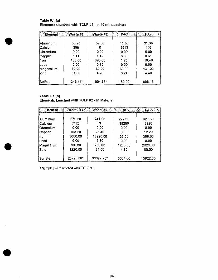
Table 6.1 (a)Elements Leached with TCLP #2 • In 40 ml. Leachate

··.·Elemei!(.··· .Waste#.1··.· WasteliZ> ... ····FAC . ···>fAF•••

Aluminum 33.96 37.06 13.88 31.38Calcium 356 0 1913 446Chromium 0.00 0.00 0.00 0.00Copper 5.41 1.42 0.00 0.61Iron 180.00 696.00 1.75 19.40Lead 0.00 0.38 0.00 0.00Magnesium 39.00 39.00 60.00 131.00Zinc 61.00 4.20 0.24 4.40

Sulfate 1346.44· 1904.86· 150.20 696.13

Table 6.1 (b)Elements Leached with TCLP #2 - ln Material

····ElelTlent •• >.• WasteJ!1(· W~Stlltf2. .•. : .•.•ii·.··... FAc·.···i.· '...... ).

Aluminum 679.20 741.20 277.60 627.60Calcium 7120 0 38260 8920Chromium 0.00 0.00 0.00 0.00Copper 108.20 28.40 0.00 12.20Iron 3600.00 13920.00 35.00 388.00Lead 0.00 7.60 0.00 0.00Magnesium 780.00 780.00 1200.00 2620.00Zinc 1220.00 84.00 4.80 88.00

Sulfate 26928.80· 38097.20· 3004.00 13922.60

• Samples \Vere leached \Vith TCLP #1.

102

Table 6.2Percentage of Elements Leached Waste #1 1 Day

Table 6.3Percentage of Elements Leached·Waste #1·14 Days

. .'M!~N9.:'.·· M,~LD, .i .•!'..!'.Câ.··•• ii"'Fe.· 1., <Al·.>} \;\Mg. \;.: I.({·eil'··,· <ii/Zn ....

1 SlLO 24.16 13.00 34.66 82.05 75.23 75.412 SlLl 50.26 20.82 33.43 93.23 84.57 81.133 SlL1Cl0 99.63 7.52 83.50 106.07 70.17 67.304 SlL1C20 81.26 10.06 118.81 99.65 6:>'.74 61.445 S1L1C30 74.09 19.45 139.85 98.82 68.77 57.926 S1L1C40 78.29 22.08 158.84 98.48 73.24 55.397 SlL1C50 78.22 34.56 165.07 100.67 74.80 54.358 S1L1Fl0 55.36 8.54 37.94 80.96 79.53 74.079 SlL1F20 55.18 7.57 34.34 87.22 76.77 74.3110 SlL1F30 55.98 10.86 42.77 81.98 68.86 67.2711 SlL1F40 59.14 7.51 42.05 80.22 70.08 62.9112 SlL1F50 61.60 7.72 40.60 73.69 62.09 50.1713 SlL2 78.97 4.65 37.39 86.31 63.54 51.8414 SlL2Cl0 86.53 16.29 94.93 92.09 71.42 47.7215 SlL2C20 90.50 25.50 123.14 107.65 78.25 79.9416 SlL2C30 90.86 34.29 141.30 113.47 82.71 84.2917 S1L2C40 105.04 37.72 160.75 121.71 82.68 95.2918 SlL2C50 94.48 50.42 164.78 140.99 72.21 84.5519 S1L2Fl0 78.83 4.86 29.80 98.89 73.49 69.2720 SlL2F20 87.72 6.24 38.39 91.69 79.39 88.7221 SlL2F30 88.99 4.05 41.88 111.26 80.24 88.9622 SlL2F40 97.31 5.75 46.47 104.09 75.34 79.1923 SlL2F50 73.32 4.41 47.48 93.09 70.75 72.1524 S1L3 80.13 2.00 31.66 84.51 62.83 75.98

M1lt!'lç: ··iMixtp, F'" ' .. '\.Fe.?' 1)·.··..-,,,·, Mg ·.··cu ···'Zn.·>.,;".

1 SlLO 22.75 4.78 16.08 82.05 60.07 81.972 SlLl 45.17 13.30 44.37 93.23 64.97 82.793 SlL1Cl0 54.48 4.87 136.38 115.93 56.83 50.934 SlLlC20 58.07 6.84 212.32 104.39 57.93 55.505 SlL1C30 71.75 6.97 253.76 94.23 56.18 42.906 SlL1C40 76.58 7.96 274.74 98.48 57.34 46.167 SlL1C50 72.97 10.02 293.69 89.72 53.59 39.538 SlL1Fl0 50.23 8.60 46.74 93.74 67.97 70.469 SlL1F20 54.58 6.65 48.63 89.08 69.99 78.22

10 SlL1F30 54.43 6.13 49.59 66.92 66.52 73.5711 SlL1F40 61.03 5.48 60.36 72.51 65.34 51.6712 SlL1F50 63.54 5.81 64.87 76.58 61.30 43.0113 S1L2 70.78 5.55 47.40 75.85 63.73 36.7914 SlL2Cl0 72.86 6.40 147.05 89.60 60.66 38.5415 SlL2C20 74.38 8.05 198.06 95.69 64.04 69.9416 SlL2C30 87.65 10.68 229.80 99.58 63.93 88.6217 SlL2C40 82.76 28.76 297.93 108.19 66.67 88.3218 SlL2C50 80.83 38.91 322.36 103.54 68.55 92.0219 SlL2Fl0 64.57 6.16 58.12 81.69 74.93 80.2120 SlL2F20 65.63 4.11 56.88 80.46 71.23 86.7521 SlL2F30 67.29 4.40 62.21 84.29 73.40 80.4922 SlL2F40 72.07 3.71 71.13 82.34 72.33 74.6723 S1L2F50 71.20 5.69 75.07 85.82 69.95 93.8024 SlL3 80.06 2.08 26.60 89.79 67.02 99.62

•

•

•103

Table 6.4Percentage of Elements Leached Waste #1 35 Days

Table 6.5Percentage of Elements Leached Waste #2 1 Day

. .1I'IÎ)tN<:i: :;Mil' J.O, . •<:\cah I ....a""<> •. AI <...•. . < Mli·· . CLi· ; , ('Zn·

1 SiLO 28.37 13.00 29.42 66.67 65.62 73.772 S1L1 50.40 7.46 27.45 93.23 57.31 86.103 S1L1C10 64.42 3.08 91.13 106.07 42.47 61.844 S1L1C20 87.66 4.96 121.80 94.90 43.84 67.395 S1L1C30 99.53 2.98 119.92 96.53 39.95 72.936 SlL1C40 94.89 3.09 133.00 82.81 35.18 57.707 SlL1C50 95.04 2.62 123.31 72.22 29.87 44.478 SlL1Fl0 67.51 4.82 30.10 89.48 57.82 66.859 Si Li F20 76.29 3.36 32.27 90.94 62.99 80.17

10 SiL1F30 85.20 3.00 37.81 68.60 58.32 84.0811 Si Li F40 72.73 2.88 45.41 75.59 52.87 65.1512 SlL1F50 86.60 2.79 52.22 91.03 52.05 66.9013 SlL2 86.98 4.53 33.94 73.23 55.81 46.8214 SlL2Cl0 96.82 2.61 85.14 84.62 42.85 51.3915 SlL2C20 97.21 3.65 112.28 90.90 40.82 77.9416 SlL2C30 98.32 3.60 111.59 83.37 34.89 71.3317 SlL2C40 99.78 2.28 83.16 85.65 30.97 83.6718 SlL2C50 97.32 1.59 63.62 85.91 28.38 74.6119 SlL2Fl0 94.80 6.53 43.17 98.89 62.23 91.1520 SlL2F20 78.78 3.12 41.02 76.72 56.24 78.8621 SlL2F30 76.82 4.90 47.99 82.61 55.70 80.4922 SlL2F40 84.58 3.73 51.87 85.45 53.24 81.4523 SlL2F50 88.12 3.81 52.17 104.73 49.20 79.3724 SlL3 87.49 1.26 8.92 87.15 49.50 72.61

·(MiltN9i C(\NI!i'J··P.+:;~~ ~"''''.Al (i "Mg.) 'l8.illi.EH:.2C ~".C1"k<'71 S2LO 0.00 8.33 33.62 30.77 42.25 92.86 0.212 S2L2 66.65 5.42 35.92 75.85 113.49 68.00 4.723 S2L2Cl0 81.59 6.27 140.87 114.49 95.44 84.85 1.184 S2L2C20 78.05 9.81 218.24 107.65 105.68 86.16 1.225 S2L2C30 83.38 L82 270.76 115.79 104.11 86.52 1.066 S2L2C40 81.37 8.15 300.42 121.71 122.00 95.86 1.027 S2L2C50 79.95 7.42 315.50 112.35 111.32 87.96 0.888 S2L2F10 88.80 6.10 38.56 90.29 105.87 74.83 3.759 S2L2F20 76.64 11.16 42.26 82.33 95.73 76.85 3.1510 S2L2F30 73.74 10.08 46.13 79.23 92.23 81.30 2.8511 S2L2F40 98.58 11.50 42.93 96.32 84.48 8:;'.39 1.5112 S2L2F50 73.76 9.05 51.15 77.09 74.90 78.38 1.3713 S2L3 81.19 2.35 53.22 87.15 267.65 139.79 10.7114 S2L3Cl0 83.63 5.26 121.88 100.44 241.12 149.81 7.4515 S2L3C20 78.30 5.42 19D.88 115.76 170.64 127.40 3.4616 S2L3C30 79.35 9.64 232.36 105.00 140.49 102.74 2.2117 S2L3C40 75.11 11.08 240.78 106.68 112.79 89.87 1.4018 S2L3C50 72.33 16.47 275.61 104.22 110.98 85.00 1.3519 S2L3F10 76.20 3.97 52.29 91.09 266.29 133.94 8.6620 S2L3F20 69.70 6.06 57.16 83.01 203.40 108.96 7.7021 S2L3F30 73.79 7.96 60.50 88.33 169.26 101.20 5.9222 S2L3F40 84.17 6.93 61.22 93.87 207.97 112.77 8.5223 S2L3F50 71.48 5.88 62.94 77.60 162.31 95.63 5.8824 S2L4 102.88 1.48 34.77 125.33 166.99 108.95 3.79

•

•

•\04

Table 6.6Percentage of Elements Leached-Waste #2-14 Oays

Table 6.7Percentage of Elements Leached-Waste #2-35 Days

"Mi~"N~/) :\Miii.p.. ·; •. ;:;;Ç<t»\ :<·<::F~:::::: ; Al.": :·:(Mg" .. ;:<\:Ol.t:·.:: .'.. :··-:"Zn;>' :·Pb... .

1 S2LO 0.00 1.64 0.73 66.67 38.03 88.10 0.002 S2L2 71.50 4.68 26.89 107.23 149.41 80.14 3.903 S2L2C10 106.81 2.90 114.86 112.00 108.85 95.45 1.254 S2L2C20 104.16 3.82 193.83 119.61 127.15 103.39 0.99S S2L2C30 107.97 3.52 232.16 143.S8 126.42 105.06 0.756 S2L2C40 101.13- 4.46 252.16 139.75 133.00 109.08 0.937 S2L2CSO 100.96 4.30 260.23 116.75 148.79 105.56 0.928 S2L2F10 97.94 4.62 31.04 88.14 154.27 89.31 4.509 S2L2F2D 103.05 4.76 34.51 59.82 142.41 91.26 3.14

10 S2L2F30 127.72 4.57 43.03 126.44 135.87 95.65 2.9011 S2L2F40 115.59 5.39 51.46 122.74 128.00 95.30 1.9712 S2L2F50 98.23 4.85 57.72 98.91 111.03 83.13 1.2413 S2L3 115.68 2.84 40.47 126.77 348.17 156.95 10.6214 S2L3C1D 128.98 3.17 120.38 148.16 297.62 171.21 6.7515 S2L3C20 108.99 2.90 170.35 144.71 190.56 121.61 3.4516 S2L3C30 124.28 4.16 193.06 163.33 184.51 127.65 2.1717 S2L3C40 116.28 7.64 214.91 158.89 134.94 113.18 1.2518 S2L3C50 107.10 10.01 228.42 150.78 127.14 99.17 1.0319 52L3F10 140.56 3.58 51.72 153.99 317.41 160.73 8.5220 S2L3F20 99.57 3.60 56.31 107.53 232.92 116.22 7.7821 S2L3F30 121.00 3.66 63.25 127.39 211.57 120.47 7.0422 S2L3F40 108.76 3.27 66.29 109.52 226.88 119.97 8.4023 S2L3F50 97.11 4.47 67.12 105.42 167.63 102.80 4.8224 S2L4 85.42 2.69 41.03 120.00 233.63 121.33 2.77

:::iN!!*::N'p';;}: ·:::'\M.i.~.:l~"Q~~{i. ::i:·'§:ii:Ç!.~i'W[:}'( ·\::-::/!iF:~:i~:.·:::i. ·::):'::.<~AJ:;)':':.::': ://:'Mg.·.·;:i . ,:.. ,./(;q':[. .. i... i\.Zn··.· ... ::-!?b.

1 S2LO 0.00 16.81 33.35 92.31 66.90 85.71 0.202 S2L2 81.35 3.44 14.50 102.00 119.96 63.14 3.673 S2L2C10 108.04 2.41 82.67 99.56 68.62 79.55 1.174 S2L2C20 100.40 5.41 171.04 126.78 127.15 103.39 1.045 S2L2C30 106.33 4.78 194.01 155.16 118.99 92.70 0.6B6 52L2C40 105.74 6.26 220.57 178.06 164.00 92.55 0.927 S2L2C50 95.96 6.15 235.53 136.58 152.00 98.52 0.778 S2L2F10 117.27 3.47 29.51 118.23 155.03 77.24 3.539 S2L2F20 82.56 3.63 28.72 95.43 109.97 84.06 2.43

10 S2L2F30 124.46 5.30 43.31 139.92 109.52 83.70 2.3311 S2L2F40 83.16 2.30 36.95 91.66 87.90 81.01 0.9912 S2L2F50 87.70 6.18 56.79 97.45 109.26 85.50 1.2913 S2L3 97.81 sotA 42.41 126.77 456.97 164.31 5.30.....14 S2L3C10 94.63 4.06 113.33 133.09 315.92 152.49 5.6015 S2L3C20 84.22 4.27 169.79 135.06 172.37 112.92 2.0716 S2L3C30 97.05 2.29 114.66 144.67 85.23 96.51 0.7617 S2L3C40 88.65 2.65 127.93 118.03 75.53 93.20 0.3518 S2L3C50 97.82 6.10 179.74 135.26 122.83 95.63 0.4719 S2L3F10 86.12 3.40 48.41 114.95 266.29 138.81 7.1920 S2L3F20 82.51 3.60 51.00 115.08 220.95 123.48 6.2121 S2L3F30 88.90 3.98 53.97 112.11 185.02 115.65 4.6522 S2L3F40 86.80 2.95 70.39 111.08 213.98 119.97 6.5123 S2L3F50 81.76 4.34 70.13 105.42 183.60 112.36 5.2124 S2L4 68.76 2.61 46.47 144.00 257.07 123.81 2.53

•

•

•lOS

•

•

•

Table 6.8Percentage of Sulfate Leached-Waste #1

/Mix~N~;. ::Mix.J.p.;: ···.·>f.Q~y·r:: :::f;14.j:Jél:Y~ <:: ::::.;1$. d~y$··:·

1 SilO 100.00 97.52 65.852 S1l1 107.76 105.11 84.683 S1l1C1D 124.06 105.97 76.384 S1L1C2D 120.30 102.90 79.925 S1L1C3D 131.80 97.88 82.336 S1L1C40 121.22 100.90 82.087 S1L1CSO 137.77 98.28 78.278 S1L1F10 119.58 108.11 80.489 S1L1F20 121.81 107.08 87.8710 SiL1F30 142.33 94.58 76.4211 S1L1F40 133.63 94.81 73.2212 S1L1F50 142.65 97.92 73.9713 S1L2 156.13 109.71 91.2714 S1L2C10 155.98 117.38 95.7715 S1l2C20 181.22 123.18 106.0516 S1L2C30 166.62 127.07 96.0017 S1L2C4D 185.43 129.02 97.6818 S1L2C50 172.04 130.83 101.8419 S1L2F1D 149.77 130.83 115.7520 S1L2F20 167.82 127.34 96.0921 S1L2F30 162.16 130.53 94.7422 S1L2F40 160.16 123.11 93.9823 S1L2F50 158.11 131.76 95.3824 S1l3 135.70 137.12 99.24

Table 6.9Percentage of Sulfate Leached-Waste #2

.·MI*:'N:Q.'V:'::· ·)Mix.JlQ{f :::.:·.::a::e;t~Yr{·:J: )::i:••14::9~Y~}:::': /:;::~~:~~Y$}(·:

1 S2LO 100.00 63.63 61.802 S2l2 87.09 69.39 72.173 S2L2C10 97.30 69.82 63.574 S2l2C20 93.61 71.13 77.045 S2L2C30 105.58 aO.96 70.036 S2L2C4D 115.03 73.16 66.987 S2L2C5D 95.48 74.48 66.898 S2L2F1D 100.14 70.74 63.889 S2L2F20 92.94 73.34 68.1410 S2L2F30 92.39 80.59 63.6911 S2L2F40 105.47 85.34 65.3712 S2L2F50 108.60 78.01 63.4413 S2L3 98.73 97.02 82.9914 S2l3C10 91.96 106.19 82.1615 S2L3C20 99.91 95.28 82.4216 S2L3C30 105.37 106.61 83.3817 S2L3C4lJ 102.58 104.62 80.1118 S2L3C50 101.55 85.03 86.7619 S2l3F10 98.58 102.08 84.1920 S2L3F20 100.75 88.72 S1.8221 S2L3F30 104.24 98.30 82.0822 S2L3F40 113.52 95.97 84.3223 s2L3F50 102.03 96.02 79.9524 S2L4 99.44 104.79 83.31

106

• Optimum Lime Content-Waste #1

14.00

•12.00 ••10.00

8.00::r: •Cl. 6.00

4.00

2.00

0.000.00 0.50 1.00 1.50 2.00 2.50 3.00 3.50 4.00

Percent Lime Added ('fo)

Figure 6.1

Optimum Lime Content-Waste #2

• 14• •

12 • •10 •8::r: •Cl.6

4

2

00 2 4 6 8 10 12

Percent Lime Added ('fo)

Figure 6.2

•107

•

•

Calcium Release From Waste #1

120.00-~ 100.00-lU 80.00

oS 60.00c:lU 40.00tJ"-If 20.00

0.00.... MLt'll'c:n .... ('l")Lt'll'm..-M

~ .,..... .- ~ ,... ('\J C\J

Sample No.

Figure 6.3

1ran Release From Waste #1

60.00

g 50.00 flU 40.00ClS! 30.00c:~ 20,00...If 10.00

0.00MLnl'c:n .... ('l")IJ"II'C'l ..... C'"l

.... ..-,.-...- .... NN

Sample No.

Figure 6.4

Aluminum Release From Waste #1

.1 day

li 14days

.35days

.1 day

1'1 14days

.35days

•

350.00

~ 300.00

'; 250.00g 200.0015 150,00

~ 100.00If 50.00

0.00

Figure 6.5

.... MLt'll'01_MLt'll'C'l.,.... P- ~ ~ .,...

Sample No.

.... MN N

.1 day

il 14days

.35days

108

• Magnesium Release From Waste #1

150.00-~.....al 100.00C1.scê 50.00

~0.00

... (T'lLn ..... cn ... ('I"')Ln cn ... (T'l.-~ .,...C\JN

Sample No.

Figure 6.6

Copper Release From Waste #1

.1 day

~ 14days

.35days

40.00

20.00•100.00-~ 80.00.....

ali 60.00-cal!:~

0.00... (T'lLn ..... m ... ("')LnI'-Cl ... M

~ ........... ..- ,.... C'J C\J

Sample No.

Figure 6.7

Zinc Release From Waste #1

.1 day

Il 14days

.35days

•

100.00-~ 80.00.....CI)

~ 60.00-~ 40.00!:If 20.00

0.00

Sample No.

Figure 6.8

... ("')N N

.1day

l'I14 days

.35days

109

•

•

•

1200 T

10.00

800

:l: 8.00...

4.00

2.00

0.00

Figure 6.9

200.00

180.00

160.00

~ 140.00-Q) 120.00

S100.00II:

B 80.00..~ 60.00

40.00

20.00

0.00

Figure 6.10

Waste #1·Waste pH Comparison

Sulfate Release From Waste #1

_ M ~ ~ ~ _ M ~ ~ ~ ~ M...... .,.-,-y- ..... NN

Sample No.

110

• pH.1 day

ml pH·14 days

• pH.35days

.1 day

m14days

.35days

•

•

Calcium Releas~ From Waste #2

150.00-~-al 100.00

1~ 50.00..~

0.00.,...('<')Ln~cn .... C"iLn~cn .... C"i

,-.,.......-~,...NN

Sample No.

Figure 6.11

Iron Release From Waste #2

20.00 Tg 15.00 1

alDl!! 10.001:al~ 5.00~

0.00.... C"iLn~cn .... C"iLn~cn .... C"i

.,..~.,.. ..... .,...NC\J

Sample No.

Figure 6.12

Aluminum Release From Waste #2

.1 day

lil14 days

.35days

.1 day

~ 14days

.35days

•

350.00

E300.00al 250.00g 200.00

~ ~~~:~~If 50.00

0.00

Sample No.

Figure 6.13

.... C"iN N

.1 day

œJ 14 days

.35days

111

1-1' ~' j ~

1':II[l ;'[illlT Il' Il,111,1,\ Il,1 "" Il

• Magnesium Release From Waste #2

200.00-ë 150.00 .1 dayall:rI

li 14days!! 100.00cfi 50.00 .35days..

8:-0.00 .... t"'l Lt'l ..... al .... t"'l lJ"l ..... al .... t"'l

........ ...- ..- ~ .... N N

Sample No.

Figure 6.14

Copper Release From Waste #2

500.00

---~ 400.00 .1 day-al01 300.00

1114daysa::l...; 200.00• (J .35daysil 100,000-

0.000- M 1J"l ..... m .... t"'l lJ"l ..... al .... t"'l..- ~ .,.... ..- .... N N

Sample No.

Figure 6.15

Zinc Release From Waste #2

200.00-..ë 150.00 .1dayCDCl

lIII14daysS 100.001:

B 50.00 .35days..8:-

0.00 .... M 1J"l ..... m .... MLt'l ..... en .... t"'l.... ~ ~ ..- .... N N

Sample No.

Figure 6.16•112

• Lead Release From Waste #2

12.00-~ 10.00-~ 8.00

.s 6.00c::fJ 4.00..8!. 2.00

o.ooU-.uNlIQ~("')Lt')1"-c:n",,('I"')Lt')1"-c:n .... (T')

,...,....~~..-C\JC\J

Sample No.

Figure 6.17

W a.'. ,.2.W aah pH Compati.on

.1day

III 14days

.35days

•• pK·1 d.y

œ pH .,~ d., •

• pH·)I d.y.

Figure 6.18

_ N ....,. .....

m m ~ =~ ~ = ~ ~ ~ ~ ~ ~ N ~ ~ ~•• ftl p.e .. a ~

Sulfate Release From Waste #2

•

120.00

100.00

-ë 80.00alg

60.00;:fi- 40.008?

20.00

0.00M ~ ~ ~ ~ ~ ~ ~ ~ ~ ~

~""~~""''''N

sample No.

Figure 6.19

113

.1 day

1lIlI14days

.35 days

• 7.0 CONCLUSIONS AND RECOMMENDATIONS

•

•

7.1 Conclusions

The solidificationlstabilization of two mine tailings in Iime/fly ash cementitious

binders was quite successful. Both types of fly ashes used had their advantages and

disadvantages. The interaction oflime with type C fly ash (FAC) was able to provide

conditions under which the irmnobilization of heavy metals such as copper, lead and zinc

was most efficient. Furthermore, the pH values resulting from this combination were the

highest in aU of the samples. Lead and copper retention was seen to be mainly the result of

pozzolanic reactions between the two additives in waste #1, while zinc solubility was also

controlled by the pH ofthe treated sample. Aluminum was better retained in the Iime-FAF

mixes, while the release of calcium was a function of the amount of lime left unreacted. In

waste #2, precipitation was seen to be the dominant immobilization process.

It was also seen that higher concentrations of a certain element in a waste need not

necessarily translate ioto higher leachability, as was the case with copper, lead and zinc.

To fully understand the reasons behind such phenomena, the forro in which metals exist

within a waste should be studied. This could lead to investigations into speciation lII1d

complexation mechanisms, as sorne workers have done recentiy [Il

Another conclusion was that care should be taken in the proportions of additives

used in the solidificationlstabilization process. Tests indicating the optimum lime content

for complete reactivity with fly ash are available and these should be employed before any

decisions are reached for mix proportions. An excess of lime or fly ash might leave

unreacted portions and result in the leacrnag of elements such as calcium and aluminum. It

was also observed that FAC could replace sorne of the lime used in the process. When

applied on a large scale basis, this option could provide a more economically feasible

alternative to lime neutralization.

114

•

•

•

Finally, the formation of calcium silicate hydrates, possibly in the amorphous phase

was deduced to be responsible for the reduction in heavy metalleachability. The formation

of ettringite was not observed, due to pH values lower than Il. 5 and a lack in reactive

alulilinum. The presence of sulfate and calcium resulted in the formation of the mineral

gypsum in most samples. However, further research is needed to assess the role of

minerals within the calcium aluminate and calcium silicate series in the immobilization

process.

The applicability of lime-fly ash binders in the treatment of tailings and sludges is

another conclusion of this project. The exact mechanisms of mixing and wetting have to

be determined by further research. However, the solidificationlstabilization of such wastes

by lime and fly ash would present an economically attractive option for their final disposaI.

7.2 Recommendations

The solidificationlstabilization project focused primarily on the chemical aspects of

heavy metal immobilization. No measurements of the physical properties o~' the treated

samples were taken. It is highly recommended that parameters such as unconfined

compressive strength and permeability be studied as weil, to fully appreciate the final

products of the SIS process. Furthermore, just as the project was directed towards finding

the best mix for least metal solubility, these studies should concentrate on finding the best

mix for highest strength and lowest permeability.

Another trend to follow might be the performance of such wastes with higher lime

contents than the optimum value. As long as enough fly ash is provided for complete

reactivity between the two additives, it would be very interesting to see if better results

could be obtained by going beyond the optimum lime content values.

Finally, detailed studies by x-ray diffraction are needed to assess the role of new

phases and minerais formed in the solidificationlstabilization process. To this end, it is

recommended that synthetic wastes with relatively simple compositions he used. This

115

•

•

•

would simplity and decrease the number of phases present, so that the aetual minerals

formed could he correctly identified. Special procedures, designed to indicate the presence

of amorphous phases, should also be fol1owed to better understand the immobilization

process within the binder.

116

•

•

•

BIBLIOGRAPHY

* American Society for Testing and Materials. Annu. Book ASTM Stand. (1988).

Chapter 2 - Acid Mine Drainage

[1] Paine, P.J. "An Historic and Geographic Overview of Acid Mine Drainage".Proceedings of Acid Mine Drainage Seminar/Workshop. Halifax, Nova Scotia, March,1987.

[2] Knapp, RA "The Biogeochemistry of Acid Generation in Sulphide Tailings andWaste Rock". Proceedings of Acid Mine Drainage Seminar/Workshop. Halifax, NovaScotia, March, 1987.

[3] Filion, M., Sirois, 1. and Ferguson, K. "Acid Mine Drainage Research in Canada".Colloque sur la Réduction et le Drainage des Effluents Acides Générés par lesActivités Minières-Conférences. Val-d'Or, Québec. 1990.

[4] Scott, J.S. and Bragg, K., editors. Mine and Mill Wastewater Treatment. WaterPollution Control Directorate. Environment Canada, Ottawa, 1975.

[5] Williams, R.E. Waste Production and Disposai in Mining, Milling, andMetallurgical Industries. Miller Freeman Publications, 1975.

[6] Colmer, A.R. and Hinkle, M.E. "The Role of Microorganisms in Acid Mine Drainage:APreliminary Report". Science, September 1947. pp. 253-256.

[7] Malourf, E.E. and Prater, J.D. "Role ofBacteria in the Alteration of Sulfide Minerais".J. Metals, 1961. pp. 353-356.

[8] Landesman, J., Duncan, D.W. and Walden, C.C. "Iron Oxidation by Washed CellSuspensions of the Chemautotroph, Thiobacillus ferrooxidans". Cano J. Microbiol., Vol.12, 1966. pp. 25-33.

[9] MacDonald, D.G. and Clark, R.H. "The Oxidation of Aqueous Ferrous Sulphate byThiobacillus ferrooxidans". Cano J. Chem. Eng., Vol. 48,1970. pp. 669·676.

[10] Lowson, R.T. "Aqueous Oxidation of Pyrite by Molecular Oxygen". ChemicalReviews. Vol. 82, No. 5, October, 1982.

[11] Torma, A.E., Walden, C.C., Duncan, D.W. and Branion, R.M.R. "The Effect ofCarbon Dioxide and Particle Surface Area on the Microbiological Leaching of a ZincSulfide Concentrate". Biotechn. and Bioeng. Vol. 15, 1972. pp. 77-786.

•

•

•

[12] Nordstrom, D.K "Aqueous Pyrite Oxidation and the Consequent Formation ofSecondary Iron Minerals". In Acid Sulphate Weathering, Soil Sei. Soc. Ann., Spec.Publ. No. 10, 1982. pp. 37-56.

[13] Matin, A "Organic Nutrition of Chemlithotrophic Bacteria". Ann. Rev. Microbiol.Vol. 32, 1978. pp. 433-468.

[14] Hawley, J.R. and Shikaze, KR. "The Problem of Acid Mine Drainage in Ontario".Proceedings, Third Annual Meeting of Canadian Mineral Processors. Mines Branch,Dept. ofEnergy, Mines and Resources, Ottawa, Ontario, Canada.

[15] Hill. R.D. Mine Drainage Treatment-State of the Art and Research Needs.Report to FWPCA, US. Dept. of the Interior, Cincinnati, Ohio, 1968.

[16] Dave, N.K., Lim, T.P., Vivyurka, Al, Bihari, B. and Kay, DA "Development ofWet Barriers on Pyritic Uranium Tailings, Elliott Lake, Ontario". Colloque sur laRéduction et le Drainage des Effluents Acides Générés par les Activités MinièresConférences. Val-d'Or, Québec. 1990.

[17] McCready, R.G. "A Review of the Physical, Chemical and Biological Measures toPrevent Acid Mine Drainage: An Application to the Pyritic Halifax Shales". Proceedingsof Acid Mine Drainage Seminar/Workshop. Halifax, Nova Scotia, March, 1987.

[18] Vachon, D., Schmidt, J., Suvik, R.S. and Wheeland, K "Treatment of Acid MineWaters and the Disposal of Lime Neutralization Siudge". Proceedings of Acid MineDrainage Seminar/Workshop. Halifax, Nova Scotia, March, 1987.

[19] Ford, C.T. and Boyer, Jr., J.F. Treatment of Ferrous Acid Mine Drainage withActivated Carbon. Office of Research and Monitoring. US Environmental ProtectionAgency. Washington, D.C. January, 1973.

[20] Murawski, S. "Heavy Metal Removal Using Peat/Wetland Treatment". CriticalIssues in Water and Wastewater Treatment National Conference on EnvironmentalEngineering. Publ by ASCE, New York, NY, USA 1994. pp. 408-414.

[21] Machemer, S.D., Reynolds, J.S., Laudon, 1.S. and Wildeman, T.R. "Balance ofS ina Constructed Wetland Built to Treat Acid Mine Drainage, Idaho Springs, Colorado,USA". Applied Geochemistry. Vol. 8, No. 6, Nov. 1993. pp. 587-603.

[22] Stefanoff, lG. and Kim, Y.-K "Reduction of Leachability of Heavy Metals in AcidMine Drainage". Journal of Environmental Science & Health Part A-EnvironmentalScience & Engineering. Vol. 29, No. 2, February 1994. pp. 371-388.

[23] Singh, K "Treating Acid Mine Drainage with BSR". Pollution Engineering. Vol.24, No. 11, June 1 1992. pp. 66-67.

•

•

•

[24] Lovell, H.L. "Coal Mine Drainage in the United States - An Overview". Mine WaterPollution, Ed. P.E. Odendall. Proc. Ilth IAWPRC Conference, Cape Town, 1982.

[25] Inland Water Directorate. Water Quality Sourcebook: A Guide to Water QualityParameters, 1979.

Chapter 3 - Solidification / Stabilization

[1] Cullinane, M.J. and Jones, L.W. Stabilization/Solidification of Bazardous Waste.Cincinnati: U.S. Environrnental Protection Agency (US. EPA) Hazardous WasteEngineering Laboratory (HWERL), EPAl600/D-86/028, 1986.

[2] Conner, J.R. Chemical Fixation and Solidification of Bazardous Wastes. VanNostrand Reinhold, New York, 1990.

[3] US. EPA Extraction Procedure. Toxicity Test Federal Register, 40CFR Part 261.24,Appendix II (May 19, 1980).

[4] US. EPA Solid Waste Leaching Procedure Manual. SW-924. Cincinnati, 1985.

[5] US. EPA. Federal Register 47(225),52687 (Nov. 22, 1982).

[6] US. EPA. Federal Register 49(206),42591 (Oct. 23,1984).

[7] US. EPA. Federal Register 52(155): 29999 (Aug. 12, 1987).

[8J Sturm, W. and Morgan, J.J. Aquatic Chemistry, 2d ed. New York: Wiley, 1973.

[9] Moore, J.N., Ficklin, W.H. and Johns, C. "Partitioning of Arsenic and Metals inReducing Sulfidic Sediments". Environ. Sei. Technol. 22: 432-437 (1988).

[10] Bishop, P.L. "Leaching of Inorganic Hazardous Constituents from Stabilized/Solidified Hazardous Wastes". Bazardous Wastes Bazardous Mater. 5(2): 129·143(1988).

[11] Prange, N.E. and Garvey, W.F. The Impact ofParticle Size on TCLP Extractionof Cement-Stabilized Metallic Wastes. St. Louis, MO: Monsanto Co., 1988.

[12] Cullinane, M.J., Bricka, R.M. and Francingues, Jr., N.R. "An Assessment ofMaterials That Interfere with Stabilization/Solidification Processes". In Proc. 13thAnnual Research Symposium, V.S. EPA: Cincinnati, OH, pp. 64-71,1987.

•

•

•

[13] Weitzmann, L., Hame~ E. and Barth, E. "Evaluation of Solidification/Stabilization asa Best Demonstrated Available Technology". In Proc. 14tb Annual ResearcbSymposium. U.S. EPA, Cincinnat~ OH, 1988.

[14] Conner, J.R. Private Study, 1988.

[15] Bhatty, M.S.Y. Fixation of Metallic Ions in Portland Cement. Portland CementAssoc., Skokie, IL, 1986.

[16] Roy, A., Eaton, RC., Cartledge, F.K. and Tittlebaum, M.E. "Solidification/Stabilization of a Heavy Metal Siudge by a Portland CementIFly Ash Binding Mixture".Bazardous Waste & Bazardous Materials. Vol. 8, No. l, 1991. pp. 33-41.

[17] Heimann, RB., Conrad, D., Florence, L.Z., Neuwirth, M., Ivey, D.G., Mikula, RJ.and Lam, W.w. "Leaching of Simulated Heavy Metal Waste Stabilized/Solidified inDifferent Cement Matrices". Journal of Bazardous Materials, 31 (1992). pp. 39-57.

[18] Tseng, D.H. "Solidification/Stabilization of Hazardous Siudges with PortlandCement". Journal ofCbinese Institute of Engineers. Vol. Il, No. 3, pp. 219-225,1988.

[19] Skalny, J., Jawed, 1. and Taylor, H.F.W. "Studies on Hydration of Cement-RecentDevelopment". World Cern. Technol., Vol. 9, No. 6, pp. 183-195 (1978).

[20] Roy, A, Eaton, RC., Cartledge, F.K. and Tittlebaum, M.E. "The Effect of SodiumSulfate on Solidification/Stabilization of a Synthetic Electroplating Siudge in CementitiousBinders". Journal of Bazardous Materials, 30 (1992). pp. 297-316.

[21] Dusing, D.C, Bishop, P.L. and Keener, T.C. "Effect ofRedox Potential on Leachingfrom Stabilized/Solidified Waste Materials". J. Air Waste Manage. Assoc. Vol. 42, No.l, pp. 56-62. January, 1992.

Cbapter 4 - LimelFly Ash Binders

[1] Lime-Fly Ash-Stabilized Bases and Subbases. Transportation Research Board.National Research Council. Washington, D.C., 1976.

[2] Davidson, D.T., Sheeler, J.B. and Delbridge, Jr., N.G. "Reactivity of Four Types ofFlyash with Lime". BRB Bull. 193 (1958), pp. 24-31 .

•

•

•

[3] Mateos, M. and Davidson, D.T. "Lime and Fly Ash Proportions in Soil, Lime and FlyAsh Mixtures, and Sorne Aspects of Soil Lime Stabilization". HRB Bull. 335 (1962), pp.40-64.

[4] Wang, J.W., Davidson, D.T., Rosauer, E.A. and Mateos, M. "Comparison ofVariousCommercial Limes for Soil Stabilization". HRB Bull. 335 (1962), pp. 65-79.

[5] Goecker, W.L., Moh, Z.C., Davidson, D.T. and Chu, T.Y. "Stabilization of Fine andCoarse-Grained Soils with Lime-Flyash Admixtures". HRB Bull. 129 (1956), pp. 63-82.

[6] Maher, M.H., Butziger, J.M., DiSalvo, D.L. and Oweis, I.S. "Lime Sludge AmendedFly Ash for Utilization as an Engineering Material". Fly Ash for Soil Improvement. Proc.Sessions Sponsored by Committees on Soil lmprovement and Geosynthetics of theGeotechnical Engineering Division of the ASCE. New York, ASCE, 1993, pp. 73-88.

[7] Berry, E.E. Fly Ash for Use in Concrete. Part 1 - A Critical Review of theChemical, Physical and Pozzolanic Properties of Fly Ash. CANMET Report 76-25.August, 1976.

[8] Sondreal, E.A., Kube, W.R. and Eider, J.1. "Technology and Use of Lignite". USBMInformation Circular 8304, pp. 39-50, 1966.

[9] Ferguson, G. "Use of Self-Cementing Fly Ashes as a Soil Stabilization Agent". FlyAsh for Soil Improvement. Proc. Sessions Sponsored by Committees on SoilImprovement and Geosynthetics of the Geotechnical Engineering Division of the ASCE.New York, ASCE, 1993, pp. 1-4.

[10] Smith, R.1. "Fly Ash for Use in the Stabilization oflndustrial Wastes". Fly Ash forSoil Improvement. Proc. Sessions Sponsored by Committees on Soil lmprovement andGeosynthetics of the Geotechnical Engineering Division of the ASCE. New York, ASCE,1993, pp. 58-72.

[11] Minnick, L.J. "Reactions ofHydrated Lime with Pulverized Coal Fly Ash". Proc. FlyAsh Utilization Conference, Bureau of Mines Information Circular 8348 (1967).

[12] Vincent, R.D., Mateos, M. and Davidson, D.T. "Variation in Pozzolanic Behavior ofFly Ashes". Proc. ASTM, Vol. 61 (1961), pp. 1094-1116.

[13] Watt, J.D. and Thome, D.1. "Composition and Pozzolanic Properties of PulverizedFuel Ashes: Il. Pozzolanic Properties of Fly Ashes as Determined by Crushing StrengthTests on Lime Mortar". Journal of Applied Chemistry, Vol. 15 (Dec. 1965), pp. 595604.

•

•

•

[14] Minnick, LJ., Webster, W.C. and Prudy, EJ. "Prediction of Fly Ash Performance".Proc. Fly Ash Utilization Conference, Bureau of Mines Information Circular 8488(1970).

[15] Shikami, G. "On Pozzo1anic Reactions of Fly Ash". Proc. Japan Cement Eng.Assoc., X, pp. 221-227, 1956.

[16) Saji, K. "The Electron Microscopy of Hardening Cement Pastes". Zement-KalkGips, 12, pp. 418-423,1959.

[17] Carles-Gibergues, A, Stambolieva, R. and Vaquier, A "Rôle Initial des Sulfatesd'une Cendre Volante dans son Caractère Pouzzolanique". Matériaux Constr. 6, pp. 2938, 1973.[18] Carles-Gibergues, A and Vaquier, A "Comportement Pseudo-pouzzolanique d'uneCendre Volante de Centrale Thermique". Matériaux Const. 6, pp. 142-148, 1971.

[19] Kokubu, M. "Fly Ash and Fly Ash Cement". Principal paper, Session IV-2, FifthInternationlll Symposium, Chemistry of Cement, Tokyo, 1968.

[20] Conner, J.R. Chemical Fixation and Solidification of Bazardous Wastes. VanNostrand Reinhold, New York, 1990.

[21] Barenberg, EJ. "Lime-Fly Ash Aggregate Mixtures in Pavement Construction".Process and Technical Data Publication, National Ash Association (I974).

[22] Sivapullaiah, P.v., Prashanth, J.P. and Sridharan, A "Optimization of Lime Contentfor Fly Ash". Journal of Testing and Evaluation, JTEVA, Vol. 23, No. 3, May 1995,pp. 222-227.

[23] Nicholson, P.G. and Kashyap, V. "Flyash Stabilization of Tropical Hawaiian Soils".Fly Ash for Soil IlI.1provement. Proc. Sessions Sponsored by Committees on SoilImprovement and GeosY!1thetics of the Geotechnical Engineering Division of the ASCE.New York, ASCE, 1993, pp. 15-29.

[24] Hassett, DJ. and Hassett, D.F. "Fixation of Leachable Elements in Composite WasteForms from North Dakota Lignite Coal Conversion Ash". Mat. Res. Soc. Symp. Proc.,Vol. 113, 1988.

[25] Roy, A. and Eaton, H.C. "SolidificationlStabilization of a Synthetic ElectroplatingWaste in Lime-Fly Ash Binder". Cement and Concrete Research. Vol. 22, pp. 589-596,1992.

[26] DebRoy, M. and Dara, S.S. "Immobilization of Zinc and Lead from Wastes UsingSimple and Fibre-Reinforced Lime-Pozzolana Admixtures". J. Environ. Sei. Bealth,A29(2), pp. 339-354 (1994).

•

•

•

[27] Akhter, H., Butler, L.G., Branz, S., Cartledge, F.K. and Tittlebaum, M.E."Immobilization of As, Cd, Cr and Pb-Containing Soils by Using Cement or PozzolanicFixing Agents". Journal of Hazardous Materials, 24 (1990), pp. 145-155.

[28] Martin, J.P., Cheng, S.C. and Fry, PA "Solidification/Stabilization of RefinerySiudge in a Pozzolan-Cemented Clay Matrix". Transportation Researcb Record 1424,pp. 8-13. Transportation Research Board, National Research Council, Washington, D.C.

[29] Joshi, R.C., Hettiaratchi, J.PA and Achari, G. "Properties of Modified Alberta FlyAsh in Relation to Utilization in Waste Management Applications". Cano J. Civ. Eng. 21,pp. 419-426.

[30] Indraratna, B., Balasubramaniam, A.S. and Khan, M.I. "Effect of Fly Ash with Limeand Cement on the Behaviour of a Soft Clay". Quarterly Journal of EngineeringGeology, 28, pp. 131-142, 1995. .

[31] Moore, A.E. and Taylor, H.F.W. "Crystal Structure of Ettringite". Acta Cryst.(1970). B26, pp. 386-393.

[32] Mehta, P.K. "Mechanism of Sulfate Attack on Portland Cement Concrete - AnotherLook". Cement and Concrete Research. Vol. 13, pp. 401-406,1983.

[33] Irassar, F. and Batie, O. "Effects of Low Calcium Fly Ash on Sulfate Resistance ofOPC Cement". Cement and Concrete Research. Vol. 19, pp. 194-202, 1989.

[34] Siedel, H., Hempel, S. and Hempel, R. "Secondary Ettringite Formation in HeatTreated Portland Cement Concrete: Influence of Different Wle Ratios and HeatTreatment Temperatures". Cement and Concrete Research. Vol. 23, pp. 453-461,1993.

[35] Grusczscinski, E., Brown, P.w. and Bothe, Jr., J.V. "The Formation of Ettringite atElevated Temperature". Cement and Concrete Research. Vol. 23, pp. 981-987,1993.

[36] Solem-Tishmack, J.K., McCarthy, G.I., Docktor, B., Eylands, K.E., Thompson, lS.and Hassett, D.I. "High-Calcium Coal Combustion By-Products: Engineering Properties,Ettringite Formation, and Potential Application in Solidification and Stabilization ofSelenium and Boron". Cement and Concrete Research. Vol. 25, No. 3, pp. 658-670,1995.

[37] Auer, S., Kuzel, H.-l, Pôllmann, H. and S,.,rrentino, F. "Investigation on MSW FlyAsh Treatment by Reactive Calcium Aluminates and Phases Formed". Cement andConcrete Research. Vol. 25, No. 6, pp. 1347-1359, 1995.

[38] Kamon, M. and Nontananandh, S. "Combining Industrial Waste with Lime for SoilStabilization". Journal of Geotecbnical Engineering. Vol. 117, No. 1, January, 1991.

•

•

•

[39] Mattias, P., Maura, G. and Rinaldi, G. "Investigation of Reactions in High.AluminaFly Ash and Lime Pastes". Materials and StructureslMatériaux et Constructions,1989, 22, pp. 287-291.

[40] Kujala, K and Nieminen, P. "On the Reactions of Clays Stabilized with GypsumLime". 8th European Conference on Soil Mechanics and Foundati!ln Engineering.Finnish Geotechnical Society. Vol. 2, 1983.

[41] Mitchell, J.K ~nd Dermatas, D. "Clay Soil Heave Caused by Lime-SulfateReactions". Innovations and Uses for Lime, ASTM STP 1135, D.D. Walker, Jr., T.B.Hardy, D.C. Hoffmann, and D.D. Stanley, Eds., American Society for Testing andMaterials, Philadelphia, 1992, pp. 41-64.

[42] Deng, M. and Tang, M. "Formation and Expansion of Ettringite Crystals". Cementand Concrete Research. Vol. 24, pp. 119-126, 1994.

[43] Long, S., Wu, Y. and Liu, C. "Investigation on the Formation of Ettringite in thePresence of BaO". Cement and Concrete Research. Vol. 25, No. 7, pp. 1417-1422,1995.

Chapter 5 - Solidification/Stabilization Project

[1] Head, KH. Manual of Soil Laboratory Testing. 2nd Ed., Vol. 2. London: PentechPress 1992.

[2] Benefield, L.D. Process Chemistry for Water and Wastewater Treatment.Englewood Cliffs, NJ. Prentice·Hall, 1982.

[3] Mattias, P., Maura, G. and Rinaldi, G. "Investigation of Reactions in High-AluminaFly Ash and L~me Pastes". Materials and StructureslMatériaux et Constructions,1989,22, pp. 287-291.

[4] Shi, C. and Day, R.L. "Acceleration of the Reactivity of Fly Ash by ChemicalActivation". Cement and Concrete Research. Vol. 25, No. 1, pp. 15-21, 1995.

[5] Alasali, M.M. and Malhotra, V.M. "Role of Concrete Incorporating High Volumes ofFly Ash in Controlling Expansion Due to Alkali-Aggregate Reaction". ACI MaterialsJournal, Vol. 88, No. 2, March-April1991.

•

•

•

[6] Langley, W.S., Carette, G.G. and Malhotra, V.M. "Strength Development andTemperature Rise in Large Concrete Blocks Containing High Volumes of Low-Calc!um(ASTM Class F) Fly Ash". ACI Materials Journal, Vol. 89, No. 4, July-August 1992.

[7] Martin, J.P., Cheng, S.C. and Fry, PA "Solidification/Stabilization of Refinery Sludgein a Pozzolan-Cemented Clay Matrix". Transportation Research Record 1424, pp. 8-13.Transportation Research Board, National Research Council, Washington, D.C.

[8] Roy, A and Eaton, H.C. "Solidification/Stabilization of a Synthetic ElectroplatingWaste in Lime-Fly Ash Binder". Cement and Concrete Research. Vol. 22, pp. 589-596,1992.

[9] Dusing, D.C, Bishop, P.L. and Keener, T.C. "Eftèct of Redox Potential on Leachingfrom Stabilized/Solidified Waste Materials". J. Air Waste Manage. Assoc. Vol. 42, No.l, pp. 56-62. January, 1992.

[10] Roy, A, Eaton, H.C., Cartledge, F.K. and Tittlebaum, M.E. "The Effect of SodiumSulfate on SolidificationiStabilization of a Synthetic Electroplating Sludge in CementitiousBinders". Journal of Hazardous Materials, 30 (1992). pp. 297-316.

[II] Wasay, S.A. and Das, HA "Immobilization of Chromium and Mercury fromIndustrial Wastes". J. Environ. Sei. Health, A28(2), pp. 285-297 (1993).

[12] Solem-Tishmack, J.K., McCarthy, G.I., Docktor, B., Eylands, K.E., Thompson, 1.S.and Hassett, D.1. "High-Calcium Coal Combustion By-Products: Engineering Properties,Ettringite Formation, and Potential Apolication in Solidification and Stabilization ofSelenium and Boron". Cement and Concrete Research. Vol. 25, No. 3, pp. 658-670,1995.

[13] Heimann, R.B., Conrad, D., Florence, L.Z., Neuwirth, M., Ivey, D.G., Mikula, R.J.and Lam, w.w. "Leaching of Simulated Heavy Metal Waste Stabilized/Solidified inDifferent Cement Matrices". Journal of Hazardous Materials, 31 (1992). pp. 39-57.

[14] U.S. EPA, "Method 1311: Toxicity Characteristic Leaching Procedure". EPA530/SW-846, pp. 1311-1, 1990.

Chapter 6 - Results and Discussion

[1] Sivapullaiah, P.V., Prashanth, J.P. and Sridharan, A. "Optirnizction of Lime Contentfor Fly Ash". Journal of Testing and Evaluation, JTEVA, Vol. 23, No. 3, May 1995,pp. 222-227.

•

•

•

Chapter 7 - Conclusions and Recommendations

[1] Mohamed, AM.O., Boily, J.F., Hossein, M. and Hassani, F.P. "Ettringite Formation inLime-Remediated Mine TailingE: 1. Thermodynamic Modeling". CIM Bulletin, Vol. 88,No. 995, November-December 1995, pp. 69-75.

•

•

•

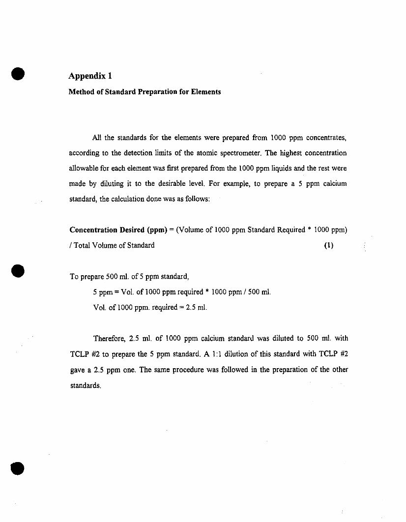
Appendix 1

Method of Standard Preparation for Elements

Ali the standards for the elements were prepared from 1000 ppm concentrates,

according to the detection Iimits of the atomic spectrometer. The highest concentration

allowable for each element was tirst prepared from the 1000 ppm liquids and the rest were

made by diluting il to the desirable level. For example, to prepare a 5 ppm calcium

standard, the calculation done was as follows:

Concentration Desired (ppm) =(Volume of 1000 ppm Standard Required • 1000 ppm)

/ Total Volume of Standard (1)

To prepare 500 ml. of 5 ppm standard,

5 ppm =Vol. of 1000 ppm required • 1000 ppm / 500 ml.

Vol. of 1000 ppm. required = 2.5 ml.

Therefore, 2.5 ml. of 1000 ppm calcium standard was diluted to 500 ml. with

TCLP #2 to prepare the 5 ppm standard. Al: 1 dilution of this standard with TCLP #2

gave a 2.5 ppm one. The same procedure was followed in the preparation of the other

standards.

•

•

•

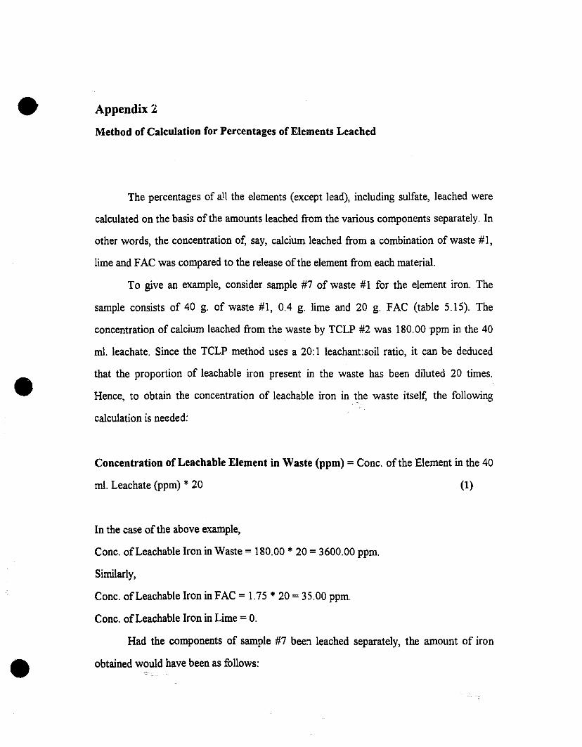
Appendix 2

Method of Calculation for Percentages of Elements Leached

The percentages of a!1 the elements (except lead), including sulfate, leached were

calculated on the basis of the amounts leached from the various components separately. In

other words, the concentration of, say, calcium leached from a combination of waste #1,

lime and FAC was compared to the release of the element from each material.

To give an example, consider sample #7 of waste #1 for the element iron. The

sample consists of 40 g. of waste #1, 0.4 g. lime and 20 g. FAC (table 5.15). The

concentration of calcium leached from the waste by TCLP #2 was 180.00 ppm in the 40

ml. leachate. Since the TCLP method uses a 20: 1 leachant:soil ratio, it can be deduced

that the proportion of leachable iron present in the waste has been diluted 20 times.

Hence, to obtain the concentration of leachable iron in the waste itself, the following

calculation is needed:

Concentration of Leachahle Element in Waste (ppm) = Conc. of the Element in the 40

ml. Leachate (ppm) *20 (1)

In the case of the above example,

Conc. ofLeachable Iron in Waste =180.00 *20 =3600.00 ppm.

Similarly,

Conc. ofLeachable Iron in FAC = 1.75 * 20 = 35.00 ppm.

Conc. ofLeachable Iron in Lime = O.

Had the components of sample #7 bee::l leached separately, the amount of iron

obtained would have been as follows:

•

•

•

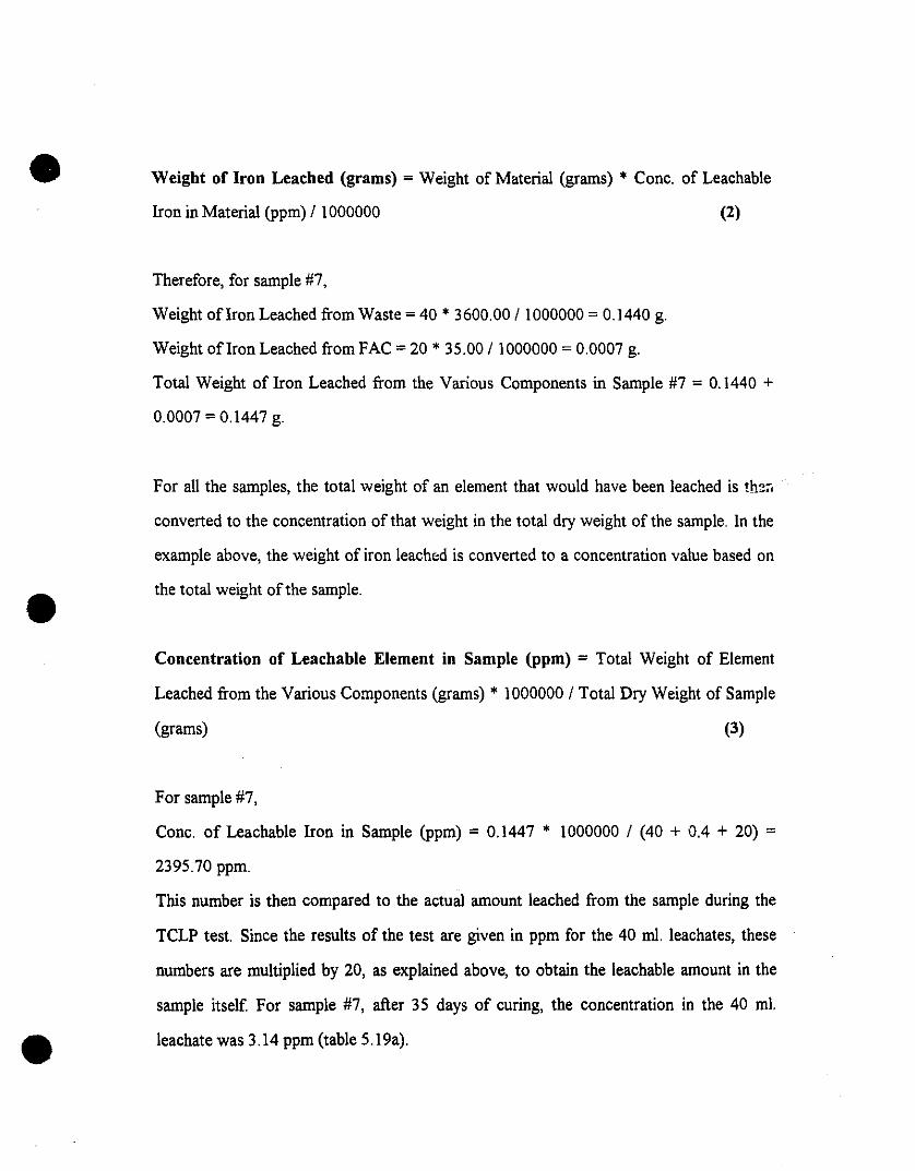
Weight of Iron Leached (grams) = Weight of Materia! (grams) * Conc. of Leachable

Iron in Materia! (ppm) /1000000 (2)

Therefore, for sample #7,

Weight oflron Leached iTom Waste =40 * 3600.00/1000000 =0.1440 g.

Weight oflron Leached iTom FAC =20 * 35.00/1000000 =0.0007 g.

Tota! Weight of Iron Leached iTom the Various Components in Sample #7 = 0.1440 +

0.0007 =0.1447 g.

For ail the samples, the total weight of an element that would have been leached is the;;

converted to the concentration of that weight in the tota! dry weight of the sample. ln the

example above, the weight of iron leached is converted to a concentration value based on

the total weight of the sample.

Concentration of Leachable Element in Sample (ppm) = Total Weight of Element

Leached iTom the Various Components (grams) * 1000000/ Tota! Dry Weight of Sample

(grams) (3)

For sample #7,

Conc. of Leachable Iron in Sample (ppm) = 0.1447 * 1000000 / (40 + 0.4 + 20) =

2395.70 ppm.

This number is then compared to the actua! amount leached iTom the sample during the

TCLP test. Since the results of the test are given in ppm for the 40 ml. leachates. these

numbers are multiplied by 20, as explained above. to obtain the leachable amount in the

sample itself For sample #7, after 35 days of curing, the concentration in the 40 ml.

leachate was 3.14 ppm (table 5.19a).

•

•

•

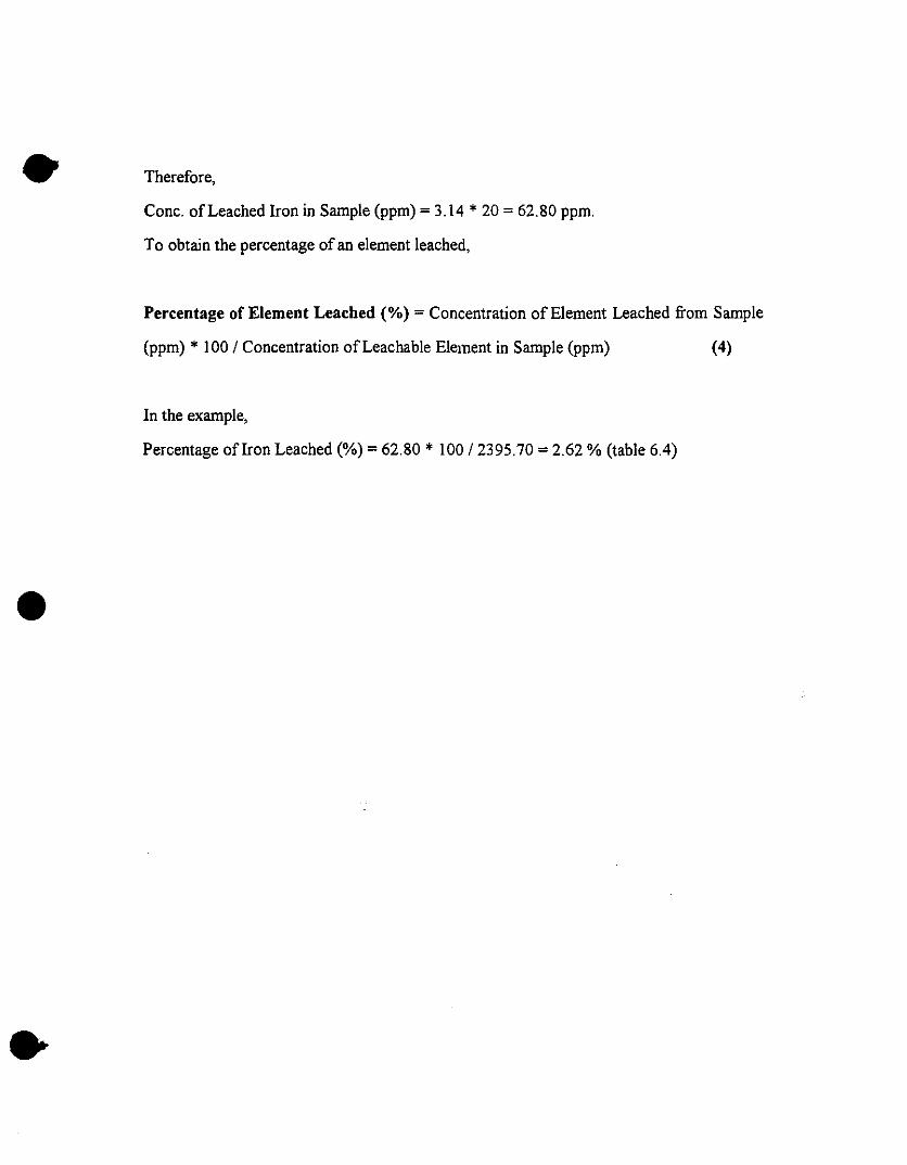
Therefore,

Conc. ofLeached Iron in Sample (ppm) = 3.14 * 20 = 62.80 ppm.

To obtain the percentage of an element leached,

Percentage of Element Leached (%) = Concentration of Element Leached from Sample

(ppm) * lOO/Concentration ofLeachable Element in Sample (ppm) (4)

In the example,

Percentage onron Leached (%) = 62.80 * 100/2395.70 = 2.62 % (table 6.4)

National Library - Bibliothèque et Archives Canada

Documents

Transcript of National Library - Bibliothèque et Archives Canada