NQ39626.pdf - Bibliothèque et Archives Canada
366
This manuscript has been repmduced from the microfilm master. UMI films the text directly from the original or copy submitted. Thus, some thesis and dissertation copies are in typewriter face, while others may be from any type of cornputer printer. The quality of thh reproduction is dependent upon the qwlity of the copy submitted. Broken or indistinct &nt, coloreci or poor quality illustrations and photographs, print bleedthrough, substandard margins, and improper alignment can adversely affect reproduction. In the unlikely event that the author did not send UMI a complete manuscript and there are missing pages, these will be noted. Also, if unauthorized copyright material had to be removed, a note wilI indicate the deletion. Oversize materials (e.g., maps. drawings, charts) are reproduced by sedoning the original, beginning at the upper left-hand corner and continuing from left to right in equal sections with small overlaps. Photographs included in the original manuscript have been reproduoed xerographically in this copy. Higher quality 6" x 9" black and white photographie pnnts are available for any photographs or ilustrations appearing in this copy for an additional charge. Contact UMI directly to order. Bell & Howell Information and Leaming 300 North Zeeb Road, Ann Arbor, MI 48106-1346 USA
-
Upload
khangminh22 -
Category
Documents
-
view
1 -
download
0
Transcript of NQ39626.pdf - Bibliothèque et Archives Canada

This manuscript has been repmduced from the microfilm master. UMI films the
text directly from the original or copy submitted. Thus, some thesis and
dissertation copies are in typewriter face, while others may be from any type of
cornputer printer.
The quality of thh reproduction is dependent upon the qwlity of the copy
submitted. Broken or indistinct &nt, coloreci or poor quality illustrations and
photographs, print bleedthrough, substandard margins, and improper alignment
can adversely affect reproduction.
In the unlikely event that the author did not send UMI a complete manuscript and
there are missing pages, these will be noted. Also, if unauthorized copyright
material had to be removed, a note wilI indicate the deletion.
Oversize materials (e.g., maps. drawings, charts) are reproduced by sedoning
the original, beginning at the upper left-hand corner and continuing from left to
right in equal sections with small overlaps.
Photographs included in the original manuscript have been reproduœd
xerographically in this copy. Higher quality 6" x 9" black and white photographie
pnnts are available for any photographs or illustrations appearing in this copy for
an additional charge. Contact UMI directly to order.
Bell & Howell Information and Leaming 300 North Zeeb Road, Ann Arbor, MI 48106-1346 USA

A Generalized Approach for Mechanics of Chip Formation in Steady-
State and Dynamic Orthogonal Metal Cutting Using a New Mode1 of
Shear Zone With Pardel Boundaries and Its Validation to Cutting-
Forces Prediction in SeIf-Piloting Machining
Mohammed Hayajneh
A Thesis
in
The Department
of
Mechanical Engineering
Presented in Partial Fulfillment of the Requirements for the Degree of Doctor of
Philosophy
at
Concordia University
Montreal, Quebec, Canada
August, 1998
Q Mohammed Hayajneh, 1998

National Library Bibliothèque nationale du Canada
Acquisitions and Acquisitions et Bibliographie Se mices services bibliographiques
395 Wellington Street 395, rue Wellington Ottawa ON KI A ON4 Ottawa ON K1A ON4 Canada canada
The author has granted a non- exclusive licence allowing the National Library of Canada to reproduce, loan, distribute or seU copies of this thesis in microform, paper or electronic formais.
The author retains ownership of the copyright in this thesis. Neither the thesis nor substantial extracts h m it may be printed or otherwise reproduced without the author's permission.
L'auteur a accordé une licence non exclusive permettant à la Bibliothèque nationale du Canada de reproduire, prêter, distribuer ou vendre des copies de cette thèse sous la fome de microfiche/film, de reproduction sur papier ou sur format électronique.
L'auteur conserve la propriété du droit d'auteur qui protège cette thése. Ni la thèse ni des extraits substantiels de celle-ci ne doivent être imprimés ou autrement reproduits sans son autorisation.

A Generalized Approach for Mechanics of Chip Formation in Steady-State and
Dynamic Orthogonal Metal Cutting Using a New Mode1 of Shear Zone With Paralle1
Boundaries and Its Validation to Cutting-Forces Prediction in Self-Pilothg Machining
Mohammed Hayajneh, PhD.
Concordia University, 1998
This study presents a novei approach to the mechanics of chip formation based on a
shear zone model with parallel boundaries that has been developed by applying the
continuum mechanics to the anaiysis of the chip formation process. Such a model is
formulated without imposing the assumptions commonly made in the single shear or pardel-
sided shear zone models.
A steady-state cutting force modd has k n derived and adapted to orthogonal
cutting of a self-piioting drilIing. In the formulated model, special attention has been
devoted to the thennomechanicd state which defines the effect of the temperature on the
yield shear stress of the work piece material.
The proposed steady state cutting force model has been extended to fomla t e a
cutting force model to analyze the dynamic behavior of the machining process in orthogonal
cutting. The cutting system was modeled using a single degree-of freedom dynamic system
where the variations of the cutting forces are represented by their total differentials.
SpeciaI mention in this study has been dedicated to experimental verifrcaîion. The
meaningful design, accuracy, precision, and the calibration of the experimental setups are
considered in details and several new experimental methodologies are proposed and used.
This study shows the fluctuation of the cutting forces is a result of chip segmentation
and not the cause. It also shows the effect of materials and cutting conditions on the cutting
signatures that has never been considered as a factor in the known studies on cutting
dynamics.
iii

Special attention has been devoteci to the chip morphology of the partially and fully
defomed chips to verQ the proposed model. A quick stop device has been designed to
obtain samples of partiaily formed chip
A new methodology has been proposed to align the machine such that the
misalignment between the tool and the workpiece is near zero to make sure that the measured
forces are not affected by any other sources. A low cost laser-carnera based system has k e n
buiit to achieve this goal.

To the Memory of M y Father

The author would like to express appreciation and gratitude to his technical
supervisors, Dr. M. O. M. Osman, Dr. V. Astakhov and Dr. V. Latinovic, who were
extremely helpfûl during the course of this research work. Professor V. Astakhov's efforts
were instrumentai in the realization of this work. His vision played an important mle in this
work.
The financial support of the Canadian International Development Agency (CIDA) and
the Natutal Sciences and Engineering Research Council(NSERC) is gratefully
acknowledged.
Special thanks to Dr. Akif Bulgaù, the director of the Canadian International
Development Agency /Jordan University of Science and Technology/Cordia University
(CIDA) project in Canada, and to Mrs. Marie Berryman, the coordinator of the project, who
were extremely helpful throughout dl stages required for this work.
1 would also like to gratefully acknowledge the use of the laboratory facilities of the
deep hole machinhg center, machine tool lab, metallurgy lab, Concordia cornputer aided
vehicle engineering center (CONCAVE), compter-integrated manufacturing (CIM) lab and
NC-machining center at Concordia University and metallurgy lab at McGill University.
1 am gratefd to my mother who is anxiously awaiting the completion of this thesis.
I am also grateful to my brothers and sisters for their support during my study.
The most sincere gratitude is to my wife, Manar Bani-Hani, for her caring,
encouragement and patience throughout the eritirety of this work Without her, it would be
impossible to wmplete this work. 1 am indebted to my son, Anas, who was born through the
course of the research work and 1 feel guilty because I could not spend enough time with him.

TABLE OF CONTENT
.................................................. LISTOFTABLES xxvi
CEAPTER 2: LITERATURE REVIEW ................................... 10
2.1 MECHANICS OF CHIP FORMATION ........................... 11
..................................... 2.1.1 Shear Plane Mode1 19
.................................. 2.1.2 SlipLine Field Tbeory 25
..................................... 2.1.3 Thick-zone Mode1 27
............................. 2.1.3.1 Flow region mode1 29
................... 2.1.3.2 PWel-sided shear zone mode1 -32
2.1 THERMOMECHANICAL BEHAVIOR OF WORKPIECE MATEEUAL IN
CUITING ................................................ 38
........................ 2.3 DYNAMICS OF THE CUïTING PROCESS 44
....................... 2.4 MEASUIUNG OF THE CUlTING FORCES 50
............................ 2.5 DEEP HOLE MACHINING PROCESS 55
.................................... 2.6 RESEARCH OBJECTIVES -57
CHAP'IXR 3: MECHANICS OF CEIP FORMATION USING SHEAR ZONE
........................ MODEL V V I T E PARALLEL BOUNDARIES 60
................. 3.1 ANALYSIS OF THE CONTINUrrY CONDITION -61
3.2 PERMXSSIBLE WLMTïES AND DISPLACEMENTS IN THE
SHEAR ZONE ............................................ 67
vii

3.3 DISTRIBUTION OF DEFORMATION IN THE CHIP
FORMATIONZONE ...................................... 77 3.4 THERMOMECHANICAL MODEL FOR THE SHEAR STRESS IN THE
.............. PRIMARY AND SECONDARY SHEAR ZONES -86
3.5SUMMARY ................................................. 89
CHAPTER 4: STEADYSTATE CUTTING FORCE MODEL IN TEE BTA
PROCESS BASED AND ITS ON THE SHEAR ZONE MODEL WITH PARALLEL
........................................................ BOUND ARIES 91
..................... 4.1 STEADY-STATE m G FORCE MODEL -91
4.2 CUTTING FORCE COMPONENTS IN BTA MACHINING USING THE
............... SHEAR ZONE WlTH PARALLEL BOUNDAEUES 95
.............................. 4.2.1 Cutting Force Components -96
.................................. 4.2.2 Cornputer Simulation 104
CHAPTER 5: AN ANALYTICAL EVALUATION OF THE CUTTING FORCES IN
ORTHOGONAL CUTTING USING THE DYNAMIC MODEL OF S H E X R ZONE
WLTHPARALLELBOUNDAIUES ..................................... 105
5.1INTRODUCZlON ............................................ 106
5.2 DYNAMliC MODEL OF SHEAR ZONE WlTH PARALLEL
BO UND- ................................................. 108
.................................. 5.2.1 GeneraLFomModel 108
............ 5.2.2 Determination of The Cutting Force Components 110
...... 5.2.3 Influence of hcremental Variations of The Shear Angle 113
5.2.4 hterpretation of the Incremental Variations in Terms of Cutiing ................................... Process Parameters 117
5.2.5Equationsof Motion .................................. 118
........... 5.2.6 Proposed Mode1 For The Cutting Force Evaluation 119
................................. 5.2.7 Cornputer Simulations 120

CHAPTER & MBALIGNlMENT ASSURANCE ........................... 122
6.1 THE DEEP HOLE DRILUNG MACHINE . . . . . . . . . . . . . O . . . . . . , . . . 125
6.2 MISALENMENT MEASUREMENT SETUP ..................... 127
6.3 CALIBRATION OF THE SYSTEM .............................. 133
CHAPTER 7: CUTTING FORCE MEASUREMENTS AND RESPONSE OF THE
DYNAMIC CUTI'ING PRO-S ....................................... 145
7.1 WORKPIECE MATERIALS .................................... 146
7.2WORKPIECETYPES . . . . . . . . . . . . . . . . . . . . . . . . . . . . . . . . . . . . . . . . . 149
7.3CUTI.INGTOOLS ......................................... ..149
7.4 CUlTINGFORCE MEASUREMENTS SETUF .................... 154
7.5 MAIN FUNCITONS OFFFT ................................... 162
7 . 6 C D R A T I O N . . . . . . . . . . . . . . . . . . . . . . . . . . . . . . . . . . . . . . . . . . . . . . 166
7.7MEASUREMENTS ........................................... 173
7.7.1 System Analysis ...................................... 173
7.7.2 Signal Analysis ....................................... 176
CHAPTER 8: METHODOLOGY OF STUDYING THE
CH-IPMORPHOLOGY . . . . . . . . . . . . . . . . . . . . . . . . . . . . . . . . . . . . . . . . . 184
8.1 QUI:CK STOP DEVICE ........................................ 187 8.2 SPEClMEN PREPARATION FOR MICROSCOPY AND MICROHARDNESS
MEASUEMENTS ...................................... -192
8.2.1 Samples Selection ..................................... 192
8.2.2Sectioning ........................................... 195
8.2.3Mounting ............................................ 195
8.2.4Grinding ............................................ 196
8.2.5 Polishing ............................................ 196
8.2.6Etching ............................................. 197
......................... 8.3 MICROHARDNESS MEASUREMENTS 198

CHAPTER 9: RESULTS AND DISCUSSION ............................ -200
9.1MISALIGNMEN?IEFFECT .................................... 201
9.2 STEADY- STATE AXIAL CTJTTlNG FORCE AND
CUTI'INGTORQUE ............................................ 206
9.3 WAVE REMOVING CUIIINGPROCESS ...................... -209
9.4CUTflJNGSIGNATURES ..................................... 210
9.5CHIPMORPHOLûGY ........................................ 213
CHAPTER 10: CONCLUSIONS AND RECOMMENDATTONS FOR FUTURE
WORK ............................................................. 314 1O.lCONCLUSIONS ............................................ 314 10.2 RECOMMENDATIONS FOR FUTURE WORK ................. -317

LIST OF FIGURES
CHAPTER2
Figure 2.1 : Shear plane model (a): the mode1 (b) the velocity diagram (Ernst and Merchant,
....... 194 1; Merchant, 1944; Merchant, 1945) ................... ... 21
Figure 2.2: Forces associated with the shear plane model (Ernst and Merchant, 1941;
Merchant, 19WT MerchantJ945) ..................................... 23
Figure 2.3: Lee and Shaffer's slip-line field for orthogonal cutting(Lee and Shaffer. 1951)
.............................................................. -28
Figure 2.4. Deformation mode1 assumeci by Okushima and Hitomi (1961) ......... -30
.......... Figure 2.5. ParalIeI-sided shear zone mode1 (Stevenson and Oxiey. 1970) -34
CHAPTER 3
Figure 3.1: Parailel boundaries shear zone model for a positive rake angle: (a) the mode1 (b)
thevelocitydia gram ............................................... 62
Figure 3.2: Parallel boundaries shear zone model for zero rake angle: (a) the model (b) the
velocitydiagram ................................................. 63
Figure 3.3: Paralle1 boundaries shear zone model for a negative rake angle: (a) the model (b)
thevelocitydiagram ............................................... 64
Figure 3.4. Location of the tangent velocities relative to the sliplines .............. 65
Figure 3.5. Effect of n on the velocity ratio v,Ot)/v, for a= 1 O0 and 5 = 1.5 ........... 69 Figure 3.6 Effect of n on the velocity ratio vx@)/vn for a=lOO and =2.O ........... -70
Figure 3.7. Effect of n on the velocity ratio vXQ)/vn for a=lOO and 6 =2S ............ 71
Figure 3.8. A mode1 of a chip formation zone with paraIlel boundaries ........... 74
Figure 3.9. Transition c w e s for different n .................................. 75
Figure 3.10: (a) The model of the chip ionnation zone and (b) the trajectory of a particle in
....................................................... ~ s z o n e 79
Figure 3.11. Distribution of the true shear stcain dong the width of the shear zone ... - 81
................................... Figure 3.12. hJh vs . n under yf$y(h) d.12 84

Figure 3.13: Distribution of the deformation rate in the deformation zone under v+ le S.'
and different n . The points cornpond to the deformation rate at the border of the
...................................... primaryandfinddeformation 85
.......................... Figure 3.14: Effect of temperature on the ratio TACT dt -88
CHAPTER 4
Figure 4.1 : Cuîting fortes representation at a distance r from the center
................................................. ofthecuttlligtool 97
Figure 42. Section of the BTA cutting profile ............................... 103
CHAPTER 5
Figure 5.1: A mode1 of shear zone with parallel boundaries as applied to evduate the
dynamic cutting forces ............................................ 109
CHAP'ïER 6
Figure 6.1: Misalignment between the axis of rotation of spindle nose and the axis of starting
bush .......................................................... 124
Figure 6.2. Deep-hole dding machine ..................................... 126
Figure 6.3. The schemaîic arrangement of the experimental setup ................ 128
Figure 6.4: A photograph of the experimental setup for misalignment measurement . 129
Figure 6.5. The p ~ c i p l e of the misalignment measurements .................... 130
Figure 6.6. Photograph of the principal elements of misalignment setup ............ 132
Figure6.7. Laser holder .................................................. 134
Figure 6.8. Accessory to mount the camera in different positions ................. 135
Figure 6.9: A photograph of the accessory for mounting the carnera in
different positions ................................................ 136
... Figure 6.10. An example of the captured image. and the results of the processing 137
..................... Figure 6.11. A systematic drawing of the coordinate device 140
........................... Figure 6.12. A photograph of the coordinate device 141
xii

Figure 6.13. The caübration setup ......................................... 142
Figure 6.14: Photograph of the caiibration setup .............................. 143
Figure 6.15:Calibration of the proposed misalignment measuring system in the horizontal
and vertical directions ............................................. 144
CHAPTER 7
Figure 7.1. A photograph of the used workpieces ............................. 150
Figure 7.2. BTAH tools of single cutting edge (American Heller design) .......... 151
Figure 7.3. BTAS twls of partioned cutting edges (Sandvik design) .............. 152
Figure 7.4. A photograph of the used cutting tools ............................. 153
Figure 7.5. Set up for measuring the cuttingforces in dming .................... 155
Figure 7.6: Set up for measuring the dynamic cutting forces in wave-removing cutting
procas ......................................................... 156
Figure 7.7: A photograph of the set up for measuring the steady-state and dynamic cutting
forces ......................................................... 157
Figure 7.8. Dynamometer ................................................ 158
Figure 7.9. A photograph of the dynamometer ................................ 159
Figure 7.10. Kistler 9065 load washer ...................................... 160
Figure 7.1 1 . Main fûnctions of FFT analyzer ................................ 161
Figure 7.12. Setup of the static calibration of the dynamometer dong the
axialdirection ................................................... 168
Figure 7.13. Setup of the static calibration of the dynamometer along the
.................................................. axiddirection. 169
Figure 7.14. Results of the static calibration a) dong the axial direction and b) along the
.................................................. torquedirection 170
Figure 7.15: Frequency response function FRF when the input is dong the axial force
................. direction: a) direct correlation and b) (cross correlation) 172
Figure 7.16: Frequency response function FRF when the input is dong the torque direction:
................... a) direct correlation and b) (cross correlation) 174

Figure 7.17: Coherence of the dynamometer signal vs. hammer signal when the input is
dong a) axial force and b) torque directions. ......................... 175
Figure 7.18: A photograph of the set up for performing the system analysis ........ 17'7 Figure 7.19: Calibration the hammer for the frequency nsponses function 0
measurements a) hammer response and b) FRF value ................... 178
Figure 7.20: Autospectra (RMS vs. PSD Format) ............................. 180
C&APTER 8
.............. Figure 8.1 : A systematic drawing of the designed quick stop device 1 88
........................... Figure 8.2.: A photograph of the quick stop device. 189
......... Figure 8.3: A photograph of the quick stop device in the loading position. 190
........ Figure 8.4: A photograph of the workpieces used in the quick stop device. 193
Figure 8.5: An illustrative quick stop samples in which a partially chip cari be seen at the
bottom of the hole. .............................................. 194
CHAPTER 9
Figure 9.1: Effect of misalignment on the steady-state axial cutting force and torque
components. Cutting conditions: workpiece, AIS1 303; tool, BTAS 1 " inch
diameter ;spinde rotationai speed n, 656 rpm; boring bar length, 2.0 m; cutting fluid
fiowrate,80Vmin~. .............................................. 216
Figure 9.2: Effect of misalignment on the steady-state axial cutting force and torque
components. Cutting conditions: workpiece, AIS1 303; tool, BTAS 1" inch
diameter ;spinde rotational speed n, 939 rpm; boring bar length, 2.0 m; cutting fluid
flow rate, 80 Vrnin. .............................................. .217 Figure 9.3: Efféct of rnisalignment on the steady-state axial cuning force and torque
components. Cutting conditions: workpiece, AIS1 303; tool, BTAS 1 " inch
xiv

diameter ; spinclle rotational spced n, 1253 Ipm; boring bar length, 2.0 m; cutting
fluidflowrate,80Vmin. . . . . . . . ....... . .. . . . . . . . . . . . . . . . . . . . . . . . . -218
Figure 9.4: Autospectra of the axial cutting force. Cutting conditions: workpiece, AISI 303;
tool, BTAS 1 " iùch diameter ; boring bar length. 2.0 m; spindle rotational speed n,
656 rpm; misalignmenf 15pm; cutting fluid fiow rate, 80 Vmin. . . . . . . . . . . -219
Figure 9 5: Autospectra of the cutting torque. Cutting conditions: workpiece, AISI 303;
tool, BTAS " inch diameter ; boring bar length, 2.0 m; spindle rotational s p d n,
656 rpm; misalignment, 1Spm; cutting fluid flow rate, 80 Vmin. . . . . . . . . . . -220
Figure 9.6: Autospectra of the axiai catting force. Cuttingconditions: workpiece, AIS1303;
tool, BTAS 1" inch diameter ; boring bar length, 2.0 m; spindle rotational speed n,
939 rpm; misalignment, 15pm; cutting fluid flow rate, 80 i/min. . . . . . . . . . . .221
Figure 9.7: Autospectra of the cutting torque. Cutting conditions: workpiece, AIS1 303;
tool. BTAS 1" inch diameter ; boring bar length, 2.0 m; spindle rotational speed n,
939 rpm; misalignment, 15pm; cutting fluid flow -, 80 Vmin. . . . . . . . . . . .222
Figure 9.8: Autospectra of the axiai cutting force. Cuning conditions: workpiece, AIS1 303;
tool, BTAS 1" inch diameter ; b o ~ g bar length, 2.0 m; spindle rotational speed n,
1253 rpm; misalignment, 15pm; cutting fiuid flow rate, 80 Vmin. . . . . . . . . . .223
Figure 9.9: Autospectra of the cutting torque. Cutting conditions: workpiece, AISI 303;
tool, BTAS 1" inch diameter ; boring bar length, 2.0 m; spindle rotational speed n,
1253 rpm; rnisalignment, 15pm; cuning fluid flow rate, 80 Ymin. . . . . . . . . . -224
Figure 9.10: Autospectra of the axid cuning force. Cutting conditions: workpiece, AISI
303; tool, BTAS 1" inch diameter ; boring bar length, 2.0 m; spindle rotational
speed n, 656 rpm; misalignment, 205pm; cutting fluid fiow rate, 80 Vrnin. . . .225
Figure 9.1 1: Autospectra of the cutting torque. Cutting conditions: workpiece, AIS1 303;
tool, BTAS 1" inch diameter ; boring bar Iength, 2.0 m; spindle rotational speed n,
656 rpm; misalignment, 205pm; cutting fluid flow rate, 80 Ymin. . . . . . . . . . -226
Figure 9.12: Autospectra of the axial cutting force. Cutting conditions: workpiece, AlSi
303; tool, BTAS 1 " inch diameter ; boring bar length, 2.0 m; spindle rotational speed
n, 939 rpm; misaiignment, 205pm; cutting fluid flow rate, 80 Ymin. . . . . . . . -227

Figure 9-13: Autospectra of the cutting torque. Cutting conditions: workpiece, AIS1 303;
tool, BTAS 1" inch diarneter ; boring bar length, 2.0 m; spindle rotational speed n,
939 rpm; misalignment, 205pm; cutting fluid flow rate, 80 Vmin. . . . . . . . . . -228
Figure 9-14: Autospectra of the axiaI cutting force. Cutting conditions: workpiece, AISI
303; tool, BTAS ln inch diameter ; boring bar length, 2.0 m; spindle rotational
speed n, 1253 rpm; misalignment, 205pm; cutting fluid flow rate, 80 Ilmin. . -229
Figure 9.15: Autospectra of the cutting torque. Cutting conditions: workpiece, AIS1 303;
tool, BTAS 1" inch diameter ; boring bar length, 2.0 m; spindle rotational speed n,
1253 rpm; misalignment, 205pm; cutting fluid flow rate, 80 Vmin. . . . . . . . . -230
Figure 9.16: Autospectra of the axial cutting force. Cutting conditions: workpiece, AISI
303; tool, BTAS 1" inch diameter ; boring bar Iength, 2.0 m; spindle rotational
speed n, 656 rpm; misalignment, 422prn; cutting fluid flow rate, 80 Vmin. . . .231
Figure 9.17: Autospectni of the cutting torque. Cutting conditions: workpiece, AISI 303;
tool, BTAS 1" inch diameter ; boring bar length, 2.0 rn; spindle rotationai speed n,
656 rpm; misalignment, 422pm; cutting fluid flow rate, 80 Ymin. . . . . . . . . . .232
Figure 9.18: Autospectra of the axial cuning force. Cutting conditions: workpiece, AIS1
303; tool, BTAS 1" inch diameter ; boring bar length, 2.0 m; spinde rotational
speed n, 939 rpm; misaügnment, 422pm; cutîing fluid flow rate, 80 Vmin. . . .233
Figure 9.19: Autospectra of the cutting torque. Cutting conditions: workpiece, AISI 303;
tool, BTAS 1" inch diarneter ; boring bar length, 2.0 rn; spindle rotational speed n,
939 rpm; misalignment, 422pm; cutting fluid flow rate, 80 I/min. . . . . . . . . . .234
Figure 9.20: Autospectra of the axial cutting force. Cutîing conditions: workpiece, AIS1
303; tool, BTAS 1" inch diameter ; boring bar length, 2.0 m; spindle rotationai
speed n, 1253 rpm; misalignrnent, 422pm; cutting fluid flow rate, 80 Ymin. . ,235 Figure 9.21: Autospectra of the cuning torque. Cutting conditions: workpiece, AJSI 303;
tool, BTAS 1" inch diameter ; boring bar length, 2.0 m; spindle rotational speed n,
1253 rpm; misalignment, 422pm; cutîing fluid flow rate, 80 Vrnin. . . . . . . . . .236
xvi

Figure 9.22: Autospecm of the axial cutting force. Cutting conditions: workpiece, AIS1
303; tool, BTAS 1" inch diameter ; boring bar Iength, 2.0 m; spinde rotational
speed n, 656 rpm; misaügmnent, 856pm; cutting fluid flow rate, 80 Umin. .. -237
Figure 9.23: Autospectra of the cuttIlig torque. Cutting conditions: workpiece, AIS1 303;
tool, BTAS 1" inch diameter ; boring bar length, 2.0 m; spindle rotational speed n,
656 rpm; misaiignment, 856pm; cutting fhid flow rate, 80 Ymin. ......... -238
Figure 9.24: Autosptra of the axial cutting force. Cutting conditions: workpiece, AIS1
303; twl, BTAS 1 " inch diameter ; boring bar length, 2.0 m; spindle rotational
speed n, 939 rpm; misalignment, 856pm; cutting fluid flow rate, 80 I/min. .. .239 Figure 9.25: Autospectra of the cutting torque. Cutthg conditions: workpiece, AIS1 303;
tool, BTAS 1" inch diameter ; boring bar length, 2.0 m; spindle rotational speed n,
939 rpm; misalignment, 856pm; c u h g fluid flow rate, 80 Ymin. ......... .24û
Figure 9.26: Autospectra of the axial cutting force. Cutting conditions: workpiece, AISI
303; tool, BTAS 1" inch diameter ; boring bar length, 2.0 m; spindle rotaiional
speed n, 1253 rpm; misalignment, 856prn; cutting fiuid 8ow rate, 80 Vmin. . .241
Figure 9.27. Autospectra of the cutting torque. Cutting conditions: workpiece, AIS1 303;
tool, BTAS 1" inch diameter ; boring bar length, 2.0 m; spindle rotational speed n.
1253 rpm; misalignment, 856pm; cutting fluid flow rate, 80 Yrnin. ........ -242
Figure 9.28: Steady-state cuning forces and torque components. Cutting conditions: .
workpiece, AISI 1045; tools, BTAH and BTAS 1 " inch diameter ; boring bar length,
2.0 m; spindle rotationai speed n, 656 ipm; misalignment, 15pm; cutting fi uid flow
.................................................... rate,80Vmin 243
Figure 9.29: Steady-state cutting forces and torque components. Cuning conditions:
workpiece, AISI 1045; tools, BTAH and BTAS 1" inch diameter ; boring bar
length, 2.0 m; spindle rotational speed n, 939 rpm; rnisalignment, 15pm; cutting
.......................................... fluidflowliite,80Vmin. 244
Figure 9.30: Steady-state cutting forces and torque components. Cutting conditions:
workpiece, AISI 1045; twls, BTAH and BTAS 1" inch diameter ; boring bar length,
xvii

2.0 m; spinde rotationai speed n, 1253 rpm; misalignment, 15pm; cutting fiaid flow
rate,gOVmin .................................................... 245
Figure 9.31: Steady-state cutting forces and torque components. Cutting conditions:
workpieze? AIS1 303; tool, BTAH nd BTAS 1" inch diameter ; boring bar length,
2.0 m; spindle rotational speed n, 656 rpm; misaiignment, 15pm; cutting fluid flow
mte,8OVmin .................................................... 246
Figure 9.32: Steady-state cuttîng forces and torque components. Cuning conditions:
workpiece, AIS1 303; tools, BTAH and BTAS 1" inch diameter ; boring bar length,
2.0 m; spinde rotational speed n, 939 rpm; misaügnment, 15pm; cutting fluid flow
rate,80Vmin. ................................................... 247
Figure 9.33: Steady-state cutting forces and torque components. Cutting conditions:
workpiece, AISI 303; tool, BTAH and BTAS 1 " inch diameter ; boring bar length,
2.0 m; spindie rotational speed n, 1253 rpm; misalignment, 15pim; cutting fluid flow
rate,80Vmin .................................................... 248
Figure 9.34: Steady-state cutting forces and torque components. Cutting conditions:
workpiece, AISI 4340; tools, BTAH and BTAS 1" inch diameter ; boring bar
Iength, 2.0 m; spindle rotational speed n, 656 rpm; dsalignment, 15prn; cutting fluid
flowmk,80Ym in.......,..,..................................... 249
Figure 9.35: Steady-state cutting forces and torque components. Cutthg conditions:
workpiece, AIS1 4340; tools, BTAH BTAS 1" inch diameter ; boring bar length,
2.0 m; spindle rotational speed n, 939 rpm; misalignment, 15pm; cutting fluid flow,
80Vm in........................................................ 250
Figure 9.36: Steady-state cutting forces and torque cornponents. Cutting conditions:
workpiece, AIS1 4340; tool, BTAH and BTAS esign 1" inch diameter ; boring bar
length, 2.0 m; spindle rotational speed n, 1253 rpm; misalignment, 15pm; cutting
......................................... fluid flow rate, 80 Vmin. .25 1
Figure 9.37: Simulation resuits (series 1) : v=140 mlmin. a=5 deg., frrquency=120 Hz,
...................................................... b=3.5mm 252
xviii

Figure 9.38: Simulation resuits (senes 2): m.19 mmlrev, a=5 deg., fiquency=120 Hz.,
b=3.5mm ..................................................... 253
Figure 9.39: Simulation resuits (series 3): r-140 mlmin, t a . 19 d r e v , fkquency=l20 Hi,
b=3.5mm, . . . . . . . . . . . . . . . . . . . . . . . . . . . . . . . . . . . . . . . . . . . . . . . . . . . . .254
Figure 9.40: Simulation results (senes 4): v=lM mlmin, t4.19 d r e v , a=5 deg., bc3.5
mm. .......................................................... 255 ........................... Fgure 9.41: Effect of feed on the dynamic forces. -256
Figure 9.42: Effect of cutting speed on the dynamic forces. .................... -257
Figure 9.43: Effect of rake angle on the dynamic forces. ...................... -258
....................... Figure 9.44: Effect of frequency on the dynamic forces. -259
Figure 9.45: Autospectra of the axial cutting force. Cutting conditions: workpieze, AIS1
1045; twl, BTAH 1" inch diameter ; boring bar length, 2.0 m; spindle rotational
speed n, 656 rpm; misalignment, 15pm; cutting fluid flow rate, 80 Ymin. ... -260 Figure 9.46: Autospectra of the cutting torque. Cutting conditions: workpiece, AIS1 1045;
tool, BTAH 1" inch diameter ; boring bar length, 2.0 rn; spindle rotational speed n,
.......... 656 rpm; misalignment, 15pm; cutting fluid flow rate, 80 Vmin. .261
Figure 9.47: Autospectra of the axial cuning force. Cutting conditions: workpiece, AIS1
1045; tool, BTAH 1" inch diarneter ; boring bar length, 2.0 rn; spindle rotational
... speed n, 939 rpm; misalignment, 15pm; cutting fluid flow rate, 80 Ymin. .262
Figure 9.48: Autospectra of the cutting torque. Cutting conditions: workpiece, AISI 1045;
tool, BTAH 1" inch diameter ; boring bar length, 2.0 m; spindle rotational speed n,
.......... 939 rpm; misaligrment, 15pm; cutting fluid flow rate, 80 Vmin. -263
Figure 9.49: Autospectra of the axiai cutting force. Cutting conditions: workpiece, AISI
1045; tool, BTAH 1" inch diameter ; boring bar length, 2.0 m; spindle rotational
.. speed n, 1253 rpm; rnisalignment, 15prn; cutting fluid flow rate, 80 Ymin. -264
Figure 9.50: Autospectra of the cutting torque. Cutting conditions: workpiece, AISI 1045;
tool, BTAH 1 " inch diameter ; boring bar Iength, 2.0 m; spinde rotational speed n,
......... 1253 rpm; misalignment, 15pm; cutting fiuid flow rate, 80 M n . .265
xix

Figure 9.5 1: Autospectra of the axial cutting force. Cutting conditions: workpiece, AISI
303; tool, BTAH 1" inch diameter ; boring bar length, 2.0 m; spinde rotational
speed n, 656 rpm; aisalignment, 15pm; cutting fluid flow rate, 80 Ymin. . . . .266
Figure 9.52: Autospectra of the cutting torque. Cutting conditions: workpiece, AIS1 303;
tooi, BTAH 1" inch diameter ; boring bar length, 2.0 m; spindle rotational speed n,
656 rpm; misalignment, 15pm; cutting fiuid 80w rate, 80 Ymin. . . . . . . . . . . .267
Figure 9.53: Autospectra of the axial cutting force. Cutting conditions: workpiece, AIS1
303; tool, BTAH 1" inch diameter ; boring bar length, 2.0 m; spindle rotational
speed n, 939 rpm; misaügnmenî, 15pm; cutting fluid flow rate, 80 Ymin. . . . .268
Figure 9.54: Autospectra of the cuaing torque. Cutting conditions: workpiece, AIS1 303;
tool, BTAH 1" inch diameter ; boring bar length, 2.0 m; spinde rotational speed n,
939 rpm; misalignment, 15pm; cutting fluid fiow rate, 80 Vmin. . . . . . . . . . . .269
Figure 9.55: Autospectra of the axial cutting force. Cutting conditions: workpiece, AISI
303; tool, BTAH 1" inch diameter ; boring bar length, 2.0 m; spindle rotational
speed n, 1253 rpm; misalignment., 15pm; cutting fhid flow rate, 80 Ymh. . . -270 Fig. 9.56 Autospectra of the cutting torque. Cutting conditions: workpiece, AIS1 303;
tool, BTAH 1" inch diameter ; boring bar length, 2.0 m; spindle rotational speed n,
1253 rpm; misalignment, 1 5pm; cutting fluid flow rate, 80 Ymin. . . . . . . . . . .27 1 Figure 9.57:. Autospectra of the axial cutting force. Cutting conditions: workpiece, AISI
4340; tool, BTAH 1" inch diameter ; boring bar length, 2.0 m; spindle rotational
speed n, 656 rpm; misalignment, 15pm; cutting fiuid flow rate, 80 Vmin. . . . ,272
Figure 9.58: Autospectra of the cutting torque. Cutting conditions: workpiece, AIS1 4340;
tool, BTAH 1" inch diameter ; bonng bar length, 2.0 m; spindle rotational speed n,
656 rpm; misalignment, 15pm; cutting fluid fiow rate, 80 l/min. . . . . . . . . . . ,273 Figure 9.59: Autospectra of the axial cutting force. Cutting conditions: workpiece, AISI
4340; tool, BTAH Heller design 1" inch diameter ; boring bar length, 2.0 m; spinde
spepd N, 939 rpm; misalignment, 15pm; cuning fluid flow, 80 Ymin. . . . . . . .274

Figure 9.m Autospectra of the cutting torque. Cuttïng conditions: workpiece, AIS1 4340;
twl, BTAH 1 " inch diameter ; boring bar length, 2.0 m; spinde rotational speed n,
939 rprn; misalignment, 15pm; cuning fluid flow rate, 80 Vmin. . . . . . . . . . . .275
Figure 9.61: Autospectra of the axial cutting force. Cutting conditions: workpiece, ATSI
4340; tool, BTAH 1" inch diameter ; boring bar length, 2.0 m; spuidle rotational
speed n, 1253 rpm; rnisalignment, 15pm; cutting fluid flow rate, 80 Vmin. . . .276 Figure 9.62. Autospectra of the cutting torque. Cutting conditions: workpiece, AIS1 4340;
tool, BTAH 1" inch diameter ; boring bar length, 2.0 m; spindle rotationai spced n,
1253 rpm; misalignment, 15pm; cutthg fluid flow rate, 80 llmin. . . . . . . . . . -277
Figure 9.63: Autospectra of the axial cutting force. Cutting conditions: workpiece, AISI
lW5; tool, BTAS 1" inch diameter ; boring bar length, 2.0 m; spindle rotational
speed n, 656 rpm; misalignment, 15pm; cutting fluid fiow rate, 80 Vmin. . . . .278
Figure 9.64: Autospectra of the cutthg torque. Cutting conditions: workpiece, AISI 1045;
tool, BTAS 1" inch diameter ; boling bar length, 2.0 rn; spindle rotationai speed n,
656 rpm; misalignment, 15pm; cutting fluid flow rate, 80 Vmin. . . . . . . . . . . .279
Figure 9.65: Autospectra of the axial cutting force. Cutting conditions: workpiecc, AISI
1045; tool, BTAS 1" inch diameter ; boring bar length, 2.0 rn; spindle rotational
speed n, 939 rpm; misalignment, 15pm; cutting fluid flow rate, 80 Ymin. . . . .280
Figure 9.66: Autospectra of the cutting torque. Cutting conditions: workpiece, AISI 1045;
tool, BTAS 1" inch diameter ; boring bar length, 2.0 m; spinde rotational speed n,
939 rpm; misalignment, 15prn; cutting fhid flow rate, 80 Vmin. . . . . . . . . . . -281
Figure 9.67: Autospectra of the axial cutting force. Cutting conditions: workpiece, AIS1
1015; tool, BTAS 1" inch diameter ; boring bar length, 2.0 m; spindle rotational
speed n, 1253 rpm; misaügnrnent, 15pm; cutting fluid fiow rate, 80 Vmin. . . -282
Figure 9.68: Autospectra of the cutting torque. Cutting conditions: workpiece, AIS1 1045;
tool, BTAS 1" inch diameter ; boring bar length, 2.0 m; spinde rotationai speed n.
1253 rpm; misalignment, 15prn; cutting fluid flow rate, 80 Ymin. . . . . . . . . . .283

Figure 9.69: Autospectra of the axial cutting force. Cuning conditions: workpiece, AIS1
303; tool, BTAS 1" inch diameter ; boring bar Iength, 2.0 m; spindle rotational
speed n, 656 rpm; misalignrnent, 15pm; cutting fluid flow rate, 80 Ymin. . . . -284
Figure 9.70: Autospectra of the cutting torque. Cuning conditions: workpiece, AISI 303;
tool, BTAs 1" inch diameter ; boring bar length, 2.0 m; spindle rotationai speed n,
656 rpm; misalignment, 15pm; cutting fluid flow rate, 80 Vmin. . . . . . . . . . . .285
Figure 9.7 1: Autospectra of the axial cutting force. Cutting conditions: workpiece, AIS1
303; tool, BTAS 1" inch diameter ; boring bar length, 2.0 m; spindle rotational
speed n, 939 qm; misalignment, 15prn; cutting ffuid flow rate, 80 Umin. . . . .286 Figure 9.72: Autospectra of the cuaing torque. Cutting conditions: workpiece, AISI 303;
tool, BTAS 1" inch diameter ; boring bar length, 2.0 m; spindle rotational speed n,
939 rpm; misalignment, 15pm; cutting fiuid flow rate, 80 Umin. . . . . . . . . . . .287
Figure 9.73: Autospectra of the axial cutting force. Cutting conditions: workpiece, AIS1
303; tool, BTAS 1" inch diameter ; boring bar length, 2.0 m; spindle rotational
speed n, 1253 rpm; misalignment, 15pm; cutting fluid flow rate, 80 Vmin. . . .288
Figure 9.74: Autospectra of the cutting torque. Cutting conditions: workpiece, AIS1 303;
tool, BTAS 1" inch diarneter ; boring bar length, 2.0 m; spindle rotational speed n,
1253 rpm; misaligxment, 15pm; cutting fluid fiow rate, 80 Ymin. . . . . . . . . . .289
Figure 9.75: Autospectra of the axial cutting force. Cutting conditions: workpiece, AISI
4340; tool, BTAS 1" inch diarneter ; boring bar length, 2.0 m; spindle rotational
speed n, 656 Tm; misalignment, 15pm; cutting fluid flow rate, 80 Ymin. . . . .290
Figure 9.76: Autospectra of the cutting torque. Cutting conditions: workpiece, AIS1 4340;
tool, BTAS 1" inch diameter ; bonng bar length, 2.0 m; spinde rotational speed n,
656 rpm; misalignment, 15pm; cutting fluid flow rate, 80 Ymin. . . . . . . . . . . -29 1
Figure 9.77: Autospectra of the axial cutting force. Cutting conditions: workpiece, AIS1
4340; tool, BTAS 1" inch diameter ; boring bar length, 2.0 m; spindle rotational
speed n, 939 rpm; misalignment, 1Spm; cutting fluid flow rate, 80 Ilmin. . . . -292

Figure 9.78: Autospectra of the cutting torque. Cutting conditions: workpiece, AISI 4340;
tool, BTAS 1 " inch diameter ; boring bar Iength, 2.0 m; spindle rotational speed n,
939 rpm; misalignment, 15pm; cutting fluid flow rate, 80 Vmin. .......... .293
Figure 9.79: Autospectra of the axial cuning force. Cutting conditions: workpiece, AIS1
4340; tool, BTAS 1" inch diameter ; boring bar length, 2.0 m; spindle rotational
speed n, 1253 rpm; misalignment, 15pm; cutting fluid flow rate, 80 V i n . .. .294
Figure 9.80: Autospectra of the cutting torque. Cutting conditions: workpiece, AIS1 4340;
tool, BTAS 1" inch diameter ; boring bar length, 2.0 m; spindle rotational speed n,
1253 rpm; rnisalignment, 15pm; cutting fluid flow rate, 80 Ilmin. ......... -295
Figure 9.8 1: Effect of cutting feed on the cuttùig signatures. Cutting conditions: tool, BTAS
and BTAH 1" inch diameter ; boring bar length, 2.0 m; misalignment, 15pm; cutting
fluid flow rate, 80 Ymin. ......................................... .296
Figure 9.82: Effect of workpiece materials on the cutting signatures. Cutting conditions: tool,
BTAS and BTAH 1" inch diameter ; boring bar le*, 2.0 m; misalignment,
15pm; cutting fluid flow rate, 80 Ilmin. .............................. .297
Figure 9.83: Effect of cutting speed on the cutting signatures. Cutting conditions: tool,
BTAS and BTAH 1 " inch diameter ; bohg bar Iength, 2.0 m; misalignment, 15pm;
cutîing fluid flow rate, 80 Vmin. ................................... .298
Figure 9.84: Microphotograph of the initial structure of AIS1 1045 steel. (mag: 100 X).
Etched with 10 mLNital, 90 ml alcohol. Structure is mainly pearlite grain (gray) with
a network of grain boundary ferrite (white). .......................... .299
Figure 9.85: Microphotograph of a fully defonned chip of AISI 1045 steel. Cutting
condition: tool ( rake angle ), 0.0; cutting speed v, 57.8 &min; feed t, 0.2 mdrev;
width of cut b, 5.0 mm. Etched with 10 mL Nitai, 90 ml dcohol. Structure reveals
a series of sliplines one following another and the grains are elongated in the
...................................... direction of the defornation. -300
Figure 9.86: Microhardness distribution (Vickers ) in a hlIy deformed chip of AIS1 1045
steel. Cutting condition: tool( rake angle ), 0.0; cutting speed v, 57.8 mlmin; feed
.............................. t, 0.2 d r e v ; width of cut b, 5.0 mm. -301

Eigure 9.87: Microphotograph of the initial structure of AISI 303 stainless steel (rnag: 400
X). Etched with 40 rnL hydrofluoric (HF), 20 mL Niûic acid (HNO3). 40 mL
gIecren. Structure is a matrix of austenite grains bound an intermetallic stringer-type
inclusions ..................................................... -302 Figure 9.88: Microphotograph of M y deformed chip of AISI 303 stainless steel. Cutting
condition: twl( rake angle ), 0.0; cutting speed v, 57.8 &min; feed t, 0.2 d r e v ;
width of cut b, 5.0 mm. Etched with 40 mL hydduoric (HF), 20 mL Nitric acid
......................................... (HNO3). 40 mL glecren. ,303
Figure 9.89: Microhafdness distribution (Vickers ) in a M y deformed chip of AIS1 303
steel. Cutting condition: tool ( rake angle ), 0.0; cutiing speed v, 57.8 &min; feed
t, 0.2 mdrev; width of cut b, 5.0 mm. .............................. .304 Figure 9.90: Microphotograph of the initial structure of ALTI 4340 steel (mag: 400 X).
Etched with 10 m . Nital, 90 ml alcohol. Structure is tempered mens i t e . . .305 Figure 9.9 1: Microphotograph of a M y deformed chip AIS1 4340 steel (mag: 50 X).
Cuning condition: tml ( rake angle ), 0.0; cuttuig speed v, 57.8 mimin; feed t, 0.2
mmlrev; width of cut b, 5.0 mm. Etched with 10 m . Nital, 90 ml alcohol. . .306 Figure 9.92: Microhardness distribution (Vickers ) in a fully deformed chip of AISI 4340
steel. Cutting condition: tml ( rake angle) , 0.0; cutting speed v, 57.8 mhin ; feed
.............................. t, 0.2 d r e v ; width of cut b, 5.0 mm. .307
Figure 9.93: Cornparison between the microphotographs of the Mly defomed chip of AIS1
1045, AISI 303 and AIS1 4340 steels( mag : 50). Cutting condition: tool ( rake angle)
0 .0; cutting speed v, 57.8 dmin; feed t, 0.2 d r e v ;
......................................... width of cut b, 5.0 mm. .308
Figure 9.94: Microphotographs of partially formed chip. Cutting condition: workpiecc, AIS1
4340; tool , BTAH 1" inch diameter, spindle rotational speed n, 1000rpm; feed t,
.................. 0.1 mdrev; Etched with 10 m . Nital, 90 ml alcohol. .309
Figure 9.95: Microphotographs of partially formed chip (mag: 50X). Cutting condition:
workpiece, AIS1 4340; tool , BTAH 1" inch diameter, spindle rotational speed n,
.... 1000rpm; feed t, 0.1 d r e v ; Etched with 10 mL Nital, 90 ml alcohol. - 3 10

Figure 9.96: Microphotographs of partially formed chip (mag: 1 0 o . Cutting condition:
workpïece, AIS1 4340; tool . BTAH 1" inch diameter; spindle rotaiional speed n,
1000rprn; feed t, 0.1 d r e v ; Etched with 10 mL Nital, 90 ml alcohol. . . . . . 3 11
Figure 9.97: Microphotographs of paaialiy f o d chip (ma& 200X). Cutting condition:
workpiece. AISI 4340; tool , BTAH 1" inch diameter; spinde rotational speed n,
1000rpm; feed t, 0.1 d r e v ; Etched with 10 mL Nital. 90 ml dcohcl. . . . . , 312
Figure 9.98: Microphotographs of partially formed chip (mag: 400X). Cuttmg condition:
workpiece, AISI 4340; tool , BTAH 1" inch diameter, spinde rotational speed n,
1000rpm; feed t, 0.1 d r e v ; Etched with 10 mL Nital, 90 ml alcohol. . . . . - 3 13

CHAPmR 5
Table 5.1 : Cutting conditions for the simuiation study ......................... 120
Table 5.2. Cutting parameters for the simulation study ......................... 121
CEWïER 7
Table7.1. Description of AIS1 1025 STEEL ................................. 147
TabIe 7.2. Description of AISI 1045 S'I'EEL ................................. 147
Table 7.3. Description of AISI 4340 STEEL ................................ 148
Table 7.4. Description of AIS1 303 STEEL .................................. 148 Table7.5. Kistler9û65 technical data ...................................... 162
CHAPTER 8
Table 8.1. The Etchants for the used materials ............................... 197
CHAPTER 9
Table 9.1. Effect of mis;ùignment on the measured axial cutting forces .......... -201
Table 9.2. Effect of rnisalignment on the measureü cutting torque ............... -201
Table 9.3. Steady-state cutting forces ( BTAH drill 1 . diameter. AIS1 1045) ........ 206
Table 9.4. Steady-state cutting forces @TAS drill lWdiameter. AISI 1045) ........ -207
Table 9.5. Steady-state cutting forces ( BTAH drill 1" diameter. AISI 303) ....... -207 Table 9.6. Steady-state cutting forces @TAS drill 1 . diameter. AIS1 303) ......... -208
Table 9.7. S teady-state cutting forces drill 1 . diameter. AIS1 4340) ............... 208
Table 9.8. S teady-state cuning forces ( BTAS drill 1 "diameter. AIS1 4340) ........ -209
Table 9.9. Effect of matenal. feed and cutting speed on the cutting
............................................. fluctuationfiequency 212

constant
area of the shear plane
tool face, Le., the surface over which the chip fi ows
cons tant
mean uncut chip thickness
mean cut chip thickness
matenai constant
Burgeis vector magnitude (m)
width of the machined surface; uncut chip width
chip width
machining constant
speed-dependent coefficient which can best be determined h m test
data
speed-dependent coeffîcient which can best be determined from test
data
specific heat capacity
distance OA ( mode1 of chip formation zone with parallel boudaries)
specific heat capacity at constant volume
Young's Modules
normal force at the tool-chip interface
fictional force at the tool-chip interface
force in the cutting direction,
force n~md to the cutting direction
shear force dong the shear plane
force normal to the shear plane
plowing force
mean tangential force and dynamic tangential force

mean cutting force and dynamic cutting force
mean shear force and dynamic shear force
mean friction force and dynamic fiction force
fkquency
An Arrhenius type function of the temperature.
shear modules
the intensity of angular defornation
shear zone width
distance OB ( mode1 of chip formation zone with paralle1 boundaries)
mechanical @valent of heat
slope of .r, vs. a diagram which can be experimentally detenaixled
for each partida- material
thermal conductivity of the work materiai
shear stress in the tool-chip interface zone
effective length the tool-chip interface
Iength of chip
contact length between the chip and tool
length of cut
Iength of the shear plane
length of the stickhg friction region
slope of the stress-strain curve
parameter characterizhg the non-uniform distribution of the
tangential velocity in the shear zone.
total power consumed in the cutting process
resuitant tool force
resultant force acting on the chip-tool interface region
chip thickness ratio or cutting ratio ( thl) always < 1
feed
distances measured dong the sliplines.

temperature
average temperature rise of the chip
temperature rise of matmal passing through the prirnary deformation
zone
initial work piece temperature
temperature in the prirnary deformation zone
temperature in the tool-chip interface zone
undeformeci chip thickness; Le., the thickness of the layer of materid
being removed by one cuüing edge at the selected point measured
normal to the d t a n t cutting direction
deforrned chip thickness, Le., the thickness of the chip produceci
during machining
dynarnic uncut chip thichess
displacement m h e d y
maximum of the function within the deformation zone.
cutting speed Le., the instantaneous velocity of the primary motion of
the selected point on the cutting edge relative to the work piece
tangent to the mutual perpendicular siipIines A and B
normal velocity to the shear plane
shear vefocity
velocity in x- direction
velocity in y- direction
velocity of chip flow
component of the chip velocity with respect to the shear zone
dynamic catting speed
the discontinuity of the tangential velocity with respect to the shear
zone
component of the work piece velocity with respect to the shear zone
displacement of the tool tip and oscillation velocity of the tool tip

displacement at the swface end of the shear zone and oscillation
velocity at the surface end of the shear plane
the value of y at which u,b) has the maximum
nominal rake angle of the tool and dynamic rake angle of the tool
cIearance angle
proportion of heat in the primary deformation zone
shear strain
shear sîrain rate
finai shear strain along the end of the deformation zone
failure shear strain
helical angle
shear strain along EF
thichess of the pafallel-sided shear zone
dynamic compression ratio
chip compression ratio calculated using the length of the chip
an@ between resultant cutting force R and the shear plane
mean angle of fiction on tool face tool cutting edge inclination
coefficient of fiction
density of work material
ultimate tensile stcess of work piece maîerial
mean compressive stress at A
mean compressive stress at B
normai stress on the tool face
normal stress on the shear plane
uniaxial dynamic yield stress
shear flow stress on the tool face in stickhg region
yield shear strength of the work material or shear stress on the shear
plane with zero normal stress applied
shear stress on shear plane

shear Dow stress dong AB
shear stresses on OA
shear stresses on OB
shear stresses on OD
shear stress dong EF
shear stresses dong CD.
mean shear angle and dynamic shear angle
principal cutting edge
rotational speed of the work piece
uniaxial ( effective) sarain
uniaxial ( effective ) strain rate
strain in the shear zone
frequency of the tool variation
frequency of the work surface dope variation

INTRODUCTION
The uitirnate objective of the science of metal cutting is the solution of practical
problems associated with the efficient and precise removal of metal fiom workpieces. A
properly founded solution of these problems is possible oniy when the laws governing the
cutting process are known. A knowledge of these laws makes it possible to fores- the
practical results of the cutting process, and thus to select the optimum cutting conditions for
each particular case. Since the knowledge exists in a fom of theory, the theory of metd
cutting should be advanced.

A vast effoa has been dedicated in the past research to develop a suitable theory of
metal cutting. But instead of developing p d c t i v e theones. which enable prediction of
cutting performance such as chip formation, cutting fom, tool Wear, and surface integrity,
theones of descriptive, pst-processing nature t& over.
Over the last hundred years an extensive shidy on the machining of met& has been
carried out Most of this focused on the dom-to-earth reduction of machining costs and
pragmatic approach to the manufacture of parts of acceptable dimensional accuracy and
surface quaüty. UnforhmateIy, a much smaüer volume of research has been devoted to
formulatiug the fundamental mechanisms underlying metal machining process in general,
as opposed to seeking case solutions for paaicular machining problems. The rpal boom in
fundamental metal cutting research, in the hes, has brought to the field both the recognition
of the need for an applicable metal cutting theory as well as the reputation of k i n g extremely
complex. Since then the practice of meial cutting has been advanced by costly ways of trial
and error while the fundamental research has experienced a slow down after producing huge
amounts of data that match the practical results only occasionaily.
The modem history of metal cutting began in 1945 when Merchant published his
vision of the metal cutîing phenomena (Merchant, 1945). As demonstrated by an excellent
survey presented by the CIRP working group on chip control (Jawahir and van Luttervelt,
1993), numerous attempts to improve the theory proposed by Merchant failed to improve its
predictive ability. As a result, no signifîcant progress has been made and, after 30 y-, the
theory is still lagging behind the practice. Shaw in his book (1984) summarizes his lifetime
expenence in the field and concludes thai it is next to impossible to predict metal cutting

performance.
Resently industry relies completely upon the empirical data as these are presented
by tool and machine tool manufacturers, as well as by professional engineering associations,
through handbooks and seminm. Since these reconimendations do not result from a
cornmon thwry behind hem, they provide ody a good "starting point" thus leaving to the
users that, at theu own coût, find out the optimal values of cutting parameters for each and
every particdar case they may encounter. And, for an outside observer with the obscure
knowledge in the field, it may appear that the industry is doing very weli this way.
At this point one may ask a logical question: "At the present stage of development,
do we really need a realistic metal cutting theory?". The answer to this question is given in
the recent CIRP workhg paper (Amiarego et al, 1996). the quote of which is as follows: "A
recent survey by a leading tool manufacturer indicates that in the USA the correct cuîîhg
tool Lr selected Zess thun 50% of tlrc time, the tool is used at the rated d n g speed on& 58%
of the time, andonly 38% of the tools are usedup to tkirfirll tool-life capability. One of the
reasom for t f i poor pe@ortluutce Lr the lack of the predicrive models fur mnchining " The
same has been found in an earlier survey of cutting regirne selection on CNC machine tools
in the Amencan aircraft industry (Amarego, 1996) showing that selected speeds are far
below the optimal economic speeds.
The present study aims to recvaluate the present models of chip formation (which
are in the very cores of the metal cutting theories) in hope to propose a better mode1 of chip
formation for steady-state machining.
This work may be thought of as consisting of two logical general parts; theoretical

and experimental parts. The theoretical part comprise the proposed model, an analytical
evaluation of the steady-state force model and dynarnic force mode1 for wave removing
process. The second part concerns with the validating d the proposed model experimentally
and cornparison of the obtained results with the theoretical values. It includes developing
a new experimental methodologies, designing the proper experiment setups and providing
the required appanihises.
The model for steady-state cutting is based on a new velocity diagram proposed by
Astakhov and Osman (1996) and Hayajneh et al (1996) contrary to dl the present studies on
metal cutting which use the Mercant's velocity diagram. It is shown tint the use of the
Merchant velocity diagram leads to the model of chip formation which is in obvious
contradiction with the mathematical theory of plasticity. According to this diagram, the
velocity of shearing exceeds the velocity of appIied load when a tool with a negative rake
angle is used that is in contrary with the principle of mass continuity condition. Using the
proposed velocity diagram and the slip-line theory, a new model for chip formaiion is
formulated. A new model to calculate the cutting forces is also proposed. Since cutting
experiment is cwried out on a deephole machine, the model was extended to be applicable
for deep-hole drüls.
The modei for wave-removing process utilizes the basics of the model for steady-state
cutting and is used to evduate the dynamic cutting forces in orthogonal cutting. The cutting
system was modeled using a single degree-of freedom dynamic system where the variation
of the cutting forces are represented by their total differentials. The influence of temperature
on the flow shear stress of workpiece materid is accounted

Since cutting experiments are cunied out to vdidate the theory. a special attention
was paid to the experimental methodology which includes the conditions of the experiment,
the characteristics of the setup us& the cuaing regime. etc. It is clear that a slight change
in the experimental conditions rnay lead to a signifiant error in the obtained results, which,
in tum. may lead to wrong concIusion about the validity of the rheory.
Among many important characteristics of the experimentai setup. the accwacy of the
relative position and motion of the tool and the workpiece was of prime concan since it
affects the resuits dramaticdy. Unfortunately, this parameter has not been qmrted in the
known experimental studies on metai cutting. In the present study. therefore, a special
attention was paid to show significance of this accuracy. Since the cutting experiments have
been curried out using deep-hole machine, a new method for inspecting machine accuracy
has been proposed. It is shown that for deep-hole machines. the misalignment between the
tool and workpiece defines the above-mentioned accuracy. The effect of any misalignment
on the cutting process has been venfied.
Cutting force measurement is an integral part of experimental studies in metal
cutting. In the present study two types of such measurement have been camed out:
+ rneasuring the steady-state component of cutting forrc
+ measuring the dynamic cornponent of cutting force.
MetaUography of the fomed and partially fonned chip is an important part of any
experimental study in metal cutting. In this work it has been maintained that this kind of
experiment makes sense if and ody if:
L The initial structure of workpiece material is reported.

The chip structure is considered at the mano- and micro levels to study, depending
on the phenomenon to be investigated, because each phenomenon cm be observed
at a certain ma-cation level and requira different preparation techniques of the
specimen.
The structures of the chip and d e f o d o n zone are compared with those predicted
theoretically to validaie the thwry used in the analysis.
A microhardness survey is peiformed on the structure to reconstnict the distribution
of stress and strain undergone by diffenmt regions of the chip and deformation zone
at the 1st stage of deformation. The results obtained are compared then with those
yielded by the theory.
Unfortunatelyt the present metallographical studies in metal cuttbg (as in, Trent,
1991) do not even mentioned these conditions. The present work aims at fllling in this gap
by proposing a detailed methodology of metallographic experiments in metal cutting.
The objective of this thesis are:
Formulation of a new model of chip formation which is not restrîcted by the most
assumptions commonly made to build the single shear plane, flow region and parallel
sided shear zone models and capable of relating the cuning forces, tool-workpiece
temperature to the cutting speed, f& tool geometry and properties of the workpiece.
Deriving a steady-statz cutting force model.
Extending the steady-state cutting force model to be applicable for the deep hole
machining process.
Fomulating a dynamic model bas& on the proposed steady-state cutting force model

to characterize the wave removing niteing process.
5. Validation of the proposeci mode1 experirnentaliy.
To achieve this goal the following steps have been perfomed:
1.
ii.
iii.
iv.
v.
vi.
Establishing of a new methodology to align the machine such that the
misalignment between the tool and the workpiece is near zero to make sure
thaî the measured forces are not afkted by any other effects. To test this
error effect on the measured forces, the tool has been intentionally
misali@, the misalignment values have been measured using a low-cost
laseramera-based system and the forces have been measured using the Fast
Fourier Transformation (FF23 Analyzer for different cutting conditions.
Measurement of the steady-state cutting force components for three different
materials and different cutting conditions.
Validating the dynamic force model by meas- the forces for a wavy
workpiece for different cutting conditions.
Monitoring and andyzing the chip formation by recoding the cutting force
signature using the FFï.
Studying the morphology of the formed chip by measuring its structure and
micro hardness.
Designing a quick stop device to fteeze the process of chip formation and
then observing the structure of the partially formed chip.
The outline of the chapters is as follows :
In chapter 2, the literaîure related to the mechanics of chip formation, chip

morphology, measuring of the cutting forces methodologies ,dynamics of the cutting process,
and deep hole macbining process is reviewed It concludes with the objectives of the
msearch.
Chapter 3 presents the mechanics of chip formation using a shear zone model with
paralle1 boundaries. This mode1 has been developed by applying the mechanics of continua
to the analysis of the chip formation zone. It concems with the following aspects -a) analysis
the principle of mass conservation in the shear zone in terms of plane slip-line field theory,
b) derivation of the equations for velocities and displacements in the defineci shear zone and
formulation of a new velocity diagram by applying the mechanics of continue, c)
examination of the strain and strain rate distribution in the chip fonning zone according to
the new velocity diagram, d) Studying the deformation process and exploring the texture of
the chip formed during orthogonal cutting and e) applying a themomechanical approach to
predict the shear stress in the shear zone. According to this model, the shear yield stress is
temperature-dependent and decreases at a certain rate with temperature increase. The
approach generalizes the effect of temperature on the shear yield stress in the shear zone.
In chapter 4 an analyticd formulation of the steady-state cutting force model has been
done using the shear zone model with parallel boundaries and the thennomechanical
approach. This model was extended to be applicable to deep-hole machining.
Chapter 5 presents formulation of a dynamics cutting force model based on the
proposed steady-state cutting force mode1 and characterization O the wave removing process.
Chapter 6 presents a methodology and specially designed setup for the machine
misalignment assurance. Also, a new calibration procedure is proposed and discussed.

Chapter 7 presents description of the materials, cutting tools, workpieces,
equipments, experimental setups, calibration and anaiysis procedures used in the experiments
of the cutting force and the cutting signature recording.
Chapter 8 presents the procedure of studying the chip morphology. It describe the
implementation of the qui& stop device which is designed to obtain samples of partially
formeci chip; then the specimens preparation stages for the rnetallographic and microhardness
tests are detailed FinaIly, the microhardness procedure is presented.
Chapter 9 presents the major results. It is showing the effect of misalignment on the
steady axial cutting force and torque as weli as on the autospectra of the dynamic axial
cutting force and torque. It proceeds with a cornparison of the experimental and theoretical
resuits of steady-state force in deep hole machining for different cutting tool geometnes,
workpiece materials and cutting regimes. The simulation results using the dynamic force
mode1 for wave removing process are compared with the experimental results. Then, the
dynamic axial cutting force and torque signatures are presented. The chapter ends with
rauits of the morphology study.
Chapter 10 contains the conclusions and the recommendations for future work.

LITERATURE REVIEW
The references related to the mechanics of chip formation, chip morphology, cutting
forces measurement, dynamics of the cutting process, and deep hole machining process are
reviewed in this chapter. The reviewed Iiterature is somewhat broad in context, but focused
primarily on five main topics :
P The models which deal with the mechanics of chip formation and study of the
deformation zones in metd cutting (primaxy deformation zone and secondary
deformation zone)-

P The models which deal with the thennomechanical behavior of workpiece materid
in cutting ,i-e. with the flow shear stress in the primary and secondary defonnation
zones.
0 The dynamics of metal cutting.
P The cutting forces measurernents.
Cl The deep hole machining process in terms of cutting forces measurements.
2.1 MECHANICS OF CEIP FORMATION
The machining of met& has been exercised since the beginningcivilization, yet, the
mechanics of the process is not fuUy understood, Most of the development and improvement
in rnachining procedures, und quite recentiy, have corne h m tnal and error methods and
empiricai investigation. Machining operations are often considered to be the most important
process in manufacturing, and in the last 50 years, a great ded of experimental and
theoreticai research has been conducted. Researchers in this field have attempted to develop
theories of the cutting process which can predict important cutting parameters without the
need for empirical formulation.
Metal cutting is often described as a complex process that involves fiction, plastic
flow and fracture of material under more extreme conditions than normally found in other
production processes or in materiai testing. Among material deformation processes the
metal cutting chip formation is unique in many ways. Perhaps the most strikiag aspect of the
deformation is the very high strain rate as large shear strain is imposed in a small
deformation zone. Another characteristic of chip formation which sets it apart fkom other

matenal pnnessing operations is the relatively unconstrained nature of the process. The
cutting tool imposes a displacement on one face of the work material while the other surfaces
are free. The proportion of the free surface is large. The result of these circumstances is a
peculiar deformation process in which si@cant heating takes places and a large change in
stress state occurs over short distance.
Alîhough a considerable amount of effort has been devoted to the analysis of the
metal cutting problem in the 1 s t hundred years. the mechanics of the chip formation process
is still far fiom clear. Jawahir and van Luttemelt (1993) presented an excellent and thorough
review of numerous approaches previously taken by investigators in the field. The number
of approach used so far reveals complexity of the problem of modeling chip formation.
Moreover. each author attempted to change something within the shear-mode1 in the h o p
to obtain a better agreement of theory with cutting experiments.
The art of metd cutting is ancient The historical development and early published
works are reviewed in detail by Ernst (1951), Finnie (1956) and DeVries (1970).
In 185 1, a French investigator Cocquillent was first involved into the investigation
on mechanics of cuaing process. He studied various materials such as iron, brass, Stone and
other materids in drilling operation to find out the work required to remove given volume
of material. Several other researchers in the cutting mechanics and chip formation in the past
were Joessel, Tresca, and Reuleaux in France, T h e , Zvorykin and Briks in Russia.
Mallock in England. Taylor in the United States- made his contribution in the area of tool
Wear and tool life (Amarego and Brown, 1969; Finnie, 1956).
Most of the analytical research in metal cuning have been done since the mid forty's.

Merchant (1944; 1945) assumed that a continuous type of chip is formed by a shearing
process on a single plane extending h m the cuttïng edge to the work surface ahead of the
tool. This plane was termeci "shear plane" and the angle it makes with the surf' generated
was called shear angle and designated by cp.
Lee and Shaffer (1951) applied the theory of plasticity for an ideally rigid-plastic
materid to the con~uous chip formation. Two essential aspects of their consideration are
of importance. Firstly, they considered the state of stress of the chip through which forces
exerted by the tool transmitted to the shear plane. Secondly, the shear plane was considered
as a line in a two-dimensiond cut dong which the tangentid component of velocity is
discontinued and this is in agreement with the mathematical theory of plasticity
Eggleston et al (1959) made extensive experimental sFdies on orthogonal cutting
using steel. aluminum doys and alpha-brass. They concluded that the angle between the
resultant force and the shear plane is not unique for any given material.
Kobayashi et al (1 960) and Kobayashi and Thomsen (1 959) experimentall y predicted
that the shedng stress on the shear plane for steel and other alloys is approximately constant
This prediction contradicts Merchant's assumption of a variable shear stress in his modified
theory,
Kececioglu (1960; 1958) studied expenmentally the effects of shear size,
compressive stress and shear strain on mean shear flow stress in metal cutting. He observed
that the shear zone size generally decreases as the rake angle and the speed increase and as
the depth of cut decreases. The compressive stress decreases as the rake angle and the depth
of cut increase and as the speed of cut decreases. The shear strain decreases as the rake

angle, the deph ofcut and the speed of cut increase. In bis conclusions he pointed out that
the strain, strain rate, size of shear zone, the normal compressive stress, temperature and the
shear flow stress are functiondy related.
Albrecht (1960a; 196ûb) emphaswd the importance of ploughing in the metal
cutting process. He estabiished an experimentai method to measure the ploughing force. His
analysis suggested that the ploughing process has an effect on chip curling and residual
stresses in the work material-
Usui and Hoshii (1963) proposcd slip-line field solution. In their analysis it was
assumed that Coulomb's law for dry slidhg niction does not hold.
Kudo (1965) proposed slipline solution for two dimensional steady state machining.
His solution is the same a s the one proposed by Lee and Shaffer, except that the sliplines
are curved to give a curling chip.
Bitans and Brown (1965) investigated the deformation of wax work pieces for
various cutting conditions. They observed a large plastic shear zone that becomes thicker
at srnalier rake angles. They also found that plastic flow occurs near the rake face and the
clearance face of the twI.
Hsu (1966) studied the normal and shear stress distributions on the face of the cutting
tool. He discussed the presence of a ploughing force in the metal cuning process and
suggested that its magnitude remains constant for different depths of cut and chip-twl
contact lengths. From cutting tests he calculateci the average normal stress a, and shear
stress a for different contact length ratios and found that the variation of r, and o, are
independent of the depth of cut.

Thomsen (1966) sîudied the shear zone in metd cutting. AAer careful examination
of a large number of chip mots he concluded that it is dificult to detennine the precise points
at which plastic deformation starts and ceases.
Goriani and Kobayashi ( 1967) studied the strain and strain rate distributions in
steady state orthogonal cutting of SAE 1113-8 steel. They estimated the maximum shear
stralli rate to be approximately equd to 1550 per second A mean shear strain rate of 1@ to
106 per second is estimated by Shaw (1950) and of 10' to ld per second by Kececioglu
(1960). They concluded that the determination of shear zone thichess is critical in
estimating the average strain rate.
Spaans (1971) measured the forces acting on a tool near the cutting edge. He noted
that the existence of a built-up layer or built-up edge is an important factor concerning the
magnitude of the extra forces near the cuttîng edge. He also developed equations to
detexmine the shape of the streamlines in the deformation zone based on constant strain rate
and flow stress in the plastic zone.
Roth and Oxley (1972) proposed a slip-line field for a straïn hardening material from
experimental results.
Liu and Barash (1976) studied the sub-layer of a surface generated by the chip
removal process. Their study concludes that the apparent strain energy, the maximum
residual smss and the maximum strain hardening index are approximately proportional to
the shear plane length or indirectly proportional to the cutting ratio for a given depth of CUL
Dewhurst (1978) considered a mode1 for the machining process where the chip
emerges from the deformation zone with a significant angular velocity. One of the
concIusions h m his analysis is that the machinhg process is not uniquely defined for any
set of steady state rnachining conditions.
Yamamoto et al (1979) analyzed the stress distribution on the tool-chip contact
surface for a transient cutting process of orthogonal cutting by a photoelastic experimental
method in which lead plates were cut with an epoxy m i n tool. The followiog are observed:
for a positive rake (a > 0) the shear stress on the rake face remains constant for a certain
distance and drops to zen, rapidly afkr th& while for negative rake (a < O), the shear stress
is zero at the cutting tip of the tool and increases to a maximum dong the tool, and maintains
this maximum for a certain range before it drops to zero. In both cases, the normal stress is
maximum at the cutting tip of the tool and decreases gradually toward the chip separation
point
Wright et al (1979) proposed that at the chip tool interface in rnachining some of the
interface regions expenence full sehure whereas others experience sliding. The proportion
of seized areas as to real area of contact A, is given by K = A/A, The constant K which
varies fiom O to 1 depends on factors such as matenal pur@ tool material and preparation,
cutting time, cutting spced, rake angle, lubrication and machine stability.
Doyle et al (1979) used a transparent sapphire cutting tool to study directly the
frictional interactions occurring at the ch@-tool interface in continuous chip formation. They
concluded that the contact length between the chip and the cutting tool may be divided into
three regions. In the first region the relative rnovement is observed at the interface. In the
second region the evaporated thin fùms on the tool were removed suggesting chip sliding.
In third region the fresh chip is exposed continually to the environment which leads to

increased adhesion and friction and is evidenced by the gross transfer of chip material to the
tool face.
Childs (1980) considered the effect of elastic contact between chip and tool which
occurs beyond the plastically stressed contact region during chip foxmation in metal cutting.
The main assumption in his analysis is that the shear stress is constant over the plastic
contact between chip and tool and decreases parabolically over the elastic contact. The ratio
of the shear stress tu the n o d stress on the rake face is constant over the elastic contact
region. It turns out, however, that the velocity on the elastic contact region is not compatible
with the holograph of the plastic zone that produces a curled chip.
Home et al (198 1) studied experirnentally the built-up edge formation in aluminum,
brass and steel using transparent sapphire cutting tools. They observed that the nature of flow
around the cutting edge causes a nahiral stagnant point around which very high shear strains
are produced. They proposed that pure materials do not exhibit a built-up edge because they
cm withstand high strains; but in deys such high strains lead to shear failures that cause
intemal separation and built-up-edge.
Wright (1981) studied the fnctional interactions at the chip-tool interface in
machining lead, aluminum, copper, iron, and nickel over arange of cutting speeds and times.
He used steel, cemented carbide and transparent sapphire cutting tools; the last allowing the
interface to be observed directly. IGs results confîmed Doyle et ai (1979) findings that there
is less transfer of work material immediately behind the cutting edge (the first region) than
at some distance h m the edge (second region).
Rarnalingam et al (1981) applied plane strain plasticity theory to metal cutting

problems. By c o n s i d e ~ g a plastic circula. arc free boundary that comects the work mateiial
with the chip they obtained the plastic zone boundaries in closed form. This was then
compareci with the experimental results of Roth and Oxiey (1972). The conclusion was that
the observeci deformation can not be accounted for with ideal plasticity formulatim.
However, in their studies the velocity requirements were not satisfied. Besides, the
calculated plastic region is not extended towards the tool face. They only compared the
caiculated shape of the plastic zone with the part of the plastic region ntar the free surfhce
that was suggested by Roth and Oxley. But, by considering velocity discontinuities in their
solution they could have matched the experimental observation satisfactorily.
Wright (1982) presented an upper round type analysis for predicting the shear plane
angle in machining, using the work material strain-hardening charactenstics. In this analysis,
fiction on the rake face and the high strain rates and temperatures that arise in practice are
neglected.
Wright et al (1982) studied the role of chiptool niction on the value of the shear
plane angle in machining. The conclusion was thaî the friction model was not W y
predictive and he suggested that the original fnctiodess model (Wright, 1982) is a good
approximation and is a useful technique as it stands, especially for softer metals.
Bagchi (1983) criticized Wright's mode1 by pointing out that except for AlSI I I I 3
steel the cornparison between the experimental and the predicted values are not close. He
suggested modiwng Wright's model by adding an ernpincal factor.
The following is a review for important nodels which tackle the mechanics of chip
formation.

2.1.1 S hearpiane Mode1
The most widely used mode1 is the one proposed by Ernst and Merchant (1941) and
Merchant (1944; 1945). In this model it is assumed that chip formation is accomplished by
the shearing of material over an incbed single imaginary plane extending h m the cutting
edge to the work surface ahead of the tool. This plane was tenned "shear plane" and the
angle it makes with the surface generated was designated as p. This shear plane AB in
Figure 2.1 across which the work velocity v is instantaneously changed to the chip velocity
v,. This requires a discontinuity ( jump) in the tangentiai component of velocity amss AB
equal to v, as shown by the velocity diagram in Figure 2.1.
The drawbacks of this model are, as analyzed by Zorev, (1966), the presence of a
single shshear plane AB and the absence of a smwth wnnection between the extemal surface
of the cut layer of metal and the chip ( point A ), which is contrary to experimental
evidence that one plastic zone is not one shear plane. Rather, it consists of a large number
of slip surf' over which plastic shearing takes place successively. As stated in (Okushima
and Hitomi, 196 1) suchcutting mechanism, based on simple shear along a single shear plane,
contains the following conflicts: a) a moving metal particle must attain an infinite
acceleration when it passes across the shear plane, changing its position fiom the work region
to the chip region, b) an infinite stress gradient exists on the shear plane, c) the rate of strain
is extremely large compared with that in static material tests, and d) extremely large strain
is produced abruptly on the shear plane, and the relationship between stress and strain in
cutting does not agree with that in static material tests.
Also the shear plane model was severely criticized by Oxley (1989) and Palmer and

Oxley (1959). Iî was pointed out that the assumption of a single shear plane and the
associated constant normal stress dong this plane were dependent on another assumption,
namely, that the flow stress of the work material does not not Vary during the deformation.
Merchant (1945) found that his mode1 agreed well with experimentai resuits obtained when
cutting synthetic plastic but agreed poorly with experimental d t s obtained for steel
machineci with a centered carbide tool. In Ernst and Merchant's fmt analysis (1 944) , the
following assumptions were made (Shaw, 1984): a) the shear stress is a maximum in the
direction of the shear plane, b) the coefficient of fiction is independent of the shear angle,
c) the resultant force R is independent of the shear angle, d) the tool tip is sharp and no
mbbing occurs between the tool and work piece, e) the deformation is two-dimensional, Le.,
no side spreaâ, f) the stress on the shear plane is u n i f o d y distributed, g) the resultant force
R on the chip applied at the shear plane is equal, opposite and coliinear to the force R*
applied to the chip at the tool-chip interface.
From these conditions a force diagram as shown in Figure 2.2 was constructeci and
the following relations can be concluded :
F, = Rcos6-a) F, = Rsin(li-a) Ff = Rsin (h) F, = Rcos ( 7 ~ )
in which, F, and F, are the forces in the cutting direction and normal to this direction
respectively , Ff and F, are the fictionai and normal forces at the tool-chip interface, F, is
the shear force along AB, r, is the shear flow stress along AB, t is the undeformed chip

chip /
. Figure 2.1: Shear plane model (a): the model (b) the velocity diagram (Ernst
and Merchant, 1941 ; Merchant, 1944 ; Merchant, 1945).

thickness, b is the width of cut mwured dong the cutting edge, a is the rake angle, <p is the
shear angle, 8 is the angle made by resultant R with AB and X is the mean angle of fkiction
used to describe the fictional condition at the tool-chip interface. From the Equations (2.1)
the cutting forces may be cietennineci, provided the shear stress r, , fiction angle X and the
shear angle cp are known. Merchant considered that r, would have the yield shear strength
for the work materid and that li would have the usud value for dry sliding friction.
Emst and Merchant (1941) proposed that the shear plane would take such a position
that the shear stress r, wouid be a maximum. They expressed the shear stress in tenns of
the tool rake angle a, the fiction angle between chip and tool rake face X and shear angle <p
and differentiated 7, in equation (2.1) with respect to shear angle cp and equating the
resulting expression to zero. This led to the resuit
Merchant (1945) presented a different derivation that led to equation (2.2) such that
the total power consumed P in the cutting process would be minimum . An expression for
the total power P consumed in the chip formation can be written as
P = F,v = .r,tbv cos @-a) sin9 cos (9 +La)
An expression identical to equation (2.2) can be obtained when P is differentiated with
respect to cp considering Ic and rM to be independent of q.
Upon finding equation (2.2) to be in poor agreement with experimental data,
Merchant (1945) presented a different approach, and a different set of assumptions were

Figure 2.2: Forces associated with the shear plane model (Ernst and
Merchant, 1941 ; Merchant, 1944 ; Merchant, 1945).

made:- a) the angle q is such that the total power is a minimum, b) the niction angle X is
independent of the shear angle cp, c) the shear stress r, on the shear plane is independent of
the shear angle 9, and d) the yield shear stress r, of the metal is increased linearly by the
presence of a normal compressive stress CF on the shear plane according to the following
equation
TH = TO+K~ (2-4)
where K is the dope of z, vs. a diagram which can be experimentally detemineci for each
particular materid. There is no clear physical reason why item (a) should be true. Many
examples may be found in nature in which non conservative processes, such as that of metai
cutting, clearly occur in such a manner that the energy consumed is not a minimum.
However, according to the formentioned assumptions, and fiom Figure 2.2, it can be seen
that
a = r,tan(q+h-a)
Substituting equation (2.5) into equation (2.4), we have
When this is substituted into equation (2.3) the following equation can be obtained
M e n P is differentiated with respect to cp and equaîing the resulting expression to
zero with t and h considered independent of cp, the following equation can be obtained

~ e r c h a n t caiIed the quantity cot%the machining constant C. AUowing C to be an adjustable
parameter which varies h m one material to another, the above expression would yield a
good approximation of the cp values to the experimental obsenrations. But the magnitude of
C is impossible to be real in some cases (Oxley, 1989).
2n1.2 Slip-line FieId The~ry
The theory of Lee and S h a e r (1951) was the result of an attempt to apply the
plasticity theoiy to the problem of orthogonal metal cutting. In d e a h g with problems using
the plasticity theory, it is necessary to make certain assumptions regarding the behavior of
the work matenal under stress as follows:
1. The material is rigid plastic, which means that the elastic strain is negligible during
deformation and that once the yield point is exceeded, deformation takes place at
constant stress.
2. The behavior of the material is independent of the rate of deformation.
3. The effect of temperature increase during deformation is neglected.
4. The inertia effect resulting from acceleration of the material during deformation is
neglected.
These assumptions have led to useful solutions of many problems in plasticity.
In th5 soIution of a problem in plasticity, the construction of a slip h e field is
necessary; this field consists of two orthogonal families of lines (caiied slip lines), indicating,

at each point in the plastic zone, the two orthogonal directions of maximum shear stress. The
slip-he field proposed by Lee and ShafTer for the orthogonal cutting of a contlliuous chip
is show in Figure 2.3. Xt can be seen that Lee and Shaffet have employed the idealized
shear-plane mode1 of cutting, where a l l the deformation takes place in a plane extending from
the tool cutting edge to the point of intersection of the fkee surfaces of the work and chip.
This transmission of forces results in the triangular plastic zone ABC, where no deformation
occurs but the material is stressai to its yield point. Thus, the maximum shear stress
throughout this zone is .r, the shear stress on the shear plane, and the two directions of this
maximum shear stress are indicated by the two orthogonal sets of straight Iines (slip lines).
If the boundaries of this tnangular zone are considered, it is clear that the shear plane
AB must give the direction of one set of slip lines since the maximum shear stress must occur
dong the shear plane. Also, since no forces act on the chip after it has passed through the
boundarydc, no stresses can be transmitted across this boundary. Thus, ACcan be regarded
as a free surface, and since the directions of maximum shear stress always meet a free surface
at d4, the angle CAB is equal to d4 . Finally, assuming that the stresses acting at the
chip-tool interface are uniform, the principal stresses at the boundary BC will meet this
boundary at angles X and (h «r12) (where X is given by taxi1( F m and is the mean chiptool
fiction angle).
From Figure 2.3, it c m be written
that is

Lee and ShafFer (1951) realized that equation (2.10) does not hold for all possible
values of h and a, narnely for high tool fiction and smail or negative rake angles. They
postulated that under such conditions, a build-up of material occurred at the nose of the tool.
However, to support this point a second solü5on was presented for the new geometry where
a built-up edge is present on the tool face.
The theories outlined above were compared with the results of independently
conducted experiments ( Pugh, 1958). It can be seen that neither of these theories approach
is in agrwment with any of the experimental rehtionships for the various materials testeci.
2.1.3 Thick-Zone Models
To eliminate the conflicts in the conventional cutting theory based upon the shear
process dong single plane many models were proposed by Okushima and Hitomi (1961),
Kececioglu (1958; 1960), Stevenson and Oxley (1970), Fenton and Oxley(1970) and others.
These models can be classified into two types the flow region model and the paraIlel-sided
model. In these models the single shear plane model is open up to get ride of the conflicts in
the shear plane model.

chip tool
45 -A
A
- --- t B
work
Figure 2.3: Lee and Shaffer's slipline field for orthogonal cutting (Lee and
Shaffer, 1951).

2.13.1 Flow tegion mdek
Okushima and Hitomi (1961) suggested the scheme shown in Figure 2.4. They
suggested that there is a fairly large transitional zone AOB for plastic deformation of metal
be taken into consideration between the rigid of work piece and the plastic region of
steady chip. In this mode1 the materiai was assumed to be ideally plastic and the shear
stresses on OA, OB and OD were considered equal to the yield shear strength r,. Thus,
and
- - 'SUA ' 'SOB - ',OD = ' 0
Fmm Figure 2.4, it can be conchded that
- Rsin cp, cos (cp, -a+X) 'SOA - tb
9
- Rsinh =soo - - b'r
where I, is the tool-chip contact length. From Equations (2.12), (2.131, and (2.14) , the angle
p, and 9, can be expressed by
and

chip
Figure 2.4: Deformation model assumed by Okushima and Hitomi (1 966).

w here
The thickness of the deformation zone can be represented by 9, so that
Experhnents on alead work piece showed that q was always positive, suggesting that
the analysis yielded sound results. It was also declared that the shear strain was much lower
than that in the shear plane model, a result which led Okushima and Hitomi to conclude that
their model was more reasonabb. However, this model is criticized by Kobayashi and
Thomsen in the discussion of their work because it is not possible to constmct a slipline
field satiswng equilibrium and continuity for the constmcted sector where each of the radial
lines is at the same time one of the maximum shear direction. Also point " O" in this model,
causes the same conflicts as in the shear plane model. This model also neglected effect of
the temperature produced during the cutting process.

2-13-2 Parallel-sided shear zone model
To get ride of the discontùluity in the velocity and to account for the effect of the
strain-hardening properties on the hydrostatic stress distribution in the chip formation zone
the parallel-sided shear zone model has been introduced by Oxley and his CO-workers
(Stevenson and Oxley, 1970; Fenton and Oxley, 1970) as shown in Figure (2.5). In this
model @araIlel-sided shear zone model) , the shear plane AB of the shear plane model
shown in Figure. 2.1 is just open up so that the boundary CD between the shear zone and
work piece and the boundary EF between the shear zone and chip are p d e l to and
equidistant h m AB. It is easy to realize that the there is no difference between shear plane
model and parallel-sided shear zone model except that shear plane AB in shear plane mode1
is open up to becorne of a finite thickness instead of zero thickness as in the shear plane
model.
The foiIowing assumptions were made to constn~ct the parallel-sided shear zone mode1:-
1. Plane strain deformation. This means that there is no side flow.
2. Steady state conditions.
3. Perfectly sharp twl edge.
4. The shear plane AB in this model is assumed to open up so that the work velocity v
is assumed to change to the chip velocity v,. in the shear zone dong smooth
geometrically identical seeamlines with no discontinuities in velocity.
5. The overall geometry of the shear zone in parallel-sided mode1 is assumed to be the
same geometry in the shear plane model with A B and cp in this model geometrically
equivalent to the shear plane and shear angle.

The force polygon of the shear plane model remains the same in the pardel-sided
shear zone model.
The ove& change in velocity in the parallel-sided model is assumed to be the same
velocity diagram as in the shear plane model.
The shear strain-rate is assumed to be constant through the shear zone.
The effect of temperature is neglected.
The shear stress rs is assumed to be constant dong AB.
According to the slipline field theory the variation in hydrostatic (mean compressive)
stress dong AB is linear with apa, .
This model assumes that AB would bend to meet the fiee surface at the required angle
n/Q in the region where it still could be taken as parallel to the cutting direction and
assuming that the angle that has to be tunied through to meet this condition (d4 - 8)
occurs within negligible distance.
Linear stress-strain relation is assumed such that A, = m y, where rn is the dope
of the stress-strain cwve-
Half of the resulted shear strain is assurned to occur at AB.
The ratio of the shear zone length to its thickness (1, I d s , ) is found experimentally
to have a value between 6 and 15 and with an average a value of 10.5.
In the parallel-side shear zcne model h is considered the mean fiction angle as the
tool-chip interface parameter in the same way as for the shear plane model solutions,
i.e. h would have the usual value as for dry sliding friction.

Figure 2.5: Parallei-sided sheer zone model (Oxley and Welsh, 1963).
34

The pardel-sided shear zone theory assumes constant velocity in the shear zone; this
means that the shear strain rate is constant throughout the shear zone. This strain-rate cm
be given as :
where, v, is the shear velocity which is equal in magnitude to the velocity discontinuity of
the shear plane model, and As, is the thickness of the shear zone. Eariy experimentd work
at low cutting speed revealed that the ratio of length to the mean thickness of the shear zone
(lm had a value between 6 and 15 for a range of work materials and cutting speed, but
for high cutting spced there are no information about that ration (Oxiey, 1989). According
to the assumptions (9), and (IO), the stress equilibnum equations referred to sliplines
becornes :-
where s, and s, are distances measured dong the sliplines.
For the assumed model (d r /dJ can be replaced by the finite difference (Ad As2) as
follow
Applying equation (2.2 1) between A and B gives

in which. o is the hydrostatic stress, o, and o, are the hydrostatic stresses at A and B . 1, is
the length of AB and +, and r, are the shear stresses dong EF and CD. Therefore, the
normal force F, acting on AB can be calcdated as :-
where b is the uncut chip width. The shear force on AB can be obtained ftom the foilowing
equation:
If the angle made by the resultant force R with AB is 9 as show in Fig. (2.6) , and by
using equation (2.23) then
According to the assumption (12). the foilowing equation can be written
Substihiting for a, into equation (2.26), it can be concluded that
0 can be expressed in tenn of the shear angle q . the mean friction angle h, and the rake angle
a by

Oxiey and Welsh (1963) related the change in the yield shear stress A, in the
parallel-sided shear zone by assuming a hear stress-strain relation (assumption (13))
Ar, = rny, (2.30)
where m is the dope of the stress-strain curve and y, is the shear strain dong EF. .(, can be
found by multiplying the t h e taken for a particle of matenai to pass through the shear zone
by the strain-rate in the shear zone (equation (2.20)). that is
where v, is the velocity normal to AB. However, some useful relationships between velocities
can be obtained h m the velocity diagram in Figure 2.5, nameiy
- v sin9 v1 - cos(cp -a)
- vcosq - cos(cp-a)
v, = vsincp
Substituting for v, and v, from Equations (2.32) into equation (2.3 1) yields
Using the assumption (14). that half of this strain will have occurred at AB then
where .r, is the yield shear strength of the work piece. Substituting Equations (2.29). (2.30),
(2.33) and (2.34) into (2.28), the following equation has been obtained:

Now. for given values of a, X, and t, it is possible to determine cp from equation (2.35)
by trail and error if a appropriate values of 7 , m and the thickness of the shear zone As, are
known. the shea. angle cp can be used together with the corresponding vdues of s, to
calculate the cutting forces from equation (2.1).
This mode1 as shown has k e n constructeci using 16 assumptions, some of them are
questionable such as the assumption that half of the resulted shear strain occurred atm, the
negleaing of the temperature, and assumption of constant shear strain-rate.
2.2 TBERMOMECHANICAL BEHAVIOR OF WORKPIECE MATERIAL IN
CUTrrNG
The goal of metal cutting research is to develop methods of predicting the quality and
cost of a machined work piece without physically machining it I f this can be done reliably,
a wider variety of potential process conditions cm be evaluated easier than currently possible
through trail-and-error experimentation, leading to more efficient process and tooling design
( h e and Kapoor, 1986; Steed, 1987). A basic requirements for achieving this goal is a
reliable method for predicting cutting forces for arbitrary process conditions. Almost al1
quantities which affect the quality and cost of the machined work piece such as, tolerance,
tool life, and power consumption , depend on cutting forces either directly or indirectly.
Since the flow shear stress r, is the main parameter affecthg the energy requirement and
the cutting forces in the machining, the estimation of this stress and its change during plastic

deforniaton remains one of the principal goals in the theory of chip formation. hvestigators
in the metal cuthg field have attempted to develop an ana1ytica.l means for the cutting
process which gives a clear understanding of the mechanism involveci and enables a
prediction of the cutting forces without a need for exhaustive empirical testing. In this
review the flow shear stress r, that occurs at the shear zone in metal cuning is wnsidered
The well known Merchant's force mode1 (Figure 2-21 is the only model accepted in
practicaily all known publications on metal cutting (Merchant, 1945; Zorev, 1966; Shaw.
1984: Oxiey, 1989). The core of the model includes determination of the shear force
component F, of the resultant cutting force as follows:
t b Fs = T,-- sin ~p
where r, is the shear flow stress almg the shear plane AB; t is the uncut chip thickness; b
is the width of c u ~ 9 is the shear angle.
Although many studies on metal cutting have been attempted to derive theoretically
or obtain experimentally the flow shear stress, this is still one of the most controversial issues
in the field. There are several principal questions concenllng the flow shear stress of
workpiece material in cutting: Could the stress-saain relations obtained in the standard
tensile (compressive) test be used in metai cutting? Would the stress in the deformation zone
stop growing or even start decreasing (an idealistic idea which stands behind so calied high-
speed machining (King, 1985)) in case of large strains such as those in metal cutting? 1s the
flow shear stress affecteci by high strain rates (10' - 108 higher than in the standard tensile
test) and high temperatures occurrïng in cutting? PracticaIly a l l serious studies done on

meta. cutting contain the direct or indirect answers to these questions.
The approaches that tackle the characteristics of the fl ow shear stress in the shear
zone cm be classified into three categories :
Those approaches that consider the flow shear stress in the shear zone equal to the
yield shear strength of the work piece. Some of these approaches consider the effects
of the shear strain rate and the temperature on the flow shear stress but these effects
are considerd to be canceling each other.
Those approaches that consider the effects of strain hardening ody, or the effect of
strain hardening and shear strain rate on the flow shear stress together.
Those approaches that consider the effects of strain hardening, shear strain rate, and
the effect of temperature on the flow shear stress.
The first effort in this direction was by Ernst and Merchant (1941) who offered an
analysis for the cutting force based on the shear plane model. They assumed that the flow
shear stress .r, on the shear plane is constant and equals to the yield shear strength T,, .
Merchant (1945) found that this theory agreed well with experimental results
obtained when cutting synthetic plastics but poorly with experhnental results obtained for
steel rnachined with a centered carbide tool. B y reconsidering the assumptions on which that
theory has been established, Merchant (1945) denved the following equation:
which resulted from the equation:
ZAB = r,+Ka
40

indicaîing that the flow shear stress s, on the shear plane increase linearly with the increase
in the normal stress, a, on the shear plane; where K is the slope of r, vs. cr diagram
experimentally cietennineci for each particular material, q~ is the shear angle. a is the rake
angle, and A is the mean friction angle. This equation agreed with the work of Bridgman
(1 937; 1943). where , in experiments on polycrystal lïne, the flow shear stress r, was shown
to be dependent on the normal stress o on the shear plane .
Shaw and F i e (1955) suggested that the small size of the deformation region may
influence the flow shear stress value. This follows fkom the theory of size effect for single
crystals which is based on the concept that at small s k the probability of finding
dislocation sources is reduced and hence the flow shear stress of a work piece rises.
Kececioglu (1960; 1958) studied the effects of the shear size, compressive stress, and
shear strain in metal cutting on the flow shear stress and he introduced the following
expression for the flow shear stress in the shear zone
where r, is the yield shear strength of the work piece, o the compressive stress acting on the
shear plane. y the shear strain undergone by the chip during its formation, As, the thickness
of the shear zone E, F, and G are materid constants.
Okushùna and Hitomi (1961) developed the flow region concept. The flow region
AOB is a transitional deformation zone which exists between the ngid region of the work and
the plastic region of steady chip as shown in Figure 2.4 in which the stress must be at the
yield level. Hence, according to Okushima, and Hitomi mode1 the flow shear stress 7, (r,,

tdB) on both boundary lines equals the yield shear strength (r, ) of the work piece material.
To explain the increase in the flow shear stress r, in the primary shear deformation
zone during machining . it has been suggested by a number of researchers that s&n
hardening plays an important role in detemiining the flow shear stress r, in metaï cutting
(Shaw and Finnie, 1955; Oxley, 1961) and Oxley (1989) suggested the following relation
for the flow shear stress 7, on the shear plane AB shown in Figure 2.5
where r, is the yield shear strength of the work piece, rn the slope of the plastic stress-strain
curve at the corresponding mean shear stralli rate in the primary shear deformation zone,
which can be experimentally determineci for each particular matexid, and y, is the fmd strain
dong the end of the deformation zone EF shown in Figure 2.5 which c m be expressed as
Von Turkovich (1970), obtained the behavior of the flow shear stress .c, by
considering the process of plastic defonnation from the viewpoint of dislocation theory. The
theory was developed for high strain rate processes and very large strains.
Klamecki and Kim (1988) developed a mode1 for the flow shear stress T, in the
primary shear deformation zone that take into account the effect of temperature T and strain
associated with the chip formation y , and thc flow shear stress pnor to the plastic
defonnation r,, which can expressed as :-
5 = r,+aF-bTn (2.42)
where a, b, m. and n are coefficients to be obtaineà through experiments. However. no
specific solution was given foryielding work materid stresdstrain behavior shown by the
previous equation, and in reaching a solution. that equation requires four additional
experimentally obtained coefficients : a, b, rn, and n, which need to be detennllied through
lengthy. expensive and very often inaccurate experimentd procedure.
Klamecki and ICim (1988) snidied the effects of the stress state transition h m plane
stress at the work piece surface to plane strain in the centrai mgion of the chip formation
zone. In their mode1 they expresseci the flow shear stress r, in terms of the yield shear stress
of the work material, strain y and temperature T using the following expression:
The strains and temperatures used in this expression are the Iocd values calculatexi
in the finite element simulation. Changes in the material behavior are specified by constants
K,n , andA.
To apply these approaches it is necessary to do many experiments in order to
determine the involved constants. Some of these experiments are lengthy. expensive and
often inaccurate. This means that the= is a need to deveIop approach enabling us to predict
the 80w shear stress in the shear zone without doing additional experiments, or with fewer
number of experiments.

2.3 DYNAMICS OF CUTïTNG PROCESS
A metal cuaing system essentialiy comprises the cutting process and the tool layout
The cutting process involves the removal of metal in form of chips fiom the workpiece by
the action of the cutting tool which is coupled to the machine structure through Merent
elastic elements. Thus, the tool traces a uniform path relative to the workpiece. Nonndy,
any small vibration caused by occasional disturbances, such as inhomogeneity of the work
maienal, the ninout and misaligrnent of the worlq>iece, would be damped out by the
stmcture of the ,cutting system. Sometimes, however, the disturbances are maintained and the
system becomes unstable and the relative periodic displacement between the tool and the
workpiece may build up to a large amplitude. This relative periodic motion between the
cutting tool and the workpiece is known as chatter (Armarego. 1969).
Chatter imposes an undesirable limit on machine tool performance because it can
imped the maintaining of the work surface f d s h and dso it has adverse effect on part
dimensional accuracy and the cutting tool life.
Machine tool dynamics against chatter vibration is a chailenging subject of metal
cutting research not only because of the level of physical complexity involved but also
because of its role as the limiting fiictor in machining productivity. A large number of
investigation in machining chatter have been undertaken in the last forty years in order to
predict the dynamic behavior of the cutting process. Even though significant progress in
approaching this goal has been made, the basic problem of establishing a universal force
relationship with respect to the dynamic variables in metal cutting apparently has not been
solved.

S tudying the wave-removing process which comprises moving the cutting tool in a
straight iine while the surface to be cut oscillates has a big advantages in knowing the
mechanism of the chatter.
Kobayashi and Shabaik (1964). using a photographie technique, which gave a direct
observation of the shear angle vatiation, confirmed that the shear angle changes with the
slope relative to the top surface of the uncut chip thickness.
Kobayshi and Kawata (1967) studied the effect of m a t u r e of work surface on metai
cutting and concluded that when the work surface has a curvature, the cutting characteristics
dBer h m that in a planning operation. It was concluded that the effects of curvature must
be taken into account when a work piece with a diameter less than 50 mm is mschined. In
the analysis of metal cutting process, a commonly assumed model is one in which the tool
makes a linear motion. However, there are many processes such as hinllng, boring and
drilling, in which the tool or the work makes a circuiar motion. In these cases the work
suxface has a certain cwature. When the curvature is convex, the process may be called an
extemal cutting whereas it may be calleci an intemal cutting in a concave case.
When the free surface of the uncut chip has a sinusoidal shape, it loses its harmonic
character after passing through the shear zone. This led Albrecht (1962) to conclude that the
accompanying shear angle variation must be essentially of the saw-tooth type. However, Das
(1965) showed that adistorted cut chip profile in no way proves the presence of a shear angle
variation. Even with a constant shear angle, a symmetrid uncut chip profile becornes
unsymmetricai after passing t hugh the Shear zone.
Das and Tobias (1967) developed amathematical model which shows the connection

between the static and dynatnic cuhg coefficients. Three cases of dynamic cutting are
considered: wave cutthg, wave removing and wave-on-wave cutting. This mode1 is based
on the assumption thaî under dynamic conditions the orientation of the shear plane remallis
unaffecteci by a variation of chip thiclaiess, provided this fluctuates relatively fast
Rubenstein (1972) anaiyzed the innuence of tool oscillation during a planning
operation. A fundamental assumption made at the outset is that only those phenomena
which have been observed to occur in stmdy-state cutting occw in dynamic cuttuig. The
Muence of tool motion is shown to be compounded of two parts, namely, tool motion dters
the geornetry of the cutting process and affects the magnitude of some of the cutting stresses
by altering the strain and the strain rate to which material passing below the tool is subject
The resulting equations for the force components dong and normal to the steady-state cutting
direction are non-linear, and are expressed in te- of the stress-strain and s t r e s s - s e rate
equations of the work piece material.
Nigm and Sadek (1977a) investigaîed expenmentally the dynamic response of the
shear plane and the variation of the dynamic cutting coefficients at various values of feed,
cutting speeà, rake angle, clearance angle, frequency, and amplitude of chip thickness
modulation. This investigation showed that the shear plane responds to the dynarnic
variations in the cutting conditions and that its angular oscillation is not in phase with the
chip thickness modulation. Moreover, the dynamic cuning coefficients are not in phase with
the chip thickness modulation. In both wave generation and wave removal, the magnitude
and phase of the dynamic cutting coefficients and shear plane oscillation are found to be
function of the cutting conditions. However, the clearance angle has no effect on these

parameters. In reference to the dynamic cutting coefficients it has been concluded thaï while
the tangentid coefficient is not affected by the amplitude of chip thickness modulation, the
thmst coefficient is slightly affectai. The experimental d t s of this investigation showed
dso that there is no difference between the DC components of the shear angle and the
CU- forces obtained under steady-state cutting.
Nigm et al (1977a) presented a dimensional andysis of the orthogonal steady state
metal cutting process. This ykided expkit mathematicai expressions for the chip thickness
ratio, the force ratio and the tennination of the built-up edge in terms of the rake angle, the
feed and the cutting speed The functions derived were found to be independent of the
cutting conditions, for a particular combination of work and tool materials, characterized by
a set of coefficients. The validity was tested expenmentally and by reference to observed
results obtained by previous investigators and a good correlation was observed in alI case.
The expressions derived, with the experimentdy detennined machining stress, permit the
predication of the cutting forces over a wide range of cutting conditions fiom a limited
number of machining tests.
Nigm et ai (197%) presented a mathematical model for determination of the
dynamic cutting coefficients fiom steady state data In other word, the physical rdationships
estblished in steady-state cutting can be applied to dynamic cutting as well, if the amplitude
of vibration is relatively small. This theory is based on a non-dimensional analysis of the
steady state orthogonal cutting process. 1t takes into consideration the oscillations of the
shear plane response tu dynamic variations of the cuaing parameters. The model was
verified, directly with dynamic cutting tests for the wave cutting and the wave removal, in

which the variations or the shear plane and those of the cutting force coefficients were
r n e a s d Indirect ~ e ~ c a t i o n was achieved by reference to the work of previous
hvestigators concerned with dynamic cutting and the stability of the cutting process.
Wu and Liu (1985a; 198Sb) developed a mathematical model of machining chatter
through an analytical approach in order to predict dynamic cutting force from steady-state
cutting tests. The model is derived h m a pseudo-static geometric configuration of the
cutting process by taking into account the fact that the mean fiction coefficient fi uchiates
dynamically responding to variation of the relative speed on the chip twl interface. The force
functions through this derivation can be used to explain a i i three basic mcchanics associateci
with chatter vibration of dl the three cases namdy, velocity dependent, regenerative, and
mode coupling effects.
Ahn et al (1985) presented anew approach to the identifkation of the cutting process
dynamics in the form of a transfer function derived h m the finite difference equation model.
Wu (1986) presented a new method of modehg the anguIar oscillation in dynamic
orthogonal cuning. The system governing equations were derived based on the
work-hardening slipline field theory in cutthg mechanics by taking into account the
changes of stress conditions on both the shear plane and the tool-chip interface.
Fujii et ai (19863 investigated the whirling vibration of the drill in the beginning of
the drilling operation experirnentally. S pecial attention is paid to how vibration develops as
the dnll proceeds into the work piece. Three types of drills with different web thicknesses
were us& and the characteristics and cause of the vibration were discussed Whirling
vibration, which has an elliptical orbit, is a self-exited vibration accompanied by a phase lag

with respect to the revolution of the work piece. The vibration energy is pmvided by the
regenerative effect at the major cutting edge, whüe the chisel edge acts to W p e n the
vibraîion.
Fujii et al (1986b) exarnined the influence of widely var id point angles. relief angles,
and helix angles on whirling vibration of drill point geomeîry at the major cutting edge. The
influence of the flank surface configuration of the major cutting edge was studied in
p;uticular. Based on the obtained results, an attempt was made to obtain usefid parameten
by which the initiation boundary of wkling could be predicted.
Marui et al (1988a) observed the primary and the regeneraîive chatter vibraiions
ocfurring in a spinde-workpiece system, and clarified the effects of the vibratory
characteristics of the system and cutting conditions on the chatter vibration.
Marui et al (1 988b) measured the effixt of the dynamic variations of cuttuig depth,
cutting velocity, and rake angle on the cutting force acting in the dynamic state of a lathe
spindle-workpiece system by unique experiments. The phase lag between the dynarnic
cutting force and vibration displacement is clarified under various cuning conditions. The
dynamic cutting force is measured when the cutting velocity and the rake angle were
dynamically change-, and the results were represented as thecutting velocity coefficients and
the rake angle coefficients. Based on these results, the energy supplied by the dynamic
cutting force was obtained and the mechanism by which the chatter vibration occurred was
discussed.
Marui et al (1988~) treaîed chatter vibration occurring in the spinde-workpiece
system of a lathe theoretically, considering the phase lag of cutting force and chatter marks.

As a result, it was clarifieci that the chatter vibration is mainly induced by the phase lag of
cutting force (primary chatter) and by the phase lag of chatter marks in successive cutting
(regenerative chatter). The dynamic variations of the cutting ve1ocity and rake angle made
the spindle-workpiece system more unstabIe under vibration. The effect of cutting velocity
variation was more remarkable than that of rake angle in both types of chatter. Chatter
vibration could effectively be suppressed by increasing the damping capacity of the system.
Wu (1 989; 1988) introduced a new concept to üevelop a comprehensive cutting force
model for analyzing the dynarnic bchavior of the machining process. The model was denved
based on the principles of the cutting mechanics, and it takes into account the fluctuation of
the mean coefficient of fictional on the tool-chip interface as well as the variations of the
nomai hydrostatic pressure distribution and the shear flow stress dong the primary plastic
defonnation zone. The model has been tested through computer simulation for orthogonal
wave-removing processes by reference to an existing experimental evidence.
2.4 MEMUREMENT OF CUT"I'ING FORCES
To place the anaiysis of the metal cutting process on a qualitative and quantitative
basis, certain investigation must be made before, during, and after the cuning (Shaw, 1984).
The number of observations that can be attained during the cutting process is rather limiteci.
One among of those is the determination of the cutting forces.
An understanding of the forces in machining process is necessary since they are
rdated to such things as tool Wear, vibrations, accuracy, power consumption, process
planning, and computer aided manufacture. Since force magnitudes can be determineci by

variety of techniques. it is important to know the methodology of rneasmment to ensure the
correct resdts. This is extremely ïmpoaant when certain aspects of a new mode1 have to be
examined knowing that results are used to judge the theory. Therefore, it would be logical
. to expect methodological research work on the cutting force measurement in order to
introduce and estabiish a certain kind of standard for such measurements to ensure thek
repeatability and reliabiiity..
In the cutting force measurement practice, it has been long recognized that although
each dynamometer must be specially designed to meet specific requirements, certain design
dteria are general and well discussed by Zorev (1966) and Shaw (19û4). Unfortunately, the
ment books on metal cutting ignore this significant aspect though they present the results
of studies including cutting forces (Oxley, 1989; Trent, 199 1; Stephenson and Agapiou,
1997). To support this point, a nurnber of examples were reporte*:
Zhang and Kapoor (1987) used a strain gages on the boring bar to detect the cutting
force signals through a Weston bridge amplifier. Nothing is mentioned how they did this.
Thangaraj and Wright (1988) used a Kistler piezoelectric platform dynamometer to
measure the downward thmst force exerted by the drill. They did not mention about the
measurement calibration procedure.
Lee et al (1989) measured cutting forces with a Kistler piezo-electnc dynamometer
type 9263k The for- signals were recorded on a charbrecorder for the static component
stored on a multi-channel magnetic recorder for the analysis of the dynamic cornponent. The
tape-recorded signals were subsequently mn on the spectrum analyzer using the Fast Fourier
Transform function to obtain frequency spectnun.

Strenkowski and Mwn (1990) measured the cutting forces using three axis
dynamometer. Nothing is reporta about the type of the used load washer and the calibration
procedure.
Elbestawi et ai (1991) used table dynamometer to measure the two in-plane
components of the cutting force by means of four piezoelectric charge tramducers, two of
each of the x- and y-directions. The forces acting on the dynamometer were collecteci
synchronously and averaged in the time domain. Approximately 20 s of actual machining
runs were recorded in each test,
Lin et al (1992) measured the cutting forces using a dynamometer. They have not
indicated what the type of the used dynamometer and how it was calibrated.
Song (1995) used a Kistler piezoelectnc dynamometer to measure the axial and
tangential cutting forces. In his work he discussed the accuracy, the reliability of the
measured parameters though he has not mentioned any kind of calibration.
Stevenson and Stephenson (1995) adapted a piezo-electric three-axis dynamometer
to measure the forces and the force signals were recorded on a data tape recorder and
displayed on a digital oscilloscope. W data reported were in time domain.
As it is seen from above examples, no researcher even mentioned the calibration of
the set-up for the force measurement, no one considered possible errors in the recording of
force signais caused by the cut-off fkequency of the recorder, no one reported the sampling
rate, cut-o ff fiequency,. .etc.
Strain-gage-based transducers have never been entirely successfûl in metal cutting
dynamometry. One reason is the high rigidity of the tool system which does not allow for

enough strain to be induced for the measurernents. Aiso, the ciifficuit conditions atound the
cutting edge can not accommodate the application of sttain gages in the close vicinity. This
necessitate the use of complex measuring setups, as an integrai part of the machine, with
intermediate elements whose dynamic contribution is di"cult to compensate for.
A new era in the cuning force dynamometry started when piezo-electric transducers
became avdable. However, a high sensitivity of such tcansducers was unusual for metal
cutting mearchersi. Instead of one simple signal (recording) fiom a dynamometer which
couid be easily analyzed using a static CaIibration curve, they started getting assemble of
signals reflecting even small dynamic unevenness of the machine, futtures, cutting tool,
awciliary components together with the environmental noise. To process signals from these
dynamometers, researchers had to use new experimental methodologies, never used before
in metal cutting expcriments, like, for example, Fast Moreover,
they had to control the theory behind the new instruments, since machine tools in general are
far h m k ing the simple linear systems.
Another thing that has never been reaily recognized is thai machine tools as dynamic
systems exist only during machining. The reason for this would be that only after the cutting
forces have been applied to take up many clearances in the assembly, thus introducing
fiction etc., as well as the questionable support at the cutting tool, the dynamic system has
been established This calls for costly real-tirne measurements with extensive use of
triggering facilities. Unfortunately, not rarely both the static and the dynamic calibration
were perfonned on a stationary machine tool without cutting. Numerous reported work
suffered from the same mistake of calibrating one system while using a completely different

one, in ternis of dynamics, when testing. This practice is st iU common today (Adolfsson and
S tahl, 1995; El-Wardany et ai, 1996)
To represent signals in the fkquency domain, new functions have been introduced,
among them most common being power spectral density function (Bendat and Piersol, 1980;
Bendat and Piersol. 197 1). This function describes the general frequency composition of the
acquired signal in te- of spectral density of its mean square value.
However, the power spectral density function has becorne the most abused statistical
function in the dpamics of metal cuning. The trouble cornes from the misunderstanding of
the word "power" that has k e n kept hem only for historical reasons. In the theory of
stochastic processes, this word means that the function standing under integral is squared so
that the power spectral density function shows the rate of change of mean square value with
frequency. In metal cutting dynamics, particularly in the cutting force measurement, this
word was thought of as refiecting the mechanical power. As a resuit, the power spectral
density function was assigned dimensions as 2 /Hz, or even W/Hz, instead of N2 /ILz and
( ~ r n ) ~ Riz when measuring forces and torques (Osman and Sankar. 1972; Sankar and
Osman, 1975; Chandrachekhar, Osman, and Sankar, 1985; Frazao et al, 1986). Moreover,
the number of Hz to scale the axes was never related to the instnunent setup. Such a wrong
resulted in a conclusion that the cutting process is fully stochastic in nature. Obviously, this
conclusion is in contradiction with the whole metal cutting practice which desperately needs
a appropnate dynamic force measurements to improve the quality and efficiency of

2.5 DEEP HOLE MACIiINING PROCESS
Since the deep hole machining process has been selected to perform the required
experiments as a typical orthogonal cutting, it is necessary to give a description of this
process. Deep hole rnachining is known to be one of the most complex of ali hole making
operations, wherein the individual drilling processes are classified by the types of tools they
use. The choice of a specific drilling process for any particdar application, starts with the
requirements of the holediameter, depth, macro- and micro enors of geometry and must
include not only the production volume, but also the specific types of drilling equipment
available. The sub-category of "deep-hole drilling" includes gun drilling, BTA drilling, and
trepanning. One of the main features of this type of machining is that the tool holding
structure is relatively slim and this adversely affects the cutting tool Me, the accuracy of the
finished hole, and the entire dynamical behavior of the machine tool.
At this stage it would be appropriate to give a short surnrnary of previous work in the
area of deep-hole machining. The review has not covered all the work in detail but the
intention is to include M y only the work that can be or has been declareci to be related, by
any means, to the analyzing and measuring the cutting forces in deep hole machining.
The meticulous research began in the Iate 60's to develop a number of good works,
most of them done by Griffith (United Kingdom) and Geman authors, These works
presented first dynamometry considerations in deep hole machining. Subsequent work
moved the emphasis towards the dynamics, with the intention to make possible the use of
higher feeds with slenderer shanks and boring bars.
Griffths (1973a; 1973b) adopted a dynamometer consisting of a thin wall tube to

which strain gauges were bonded to measure the mean value of static thnist and torque.
Weghar (1977) introduced the whole line of research which tried to mode1 design
criteria for securing static stability of the seIf-guided tools. He introduced a comprehensive
analysis of forces acting on a multi-insert BTA tool. He explaineci the role of the supporting
pads in balancing the cutting forces and featured the need for meaningful location of the
supporting pads to insure stabiIity in the presence of the dynamic component of the resultant
cutting force. He showed, experimentaiïy with gun drills, that the location of the supporthg
pads is relateci to the drift of the tool to oversize or undersize the holes. He measured the
cutting and the burnishing forces using simple strain-gage based transduceîs to estimate
stabiiity.
Sakuma et al (1980~ 1980b) measured the torque and thnist using a dynamic strain
meter and a direct recording electro-magnetic oscillograph by two a cross type strain gauge
roset bonded on the periphery of the boring bar near its mounting holder.
Del Taglia and Tani (1982) proposecl a method for measuring al1 the three
cornponents of forces in boring using a combination of a dynamo metric table and an
angular position transducer. The dynamo meûic table measures the axial component of the
cutting force and the angular position transducer gives the radial and tangentid force.
Sun, et al (1982) introduced a piezoelectric shank type dynamometer and have used
it to measure the cutting forces in turnuig operation. Here the piezoelectric quartz three
component transducer is placed in an oval opening of the tool shank to reduce the
cross-correlation.
Chandrashelchar (1984) took an impractical approach towards the dynamics of a

deep-hole machine tool. When examining the dynamic model of a machine tool, he set up
with many spnngs and dashpots to close up with the boring bar and unclear boundary
conditions. With a view of the machine tool as a stochastic system, he presented a stream of
analytid expressions with often missing nomenclature thus making it impossible for a
reader to follow. A little measurement that was attempted resulted in frequency spectra with
wrong dimensions.
Salruma et al (1981) investigated runout in deep holes drilleci under different
rnisalignment conditions. The nuiout was measured on holes drilled with a misaligneci guide
bushing, They did not provide any information about the eff- of the misalignment on the
cutting forces.
As seen fiom the above review, the condition of the used machine has never been
even mentioned especidy the misalignment condition which fields discrepancy between
the results reported by -th(l982, 1978). Chandarcheckar(l984), and Sakuma et al
(1980% 1980b; 198 1). The rnisdignxnent between boring bar and the workpiece change the
location of the tool and the contact points and this will lead to change the rake angle and
flank angle. This lead to a large effect on the cutting forces, dynamics of the cutting process,
the tool Wear which result in changing the whole picture.
2.6 RESEARCH OBJlECTIVES
In view of the above, the ultimate objectives of this investigation are:
1. Proposing a new model of chip formation which is not limited by the most
assumptions usually build in the single shear plane, flow region and parallel sided

shear zone models and in the s m e time capable of relating the cutting forces, tool-
workpiece and temperature to the cutting speed, f& tool geometry and properties
of the workpiece material. The proposed mode1 involves the development of the
shear zone model with parallel boundaries. This model have been developed by
applying the continuum mechanics to the analysis of the chip formation zone.
2. Studying a thennomechanical approach to predict the shear stress in the shear zone.
Accordhg to this model, the yield shear stress in the shear zone is temperature-
dependent and decrease at a defhte rate as tempe- increases. This approach
generalizes the e h t of temperature on the yield shear stress in the shear zone.
3. Providing an aoalytical formulation of a tool cutting force system, exafnining the
characteristics of the cutting process and deriving a steady-state force model using
the shear zone mode1 with parallel boundaries.
4. Extending the steady-state cutting forces model to be applicable for the deep hole
machining process.
5. Deriving a dynamic mode1 based on the proposed steady-state cutting force model
to characterue the wave removing cutting process.
6. Vermng the proposeci models experimentally. To achieve this goal the following
steps have been performed:-
a Proposing a new methodology to align the machine such that the
misalignrnent between the tool and the workpiece is near zero to
make sure that the measured forces are not affected by misalignrnent.
To qua* the effect of misalignment on the cutting forces, the tool

has been deliberately misalignecl where the misalignment values have
been measured using a Iow cost Iaser-camera based system and the
forces have been measured using the Fast Fourier Transfomtion
(FFï) Anaiyzer.
Valiàaîïng steady-state cuîting force mode1 by measuring the forces
for three different materials and different cutting conditions.
Validating the dynamic force model by measuring the forces for a
wavy workpiece for Merent cutting conditions.
Monitoring and investigating the chip formation by measuring the
cutting forces signature using the FFT
Studying the morphology of the formed chip by investigation its
structure and micro hardness distributions..
Designing a quick stop device to freeze the prmess of the chip
formation then investigating the structure of the partially formed chip.

MECHANICS OF CHIP FORMATION USING SHEAR ZONE MODEL WITH PARALLEL BOUNDARIES
The proposed approach involves the development of the shear zone mode1 with
parallel boundaries, as well as the analysis of the basic relationship of metai cutting
(Hayajneh et al, 1996). The concept of the shear zone with parallel boundaries has been
proposed many years ago(Kececloglu, 1960, Oxley and Welsh, 1963 ) and a strong
experimentd evidence of such a shape is provided by Spaans (1972). However, it was
assumed that both the shear stress and the nonnd stress are constant within the deformation
zone limits that evidently is in contradiction with mechanics of materials (Dieter, 1986).

3.1 ANALYSIS OF THE CONTINUITY CONDITION
The proposed mode1 is shown in Figures 3. la , 32a, and 3.3a for different rake
angles, where the tool is single-point that is characterized by the rake angle a and intensive
shear action is created on the metal ahead of the tool as a result of the applied force. A cut
of layer t tums into a chip of thickness t , as a result of shear action in a narrow zone that nuis
from the cutting edge of the tool to the work piece-chip fiee sufface. This zone is designated
by the region ABCD with pardel boundaries occming at ashear angle (p. In te= of plane
straixl slipline field theory, the continuity condition cm be written as follows (Keceloglu,
196û; Johnson et al, 1982).
This condition c m be simplified by using the known fact that the upper boundary of
the shear zone is a slipline. It is hown that for velocities v, and v,, tangent to the mutual
perpendicular slip-lines A and B as show in Figure 3.4, the Geinnger equations are vdid
(Fredental and Geiringer, 1962):
duA -v$kPA =O (3-2)
dvg +v@pB =O (33)
Since the upper boundary of the shear zone is straight line, d<p, =O. Then, equation
(3.2) becomes
dv,=O - v, =constant (3-4)
Hence, the velocity dong a straight slip-line is constant and this leads to

v 't-
Figure 3.1 : Parallel boundaries shear zone model for a positive rake angle: (a)
the model (b) the velocity diagram.

f Y chip
Figure 3.2: Parallel boundaries shear zone model for zero rake angle: (a) the
model (b) the velocity diagram.

Figure 3.3: Parallel boundaries shear zone model for a negative rake angle:
(a) the model (b) the velocity diagram.

Figure 3.4: Location of the tangent velocities relathre to the slip-lines.
65
and equation (3.1) becornes
Since v,= constant, then fiom equation (3.3) it can be concluded that dv, = 0.
Therefore, the following equation can be written
dqB=O - <p,=co12~fant (3.7)
Hence, the second family of the sliplines is a set of straight lines. Due to the
orthogonality of the slip-lines, the second deformation zone with paralle1 sliplines is
attached to the straight upper boundary. The condition (3.6) can be rewritten in the
foibwing form
vsincp =v, cos(cp -a) (3.8)
The ratio of velocities v and v,, or the ratio of the length of cut L, and the chip length
L, are known as the chip compression ratio which can be wrÏtten as (Zorev, 1966):
Therefore, this well-known equation is another form of the continuity condition.
However, this equation shows the ways by which the chip compression ratio can be
detennined experirnentally (Zorev, 1966; AstaWiov, 1983 ). It follows from previous
considerations that equaîion (3.9) is st.üi valid for any accepted shape of the shear zone with
a straight upper boundary. This non-dimensional parameter (a compression ratio) is widely
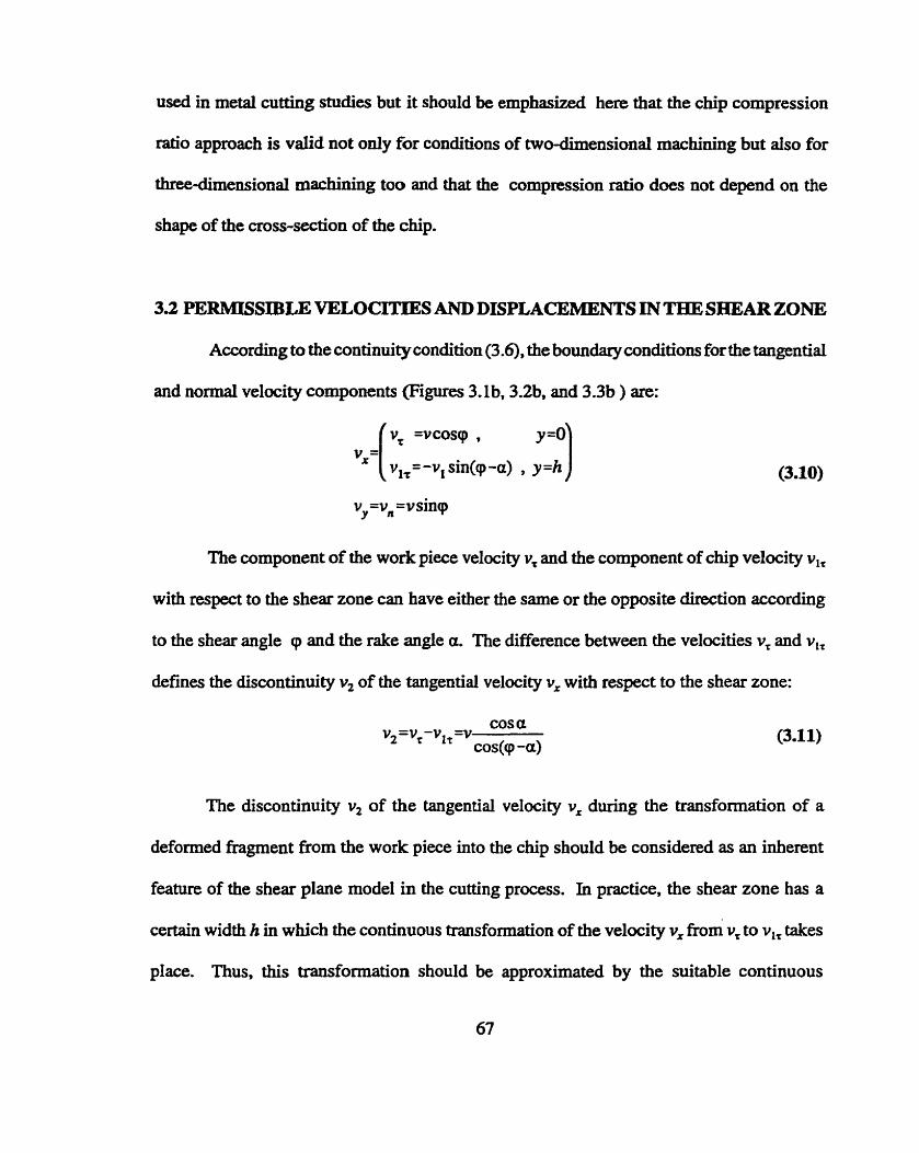
used in metal cuttiag studies but it should be emphasized here that the chip compression
ratio approach is valid not only for conditions of two-dimensional machining but also for
three-dimensional rnachining too and that the compression ratio does not depend on the
shape of the cross-section of the chip.
3.2 PERMISSIBXIE VELOCITIES AND DEPLACEMENTS IN THE SEIEAR ZONE
According to the continuity condition (3.6). the boundary conditions for the tangentid
and normal velocity components (Figures 3.1 b, 3.2b. and 3.3b ) are:
v,, =v, =v sincp
The component of the work piece velocity v, and the component of chip velocity v,,
with respect to the shear zone can have either the same or the opposite direction according
to the shear angle cp and the rake angle a. The difference between the velocities v, and v,,
defnes the discontinuity v, of the tangential velocity v, with respect to the shear zone:
The discontinuity v, of the tangential velocity v, during the transformation of a
deformed fragment from the work piece into the chip should be considered as an inherent
feature of the shear plane mode1 in the cutting process. In practice, the shear zone has a
certain width h in which the continuous transformation of the velocity v, fkom v, to v,, takes
place. Thus, this transformation should be approximated by the suitable continuous

transition curve justifj4ng the boundary conditions (3.10) as shown in Figures 3. lb, 3 .2b7 and
3.3b. Since the slip-lines are straight lines, the velocity v, depends on the y coordinate ody.
The law governing this dependence is unhown. However, using the experirnental data and
existing experience (KececlogIu, 1960; Poletica, 1976; Trent, 199 1; Bobrov, 1984; Scmtton,
1968; The. 1975). the curve v f i ) c m be approximated by the following andytical function:
where n is a parameter characterizing the non-uniform distribution of the tangential velocity
in the shear zone.
The effect of n on velocity ratio vjv, is shown in Figures (3 S), (3 -6). and (3.7) for
different chip compression ratios. These figures reveal that the shear zone is composed of
two regions. The first region is tenned as the "wide region" where the tangential velocity v,
changes at a smaii rate. The second region is termed as the ''narrow region " where the
tangential velocity v, changes at a high rate. Also, it can be seen that as n increases, the
"wide region" becomes larger and the " narrow region" becomes smaller. This conclusion
is in a good agreement with the results of the study of coordinate grid deformation (Poletica,
1976; Bobrov, 1984). The narrow region where a signincant change of the tangential
velocity takes place may be thought as the region of the discontinuity of this velocity. This
mode1 plays a principal role in the foregoing analysis because both the state of stress and the
state of strain and the resistance of the work material to cutting in this " narrow region" are
very specific.

Figure 3.5: Effect of n on the velocity ratio vx(y)Nn for a=10* and c=1.5.

Figure 3.6: Effect of n on the velocity ratio v,(y)/v, for a=10~ and Ct2.0.

Figure 3.7: Effect of n on the velocity ratio vx(ym,, for a=1 o0 and 6=2.5.

Iiitegration of equation (3.12) gives the displacement ux@) reached at y as:
The velocity v,, and the velocity v . have opposite direction because the shear angle
q is usually larger than the rake angle y. Therefore, as shown in Figure 3.8, the function ux@)
has the maximum O>', u'J within the deformation zone. By increasing n, this maximum is
shifting closer to the upper boundary.
Function uxQ) defines the streamlines in the deformation zone bounded by pardel
boundaries. Thus, it describes the transition line CDE between the fkee surface of the work
piece and the chip as shown in Figure 3.8. The tangents to CDE at their intersection points
with the lower and upper boundarÏes are coUinear with the velocity v and the velocity v,.
It is known that the streamlines in the deformation zone are equidistant lines (Zorev,
1966; Poletica. 1976 ). Therefore, to jusw the continuity condition, the zone OAB of heavy
deformation should be attached to the rake surface as shown in Figure 3.8. This zone is
separated fiom the defoxmation zone by the streamline line AB, from the workpiece by the
line OB ( h,)and from the rake surface by the line OA ( c,).
To calculate lengths of OA and OB, consider the equations for tangents CF and E R
xcF=y cotcp (3.14)

From the tangents intersection at point F which has the coordinate y,. it can be
u,(h) =[cotq +tan@ -a)&-htan(cp -a)
it foilows nom equations (3.14-3.16):
where y is the shear strain.
In particular case a = <p for a large rake angle, equation (3.17) can be M e r
simplifiecl:
It follows fiom equation (3.18) that with increasing n the shear plane approaches the
upper boundary of the deformation zone. At that point, the shape of the transition curve
changes dramatically as shown in Figure 3.9. For large n. a major part of this curve
coincides with the tangent at the initial point C. This phenornenon c m be considered as the
reduction of the transition curve length. From observations of the fkee surface of the
workpiece and chip, it follows that, the change of the transition curve shape and position of
the shear plane with increasing n corresponds to the increase in the cutting speed.

Figure 3.8: A model of a chip formation zone with parallel boundaries.

Figure 3.9: Transition curves for dgHferent n.

Also, it can be deduced from Figure 3.8 that
Taking into account thai Nt = 0.3. . . O S and sinp changes within the same limits,
the following approximations for c, and h, can be obtained
ho='
c,=O. l t (3.22)
The region OB = h, plays the same role in the cutîing theory as the wear-land on the
fi ank surface. Therefore, this region should be taken into consideration in the dculation of
temperatures and forces on the flank surface. The region OA on the rake surface reduces the
achial contact tool-chip length. For small a this region does not play any significant role and
can be ignored. However, when a becomes larger, this region plays a significant role iri the
mechanics of metal cutting because it causes the formation of the built-up edge (BUE).

3.3 DISTRIBUTION OF DEFORMATION IN THE CEIP FORMATION ZONE
In studying the deformation in metal cutting the main mntion is usuaily paid to the
deformation rate which takes place in the shear zone. The rate of defonnation is closely
related to the displacement and the velocities. To calculate the deformation rate a number of
different approaches and formulas were proposed (Boothroyd and Knight, 1989). The known
approaches are based on the known velocity diagram (Merchant, 1945) which has to be
correcteci as shown previously. Therefore, the deformation rate for the mode1 of
deformation zone with parallel boundaries requires additional study. -
In many studies of metal cutting, the defonnation in the chip formation zone is
characterized by the shear strain calculated as:
v2 cosa - - c2 -2bina + 1 Y=-= V, cos@ -a)sin<p &osa
The reported denvation of this formulais not strict enough (Rozenberg, 1956). The
study of deformation using the grid method refiites the assumption that the deformation in
the shear zone is a simple shear (Bhattacharyya and Ham, 1969). According to experimental
data, the defonnation in metai cutting is a complex defonnation which cannot be
characterized by the simple shear strain.
Under accepted model of deformation shown in Figures 3.1,3.2, and 3.3, the tensor
of intinitely smaU increments of deformations can be represented by only two (which are
equal due to the symmetry of the tensor) non-zero shear strain components.
The other two components of that tensor are equal to zero, that is

and
Since the normal velocity v, is constant anoss the shear zone and the sliplines are
straight, the displacement increment dong the x-coordinate depends only on ycoorcîinate.
Since de, and de , are equal to zero, the corresponding components of final
deformation are also equal to zero. Therefore, the maximum shear strain rate can be
expressed as
To calculate the engineering shear strain, consider the displacements in the
deformation zone with the parallel boundaries shown in Figure 3.10. The x-coordinate
coincides with the direction of shearing and the y-coordinate is in the direction of v,. In this
coordinate system, the displacement u&) becomes:
According to the theory of deformation, an infinitely small increment of angular

Y chip
Figure 3.10: (a) The model of the chip formation zone and (b) the trajectory
of a particle in this zone.

deformation can be defined as the sum of partial s t ra in increments dong the x and y
coordinates (Fredental and Geiringer, 1962):
The shear strain y@) in the chip formation zone may be obtained by the integmtion
of equation (3.28) which gives:
The final engineering shear shain y@), when y = h, coincides with the strain defined
by equation (3.23) which is co~~monly used in practice and can be written in the following
fom:
It follows from equation (3.30) that the final engineering shear strain y(h) ( when the
defonnation of work material is considered in the zone with paralle1 boundaries) does not
depend neither on the width of the zone h, nor on n, but is entirdy defined by the values of
the velocity break v, and of the normal velocity v,. Since y(h) does not depend on n, it can
be concluded that equation (3.29) is also vatid for the model with single shear plane, which
can be considered as a limiting case of the model with parallel boundaries when n - 0.
Figure 3.1 1 reveais the function (3.29) as well as the expenmental results obtained in cutting
of copper with smali cuning speeds (Kufarev, 1970). The cornparison between the calculated
and experîmental results shows that the experimental results can be well approximated by

Figure 3.11: Distribution of the true shear strain along the width of the shear zone.

function (3.29) when n=3.
As it follows h m Figure 3.1 1, a major part of the plastic defonnation takes place in
the closed neighborhood of the upper boundary of the deformation zone. The increase in
cutting speed increases this tendency.
The conditional separation of the deformation zone into two parts as mentioned
before, assumes that conditional boundary exists between "wide" and "narrow" parts of this
zone. The position of this boundary should be estimated quantitatively. Such a . estimation
requires a certain idealization of a r d cutting process. The objective of this ideaikation is
to define the resistance of the work material to cutting, Because the yield shear stress in
cutting is correlated to the mechanical characteristics in tensile tests, the value of engineering
strain, which is equal to the intensity of angular deformation in a tensile test at the instant
of necking initiation, is taken as a cnterion of separation between "wide" and "narrow" parts
of the deformation zone. This critenon is already used by a number of investigators for the
cornparison of cutting and tensile tests.
When the elastic part of defonnation is not considered, the failure shear strain yfa and
failure strain % relationship may be taken as a criterion to define the boundary separated
"wide" and "narrow" parts of the deformation zone:
Y* =Oh( 1 +cf=) (3.31)
For the typical cutting conditions the final average strain y(h)=2.5, and efa==û.2.
Therefore, as the fust approximation, the deformation in the wide zone for the typical
practicd conditions is as large as 1045% of the final strain. With an increase in the rake
angle a and the failure strain of the work piece material, the part of deformation, which takes

place in the wide zone, is growing.
Assuming for particular case yfa &@)=O. 12 and using equation (3.29). the ratio hJh
( h, is the size of the zone of the main deformations ) as a fwiction of n may be found as
shown in Figure 3-12 :
Examination of Figure 3.12 shows that with increasing n the size of h, becornes
smaller. The same tendency was observeà with increase in the cutting speed. Changing the
cutting speed h m 0.3 to 3 d s leads to the reduction of the defomiation zone by half. In a
conclusion, it can be stated that, for practicai conditions of machining of steels by the carbide
tools, the value of n =4-8 is a good approximation. The shear strain rate and its distribution
in the deformation zone play a vital role in metai cuning studies. This rate can be calculateci
as :
w here y = v ~ .
Taking the width of the deformation zone, h, approximately equal to the half of uncut
chip thichess, t, it can be concluded that, for the typical cutting conditions, the terni vJI<
is of the order of 10' sec-' as shown in Figure 3.13 (in logarithmic scale) shows the
distribution of the strain rate in the deformation zone for different n. It can be seen that the
strain rate at the border of the preliminq and final deformation zone reaches high values
104 sec-' but almost, does not depend on n when n = 4-8. Therefore, it is not necessary

Figure 3.12: hlh vs. n under ~ ' 1 % =0.12.

Figure 3.13: Distribution of the deformation rate in the deformation zone under v&=lo4 s-' and different n. The points correspond to the deformation rate at the border of the primary and final deformation.

to measure the values of n experimentally. The strain rate y*,-,, at the border of the wide and
final approximation zone is
It can be seen fiom equation (3.34) that for the practically reasonable remes, both
the values of vJh and the failure strain rate are of the same order.
The strain rate reaches its rnaxhum value when it approaches the upper border of
the deformation zone and it reaches
It foiiows h m equation (3.35) th& when h-O . the strain rate ym(h) -m. This model
corresponds to one shear plane model and, to a big surprise, is not contradct with the
mechanics of materiais because, even under this extreme conditions, the inertia stress
remains relatively small.
3.4 TBERMOMECIIANICAL MODEL FOR THE SHEAR STRESS IN TEE
PRIMARY AND SECONDARY SEEAR ZONES
The thennomechanical model of the work piece material resistance to cutting was
first proposed by Kushnir (1982) and modified by Astakhov (1994). According to the
themomechi1IIlcd mdel, the flow shear stress of the workpiece material is
temperature-dependan t and decreases at a defined rate as temperature increases. Summarized

to measure the values of n experimentally. The strain rate y',, at the border of the wide and
f i a l approximation zone is
1t can be seen fiom equation (3.34) that for the practically reasonable regimes, both
the values of vJh and the failure strain rate are of the same order.
The strain rate reaches its maximum value when it approaches the upper border of
the deformation zone and it reaches
It follows from equation (3.35) that when h-O , the strain rate y'(h) -m. This model
corresponds to one shear plane model and, to a big surprise, is not contradict with the
mechanics of materials because, even under this extreme conditions, the inertia stress
remains relatively smail.
3.4 THERMOIVECHANICAL MODEL FOR THE SHEAR STRESS IN THE
PRIMARY AND SECONDARY SHEAR ZONES
The thermomechanicd model of the work piece materid resistance to cutting was
fmt proposed by Kushnir (1982) and modified by Astakhov (1994). According to the
thennomechanical model, the flow shear stress of the workpiece matenal is
temperature-dependant and decreases at a defined rate as temperature increases. Summarized

the experimental data for a wide range of the workpiece materials shown in Figure 3.17.
reveals that this rate is a constant The basic relaîionship of this mode1 can be presented in
the following form:
r=a,(i -.O05 2') (3-36)
where r is the yield shear stress of the workpiece in the shear zone (Mpa), ad is the ultimate
tensiie strength of work piece material (Mpa) and T is the temperatme in centigrade (Co).
Analysis of reportedstudying temperature in metalcutting (Boothroyci, 1963; Kushner. 1982;
Boothroyd and Knight, 1989; Oxley, 1989; Astakhov, 1992) shows that the average
temperature in the shear zone, cm be predicted by :
where c, is the specific heat capacity of the workpiece maîerial and p the density of the
workpiece material.
Substituting equation (3.37) into equation (3.36), the following equation can be
obtained
The average temperature dong the plastic part of the tool-chip interface, Tf , c m be
defined as (Kushner, 1982):

I+AISI 4140 -AISI 1065 A8% Ni, 1896 Cr, steei .AISI 1 W S 1
Figure 3.14: Effect of temperature on the ratio d ouk (Kushner, 1982).

where Z, is the length of the plastic part of the tool-chip contact length (m), 6 is the chip
compression ratio, t is the uncut chip thickness (m) and Pe is the Peclet number whicb can
be defined as foUow:-
where v is the cutting speed (ds), t is the uncut chip thickness (m) and w is the thermal
diffusiticity of the workpiece materiai ( a s ) . By substituting equation (3.40) into equation
(3.39), it can be obtained:
3.5 SUMMARY
The shear zone model with paralle1 boundaries has been chosen as a model for
mechanics of cutting and cutting force determination. The analysis leads to the following
conclusions:
1. Two families of straight sliplines constitute the deformation zone in metal cutting:
one family is parallel and another is perpendicular to the straight upper boundary of
this zone.
2. The weLi-known equation for the chip compression ratio is another f o m of the

continuity condition. This equation is valid for any shape of shear zone with a
straight upper boundary.
3. The discontinuity of the tangentid velocity (the component of the cutting speed
which is parallel to the boundary of the shear zone) during the transformation of a
defonned fiagrnent fiom the work piece into the chip is an amibute of the shear plane
mode1 phenomenon in the cutting process. In practice, the shear zone always has a
certain width, within which the conthuous transformation of the velocity takes place.
Therefore, the acceleration, strain and strain-rate in the shear zone with paraiiel
boudaries are not unifonnly distributed as thought before. The final tnie shear
strain does not depends upon neitbet the zone's width, nor the exponent of
non-uniform strain distribution of strain, but is entirely defined by the values of the
discontinuity of the tangential velocity and normal velocity. Therefore, the shear
plane model may be considered as a limiting case of the shear zone model with
parailel boundaries.
4. Thermomechanical model of the work-material resistance to cutting defmes the ratio
of the yield shear stress (in the shear zone and in the plastic zone on the twl rake )
to the ultimate tensile strength and it is a Iinear function of cutting temperature.
5. Based on this, shear zone a model for cutting force components is suggested as will
be seen in the next chapter. To avoid the determinafion of friction angle, computation
of the tangential force acting on the tool face is proposed.

STEADY-STATE CUTTING FORCE MODEL BASED ON THE SHEAR ZONE MODEL WITH PA.IULLEL BOUNDARIES AND ITS APPLICATION TO THE BTA PROCESS.
This chapter comprises the analytical evaluation of the steady-state force model
which has been derived using the mode1 of shear zone with parallel boundaries. Then this
model has been applied to the deep hole rnachining process as typical orthogonal..
4.1 STEAûY-STATE CUïTING FORCE MODEL
Theoretical detemination of the cutting forces is one of the main concerns in metd
cutting. The cutting force components acting dong the correspondhg axes, namely the
cutting force F, and the thrust force F, can be determinecl from the following equation:
91

- C cos (q -a) F ~ O S ~ -F, sina
F, = cos (9 -a)
wben F' is the shear force dong the shear zone boundaries, Ff is the tangentid force on the
rake face, cp is the shear angle, and a is the rake angle. To calculate these components it is
necessary to know shear force F, in the shear zone and the tangentid force Ff on the rake
face. The shear force F, can be calculated as:
where t, is the shear fiow stress in the shear zone; b is the width of cut; t is the uncut chip
thickness; and cp is the shear angle.
It is also hown that the shear flow stress of the workpiece materiai is temperature
dependent and it decnases at a constant rate with temperature oieter, 1986). It has been
shown by Kushner (1982) that for avast varîety of steels, the shear flow stress may be related
to the ultimate tensile strength in te- of temperature as foliows:
where T is the shear flow stress of the workpiece material (Mpa), O, is ultimate tensile
strength of the workpiece material (Mpa) at 20 CO and T is the temperature (CO).
The temperature in the shear zone , T, can be defined as (Oxley 1989):

where c, is the -c heat capacity at constant volume of deformed matenal and 7 is the
final shear strain which is h o w n to be (Merchant, 1945):
cosa Y = sin9 cos(rp -a)
Substitutkg equation (4.5) into equation (4.4) one may obtain:
cosa =urt
T, = sinpcos(cp -a)
cv
Substituting equation (4.6) into equation (4.3):
Substituting equation (4.7) into equation (4.2):
The tangential force Ffacting dong the tool-chip interface can be obtained as (Zorev,
1966)
here le is the effective length of the tool-chip interface and zl is the shear flow stress dong
the chiptool interface which can be obtained h m the thennomechanical mode1 knowing

the tool-chip interface temperature as
where 5 is the tool-chip interface temperature (Kushner, 1982)
where 1, is the length of the plastic part of the tod-chip interface and Pe is the peclet number
which can be wrïtten as
where w is the diffusity of the workpiece material which c m be written as
where k is the thermal conductivity of the workpiece material,
However, the experimental work done by AstaWiov (1994; 1983 ) shows that the full
tool-chip interface length I / , the effective length band the length of the plastic part of the
tool-chip interface 1, can be written in ternis of chip compression ratio 5 as foUow:
The shear flow stress in the tool-chip interface can be caiculated as

here, f, is the length of the plastic part of the toolchip interface, w is the thermal diffuseness
of workpiece material and is the chip compression ratio.
Substitutingequation (4.15) into equation (4.9) the tangential force Ff dong the tool-
chip interface can be written as
Knowing the shear force F, and F' the cutting force F, and the tangential force F, can
be obtained from the following equation:
4.2 CUTCINGPORCE COMPOriiENTS IN BTA MACHININGUSING TIiE SEEAR
ZONE WITH PARALLEL BOUNDARES
The BTA method basically utilizes single or multi cutting edge tool with an intemal
chip removal. The cutting edge gwmetry is important because it defines the mode1 for
metal cutting, cuning force distribution, chip formation, cutting edges Wear, and the surface
accuracy of the hole produced.

4.2.1 Cutting Force Components
Based on the tool geometry and due to the fact that the velocity of cutting is
perpendicular to the cutting edges. the deep-hole machining operation may be considered as
an orthogonal machining operation. The resultant cutting force is commonly resolved into
three components (Latinovic, 1978):
1. The tangential contributing component F. parailel to the cutting veIocity vector.
2. The radial cornpunent Fr dong the radius of the tw1.
3. The aual component Fa dong the axis of the tool.
The fomiulation of the steady state cuning force equations requires evidence on the
nature of the defonnation zone. A complete force system in the deep-hole machining
operation is specified by the axial, tangential. radiai force components and the point of
application of the resultant force. This system will be modified by shifting the force to the
axis of the tool. But such a shift of the three forces leads to an introduction of a torque acting
dong the axis of the boring bar-cutting tool system. Therefore to speciw the BTA deep hole
machining operation not only are the axial, radial and tangential forces to be evaluated, but
also an expression for torque is to be obtained.
For the purpose of evaluating the total cutting force, the entire cutting edge can be
considered as k ing made up of srnaIl increments of cutting edge "dr" and then summing up
the contributions due to these over a radius of hole.
The force system on an incremental of the cutting profile is s h o w in Figure 4.1.
Since the cutting velocity at each increment is at right angles to the cutting profile the
machining is an orthogonal operation and the cutting force at each section can t be described.

Figure 4.1 : Cutting force representation at a distance rfrom the center of the
cutting tool.

The shear flow stress at distance r can be defined using the thermo mechanical mode1
' ~ ~ ( r ) = cuu(l -0.0005 T(r) ) (4.18)
where Ts(r) is the temperature in the shear zone which can be defined as (Oxley, 1989)
where y@) is the shear strain in the shear zone at distance r and pc, is tht heat capacity of
the workpiece material. The shear strain y(r) can be wrïtten as
where a(r) and q(r) are the rake and shear angles at radius r, respectively.
Substituthg equation (4.19) into equation (4.18)
The relationship between the shear angle q(r) and the rake angle a(r) and the chip
compression ratio c(r) at certain point can be written as
It is weil known that the shear angle cp(r) depends upon the velocity of the machining
Nr), the feed t, the rake angle a(r), cutting tool, workpiece material, and cutting fluid.
Mathematically it cm be expressed in the following fonn:

As it was suggested (Mgm and Sadek, 1977). the following equation for chip
compression ratio C(r) can be written
where e, J g, h, k n and q are constants, t is the undeformeci chip thickness (m) and v(r) is
the cutting speed (mh).
The shear flow stress at the chiptool interface at distance r can be wrîtten as
zhr) = oUl1(1 -0.0005 Tkr)) (4.25)
where Tkr) is the tool-chip interface at distance r h m the center of rotation which can be
where Pe(r) is the peclet number at distance r which c m be written as
and l,(r) is the length of the plastic part of the tool-chip interface. Using equation (4.14) the
full tool-chip interface length I / , the effective length band the length of the plastic part of
the tool-chip interface 2, at a distance r from the axis of the cutting tool c m be written as

The shear force on an incremental thickness dr of the cutting proNe at distance r can
be written as
which can be wntten as
Also the tangentid force Fkr) on the rake face at distance r can be written as
which can be written as
Knowing the shear force Fs(r) and the tangentid fiction force FA?-), the cutting
forcees on an incremental thichess as shown in Figure 4.1 can be obtained fiom the
Hence

From the geometry of the cutting edge, the expression for the radial and axial
components of the cutting force in the region under consideration can be written as
where x(r) is the approach angle of the cutting edge at distance r.
The tangentid, radial and axial forces can be written in the foliowing f o m
which can be rewritten as
where
A complete specification for any rotating tool req- an expression for the torque
acting on the cutting edge. The torque on a given section can be written as

which can be written as
&(r) = A(r)rdr (4.40)
The forces and torque consist of two components, the steady and the dynamic
components, that is
where F&), F,&) and F,(r) are the steady forces on the incremental thichess at distance
r, Mt@), U r @ ) and hF,(r) are the dynamic components of these forces, Tm@) is the steady
torque component and AT@) is the dynamic components of the torque.
The steady components of the tangentid, radial and axial forces over the entire
cutting edge can be wxitten as
Fm = 1 M(r)sinx(r)dr+ M(r)sinx(r)dr+ ....... 1 M(r)sinx(r)dr secrion i= 1 secn'on i=2 section i=n (4.42)
Fm = M(r)cosx(r)dr+ M(r)cosx(r)dr +. . . . . .. M(r)cosx(r)dr section i= 1 secnon i=2 section i=n
Tm = f A(r)rdr+ [ A(r)rdr+ ....... 1 A(r)rdr section i = 1 section i=2 section i=n
where n is the nurnber of the sections over the diameter of the tool as seen Figure 4.2
(Latinovic, 1978).

Figure 4.2: Section of the BTA cutting profile.
103

4.23 Compnter Simulations
Four series of testing prograrns were cUmed out to assess the effects of the cutting
tml geometry, f& cuithg speed, and woricpiece material on the steady state cutting forces.
A Fortran program has been written to simulate the formuiated model. The results of this
simulation together with the obtained experimntai results are presented in chaptcr nine.

AN ANALYTICAL EVALUATION OF THE CUTTING FORCES IN ORTHOGONAL CUTTING USING THE DYNAMIC MODEL OF SHEAR ZONE WITH PAIULLEL BOUNDARIES
This chapter present an evaluation of the dynarnic forces in orthogonal cutting using
the shear zone model with parallel boundaries (Hayajneh et al, 1997% 1997 b). The cutting
system was modeled using a single degree-of freedom dynamic system where the variations
of the cutting forces are represented by theirtotal differentials. The influence of temperature
on the shear flow stress of workpiece material is accounted. The experimental verification
of the proposed model was perfomed using a two-component piezoelectric dynamometer
and applying the rotating cutting tool-stationary workpiece method.

5.1 INTRODUrnON
In order to study the chatter, it is important to distinguish the sources of vibrations.
Basically, the machining vibrations are usually classified into the following four main
categories (Nigm et al, 1977):
1. Free vibration which may be initiated by some impact or shock. This vibration
usually decays under the damping action of the machine tool.
2. Forced vibration caused by a source other than cutting. This may be initiated by
unbalance in the machine-tool drive. Knowing the source of these forced vibrations,
they can be prevented by redesign of the machine tool structure.
3. Forced vibration initiated by the inherent periodicity in the cutting process such that
the built-up edge and discontinuity of the chip.
4. Self-excited vibration. This type is classified into a regenerative and a non-
regenerative chatter. The regenerative effect is caused by the superposition of
successive cuts, where the tool removes a wavy surface generated in the previous
pass. The non-regenerative vibration is maintained by cutting force fluctuations that
are induced by the cutting tool-workpiece relative displacement of periodic nature.
In order to understand the mechanisms leading to the chatter, it is essential to know
how the cutting forces Vary with variation of cutting conditions and tool-workpiece relative
motion. The cutting forces depend on a large number of cutting system parameters which
make the formulation of an analytical dynamic cutting force mode1 a rather difficult task.
Many techniques have been developed over the past 50 years for machine tool-cutting
process identification. The general approach of these techniques is to assume that the cutting

forces are an approximak linear function of relative tool-workpiece position and velocity
(Peters et al, 197 1). The coefficients of this function, h o w n as dynamic force coefficients,
are the induced stïffhess and the damping. Traditionally, the dynamic force functions are
assumed to be linear expressions in temis of a number of time-dependent variables, which
include the imer and outer modulations of the uncut chip thickness and their f i t time
denvatives. The coefficients of these variation terms may be detemineci through
experimental or analytical technique. The experirnental technique is to develop an
experimentd method for direct measurement of the transfer function between the cutting
force and the variables in the modulation of the uncut chip thickness (Peter et al, 197 1). The
experimental method is highly empirical and requires a very sophisticated test apparatus and
analysis procedures.
The promising way of forrndating a proper dynamic cutting force is using the
mechanics of chip formation Wigm et al, 1977; Das and Tobias, 1967; Rubenstein, 1972).
However, the models for chip formation used so far for this purpose are not in good
agreement with the results of experiments. For example, Wu and Liu (1985% 198%) and
Wu (1986; 1988; 1989) developed a dynamic cutting force mode1 using the single shear
plane model for orthogonal cutting which exhibits senous shortcomings (Astakov and
Osman, 1996; Oxley, 1989). Therefore, it is reasonable to suggest that a new model of chip
formation which is in better agreements with the experiments should be used.
Astakhov and Osman (1996) proposed a mode1 of chip formation with parailel
boundaries which appears to be free from many of the known conaadictions associated with
the other reported models. It would bc logical to incorporate it into the dynarnic analysis

of the cutting forces. This is one of the main objectives of the work.
5.2 DYNAMIC MODEL OF SEWR ZONE VYITH. PARALLEL BOUNDARIES
5.2.1 General Force Mode1
In the present study, the real machining system is approximated with a single
degree-of-Wom dynamic system shown in Figure 5.1. In this figure, a flexible cutting
tool, vibrating normal to the cutting direction, is set to remove a layer of work material with
a wavy top surface produced during previous cuts. The cutting speed, the mean uncut chip
thickness, and the rake angle are preset to be v, f , and a, respectively. The coordinate
system, iiiustrated in Figure 5.1, is described as follows:
the x - a i s is nomial to the direction of the cutting speed and this axis wiU be referred
to as the vibration axis;
the y-axis is perpendicdar to the x-axis as s h o w in Figure 5.1.
At any instant, the tool tip has the displacement x, dong the vibration axis, while the
surface end of the shear plane has the displacement x, relative to its equilibrium position, as
shown in Figure (5.1). The oscillation velocities of the tool tip and the surf' end of the
shear plane are denoted by x., and x i , respectively.
It is known (Merchant, 1945) that for steady-state machining the cutting forces are
detennined only by an invariable cutting configuration. Once that configuration is known,
the cutting force components acting dong the corresponding axes, namely the tangential F,
and the radial F, cutting force (Figure 5.1) can be detennined as follows

force polygon
Figure 5.1: A mode1 of shear zone with parallel boundaties as applied to
evaluate the dynamic cutting force.

- Y cos (tp -a)
where F, is the shear force dong the shear zone boundaries, FI is the tangentid force on the
rake face and <p is the shear angle.
Since in the present study the configuration of the cutting system is considered to be
variable then the dynamic values of these forces should be considered as functions of the
correspondhg dynamic cutting parameters such as shear force, shear angle, and rake angle
which are denoted as Ffi, F,, pi, and ai, respectively. Therefore, a general force mode1 may
be represented in the foilowing fom:
- F, cosai +Ffi shqi F,. -
cos (q+-ai) F9 coscp, -F, sina,
Fi = cos (pi -a,)
The dynamic value of each model's component may be represented by the the sum
of its steady-state value and its incremental variation as follows:
5.2.2 Determination of the Cutting Force Components
The incremental variations of the cutting forces F, and F, may be represented by

their total differentials. Using equation (5.2) and negiecting the terms of high orders, one
may obtain these incremental variations in the following form
where the coefficients of qat ion (5.4) are
- F~osqcos(q -a) +(F, cosa +Fpincp)sin(q -a) g3 -
cos2(cp -a) - -Fssinacos(cp -a) +(Fscosa+Fpinq)sin(cp -a)
g4 - COS^(^ -a)
and
It is known (Merchant, !945) that the shearing force F, is calculated as:
where t, is the shear flow stress in the shear zone; b is the width of cut; t is the uncut chip

thickness; and p is the shear angle.
The incremental variation of the shearing force F, rnay be represented by its total
ciifferentai. Using equation (4.8) and neglecthg the te- of high orders, one may obtain:
dF, = n,dt + n2dp + n3da where the coefficients n , n, and 5 are calculateci as
The incremental variation of the tangentid force F,may be represented by its total
differential. Using equation (4.16) and neglecting the ternis of high orders, one may obtain:
dF' = ml& + m , 4 + m,dv + m4dp + m+ia
where rn, , 4, %, m, and m5 are

5.23 Influence of Incremental Variations of the Shear Angle
The mode1 of shear zone with paralle1 boundanes utilizes the Merchant's expression
for the shear angle cp (Merchant, 1945):
Here, the chip compression ratio and rake angle are constant. However, this is not
the case in the present consideration. Therefore, dynamic variations of these parameters
shouid be considered-
The incremental variation of the shear angle may be represented by its total
differential in the following form:

As can be seen, equation (5.13) contains three tenns instead of two as might be
expected h m equation (5.12). We may explain this as follows. The angle iy represent the
angie between the free surface of the workpiece and the y-direction. Since in the steady-state
consideration this angle is zero, it does not appear in equaîion (5.12). In the dynamic
consideration, however, this angle plays an important role. In wave cutting , the dynamic
direction of cutting is at an angle @, with the direction against which the rake angle of the
tool is measured that increases the rake angle. In wave removing, the oppsite is the case so
that dy, decreases the rake. In actuaï practice, a certain combination of the above two
types (wave cutting and wave removing) is the case. Therefore, the static rake angle is
modified by the incremental variation of angle W. This incremental variation can be
represented as:
Bearing in rnind the foregoing consideration, one may express equation (5.13) as
follows:
where s, and s, are

The compression ratio 5 can be written as (Nigm et ai, 1977):
where e, g, h, p, n and q are constants, t is the undeforrned chip thickness (m) and v is the
cutting speed (mls).
As might be expected, the chip compression ratio varies with other cutting parameters
(Astakhov and Osman, 1996; Nigm and Sadek, 1977). The incremental variation of the
compression ratio can be represented by its total differential in the foIlowing form:
which can be simplified as
where l,, L, and S are

Substituting equation (5.19) into equation (5.15), one may obtain:
dq = sllldt + sl12dv + (s,l,+s2)da + spYr (521)
The incrernentai variation of the shearing force is obtained by substihiting equations
(5.19) and (5.21) into equation (5.10)
q=P1dt+P2dv +P#a +P4dyr
where P, , P,, P, and P, are
Similady, substituting equation (5.2 1 ) into equation (5.8), one may get
dF, =T,dt + T2dv +T,da + T4@
where Tl, T,, T, and T' are

Emaliy, the incremental variations of the cutting force's coordinate cornponents are
obtained by substituthg equations (5.21). (5.22) and (5.24) into equation (5.4):
where A , A, , A, A, are
and
dFx =A=A,dt+A,dv+Auda+AyDmy
where A, A,, A, 4, are
53.4 Interpretation of The Incremental Variations in Terms of Cutting Pn>eess
Parameters
If the motion of the lower chip boundary is designated by x.,, and the motion of the
upper chip boundary is designated by iz then the variation of the cutting parameters are

where E is the geometric lead of the free end of the shear zone rdatively to its end on the twl
cuning edge. Simple analysis of the mode1 in Figure. (5.1) shows that:
E = tcotq 631) Substituthg equation (5.30) and (5.44) into equations (5.26) and (5.28), one may obtain:
and
5.2.5 Equations of Motion
Multiple observations and measurements of the profile of the surface of cut show that
x, and* may be assumed to be harmonic finctions having corresponding frequencies a, and
0, , that is

where CU,, CO, are defined by the chosen cutting regime and the diameter of the w orkpiece if
the chip formation process is stable (Astakhov et ai, 1977).
5.2.6 Proposed Modei for the Cutting Force Evaluation
The proposed mode1 for the cutting force evaluation is obtained by substituting
equation (5.34) into equations (5.32) and (5.33) and by substituting the result into equation
(5.3):
and

5.2.7 Cornputer Simulations
Four senes of testing pmgrams were carrieci out to assess the effects of the cutting
feed, cutting speed rake angle and frequency of the waves on the work surface on the
dynamic forçe components F, and F,. T able 5.1 presents the cutting conditions and Table
5.2 presents the cutting regimes used in the simulations. A Fortran program has been written
to simulaie f o d a t e d model. In chapter nine, the resdts
presented together with the experimental results.
Table 5.1. Cuîthg conditions for the simulation study
of the simulation has been
Workpiece material
Cutting tool
Width of cut
Hot finished mild steel 0.25% C
Carbide inserts (rake angles O, 5, 10 degree)
3.5 mm
Work surface
Tool vibration
Cutting method
Clearance angle
Sinusoidd wave form of 0.05 mm amplitude
Sinusoidal wave f o m of 0.05 mm amplitude
Orthogonal dry cutting
10 degree

Table 5.2. Cutüng parameters for the simulation sbidy
Objective: effect of feed speed rake ange frequency
Feed ( d m v ) 0.075-0.300 O. 19 O. 19 O. 19
speed (&min) 140 6û-240 140 140
Rake angle (deg.) 5 5 0-10 5

MISALIGNMENT ASSURANCE
As suggested in chapters 1 and 2, the relative position and motion between the tool
and workpiece may affect both the steady-state and dynamic cutting forces dramatically. So
that it become mcult to distinguish between the cutting signature due to the dynamic
response of the cutting process and that due to the noise onginating from the inaccuracy in
the position of the workpiece relative to the cutting tml. Nevertheless, the accuacy of the
workpiece rotation bas never been a factor in cutting force studies. A great scatter in the
reported results on the cutting force measurements may be paxtially explained by the
mentioned inaccuracy. This becornes particularly important if a new mode1 of chip formation
has to be verified by experiments and, in doing so, the results of predicted and measured
cutting forces have to be compared.
Since in the present study the experiments on the cutting force determination have
been carried out using deep-hole machining and their results were compared with

experiments, the discussed problem becomes even more significant because in deephole
machiniog the problem of the relative location of the worlcpiece and the tml can be solved
only by proper setting of the machine component.
In deep-hole machining, the relative location of the tool and the workpiece is defined
by the relative location of the axes of rotation of the tool, workpiece and starting bush as
s h o w in Figure 6.1.
nie problem may become so severe such that many researches, analyzhg the signai
h m the force dynamometer in deep-hole machbhg, concluded that the cutting force and the
process itself have stochastic nature (Osman and Chandrashekhar, 1984). Such a conclusion
has no physical justifications since there is no randornly changing components in the
machining system. The property of the tool (its geometry and tool materiai) does not change
significantly during the process, the machining regime is maintaineci with reasonable
accuracy, the mechanical properties of the workpiece may change no more then 2-396.
Therefore, this simple consideration shows that the noisy signai may give false impression
not only about the magnitude of the cutting force but also about its frequency composition and
even its nature.
This chapter presents the proposed methodology and the specially designed setup for
misalignment assurance. The chapter begins with a general description of the various
components of the deep hole drilling machine which have been used in the designed setup.
Then, the principal elements of this setup and overall configuration of the measuring system
have been detailed of. Next, a newly-developed calibration procedure is presented.

on of th0 workpluo
f rotdion of th8 startlng bush
Strady ~'~uun Tooi driva haad L
tatlon of starflng burh
contor of rofatton of dartïng burh mfrallgnmmnt
1 / Màgndlc smpamtor Pump nltom
Figure 6.1 : Misalignment between the axls of rotation of spindle nose and the
axis of starting bush.

6.1 TEE DEEP HOLE DRILLING MACHINE
The machine used in this investigation is 30HP Schacrer HPD 63 1 lathe retrofitted
for deep-hole drilIing as shown in Figure 6.2. To obtain variable feed drive and speed contrd,
the drive unit motor was replaced with 15 KW variable speed AC motor and the feed motor
was replaced with 5 KW variable speed AC motor. The motors are individually controlled
by AC invertors. The AC invertors are designed to provide required Volts/Hertz ratio,
allowing the AC motors to run at their optimum efficiency. The control section of the AC
inventors consists of a control board with a 16-bit microprocessor and keypad interface with
an 8-bit microprocessor.
The following is a description for main components of the dtxp-hole machine used
in the experiments.
(A) Cuning Toul Drive Unir. The drive unit consists of two variable speed motors that
controls the feed and the rotating speed of the boring bar-twl assembly. The primary
rotational motion is applied to the boring bar and the feed motion is applied to the the drive
unit sliding dong the ways of the machine bed. The boring bar-tool assembly is clarnped
onto the drive unit spindle. The spindle is mounted on high-precision bearings to minimize
its runout and end play.
fB Pressure Reaa : The pressure head is used to provide :
b Cutting fluid suppl y to the drill
b Initial support to the tool by means of the starting bush mounted in the pressure head
w Support and centering for the workpiece by means of a chamfered reception plate
installed on high-precision bearings mounted in the pressure head.

Steady Pres urs Tool drive head "\ Teel h?ad \
1 h4àgnetlc separator Purnps Filters
Figure 6.2: Deep-hole drilling machine.
126

The pressure head can be moved dong the machine bed to accommodate workpieces of
dinerent lengths. The motion of the pressure head is provided by means of a split nut and
lead screw co~ected to the feed cirive. hiring machinhg the pressure head is locked at its
position ensuring that no leakage occurs at the workpiecsprtssure-head reception plate
interface,
/C Worbkce Drive Unit: The machine is designed with possibility to rotate the workpiece.
However, in the designed setup, the rotation tool-stationary workpiece scheme has been used.
6.2 MISALIGNMEIYT MEASUREMENT SE:TUP
The schematic arrangement of the experimentd setup on the deep-hole machine is
shown in Figure 6.3. A photograph of the experimental setup is show in Figure 6.4. A laser-
based measurement system has been deveIoped to measure the misaügnment between the
axis of rotation of spindle nose and the axis of sîarting bush of the deep hole machine. A
reference laser beam has been generated by a laser tube, which is held the chuck of the
machine using a special case. The laser beam is captured by a photo sensor camera having
a capture video carci. The output images are sent to image precessing software capable to
crack the laser beam position by processing these images. The output fiom the image
processing software represent the position of the centroid of the laser beam on the photo
sensor in a certain position dong the axis of rotation of the machine. The misalignments have
been calculated by comparing the average centroid of the of the images which have been
captured when the photo sensor camera and starting bush axes coincide and when the camera
and nose spindle axis coincide (Figure 6.5). To align the machine, these centroid must be

/ / M' gnetlc separator Pumps n i ten t
accrssory to hold the cornera
laser
cornera
PC cornputsr provfded by vidso card and Image pracessor.
Figure 6.3: The schematic arrangement of the experimental setup.
128

Figure 6.4: A photograph of the experimental setup for misalignment measurement.

x (Horizontal)
Posftton 2
Figure 6.5: The principle of the misalignment measurements.
130

brought to coincide with the zero reference point The zero reference point was estabiished
on the axis of the cylindrical camera housing within a reasonable tolerance (0.5 micrometer).
A special accessory has been designed to hold the photo sensor camera in Merent position
dong the axis of rotation of the machine. To study the effet of misaiignment, the startllig
bush was intentiondy misaligneci by moving the pressure head over the camiage using the
lead screw of the cross slide.
The principal elements of this setup (Figure 6.6 ) are as foilow:
1. Laser (LTI'4H Adjustable Aügnment Tool, Emerging Technologies Inc., Laseraim
tool division, Little Rock, AR, USA) : This laser project a laser beam visible as a
"dot" of laser light on distant surfaces. The laser beam is projected in perfectly
straight line fiom the laser referred as the tool. This beam is used as a straight
reference line over the entire length of the beaxn. The tool have adjustable focus
feature which allows to control the laser dot size on a surface located perpendicular
to the beam (referred to as the screen). This adjustment allows the use of the smallest
possible dot size at specific distance thus facilitates more accurate measurements.
Since the focus adjustment is also linear, a change in the focus will not affect the
units X and Y alignment In practical temis it means that the smallest possible dot
size may be used at a close distance from the tool and then, when the screen in
placed further, the tool may be re-focused again to the smallest possible dot keeping
the centroid of these two dots on the same plane.
2 A photo-sensor digital camera Pulinx TM7 has been used as the screen. This camera
contains high resolution interline transfer 44 " CCD (charge-coupled device). The
camera was requested from the manufacturer to be of super mini size that allows it
131

Figure 6.6: Photograph of the principal elements of misalignment setup.

accurate and convenient mounting within the setup.
3. A special case to hold the laser in the chuck as depicted in Figure 6.7.
4. A special case to mount the camera in different positions along the machine bad.
This case , as shown in Figure 6.8, was precisely manufactured to achieve: a) to
match the cone in the starting bushing liner, b) to match the diameter of the camera,
and c) to match the outer diameter of the spinde nose. Figure 6.9 shows a picture of
these accessories.
5. Video capture card : This card is a single-slot, acctlerated, 24 bit-per-pixel, mie-
color, designed to capture and display high quality vide0 images. The card provides
the complete set of carnera control funciion required for capturing high quaiity
images. The card is also supporteci with a fuily comprehensive software that allows
fully exploitation of the hardware architecture. Captured images are saved as BMP
or TIFF files.
6. Image processing software (Matrox Inspecter, Version 2.0) : The images captured by
the camera were precessed to fmd the centroid of the images. This centroid represent
the center of rotation of the boring bar. A typical example of the captured images and
the processed images along with the results of the processing is shown in Figure 6.10.
6.3 CALIBRATION OF THE SYSTEM.
To ensure the repeatability and reproducibility of the proposed technique, a special
care has been paid to the calibration of the proposed system.
The fmt step in the calibration procedure is to align the laser beam to be parallel with
the case of the laser. This provides a laser beam paraIlel to the laser case at any distance and
133

Figure 6.7: Laser holder.
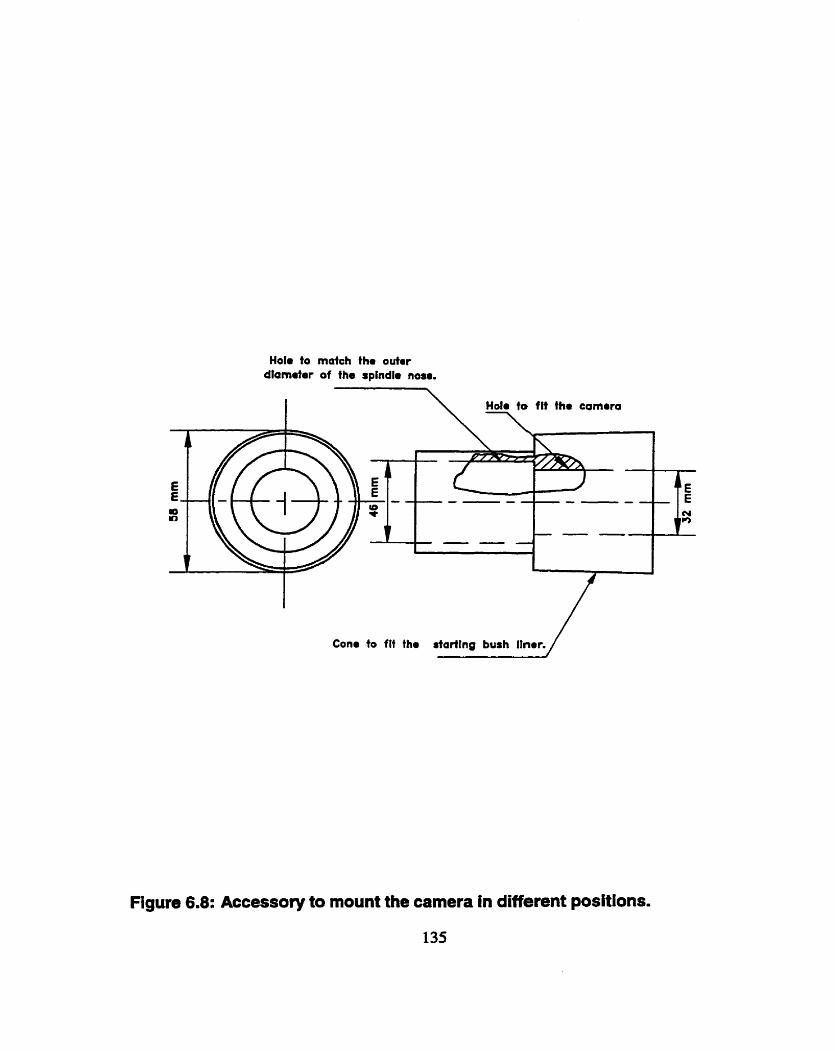
Ho10 to match tha outar dlarndor of the spindi. nosa.
Cons to fit th. starilnp burh Ilner./
Figure 6.8: Accessory to mount the camera in different positions.
135

Figure 6.9: A photograph of the accessory for mounting the camera in different positions

v n f Area Centroid X Centroid Y 1
Figure 6.10: An example of the captured image, and the results of the image processing.

can be used as a reference over the entire length of the beam. To align the laser, a V-block
has been used. The following nine-steps procedure has been developed and recommended:
Project the laser beam onto a screen placed approximately 20 meters away.
Rotate the case until the switch is in the straight up 12 o'clock position.
Mark the exact center of the laser dots over the distant surface,
Rotate the tool 180 degrees so that the switch is straight down in the 6 o'clock
position.
Mark the exact center of the laser dots again.
Draw a line comecting the marks. .
Measure the length of the line and mark the center point between the two marks.
Adjust the tool using the X and Y micrometer headr until the center of the laser dot
covers the center point between the two marks.
Check the result by rotating the tool on V-block. The projected dot image shouid tum
on itself. The center of the dot should remain in the same position. If the center of the
dot moves or the dot draws a circular pattern when rotateci, the alignment
procedures should be repeated again until center of the dot remains in a constant
position when the tool is rolled.
The second step is to check that the tool coincides with the axis of the chuck. To do
this, the following steps have to be executed:
1. Hold the laser case in the chuck of the machine.
2. Focus the beam on the screen to shoot the smallest possible dot.
3. Rotate the chuck by hand
4. Mark the circle produced by the dot.
138

5, Find the center of this circle.
6. Adjust the laser using the X and Y micrometer heads and bnng the dot to the center
of the circle until the dot does not rnove when rotating the chuck and the projected
dot image tums on itself.
The third step is to calibrate the laser-camera-image processor system. To do this,
a coordinate device has been designed as shown in Figs. 6.1 1 and 6.12. The setup of the
calibration is shown in Figure 6.13 and pictured in Figure 6.14. The camera has k n
mounted on the coordinate device and was displaced in the X- and Y- directions by the
micrometer heads. The images produced by the laser beam have been captured and processed
by the image processing. The results of the image processing have been compared with the
actual displacements of the cmrdinate device. Figures 6.15 shows the caiibration curves for
the system. It can be seen that an excellent agreement between the actual and the measured
value was achieved.

Hola to flt thi camera 1
Figure 6.1 1 : A systematic drawing of the coordinate device.
140

Figure 6.12: A photograph of the coordinate device.

l Flow ma
Pumps Fil
Chip trap f / bhagnetic separator
rs
PC tompufar (Gmpar) and Image processoi-.
Figure 6.13: The calibration setup.
142

Figure 6.1 4: Photograph of the calibration setup.

Horizontal
Vertical
Figure 6.15: Calibration of the proposed misalignrnent measuring system in the horizontal and vertical directions.

CUTTING FORCE MEASUREMENTS AND RESPONSE OF THE DYNAMIC CUTTING PROCESS
As pointed gut in Chapters 1 and 2, experimental vemcations are required to
validate the proposed models in t e m of the steady-state, dynamic cutting forces and the
dynamic response of the cutting process. In doing so, four types of expenments included
cutting force measurements have been carrieci out:
1. Investigation the effect of misalignment on the steady-state and dynamic cutting force
and torque.

2. Measurhg the steady-state cutting force for three different materials using two types
of cuaing tools under different cutting regimes.
3. Measuring the dynamic cuning force for wave removing process.
4. Investigation and monitoring of the dynamic response of the chip formation by
measuring the cutting force and torque signahues.
This chapter presents full descriptions for the materials, cutting tools, workpiece,
equipments , experimental sehips , calibraiions and aaalysis procedures used to perform the
required experiments.
Four types of workpiece material, representing four major groups of materials used
in industry, were selected to the shidy:
1. AIS1 1025 HR ASTM A576 RD.
2. AISI 1045 HR ASTM A576 RD.
3. AISI 4340 HR ANN RD ASTM 322 91.
4. AIS1 303 ANN CF RD ASTM A582 93.
Tables '7.1,7.2,7.3 and 7.4 show the chernical compositions of the selected materials.
The composition, and the elernent limits for these materials had been chosen accordhg to
the requirements of standard ANSVASME BWSSM-lg8S and were requested fromthe steel

Table 7.1: Description of AIS1 1025 STEEL. - - -
Description : 1025 HR
Specification: ASTM AS76
1 CHEMICAL ANALYSIS 1
Table 7.2: Description of AISI 1045 STEEL-
Description : 1045 HR A576 RI>
S pecif ication: ASTM A576

Table 73: Description of AISI 4340 STEEL.
Description : 4340 HEt ANN RD
Specification: ASTM A322 9 1
Table 7.4: Description of AIS1 303 STEEL.
Description : 303 ANN CF RD
Specification: ASTM A582 93

7.2 WORKFIECE TYPES
Three types of workpiece specimens were used :
1. Test specimens of 37.5 mm diameter and of 600 mm length. These specimens were
welded with fianges which, in tum, were clamped to the dynamometer. Six samples
from AISA 1045, AISA 4340 and AISA 303 materials were prepared (Figure 7.1).
2. Test samples of 37.5 mm diameter andof 600 mm length made from AIS1 1025 steel.
These samples were welded with flanges which in tums were clamped to the
dynamometer. The outer surface of these workpiezes has been waved using CNC
machine to obtain sinusoidal wave of 0.05 mm amplitude.
7.3 CUTI'LNG TOOLS
Two types of machining process have been used in the experiments, namely, tuming
and deephole drilling. Consequently, two different types of cutting tools have been utüized:
@) Cuninp Took-r the tu min^ Prucess : A specid tool holder and indexable carbide
inserts were used. The inserts were grinded with different rake angles. Tool material was
carbide Cd. The inserts used were ground with a zero nomllial cutting edge radius which
were controlkd using a computer-controlled opticai corporator ( Mihitoy PH 350). The
actual radius did not exceed values of 0.0 15 mm.
[BI Cuttinp Took for Dezo-RoZe Drinin~ Process : Two commonly tools have been used
in this process, single cutting edge BTAH (American Heller design) and partioned cutting
edge BTAS (Sandvik design) drills as shown in Figures 7.2 and 7.3 respectively. Figure
7.4 pictured these cutting tools.

Figure 7.1: A photograph of the workpieces used.

zone I
sscfion A-A
section D-D
Figure 7.2: BTAH tools of single cutting edge (American Heller design).

..tttocr A-A
C-C
I - P 25.4 - I
Figure 7.3: BTAS tools of partioned cutting edges (Sandvik design).

Figure 7.4: A photograph of the cutting tools used.

7.4 CUïTNG FORCES MEASUREMENT SETUP
The setup for measuring the static and dynamic cutting forces consists of the
following sub-systems as shown in Fi-s 7.5 and 7.6 and pictured in Figure 7.7 :
1. Deep-hole drïlling machine (described in the previous chapter).
2. Dynamometer : The dynamometer shown in Figure 7.8 (pictured in Figure 7.9) has
been designed to insert a 2-component load washer, Kistier Type 9065 according to
the standard specified by the supplier (Kistler) (Figure 7.10). As recommended, the
load washer was pre-loaded to 120 KN to measure the cutting force over a range
from -20 to +20 KN and the cutihg toque over a range fkom -200 to +200 Nm.
Table 7.5 presents the technical data of the load washer used in the experiments..
3. Charge preamplifiers: Two charge preamplifiers ( Kistler mode1 5004) have been
used to convert the output of the load washer into voltage and feed it to the FFT
anaiyzer.
4. Dualchanne1 Fast Fourier Transformation (FIT) spectnun analyzer (B&K Analyzer
Type 2032) : The data acquisition was performed by means of the FFT Spectrwn
Analyzer using functions in both time and frequency domain. Figure 7.1 1 shows the
main functions of this analyzer. The FFT unit is provided with low-pass fîiters
which cut off at 25600 Hz, (the antialiasing filters), and with additional filters which
cut off at 6400 Hz. During the measurements, both sets of füters have been used at
fiequencies below 6400 HZ, since this give extra dynamic range, and avoid effects
due to the transducer resonances.
5. User interface between the FFî and PC to control the measurements.

Figure 7.5: Set up for measuring the cutting forces in drilling.

Staady Er~,.dura Tool drive head \ , \ \
gnetlc saparafor
PC ccrnputar
Figure 7.6: Set up for measuring the dynamic cutting forces in wave- removing cutting process.

Figure 7.7: A photograph of the set up for measuring the steady-state and dynamic cutting forces.

load warher
chuck
Figure 7.8: Dynamometer.

Figure 7.9: A photograph of the dynamometer.

Figure 7.1 0: Kistfer 9065 load washer.

Channol B Channol A
I iimo b(t) 1 I Tirno a(t) I v
Indant Spectnim B(f) [instant Spesmim ~ ( f ) ]
1 Auto-spactrum 04f)l Auto-rpoctrurn G d f )
I v t r
Cross Spectrum G d f ) Ii
# \
Figure 7.1 1 : Main fundions of FFT analyzer.

TabIe 7.5: gistler 9065 technid data
7.5 MAIN FWNCTIONS OF m
This section presents a bnef description of the main FET functions which were used
in the cumnt study to calibrate the experiment setups and to perform the system and signals
anaiyses.
The main objective of system analysis is to investigate the input-output relationships.
A dual-channel Fast Fourier Transform FFI' analysis of the input and output of a system
pennits the calculaiion of hinctions which describe its dynamic behavior. These functions,
which are the Impulse Response Function RF, h(z), and the Frequency Response Function
FRF, Hm, are related via the Fourier transforrn and contain the same information about the
system in two different formats referred as time domain and frequency domain. If the system
input signal is A@) and output signai is B(t) then the Fourier transfom of A(t) and B(t) are
designated as AV) and B o , respectively. In the frequency domain thete is a simple

relaîionship between the input and output given by:
BV) = H V ) - A #
fiom which it is easy to derive the FRF, Hm.
A dual-channe1 measurernent can be considerd to be a simultaneous rneasurement
of the cross-spectnim between the signals in the two charnels, and of the autospectnim of
each of the two channeIs. Al1 other functions such as FRF and coherence are denved fiom
these three spectra (Randall, 2987 ).
[BI Automectru and Cross-s~ectra
The autospectmm G,V) defined as the mean square of the Fourier spectnun, c m be
defined through AV) as:
G,V) = A'(#) *A(#) (7-2)
In this equation the over line denotes an averaged value and the asterisk a complex
conjugate. The autospectnun is real and positive because of the complex squaring, whereas
the Fourier spectnim is cornplex. Expressed in different tenns, one could Say that the
autospectnim has zero phase. The cross-spcctnim is defined in a similar way (Randali,
1987).
GAe@ = A 'V) - Bÿ) (73)
Gu#) is complex and thus contains a phase, which is the phase between the output and the
input of the system under test This can be verified as follows. Since the input signai may
be represented as
AV) = - eiP"@
and output signal as

BV) = I B V ) ~ - eiq8'
Le. they are the two complex Fourier spectra in the polar coordinates.
The complex conjugate of the input is:
Thus the cross-spectrum is calculateci as:
where the phase of the cross-spectrum:
(P&,V) ='p*69 -fP,!,V)
is the phase difference between the output and the input of the system.
Rearranging Equation (7. l), the FRF is d e f d as:
Since the dud-channel FFî anaiyzer produces three fundamental spectra, G,V), GBB@ and
Gu@, these spectra m u t be used for the calculations. As an example, muitiply both the
numerator and the denominator by the complex conjugate of Aÿ) and then average both of
them:

This produces the H, estimator.
Similady,
and
Hl. H, and H, represent three methods of presenting the FRE It cm be seen h m the
formulae th& H, is the best estimaîor when there is an output noise problem since GBB is not
used in the calculaiion. In similar way H, is preferable if there is an input noise. R, is a
compromise between Hl , and H, estimaton.
{Cl Coherence Funetion
Consider two sipals A(?) and B(t). Their coherence function is defined as
where G,V), GBV) are the respective autospectra of A(?) and B(t), and G,V) is the cross-
spectnim between A(t) and B(t). It follows that:
1. If A(?) and B(t) are completely uncorrelateci so that G,(#')=û for all the frequencyf,
then the coherence function y2(f)=0 for allf.
2. HA(?) and B(t) are completely correlated, then the coherence function y2w=1 for all
f.
3. Othenvise, 0ay2(f)s 1 for allf. In actud practice, the coherence function is pater

than but less than unity as one or more of the following main conditions exist
(Bendat and Piersol, 1980):
a. the output l(t) is due to other inputs besides A(t) for an A(t) input-B(t) output
system;
b. extraneous noise is present in the measurements;
c. resolution b i s errors are present in the spectral estimation;
d. the system relating B(t) and A(t) is nonlinear.
Low coherence function express the degree of hear relationship between AV) and
B o . Low coherence can be due to either dificult or bad measurements.
7.6 CALIBRATION
To check and validate the measurements, the setup was calibrated staticdy and
dynamically :
(A) S*ltie CaIibrafiot~: The objective of the static calibration is to establish a relation
between the measured and the actual values of the forces to be measured, a static calibration
has been perfonned. In spite of the fact that the piezoelectric tramducers are generally used
to sense dynamic quantities, the static calibration is possible because of the high insulation
resistance of the load washer, and because of the high input impedance provided by the
charge amplifier. Thus, for any value of the load, less than the maximum value, in both the
axial and torque dùection, the time duration of the signal is sufficiently large enough to
permit the reading on a digital voltmeter. The static calibration of the dynamometer has been
carried out by applying various loads of known magnitudes, meastuing the output of the

dynamometer, and establishing a graphicd relation between the measured quantities and the
applied forces. In calibraîion of the dynamometer dong the axial direction, a known Ioad was
applied using a vertical Ioading machine (Figure 7.12). hiring the measurement, the charge
preamplifiers were set to "long8', so that the time constant of the system becornes large, and
the rate of decay of charge during the static measurement is reduced. This minimizes
considerably the error introduced in static cdibration. The load was incrementally increased
from zero to 10 KN and readings were recorded. The output fiom the torque channel was
also recorded to estimate the cross coupling between the channels. Sunila. readings were
recorded during the unloading cycle. The s u c calibration of the dynamometer along the
torque direction has been carried out by applying a pure torque of known value (Figure 7.13).
A bar was attached symmetrically on the chuck. Dead weights were introduced at the free
ends of this bar. So, the resultant torque introduced equals the moment a m times the I o d
Similar :O the calibration procedure described above, the charge preamplifiers were set to
"long" so that the e m r introduced in static calibration is a minimum. The Ioad was increased
gradually fiom zero to about 90 N and the voltage readings were recorded. The output from
the axial force channel was also recorded to estimate the influence of the torque on the axial
force. Similar voltage readings were recorded during an unloading sequence. The static
calibration of the dynamometer enables the determination of a relation between the charge
developed and the magnitude of the axial force and torque. Figure 7.14a shows the results
of the static calibration along the axial direction where figure 7.14b shows the results of the
static calibration h g the torque direction.
[B) Dvnamic Cacibrcrfion: A dynamic calibration of the dynamometer-workpiece-machine

Figure 7.12: Setup of the static calibration of the dynamometer along the axial
direction.

charge charge amplifier
Figure 7.13: Setup of the static calibration of the dynamometer along the
torque direction.

a) along axial force dirsction
10 -- *Loedine UUnloadiwJ
8 --
b) along the torque direction.
Figure 7.14: Results of the static calibration a) along the axial direction and b) along the torque direction.

tool system has been d e d out to:
1. Avoid measuring the vibration of the tool instead of the force fluctuations.
2. Detemine the muency band, over which the dynamometer can be used for reliable
measurements,
3. Determine the resonant frequencies of the system so as to make sure that the response
of the cutting process is not in the neighborhood of the dynamometer resonant
frequencies.
4. Detennine the range of frequencies of the cutthg forces which could be measured
accurately without distortion.
A hammcr B&K 8203 with a built-in ce11 has been used to supply an impulse
excitation to machine dynamometer-workpiece system whiIe the FFT has been used to
resolve the signals coming out from the harnmer and the load washer. The frequency
response function (FRF), Hl@, of the machine dynamometer-workpiece system was
determinecl in order to find out the frequency band in which the FRF hinction remains
constant. This fkequency band determines the range of frequencies of the resdtant force
system, which can be measured without the introduction of any signal distortion due to the
system nonlinearities. The experiment to determine the frequency response function was
performed with the workpiece fixed to the dynamometer. Figure 7.15a shows that the FRF
(direct correlation) was very close to unity in the frequency range of 0-1 100 Hz where
Figure 7.15b that the FRF (cross-correlation) has a constant value of 0.02 in the in the same
range. The FRF determination of the machine dynamometer-workpiece system when the
input force is dong the torque direction was carried out using the same experimental set up

b) cross comtation
Figure 7.15: Frequency response function FRF when the input is along the axial force direction: a) direct correlation and b) cross correlation.

used to perform the staîic calibration for the torque. A similar calibration procedure, to the
one describeci previously, was carried out The results showed that the FRF is unity in the
frequency range of 0-1070 Hz as shown in Figure 7.16a The cross correlation plots show
that the FRF has a constant value of 0.01 in the frequency range 0-1 100 Hz as shown in
Figure 7.16b.
fC 1 Examinhg the Vu- of the Meusutements: The validity of the measurements have
'ken checked by calculating the coherence function y2v) for the measured spectnims as
shown in Figs. 7.17a and 7.1%. The coherence gives a measure of the degree of linear
dependenœ between any two signals over the frequency &S. It is calculateci from the two
autospectra and the cross spectnun. As seen from these figures, this function is close to unity
that conform the linear independency of the measurements.
7.7 MEASUREMENTS
To obtain as complete as it is possibIe information about the dynamics of the machine
tool used in the expriment and its effect on the cutting force measurement, a system and
signal analyses have been accomplished. In these analysis, the Fast Fourier Transform (FET)
unit has been used to define the system autospectra over a muency range and facilitate the
interpretation of the results.
7*7.1 System Anal ysis
A hammer ( BBrK 8203 ) with a built-in ce11 has been used to supply an impulse
excitation to the boring bar mounted on the machine while the accelerometer (KD-2350) has

-
a) direct correlation
I
- 4
* O 200 400 600 800 IO00 1200 1400 1600
Fnqwncy (tb)
b) cross correlation
Figure 7.16: Frequency response function FRF when the input is along the torque direction: a) direct correlation and b) (cross correlation).

a) the input is along axial force direction
-
b) the input b along torque direction
Figure 7.17: Coherence of the dynamometer signal vs. hamrner signal when the input h along a) axial force and b) torque directions.

been used to measure the response and the FIT has been used to resolve the sipals coming
out nom the hammer and the accelerometer as shown in Figure 7.18. To perfonn the system
anaiysis, the whole chain including both the transducers with allied pre-amplifiers and the
FFT analyzer has been calibrateci to ensure the accurate frequency response function (FRF)
measurernents. Fit, the autospectnun of the input channe1 (hammer) has been obtained to
ensure that the hammer is capable of providing enough energy over the fiequency range of
interest Since the response is a transient function, the autospectrum has been scaled to show
the energy spectral density of the signal (ESD). When equipped with a metal tip, the hammer
has provideci a &orm input over a broad frequency range k m O H z to 6.4ktIz as shown in
Figure 7.19a. Here, a drop of less than 20dB has been aiiowed complying with the common
recommendation for resonance measurements (Randaii, 1987) which is in good agreement
with the obtained results. The whole meastuement chah including both transducers with
ailied preamplifiers and the FFI' analyzer has been caiibrated by hii~ll~~lering a known mass
(1 .O kg). By checking on the value of the fkquency response function (FRF), the setup has
been cdibrated for the correct ratio to ensure the accurate FRF measurements as shown in
Figure 7. Nb.
7.7.2 Signal Anaiysis
A signal analysis would be the logical choice to start the study of the dynamics of the
cutting process because this analysis offers the advantages of achial results since the
measurements are carried out under real operation conditions.
The first step in the analysis is knowing the type of the obtained signal because the

Figure 7.18: A photograph of the set up for performing the system analysis.

Figure 7.19: Calibration of the hammer for the frequency responses function (FRF) measurements a) hammer response and b) FRF value.

type of the signal to be analyzed has an Muence on the type of the analysis to be carrieci out
and also on the choice of the mdysis parameten.
However, the most funàamental division of the signals is into stationary and non-
stationary signals ( Randali, 1987). Stationary signals are those whose average propertîes do
not vary with t h e and are thus independent of the particular sample record used to determine
hem This applies to both deterministic and random signals, but in particular in the later case
it is important to reaiize that the results obtained from dif5erent records a~ not necessarily
identical. Non-stationary signals are those whose average properties vary with time and are
dependent on the particdar sample record. 1t may be roughly divideci into continuous non-
stationary signais and transient signals which may be defined as those which start and finish
at zero. Transient signals are treated and analyzed as a whole, whereas a continuous non-
stationary signal wiIl n o d y be analyzed in short sections, each of which will often be
quasi-stationary. Figure 7.20 shows two autospectra of the axial cutting force which have
been acquired simultaneously but scaled using two different measures Le. the root mean
square value of the signal (RMS) and the power spectral density (PSD). The record reveals
the discrete forrn of the spectra thus confirming that the signal is stationary detenninistic as
one would expect from a mechanical system faturing rotating components. The figure
shows that, for the analysis bandwidth sufficiently narrow to separate al l individual
components, the use of RMS format is f U y justified. The only reason for using the PSD
format as a more complex measure normalizing the ' power " with respect to the analysis
bandwidth could be that, for random signals, the RMS value for each frequency is zero since
an infinie number of frequencies are present and the total power is finite. The obtained

a) RMS FORMAT
Figure 7.20: Autospectra (RMS vs. PSD Format).

results is in conkadiction with the ones reportai by some previous works (Osman et aï, 1974;
Chandrashekhar et ai, 1984) where it the conclusion about stochastic nature of the cutting
force has been made so that the use of the PSD maure as applicable to the continuous
spectra of random signals was rieconmended
Then it was necessary to set many parameters which define the measurement setup:
[A 1 Measurements Mode
The measurement mode is the most important elernent in deteRnining how the
measurements are carrieci out, There are four measurements modes available with the used
analyzers: a) Spcctnun averagùig mode, b) Spectrur~ averaging, zero pad mode, c) lln
Octave spectnun averaging mode and d) Signal enhancement mode. The fbt mode i.e.
spectrum averaging mode was used in the experiments because this mode is suitable for
signal and system analysis where the oahers mode have their implementation for other types
of measurements (RandaIi, 1987).
[BI ,9vecfral Unes
A 800 spectral lines option has been selected to get the best fRquency resolution
since there is no large change in signal amplitude or frequency within the signal record
(Bruel & Kajaer, 1992).
The FFI' andyzer can not execute the Fourier transformation continuously. It has a
dedicated intemal cornputer that is very fast to perform these calculations, but it must look
at a tirne block of data This is the purpose of the sampling zone in the FFT analyzer. The
typical spectmm analyzer takes about 50,000 readings per second on the input wavefonn.

The andyzers measures this fast to overcorne aproblem of king able to track high fkquency
signals. An analyzer that has a frequency range of O to 20,000 Hz must measure the voltage
of the input signai as fast as twice of this frequency ( or 40,000 Hz ) to be able to see
changes at 20,000 Hz. This is d e d the Nyquist criterion (Victor Work, 199 1). For the used
sehip, the sampling frequency was set to 1600 Hz to see the change in at 800 Hz which is the
range of interest
[Dl Avem &g Number
This is a number, ranging h m 1 to 32767, which detennines the number of spectra
that contribute to the average. Choosing this number depends on: a) the desired accuracy;
the -ter the accuracy, the higher the required averaging nurnber, b) the amount of the
noise in the measurements and c) the type of signal being analyzed. For stationary signals,
only a few averages are needed to obtain a good estimate. However, averaging of 15 has ken
chosen in the experiments setup to i n m e the accuracy and to get ride of the noise as much
as possible.
fE) Anfilaüàsin~ the ,CiPltLL[ Record
Aliasing is a mirmr of the high frequency signals into the lower frequency range
where the high fkquency signals can f o m false peaks in the frequency domain. This is a
consequence of the digitizing process. They appear as vertical lines in the frequency domain
of the FFI: spectrum analyzer. They are the ghost images of hi& frequency data that is input
to the analyzer. Aiiasing has been overcome by two methods. The fmt method is measuring
the input data at more than the twice the highest frequency of interest The second methods
,used in conjunction with the first tnethod, is applying the analyzer built-in low pass filters

appropriate to each fÎequency range with cutoff frequency at about 80% of the Nyquist
fresuency and displaying the resuits unaffecteci by filter. Typically for 2048 points, 800
fnquency lines are displayed (or 801 where the DC components is included).
fG) Wïndowin~ the Data
Widowing the data is the most important parameter that the experimentalist needs
to be aware of. . In the FFI' analyzer, the digital sampling takes place during discrete blocks
of time. The FFI' andyzer assumes that the signal which exists in that blick of time also
exists for al1 the time before and after the sampling. This block processing is necessary in
red-tirne data acquisition. Therefore, it is not possible for the analyzer to wait for an
extended time period to check if the signa1 is periodic. The Fourier transformation, however,
should make assumption of periodicity to start the acquisition process. In doing so, it cm
produce an e m r cailed leakage if the signal does not match up at the beginning and end of
the current time block. This Ieakage is undesirable since it may hide low level signals
causing distortions in the resultant spectrum. To avoid this leakage, the input data is
weighted with a mathematical function that favors the data in the center of the time block and
reduces the data at both ends to zero. There are many usefil window function which can be
used such as rectangular. Hanning, hamming,, Kaiser-Bessel, and flat top.
A better choice of window function for stationary signals, as it is the case with the
signal of the cutting force, is one which is equal to zero at each end, and whose amplitude
varies smoothly. An excellent window function which meets these requirements is Hanning
which has been used to process the expriment data (Bendat and Piersol, 1980) .

METHODOLOGY OF STUDYING THE CHIP MORPHOLOGY
To put the analysis of any chip formation mode1 on a qualitative and quantitative
basis, certain observations must be made during, and after the cutting (Shaw, 1984). While
the modem experimentalist has many investigation techniques at his disposal, the optical
reflection microscope remains the most effective mean for examining the structures of
workpiece material, deformation zone and chip. In particular, the chips is the only testimony
which reflect the history of the loading, strain and strain rate of the cutting process and since

any proposed cutting mode1 considers the structure of defomed and partially deformecl chip,
a special attention has been paid to the chip morphology to verify the proposed model. With
skiil and experience there is dways much more to be gaineci. The recognition of significant
feahires cornbinecl with an appreciation of physical metaiiurgy provides a powerfid basis for
ratïonalization and diagnosis (Rostoker and Dvorak, 1977).
While metallography remains a versatile tool, modern metallurgy makes use of a wide
variety of physical and mechanical properties and radiation interactive measuxements in the
definition of states of a metal as polycrystalline. In sober appraisal there is little room for
controversies on the relative merits of various tools. The fact stands out that no tool is self-
sufficient to describe different aspects of the nature of a matenal. Considemci separately,
these aspects may not be adequate but in join appraisal may permit unambiguous
interpretation. It remains, therefore, to identify properly the limitations as well as the
capabilities of the tools of metallurgicd study.
Metdlography of the chip was fint presented by Ernst (Ernst, 1938). Based on the
remlts of his metallographic study, Ernst has idenWied three basic types of chip found in
metal cutting. Although no magnification, sample preparation technique, cutting regime and
worlcpiece material have been reported, Merchant (1945) considered these results as classical
exarnples. Merchant did not provide any explanations why these examples do not mach his
own model shown in his classical papa (Merchant, 1945) nght after the discussed exarnples.
Since then, these examples are used in many of the work on rnetal cutting and in textbooks
(Boothroyd and Knight, 1989).
Trent in his book (1 99 1) presents a great number of microstructure of the formed and

partiaUy f o d chips to support l is quditative description of the metal cutting process.
Unfortunately, they are not related to any particular mode1 of chip formation. As a results,
there is no justification for the mgnifications selected, chernicd treatment of different
phases used, and deformation mechanism.
Metallography can be considered as a kind of visual art unless one or more of the
following conditions are justifie&
The initial structure of workpiece material should be reported.
The chip structure is considered at the macro- and micro levels to study, depending
on partidar phenomenon to be investigated, because each phenomenon cari be
obsemed at a certain magnificaîion and requires different preparation techniques of
the specimen.
The structures of the chip and deformation zone are compared with those predicted
theoretically to v e w the theory used in the analysis.
A rnicrohardness survey is performed on the structure to reconstxuct the distributions
of stress and strain gained by different regions of the chip and deformation zone at
the last stage of deformation. The obtained results are compared then with those
obtained theoretically.
Unfominately, the h o w n metallographical studies in metal cutting (Shaw, 1984;
Oxley, 1989; Trent, 199 1) only partiaiiy meet these conditions. The reported structures have
never been compared with the initial structures of workpiece materials so that it is next to
impossible to distinguish the changes producecl by the cutting process. The known studied
on macrohardness of the chip do not account on the grain location in the chip that may result

in non-adequate resuits s ina the microhardeness of the grain boundanes (pearlite) is higher
then that of grains (femte). Therefore, these boundaries should be avoided in the
measurements which has to be produced with the aid of a special microscope.
The d o n concems itseIf with techniques of preparation of rnetallic specimens for
examination. A detailed description of the equipments, devices and procedure of
preparation and testing the specimens are presented. It begins with a description of the quick
stop device which is designed to obtain samples of p a d d y formeci chip. This is followed
by the detaiis of the stages for the preparation of the specimens for the metallographic and
microhardness tests. Next, the microhardness procedure is presentd
8.1 QUI= STOP DEVICE
Quick stop devices has became essential tooI for any fundamental research of the
mechanics of chip formation (Trent, 1991). The quick stop technique is one in which the
velocity of the tool relative to the workpiece is rapidly brought to zero. This can be
performed by amesthg the machining operation by disengaging the tool and workpiece
quickly so that the resulting static situation accuraîely represents the actud dynamic
situation. Detachment of the tool and the workpiece can be achieved by either accelerating
the workpiece from the tool or by accelerating the tool from the workpiece.
Since the cutting experiments in the present shidy have been performed using a deep
hole machine. a special quick-stop device has been designed. Figures 8.1 shows a systematic
drawing of the designed quick stop device which is pictured in Figures 8.2 and 8.3. As c m
be seen fiom these figures, the quick stop body has the foliowing components:

Figure 8.1 : An assembly drawing of the designed quick stop device.

Figure 8.2: A photograph of the quick stop device.

Figure 8.3:A photograph of the quick stop device in the loading position.

A longitudinal hollow cylinder (1) through it the workpiece (2) can slide freely.
A helical piloting slot (3) in the direction of the rotating of the tool head located at
the front end of longitudinal hollow cylinder.
An arm (4) protruding radially fkom a hole (5) located nearly at the middie of the
workpiece (6) (Figure 8.4). The worlcpiece and the arm assembly is constrained to
move in a helical direction (axial and radial directions) dong the piloting helical slot
with speed exceeding the cuning speed..
A mechanism (6) has a lever ami where the short part of the lever arm is used to
prevent the workpiece and arm assembly moving during the drilling operation by
holding a pin in front of the a m protruding from the workpiece. The long part of the
lever arm is used to activate the separation of the workpiece and arm assembly dong
the helical slot from the tool head. Striking the far end of the long part of lever arm
causes large force sufficient to disengage the workpiece and ami assembly.
Two rectanguiar dots (7) 90 degree apart nom the helical slot
A rod (8) passing a hole (9) at the rear end of the workpiece and the above
mentioned two slots (7) is held by two high stiffhess springs (10) fixed to the base
of the device.
To load the quick stop device, the foliowing steps are taken:
Inserting the rod (8) through the two slots (7) and the hole at the rear end of the
workpiece.
Attaching the springs with ends of the rod (8).
Assembling the ann (4) and the workpiece (2).

a Pushing the workpiece and the a m assembly using pressing machine to overcome
the springs forces.
a bcking the ann(4) by raising the long part of the lever ann up.
To capture a quick stop device sample at the desirable instant, the device is activated
by hitting d o m the long part of the lever ami quickly during the drillhg operation after the
pads had M y entered the hole such that the workpiece and the ami assembly is rotating in
a helical direction with angular speed more than the angular speed of the boring bar by the
action of the springs force.
An illustrathe quick stop samples is shown in Figures 8.4., and 8.5 in which a
partially formed chip can be seen at the bottom of the hole.
8.2 SPECIMEN PREPARATION FOR MICROSCOPY AND MICROEARDNESS
MEASUREMENTS
The preparation steps for microscopy are of great importance, since the tme
microstructure may be M y obscured by pwr technique or execution. Improperly prepared
samples cm lead to misled interpretations. Therefore, a special care have been paid in the
preparation the samples. A standard methods of pnparation of metallographic specimens
according to the ASTM E 3-86, ASlU E 340-89 and ASTM E 407-87 have been used.
8.2.1 Samples Selection
The fmt step in metallographic analysis is to select a sample that represents the
material to be studied In this snidy three types of specimens has been investigated:

Figure 8.4: A phonograph of the workpieces used in the quick stop device.

Figure 8.5: lllustrative quick stop samples in which a partially chip can be seen at the bottorn of the hole.

1. Samples to study the initial structure of workpiece material. Three samples from
each material have been selected fiom the bulk material at certain distance from the
surface of the workpieces to avoid the influence of primary process (hot rolling) on
the samples' microstrcture.
2. Sampks of the chip. Three samples have been selected randomly h m the chips for
each matenal after the cutting.
3. Samples of partidy formed chips as obtained using the quick-stop device.
82.2 Sectioning
Sectioning of a metallographic sample must be perfonned carefdly to avoid altering
or destroying the structure of interest. A abrasive cutoff saw has been used to section the
sample that is of interest. To minirnize buniing and deformation, a lubricant of high flow rate
has k e n used in the cutoff operations.
8.23 Mounting
Mounting facilitates the handling of the specimens especially when it is very small.
Mounting involves placing the specimen in a mold and surrounding it with the appropriate
powders.
Two types of mounting have k e n used in this study, hot mounting for the initiai
structure material and cold mounting for the chip specimens. The hot mounting is easier in
tenns of grinding and polishing but it is not good for very small specirnen such as the chip
because the pressure and temperature may alter the structure of the tested specimens. In hot

mounting, the mold and its content ( specimeu and bakelite powder) are heated under
pressure to the thermosettllig temperature of the content. Once the powder is cured,
thermosetting mounts is removed and cooled to the ambient temperature. In cold mounting
plastic set at room temperature. Epoxy resins material has been used in this study.
8.2.4 Grinding
Grinding is an important phase of the sample preparation sequence because the
damage intn>duced by sectioning must be removed at this phase. If sectioning produces an
extensive damage then it cannot re remover by grinding. It is usudy better to nsection the
materiai in unaffecteci area with more gentle cutting method. Special care was taken to
xninimize mechanical s u f a c e damage especially in this study where it is important to
preserve the surface without any alteration.
Grinding is generally performed by the abrasion of the specimens s u r f . . against
water-lubncated abrasive wheels. The specimens have been subjecting to mechanical
grinding beginning with 120-grits papers and proceeding to 240,320,400,600,800 grït Sic
papers. Scratches and damage to the specimen surface fiom each grit must be removed by
the next finer grinding step. A distilleci water has been used to clean the specimens before
it is subjected to the next grit.
8.2.5 Poiishing
The surface damage remaining on the specimen afier grinding must be removed by
polishing. Polishing of the metailographic specimen generally involves rough polishing and
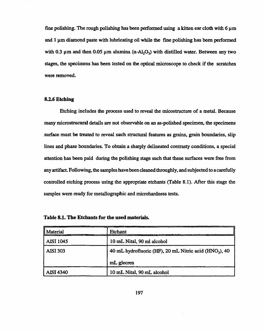
fine polishing. The rough polishing bas been performed using a kitten ear cloth with 6 p m
and 1 p m diamond paste with lubricaihg oil while the fine polishing has been performed
with 0.3 pm and then 0.05 p m alumina @-Al&) with distiiied water. Between any two
stages, the specimens has been tested on the optical microscope to check if the scratches
were removed.
8.2.6 Etching
Etching includes the process used to reveal the micostructure of a metal. Because
many microstrucural details are not observable on an as-polished specimen, the specimens
surface must be mted to reveal such structural features as grains, grain boundaries, slip
lines and phase boundanes. To obtain a sharply delineated contras@ conditions, a special
attention has ken paid during the polishing stage such that these surfaces were fke fkom
any artifact. Foliowing, the samples have been cleaned throughly, and subjected to acarefully
controlled etching process using the appropriate etchants (Table 8.1). Mer this stage the
samples were ready for metallographic and microhardness tests.
Table 8.1. The Etchants for the used materiais.
1 10 mL Nital, 90 ml alcohol 1
I 303 I 40 mZ. hydrofluonc (HF), 20 mL Nitric acid mo3), 40 I 1 AIS1 4340 1 10 mL Nital, 90 mL alcohol 1

8 3 MXCROHARDNESS MEASUREMENTS
It is h o w n that the microhardness of the deformed maîerial is related with the
preceding defomation and with the shear stress gained by the specimen under consideration
at the final stage of its deformation. This rnakes it possible to know the distribution of
defomation on the b a i s of microhardness measurements. The flow shear stress is related
with rnicrohardness as (Astakhov, 1998; Nakayama and Tama, 1964)
HV=5.2 z* (W
where HV is the hardness ("Vickeres) and e is the strain.
A microhardness survey of the fonned chips was undertaken to map out different
zones through the chip section. The microhamess tests have been carrïed out accordhg to
the ASIUE.384-84 standard. In this study, a Lem M-400G2 rnicrohardness tester has been
useci. This tester supports the mounting specimens and pennits the indenter and the
specimen to be bmught into contact gradudy and smoothly under apredetennined load. This
tester has a feature such that no rocking or lateral movement of the indenter or specimen is
permitted while the load is king applied or removed. A measuring microscope is mounted
on the tester in such a manner that the indentation may be readily located in the field of view.
The following steps have been made to do the microhardness tests:
1. Verifîcation of the rnicrohardness tester by making a series of indentations on
standardized hardness test blocks.
2. Preparation of the specimens as mentioned above.
3. Supporthg the specimens so that the test surface is normal to the axis of the indenter.
4. Selecting the correct objective by adjusting the optical equipment.

5 Deciding on the test panuneters where the test load is fixed by means of two dials
towards the top right of the machine and the loading speed is set in conjunction with
the test load to give the largest measUrable indentation. A 25 g load was selected so
that tests could be taken very close to the edges.
6. Using a highly polished , pointai and square-based pyramidal diamond with face
angles of 136' to indent the specimen.
7. Measuring the diagonals of the indentation by a micrometer screw.
8, Reading the microhardness value k m the hardness display.

RESULTS AND DISCUSSION
This chapter presents the major results obtained in the experimental part of the study.
The experiments have been cunied out to conform the developed theory of metal cutting and
to understand the relationship between modeled and real cutting conditions. The
experimentd methodologies are discussed in details in Chapters 6 ,7 and 8.
Io the view of the discussion presented in the previous chapter, the output has been
chosen to cuver:
1. The influence of misalignment on the cutting process (the steady-state and dynamic

cutting forces).
2. Comparison between the measured and the predicted steady state cutting forces
under neariy perfect alignment conditions.
3. Comparison of the results of the simulation study of proposed dynamic model for
wave removing process with those predicted by the proposed model.
4. Frequency autospectra for the axial cutting forces and the cutting torque for different
cutting conditions.
5. Dynamic system signatures for different cutting conditions.
6. Results of the study of chip morphology for the M y and partially fomed chips.
9.1 MISALIGNMENT EFFE3CT
Tables 9.1 and 9.2 together with Figures 9.1 through 9.3 quanti@ the effect of
misalignment on the steady-state axial cutting force and cutting torque for different cutting
regixnes. As seen fiom these tables and figures. the rnisalignrnent affects the results
dramatically where an increase in the steady-state axial cutting force and cutting torque c m
be noted as the rnisalignrnent increases. In particular, the cutting axial cutiing force and
cutting torque increase with increasing the cutting feed much more significant than that with
the cutting speed.
Using the obtained experirnental results, we have arrived to the following
conclusions:

Table 9.1. E f h t of misaliment on the measured axial cutting forces.
Cotting toal: Singie cuaing eëge BTAS -1" (25.4 II=) dipiiictcr. Mntcrint: AlSI 3û3
tof
Table 9.2. Effet of f g n m e n t on the measnred cutüng torque. 1
ide ulgc BTAS drill 1" (SA nnn) dhutcr.

1. A s i w c a n t scatter in the reported experimental results on the steady-state cutting
force measurements in deephole machining. (Griff i , 1982; Griffith, 1978,
Chandarcheclcar, 1984; Salcuma et al , l98Oa; Sakuma et al, 1980b; Sakurna et al,
198 1) is readily explained with the obtained results as follows. Since in the known
studies, the misalignment has never been reported thus controUed, these are obtained
under different misalignment of the deep-hole machines. For this reason, therefore,
the results reporteci by different researches cannot be compared with each other
or/and be used to ver@ any proposed theory.
2. The reported experimental results cannot be used to design the deephole process as
the whole. Deephole machining combines two machining processes namely clrilling
and burnishing and forces generated in drillhg are used to complete burnishing. As
shown by Astakhov (1994). bumishing process defmes the quality of the machined
surface in terms of its roughness, roundness, residual stresses, etc. It is also known
that this process is relatively sensitive to the bumishing force applied. For a given
drill design, the ration 'cutting force-buniishing force' is constant and, therefore, a
change in the cutting force directly affects the corresponding change in the
bumishing force. This simple consideration explains a significant scatter in the
reported results on quality in the machining surface in deep hole machining. This
also explains a relatively poor reproductivity of the deephole machining results since
the same tools are used in the machines having different misdignments that causes
the scatter.

Figures 9.4 through 9.27 show the frequency autospectra of the axiai dynamic cutting
force and dynamic cutting torque for different cutting regirnes under different misalignments.
The misalignment shows up as a series of hannonics associated with the nuining speed.
Comparing the autospectra of the axiai cutting force under difîerent misalignments
for the same cutting feed and spindle rotational speed show that the misalignment introduce
a series of different ampIitude harmonics at frequencies associated with the multiple of the
d g speed (2X, 4X, 6X etc, X is the frequency corresponding of the nuining speed). For
example at running speed of 654 rpm, the misalignment show up at 22Hz, 44Hz, 66Hz.
66Hz, 88Hz etc.
In the case of the cutting torque, the misalignments also show up as a series of
different amplitude harmonics but at frequencies associated with an odd number of the
running speed (3-X, 7X, 9X etc, X is the frequency corresponding of the running speed).
For example at ruhng speed of 654 rpm, the misaligrnent show up at 33Hz, 55Hz, 66Hz,
99Hz, etc*
Cornparhg the autospectra of the axial cutting force and cutting torque under
different misalignment for the same cutting feed and spindle rotational speed show that the
amplitudes of the different harmonics increase as the misalignment hcreases.
Also, it cm be noted that in the case of the axial cutting forces, the dominant
amplitude is associated with the second harmonic (2X) of the operating speed where the
amplitudes of the spikes which are observed at the forth, sixth, etc harmonic are seen to
progressively lowered. In the case of torque, the dominant amphde is associated with the
third harmonic of the operating speed. This spike which was obsemed at the thkd harmonic

was dso seen at Nth, seventh, etc. though the amplitude was seen to progressively reduced
The following important conclusions foUow k m the obtained results:
1. The deep-hole machining system has very distinctive dynarnic signatures under
different misaiignments. As seen from the results, if the deep-hole machining system
is aligned, it much more stable dynamicaiiy. In practicai ternis it means the
foilowing. Fint of ali, there is no chance for lobbing as hole defects (considered as
an inherent feature of deep-hole machining ( S a b a et ai , l98Oa; Sakuma et ai,
1980b; Sakuma et al, 1981) to occur. Moreover, there wouid be no spiraihg
(Gessesse, 1990) to be observed since spiraihg is caused by dynamic system
instability. Unfomnately, in the known studies of these cornmon defects, the
misalignment has never been considered.
2. The misalignment change the autospectra in a such manner that it becomes difficult
to distinguish between the spectra that reflects the cutting process contribution and
the spectra that corne fiom other sources. This produces the signal fiom the force
tramducers with high noise. This explains why the known studies (Chandrachaker,
1984) concluded that the cutting force in deephole machining has random nature.
High-noisy signai üsed in these studies to judge the nature of the cutting force
resulted in such a conclusion.

93 STEADY- STATE AXIAL CUTFING FORCE AND CUTFING TORQUE
Tables 9.3 through 9.8. show a cornparison between the measured and the predicted
steady-state axial cutting force and cutting torque for two cutting tools (American HeUer
design (BTAH) and Sandvic design (BTAS)) and three different matends (AISI 1045, AIS1
303 and AIS1 4340) under different cutting regimes. These tables reveal fairly good
agreement between the experimental and predicted values. Also, these tables shows that
always the experimental values are Iittle more than the predicted ones. The explanaîion may
be that the oil whirling augment the steady state axial cuttbg force and torque.
Figures 9.28 through 9.36 show the variations of the cutting forces (axial, radial and
tangentid ) and cutting torque with feed for each cutting tool and material under dBerent
cutting spsed. AIso, these figures reveai the experimental results for the axial cutting force
and cutîhg torque.
Table 9.3. Steady-state cutting forces ( BTAH drin 1" diameter, AIS1 1045).

Table 9.4. Steady-state cutting forces @TAS drill lm'diameter, AIS1 1045).
Table 9.5. Steady-state cutting forces ( BTAH drill 1" diameter, AISI 303).
Rota t id
spindle S m
( ~ m )
626
939
11.7 243 1 2036 162 -
lS3 100 0.12 3700.8 3298.8 10.9 33.86 3038 10.1
Cutting
speed
(&min)
50
75
F d
(-1
0.08
0.12
Axial cuecing force ( N) Cutting torW ( N J ~ )
enw%
13.8
10.7
6.6
11.0
73
7.1
Mtasund
266 1 3
38002
M d
24.62
35-81
44.74
23.93
35-87
45.78
Caicolatod
22942
3393.9
44728
22662
3343.8
43982
0.16 4790.7
20.92
3 1.20
41 -42
2û.64
30.61
41.02
0.08
O. 12
0.16
amr% I
15.0
128
7.3
13.6
145
102
25455
3608.8
47327
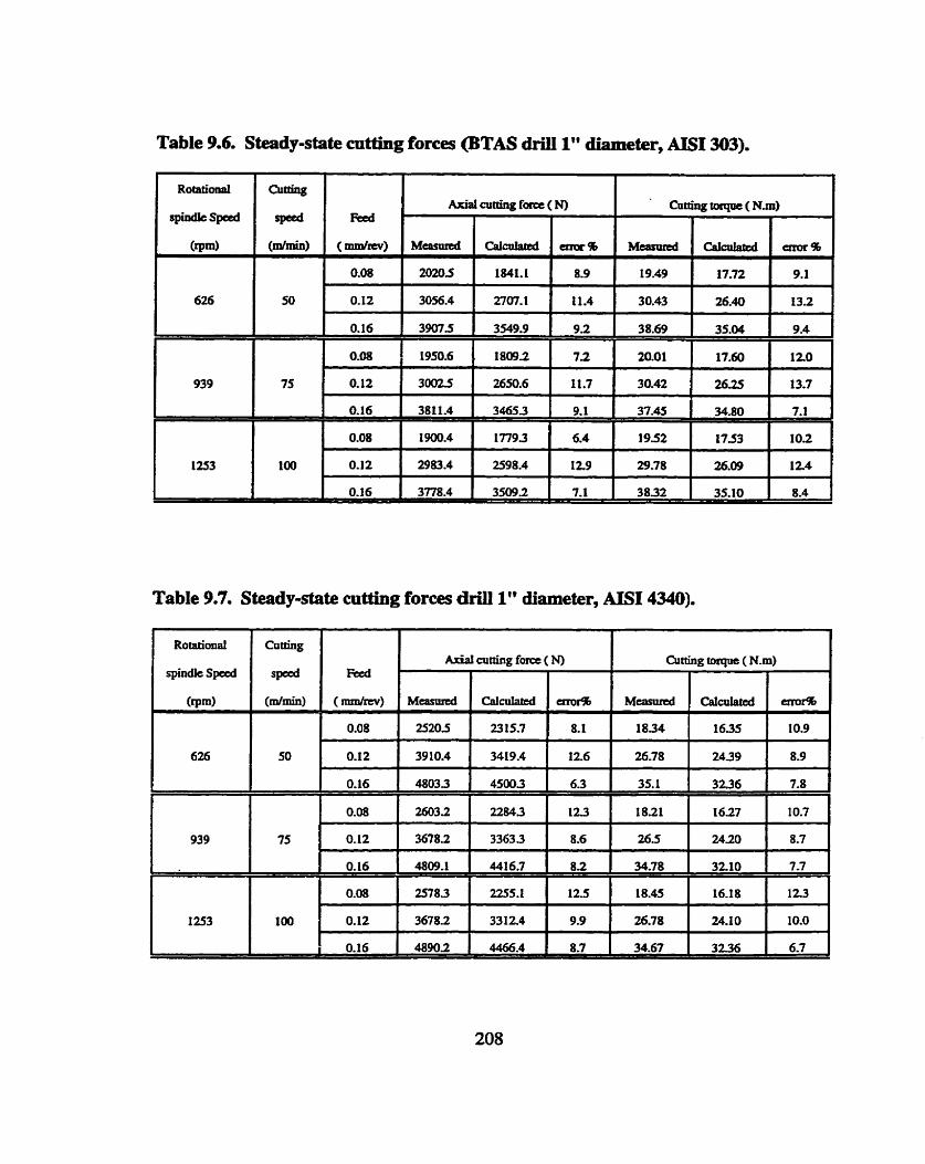
Table 9.6. Steadp-state cntang forces @TAS drill 1" niameter, AISI 303).
Table 9.7. Steady-state catting forces driilll' diameter, AIS1 4340).
acting
spced
(mlmin)
50
75
100
Red
(dm)
0.08
0.12
0.16
Axial cutting for# ( N) L
M d
2020.5
3056.4
3907.5
fi- torqr# ( N d
MeaPwd
19.49
30.43
38.69
20.01
30.42
37.45
1952
29.78
3832
0.08 1 19S0.6
Cal-
1841.1
2707.1
3549.9 ,
18092
2650.6
34653
t 7793
2598.4
3509.2
O. 12
0.16
0.08 I
0.12
0.16
emr%
8 9
11.4
9.2
7 3
11.7
9.1
6.4
129
7. 1 -
chIalkd
17.72
26-40
35.04
17.60
26s
34.80
1753
26.09
35.10
30025
3811.4
1900.4
2983.4
3778.4
arcr%
9.1
132
9.4
120
13.7
7.1
10.2
12.4
8.4

Table 9.8. Steady-state cutting forces ( BTAS drill Pdiarneter, AIS1 4340).
93 WAVE REIMOVING CUTTING PROCESS
Figures 9.37 through 9.40 show the simulation results for the wave removing process
for different cutting conditions. The simulation has been carried out based on the dynamic
mode1 of shear zone with paralle1 boudaries where four series of testing prograrns were
cumed out to assess the effects of the cutting feed, cutting speed, rake angle and f'requency
of the waves on the work surface on the dynamic force components F, and F,. These figures
reveal the variations of the force components which follow approximately sinusoidal waves.
A certain phase lag relative the vanation of the uncut chip thickness is clearly seen.
Figures 9.41 through 9.44 show the cornparison between the predicted and the
measured dynamic forces. Here, the experimental results obtained in by Nagim and Sadek
(1977) are also shown. The comparison shows that the proposed mode1 gives a good
agreements with the experimental results.
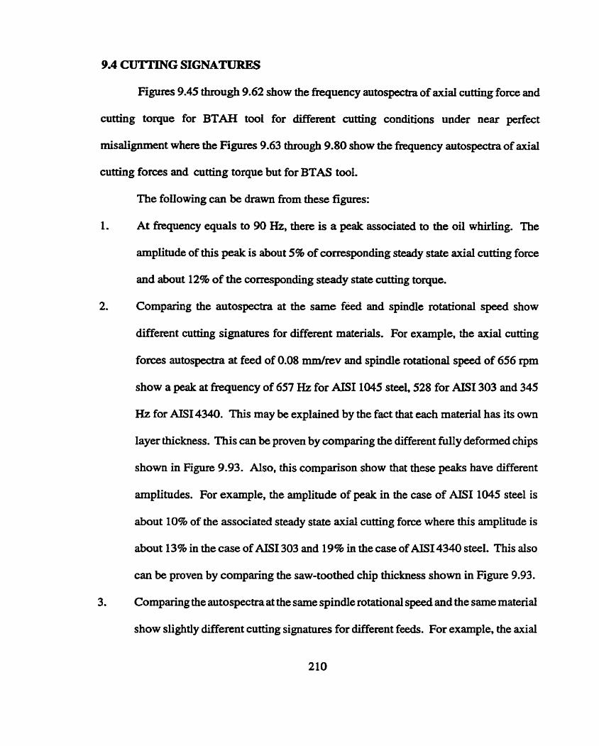
9.4 cuTTrNG SIGNATURES
Figures 9.45 thmugh 9.62 show the frequency autospectra of axial cutting force and
cutting torque for BTAH tool for different cutting conditions under near perfect
misalignment where the Figures 9.63 through 9.80 show the frequency autospectra of axial
curting forces and cunuig torque but for BTAS tool.
The following can be drawn h m these figures:
1. At frequency equals to 90 Hi, there is a peak associated to the oil whirling* The
amplitude of this peak is about 5% of wrresponding steady state axial cutting force
and about 12% of the correspondhg steady state cuning torque.
2. Cornparhg the autospectra at the same feed and spindle rotational speed show
different cutting signatures for different matenals. For example, the axial cutting
forces autospectra at feed of 0.08 mm/rev and spindle rotational speed of 656 rprn
show a peak at frequency of 657 J3z for AIS1 1045 steel, 528 for AIS1 303 and 345
Hz for AIS1 4340. This may be explained by the fact that each matenal has its own
layer thickness. This can be proven by comparing the different fully deformeci chips
shown in Figure 9.93. Also, this cornparison show that these peaks have different
amplitudes. For example, the amplitude of peak in the case of AIS1 1045 steel is
about 10% of the associated steady state axial cutting force where this amplitude is
about f 3% in the case of AIS1 303 and 19% in the case of AISI4340 steel, This also
can be proven by comparing the saw-toothed chip thickness s h o w in Figure 9.93.
3. Comparing the autospectra at the same spindle rotationai speed and the same material
show slightly different cutting signatures for different feeds. For example, the axial

cutthg force autospectra of ALTI 303 at spindle rotational speed of 656 rpm show a
peak at fkequency of 528 HZ for 0.081drev feed, 520 Hz for 0.12 d r e v and 515
Hz for 0.16 mdrev. This may be explained by the fact that the bending moment
which cause the chip formaton (Astakhov et ai. 1997b) depend on the feed. In
particular.. the bending moment increase with feed that Iowers the frequency of chip
formation. Also, this comparison show that these peaks have different amplitudes
and this amplitude increases as the feed increases. For example, the amplitude of
peak in the case of 0.08 mm/rev is about 13% of the associateci steady state axial
cuttiag force where this amplitude is about 16% when the feed is 0.12 d r e v and
19% when the feed is 0.16 mmhev.
4. Comparing the autospectra at the same feed and the same material show slightly
different cutting signatures for different spindle rotational speed. For example, the
axial cutting force autospectra of AISI 303 at feed 0.08 mdrev show a peak at
frequency of 528 Hz for n=656 rpm, 589 Hz for n=939 rpm and 665 Hz for n=1253
rpm. This may be explained by the fact that with increasing the cutting speed, the
length of the machined surface per unit tune is increased, then more sliding surfaces
form. Also. this comparison show that these peaks have aimost the same amplitude
for different cuning speed.
5. Comparing the autospectra at the same feed, spindle rotational speed and the same
material show alrnost the same cutting signatures for the two types of the tool used
in the experîments.
Table 9.9 and the figures 9.8 L through 9.83 summerize the effect of the feeds,

workpieces matenal and the cutting speds on the cutting signaturesatures
This study shows the fluctuation of the cutting forces is a result ofchip segmentation
and not the cause of it. Also this study show the effect of materials and cutting conditions
on the cutting signatures.
Table 9.9. Effect of materiai, feed and cutting speed on the cutting fluctuation
frequency.

9.5 CHIP MORPHOLOGY
The morphology of the fonned and partially formed chip is presented in this section.
Figures 9.84 through 9.93present the results of the chip morphology for the fuliy formed chip
where the Figures 9.94 h u g h 9.98 show resuits of chip morphology for the partially
formed chip.
Figure 9.84 show the initial structure for the AISI 1045. This structure is mainly
peariite grain (gray) with a network of grain boundary ferrite (white). Figure 9.85 reveal the
configuration for the fully f o m d chip of the AIS1 1045 at different magnificaîions. As c m
be seen by compdng the initiai structure and the formed one, it can easily note the
elongation of the grains in the direction of deformation. Figure 9.86 present a typical saw-
toothed chip showing the distribution of the microhardness across the chip section. The
figure reveal that the microhardness values starts with values equal to the initial matenal
hardness and increase to a certain limit and then start fiom the beginning again. This proves
that the deformation is non-unifonn,
Figure 9.87 show the initial structure for the AISI 303. This structure is a matrix of
austenite grains bound an intermetailic stringer type inclusions.. Figure 9.88 reveal the
configuration for the fdly formed chip of the AIS1 303 at different magnifications. As can
be seen by comparing the initial structure and the formed one, it can easily note the
elongation of the grains in the direction of deformation. This figure reveals that the shear
zone is composed of two regions. The first region (A) is the "wide region" where the
deformation changes at a small rate The second region (B) is the "narrow region " where the
deformation changes at a high rate. Figure 9.89 support the previous finding where the rate

of microhardness change in the narrow region is bigger than that in the wide region.
Figure 9.90 show the initial structure for the AJSI 4340. This stnicture is tempered
martemite. Figure 9.91 reveal the configuraiion for the fdly formed chip of the AISI 4340
at different magnincations. As can bc seen by comparing the initial structure and the fomed
one, it c m easily note the elongation of the grains in the direction of defoxmation. Figure
9.92 present a typical saw-toothed chip showing the distribution of the microhardness across
the chip section. The figure reveal that the microhardness values starts with values equal
to the initial material hardness and increase to a certain limit and then start Erom the
beginning again. This proves that the deformation is non-uniform.
In studying the defonnation in metal cutting the main attention is usually paid to the
defonnation rate which takes place in the shear zone. The rate of deformation is closely
related to the displacement and the velocities. To calculate the defonnation rate a number
of different approaches and formulas were proposed (Boothroyd and Knight, 1989). The
known approaches are based on the known velocity diagram (Merchant, 1945) which has to
be corrected as s h o w previously in chapter three. Therefore, the deformation rate for the
model of deformation zone with parallel boundaries requins additional shidy.
Figures 9.94 through 9.97 show the microphotographs of the paaially formed chip.
Figure 9.97 shows that the deformation is non uniform across the shear zone.
The morphology study support the theoretical considerations of the paralle1 shear
zone model with parallel boundaries where the study reveal that the shear zone is composed
of two regions (Manyindo and Oxley, 1986). The first region is terrned as the '%ide region"
where the tangential velocity v, changes at a small rate. The second region is termed as the

" n m w region " where the tangentid velocity v, changes at a high rate. Also, it can be seen
that as n increases, the "wide region" becomes larger and the " narrow region" becomes
smaller. The narrow region where a significant change of the tangentid velocity takes place
may be thought as the region of the discootinuity of this velocity. This model plays a
principal role for the foregoing analysis because both the state of stress and strain and the
resistance of the work material to cutting in this " narrow region" are very specific.
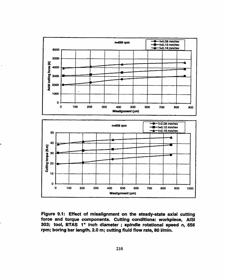
Figure 9.1: Effect of misalignment on the steady-state axial cutting force and torque components. Cutting conditions: workpiece, AlSI 303; tool, BTAS ln inch diameter ; spindle rotational speed n, 656 rprn; boring bar Iength, 2=0 m; cutting fluid flow rate, 80 Vmin.

n a 9 rpm +f=û.OB mdrev + 14.1 2 mdrev
Figure 9.2: Effect of misalignment on the steady-state axial cutting force and torque components. Cutting conditions: workpiece, AISI 303; tool, BTAS 1" inch diameter ;spindb rotational speed n, 939 rpm; boring bar length, 2.0 m; cutting fluid flow rate, 80 Vmin.

Figure 9.3: Effect of misalignment on the steady-state axial cutting force and torque components. Cutting conditions: workpiece, AISI 303; tool, BTAS 1" inch diameter ; spindle rotational speed n, 1253 rpm; boring bar length, 2.0 m; cutting fluid flow rate, 80 Vmin.
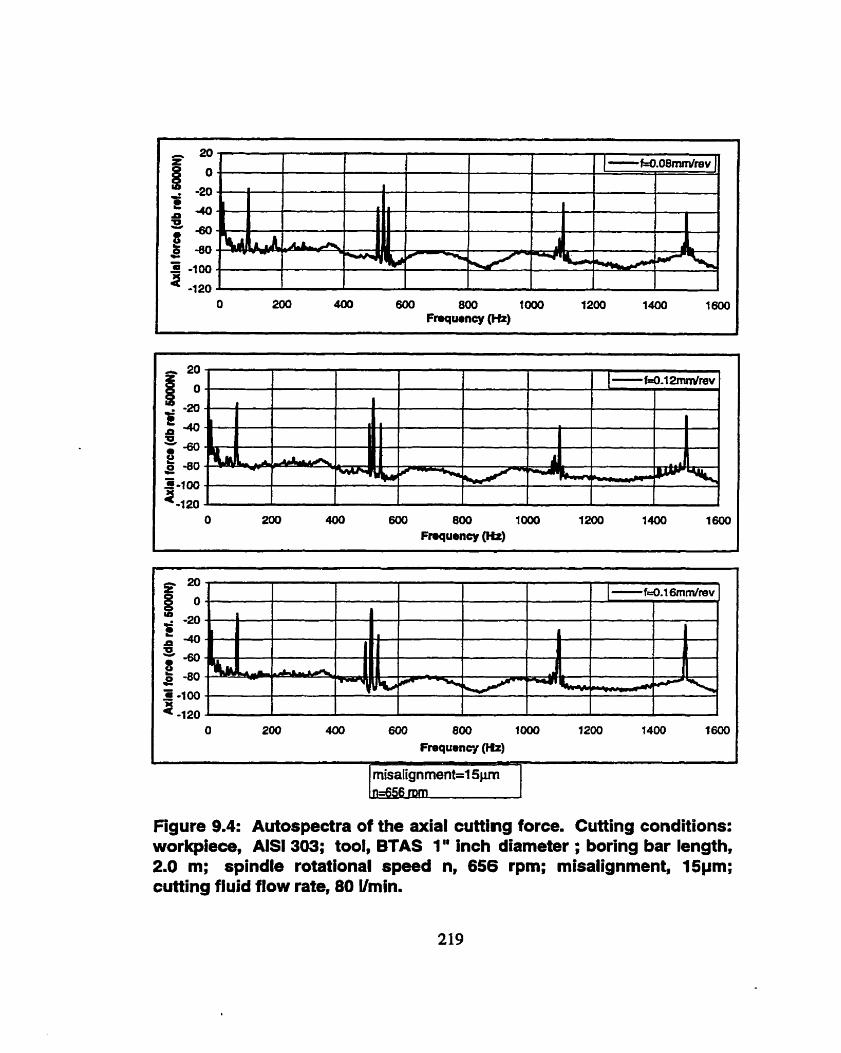
600 800 1000
Frequsncf (Hz)
Figure 9.4: Autospectra of the axial cutting force. Cutting conditions: wdcpiece, AIS1 303; tool, BTAS 1" inch diameter ; boring bar length, 2.0 m; spindle rotational speed n, 656 rpm; misalignment, 15pm; cutting fluld flow rate, 80 Umin.

Figure 9.5: Autospectra of the cutting torque. Cutüng conditions: workpiece, AlSI 303; tool, BTAS " inch diameter ; boring bar length, 2.0 m; spindle rotational speed n, 656 rpm; misalignment, 15pm; cutting tluid flow rate, 80 Vmin.

Figure 9.6: Autospectra of the axial cutting force. Cutting conditions: workpiece, AIS1 303; tool, BTAS 1" inch diameter ; boring bar length, 2.0 m; spindle rotational speed n, 939 rpm; misalignment, 15pm; cutting fluid flow rate, 80 Vmin.

Figure 9.7: Autospectra of the cutting torque. Cutting conditions: workpiece, AIS1 303; tool, BTAS ln inch diameter ; boring bar length, 2.0 m; spindle rotational speed n, 939 rpm; misalignment, 15pm; cutting fluid Row rate, 80 Vmin.

Figure 9.8: Autospectra of the axial cutting force. Cutting conditions: workpiece, AIS1 303; tool, BTAS 1" inch diameter ; boring bar length, 2.0 m; spindle rotational speed n, 1253 rpm; misalignment, 15pm; cutting fluid flow rate, 80 Vmin.

Figure 9.9: Autospectra of the cuttlng torque. Cutting conditions: workpiece, AIS1 303; tool, BTAS 1" inch diameter ; boring bar length, 2.0 m; spindle rotational speed n, 1253 rpm; misalignment, 15pm; cutting fluid flow rate, 80 Vmin.

Figure 9.1 0: Autospectra of the axial cutting force. Cutting conditions: workpiece, AIS1 303; tool, BTAS 1" inch diameter ; boring bar length, 2.0 m; spindle rotational speed n, 656 rpm; misalignment, 205pm; cutting fluid flow rate, 80 Vmin.

Figure 9.1 1 : Autospectra of the cutting torque. Cutting conditions: workpiece, AIS1 303; tool, BTAS lu inch diarneter ; boring bar length, 2.0 m; spindk rotational speed n, 656 rpm; misalignment, 205prn; cuttinn fluid ftow rate, 80 Urnin.

Figure 9.1 2: Autospectra of the axial cutting force. Cutting conditions: workpiece, AIS1 303; tool, BTAS 1" inch diameter ; boring bar length, 2.0 m; spindle rotational speed n, 939 rpm; misalignment, 205pm; cutting fluid flow rate, 80 Umin.

Figure 9.1 3: Autospectra of the cutting torque. Cutting conditions: workpiece, AIS1 303; tool, BTAS 1" inch diameter ; boring bar length, 2.0 m; spindle rotational speed n, 939 rpm; misalignment, 205prn; cutting fluid flow rate, 80 Vmin.

Figure 9.14: Autospectra of the axial cutting force. Cutting conditions: workpiece, AIS1 303; tool, BTAS 1" inch diameter ; boring bar length, 2.0 m; spindle rotational speed n, 1253 rpm; misalignment, 205pm; cutting fhid flow rate, 80 Vrnin.

Figure 9.1 5: Autospectra of the cutUng torque. Cutting conditions: workpiece, AIS1 303; tool, BTAS In inch diameter ; boring bar length, 2.0 m; spindle rotational speed n, 1253 rpm; rnisalignment, 205pm; cutting fluid ftow rate, 80 Vmin.

Figure 9.1 6: Autospgctra of the axial cutting force. Cutting conditions: workpiece, AlSI 303; tool, BTAS ln inch diameter ; boring bar length, 2.0 m; spindle rotational speed n, 656 rpm; misalignment, 422pm; cutting fluid Pow rate, 80 Vmln.

Figure 9.17: Autospectra of the cutting torque. Cutting conditions: workpiece, AlSl 303; tool, BTAS ln inch dlameter ; boring bar length, 2.0 m; spindle rotational speed n, 656 rpm; misalignment, 422pm; cutting fluid flow rate, 80 Vmin.

Figure 9.1 8: Autospectra of the axial cutting force. Cutting conditions: workpiece, AIS1 303; tool, BTAS 1" inch diameter ; boring bar length, 2.0 m; spindle rotational speed n, 939 rpm; misalignment, 422pm; cutang fluid flow rate, 80 Vmin.

Figure 9.1 9: Autospectra of the cutting torque. Cutting conditions: workpiece, AIS1 303; tool, BTAS ln inch diameter ; boring bar length, 2.0 m; spindle rotational speed n, 939 rpm; misalignment, 422pm; cutting fluid flow rate, 80 Umin.

600 800 1000 Froquoncy (Hz)
Figure 9.20: Autospectra of the axial cutting force. Cutting conditions: workpiece, AIS1 303; tool, BTAS 1" inch diemeter ; boring bar length, 2.0 m; spindle rotational speed n, 1253 rpm; misalignment, 422pm; cutting M d flow rate, 80 Vmin.

Figure 9.21: Autospectra of the cutting torque. Cutting conditions: workpiece, AIS1 303; tool, BTAS ln inch diameter ; boring bar length, 2.0 m; spindle rotational speed n, 1253 rpm; misalignment, 422pm; cutting fluid flow rate, 80 Vmin.

Figure 9.22: Autospectra of the axial cutting force. Cutting conditions: workpiece, AIS1 303; tool, BTAS 1" inch diameter ; boring bar length, 2.0 m; spindle rotational speed n, 656 rpm; misalignment, 856pm; cutting fluid flow rate, 80 Umin.
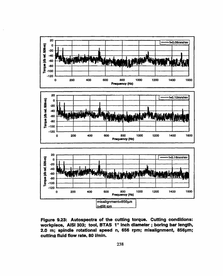
Figure 9.23: Autospectra of the cutting torque. Cutting conditions: workpiece, AIS1 303; tool, BTAS 1" inch diameter ; boring bar length, 2.0 m; spindle rotational speed n, 656 rpm; rnisalignment, 856pm; cutting fluid flow rate, 80 Vmin.

Figure 9.24: Autospectra of the axial cutting force. Cuttlng conditions: workpiece, AIS1 303; tool, BTAS 1" inch diameter ; boring bar length, 2.0 m; spindle rotational speed n, 939 rpm; misalignment, 856pm; cutting fluid flow rate, 80 Vmin.

Figure 9.25: Autospectra of the cutting torque. Cutting conditions: workpiece, AIS1 303; tool, BTAS In inch diameter ; boring bar length, 2.0 m; spindle rotational speed n, 939 rpm; rnisalignment, 856pm; cutting fluid flow rate, 80 Umin.

Figure 9-26: Autospectra of the axial cutting force. Cutting conditions: workpiece, AIS1 303; tool, BTAS 1" inch diameter ; boring bar length, 2.0 m; spindle rotational speed n, 1253 rpm; misallgnment, 856pm; cutting fluid flow rate, 80 Ilmin.

Figure 9.27. Autospectra of the cutting torque. Cutting conditions: workpiece, AIS1 303; tool, BTAS 1' inch diameter ; boring bar length, 2.0 m; spindle rotational speed n, 1253 rpm; misalignment, 856pm; cutting fluid flow rate, 80 Vmin.

Figure 9.28: Steady-state cutting forces and torque components. Cutting conditions: workpiece, AISI 1045; tools, BTAH and BTAS 1" inch diameter ; boring bar length, 2.0 m; spindle rotational speed n, 656 rpm; misalignment, 15pm; cutting fluid flow rate, 80 Umin.

Figure 9.29: Steady-state cutting forces and torque components. Cutting conditions: workpiece, AIS1 1045; tools, BTAH and BTAS 1" inch diameter ; boring bar length, 2.0 rn; spindle rotational speed n, 939 rpm; misalignment, 15pm; cutting fluid flow rate, 80 Vmin.

3TAS 1 Food (mmlnv)
AiSI 1045 114253 rpm
Figure 9.30: Steady-state cutting forces and torque components. Cutting conditions: workpiece, AlSI 1045; tools, BTAH and BTAS 1" inch diameter ; boring bar length, 2.0 m; spindle rotational speed n, 1253 rpm; misalignment, 15pm; cutting fluid flow rate, 80 Vmin.

BTAS 1 Feed ( m m )
Figure 9.31: Steady-state cutting forces and torque components. Cutting conditions: workpiece, AIS1 303; tool, BTAH nd BTAS 1" inch diameter ; boring bar length, 2.0 m; spindle rotational speed n, 656 rpm; misalignment, 15pm; cutting fluid flow rate, 80 Vmin.

Figure 9.32: Steady-state cutting forces and torque components. Cutting conditions: workpiece, AIS1 303; tools, BTAH and BTAS 1" inch diameter ; boring bar length, 2.0 m; spindle rotational speed n, 939 rpm; misallgnment, 15pm; cutting fluid flow rate, 80 Umin.

Figure 9.33: Steady-state cutting forces and torque components. Cutting conditions: workpiece, AIS1 303; tool, BTAH and BTAS 1" inch diameter ; boring bar length, 2.0 m; spindle rotational speed n, 1253 rpm; misalignment, 1Spm; cutHng fluid flow rate, 80 Vmin.

Figure 9.34: Steady-stete cutting forces and torque cornponents. Cutting conditions: workpiece, AIS1 4340; tools, BTAH and BTAS 1" inch diameter ; boring bar length, 2.0 m; spindle rotational speed n, 656 rpm; misalignment, 1Spm; cutting fluid flow rate, 80 Umin.

0.00 0.02 0.04 0.06 0.08 0.10 0.12 0.14 0.16 0.18
BTAS I Food ( m d n v )
Figure 9.35: Steady-stae cutting forces and torque components. Cutting conditions: workpiece, AIS1 4340; tools, BTAH BTAS 1" inch diameter ; boring bar length, 2.0 m; spindle rotational speed n, 939 rpm; rnisalignment, 15pm; cutting M d flow, 80 Vmin.

10000 -.
8000 - A s i! -- ,O rn g - - ,
O
m-
O 0.00 0.02 0.04 0.06 0.08 0.10 0.12 0.14 0.16 0.18
BTAH 1 F d (mmlnv)
I
0.00 0.02 0.04 0.06 0.08 0.10 0.12 0.14 0.16 0.18
BTAS 1 Feed (mdrev)
Figure 9.36: Steady-state cutting forces and torque components. Cutting conditions: workpiece, AIS1 4340; tool, BTAH and BTAS esign 1" inch diameter ; boring bar length, 2.0 m; spindle rotational speed n, 1253 rpm; misalignment, 15vm; cutting fluid flow rate, 80 Umin.

uncut chip thickness variation - - - - - - - - force variation in x-direction ( vertical force). - - . . - - - - - force variation in y-direction ( horizontal force).
8 1 O 12 14 16 18 20 Time (ms)
8 IO 12 nme (ms)
Figure 9.37: Simulation results (series 1) : v=140 mlmin, a=5 deg., frequency=l20 Hz, b=3.5 mm.

uncut chip thickness variation . , , , , - - , , force variation in xdirection ( vertical force). , , , , , , , , , , , , , , , force variation in y-direction ( horizonta1 force).
8 10 12 14 16 18 20 Time (ms)
Figure 9.38: Simulation results (series 2): td.19 rnmlrev, a=5 deg., frequency=120 Hz, b=3.5 mm

uncut chip thickness variation - - - - - - - - - force variation in x-direction ( vertical force). - - - - - - - - - - - - - - - force variation in ydirection ( horizontal force).
O 2 4 6 8 10 12 14 16 18 20 ïïme (ms)
Figure 9.39: Simulation results (series 3): v 4 4 0 mlmin, t=0.19 mm/rev, frequency=120 Hz, b=3.5 mm.

uncut chip thickness variation - - - - - - - - force variation in x-direction ( vertical force). - - - - - - - - - - - - - - - force variation in y-direction ( horizontal force).
O 2 4 6 8 10 12 14 16 18 20 7lme (ms)
8 10 12
Time (mr)
Figure 9.40: Simulation results (series 4): v=140 mlmin, t=0.19 mdrev, a=5 deg., b=3.5 mm.

expriment
O expenrnent
Figure 9.41: Effect of feed on the dynamic forces.

(Nigrn et a!, 1977) - predidion Fy experirnent
100 150 200
Cutting speed (m/mln)
Figure 9.42: Effect of cutting speed on the dynamic forces.

(Mgmetal,1977') - - O - - - predicüon Fx O experiment I
O 2 4 6 8 1 O 12 14 16 18 20
Rake angle (deg.)
Figure 9.43: Effect of rake angle on the dynamic forces.
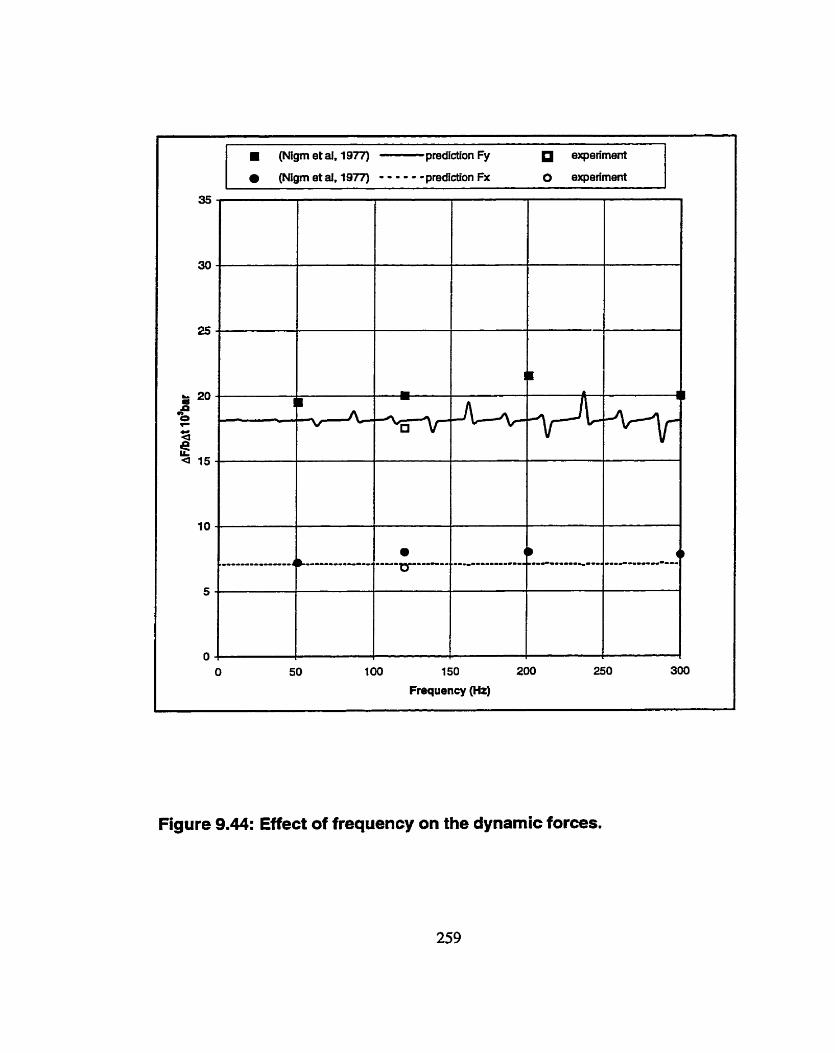
(Nigm et al. 1977) - predicüon Fy expriment
1 (Mgrnetai.1977) - - - - - - predicüon Fx O experiment
100 150 200
Frequency (Hz)
Figure 9.44: Eîfect of frequency on the dynamic forces.

BTAH; AlSI 1 045 11456 rpm
Figure 9.45: Autospectra of the axial cutting force. Cutting conditions: workpiece, AlSI 1045; tool, BTAH lu inch diameter ; boring bar length, 2.0 m; spindle rotational speed n, 656 rpm; misalignment, 15pm; cutting fluid flow rate, 80 Vmin.

600 800 1000 Frequency (Hz)
C & -7
BTAH; AlSI 1 045 n=656 rpm
Figure 9.46: Autospectra of the cutting torque. Cutting conditions: workpiece, AlSI 1045; tool, BTAH 1" inch diameter ; boring bar length, 2.0 m; spindle rotational speed n, 656 rpm; misalignment, 15pm; cutting fluid flow rate, 80 Umin.

O 200 400 600 800 1000 1 200 1400 1600
Frequency (Hz)
O 200 400 600 800 IO00 Frequency (Hz)
BTAH; AiSI 1045 n=939 rpm
Figure 9.47: Autospectra of the axial cutting force. Cutting conditions: workpiece, AIS1 1045; tool, BTAH 1 " inch diarneter ; boring bar length, 2.0 m; spindle rotational speed n, 939 rprn; misalignment, 15pm; cutting fluid flow rate, 80 Vmin.

O 200 400 600 800 IO00 1200 1400 1600 Frequency (Hz)
7 - BTAH; AlSI1045 n=939 rpm
Figure 9.48: Autospectra of the cutting torque. Cutting conditions: workpiece, AIS1 1045; tool, BTAH 1 " inch diameter ; boring bar length, 2.0 m; spindle rotational speed n, 939 rpm; misalignment, 15pm; cutting fluid flow rate, 80 Umin.

600 800 1000 Frequency (Hz)
1
BTAH; AIS 11 045 -n=1253 rpm -
Figure 9.49: Autospectra of the axial cutting force. Cutting conditions: workpiece, AISI 1045; tool, BTAH 1" inch diarneter ; boring bar length, 2.0 m; spindle rotational speed n, 1253 rpm; misalignment, 15pm; cutting fluid fiow rate, 80 Vmin.

O 200 4QO 600 800 1000 1200 1400 1600 Frequency (Hz)
600 800 1000 Frequency (Hz)
Figure 9.50: Autospectrr of the cutting torque. Cutting conditions: workpiece, AIS1 1045; tool, BTAH 1" inch diameter ; boring bar length, 2.0 m; spindle rotational speed n, 1253 rpm; misalignment, 15prn; cutting fluid flow rate, 80 Umin.

600 800 1000 1200 1400 Frequency (Hz)
Figure 9.51: Autospectra of the axial cutting force. Cutting conditions: workpiece, AIS1 303; tool, BTAH 1" inch diameter ; boring bar length, 2.0 m; spindle rotational speed n, 656 rprn; misalignment, 15pm; cutting fluid flow rate, 80 Vmin.

- BTAH; AIS1303 n=656 rpm
Figure 9.52: Autospectra of the cutting torque. Cutting conditions: workpiece, AIS1 303; tool, BTAH 1" inch diameter ; boring bar length, 2.0 m; spindle rotational speed n, 656 rpm; misalignment, 15pm; cutting fluid flow rate, 80 Vmin.

O 200 400 ô00 800 1000 1 200 1400 1600 Fraquen y (Hz)
400 600 800 1000 1 200 Frequency (Hz)
[n=939 rpm I
Figure 9.53: Autospectra of the axial cutting force. Cutting conditions: workpiece, AIS1 303; tool, BTAH 1" inch diameter ; boring bar length, 2.0 m; spindle rotational speed n, 939 rpm; misalignment, 15pm; cutting fluid flow rate, 80 Ilmin.

Figure 9.54: Autospectra of the cutting torque. Cutting conditions: workpiece, AIS1 303; tool, BTAH 1 " inch diameter ; boring bar length, 2.0 m; spindle rotational speed ri, 939 rpm; misalignment, 15pm; cutting fluid flow rate, 80 Urnin.

600 800 1000 Frequency (Hz)
- - -
n=1253 rpm
Figure 9.55: Autospectra of the axial cutting force. Cutting conditions: workpiece, AIS1 303; tool, BTAH 1" inch diameter ; boring bar length, 2.0 m; spindle rotational speed n, 1253 rpm; misalignment, 15pm; cutting fluid flow rate, 80 Vmin.

600 800 IO00 Frequency (Hz)
BTAH; AS1303 7n=1253 rpm
Fig. 9.56: Autospectre of the cutting torque. Cutting conditions: workpiece, AIS1 303; tool, BTAH 1" inch diameter ; boring bar length, 2.0 m; spindle rotational speed n, 1253 rpm; misalignment, 15pm; cutting fluid flow rate, 80 Umin.

20 g O
-20
40 D ' -60 O Ô -00 - -
-120 O 200 400 600 800 1000 1200 1400 1600
Frequency (Hz)
BTAH; AISI 4340 n=656 rpm
Figure 9-57:. Autospectra of the axial cutting force. Cutting conditions: workpiece, AISI 4340; tool, BTAH 1" inch diameter ; boring bar length, 2.0 m; spindle rotational speed n, 656 rpm; misalignment, 15pm; cutting fluid flow rate, 80 Vmin.

BTAH; AlSI 4340 n=656 rprn
Figure 9.58: Autospectra of the cutüng torque. Cutting conditions: workpiece, AIS1 4340; tool, BTAH 1 " inch diameter ; boring bar length, 2.0 m; spindle rotational speed n, 656 rpm; misalignment, 15pm; cutting fluid flow rate, 80 Vmin.

Figure 9.59: Autospectra of the axial cutting force. Cutting conditions: workpiece, AISI 4340; tool, BTAH Heller design 1" inch diameter ; boring bar length, 2.0 m; spindle speed N, 939 rpm; misalignment, 15prn; cutting fluid flow, 80 Ilmin.
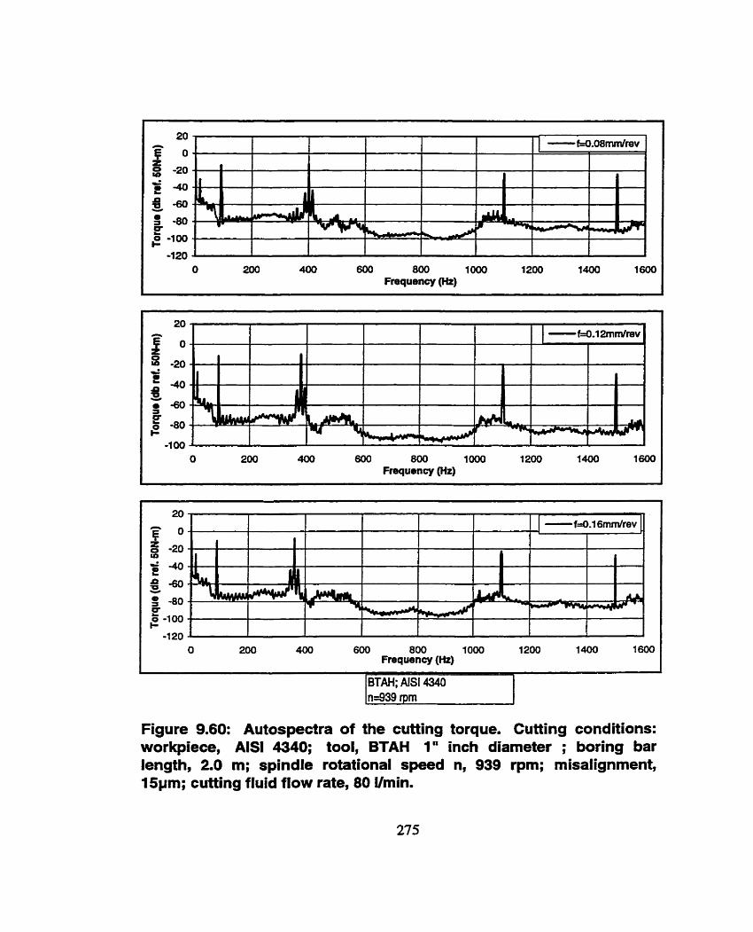
600 800 1000 Frequency (Hz)
Figure 9.60: Autospectra of the cutting torque. Cutting conditions: workpiece, AlSI 4340; tool, BTAH 1" inch diametei ; boring bar length, 2.0 m; spindle rotational speed n, 939 rpm; misalignment, 1Svm; cutting fluid ftow rate, 80 Ilmin.

I *: ,: -20 : -40 po 0 -80 L = -100
9 -120 O 200 400 600 800 1000 1200 1400 1600
Frequency (Hz)
200 400 600 800 1000 Frequency (Hz)
ln=1253 rpm
Figure 9.61: Autospectra of the axial cutting force. Cutting conditions: workpiece, AISI 4340; tool, BTAH lut inch diarneter ; boring bar length, 2.0 rn; spindle rotational speed n, 1253 rprn; misalignment, 15pm; cutting fluid flow rate, 80 Vmin.

600 800 Io00 Frequency (Hz)
600 800 1000 Frequency (Hz)
Figure 9.62. Autospectra of the cutting torque. Cutting conditions: workpiece, AISI 4340; tool, BTAH 1" inch diameter ; boring bar length, 2.0 m; spindle rotational speed n, 1253 rpm; misalignment, 15pm; cutting fluid flow rate, 80 Umin.

20
f o Lb -20 2 P -40 u z-60 0, 0 -80 - 0 -100
420 O 200 400 600 800 IO00 1200 1400 1 600
Frequency (Hz)
BTAS; AlSI 104% n=656 rpm
Figure 9.63: Autospectra of the axial cutting force. Cutting conditions: workpiece, AlSI 1045; toot, BTAS 1" inch diameter ; boring bar length, 2.0 m; spindle rotational speed n, 656 rpm; misalignment, 15pm; cutting fluid flow rate, 80 Vmin.

BTAS; AÏSI 1045 nS56 rpm
Figure 9.64: Autospectra of the cutting torque. Cutting conditions: workpiece, AIS1 1045; tool, BTAS 1" inch diameter ; boring bar length, 2.0 m; spindle rotational speed n, 656 rpm; misalignment, 15pm; cutting fluid flow rate, 80 Umin.

600 800 1000 Frequency (Hz)
A 20
I O Ld -20 : 4 O : -60
5 -80 - -1 20
O 200 400 600 800 1000 1200 1400 1600 Frequency (Hz)
BTAS; AlSi 1045 n=939 rpm
Figure 9.65: Autospectre of the axial cutting force. Cutting conditions: workpiece, AIS1 1045; tool, BTAS 1" inch dismeter ; boring bar length, 2.0 m; spindle rotational speed n, 939 rpm; misalignment, 15pm; cutting fluid flow rate, 80 Vmin.

1 BTAS; AISI IO& I
Figure 9.66: Autospectra of the cutting torque. Cutting conditions: workpiece, AlSI 1045; tool, BTAS 1" inch diameter ; boring bar length, 2.0 m; spindle rotational speed n, 939 rpm; misalignment, 15pm; cutting fluid flow rate, 80 Vmin.

la ; -20
140 s
-60 g 40 -
0 -100
3 -120 O 200 400 600 800 IO00 1200 1400 1600
Frequency (Ht)
0 20
I O & -20 2 n 40 Y t -60
3 -80 - s -IO0 -1 20 O 200 400 600 800 1000 1200 1400 1600
Frequency (Hz)
- - BTAS; AlSi 1045 n=1253 rpm
Figure 9.67: Autospectra of the axial cutting force. Cutting conditions: workpiece, AlSI 1045; tool, BTAS 1" inch diarneter ; boring bar length, 2.0 m; spindle rotational speed n, 1253 rpm; misalignment, 15pm; cutting fluid flow rate, 80 Umin.

O 200 400 600 800 IO00 1200 1400 1600 Frequency (Hz)
BTAS; AIS1 1 045 n=1253 rprn
Figure 9.68: Autospectra of the cutting torque. Cutting conditions: workpiece, AIS1 1045; tool, BTAS 1" inch diameter ; boring bar length, 2.0 m; spindle rotational speed n, 1253 rpm; misalignment, 15pm; cutting fluid flow rate, 80 Vrnin.

600 800 IO00 Frequency (Hz)
Figure 9.69: Autospectra of the axial cutting force. Cutting conditions: workpiece, AIS1 303; tool, %TAS 1" inch diameter ; boring bar length, 2.0 m; spindle rotational speed n, 656 rpm; misalignment, 15pm; cutting fluid flow rate, 80 Vmin.

600 800 IO00 Frequency (Hz)
Figure 9.70: Autospectra of the cutting torque. Cutting conditions: workpiece, AIS1 303; tool, BTAS 1 " inch diameter ; boring bar length, 2.0 m; spindle rotational speed n, 656 rpm; misalignment, 15pm; cutting fluid flow rate, 80 Umin.

1 BTAS; AlSI 303
Figure 9.71 : Autospectra of the axial cutting force. Cutting conditions: workpiece, AIS1 303; tool, BTAS 1" inch diameter ; boring bar length, 2.0 m; spindle rotational speed n, 939 rpm; misalignment, 15pm; cutting fluid flow rate, 80 Vmin.

20
F o Z 8 -20
5 4 0
8 -SO Y
s -80 F et00
-120 O 200 400 600 800 IO00 1200 1400 1600
Frequency (Hz)
BTAS; AlSI 303 n=939 rpm
Figure 9.72: Autospectra of the cutting torque. Cutting conditions: workpiece, AIS1 303; tool, BTAS 1" inch diameter ; boring bar length, 2.0 rn; spindle rotational speed n, 939 rpm; misalignment, 15pm; cutting M d flow rate, 80 Umin.

20 8 O
-20 I a 40 =
-60 B g -80 - 2 -100
-120 O 200 400 600 800 1000 1200 1400 1600
Frequency (Hz)
- I "V ..
O 200 400 600 800 IO00 1200 1400 1 600 Frequency (Hz)
BTAS; AISI 303 n=1253 rpm
Figure 9.73: Autospectra of the axial cutting force. Cutting conditions: workpiece, AIS1 303; tool, BTAS 1 " inch diameter ; boring bar length, 2.0 m; spindle rotational speed n, 1253 rpm; misalignment, 15pm; cutting fluid flow rate, 80 Umin.

20
F O 2 g -20
$40 n s-60 7 -80 f g-100
-1 20 O 200 400 600 800 1000 1200 1400 1 600
Ffequency (Hz)
Figure 9.74: Autospectra of the cutting torque. Cutting conditions: workpiece, AIS1 303; tool, BTAS 1" inch diameter ; boring bar length, 2.0 rn; spindle rotational speed n, 1253 rpm; misalignment, 15pm; cutting fluid flow rate, 80 Vmin.

600 800 IO00 Frequency (Hz)
O 200 400 600 800 IO00 1200 1400 1600 Frequency (Hz)
BTAS; AlSi 4340 11456 rpm
Figure 9.75: Autospectra of the axial cutting force. Cutting conditions: workplece, AlSI 4340; tool, BTAS 1" inch diameter ; boring bar length, 2.0 m; spindle rotational speed n, 656 rpm; misalignment, 15pm; cutting fluid flow ratey 80 Vmin.

600 800 IO00 Frequency (Hz)
Figure 9.76: Autospectra of the cutting torque. Cutting conditions: workpiece, AIS1 4340; tool, BTAS 1" inch diameter ; boring bar length, 2.0 m; spindle rotational opeed n, 656 rpm; rnisalignment, 15prn; cutting fMd flow rate, 80 Umin.

600 800 1000 Fmquency (Hz)
BTAS; AISI 4340 n=939 rprn
Figure 9.77: Autospectra of the axial cutting force. Cutting conditions: workpiece, AIS1 4340; tool, BTAS 1" inch diarneter ; boring bar length, 2.0 m; spindle rotational speed n, 939 rpm; misalignrnent, 15pm; cutting fluid flow rate, 80 Vmin.

BTAS; AlSI 4340 n=939 rpm
Figure 9.78: Autospectra of the cutting torque. Cutting conditions: workpiece, AIS1 4340; tool, BTAS 1" inch diameter ; boring bar length, 2.0 m; spindle rotational speed n, 939 rpm; misalignment, 15pm; cutting fluid flow rate, 80 Vmin.

6OQ 800 1000 Frequency (Hz)
O 200 400 600 800 1 000 1200 1400 1600 Frequency (Hz)
BTAS; AISI 4340 n=1253 rpm
Figure 9.79: Autospectra of the axial cutting force. Cutting conditions: workpiece, AISI 4340; tool, BTAS 1" inch diameter ; boring bar length, 2.0 m; spindle rotational speed n, 1253 rpm; misalignment, 15pm; cutting ftuid flow rate, 80 Vmin.

O 200 400 600 800 Io00 1200 1400 1600 Frequency (HZ)
600 800 1000 Frequency (Hz)
Figure 9.80: Autospectra of the cutting torque. Cutting conditions: workpiece, AIS1 4340; tool, BTAS 1" inch diameter ; boring bar length, 2.0 rn; spindle rotational speed n, 1253 rpm; misalignment, 15pm; cutting fluid flow rate, 80 Vmin.

900 AlSI 1045
g 800
700 a u esoo IL
5007 0.06 0.08 0.1 0.1 2 0.14 0.1 6 0.1 8
Feed (mmhev)
+ N=626 rpm -1- Na39 rpm + 7 N=1253 mm
0.1 0.12 0.14
Feed (mmlrev)
+Nd39 rpm
Figure 9.81: Effect of cutting feed on the cutting signatures. Cutting conditions: tool, BTAS and BTAH 1" inch diameter ; boring bar length, 2.0 m; misalignment, 15pm; cutting fluid flow rate, 80 Ilmin.

O ! I 1 I I 1 I 0.06 0.08 O. 1 0.1 2 0.1 4 0.1 6 0.1 8
Feed (rnmhv)
ml253 mm
c +AISI 303 +AISI 4340
O 3 1
O. 1 0.14 0.16 0.1 8 0.06 0.08 0.1 2
Feed (mmlrev)
Figure 9.82: Effect of workpiece materials on the cutting signatures. Cutting conditions: tool, BTAS and BTAH 1" inch diameter ; boring bar length, 2.0 m; misalignment, 1Spm; cutang fluid flow rate, 80 Vmin.

400 600 800 1000 1200 1400 Cuttlng speed (rprn)
Figure 9.83: Effect of cutting speed on the cutting signatures. Cutting conditions: tool, BTAS and BTAH 1" inch diameter ; boring bar length, 2.0 m; misalignment, 15pm; cutting fluid flow rate, 80 Vmin.

Figure 9.84: Microphotograph of the initial structure of AISI 1045 steel. (mag: 100 X). Etched with 10 mL Nital, 90 ml alcohol. Structure is mainly pearlite grain (gray) with a network of grain boundary ferrite (white).

Figure 9.85: Microphotograph of a fully deformed chip of AlSI 1045 steel. Cutting condition: tool ( rake angle ), 0.0; cutting speed v, 57.8 mlmin; feed t, 0.2 mmkev; width of cut b, 5.0 mm. Etched with 10 mL Nital, 90 ml alcohol. Structure reveals a series of sliplines one following another and the grains are elongated in the direction of the deformation.

Figure 9.86: Microhardness distribution (Vickers ) in a fully deformed chip of AiSI 1045 steel. Cutting condition: tool ( rake angle ), 0.0; cutting speed v, 57.8 mlmin; feed t, 0.2 mmlrev; width of cut b, 5.0 mm.

Figure 9.87: Microphotograph of the initiai structure of AlSI 303 stainless steel (mag: 400 X). Etched with 40 mL hydrofluoric (HF), 20 mL Nitric acid (HN03), 40 mL glecren. Structure is a matrix of austenite grains bound an intermetallic stringer-type inclusions.
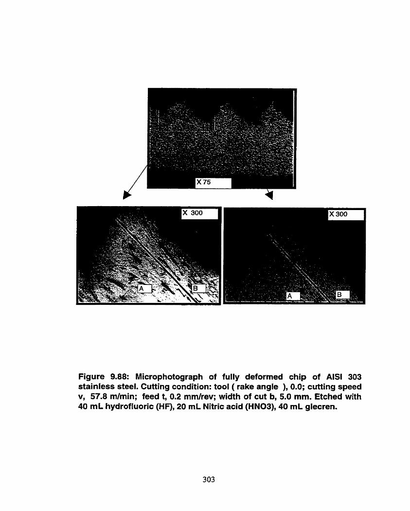
Figure 9.88: Microphotograph of fully deformed chip of AISI 303 stainless steel. Cutting condition: tool ( rake angle ), 0.0; cutting speed v, 57.8 mlmin; feed t, 0.2 mm/rev; width of cut b, 5.0 mm. Etched with 40 mL hydrofluoric (HF), 20 mL Nitric acid (HN03), 40 mL glecren.

\ Initial hardness =152 HV
Figure 9.89: Microhardness distribution (VI~kers ) in a fully deformed chip of AlSI 303 steel. Cutting condition: tool ( rake angle ), 0.0; cutting speed v, 57.8 rnlmin; feed t, 0.2 mmlrev; width of cut b, 5.0 mm.

Figure 9.90: Microphotograph of the initial structure of AlSI 4340 steel (mag: 400 X). Etched with 10 mL Nital, 90 ml alcohol. Structure is tempered rnartensite.

Figure 9.91: Microphotograph of a fully deformed chip AlSI 4340 steel (mag: 50 X). Cutting condition: tool ( rake angle ), 0.0; cutting speed v, 57.8 mlmin; feed t, 0.2 rnmlrev; width of cut b, 5.0 mm. Etched with 10 mL Nital, 90 ml alcohol.

sfeel AlSI 4340
Infial hardness =224 HV
t 2% 2% t $ 3% t,,,
Figure 9.92: Microhardness distribution (Vickers ) in a fully deformed chip of AISI 4340 steel. Cutting condition: tool ( rake angle) , 0.0; cutting speed v, 57.8 mlmin; feed t, 0.2 mmlrev; width of cut b, 5.0 mm.

Figure 9.93: Copmarison between the microphotographs of the fully deformed chip of AISI 1045, AISI 303 and AlSl 4340 steels( mag : 50). Cutting condition: tool ( rake angle ), 0.0; cutting speed v, 57.8 rnfmin; feed t, 0.2 mrnfrev; width of cut b, 5.0 mm.

Figure 9.94: Microphotographs of partially formed chip. Cutting condition: workpiece, AIS1 4340; tool , BTAH 1" inch diameter; spindle rotational speed n, 1000rpm; feed t, 0.1 mmlrev; Etched with 10 mL Nital, 90 ml alcohol.

Figure 9.96 F l
Figure 9.95: Microphotographs of partiafly formed chip (mag: 50X). Cutting condition: workpiece, AlSl4340; tool , BTAH 1" inch diameter; spindle rotational speed n, 1000rpm; feed t, 0.1 mrnlrev; Etched with 10 mL Nital, 90 ml alcohol.

Figure 9.96: Microphotographs of partially formed chip (mag: 100X). Cutting condition: workpiece, AISI 4340; tool , BTAH 1" inch diameter; spindle rotational speed n, 1000rpm; feed t, 0.1 mmlrev; Etched with 10 me Nital, 90 ml alcohol.

Figure 9.98 F-l
Figure 9.97: Microphotographs of partially formed chip (mag: 200X). Cutting condition: workpiece, AlSI 4340; tool , BTAH 1" inch diameter; spindle rotational speed n, 1000rpm; feed t, 0.1 mmlrev; Etched with 10 mL Nital, 90 ml alcohol.

Figure 9.98: Microphotographs of partially formed chip (mag: 400X). Cutting condition: workpiece, AISI 4340; tool , BTAH 1" inch diameter; spindle rotational speed n, 1000rpm; feed t, 0.1 mrnhev; Etched wfth 10 mL Nital, 90 ml atcohol.

CONCLUSIONS AND RECOMMENDATIONS FOR
FUTURE WORg
10.1 CONCLUSIONS
A new model of chip formation has been developed. This mode1 is not limited by the
most assumptions usually made to build the single shear plane, flow region and paraUe1 sided
shear zone models and in the same time capable of relating the cutting forces, tool-workpiece
and temperature to the cutting speed, feed, tool geometry and properties of the workpiece
material. The proposed model involves the formulation of the shear zone mode1 with parallel
boundaries. It has been defined by applying the mechanics of continuum to the analysis in

the chip formaiion zone. The analysis yields the following conclusions:
a Two families of straight slip-lines constitute the deformation zone in metal
cutting: one family is parallel and another is perpendicular to the straight
upper boundary of the zone.
b. The weU-known equation for the chip compression ratio is a form of the m a s
conservation principle.
c. As a results of the consideration of slip-line structure of the shear zone
combined with the boundary conditions, a new feature of velocity diagram is
constructed.
d. The discontinuity of the tangential velocity (the component of the cutting
speed which is parallel to the boundary of the shear zone) during the
transformation of a defomed fkagment from the workpiece into the chip is
attributed to the shear plane model phenornenon in the cutting process. In
practice, the shear zone always has a certain width dong which a continuous
velocity is maintaineci. Therefore, the acceleraîion, strain and strain-rate in
the shear zone with parallel boundaries are not un i fody distributed as
thought before. The final tme shear strain depends upon neither the zone's
width, nor the power of non-uniform distribution of strain, but is entirely
defmed by the values of the discontinuity of the tangentid and normaI
velocity components.
Therrnomechanical model of the work-material resistance to cutting defines the ratio
of the flow shear stress (in the shear zone and in the plastic zone dong the tool rake face )

to the dtimate tende stress as a linear fiction of cutting temperature. Based on this , a
model for the cutting force components is proposed To avoid the determination of the
friction angle, the computation of the tangentid force acting on the tool face is formulated.
The proposed model have been used to calculate the dynamic cutting forces in
orthogonal cuttîng. The cutting system was modeled using a single degre-e-of fkedorn
dynamic system where the variations of the cutting forces are represented by their total
diffenntials. This study shows that the shear zone with parallel boundanes accommodates
the dynamic variations in cutting conditions.
The andysis of the axial force and torque measurements reveals that the torque and
axial force are stationary detenninistic in nature.
This study shows that fluctuation of the cutting forces is a result of chip segmentation
and not the cause of it. It also reveals the effect of material and cutting conditions on the
cuttuig signatures that have never been considered as a factor in the previous studies of the
cutting dynamics.
A new methodology has been established to align the machine such that the
. . . misalignment between the tool and the workpiece is muumized to make sure that the
measured forces are not &ected by this effect. A low cost laser-camera based system has
been designed and build to achieve this goal.
The effect of misalignment on the cutting process has been investigated The shldy
shows that the misalignment affects the result dramatically. To test this eEect on the forces
measured, the cutting tool has been deliberately misaligned. The misalignment values have
been measured using the laser-carnera based system and the forces have been recorded using

using the FFT Analyzer. The study shows that increased the misalignrnent causes increase
in the steady-state axial cutting force and cutting torque. The study aIso shows effect of
misalignment on the axial dynamic cutting force and cutting torque; the misalignment effect
shows up as a series of different amplitude harmonies.
The morphology study supports the theoretical finding of the parallel shear zone
model with parallel boundaries. The study reveds that the shear zone is composed of two
regions. The nrst region is termed as the "wide region" where the tangentid velocity v,
changes at a srnail rate. The second region is termed as the "narrow region " where the
tangentid velocity v, changes at a high rate.
10.2 RECOMMENDATIONS FOR FUTURE WORK
One may consider the present work as step toward a predictive theory of metal
cutting. It is, therefore, reasonable to point out the issues that would be necessary to address
to advance such a model and to further use it M e r as a powerful toot in the process
planning practice. Here are the issues to focus on:
1. Exact deformation state causing chip formation is yet to be identified using the
proposed velocity diagrarn through determinhg the state of stress in the deformation
zone. As shown and discussed, the defonnation zone is not simple shearing as it is
believed. A good starting point might be to account for the bending moment in the
deformation zone which in combination with the shear stress in the deformation
zone causes chip formation (Astakhov, 1997b). The main question to answer is the
ratio of bending and shear stress in the defonnation zone that is sufficient to trigger

chip formation. If this ratio is a material constant then a novel approach to optimize
the cutting process may be in sight
2. F i t e element analysis of the stress and strain distribution in the deformation zone
could be conducted using the d e W state of stress and deforinaiion. As a result, the
cutthg forces may be determineci for different cutting conditions. To accomplish the
job. however, the thermomechanical behavior of workpiece material in cutting should
be laiown.
3. To find the exact thermomechanical behavior of workpiece matenal in cutting, the
physics of plastic deformation should by employed. The stress-strain conditions
associated with cutting should be detennined precisely.
4. Combining the known themiornechanicd behavior of workpiece material in
deformation with defined state of stress in the deformation zone, it might be possible
to predict machinability of engineering material as the first stage. The further
research would be toward improving machinability on the basis of the proper
selection of process parameters which affect state of stress. By optimizing these
parameters the minimum energy consumption and maximum process economy can
be achieved.
5. The defined state of stress in the deformation zone rnight be considered as the first
phase toward controllability of the cutting process. Since this state of stress can be
altered by the process parameters and by the tool geometry two principal ways to
improve the cutting process may be feasible. The first is to optimize the geometry
of the cutting tool to achieve any desirable state of stress in the deformation zone in

order to cut a given materid with minimum energy consumed, The second is to Vary
the process parameters over the machining cycle; it might be possible to maintain the
desired state of stress in the machining zone over this cycle.
6. The defmeà state of stress in the deformation zone may be extended to define the
state of stress in the paaially formed chip. Having this state of stress defined, one
might select a particular chipbreaker just to increase the chip bending in a particular
direction to break the chip with minimum additional effort. ActuaIIy, the whole chip
formation process might be designed to achieve this objective.
7. To achieve al1 these objectives, the following caution should be undertaken. The
experimental results obtained by diKerent research teams should be compatible. A
special set of standards on the expenmentd methodologies used in metal cutting
should be set through professional associations as ASME, CIRP, etc.
It seems, metal cutting is just at the beginning of its renaissance and its full
capabilities are to be discovered.

REFERENCES
Adolfsson C. and Stahl LE., 1995, "Cutting Force Mode1 for Multi-Toothed Cutting
Rocesses and Force Measuring Equipment for Face Milling," Int. Mach Tools
Mwtufact. Vol. 35, No. 12. p. 1715-1728.
Ahn, T. Y., Ehrnan, K. F. and Wu, M. S., 1985, "Cutting Dynamics Identification by
Dynamic Data System, Modeling Approach," ASME Journal of Engineering for
Indus@, Vol. 107, p. 9 1-94.
Albrech P.t, 1962, Truns. Am Soc. Mech Engrs B 84, p. 405.
Albrecht P., 1960a, 'Wew Development in the Theory of the Metal Cutting Process:
Part L. The Ploughing Process in Metal Cutting," ASME Journal of Engineering for
Industiy, Vol. 83, p. 348.
Albrecht P., f96Qb, "New Development in the Theory of the Metal Cutting Process:
Part IL The Theory of Chip Formation," ASME Journal of Engineering for Industry,
Vol. 83, p. 557.
Arnerican Society of Metals, 1979 , Metals Handbook, 9th Ed., Vol. 2,
Amiarego, E. J. A., Jawahir, L. S., and Ostafïev, V. K. 1996, Working Paper, STC

I l .
'C', Working Group Wodeling of Machining Operations". CIRP, Paris, France.
Amarego, E. J., 1996," Predictive modeling of machine operations - a means of
bndging the gap between theory and practice," CSME F o m SCGM ccMmufacturing
Science and Engineerulg," Hamilton , Canada, p. 18.
hnarege E. J. And Brown R H., 1969, "The Machining of Metals, " Prentice Hall.
Astakhov, V.P., "System Approach in Metal Cutting," Journal of MateMI
Processing Technobgy, to be published in 1998)
Astakhov, V. P., Shvets, S. V. and Osman, M. O. M., 1997% " Chip structure
classification based on mechanism of its f o d o n , J. of Matehls Processing
Technology, 71,247,
Astakhov, V. P., Shvets, S. V. and Osman, M. O. M., 1997b, "TheBending Moment
as A cause of Chip Formation in Metal Cutting," Proceedings ASME Symposium
IMECE-97, f 977, November 16-21, Dallas, Texas, USA.
Astakhov, V.P., and Osman, M.O.M., 1996, "An Analyticd Evaluation of the
Cutting Forces in Self-piloting Drilling Using the Mode1 of Shear Zone with Paralle1
Boundaries. Pari 1: Theory," International J o d of Machine Tools &
Mmufiacture, Vol. 36, No. 1 1, p. 1 187- 1200.
Astakhov V. P., 1994, "A Methodology for the Experimentai Force Detexmination
in Self-pilotuig Drang," Metallorezuchi Stunky7 (In Russian) Vol. 43, p. 40-49.
Astakhov V. P., 1983, "Method of Determination of the Chip Compression Ratio,"
Patent No. 1004012 (USSR).
Bagchi, A., 1983, 'Technical Note on Wright's Paper : Predicting the Shear Plane
Angle in Machining from Work Matenal Strain-hardening Characteristics," ASME
Journal of Engineering for Industry, Vol. 105, p. 129- 13 1.
Bendat, J.s., and Piersol, A.g., 1980, "Engineering Applications of Correlation and
Spectral anaiysis," John Wiley, New York.
Bendat, J. S., and Piersol, A. G., 197 1, "Random Data: Andysis and Measurement
Procedures ," Wiley Inter Science.
Bendat, J.S., and Piersol, A.G., 1966, "Measurement And Analysis Of Random

Data", WZey Inter Science.
Bhattacharyya, A. and Ham L ,1969, " Design of Cutting Tool Use of Metal Cutting
Theory", Asm. Bobrov, V., 1984, "Metal Cutting", M o s c m Mashinostrostroenie, (In Russian).
Boothroyd, G., 1963, " Temperatures in Orthogonal Metal Cutting," Proc. Inst.
Mech. Eng., Vol. 177, p. 789-802.
Boothroyd, G. and Knighf W. A., 1989, " Fundamentals of Machining and Machine
Tools, " New York
Bridgman, P. W., 1943 , "On Torsion Combined with Compression," Juuml of
Applied Physics, Vol. 14, p. 273.
Bridgman, P. W., 1937, Flow Phenomena in Heavily Stressed Metals, " Journal of
Appüed Physics, Vol. 8, p. 329.
Chandrashekhar, S., Osman, M.O.M., and Sankar, T.S., 1985, "An Experimental
Investigation for the Stochastic Modeling of the Resultant Force System in BTA
Deep-Hole machining," International Journal of Production Research, Vol .23, No.
4,657-673.
Chandrashekhar, S., 1984, " An Analytical and Experimentd stochastic modeling of
the resultant force system in BTA Deep hole machining and its influences on the
dynamic of machine tool workpiece system," Concordia University, Ph.D. thesis.
Childs, T.H., 1980,"EIastic Effects in Metal Cutting Chip Fornation," In?. J. Mech.
Sci., Vol. 22, p. 457.
Das, K. and Tobias S. A., 1967, "The Relation Between The Static and the Dynaniic
Cutting of Metais," ht. J. Mach. Tool Des. Res., Vol. 7, p. 63-89.
Das, S. A., 1965, Ph.d Thesis, University of Binninghmn.
Del Taglia, A., and Tani, G., 1982, "A Method for Measuring Cutting Forces in
Bonng Operation", Int. J. of Mac. Tool Des. Res.. Vol. 22. No. 1, p. 23.
Devries M. F., 1970, "Review of Metal Cutting Theory," Society of Manufacturing
Engineer Technical Paper Mr 70-142.
Dewhurst, P., 1978, "On the Non-uniqueness of the Machining Process," Proc. R

Soc. London. A. 360, p. 587.
Dieter, G.e., 1986,'MechchaaI Metallurgy,"3ed. Ed., Mcgraw-Hill Publishing
Company, New York
Doyle. E. D., Home, J. G. and Tabor, D., 1979," Fnctional Interactions Between
Chip and Rake Face in Continuous Chip Formation," Proc. R. Soc. , London, Vol.
366, p. 173.
Eggleston, DM., Herzog, R. N. and Thomsen E.G., 1959," Observations on the
Angle Relationships in Metd Cutting," MME Journal of Engineering for Industry,
Vol. 8 1, p. 263.
Elbestawi, M.A., Papazafuiou, T. A., and Du, R X., 1991, "In-Process Monitoring
of Tool Wear in Milling Using Cutting Force Signature," In?. J. Mach. Tmls
Mcuzifuc. Vol. 31, No. 1, p. 55-73.
El-Wardany, T.I., Gao, D, and Elbestawi, M.A., 1996, "Tool Condition Monitoring
in Drilling Using Vibration Structure Analysis, " Int.J.Mach. Tools Manufaet. VoI.
36, NO 6, 687-7 1 1.
Ernst H., 195 1, ''Fundamental Aspects of Metal Cutting and Cutting Fluid Action,"
A m h @the New YorkAcudemy of Sciences. Vol. 53, p. 936.
Ernst H. And Merchant M. E., 1941, "Chip Formation, Friction and High Quality
Machined Surfaces, in the Surface Treatment of Metals," Arnerhn Socieq of
Metah, Vol. 29, p. 299.
Fenton, R. G. and Oxley, P. L., 1970,"Mechanics of Orthogonal Machining:
Predicting Chip Geometry, Cutting Forces, Etc. from Work Material Properties and
Cutting Conditions," Proc. R Soc., London, Vol. 184, p. 927.
Finnie I., 1956, "Review of the Metal Cutting Analyses of the pst Hundred
Years,"Mech. Engineering., Vol. 78, No. 8, p. 715.
Frazao, J., Chandrashekhar, S., Osman, M.O.M., and Sankar T.S., 1986, "On the
Design and Development of a New BTA Tool to Increase Productivity and
Workpiece Accuracy in Deep Hole Machining," The International Journal of
Advanced Munujiacturing Technology, Vol. 1, No. 4, p.3-23.

Fredentai, L and Geinnger X., 1962, "Mathematical Theories of Inelastic Solids ". Moscow
Fujii, & , Manii, E. and Ema, S., 1986% 'Whirling Vibration In Drilling. Part 1:
Cause of Vibration And Role of Chisel Edge,"ASME Jouml of Engineering for
Industry., Vol. 108, P. 157-162.
Fujii, H. , Marui. E. and Ema, S. , 1986b," Whiriing Vibration In Drilling Part 2:
Infiuence of Drill,"ASME Jouml of Engineering for Industry, Vol. 108, p. 157-162.
Gessesse, Y. B., "1990, Stability of BTA Deep Hole Machining F%cess," MASc
Thesis, Concordia University, Montreal.
Goriani, V. L and Kobayashi, S., 1967, "Strain and S e - r a t e Distributions in
Orthogonal Metal Cutting," Annais of CIRP, Vol. XV, p. 425.
Griffith, B. J., 1982, " An Investigation into the Role of the Burnishing Pads in the
Deep Hole Machining Process," PlrD. Zlesis, Depf. of Production Technology,
Brunel University.
Gri=ths, B. J., 1977,"An Introduction to Deep Hole Drilling and Bonng,"
Proceedings of the Second International Conference on Deep HoZe Drilling and
Bon'ng, Bumel University, G e m y
Griffths, B.J., 1973, "The Measurement of Thmst and Torque in Deep-hole Boring",
Symposium Bnmel Univers@, Gemany.
Griffttis, BJ., 1973, 'The Machining Action During Deep-hole Boring and the
Resultant Hole Force and Force Systern", Proc. Second lnt. Con. on Prod. Res..
Hayajneh M., Osman M. O. M. and Latinovic V. N., 1997% "A Study of
Wave-removing Cutting Process Using a Moclel of Shear Zone with Parallel
Boundaries", Proceedings ASME Synposim IMECE-97. 1977, November 16-21,
Dallas, Texas, USA.
Hayajneh M. T., Astakhov V.P., and Osman M.O.M., 1997b, "An Analytical
Evaluation of the Cutting Forces in Orthogonal Cutting Using the dynamic Mode1 of
Shear Zone with Parallel Boundaries," J. of Materials Processing Technology, (in
print, 1997) to be published in October 1998.

Hayajneh M. T., Astakhov V. and Osman M.0, 1996," A Novel Approach to the
Mechanics of Chip Formation Using Shear Zone Mode1 with Parallel Boundanes,"
Proceedings CSME F o m SCGM 1996. 13th Symposium on Engineering
Application of Mechanics Manufacturing Science and Engineering, McMaster
University, Canada
Home, J.G., Wright, P. K. and Bagchi, 198 1 , "A S tudy of Built-up-edge Formation
Using Transparent Cutting Tools," 9th North Amen'can Research Conference
Proceedings, p. 223.
Hsu, T.C., 1966, "A Study of the Noma1 and Shem Stresses on a Cutting Tool,"
ASME Journal of Engineering for IIUIwtry, Vol. 88, p. 5 1.
Huang, H., Went, C. and Chen, C., 1994," Prediction of Thrust and Torque for
Multifaced Drills ," ASME Jountnl of Engineering for Industry¶ Vol. 1 1 6. p. 1-7.
lawahir, L S. and van Luttervelt, C. A., 1993,''Recent developments in chip control
research and applications," CTRP A m l s , V o l . 42, p. 659
Johnson, W., Sowerby, R. and Venter, R D., 1982, "Plane-strain Slip-line Fields for
Metal-Deformation Process", P e r g m n , Oxford*
Kececloglu D., 1 960, "Shear-zone Size, Compressive Stress, and Shear S train in
Metai Cutting and Their Effect on Mean Shear-flow Stress," ASME Journal of
Engineering for Industry, Vol. 82, p. 79-86.
Kececioglu, D., 1958, "Shear-Zone Temperature in Metal Cutting and its Effect on
Shear Flow Stress," Transactions of ASME, Series B, Journal of Engineering for
Indusfry, Vol. 80, p. 541-546.
Klamecki B. E. and Kim S., 1988, "On the Plane Stress to the Plane Strain Transition
Across the Shear Zone in the Metal Cutting ," ASME Journal of Engineering for
Industry , Vol. 104, p. 322-325.
Kistler, Piezo-instrumentation Kistler, "2-component Load Washer (Fz, Mz) Type
9065," Nr. 6.9065 de.
Kobayshi M . And Kawata K ,1967,"Effects Of The Curvature Of Work Surface On
Metal îutting," Annals Of nie CIRP, Vol. XV, p. 393-403

Kobayashi S. And Shabaik A, 1964, "Chip Formation With Varying Under Chip
Thickness At Very Slow Speed,"ASME Journal Of Engineering For Industry, p.389-
394.
Kobayashi, S., Herzog, R. B., Eggieston, D. M. and Thomsen, E. G., 1960, 'A
Critical Cornparison of Metal Cuning Theories with New-experimental Data," ASME
Journal of Engineering for Industry, Vol. 82, p. 337
Kobayashi, S. and Thomsen, E., 1959, "Some Observations of the Shearing Rocess
in Metal Cutting," T m . A m r . Soc. Mech. Engineering., Series B. Joumul of
Engineering for Industry, Vol. 81, p. 251.
Kudo, H., 1965, "Some New Slip-Iine Solutions for Two-dimensional Steady-state
Macfiining," Znt. J. Mech. Sci., p. 43.
Kushner, V. S. , 1982, "Thermomechanical Approach in Metd Cutting," Irkutsk
University Pabl. Ltd, (In Russian).
Kufarev G., 1970, " Chip Formation and High Quaiity Machineci Surfaces under
Conditions of Oblique ", (In Russian) Frunz: Mechtep.
Latinovic V. , 1978," An Investigation of the Theoretical and Design Aspects of
Unsymmeûical Multi-Cutting Action in Dep-Hole Machining," Ph.D. thesis,
Concordia University, Montreal.
Lee, L.C., Lee, K.S., and Gan, CS., 1989, "On the Correlation Between Dynamic
Cutting Force and Tool Wear," Int J. Mach. Took Mmufuct., Vol. 29, No. 3, p. 295-
303.
Lee E. H., and S h a e r B. W., 195 1, 'Vie Theory of Plasticity AppIied to the Problem
of Machining," Trans ASME J o u m l of Applied Mechanics, Vol. 1 8,, p. 405-4 1 3.
Lee S.J. and Kapoor S.G., 1986, "Cutting Process Dynamics Simulation for Machine
Tool Stnicture Design,"ASME Journal of Engineering for Indwtry , Vol. 1 08, p. 68-
74.
Liu, C.R. and Barash, M.M., 1976, "The Mechanicd State of the SubIayer of a
Surface Generated by Chip Removal Process, Part 1: Cutting with a Sharp Tool,"
ASME Journal of Engineering for Zndustry, Vol. 98, P. 1192.

Manyindo B. and Oxley P. L- ,1986," Modehg the Catastrophic Shear Type of Chip
when Machining StaÎnless Steel," Proceedings h s t Mech. Eng., Vol. 200, p. 349-
358.
Marui, E. , Kato, S., Hashimoto, M. and Yamada, T., 1988% "The Mechanism Of
Chatter Vibration System: Dynamic Vibration In A Spindle-workpiece Part 1-
properties Of Self-excited Chatter Vibration In Spindle-working System," ASME
Journal of Engineering for Industry, Vol. 1 10, p. 236-242.
Marui, E., Kato, S., Hashïmoto, M, and Yamada, T., 1988b, "The Mechanism of
Chatter Vibration in a Sphdle-Workpiece S ystem: Part 2-Characteristics of Dynamic
Cutting Force and Vibration Energy,"ASME Journal of EngineeBng for Industry,
Vol. 1 10, p. 242-247.
Marui, E. , Kato, S., Hashimoto, M. and Yamada, T., 1988c, 'The Mechanism Of
Chaiter Vibration System: Dynarnic Vibration h A Spindle-workpiece Part 3-
analytical Considerations," ASME Joumul of Engineering for Zndusîry, Vol. 1 10, p.
242-247.
Merchant M. E., 1945, " Mechanics of the Metal Cutting Process. L Orthogonal
Cuaing and a Type Chip; Plasticity Conditions in Orthogonal Cutting," Journal of
Applied Physics, Vol. 1 6, p. 267, and p. 3 1 8-324.
Merchant M. E., 1944, "Basic Mechanics of Cutting Process," Journal of Applied
Physics, Vol. 1 1, p. 168-175.
Nakayarna K. and Tamra K., 1964, " Hardness Test of Chip," Bulletin of the Faculty
of Eng., Yokohama National Unversity, Japan, Vol. 13, p. 17.
Nigm M. M. and Sadek M. M., 1977,"Experimental Investigation of the
Characteristics of Dynamic Cutting Process,"ASME Journal of Engineering for
Industry, p. 410-418.
Nigm M. M.,Sadek M. M. And Tobias S. A., 1977% "Dimensional Analysis of the
Steady State Orthogonal Cutting Process," Int. J. Mach Tool Des. Res., Vol. 17, p.
1-18.
Nigm M. M. , Sadek M. M. And Tobias S. A, 1977b, "Determination Of Dynamic
Cuning Coefficients From Steady State Cutting Data," Int. Mach Tool Des. Res.,
VOL 17, p. 19-37.
Okushima, K. and Hitomi, K, 196 1, "An Analysis of the Mechanism of Orthogonal
Cutting and its Application to Discontinuous Chip Formation, "ASME Jouml of
Engineering for Industry, p. 545-556.
Osman, M.O.M., and Sankar, T.S., 1972, "Short-time Acceptance Test for Machine
Tools Based on the Random Nature of the Cutting Forces",ASME Jounuzl of
Engineehg for Industry, Vol. 94, No. 4, P. 1020.
Osman, M.O. Sankar, T.S. and GD. Xistris, 1974, "Meanirement and Analysis of
Random Cutting Forces in Single Point Machining" Presented in the 20th
International Instrumentation Symposium, May 21-23, 1974 , Albequerque, New
Mwxico, ISA, 1974 p. 259-264.
Oxley P. L. and Welsh M. J., 1963 " Calculation the Shear Angle in ûrthogonal
Metal Cutting fiom Fundamental Stress, Strain, Strain-Rate Properties of the Work
Material," Proceeding 4* International Machine Tool design and Research
Conference, Pergaman, Oxford. p. 73-86.
Oxley P. L., 1989, "Mechanics of Machining - An analytical Approach to Assessing
Machinability", John Wiley & Sonr, New York.
Poletica M., 1976, "Contact Loads dong the Cuttîng Surfaces of Tools,"
Moscow:mashinostrostroenie, (In Russian)
Palmer, W-b. and Oxley, PL., 1 959, 'Mechanics of Orthogonal Machining," Proc.
Instr. Mech. Engrs.,Vol. 173, P. 623.
Peters, J.,1976, "Dynamic Analysis Of Machine Tools Using Complex Modal
Methol", Anm2.s CIRP. Vo.. 25, No. 1, p. 257.
Weghar, F., 1977, "Guidelines for Deep Hole Tool Design," WT Zeitschrijtfier
Industn'elle Femgung, 67, p. 2 1 1-21 8, (in German).
Pugh, H. D., 1958,"Mechanics of Cutting Process," Proc. Zme Con$ Tech. Eng.
Manrrfacture, hndon, P. 237.
Randall, R. B., 1987, " Frequency Analysis ," K. Larsen & Son. Clostnip, Denmark.

Rostoker, W. and Dvorak, J. R, 1977, "hterprebtion of Metallographic Structures,"
2nd Ed, Academic Press, New York-
Rubenstein C. ,1972, "An Andysis Of Dynamic Cutting When A Plane Surface :Is
Cut With An Oscillating Tool -Ii General Equations," Int. .L M d Tool Des. Res.,
Vol. 12, p. 179-191.
Rubenstein C. , 1972, "An Analysis of Dynarnic Cuning when A Plane Surface :is
Cut With An Oscillating Tool," Int. J . Mach. Tool Des. Res., Vol. 12, p. 249.
Ramalingam S., Desai P. V. and Kim K., 198 1, 198 1, "On the Determination of the
Domain of Plaçticity Associated with a Plastic Free Boundary and its Application to
the Machining Problem," 9th North Amen'cm Research Conference Proceedings,
p. 334.
Roth, R.N., and Oxley PL, 1972, ccSlipline Analysis for Orthogonal Machining
Based upon Experimental Flow Fields," Mech Engr. Sci., Vol. 14, p. 85 . Rozenberg, A., 1956, " Elements of Metal Cutting Process", (In Russian) Marhgiz-
Moscow.
Sakuma, K., Taguchi, K., and Katsuki, A., 198 1, "Self Guiding Action Of Deephole
Drilling Tools", ANiaLÎ CZW, Vol. 30, No. 1, p. 3 1 1
Sakuma, K., Taguchi, IC, And Katsdci, A., 1980a, "Study On Deep-hole Drilling
With Solid Boring Tool The Burnishing Action of Guide Pads and Their Influence
On Hole Accuracies7', Bull. Of The JSME, Vol. 23, No. 185, p. 121.
Sakuma, K., Taguchi, K., And Katsuki, A., 1980b, "Study On Deep-ho1e Boring By
A Bta System Solid Boring Tool-behaviour of Tool and Its Effects On The Profile
of The Machined Hole", Bull of The Jspe, Vol. 14, No. 3, p. 143.
Sankar, T.S., and Osman, M.O., 1975, "Profile Characterization Of Manufactured
Surfaces Using Random Function Excursion Technique Part 1: Theory,"ASME
Journal of EngineeBng for ~ndustry., Vol. 97, p. 190.
Scrutton, R., 1968, 'The Geometry of the Shear Zone in Metal Cutting," ASME
J o m l of Engineering for Industry, p. 420-424.
Shaw, M. C., 1984," Metal Cutting Principles, "Clarendon Press, Oxford,.

Shaw, M. C. and Finnie L, 1955, "The Shear Stress in Metal Cutting," ASME, Vol.
77, P. 115-125.
Song, X., 1995, "S train-Hardening and Thermal-Softening Effects on Shear Angle
Prediction: New Model Development and Validation,"AS.ME Journul of Engineering
for Indwtry, Vol. 1 17, p.28-32.
Stevenson R. and Stephenson D.A., 1995, "The Mechanical Behaviour of Zinc
During Machining," ASME Joumal of Engineering for Zndustry, Vol. 117, p. 172-
178.
Strenkowski, J.S. and Moon, KJ., 1990, "Fite Element Prediction of Chip
Geometry and TooVWorkpiece Temperatures Distributions in Orthogonal Metd
Cutting,It ASME Joumal of Engineering for Industry, Vol. 112, p. 3 13-3 18.
Sun, P., Chang, Y.K., Wang, T.C., and Lui, P.t,1982 "A Simple and Practicai
Piezo-electric Shank Type Dynamometer", Int. J. of Mach. Tool Des. Res., Vol. 22,
No. 2, p. 111.
Spaans C., 1972, " A Treatise on the Streamlines and the Stress, Strain Rate
Distributions, and on Stability in the frimary Shear Zone in Metal Cutting ", ASME
J o u ~ l of Engineering for Industry, 94, p. 690-696.
Steed W. E. ,1987 ,"Chip Removal Simulation to Predict Part Error and Vibration,"
Proc. ASME Cm$ Cornputers in Engineering, Vol. IL p. 447-455.
Stephenson, D.A. and Agapionu, J.S. ,1997, "Metal Cutting Theory and
Practice,"Marcel Dekker, Inn., Ney York.
Stevenson,. M. G. and Oxley, P. L., 1969-1970, " An Experimental Investigation of
the Influence of Speed and Scale on the Strain-rate in a Zone of Intense Plastic
Deformation,' ' Proc. Znst. Mech. Engineering, Vol. 184, P. 56 1-576.
The, J., 1975, "The Quaciratic Curve and the Trajectory in the Shear Zone in Metal
Cutting," ASME Journal of Engineering for hdust?y., p.UO5- 1 1 1 1.
Thangaraj, A And Wright, P.K. 1988, "Computer-assisted Prediction of Drill-failure
Using In-process Measurements of T h s t Force," ASME Journal of Engineering for
Industry, Vol. 1 1 O, p. 192-200.

Thomsen, hg., 1966, "Applications of the Mechanics of Plastic Deformation to Metal
Cutting," AnnaLF of the CIRP., Vol. X[V, p. 1 13.
Trenb E., 199 1, "Metai Cutting," Bmerworth- Heinemann.
Usui, E. and Hoshi K, 1963,"Slip-line Field in Metal Machining Which Involve
Centered Fans," Intemution Producrion Engineering Research Conference
Proceedhgs, (Pittsburgh), p. 6 1.
Wright P. K ,1982. "Prediction the Shear Plane Angle in Machining from Work
Material Strain-hardening Characteristics," ASME Jouml of Engineering for
Industry, Vol. 104, p. 285-292.
Wright P.k, Bagchi k and Chow J. G., 1982,'lnfluence of Friction on the Shear
Plane Angie in Machining," lO?h Nonh American Research Conference Proceedings,
p. 255.
Wright, P.K., 198 1, 'Frictional Interactions in Machining: Cornparisons Between
Transparent Sapphire and Steel Cutting Tools," Metals Technolugy, Vol. 8, p. 150.
Wu D. W., 1989, "A New Approach of Formulating the Transfer Function for the
Dynamic Cuning Processes," ASME J o u d of Engineering for Industry, Vol. 1 1 1,
p. 37-47.
Wu, D. W., 1988, Tomprehensive Dynamic Cutting Force Model and its
Application to Wave-removing Processes," ASME Jowtal of Engineering for
Industry, Vol. 110, p. 153-161.
Wu, D. W., 1986, "Goveming Equations of The Shear Angle Oscillation In Dynarnic
Orthogonal Cutting,"ASME JournaL ofEngineerUlg for I ' t r y ,Vol. 108,, p. 280-
287.
Wu, D. W and. Liu, C. R., 1985% "An Analyticd Model Of Cutting Dynamics Part
1 : Model Building," ASME J o u d of Engineering for 1ndmtr-y , Vol. 2 07, p. 107-
111.
Wu, D. W and Liu, C. R. ,19850, "An Analytical Model of Cutting Dynamics Part
2 : Verification ," ASME Joumal of Engineering for Zndustry, Vol. 107, p. 107-1 1 1.
Yamamoto, A., Nakamura S., Toyama K. and Kawamura I, 1979, 'hoposal of

Stresses Distribution Models on Rake Surface in Orthogonal Cutting,"/. offiecision
Engr., Vol 45, p. 90.
133. Zhang GM. and Kapoor S.G.. 1987, "Dynamic Modeling and Analysis of the Boring
Machine S ystem, "ASME Journal of Engineering for I ~ U S Q , Vol. 109. p. 2 19-226
134. Zorev N. N., 1966. " Metal Cutting Mechanics," Pergamon.