
National Conference on the Economics of Competition Law ...
287
National Conference on the Economics of Competition Law, 2017
-
Upload
khangminh22 -
Category
Documents
-
view
1 -
download
0
Transcript of National Conference on the Economics of Competition Law ...

National Conference on the
Economics of Competition Law,
2017

Index
Measurement of market power and cost efficiency in mango pulp industry of Andhra Pradesh
On the economics of cartel investigation: the case of cement in India
Applicability of Stated Preference Techniques in defining Relevant Markets
Market definition through SSNIP Tests applied to consumption expenditure data
Application of Economic Tools for Relevant Market Definition: The Experience in India
Making Indian Pharmaceuticals Competitive: The Dilemma for Regulation
Studying Competitiveness of Indian Industry: A Methodological Exploration
How have Mergers and Acquisitions Affected Firms’ Business Performance? Empirical Evidence of
Indian Manufacturing Sector
Presence of Profit and Competition in Indian Industry
Economics of Mergers and Acquisitions in India’s Drugs and Pharmaceutical Industry: Implications
for Competition Policy
Maximum Retail Price Policy of India: A Comparative Law and Economic Inquiry
‘Structural Change and Competition in the Indian Non-life Insurance Industry: A Study in the Post-
reform Period’

1
MEASUREMENT OF MARKET POWER AND COST EFFICIENCY
IN MANGO PULP INDUSTRY OF ANDHRA PRADESH1
P.A.LAKSHMI PRASANNA
SENIOR SCIENTIST (AGRICULTURAL ECONOMICS),
ICAR- INDIAN INSTITUTE OF RICE RESEARCH, RAJENDRANAGAR- HYDERABAD,
TELANGANA STATE - 500 030
I. Introduction:
In the context of reported implications of imperfect competition on efficiency and
distribution of welfare of different policy and technological interventions, now it is being
felt that investigation of competition in the market, measuring extent of imperfection in
competition, identifying sources of market power is an important precursor to conducting
policy analysis. Rogers and Sexton (1994) suggested some structural features as
indicators to identify sectors which have more probability of experiencing oligopsony
condition. The features suggest that food-processing sector can be a sector with
imperfect competition. In the present study mango pulp industry is taken as a test case.
Andhra Pradesh being one major mango producing state in India and significant
contributor to total pulp production of the country, was selected for the present study.
The specific objectives formulated in the present study are i) to analyze cost
efficiency of mango pulp units, (ii) to test for market power in procurement of mango for
pulp production, and (iii) to analyze the extent of trade-off between cost efficiency and
market power if any.
The paper is organized as follows. Following introduction, in section two brief
account of mango pulp industry in study area is presented. In section three methodology
followed in the study is discussed. In section four results are presented and discussed and
is followed by conclusions.
II. Brief account of mango pulp industry:
Mango which is national fruit of India, was cultivated in 2163 thousand hectares
in 2014-15, constituting 34.69 percent of total area under fruits in India. In 2014-15
Andhra Pradesh is the number one state in terms of area under Mango (315.69 thousand
1 The paper is largely drawn from the Ph. D thesis work submitted by the author to Tamil Nadu
Agricultural University, Coimbatore, Tamil Nadu
1

2
ha). Other important Indian states cultivating mango are Uttar Pradesh, Bihar, Tamil
Nadu, Maharashtra, Gujarat and Karnataka. Mango Pulp is one of the major processed
product with high export potential and is prepared from fruits of selected varieties of
mango viz Totapuri, Alphonso, and Kesar. In 2014-15 India exported mango pulp of
value 841.38 crore Rs, out of which major value export was through Chennai Port in
Tamil Nadu. There are two major clusters of mango Pulp in India viz; Chittoor in Andhra
Pradesh and Krishnagiri in Tamil Nadu. From Chittoor mango pulp is exported through
Chennai port. In 2014-15 year, 112515.24 metric tonnes of mango pulp was exported
through Chennai port (accounting for 73 percent of total mango pulp export from India)
and in the same year mango pulp production from pulp units of Chittoor district was
102670.75tonnes (constituting 91.25 percent of total mango pulp exported through
Chennai Port) . Chittoor was notified as Agri Export Zone (AEZ) for mango pulp on 08-
03-2002.
Fruit processing activity in Chittoor commenced during 1965 with setting up of a
small unit, which worked for some years and closed later. "India canning" is the first
mechanized fruit processing unit established in the district in 1970. But no new unit was
established during 1971-80. Later mango pulp units establishment progressed and in the
year 2005, 51 units worked, out of which 7 were aseptic units. As on today 85 pulp
processing units are there in the district, out of which 15 are aseptic units. Aseptic units
use a technology which involves separate sterilization of pulp and container which are
then combined in sterile environment. In addition to this, several operations in pulp
manufacturing are mechanized in aseptic units. Aseptic units pack mango pulp in
containers of size 200 Kg each, on the other hand conventional units pack mango pulp in
cans of 3.1Kg each.
Mango pulp units in Chittoor district are working under two systems viz; (i) own
processing and (ii) job work. Under job work system, buyers of mango pulp
(merchandise exporters, food product manufacturers, NDDB etc) provide raw materials
like mangoes, additives like sugar and chemicals) and packaging materials, the
processing units have to bear labor, fuel and electricity costs. The firms will receive job
work rate on tonnage basis of pulp produced. A federation viz; "Chittoor fruit processors
federation" is working in the district.
2

3
III. Methodology:
Earlier, Structure - Conduct and Performance (SCP) was the method used in
marketing studies which mostly used cross sectional data across industries. Subsequently
to overcome limitations associated with SCP methodology viz; (i) inability to capture
heterogeneity in industries (ii) endogeneity of structural variables (iii) problems in
classification of industries and (iv) usage of accounting cost data which represent average
cost but not marginal cost, new methods of analysis were developed (Kadiyala etal, 2001).
Among these, New Empirical Industrial Organization approach (NEIO) is one. Several
positive features are associated with the approach. It can be used for theory testing. The
NEIO approach is explicitly linked to behavioral theory and provides options to perform
" what -if analysis". NEIO also enables decomposition of the determinants of market
power and profitability ((Kadiyala etal,2001; Einav and Levin, 2010). There are different
NEIO methods, the most widely used methods are Conjectural Variation (CV) approach
and Menu approach (Roy et al, 2006). Using these approaches, several studies focusing
on analysis of competition in agricultural and food industry were carried out in the past.
These studies were surveyed and compared by Perekhozhuk and Glauben (2017). In the
current study CV approach with some modifications is used. The CV approach is
pioneered by Iwata(1974). In this model it is postulated that firms will have conjectures
about how competitors will react to changes in their quantity/price strategy and
incorporate these conjectures into their decisions.
In the present study, underlying theoretical model for analyzing existence of
market power is based on competition in terms of quantity (i.e Cournot model) and is
based on the assumptions: (i) profit maximizing is the objective of the firms (ii) n
(indexed i= 1, 2….n) pulp manufacturing firms in the industry are producing a
homogeneous product, i.e mango pulp and (iii) the firms are using a quasi-fixed
proportions technology in which there is a fixed proportional relationship between the
material input (mango) and the output (mango pulp), but the firms use other non-material
inputs in variable proportions. This assumption facilitates the representation of both the
firm ( iq ) and industry ( iQ q ) level quantities of the material input and output
with the same variable.
3

4
Let the mango supply curve faced by pulp industry be given by,
( , )mQ h W Z ---- Eq .1
Where iQ q is the industry quantity of the material input and output, mW is the
mango price and Z is a vector of exogenous variables that shift supply.
Solving equation 1 for Wm
yields the inverse mango supply curve,
( , )mW g Q Z ---- Eq .2
Assuming competitive behavior in output and nonmaterial input markets, pulp producing
firms face the following profit maximization problem
( , )iq i i m i i iMax Pq W q C q W ---- Eq .3
Subject to constraint of Equation 2
Where,
iq = Output of the ith firm
P = Parametric prices of output i.e. mango pulp
iC = Total processing cost of the ith firm and
W = Parametric prices of non-material inputs (prices of inputs other than mango).
Differentiating Equation 3 with respect to iq and assuming the second order
necessary conditions for a unique maximum are satisfied, yields equation
/ ( / )( / ) / 0i i m i i i iq P W q g Q Q q C q ---- Eq .4
Where /g Q is the slope of the inverse industry mango supply curve
/ iQ q is the change in industry quantity with respect to a change in the quantity of
the ith firm
/i iC q is firm specific marginal processing cost .
4

5
Letting /i iQ q and rearranging equation 4 yields
( / ) /m i i i iW q g Q P C q ---- Eq .5
The equation 5 indicates that in equilibrium canning firms equate their perceived
marginal mango expenditure to the value marginal product (VMP) of output net marginal
processing cost. Solving equation 5 for mW yields equation
/ ( / )m i i i iW P C q q g Q ---- Eq .6
Equation 1 and 6 constitutes the model. Empirical implementation requires choosing
functional forms for mango supply curve.
To estimate the model at Industry level, the counterpart to equation 6 can be
obtained by multiplying the equation with Q/Q and taking the sum over all firms.
This yields the industry level equation as
/ ( / )mW P C Q Q g Q ---- Eq .7
The derivation of industry level derived demand equation is dependent on the
assumption that the conditions for consistent aggregation over firms are satisfied.
The λ in the equation 7 is a weighted average of λi , where the weights are each
firm’s share of material input usage.
In the earlier studies the model is solved either by (i) estimation using
simultaneous equations or individual equations or (ii) calibration by drawing necessary
parameter values from previous studies. In the present study, equation 1 is estimated.
Using supply elasticity estimates resulting from estimation of equation .1 together with
marginal processing cost resulting from cost function is used in calibration, for analyzing
market power.
Estimation of mango supply function:
In the present study supply function of mango is estimated using two methods
thereby accounting for perennial nature of mango crop and consequent age/yield
dynamics. Given the limited data availability regarding new plantings, removals,
5

6
replanting and age-wise distribution of perennial crops area, more frequently used
approach in modeling supply response of perennial crops is the distributed lag model. In
several studies area response and yield response are estimated separately using lagged
price and lagged area as explanatory variables. Drawing on this model in the present
study supply relation is estimated using equation
0 1 2 1 3 1 4t t k t k t t iQ P P Q R e ---- Eq .8
Where
tQ = Mango production in the year t
k = Gestation period of the perennial crop
P = Price of the output of the crop.
tR = rainfall in the year t
In the present study one more version of supply model is estimated. This model is
formulated drawing on the model of Elnagheeb and Florkowski (1993). In the model
total potential output (*
tQ ) is the summation of the product of yield per (tree) acre for
trees in the age group i ( itY ) and number of (trees) acres in age group i at time t ( itI ).
*
0
n
t it it
i
Q Y I
---- Eq.9
Actual production is a function of potential output, climatic variables, price and
lagged output.
*
0 1 1
1
m
t t i t i t t t
i
Q Q P W Q u
---- Eq .10
To overcome the problem of infinite horizon, the first difference equation is used
*
1
1
m
t t i t i t t
i t
Q Q P W Q u
---- Eq .11
For computing potential output, data on tree age-wise mango yield in different
years and age-wise number of acres in different years is required. For computing age
6

7
wise yield the method of Lagrangian interpolation is used. Suppose information is
available regarding age –wise yield of a perennial crop at discrete points such as yield at
5 years age, yield at 10 years age, yield at 20 years age and yield at 40 years age, then
age-wise yield can be computed using Lagrangian interpolation formula
3)23)(13)(03(
)2)(1)(0(2
)32)(12)(02(
)3)(1)(0(
1)31)(21)(01(
)3)(2)(0(0
)30)(20)(10(
)3)(2)(1(
yxxxxxx
xxxxxxy
xxxxxx
xxxxxx
yxxxxxx
xxxxxxy
xxxxxx
xxxxxxY
---------------Eq.12
Where x0,x1,x2 and, x3 are the age of trees for which yield data is available, y0, y1,y2
and y3 are yield at the ages of x0,x1,x2 and x3, x is the age for which we want to
estimate yield(y) using interpolation method.
The available information regarding mango bearing and yield pattern is as follows.
Mango starts bearing from fifth year onwards. At the start of bearing the yield may be as
low as 10-15 fruits (2-3kg) per tree, rising to 50-70 fruits (10-15kg) in subsequent years
and to about 500 fruits (100 kg) in its 10 th year. In the age group 20-40 years, a tree
bears 1000-3000 fruits (200-600kg) in an ‘on ‘year (source: Ikisan). Based on farmer’s
survey it was identified that the in general practice, number of trees per hectare is 150.
Using this information yield per hectare of 5 years age mango trees is computed as 0.375
tonnes. Similarly yield per hectare of 10, 20, and 40 years old trees are computed as 15,
30 and 90 tonnes respectively. Using these discrete values of ages x0,x1,x2 and x3
(5,10,20,and 40) and yields y0,y1,y2 and y3 (0.375,15,30 and 90 tonnes), iy values are
computed using Lagrangian method of interpolation. From the computed iy values yield
index is constructed taking yield per hectare of 5 years tree as base. Using this index,
together with annual average yield data, itY values are computed.
For computing age wise area distribution in the present study, it is assumed that
there are no removals and difference in area between successive years (i.e year t-1 and t)
constitutes new planting with the age one (in year t). In the next year (t+1), this area
7

8
constitutes acreage of 2 years age trees. Likewise age-wise distribution of area is
computed. Further as the first mango-pulp manufacturing firm started in 1970, whatever
acreage of mango is there in the district in the year 1980-81, is assumed as 10 years old.
Starting from this year new additions are computed and age dynamics of these new
additions are captured over years up to 2005-06. Then change in potential yield in each
year is computed as summation of product of change in yield of trees (5 years and above
5 years) and change in respective acreages. In deciding about the lag length of price, the
criteria of change in sign of coefficient of at least one variable (contrary to expected sign
based on theory) is adopted in the present study.
Estimation of Cost function
For computing marginal processing cost, cost function is estimated in the present
study. Cost function is estimated for pooled data. The empirical model for cost function
for pooled data is specified as
1 2 3 4 5 60 1 2 3 4 5 6 7d d d d d dY Y Y Y Y YC Q Q Q Q Q Q Q ei ---- Eq .13
As analyzing cost efficiency is one of the objective in the study, besides pooled
cost function, cost function for aseptic pulp units and conventional pulp units were
estimated separately. Further cost function was estimated separately for own operated
pulp units and units working under job work system.
Trade-off between market power and efficiency
According to Azzam and Schroeter (1995) model, V is the initial
(pre-consolidation) oligopsony distortion indicating the proportional gap between the
value of the marginal product of the raw material input (P) net of marginal processing
cost (c) and the price of the raw material input (W).
P c WV
W
---- Eq .14
Assuming that consumer demand and raw material input supply functions take the
constant elasticity forms, and setting pre-consolidation output (Q) as 100 units,
8

9
pre-consolidation price of input (W) as equal to one, the authors formulated the trade-off
model in terms of the following equations.
Q AP ---- Eq.15
‘Consumer demand for final product’
eQ BW ---- Eq .16
‘Raw material input supply function’
1/ 1/(1 )100P V c Q ---- Eq .17
‘Inverse consumer demand function’
1/ 1/100 e eW Q ---- Eq .18
‘Inverse raw material input supply function’
Where A and B are constants, η is the price elasticity of demand and e is the price
elasticity of raw material supply. The height of the pre-consolidation derived demand
curve for the raw material at a given quantity is its price net of marginal processing cost.
1/ 1/(1 )100W V c Q c ---- Eq .19
With drastic reconfiguration of the industry, that results in lower marginal processing
cost due to plant scale economies or multi-plant economies, 0<s<1 denotes the
proportionate cost reduction. Accordingly the post-consolidation marginal cost is (1-s) c.
Assuming that consolidation leaves the industry with greater concentration and
correspondingly greater market power resulting in a post-consolidation distortion V * >V,
and post-consolidation output as Q*, input price W* and output price P* the following
equations of welfare change are derived.
(1 )
1/ *1(1 )(100 100 )
(1 )CS V c Q
---- Eq. 20
1/ *(1 ) /1(100 100)
1
e e ePS Qe
---- Eq .21
9

10
1/ *1/ 1/ *1/ *{(1 )100 (1 ) 100 } 100e eV c Q s c Q Q V
Change in oligopsony rents ---- Eq .22
* 1/ *(1 ) / *
1/ *(1 ) /
(1 )(100 100 )1
100 (100 100 )1
e e e
SW scQ V c Q cQ
ec Q
e
---- Eq .23
‘Net change in social welfare’
In the Equation 23, the term scQ* represents the value of the post consolidation cost
savings for Q* units and the rest of the terms together represent the additional
“deadweight loss” associated with the oligopsony. The cost reduction necessary to offset
the deadweight loss is found by setting the net change in social welfare equation to zero
and solving for s. But doing this requires knowledge of Q*. For determining Q*, post
consolidation distortion equation is rewritten as
***
*
(1 )P s c WV
W
1/ *1/ 1/ *1/
1/ *1/
(1 )100 100 (1 )
100
e e
e e
V c Q Q s c
Q
---- Eq .24
Given estimates of the pre-consolidation distortion V, the post-consolidation
distortion V*, marginal processing cost c, the price elasticity of consumer demand and
price elasticity of raw material (input) supply, equations 23 and 24 can be solved
simultaneously (by using numerical method) by setting ΔSW equation to zero, for
finding out two unknowns Q* and s. In the present study pre AEZ situation and post-
AEZ situations are considered. As number of processing units are higher in post-AEZ
situation compared to pre-AEZ situation , it is hypothesized that the marginal processing
cost is higher in post-AEZ situation as the quantity processed by each processing unit
declines (because of hypothesized inelastic supply of mango). It is also hypothesized that
market power is lower under post-AEZ situation. For this, empirical facts were analyzed
10

11
in the study and accordingly the trade-off model is modified in
the present study.
Data: For analyzing mango processing cost efficiency and market power in mango
processing, data from 20 pulp producing units were collected. From each mango pulp
producing unit data was collected for 7 years i.e from 2000-2006. Other necessary data
regarding mango area in Chittoor district was taken from “Season and Crop report of
Andhra Pradesh” in different years. Data on mango price was collected from regulated
markets of Chittoor district, in which mango was notified commodity. Data on Mango
pulp exports and mango pulp export price were collected from APEDA website. Data on
per capita GDP of importing countries were obtained from IMF/World bank Website.
IV. Results and Discussion:
1. Cost efficiency:
Results of estimation of cost function are presented in the table.1. Using the
coefficients of estimated pooled cost function, marginal cost was derived for various
years and compared with the average cost (Table.2). The comparison shows that in all
the years marginal cost is less than average cost indicating economies of scale (costs
increase less than proportionately with output).
Table .1. Mango pulp cost function (pooled)
Variables Coefficients t Stat P-value
Intercept 2203679.12 2.60 0.01
Q 7546.36 24.66 2.23695E-53
1dYQ 1004.11 0.77 0.44
2dYQ 2033.30 1.90 0.06
3dYQ 1386.25 1.14 0.26
4dYQ 747.99 0.76 0.45
5dYQ 277.72 0.49 0.62
6dYQ -77.72 -0.16 0.87
R Square =0.8867 Adjusted R Square =0.8812
11

12
Scale Economies Index (SCI) is computed to measure the economies of scale effect using
formula SCI= 1- Ec Where Ec is cost-output elasticity = Marginal cost/Average cost, Ec
is the per cent change in the average cost of production resulting from a one per cent
increase in output. From the table.2 it can be observed that cost-output elasticity ranged
from 0.81 to 0.94 in various years, and average pulp production ranged from 995 to 4288
tonnes.
Table.2. Cost - output elasticity and SCI of mango pulp units (Pooled)
Year
Average quantity of
pulp produced
(tonnes)
Marginal cost
(Rs)
Average cost
(Rs)
Cost-output
elasticity SCI
2000 1114.03 8550.47 9784.38 0.87 0.13
2001 1205.65 9579.66 10625.30 0.90 0.10
2002 995.41 8932.61 9974.35 0.90 0.10
2003 1300.84 8294.35 10025.20 0.83 0.17
2004 1955.84 7824.09 9346.35 0.84 0.16
2005 2453.02 7468.64 9130.93 0.82 0.18
2006 4288.13 7546.36 8002.13 0.94 0.06
Table.3 Cost - output elasticity and scale economies index of pulp production in
aseptic units and conventional units.
Year
Average quantity of
pulp produced
(tonnes)
Average cost
(Rs)
Marginal cost
(Rs)
Cost output
elasticity
Scale
economies
index
Aseptic technology
2003 3400.00 8036.27 -3208.61 -0.40 1.40
2004 6373.42 8320.32 2270.10 0.27 0.73
2005 10739.95 8028.40 3607.46 0.45 0.55
2006 14202.24 7713.21 4961.95 0.64 0.36
Conventional technology
2000 1114.03 9784.38 10899.78 1.11 -0.11
2001 1205.65 10625.35 9834.73 0.93 0.07
2002 995.41 9974.35 10563.61 1.06 -0.06
2003 1118.31 10551.04 10091.25 0.96 0.04
2004 1219.58 10240.01 10570.56 1.03 -0.03
2005 1209.98 10598.86 10414.12 0.98 0.02
2006 570.34 10700.07 10829.62 1.01 -0.01
12

13
Table.4 Cost - output elasticity and SCI for job-work and own processing
Year Technology
Average quantity
of pulp produced
(tonnes)
Average cost
(Rs)
Marginal
cost
(Rs)
Cost output
elasticity SCI
Job work
2003
Aseptic
2000.00 12712.00 13171.98 1.04 -0.04
2004 2700.00 12939.00 13279.73 1.03 -0.03
2000 1292.65 10168.05 9737.46 0.96 0.04
2001 1530.94 10529.70 9981.23 0.95 0.05
2002 2339.80 10794.52 10424.66 0.97 0.03
2003 Conventional 1448.66 10711.12 10253.87 0.96 0.04
2004 1618.60 10852.93 10361.62 0.95 0.04
2005 1661.34 10839.80 10610.72 0.98 0.02
2006 714.18 10732.46 9923.38 0.92 0.08
Own processing
2003 4800.00 6088.04 -6545.13 -1.07 2.07
2004 7597.89 7773.21 -186.21 -0.02 1.02
2005 Aseptic 10739.94 8028.39 1681.36 0.21 0.79
2006 14202.23 7713.21 3512.13 0.45 0.54
2000 782.29 8607.00 9247.45 1.07 -0.07
2001 555.07 11153.02 14923.16 1.34 -0.34
2002 593.99 7282.05 8442.15 1.16 -0.16
2003 Conventional 363.22 9091.78 3005.77 0.33 0.67
2004 554.56 7258.47 9364.69 1.29 -0.29
2005 371.73 8599.13 11232.27 1.31 -0.31
2006 185.06 10200.13 13063.04 1.28 -0.28
In order to estimate SCI of aseptic units and firms using conventional technology,
separate cost functions were estimated, SCI was computed and results are presented in
the table.3. It can be observed that SCI was always positive in the case of aseptic units.
When analysis was carried out separately for aseptic units and conventional units
according to system of operation i.e job work and owned processing. It is observed that in
job-work processing, firms using aseptic-technologies experienced diseconomies of scale
and firms using conventional technologies were having positive economies of scale
(Table.4). This might be due difference in conversion charge (job-work charge). The
conversion charge in the case of conventional technology was Rs 2200 per tonne of pulp
and in the case of aseptic processing; the charge was Rs 4500 per tonne of pulp in the
year 2005. In the own-processing, firms using aseptic technology are having economies
of scale but conventional units are facing diseconomies of scale. This in-turn is due to
13

14
lower time for sterilization in aseptic processing, thereby saving time and heating
material. This inturn facilitates more per day processing of pulp in aseptic units. Further
lower labor cost in case of aseptic technology contributes to scale economy. Thus cost
efficiency in mango pulp production varied with both technology and system of operation.
2. Mango Supply response:
As discussed in methodology section various versions of supply response models were
estimated accounting for perennial nature of the crop and dynamics of yield. These
models yielded price elasticity ranging from 0.48 to 0.76. Islam (1990) estimated price
elasticity of fresh tropical fruit supply to be 0.48 for all countries. Jedele et al.(2003) in
their study analyzing the world market for mangoes, assumed that the three major mango
producing regions Africa, Latin America and mango-producing Asia have supply
elasticities of 0.58 because they tend to have a greater impact with changes in production
and supply than the other regions. Having these facts from literature in backdrop, price
elasticity of supply of 0.48 is considered in further calculations in the study.
3. Market Power
As indicated in methodology section calibration method is used in evaluating market
power in the present study. Calibration is a method of identifying parameter values as
theoretically required "residuals" by assuming that the necessary equilibrium conditions hold
in the system. The advantage with this method in the present context is that, it facilitates
measurement of time varying market power. The equation for testing industry level market
power in mango industry is
/ ( / )mW P C Q Q g Q
Where Wm = mango price
Q = total pulp production
g / Q = inverse supply elasticity of mango
C / Q = marginal cost of processing
λ = degree of market power
Having the above equation as base, using (i) supply elasticity figure of 0.48 (ii)
marginal costs from pooled cost function (iii) mango price and mango pulp price in
various years and (iv) total mango pulp production in various years, industry level
14

15
oligopsony power measures are obtained. Further using Azzam and Schroeter (1991)
demonstration that,
[ ( 1)]m
m
P MC W H
W Es
= Price distortion
Where H = Herfindahl index and
Es = supply elasticity of mango and
α = firms’ implicit coordination in input market
Price distortion and level of implicit coordination in input market (mango market in the
present context) is measured for various years and is presented in the Table 5.
Table 5. Industry level oligopsony market power, price distortion and firms’
coordination in mango market
Year Market power Price distortion
Level of firms’
coordination in
mango market
2003 0.0640 0.80 0.3628
2004 0.0299 0.56 0.2385
2005 0.0226 0.39 0.1374
If the market power equals zero, it indicates perfect market. On the other hand, if
it equals to unity, it indicates monopsony. The measured market power in the present
context is in between, indicating oligopsony. But the oligopsony power is declining over
the years indicating movement towards perfect competition. Thus price distortion is also
declining over years. Price distortion value varies with both concentration level and level
of coordination among firms. Zero value of level of coordination indicates Cournot
conduct implying non-cooperative behavior and unity indicates perfect collusion. In the
present context the level of firm’s coordination is falling in-between one and zero, and is
declining over the period 2003-05 moving towards zero value (non-cooperative behavior).
It is observed that Herfindahl index increased over the period 2003-05. These two factors
together interactively resulted in the observed price distortion values. Hence the
behavioral model yielded results which are contrary to expectation based on structural
15

16
indices like n firm concentration ratio, Herfindahl index and Gini ratio (for the period
2003 to 05).
Table 6. Simulation of market power and level of coordination under different values
of estimated supply elasticity
Supply elasticity
Period
2003 2004 2005
Market power
0.48 0.064 0.030 0.023
0.61 0.082 0.038 0.029
0.68 0.091 0.042 0.032
0.76 0.102 0.047 0.036
Level of firms coordination
0.48 0.363 0.238 0.138
0.61 0.473 0.315 0.192
0.68 0.532 0.356 0.221
0.76 0.598 0.402 0.254
To analyze the extent of market power under different supply response estimates
obtained in four versions of supply response model, simulations have been carried out
and the results are presented in Table 6. The results indicate that market power is
increasing with supply elasticity. Using estimated price distortions, actual Herfindahl
index value for different years and different estimated supply elasticity values, level of
firms’ coordination values are derived. The results indicate that level of firms’
coordination is increasing with increasing supply elasticity. This increasing coordination
(collusion) can be the underlying factor for increasing market power with increasing
supply elasticity.
The results of present study are in line with Stigert et al. (1993) reporting. They
reported that in beef packing industry as anticipated supply decreases, the mark down
decreases due to aggressive bidding, and during periods of anticipated supply increase,
the markdown increases due to less aggressive bidding. Ji and Chung (2011) also
reported that seasonality and cattle cycle affected market power in U.S cattle market. The
key finding from the present analysis is that irrespective of supply elasticity estimate used,
over the period 2003-05, market power is declining.
16

17
Is there any market power exertion by top most firm? To examine this aspect,
market power of top most firm is evaluated using the equation
/ ( / )m i i i iW P C q q g Q
The equation differs from industry level market power equation in that here firm
specific output quantity and firm specific marginal cost variables are used. The results
are presented in Table.7
It can be observed from the Table.7 that, market power of top most firm is higher
compared to industry level market power, but also declining over the period 2003-05.
This effect could be due to the fact that, to reap the benefits of scale economy, the firms
are having objective function of maximizing their share in market, rather than having the
objective function of profit maximization. Higaki (1997), in the context of analysis of
competition (oligopoly) in Japanese potato market, made similar observation.
Table 7. Market power and price distortion at the top most firm level
Year
Technology used
by the top most
firm
Quantity of
pulp produced
by the top most
firm
(tonnes)
Share of the
top most unit
in total pulp
production
(per cent)
Market
power
Price
distortion
2003 Conventional 3200 7.00 0.647 0.56
2004 Aseptic 11000 13.50 0.460 1.17
2005 Aseptic 19000 19.92 0.211 0.73
4. Complementarity /trade-off between market power and marginal cost
What are the changes in consumer surplus, producer surplus and oligopsony rents
in post AEZ situation compared to pre-AEZ situation. In order to analyses these issues
using Azzam and Schroeter (1995) model, parameter of demand elasticity for mango pulp
is needed. Mango pulp is consumed both domestically and also exported. Time series
17

18
data on India’s mango pulp exports is available (APEDA) but total pulp production data
is not published. APITCO reported that during 1998-99 mango pulp exports from
Chittoor cluster was 27075 tonnes accounting for 71.20 per cent of mango pulp
production indicating export demand is major demand compared to domestic demand.
Hence using data from 1990-91 to 2005-06 on India’s mango pulp exports, unit value of
exports and GDP of major 14 importers of mango pulp from India (Imports of these 14
countries accounted for 86 to 89 per cent of India’s mango exports during 2002-05),
mango pulp demand function is estimated and the results are presented in the Table .8
Table .8 Mango pulp demand function
Coefficients t Stat P-value
Intercept -112396.00 -6.60 1.69E-05
Price -0.29 -0.63 0.54
Imp GDP 8.72 9.26 4.33E-07
R Square = 0.89, Adjusted R Square = 0.88,
Price elasticity = -0.14, Income elasticity = 3.10
Using the estimated mango pulp demand elasticity and mango supply elasticity
(from different versions of supply model), together with base parameters of pre-AEZ
situation (data of year 1999) and test case parameters of post-AEZ situation (data of year
2005), welfare changes are projected for post-AEZ situation and the results are presented
in the Table 9. Here for pre-AEZ situation, data of 1999 is considered because data on
firm-wise pulp production data for the years 2000-02 (needed for computing Herfindahl
index) were not available. Further, as cost function is estimated using data from year
2000 only, in the present study an assumption is made that marginal cost in year 1999 is
same as that of year 2000.
From Table.9 it can be observed that as supply elasticity increases, decline in
oligopsony rent is also increasing under welfare neutralizing situation. Further the
negative value of welfare neutralizing cost reduction indicates that marginal cost has to
18
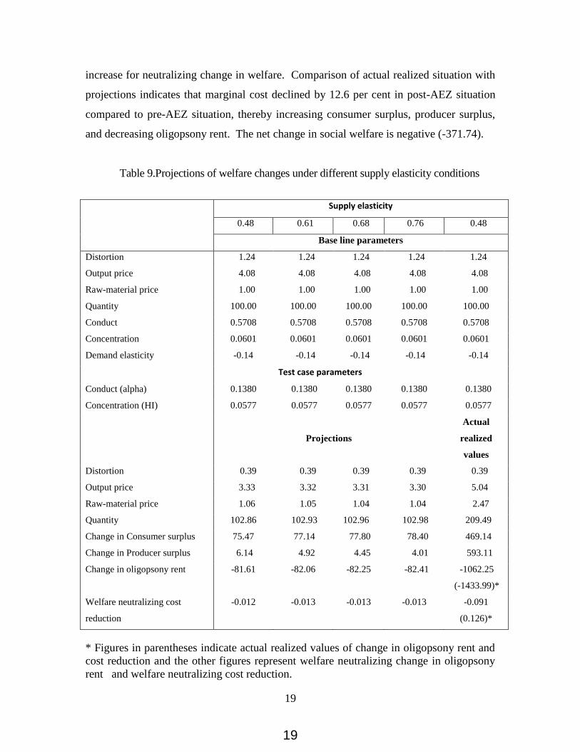
19
increase for neutralizing change in welfare. Comparison of actual realized situation with
projections indicates that marginal cost declined by 12.6 per cent in post-AEZ situation
compared to pre-AEZ situation, thereby increasing consumer surplus, producer surplus,
and decreasing oligopsony rent. The net change in social welfare is negative (-371.74).
Table 9.Projections of welfare changes under different supply elasticity conditions
Supply elasticity
0.48 0.61 0.68 0.76 0.48
Base line parameters
Distortion 1.24 1.24 1.24 1.24 1.24
Output price 4.08 4.08 4.08 4.08 4.08
Raw-material price 1.00 1.00 1.00 1.00 1.00
Quantity 100.00 100.00 100.00 100.00 100.00
Conduct 0.5708 0.5708 0.5708 0.5708 0.5708
Concentration 0.0601 0.0601 0.0601 0.0601 0.0601
Demand elasticity -0.14 -0.14 -0.14 -0.14 -0.14
Test case parameters
Conduct (alpha) 0.1380 0.1380 0.1380 0.1380 0.1380
Concentration (HI) 0.0577 0.0577 0.0577 0.0577 0.0577
Projections
Actual
realized
values
Distortion 0.39 0.39 0.39 0.39 0.39
Output price 3.33 3.32 3.31 3.30 5.04
Raw-material price 1.06 1.05 1.04 1.04 2.47
Quantity 102.86 102.93 102.96 102.98 209.49
Change in Consumer surplus 75.47 77.14 77.80 78.40 469.14
Change in Producer surplus 6.14 4.92 4.45 4.01 593.11
Change in oligopsony rent -81.61 -82.06 -82.25 -82.41 -1062.25
(-1433.99)*
Welfare neutralizing cost
reduction
-0.012 -0.013 -0.013 -0.013 -0.091
(0.126)*
* Figures in parentheses indicate actual realized values of change in oligopsony rent and
cost reduction and the other figures represent welfare neutralizing change in oligopsony
rent and welfare neutralizing cost reduction.
19

20
Simulations have been carried out to analyse implications of increased concentration
(doubling HI) under different levels of coordination and the results are presented in Table 10.
Table.10. Simulation of welfare changes under different conduct and concentration
situations
Component /Parameters
Scenarios
1 2 3 4 5
Base line parameters
Distortion 1.24 1.24 1.24 1.24 1.24
Output price 4.08 4.08 4.08 4.08 4.08
Raw-material price 1.00 1.00 1.00 1.00 1.00
Quantity 100.00 100.00 100.00 100.00 100.00
Supply elasticity 0.48 0.48 0.48 0.48 0.48
Demand elasticity -0.14 -0.14 -0.14 -0.14 -0.14
Conduct 0.5708 0.5708 0.5708 0.5708 0.5708
Concentration 0.0601 0.0601 0.0601 0.0601 0.0601
Test case parameters
Conduct (alpha) 0.0000 1.0000 0.0000 0.1380 1.0000
Concentration (HI) 0.0577 0.0577 0.1200 0.1200 0.1200
Projections
Distortion 0.12 2.08 0.25 0.50 2.08
Output price 3.08 4.75 3.20 3.44 4.75
Raw-material price 1.09 0.96 1.08 1.05 0.96
Quantity 104.02 97.89 103.44 102.43 97.89
Change in Consumer surplus 101.97 -66.45 89.09 64.94 -66.45
Change in Producer surplus 8.73 -4.30 7.44 5.18 -4.30
Change in oligopsony rent -110.70 70.75 -96.53 -70.12 70.75
Welfare neutralizing cost
reduction
-0.014 0.019 -0.014 -0.011 0.019
20

21
From the table .10 it can be observed that, irrespective of level of concentration,
under conditions of perfect collusion, price distortion is attaining it maximum limit value (of
1/supply elasticity) and is resulting in decline of producer surplus and consumer
surplus(scenarios 2 and 5). Under this situation welfare neutralizing cost reduction is positive,
indicating that cost reduction is needed to offset deadweight loss. When concentration is
almost same (0.0601 and 0.0577), moving towards non-cooperative behavior is leading to
decline in price distortion (scenario 1). Under non-cooperative condition, increase in
concentration is leading to increased price distortion (scenario 3). Thus interaction of firm
level coordination and industry concentration is the determinant of welfare changes under
situations where there is decreasing coordination level and increasing concentration and vise
versa (scenario 4). When price distortion is increasing change in oligopsony rent is positive.
When price distortion is decreasing, change in oligopsony rent is negative, necessitating
increase in marginal costs to nullify this effect. When both level of coordination and
concentration are declining price distortion declined, oligopsony rent declined necessitating
once again cost increase for offsetting the deadweight loss. But the realized decline in
oligopsony rent is more than the realized increase of consumer surplus and producer surplus.
This, in turn, is due to decline in marginal cost and increase in SCI in post-AEZ situation
compared to pre-AEZ situation.
Conclusions:
The study results indicates that for monitoring competition in an agro-processing industry,
it is not enough to look into concentration alone, but attention need to paid on other
determinants viz: coordination level and supply response of raw material from agriculture.
Market power analysis at the top most firm level showed greater market power compared
to industry. This can have effect on performance of other firms in the industry and social
welfare. This is an important issue in the context of absence of any policy regulating
procurement price of mango by the mango pulp units. Hence market power at top most
firm need to be monitored constantly.
From review of literature it is observed that diverse hypotheses are there
regarding determinants of market power and diverse methods for measuring market
power. It is the data availability that dictated the methodology in the present study. More
21

22
data availability regarding the industry in future will facilitate more realistic assessment
of market power in the sector through application of diverse methods.
References
APITCO, (1999), “ Diagnostic study report on Chittoor fruit processing cluster”, vol 1&2
Andhra Pradesh Industrial and Technical Consultancy organization Ltd.
Azzam Azzeddine M., and Schroeter John R., (1995), “The tradeoff between oligopsony power
and cost efficiency in horizontal consolidation : an example from beef packing”
American Journal of Agricultural Economics, vol 77 , pp: 825-836.
Azzam M. Azzeddine and Schroeter John R., (1991), “Implications of increased regional
concentration and oligopsonistic coordination in the beef packing Industry” Western
Journal of Agricultural Economics, vol 16 (2), pp: 374-381.
Einav Liran and Levin Jonathan (2010) " Empirical Industrial Organization: a progress report"
Journal of Economic Perspectives, Vol 24(2), pp: 145-162
Elnagheeb Abdelmoneim H., and Florkowski Wojciech. J., (1993), “Modeling Perennial crop
supply: an illustration from the Pecan industry” Journal of Agricultural and Applied
Economics, vol 25, pp:187-196.
Higaki Yusuke, (1997), “Competition in the Japanese potato Market “ Unpublished M.Sc thesis,
Department of Agricultural Economics, Macdonald Campus of McGill University,
Montreal, Quebec, Canada.
Islam Nurul, (1990), “Horticultural Exports of Developing countries : past performances, future
prospects and policy issues” Research Report 80, April 1990, International Food Policy
Research Institute, Washington.
Iwata. G (1974) " Measurement of conjectural variation in oligopoly" Econometrica, vol 42(5),
pp:947-966
Jedele, Stefan, Angela Maria Hau, Matthias Von Oppen, (2003), “An analysis of the World
Market for Mangoes and its importance for developing Countries” Conference on
International Agricultural Research for Development, October
8-10, 2003, Gottingen.
22
23
Ji In Bae and Chung Chanjin (2011) " Dynamic assessment of Bertrand Oilogopsony in the U.S.
Cattle procurement market" Selected paper prepared for presentation at the Agricultural
& Applied Economics Association's 2011 AAEA & NAREA Joint annual meeting,
Pittsburgh, Pennsylvania. July 24-26,2011
Kadiyali Vrinda, K. Sudhir and Vithala R. Rao., (2001), ”Structural analysis of competitive
behavior: new empirical industrial organization methods in marketing” International
Journal of Research in Marketing, vol 18 , pp: 161-186
PereKhozhuk Oleksandr and Glauben Thomas (2017) " Approaches and methods for the
econometric analysis of market power: a survey and empirical comparison" Journal of
Economic Surveys, Vol .31(1),pp: 303-325
Rogers Richard, T., and Sexton Richards, J., (1994), “Assessing the importance of oligopsony
power in agricultural markets” American Journal of Agricultural Economics, vol 76, pp:
1143-1150.
Roy Abhik, Kim Namwoon and Jagmohan S.Raju (2006) " Assessing new empirical industrial
organization (NEIO) methods: the cases of five industries" International Journal of
Research in Marketing, Vol 23, pp: 369-383
Stiegert Kyle W., Azzeddine Azzam and B. Wade Brorsen, (1993), “Markdown pricing and
cattle supply in the beef packing industry” American Journal of Agricultural Economics,
vol 75, pp: 549-558.
23

On the economics of cartel investigation: the case of cement in India
Dr. Debdatta Saha (Faculty of Economics, South Asian University)
Manisha Kapoor (Researcher, Institute for Competitiveness) Short abstract: This paper contributes to the ongoing debate about cartelization in the Indian cement
industry. The issue sprang up with the 2010 complaint by the Builders Association of
India with the CCI and is currently resonating in anti-trust forums with the recent order
of the Commission (29 of 2010), which finds the conduct of 11 cement firms and the
CMA in contravention of the provisions of Section 3(3) (a) and 3(3)(b). We focus on
cartel-induced overcharges. Depending on the econometric method (dummy variable
technique and Dynamic Treatment Effects), our estimates indicate potential overcharges
attributable to cartelization.
Keywords: Cement cartels, Cartel-induced overcharges, Dummy variable
technique,Dynamic Treatment Effects (DTE) method JEL classification codes: L40, L61, C54, C31
24

I. Introduction "The first thing for any new competition regulator is to go out and find the cement cartel. My experience of this subject is, it is always there, somewhere, the only countries in which I had been unable to find the cement cartel is where there is a national state-owned monopoly for cement." -Richard Whish In competition law parlance, one of the most extensively studied and discussed is the
problem of cartel detection. Most competition authorities have strict provisions for cartels,
and in some countries, are part of criminal law. Received wisdom suggests most cartels
harm the economy as it eats into the consumer surplus, by raising prices above the
equilibrium level. If firms in an industry compete, then this competition drives down the
prices which eventually benefit the consumers. This fall in prices will lead to reduced
inflation and hence enhancing economic growth. Cartels allow firms to enter soft
competition and are thus used to keep prices high. The participating firms act as near
monopoly extracting the entire surplus from the consumers. Collusive practices that aim at
fixing either prices or market shares are considered as damaging per se as firms get an
opportunity to block the entry of new rivals or to overcharge for their products or services.
The theme of our paper is to investigate the impact on prices due to alleged cartelization of
the Indian cement industry. Cement is an important input into the construction sector of the
economy and any artificial price rise (due to collusion among cement firms) will spill over
to the macroeconomy. Anecdotally, The Economist (29 March 2014) notes that cartels are
robbing poor countries’ consumers of tens of billions of dollars a year: if so, negating all
the aid that rich countries’ governments send them. Additionally, as the quotation of Dr.
Whish in the beginning of this section indicates, cement is a peculiar industry which has a
cartel in almost every country. Authorities have been successful in proving cement cartels in many countries, with the
help of leniency programs, circumstantial and economic evidence. The table below show
some of the countries where cartels in the cement industry have been found.
25

Table I.1: Worldwide Cement Cartels
Period of Cartel Country
1981-1999 Argentina
1986-2007 Brazil
1990—2002 Germany
1995-2009 South Africa
1997-2005 Taiwan
1998-2009 Poland
2002-2003 South Korea
2002-2004 Turkey (Aegean region)
2002-2006 Australia
2003-2006 Egypt
2005-2007 Hungary
2006-2010 Colombia
2008-2009 Pakistan
n/a-2009 Indonesia
Source: Author’s own calculations
Based on respective country’s anti-trust authorities
It is interesting to study cartel dynamics in country-specific context, given the presence of
country-specific anti-trust legislation, leniency programs in particular.
26

The Indian cement cartel case has been resonating in anti-trust forums from the day when
a complaint was filed by Builders Association of India on 26 July 2010 against 11 cement
companies & the Cement Manufacturers Association accusing them of restricting the
supply of cement despite the available capacity to control cement prices. Builders
Association of India (BAI) claimed that prices of cement have been increasing
continuously at alarming rates and have adversely impacted the construction sector. The
Informant i.e. BAI, alleged that the Cement Manufacturer’s Association (CMA) was
complicit in aiding collusive practices among the 11 companies, two of whom (ACC
Cements & Gujrat Ambuja Cements) had withdrawn as members from CMA due to a
widespread belief that the CMA is party to collusive and anti-competitive practices in the
cement industry in India. The Informant opined that the forces of demand & supply were
not at play behind the price increase. The subsequent order of the Commission was
challenged at the COMPAT leading to the recent revised order of the Commission (29 of
2010), which finds the conduct of 11 cement firms and the CMA in contravention of the
provisions of Section 3(3) (a) and 3(3)(b) of the Competition Act.
The empirical exercises in our paper is primarily to enrich the analysis of the competition
authority, by investigating some collusive markers (for tacit collusion) suggested by
theory, in the hope that Commission considers these measures for future cartel analysis.
Our intention is not to question the choice of colluding firms as well as the collusive
phase. We take the regulator’s choice as given (for this paper) and attempt to understand
the nature of competition and the extent of cartel-induced overcharge. The final objective
is to understand the rationale for the penalty imposed by the regulator on the
colludingfirms.
We formulate our research agenda in three stages, in the form of the following three
testable hypotheses: Hypothesis 1 (Market structure and nature of competition in cement industry in
India):There is fringe competition in the market, with stability in market shares of the
collusive firms between June 2009 to March 2011.
27

Hypothesis 2 (Testing for the stability in tacit collusion among 11 firms in the
industry):There is no significant difference between the set of colluding and non-colluding
firms. Hypothesis 3 (Testing for the ex-post impact on wholesale price of cement): The
overcharges created by the cartel are positive and significant. The rationale for our hypothesis follows from the rich theoretical literature on cartels
(summarized in a later section), which gives us some standard collusive markers that are
present in most cartelized industries. Our first hypothesis is motivated by the fact that
collusion tends to yield static market shares of colluding firms. Theory suggests that firm-
level homogeneity aids collusion, by reducing the incentives to break away from the
cartel. While complete homogeneity is rare, cartel members try to reduce incentives to
deviate from collusive pricing by ensuring stability in market shares (for instance, using
buy-backs to compensate cartel members (Harrington, 2006)). Stability in market shares
also helps detect deviation by any member firm in the cartel. Our second hypothesis is
motivated by the observation that at the time of the investigation of the Directorate
General (DG), 49 cement companies were functional in the industry, out of which 11 were
alleged by the BAI to be members of a cartel. It is easier establish the existence of an
industry-wide cartel with less than 10 firms. However, investigating the possibility of a
cartel with 11 insiders and 38 outsiders immediately raises the question about the
incentive of the outsiders to destabilize the cartel. A counter to this line of reasoning is
that there are positive spillovers for the outsiders, if a few firms have successfully
cartelized, as they benefit from higher prices without running the risk of being
investigated. An indirect test of this is to check for the degree of homogeneity among the
alleged cartel insiders and outsiders. A higher degree of homogeneity is indicative of less
incentives for outsiders to destabilize the cartel (possibly due to high positive spillovers in
prices for all industry players).
Our third hypothesis investigates the effectiveness of the alleged cartel in raising prices
and to formulate a theory of harm due to collusive actions. While ex-post cartel analysis is
limited by the availability of secondary data, it informs anti-trust authorities about patterns
in the data that can be exploited to watch out for potential collusive behavior among firms
in any industry. At the same time, identification of collusive markers from such studies
28
are complementary aids for the regulator. The primary action in cartel detection relies on
leniency programs, which reduce the incentive to collude among firms in any industry.
This paper is structured as follows. Section II presents a short literature review on cartels
in general and cement cartels in particular, and draws out common collusive markers that
enlighten anti-trust analysis. Section III provides a brief review of the cement cartel
analysis conducted by the Competition Commission of India (CCI) and pronounces
additional plus factors that can enrich the analysis. Section IV presents our results on the
three hypotheses discussed earlier. Section V concludes with a discussion on leniency
programs.
29

II. Literature Review
II.1 Theoretical foundation on the formation and sustainability of cartels
Economic literature treats cartel as a result of a particularly unique conduct among a set of/all
firms in a particular industry. This typically results in pricing very different from competitive
prices, mostly higher than the latter benchmark. Two main kinds of collusive conduct is
discussed in the economic literature: tacit and explicit collusion. In the former, firms do not
resort to agreements to enforce collusion. All that is needed to support tacit collusion is a
meeting of minds between the firms and the understanding of the fact if firms deviate then
punishments will be meted out that will affect all the firms, regardless of who deviated. On
the contrary, explicit collusion is the case where firms engage in direct communication
regarding the setting of prices, capturing market share etc. While economic theory does not
dwell much on the fine differences between the two modes of collusion, anti-trust practice
does.
From a legal perspective, different countries have defined cartel through the provisions of
their competition regulation. In India, where cartelization is a civil offence, the Competition
Act (2002) in Section 2 (c) defines cartel as follows: “Cartel” includes an association of
producers, sellers, distributors, traders or service providers who, by agreement amongst
themselves, limit, control or attempt to control the production, distribution, sale or price of,
or, trade in goods or provision of services”. These arrangements can take various forms like
increasing prices by creating artificial scarcity, division of markets among various firms so
they can create a monopoly in a particular area etc. These agreements help them exert market
power and extract higher consumer surplus than what they would get if they did not act in
concert. The general consensus is that such arrangements are welfare reducing and should be
punished.
There is an extensive body of theoretical literature on cartels, generalizing the nature of
collusive markers across industries. One branch of theory investigates collusive actions and
their relationship with changes in business cycles, particularly whether the behaviour of
30

collusive prices are countercyclical or procyclical. The much cited Green and Porter (1984)
model discusses cartel formation in the presence of demand uncertainty. Specifically, firms
do not observe rivals’ demand conditions and are uncertain the reason behind a low demand
state in their own operations. It might be due to deviation by a rival from the collusive high
price determined by all firms (undercutting this firm and reducing its demand) or it might be
due to low demand for all players. The model assumes that firms use a “trigger price"
strategy, which is a benchmark price to which they compare the market price when they set
their production. Whenever the market price dips below the trigger price during the collusive
phase, they revert to Cournot quantity competition for some fixed amount of time before
resuming monopolistic conduct again. The result in this paper is that it is a rational response
for plays to participate in a reversionary episode as they cannot observe the reason for
demand fluctuations. Reversionary episodes play an essential role in maintaining collusive
outcomes and do not signal the breakdown of a cartel agreement. Hence, episodes with low
demand see competitive pricing, whereas collusive pricing is more likely during a business
upswing and high demand condition. In sharp contrast, Rotemberg and Saloner (1986) have
theoretically argued that colluding oligopolies behave competitively in periods of high
demand. They point out that it is the boom period and not the recession period that will see
the breakdown of cartels arguing on the grounds that firms will then have a major incentive
to deviate. If price is the strategic variable of choice and demand is relatively high, the
benefit to a single firm from undercutting the price that maximizes joint profits is larger. This
result holds under the assumptions of no capacity constraints and that industry demand is
observable. Haltiwanger and Harrington (1991) investigate these results in the presence of
correlation in present and future demand, specifically assuming that a strong demand today
signals a strong demand tomorrow. If one firm cheats during period of high demand that will
mean giving up on more profits in future. Therefore, a high demand condition at present will
not make collusion difficult instead it will help collusive outcomes. They conclude on the
note that firms find it difficult to collude during recession as the foregone future profits will
be relatively lower that the current gain from deviation. Investigation in cement (Rotemberg
and Saloner (1986)) indicates that cement price tends to move countercyclically.
31

II.2 Institutions and collusion: trade associations and leniency programs Trade associations are known to provide a convenient platform for firms to share important
information on price, quantity, capacity etc. A discussion on these associations is relevant
due to the alleged role of CMA in the Indian cement cartel case. Exchange of information
reduces the possibility of a scenario akin to Green and Porter (1984), where cartels are forced
into reversionary competitive phases. At the same time, such associations help new entrants
access industry information at a low cost. In fact, regulation of associations might be
counterproductive as demonstrated in McCutcheon (1997). This paper analyses Sherman Act
which is thought to operate in public interest, whereas the paper finds the self-same Act may
actually serve to benefit firms rather than consumers. An examination of the interpretation
and enforcement of section 1 of the Sherman Act reveals that firms find it costly, but not
very costly, to meet to discuss prices. Making meetings somewhat costly benefits firms when
they design collusive agreements that rely on marketplace punishments that harm all firms in
the agreement when one firm cheats. Because all firms find punishment an undesirable
outcome when punishment is called for, they would rationally choose to meet again and
renegotiate the original agreement when they find themselves punishing a cheater. Therefore,
there is no conclusive view regarding the role associations play.
A different strand of literature explores the role of leniency programs on cartel detection. In
essence, such programs offer firms involved in a cartel either total immunity from fines or a
reduction of fines which the commission would have otherwise imposed on them if they
report and hand over the evidence to the authority. It also benefits the Commission, allowing
it not only to pierce the cloak of secrecy in which cartels operate but also to obtain insider
evidence of the cartel infringement.1The leniency policy also has a large deterrent effect on
cartel formation and it destabilizes the operation of existing cartels as it seeds distrust and
suspicion among cartel members.
Recently, in the cement cartel case in South Africa, South Africa’s Competition Commission
has reached a settlement agreement with AfriSam, where the latter has admitted that it took
part in a cement cartel. Nonetheless, consensus regarding the effectiveness of leniency
1http://ec.europa.eu/competition/cartels/leniency/leniency.html
32

programs is yet to come forth. A strand in the literature indicates that leniency might induce
collusion, since they decrease the expected cost of misbehavior.
II.3 Empirical literature: Cartel induced overcharges A lot of empirical studies have been conducted by applying different variety of available
approaches in quantifying the damages faced by the society due to the operations of cartel,
mostly in relation to cartel-induced overcharges. Price overcharge refers to the increase in
prices during cartel period over some benchmark prices. Thus, calculating the overcharge
often involves comparing the price actually paid by buyers during the anticompetitive period
(“cartel period”) to estimates of the price that would have prevailed in the absence of such
conduct but where conditions are otherwise the same (the “counterfactual” condition).
(Govinda, Khumalo and Mkhwanazi, 2001).
Empirical evidence suggests that cartel-induced overcharges vary based on duration, legal
environment; organizational characteristics of the cartel and to a lesser extent, method of
overcharge calculation (Connor and Bolotova, 2006). Posner (2001) reviewed overcharges
for 12 cases and found a median overcharge of 28%. Similarly, Werden (2003) reviewed 13
studies and arrived at a median of 15%. A study by the OECD (Organisation for Economic
Cooperation and Development) surveyed cartel cases of its members and found a median
overcharge of 13% to 16% (OECD, 2002). Mncube (2014) studies the South African flour
cartel (active from 1999 to 2007). The paper concludes that the overcharges to independent
bakeries range from 7 per cent to 42 per cent and that the cartel profits were approximately
two times higher during the cartel than the price war year 2002 or the post collusion year
2008. For the precast concrete products cartel, Khumalo et al (2012) estimate the cartel
overcharge to be in the range of 16.5 per cent to 28 per cent for the Gauteng region and
51per cent to 57 per cent for the KwaZulu-Natal region.
The common belief is that collusive conduct generally leads to higher prices generating
welfare loss. However, contrary to this, some economists argue that cartels can be cost-
reducing. By cooperating on areas such as research or advertising, colluding firms can obtain
cost advantages that ultimately can result in lower prices (Bork, 1978). Bolotova, Connor and
Miller (2008) shows that the minimum value of overcharge is -5.26 percent and the
33
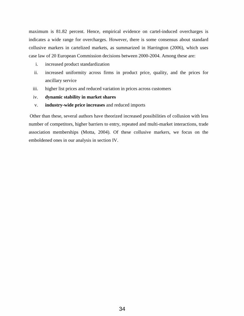
maximum is 81.82 percent. Hence, empirical evidence on cartel-induced overcharges is
indicates a wide range for overcharges. However, there is some consensus about standard
collusive markers in cartelized markets, as summarized in Harrington (2006), which uses
case law of 20 European Commission decisions between 2000-2004. Among these are:
i. increased product standardization
ii. increased uniformity across firms in product price, quality, and the prices for
ancillary service
iii. higher list prices and reduced variation in prices across customers
iv. dynamic stability in market shares
v. industry-wide price increases and reduced imports
Other than these, several authors have theorized increased possibilities of collusion with less
number of competitors, higher barriers to entry, repeated and multi-market interactions, trade
association memberships (Motta, 2004). Of these collusive markers, we focus on the
emboldened ones in our analysis in section IV.
34

III. Cement Cartel in India: A Brief
Some of the salient facts of the cartel case that require attention are:
I. The Informant, BAI, is a society registered under the Societies Registration Act,
1860. It is an association of builders and other entities involved in the business of
construction. The members of BAI are one of the largest consumers of cement in the
Indian market and are directly affected by high cement prices. Given the upstream-
downstream nature of the relationship between the Opposite Parties and the
Informant, the latter is likely to be privy to inside information about the nature of
competition in
the upstream cement market.
II. BAI provided evidence from secondary data2 about potential collusion among 11
cement firms, namely: Associated Cement Co. Ltd. (OP-2/ ACC), Gujarat Ambuja
Cement Ltd. (OP-3/ ACL), Grasim Cement (OP-4/Grasim), UltraTech Cement Ltd.
(OP-5/ UltraTech), Jaypee Cement (OP-6/ Jaypee), The India Cements Ltd. (OP-7/
India Cements), J. K. Cement (OP-8/ JK Cement),Century Cement (OP-9/ Century),
Madras Cements Ltd. (OP-10/ Madras Cements/ Ramco), Binani Cement Ltd. (OP-
11/ Binani) and Lafarge India Pvt. Ltd. (OP-12/ Lafarge) out of a population of 49
functional cement firms in the industry. Few mechanisms mentioned by the BAI in
its allegation of collusion are:
i. complicity of the CMA (OP-1/CMA3): in particular, withdrawal of
ACC Cements and Ambuja Cements Ltd. from its membership
ii. underutilization of capacity despite the growth of the sector in 2009-10
iii. division of the Indian Territory into 5 zones in order to limit the supply
easily
2In the wake of financial crises of 2008, government announced various stimulus packages in the form of reduction in excise duties, coal, petrol etc but the price per bag of cement increased between December 2008 –February 2009 by Rs 5.
3The meetings of High Powered Committee of CMA were held on 3.01.2011, 24.02.2011 and 4.03.2011 after which price of top companies increased.
35

III. Independent investigation by the DG revealed the following facts about competition in
this sector in India:
i. The industry constituted 49 companies operating with more than 173 large
plants.
ii. Of these, the DG investigated 12 players with around 75 per cent market
share, i.e. ACC Ltd., Ambuja Cement Ltd., Ultratech Cement Ltd., Jaypee
Cement Ltd., India Cement Ltd, Shree Cements Ltd., Madras Cement Ltd.,
Century Cement Ltd., J.K. Cements, J.K. Lakshmi Cements Ltd., Binani
Cement Ltd., Lafarge India Pvt. Ltd.
iii. The DG commented on the oligopolistic nature of competition along with
market concentration. For the alleged colluders, the DG found evidence of
low capacity utilization (73 per cent in 2010-11), parallelism in price,
production and dispatch.
iv. Almost all the cement manufacturers were operating at a profit margin of
around 25 per cent and prices are higher than competitive levels.
v. Price of cement has been independent of cost of sales and there has been a
continuous divergence between the cement price index and index price
of inputs. Between 2004-11, whereas cost of sales increased about 30 per
cent, the price of bag of cement increased by 100 per cent. IV. The DG conducted various tests including price, dispatch and production parallelism.
The order stated that price of all the companies moved in the same direction, coefficient
of correlation of change in prices of all companies was positive and close to each other
(more than 0.5 per cent). The correlation coefficient of dispatch data among the largest
companies exhibited a very strong correlation, indicating a situation of meeting of minds.
DG also brought out the spatial nature of the market. The market has been divided in 5
zones and market strategies are planned zone wise as transportation costs are high. V. The CCI observed the following:
i. Abuse of dominance by any player: the Indian cement market was found to be
characterized by several players with no single firm or group was in a position to
operate independently of competitive forces.
ii. Relying on international practice and the clandestine nature of cartels, the
Commission noted that circumstantial evidence is of no less value than direct
36

evidence to prove cartelization. For instance, in the two months of November and
December 2010, the dispatch was lower than the actual consumption for the
corresponding months of 2009. The CCI contends that even though the market
could absorb the supplies, lower dispatches coupled with lower utilization
establishes that the cement companies indulged in controlling and limiting the
supply of cement in the market.
iii. In view of the evidence the contraventions of sections 3(3) (a) and (b) stood
established and a penalty of approximately six thousand crores was imposed in an
order dated 20.06.2012 against the colluding firms (ACC Ltd., Ultratech Cement
Ltd., India Cements Ltd., Ramco Cements Ltd, J K Cement Ltd.., Binani Cement
Ltd., Lafarge India Pvt. Ltd. Jaypee Cement Corpn. Ltd., Ambuja Cements,
Grasim Cements and Century Cements).
VI. The cement manufacturers appealed against this decision of the CCI before the
COMPAT. The COMPAT in its order dated 11 December 2015, set aside the matter on
the ground of violation of the legal principle that 'only one who hears can decide’.
The CCI has revisited the original order via its final ruling (case no. 29 of 2010) on
31 August 2016 and has announced a fine of INR 6700 crore based on 0.5 per cent
of net profits for 2009-10 (from 20.05.2009) and 2010-11 for cement manufacturers
named as Opposite Parties in this case.
37

IV. Empirical Analysis: Market structure and Cartel-induced
Overcharges
The investigation of the Commission rests crucially on the argument that despite a
healthy growth rate of the construction industry (measured at factor cost) at 7 per
cent and 8.1 per cent over the years 2009-10 and 2010-11 respectively4, growth in
cement production and dispatches had been to the tune of only 4.74 per cent and
4.75 per cent in 2009-10 and 2010-11 respectively. Going into the year 2010-11 in
detail, the final order of the Commission states “the third and fourth quarter of 2010-
11 witnessed a GDP growth rate of 8.3 per cent and 7.8 per cent at factor cost
respectively and the construction industry witnessed a growth of 9.7 per cent and 8.2
per cent in Q3 and Q4 of 2010-11 respectively. However, the cement industry
registered a negative growth rate of 5.43 per cent and 3.41 per cent in cement
production in November and December of 2010-11, respectively. Even in case of
cement dispatches, a negative growth rate of 6.33 per cent and 4.90 per cent was
observed in the months of November and December 2010, respectively, over the
corresponding months in the previous year. Even in January, 2010-11, the growth
rate in cement production and dispatches was very low.” Additionally, capacity
utilization was observed to have fallen significantly in 2010-11 “even though certain
Opposite Parties including Lafarge India Pvt. Ltd. and Century Cements have stated
that some of their plants were working with a capacity utilization of 98-100%.”
Without satisfactory demand condition factors explaining the low rate of growth of the
cement industry, the Commission stood by its original finding of cartelization by the 11
alleged firms in the cement industry. In arriving at this conclusion, the statistical tools
employed are price correlation analysis5 and a mention of the low rates capacity
4These growth rates are higher at 11.1 per cent in 2009-10 and 18 per cent in 2010-11 if measured at current prices.
5To correct for the confusion arising from different sets of prices used by the DG for conducting this analysis, the Commission independently conducted state-wise correlation analysis for the period January 2007 to February 2011 using the data submitted by the Opposite Parties to the DG. The Commission has used data for the same/ common city as a representative of the price at the state level for each company wherever such data was available. In all other cases, a representative city has been used to reflect the prices at the state level for a company.
38

utilization6 coupled with evidence of production and dispatch parallelism and a noting
of the company-wise state-wise price per bag of cement for the months of September
and November in year 2010 and January-February in 2011.
While it is a fair contention by the Commission to state that usage of “high level
econometrics or statistical tools” is irrelevant for the analysis of price parallelism
among the potential colluders, a more sophisticated ex-post data analysis can
strengthen the economic arguments which explores the incentives for the firms to
collude in the first place.
To further this cause, we consider our three hypotheses and use secondary data to
examine them. For cement prices, we use the latest monthly wholesale price index
for cement with base year 2004-05 released on 14 September 2010 by the
Department of Industrial Policy and Promotion (DIPP), Ministry of Commerce.
Monthly cement consumption data is taken from Indiastat7 which provides secondary
level socio-economic statistical information about India, its states, regions and
sectors. For analyzing, we use the CMIE database (ProwessIQ) which provides
audited annual financial reports of companies. It is by far the most comprehensive
and reliable source of data on the Indian economy.
IV. 1. Hypothesis 1 (Market structure and nature of competition
in cement industry in India)
The Herfindahl-Hirschman index (HHI) is a commonly accepted measure of market
concentration. It is a measure of the size of firms in relation to the industry and an
indicator of the amount of competition among them. It is calculated by squaring the
market share of each firm competing in a market, and then summing the resulting
numbers. HHI is commonly used in US merger cases, its application in cartel cases
has been very less.
Interpretation: An HHI below 0.01 (or 100) indicates a highly competitive industry. 6The final order of the Commission considered the capacity utilization of 75 per cent rather than 73 per cent reported by the DG (excluding the data pertaining to ACC Ltd. and ACL) as given in CMA report which is calculated on the basis of available capacity of 224.41 MT of the remaining cement companies as on 31.03.2011.
7It is a cluster of 56 associate websites wherein 19 websites are sector-specific, 6 are regional websites and 31
websites are state-specific.
39

An HHI below 0.15 (or 1,500) indicates an unconcentrated industry, while an HHI
between 0.15 to 0.25 (or 1,500 to 2,500) indicates moderate concentration. An HHI
above 0.25 (above 2,500) indicates high concentration. Higher the value of the index,
lower is the level of competition and higher is market concentration in the industry.
We calculate the HHI for the cement industry from 1998-2014 using the metric of
sales of goods in the ProwessIQ database. Table IV.1 reveals that the cement industry
has been quite unconcentrated, even in the period when cartel was functional, which
means that collusive market is not easy to sustain.
Table IV.1 Herfindahl-Hirschman Index for the Indian Cement Industry (1998-2014)
Year Index HHI points Interpretation
1998 0.080496 804.9648386 Unconcentrated Index
1999 0.068271 682.71091 Unconcentrated Index
2000 0.070525 705.2500813 Unconcentrated Index
2001 0.072972 729.716901 Unconcentrated Index
2002 0.072773 727.7343974 Unconcentrated Index
2003 0.071713 717.1271482 Unconcentrated Index
2004 0.070022 700.215191 Unconcentrated Index
2005 0.087036 870.3621726 Unconcentrated Index
2006 0.079459 794.585736 Unconcentrated Index
2007 0.074214 742.1361141 Unconcentrated Index
2008 0.07172 717.2043082 Unconcentrated Index
2009 0.066094 660.942503 Unconcentrated Index
2010 0.078262 782.6245228 Unconcentrated Index
2011 0.085898 858.9780754 Unconcentrated Index
2012 0.086035 860.3536724 Unconcentrated Index
2013 0.086942 869.4165445 Unconcentrated Index
2014 0.092855 928.5516623 Unconcentrated Index
Source: Authors’ own calculations based on ProwessIQ data
A low HHI in itself does not necessarily rule out collusion. We investigate the
concentration scenario using the concentration ratio for the top eight firms (CR8) i.e.
the market share of top eight firms in the industry for the same period. Unlike the
HHI, this measure shows that around 60 per cent of the entire market belonged to just
the top 8 firms, despite 149 operational firms as per ProwessIQ.
40

Table IV.2 CR8for the Indian Cement Industry (1998-2014)
Year CR8 Interpretation
1998 65.52875781 Medium Concentration- Oligopolistic Market
1999 60.99295565 Medium Concentration- Oligopolistic Market
2000 62.08465208 Medium Concentration- Oligopolistic Market
2001 61.03203024 Medium Concentration- Oligopolistic Market
2002 60.52876734 Medium Concentration- Oligopolistic Market
2003 62.71965402 Medium Concentration- Oligopolistic Market
2004 61.37760145 Medium Concentration- Oligopolistic Market
2005 64.56755452 Medium Concentration- Oligopolistic Market
2006 65.47679678 Medium Concentration- Oligopolistic Market
2007 65.06451113 Medium Concentration- Oligopolistic Market
2008 63.86488858 Medium Concentration- Oligopolistic Market
2009 63.17818732 Medium Concentration- Oligopolistic Market
2010 64.82938942 Medium Concentration- Oligopolistic Market
2011 65.78314604 Medium Concentration- Oligopolistic Market
2012 65.22533372 Medium Concentration- Oligopolistic Market
2013 65.82576688 Medium Concentration- Oligopolistic Market
2014 68.70535772 Medium Concentration- Oligopolistic Market
Source: Authors’ own calculations
Our analysis corroborates the DG’s finding that the market is oligopolistic in
nature, with significant concentration in market shares among the top eight
firms. However, we can qualify this statement further. Table IV.3 shows the descriptive statistics for the market shares of the top eight
firms. Note the extremely low variance in market shares, indicating dynamic
stability in this variable which we noted earlier as an important collusive
marker.
41

Table IV.3 Descriptive Statistics for Market Shares of Top Eight Firms (1998-2014)
ACC Ultratech India Ramco Binani Lafarge Jaypee Gujarat
Mean 0.15 0.11 0.06 0.04 0.02 0.02 0.00 0.01
Max 0.21 0.22 0.11 0.05 0.03 0.05 0.02 0.01
Min 0.00 0.00 0.00 0.00 0.00 0.00 0.00 0.00
Standard
Deviation 0.05 0.09 0.02 0.01 0.01 0.02 0.01 0.00
Skewness -1.04 -0.11 -0.12 -2.68 -1.95 0.69 1.35 -0.59
Kurtosis 4.56 1.61 4.23 10.85 7.67 1.80 2.87 2.48
Observations 18.00 18.00 18.00 18.00 18.00 18.00 18.00 18.00
Variance 0.00 0.01 0.00 0.00 0.00 0.00 0.00 0.00
Source: Authors’ own calculations
Table IV.4 shows the Spearman’s rank correlation coefficient for market shares of
these firms. Our results indicate a high degree of positive and statistically significant
correlation among market shares of these firms.
Table IV.4 Spearman’s Rank Correlation for Market Shares ofTop Eight Firms
Spearman's Rank Correlation (1998-
2014) India
ACC Ultratech Cements Ramco Binani Lafarge Jaypee Gujarat
ACC 1 -
Ultratech 0.5907*
India
Cements 0.8308* -0.6223* 1
Ramco 0.4303 0.0168 0.4262 1
Binani 0.4469 -0.2996 0.5707* 0.5769* 1
Lafarge 0.6888* -0.4097 0.4452 0.1643 0.0091 1 - -
Jaypee 0.5810* 0.7783* -0.5623* 0.1326 0.1232 0.6495* 1
Gujarat 0.7193* -0.5088* 0.9257* 0.5583* 0.5728* 0.3727 -0.459 1
* 5% level of significance Source: Authors’ own calculations
In order to examine our first hypothesis, we construct the mobility matrix of market shares
based on share of sale of goods. The matrix helps us in analyzing the nature of
concentration in the market. It has been formed in the following manner:
42
We take the pre-cartel period as 2006-2009, following the CCI order the cartel period was
20.5.2009-31.3.2011, as we have yearly data on sales.8 We first calculate the market share
for each firm for the period 2006-2011 based on sale of goods. Next, a simple average of
market share is taken for the two periods i.e. pre-cartel & cartel. Finally, we classify firms as
per their market share in 4 categories. The selection of these four categories is based on CR8
accounting for almost 60 per cent of total market share.9
8A robustness check was done by taking the cartel period as 2009-2010 and the results did not change significantly.
9The data was available for a total of 145 firms but those have been removed for which the value was zero for both the pre-cartel & cartel period. The firms for which value was zero for only 1 period have been kept. The value zero not always mean share was zero, it also indicates that data was not available.
43

Table IV.5 Mobility Matrix for Market Shares Cartel Period
2009-2011
Top 20% Firms
(By market share)
30-50% Firms
(By Market Share)
50-80% Firms
(By Market Share)
Bottom 20% Firms
(By Market Share)
Pre C
arte
l P
erio
d
2006
-20
08
Top
20%
Fir
ms
(By m
ark
et
share)
A C C Ltd., Ambuja
Cements Ltd., Ultratech
Cement Ltd., India
Cements Ltd.,Shree
Cement Ltd., Ramco
Cements Ltd.10, Birla
Corporation Ltd., J K
Cement Ltd., J K Lakshmi
Cement Ltd., Binani
Cement Ltd., Penna
Cement Inds. Ltd., Chettinad
Cement Corpn. Ltd., O C L
India Ltd., Prism Cement
Ltd.
Sanghi Industries Ltd., My
Home Inds. Pvt. Ltd.,
Lafarge India Pvt. Ltd.
30-5
0%
Fir
ms
(By
Ma
rk
et
Sh
are)
Zuari Cement Ltd. Rain Cements Ltd.,
Heidelberg Cement India
Ltd.,Saurashtra Cement Ltd.,
Mangalam Cement Ltd.,
Gujarat Sidhee Cement Ltd.,
Cement Corpn. Of India
Ltd., K C P Ltd., Shree
Digvijay Cement Co. Ltd.,
Malabar Cements Ltd., N C
L Industries Ltd., Cement
Manufacturing Co. Ltd.,
Meghalaya Cement Ltd.,
Sagar Cements Ltd.,
Kalyanpur Cements Ltd.,
Panyam Cements & Mineral
Inds. Ltd., Anjani Portland
Cement Ltd., Srichakra
Cements Ltd., Megha
Technical & Engineers Pvt.
Ltd., Keerthi Industries Ltd.,
Deccan Cements Ltd.
Tamil Nadu Cements Corpn.
Ltd.
Visaka Cement Industry Ltd.
[Merged], Sri Vishnu
Cement Ltd. [Merged],
Indorama Cement Ltd.
[Merged]
50-8
0%
Fir
ms
(By M
ark
et
Sh
are)
Jaypee Cement Corpn.
Ltd.
Bheema Cements Ltd.,
Barak Valley Cements Ltd.,
Hemadri Cements Ltd.,
Vinay Cements Ltd.
Travancore Cements Ltd.,
Cochin Cements Ltd.,
Burnpur Cement Ltd.,
Greygold Cements Ltd.,
Cement International Ltd.,
Sri Mata Infratech Ltd., Shri
Keshav Cements & Infra
Ltd., Khalari Cements Ltd.,
Sorabh Cement Ltd., Deva
Drill Tech (India) Ltd.,
Balaram Cements Ltd.,
Necem Cements Ltd., P R
Cements Ltd., Virgo
Cements Ltd., Shaktiman
Cements Ltd., Namo
Cements Ltd.,
Alcon Cement Co. Pvt. Ltd.,
Cheran Cement Ltd.,
Nirman Cements Ltd.,
Rajapalayam Cement &
Chemicals Ltd., K J S
Cement Ltd.,
Bott
om
20%
Fir
ms
(By
Mark
et
Sh
are)
Samruddhi Cement Ltd.
[Merged], Dalmia Cement
(Bharat) Ltd.
BhilaiJaypee Cement Ltd.,
Trinetra Cement Ltd.
Bharathi Cement Corpn.
Pvt. Ltd., Bhavya Cements
Ltd., Dalmia Cement East
Ltd., Calcom Cement India
Ltd., Encore Cement &
Additives Pvt. Ltd.
[Merged]
Sanjay Intra Ltd., Rishi
Cement Co. Ltd., Chenab
Cement Ltd., Saurabh
Cement Ltd., Varun
Cements Ltd., Gangotri
Cement Ltd., Someswara
Cements & Chemicals Ltd.,
S C L Cements Ltd.
Source: Author’s own calculations
10 Madras Cement has been renamed as Ramco Cements. The data for 2 colluding firms i.e. Century Cements Ltd &
Grasim Cements is not available on prowess.
44

The matrix can be read as follows: If a firm was in top 20% in both the periods it is
in the first cell of the matrix. If its share has changed between the periods, then it
will lie in the non-diagonal cells of the matrix. As most of the firms lie on the
diagonal elements of the matrix, we have evidence of stickiness in market shares.
Firm names in red are the allegedly colluding firms. Of the nine alleged colluders on
which we found secondary data from ProwessIQ on market shares, note that seven
are in the first cell of this table. One firm has retained its position in the 30 to 50 per
cent range, while only one firm (Lafarge India Pvt. Ltd.) has moved down the ranks
from top 20 per cent to bottom 20 per cent. Majority of the alleged colluders retained
their position in the top 20 per cent market share. The following table provides the
figures on average market shares for firms in each of the cells, the first number being
that for the row category for market share and the second being that for the column
value for the market share.
Table IV.6 Mobility Matrix for Average Market Shares
45

2009-2011
Top 20% 30-50% 50-80% Bottom 20%
2
0%
78.09413, 76.6309 3.491177, 2.509548 - 2.145079719, 0
T o p
30
-50
% 1.199711606,
12.7995, 10.5071 0.4386227,
0.810203, 0
Pre
Ca
rtel
Per
iod
1.691837891 0.098925893
20
06
-20
08
50-
80%
- 0.016092959,
0.952002, 0.792794 0.046113, 0.008383
0.656909732
20
%
Bo
tto
m
0,6.143688 0, 0.635001 0, 0.317851 0.007366, 0.00711
Source: Authors’ own calculations
Tables IV. 6 clearly shows how small the average market shares of the bottom firms in this
industry was and the stickiness in relative market share ranks in the Indian cement market prior
to and during the cartel period. This indicates that we cannot reject our first hypothesis:
Hypothesis 1: There is fringe competition in the market, with stability in market shares of
the collusive firms between June 2009 to March 2011.
Fringe competition is said to arise when there a few small firms in the market, that capture a large
market share and many small sellers. Due to unchanging market share dynamics despite the
presenceof a large number of firms in the market, one of the collusive markers is corroborated: fringe
firms cannot pose potential threats to the top firms and if anything, would benefit from positive price
spillovers arising due to collusion among the top entities.
46

IV. 2. Hypothesis 2 (Testing for the stability in tacit collusion among 11
firms in the industry)
If we compare the average profits of the 11 firms against that of the remaining 38
firms from the period 2005 to 2011, we find that there is a clear positive correlation
in these figures, though in absolute value terms, the average profit of the former
group is about 9 times higher than that of the latter for most of these years. There is a
slightly higher variation in average profits of the colluding set of firms than that of
the non-colluding firms. Nonetheless, the upward movement in average profits is the
same for all the firms, indicating some form of ‘umbrella pricing’ present in the
industry. While this is not a strong test of similarity between the groups of firms, it is a
preliminary exercise that we conducted given some data limitations. Hence, we find weak support for our second hypothesis11:
Hypothesis 2: There is no significant difference between the set of colluding and non-
colluding firms.
This establishes that there was a possibility of stability in collusion as the non-
colluding set of firms were also making positive and increasing profits in the cartel
period (presumably due to positive spillovers in pricing for all firms softening
overallcompetition in the industry).
IV.3. Hypothesis 3 (Testing for the ex-post impact on wholesale price of cement)
IV.3.1. Methodology
Literature suggests that three types of approaches are available for estimating the
harm caused by cartels. They are i) Comparator based, ii) Financial analysis
based, iii) Market-structure based.
Comparator based approaches try to look at what would have happened had the cartel not
been there by looking at time periods before or after infringement or by looking at a
11 A co-movement in profits matters more for this hypothesis, as collusion among a set of firms in the industry then
creates positive externalities for all players in the market, reducing the possibility of a break-down of collusion or
using complicated trigger strategies to sustain collusion.
47

similar market in which a cartel did not exist. This can be applied using three ways: i)
cross-sectional analysis i.e. comparing different geographic or product markets, ii)
time-series comparisons by analyzing prices before, during and/or after an infringement);
and iii) combining the above two in ‘difference-in-differences’ models. Financial
approaches use financial information such as rate of return, costs on comparator firms
and industries to estimate the counterfactual scenario. There are two types of approach
that use this information. First are the ones examining financial performance. These
include assessing the profitability and comparing this against a benchmark. For example,
event studies of how stock markets react to information. The second type is a group of
financial tools, such as discounting, multiples etc.
Market structure based approaches use theory as their base to set up a suitable model
depending upon the market structure and reaching a counter factual situation. The
models can be calibrated using the econometrics techniques described under the
comparator-based approaches.
We employ the comparator-based method to look at the dynamics of pricing in the
cement industry. We focus on the before-and-after effect of cartelization on
wholesale cement prices. The choice of this approach is informed by the data at
disposal and due to the fact that there is no credible comparator to allow for the use
of difference-in-difference (DiD) approach. In essence, while our method compares
price during the cartel period with the price in the same market before and/or after
the cartel period, the DiD method evaluates price developments at different points in
time across different markets, exploring the price effects of a cartel from both a time
perspective and a geographic perspective.
There are two ways by which before-and- after approach can be applied. One is simply
comparing the price averages between these periods. Alternatively, the price overcharge
can be estimated by multivariate models that take into account relevant control variables.
The ability to measure the overcharge accurately depends upon how reliably and
precisely the analysis can distinguish the collusive effect on prices from other influences
that are unrelated to the anticompetitive conduct (Nieberding, 2006). Thus, the attractive
feature of multivariate models is that they allow for the inclusion of other determinants
48

of price in the cartel and non-cartel periods, such as seasonal effects, technological
effects or structural changes. Again, for conducting multivariate comparison, two
approaches exist. The dummy variable approach involves calculation of cartel
overcharge through coefficient parameter by introducing indicator variable for the
cartel period with value 1 during cartel. The forecasting approach (Dynamic
Treatment Effects (DTE)) involves predicting the price during the cartel period on
the basis of the prices in the non-cartel period given the structural changes in the
market. (Govinda, Khumalo and Mkhwanazi, 2001). As most of our variables are
non-stationary, the simple OLS regression for implementing the dummy variable
technique is not reliable. Hence, we present results from the estimation of the DTE
model for cartel-induced overcharges.
The “before-and-after” method has certain key advantages that explain its frequent
application in overcharge estimations. First, data requirements are limited to time
series of the cartelized product. Second, an estimation of the overcharge is
technically relatively easy to implement and therefore suitable for implementation in
a relatively short time window for the analysis. Third, it is not necessary to make any
assumptions on industry conduct absent the cartel (Hüschelrath et al, 2013).
However, the performance of this approach relies on the extent to which the period
before or after the cartel provides a good approximation of the competitive price. One
reason why this might not be the case is the possible persistence of cartel prices after
the cartel has been uncovered. This is the transition period, in which prices continue
to follow the cartel period price trend. Residual collusion is one of the factors that
provide an explanation for transition period. Therefore, ignoring the transition period
is likely to lead to biased estimates of the price overcharge of the cartel.
IV.3.2. Variable Measurement
The main dependent variable for us is the monthly Wholesale Price Index12 (WPI)
of Grey Cement. It is also known as Ordinary Portland Cement (OPC). The reason
12 The selection of data sources for the manufactured products is done on the basis of sampling. Also, a list of top manufacturers is considered for a regular supply of price quotations from them. This ensures that the wholesale prices are appropriate for usage here in the calculation of overcharges.
49

for choosing OPC is that it accounts for 70 per cent of the total domestic
consumption.
Independent variables include:
The main independent variable:
1. Cartel period: It is a dummy variable for cartel. The coefficient of this
willcapture the impact of cartel on the WPI of grey cement. In other words,
the overcharges created by the cartel. It takes value 1 for the period June 2009
– March 2011 and 0 otherwise.
Supply side controls (input prices):
2. Wholesale Price Index of Limestone: Limestone is a major input used in
theproduction of cement. About 1.5 tonnes of limestone is used in the
manufacture of 1 tonne of cement. Limestone is available in large quantities
in Rajasthan, Madhya Pradesh, Gujarat, Andhra Pradesh, Karnataka, Tamil
Nadu, and parts of Bihar.
3. Wholesale Price Index of Power: Power and Fuel accounts for 8 per
centof cost of sales of OPC.
Demand side control:
4. Consumption: Consumption of cement is taken as a proxy for demand due
tothe unavailability of monthly demand of cement data. It is likely to increase
the price of cement, as explained by the normal demand supply forces.
Other controls:
5. Seasonality: The main demand of cement comes from the construction
sector.It can be further decomposed into housing construction (accounting for
64 per cent of total demand), industrial construction, Infrastructure and
commercial & institutional. The construction sector is known for having
seasonal trends as construction booms during summer season. Therefore, it is
important to capture those trends by using monthly dummies.
50

6. Index of Industrial Production: This is taken as a relevant
businesscycle control variable. Basic goods IIP has been taken as
among used based indices, cement is classified under basic goods.
IV.3.3. Results and Discussion
I. The Dummy Variable Technique
The impact of the cartel is estimated through a simple Ordinary Least Squares
regression of the form:
WPI_Cementt= β0 +β1WPI_Limestonet + β2WPI_Powert + β3Consumptiont +
β4 IIPt + β5Dc +∑ ℎ𝑖
11𝑖=1 𝑀𝑖 + et
Note here that is a set of monthly controls, et is the random error term and the
coefficient of interest is β5, which measures the effect of the cartel period
(measured by the dummy variable Dc) on the WPI of OPC. The coefficient of
the cartel dummy captures the ceteris paribus effect of the cartel on price.
Table IV.7: Dummy Variable Model for the WPI of Cement, January2004 –
December 2011
Log (Variable) Model (1)
WPI_Limestonet 0.203374
(.091947)**
WPI_Powert -0.598713
(.095357)***
Consumptiont 0.214725
(0.078806)***
IIPt 1.437284
(0.115327)***
Cartel Period Dummy .019757
(.011625)*
Constant -0.769439
(0.229205)***
Number of observations
R-squared
Adjusted R-squared
84
0.9587
0.9489
Monthly dummies Yes
Notes:
***, ** and * indicate significance at 1, 5 and 10%, respectively.
Standard errors in parenthesis below coefficients. Source: Author’s own calculations
51

The cartel period as stated in the order is 20.05.2009-31.03.2011. So we take
the period to be June 2009- March 2011. The table IV.7 shows the estimation
results for the case of natural logarithm of the respective variables. It can be
inferred from the dummy coefficient that the price difference between the
cartel period and the non-cartel period i.e. the avoided price is exp(0.019756)
– 1 = 1.99%, statistically significant at 1%. Apart from the specification
mentioned here, three other models have also been tried – a model without the
natural logs of the variables, another specification including a time trend and a
third variant with lags of the variable. The specification with the of the
logarithms of the variables presented below provided the best fit.The results of
other three specifications are presented in Appendix 1.
A naïve reading of this result indicates that there was a significant effect of the
cartel period on prices. However, we should note the possibility of a spurious
result here as some of the independent variables (WPI _Cement, WPI_ Power
and IIP) are non-stationary, as Table IV.8 shows.13
Table IV.8 Unit Root Tests
(AIC Criteria, Max Lag Length=10) Variable ADF_t-statistic p-value
WPI _Cement -1.797453 0.6911
WPI _Limestone -3.624167 0.0382
WPI_ Power -2.690152 0.2455
Consumption -6.826471 0.0001 IIP -0.271903 0.9890
Notes: ADF_t-statistic indicates the t-value with both intercept and trend. MacKinnon (1996) one sided p-values are noted.
Source: Authors’ own calculations
II. Dynamic Treatment Effects (DTE)
We investigate whether a co-integrating relationship exists among these
variables. Despite non-stationarity in individual variable time series, a co-
integrating relationship is a combination of these variables which is stationary
13Despite the spurious nature of a naïve OLS regression in this context, the empirical literature has routinely
reported these results upfront, for example in Notaro (2014).
52

and we can comment on long-run dynamic patterns in the data. The
Autoregressive Distributive Lag Model (ARDL) bound test (we have two I(0)
variables and three I(1) variables) to test for the existence of a cointegrating
relationship among the variables. As we find that the value of the f-statistic of
this test is higher than the critical upper value bounds at even 1 per cent level
of significance, we reject the null hypothesis of no cointegration.
Table IV.9 ARDL Bound Test for Cointegration
Test Statistic Value K F-statistic 9.558818 4
Significance
Critical Value Bounds
I1 Bound I0 Bound 10% 2.2 3.09
5% 2.56 3.49
2.5% 2.88 3.87
1% 3.29 4.37
Source: Authors’ own calculations
Accepting that there is a cointegrating relationship among the variables of interest,
we estimate the ARDL model, with WPI_Cement as the dependent variable as shown
in Table IV.10. The cointegrating relationship is shown in the equation below:
WPIC = (-0.7773*WPIL + 0.0874*WPIPR + 10.4169*CONS + 0.3593*IIP + 34.3167)
53

Table IV.10. Long Run Relationship – ARDL Model (January 2005- May 2009)14
Variable Model (1) Probability
WPI _Limestone -0.777317 (0.575488) 0.1876
WPI _Power 0.087361 (0.463673) 0.8519
Consumption 10.416912 (6.456068) 0.1178
IIP 0.359304 (0.783266) 0.6500
Constant 34.316693 (44.6563) 0.4486
Notes: Standard errors in parenthesis. Source: Authors’ own calculations
Standard diagnostic tests for normality, heteroscedasticity and auto correlation were
conducted for the ARDL specification. The results, reported in Appendix 2 prove that
none of these problems show up with our specification. There is no evidence of structural
break in the ARDL specification (in our CUSUM plots). The but-for or counterfactual
scenario is now created by using the price of cement predicted by this model and
forecasting future prices (from June 2009 to March 2011). This is the price that would
prevail in the absence of any potential cartelization between June 2009 to March 2011.
The following graph contrasts the price path of cement as predicted by the model (in
blue) and actual cement prices (in red).It should be noted that the actual price path is
within ±2 S.E. (Standard Error) band of the prediction 15.
Figure IV. 1. Comparing ARDL forecasted cement price with actual cement price
14The cartel overcharge calculation tables (Table IV.7 and Table IV.10) are notable for negative sign
of Power (by the OLS method) and Limestone (by the ARDL approach) indicating the limitations of
the approaches. However, it is observed that some of the papers aimed at calculating cartel
overcharges have faced similar problems. For instance, in Notaro, G. (2014). Methods for Quantifying
Antitrust Damages: The Pasta Cartel in Italy. Journal of Competition Law and Economics, 10(1), 87-
106. – A pasta cartel overcharge calculation shows negative sign of energy. Also, in Govinda, H.,
Khumalo, J., &Mkhwanazi, S. “On measuring the economic impact: savings to the consumer post
cement cartel burst.” In Competition Law,Economics and Policy Conference (Vol. 4). the coefficients
of limestone and oil were negative and were which taken as proof for some amount of inconsistency
in the data. 15The error band for the prediction is shown in Appendix 3.
54

However, caveats is due about our ARDL specification: the sign of the coefficient of
WPI_limestone in our estimated model is negative. This result of wrongly signed
inputs is common to the empirical literature on price-related overcharges arising due
to collusion. A potential possibility is that distorted market competition exists in the
entire supply chain for cement, resulting in such anomalies. Investigating this is part
of future work.Second, other than the constant term, none of the regressors are
significant in our ARDL specification.
90
100
110
120
130
140
150
160
2005 2006 2007 2008 2009 2010 2011
WPICF WPIC
55

Figure IV. 2. Wholesale Price of Limestone from 2005 to 201116
Source: Authors’ own calculations based on DIPP data
Following Bolotova, Connor and Miller (2008), we measure overcharges from our
model as the following rate:
𝑂𝑂𝑂𝑂𝑂𝑂𝑂𝑂𝑂𝑂 𝑂𝑂𝑂𝑂 =𝑂𝑂𝑂𝑂𝑂𝑂𝑂𝑂𝑂𝑂 − 𝑂𝑂𝑂𝑂𝑂𝑂𝑂𝑂𝑂𝑂
𝑂𝑂𝑂𝑂𝑂𝑂𝑂𝑂𝑂𝑂
These results are summarized in table IV.11, which gives us an average overcharge
rate of around 8.73 per cent.This rate of overcharge, while on the low side, is part
of the observed range for cartel -induced overcharges. As the forecast price falls
within the predicted band for the predicted price, we should not expect very large
overcharge rates, as we find only a weak evidence for collusion through our
empirical analysis in this section.
16The time series movements of other variables are presented in Appendix 4.
56

Table IV.11. Overcharge calculation from ARDL model
Year WPI Cement Forecast Overcharge (%)
Jun-09 149.2 148.79 0.28
Jul-09 149.5 151.21 -1.13
Aug-09 149.3 148.01 0.87
Sep-09 149.1 143.42 3.96
Oct-09 150.2 139.9 7.36
Nov-09 148.4 138.14 7.43
Dec-09 146.2 136.58 7.04
Jan-10 147.6 135.81 8.68
Feb-10 150.6 134.76 11.75
Mar-10 151.3 134.39 12.58
Apr-10 151.8 135.83 11.76
May-10 152.5 135.3 12.71
Jun-10 150.3 135.1 11.25
Jul-10 153.8 137.42 11.92
Aug-10 151.6 136.72 10.88
Sep-10 150.3 136.76 9.90
Oct-10 151.5 136.28 11.17
Nov-10 148.3 136.5 8.64
Dec-10 147.8 135.85 8.80
Jan-11 147.9 134.61 9.87
Feb-11 150.9 136.32 10.70
Mar-11 153.7 132.94 15.62
Source: Authors’ own calculations
With an average overcharge rate which is less than 10 per cent and the fact that the actual price
path (though higher than the predicted price path) has not crossed the accepted error bounds for
prediction, the final test is on the calculation of penalties. While the CCI has concluded that there
is enough evidence of collusion and has imposed a penalty based on 0.5 per cent of net profits in
2009-10 (20 May 2009 onward) and 2010-11, our analysis does not provide direct evidence for
such penalty calculation to remedy potential harm.
Going forward, the limitations of ex-post analysis using publicly available data of the kind we found
available to comment on overcharges and potential harm should alert the Competition Authority that
other methods such as its Leniency Programme might be better alternatives to detect collusion in
industries with distorted competition, such as cement. However, such programmes, unless well
57

designed might help colluding firms achieve better coordination (McCutcheon 1997). Extending the
analysis to sub-regional competition issues, keeping in mind the regional fragmentation of the
cement market is limited by the availability of publicly available data, but is part of our longer run
research agenda.
V. Conclusion
The discussion on the Indian cement cartel case is interesting as well as academically
challenging, given that the Commission has not reversed its original conclusion that the
Opposite Parties are guilty of cartelization of the cement industry between June 2009 to
March 2011. Worldwide, successful cartel investigation rests on a clever usage of the
leniency and whistleblower programs that provide direct evidence of cartelization. Our
first hypothesis clearly indicates the difficulty of creating a but-for counterfactual as the
cement market is clearly oligopolistic in nature, with some fringe competition. Ex-post
cartel analysis might consider employing some of the statistical techniques that we
discuss to elucidate on the extent of harm and cartel-induced overcharges. While the
selection of firms in the collusive set and the cartel period are open to debate, what is
undeniably established is the stability of market shares of the alleged colluding firms.
Wecontrasted the market shares of these firms against market shares of a Polish cement
cartel case in 2009 (Bejger, 2011), where two of the colluders (one of thembeing Lafarge
confessed to cartelization under the Polish leniency program. Given the homogeneous
nature of cement and oligopolistic competition across countries, we contrasted the
market share volatility of alleged colluders in India with the Polish case. Hearteningly,
we find that market share volatility is lower for the allegedly colluding Indian firms than
for the Polish conspirators.
58

VI. Bibliography
1. Bolotova, Y., Connor, J. M., & Miller, D. J. (2008). “The impact of
collusion on price behavior: Empirical results from two recent cases.”
InternationalJournal of Industrial Organization, 26(6), 1290-1307.
2. Hüschelrath, K., Müller, K., &Veith, T. (2013). “Concrete shoes for
competition: the effect of the German cement cartel on market price.”
Journalof Competition Law and Economics, 9(1), 97-123.
3. Rotemberg, J. J., &Saloner, G. (1986). “A supergame-theoretic model of
price wars during booms.” The American Economic Review, 390-407.
4. Connor, J. M. &Bolotova,Y. (2006). “A Meta-Analysis of Cartel
Overcharges”International Journal of Industrial Organization, 24: 1109-
1137.
5. Berget, J. (2014). “Price Developments in Post Cartel Periods.”Masters thesis
6. Green, E. J., & Porter, R. H. (1984). “Noncooperative collusion under
imperfect price information.” Econometrica: Journal of the
EconometricSociety, 87-100.
7. Ellison, G. (1994). “Theories of cartel stability and the joint executive
committee.” The Rand journal of economics, 37-57.
8. Hay, G. A., & Kelly, D. (1974). “An Empirical Survey of Price Fixing
Conspiracies,” 17J. L. & Econ, 13, 14.
9. Levenstein, M. C., &Suslow, V. Y. (2006). “What determines cartel success?.”
Journal of Economic Literature, 43-95.
10. Govinda, H., Khumalo, J., &Mkhwanazi, S. “On measuring the economic
impact: savings to the consumer post cement cartel burst.” In Competition
Law,Economics and Policy Conference (Vol. 4).
11. Haltiwanger, J., & Harrington Jr, J. E. (1991). “The impact of
cyclical demand movements on collusive behavior.” The
RANDJournal of Economics, 89-106.
12. Arora, R. R., & Sarkar, R. (2006). “Detecting Cartels in the Indian Cement
Industry: An Analytical Framework.”
59

13. Porter, R. H. (1983). “A study of cartel stability: the Joint ExecutiveCommittee,
1880-1886.” The Bell Journal of Economics, 301-314.
14. Kleit, A. N., &Palsson, H. P. (1996). “Is there anti-competitive behaviour in the
central Canadian cement industry? Testing arbitrage cost
hypotheses.”Canadian Journal of Economics, 343-356.
15. Harrington, J.E. (2006). "How Do Cartels Operate?", Foundations
andTrends® in Microeconomics: Vol. 2: No. 1, pp 1-105.
16. Frass, A. G., & Greer, D. F. (1977). “Market structure and price collusion:
An empirical analysis.” The Journal of Industrial Economics, 21-44.
17. Mncube, L. (2014). “The South African wheat flour cartel: overcharges at
themill.”Journal of Industry, Competition and Trade, 14(4), 487-509.
18. Bolotova, Y., Connor, J. M., & Miller, D. J. (2009). “Factors influencing the
magnitude of cartel overcharges: An empirical analysis of the US
Market.”Journal of Competition Law and Economics, 5(2), 361-381.
19. Mariuzzo, F., Walsh, P. P., & Van Parys, O. (2009). “Estimating the price
overcharge from cartelisation of the Irish automobile industry.” The
Economic and Social Review,40(2), 165-182.
20. Motta, M. (2004). Competition policy: theory and practice. Cambridge
University Press.
21. Belleflamme, P. and Peitz M. (2010). Organization Market and Strategies,
Cambridge University Press.
22. Crisil Research Report (2011): Moderate consolidation with two
playersholding around 34 per cent of market share; Crisil Research
23. McCutcheon, B. (1997). “Do Meetings in Smoke‐ Filled Rooms FacilitateCollusion?”
Journal of Political Economy, 105(2), 330-350.
24. Bejger, S. (2011). “Polish cement industry cartel - preliminary examination
of collusion existence.”Business and Economic Horizons, 4(1), 88-107.
25. Notaro, G. (2014). Methods for Quantifying Antitrust Damages: The Pasta
Cartel in Italy. Journal of Competition Law and Economics, 10(1), 87-106.
60

VII. Appendix
Appendix 1: Various OLS specifications
Model 2: The specification without logs
Dependent Variable: WPIC
Method: Least Squares
Date: 05/01/16 Time: 10:37
Sample: 2005M01 2011M12
Included observations: 84
Variable Coefficient Std. Error t-Statistic Prob.
CARTEL 2.436935 1.663002 1.465383 0.1475
WPIL 0.209752 0.109371 1.917809 0.0594
WPIPR -0.539691 0.104018 -5.188423 0.0000
CONS 1.894667 0.810558 2.337485 0.0224
IIP 1.455042 0.131031 11.10456 0.0000
@SEAS(2) 11.65804 2.630728 4.431486 0.0000
@SEAS(3) -7.755717 2.683347 -2.890314 0.0052
@SEAS(4) 16.00878 2.643028 6.056984 0.0000
@SEAS(5) 11.66191 2.600353 4.484742 0.0000
@SEAS(6) 16.55690 2.722081 6.082443 0.0000
@SEAS(7) 18.52118 2.783121 6.654823 0.0000
@SEAS(8) 20.25109 2.913426 6.950953 0.0000
@SEAS(9) 23.57692 2.974807 7.925529 0.0000
@SEAS(10) 13.30128 2.707807 4.912196 0.0000
@SEAS(11) 17.98231 2.819460 6.377928 0.0000
@SEAS(12) 3.745541 2.579941 1.451793 0.1512
C -42.09775 6.040759 -6.968950 0.0000
R-squared 0.949138 Mean dependent var 134.0929
Adjusted R-squared 0.936992 S.D. dependent var 18.99098
S.E. of regression 4.766984 Akaike info criterion 6.139943
Sum squared resid 1522.517 Schwarz criterion 6.631894
Log likelihood -240.8776 Hannan-Quinn criter. 6.337703
F-statistic 78.14387 Durbin-Watson stat 1.346283
Prob(F-statistic) 0.000000
61

Model 3: The specification with time trend
Model 4: The specification with lags
Dependent Variable: WPIC
Method: Least Squares
Date: 02/19/17 Time: 10:53
Sample: 2005M01 2011M12
Included observations: 84
Variable Coefficient Std. Error t-Statistic Prob.
C 146.6497 15.12291 9.697185 0.0000
WPIPR -0.723294 0.108044 -6.694461 0.0000
WPIL 0.175535 0.106448 1.649017 0.1032
CONS 0.249363 0.691240 0.360748 0.7193
IIP 0.110381 0.144191 0.765517 0.4463
@TREND 1.102155 0.098637 11.17388 0.0000
@DURING("2009M06 2011M03") -4.857860 1.760649 -2.759130 0.0072
R-squared 0.942404 Mean dependent var 134.0929
Adjusted R-squared 0.937916 S.D. dependent var 18.99098
S.E. of regression 4.731913 Akaike info criterion 6.026191
Sum squared resid 1724.107 Schwarz criterion 6.228759
Log likelihood -246.1000 Hannan-Quinn criter. 6.107622
F-statistic 209.9836 Durbin-Watson stat 0.316379
Prob(F-statistic) 0.000000
Dependent Variable: WPIC
Method: Least Squares
Date: 02/19/17 Time: 11:00
Sample (adjusted): 2005M05 2011M12
Included observations: 80 after adjustments
Variable Coefficient Std. Error t-Statistic Prob.
C -14.38409 7.349097 -1.957260 0.0541
@DURING("2009M06 2011M03") 7.481617 1.780702 4.201498 0.0001
WPIPR(-4) 0.117961 0.116844 1.009563 0.3160
WPIL(-4) 0.164605 0.137862 1.193989 0.2363
CONS(-4) 2.612704 0.590759 4.422624 0.0000
IIP(-3) 0.626448 0.102293 6.124039 0.0000
R-squared 0.885639 Mean dependent var 135.7687
Adjusted R-squared 0.877912 S.D. dependent var 17.86451
S.E. of regression 6.242057 Akaike info criterion 6.572535
Sum squared resid 2883.283 Schwarz criterion 6.751187
Log likelihood -256.9014 Hannan-Quinn criter. 6.644162
F-statistic 114.6147 Durbin-Watson stat 0.579134
Prob(F-statistic) 0.000000
62

Appendix 2: Results of tests of normality, serial auto-correlation and
heteroscedasticity
0
1
2
3
4
5
6
7
8
9
-2.0 -1.5 -1.0 -0.5 0.0 0.5 1.0 1.5 2.0 2.5
Series: Residuals
Sample 2005M05 2009M05
Observations 49
Mean -1.04e-14
Median -0.118058
Maximum 2.380565
Minimum -1.881939
Std. Dev. 0.950491
Skewness 0.403783
Kurtosis 2.757772
Jarque-Bera 1.451294
Probability 0.484011
63

Breusch-Godfrey Serial Correlation LM Test:
F-statistic 2.237866 Prob. F(4,24) 0.0949
Obs*R-squared 13.31114 Prob. Chi-Square(4) 0.0099
Test Equation:
Dependent Variable: RESID
Method: ARDL
Date: 02/18/17 Time: 18:28
Sample: 2005M05 2009M05
Included observations: 49
Presample missing value lagged residuals set to zero.
Variable Coefficient Std. Error t-Statistic Prob.
WPIC(-1) 0.020391 0.057119 0.356985 0.7242
WPIL -0.004115 0.064632 -0.063662 0.9498
WPIL(-1) 0.019005 0.081632 0.232816 0.8179
WPIL(-2) -0.014416 0.081739 -0.176371 0.8615
WPIL(-3) 0.008238 0.086898 0.094806 0.9253
WPIL(-4) -0.004109 0.068665 -0.059845 0.9528
WPIPR 0.019552 0.160362 0.121926 0.9040
WPIPR(-1) -0.024084 0.193428 -0.124511 0.9019
WPIPR(-2) -0.012873 0.182428 -0.070564 0.9443
WPIPR(-3) -0.015488 0.157989 -0.098035 0.9227
WPIPR(-4) 0.029014 0.138211 0.209927 0.8355
CONS -0.190966 0.443329 -0.430755 0.6705
CONS(-1) -0.038681 0.537457 -0.071970 0.9432
CONS(-2) -0.173424 0.455310 -0.380893 0.7066
CONS(-3) 0.082526 0.434120 0.190100 0.8508
CONS(-4) -0.030289 0.440307 -0.068791 0.9457
IIP 0.017114 0.073298 0.233491 0.8174
IIP(-1) 0.001787 0.089256 0.020023 0.9842
IIP(-2) 0.012923 0.084756 0.152475 0.8801
IIP(-3) -0.009413 0.076171 -0.123572 0.9027
C -0.637566 4.510928 -0.141338 0.8888
RESID(-1) -0.484675 0.215121 -2.253036 0.0337
RESID(-2) -0.628869 0.243306 -2.584682 0.0163
RESID(-3) -0.276723 0.253482 -1.091687 0.2858
RESID(-4) -0.158399 0.234917 -0.674278 0.5066
R-squared 0.271656 Mean dependent var -1.04E-14
Adjusted R-squared -0.456688 S.D. dependent var 0.950491
S.E. of regression 1.147180 Akaike info criterion 3.419132
Sum squared resid 31.58451 Schwarz criterion 4.384346
Log likelihood -58.76873 Hannan-Quinn criter. 3.785333
F-statistic 0.372978 Durbin-Watson stat 1.977550
Prob(F-statistic) 0.990493
64

Heteroskedasticity Test: Breusch-Pagan-Godfrey
F-statistic 0.588341 Prob. F(20,28) 0.8887
Obs*R-squared 14.49888 Prob. Chi-Square(20) 0.8043
Scaled explained SS 4.160935 Prob. Chi-Square(20) 0.9999
Test Equation:
Dependent Variable: RESID^2
Method: Least Squares
Date: 02/18/17 Time: 18:14
Sample: 2005M05 2009M05
Included observations: 49
Variable Coefficient Std. Error t-Statistic Prob.
C 2.418881 4.935442 0.490104 0.6279
WPIC(-1) -0.026608 0.064174 -0.414629 0.6816
WPIL 0.012871 0.072106 0.178500 0.8596
WPIL(-1) -0.015153 0.090683 -0.167100 0.8685
WPIL(-2) 0.044430 0.090752 0.489575 0.6282
WPIL(-3) -0.125171 0.097327 -1.286083 0.2089
WPIL(-4) 0.115195 0.077628 1.483923 0.1490
WPIPR -0.244473 0.170853 -1.430895 0.1635
WPIPR(-1) 0.312355 0.207800 1.503154 0.1440
WPIPR(-2) -0.161914 0.201990 -0.801594 0.4295
WPIPR(-3) 0.202969 0.176001 1.153228 0.2586
WPIPR(-4) -0.196357 0.152704 -1.285865 0.2090
CONS 0.682324 0.487563 1.399457 0.1727
CONS(-1) -0.517225 0.598770 -0.863813 0.3950
CONS(-2) 0.063026 0.509849 0.123616 0.9025
CONS(-3) 0.178167 0.489644 0.363870 0.7187
CONS(-4) 0.130258 0.497370 0.261893 0.7953
IIP -0.052573 0.082449 -0.637643 0.5289
IIP(-1) 0.132805 0.100635 1.319672 0.1976
IIP(-2) -0.053461 0.094825 -0.563784 0.5774
IIP(-3) -0.011100 0.085799 -0.129373 0.8980
R-squared 0.295895 Mean dependent var 0.884996
Adjusted R-squared -0.207036 S.D. dependent var 1.185496
S.E. of regression 1.302448 Akaike info criterion 3.663895
Sum squared resid 47.49839 Schwarz criterion 4.474675
Log likelihood -68.76544 Hannan-Quinn criter. 3.971504
F-statistic 0.588341 Durbin-Watson stat 2.246857
Prob(F-statistic) 0.888691
65

Appendix 3: Prediction band of the ARDL model
Appendix 4: Wholesale Price of Cement (June 2009 – March 2011)
90
100
110
120
130
140
150
160
170
II III IV I II III IV I II III IV I II III IV I II III IV I II III IV I
2005 2006 2007 2008 2009 2010 2011
WPICF ± 2 S.E.
Forecast: WPICF
Actual: WPIC
Forecast sample: 2005M01 2011M03
Adjusted sample: 2005M05 2011M03
Included observations: 71
Root Mean Squared Error 7.358138
Mean Absolute Error 4.217383
Mean Abs. Percent Error 2.871213
Theil Inequality Coefficient 0.027803
Bias Proportion 0.260145
Variance Proportion 0.161104
Covariance Proportion 0.578752
66

Appendix 5: Time series movements of variables (dependent and independent)
Wholesale Price Index of Cement Consumption of Cement
Index of Industrial Production Wholesale Price Index of Power
67
National Conference on Economics of Competition Law, Competition Commission of India |
Contents
00
Applicability of Stated Preference Techniques in
defining Relevant Markets
National Conference on Economics of Competition
Law, Competition Commission of India
Research Paper by Amit Bansal, Shruti Gupta and Bhavya Arora, Deloitte Touche Tohmatsu India, LLP
January 2017
68
National Conference on Economics of Competition Law, Competition Commission of India |
Contents
01 ©2017 Deloitte Touche Tohmatsu India LLP
Contents
Contents 1
Short Abstract 2
Extended Paper 3
Bibliography 12
69

National Conference on Economics of Competition Law, Competition Commission of India | Short Abstract
02
Short Abstract
Determining the relevant market is the keystone of most antitrust cases as it is the first stage of analyzing
competitive effects of a merger or a particular business practice under anti-trust investigation. Defining the
boundaries of the relevant market entails conducting a substitutability exercise based on a comparison of the
product characteristics of potentially competing products and the applicable geographic boundaries for the
product. Incorporation of “consumer preferences” to demonstrate actual substitutability patterns is a pivotal
aspect of this exercise. Consumer preferences can be studied with the help of two techniques of economic
analysis, viz., Revealed Preference and Stated Preference. Revealed Preference analysis requires real world
evidence, which may not be readily available all the time. In such a situation, dedicated consumer surveys may
be used to represent specific preferences of consumers. In most jurisdictions, such an analysis qualifies as
permissible economic evidence in support of the market definition exercise. In this paper we assess the
applicability of consumer surveys1 in representing consumer preferences using Stated Preference techniques
(including Discrete Choice and Contingent Valuation models). Additionally, we evaluate the potential applicability
of Stated Preference techniques to some past Indian anti-trust cases and examine whether such techniques can
aid in performing economic analysis (such as the small but significant and non-transitory increase in price
(SSNIP) test).
1 Stated Preference techniques are essentially survey-based techniques. Therefore, in the context of this paper Stated Preference technique and consumer surveys are used interchangeably.
70

National Conference on Economics of Competition Law, Competition Commission of India | Extended Paper
03 ©2017 Deloitte Touche Tohmatsu India LLP
Extended Paper
Introduction
Relevant market assessment is a critical aspect of all competition law matters as it is a means to identify those
substitute products or services, which exert an effective competitive constraint on the product(s) and/or the
services under evaluation. Defining relevant markets entails substitutability analysis, based on a comparison
of the product characteristics of potentially competing products (relevant product market) and the applicable
geographic boundaries (relevant geographic market) for the product. Several factors are considered and
assessed in order to identify the area of effective competition and competitive constraints that an undertaking
involved may face.
One of the important tenets of defining relevant market in an anti-trust case—is the evaluation of consumer
preferences—and the incorporation of these preferences in the relevant market definition. The Indian
Competition Act of 2002 also regards consumer preferences amongst one of the many factors considered while
defining relevant markets.2 According to economic literature, consumer preferences can be assessed primarily
through two types of techniques viz., Revealed Preference (“RP”) and Stated Preference (“SP”).
RP techniques use actual consumer choice data to assess consumer perception and preferences regarding alternative products. RP techniques require information to be collected on actual consumer switching behavior in response to a price increase or new product coming into the market. However, in the Indian context, such
quantitative data required to implement RP techniques may not always be available, or if available, may not be
sufficient to conduct economic analysis. Moreover, in situations where the potential impact on competition caused by a proposed merger or a combination has to be assessed, real world evidence on how consumers may respond would not be available. In such scenarios, a well-designed consumer survey that measures hypothetical preferences of consumers across products and alternatives can be used to assess the nature of consumer demand and in turn delineate the boundaries of relevant market.
Consumer surveys qualify as permissible and accepted economic evidence in many jurisdictions. Anti-trust
regulators including, the Office of Fair Trading3 (“OFT”), UK, the European Commission and the Competition Authority of Kenya have undertaken consumer surveys in the past to ascertain consumer preferences and evidence from these surveys has formed an important component of their findings on the delineation of relevant market. In particular, the OFT promotes the use of consumer surveys and states that “use of statistically-robust consumer survey research can help in informed decision making”.4 This is demonstrated by the fact that the OFT has used consumer surveys in almost half of the 31 merger enquiries they completed between 2003 and 2006.5
In light of the rising acceptance of consumer surveys as a form of economic evidence in various jurisdictions, this paper discusses the methodologies for implementing SP techniques. Starting with a brief recapitulation of
RP and SP techniques, this paper then reviews some specific SP techniques (Contingent Valuation and Discrete choice models) demonstrated through case examples. We further discuss the application of SP techniques in other international jurisdictions and demonstrate the application of SP techniques to some past Indian anti-trust cases.
Revealed Preference and Stated Preference
A key area in defining relevant markets is substitutability analysis, which entails the assessment of consumer
perception about the following aspects:
i. Price sensitiveness and willingness to pay (“WTP”);
ii. Importance and value of the product/service attributes that are being consumed ; and,
2 The Competition Act, 2002, Chapter 4 (Section 19(7)). 3 From 1 April 2014 Competition Markets Authority (CMA) took over many of the functions of the Competition Commission (CC) and the Office of Fair Trading (OFT). 4 Good practice in the design and presentation of consumer survey evidence in merger enquiries, Office of Fair Trading and Competition Commission, UK. 5 Customer surveys and critical loss analysis for market definition, Oxera.
71

National Conference on Economics of Competition Law, Competition Commission of India | Extended Paper
04 ©2017 Deloitte Touche Tohmatsu India LLP
iii. Change in consumer behavior if alternatives (with respect to the good under consumption) available
were to change
Consumer preferences about these particular aspects can be represented through RP or SP Techniques. In the
case of RP, consumer preferences are revealed through consumer actions in real markets. RP techniques
represent real-world evidence on the choices that consumers exercise and are revealed by consumers’ decisions
in actual market situations. Consumer preferences can be measured through a study on actual purchase patterns
of consumers revealed through historical sales and purchase data maintained by organizations. As against this,
SP techniques are survey based techniques used to elicit consumer valuations and preferences. Specifically, SP
techniques are of two types - Contingent Valuation Technique (“CVT”) and Discrete Choice Experiments (“DCE”).
SP techniques can be used for both market and non-market goods as it measures hypothetical preferences as
well. In the subsequent section, we provide a brief comparison of SP and RP techniques based on few key
differentiating characteristics.
Comparison of Revealed Preference and Stated Preference techniques
RP techniques represent the use-value of the good, viz., the direct value of consuming the goods. Conversely,
SP Techniques represent the economic value of the good (use and non-use value6), viz., the extent to which
consumers would be willing to sacrifice something else in order to obtain the good under consideration. Use
value is direct value derived by consuming the good (e.g. visiting an amusement park) or indirectly securing
some benefit from the good (e.g. saving funds for children’s future education also referred as options value).
Non-use values, also referred to as passive values, arise in situations in which an individual is willing to pay for
provision of the goods even though he is not directly consuming the good currently or in the future. For example,
individual willing to pay for conservation of an imperiled World Heritage Site. As SP techniques can express
option and non-use values as well, they can be used for valuing potential future or hypothetical goods, whereas
RP techniques are restricted to real goods only. This characteristic of SP technique has a far reaching potential;
these techniques can prove to be a very useful tool in evaluating the potential impact of a proposed merger or
a combination.
RP techniques draw inferences about consumer preferences from the actual choices that consumers have
exercised over goods that are available at a given point in time. However, in imperfect markets, some goods
may not be available at a given point due to imperfections such as existence of supply side constraints. In such
a scenario, actual choices exercised by the consumer cannot be considered to be representative, as the consumer
did not have access to the full choice set while making the decision. SP techniques overcome these problems
associated with imperfect markets as they draw inferences based on hypothetical questions. However, there are
certain issues that need to be kept in mind while implementing SP techniques.
SP techniques may be subject to biases arising from the hypothetical nature of the technique. For example,
there could be potential problems associated with hypothetical responses such as strategic responses or a failure
to properly consider behavioral constraints. Furthermore, since SP techniques are primarily survey techniques,
they could suffer from issues of sampling bias if the sample is non-random and does not accurately represent
the underlying population under study.
In table 1, we briefly summarize the key features of the two techniques.
Table 1: Revealed and Stated Preference Techniques
Revealed Preference Stated Preference
Underlying principle Consumer preferences revealed through real world evidence
Consumer preferences are captured using
survey techniques
Methodology Competitive Price Analysis Contingent Valuation
Discrete Choice Method
6 Non-use value refers to the value not arising due to the direct consumption of the good. For instance: a consumer may be willing to pay for a good that he is
conserving for future value (options value).
72

National Conference on Economics of Competition Law, Competition Commission of India | Extended Paper
05 ©2017 Deloitte Touche Tohmatsu India LLP
Revealed Preference Stated Preference
Travel Cost Method7
Hedonic Pricing method8
Applicable
goods
Real goods Real and hypothetical goods
Advantages Reliance on actual choices reduces the potential problems associated with hypothetical responses
Preferences that cannot be evaluated with real
world evidence can be captured through survey
techniques
Disadvantages Data on actual consumption patterns
may not be readily available Presence of market imperfections reduce
the choice set for consumers Analysis is limited to observable state
of the world
Problems associated with hypothetical
responses such as strategic responses or a failure to properly consider behavioral constraints (such as consumers overstating their likely reaction to a change in the market)
Sampling bias and non-response error9
Owing to the advantages and disadvantages emanating from RP and SP techniques, researchers suggest that
these two techniques should be used in conjunction. Combination of the two techniques can help in addressing
the inherent weakness of both methodologies.
RP techniques can be a useful tool to gain insight into actual consumer behavior as the analysis is based on real
market observations, however, their use is limited in situations that involve new products or services.
Conversely, SP techniques can be used to ascertain consumer responses with respect to new products,
particularly, in merger assessments that are forward looking and involve assessment of consumer response to
hypothetical situations. Since SP techniques remain hypothetical in nature, combining them with RP techniques
can help in mitigating the hypothetical bias as well as assess the validity and reliability of SP data.
Furthermore, RP data can exhibit high degree of multicollinearity, i.e., attributes (independent variables) may
be correlated with each other or there may be endogeneity, i.e. attributes are correlated with the error term.
These issues make it difficult to assess the causal impact of attributes on the outcome of interest. Combination
of RP and SP techniques under appropriate experimental design can help control for multicollinearity and
endogeneity issues10.
In the Indian context, data required for implementing RP techniques is limited. Additionally, in prospective
merger and combination scenarios, capturing preferences through RP technique is not possible as appropriate
proxy markets do not exist. SP Techniques can predict consumer choices in both these scenarios – when the
required data is not available and when the real market for goods does not exist. Therefore, in this paper, we
discuss few specific survey based stated preference techniques that can used to model consumer behavior in
real life scenarios.
Stated Preference techniques: Discrete Choice and Contingent Valuation Technique
Significant literature has been developed around designing SP techniques in the absence of data required for RP
techniques. Stated Preference Techniques are primarily of two types - (i) Contingent Valuation Technique (“CVT”)
and (ii) choice modelling techniques including Discrete Choice Experiments (“DCE”).
7 It is a non-market valuation technique by using consumption behavior in the market, where travel cost is a measure of the preferences for the good. 8 The hedonic pricing approach considers the values of a good as a function of each attribute of that good and value of an attribute is the implicit price (hedonic price)
as it cannot be observed in the real market. 9 Nonresponse error occurs when sampling units selected for a sample are not interviewed. Sampled units typically do not respond because they are unable, unavailable, or unwilling to do so 10 Multicollinearity may arise in situations where there is correlation between explanatory variables. For e.g., correlation between vehicle efficiency and vehicle type
when regression specification is estimating the impact of vehicle efficiency on the price of the vehicle. Endogeneity may arise if any of the explanatory variable is
correlated with the error term. For e.g., when estimating the impact of fuel efficiency on price we have an omitted explanatory variable such as vehicle type. This
omitted explanatory variable will be captured in the error term. Consequently, the error term will be correlated with the explanatory variable and this phenomena may
lead to endogeneity.
73

National Conference on Economics of Competition Law, Competition Commission of India | Extended Paper
06 ©2017 Deloitte Touche Tohmatsu India LLP
CVT elicits preferences regarding the economic or the monetary value of the product as a whole. In other words,
it measures consumer’s maximum willingness to pay for a product or a service. For example; to ascertain the
substitutability between different modes of transport, consumers are asked the following question: what is the
maximum journey cost that you are willing to accept to travel by Metro between Delhi and Gurgaon before you
stop using the mode of transport (Metro in this case).
It is evident from the CVT technique example above that it does not provide any information about the value
placed by consumers on the different attributes that comprise that good. In the above question, CVT approach
assumed that only one attribute (price) varied while other attributes (frequency, travel time) remained the same.
DCE technique on the other hand do not ask for monetary valuations, but rather asks for consumers to choose
between alternatives based on a comparison of all the attributes of the considered good. All choice modelling
techniques assume that goods and services can be described in terms of their product attributes and
characteristics. For example, if we apply the DCE technique to the transportation problem discussed above, we
see how Discrete Choice Modelling Approach (table 2) highlights the trade-offs between different attributes of
various modes of transport available for commuting between Delhi and Gurgaon.
Table 2: Modes of Transport
Bus Metro Radio Taxi
Frequency of service
5-10 minutes 2-3 minutes 4-7 minutes
Travel Time 60-80 minutes 60 minutes 60-80 minutes
Reliability Moderate High High
Number of
interchanges
1 1 0
Price INR 20-30 INR 40-50 INR 100-250
Source: Deloitte Analysis
DCE techniques are more suitable in situations where the focus is on the economic value of different
characteristics of the good – for instance, in the above example, trade-off between characteristics of different
modes of transport, viz., frequency, travel time and reliability could be evaluated using DCE. However, it is
important to note that these characteristics or attributes of the good should not be correlated and there should
be a clear trade-off between them. Additionally, DCE can be used to measure the value of the whole good – as
the approach inherently assumes that the economic value is the sum of the attributes of the good.
As demonstrated above, DCE provides for a more direct evaluation of product characteristics and attributes as
compared to CVT; therefore DCE appear to be in ascendancy to CVT.
Applicability of Stated Preference Technique in other jurisdictions
In this section, we review the application of SP Techniques by competition regulators in other jurisdictions.
Competition agencies and regulators from other jurisdictions such as the European Union (“EU”) and United
Kingdom (“UK”), routinely use SP techniques for merger assessments and market definition analysis to conduct
competition assessments. As the implementation of actual Small but significant non transitory increase in price
(“SSNIP”) test has rigorous and extensive data requirements, regulators often use SP techniques for
implementing SSNIP. Critical Loss Analysis is a tool used to implement SSNIP and the estimation of demand
responsiveness for the purpose of delineating relevant markets.11 Beginning with a brief recap of SSNIP and the
critical loss analysis, we turn to the review of the application of SP techniques in the context of market definition
by other Competition Regulators (OFT and other European competition regulators).
11 In order to implement the actual SSNIP, robust estimates of own and cross price elasticities for all the possible substitute products are required.
74

National Conference on Economics of Competition Law, Competition Commission of India | Extended Paper
07 ©2017 Deloitte Touche Tohmatsu India LLP
Implementation of SSNIP using the Critical Loss Analysis Relevant Markets are commonly defined on the basis of the SSNIP test. SSNIP or the Hypothetical Monopolist
test aims to find the narrowest product market in which it is possible for the hypothetical monopolist to exert
monopoly power. The hypothetical monopolist test attempts to answer the question – if all the products in the
proposed market were controlled by the hypothetical monopolist, would the monopolist still find it profitable to
exert a SSNIP in the proposed market? In order to ascertain whether a SSNIP will be profitable for the
hypothetical monopolist, critical loss analysis is undertaken.
The hypothetical monopolist’s incentive to raise price (impose SSNIP) depends on the extent of likely substitution
away from monopolist’s products in the candidate market12 and on the quantum of profit margins earned on
those products. The data on likely substitution away from monopolist’s products (“actual loss of sales”) can be
obtained through SP techniques such as a consumer survey. On the other hand, “critical loss”13 can be estimated
using the gross margin estimates for the hypothetical monopolist. The “actual loss” is then compared with the
“critical loss”. If the actual loss of sales is less than the critical loss benchmark,14 the SSNIP is profitable and
therefore the relevant market definition is considered to be close to the candidate market considered at the
beginning of the analysis. However, if the actual loss exceeds the critical loss, the SSNIP is unprofitable and the
relevant market to be considered needs to be expanded to include the products to which consumers switch to
and therefore is likely to be wider than the original candidate market.
Application of SP Techniques in the context of market definition
Use of Consumer Surveys to implement Critical Loss Analysis, Office of Fair Trading (OFT)
The OFT routinely uses the above discussed methodology to determine the boundaries of relevant market in the
case of merger assessments. LOVEFiLM International Limited, an online DVD and games rental (“ODR”) provider
was seeking to acquire Amazon’s online DVD Rental subscription service.15 The issue under consideration was –
whether the relevant product market to be considered for the acquisition was limited to the online DVD rental
market, or it included other differentiated channels available for accessing video content such as the bricks-and-
mortar DVD rental providers and other digital delivery channels for video content. The OFT examined this issue
by instructing the parties to commission a consumer survey, which facilitated the implementation of critical loss
analysis and in turn SSNIP. The hypothetical monopolist with regards to this case was – the hypothetical
monopolist of online DVD rental services. The involved parties undertook an online survey of more than 2000
ODR consumers and asked the consumers – what would they do if all ODR prices increased by 10%.
Approximately, 30-40%16 of the consumers said that they would shift to a non-ODR providers – this figure
represents the actual loss for the hypothetical monopolist.17 The estimate of critical loss based on certain gross
margin assumptions was 20-30%. Therefore, since the actual loss to the hypothetical monopolist exceeded the
critical loss in this case, the analysis indicated that the market was wider than just online DVD rentals. Based on
consumer survey results along with other factors that were examined to assess the closeness of competition
between the merging parties, the OFT cleared the merger unconditionally.
Use of Consumer Surveys to assess Consumer preferences, Austrian Regulatory Authority (RTR)
Evidence from consumer surveys from the perspective of market definition analysis has also found application
by other European regulators. Below is an example from the telecom sector. European Commission expressed
concerns over the market definition of broadband access, which was considered by the Austrian Regulatory
Authority for Broadcasting and Communication (“RTR”). The issue under evaluation was – whether residential
customers regard mobile broadband access as an adequate substitute for fixed broadband access. Austrian
Regulator asserted that in Austria the residential retail market for broadband access included both mobile and
fixed line broadband connections. In support of their decision regarding this market definition, RTR submitted
additional evidence garnered using consumer surveys. The results of the consumer survey revealed that 76% of
residential mobile broadband customers use their connection on a standalone basis thereby suggesting that
12 Hypothetical Monopolist’s market considered at the beginning of the evaluation is the candidate market
13 It measures the maximum amount by which sales of the products in the candidate market can fall following the hypothesized price increase and still endure that
the profits of hypothetical monopolist do not fall. .i.e. the point at which the two effects exactly offset each other. It provides a benchmark to assess “actual loss of
sales” gathered through consumer surveys and switching analysis 14 Critical Loss benchmark measures lowest sales volume that the hypothetical monopolist will lose as a result of SSNIP for the price increase to be unprofitable. 15 https://assets.publishing.service.gov.uk/media/555de389ed915d7ae2000093/lovefilm.pdf 16 These numbers are different from the actual numbers. The actual numbers were not available in public domain due to commercial reasons. Lovefilm International
Limited and Amazon Inc. Office of Fair Trading, 15th April, 2008 17 Hypothetical monopolist in this case is the market for all ODR providers together.
75

National Conference on Economics of Competition Law, Competition Commission of India | Extended Paper
08 ©2017 Deloitte Touche Tohmatsu India LLP
mobile broadband services are a substitute rather than a complement to fixed broadband. RTR submitted the
evidence from the consumer survey to support their decision of a broader market definition18.
It is apparent from the above examples that regulators often use SP Techniques to implement the SSNIP test
and gauge consumer’s price sensitivity in the absence of rigorous data that is needed for the actual
implementation of the SSNIP test. In the subsequent section, we discuss how these SP techniques can be
replicated in the Indian Anti-Trust scenario.
Applicability of Stated Preference Technique in the Indian Anti-trust scenario
While consumer surveys are useful in assessing consumer behavior, the application of consumer survey
techniques is feasible in sectors that have a large and a direct consumer base. This is because the availability of
a large consumer base gives an opportunity to select a random unbiased sample. In the light of this observation,
we discuss which sectors in India display the potential of utilizing these survey techniques.
Indian scenario has the potential of utilizing consumer surveys as a form of empirical evidence that can aid in
the assessment of relevant market definition and competitive analysis. Of the 586 information requests received
by the Competition Commission of India (“CCI”) up to March, 2015, 30%19 pertain to sectors such as
pharmaceuticals, real estate and automobiles that have a large direct consumer base. Moreover, the
pharmaceutical sector also recorded the highest number of combination requests in the FY 2014-15. Prominence
of pharmaceutical sector in combination cases, presents an opportunity to commission consumer surveys to
ascertain the closeness of competition between the products provided by the merging parties.
Design and Analysis of Consumer Surveys
Case in point - Hiranandani Hospital
In this section, we highlight the key considerations that need to be taken into account while commissioning a
Stated Preference Study. It highlights the various stages of design and analysis that such studies require. We
demonstrate the application of the SP Technique through a practical case study example of Hiranandani Hospital,
Mumbai.
Background to the case CCI imposed a penalty on Hiranandani Hospital, Mumbai for entering into anti-competitive agreements and abusing its dominant position in the relevant market thereby violating Section 3 and 4 of the Competition Act. The informant to the case alleged that Hiranandani Hospital entered into an exclusive supply agreement with
Cryobank International – a stem cell banking service provider and did not allow the stem cells to be collected by any other service provider except Cryobank. Director General’s (“DG”) investigation concluded that Hiranandani Hospital was dominant in the relevant market i.e. “Provision of maternity services by super specialty and high-end hospitals within a distance of 12 kilometers from the Hiranandani Hospital”.20 While arriving at the relevant market definition, DG considered several factors including the economic and social strata of the patient, services provided by super specialty hospital (according to National Accreditation Board for Hospitals and Health Care Hospitals classification) and the catchment area defined on the basis of sample data.21 Dr. Geeta Gouri, former
member of the Competition Commission of India (CCI), in her dissent order raised concerns over DG’s market definition and highlighted that the market definition failed to identify nuances of the healthcare industry where price versus quality trade-off plays a significant role in determining consumer’s choices.22 The dissent order further stated that the non-price factors such as the choice of gynecologist and family traditions, which influence
consumer’s actual choice were not given due consideration.23 Preferences in healthcare industry are likely to be driven by strict consumer preferences in terms of doctors to consult, the hospitals to use, etc. and hence distance alone may not adequately capture the competitive constraints that play out in this industry. It is in such instances
that use of consumer surveys can be considered informative about consumer preferences. Below we briefly talk about few essential features that should be kept in mind while designing and commissioning consumer surveys.
18 Case number 39, 2012, Ramakant Kini vs. Hiranandani Hospital, Geeta Gouri, CCI 19 CCI Annual Report, 2014-15 20 Case number 39, 2012, Ramakant Kini vs. Hiranandani Hospital, Geeta Gouri, CCI, paragraph 29 21 Sample data of 252 patients who had availed both maternity services and stem cell banking services at Hiranandani Hospital According to National Accreditation
Board for Hospitals and Health Care Providers
22 Case number 39, 2012, Ramakant Kini vs. Hiranandani Hospital, Geeta Gouri, CCI, paragraph 34
23 Case number 39, 2012, Ramakant Kini vs. Hiranandani Hospital, Geeta Gouri, CCI, paragraph 35
76

National Conference on Economics of Competition Law, Competition Commission of India | Extended Paper
09 ©2017 Deloitte Touche Tohmatsu India LLP
Implementing a stated preference study – Hiranandani Case
I. Outline the research question/problem (Transparency of Objectives24): The first step in any Stated
Preference Study is to outline the research question and the objective of the exercise. For example, with
respect to the Hiranandani case example, the SP exercise should be focused on assessing the:
the drivers of consumer’s choice regarding maternity services including price and non-price factors;
and,
the extent to which hospitals located around Hiranandani hospital (including maternity care centers)
compete with each other and Hiranandani Hospital.
II. Choice of the valuation technique and survey method (reliability of the valuation method)–The
choice of the SP technique to be employed in the study is contingent on the level of detail required on the
characteristics of the product or the service. In the present case the focus is on evaluating the economic
value consumers attach to non-price factors such as choice of gynecologist and family traditions while
taking a decision about maternity services at a hospital. Therefore, a discrete choice modelling technique
that values characteristics associated with the service would be ideal. Once the valuation technique is
decided, the next step is to choose a survey method. The type of survey methodology (e.g., face to face
interviews, telephone survey, and email surveys) depends on the time and the resources that are available
for the study. The subject matter of this SP exercise is complex as it involves evaluating consumer
preferences regarding choice of hospital for maternity services. Therefore, it would be preferred to conduct
face to face surveys as they would enable probing and clarification that may be needed from the
interviewers.
III. Determining the population and sampling technique (Representativeness of the Sample):
Choosing a sample from the population involves identifying a target population and then selecting a
representative sample from the target population. The target population in relation to the Hiranandani
Case would comprise of women in child bearing age group (20-50 years) and their associated family
members in Mumbai city. Consequently, one would be required to draw a random sample from the
identified target population using probability sampling techniques. In order to ensure precision and
accuracy of the results we usually determine the sample size according to widely used benchmark— 95%
confidence level. Additionally, variance in the underlying population should also be examined to ensure
that if the variance in the population is larger, a bigger sample size should be selected.
IV. Structure and Design of the survey questionnaire: The structure and the design of the questionnaire
plays a very important role in eliciting responses from consumers. A survey should be designed in such a
way that it encourages survey respondents to re-live their purchasing decisions. Keeping into consideration
the Hiranandani case discussed above, below we list the key aspects that the design of a discrete choice
valuation questionnaire should include (Table 3).
Table 3: Stated Preference Technique - Hiranandani Hospital
Area Particulars
Purpose of the questionnaire Understand the factors driving consumer choice with
respect to maternity services at hospitals for the purpose
of defining relevant market for Hiranandani Hospital
Socio economic characteristics Capture some basic socio-economic characteristics such as
age, sex, interests, income and education. This information
is useful to test if consumer’s choice regarding the choice
of hospital varies with level of income, education, etc.
Matters of Fact (i.e. simple factual details
about the use of the service and the context
in which the service is used)
Understand whether the consumer will be a direct
consumer of the service or is an indirect consumer, i.e., a
family member
24 Good practice in design and presentation of consumer survey evidence in merger enquiries, OFT and Competition Commission, UK
77

National Conference on Economics of Competition Law, Competition Commission of India | Extended Paper
10 ©2017 Deloitte Touche Tohmatsu India LLP
Matters of behavior (i.e., which other
alternatives are considered)
List down other alternative hospitals that the consumers
are willing to conside for availing the maternity care
services
Matters of choice (i.e. which factor influence
the particular choice among the alternatives)
List down factors, which are significant determinants of
consumer’s choice and ask the consumers to rank these
factors according to the order of importance/desirability
(contingent ranking). Some of these factors include:
Proximity to the hospital
Family traditions
Choice of gynecologist
Health insurance
Attitudinal questions (i.e. what respondents
would do under different circumstances)
Ask the consumers what would they do if their
preferred hospital raised prices by 5% or 10%?
Ask the consumers what would they do if Hiranandani
hospital raised prices by 5% or 10%?
Ask the consumers what would they do if all hospitals
in a certain region raised their prices by 5% or 10%?
V. Pilot survey – In order to test the efficacy and design of the questionnaire, the survey should be
implemented on a smaller group of respondents. Adequate piloting before the full survey is implemented
is essential to ensure the credibility of results. The size of the pilot sample may vary from 25-100 people
depending on the size of the full sample considered. The draft questionnaire may be revised based on the
responses received during the pilot stage.
VI. Commissioning the main survey – Once the questionnaire is finalized (after the incorporation of inputs
from the pilot stage), the final version of the survey should be administered to the full sample. The
implantation of the survey should be conducted by trained professionals, particularly trained for
implementing SP techniques.
VII. Data analysis – Once the survey data has been tabulated in electric format and cross checked for input
errors, the analysis of the data can be carried out. The analysis stage of the SP study is the stage at which
data collected in the survey is transformed into useable output. With respect to the relevant market
definition for Hiranandani Hospital, the focus should be on– questions on matters of choice and attitudinal
questions.
Questions on matter of choice – the responses to these questions can provide insight on which
characteristics or attributes do consumers actually consider while selecting a hospital for maternity
service. In particular, it can help us in evaluating the hypothesis –does price play a significant role in
determining consumer choice in this case. These responses will aid in evaluating if a low priced hospital
constraints a high end competitor in providing maternity services. Additionally, the questionnaire will
assist in evaluating whether non-price factors influence consumer’s choice of hospital with respect to
provision of maternity services.
Attitudinal questions – These questions will help in delineating the boundaries of the relevant market
for Hiranandani Hospital. A SSNIP can be implemented using the Critical Loss Methodology discussed
in the previous section. The “actual loss” to the consumers can be estimated and it can be compared
with the “critical loss” benchmark. If the actual loss is greater than the critical loss, then the relevant
market is wider than the candidate market considered at first.
The above mentioned case study clearly highlights out that SP techniques can be used to gather insight into
consumer preferences and factors determining consumer choice. However, certain design elements such as the
sampling technique, design of the questionnaire, and choice of valuation technique should be given due
consideration to before commissioning a consumer survey.
78

National Conference on Economics of Competition Law, Competition Commission of India | Extended Paper
11 ©2017 Deloitte Touche Tohmatsu India LLP
Conclusion
This paper discusses the methodologies for assessing consumer preferences viz., Revealed Preference (“RP”)
and Stated Preference (“SP”). The paper further highlights the importance of use of consumer surveys in eliciting
consumer perception and their acceptance as a form of economic evidence for conducting relevant market
assessment by various competition authorities. In particular, it reveals that consumer surveys can be a valuable
source of information to implement complex economic tests such as the SSNIP. While consumer surveys can fill
in gaps in knowledge regarding consumer preferences, they should be designed and implemented in such a
manner that it elicits respondents to re-experience their purchasing decisions. An effective consumer survey
research should respect four general principles, viz., transparency of objectives, representativeness of the
sample, reliability of the valuation method, and full disclosure of results.25 The research question or the
hypothesis of the study should be clearly stated and the sample drawn should be representative of the underlying
population. In order to ensure more reliable responses from consumers, questions on matters of fact, behavior
and choice should be asked before questions on matters of attitude. Finally, the results of the survey should be
reported in full, with entire supporting data made available to allow for the replication of results. In order to
enhance the evidential value of consumer surveys, it is essential that the implementation agencies adhere to
the four general principles outlined above. It is important to note that the application of survey based techniques
is not only limited to defining relevant markets; these techniques can serve as a useful tool in developing optimal
pricing strategies and forecasting response to price changes.
25 Good practice in design and presentation of consumer survey evidence in merger enquiries, OFT and Competition Commission, UK
79

National Conference on Economics of Competition Law, Competition Commission of India | Bibliography
12 ©2017 Deloitte Touche Tohmatsu India LLP
Bibliography
Heywood, C., and M. Stephens. "Review of stated preference and willingness to pay methods." (2003).
Competition and Markets Authority, “Good practice in design and presentation of consumer survey evidence in
merger inquiries”. (2011)
Competition, Directorate General. "Best practices for the submission of economic evidence and data collection
in cases concerning the application of articles 101 and 102 TFEU and in merger cases." (2010).
Wardman, Mark. "A comparison of revealed preference and stated preference models of travel
behaviour." Journal of transport economics and policy (1988): 71-91.
Kjaer, T. (2005) A review of the discrete choice experiment - with emphasis on its application in health care. Health Economics, University of Southern Denmark. Green, P. & Rao, V. (1971) Conjoint measurement for quantifying judgement data.
Journal of Marketing Research, 8, 355-363.
Walters, Chris. “Customer survey and critical loss analysis for market definition”. (2008)
Bateman, Ian J., et al. "Economic valuation with stated preference techniques: a manual." Economic valuation with
stated preference techniques: a manual (2002).
80

1 Market definition through SSNIP Tests applied to consumption expenditure data
Market definition through SSNIP Tests applied to consumption expenditure data
Gaurav S. Ghosh, Ph.D.1
Abstract
The definition of the relevant antitrust market is a critical first step in a competition economics investigation. It is often based on a SSNIP Test that compares demand elasticity in the relevant market to a benchmark critical elasticity. The demand elasticity is estimated from actual data and is the empirical driver of the SSNIP Test and indeed the entire market definition exercise. This paper shows that, for certain products, publicly available data in the form of the large sample Household Consumption Expenditure (“HCE”) survey, conducted every five years by the National Sample Survey Office (“NSSO”), can be used to implement SSNIP Tests. This is a large data set that can be used to estimate demand elasticities for a range of goods at different levels of geographic aggregation. However, working with sample data poses empirical challenges, which can lead to biased elasticity estimates and erroneously defined markets. The Heckman sample selection model corrects for sample selection biases and specification errors. The empirical component of this paper consists of an application of this model to HCE data to yield bias-corrected elasticity estimates for a set of consumption goods. Ordinary least squares (“OLS”) estimates are also presented. Comparison of the Heckman and OLS results provides inference on the bias that results from simplistic analysis of survey data. The impact of this bias on the market definition exercise is also discussed.
Keywords: Antitrust, competition policy, econometrics, Heckman model, market definition,
sample selection, SSNIP
JEL Class: C34, C36, C55, K21, L41, L42, L66,
1 Manager, Ernst & Young LLP, Divyasree Chambers, #11 O’Shaughnessy Road, Bengaluru 560025; email: [email protected]
81

2 Market definition through SSNIP Tests applied to consumption expenditure data
Competition economics is concerned with the determination and measurement of market
abuse. Practitioners identify and measure market abuse by considering factors on both the
demand and supply sides of the market. On the demand side, the key question is whether
consumers will switch away from the alleged market abusing firm(s) if they raise prices or
engage in other anti-competitive behavior. On the supply side, the key question is whether
competitors, upstream and downstream commercial relationships, legal and administrative
rules and other conditions constrain anti-competitive behavior. Diverse methods are used to
answer both key questions: price analysis, own- and cross-price elasticity estimation,
customer and competitor surveys, qualitative evidence and so on.
However, this methodological arsenal can only be brought to bear once the market has been
defined. Without market definition, an antitrust investigation cannot proceed. Market
definition is therefore a necessary and critical first step in any evaluation of market power
and the anti-competitive effects of business conduct (Baker, 2007). It is an initial discrete
exercise to determine whether a given product or service lies within a given market or not
(Amelio & Donath, 2009).
The starting point of a market definition exercise, and therefore the starting point of an
antitrust investigation, is typically the SSNIP Test (Harbord & von Graevenitz, 2000), where
the SSNIP is defined as a Small but Significant and Non-transitory Increase in Price. It is
standard practice to assume that a 5-10 percent price increase is small, but significant.2 The
SSNIP Test was first defined in the 1982 Merger Guidelines promulgated by the US
Department of Justice (“DOJ”) and has since found broad acceptance among practitioners
around the world. The European Union, for example, accepted the SSNIP concept in 1997
(European Commission, 1997).
The Indian Competition Act3 does not explicitly mention either market definition or the
SSNIP Test, but perusal of orders from the Competition Commission of India (“CCI”)
indicates that both concepts are accepted by practitioners and the CCI itself. Indeed, market
definition is always a matter of careful consideration; the starting point in published orders.
In these orders, markets were not defined through explicit application of SSNIP Tests, but the
underlying factors motivating such Tests – prices, demand and the potential for their
2 Five percent was originally considered appropriate in the US 1982 Merger Guidelines and reconfirmed in the US 1992 Horizontal Merger Guidelines, but ten percent is more commonly used by practitioners and law enforcement; a 5-10 percent range was endorsed by the more recent US 2010 Horizontal Merger Guidelines and is used as a standard benchmark in other jurisdictions. 3 As downloaded from the website of the Competition Commission of India on 14 November 2016: http://www.cci.gov.in/competition-act
82

3 Market definition through SSNIP Tests applied to consumption expenditure data
manipulation by market-dominant entities – were always salient factors. We infer that SSNIP
Tests are acceptable in India and their lack of use may be ascribed to challenges in
implementation. The obvious challenge to implementation is data scarcity: price and quantity
data are needed to estimate elasticities in the candidate relevant market.
The main idea behind this paper is that obstacles posed by data scarcity are surmountable
through recourse to reliable third party data, which may be collected for purposes other than
competition analysis. Such data, when they contain demand and expenditure information on
products within the candidate antitrust market, can be used in SSNIP Test analysis. Indeed,
because these data sets often contain supplementary information on demographic and other
variables, they allow better inference than data that were directly obtained from industry
sources. Demand estimation requires data on consumer demand, i.e. retail data. However,
firms often have sales data only at the wholesale level: detailed records of sale to wholesalers
and shops, but less on sales to end-consumers. They also do not have demographic and other
data that improve the statistical properties of demand estimates.
Third party data well suited to demand estimation and SSNIP Tests are retail consumption
records and surveys of consumption expenditure. Retail consumption records are often
obtained from supermarket scanner data. But such analysis is better suited to countries with
mature retail markets, where scanner data cover a preponderance of all retail transactions. In
countries like India, with large unorganized sectors, such data would not cover most of the
population, particularly economically weaker sections. Any inference would be biased.
Resulting SSNIP Tests would apply to a wealthy minority only.
A more promising approach would be to use surveys of consumption expenditure with pan-
India coverage. The most comprehensive of such efforts is the Household Consumption
Expenditure (“HCE”) survey by the National Sample Survey Office (“NSSO”). This survey
samples every district in the country, covers all income groups, and records consumption
behavior for hundreds of goods. It is the Government’s primary data source on consumption
by different population segments at state and national levels (NSSO, 2012). HCE data is used
by policy makers and academics to design policy and study microeconomic behavior.
In this paper, we show how HCE data can be used for SSNIP Tests for consumer products.
We also show that reliable inference from survey data such as the HCE survey is complex.
Analyses based on conventional estimators like ordinary least squares (“OLS”) lead to biased
demand elasticity estimates because of sample selection problems. Bias-correcting estimators
like the Heckman estimator should be used instead.
83

4 Market definition through SSNIP Tests applied to consumption expenditure data
The structure of this paper is as follows: Section 1 looks into the question of market
definition and, in this context, defines the SSNIP Test. Section 2 describes the HCE data set
and the estimation strategy. Section 3 covers the empirical results and Section 4 concludes.
1. Understanding SSNIP Tests
The SSNIP Test is applied by implementing an algorithm set out in the 1992 US Horizontal
Merger Guidelines and is predicated upon the behavior of a Hypothetical Monopolist. The
algorithm starts with a narrowly defined product market and considers whether a
Hypothetical Monopolist could impose a SSNIP in this market. Factors to consider when
making this deliberation include substitute products, competitors, and the timing and cost of
switching products (DOJ & Federal Trade Commission, 1992). If a SSNIP is feasible, then
the relevant antitrust market is defined and the market abuse investigation begins. If not, then
product market is expanded to include close substitutes and the SSNIP question posed again,
i.e. can a Hypothetical Monopolist impose a SSNIP on the expanded product market? These
steps iterate until the relevant antitrust product market is defined. Then, the SSNIP Test is
applied on the geographic dimension, moving from a small market region outwards. Overall,
the SSNIP Test identifies the smallest market over which a Hypothetical Monopolist could
implement a SSNIP (Massey, 2000).
The SSNIP Test, as defined above, is conceptual. In its implementation, it is empirical. A
common empirical method is Critical Elasticity Analysis (“CEA”), where actual demand
elasticities in the candidate relevant market are compared to a critical elasticity of demand.
This critical elasticity is a threshold value, equal to the highest demand elasticity that is
consistent with SSNIP profitability. If the demand elasticity were above this threshold then,
because of price-sensitivity, customers would reduce consumption to an extent that the
attendant fall in revenues would render the SSNIP unprofitable. The relevant antitrust market
becomes a set of products within a specified region within which elasticities are high, but
outside which elasticities are low (Kamerschen & Kohler, 1993).
A related method is Critical Loss Analysis (“CLA”), developed by Harris & Simons (1989).
Under this method, the actual loss in quantity sold by the Hypothetical Monopolist is
compared to a critical loss in quantity. If the actual quantity loss exceeds the critical loss, then
SSNIP is unprofitable and vice versa (Hueschelrath, 2009). Critical elasticity and critical loss
are related concepts and share a common derivation.
84

5 Market definition through SSNIP Tests applied to consumption expenditure data
Formally, the critical elasticity of demand (𝜀𝜀𝐷𝐷) is defined as the inverse of the sum of the
price-cost margin (𝑚𝑚) and the SSNIP (𝑡𝑡) (Massey, 2000), as shown in equation (1).
𝜀𝜀𝐷𝐷 = 1𝑚𝑚+𝑡𝑡
(1)
Equation (1) is derived from the definition of profit 𝜋𝜋, which is the difference between price
𝑝𝑝 and unit cost 𝑐𝑐 multiplied by the quantity sold 𝑞𝑞, 𝜋𝜋 = (𝑝𝑝 − 𝑐𝑐)𝑞𝑞. The derivation proceeds by
totally differentiating the profit equation with respect to 𝑝𝑝 and 𝑞𝑞 and recognizing that, at the
optimum, marginal profit is zero, Δ𝜋𝜋 = 0. Equation (1) follows by defining the price-cost
margin as 𝑚𝑚 = (𝑝𝑝 − 𝑐𝑐)/𝑝𝑝 and the SSNIP as 𝑡𝑡 = Δ𝑝𝑝/𝑝𝑝 and rearranging terms.
The critical loss 𝑙𝑙𝐷𝐷, which is the marginal change in demand Δ𝑞𝑞/𝑞𝑞, is defined as
𝑙𝑙𝐷𝐷 = 𝑚𝑚𝑚𝑚+𝑡𝑡
(2)
The derivation is analogous to that for 𝜀𝜀𝐷𝐷. Interested readers may refer to Hueschelrath
(2009) or O’Brien & Wickelgren (2003) for details. From equations (1) and (2), we see that
𝑙𝑙𝐷𝐷 = 𝜀𝜀𝐷𝐷𝑚𝑚, or the critical loss is the product of the critical elasticity and the price-cost margin.
Practitioners use both CEA and CLA when applying SSNIP Tests and there is no conceptual
contradiction between the two. Differences arise in practice because of data availability.
When it is more feasible to estimate actual losses [elasticities], CLA [CEA] is used. Given the
HCE survey data, elasticity estimation is feasible. This paper applies SSNIP Tests by using
CEA. Application of CEA requires definition of reference critical elasticities. Four critical
elasticities are defined in Table 1, assuming SSNIPs of 5 and 10 percent and price-cost
margins of 10 and 50 percent.
Table 1: Critical elasticities under SSNIP and price-cost margin assumptions
Price-cost margin 10% 50%
SSNIP 5% 6.67 1.82
10% 5.00 1.67 Source: own calculations
A price-cost margin of 10 percent is consistent with a competitive market with easy entry and
exit conditions. The 50 percent price-cost margin is consistent with oligopolistic markets,
where the market structure allows incumbent firms to defend high profit margins. Such
markets that are more likely to face market abuse. The critical elasticity for a 10 percent
85

6 Market definition through SSNIP Tests applied to consumption expenditure data
SSNIP for a firm with a 50 percent price-cost margin is 1.67 and will be used as the
benchmark in the analysis in Section 3.
2. Data Notes & Estimation Strategy
The NSSO has conducted a large sample HCE survey every five years since the 27th survey
Round in 1972-73. There have been nine large sample HCE surveys to date, with the latest
being held during the 68th Round in July 2011 – June 2012. The HCE surveys play an
important role in Indian policy design (NSSO, 2012). One of the core statistics computed
from the data is monthly per capita expenditure. The distribution of this variable and its
components across states and socio-economic groups provides information on poverty,
inequality, food consumption and nutrition. The HCE surveys are also used to estimate
budget shares for commodity bundles, which are then used to estimate consumer price
indices. Given the prominence and use of this survey in the Indian policy landscape, there is
no reason to doubt its suitability in the estimation of demand elasticities and SSNIP Tests.
This paper uses the 68th Round HCE Survey for demand elasticity and SSNIP Test analysis.4
In this Round, 101,651 households across 7,469 villages and 5,268 urban frame survey
(“UFS”) blocks were surveyed. Geographical coverage extended across the entire country
except for remote parts of Nagaland and the Andaman & Nicobar islands. All population
groups were considered for sampling except residents of institutions like orphanages, prisons,
hospitals, ashrams and barracks. The sample was collected using a stratified multi-stage
design. Sampling details, including discussion of how the stratified design was implemented,
are found in NSSO (2011).
Survey data were collected on the consumption and expenditure of about 350 consumption
goods. For the purposes of this paper, it is not necessary to use the entire data set: own- and
cross-price elasticities are only calculated for three consumption goods. The three
consumption goods are the alcohol types covered by the HCE. These are beer; country spirits
including toddy (collectively country liquor or “CL”); and wine and Indian-made and
foreign-made foreign liquors (collectively “FL”). One of the aims of this analysis is to show
4 One may suppose that the use of 2011-12 data may lead to dated inference on demand elasticity. This would be true only if consumer preferences were unstable. Such an assumption is troublesome for two reasons. First, it runs counter to standard microeconomic theory. As shown by Becker (1962), stable preferences are a sufficient condition for downward sloping demand curves. Second, the assumption contradicts an intuitive understanding of consumer preferences: how many vegetarians are likely to switch to meat? This is not to suppose that preferences are wholly static: changes may occur, but gradually, particularly when aggregated across an entire economy. Changes in societal preferences would be small over a five-year period. In any case, preference instability does not contradict the broader thesis of this paper, which is that reliable third party data is suitable for the implementation of SSNIP Tests. Neither does it exclude the use of NSSO data: the NSSO also conducts annual thin sample HCE surveys, which can be used for more recent elasticity estimates. The caveat is that smaller samples may yield less precise estimates.
86
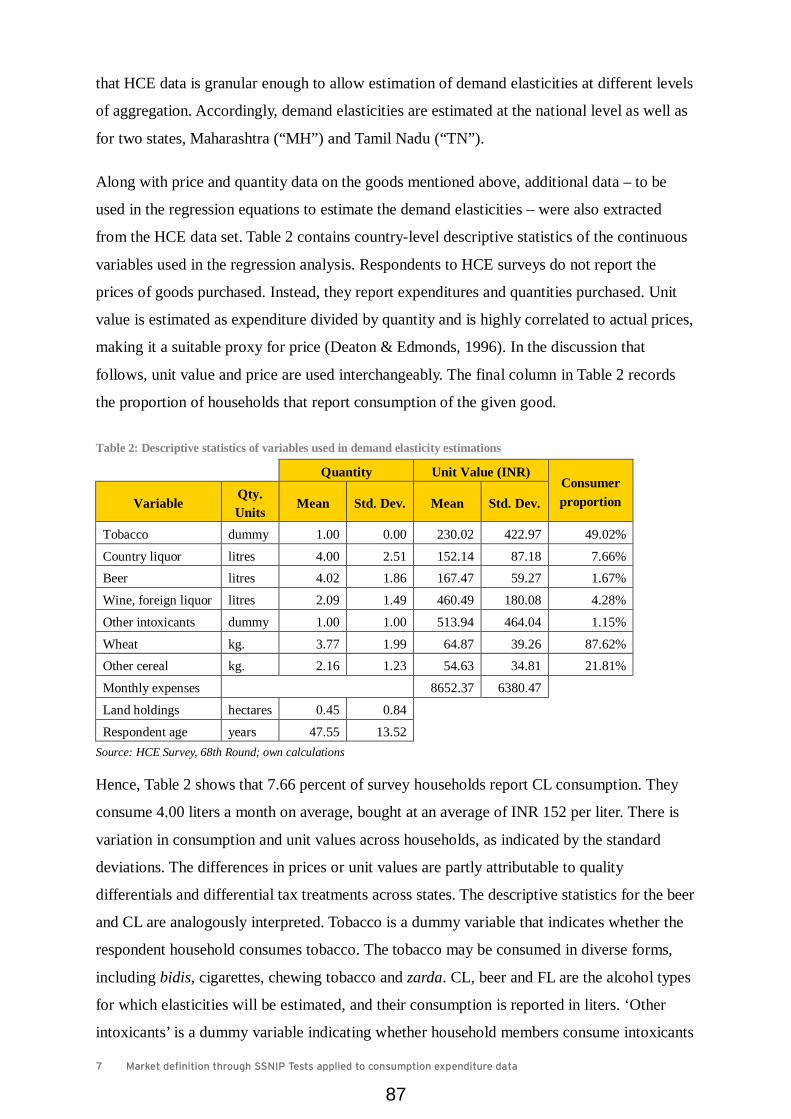
7 Market definition through SSNIP Tests applied to consumption expenditure data
that HCE data is granular enough to allow estimation of demand elasticities at different levels
of aggregation. Accordingly, demand elasticities are estimated at the national level as well as
for two states, Maharashtra (“MH”) and Tamil Nadu (“TN”).
Along with price and quantity data on the goods mentioned above, additional data – to be
used in the regression equations to estimate the demand elasticities – were also extracted
from the HCE data set. Table 2 contains country-level descriptive statistics of the continuous
variables used in the regression analysis. Respondents to HCE surveys do not report the
prices of goods purchased. Instead, they report expenditures and quantities purchased. Unit
value is estimated as expenditure divided by quantity and is highly correlated to actual prices,
making it a suitable proxy for price (Deaton & Edmonds, 1996). In the discussion that
follows, unit value and price are used interchangeably. The final column in Table 2 records
the proportion of households that report consumption of the given good.
Table 2: Descriptive statistics of variables used in demand elasticity estimations
Quantity Unit Value (INR) Consumer proportion Variable
Qty. Units
Mean Std. Dev. Mean Std. Dev.
Tobacco dummy 1.00 0.00 230.02 422.97 49.02%
Country liquor litres 4.00 2.51 152.14 87.18 7.66% Beer litres 4.02 1.86 167.47 59.27 1.67%
Wine, foreign liquor litres 2.09 1.49 460.49 180.08 4.28%
Other intoxicants dummy 1.00 1.00 513.94 464.04 1.15%
Wheat kg. 3.77 1.99 64.87 39.26 87.62% Other cereal kg. 2.16 1.23 54.63 34.81 21.81%
Monthly expenses 8652.37 6380.47
Land holdings hectares 0.45 0.84
Respondent age years 47.55 13.52 Source: HCE Survey, 68th Round; own calculations
Hence, Table 2 shows that 7.66 percent of survey households report CL consumption. They
consume 4.00 liters a month on average, bought at an average of INR 152 per liter. There is
variation in consumption and unit values across households, as indicated by the standard
deviations. The differences in prices or unit values are partly attributable to quality
differentials and differential tax treatments across states. The descriptive statistics for the beer
and CL are analogously interpreted. Tobacco is a dummy variable that indicates whether the
respondent household consumes tobacco. The tobacco may be consumed in diverse forms,
including bidis, cigarettes, chewing tobacco and zarda. CL, beer and FL are the alcohol types
for which elasticities will be estimated, and their consumption is reported in liters. ‘Other
intoxicants’ is a dummy variable indicating whether household members consume intoxicants
87

8 Market definition through SSNIP Tests applied to consumption expenditure data
other than those specifically listed in the HCE survey questionnaire. It largely refers to drug
consumption. Land holdings is a proxy for wealth and, along with age, is used as a control
variable. Monthly household expenses are INR 8652 with high variance.
Along with the variables in Table 2, data is also collected on factor variables, which are used
as fixed effects in the regressions. The factor variables are states, regions within states (as
defined in the HCE survey), cooking fuel type, and social group. The fixed effects capture
unmeasured variations in household characteristics, thereby improving estimator properties.
The “State” fixed effect, for example, captures state-level heterogeneity in household
consumption. Households in Maharashtra and Tamil Nadu are embedded in different social
and cultural milieus, which leads to differences in their consumption patterns. These socio-
cultural factors are not recorded in the data, but are captured through the use of fixed effects.
Some statistics on fixed effects are shown in Appendix A.
To estimate demand elasticities from the HCE data, the Heckman sample selection model
(Heckman, 1979) is applied. This model corrects for a common statistical sampling problem
referred to as the sample selection or incidental truncation problem. It appears when the
sample of interest (e.g. beer consumers in the HCE data) has different underlying
characteristics and is therefore not representative of the overall population (Heckman &
MaCurdy, 1986). This obscures the “true” causal effect between the outcome (e.g. beer
demand) and the causal factor (e.g. beer price). It becomes infeasible to determine which part
of the outcome is attributable to causal factor and which part to differences between the
sample and the general population (Toomet & Henningsen, 2008). This leads to problems
with the statistical properties of conventional estimators such as least squares (Greene, 2002).
An empirical strategy like the Heckman sample selection model is needed to separate these
two effects. This model is described in Appendix B.
The Heckman strategy models the sample selection problem as a two-step decision making
process. The first step consists of “selecting” whether to take an action or not (e.g. to drink
beer). The second step, which is contingent on the first, requires actions that lead to the
observed “outcome” (actual beer consumption). Both steps are modeled through two
regression equations: the selection and outcome equations.
In practice, most explanatory variables for the selection equation are also needed for the
outcome equation. This can introduce multicollinearity into the model, which leads to inflated
variances for parameter estimates. The estimates become inefficient. To control for
multicollinearity in Heckman sample selection models, instrumental variables are used
88

9 Market definition through SSNIP Tests applied to consumption expenditure data
(Sousa, 2014; Toomet & Henningsen, 2008). Strong candidates for instrumental variables are
those that are correlated with the selection decision, but are uncorrelated with the error in the
outcome equation. In other words, these are variables that correlate with the decision to drink
or not drink beer, but once the beer-drinking decision has been made, do not affect the
quantity of beer consumed. Our selected instruments are the decisions to consume other
alcohol types. This is because consumers of beer are also likely consume other types of
alcohol and vice versa. Hence, beer selection will be correlated with FL and CL selection. At
the same time, selection of FL and CL does not affect the quantity of beer consumed by an
individual (i.e. the beer outcome). The alcohol selection decision is captured by a dummy
variable that is constructed from the HCE data.
Along with the instrumental variables, the regression analysis also uses control variables. If
these variables were not considered, then the model would suffer from omitted variable bias.
The selected control variables are state or region-level fixed effects, fixed effects for cooking
fuel type and social group, age, land ownership, and some dietary elements. Age refers to the
age of the primary householder. The dietary controls account for household level
heterogeneity as well as some household expenses.
3. Empirical Results
Table 3 presents regression results under an OLS estimation. Nine OLS estimations were run
in total. In each regression, the dependent variable was the log of quantity consumed. The
relevant explanatory variables are listed in the left-most column. 𝑑𝑑𝑡𝑡𝑡𝑡𝑡𝑡 is a dummy variable
indicating whether one or more members of the household consumes tobacco and 𝑝𝑝𝑡𝑡𝑡𝑡𝑡𝑡 is the
monthly expenditure on tobacco. 𝑝𝑝𝐶𝐶𝐶𝐶 ,𝑝𝑝𝑡𝑡𝑏𝑏𝑏𝑏𝑏𝑏 and 𝑝𝑝𝐹𝐹𝐶𝐶 are monthly household expenditures on
country liquor, beer and foreign liquor respectively and 𝑀𝑀𝑀𝑀𝑀𝑀 is the total monthly household
expenditure. Logs of prices and expenditure are used because this allows their coefficients to
be interpreted as elasticities or semi-elasticities. The regression also includes control
variables whose coefficients are not reported for brevity. The control variables and their use
are discussed in Section 2.
Table 3: Elasticity estimates under OLS
Country liquor Beer Wine & foreign liquor IN MH TN IN MH TN IN MH TN
𝐼𝐼𝐼𝐼𝑡𝑡𝐼𝐼𝐼𝐼𝑐𝑐𝐼𝐼𝑝𝑝𝑡𝑡 -0.027 1.438 11.620* -0.260 -1.561 0.650 -1.615** 0.340 -3.164**
𝑑𝑑𝑡𝑡𝑡𝑡𝑡𝑡 -0.103** -0.030 -0.081 -0.006 -0.011 -0.107 0.015 -0.111 0.171**
𝑙𝑙𝑙𝑙𝑙𝑙(𝑝𝑝𝑡𝑡𝑡𝑡𝑡𝑡) 0.119** - 0.121 0.076** 0.164* 0.040 0.102** - 0.129**
𝑙𝑙𝑙𝑙𝑙𝑙(𝑝𝑝𝐶𝐶𝐶𝐶) -0.423** -0.557** -0.449** -0.067** 0.143 -0.097 0.017 0.614† -0.074
89

10 Market definition through SSNIP Tests applied to consumption expenditure data
Country liquor Beer Wine & foreign liquor IN MH TN IN MH TN IN MH TN
𝑙𝑙𝑙𝑙𝑙𝑙(𝑝𝑝𝑡𝑡𝑏𝑏𝑏𝑏𝑏𝑏) -0.023 -0.134 -0.335 -0.073** -0.348** -0.402** -0.016 -0.276 -0.016
𝑙𝑙𝑙𝑙𝑙𝑙(𝑝𝑝𝐹𝐹𝐶𝐶) -0.047** -0.120 -1.591† -0.122** -0.063 -0.041 -0.518** -0.745** -0.122
𝑙𝑙𝑙𝑙𝑙𝑙(𝑀𝑀𝑀𝑀𝑀𝑀) 0.333** 0.489** 0.267† 0.296** 0.347** 0.359** 0.499** 0.360** 0.433**
Observations 7785 480 67 1694 110 152 4349 94 695
F Statistic 271.77** 10.81** 2.70* 25.89** 3.35** 4.66** 177.88** 5.39** 20.90**
Adjusted 𝑅𝑅2 0.28 0.27 0.15 0.16 0.13 0.18 0.25 0.32 0.17 Note: **, * and † indicate significance at the 1%, 5% and 10% levels. Source: own calculations
The second to fourth columns from the left contain the results for CL, the next three columns
contain the beer results and the three right-most columns contain the results for FL. Results
are estimated for India as a whole, and for the states of Maharashtra and Tamil Nadu. All
own-price elasticities are highlighted in yellow.
All own-price elasticities are negative and significant (with the exception of FL in TN) at the
one percent level. The significant own-price elasticities hover around -0.50 across
geographies and alcohol types and never exceed -0.75. The OLS results therefore indicate
that consumers are own-price inelastic in their demand for alcohol. This is particularly true
for beer consumption at the all-India level: demand appears almost completely inelastic.
Own-price elasticity indicates the percentage change in demand because of a one percent
change in price. An elasticity of -0.50 therefore indicates that demand falls by 2.5% and 5%
for 5% and 10% SSNIPs respectively. The own-price elasticities in Table 3 are below the
reference critical elasticities in Table 1, which indicates that a Hypothetical Monopolist
would be able to implement a SSNIP in these markets. These markets could therefore be
defined as relevant antitrust markets.
Once the relevant market has been defined, the competitiveness analysis can begin. One
method for assessing market power is to consider cross-price elasticities with substitute
products. Table 3 shows that cross-price elasticities are either low or not significant,
indicating limited substitution across alcohol types. The remaining coefficients reported in
Table 3 pertain to smoking and monthly household expenditure. The tobacco dummy and
price are included are control variables because of the correlation between tobacco and
alcohol consumption (Sousa, 2014). The coefficients for 𝑙𝑙𝑙𝑙𝑙𝑙(𝑀𝑀𝑀𝑀𝑀𝑀) indicate that consumers
are income-inelastic with respect to alcohol consumption. A one percent increase in income
only increases alcohol demand by 0.27 – 0.50 percent, depending on alcohol type and region.
90

11 Market definition through SSNIP Tests applied to consumption expenditure data
Table 4 presents regression results under the Heckman sample selection model. The same
products and regions were considered as in the OLS regressions. The dependent variable in
the selection equation is, as indicated in equation (5), a consumption dummy. The dependent
variable in the outcome equation is the log of quantity consumed. The outcome equation and
the OLS regressions have the same dependent variables. Covariance parameters (𝜌𝜌) are
significant for all regressions, indicating correlation between errors in the selection and
outcome equations. One may infer that the OLS results are significantly biased.
Table 4: Elasticity estimates under the Heckman sample selection model
Country liquor Beer Wine & foreign liquor IN MH TN IN MH TN IN MH TN
Selection equation
𝐼𝐼𝐼𝐼𝑡𝑡𝐼𝐼𝐼𝐼𝑐𝑐𝐼𝐼𝑝𝑝𝑡𝑡 -0.269 -0.771 -3.157 -4.744** -6.977** 2.406 -5.247** -10.144** -1.416
𝑑𝑑𝑡𝑡𝑡𝑡𝑡𝑡 0.789** 0.997** 0.817** 0.454** 0.443** 0.525** 0.730** 0.594** 1.044**
𝑑𝑑𝐶𝐶𝐶𝐶 - - - -0.315** -0.601* -0.553 -0.508** -0.873** -0.926**
𝑑𝑑𝑡𝑡𝑏𝑏𝑏𝑏𝑏𝑏 -0.406** -0.769* -0.603 - - - -0.296** -0.596 -1.107**
𝑑𝑑𝐹𝐹𝐶𝐶 -0.613** -0.803** -0.748** -0.253** -0.600 -0.992** - - -
𝑙𝑙𝑙𝑙𝑙𝑙(𝑝𝑝𝑡𝑡𝑡𝑡𝑡𝑡) 0.039** 0.105** -0.122 0.112** 0.279** 0.1 0.106** - 0.186**
𝑙𝑙𝑙𝑙𝑙𝑙(𝑝𝑝𝐶𝐶𝐶𝐶) -0.453** -0.526** -0.402** -0.181** 0.045 -0.01 -0.056** 0.362 0.221**
𝑙𝑙𝑙𝑙𝑙𝑙(𝑝𝑝𝑡𝑡𝑏𝑏𝑏𝑏𝑏𝑏) -0.042* 0.255* 0.329† -0.385** -0.467* -0.518** 0.028 0.126 0.074
𝑙𝑙𝑙𝑙𝑙𝑙(𝑝𝑝𝐹𝐹𝐶𝐶) 0.040† -0.071 0.318 0.026 0.052 -0.848* -0.469** -0.343† -0.660**
𝑙𝑙𝑙𝑙𝑙𝑙(𝑀𝑀𝑀𝑀𝑀𝑀) 0.062** 0.009 0.232* 0.476** 0.559** 0.482** 0.562** 0.764** 0.336**
Outcome equation
𝐼𝐼𝐼𝐼𝑡𝑡𝐼𝐼𝐼𝐼𝑐𝑐𝐼𝐼𝑝𝑝𝑡𝑡 0.117 1.590 12.945** -0.076 -5.931 0.015 -1.813** -10.124* -5.031**
𝑑𝑑𝑡𝑡𝑡𝑡𝑡𝑡 -0.158** -0.201 0.144 -0.038† 0.170 -0.202* 0.039† 0.429† 1.176**
𝑙𝑙𝑙𝑙𝑙𝑙(𝑝𝑝𝑡𝑡𝑡𝑡𝑡𝑡) 0.115** - 0.093 0.054** 0.273* 0.023 0.109** - 0.268**
𝑙𝑙𝑙𝑙𝑙𝑙(𝑝𝑝𝐶𝐶𝐶𝐶) -0.391** -0.474** -0.573** -0.033† 0.212 -0.120 0.022 0.955* 0.193**
𝑙𝑙𝑙𝑙𝑙𝑙(𝑝𝑝𝑡𝑡𝑏𝑏𝑏𝑏𝑏𝑏) -0.018 -0.183 -0.316 -0.018 -0.543* -0.303** -0.013 0.034 0.049
𝑙𝑙𝑙𝑙𝑙𝑙(𝑝𝑝𝐹𝐹𝐶𝐶) -0.054** -0.097 -1.832* -0.093** 0.068 0.118 -0.530** -1.043** -0.690**
𝑙𝑙𝑙𝑙𝑙𝑙(𝑀𝑀𝑀𝑀𝑀𝑀) 0.328** 0.496** 0.257† 0.254** 0.596* 0.343** 0.508** 0.968** 0.483**
Variance-covariance parameters
𝜌𝜌 -0.181** -0.288† 0.534* -0.348** 0.751* -0.483* 0.080* 0.939** 0.991**
𝜎𝜎 0.604** 0.689** 0.639** 0.454** 0.635* 0.445** 0.618** 1.120** 1.165**
Observations 101,651 8,044 6,646 101,651 8,044 6,646 101,651 8,044 6,646 Note: **, * and † indicate significance at the 1%, 5% and 10% levels. Source: own calculations
As discussed in Appendix B, the selection equation is estimated by probit. The coefficients in
a probit regression are log-odds, which can be used to estimate the marginal effects that have
a direct economic interpretation. Marginal effects are estimated and reported in the selection
equation results in Table 4, instead of log odds. The coefficients for continuous explanatory
91

12 Market definition through SSNIP Tests applied to consumption expenditure data
variables, such as log price, are thereby interpreted as the percentage change in the number of
consumers because of a one percent change in the explanatory variable defined at the mean.
The Heckman model is identified by using consumption dummies for other alcohol types
(𝑑𝑑𝐶𝐶𝐶𝐶 , 𝑑𝑑𝐹𝐹𝐶𝐶 , 𝑑𝑑𝑡𝑡𝑏𝑏𝑏𝑏𝑏𝑏) as instruments in the selection equation. These dummies are significant,
which indicates that they are appropriate instruments. A tobacco consumption dummy and
tobacco price are also included as control variables, along with fixed effects and demographic
variables mentioned in Table 2 and Appendix A.
The selection equation variables relevant to CEA are the logs of the prices of CL, beer and
FL. The own-price effects on the decision to consume (highlighted in light yellow) are
negative and significant. Thus, a significant proportion of consumers stop consuming a given
alcohol type when the price of that alcohol type increases marginally. This effect is wholly
uncaptured by an OLS regression framework. The cross-price coefficients are positive and
negative, depending on the region and alcohol type, indicating substitutability as well as
complementarity among alcohol types.
The outcome equation results are analogous to the OLS results in Table 3 and are similarly
interpreted. Own-price elasticities are negative and significant, and differ from the OLS
equivalents. The differences exist because of the sample selection bias in the OLS estimates.
In some cases, the bias has a large impact on the elasticity estimates. Own-price elasticity for
FL in Maharashtra, for example, goes from inelasticity under OLS (-0.75) to unit elasticity
after selection bias is accounted for (-1.04).
The results in Table 3 and Table 4 can be used in CEA, but since OLS is biased, the Table 3
results would lead to incorrect market definition. As estimated in Table 1, the critical
elasticity under a 10 percent SSNIP and a 50 percent price-cost margin is 1.67. The actual
elasticity under OLS is less than this for all region-product market combinations, indicating
that the relevant antitrust market is defined. The actual elasticity under the Heckman model is
also less than the critical elasticity (as shown by the outcome equation results in Table 4).
However, this elasticity estimate only accounts for customers who reduce demand in response
to the SSNIP. It does not account for customers who stop consumption completely in
response to the SSNIP (i.e. the selection equation results). By using the definition of elasticity
and the functional form of the selection equation, an adjusted elasticity estimate can be
calculated, which account for both selection and outcome effects. A comparison of all
elasticity estimates is found in Table 5.
92

13 Market definition through SSNIP Tests applied to consumption expenditure data
Table 5: Comparison of actual and critical elasticities
Country Liquor Beer Wine/IMFL/FMFL IN MH TN IN MH TN IN MH TN
𝜀𝜀𝑐𝑐𝑏𝑏𝑐𝑐𝑡𝑡 -1.667 -1.667 -1.667 -1.667 -1.667 -1.667 -1.667 -1.667 -1.667
𝜀𝜀𝑂𝑂𝐶𝐶𝑂𝑂 -0.423 -0.557 -0.449 -0.073 -0.348 -0.402 -0.518 -0.745 -0.122
𝜀𝜀𝐻𝐻𝐻𝐻 -0.391 -0.474 -0.573 -0.018 -0.543 -0.303 -0.530 -1.043 -0.690
Adjusted 𝜀𝜀𝐻𝐻𝐻𝐻 -0.474 -0.564 -0.639 -0.090 -0.622 -0.395 -0.599 -1.088 -0.786
𝐵𝐵𝐵𝐵𝐵𝐵𝑠𝑠𝑂𝑂𝐶𝐶𝑂𝑂 -0.051 -0.007 -0.190 -0.017 -0.274 0.007 -0.081 -0.343 -0.664 𝐵𝐵𝐵𝐵𝐵𝐵𝑠𝑠𝑂𝑂𝐶𝐶𝑂𝑂 / adj. 𝜀𝜀𝐻𝐻𝐻𝐻 10.67% 1.28% 29.70% 18.46% 44.06% -1.72% 13.53% 31.52% 84.47%
Source: own calculations
When both selection and outcome effects in the Heckman sample selection model are
considered, then the elasticity of demand is consistently higher than under OLS. But even this
higher adjusted Heckman elasticity of demand (adjusted 𝜀𝜀𝐻𝐻𝐻𝐻) is always less than the critical
elasticity (𝜀𝜀𝑐𝑐𝑏𝑏𝑐𝑐𝑡𝑡). Thus, both OLS and the Heckman methods show that the relevant antitrust
market can be defined at the state level in MH and TN. Further analysis may reveal that
actual elasticities exceed the critical elasticity in other states. In these cases, a state-level
market definition is too narrow. The pan-India market would then be the relevant market.
Table 5 shows that the OLS bias, defined as (adjusted 𝜀𝜀𝐻𝐻𝐻𝐻 − 𝜀𝜀𝑂𝑂𝐶𝐶𝑂𝑂) tends to be negative. The
sole positive bias, for beer in TN, is very small. The size of the bias varies substantially from
0.007 to -0.664. In percentage terms, the bias varies from -1.7 percent (beer in TN) to 84
percent (wine in TN). Not accounting for sample selection bias can therefore lead to severe
problems in elasticity estimation.
4. Conclusions
Indian practitioners of competition economics seldom use CEA and SSNIP Tests when
defining relevant antitrust markets. In this paper, we demonstrate that large sample, third
party data sets, which may have been collected for other reasons, like the HCE data collected
by the NSSO, contain the depth of information necessary for the implementation of SSNIP
Tests for a range of consumer goods. Apart from implementing SSNIP Tests, the HCE data is
also suitable for cross-elasticity analysis, which can be used as a quantitative element of the
competition analysis subsequent to market definition.
We also show that the application of conventional estimators like OLS can lead to biased
estimates and incorrect market definition, because these estimators do not control for sample
selection or incidental truncation problems. To get rid of the bias in OLS and other
conventional estimators, estimators like those designed in Heckman (1979) can be used.
93

14 Market definition through SSNIP Tests applied to consumption expenditure data
Our comparison of the OLS and Heckman results shows that the OLS tends to bias demand
elasticity estimates towards zero, thereby leading the competition economist to narrower
market definition than might actually be warranted. In some cases, the amount of bias is
substantial. In the nine candidate markets considered by us, the size of the bias ranged from
1.7 percent to 84 percent of the bias-corrected Heckman demand elasticity estimate.
One can see how biased elasticity estimates can lead to incorrect market definition by
considering an example. Consider, a case where critical elasticity is 1.67, OLS elasticity is
1.50 and the true elasticity is 1.80. If only OLS was used, then the competition economist
would come to the incorrect conclusion that the market was defined. In actuality, the market
would have to be expanded to find the relevant market.
This paper represents a preliminary attempt at surmounting challenges in market definition in
India. Further avenues of research could look at alternate third party data sources; or design
or identify alternate estimation strategies for market definition and other quantitative
exercises relevant to the economics of competition law in India.
Bibliography
Amelio, A., & Donath, D. (2009). Market definition in recent EC merger investigations: The role of empirical analysis. Concurrences, 3, 1-6.
Baker, J. (2007). Market definition: An analytical overview. Antitrust Law Journal, 74(1), 129-173.
Becker, G. (1962). Irrational behavior and economic theory. Journal of Political Economy, 1-13.
Cameron, A., & Trivedi, P. (2005). Microeconometrics: Methods and Applications. New York: Cambridge University Press.
Deaton, A., & Edmonds, E. (1996). Measuring consumption and price in LSMS surveys. Princeton, NJ: Research Progam in Development Studies, Princeton University.
DOJ & Federal Trade Commission. (1992). Horizontal Merger Guidelines. Washington, DC: DOJ.
DOJ & FTC. (2010). Horizontal Merger Guidelines. Washington, DC: DOJ. DOJ. (1982). Merger Guidelines. Washington, DC: DOJ. European Commission. (1997). Commission notice on the definition of relevant market for
the purposes of Community competition law. Official Journal of the European Commission, C372, 5-13.
Greene, W. (2002). Econometric Analysis (5th ed.). Prentice Hall. Harbord, D., & von Graevenitz, G. (2000). Market definition in oligopolistic and vertically
related markets: Some anomalies. European Competition Law Review, 21(3), 151-158.
Harris, R., & Simons, J. (1989). Focusing market definition: How much substitution is necessary? Journal of Research in Law and Economics, 12, 207-226.
Heckman, J. (1979). Sample selection bias as a specification error. Econometrica, 47(1), 153-161.
Heckman, J., & MaCurdy, T. (1986). Labor econometrics. In Z. Griliches, & M. Intriligator
94

15 Market definition through SSNIP Tests applied to consumption expenditure data
(Eds.), Handbook of Econometrics (Vol. 3, pp. 1917-1977). Amsterdam: Elsevier. Hueschelrath, K. (2009). Critical loss analysis in market definition and merger control.
Mannheim: Centre for European Economic Research Discussion Paper No. 09-083. Kamerschen, D., & Kohler, J. (1993). Residual demand analysis of the ready-to-eat breakfast
cereal market. Antitrust Bulletin, 38(4), 903-942. Massey, P. (2000). Market definition and market power in competition analysis: Some
practical issues. The Economic and Social Review, 31(4), 309-328. NSSO. (2011). Introduction: Coverage, Concepts, Design, Definitions. In NSSO, NSS 68th
Round Instructions to Field Staff. New Delhi: Ministry for Statistics & Program Implementation.
NSSO. (2012). Household consumer expenditure across socio-economic groups, 2011-12. New Delhi: Ministry of Statistics & Programme Implementation, NSS Report No. 562.
O'Brien, D., & Wickelgren, A. (2003). A critical analysis of critical loss analysis. FTC Working Paper.
Sousa, J. (2014). Estimation of price elasticities of demand for alcohol in the UK. London: HM Revenue & Customs Working Paper 16.
Toomet, O., & Henningsen, A. (2008). Sample selection models in R: Package sampleSelection. Journal of Statistical Software, 27(7).
Woolridge, J. (2003). Introductory Econometrics: A Modern Approach (2nd ed.). Thomson South-Western.
95

16 Market definition through SSNIP Tests applied to consumption expenditure data
Appendix A Descriptive statistics for fixed effects
Demand elasticity estimation using HCE survey data requires the use of factor variables, which are used as fixed effects. The factor variables are cooking fuel, social group, states (for the nation-level estimation) and regions within states (for the state-level estimations). The regions within states have been defined by the NSSO. Table 6 shows the distribution of the sample population by the type of cooking fuel used. Most households in the sample – and by inference in India – use either firewood, liquefied petroleum gas (“LPG”) or electricity when cooking food. These categories account for 87% of all households. Cow dung or gobar is the preferred cooking fuel for five percent of households. The remaining households use coal or kerosene, or do not cook at home.
Table 6: Distribution of sample households by cooking fuel type
Type of cooking fuel Frequency Proportion No cooking 1,873 1.84%
Coal / Charcoal 1,711 1.68% Firewood 44,893 44.16%
LPG / Electricity 43,796 43.08%
Cow dung 4,870 4.79%
Kerosene 2,526 2.48% Other (unspecified) 1,982 1.95%
Total 101,651 100% Source: HCE Survey, 68th Round; own calculations
Table 7 shows the distribution of sample households by social group. The social groups considered in the HCE survey are Scheduled Tribes (“ST”), Scheduled Castes (“SCs”), Other Backward Classes (“OBCs”) and an Others or general category. The greatest proportion of the sample is drawn from the OBC category and smaller proportions from the SC and ST categories. To the extent that the HCE sample is representative of the overall population, the proportions in Table 7 would apply to India as a whole.
Table 7: Distribution of sample households by social group
Social Group Frequency Proportion Unspecified 15 0.01%
Scheduled Tribes 13566 13.35% Scheduled Castes 15757 15.50%
Other Backward Classes 39677 39.03%
Others 32636 32.11%
Total 101651 100.00% Source: HCE Survey, 68th Round; own calculations
Figure 1 presents data on the distribution of the sample population and cooking fuel types across the states selected for demand elasticity estimation. The lowest bar (Respondents) indicates the percentage of the total sample drawn from a given state. It indicates that the two selected states account for almost 15% the 100,000+ sample. MH accounts for 7.9% of all sampled households, while TN accounts for 6.5%. These proportions are commensurate with the states’ populations.
The other bars in Figure 1 show the contributions of the states to the total number of users of the different cooking fuel types. By comparing the sizes of the color bars to the Respondents color bar, one may determine whether a given state is over- or under-represented in the use of a given cooking fuel. Compare, for example, the bars for cow dung and coal to that for Respondents. The grey bar for MH for cow dung and coal is smaller than for Respondents. There is no blue bar for TN for cow dung and coal. This indicates that MH and TN have proportionately lesser representation among households who use cow dung or coal for cooking, when compared to the national average. These results are consistent with the hypothesis that cow dung and coal use is proportionately greater among the rural poor. Since MH and TN are less rural and have higher monthly per capital expenditures than the average they have a proportionately lesser presence among cow dung users.
96

17 Market definition through SSNIP Tests applied to consumption expenditure data
Figure 1: Proportions of cooking fuel types in selected states
Source: HCE Survey 68th Round; own calculations
Figure 2 replicates the analysis in Figure 1, but for social groups. One sees, for example, that OBCs are over-represented when TN and MH are considered together. But, by comparing the OBC row and the Respondents row, one sees that this over-representation is wholly attributed to TN. MH slightly under-represented. The other social groups are underrepresented slightly. It is interesting to note that the majority of the TN sample is drawn from the SC and OBC categories. To the extent that this sample represents the TN population, it indicates that the vast majority of the TN population self-selects into these social groups. It would be interesting to research the correlation between this self-selection and the political and reservation structures in the state. MH, by contrast, has a less distorted distribution across social groups.
Figure 2: Proportions of social group types in selected states
Source: HCE Survey 68th Round; own calculations
97

18 Market definition through SSNIP Tests applied to consumption expenditure data
Appendix B The Heckman sample selection model
Our elucidation of the Heckman sample selection model is drawn from Toomet & Henningsen, (2008). Other resources include Greene (2002), Woolridge (2003) and Cameron & Trivedi (2005). The model begins with the assumption of an unobserved structural process, which is characterized by the selection and outcome equations [(3) and (4)] below.
𝑦𝑦𝑐𝑐𝑂𝑂∗ = 𝑥𝑥𝑐𝑐𝑂𝑂𝛽𝛽𝑂𝑂 + 𝜀𝜀𝑐𝑐𝑂𝑂 (3)
𝑦𝑦𝑐𝑐𝑂𝑂∗ = 𝑥𝑥𝑐𝑐𝑂𝑂𝛽𝛽𝑂𝑂 + 𝜀𝜀𝑐𝑐𝑂𝑂 (4)
The structural process models a two-step choice decision process. The first step consists of a selection choice. The second step consists of a follow-on choice contingent on the earlier selection, which leads to the outcome. 𝑦𝑦𝑐𝑐𝑂𝑂∗ is the latent or unobserved selection decision by individual 𝐵𝐵 and 𝑦𝑦𝑐𝑐𝑂𝑂∗ is the latent outcome. 𝑥𝑥𝑐𝑐𝑂𝑂 and 𝑥𝑥𝑐𝑐𝑂𝑂 are the explanatory variables for the selection and outcome equations respectively. Although 𝑦𝑦𝑐𝑐𝑂𝑂∗ and 𝑦𝑦𝑐𝑐𝑂𝑂∗ are not observed, two indicator variables 𝑦𝑦𝑐𝑐𝑂𝑂 and 𝑦𝑦𝑐𝑐𝑂𝑂 are, where
𝑦𝑦𝑐𝑐𝑂𝑂 = �0 𝐵𝐵𝑖𝑖 𝑦𝑦𝑐𝑐𝑂𝑂∗ < 01 𝑙𝑙𝑡𝑡ℎ𝐼𝐼𝐼𝐼𝑒𝑒𝐵𝐵𝑠𝑠𝐼𝐼
(5)
𝑦𝑦𝑐𝑐𝑂𝑂 = �
0 𝐵𝐵𝑖𝑖 𝑦𝑦𝑐𝑐𝑂𝑂 = 0𝑦𝑦𝑐𝑐𝑂𝑂∗ 𝑙𝑙𝑡𝑡ℎ𝐼𝐼𝐼𝐼𝑒𝑒𝐵𝐵𝑠𝑠𝐼𝐼
(6)
Coming back to our beer example, the model in equations (3)-(6) describes a decision process where individual 𝐵𝐵 first selects whether or not to drink beer. This decision is affected by explanatory variables 𝑥𝑥𝑂𝑂 and unmeasured factors and random error 𝜀𝜀𝑂𝑂. If he decides not to drink, then 𝑦𝑦𝑐𝑐𝑂𝑂 = 0, otherwise 𝑦𝑦𝑐𝑐𝑂𝑂 = 1. If 𝐵𝐵 selects to drink beer, his follow-on decision is about how much beer (𝑦𝑦𝑐𝑐𝑂𝑂∗) to drink, which is affected by 𝑥𝑥𝑂𝑂 and 𝜀𝜀𝑂𝑂. The contingency of the second decision on the first is shown by equation (6), which tracks observed beer consumption. Because of the structure of the decision process, 𝑦𝑦𝑂𝑂 is observed only when 𝑦𝑦𝑂𝑂∗ > 0. The dependence of 𝑦𝑦𝑂𝑂 and 𝑥𝑥𝑂𝑂 can thereby be written as
𝑀𝑀[𝑦𝑦𝑂𝑂|𝑥𝑥𝑂𝑂 = 𝑥𝑥𝑐𝑐𝑂𝑂 , 𝑥𝑥𝑂𝑂 = 𝑥𝑥𝑐𝑐𝑂𝑂;𝑦𝑦𝑂𝑂 = 1] = 𝑥𝑥𝑐𝑐𝑂𝑂𝛽𝛽𝑂𝑂 + 𝑀𝑀[𝜀𝜀𝑂𝑂|𝜀𝜀𝑂𝑂 ≥ −𝑥𝑥𝑐𝑐𝑂𝑂𝛽𝛽𝑂𝑂] (7)
Let 𝑀𝑀[𝜀𝜀𝑂𝑂|𝜀𝜀𝑂𝑂 ≥ −𝑥𝑥𝑐𝑐𝑂𝑂𝛽𝛽𝑂𝑂] be defined as the control function. Since the control function is non-zero unless 𝜀𝜀𝑂𝑂 and 𝜀𝜀𝑂𝑂 are independent, conventional estimators of 𝑦𝑦𝑂𝑂, like OLS, are biased. The Heckman model assumes that 𝜀𝜀𝑂𝑂 and 𝜀𝜀𝑂𝑂 are distributed bivariate normal with correlation 𝜌𝜌 (see equation (8)). When 𝜌𝜌 > 0, then 𝜀𝜀𝑂𝑂 and 𝜀𝜀𝑂𝑂 are positively correlated, and vice versa.
�𝜀𝜀𝑂𝑂
𝜀𝜀𝑂𝑂�~𝑁𝑁��
00� , �
1𝜌𝜌𝜌𝜌𝜎𝜎2��
(8)
Given this assumption, the Heckman strategy proceeds by first estimating the control function from equations (3) and (5) by probit, and then inserting this estimate into the outcome equation (4) as additional covariates. Using the properties of a bivariate normal distribution one obtains the outcome estimation equation (9)
𝑦𝑦𝑐𝑐𝑂𝑂 = 𝑥𝑥𝑐𝑐𝑂𝑂𝛽𝛽𝑂𝑂 + 𝑀𝑀[𝜀𝜀𝑂𝑂|𝜀𝜀𝑂𝑂 ≥ −𝑥𝑥𝑐𝑐𝑂𝑂𝛽𝛽𝑂𝑂] ≡ 𝑥𝑥𝑐𝑐𝑂𝑂𝛽𝛽𝑂𝑂 + 𝜌𝜌𝜎𝜎𝜌𝜌(𝑥𝑥𝑐𝑐𝑂𝑂𝛽𝛽𝑂𝑂) + 𝜈𝜈𝑐𝑐 (9)
where 𝜌𝜌(⋅) = 𝜙𝜙(⋅)/Φ(⋅) is the inverse Mills ratio, 𝜙𝜙(⋅) and Φ(⋅) are probability and cumulative distribution functions of a standard normal distribution, and 𝜈𝜈 is an independent and identically distributed error term. As noted by Toomet & Henningsen (2008), the Heckman method repurposes sample selection problem as an omitted variable problem, where 𝜌𝜌(⋅) is the omitted variable that is estimated by probit as a first step.
The sign on 𝜌𝜌 indicates the direction of bias when conventional estimators like OLS are used because it affects the sign of the control function (see (9)). This is known because 𝜎𝜎 and 𝜌𝜌(⋅) are positive by definition. 𝜌𝜌 > 0 implies a positive control function, which in turn implies that observable outcomes have positive realizations of 𝜀𝜀𝑂𝑂 in the mean; a phenomenon referred to as “positive selection”. The observed outcomes 𝑦𝑦𝑐𝑐𝑂𝑂∗ are higher than they would be if 𝜀𝜀𝑂𝑂 and 𝜀𝜀𝑂𝑂 were not positively correlated. Further details, including those related to consistent estimation of the variance covariance matrix are not provided.
98

Application of Economic Tools for Relevant Market Definition: The
Experience in India
By
Jincy Elizabeth Francis
Managing Economist, Nathan Economic Consulting India Pvt Ltd
March 2017
Paper presented at CCI’s National Conference on the Economics of Competition Law, 2017
on 2 March 2017
99
1
Abstract
Relevant market definition is an important tool in competition assessment. Economic analysis
enables relevant markets to be defined in a scientific and robust manner. However, there
exist certain practical challenges related to data availability and applicability of the tools
that need to be considered while applying these tools. Over the years, in India, economic
tools (such as catchment area analysis and Elzinga Hogarty test) have been increasingly
used to define the relevant market. This paper discusses India’s experience in applying
economic tools for relevant market definition, including areas for potential improvement.
100

2
Introduction
Relevant market comprises of two components – relevant product market1 and relevant
geographic market.2 It includes “all reasonably substitutable products or services, and all
nearby competitors, to which consumers could turn in the near term” if the price increased
by a small but significant amount.3
Despite recent discussion in the antitrust community regarding the significance of market
definition in competition assessment, defining the relevant market continues to be an
important step in assessing the extent of competitive constraint in abuse of dominance
investigations and merger control.4
Appropriate definition of the relevant market is extremely important because an incorrectly
defined relevant market can result in wrong conclusions about market power and, therefore,
effect on competition. On the one hand, a relevant market defined too narrowly can result in
the incorrect conclusion that a firm possesses market power (when in reality it does not). On
the other hand, a relevant market defined too broadly can result in the wrong inference that a
firm does not possess market power (although in the correctly defined relevant market it may
be dominant).
This paper provides an overview of the various economic tools that can be used to define the
relevant market (with practical examples from advanced jurisdictions), highlights key
practical points that need to be considered while applying these tools, and discusses India’s
experience with the application of such tools.
Economic tools used to delineate the relevant market
To ensure that the relevant market defined for competition assessment is robust and scientific
(and therefore reliable), antitrust practitioners often use a wide variety of economic tools. In
this section, we discuss some of the commonly used tools.
1 The Competition Act, 2002, defines the relevant product market as “a market comprising all those products or
services which are regarded as interchangeable or substitutable by the consumer, by reason of characteristics
of the products or services, their prices and intended use”. Source: Section 2(t) of Competition Act, 2002. 2 According to the Competition Act, 2002, the relevant geographic market comprises “the area in which the
conditions of competition for supply of goods or provision of services or demand of goods or services are
distinctly homogenous and can be distinguished from the conditions prevailing in the neighbouring areas.”
Source: Section 2(s) of Competition Act, 2002 3 Continued Work on the Elaboration of a Model Law or Laws on Restrictive Business Practices (20 February
1998). UNCTAD, TD/B/RBP/81/Rev.5 4 Market Definition (11 October 2012). OECD Policy Roundtables. Directorate For Financial And Enterprise
Affairs Competition Committee. DAF/COMP(2012)19. Retrieved from
<http://www.oecd.org/daf/competition/Marketdefinition2012.pdf>
101

3
i. Small but Significant and Non-transitory Increase in Price (SSNIP) Test
This test (also known as the hypothetical monopolist test) is based on the concept of demand
substitution and can be used to define the relevant product or geographic market. The SSNIP
test starts with the narrowest possible market and assesses whether a hypothetical monopolist
can profitably increase the price of the product in the particular area by 5-10%.5 If consumers
respond to the price increase by switching to an alternate product (or supplier from a different
area) making the price increase unprofitable, then the relevant market is expanded to include
the substitute product or area.6
This test was used to define the relevant market in Nestlé/Perrier. Nestlé submitted that there
is no separate market for bottled source water and that the relevant product market should
include all non-alcoholic refreshment beverages, including both bottled source water and soft
drinks.7 However, the European Commission (EC) concluded that “it cannot be reasonably
expected that an appreciable non-transitory increase in the price of source waters compared
with that of soft drinks would lead to a significant shift of demand from source waters to soft
drinks for reasons of price only”.8 The EC arrived at this conclusion based on the following
factors: (a) there was a significant difference in the absolute prices of bottled water and soft
drinks (the price ratio was between 2 and 3); (b) bottled water is advertised as natural, pure
and healthy, which affects substitution of bottled water with soft drinks for daily use at home;
and (c) the prices of the two products moved differently over the last five years (the price of
bottled water increased in both absolute and real terms, despite the price of soft drinks
declining during this period).9
The SSNIP test may be applied using different economic analysis.10 For instance, the critical
loss analysis assesses how the actual loss in sales borne by a firm from a price increase
5 Horizontal Merger Guidelines (19 August 2010). U.S. Department of Justice and Federal Trade Commission.
Retrieved from < https://www.justice.gov/atr/horizontal-merger-guidelines-08192010> 6 Ibid 7 92/553/EEC: Commission Decision of 22 July 1992 relating to a proceeding under Council Regulation (EEC)
No 4064/89 (Case No IV/M.190 - Nestlé/Perrier); Official Journal L 356 , 05/12/1992 P. 0001 – 0031
<http://eur-lex.europa.eu/legal-content/EN/TXT/?uri=CELEX%3A31992D0553> 8 Ibid 9 Ibid 10 ‘Could’ or ‘Would’? The Difference between Two Hypothetical Monopolists (November 2008). Oxera.
Retrieved from < http://www.oxera.com/Oxera/media/Oxera/downloads/Agenda/Hypothetical-
monopolists.pdf>
Diversion Ratios: Why Does It Matter Where Customers Go If A Shop Is Closed (February 2009). Oxera.
Retrieved from < http://www.oxera.com/Oxera/media/Oxera/downloads/Agenda/Diversion-
ratios.pdf?ext=.pdf>
102

4
compares to the “critical loss” benchmark (where the fall in sales due to certain consumers
not buying the firm’s product anymore is offset by the rise in profits from the higher price
being paid by consumers who continue to buy the product).11 If the actual loss in sales is
greater than the critical loss benchmark, it implies that the price increase will be unprofitable.
Another analysis that is used as part of the SSNIP test to identify closest substitutes is
diversion ratios, which “measure the proportion of sales captured by different substitute
products when the price of a product is increased”.12 When the hypothetical monopolist
increases price by 5-10%, the substitute to which a larger proportion of consumers shift is the
closest substitute for the product, and is therefore included in the relevant market.13 Diversion
ratios are particularly useful in identifying the closest substitute in the case of differentiated
products.14 It may be estimated from data collected by businesses using demand estimation
techniques, or through consumer surveys.15
ii. Price Analysis
Price analysis can be used to define the relevant product or geographic market. The most
commonly used price analysis to define the relevant market is price correlation analysis.
Correlation analysis is a statistical tool used to assess the extent to which two or more
variables move together. The rationale behind using price correlation analysis to define the
relevant market is that if two products/areas are part of the same relevant market, their prices
tend to move similarly because of the competitive pressure exerted by one on the other.16
However, it is important to note that strong correlation between prices could also be due to
various other factors such as similarity in costs, general economic condition, or seasonal
factors. Therefore, more rigorous techniques of price analysis such as correlation between
price differences,17 stationarity analysis,18 and assessment of a long run co-integrating
relationship between the prices19 may be more appropriate.
11 ‘Could’ or ‘Would’? The Difference between Two Hypothetical Monopolists (November 2008). Oxera,
Retrieved from < http://www.oxera.com/Oxera/media/Oxera/downloads/Agenda/Hypothetical-
monopolists.pdf> 12 Diversion Ratios: Why Does It Matter Where Customers Go If A Shop Is Closed (February 2009). Oxera.
Retrieved from < http://www.oxera.com/Oxera/media/Oxera/downloads/Agenda/Diversion-
ratios.pdf?ext=.pdf> 13 Ibid 14 Ibid 15 Ibid 16 Katsoulacos Y., Konstantakopoulou K., Metsiou E. and Tsionas E. G. (2013). Quantitative Price Tests in
Antitrust Market Definition with an Application to the Savory Snacks Markets. Working Paper Series. Athens
University of Economics and Business. 17 “It is customary to compute the correlation coefficient using the natural logarithm (log) of the price series,
both due to efficiency reasons and because the first log difference is an approximation of the growth rate.
103

5
In Arsenal/DSP, the EC used transaction-level data using invoices to undertake both price
correlation and stationarity analyses to define the relevant geographic market as the European
Economic Area (EEA).20 According to the EC’s analysis, “DSP's and Velsicol's prices of
benzoic acid in the EEA, Asia and North America have been diverging over time, and there
does not appear to be any close relationship between them. This finding is not consistent with
a hypothesis that DSP and Velsicol set prices in such a way that there is a global market and
instead points to an EEA-wide geographic market definition.”21
iii. Catchment Area Analysis
Competition authorities often use catchment areas analysis to define the relevant geographic
market using the distance (or time) that a consumer is willing to travel to consume the
product (or service). Catchment area refers to the area around a firm or a business that
accounts for a large proportion (80-90%)22 of its customers.23
In the anticipated acquisition by Travis Perkins plc of the BSS Group plc, the Office of Fair
Trade (OFT) defined the relevant geographic market using catchment area analysis (based on
time).24 The OFT’s assessment showed that 15 to 20 minutes’ drive time (which is around 10
miles) captures around 80 percent of the sales of plumbing and heating specialists.25
While the catchment area of a firm provides useful evidence of competition in the market, it
may underestimate the degree of competition when there are firms located at the edge or just
outside the catchment area of the firm under consideration. In such situations, there is an
overlap in the firms’ catchment areas, implying that the relevant geographic market may not
be just the catchment area of the firm under consideration but might include the catchment
Equal changes in the log represent equal percentage changes in price. Correlations should always be
computed both between levels and differences in the log prices.” Source: Quantitative techniques in
competition analysis (October 1999), Research Paper 17, Office of Fair Trading 18 Stationarity analysis assesses whether the relative price of two products or regions tends to a constant value
over time. 19 Co-integration primarily refers to the existence of a long run relationship between pairs of variables. 20 Commission Decision of 9 January 2009 declaring a concentration to be compatible with the common market
and the EEA Agreement (Case No COMP/M.5153 - ARSENAL/ DSP)
<http://ec.europa.eu/competition/mergers/cases/decisions/m5153_20090109_20600_en.pdf> 21 Ibid 22 Techniques For Defining Markets For Private Healthcare In The UK (November 2011). Oxera. Retrieved
from
<https://assets.digital.cabinet-office.gov.uk/media/53315caded915d0e5d0003a5/Oxera_Market_definition.pdf> 23Shop 'Till You Drop: Retail Mergers and the U.K. Competition Review Process (October 2012) Competition
Policy International. Retrieved from
<http://www.cliffordchance.com/content/dam/cliffordchance/PDF/Article_shop_til_drop.pdf > 24 Anticipated acquisition by Travis Perkins plc of the BSS Group plc. ME/4609/10 (26 October 2010). The
OFT's decision on reference under section 33(1). Retrieved from
<https://assets.publishing.service.gov.uk/media/55702bd1ed915d15be000016/travis-perkins_FTD.pdf> 25 Ibid
C
104
6
areas of the other firms in the periphery as well. This is because, for consumers located in the
area of overlap between the two firms’ catchment areas, products of both firms are
substitutes. Based on this possibility of chains of substitution across the overlapping
catchment areas, the relevant geographic market may in fact be broader. This is in line with
literature on market definition, which states that “[w]ithin a relevant market, it is not
necessary that all products or services (or regions) are substitutes for each other: it might be
sufficient for some products to be indirect substitutes to other products to be included in the
same market”.26
iv. Shipment Data Analysis
Reliance on analysis of shipment data to determine the relevant geographic market is based
on the understanding that regions that are significantly engaged in trade in the relevant
product with each other, exert a competitive constraint on each other. Elzinga-Hogarty (E-H)
test is a commonly used technique to define the relevant geographic market using shipment
data. Under the E-H test, the relevant geographic market for a product (or service) is
determined based on quantitative analysis of the product’s trade to and from an area.
Specifically, the E-H test assesses if there is significant inflow (measured by the proportion
of imports in the region’s consumption) and outflow (measured by the proportion of exports
in the region’s production). If the area under consideration has significant trade (inflow or
outflow) in a product, then the relevant geographic market is expanded to include the
region(s) with which the trade in the product (or service) is higher than a certain threshold.27
In United States v. Oracle Corp, based on the E-H test, the US Federal Court concluded that
the relevant geographic market for the market for enterprise resource planning software was
global.28 Based on this relevant market definition, Oracle was allowed to proceed with its
acquisition of PeopleSoft.29
26 Aproskie, J and Lynch. S (August 2010).The Chain of Substitution in Market Definition. Pitfalls in
Application (August 2012). Retrieved from <http://www.compcom.co.za/assets/Uploads/events/SIxth-
Annual-Competition-Law-Economics-and-Policy-Conference-in-South-Africa-2012/NewFolder-4/Aproskie-
and-Lynch-Chain-of-substitution-in-market-definition-Competition-Conference-2012.pdf> 27 Willem H. Boshoff (3 May 2006). Quantitative Techniques in Competition Policy – The Elzinga-Hogarty
Test, Econex, Research Note. 28 U.S. and Plaintiff States v. Oracle Corp (9 September 2004). No C 04-0807 VRW Findings of Fact,
Conclusions of Law and Order Thereon. Retrieved from <https://www.justice.gov/atr/case-
document/findings-fact-conclusions-law-and-order-thereon> 29 Ibid
105

7
Practical challenges to the application of economic tools for relevant market definition
While there are various economic tools that can be used to define the relevant market, certain
practical issues may limit their applicability. One such issue is data paucity – application of
the economic tools requires extensive amounts of data, which is often unavailable. For
instance, in the case of the SSNIP test, to determine whether a price change is likely to be
profitable or not, one may have to estimate how much quantity demanded by the consumers
changes in response to a change in price (elasticity of demand). This would require
developing a well-specified demand model that can be estimated through relevant data on
demand for the product, price of the product and its substitutes, and other factors influencing
demand such as income, seasonal factors, etc. Unfortunately, such data may often not be
available.
In advanced jurisdictions like the European Union (EU) and the United States (US), when the
information required to conduct a relevant market analysis (for instance information on
substitution by consumers) is unavailable, it is common to rely on surveys to collect this
information. However, in doing so, it is critical to ensure that the methodology relied on for
the survey is scientifically accurate. For instance, in the US, the Federal Judicial Center has a
Reference Manual on Scientific Evidence, which discusses various practical points that one
needs to be careful about when conducting a survey (so that the authenticity and results of the
survey can be defended). Specifically, according to the reference guide, following are some
points to consider when using surveys to collect evidence:30
The survey must be designed to address the relevant question(s) and be administered
and interpreted to ensure objectivity of the survey;
The survey should be designed, conducted and analysed by skilled and experienced
experts; and,
The survey should not be biased due to improper sampling, non-response, or
questions being biased or unclear.
In certain cases, reliance on economic tools to define the relevant market is also hindered by
the fact that these tests may not be applicable in the case of certain non-traditional markets.31
30 Diamond S. S. (2011) Reference Guide on Survey Research. Reference Manual on Scientific Evidence. Third
Edition. Federal Judicial Center and National Research Council of the National Academies. 31 Roundtable on Market Definition -- Note by the Delegation of the European Union (June 2012). Retrieved
from <http://ec.europa.eu/competition/international/multilateral/2012_jun_market_definition_en.pdf>
106

8
For instance, in a two-sided market32 (say television or newspapers), application of traditional
tools such as the SSNIP test may result in an incorrect definition of the relevant market.33
Specifically, a price increase on one side of a two-sided platform market influences demand
on the other side as well. For instance, increase in newspaper subscription price may result in
lower subscription by readers, which in turn may result in lower advertising in the paper as
well (since demand for advertising is dependent on popularity of the paper among
subscribers). Thus, given the interdependence between demand on both sides of such
markets, relying on the standard SSNIP test may result in the relevant market being defined
too narrowly.34 Specifically, price increase may be profitable in one side of the market, but
not profitable when the impact on both sides of the market is considered. Therefore, to
correctly define the relevant market in a two-sided market (such that all competitive
constraints are identified), the SSNIP test should take into account effects on both sides of the
market.35
Economic tools in their traditional form may also not be applicable in the case of markets
with differentiated products.36 Competition in such markets is based not just on price but also
on the differentiating attributes of the product/service. Since economic tools such as SSNIP
test and price correlation analysis focus on just price and ignore competition based on non-
price factors, the relevant market defined using such tools in the case of markets with
differentiated products, may be incorrect.37 Similarly, the E-H test is also not applicable in
the case of industries with differentiated products and services.38 For instance, while the E-H
test was used to define the relevant geographic market in the case of hospital services in the
32 Two-sided platform markets are markets with two distinct sets of users who interact with each other through a
common platform and the value of joining the platform depends on their expectations about the network size. 33 Ibid 34 Ibid.
Market Definition (11 October 2012). OECD Policy Roundtables. Directorate For Financial and Enterprise
Affairs Competition Committee. DAF/COMP(2012)19. Retrieved from
<http://www.oecd.org/daf/competition/Marketdefinition2012.pdf> 35 Market Definition (11 October 2012). OECD Policy Roundtables. Directorate For Financial and Enterprise
Affairs Competition Committee. DAF/COMP(2012)19. Retrieved from
<http://www.oecd.org/daf/competition/Marketdefinition2012.pdf> 36 Differentiated products/services refer to products/services that are intended for similar uses, but have different
characteristics (the difference could be based on intrinsic quality differences (e.g. fuel efficiency in cars, size
of the hard drive in computers, after-sales services) or perceived quality differences (e.g. reputation of a brand
in consumer goods). 37 Roundtable on Market Definition -- Note by the Delegation of the European Union (June 2012). Retrieved
from <http://ec.europa.eu/competition/international/multilateral/2012_jun_market_definition_en.pdf>.
Diversion ratios are commonly used to identify the intensity of competition between various differentiated
products. 38 Competition Law: Hospitals (July 2004). Improving Health Care: A Dose of Competition - A Report by the
Federal Trade Commission and the Department of Justice. Retrieved from
<https://www.justice.gov/atr/chapter-4-competition-law-hospitals#2a1>
107

9
United States, its applicability and relevance for hospitals is widely debated. This is because
the products and services provided by hospitals are not homogenous; and decision of
consumers to travel or not for healthcare depends on various other factors such as difference
in the perceived and actual quality of service, insurance coverage, out-of-pocket cost, family
connections, etc.39
Further, one also needs to be prudent while defining the relevant market in the case of high
innovation technology markets.40 Substitutes in such markets keep changing with
technological developments including introduction of new products, integration of previously
separate functionalities into one product, and easier entry due to process innovation.41 As a
result, the boundaries of the relevant market in such high innovation markets are unstable –
they may shift rapidly.42 Therefore, application of economic tools to define the relevant
market in such cases may not be as straightforward. For instance, the SSNIP test considers
the currently available substitutes to the product in question, implying that it is based on the
static concept of demand substitution.43 However, in dynamic high-innovation markets, new
substitutes can emerge due to rapid technological change or previously unviable substitutes
may become stronger substitutes due to lower cost of production resulting from process
innovation.44 According to competition law commentators, relevant market definition in such
markets “should not focus only on short-term demand substitution but also on long term
supply-side substitution and potential entry”.45 Applying traditional tests such as SSNIP,
which focuses on existing substitutes and does not consider substitutes that may become
available in the future, may result in the relevant market being defined too narrowly.46
In the case of some markets, for instance price discrimination markets, economic tools such
as SSNIP test may not be applicable in their traditional form and may have to be adapted to
the market characteristics.47 In markets categorized by price discrimination, there are various
39 Ibid 40 Roundtable on Market Definition -- Note by the Delegation of the European Union (June 2012). Retrieved
from <http://ec.europa.eu/competition/international/multilateral/2012_jun_market_definition_en.pdf>. 41 Market Definition (11 October 2012). OECD Policy Roundtables. Directorate For Financial and Enterprise
Affairs Competition Committee. DAF/COMP(2012)19. Retrieved from
<http://www.oecd.org/daf/competition/Marketdefinition2012.pdf> 42 Ibid 43 Ibid 44 Ibid 45 Merger and Antitrust Analysis in High-Technology Markets: Current Issues (July 2010). Skadden, Arps,
Slate, Meagher & Flom LLP. 46 Ibid 47 Market Definition (11 October 2012). OECD Policy Roundtables. Directorate For Financial and Enterprise
Affairs Competition Committee. DAF/COMP(2012)19. Retrieved from
<http://www.oecd.org/daf/competition/Marketdefinition2012.pdf>
108
10
groups of consumers who are charged different prices. Therefore, in addition to a product and
geographic component, the relevant market will also have a consumer group component.48
Specifically, the SSNIP test should assess whether the hypothetical monopolist can profitably
increase price of a product in a particular geography by 5-10% for a particular group of
consumers, and not all consumers considered together.49
One also needs to be cautious while applying the SSNIP test in the case of aftermarkets -
products that are used only in combination with another good (for instance printers and their
cartridges). The complementary nature of use of aftermarket products implies that their price
(cartridges) may influence consumer’s demand in the primary market (for printers),
particularly if the consumers take into consideration the price in the aftermarket when making
consumption choice in the primary market.50 In such a situation, one needs to determine
whether the relevant market should be defined separately for the primary product (printer)
and the secondary product (cartridge), or whether both the products should be considered
together (as a system) as part of the same relevant market.51 If the supplier of the primary
product cannot exercise any market power in the aftermarket, then it implies that there is no
distinct relevant market for the secondary product – the relevant market is in fact a systems
market.52 In such a situation, the SSNIP test should be applied to the whole system and not
the primary and secondary product separately.53
Thus, while relying on economic tools to define the relevant market, it is pertinent to first
determine the applicability of the test in the specific case. For instance, the SSNIP test and
the related critical loss analysis may result in flawed conclusions when price charged by an
already dominant firm is considered.54 According to economists, in such a scenario, price
may be set so high in the beginning that a further increase in price will definitely lead to
48 Ibid 49 Ibid 50 Ibid 51 Ibid 52 Ibid.
There are situations when a separate relevant market for the aftermarket may be defined. For instance, in
markets with several primary and secondary products, where the secondary products are compatible with the
primary products, a separate aftermarket may be defined for the secondary products. This is because
consumers are free to choose any combination of primary and secondary products. 53 Ibid 54 Katsoulacos K., Konstantakopoulou I., Metsiou E. and Tsionas E. G. (2013). Quantitative Price Tests in
Antitrust Market Definition with an Application to the Savory Snacks Markets. Working Paper Series. Athens
University Of Economics And Business
109

11
lower profits despite close substitutes at competitive price not being available (this is
commonly referred to as the cellophane fallacy).55
India’s experience with relevant market definition
In the initial years of competition law enforcement in India, the Competition Commission of
India (CCI) and other stakeholders (businesses, lawyers, and economists) relied extensively
on qualitative analysis to define the relevant market. In other words, relevant market
definition was based on qualitative factors such as consumer preference, transport cost,
product characteristics and its end use, etc., which were used to assess the extent of
substitutability between two products/geographies.
However, delineation of the relevant market based on qualitative factors alone may be subject
to differing opinions by different stakeholders thereby resulting in conflicting relevant market
definitions. For instance, in a case related to the real estate sector where the relevant market
was defined qualitatively, the Informant and the Opposite Party disagreed with the relevant
market defined by the Director General, CCI (DG). In fact, in this case, even the DG revised
its definition of the relevant market in a supplementary report.56 In its initial report, the DG
defined the relevant market as the market for “the provision of services for development and
sale of residential apartments in Noida and Greater Noida”, but in its supplementary report,
the definition was changed to “provision of services for development of integrated township
in the territory of Noida and Greater Noida”.57 The CCI, in its order, defined the relevant
market as that identified by the DG in its initial report - provision of services for development
and sale of residential apartments in Noida and Greater Noida regions.58 Thus, since
everyone’s perception of what is substitutable and what is not may differ, relevant market
definition based on qualitative factors is subject to ambiguity.
Over the years, driven by increasing reliance on economists for analysis, application of
economic tools to define the relevant market has increased in India. For instance, catchment
area analysis and E-H test are being increasingly used to determine the relevant markets
(some examples being Ultratech’s acquisition of Jaypee Cement and Lafarge-Holcim
55 Ibid 56 CCI Order on Case Nos. 72 of 2011; 16, 34 & 53 of 2012; and 45 of 2013 (26 October 2015). Retrieved from
<http://www.cci.gov.in/sites/default/files/722011_0.pdf> 57 Ibid. The CCI however went with the relevant market delineated by the DG in its initial report. 58 Ibid
110

12
merger).59 Reliance on such economic tools highlights the need for data-based evidence to
define the relevant market while providing clarity to the stakeholders on the possible
approaches that can be used to define the relevant market, allowing them to rely on such
empirical analysis in the future. Increasing reliance on such economic tools for competition
assessment implies that competition law in India is moving in the right direction.
However, there is still a lot of ground that needs to be covered by the CCI, especially with
respect to clarity on thresholds. For instance, in the global merger between Holcim Ltd and
Lafarge S.A. (Holcim-Lafarge), while applying empirical tests, the CCI did not rely on
specific thresholds, and stated that “regardless of the choice of the threshold level for the
purpose of EH Test and catchment area tests, there should be sufficient cause in terms of the
competitive constraints for inclusion of an additional state/area in the relevant geographic
market”.60 The fact that the CCI did not endorse any clear threshold and left scope for
discretion in determining whether a region should be included in the relevant market or not,
results in ambiguity in the application of such tests in the future. Also, the CCI’s inability to
provide valid economic justifications for the open-ended approach of defining the relevant
market in the said case, creates uncertainty for stakeholders.
Ambiguity in the CCI’s approach towards relevant market definition is also highlighted by its
varying application of the concept of chains of substitution in competition cases. In the
combination between IndusInd Bank and Royal Bank of Scotland (IndusInd-RBS) involving
the market for provision of banking services to commercial enterprises by scheduled
commercial banks, the CCI defined the relevant market on the basis of chains of substitution.
In its order in IndusInd-RBS, the CCI, while recognizing that the primary service area is a
radius of about [15-20] kilometres, stated that “in view of a chain reaction sequence, there
could also be a possibility that even those competitors, who do not have a direct overlap in
the primary service area of the Parties, will also be a part of the relevant geographic market,
since the customers forming part of all areas covered by the chain reaction sequence could
be sensitive to a small but significant increase in the service charges and/or credit rates by
their respective banks. Given the well-established connectivity between the districts of
Mumbai and Mumbai sub-urban (collectively “Mumbai”), it may be presumed that the said
59 CCI orders on Combination Registration No. C-2013/10/135 (20 December 2013); Combination Registration
No. C-2015/02/246 (10 April 2015); Combination Registration No. C-2014/07/190 (30 March 2015); and
Combination Registration No. C-2016/04/394 (4 August 2016). 60 Notice u/s 6 (2) of the Competition Act, 2002 given by Holcim Limited and Lafarge SA (30 March 2015).
Combination Registration No. C-2014/07/190. Retrieved form
<http://www.cci.gov.in/May2011/OrderOfCommission/CombinationOrders/C-2014-07-190.pdf>
111

13
districts will at least form part of the chain reaction sequence. Therefore, in the present case,
the relevant geographic market may be considered as comprising of at least the said districts
which form part of Mumbai.”61
The CCI, however, failed to apply this same logic of chains of substitution in the recent
acquisition of DT Cinemas by PVR (PVR-DT). Despite the Parties having highlighted the
application of chains of substitution in IndusInd-RBS, in their submission to the CCI, the CCI
simply denied its applicability in this case citing “difference in characteristics of the relevant
market in the two cases” as the reason.62 If the CCI had clarified the exact difference in
nature between the two cases that deterred the applicability of chains of substitution in PVR-
DT, it would have provided clarity to stakeholders with respect to when chain of substitution
is applicable and when it is not.
Thus, while the CCI has been taking steps in the right direction in relation to relevant market
definition, there is still a long way ahead with respect to the application of economic tools,
particularly related to mitigating ambiguity in the CCI’s approach. The CCI needs to draw
from the experience of advanced jurisdictions, while at the same time ensuring that its
approach is in line with the conditions in India. Clarity in its approach, especially with
respect to thresholds, through guidelines can contribute to taking competition assessment in
India forward. A key step in this direction is that the CCI and other stakeholders recognize
the role of economists and economic analysis in competition assessment, which can play a
pivotal role in promoting the application of robust economic tools in competition analysis in
India.
A major factor limiting the reliance on economic tools for relevant market definition in India
is the paucity of reliable data. Competition authorities in advanced jurisdictions frequently
rely on consumer surveys, market studies, transactional data, and secondary market and
industry level data for economic analysis to determine the relevant market. However in India,
availability of reliable primary and secondary data for analysis is a key constraint. For
instance, in the case of Ultratech Cement’s acquisition of certain assets of Jaypee Cement
(which was notified to the CCI in October 2013), the data used to assess shipment of cement
61 Notice under Section 6 (2) of the Competition Act, 2002 given by IndusInd Bank Limited. CCI Order (15
June 2015). Combination Registration No. C-2015/04/268 62 Combination Registration No. C-2015/07/288 (4 May 2016). Retrieved from
<http://www.cci.gov.in/sites/default/files/event%20document/C-2015-07-288.pdf>
112

14
across states was for the year 2011-12 since similar data since then was not available.63
Unavailability of data may thus in certain cases limit the applicability of economic tools for
relevant market definition.
As mentioned previously, in advanced jurisdictions such as the US and EU, when data
required for relevant market analysis is unavailable, it is common practice for the competition
authorities to undertake surveys to collect relevant data, particularly in relation to the
perception of consumers/competitors about substitutes.64 However, the CCI is yet to adopt
this approach. For instance, in PVR-DT, the key determining factor for defining the relevant
geographic market was the distance travelled by consumers to watch movies. Despite
recognizing this, the CCI failed to undertake a proper consumer survey to determine this
distance, and instead relied on the information provided by competing theatres to identify the
distance that consumers generally travel to watch movies. Moreover, in instances when data
is unavailable and the client conducts consumer survey to collect data for economic analysis,
the genuineness of the information may be questioned by the CCI, which further limits the
economic analysis provided by the parties in their submissions to the regulator.
Conclusion
Defining the relevant market correctly is key for competition assessment in abuse of
dominance investigations and merger control. This paper aims to assist stakeholders in
defining the relevant market correctly by discussing the commonly used economic tools to
determine the relevant product and geographic market, along with examples from advanced
jurisdictions. These include the SSNIP test, price analysis, catchment area analysis, and E-H
test. Reliance on such economic tools to define the relevant market highlights the need for
data-based evidence to determine the relevant market, provides clarity to the stakeholders on
the possible approaches that can be used to define the relevant market, and enables them to
rely on such empirical analysis in the future.
Further, the paper also highlights key points that need to be considered by stakeholders
before relying on these tests to define the relevant market. Specifically, one needs to ascertain
whether these tools are applicable or not in the given instance (given data availability and
industry characteristics) and whether the methodology adopted is scientific such that it does
not result in biased results.
63 CCI Order for Combination Registration No. C-2013/10/135 (20 December 2013). Retrieved from
<http://www.cci.gov.in/sites/default/files/C-2013-10-135%20Main%20Order.pdf> 64 Roundtable on Market Definition -- Note by the Delegation of the European Union (June 2012). Retrieved
from <http://ec.europa.eu/competition/international/multilateral/2012_jun_market_definition_en.pdf>
113

15
This paper also discusses in detail India’s experience with the adoption of economic tools for
relevant market definition. While the application of economic tools in competition
assessment has increased in India over the years, there are still challenges related to data
availability and clarity on thresholds for the applicability of economic tests that restrict
stakeholders’ reliance on economic analyses while defining the relevant market. Over the
years, relevant market definition in India has evolved from being extensively reliant on
qualitative analysis (which may be subject to discrepancy with different stakeholders arriving
at different relevant market definitions) to more scientifically defined markets using
economic tools.
However, there is still a long way ahead with respect to the application of economic tools to
determine the relevant market in India. To improve on this, the CCI and other stakeholders
need to increasingly recognize the role of economic analysis in competition assessment.
Additionally, it is important to identify how data can be collected (including through surveys)
that can then be relied on for economic analysis. The CCI also needs to mitigate ambiguity in
relation to thresholds and analyses used so that stakeholders have better clarity – this can be
achieved by developing guidelines for stakeholders. These steps are important because
market definition based on economic tools and strong analysis will build a consistent body of
case law and avoid the pitfalls of over enforcement and under enforcement that come along
with an erroneous definition of the relevant market.
114
16
Bibliography
92/553/EEC: Commission Decision of 22 July 1992 relating to a proceeding under Council
Regulation (EEC) No 4064/89 (Case No IV/M.190 - Nestlé/Perrier); Official Journal L
356, 05/12/1992 P. 0001 – 0031 <http://eur-lex.europa.eu/legal-
content/EN/TXT/?uri=CELEX%3A31992D0553>
Anticipated acquisition by Travis Perkins plc of the BSS Group plc. ME/4609/10 (26 October
2010). The OFT's decision on reference under section 33(1). Retrieved from
<https://assets.publishing.service.gov.uk/media/55702bd1ed915d15be000016/travis-
perkins_FTD.pdf>
Aproskie, J and Lynch. S (August 2010).The Chain of Substitution in Market Definition.
Pitfalls in Application (August 2012). Retrieved from
<http://www.compcom.co.za/assets/Uploads/events/SIxth-Annual-Competition-Law-
Economics-and-Policy-Conference-in-South-Africa-2012/NewFolder-4/Aproskie-and-
Lynch-Chain-of-substitution-in-market-definition-Competition-Conference-2012.pdf>
CCI Order on Case Nos. 72 of 2011; 16, 34 & 53 of 2012; and 45 of 2013 (26 October 2015).
Retrieved from <http://www.cci.gov.in/sites/default/files/722011_0.pdf>
CCI Orders on Combination Registration No. C-2013/10/135 (20 December 2013);
Combination Registration No. C-2015/02/246 (10 April 2015); Combination Registration
No. C-2014/07/190 (30 March 2015); and Combination Registration No. C-2016/04/394
(4 August 2016).
Combination Registration No. C-2015/07/288 (4 May 2016). Retrieved from
<http://www.cci.gov.in/sites/default/files/event%20document/C-2015-07-288.pdf>
Commission Decision of 9 January 2009 declaring a concentration to be compatible with the
common market and the EEA Agreement (Case No COMP/M.5153 - ARSENAL/ DSP)
<http://ec.europa.eu/competition/mergers/cases/decisions/m5153_20090109_20600_en.p
df>
Continued Work on the Elaboration of a Model Law or Laws on Restrictive Business
Practices (20 February 1998). UNCTAD, TD/B/RBP/81/Rev.5
115
17
Competition Law: Hospitals (July 2004). Improving Health Care: A Dose of Competition - A
Report by the Federal Trade Commission and the Department of Justice. Retrieved from
<https://www.justice.gov/atr/chapter-4-competition-law-hospitals#2a1>
‘Could’ or ‘Would’? The Difference between Two Hypothetical Monopolists (November
2008). Oxera. Retrieved from <
http://www.oxera.com/Oxera/media/Oxera/downloads/Agenda/Hypothetical-
monopolists.pdf>
Diamond S. S. (2011) Reference Guide on Survey Research. Reference Manual on Scientific
Evidence. Third Edition. Federal Judicial Center and National Research Council of the
National Academies.
Diversion Ratios: Why Does It Matter Where Customers Go If A Shop Is Closed (February
2009). Oxera. Retrieved from <
http://www.oxera.com/Oxera/media/Oxera/downloads/Agenda/Diversion-
ratios.pdf?ext=.pdf>
Horizontal Merger Guidelines (19 August 2010). U.S. Department of Justice and Federal
Trade Commission. Retrieved from < https://www.justice.gov/atr/horizontal-merger-
guidelines-08192010>
Katsoulacos Y., Konstantakopoulou K., Metsiou E. and Tsionas E. G. (2013). Quantitative
Price Tests in Antitrust Market Definition with an Application to the Savory Snacks
Markets. Working Paper Series. Athens University of Economics and Business.
Market Definition (11 October 2012). OECD Policy Roundtables. Directorate For Financial
And Enterprise Affairs Competition Committee. DAF/COMP(2012)19. Retrieved from
<http://www.oecd.org/daf/competition/Marketdefinition2012.pdf>
Merger and Antitrust Analysis in High-Technology Markets: Current Issues (July 2010).
Skadden, Arps, Slate, Meagher & Flom LLP.
Notice u/s 6 (2) of the Competition Act, 2002 given by Holcim Limited and Lafarge SA (30
March 2015). Combination Registration No. C-2014/07/190. Retrieved form
<http://www.cci.gov.in/May2011/OrderOfCommission/CombinationOrders/C-2014-07-
190.pdf>
116

18
Notice under Section 6 (2) of the Competition Act, 2002 given by IndusInd Bank Limited.
CCI Order (15 June 2015). Combination Registration No. C-2015/04/268
Roundtable on Market Definition -- Note by the Delegation of the European Union (June
2012). Retrieved from
<http://ec.europa.eu/competition/international/multilateral/2012_jun_market_definition_e
n.pdf>
Shop 'Till You Drop: Retail Mergers and the U.K. Competition Review Process (October
2012) Competition Policy International. Retrieved from
<http://www.cliffordchance.com/content/dam/cliffordchance/PDF/Article_shop_til_drop.
pdf >
Techniques For Defining Markets For Private Healthcare In The UK (November 2011).
Oxera. Retrieved from <https://assets.digital.cabinet-
office.gov.uk/media/53315caded915d0e5d0003a5/Oxera_Market_definition.pdf>
The Competition Act of India, 2002
U.S. and Plaintiff States v. Oracle Corp (9 September 2004). No C 04-0807 VRW Findings
of Fact, Conclusions of Law and Order Thereon. Retrieved from
<https://www.justice.gov/atr/case-document/findings-fact-conclusions-law-and-order-
thereon>
Willem H. Boshoff (3 May 2006). Quantitative Techniques in Competition Policy – The
Elzinga-Hogarty Test, Econex, Research Note.
117
Making Indian Pharmaceuticals Competitive:
The Dilemma for Regulation
Rajat Kathuria
Mansi Kedia
Smriti Chandrashekar
January 2017
INDIAN COUNCIL FOR RESEARCH ON INTERNATIONAL ECONOMIC RELATIONS
118

i
Table of Contents
1. Introduction ........................................................................................................................ 1
2. Competition in India’s Pharmaceutical Industry ........................................................... 2
3. Impact of Drug Price Control on Prices and Competition ............................................ 4
3.1 Impact of Drug Price Control on Prices and Competition ......................................... 5
3.2 Benchmarking and Comparison of Drug Price Regulations .................................... 10
3.3 Overcharging and Legal Disputes ............................................................................ 13
4. Patenting Law and Impact on Market ........................................................................... 15
4.1 Novartis AG vs. Union of India: ............................................................................... 15
4.2 Compulsory Licensing and Bayer:............................................................................ 16
5. Conclusions ....................................................................................................................... 17
Bibliography ........................................................................................................................... 19
Appendix 1:............................................................................................................................. 21
Appendix 2:............................................................................................................................. 21
Appendix 3:............................................................................................................................. 21
Appendix 4:............................................................................................................................. 22
Appendix 5 .............................................................................................................................. 22
Appendix 6:............................................................................................................................. 25
List of Tables
Table 1: Comparison of HHI in the Scheduled and Non-Scheduled Drugs within the Cardio
Vascular Therapeutic Group .................................................................................... 7
Table 2: Comparison of Prices for Scheduled and Non-Scheduled Drugs within the Cardio
Vascular Therapeutic Group .................................................................................... 7
Table 3: Comparison of HHI in the Scheduled and Non-Scheduled Drugs within the
Agents Acting on the Renin-Angiotensis System Class .......................................... 8
Table 4: Comparison of Prices for Scheduled and Non-Scheduled Drugs within the Agents
Acting on the Renin-Angiotensis System Class ...................................................... 8
Table 5: Comparison of HHI in the Scheduled and Non-Scheduled Drugs within the
Angiotensin II Antagonists, Plain Group ................................................................. 9
Table 6: Comparison of Prices for Scheduled and Non-Scheduled Drugs within the
Angiotensin II Antagonists, Plain Group ................................................................. 9
Table 7: Comparison of Drug Price Regulations across Countries...................................... 12
Table 8: Cases of overcharging under DPCO 1995 and DPCO 2013.................................. 13
Table 9: Market for Bayer’s Nexavar drug before and after the compulsory licensing order .. 17
119

1
Making Indian Pharmaceuticals Competitive: The Dilemma for Regulation
1. Introduction
The Indian pharmaceutical market is large and fragmented. The industry has expanded
rapidly with more than 20,000 registered units recorded recently. About 250 large units and
8000 small scale units form the core of the pharmaceutical industry in India1. In June 2016,
the industry was valued at Rs 107,019 crores on a Moving Annual Turnover (MAT) basis.
The top 10 players in the industry contribute to 43% of overall sales, and those ranked from
11-20 contribute about 21%2. India is the largest provider of generics drugs globally. Drug
prices in India driven by intense competition in generics are among the lowest in the world.
The Indian pharmaceutical industry is also the third largest in terms of volume of sales and
tenth in terms of value. From a preferred destination for multinational drug manufacturing,
India is now becoming the hub for other outsourcing activities such as discovery research and
clinical trials. However, domestic companies continue to dominate the industry with a market
share of close to 78%3.
Public health objectives drive the host of regulations that govern this industry. Out-of-pocket
health care expenditure by households in India is estimated at almost 69%4, of which
expenditure on medicines is significant. Affordability and universal access to health care are
leading objectives of government policy, which include price regulations, research and
development, insurance, drug procurement, patenting, drug promotion and advertising, drug
safety, etc. Regulations have played a key role in how the market structure for
pharmaceutical industries has evolved in India. In fact, early growth of the industry is
attributed to the patent policy adopted by the government in the 1970s. Competition
authorities work within this regulatory backdrop to achieve the twin objectives of promoting
drug innovation and consumer welfare.
Competitive forces work uniquely in the pharmaceutical industry. The prescription drug
market creates information asymmetries since the patient (consumer) who pays for the drug is
not the one who selects it. Physicians, acting as agents, are the primary decision makers for
the final consumer. This phenomenon intensifies the market dominance that is laid down by
product patenting. Moreover, the abuse of market power is not always observable in prices.
Unethical marketing, collusion along retail distribution and other exploitative practices for
drug promotion are also approaches resulting in anti-competitive outcomes. Despite the large
number of manufacturers, such market failures result in monopolistic and/or oligopolistic
outcomes. On the other hand, excessive regulation runs the risk of limiting competition. The
recent increase in price controls intended to achieve universal access may have the
unintended adverse impact on viability of the industry. The estimated investment loss
attributed to drug price regulation in India is USD 20 billion by 2020. Thus regulation aimed
1 ASA & Associates LLP, July 2015, “A Brief Report on Pharmaceutical Industry in India”
2 IMS Health Market Reflect Report for June 2016
3 Ibid
4 National Health Accounts, 2014
120

2
at correcting for the alleged lack of competition needs careful thought. For example,
regulated prices are often set higher than those achieved by free markets. Another commonly
cited anti-competitive policy pursued by the Indian government is the imposition of anti-
dumping duties on the import of certain bulk drugs5.
A cross-country study on the impact of price regulation in pharmaceutical markets found that
price competition between generic manufacturers was significant in relatively unregulated
markets, and that regulation sometimes undermines competition in regimes where it is
stringent.6 On balance, regulatory stringency is associated with growth slowdown in the
pharmaceutical sector. Evidence points to the negative impact of regulations on drug safety
and quality on innovation including in developed countries. The rate of R&D productivity
declined in UK due to the negative effects of increased regulation7. At the same time, policy
makers constantly struggle to strike a balance between the cost and benefits of intervention in
complex markets like pharmaceuticals where safety, access and affordability are prime
drivers of regulation. The paper attempts to explore some aspects of this dilemma.
We centre our analysis around key policy changes in drug price regulation and patenting to
understand its impact on market structure and prices in the industry. Section 2 briefly
outlines the state of competition within the industry. Section 3 illustrates the evolution of
drug price control order and the impact it has on competition and sale of drugs in the
industry. In this section we also provide a comparison of drug price control regulations for
India and other select countries. Section 4 briefly maps the history of patenting in India’s
pharmaceutical industry and evaluates the impact of policy with respect to two significant
regulatory events. Section 5 concludes and offers some policy recommendations.
2. Competition in India’s Pharmaceutical Industry
Drugs are divided into therapy groups, in addition to a list of unclassified formulations. Anti-
infectives, cardiac and gastrointestinal are among the largest therapy groups. Therapy groups
are further divided into super groups, which are subdivided into classes, followed by further
reclassification into sub groups and finally formulations. Since pharmaceuticals are a large
and complex industry, competition analysis at the industry level does not yield meaningful
results. In an analysis from 2014, we find that the level of market concentration increases
with the degree of disaggregation8. Illustration 1 provides the direction of disaggregation and
the associated levels of market concentration at each level. Therefore, an industry that
appears competitive may not in fact be, if the relevant market is defined correctly. Market
5 Bhattacharjea and Sindhwani, 2014, “Competition Issues in the Indian Pharmaceutical Sector” Project
Sponsored by CUTS-CIRC 6 Danzon and Chao, 2000, “Does Regulation Drive Out Competition in Pharmaceutical Markets?” Journal of
Law and Economics, Vol 43, No 2 (October 2000), pp 311- 358 7 Grabowski Vernon and Thomas, 1978, “Estimating the Effects of Regulation on Innovation: An
International Comparative Analysis of the Pharmaceutical Industry”, The Journal of Law & Economics,
Vol 21, No. 1 (Apr 1978), pp 133-163 8 Presentation by Sakthivel Selvaraj on NPPA Foundation Day Conference on Affordable Medicines for All,
New Delhi , August 2016
121

3
definition is therefore at the core of competition analysis. While competition law and court
decisions across jurisdictions provide the basis for defining thresholds, experience suggests
that in non-merger cases, competition authorities and private plaintiffs generally argue in
favour of narrow markets9.
Illustration 1: Levels of high market concentration at each level of disaggregation
within the pharmaceutical industry
In an extensive analysis on competition issues in the pharmaceutical market, Bhattacharjea
and Sindhwani (2014)10
, compute measures of market concentration (price cost margins, four
firm concentration, HHI, etc.) and find evidence of extreme fragmentation and concentration
at the top. However, the authors assert that the measures of concentration are likely to be
underestimates given that the analysis is at the industry level. The study also uses a linear
regression model, employing panel data techniques to measure the impact of market share on
price cost margins. The results show that higher market shares are associated with higher
price cost margins. Some of the other explanatory variables driving price cost margins are
export intensity, assets of the firm and R&D intensity.
Evaluation of mergers and acquisitions that accelerated post 2000 in the pharmaceutical
sector is also very significant to competition analysis. The regulatory basis for merger control
is that it potentially lessens competition. Companies buy out other firms to gain market power
9 Competition Law and Indian Pharmaceutical Industry, 2010, Centre for Trade and Development
(CENTAD), New Delhi 10
Bhattacharjea and Sindhwani, 2014, “Competition Issues in the Indian Pharmaceutical Sector” Project
Sponsored by CUTS-CIRC
122
4
or to work out strategic positioning as a global player. With the opening of FDI in the sector,
multi-national corporations are increasing investments to expand presence in India. In an
analysis on the impact of mergers & acquisitions (M&A)in the industry, it was established
that in some cases it helped bring down prices in certain therapeutic groups, but not
necessarily for selected molecules of the acquired company. In terms of product availability,
the analysis suggested an increased focus on exports and launch of new products in the
portfolio of the merged entity11
. According to a recent survey of 100 companies by Grant
Thorton, India will see the largest number of M&A deals in the near future. One fourth of the
respondents were optimistic about acquisitions in the pharmaceutical sector. Competition
authorities thus have their work cut out to ensure positive outcomes for “Access to
Medicines” in the future.
In the following sections we analyse secondary data to build evidence on the effects of the
drug price control order and patent policy on competition, prices and access to drugs in the
Indian pharmaceutical market.
3. Impact of Drug Price Control on Prices and Competition
Drug Price Control in India was introduced with the Drugs (Display of Prices) Order, 1962
and the Drugs (Control of Prices) Order, 1963 under the Defence of India Act. This was
followed by a series of Orders on price controls with different objectives and outcomes. Drug
Price Control Order (DPCO) 1995 was revolutionary in that the price controls were decided
on the basis of market share where only drugs manufactured by companies whose turnover or
market share met the threshold limit were subject to price control.12
The Drug Price Control
Policy, 2002 revised the turnover and market share thresholds in line with increased FDI limit
for greenfield investments, upto 100% under the automatic route.13
The Ministry of Health in 2011 introduced the new National List of Essential Medicines
(NLEM 2011)14
where drugs were divided into Scheduled and Non-Scheduled categories.
Scheduled drugs were subject to price ceiling as defined in the Order, while non-scheduled
drugs operated in a free market, though monitored for overcharging. The government
thereafter introduced the National Pharmaceuticals Pricing Policy 2012 (NPPP 2012) to
replace the Drug Policy enunciated in September 1994.
The NPPP 2012 was introduced with an objective of promulgating the principles for pricing
of Essential Drugs as laid down in NLEM 2011. The NPPP 2012, proposed to regulate prices
on the principles of essentiality of drugs. This was a departure from the market share
11
“Impact of Merger & Acquisitions in Indian Pharma on Production, Access and Pricing of Drug”,
Knowledge Partnership Programme, IPE Global. Available at
http://www.ipekpp.com/admin/upload_files/Knowledge_2_39_Impact_2575324832.pdf 12
Ibid. 13
Pharmaceutical Policy-2002, February 15, 2002. Available at http://nppaindia.nic.in/may-2002/policy-
02.html; Cumulative FDI in the pharmaceutical sector accounts for 5% of total FDI in India until September
2016. 14
The earlier version of the National List of Medicines were introduced in 1996 and 2003
123

5
principle adopted in the earlier policy15
. Regulating prices of formulations only, under the
NPPP 2012 was also a shift from the earlier practice of regulating prices of specified bulk
drugs. Regulation of bulk drug manufacturing hindered the entry of new companies as well as
formulations into the price-controlled sector, leading to a decline in competition. It was
understood that price control on formulations guaranteed price control only of specific
medicines prescribed by medical practitioners.
Another change brought under NPPP 2012, was Market Based Pricing (MBP) principles for
determination of ceiling prices.16
The annual increase in price of drugs listed under NLEM
2011 is tied to changes in the Wholesale Price Index (WPI). NLEM 2015 contains a total of
376 medicines and 799 formulations. From a list of 348 medicines in NLEM 2011, 106
medicines were added, and 70 medicines were deleted17
. NPPA started the exercise of
determining ceiling prices of medicines listed in NLEM 2015 and notified the ceiling price of
464 formulations as on September, 201618
.
3.1 Impact of Drug Price Control on Prices and Competition
There have been many critics of the new regime alleging escalation of ceiling prices under
market based pricing of essential medicines or exclusion of life saving drugs under the
principles of essentiality. Price controls, whether cost based or market based have their own
limitations with respect to promoting competition. We compare data on scheduled and non-
scheduled drugs to evaluate the impact of drug price control on the market for cardiovascular
drugs in India. We measure change in volume and value of sales, prices and levels of market
concentration over a five-year period from the date of notification of NPPP 2012\. We use
data from AIOCD Pharmasoftech AWACS Pvt Ltd. This data captures the market for
retailers/ stockists that in turn sell medicines to final consumers/ patients. Since the market
structure of different therapeutic drugs varies, we cannot extend the findings of our analysis
in this paper to the industry in general. However, the results from our analysis in the paper
indicate the need for a detailed analysis on the efficacy of a price control policy for
pharmaceuticals in India.
15
There was an imminent need to break away from the economic criteria/market share principle. Out of 348
medicines listed in NLEM 2011, only 34 drugs were included amongst the 74 drugs listed in the First
Schedule of the DPCO, 1995. This “essentiality” criterion is met through the NLEM, which is revised from
time to time in consultation with the World Health Organization’s (WHO) model list of essential medicines,
essential lists of medicines in various states, medicines used in various National Health Programmes and
emergency care drugs 16
Ceiling price of a drug, listed in the NLEM, is the simple average of prices of all brands having a market
share of more than or equal to 1 per cent of that drug, calculated for six months prior to the date of the new
Policy taking effect. The calculations are based on IMS Health’s readily monitored data verified through
surveys by National Pharmaceutical Pricing Authority (NPPA). The IMS price is increased by 16 per cent
(as margin to the retailer) to arrive at the ceiling for retail prices. 17
Report of the Core-Committee for Revision of National List of Essential Medicines, November 2015.
Available at http://cdsco.nic.in/WriteReadData/NLEM-2015/Recommendations.pdf 18
http://pib.nic.in/newsite/PrintRelease.aspx?relid=151146
124

6
Cardiovascular diseases (CVD) are one of the leading causes of deaths in India. The World
Health Rankings on Coronary Heart Diseases ranks India at 39 out of 172 countries (higher
ranks imply higher risk19
). According to another recent report, a quarter of all mortality in the
country is attributed to cardiovascular diseases20
. Given the intensity of incidence of CVDs in
India, the analysis on impact of drug price control on prices and levels of competition is
significant for this therapeutic category.
From the available data we have a set of 1957 and 4134 formulations falling under the
scheduled and non-scheduled21
category of cardiovascular drugs respectively. Using Moving
Annual Turnovers (MAT) from November 2012 to November 2016, we find that the market
share of scheduled drugs has been declining. In terms of value of sales, scheduled drugs
comprised 42.4% of the market for cardiovascular drugs in 2012 as compared to 30.7% in
2016. The average annual growth rate for quantity of sales in the non-scheduled category was
8.2% compared to 1% in the scheduled drugs category. The average annual growth rate in
terms of value of sales was 16% and 2.8% for non-scheduled and scheduled drugs
respectively22
.
We compute market concentration under the two categories using the Herfindahl Hirschman
Index (HHI). HHI is a very common concentration measure used in competition analysis and
is measured using the formula
HHI = s1^2 + s2^2 + s3^2 + ... + sn^2
(where si is the market share of the ith firm, where i goes from 1 to n)
Estimates of annual HHI from 2012 to 2016 find that the market for non-scheduled drugs is
more competitive than that for scheduled drugs, both in terms of volume and value of sales23
.
(Refer Table 1). While HHI has marginally increased within the scheduled category in the
last two years of analysis, it remains more or less unchanged in the non-scheduled category24
.
Under the traditional understanding of market structure and competition we would expect
prices in the market with higher concentration to be higher than that with lower market
concentration. The results for price estimates in the cardiovascular therapeutic group are in
fact the opposite.
19
http://www.worldlifeexpectancy.com/cause-of-death/coronary-heart-disease/by-country/ 20
Prabhakaran, Jeemon and Roy, 2016, “Cardiovascular Diseases in India: Current Epidemiology and Future
Directions”Available at http://circ.ahajournals.org/content/133/16/1605 21
The scheduled and non-scheduled categorizations are based on NLEM 2015AND NLEM 2011. These do
not necessarily include all formulations listed under Paragraph 19, DPCO 2013. Non-Scheduled drugs are
as of 2015. 22
Refer Appendix 1 for data on sales of cardio vascular drugs 23
HHI Calculations are based on 222 companies and 1957 formulations in the scheduled category and 283
companied and 4134 formulations in the non-scheduled category. 24
A similar analysis using only 1099 formulations added under NLEM 2015, also finds the difference
between HHIs for scheduled and non-scheduled drugs significant, non-scheduled drugs being the more
competitive market
125

7
Using data on value and volume of sales we have computed the price of each formulation
under both categories. While computing average prices we have finessed the problems of
aggregation across dissimilar drugs assuming that any errors would cancel out between the
two groups, scheduled and non-scheduled. The average price of all non-scheduled drugs is
consistently higher than that for scheduled drugs over the five-year period. The difference in
prices between the two categories ranges from 29% in 2013 to 51% in 2016 (Refer Table 1).
A two sample t-test finds the means for the two groups to be significantly25
different for each
of the five years.
Market distortion created by regulatory intervention can partly explain these results. We
hypothesize that firms manufacturing drugs under the scheduled category may have been
forced to exit the market, finding business increasingly unprofitable. On the other hand the
market for non-scheduled drugs having become more attractive could have witnessed an
upsurge in the manufacturers. This also explains the steady increase in sales of drugs in the
non-scheduled category vis-à-vis the scheduled category.
Table 1: Comparison of HHI in the Scheduled and Non-Scheduled Drugs within the
Cardio Vascular Therapeutic Group
HHI By Quantity HHI By Value
Year Scheduled Non-Scheduled Scheduled Non-Scheduled
2012 0.038 .039 0.042 .037
2013 0.039 .039 0.042 .037
2014 0.039 .04 0.042 .037
2015 0.04 .04 0.044 .037
2016 0.04 .04 0.043 .037
Source: Author’s estimates based on AWACS data
Table 2: Comparison of Prices for Scheduled and Non-Scheduled Drugs within the
Cardio Vascular Therapeutic Group
Year
Average Price (in Rs) Difference in price between the two
categories (in %) Scheduled Non-Scheduled
2012 56 74 31.9
2013 59 76 28.5
2014 57 77 35.2
2015 58 81 39.98
2016 57 86 51.1
Source: Author’s estimates based on AWACS data
A preliminary analysis of market structure for the cardiovascular therapeutic category does
not conclusively reflect if the access and affordability objectives of price control have been
achieved. There could be drivers other than price control explaining why demand and
competition are higher in the non-scheduled category. These include consumer preferences,
marketing strategy of pharmaceutical companies, exploitation of lacunae in the price control
regime (such as use of irrational combinations to circumvent price ceilings), etc. Moreover,
25
Two –tailed significance level of 0.05. Refer Appendix 2 for test results
126

8
HHIs are one of the many measures used in competition analysis. Besides market
concentration ratios, comparisons of price cost margins of different manufacturers also
facilitate a strengthened understanding of market structures. The scope of this study is limited
in that way.
We conduct the same analysis at the class and group level within the cardio vascular
therapeutic group to identify reasons for existing consumption patterns despite the exercise of
an extensive price control regime.
Within the cardiovascular therapeutic group, Agents acting on the renin- angiotensin system
is the largest class of formulations (with respect to number of formulations) with 637 and
1099 drugs under the scheduled and non-scheduled category. Within this class, the sale (by
volume) of non-scheduled drugs has increased annually at a rate double than that for
scheduled drugs on average. For sale in terms of value, this ratio is about three times26
. The
HHI estimates27
for the market of agents acting on the renin-angiotensis system also reflect
outcomes that are similar to that for the overall market of cardiovascular drugs. In fact, the
non-scheduled market in this class of drugs is much more competitive than the scheduled
category (Refer Table 3). At the same time, price difference between scheduled and non-
scheduled drugs of this class is more pronounced than that for the super category of
cardiovascular drugs. Price within the non-scheduled category has steadily increased, while
that for scheduled drugs has remained range bound (Refer Table 4).
Table 3: Comparison of HHI in the Scheduled and Non-Scheduled Drugs within the
Agents Acting on the Renin-Angiotensis System Class
HHI By Quantity HHI By Value
Year Scheduled Non-Scheduled Scheduled Non-Scheduled
2012 .051 .03 .071 .032
2013 .048 .025 .072 .031
2014 .049 .023 .073 .029
2015 .051 .023 .073 .029
2016 .054 .023 .076 .031
Source: Author’s estimates based on AWACS data
Table 4: Comparison of Prices for Scheduled and Non-Scheduled Drugs within the
Agents Acting on the Renin-Angiotensis System Class
Year Average Price (in Rs) Difference in price between the
two categories (in %) Scheduled Non-Scheduled
2012 44 71 59.9
2013 46 74 60.04
2014 46 76 65.4
2015 47 80 70.8
2016 46 84 83.3
Source: Author’s estimates based on AWACS data
26
Refer Appendix 3 for data on sales of drugs within this class 27
The HHI estimates are based on 408 companies and 1099 formulations within the non-scheduled category
and 143 companies and 637 drugs in the scheduled category
127

9
We finally move to the level of the Group, which is the second most disaggregated level of
drug categories28
. We use the second largest group Angiotensin II Antagonists, Plain to make
comparisons between the scheduled and non-scheduled markets. The Angiotensin II
Antagonists, Plain group includes 497 scheduled and 57 non-scheduled drugs. Tables 5 and
6, use the same format as that for the broader category of drugs to offer some analysis.
Angiotensin II Antagonists, Plain is a group dominated by scheduled drugs. However, the
growth rate in sales continues to be higher for the non-scheduled category29
. The HHI30
comparisons are reversed within this group. The scheduled category shows a higher degree of
competition. This may be because the group includes a larger variety of scheduled drugs and
also because drugs within the non-scheduled category sub-groups such as Candesartan,
Valsartan and Olmesartan are served by few manufacturers including Micro Labs, Ranbaxy,
Zydus Cadila and Indus Cadila. The average price within the non-scheduled category remains
higher as in most other cases. However the difference is smaller than that in the broader
categories of analysis that are well represented by both scheduled and non-scheduled drugs.
This is the only case where our theoretical understanding of competition analysis holds true
(markets with higher concentration exhibit higher prices), but does not adequately explain
outcomes of a price control regime in the absence of a large sample of non-scheduled drugs.
Table 5: Comparison of HHI in the Scheduled and Non-Scheduled Drugs within the
Angiotensin II Antagonists, Plain Group
HHI By Quantity HHI By Value
Year Scheduled Non-Scheduled Scheduled Non-Scheduled
2012 .067 .186 .091 .209
2013 .06 .173 .0896 .185
2014 .061 .175 .0897 .187
2015 .064 .173 .0904 .186
2016 .066 .174 .0971 .178
Source: Author’s estimates based on AWACS data
Table 6: Comparison of Prices for Scheduled and Non-Scheduled Drugs within the
Angiotensin II Antagonists, Plain Group
Year Average Price (in Rs 10,000) Difference in price between the two
categories (in %) Scheduled Non-Scheduled
2012 46 51 10.8
2013 48 50 4.2
2014 49 56 14.3
2015 49 57 16.3
2016 48 59 22.9
Source: Author’s estimates based on AWACS data
28
We do not use the group Angiotensin II Antagonists + Diuretics with 582 formulations for analysis since
579 drugs within this group fall under the non-scheduled category and do not offer scope for comparison. 29
Refer to Appendix 4 for data on sales within this group 30
The HHI estimates are based on 27 companies and 57 formulations within the non-scheduled category and
132 companies and 497 drugs in the scheduled category
128

10
The basic elements of the Structure- Conduct- Performance paradigm, would suggest that our
results of higher market concentration from HHIs, point towards cases of market abuse that is
an increased entry barrier and higher price cost margins of leading firms in the defined
market. Our results on the contrary, reflect that in categories where both scheduled and non-
scheduled drugs are adequately represented, the usual outcomes do not hold true. This, as
suggested above, could be a result of market distortions created by regulatory intervention.
We hypothesize that price regulations drive out competition from India’s pharmaceutical
markets resulting in higher HHIs within the scheduled category when compared to the non-
scheduled category. Companies finding business unviable under the price control order may
eventually exit the market or shift to manufacturing of formulations that fall outside the price
regime. The policy outcome, as is true for some other countries, may be counterproductive,
completely failing its objective to facilitate affordable access to medicines. Over the five-year
period, scheduled drugs, at least under the cardiovascular category, have not shown a
comparable increase in sale to the unregulated category, which by virtue of market-based
competition have grown in volume and value.
Analysis of the cardiovascular therapeutic category is by no means sufficient to draw
conclusions on the efficacy of the overall price control regime in India. The fragmented
nature of the industry limits the scope of a broad-brush analysis on the state of competition.
While the paper attempts to drill down to disaggregated levels of the market, abuse of market
power could arise from exploitative practices of a manufacturer in a very small segment of
the market. Lower HHIs do not rule out the possibility of abuse of dominance. We often find
competition authorities dealing with issues on a case-to-case basis to overcome this problem.
Defining the relevant market ex-ante is particularly restrictive in its capacity to determine the
level of market competition or abuse of dominance.
While absence of regulation is not a proposal that follows from the analysis, for an industry
with serious implications on health and safety of citizens, drug price control ought to be
rigorous and evidence based. In recent times price control has led to a wide-range of legal
disputes thus resulting in suboptimal resource allocation that eventually detracts from the
twin objectives of affordability and access. Litigation on issues of overcharging has led to
increased demands on administrative resources and regulatory costs. We discuss this issue in
more detail in Section 3.4 of the paper. The next section provides a few illustrations from the
experience of other countries in drug price control. There are several challenges related to
identification of essential drugs, determination of reference prices/ ceiling prices, etc. which
price control regulations must invest in. Whether or not price control will benefit
pharmaceutical manufacturing and its consumption in India is a question that requires deeper
investigation at different levels of disaggregation within the industry. Policy makers must
recognize the resultant trade-offs from such interventions.
3.2 Benchmarking and Comparison of Drug Price Regulations
In every country across the globe, it is almost safe to state that healthcare objectives remain
uniform. Drug price control by governments is a way of plugging unnecessary healthcare
costs and achieving the objective of universal access to healthcare. This is a process wherein
129

11
instead of relying on market demand to determine the price of a drug, the government
intervenes to set the price of a drug in whatever manner deemed fit.
A report by the U.S. International Trade Administration found that at least 11 Organization
for Economic Cooperation and Development (OECD) member countries adopt some form of
price control for drugs. In the report it was observed that the aggregate prices for popular
patented drugs were almost 18 to 67 per cent lower in the OCED member countries with
price control mechanisms than in the unregulated market of the United States.31
While there is ample support and also evidence towards government price controls enabling
access and affordability of drugs, the policy is oftentimes perceived as a threat to innovation
and competition. However, a closer look at the structure of pharmaceutical markets reveals
that this complex market is built through provisional monopolies facilitated by patent
protection. In the absence of regulation, the pharmaceutical companies are empowered to
arbitrarily set a price at the cost of patients. This is especially unfair in the case of
exploitative pricing for life saving and other essential medicines where patients have to
endure massive costs. Thus it becomes imperative for the price control regimes to balance the
interests of pharmaceutical companies and the consumer while facilitating profits for the
former and containing costs for the latter. As regards innovation, the governments once again
have to incentivize innovation through various policies and also subsidize research in
pharmaceuticals wherever possible.
Both developed and developing economies have adopted price regulation policies to prevent
pharmaceutical companies from over charging. The most popular methods include reference
pricing,32
approval delays and procedural barriers, restrictions on dispensing and prescribing,
and reimbursement. Of these, the straight forward of them all is where the government
decides the sale price of drugs and penalizes any sale in violation of such price.33
From Table 7 below, it becomes clear that China and U.S. are the only major economies,
which do not regulate drug pricing. The U.S. however is also a glaring example where the
prices of prescription drugs are immoderate and exorbitant. China’s latest move to deregulate
drug pricing also met with severe criticism. It is not always that price control policies achieve
their intended objectives, but health as a public good demands careful implementation of such
policies that severely impact innovation, access and pricing.
31
US Department of Commerce, International Trade Administration- Pharmaceutical Price Controls in
OECD Countries, Implications for US Consumers, Pricing, Research Development and Innovation.
Available at http://www.trade.gov/td/health/drugpricingstudy.pdf 32
Reference pricing (as seen from Table 7) is the most popular method adopted by countries to determine the
price of drugs. It is a practice of using the price(s) of medicine in one or more countries or a therapeutic
group to arrive at a standard that is further used in setting or negotiating the price of a medicine in a given
country or a given therapeutic group. Legislations in some countries also provide for price monitoring in
time intervals ranging between three months to five years. 33
In some of the countries reimbursement price being the de facto market price, for new drugs, is set well
below the market prices and any charge above the regulated price is borne by consumers. There are also
some countries where prices of drugs already on the market are subject to regular cuts by the government.
130

12
Table 7: Comparison of Drug Price Regulations across Countries
Country
Control
Prices at
Launch
Control
Reimbursement
Prices
Prescriptio
n Drugs
Patented
Drugs
Reference
Pricing
Financial/Profit
Controls
Value based
pricing
Free
Pricing
Pharmacy
Selling Price
Wholesaler
selling price
Belgium
Denmark
Finland
France
Germany
Ireland
Italy
Luxembourg
Netherlands
Norway
Spain
Sweden
Switzerland
Turkey
United Kingdom
Canada
United States of
America
Japan
China
South Africa
Brazil
Source: See Appendix 5
131

13
3.3 Overcharging and Legal Disputes
As stated above, NPPA, the drug price regulator currently fixes ceiling price, based on
average price of all brands in a specified drug category with a market share of 1 per cent or
more. In its authority to regulate drug prices, NPPA also penalizes any violation of prescribed
price controls. Non-compliance with the notified ceiling price tantamount to overcharging
and is liable to be recovered along with interest thereon from the date of overcharging.
In an attempt to study the price movement of medicines, during the month of August 2015,
NPPA found that the prices of 4724 (829 scheduled and 3895 unscheduled) pharma Stock
Keeping Units (SKUs) out of the 101,418 (12,213 scheduled and 88,811 unscheduled) SKUs
studied were beyond permissible limits under DPCO 2013.34
The remaining complied with
the Order - prices of 17,226 SKUs rose within permissible limits35
, prices of 18,104
SKUs declined and there was no change in 60,998 SKUs.36
Table 8 lists the extent of
overcharging under DPCO 1995 and DPCO 2013.
Table 8: Cases of overcharging under DPCO 1995 and DPCO 2013
DPCO 1995
Year Number of cases Overcharge amount demanded
including interest
Amount realised in
percentage
Upto March 2009 653 2636.3 15.23
2009-10 87 71.23 33.41
2010-11 42 107.11 19
2011-12 40 60.81 14.6
2012-13 103 129.22 8.02
2013-14 88 415.9 13.23
2014-15 91 526.06 2.26
2015-16 160 907.43 0.54
2016-17 (Upto
October 2016) 19 23.72
DPCO 2013
Year Number of
cases
Overcharge
amount demanded
including interest
Amount realised
in percentage
2013-14 2 0
2014-15 39 53.99 100%
2015-16 103 20.45 25.53%
2016-17 (Upto October 2016) 40 6.57 11.72%
Source: NPPA
34
Monitoring price movements of medicines under DPCO, 2013
http://www.nppaindia.nic.in/order/webisteSheetsPharmaTrac19022016.pdf 35
Ibid. 36
Ibid.
132

14
The Indian judiciary has also frequently reiterated and adjudged on the importance of price
control and upheld price caps on drugs in various cases. The highlight is Supreme Court
upholding NPPA’s notification to control prices of some non-essential medicines.
The Court dismissed the plea by the Indian Pharmaceutical Alliance against the 2014 NPPA
notification seeking to regulate prices of 108 diabetic and cardiovascular drugs which were
not included in the list of NLEM. The 2014 notification sought to regulate the prices of non-
scheduled drugs. The notification was challenged on the ground that NPPA in issuing such
notification had exceeded its authority.37
Further, the NPPA has issued internal guidelines for identifying cases and initiating action
against overcharging by manufacturers and/or marketers under DPCO, 2013, 1995 and 1987.
Under the guidelines, the Monitoring and Examination (M&E) division will scrutinize and
identify cases of overpricing from different sources. The M&E division relies on data
furnished by manufacturers or data available on the Indian Pharmaceutical Database
Management System (IPDMS or Pharma Data Bank).38
Since NPPA is itself struggling with
manufacturers not submitting data online39
, the operation of these guidelines is dubitable.
NPPA issues orders and revisions in ceiling prices from time to time. The DPCO gives NPPA
the power to fix ceiling prices of drugs as and when NLEM is revised. The NPPA thus
recently revised ceiling prices of essential drugs twice within a matter of few months. Such
multiplicity in regulations results in increasing compliance cost for manufacturers and deters
submission of data and pricing in accordance with the DPCO. The increasing number of
overcharging cases can be attributed to the lack of clarity in regulations and the inability of
manufacturers to keep up with recurring changes in price ceilings. A robust yet clear
regulatory ecosystem can improve compliance by both Indian and foreign manufacturers.
The sector is also crowded with other regulators controlling standards, pricing and quality of
drugs. The Central Drugs Standard Control Organization (CDSCO) is responsible for
approval of new drugs, clinical trials, quality management of imported drugs, etc. Patent
authorities determine future use and market potential of a new drug. The continuous changes
in regulatory requirements coupled with administrative complexities in dealing with multiple
regulatory bodies, definitely impacts the ease of doing business in the Indian pharmaceutical
industry.40
37
Drug pricing: Supreme Court upholds capping of prices of 108 anti-diabetes, cardiovascular drugs, The
Financial Express, 25 October, 2016. Available at http://www.financialexpress.com/economy/supreme-
court-upholds-capping-of-prices-of-108-drugs/428872/ 38
NPPA issues guidelines to expedite monitoring & recovery in overcharging cases, Pharmabiz.com, August
29, 2016. Available at http://www.pharmabiz.com/NewsDetails.aspx?aid=97135&sid=1 39
NPPA notice regarding submission of information through IPDMS dated 10.06.2016
Available at http://www.nppaindia.nic.in/order/ipdms10062016.pdf 40
Paul Howard, To Lower Drug Prices, Innovate, Don’t Regulate, The New York Times, 23 September 2016.
Available at http://www.nytimes.com/roomfordebate/2015/09/23/should-the-government-impose-drug-
price-controls/to-lower-drug-prices-innovate-dont-regulate
133

15
While the industry has pushed for abolition of the NPPA to remove “unnecessary hurdles”
and to facilitate “ease of doing business”, any step in altering the regulatory framework has to
be considered alongside the costs and the ensuing outcomes namely industry growth, public
health, and innovation.41
4. Patenting Law and Impact on Market
In the absence of product patents, until before India’s accession to the WTO, pharmaceutical
companies were able to produce innumerable generic drugs. This helped establish India as
one of the leading generic drug manufacturers in the world. In an attempt to balance access to
affordable drugs alongside effective intellectual property protection, the Indian government
created a law that extended intellectual property right protection to pharmaceuticals only if
they constituted brand new chemical substances or enhanced the therapeutic “efficacy” of
known substances - Section 3(d). This has attracted fierce criticism from industry players
worldwide especially in the context of innovation.
Recent landmark decisions of the Supreme Court of India on drug patenting are illustrated
below. We analyze the impact of such decisions if any, on the market of the affected drug
4.1 Novartis AG vs. Union of India42
:
Novartis challenged the validity of Section 3(d) and contested its compatibility with the WTO
TRIPS Agreement, which was dismissed by the High Court of Madras in 2007. Novartis in
2013 approached the Supreme Court in an appeal against rejection by the India Patent Office
of a product patent application for the beta crystalline form of Imatinib mesylate. Imatinib
mesylate is said to be used in treating myeloid leukemia and is marketed by Novartis as
“Glivec” or “Gleevec”. Upholding the rejection, the Supreme Court confirmed that the beta
crystalline form of imatinib mesylate did not fulfill the test prescribed by Section 3(d). The
Court also clarified that efficacy as contemplated under Section 3(d) is therapeutic efficacy.
Critics have condemned the Supreme Court decision that it is halts the progress of innovation
and R&D in India.43
But a closer look at the judgment divulges more than a plain attempt to
fit the requirements of Section 3(d). Section 3(d) was proposed to address concerns that
introduction of pharmaceutical product patent protection would substantially constrain the
availability of medicines for the population of India and also many developing countries. The
legislature sought to limit practices that might result in the grant of patents for insubstantial
technological contributions.
41
As SC Tries Case on Drug Price Ceiling, Government Mulls Dismantling Price Control Body, The Wire, 09
November 2016. Available at https://thewire.in/78965/as-sc-tries-case-on-drug-price-ceiling-government-
mulls-dismantling-price-control-body/ 42
Novartis AG vs. Union of India, Civil Appeal 2706-2716 of 2013, Supreme Court of India. Available at
http://judis.nic.in/supremecourt/imgs1.aspx?filename=40212 43
Supra note at 42.
134

16
It is pertinent that several licenses have been granted by the Drug Controller General of India
for various crystal forms of imatinib mesylate to other manufacturers, including Cipla, Sun
Pharmaceutical Industries etc. Natco Pharma, one such licensee had filed an opposition to the
patent claim made by Novartis India Ltd. Novartis obtained exclusive marketing rights
(EMRs) for imatinib mesylate and Natco challenged the grant of EMRs for the drug to
Novartis. However, in this challenge it seems like the Apex Court missed the dominant
position of Natco Pharma before and post the pronouncement of the decision. During the
period 2012- 2016 Natco Pharma accounted for an average 70% market share of Imatinib
Mesylate. Refer to Appendix 6 for market concentration estimates in this market.
Thus refusal to grant patent protection to Novartis by Supreme Court no doubt fulfills the
mandate of Section 3(d), but does not explain how market concentration by Natco Pharma
continues to remain unchallenged and of its impact on pricing. Do high HHI levels not
translate into abuse of dominance or has the ethos of access and affordability failed to meet
the judicial eye?
4.2 Compulsory Licensing and Bayer:
Section 84 of the Indian Patents Act provides commercial utilization of the patented
invention. Any individual/ company can make a request for grant of Compulsory License
after three years from the date of grant of a patent. Under a compulsory license, an individual
or company seeking to use another's intellectual property can do so without seeking the rights
holder's consent, and pays the rights holder a set fee for the license.
In 2011 Natco Pharma Ltd. filed a compulsory license application for Bayer’s anti-cancer
drug, Nexavar. Bayer was selling the drug at 2.8 lakh for a monthly course, while Natco
agreed to make the same available at about 3 per cent of Bayer’s price. The Controller of
Patent decided against Bayer on grounds of not meeting reasonable requirement of the public
at a reasonable price and patented invention not being worked in India. In the order granting
the license, the Patent Controller had noted that as against the demand of 8842 patients in the
year 2011, Bayer had supplied the drug to less than 200 patients after more than three years
of the grant of the patent. The Patent Controller granted the license to Natco with royalty rate
of 6% further increased to 7% on appeal. On approaching the Apex Court, in what came to be
a landmark judgment, the Supreme Court of India, refused to entertain Bayer’s plea to set
aside the compulsory license on Sorafenib (Nexavar).
Yet again, Bayer’s failure to have the compulsory license set aside on Nexavar, did not have
a significant impact on the market structure. It is clear that the price of Bayer’s Nexavar was
exorbitant and that Natco Pharma sought to manufacture the same drug at a much lesser price
through a compulsory license. However, Cipla has for long now manufactured and sold the
drug at about the same price claimed by Natco Pharma under the compulsory licensing
135
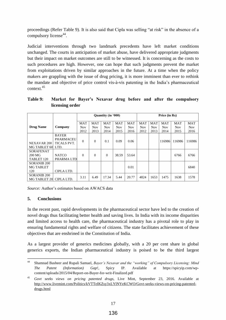
17
proceedings (Refer Table 9). It is also said that Cipla was selling “at risk” in the absence of a
compulsory license44
.
Judicial interventions through two landmark precedents have left market conditions
unchanged. The courts in anticipation of market abuse, have delivered appropriate judgments
but their impact on market outcomes are still to be witnessed. It is concerning as the costs to
such procedures are high. However, one can hope that such judgments prevent the market
from exploitations driven by similar approaches in the future. At a time when the policy
makers are grappling with the issue of drug pricing, it is more imminent than ever to rethink
the mandate and objective of price control vis-à-vis patenting in the India’s pharmaceutical
context.45
Table 9: Market for Bayer’s Nexavar drug before and after the compulsory
licensing order
Drug Name
Company
Quantity (in ‘000)
Price (in Rs)
MAT
Nov
2012
MAT
Nov
2013
MAT
Nov
2014
MAT
Nov
2015
MAT
Nov
2016
MAT
Nov
2012
MAT
Nov
2013
MAT
Nov
2014
MAT
Nov
2015
MAT
Nov
2016
NEXAVAR 200
MG TABLET 60
BAYER
PHARMACEU
TICALS PVT.
LTD.
0 0 0.1 0.09 0.06 116986 116986 116986
SORAFENAT
200 MG
TABLET 120
NATCO
PHARMA LTD
0 0 0 38.59 53.64 6766 6766
SORANIB 200
MG TABLET
120 CIPLA LTD.
0.01 6840
SORANIB 200
MG TABLET 20 CIPLA LTD. 3.11 6.49 17.34 5.44 20.77 4824 1653 1475 1638 1578
Source: Author’s estimates based on AWACS data
5. Conclusions
In the recent past, rapid developments in the pharmaceutical sector have led to the creation of
novel drugs thus facilitating better health and saving lives. In India with its income disparities
and limited access to health care, the pharmaceutical industry has a pivotal role to play in
ensuring fundamental rights and welfare of citizens. The state facilitates achievement of these
objectives that are enshrined in the Constitution of India.
As a largest provider of generics medicines globally, with a 20 per cent share in global
generics exports, the Indian pharmaceutical industry is poised to be the third largest
44
Shamnad Basheer and Rupali Samuel, Bayer’s Nexavar and the “working” of Compulsory Licensing: Mind
The Patent (Information) Gap!, Spicy IP. Available at https://spicyip.com/wp-
content/uploads/2015/04/Report-on-Bayer-for-writ-Finalized.pdf 45
Govt seeks views on pricing patented drugs, Live Mint, September 23, 2016. Available at
http://www.livemint.com/Politics/kVTTeIKZsy3xLYlNYeKCWO/Govt-seeks-views-on-pricing-patented-
drugs.html
136

18
pharmaceutical market by 2020. While India’s pharmaceutical industry boasts of a relatively
lower cost of production than that of U.S. and Europe, it is also important to have a
supportive enabling and comprehensive regulatory framework. Although the industry shows
great potential and progress, backed by a comprehensive regulatory framework, it is bound to
witness not only more competition but also facilitate accomplishment of primary health
policy objectives.
The absence of national healthcare system, reimbursement schemes and rising costs of
medicines coupled with out of pocket expenditure for medicines and drugs by consumers
make India’s pharmaceutical sector further unique. Although initiatives like Pradhan Mantri
Jan Aushadi Yojana, increase availability of generic drugs at lower prices, there is need to
widen the scope of existing policies to address the demand for these drugs in India and also
worldwide.
Generics are no doubt available for prices lower than in most other countries, but India’s
pharmaceutical industry has come under scrutiny for the poor patent protecting standards
affecting not only innovation in drugs but also the cost for many multinational manufacturers.
Thus, there has been a need more than ever to study the interaction of innovation, profits,
access and regulation in the context of India’s pharmaceutical industry. Through this paper,
we have thus attempted to understand the impact of regulation on market structures and
competition in the industry while analysing data on pricing, sales, etc. The main focus of our
inquiry is drug price control regulation and patenting policies in India. However, other factors
in enabling competition and the objective of universal healthcare cannot be ignored. The
results of the study should be viewed as interim and aimed at initiating further discourse on
the regulation competition interface in the pharmaceutical industry. As explained earlier, the
pharmaceutical market is highly fragmented and the results are not easily generalisable given
that the study focuses on one amongst the many therapeutic groups and two amongst the
many crucial regulations concerning the industry.
Our analysis shows that the intended objective of price regulation, i.e., affordable access has
not been realized in full. A cautionary word is on order though. At best of times it is difficult
to achieve competitive outcomes in regulated markets due to well known reasons. The
interplay of regulation and competition should be examined empirically by expanding this
analysis to other therapeutic groups to strengthen the hands of policy makers. Thus it is
critical to measure the costs and benefits of regulating price and innovation in the
pharmaceutical industry. While deregulation and free markets may not be the road ahead, but
time is ripe to test the effectiveness of alternative policies to achieve similar objectives. Any
step forward should be taken with a detailed understanding of the market in its entirety,
purchasing power, insurance, procurement schemes and the like.
137

19
Bibliography
ASA & Associates LLP, A Brief Report on Pharmaceutical Industry in India, July
2015
A Kaleidoscope of Drug Price Control Spanning Across the World and Its Relevance
to India- http://www.tapanray.in/a-kaleidoscope-of-drug-price-control-spanning-
across-the-world-and-its-relevance-to-india/
As SC Tries Case on Drug Price Ceiling, Government Mulls Dismantling Price
Control Body, The Wire, 09 November 2016. Available at https://thewire.in/78965/as-
sc-tries-case-on-drug-price-ceiling-government-mulls-dismantling-price-control-
body/
Bhattacharjea and Sindhwani, Competition Issues in the Indian Pharmaceutical
Sector, Project Sponsored by CUTS-CIRC, 2014
Centre for Trade and Development (CENTAD), New Delhi, Competition Law and
Indian Pharmaceutical Industry, 2010
Coronary Heart Disease, World Health Rankings. Available at
http://www.worldlifeexpectancy.com/cause-of-death/coronary-heart-disease/by-
country/
Danzon and Chao, Does Regulation Drive Out Competition in Pharmaceutical
Markets? Journal of Law and Economics, Vol 43, No 2, October 2000
Drug pricing: Supreme Court upholds capping of prices of 108 anti-diabetes,
cardiovascular drugs, The Financial Express, 25 October, 2016. Available at
http://www.financialexpress.com/economy/supreme-court-upholds-capping-of-prices-
of-108-drugs/428872/
European Commission, Study on enhanced cross-country coordination in the area of
pharmaceutical product pricing; Available at
http://ec.europa.eu/health//sites/health/files/systems_performance_assessment/docs/ph
armaproductpricing_frep_en.pdf;
Govt seeks views on pricing patented drugs, Live Mint, September 23, 2016.
Available at http://www.livemint.com/Politics/kVTTeIKZsy3xLYlNYeKCWO/Govt-
seeks-views-on-pricing-patented-drugs.html
Grabowski Vernon and Thomas, 1978, Estimating the Effects of Regulation on
Innovation: An International Comparative Analysis of the Pharmaceutical Industry,
The Journal of Law & Economics, Vol 21, No. 1, April 1978
138

20
Impact of Merger & Acquisitions in Indian Pharma on Production, Access and
Pricing of Drug, Knowledge Partnership Programme, IPE Global. Available at
http://www.ipekpp.com/admin/upload_files/Knowledge_2_39_Impact_2575324832.p
df
IMS Health Market Reflect Report, June 2016
Monitoring price movements of medicines under DPCO, 2013
http://www.nppaindia.nic.in/order/webisteSheetsPharmaTrac19022016.pdf
Novartis AG vs. Union of India, Civil Appeal 2706-2716 of 2013, Supreme Court of
India. Available at http://judis.nic.in/supremecourt/imgs1.aspx?filename=40212
NPPA issues guidelines to expedite monitoring & recovery in overcharging cases,
Pharmabiz.com, August 29, 2016. Available at
http://www.pharmabiz.com/NewsDetails.aspx?aid=97135&sid=1
Paul Howard, To Lower Drug Prices, Innovate, Don’t Regulate, The New York
Times, 23 September 2016. Available at
http://www.nytimes.com/roomfordebate/2015/09/23/should-the-government-impose-
drug-price-controls/to-lower-drug-prices-innovate-dont-regulate
Prabhakaran, Jeemon and Roy, 2016, Cardiovascular Diseases in India: Current
Epidemiology and Future Directions. Available at
http://circ.ahajournals.org/content/133/16/1605
Pricing and Reimbursement Questions-Conference Bleue--European Lawyers’
Conference on Pharmaceutical and Healthcare Affairs; Available at
http://www.arthurcox.com/wp-content/uploads/2015/06/Pricing-and-Reimbursement-
Questions.pdf
Report of the Core-Committee for Revision of National List of Essential Medicines,
November 2015. Available at http://cdsco.nic.in/WriteReadData/NLEM-
2015/Recommendations.pdf
US Department of Commerce, International Trade Administration- Pharmaceutical
Price Controls in OECD Countries, Implications for US Consumers, Pricing,
Research Development and Innovation. Available at
http://www.trade.gov/td/health/drugpricingstudy.pdf
139

21
Appendix 1: Sale of Drugs in the Scheduled and Non-Scheduled categories of
Cardiovascular Drugs
Year
Quantity (in '000) Value (Rs Crore)
Scheduled Non-Scheduled Scheduled Non-Scheduled
2012 660433 777097 2522 3415
2013 662993 835839 2605 3917
2014 668210 907408 2586 4551
2015 680129 1014992 2832 5446
2016 688825 1064448 2801 6312
Source: Authors estimates from AWACS
Appendix 2: Results from a Two-Sample t test with equal variance to measure the
difference in average price of scheduled and non-scheduled drugs in the
Cardiovascular Therapeutic Group
-------------------------------------------------------------------------------------------------
Group | Obs Mean Std. Err. Std. Dev. [95% Conf. Interval]
---------+---------------------------------------------------------------------------------------
0 | 1375 .00557 .000505 .018726 .0045793 .0065606
1 | 2454 .0073872 .0002189 .0108421 .006958 .0078164
---------+--------------------------------------------------------------------------------------
combined | 3829 .0067346 .0002297 .014211 .0062844 .0071849
---------+--------------------------------------------------------------------------------------
diff | -.0018173 .0004779 -.0027542 -.0008803
-------------------------------------------------------------------------------------------------
diff = mean(0) - mean(1) t = -3.8028
Ho: diff = 0 degrees of freedom = 3827
Ha: diff < 0 Ha: diff != 0 Ha: diff > 0
Pr(T < t) = 0.0001 Pr(|T| > |t|) = 0.0001 Pr(T > t) = 0.9999
Appendix 3: Sale of Drugs in the Scheduled and Non-Scheduled categories of Agents
Acting on the Renin-Angiotensin Class of Cardiovascular Drugs
Quantity (in '000) Value (Rs Crore)
Year Scheduled Non-Scheduled Scheduled Non-Scheduled
2012 159987 142719 717 888
2013 162675 153938 761 1021
2014 165593 166929 776 1167
2015 180814 189327 860 1391
2016 187074 196761 882 1568
140

22
Appendix 4: Sale of Drugs in the Scheduled and Non-Scheduled categories of
Angiotensin II Antagonists, Plan Group of Cardiovascular Drugs
Quantity (in '000) Value (Rs Crore)
Year Scheduled Non-Scheduled Scheduled Non-Scheduled
2012 119715 2919 530 22.04
2013 121710 3264 569 18.48
2014 128428 3569 597 14.87
2015 145610 4125 702 13.23
2016 152097 4527 733 11.61
Appendix 546
Country Drug Price Controls
Belgium ERP on the basis of average price of reference country or alternatively the price in
the country of origin is used as supportive guide. Price cuts were introduced in 2013
on the basis of international prices for reimbursed patented medicines, which are
prevalent in the market for at least five years. Requires a price to be negotiated with
national authorities before a prescription medicine can be marketed.
Denmark ERP acts as a price ceiling for new medicines in the hospital sector and contribute to
cost containment. Medicinal products used in public hospitals are available free of
charge for patients. In the out-patient sector, prices are set by the manufacturers
(free-pricing). There have been instances where Market authorization holders (MAH)
have lowered the prices to maintain general reimbursement status for a drug.
Prescription only drugs are partly reimbursed upon being granted an automatic or
conditional reimbursement status upon application from the MAH.
Finland No requirement on MAH/distributor or local representative to obtain approval of the
price or reimbursement status for drugs before they are placed on the market. But
reimbursement available only when the MAH has applied for, along with a
reasonable wholesale price and the Pharmaceutical Pricing Board has confirmed
these. A drug can be thus be marketed without a confirmed reasonable wholesale
price but the same is not eligible for reimbursement under the Health Insurance Act.
Reasonable wholesale price is the price of the drug in countries situated in the
European Economic Area. Reference pricing is adopted where drugs are divided in
reference groups by substances. Reference prices are determined based on MAH’s
price notifications.
France A manufacturer is free to decide whether or not to be a part of the reimbursement
regime. Price negotiations are key to the reimbursement regime. Pharmaceutical
companies based on the quantities of drugs sold pay a tax called “remises”. Each
year, market is divided into therapeutic groups of products and allows a level of
46
Pricing and Reimbursement Questions-Conference Bleue--European Lawyers’ Conference on
Pharmaceutical and Healthcare Affairs; Available at http://www.arthurcox.com/wp-
content/uploads/2015/06/Pricing-and-Reimbursement-Questions.pdf; European Commission, Study on
enhanced cross-country coordination in the area of pharmaceutical product pricing; Available at
http://ec.europa.eu/health//sites/health/files/systems_performance_assessment/docs/pharmaproductpricing_f
rep_en.pdf; A Kaleidoscope of Drug Price Control Spanning Across the World and Its Relevance to India-
http://www.tapanray.in/a-kaleidoscope-of-drug-price-control-spanning-across-the-world-and-its-
relevance-to-india/
141

23
increase in the quantity of drugs sold for each of these groups. If the increase is
beyond the authorized level, a percentage of the income has to be paid by the
company selling products within the said group. There is also remise on the turn over
of the company if the yearly turnover exceeds the fixed percentage.
The price of a generic drug is at least 60 per cent less than the price of the innovator
product. The price of innovator drug however has to decrease gradually to the price
of the 1st generic drug within a 5 year period. The first reduction of price of the
innovator drug is 20 per cent at the launch of the 1st generic drug.
Germany Combination of free pricing, EPR and VBP. An early benefit assessment is
conducted for medicines with a new active ingredient based on the remuneration
calculation model. MAH are empowered to set prices which are reimbursed entirely
and a year later, the price are renegotiated taking into account the results of the
assessment. Considering the added therapeutic benefit, the Federal Joint Committee
decides on the added value and price negotiations, taking into account also the
international prices. Laws provide for EPR but not used in practice. Reference price
groups often drive the reimbursement price once generics enter the market. The
doctors are required by law to prescribe the cheapest of the therapeutically equivalent
drugs and this often means generics become a favourite eventually.
Ireland EPR is a supportive guide to set prices for new single source on-patient medicines
while it is the guiding point for re-alignment of existing prices. Maximum Retail
Price for prescription drugs are determined in relation to the price of the same
product in the neighbouring countries using a published formula. Upon entry of a
generic, the price of the patented drug is reduced to 70% of the original price with a
further reduction to 50% of the original price twelve months following the initial
price reduction.
Italy Average European price for old drugs and a contractual model derived price for new.
For prices outside the reimbursement scheme, the manufacturer freely sets the prices.
Mostly ex factory prices is the maximum sale price to the public hospitals but in
within the public procurement, discounts are manufacturer’s individual discretion. In
order to maintain competition, the offered prices ought to consider the reference
average price for the concerned category of drugs and significant deviations from the
average price is not considered appropriate. The drugs in the non-reimbursed
category are subject to a statutory 50% price cut when sold to public hospitals.
Generics and bio-similar are placed in the same category as the parent referenced
product. The price is deemed to be “clearly convenient” when it is lower than the
price of the patented drug according to the prescribed reduction percentage (20% or
lower). The rebate of this nature is dependent on the price of the original drug and
the average national health expenditure over the last 3 year period on the original
drug.
Luxembourg The Ministry of Social Security controls all products registered as “medicines” under
its “national number”. The price is the ex factory price which refers to the price
charged by the manufacturer. The Health Ministry established a list of groups of
products called generic groups containing the same API no longer protected by
patent. EPR is applied for reimbursed, prescription only and innovative drugs with
the price calculated based on the lowest price in basket of referenced countries.
Norway The Norwegian Medicine Agency regulates maximum pharmacy purchasing price
and the pharmacy mark up for prescription only drugs irrespective of their patent
protection. The prices of over the counter (OTC) drugs are not regulated. The prices
of generic prescription only drugs cannot exceed the maximum market price of the
original product. Under the stepped price model introduced in 2005, a maximum
reimbursement price is set for affected medicines (branded and generics included),
and this price level is reduced in steps following the patent expiry. The size of price
cuts depends on annual sales before establishment of generic competition and the
time since competition was established. Stable generic competition is a precursor to
142

24
application of stepped price model and happens when the products are placed on the
substitution list and no delivery issues are recorded. The price reduces by 30% when
stable generic competition takes place and 55% six months after this.
Sweden Although there is no traditional price control for drugs, the pharmaceutical
companies experience difficulties in selling their products (other than OTC) without
being a part of the reimbursement regime. VBP, decided on the basis of 1) societal
perspective- principles of human value, need and solidarity and cost effectiveness. 2)
Threshold value- based on the individuals’ willingness to pay for a quality adjusted
life year gained. 3) Marginal decreasing utility of treatments- that the benefits of a
treatment vary by indication or by degree of severity.
Switzerland To ensure cost effectiveness, in case of a high priced drug, whose sales are not
estimated at the time of launch, the authority is empowered to fix a sales cap and the
company is then obliged to transfer sales above such cap to a general account of the
health insurances. Following ERP, the ex factory price cannot be higher than the
average ex factory price in the referenced countries. In addition to the price
comparison, there is also a therapeutic cross comparison conducted if the product is
unavailable in the foreign market. No explicit legal requirement to lower the price
upon entry of a generic into the market, but the competent authority is empowered to
assess the price of the branded drug upon expiry of patent and the price is lowered by
this time.
Turkey Using the reference pricing method for originator products, the price is arrived
according to the lowest ex-factory price among the selected five EU countries. In
case of non-availability of ex-factory price, the price is calculated by deducting mark
ups and VAT from the retail price.
United
Kingdom
MAH are empowered to freely determine the prices of branded medicines with a new
active ingredient subject to the Pharmaceutical Pricing Regulation Scheme (PPRS)
that regulates the maximum profit of manufacturers. This freedom to fix prices is
subject to the prior approval of prices by the Department of Health. With respect to
the new branded medicines by companies who are members of the PPRS, the
Secretary of State is empowered to specify the maximum price at which the product
can be brought to the National Health Service (NHS). Products not subject to NHS
are not regulated. Although there is no requirement for the manufacturer to comply
with the price of a new non-branded generic with the Health Department, the
Department under its voluntary price regulation scheme with the generic
manufacturers has established that the generics can be priced freely except that the
price cannot exceed that of the branded product. VBP is followed based on the
Quality Adjusted Life Year (QALY) gains in relation to costs (innovation, burden of
illness, rare diseases, wider societal benefits etc., are considered)
Canada Only the patented drugs are subject to price control. These prices are regulated in a
manner that the price is along the lines of the cost of therapy for existing drugs sold
in Canada used to treat the same disease. The existing patented drug prices cannot
increase by more than the Consumer Price Index. The Canadian prices of patented
medicines can never be the highest in the world. Public drug plans control drug
prices through listing of drugs on their respective formulations for reimbursement. A
maximum ex-factory price is determined at the federal level by reference to prices in
other countries for most innovative products and with reference to existing prices in
Canada for less innovative ones.
United
States of
America
Free market pricing is observed in pharmaceutical companies for three apparent
reasons: 1)Direct advertisements by manufacturers to patients has ensured sustained
demand. 2) Price increases have been largely invisible to both patients and their
doctors, because of the health-insurance plans. 3) Medicare, the public-health
programme for those aged 65 and older, is the largest drug customer, but is not
allowed to negotiate prices with drug companies.
Mexico Price caps on patented medicines based on international referencing on the average
143

25
ex-factory price in six largest markets for a given product globally. Reimbursement
methods exist but are limited to generics based on health technology assessment.
MRP capped for private sector.
Japan Ever drug needs to obtain regulatory approval prior to marketing. For a new drug to
be brought under health insurance, the NHI price listing procedure is needed.
Reference pricing method is adopted where price of a drug is decided based on the
price of a similar comparable drug on the market. A comparable drug is identified
from existing, reimbursed drugs based on similarities in indication, action, molecular
formula, manner of administration, and dosage. The daily price of the new drug is set
as the same daily cost of the comparable drug to ensure competition in the market.
Premiums are at times added to the calculated price innovativeness/usefulness,
support for small market size, and support for a pediatric indication. In the absence of
comparable drug, price is calculated in the cost accounting method with profit
percentage adjusted depending on the novelty, efficacy, and safety of the drug in
comparison with existing therapies. The price is compared with the average price in
other countries and also adjusted in case of substantial difference.
China Prior to 2015, Chinese government set the maximum price of drugs in the country. In
a 2015 policy, the government deregulated these prices allowing the market
competition to determine the prices. The government would be present in a
supervisory, advisory capacity to monitor prices and penalize unreasonable pricing.
Under the same policy however, anesthetics and grade one psychiatric medications
were still be subject to price caps.
Appendix 6: Market Share and HHI estimates for Imatinib Mesylate
Market Share in Terms of Volume Market Share in Terms of Value
2012 2013 2014 2015 2016 2012 2013 2014 2015 2016
ALKEM
LABORATORIE
S LTD.
0.006 0.011 0.010 0.006 0.003 0.005 0.010 0.009 0.007 0.004
CADILA
PHARMACEUTI
CALS LTD
0.000 0.000 0.001 0.001 0.000 0.000 0.000 0.001 0.001 0.000
CELON LABS 0.000 0.012 0.013 0.005 0.012 0.000 0.005 0.006 0.003 0.007
NEON
LABORATORIE
S LTD
0.000 0.000 0.000 0.000 0.003 0.000 0.000 0.000 0.000 0.001
NOVARTIS
INDIA LTD 0.000 0.000 0.000 0.003 0.005 0.000 0.000 0.001 0.004 0.009
ZUVENTUS
HEALTHCARE
LTD
0.000 0.000 0.006 0.014 0.014 0.000 0.000 0.007 0.017 0.018
SUN PHARMA
LABORATORIE
S LTD.
0.014 0.012 0.014 0.004 0.005 0.007 0.006 0.007 0.002 0.003
INTAS
PHARMACEUTI
CALS LTD
0.040 0.040 0.043 0.043 0.042 0.036 0.035 0.051 0.070 0.058
ZYDUS CADILA 0.031 0.086 0.136 0.048 0.036 0.009 0.027 0.064 0.028 0.026
HETERO
HEALTHCARE
LTD
0.001 0.001 0.001 0.002 0.000 0.000 0.000 0.001 0.001 0.000
144

26
CIPLA LTD. 0.015 0.017 0.031 0.008 0.012 0.009 0.010 0.021 0.006 0.007
RELIANCE LIFE
SCIENCE 0.000 0.000 0.000 0.000 0.001 0.000 0.000 0.000 0.000 0.000
FRESENIUS
KABI INDIA
PVT LTD
0.003 0.001 0.002 0.000 0.000 0.003 0.001 0.002 0.000 0.000
UNIMARK
REMEDIES LTD 0.001 0.000 0.000 0.000 0.000 0.000 0.000 0.000 0.000 0.000
DR. REDDYS
LABORATORIE
S LTD
0.035 0.033 0.032 0.022 0.017 0.035 0.028 0.025 0.023 0.025
LUPIN LTD 0.013 0.009 0.011 0.009 0.007 0.006 0.005 0.007 0.007 0.006
GLENMARK
PHARMACEUTI
CALS LTD.
0.006 0.003 0.003 0.002 0.006 0.003 0.001 0.002 0.001 0.004
SAMARTH LIFE
SCIENCES PVT
LTD
0.000 0.000 0.000 0.005 0.003 0.000 0.000 0.000 0.000 0.000
RPG LIFE
SCIENCES LTD. 0.000 0.000 0.000 0.000 0.000 0.000 0.000 0.000 0.000 0.000
NATCO
PHARMA LTD 0.830 0.776 0.694 0.826 0.834 0.884 0.871 0.797 0.811 0.832
RANBAXY
LABORATORIE
S LTD
0.006 0.000 0.002 0.002 0.000 0.003 0.000 0.002 0.003 0.000
HHI
ESTIMATES 0.693 0.613 0.505 0.687 0.699 0.785 0.762 0.643 0.664 0.698
145

Studying Competitiveness of Indian Industry:
A Methodological Exploration ARYAMAN BHATNAGAR, PRADEEP SAHOO, CHINMAY PANT, MANORANJAN PATTANAYAK,
RANEN BANERJEE
National Conference on Competition Economics
Competition Commission of India
146

Studying Competitiveness of Indian Industry: A Methodological Exploration
1
*Views expressed in this paper are strictly personal and do not reflect the view of the organisation
where the authors are presently working or worked earlier. This is a working paper version of the
document prepared solely for the purpose of presentation in the National Conference of Competition
Economics organized by the Competition Commission of India. Please do not quote this paper without
the written permission of the author(s). Contact details:
[email protected], Mobile: +91-9871176763
ABSTRACT*
This research paper aims at assessing the competitiveness of Indian industries with the ultimate
objective of identifying industries with higher possibilities of collusion. In order to complement
the competition enforcement toolkits of the Competition Commission of India (CCI), this paper
has also made an attempt to develop a suitable competition index using firm level data of Indian
industries. The methodology is based on a weighted average score against key economic
indicators identified on the basis of the theoretical underpinnings from industrial organisation
literature as well as the intrinsic characteristics of the industry subject to certain limitations
related to aggregation and availability of the data. The results presented in the paper may
provide useful inferences to the CCI in identifying and screening industries which are exposed
to higher possibilities for collusion.
JEL Classification: L13, L22, L50, L70
147

Studying Competitiveness of Indian Industry: A Methodological Exploration
2
Studying Competitiveness of Indian
Industry
A Methodological Exploration
I
Background and Introduction
Deterrence and detection of anti-competitive practices remain the most important enforcement
priorities of competition authorities around the world. More than ever, competition authorities
have been proactively screening the sectors by using sophisticated economic tools in their efforts
to detect suspicious instances of anti-competitive practices across industries. Antitrust literature
suggests that these tools have been quite effective in especially those competition jurisdictions
where other competition enforcement measures such as leniency, complaints have not gained
traction in triggering and reporting competition issues.
In order to complement the competition enforcement toolkits of the CCI, we have made an attempt
to develop an economic detection instrument: the Competition Index (CI). This instrument has
been methodologically developed through assessing the level of competition of around 66
industries1 of the Indian economy. In developing the instrument, we have used similar approaches
that have been utilized by the other competition authorities and have enhanced those approaches
by using additional techniques in our analysis. For instance, apart from simple average weighting
and weighted average system, we have used Principal Component Analysis to allocate weights to
economic indicators and verifying the results. The tool may help the CCI in proactively monitoring
the industries for seeking out cartels and launching suo moto investigations in a wide range of
sectors. The toolkit may also add significant value in combination investigations as it will provide
a macro overview of the level of competition of the industry pertaining to the case.
1 Complete list of industries analyzed is attached in Annexure 3
148

Studying Competitiveness of Indian Industry: A Methodological Exploration
3
The paper is divided into ten sections. Section II reviews the related antitrust literature on empirical
techniques of assessing competition in the markets. Section III discusses the indicators chosen for
the construction of the index. Section IV describes the data collection process along with summary
statistics. Section V presents the consistency check on the data collected. The standardization
process and the weighting approaches are discussed in sections VI and VII respectively. Section
VIII highlights the results of the model. In section IX, we have conducted the robustness check for
the model and present the findings. Finally, section X provides the conclusion along with the
limitations and caveats of the study.
II
Literature Review
Over the years, quantitative methodologies of assessing competitiveness have garnered
considerable attention from antitrust authorities around the world. Competition authorities have
been applying quantitative methodologies using industry level data to measure competitiveness
across the levels of the industries. In the following paragraphs we will review antitrust literature
which is pertinent to this study. Specifically, we shall discuss the key economic indicators that
have been quite effective in assessing competitiveness across industries/sectors. In similar
previous studies, number of economic indicators have been explored, developed and tested in order
to measure the degree of competition or its absence. On the basis of previously conducted studies,
we have discussed the implications of several economic indicators on competition or collusion
including barriers to entry and exit, capital intensity, concentration, demand, interaction, product
characteristics, profits and market stability. Based on the antitrust literature available, we have also
briefly highlighted the empirical relationship of competition with key economic indicators.
A report by Paul A Grout and Silvia Sonderegger (2005) on “Predicting Cartels”, found that higher
entry barriers have a negative impact on competition and facilitate collusion. Higher entry barriers
encourage formation of cartels as they decrease the competitiveness in the markets. If prices
become higher in sectors with low entry barriers then it attracts more competitors in the future and
will increase competitiveness in the markets. On the contrary, high entry barrier will decrease
competition as the number of competitors will remain the same. The study concludes that entry
and potential entry is damaging in two ways. Firstly, it destabilizes the existing cartels and also
149

Studying Competitiveness of Indian Industry: A Methodological Exploration
4
their future probabilities due to disagreements between them. Secondly, it enhances the cartel
members need to coordinate their activities, thereby making their collusive agreement more
explicit and easy to prove. This argument corroborates the theoretical view that an increase in the
number of market participants, either in the present or in the future, renders collusion harder to
sustain.
In another study, George Symeonidis (2003) uses capital intensity and advertising intensity to
measure competition. According to the research, high capital intensity has a negative impact on
competition, as it decreases the competitiveness in the industry. In contrast, high advertising
intensity has a positive impact on competition and increases the competitiveness in the market.
The author used a comprehensive data set on the incidence of price-fixing across UK
manufacturing industries in the 1950s. The econometric results suggest that collusion is more
likely in industries with higher degree of capital intensity and less likely in high advertising
industries.
Another indicator that has been most commonly used by researchers to measure competition is
concentration. Concentration within industries has been studied and researched extensively in the
past. Various quantitative techniques have been established in order to capture the magnitude of
industrial concentration (Bikker & Haaf, 2012). Despite the variety of techniques, the general
format of a concentration index remains as follows:
𝐶𝐼 =∑ 𝑠𝑖𝑤𝑖𝑛
𝑖=1
Where CI is concentration index, si is the market share, wi is the weight attached to the market
share and n is the number of firms
Most indices use the above form as a base. The K firm concentration ratio for instance essentially
sums up the market share of the largest k number of firms. The simplicity of the ratio as well as
limited data requirements make it a frequently used measure of concentration. The most widely
used concentration index is the Hirschman- Herfindahl index. The HHI is basically the summation
of squared market shares of all firms in the industry. The squaring of market shares ensures greater
weightage to larger firms. Another index is the comprehensive industrial competition index. This
is the sum of the proportional share of the leading firm and the summation of the squares of the
150

Studying Competitiveness of Indian Industry: A Methodological Exploration
5
proportional sizes of each firm, weighted by a multiplier reflecting the proportional size of the rest
of the industry. There are other indicators which are being used in the industrial Organization
literature as well as by practitioners are Hall Tideman index (where the market share is weighted
by the firm’s rank), the U index centered on the concept of inequality, the Hause index (based on
interpretations of the Cournot model) etc.
Another economic linkage that has been extensively studied by the antitrust economists is the
relation between competition and demand. In his paper “Competition Policy, Theory and Practice”,
Massimo Motta (2004) used indicators like demand elasticity and stability of demand to study
linkages between demand and competition. The paper establishes that high demand elasticity has
a positive impact on competition. On the contrary, stability of demand has a negative impact on
competition.
Interaction is also an important indicator through which competition in an industry or market can
be measured. To measure the interaction in an industry, indicators like communication, industry
associations and multi-market contact were used. In a paper by Robert Porter (2005), “Detecting
Collusion”, the author has used communication as an indicator to measure the competition and
likelihood of cartelization in an industry. He observed that communication is negatively related to
competition. In another report prepared for the Office of Fair Trading, by Paul A Grout and Silvia
Sonderegger, number of industry associations and competitiveness of the industry were found to
be inversely related.
Other indicators that are used to measure competition in a market are innovation, productivity
and prices. Innovation fosters competition as the innovation leads to lower prices or better
quality products which ultimately increases the demand of the product. NERA also found that
low productivity has a negative impact on competition as it is inefficient and hence will result in
lower output due to which the firm will not be able to compete successfully in a market. Hence,
low productivity reduces the competitiveness in the industry. The costs and pricing of goods and
services are also an important factor in measuring competition. Reports and papers by NERA,
Motta and Grout & Sonderegger validate the linkage between competition and the cost, as well
as pricing of products. High prices have a negative effect on competition as it thwarts demand of
151

Studying Competitiveness of Indian Industry: A Methodological Exploration
6
the product to increase. The cost of a product also impact the pricing of goods. Higher employee
costs and manufacturing costs will result in higher prices which will have a negative effect on the
competitiveness of the industry.
Factors that impact the competition in an industry can also be associated with the characteristics
of the product. Product homogeneity and symmetry have a negative effect on competition (Motta,
2004). Motta also observed that excess capacity and inventories decrease the competition in the
market. Lorenz (2008) noticed that that low capacity utilization, dysfunctional growth of capacities
and low volatility of market shares have a negative effect on market shares. These indicators are
related to the symmetry and stability of markets in the industry.
Profits have also been used as an indicator to measure competition. Typically, high and stable
profits are linked with anticompetitive markets. Price cost margins are frequently analyzed in order
to determine the nature of competition in an industry. Higher margins suggest prevalence of
anticompetitive tendencies. For instance, if competition is intensified through a reduction in entry
barriers, the incumbents are forced to lower prices to compete with the entrants. A rise in
competition is then associated with a reduction in price-cost margins.
Profit elasticity is a new concept that has been used in this area (Boone, 2008). Essentially, this
requires measuring the percentage fall in a firm’s profit in response to a 1% fall in the firm’s
efficiency. A fall in efficiency would lead to a fall in profits for all types of firms (including
monopolists). However, in more competitive markets, the fall would be steeper. Hence, it can
provide a fair idea with regards to the nature of the industry.
Market stability is another economic criteria that has been frequently used as a proxy to assess the
competition in an industry. Markets with high levels of anticompetitive practices generally display
a stable trend. For instance, prices do not fluctuate much in these markets as they are fixed within
a range. Market growth is also generally on the balanced side. Many other concepts of stability
have been identified recently. For instance, Lorenz 2008 uses indicators like technical innovation
and variance of market shares as proxies for market dynamism. Stability of the number of firms,
output, demand and costs are also useful indicators for measuring competition.
152

Studying Competitiveness of Indian Industry: A Methodological Exploration
7
III
Objective, Approach and Methodology
The objective of this paper is to assess the competitiveness of 66 industries (division level) and
subsequently develop a competition index which can be used by the CCI to monitor the industries
and pre-empt any damaging anti-competitive behaviour. While the data presented here shows the
ex-post scenario, this index can be updated on a regular basis so that a concurrent monitoring could
be done. Industries displaying less anti-competitive characteristics might not attract the attention
of competition authority today, however, the index if updated and monitored at a regular intervals
can provide useful inferences regarding market dynamics and competitiveness of the industry.
While in a free market economy, infringement by competition authorities in normal business
activity can be damaging, at the same time remaining vigilant can act as a deterrent towards
building up of sectoral anti-competitive character.
In the following paragraphs, we show the selection of specific indicators for this study. The first
step in the construction of the index was towards selection of the indicators for developing the
index. We have conducted an antitrust literature review covering economic detection instruments
and various other screening methods. Based on the antitrust literature and availability of the data,
we have selected nine indictors for assessing the competitiveness of the industry and subsequently
developing the competition index.
HHI: The Hirschman-Herfindahl index (HHI) was selected as a proxy for concentration within
industries. HHI is considered to be the best and most widely used indices among all concentration
indices. Antitrust literature suggest that a higher HHI value indicates a less competitive industry.
Few studies also suggest that HHI is positively related with market asymmetry. Thus, if the
industry has a skewed market share distribution (i.e. a few firms enjoy the majority of the market
share) then the HHI will be higher. Furthermore, the HHI is negatively related with the number of
firms existing in an industry. Based on HHI, the U.S. Federal Trade Commission and U.S.
Department of Justice have classified markets into three types. Markets in which the HHI is below
than 1500 are characterised as ‘unconcentrated’ markets. HHIs between 1500 and 2500 indicate
‘moderately concentrated’ markets, which may or may not raise competition concerns. Markets
with HHIs over 2500 are ‘highly concentrated’ and are more likely to pose competition concerns.
153

Studying Competitiveness of Indian Industry: A Methodological Exploration
8
Number of firms: Antitrust literature indicates that an industry with more number of firms tends
to be more competitive than an industry with lesser number of firms. This is because a reduction
in the number of firms essentially means a direct reduction in the number of competitor.
Effective Churn Rate: The churn rate is used as a proxy to measure the degree of dynamics of an
industry. It is defined as the number of firms entering or exiting an industry compared to the
number of existing firms. Thus it reflects how actively the competition landscape of an industry is
changing. It also provides a signal regarding entry and exit barriers. Higher barriers would mean a
lower churn rate.
Survival Rate: The survival rate reflects the degree of stability of a market. It is defined as the
number of firms that have been active for at least the previous five years, in relation to the average
existing number of firms for those years. A high survival rate implies repeated interaction among
firms. If, for instance, all of the existing companies were the only ones present in the market, for
the previous five years, that might suggest possible communication, or at least mutual knowledge
of the firms’ strategic decisions (and therefore effortless anticipation of each other’s behavior).
Furthermore, the survival rate can also serve as a proxy for the entry and exit barriers. The absence
of entrants or leavers (i.e. a survival rate of 1) suggests high barriers and may impede effective
competition. The survival rate and the churn rate are, to some extent, similar. This aspect is
incorporated in the weighting schemes.
Volatility in market shares: Markets with anticompetitive tendencies display stable market
shares. Lorenz, 2008, in his paper “Screening markets for cartel detection” discussed that if the
industry is open to competition then the market shares tend to fluctuate rapidly.
Market Growth: A stable market growth typically reflects an environment conducive for
collusive behavior. On the other hand, collusion attempts will fail in declining market growth due
to economic problem and in booming markets due to ease of market entry in such markets.
Labour Unions: Over the years, a large and rapidly expanding body of literature on implications
of trade unions on competition has emerged. The economic literature suggests that inherent
154

Studying Competitiveness of Indian Industry: A Methodological Exploration
9
functioning of the market is negatively impacted by the number of Labour unions existing in the
industry and thus making the market difficult from reaching a competitive equilibrium. In our
study, industries with higher number of labour unions has been assumed to represent higher
anticompetitive tendencies.
Profits: As per the traditional industrial organizational theories, in a perfectly competitive market,
price equals the marginal cost and thus no supernormal profits exist in such economic scenarios.
On the contrary, high and stable profits are representative of imperfect markets with higher
probabilities of anti-competitive activities.
R&D rate: Economic literature suggests that highly innovative markets are less prone to
anticompetitive practices. Firms with high R&D expenses are assumed to be mutually competitive,
whereas, the absence or avoidance of R&D expenses might point to possible collusive behavior.
IV
Data Description and Sources
For the purpose of our analysis we have used division level data from Capitaline. Out of total
industries, data was available for 83 industries. However, for our study, 66 of these industries were
finalized as they had data for all the 9 indicators. Besides Capitaline, we have obtained the trade
union information from the labor bureau. The summary statistics for the data are provided in
appendix 5.
Table 1 explains the construction of the index:
Table 1: Construction of the Index
Indicator Process
Number of Firms We first obtained the gross sales for all the companies for the last five
years (2012-2016). Based on this, for each industry we calculated the
average number of firms for those years.
Average Market
Growth
Using total sales we calculated the average market growth for each
industry (year on year growth in total sales).
Volatility of Market
Shares
Market Shares for each company were calculated using sales figures. The
volatility of market shares was estimated using the coefficient of variance
(by dividing the standard deviation of each firm’s market share by the
155

Studying Competitiveness of Indian Industry: A Methodological Exploration
10
average market share across the time period). We then took the average
coefficient of variance for each firm to arrive at the volatility of market
shares by industry.
Hirschman Herfindahl
Index
The Hirschman Herfindahl Index for each industry was calculated by
squaring and summing market shares of each firm in that industry.
Effective Churn Rate To calculate the churn rate we identified the total entry and exit in each
industry for each year2. This was divided by the average number of firms
for each industry to get the corresponding churn rate.
Survival Rate The survival rate was calculated by dividing the number of active firms in
the last five years by the average number of firms in the same time period
for each industry. Active firms were defined as those whose gross sales
were greater than zero in all the five years.
Research and
Development
To measure research and development, we used expenditure on research
and development as a percentage of net turnover as a proxy. This figure
was obtained for each company and then the average was taken to get
expenditure on research and development by industry.
Profits To measure profit margin we obtained the net profit before tax for each
company for each year and divided it by the total sales. Then we calculated
the median net profit ratio for each company. Industry wise net profit ratio
was calculated by taking the average within each industry.
Number of Trade
Unions
The number of trade unions in each industry were obtained from the
Labour bureau.
V
Data Consistency
Prior to standardization, we checked for the consistency of the data. The results are presented in
the figure below.
The upper triangular matrix displays the Pearson’s correlation values between variables while the
lower triangular matrix displays pairwise scatter plot along with the corresponding regression
lines. The diagonal presents the density plot for all the nine variables.
As we can see, the correlation signs reaffirm the theoretical hypothesis that we presented above.
Variables like HHI, survival rate and profits which have an adverse impact on competition are
positively correlated with each other while the remaining variables are negatively correlated
amongst themselves.
2 Calculation of entry/ exit of a firm is based on whether the firm had positive sales or not. This might lead to inaccurate results if there are
reporting issues.
156

Studying Competitiveness of Indian Industry: A Methodological Exploration
11
Out of 36 correlation values only 7 are above 0.3 (or below -0.3) thus signifying that the variables
are not very highly correlated. These weak correlations suggest that all the variables actually add
information to the model.
The density plots reveal the distributions of these variables. Market growth, variance in market
share and profits before taxes display a bell curve distribution. Number of trade unions, number of
firms, churn rate and R&D are skewed to the right, while survival rate is skewed to the left.
Figure 1: Pairwise Plot
157

Studying Competitiveness of Indian Industry: A Methodological Exploration
12
VI
Standardization of Data: Using Fuzzy Logic
In mathematics, a set is a collection of things that belong to some definition. For example, let’s
say there is a set of tall people X. An individual belongs to set X if and only if his height is greater
than six feet. If his height is less than six feet then he belongs to the set X’ (not tall). Thus, an
individual is either tall (belongs to X) or not tall (does not belong to X). There is nothing in
between. This sharp edged membership functions works nicely for binary operations and
mathematics, but it does not work as nicely in describing the real world. The regular set theory
makes no distinction between somebody who is 6'1" and someone who is 7'1", they are both simply
tall. In contrast, Fuzzy sets are those sets whose elements have degrees of membership. Formally:
Let X be a nonempty set. A fuzzy set A in X is characterized by its membership function µA : X →
[0, 1] and µA(x) is interpreted as the degree of membership of element x in fuzzy set A for each x
∈ X.3
Hence, the membership is defined over the interval of 0 to 1, instead of just two possible values
of 0 and 1.
For the purpose of our analysis, we have used fuzzy sets or membership functions for all the
variables. Essentially, we have standardized all the indicators on a scale of 0 to 1, with 0 being
the least anticompetitive and 1 being the most anticompetitive. The slopes of these functions
is based on competition theory. The range of all these membership functions is the minimum and
maximum values of the respective indicator. Here, we will briefly comment on each indicator’s
slope of the membership function.
3 (Ragin, 2000)
158

Studying Competitiveness of Indian Industry: A Methodological Exploration
13
Figure 2 displays the market growth curve. As we can see, the curve is shaped like an inverted V.
This is because we assume that anticompetitive practices are most rampant when market growth
is stable and positive. It is difficult to collude in volatile markets. The functional form for Market
growth is as follows:
CI=𝑋2 If X<12
=1 − 𝑋1/2 If X>=12
Figure 2: Market Growth
The second variable was number of trade unions. In our analysis, we found that the number of
trade unions had a positive correlation with the number of firms. This is rational since larger
industries tend to have more trade unions. Hence to disentangle the impact and normalize this
variable we have divided the number of trade unions by the number of firms. After that we used a
membership function for standardization. Figure 3 refers to trade unions membership function
(tuf). This is an upward sloping curve since higher number of trade unions would have an adverse
impact on competition. The curve is concave because the marginal effect of additional number of
trade unions is less. The functional form for Trade Unions is given as:
CI=𝑋1/2
159

Studying Competitiveness of Indian Industry: A Methodological Exploration
14
Figure 3: Number of Trade Unions
Figure 4 refers to the number of firms in the industry. This is a downward sloping curve since
higher number of firms would have a positive impact on competition. The curve is steep initially
and then flattens. This is because once again the marginal impact of the additional number of firms
declines as the number of firms increases. For example, let’s say industry X is a monopoly. Now
if another firm enters the market the positive competition impact will be massive. On the other
hand, let’s say industry X had 500 firms. In this case, adding another firm will have negligible
impact on competition. The functional form for Number of Firms is given as:
CI =1 − 𝑋1/4
Figure 4: Number of Firms
160

Studying Competitiveness of Indian Industry: A Methodological Exploration
15
Figure 5 displays the curve for survival rate. It’s an upward sloping straight line since every one
percent increase in survival rate is assumed to have a constant negative impact on competition.
The functional form for Survival Rate is defined as:
CI=𝑋
Figure 5: Survival Rate
Figure 6 displays the curve for churn rate. Like the curve for number of firms, this is also a
downward sloping convex curve. The reasoning is the same. The functional form for Churn Rate is
given as:
CI =1 − 𝑋1/4
Figure 6: Churn Rate
161

Studying Competitiveness of Indian Industry: A Methodological Exploration
16
Figure 7 displays the curve for HHI. It’s an upward sloping curve since higher HHI would have
an adverse impact on competition. The first part of the curve is concave whereas the curve becomes
convex after the 2000 mark. This is because it is after this mark that higher HHI becomes
increasingly problematic. The functional form for HHI is defined as:
CI= Beta distribution with parameters 1/5 and 1/10
Figure 7: Hirschman Herfindahl Index
Figure 8 refers to the curve for variance of market share. Like the curve for number of firms and
churn rate, this is also a downward sloping convex curve. The reasoning is the same. The functional
form for Variance in Market Share is given as:
CI =1 − 𝑋1/4
Figure 8: Variance of Market Share
162

Studying Competitiveness of Indian Industry: A Methodological Exploration
17
Figure 9 displays the curve for profit before taxes. It’s an upward sloping curve since higher
PBT would have an adverse impact on competition. The first part of the curve is concave whereas
the curve becomes convex once profits become positive. The functional form for Profit before tax
is defined as:
CI= Beta distribution with parameters 1/5 and 1/10
Figure 9: Profit before tax
Figure 10 refers to the curve for Research and
Development. Like the curve for number of firms and churn rate, this is also a downward
sloping convex curve. The functional form for Research and Development is given as:
CI =1 − 𝑋1/4
Figure 10: Research and Development
163

Studying Competitiveness of Indian Industry: A Methodological Exploration
18
VII
Weighting Scheme
For the purpose of our analysis we have used three different weighting systems.
Table 2: Vector of Weights
Indicator Method 1 Method 2 Method 3
Market Growth 11% 10% 1%
Number of Trade Unions 11% 15% 11%
Number of Firms 11% 5% 15%
Survival Rate 11% 5% 13%
Churn Rate 11% 5% 24%
HHI 11% 20% 14%
Variance in Market Share 11% 10% 17%
Profit Before Tax 11% 15% 1%
Research and Development 11% 15% 6%
Method 1 is a simple average weighting system. Each indicator is thus assigned 11% weight.
Method 2 is a weighted average system. Here, the maximum weight has been assigned to HHI
since it is the most widely used measure for anticompetitive tendencies. Since 20% weight is
assigned to this, only 5% is assigned to the number of firms as both of them essentially indicate
the degree of concentration. Similarly, survival rate, churn rate, variance in market share and
market growth get 10% weightage each as they jointly refer to the dynamism of the market. The
remaining variables namely number of trade unions, profits and research and development all get
15% weightage. Method 3 weights are obtained by conducting a principal component analysis4.
For this we first standardized the variables as mentioned in the previous section. Then we created
a correlation matrix. Based on the correlation matrix, we identified the principal components and
arrived at the weights. These weights are provided in Table 2.
Figure 11 elaborates on the principal component analysis. The points correspond to the PCA scores
received by each industry. They have been categorized into anticompetitive, moderately
competitive and competitive based on the competition index scores received using the weighted
average approach. The nine indicators become 9 axis of measurement. As we can see, HHI and
4 Principal component analysis (PCA) is a statistical procedure that uses an orthogonal transformation to convert a set of observations of possibly correlated variables into a set of values of linearly uncorrelated variables called principal components
164

Studying Competitiveness of Indian Industry: A Methodological Exploration
19
number of firms are almost exactly in the opposite direction thus showing that these two indicators
are highly correlated. Similarly, survival and churn rate are also pointing in the opposite direction.
In Figure 11 , we can see that the industries which appear competitive on the index have certain
features. For instance, all competitive industries (green dots) are in the direction of “firms”, “var”
and “churn”. In other words, they have a large number of firms, along with high variance of market
share and a high churn rate. Less competitive industries (red dots) are in the direction of “survival”,
“HHI” and “tuf”. In other words they have a high survival rate, HHI and a large number of trade
unions. The horizontal length of the arrows depicts the weightage assigned to each indicator (since
we are considering only the first Principal component (PC1). As we can see, the PCA assigns very
little weightage to market growth, profits and research and development.
165

Studying Competitiveness of Indian Industry: A Methodological Exploration
20
Figure 11: Source of Variance in the Competition Index
VIII
Results of the Study
Annexure 1 presents the top 10 and bottom 10 industries based on the PCA analysis, simple
average as well as the weighted average. It is important to note that we have excluded a few
industries from the final results since we did not have enough information and the companies were
not adequately representative of their industry.5
5 Since a large proportion of the Indian economy belongs to the informal sector, data is neither recorded not reported for most of these companies in such sectors. Hence it would be incorrect to display their results.
166
Studying Competitiveness of Indian Industry: A Methodological Exploration
21
The index is on a scale of 0 to 1 with 0 being the most competitive and 1 being the least
competitive. Based on the results we can see that the average PCA score is 0.43. The table
mentioned in the aforesaid annexure also presents standardized scores for all the indictors.
Air transport, manufacture of beverages and manufacture of tobacco products are the top three
industries displaying the most anticompetitive tendencies. As we can see, in air transport, barring
profitability all other indicators are above economy average. Variance of market share in particular
contributes a lot to the score for this sector (market shares are very stable in this sector). For
beverages, high and stable growth (around 10%) is one of the major factors. For manufacture of
tobacco products, the HHI is extremely high. This is because one company owns almost 80% of
the market share in this industry.
Furthermore, we can see that the survival and churn rate are 1 for most of the highly
anticompetitive industries (this means 100% survival rate and 0% churn rate). This might seem to
suggest that those industries which have high standardized survival and churn rate scores are the
ones who will by default be at the top of this table. However, even in the weighted average scenario
where we give only 5% weightage to survival and churn rate, the same industries top the table.
Thus, it only corroborates the fact that highly anticompetitive industries by their very nature have
high standardized scores in survival and churn rate (in other words high survival rate and low churn
rate).
The bottom half of the table displays the highly competitive industries. Manufacture of computer
and electronics gets the PCA score of 0.32. A major reason for this industry getting the low PCA
score is that it has the low HHI, few trade unions and High variance of market shares in comparison
to the other industries. Manufacturing of textiles is the other sector which is placed right at the
bottom of the table with a score of 0.33. The reason for this is that this industry displays extremely
low concentration (low HHI and high number of firms), low TU score, high churn rate, low
survival rate and high variance in market share.
167

Studying Competitiveness of Indian Industry: A Methodological Exploration
22
IX
Robustness Check
In this section, we test the robustness of the model. The first test relates to impact of changing the
weights assigned to the indicators. As mentioned above, the industries were ranked using three
different vector of weights. A Spearman Rank correlation was conducted on these three different
rank outputs. The correlations are as follows:
Between Method 1 & 2 0.966
Between Method 1 & 3 0.961
Between Method 2 & 3 0.904
As we can see, the correlation is extremely high thus indicating that changing weights does not
have a significant impact on the results of the model.
The second test pertains to a consistency check on the standardized data. The figure below explains
the consistency check. The lower triangular matrix displays the Pearson’s correlation values
between variables. As we can see almost all the standardized variables have a positive correlation,
thus reaffirming the fact that they are moving in the same direction and an increase in all the
standardized variables increases the value of the composite index and vice versa. Even more
importantly, the last three rows explain the correlation between the three ranking scores and the
nine indicators. It is clear that all the correlations are positive thus highlighting the fact that the
variables are in sync with the final scores and there is no conflict.
168

Studying Competitiveness of Indian Industry: A Methodological Exploration
23
Table 3: Correlation Matrix of Standardized Variables
We also conducted a robustness check for the functional forms used in the standardization process.
For each indicator, functional forms of the membership functions were changed and then Pearson
correlation values were calculated for the standardized variables with the initial and new functional
forms. Table 4 highlights the results of this robustness check. As we can see, there is very high
positive correlation between the initial and new standardized variables even when we tweak the
slopes of the membership functions for the indicators. Thus, it is evident that the model is robust
against changes made in the functional forms of membership functions.
Table 4: Robustness check for functional form
Indicator Initial Functional Form New Functional Form Correlation
Market Growth CI=𝑋2 If X<12
=1 − 𝑋1/2 If X>=12
CI=𝑋4 If X<12
=1 − 𝑋1/4 If X>=12 0.95
Number of Trade Unions CI=𝑋1/2 CI=𝑋1/4 0.95
Number of Firms CI =1 − 𝑋1/4 CI =1 − 𝑋1/2 0.94
Survival Rate CI=𝑋 CI=𝑋1/2 0.95
Churn Rate CI =1 − 𝑋1/4 CI =1 − 𝑋1/2 0.95
HHI CI= Beta distribution with parameters 1/5 and 1/10
CI= Beta distribution with parameters 1/2 and 1/5
0.99
Variance in Market Share CI =1 − 𝑋1/4 CI =1 − 𝑋1/2 0.95
Profit Before Tax CI= Beta distribution with parameters 1/5 and 1/10
CI= Beta distribution with parameters 1/2 and 1/5
0.98
Research and Development CI =1 − 𝑋1/4 CI =1 − 𝑋1/2 0.87
MG TU Firms SR CR HHI Var Profits R&D SA WA PCA
Market Growth Average
Number of Trade Unions 0.01
Number of Firms -0.14 0.47
Survival Rate 0.15 0.31 0.32
Churn Rate 0.13 0.36 0.56 0.85
HHI -0.18 0.39 0.79 0.30 0.47
Variance in Market Share -0.01 0.40 0.62 0.57 0.64 0.87
Profits 0.22 0.09 -0.05 0.06 0.08 -0.08 0.01
R&D -0.28 0.33 0.54 -0.03 0.14 0.32 0.18 0.03
Average score 0.20 0.63 0.78 0.70 0.83 0.74 0.82 0.16 0.39
Weighted Average 1 0.13 0.69 0.80 0.55 0.70 0.80 0.82 0.18 0.49 0.97
PCA 0.01 0.57 0.80 0.74 0.88 0.78 0.86 0.04 0.34 0.97 0.92
169

Studying Competitiveness of Indian Industry: A Methodological Exploration
24
X
Conclusion of the study along with Caveats
This paper attempts to develop a comprehensive index which measures anticompetitive tendencies
across industries. We have covered around 66 industries for our analysis. However, some of them
had to be dropped as they were not adequately representative of their sector. The primary reason
for this is because a large number of such industries (especially in the agriculture sector for
instance) belong to the informal sector. These companies in such sectors do not record or report
any data to databases like Capitaline.
In spite of this caveat, the study has a wide coverage amongst other sectors. More than 3500
companies have been analyzed while constructing the index. Data was collected on nine indicators
for these 3500+ companies over a period of five years (2012-2016) thus providing for more than
1.5 lakh data points. This makes the study adequately robust and reliable.
The main findings of the study include a high level of anticompetitive tendencies in industries such
as air transport, beverages and tobacco products. These industries display low dynamism (high
survival rate, low churn rate and low variance of market share) and high concentration (low number
of firms and high Hirschman Herfindahl index). In air transport and beverages, the market growth
too is ideal for collusive attempts as it is high and stable (8.37% and 9.58% respectively).
Industries, specifically in the manufacturing sector, viz. Manufacture of textiles, manufacture of
computer and electronics and manufacture of food products appear to be highly competitive
primarily because of higher activity and lesser concentration. All three of them display low HHI,
high activities and few number of trade unions in the industry.
170

Studying Competitiveness of Indian Industry: A Methodological Exploration
25
References
Bikker, J. A., & Spierdijk, L. (2009). Measuring and explaining competition in the financial sector.
Tjalling C. Koopmans Research Institute.
Bikker, J., & Haaf, K. (2012). Measures of competition and concentration in the banking industry: A
review of the literature. Economic and financial modelling.
Boone, J. (2008). A new way to measure competition. The Economic Journal , 1245-1261.
Boone, J., van Ours, J., & van der Wiel, H. (2007). How (not) to measure competition. CPB Discussion
Paper.
Davies, S. (1979). Choosing between competition indices: The iso-concentration curve. Economica, 67-75.
Don, H. (2000). Measuring competition: How are cost differentials mapped into profit differentials? CPB
Netherlands Bureau for Economic Policy Analysis, The Hague.
Grout, P., & Sonderegger, S. (2005). Predicting Cartels. Office of Fair Trading.
Lorenz, C. (2008). Screening markets for cartel detection: collusive marker in the CFD cartel-audit.
European Journal of Law and Economics, 213-232.
Motta, M. (2004). Competition Policy: Theory and Practice. Cambridge University Press.
National Economic Research Associates. (2004). Empirical indicators for market investigations. Office of
Fair Trading.
Petit, L. (2012). The Economic Detection Instrument of the Netherlands Competition Authority. NMa
Working Papers.
Porter, R. (2005). Detecting Collusion. Review of Industrial Organization, 147-167.
Ragin, C. (2000). Fuzzy-set social science. University of Chicago Press.
Rey, P. (2006). On the Use of Economic Analysis in Cartel Detection, in: European Competition Law
Annual 2006: Enforcement of Prohibition of Cartels. Hart publishing.
Shaffer, S. (1993). A test of competition in Canadian banking . Journal of money, credit and banking, 49-
61.
Symeonidis, G. (2003). In Which Industries Is Collusion More Likely? Evidence From The U.K. George
Symeonidis.
Vermeulen, T. (2007). Detecting Collusion: The Cartel Index applied to the Dutch economy. Erasmus
University Rotterdam.
171
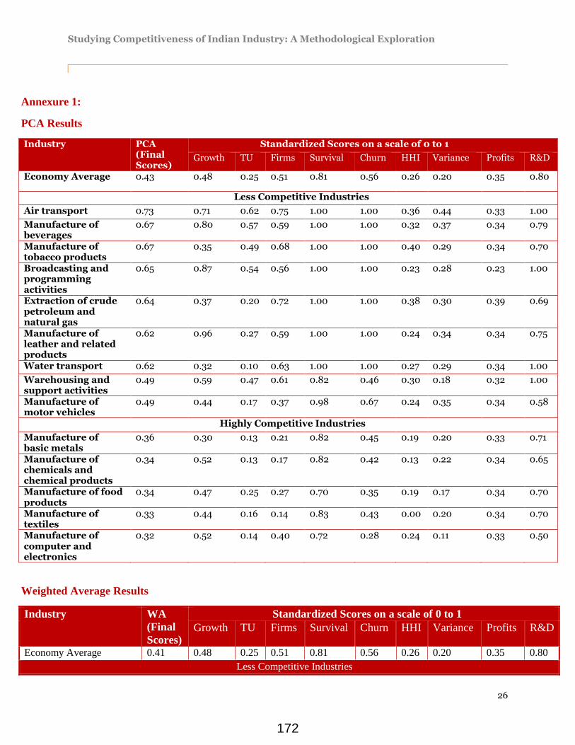
Studying Competitiveness of Indian Industry: A Methodological Exploration
26
Annexure 1:
PCA Results
Industry PCA (Final Scores)
Standardized Scores on a scale of 0 to 1
Growth TU Firms Survival Churn HHI Variance Profits R&D
Economy Average 0.43 0.48 0.25 0.51 0.81 0.56 0.26 0.20 0.35 0.80
Less Competitive Industries
Air transport 0.73 0.71 0.62 0.75 1.00 1.00 0.36 0.44 0.33 1.00
Manufacture of beverages
0.67 0.80 0.57 0.59 1.00 1.00 0.32 0.37 0.34 0.79
Manufacture of tobacco products
0.67 0.35 0.49 0.68 1.00 1.00 0.40 0.29 0.34 0.70
Broadcasting and programming activities
0.65 0.87 0.54 0.56 1.00 1.00 0.23 0.28 0.23 1.00
Extraction of crude petroleum and natural gas
0.64 0.37 0.20 0.72 1.00 1.00 0.38 0.30 0.39 0.69
Manufacture of leather and related products
0.62 0.96 0.27 0.59 1.00 1.00 0.24 0.34 0.34 0.75
Water transport 0.62 0.32 0.10 0.63 1.00 1.00 0.27 0.29 0.34 1.00
Warehousing and support activities
0.49 0.59 0.47 0.61 0.82 0.46 0.30 0.18 0.32 1.00
Manufacture of motor vehicles
0.49 0.44 0.17 0.37 0.98 0.67 0.24 0.35 0.34 0.58
Highly Competitive Industries
Manufacture of basic metals
0.36 0.30 0.13 0.21 0.82 0.45 0.19 0.20 0.33 0.71
Manufacture of chemicals and chemical products
0.34 0.52 0.13 0.17 0.82 0.42 0.13 0.22 0.34 0.65
Manufacture of food products
0.34 0.47 0.25 0.27 0.70 0.35 0.19 0.17 0.34 0.70
Manufacture of textiles
0.33 0.44 0.16 0.14 0.83 0.43 0.00 0.20 0.34 0.70
Manufacture of computer and electronics
0.32 0.52 0.14 0.40 0.72 0.28 0.24 0.11 0.33 0.50
Weighted Average Results
Industry WA
(Final
Scores)
Standardized Scores on a scale of 0 to 1
Growth TU Firms Survival Churn HHI Variance Profits R&D
Economy Average 0.41 0.48 0.25 0.51 0.81 0.56 0.26 0.20 0.35 0.80
Less Competitive Industries
172

Studying Competitiveness of Indian Industry: A Methodological Exploration
27
Air transport 0.62 0.71 0.62 0.75 1.00 1.00 0.36 0.44 0.33 1.00
Manufacture of beverages 0.57 0.80 0.57 0.59 1.00 1.00 0.32 0.37 0.34 0.79
Broadcasting and
programming activities 0.56 0.87 0.54 0.56 1.00 1.00 0.23 0.28 0.32 1.00
Manufacture of leather and
related products 0.51 0.96 0.27 0.59 1.00 1.00 0.24 0.34 0.34 0.75
Manufacture of tobacco
products 0.51 0.35 0.49 0.68 1.00 1.00 0.40 0.29 0.34 0.70
Warehousing and support
activities 0.50 0.59 0.47 0.61 0.82 0.46 0.30 0.18 0.32 1.00
Information service
activities 0.49 0.66 0.12 0.60 1.00 1.00 0.26 0.23 0.35 1.00
Extraction of crude
petroleum and natural gas 0.47 0.37 0.20 0.72 1.00 1.00 0.38 0.30 0.39 0.69
Water transport 0.46 0.32 0.10 0.63 1.00 1.00 0.27 0.29 0.34 1.00
Manufacture of wearing
apparel 0.46 0.90 0.20 0.53 0.69 0.39 0.22 0.16 0.34 1.00
Highly Competitive Industries
Manufacture of rubber and
plastics products 0.36 0.49 0.14 0.28 0.84 0.43 0.18 0.23 0.34 0.66
Manufacture of chemicals
and chemical products 0.34 0.52 0.13 0.17 0.82 0.42 0.13 0.22 0.34 0.65
Manufacture of electrical
equipment 0.34 0.22 0.14 0.31 0.91 0.53 0.22 0.22 0.32 0.62
Manufacture of basic
metals 0.34 0.30 0.13 0.21 0.82 0.45 0.19 0.20 0.33 0.71
Manufacture of computer
and electronic products 0.33 0.52 0.14 0.40 0.72 0.28 0.24 0.11 0.33 0.50
Manufacture of textiles 0.31 0.44 0.16 0.14 0.83 0.43 0.00 0.20 0.34 0.70
Simple Average Results
Industry SA
(Final
Scores)
Standardized Scores on a scale of 0 to 1
Growth TU Firms Survival Churn HHI Variance Profits R&D
Economy Average 0.45 0.48 0.25 0.51 0.81 0.56 0.26 0.20 0.35 0.80
Less Competitive Industries
Air transport 0.69 0.71 0.62 0.75 1.00 1.00 0.36 0.44 0.33 1.00
Manufacture of beverages 0.64 0.80 0.57 0.59 1.00 1.00 0.32 0.37 0.34 0.79
Manufacture of leather and
related products 0.61 0.96 0.27 0.59 1.00 1.00 0.24 0.34 0.34 0.75
Manufacture of tobacco
products 0.58 0.35 0.49 0.68 1.00 1.00 0.40 0.29 0.34 0.70
Information service
activities 0.58 0.66 0.12 0.60 1.00 1.00 0.26 0.23 0.35 1.00
173
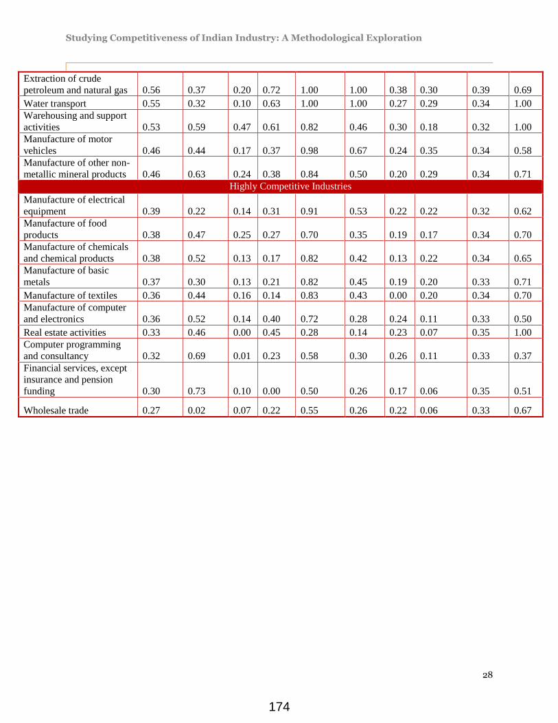
Studying Competitiveness of Indian Industry: A Methodological Exploration
28
Extraction of crude
petroleum and natural gas 0.56 0.37 0.20 0.72 1.00 1.00 0.38 0.30 0.39 0.69
Water transport 0.55 0.32 0.10 0.63 1.00 1.00 0.27 0.29 0.34 1.00
Warehousing and support
activities 0.53 0.59 0.47 0.61 0.82 0.46 0.30 0.18 0.32 1.00
Manufacture of motor
vehicles 0.46 0.44 0.17 0.37 0.98 0.67 0.24 0.35 0.34 0.58
Manufacture of other non-
metallic mineral products 0.46 0.63 0.24 0.38 0.84 0.50 0.20 0.29 0.34 0.71
Highly Competitive Industries
Manufacture of electrical
equipment 0.39 0.22 0.14 0.31 0.91 0.53 0.22 0.22 0.32 0.62
Manufacture of food
products 0.38 0.47 0.25 0.27 0.70 0.35 0.19 0.17 0.34 0.70
Manufacture of chemicals
and chemical products 0.38 0.52 0.13 0.17 0.82 0.42 0.13 0.22 0.34 0.65
Manufacture of basic
metals 0.37 0.30 0.13 0.21 0.82 0.45 0.19 0.20 0.33 0.71
Manufacture of textiles 0.36 0.44 0.16 0.14 0.83 0.43 0.00 0.20 0.34 0.70
Manufacture of computer
and electronics 0.36 0.52 0.14 0.40 0.72 0.28 0.24 0.11 0.33 0.50
Real estate activities 0.33 0.46 0.00 0.45 0.28 0.14 0.23 0.07 0.35 1.00
Computer programming
and consultancy 0.32 0.69 0.01 0.23 0.58 0.30 0.26 0.11 0.33 0.37
Financial services, except
insurance and pension
funding 0.30 0.73 0.10 0.00 0.50 0.26 0.17 0.06 0.35 0.51
Wholesale trade 0.27 0.02 0.07 0.22 0.55 0.26 0.22 0.06 0.33 0.67
174

Studying Competitiveness of Indian Industry: A Methodological Exploration
29
Annexure 2: PCA output6
6 For the purpose of choosing weights we have selected the first Principal Component PC1. As is clear from the summary command, the first principal component explains around 47% of the variance of the data set.
175

Studying Competitiveness of Indian Industry: A Methodological Exploration
30
Annexure 3: List of Industries Covered
Industry Name
Division 01 Crop and animal production, hunting and related service
activities
Division 03 Fishing and aquaculture
Division 05 Mining of coal and lignite
Division 06 Extraction of crude petroleum and natural gas
Division 07 Mining of metal ores
Division 08 Other mining and quarrying
Division 09 Mining support service activities
Division 10 Manufacture of food products
Division 11 Manufacture of beverages
Division 12 Manufacture of tobacco products
Division 13 Manufacture of textiles
Division 14 Manufacture of wearing apparel
Division 15 Manufacture of leather and related products
Division 16 Manufacture of wood and products of wood and cork,
except furniture; (manufacture of articles of straw and plaiting
materials)
Division 17 Manufacture of paper and paper products
Division 18 Printing and reproduction of recorded media
Division 19 Manufacture of coke and refined petroleum products
Division 20 Manufacture of chemicals and chemical products
Division 21 Manufacture of pharmaceuticals, medicinal chemical and
botanical products
Division 22 Manufacture of rubber and plastics products
Division 23 Manufacture of other non-metallic mineral products
Division 24 Manufacture of basic metals
Division 25 Manufacture of fabricated metal products, except
machinery and equipment
Division 26 Manufacture of computer, electronic and optical products
Division 27 Manufacture of electrical equipment
Division 28 Manufacture of machinery and equipment n.e.c.
Division 29 Manufacture of motor vehicles, trailers and semi-trailers
Division 30 Manufacture of other transport equipment
Division 31 Manufacture of furniture
Division 32 Other manufacturing
Division 35 Electricity, gas, steam and air conditioning supply
Division 36 Water collection, treatment and supply
Division 37 Sewerage
176

Studying Competitiveness of Indian Industry: A Methodological Exploration
31
Division 38 Waste collection, treatment and disposal activities;
materials recovery
Division 41 Construction of buildings
Division 42 Civil engineering
Division 43 Specialized construction activities
Division 45 Wholesale and retail trade and repair of motor vehicles
and motorcycles
Division 46 Wholesale trade
Division 47 Retail trade
Division 49 Land transport and transport via pipelines
Division 50 Water transport
Division 51 Air transport
Division 52 Warehousing and support activities for transportation
Division 55 Accommodation
Division 56 Food and beverage service activities
Division 58 Publishing activities
Division 59 Motion picture, video and television programme
production, sound recording
Division 60 Broadcasting and programming activities
Division 61 Telecommunications
Division 62 Computer programming, consultancy and related
activities
Division 63 Information service activities
Division 64 Financial services, except insurance and pension funding
Division 66 Other financial activities
Division 68 Real estate activities
Division 71 Architecture and engineering activities; technical testing
and analysis
Division 72 Scientific research and development
Division 77 Rental and leasing activities
Division 79 Travel agency, tour operator and other reservation service
activities
Division 80 Security and investigation activities
Division 82 Office administrative, office support and other business
support activities
Division 85 Education
Division 86 Human health activities
Division 90 Creative, arts and entertainment activities
Division 93 Sports activities and amusement and recreation activities
Division 95 Repair of computers and personal and household goods
177

Studying Competitiveness of Indian Industry: A Methodological Exploration
32
Annexure 4: Summary Statistics of the raw data7
Measure Growth Trade Unions No. of Firms survival churn
Mean 7.56 59.95 49.89 94.57 3.49
Standard Error 1.70 10.36 9.73 0.71 0.59
Median 5.88 32.00 15.40 95.26 2.63
Standard
Deviation
13.83 84.19 79.07 5.80 4.82
Kurtosis 3.51 14.58 12.92 3.15 10.55
Skewness 1.22 3.25 3.16 -1.49 2.85
Range 83.22 530.00 475.60 28.57 27.74
Minimum -21.94 0.00 1.00 71.43 0.00
Maximum 61.28 530.00 476.60 100.00 27.74
Measure HHI Variance of Market Share Profit R&D
Mean 3275.90 0.41 7.10 1.36
Standard Error 339.11 0.03 3.40 0.82
Median 2275.31 0.39 6.63 0.01
Standard
Deviation
2754.98 0.24 27.63 6.64
Kurtosis 0.61 -0.33 10.92 61.23
Skewness 1.24 0.37 -0.69 7.71
Range 9774.36 0.98 235.92 53.56
Minimum 225.64 0.00 -22.79 0.00
Maximum 10000.00 0.98 113.13 53.56
7 The summary statistics provided here are for the raw data including all the industries analyzed for the study. The final result includes only those industries for which we could gather substantially representative data.
178

1
How have Mergers and Acquisitions Affected Firms’ Business Performance? Empirical
Evidence of Indian Manufacturing Sector
Pulak Mishra1
Abstract
Given the significant increase in the number of mergers and acquisitions (M&A) during the last
two and half decades of economic reforms in India, the present paper attempts to examine how
such strategic combinations have affected firms’ financial performance. Using secondary data
collected from the Prowess IQ database of the Centre for Monitoring Indian Economy (CMIE)
and applying Arellano-Bond dynamic panel data estimation techniques, the paper finds that
M&A do not cause any significant influence on firms’ financial performance due to the
multidirectional structure-conduct-performance relationships. Findings of the present paper,
therefore, suggest for relook at the policies and regulations relating to M&A, international trade
and intellectual property as they are expected to influence the market structure, firms’ business
strategies, efficiency and competitiveness, and hence their financial performance.
Keywords: Economic Reforms, Mergers and Acquisitions, Financial Performance,
Competition Policy, India
(Acknowledgement: An earlier version of this paper was presented in the National Conference
on Economics of Competition Law organized by the Competition Commission of India in New
Delhi during 2-3 March, 2017. The author is thankful to the session chair, discussant of the paper
and other conference participants for their valuable comments and suggestions. The author is
also thankful to Prof. Rakesh Basant for having useful discussions in different stages of writing
this paper. Thanks are also due to Mr. Aman Mahawar and Ms. Neha Jaiswal for their excellent
support in compilation of data. Usual disclaimers apply.)
1Associate Professor, Department of Humanities and Social Sciences, Indian Institute of Technology Kharagpur, India,
Email: [email protected]
179

2
How have Mergers and Acquisitions Affected Firms’ Business Performance? Empirical
Evidence of Indian Manufacturing Sector
Introduction:
Policy initiatives and regulatory changes made during the last two and half decades of economic
reforms have led to considerable changes in the basic environment and functioning of Indian
manufacturing sector. Although the pace of economic reforms has slowed down in recent years,
the policy changes and regulatory measures in general continue to aim at strengthening market
disciplines and enhancing competition. It is expected that greater market competition would
bring in efficiency and competitiveness and thus facilitate achieving optimality in allocation of
resources and distribution of goods and services.
While the domestic firms have responded to the policy and regulatory changes in a variety of
ways, many of them have relied largely on mergers and acquisitions (M&A) as strategies to
restructure their business for existence and growth under the new business conditions2. As a
result, there has been significant increase in number of M&A during the post-reform period
(Beena, 2014; Basant and Mishra, 2016). Given the policy induced flexibilities, domestic private
firms, especially those from the same business groups, have taken the route of mergers to
consolidate their business. A large number of them have also used the opportunities to raise
monopoly power. The foreign firms, on the other hand, have relied mainly on acquisitions to
enter into specific markets and raising control therein.
It is observed that involvement of the multinational corporations (MNCs) in M&A has been
substantially high and acquisition of shares of the incumbents has become a predominant channel
of foreign investment inflows into the country during the post-reform period3. The share of
acquisitions in equity inflows has increased from 11 percent during 1995-2000 to 27 percent
during 2000-2012 (ISID, 2014). Hence, although the liberal policy and regulatory measures have
resulted in a significant increase in foreign investment inflows, high share of acquisition is likely
to have important implications for overall development of the economy in general and market
structure and firms’ performance in particular.
Given this backdrop and findings of the existing studies, one may expect that M&A in Indian
manufacturing sector would help the firms to improve their financial performance through either
larger market power and/or greater efficiency4. The structure-conduct-performance framework of
2Although mergers and acquisitions are different in definitions and statutory procedures, the present paper makes no
distinction between the two as their economic effects are by and large the same. 3The share of cross-border deals was as high as 34 percent during 2000-2008 (Saraswathy, 2015). 4Thus, the impact of M&A on financial performance can be considered as the balance of the anti-competitive market
180
3
Bain (1956) suggests that, given the market structure, M&A as business strategies influence firms’
financial performance. Many of the existing studies (e.g., Healy et al. 1992; Grabowski et al., 1995;
Switzer, 1996; Waldfogel and Smart, 1994; Vander, 1996) empirically support the proposition that
M&A lead to better financial performance. However, there are also studies (e.g., Dickerson et al.,
1997; Ravenscraft and Scherer, 1987; Mueller, 1985; Ghosh, 2001) that report results at odds with
the view that M&A improve financial performance. Further, Ikeda and Doi (1983), Cosh et al.
(1984), Kumar (1984), Geroski (1988), Odagiri (1992) also find either such negative impact or little
changes in firms’ operating performance following M&A.
Thus, the nature of impact of M&A on firms’ financial performance is not conclusive as the existing
studies report mixed results with the findings ranging from slightly positive improvement to
significantly negative or no improvement. The issue is more pertinent in Indian context given that
there is little evidence of improvement in firms’ financial performance (Basant and Mishra, 2016),
whereas a large number industries have recorded either decline or no change in market
concentration during the post-reform period (Mishra and Rao, 2014). Further, wherever market
concentration has increased, it might not have necessarily influenced firms’ financial performance
as concentration-markup relationship is not significant in dynamic context (Mishra, 2008). On the
other hand, the wave of M&A during the post-reform period has enhanced firms’ export
competitiveness in Indian manufacturing sector (Mishra and Jaiswal, 2012). Besides, in recent
years, India has transformed its image from being a FDI destination to an emerging foreign direct
investor with many of the Indian companies venturing abroad, especially in the areas software,
biotechnology, automotive and oil and becoming globally competitive (Pradhan, 2008). Thus, one
may argue that M&A in Indian manufacturing sector during the post-reform period have enhanced
firms’ competitiveness making the markets more competitive or leaving them largely unchanged5.
The above developments in Indian manufacturing sector during the post-reform period raise an
important question, how has the wave of M&A affected firms’ financial performance given the
ongoing process of policy and regulatory changes and subsequent fine tuning of business strategies?
Addressing this question in the context of competition law and policy is necessary for three reasons.
First, while cost-efficiencies of firms in Indian manufacturing sector do not show any evidence of
improvement during the post-reform period, export orientation has increased significantly across
major industries and import penetration has recorded a decline, though marginally (Basant and
Mishra, 2016). The increase in firms’ export competitiveness in Indian manufacturing sector can
largely be contributed to M&A (Mishra and Jaiswal, 2012). On the other hand, financial
performance, particularly profitability shows sign of improvement only at a very slow rate possibly
power effect (Stigler, 1950) and the pro-competitive efficiency effect (Williamson, 1968). 5 In a recent study, Mishra and Jaiswal (2017) found that the wave of M&A has caused significant positive influence
on both incidence and extent of firms’ export competitiveness in Indian drugs and pharmaceutical industry.
181

4
due to increasing competition in different markets and failure of firms in choosing appropriate
strategies and/or enhancing cost efficiency.
Second, there are evidences of failure of M&A in enhancing business performance in Indian
context as well. For example, using panel data of 52 drugs and pharmaceutical companies for the
period 2000-2008, Mishra and Chandra (2010) found that M&A have failed to cause any
significant impact on firms’ profitability. Instead, their financial performance has varied directly
with asset base, selling efforts and export and import intensities, but inversely with market share
and demand for the products (Mishra and Chandra, 2010). Similarly, according to Saple (2000),
mergers could not generate high monopoly rents or impede the competitive process. On the other
hand, Das (2000) found rise in post-merger average sales and net worth with very less proportion
of the firms experiencing a decline in post-merger profitability. This is contradictory to many of
the existing studies in Indian context.
Third, M&A may not necessarily cause any significant impact on financial performance when it
is assessed in combination with other business strategies of firms as well as various market
structure and policy related aspects. This issue is very important given that economic reforms
have deepened over the years in areas like FDI, competition policy, privatization and intellectual
property regulation. Such policy and regulatory changes are likely to cause differences in nature
and intensity of firms’ strategic responses and changes in structure of the markets. When it is so,
performance enhancing effects of M&A may not be significant.
Given this backdrop, it is, therefore, necessary to revisit the impact of M&A on firms’ financial
performance in Indian manufacturing sector controlling influence of their other business
strategies (other than M&A), various structural aspects of the markets and policies and
regulations of the government. The present paper is an attempt in this direction. Since M&A are
industry specific activities (Mitchell & Mulherin, 1996), and distribution of number of M&A as
well as financial performance vary across different industries (Basant and Mishra, 2016), the
present paper attempts to examine the impact of such combinations on financial performance at
industry level. More specifically, the objective of the paper is to examine how financial
performance has varied across major industries of Indian manufacturing sector following M&A
during the post-reform period.
The paper is organized in five sections. While the second section specifies the econometric
model and hypothesizes possible impact of the independent variables, the third section discusses
the estimation techniques applied and sources of data used in the paper. Measurements of the
variables are also given in this section. The fourth section presents the regression results and
discusses their implications. The findings are summarized and their policy and regulatory
implications are highlighted in the fifth and the final section of the paper.
182

5
2. Model Specification
In order to examine the impact of M&A on firms’ financial performance, the present paper uses
the structure-conduct-performance (SCP) framework of Bain (1956). Although the traditional
SCP paradigm postulates unidirectional relationships between market structure, firms’ conduct
and their performance, successive developments in the industrial organization literature suggest
for a multidirectional structure-conduct-performance framework (Scherer and Ross, 1990). This
new framework recognises both way causalities between market structure and firms’ conducts,
between conducts and financial performance and between market structure and financial
performance (Tirole, 1988). The other important development in the SCP paradigm is inclusion
of public policies relating to taxes, subsidies, international trade, investment, etc. (Scherer and
Ross, 1990).
Given these developments in the literature, the present paper considers M&A as a conduct variable
and explores the impact on financial performance controlling for influences of various structural
aspects of the market, other business strategies (other than M&A) of firms and changes in policies
and regulations by the government. Further, the present paper also recognizes various feedback
effects. Accordingly, the following analytical framework is envisaged:
Policy and
Regulatory Changes
Mergers and
Acquisitions
Changes in
Market Structure
Impact on
Performance
Efficiency and
Competitiveness
Market Power Other Business
Strategies
Basic Market
Conditions
183

6
On the basis of this framework, it is assumed that current financial performance of firms in an
industry (PERt) depends on current market concentration (CONt), current capital intensity
(KIRt), ratio of current imports to current exports (IMEXt), lagged mergers and acquisitions
(M&At-1), current advertising intensity (ADVTt), current marketing and distribution intensity
(MADt), lagged R&D intensity (R&Dt-1), current foreign technology purchase intensity (FTPt),
and lagged financial performance (PERt-1), i.e.,
),,&,,,&,,,( 1,1,1, itittiitittiitittiit IMEXFTPDRMADADVTAMCONKIRPERfPER
The present paper uses CONt, KIRt and IMEXt to capture structural aspects of the market,
M&At-1, ADVTt, MADt, R&Dt-1 and FTPt for firms’ business strategies and PERt-1 for past
performance. In addition, while the variable M&A captures changes in investment policies in
general and competition policy in particular, IMEX controls for the impact of trade related policy
changes. On the other hand, R&D and FTP act as proxies for changes in technology related
policies of the government including regulation of intellectual properties. Since the relationships
amongst many of these variables are not instantaneous, following Kambhampati (1996), suitable
lags have been introduced. For example, it is assumed that M&A can influence financial
performance only after an interval. Similarly, in-house R&D efforts require gestation lags to
influence financial performance.
The present paper examines firms’ financial performance in terms of their profitability (PROF)
and the rate of returns on capital employed (ROCE). While the profitability shows the
relationship between profit and output or sales, the rate of returns ratio reflects the association
between profit and investment. The present paper uses these two alternative measures of
financial performance to substantiate the findings. Further, the Herfindahl-Hirschman index is
used as a measure of the degree of sellers’ concentration in a market.
Possible Impact of the Independent Variables
Current Market Concentration (CONt): It is postulated that industries with concentrated
markets facilitate collusion leading to supernormal profit (Bain, 1951; Chamberlin, 1933; Stigler,
1964). While the positive relationship between market concentration and price-cost margin or
profitability is well documented in the literature (e.g. Weiss, 1974; Ravenscraft, 1983,
Kambhampati, 1996; Goldar and Aggarwal, 2004), the strength of the relationship differs
depending on firms’ conducts (Mishra, 2008). Further, greater market concentration may not be
necessary for better financial performance when the firms’ have superior efficiency (McGee,
1971; Demsetz, 1973). On the other hand, greater market concentration may not be sufficient for
184

7
better financial performance if there are limited or no barriers to entry (Hay and Morris, 1991)6.
In the long-run, impact of market concentration on financial performance depends on how these
diverse forces empirically dominate each other. For example, using dynamic framework, Mishra
(2008) found that the traditional positive relationship between market concentration and mark-up
does not hold when other structural aspects of the market, firms’ business strategies and policies
of the government are controlled.
Current Capital Intensity Ratio (KIRt): High capital intensity indicates large sunk costs that
create entry barriers and thereby give rise to monopoly profit (McDonald, 1999). High capital
intensity can also make the domestic firms globally more competitive, particularly when capital
goods embody better technology. On the other hand, high capital intensity may result in lesser
flexibility in respect of adjustments to various market shocks causing adverse impact on financial
performance. Besides, higher capital intensity of larger firms can make the smaller entities less
competitive due to capital market imperfections (Basant and Saha, 2005).Thus, the nature of the
relationship between capital intensity and financial performance is ambiguous.
Lagged Mergers and Acquisitions (MAt-1): While the efficiency theory suggests that M&A are
planned and executed to reduce costs production through scale economies (Porter, 1985; Shelton,
1988), the monopoly theory considers such combinations as the routes to raise market power
(Steiner, 1975, Chatterjee, 1986). Hence, M&A are expected to result in better financial
performance of the firms through greater market power and/or efficiency gains. However, given
the multidirectional structure-conduct-performance framework of Scherer and Ross (1990),
financial performance is also likely to be affected by a set of other factors relating to structural
aspects of the market, firms’ business strategies (other than M&A), their business performance in
the past and policies and regulations of the government. Thus, when impact of other factors are
controlled, M&A may not necessarily cause any significant influence on financial performance.
Current Advertising Intensity (ADVTt): On the one hand, advertising creates image advantage
over the rivals. Besides, advertising can also lead to product differentiation and entry barriers
(Comanor and Wilson, 1967)7. Thus, industries with higher advertising intensity are expected to
experience better financial performance of firms. There are evidences (e.g., Scherer and Ross,
1990) of positive relationship between profitability and advertising intensity. However,
informative advertising may not necessarily help in enhancing financial performance. There are
evidences (e.g., Delorme et al., 2002) of no significant impact of advertising on profitability.
Some other studies finding no systematic relationship between advertising and profitability
include Imel and Heimberger (1971), Grabowski and Mueller (1978) and Nagle (1981).
6As mentioned earlier, Mishra (2008) found no significant relationship between market concentration and price-cost
margin in Indian manufacturing sector in the 1990s.
7 High advertising intensity may require the potential entrants to incur disproportionately high advertising expenses to
win over the incumbents and this may discourage entry.
185

8
Current Marketing and Distribution Intensity (MADt): Expenditures on promoting the
products or developing distribution networks result in related complementary assets. While
marketing related expenditures help in promoting the products by reaching the consumers, wider
distribution networks provide easy and timely access to the same. Thus, industries with greater
marketing or distribution related efforts by firms are expected to record better financial
performance. There are evidences of better financial performance following increase in
expenditure on distribution and marketing related activities (Majumdar, 1997).
Lagged R&D Intensity (RDt-1): While product development strengthens/extends market
orientation, process innovation reduces the costs of production. Sustained in-house R&D efforts
can also act as an important instrument of maintaining entry barriers (Mueller, 1990), resulting in
higher profitability in the long run. According to Cefis (1998), persistent innovators earn above
the average profit. However, in the absence of effective regulation, competitors may imitate the
outcomes and the firms engaged in innovation may lose the edge. Further, the existing
accounting practices that allow firms to express R&D expenses entirely in the year incurred
instead of amortizing it to recognize its future benefits create the possibility of negative impact
of in-house R&D on profitability (Mishra and Chandra, 2010). There are evidences (e.g., Mishra
and Chandra, 2010; Mishra and Vikas, 2010) of no significant impact of in-house R&D on firms’
profitability in Indian pharmaceutical industry.
Current Foreign Technology Purchase Intensity (FTPt): Acquisition of foreign technologies
helps in lowering operating costs and prices (Hinomoto, 1965; Balcer and Lippman, 1984). Use
of such technologies can also enhance product quality and hence demand in domestic markets.
Thus, foreign technology purchase is likely to improve firms’ financial performance. In addition,
foreign technology purchase also helps in creating strategic entry barriers. This means that
industries with greater foreign technology purchase intensity are likely to record better financial
performance. However, reaping the benefits of these technologies in the long run requires their
proper application and development of complementary indigenous technologies. Further, when the
technologies purchased from abroad are obsolete, the domestic firms may not have any distinct
edge, vis-à-vis the MNCs.
Lagged Financial Performance (PERt-1): Better financial performance is expected to
strengthen firms’ market position and enable them to develop complementary assets relating to
manufacturing, selling and technology. As a result, the incumbents are expected to record better
financial performance in future. However, better financial performance of the incumbents is also
likely to attract new firms into the industry making the market more competitive and causing
downward pressures on financial performance of the incumbents’, especially in the absence of
effective entry barriers. Better financial performance in the past can also cause adverse impact on
186

9
its current level through X-inefficiency. Impact of past financial performance on its current level,
therefore, depends on the relative strength of these diverse forces.
Ratio of Current Imports to Current Exports (IMEXt): Greater penetration of imported
goods increases competitive pressures in the domestic market. When such competitive pressures
enhance efficiency, financial performance may improve (Majumdar, 1997). On the other hand,
one may expect positive impact of exports on financial performance (Majumdar, 1997),
particularly when the extent of competition differs between the domestic and the international
market. When such penetration into the international market is backed by greater efficiency and
competitiveness, financial performance may improve. For example, Saluja (1968), Panchamukhi
(1974) and Katrak (1980) found that price-cost margin is higher in Indian manufacturing
industries with relatively less import competition and high export orientation. Impact of imports
vis-à-vis exports on financial performance is, therefore, largely an empirical issue.
From the above discussion it is evident that, in addition to M&A, firms’ financial performance
depends on a variety of other factors and the nature and extent of impact depends on balancing of
the diverse forces. Hence, understanding the impact of M&A on firms’ financial performance
requires systematic investigation through econometric modelling controlling effects of other
forces. What follows next is an attempt in this direction.
3. Estimation Techniques and Data Sources
The functional relationship envisaged in the previous section is estimated with a panel dataset of
84 industries over the period from 2001-2002 to 2010-11. Selection of the study period is based
on three specific reasons. First, since M&A during 1995-2000 had significant involvement of the
MNCs, financial performance is likely to be affected considerably as these firms have distinct
edge in respect of financial resources, technologies, human resources and markets. Second, the
amendments to the Indian Patent Act (1970) since the late 1990s, viz., Patent First Amendment
Act (1999), Patent (Second Amendment) Bill (2002) and Patent (Amendment) Bill (2005) were
expected to incentivize firms towards in-house R&D. Such incentives are likely to influence
financial performance through in-house R&D. Third, stable economic conditions and changes in
macroeconomic policies since the early 2000s are also likely to have considerable implications
for firms’ financial performance during this period. However, the present paper does not
consider data period beyond 2010-11 as the pace of M&A slackened during 2008-2014 (Basant
and Mishra, 2016). Further, due to economic slowdown since 2009-10, consideration of this
phase may cause unusual truncation in the envisaged relationships.
It is expected that carrying out panel data analysis in the present paper would help in capturing
variations in the variables both across the industries and over time. This relaxes the assumption
made in cross-section analyses that the same structure-conduct-performance relationships prevail
187

10
across all industries at a particular point of time. Necessary data are sourced from the Prowess IQ
database of the Centre for Monitoring Indian Economy (CMIE). The details on measurement of
the variables are given in Table – 1.
Table 1: Measurement of the Variables
Variable Measurement
Dependent Variables
Profitability (PROFt) Ratio of profit before tax to industry sales
Returns on Capital Employed (ROCEt) Ratio of profit before tax to capital employed
Independent Variables
Current Capital Intensity (KIRt) Ratio of capital employed to industry sales in the
current year
Current Market Concentration (CONt) Herfindahl-Hirschman Index of market
concentration
Current Import-Export Ratio (IMEXt) Ratio of current imports to current exports
Lagged Mergers and Acquisitions (MAt-1) Natural logarithm of total number of mergers and
acquisitions during the last three years excluding
the year under reference
Current Advertising Intensity (ADVTt) Ratio of advertising expenditure to industry sales in
the current year
Current Marketing and Distribution
Intensity (MADt)
Ratio of marketing and distribution related
expenditure to industry sales in the current year
Lagged In-house R&D Intensity (R&Dt-1) Ratio of in-house R&D expenditure to industry
sales in the previous year
Current Foreign Technology Purchase
Intensity (FTPt)
Ratio of expenditure on foreign technology
purchase to industry sales in the current year
Lagged Profitability (PROFt-1) One year lagged value of profitability
Lagged Returns on Capital Employed
(ROCEt-1)
One year lagged value of the returns on capital
employed
In the present paper, Arellano-Bond (1991) dynamic panel data model of the following form is
estimated to examine the impact of M&A on firms’ financial performance:
it
m
j
itjjtiit uxyy
1
,1,
The estimation techniques for the above model are based on the generalized method of moments
(GMM). As compared to the method of instrumental variables (e.g., Balestra and Nerlove, 1966;
Anderson and Hsiao, 1981; Bhargava and Sargan, 1983), the GMM estimators can bring in more
information on data (Ahn and Schmidt, 1995). The Arellano-Bond (1991) estimators are also
consistent and more efficient than the Anderson-Hsiao (1981) estimators. In addition, the
Arellano-Bond (1991) estimators have generalizations that can address the problem of
autocorrelation, heteroscedasticity, specification errors, etc.
188

11
The Arellano-Bond dynamic panel data estimation techniques uncover the joint effects of the
explanatory variables on the dependent variable while controlling potential bias due to
endogeneity of the explanatory variables including the lagged dependent variable8. The paper
also uses one-year lagged values of the predetermined variables as the instruments to control the
endogeneity bias further. In the present model, inclusion of the lagged dependent variable as one
of the explanatory variables accounts for the dynamic effects9.
In addition, presence of autocorrelation problem and validity of instruments are tested by
applying the Arellano-Bond (1991) test for autocovariance and the Sargan test (1958) of over-
identifying restrictions respectively. The present paper uses both the one-step and two-step
estimators. The two-step estimators are used for testing specification and overall significance of
the estimated model as they yield standard errors that are asymptotically robust to both
heteroscedasticity and autocorrelation. On the other hand, inferences on individual coefficients
are based on one-step estimators due to their unbiased and reliable asymptotic robust standard
errors. It may be noted that, in case of one-step estimators, the Sargan test over-rejects the null
hypothesis of over-identifying restrictions, whereas the asymptotic standard errors of the two-
step estimators can be severely downward biased in small samples. Hence, the present paper uses
both the one-step and two-step estimators to test significance of the overall model and the
individual coefficients respectively.
Further, the variance inflation factors (VIF) for each of the independent variables are computed
to examine if the estimated models suffer from severe multicollinearity problem. Since the
present study uses an unbalanced panel dataset of 84 industries over a period of 10 years, Fisher-
type panel data unit root test is carried out to examine if the variables used in regression analysis
are non-stationary. The test is based on the null hypothesis that that all panels contain a unit root
again the alternative hypothesis is that at least one of the panels is stationary. Both the
Augmented Dickey-Fuller (ADF) and the Phillips–Perron (PP) unit-root tests are carried out to
ensure consistency in the results of the tests.
Following Choi (2001), two methods have been applied to carry out the tests, viz., Inverse χ2,
and Modified Inverse χ2. Since the mean of financial performance of an industry may be zero,
the drift option is not included. However, for both the methods, the trend components are added
and the cross sectional means are removed through demeaning. A lag length of 2 years is
selected by using the Newey and West’s (1994) plug-in procedure (i.e., the nearest integer of
4*(T/100)2/9 with T being the time length of the panels).
8 Since industry is the unit of observation in the present context, endogeneity problem is unlikely to be acute as it
normally is when firm or the line of business is the unit of observation (Salinger, 1990).
9 The use of such dynamic models is favoured, especially, for panels that have a large number of cross-sectional units
with a small number of time periods, as we have in the present case. This is so because the estimation methods in such
cases do not require larger time periods to obtain consistent estimators.
189

12
4. Regression Results and Discussions
Table 2 presents the summary statistics of the variables used in regression analysis. The partial
correlation coefficients between the dependent and the independent variables are given in Table
3. It is found that, except the ratio of imports to exports, rests of the independent variables have
statistically significant partial association with either of the two alternative measures of financial
performance, though statistical significance and the nature of correlation differ across the
indicators. Notably, mergers and acquisitions are found to have statistically significant (partial)
positive correlation with returns on capital employed, whereas the correlation coefficient is not
statistically significant when profitability is considered as a measure of financial performance.
Further, low values of variance inflation factors (VIFs) suggest that there is no severe
multicollinearity problem in the envisaged relationships (Table 3).
Table 2: Summary Statistics of Variables Used in Regression Models
Variable Number of
Observation
Mean Standard
Deviation
Minimum
Value
Maximum
Value
PROFt 840 840 0.051 0.085 -0.520
ROCEt 840 840 0.070 0.096 -0.433
HHIt 840 840 0.189 0.161 0.013
KIRt 840 840 0.917 0.483 0.232
MAt-1 840 815 1.959 1.001 0.000
ADVTt 827 827 0.013 0.020 0.000
MADt 840 840 0.054 0.035 0.005
RDt-1 812 809 0.006 0.031 0.000
FTPt 700 698 0.031 0.073 0.000
IMEXt 698 700 0.890 3.085 0.000
The results of panel unit root tests are reported in Table 4. In case of the ratio of imports to exports
(IMEX), the test statistics of the Augmented Dickey-Fuller test are based on one-year lags, whereas
those for in-house R&D in Phillips-Perron test are estimated without demeaning. It is found that
none of the variables used in the regressions analysis suffers from the problem of unit root. In other
words, all the variables included in regression analysis are stationary in nature.
Table 3: Partial Correlation Coefficient between the Dependent and the Independent Variables
Independent Variable Partial Correlation Coefficient VIF
PROF ROCE
HHIt 0.2313** 0.1905** 1.58
KIRt 0.0573 -0.2690** 1.28
MAt-1 0.0471 0.2086** 1.61
ADVTt 0.0897** -0.1332** 1.40
MADt -0.0851** 0.0573 1.26
190

13
RDt-1 0.1249** 0.0690* 1.15
FTPt 0.1786** 0.0382 1.33
IMEXt 0.0162 0.0066 1.02
Note: **Statistically Significant at 5 percent; *Statistically Significant at 10 percent
Table 5 and 6 report the Arellano-Bond dynamic panel data regression results of the envisaged
model with profitability and the returns on capital employed being the alternative measures of
financial performance. It is found that, in both the cases, the Wald-2 statistics are significant.
This means that both the estimated models are statistically significant. Further, since the Sargan
test statistics are not statistically significant, the estimated models do not suffer from the problem
of over identification of restrictions. In addition, the Arellano-Bond test for autocorrelation
suggests for no autocorrelation problem of second order, as the respective test statistics are not
statistically significant.
Table 4: Results of Fisher-Type Panel Unit Root Tests
Based on Augmented Dickey-Fuller Tests Based on Phillips-Perron Tests
Variable Inverse 2 Modified Inverse 2 Inverse 2 Modified Inverse 2
PROFt 394.13 12.34 621.48 24.74
ROCEt 419.69 13.73 296.08 6.99
HHIt 283.73 6.31 249.73 4.46
KIRt 436.62 14.65 279.64 6.09
MAt-1 430.57 14.32 409.38 13.17
ADVTt 647.79 26.44 378.91 11.69
MADt 563.65 21.58 404.49 12.90
RDt-1 292.30 7.08 330.93 9.22
FTPt 160.70 1.37 383.45 13.90
IMEXt 203.89 3.39 1183.66 59.17
Note: (1) In case of FTP, the Dickey-Fuller test statistics are significant at 10 percent level of
significance, whereas the rests are statistically significant at 5 percent level of
significance.
(2) In case of IMEX, 1 year lag is used for the Augmented Dickey-Fuller test.
(3) The Philips-Perron test for R&D is not mean corrected.
As mentioned earlier, the present paper uses the one-step estimates for examining statistical
significance of the individual coefficients. It is found that, for both the models, the coefficients of
past financial performance, capital intensity, marketing and distribution related efforts, and
foreign technology purchase intensity are statistically significant. This means that variations in
financial performance across different industries of Indian manufacturing sector have been
caused by these factors. However, while the coefficients of past performance and foreign
technology purchase are positive, that of capital intensity ratio and marketing and distribution
related efforts are negative. This means that financial performance have been better or have
improved in industries that had better financial performance in the past or have spent relatively
191
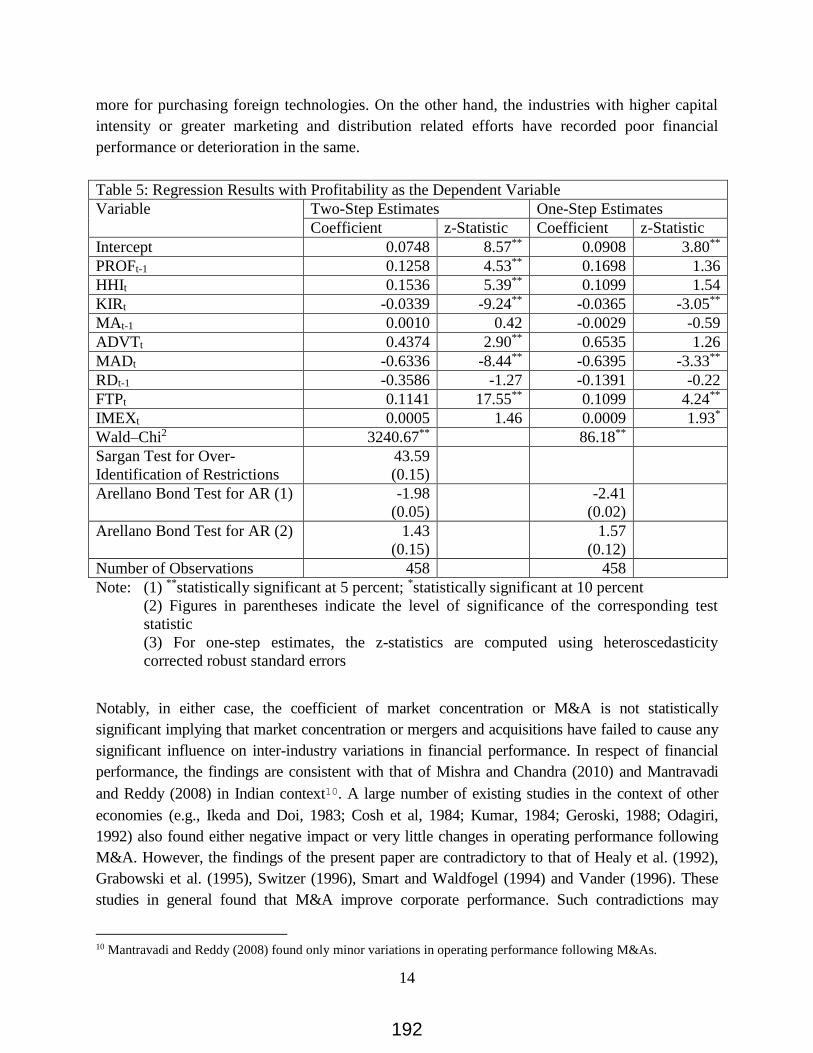
14
more for purchasing foreign technologies. On the other hand, the industries with higher capital
intensity or greater marketing and distribution related efforts have recorded poor financial
performance or deterioration in the same.
Table 5: Regression Results with Profitability as the Dependent Variable
Variable Two-Step Estimates One-Step Estimates
Coefficient z-Statistic Coefficient z-Statistic
Intercept 0.0748 8.57** 0.0908 3.80**
PROFt-1 0.1258 4.53** 0.1698 1.36
HHIt 0.1536 5.39** 0.1099 1.54
KIRt -0.0339 -9.24** -0.0365 -3.05**
MAt-1 0.0010 0.42 -0.0029 -0.59
ADVTt 0.4374 2.90** 0.6535 1.26
MADt -0.6336 -8.44** -0.6395 -3.33**
RDt-1 -0.3586 -1.27 -0.1391 -0.22
FTPt 0.1141 17.55** 0.1099 4.24**
IMEXt 0.0005 1.46 0.0009 1.93*
Wald–Chi2 3240.67** 86.18**
Sargan Test for Over-
Identification of Restrictions
43.59
(0.15)
Arellano Bond Test for AR (1) -1.98
(0.05)
-2.41
(0.02)
Arellano Bond Test for AR (2) 1.43
(0.15)
1.57
(0.12)
Number of Observations 458 458
Note: (1) **statistically significant at 5 percent; *statistically significant at 10 percent
(2) Figures in parentheses indicate the level of significance of the corresponding test
statistic
(3) For one-step estimates, the z-statistics are computed using heteroscedasticity
corrected robust standard errors
Notably, in either case, the coefficient of market concentration or M&A is not statistically
significant implying that market concentration or mergers and acquisitions have failed to cause any
significant influence on inter-industry variations in financial performance. In respect of financial
performance, the findings are consistent with that of Mishra and Chandra (2010) and Mantravadi
and Reddy (2008) in Indian context10. A large number of existing studies in the context of other
economies (e.g., Ikeda and Doi, 1983; Cosh et al, 1984; Kumar, 1984; Geroski, 1988; Odagiri,
1992) also found either negative impact or very little changes in operating performance following
M&A. However, the findings of the present paper are contradictory to that of Healy et al. (1992),
Grabowski et al. (1995), Switzer (1996), Smart and Waldfogel (1994) and Vander (1996). These
studies in general found that M&A improve corporate performance. Such contradictions may
10 Mantravadi and Reddy (2008) found only minor variations in operating performance following M&As.
192

15
largely be due to the multidirectional structure-conduct-performance relationships as propounded by
Scherer and Ross (1990) and the analytical framework depicted above. On the other hand, the
findings in respect of market concentration are consistent with Mishra (2008).
It is also found that the coefficient of efforts towards developing marketing and distribution
related complementary asset is negative. Alternatively, both profitability and returns on capital
employed have varied inversely with development of marketing and distribution related
complementary assets. This is not only surprising, but also contradictory to Majumdar (1997).
Hence, detailed scrutiny is necessary to understand why firms’ efforts towards developing
marketing and distribution related complementary assets failed in improving their financial
performance.
Table 6: Regression Results with Returns on Capital Employed as the Dependent Variable
Variable Two-Step Estimates One-Step Estimates
Coefficient z-Statistic Coefficient z-Statistic
Intercept 0.1786 15.44** 0.2011 5.82**
ROCEt-1 0.1332 12.47** 0.1352 1.49
HHIt 0.1098 4.02** 0.0722 0.71
KIRt -0.0842 -9.55** -0.0940 -2.83**
MAt-1 -0.0051 -1.57 -0.0086 -1.36
ADVTt 0.1528 0.53 0.6391 0.87
MADt -0.8438 -8.63** -0.9230 -2.59**
RDt-1 -1.2895 -7.10** -1.1472 -1.17
FTPt 0.0689 7.93** 0.0692 2.31**
IMEXt 0.0003 0.78 0.0007 1.20
Wald–Chi2 709.97** 37.21**
Sargan Test for Over-Identification
of Restrictions
45.03
(0.12)
Arellano Bond Test for AR (1) -1.49
(0.13)
-1.78
(0.08)
Arellano Bond Test for AR (2) 1.03
(0.30)
1.22
(0.22)
Number of Observations 458 458
Note: (1) **statistically significant at 5 percent; *statistically significant at 1 percent
(2) Figures in parentheses indicate the level of significance of the corresponding test
statistic
(3) For one-step estimates, the z-statistics are computed using heteroscedasticity
corrected robust standard errors
However, in either case, the coefficient of advertising is not statistically significant indicating
that product differentiation or creating entry barriers through advertising does not have any
significant influence on firms’ financial influence. This is very important given that impact of
advertising on performance is not consistent in the literature. For example, Greuner et al (2000)
193

16
found that advertising fails to increase profitability, whereas Delorme et al (2002) did not find
any significant impact of advertising on profitability in the US manufacturing sector. On the
other hand, a number of studies (e.g., Robinson, 1933; Kaldor, 1950; Bain, 1956; Comanor and
Wilson, 1974) show that profitability is influenced directly by firms’ selling efforts. In Indian
context also advertisement intensity is expected to be an important determinant of profit
(Siddharthan and Dasgupta 1983). It is, therefore, necessary to understand why impact of non-
price competition through advertising is not significant and this can be an interesting area for
further research.
The paper also finds that in-house R&D efforts do not affect firms’ financial performance and this is
contradictory to the findings of Delorme et al. (2002) that show inverse impact of innovative efforts
on financial performance. While this may largely be due to the required gestation lags and the
problem of amortization in recognizing future benefits, it is also possible that in-house R&D efforts
have failed in delivering the desired outcomes. On the other hand, as it is expected, the present
paper finds that foreign technology purchase has enhanced firms’ financial performance. This is so
because acquisition of new technology helps in lowering operating costs and hence the prices
(Hinomoto, 1965; Balcer and Lippman, 1984). In addition to enhancing competitive edge, it also
benefits the firms by creating entry barriers. However, the negative coefficient of capital intensity,
though consistent with Bhandari (2010), is contradictory to the findings of Ornstein (1975),
Liebowitz (1982), Domowitz et al (1986) and Martin (1988) that found its positive impact on price-
cost margin.
Importantly, the paper finds that the coefficient of imports to exports in respect of profitability is
statistically significant and positive. However, the coefficient is not statistically significant in case
of returns on capital employed. Alternatively, while profitability has varied directly with larger
import competition vis-à-vis exports, it failed to cause any significant impact on returns on capital
employed. Such differences in impact across alternative measures of performance are surprising as
well as very important given that both competition from imports and export competitiveness have
important implications for competition law and policy.
5. Summary and Conclusions
In the context of significant increase in number of M&A during the last two and half decades of
economic reforms in India, the present paper attempts to examine how such combinations have
affected firms’ financial performance in Indian manufacturing sector. Using secondary data
collected from the Prowess IQ database of the CMIE and applying the Arellano-Bond dynamic
panel data estimation techniques, the paper finds that M&A do not have any significant influence
on inter-industry variations in financial performance possibly due to multidirectional structure-
conduct-performance relationships as suggested by Scheerer and Ross (1990). Further, wherever
194

17
M&A have enhanced operational efficiency or market power of a firm, strategic reactions of
other firms or policy and regulatory interventions by the government seem to have limited the
benefits of M&A in respect of achieving better financial performance. The paper also finds that
other business strategies like foreign technology purchase and development of marketing and
distribution related as well as structural aspects like capital intensity influence firms’ financial
performance. While foreign technology purchase enhances financial performance, marketing and
distribution related efforts and capital intensity impact the same inversely.
Findings of the present paper, therefore, suggest for rethinking on policies and regulations
relating to M&A, international trade (especially in respect of technology imports) and
intellectual property as they can play significant role in determining firms’ business strategies as
well as enhancing their operational efficiency, competitiveness and financial performance. In
specific, the present paper suggests for a relook at the understanding of and approach to
regulation of sellers’ concentration in different markets as it does not have significant impact on
financial performance. Further, the policies for and regulation of M&A also require further
scrutiny, particularly as they do not cause any significant impact on financial performance. This
is very important considering that integration of (weaker) firms or access to better technology or
enhancing scale of production through M&A can enhance efficiency and competitiveness and
restrict emergence of monopoly power. The findings of the present paper also create doubts on
the rationale for application of uniform thresholds on assets and turnovers in regulating M&A
across different industries given that the nature and extent of impact on market concentration and
financial performance may differ depending on various industry-specific factors.
Further, the finding that in-house R&D efforts do not cause any significant impact on financial
performance also requires serious scrutiny, particularly in respect of identifying the underlying
reasons and examining the efficacy of the existing policies and the patent laws. This is so
because in-house R&D intensity in Indian manufacturing sector is still very low, though it has
recorded significant growth in recent year and M&A and inward FDI are considered as alternative
routes of sourcing technology (Basant and Mishra, 2016). On the other hand, there is little
empirical evidence that stronger intellectual property rights stimulate local innovation
(Branstetter, 2004). In Indian context also the new patent regime seems to have failed so far to
make the increasing R&D efforts widespread across the firms or industries (Mishra, 2010).
These aspects should be addressed while designing policies for technology development and it
has important implications for market competition. Probably, integration of different policies and
regulations with greater industry-specific flexibilities is required for reaping better outcomes.
This is particularly so as the process of economic reforms has deepened in the areas like FDI,
privatization and disinvestment, intellectual property regulation, etc. and a considerable portion of
FDI inflows in recent years have taken the route of M&A.
195

18
However, the findings of this paper may be tentative and robust conclusions in this regard
require further exploration. While a better understanding of the impact of M&A on financial
performance should also emphasise on size (i.e., value) of the deals along with their numbers, the
present paper fails to capture this aspect due to lack of systematic data. This is very important as
different deals may be of different size and simply by considering the number of M&A and thus
assigning equal weights may lead to underestimation/overestimation of the impact. In addition,
efforts should be made towards understanding the impact on performance according to type
M&A, i.e., whether the deals horizontal, vertical and conglomeration in nature. The existing
literature suggest that the objectives and hence impact of M&A are likely to differ depending on
the type of the deals. More importantly, drawing implications for competition law and policy
requires detailed scrutiny of the relationships at firm level. This is so because industry level
analysis, as it is done in the present paper, can capture only impact for the average firm in an
industry. On the other hand, the issue of market power or efficiency is more relevant at the firm
level. Furthermore, a firm level analysis can also help in controlling strategic conjectures
following M&A along with examining impact on performance in a broader perspective of
changes in product quality and prices, consumers’ position in the market (in terms of access to
information, choice, etc.), firms’ efforts towards innovation, etc. and role of regulatory agencies
in this regard.
(The views expressed in this paper are strictly the author’s personal and do not have any
association with Institute where he works. Usual disclaimers apply.)
References:
Arellano, M., & Bond, S. (1991) Some Tests of Specification for Panel Data: Monte Carlo
Evidence and an Application to Employment Equations, The Review of Economic Studies, 58,
pp. 277–297.
Anderson, T. W., & Hsiao, C. (1982) Formulation and Estimation of Dynamic Models using
Panel Data, Journal of Econometrics, 18, pp. 47-82.
Ahn, S. C., & Schmidt, P. (1995) Efficient Estimation of Models for Dynamic Panel Data,
Journal of Econometrics, 68, pp. 5-27.
Bain, J. S. (1951) Relation of Profit Rate to Industrial Concentration: American Manufacturing,
1936-1940, Quarterly Journal of Economics, 65, pp. 293-324.
Bain, J. S. (1956). Barriers to New Competition: Their Character and Consequences in
Manufacturing Industries, Cambridge: MA: Harvard University Press.
Balcer, Y., & Lippman, S. A. (1984) Technological Expectations and Adoption of Improved
Technology, Journal of Economic Theory, 34, pp. 292-318.
196

19
Basant, R., and Saha, S. N. (2005) Determinants of Entry in the Indian Manufacturing Sector,
Working Paper No 2005-01-01, Indian Institute of Management, Ahmedabad.
Basant, R., & Mishra, P. (2016) Trends in Strategies and Performance of the Indian Corporate
Sector What has Changed in Two Decades of Economic Reforms?, Working Paper No 2016-03-
31, Indian Institute of Management Ahmedabad.
Balestra, P., & Nerlove, M. (1966) Pooling Cross Section and Time-series Data in the Estimation
of a Dynamic Model: The Demand for Natural Gas, Econometrica: Journal of the Econometric
Society, pp. 585-612.
Beena, P. L. (2014): Mergers and Acquisitions: India under Globalization, India: Routledge.
Bhandari, A. (2010) Concentration, Entry Barriers and Profitability in the Indian Industries: An
Empirical Analysis, Journal of Quantitative Economics, 8, pp. 61-80.
Branstetter, L. G. (2004) Do Stronger Patents Induce More Local Innovation, Journal of
International Economic Law, 7, pp.359-370.
Cefis, E. (1998) Persistence in Profitability and in Innovative Activities, Working Paper,
Bocconi University and University of Bergano.
Chamberlin, E. H. (1933): The Theory of Monopolistic Competition, Harvard University Press,
Cambridge, Mass.
Chatterjee, S. (1986), Types of Synergy and Economic Value: The Impact of Acquisitions on
Merging and Rival Firms, Strategic Management Journal, 7, pp. 119-139.
Cosh, A., Hughes, A., & Singh, A. (1984).The Causes and Effects of Takeover in the UK: An.
Empirical Investigation for the Late 1960s at the Microeconomic Level, Economics Reprints No.
87, Cambridge: Department of Applied Economics, University of Cambridge.
Comanor, W. S., & Wilson, T. A. (1967) Advertising, Market Structure and Performance,
Review of Economics and Statistics, 49, pp. 423–440.
Das, N. (2000) A Study of the Corporate Restructuring of Indian Industries in the Post-New
Industrial Policy Regime: The Issue of Amalgamations/Mergers’, Unpublished Ph.D. Thesis,
University of Calcutta, Calcutta.
Demsetz, H. (1973): Industry Structure, Market Rivalry and Public Policy, Journal of Law and
Economics, 16, pp. 1-9.
Delorme Jr., C. D., Kamerschen, D. R., Klein P. G., & Voeks, L. F. (2002) Structure, Conduct
and Performance: A Simultaneous Equations Approach, Applied Economics, 34, pp. 2135-2141.
197

20
Dickerson, A. P., Gibson, H. D., & Tsakalotos, E. (1997) The Impact of Acquisitions on
Company Performance: Evidence from a Large Panel of UK Firms, Oxford Economic Papers,
49, pp. 344-61.
Domowitz, I, Hubbard, R. G., & Petersen, B. C. (1986) Business Cycles and the Relationship
between Concentration and Price-Cost Margins, Rand Journal of Economics, 17, pp. 1-17.
Ghosh, A. (2001) Does Operating Performance Really Improve Following Corporate
Acquisitions? Journal of Corporate Finance, 7, pp. 151-178.
Geroski, P. (1988) Is Corporate Success Predictable and Does it Persist? Working Paper Series
No. 48, Centre for Business Strategy, London Business School.
Goldar, B. & Aggarwal S. C. (2004) Trade Liberalization and Price-Cost Margin in Indian
Industries, Working Paper No. 130, Indian Council for Research on International Economic
Relations, New Delhi.
Grabowski, H. G., & Mueller, D. C. (1978) Industrial Research and Development, Intangible
Capital Socks, and Firm Profit Rates, Bell Journal of Economics, 9, pp. 328-343.
Healy, P. M., Palepu, K. G., & Ruback, R. S. (1992) Do Mergers Improve Corporate
Performance? Journal of Financial Economics, 31, pp. 135-175.
Hay, D., & Morris, D. (1991) Industrial Economics and Organization (ed.), Oxford: Oxford
University Press.
Hinomoto, H. (1965) Capacity Expansion with Facilities under Technological Improvement,
Management Sciences, 11, pp. 581–592.
Ikeda, K., & Doi, N. (1983) The Performance of Merging Firms in Japanese Manufacturing
Industry 1964-75, Journal of Industrial Economics, 31. pp. 257-266.
Imel, B., & Helmberger, P. (1971) Estimation of Structure-Profits Relationships with
Application to the Food Processing Sector, American Economic Review, 61, pp. 614-627.
ISID (2014) FDI into India’s Manufacturing Sector via M&As: Trends and Composition,
Working Paper No. 161, Institute for Studies in Industrial Development, New Delhi
Katrak, H. (1980) Industry Structure, Foreign Trade and Price-Cost Margins in Indian
Manufacturing Industries, Journal of Development Studies, 17, pp. 62-79.
Kumar, M. S. (1984) Growth, Acquisition and Investment, Cambridge: Cambridge University
Press.
Kambhampati, U. S. (1996) Industrial Concentration and Performance; A Study of the Structure,
Conduct and Performance of Indian Industry, Delhi: Oxford University Press.
198
21
Kaldor, N. (1950) The Economic Aspect of Advertising, Review of Economic Studies, 18, pp. 1-
27.
Liebowitz, S. J. (1982) What Do Census Price-Cost Margins Measure? Journal of Law and
Economics, 25, pp. 231-246.
Majumdar, S. (1997) The Impact of Size and Age on Firm-Level Performance: Some Evidence
from India, Review of Industrial Organization. 12, pp. 231–241.
Mantravadi, P. & Reddy, A. V. (2008) Post-Merger Performance of Acquiring Firms from
Different Industries in India, International Research Journal of Finance and Economics, 22, pp.
193-204.
Martin, S. (1988) Market Power and/or Efficiency? Review of Economics and Statistics, 70, pp.
331-335.
Mathur, G. R., & Rangan, N. (1995) The Role Takeover in Increasing Efficiency, Managerial
and Decision Economics, 16, pp. 211-223.
McDonald, J. T. (1999) The Determinants of Firm Profitability in Australian Manufacturing,
Economic Record, 75, pp 115-26.
McGee, J S (1971) In Defense of Industrial Concentration, New York: Praeger.
Mishra, P. (2008) Concentration-Markup Relationship in Indian Manufacturing Sector,
Economic and Political Weekly, 43(39), pp. 74-81.
Mishra, P. (2010) R&D Efforts by Indian Pharmaceutical Firms in the New Patent Regime,
South East European Journal of Economics and Business, 5, pp. 83-94
Mishra, P., & T. Chandra (2010) Mergers, Acquisitions and Firms’ Performance: Experience of
Indian Pharmaceutical Industry, Eurasian Journal of Business and Economics, 3, pp. 111-126.
Mishra, P., & Vikas (2010) Structure, Conduct and Performance in Indian Pharmaceutical
Industry, A Simultaneous Equations Investigation, Review of Development and Change, 15, pp.
69-99.
Mishra, P. & Jaiswal, N. (2012) Mergers, Acquisitions and Export Competitiveness: Experience
of Indian Manufacturing Sector, Journal of Competitiveness, 4, pp. 3-19.
Mishra, P., & Rao, U. S. (2014) Concentration vs Inequality Measures of Market Structure: An
Exploration of Indian Manufacturing, Economic and Political Weekly, 49(33), pp. 59-65.
199

22
Mishra, P. & Jaiswal, N. (2016) The Impact of Mergers and Acquisitions on Firms’ Export
Competitiveness: Experience of Indian Pharmaceutical Industry”, South Asian Economic
Journal, 18(1), pp. 1-20
Mitchell, M., & J. Mulherin (1996) The Impact of Industry Shocks on Takeover and
Restructuring Activity, Journal of Financial Economics, 41, pp. 193– 229.
Mueller, D.C. (1985) Mergers and Market Share, Review of Economics and Statistics, 67, pp.
259–267.
Mueller, D. C. (1990) The Dynamics of Company Profits: an International Comparison,
Cambridge: Cambridge University Press.
Nagle, T. (1981) Do Advertising-Profitability Studies Really Show that Advertising Areates a
Barrier to Entry? Journal of Law and Economics, 24, pp. 33-49.
Newey, W. K., & West, K. D. (1994) Automatic Lag Selection in Covariance Matrix Estimation,
The Review of Economic Studies, 61, 631-653.
Odagiri, H. (1992) Growth through Competition, Competition through Growth: Strategic
Management and the Economy in Japan, Oxford: Clarendon Press.
Ornstein, S. I. (1975) Empirical Uses of the Price-Cost Margin, Journal of Industrial Economics,
24, pp. 105-117
Panchamukhi, V. R. (1974) A Quantitative Analysis of Trade Policies in India, in The Indian
Economy: Performance and Prospects, J. C. Sandesara (Eds.), University of Bombay.
Porter, M. E. (1985): The Competitive Advantage, New York: The Free Press.
Pradhan, J. P. (2008) The Evolution of Indian Outward Foreign Direct Investment: Changing
Tends and Patterns, International Journal of Technology and Globalization, 4, pp.70–86.
Ravenscraft, D. J. (1983) Structure-Profit Relationships at the Line of Business and Industry
Level, Review of Economics and Statistics, 65, pp. 22-31.
Ravenscraft, D. J., & Scherer, F. M. (1987). Life after Takeover, The Journal of Industrial
Economics, 36, pp. 147-156.
Robinson, J. (1933) The Economics of Imperfect Competition, London: Macmillan.
Saluja, M. R. (1968) Structure of Indian Economy: Inter-Industry Flows and Pattern of Final
Demands 1964-65, Sankhya, Series B, 30, pp. 97-122.
200

23
Saple, V. (2000) Diversification, Merger and their Effect on Firm Performance: A Study of the
Indian Corporate Sector, Unpublished Ph.D. Thesis, Indira Gandhi Institute of Development
Research, Mumbai.
Sargan, J. D. (1958) The Estimation of Economic Relationships using Instrumental Variables,
Econometrica: Journal of the Econometric Society, 26, pp. 393-415.
Scherer, F. M. & Ross, D. (1990) Industrial Market Structure and Economic Performance,
Chicago: Rand Mcnally.
Shelton, L. M. (1988) Strategic Business Fits and Corporate Acquisitions: Empirical Evidence,
Strategic Management Journal, 9, pp. 279-287.
Siddharthan, N. S., & Dasgupta A. K. (1983) Entry Barriers, Exports, and Inter-Industry
Differences in Profitability, Developing Economies, 21, pp. 14-23.
Smart, S. B., & Waldfogel, J. (1994) Measuring the Effect of Restructuring on Corporate
Performance: The Case of Management Buyouts, Review of Economics and Statistics, 76,
pp. 503-511.
Steiner, P. O. (1975) Mergers, Motives, Effects and Policies, Ann Arbor, MI: University of
Michigan Press,.
Stigler, G. J. (1950) Monopoly and Oligopoly by Merger, American Economic Review, 40, pp.
23-34.
Stigler, G. J. (1964) A Theory of Oligopoly, Journal of Political Economy, 72, pp 44-61.
Saraswathy, B. (2015) Production Efficiency of Firms with Mergers and Acquisitions in India,
Working Paper No. 299, Indian Council for Research on International Economic Relations, New
Delhi.
Switzer, J. A. (1996) Evidence of Real Gains in Corporate Acquisitions, Journal of Economics
and Business, 48, pp. 443-60.
Tirole, J. (1988) The Theory of Industrial Organization, MIT Press.
Vander, V. R. (1996) The Effect of Mergers and Acquisitions on the Efficiency and Profitability
of EC Credit Institutions, Journal of Banking and Finance, 20, pp. 1531-1558.
Weiss, L. W. (1974) The Concentration-Profits Relationship and Antitrust' in H J Goldschmid, H
Michael Mann and J Fred Weston (eds), Boston: Industrial Concentration, The New Learning;
Little Brown.
Williamson, O. (1968) Economies as an Antitrust Defense: The Welfare Tradeoffs, The American
Economic Review, 58, pp. 18-36.
201

1
Presence of Profit and Competition in Indian Industry
Nitya Nanda, Saswata Chaudhury and Bhawna Tyagi
The Energy and Resources Institute (TERI)
New Delhi
ABSTRACT
Competition increases efficiency in resource allocation and utilization in manufacturing industry.
Through entry and exit of firms, competition ensures neutralization of economic profit. Abnormal profit
arises and persists for temporary period but because of competition, it erodes over time. Firms need to be
efficient and innovative (R&D, access to critical raw material etc.) to enjoy short term profit. This paper
explores the dynamic nature of competition and measures it for selected manufacturing industries in India
for the period 2002-15. Based on the methodology developed by Mueller, persistence of profits is
analyzed in select Indian manufacturing industries. It is found that there has not been much change in
terms of long term competitive profit. But as compared to earlier studies, persistence of profits might have
increased and also varies across and within sectors.
Key words: Industry studies: Manufacturing, Firm behaviour: Empirical analysis, Competition
JEL Classification: L6; D22; D41
202

2
I. INTRODUCTION
With the emergence of World Trade Organization (WTO), countries have been under pressure to
become economically competitive. There is a widely held perception that there is a need to
become domestically competitive first, to become globally competitive. These factors
contributed to shift in policy thrust of various economies to create competitive environment in
domestic economy. Thus, it becomes crucial to understand the nature and degree of competition
prevailing in an economy.
Competition evolves due to the presence of abnormal profit in an industry. According to theory
of perfect competition, abnormal profits cannot persist in an industry for long time. Such
abnormal profit arises and persists for temporary period due to presence of barriers to entry and
exit in the short run. The above normal profit, even in a competitive environment, can also be
justified by variation in innovation efforts. Using R&D, business agents develop new product or
efficient production process which attracts profit. Presence of profit in excess of the normal rate
of return (enjoyed by any business agent such as firm etc.) will attract other business agent to
enter the industry. But in the long run, if there is no entry or exit barrier, development of
competitive product or process also takes place. This results in more and more number of
business agents competing for customers and thus, such process of competition results in erosion
of abnormal profits over time.
There are broadly two views (static and dynamic) regarding persistence of profit in a competitive
environment. Cournot and Bain (1956) are the proponents of static view which tries to explain
persistence of above normal profit through industry characteristics like industry concentration
and industry elasticity of demand. On the other hand, Joseph Schumpeter (1934, 1950) is the
proponent of dynamic view which tries to explain the persistence of abnormal profit by
characteristics of business agents (firms) like size/growth/share of a firm, effectiveness of R&D
of a firm. In a competitive environment, firms compete with each other by new innovation
and/or copying innovation of its competitor. New innovation provides ‘first mover advantage’ to
firm and provides them opportunity to earn above normal profit in the short run. Over time, when
such innovation is adopted by other competitors, the ‘monopoly power’ of the innovator
converges to ‘competition’ and results in erosion of above normal profit. This is consistent with
rise and persistence of above normal profit for some point of time. Thus, it is important to
203

3
identify and measure different firm and industry characteristics/behaviour to explain persistence
and erosion of abnormal profit.
The paper is divided into five sections. Section two provides review of literature with regard to
competition. The third section discusses the objective of the paper and also elaborates on the
methodology and data used in the paper. The fourth section provides analyses the empirical
findings, while the fifth section concludes the paper.
II. LITERATURE REVIEW
The persistence of profit literature discusses the static and dynamic long-run equilibrium profit.
Other than the seminal work by Mueller (1977, 1986, 1990), there are some other important
work including Geroski and Jacquemin (1988), Kambhampati (1995), Connolly and Schwartz
(1985), Jacobsen (1988), Waring (1996) and Cable and Jackson (2008). These studies have
analyzed persistence of abnormal profit for different economies in different time periods.
Mueller (1990) found, using a sample of nearly 600 firms for the period 1950 to 1972 (23 years)
that firms tend to converge to the industry-average profit rate, but that the convergence process is
incomplete. Geroski and Jacquemin (1988) analyzed the data of large German, French and
British firms and found that the British firms have less variation in profits and these profits
persist over time. In contrast, the German and French firms have larger variation in profits and
also tend to converge more quickly to the industry-average profit rate. Similar results are
obtained by Schwalbach, Grasshoff and Mahmood (1988) for German firms. In a similar study,
using a sample of 241 American firms over a 20 year period, Jacobsen (1988) finds that industry
concentration has no significant effect on the level of profitability and abnormal profit rates
vanishes over time. Connolly and Schwartz (1985) find an asymmetry in the convergence
process between firms, where less successful firms (below an industry-average profitability), did
converge to the competitive return, whilst more profitable firms (above industry-average
profitability) showed more persistent returns. Waring (1996) examines industry aggregates for
American firms over a period of 20 years. They provide evidence that the convergence process is
industry specific and that industry specificities, such as R&D, has a significant impact on the
speed of convergence. Cable and Jackson (2008) used trend based analysis instead of standard
first‐order auto-regression model to study the persistence of profits for a sample of UK
companies. They found that non-eroding profit persistence to be present in around 60% of the
204

4
companies. Gschwandtner (2010) analyzed the data for US firms allowing the assumption that
firms can enter or exit the industry. They observed constant increase in competition in the US
economy post the opening of the economy to international competition in the 1960–80s. They
highlighted that the key determinants of persistence of profit are the firm and industry size,
industry growth, and more recently risk, advertising and exports.
However, there are very few studies which have measured the level of competition in Indian
context in either the pre –liberalization period or mix of pre and post liberalization period. One
important Indian study is by Kambhampati (1995) which focuses on pre-liberalization period.
The study considered 16 year data (1970-85) and 42 firms to explain the persistence of profit in
Indian industry. It observed that large number of industries experience above average profit that
persist over time and such persistence is higher in fast growing industries where price
competition is minimized and, in industries with high strategic barriers such as advertising-sales
ratio. Another study by Glen et al. (1999) also measured competition in industries of nine
developing countries (Argentina, India, Jordan, South Korea, Malaysia, Mexico, Peru, Thailand
and Zimbabwe) for the period 1980-92 and tried to separate the results for pre and post
liberalization period. In post –liberalization period, they observed improvement in capital
efficiency and reduction in profit margin in the emerging markets. They also concluded that
intensity of competition in developing countries is no less intense than developed countries.
While in another study Glen et. al (2001) found different results when they considered seven
emerging markets (including Jordan) and dropped three countries Argentina, Peru and Thailand.
They found that persistence of profit rate is lower in emerging economics than advanced
economies.
There is a possibility of bias given the choice of period of analysis due to the limited availability
of post-liberalization data in Glenn (1999, 2001) study. In India, post-1991 economic
liberalization and economic changes (like abolition of license raj, allowance of FDI in different
sectors) afterwards has completely changed the Indian industrial structure. Because of domestic
protection before 1991, firms might have enjoyed abnormal profit if domestic competition was
not high due to prevalence of licensing system. Also, identification of long run profit which is a
crucial factor affecting convergence of profit was not addressed in those studies. Thus, it
205

5
becomes crucial to analyze the impact and how the firms and overall industry behave(s) when
the economy is opened up.
However, very few studies have measured competitive rate of profit in case of Indian
manufacturing industry. Study by Pushpangadan and Shanta (2008) studied the dynamic view of
competition in Indian manufacturing industries. They estimated that competitive rate of profit is
5% and observed average profit rate is 50%. However, the period analyzed by them is till 2000.
Also post-1995, India has adopted TRIPS which had impact on the manufacturing industry
especially in drugs and pharmaceuticals post-2005. No other study based on recent data on
Indian context is available which can throw light on the issue of competition in Indian industries
for recent years. Thus, this paper makes an attempt to fill the gap by analyzing the presence and
nature of competition and persistence of profit (for selected manufacturing industries) for the
recent years (2002-2015).
III. OBJECTIVE AND METHODOLOGY
The paper explores the presence and nature of competition (industry structure, industry and firm
characteristics etc.) in selected manufacturing industries (based on their relevance in Indian
economy) and measure the level of competition in those industries. With most recent available
data (from 2002 onwards), this paper assesses dynamics of competition through persistence of
profit using Mueller’s methodology. It also measures competitive rate of profit for the selected
manufacturing industries which helps to decompose the profit rate into short term and long term
components. Lastly, paper evaluates the strength of competition using Cubbin-Geroski’s (1990)
half-life measure.
To explore the persistence of profit, decomposition of profit is necessary. Total profit (Pit)
enjoyed by a firm can be broadly decomposed into normal competitive return (C ), firm specific
permanent rent (Ri) and a transitory rent (Sit) which is also firm specific and tend to erode over
time.
Pit = C + Ri + Sit
Under competitive environment, in the long run, above normal profit cannot exist. Thus,
equilibrium profit will be equal to the competitive return. In that case, Ri = 0 and E(Sit) = 0 as t
206

6
approaches infinity. Another important assumption is that short run rents are inter-temporally
related but converge to zero over time.
Sit = iSit-1 + i
where i < 1 for stability and convergence over time and i is error term with zero mean and
constant variance.
Arranging the above two equations, we can have
Pit = i + I Pit-1 + i
Where i = (1- i)(C + Ri).
The above final equation represents the dynamic process (autoregressive time series of order 1
(AR1)). This equation will provide us the long run estimated profit ( iP ) where
i
iiP
ˆ1
ˆˆ
iP represents permanent rents which cannot be eroded by competition. i is a measure of
competition. If it is close to zero, competition is strong and adjustment process is fast. Now, i
and i represent the firm and industry characteristics. Industry size, industry growth, firm size,
firm growth, growth of competitive firms, share of the firm in the industry, R&D in the firm and
in its competitor are some of the important characteristics (other than industrial policy) which
lead to generation of abnormal profit or convergence to permanent rent.
The paper uses firm level data from Capitaline database. The database is an unbalanced panel.
The nature of the data set is such that the sample changes every year as some being dropped and
some new being added. The most probable reason for dropping some firms is non-availability of
data and therefore we cannot consider the assumption of entry or exit of firms from an industry
in our analysis. The paper considers a panel of 154 firms for the period 2002/03-20015/16. Apart
from all industry analysis, the paper also evaluates nature and strength of competition in five
207

7
major industries Indian manufacturing industries: Cotton Textiles, Electrical Machinery,
Electronics, Food products and Drugs and Pharmaceuticals.
IV. EMPIRICAL FINDINGS
Profit of a firm can be measured by different indicators like profit after tax, profit before tax etc.
This paper has defined profit rate as the profit after tax plus interest payment as a share of total
asset (excluding revaluation and depreciation). This is the most common and widely used
definition of profit rate in literature. The paper has checked for the presence of auto-correlation
(auto-correlation of order one was present) and data was adjusted accordingly for further
analysis.
The paper has considered the most recent data for Indian manufacturing industries (2002-15).
Data has been collected from Capitaline database. Few data points (data for a particular year) are
missing for number of firms. It may or may not indicate entry and exit of firms. Thus, this paper
has considered the firms for which most continuous data is available within the select time span.
Finally, 154 firms qualified for this analysis which is distributed across five manufacturing
industries, viz., Cotton textiles (37), Drug and pharmaceuticals (67), Electronics (13), Electric
machinery (23) and Food products (14).
The paper first examines the persistence of profit rates and the distribution of short term (λi) and
long term (πip) profit rates of Indian manufacturing industries (selected industries) considered
together to understand the nature and trend of short term and long term profit rates. Based on
Mueller’s search method, study has identified and estimated the competitive rate of profit to
facilitate decomposition of the observed profit rate into three broad components – the
competitive rate, long term and short term rent. Inter-industry variation has been analyzed based
on this decomposition. Finally, the paper has evaluated the strength of competition for each
industry selected for the study.
The auto-profit equations are estimated for 154 firms to identify and measure the permanent
component of profit rate and the short term profit rate which is carried over from one year to next
year. Table 1 shows the average value of λi (short term profit rate) and πip (long run profit rate).
Table 1 reveals that while on an average short term profit rate is about 38%, long term profit rate
208

8
is only 5%, for the selected industries taken together. One previous study (Glenn et al, 2001) has
found that short term profit was 22% in 1982-92. Another study by Pushpangadan and Shanta
(2008) using Indian Industry data till 2000 found that short term profit rate was 47%. Thus over
time, short term profit rate and hence competition changed in Indian industry. But, in the recent
years (post-2000), short term profit has declined.
Table 1: Summary of λi (short run profit rate) and πip (long run profit rate)
Variable Obs Mean Min Max Standard Error
πip 154 .0498773 -2.53094 .4712557 0.020781586
λi 154 .3896603 -3.059321 7.295678 0.063002084
To explore the nature and trend of short term and long term profit rate, evaluation of frequency
distribution of λi and πip is important. Figure 1 and 2 displays the frequency distribution of λi
and πip respectively. Out of 154 firms, 41 (2+2+25+12) firms lie beyond the range specified in
the profit function i.e., outside (0-1) range (Figure 1). Only 73% of the sample firms (113 firms
out of 154) are valid, i.e., had λi positive and significantly different from zero (at 5% level of
confidence).
Figure 1: Distribution of adjustment coefficient of short run profit rate (λi) of 154 firms
2 2
25
65
48
120
10
20
30
40
50
60
70
Less than -1 Between -1and -0.5
Between -0.5 and 0
Between 0and 0.5
Between0.5 and 1
Greaterthan 1
Distribution of λi
Frequency
209

9
As per figure 2, 29 firms have negative long run profit rate and maximum number of
observations (number of firms) lies in the range (0.1-0.5) and (0-0.1). Thus, it indicates that
competitive profit rate will belong in the range (0 – 0.5). The exact value of competitive long run
profit rate is calculated based on the Mueller’s search procedure.
Figure 2: Distribution of long run profit rates (πip)
According to Mueller (1990), competitive rent is the level of profit for which number of firms is
minimum. If profit increases beyond that level, more firms are attracted towards the industry,
and this competition (given there is free entry and exit) will lead to erosion of profit to the
permanent rent level. Based on Mueller’s search procedure, this study estimates the permanent
rent for the Indian manufacturing industry. We checked the distribution of πip and repeating t-
test for each profit level, this study finds that 0.01 is the permanent rate of profit for the Indian
manufacturing industry. This also helps to estimate the long term firm specific rent which is
measured by long term profit rate less the permanent rent. As per the sample, the firm specific
long term rent is about 4% (4.987%– 1%) for Indian industry. One previous study by
Pushpangadan and Shanta (2008) using Indian Industry data till 2000, found that competitive
profit rate was 5% but long run firm specific rent was 4.2%.
The study also estimates the inter-industry variation of observed profit rate and its components.
Figure 3 indicates the average profit rate and its decomposition across various industries. It
reveals that all the selected industries enjoy presence of positive level of observed profit. Among
4 5
20
61 64
00
10
20
30
40
50
60
70
Less than -0.5
Between -0.5 and -
0.1
Between -0.1 and 0
Between 0and 0.1
Between0.1 and 0.5
Greaterthan 0.5
Distribution of πip
Frequency
210
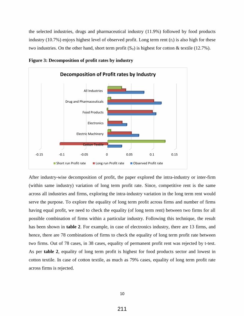
10
the selected industries, drugs and pharmaceutical industry (11.9%) followed by food products
industry (10.7%) enjoys highest level of observed profit. Long term rent (ri) is also high for these
two industries. On the other hand, short term profit (Sit) is highest for cotton & textile (12.7%).
Figure 3: Decomposition of profit rates by industry
After industry-wise decomposition of profit, the paper explored the intra-industry or inter-firm
(within same industry) variation of long term profit rate. Since, competitive rent is the same
across all industries and firms, exploring the intra-industry variation in the long term rent would
serve the purpose. To explore the equality of long term profit across firms and number of firms
having equal profit, we need to check the equality (of long term rent) between two firms for all
possible combination of firms within a particular industry. Following this technique, the result
has been shown in table 2. For example, in case of electronics industry, there are 13 firms, and
hence, there are 78 combinations of firms to check the equality of long term profit rate between
two firms. Out of 78 cases, in 38 cases, equality of permanent profit rent was rejected by t-test.
As per table 2, equality of long term profit is highest for food products sector and lowest in
cotton textile. In case of cotton textile, as much as 79% cases, equality of long term profit rate
across firms is rejected.
-0.15 -0.1 -0.05 0 0.05 0.1 0.15
Cotton Textile
Electric Machinery
Electronics
Food Products
Drug and Pharmaceuticals
All Industries
Decomposition of Profit rates by Industry
Short run Profit rate Long run Profit rate Observed Profit rate
211

11
Table 2: Test of equality of permanent profit rates by industry
Industry No. of Firms No. of Tests
No. of Tests
statistically
significant*
Cotton Textile 37 666 525(79%)
Electric Machinery 23 253 142(56%)
Electronics 13 78 38(49%)
Food Products 14 91 21(23%)
Drug and Pharmaceuticals 67 2211 1083(49%)
* 5% level of significance (two –tailed t-test)
Finally, the study assesses the strength of competition at firm level. Strength of competition
depends on the short term profit or the transitional part (λi) of the profit rate which is carried over
from one year to next year. Higher is the value of λi, higher is the persistence of profit rate and
lower is the competition. Strength of competition can be measured in terms of the time required
to wipe out the transitional component of profit. However, as suggested by Cubin-Geroski
(1990), this study measures the strength of competition as the time required for the transitional
profit to be halved (half-life).
As per model specification, λi should vary within the range (0-1). This study calculates the
strength of competition for the firms which satisfies this criterion. Table 3 portrays the strength
of competition in each of the selected manufacturing industries in terms of average λi value
(transitional profit carried over from one period to next period) and half-life (time required to
wipe out the transitional profit to be halved). As revealed by table 3, persistence of profit
(transitional) is highest for cotton textile sector while minimum for electronics sector. λi itself
indicates variation of strength of competition across selected industries. But as a second measure,
half-life time is also calculated as per Cubbin-Geroski (1990), where half-life is measured as
T=log (1/2)/log λi. This also indicates that cotton textile sector has the highest half-life time (1.47
years). Pushpangadan and Shanta (2008) using Indian Industry data till 2000 also found that
212

12
cotton textile (1.12 years) had second highest half-life time. A minute comparison indicates that
while half-life time increases for cotton textile and pharmaceuticals, for other sectors it has
declined over time.
Table 3: Strength of competition in Indian manufacturing industries
Industry No. of Firms λi Mean Time (in years)
Cotton Textile 29 0.6248281 1.47
Electric Machinery 17 0.4250699 0.81
Electronics 11 0.3300672 0.63
Food Products 11 0.3329324 0.63
Drug and Pharmaceuticals 47 0.412035 0.78
All Industries 115 0.4464182 0.86
V. CONCLUSION
It appears that not much has changed when it comes to long term profit in Indian industry. While
long term permanent profit is about 10%, the long term firm specific rent is about 4% However,
immediately after the liberalization exercise, short run profit might have had increased, though in
recent years, it might have declined. However, it needs to be noted that short run profit is quite
significant in Indian industry.
As with the observed profits, long term rent is also high in pharmaceuticals and food products,
while short term profit is relatively high in cotton and textile industry. Persistence of profit is
highest in the cotton textile industry and lowest in the electronics industry. Long terms profits of
pharmaceuticals are high globally and hence it is quite expected particularly in the post-TRIPS
scenario. Pharmaceutical industry is also characterized by a situation where consumers do not
make buying decisions and the doctors might not decide the cheapest available alternatives for
the patients. This might have led to higher profitability and lower efficiency in the industry.
Equality of profit across firms within an industry is highest for food products industry, while
lowest in the cotton textile industry. The study has considered only the large firms in the food
products industry who might have equal competitive strength which might be reflected in the
equality of profit. However, the lower level of equality of profit in the textile industry, prima
213

13
facie, appears to be surprising given that with the dismantling of not only the domestic protection
but also the global Multi-Fibre Agreement, this industry should be more competitive. However,
it could be due to the fact that a developing country market for textiles and clothing industry has
one group of firms that compete on price while there are firms that compete on their brand value.
VI. REFERENCE
* Bain, J. S. (1956). Barriers to New Competition. Harvard University Press, Cambridge.
* Cable, J. & Jackson, R.H.G. (2008). The Persistence of Profits in the Long Run: A New
Approach. International Journal of the Economics of Business, Vol. 15, No. 2, pp. 229-
244.
* Capitaline database. URL: https://www.capitaline.com
* Cubbin, J.S. & Geroski, P.A. (1990). The Persistence of Profits in the United Kingdom,
in: Muller, D.C., ed., The Dynamics of company Profits: An International Comparison,
Cambridge University Press, New York.
* Geroski, P. A., (1990) “Modeling Persistent Profitability”, in The Dynamics of Company
Profits: an International Comparison, edited by Dennis C. Mueller, Cambridge University
Press.
* Geroski, P.A. & Jacquemin, A. (1988). The Persistence of Profits: A European
Comparison. The Economic Journal, 98, pp. 375-389.
* Glenn, J., Lee, K., & Singh, A. (2001). Persistence of Profitability and Competition in
Emerging Markets. Economics Letters, 72, pp. 247-253.
* Glenn, J., Singh, A & Matthais, R. (1999). How intensive is competition in the Emerging
Markets: An analysis of Corporate Rates of Return from Nine Emerging Markets. IMF
Working Paper 99/32, Washington DC, USA
* Gschwandtner, A. (2010). Evolution of Profit Persistence in the US: Evidence from
Three Periods.
* Jacobsen, R. (1988). The Persistence of Abnormal Returns. Strategic Management
Journal, 9(5), pp. 415-430.
* Kambahampati, U.S. (1995). The Persistence of Profit Differentials in Indian Industry.
Applied Economics, 27, pp. 353-61.
* McGahan, A. M. & Porter, M. E. (1999). The Persistence of Shocks to Profitability. The
Review of Economics and Statistics, 81 (1), pp. 143-153.
214

14
* Mueller, D. C. (1990). The Persistence of Profits in the United States.” in The Dynamics
of Company Profits: an International Comparison, edited by Dennis C. Mueller,
Cambridge. University Press.
* Mueller, D.C. (1977). The Persistence of Profits above the Norm. Economica, 44, pp.
369-380.
* Mueller, D.C. (1986). Profits in the Long Run. Cambridge University Press, Cambridge.
Profits: an International Comparison, edited by Dennis C. Mueller, Cambridge University
Press.
* Pushpangadan, K. & Shanta, N. (2008). Competition and Profitability in Indian
Manufacturing Industries. Indian Economic Review, 43(1), pp. 103-123.
* Schumpeter, J. A. (1934). The Theory of Economic Development. Cambridge, MA:
Hardvard University Press; first published in German, pp.1911.
* Schumpeter, J. A. (1950). Capitalism, Socialism and Democracy. New York: Harper and
Row.
* Schwalbach, J., Grasshoff, U. & Mahmood, T. (1989). The Dynamics of Corporate
Profits. European Economic Review, 33,pp. 1625-1639.
* Waring, G. F. (1996). Industry differences in the Persistence of Firm-Specific Returns.
American Economic Review, 86(5), pp. 1253-1265.
215

1
Economics of Mergers and Acquisitions in India’s Drugs and Pharmaceutical Industry:
Implications for Competition Policy
Simrit Kaur
Professor, Faculty of Management Studies, University of Delhi, India
Phone:+91 9811137375, Email: [email protected]
Paramjeet Kaur
Associate Professor, Sri Guru Gobind Singh College of Commerce, University of Delhi, India
Phone:+91 9811263328, Email: [email protected]
1. Introduction
Mergers and Acquisitions (M&As) form an important part of the commercial activity of most
economies, with 46,000 such transactions being reported in 2015 itself amounting to US$4.7
trillion1. This constitutes about 6.3% of the global GDP
2. In India, transactions totaling about
$26 billion were reported in 2015. Though small, this number is likely to increase as the Indian
economy continues to grow and more firms seek to use M&As to achieve corporate
objectives3. Owing to the surge in globalization, incidences of cross-border M&As have grown
manifold and as such, the current era is sometimes also known as "New Era of Global
Economic Discovery" (Cromwell, 2012). In 2014, Europe witnessed its highest ever activity
level of M&As deals since its financial crisis. This substantial increase was about 40% increase
over the 2013 levels. It is attributed primarily to the interest shown by the US and Asian
acquirers4. Similar effect can be seen in other parts of the world as well. The growth in M&As
activity is believed to be a result of various factors like improved financing conditions in
various parts of the world, stronger cash reserves available with Companies, promising
investment returns in private equity/ investment funds and search for talent and new
technologies.
A number of factors drive M&As activity including increasing market share / market power,
swifter access to markets, industry capacity considerations, securing access to proprietary
technology, cheaper skills and distribution channels, managing business operation risks and
performance, increasing portfolio of offerings (vertically or horizontally) and tax
considerations (Steiner, 1975; Chatterjee, 1986; Porter, 1985; Shelton, 1988)5. M&As are the
most common way of restructuring. Merger is joining of two or more firms into one, where
1https://imaa-institute.org/mergers-and-acquisitions-statistics/ (2016)
2http://databank.worldbank.org/data/download/GDP.pdf (2016)
3 Transactions 2016: PE and outbound to drive M&A – Ernst & Young, India (2016)
4https://www.transactionadvisors.com/insights/newfound-attractiveness-european-ma
5Steiner, Peter O. (1975) Mergers, Motives, Effects and Policies (Ann Arbor, MI: University of Michigan Press);
Chaudhuri, S. (2005) The WTO and India’s Pharmaceuticals Industry: Patent Protection TRIPS and Developing
Countries (New Delhi: Oxford University Press); Shelton, Lois M. (1988) Strategic Business Fits and Corporate
Acquisitions: Empirical Evidence, Strategic Management Journal, 9(3), pp. 279-287; Porter, M.E. (1985)
Competitive Advantage: Creating and Sustaining Superior Performance (New York: Free Press)
216

2
assets and liabilities of all firms are vested into one surviving firm. The surviving firm can be
one of the existing firm (A+B=A or A+B=B) or it can be a new entity (A+B=C).The former is
defined as merger through absorption where the surviving entity is called the merging firm and
the latter is called merger through amalgamation, where the newly formed firm is called the
amalgamated entity. The macroeconomic environment and regulatory framework of any
economy are the two major determinants of M&As activity. A number of factors such as,
opening of economies on account of liberalization and deregulation, increasing privatization,
financial liberalization and global integration of production systems due to advancement of
information and communication technologies have led to rising M&As activity globally for
past few decades.
A merger may bring changes in the economic efficiency of a firm in any direction. On account
of reaping of economies of scale and other synergistic gains, productive efficiency and
profitability may enhance post-merger. It may also result in losses in the form of decreasing
profit margins, reducing quality and variety of products. However, along with this we also need
to consider the possible effects of mergers on the level of industrial concentration and
competition and thus, on the price-cost margins of firms. A firm may have greater power to
impact or determine prices in the market due to exit of a firm, which is on account of merger.
The market power of a firm is defined as the capacity of a firm to influence prices above the
level that would prevail in the competitive market. Under the competitive conditions, firms are
expected to have no monopoly power to influence prices in any way, and price is equated to
marginal cost of the firm. Therefore, the concept used to measure market power is markup over
price charged by the firm. It is defined as (P-C)/P, and is called the Lerner index.
Many analytical and empirical studies have been carried out to understand the pertinent post-
merger issues of firms’ price-cost margins (PCM), profitability and market shares and their
impact on the market power of firms, level of industrial concentration and further its
consequential impact on the level of competition in the economy. Some of these works are
reviewed below.
Culha and Yalcin (2015), using panel data technique, examine the determinants of PCM in
Turkish manufacturing firms during 1995-20036. By controlling for size, age, ownership and
export orientation of a sample of four thousand manufacturing firms, the study found that there
exist striking differences in the pricing behavior of firms depending on their market shares. The
price-cost margins of small and large firms behave fairly in opposite direction depending on
the control variables. It is observed that interest income has a positive impact on price-cost
margins for all groups, though less vigorous for small, exporter and young firms. They found
export-intensity of firms had an important role to play to enhance competition while import-
intensity was not effective in reducing the price-cost margins of firms. 6 This period is of special importance as, in the year 1995, Turkey joined the custom union with EU which
resulted in liberalization of its foreign trade and thus increasing the competitive pressures faced by the firms.
Also, Turkey experienced an economic crisis in 2001.
217

3
McClogham, Lyons, and Batt (2007) state that competition policy of a country has an
important role to play in determining the market price-cost margins. Therefore, they suggest
that governments must facilitate an effective competition policy to curtail exercise of market
power of firms. The effectiveness of competition policy has been measured using the ratings of
national competition authorities (NCAs) which is published by The Global Competition
Review (GCR). The authors find that countries with more effective competition policy have
lower price-cost margins than their counterparts in countries with less effective competition
policy. Further, they find that market growth plays a significant positive role while excess
capacity and import penetration are non-significantly and negatively associated with price-cost
margins. In contrast to this, Kee and Hoekman (2007) and Konings et al. (2001) suggest that
competition policy does not have a prominent role to play in curbing price-cost margins and
thus market power.
Aghion et al. (2005) investigate the relationship between market competition and innovation,
based on panel data of a sample of 311 UK firms from seventeen industries over the period
1973-1994. They find a strong evidence of an inverted-U shape relationship between
innovation and competition, implying that competition may increase incremental profits from
innovating for those firms that are in neck-and-neck competition (called “escape-competition
effect”), though it may also reduce innovation incentives for laggards (labeled “Schumpeterian
effect”). The paper supports the role played by competition in improving economic
performance of a country. In trying to examine whether the changed entry conditions impacted
the productivity growth of incumbents, Aghion et al. (2004) explored the opening up of the UK
economy during the 1980s. Based on a sample of 166 four-digit manufacturing industries
during 1980-1993, they find that increased entry (measured by a higher share of industry
employment in foreign firms) had led to faster total factor productivity growth of the
incumbent firms and in turn faster growth of aggregate productivity. They also demonstrate
that this happened because entry of foreign firms significantly improved the innovative activity
of incumbent firms.
Nickell (1996) investigates the relationship between competition and corporate performance.
The analysis based on a sample of 670 UK firms supports the view that competition improves
corporate performance. The two main results of the paper are: market power as captured by
market share, generates reduced level of productivity and that competition, measured by
increased number of competitors, is associated with both higher level and the growth of total
factor productivity of firms.
In addition to the studies reviewed above, a few important works in this area are by Alfaro and
Chari (2012), Syverson (2004) and Campbell, (2005).
218

4
M&As in the Drugs and Pharmaceuticals Sector7: The M&As in the Drugs and
Pharmaceuticals sector in India has seen significant activity. In 2015 alone, transactions
totaling $4.1 billion in M&As took place. These include outbound (Indian companies engaging
foreign firms in transactions), inbound (foreign companies engaging Indian firms in
transactions) and domestic (Indian firms engaging each other in transactions). One of the most
studied cases pertaining to M&As in the pharmaceutical industry is acquisition of Ranbaxy by
Sun Pharmaceuticals, wherein the deal size was to the tune of USD 4billion. The deal entailed
16.4% dilution of equity capital of Sun Pharmaceuticals. This enabled the Company to fill in
therapeutic gaps experienced in the United States, expand its market share through deeper
market penetration and bolster its presence in the domestic market. It was through this deal that
Sun Pharmaceuticals became one of the leading pharmaceutical firms producing generic drugs
in the dermatology space8.
It is nevertheless considered that despite such M&As, these transactions have not had
retrograde impacts on the competitive landscape of the industry vis-à-vis the Indian consumer.
This can be attributed to the strong price control mechanisms managed by the National
Pharmaceutical Pricing Authority, which regulates the ceiling prices for scheduled
formulations and monitors unscheduled formulations too. This ensures that key drugs are
available to consumers at affordable prices9. However, these controls tend to discourage
investments in the sector.
According to Mckinsey report (2010), the generics market has seen consolidation and is likely
to witness more M&As activity, since the Indian market is largely fragmented10
.
Drugs and Pharmaceuticals Sector in India11
: The outlook of Indian Drug & Pharmaceutical
Industry appears to be very positive and with an overall turnover of around USD 20bn, it ranks
third (3rd
) in the world in terms of volume and fourteenth (14th
) in terms of value. The Drugs
and Pharmaceuticals has been one of the fastest growing sectors of the economy, expanding at
12% per annum and it is likely to reach $55 billion by 2020. However, the industry is
fragmented and competitive, with the top four companies accounting for 20%market share
and the top 10 companies for nearly 39% of the market share in 2015. Further, as many as 160
pharmaceutical firms are listed on the Bombay stock exchange12
and many more are privately
owned. Moreover, the Pharmaceutical business in India is concentrated around
Hyderabad, Mumbai, Bangalore, Visakhapatnam and Ahmadabad13
.
7 Transactions 2016: PE and outbound to drive M&As – Ernst & Young, India (2016)
8http://www.edupristine.com/blog/mergers-acquisitions
9 Annual Report 2015-16, Department of Pharmaceuticals, Ministry of Chemicals and Fertilizers (2016)
10 India Pharma 2020: Propelling access and acceptance, realizing true potential, Mckinsey and Company, India
(2010) 11
Pharmaceuticals – Sectoral Report, November 2016, IBEF (2016) 12
http://www.bseindia.com/markets/Equity/EQReports/IndustryView.aspx?expandable=2&page=60101001+&scri
pname=Pharmaceuticals 13
https://en.wikipedia.org/wiki/Pharmaceutical_industry_in_India
219

5
Over the last decade, pharmaceutical firms all across the world have been experiencing
immense pressure mounting over their core activities like drug manufacturing, Research &
Development and various legal/regulatory aspects primarily because of an increasing
competition in the pharmaceutical industry. This has resulted in significant dampening of the
growth of pharmaceutical industry worldwide. To make things worse, decline in requirement
of prescribed branded drugs and emergence of cost-effective generic drug products has further
stifled the growth of pharmaceutical industry. As a cascading effect, branded drugs produced
by major pharmaceutical firms resort to price increase to cover up for their declining margins,
inhibiting presence of a conducive market environment for them to operate and earn
sustainable profits.
The post-reform period has been a challenging one for the Indian corporate sector. During this
period, the Indian industry not only liberalized, but was also forced to restructure its businesses
to survive in the new competitive environment. In its effort to do so, mergers and acquisitions
(M&As), as a means to have quick expansion and as a corrective measure to its pre-reform
policies, were adopted in large numbers. As expected, the phenomenon of M&As has
accelerated in volume and value in the era of globalization, necessitating merger review on a
broad range of issues. M&As activity in the pharmaceutical sector has been analyzed in a
number of studies (Mishra, 2005; Beena, 2006; Mishra and Chandra 2010; Kaur 2002)14
.
However, no recent study analyzes the implications of such transactions on the competitive
dynamics of the industry. With this background, our paper examines the consequential effects
of Indian M&Ason industrial concentration, firm’s price cost margins and profitability. This is
undertaken with special reference to the drugs and pharmaceutical (D&P) industry. In light of
our results, appropriate policies are proposed.
The paper has 5 sections. Having given a brief introduction in Section 1, Section 2 analyzes the
trends in M&As in India’s Drugs and Pharma Sector. Thereafter, in Section 3, we analyze
variables such as market shares, Hirshman-Herfindahl index (HHI) and Price Cost Margins in
the D&P sector. Needless to say, analyzing such variables is expected to provide insight to
regulatory authorities while formulating competition policies. Thereafter, in Section 4, we
econometrically examine the impact of size (proxied by market share and capital employed) on
price cost margins and profitability of firms. This is done separately for Merging firms, Non-
merging firms and for the overall sample consisting both Merging and Non-merging firms. In
addition to the main variable of interest, viz. market share and M&As (as captured by a dummy
variable in the Pooled Econometric specification), some of the firm-specific control variables
included in the study are: leverage ratio; age of the firm, labour productivity and firm intensity
14
Beena ,S (2006), “ Mergers and Acquisitions in the Indian Pharmaceutical Industry: Nature, Structure and
Performance”, available at http://mpra.ub.uni-muenchen.de/8144/; Mishra, P. (2005) Mergers and Acquisitions in
the Indian Corporate Sector in the Post- Liberalization Era: An Analysis, Ph.D Dissertation, (West Bengal:
Vidyasagar University); Mishra, P. and Chandra, T (2010) Mergers, Acquisitions and Firms’ Performance:
Experience of Indian Pharmaceutical Industry, Eurasian Journal of Business and Economics 2010, 3 (5), 111-126
220

6
measured in terms of R&D intensity, Export intensity and Import intensity. Finally, in Section
5, the paper concludes from a broad policy perspective.
2. Trends in M&As in India’s Drugs and Pharmaceutical Sector during 1999-2015
Akin to the global pharmaceutical industry, the Indian D&P industry is also one of the most
merger-intensive industries. Soon after the initiation of the economic reform process in 1991-
92, the pharma companies started consolidating their capacities through mergers and
acquisitions of brands, plants and assets, divisions and units of firms. The driving force behind
M&As was to consolidate the highly fragmented pharma sector to achieve faster growth, to
avoid delays associated with building a new plant and increasing their shares.
The growth of few companies undertaking mergers, such as Sun Pharmaceutical and Mylan
Laboratories Ltd., is spectacular and worth mentioning. With both organic and external growth
through aggressive and strong M&As strategy, Mylan Laboratories Ltd. has grown by more
than 155 times i.e. from a turnover of Rs 45 crore in 2002, to 7000 crores in 2014, and its profit
margin has grown by more than 11 times during the same period. After successfully merging
with Medicorp Technologies India Ltd. and Vorin Laboratories Ltd in 2002-03, it continued its
appetite for M&As and in 2004-05, it struck a number of deals, such as merger with Strides
Arcolab, Fine Drugs & Chemicals Ltd., Medikon Laboratories Ltd. and Vera Laboratories Ltd.
During 2001-2005, it entered into mergers with 9 firms. Similarly, Sun Pharmaceutical, with
the ability to integrate various entities and successfully consolidate them, is on a high-rise
growth path through mergers and acquisitions. It has grown by more than 150 times in its sales
and by approximately 900 times in total assets since its inception in 1993. It got 14 firms
merged into it, with 11 mergers taking place during 2000-2015.
Concerning trends in mergers in D&P industry, it is observed that close to 170 mergers took
place during 2000-01 to 2014-15 (Refer to Table 1). With a few exceptions, most of these
mergers were horizontal in nature. In the initial phase of economic liberalization, merger
activity was quite slow and acquisition of brands was more common among the firms. In the
mid-1990s, the M&As activity picked up moderately and in the early years of this century, the
merger activity accelerated rapidly. This has also affected the concentration levels in the
industry.
More than 50 percent of the total mergers during 2000-2015 were undertaken in the first seven
years and approximately 30 percent took place in the next seven years. An important feature of
this activity is that about 20 firms were involved in undertaking more than 100 mergers. Few
firms are very aggressive in nature and have undertaken mergers in large numbers. For
example, during the period 2000-15, Sun Pharmaceutical Industries Ltd undertook 14 mergers,
Piramal Enterprises Ltd. 13, Cadila Healthcare Ltd. 10, Mylan laboratories 9 and Dr. Reddy’s
Laboratories Ltd. Was involved in 4 mergers.
221

7
Table 1: Year-wise Distribution of Mergers in D&P industry during 2000-2015
Year No. of Mergers
2000-01 15
2001-02 11
2002-03 13
2003-04 18
2004-05 13
2005-06 9
2006-07 12
2007-08 5
2008-09 11
2008-10 10
2010-11 6
2011-12 7
2012-13 7
2013-14 10
2014-15 23
Total 170 Source: Based on Prowess database (CMIE, 2016).
Given the highly fragmented nature of the Drugs and Pharmaceutical industry, market share
becomes an important variable in this industry. Out of the total, approximately, ten thousand
firms in the industry (including the organised and unorganised sectors) roughly less than 5
percent firms are in the organised sector. The sample of 62 acquiring firm considered for this
study accounted for 60 percent of the total sales of the industry in 2004-2005. This indicates a
very high concentration of sales among very few firms in the industry. In the last few years, the
D&P industry has witnessed intense competition among firms in undertaking M&As. The
inter-firm rivalry to increase market share is discernible not only through competitive bids
made by different firms, but also through acquisition of brands and plants and other assets of
firms. In a situation where a firm’s rivals are making acquisitions, it may also be compelled to
make acquisitions to prevent rivals from building dominant market positions.
In light of the above discussion and in view of the fact that D&P industry is one of the most
merger-intensive industry witnessing competitive bids and high rivalry among firms in the
post-liberalised period, this phenomenon requires special attention from the point of view of its
effect on the market shares of firms and level of concentration in the industry.
3. HHI, Price Cost Margins and Market Share of Drugs and Pharma Firms
In the empirical literature, several measures of competition are used. Primary among them are
concentration measures, such as the Hirshman-Herfindahl index (HHI) and the price cost
margins (PCMs). The use of concentration as a measure of competition goes back to the
structure-conduct-performance framework. High concentration is seen as a signal of weak
competition which leads to high prices and high price cost margins (Scherer and Ross, 1990).
0
5
10
15
20
25
19
99
-00
20
01
-02
20
03
-04
20
05
-06
20
07
-08
20
08
-10
20
11
-12
20
13
-14
222
8
In this Section, a brief is provided on Hirshman-Herfindahl index, Trends in market shares of
Merging and Non-Merging firms, and Price Cost Margins of Firms in the D&P sector.
3.1.Concentration Ratio: Hirshman-Herfindahl Index (HHI)
The concentration ratio is a summary statistics used to measure the degree to which an industry
is dominated by a few large firms. It can be measured by the percentage of total industry sales15
supplied by the largest 4, 8 and 12 firms in the industry. If the 4-firm concentration ratio is
close to 100 or even greater than 60 percent, the concentration is high and it is known as an
oligopolistic firm. If it is low or less than 60 percent, then the concentration is low. However,
the limitation of this method is that it does not consider the sales of each firm in the industry.
Another method of estimating the degree of concentration in an industry is the Herfindahl
index (denoted by HHI). The advantage of this method is that it measures the information on all
the firms and is not limited to the shares of the few largest firms in the industry.
Assuming there are N firms in an industry, let si be the market share of the ith
firm (defined as
the ratio of sales of ith
firm to total sales of the industry), the Herfindahl index is the sum of the
squared values of the market shares (measured in percentage) of all the firms in the industry.
Thus,
HHI = s12 + s2
2+ s3
2 + s4
2+…. + sn
2
The index takes a value between 0 and 10,000 (0 HHI 10,000), where the value 0 indicates
no concentration and 10,000 indicates the case of monopoly. If there is only one firm in the
industry, then HHI = (100)2 = 10,000. If there are two firms in the industry sharing the market
equally, then HHI = (50)2 + (50)
2 = 5000. With the 100 equal-sized firms in the industry
(perfectly competitive) HHI = (1)2
+ (1)2 + (1)
2 + ……. + (1)
2 = 100. The lower the value of
HHI, the more competitive is the market, and higher the HHI, the greater is the market
concentration. Another advantage of this method is that, by taking the squares of share of each
firm, the index gives higher weight to larger firms in the industry (Salvatore, 1996).
From Table 2 and Figure 1, four distinct phases in HHI can be noticed. In the first phase, it is
noted that during the time span of 10 years i.e. 1988-89 to 1998-99, the HHI index fell
continuously to less than half of its value of 1988-89. In the second phase, HHI rose. There is a
perceptible rise in HHI index since 1999-00 until the year 2004, beyond which in the third
Phase, it again began to decline. However, in its fourth phase that commenced in 2010, yet
again the HHI has risen, indicating a rise in concentration level in the D&P industry.
15
The industry’s sales are based on all the firms covered in Prowess database (CMIE, 2005).
223

9
Table 2: Concentration Levels in D&P Industry, 1999-2015
Year HHI Year HHI
Mar-90 351 Mar-03 239
Mar-91 314 Mar-04 240
Mar-92 260 Mar-05 221
Mar-93 250 Mar-06 193
Mar-94 253 Mar-07 198
Mar-95 220 Mar-08 181
Mar-96 189 Mar-09 175
Mar-97 205 Mar-10 167
Mar-98 215 Mar-11 170
Mar-99 173 Mar-12 183
Mar-00 180 Mar-13 194
Mar-01 194 Mar-14 209
Mar-02 221 Mar-15 282
Source: Calculations based on Prowess database (CMIE, 2016)
Figure 1:Hirshman-Herfindahl Index (HHI) for the Period 1999 to 2015
Source: Calculations based on Prowess database (CMIE, 2016).
In trying to further explore this issue and provide an explanation for the change in the
concentration level, we analyse the entry and exit phenomenon in the sector. This is given in
Table 3.
387
351
314
260 250 253 220
189 205 215
173 180 194
221 239 240
221 193 198
181 175 167 170 183 194 209
282
0
50
100
150
200
250
300
350
400
450
1988-89 Mar-92 Mar-95 Mar-98 Mar-01 Mar-04 Mar-07 Mar-10 Mar-13
224

10
Table 3: Distribution of Firms in the D&P industry according to year of Incorporation
Period No. of Entrants
before 1950 41
1951-1980 114
1981-1990 261
1991-1995 177
1996-2000 71
2001-2002 18
2003-2004 21
2005-2006 36
2007-2008 17
2009-2010 8
2011-2012 6
2012-2014 7
One of the plausible reasons of continuous reduction in the concentration ratio during the first
phase is entry of new firms outstripping the exit of firms (during 1990 to2000). From Table 3,
we find that approximately 250 firms joined the D&P industry during the first 10 years of
liberalization. However, after the year 2000, a continuous fall in the firms joining the industry
is a clear indication of the exit of firms dominating the entry (may be due to heightened merger
activity in the industry). In a span of five years i.e. 2000-05, close to 70 firms from D&P got
merged to other firms within the D&P industry whereas there were only 75 new entrants in the
industry during this period. Recently on account of rise in mergers and slowdown in the entry,
we find again a rise in the Herfindahl index since the post 2010 period.
3.2: Trends in the market shares of Merging and Non-merging firms:
Based upon the analysis of changes in the market shares of the few prominent merging and
non-merging firms during the period under consideration, the following findings are
noticeable:
i. The market shares of the merging firms have continuously risen, while those of non-
merging firms are showing declining trend (Figure2a and 2b respectively).
ii. The highest rise in the market share was experienced by Dr. Reddy's Laboratories Ltd.
Its share rose from 2.05% in 2000 to 5.63% in 2002 and further to 6.5% in 2015.
Similarly, market share of Mylan Laboratories Ltd. rose from 0.19% in 2000 to 4.15 %
in 2014. Other merging firms, such as, Lupin Ltd., Emami Ltd., and Alkem
Laboratories Ltd. too showed a rising trend in their market share over the period 2000
to 2015.
iii. Among the non-merging firms, Alembic Ltd.experienced a fall in market share from
2.19% in 2002 to 0.09% in 2015. Astrazeneca Pharma India Ltd’s. share reduced from
225

11
0.45% in 2000 to 0.27% in2012. For Biological E. Ltd. as well, its market share
declined from 0.54% to 0.16% over the period under consideration.
Figure 2(a): Trends in the Market Shares of Select Merging firms
Figure 2(b): Trends in the Market Shares of Select Non-merging firms
3.396
0.00 0.50 1.00 1.50 2.00 2.50 3.00 3.50 4.00 4.50 5.00 5.50 6.00 6.50 7.00
Jan
-99
Jan
-00
Jan
-01
Jan
-02
Jan
-03
Jan
-04
Jan
-05
Jan
-06
Jan
-07
Jan
-08
Jan
-09
Jan
-10
Jan
-11
Jan
-12
Jan
-13
Jan
-14
Jan
-15
Dr. Reddy'S Laboratories Ltd.
Lupin Ltd.
Aurobindo Pharma Ltd.
Mylan Laboratories Ltd.
Cadila Healthcare Ltd.
Glenmark Pharmaceuticals Ltd.
0.00
0.50
1.00
1.50
2.00
2.50
Jan
-00
Jan
-01
Jan
-02
Jan
-03
Jan
-04
Jan
-05
Jan
-06
Jan
-07
Jan
-08
Jan
-09
Jan
-10
Jan
-11
Jan
-12
Jan
-13
Jan
-14
Jan
-15
Ajanta Pharma Ltd.
Alembic Ltd.
Arvind Remedies Ltd.
Astrazeneca Pharma India Ltd.
Biological E. Ltd.
Cadila Pharmaceuticals Ltd.
226

12
3.3.Price Cost Margins, Market Shares and Sales
In Table 4, we provide the descriptive statistics pertaining to merging and non-merging firms
and the overall sample for the following three variables:
Price Cost Margins
Market Shares, and
Sales
Pertinent observations based on Table 4 are hereby listed:
i. Price Cost Margins: The average value of PCM for Merging firms is higher than that of
Non-merging firms (0.46 and 0.37 respectively). Further, the standard deviation of the
same is lower for Merging firms as compared to Non-merging firms (0.19 and 0.50
respectively).
ii. Market Shares: The average market share of Merging firms is higher than for Non-
merging firms (1% and 0.2% respectively). Further, the maximum market share ever
attained by Merging firms is also higher (Close to 10% for Merging firms as compared
with 6.6% for Non-merging firms). The average market share of each firm in the D&P
sector is less than half percent.
iii. Sales: Firms that have undertaken M&As as a strategic route, on an average have
higher sales viz. a viz. their counterparts that never merged. However, the standard
deviation across the mean is also higher for the merged firms.
Table 4: Descriptive Statistics with respect to Price Cost Margins,
Market Share and Sales
Merging Firms
Variable Obs Mean Std. Dev. Min Max
Price Cost Margin 1006 0.46223 0.19556 -1.901 0.982456
Market Shares 1054 0.94869 1.24330 0 9.581405
Sales 1006 7849.659 12655.62 0.5 100939
Non Merging Firms
Variable Obs Mean Std. Dev. Min Max
Price Cost Margin 1933 0.37195 0.50877 -16.5 1
Market Shares 2091 0.20879 0.53839 0 6.570986
Sales 1926 1774.868 5680.977 0.1 102277.9
All Firms
Variable Obs Mean Std. Dev. Min Max
Price Cost Margin 2939 0.40285 0.43027 -16.5 1
Market Shares 3145 0.45675 0.91238 0 9.581405
Sales 2932 3859.193 9188.848 0.1 102277.9
227
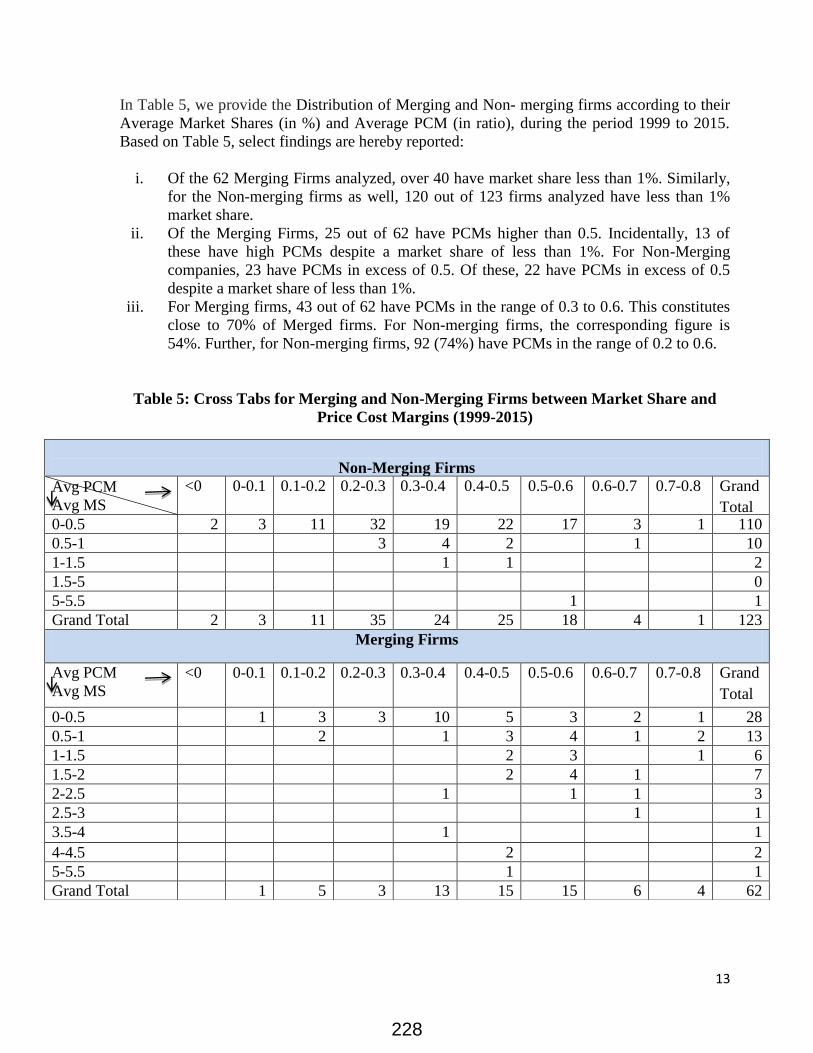
13
In Table 5, we provide the Distribution of Merging and Non- merging firms according to their
Average Market Shares (in %) and Average PCM (in ratio), during the period 1999 to 2015.
Based on Table 5, select findings are hereby reported:
i. Of the 62 Merging Firms analyzed, over 40 have market share less than 1%. Similarly,
for the Non-merging firms as well, 120 out of 123 firms analyzed have less than 1%
market share.
ii. Of the Merging Firms, 25 out of 62 have PCMs higher than 0.5. Incidentally, 13 of
these have high PCMs despite a market share of less than 1%. For Non-Merging
companies, 23 have PCMs in excess of 0.5. Of these, 22 have PCMs in excess of 0.5
despite a market share of less than 1%.
iii. For Merging firms, 43 out of 62 have PCMs in the range of 0.3 to 0.6. This constitutes
close to 70% of Merged firms. For Non-merging firms, the corresponding figure is
54%. Further, for Non-merging firms, 92 (74%) have PCMs in the range of 0.2 to 0.6.
Table 5: Cross Tabs for Merging and Non-Merging Firms between Market Share and
Price Cost Margins (1999-2015)
Non-Merging Firms
Avg PCM
Avg MS
<0 0-0.1 0.1-0.2 0.2-0.3 0.3-0.4 0.4-0.5 0.5-0.6 0.6-0.7 0.7-0.8 Grand
Total 0-0.5 2 3 11 32 19 22 17 3 1 110
0.5-1 3 4 2 1 10
1-1.5 1 1 2
1.5-5 0
5-5.5 1 1
Grand Total 2 3 11 35 24 25 18 4 1 123
Merging Firms
Avg PCM
Avg MS
<0 0-0.1 0.1-0.2 0.2-0.3 0.3-0.4 0.4-0.5 0.5-0.6 0.6-0.7 0.7-0.8 Grand
Total
0-0.5 1 3 3 10 5 3 2 1 28
0.5-1 2 1 3 4 1 2 13
1-1.5 2 3 1 6
1.5-2 2 4 1 7
2-2.5 1 1 1 3
2.5-3 1 1
3.5-4 1 1
4-4.5 2 2
5-5.5 1 1
Grand Total 1 5 3 13 15 15 6 4 62
228

14
4. Impact of M&As and Market Shares on Price Cost Margins and Profitability of
Firms in D&P Sector: Econometric Analysis
Methodology and Variables:
Having estimated and analyzed the concentration ratios through Hirshman-Herfindahl Index
(HHI) in the Indian D&P Industry, the effect of M&As on the following variables is examined,
Price Cost Margins, and
Profitability
A total of 185 firms have been analyzed, of which 62 have adopted Mergers as a strategy,
while 123 have not merged. The time period of study is 1999 to 2015. The sample consists of
62 merging and 123 non-merging firms. The study focuses on only those merging firm that
entered into mergers during 1999-2015. It is observed that approximately all the mergers are
horizontal in nature i.e. both the firms entering into merger engaged in the same lines of
business. The sample of 62 merging firms included for our study, on average contributed
between 55% and 65% of the industry sales during 2000-2015. During 2003 to 2008, the
weight of these firms in the industry’s sales was above 60%, with maximum of 65% in the year
2004-05. As far as the sample of non-merging firms is concerned, their contribution varied
between 25%and 29% for the period under consideration.
The following panel regression is estimated:
+ + + + +…
Where,
represents either the Price Cost Margins (PCM) or Profitability of the firm.
PCM has been measured as: (Total income – Total cost)/ total income
Where total cost is sum of following four components, viz,
Cost of raw materials, stores and spares
Cost of power, fuel and water charges
Compensation to employees, and
Selling and distribution expenses
Profitability has been measured as Profit Before Tax (PBT) as % of total
income.
represents firm specific variables such as:
1. Size of the firm: In the present paper, size is analyzed primarily in terms of
market shares (defined as the ratio of the amount of a specific firm’s sales to the
sales of the industry) and by capital employed. It is hypothesized that size, as
proxied by market share and capital employed impacts PCM and profitability
positively.
2. Leverage ratio: It is a measure of indebtedness and is defined as the ratio of
Total term liabilities / tangible net worth. It is hypothesized that greater the
firm’s indebtedness, lower will be the PCM and profitability.
229

15
3. Import Penetration: It gives a measure of firm’s import intensity. It is
estimated as: Raw material imports / Raw material purchases (%)
It is expected that greater dependence on imports, is likely to constraint the
flexibility to exercise monopoly power. As such one would expect lower PCM
and profitability.
4. Export intensity: exports of firm/sales of the firm (%). An inverse relationship
is expected between export intensity and PCM since greater the ratio of exports,
greater is the expected competition the firm faces in the international market,
thereby forcing it to not have high PCM and profitability.
5. Age of a firm: The reason to consider this variable as one of the determinants of
PCM/Profitability is to understand whether mature firms (being more
experienced) have higher PCM/profitability or do relatively younger firms
(being more aggressive and vibrant) are likely to have higher PCM/profitability.
Empirically, this variable has been considered as a proxy for the firm’s
maturity.
6. Labour productivity: It is measured as total sales/compensation to employees.
Economic literature states that higher labour productivity lowers the cost of
production. This is expected to increase PCM and/or profitability. While prices
may also fall on account of improved productivity, in general, one would
exopect the price fall to be less than the fall in labour costs.
7. R&D intensity: expenditure on R&D as a ratio of sales.
8. Dummy variable: It takes a value of 1 for post merger years, and 0 otherwise.
Firms that never entered into a merger also have a value of 0.
Analysis of Results:
The regression results are reported in Tables 6 and 7. In general the following findings emerge:
Impact on Price Cost Margins:
i. Market Share: In general market shares have a non-significant impact on PCMs.
However, for the Pooled data, market shares have been estimated to have a positive and
significant impact on PCMs for all D&P firms over the period of study. Further, for the
Merging firms, the post merger market share (captured by the interaction between
market share and post merger years), continues to remain non-significant.
ii. Capital employed: High capital costs are often associated with high fixed costs that act
as a deterrent to entry. With difficult entry, markets are expected to be concentrated
thereby increasing PCMs. Our empirical estimates indicate that capital employed has a
non-significant impact on PCMs across Firm Groupings and Model Specifications.
Thus one may conclude that capital costs do not act as a deterrent for entry of new
firms into the market.
230

16
iii. Labour Productivity: Labour productivity has been estimated to impact PCMs
adversely. This is true across Firm Groupings and Model Specifications. Moreover, the
coefficients are highly significant (often at the 1% level). This implies that as the labour
productivity improves, the PCM reduces. An important implication of the same is that
more than proportionate fall in labour costs are passed on to the consumer. This result
has important implications for policy. For instance, while the trend analysis of market
shares for select companies shows that market shares went up post merger, the same did
not lead to increase in concentration as captured by PCM. This result is reinforced by
the negative coefficient of labour productivity. Had competition not been intense in
India’s D&P sector, improved efficiency on account of enhanced labour productivity
would not have led to lowering of PCMs. Thus, it can be stated that negative coefficient
of labour productivity with respect to PCM is indicative of intense competition.
iv. R&D intensity: For the Merging Firms, the coefficient of R&D remains negative and
significant. For other two Firm Groupings (Non-Merged and Pooled), the impact of
R&D on PCM remains non-significant.
v. Leverage Ratio: The impact of leverage ratio remains negative across Model
Specifications, though the same is significant for Merging Firms only.
vi. Import Intensity: It has been estimated to have a positive and significant impact on
PCMs. However, the impact is often low/negligible.
vii. Other variables, such as, age and export intensity have been estimated to have a non-
significant impact on PCM.
Our econometric analysis of correlates of PCM indicates that neither market shares, nor merger
activity impacts PCM. While PCM remains an important measure to understand intensity of
market competition, nevertheless, from a theoretical point of view recent literature discusses
the inappropriateness of PCM and HHI as measures of concentration. Recent literature states
that sometimes their interpretation is not straight forward, especially if intensity of competition
is high (Tirole, 1988). This is elaborated further.
It is often believed that market competition can be intensified in the following two ways:
(i) When more firms enter a market due to a fall in entry barriers: When more firms
enter a market, it tends to lower concentration, thereby lowering HHI.
(ii) When there is more aggressive conduct by incumbent firms: In this case, there
could be a problem in interpreting the typical value of concentration ratios. The
problem with concentration measures as indicators of competition is that a switch to
more aggressive behavior by firms forces inefficient firms out of the market and/ or
get merged (selection effect of competition). This raises concentration, though it
should (clearly) not be interpreted as a fall in competition.
231

17
Table 6: Impact on PCM for Merging, Non-Merging and All Firms
(Robust Standard Errors)
Merging Firms#
Non-Merging
Firms#
All Firms^
(1) (2) (3) (4) (5) (6)
Market Share 0.006
(0.028)
-0.042
(0.064)
0.054
(0.066)
0.105***
(0.033)
Dummy Merge
-0.106
(0.099)
-0.095
(0.245)
0.183***
(0.064)
-0.112
(0.238)
Market Share*Dummy
for Merger
0.059
(0.057)
-0.040
(0.037)
Capital Employed (Log)
-0.030
(0.071)
-0.044
(0.039)
Capital
Employed*Dummy for
Merger
0.006
(0.030)
0.051
(0.037)
Labour Productivity -0.003***
(0.001)
-0.003***
(0.001)
-0.003***
(0.001)
-0.002
(0.002)
-0.004***
(0.001)
-0.004***
(0.001)
R & D Intensity -0.025**
(0.010)
-0.025**
(0.010)
-0.024**
(0.010)
-0.010
(0.013)
-0.014
(0.011)
-0.011
(0.013)
Leverage Ratio -0.012*
(0.006)
-0.010*
(0.006)
-0.010*
(0.005)
-0.000
(0.002)
-0.001
(0.002)
-0.001
(0.002)
Export Intensity 0.003
(0.002)
0.003
(0.002)
0.003
(0.002)
-0.001
(0.001)
-0.001
(0.001)
-0.000
(0.001)
Import Intensity 0.003*
(0.002)
0.004*
(0.002)
0.003*
(0.002)
0.000***
(0.000)
0.000***
(0.000)
0.000***
(0.000)
Age -0.006
(0.006)
-0.002
(0.005)
0.002
(0.012)
-0.003
(0.007)
0.002
(0.002)
0.004*
(0.002)
Constant -0.738***
(0.194)
-0.799***
(0.163)
-0.719**
(0.290)
-0.914***
(0.208)
-1.044***
(0.082)
-0.828***
(0.149)
N 922.000 922.000 922.000 1916.000 2841.000 2775.000
Groups 62.000 62.000 62.000 123.000 185.000 185.000
R2 Within 0.108 0.114 0.112 0.002 0.003 0.008
R2 Overall 0.000 0.023 0.036 0.001 0.047 0.037
R2 Between 0.015 0.002 0.018 0.002 0.195 0.125
Rho 0.627 0.584 0.566 0.206 0.155 0.147
Sigma_u 0.419 0.382 0.368 0.461 0.328 0.317
Sigma_e 0.323 0.322 0.323 0.905 0.767 0.764 #Fixed Effects Results (with Robust Standard Errors) as supported by Hausman Test. ^Random Effects
Specification with Robust Standard Errors.
Standard errors in parentheses * p < 0.10,
** p < 0.05,
*** p < 0.01
Note: The Dummy variable used in case of Merging Firms takes the value 1 post merger of the firm. The Dummy
variable used in case of All Firms takes the value 1 for all Merging Firms.
232

18
Incorrect implication with respect to HHI: When there is more aggressive conduct
by incumbent firms, it tends to raise the market shares of efficient firms at the
expense of inefficient firms. Such a reallocation (of market share) effect raises HHI
as well. The reason why HHI incorrectly suggests a fall in competition when the
interaction between firms becomes more aggressive is the reallocation effect. As
competition becomes more intense, market share is reallocated from inefficient
firms (with low initial market shares) to efficient firms (with relatively high initial
market shares). Some inefficient firms may even go bankrupt or get merged due to
the intensified competition. This raises concentration in the market, incorrectly
suggesting a fall in competition. This has been particularly witnessed in the Indian
D&P industry. The firms that were small, unprofitable, and highly leveraged were
attractive targets for merger by efficient firms. On account of pressure due to lack
of funds, these firms preferred getting merged with efficient firms, instead of going
bankrupt and exiting the industry. The merging firm is doubly advantageous; it is
cheaper to buy such firms; and there is a possibility of getting tax advantage on the
enhanced amount of debt post-merger. This raises market share of merging firm and
concentration, incorrectly suggesting a fall in competition.
Incorrect implication with respect to PCM: Since in highly concentrated markets,
an increase in PCM can be caused by more intense competition, PCM is often not
considered a good measure of monopoly power (Fisher, 1987). Sometimes, another
problem may also arise with respect to PCM as a measure of competition.
Specifically, if a firm’s costs fall over time, its PCM tends to go up. Such an
increase in PCM should not be interpreted as a fall in competition. Indeed,
conditional on a firm’s costs, a high PCM indicates market power. But, conditional
on price, high PCM reflects efficiency.
Using simulations Boone et al (2007) illustrate that the competition measures, as captured by
PCM and HHI work well in the former case, but not in the latter. This particularly involves
HHI. They therefore argue for an alternate measure of competition that picks up both forms of
changes in competition correctly. The alternate measure of competition proposed is of “profit
elasticity” (Boone et al., 2007; Boone, 2008). It is considered to be more robust both from
theoretical and empirical perspective. Profit elasticity (PE), is measured for a market and is
defined as the percentage fall in profits due to a percentage increase in (marginal) costs. While
an increase in marginal costs reduces a firm’s profits, regardless of the market structure;
however, in a more competitive market, the same percentage increase in costs is expected to
lead to a bigger fall in profits. This is because in more competitive markets, firms are punished
more harshly (in terms of profits) for being inefficient.
For the present paper, as a proxy for profit elasticity, we estimate how profitability is impacted
by labour productivity. Labour productivity and marginal costs are expected to be inversely
related, since rise in labour productivity by improving firm’s efficiency, is expected to lower
costs.
233

19
Impact on Profitability:
i. Market Share: Where significant, market shares have been estimated to have a positive
and significant impact on Profitability of Firms. As an additional exercise, we interact
the dummy of merging firms with market shares (Model specification 2 and 5). Our
estimates indicate a non-significant impact of the same on profitability of firms. In
Model Specification 6, the estimates indicate that, in general, Merging Firms have
higher profitability vis. a vis. Non-merging firms.
ii. Capital Employed: In our econometric analysis, the coefficient of capital employed
remains positive and significant. High capital employed is indicative of Firm’s size. It
is also reflective of high costs that may act as a deterrent to entry. Difficult entry is
expected to enhance firm’s profitability. Our estimates do indicate the same since
increase in capital employed has been estimated to increase profitability.
iii. Labour Productivity: For all the Firm Groupings (Merging, Non-Merging and Pooled),
labour productivity has been estimated to have a favourable impact on profitability. In
other words, as the labour productivity improves, so does the profitability of the firm. It
is important to note that while increase in labour productivity has been estimated to
decrease PCMs, the same increases firm’s profitability. This result has important
implications for policy for D&P sector..
iv. R&D intensity: This has been estimated to impact profitability adversely across firms.
The coefficient of the same remains negative and significant across firm groupings
(Merging, Non-merging and Pooled). Since high R&D intensity impacts both
profitability and PCMs adversely, policy makers need to address such issues by
adopting appropriate tax-cum-subsidy policies that promote innovation activities in the
D&P sector.
v. Other variables, such as, age, leverage ratio, export and import intensity have been
estimated to have a non-significant impact on profitability.
234

20
Correct Table 7: Impact on Profitability for Merging, Non-Merging and All Firms
(Robust Standard Errors)
Merging Firms#
Non-Merging
Firms#
All Firms^
(1) (2) (3) (4) (5) (6)
Market Share 4.699*
(2.393)
-0.012
(6.852)
12.666*
(6.900)
12.467
(7.756)
Dummy Merge
-2.833
(6.767)
-18.783
(56.948)
16.751**
(8.352)
79.134
(62.664)
Market Share*Dummy
for Merger
5.265
(6.809)
-3.862
(8.272)
Capital Employed (Log)
7.326**
(3.435)
21.261**
(9.927)
Capital
Employed*Dummy for
Merger
2.322
(7.321)
-11.722
(9.420)
Labour Productivity 0.232*
(0.135)
0.231
(0.139)
0.222*
(0.120)
2.115*
(1.219)
0.611*
(0.315)
0.534*
(0.282)
R & D Intensity -2.176***
(0.588)
-2.180***
(0.566)
-2.381***
(0.596)
-5.342***
(0.122)
-5.786***
(0.815)
-6.079***
(0.697)
Leverage Ratio 0.891
(0.727)
0.953
(0.713)
0.738
(0.638)
1.013**
(0.492)
0.359
(0.346)
0.009
(0.505)
Export Intensity 0.121
(0.599)
0.109
(0.581)
0.106
(0.549)
0.242
(0.208)
0.486**
(0.219)
0.099
(0.141)
Import Intensity 0.234
(0.167)
0.241
(0.157)
0.229
(0.138)
-0.002
(0.004)
0.012
(0.011)
0.015***
(0.005)
Age -0.330
(1.459)
-0.351
(1.333)
-1.776
(2.167)
2.269*
(1.266)
0.584*
(0.303)
0.268
(0.220)
Constant 1.254
(32.037)
4.424
(32.413)
-6.490
(46.276)
-112.266**
(46.435)
-48.028**
(24.259)
-
153.282**
(70.561)
N 930.000 930.000 930.000 1967.000 2900.000 2829.000
Groups 62.000 62.000 62.000 123.000 185.000 185.000
R2 Within 0.044 0.045 0.050 0.022 0.017 0.022
R2 Overall 0.090 0.083 0.020 0.019 0.028 0.037
R2 Between 0.182 0.154 0.019 0.037 0.140 0.206
Rho 0.217 0.223 0.408 0.079 0.000 0.000
Sigma_u 26.773 27.271 42.103 93.986 0.000 0.000
Sigma_e 50.828 50.855 50.715 321.094 266.424 268.492 #Fixed Effects Results (with Robust Standard Errors) as supported by Hausman Test. ^Random Effects
Specification with Robust Standard Errors.
Standard errors in parentheses * p < 0.10,
** p < 0.05,
*** p < 0.01
Note: The Dummy variable used in case of Merging Firms takes the value 1 post merger of the firm. The Dummy
variable used in case of All Firms takes the value 1 for all Merging Firms.
235

21
5. Summary, Conclusion and Policy Implication
Several studies on M&As have been undertaken, covering issues, such as trends, industrial
clustering, reverse mergers, mergers by sick companies, and pre and post-merger performance.
However, most of the studies lack in application of econometric tools as also its implications
for regulatory and competition authorities. Further, since M&As could have differential
economic impact, depending on the sector and county’s level of development, it remains
important to have not just country-specific studies, but also studies that are sector-specific. In
this context, in order to deepen our understanding of the subject and assess its impact on issues
such as competitive environment, and concentration in the industrial structure, the present
study analyzes market shares and M&As in the Indian Drugs and Pharmaceutical sector.
Often, high market shares and rise in industrial concentration are looked upon with skepticism
by competition authorities. This is because they are reflective of firm’s and industry’s
monopoly power, with its associated potential of being abused. In this context, an important
implication of our paper is that competition authorities and regulators need to be careful while
interpreting an observed increase in concentration measures such as HHI and PCMs as
evidence of collusion or abuse of a dominant position. This is because if the industry is already
quite concentrated, such trends may actually be caused by rising intensity of competition,
rather than a reduction in the same. Since some inefficient firms may exit the market and/or get
merged due to the intensified competition, the act would raise concentration in the market
incorrectly, suggesting a fall in competition. Under such circumstances, estimating profit
elasticity may be a better way to determine whether competition has actually intensified or not.
An increase of this elasticity indicates an increase in competition because firms are punished
more harshly for losing efficiency.
The findings of our study are also reflective of the same. Our results indicate that while the
market share of merging firms increased over time, it did not significantly impact the firm’s
price cost margins. The lack of such a relationship could be on account of few entry barriers in
the industry. As such, the threat of potential competition may have deterred merging firms, as
well as, firms with high market share to increase their respective price cost margins. Our
findings also substantiate that while market shares of select firms did go up, the overall HHI
for the industry did not necessarily move in the same direction. In view of our results, we
conclude that for the Indian D&P sector, rise in market shares in general and M&As in
particular, need not necessarily be looked upon with suspicion by the competition authorities.
Further, an important implication arises when PCMs and Profitability are analyzed with respect
to labour productivity. Concerning the contention that M&As increase concentration, it must
be noted that in the Indian drugs and pharmaceutical sector, the industrial concentration fell till
2000. Evidence of mergers increasing concentration exists only for short spans of time.
Further, so long as increasing concentration is not associated with any entry deterring effects, it
is not necessarily considered to have adverse effects on the economy. Additionally, even if a
236

22
rise in concentration leads to emergence of a few dominant firms, this is not a sufficient ground
for a case against the development of market for mergers, acquisitions and takeovers if the
synergies associated with M&As lead to welfare gains. In this context, what remains important
is effective regulation of the Competition Law. The Law clearly states that it is not dominance
per se but the abuse of dominance that is to be challenged. If Competition Commission of India
(CCI) is effective enough to prevent misuse of dominance, there is a case for market for
corporate control (MCC) to evolve.
********
REFERENCES
Afghion, P., Bloom, N. Blundell, R., Griffith, R. and Howitt, P. (2005), ‘Competition and
Innovation: An inverted U-Relationship’, Quarterly Journal of Economics, 120(2),
701-728
Afghion, P., Blundell, R., Griffith, R., Howitt, P., and Prantl, S. (2004), ‘Entry and
Productivity Growth: Evidence from Micro level Panel Data’ Journal of the
European Economic Association, April-May, 2 (2-3), 265-276
Annual Report (2015-16), Department of Pharmaceuticals, Ministry of Chemicals and
Fertilizers (2016)
Beena, S. (2006), ‘Mergers and Acquisitions in the Indian Pharmaceutical Industry: Nature,
Structure and Performance’, available at http://mpra.ub.uni-muenchen.de/8144/;
Boone, J. (2008), ‘A New Way to Measure Competition’, Economic Journal, 118, pp. 1245-
1261. Available online at:http://pareto.uab.es/xmg/Docencia/IO-
en/IOReadings/Measure Competition/ Boone.pdf
Boone, J., van der Wiel, H. and van Ours, J.C. (2007), ‘How (not) to Measure Competition’,
CEPR Discussion Papers 6275, Available Online at: http://www.cpb.nl/sites/
default/files/publicaties/ download/how-not-measure- competition.pdf
Campbell, J. R., and Hopenhayn, H.A. (2005), ‘Market Size Matters’, Journal of Industrial
Economics, 53, 1-25.
Chaudhuri, S. (2005), ‘The WTO and India’s Pharmaceuticals Industry: Patent Protection
TRIPS and Developing Countries’ (New Delhi: Oxford University Press).
Culha, A., and Yalcin, C. (2005), ‘The Determinants of the Price-Cost Margin of the
Manufacturing Firms in Turkey’, Research and Monetary Policy Department
Working Paper No.:05/15, The Central Bank of the Republic Of Turkey.
Fisher, F. (1987), ‘On the Misuse of the Profits-Sales Ratio to Infer Monopoly Power’, RAND
Journal of Economics, vol. 18, pp. 384–396.
India Pharma (2020), ‘Propelling Access and Acceptance, Realizing True Potential’,
Mckinsey and Company, India (2010)
Kee, H. L., and Hoekman, B. (2007), ‘Imports, Entry and Competition Law as Market
Disciplines’, European Economic Review, 51,831-858.
237

23
Konings, J., Van Cayeele, P. and Warzynski, F. (2001), ‘The Dynamics of Industrial Mark-
Upsin Two small open Economies: Does National competition Policy matter’,
International Journal of Industrial Organization, 19,841-859.
McClogham, P., Lyons, S., and Batt, W. (2007), ‘The Effectiveness of Competition Policy
and the Price-Cost Margin: New Econometric Evidence’ ESRI Working Paper,
ESRI Series Number: 209.
Mishra, P. (2005), ‘Mergers and Acquisitions in the Indian Corporate Sector in the Post-
Liberalization Era: An Analysis’, Ph.D Dissertation, (West Bengal: Vidyasagar
University);
Mishra, P., and Chandra, T. (2010), ‘Mergers, Acquisitions and Firms’ Performance:
Experience of Indian Pharmaceutical Industry’, Eurasian Journal of Business and
Economics, 2010, 3 (5), 111-126
Nickell, Stephen J. (1996), ‘Competition and Corporate Performance’, The Journal Of
Political Economy, Vol. 104, No. 4 (Aug., 1996), 724-746
Pharmaceuticals – Sectoral Report, November 2016, IBEF (2016)
Porter, M.E. (1985), ‘Competitive Advantage: Creating and Sustaining Superior
Performance’ (New York: Free Press).
Scherer, F. and Ross, D. (1990), ‘Industrial Market Structure and Economic Performance’,
Houghton Mifflin Company, 3rd ed.
Shelton, Lois M. (1988), ‘Strategic Business Fits and Corporate Acquisitions: Empirical
Evidence’, Strategic Management Journal, 9(3), pp. 279-287;
Steiner, Peter O. (1975), ‘Mergers, Motives, Effects and Policies’ (Ann Arbor, MI: University
of Michigan Press);
Syverson, C. (2004), ‘Market Structure and Productivity: A Concrete Example’, Journal of
political economy, 112, 1181-1222.
Tirole, J. (1988), ‘The Theory of Industrial Organization’, MIT Press.
Transactions (2016): ‘PE and outbound to drive M&A’ – Ernst & Young, India (2016)
WEBSITES
https://imaa-institute.org/mergers-and-acquisitions-statistics/ (2016)
http://databank.worldbank.org/data/download/GDP.pdf (2016)
https://www.transactionadvisors.com/insights/newfound-attractiveness-european-ma
http://www.edupristine.com/blog/mergers-acquisitions
http://www.bseindia.com/markets/Equity/EQReports/IndustryView.aspx?expandable=2&page
=60101001+&scripname=Pharmaceuticals
https://en.wikipedia.org/wiki/Pharmaceutical_industry_in_India
*************
238

Krishnan and Rajput This is Draft Version – Work in Progress
1
Maximum Retail Price Policy of India: A Comparative
Law and Economic Inquiry
Shivans Rajput1, Akash Krishnan
2
Introduction
In India, as a consumer protection mechanism, it is obligatory for the manufacturers of pre-
packed goods in India to print a Maximum Retail Price (MRP) on the products meant for sale
and consumption in India.3It is obligatory for the retailers irrespective of any circumstances to
sell such products not above MRP.4The government reasons that such rule will prohibit retailers
from indulging in price gouging which of course does not find full support in economic theory as
we will see later. On the other hand, the government has failed completely to appreciate the
economic incentives it creates for or problems faced by manufacturers when they are mandated
to decide uniform MRP for their products which are sold across country as varied and as big as
India. The MRP policy stands on a very unsound economic premise that it helps consumers to
avail lower prices as retailers cannot charge above MRP. MRP policy will be a good consumer
protection policy if with certainty it can be established that manufacturers are able to take into
consideration all variables that effect retail prices all across India and that their self-interest is
perfectly aligned with consumers‟ interest which is a far cry from reality. Not only that MRP
policy is based on an unsound economic premise but it is in direct conflict with the modern
competition policy and law as will be shown later.
MRP policy creates a ubiquitous network of arrangements in the Indian pre-packed
consumer goods market which would have been rarely seen had there been no such mandatory
rules because such arrangements are not warranted in competitive markets as shown below. In
other words, given the organization of retail market of pre-packed consumer goods in India
characterized by millions of small shops and miniscule share of big retail chains there is no need
1 Research Associate, Administrative Staff College of India (ASCI), Hyderabad, and Doctoral Student, Rotterdam
Institute of Law and Economics, University of Rotterdam, Teh Netherlands. Email: [email protected], Cell:
9160109462. 2Doctoral Student (Economics) at the Indian Institute of Management Calcutta. Email: [email protected], Cell:
+91 7044089191. 3For details see Standard of Weights and Measure Act 1976 and Legal Metrology Act 2009. India is the only
country in the world to have such a price regulation law. 4For details see India‟s Consumer Protection Act 1986.
239

Krishnan and Rajput This is Draft Version – Work in Progress
2
for imposing MRP. India‟s MRP rule acquires features of maximum Resale Price Maintenance
(RPM) which are seldom used by manufacturers to address any inefficiency that is present in the
downstream retail market5 and such arrangements are not always legal under competition laws as
such arrangements though sometimes may be privately beneficial to a manufacturer and a retailer
they are not invariably beneficial to society at large.
The Ministry of Consumer Affairs has commissioned two Expert Committees in the year
19946 and 2007
7 respectively with the mandate to review and suggest best method of declaration
of retail sale price on pre-packed products. Both expert committees recommended continuation
of MRP because in their opinion it protects consumers‟ interest besides providing a fixed
benchmark for collecting excise duty on finished consumer products despite the fact that several
representatives of the manufacturing sector hinted towards flaws of the MRP rule and the
problems that they face while deciding the MRP. The representatives from manufacturing
companies lamented that it is problematic for manufacturers to print the MRP which is
applicable for a country as big as India as they face different costs and overheads in different
locations but it is not feasible for them to print different MRP for different regions of India.
Besides that different rates of excise, different distribution channels, different transportation
costs, different rates of octroi and taxes across states adds to the complexity which make it even
more difficult to calculate the optimal MRP. Representatives of FICCI, ASSOCHAM, and CII
mentioned that one of the reasons why the MRP of packaged products is on the higher side
because very often than not manufacturers consider highest tax rate prevailing in a particular
region while arriving at a MRP.
5Manufacturers seldom use maximum RPM to address inefficiencies in supply chain as there are other effective
ways of doing that like having two-part tariff(as in franchisee system) or acquiring a firm downstream or upstream
as the case may be. In jurisdictions that permit maximum RPM we do not necessarily witness that manufacturers
invariably indulge in imposing maximum RPM because besides being attracting anti-trust scrutiny it is difficult to
set a maximum RPM that results in profit maximization because manufacturers can never have perfect information
about local market conditions that retailers can boast of. 6Ministry of Civil Supplies, Consumer Affairs and Public Distribution, (n.d.): Report of the Expert Committee on
Best Method of Determining the Declaration of Retail Sale Price on Pre-Packed Commodities. The report is not
available in public domain. It is on record with the Authors. 7Department of Consumer Affairs, (n.d.): Report of the Expert Committee on Review and Suggest Best Method of
Declaration of Retail Sale Price on Pre-Packed Commodities. consumeraffairs.nic.in/consumer/sites/.../finalrecomendationexpertcommittee.doc on 10.10.2016.
240

Krishnan and Rajput This is Draft Version – Work in Progress
3
Incompatibility of MRP Rule with Competition Act 2002
Section 3 and Section 4 of the Competition Act 2002 prohibit anti-competitive agreement and
abuse of dominance respectively. MRP rule de facto acquires the features of maximum RPM
agreement which is per se legal under the Competition Act 2002. But de jure it can be seen as a
unilateral conduct by a manufacturing enterprise towards a retailing enterprise as there is absence
of any bilateral agreement among the two as against a commonly observed maximum RPM
arrangement. Therefore, MRP is closer to unilateral conduct than agreement though the unilateral
conduct is a result of state policy rather than a voluntary business decision. It can be surmised
that the MRP policy is in conflict with the provisions that prohibit abuse of dominant position as
per section 4 of the Competition Act 2002.
Hypothetically speaking, if it were not a mandate of State policy to impose MRP and in
such a scenario a dominant manufacturer voluntarily decided to impose a MRP on its retailers
(without an express agreement), then it would have been caught by Section 4 (2) (a) of
Competition Act 2002. In fact, for instance in some product markets like tobacco products,
chocolates, and soft drinks single company holds more than 50% of market share in India.8 If
there was no MRP rule prevailing in India and if these dominant companies unilaterally imposed
maximum RPM they would have been caught by Section 4 of Competition Act 2002. Further,
the economic literature also shows that requiring companies to publish their prices openly runs
the risk of facilitating coordination among companies which is otherwise difficult in the absence
of such requirement. In other words such government policies render cartel provisions of
competition laws ineffective. In a nutshell, MRP policy is undoubtedly at odds with the cartel
and abuse of dominance provisions of the Competition Act 2002 and there is a need to resolve
this antinomy between the two laws. In the section on “Legality/Illegality of State Authorized
Anti-Competitive Conduct‟ it will be explored how such antinomies can be resolved. For now it
is to be explored how other jurisdictions deal with maximum RPM conduct.
8 India Tobacco Company (ITC) has 81% market share in cigarettes; Cadbury has 72% market share in chocolates;
Coca Cola has 60% share in carbonated soft drinks market in India. There are many more consumer goods
manufacturers in India which enjoy more than 30% market share. Market share data obtained from
http://prowess.cmie.com/ in 2012. Above 30% market share enterprises in the EU do not qualify for block
exemption for using maximum RPM.
241

Krishnan and Rajput This is Draft Version – Work in Progress
4
Inconsistency of MRP Policy with Global Approach
Mandatory printing of MRP by manufacturer is not consistent with the global practice for in the
US and the EU, maximum RPM is prohibited prima facie as it has anti-welfare effects9 such as
focal-point effect, but it is not prohibited per se because it has pro-welfare effects primarily
under double-marginalization situations characterized by an upstream and downstream
monopoly in supply chain.10
European Commission Guidelines on Vertical Restraints of 2000
states that when the market share of suppliers exceed above 30% then there are various
competition risks of maximum RPM. There is a possibility that maximum price will work as the
focal point for resellers and might be followed by most or all of them. At the supplier level
publishing maximum price may facilitate collusion between suppliers especially in markets
characterized by a narrow oligopoly as they can easily exchange information on the preferred
price level thereby reducing the likelihood of lower resale prices.11
In the EU, prior to the year
2000, maximum RPM was considered hard-core restrictions and were illegal per se.12
Currently,
maximum or recommended resale prices are not considered hard-core as they enjoy presumed
legality under Block Exemption Regulation (BER) when market share of each of the parties to an
agreement is 30% or less of a total relevant market.13
However, maximum or recommended
resale price agreements can be vulnerable to disapplication of BER if parallel networks of similar
maximum or recommended resale price agreements cover more than 50 per cent of a relevant
market.14
In India, practically, 100% of the market for majority of pre-packed products is
characterised by such networks.
In the US, in Albrecht v. Herald Co15
the latter a newspaper publisher stopped supplying
to Albrecht, a newspaper carrier because it did not adhere to the maximum RPM imposed by the
latter. The Court ruled in favour of Albrecht asserting that maximum prices are per se illegal
under the Sherman Act on the grounds that maximum prices may be fixed too low, maximum
prices may channelize distribution through large or advantaged dealers or maximum prices can
9See Guidelines on Vertical Restraints (2000). Official Journal of the European Communities. Page 44.
In the US, post 1997 after Khan decision by the US Supreme Court maximum RPM is still a violation of Section 1
of the Sherman Act but it is not prohibited per se. 10
For details on double marginalization see below the section on Economics of Maximum RPM. 11
Guidelines on Vertical Restraints (2000). Official Journal of the European Communities. Page 44. 12
Green Paper on Vertical Restraints in EC Competition Policy, Com (96), 721, para 157 at 46. 13
Article 3 of the Block Exemption Regulation has this provision. See Guidelines on Vertical Restraints, 2010, para
23. 14
For the detailed disapplication procedure of BER see Guidelines on Vertical Restraints, 2010, para 79-85. 15
Albrecht v. Herald Co. 390 U.S. 145 (1968).
242

Krishnan and Rajput This is Draft Version – Work in Progress
5
be used to actually fix minimum prices. These arguments were based in economic theory but not
sufficient to hold maximum RPM per se illegal for eternity. Hence, in 1997 the US Supreme
Court in Khan16
reversed Albrecht with reasoning that “there is insufficient economic
justification for per se invalidation of vertical maximum price fixing” and set the precedent that
maximum RPM will be given a rule of reason treatment.
In Australia,17
Canada,18
and New Zealand19
maximum RPM is per se legal probably
with a presumption that whenever manufacturers use maximum RPM it will have pro-welfare
effects which is not necessarily always true. Brebner (2001) rightly argues that exemption given
to maximum RPM under Australia‟s Competition and Consumer Act 2010 should be withdrawn
because though the anti-competitive effects of maximum RPM will be rare but those rare cases
should be subject to scrutiny under the competition law.20
On the other hand, in Japan maximum RPM is prohibited per se regardless of market
power21
probably with a presumption that such conduct invariably results in anti-welfare effects
which is also not true under the light of economic theory. Whereas, in Korea, maximum RPM
though is prohibited prima facie but it is permitted provided the company involved does not have
market power and the arrangement does not have the purpose or likely effect of substantially
lessening competition.22
Hence, both per se illegal and per se legal standards are not consistent
with the economic literature available on the maximum RPM so far. But, the legality standard
followed in the US and the EU and to some extent in South Korea on the issue of maximum
RPM though not perfect is consistent with the economic theory. Given this global approach it
can be safely surmised that the legality standard on the issue of maximum RPM prevailing in
India i.e. obligatory imposition of maximum RPM by manufacturers on retailers is a far cry. To
16
State Oil Company v. Barkat U. Khan and Khan & Associates, Inc. 522 U.S. 3 (1997). 17
Section 45(5)(c)(iii) of Competition and Consumer Act 2010 of Australia exempts maximum RPM even in cases
where it can substantially lessens competition. 18
Under Canada‟s Competition law maximum RPM are deeemed lawful as it raises usually less competition
concersn. See Larry Markowitz (n.d.). Price Maintenance: The View from Canada. Distribution Law Commission
Newsletter No. 1. Page 1. Accessed on 10.10.2016
athttp://www.mcmillan.ca/Files/ARTICLE_Price_Maintenance_View_from_Canada_0310.pdf. 19
Commerce Commission, the enforcer of Competition Act in New Zealand in its guidance to suppliers on RPM
states that they can set maximum price for the on-sale of goods. See http://www.comcom.govt.nz/business-
competition/fact-sheets-3/resale-price-maintenance-2/. 20
Julie Brbner (2001). Resale Price Maintenance – The Need for Further Reform. 9 Trade Practices Law Journal.
Page 14. 21
Antitrust Asia (n.d.). Where are my arrangements at risk? Page 2. Accessed on 01.10.2016 at
http://antitrustasia.com/sites/default/files/banners/G+T_Vertical-Arrangements.pdf. 22
Antitrust Asia (n.d.). Where are my arrangements at risk? Page 2. Accessed on 01.10.2016 at
http://antitrustasia.com/sites/default/files/banners/G+T_Vertical-Arrangements.pdf
243

Krishnan and Rajput This is Draft Version – Work in Progress
6
summarize, various jurisdictions and the legal standard they apply to the institution of maximum
RPM can be plotted on a continuum as follows:
India‟s legal standard of making it mandatory by way of a statute is grossly inconsistent with any
of the legal standard applicable across various jurisdictions globally.
Legality/Illegality of State Authorized Anti-Competitive Conduct
After looking at how the MRP rule is inconsistent with the competition law of India and also its
divergence vis-à-vis global practice it warrants an effort to explore ways in which this can be
rectified. It is common wisdom that governments do not solely rely on competition compliant
regulation for advancing social welfare. Socio-economic welfare can be achieved by other
government regulation which at times conflicts with the substantive provisions of competition
law. Under competition laws it is possible to challenge government regulation if it leads to anti-
competitive effects and this stands true for the competition law of India too. However, in these
circumstances the courts have to decide if both competition law and anti-competitive measure
instituted by a government can coexist or one prevails over the other. There is no simple answer
to this question. However, on the basis of case law developed in the US and the EU it can be
safely surmised that furthering social welfare does not necessarily require upholding competition
law invariably disregarding other government regulation neither it does require always giving
supremacy to a particular government regulation over competition law.They have developed a
set of elaborate doctrines though not set in stone but well evolved to give guidance on when
competition law prevails over regulation and vice-versa.
State action liability doctrine of the EU
In the EU, when a Member State either requires or favours the adoption of agreements, decisions
or concerted practices contrary to Article 101 or to reinforce their effects(or) when the Member
State deprives its own legislation of its official character by delegating to private traders the
Australia, Canada, and
New Zealand
Japan US, EU and South
Korea
Per se illegal Rule of reason Per se legal
244

Krishnan and Rajput This is Draft Version – Work in Progress
7
responsibility for taking decision affecting economic sphere it is held liable under the State
action liability doctrine.
In GB-INNO-BM,23
the Belgian legislation required manufacturers or importers of tobacco
products to mention the retail price on the product itself on the tax label and prohibited retailers
to sell it above or below the price mentioned on the tax label and retail price was independently
set by manufacturer or importer without any intervention by any State authorities. The ECJ ruled
that the above scheme might encourage abuse of dominant position and hence state legislation
encouraging such conduct is prohibited by Article 102 of TFEU and the State delegated to
private parties the responsibility for taking decision affecting economic sphere. Hence, it ruled
that the above government decree is incompatible with competition law provisions of the TFEU.
In Cullet,24
as per the French State Order of 1945 and Decrees of 1982 the State
authorities independently set the maximum and minimum retail price of fuel.25
Private
undertakings had no role in setting either the ceiling price or floor price. The refiners or
importers only had the independence to set the wholesale price called ex-refinery price which has
to be below the retail price set by State authorities. This Member State was not held liable for
this anti-competitive conduct because the economic decision making powers fully rested with the
State authorities unlike in GB-INNO-BM.
State action immunity doctrine of the US
In the US, an anti-competitive State action will be immune to anti-trust scrutiny if it can be
shown that first, „the challenged conduct must be „one clearly articulated and affirmatively
expressed as state policy‟; second, the policy must be „actively supervised‟ by the State itself. An
anti-competitive State action has to pass both tests to avail immunity from Sherman Act. Clear
articulation test is fulfilled when the state requires, compels or authorizes a conduct but not when
a conduct is merely prompted or approved by the state.
In Midcal,26
the California statute required all wine producers and wholesalers to file fair
trade contracts or price schedules with the State. In Ticor27
and Town of Hallie,28
the challenged
23
Case 13/77 GB-INNO-BM v. ATAB (1977), ECR 2115 24
Case 231/83 Cullet v. Leclerc (1985), ECR 305. 25
This is similar to the State policy India had before 2010 for petrol prices and before 2014 for diesel prices when it
independently and directly decided the price of petroleum products in India. Such policy though anti-competitive in
nature is unlikely to be held as incompatible with Competition Act 2002. 26
California Liquor Dealers v. Midcal Aluminum, Inc. 445 U.S. 97 (1980)
245

Krishnan and Rajput This is Draft Version – Work in Progress
8
conduct was though not required by the State but it was authorized by the State. In all the above
three cases the Court ruled that the conduct passed the clear articulation test. However, in
Goldfarb,29
Fairfax County Bar Association adhered to the minimum fees (price floor) schedule
published by the State Bar and claimed that it was prompted by the action of the State Bar but
the Court reasoned that it is not enough that the anticompetitive conduct is „prompted‟ by state
action to avail anti-trust immunity. In Cantor,30
private electricity Supply Company engaged in
light bulb exchange scheme (also called tie-in scheme). The Michigan Public Service
Commission which is a State agency merely approved the light bulb exchange scheme. The
Court reasoned that approval of challenged conduct by a state authority is not the kind of state
action which enjoys immunity from Sherman Act.
Active supervision standard is set very high; first, the state must have the power to review
reasonableness of an anti-competitive activity; second, state must not only have the power to
review reasonableness but also must have the power to disapprove an anti-competitive activity of
private actors; third, not only that the state must have the potential to do the above two but it
must exercise that power in reality as regards particular anti-competitive acts and; fourth, the
state not only must exercise the power but also that the state must exercise such power
sufficiently.
In Patrick,31
the Court concluded that there was no immunity because the State did not
have the authority to review the anticompetitive action undertaken by the private parties
involved. In Midcal,32
the Court ruled that the California State statute failed active supervision
test because the State simply authorized price setting and enforced the prices established by
private parties; the State neither established prices nor reviewed the reasonableness of the price
schedules. In Ticor,33
the Court found that the State Officials though had the power to review the
reasonableness of rates set for title search and title examination fees by insurance companies they
did not supervise the private conduct sufficiently. Hence, the conduct does not pass the active
supervision test and no immunity was granted. In the US, a State action must pass both the test;
failing on either test renders the State action ineligible for anti-trust immunity.
27
FTC v. Ticor Title Inc. Co., 504 U.S. 621 (1992) 28
Town of Hallie v. City of Eau Claire, 471 U.S. (1985) 29
Goldfarb v. Virginia State Bar 421 U.S. 773 (1975) 30
Cantor v. Detroit Edison Co. 428 U.S. 579 (1976) 31
Patrick v. Burget, 486 U.S. 94, 101 (1988) 32
California Liquor Dealers v. Midcal Aluminum, Inc. 445 U.S. 97 (1980) 33
FTC v. Ticor Title Inc. Co., 504 U.S. 621, (1992)
246

Krishnan and Rajput This is Draft Version – Work in Progress
9
In a nutshell, as per the established case law a government regulation which requires,
adopts, enforces or facilitates an anti-competitive activity through private economic actors is
deemed contrary to competition law.
Learnings for India
India‟s MRP policy, if looked from US perspective will pass the clear articulation test but will
definitely fail the active supervision test. MRP rule is very clearly articulated as State action and
is an outcome of the two statues viz. Legal Metrology Act 2009 and Consumer Protection Act
1986. Both the statutes respectively require manufacturer to print MRP and retailer to refrain
from breaching the printed MRP similar to Midcal case. However, Department of Consumer
Affairs, India that enforces the MRP policy does not examine the reasonableness of the MRP of
any product and in fact the Supreme Court of India in ITC34
case ruling has categorically
remarked that it is not open for the Excise Department of Government of India to question the
reasonableness of MRP. The Department of Consumer Affairs has stated in response to a
question raised about the issue in the Rajya Sabha35
that it does not aim at controlling MRP itself
and there is no authority that authorizes or approves MRP printed by manufacturers.36
Similarly, if the MRP policy is scrutinized on the lines of EU state liability doctrine then
it is certainly contrary to the provisions on abuse of dominant position of the Competition Act
2002 and the the State authorities have delegated to private traders the responsibility for taking
decision affecting economic sphere as they do not oversee or check reasonableness of the MRP
printed by the manufacturers. Further, the MRP policy also facilitates adoption of agreements
(cartelization by manufacturers) that are contrary to Section 3 of Competition Act 2002.
In light of the above conclusion can it be surmised that the MRP rule should yield to the
Competition Act 2002. It is not so straight forward because both the Competition Act 2002 and
MRP rule are Central Acts whereas the antinomy witnessed in the US and EU is between laws at
different levels of hierarchy in government i.e. in the US anti-competitive States‟ laws yielded to
the Sherman Act which is a Federal law. On the other hand, in the EU anti-competitive Member
States‟ laws yielded to the TFEU law which is the domain of Supra-National body, the European
Union.
34
2004 Supp(4) SCR 293 ITC v. Commissioner of Central Excise. 35
Rajya Sabha is Upper House of Indian Parliament. 36
Rajya Sabha Question and Answer Sessions discussing the issue of MRP is on record with the authors.
247

Krishnan and Rajput This is Draft Version – Work in Progress
10
Nevertheless, the state action doctrines of US and EU do not necessarily upheld one law
over the other on the basis of hierarchy of law but on the principle that whether the government
has the ultimate authority to decide the level of anti-competitive harm or does it leave it to the
private economic actors to decide the level of harm. In the case of MRP policy, the government
authority unarguably does the latter.
Apart from the above challenge there are other challenges that can come in the way of
changing/scrapping the law. There will be huge resistance from excise department as it is now
well accepted that MRP provides a fixed benchmark to levy excise duty compared to earlier
method of levying excise duty on the basis of value of transaction which caused uncertainty
among excise department and manufacturers and led to undesirable amount of litigation in the
past. Expert committees set up to evaluate MRP rule further reinforced this belief through their
recommendation that the MRP rule should continue despite its adverse welfare effects as it
provides fixed benchmark for collection of excise duty. Consumer Associations on the other
hand not content with the MRP rule are bent upon having more regulations to oblige
manufacturers to display even factory price. There will be strong resistance from them as well if
government were to decide to change the MRP rule.
In the coming sections, we analyze developments in economic literature on issues of
maximum RPM and present a model trying to capture the dynamics of the whole system in the
presence of MRP.
The Economics of Maximum Retail Price
Maximum Retail Price (MRP) is commonly referred to as Maximum Resale Price Maintenance
(RPM) in Industrial Organization literature. It is a price ceiling imposed by the manufacturer on
the retailer. Minimum RPM has received a lot more attention among scholars than Maximum
RPM. Studies pertaining to Maximum and Minimum RPM could be broadly classified into three
categories (Mathewson & Winter, 1998). We summarize the essential arguments of each school
of thought below:
1. Efficiency of the Distribution System: The most popular argument in favour of Maximum
RPM is the fact that it makes the whole supply chain efficient by avoiding the problem of double
marginalization. Double marginalization is the phenomenon wherein each agent in the supply-
chain decides the output and price that maximizes his/her own profit to the detriment of the
248

Krishnan and Rajput This is Draft Version – Work in Progress
11
whole supply chain. The resulting profit that emerges under double marginalization would be
lower than if agents‟ interests could have been aligned under vertical integration.
Figure 1: Showing double marginalization problem in the presence of retailer and wholesaler37
The diagram above depicts a situation where the wholesaler and retailer independently fix prices,
resulting in lower profits for each of them, and also the consumers being worse off. One can
clearly comprehend this phenomenon by observing in the diagram above that the area of joint
profits is larger than both the retailer‟s and wholesaler‟s profits combined. By imposing a
Maximum RPM, the manufacturer would ensure that the retailer does not further increase prices
beyond an optimum level, thus preventing loss of sales. A two-part tariff is an alternative to
imposing a maximum RPM in order to overcome double marginalization. A non-price vertical
restraint often used by the manufacturers to overcome the problem of investment externalities is
exclusive territories. Non-price vertical restraints have been looked at more favourably by courts
in the US than vertical restraints involving price. The GTE Sylvania case38
(Continental T.V., Inc.
v. GTE Sylvania, Inc., 1977) is a classic example of this fact wherein the courts repealed the per
se illegality of exclusive territories on the grounds that it was efficiency enhancing.
2. Cartel Among Retailers: A cartel among the retailers may be benefitted by ensuring that the
manufacturers imposeMinimum RPM (a floor price) as a barrier to entry toward firms that would
otherwise make an entry into the market with low cost and high volume.
37
Source: (Senadin, 2016) – URL: http://www.ken-szulczyk.com/economics/production_lecture_11.php 38
URL - https://supreme.justia.com/cases/federal/us/433/36/case.html
249
Krishnan and Rajput This is Draft Version – Work in Progress
12
3. Cartel Among Manufacturers: A cartel among manufacturers may want to impose Maximum
RPM as retail prices can be better monitored than say wholesale prices. A cartel has to constantly
ensure that none of its members are defaulting on their commitment provided, as there is always
the incentive to default. In order to ensure that all manufacturers sell their prices as committed, it
is easy for the cartel to keep a tab of individual manufacturer‟s retail prices. Nevertheless, there
may be certain inefficiencies associated with manufacturers setting a price ceiling, as
manufacturers are not familiar with the local demand and supply conditions(Jullien & Rey,
2007). Jullien and Rey argue that since retailers are best aware of local demand and supply
conditions, they would be the best persons on the supply-chain to maximise profit by setting
prices as per what the circumstance demands. Beck however has an empirical result which shows
that focal prices are not an outcome of RPM imposed but are rather efforts of competition
coordination (Beck, 2004). The study was based on cross section data obtained from the German
book market.
RPM imposition by the manufacturer was illegal per se in most jurisdictions up until
1998 or so. Since 2000s, there has been a drastic reversal of jurisprudence, with courts
acknowledging the economic merits of RPM and considering material on a case-to-case basis
(Comanor & Rey, 1997). Another twist has nevertheless been witnessed globally with the
Chinese courts giving their judgement in favour of the plaintiff regarding a vertical restraint case
involving Ruiban (plaintiff) and Johnson and Johnson (defendant) in 2012 (Dodoo, 2013).
In what follows, we present a simple model to depict the fact that a cartel among
manufacturers would clearly be benefitted by imposing Maximum RPM. We undertake a
simulation exercise to show that retail prices are higher when RPM is imposed than when they
are not imposed. This clearly has policy implications for a country like India where the
Maximum Retail Price is considered the norm and has been taken for granted.
250

Krishnan and Rajput This is Draft Version – Work in Progress
13
Maximum Retail Price: A System Dynamics Approach
The advantage of a system dynamic approach is that it gives one a bird‟s eye view of
all factors that tend to undergo a change when there is any policy intervention or shock to a
system. In the real world, no sector responds to policy interventions in isolation, and one
intervention could have unintended consequences on other sectors or a feedback process that was
not anticipated in the intended sector. This is precisely what systems thinking attempts to
capture.
System dynamics typically consists of causal loop diagrams that provide information as
to the transmission mechanism of a particular policy intervention. Apart from this, there are
stock and flow variables. A flow variable captures the rate of change, like for instance, income.
Income is a flow variable as it reflects the increase/decrease in a person‟s wealth during a year.
Stock variables on the other hand are an aggregation of a flow variable. Wealth for instance, is
an aggregation of an individual‟s income earned across the years.
The influence diagram and simulations were carried out using Vensim PLE with a time
window of 120 years with a time step of 1. We present below a simple model comprising of
consumers, retailers and manufacturers interacting in an economy with some level of GDP
growth and inflation. We assume perfect competition in both the retail market and the
manufacturer markets. A glance at the model below reveals three major blocks, namely the
economy comprising of national reserves, growth rate and inflation, secondly the interaction
between the consumer and the retailers and thirdly, the manufacturing sector. We discuss below
transmission mechanism in the system and important results. Refer appendix for exact equations
associated with each variable that was used for simulation.
251

Krishnan and Rajput This is Draft Version – Work in Progress
14
Figure 2: A Simple Model of a market involving Consumers, Retailers and Manufacturers
The variables in boxes are stock variables, namely manufacturers‟ consumers, total
manufacturers, retailers‟ consumers, retailer density and national reserves that form the
cumulative of all the flow variables. There exist ten stock variables namely growth rate, rate of
inflation, consumer acquisition rate, consumer attrition rate, increase in retailers, decrease in
retailers, entry of new manufacturers, exit of manufacturers, retailer acquisition rate and retailer
attrition rate. As mentioned earlier, these measure the rate of change of the stock variables.
Now coming to the economy block of the system, „National Reserves‟ refer to the
accumulation of income over the period, while inflation is taken to be 4% while the growth rate
is taken to be 8%, somewhat reflections of the Indian Economy.
National
Reserves Growth
Inflation
Retailers'
ConsumersConsumer
Attrition Rate
Consumer
Acquisition Rate
Retail Price
Consumer
Willingness to Pay
Consumer Surplus
Manufacturer Price
Manufacturer Cost
Collusion
Probability
Manufacturers'
ConsumersRetailer
Acquisition RateRetailer Attrition
Rate
Retailer Margins
Number of
Retailers
TotalManufacturers
ExitEntry
Increase Decrease
252

Krishnan and Rajput This is Draft Version – Work in Progress
15
In the Consumer-Retailer interaction block, Consumer Willingness-To-Pay (WTP) is
taken as a proxy for the measure of utility obtained through consumption. A Permanent-Income-
Hypothesis (Friedman, 1957)approximation to consumption is undertaken, wherein WTP of the
consumer depends on the National Reserves. Retail Price is modelled as a function of National
Reserves, Inflation and the Collusion Probability. It is important to mention here that we have
implicitly assumed the starting margin of a retailer to be 30%, which over time would increase as
a function of Inflation and National Reserves. Consumer Acquisition and Attrition Rates are both
functions of Retail Price. Number of retailers gives a retailer countin a fixed geographical
location, say, a country. It is influenced by more people getting into retail business and some
retailers closing shop and seeking an alternative means of livelihood.The most important variable
of interest in the consumer-retailer block is the Consumer Surplus which is modelled as the
difference between the WTP of the Consumers and the Retail Price.
In the Manufacturers‟ block, manufacturers‟ cost is a function of Inflation, and an
implicit cost that we have assumed as part of the model, such that the initial manufacturers‟
margins amount to 40%, and grow thereafter as a function of inflation. Manufacturers‟ price is a
function of inflation, the implicit starting margin of 40% and Consumer Surplus of the retail
consumer. Retailer Acquisition and Attrition has been taken as a function of Manufacturers‟
Prices. Total Manufacturers captures the number of manufacturers in the country at a particular
point of time, and is influenced by new manufacturers entering the business and old ones leaving
the business. Total manufacturers also affect the Collusion Probability which could take two
discrete values, 0 or 1. A collusion probability of 1 can be achieved when the total number of
manufacturers is less than or equal to 20, and any number above 20 would mean that this
probability is reduced to 0. The rationale behind this is the standard result in oligopoly theory
that it is easier to establish a collusive agreement when there are fewer competitors than when
there are many competitors (Cabral, 2013).
Now, we proceed to test our hypothesis that consumer surplus would be lower in the
presence of MRP, translating into a higher retail price in comparison to a situation without MRP.
Our simulation results clearly confirm the fact that Consumer Surplus is higher in the absence of
MRP and Retail Prices are clearly higher in the presence of MRP. Consumer Surplus without
MRP reaches the $8,000 mark at the end of the 120 year period, while in the presence of MRP it
253

Krishnan and Rajput This is Draft Version – Work in Progress
16
manages to reach about $5,000. In the case of Retail Prices, a mark of $4,500 is breached in the
presence of MRP while in its absence, it reaches a maximum figure of $1,300.
A comparison of the simulated manufacturer price makes for interesting analysis. The
Manufacturer Price without MRP hits close to $500 in the 120 year window while in the
presence of MRP this figure rises to about $1,500. The lower manufacturer prices in the absence
of MRP imposed by the manufacturer means that the manufacturers can‟t effectively maintain a
cartel with efficient monitoring of MRP to ensure that cartel members adhere to the terms
discussed. This lack of ability to monitor leads to a reduction in both the retail prices and the
manufacturer prices.
The retail prices also vary with and without the manufacturers imposing the MRP on the
retailers. In the presence of the imposition of MRP, the retail prices soar above $4,500 while in
the absence of this MRP imposition by the manufacturer the corresponding figure stays at around
$1,250.
Thus, we have clearly depicted higher retail prices in the presence of MRP which is in
favour of our hypothesis. This translates into a larger consumer surplus, and hence there was
economic merit in the US and UK deeming Maximum RPM as per se illegal prior to the 2000s.
In India, retailers are constrained by the prices imposed on them by the manufacturers. This not
only may lead to the reduction in margin of the retailers, but also a reduction in the total
consumer welfare, as we have depicted above. Hence, we urge the regulator to debate the issue at
hand and initiate a policy discussion which has so far been missing on this issue in the country.
254

Krishnan and Rajput This is Draft Version – Work in Progress
17
Figure 3: Comparison of Simulation Results for Consumer Surplus, Retail Price and Manufacturer Price with and
without MRP
Conclusion and the Way Forward
Absence of a law in India to mandate retailers to display an offer price further adds to the
challenge as MRP policy besides being a price controlling measure acts as a price display
mechanism for consumers to make an informed choice (though it is not the best policy as the
paper argues). A great majority of the countries across the world mandate retailers to display a
price prominently in their stores instead of mandating manufacturers to do so. This was also
Manufacturer Price
2000
1000
0
0 24 48 72 96 120
Time (Year)$
Manufacturer Price : Without MRP
Manufacturer Price : MRP
Retail Price
5000
2500
0
0 24 48 72 96 120
Time (Year)
$
Retail Price : Without MRP
Retail Price : MRP
Consumer Surplus
9000
4500
0
0 24 48 72 96 120
Time (Year)
uti
ls
Consumer Surplus : Without MRP
Consumer Surplus : MRP
255

Krishnan and Rajput This is Draft Version – Work in Progress
18
suggested by the manufacturing fraternity to the Expert Committee when they were asked to give
their views on the best method of declaring the price of pre-packed products. It would be
appropriate for policy makers in India to get thinking about aligning rules in India with the
global practice to reap maximum benefits of the market forces for the benefit of all the
stakeholders concerned in the pre-packed consumer goods industry in India.
256

Krishnan and Rajput This is Draft Version – Work in Progress
19
REFERENCES
Continental T.V., Inc. v. GTE Sylvania, Inc., 433, US 36 (US Supreme Court June 23, 1977).
Beck, J. (2004, December). Fixed, Focal or Fair: Book Prices Under Optional Resale Price
Maintenance. Retrieved January 5th, 2017, from SSRN:
https://papers.ssrn.com/sol3/papers.cfm?abstract_id=645861
Cabral, L. (2013). Collusion. In L. Cabral, Introduction to Industrial Organization (p. 137). MIT Press.
Comanor, W., & Rey, P. (1997). Competition Policy Toward Vertical Restraints in Europe and the United
States. Empirica, 37-52.
Dodoo, N. (2013). Rethinking Resale Price in China. Competition Policy International, 2-12.
Friedman, M. (1957). The Permanent Income Hypothesis. In M. Friedman, A Theory of the Consumption
Function (pp. 20-37). Princeton University Press.
Jullien, B., & Rey, P. (2007). Resale Price Maintenance and Collusion. Rand Journal of Economics, 983-
1001.
Mathewson, F., & Winter, R. (1998). The Law and Economics of Resale Price Maintenance. Review of
Industrial Organization, 57-84.
Senadin, J. (2016). Vertical Integration - Lecture 11. Retrieved January 2, 2017, from KRS:
http://www.ken-szulczyk.com/economics/production_lecture_11.php
257

Krishnan and Rajput This is Draft Version – Work in Progress
20
APPENDIX
Here‟s a list of equations for all the variables used in the simulation:
(01) Collusion Probability=
IF THEN ELSE( Total Manufacturers<400000 , 1 , 0 )
Units: Discrete Probability [0,1]
(02) Consumer Acquisition Rate=
0.3*Retailers' Consumers-5*Retail Price
Units: Customers/Period
(03) Consumer Attrition Rate=
0.01*Retailers' Consumers+0.001*Retail Price
Units: Customers/Period
(04) Consumer Surplus=
Consumer Willingness to Pay-Retail Price
Units: utils
(05) Consumer Willingness to Pay=
0.09*National Reserves
Units: utils
(06) Decrease=
0.01*Number of Retailers-0.05*(Retailer Margins)^2
Units: Retailers
(07) Entry=
0.05*Total Manufacturers+0.05*Manufacturers' Consumers
Units: Manufacturers
(08) Exit=
258

Krishnan and Rajput This is Draft Version – Work in Progress
21
0.018*Total Manufacturers-0.002*Manufacturers' Consumers
Units: Manufacturers
(09) FINAL TIME = 120
Units: Year
The final time for the simulation.
(10) Growth=
0.08*National Reserves
Units: {%}
(11) Increase=
0.1*(Number of Retailers)+0.1*(Retailer Margins)^2
Units: Retailers
(12) Inflation=
0.04*National Reserves
Units: **undefined**
(13) INITIAL TIME = 0
Units: Year
The initial time for the simulation.
(14) Manufacturer Cost=
3+0.1*Inflation
Units: **undefined**
(15) Manufacturer Price=
Manufacturer Cost+4+0.2*Consumer Surplus*Collusion Probability
259

Krishnan and Rajput This is Draft Version – Work in Progress
22
Units: $
(16) Manufacturers' Consumers= INTEG (
Retailer Acquisition Rate-Retailer Attrition Rate,
10)
Units: Retailers/Period
(17) National Reserves= INTEG (
Growth-Inflation,
1000)
Units: $
(18) Number of Retailers= INTEG (
Increase-Decrease,
10)
Units: Retailers in a Country
(19) Retail Price=
10+0.3*Inflation+(Collusion Probability*0.03*National Reserves)
Units: $
(20) Retailer Acquisition Rate=
0.1*Manufacturers' Consumers-0.03*Manufacturer Price
Units: **undefined**
(21) Retailer Attrition Rate=
0.003*Manufacturers' Consumers+0.001*Manufacturer Price
Units: **undefined**
(22) Retailer Margins=
Retail Price-Manufacturer Price
260

Krishnan and Rajput This is Draft Version – Work in Progress
23
Units: **undefined**
(23) Retailers' Consumers= INTEG (
Consumer Acquisition Rate-Consumer Attrition Rate,
10)
Units: Total Customers
(24) SAVEPER =
TIME STEP
Units: Year [0,?]
The frequency with which output is stored.
(25) TIME STEP = 1
Units: Year [0,?]
The time step for the simulation.
(26) Total Manufacturers= INTEG (
Entry+Exit,
2)
Units: **undefined**
261

1
‘Structural Change and Competition in the
Indian Non-life Insurance Industry: A Study in the Post-reform
Period’
Tapas Kumar Parida1
Debashis Acharya2
ABSTRACT
To promote competition in the Indian insurance industry, Government of India has opened up
the sector to private players with 26% foreign equity capital participation of the company in
August 2000. This has been raised to 49% in 2015. It has now been more than a decade and
half since the sector was liberalized and this is time to review the industry by studying the
trends emerging and benchmarking its status with respect to that prior liberalization (2000).
So, the paper attempts to assess the state of competition and measure the structural change in
the line of business (LOB) in the Indian non-Life Insurance industry.
To assess the level of ‘competition’ in the non-life insurance industry, a set of concentration
indices such as the K‐Concentration Ratio (CRk), Herfindahl‐Hirschman Index (HHI), The
Hall‐Tideman Index (HTI), Horvath Index (HOV), Entropy Index (ENT), Ginevicius Index, and
GRS Index is estimated for each year separately, starting from 2000-01 to 2014-15. The study
has used two important structural change indices (SCI) for the period 2005-06 (data available)
to 2014-15 (latest data available) to measure ‘structural change’ in the non-life insurance
industry.
The results indicate that concentration in the non-life business segment is moderate. All the
measures quantified indicate healthy competition in Indian non-life insurance business. The
average numbers of HHI, GIN and GRS indices yield low market concentration. However,
HOV index confirm moderate concentration. The structural change indices indicate that the
structure of the non-life insurance has changed but slowly over the years. However, in business
segments, there has been significant structural change in health insurance, followed by fire
and motor insurance.
Key Words: Concentration, Competition, Structural Change, Insurance and Premium
1 Economist, Economic Research Dept., State Bank of India, Corporate Centre, Madame Cama Road, Nariman
Point, Mumbai – 400021. E-mail: [email protected], [email protected],
2 Professor, School of Economics, University of Hyderabad, Central University, Hyderabad-500046, India. E-
mail: [email protected], [email protected]
262

2
1. Introduction
The existence of non-life insurance in India dates back to the pre-nationalisation era, but the
sector has not been so developed compared to other global peers. In August 2000, the
Government of India has allowed private insurers to enter into the Indian market with foreign
equity participation of up to 26%. The new insurers have explored the market, though not fully,
by innovation in products, services and distribution channels. Some of these players have
established themselves as reputed insurers in the sector. At present, the non-life sector
comprises of 29 insurers (including 7 specialised insurers and 1 reinsurer), competing with
each other to attract new customers. In the post reform period (after 2000), the non-life
insurance premium underwritten has witnessed an average growth of 15.7% compared to
India’s average GDP growth of 7.4% in the period 2000-01 to 2014-15. Among the different
business segments of non-life insurance, the emergence and growth of ‘health insurance’
business in India is noteworthy. However, the concern is that, the non-life insurance penetration
in India is only 0.7% in 2015, compared to advanced countries like US (7.3%), UK (10.6%)
and South Africa (14.0%).
To increase the insurance penetration in the country, in the last 2-years Government has taken
a number of steps like, FDI limit hike up to 49%, insurance for all at nominal prices (Jan
Suraksha), and health insurance for BPL families etc. In addition to that the insurance regulator,
Insurance Regulatory and Development Authority of India (IRDAI), has allowed the insurers,
who have completed 10-years of operations in India, to raise capital through Initial public
offerings (IPOs) from the market. Further, to meet the desired capital and bring efficiency in
the 4 public sector non-life insurance companies, in the Budget 2016-17, Government has
planned to reduce their stakes by registering in the stock exchanges. In September 2016, ICICI
Prudential Life Insurance Company has raised Rs 6000 crore through IPO.
Since it’s been more than a decade and half since the sector was liberalized, the industry merits
review in terms of emerging trends and structural changes compared to its pre-liberalization
period (2000). This paper attempts to assess the state of competition and measure the structural
change in the line of business (LOB) in the Indian non-life insurance industry.
2. A Brief Overview of the Indian Non-Life Insurance Sector
2.1 Performance & Growth of the Industry
Prior to liberalisation of the sector, there were only 5 public non-life insurers in India, namely
General Insurance Corporation (GIC) of India and four of its subsidiaries. It was also noticed
263

3
that there was less competition between them for acquiring business in the sector. However,
after deregulation of the sector in 2000, a number of private players entered into the market
with joint ventures (JVs) with foreign insurers. But the penetration of non-life insurance sector
in the country remained steady in the range of 0.5%-0.8%. However, its density has gone up
from USD 2.4 in 2001 to USD 11.5 in 2015 (refer graph 1).
Graph 1: Development of Non-life Insurance in India
Source: IRDAI
As of 31st March 2015, the
non-life insurance sector
consists of 29 insurers,
including national reinsurer
‘GIC Re’, 5- Standalone
Health insurer 3and 2-
Specialised Insurer (AIC &
ECGC)4, and 21 general
insurers. The structure of the
non-life insurance market
based on the market share of
3 Star Health & Allied Insurance Co., Apollo Munich Health Insurance Co., Max Bupa Health Insurance Co.,
Religare Health Insurance Co., and Cigna TTK Health Insurance Company. 4 AIC: Agriculture Insurance Company of India Ltd & ECGC: Export Credit Guarantee Corporation of India Ltd
Graph 2: Non-life Insurers Group wise Share* (2015)
Source: IRDAI *Gross Direct Premium Income in India
264

4
the insurers in 2015 in Gross Direct Premium in India is given in graph 2. Till now, the public
sector insurers hold a major share of 50%.
In the post-reform period (2000-01 to 2014-15), the non-life industry premium underwritten
grew at an average growth rate of 15.7%, compared to around 10% growth in the period 1996-
97 to 2000-01. However, due to lower economic activity, the industry’s growth slowed since
2011-12 from 24.2% to 20.0% in 2014-15. The private insurers has been gaining their market
share from 0.1% in 2000-01 to 43.8% in 2014-15. The business performance of the non-life
insurance companies are highlighted in the table 1 (Parida, 2015).
Table 1: Non-Life Insurance Sector in Post-reform Period
Particulars 2000-01 2001-02 2005-06 2010-11 2011-12 2012-13 2013-14 2014-15
No. of Insurers (incl reinsurer) 9 13 15 25 25 27 28 29
No. of Offices - - - 6,660 7,050 8,099 9,872 10,407
No of New Policies issued (in lakhs) - - 511 793 857 1,070 1,025 1,183
Gross Direct Premium^ (Rs Crore) - 12,385 21,339 43,842 54,578 62,973 70,610 77,640
% Growth - - 15.6 22.4 24.2 19.1 12.1 10.0
Market Share of PSUs* - 96.2 74.9 60.2 59.1 57.0 56.1 56.0
Incurred Claims Ratio 88 78.3 88.4 93.3 88.9 82.8 81.98 81.70
Profit After Tax (Rs Crore) -14 -72 1,747 -1,019 25 3,282 4,439 4,738
Source: Parida, 2015 * excluding GIC, AIC & ECGC, ^ Within & outside India, # net incurred claims to net premium, ‘-‘NA
Among the non-life insurance companies, ‘New India’ insurance company is the biggest
insurance company, which holds 19.3% of market share, followed by the other three public
insures. While, the private insurer, ICICI Lombard, has placed at the 5th rank with a market
share of 8.3%.
Table 2: Market Shares of the Non-Life Insurers*
INSURER/YEAR FY01 FY02 FY03 FY04 FY05 FY06 FY07 FY08 FY09 FY10 FY11 FY12 FY13 FY14 FY15
Bajaj Allianz -- 1.1 2.0 2.9 4.6 6.0 6.9 8.3 8.3 6.9 6.5 6.0 6.2 6.2 6.5
Cholamandalam -- -- 0.1 0.6 0.9 1.0 1.2 1.8 2.2 2.2 2.2 2.5 2.5 2.5 2.4
HDFC ERGO -- -- 0.1 0.7 1.0 0.9 0.7 0.8 1.1 2.6 2.9 3.4 3.8 4.0 4.0
ICICI Lombard -- 0.2 1.4 2.9 4.7 7.4 11.5 11.5 10.8 9.2 9.7 9.4 9.4 9.4 8.3
IFFCO Tokio 0.1 0.6 1.4 1.9 2.7 4.2 4.4 3.9 4.4 4.1 4.1 3.6 3.9 4.0 4.2
Reliance 0.0 0.6 1.2 1.0 0.9 0.8 3.5 6.8 6.1 5.5 3.8 3.1 3.1 3.3 3.4
Royal Sundaram 0.0 0.6 1.2 1.6 1.8 2.1 2.3 2.4 2.6 2.5 2.6 2.7 2.4 2.0 2.0
TATA AIG -- 0.6 1.6 2.1 2.4 2.7 2.7 2.7 2.6 2.4 2.7 3.0 3.3 3.2 3.4
PRIVATE
SECTOR 0.1 3.8 9.1 13.6 19.0 25.1 33.3 38.2 39.2 39.0 39.7 40.9 43.0 43.9 43.8
National 21.2 19.7 19.3 20.6 20.6 16.6 14.8 14.0 13.7 13.0 14.2 14.3 14.1 14.1 14.1
New India 33.3 33.9 32.4 29.8 27.6 26.6 22.9 21.4 20.5 19.8 18.8 18.5 18.3 18.8 19.3
Oriental 21.4 20.2 19.3 17.5 16.7 16.9 15.5 13.5 13.0 13.6 12.7 11.3 10.4 10.0 9.4
United 24.0 22.5 20.0 18.5 16.0 14.8 13.5 13.0 13.6 14.6 14.5 15.0 14.3 13.3 13.3
PUBLIC
SECTOR 99.9 96.2 90.9 86.4 81.0 74.9 66.7 61.8 60.8 61.0 60.3 59.1 57.0 56.1 56.2
Source: IRDAI, Parida (2015)’ *Gross Direct Premium
265

5
2.2 Changing Business Structure
Though, the ‘health insurance’ products were launched in India in 2005 but the business
segment has been growing in a diverse path than the other lines of business (LOB) segments.
This has led to changes in the structure of the non-life insurance business in India, which can
be noticed from graph 3 and table 3. However, the structure of marine insurance and motor
insurance business segments has not changed, which may be due to regulatory decision to buy
mandatory insurance for both the business segments. So, this would be more interesting to
evaluate the degree of change in business structure and competition level in the Indian non-
life insurance sector.
Table 3: Business Segment-wise Non-Life Insurance Market Share* (India)
FY06 FY07 FY08 FY09 FY10 FY11 FY12 FY13 FY14 FY15
CAGR Growth
in FY06 to
FY15
Fire 18.54 16.59 12.43 11.15 11.18 10.70 10.27 10.57 10.43 10.38 8.79
Marine 6.31 6.54 6.47 6.44 6.26 5.92 5.44 4.81 4.48 3.89 9.97
Motor 42.90 42.95 45.59 43.94 43.46 42.70 45.84 47.05 47.90 48.14 17.53
Health 10.91 13.33 17.59 20.06 21.12 23.36 22.27 22.19 24.63 25.37 27.44
Others 21.35 20.60 17.92 18.41 17.98 17.33 16.18 15.37 12.57 12.22 9.06
Total 100 100 100 100 100 100 100 100 100 100
Source: IRDAI, Parida (2015), *calculated based on Gross Direct Premium
Graph 3: Business Segment wise Change in Market Share* of Non-Life Insurance
Source: IRDAI, Parida (2015) *based on Gross Direct Premium
266

6
2 Review of Literature
There are few empirical studies available on the Indian insurance sector and most of them aim
to investigate performance of the insurance companies by analysing the profitability ratios.
However, the issue of ‘measuring competition’ is dealt with in a number of papers for other
sectors like manufacturing, banking etc. The scarcity of empirical studies on assessing
competition is mostly due to shortage of historical data relating to insurers. However, in
developed insurance markets a number of studies are available, which have examined different
aspects of the insurance industry. A brief overview of the past studies on measuring
competition in insurance (both life and non-life) industry around the World is presented below:
A study by Eling & Luhnen (2008) has described the price competition in German motor
insurance market since 1994, (1996-99 & 2005-06 are two price war periods and times of
intense competition in this industry) and compare it to that of other property-liability lines of
business. The authors concluded the motor insurance market has experienced intense price
competition since regulation of the European insurance markets in 1994. An indicator of this
development is the steady decline in premiums per vehicle since 1994. The average premiums
per vehicle declined by 18% from €484 in 1994 to €393 in 2006, whereas average premium in
other lines of property-liability insurance remained stable or increased.
In a paper by Njegomir, Stojić and Marković (2011), has examined the market structure,
liberalisation and performance relationship for the non-life insurance industry in the Ex-
Yugoslavia region. They used country-specific fixed effects models for panel data allowing
each cross-sectional unit to have a different intercept term serving as an unobserved random
variable that is potentially correlated with the observed regressors. Three models were
presented, each placing market structure, liberalisation and profitability in distinct
surroundings defined by related control variables. The research results indicate strong influence
of market structure and liberalisation on market profitability.
Sastry (2012) has calculated the completion level through a set of concentration indices of the
Indian insurance industry (both life and non-life) for the period 2003-04 to 2007-08. The results
concludes that the concentration in the industry is slowly declining and competition is
emerging. So, the monopolistic nature of the insurance market in India which was observed at
the time of opening up of the sector is slowly giving way to competition. However, the study
indicate that the results need to be interpreted with carefully as there are a small number of
companies operating with differences in their composition and business models.
267

7
Parida and Acharya (2016) assessed the state of competition in the Indian life insurance
industry for the period 2000-01 to 2014-15 highlighting the nature of competition after the
economic reforms in the economy. The study used a set of concentration measures to assess
the state of competition. Accuracy of these indices is also tested along with use of concentration
curves and indices. The concentration indices value indicate that there exists a uniform trend
across various concentration measures, showing a fall in the concentration across all indices of
the life insurers for both the samples including and excluding LIC in terms of total premium
and first year premium except in the year 2013-14. Secondly, though reform process seems to
have reduced concentration in the life insurance sector, the speed of reduction is noticeably
slow. By following the Ginevičiusa and Čirba (2009) criterion, GRS index is found to be the
most accurate index to measure concentration in life insurance in India. The GRS index
indicates that though the concentration in the market has declined, still it remains at a relatively
higher level. So, there is adequate scope for the regulator to promote competition in the life
insurance industry in India.
Rothschild and Stiglitz (1997) raise an important point when they describe the insurance
markets from being different from most other markets because in insurance, market
competition can destroy the market rather than working better. One dimension along which
insurance companies compete is underwriting, i.e. trying to ensure that the risks covered are
‘good’ risks or that if a high risk is insured; the premium charged is at least commensurate with
the potential cost. The resulting partitioning of risk limits the amount of insurance that potential
insurance customers can buy. In the extreme case, such competitive behaviour will destroy the
insurance market altogether. The paper concludes that an important problem both for theory
and policy is to devise ways for providing health insurance that use the power of competition
to bring about efficiencies without severely limiting people’s ability to insure against
misfortune. Envisioning competition and insurance twenty years from then, the author states
that as the ability to predict health outcome improves, this issue will become more salient. To
date policy makers have not had enough good information about health status to make risk
adjustment practical. It may be possible that revolution in genetic science will provide insurers
and regulators with enough information to make real risk adjustment possible.
Rao (2000) remarks in his paper that conventional theory of competitive markets does not apply
directly in the study of insurance business in less developed economies where credit and
insurance markets are either thin or non-existent and in many developing economies the market
is regulated. To be specific, in the insurance market, asymmetry of information leads to moral
268

8
hazard and adverse selection. Being incapable of incurring high monitoring costs, the
insurer/lender fails to gather sufficient information on the economic agent. Moral hazard arises
when the insurer or lender is unable to discern the undertaken activities of the insured/borrower
and fails to foresee the probability of an adverse event. If the insured/borrower knows his/her
own risk but the insurer/lender does not, then it affects the realized ex post profitability which
falls below the ex-ant profitability of a contract signalling adverse selection. The insurer may
charge premiums based on its calculated average experience, but it may happen that the low
risk individual being aware of the riskiness of the enterprise may not opt for insurance. And in
this process low risk prone individuals end up with less insurance, but paying a low premium.
Thus, the insurer is exposed to high risk leading to market failure. The paper highlights that
macroeconomic implications of privatization and foreign participation in the insurance sector
are far reaching but the path must be approached cautiously with a ‘step-by-step’ approach and
should be preceded by microeconomic institutional and legal reforms.
Rastogi and Sarkar (2007), identify the causes and the objectives with which the insurance
sector was reformed in 2000 to conclude that only in the last decade, the hybrid model of
privatization with regulation adopted by the Government has yielded positive results and the
sector has started to look up. The sector in its present form looks promising for the consumers,
the insurers and the nation as a whole. Thus the firms, the industry and the nation are healthier
than ever before having adopted this model.
Acharya (2012) examines the state of competition in life and non-life insurance sectors in India
primarily by using a variety of concentration measures. The results indicate that the market
concentration of the life insurers is high in presence of LIC than in its absence. There is a fall
in the concentration for the 9 years period (2001-02 to 2009-10) of the life insurers in both the
samples including and excluding LIC. The study also summarized the discussions and field
interviews with middle and senior managers (with an average of 10-12 years of industry
experience) on understanding the level of commoditization and the marketing response by the
insurance companies. Most of the executives found the product offering by their companies to
be homogeneous and easily inter-changeable with the competitor offering. Both private and
public sector insurers pointed that the customers gravitate towards lowest price products and
covert commission kick-backs are fairly common. Most of the executives saw no risk for the
customers if they switched insurance providers. The executives felt that there has been no
change in the product mix offered by the insurance companies since the start of the financial
269

9
crisis. In fact, the insurance companies had dared for product innovation through ULIPS which
did not find favour with the regulators.
Miller (1995) tries to examine the significance of various measures of monopoly power and
concentration for both economic analysis and public policy. It is perhaps a sign of the
immaturity of the Science of economics that the notion should persist that the competitiveness
of the economy or of a sector of the economy can ultimately be characterized by some single
number or set of numbers. One might have supposed that theoretical and empirical
developments in the last two decades would have brought home the essentially heterogeneous
nature of our industrial structure and behaviour. But the illusion still persists in influential
quarters that there is some simple key which will enable us to separate the monopolistic from
the competitive. This paper was designed not to disparage progress to date but rather by
underlining its limitations to suggest the magnitude of the task ahead.
Bikker and Leuvensteijn (2008) investigate competition by analysing several factors which may
affect the competitive nature of a market and various indirect measurement approaches. After
discussing various supply and demand factors which may constitute a so-called tight oligopoly,
we establish the existence of scale economies and the importance of cost X-inefficiency, since
severe competition would force firms to exploit available scale economies and to reduce X-
inefficiencies. Both scale economies and X-inefficiencies turn out to be substantial, although
more or less comparable to those found for insurers in other countries and to other financial
institutions. Further, they applied the Boone indicator, a novel approach to measuring the
effects of competition. This indicator points to limited competition in comparison to other
sectors in the Netherlands. Further investigations of submarkets should reveal where policy
measures in order to promote competition might be appropriate.
Ginevicius and Cirba (2009), examine effectiveness of the additive measures to assess market
concentration most effectively. The analysis shows that all currently used measures, including
the most widely used Herfindahl index, have some limitations and, therefore, cannot adequately
describe the market state. This index is still widely used because it is easy to calculate.
However, now, when calculation is computer-aided, this argument has hardly any sense. A
possibility to assess the state of the market much more accurately, searching for new, more
precise measures, is more relevant now. The accuracy of some particular measures may be
defined by the total difference between the relative value of market criterion bearers in the
market and their value calculated by the formula of a particular concentration measure. The
smaller the total difference between the relative value of the criterion bearer in the market and
270

10
relative value calculated by the formula of an additive measure, the more accurate is the
additive measure. A new formula suggested in the paper, i.e. GRS index, which yields zero
deviation, therefore, it may be used both in theoretical research and practical calculations.
Mishra, Divesh and Parimal (2011), attempt to examine the accuracy of the conventional
additive measures of market concentration by using the criteria as suggested by Ginevicius and
Cirba (2009) in relation to Indian Manufacturing Sector. The study found that the GRS Index
of Ginevicius and Cirba (2009) is a more accurate measure of market concentration. The
Herfindahl- Hirschman Index, the most widely used measure of market concentration, deviates
far from accuracy. Hence, examining market concentration on the basis of the conventional
indices may result in misleading conclusions and hence guide policy formulations in wrong
directions
A theoretical approach of 10 market concentration measures and similarities between them in
applications has given by Bikker and Haaf (2000). The measures of competition in literature is
divided into two approaches, namely structural and non-structural. The structural approaches
to measure concentration indices acquired the central position in order to describe the market
structure, forging a link between concentration and competition in an industry. The impact of
market concentration values on market performance has its roots in both the oligopoly theory
and the structure-conduct-performance (SCP) paradigm. While, the non-structural approaches
to measure competition in an industry not depends on the concentration level in an industry. In
another study by Ginevičius and Čirba (2009), has examined effectiveness of the additive
measures to assess market concentration most effectively. They suggested a new measure that
is the GRS index, which termed as most accuracy measure of concentration in literature.
Literature and the associated empirical evidences, illustrate both advantages and disadvantages
of concentration in the service led industry like, banking and insurance (Beck et al; 2006). The
advantages are: (a) the impact of systematic crisis is expected to be less in a more concentrated
market; (b) it is often argued that it is easier to supervise a few large players than a number of
small players in the industry. However, on the flip side, (a) high concentration is often
associated with higher price (premium) resulting from a collusion among the insurers; (b) the
risks of too-big fail are more acute in the highly concentrated sector; (c) it is observed that more
competitive the industry, the country will suffer less from any crisis or market failure.
271

11
3 Objective, Data and Methodology
3.1 Objective
Since it’s been more than a decade and half since the sector was liberalized, the industry merits
review in terms of emerging trends, level of competition for business and structural changes
compared to its pre-liberalization phase. This study tries to examine the structural change in
line of business, market structure and level of competition in the Indian non-life insurance
industry. Further, an attempt is made to suggest the best concentration index to study the state
of competition in Indian non-life insurance industry.
3.2 Data
To assess the level of competition in the Indian non-life insurance industry, the study used
insurer wise data on ‘Gross direct premium’ for the period 2000-01 to 2014-15 (latest data
available). While to the structural change, we have considered the period 2005-06 to 2014-15,
as the health insurance business segment started its operation in 2005. All the data are of annual
frequency and are secondary in nature. The data of the insurers are collected from different
publications of IRDAI like Quarterly Journal, Annual Reports and Handbook of Indian
Insurance. However, some of the financial indicators of the individual life insurers are collected
from the balance sheet of the respective insurers. As competition needs to be calculate for the
life insurance industry as a whole, so here we include all the companies operated in the study
period. To build a level playing market, the study includes 21 non-life insurers in the sample
and excludes the 7 specialised insurers and 1 reinsurer.
3.3 Methodology
To measure the competition in the Indian non-life sector and structural change in the line of
business, the following methodology has been employed:
3.3.1 Measuring Competition
To measure competition in a market, it is a well-accepted practice to use the concentration
ratios mainly due to their ability to capture structural features of the market. In industrial
economics, concentration ratio is a measure of the total output produced in an industry by a
given number of firms in the industry. This ratio reflects the changes in market concentration
as a result of the entry or exit of a company into the market or caused by a merger. In literature,
there are mainly two approaches to measure competition in any market economies are: (a)
272

12
Structural Approach and (b) Non-Structural Approach. The concentration ratios are often used
in structural models to explain the competitive behaviour in the insurance and banking industry.
To assess the level of ‘competition’ in the non-life insurance industry, a set of concentration
indices such as the K‐Concentration Ratio (CRk), Herfindahl‐Hirschman Index (HHI), Hall‐
Tideman Index (HTI), Horvath Index (HOV), Entropy Index (ENT), Ginevicius Index (GIN),
and GRS Index is estimated for each year separately.
In general, the concentration indices (CI) exhibiting the following form:
CI = ∑ 𝑆𝑖𝑛𝑖=1 Wi …… (1)
Here, Si is the market share of the firm/company, wi is the weight attached to the market share
and n is the number of firms/companies in the industry.
Before going ahead, a theoretical foundation of the various market concentration indices is
needed. So, the mathematical formulae and the basic properties of each of the measures are
discussed below (Bikker and Haaf; 2000 & 2002).
a) The K-Concentration Ratio (CRk)
The ratio is defined as the sum of market shares of n largest insurer in the market and it takes
the form:
𝐶𝑅𝑘 = ∑ 𝑆𝑖𝑘𝑖=1 ………………… (2)
Where, Si is the market share of insurer i and k is the number of insurance companies in the
industry (i = 1 2…k). Under this method, the concentration ratio gives equal emphasis to all
the ‘k’ leading insurers and neglects the effect of many small companies in the market. There
is no general rule determining the optimal value of ‘k’. However, in the empirical analysis, ‘k’
is generally determined to be 3, 4 or 5. The ratio ranges between 0 and 1. It approaches zero, if
there is an infinite number of very small insurance companies in the system and it equals 1, if
there is a single insurer in the market
The index provides information only about shifts in market shares between the top n insurers
and the remaining small insurance companies, but does not capture changes in distribution
within these two groups. Moreover, it ignores the structural changes in the part of the industry
which is not included in concentration ratio and also neglects the competitive influence of small
companies on the decisions of the large banks in the market (Bikker and Haaf; 2002).
273
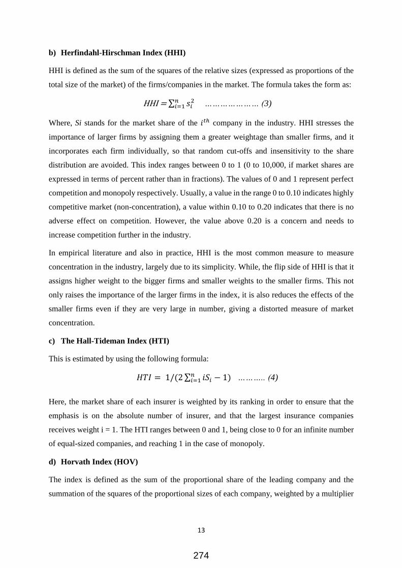
13
b) Herfindahl-Hirschman Index (HHI)
HHI is defined as the sum of the squares of the relative sizes (expressed as proportions of the
total size of the market) of the firms/companies in the market. The formula takes the form as:
HHI = ∑ 𝑠𝑖2𝑛
𝑖=1 ………………… (3)
Where, Si stands for the market share of the 𝑖𝑡ℎ company in the industry. HHI stresses the
importance of larger firms by assigning them a greater weightage than smaller firms, and it
incorporates each firm individually, so that random cut-offs and insensitivity to the share
distribution are avoided. This index ranges between 0 to 1 (0 to 10,000, if market shares are
expressed in terms of percent rather than in fractions). The values of 0 and 1 represent perfect
competition and monopoly respectively. Usually, a value in the range 0 to 0.10 indicates highly
competitive market (non-concentration), a value within 0.10 to 0.20 indicates that there is no
adverse effect on competition. However, the value above 0.20 is a concern and needs to
increase competition further in the industry.
In empirical literature and also in practice, HHI is the most common measure to measure
concentration in the industry, largely due to its simplicity. While, the flip side of HHI is that it
assigns higher weight to the bigger firms and smaller weights to the smaller firms. This not
only raises the importance of the larger firms in the index, it is also reduces the effects of the
smaller firms even if they are very large in number, giving a distorted measure of market
concentration.
c) The Hall-Tideman Index (HTI)
This is estimated by using the following formula:
𝐻𝑇𝐼 = 1/(2 ∑ 𝑖𝑆𝑖𝑛𝑖=1 − 1) ……….. (4)
Here, the market share of each insurer is weighted by its ranking in order to ensure that the
emphasis is on the absolute number of insurer, and that the largest insurance companies
receives weight i = 1. The HTI ranges between 0 and 1, being close to 0 for an infinite number
of equal-sized companies, and reaching 1 in the case of monopoly.
d) Horvath Index (HOV)
The index is defined as the sum of the proportional share of the leading company and the
summation of the squares of the proportional sizes of each company, weighted by a multiplier
274

14
reflecting the proportional size of the rest of the industry. The index owes its intellectual
heritage to the HHI and is defined as:
HOV = 𝑠1 + ∑ 𝑠𝑖2𝑛
𝑖=2 (2 - 𝑠𝑖) ………….(5)
Here, 𝑠1 represents market share of the largest firm in the industry. The value of the index
ranges between 3𝑛2−3𝑛+1
𝑛3 (for n ≠ 2) and 1, i.e., 3𝑛2−3𝑛+1
𝑛3 ≤ HOR ≤ 1 with n being the number
of firms in the industry. This index assigns larger weights to all the market players, compared
to HHI.
e) Entropy Index (ENT)
The Entropy measure is defined as,
ENT = ∑ 𝑠𝑖 𝑛𝑖=1 ln (
1
𝑠𝑖) ……………(6)
This index generally measures the degree of uncertainty faced by a firm in the marketplace.
The value of the Entropy varies inversely to the degree of concentration. In case of monopoly
there is no uncertainty in the market and the index takes the value zero. On the other hand,
when there is ‘n’ number of firms and all of them are equal in size, there are uncertainties in
the market and the index takes the value ln (n). Hence, the index ranges between 0 and ln (n),
and is therefore not restricted to [0, 1], as most of the other measures of concentration presented
above.
This index is criticised for using the logarithm of the market share rather than its value as the
weight. As a result, the importance of the larger firms decreases, while that of the smaller ones
relatively increases.
f) Ginevicius Index
The Ginevicius Index is given by the formula
GIN = ∑ (𝑠𝑖
1+𝑛(1−𝑠𝑖)
𝑛𝑖=1 ) ………………(7)
This index is intended to assess two basic market indicators, the number of firms in the industry
and their market share in a balanced way. It is based on the assumption that larger the number
of suppliers, greater is the competition hence higher is the uncertainty in the market. The degree
of this uncertainty depends on market shares of the firms when there is monopoly GIN = 1. On
the other hand, as n → ∞, GIN → 0. In other words, as the number of firms in the industry
275

15
increases, the degree of seller’s concentration in the market declines. Hence, this index takes
the; 0 ≤ GIN ≤ 1.On a positive note, that GIN index gives emphasis to both the number of firms
in the industry and their market share. However, it fails to represent the true scenario of market
concentration, particularly when the distribution of market share is highly skewed towards few
firms.
g) GRS Index
The GRS Index suggested by Ginevicius and Cirba (2009) is an attempt to overcome the
weighting problem and thereby to provide a more accurate measure of market concentration.
In this index, the weights to different firms are assigned in such a way that (i) the value of the
index ranges from 0 to 1, i e, 0 ≤ GRS ≤ 1, (ii) if all firms in the industry have equal market
share, i e, if 𝑠𝑖 = 1
𝑛, GRS =
1
𝑛 , and (iii) it gives a more accurate measure of market concentration.
Accordingly, the index is defined as,
GRS = ∑ (𝑛2𝑠1+0.3 𝑠𝑖
2
𝑛2+0.3𝑛𝑠1𝑠𝑖
𝑛𝑖=1 𝑠𝑖) ……………….(8)
Where, 𝑠1 stands for market share of the largest firm in the industry.
Table 4: Features of Concentration Measures
Index
Type Defined as Range Features
CRk 𝐶𝑅𝑘 = ∑ 𝑆𝑖𝑘
𝑖=1
0<CRk=1 Takes only large companies into
account; arbitrary cut off
HHI HHI = ∑ 𝑠𝑖2𝑛
𝑖=1
1/n=HHI
=1
Considers all insurers; sensitive to
entrance of new companies
Horvath CCI = HOR = 𝑠1 + ∑ 𝑠𝑖
2𝑛𝑖=2 (2 - 𝑠𝑖)
0<CCI=1 Address relative dispersion and
absolute magnitude;
Suitable for cartel markets
Entropy ENT = ∑ 𝑠𝑖
𝑛𝑖=1 ln (
1
𝑠𝑖)
0=ENT=
Ln(n)
Uses the logarithm of the market share
rather than its value as the weight value;
Importance of larger firms decreases
while smaller ones relatively increases
Ginevicius
Index GIN = ∑ (
𝑠𝑖
1+𝑛(1−𝑠𝑖)
𝑛𝑖=1 ) 0≤GNI≤1
It emphasises both the number of firms
and their market share;
Fails to represent true scenario of
market concentration particularly when
the distribution of market share is
highly skewed towards few firms
GRS
Index GRS = ∑ (
𝑛2𝑠1+0.3 𝑠𝑖2
𝑛2+0.3𝑛𝑠1𝑠𝑖
𝑛𝑖=1 𝑠𝑖)
0≤GRS≤1
Attempt to overcome the weighting
problem to provide a more accurate
measure of market concentration
HTI Index 𝐻𝑇𝐼 = 1/(2 ∑ 𝑖𝑆𝑖
𝑛
𝑖=1− 1)
0<HTI=1
Market share of each insurer is
weighted by its ranking in order to
ensure that the emphasis is on the
absolute number of companies
276

16
Among the above discussed approaches to measure the concentration in an industry, the choice
of the concentration index is mainly dependent on the policy makers’/researchers’ perception
of the relative influence on competition attached to large and small firms or companies. The
HHI and the K-concentration ratio appear most frequently, both in theory and practice. The
simple structure of these two indices and the limited data requirement of the CRk contribute to
this success.
3.3.2 Measuring Structural Change
To see the structural change, two different indices are calculated, following Dietrich (2012).
The first is the simplest measure of structural change (SC), the Norm of Absolute Values
(NAV) and the second index is the modified Lilien index (MLI). Both the indices are discussed
below:
a) Norm of Absolute Values (NAV)
The Norm of Absolute Values (NAV) index is defined as:
𝑁𝐴𝑉 = 0.5 ∑ 𝐼 𝑋𝑖𝑡 − 𝑋𝑖𝑠 𝐼𝑛𝑖=1 ……………………… (9)
Where, the terms xit and xis are the market share of ith line of business at points of time t and s.
The absolute (modulus) values of the difference of the two is taken and summed over all lines
of business. It varies from 0 to 100 (if shares are expressed in per cent) or from 0 to 1 (if shares
are expressed in proportions). The amount of structural change equals exactly the share of the
movements of the sectors as a percentage of the whole economy. If the structure remains
unchanged the indicator is equal to zero and if all sectors change at its most, which means the
whole industry has a total change then the index is equal to unity. One of the disadvantages of
NAV is that there might be similar impact due to huge movements in a few components and
due to light movement in many components.
b) Modified Lilien Index (MLI)
The Lilien index is an important measure of structural change in a number of fields of economic
research. Here, we used Lilien index as a measure of structural change in the Indian non-life
insurance industry. It is derived from an axiomatic analysis of structural change indices. The
index is defined as:
𝑀𝐿𝐼 = 𝑆𝑄𝑅𝑇 [∑ 𝑋𝑖𝑡 ∗ 𝑋𝑖𝑠 ∗ (𝐿𝑛 𝑋𝑖𝑡
𝑋𝑖𝑠)^2], 𝑡 > 𝑠 ……..(10)
277

17
Where, Xit as the market share of sector i at time t. The index has to be equal to zero if the sectoral
composition is unchanged.
4 Empirical Results & Discussions
This paper attempts to assess the state of competition and measure the structural change in the
business segments in the Indian non-life Insurance industry. To access the competition level,
a group of concentration measured tested for the period 2000-01 to 2010-15. An attempt also
made to suggest the best concentration index to study the state of competition in Indian non-
life insurance industry. Further, to measure structural change in the sector after health insurance
business started operation in 2005, the study calculated tow SC index for the period 2005-06
to 2014-15.
4. 1 Competition Results
In literature, it is well evident that concentration in a market weakens competition by promoting
collusive behaviour between the firms. More specifically, competition in an industry depends
on the degree of concentration in the sector. In market economics, read in micro-economics, a
market is classified into four categories, viz Monopoly, Oligopoly, Monopolistic Competition
and Perfect competition, which is linked with the level of market competition/concentration.
In perfect competition, there is no concentration of power and the concentration index would
be zero. However, in monopoly, the index would be one. Here, the results are calculated by
using 9-concentration indices to measure market concentration in the Indian non-life insurance
sector by using the market share of the insurers based on ‘Gross Direct premium’ for the period
2000-01 to 2014-15. The indices are calculated every year by considering all the insurance
companies operating in the sector in that year, which varies from 7 in 2000-01 to 21 in 2014-
15.
The results are outlined in the table 5 and the concentration curves presented in graph 4. As
CRn index considers the top n companies in market based on share, so, we have calculated
CR3, CR5 and CR10 to have a clear representation of the index. The all 3-CR indices indicate
the same trend that concentration in the Indian non-life insurance sector declined over the
period but not significantly. The indices, HHI (used mostly by the regulators due to the
simplicity), HTI and GIN indicates that there was less concentration in 2000-01 but declined
further in 2014-15, may be due to the entry of new players in the sector. HOV and GRS indicate
the same trend, though the index value differs. Finally, ENT index also shows a rising
278

18
concentration curve, which means decline in concentration in the sector. Some indices indicate
that concentration in the sector started to increase in 2014-15, which may be temporary.
Table 5: Concentration Indices of the Indian Non-Life Insurance Industry
Year Number of
Insurers CR3 CR5 CR10 HHI ENT HOV HTI GIN GRS
2000-01 7 0.787 1.000 - 0.259 1.373 0.597 0.277 0.162 0.332
2001-02 10 0.765 0.974 1.000 0.245 1.533 0.572 0.258 0.118 0.338
2002-03 12 0.716 0.929 0.998 0.220 1.707 0.533 0.224 0.098 0.323
2003-04 12 0.688 0.893 0.987 0.199 1.841 0.497 0.202 0.095 0.297
2004-05 12 0.650 0.857 0.982 0.179 1.948 0.463 0.186 0.093 0.276
2005-06 12 0.601 0.823 0.983 0.161 2.035 0.433 0.171 0.091 0.266
2006-07 12 0.532 0.782 0.980 0.139 2.143 0.391 0.151 0.089 0.229
2007-08 14 0.489 0.733 0.974 0.128 2.205 0.369 0.141 0.076 0.213
2008-09 16 0.478 0.716 0.956 0.123 2.274 0.357 0.134 0.067 0.205
2009-10 17 0.480 0.702 0.918 0.117 2.362 0.344 0.124 0.063 0.198
2010-11 19 0.476 0.700 0.899 0.113 2.403 0.334 0.119 0.056 0.188
2011-12 21 0.478 0.686 0.877 0.109 2.453 0.326 0.113 0.056 0.185
2012-13 21 0.467 0.664 0.867 0.105 2.500 0.317 0.108 0.051 0.183
2013-14 21 0.462 0.561 0.797 0.103 2.528 0.247 0.137 0.051 0.162
2014-15 21 0.468 0.562 0.792 0.103 2.539 0.318 0.104 0.051 0.193
Average - 0.569 0.772 0.929 0.154 2.123 0.406 0.157 0.081 0.233
^based on Gross Direct Premium
Thus, the results indicate that concentration in the non-life business segment is moderate. All
the measures quantified indicate healthy competition in Indian non-life insurance industry. The
average indices value of HHI, GIN and GRS indices yield low market concentration. However,
HOV index confirm moderate concentration. Additionally, there is a significant improvement
between the results of the CR3, CR5 and CR10, which indicate that as the sample size increases
the indices approaches to one. In other words, the business in non-life industry is well
distributed among the insurers. The ENT index results interpreted in an opposite way to the
other indices. If the indices value increases the there is competition in the market is increasing.
Another interesting point to note that the global financial crisis of 2008 has not impacted the
concentration results in the non-life insurance industry, as all the industry trends are
continuously declining. Though, the concentration indices indicate the same trend but which
index is more appropriate to study the state of competition in Indian non-life insurance industry,
is discussed in the next section.
279

19
Graph 4: Concentration Curves of Non- Life Insurance Industry (Gross Direct Premium)*
Where,
CR3: 3-firm Concentration Index
CR5: 5-firm Concentration Index
CR10: 10-firm Concentration Index
HOV: Horvath Index
HHI: Herfindahl-Hirschman Index
ENT: Entropy Index
GIN: Ginevicious Index
GRS: GRS Index
HTI: Hall and Tideman Index
Note: ENT index indicate that ‘0’ means higher concentration, i.e.
monopoly in the industry
Note: * Gross Direct Premium
280

20
4.2 Testing Accuracy of Concentration Indices
In order to investigate the accuracy of the concentration indices used to compute the level of
market concentration in the life insurance industry in India, the study followed the criterion
suggested by Ginevicius and Cirba (2009). The criterion takes the form:
Rj = ∑ |𝑆𝑖𝑗 − 𝑆𝑖𝑗𝑛𝑖=1 *|.............. (11)
Here, ‘Rj’ is the criterion of accuracy of j-th concentration measure; Sij* is the relative value of
the market share as per the formula of j-th concentration measure and Sij is the actual calculated
market share.
According to Ginevicius and Cirba (2009), a concentration measure will be most accurate,
when Rj = 0, it ideally reflects the market situation. The calculated Rj values are presented in
table 10, which indicates that none of the concentration measures is ideally accurate, i.e., R =
0. The difference between the actual market share and the relative market share is more than
zero in all the cases. So, to find out a more accurate measure of concentration and not the most
accurate measure, it is assumed that smaller the ‘R’, the more accurate is the measure of market
concentration. To have a better insight, the values of ‘R’ in table 6, ranked by assigning 1 to
the lowest value and then 2 to the next value in ascending order.
Table 6: Comparison of the Accuracy of Concentration Measures
Year FY01 FY02 FY03 FY04 FY05 FY06 FY07 FY08 FY09 FY10 FY11 FY12 FY13 FY14 FY15
Index Value of ‘R’ in Non-Life Insurance (Gross Direct Premium) Variable
HHI 0.188 0.260 0.303 0.310 0.366 0.374 0.349 0.329 0.355 0.426 0.437 0.463 0.474 0.487 0.518
ENT 0.132 0.211 0.270 0.311 0.313 0.285 0.233 0.206 0.224 0.256 0.267 0.275 0.271 0.274 0.273
HOV 0.450 0.507 0.568 0.601 0.640 0.697 0.713 0.731 0.741 0.757 0.749 0.763 0.786 0.539 0.830
HTI 0.441 0.481 0.518 0.529 0.553 0.558 0.547 0.537 0.553 0.594 0.604 0.627 0.636 0.434 0.660
GIN 0.058 0.077 0.081 0.069 0.071 0.065 0.051 0.044 0.045 0.052 0.051 0.053 0.053 0.054 0.057
GRS 0.000 0.000 0.000 0.000 0.000 0.000 0.000 0.000 0.000 0.000 0.000 0.000 0.000 0.000 0.000
Index Ranking of ‘R’ in Non-Life Insurance (Gross Direct Premium) Variable
HHI 4 4 4 3 4 4 4 4 4 4 4 4 4 5 4
ENT 3 3 3 4 3 3 3 3 3 3 3 3 3 3 3
HOV 6 6 6 6 6 6 6 6 6 6 6 6 6 6 6
HTI 5 5 5 5 5 5 5 5 5 5 5 5 5 4 5
GIN 2 2 2 2 2 2 2 2 2 2 2 2 2 2 2
GRS 1 1 1 1 1 1 1 1 1 1 1 1 1 1 1
Source: Calculated
281

21
The ranking of indices in table 6 indicate that GRS is more accurate measure of concentration,
followed by GIN index and ENT index, in case of Indian non-life insurance industry. HHI
ranked at fourth place and HOV ranked at last. Thus, it may conclude that GRS index is the
more ideally accurate measures of concentration in case of the Indian non-life insurance
industry.
4.3 Structural Change Results
The table 7 provides the NAV for various components of non-life business. The NAV values
indicate that the structure of the non-life insurance is changed but slowly over the years. Among
the business segments, the NAV value for health insurance indicate a sharp rising, followed by
fire and motor insurance. While, the marine insurance business segments structure has not
changed significantly.
Table 7: Norm of Absolute Values (NAV) Index for the period 2005-06 to 2014-15
FY06 FY07 FY08 FY09 FY10 FY11 FY12 FY13 FY14 FY15
Fire 0.00 0.97 3.05 3.69 3.68 3.92 4.14 3.98 4.06 4.08
Marine 0.00 0.11 0.08 0.07 0.02 0.20 0.44 0.75 0.91 1.21
Motor 0.00 0.03 1.35 0.52 0.28 0.10 1.47 2.08 2.50 2.62
Health 0.00 1.21 3.34 4.58 5.11 6.22 5.68 5.64 6.86 7.23
Others 0.00 0.38 1.72 1.47 1.68 2.01 2.58 2.99 4.39 4.56
Total 0.00 2.70 9.54 10.33 10.78 12.45 14.31 15.44 18.72 19.71
Source: IRDAI
As the index values not so much different, we have tested with the next method, i.e., Modified
Lilien Index (MLI). The computed values of MLI are provided in the table 4. The MLI values
indicate that fire and health insurance business segments have influenced the structure of Indian
non-life insurance significantly in the study period.
Table 4: Modified Lilien Index (MLI) for the period 2005-06 to 2014-15
FY06 FY07 FY08 FY09 FY10 FY11 FY12 FY13 FY14 FY15
Fire 0.00 3.79 36.80 53.42 53.07 59.95 66.44 61.80 64.02 64.79
Marine 0.00 0.05 0.02 0.02 0.00 0.15 0.76 2.23 2.07 5.73
Motor 0.00 0.00 7.27 1.09 0.32 0.04 8.67 17.27 17.58 27.52
Health 0.00 5.84 43.83 81.19 100.55 147.68 123.83 122.12 135.52 197.05
Others 0.00 0.57 11.74 8.65 11.33 16.12 26.55 35.43 28.97 81.19
Total 0.00 3.20 9.98 12.02 12.86 14.96 15.04 15.45 15.75 19.40
Source: IRDAI
282

22
Thus, both the indices indicate the same trend that the structure of the Indian non-life insurance
industry has changed by health insurance business during the study period (2005-06 to 2014-
15), which is mainly due to the high growth of health insurance business in India. As the health
insurance in India is largely by demand-driven and the segment may continue to dictate the
structure of Indian non-life insurance industry in future also.
5 Concluding Remarks
To sum up, the structural change and concentration indices in the non-life insurance industry
in India shows (i) a uniform trend across various measures; (ii) though reform process has
reduced concentration in the non-life segment significantly during the period 2000-01 to 2014-
15 but noticeably slow. It is also interesting to note that health insurance business segments
have influenced the structure of non-life insurance in the period 2005-06 to 2014-15. The GRS
is found to most accurate concentration index for the Indian non-life insurance industry to study
the competition in the sector.
The GRS index values indicate that the concentration has declined to 0.193 in 2014-15 from
0.332 in 2000-01. In other words, the model of privatization adopted by the Government of
India has yielded positive results and the sector has started to be comparable to its global peers.
However, there is adequate scope for the regulator to promote further competition in the sector,
to increase efficiency in the market as the concentration index is still at above 0.10 or 10%
(0.193 in 2014-15). Going forward, the sector in its present form looks promising for the
consumers, the insurers and the nation as a whole.
*****
283

23
References
Acharya, D. (2012), ‘Competition in Insurance Sector: Issues and Evidences’, UGC Major
Research Project Report, 2012, New Delhi.
Beck, T., Kunt, A. and Levine, R. (2006), ‘Bank Concentration, Competition and Crises: First
Results’, Journal of Banking & Finance, Vol. 30, No. 5, 2006, pp. 1581–1603.
Bikker, J. A. and Haaf, K. (2000), ‘Measures of Competition and Concentration in the Banking
Industry: A Review of the Literature’, De Nederlandsche Bank Research Series Supervision,
No. 27, September 2000.
Bikker, J. A., and Haaf, K. (2002), ‘Measures of competition and Concentration in the Banking:
a Review of Literature’, Economic and financial Modelling, 9, 53-98. Summer 2002.
Bikker, J.A. and Leuvensteijn, M. V. (2008), ‘Competition and Efficiency in the Dutch Life
Insurance Industry’, Applied Economics, Vol. 40, 2008, pp. 2063-2084.
Dietrich, A. (2010), “Does Growth Cause Structural Change, or Is it the Other Way Round? A
Dynamic Panel Data Analysis for Seven OECD Countries”, Empirical Economics, December
2012, Vol. 43, Issue 3, pp 915-944.
Eling, M. & Luhnen, M. (2008), ‘Understanding Price Competition in the German Motor
Insurance Market’, Zvers wiss, December 2008, Vol. 97, Issue 1 Supplement, pp 37-50,
Springer-Verlag.
Ginevičiusa, R. & Čirbab, M. (2009), ‘Additive measurement of market concentration’,
Journal of Business Economics and Management, Vol 10, Issue 3, pp 191-198, 2009
Hall, M. & Tideman, N. (1967), ‘Measures of Concentration’, Journal of the American
Statistical Association, Vol. 62, No. 317 (Mar., 1967), pp. 162-168.
Horvath, J. (1970), ‘Suggestion for a Comprehensive Measure of Concentration’, Southern
Economic Journal, Vol. 36, No. 4 (Apr., 1970), pp. 446-452
IRDAI (2015), ‘Annual Report 2014-15’, Insurance Regulatory and Development Authority of
India (IRDAI), Hyderabad.
IRDAI (2015), ‘Hand Book on Indian Insurance Statistics’, Insurance Regulatory and
Development Authority of India (IRDAI), 2015, Hyderabad
284

24
Miller, J. P. (1955), ‘Measures of Monopoly Power and Concentration: Their Economic
Significance’, Universities-National Bureau, Princeton University Press, Vol. 55-1, 1955, pp.
117-138.
Mishra, P., Divesh, M. and Parimal (2011), ‘Market Concentration in Indian Manufacturing
Sector: Measurement Issues’, Economic & Political Weekly, Vol. xlvi, No 49, 03 December
2011, pp. 76-80.
Njegomir, V., Stojić, D. and Marković, D. (2011), ‘Liberalization, Market Concentration and
Performance in the Non-Life Insurance Industry of Ex-Yugoslavia’, Ekon Misao Praksa, No.
1, 2011, pp. 21-40.
Parida, T. K. (2015), ‘Life Insurance in India: Competition, Efficiency, and Regulation’, PhD
thesis Submitted to and Approved by the University of Hyderabad.
Parida, T. K. and Acharya, D. (2016), ‘Competition in Indian Life Insurance Industry: Post
Liberalisation Evidence’, International Journal of Business Competition and Growth, Vol. 5,
Nos. 1/2/3, 2016.
Rao, D. T. (2000), “Privatization and Foreign Participation in Life Insurance Sector”,
Economic and Political Weekly, March 25, pp. 1107-1119.
Rastogi, S. and Sarkar, R. (2007), “Enhancing Competitiveness: The Case of the Indian Life
Insurance Industry”, Paper presented at the ‘Conference on Global Competition &
Competitiveness of Indian Corporate, Indian Institute of Management Kozhikode.
Rothschild, M. and Stiglitz, J. E. (1997), “Competition and Insurance Twenty years Later”, The
Geneva Papers on Risk and Insurance Theory, (1997) 22, pp. 73-79.
Sastry, D. (2012), ‘Concentration and Indian Insurance’, Journal of Quantitative Economics,
Vol. 10, No.2, July 2012.
*****
285