Natalini, Bravo 2013 Encouraging sustainable transport choices in american households

Sustainability 2014, 6, 50-69; doi:10.3390/su6010050

sustainability ISSN 2071-1050

www.mdpi.com/journal/sustainability

Article

Encouraging Sustainable Transport Choices in American

Households: Results from an Empirically Grounded

Agent-Based Model

Davide Natalini 1,* and Giangiacomo Bravo

2

1 Global Sustainability Institute, Anglia Ruskin University, East Road, Cambridge CB1 1PT, UK

2 Department of Social Studies, Linnaeus University, and Collegio Carlo Alberto, Universitetsplatsen 1,

35252 Växjö, Sweden; E-Mail: [email protected]

* Author to whom correspondence should be addressed; E-Mail: [email protected];

Tel.: +44-845-196-5115.

Received: 3 September 2013; in revised form: 5 December 2013 / Accepted: 9 December 2013 /

Published: 20 December 2013

Abstract: The transport sector needs to go through an extended process of decarbonisation

to counter the threat of climate change. Unfortunately, the International Energy Agency

forecasts an enormous growth in the number of cars and greenhouse gas emissions by

2050. Two issues can thus be identified: (1) the need for a new methodology that could

evaluate the policy performances ex-ante and (2) the need for more effective policies.

To help address these issues, we developed an Agent-Based Model called Mobility USA

aimed at: (1) testing whether this could be an effective approach in analysing ex-ante

policy implementation in the transport sector; and (2) evaluating the effects of alternative

policy scenarios on commuting behaviours in the USA. Particularly, we tested the effects

of two sets of policies, namely market-based and preference-change ones. The model

results suggest that this type of agent-based approach will provide a useful tool for testing

policy interventions and their effectiveness.

Keywords: Agent-Based Model; environmental policies; price-based policies;

preference-based policies; sustainability; transports

1. Introduction

During the last few decades, many policies have been implemented to address the ever-growing

emission trends generated by the transport sector. Notwithstanding the steps taken in promoting more

OPEN ACCESS

Sustainability 2014, 6 51

sustainable travels, the sector still accounts for 22% of global CO2 emissions [1] and up to 50% in

cities [2]. In addition to that, the International Energy Agency (IEA) forecasts an increase of 250%–375%

in the number of cars by 2050 [3]. Correspondingly, CO2 emissions from this sector are projected to

experience a 300% growth in the same period [3]. Note that the latter figure is almost five times higher

than the reduction recommended by the IEA to meet Intergovernmental Panel on Climate Change‘s (IPCC)

target of avoiding catastrophic climate change [4].

The attention given to the transport sector for its potential contribution to the reduction in global

CO2 emissions led to a proliferation of policies for sustainable transports. These can be grouped in

three broad categories [5–9]: (1) market-based policies; (2) structural policies; and (3) preference-change

policies. The first category comprises all the price-related policies, e.g., carbon, fuel or kilometre taxes,

cap and trade schemes, subsidies to public transport, increase in parking charges, motor vehicle fuel

economy labelling, fuel efficiency and renewable fuel standards. The second category includes policies

aimed at promoting investments in infrastructures and sustainable practices, e.g., development of plans

for mixed vehicle uses, build and improve cycle lanes, provide cycle parking, wider, better maintained

and cleaner pavements, improved street furniture, safer neighbourhoods and crossings and promoting

investments for the development and adoption of alternative fuels. The third category comprises

policies directly aimed at changing people‘s preferences, such as advertising and marketing

campaigns, education in sustainable practices, eco-driving campaigns and knowledge transfer.

Despite the widely recognised role of technology in the abatement of CO2 emissions from the

transport sector (e.g., through the spreading of low-emission vehicles), it is difficult to foresee a quick

shift to a zero- or, at least, a low-emission fleet. In fact, the implementation of more aggressive

technology-oriented policies is likely to be difficult and would involve strong equity issues [10]. Thus,

the policy-making field should also focus on policies that could facilitate a shift to sustainable

behaviours. However, it is clear that no ―panacea‖ exists, i.e., a single type of governance system able

to succeed in all or, at least, in most cases [11].

Given the impressive amount of policies being developed in the transport field, and because no

panacea looks possible, there is an increasing need for new methodologies that could assess ex-ante

(i.e., before the implementation of the policy itself) their performance. To address this issue, we

created the Mobility-USA (MUSA) model, an Agent-Based Model (ABM) able to test the

implementation of policies in the transport sector, and we analysed the response of a sample of

American commuters to a set of policies aimed at reducing private car use. Our focus on the USA is

for three main reasons: (1) the overall impact of the country‘s transport system on the global climate;

(2) the low price of oil in the country, which contributes to a large share of private-motor-vehicle

transportation; (3) the availability of reliable data.

We focussed on commuters because they are an important target for policy-making due to their

systematic and customary nature. According to the 2009 National Household Travel Survey (NHTS),

the percentage of commutes by mode of transport in the USA is: 91.4% by private vehicles,

3.7% public transit, 3% walk, 1.9% other [12]. This overview of the commuting sector in the USA

highlights a clear need for sound reform. Indeed, the implementation of sound and effective policies to

stimulate the use of public and non-motorised transport—consequently encouraging a decrease in the

share of private motorised transportation—could improve mobility options, reduce energy use and

decrease Greenhouse Gases (GHG) emissions from the transport sector [13].


To test our modelling approach we analysed two groups of policies: market-based policies and

preference-change policies. These have been chosen because they could be easily applied to our model

and because of their common implementation in the transport sector [14]. The former aim at

internalising the externalities involved in the production and consumption of a given good/service

through the imposition of a tax/fee, whereas the latter are meant to change consumers‘ behaviour by

acting directly upon their preferences.

The existing literature is inconclusive in showing which of these two types of policy is more

effective in encouraging sustainable transport behaviours. On one hand, some authors argue that

economic incentives and structural changes are more powerful than environmental knowledge in

supporting environmentally-oriented behaviours [15–18]. Others go further saying that soft-policies

are not likely to achieve considerable reductions in the CO2 emissions from the transport sector [6].

On the other hand, many scholars encourage an approach that indirectly affects people‘s behaviours

through preferences and changes in attitudes. For instance, some authors proposed environmental

education as a possible measure to shape more sustainable life-styles [8,19]. Conversely, Jackson [20]

argues that information campaigns are less effective than other forms of learning in promoting green

behaviours and Dobson [21] considers market-based instruments and social learning as being

complementary instruments. Accordingly, Flachsland et al. [14] suggests that non-market policies

become of pivotal importance when market failures neutralise the impacts of market-based ones.

The combination of these policies is seen as an optimal strategy by different authors (e.g., [6]). On the

other hand, other authors argue that information and education policies are necessary, but are not

sufficient to bring about changes in behaviour [22].

The potential outcome of these policies is evaluated using the MUSA [23] model on that

incorporates data derived from a sample of commuters drawn from the 2009 NHTS. In particular, we

evaluate which scenario (i.e., policies implemented singularly or combined) is more effective in

promoting the use of less polluting means of transport.

In order to ease the understanding of the policies being implemented in MUSA (i.e., market-based

and preference-change), we provide some examples: the first type of policy could be a carbon tax that

is meant to affect the use of motorised transports by increasing their price of use. The second type of

policy could be imagined both as a combination of policies such as marketing campaigns, provision of

information about the commuting alternatives of the agents, etc., or as a single and effective policy,

such as the introduction of classes on environmental education through formal compulsory education.

The remainder of this paper is organised as follows: Section 2 defines the model following the

Overview, Design concepts, Details (ODD) Protocol and provides the data on which the model relies.

Section 3 grounds the model into empirical data and Section 4 presents the outcomes resulting from

the policy scenarios. Finally, Section 5 presents the conclusions.

2. Methods

The analysis below is centred on an agent-based model, i.e., ―a computational method that enables a

researcher to create, analyse, and experiment with models composed of agents that interact within an

environment‖ [24]. This definition highlights four elements that uniquely characterise ABMs: (1) an

environment, i.e., a set of objects the agents can interact with; (2) a set of interactive agents; (3) a set


of relationships linking objects and/or agents; and (4) a set of operators that allow the interaction

between the agents and the objects. In particular, ABMs implement a generative approach, which

allows the investigation of social patterns using a bottom-up technique. There is a notable difference

between bottom-up (e.g., ABMs) and top-down (e.g., System Dynamics) approaches: in the first case,

the data gathering procedure may be time-consuming and simulations may be more complex than

top-down ones. However, the resulting overall macro-picture will probably be more informative [25].

Moreover, the generative approach allows the consideration of emerging properties: a given

macro-behaviour cannot be represented as a simple aggregation of several micro-behaviours. In fact,

ABMs can be used to analyse the non-linearity of aggregated behaviours with respect to individual

ones. This bottom-up approach can bring about unexpected outcomes, which can represent emerging

properties, regularities and structures [26].

2.1. The MUSA Model

This section has been organised following the ODD Protocol first developed by Grimm and

Railsback [27] and further improved by Grimm et al. [28] and Grimm et al. [29]. The purpose of this

protocol is that of providing a sequence of steps when formalising an ABM in order to arrange all the

relevant information about the model in a neat and logic way. Moreover, the implementation of such

protocol is also useful to the process of replication and verification of the model when these are being

carried out by people others than the authors [27–30]. Notwithstanding some limitations of the ODD

protocol, e.g., the possible redundancy between the categories included, it is a very good way to

increase the clarity of the model specifications [29,30].

2.1.1. Purpose

MUSA is an ABM that aims at reproducing the transport choices of a sample of American citizens

and the GHG emissions related to their daily commutes. Specifically, it was designed to test whether

the ABM approach is suitable to investigate commuting behaviours and to evaluate ex-ante the

consequences of policy implementation.

2.1.2. Entities, State Variables and Scales

MUSA includes only one type of agent—American commuters. The state variables of the agents

are: their initial and final preference for each of the modes of transport, the importance they give to

their social and personal satisfaction, the number of their neighbours, their previous and current

satisfaction given by the choice of the mode of transport, the uncertainty they experience while

choosing the preferred mode of transport and whether they decide to make a short or a long commute

(i.e., SC or LC).

The agents‘ position in the 3D space corresponds to their preferences for each mode of transport

(i.e., the preferences act as coordinates for the dimensions x, y and z), hence there is no absolute

concept of spatial scale in the model (i.e., the fact that two agents are close in the 3D space does not

necessarily mean they are neighbours in the reality).


According to their position in the 3D space, the agents are clustered in neighbourhoods. The agents

that belong to the same neighbourhood are connected by links, while longer links can span across

neighbourhoods. This allows social influence to be taken into account when the agents make decisions.

The second entity included in MUSA is the government. It is represented in the model in an abstract

form and it acts—directly or indirectly—on the agents‘ preferences by implementing two types of

policies: market-based and preference-change policies.

As far as the time scale is concerned, one time step corresponds to one commute for every agent.

Assuming that each person commutes on average twice a day, this temporal unit could be interpreted

as half a day.

2.1.3. Process Overview and Scheduling

MUSA considers one main process, the commuters‘ decision about what means of transport to

travel in. The agents start with a set of preferences—one for each mode of transport—that have been

assigned to them and that place them in the 3D space. Throughout the process, these are influenced by

the relative price of the different means of transport, by social influence and by the intensity of the

policies applied.

After the assignment of the preferences to the agents, the social network is initialised and the

neighbourhoods are formed according to the closeness of the initial preferences of the agents. During

the following step they decide whether to make an SC or an LC and then they decide what means of

transport to use.

The agents, while performing the procedures, do not follow any particular order and the variables

included in the model are synchronously updated at the end of each procedure. At the following time

step the process starts all over again.

2.1.4. Design Concepts

Basic principles: One of the core assumptions made in MUSA is that SCs and LCs differ for the

selection of the eligible means of transport. For SCs, agents can choose whether to commute by

private motorised vehicles (M), private non-motorised vehicles (NM) or by public transportation

(PT). Conversely, for LCs the choice is limited to M and PT. This distinction is based on the

assumption that long distances cannot be covered with NM (See Section 2.1.6).

Agents‘ decisions are based on the ―consumat‖ framework developed by Jager [31] to explain

the environmental behaviour of consumers. This was first translated into an actual model by Jager

and Janssen [32] and—more recently—by Bravo et al. [33]. According to this framework, agents‘

decisions about the means of transport rely on a set of four possible processes. Depending on their

satisfaction and uncertainty, agents can employ (1) rational deliberation, (2) imitate others‘

behaviour, (3) compare their own satisfaction with their neighbours‘ one, or (4) repeat the

previously chosen behaviour (see Section 2.1.7). Agents are linked in a network following a

principle of homophily in preferences. Unlike Janssen and Jager [32], who employed a small-world

network, we chose to use the ―social circle‖ structure, first introduced by Hamill and Gilbert [34],

which better incorporates key aspects of large social networks such as low density, high clustering and

assortativity of the connectivity degree. The network is based on the ideas of social space and distance.


Emergence: One of the principal features of the ―consumat‖ model is the introduction of social

influence in the agents‘ decisions. Hence, the patterns in the use of each means of transport are

emergent in the sense that they are the result of single agents‘ behaviours that in turn are influenced

by those of their neighbours.

Adaptation: This is another feature of the ―consumat‖ model. Agents can employ different

deliberative processes according to the situation they find themselves in. This is particularly

relevant in the policy scenarios, where agents have to adapt their decisions to different relative

prices of the means of transport or to influences on their initial preferences.

Objectives: The agents, while deciding what means of transport to commute in, try to maximise

their personal and social satisfaction taking their uncertainty into account (i.e., how many times

they change their minds about what means of transport to commute in) (see Section 2.1.7).

Learning: The agents, while trying to achieve their objective, can employ several deliberative

processes that compare the total level of satisfaction gained by the decision taken in the previous

time step and their uncertainty.

Sensing: Two of the deliberative processes that the agents can employ while making a decision are

imitation and social comparison. In both cases they will compare their past overall satisfaction with

that of their neighbours.

Interaction: The interaction between the agents occurs through the social network they are

embedded in.

Stochasticity: Randomness is included in different parts of the model. Some randomness is

introduced in the agents‘ locations to avoid the building of exactly the same network at every run.

Moreover, it is introduced when choosing a type of commute (i.e., SC or LC) and while weighing

social and personal satisfaction.

Collectives: The agents are grouped into neighbourhoods according to their position in the 3D space,

which is in turn the result of their preferences for the different means of transport and some

randomness. These neighbourhoods are represented in the 3D space as clusters of agents.

Observation: The values collected and stored at the end of every time step are the number of agents

making SCs and LCs, the means of transport they decide to use, the deliberative process they

employ and the CO2 emissions related to each type of commute.

2.1.5. Initialisation

When the simulation starts, the characteristics of each means of transports are initialised. Each of

them is provided with a specific relative price that can be chosen by the user in the model interface

(see Section 2.2.2), average CO2 emissions per mile and an environmental index (see Section 2.2.2).

Moreover, the model sets a propensity for the type of commute, which is the likelihood of one agent to

choose to make an SC or an LC (see Section 2.1.6). Then MUSA creates the agents, placing them into

a network built following the procedure described in Hamill and Gilbert [34]. Agents have a set of

initial preferences derived from empirical data (see Sections 2.2 and 3), which also affects their

position in the 3D space. Each dimension of the space maps one of the agent‘s preferences. Then each

agent creates links with all the other agents within a certain distance, determined by the link-distance

parameter. This parameter can be chosen in the model interface and in our simulations was set to a value


leading to a degree distribution approaching a power law, as is common in many social networks [35].

Then another procedure checks if there is any lone agent. If so, this gets linked with its closest neighbour.

Finally, the agents‘ uncertainty is set to zero and their total level of satisfaction is computed (see

Section 2.1.7).

2.1.6. Input Data

In MUSA, each agent i is characterised by a set of preferences Pi = {pi1, …, pim} where m = 3, the

set of the eligible modes of transport. Each agent maps one of the 5000 respondents selected as a

subsample from the 2009 NHTS survey [36] and their preferences are derived from the answers given

in the survey (see Section 2.2). The analysis of the commute length declared by the participants in the

2009 NTHS led us to define SCs as between 0 and 3 miles in length—a distance that can be easily

covered walking or cycling—whereas LCs are all commutes longer than 3 miles. According to the

analysis on the survey, 80% of the commutes were LCs and 20% SCs. This parameter has been used to

inform the choice of the agents when they had to decide whether to make an SC or an LC. The same

survey has then been used to compare the results of the calibration of MUSA (see Section 3).

Another external input concerns the relative prices of the means of transport and their average

emissions. These are presented in detail in Section 2.2.

2.1.7. Submodels

In the consumat framework, agents have both personal and social needs and their satisfaction is

affected by both dimensions [31]. Personal need satisfaction ( ) is assumed to be equal to pij where j

is the means of transport used by agent i. This means that the current personal need satisfaction of agent i

depends on the relationship between its preferences and its transportation choice in the previous time step.

Social satisfaction can be defined as the proportion of agents in agent i‘s neighbourhood using the

same means of transport j as i. Agents‘ social need satisfaction can thus be computed as follows:

(1)

where is the social need satisfaction of agent i who chose the means of transport j,

is the number

of agents in i's neighbourhood who chose the means of transport j and ni is the total number of agents

in the neighbourhood taking the same type of commute as agent i.

According to Jager [31], the total level of need satisfaction depends on both personal and social

satisfaction, along with the relative price of the different modes of transport:

(2)

where Nij is the total need satisfaction of agent i who chose j means of transport, βi ∈ [0,1] is a

randomly distributed agent parameter that weights personal needs against social ones and rj is the

relative price for the j means of transport (see Section 2.2.2). A low value of βi implies giving more

importance to personal needs than to social ones and vice versa.


Uncertainty is the second variable affecting the selection of the deliberation procedure. It depends

on the variation of agents‘ satisfaction over time. Since forecasting the outcome of a given behaviour is

difficult when high variability is involved, it is assumed that the higher the variability, the higher the

uncertainty. Following Bravo et al. [33] and Janssen and Jager [32], uncertainty is defined as:

(3)

where t is the time step at which agent i has to make a choice about which deliberative process to use,

Nit is agent i‘s satisfaction at time t and Ni(t-1) is agent i‘s satisfaction at the time (t – 1).

The deliberative process selection is affected by two parameters: τn and τu, both bounded within the

[0,1] interval. The first one represents agents‘ needs, while the second refers to their tolerance towards

uncertainty. Both of them can be defined by the user in the model interface. Depending on the

relationship between these parameters—and thus on the relationship between agents‘ need satisfaction

and uncertainty—different deliberative processes are selected. If Ni ≥ τn and Ui > τu (satisfied and

uncertain agents), the agent i will imitate the most adopted behaviour in his neighbourhood; if Ni < τn

and Ui ≤ τu (dissatisfied and certain agents) the agent i will employ rational deliberation, i.e., it will

compute the satisfaction that may derive from choosing each means of transport and select the most

satisfactory one; if Ni ≥ τn and Ui ≤ τu (satisfied and certain agents) the agent i will simply repeat its

previous decision; finally, if Ni < τn and Ui > τu (dissatisfied and uncertain agents) the agent i will

compare the satisfaction that would derive from repeating its previous choice and the one deriving

from the adoption of the most common behaviour in its neighbourhood. In other words, this

deliberative process will make the agent choose the means of transport that brings most satisfaction.

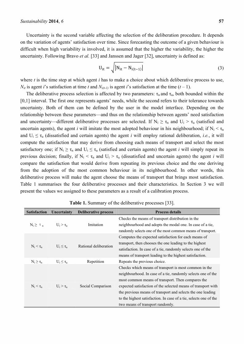
Table 1 summarises the four deliberative processes and their characteristics. In Section 3 we will

present the values we assigned to these parameters as a result of a calibration process.

Table 1. Summary of the deliberative processes [33].

Satisfaction Uncertainty Deliberative process Process details

Ni ≥ τn Ui > τu Imitation

Checks the means of transport distribution in the

neighbourhood and adopts the modal one. In case of a tie,

randomly selects one of the most common means of transport.

Ni < τn Ui ≤ τu Rational deliberation

Computes the expected satisfaction for each means of

transport, then chooses the one leading to the highest

satisfaction. In case of a tie, randomly selects one of the

means of transport leading to the highest satisfaction.

Ni ≥ τn Ui ≤ τu Repetition Repeats the previous choice.

Ni < τn Ui > τu Social Comparison

Checks which means of transport is most common in the

neighbourhood. In case of a tie, randomly selects one of the

most common means of transport. Then compares the

expected satisfaction of the selected means of transport with

the previous means of transport and selects the one leading

to the highest satisfaction. In case of a tie, selects one of the

two means of transport randomly.


2.2. Empirical Foundation of MUSA

The approach used to ground MUSA into empirical values is Multilevel Validation [25]. This has

been allowed by the structure of the 2009 NHTS database, which is composed by four sub-datasets,

namely Household File, Person File, Vehicle File and Travel Day Trip File. The data drawn from the

Person file was used as inputs for MUSA to determine agents‘ preferences, while data from the Travel

Day Trip file (TDTD) served as reference for the model outputs.

2.2.1. Agents‘ Preferences

In order to build the agents‘ preferences we analysed the Person file, focussing on those variables

that expressed the properties of habitual commuting patterns [37]. Note that, instead of recording the

preferences of respondents in a strict sense, the NHTS database records their behaviour. The advantage

of using behavioural data is that we no longer need to take into account the value-action gap often

existing in environment-related situations (e.g., [15,38]), hence avoiding the risk of over-estimating

environmental-friendly choices in our sample.

Firstly, we identified a set of core variables that could allow us to trace the commuting habits of the

respondents who had a job (e.g., person ID, state of residence, number of walk trips, etc.). Secondly,

we selected a group of respondents who all answered to the same questions. In other words, we

ignored incomplete records to make sure that the data we would work with was consistent.

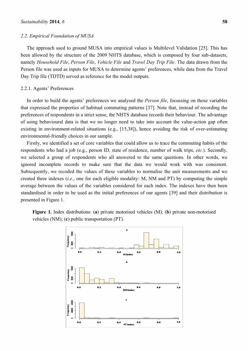
Subsequently, we recoded the values of these variables to normalise the unit measurements and we

created three indexes (i.e., one for each eligible modality: M, NM and PT) by computing the simple

average between the values of the variables considered for each index. The indexes have then been

standardised in order to be used as the initial preferences of our agents [39] and their distribution is

presented in Figure 1.

Figure 1. Index distributions: (a) private motorised vehicles (M); (b) private non-motorised

vehicles (NM); (c) public transportation (PT).


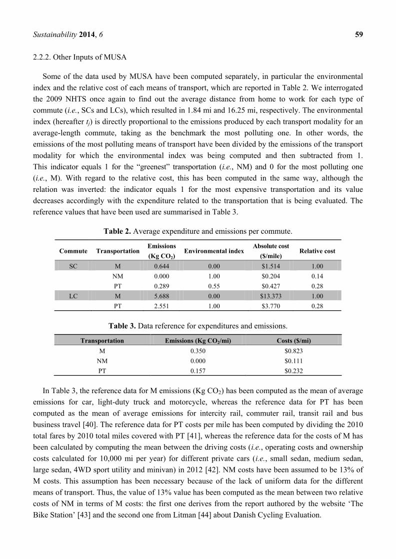
2.2.2. Other Inputs of MUSA

Some of the data used by MUSA have been computed separately, in particular the environmental

index and the relative cost of each means of transport, which are reported in Table 2. We interrogated

the 2009 NHTS once again to find out the average distance from home to work for each type of

commute (i.e., SCs and LCs), which resulted in 1.84 mi and 16.25 mi, respectively. The environmental

index (hereafter tj) is directly proportional to the emissions produced by each transport modality for an

average-length commute, taking as the benchmark the most polluting one. In other words, the

emissions of the most polluting means of transport have been divided by the emissions of the transport

modality for which the environmental index was being computed and then subtracted from 1.

This indicator equals 1 for the ―greenest‖ transportation (i.e., NM) and 0 for the most polluting one

(i.e., M). With regard to the relative cost, this has been computed in the same way, although the

relation was inverted: the indicator equals 1 for the most expensive transportation and its value

decreases accordingly with the expenditure related to the transportation that is being evaluated. The

reference values that have been used are summarised in Table 3.

Table 2. Average expenditure and emissions per commute.

Commute Transportation Emissions

(Kg CO2) Environmental index

Absolute cost

($/mile) Relative cost

SC M 0.644 0.00 $1.514 1.00

NM 0.000 1.00 $0.204 0.14

PT 0.289 0.55 $0.427 0.28

LC M 5.688 0.00 $13.373 1.00

PT 2.551 1.00 $3.770 0.28

Table 3. Data reference for expenditures and emissions.

Transportation Emissions (Kg CO2/mi) Costs ($/mi)

M 0.350 $0.823

NM 0.000 $0.111

PT 0.157 $0.232

In Table 3, the reference data for M emissions (Kg CO2) has been computed as the mean of average

emissions for car, light-duty truck and motorcycle, whereas the reference data for PT has been

computed as the mean of average emissions for intercity rail, commuter rail, transit rail and bus

business travel [40]. The reference data for PT costs per mile has been computed by dividing the 2010

total fares by 2010 total miles covered with PT [41], whereas the reference data for the costs of M has

been calculated by computing the mean between the driving costs (i.e., operating costs and ownership

costs calculated for 10,000 mi per year) for different private cars (i.e., small sedan, medium sedan,

large sedan, 4WD sport utility and minivan) in 2012 [42]. NM costs have been assumed to be 13% of

M costs. This assumption has been necessary because of the lack of uniform data for the different

means of transport. Thus, the value of 13% value has been computed as the mean between two relative

costs of NM in terms of M costs: the first one derives from the report authored by the website ‗The

Bike Station‘ [43] and the second one from Litman [44] about Danish Cycling Evaluation.


3. Model Calibration

The calibration of MUSA has been carried out by checking whether the model is able to represent

the current distribution of commuting habits in the USA, derived from the TDTD dataset. We varied

the need satisfaction (τn) and the uncertainty (τu) thresholds in the {0.1, 0.2, …, 0.9} set, running 100

repetitions of the model for each parameter combination. The starting point of the model was a

situation where everybody used M.

We then chose the parameter combination leading to the average modality distribution—both for

SCs and LCs—closest to the one derived from the TDTD database. More specifically, we aggregated

the simulation outcomes for each parameter combination keeping SCs and LCs separated, obtaining as

a result a single value for each means of transport for each type of commute. Subsequently, we

computed the mean squared error (hereafter MSE) between the simulation results and TDTD data for

each parameter combination. These are presented in Figure 2.

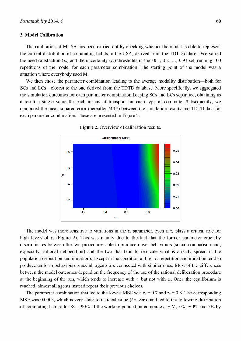
Figure 2. Overview of calibration results.

The model was more sensitive to variations in the τn parameter, even if τu plays a critical role for

high levels of τn (Figure 2). This was mainly due to the fact that the former parameter crucially

discriminates between the two procedures able to produce novel behaviours (social comparison and,

especially, rational deliberation) and the two that tend to replicate what is already spread in the

population (repetition and imitation). Except in the condition of high τn, repetition and imitation tend to

produce uniform behaviours since all agents are connected with similar ones. Most of the differences

between the model outcomes depend on the frequency of the use of the rational deliberation procedure

at the beginning of the run, which tends to increase with τn but not with τu. Once the equilibrium is

reached, almost all agents instead repeat their previous choices.

The parameter combination that led to the lowest MSE was τn = 0.7 and τu = 0.8. The corresponding

MSE was 0.0003, which is very close to its ideal value (i.e. zero) and led to the following distribution

of commuting habits: for SCs, 90% of the working population commutes by M, 3% by PT and 7% by


NM. As far as LCs are concerned, 96% of the working population commutes by M, whereas 4% uses

PT. These are presented in Table 4.

Table 4. Difference between empirical and simulated commuting behaviours (proportions).

Commute Means of transport Simulated Empirical Difference

SC M 0.896 0.886 0.010

PT 0.030 0.170 0.013

NM 0.073 0.096 −0.023

LC M 0.963 0.979 −0.017

PT 0.037 0.017 0.020

4. Results

This section presents the results of the policy scenarios. In order to investigate the possible

behavioural change of the agents corresponding to the implementation of the policies, τn and τu have

been kept fixed at the values given above while changing the price and preference parameters as

indicated below.

4.1. Market-Based Policies

In this scenario we increased the prices of the modes of transport by (1–tj) δ1 where δ1 ∈

{0.1, 0.2, …, 1.0} represents the policy intensity (i.e., the price increase) and tj is the environmental

index of each transport modality. This means that the higher the environmental impact of each

modality, the larger the increase in its price, with δ1 = 1 meaning a doubling of the price of M. A

summary of the relative prices of the means of transport corresponding to the policy intensity (i.e., δ1)

is presented in Table 5. Figure 3 plots the model outcomes for all the δ1 values both for SCs and LCs.

Table 5. Summary of the relative prices of the means of transport corresponding to the

market-based policy intensity.

Transportation δ1 = 0.1 δ1 = 0.2 δ1 = 0.3 δ1 = 0.4 δ1 = 0.5 δ1 = 0.6 δ1 = 0.7 δ1 = 0.8 δ1 = 0.9 δ1 = 1.0

M 1.10 1.20 1.30 1.40 1.50 1.60 1.70 1.80 1.90 2.00

NM 0.14 0.14 0.14 0.14 0.14 0.14 0.14 0.14 0.14 0.14

PT 0.33 0.37 0.42 0.46 0.51 0.55 0.60 0.64 0.69 0.73

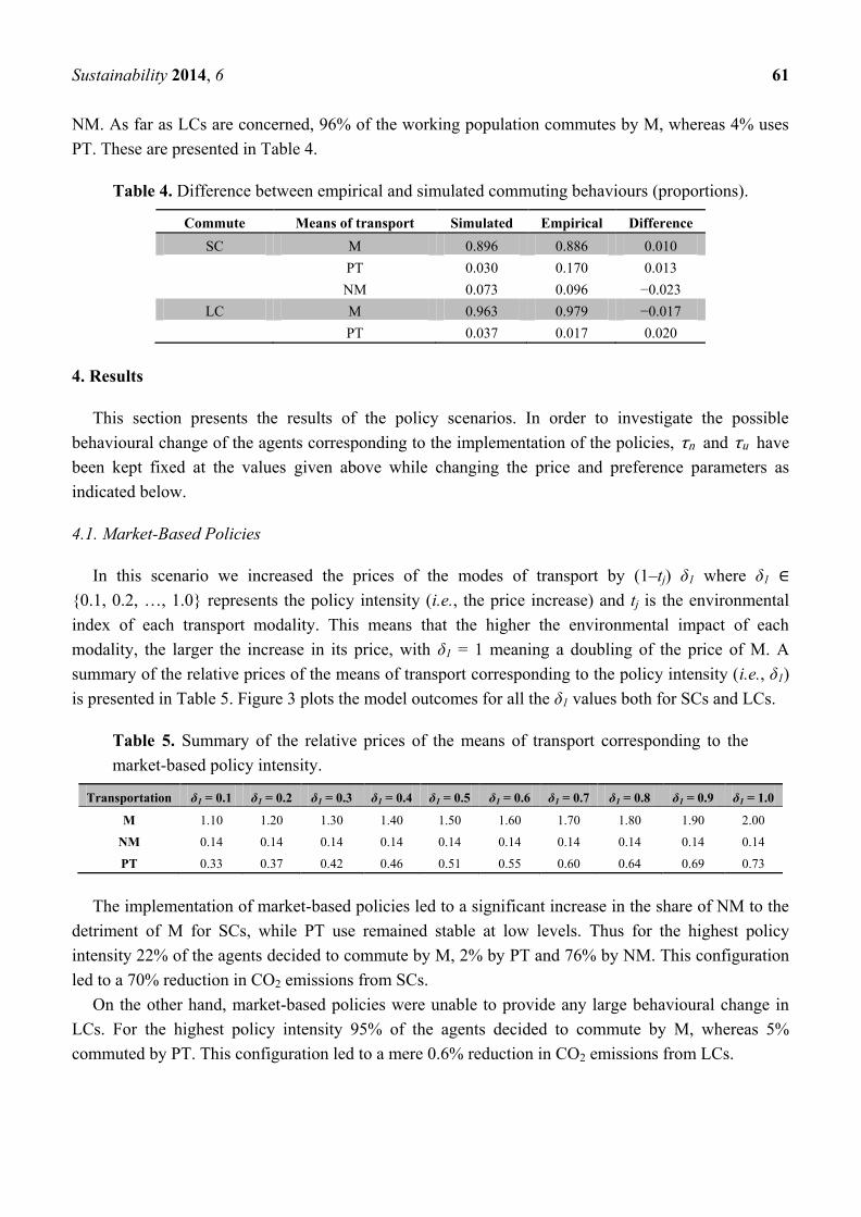
The implementation of market-based policies led to a significant increase in the share of NM to the

detriment of M for SCs, while PT use remained stable at low levels. Thus for the highest policy

intensity 22% of the agents decided to commute by M, 2% by PT and 76% by NM. This configuration

led to a 70% reduction in CO2 emissions from SCs.

On the other hand, market-based policies were unable to provide any large behavioural change in

LCs. For the highest policy intensity 95% of the agents decided to commute by M, whereas 5%

commuted by PT. This configuration led to a mere 0.6% reduction in CO2 emissions from LCs.


Figure 3. Market-based policies results for short commutes (SCs) and long commutes (LCs).

The red line represents M, the green one represents NM and the blue one represents PT.

4.2. Preference-Change Policies

In this scenario, we tested the implementation of a ―green-oriented‖ combination of policies that

could discourage the use of M while simultaneously favouring the use of less polluting means of

transports. These are ―preference-change‖ in the sense that their goal is to change commuters‘

behaviours starting from their beliefs and concerns. Here, we assumed that all agents are affected

equally by these policies.

Practically, preference-change policies affect agents‘ preferences through a parameter δ2 ∈

{0.1, 0.2, …, 1.0} which represents the policy intensity. In this case, the policy intensity is measured

as the increase in investments in this type of policy by the relevant stakeholders (e.g., public

authorities). Recalling the example given in Section 1, if this policy was actually a combination of

policies like marketing campaigns, provision of information about the commuting alternatives of the

agents, or the introduction of environmental education throughout the period of formal compulsory

education, the policy intensity could be measured as the increase in investments made by the relevant

stakeholders (e.g., public authorities) to increase the effectiveness of these policies. This parameter is

subtracted from the M preferences, while it is added to the preferences for NM and PT to model a

decrease in the willingness to adopt M transportation and an increase in the willingness to use both

NM and PT. The results of the scenarios are presented in Figure 4 both for SCs and LCs.

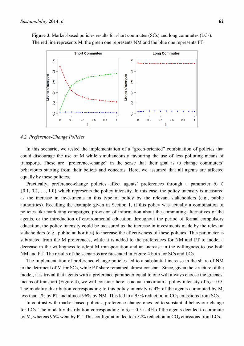
The implementation of preference-change policies led to a substantial increase in the share of NM

to the detriment of M for SCs, while PT share remained almost constant. Since, given the structure of the

model, it is trivial that agents with a preference parameter equal to one will always choose the greenest

means of transport (Figure 4), we will consider here as actual maximum a policy intensity of δ2 = 0.5.

The modality distribution corresponding to this policy intensity is 4% of the agents commuted by M,

less than 1% by PT and almost 96% by NM. This led to a 95% reduction in CO2 emissions from SCs.

In contrast with market-based policies, preference-change ones led to substantial behaviour change

for LCs. The modality distribution corresponding to δ2 = 0.5 is 4% of the agents decided to commute

by M, whereas 96% went by PT. This configuration led to a 52% reduction in CO2 emissions from LCs.


Figure 4. Preference-change policy results for SCs and LCs. The red line represents M,

green = NM and blue = PT.

4.3. Interactions among Policies

In this scenario we simultaneously implemented both policies (i.e., market-based and preference-

change). The aim of this test was to investigate whether by combining these two policies we could

bring about positive synergies, i.e., a change in behaviours at lower policy intensities. The results of

this scenario are presented in Figure 5.

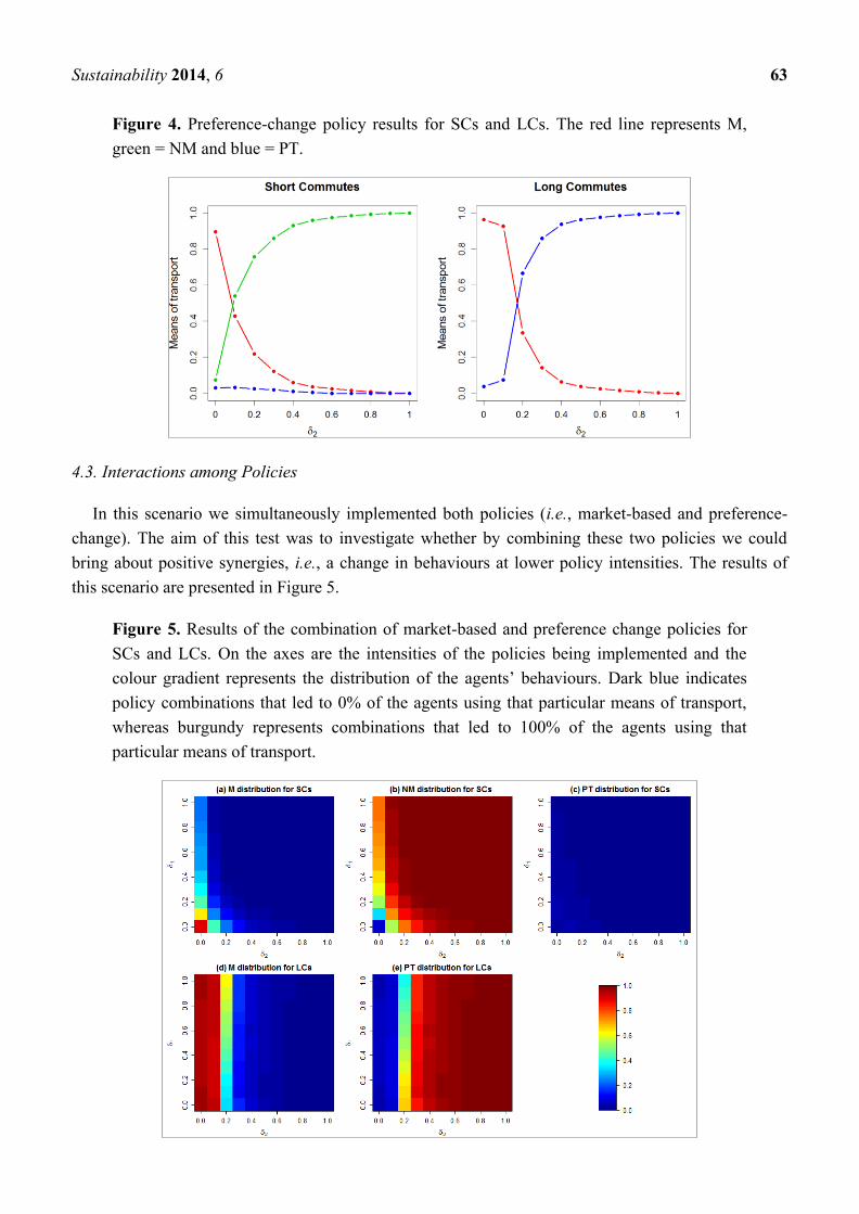
Figure 5. Results of the combination of market-based and preference change policies for

SCs and LCs. On the axes are the intensities of the policies being implemented and the

colour gradient represents the distribution of the agents‘ behaviours. Dark blue indicates

policy combinations that led to 0% of the agents using that particular means of transport,

whereas burgundy represents combinations that led to 100% of the agents using that

particular means of transport.


The combination of market- and preference-based policies brings about the switch to NM

transportation at lower policy intensities for SCs (Figure 5a–c). Indeed, when market-based policy

intensity equals 0.25 and preference-change equals 0.2 (and vice versa) 100% of the agents commuted

by NM. The same does not hold for LCs, where the only policy affecting agents‘ behaviours is

preference-change (Figure 5d,e).

To sum up, the combination of the two policies brings about positive synergies in the SCs but not in

the LCs, where the preference-change policies appear to be more effective than market-based ones.

5. Discussion

MUSA is an agent-based model developed both to show that this method could be a sound

approach to test policy implementation in the transport sector and to analyse the outcomes of the

implementation of two sets of policies in the USA‘s commuting sector. In order to represent the habits

of the USA population as realistically as possible, the construction of MUSA followed a multilevel

validation, i.e., the initial preferences of the agents have been drawn from the 2009 NHTS and the

outputs of the calibration have been checked against different data drawn from the same survey.

The calibration results showed that MUSA was able to reproduce the current commuting habits in

the USA. This is partly due to the behavioural richness that has been included in the model by applying

the ―consumat‖ framework developed by Jager [31], which gains even more value when coupled with

a realistic social network such as the one implemented in our model following the Hamill and Gilbert [34]

procedure. These features were critical for both the calibration and policy-testing phases of MUSA.

We tested two types of policies: market-based and preference-change. It is worth noting here that it

is not possible to better define the impact of the policies on the overall economy represented in our

model. This is because the level of abstraction of MUSA is higher than the different types of policy

that can be implemented. Moreover, we assume that the policies being implemented do produce the

expected effect, i.e., an increase in the prices of motorised transports and an incentive to prefer

non-motorised transports to motorised transports, respectively.

Market-based policies proved to be effective in promoting green behaviours for short commutes.

The same cannot be said for long commutes, where the share of private motorised transports remains

predominant—and almost unaltered—even after the implementation of the policy. This result is

consistent with the existing literature, which often finds transport demand is not price sensitive for

long commutes [45].

Preference-change policies, instead, led to the highest share of non-motorised transports and CO2

emissions reduction for both short and long commutes. Nevertheless, the model results suggest that the

combination of these policies can be remarkably effective on short commutes, but not on long ones.

In the first case their simultaneous implementation creates a positive synergy that is a modal shift to

non-motorised transportation at lower policy intensities (Figure 5a–c). This finding appears especially

important in terms of policy feasibility since higher effectiveness at lower policy intensities possibly

translates into smaller investments to achieve similar results. Conversely, the combination of policies

seems to be ineffective for long commutes, where preference-change is the only factor driving the

change in agents‘ behaviour.


The fact that market-based policies did not significantly affect long commutes resulted in limited

benefits in terms of CO2 emission. A doubling of the price of private motorized transport,

corresponding to 1 = 1, indeed led only to a 0.6% emission decrease. The same reduction could be

achieved by setting 2 = 0.1, which probably represents a much easier target in terms of policy

feasibility, while higher levels of preference change led to emission reductions up to 52% for 2 = 0.5.

Preference-change policies seem therefore to be more effective than price-based ones.

Note also that, in general, the share of public transports is almost never significant for short

commutes. This may reflect MUSA‘s sensitivity to the initial preferences of the agents. As Figure 1c

clearly shows, the modal distribution of the public transport index is zero. Hence, this attitude is deeply

rooted in American commuters and probably depends on structural motives (e.g., the lack of reliable

public transport infrastructures). These cannot be affected by simply increasing the prices of the other

modalities—at least under reasonable limits—but only by acting upon the consumers‘ preferences and

opportunities, for instance by significantly improving the current infrastructure level. This is clearly

shown by our model. This particular result shows one of the limits of MUSA: the model does not take

into account complicating factors such as the diffusion/lack of public transport in the US ground,

which might explain the very low preferences among the agents for this means of transport. Other

complicating factors might be the presence of adequate infrastructures in general (e.g., cycling and

walking lanes, highways, etc.), the income of the commuter and the presence of disabled in the family

that can prevent its members to using means of transport in preference to another.

Moreover, the insensitivity of the preferences for public transport is probably reinforced by social

influence, represented in MUSA through a social network in which the agents are embedded.

This feature had a clear effect in locking the agents into unsustainable behaviours. On the other hand,

that behaviours related to short commutes could be easily influenced by policy-making decisions is

linked to the much more even preference distribution of the non-motorised transport (see Figure 1b).

Thus, even relatively weak policy intensities could significantly affect the behaviours of the agents that

commute for short distances, this time favoured by the social influence effect. Note that both these

features are consistent with the dynamics of consumption assumed by Jager [31] and highlighted both

in Janssen and Jager [32] and Bravo et al. [33] models.

Notwithstanding the good results obtained by both policies and their combination—at least in short

commutes—it is worth noting that economic incentives (i.e., our market-based policies) apparently

have to be large to affect travellers‘ behaviours [46] and that their implementation is likely to bring

about only a temporary change in behaviours. Indeed, Dobson [21] found that once these measures are

stopped, people‘s behaviours are likely to revert to those they had before the market-based policy was

implemented. It is hence recommended to keep them as a permanent tool to correct market distortions

and not just as a temporary incentive. Moreover, Dobson [21] argued that the only way to permanently

change behaviours is by changing attitudes, which can be achieved through environmental education

and through the formal education system (i.e., our preference-change policies). Indeed, MUSA‘s

results seem to be in line with the idea that preference-change policies are more effective in promoting

stable and widespread sustainable behaviours.

Nonetheless, we are aware that convincing people not to use their cars is a real challenge. However,

the results related to the implementation of our preference-change policies suggest that if we could find

a ―trigger policy‖ that could act on the reason why they prefer to use cars instead of other means of


transport, their impact could be critical. The formalisation of this kind of policy is a challenge in itself

because different communities have different ―triggers‖, but tailoring of policies (e.g., [6,47]) to make

them fit closely to the targeted segments of population could bring about successful behaviour change.

In conclusion, two lessons can be learnt from this study. First, the implementation of agent-based

modelling in the transport field appears a sound way to test the performances of different policies

ex-ante (i.e., before the actual implementation of the policy). This approach needs much lower

investments, in terms of both time and money, than ex-post evaluation methods, however depends on

the availability and quality of data that is able to inform agents‘ behaviours and networks to reflect real

behaviours. Second, our model based on the data available, shows that the use of different policy

interventions are not mutually exclusive. National administrations should therefore use all policy

analysis tools available, including agent-based modelling, to test not a single specific policy, but rather

the right combination of measures leading to sustainable commuting-styles.

Acknowledgments

The authors would like to thank Candice Howarth and Robert Evans from the Global Sustainability

Institute and three anonymous reviewers for their comments on a previous version of the paper.

Conflicts of Interest

The authors declare no conflict of interest.

References and Notes

1. International Energy Agency. CO2 Emissions from Fuel Combustion 2012: Highlights;

International Energy Agency Publications: Paris, France, 2012; pp. 1–125.

2. Viceminister of Transport for the Republic of Colombia. Powerpoint Presentation at the 17th

Conference of the Parties. In Proceedings of the United Framework Convention on Climate

Change, Durban, South Africa, 28 November–9 December 2011.

3. Replogle, M.; Hughes, C. Moving Toward Sustainable Transport. In State of the World 2012:

Moving Toward Sustainable Prosperity; Island Press: Washington, DC, USA, 2012; p. 53.

4. International Energy Agency. Transport, Energy and CO2—Moving Towards Sustainability;

International Energy Agency: Paris, France, 2009.

5. Creutzig, F.; McGlynn, E.; Minx, J.; Edenhofer, O. Climate Policies for road transport revisited (I):

Evaluation of the current framework. Energ. Policy 2011, 39, 2396–2406.

6. Santos, G.; Behrendt, H.; Teytelboym, A. Part II: Policy Instruments for Sustainable Road

Transport. Res. Transport. Econ. 2010, 28, 46–91.

7. Black, W.R. Sustainable transportation: A US perspective. J. Transport. Geogr. 1996, 4, 151–159.

8. Black, W.R. Sustainable Transportation: Problems and Solutions; Guilford Press: New York,

NY, USA, 2010.

9. Replogle, M.; Hughes, C. Sustainable Low Carbon Transport: A Weapon against Climate Change.

In Future Transport—Cities of the Future; Institute for Transportation and Development

Technology (ITDP): New York, NY, USA, 2011; pp. 173–175.


10. Marsden, G.; Bache, I.; Kelly, C. A Policy Perspective on Transport and Climate Change Issues.

In Transport and Climate Change, Transport and Sustainability; Ryley, T., Chapman, L., Eds.;

Emerald Group Publishing Limited: Bingley, UK, 2012; Volume 2, pp. 197–396.

11. Ostrom, E.; Janssen, M.A.; Anderies, J.M. Going beyond Panaceas. Proc. Natl. Acad. Sci. USA

2007, 104, 15176–15178.

12. Santos, A.; McGuckin, N.; Nakamoto, H.Y.; Gray, D.; Liss, S. Summary of Travel Trends: 2009

National Household Travel Survey. Available online: http://nhts.ornl.gov/2009/pub/stt.pdf

(accessed on 10 June 2012).

13. Buehler, R.; Pucher, J. Making public transport financially sustainable. Transport Policy 2011,

18, 126–138.

14. Flachsland, C.; Brunner, S.; Edenhofer, O.; Creutzig, F. Climate policies for road transport

revisited (II): Closing the policy gap with cap-and-trade. Energ. Policy 2011, 39, 2100–2110.

15. Diekmann, A.; Preisendörfer, P. Green and greenback: The behavioral effects of environmental

attitudes in low-cost and high-cost situations. Ration. Soc. 2003, 15, 441–472.

16. Diekmann, A.; Preisendörfer, P. Environmental behavior: Discrepancies between aspirations and

reality. Ration. Soc. 1998, 10, 79–102.

17. Dunlap, R.E.; McCright, A.M. A widening gap: Republican and democratic views on climate

change. Environment 2008, 50, 26–35.

18. Schultz, P.W. Empathizing with nature: The effects of perspective taking on concern for

environmental issues. J. Soc. Iss. 2000, 56, 391–406.

19. Young, W.; Hwang, K.; Mcdonald, S.; Oates, C.J. Sustainable consumption: Green consumer

behaviour when purchasing products. Sustain. Dev. 2010, 18, 20–31.

20. Jackson, T. Motivating sustainable consumption: A review of evidence on consumer behaviour

and behavioural change. Available online: http://www.sd-research.org.uk/wp-content/uploads/

motivatingscfinal_000.pdf (accessed on 13 October 2013).

21. Dobson, A. Environmental citizenship: Towards sustainable development. Sustain. Dev. 2007, 15,

276–285.

22. Anable, J.; Lane, B.; Kelay, T. An evidence based review of public attitudes to climate change

and transport behaviour. Available online: http://assets.dft.gov.uk/publications/pgr-sustainable-

reviewtransportbehaviourclimatechange-pdf/iewofpublicattitudestocl5730.pdf (accessed on 13

October 2013).

23. The MUSA model has been developed using the NetLogo platform (see: Wilensky, U. NetLogo;

Center for Connected Learning and Computer-Based Modeling, Northwestern University:

Evanston, IL, USA, 1999.) and is available at the following website http://www.openabm.org.

24. Gilbert, N. Agent-Based Models; Sage Publications: Los Angeles, CA, USA, 2008; p. 98.

25. Squazzoni, F. Agent-Based Computational Sociology; Wiley: Chicester, UK, 2012.

26. Gabbriellini, S. Simulare Meccanismi Sociali Con NetLogo. Una Introduzione (in Italian);

FrancoAngeli: Milano, Italy, 2011.

27. Grimm, V.; Railsback, S.F. Individual-Based Modeling and Ecology; Princeton University Press:

Princeton, NJ, USA, 2005.


28. Grimm, V.; Berger, U.; Bastiansen, F.; Eliassen, S.; Ginot, V.; Giske, J.; Goss-Custard, J.; Grand, T.;

Heinz, S.K.; Huse, G.; et al. A standard protocol for describing individual-based and

agent-based models. Ecol. Model. 2006, 198, 115–126.

29. Grimm, V.; Berger, U.; DeAngelis, D.L.; Polhill, J.G.; Giske, J.; Railsback, S.F. The ODD

protocol: A review and first update. Ecol. Model. 2010, 221, 2760–2768.

30. Polhill, J.G.; Parker, D.; Brown, D.; Grimm, V. Using the ODD protocol for describing three

agent-based social simulation models of land-use change. J. Artif. Soc. Soc. Simulat. 2008, 11,

No. 23.

31. Jager, W. Modelling Consumer Behaviour. Ph.D. Dissertation, University of Groningen,

The Netherlands, 2000. Available online: http://irs.ub.rug.nl/ppn/240099192 (accessed on 12

October 2013).

32. Janssen, M.A.; Jager, W. Stimulating diffusion of green products: Co-evolution between firms

and consumers. J. Evol. Econ. 2002, 12, 283–306.

33. Bravo, G.; Vallino, E.; Cerutti, A.K.; Pairotti, M.B. Alternative scenarios of green consumption in

Italy: An empirically grounded model. Environ. Model. Software 2013, 47, 225–234.

34. Hamill, L.; Gilbert, N. Social circles: A simple structure for agent-based social network models.

J. Artif. Soc. Soc. Simulat. 2009, 12, No. 3.

35. Barabási, A. Scale-free networks: A decade and beyond. Science 2009, 325, 412–413.

36. U.S. Department of Transportation, Federal Highway Administration. 2009 National Household

Travel Survey (Data File and Codebook). Available online: http://nhts.ornl.gov/download.shtml

(accessed on 3 May 2012).

37. See the additional materials for a comprehensive list of the selected variables.

38. Flynn, R.; Bellaby, P.; Ricci, M. The ‗value-action gap‘ in public attitudes towards sustainable

energy: The case of hydrogen energy. Sociol. Rev. 2009, 57, 159–180.

39. All the statistical analyses were performed using the R 3.0 platform (see: R Core Team. R: A

Language and Environment for Statistical Computing; R Foundation for Statistical Computing:

Vienna, Austria, 2012. Available online: http://www.R-project.org/ (accessed on 3 May 2012).

40. United States Environmental Protection Agency, Office of Air and Radiation. Optional Emissions

from Commuting, Business Travel and Product Transport; United States Environmental

Protection Agency: Washington, DC, USA, 2008.

41. National Transport Department. TS 2.2—Service Data and Operating Expenses Time-Series by

System (Data File). Available online: http://www.ntdprogram.gov/ntdprogram/data.htm (accessed

on 3 May 2012).

42. American Automobile Association. Your Driving Costs: How Much Are You Really Paying to

Drive? American Automobile Association: Miami, FL, USA, 2012.

43. The Bike Station. A Better Way to Work: Travel Mode Cost Comparison. Available online:

http://www.thebikestation.org.uk/storage/BS_Travel_Cost_Comparison_2011.pdf (accessed on 3

May 2012).

44. Litman, T. Evaluating Non-Motorized Transportation Benefits and Costs; Victoria Transport

Policy Institute: Victoria, Canada, 2012.

45. De Jong, G.; Gunn, H. Recent evidence on car cost and time elasticities of travel demand in

Europe. J. Transport Econ. Policy 2001, 35, 137–160.


46. Dargay, J. Personal transport choice. OECD J. 2008, 2, 59–93.

47. Anable, J. ‗Complacent car addicts‘ or ‗aspiring environmentalists‘? Identifying travel behaviour

segments using attitude theory. Transport Policy 2005, 12, 65–78.

© 2013 by the authors; licensee MDPI, Basel, Switzerland. This article is an open access article

distributed under the terms and conditions of the Creative Commons Attribution license

(http://creativecommons.org/licenses/by/3.0/).

Natalini, Bravo 2013 Encouraging sustainable transport choices in american households

Documents

Transcript of Natalini, Bravo 2013 Encouraging sustainable transport choices in american households