MULTIPLE CHANGE-POINT DETECTION FOR NON-STATIONARY TIME SERIES USING WILD BINARY SEGMENTATION

Preprint, 29 July 2015 1

MULTIPLE CHANGE-POINT DETECTION FOR NON-STATIONARY TIME SERIES

USING WILD BINARY SEGMENTATION

Karolos K. Korkas and Piotr Fryzlewicz

London School of Economics

Abstract: We propose a new technique for consistent estimation of the number

and locations of the change-points in the second-order structure of a time series.

The core of the segmentation procedure is the Wild Binary Segmentation method

(WBS), a technique which involves a certain randomised mechanism. The advan-

tage of WBS over the standard Binary Segmentation lies in its localisation feature,

thanks to which it works in cases where the spacings between change-points are

short. In addition, we do not restrict the total number of change-points a time

series can have. We also ameliorate the performance of our method by combining

the CUSUM statistics obtained at different scales of the wavelet periodogram, our

main change-point detection statistic, which allows a rigorous estimation of the

local autocovariance of a piecewise-stationary process. We provide a simulation

study to examine the performance of our method for different types of scenarios.

A proof of consistency is also provided.

Key words and phrases: non-stationarity, binary segmentation, change-points, lo-

cally stationary wavelet processes

1 Introduction

The assumption of stationarity has been the dominant framework for the analysis

of many real data. However, in practice, time series entail changes in their depen-

dence structure and therefore modelling non-stationary processes using station-

ary methods to capture their time-evolving dependence aspects will most likely

result in a crude approximation. As pointed out by Mercurio and Spokoiny

(2004) the risk of fitting a stationary model to non-stationary data can be high

in terms of prediction and forecasting. Many examples of non-stationary data ex-

ist; for example, in biomedical signal processing of electroencephalograms (EEG)

see Ombao et al. (2001); in audio signal processing see Davies and Bland (2010);

in finance see Starica and Granger (2005); in oceanography see Killick et al.

(2013). In this paper we deal with piecewise stationarity, arguably the simplest

2 Karolos K. Korkas and Piotr Fryzlewicz

type of deviation from stationarity. This implies a time-varying process where

its parameters evolve through time but remain constant for a specific period of

time.

The problem of change-point estimation has attracted significant attention.

A branch of the literature deals with the estimation of a single change-point

(for a change in mean see e.g. Sen and Srivastava (1975); for time series see

Davis et al. (1995), Gombay (2008), Gombay and Serban (2009) and references

therein) while another extends it to multiple change-points with many changing

parameters such as Ombao et al. (2001) who divide a time series into dyadic

segments and choose the one with the minimum cost. The latter branch can

be further categorised. On the one hand, the multiple change-point estimation

can be formulated through an optimisation task i.e. minimising a multivariate

cost function (or criterion). When the number of change-points N is unknown

then a penalty is typically added e.g. the Schwarz criterion (see Yao (1988)). In

addition, the user can adopt certain cost functions to deal with the estimation

of specific models: the least-squares for change in the mean of a series (Yao and

Au (1989) or Lavielle and Moulines (2000)), the Minimum Description Length

criterion (MDL) for non-stationary time series (Davis et al. (2006)), the Gaussian

log-likelihood function for changes in the volatility (Lavielle and Teyssiere (2007))

or the covariance structure of a multivariate time series (Lavielle and Teyssiere

(2006)).

Several algorithms for minimising a cost function are based on dynamic pro-

gramming (Bellman and Dreyfus (1966) and Kay (1998)) and they are often used

in solving change-point problems, see e.g. Perron (2006) and references therein.

Auger and Lawrence (1989) propose the Segment Neighbourhood method with

complexity O(QT 2) where Q is the maximum number of change-points. An al-

ternative method is the exact method of Optimal Partitioning by Jackson et al.

(2005), but its complexity of O(T 2) still makes it suitable mostly for smaller

samples.

Change-point estimators that adopt a multivariate cost function often come

with a high computational cost. An attempt to reduce the computational burden

is found in Killick et al. (2012) who extend the Optimal Partitioning method of

Jackson et al. (2005) (termed PELT) and show that the computational cost is

On change-point detection for non-stationary time series 3

O(T ) when the number of change-points increases linearly with T . Another

attempt is found in Davis et al. (2006) and Davis et al. (2008) who suggest a

genetic algorithm to detect change-points in a piecewise-constant AR model or

non-linear processes, respectively, where the MDL criterion is used.

On the other hand, the estimation of change-points can be formulated as a

problem of minimising a series of univariate cost functions i.e. detecting a single

change-point and then progressively moving to identify more. The Binary Seg-

mentation method (BS) belongs to this category and uses a certain test statistic

(such as the CUSUM) to reject the null hypothesis of no change-point. The BS

has been widely used and the main reasons are its low computational complex-

ity and the fact that it is conceptually easy to implement: after identifying a

change-point the detection of further change-points continues to the left and to

the right of the initial change-point until no further changes are found.

The BS method has been adopted to solve different types of problems. In-

clan and Tiao (1994) detect breaks in the variance of a sequence of independent

observations; Berkes et al. (2009) use a weighted CUSUM to reveal changes in

the mean or the covariance structure of a linear process; Lee et al. (2003) apply

the test in the residuals obtained from a least squares estimator; and Kim et al.

(2000) and Lee and Park (2001) extend Inclan and Tiao (1994) method to a

GARCH(1,1) model and linear processes, respectively. A common factor of most

of these methods is the estimation of the long-term variance or autocovariance;

a rather difficult task when the observations are dependent. Cho and Fryzlewicz

(2012) apply the binary segmentation method on the wavelet periodograms with

the purpose of detecting change-points in the second-order structure of a non-

stationary process. Using the wavelet periodogram, Killick et al. (2013) propose

a likelihood ratio test under the null and alternative hypotheses. The authors

apply the binary segmentation algorithm but assume an upper bound for the

number of change-points. Fryzlewicz and Subba Rao (2014) adopt the binary

segmentation search to test for multiple change-points in a piecewise constant

ARCH model. BS is also used for multivariate (possibly high-dimensional) time

series segmentation in Cho and Fryzlewicz (2015) and in Schroder and Fryzlewicz

(2013) in the context of trend detection for financial time series.

In this paper we develop a detection method to estimate the number and


locations of change-points in the second-order structure of a piecewise stationary

time series model using the non-parametric Locally Stationary Wavelet (LSW)

process of Nason et al. (2000). The LSW model provides a complete description

of the second-order structure of a stochastic process and, hence, it permits a fast

estimation of the local autocovariance through the evolutionary wavelet spec-

trum. This choice, however, should not be seen as a restriction and potentially

other models can form the basis for our algorithm.

In order to implement the change-point detection we adopt the Wild Binary

Segmentation (WBS) method, proposed in the signal+iid Gaussian noise set-

up by Fryzlewicz (2014), which attempts to overcome the limitations of the BS

method. Our motivation for doing so is the good practical performance of the

WBS method in this setting. Under specific models in which many change-points

are present the BS search may be inefficient in detecting them. This stems from

the fact that the BS starts its search assuming a single change-point. To correct

this limitation, Fryzlewicz (2014) proposes the WBS algorithm that involves a

“certain random localisation mechanism”. His method can be summarised as

follows. At the beginning of the algorithm the CUSUM statistic is not calculated

over the entire set {0, ..., T − 1} where T is the sample size but over M local

segments [s, e]. The starting s and ending e points are randomly drawn from

a uniform distribution U(0, T − 1) and the hope is that for a large enough M ,

at least some of the intervals drawn will only contain single change-points, and

therefore be particularly suitable for CUSUM-based detection. The location

where the largest maximum CUSUM over all intervals drawn is achieved serves

as the first change-point candidate. The method then proceeds similarly to BS:

if the obtained CUSUM statistic exceeds a threshold then it is deemed to be a

change-point and the same procedure continues to its left and right.

In order to adapt the WBS technique to our aim of detecting change-points

in the second-order structure of a time series, we firstly adapt WBS for use in

the multiplicative model setting, where the input sequence is a typically au-

tocorrelated random scaled χ21-distributed sequence with a piecewise constant

variance. This is more challenging to achieve than in the standard BS setting

(Cho and Fryzlewicz (2012)) due to the fact that many of the intervals consid-

ered are short, which typically causes spurious behaviour of the corresponding


CUSUM statistics. We note here that this phenomenon does not arise in the

signal+iid Gaussian noise setting (Fryzlewicz (2014)) and is entirely due to the

distributional features of the above multiplicative setting. This challenge requires

a number of new solutions proposed in this work, which include introducing the

smallest possible interval length, and limiting the permitted “unbalancedness”

of the CUSUM statistics, which is achieved without a detrimental effect on their

operability thanks to the suitably large number of intervals of differing lengths

considered at each stage by WBS.

Change-point detection for the second-order structure of a time series is

achieved by combining information from local wavelet periodograms (each of

which can be viewed as coming from the multiplicative model described above)

across the resolution scales at which they were computed. This paper introduces

a new way of combining this information across the scales, with the aim of further

improving the practical performance of the proposed methodology.

One “high-level” message that this work attempts to convey is the introduc-

tion of a new modus operandi in time series analysis, whereby, in order to solve

a specific problem, a large number of simple problems are solved on sub-samples

of the data of differing lengths, and then the results combined to create an over-

all answer. In this work, this is done via the WBS technique with the aim of

detecting change-points, but related techniques could be envisaged e.g. for trend

and seasonality detection, stationarity testing or forecasting. We hope that our

work will stimulate further work in this direction.

The paper is structured as follows: in Section 2 we present and review the

WBS algorithm in the context of time series. The reasons for selecting the

LSW model as the core of our detection algorithm are given in Section 3. The

main algorithm is presented in Section 4 along with its theoretical consistency in

estimating the number and locations of change-points. In addition, we conduct

a simulation study to examine the performance of the algorithm; the results are

given in Section 5. Finally, in Section 6 we apply our method to two real data

sets. Proofs of our results are in the Appendix.

2 The Wild Binary Segmentation Algorithm

The BS algorithm for a stochastic process was first introduced by Vostrikova

(1981) who showed its consistency for the number and locations of change-points


for a fixed N . A proof of its consistency is also given by Venkatraman (1992)

for the Gaussian function+noise model, though the rates for the locations of the

change-points are suboptimal. Improved rates of convergence of the locations of

the change-points for the BS method are given by Fryzlewicz (2014).

As a preparatory exercise before considering segmentation in the full time

series model (1.6) we first examine the following multiplicative model

Y 2t,T = σ2t,TZ

2t,T , t = 0, ..., T − 1 (1.1)

where σ2t,T is a piecewise constant function and the series Zt,T are possibly au-

tocorrelated standard normal variables. This generic set-up is of interest to us

because the wavelet periodogram, used later in the segmentation of (1.6), fol-

lows model (1.1), up to a small amount of bias which we show can provably be

neglected.

A potential change-point b0 on a segment [s, e] is given by

b0 = argmaxb

∣

∣

∣Y bs,e/qs,e

∣

∣

∣

where Y bs,e is the CUSUM statistic

Y bs,e =

√

e− b

n(b− s+ 1)

b∑

t=s

Y 2t −

√

b− s+ 1

n(e− b)

e∑

t=b+1

Y 2t , (1.2)

qs,e =∑e

t=s Y2t /n and n = e− s+1. It can be shown that b0 is the least-squares

estimator of the change-point location in the case of [s, e] containing exactly one

change-point.

The value |Y b0s,e/qs,e| = maxb |Y b

s,e/qs,e| will be tested against a threshold ωT

in order to decide whether the null hypothesis of no change-point is rejected or

not. The BS proceeds by recursively applying the above CUSUM on the two,

newly-created segments defined by the already detected b0, i.e [s, b0] and [b0+1, e].

The algorithm stops in each current interval when no further change-points are

detected, that is, the obtained CUSUM values fall below threshold ωT .

The BS method has the disadvantage of possibly fitting the wrong model

when multiple change-points are present as it searches the whole series. The

application of the CUSUM statistic (1.2) can result in spurious change-point

detection when e.g. the true change-points occur close to each other. This is due


to the fact that the BS method begins by assuming a single change-point exists

in the series and, hence, the CUSUM statistic may be flatter (as a function of

b) in the presence of multiple change-points. Especially, the BS method can fail

to detect a small change in the middle of a large segment (Olshen et al. (2004))

which is illustrated in Fryzlewicz (2014).

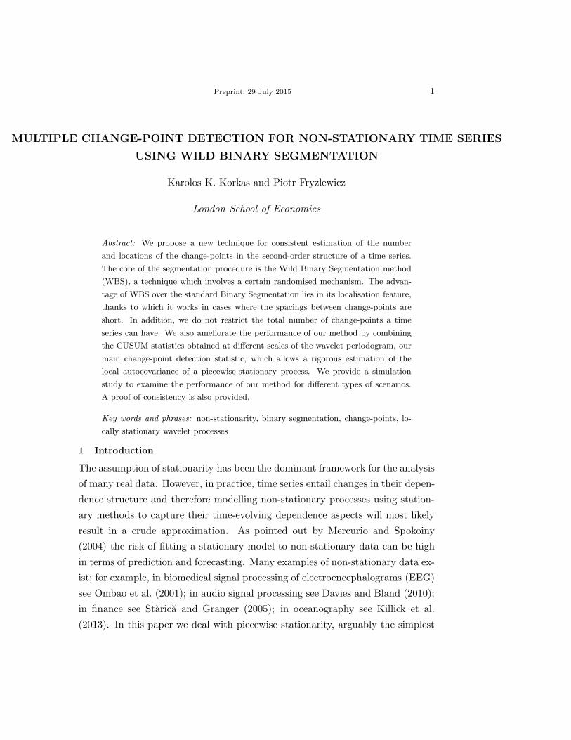
Fryzlewicz (2014) proposes a randomised binary segmentation (termed Wild

Binary Segmentation – WBS) where the search for change-points proceeds by

calculating the CUSUM statistic in smaller segments whose length is random. By

doing so, the user is guaranteed, with probability tending to one with the sample

size, to draw favourable intervals containing at most a single change-point, which

means the CUSUM statistic will be an appropriate one to use over those intervals

from the point of view of model choice. The maximum of the CUSUM statistics

in absolute value, taken over a large collection of random intervals (see Figure

1.1 for an illustration), is considered to be the first change-point candidate, and

is tested for significance. The binary segmentation procedure is not altered,

meaning that after identifying a change-point the problem is divided into two

sub-problems where for each segment we again test for further change-points

in exactly the same way. The computational complexity of the method can be

reduced by noticing that the randomly drawn intervals and their corresponding

CUSUM statistics can be calculated once at the start of the algorithm. Then, as

the algorithm proceeds at a generic segment [s, e], the obtained statistics can be

reused making sure the random starting and end points fall within [s, e].

The main steps of the WBS algorithm modified for the model (1.1) are

outlined below.

• Calculate the CUSUM statistics over a collection of random intervals [sm, em].

The starting and ending points are not fixed but are sampled from a uniform

distribution with replacement making sure that

em ≥ sm +∆T (1.3)

where ∆T > 0 defines the minimum size of the interval drawn.

Denote by Ms,e the set of indices m of all random intervals [sm, em] where

m = 1, ...,M such that [sm, em] ⊆ [s, e]; then the likely location of a change-


Time

y

0 100 200 300 400 500

−4

−2

02

Time

scal

e=−

1

0 100 200 300 400 500

05

1015

2025

Time

CU

SU

M

0 100 200 300 400 500

05

1015

2025

0 100 200 300 400 500

05

1015

2025

index

Col

lect

ion

of r

ando

m C

US

UM

Figure 1.1: A simulated series (top-left) of an AR(1) model yt = φtyt−1 + εt with φt = (0.5, 0.0)

and change-points at {50, 100, ...,450}. The Wavelet Periodogram at scale −1 (top-right). The CUSUM

statistic of scale −1 (bottom-left) as in the BS method; the red line is threshold C log(T ) with C chosen

arbitrarily (for comparative illustration only). The rescaled Ybsm,em

for m ∈ Ms,e and b ∈ sm, ..., em−1

(bottom-right) as in the WBS method; the red line is the same threshold.

point is

(m0, b0) = argmax(m∈Ms,e,b∈sm,...,em−1)

∣

∣

∣Y bsm,em/qsm,em

∣

∣

∣(1.4)

such that

max

(

em0− b0

em0− sm0

+ 1,b0 − sm0

+ 1

em0− sm0

+ 1

)

≤ c⋆ (1.5)

where c⋆ is a constant satisfying c⋆ ∈ [2/3, 1). The conditions (1.3) and

(1.5) do not appear in the original work by Fryzlewicz (2014), but they are

necessary from the point of view of both theory and practical performance

in the multiplicative model (1.1).

• The obtained CUSUM values are rescaled and tested against a threshold ωT .


This will ensure that with probability tending to one with the sample size,

only the significant change-points will survive. The choice of the threshold

ωT is discussed in Section 4. If the obtained CUSUM statistic is significant

then the search is continued to the left and to the right of b0; otherwise

the algorithm stops. This step differs from the original WBS method of

Fryzlewicz (2014) in that the CUSUM statistics are rescaled using qsm,em

so that ωT does not depend on σ2t,T .

Although from the theoretical point of view, sampling distributions other

than the uniform are also possible and lead to practically the same theoretical

results (as long as their probability mass functions, supported on [0, 1, . . . , T −1]

are uniformly of order T−1, as is apparent by examining formula (6.3)), the

uniform distribution plays a special role here as it provides a natural and fair

subsampling of the set of all possible sub-intervals of [s, e], which would be the

optimal set to consider were it not for the prohibitive computational time of such

an operation.

3 Locally Stationary Wavelets and the Multiplicative Model

In this section we introduce the reader to the LSW modelling paradigm of Nason

et al. (2000). The LSW process enables a time-scale decomposition of a process

and thus permits a rigorous estimation of the evolutionary wavelet spectrum and

the local autocovariance and can be seen as an alternative to the Fourier based

approach for modelling time series.

We now provide the definition of the LSW from Fryzlewicz and Nason (2006):

a triangular stochastic array {Xt,T }T−1t=0 for T = 1, 2, ..., is in a class of Locally

Stationary Wavelet (LSW) processes if there exists a mean-square representation

Xt,T =

−1∑

i=−∞

∞∑

k=−∞

Wi(k/T )ψi,t−kξi,k (1.6)

with i ∈ −1,−2, ... and k ∈ Z are, respectively, scale and location parameters,

(ψi,0, ..., ψi,L−1) are discrete, real-valued, compactly supported, non-decimated

wavelet vectors with support length L = O(2−i), and the ξi,k are zero-mean,

orthonormal, identically distributed random variables. In this set-up we replace

the Lipschitz-continuity constraint onWi(z) by the piecewise constant constraint,

which allows us to model a process whose second-order structure evolves in a


piecewise constant manner over time with a finite but unknown number of change-

points. Let Li be the total magnitude of change-points in W 2i (z), then the

functions Wi(z) satisfy

• ∑−1i=−∞W 2

i <∞ uniformly in z

• ∑−1i=−I 2

−iLi = O(log T ) where I = log2 T .

The simplest type of a wavelet system that can be used in formula (1.6) are

the Haar wavelets. Specifically,

ψi,k = 2i/2I0,...,2−j−1−1(k) − 2i/2I2−j−1,...,2−i−1(k)

for i = −1,−2, ..., k k ∈ Z where IA(k) is 1 if k ∈ A and 0 otherwise. Further,

small absolute values of the scale parameter i denote “fine” scales, while large

absolute values denote “coarser” scales. In fine scales the wavelet vectors are most

oscillatory and localised. By contrast, coarser scales have longer, less oscillatory

wavelet vectors. Throughout the paper, we only use Haar wavelets, noting that

the theoretical analysis using any other compactly supported wavelets would

not be straightforward due to the unavailability of a closed formula for their

coefficient values.

Throughout this paper, we assume that ξi,k are distributed as N(0, 1) even

though extensions to other cases are possible but technically challenging as they

would entail consideration of quadratic forms of correlated non-Gaussian vari-

ables.

Of main interest in the LSW set-up is the Evolutionary Wavelet Spectrum

(EWS) Si(z) = W 2i (z), i = −1,−2, ..., defined on the rescaled-time interval

z ∈ [0, 1]. The estimation of the EWS is done through the wavelet periodogram

(Nason et al. (2000)) and its definition is given below:

Definition: Let Xt,T be an LSW process constructed using the wavelet

system ψ. The triangular stochastic array

I(i)t,T =

∣

∣

∣

∣

∣

∑

s

Xs,Tψi,s−t

∣

∣

∣

∣

∣

2

(1.7)

is called the wavelet periodogram of Xt,T at scale i.

The wavelet periodogram is a convenient statistic for us to use, for the fol-

lowing reasons: (a) wavelet periodograms are fast to compute, (b) for Gaussian


processes Xt, they arise as χ21-type sequences which are easier to segment than,

for example, empirical autocovariance sequences of the type {XtXt+τ}t, (c) be-

cause wavelets “decorrelate” a wide range of time series dependence structures

and (d) because the expectations of wavelet periodograms encode, in a one-to-

one way, the entire autocovariance structure of a time series, so it suffices to

estimate change-points in those expectations in order to obtain segmentation of

the autocovariance structure of Xt, which is our ultimate goal.

We also recall two further definitions from Nason et al. (2000): the autocor-

relation wavelets Ψi(τ) =∑

k ψi,kψi,k−τ and the autocorrelation wavelet inner

product matrix Ai,k =∑

τ Ψi(τ)Ψk(τ). Fryzlewicz and Nason (2006) show that

EI(i)t,T is “close” (in the sense that the integrated squared bias converges to zero)

to the function βi(z) =∑−1

j=−∞ Sj(z)Ai,j , a piecewise constant function with at

most N change-points, whose set is denoted by N . Every change-point in the

autocovariance structure of the time series results in a change-point in at least

one of the βi(z); therefore, detecting a change-point in the wavelet periodogram

implies a change-point in the autocovariance structure of the process.

In addition, note that each wavelet periodogram ordinate is a squared wavelet

coefficient of a standard Gaussian time series and it satisfies

I(i)t,T = EI

(i)t,TZ

2t,T (1.8)

where {Zt,T }T−1t=0 are autocorrelated standard normal variables (or equivalently

the distribution of the squared wavelet coefficient I(i)t,T is that of a scaled χ2

1

variable). Then, the quantities I(i)t,T and EI

(i)t,T can be seen as special cases of Y 2

t,T

and σ2t,T respectively of the multiplicative model (1.1). To enable the application

of the model (1.8) in this context, we assume the following condition:

(A0): σ2t,T is deterministic and “close” to a piecewise constant function

σ2(t/T ) (apart from intervals around the discontinuities in σ2(t/T ) which have

length at most K2−i) in the sense that T−1∑T−1

t=0 |σ2t,T −σ2(t/T )|2 = o(log−1 T )

where the rate of convergence comes from the integrated squared bias between

βi(t/T ) and EI(i)t,T (see Fryzlewicz and Nason (2006)).


4 The Algorithm

In this section we present the WBS algorithm within the framework of the LSW

model. First, we form the following CUSUM-type statistic

Yb(i)sm,em =

√

em − b

n(b− sm + 1)

b∑

t=sm

I(i)t,T −

√

b− sm + 1

n(em − b)

em∑

t=b+1

I(i)t,T (3.1)

where the subscript (.)m denotes an element chosen randomly from the set

{0, ..., T − 1} as in (1.3), n = em − sm + 1 and I(i)t,T are the wavelet periodogram

ordinates at scale i that form the multiplicative model I(i)t,T = EI

(i)t,TZ

2t,T discussed

in Section 3. The likely location of a change-point b0 is then given by (1.4).

The following stages summarise the recursive procedure:

Stage I: Start with s = 1 and e = T .

Stage II: Examine whether hm0= |Yb0

sm0,em0

|/qsm0,em0

> ωT = C log(T )

where qsm0,em0

=∑em0

t=sm0I(i)t,T /nm0

, nm0= em0

− sm0+ 1 and m0, b0 as in

(1.4); C is a parameter that remains constant and only varies between scales.

Define h′m0= hm0

I(hm0> ωT ) where I(.) is 1 if the inequality is satisfied and 0

otherwise.

Stage III: If h′m0> 0, then add b0 to the set of estimated change-points;

otherwise if h′m0= 0 stop the algorithm.

Stage IV: Repeat stages II-III to each of the two segments (s, e) = (1, b0)

and (s, e) = (b0 + 1, T ) if their length is more than ∆T .

The choice of parameters C and ∆T is described in Section 4.4. We note

that in addition to the random intervals [sm, em] we also include into Ms,e the

index (labelled 0) corresponding to the interval [s, e]. This does not mean that the

WBS procedure “includes” the classical BS, as at the first stage the WBS and BS

are not guaranteed to locate the same change-point (even if WBS also examines

the full interval [s, e]), so the two procedures can “go their separate ways” after

examining the first full interval. The reason for manually including the full

interval [s, e] is that if there is at most one change-point in [s, e], considering the

entire interval [s, e] is an optimal thing to do.

Further, we expect that finer scales will be more useful in detecting the

number and locations of the change-points in EI(i)t,T . This is because as we move

to coarser scales the autocorrelation within I(i)t,T becomes stronger and the in-


tervals on which a wavelet periodogram sequence is not piecewise constant be-

come longer. Hence, we select the scale i < −I⋆ where I⋆ = ⌊α log log T ⌋ and

α ∈ (0, 3λ] for λ > 0 such that the consistency of our method is retained.

In stage II, we rescale the statistic hm0before we test it against the threshold.

This division plays the role of stabilising the variance, which is exact in the mul-

tiplicative model in which the observations are independent, over intervals where

the variance is constant. In all other cases, the variance stabilisation cannot be

guaranteed to be exact, but in the case where the process under consideration is

stationary over the given interval (i.e. there are no change-points), the cancella-

tion of the variance parameter still takes place and therefore the distribution of

the rescaled CUSUM is a function of the autocorrelation of the process, rather

than its entire autocovariance. This reduces the difficulty in choosing the thresh-

old parameter ωT and one can still hope to obtain “universal” thresholds which

work well over a wide range of dependence structures. Exact variance stabilisa-

tion in the non-independent case would require estimating what is referred to as

the “long-run variance” parameter (the variance of the sample mean of a time

series), which is a known difficult problem in time series analysis and if we were

to pursue it, the estimation error would likely not make it worthwhile. In other

words, we choose this rescaling method as a mid-way compromise between doing

nothing and having to estimate the long-run variance.

Finally, we notice that Horvath et al. (2008) propose a similar type of

CUSUM statistic which does not require an estimate of the variance of a stochas-

tic process by using the ratio of the maximum of two local means. The authors

apply the method to detect a single change-point in the mean of a stochastic

process under independent, correlated or heteroscedastic error settings.

4.1 Technical assumptions and consistency

In this section we present the consistency theorem for the WBS algorithm for the

total number N and locations of the change-points 0 < η1 < ... < ηN < T − 1

with η0 = 0 and ηN+1 = T . To achieve consistency, we impose the following

assumptions:

(A1): σ2(t/T ) is bounded from above and away from zero, i.e. 0 < σ2(t/T ) <

σ⋆ <∞ where σ⋆ ≤ maxt,T σ2(t/T ). Further, the number of change-points N in

(1.1) is unknown and allowed to increase with T i.e. only the minimum distance


between the change-points can restrict the maximum number of N .

(A2): {Zt,T }T−1t=0 is a sequence of standard Gaussian variables and the au-

tocorrelation function ρ(τ) = supt,T |cor(Zt,T , Zt+τ,T )| is absolutely summable,

that is it satisfies ρ1∞ <∞ where ρp∞ =∑

τ |ρ(τ)|p.(A3): The distance between any two adjacent change-points satisfies minr=1,...,N+1 |ηr−

ηr−1| ≥ δT , where δT ≥ C log2 T for a large enough C.

(A4): The magnitude of the change-points satisfy inf1≤r≤N |σ((ηr +1)/T )−σ(ηr/T )| ≥ σ⋆ where σ⋆ > 0.

(A5): ∆T ≍ δT where ∆T as defined in (1.3).

Theorem 1 Let Y 2t,T follow model (1.1), and suppose that Assumptions (A0)-

(A5) hold. Denote the number of change-points in σ2(t/T ) by N and the locations

of those change-points as η1, ..., ηN . Let N and η1, ..., ηN be the number and

locations of the change-points (in ascending order), respectively, estimated by the

Wild Binary Segmentation algorithm. There exist two constants C1 and C2 such

that if C1 log T ≤ ωT ≤ C2

√δT , then P (ZT ) → 1, where

ZT = {N = N ; maxr=1,...,N

|ηr − ηr| ≤ C log2 T}

for a certain C > 0, where the guaranteed speed of convergence of P (ZT ) to 1 is

no faster than Tδ−1T (1 − δ2T (1 − c)2T−2/9)M where M is the number of random

draws and c = 3− 2/c⋆.

For the purpose of comparison we note that the rate of convergence for the

estimated change-points obtained for the BS method by Cho and Fryzlewicz

(2015) is of order O(√T log(2+ϑ) T ) and O(log(2+ϑ) T ) for ϑ > 0 when δT is T 3/4

and T respectively. In the WBS setting, the rate is square logarithmic when

δT is of order log2 T , which represents an improvement. In addition, the lower

threshold is always of order log T regardless of the minimum space between the

change-points.

We now discuss the issue of the minimum numberM of random draws needed

to ensure that the bound on the speed of convergence of P (ZT ) to 1 in Theorem

1 is suitably small. Suppose that we wish to ensure

Tδ−1T (1− δ2T (1− c)2T−2/9)M ≤ T−1.

Bearing in mind that log(1− y) ≈ −y around y = 0, this is, after simple algebra,


(practically) equivalent to

M ≥ 9T 2

δ2T (1− c)2log(T 2δ−1

T ).

In the “easiest” case δT ∼ T , this results in a logarithmic number of draws, which

leads to particularly low computational complexity. Naturally, the required M

progressively increases as δT decreases. Our practical recommendations for the

choice of M are discussed in Section 4.4.

4.2 Simultaneous across-scale post-processing

Theorem 1 covers the case of the multiplicative model (1.1). We now consider

change-point detection in the full model (1.6). Recall from Section 3 that a

change-point in βi(z) for i = −1,−2, ...,−I⋆ would signal a change-point in the

second-order covariance structure of Xt,T . To accomplish this we propose two

methods.

Method 1: The search for further change-points in each interval (sm, em)

proceeds to the next scale i − 1 only if no change-points are detected at scale i

on that interval. It therefore ensures that the finest scales are preferred (since

change-points detected at the finest scales are likely to be more accurate) and only

moves to coarser if necessary. Cho and Fryzlewicz (2012) use a similar technique

to combine across scales change-points, but involving an extra parameter. The

role of this parameter is to create groups of estimated change-points which are

close to each other. Then, only one change-point (detected at the finest scale)

from each of these groups will survive the post-processing. Hence, their method

will be used as a benchmark for our first type of across-scale post-processing.

Method 2: Alternatively, we suggest a method that simultaneously joins

the estimated change-points across all the scales such that all the information

from every scale is combined. Namely, motivated by Cho and Fryzlewicz (2015)

who propose an alternative aggregation method to these of Groen et al. (2013) in

order to detect change-points in the second order structure of a high-dimensional

time series we define the following statistic

Ythrt =

−1∑

i=−I⋆

Y(i)t I(Y(i)

t > ω(i)T ) for i = −1, ...,−I⋆ (3.2)

where Y(i)t = |Yb(i)

sm,em|/q(i)sm,em |. This statistic differs from that of Cho and Fry-


zlewicz (2015) in that it applies across the scales i = −1,−2, ...,−I⋆ of a uni-

variate time series, whereas Cho and Fryzlewicz (2015) calculate their statistic

across multiple time series.

The algorithm is identical to the algorithm in Section 4 except for replacing

(3.1) with (3.2). In addition, if the obtained Ythrt > 0 there is no need to test

further for the significance of b0.

Below, we present the consistency theorem for the across-scale post-processing

algorithm:

Theorem 2 Let Xt follow model (1.6), and suppose that Assumptions (A0)-

(A5) for σ2(t/T ) hold for each βi(z). Denote the number of change-points in βi(z)

as N and the locations of those change-points as θ1, ..., θN . Let N and θ1, ..., θN be

the number and locations of the change-points (in ascending order), respectively,

estimated by the across-scale post-processing method 1 or 2. There exist two

constants C3 and C4 such that if C3 log T ≤ ωT ≤ C4δT , then P (UT ) → 1, where

UT = {N = N ; maxr=1,...,N

|θr − θr| ≤ C ′ log2 T}

for a certain C ′ > 0, where the guaranteed speed of convergence is the same as

in Theorem 1.

Even though the two Methods 1 and 2 achieve the same rate of conver-

gence for the estimated change-points, their relative performance is empirically

examined in Section 5.

4.3 Post-processing

In order to control the number of change-points estimated from the WBS algo-

rithm and to reduce the risk of over-segmentation we propose a post-processing

method similar to Cho and Fryzlewicz (2012) and Inclan and Tiao (1994). More

specifically, we compare every change-point against the adjacent ones using the

CUSUM statistic making sure that (1.5) is satisfied. That is, for a set N =

{θ0, ..., θN+1} where θ0 = 0 and θN+1 = T we test whether θr satisfies

Ythrt =

−1∑

i=−I⋆

Y(i)t I(Y(i)

t > ω(i)T ) > 0 for i = −1, ...,−I⋆


where Y(i)t = |Yθr(i)

θr−1,θr+1

|/q(i)θr−1,θr+1

| and

max

(

θr+1 − θr

θr+1 − θr−1 + 1,θr − θr−1 + 1

θr+1 − θr−1 + 1

)

≤ c⋆. (3.3)

If Ythrt = 0 then change-point θr is temporarily eliminated from set N . In

the next run, when considering change-point θr+1, the adjacent change-points

are θr−1 and θr+2. When the post-processing finishes its cycle all temporarily

eliminated change-points are reconsidered using as adjacent change-points those

that have survived the first cycle. It is necessary for θr to satisfy (3.3) with its

adjacent estimated change-points θr−1 and θr+1, otherwise it is never eliminated.

The algorithm is terminated when the set of change-points does not change.

The post-processing step does not involve any extra parameters since it only

uses those already mentioned in Section 4. In the next section we discuss the

choice of the parameters.

4.4 Choice of threshold and parameters

In this section we present the choices of the parameters involved in the algorithms.

From Theorems 1 and 2 we have that the threshold ωT includes the constant

C(i) which varies between the scales. The values of C(i) will be the same for

all the methods presented, either BS/WBS or the Methods 1 and 2 in Section

4.2. Therefore, we can use the thresholds by Cho and Fryzlewicz (2012) who

conduct experiments to establish the value of the threshold parameter under the

null hypothesis of no change-points such that when the obtained statistic exceeds

the threshold the null hypothesis is rejected. However, in that work the threshold

is of the form τ0Tϑ0√log T where ϑ0 ∈ (1/4, 1/2) and τ0 > 0 is the parameter

that changes across scales. For that reason, we repeat the experiments which are

described below.

We generate a vectorX ∼ N(0,Σ) where the covariance matrix Σ = (σκ,κ′)Tκ,κ′=1

and σκ,κ′ = ρ|κ−κ′|. Then we find v that maximises (3.1). The following ratio

C(i)T = Y

(i)v (log T )−1

(

T∑

t=1

I(i)t,T

)−1

T

gives us an insight into the magnitude of parameter C(i). We repeat the exper-

iment for different values of ρ and for every scale i we select C(i) as the 95%


quantile. The same values are used for the post-processing method explained in

Section 4.3. Our results indicate that C(i) tends to increase as we move to coarser

scales due to the increasing dependence in the wavelet periodogram sequences.

Since our method applies to non-dyadic structures it is reasonable to propose a

general rule that will apply in most cases. To accomplish this we repeated the

simulation study described above for T = 50, 100, ..., 6000. Then, for each scale

i we fitted the following regression

C(i) = c(i)0 + c

(i)1 T + c

(i)2

1

T+ c

(i)3 T 2 + ε.

The adjusted R2 was above 90% for all the scales. Having estimated the values

for c(i)0 , c

(i)1 , c

(i)2 , c

(i)3 we were able to use fitted values for any sample size T . For

samples larger than T = 6000 we used the same C(i) values as for T = 6000.

Further, based on empirical evidence (see the online supplementary material)

we select the scale I⋆ by setting λ = 0.7. In stage III of the algorithm, the

procedure is terminated when either the CUSUM statistic does not exceed a

certain threshold or the length of the respective segment is ∆T . This also defines

the minimum length of a favourable draw from (1.3). We choose ∆T to be of the

same order as δT since this is the lowest permissible order of magnitude according

to (A5). Practically, we find that the choice ∆T = ⌊log2 T/3⌋ works well. In

addition, a simulation study found in the online supplementary material provides

empirical arguments for the choice c⋆ = 0.75. The main idea of this parameter

is to ensure that long enough stretches of data are included in the computation

of our CUSUM statistics, or otherwise the computed CUSUM statistics will be

too variable to be reliable. This is particularly important in the autocorrelated

multiplicative setting where there tends to be a large amount of noise so the use

of such a parameter is needed to suppress the variance of the CUSUM statistics.

Finally, our recommendation for the parameter M is 3500 when T does not

exceed 10000. These values are used in the remainder of the paper.

5 Simulation study

We present a set of simulation studies to assess the performance of our methods.

In all the simulations we assume sample sizes to be 1024 over 100 iterations.

In the online supplementary material smaller and larger sample sizes are also

considered. For comparison we also report the performance of the method by


Table 4.1: Stationary processes results. For all the models the sample size is 1024 and

there are no change-points. Figures show the number of occasions the methods detected

change-points with the universal thresholds C(i) obtained as described in Section 4.4.

Figures in brackets are the number of occasions the methods detected change-points with

the thresholds C(i) obtained as described in Section 5.1.

Model BS1 WBS1 BS2 WBS2 CF

S1: iid standard normal 1 [0] 3 [2] 0 [0] 1 [0] 4

S2: AR(1) with parameter 0.9 3 [1] 5 [1] 1 [1] 5 [1] 9

S3: AR(1) with parameter −0.9 58 [0] 93 [0] 46 [0] 48 [5] 79

S4: MA(1) with parameter 0.8 2 [3] 7 [4] 3 [3] 1 [0] 7

S5: MA(1) with parameter −0.8 2 [0] 4 [2] 4 [0] 0 [0] 7

S6: ARMA(1,0,2) with AR= {−0.4} and MA= {−0.8, 0.4} 8 [0] 27 [0] 8 [0] 8 [0] 25

S7: AR(2) with parameters 1.39 and −0.96 88 [3] 99 [4] 88 [3] 88 [5] 96

Cho and Fryzlewicz (2012) – henceforth CF – using the default values specified

in their paper. BS1 and BS2 refer to the Method 1 and Method 2 of aggregation

(as described in Section 4.2) using the BS technique, respectively. WBS1 and

WBS2 refer to the Method 1 and Method 2 of aggregation (as in Section 4.2)

using the Wild Binary Segmentation technique, respectively. To briefly illustrate

computation times, our code, executed in pure R on a standard PC, runs in

approximately 25 seconds for a time series of length 10000 with 10 change-points.

5.1 Models with no change-points

We simulate stationary time series with innovations εt ∼ N(0, 1) and we report

the number of occasions (out of 100) the methods incorrectly rejected the null

hypothesis of no change-points. The models S1-S7 (Table 4.1) we consider here

are taken from Nason (2013).

The results of Table 4.1 indicate our methods’ good performance over that

of Cho and Fryzlewicz (2012) apart from models S3 and S7 where all methods

incorrectly reject the null hypothesis on many occasions. A visual inspection of

an AR(1) process with φ = −0.9 could confirm that this type of process exhibits

a “clustering behaviour” which mimics changing variance. Hence, the process is

interpreted as non-stationary by the wavelet periodogram resulting in erroneous

outcomes. A similar argument is valid for S7 model. To correct that limitation,

parameter C(i) should be chosen with care. Higher values will ensure that the

null hypothesis is not rejected frequently. This is achieved by not using universal


thresholds (as shown in Section 4.4) but calculating them for every instance.

Specifically, given a time series yt we fit an AR(p) model. Then we generate 100

instances of the same length and with the same AR(p) coefficients. Similarly

with Section 4.4 we select C(i) as the 95% quantile. This procedure is more

computationally intensive but improves the method significantly; see the figures

in brackets (Table 4.1). An alternative approach in obtaining thresholds, by

taking time-averages of spectrum values for each i = −1,−2, ...,−I⋆ and then

simulating stationary models, described in the online supplementary material,

does generally well but not as well as our suggestion above.

5.2 Non-stationary models

We now examine the performance of our method for a set of non-stationary

models by using and extending the examples from Cho and Fryzlewicz (2012).

Since the WBS method has improved rates of convergence new simulation results

are presented which assess how close to the real change-points the estimated ones

are. For this reason we report the total number of change-points identified within

⌊5% · T ⌋ from the real ones. Results for ⌊2.5% · T ⌋ distances are reported in the

online supplementary material.

The accuracy of a method should be also judged in parallel with the total

number of change-points identified. We propose a test that tries to accomplish

this. Assuming that we define the maximum distance from a real change-point

η as dmax, an estimated change-point η is correctly identified if |η − η| ≤ dmax

(here within 5% of the sample size). If two (or more) estimated change-points

are within this distance then only one change-point which is the closest to the

real change-point is classified as correct. The rest are deemed to be false, except

if any of these are close to another change-point. An estimator performs well

when the following hit ratio HR

HR =#correct change-points identified

max(N, N )

is close to 1. By using the term max(N, N) we aim to penalise cases where,

for example, the estimator correctly identifies a certain number of change-points

all within the distance dmax but N < N . It also penalises the estimator when

N > N and all N estimated change-points are within the distance dmax of the

true ones.


Finally, histograms of the estimated change-point locations for every model

can be found in the online supplementary material.

Model A: A non-stationary process that includes one AR(1) and two AR(2)

processes with two clearly observable change-points

yt =

0.9yt−1 + εt, εt ∼ N(0, 1) for 1 ≤ t ≤ 512

1.68yt−1 − 0.81yt−2 + εt, εt ∼ N(0, 1) for 513 ≤ t ≤ 768

1.32yt−1 − 0.81yt−2 + εt, εt ∼ N(0, 1) for 769 ≤ t ≤ 1024.

BS2 is the best option, marginally ahead of WBS1 and WBS2. The fact that

BS performs well here is unsurprising given the fact that the change-points are

far apart and prominent. However, it is reassuring to see the WBS methods also

performing well.

Model B: A non-stationary process with two less clearly observable change-

points

yt =

0.4yt−1 + εt, εt ∼ N(0, 1) for 1 ≤ t ≤ 400

−0.6yt−1 + εt, εt ∼ N(0, 1) for 401 ≤ t ≤ 612

0.5yt−1 + εt, εt ∼ N(0, 1) for 613 ≤ t ≤ 1024.

The WBS methods move into the lead, marginally ahead of the BS methods.

This is again not unexpected given the fact that the change-points here are less

prominent than in Model A.Model C: A non-stationary process with a short segment at the start

yt =

0.75yt−1 + εt, εt ∼ N(0, 1) for 1 ≤ t ≤ 50

−0.5yt−1 + εt, εt ∼ N(0, 1) for 51 ≤ t ≤ 1024.

In this type of model both BS2 and CF perform well compared to the BS1,

WBS1 and WBS2 methods. It is expected that binary segmentation methods

will perform better due to the fact that they start their search assuming a single

change-point.

Model D: A non-stationary process similar to model B but with the two

change-points at a short distance from each other. In this model, the two change-

points occur very close to each other i.e. (400, 470) instead of (400, 612). The

CF method, BS1 and BS2 do not perform well as the two change-points were


detected in less than half of the cases. By contrast, the WBS1 andWBS2 methods

achieved high hit ratio (almost double that of the BS methods).

Model E: A highly persistent non-stationary process with time-varying vari-

ance

yt =

1.399yt−1 − 0.4yt−2 + εt, εt ∼ N(0, 0.8) for 1 ≤ t ≤ 400

0.999yt−1 + ǫt, εt ∼ N(0, 1.22) for 401 ≤ t ≤ 750

0.699yt−1 + 0.3yt−1 + εt, εt ∼ N(0, 1) for 751 ≤ t ≤ 1024.

The CF and BS1 methods perform well since they detect most of the change-

points within 5% distance from the real ones. From our simulations we noticed

that in most cases the two change-points where found in the finest scale (i = −1).

The aggregation Method 2 does not improve the estimation since its purpose is to

simultaneously combine the information from different scales not just from a sin-

gle one. On the other hand, the CF method and Method 1 favour change-points

detected in the finest scales and this is the reason for their good performance.

Model F: A piecewise constant ARMA(1,1) process

yt =

0.7yt−1 + ǫt + 0.6εt−1, for 1 ≤ t ≤ 125

0.3yt−1 + ǫt + 0.3εt−1, for 126 ≤ t ≤ 532

0.9yt−1 + ǫt, for 533 ≤ t ≤ 704

0.1yt−1 + ǫt − 0.5εt−1, for 704 ≤ t ≤ 1024.

The first change-point is the least apparent and is left undetected in most cases

when applying the CF method. Our methods are capable of capturing this point

more frequently and within 5% from its real position.

Model G: A near-unit-root non-stationary process with time-varying vari-

ance

yt =

0.999yt−1 + εt, εt ∼ N(0, 1) for 1 ≤ t ≤ 200, 401 ≤ t ≤ 600 and 801 ≤ t ≤ 1024

0.999yt−1 + εt, εt ∼ N(0, 1.52) for 201 ≤ t ≤ 400 and 601 ≤ t ≤ 800.

In this near-unit-root process there are 4 change-points in its variance. All

binary segmentation methods do not perform well as they often miss the middle

change-points. Both WBS1 and WBS2 manage to detect most of the change-

points achieving a hit ratio almost three times higher than BS2. In almost 70%

of the occasions WBS2 detects at least 4 change-points.


Model H: A non-stationary process similar to model F but with the three

change-points at a short distance from each other. In this model the three change-

points occur close to each other, i.e. N = (125, 325, 550). The first two change-

points fail to be detected by the CF in many instances. By contrast, BS1 and BS2

do well while WBS1 and WBS2 perform slightly better in this case by identifying

them more often. This results in a higher hit ratio.

Model I: A non-stationary AR process with many changes within close dis-

tances. We simulate instances with 5 change-points occurring at uniformly dis-

tributed positions. We allow the distances to be as small as 30 and not larger

than 100.

In this scenario, CF correctly identifies more than 4 change-points in 15%

instances while BS1 and BS2 in 24% and 23% respectively. Again, the WBS

methods do well in revealing the majority of the change-points and in many

cases close to the real ones.

In summary, the WBS methods offer a reliable default choice. In terms of the

hit ratio, they perform the best or nearly the best in 7 of the 9 models studied,

and do not perform particularly poorly in the other 2 models, especially if the

total number of detected change-points is also taken into account. All of: BS1,

BS1 and CF perform poorly in at least 3 of the models. In terms of the hit ratio,

both BS methods are in or close to the lead only in 2 models. Overall, the WBS

methods seem to be clear winners here. Our recommendation to the user is to

try the WBS2 method first since overall it appears to be the most reliable one.

6 Applications

6.1 US Gross National Product series (GNP)

We obtain the GNP time series from the Federal Reserve Bank of St. Louis web

page (http://research.stlouisfed.org/fred2/series/GNP). The seasonally adjusted

and quarterly data is expressed in billions of dollars and spans from 1947:1 until

2013:1 but we only use the last 256 observations. In the left panel of Figure 5.2

one can see the logarithm of the GNP series. As in Shumway and Stoffer (2011),

we only examine the first difference of the logarithm of the GNP (also called

the growth rate) since there is an obvious linear trend. In the right panel of the

same figure, which illustrates the growth rate, it is visually clear that the series

exhibits less variability in the latter part. We are interested in finding whether

Table 4.2: Non-stationary processes results for T = 1024 (Models A - I). Table shows

the number of occasions a method detected the given number of change-points within a

distance of 5% from the real ones. Bold: the method with the highest hit ratio or within

10% from the highest.

Number of Change-points

Model A B C

BS1 BS2 WBS1 WBS2 CF BS1 BS2 WBS1 WBS2 CF BS1 BS2 WBS1 WBS2 CF

0 2 0 1 0 3 0 0 0 0 0 39 12 35 21 6

1 29 15 16 21 29 11 8 4 9 7 61 88 65 79 94

2 69 85 83 79 68 89 92 96 91 93 - - - - -

Hit ratio 0.768 0.850 0.817 0.808 0.712 0.928 0.921 0.966 0.928 0.865 0.580 0.860 0.600 0.746 0.853

Model D E F


0 36 52 12 11 48 6 12 8 11 1 2 0 0 0 1

1 58 14 9 11 12 40 42 59 53 40 18 6 5 3 7

2 6 34 79 78 40 54 46 33 36 59 32 32 22 24 45

3 - - - - - - - - - - 48 62 73 73 47

Hit ratio 0.428 0.403 0.835 0.835 0.436 0.712 0.649 0.610 0.611 0.743 0.744 0.847 0.890 0.894 0.765

Model G H I


0 58 60 9 11 39 0 0 2 2 0 0 2 1 0 0

1 11 11 13 6 20 40 33 23 16 29 39 33 8 8 39

2 20 21 20 20 30 38 37 38 40 57 16 15 8 7 27

3 6 5 15 22 5 22 30 37 42 14 23 27 20 18 25

4 5 3 43 41 6 - - - - - 14 11 22 18 3

5 - - - - - - - - - - 8 12 41 49 6

Hit ratio 0.222 0.200 0.671 0.686 0.297 0.605 0.654 0.693 0.732 0.603 0.472 0.496 0.745 0.779 0.419


Table 4.3: Non-stationary processes results for T = 1024 (Models A - I). Table shows

the percentage of occasions a method detected the given number of change-points. True

number of change-points is in bold.

Number of Change-points

Model A B C


0 0 0 0 0 0 0 0 0 0 0 34 9 6 4 2

1 5 0 0 1 0 0 0 0 0 1 59 86 78 84 81

2 59 77 65 70 65 78 81 79 80 70 7 5 11 8 16

≥ 3 36 23 35 30 35 22 19 21 20 29 0 0 5 4 1

Total 100 100 100 100 100 100 100 100 100 100 100 100 100 100 100

Model D E F


0 49 42 8 3 38 0 0 1 1 0 0 0 0 0 0

1 5 9 0 1 17 22 21 22 24 19 14 0 0 0 1

2 45 45 87 88 38 63 65 65 61 65 13 9 12 8 19

3 1 4 5 8 7 14 11 10 12 15 63 82 78 81 65

≥ 4 0 0 0 0 0 1 3 2 2 1 10 9 10 11 15

Total 100 100 100 100 100 100 100 100 100 100 100 100 100 100 100

Model G H I


0 59 59 7 4 38 0 0 0 0 0 0 0 0 0 0

1 7 8 3 2 16 24 20 13 16 12 33 30 8 1 22

2 23 21 17 22 32 32 24 30 22 51 9 6 2 2 28

3 1 2 4 2 3 41 50 48 55 30 22 23 10 11 24

4 9 10 62 66 11 3 6 7 6 7 12 18 14 13 11

≥ 5 1 0 7 4 0 0 0 2 1 0 24 23 66 73 15

Total 100 100 100 100 100 100 100 100 100 100 100 100 100 100 100

our method is capable of spotting this change and/or possibly others.

Applying our method i.e. BS2 and WBS2 (BS1 and WBS1 produced iden-

tical results) we find that BS2 detects two change-points η = {133, 222} while

the WBS2 detects three at positions {18, 131, 230}. For the sake of comparison,

CF detects two possible change-points i.e. η = {134, 234}. The acf graphs (not

shown here) confirm that there may be changes in the autocovariance structure

occurring at all of these estimated change-points.

Change-point 18 i.e. 1953(3) almost exactly coincides with a peak of the

GNP growth as decided by the Business Cycle Dating Committee of the National

Bureau of Economic Research where the official date is July 1953 (note that

cycles do not necessarily overlap with the quarterly publications of the GNP). In


Time

log(

GN

P)

0 50 150 250

67

89

TimeG

NP

gro

wth

0 50 150 250

−2

02

46

Figure 5.2: Natural logarithm of the GNP series (left) and its first difference (right). The black, green

and red vertical lines are the change-points as estimated by BS2, CF and WBS2 respectively.

addition, change-points 131, 133 and 134 lie within a cycle that peaks in January

1981 and has a trough in November 1982. This cycle corresponds to the start of

the Great Moderation (around 1980s), a period that experienced more efficient

monetary policy and shocks of small magnitude, see Clark (2009) and references

therein. Finally, we note that all three methods detected a change-point towards

the end of the series - 222, 230, 234 which are dated 2004(3), 2006(3) and 2007(3)

respectively. According to e.g. Clark (2009) the Great Moderation had reversed

and the decline was offset by negative growth rates due to the recent economic

recession.

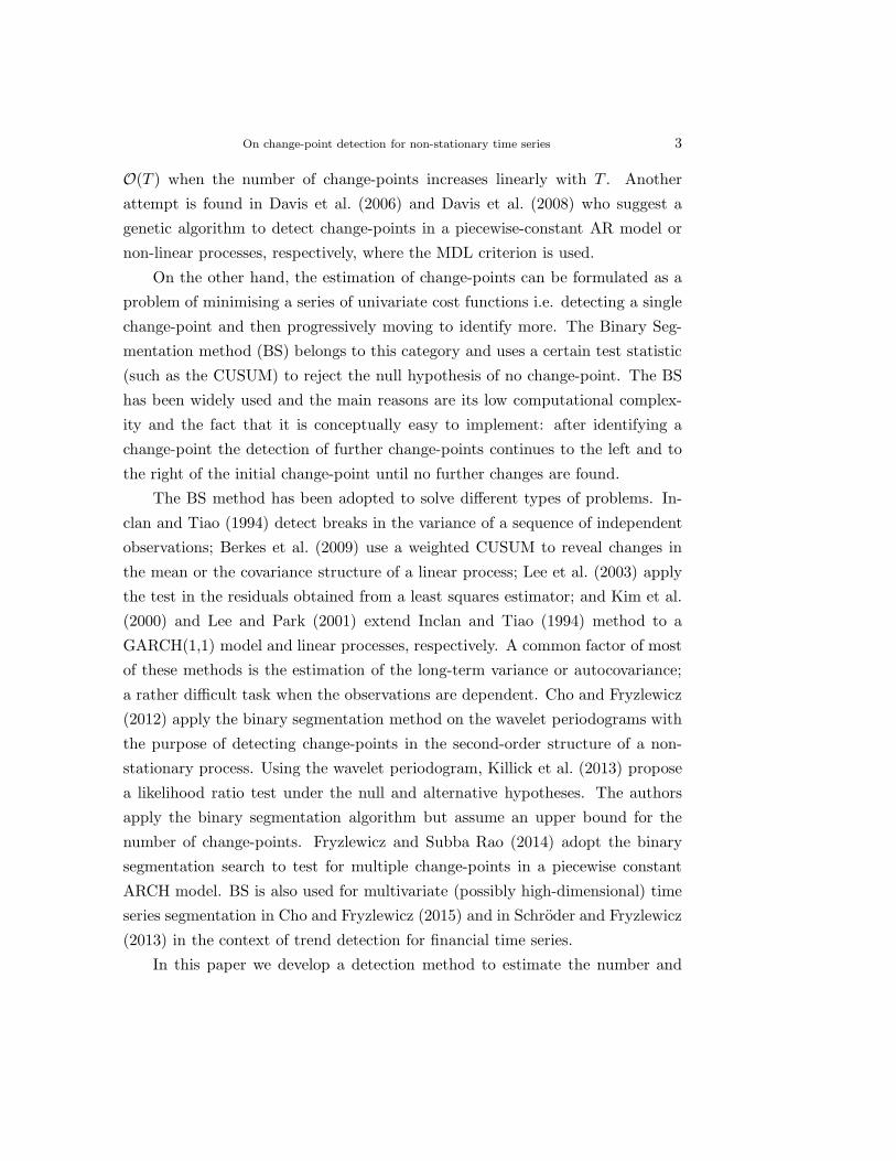
6.2 Infant Electrocardiogram Data (ECG)

We apply the three methods (CF, BS2, WBS2) to the ECG data of an infant

found at the R package wavethresh. This is a popular example of a non-stationary

time series and it has been analysed in e.g. Nason et al. (2000). The local

segments of possible stationarity indicate the sleep state of the infant and it is

classified on a scale from 1 to 4, see the caption of Figure 5.3. The same figure

plots the time series with the respective estimated change-points (the methods

were applied on the first difference so that its mean is approximately zero). All

methods identify most of the sleep states and, notably, WBS2 detects an abrupt

change of short duration (quiet sleep-awake-quiet sleep) towards the end of the


8010

014

018

0

Time

Bab

yEC

G

Figure 5.3: Plot of BabyECG data. The top blue, middle red and bottom purple vertical lines are the

change-points as estimated by CF, WBS2 and BS2 respectively. The horizontal dotted line represents

the sleep states i.e. 1 = quiet sleep, 2 = quiet-to-active sleep, 3 = active sleep, 4 =awake.

series.

7 Conclusion

The work in this paper has addressed the problem of detecting the change-points

in the autocovariance structure of a univariate time series. As discussed in the

Introduction, there are many types of non-stationary time series which require

segmentation methods. Using the WBS framework we are able to detect multiple

change-points that are small in magnitude and/or close to each other. The

simulation study in Section 5 indicates that the WBS mechanism leads to a

well-performing methodology for this task.

Appendix

Proof of Theorem 1

The proof of consistency is based on the following multiplicative model

Yt,T = σ(t/T )2Z2t,T , t = 0, ..., T − 1.

We define the following two CUSUM statistics

Ybs,e =

√

e− b

n(b− s+ 1)

b∑

t=s

Yt,T −√

b− s+ 1

n(e− b)

e∑

t=b+1

Yt,T


and

Sbs,e =

√

e− b

n(b− s+ 1)

b∑

t=s

σ2(t/T )−√

b− s+ 1

n(e− b)

e∑

t=b+1

σ2(t/T )

where n = e− s+ 1, the size of the segment defined by (s, e).

Ybs,e can be seen as the inner product between sequence {Yt,T }t=s,...,e and a

vector ψbs,e whose elements ψb

s,e,t are constant and positive for t ≤ b and constant

and negative for t > b such that they sum to zero and sum to one when squared.

Similarly for Sbs,e.

Let s, e satisfy ηp0 ≤ s < ηp0+1 < ... < ηp0+q < e ≤ ηp0+q+1 for 0 ≤ p0 ≤N − q. The inequality will hold at all stages of the algorithm until no undetected

change-points are remained. We impose at least one of the following conditions

s < ηp0+r′ − CδT < ηp0+r′ + CδT < e, for some 1 ≤ r′ ≤ q (6.1)

{(ηp0+1 − s) ∧ (s− ηp0)} ∨ {(ηp0+q+1 − e) ∧ (e− ηp0+q)} ≤ CǫT (6.2)

where ∧ and ∨ denote the minimum and maximum operators, respectively. These

inequalities will hold throughout the algorithm until no further change-points are

detected.

We define symmetric intervals ILr and IR

r around change-points such that

for every triplet {ηr−1, ηr, ηr+1}

ILr =

[

ηr −2

3δrmin, ηr −

1

3δrmin (1 + c)

]

and

IRr =

[

ηr +1

3δrmin (1 + c) , ηr +

2

3δrmin

]

for r = 1, ..., N + 1

where δrmin = min{ηr−ηr−1, ηr+1−ηr} and c = 3− 2c⋆

for c⋆ as in (1.5). We recall

that at every stage of the WBS algorithm M intervals (sm, em), m = 1, ...,M are

drawn from a discrete uniform distribution over the set {(s, e) : s < e, 0 ≤ s ≤T − 2, 1 ≤ e ≤ T − 1}.

We define the event DMT as

DMT = {∀r = 1, ..., N ∃ m = 1, ...,M (sm, em) ∈ IL

r × IRr }.


Also, note that

P ((DMT )c) ≤

N∑

r=1

M∏

m−1

(1− P ((sm, em) ∈ ILr × IR

r )) ≤T

δT(1− δ2T (1− c)2T−2/9)M .

(6.3)

On a generic interval satisfying (6.1) and (6.2) we consider

(m0, b) = arg max(m,t):m∈Ms,e,sm≤t≤em

|Y tsm,em| (6.4)

where Ms,e = {m : (sm, em) ⊆ (s, e), 1 ≤ m ≤M}.

Lemma 1

P

(

max(s,b,e)

∣

∣

∣Ybs,e − S

bs,e

∣

∣

∣ > λ1

)

→ 0 (6.5)

for

λ1 ≥ log T.

Proof: We start by studying the following event∣

∣

∣

∣

∣

e∑

t=s

ctσ(t/T )2(Z2

t,T − 1)

∣

∣

∣

∣

∣

>√nλ1

where ct =√

(e − b)/(b − s + 1) and ct =√

(b− s + 1)/(e − b) for t ≤ b and

b + 1 ≤ t respectively. From (1.5), we have that ct ≤ c⋆ ≡√

c⋆1−c⋆

< ∞. The

proof proceeds as in Cho and Fryzlewicz (2015) and we have that (6.5) is bounded

by

∑

(s,b,e)

2 exp

(

− nλ214c2⋆ maxz σ2(z)nρ2∞ + 2c⋆ maxz σ(z)

√nλ1ρ1∞

)

≤ 2T 3 exp(

−C ′1(c⋆−2) log2 T

)

which converges to 0 since n ≥ δT = O(log2 T ) and ρ1∞ <∞ from (A2).

Lemma 2 Assuming that (6.1) holds, then there exists C2 > 0 such that for

b satisfying |b − ηp0+r′ | = C2γT for some r′, we have |Sηp0+r′

sm0,em0

| ≥ |Sbsm0,em0

| +CγT δ

−1/2T ≥ |Sbsm0

,em0|+ 2λ1, where γT =

√δTλ1.

Proof: From the proof of Theorem 3.2 in Fryzlewicz (2014) and Lemma 1 in

Cho and Fryzlewicz (2012) we have the following result

|Sbsm0,em0

| ≥ |Ybsm0

,em0| − λ1 ≥ C3

√

δT (6.6)


provided that δT ≥ C4λ21.

By Lemma 2.2 in Venkatraman (1992) there exists a change-point ηp0+r′

immediately to the left or right of b such that

|Sηp0+r′

sm0,em0

| > |Sbsm0,em0

| ≥ C3

√

δT .

Now, the following three cases are not possible:

1. (sm0, em0

) contains a single change-point, ηp0+r′ , and both ηp0+r′ − sm0and

em0− ηp0+r′ are not bounded from below by c1δT .

2. (sm0, em0

) contains a single change-point, ηp0+r′ , and either ηp0+r′ − sm0or

em0− ηp0+r′ are not bounded from below by c1δT .

3. (sm0, em0

) contains two change-points, ηp0+r′ and ηp0+r′+1, and both ηp0+r′−sm0

and em0− ηp0+r′+1 are not bounded from below by c1δT .

The first case is not permitted by (A5). For the last two, if either case

were true, then following the arguments as in Lemma A.5 of Fryzlewicz (2014),

we would obtain that maxt:sm0≤t≤em0

|Stsm0,em0

| was not bounded from below by

C3

√δT which contradicted (6.6). Hence, interval (sm0

, em0) satisfies condition

(6.1) and following a similar argument to the proof of Lemma 2 in Cho and

Fryzlewicz (2012) we can show that for any b satisfying |b − ηp0+r′ | = C2γT , we

have |Sηp0+r′

sm0,em0

| ≥ |Sbsm0,em0

|+ CγT δ−1/2T .

Lemma 3 Under conditions (6.1) and (6.2) there exists 1 ≤ r′ ≤ q such that

|b − ηp0+r′ | ≤ ǫT , where b is given in (6.4) and ǫT = C log2 T for a positive

constant C.

Proof: First, we mention that the model (1.1) can be written as Yt,T = σ(t/T )2+

σ(t/T )2(Z2t,T − 1) which has the form of a signal+noise model i.e. Yt = ft +

εt. Now, let fdsm0,em0

define the best function approximation to ft such that

argmaxd |〈ψdsm0

,em0, f〉| = argmind

∑em0

t=sm0(ft − fdsm0

,em0) where fdsm0

,em0= f +

〈f, ψdsm0

,em0〉ψd

sm0,em0

, f is the mean of f and ψdsm0

,em0is a set of vectors that are

constant and positive until d and then constant and negative from d + 1 until

em0.


If it can be shown that for a certain ǫT < C2γT , we have

em0∑

t=sm0

(Yt − Y dsm0

,em0,t)

2 >

em0∑

t=sm0

(Yt − fηp0+r′

sm0,em0

,t)2 (6.7)

as long as

ǫT ≤ |d− ηp0+r′ |

then this would prove necessarily that |b− ηp0+r′ | ≤ ǫT .

By Lemma 2 and Lemma A.3 in Fryzlewicz (2014), we have the same triplet

of inequalities as in the argument in the proof of Theorem 3.2 in Fryzlewicz

(2014) i.e.

|d− ηp0+r′ | ≥ C(λ2|d− ηp0+r′ |δ−1/2T ) ∨ (λ2|d− ηp0+r′ |−1/2) ∨ (λ22). (6.8)

Hence, with the requirement that |d− ηp0+r′ | ≤ C2γT = C2λ1√δT we obtain

δT > C2λ22 max(C2C−22 λ−2

1 λ22, 1)

and ǫT = max(1, C2)λ22. From Lemma 1 λ1 is of order O(log T ). For λ2, which

appears in the following two terms of the decomposition of (6.7)

I =1

d− sm0+ 1

d∑

t=sm0

εt

2

and II =1

em0− d+ 1

( em0∑

t=d+1

εt

)2

we show below that with probability tending to 1, I ≤ λ22 = log2 T . From Lemma

1 we have that ct = 1 for t = sm0, ..., d and thus

P

1√

d− sm0+ 1

∣

∣

∣

∣

∣

∣

d∑

t=sm0

εt

∣

∣

∣

∣

∣

∣

> λ2

→ 0

since by the Bernstein inequality the probability is bounded by

2T 2 exp

(

− (d− sm0+ 1)λ22

4maxz σ2(z)(d − sm0+ 1)ρ2∞ + 2c′ maxz σ(z)

√

d− sm0+ 1λ2ρ1∞

)

≤ 2T 2 exp(

−C ′3λ

22

)

which converges to 0 due to (d− sm0+ 1) = O(δT ) from (1.5). Note that II has

similar order and we omit the details. This concludes the lemma.


Lemma 4 Under conditions (6.1) and (6.2)

P

(

|Ybsm0

,em0| > ωT

∑em0

t=sm0Yt

nm0

)

→ 1

where b is given in (6.4).

Proof: We define the following two eventsA ={

|Ybsm0

,em0| < ωT

1nm0

∑em0

t=sm0Yt,T

}

and B ={

1nm0

∣

∣

∣

∑em0

t=sm0Yt,T −∑em0

t=sm0σ(t/T )2

∣

∣

∣ < σ = 12nm0

∑em0

t=sm0σ2(t/T )

}

.

Since P (A) ≤ P (A ∩ B) + P (Bc) we need to show that P (B) → 1 and

P (A ∩ B) → 0. To show that P (B) = P(

1nm0

∑em0

t=sm0Yt,T ∈ (σ/2, 3σ/2)

)

→ 1

we apply the Bernstein inequality as in Lemma 1 and we have that

P (B′) = P

1

nm0

∣

∣

∣

∣

∣

∣

em0∑

t=sm0

Yt,T −em0∑

t=sm0

σ(t/T )2

∣

∣

∣

∣

∣

∣

> σ

= P

∣

∣

∣

∣

∣

∣

em0∑

t=sm0

σ(t/T )2(Z2t,T − 1)

∣

∣

∣

∣

∣

∣

> nm0σ

.

Hence,

P (B′) ≤ 2 exp

(

− n2m0σ2

4maxz σ2(z)nm0ρ2∞ + 2c′ maxz σ(z)nm0

σρ1∞

)

≤ 2T 2 exp(

−C ′4 log

2 T)

which converges to 0 since nm0≥ δT = O(log2 T ) and ρ1∞ <∞ from (A2).

Now, from Lemma (3), we have some η ≡ ηp0+r′ satisfying |b − η| ≤ CǫT .

Turning to P (A ∩ B) we have from conditions (6.1) and (6.2)

|Ybsm0

,em0| ≥ |Yη

sm0,em0

| ≥ |Sηsm0,em0

| − log T

=

∣

∣

∣

∣

∣

√

(η − sm0+ 1)(em0

− η)

nm0

(

σ( η

T

)2− σ

(

η + 1

T

)2)∣

∣

∣

∣

∣

− log T

=

√

em0− η

nm0(η − sm0

+ 1)(η − sm0

+ 1)σ⋆ − log T ≥ C√

δT − log T > ωT 3σ/2,

which concludes the Lemma.

Lemma 5 For some positive constants C, C ′, let s, e satisfy either

• ∃1 ≤ p ≤ N such that s ≤ ηp ≤ e and (ηp − s+ 1) ∧ (e− ηp) ≤ CǫT or

• ∃1 ≤ p ≤ N such that s ≤ ηp+1 ≤ e and (ηp − s+ 1) ∨ (e− ηp+1) ≤ C ′ǫT .


Then,

P

(

|Ybsm0

,em0| < ωT

∑em0

t=sm0Yt

nm0

)

→ 1

where b is given in (6.4).

Proof: A similar argument to the proof of Lemma 5 is applied here. We only need

to show that P (A∩B) → 0 where now eventA ={

|Ysm0,b,em0

| > ωT1

nm0

∑em0

t=sm0Yt,T

}

.

Using condition (i) or (ii) we have that

|Ybsm0

,em0| ≤ |Sbsm0

,em0|+ log T

=

∣

∣

∣

∣

∣

√

b− sm0+ 1√

em0− b

√nm0

(

σ2(b/T )− σ2((b+ 1)/T ))

∣

∣

∣

∣

∣

+ log T

≤ σ∗C√ǫT + log T < ωT σ/2.

The proof of Theorem 1 proceeds as follows: at the start of the algorithm

when s = 0 and e = T − 1 all the conditions of (6.1) & (6.2) required by Lemma

4 are met and thus it detects a change-point on that interval defined by formula

(6.4) within the distance of CǫT (by Lemma 3). The conditions of Lemma 4

are satisfied until all change-points have been identified. Then, every random

interval (sm, em) does not contain a change-point or the conditions of Lemma 5

are met; hence no more change-points are detected and the algorithm stops.

Finally, we examine whether the bias present in EI(i)t,T (see condition (A0))

will affect the above result. We define Sts,e similarly to S

ts,e by replacing σ(t/T )2

with σ2t,T . Assume that ηr is a change-point within the interval [sm0, em0

] and

b = argmaxt∈(sm0,em0

) |Sbsm0,em0

| and b = argmaxt∈(sm0,em0

) |Sbsm0,em0

|. Recall

that EI(i)t,T is constant within each segment apart from short intervals around

true change-point ηr i.e. [ηr −K2−i, ηr +K2−i]. In addition, from Theorem 2 in

Cho and Fryzlewicz (2015) the finest scale should satisfy i ≥ I⋆ = −⌊α log log T ⌋in order for (A4) to hold. Then, |b−b| ≤ K2I

⋆

< ǫT holds since I⋆ = O(log log T ).

Therefore, bias does not affect the above result and the consistency is preserved.

Proof of Theorem 2

We start by the first method of aggregation. From the invertibility of the

autocorrelation wavelet inner product matrix A, there exists at least one ordinate

of wavelet periodogram in which a change-point θr is detected. From Theorem


1 it holds that |θr − θr| ≤ CǫT with probability converging to 1 regardless of

the scale i. Since the algorithm begins its search from the finest scale and only

proceeds to the next one if no change-point is detected (until scale I⋆) then

consistency is preserved.

We now turn to the second method of aggregation. We note that Ythrt has the

same functional form with each of Y(i)t i.e. h(i)(x) = (x(1− x))−1/2(c

(i)x x+ d

(i)x x)

for x = (t−sm+1)/n ∈ (0, 1), where c(i)x , d

(i)x are determined by the location and

the magnitude of the change-points of I(i)t,T . Let b = argmaxsm0

<t<em0Ythrt ; then

following a similar argument to Lemma 2 of Fryzlewicz (2014) we can show that

Ythrt must have a local maximum at t = θp0+r′ and that |b−θp0+r′ | ≤ C5γT . With

this result, we can show that |b− θp0+r| ≤ C ′ǫT for some 1 ≤ r′ ≤ q as in Lemma

3 above by constructing a signal+noise model yt = ft + εt and substituting ft

with∑−1

i=−I⋆ EI(i)t,T I(Y

(i)t > ω

(i)T )/q

(i)sm,em. Then, conditions (6.1) and (6.2) are

satisfied within each segment for at least one scale i ∈ {−1, ...,−I⋆}. When all

change-points have been detected every subsequent random interval (sm, em) will

satisfy the conditions of Lemma 5 for every i ∈ {−1, ...,−I⋆} and the algorithm

stops.

References

I. Auger and C. Lawrence. Algorithms for the optimal identification of segment neighborhoods.Bulletin of Mathematical Biology, 51:39–54, 1989.

R. Bellman and S. Dreyfus. Applied Dynamic Programming, volume 2. Princeton UniversityPress, 1966.

I. Berkes, E. Gombay, and L. Horvath. Testing for changes in the covariance structure of linearprocesses. Journal of Statistical Planning and Inference, 139:2044–2063, 2009.

H. Cho and P. Fryzlewicz. Multiscale and multilevel technique for consistent segmentation ofnonstationary time series. Statistica Sinica, 22:207–229, 2012.

H. Cho and P. Fryzlewicz. Multiple change-point detection for high-dimensional time seriesvia Sparsified Binary Segmentation. Journal of the Royal Statistical Society Series B, 77:475–507, 2015.

T. Clark. Is the great moderation over? An empirical analysis. Federal Reserve Bank of KansasCity Economic Review, 94:5–42, 2009.

S. Davies and D. Bland. Interestingness detection in sports audio broadcasts. In MachineLearning and Applications (ICMLA), 2010 Ninth International Conference on, pages 643–648. IEEE, 2010.

R. Davis, D. Huang, and Y. Yao. Testing for a change in the parameter values and order of anautoregressive model. The Annals of Statistics, 23:282–304, 1995.

R. Davis, T. Lee, and G. Rodriguez-Yam. Structural break estimation for nonstationary timeseries models. Journal of the American Statistical Association, 101:223–239, 2006.


R. Davis, T. Lee, and G. Rodriguez-Yam. Break detection for a class of nonlinear time seriesmodels. Journal of Time Series Analysis, 29:834–867, 2008.

P. Fryzlewicz. Wild binary segmentation for multiple change-point detection. The Annals ofStatistics, 42:2243–2281, 2014.

P. Fryzlewicz and G. Nason. Haar–Fisz estimation of evolutionary wavelet spectra. Journal ofthe Royal Statistical Society: Series B, 68:611–634, 2006.

P. Fryzlewicz and S. Subba Rao. Multiple-change-point detection for auto-regressive conditionalheteroscedastic processes. Journal of the Royal Statistical Society: Series B, 76:903–924, 2014.

E. Gombay. Change detection in autoregressive time series. Journal of Multivariate Analysis,99:451–464, 2008.

E. Gombay and D. Serban. Monitoring parameter change in time series models. Journal ofMultivariate Analysis, 100:715–725, 2009.

J. Groen, G. Kapetanios, and S. Price. Multivariate methods for monitoring structural change.Journal of Applied Econometrics, 28:250–274, 2013.

L. Horvath, Z. Horvath, and M. Huskova. Ratio tests for change point detection. Inst. Math.Stat. Collections, 1:293–304, 2008.

C. Inclan and G. Tiao. Use of cumulative sums of squares for retrospective detection of changesof variance. Journal of the American Statistical Association, 89:913–923, 1994.

B. Jackson, J. Scargle, D. Barnes, S. Arabhi, A. Alt, P. Gioumousis, E. Gwin, P. Sang-trakulcharoen, L. Tan, and T. Tsai. An algorithm for optimal partitioning of data on aninterval. Signal Processing Letters, IEEE, 12:105–108, 2005.

S. Kay. Fundamentals of Statistical Signal Srocessing, Volume 2: Detection Theory. PrenticeHall PTR, 1998.

R. Killick, P. Fearnhead, and I. Eckley. Optimal detection of changepoints with a linear com-putational cost. Journal of the American Statistical Association, 107:1590–1598, 2012.

R. Killick, I. Eckley, and P. Jonathan. A wavelet-based approach for detecting changes insecond order structure within nonstationary time series. Electronic Journal of Statistics, 7:1167–1183, 2013.

S. Kim, S. Cho, and S. Lee. On the cusum test for parameter changes in GARCH(1, 1) models.Communications in Statistics-Theory and Methods, 29:445–462, 2000.

M. Lavielle and E. Moulines. Least-squares estimation of an unknown number of shifts in atime series. Journal of time series analysis, 21:33–59, 2000.

M. Lavielle and G. Teyssiere. Detection of multiple change-points in multivariate time series.Lithuanian Mathematical Journal, 46:287–306, 2006.

M. Lavielle and G. Teyssiere. Adaptive detection of multiple change-points in asset price volatil-ity. Long Memory in Economics, pages 129–156, 2007.

S. Lee and S. Park. The cusum of squares test for scale changes in infinite order moving averageprocesses. Scandinavian Journal of Statistics, 28:625–644, 2001.

S. Lee, O. Na, and S. Na. On the cusum of squares test for variance change in nonstationaryand nonparametric time series models. Annals of the Institute of Statistical Mathematics, 55:467–485, 2003.

D. Mercurio and V. Spokoiny. Statistical inference for time-inhomogeneous volatility models.Annals of Statistics, 32:577–602, 2004.


G. Nason. A test for second-order stationarity and approximate confidence intervals for localizedautocovariances for locally stationary time series. Journal of the Royal Statistical Society:Series B, 75:879–904, 2013.

G. Nason, R. Von Sachs, and G. Kroisandt. Wavelet processes and adaptive estimation of theevolutionary wavelet spectrum. Journal of the Royal Statistical Society: Series B, 62:271–292,2000.

A. Olshen, E. Venkatraman, R. Lucito, and M. Wigler. Circular binary segmentation for theanalysis of array-based DNA copy number data. Biostatistics, 5:557–572, 2004.

H. Ombao, J. Raz, R. von Sachs, and B. Malow. Automatic statistical analysis of bivariatenonstationary time series. Journal of the American Statistical Association, 96:543–560, 2001.

P. Perron. Dealing with structural breaks. Palgrave Handbook of Econometrics, 1:278–352,2006.

A. Schroder and P. Fryzlewicz. Adaptive trend estimation in financial time series via multiscalechange-point-induced basis recovery. Statistics and Its Interface, 6:449–461, 2013.

A. Sen and M. Srivastava. On tests for detecting change in mean. The Annals of Statistics, 3:98–108, 1975.

R. Shumway and D. Stoffer. Time Series Analysis and Its Applications: with R Examples.Springer, 2011.

C. Starica and C. Granger. Nonstationarities in stock returns. Review of economics and statis-tics, 87:503–522, 2005.

E. Venkatraman. Consistency results in multiple change-point problems. PhD thesis, Departmentof Statistics. Stanford University, 1992.

L. Vostrikova. Detecting disorder in multidimensional random processes. Soviet MathematicsDoklady, 24:55–59, 1981.

Y. Yao. Estimating the number of change-points via Schwarz’ criterion. Statistics & ProbabilityLetters, 6:181–189, 1988.

Y. Yao and S. Au. Least-squares estimation of a step function. Sankhya: The Indian Journalof Statistics, Series A, 51:370–381, 1989.

Department of Statistics, London School of Economics, Columbia House, LSE, Houghton Street,London, WC2A 2AE, UKE-mail: [email protected] of Statistics, London School of Economics, Columbia House, LSE, Houghton Street,London, WC2A 2AE, UKE-mail: [email protected]

MULTIPLE CHANGE-POINT DETECTION FOR NON-STATIONARY TIME SERIES USING WILD BINARY SEGMENTATION

Documents

Transcript of MULTIPLE CHANGE-POINT DETECTION FOR NON-STATIONARY TIME SERIES USING WILD BINARY SEGMENTATION