multiple and joint purchases - INGELA ALGER

736 Copyright q 1999, RAND

RAND Journal of EconomicsVol. 30, No. 4, Winter 1999pp. 736–757

Consumer strategies limiting themonopolist’s power: multiple and jointpurchases

Ingela Alger*

I characterize the menu of bundles (price-quantity combinations) offered by a monop-olist when consumers can buy several bundles, share bundles with others, or do both,in a two-type setting. I find that although perfect arbitrage prevents any price discrim-ination, partial arbitrage in the form of multiple or joint purchases may actually leadto more pronounced price discrimination than when consumers can only pick one singlebundle. Further, clear predictions emerge for the price pattern, contrasting with theexisting literature: with multiple purchases only, the firm offers strict quantity dis-counts; with joint purchases only, discounts are infeasible.

1. Introductionn Firms often market their goods by offering a menu of choices: consumers maychoose between goods with different quality, or between packages containing differentquantities of the same good. It allows the firm to price discriminate when demand isheterogeneous, but any individual consumer’s demand is not observable. This practice,known as second-degree price discrimination, has been studied extensively in the lit-erature (see, for instance, Mussa and Rosen, 1978; Maskin and Riley, 1984; and Wilson,1992). Surprisingly, however, no model unambiguously predicts such a common phe-nomenon as quantity discounts, which always come at the price of restrictions on theparameters. The analysis in this article reveals that this shortcoming is due to theincomplete modelling of consumer behavior.

An assumption invariably found in previous articles is that consumers may onlypick one single item, or bundle, from the menu offered by the firm. In reality, consum-ers often have access to other forms of arbitrage: for many goods, they can buy severalbundles from the menu, share a bundle with other consumers, or do both. This articlecharacterizes the price schedule that maximizes a monopolist’s expected profit when

* Boston College; [email protected] article is based on a chapter of my Ph.D. thesis submitted to the Universite des Sciences Sociales

de Toulouse. I am grateful to Jean-Jacques Laffont for guidance, and to Guillermo Alger, Thomas Mariotti,Nour Meddahi, Patrick Rey, Francois Salanie, Susanna Sallstrom, Jean Tirole, Dimitri Vayanos, WilfriedZantman, and seminar participants at the London School of Economics and the University of Virginia foruseful comments. I am particularly indebted to Regis Renault for many valuable discussions. I also thankEditor Glenn Ellison and two anonymous referees for detailed and helpful comments. Financial support fromThe Royal Swedish Academy of Sciences (C C Soderstroms fond), the Swedish Institute, and the SixtenGemzeus foundation is thankfully acknowledged.

ALGER / 737

q RAND 1999.

consumers have access to multiple and/or joint purchases, in a two-type setting. Thepredictions are clear: when only multiple purchases are possible, as for consumer goods,the firm offers strict quantity discounts; when only joint purchases are relevant, as forlarge consumer durables sold in units of different qualities, the good is sold with aquality premium or at a linear price; finally, when both joint and multiple purchasesare relevant, as for clothes, neither quantity discounts nor premia are feasible.1

Although very satisfying, the strict quantity discount result is surprising: indeed,the common belief is that multiple purchases only make quantity premia infeasible.Other conjectures that have been put forward in the literature, and that the model allowsus to analyze, include the following. Wilson makes the conjecture that quantity dis-counts should be sufficient to deter multiple purchases, as shown in the followingexcerpt from his book (1992, p. 71): ‘‘[subadditivity, which] means that the charge forseveral small purchases is no less than the charge for the purchase that is the sum ofthe smaller amounts, . . . prevents a customer (or arbitrageur) from circumventing thetariff by dividing a large purchase into several smaller ones.’’ In spite of its intuitiveappeal, the belief that quantity discounts should be sufficient to deter multiple purchasesproves to be wrong, as will be seen shortly. Finally, the absence of multiple and jointpurchases is generally seen as a necessary condition for the firm to be able to pricediscriminate. This is partially confirmed: indeed, unless consumers have access to bothmultiple and joint purchases, nonlinear pricing is feasible.

As a benchmark, I first analyze the classic single-bundle model. At the solutionthe high-valuation consumer is offered the socially optimal quantity and obtains a rent,whereas the low-valuation consumer obtains no rent and consumes a suboptimal quan-tity. As mentioned above, a feature of the single-bundle solution is that it may yieldeither quantity discounts or quantity premia, depending on the parameter values.

As expected, the single-bundle solution is not robust to multiple and/or joint pur-chases. Surprisingly, however, quantity discounts are not sufficient to prevent multiplepurchases in the two-type setting. The key to understanding this is that through multiplepurchases, the high-valuation consumer is not restricted to ‘‘dividing a large purchaseinto several smaller ones’’ as Wilson suggests—he can also choose to consume moreor less than if he chose the bundle meant for him. Thus consumers do not arbitrageonly to get a lower price, but also to influence the quantity they consume. This is aconsequence of the firm offering price-quantity combinations, as opposed to setting theprice and letting the consumers choose the quantity; indeed, this enables the firm tooffer bundles that are above the demand curve. In other words, the average unit pricepaid by a consumer exceeds his marginal utility; given that price, he would thereforeconsume less. With multiple purchases, the high-valuation consumer may consume lessby buying several small bundles; this may give him a higher utility than buying thelarge bundle, even if he ends up paying a slightly higher unit price.

Next, I characterize the profit-maximizing price schedule when consumers maymake multiple and joint purchases, analyzing each type of arbitrage separately. To avoidinteger problems, I model multiple purchases as the possibility to purchase any realnumber above one of any bundle. Conversely, joint purchases are modelled as theability to buy any real number between zero and one of any bundle.

When consumers can make multiple purchases only, the price schedule turns outto be qualitatively similar to the schedule in the single-bundle model: only the high-valuation consumer obtains a rent, and the quantity sold to the low-valuation consumer

1 As these predictions indicate, the quantity and quality interpretations of the model do not apply equallywell to the various settings I consider. When developing the general ideas below, for simplicity I refer onlyto the quantity interpretation.

738 / THE RAND JOURNAL OF ECONOMICS

q RAND 1999.

is distorted downward compared to the socially efficient level. This similarity is relatedto the intuition developed above: in both the single-bundle and the multiple-purchasecases, only the high-valuation consumer may consume less than the bundle meant forhim through arbitrage: in one case by buying the small bundle, in the other by buyingseveral small bundles. Therefore, only the high-valuation consumer obtains a rent. Andas in the single-bundle case, to limit this rent the monopolist distorts the quantityoffered to the low-valuation consumer downward compared to the socially optimallevel. The quantity may, however, be more or less distorted than in the single-bundlemodel. When it is less distorted, total welfare and the high-valuation consumer’s utilityis higher. In contrast, when the distortion is larger, total welfare is smaller, and thehigh-valuation consumer’s utility may in fact be lower than in the single-bundle model.But the firm’s expected profit is always smaller.

A striking result is that the amount of discrimination, measured by the differencein the unit price in the small and large bundles, may be higher than in the single-bundle model. This is at first sight counterintuitive: intuition would suggest that betterconsumer arbitrage reduces the firm’s ability to price discriminate. Nevertheless, theresult is quite natural: given that quantity discounts are not sufficient to prevent multiplepurchases, it follows that a way to prevent them is to further increase the discount.

Finally, I confirm that quantity premia are not feasible when consumers can makemultiple purchases. Surprisingly, however, strict quantity discounts are always optimal.It is surprising because the following argument seems natural: if it is optimal for thefirm to impose a quantity premium at the single-bundle solution, then the infeasibilityof quantity premia through multiple purchases should imply that the firm offers a linearprice scheme, i.e., both types of consumers pay the same unit price. The intuition behindthe strict discount result is as follows. Given a linear price and multiple purchases, thefirm cannot force the high-valuation consumer to purchase a bundle that is not on hisdemand curve. Moreover, the price must exceed marginal cost (otherwise, the firmwould not be a monopolist). Thus with a linear price, the high-valuation consumerwould choose a socially suboptimal quantity. Clearly, then, the firm can increase itsprofit by increasing the quantity and decreasing the price in the large bundle: totalwelfare increases, whereas the high-valuation consumer’s utility is unaffected.

Turning to the effects of joint purchases only, the results are qualitatively differentcompared to the single-bundle and the multiple-purchase cases. First, the low-valuationconsumer obtains a strictly positive utility. As opposed to the single-bundle and multiple-purchase cases, the low-valuation consumer is here an active arbitrageur: he may indeedconsume less than the small bundle by sharing a bundle with others. Being an activearbitrageur, he obtains a rent. Second, joint purchases prevent the monopolist fromimposing an implicit unit price exceeding marginal utility, in contrast with the single-bundle and multiple-purchase cases. If the firm were to impose such a price, the con-sumers would simply make joint purchases in order to diminish their consumption tothe point where unit price equalled marginal utility. As a consequence, the monopolistmust offer bundles along the respective demand curves, in contrast with the single-bundle and multiple-purchase cases. Note that this further implies socially suboptimalquantities to both types of consumers. The firm being a monopolist, it will set theaverage unit prices above marginal cost. Social inefficiency then follows from the factthat the bundles are on the demand curves, i.e., that average unit price equals marginalutility for both types of consumers.

As in the multiple-purchase case, the firm is worse off with joint purchases thanin the single-bundle case, and the high-valuation consumer may be worse or better off.Furthermore, the intuition that joint purchases preclude quantity discounts is formally

ALGER / 739

q RAND 1999.

confirmed. Hence, put together, multiple and joint purchases make any price discrim-ination infeasible. Nevertheless, an important conclusion is that if arbitrage is not per-fect in the sense that either multiple or joint purchases are not possible consumeractions, the monopolist can price discriminate and may even discriminate more thanin the single-bundle case.

The related literature is small, and it deals with quite distinct problems. McManus(1998) provides an analysis of two-part tariffs, when a high-demand and a low-demandconsumer can cooperate in order to pay the fixed fee only once. In contrast with myresults, the firm is almost always better off when the consumers can cooperate. Thereason is simple: when consumers of different types can cooperate (which is not thecase in my model), the firm can set the fixed fee equal to the sum of the gross surpluses,whereas without consumer arbitrage, the fee cannot exceed the smallest of these sur-pluses. Further, Innes and Sexton (1993, 1994, 1996) study the issue of coalition for-mation among consumers, but in a very different context. The threat of the coalitionsis to set up their own production units in order to compete with the monopolist. Con-sumers are supposed to be homogeneous, implying that nondiscrimination is optimalwhen there is no threat of collusion. A central result of Innes and Sexton’s research isthat price discrimination emerges as the optimal way to prevent collusion betweenconsumers. Finally, Hammond (1987) shows in a general equilibrium model that goodsthat are exchangeable between consumers must be sold at linear prices: the exchange-ability allows consumers to equalize their marginal rates of substitution. In contrastwith that model, the present approach allows for a more detailed analysis by makinga distinction between multiple and joint purchases.

The remainder of the article is organized as follows. Section 2 summarizes thesingle-bundle model and shows that it may not be robust to multiple and joint pur-chases. Section 3 characterizes the profit-maximizing price scheme when consumershave access to multiple purchases only, and compares it to the single-bundle solution.Section 4 first allows for joint purchases only, then for both multiple and joint pur-chases. Section 5 provides a conclusion and relates some empirical evidence to theresults.

2. The single-bundle model: results and propertiesn Consider a monopolist who produces a good at constant marginal cost c . 0. Themarket for the good consists of a large number of consumers (normalized to a contin-uum with mass 1). Consumers have heterogeneous tastes. A consumer of type u derivesnet surplus U(u, q, t) 5 uV(q) 2 t from consuming a bundle with q units of the goodat total price t. An alternative interpretation is that q stands for the quality of the good,sold in single units.2 V is a twice continuously differentiable and strictly concave func-tion defined on [0, `), with V(0) 5 0, V9 . 0, V0 , 0. For each consumer, the parameteru takes the value u . 0 with probability a, and the value u . u with probability(1 2 a). There is thus a proportion a of low-valuation consumers and a proportion1 2 a of high-valuation consumers. In equilibrium the monopolist offers two bundles,denoted { , t} and {q, t}, the former being meant for the low-valuation consumer andqthe latter for the high-valuation consumer. Further, let [ t/ and p [ t/q denote thep qimplicit unit prices.

The feature that renders the firm’s problem nontrivial is the crucial, and plausible,assumption that an individual consumer’s valuation u is private information. Indeed,

2 At the end of this section I give examples of goods that are relevant for the quantity and the qualityinterpretations in the single-bundle, multiple-purchase, and joint-purchase cases.


q RAND 1999.

FIGURE 1

THE SOLUTION UNDER COMPLETE INFORMATION

otherwise the monopolist would choose the quantity that maximizes the social surplusuV(q) 2 cq and extract the whole surplus from the consumer by setting t(q) 5 uV(q).Let q* and * denote the first-best consumption levels, i.e., uV9(q*) 5 c and uV9( *)5 c.q qFigure 1 shows the complete-information solution, with Q* and Q* denoting the re-spective bundles. In the figure, the indifference curves corresponding to zero utility forboth types of consumers are drawn. Note that since utility is increasing in q and de-creasing in t, points below an indifference curve strictly dominate those on the curve.Further, note that the slope of the line passing through the origin and a given bundleis the unit price implicit for that bundle.

Given that u is private information, full rent extraction with socially optimal quan-tities is not an implementable scheme. For instance, a consumer of type u strictly prefersthe bundle {q, t} 5 { *, uV( *)} to the bundle {q*, uV(q*)}.q q

In the single-bundle model, the consumer has two options: choose one bundle orthe other. Given this type of arbitrage, it is easy to show that it is optimal for themonopolist to deter the high-valuation consumer from choosing the low-valuation con-sumer’s bundle (and vice versa). The bundles that maximize the firm’s expected profita(t 2 c ) 1 (1 2 a)(t 2 cq) are such that the incentive constraint for the high-valuationqconsumer (1) and the participation constraint for the low-valuation consumer (2) arebinding.

uV(q ) 2 t $ uV(q ) 2 t (1)

uV(q ) 2 t $ 0. (2)

The high-valuation consumer thus obtains a rent equal to (u 2 u )V( ). The firmqmakes a first-order gain by reducing this rent, at a second-order cost of reducing qcompared to the first-best *. More precisely, the quantity offered to the low-valuationqconsumer, s, is defined by the following expression, where the superscript s stands forqsingle-bundle:

ALGER / 741

q RAND 1999.

1 2 as suV9(q ) 5 c 1 (u 2 u )V9(q ).a

To summarize, the following two bundles maximize the monopolist’s expectedprofit in the two-type case in the single-bundle model:

s s s s s s s{q , t } 5 {q*, uV(q*) 2 (u 2 u )V(q )}, {q , t } 5 {q , uV(q )}.

This characterization of the solution is incomplete, however. The monopolist may in-deed prefer not to serve the low-valuation consumers at all; it would then be able toextract the whole surplus of the high-valuation consumer. To avoid that solution, onemay assume either that V9(0) 5 1` or that a is sufficiently large. I assume the latterthroughout the model. Due to the implicit nature of the solution, however, I do notdetermine the relevant threshold but instead rely on numerical examples to ensure thatI am not working on the empty set.

In Figure 2, points L and H depict a possible solution in the single-bundle model.The binding participation constraint for the low-valuation consumer implies that theindifference curve for this type of consumer through { s, ts} passes through the origin.qAlso, the indifference curve of the high-valuation consumer through {q s, t s} passesthrough { s, ts}, reflecting the fact that the incentive-compatibility constraint is binding.q

Without further conditions on the parameters, there may be quantity premia or quantitydiscounts, i.e., ps . s or ps , s.3 For instance, for the function V(q)5 [12 (12 q)2]/2,p p

p s . s ⇔ c . u[u 2 (1 2 a)u]/[(2a 2 1)u 1 (1 2 a)u].p

The solution depicted in Figure 2 is such that p s , s. Now recall that pointspunder an indifference curve are strictly preferred to those on the curve. In particular,the low-valuation consumer strictly prefers J to L, and the high-valuation consumerstrictly prefers M to H. Now M is attainable by buying two small bundles, and J isaccessible by buying one small bundle jointly with another consumer. Hence:

Observation 1. The single-bundle solution may not be robust to consumer actions suchas multiple and joint purchases, where these are possible.

This is not very surprising per se although it indicates that modelling multiple andjoint purchases is called for. Figure 2, however, allows for a more surprising conclusion:

Observation 2. A decreasing average unit price is not sufficient to prevent multiplepurchases. Similarly, an increasing average unit price is not sufficient to prevent jointpurchases.

Indeed, in Figure 2, the average unit price is decreasing (p s , s). Nevertheless,pthe high-valuation consumer prefers to buy two small bundles (be at M in the figure)to buying one large bundle (be at H). Clearly, then, subadditivity is not sufficient toprevent multiple purchases of the small bundle. Further, note that the low-valuationconsumer prefers to share a small bundle with another consumer (be at J) to buying awhole small bundle (be at L). Note also that this is true independently of p s, and henceeven if there is a quantity premium, p s . s.p

3 This is not particular to the discrete case: in the single-bundle model with a continuum of types, adecreasing average unit price is implied by a nondecreasing hazard rate for the distribution of types; althoughthis is a common feature of many distributions, it is still a restriction.


q RAND 1999.

FIGURE 2

THE SINGLE-BUNDLE SOLUTION

Observation 2 indicates that consumers do not arbitrage only to obtain the goodat the lowest unit price. The key to understanding the above observation is that whena firm offers bundles as opposed to setting prices and letting the consumers choose thequantities, it seeks to offer bundles that are above the demand curve, i.e., such that theaverage unit price exceeds marginal utility. In Figure 2, at H the slope of the high-valuation consumer’s indifference curve (i.e., the consumer’s marginal utility) is smallerthan the slope of the line passing through the origin and H (i.e., the implicit unit pricep s). It follows that a high-valuation consumer would buy less than q* given the implicitunit price. And he may actually be better off with several small bundles than with thelarge bundle, even if he pays a higher unit price (of course, he may ultimately prefersharing a large bundle with other consumers, but that is not relevant here).

Let me briefly comment on the continuum-of-types case in relation to Observation2. Indeed, under some circumstances a nonincreasing average price is sufficient toprevent multiple purchases with a continuum of types. In particular, that is true if thetypes are distributed on some interval [0, u]. To see this, think of the single-bundlesolution in that case (see Maskin and Riley, 1984, or Tirole, 1988): under someregularity assumptions, the menu of bundles {q(u), t(u)} is a monotonic functiont: [0, q*] → R; further, for every type u, the utility is maximized at {q(u), t(u)}, meaningthat the indifference curve of a consumer of type u is tangent to t at {q(u), t(u)}. Inthat case, a nonincreasing average unit price implies that t is concave. Clearly, this isrobust to multiple purchases. However, a nonincreasing average price may not be suf-ficient to prevent multiple purchases if the types are distributed on some interval [u, u],where u . 0. Indeed, in that case a menu of bundles exhibiting quantity discounts isstill a concave function, but it does not start at the origin. A consumer with a high u,say , may therefore strictly prefer buying several small bundles to buying the bundleumeant for him: indeed, the line from the origin through the smallest bundle on themenu may lie strictly below consumer ’s indifference curve that is tangent to theumenu.

Before analyzing the effects of multiple and joint purchases, it is useful to discussthe applicability of the various settings, in particular with respect to the two possibleinterpretations of q, namely quality and quantity. Let me start with the quantity inter-pretation. It is difficult to find goods for which neither multiple nor joint purchases are

ALGER / 743

q RAND 1999.

possible. One potential example is utilities, such as electricity, gas, and telephone, forwhich there are obvious technical difficulties with joint purchases, and multiple pur-chases does not make much sense. It is much easier to find goods for which multiplepurchases are possible. For some of those, prohibitive transaction costs effectively ruleout joint purchases. Relevant goods include most of those found in a supermarket, likechocolate bars, cereals, vegetables, soft drinks, etc. Goods for which it is relevant toconsider both multiple and joint purchases include large consumer goods, for whichtransaction costs are relatively low. An example is clothes. Obviously if jeans are soldin bundles, it may be of interest to buy a large bundle with a friend if there is a quantitydiscount. Conversely, a consumer may want to buy two sweaters instead of a bundleof four sweaters. Finally, I can think of no good for which only joint purchases arepossible for the quantity interpretation.

When it comes to the quality interpretation, it is easier to find applications for thesingle-bundle model: any good for which a consumer typically has a ‘‘true’’ unit de-mand (i.e., either he buys one unit or no unit at all) is suitable. Cars for everyday useare an example of such a good. Other examples could be computers for everydayextensive use, transportation between city x and y on a certain date by airplane or train,and seats in a theater. In contrast, it is difficult to find relevant examples for multiplepurchases as modelled here. Indeed, it requires finding goods for which there is a lineartradeoff between quantity and quality (i.e., consuming two units with quality x is equiv-alent to consuming one unit with quality 2x). However, such tradeoffs probably do notexist to a significant extent. Indeed, taking wine as an example, a consumer who hasdeveloped a taste for quality, and who can afford quality, probably does not evenconsider that several bottles of low-quality wine could replace one bottle of high-qualitywine. Finally, examples of goods worth purchasing jointly, but not multiply, are of twokinds. First, for some goods consumers do not have a true unit demand, because thegood is not consumed at all times. Examples include lawn mowers, snow blowers, andswimming pools. Neighbors may quite easily buy these goods jointly.4 The joint pur-chase implies a saving but does not necessarily imply that a different quality level ispurchased than if no joint purchase was made. For the second category, interpret u asthe income level (see Tirole, 1988). For people with a low u, making a joint purchasecould be the only way to consume the high-quality good. Taking wine (or any high-quality food) as an example, a consumer might wish to but could not afford to spenda thousand dollars alone on an exclusive wine, but he would accept buying the bottlejointly with some friends.

To summarize, for the quantity interpretation of q, both multiple purchases andjoint purchases are highly relevant, although for some goods joint purchases are ruledout due to transactions costs. For the quality interpretation, joint purchases seem morerelevant than multiple purchases. Further, the single-bundle model appears to applymore easily to the quality than to the quantity interpretation. Keeping these observationsin mind, I nonetheless refer only to the quantity interpretation when developing themodel below, in order to keep the exposition simple.

3. Multiple purchasesn In this section, consumers may make multiple but not joint purchases. If the firmcould identify a consumer, it could prevent multiple purchases simply by forbiddingthem. I therefore assume that purchases are made anonymously, implying that the firm

4 Note that there should be significant moral hazard problems connected with such joint purchases. Alltransactions costs will, however, be disregarded in the model.


q RAND 1999.

cannot impose any restriction on the number of bundles bought by any consumer. Ialso assume that a bundle sold to a consumer cannot depend on the bundles sold toother consumers. These are realistic assumptions for consumer goods. It would be idealto assume that a consumer can only buy discrete numbers of bundles. However, thisturns out to be technically problematic. Therefore, I assume from the start that theconsumer can buy any real number (exceeding one) of bundles when making multiplepurchases, although I will comment on the integer case at the end of this section. InFigure 1, all price-quantity combinations on the price lines above Q* and Q*, respec-tively, are attainable through multiple purchases.

N The profit-maximizing price schedule. To determine the profit-maximizing priceschedule, I need to know how the consumers behave in equilibrium: how many bundleswill each type of consumer buy? Fortunately, the revelation principle applies here:given any two bundles {t, } and {t, q}, and whatever the choice of any type ofqconsumer facing these bundles, the monopolist can redesign the bundles so as to rep-licate this choice. Therefore, attention can be restricted to bundles such as in equilib-rium the high-valuation consumer buys one bundle {t, q} and the low-valuationconsumer buys one bundle {t, }. The expected profit of the monopolist is thus5q

a(t 2 c ) 1 (1 2 a)(t 2 cq).q (3)

To ensure the above-described equilibrium behavior, the bundles must satisfyindividual-rationality and incentive-compatibility constraints. For a consumer of typeu to prefer one bundle { , t} to any number of bundles { , t} or {q, t}, the followingq qtwo sets of incentive-compatibility constraints must be respected (in the constraints, kand k9 are real numbers):

uV(q ) 2 t $ uV(kq ) 2 kt ∀ k $ 1 (4)

uV(q ) 2 t $ uV(kq ) 2 kt ∀ k . 1 (5)

uV(q ) 2 t $ uV(kq 1 k9q ) 2 kt 2 k9t ∀ k, k9 $ 1. (6)

The first set of constraints ensures that a consumer of type u prefers one bundle { , t}qto any number k $ 1 of bundles {q, t}; the second set ensures that if the same consumercould choose between any other number k $ 1 of bundles { , t}, he chooses exactlyqone such bundle; and the third set ensures that the same consumer would not be betteroff with any combination of the two bundles. Then, for a consumer of type u to preferone bundle {q, t} to any other number of bundles {q, t} or { , t}, the incentive-qcompatibility constraints to satisfy are6

uV(q ) 2 t $ uV(kq ) 2 kt ∀ k $ 1 (7)

uV(q ) 2 t $ uV(kq ) 2 kt ∀ k . 1 (8)

uV(q ) 2 t $ uV(kq 1 k9q ) 2 kt 2 k9t ∀ k, k9 $ 1. (9)

It might seem odd to think that the monopolist would prevent a consumer from

5 As in the single-bundle case, it is sufficient to assume that a is sufficiently large for the firm to servethe low-valuation consumers, i.e., for . 0.q

6 Note that there is no solution if V is linear. Indeed, should a consumer enjoy a positive rent from

ALGER / 745

q RAND 1999.

consuming several bundles if he makes a nonnegative profit on the sale of one bundle.Writing the constraints in this manner, however, is only an implication of the revelationprinciple. If the monopolist proposes a bundle {q, t} such that a consumer of type uactually buys two such bundles, he might as well propose the bundle {q9, t9} 5 {2q, 2t}to u . The incentive-compatibility constraints guarantee that this would indeed be thecase. The participation constraints complete the list of constraints defining the multiple-purchase problem:

uV(q ) 2 t $ 0 (10)

uV(q ) 2 t $ 0. (11)

Although the maximization problem seems complex, many constraints can beeasily eliminated. As argued in the previous section, the monopolist seeks to offerbundles that are above the demand curves. A declining marginal utility therefore im-plies that a consumer does not wish to buy multiples of the bundle meant for him (thuseliminating constraints (5) and (8)). Further, it is quite obvious that constraints (6) and(9) are slack: buying only bundles with the lowest average unit price is better than anycombination of the two bundles. As described in the proposition below, the two bindingconstraints are the participation constraint for the low-valuation consumer (11) and oneof the incentive-compatibility constraints (7) for the high-valuation consumer, namelythe one corresponding to the high-valuation consumer’s preferred number of smallbundles. In the proposition the superscript m stands for multiple purchases.

Proposition 1. When consumers can make multiple purchases of bundles, the profit-maximizing price-quantity schedule is such that the low-valuation consumer gets norent, whereas the high-valuation consumer gets a strictly positive rent. The transfers tmand t m are uniquely determined by the binding constraints (11) and (7) for k*( ), whereqk*( ) $ 1 is the preferred number of bundles { , tm} of the consumer of type u :q q

m mt (q , q ) 5 uV(q ) t (q , q ) 5 uV(q ) 2 uV(k*(q )q ) 1 k*(q )uV(q ).

Proof. See the Appendix.

The result corresponds to the intuition developed in the previous section: only thehigh-valuation consumer is attracted by multiple purchases. Thus the rent pattern is thesame as in the single-bundle model, although the rent to the high-valuation consumernow is determined not by the utility he would get by buying one small bundle, but byhis preferred number k*( ) $ 1 of such bundles. The high-valuation consumer’s rentqis therefore

uV(k*( ) ) 2 k*( )uV ( ) . 0.q q q q

This rent is increasing in . Indeed, since the high-valuation consumer is able to pur-qchase any quantity larger than one of the small bundle, the lower the average unit pricein the small bundle, the higher his utility. And the implicit unit price in the smallbundle is a decreasing function of , given that the low-valuation consumer’s utility isqzero and that V is strictly concave. I therefore obtain the following:

consuming one bundle, which must be the case for a consumer of type u not to choose { , t}, he would buyqan infinite number of bundles, if the rent were linear in k.


q RAND 1999.

Proposition 2. When the consumers can make multiple purchases of bundles, the profit-maximizing price-quantity schedule is such that

(i) the quantity offered to the high-valuation consumer is the efficient one: qm 5 q*;(ii) the quantity offered to the low-valuation consumer is always distorted down-

ward compared with the first best. The following expression defines m:q

1 2 am m m m muV9(q ) 5 c 1 k*(q )[uV9(k*(q )q ) 2 uV9(q )].a


Figure 3 depicts a possible solution in the multiple-purchase case: the high-valuation consumer is indifferent between the large bundle and his preferred numberof small bundles. Note that qm . k*( m) m; this is a general property of the solutionq q(see the proof of Proposition 2).

Although the qualitative features are the same as in the single-bundle model,7further analysis reveals some interesting differences between the multiple-purchase caseand the single-bundle model.

N Comparing the multiple-purchase and the single-bundle solutions. To startwith, a striking general qualitative difference exists between the two solutions:

Proposition 3. If the high-valuation consumer can buy any real number k ∈ [1, `) ofbundles { , t}, the profit-maximizing bundles {tm, m} and {t m, qm} are such that theq qimplicit unit price is strictly decreasing: m . pm.p

Proof. When k*( m) is an interior solution, the result follows from the tangency of theqindifference curve of the high-valuation consumer to the line defined by the equationt 5 mq, together with the fact that qm . k*( m) m (see the proof of Proposition 2).p q q

If k*( m) is not an interior solution, then k*( m) 5 1, and p , is implied byq q pqm . m together with the fact that the line defined by the equation t 5 mq to theq pright of m must lie above the indifference curve of the high-valuation consumer forqk*( ) 5 1. Q.E.D.q

When consumers can choose their preferred real number of bundles, the quantityin the large bundle can be exactly replicated by a certain number of small bundles, inwhich case the firm would not sell any large bundles if there were a quantity premiumm , pm. Thus, a nonincreasing average unit price is necessary. But the above prop-position further indicates that the solution always exhibits strict quantity discounts. Thisis quite surprising. Indeed, consider parameter values for which the firm imposes quan-tity premia in the single-bundle model ( s , p s); intuition would suggest that for thepsame parameter values, the firm would simply sell the good at a linear price m 5 pmpwhen the threat of multiple purchases makes premia infeasible. But as Proposition 3shows, this is not true. The reason behind this result is that if the firm sells the goodat a linear unit price, then the quantity offered to the high-valuation consumer cannotexceed the quantity demanded by that consumer at that price for the multiple-purchaseconstraints to be satisfied. Therefore, marginal utility exceeds marginal cost, implyingthat total surplus can be increased by increasing q: by also decreasing p, the consumer’sutility can be kept constant, implying that the firm’s profit increases.

7 Note, moreover, that the single-bundle model appears as a special case; just set k*( ) [ 1.q

ALGER / 747

q RAND 1999.

FIGURE 3

THE SOLUTION WITH MULTIPLE PURCHASES ONLY

The firm’s expected profit is nevertheless inferior compared to the single-bundlemodel. Let and denote the firm’s expected profit in the single-bundle ands mp pmultiple-purchase models, respectively.

Proposition 4. The firm’s profit is larger if consumers can only pick a single bundlethan if they can make multiple purchases of bundles: $ .s mp p

Proof. The result follows from a revealed preference argument: at the multiple-purchasesolution described in Propositions 1 and 2, all the constraints of the single-bundle modelare satisfied. Hence, the multiple-purchase solution can be chosen in the single-bundlemodel; if it is not chosen, it must yield a lower expected profit than the single-bundlesolution. Q.E.D.

This is very intuitive: given that the consumers have access to a more efficientarbitrage technology, the firm is worse off. Letting Us and Um denote the high-valuationconsumer’s utility in the single-bundle and multiple-purchase models, respectively, thefollowing is implied by Proposition 4.

Corollary 1. If m . s, social surplus is higher when consumers can make multipleq qpurchases as opposed to when they can only pick a single bundle, implying that Um .Us.

However, it is not generally true, nor false, that m . s, as shown by the examplesq qin Table 1. The examples also indicate that it may be the case that Um , Us if m , s.8q qThe possibility to make multiple purchases, as opposed to being able to arbitrage onlybetween two given bundles, therefore does not necessarily increase the high-valuationconsumer’s utility.

Finally, let me compare the amount of discrimination itself, naturally defined asthe difference in average unit price between the two bundles, 2 p. Recall frompObservation 2 that quantity discounts are not sufficient to prevent multiple purchases.This intuitively suggests that if there is a quantity discount at the single-bundle solution( s 2 p s . 0), and the single-bundle solution is not robust to multiple purchases, thenp

8 The examples show only the values that are relevant for a particular result or observation. For eachexample, the values of all variables have been calculated; all examples are such that . 0, q . 0, andqk*( ) . 1. All numerical examples are available upon request from the author.q


q RAND 1999.

TABLE 1 Examples of the Single-Bundle and Multiple-Purchase Solutions: q and U

V(q) u u c a a qs qm U s Um

q(2 2 q)2

8.0 14 5.0 .75 — .17 .29 .92 1.83

12aq1 2 a

40.0 116 10.0 .8 .4 6.4 2.1 385.5 274.6

the discrimination should be even more pronounced for the multiple-purchase solution:m 2 pm . s 2 p s . 0. This may be the case, as in the first example in Table 2.p pHowever, it appears not to be generally true, as the second example shows.

N The integer case. I have partially analyzed the case when consumers can buyonly discrete numbers of bundles, and the following summarizes the findings.9 Someof the above results apply. In particular, Proposition 1 is valid as it stands, the onlydifference being that the preferred number of bundles k*( ) must be an integer. Further,qthe single-bundle solution may be robust to multiple purchases. Related to this, quantitypremia are feasible under some circumstances. To see this, assume that there is aquantity premium and that u 2 u is small. Then, making a multiple purchase of thesmall bundle could imply a much larger consumption than with one large bundle. Ifp 2 is small enough, the high-valuation consumer prefers the large bundle to two orpmore small bundles. Turning to the quantities, there is no distortion at the top (q 5 q*);the determination of is problematic, since it involves differentiating k*( ). Interest-q qingly, intuition suggests that may be distorted upward. To see this, set the quantityqin the small bundle to * and assume that the high-valuation consumer then prefersqtwo small bundles to one large, but that a small increase of implies that he prefersqthe large bundle to two small ones. This remains to be formally confirmed, however.

4. Multiple and joint purchasesn I start this section with an analysis of the effects of joint purchases alone, assumingthat multiple purchases are not possible. Then I proceed to the case in which both jointand multiple purchases are possible consumer actions.

N Joint purchases only. A joint purchase occurs when a group of consumers buysone or more bundles to divide among themselves. In reality, consumers’ access to jointpurchases depends on a number of factors, e.g., the information consumers have abouteach other, the number of consumers, transactions costs, etc. For simplicity I disregardthese factors. First, I assume that every consumer knows that the other consumers exist,as well as their types. Second, I disregard transactions costs.10 Third, I impose onerestriction on the joint-purchase possibilities: I assume that only consumers of the sametype make joint purchases. This simplifies the analysis, since I need not define howconsumers of different types share bundles. Moreover, the assumption is realistic inmany circumstances; neighbors buying a good jointly are more likely than not to haveapproximately the same income level (as noted above, the different types can indeedbe interpreted as representing different income levels). Together with the assumptionthat there is a continuum of consumers, these assumptions imply that a consumer may

9 The details of these are available upon request from the author.10 The Internet may prove to make these assumptions realistic in the near future.

ALGER / 749

q RAND 1999.

TABLE 2 Comparing Amount of Price Discrimination inSingle-Bundle and Multiple-Purchase Solutions:Two Examples

V(q) u u c a ps 2 p s pm 2 pm

q(2 2 q)2

4.0 6.9 1.0 .50 .16 .36

q(2 2 q)2

4.0 6.0 1.0 .42 .53 .46

effectively consume any fraction of any bundle by making a joint purchase with theother consumers of the same type. In Figure 1, with joint purchases a consumer hasaccess to any price-quantity combination on the lines between the origin and Q*, andbetween the origin and Q*, respectively.

As in the multiple-purchase case, it is easy to verify that the revelation principleholds, implying that standard techniques may be used to characterize the profit-maximizing price schedule.11 The monopolist can therefore restrict attention to bundles{t, } and {t, q} such that in equilibrium a low-valuation consumer buys the formerqbundle and the high-valuation consumer buys the latter bundle. For this to be theequilibrium behavior, each type of consumer must prefer buying the bundle meant forhis type to any fraction of any bundle. Thus, the following incentive-compatibilityconstraints must be satisfied.

1 1uV(q ) 2 t $ uV q 2 t ∀ n . 1 (12)1 2n n

1 1uV(q ) 2 t $ uV q 2 t ∀ n $ 1 (13)1 2n n

1 1 1 1uV(q ) 2 t $ uV q 1 q 2 t 2 t ∀ n, n9 $ 1 (14)1 2n n9 n n9

1 1uV(q ) 2 t $ uV q 2 t ∀ n $ 1 (15)1 2n n

1 1uV(q ) 2 t $ uV q 2 t ∀ n . 1. (16)1 2n n

1 1 1 1uV(q ) 2 t $ uV q 1 q 2 t 2 t ∀ n, n9 $ 1. (17)1 2n n9 n n9

Note that multiple purchases are ruled out since n, n9 $ 1. Together with theparticipation constraints (10) and (11), the incentive constraints define the set of feasiblebundles. The firm’s objective is to find the pair of bundles in that set which maximizesthe expected profit:

a(t 2 c ) 1 (1 2 a)(t 2 cq).q

The following result, which is qualitatively different from the single-bundle so-lution, is immediate:

11 This would not generally be true with a finite number of consumers. See the discussion about thefinite case at the end of this section.


q RAND 1999.

Proposition 5. When consumers can make joint purchases, the monopolist leaves astrictly positive utility to both types of consumers.

Proof. Take the constraint (12) for some n . 1, multiply it by n, and rewrite it toobtain

1(n 2 1)[uV(q ) 2 t ] $ nuV q 2 uV(q ).1 2n

By strict concavity of V, the right-hand side is strictly positive given that . 0.qThus the utility of the low-valuation consumer, uV( ) 2 t, is strictly positive. Thenq(15) for n 5 1 implies that the high-valuation consumer also obtains a strictly positiveutility. Q.E.D.

This result is in stark contrast with both the single-bundle and the multiple-purchaseresults. The reason is simple: as noted above, at the single-bundle solution consumerspay an implicit unit price exceeding their marginal utility. Therefore, they would con-sume less if they could. Access to joint purchases enables the low-valuation consumerto consume less, implying that he must obtain a strictly positive rent.

Now, intuition suggests that joint purchases make quantity discounts infeasible.This intuition is confirmed in the following proposition, where and h are the elas-hticities of demand for low-valuation and high-valuation consumers, respectively, andthe superscript j stands for joint purchases.

Proposition 6. With a continuum of consumers, access to joint purchases implies thatthe average unit price is nondecreasing: j # p j. Furthermore:p

(i) both types of consumers pay an average unit price equal to their marginal utility:uV9( j) 5 j and uV9(q j) 5 p j;q p

(ii) both quantities are distorted downward compared to the first-best: j , * andq qq j , q*;

(iii) the constraint (15) for n 5 1 may or may not be binding, depending on theparameter values. When it is not binding, the monopolist offers the menu of bundles{ j, t j} 5 { j, j j} and {q j, t j} 5 {q j, p j q j}, where j and p j are defined by theq q p q pstandard formulas

j jp 2 c 1 p 2 c 15 2 5 2 ,j jp h p h

and j and q j are given by uV9( j) 5 j and uV9(q j) 5 p j.q q p


Figure 4 shows the joint-purchase solution when constraint (15) for n 5 1 is notbinding.

Proposition 6 contains several insights worth commenting on. First, the intuitionthat joint purchases preclude quantity discounts is formally confirmed. It recalls themultiple-purchase case, although the reverse is happening: if the small bundle can bereplicated by a fraction of the large bundle, then quantity discounts are not feasible.However, strict quantity premia are not necessary.12

12 As an example, constant elasticity demand implies 5 p, whereas linear demand implies , p.p p

ALGER / 751

q RAND 1999.

FIGURE 4

THE SOLUTION WITH JOINT PURCHASES ONLY

Interestingly, and in contrast with the single-bundle and multiple-purchase cases,joint purchases prevent the monopolist from offering bundles that are not on the de-mand curve. This is easily understood, however: given that any fraction of any bundleis attainable through joint purchases, if the implicit unit price exceeds marginal utility,the consumers will simply make joint purchases to reduce their consumption to thepoint where unit price equals marginal utility. Joint purchases thus take us back to theusual monopoly-pricing model, the specificity here being that there are two demandcurves.13 Therefore I find the regular monopoly-pricing solution if the incentive con-straint, i.e., constraint (15) n 5 1, is not violated at that solution: the unit price chargedto a consumer is defined by the Lerner index, and the consumer gets the quantity atwhich his marginal utility equals the unit price.

Finally, as in the usual monopoly-pricing model, the production levels are sub-optimal (both quantities are distorted downward compared to the first best). It shouldbe noted, however, that the distortion at the top, q , q*, is a very unusual feature forthis type of hidden-information model. The distortion is explained by the usual rent-efficiency tradeoff: the rent obtained by the high-valuation consumer is increasing inq; distorting q slightly induces a second-order loss for the monopolist but allows afirst-order gain, namely to increase the extracted surplus. The fact that the rent isincreasing in q follows from the tangency of the indifference curve with the price line,together with the strict concavity of V.

As in the multiple-purchase model, one can use a simple revealed preference ar-gument to show that the firm’s profit is higher given the single-bundle solution thanwith the joint-purchase solution. However, it is not clear whether total welfare is higheror lower than in the single-bundle case. There is a welfare loss in that the large quantityq is socially suboptimal when joint purchases are possible, but the low-valuation con-sumer’s quantity may be less distorted than in the single-bundle case. It is not excludedthat this lesser distortion may offset the welfare loss due to the distortion of the largequantity, although I have not found a numerical example corroborating this. In the

13 Note that if the high-valuation consumer strictly prefers the large to the small bundle (i.e., if the‘‘classical’’ incentive constraint is not binding), the solution is actually the third-degree price discriminationsolution, the difference being that there is no external distinction between the different types of consumershere.


q RAND 1999.

numerical examples in Table 3, total expected welfare (TEW) is therefore lower in thejoint-purchase than in the single-bundle case. Interestingly, the high-valuation consum-er’s utility U may be higher or lower. Also, the amount of price discrimination here ishigher with than without joint purchases.

That the firm is worse off with than without joint purchases contrasts withMcManus’s (1998) analysis: he finds that the firm may be better off when consumerscan make joint purchases by agreeing to pay the fixed fee only once in a two-part tariffsetting. The reason is that McManus allows for joint purchases between consumers ofdifferent types, whereas I do not; in my model, the bundles therefore need to satisfyparticipation constraints for each type of consumer, whereas in the framework ofMcManus, there is only a participation constraint for the coalition of consumers. InMcManus’s model the firm can therefore extract a larger surplus.

N The finite case. The following discussion is intended to provide some insightsinto the modelling of joint purchases with a finite number of consumers. A modellermust consider the following three issues, each of them with a number of alternateroutes.

First, one may or may not allow for joint purchases made by consumers of differenttypes. Although allowing for them could add realism to the model, I believe this wouldmake it more complex without yielding essential insights. Second, one may or maynot take into account transactions costs. Third, and most important, the monopolist’sinformation about realized demand structure may or may not be complete, where com-plete information means that the monopolist knows the total number of consumers ofeach type. Since the monopolist does not serve all consumers at once, there is stillincomplete information about the type of each consumer. If information is incomplete,the model must settle on one particular form of uncertainty: either the monopolistknows the total number of consumers and the expected distribution of types but notthe realized distribution,14 or there is uncertainty about the total number of consumersas well as about the realized distribution of types.

It is tempting to choose one of the incomplete-information settings, for the sakeof realism. The analysis of these, however, appears quite complex. I indeed conjecturethat the revelation principle does not always apply in an incomplete-information setting.In other words, it may be optimal for the firm to allow for joint purchases in equilib-rium. The intuition for this is the following: there exist states in which joint purchasesare not relevant15 or not very costly to prevent.16 If these states are sufficiently likely,it is probably not profitable to deter joint purchases in all possible states. In contrast,it is easy to verify that it is optimal for the monopolist to deter any joint purchases inthe complete-information case.

Nevertheless, the complete-information case is not simple either. I have analyzedthe case in which the monopolist knows there are two consumers of each type, assum-ing that only consumers of the same type make joint purchases. In that setting, anyconsumer has four alternatives: one small bundle, one large bundle, half a small bundle,and half a large bundle. The main insights from the analysis are the following. First,the low-valuation consumer obtains a strictly positive rent (the proof of Proposition 5

14 In this case, one may actually further assume either that all consumers are of the same type, i.e.,there is ex post homogeneity of demand, or that there is ex post heterogeneity of demand.

15 With two consumers only, and assuming that only consumers of the same type make joint purchases,if the realized state is one consumer of each type, the consumers cannot make any joint purchases.

16 Assume uncertainty about the total number of consumers and ex post demand homogeneity. Thenthe number of possible joint purchases increases with the number of consumers. It should therefore be morecostly for the monopolist to deter joint purchases the larger the consumer population.

ALGER / 753

q RAND 1999.

TABLE 3 Comparing Single-Bundle and Joint-Purchase Solutions: Two Examples

V(q) u u c a TEWs TEWj U s U j ps 2 ps p j 2 p j

q(2 2 q)2

5.0 15.0 4.0 .99 .14 .10 1.67 1.0 2.7 5.0

q(2 2 q)2

3.0 9.0 2.5 .94 .16 .14 .26 .59 2.45 3.0

applies). Actually, this result holds as soon as there are two low-valuation consumers.Second, q is distorted downward compared to the efficient q* if any coalition is at-tracted by the bundle {q, t} (i.e., if at the optimum any consumer is indifferent betweenthe bundle meant for him and buying half of the large bundle). The explanation is thesame as in the infinite case. Third, there may be quantity premia or discounts. Indeed,as in the multiple-purchase integer case, here the consumers have access to only alimited number of points, and it may therefore be the case that a quantity discount isfeasible with joint purchases. For instance, if there is a large difference between thequantities in the two bundles, the low-valuation consumers may not be interested inbuying half a large bundle even if they end up paying a lower unit price. Fourth, andrelated to the third point, the profit-maximizing bundles are off the demand curves.When consumers cannot purchase any fraction of any bundle, the monopolist cancharge an implicit unit price exceeding marginal utility.

N Multiple and joint purchases. Coming back to the continuum-of-consumers as-sumption, it comes as no surprise that taken together, multiple and joint purchasesimply that the firm cannot price discriminate. This follows from Propositions 3 and 6.

Corollary 2. When there is an infinite number of consumers and all the consumers canbuy their preferred real number of bundles, either through multiple or joint purchases,the monopolist cannot price discriminate and offers the good according to a linear priceschedule. The price is defined by the Lerner index:

,p 2 c 15 2 ,

,p h

where h [ (dq/dp)( p/q) is the elasticity of demand, q denoting the (average) demanda 1 (1 2 a)q per consumer.q

The model thus provides a formalization of the old conjecture that perfect arbitrageinduces linear pricing (see Tirole, 1988). Indeed, as modelled here, multiple and jointpurchases taken together implies perfect arbitrage possibilities for the consumers.

5. Conclusionn In this article I have characterized the menu of bundles offered by a monopolistto a population with two types of consumers, given that consumers can purchase severalbundles and/or share bundles with others. I find that although the absence of perfectarbitrage is a necessary condition for the firm to be able to price discriminate, partialarbitrage in the form of either multiple or joint purchases does not preclude pricediscrimination. In fact, partial arbitrage can even lead to a more pronounced discrim-ination than if the consumers could pick only one single bundle, as was assumed in


q RAND 1999.

the previous literature. Interestingly, a more pronounced discrimination does not nec-essarily imply a lower utility for consumers. Nevertheless, the firm is worse off whenconsumers can make multiple or joint purchases than when they can pick only onesingle bundle.

Furthermore, and in contrast with earlier literature, the model yields clear predic-tions for when one should observe quantity and quality discounts or premia. As thefollowing discussion suggests, casual observations and some empirical studies are con-sistent with the predictions. I first focus on the quantity interpretation and then turn tothe quality interpretation of the model.

As argued in Section 2, multiple purchases are always relevant for the quantityinterpretation, except when there are physical restrictions. For many consumer goods,joint purchases are ruled out by transactions costs that are high relative to the value ofthe good. For such goods, the model predicts that quantity discounts should be ob-served, and that is clearly the case. Further, for goods of higher value, joint purchasesare also relevant. Then neither quantity discounts nor quantity premia should be fea-sible, a prediction that is confirmed for at least some goods: clothes, for instance, areonly rarely sold in bundles of more than one unit (those sold in bundles are typicallysmall items like socks). Finally, Wilson (1992) gives several examples of the complextariffication applied to different utilities, which are goods fitting into the single-bundleframework. They indicate that quantity discounts are observed. It should be noticed,however, that firms mostly offer two-part tariffs instead of menus of bundles for thesegoods.

When it comes to the quality interpretation, it seems justifiable to believe that alarger quantity of low-quality goods is rarely seen as the equivalent of a high-qualitygood, making multiple purchases irrelevant. In contrast, joint purchases seem worthcontemplating for many goods, such as large consumer durables or high-quality foodor drinks. For these goods, the model predicts quality premia. Further, there are manygoods for which the single-bundle model applies. These goods may be sold with eitherquality discounts or quality premia, according to the model. The only empirical studiesI am aware of indicate quality premia: Kwoka (1992) analyzes car prices in the UnitedStates, and Sallstrom (1991) investigates jam prices in Sweden. Further, let me cite twoexamples that are meant to support my belief that quality premia are not uncommon:the price differential for airline tickets in first class and economy class seems to belarger than the objective quality differential; a dress sold by some known designer aspart of a haute couture line may be 10 or 30 times more expensive than a dress madeby the same designer for the pret-a-porter line, whereas the objective quality differencemay be negligeable. There are, however, obvious problems when it comes to measuringquality objectively, and further empirical studies are called for to establish a body ofstylized facts.

The model in this article was set in a world with two types of consumers. It wouldof course be interesting to check whether the results hold with a continuum of types.Further, as suggested in the previous section, the results under joint purchases areexpected to be altered if the coalition formation among consumers is modelled differ-ently. That issue deserves further investigation.

Appendixn The proofs of Propositions 1, 2, and 6 follow.

Proof of Proposition 1. The aim of this proof is to identify the binding constraints, which define the transferst and as functions of and q. To begin with, note that as usual (10) cannot be binding, as implied by (7),t qk 5 1, together with (11). Next, the constraints (6) and (9) are slack, as shown by a simple argument: if the

ALGER / 755

q RAND 1999.

average unit prices in the two bundles are different, then buying only bundles with the lowest average unitprice is strictly better than any combination of the two bundles; and if the average unit prices are the same,any combination of the two bundles can be replicated by a certain number of only one type of bundle.Further, constraints (4), k . 1, do not bind either. Indeed, given that (4), k 5 1, is satisfied, strict concavityof V implies that these constraints are satisfied with slack. To summarize, the following constraints remain:(11), (5), (7), and (8) for k . 1, and (4) for k 5 1.

Suppose that the constraints (4) for k 5 1, (5) for k . 1, and (8) for k . 1 are slack. This will beverified below. Then (11) is binding and there remains only one set of incentive-compatibility constraints,namely, (7), k $ 1, which can now be written

uV(q ) 2 t $ uV(kq ) 2 kuV(q ) k $ 1.

This is a continuum of constraints; for a given value of , the right-hand sides of the constraints togetherqconstitute a function of k. I now show that for every , there exists a unique k*( ) that maximizes thatq qfunction F(k, ) [ uV(k ) 2 kuV( ). The first-order condition for an interior solution is (note that k*( ) 5 1q q q qif no interior solution exists):

]F(k, q )5 0 ⇔ q uV9(k(q )q ) 2 uV(q ) 5 0.

]k

The solution to this equation is a maximum, since the second derivative is negative:

[]2F(k, )]/]k2 5 2uV0(k ) , 0, ∀ k,q q q

by strict concavity of V. The second derivative being strictly negative, []F(k, )]/]k is a strictly monotoneqfunction , so there is a unique solution to the above equation for every .q q

Returning to the constraints, (7), k ± k*( ), are implied by (7) for k 5 k*( ). Thus there is just oneq qincentive constraint left, namely, (7) for k 5 k*( ). The monopolist binds this constraint at the optimum,qotherwise can be increased without jeopardizing any constraint, contradicting optimality. Together withtconstraint (11), this constraint uniquely defines the transfers t and , given any vector of quantities ( , q),t qyielding the expressions in the proposition.

Next verify that (5) k . 1 and (8) k . 1 are slack. A sufficient condition is that the implicit unit priceexceeds marginal utility at the respective bundles. This is true for the bundle { , t} 5 { ,uV( )} by strictq q qconcavity of V. For the bundle {q, }, note that the definition of k*( ) and the fact that (7) for k 5 k*( ) ist q qbinding (together with (11) binding) imply that the indifference curve of the high-valuation consumer istangent to the line defined by the equation t 5 q at any interior solution (see Figure 3). It follows that forpthe implicit unit price to exceed marginal utility, it is sufficient that q 2 k*( ) . 0. This will be verifiedq qin the proof of Proposition 2.

Last, verify that (4) for k 5 1 is slack. Using t and as defined by the binding constraints as showntabove, rewrite it

u[V(q) 2 V(k*( ) )] $ u[V(q) 2 k*( )V( )].q q q q

A sufficient condition is that V(q) 2 V(k*( ) ) . 0, since u . u, and V(k*( ) ) , k*( )V( ) byq q q q q qconcavity of V. As mentioned above, it will be verified in the proof of Proposition 2 that q 2 k*( ) . 0.q qQ.E.D.Proof of Proposition 2. Replace t and by their optimal values as given in Proposition 1 in the objectivetfunction to obtain

a[uV(q ) 2 cq ] 1 (1 2 a)[uV(q ) 2 uV(k*(q )q ) 1k*(q )uV(q ) 2 cq ].

This is to be maximized with respect to and q. By Berge’s maximum theorem, k* is a continuousqand differentiable function of . Assuming that the objective function is concave,17 the following two first-qorder conditions define the solution:

(1 2 a)[uV9(q ) 2 c] 5 0

]k*(q )a[uV9(q ) 2 c] 5 (1 2 a)k*(q )[uV9(k*(q )q ) 2 uV9(q )] 1 (1 2 a) [uV9(k*(q )q )q 2 uV(q )].

]q

The last term of the second equation is equal to zero from the definition of k*( ) (see the proof ofqProposition 1), so the expression in the proposition obtains.

17 It is easy to verify that there exist functions V and parameter values such that this is true, ensuringthat I am not working on the empty set.


q RAND 1999.

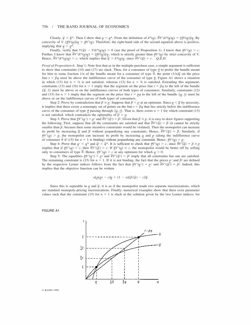
FIGURE A1

Clearly, q 5 q*. Then I show that , *. From the definition of k*( ), uV9(k*( ) ) 5 [uV( )]/ . Byq q q q q q qconcavity of V, [uV( )]/ . uV9( ). Therefore, the right-hand side of the second equation above is positive,q q qimplying that , *.q q

Finally, verify that V(q) 2 V(k*( ) ) . 0 (see the proof of Proposition 1). I know that uV9( ) . c.q q qFurther, I know that uV9(k*( ) ) 5 [uV( )]/ , which is strictly greater than uV9( ) by strict concavity of V.q q q q qHence, uV9(k*( ) ) . c, which implies that q . k*( ) , since uV9(q) 5 c. Q.E.D.q q q q

Proof of Proposition 6. Step 1: Note first that as in the multiple-purchase case, a simple argument is sufficientto show that constraints (14) and (17) are slack. Then, for a consumer of type u to prefer the bundle meantfor him to some fraction 1/n of the bundle meant for a consumer of type u , the point (1/n)q on the priceline t 5 pq must lie above the indifference curve of the consumer of type u. Figure A1 shows a situationin which (13) for n 5 Ω is not satisfied, whereas (13) for n 5 æ is satisfied. Extending this argument,constraints (13) and (16) for n . 1 imply that the segment on the price line t 5 pq to the left of the bundle{q, } must lie above or on the indifference curves of both types of consumers. Similarly, constraints (12)tand (15) for n . 1 imply that the segment on the price line t 5 q to the left of the bundle { , t} must liep qabove or on the indifference curves of both types of consumers.

Step 2: Prove by contradiction that p $ . Suppose that p , at an optimum. Since , q by necessity,p p qit implies that there exists a nonempty set of points on the line t 5 pq that lies strictly below the indifferencecurve of the consumer of type u passing through { , t}. That is, there exists n . 1 for which constraint (13)qis not satisfied, which contradicts the optimality of p , .p

Step 3: Prove that uV9( j) 5 j and uV9(q j) 5 p j. Given that p $ , it is easy to draw figures supportingq p pthe following. First, suppose that all the constraints are satisfied and that uV9(q) . p (it cannot be strictlysmaller than p, because then some incentive constraints would be violated). Then the monopolist can increaseits profit by increasing q and p without jeopardizing any constraints. Hence, uV9(q ) 5 p. Similarly, ifuV9( ) . , the monopolist can increase its profit by increasing and (along the indifference curveq p q pof consumer if (15) for n 5 1 is binding) without jeopardizing any constraint. Hence, uV9( ) 5 .u q p

Step 4: Prove that j , * and qj , q*. It is sufficient to check that uV9( ) . c, since uV9(q) 5 p $q q q pimplies that if uV9( ) . c, then uV9(q ) . c. If uV9( ) # c, the monopolist would be better off by sellingq qonly to consumers of type u . Hence, uV9( ) . c at any optimum for which . 0.q q

Step 5: The equalities uV9( j) 5 j and uV9(q j) 5 p j imply that all constraints but one are satisfied.q pThe remaining constraint is (15) for n 5 1. If it is not binding, the fact that the prices j and p j are definedpby the respective Lerner indices follows from the fact that uV9( j) 5 j and uV9(q j) 5 p j. Indeed, thisq pimplies that the objective function can be written

a[ ( ) 2 c] 1 (1 2 a)[p (q ) 2 c]q.p q q

Since this is separable in and q, it is as if the monopolist made two separate maximizations, whichqare standard monopoly-pricing maximizations. Finally, numerical examples show that there exist parametervalues such that the constraint (15) for n 5 1 is slack at the solution given by the two Lerner indices; for

ALGER / 757

q RAND 1999.

other parameter values, however, it is violated, implying that it may be binding at the optimum. In that case,the monopolist maximizes the above expected profit with respect to and q, under the additional constraintq

u[V(q ) 2 qV9(q )] 5 uV( ) 2 u V9( ).q q q

Q.E.D.

References

HAMMOND, P.J. ‘‘Markets as Constraints: Multilateral Incentive Compatibility in Continuum Economies.’’Review of Economic Studies, Vol. 54 (1987), pp. 399–412.

INNES, R. AND SEXTON, R. ‘‘Customer Coalitions, Monopoly Price Discrimination and Generic Entry Deter-rence.’’ European Economic Review, Vol. 37 (1993), pp. 1569–1597.AND . ‘‘Strategic Buyers and Exclusionary Contracts.’’ American Economic Review, Vol. 84

(1994), pp. 566–584.AND . ‘‘Divide and Conquer Price Discrimination in Entry Games with Strategic Buyers.’’ In

D. Martimort, ed., Agricultural Markets: Mechanisms, Failures, and Regulations. New York: North-Holland, 1996.

KWOKA, J.E., JR. ‘‘Market Segmentation by Price-Quality Schedules: Some Evidence from Automobiles.’’Journal of Business, Vol. 65 (1992), pp. 615–628.

MASKIN, E. AND RILEY, J. ‘‘Monopoly with Incomplete Information.’’ RAND Journal of Economics, Vol. 15(1984), pp. 171–196.

MCMANUS, B. ‘‘Two-Part Pricing with Costly Arbitrage.’’ Mimeo, Department of Economics, University ofVirginia, 1998.

MUSSA, M. AND ROSEN, S. ‘‘Monopoly and Product Quality.’’ Journal of Economic Theory, Vol. 18 (1978),pp. 301–317.

SALLSTROM, S. ‘‘Kvalitet—en nationalekonomisk studie.’’ Mimeo, Department of Economics, StockholmSchool of Economics, 1991. (In Swedish.)

TIROLE, J. The Theory of Industrial Organization. Cambridge, Mass.: MIT Press, 1988.WILSON, R. Nonlinear Pricing. Oxford: Oxford University Press, 1992.

multiple and joint purchases - INGELA ALGER

Documents

Transcript of multiple and joint purchases - INGELA ALGER