
Multimode microwave circuit optomechanics as a platform to ...
226
2019 Acceptée sur proposition du jury pour l’obtention du grade de Docteur ès Sciences par NATHAN RAFAËL BERNIER Présentée le 30 janvier 2019 Thèse N° 9217 Multimode microwave circuit optomechanics as a platform to study coupled quantum harmonic oscillators Prof. H. M. Rønnow, président du jury Prof. T. Kippenberg, Dr O. Feofanov, directeurs de thèse Prof. K. Hammerer, rapporteur Prof. M. Sillanpää, rapporteur Prof. C. Galland, rapporteur à la Faculté des sciences de base Laboratoire de photonique et mesures quantiques (SB/STI) Programme doctoral en physique
-
Upload
khangminh22 -
Category
Documents
-
view
1 -
download
0
Transcript of Multimode microwave circuit optomechanics as a platform to ...

2019
Acceptée sur proposition du jury
pour l’obtention du grade de Docteur ès Sciences
par
NATHAN RAFAËL BERNIER
Présentée le 30 janvier 2019
Thèse N° 9217
Multimode microwave circuit optomechanics as a platform to study coupled quantum harmonic oscillators
Prof. H. M. Rønnow, président du juryProf. T. Kippenberg, Dr O. Feofanov, directeurs de thèseProf. K. Hammerer, rapporteurProf. M. Sillanpää, rapporteurProf. C. Galland, rapporteur
à la Faculté des sciences de baseLaboratoire de photonique et mesures quantiques (SB/STI)Programme doctoral en physique


Acknowledgements
The journey of a doctoral student is a long and winding road, and I wasfortunate to be well surrounded by colleagues and have more than a littlehelp from my friends and family. I thank Tobias who initially gave me thisopportunity to partake in scientific research at such a high level, trusting mewho had only done theory before to learn how to deal with the realities ofexperimental work, and for his continuous interest and enthusiasm for theproject, always finding time in his busy schedule. I thank Alexey for alwaysbeing available to share his plentiful experience (even while travelling abroad,in a few emergencies), all the while trusting me to work independently, and forstaying dedicated to help with my thesis beyond his official presence at EPFL.I cannot forget the unsung heroes who keep the complicated machinery of alarge research group ticking day after day. Helene, Antonella and Kathleentolerated my inquiries and helped me many times along the years not onlywith great patience but a guarantee to raise a smile.
A large research group means a large number of colleagues whom I wasglad to share this time with. In particular, I am very grateful to Daniel, whohad the patience to work in very close collaboration with me for many years,enduring my constant blabber and occasional singing. The two of us sharemany happy memories in and outside the lab and I hope the road that wewill share stretches long out ahead. Thanks to Philippe, who unsuccessfullytried to escape me after our common Bachelor’s and Master’s, for alwayskeeping me updated with every significant cultural event of the Lemanicregion and for giving me practice as an amateur psychoanalyst by regularlydropping by my office to unload his mind. I had the chance to engage inilluminating exchanges of ideas with many colleagues over the years, bothof a scientific and non-scientific nature, which provided necessary breaksfrom the routine of daily work and stimulation for creativity. Without going

iv
through an exhaustive list, let me briefly mention lively debates with Nico andVictor, forays in the esoteric aspects of optomechanics theory with Vivishek,swapping cultural references with Miles, and the generosity of Itay in sharinghis positive outlook on life and general good humor. I’m glad that I couldshare my passion for whisky and beer with many and in particular withfellow taste snobs Philippe, Daniel and Nils. Outside of EPFL, I was blessedto have the opportunity to collaborate with Andreas Nunnenkamp and DanielMalz. I thank Daniel for his relentless energy that he put in our theoreticalcollaboration, as well as for sharing an apartment and his flu in Trieste withme. Finally I am in tremendous debt to Amir and Nick, who picked up themicrowave optomechanics project to carry it into the future, infusing it withnew ideas and improvements despite my grumblings.
I am very grateful to my family, and especially to my sister, father andmother, who were there for me in the good and the less good times, andsupported me through all those years, even tolerating most of my jokes.Thanks to my friends for helping me balance my private and professionallife and for joining me to the many films, theater plays and concerts that Iinvited them to attend through the years. Finally thanks to my soon-to-bewife Ada, for constantly radiating positive energy and making my life anexciting adventure full of possibilities.

Resume
Les oscillateurs harmoniques font partie des objets les plus fondamentauxdecrits par la physique, mais restent malgre tout un sujet de recherche actuel.Les proprietes topologiques associees aux points exceptionnels qui peuventapparaıtre lorsque deux modes interagissent ont suscite un grand interetrecemment. Les oscillateurs harmoniques sont au coeur de nouvelles tech-nologies quantiques : la longue duree de vie de resonateurs a haut facteurQ en fait d’excellentes memoires quantiques ; ils sont aussi employes pourtraiter des signaux quantiques de faible bande passante, par exemple dansles amplificateurs parametriques Josephson.
Le but de cette these est d’explorer differents regimes fondamentaux dedeux oscillateurs harmoniques couples en utilisant l’optomecanique commesupport experimental. Suite au progres constant dans leurs facteurs de qua-lite, les resonateurs mecaniques et electromagnetiques realisent des oscil-lateurs harmoniques quasi-ideaux. Avec une modulation parametrique ducouplage optomecanique non-lineaire qui les lie, on peut realiser un cou-plage lineaire dont la force et la frequence relative des deux modes peuventetre controles. Ainsi, l’optomecanique constitue une plateforme qui permetd’etudier un systeme de deux oscillateurs couples, en reglant precisementleurs parametres. Les systemes optomecaniques que nous utilisons sont descircuits supraconducteurs dans lesquels la plaque superieure d’un condensa-teur vibre et sert d’element mecanique. Des circuits multimodes sont realises,dans lesquels deux modes micro-ondes interagissent avec un ou deux modesmecaniques. Les modes supplementaires servent soit d’intermediaires dans larelation des deux modes principaux, soit d’auxiliaires pour le controle d’unparametre du systeme.
Trois resultats experimentaux principaux sont obtenus. Premierement, unmode micro-onde auxiliaire permet de controler le taux de dissipation effec-

vi
tif d’un oscillateur mecanique. Ce dernier joue alors le role d’un reservoirthermodynamique pour le mode micro-onde principale avec lequel il inter-agit. La susceptibilite du mode micro-onde peut etre modifiee, ce qui resulteen une instabilite analogue a celle du maser et a l’amplification resonantedes signaux micro ondes incidents avec un bruit proche du minimum quan-tique. Deuxiemement, nous etudions les conditions dans lesquelles la relationentre deux modes micro-ondes devient non-reciproque, telle que l’informa-tion est transmise dans une direction mais pas dans l’autre. Les deux modesinteragissent par le biais de deux oscillateurs mecaniques, ce qui permetune conversion en frequence entre les deux cavites micro-ondes. La dissi-pation des modes mecaniques est essentielle pour deux raisons : elle per-met une phase reciproque necessaire a l’interference et permet d’eliminerles signaux indesirables. Troisiemement, nous realisons une attraction de ni-veaux entre un mode micro-onde et un mode mecanique, dans laquelle lesfrequences propres du systeme se rapprochent a cause de l’interaction, aulieu de s’eloigner comme dans le cas plus usuel de repulsion de niveaux. Lephenomene est relie de maniere theorique aux points exceptionnels, ce quipermet une classification generale des differents regimes d’interactions entredeux modes harmoniques, dont la repulsion et l’attraction de niveaux consti-tuent deux exemples.
Mots-cles : optomecanique, circuits supraconducteurs micro-ondes, re-servoirs quantiques, amplification a la limite quantique, non-reciprocite, at-traction de niveaux

Abstract
Harmonic oscillators might be one of the most fundamental entities describedby physics. Yet they stay relevant in recent research. The topological prop-erties associated with exceptional points that can occur when two modesinteract have generated much interest in recent years. Harmonic oscillatorsare also at the heart of new quantum technological applications: the longlifetime of high-Q resonators make them advantageous as quantum memo-ries, and they are employed for narrowband processing of quantum signals,as in Josephson parametric amplifiers.
The goal of this thesis is to explore different fundamental regimes of twocoupled harmonic oscillators using cavity optomechanics as the experimen-tal platform. With consistent progress in attaining ever increasing Q fac-tors, mechanical and electromagnetic resonators realize near-ideal harmonicoscillators. By parametrically modulating the nonlinear optomechanical in-teraction between them, an effective linear coupling is achieved, which istunable in strength and in the relative frequencies of the two modes. Thuscavity optomechanics provides a framework with excellent control over sys-tem parameters for the study of two coupled harmonic modes. The specificoptomechanical implementation employed are superconducting circuits withthe vibrating top plate of a capacitor as the mechanical element. Multimodeoptomechanical circuits are realized, with two microwave modes interactingwith one or two mechanical oscillators. The supplementary modes serve ei-ther as intermediaries in the relation of the two modes of interest, or asauxiliaries used to control a parameter of the system.
Three main experimental results are achieved. First, an auxiliary mi-crowave mode allows the engineering of the effective dissipation rate of amechanical oscillator. The latter then acts as a reservoir for the main mi-crowave mode with which it interacts. The microwave mode susceptibility
viii
can be tuned, resulting in an instability akin to that of a maser and in reso-nant amplification of incoming microwave signals with an added noise closeto the quantum minimum. Second, we study the conditions for a nonrecipro-cal interaction between two microwave modes, when the information flows inone direction but not in the other. The two modes interact through two me-chanical oscillators, leading to frequency conversion between the two cavities.Dissipation in the mechanical modes is essential to the scheme in two ways:it provides a reciprocal phase necessary for the interference and eliminatesthe unwanted signals. Third, level attraction between a microwave and amechanical mode is demonstrated, where the eigenfrequencies of the systemare drawn closer as the result of interaction, rather distancing themselves asin the more usual case of level repulsion. The phenomenon is theoreticallyconnected to exceptional points, and a general classification of the possibleregimes of interaction between two harmonic modes is exposed, includinglevel repulsion and attraction as special cases.
Keywords: cavity optomechanics, superconducting microwave circuits,quantum reservoirs, quantum-limited amplification, nonreciprocity, level at-traction

List of publications
• C. Javerzac-Galy, K. Plekhanov, N. R. Bernier, L. D. Toth, A. K. Fe-ofanov and T. J. Kippenberg: On-chip microwave-to-optical quantumcoherent converter based on a superconducting resonator coupled toan electro-optic microresonator. Physical Review A 94, 053815 (2016).Arxiv: https://arxiv.org/abs/1512.06442
• L. D. Toth1 , N. R. Bernier1, A. Nunnenkamp, A. K. Feofanov andT. J. Kippenberg: A dissipative quantum reservoir for microwave lightusing a mechanical oscillator. Nature Physics 13, 787-793 (2017).Arxiv: https://arxiv.org/abs/1602.05180
• N. R. Bernier1, L. D. Toth1, A. Koottandavida, M. A. Ioannou, D.Malz, A. Nunnenkamp, A. K. Feofanov and T. J. Kippenberg: Non-reciprocal reconfigurable microwave optomechanical circuit. NatureCommunications 8, 604 (2017).Arxiv: https://arxiv.org/abs/1612.08223
• L. D. Toth1, N. R. Bernier1, A. K. Feofanov and T. J. Kippenberg:A maser based on dynamical backaction on microwave light. PhysicsLetters A 382, 2233 (2018).Arxiv: https://arxiv.org/abs/1705.06422
• D. Malz, L. D. Toth, N. R. Bernier, A. K. Feofanov, T. J. Kippenbergand A. Nunnenkamp: Quantum-limited directional amplifiers with op-tomechanics. Physical Review Letters 120, 023601 (2018).Arxiv: https://arxiv.org/abs/1705.00436
• N. R. Bernier, L. D. Toth, A. K. Feofanov and T. J. Kippenberg:Nonreciprocity in microwave optomechanical circuits. Special issue“Magnet-less Nonreciprocity in Electromagnetics” in IEEE Antennas
1 Equally contributing authors.

x
and Wireless Propagation Letters, 17, 1983–1987 (2018).Arxiv: https://arxiv.org/abs/1804.09599
• N. R. Bernier, L. D. Toth, A. K. Feofanov and T. J. Kippenberg:Level attraction in a microwave optomechanical circuit. Physical Re-view A, 98, 023841 (2018).Arxiv: https://arxiv.org/abs/1709.02220

Contents
Acknowledgements iii
Resume v
Abstract vii
List of publications ix
Contents xi
List of Figures xv
List of Symbols xix
1 Introduction 1
2 Theoretical background 72.1 A short review of cavity optomechanics . . . . . . . . . . . . . 7
2.1.1 The optomechanical interaction . . . . . . . . . . . . . 82.1.2 The Langevin formalism . . . . . . . . . . . . . . . . . 92.1.3 Linearization in the Langevin picture . . . . . . . . . . 112.1.4 Linearization in the Hamiltonian picture . . . . . . . . 142.1.5 Optomechanical damping and amplification . . . . . . 15
2.2 Quantum noise and amplification . . . . . . . . . . . . . . . . 192.2.1 Input and output modes . . . . . . . . . . . . . . . . . 192.2.2 The Wiener-Khinchin theorem and the spectral density 212.2.3 The linear amplifier and its quantum limits . . . . . . . 24
2.3 Optomechanical microwave circuits . . . . . . . . . . . . . . . 27

xii CONTENTS
2.3.1 Optomechanics with LC circuits . . . . . . . . . . . . . 272.3.2 Transmission line theory . . . . . . . . . . . . . . . . . 302.3.3 Input and output relations for an inductively coupled
LC circuit . . . . . . . . . . . . . . . . . . . . . . . . . 342.3.4 Quantization of the microwave and mechanical modes . 38
3 Design and measurement of optomechanical microwave cir-cuits 433.1 Fabrication of the devices . . . . . . . . . . . . . . . . . . . . 433.2 Simulation tools as aides for design and characterization . . . 46
3.2.1 Sonnet software . . . . . . . . . . . . . . . . . . . . . . 483.3 Experimental setup . . . . . . . . . . . . . . . . . . . . . . . . 51
3.3.1 Sample holder . . . . . . . . . . . . . . . . . . . . . . . 513.3.2 Mounting and bonding the chip . . . . . . . . . . . . . 533.3.3 Inside the dilution refrigerator . . . . . . . . . . . . . . 553.3.4 Room-temperature equipment . . . . . . . . . . . . . . 59
3.4 Noise calibrations . . . . . . . . . . . . . . . . . . . . . . . . . 633.4.1 Phase and amplitude noise of the sources . . . . . . . . 633.4.2 Calibration of the HEMT . . . . . . . . . . . . . . . . 65
3.5 Characterization of the chip . . . . . . . . . . . . . . . . . . . 683.5.1 Fitting microwave resonances with circles . . . . . . . . 693.5.2 Measurement of g0 . . . . . . . . . . . . . . . . . . . . 77
3.6 Routine optomechanical measurements . . . . . . . . . . . . . 813.6.1 Sideband cooling . . . . . . . . . . . . . . . . . . . . . 813.6.2 Optomechanically induced transparency and absorption 83
4 A dissipative quantum reservoir for microwaves using a me-chanical oscillator 874.1 Introduction . . . . . . . . . . . . . . . . . . . . . . . . . . . . 884.2 Dark and bright modes . . . . . . . . . . . . . . . . . . . . . . 894.3 Realization of a mechanical reservoir . . . . . . . . . . . . . 934.4 Tuning a mode using a reservoir . . . . . . . . . . . . . . . . . 954.5 Interpretation as dynamical backaction . . . . . . . . . . . . . 95
4.5.1 Origin of the concept of dynamical backaction . . . . . 954.5.2 Modeling dynamical backaction . . . . . . . . . . . . . 98
4.6 Controllable microwave susceptibility . . . . . . . . . . . . . . 1004.7 Maser action and amplification . . . . . . . . . . . . . . . . . 1024.8 Near-quantum-limited amplification . . . . . . . . . . . . . . . 1064.9 Injection locking of the maser tone . . . . . . . . . . . . . . . 1094.10 Conclusions . . . . . . . . . . . . . . . . . . . . . . . . . . . . 111

CONTENTS xiii
5 Nonreciprocity in microwave optomechanical circuits 1135.1 Introduction . . . . . . . . . . . . . . . . . . . . . . . . . . . . 1135.2 Gyrators and nonreciprocity . . . . . . . . . . . . . . . . . . . 115
5.2.1 The gyrator-based isolator . . . . . . . . . . . . . . . 1155.2.2 Nonreciprocity in optomechanical systems . . . . . . . 117
5.3 Optomechanical isolator . . . . . . . . . . . . . . . . . . . . . 1215.3.1 Theoretical model . . . . . . . . . . . . . . . . . . . . . 121
5.4 Experimental results . . . . . . . . . . . . . . . . . . . . . . . 1255.4.1 Transmission measurements . . . . . . . . . . . . . . . 1275.4.2 Noise measurements . . . . . . . . . . . . . . . . . . . 131
5.5 Optomechanical circulator . . . . . . . . . . . . . . . . . . . . 1335.6 Outlook . . . . . . . . . . . . . . . . . . . . . . . . . . . . . . 135
6 Level attraction in a microwave optomechanical circuit 1376.1 Introduction . . . . . . . . . . . . . . . . . . . . . . . . . . . . 1376.2 Theoretical exposition of level attraction . . . . . . . . . . . . 140
6.2.1 Symmetry of level repulsion and attraction . . . . . . 1436.2.2 Classification of exceptional points . . . . . . . . . . . 145
6.3 Optomechanical level attraction . . . . . . . . . . . . . . . . . 1486.3.1 Experimental results . . . . . . . . . . . . . . . . . . . 149
6.4 Outlook . . . . . . . . . . . . . . . . . . . . . . . . . . . . . . 153
7 Outlook on high-efficiency optomechanical measurements witha traveling-wave parametric amplifier 1557.1 Introduction . . . . . . . . . . . . . . . . . . . . . . . . . . . . 1557.2 Installing and operating the TWPA . . . . . . . . . . . . . . . 1567.3 Detailed balance in sideband cooling . . . . . . . . . . . . . . 158
7.3.1 Theoretical model . . . . . . . . . . . . . . . . . . . . . 1597.3.2 Preliminary experimental results . . . . . . . . . . . . 160
7.4 Precise noise calibration . . . . . . . . . . . . . . . . . . . . . 162
8 Conclusions and outlook 1678.1 Summary of the results . . . . . . . . . . . . . . . . . . . . . . 1678.2 Outstanding challenges and outlook . . . . . . . . . . . . . . . 168
A The rotating wave approximation 171
B Heterodyne detection as amplification 175B.1 Quantum measurements and spectral densities . . . . . . . . . 176B.2 Direct photodetection . . . . . . . . . . . . . . . . . . . . . . . 177B.3 Optical heterodyne detection . . . . . . . . . . . . . . . . . . . 179

xiv CONTENTS
B.4 Comparison between heterodyne detection and phase-preservingamplification . . . . . . . . . . . . . . . . . . . . . . . . . . . 181
C Samples used in the experiment 183
Bibliography 189
Curriculum Vitae 203

List of Figures
1.1 The circular motion of a harmonic oscillator . . . . . . . . . . 3
2.1 Archetypical optomechanical system. . . . . . . . . . . . . . . 82.2 Schematic representation of a linear scattering amplifier . . . . 252.3 Ideal LC circuit with an inductor in series with a capacitor. . 282.4 Lumped-element model of the transmission line. . . . . . . . . 322.5 Different loads on the line for which the reflection coefficient
are computed. . . . . . . . . . . . . . . . . . . . . . . . . . . 332.6 Lumped-element model of the resonator coupled to the line. . 36
3.1 Photograph and scanning-electron micrograph of the optome-chanical circuit . . . . . . . . . . . . . . . . . . . . . . . . . . 44
3.2 Schematic of the main steps of fabrication of the chips. . . . . 463.3 Example of Sonnet simulation . . . . . . . . . . . . . . . . . . 483.4 Microwave resonances simulated with Sonnet for the sample
HYB-20150924-4-24 . . . . . . . . . . . . . . . . . . . . . . . . 503.5 Photographs of the sample holder. . . . . . . . . . . . . . . . . 523.6 Schematics of the setup inside the dilution refrigerator. . . . . 573.7 Room-temperature equipment. . . . . . . . . . . . . . . . . . . 603.8 Filter cavity photograph and response . . . . . . . . . . . . . . 623.9 Measured phase and amplitude noise of Rohde & Schwartz
SMF 100A . . . . . . . . . . . . . . . . . . . . . . . . . . . . . 653.10 Scheme for the calibration of the HEMT amplifiers . . . . . . 663.11 Example measurement for the calibration of the HEMT . . . . 693.12 Example of fitting a circle to the complex response S11. . . . . 713.13 Model for impedance mismatch . . . . . . . . . . . . . . . . . 743.14 Calibration of g0 . . . . . . . . . . . . . . . . . . . . . . . . . 803.15 Sideband cooling of the mechanical mode . . . . . . . . . . . . 82

xvi LIST OF FIGURES
3.16 Measurement of OMIT/OMIA with a red-detuned pump tone 843.17 OMIT power sweep to the onset of strong coupling . . . . . . 85
4.1 Realization of a mechanical reservoir for a microwave cavityin circuit optomechanics. . . . . . . . . . . . . . . . . . . . . . 90
4.2 Unsuccessful design to obtain asymmetrically coupled microwavemodes . . . . . . . . . . . . . . . . . . . . . . . . . . . . . . . 92
4.3 Device, experimental setup, and characterization of the elec-tromechanical circuit . . . . . . . . . . . . . . . . . . . . . . . 94
4.4 The role of dissipation in dynamical backaction. . . . . . . . . 974.5 Dynamical backaction on the microwave mode using an engi-
neered mechanical reservoir. . . . . . . . . . . . . . . . . . . . 1014.6 Amplified vacuum fluctuations and parametric instability of
the microwave mode (masing). . . . . . . . . . . . . . . . . . . 1034.7 Interaction between modes of positive and negative energy as
population inversion . . . . . . . . . . . . . . . . . . . . . . . 1054.8 Near-quantum-limited phase-preserving amplification. . . . . . 1074.9 Injection locking of a maser based on dynamical backaction . . 110
5.1 Gyrator and optomechanical coupling. . . . . . . . . . . . . . 1165.2 Gyrator-cased isolator compared to optomechanical multimode
schemes. . . . . . . . . . . . . . . . . . . . . . . . . . . . . . . 1185.3 Scheme for a multimode optomechanical isolator . . . . . . . . 1225.4 Implementation of a superconducting microwave circuit op-
tomechanical device for nonreciprocity. . . . . . . . . . . . . . 1265.5 Diagram of the measurement chain for frequency conversion . 1285.6 Experimental demonstration of nonreciprocity. . . . . . . . . . 1305.7 Asymmetric noise emission of the nonreciprocal circuit. . . . . 1325.8 Proposal for a microwave optomechanical circulator. . . . . . . 1345.9 Schemes for directional amplification with an optomechanical
circuit . . . . . . . . . . . . . . . . . . . . . . . . . . . . . . . 136
6.1 Level repulsion and attraction. . . . . . . . . . . . . . . . . . . 1396.2 The effect of dissipation on level attraction. . . . . . . . . . . 1416.3 Systematic comparison of level repulsion and attraction. . . . 1466.4 Engineering dissipation in a multimode optomechanical circuit. 1506.5 Experimental demonstration of level repulsion and attraction
in a microwave optomechanical circuit. . . . . . . . . . . . . . 1526.6 Amplitude and complex responses for level repulsion and at-
traction . . . . . . . . . . . . . . . . . . . . . . . . . . . . . . 154
7.1 Setup for the TWPA . . . . . . . . . . . . . . . . . . . . . . . 157

LIST OF FIGURES xvii
7.2 Scheme for tone cancellation . . . . . . . . . . . . . . . . . . . 1587.3 Sideband asymmetry experiment with the TWPA . . . . . . . 1617.4 Comparison of the sideband measurement with the TWPA
turned on and off . . . . . . . . . . . . . . . . . . . . . . . . . 1637.5 Setup for the calibration of the TWPA . . . . . . . . . . . . . 164
8.1 Proposal for a new geometry for the capacitor . . . . . . . . . 170
A.1 Comparison of cases when the RWA is valid or not. . . . . . . 172
B.1 Scheme for heterodyne detection. . . . . . . . . . . . . . . . . 181


List of Symbols
G Position-dependent optomechanical couplingconstant; definition p. 8, expression for the ca-pacitor p. 30.
g0 Vacuum optomechanical coupling strength;definition p. 9, expression for the capacitorp. 41.
κex External coupling rate of the electromagneticcavity; definition p. 10, expressions for an LCresonator in reflection p. 35 and in transmis-sion p. 37, expressions in the presence of animpedance mismatch p. 73 in transmission andp. 76 in reflection.
κ0 Internal dissipation rate of the electromag-netic cavity; definition p. 10, expression foran LC resonator p. 35.
Γm Mechanical dissipation rate; definition p. 10.ωc Cavity resonance frequency: definition p. 10,
expression for an LC resonator p. 28, expres-sions in the presence of an impedance mis-match p. 73 in transmission and p. 76 in re-flection.
κ Electromagnetic dissipation rate; definitionp. 10.
Ωm Mechanical resonance frequency; definitionp. 10.
nc Mean intracavity photon number due to adriving tone; definition p. 12.

xx List of Symbols
Δ Pump tone frequency detuning; definitionp. 13.
g Linearized field-enhanced optomechanicalcoupling strength definition p. 13.
Γeff Effective mechanical dissipation rate; defini-tion p. 17.
C Optomechanical cooperativity; definitionp. 17.
nm,th Mean mechanical number occupancy at ther-mal equilibrium; definition p. 17.
nm Mean mechanical number occupancy; defini-tion p. 18.
nth Mean thermal occupancy for a travelling elec-tromagnetic wave; definition p. 20.
S Spectral density; classical definition p. 21,quantum definition p. 23.
S Symmetrized spectral density; definition p. 23.G Amplifier gain; definition p. 24.N Added noise of an amplifier (in quanta); defi-
nition p. 26.meff Effective mass of the mechanical oscillator;
definition p. 39.

Chapter 1
Introduction
Motion in a circle has exerted a strong fascination on the human mindthrough the ages. It is most evident in cosmology and the “changing vi-sion of the universe” (Koestler, 1959). The idea of heavenly bodies thatrotate in circles around a spherical earth can be traced back to the school ofPythagoras in the 6th century BCE. Their global vision of sciences, imbuedwith mysticism, encompassed mathematics, medicine and the arts. The mu-sical notes produced by the rotation of each cosmic body at various speedscomposed a harmony of the spheres that supposedly only Pythagoras himselfcould hear.
Plato, in the 4th century BCE, confirmed the Pythagorean intuition by apriori reasoning concluding that the universe should have the perfect shapeof a sphere and the perfect motion of a circular trajectory at uniform speed.Subsequently, his contemporary Aristotle formalized this notion into a dogmaof circular motion that humanity only abandoned two thousand years later.The spherical earth, immobile in the center of the universe belongs to thesublunar realm of change and decay. It is surrounded by nine concentricspheres, increasing in purity and holiness with radius, all moving in circlesaround their center. The relative motion of spheres rotating with respect toeach other uniformly (54 spheres in total in the complete Aristotelian modelthat result in convoluted trajectories for the nine spheres that carry celestialobjects) could only very roughly account for the actual apparent movementsin the sky. Ptolemy, in 2nd century BCE, discarded the spheres and onlykept the rule of circular motion at the letter. His planets move uniformly incircles around points that themselves follow a circular orbit around the earth

2 Introduction
(or rather a point slightly away from the earth, named the eccentric). Byvarying the radii and relative velocity of those circular motions, complicatednoncircular trajectories on the epicycles can be constructed from circles only.Through that technique, the strange wandering of the planets could be ap-proximately accounted for, at least well enough for the needs of time keepingand navigation at the time. Copernicus in the 16th century, unsatisfied withthe status quo, attempted a new model that placed the sun in the center ofthe orbits of all planets (as Philolaus, Heraclides and Aristarchus had donelong before). That model simplified things slightly, but could not escape thecurse of the circular dogma, filled as the Ptolemaic system with complicatedepicycles.
The holiness of circular motion was so well entrenched that it took untilthe 17th century for Kepler to finally renounce it and introduce elliptic orbitsinstead. Motivated by a mystical urge to decrypt the universe with the lan-guage of mathematics, he took the very modern step of comparing a modelto precise data. The inevitable conclusion came at great pains to Keplerwho despaired that giving up on the circles and epicycles that had clutteredastronomy for millenia left him with “only a single cart-full of dung”1, theellipse. Such was the strength of the delusion that Galileo, a contempo-rary who had access to Kepler’s results but believed firmly in Copernicus’sepicycles, held that matter, left to its own device, would naturally move incircles. Finally, Descartes found soon afterwards the correct law of inertia,pronouncing the infinite line as the natural trajectory of matter.
I will argue that the obsession with circular motion was only misdirectedwhen applied to astronomy. A circular orbit is indeed only possible for abody whose initial velocity and distance from the sun are such that thegravitational force precisely corresponds to the centripetal force required tobend the trajectory into a circle. Any other initial conditions and the orbitforms an ellipse. There is however an entity that always travels on a circleat uniform velocity: the harmonic oscillator in phase space.
The harmonic oscillator is a physical abstraction that represents an idealperiodic motion in a quadratic potential. Its archetype is a mass bouncing ona linear spring, as shown in fig. 1.1a. When the mass m departs its equilib-rium position, a recoil force F (x) = −kx (with k the spring constant) pullsit back. The resulting motion is periodic, with x(t) = x0 sin(ω0t+ φ), wherethe amplitude x0 and phase φ are determined by the initial condition, andω0 =
√k/m is the oscillation frequency (fig. 1.1b). The velocity oscillates
out of phase with the position as v(t) = ω0x0 cos(ω0t + φ) (fig. 1.1b). Rep-
1 Letter to Longomontanus, 1605, as quoted by Koestler (1959).

3
x
(a) (b) (c)
Figure 1.1: The circular motion of a harmonic oscillator. (a) Archetypicalharmonic oscillator formed by a mass on a spring. (b) Periodic oscillations ofthe position x and velocity v of the oscillator. (c) Phase space representationof the circular trajectory on the plane formed by x and v.
resented in the phase space in fig. 1.1c, with x the horizontal axis and v thevertical one, it follows a circular trajectory at uniform speed. The periodicoscillation can be interpreted as stemming from a competition between thekinetic energy 1
2mv2 and the potential spring energy 1
2kx2, with an increase
in velocity when the distance reduces and a decrease in velocity when thedistance increases. Written in terms of the normalized position q =
√k/ω0 x
and momentum p =√m/ω0 v, the total energy E = 1
2ω0(q
2 + p2) describesgeometrically a circle on the plane formed by q and p (with a radius of√2E/ω0). The quadratic form of the potential is essential to this property.
It is a posteriori clear how doomed the ancient astronomers were, who wres-tled unknowingly with a gravitational potential of the form −GM/r, failingto fit circles in the resulting motion.
The harmonic oscillator is perhaps the most fundamental object describedby physics. Beyond mechanical resonators, it models the periodic changesof any degree of freedom in a quadratic potential: electromagnetic radiationbouncing back and forth in optical cavities, sound waves resonating as a notein a musical instrument, or the vibrations of fundamental quantum fieldsthat constitute the particles of the standard model. Despite its simplicity(or perhaps because of it), the realization of an actual near-ideal harmonicoscillator is technically challenging and an engineering goal to this day.
Two practical constraints prevent the implementation of an ideal oscilla-tor a priori: deviations from the quadratic harmonic potential and dampingof the oscillations due to the environment. The former, known as anhar-monicities, can be easily remedied. By reducing the oscillation amplitude,

4 Introduction
any higher-order component of the potential beyond the quadratic eventuallybecomes negligible. For instance the pendulum, whose nonlinear recoil forceis F (θ) = −mg sin θ, is a harmonic oscillator for small angles θ for which theforce is approximately linear, with F (θ) ≈ −mg θ. In fact, the principal de-viation of practical oscillators from the ideal originate from their interactionwith the environment. Through friction, a pendulum loses momentum os-cillation after oscillation and the amplitude of motion continuously reducesuntil the pendulum eventually reaches a stop. This loss of energy can bequantified and defined to occur at a rate κ called the energy dissipation rate,such that after a time Δt the energy is reduced by a factor e−κΔt. Thequality factor Q = ω0/κ is a measure of how close to the ideal the oscillatoris: it counts the number of free oscillations before the energy decays to e−2π
of its initial value, a number that tends to infinity for the perfect harmonicoscillator.
The last decades have seen a substantial rise in the Q factors of bothmechanical and electromagnetic resonators. The natural decoupling of me-chanical elements to their environment makes them technologically appealingas narrowband oscillators, with quartz oscillators ubiquitous in applicationsof timekeeping and MEMS devices used for narrowband filtering in telecom-munication (Lam, 2008). Recently, through new techniques such as softclamping and strain engineering, nanomechanical oscillators have been real-ized with Q factors of up to nearly 109 (Tsaturyan et al., 2017; Ghadimi etal., 2018). In parallel, tremendous progress has also been achieved in electro-magnetic resonators. Optical cavities such as Fabry-Perot etalons are used asfrequency references (Kruk et al., 2005) and to form lasers (Bromberg, 2008).The nonlinear medium of certain high-Q microresonators can spawn opticalfrequency combs of regularly spaced emission (Kippenberg, Holzwarth, andDiddams, 2011). In the microwave range, superconducting resonators formedby 3D cavities or circuits have been realized with high Q factors (Megrantet al., 2012; Bruno et al., 2015; Romanenko and Schuster, 2017). Both op-tical (Walther et al., 2006) and microwave (Devoret and Schoelkopf, 2013)cavities have been exploited to interact with natural and artificial atoms atthe quantum level.
A single harmonic oscillator, while useful as a timekeeper or filter, pre-dictably beats at the same frequency and lacks interesting dynamics. Twocoupled oscillators however offer a much more colorful panel of associatedphenomena. Cavity optomechanics (Aspelmeyer, Kippenberg, and Mar-quardt, 2014), or the study of interaction between a mechanical oscillatorand an electromagnetic cavity, realizes a coupling between two near-idealharmonic oscillators. Through the optomechanical interaction, mechanical

5
oscillators have been cooled close to their ground state (Teufel, Donner, etal., 2011), squeezed light has been produced (Purdy et al., 2013), and themechanical motion measured by evading the backaction usually imposed byquantum mechanics (Møller et al., 2017), among many other demonstra-tions. It also sets fundamental limits on the sensitivity of gravitational-wavedetectors (Evans et al., 2015).
The nonlinear optomechanical interaction can be linearized through para-metric modulation by applying an electromagnetic driving tone to the sys-tem. The resulting linear coupling is tunable in strength and the relativefrequencies of the two harmonic modes (in a rotating frame) can be varied aswell. Thus, optomechanical systems are highly controllable platforms for theexploration of the fundamental properties of linearly interacting harmonicoscillators.
That constitutes the thread of Ariadne that binds together the resultsof this thesis. An optomechanical system allows us to explore the wealth ofphenomena arising from a linear coupling between two harmonic modes. Thespecific implementation is a microwave optomechanical circuit (Teufel, D. Li,et al., 2011), where the electromagnetic mode is a superconducting LC res-onator and the mechanical element is the vibrating top plate of the capacitor.More specifically, the possibilities of multimode optomechanical systems areexplored, where two microwave modes interact with one or two mechanicalmodes. When considering the interplay between two given oscillators, thesupplementary modes act either as intermediaries in the relation or auxiliarydegrees of freedom that permit the tuning of a system parameter.
In summary, the present thesis is structured as follows. In chapter 2, aquick overview of the necessary theoretical models is attempted. In chapter 3,the main features of the experiments are exposed, including short summariesof the nanofabrication of the devices and the numerical simulation tools used.In chapter 4, the first main experimental result is presented, concerning therealization of a reservoir for a microwave cavity using an auxiliary microwavemode to engineer the dissipation of a mechanical oscillator. In chapter 5, thesecond result is discussed, about the possibility to construct a nonreciprocalpathway between two microwave modes with two mechanical modes servingas intermediaries. In chapter 6, the third main result is introduced: we de-scribe theoretically the classes of interaction between two harmonic modesand demonstrate experimentally level attraction between a microwave anda mechanical mode. In chapter 7, recent progress is reported on the imple-mentation of a new experimental tool to achieve higher quantum efficiencyin measurements. In chapter 8, we finally conclude and provide an outlookfor future possible extensions of the work.

6 Introduction
Supporting data and code to the results of this thesis are available on-line (Bernier, 2018). This includes the files of the design of custom com-ponents fabricated for the experiment, code used to produce the figurescontained in this thesis, and the measurement scripts used to acquire theexperimental data.

Chapter 2
Theoretical background
In this chapter, we present the different theoretical models that constitute thebackbone of the phenomena studied in this thesis. In section 2.1, we presenta theoretical background for general cavity optomechanics. In section 2.2,the notion of quantum noise as it applies to amplification and our system isdeveloped. Finally, in section 2.3, we introduce our specific implementationof an optomechanical system using superconducting LC circuits. The aim isnot to provide an exhaustive review of cavity optomechanics, but only thefundamental theoretical tools required to present the results of this thesis.We refer the reader interested in a more thorough presentation to the existingliterature (Aspelmeyer, Kippenberg, and Marquardt, 2014; Bowen and G. J.Milburn, 2015).
2.1 A short review of cavity optomechanics
Here we expose rapidly the fundamental ideas of cavity optomechanics. Insection 2.1.1, the optomechanical interaction is introduced, leading to thequantum optomechanical Hamiltonian in eq. (2.2). In section 2.1.2, theLangevin equation for a quantum mode (2.4) is introduced that accountsfor the dissipation in the open system. In sections 2.1.3 and 2.1.4, the non-linear optomechanical interaction is linearized in the presence of a drivingtone, first in the Langevin formalism, then at the level of the Hamiltonian.In section 2.1.5, the immediate consequences of the linearized optomechanicalinteraction are presented, in the form of a shift in the mechanical frequency

8 Theoretical background
ab
Figure 2.1: Archetypical optomechanical system. A Fabry-Perot cavity withan optical mode a has one mirror that is mounted on a spring. Its mechanicalmotion, the mode b, modulates the resonance frequency of mode a and inturn the light in the mode a exerts a force on the oscillator b due to radiationpressure.
and dissipation rate.
2.1.1 The optomechanical interaction
The defining feature of cavity optomechanics is a specific form for the in-teraction between two harmonic oscillators. Independently of the nature ofthe two modes, the coupling will determine the dynamics and associatedphenomena, whichever system is used for its realization.
Consider two harmonic oscillators with quadratures x1, p1 and x2, p2,and frequencies ω1 and ω2. We define the optomechanical interaction as thecoupling that results from the linear dependence of the frequency of the firstmode on a quadrature of the second mode, such that
ω1(x2) = ω1,0 +Gx2. (2.1)
The coupling constant G depends on the choice of normalization for thequadrature x2 and is in general not always clearly defined.
The archetypal example of optomechanical interaction, shown in fig. 2.1 isan optical Fabry-Perot cavity formed by two parallel mirrors, one of which isattached to a spring and constitutes a mechanical harmonic oscillator. Thedisplacement of the mirror changes the length of the optical cavity and thusits frequency. For small enough oscillation amplitudes, the dependence inposition can be linearized such that eq. (2.1) is obtained. There is howevernothing requiring the first mode to be optical and the second to be mechanicalin nature. Only the structure of the Hamiltonian (as well as the interactionwith the environment in the form of the dissipation rate, as explained insection 2.1.5) determine the dynamics of the system.

2.1 A short review of cavity optomechanics 9
We note that other types of optomechanical couplings have been studiedas well. In particular, the quadratic optomechanical interaction ω1(x2) =ω1,0 +G2x
22 has been experimentally achieved with membrane-in-the-middle
experiments (Jayich et al., 2008; Thompson et al., 2008; Sankey et al., 2010)and photonic crystals (Paraıso et al., 2015). Within this thesis, we are onlyconcerned with the linear kind and we will always mean a coupling of theform eq. (2.1) by “optomechanical interaction”.
In the language of quantum mechanics, which we will use throughout thisthesis, the two modes are described by the annihilation operators a, b, suchthat the quadratures of the two modes (now promoted to operators) take theform x1 ∝ a+ a†, p1 ∝ i(a† − a), x2 ∝ b+ b†, p2 ∝ i(b† − b). They obey thebosonic canonical commutation relations [a, a†] = 1 and [b, b†] = 1. In thatlanguage, the Hamiltonian for the system is expressed as
H = �ω1(x2)a†a+ �ω2b
†b = �ω1,0a†a+ �ω2b
†b+ �g0(b+ b†)a†a, (2.2)
where g0 is called the vacuum optomechanical coupling strength and corre-sponds to G when the second mode quadrature has the dimensionless nor-malization x2 = b + b†. We will refer to the last term of eq. (2.2) as theoptomechanical coupling term.
2.1.2 The Langevin formalism
A capital aspect that is not taken into account in the Hamiltonian formalismis the interaction with the environment. This is not merely a non-idealfeature of the system implying dissipation and loss, but an essential one.One of the two modes at least must be accessible through a channel in orderto transfer information to and from the system for any measurement to takeplace. We use the quantum Langevin formalism to account for the role ofthe environment, and briefly review it here. A thorough exposition can befound in the appendix E.2 of the review on quantum noise by Clerk et al.(2010).
The mode of interest, which we will denote by the annihilation operator a,is assumed to interact with a number of bath modes, of annihilation operatorscq, through the coupling Hamiltonian
Hbath = −i�∑q
[λa†cq − λ∗c†qa
], (2.3)
with λ an (a priori complex) coupling strength. In the case of the interactionwith a waveguide channel, the bath modes are standing modes of the waveg-uide (determined by the boundary conditions, including the cavity itself).

10 Theoretical background
In the case of internal loss mechanisms, the bath modes are any externaldegrees of freedom coupled to the mode of interest that are not described bythe model (such as power radiating away from the cavity).
The equation of motion for each bath mode is first solved exactly, and theresult, that depends both on the initial conditions cq(t = 0) and on the stateof the mode a(t), is inserted in the equations of motion for a(t). This resultsin
˙a(t) = −iω1,0a(t)−κ
2a(t) +
√κain(t), (2.4)
where the dissipation rateκ = 2π|λ|2ρ (2.5)
depends on the density of states by frequency unit ρ of the bath modes. Theinput mode is identified as the operator
ain(t) =1√2πρ
∑q
e−iωqtcq(0), (2.6)
where ωq is the resonance frequency of the mode cq. The input mode is alinear combination of the reservoir modes that can be interpreted as rep-resenting the incoming flux of quanta arriving at the mode a through thechannel. Note that since ρ has units of ω−1, ain has units of
√ω (such that
a†in(t)ain(t) gives a number of quanta per unit time). Equation (2.4) is calleda quantum Langevin equation.
The procedure can be done independently for each bath. In particular forthe mode a, which we will identify as the electromagnetic one, a distinctionshould be made between the coupling to the waveguide used to probe thecavity, of rate κex, and all other degrees of freedom that interact with thecavity, of rate κ0 (representing internal losses). For the mode b, identifiedwith the mechanical motion, no communication exists (in our system), onlylosses, at a rate Γm. The full equations of motion, taking into account boththe interaction of eq. (2.2) and the loss terms from the Langevin treatment,are
˙a = −(iωc +κ
2)a− ig0(b+ b†)a+
√κexain(t) +
√κ0a0(t), (2.7)
˙b = −(iΩm +
Γm
2)b− ig0a
†a+√Γmb0(t), (2.8)
where κ = κex + κ0 and we use the new notation ωc = ω1,0 and Ωm = ω2.
Two assumptions used in the derivation of the Langevin equation eq. (2.4)are worth mentioning. First, a major assumption is that the reservoir modescan be approximated by an infinite continuum of modes. This is required

2.1 A short review of cavity optomechanics 11
for the reservoir to be Markovian in the sense that it instantly forgets allinformation about the mode a. If only a finite number of modes existed, theinformation dissipated from a would bounce between them and eventuallybe fed back into a. Then the past state of the mode could affect its currentstate. In a realistic system, the bath modes (although maybe not infinite)are themselves interacting with many other degrees of freedom such that allinformation about a is diluted and lost, making in practice the continuum ofmodes a valid hypothesis.
A second assumption is that all reservoir modes are coupled to the modea with the same coupling strength λ. This can be justified in a self-consistentmanner. There might be differences between the bath modes, such that thecoupling strength λq effectively has a dependence on the frequency ω. How-ever, we find retrospectively that the mode a is only sensitive to perturbationin a finite bandwidth κ. The assumption is then only that the mode band-width κ (itself due to interaction with the reservoir) is narrow compared toany variation as a function of frequency of the coupling to the bath modes.
Finally, the quantum Langevin equation eq. (2.4) can be understood as anexample of the fluctuation-dissipation theorem (Callen and Welton, 1951).Interacting with its reservoir, the mode a is damped. This cannot happenwithout fluctuations from the modes of the reservoir in turn driving the sys-tem through the input mode ain(t). As we will show in section 2.2.2, thefluctuations have an effective temperature to which the mode a will equili-brate.
2.1.3 Linearization in the Langevin picture
The optomechanical interaction (eq. (2.2)) is a nonlinear three-wave-mixingcoupling that is rather weak for most systems. The coupling strength g0is usually much smaller than most other rates in the system (except Γm
typically). In order to effectively amplify this interaction, an electromagneticdrive is applied to the cavity a. We outline here how this drive linearizes thecoupling with a much increased coupling strength.
Through the input channel of mode a is introduced a driving tone at thefrequency ωd. The input operator can be decomposed as
ain(t) =√nine
−iφe−iωdt + δain(t), (2.9)
where the first term represent a classical flux of nin quanta per unit time andthe second term δa contains the leftover quantum fluctuations. The phase φof the coherent field is left arbitrary. No approximation is made in eq. (2.9);

12 Theoretical background
the creation operator is just displaced by a term proportional to the identityoperator.
The coherent drive induces coherent oscillations in a and the resultingfield intensity displaces the equilibrium position of the mechanical oscillatorwith a radiation-pressure force. The operators for the two modes can berewritten with the ansatz solutions
a =√nce
−iωdt + δa, (2.10)
b = bshift + δb, (2.11)
where nc is the squared amplitude of coherent oscillations of the cavity fielddue to the drive (in units of quanta) and bshift is the new rest position of themechanical mode.
We insert eqs. (2.10) and (2.11) in the Langevin eqs. (2.7) and (2.8) andsolve order by order in the powers of the quantum fluctuations δa, δb.
At zeroth order, the purely classical response of the system to the drivegives
−iωd
√nc = −
(iωc +
κ
2
)√nc − ig0 (bshift + b∗shift)
√nc +
√κex
√nine
−iφ,
(2.12)
0 = −(iΩm +
Γm
2
)bshift − ig0nc (2.13)
The coupling term in eq. (2.12) makes the equation nonlinear and in generalcomplicated to solve. It can however usually be neglected, since the fieldamplitude is small, such that ncg0
2/√Ωm
2 + Γm2/4 �
√(ωd − ωc)2 + κ2/4.
In that case, the equations are solved by
√nc =
√κexe
−iφ√nin
−i(ωd − ωc) + κ/2, (2.14)
bshift =−ig0nc
iΩm + Γm/2. (2.15)
Note that taking the nonlinearity of the equations into account results only ina small renormalization of those results, except for very large amplitudes, forwhich it is possible that the system has multiple stable solutions (Marquardt,Harris, and Girvin, 2006). For convenience of notation, we can assume φ suchthat nc is real, as a shift in the phase is simply equivalent to a change in theorigin of time.

2.1 A short review of cavity optomechanics 13
At the first order in δa, δb, the linear equations of motion for the fieldsare
δa = −(iωc
′ +κ
2
)δa− ig0
√nce
−iωdt(δb+ δb†) +√κexδain +
√κ0a0, (2.16)
˙δb = −
(iΩm +
Γm
2
)δb− ig0
√nc(e
−iωdtδa† + eiωdtδa) +√Γmb0. (2.17)
The static displacement of the mechanical oscillator results in a small shiftin the cavity resonance frequency ωc
′ = ωc + g0(bshift + b∗shift).
We arrive at the first important approximation, which is to neglect higher-order terms in δa, δb and only consider the linear equations of motion. Thisis justified when the coherent amplitude nc is large and dominates over anyother signals in δa, whether quantum fluctuations or any other classical signalor noise.
The time-dependence of eqs. (2.16) and (2.17) is removed by going to arotating frame. A change of variable is done for the cavity δa, with the newoperators given by δa′ = δaeiωdt, δa′in = δaine
iωdt, a′0 = a0eiωdt. The new
equations of motion become (removing an overall factor e−iωdt from the firstequation)
δa′ =(iΔ− κ
2
)δa′ − ig
(δb+ δb†
)+√κexδa
′in +
√κ0a
′0, (2.18)
˙δb = −
(iΩm +
Γm
2
)δb− ig
(δa′† + δa′
)+
√Γmb0. (2.19)
We have defined the detuning Δ = ωd − ωc′ and the linear field-enhanced
optomechanical coupling strength g = g0√nc.
The equations eqs. (2.18) and (2.19) involve both creation and annihilationoperators. They belong to a set of 4 linear equations, including the equationsof motion for δa′†, δb†. Together, they can be solved by inverting a matrixto obtain the response of the system δa′, δb for a certain input δa′in, a′0,b0. Under certain conditions, a rotating-wave approximation (RWA) can bemade to keep only two equations. The detailed conditions for the RWA arediscussed in appendix A, and we discuss only briefly the approximation in thefollowing. If a red detuning Δ < 0 is chosen such that the effective frequencyof the cavity δa′ in the rotating frame is close to the mechanical frequency(Δ ≈ −Ωm), the free oscillations of the two modes (when g = 0) are at asimilar frequency with δa′(t) = eiΔtδa′(0), δb(t) = e−iΩmtδb. For small enoughcoupling strengths g, the frequencies will not be modified. As a result, theterm of eq. (2.18) in δb† and the one in eq. (2.19) in δa′† are counter-rotating,with a relative frequency of 2Ωm with respect to the other terms. They canbe neglected, since they oscillate very fast and cancel out on average. In

14 Theoretical background
the related case of a blue detuning, with Δ ≈ Ωm, the opposite terms canbe neglected such that δa′ couples only to δb†. In that case, the cavity δa′
effectively has a negative frequency in the rotating frame, as it oscillates ata slower rate compared with the drive frequency ωd in the laboratory frame.The effective negative frequency is key for the phenomenon of level attractiondiscussed in section 6.3.
2.1.4 Linearization in the Hamiltonian picture
Alternatively, it is instructive to study the linearization of the optomechanicalcoupling at the level of the Hamiltonian. The ansatz solutions of eqs. (2.10)and (2.11) are inserted in the Hamiltonian eq. (2.2), which can then beexpanded in powers of δa, δb, order by order.
At zeroth order, there is a constant shift in energy, with no influence onthe dynamics, that can be ignored. At first order, we get the expression
H1st = �ωc(√nce
−iωdtδa† +√nce
iωdtδa) + �Ωm(b∗shiftδb+ bshiftδb
†)
+ �g0nc(δb+ δb†) + �g0(bshift + b∗shift)(√nce
−iωdtδa† +√nce
iωdtδa). (2.20)
The equations of motion deriving from eq. (2.20) result in eqs. (2.12) and (2.13)when the dissipation and input terms are added. Their solution are the mean-field responses for
√nc and bshift introduced above.
At second order, we find a time-dependent bilinear coupling with
H2nd = �ωc′δa†δa+ �Ωmδb
†δb+ �g(δb+ δb†)(e−iωdtδa† + eiωdtδa). (2.21)
Once again, as a first approximation we neglect higher-order terms. ThisHamiltonian can be made time-independent by rotating the reference frame,using the interaction picture with respect to the reference Hamiltonian H0 =�ωdδa
†δa. All operators O then evolve as OI(t) = eiHIt/�O(0)e−iHIt/� withthe effective Hamiltonian HI = eiH0t/�(H −H0)e
−iH0t/�, here given by
H2nd,I = −�Δδa†δa+ �Ωmδb†δb+ �g(δb+ δb†)(δa+ δa†). (2.22)
The RWA here consists in neglecting terms that do not conserve the numberof excitations resulting in
H2nd,I ≈ −�Δδa†δa+ �Ωmδb†δb+ �g(δaδb† + δa†δb), for Δ ≈ −Ωm, (2.23)
H2nd,I ≈ −�Δδa†δa+ �Ωmδb†δb+ �g(δaδb+ δa†δb†), for Δ ≈ Ωm. (2.24)
The conditions of validity of the RWA are derived in details in appendix Aand are κ � 4Ωm, ||Δ| − Ωm| � 2Ωm, and g � 2Ωm.

2.1 A short review of cavity optomechanics 15
The linearized optomechanical interaction is an example of parametric in-teraction (Mumford, 1960; Bertet, Harmans, and Mooij, 2006; Tian, Allman,and Simmonds, 2008), where a parameter of the system is modulated exter-nally in a way that affects two subsystems and thus couple them together. Inthis case, the electromagnetic drive modulates the cavity field. This affectsthe mechanical mode, as a the field intensity applies a force to the oscillator,and the cavity as well, since a mechanical displacement changes the cavityresonance frequency. The pump tone effectively linearizes the coupling bybridging the gap in frequency between the electromagnetic and mechanicalharmonic modes.
The linearized system offers an ideal playground to study the interactionbetween two harmonic oscillators. Their linear coupling strength can be ad-justed by varying the intensity of the driving field. The effective relativefrequency of the modes (in the rotating picture) can also be tuned, with thepump detuning. Even effectively negative frequencies can be achieved for oneof the oscillator. Overall, almost all the parameters in the Hamiltonian forlinearly coupled harmonic oscillators can be tuned experimentally and cho-sen at will. In the Langevin picture, the interaction with the environmentand the dissipation rates appear fixed to their original values. As detailedin the following section 2.1.5, the linear coupling in fact results in a changeof the effective dissipation rate for one of the two modes. Generalizing thisnotion, a significant result of this thesis, detailed in chapter 4, is an experi-mental technique to independently tune the dissipation rate of one of the twooscillator in an independent way. Thus we gain control over almost all theparameters that determine the dynamics of this two-mode system and canstudy the interaction of the two modes in all possible regimes, as explainedin chapter 6.
2.1.5 Optomechanical damping and amplification
The linearized Hamiltonian eq. (2.22) is symmetric for the modes δa and δb.The drive tone even bridges the frequencies such that the two modes, withfrequency scales orders of magnitude apart in the laboratory frame, havesimilar frequencies in the rotating frame Hamiltonian. It is therefore naturalto expect a symmetric effect for both modes. That is not the case however.The dissipation rates κ and Γm enforce a strong hierarchy of time scales,with κ � Γm for most systems (since the electromagnetic mode frequency isusually much greater than the mechanical one). The way that the mechanicaland electromagnetic modes are affected by the coupling is therefore quitedifferent. The cavity mode can be interpreted as constituting a reservoir

16 Theoretical background
mode for the mechanical oscillator, altering the effective dissipation rate andresonance frequency of the latter. In chapter 4, we will see how those tworoles can be reversed.
We first consider the linearized interaction in the Langevin picture ofeqs. (2.18) and (2.19), for a detuning nearly resonant with the red mechanicalsideband Δ ≈ −Ωm. We consider how the response of the modes to theirinputs δain and b0 is affected by the interaction. To solve the equationsof motion, which are invariant under time translations, we use the Fouriertransform, defined as
O[ω] =
∫ +∞
−∞dt eiωtO(t). (2.25)
In section 2.2, where we define the power spectra of the input and outputmodes, the use of the Fourier transform is made more precise. Here, thedefinition above is sufficient to study the response of the modes as a functionof frequency.
Note that since we consider the mode δa in the rotating frame, the fre-quency ω is the relative frequency with respect to the pump frequency ωd
when considering the cavity mode δa. For the mechanical mode, ω is the realfrequency in the laboratory frame. The frequencies are bridged by the drivefield, that upconverts the mechanical signal to electromagnetic frequenciesand downconverts electromagnetic signals to mechanical frequencies. Thismeans that from the point of view of the mechanical mode, there is a copyof the cavity mode with which it interacts at a nearby frequency, and recip-rocally the cavity mode sees a copy of the mechanical mode as well.
In Fourier frequency and using the RWA in the case Δ ≈ −Ωm, we rewriteeqs. (2.18) and (2.19) as(
−i(ω +Δ) +κ
2
)δa[ω] = −igδb[ω] +
√κexδain[ω], (2.26)(
−i(ω − Ωm) +Γm
2
)δb[ω] = −igδa[ω] +
√Γmδb0[ω], (2.27)
where the electromagnetic input noise a0 is neglected. In the absence of anoptomechanical coupling g, the two modes have the responses
δa[ω] =
√κex
−i(ω +Δ) + κ/2δain[ω] = χc[ω]δain[ω], (2.28)
δb[ω] =
√Γm
−i(ω − Ωm) + Γm/2b0[ω] = χm[ω]b0[ω] (2.29)

2.1 A short review of cavity optomechanics 17
to the external perturbation δain[ω] and b0[ω], where we have defined therespective susceptibilities χc and χm for each mode. In amplitude, the sus-ceptibilities |χc|2, |χm|2 correspond to Lorentzians of respective widths κ andΓm. Since in general κ � Γm, the mechanical mode is sensitive to stimuliin a much narrower bandwidth than the electromagnetic mode. In compari-son, the cavity response looks flat in frequency from the point of view of themechanical oscillator and equivalent to a continuum of bath modes.
To see the change in the mechanical response due to the optomechanicalinteraction, we solve eq. (2.26) with respect to δa[ω] (neglecting the inputδain[ω]) and insert it in eq. (2.27) to obtain(
−i(ω − Ωm) +Γm
2+
g2
−i(ω +Δ) + κ/2
)δb[ω] =
√Γmb0[ω]. (2.30)
The supplementary third term in the parentheses is proportional the cavitysusceptibility and varies very slowly compared to the bare mechanical re-sponse. It can be approximated by its value at the mechanical resonanceω = Ωm. The modified mechanical response becomes
δb[ω] =
√Γm
−i(ω − Ωm′) + Γeff/2
b0[ω] (2.31)
with a modified frequency Ωm′ = Ωm + Im(g2/(−i(Ωm +Δ) + κ/2)) and a
modified effective dissipation rate Γeff = Γm +Re(2g2/(−i(Ωm +Δ)+ κ/2)).The first effect is called the optical spring effect and is an effective modifica-tion of the mechanical spring constant due to the optomechanical coupling.The second effect is the optomechanical damping. The effective dissipationrate is always increased with respect to the bare rate when Δ ≈ −Ωm. Thecavity acts as a supplementary reservoir that damps the mechanical motion.On resonance Δ = −Ωm, the expression becomes
Γeff = Γm + 4g2/κ = Γm(1 + C) (2.32)
where we have defined the optomechanical cooperativity as C = 4g2/(κΓm).
Since the frequency of the cavity is much larger than the mechanical fre-quency, its thermal occupancy in terms of quanta is much lower (as explainedin section 2.2). As a result, the mechanical mode sees two thermal baths attwo very different effective temperatures and settles to some average of thetwo, in this case to a lower temperature than in the absence of the op-tomechanical coupling. If the mechanical oscillator is initially at thermalequilibrium, with an occupancy given by the Bose-Einstein statistics
nm,th =1
e�Ωm/kBT − 1, (2.33)

18 Theoretical background
in sideband cooling it reduces to (Aspelmeyer, Kippenberg, and Marquardt,2014, section VII.A)
nm =Γomnmin + Γmnm,th
Γm + Γom
(2.34)
where Γom = CΓm and nmin represents the lowest achievable mechanical oc-cupancy. This is why driving an optomechanical with a tone detuned closeto the red mechanical sideband (Δ ≈ −Ωm) is referred to as the sidebandcooling of the mechanical oscillator. In section 3.6.1, we demonstrate such ameasurement.
Similarly, we can compute the effect of the mechanical mode for the cavityresponse. We find(
−i(ω +Δ) +κ
2+
g2
−i(ω − Ωm) + Γm/2
)δa[ω] =
√κexδain[ω]. (2.35)
Here the supplementary term is fast compared to the bare cavity response.It acts as a resonance within the resonance. The phenomenon is namedoptomechanically induced transparency (OMIT) or absorption (OMIA), de-pending whether it locally increases or decreases the amplitude response ofthe cavity mode.
The procedure can be repeated for a blue-detuned pump, with Δ ≈ Ωm.In that case, the equations of motion in Fourier frequency can be written as1(
−i(ω −Δ) +κ
2
)δa†[ω] = igδb[ω] +
√κexδain
†[ω], (2.36)(−i(ω − Ωm) +
Γm
2
)δb[ω] = −igδa†[ω] +
√Γmb0[ω]. (2.37)
Here δa has a negative frequency and δb couples to δa†. Because of the signchange in the coupling term, the mechanical response is now(
−i(ω − Ωm) +Γm
2− g2
−i(ω −Δ) + κ/2
)δb[ω] =
√Γmb0[ω]. (2.38)
The optical spring effect is Ωm′ − Ωm = − Im{g2/(−i(Ωm − Δ) + κ/2)}.
More importantly, the optomechanical damping becomes negative (or anti-damping) with Γeff − Γm = −Re{2g2/(−i(Ωm − Δ) + κ/2)} The effectivedissipation rate is reduced, corresponding to amplification of the mechanical
1 Note the notation subtlety between δa†[ω] =∫
dt eiωtδa†(t) and [δa[ω]]† =∫dt e−iωtδa†(t) = δa†[−ω].

2.2 Quantum noise and amplification 19
mode by the cavity. For a critical coupling strength, the mechanical linewidthreaches Γeff = 0. This is called the optomechanical parametric instability.Mechanical oscillations are no longer damped and grow until they are stoppedby higher-order nonlinear terms.
2.2 Quantum noise and amplification
The issue of quantum noise, or how to characterize power spectra accordingto quantum mechanics, is central to our study of an optomechanical system.Since in most cases only linear coupling terms dominate, the system is linearand the equations of motion (2.18) and (2.19) do not differ between theclassical and quantum cases. The only quantum characteristics are due tothe nature of the noise coming from the input operators δain, a0 and b0.Only when they have quantum attributes, such as limitations due to thevacuum fluctuations or quantum squeezed quadratures, can the state of theoptomechanical system not be described classically.
We provide here an overview of the indispensable notions of quantum noiserequired to understand the results of this thesis. The much more thoroughreview by Clerk et al. (2010) might be useful for the reader to dig deeper in thesubject, and was used as the main reference. In particular, their appendix Eanalyzes quantum noise for the Langevin equations for a harmonic mode.
First, in section 2.2.1, we elaborate on the quantum properties of theinput mode defined in section 2.1.3 and introduce the output mode. In sec-tion 2.2.2, the capital notion of spectral densities is introduced, for bothclassical and quantum signals, using the Wiener-Khinchin theorem. Finally,in section 2.2.3, the linear amplifier is exposed and its quantum limits dis-cussed.
2.2.1 Input and output modes
We recall the definition of the input mode in eq. (2.6) from the treatment ofthe Langevin equation for a general mode a of section 2.1.2,
ain(t) =1√2πρ
∑q
e−iωqtcq(0). (2.39)
Note that the density of states in frequency ρ allows the switch from discretemodes to a continuum with
∑q . . . →
∫ρ . . . dω, for the Markovian approx-
imation taken in the following. Similarly, an output operator can be defined
20 Theoretical background
as
aout(t) =1√2πρ
∑q
e−iωq(t−t1)cq(t1) (2.40)
where t1 is a time long compared to all the timescales in the system. Theoperator aout represents the field in the waveguide travelling away from themode after interacting with it. It can be shown that the fields obey theinput-output relation (Gardiner and Collett, 1985)
aout(t) = ain(t)−√κexa(t). (2.41)
This relation can also be obtained independently from the Langevin treat-ment, through considerations of power conservation and time-reversal sym-metry (Haus, 1983, Chapter 7).
The operators ain and aout represent travelling modes and as such differfrom standard harmonic-oscillators operators. While the reservoir modes cqobey the canonical commutation relations[
cq, c†q′
]= δq,q′ and
[cq, cq′
]= 0, (2.42)
the travelling mode operators obey the different commutation relations[ain(t), a
†in(t
′)]= δ(t− t′), (2.43)[
aout(t), a†out(t
′)]= δ(t− t′). (2.44)
They represent fluxes of quanta and have units of rates. Thanks to theMarkovian approximation of a continuum of bath modes, they have no mem-ory and commute for different times. The quantum noise has a vanishinglyshort correlation time and, as we will see next in section 2.2.2, a white spec-trum as a result.
We now want to study the noise characteristics of the travelling fieldfor a given thermal occupancy of the reservoir modes. In the case of theelectromagnetic cavity, the driving field is subtracted from the input modeto only consider the spectrum due to the bath δain. If the reservoir modesare in thermal equilibrium at temperature T , they have the average numberof quanta ⟨
c†q(0) cq(0)⟩= nth =
1
e�ωq/kBT − 1(2.45)
that obeys Bose-Einstein statistics. The corresponding thermal “occupancy”for the travelling input mode is⟨
δa†in(t) δain(t′)⟩= nthδ(t− t′), (2.46)⟨
δain(t) δa†in(t
′)⟩= (nth + 1)δ(t− t′). (2.47)

2.2 Quantum noise and amplification 21
The input operators a0 and b0 have spectra of an effective noise temperatureas well and obey similar expressions.
The conditions for the Markovian approximation that implies vanishingcorrelation time and a white noise spectrum for the input travelling modesare not very stringent. The modes a and b are only sensitive to noise in thenarrow bandwidth corresponding to their dissipation rates. Even when theinput modes cannot be said to be in thermal equilibrium and emit colorednoise, an effective noise temperature can still be defined at the resonancefrequency. The only requirement is for the noise to be “flat enough” at thescale of the mode linewidth.
The Markovian approximation and the continuum of modes imply thatthe instantaneous rate of photos
⟨δa†in(t)δain(t)
⟩= δ(0) formally diverges.
All white noises have this property; since they have constant power for allfrequencies, that implies an infinite power overall through a type of ultravi-olet catastrophe. Some kind of regularization with a cutoff frequency mustbe done in order to deal with the infinity. One can assume that the infinitelynarrow correlation functions (2.46), (2.47) are only an approximation. Inpractice, the correlation time just has to be narrow compared to the band-width of the detector. The real instantaneous power has a finite value.
2.2.2 The Wiener-Khinchin theorem and the spectraldensity
An indispensable quantity in the study of random signals, whether classicalor quantum, is that of the spectral density. It is a measure of the “intensity”(or power) of the signal at a given frequency ω. The Wiener-Khinchin the-orem allows its definition purely in terms of the auto-correlation function ofthe signal. This circumvents all issues of convergence that arise for Fouriertransforms of infinite-time functions and gives a tidy prescription of how tocompute spectral densities in practice.
We want to define the spectral density for the random signal V (t), assumedto be stationary and to have zero average (
⟨V (t)
⟩= 0) (Clerk et al., 2010,
Appendix A). With this aim, we define the windowed Fourier transform
VT [ω] =1√T
∫ T/2
−T/2
dt eiωtV (t). (2.48)
The spectral density is then defined as
SV V [ω] = limT→∞
⟨|VT [ω]|2
⟩(2.49)

22 Theoretical background
where the average is taken over the ensemble of the random process. Thenormalization by 1/
√T is important for convergence. Since the signal V (t)
has in general non-zero fluctuations for an infinite time (as it is stationary), itin effect contains infinite “energy” and its Fourier transform is not necessarilywell-defined. The only assumption here is for V (t) to have a finite correlationtime τ . Then the integral in eq. (2.48) can be roughly split in segments ofτ that each gives an independent random variable. For a stationary process,the result is a sum of ∼ T/τ identical uncorrelated random variables. Bythe central limit theorem, the variance of the sum scales with
√T/τ . The
normalization then ensures that⟨|VT [ω]|2
⟩converges to a finite value for
T → ∞.
By construction, the power spectral density is designed such that it givesthe average “power” P in the signal, when integrated over all frequencies
P =
∫ ∞
−∞SV V [ω]
dω
2π(2.50)
with P defined by
P = limT→∞
1
T
∫ T/2
−T/2
dt |V (t)|2 . (2.51)
The normalization of the Fourier transform means that the spectral densitycan be interpreted as a density in frequency f rather than in pulsation ω. Fora constant spectral density SV V , the power in a bandwidth B (in frequencyunits) is given by SV VB. Note also that the spectral density is definedfor positive and negative frequencies. In certain contexts and depending onthe convention, a factor 2 must be used to sum over positive and negativefrequencies in a certain bandwidth (the so-called one-sided spectral density).
TheWiener-Khinchin theorem states that the spectral density correspondsto the Fourier transform of the correlation function, as
SV V [ω] =
∫ ∞
−∞dt eiωt
⟨V (t)V (0)
⟩. (2.52)
Note that since the process is stationary, its correlation function is indepen-dent of time:
⟨V (t)V (0)
⟩=
⟨V (t0 + t)V (t0)
⟩∀t0. In fact, for all intents and
purposes, the Wiener-Khinchin result of eq. (2.52) can be taken as the defini-tion of the spectral density for V (t). As an added advantage compared to themore physical definition of eq. (2.49), the convergence of the regular Fouriertransform is guaranteed if V (t) has a finite correlation time and
⟨V (t)V (0)
⟩decays sufficiently fast for large t. For practical purposes, a supplementarybenefit is that the signal needs only to be recorded for a time comparable
2.2 Quantum noise and amplification 23
to the correlation time τ , even if in reality the signal is recorded for muchlonger in order to use a time average to approximate the ensemble average.
While V (t) is classical, we have assumed very little in our definitions. Theonly difference between the classical and the quantum cases is that whenV (t) is promoted to a quantum operator, it might no longer commute withitself when evaluated at different times. For a classical signal,
⟨V (t)V (0)
⟩=⟨
V (0)V (t)⟩=
⟨V (−t)V (0)
⟩implies that the spectral density is symmetric
in frequency, with Scl.V V [ω] = Scl.
V V [−ω]. This does not have to be the case inthe quantum world.
In general, for a non-Hermitian operator A, the spectral density can bedefined as
SA†A[ω] =
∫ ∞
−∞dt eiωt
⟨A†(t)A(0)
⟩. (2.53)
A symmetrized spectral density, that mimics the classical case can be definedas
SA†A[ω] =1
2
∫ ∞
−∞dt eiωt
(⟨A†(t)A(0)
⟩+
⟨A(0)A†(t)
⟩). (2.54)
In what exact sense it resembles the classical case is not evident in the caseof non-Hermitian operator, where the definition does not in fact guaran-tee a symmetric spectral density SA†A[ω] = SA†A[−ω] in general. For thesymmetrized spectral density to be symmetric in frequency, the correlationfunction should be even with
⟨A†(t)A(0)
⟩=
⟨A†(−t)A(0)
⟩, in which case the
unsymmetrized spectral density function SA†A[ω] is symmetric as well. Asemphasized in appendix B where the case of heterodyne detection is detailed,the details of the quantum measurement must be taken into account in orderto use the correct definition of the quantum spectral density.
For the travelling-wave signal δain(t), with correlation functions given ineqs. (2.46) and (2.47), the spectral densities are
S inδa†δa[ω] =
∫ ∞
−∞dt eiωt
⟨δa†in(t)δain(0)
⟩= nth, (2.55)
S inδaδa† [ω] =
∫ ∞
−∞dt eiωt
⟨δain(0)δa
†in(t)
⟩= nth + 1, (2.56)
S inδa†δa[ω] =
1
2
∫ ∞
−∞dt eiωt
(⟨δa†in(t)δain(0)
⟩+
⟨δain(0)δa
†in(t)
⟩)(2.57)
=1
2
(S in
δa†δa[ω] + S inδaδa† [ω]
)= nth +
1
2.
The noise is white with a flat spectrum independent of frequency. All threespectral densities are thus symmetric in frequency, if not classical. While

24 Theoretical background
the spectral densities seem dimensionless, there is in fact an implicit unit.They are densities in frequencies of the “power” as defined by δa†inδain, whichhas units of a flux of quanta per second. As a result, the number nth givesthe number of photons per second in a bandwidth of 1 Hz and the spectraldensity has the units of quanta× s−1Hz−1.
Even for a noise that is not flat in frequency, an effective temperature canbe defined from the imbalance between S in
δa†δa[ω] and S inδaδa† [ω]. Because of
the commutation relation (2.43), the relation
S inδa†δa[ω]− S in
δaδa† [ω] = 1 (2.58)
always holds. The effective temperature corresponding to given level of noiseat the frequency ω is
Teff =�ω/kB
lnS inδaδa† [ω]− lnS in
δa†δa[ω]. (2.59)
2.2.3 The linear amplifier and its quantum limits
Linear amplifiers play a central role in the experimental results of this the-sis. Firstly, they are the only available practical tool to perform quantummeasurements at microwave frequencies. The weak signals carrying quantuminformation (or at least close to having only vacuum fluctuations as the back-ground noise) must be first amplified with minimal added noise before theyare analyzed using standard microwave equipment. Precise calibration of theadded noise of the measurement chain (mostly due to the first amplifier) isrequired in order to have an absolute power reference for the signals beforethey are amplified. Secondly, part of the results of this thesis, detailed insection 4.8, is to build and characterize a microwave amplifier that functionsclose to the quantum limit of added noise using an optomechanical system.We therefore expose here the fundamental quantum limits for a linear am-plifier (Caves, 1982) and how it can be interpreted as performing a quantummeasurement.
We consider a scattering linear amplifier that is phase-preserving, repre-sented schematically in fig. 2.2. For an input travelling-wave mode din, theoutput field dout is an outgoing wave, proportional to the input with an am-plification factor
√G. The relation between input and output is given by
dout(t) =√Gdin(t) + F (t). (2.60)

2.2 Quantum noise and amplification 25
GNadded
din dout
Figure 2.2: Schematic representation of a linear scattering amplifier. Theamplification of power gain G, adds a noise Nadded to the signal.
The fluctuations F must be added to the signal for both input and outputoperators to obey the canonical commutation relations[
din(t), d†in(t
′)]= δ(t− t′) and
[dout(t), d
†out(t
′)]= δ(t− t′). (2.61)
This implies that the fluctuation operator must obey[F (t), F †(t′)
]= (1− G)δ(t− t′). (2.62)
The simplest way to satisfy this requirement is for the fluctuations to comefrom an idler mode dfluct with
F (t) =√G − 1d†fluct(t) and
[dfluct(t), d
†fluct(t
′)]= δ(t− t′). (2.63)
From this we can derive some constraints on the minimal noise that can beadded during amplification. The fluctuation mode dfluct is assumed to containthermal noise and obey⟨
d†fluct(t)dfluct(t′)⟩= nfluctδ(t− t′) (2.64)
where nfluct is the occupancy of the mode. The output field dout combinesthe noise of both the input and the fluctuations with⟨
d†out(t)dout(t′)⟩= G
⟨d†in(t)dout(t
′)⟩+ (G − 1)
⟨dfluct(t)d
†fluct(t
′)⟩, (2.65)⟨
dout(t)d†out(t
′)⟩= G
⟨din(t)d
†out(t
′)⟩+ (G − 1)
⟨d†fluct(t)dfluct(t
′)⟩. (2.66)
The amplifier can be characterized by how it modifies the spectral densityof its output with respect to its input. For the comparison to be on equalfooting, the spectral density of the output field is divided by the power gainG to get the equivalent signal at the input of the amplifier. It is however nota priori evident which definition of the spectral density is relevant and the

26 Theoretical background
exercise is done for the three kinds defined in eqs. (2.55) to (2.57), resultingin
Soutd†d
[ω]
G = S ind†d[ω] +
G − 1
G nfluct + 1− 1
G ≈ S ind†d[ω] + nfluct + 1, (2.67)
Soutdd†
[ω]
G = S indd† [ω] +
G − 1
G nfluct ≈ S indd† [ω] + nfluct, (2.68)
Soutd†d
[ω]
G = S ind†d[ω] +
G − 1
G nfluct +1
2− 1
2G ≈ S ind†d[ω] + nfluct +
1
2. (2.69)
The approximation are for the case of large gain G � 1 that is of interest.
The added noise of the amplifier is often defined with the symmetrizedoutput spectral density (2.69). It is the excess noise compared to the ampli-fied signal in the output, referred to the input, Nadded = Sout
d†d[ω]/G − S in
d†d[ω].
The added noise is here
Nadded = nfluct + 1/2. (2.70)
The limit of 1/2 for the lowest possible added noise even in the absence ofany thermal excitation in the fluctuations dfluct is a fundamental quantumlimit for a linear phase-preserving amplifier2. It can be directly traced to thecommutation relations (2.62) that the fluctuations F must satisfy. In somesense, Sout
d†d[ω] has an added noise of nfluct + 1 and Sout
dd†[ω] an added noise of
nfluct only, averaging to nfluct + 1/2 for the symmetrized spectrum.
By comparing the spectral density of the output to the input, the defi-nition of added noise is hypothetical. It is assumed that a measurement ofthe output field is performed such that the unsymmetrized spectral densitycorresponds to the outcome of the measurement. This is compared to thegedanken experiment of performing the exact same measurement on the in-put signal when the amplifier is removed. When the amplifier is used andthe signal amplified, the spectral density of the input is not experimentallyaccessible.
Examining the non-symmetrized output spectral densities in eqs. (2.55)and (2.56), we find that the spectral density is in effect symmetric. Usingthe relation (2.58), we have that
Soutd†d
[ω]
G = S ind†d[ω] + nfluct + 1 =
Soutdd†
[ω]
G (2.71)
2 Phase-sensitive amplifiers that amplify only one quadrature from the signal can reachan arbitrarily low added noise. The cost is for extra noise in the other quadrature.

2.3 Optomechanical microwave circuits 27
in the approximation of large G. The only asymmetry is due to the vacuumfluctuations of the outgoing field dout (from its commutation relations (2.61))that give the term 1/G in eq. (2.67). It becomes negligible compared to othersources of noise that have been amplified greatly. The vacuum fluctuationsof dfluct are amplified and imprinted on Sout
d†d[ω]. They match exactly the
amplified vacuum fluctuations due to the input mode din in Soutdd†
[ω]. In effect,the vacuum fluctuations from the input have become classical in the output,as they were amplified greatly. For a classical signal, the order of the operatordoes not matter and the spectral density must be independent of the ordering.
2.3 Optomechanical microwave circuits
The implementation of cavity optomechanics used for the work of this thesisis through superconducting microwave LC circuits with vibrating capacitors.In the following, we present the concepts that are characteristic of this specificimplementation. A few necessary elements of microwave engineering willbe introduced as needed. The textbook of Pozar (2011) serves as a mainreference for the microwave engineering aspects.
In section 2.3.1, we start by introducing LC resonators and how theybecome optomechanical if the capacitance is modulated by a mechanicaloscillator. In section 2.3.2, the model of the transmission line is developed,that allows the description of the interaction of incoming microwave signalswith the circuit. In section 2.3.3, the interaction of the optomechanical circuitand the transmission line is described. Finally, in section 2.3.4, the modelfor the optomechanical circuit is quantized and the vacuum optomechanicalcoupling strength g0 is defined for our system.
2.3.1 Optomechanics with LC circuits
We start by introducing the relevant circuit on its own, illustrated in fig. 2.3.We first describe the microwave mode, and then the mechanical oscillationsof the capacitor plate.
The microwave cavity that serves as the electromagnetic degree of freedomin the optomechanical system is an LC resonator. In its ideal realization,a capacitor of capacitance C is in series with an inductor of inductance L.The dynamical equation for the voltage of the capacitor (U = 1
CI) and for

28 Theoretical background
L C(x)
Figure 2.3: Ideal LC circuit with an inductor in series with a capacitor. Thelatter’s capacitance C is modulated by the displacement x of a mechanicaloscillator.
the voltage of the inductor3 (U = −LI) are combined to obtain
U = − 1
LCU, (2.72)
an equation for harmonic oscillations at a resonance frequency ωc = 1/√LC.
Alternatively, the resonance frequency can also be defined as the frequencyat which the equivalent impedance of the circuit4
ZLC = i
(1
ωC− ωL
)(2.73)
cancels (or has a minimum in the presence of resistance).
The second main role is played by the motional degree of freedom of thecapacitor. The simplest model is to represent one electrode of a parallel-platecapacitor as a mass m on a spring of constant k, with the equation of motion
x = − k
mx (2.74)
where the position of the plate is taken be x = 0 at rest. That is preciselythe definition of a harmonic oscillator of resonance frequency Ωm =
√k/m.
Bringing the two elements together, the motion of the plate modulatesthe capacitance that in turns modulates the cavity resonance frequency. Thecapacitance becomes position-dependent, with
C(x) = εA
d+ x(2.75)
where ε is the (average) dielectric constant between the plates, A their surfaceand d their distance when the mechanical oscillator is at rest. For oscillationsof small amplitude, the linear expansion approximation C(x) ≈ C0(1− x/d)
3 Note the minus sign because of the opposite direction for the current in the inductor.4The sum of the impedances of a capacitor i/(ωC) and an inductor −iωL, since the
two elements are in series in the resonator.

2.3 Optomechanical microwave circuits 29
can be taken. In turn, the change in capacitance implies a modulation infrequency of the microwave cavity as
ωc(x) =1√
LC(x)≈ ωc,0 +Gx (2.76)
with the linear constant G = ωc,0/(2d) and the rest cavity frequency ωc,0 =1/√LC0.
That such a simplistic model captures the dynamics of a realistic systemwarrants some justifications and caveats. In the physical capacitor that weuse, the plate does not move rigidly constrained by an external linear springforce. Rather, it deforms into a complicated shape and is subjected to internalforces from its elastic properties, that can in general be nonlinear.
The first major assumption is that for small enough deformation, thelinear elastic terms dominate. A displacement field u(r, t) can be definedto describe how each point in the solid goes from its rest position at r to adeformed position r+u(r, t). If only the linear order is kept for the elastic-strain properties, the field obeys a quadratic field equation (Sudhir, 2018).Subject to boundary conditions, this equations has eigensolutions of the form
u(r, t) = x(t)un(r) with x = −ωnx (2.77)
that are the normal modes of the structure. For a given mode labeled by n,the motion is decomposed into a certain fixed deformation un(r) and a time-dependent amplitude x(t) that obeys the equation of motion of a harmonicoscillator. Note that the units of x and un are arbitrary. For instance, x(t)can be taken to be the position of the highest amplitude point or the averagedisplacement of the plate, and the deformation un(r) would be unitless. Inthose cases, the motion x(t) maps precisely to the motion of an ideal masson a spring examined above.
The next question is how to account for the change in capacitance dueto a specific vibrational mode of a plate of an arbitrary deformation shape.If the plate is thin and taken to be deformed along the vertical axis only,such that u(r) = uz(x, y)z, the resulting capacitance can be computed as anintegral over the surface of the plate as
C(x) = ε
∫dxdy
d+ un,z(x, y)x≈ C
(1− x
d
∫un,z(x, y) dxdy
A
), (2.78)
valid for small amplitude of the mode. The same linear expansion can bedone for each eigenmode. Expanding the resonance frequency similarly, the

30 Theoretical background
expression of eq. (2.76) is recovered, with x now standing for the amplitudeof motion of a given mode, and a generalized coupling constant given by
G =ωc,0
2d
Aeff
A(2.79)
where Aeff =∫un,z(x, y) dxdy is the effective area of the capacitor that is
modified by the motion of the mode. The arbitrariness of the definitionof the coupling constant G becomes clear, as it depends on the choice ofnormalization of the decomposition into x and un for each eigenmode, withno unique objective way to do it. The right way to uniquely characterize thecoupling between the motional and microwave modes is through the quantumcoupling strength g0, introduced in section 2.3.4 where the degrees of freedomare quantized.
For small enough mode amplitudes x(t), the linear expansion, neglectinghigher-order terms, is in general valid. The only requirement is that the linearcoupling term of mode n, proportional to
∫un,z dxdy, does not vanish. This
could be the case for higher-order modes with nodes such that the averagedisplacement is zero. In conclusion, it is an important feature of cavityoptomechanics, not unique to this implementation, that under broadly validassumptions even complicated realistic systems behave close to the canonicalexample of the mass on a spring modulating the cavity resonance frequencylinearly. The small lengthscale of displacement guarantees the validity of themodel.
2.3.2 Transmission line theory
At microwave frequencies, the wavelength of electromagnetic waves is smallcompared to the length of cables where the signals propagate, and comparableto the size of circuits. A proper account of wave propagation is thereforecapital. Input signals interrogating the circuit and output signals carryingthe outcome of measurement take a finite time to travel. They can reflect oncertain microwave elements and interfere with themselves.
The waveguide that is used in our case is a microwave transmission line,composed of two conductors that are layed out parallel to each other. Thiscan for instance be a coaxial cable or a microstrip line on the chip. They allfollow the same general theory, that we will briefly outline here. For a morein-depth and exhaustive exposition, the reader is referred to Pozar (2011).
Lumped elements can be used to model the transmission line. The mi-crowave properties of the line are assumed to be locally equivalent to theeffect of combined individual ideal microwave elements. A small section of

2.3 Optomechanical microwave circuits 31
length Δx is shown in fig. 2.4. The voltage V (x) and current I(x) are com-pared before and after that section. The length of line is supposed to havesome inductance and resistance, as well as a capacitance with respect to thesecond conductor. They are assumed to be proportional to the length, withan inductance lΔx, a resistance rΔx and a capacitance cΔx. The changesin voltage and current are given by
V (x+Δx) = V (x)− rΔxI(x)− lΔx∂I
∂t(x), (2.80)
I(x+Δx) = I(x)− cΔx∂U
∂t(x+Δx). (2.81)
Taking the limit of infinitesimal length Δx → 0, we get continuous partialdifferential equations linking voltage and current as
∂V
∂x= −rI − l
∂I
∂t, (2.82)
∂I
∂x= −c
∂U
∂t. (2.83)
They can be combined to obtain a wave equation for the voltage
∂2V
∂x2− rc
∂V
∂t− lc
∂2V
∂t2. (2.84)
It is solved by the ansatz solutions
V (x, t) = V +0 ei(kx−ωt) + V −
0 ei(−kx−ωt), (2.85)
I(x, t) = I+0 ei(kx−ωt) + I−0 e
i(−kx−ωt), (2.86)
with forward and backward travelling waves. Inserting this expression ineq. (2.84), we get the complex dispersion relation
k2 = lcω2 + ircω. (2.87)
In the lossless case r = 0, this gives a phase velocity vp = ω/k =√lc for the
waves. The amplitudes of the voltage to current for the travelling waves areconstrained to follow
V +0
I+0= −V −
0
I−0= Z0 (2.88)
where Z0 =√l/c is called the characteristic impedance of the line. The
transmission line can be characterized by its phase velocity vp and its char-acteristic impedance Z0, alternatively to the lumped-element parameters land c.

32 Theoretical background
lΔxrΔx
cΔx V(x+Δx)V(x)
I(x+Δx) I(x)
Figure 2.4: Lumped-element model of the transmission line. A short segmentof length Δx is modeled as a resistance and inductance along the line and acapacitance between the two conductors, all proportional to the length.
On an infinite transmission line with constant impedance Z0, waves keeptravelling indefinitely. Boundary conditions, involving changes of impedance,cause reflections of the waves. We analyze a few such cases in the following.
First, the simple case of a transmission line of impedance Z0 terminatedby a load Z, shown in fig. 2.5a, is analyzed. This boundary condition impliesa certain relation between the incoming wave amplitude V +
0 and the reflectedoutgoing wave amplitude V −
0 . By definition, the impedance of the load isthe ratio of the total voltage V to total current I given by
Z =V
I=
V +0 + V −
0
I+0 + I−0= Z0
V +0 + V −
0
V +0 − V −
0
(2.89)
where the phases of the waves (kx and −kx) are set to be zero at the load.The reflection coefficient is then
V −0
V +0
=Z − Z0
Z + Z0
. (2.90)
If Z = Z0, the load is said to be matched to the line. There are no reflectionsand the wave is perfectly absorbed by the load. The situation is indistin-guishable from an infinitely long transmission line from the point of view ofthe incoming wave. For an open circuit, Z → ∞, the total current must bezero I = I+0 + I−0 = 0 implying V −
0 = V +0 . The wave is perfectly reflected
with the same phase. For a short circuit, Z = 0, the total voltage is zerowith V −
0 = −V +0 . The wave is perfectly reflected, with a phase-shift of π.
Second, we consider how the situation is changed if we set the referenceplane of zero phase a length L of line before the load Z, as shown in fig. 2.5b.The voltage and current at the load now follow
Z =V
I= Z0
V +0 eikL + V −
0 e−ikL
V +0 eikL − V −
0 e−ikL. (2.91)

2.3 Optomechanical microwave circuits 33
V0+
V0- Z
(a) V0
+
V0- ZL
(b)
V1+
V1- Z0,1 Z0,2
V2+
(c)
Figure 2.5: Different loads on the line for which the reflection coefficient arecomputed. (a) Case of a simple load of impedance Z. (b) Same but precededby a length L of transmission line. (c) Impedance mismatch between twotransmission lines of characteristic impedances Z0,1 and Z0,2.
The reflection coefficient becomes
V −0
V +0
= e−2ikLZ − Z0
Z + Z0
=Zeq − Z0
Zeq + Z0
(2.92)
where the equivalent impedance at the reference plane Zeq was defined, givenby
Zeq = Z0Z + iZ0 tan kL
Z0 + iZ tan kL. (2.93)
The length of line L in general modifies the apparent impedance of the load.The equivalent impedance rotates on the complex plane, from the bare loadZ when kL = nπ to the inverse load Z2
0/Z when kL = π2+nπ. For instance,
a length L = π2k
transforms an open circuit boundary condition to a shortcircuit, and conversely. Only the matched load Z = Z0 stays unchanged,with Zeq = Z0 no matter the length L.
Finally, the case of the junction between two transmission lines is con-sidered, shown in fig. 2.5c. An incoming wave of amplitude V +
1 on a line ofimpedance Z0,1 arrives at the boundary and is split between a reflected com-ponent of amplitude V −
1 and a transmitted component of amplitude V +2 on
the second line of impedance Z0,2. By continuity, the voltages and currentson the left and right must be the same, with
V +1 + V −
1 = V +2 , (2.94)
1
Z0,1
(V +1 − V −
1
)=
1
Z0,2
V +2 . (2.95)

34 Theoretical background
From this we deduce the transmission and reflected components
V +2
V +1
=2Z0,2
Z0,1 + Z0,2
, (2.96)
V −1
V +1
=Z0,2 − Z0,1
Z0,1 + Z0,2
. (2.97)
If another wave impinges on the junction from the right, it must obey sim-ilar equations for its own reflection and transmission to the left. The twosolutions can be added together by linearity. Note the strong similaritiesbetween eq. (2.97) and eq. (2.90). They are not accidental. In fact, sincewe consider only right-travelling waves, the same result could have been ob-tained by assuming the second line terminated by a matched load Z = Z0,2.As explained above, the length of line of impedance Z0,2 before the load isirrelevant for the circuit properties, and can be taken to be zero. The samereflected wave, given by eq. (2.90) would occur. The transmitted wave canbe extracted from this simplified model as well, as the voltage dissipated atthe load, given by V +
1 + V −1 .
2.3.3 Input and output relations for an inductivelycoupled LC circuit
We are now equipped to model the interaction with our LC cavity withincoming signals propagating on a transmission line which are inductivelycoupled. Before the full problem is tackled, the cavity on its own is oncemore considered, with a resistor added to model losses. This allows us toconnect with the language that was used in section 2.1.2 and section 2.2.1 todescribe a generic electromagnetic cavity in the Langevin picture.
In a RLC resonator, a resistor, inductor and capacitor are in series, obey-ing their respective constitutive equations VR = RI, VL = LI, VC = I/C.They can be combined together, using the the fact that the total voltage inthe loop must be zero VR + VL + VC = 0 to obtain the differential equationfor the current
I +R
LI +
1
LCI = 0. (2.98)
It can be solved with the ansatz I(t) = I0eαt, giving a quadratic equation for
α, solved by
α1,2 = − R
2L±
√(R
2L
)2
− 1
LC≈ − R
2L± i
1√LC
(2.99)

2.3 Optomechanical microwave circuits 35
where the approximation can be made if R �√
L/C, valid when the qualityfactor of the resonator is large. On top of the previously identified resonancefrequency ωc = 1/
√LC at which the resonator oscillates, there is an expo-
nential decay of the current, as e−12(R/L)t. The energy, which is proportional
to the square of the current, decays at double the rate κ0 = R/L, which weidentify to the internal energy decay rate introduced in section 2.1.2.
In the experiment, the RLC circuit couples to the line via a mutual induc-tance M (as illustrated in fig. 2.6a). Two situations were realized: one wherethe line extends beyond the resonator in the so-called “notch configuration”;the other where the line is short-circuited after the cavity and the resonancecan only be probed in reflection. We model both cases in the following.
First, we analyze the situation of the cavity measured in reflection. Westart by studying how the coupling affects the dynamics of the RLC circuititself. If the resonator is excited with some energy then let to decay, there willbe only outgoing waves on the line. The line can in this case be replaced bya matched impedance Z0 that effectively dissipates the signals (see fig. 2.6d).The goal is then to model the effect of the line as an effective impedance Zcoup
added to the RLC circuit, as shown in fig. 2.6b. The voltage and current onthe line obey
VM,2 = −Z0I2 = −iωMI1 (2.100)
where the second equality is the constituting equation of the mutual induc-tance. By expressing I2 in terms of I1 and inserting the expression of theinduced voltage in the resonator, we find
Zcoup =VM,1
I1= −iωM
I2I1
=ω2M2
Z0
≈ ωc2M2
Z0
. (2.101)
The interaction to the line results in an increase of the effective resistancein the RLC resonator. The extra dissipation corresponds precisely to theexternal dissipation rate as
κex =ωc
2M2
LZ0
(2.102)
in analogy with the argument above. The approximation of evaluating theimpedance at resonance (ω → ωc) is valid if κex � ωc, equivalent to requiringa large quality factor for the external coupling as well for internal losses. Notethat an advantage of inductive coupling is that it exclusively adds resistanceto the circuit and does not change the resonance frequency at all, unlikecoupling the circuit capacitively for instance.
The next step towards the reflection coefficient is to compute the effectiveimpedance Zeq of the circuit for the transmission line (see fig. 2.6d). The

36 Theoretical background
VM,1
I1
I2
VM,2
R L C
(a)
R L C
ZCoup
(b)
Zeq
Z0 Z0
(c)
Zeq
Z0
(d)
Figure 2.6: Lumped-element model of the resonator coupled to the line.(a) Model for the resonator coupled to the line. The coupling, throughmutual inductance, implies that a current on the line I2 creates a voltage inthe circuit VM,1 and reciprocally a current in the circuit I1 creates a voltageon the line VM,2. (b) The coupling to the line is modeled as the equivalentimpedance Zcoup (or Zn
coup for the two-sided cavity). (c,d) The resonator canbe modeled as contributing an equivalent impedance Zeq on the transmissionline. The transmission line are modeled by their characteristic impedance Z0,sufficient to take into account outgoing signals. The circuit is shown bothfor the two-sided cavity (c) and for the one-sided cavity when one end of thetransmission line is shorted.

2.3 Optomechanical microwave circuits 37
inverse procedure is done compared to computing Zcoup above. First, thecurrent in the RLC resonator I1 due to the induced voltage VM,1 is found tobe
VM,1 = −(R− iωL+
i
ωC
)I1 = −iωMI2. (2.103)
The effective impedance is given by
Zeq =VM,2
I2=
ω2M2
R + i( 1ωC
− ωL)≈ ωc
2M2/(2L)R2L
− i(ω − ωc)= Z0
12κex
12κ0 − i(ω − ωc)
.
(2.104)
In the short-circuited case, this equivalent impedance is the load on theline. The reflection coefficient is given by
V −0
V +0
=Zeq − Z0
Zeq + Z0
= −12(κ0 − κex)− i(ω − ωc)
12(κ0 + κex)−−i(ω − ωc)
. (2.105)
Up to an overall minus sign, this is exactly what is expected from the generictreatment of a mode with Langevin equation (2.4) and input-output rela-tion (2.41). The phaseshift of π comes from the short-circuit. The input-output relation should here be aout = −ain +
√κexa rather than eq. (2.41) to
reflect the correct boundary condition.
We now analyze the situation where the line continues after interactingwith the cavity (two-sided cavity). When considering the decay of the signalin the cavity, outgoing waves propagate in both direction. Both lines can bemodeled by matched loads Z0, with total load given by the two in series as2Z0 (see fig. 2.6c). The equivalent impedance in the circuit is here
Zncoup ≈ ωc
2M2
2Z0
, (2.106)
twice as small as for a cavity in reflection. Keeping all parameters the same,the total external dissipation rate κex
n,tot. = Zncoup/L is half what it is in the
case of a short-circuited line. Moreover, this is the sum of the coupling ratefor the transmission line in each direction. The individual channel couplingrate is κex
n = κexn,tot./2.
To find the reflection coefficient, the line on the right, carrying the trans-mitted wave can be replaced by a matched load Z0. We find
V −0
V +0
=(Zeq + Z0)− Z0
(Zeq + Z0) + Z0
=12κexn
12(κ0 + κex
n)− i(ω − ωc). (2.107)

38 Theoretical background
For the transmitted wave, the voltage amplitude of the outgoing wave isequivalent to the voltage that dissipates in the load Z0. The transmissioncoefficient is given by
V +1
V +0
=1
V +0
Z0
Z0 + Zeq
(V +0 + V −
0
)=
2Z0
Zeq + Z0
=1
1 + κexn
κ0−i2(ω−ωc)
. (2.108)
2.3.4 Quantization of the microwave and mechanicalmodes
So far, we gave a classical analysis of the LC resonator and how it inter-acts with the motion of the capacitor plate. In order to recover the resultsof the general analysis of sections 2.1 and 2.2 and consider the quantumimplications, the two modes should be quantized. A standard quantizationprocedure is done (Le Bellac, 2012), through the definition of a general-ized coordinate and its conjugated momentum for each mode in a classicalHamiltonian formalism, which are then promoted to quantum operators sat-isfying the canonical commutation relations. First the microwave resonatoris analyzed, then the mechanical oscillator and finally the resulting quantuminteraction.
We start with the quantization of the current and charge in the LC res-onator. The classical Hamiltonian of the system corresponds to the totalenergy, that sums the energy in the capacitor and in the inductor as
HclLC =
1
2
1
CQ2 +
1
2LI2. (2.109)
It should result in the dynamical equation (2.72) that can be expressed asLI = − 1
CQ, with I = Q. If we take the charge to be the generalized coordi-
nate of the system, then its conjugated momentum must be P = LI. Thisproduces the correct Hamiltonian equations of motion
Q =∂H
∂P= I, (2.110)
P = −∂H
∂P= − 1
CQ. (2.111)
The quantization procedure amounts simply to promote Q and P to op-erators that satisfy the canonical commutation relation[
Q, P]= i�. (2.112)

2.3 Optomechanical microwave circuits 39
Renormalized conjugated operators can be defined as Q′ = 4√
L/�2C Q and
P ′ = 4√
C/�2L P , such that the Hamiltonian can be written in the symmetricform
HLC =1
2
1
CQ2 +
1
2
1
LP 2 =
1
2�ωc(Q
′2 + P ′2). (2.113)
Finally, the annihilation operator a can be defined from the unitless conju-gated operators as a = 1√
2(Q′ + iP ′). By design, it obeys the commutation
relation [a, a†] = 1. The Hamiltonian takes its recognizable form
HLC = �ωc(a†a+
1
2) (2.114)
introduced in section 2.1. The term 12�ωc is the energy of the vacuum state
and can in general be omitted as it has no effect on the dynamics.
We now proceed to quantize the mechanical degree of freedom. In sec-tion 2.3.1, it was shown that quite generally the motion of the capaci-tor plate can be decomposed into normal modes with displacement fieldsu(r, t) = x(t)un(r) (where n labels the mode). The coordinate x(t) de-scribes the collective motion of the deformed plate, following the equation ofmotion x = −Ωm
2x. The same equations of motion can be derived from theclassical Hamiltonian of a harmonic oscillator
Hclm =
1
2meff x
2 +1
2meffΩm
2x2. (2.115)
Note that the equations of motion are independent of the effective mass meff .In order for the Hamiltonian Hcl
m to correspond to the energy of the oscillator,the effective mass should be such that the first term gives the kinetic energyof the deformed plate
UK =
∫d3r
1
2ρ |xun(r)|2 =
1
2x2ρ
∫d3r |un(r)|2 (2.116)
where ρ is the mass density of the material. The effective mass is identifiedas
meff = ρ
∫d3r |un(r)|2 . (2.117)
The arbitrariness in the definitions of the relative scales of x(t) and un(r) (asdiscussed in section 2.3.1) in turn makes the definition of the effective massarbitrary. In particular, it does not have to correspond to the mass of theoscillating plate or any other physical mass. Rather, it is the mass density ρmultiplied by an effective volume, that is weighted by the deformation profileof the mode un.

40 Theoretical background
Conjugated coordinate q and momentum p are defined as q = x, p = meff xin order to reproduce the equations of motion
q =∂Hcl
m
∂p=
p
meff
, (2.118)
p = −∂Hclm
∂q= −meffΩm
2q. (2.119)
Quantized versions of the coordinate and momentum, q and p, are definedas obeying the commutation relation[
q, p]= i� (2.120)
as for the microwave mode. The renormalized unitless operators are definedto be q′ = q
√mΩm/� and p′ = p/
√mΩm�. Finally, the annihilation operator
of the mechanical mode b is defined as b = (q′ + ip′)/√2. The quantum
Hamiltonian is then
Hm =1
2�Ωm(q
′2 + p′2) = �Ωm(b†b+
1
2). (2.121)
Of particular interest are the fluctuations in position of the ground stateof the mechanical oscillator, the vacuum state |0〉 that obeys b |0〉 = 0. Theycan be computed as
x2zpf =
⟨q2
⟩=
1
2
⟨0|(b+ b†)(b+ b†)|0
⟩ �
meffΩm
=�
2meffΩm
. (2.122)
They are called the zero-point fluctuations of the oscillator. They depend onthe effective mass and therefore on the arbitrary normalization of the motionx.
Finally, the quantum optomechanical interaction can be reconstructed.Classically, eq. (2.76) means that a displacement x induces a change in thecavity frequency of Gx. The corresponding quantum Hamiltonian term is
HOM = �Gq
(a†a+
1
2
). (2.123)
The contribution of 1/2 is similar to a Casimir pressure force, due to thevacuum fluctuations of the LC resonator. It can be absorbed in a renormal-ization of the mode x with a slightly displaced rest position.
Using the expression for G from eq. (2.79) and q = xzpf(b + b†), theoptomechanical coupling can be reconstructed as
HOM = �g0(b+ b†)a†a (2.124)

2.3 Optomechanical microwave circuits 41
with the vacuum optomechanical coupling strength
g0 =
√�
2meffΩm
ωc
2d
Aeff
A. (2.125)
Note that although both Aeff and meff depend on the arbitrary normalizationof x(t) and un,z(x, y), g0 does not, as any change of normalization is canceledin the ratio Aeff/
√meff .
For the simple case of a plate that moves uniformly with un,z = 1 (as arigid object attached to a spring), the expression simplifies to
g0rigid =
√�
2mΩm
ωc
2d(2.126)
where m = ρhA is the physical mass of the plate. For a more generaldisplacement profile un,z(x, y), the coupling strength of eq. (2.125) is thesimple expression of eq. (2.126) multiplied by the geometrical factor∫
un,z(x, y) dxdy√A
∫u2n,z(x, y) dxdy
. (2.127)
If the average of an arbitrary function f(x, y) over the surface of the capacitoris defined as
⟨f⟩= 1
A
∫f(x, y)dxdy, this geometric factor can be rewritten
as (1 +
⟨ (un,z −
⟨un,z
⟩)2 ⟩⟨un,z
⟩2)−1/2
. (2.128)
The maximum is 1 for a rigid plate where un,z =⟨un,z
⟩. For any other
deformation profile, un,z differs from the average and the factor is reduced.It can be interpreted as the change in capacitance due to the displacementnormalized by the cost in terms of kinetic energy.


Chapter 3
Design and measurement of op-tomechanical microwave circuits
In this chapter, we present the experimental background information re-quired to understand how the results of this thesis were obtained. A genericequipment configuration valid for most measurements is described here. Inthe following chapters, specific setup requirements and techniques are intro-duced for the relevant experiments.
In section 3.1, we allude to the fabrication process for the optomechanicalcircuits. In section 3.2, we explain how simulation has aided the design andcharacterization of the circuits. In section 3.3, we delve into the differentpieces of equipment and components that comprise the experimental setup.In section 3.4, we present the schemes for the noise calibration, both ofthe emitted noise of the microwave sources and of the added noise of theHEMT amplifiers. In section 3.5, the main characterization procedures forthe chip are described. Finally, in section 3.6, we present a few standardmeasurements for an optomechanical system.
3.1 Fabrication of the devices
The systems at the heart of the experimental results of this thesis are op-tomechanical microwave circuits, an example of which is illustrated in fig. 3.1.Here we present briefly their general structure, as well as a succinct overviewof their fabrication. A much more detailed account of the numerous steps
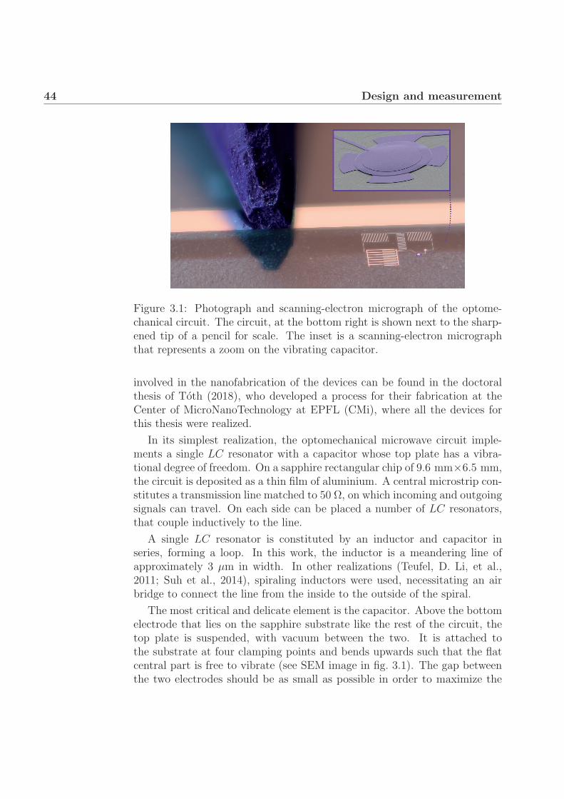
44 Design and measurement
Figure 3.1: Photograph and scanning-electron micrograph of the optome-chanical circuit. The circuit, at the bottom right is shown next to the sharp-ened tip of a pencil for scale. The inset is a scanning-electron micrographthat represents a zoom on the vibrating capacitor.
involved in the nanofabrication of the devices can be found in the doctoralthesis of Toth (2018), who developed a process for their fabrication at theCenter of MicroNanoTechnology at EPFL (CMi), where all the devices forthis thesis were realized.
In its simplest realization, the optomechanical microwave circuit imple-ments a single LC resonator with a capacitor whose top plate has a vibra-tional degree of freedom. On a sapphire rectangular chip of 9.6 mm×6.5 mm,the circuit is deposited as a thin film of aluminium. A central microstrip con-stitutes a transmission line matched to 50 Ω, on which incoming and outgoingsignals can travel. On each side can be placed a number of LC resonators,that couple inductively to the line.
A single LC resonator is constituted by an inductor and capacitor inseries, forming a loop. In this work, the inductor is a meandering line ofapproximately 3 μm in width. In other realizations (Teufel, D. Li, et al.,2011; Suh et al., 2014), spiraling inductors were used, necessitating an airbridge to connect the line from the inside to the outside of the spiral.
The most critical and delicate element is the capacitor. Above the bottomelectrode that lies on the sapphire substrate like the rest of the circuit, thetop plate is suspended, with vacuum between the two. It is attached tothe substrate at four clamping points and bends upwards such that the flatcentral part is free to vibrate (see SEM image in fig. 3.1). The gap betweenthe two electrodes should be as small as possible in order to maximize the

3.1 Fabrication of the devices 45
optomechanical coupling strength (see eq. (2.125)). We estimate the gap tobe approximately 40 nm for most working devices (the estimation relies onsimulations, as detailed in section 3.2).
The fabrication of the capacitor compounds several challenges. For one, afloating structure is especially vulnerable. For instance, the slanted sidewallfrom the clamping point to the flat electrode can tear, or under some condi-tions the whole top plate can collapse and stick permanently to the bottomplate. Moreover, the design of the resonance frequency of the microwavecircuit depends critically on the rest position of the plate, which is hard tocontrol. Beyond the constraints on the microwave properties, the top plateshould also have good mechanical properties, such as a stable resonance fre-quency and low mechanical losses. The local stress in the aluminium filmaffects strongly those properties and is hard to be made uniform and repro-ducible. It depends on the details of the deposition process but can also bemodified by heating, for instance by intentionally annealing the sample afterfabrication.
A schematic representation of the main steps in the fabrication processis shown in fig. 3.2. The bottom layer of aluminium is first deposited (I)and patterned (II) to form most of the circuit and the bottom plate. Thena layer of amorphous silicon is deposited as a sacrificial layer (III) and itselfpatterned (IV and V). This forms the protective layer that preserves a gapwith the bottom plate when the second aluminium film is deposited to formthe top plate (VI) and patterned (VII). Both aluminium films are 100 nmthick. The final crucial step is to etch the sacrificial layer (VIII) that must beremoved in order to release the top plate that eventually floats freely abovethe bottom plate.
This final release is one of the most important as well as delicate steps.This is done with a pulsed vapour XeF2 etch. Relatively small openings onthe sides prevent the etching from being uniform and must progress fromthe circumference to the center of the electrode. The chemical process isexothermic and care must be taken for it not to be too fast and damage thetop film by overheating it, since the heat changes the stress in an undesiredway. This might increase the chance for the top plate to collapse or affect themechanical properties by making the vibrational mode spatially distorted.

46 Design and measurement
Sapphire (RCA cleaned, annealed) SapphireAl (100nm)
SapphireAl
SapphireAlaSi
~150 nm
SapphireAlaSi
SapphireAlaSi
Al (100nm)
SapphireAlaSiAl
SapphireAl
Al
AZ1512
SapphireAlaSi
I. II.
III.
IV.V.
VI.
VII. VIII.
Figure 3.2: Schematic of the main steps of fabrication of the chips. See maintext for a description of each step. Figure courtesy of L. D. Toth, reproducedfrom Toth (2018).
3.2 Simulation tools as aides for design and
characterization
Since the aim is to construct devices that realize ideal LC resonators, thenecessity of simulations tools is not evident and should be motivated. Aswas shown in sections 2.3.1 and 2.3.3, only a few constants (L, C and themutual inductance M) are required to know the resonance frequency of themicrowave resonator and how it couples to the waveguide. They can inprinciple be estimated purely based on the geometry. Only the resistance ofthe circuit R is a priori fabrication-dependent and should be measured.
In fact, the lumped-element model is not always valid for our devices.Their relatively large size, of several millimeters, amounts to a significantfraction of the wavelength of microwaves at the frequency of interest (about3 cm at a frequency of 5 GHz), due the finite velocity of electromagneticwaves that travel at around half the vacuum velocity c in microwave circuits.Take for example a loop of wire, which normally has an inductance scalingwith the inscribed area. For large frequencies at which the loop length iscomparable to the wavelength, the effective inductance is reduced. Not allthe wire carries the same current. The changing phase of the travelling waveimplies that the current oscillates along the wire and cancels at nodes everyhalf wavelength.
Simulations are thus required for larger circuits that cannot be properlymodeled with lumped elements such as individual capacitors and inductors.

3.2 Simulation tools 47
The effective role of each element in the circuit depends critically in practiceon the boundary conditions and surrounding elements. Two parts of a circuitmight behave differently when connected to one another compared to on theirown. For this reason, on top of estimations and simulations for the individualcomponents, it is useful to simulate the circuit as a whole in order to verifythat the model makes sense.
For the work of this thesis, simulations were used mainly to aid the designof the circuit on the chips. As the nanofabrication of the devices is costlyin terms of labor and time, a new design should ideally be well simulatedbefore it is implemented. This is unfortunately not entirely feasible. Theactual properties of the circuit depend on details in the fabrication processthat cannot be known perfectly a priori. Namely those are the rest positionof the capacitor plate after release, when cooled at cryogenic temperatures,and the kinetic inductance of the material.
Superconducting materials have two contributions to their inductance.The first, “geometric” component relates to the potential energy of the mag-netic field induced by the currents in the material, which scales with theinscribed area for a loop. On top of that there is a second, kinetic contri-bution to the inductance (Cardwell and Ginley, 2003). Since resistance isvirtually absent from superconductors, the Cooper pairs that carry chargescan reach very large velocities to supply a given current. Despite their lowmasses, this can make their kinetic energy appreciable and comparable to themagnetic energy. The kinetic inductance depends on the number of availablecharge carriers in the material: the fewer there are, the faster they musttravel to achieve a given current and therefore the larger the kinetic energyrequired. This depends heavily on the fabrication as it depends on the exactcross-section of the material, and the width and thickness of the lines canvary slightly for different fabrication processes.
Simulations cannot then predict measurements ex nihilo. The two mustwork hand in hand. A typical chronology is the following. A new circuitdesign is conceived based on approximate estimations of the gap distance andthe kinetic inductance based on earlier experiments. The design is fabricatedmultiple times on the same wafer with a range of variation for the topologyof the circuits, with different sizes for the inductors or the capacitors. Oneof the fabricated devices is measured and its properties are compared to thesimulation. This allows the correct gap size and kinetic inductance of thebatch to be computed. Finally, the device with the ideal parameters can beselected in the parameter range and measured.

48 Design and measurement
Mag
nitu
de o
f cur
rent
den
sity
(a.u
.)100
101
102
feedline feedline
anti-symmetric, dark mode at 4.26 GHz(used as primary mode)
symmetric, bright mode at 5.48 GHz(used as auxiliary mode)
current cancelled
Figure 3.3: Example of a Sonnet simulation. The current density is rep-resented in a simulation of the full circuit, including its coupling to thetransmission line (labeled feedline). The circuit in question is the hybridcircuit introduced in section 4.2. Figure reproduced from the supplementaryinformation of Toth, Bernier, Nunnenkamp, et al. (2017).
3.2.1 Sonnet software
The main simulation tool that we used in the work of this thesis is Sonnet1.This is a general software to compute the response of microwave circuitswith a flat topology (or constituted of several flat parallel layers). As wellas simulating individual components to design the inductors and capacitors,it is powerful enough to simulate the circuit in its entirety, even including atransmission line (as illustrated in fig. 3.3). This makes it a very completetool and extremely useful to test the limits of the lumped-element model.
We review schematically how Sonnet functions in the following. A morethorough exposition of the theory is done in Rautio, J. C. (1986) and Rautioand Harrington (1987). The box that contains the circuit is modeled as avertical waveguide in which several horizontal planes form boundary condi-tions between different dielectric layers. Sitting on top of a dielectric thatrepresents the substrate, the circuit is constituted of metal patches on one (ormore) such boundary planes. The patches are conceptually split into a num-ber of segments. If a current flows into one of the segments, electromagneticwaves will be emitted in the waveguide, both upwards and downwards, andwill reflect on the boundary conditions to form standing waves. The fields
1 https://www.sonnetsoftware.com/
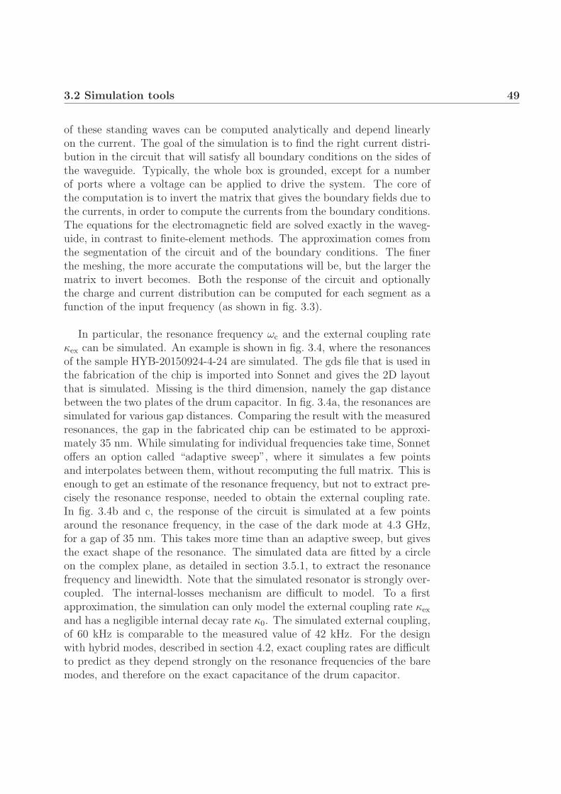
3.2 Simulation tools 49
of these standing waves can be computed analytically and depend linearlyon the current. The goal of the simulation is to find the right current distri-bution in the circuit that will satisfy all boundary conditions on the sides ofthe waveguide. Typically, the whole box is grounded, except for a numberof ports where a voltage can be applied to drive the system. The core ofthe computation is to invert the matrix that gives the boundary fields due tothe currents, in order to compute the currents from the boundary conditions.The equations for the electromagnetic field are solved exactly in the waveg-uide, in contrast to finite-element methods. The approximation comes fromthe segmentation of the circuit and of the boundary conditions. The finerthe meshing, the more accurate the computations will be, but the larger thematrix to invert becomes. Both the response of the circuit and optionallythe charge and current distribution can be computed for each segment as afunction of the input frequency (as shown in fig. 3.3).
In particular, the resonance frequency ωc and the external coupling rateκex can be simulated. An example is shown in fig. 3.4, where the resonancesof the sample HYB-20150924-4-24 are simulated. The gds file that is used inthe fabrication of the chip is imported into Sonnet and gives the 2D layoutthat is simulated. Missing is the third dimension, namely the gap distancebetween the two plates of the drum capacitor. In fig. 3.4a, the resonances aresimulated for various gap distances. Comparing the result with the measuredresonances, the gap in the fabricated chip can be estimated to be approxi-mately 35 nm. While simulating for individual frequencies take time, Sonnetoffers an option called “adaptive sweep”, where it simulates a few pointsand interpolates between them, without recomputing the full matrix. This isenough to get an estimate of the resonance frequency, but not to extract pre-cisely the resonance response, needed to obtain the external coupling rate.In fig. 3.4b and c, the response of the circuit is simulated at a few pointsaround the resonance frequency, in the case of the dark mode at 4.3 GHz,for a gap of 35 nm. This takes more time than an adaptive sweep, but givesthe exact shape of the resonance. The simulated data are fitted by a circleon the complex plane, as detailed in section 3.5.1, to extract the resonancefrequency and linewidth. Note that the simulated resonator is strongly over-coupled. The internal-losses mechanism are difficult to model. To a firstapproximation, the simulation can only model the external coupling rate κex
and has a negligible internal decay rate κ0. The simulated external coupling,of 60 kHz is comparable to the measured value of 42 kHz. For the designwith hybrid modes, described in section 4.2, exact coupling rates are difficultto predict as they depend strongly on the resonance frequencies of the baremodes, and therefore on the exact capacitance of the drum capacitor.

50 Design and measurement
(a)
(b) (c)
Figure 3.4: Microwave resonances simulated with Sonnet for the sampleHYB-20150924-4-24. (a) Approximate resonance frequencies of the two hy-brid modes as a function of the capacitor gap size. The horizontal dashedlines give the resonances measured in the experiment, which correspond to agap of about 35 nm. The adaptive sweep is used in Sonnet to find approx-imate resonance frequencies. (b,c) Fitted response of the dark mode near4.3 GHz, to extract the precise resonance frequency and the external cou-pling rate κex, for a simulated gap of 35 nm. The resonance is fitted with acircle on a complex plane, as explained in section 3.5.1.

3.3 Experimental setup 51
3.3 Experimental setup
We list in the following the equipment and components that are employedin the experiment. In section 3.3.1, we describe the design and assembly ofthe sample holder in which fabricated chips are fixed for measurement. Insection 3.3.2, the mounting and wire bonding of the chip inside the holderis detailed. In section 3.3.3, the components installed inside the dilutionrefrigerator are presented. In section 3.3.4, the equipment that stands outsidethe dilution refrigerator at room temperature is described.
3.3.1 Sample holder
The chips that contain the circuits to be studied are mounted inside a sampleholder to perform the measurements. We describe here the design of thesample holders and how it is assembled.
The sample holder fulfills multiple purposes. On a very pragmatic level,it provides a structure with SMA connectors that can easily be connected tothe rest of the experimental setup by attaching coaxial cables. Importantly,it constitutes a grounded shielding that protects the circuit from any strayradiation. This both reduces the possibility for microwave noise to couplein the cavities and prevents higher frequency radiation from disturbing thesuperconductors, for instance by creating quasiparticles (Barends et al., 2011;Corcoles et al., 2011). Finally, it forms a large heat reservoir that should bewell thermally coupled to the cryogenic environment such that the circuit issurrounded by a cold environment and cools down properly.
The sample holder design is shown in fig. 3.5 and the files are availableonline (Bernier, 2018). The central compartment, shaped like an “H” holdsthe chip. On both sides are rectangular receptacles to place small printedcircuit boards (PCB) that serve as intermediary between the chip and the twoSMA connectors. The connectors are placed on both ends through cylindricalholes and held in place by screws in threaded holes (M2.5) on the outside.Next to the PCB receptacles are pads where certain parts of the circuits canbe grounded directly. A lid is designed to close the box, leaving as littleopen volume as possible inside. This pushes the resonance frequencies of the3D cavity modes upwards much beyond the frequencies of the circuit, wherethey cannot disturb it. Two vertical holes pass through the box and lid, withthreading in the box (M3). This serves the double purpose of closing the lidtightly and securely, as well as clamping the sample holder to the breadboardin the the cryostat to ensure good thermalization (see fig. 3.6).

52 Design and measurement
(a) (b)
Figure 3.5: Photographs of the sample holder. (a) Photograph of themounted sample holder with a chip mounted and wire-bonded. A shortedcap is attached to one port to measure in reflection. (b) Photograph takenwith a microscope, zooming on the wire bonds between the chip and thePCB transmission line. The soldering of the SMA central pin to the PCB isvisible in the top right.
The sample holders are realized out of a single piece of OFHC (oxygen-free high conductivity) copper, at the mechanical workshop of the instituteof physics at EPFL2. It is important to use OFHC copper for two reasons.First, it has a high thermal conductivity even at cryogenic temperatures.Second, it contains minimal magnetic impurities whose stray magnetic fieldscan create vortices in the superconductor. The PCBs are fabricated by theelectronic workshop (ACI) of the electrical engineering institute of EPFL3.Layers of 18 μm of copper are deposited on both sides of a substrate of 0.3 mmthickness made of FR-4 (a dielectric material that works well at cryogenictemperatures).
To assemble the sample holders, the PCB must be glued in place andthe SMA connectors soldered to the PCBs. The conductive epoxy Epo-TekH20E is used to keep the PCB solidly in place cooldown after cooldown, andconnect its ground plane to the sample holder. First, both the sample holderreceptacle surface and the ground plane of the PCB are cleaned with a fiberbrush to remove the copper oxide layer and guarantee good long-term adhe-sion. The corners of the PCB can be cut with pliers such that it fits betterthe receptacle which has rounded edges. After cutting the PCB, the roughedges can be smoothed with sand paper. While we would like the wire bondsbetween the chip and the PCB to be as short as possible, it is not possible tofabricate the PCB with a copper transmission line until the edge. One cancut the end of the PCB with pliers to have the transmission line as close to
2https://iphys.epfl.ch/page-139526-en.html3https://sti-ateliers.epfl.ch/page-19942.html

3.3 Experimental setup 53
the edge as possible. The mixed epoxy is applied in small quantity and thepieces assembled. To cure the epoxy, the lowest recommenced temperatureof 80 ◦C is used, placing the sample holder on a hot plate for at least 90 mn.
The final step to prepare the sample holder is to solder the SMA connector.We used the model R125.462.001 from Radiall. It is critical to prevent theflux from covering all the surface of the PCB copper plate when soldering.One technique is to protect the half of the copper line that is closest to thechip with a piece of masking tape. The SMA connector is fixed with twoscrews and the central pin is soldered to the PCB (see the assembled sampleholder in fig. 3.5). It is advisable to test the sample holder with a multimeterto check the soldering and ensure that there is no accidental short circuit ofthe central pin to the ground. One location to be wary of is between thedielectric of the SMA connector and the PCB. There can be a gap, whereconductive debris might fall and short the central pin.
With every cooldown of new chips, successive wire bonding to the PCBline degrades the copper surface. At some point, it becomes difficult to wirebond successfully close to the edge and minimize the bond length. The PCBcan then be replaced. The connector is unsoldered and removed. Then thePCB is detached using a blade to break the epoxy. The surface of the sampleholder is cleaned thoroughly with a fiber brush or a piece of sand paper toremove all traces of the epoxy. Finally a new PCB can be glued in place withthe steps outlined above and the sample holder reassembled.
3.3.2 Mounting and bonding the chip
The chips are glued and wire-bonded to the sample holder to be measuredat cryogenic temperatures. We describe here this procedure.
First, the sample holder is thoroughly cleaned. Residues of glue in thecentral compartment are removed with isopropanol and all surfaces to beglued or wire bonded are brushed to remove the oxide layer. Small debrisare removed using compressed air. The cleaning should be completed at thisstage, since once the chip is glued it is no longer possible to do so in ordernot to damage the fragile capacitors.
Silver conductive paint is used to attach the chip to the sample holder.It must conduct to connect electrically the backside aluminium layer to thesample holder and form the ground plane. Not too much glue should beused. The excess overflows on the sides when the chip is gently pressed downto ensure good contact on the whole surface. It can short-circuit the centralline of the PCB or the chip and accidentally ground them. Before cooling

54 Design and measurement
down the chip, it is useful to verify with a multimeter if the central line isaccidentally grounded, either with paint or with a fallen wire bond. Thepaint used is CMR RS186 (manufactured by RS components). The glue isleft to dry for about an hour at least to ensure the chip is firmly fixed beforeit is wire bonded.
The wire bonding is performed with a TPT HB10 machine from the CMi,with an aluminium wire 33 μm in diameter. Both ends of the central trans-mission line on the chip are connected to the PCBs with about 10 bondseach. If the device is measured in reflection, it is also possible to bond oneend of the line to one ground pad of the sample holder next to the PCB.
The sample holder has two ports such that the chip can be measured bothin transmission and in reflection. There are advantages and inconveniencesfor both cases. As explained in section 3.5.1, measuring the microwave reso-nances in transmission is required to calibrate out any impedance mismatchon the line and extract precisely the internal and external dissipation ratesκ0 and κex. This comes at the cost of a reduced coupling rate compared to asingle-sided cavity (see section 2.3.3). More importantly, it also reduces thesignal to noise for the emissions from the cavity. Outgoing signals divide intotravelling waves in two directions and at best only half of the total signal canbe measured in any single direction. For measurements where the signal-to-noise ratio is essential (for emission close to the quantum limit), a one-sidedcavity is greatly beneficial and the devices are measured in reflection only.
Altering appropriately the boundary conditions at one end of the centraltransmission line of the chip reflects incoming signals and allows single-sidedmeasurements. Not all reflecting boundary conditions are equivalent. Asshown in section 2.3.2, both open and short-circuited transmission lines arefully reflective. However, the resonators are coupled inductively to the feed-line and the coupling strength depends on the amplitude of current locallyon the line. An open boundary condition forms a node in the current whichcancels exactly at the boundary point. Near an open boundary, any inductivecoupling is strongly reduced up to a distance of a quarter wavelength awaywhere the current has an antinode and the coupling is restored. To achievesufficient coupling rates, short-circuited boundaries are beneficial since theyhave a maximum of current instead. The distance on the line between theshort circuit and the resonator determines the coupling rate. For consistentcoupling rates, the resonators are placed always at the same position on thechip.
A short-circuited cap, shown in fig. 3.5a, is connected to the sample holderto achieve reflective boundary conditions in a non-destructive way. It isconstructed by soldering the central pin of an SMA connector to the outer

3.3 Experimental setup 55
shield to ground it. Optionally, the line can also be grounded to the sampleholder with wire bonds. This gives a shorted boundary condition a fewmillimeters closer to the chip.
3.3.3 Inside the dilution refrigerator
The devices are mounted inside a BF-LD250 dilution refrigerator from BlueFors. We describe here what components are installed inside. One set oflines for input and output signals to a sample holder is described. Usually,two similar sets are installed such that two devices can be measured in agiven cooldown. We review in the following what a typical setup entails andthe rationale behind each component. The actual components used for theexperiments of this thesis deviate slightly and the differences are introducedin the respective chapters.
In summary, input and output lines are needed for signals to propagate toand back from the device that is mounted to the plate of the mixing chamber,the coldest point of the dilution refrigerator. Three lines are needed in fact.One carries the input signals to the chip. A second carries away the outputsignals to be amplified and measured. A third, auxiliary, line can be used toperform tone cancellation if required. In the following, we first describe theinput lines and how the signal is attenuated to lower the thermal noise, thenhow the signals are coupled to the chip at the base plate, finally the outputline and how the outgoing signal is amplified.
One key requirement when interfacing microwave signals from room tem-perature with devices at cryogenic temperatures is to reduce the intrinsicthermal noise of the former as to not disturb the latter. At 300 K, thethermal noise emitted from any load has a symmetrized spectral density of1250 quanta/s/Hz at 5 GHz (from eq. (2.57)). This corresponds in units ofpower to -173.8 dBm/Hz. This level of noise provides a thermal bath muchlarger than the cryogenic temperature and would heat the system, prevent-ing any measurement of weak quantum signals. The noise travelling on theinput line must be reduced with attenuators that are thermalized to a lowertemperature.
An attenuator can be modeled as a beam-splitter that takes a fraction αof the incoming signal and replaces it with a fraction 1 − α of the noise ofa matched load. This added noise is necessary for the time-evolution to beunitary and the commutation relations of the travelling mode to be preserved.This implies
Soutδa†δa[ω] = αSin
δa†δa[ω] + (1− α)Sloadδa†δa[ω] (3.1)
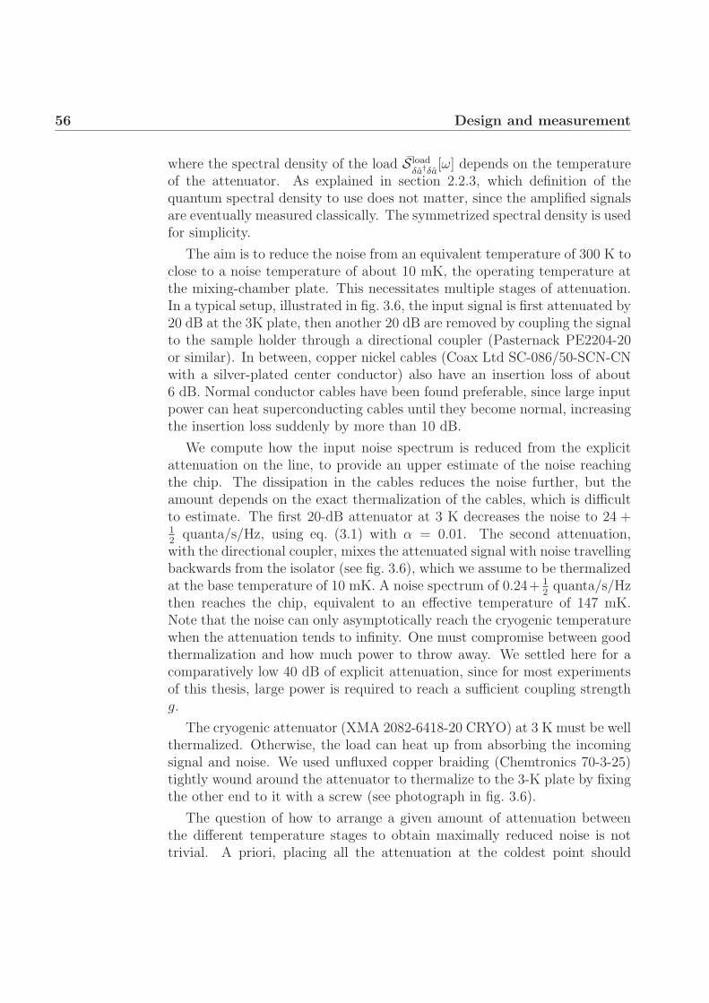
56 Design and measurement
where the spectral density of the load S loadδa†δa[ω] depends on the temperature
of the attenuator. As explained in section 2.2.3, which definition of thequantum spectral density to use does not matter, since the amplified signalsare eventually measured classically. The symmetrized spectral density is usedfor simplicity.
The aim is to reduce the noise from an equivalent temperature of 300 K toclose to a noise temperature of about 10 mK, the operating temperature atthe mixing-chamber plate. This necessitates multiple stages of attenuation.In a typical setup, illustrated in fig. 3.6, the input signal is first attenuated by20 dB at the 3K plate, then another 20 dB are removed by coupling the signalto the sample holder through a directional coupler (Pasternack PE2204-20or similar). In between, copper nickel cables (Coax Ltd SC-086/50-SCN-CNwith a silver-plated center conductor) also have an insertion loss of about6 dB. Normal conductor cables have been found preferable, since large inputpower can heat superconducting cables until they become normal, increasingthe insertion loss suddenly by more than 10 dB.
We compute how the input noise spectrum is reduced from the explicitattenuation on the line, to provide an upper estimate of the noise reachingthe chip. The dissipation in the cables reduces the noise further, but theamount depends on the exact thermalization of the cables, which is difficultto estimate. The first 20-dB attenuator at 3 K decreases the noise to 24 +12quanta/s/Hz, using eq. (3.1) with α = 0.01. The second attenuation,
with the directional coupler, mixes the attenuated signal with noise travellingbackwards from the isolator (see fig. 3.6), which we assume to be thermalizedat the base temperature of 10 mK. A noise spectrum of 0.24+ 1
2quanta/s/Hz
then reaches the chip, equivalent to an effective temperature of 147 mK.Note that the noise can only asymptotically reach the cryogenic temperaturewhen the attenuation tends to infinity. One must compromise between goodthermalization and how much power to throw away. We settled here for acomparatively low 40 dB of explicit attenuation, since for most experimentsof this thesis, large power is required to reach a sufficient coupling strengthg.
The cryogenic attenuator (XMA 2082-6418-20 CRYO) at 3 K must be wellthermalized. Otherwise, the load can heat up from absorbing the incomingsignal and noise. We used unfluxed copper braiding (Chemtronics 70-3-25)tightly wound around the attenuator to thermalize to the 3-K plate by fixingthe other end to it with a screw (see photograph in fig. 3.6).
The question of how to arrange a given amount of attenuation betweenthe different temperature stages to obtain maximally reduced noise is nottrivial. A priori, placing all the attenuation at the coldest point should

3.3 Experimental setup 57
20 dB DUT
3 K
800 mK
10 mK
20 dB HEMT
input outputaux.
Figure 3.6: Schematics of the setup inside the dilution refrigerator. Illus-trative photographs are shown for corresponding key components. In a redframe, the 20-dB attenuators on the the 3-K plate. In a light-blue frame, thechip in the sample holder is interfaced with a directional coupler. In a yellowframe, cryogenic circulators isolate the device from backpropagating noise.In a green frame, low-pass filter shield the superconducting circuit from highfrequency radiation. In a purple frame, the HEMT amplifiers are insulatedfrom the line by inner DC blocks.

58 Design and measurement
provide the lowest noise, since the removed noise is replace by the lowestpossible amount. Technical limitations make this solution not ideal. Thedilution refrigerator has a finite cooling power at the mixing chamber (of theorder of 10 μW). Dissipating all the power there would heat up the wholeplate. The compromise is to remove a large part of the noise at the 3 Kplate where the cooling power is larger. One trick to limit the absorption atthe base plate is to use a directional coupler instead of an attenuator. Sincethe four arms of the beam splitters are controlled, this allows the discardedsignal and noise to be redirected to higher temperature stages for dissipation,while adding noise that is thermalized at base temperature.
We now describe the components mounted on the base plate. Tubularfilters (K&L 6L250-00089 low-pass up to 12 GHz) are used on all lines (seephotograph in fig. 3.6) to protect from higher frequency noise that can affectthe superconducting circuits by creating quasiparticles. Formable coppercables (Pasternack PE39415) connect the lines to the components placedon the breadboard plate. We removed the paint on the backside of thedirectional coupler (Pasternack PE2204-20 or similar) with sand paper tohave better thermal contact to the copper plate. The sample holder bottomthickness was designed for it to be level with the directional coupler, andconnect them with a male-male SMA connector (see photograph in fig. 3.6).Before attaching the sample holder to the breadboard plate, the two surfacesthat will become in contact are cleaned with a fiber brush to remove theoxide layer and increase the thermal contact.
The discarded signal from the directional coupler travels upwards on aline identical to the input line. The power dissipates in the cables and atthe attenuator at 3 K. This line can also be used for tone cancellation of themicrowave pump tones before amplification.
In the output line, cryogenic isolators are used to prevent noise from prop-agating backwards to the device. Cryogenic circulators (Raditek RADC-4-8-Cryo with a bandwidth 4-8 GHz) are used with one port terminated bya cryogenic 20 dB attenuator and a cryogenic 50-Ω matched load (XMA2001-6112-02). The attenuator is redundant but provides a better surface totighten the copper braiding for thermalization (see photograph in fig. 3.6).Alternatively, cryogenic isolators (Quinstar QCI-075900XM00 with a band-width 3-12 GHz) are also used for a larger bandwidth. The sample holder istypically terminated by a shorted cap to measure in reflection.
Finally, we describe the output lines. The signal to be measured trav-els upwards on niobium titanium superconducting cables (Coax Ltd SC-086/50-NbTi-NbTi) to the 3 K plate where it is amplified with a high-electron-mobility-transistor (HEMT) amplifier. An inner DC block (Paster-

3.3 Experimental setup 59
nack PE8210) thermally decouples the amplifier from the superconductinglines and prevents the amplifier heat increasing the temperature of the cablesuntil they are no longer superconducting. Four HEMT models were used allfrom Low Noise factory: LNF-LNC4-16A with bandwidth 4-16 GHz, twounits LNF-LNC1-12A with bandwidth 1-12 GHz, and LNF-LNC4-8C withbandwidth 4-8 GHz with a lower added noise. The amplifiers do dissipateheat, which should be removed. To that end, they are thermally coupledto the 3 K plate with copper braids, attached to the HEMT bodies withscrews (see fig. 3.6). The excess length of the DC lines for the power sup-plies of the amplifiers were attached to the dilution refrigerator posts withPTFE (“teflon”) tape (Klingerflon BS7786) that is compatible with vacuumand cryogenic temperatures. Between the 3 K plate and room temperature,beryllium copper cables (Coax Ltd SC-219/50-B-B) are installed for inputand output lines.
3.3.4 Room-temperature equipment
In this section, we review the microwave components outside the dilutionrefrigerator, for a typical experiment (as schematically represented in fig. 3.7).The two most common measurements are of the linear microwave responseof the system, and of the emitted spectrum. They are done while one ormultiple microwave tones are applied to the system to alter its state.
Many microwave sources are employed in the experiments of this thesis.They are Rohde & Schwartz SMB 100A, Rohde & Schwartz SMF 100A,Keysight MXG N5183B, and Rohde & Schwartz SGS 100A. For weak tones,the sources can be used interchangeably. Only for the strong microwavepumps needed to attain large coupling strengths g do the noise properties ofthe source become relevant. Usually, the measured system is only sensitive tonoise in a given quadrature (for example phase noise in sideband cooling) andat the specific narrow frequency range that corresponds to the mechanicalsideband frequency (offset from the tone by Ωm). The sources all have variousnoise emission that depends on the frequency of the source, the frequency ofnoise with respect to the carrier, and on the power setting. We calibrate thenoise level for all the sources (see section 3.4.1) and select the device withthe lowest noise in the relevant bandwidth when the noise is critical.
We filter the signal from the sources in multiple stages. Ideally, the noisein the sensitive bandwidth should be reduced to the level of the thermalnoise background, although in practice that is not always possible for thestrongest pump powers. First, when we work simultaneously with multiplemicrowave resonances of the optomechanical circuit, the far-detuned noise of

60 Design and measurement
VNAPump SAProbe
20 dBlter
cavity
ϕ
input outputaux.
Figure 3.7: Room-temperature equipment that is connected to the ports ofthe dilution refrigerator (see fig. 3.6). The microwave sources (here labeledPump and Probe) are filtered by band-pass (or high- and low-pass) filtersand combined. For very large pump powers, it is necessary to use a filtercavity to reduce noise in the sensitive bandwidth. The output port of theVNA is combined to the signals with a 20-dB directional coupler, before thesignals are sent to the input port. A double DC block prevents ground loopsinside the dilution refrigerator. The output signals go through a double DCblock and an isolator before being amplified. They are measured either byconnecting the line to the input port of the VNA for a response measurementor by connecting the line to the spectrum analyzer (SA). Optionally, part ofthe strong pump power is split off at the input for tone cancellation. Variableattenuators and phase shifters are used to set its amplitude and phase, inorder to cancel the pump tone after it interacts with the chip.

3.3 Experimental setup 61
the sources is relevant, since the noise of a pump at one frequency can affectanother cavity hundreds of MHz away. Standard filters (such as the band-pass filter Mini-Circuits VBFZ-5500-S+) easily solve the issue by removingthe noise far from the carrier.
For the noise close to the tone frequency, custom tunable filter cavities(shown in fig. 3.8) filter out the noise in the critical bandwidth. The cavities,similar in design to those of Lecocq, Teufel, et al. (2015), are fabricated bythe mechanical workshop out of two blocks of copper. A threading betweenthe two pieces allows the tuning of the resonance frequency by choosing thelength of the inner 3D cylindrical cavity. A threaded ring can block thecavity in a specific setting. A female-female SMA connector serves as aninterface to the cavity. Inside, a short length of solder wire (about 2 cm)is inserted in the connector and serves as a formable antenna that can bebent to vary the coupling rate of the cavity to the line. The goal is to reachthe critical coupling rate, with equal internal and external dissipation rates.Then the reflection coefficient dips to zero at the resonance frequency. Acirculator (Pasternack PE8402) turns the single-sided cavity into a notchfilter, which removes noise at the resonance frequency. Varying the lengthof the cavity allows the tuning of the filtered frequency over about 1 GHz.Multiple cavities of different sizes are needed to cover the range of microwavecavity frequencies in the optomechanical circuits. A cavity linewidth of about1 MHz close to critical coupling is achieved. A small enough bandwidth isnecessary to reduce the noise Ωm/(2π) ≈ 5 − 10 MHz away from the tonefrequency without absorbing the tone as well.
For a given measurement, the procedure is the following. First the sys-tem is measured without the filter cavity. The frequency of the relevantmechanical sideband is measured precisely. Then the filter cavity frequencyis tuned and locked to that frequency, while monitoring its response. Forfastest measurement, the response of the filter cavity is measured with theVNA. Since the filter cavity can be affected by moving the cables, it is betterto do the final tuning when it is connected to the source it should filter. Weuse the source as a probe tone, and measure the amplitude response with thespectrum analyzer. This allows the precise tuning of the filter cavity in situ,with no need to change the connected cables afterwards. The coupling ratecan be adjusted by rotating the SMA connector, to change the orientationof the antenna inside the cavity and its overlap with the mode.
The pump tone can be split in two and one half sent to the auxiliary linefor tone cancellation. A variable attenuator (Pasternack PE7065-7) and avariable phase shifter (Pasternack PE8246) are tuned in order for the toneto cancel right after the directional coupler in the dilution refrigerator. Tone
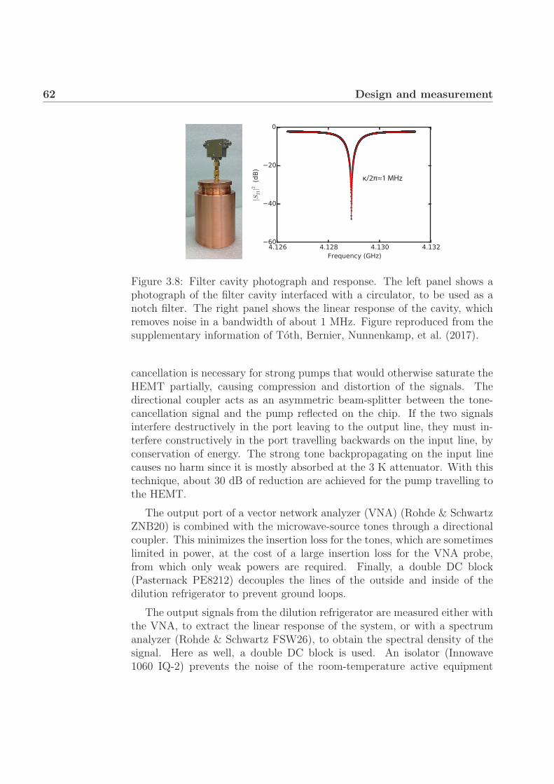
62 Design and measurement
κ/2π≈1 MHz
Figure 3.8: Filter cavity photograph and response. The left panel shows aphotograph of the filter cavity interfaced with a circulator, to be used as anotch filter. The right panel shows the linear response of the cavity, whichremoves noise in a bandwidth of about 1 MHz. Figure reproduced from thesupplementary information of Toth, Bernier, Nunnenkamp, et al. (2017).
cancellation is necessary for strong pumps that would otherwise saturate theHEMT partially, causing compression and distortion of the signals. Thedirectional coupler acts as an asymmetric beam-splitter between the tone-cancellation signal and the pump reflected on the chip. If the two signalsinterfere destructively in the port leaving to the output line, they must in-terfere constructively in the port travelling backwards on the input line, byconservation of energy. The strong tone backpropagating on the input linecauses no harm since it is mostly absorbed at the 3 K attenuator. With thistechnique, about 30 dB of reduction are achieved for the pump travelling tothe HEMT.
The output port of a vector network analyzer (VNA) (Rohde & SchwartzZNB20) is combined with the microwave-source tones through a directionalcoupler. This minimizes the insertion loss for the tones, which are sometimeslimited in power, at the cost of a large insertion loss for the VNA probe,from which only weak powers are required. Finally, a double DC block(Pasternack PE8212) decouples the lines of the outside and inside of thedilution refrigerator to prevent ground loops.
The output signals from the dilution refrigerator are measured either withthe VNA, to extract the linear response of the system, or with a spectrumanalyzer (Rohde & Schwartz FSW26), to obtain the spectral density of thesignal. Here as well, a double DC block is used. An isolator (Innowave1060 IQ-2) prevents the noise of the room-temperature active equipment

3.4 Noise calibrations 63
from travelling back inside the dilution refrigerator. An amplifier (Mini-circuits ZVA-183-S+) gives the last stage of gain (26 dB) before the cableis either connected to the VNA or the spectrum analyzer, depending on themeasurement. It is important for the added noise of the last amplifier tobe small compared to the output noise of the HEMT, to ensure that thewhole amplification chain is limited by the HEMT. The cables are room-temperature are Huber Suhner Sucotest 18 cables, as well as formable cables(Pasternack PE39415) for smaller lengths.
All the microwave sources as well as the VNA and the spectrum analyzerare locked to the same reference clock. This ensures that the uncertainty inthe relative frequencies of all tones is minimal, and that the relative phases ofthe microwave sources are fixed. The reference clock from the FSW spectrumanalyzer is distributed to all other devices using a low-noise distributionamplifier (Oscilloquartz OSA 5020).
3.4 Noise calibrations
The experiments of this thesis are restricted to linearized interaction betweenharmonic oscillators. As such, the only quantum aspect resides in the limitof the lowest amount of noise imposed by quantum mechanics. Careful cal-ibration of the noise sources in the experiment is capital, if any statementabout quantum noise is to be made. Apart from the thermal noise fromroom temperature, that need to be dealt with through attenuation at cryo-genic temperatures (see section 3.3.3), there are two main sources of noisefrom active devices in the measurement. The first is the microwave signalgenerators, whose tones have phase and amplitude noise. The second is theadded noise of the HEMT in the amplification process. In the following, wedetail how both are calibrated.
3.4.1 Phase and amplitude noise of the sources
The noise of the microwave sources must be taken into account in the ex-periment. Close to the tone frequency, it can greatly exceed the thermallevel and correspond to a very high effective temperature for the incomingmicrowave field. The optomechanical circuit is however not sensitive at allfrequencies. In general, only two frequency ranges are relevant. First arethe resonances of the microwave cavities. If there is a large noise within theresonance linewidth, the microwave cavity effectively heats up, as it thermal-izes to an average of its internal and external bath temperatures. Second,

64 Design and measurement
if microwave pumps are applied to the optomechanical system, there arefrequencies at which the mechanical mode becomes sensitive to incomingmicrowave signals. Those correspond precisely to the frequencies of the me-chanical sidebands of the pump. At those frequencies, the microwave fieldbeats with the strong pump and results in a force unto the mechanical os-cillator. Equivalently, the pump can be understood to mediate a frequencyconversion pathway between microwave and mechanical frequencies. Thenoise from the mechanical thermal bath is converted to microwave frequen-cies (as the mechanical sideband) and reciprocally microwave noise at thesame frequency is converted to mechanical motion. In effect, the mechani-cal mode is sensitive to the effective temperature of the microwave cavity atthose particular frequencies. In practice, we are concerned mainly with thenoise that reaches the mechanical mode. It is sufficient to have the effectivetemperature of the microwave cavity low enough locally at the frequency thatcorresponds to the mechanical resonance.
Phase and amplitude noise measurement are performed by connecting themicrowave sources to a signal source analyzer (Rohde & Schwartz FSUP).Alternatively, the spectrum analyzer (Rohde & Schwartz FSW26) can beused, with the software option for the Phase Noise application. In the PhaseNoise application, the device locks to the tone of the source. It then measuresthe noise relative to the carrier frequency and power, in dBc/Hz units (noisedensity relative to the power of the carrier). The FSW has an option forAM noise rejection, that removes amplitude noise to measure only phasenoise. That option is only possible when the device is set to the I/Q sweepmode. Otherwise, it is silently ignored. An estimate of the amplitude noiseis obtained by subtracting the phase noise from the total noise.
An example of the noise spectrum of the microwave source Rohde &Schwartz SMF 100A is shown in fig. 3.9. Phase noise dominates over ampli-tude noise for most frequencies. In fig. 3.9b, there is a sharp increase of thenoise when the power increases to 0 dBm. That is related to a change in theinternal setting of the device that depends on the exact implementation ofthe device and is impossible to predict. Amplitude noise increases for largeroutput powers of the device, until it is commensurate with phase noise at20 dBm.
In practice, the measurement should be performed at the precise carrierfrequency and power needed for the microwave pump in a given experiment,since the relative noise can change for different internal settings of the source.When the noise properties are critical, the microwave source with the lowestnoise in the relevant frequency range is picked for that particular experiment.Even the best performing microwave source has a noise exceeding the thermal

3.4 Noise calibrations 65
(a) (b)
Figure 3.9: Measured phase and amplitude noise of Rohde & Schwartz SMF100A. (a) Noise spectrum as a function of frequency offset from the carrierset at a frequency of 6 GHz and at a power of 10 dBm. (b) Noise spectrumas a function of the tone power, offset by 10 MHz from the carrier.
level of -174 dBm/Hz at higher powers and a tunable filter is employed toreduce it as much as possible, as detailed in section 3.3.4.
3.4.2 Calibration of the HEMT
The added noise in the amplification chain to the emission spectrum is im-portant to know, since it gives an absolute scale to which to compare thesignals. In a microwave measurement setup, the many cables and compo-nents prevent from estimating precisely the insertion loss on the line a priori.Even if the characteristics of the individual components are known, theircombination can have reflections and standing waves from slight impedancemismatches that modify the insertion loss as a function of frequency in anon-trivial way. Calibrating the added noise of the full chain, as it stands inthe experiment, allows the reconstruction of the absolute power of the signalas it was emitted at the beginning of the chain. In the following, we give amodel for the gain and added noise in our system, and present the methodused to calibrate the added noise of the HEMT in the signal path.
First, we model the measurement chain and what is the added noise,as represented schematically in fig. 3.10b. The signal of interest, of powerPs is emitted from the device in the sample holder. That constitutes thereference point where we want to know the power of the signal. It is thenattenuated by a fraction α, due to all the components and cables on its way

66 Design and measurement
3 K
800 mK
Variable T
HEMT
output(a)
deviceα GHEMT
attenuation
NTNHEMT
GRT
out(b)
GHEMT
NT
NHEMT
GRT
out(c)
Figure 3.10: Scheme for the calibration of the HEMT amplifiers. (a) Exper-imental setup to calibrate the HEMT. A cryogenic matched load is attachedto the output lines at the base plate. The temperature of the whole plateis tuned to control the temperature of the matched load and inject a knownamount of Johnson noise in the HEMT amplifier. (b) Model of the amplifi-cation chain in a normal experiment, including the insertion loss α betweenthe device and the HEMT. (c) Model for the calibration method. The in-sertion loss α is not accounted for with this method and must be estimatedindependently.

3.4 Noise calibrations 67
to the HEMT. The HEMT amplifier adds a noise NHEMT, then amplifiesboth signal and noise by the power gain GHEMT. The signal travels finally tothe spectrum analyzer where it is measured, with a gain GRT that includesboth room-temperature amplification and all the insertion loss along the line.The measured power is
Pmeas = GRT GHEMT (αPs + (1− α)NT +NHEMT) . (3.2)
The insertion loss before the HEMT contributes a noise NT , due to theeffective temperature of the dissipative part of the attenuation. Ideally, theamplification and added noise at room-temperature after the HEMT shouldadd a noise negligible compared to the amplified HEMT noise GHEMTNHEMT.There is no need to suppose this however. Any extra noise can be absorbedin a slightly increased effective NHEMT, which is taken into account in thecalibration. The complete added noise with respect to the reference point atthe device is
Nadded =1
αNHEMT +
1− α
αNT . (3.3)
The first term is the HEMT noise that is effectively increased by the insertionloss, since the signal-to-noise ratio decreases as a result. The second term,the thermal noise due to the temperature of the dissipative component ofthe attenuation, is normally much smaller than the HEMT noise (with aneffective temperature of ∼ 100 mK compared to ∼ 4 K for the HEMT).While it can usually be neglected, in principle it can also be calibrated aspart of the added noise.
Ideally, the full added noise Nadded can be calibrated. A perfect calibrationscheme consists in replacing the device by a tunable source of noise N knownon an absolute scale. The measured output noise is then
P ideal cal.meas = GRTGHEMTα (N +Nadded) . (3.4)
Two measurements of the output noise for two different known levels of thenoise N suffice to calibrate both the added noise and the absolute gain ofthe full measurement chain Gchain = GRTGHEMTα. The tunable noise sourcemust affect neither the HEMT performance nor the effective temperature ofthe attenuation before the HEMT.
We present now the implemented calibration scheme and how it deviatesfrom the ideal case. The setup is illustrated in fig. 3.10a. The noise source isa cryogenic matched load (XMA 2001-6112-02) fixed to the mixing-chamberplate for thermalization. That implies that the insertion loss between thedevice and the plate is not taken into account in the calibration. Differentnoise temperatures are reached by stabilizing the base plate temperature

68 Design and measurement
to different levels. The mixture of helium 3 and 4 in the dilution cycle isfirst collected, then a small proportion is reinjected and circulated to helpstabilize the temperature. Using a heater at the base plate, the temperaturecan be swept from about 0.8 K to 10 K in a controllable manner. As aconsequence, the leftover attenuation between the base plate and the HEMT(coming mainly from cable losses) is heated as well as the matched load.One cannot then assume that its temperature is constant. In our model,shown in fig. 3.10c, we neglect this contribution to the insertion loss. Thatis equivalent to assuming that the dissipative elements in the insertion lossthermalizes to the same temperature as the matched load. The measurednoise is
P cal.meas = GRTGHEMT (NT +NHEMT) = GRTGHEMTλ (T + THEMT) . (3.5)
The noises NT and NHEMT are large enough to be classical and proportionalto a corresponding effective temperature through a proportionality constantλ. For each frequency point, the measured noise can be fitted as a linearfunction of T (an example is shown in fig. 3.11a). Its intercept with thex-axis corresponds to −THEMT. In effect, the added noise of the HEMT iscompared to the Johnson noise at different temperatures. The calibratedthermometer at the base plate provides the absolute scale that anchors thecalibration. An example of the noise temperature as a function of frequencyis given for the HEMT amplifier LNF-LNC1-12A in fig. 3.11b.
Since it is not calibrated, the insertion loss α must be independently es-timated to properly account for the effective added noise Nadded. The maincontribution comes from the cables, directional coupler and the cryogenic iso-lators between the sample holder and the mixing-chamber plate. In the caseof two Quinstar isolators, their insertion loss was measured to be 1.6 dB at77 K. The components were immersed in liquid nitrogen and their insertionloss measured with the VNA. The insertion loss of these components at basetemperature should be lower (since the resistivity of normal metals increasewith temperature), and this estimate provides an upper-limit for the addednoise. However, the relevant attenuation includes the cables and connectionsbetween the base plate and the HEMT, that is not completely taken intoaccount in our calibration scheme.
3.5 Characterization of the chip
The first step for a newly cooled device is to subject it to a set of character-ization routines and extract important experimental parameters. First, the

3.5 Characterization of the chip 69
(a)
2 4 6 8 10 12Frequency [GHz]
0
5
10
15
20
25
30
Noise
temperature[K]
(b)
Figure 3.11: Example measurement for the calibration of the HEMT modelLNF-LNC1-12A. (a) For each frequency (here 4.13 GHz) the output noise asa function of temperature is fitted, to extract the added noise temperatureof the HEMT from the x-axis intercept. (b) Calibrated noise temperature asa function of frequency. Figure adapted from the supplementary informationof Toth, Bernier, Nunnenkamp, et al. (2017).
microwave resonances of the chip are probed and fitted. Then, we look formechanical modes associated to the various microwave cavities. A few mea-surements are done on the mechanical oscillator to deduce its resonance fre-quency, its dissipation rate and the vacuum optomechanical coupling strengthg0. In the following, we detail the relevant characterization procedures andthe theoretical models that support them. In appendix C, the measured pa-rameters of the different samples used for the experimental results of thisthesis are listed.
3.5.1 Fitting microwave resonances with circles
When measuring the linear response of the chip with the VNA, the microwaveresonances of the circuit are evidenced by sharp dips in amplitude and fastvariation in phase. From the response in transmission S21 = V +
1 /V +0 or in
reflection S11 = V −0 /V +
0 (see definitions in section 2.3.3), should be extractedthe parameters of the cavity: the resonance frequency ωc, the full dissipationrate κ and the internal and external rates κ0, κex. The resonance frequencyin particular must be known precisely, as it determines the detuning Δ ofthe microwave pumps applied to the optomechanical system. The dissipationrates are required in the characterization of g0 (see section 3.5.2).
In the ideal case, the response (given by eq. (2.105) for a one-sided cavity

70 Design and measurement
and by eq. (2.108) for a two-sided cavity in transmission) gives a Lorentziandip in amplitude, of width κ and centered on the resonance frequency ωc.From the depth, the ratio κ0/κex can be deduced as well. In the actualexperiment, the response is altered in two respects. First, attenuation anddelay along the line imply that the ideal response is overall multiplied by acomplex number of unknown modulus and phase. Renormalizing properlythe response solves this issue and it can still be fitted by a Lorentzian. Sec-ondly, there exist in general slight impedance mismatches along the line thatcause reflections near the cavity on the transmission line of the chip. Theseresult in interferences which modify the resonance shape into a Fano func-tion (Fano, 1961) rather than a Lorentzian dip in amplitude. Fortunately, theeffect of the impedance mismatch can be modeled and the correct parametersstill be extracted.
The solution comes from considering both complex components of S21 andS11 at once rather than fitting individually their amplitude and phase. Theresponse of a harmonic mode forms a circle when represented on the complexplane, as a function of frequency ω. This is one more link between harmonicoscillators and circles. The effect of impedance mismatch amounts to a rota-tion and a change of diameter of this circle, but the parameters can still beextracted in general (Khalil et al., 2012; Megrant et al., 2012; Deng, Otto,and Lupascu, 2013). An example of how the Fano resonance forms a circlein the complex plane is shown in fig. 3.12. The transmission response of atwo-sided cavity (“notch” configuration) is particularly beneficial as it allowsthe precise characterization of both κ0 and κex as well as κ and ωc (Probstet al., 2015). For practical reasons, we often measure in reflection only, whichmakes the parameters harder to estimate (Stevens, 2017). In practice, thecomplex functions S21 and S11 are fitted by circles, using code adapted fromProbst et al. (2015).
In the following, we give a theoretical description of how resonances formcircles on the complex plane. First, the two-sided cavity measured in trans-mission is analyzed. All the parameters can conveniently be extracted inthat case. Second, the one-sided cavity measured in reflection is exposed.While the resonance frequency ωc and the full dissipation rate κ can still befitted, it is not clear whether the internal and external dissipation rates canbe known in general. In both cases, the ideal case is contrasted with whathappens in the presence of impedance mismatch.
Before specific models are explored, we start by analyzing how a circle onthe complex plane can be constructed. Consider the function
S(x) =1
1 + ix(3.6)

3.5 Characterization of the chip 71
0.2 0.1 0.0 0.1 0.2
ReS11
0.2
0.1
0.0
0.1
0.2
ImS11
200 100 0 100 200
Probe detuning (kHz)
5
0
5
jS11j2
(dB
)
(a) (b)
Figure 3.12: Example of fitting a circle to the complex response S11. Thevery asymmetric Fano response in amplitude (a) corresponds to a perfect cir-cle when both amplitude and phase are considered as a complex response (b).The data corresponds to the matching color curve in fig. 4.5b. Figure repro-duced from the supplementary information of Toth, Bernier, Nunnenkamp,et al. (2017).
with x a real parameter. To understand that this function describes a circleon the complex plane, one can rewrite it as
S(x) =1
2+
(1
1 + ix− 1
2× 1 + ix
1 + ix
)=
1
2+
1
2× 1− ix
1 + ix
=1
2
(1 + e−i2 arctan(x)
).
(3.7)
From this, one deduces that S(x) describes a circle of radius 1/2 centeredon the point 1/2. Far from resonance (|x| � 1), S(x) ≈ 0 and on resonance(x = 0), S(0) = 1. The aim in the following will be to rewrite the differentexpressions for the responses in the form of eq. (3.6) in order to identify thecircle.
In the fitting algorithm, the position and size of the circle is first deter-mined. Then the function of the angle with respect to the center of thecircle 2 arctan(x) is deduced. By fitting this function, one can extract boththe angular velocity as a function of the frequency ω, and the frequencythat corresponds to x = 0, the point at which the angle changes the fastest.The first general gives information about the dissipation rate, and the latterusually corresponds to the resonance frequency.

72 Design and measurement
Two-sided cavities
We start with the ideal case of the two-sided cavity. The expression for S21,already derived in eq. (2.108), can be rearranged as
S21 =12κ0 − i(ω − ωc)12κ− i(ω − ωc)
= 1− κexn
κ
1
1− i2(ω − ωc)/κ. (3.8)
It forms a circle of radius κexn/κ, that starts at S21 = 1 for ω → ±∞ and gives
S21 = 1− κexn/κ at resonance ω = ωc. For κex
n = κ, the coupling is critical andthe circle crosses the origin. The angular velocity corresponds to the totaldissipation rate κ and the fastest point (x = 0) to the resonance frequencyωc.
The inverse of the response function S−121 gives information about the
resonance as well. It is expressed as
S−121 = 1 +
κexn
κ0
1
1− i2(ω − ωc)/κ0
. (3.9)
The circle also starts at 1 but lies away from the origin. The fastest point isalso at resonance, but the angular velocity now corresponds to the internaldissipation rate κ0.
An impedance mismatch can be modeled as an additional impedance ΔZin series with Zeq, the equivalent impedance of the resonator coupled to theline (derived in eq. (2.104)), as shown in fig. 3.13a. Note that in the model itdoes not matter whether the impedance mismatch physically occurs beforeor after the resonator, or even spread at different location. It is always equiv-alent to a modification of the impedance in series with Zeq. We first considerthe modification of the dynamics of the resonator due to ΔZ. Following amethod similar to what was used in section 2.3.3, we compute the equivalentimpedance in the RLC circuit due to the coupling to the transmission line,to be
Zncoup =
ω2M2
2Z0 +ΔZ=
ω2M2
|2Z0 +ΔZ|eiφ (3.10)
where φ is the complex phase of 1/(2Z0 +ΔZ). Here Zncoup can be complex,
since there can in general be a reactance component to ΔZ. In the absenceof an impedance mismatch ΔZ, when Zn
coup is purely real, it increases the
bare dissipation rate κ0 by an amount κexn. For a complex Zn
coup, its imaginarycomponent will modify the resonance frequency of the resonator ωc as well.In the high-Q limit which we consider, the external coupling rate is smallcompared to the frequency and the change in frequency must be small. We
3.5 Characterization of the chip 73
therefore neglect any higher order nonlinear effect coming from the frequencydependence of eq. (3.10) and substitute ω → ωc. The total impedance in theRLC resonator is given by
Zres = R− iLω +i
ωC+ Zn
coup
≈ Lκ0 − iL(ω − ωc) + Zncoup
= L(κ0 + κn,tot.ex )− iL(ω − ωn
c ).
(3.11)
The resonance frequency has shifted according to4
ωnc = ωc +
1
LIm{Zn
coup} = ωc +ωc
2M2
L |2Z0 +ΔZ| sinφ = ωc + κexn,∗ sinφ. (3.12)
The total external coupling rate is
κn,tot.ex =
1
LIm{Zn
coup} =ωc
2M2
L |2Z0 +ΔZ| cosφ = κexn,∗ cosφ. (3.13)
For convenience of notation, we have introduced
κexn,∗ =
ωc2M2
L |2Z0 +ΔZ| . (3.14)
The total external coupling rate κn,tot.ex includes the power emitted in both
transmission lines (dissipated in each Z0 in the model), as well as what isdissipated in the resistive part of ΔZ (which can be thought of as an extracontribution to the internal losses). The coupling rate for each individualchannel is given by
κnex =
ωc2M2Z0
L |2Z0 +ΔZ|2= κex
n,∗ Z0
|2Z0 +ΔZ| . (3.15)
Note that in the present context, the resonator resonance frequency isdefined as the frequency at which the imaginary component of Zres vanishes.
4 There is an apparent paradox in this shift of frequency. In eq. (3.11), the ex-pression is expanded around ω = ωc keeping only the first order ω − ωc. If the othervalid solution ω = −ωc is taken instead, then the change in frequency seems opposite:ωnc = −ωc +
1L Im{Zn
coup} instead of ωnc = −ωc − 1
L Im{Zncoup} to be consistent with the
derived expression. One must remember that complex impedances are defined in theFourier frequency domain. The change of sign in frequency ω → −ω must be accompa-nied by a conjugation of the complex phase of all impedances, such that φ → −φ andIm{Zn
coup} → − Im{Zncoup}.

74 Design and measurement
Zeq
Z0 Z0
ΔZ
(a)
Zeq
Z0
ΔZ
(b)
Figure 3.13: Model for impedance mismatch. The impedance mismatch ismodeled as adding a potentially complex impedance ΔZ in series with theequivalent impedance of the resonator Zeq to the ideal model shown in fig. 2.6,both in the case of a two-sided cavity (a) and a one-sided cavity (b).
It corresponds to the minimal absolute impedance |Zres| where an input ex-citation elicits the largest response. That is the relevant resonance frequencyin the optomechanical interaction. The mechanical mode is only “aware” ofthe actual frequency where the microwave circuit has a resonance ωn
c , not ofthe bare frequency ωc at which the circuit would resonate in the alternativesituation where the impedance mismatch is absent.
With the impedance mismatch ΔZ, the response becomes
S21 =2Z0
2Z0 + Zeq +ΔZ=
2Z0
2Z0 +ΔZ
κ0/2− i(ω − ωc)12(κ0 + κex
n,∗eiφ)− i(ω − ωc)
= 1− κexn,∗eiφ
κ0 + κnex
1
1− i2(ω − ωnc )/(κ0 + κn
ex).
(3.16)
The original circle of eq. (3.8) is transformed. Its diameter is increased andthe circle is rotated by an angle φ, keeping the point 1 fixed. This rotation isdeforming the origin Lorentzian function for the amplitude to an asymmetricFano function. On the complex plane however, the circle stays a circle. Thefastest rotation still occurs at the resonance frequency, now ωn
c , and theangular velocity gives the total dissipation rate κ = κ0 + κn
ex. Conveniently,any overall change of the amplitude and phase in the measurement chain canbe normalized away by requiring that S21 → 1 off resonance as ω → ±∞.
The inverse response is now expressed as
S−121 =
(1 +
ΔZ
2Z0
) (1 +
κexn,∗eiφ
κ0
1
1− i2(ω − ωc)/κ0
). (3.17)
Here the apparent resonance frequency when the angle rotates the fastestis the bare one ωc, not taking into account ΔZ. The angular velocity di-rectly gives the internal dissipation rate κ0 without any further calculation

3.5 Characterization of the chip 75
required. Fitting this expression is especially useful in the context of opti-mizing the internal quality factor of the microwave resonator when it shouldbe determined precisely (Probst et al., 2015).
One-sided cavities
We turn to one-sided cavities measured in reflection. The reflection coefficientin the ideal case, already given in eq. (2.105), can be expressed as
S11 = −1 +2κex
κ
1
1− i2(ω − ωc)/κ. (3.18)
Because of the short-circuit boundary condition, the reflection coefficient is−1 away from resonance. The resonance is a circle of radius 2κex/κ, goingtowards the origin. At critical coupling κex = κ0, the diameter is 1 andthe circle crosses the origin. For an overcoupled cavity κex > κ0, the circleencompasses the origin. The fastest point is at resonance ωc and the angularvelocity gives the total dissipation rate κ.
The inverse response is computed to be
S−111 = −1− 2κex
κ0 − κex
1
1− i2(ω − ωc)/(κ0 − κex). (3.19)
The circle still starts from −1, but stands to the left or the right dependingon whether the cavity is under- (κex < κ0) or over-coupled (κex > κ0). Italso rotates one direction or the other, depending on the the case, with aangular velocity that corresponds to κ0−κex. In the limit of critical couplingκex = κ0, the circle asymptotically becomes a vertical line: it starts at −1for ω → −∞, then goes to −1 + i∞ as ω → 0−; then it jumps to −1 − i∞for ω → 0+ and finishes back at −1 for ω → ∞.
An impedance mismatch is also equivalent to adding ΔZ in series withthe resonator equivalent impedance Zeq, as shown in fig. 3.13b. As in thecase of the two-sided cavity, it does not matter in the model where theimpedance mismatch occurs physically, whether before the cavity or nearthe short circuit.
We start by analyzing the impact of ΔZ on the dynamics of the RLCresonator. The equivalent impedance of the rest of the circuit is
Zcoup =ω2M2
Z0 +ΔZ=
ω2M2
|Z0 +ΔZ|eiφ (3.20)
where φ refers now to the complex phase of 1/(Z0 + ΔZ). Following thesame argument as above, the resonance frequency and the total external

76 Design and measurement
dissipation rate become
ωc = ωc + κ∗ex sinφ, (3.21)
κtot.ex = κ∗
ex cosφ (3.22)
with
κ∗ex =
ωc2M2
L |Z0 +ΔZ| . (3.23)
The coupling rate κ∗ex includes both the power emitted back in the trans-
mission line and what is dissipated in the resistive component of ΔZ. Thecoupling rate for the transmission line is
κex = κexZ0
|2Z0 +ΔZ| . (3.24)
The reflection response with the impedance mismatch is
S11 =(Zeq +ΔZ)− Z0
(Zeq +ΔZ) + Z0
= −Z0 −ΔZ
Z0 +ΔZ
[1− 2Z0
Z0 −ΔZ
κ∗exe
iφ
κ
1
1− i2(ω − ωnc )/κ
] (3.25)
where κ = κ0+κex is the total dissipation rate. The overall factor comes fromthe modification of the reflection boundary condition due to the impedancemismatch ΔZ. As a consequence, the circle is not simply rotated by an angleφ as in the case of the two-sided cavity. It becomes more difficult to extractκ0 and κex from the diameter of the circle, as it now depends on ΔZ in acomplicated way. Fortunately, the rotation around the circle still gives thecorrect resonance frequency ωn
c and the total dissipation rate κ.
The inverse response can be expressed as
S−111 = −Z0 +ΔZ
Z0 −ΔZ
[1 +
2Z0
Z0 −ΔZ
κ∗exe
iφ
κ0 − κex
1
1− i2(ω − ωc)/(κ0 − κex)
].
(3.26)The apparent resonance frequency
ωc = ωc − Im
{ωc
2M2
L(Z0 −ΔZ)
}(3.27)
is shifted in the wrong direction by a different amount compared to thephysical resonance frequency ωn
c . The apparent dissipation rate, deducedfrom the angular velocity,
κ0 − κex = κ0 − Reωc
2M2
L(Z0 −ΔZ)(3.28)

3.5 Characterization of the chip 77
does not seem to correspond to any physical quantity either.
In conclusion, there is a cost to measuring the chip only in reflection.Not all the parameters can be extracted exactly in the most general case,unlike for transmission in a two-sided cavity. They can only be estimatedapproximately (Stevens, 2017). Nevertheless, the resonance frequency ωn
c
and the total dissipation rate κ can still be easily extracted from the fittinga circle to S11 (similarly to S21 for the two-sided cavity). In practice, weonly need to estimate κex in order to calibrate precisely g0 and in somecases to fit the model. The most important parameter to know exactly isωnc . It is required to set correctly the detunings of the microwave pumps that
determine the linearized optomechanical coupling. As was shown above, thatis always possible, regardless of the impedance mismatch.
3.5.2 Measurement of g0
The vacuum optomechanical coupling strength g0 (eq. (2.125)) is a measureof how strongly the two quantum harmonic oscillators are coupled together.Unlike the coupling strength G in units of frequency shift per unit length(eq. (2.79)), g0 is uniquely defined and can be used without ambiguity tocompare different systems. In most cases of interest, a good performanceindicator is the vacuum cooperativity C0 = 4g0
2/(κΓm). For given microwaveand mechanical quality factors, a higher value for g0 enables stronger linearcoupling strengths g to achieve better quantum control of the system. It istherefore important to correctly calibrate g0 to be able to gauge the relativestrengths of different designs for optomechanical systems.
In the following, we explain our method to calibrate g0 using the mechan-ical sideband and a reference calibration tone. The theoretical model is firstexposed, including the required assumptions. Then the measurement schemeis presented.
Theoretical model
A relatively weak microwave pump tone is set on resonance (Δ = 0), pro-ducing two mechanical sidebands. They are equivalent and we will considerthe measurement of the upper sideband (ω = Ωm) for the purpose of the cal-culations. The noise emission in the sidebands corresponds mainly to noiseoriginating from the mechanical thermal bath. If we suppose the mode wellthermalized at a given temperature, the absolute scale of this noise as it isemitted is known up to the rate g0. With a weak calibration tone that travels

78 Design and measurement
along the pump tone, the unknown attenuation and gain of the measurementchain can be factored out to calibrate g0.
The Langevin equations (eqs. (2.18) and (2.18)) with a pump of detuningΔ = 0 in the Fourier domain are(
−iω +κ
2
)δa[ω] = −ig
(δb[ω] + δb†[ω]
), (3.29)(
−iω +κ
2
)δa†[ω] = +ig
(δb[ω] + δb†[ω]
), (3.30)(
−i(ω − Ωm) +Γm
2
)δb[ω] = −ig
(δa[ω] + δa†[ω]
)+
√Γmb0[ω], (3.31)(
−i(ω + Ωm) +Γm
2
)δb†[ω] = +ig
(δa[ω] + δa†[ω]
)+
√Γmb
†0[ω]. (3.32)
We are interested in the mechanical noise emission, that is dominated by themechanical bath noise b0. The microwave thermal baths are assumed to beclose to the ground state and negligible compared to the classical mechanicalthermal noise. We assume also that the pump power, while relatively weakto disturb the system as little as possible, is still large enough compared tothe vacuum fluctuations to linearize the interaction with a linear couplingstrength g. For Δ = 0, the two modes have very different frequencies in therotating frame and it is not possible to take the RWA; the four equations forδa[ω], δa†[ω], δb[ω] and δb†[ω] must be considered.
In the absence of microwave noise, δa[ω] + δa†[ω] = 0 (from the sum ofeqs. (3.29) and (3.30)) and the mechanical motion is only due to its thermalnoise with
δb[ω] =
√Γm
−i(ω − Ωm) + Γm/2b0[ω] and δb†[ω]r
√Γm
−i(ω + Ωm) + Γm/2b†0[ω].
(3.33)The output microwave field δaout[ω] = −√
κexδa[ω] carries the mechanicalsignal as
δaout[ω] =ig√κexΓm
−iω + κ/2
(b0[ω]
−i(ω − Ωm) + Γm/2+
b†0[ω]−i(ω + Ωm) + Γm/2
).
(3.34)The white noise from b0 is filtered by two Lorentzians centered at ω = ±Ωm,resulting in two mechanical sidebands. Considering the upper sideband atω = +Ωm, the b†0 term in eq. (3.34) can be neglected due to the Lorentziansuppression, supposing Ωm � Γm (valid for a high mechanical Q factor). Thesymmetrized output spectrum can then be expressed as
Soutδa†δa[ω] =
g2κexΓm
ω2 + (κ/2)2nm(T )
(ω − Ωm)2 + (Γm/2)2(3.35)

3.5 Characterization of the chip 79
where we inserted the expression for the thermal noise spectrum S0b†b
=nm,th(T ) + 1/2 ≈ nm,th(T ), with nm,th(T ) the Bose-Einstein thermal occu-pancy of the mechanical mode at temperature T . There are two Lorentzianfunctions with widths of vastly different scales. The narrow mechanical side-band of linewidth Γm has an amplitude that depends on the state density ofthe microwave mode at ω = Ωm. Since κ � Γm, we neglect the slow variationof the cavity profile and substitute ω → Ωm in the first factor of eq. (3.35)from hereon. The total power in the sideband gives a measure of the rate ofthe anti-Stokes scattering process
Γscat =
∫dω
2πSoutδa†δa[ω] =
g2κex
Ωm2 + (κ/2)2
nm,th(T ) (3.36)
Alternatively, the same expression can be derived using Fermi’s golden rulefor the scattering rate at first order.
The coupling strength g = g0√nc depends on the strength of the pump
tone, measured in the equivalent mean photon number as
nc =κex
(κ/2)2Pp
�ωc
(3.37)
for a pump power Pp reaching the cavity on resonance. The power in thesideband (in units of W) can be expressed as
PSB = �(ωc + Ωm)Γscat = 4g02nm,th(T )
(κex/κ)2
Ωm2 + (κ/2)2
ωc + Ωm
ωc︸ ︷︷ ︸∼1
Pp. (3.38)
The powers Pp and PSB are as measured respectively right before and rightafter interacting with the cavity and are inaccessible in the experiment. Thepump power at the microwave source P src
p , is attenuated by an insertion lossα before it reaches the cavity. The sideband emission as measured Pmeas
SB isamplified with an overall gain G. In order to calibrate out these unknownvariables, a weak calibration tone is introduced, that follows an identical pathas the pump tone. It is tuned near the sideband at ω ≈ Ωm. We supposethat it is subjected to the same insertion loss α, being only a few MHz awayin frequency. The measured sideband and calibration powers are
PmeasSB = GPSB = GPSB
Pp
αP srcp , (3.39)
Pmeascal. = GαP src
cal.. (3.40)

80 Design and measurement
−2 0 2Relative frequency (kHz)
−110
−100
−90
−80
−70
−60
Spe
ctru
m(d
Bc/
Hz)
Cal. tone
0 50 100 150 200T (mK)
0
200
400
600
800
nm
(a) (b)
Figure 3.14: Calibration of g0. (a) Mechanical sideband power as a functionof the temperature of the mixing chamber plate. For large temperature, themechanical thermal noise is proportional to temperature, implying it is wellthermalized. The emitted power is given in units of nm by using the fitat larger temperatures and assuming thermalization using a classical linearexpression for the noise. (b) Measured sideband and calibration tone powerfor the calibration of g0. Figure adapted from the supplementary informationof Toth, Bernier, Nunnenkamp, et al. (2017).
Taking the ratio of eqs. (3.39) and (3.40), α and G are eliminated and wefinally obtain an expression for the vacuum coupling strength
g02 =
1
4nm,th(T )
Ωm2 + (κ/2)2
(κex/κ)2P srccal.
P srcp
PmeasSB
Pmeascal.
. (3.41)
We have assumed that the calibration tone does not interact with the cav-ity. That is only valid in the sideband resolved limit Ωm � κ. Otherwise,a correction should be included to take into account the fraction of the cal-ibration tone power that is absorbed by the cavity. This fraction is givenby the relative amplitude in a linear response measurement of the cavity atthe frequency of interest compared to the background level. Note that κex
in the derivation above refers to the external coupling rate for an individualchannel. In the case of a two-sided cavity, it corresponds to half the totalexternal coupling rate κex
n,tot..
Experiment
An important assumption in the calibration of g0 is that the mechanicalmode is thermalized to a known temperature. That is not the case at basetemperature in the dilution refrigerator. We have measured the mode to beat an effective temperature of about 50 mK when the mixing-chamber plateis at the base temperature of 10 mK (see fig. 3.14a) For this reason, the

3.6 Routine optomechanical measurements 81
temperature is elevated to about 200 mK to perform the g0 measurements,where it is safe to assume the mode to be well thermalized. We are careful touse the same cable type of the same length to connect the microwave sourcesfor the pump and calibration tones to a combiner before the signals are sentinto the dilution refrigerator. We present the spectrum from a typical g0measurement in fig. 3.14b.
3.6 Routine optomechanical measurements
We describe in the following a few standard measurements that are commonlydone on an optomechanical system. In section 3.6.1, sideband damping andcooling of the mechanical mode is demonstrated. In section 3.6.2, the modi-fication of the susceptibility of the microwave mode through the interactionwith the mechanical mode is shown, called OMIT or OMIA depending onthe parameters.
3.6.1 Sideband cooling
When a driving tone is applied to the red sideband (Δ = −Ωm), the me-chanical mode is damped and cooled, as explained in section 2.1.5. Wemeasure the spectra of the mechanical sideband on resonance, as a pumptone is swept in power. The resonator with a resonance at 5.3 GHz of thesample HYB-20150924-4-17 was measured. The result is shown in fig. 3.15a.The linewidth of the mechanical sideband, that corresponds to the effectivemechanical dissipation rate Γeff increases linearly with power, as shown infig. 3.15d. This increase in damping of the mechanical motion results in areduction of its average energy, since the thermal bath constituted by themicrowave mode is effectively at a much lower temperature than the internalthermal mechanical bath. While the mechanical sideband power does not de-crease with cooling power, the sideband spectrum normalized by the pumppower is proportional to the displacement spectrum and gives a measure ofthe effective temperature of the mechanical oscillator.
The deduced mechanical mean occupancy nm is shown in fig. 3.15e. Tonormalize the data properly, they are anchored to the thermal occupancy ofthe mechanical oscillator in the absence of cooling, at the effective temper-ature of 50 mK. This is above the base temperature of the mixing chamber(at about 10 mK), as the mechanical mode is not perfectly thermalized (seefig. 3.14a). The theoretical curve is a fit of the expression in eq. (2.34) tothe data. In this example, the mechanical occupancy is reduced to about

82 Design and measurement
(a)
(c)
ω
(b)
(d) (e)
Figure 3.15: Sideband cooling of the mechanical mode. (a) Spectra of themechanical sideband on resonance for increasing power of a pump tone on thered sideband (Δ ≈ −Ωm). (b) Scheme for the experiment in the frequencydomain. A pump tone is place red-detuned from the microwave cavity reso-nance ωc by the mechanical frequency Ωm, and its blue modulated sidebandis measured on resonance. (c) Individual spectra corresponding to the pow-ers 0, 10, 15, 20 dBm in (a) (increasing powers from yellow to dark red).(d) Fitted linewidth of the Lorentzian sidebands in (a), corresponding to theeffective mechanical dissipation rate Γeff = Γm(1 + C). (e) Mean mechanicaloccupancy nm as a function of pump power. The integrated power in thesideband divided by the pump power is proportional to the occupancy. Thedata is normalized by anchoring the extrapolation at low pump powers tothe mechanical thermal occupancy at the estimated equilibrium temperatureof 50 mK.

3.6 Routine optomechanical measurements 83
6.7 quanta, corresponding to an effective temperature of 3 mK. The cali-bration is subject to many systematic issues, which imply potentially largeerror in the mean occupancy at large cooling rates. Alternative calibrationtechniques, such as using the added noise of the HEMT as an absolute powerreference (see section 4.8) or using sideband asymmetry for thermometry(see section 7.3) can give a more precise estimation of the effective mechani-cal temperature.
3.6.2 Optomechanically induced transparency and ab-sorption
When a driving tone is applied near the red or blue mechanical sidebandof the microwave resonance, the two modes interact, with nearly the samefrequency in a rotating frame. The microwave susceptibility is modified ac-cording to eq. (2.35) for a red-detuned pump tone. An example measurementis shown in fig. 3.16. The response in amplitude of fig. 3.16a, shows a quickvariation in the middle of the cavity resonance. This corresponds to a copyof the mechanical susceptibility, that is translated to microwave frequenciesthrough the parametric interaction. On the complex plane (fig. 3.16b), it cor-responds to two circles, one for each resonance. A circle with the angle mov-ing slowly with respect to the frequency describes the microwave resonance(see section 3.5.1). Within this circle, a second circle with an angle changingfaster with frequency corresponds to the mechanical resonance. For a pumpon the red sideband (Δ ≈ Ωm), the two circles rotate in the same direction,with the mechanical circle inscribed in the microwave one. In fig. 3.16c, themechanical feature of OMIT is shown on the complex plane for three differentdriving tone powers. For low powers, the mechanical-resonance circle startswith a small radius, that increases with the pump power until it reaches thesame size as the microwave resonance circle. The speed of the angle aroundthe circle correspond to the effective mechanical dissipation rate Γeff thatalso increases with power. The resonator with a resonance at 6.43 GHz ofthe sample AY old moreH-20180516-1-21 was used for the results shown.
In fig. 3.17, OMIT transmission amplitudes are shown for a sweep of thepump power. The effective mechanical dissipation rate Γeff grows linearlywith the power until it reaches a significant fraction of the microwave dissipa-tion rate κ (fig. 3.17b). This corresponds to the onset of the strong-couplingregime (Groblacher et al., 2009; Teufel, D. Li, et al., 2011; Verhagen et al.,2012). Such a strong damping rate is a necessary condition for the engineer-ing of a mechanical dissipative reservoir, as detailed in chapter 4. The brightresonance at 5.48 GHz of the sample HYB-20150924-4-24 is used for these

84 Design and measurement
(a) (b)
(c)
Figure 3.16: Measurement of OMIT/OMIA with a red-detuned pump tone.(a) Response of the microwave cavity in amplitude, with a narrow feature thatcorresponds to the mechanical resonance. Both the microwave resonance andthe narrow mechanical feature have a Fano shape, such that the distinctionbetween OMIT and OMIA (transparency or absorption) has little meaning inthis case. (b) Same response shown on the complex plane. The mechanicalfeature of OMIT/OMIA with a red-detuned pump tone corresponds to acircle within the circle of the mechanical resonance. (c) OMIT/OMIA featurefor increasing powers (light to dark green). The circle of the mechanicalresonance increases in size with power until it has the same radius as thecircle of the microwave resonance.

3.6 Routine optomechanical measurements 85
(a)
(b)
(c)
(d)
(e)
Figure 3.17: OMIT power sweep to the onset of strong coupling. (a) Trans-mission amplitude of the microwave cavity while a pump tone on the redsideband (Δ = −Ωm) is swept in power. (b) Fitted mechanical effectivelinewidths Γeff extracted from the traces of the panel (a). (c,d,e) Tracescorresponding to the line cuts of matching colors in the panel (a).
data.


Chapter 4
A dissipative quantum reservoirfor microwaves using a mechan-ical oscillator
We explain here how a mechanical oscillator can be turned into a dissipativereservoir for a microwave cavity. This chapter is adapted from the text oftwo previous publications (Toth, Bernier, Nunnenkamp, et al., 2017; Toth,Bernier, Feofanov, et al., 2018). In section 4.1, we introduce the experi-ment. In section 4.2, we explain how the circuit was designed with hybridizedmicrowave modes in order to obtain the required dissipation rates. In sec-tion 4.3, we give details on the realization of the circuit. In section 4.4, weshow how the interaction with the mechanical reservoir results in a modifi-cation of the parameters of the microwave cavity similarly to how the me-chanical mode is modified through the usual optomechanical interaction (seesection 2.1.5). In section 4.5, we explain the same mechanism in terms ofdynamical backaction as originally introduced by Braginsky. In section 4.6,we give the experimental results of the modified microwave susceptibility. Insection 4.7, we show how microwave amplification can result from the inter-action with the mechanical reservoir, leading to an instability akin to that ofa maser. In section 4.8, we measure the performance of the amplifier, whichworks close to the quantum limit in terms of added noise. In section 4.9, in-jection locking of the masing tone is demonstrated. Finally, in section 4.10,we conclude.

88 Mechanical reservoir for microwaves
4.1 Introduction
Dissipation can significantly affect the quantum behavior of a system andeven completely suppress it (Caldeira and Leggett, 1981). However, if care-fully constructed, dissipation can relax the system of interest to a desired tar-get quantum state. This pioneering insight was originally theoretically con-ceived and studied in the context of trapped ions (Poyatos, Cirac, and Zoller,1996), experimentally first realized with trapped atomic ensembles (Krauteret al., 2011) and later with trapped ions (Barreiro et al., 2011; Lin et al.,2013; Kienzler et al., 2015). Moreover, reservoir engineering has recently alsobeen realized in the context of circuit QED (Murch et al., 2012; Shankar etal., 2013; Leghtas et al., 2015). In these experiments the optical or microwavefield provides a dissipative reservoir to the quantum systems. In cavity op-tomechanics (Aspelmeyer, Kippenberg, and Marquardt, 2014), in which amechanical oscillator and electromagnetic degree of freedom are parametri-cally coupled, analogous ideas have been developed and reservoir engineeringfor the preparation of squeezed mechanical states has been theoretically pro-posed (Kronwald, Marquardt, and Clerk, 2013; Woolley and Clerk, 2014)and recently demonstrated (Wollman et al., 2015; Pirkkalainen, Damskagg,et al., 2015; Lecocq, Clark, et al., 2015). As in the atomic physics case,the electromagnetic field acts as the engineered environment of the quantumsystem of interest.
In contrast, recent theoretical work (Wang and Clerk, 2013; Metelmannand Clerk, 2014; Nunnenkamp et al., 2014; Kronwald, Marquardt, and Clerk,2014; Metelmann and Clerk, 2015) has considered the opposite scenariowhere the mechanical degree of freedom is employed to provide a cold dissi-pative bath for light. This engineered bath can then be employed to achievedesirable quantum states of light or to modify the optical field properties. Forexample, such a dissipative reservoir for light can be exploited for amplifica-tion (Metelmann and Clerk, 2014; Nunnenkamp et al., 2014), entanglementgeneration (Wang and Clerk, 2013) or dissipative squeezing of electromag-netic modes (Kronwald, Marquardt, and Clerk, 2014). Moreover, it providesan ingredient to realize nonreciprocal devices (Metelmann and Clerk, 2015)such as isolators, circulators or directional microwave amplifiers. For a suffi-ciently cold mechanical reservoir, nonreciprocal devices implemented in thismanner can operate in the quantum regime, with minimal added noise.
Here we engineer a mechanical oscillator into a quantum reservoir for mi-crowave light. This is achieved in a microwave optomechanical system (Teufel,D. Li, et al., 2011) by engineering the mechanical dissipation rate to exceedthat of the electromagnetic mode. This regime allows the demonstration of

4.2 Dark and bright modes 89
dynamical backaction (V. Braginsky and A. Manukin, 1977) on microwavelight, and the control of a microwave mode by tuning its coupling to the reser-voir. Backaction amplification leads to stimulated emission of microwavesand maser action using the mechanical oscillator as the gain medium. Belowthe masing threshold, we implement a large-gain phase-preserving amplifierthat operates with added noise 0.87 quanta (or a factor 2) above the quantumlimit. Critically, this demonstrates that the mechanical reservoir for light canfunction as a useful quantum resource.
4.2 Dark and bright modes
We utilize a scheme in which two microwave modes are coupled to the samemechanical oscillator (Nunnenkamp et al., 2014). One (auxiliary) electro-magnetic mode is used to damp the oscillator via optomechanical sidebandcooling (Teufel, Harlow, et al., 2008; Schliesser, Riviere, et al., 2008) andengineer it into a cold bath for the other (primary) electromagnetic mode(fig. 4.1a). A key ingredient for the scheme is an optomechanical cooling ratefrom the auxiliary mode that greatly exceeds the electromagnetic decay rateof the primary microwave mode, necessitating vastly different decay rates forthe employed microwave cavities. This is challenging to achieve with pre-viously realized dual-mode circuits (Lecocq, Clark, et al., 2015), since anyparasitic coupling between the two modes opens a decay channel, equilibrat-ing their decay in energy. Here, we address this challenge by engineeringhybridized modes with inherently dissimilar decay rates arising from inter-ference in the output channel (cf. fig. 4.1b, c).
Specifically, we design an electromechanical circuit using two LC res-onators both coupled inductively to a common feedline, one of which hasa mechanically compliant vacuum-gap capacitor (Cicak et al., 2010) cou-pling mechanical vibrations to the microwave mode. The two resonatorsare strongly coupled through sharing a common inductor (cf. fig. 4.1b). Interms of the annihilation operators a1 and a2 of the bare modes, the resultinginteraction Hamiltonian is given by
Hint = �J(a†1a2 + a†2a1) + �g0a†1a1(b+ b†), (4.1)
where b designates the annihilation operator for the mechanical mode, J theintermode coupling strength, and g0 the vacuum electromechanical couplingstrength to the first mode (� is the reduced Planck’s constant). The symmet-ric and antisymmetric superpositions of the bare modes as,a = 1√
2(a1 ± a2)

90 Mechanical reservoir for microwaves
(d)mechanical element
Mechanical mode as a cold dissipative reservoir
m auxainaout
(a)
auxc
aux2J
aux
c
0
ain
aout
(b)
(c)
0
primary mode(anti-symmetric, dark)
auxiliary mode(symmetric, bright)
Figure 4.1: Realization of a mechanical reservoir for a microwave cavity incircuit optomechanics. (a) Schematic representation of a multi-mode elec-tromechanical system in which a microwave mode with energy decay rate κis coupled to an engineered mechanical mode acting as a dissipative reservoirwith an effective energy decay rate Γeff much greater than κ. (b) Circuitrealization of the electromechanical system. Two lumped-element LC cir-cuits – one containing a mechanically compliant capacitor – with matchingresonance frequencies are inductively coupled and show normal-mode split-ting, forming dark and bright modes (respectively used as the primary andauxiliary modes) to achieve κaux � κ. (c) Visual representation of the modestructure and the resulting asymmetric dissipation rates, originating from theinterference in the output coupling. (d) Optomechanical sideband cooling themechanical mode with the auxiliary, bright mode realizes a cold, dissipativemechanical reservoir for the primary, dark mode. Figure reproduced fromToth, Bernier, Nunnenkamp, et al. (2017).
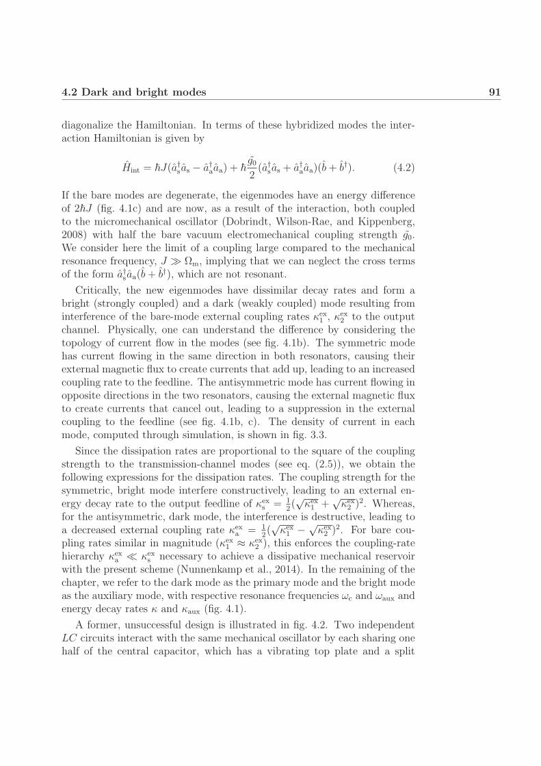
4.2 Dark and bright modes 91
diagonalize the Hamiltonian. In terms of these hybridized modes the inter-action Hamiltonian is given by
Hint = �J(a†s as − a†aaa) + �g02(a†s as + a†aaa)(b+ b†). (4.2)
If the bare modes are degenerate, the eigenmodes have an energy differenceof 2�J (fig. 4.1c) and are now, as a result of the interaction, both coupledto the micromechanical oscillator (Dobrindt, Wilson-Rae, and Kippenberg,2008) with half the bare vacuum electromechanical coupling strength g0.We consider here the limit of a coupling large compared to the mechanicalresonance frequency, J � Ωm, implying that we can neglect the cross termsof the form a†s aa(b+ b†), which are not resonant.
Critically, the new eigenmodes have dissimilar decay rates and form abright (strongly coupled) and a dark (weakly coupled) mode resulting frominterference of the bare-mode external coupling rates κex
1 , κex2 to the output
channel. Physically, one can understand the difference by considering thetopology of current flow in the modes (see fig. 4.1b). The symmetric modehas current flowing in the same direction in both resonators, causing theirexternal magnetic flux to create currents that add up, leading to an increasedcoupling rate to the feedline. The antisymmetric mode has current flowing inopposite directions in the two resonators, causing the external magnetic fluxto create currents that cancel out, leading to a suppression in the externalcoupling to the feedline (see fig. 4.1b, c). The density of current in eachmode, computed through simulation, is shown in fig. 3.3.
Since the dissipation rates are proportional to the square of the couplingstrength to the transmission-channel modes (see eq. (2.5)), we obtain thefollowing expressions for the dissipation rates. The coupling strength for thesymmetric, bright mode interfere constructively, leading to an external en-ergy decay rate to the output feedline of κex
s = 12(√κex1 +
√κex2 )2. Whereas,
for the antisymmetric, dark mode, the interference is destructive, leading toa decreased external coupling rate κex
a = 12(√κex1 − √
κex2 )2. For bare cou-
pling rates similar in magnitude (κex1 ≈ κex
2 ), this enforces the coupling-ratehierarchy κex
a � κexs necessary to achieve a dissipative mechanical reservoir
with the present scheme (Nunnenkamp et al., 2014). In the remaining of thechapter, we refer to the dark mode as the primary mode and the bright modeas the auxiliary mode, with respective resonance frequencies ωc and ωaux andenergy decay rates κ and κaux (fig. 4.1).
A former, unsuccessful design is illustrated in fig. 4.2. Two independentLC circuits interact with the same mechanical oscillator by each sharing onehalf of the central capacitor, which has a vibrating top plate and a split

92 Mechanical reservoir for microwaves
(a) (b)
Figure 4.2: Unsuccessful design to obtain asymmetrically coupled microwavemodes. (a) Optical microscope image of a fabricated chip. Two LC res-onators are coupled to the same mechanical modes by sharing a capacitorwith a split bottom plate. By design, the mode that is further from the trans-mission line is meant to have a lower inductive coupling rate. (b) Simulatedcharge density at the frequency of resonance of the top mode. The bottompart of the circuit, that is not resonant, acts as a capacitive coupling to thetransmission line, increasing the total coupling rate.
bottom plate. An optical micrograph of a fabricated sample is shown infig. 4.2a. By design, the microwave cavity placed further from the centraltransmission line should have a lower inductive coupling than the other cav-ity. In fact, capacitive coupling compensates for the difference in inductivecoupling, such that the total external coupling rate of each cavity is simi-lar. Numerical simulation with Sonnet (see section 3.2.1) confirms this. Thecharge density is computed at the resonance frequency of the top mode andshown in fig. 4.2b. There are significant charge fluctuations in the bottompart of the circuit, which is nonresonant and acts as a capacitive finger tothe transmission line. The circuit with dark and bright modes is designedto correct those shortcomings. The hybridized modes have currents flowingin the entire circuit for each resonance, such that there is no idle part of thecircuit that can act as a capacitance to the transmission line, leaving onlyinductive coupling.

4.3 Realization of a mechanical reservoir 93
4.3 Realization of a mechanical reservoir
We realize the electromechanical circuit experimentally by fabricating twolumped-element LC circuits coupled to each other via a common inductor,made from thin-film aluminium on a sapphire substrate. The sample is HYB-20150924-4-24. The primary and auxiliary modes respectively have resonancefrequencies (ωc, ωaux) = 2π × (4.26, 5.48) GHz and total energy decay rates(κ, κaux) = 2π × (118, 4478) kHz, (thus, κaux/κ ≈ 38). This clear hierarchyin the energy relaxation rates indeed originates from the vastly dissimilarengineered external coupling to the feedline, with κex = 2π × 42 kHz ≈1% of κex
aux. The mechanical resonator is a parallel-plate capacitor with asuspended top electrode, having a resonance frequency of the fundamentalflexural mode Ωm = 2π × 5.33 MHz and a decay rate Γm = 2π × 30 Hz.This mechanical mode couples to both the primary and auxiliary modeswith a vacuum electromechanical coupling strength g0 = g0/2 = 2π× 60 Hz.The characterization of the coupling strength g0 is described in section 3.5.2.Importantly, the resolved sideband regime is still attained for both microwavemodes, with Ωm > κaux � κ.
Figure 4.3a, b show respectively an optical image of the fabricated circuitand a scanning electron micrograph of the drum-type capacitor. The simpli-fied measurement setup is shown in fig. 4.3c. In brief, the device is mountedon the base plate of a dilution refrigerator and cooled to a base temperatureof ca. 10 mK. The microwave input lines are heavily attenuated to suppressresidual thermal noise and, in addition, filter cavities are employed to removeunwanted frequency noise from the applied tones (see section 3.3.4). Afteramplification with a commercial high-electron-mobility transistor (HEMT)amplifier mounted on the 3 K plate, the signal is measured with a spectrumanalyzer or a vector network analyzer.
To prepare a cold, dissipative mechanical bath we follow the approachoutlined by Nunnenkamp et al. (2014) and use optomechanical sideband cool-ing (Teufel, Harlow, et al., 2008; Schliesser, Riviere, et al., 2008) to engineerthe dissipation of the mechanical oscillator. We proceed by pumping the aux-iliary mode on the lower motional sideband (fig. 4.1d). We strongly damp themechanical oscillator to an effective energy decay rate Γeff ≈ 2π × 500 kHz(corresponding to a mean intra-cavity photon number of nc
aux ≈ 1.5× 10⁸),while still remaining in the weak-coupling regime for the auxiliary mode.Examples of OMIT curves taken in such a regime are shown in fig. 3.17.Thereby, we realize a dissipative mechanical reservoir for the primary, high-Q mode, since Γeff � κ. The effective temperature of this reservoir and itsutility as a quantum resource are studied below in the following.

94 Mechanical reservoir for microwaves
(a)
VNAin
ESA
+
(c)
10 mK
HEMT
(b)
2 μm
200 μm 3 K
300 K
κ = 2π · 118 kHz κaux = 2π · 4.48 MHz ≈ 38κ
(d)
Figure 4.3: Device, experimental setup, and characterization of the elec-tromechanical circuit (a) Inverted-colour optical micrograph of the circuitconsisting of two coupled LC resonators, one having a mechanically compliantcapacitor. Dark blue regions show aluminium and grey regions that are theexposed sapphire substrate. (b) False-colour scanning electron micrographof the mechanically compliant drum capacitor. (c) Simplified schematics ofthe measurement setup with the circuit. The input lines are filtered andattenuated at various stages before reaching the device mounted in a dilu-tion refrigerator. Both the coherent response and the spectral emission canbe measured. (d) Linear response measurement of the device revealing thesymmetric (bright, used as the auxiliary) and anti-symmetric (dark, usedas the primary) microwave modes. Figure reproduced from Toth, Bernier,Nunnenkamp, et al. (2017).

4.4 Tuning a mode using a reservoir 95
4.4 Tuning a mode using a reservoir
We first study the modified microwave cavity susceptibility resulting frominteraction with the mechanical reservoir. The engineered bath provided bythe mechanical resonator modifies the response of the electromagnetic modewhen a microwave tone is applied (Nunnenkamp et al., 2014). With a pumpdetuned by Δ from the primary microwave cavity resonance, the frequencyand the decay rate of the mode shift by
δωom = ReΣ and κom = −2ImΣ. (4.3)
The self-energy Σ is defined as
Σ = −ig2(
1
Γeff/2 + i (Δ + Ωm)− 1
Γeff/2 + i (Δ− Ωm)
), (4.4)
where g = g0√nc is the effective electromechanical coupling strength en-
hanced by the mean intracavity photon number of the primary mode nc.This effect can be viewed as radiation-pressure dynamical backaction (V.Braginsky, A. Manukin, and Tikhonov, 1970; Kippenberg, Rokhsari, et al.,2005; Schliesser, Riviere, et al., 2008) onto the microwave mode, an interpre-tation further elaborated in section 4.5.
The change in susceptibility leads to a change in the reflection fromthe microwave cavity (defined as aout(ω) = S11(ω)ain(ω), where ain,out(ω)are Fourier-domain operators associated with the input and output fields,cf. fig. 4.1b). The response becomes
S11(ω) =κ0 + κom − κex − i2(ω − ω′
c)
κ0 + κom + κex − i2(ω − ω′c), (4.5)
where κ0 is the internal loss of the primary mode and ω′c = ωc + δωom the
modified resonance frequency.
4.5 Interpretation as dynamical backaction
In this section, we discuss the interaction between the microwave cavity andits mechanical dissipative reservoir in the framework of dynamical backaction.
4.5.1 Origin of the concept of dynamical backaction
More than 50 years ago, the seminal work of Braginsky (Braginski and A. B.Manukin, 1967; V. Braginsky, A. Manukin, and Tikhonov, 1970) introduced

96 Mechanical reservoir for microwaves
the notion of radiation pressure dynamical backaction. While a mechani-cal oscillator coupled parametrically to an electromagnetic mode enables themeasurement of mechanical motion with high precision, as required in partic-ular for gravitational wave detectors, radiation pressure poses a limitation.As the cavity field adjusts to the oscillator motion, the radiation pressureforce it generates acts as a feedback force which can acquire an out-of-phasecomponent due to the finite cavity delay and modify the mechanical dampingrate. This dynamical backaction limits the circulating power in Fabry-Perotinterferometers, due the parametric oscillatory instability, in which amplifica-tion compensates for the intrinsic mechanical losses, leading to regenerativeoscillations of the mechanical end mirror.
The radiation-pressure parametric instability, as proposed by Braginsky (V. B.Braginsky, Strigin, and Vyatchanin, 2001) was first observed in toroid micro-resonators in 2005 (Kippenberg, Rokhsari, et al., 2005), and gives rise to arich nonlinear dynamics (Marquardt, Harris, and Girvin, 2006). Soon there-after, dynamical backaction cooling, an effect Braginsky predicted (V. B.Braginsky and Vyatchanin, 2002) to occur for red-detuned laser excita-tion, was demonstrated (Gigan et al., 2006; Arcizet et al., 2006; Schliesser,Del’Haye, et al., 2006). While the parametric instability was first analyzedfor a single electromagnetic mode coupled to a mechanical oscillator, the ef-fect can also occur for multimode systems in which modes are spaced by themechanical frequencies (Kells and D’Ambrosio, 2002), a scenario in whichthe parametric oscillator stability in advanced LIGO at the Livingston ob-servatory (Evans et al., 2015) was observed.
Although undesirable in the context of LIGO, the ability to amplify andcool mechanical motion using dynamical backaction is at the heart of theadvances in cavity opto- and electromechanics over the past decade (As-pelmeyer, Kippenberg, and Marquardt, 2014) that have enabled mechanicalsystems to be controlled at the quantum level. Dynamical backaction controlover mechanical oscillators has enabled the cooling of micro- and nanome-chanical oscillators to unprecedentedly low entropy states (Verhagen et al.,2012; Teufel, Donner, et al., 2011; Chan et al., 2011), and thereby openeda path to study optomechanical quantum effects ranging from optomechan-ical squeezing, mechanical squeezed states, sideband asymmetry, to entan-glement of mechanical motion with microwaves (Safavi-Naeini, Groblacher,et al., 2013; Purdy et al., 2013; Sudhir et al., 2017; Nielsen et al., 2017;Wollman et al., 2015; Palomaki et al., 2013; Pirkkalainen, Damskagg, et al.,2015; Lecocq, Clark, et al., 2015; Riedinger et al., 2016).
It is interesting to highlight the role of dissipation in dynamical backaction.Indeed dissipation determines the resulting modification of the mechanical

4.5 Interpretation as dynamical backaction 97
κ Γm
(a) (b)
mech.mode
EMmode
Ωm
χmech χEMΓeff
Γm
κeff
ωc
κ
pressure force
cavity modulation
in out
EMmode
mech.mode
pressure force
cavity modulation
in out
Γm κ
Figure 4.4: The role of dissipation in dynamical backaction. (a) An electro-magnetic mode (with resonant frequency ωc and energy dissipation rate κ) iscoupled to a mechanical oscillator (with resonant frequency Ωm and energydissipation rate Γm) through the optomechanical interaction, in which the for-mer exerts radiation pressure force, while the latter modulates the resonantfrequency of the cavity. In standard optomechanical systems, the dissipa-tion rates satisfy the hierarchy κ � Γm and this interaction can be viewedas a feedback mechanism acting on the mechanical oscillator. This modifiesthe oscillator’s damping rate, in a process coined as “dynamical backaction”by Braginsky. (b) In the scenario where the optical mode is coupled to amechanical oscillator whose dissipation rate dominates over that of the opti-cal mode, the role of the modes is reversed. The mechanical mode providesthe feedback mechanism (dynamical backaction) for the optical mode, there-fore modifying the microwave mode’s resonance frequency and damping rate.Figure reproduced from Toth, Bernier, Feofanov, et al. (2018).

98 Mechanical reservoir for microwaves
and optical susceptibility due to the optomechanical interaction. In almostall optomechanical systems ranging from gravitational wave observatoriesto nano-optomechanical systems, the electromagnetic dissipation dominatesover the mechanical one, leading to the above mentioned optomechanicalphenomena. In contrast, if the mechanical oscillator is more dissipative thanthe electromagnetic mode, the roles are reversed (Nunnenkamp et al., 2014).In this situation1, the dynamical backaction that occurs for detuned laser ex-citation causes a feedback force that is applied to the electromagnetic mode,resulting in amplification or damping. This electromagnetic dynamical back-action leads to a parametric oscillatory instability that corresponds to theaction of a maser (the stimulated emission of microwaves).
4.5.2 Modeling dynamical backaction
We start by reformulating Braginsky’s original derivation of dynamical back-action (Braginski and A. B. Manukin, 1967; V. B. Braginsky, Strigin, and Vy-atchanin, 2001) for the case of a blue-detuned pump, in a way that showcaseshow the process is reversed in the case of an opposite dissipation hierarchy.Consider an electromagnetic mode with frequency ωc and energy dissipationrate κ coupled, via the standard optomechanical coupling, to a mechanicalmode with resonant frequency Ωm and energy dissipation rate Γm. WhileBraginsky considered the limit Ωm ≤ κ to derive the delayed feedback forceexperienced by the mechanical oscillator due to the electromagnetic field,we consider here the sideband-resolved regime, Ωm � κ (Marquardt, J. P.Chen, et al., 2007; Wilson-Rae et al., 2007; Schliesser, Riviere, et al., 2008),relevant to our experiment. We consider the equations of motion parametri-cally coupling the mechanical oscillator to the electromagnetic cavity. These(for simplicity classical and linearized) equations can be written in a rotatingframe for the phasors of the two modes; in the case of a pump driving thesystem on the upper motional sideband at a detuning Δ = Ωm, they aregiven by the coupled-modes equations
a∗(t) = −κ
2a∗(t) + igb(t) = −κ
2a∗(t)− iFa(t) (4.6)
b(t) = −Γm
2b(t)− iga∗(t) = −Γm
2b(t) + iFb(t), (4.7)
where b(t) = (√mΩmx(t) + i
√1/mΩmp(t))/
√2 describes the state of the
mechanical mode of mass m, a(t) is the phasor for the electromagnetic mode
1It is still assumed that the mechanical dissipation occurs on a timescale that is longcompared to the mechanical oscillator period, or equivalently that the mechanical qualityfactor still exceeds unity.

4.5 Interpretation as dynamical backaction 99
and g = g0|α0|2 is the vacuum optomechanical coupling strength g0 enhancedby the field α0 of the blue-detuned pump. In the rotating frame, the variablesdescribe the slowly changing amplitude and phase of the rapidly oscillatingfield and oscillator, at ωc and Ωm. Each of the two harmonic oscillatorsis subject to a “force” (denoted by Fa(t) and Fb(t)) proportional to thestate of the other harmonic oscillator, establishing a feedback mechanism:cavity intensity fluctuations create a radiation pressure force acting on themechanical oscillator, while mechanical displacement modulates the cavityresonance frequency. The symmetry of the relationship is broken by thedifferent scales of the dissipation rates.
Braginsky originally considered the case where electromagnetic dissipa-tion dominates (κ � Γm). This is natural in most systems as the qualityfactors are commensurate for the electromagnetic and mechanical modes,while there is a large (many orders of magnitude) separation of scales intheir respective frequencies. In this limit, the electromagnetic field envelopealmost instantly adapts to the mechanical displacement (a∗(t) ≈ 0) and be-comes proportional to it such that a∗(t) = i(2g/κ)b(t). The field then exertsa force on the mechanical oscillator proportional to the state of the latter,given by Fb(t) = −i(2g2/κ)b(t). Therefore, the interaction can be viewed asa feedback loop. The factor −i represents a delay of a quarter period for thefeedback force acting on the mechanical oscillator. This delay means thatthe force, acting in quadrature, increases the amplitude of the phasor, equiv-alent to a decrease in mechanical damping or gain. If the pump detuningΔ does not fall exactly on the sideband, the delay is not exactly i and theforce has an in-phase component, modifying the frequency of the mechanicaloscillator (this effective change of the mechanical spring constant is calledthe optical spring effect). The amplification process can be understood asa positive feedback that measures the state of the mechanical oscillator andreturns it with a delay as a force: a dynamical backaction (see fig. 4.4a). Forsufficiently high coupling strength g, this leads to a parametric oscillatoryinstability, that causes regenerative oscillations of the mechanical oscillator,and thus limits the maximal circulating power for a gravitational wave de-tector (V. B. Braginsky, Strigin, and Vyatchanin, 2001).
Here, we study the converse process, where the mechanical dissipationrate dominates (Γm � κ). The envelope of mechanical oscillations nearlyinstantly adjusts to the state of the electromagnetic field (b(t) ≈ 0) andis proportional to it such that b(t) = −i(2g/Γm)a
∗(t). The field is thensubject to an in-quadrature “force” proportional to its own state Fa(t) =i(|κDBA|/2)a∗(t) where κDBA = −4g2/Γm = −κC, introducing the multipho-ton cooperativity C = 4g2/(κΓm). Similarly to above, the force has a delay

100 Mechanical reservoir for microwaves
+i of a quarter period and increases the amplitude of electromagnetic oscil-lations, compensating for damping by an amount given by κDBA, such thatthe effective energy decay rate of the cavity is κ+ κDBA. A change in detun-ing Δ would again slightly modify this delay and create components of thein-phase force component, changing the speed of oscillations, and displac-ing the resonance frequency of the cavity. This is equivalent to a feedbackloop for the electromagnetic mode (see fig. 4.4b), and implies that the me-chanical oscillator is responsible for dynamical backaction on the microwavecavity. As above, the positive feedback can lead to a parametric instability.For κDBA = −κ, the anti-damping caused by this feedback exactly com-pensates for the losses (both intrinsic and external) of the electromagneticmode, and the cavity develops self-sustained oscillations: it acts as a maser.The intrinsic optomechanical nonlinearity sets the maximum amplitudes ofthe oscillations (Nunnenkamp et al., 2014) and the dynamics is no longercaptured by the linearized eqs. (4.6) and (4.7).
4.6 Controllable microwave susceptibility
The engineered reservoir therefore supplies a way to tailor the susceptibilityof the primary electromagnetic mode, which we can directly probe using acoherent response measurement.
We fix the detuning to either motional sideband of the primary mode(Δ = ∓Ωm), and measure S11(ω) while the power is varied. For this choiceof detuning, we have δωom = 0 (neglecting a term ∝ Γeff
2/Ωm) and the changein the microwave decay rate simplifies to
κom = ±Cκ, (4.8)
directly proportional to the cooperativity C = 4g2/(κΓeff). Figure 4.5a, bshow the linear response for a tone on the lower and upper sideband for vari-ous pump powers. The width of the resonance, corresponding to the effectivecavity decay rate, increases (for Δ = −Ωm) or decreases (for Δ = +Ωm)linearly with C. The depth of reflection on resonance |S11(ωc)|2 varies sig-nificantly to reflect this change (fig. 4.5c). The effective internal loss of thecavity κ0 + κom can be tuned on demand by changing the coupling to thedissipative reservoir via the pump tone. While the microwave cavity is ini-tially undercoupled (κex < κ0), pumping on the upper sideband reduces theeffective internal loss and increases the depth on resonance until the cavitybecomes critically coupled (the effective internal loss matches the externalcoupling, κ0 + κom = κex). Increasing the power further, the cavity becomes

4.6 Controllable microwave susceptibility 101
(a) (b)
(c)
(d) (e)
Figure 4.5: Dynamical backaction on the microwave mode using an engi-neered mechanical reservoir. (a,b) Modification of the susceptibility of themicrowave cavity when a pump tone is placed on the lower and upper mo-tional sideband of the primary mode, for various values of the multiphotoncooperativities (C = 1 corresponds to a mean intracavity photon number ofnc ≈ 5×10⁶). The slight frequency shift of the peak center is due to the finitesideband resolution parameter of the auxiliary mode (Ωm/κaux). (c) Depthof the resonance as a function of the effective internal losses κ0 + κom, witha pump tone on the lower (Δ = −Ωm, red squares) and upper sideband(Δ = +Ωm, blue circles), and a theoretical fit. (d,e) Using a fixed pumppower, the detuning Δ of the pump tone is swept and the change in themicrowave resonance frequency and decay rate is recorded. The theoreticalfit corresponds to eq. (4.3), showing good agreement with the experimentaldata. Figure adapted from Toth, Bernier, Nunnenkamp, et al. (2017).

102 Mechanical reservoir for microwaves
overcoupled (κ0 + κom < κex) and resonant reflection increases again. Whenκ0 + κom becomes negative, there is a net internal gain: the absorptive fea-ture in the cavity reflection becomes a peak, indicating amplification of thereflected microwave signal. By pumping on the lower sideband (Δ = −Ωm),extra damping is introduced and the resonance becomes increasingly under-coupled. The mechanical mode provides a dissipative bath for the microwaveresonator, down-converting the cavity photons to the pump. In fig. 4.5c weplot the resonant reflection and observe good agreement with the expecteddependence according to eq. (4.5). For the data corresponding to the pumptuned to the lower motional sideband (Δ = −Ωm), the depth of the resonanceis systematically lower than expected, due to a decrease in the intrinsic mi-crowave cavity loss in the presence of a strong pump (Megrant et al., 2012).
In fig. 4.5d, e, we keep the pump power constant and sweep the detuningΔ to measure the change in the microwave resonance frequency and dampingrate. For the frequency shift δωom, intrinsic non-linearities redshift the reso-nance frequency in an asymmetric fashion, providing a different backgroundfor the red and blue sidebands. The effect agrees well with the predictionfrom eq. (4.3) when the two sidebands are fitted independently with differentconstant offsets. We note that the modification of the resonance frequency asa function of detuning has the opposite parity compared to the better knowncase of the optical spring effect (Aspelmeyer, Kippenberg, and Marquardt,2014).
4.7 Maser action and amplification
In the following, we demonstrate the cold nature of the dissipative mechanicalreservoir by studying the noise properties of the system. To this end, we fixthe microwave drive to the upper sideband (Δ = +Ωm) and study the regimewhere the pump introduces net gain in the microwave cavity (κ0 + κom < 0).We use a different device, HYB-20160524-1-12, for this analysis with opti-mized properties: higher coupling strengths of g0 = 2π × (106, 79) Hz re-spectively for the primary and auxiliary modes, and an overcoupled primarymode (κex/κ = 0.76). In fig. 4.6a, the emitted noise spectra of the microwavecavity are shown for different pump powers. The measured power spectrumis rescaled to the symmetrized cavity output field spectrum (Clerk et al.,2010) Saa(ω) in units of photons per second per unit bandwidth (see def-inition in section 2.2.2), using the noise temperature of the HEMT as anabsolute noise reference (see section 3.4.2). To confirm the calibration, weuse the mechanical sideband spectrum obtained from the measurement of
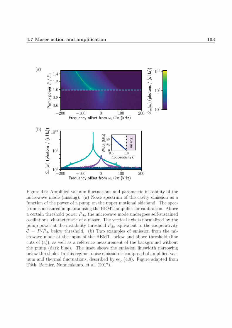
4.7 Maser action and amplification 103
(a)
(b)
Figure 4.6: Amplified vacuum fluctuations and parametric instability of themicrowave mode (masing). (a) Noise spectrum of the cavity emission as afunction of the power of a pump on the upper motional sideband. The spec-trum is measured in quanta using the HEMT amplifier for calibration. Abovea certain threshold power Pth, the microwave mode undergoes self-sustainedoscillations, characteristic of a maser. The vertical axis is normalized by thepump power at the instability threshold Pth, equivalent to the cooperativityC = P/Pth below threshold. (b) Two examples of emission from the mi-crowave mode at the input of the HEMT, below and above threshold (linecuts of (a)), as well as a reference measurement of the background withoutthe pump (dark blue). The inset shows the emission linewidth narrowingbelow threshold. In this regime, noise emission is composed of amplified vac-uum and thermal fluctuations, described by eq. (4.9). Figure adapted fromToth, Bernier, Nunnenkamp, et al. (2017).

104 Mechanical reservoir for microwaves
g0 (see section 3.5.2) to locally compare the known sideband power to thebackground noise that corresponds to the HEMT added noise. This providesan independent calibration of the HEMT noise, which in this case was foundto agree within 1.4 dB.
As the blue-detuned pump compensates for the losses, the width of theemitted noise spectrum, corresponding to the cavity linewidth κeff = (1−C)κ,decreases linearly with the pump power towards zero (at unity cooperativityC = 1), as shown in the inset of fig. 4.6b. In this below-threshold regime,the peak photon flux spectral density emitted from the cavity increases withpower, as the vacuum noise and the residual thermal microwave noise (con-sisting in both a finite residual occupancy nm of the dissipative mechanicalreservoir and a finite thermal microwave occupancy of the cavity ncav) areamplified according to
Saa(ω) = κex
(κex − κeff)12+ Cκ(nm + 1
2) + κ0(ncav +
12)
(κeff
2)2 + (ω − ωc)2
(4.9)
where the thermal input noise is neglected and only the amplified noise isconsidered. We analyze the noise properties of the device in detail belowwhen considering amplification and added noise. We find the residual thermaloccupancy of the dissipative reservoir to be nm = 0.66, when neglecting ncav.Equation (4.9) then implies that 60% of the emitted noise from the cavity isamplified vacuum fluctuations, when C → 1.
For C = 1 and greater pump powers, the microwave mode undergoesself-sustained oscillations. This regime leads to a parametric instability andstimulated emission of microwave photons into the microwave cavity, analoga maser. The salient features of the instability are a transition from sub-to above-threshold masing, as well as linewidth narrowing. These observa-tions are analogues to the radiation-pressure-induced parametric instabilityof a mechanical mode in the normal optomechanical regime (κ � Γm) (Kip-penberg, Rokhsari, et al., 2005; Marquardt, Harris, and Girvin, 2006; V.Braginsky and A. Manukin, 1977; Grudinin et al., 2010). In the experi-ments a clear threshold behavior, characteristic of masing, is demonstratedwhen the emitted noise abruptly increases in strength at C = 1 (fig. 4.6b).Such masing in superconducting circuits has previously been demonstratedusing a single artificial atom (Astafiev et al., 2007). Due to the large photonpopulation generated by masing, nonlinearities of the cavities red-shift thefrequency of emission. This clearly distinguishes masing from the mechanicalparametric instability (also called phonon lasing) (Grudinin et al., 2010) inthe normal optomechanical regime. In the latter case, the emission does notfollow the cavity but has a constant detuning of −Ωm with respect to the

4.7 Maser action and amplification 105
E
ωb
ωa
Figure 4.7: Interaction between modes of positive and negative energy aspopulation inversion. In the rotating frame, the microwave and mechanicalmodes have a negative and a positive energy, and their energy levels canbe represented on two inverted parabolas. Through the interaction, the twomodes can exchange an excitation that moves the state up the energy ladderon the left and down the energy ladder on the right. This process can berepeated infinitely, leading to amplification and the masing instability.
pump.
In a usual maser, the microwave mode is amplified by interacting with atwo-level system in a state of population inversion. The amplification mecha-nism here can be interpreted similarly. When a blue-detuned drive is appliedto the system, the microwave mode has a negative energy in the rotatingframe, where the Hamiltonian is time-independent (see eq. (2.22)). The twomodes can be represented as in fig. 4.7 with energy levels in two parabolas,inverted with respect to each other. The first mode can always gain energyby exchanging an excitation with the second mode, which can always be low-ered in energy. The two ladders of energy levels, one of them can be infinitelyclimbed up and the other down, lead to amplification of the oscillations inthe modes and eventually to the masing instability. The downward parabolais an analog of the inverted population of a two-level system. In the latter,the energy can always be lowered by swapping excitations with the masermode, since the system is instantly pumped back to the state of populationinversion.
Below the masing threshold, the microwave mode coupled to the dissi-pative bath acts as a phase-insensitive parametric amplifier (Caves, 1982;

106 Mechanical reservoir for microwaves
Nunnenkamp et al., 2014) for incoming signals. For κ0 + κom < 0, there isa net internal gain and the susceptibility S11(ω) develops a peak, such thatreflection is larger than input for signals within the resonance bandwidth(in-band). The power gain of the amplifier is defined as the resonance peakheight above the background, given by
G(ωc) = |S11(ωc)|2 =∣∣∣∣∣(2κex
κ− 1
)+ C
1− C
∣∣∣∣∣2
. (4.10)
The bandwidth of the amplifier is the linewidth of the microwave resonance,given by κeff = (1 − C)κ. In order to measure the gain, bandwidth andnoise properties of the amplifier, we inject, in addition to the pump toneon the upper sideband (Δ = +Ωm), a weak signal tone (swept in frequencyaround the cavity resonance) and measure the reflected signal as a functionof the pump tone power. With increasing pump power, a narrowing of thecavity bandwidth (fig. 4.8a) is observed, as well as an increase in the powerof the reflected signal (i.e. gain). By fitting the reflected power, the gainand bandwidth as a function of cooperativity are extracted, and found tobe in good agreement with the theoretical predictions given by eq. (4.10)(fig. 4.8b). The observed gain exceeds 42 dB.
4.8 Near-quantum-limited amplification
Next, we study the added noise of the dissipative amplification process. Theadded noise N , referred to the input of the amplifier, is given by the noiseoutput of eq. (4.9) subtracting the input noise and dividing by the gain G(ωc).On resonance, it is found to be
N (ωc) =4C(κex/κ)(nm + 1
2) + 4(κexκ0/κ
2)(ncav +12)
(C − 1 + 2κex/κ)2 , (4.11)
which, in the high gain limit (C → 1), simplifies to N (ωc) → (κ0/κex)(ncav +12) + (κ/κex)(nm + 1
2). This quantity can be measured by recording the im-
provement of the signal-to-noise ratio (SNR) of amplification in and out of thebandwidth of our device. This directly compares the noise performance of ourdevice with the commercial HEMT amplifier, which is used as a calibratednoise source (the noise temperature of the HEMT is measured separately atωc and found to be 3.95 ± 0.02 K, corresponding to NHEMT = 20.0 ± 0.1quanta (see section 3.4.2). In fig. 4.8c, the gain of the device is compared tothe noise output of the chain, normalized to the HEMT noise background.

4.8 Near-quantum-limited amplification 107
−100 −50 0 50 100Frequency offset from ωc (kHz)
0
10
20
30
40
Rel
ativ
ega
inan
dno
ise
(dB
)
GN
−2 0 2
30
40
20 25 30 35 40 45Gain (dB)
0
1
2
3
N(ω
c)
(pho
tons
/(sH
z))
device quantum limit
−100 −50 0 50 100Probe detuning Δp/2π (kHz)
0
10
20
30
40
|S11|2
(dB
)
mp
0.6 0.8 1.0Cooperativity C
0
20
40
60
Ban
dwid
th(k
Hz)
()
0
10
20
30
40
Gai
nG
(dB
)()
(a) (b)
(c) (d)
Figure 4.8: Near-quantum-limited phase-preserving amplification. (a) Linearresponse of the cavity, with increasing powers of the pump on the uppersideband from red to blue. (b) Power gain (triangles) and bandwidth (circles)of the amplifier extracted from a fit of the linear response, as a function ofthe cooperativity of the pump on the upper sideband. The colored pointscorrespond to the curves in (a). (c) Relative gain and noise of the amplifier,sharing the same baseline. The difference from noise to gain correspondsto over 12 dB of apparent signal-to-noise ratio improvement of our deviceover the HEMT, from which the insertion loss between the HEMT and thedevice (measured separately to be 1.6 dB) must be subtracted to infer thereal improvement. (d) Added noise of the amplification referred to the input,expressed in quanta. The total added noise in the high-gain limit amountsto 1.68 ± 0.02 quanta. This is only 0.87 quanta above the device quantumlimit nDQL, defined in eq. (4.12). Figure reproduced from Toth, Bernier,Nunnenkamp, et al. (2017).

108 Mechanical reservoir for microwaves
This calibration is corroborated by a second, independent calibration tech-nique, which uses the scattered power in the motional sideband in conjunctionwith the knowledge of the intracavity photon number and g0. The relativegain of the signal exceeds the relative noise by over 12 dB. From this apparentSNR improvement, one must subtract the insertion loss of the componentsbetween the device and the HEMT, measured independently at 77 K to be1.6 dB. (cf. section 3.4.2). The analysis reveals therefore that the optome-chanical amplifier provides more than 10 dB of improvement over the SNRof the HEMT.
The inferred added noise on resonance is shown as a function of gain infig. 4.8d. In the high-gain limit, it is a constant value of N (ωc) = 1.68 ±0.02 quanta per second per unit bandwidth (with the uncertainty given bystatistical fluctuations). Using eq. (4.11) and assuming ncav = 0, the effectiveoccupancy of the dissipative reservoir is found to be nm = 0.66. However, thestrong cooling pump increases the temperature of the cavity thermal bathto an occupancy ncav = 1.03, obtained by measuring the emitted thermalnoise of the microwave cavity. Taking the residual cavity thermal noise intoaccount, the estimate for the mechanical occupancy is reduced to nm = 0.41.This demonstrates that the dissipative mechanical reservoir constitutes aquantum resource.
The calibration of the added noise of the amplifier provides a convenientway to measure the occupancy of the cooled mechanical oscillator. Thenear-quantum limited fluctuations of the mechanical motion are amplifiedby a large gain and can be measured with a large SNR (see fig. 4.8c). Onlythe regime considered, with the mechanical oscillator serving as a reservoirfor the microwave cavity, with a much larger dissipation allows this. In asense, the amplification is not sufficient to compensate the large cooling rateof the mechanical oscillator provided by the auxiliary cavity, such that thecooled mechanical fluctuations are amplified without heating the oscillator.
We note that even in the case when all the thermal noise sources arereduced to zero (neff = ncav = 0), the added noise of the amplifier is
nDQL =1
2+
κ0
κex
, (4.12)
which we call the device quantum limit and deviates from 1/2 due to thefinite internal dissipation rate κ0. For the present system the device quantumlimit amounts to 0.81 quanta for the coupling ratio of κex/κ = 0.76, whichis only 0.87 quanta below the added noise we measure. It is interesting tocompare the present amplifier scheme, relying on a dissipative reservoir, tothe microwave parametric amplifiers used in circuit QED. In the latter case,

4.9 Injection locking of the maser tone 109
typically both idler and signal are resonant with one or more microwavecavities (Bergeal et al., 2010; Eichler et al., 2014; Castellanos-Beltran, Irwin,et al., 2008). As the gain increases, this leads to a simultaneous increase inboth the signal and idler mode population. In contrast, while the presentamplifier scheme uses a parametric interaction as well, the large dissipationrate for the (mechanical) idler mode only leads to the generation of a signalphoton (microwave field), suppressing the idler; the situation is akin to aRaman-type interaction found in nonlinear optics (Bloembergen, 1996).
4.9 Injection locking of the maser tone
We now demonstrate the locking of our maser with a weak injected tone.This is performed on the same sample HYB-20160524-1-12, as before, thatwas kept at the elevated temperature of 200 mK to increase the mechanicalstability. The sample parameters have shifted slightly and it has resonancefrequencies ωc = 2π×4.08 GHz and ωaux = 2π×5.19 GHz, and a mechanicalresonance frequency Ωm = 2π × 6.5 MHz.
Injection locking is a synchronization phenomenon for lasers and ma-sers (Siegman, 1986), and has been demonstrated in many systems, includingrecently in a trapped-ion phonon laser (Knunz et al., 2010), a quantum cas-cade laser (St-Jean et al., 2014), a quantum-dots maser (Liu et al., 2015)as well as an AC Josephson junction maser (Cassidy et al., 2017). A weaktone of frequency ωinj close to the maser emission frequency ωmas competesfor gain with it in a way that effectively couples the two oscillations and per-mits synchronization. The phenomenon is generally described by the Adlerequation (Adler, 1946)
dφ
dt+ (ωinj − ωmas) = −1
2Δωinj sin (φ) (4.13)
which models the dynamics of the relative phase φ of the two oscillations. Ifthe injected tone falls within a locking range of width
Δωinj = 2κex
√αPinj/Pmas (4.14)
centered around the masing frequency ωmas, the two tones lock and the phasedifference φ becomes constant. This range depends on the ratio between theinjected tone power Pinj, attenuated by factor α at the input of the cavity,and the maser emission power Pmas. Outside this range, the Adler equa-tion predicts that the maser frequency is pulled towards the injected tone

110 Mechanical reservoir for microwaves
(a) (b)
(c) (d)
Figure 4.9: Injection locking of a maser based on dynamical backaction(a) Output spectrum of the maser, as the power Pinj of an injected tonedetuned 5 kHz to the red is increased. The power is measured at the outputof the corresponding microwave source. Above a threshold power of about-30 dBm, the maser locks to the tone, considerably suppressing the noise andeliminating the frequency jitter present in the free-running case. The intrin-sic nonlinearity results in distortion sidebands from the two tones beatingbelow threshold. (b) Spectra corresponding to cuts of A along the dashedlines, below and above the locking threshold. (c) Output spectrum of themaser as the frequency ωinj of a weak tone of constant power Pinj = −40dBm is swept across the free-running maser frequency ωmas. The lockingrange Δωinj, wherein the two oscillations are frequency locked, is highlighted.(d) The locking range Δωinj as a function of the injected tone power Pinj. Afit on the logarithmic scale gives a slope of 0.51, confirming the expectedscaling Δωinj ∝
√Pinj. The inset depicts the actual limiting points of the
locking range as a function of tone power Pinj, illustrating the Arnold tongueof the system. Figure adapted from Toth, Bernier, Feofanov, et al. (2018).

4.10 Conclusions 111
and that distortion sidebands appear due to beating of the two tones andthe intrinsic nonlinearity (Adler, 1946). We first study this phenomenon byplacing the injected tone 5 kHz away from the maser and monitoring the out-put spectrum while the injected power Pinj is varied (fig. 4.9a). The maseremission is pulled towards the injected tone and finally locks at an injectedpower threshold corresponding to about -30 dBm. As the two tones becomecomparable in strength, distortion sidebands from the beating increase in am-plitude. In the locked region, the noise surrounding the peak is considerablysuppressed compared to the free-running case and the frequency jitter (orig-inating from frequency instability of the cavity and the mechanical mode)is eliminated (fig. 4.9b). We proceed to measure the locking range Δωinj,by fixing the injected power Pinj and sweeping its frequency ωinj across themaser frequency (fig. 4.9c). When the frequency difference is below Δωinj, thetwo tones lock. The noise around the peak is suppressed and the frequencyjitter of the maser ceases. Repeating the measurement at different injectedpowers Pinj, the locking range is shown to obey the expected scaling lawΔωinj ∝
√Pinj (fig. 4.9d). Finally, the limit points of locking are shown in an
inset as a function of power, drawing the so-called Arnold tongue (Pikovsky,Rosenblum, and Kurths, 2003). The asymmetric shape is due to drift of themasing frequency ωmas during the measurement, which does not affect thelocking range Δωinj.
4.10 Conclusions
In summary, we have implemented and studied a new regime of circuit elec-tromechanics by coupling an electromagnetic cavity mode to an engineeredcold dissipative reservoir formed by a mechanical oscillator. The usual rolesof the two modes are reversed, allowing for dynamical backaction on the mi-crowave mode using the mechanical reservoir. We demonstrate the control ofthe internal losses of the cavity in the form of backaction-induced amplifica-tion, damping, and masing of the microwave field. By performing microwaveamplification close to the quantum limit, we show that the mechanical reser-voir functions as a useful quantum resource.
The near-quantum-limited amplification with a mechanical reservoir ex-tends the available quantum information manipulation toolkit, adding to theexisting devices based on Josephson junctions (Bergeal et al., 2010; Eich-ler et al., 2014; Castellanos-Beltran, Irwin, et al., 2008; Sliwa et al., 2015).While the present amplifier is not frequency-tunable, recent advances in cir-cuit electromechanics have demonstrated such functionality (Andrews, Reed,

112 Mechanical reservoir for microwaves
et al., 2015). The observed reservoir-mediated microwave damping may al-low to remove residual thermal occupancy from the microwave cavity, akin tocooling schemes developed in circuit QED (Grajcar et al., 2008). Moreover,the control over internal dissipation enables all-electromechanical tuning ofthe coupling of the microwave resonator to the feedline, offering the potentialfor an electromechanical reconfigurable network (Kerckhoff, Andrews, et al.,2013). While the present scheme employs a single pump tone, dual tonepumping would lead to the preparation of squeezed states of the microwavecavity (Kronwald, Marquardt, and Clerk, 2014). Viewed more broadly, therealization of a cold mechanical reservoir for microwave light provides a cen-tral ingredient for novel electromechanical devices. Indeed, the circuit can beextended to multiple microwave resonators coupled to a shared mechanicalreservoir and implement the dissipative cavity-cavity interactions that are atthe heart of recent schemes to entangle microwave photons (Wang and Clerk,2013) and, combined with coherent interactions, to perform nonreciprocalmicrowave transmission (Metelmann and Clerk, 2015). Such nonreciprocaldevices can be of use for the rapidly expanding field of circuit QED (Wallraffet al., 2004; Devoret and Schoelkopf, 2013).

Chapter 5
Nonreciprocity in microwave op-tomechanical circuits
We describe here a scheme to perform nonreciprocal frequency conversionwith a multimode microwave optomechanical circuit. This chapter is adaptedfrom the text of two previous publications (Bernier, Toth, Koottandavida,et al., 2017; Bernier, Toth, Feofanov, et al., 2018b). In section 5.1, we intro-duce nonreciprocity in the context of cavity optomechanics. In section 5.2,we develop an intuitive picture of how to achieve nonreciprocal transmission,using the gyrator as a conceptual starting block. In section 5.3, we presentthe scheme to implement an isolator using a multimode optomechanical mi-crowave circuit. In section 5.4, our experimental results are detailed. Insection 5.5, the optomechanical circulator is introduced as a possible exten-sion of this working, necessitating an additional microwave cavity. Finally,in section 5.6, we conclude and give an outlook for optomechanical nonre-ciprocity.
5.1 Introduction
Nonreciprocal devices, such as isolators, circulators, and directional ampli-fiers, exhibit altered transmission characteristics if the input and outputchannels are interchanged. They are essential to several applications in sig-nal processing and communication, as they protect devices from interferingsignals (Pozar, 2011). At the heart of any such device lies an element break-

114 Nonreciprocity with optomechanics
ing Lorentz reciprocal symmetry for electromagnetic sources (Feynman, 1988;Jalas et al., 2013). Such elements have included ferrite materials (Auld, 1959;Milano, Saunders, and Davis, 1960; Fay and Comstock, 1965), magneto-optical materials (Aplet and Carson, 1964; Shirasaki and Asama, 1982; Satoet al., 1999; Bi et al., 2011), optical nonlinearities (Manipatruni, Robinson,and Lipson, 2009; L. Fan et al., 2012; Guo et al., 2016), temporal modu-lation (Anderson and Newcomb, 1965; Z. Yu and S. Fan, 2009; Lira et al.,2012; Kang, Butsch, and Russell, 2011; Estep et al., 2014; Peng, Ozdemir,Lei, et al., 2014), chiral atomic states (Scheucher et al., 2016), and physicalrotation (Fleury et al., 2014).
Typically, a commercial nonreciprocal microwave apparatus exploits fer-rite materials and magnetic fields, which leads to a propagation-direction-dependent phase shift for different field polarizations. A significant draw-back of such devices is that they are ill-suited for sensitive superconductingcircuits, since their strong magnetic fields are disruptive and require heavyshielding. In recent years, the major advances in quantum superconductingcircuits (Devoret and Schoelkopf, 2013), that require isolation from noiseemanating from readout electronics, have led to a significant interest in non-reciprocal devices operating at the microwave frequencies that dispense withmagnetic fields and can be integrated on-chip.
As an alternative to ferrite-based nonreciprocal technologies, several ap-proaches have been pursued towards nonreciprocal microwave chip-scale de-vices. Firstly, the modulation in time of the parametric couplings betweenmodes of a network can simulate rotation about an axis, creating an artificialmagnetic field (Anderson and Newcomb, 1965; Estep et al., 2014; Kerckhoff,Lalumiere, et al., 2015; Ranzani and Aumentado, 2014) rendering the systemnonreciprocal with respect to the ports. Secondly, phase matching of a para-metric interaction can lead to nonreciprocity, since the signal only interactswith the pump when copropagating with it and not in the opposite direc-tion. This causes travelling-wave amplification to be directional (Ranzaniand Aumentado, 2014; White et al., 2015; Macklin et al., 2015; Hua et al.,2016).
Phase-matching-induced nonreciprocity can also occur in optomechanicalsystems (Aspelmeyer, Kippenberg, and Marquardt, 2014; Bowen and G. J.Milburn, 2015), where parity considerations for the interacting spatial modesapply (Hafezi and Rabl, 2012; Shen et al., 2016; Ruesink et al., 2016). Fi-nally, interference in parametrically coupled multi-mode systems can be used.In these systems nonreciprocity arises due to interference between multiplecoupling pathways along with dissipation in ancillary modes (Ranzani andAumentado, 2015). Dissipation is a key resource there to break reciprocity, as

5.2 Gyrators and nonreciprocity 115
it forms a flow of energy always leaving the system, even as input and outputare interchanged. It has therefore been viewed as a kind of reservoir engi-neering (Metelmann and Clerk, 2015). Following this approach, nonreciproc-ity has recently been demonstrated in Josephson-junctions-based microwavecircuits (Sliwa et al., 2015; Lecocq, Ranzani, et al., 2017) and in a photonic-crystal-based optomechanical circuit (Fang, Luo, et al., 2017). These re-alisations and theoretical proposals to achieve nonreciprocity in multi-modesystems rely on a direct, coherent coupling between the electromagnetic inputand output modes.
5.2 Gyrators and nonreciprocity
Here we explain the origin of nonreciprocity in optomechanical systems byusing the gyrator-based isolator as a conceptual starting point.
5.2.1 The gyrator-based isolator
Any linear quadrature-preserving two-port device can be described by itsscattering matrix S, linking the incoming modes ai,in to the outgoing modesai,out by (
a1,outa2,out
)=
(S11 S12
S21 S22
) (a1,ina2,in
)+
(N1
N2
), (5.1)
where Ni represent added noise from the device. A starting definition for non-reciprocity is that a device is nonreciprocal when S21 �= S12. This correspondsto a change in scattering when input and output modes are interchanged.
In order to develop an intuitive picture for nonreciprocity, we introduce thegyrator as a canonical nonreciprocal element. The gyrator is a 2-port devicewhich provides a nonreciprocal phase shift (Pozar, 2011), as illustrated infig. 4.1a. In one direction, it imparts a phase shift of π, while in the otherdirection it leaves the signal unchanged. The scattering matrix of a lossless,matched gyrator is given by Sgyr = ( 0 1−1 0 ). Recently, new implementations ofmicrowave gyrators relying on the non-commutativity of frequency and timetranslations (Rosenthal et al., 2017) have been demonstrated with Josephsonjunctions (Abdo, Brink, and Chow, 2017; Chapman et al., 2017). The gyratoris in itself is not commonly used in technological applications, but rather asa fundamental nonreciprocal building block to construct other nonreciprocaldevices.

116 Nonreciprocity with optomechanics
a
(a)aine
iπ
ain
(b)
a1 a2e±iϕ
ain
g g
Γm
ˆin
ˆˆ
ˆ
Figure 5.1: Gyrator and optomechanical coupling. (a) The gyrator is acanonical nonreciprocal component. It is a two-port device, which adds aπ phase shift when a wave is traveling one way but no phase shift in thereverse direction. (b) A simple multimode optomechanical system consists oftwo electromagnetic modes coupled to the same mechanical oscillator. Due tothe two microwave drive tones which linearize the optomechanical coupling,the conversion from a1 to a2 formally imparts a nonreciprocal phase shift,similarly to the gyrator. In the case of frequency conversion, this phase shiftbetween tones at different frequencies is not measureable, as it depends onthe reference frame. Figure reproduced from Bernier, Toth, Feofanov, et al.(2018b).
An isolator is a useful nonreciprocal device that can be assembled froma gyrator and additional reciprocal elements (Pozar, 2011), as illustrated infig. 5.2a. A beam splitter divides a signal in two; one part goes through agyrator while the other propagates with no phase shift. Recombining thesignals with a second beam splitter results in a 4-port device that interferesthe signal nonreciprocally. For a signal injected in port 1, the recombinedsignal after the second beam splitter interferes destructively in port 4, butconstructively in port 2. In contrast, a signal injected from port 2, reachesport 3 instead of port 1, since one arm of the signal is in this case subjectedto a π shift. Overall, the device is a four-port circulator that redirects eachport to the next. To obtain a two-port isolator, two of the four ports areterminated by matched loads to absorb the unwanted signal. The scatteringmatrix for the remaining two ports is that of an ideal isolator, Sis = ( 0 0
1 0 ).
The gyrator-based scheme helps to summarize three sufficient ingredientsto realize an isolator. Firstly, an element breaks reciprocity by inducing anonreciprocal phase shift. Secondly, an additional path is introduced forsignals to interfere such that the scattering matrix becomes asymmetric inthe amplitude with |S21| �= |S12|. Finally, dissipation is required for anisolator, since its scattering matrix between the two ports is non-unitaryand some signals must necessarily be redirected to an external degree of

5.2 Gyrators and nonreciprocity 117
freedom. The gyrator-based isolator provides a framework to understandhow nonreciprocity arises in microwave optomechanical implementations.
5.2.2 Nonreciprocity in optomechanical systems
Microwave optomechanical schemes for nonreciprocity rely on scattering be-tween coupled modes (Ranzani and Aumentado, 2014; Ranzani and Aumen-tado, 2015). As a first step towards optomechanical isolators, we introduceoptomechanical frequency conversion (Lecocq, Clark, et al., 2016) and howit relates to the gyrator.
The simplest optomechanical scheme to couple two electromagnetic modesa1 and a2 is that both interact through a mechanical oscillator b (fig. 4.1b).The optomechanical coupling terms �g0,i a
†i ai (b+ b†) (i = 1, 2), where g0,i is
the vacuum coupling rate of ai and b, can be linearized using two appliedtones, detuned by Δi with respect to each cavity resonance (Aspelmeyer,Kippenberg, and Marquardt, 2014). In a frame rotating at the pump fre-quencies, keeping only the linear terms and taking the rotating-wave approx-imation, the effective Hamiltonian becomes (Aspelmeyer, Kippenberg, andMarquardt, 2014)
H = −�Δ1a†1a1 − �Δ2a
†2a2 + �Ωmb
†b
+ �g1
(eiφ1 a1b
† + e−iφ1 a†1b)+ �g2
(eiφ2 a2b
† + e−iφ2 a†2b), (5.2)
where Ωm is the mechanical frequency, gi = g0,i√nc,i is the coupling rate en-
hanced by the photon number nc,i due to the pump field, and φi is the phaseof each pump field. For the resonant case Δ1 = Δ2 = −Ωm, the frequencyconversion between the two modes through mechanical motion is charac-terized by the scattering matrix elements (in the middle of the conversionfrequency window) (Safavi-Naeini and Painter, 2011)
S21 =2√C1C2
1 + C1 + C2ei(φ1−φ2) and S12 = S∗
21, (5.3)
where κi is the energy decay rate of mode ai, and Ci = 4g2i /(κiΓm) is thecooperativity with Γm the energy decay rate of the mechanical oscillator (forsimplicity, the cavities are assumed to be overcoupled).
While eq. (5.3) apparently fulfills the condition S21 �= S12 for nonreciproc-ity, the situation is more subtle when the two modes are at different frequen-cies in the laboratory frame. The time-dependence for the two modes canbe written explicitly to understand where the issue lies. The first incoming

118 Nonreciprocity with optomechanics
50:50 50:50
diss.
diss.in/out
in/out
(a)
(b) (c)
(d) (e)
a1 a2
g g
1
3
4
2
π
φ
J a1 a2
g g
φ
g g
Tran
smis
sion
Tran
smis
sion
Figure 5.2: Gyrator-cased isolator compared to optomechanical multimodeschemes. (a) An isolator can be built by combining the gyrator with otherreciprocal elements. By combining the gyrator with two beam splitters and atransmission line, a four-port circulator is realized. Dissipation (provided byline terminations) eliminates the unwanted ports. (b) Three-mode optome-chanical isolator in which two electromagnetic modes have a direct coher-ent J-coupling, and interact through a shared mechanical mode. (c) Four-mode optomechanical isolator, in which two electromagnetic modes interactthrough to different mechanical modes. (d) In the scheme (b), frequencyconversion through the J coupling (light blue) and through the mechanicalmodes (green) interfere differently in the forward and backward directionwhen combined. (e) In the scheme (c), the frequency conversion througheach mechanical mode (green curves) are offset in frequency to interfere ina nonreciprocal manner. Figure reproduced from Bernier, Toth, Feofanov,et al. (2018b).

5.2 Gyrators and nonreciprocity 119
mode a1,in(t) = e−iω1tA1 converts to a2,out(t) = S21e−iω2tA1 and reciprocally
the other mode a2,in(t) = e−iω2tA2 converts to a1,out(t) = S12e−iω1tA2, where
ωi are the mode angular frequencies and Ai are constant amplitudes. If anew origin of time t0 is chosen, the fields transform as a′i(t) = e−iωit0 ai(t),equivalent to a frequency-dependent phase shift for each mode. In this newreference frame, the scattering matrix transforms as S ′
21 = S21e−i(ω2−ω1)t0 and
S ′12 = S12e
+i(ω2−ω1)t0 . For different frequencies ω1 �= ω2, there always exists at0 for which the phases of S ′
21 and S ′12 are the same. A nonreciprocal phase
shift is therefore unphysical for frequency conversion, as the phase depends onthe chosen reference frame. For this reason, Ranzani and Aumentado (Ran-zani and Aumentado, 2015) pose the stricter requirement |S12| �= |S21| fornonreciprocity in coupled-modes systems. The pump tones that linearize theoptomechanical coupling break reciprocity, as they are held fixed when inputand output are interchanged and impose a fixed phase φ1 − φ2 for the cou-pling. Nevertheless, there is always a frame with a different origin of time inwhich the two pumps have the same phase and φ′
1 − φ′2 = 0. In that frame,
the symmetry between the two ports is apparently restored.
While a frame change to a new origin of time turns a phase-nonreciprocalsystem reciprocal for coupled-mode systems, it simultaneously turns recip-rocal systems phase-nonreciprocal. With (ω2 − ω1)t0 = π/2, the gyra-tor scattering matrix transforms from Sgyr = ( 0 1−1 0 ) to S ′
gyr = eiπ/2( 0 11 0 )
while the transmission line scattering matrix transforms from Stl = ( 0 11 0 ) to
S ′tl = eiπ/2( 0 1−1 0 ). In effect, gyrators and transmission lines are mapped to
each other. Importantly, the combination of a gyrator and a transmission lineis preserved. The isolator of fig. 5.2a is built precisely like this, combining agyrator and a transmission line. The frequency-converting equivalent is anisolator regardless of the chosen time frame. Note that the frame-dependentnonreciprocal phase resembles the gauge symmetry of electromagnetism thatcan realize the Aharonov-Bohm effect when a loop is created (Fang, Z. Yu,and S. Fan, 2012; Fang, Z. Yu, and S. Fan, 2013; Tzuang et al., 2014). Tobuild an optomechanical isolator, one method is therefore to realize two pathsbetween a1 and a2, one similar to a gyrator and the other to a transmissionline, which can be done following one of two proposed schemes.
The first scheme, shown in fig. 4.3b, combines an optomechanical linkbetween two electromagnetic modes a1 and a2 and a direct coherent cou-pling of strength J . The interaction term of the latter, given by Hcoh =�J(eiθa1a
†2+ e−iθa†1a2) induces by itself conversion between the two modes as
S21 =2√Ccoh
1 + Ccohieiθ and S12 =
2√Ccoh
1 + Ccohie−iθ (5.4)

120 Nonreciprocity with optomechanics
where Ccoh = 4J2/(κ1κ2). Compared to eq. (5.3), there is an intrinsic recip-rocal phase shift of i = eiπ/2. By choosing the phases φ1 = φ2 and θ = π/2,the optomechanical link realizes a reciprocal transmission line while the co-herent link breaks the symmetry and realizes a gyrator. The combination,with matching coupling rates, functions as an isolator between the modes a1and a2. One cannot tell which of the optomechanical or direct link breaksreciprocity, as it depends on the chosen frame. Nonetheless, there is a frame-invariant phase φ = φ1 − φ2 + θ that globally characterizes the broken sym-metry and can be seen as a synthetic magnetic flux(Peano, Brendel, et al.,2015; Fang, Luo, et al., 2017).
The second scheme to realize isolation, shown in fig. 4.3c, uses two op-tomechanical conversion links with two different mechanical modes. Fromeq. (5.3), one cannot realize the scattering matrices of a gyrator and a trans-mission line with the same reciprocal phase factor. Dissipation of the mechan-ical modes is the key to tune the overall reciprocal phase factor of conversion.By detuning the two mechanical modes in frequency, the mechanical suscep-tibilities induce different phases. Advantageously over the first scheme, nodirect coherent coupling must be engineered and the modes a1 and a2 do notneed to have the same frequency.
The first scheme (fig. 4.3b) derives from a proposal by Metelmann andClerk (Metelmann and Clerk, 2015), who describe the optomechanical link asan effective dissipative interaction between the modes a1 and a2. It is equiv-alent to a non-Hermitian Hamiltonian term Hdis = −i�Γdis(e
i(φ1−φ2)a1a†2 +
e−i(φ1−φ2)a†1a2) with Γdis = 2g1g2/Γm. With suitable parameters, the totalinteraction Hcoh +Hdis can be made unidirectional, with for instance a termproportional to a†1a2 but not a1a
†2. We note that while resonant modes are
considered here, parametric interactions can implement a direct coherent J-coupling even between modes at different frequencies. The second scheme(fig. 4.3c) can be understood in the same framework, as each detuned me-chanical conversion link is equivalent to an effective interaction between themodes a1 and a2 with both a coherent and a dissipative component. Thetotal effective interaction can be made unidirectional when the total directcoherent component matches the total dissipative component and they in-terfere.
Both methods to achieve nonreciprocal isolation can be decomposed interms of the three ingredients identified in the gyrator-based isolator. At theheart is the breaking of reciprocity that occurs through the time-dependentdrives applied to the system that impart a complex phase to the interac-tion. Then a loop constituted by two arms allow the unwanted signal tobe canceled in the backward direction through destructive interference while

5.3 Optomechanical isolator 121
preserving it in the forward direction. The mechanical dissipative baths areused to eliminate the backward signal. As a consequence, the nonreciprocalbandwidth (where S21 and S12 differ) is limited by the mechanical dissipationrates, as illustrated in fig. 4.3d and e. Dissipation plays a double role here,since it also gives the different reciprocal phase shift in each arms necessaryto implement both a gyrator and a transmission line.
In the following, we present an experimental implementation of the secondmethod described above, using a multimode microwave optomechanical cir-cuit. In parallel to our work, similar systems were realized elsewhere (G. A.Peterson et al., 2017; Barzanjeh et al., 2017). The first method was real-ized in the optical domain(Fang, Luo, et al., 2017) using two mechanicaloscillators coherently coupled to implement the optomechanical pathway.
5.3 Optomechanical isolator
We describe here a scheme to attain reconfigurable nonreciprocal transmis-sion without a need for any direct coherent coupling between input andoutput modes, using purely optomechanical interactions (Aspelmeyer, Kip-penberg, and Marquardt, 2014; Bowen and G. J. Milburn, 2015). Thisscheme neither requires cavity-cavity interactions nor phonon-phonon cou-pling, which are necessary for the recently demonstrated optomechanicalnonreciprocity in the optical domain (Fang, Luo, et al., 2017). Two pathsof transmission between the microwave modes are established, through twodistinct mechanical modes. Interference between those paths with differ-ing phases forms the basis of the nonreciprocal process (X.-W. Xu et al.,2016; Tian and Z. Li, 2016). In fact, due to the finite quality factor of theintermediary mechanical modes, both conversion paths between the electro-magnetic modes are partly dissipative in nature. Nonreciprocity is in thiscase only possible by breaking the symmetry between the two dissipativecoupling pathways. We describe the mechanism in detail below.
5.3.1 Theoretical model
We theoretically model our system to reveal how nonreciprocity arises. Weconsider two microwave modes (described by their annihilation operators a1,a2) having resonance frequencies ωc,1, ωc,2 and dissipation rates κ1, κ2, whichare coupled to two mechanical modes (described by the annihilation opera-tors b1, b2) having resonance frequencies Ω1, Ω2 and dissipation rates Γm,1,Γm,2 (fig. 5.3a). The radiation-pressure-type optomechanical interaction has

122 Nonreciprocity with optomechanics
(a)
(b) (c)
Figure 5.3: Scheme for a multimode optomechanical isolator. (a) Two mi-crowave modes a1 and a2 are coupled via two mechanical modes b1 and b2through optomechanical frequency conversion (as given by the coupling con-stants g11, g21, g12, g22). Nonreciprocity results from the interference betweenthe two optomechanical (conversion) pathways g11, g21 and g12, g22, in thepresence of a suitably chosen phase difference φ between the coupling con-stants as well as the deliberate introduction of an asymmetry in the path-ways. (b,c) The symmetry between the pathways can be broken by off-setting the optomechanical transmission windows through each mechanicalmode (dashed lines in dark and light green) by a frequency difference 2δ,resulting in different |S21| and |S12| (solid lines). Each single pathway, in theabsence of the other mode, is described by eq. (5.6). In the forward direction(b), the two paths interfere constructively, allowing transmission and a finitescattering matrix element S21 on resonance with the first microwave cavity.In contrast, in the backward direction (c), the paths interfere destructively,such that S12 ≈ 0 on resonance, thereby isolating the first microwave cav-ity from the second. The isolation bandwidth is determined by the intrinsicdissipation rate of the mechanical modes. Figure reproduced from Bernier,Toth, Koottandavida, et al. (2017).

5.3 Optomechanical isolator 123
the form1 g0,ij a†i ai(bj + b†j) (Aspelmeyer, Kippenberg, and Marquardt, 2014;
Bowen and G. J. Milburn, 2015), where g0,ij designates the vacuum optome-chanical coupling strength of the ith microwave mode to the jth mechanicalmode. Four microwave tones are applied, close to each of the two lower side-bands of the two microwave modes, with detunings of Δ11 = Δ21 = −Ω1 − δand Δ12 = Δ22 = −Ω2 + δ (fig. 5.4c). We linearise the Hamiltonian, neglectcounter-rotating terms, and write it in a rotating frame with respect to themode frequencies as
H = −δ b†1b1 + δ b†2b2 + g11(a1b†1 + a†1b1) + g21(a2b
†1 + a†2b1)
+ g12(a1b†2 + a†1b2) + g22(e
iφa2b†2 + e−iφa†2b2) (5.5)
where ai and bj are redefined to be the quantum fluctuations around thelinearised mean fields. Here gij = g0,ij
√nij are the field-enhanced optome-
chanical coupling strengths, where nij is the contribution to the mean intra-cavity photon number due to the drive tone with detuning Δij. Although inprinciple each coupling is complex, without loss of generality we can take allto be real except the one between a2 and b2 with a complex phase φ.
We start by considering frequency conversion through a single mechanicalmode. Neglecting the noise terms, the field exiting the cavity a2 is given bya2,out = S21a1,in + S22a2,in, which defines the scattering matrix Sij. For asingle mechanical pathway, setting g12 = g22 = 0 and δ = 0, the scatteringmatrix between input and output mode becomes
S21(ω) =
√κex,1κex,2
κ1κ2
√C11C21Γm,1
Γeff,1
2− iω
, (5.6)
where κex,1, κex,2 denote the external coupling rates of the microwave modesto the feedline, and the (multiphoton) cooperativity for each mode pair isdefined as Cij = 4g2ij/(κiΓm,j). Conversion occurs within the modified me-chanical response over an increased bandwidth Γeff,1 = Γm,1 (1 + C11 + C21).This scenario, where a mechanical oscillator mediates frequency conversionbetween electromagnetic modes, has recently been demonstrated (Lecocq,Clark, et al., 2016) with a microwave optomechanical circuit (Teufel, D. Li,et al., 2011), and moreover used to create a bidirectional link between amicrowave and an optical mode (Andrews, R. W. Peterson, et al., 2014).Optimal conversion, limited by internal losses in the microwave cavities,reaches at resonance |S21|2max = κex,1κex,2
κ1κ2in the limit of large cooperativi-
ties C11 = C21 � 1.
1When written in units where � = 1.

124 Nonreciprocity with optomechanics
We next describe nonreciprocal transmission of the full system with bothmechanical modes. We consider the ratio of transmission amplitudes givenby
S12(ω)
S21(ω)=
g11χ1(ω)g21 + g12χ2(ω)g22e+iφ
g11χ1(ω)g21 + g12χ2(ω)g22e−iφ(5.7)
with the mechanical susceptibilities defined as χ−11 (ω) = Γm,1/2 − i (δ + ω)
and χ−12 (ω) = Γm,2/2 + i (δ − ω). Conversion is nonreciprocal if the above
expression has an magnitude that differs from 1 (Ranzani and Aumentado,2014; Ranzani and Aumentado, 2015). If S21 and S12 differ only by a phase,a change of time frame removes the apparent asymmetry, as explained insection 5.2.2. Upon a change in the conversion direction, the phase φ of thecoherent coupling (between the microwave and mechanical mode) is conju-gated, while the complex phase associated with the response of the dissipativemechanical modes remains unchanged. Physically, scattering from 1 → 2 isrelated to scattering from 2 → 1 via time-reversal, which conjugates phasesdue to coherent evolution of the system. Dissipation is untouched by such anoperation and thus remains invariant. Indeed, the mechanical dissipation isan essential ingredient for the nonreciprocity to arise in this system, but notsufficient on its own. In fact, if we align the frequency conversion windowscorresponding to the two mechanical modes by setting δ = 0, the systembecomes reciprocal on resonance (ω = 0), since there is no longer any phasedifference between numerator and denominator. This situation correspondsto two symmetric pathways resulting from purely dissipative couplings; theycan interfere only in a reciprocal way.
Optimal conditions
We study the conditions for isolation, when the backward transmission S12
vanishes while the forward transmission S21 is non-zero. A finite offset 2δ be-tween the mechanical conversion windows causes an intrinsic phase shift forsignals on resonance (ω = 0) between the two mechanical pathways, as theyfall either on the red or the blue side of each mechanical resonance. The cou-pling phase φ is then adjusted to suppress propagation in the backward direc-tion S12 (fig. 5.3c), by canceling the two terms in the numerator of eq. (5.7).In general, there is always a frequency ω for which the two mechanical path-ways have the same conversion amplitude, |g11χ1(ω)g21| = |g12χ2(ω)g22|, suchthat the phase φ can be tuned to cancel transmission in one direction. Specifi-cally, for two mechanical modes with identical decay rates (Γm,1 = Γm,2 = Γm)and symmetric couplings (g11g21 = g12g22), we find that transmission from

5.4 Experimental results 125
ports 2 to 1 vanishes on resonance if
Γm
2δ= tan
φ
2. (5.8)
The corresponding terms of the denominator have a different relative phase,and the signal adds constructively in the forward direction (fig. 5.3b). Thedevice thus acts as an isolator from a1 to a2, realised without relying on theJosephson nonlinearity (Sliwa et al., 2015; Lecocq, Ranzani, et al., 2017).
We now describe the conditions to minimise insertion loss of the isolator inthe forward direction. Still considering the symmetric case, the cooperativityis set to be the same for all modes (Cij = C). For a given separation δ,transmission on resonance (ω = 0) in the transmitting direction has themaximum
|S21|2max =κex,1κex,2
κ1κ2
(1− 1
2C
)(5.9)
for a cooperativity C = 1/2 + 2δ2/Γm2. As in the case for a single mechani-
cal pathway in eq. (5.6), for a large cooperativity the isolator can reach aninsertion loss only limited by the internal losses of the microwave cavities.
The unusual and essential role of dissipation in this nonreciprocal schemeis also apparent in the analysis of the bandwidth of the isolation. Althoughthe frequency conversion through a single mechanical mode has a bandwidthΓeff,j (see eq. (5.6)), increased from the bare mechanical dissipation rate Γm
by the optomechanical damping of the pumps on the lower sidebands, thenonreciprocal bandwidth is set by the intrinsic mechanical damping rates.Examination of eq. (5.7) reveals that nonreciprocity originates from the in-terference of two mechanical susceptibilities of widths Γm,j. One can concludethat the intrinsic mechanical dissipation, which takes energy out of the sys-tem regardless of the transmission direction, is an essential ingredient for thenonreciprocal behaviour reported here, as discussed previously (Ranzani andAumentado, 2015; Metelmann and Clerk, 2015). In contrast, optomechanicaldamping works symmetrically between input and output modes. By increas-ing the coupling strengths, using higher pump powers, the overall conversionbandwidth increases, while the nonreciprocal bandwidth stays unchanged.
5.4 Experimental results
We experimentally realise this nonreciprocal scheme using a superconductingcircuit optomechanical system in which the mechanical motion is capacitivelycoupled to a multi-mode microwave circuit (Teufel, D. Li, et al., 2011). The

126 Nonreciprocity with optomechanics
(a) (b)
(c)
In
Out
Ω1 − δ
Ω2 + δ
Ω1 − δ
Ω2 + δ
ωs,2ωs,1ωc,1 ωc,2
eiφp
(0,1) (0,2)
0
1
Dis
plac
emen
t [a.
u.](d)
Figure 5.4: Implementation of a superconducting microwave circuit optome-chanical device for nonreciprocity. (a) A superconducting circuit featuringtwo electromagnetic modes in the microwave domain is capacitively coupledto a mechanical element (a vacuum-gap capacitor, dashed rectangle) and in-ductively coupled to a microstrip feedline. The end of the feedline is groundedand the circuit is measured in reflection. (b) Scanning electron micrographof the drum-head-type vacuum gap capacitor (dashed rectangle in (a)) witha gap distance below 50 nm, made from aluminium on a sapphire substrate.The scale bar indicates 2 μm. (c) Frequency domain schematic of the mi-crowave pump setup to achieve nonreciprocal mode conversion. Microwavepumps (red bars) are placed at the lower motional sidebands - correspond-ing to the two mechanical modes - of both microwave resonances (dashedpurple lines). The pumps are detuned from the exact sideband conditionby ±δ = 2π × 18 kHz, creating two optomechanically induced transparencywindows detuned by 2δ from the microwave resonance frequencies (denotedby ωc,1 and ωc,1, vertical dashed line). The phase φp of one the pumpsis tuned. The propagation of an incoming signal (with frequency ωs,1 orωs,2, solid grey bar) in the forward and backward direction depends on thisphase and nonreciprocal microwave transmission can be achieved. (d) Finite-element simulation of the displacement of the fundamental (0, 1) and secondorder radially symmetric (0, 2) mechanical modes (with respective measuredresonance frequencies Ω1/2π = 6.5 MHz and Ω2/2π = 10.9 MHz), whichare exploited as intermediary dissipative modes to achieve nonreciprocal mi-crowave conversion. Figure reproduced from Bernier, Toth, Koottandavida,et al. (2017).

5.4 Experimental results 127
sample is HYB-20160524-1-12. The circuit, schematically shown in fig. 5.4a,supports two electromagnetic modes with resonance frequencies (ωc,1, ωc,2) =2π × (4.1, 5.2) GHz and energy decay rates (κ1, κ2) = 2π × (0.2, 3.4) MHz,both of them coupled to the same vacuum-gap capacitor. We utilise the fun-damental and second order radially symmetric (0, 2) modes of the capacitor’smechanically compliant top plate (Cicak et al., 2010) (see fig. 5.4b, d) withrespective resonance frequencies (Ω1,Ω2) = 2π × (6.5, 10.9) MHz, intrinsicenergy decay rates (Γm,1,Γm,2) = 2π × (30, 10) Hz and optomechanical vac-uum coupling strengths (g0,11, g0,12) = 2π × (91, 12) Hz (with g0,11 ≈ g0,21and g0,12 ≈ g0,22, as the two microwave cavities are symmetrically coupledto the mechanical modes). The device is placed at the mixing chamber of adilution refrigerator at 200 mK and all four incoming pump tones are heavilyfiltered and attenuated to eliminate Johnson and phase noise. We establisha parametric coupling between the two electromagnetic and the two mechan-ical modes by introducing four microwave pumps with frequencies slightlydetuned from the lower motional sidebands of the resonances, as shown infig. 5.4c and as discussed above.
5.4.1 Transmission measurements
Certain calibrations are required in order to measure the scattering coeffi-cients for a frequency conversion experiment. The diagram of the measure-ment chain is shown in fig. 5.5. The complication arises from the fact thatthere is an unknown attenuation on the input line α(ω) and an overall mea-surement gain after the device G(ω) that are both frequency dependent. Wedescribe here the model for a measurement of frequency conversion from ω1
to ω2. A tone at frequency ω1 and power P srcin (ω1) is sent to the device.
After an attenuation α(ω1), it is converted to ω2 with a power coefficient|S21|2, then amplified by a gain G(ω2) before it is measured to have a powerPmeasout (ω2). The scattering coefficient is given by
|S21|2 =1
α(ω1)G(ω2)
Pmeasout (ω2)
P srcin (ω1)
. (5.10)
The constants α(ω1) and G(ω2) must be calibrated through some auxiliarymeasurements. We rely on the calibration of the HEMT amplifier that is thedominating source of added noise (see section 3.4.2) as an absolute scale forpower at the device level.
To estimate the attenuation α(ω), we employ a calibration tone and com-pare the signal strength to the noise background. We assume that the HEMT

128 Nonreciprocity with optomechanics
G HEMT(ω2)N(ω2)
outin
α(ω1)
device
ω1 ω2
Figure 5.5: Diagram of the measurement chain for frequency conversion. Theincoming signal at ω1 is first attenuated by α(ω1). It is then converted tothe frequency ω2 by the optomechanical isolator. Finally, it is combined withthe HEMT added noise NHEMT(ω2) and amplified by an overall gain G(ω2)before it is measured.
added noise NHEMT(ω) is the dominating source of added noise in the mea-surement chain. That means that the SNR of a calibration tone of powerP srccal.(ω) against the noise background is the same at the level of the device
and at the end of the measurement chain. The same overall gain G(ω) am-plifies both the calibration tone after the device (of power α(ω)P src
cal.(ω)) andthe HEMT added noise NHEMT(ω) that constitutes the noise background.They are given by
SNRcal.(ω) =Pmeascal. (ω)
Nmeas(ω)=
α(ω)P srccal.(ω)
NHEMT(ω)(5.11)
where Nmeas(ω) is the measured level of the noise background. The attenu-ation is therefore
α(ω) =Pmeascal. (ω)
P srccal.(ω)
NHEMT(ω)
Nmeas(ω)(5.12)
where all quantities and known and measured. In practice, the calibrationtone is set outside the cavity resonance, to avoid absorption by the cavity. Itis assumed that the attenuation α varies little with frequency over a frequencyrange in the order of the cavities linewidths κ1,2.
The calibration of G(ω) only requires the measurement of the noise back-ground. Since we assume that the HEMT added noise dominates, the mea-sured background Nmeas(ω) is the HEMT noise amplified by the overall gainG(ω), such that
G(ω) = Nmeas(ω)
NHEMT(ω). (5.13)
To measure |S21|2, we use a weak probing tone at frequency ω1+ δ that ismeasured at ω2+δ with a spectrum analyzer. This gives the measured powerof the converted signal Pmeas
out (ω2+δ) as a function of an input power P srcin (ω1+

5.4 Experimental results 129
δ). From eq. (5.10), and the calibration of α(ω1) and G(ω2), we deducethe scattering coefficient |S21|2. The frequency offset δ is spanned to coverthe frequency dependence of transmission in the optomechanically mediatedfrequency conversion. Conversely, to measure |S12|2, the same procedure isdone with the probing tone set at ω2 + δ and the converted tone measuredat ω1 + δ.
Frequency conversion in both directions, |S21(ω)|2 and |S12(ω)|2, are mea-sured and compared in fig. 5.6a-c. The powers of the four pumps are chosensuch that the associated individual cooperativities are given by C11 = 520,C21 = 450, C12 = 1350 and C22 = 1280. The detuning from the lower mo-tional sidebands is set to δ = 2π× 18 kHz. By pumping both cavities on thelower sideband associated with the same mechanical mode, a signal injectedon resonance with one of the cavities is converted in frequency to the othercavity. This process can add negligible noise when operating with a suffi-ciently high cooperativity, as demonstrated recently (Lecocq, Clark, et al.,2016). In the experiment, the four driving tones are all phase-locked and thephase of one tone φp is varied continuously from −π to π. The pump phaseis linked to the coupling phase φ by a constant offset, in our case φp ≈ φ+π.Between the two transmission peaks corresponding to each mechanical mode,a region of nonreciprocity develops, depending on the relative phase φp.
The amount of nonreciprocity that occurs in this process is quantified andmeasured by the ratio of forward to backward conversion |S21/S12|2. Fig-ure 5.6d shows this quantity as a function of probe detuning and the relativepump phase. Isolation of more than 20 dB is demonstrated in each directionin a reconfigurable manner. The direction of isolation can be switched bytaking φp → −φp, as expected from eq. (5.8).
The ideal theoretical model, which takes into account Γm,1 �= Γm,2, pre-dicts that the bandwidth of the region of nonreciprocity is commensuratewith the arithmetic average of the bare mechanical dissipation rates, whichis ∼ 2π × 20 Hz. However, given the significantly larger coupling strengthof the fundamental mechanical mode compared to the second-order mode,and that κ2/Ω1,2 is not negligible, the pump detuned by Ω2 − δ from the mi-crowave mode a2 introduces considerable damping for the fundamental mode.This cross-damping, measured separately to be Γ
(cross)m,1 ≈ 2π× 20 kHz at the
relevant pump powers, widens the effective bandwidth of nonreciprocal be-haviour by over two orders of magnitude and effectively cools the mechanicaloscillator. It also acts as a loss in the frequency conversion process and thuseffectively lowers the cooperativities to (C11, C21) ≈ (0.78, 0.68). This loweredcooperativity accounts for the overall ∼10 dB loss in the forward direction.This limitation can be overcome in a future design by increasing the sideband

130 Nonreciprocity with optomechanics
(a) (b) (c)
(d)
(e)
Figure 5.6: Experimental demonstration of nonreciprocity. (a-c) Power trans-mission between modes 1 and 2 as a function of probe detuning, shown inboth directions for pump phases φp = −0.8π, 0, 0.8π radians (respectively (a),(b) and (c)). Isolation of more than 20 dB in the forward (c) and backward(a) directions is demonstrated, as well as reciprocal behaviour (b). (d) Theratio of transmission |S21/S12|2, representing a measure of nonreciprocity, isshown as a function of pump phase φp and probe detuning. Two regionsof nonreciprocity develop, with isolation in each direction. (e) Theoreticalratio of transmission from eq. (5.7), calculated with independently estimatedexperimental parameters. The theoretical model includes effectively loweredcooperativities for the mechanical mode b1 due to cross-damping (optome-chanical damping of the lower frequency mechanical mode by the pump onthe sideband of the higher frequency mechanical mode) acting as an extra losschannel. Figure adapted from Bernier, Toth, Koottandavida, et al. (2017).

5.4 Experimental results 131
resolution with decreased κi or using the fundamental modes of two distinctmechanical elements with similar coupling strengths. To compare the exper-iment to theory we use a model that takes into account the cross-dampingand an increased effective mechanical dissipation of the fundamental mode.The model is compared to the experimental data in fig. 5.6e, showing goodqualitative agreement.
5.4.2 Noise measurements
From a technological standpoint, it does not suffice for an isolator to have therequired transmission properties. Since its purpose is to protect the inputfrom any noise propagating in the backward direction, the isolator’s ownnoise emission is relevant. We therefore return to the theoretical descriptionand derive the noise properties expected from the device, in the limit ofovercoupled cavities (κex,i ≈ κi).
In the forward direction on resonance, the emitted noise amounts to
Nfw(0) = 1/2 + (nm,1 + nm,2)/(4C), (5.14)
where nm,j is the thermal occupation of each mechanical mode. In the limit ofa large cooperativity (implying a low insertion loss), the added noise becomesnegligible in the forward direction.
More relevant for the purpose of using an isolator to protect sensitivequantum apparatus is the noise emitted in the backward direction, given by
Nbw(0) = 1/2 + (nm,1 + nm,2)/2. (5.15)
Here the noise is directly commensurate with the occupation of the mechanicswhich can be of hundreds of quanta even at cryogenic millikelvin tempera-tures, due to the low mechanical frequencies. This is a direct consequence ofisolation through absorption, since it prevents fluctuations from either cavityto emerge in the backward direction. In order to preserve the commutationrelations of the bosonic output modes, the fluctuations have to originatefrom the mechanical modes. A practical low-noise design therefore requiresa scheme to externally cool the mechanical modes, for instance via sidebandcooling using an additional auxiliary microwave mode.
The origin of this noise asymmetry can be understood as noise interfer-ence. The thermal fluctuations of one mechanical oscillator are converted tomicrowave noise in each cavity through two paths, illustrated in fig. 5.7a, d:a direct (orange) and an indirect (yellow) link. Each pathway, on its own and

132 Nonreciprocity with optomechanics
(a) (b) (c)
(d) (e) (f)
S21
S12
Figure 5.7: Asymmetric noise emission of the nonreciprocal circuit. The noiseemission is mainly due to mechanical thermal noise, that is converted throughtwo paths to the microwave modes. The resulting interference creates a dif-ferent noise pattern in the forward (a-c) and the backward (d-f) directionswhen the circuit is tuned as an isolator from mode a1 to a2. (a,d) The twopossible paths for the noise are shown for each mechanical mode. For b2, thedirect path (orange) and the indirect path going through mode b1 (yellow)are highlighted (the corresponding paths for b1 are shown in grey). (b,e) Eachpath on its own would result in a wide noise spectrum that is equally dividedbetween the two microwave cavities (dashed yellow and orange lines). Whenboth paths are available however, the noise interferes differently in each di-rection (solid lines). In the backward direction (e), a sharp interference peakappears, of a much larger amplitude than the broad base. The theoreticalcurves (on an arbitrary logarithmic scale) are shown for the symmetric case(Γm,1 = Γm,2) and for the single mode b2. Note that for the mode b1, theshape of the asymmetric peak in the backward noise would be the mirrorimage. (c,f) Measured output spectra of modes a2 (c) and a1 (f), calibratedto show the photon flux leaving the circuit. Because cross-damping providesextra cooling for the mode b1, the thermal noise of b2 is expected to dominate.Figure reproduced from Bernier, Toth, Koottandavida, et al. (2017).

5.5 Optomechanical circulator 133
with the same coupling strength, would result in symmetric noise that de-creases in magnitude with increasing cooperativity. When both are present,however, the noise interferes with itself differently in each direction. In theforward direction, the noise interferes destructively (fig. 5.7b) leading to lowadded noise, but in the backward direction a sharp interference peak arises(fig. 5.7e) with finite noise in the nonreciprocal bandwidth even in the high-cooperativity limit. In an intuitive picture, the circuit acts as a circulatorthat routes noise from the output port to the mechanical thermal bath andin turn the mechanical noise to the input port, similarly to the gyrator-basedisolator of fig. 5.2a.
We demonstrate experimentally the noise asymmetry by detecting theoutput spectra at each microwave mode while the device isolates the modea1 from a2 by more than 25 dB (fig. 5.7c, f). The measurement is done atthe elevated temperature of 200 mK to help stabilize the mechanical modeemission and increase the overall noise visibility. The cooperativities arehere set to (C11, C21, C12, C22) = (20.0, 14.2, 106, 89) with a cross-damping
Γ(cross)m,1 ≈ 2π × 2.6 kHz, in order to optimise the circuit for a lower insertion
loss and increase the noise visibility. As there is additional cooling from theoff-resonant pump on mode b1, we expect noise from b2 to dominate.
5.5 Optomechanical circulator
There exists a way to circumvent the mechanical noise entirely: by introduc-ing one extra microwave mode a3, we can realise a circulator, where instead ofmechanical fluctuations, fluctuations from the third microwave mode emergein the backward direction. The scheme is illustrated in fig. 5.8a. As before,the two mechanical modes are used to create two interfering pathways, nowbetween the three microwave cavities. Since there are now two independentloops, two phases matter; we choose the phases associated to the couplingsg11 and g21 and set them respectively to φ1 = 2π/3 and φ2 = −2π/3. With
the mechanical detunings set to δi =√32(C + 1
3)Γm,i, the system then be-
comes a circulator that routes the input of port a1 to a2, a2 to a3 and a3to a1. Critically and in contrast to the isolator, counter-propagating sig-nals are not dissipated in the mechanical oscillators, but directed to anotherport, with two advantages. First, the bandwidth of nonreciprocity is notlimited to the mechanical dissipation rate, but instead increases with C untilit reaches the ultimate limit given by the cavity linewidth (see fig. 5.8b, c).Second, the mechanical noise emission is symmetrically spread between thethree modes, and over the wide conversion bandwidth (see fig. 5.8d, e). In
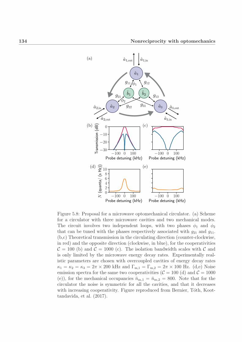
134 Nonreciprocity with optomechanics
(b) (c)
(d) (e)
3
g13
g31g22
g21
g11 g12
,out3
,in3
,in
,out
,in,out
1
2
(a)
Figure 5.8: Proposal for a microwave optomechanical circulator. (a) Schemefor a circulator with three microwave cavities and two mechanical modes.The circuit involves two independent loops, with two phases φ1 and φ2
that can be tuned with the phases respectively associated with g21 and g11.(b,c) Theoretical transmission in the circulating direction (counter-clockwise,in red) and the opposite direction (clockwise, in blue), for the cooperativitiesC = 100 (b) and C = 1000 (c). The isolation bandwidth scales with C andis only limited by the microwave energy decay rates. Experimentally real-istic parameters are chosen with overcoupled cavities of energy decay ratesκ1 = κ2 = κ3 = 2π × 200 kHz and Γm,1 = Γm,2 = 2π × 100 Hz. (d,e) Noiseemission spectra for the same two cooperativities (C = 100 (d) and C = 1000(e)), for the mechanical occupancies nm,1 = nm,2 = 800. Note that for thecirculator the noise is symmetric for all the cavities, and that it decreaseswith increasing cooperativity. Figure reproduced from Bernier, Toth, Koot-tandavida, et al. (2017).

5.6 Outlook 135
the large cooperativity limit, the nonreciprocal process becomes quantumlimited, irrespective of the temperature of the mechanical thermal baths.
5.6 Outlook
In conclusion, we described and experimentally demonstrated a new schemefor reconfigurable nonreciprocal transmission in the microwave domain usinga superconducting optomechanical circuit. This scheme is based purely onoptomechanical couplings, thus it alleviates the need for coherent microwavecavity-cavity (or direct phonon-phonon) interactions, and significantly facil-itates the experimental realisation, in contrast to recently used approachesof optomechanical nonreciprocity in the optical domain (Fang, Luo, et al.,2017).
An intuitive picture built on the gyrator helps to explain the origin ofnonreciprocity in the system. It arises due to interference in the two me-chanical modes, which mediate the microwave cavity-cavity coupling. Thisinterference also manifests itself in the asymmetric noise output of the circuit.Moreover, an additional microwave mode would enable quantum-limited mi-crowave circulators on-chip with large bandwidth, limited only by the energydecay rate of the microwave modes.
The isolator scheme can be readily extended to implement quantum-limited phase-preserving and phase-sensitive directional amplifiers (Malz etal., 2018), as illustrated in fig. 5.9. Swapping two blue-detuned pump tonesfor two of the red-detuned pump tones in fig. 5.4c transforms the isolatorinto a directional phase-preserving amplifier (fig. 5.9a,b). With two addi-tional red-detuned pump tones, the amplification becomes phase-sensitive(fig. 5.9c,d). While the added noise in the forward direction can be quantum-limited for large cooperativities, the back-propagating noise is not. As in thecase of the isolator discussed in section 5.4.2, noise commensurate with thelarge mechanical thermal fluctuations is emitted backwards. An additionalauxiliary microwave mode could be used to cool the mechanical motion andmake the directional amplifiers compatible with sensitive quantum devices.
Finally, the presented scheme can be generalised to an array, and thus forma platform to study topological phases of light and sound (Peano, Brendel, etal., 2015) or topologically protected chiral amplifying states (Peano, Houde,et al., 2016) in arrays of electromechanical circuits, without requiring cavity-cavity or phonon-phonon mode hopping interactions.

136 Nonreciprocity with optomechanics
input output
cavity 1 cavity 2
frequency
input
(a)
(b)
input output
cavity 1 cavity 2
frequency
input
(c)
(d)
Figure 5.9: Schemes for directional amplification with an optomechanicalcircuit. (a,b) Using two blue-detuned and two red-detuned pump tones,the system of fig. 5.3a can be used as a phase-preserving directional ampli-fier. (c,d) With two additional red-detuned pump tones, the amplification isphase-sensitive. The amplification in both cases becomes quantum-limited inits added noise for large coupling rates. The noise emitted in the backwardsdirection is however limited by the mechanical thermal fluctuations. Figureadapted from Malz et al. (2018).

Chapter 6
Level attraction in a microwaveoptomechanical circuit
We here introduce the concept of level attraction and explain how it can bestudied with a microwave optomechanical circuit. This chapter is adaptedfrom the text of a previous publication (Bernier, Toth, Feofanov, et al.,2018a). In section 6.1, we introduce level attraction. In section 6.2, we givea theoretical exposition of the phenomenon and how it is linked to exceptionalpoints. In section 6.3, we demonstrate level attraction experimentally in amultimode optomechanical circuit. Finally, in section 6.4, we conclude andprovide an outlook.
6.1 Introduction
Level repulsion of two coupled modes with an energy crossing has applicationsranging from solid state theory (Ashcroft and Mermin, 1976) to quantumchemistry (Atkins and Paula, 2009). While deceptively simple, it underpinsmore exotic phenomena. With the introduction of dissipation or gain, an ex-ceptional point (Heiss, 2012) appears that is topologically non-trivial (Dem-bowski et al., 2001; Uzdin, A. Mailybaev, and Moiseyev, 2011; T. J. Mil-burn et al., 2015). The special case of two modes with equal dissipationand gain rates is an example of parity-time symmetry (Bender, 2005; Ben-der, Berntson, et al., 2013). The spontaneous breaking of that symmetry ismarked by the exceptional point. In recent years, exceptional points gathered

138 Level attraction
significant interest and they were demonstrated in a variety of systems includ-ing active microwave circuits (Stehmann, Heiss, and Scholtz, 2004; Schindleret al., 2011; Assawaworrarit, X. Yu, and S. Fan, 2017), lasers (Brandstetteret al., 2014; Peng, Ozdemir, S. Rotter, et al., 2014) and optical microres-onators (Bender, Gianfreda, et al., 2013; Peng, Ozdemir, Lei, et al., 2014;W. Chen et al., 2017). In particular, the topological transfer of energy be-tween states by circling an exceptional point has been demonstrated with amicrowave cavity (Dembowski et al., 2001), a microwave waveguide (Doppleret al., 2016), as well as an optomechanical system (H. Xu et al., 2016; Jinget al., 2014).
Strikingly, if one mode has negative energy, the energy levels of two in-teracting modes do not repel, but attract instead (Bernier, Dalla Torre, andDemler, 2014; Eleuch and I. Rotter, 2014; Seyranian, Kirillov, and A. A.Mailybaev, 2005). The Hamiltonian leads to hybridized modes of complexeigenfrequencies, one of which is unstable. As in level repulsion, an excep-tional point marks the transition between the regimes of real and complexfrequencies. In the process, the real components of the frequencies becomeidentical in a way that is reminiscent of the synchronization of driven oscil-lators (Pikovsky, Rosenblum, and Kurths, 2003).
Negative-energy modes (equivalent to harmonic oscillators with negativemass) have been studied in schemes to evade quantum measurement backac-tion (Tsang and Caves, 2012; K. Zhang, Meystre, and W. Zhang, 2013; Polzikand Hammerer, 2015). Such a scheme was recently demonstrated with anatomic spin ensemble, prepared in its maximal-energy spin state in a mag-netic field (Møller et al., 2017). Spin flips decrease the energy and correspondto excitations of a harmonic oscillator with a negative mass. Alternatively,the negative-energy mode can be effectively realized in a frame rotating fasterthan the mode itself (Woolley and Clerk, 2013; Ockeloen-Korppi et al., 2016).
In cavity optomechanics (Aspelmeyer, Kippenberg, and Marquardt, 2014),a blue-detuned pump tone induces a time-dependent interaction betweenthe electromagnetic mode and the mechanical oscillator. In a frame rotat-ing at the pump frequency, the Hamiltonian is time-independent, and theelectromagnetic mode appears to have negative energy. While level repul-sion was demonstrated in the strong coupling regime of cavity optomechan-ics (Groblacher et al., 2009; Teufel, D. Li, et al., 2011; Verhagen et al., 2012),level attraction has so far not been observed.
Here we construct a general theoretical framework for level attractionand demonstrate the phenomenon in a microwave optomechanical circuit us-ing engineered dissipation. First in section 6.2, it is shown how a coherentcoupling between modes of positive and negative energy gives rise to level

6.1 Introduction 139
(a) (b)
Figure 6.1: Level repulsion and attraction. Two modes, whose bare frequen-cies depend on a parameter λ, have a level crossing (dotted lines). A coherentcoupling in general lifts the degeneracy. (a) In the more usual case, level re-pulsion, the coupling opens a gap between the frequencies of the hybridizedeigenmodes ω (blue solid lines) and the eigenfrequencies bend away fromeach other. (b) In contrast, if one of the modes has negative energy, levelattraction occurs. The real components of the eigenfrequencies ω (blue solidlines) bend towards each other and converge. They meet at two exceptionalpoints, where the curves have kinks. A gap opens in the imaginary compo-nents of the frequencies (orange dashed lines). The mode with a negativeimaginary component to the frequency is unstable and grows exponentially.Figure reproduced from Bernier, Toth, Feofanov, et al. (2018a).

140 Level attraction
attraction. The role of dissipation is discussed and explains the difficulty inobserving level attraction in such systems, as the dissipation rates of the twomodes must be similar. The symmetry between level repulsion and attrac-tion is explicited in section 6.2.1. And an intuitive way to classify differenttypes of exceptional points in two-modes system is developed in section 6.2.2,with level repulsion and attraction as special cases. In section 6.3, both levelattraction and repulsion are demonstrated experimentally in the same mi-crowave optomechanical circuit, where the mechanical dissipation rate canbe engineered to match the microwave one.
6.2 Theoretical exposition of level attraction
We start with a general theoretical model of a positive-energy mode coher-ently coupled to a negative-energy one. The two modes, of annihilationoperators a and b and coherently coupled with strength g, are described bythe Hamiltonian
H = −�ω1(λ)a†a+ �ω2(λ)b
†b+ �g(ab+ a†b†
)(6.1)
where the two positive frequencies ω1 and ω2 vary with respect to an externalparameter λ. The linear coupling chosen here is quite general: if we assumethe modes close in frequency, other linear terms a†b, ab† can be neglected inthe rotating wave approximation (valid only if the frequencies ω1,2 dominateover the dissipation rates for an open system, see appendix A). The couplingrate g is chosen to be real, as any complex phase can be absorbed in aredefinition of a or b.
In the Heisenberg picture, this leads to the equations of motion
d
dt
(a
b†
)= i
(ω1 −gg ω2
) (a
b†
)(6.2)
where we drop the explicit λ dependence. We note that the uncoupled, baremodes evolve as a(t) = eiω1ta(0) and b†(t) = eiω2tb†(0) with a positive phase.The hybridized eigenmodes of the system are found by diagonalizing thematrix in eq. (6.2), and have eigenfrequencies
ω1,2 =ω1 + ω2
2±
√(ω1 − ω2
2
)2
− g2. (6.3)
The negative sign in front of g2 is the only difference with the eigenfrequenciesfor the case of level repulsion (when a has positive energy) but dramaticallyimpacts on the resulting dynamics.

6.2 Theoretical exposition of level attraction 141
(a)
(b)
Figure 6.2: The effect of dissipation on level attraction. Two modes, a andb cross in frequency (the mode a having negative energy), with respectivedissipation rates κ and Γ. The real component of the frequency is the solidblue line and the imaginary component the dashed orange line. (a) Whilea finite average dissipation rate simply translates the imaginary componentsof the frequency, a difference in the two rates (κ �= Γ) affects qualitativelylevel attraction. The kinks and the exceptional points disappear and thepicture is overall smoothed out. (b) When the dissipation rates differ sig-nificantly, no trace of level attraction is visible anymore. In both cases, oneof the hybridized mode becomes unstable if the imaginary component of itsfrequency turns negative. Figure reproduced from Bernier, Toth, Feofanov,et al. (2018a).
In fig. 6.1, level attraction is compared to level repulsion, with two strik-ing features. First, instead of avoiding each other, the eigenfrequencies pulltowards one another. Second, when they meet at 4g2 = (ω1 − ω2)
2, the fre-quencies acquire positive and negative imaginary parts, causing exponentialdecay and growth. The hybridized mode with a negative imaginary compo-nent grows exponentially and is therefore unstable.
The transition between the regimes of real and complex eigenfrequenciesis marked by exceptional points, which can be understood by studying thematrix of eq. (6.2). Decomposed in terms of Pauli matrices1 and omitting theterm proportional to the identity, it can be expressed as 1
2(ω1−ω2)σz − igσy.
1 The Pauli matrices are defined as σx = ( 0 11 0 ), σy = ( 0 −i
i 0 ) and σz = ( 1 00 −1 ).

142 Level attraction
In contrast with level repulsion for which the interaction term would be gσx,the Hermitian Pauli matrix is here multiplied by an imaginary coefficient. Ifthe first term has a larger amplitude, the eigenfrequencies are real, while theyare complex if the second term dominates. When the two Pauli matrices havecoefficients of the same amplitude, the matrix is proportional to σz − iσy. Atthis point, the two eigenvectors coalesce and a single eigenvector with a singleeigenvalue subsists: it is an exceptional point (Heiss, 2012). More generallyfor all two-mode systems, any point for which the dynamics is determinedby a matrix proportional to σα+ iσβ, with α �= β, is an exceptional point. Inthe section 6.2.2, we develop this decomposition and construct an intuitiveclassification of the various realizations of exceptional points.
Level attraction arises whenever the coupling term consists of a Pauli ma-trix with an imaginary coefficient. In fact, coupled oscillators of positiveand negative energy are only one way to achieve this. An alternative relieson linking the two modes with a coupling that cannot be derived from aHamiltonian, such as a dissipative interaction through one or multiple in-termediary modes (Metelmann and Clerk, 2014). The mode hybridizationobserved between positive-energy oscillators with dissipative (H. Xu et al.,2016; Khanbekyan et al., 2015) and non-conservative (Gloppe et al., 2014)interactions can be interpreted as level attraction.
While level attraction of two linearly coupled modes displays intriguingsimilarities with the synchronization of driven oscillators, important differ-ences exist. As in synchronization, the real components of the frequencies“lock” over a frequency range that increases with the coupling rate g, form-ing the equivalent of an Arnold tongue (Pikovsky, Rosenblum, and Kurths,2003). The physical process differs however. In synchronization, one startswith two oscillators that are driven nonlinearly to their limit-cycles, then acoupling is introduced that locks their frequencies and their phases (Weiss,Kronwald, and Marquardt, 2016). In level attraction by contrast, the fre-quencies of the two modes attract through linear dynamics until they becomeidentical. The state of the two hybridized modes remain independent andtheir phases can be set arbitrarily.
To understand why level attraction is in practice less common than levelrepulsion, the role of dissipation should be studied. We open the system andinclude in our treatment the energy dissipation rates κ and Γ respectively forthe modes a and b. They can be introduced as positive imaginary componentsof the bare frequencies in the equations of motion. The results of eq. (6.2) and(6.3) can be extended by replacing ω1 with ω1 + iκ/2 and ω2 with ω2 + iΓ/2.In fig. 6.2, we compare the resulting eigenfrequencies. If the dissipation ratesare equal (κ = Γ), the level structure of fig. 6.1b is reproduced with the

6.2 Theoretical exposition of level attraction 143
imaginary components translated to a finite average. However, in the case ofeven slightly mismatched dissipation rates κ � Γ (fig. 6.2a), the exceptionalpoints and the kinks in the frequencies disappear. For increasingly dissimilarrates κ � Γ (fig. 6.2b), the level-attraction picture progressively disappearsuntil the modes seem to cross without interacting. Therefore, only in asystem where dissipation rates can be tuned to closely match each other islevel attraction observable.
6.2.1 Symmetry of level repulsion and attraction
To understand better the relation between level repulsion and attraction, weexplicitly derive here a minimal model for each. We show that a symmetryrelation links the two cases; they are images of each other under the exchangeof frequency and dissipation rates.
First, we review level repulsion. Two modes of positive energy (withannihilation operators a and b, and respective frequencies ω1 and ω2) interact,as described by the Hamiltonian
HLR = �ω1a†a+ �ω2b
†b+ �g(ab† + a†b
)(6.4)
with g the linear coupling strength. The equation of motion in the Heisenbergpicture is given by
d
dt
(a
b
)= −i
(ω1 gg ω2
) (a
b
). (6.5)
To solve the system in terms of eigenmodes, the matrix is diagonalized. Theeigenfrequencies are given by
ωLR1,2 =
ω1 + ω2
2±
√(ω1 − ω2
2
)2
+ g2. (6.6)
The model is extended to describe modes with dissipation by adding imagi-nary components to the bare frequencies, substituting ω1 → ω1 − iΓ1/2 andω2 → ω2−iΓ2/2. Note that a negative sign is required to obtain decaying ex-ponentials. For ease of notation, we define ω0 = (ω1+ω2)/2, Γ0 = (Γ1+Γ2)/2,Δω = ω1 − ω2, and ΔΓ = Γ1 − Γ2. The eigenfrequencies can now be writtenas
ωLR1,2 = ω0 − i
Γ0
2±
√(Δω − iΔΓ/2
2
)2
+ g2. (6.7)

144 Level attraction
The frequency of oscillation of the eigenmodes is given by the real componentof ωLR
1,2 and the dissipation rate by twice its imaginary component (with aminus sign).
We now consider level attraction. One (and only one) mode has negativeenergy such that the system is described by the Hamiltonian
HLA = −�ω1a†a+ �ω2b
†b+ �g(ab+ a†b†
). (6.8)
The equations of motion are given by(a
b†
)= i
(ω1 −gg ω2
) (a
b†
)(6.9)
with eigenfrequencies
ωLA1,2 =
ω1 + ω2
2±
√(ω1 − ω2
2
)2
− g2. (6.10)
The only difference with eq. (6.6) is the sign in front of g2, which can resultin a complex eigenvalue, meaning an instability for the system.
It might be unintuitive that the Hermitian Hamiltonian in eq. (6.8) leadsto complex eigenfrequencies and unstable dynamics. In fact, in an infinite-dimensional Hilbert space, an operator must be compact as well as Hermitianto guarantee the existence of real eigenvalues (Le Bellac, 2012), which is notthe case here. We also note that only when the eigenfrequencies are real canthe eigenoperators be interpreted as Bogolyubov modes (Fetter, Walecka,and Physics, 2003). When the eigenfrequencies are complex, the requiredcommutation relations cannot be satisfied.
In order to include dissipation, we substitute again ω1 → ω1 + iΓ1/2 andω2 → ω2 + iΓ2/2. Note that the opposite sign for the imaginary compo-nent is required here to obtain decaying exponentials. The eigenfrequenciesincluding dissipation become
ωLA1,2 = ω0 + i
Γ0
2±
√(Δω + iΔΓ/2
2
)2
− g2. (6.11)
There is a symmetry between eq. (6.7) and eq. (6.11). They are equivalentunder the transformation ω′ = Γ/2 and Γ′ = 2ω, if eq. (6.11) is multipliedby a factor −i:
ω′LA1,2 = ω′
0 − iΓ′0
2±
√(Δω′ − iΔΓ′/2
2
)2
+ g2. (6.12)

6.2 Theoretical exposition of level attraction 145
We conclude that level attraction and repulsion are equivalent to each otherthrough the exchange of frequency and dissipation rates (within a factorof 2). In fig. 6.3, this symmetry is highlighted by contrasting equivalentsituations for both level repulsion and level attraction Hamiltonians. Infig. 6.3a-d, the curves for the real and imaginary parts of the eigenfrequenciesare interchanged when going from the left column (level repulsion) to theright (level attraction). Figure 6.3e-f can be compared with fig. 6.1, where thecharacteristic shape of level attraction is here seen for the dissipation rates ofthe level-repulsion Hamiltonian and vice versa. In general, for level repulsion,when a coupling is introduced the frequencies repel, while the dissipation ratesattract. The exact opposite is true for level attraction: a coupling makes thedissipation rates repel and the frequencies attract.
6.2.2 Classification of exceptional points
We describe here how to classify exceptional points of 2 × 2 matrices usingPauli matrices. The classification is then used to sort recent experimentaldemonstrations of exceptional points.
In general, the equations of motion for a 2-modes system can be writtenin the form
id
dt
(d1d2
)= M
(d1d2
)(6.13)
where d1, d2 are operators for the two modes and M is a 2 × 2 matrix.The eigenmodes of the system and their eigenfrequencies correspond to theeigenvectors and eigenvalues of M . If for some parameter values, M onlyhas a single eigenvector and a single eigenvalue, this is called an exceptionalpoint.
The matrix M can always be decomposed in terms of the Pauli matrices,defined as
σx =
(0 11 0
), σy =
(0 −ii 0
), and σz =
(1 00 −1
), (6.14)
in the form
M = a01 + a1σx + a2σy + a3σz (6.15)
with 1 the identity matrix and ai complex numbers. The eigenvalues of Mare now easily expressed as
λ1,2 = a0 ±√a21 + a22 + a23. (6.16)

146 Level attraction
(a) (b)
(c) (d)
(e) (f)
Figure 6.3: Comparison of the real (solid blue lines) and imaginary (dashedorange lines) components of the eigenfrequencies ω for the level-repulsionHamiltonian HLR (left column) and the level-attraction Hamiltonian HLA
(right column). (a,b) The transition through an exceptional point, as afunction of the coupling strength g. For level repulsion (a), the modes areoriginally degenerate (Δω = 0), while for level attraction (b) they originallyhave matching dissipation rates (ΔΓ = 0). (c,d) Same as (a,b) with a slightnondegeneracy (Δω �= 0 for level repulsion (c) and ΔΓ �= 0 for level attrac-tion (d)), such that the exceptional point is avoided. (e,f) The difference indissipation rates ΔΓ is varied, for degenerate modes Δω = 0. For level repul-sion (e), the imaginary component of the frequency attract and converge in aregion where a gap opens in the real components of the frequency. For levelattraction (f), the real component is unchanged while the dissipation rateshave an avoided crossing. Figure reproduced from Bernier, Toth, Feofanov,et al. (2018a).

6.2 Theoretical exposition of level attraction 147
Note that the first term in eq. (6.15), proportional to the identity, onlyshifts the eigenvalues by a constant and has no effect on the eigenvectors.Anytime that the matrix M can be written as a multiple of σα+ iσβ (α �= β)(omitting the identity), there is only one eigenvalue and this is an exceptionalpoint (Steeb and Hardy, 2014). We can use this decomposition to classifyexamples of exceptional points.
(I) The most common case is the level repulsion of two (positive-energy)modes of degenerate frequencies due to a coherent coupling. Many experi-mentally demonstrated exceptional points fall in this category (Dembowskiet al., 2001; Schindler et al., 2011; Bender, Gianfreda, et al., 2013; Brandstet-ter et al., 2014; Peng, Ozdemir, Lei, et al., 2014; Peng, Ozdemir, S. Rotter,et al., 2014; Doppler et al., 2016; Assawaworrarit, X. Yu, and S. Fan, 2017).The two modes are d1 = a and d2 = b, in our previous notation. The matrixM can be written as
M =
(ω0 − i
Γ0
2
)1 − i
ΔΓ
4σz + gσx. (6.17)
For a low coupling rate g, M is diagonal with a gap for dissipation rates. Fora large g, the last term dominates such that the eigenmodes are eigenvectorsof σx: g opens a gap in frequency, while the dissipation rates are evenlydistributed between the modes. The transition between the regimes is markedby an exceptional point at g = ΔΓ/4.
(II) Here, we consider the case of level attraction between modes of nega-tive and positive energies and matching dissipation rates. The operators ared1 = a and d2 = b† in our notation. The matrix M can be written as
−M =
(ω0 + i
Γ0
2
)1 +
Δω
2σz − igσy. (6.18)
For a low coupling g, there is a gap in frequency, while for a large coupling, theσy term opens a gap in dissipation rates and the frequencies are identical. Anexceptional point marks the transition at g = Δω/2. Note that the coherentcoupling corresponds to a term with an imaginary coefficient for a systemwith one mode of negative energy.
(III) Level attraction of two modes can be realized in any system in whichthe coupling term has an imaginary component. In particular, dissipativeinteractions (Metelmann and Clerk, 2014) represent an alternative way tothe one presented in this article. Two modes are coupled by both interactingwith a third oscillator. When the third mode is eliminated, the effectiveinteraction between the two modes is expressed by the matrix M as
M =
(ω0 − i
Γeff
2
)1 +
Δω
2σz + igdisσx (6.19)

148 Level attraction
where for simplification the effective dissipation rate Γeff of the two coupledmodes is taken to be approximately equal. The effective interaction betweenthe two modes has an imaginary coefficient and they have an increased effec-tive dissipation rate Γeff due to the dissipative interaction as well. Similarlyto the previous case, by increasing the coupling gdis the original gap in fre-quency is closed and a difference in dissipation rates is created. In contrasthowever, Γeff grows proportionally with gdis, such that the gap in dissipa-tion rates does not result in an instability. The mode hybridization betweenmodes of positive energy coupled with dissipative interactions can be inter-preted as level attraction.
Examples of this type of exceptional points were realized experimentally.In the experiment of H. Xu et al. (2016), two mechanical oscillators areeffectively coupled by both interacting with the same optical cavity. In theexperiment of Khanbekyan et al. (2015), two modes of an optical resonatorinteract through multiple quantum dots. In the experiment of Gloppe etal. (2014), two modes of a nanowire interact through the non-conservativeforce of an optical field, which although not dissipative in nature, cannot bederived from a Hamiltonian in a similar way.
(IV) Finally, yet another way to implement an exceptional point was re-alized in the experiment of W. Chen et al. (2017). The clockwise and coun-terclockwise modes of a whispering-gallery-mode resonator (of degeneratefrequencies and dissipation rates) interact through two Rayleigh scatterers.This results in a combination of coherent and dissipative interaction that canbe described by
M =
(ω0 − i
Γ0
2
)1 + gcohσx + igdisσy. (6.20)
As the coupling gcoh and gdis are varied, the relative phases of the baremodes that compose the hybrid eigenmodes change. When the two cou-pling strengths match (gcoh = gdis), the two eigenmodes coalesce and there isan exceptional point. Interestingly, this corresponds to a point of maximalnonreciprocity, with one bare mode coupled to the second but not the otherway around (Metelmann and Clerk, 2015).
6.3 Optomechanical level attraction
Cavity optomechanics provides an ideal setting to study level attraction andcompare it to level repulsion. We now take a to represent an electromagneticmode and b a mechanical oscillator, coupled through the optomechanical in-

6.3 Optomechanical level attraction 149
teraction �g0a†a(b+b†), where g0 is the vacuum optomechanical coupling (As-
pelmeyer, Kippenberg, and Marquardt, 2014). With a blue-detuned pumptone applied to the system, the three-wave-mixing coupling is linearized andthe Hamiltonian reduces to the form of eq. (6.1)
H = −�Δa†a+ �Ωmb†b+ �g
(ab+ a†b†
), (6.21)
where Δ is the detuning of the pump tone, Ωm the mechanical mode fre-quency and g = g0
√nc the linear coupling enhanced by the mean cavity
photon number nc due to the pump tone. As above, we neglect counter-rotating terms and assume the detuning Δ to be close to Ωm. Critically, theHamiltonian is expressed in a frame rotating at the pump frequency in orderto be time-independent. Hence, for a blue detuning Δ > 0, the cavity modeeffectively has a negative energy, since the photons have a negative relativefrequency with respect to the pump.
In this context, the well-known parametric instability of optomechan-ics (Aspelmeyer, Kippenberg, and Marquardt, 2014) can be interpreted asresulting from the physics of level attraction. The instability stems from thenegative imaginary component that develops in the eigenfrequencies of theequations of motion, above the critical coupling gcrit =
√κΓ/2.
For level attraction to be observable, the magnitudes of κ and Γ shouldbe close. For usual experimental parameters, however, the electromagneticdecay rate κ is much larger than the mechanical rate Γ, and no attractioncan in practice be observed for the mechanical and electromagnetic modes.
6.3.1 Experimental results
In our experiment, the effective mechanical energy decay rate Γeff is artifi-cially increased to match κ using sideband cooling with an auxiliary mode.We use a superconducting electromechanical circuit (Teufel, D. Li, et al.,2011) containing two microwave LC modes interacting with the vibrationalmode of a vacuum-gap capacitor (represented schematically in fig. 6.4a andshown in fig. 6.4b). The design, which is described in section 4.2, uses twohybridized electromagnetic modes of the circuit to ensure that one has amuch larger external coupling rate to the microwave feedline than the other.The more dissipative, auxiliary mode aaux is used to perform sideband cool-ing of the mechanical oscillator with a red-detuned pump tone. This dampsthe oscillator and increases its effective dissipation rate to Γeff ≈ κ. Mean-while, the less dissipative, primary mode a undergoes level attraction withthe damped mechanical oscillator.

150 Level attraction
inout
(a) 200 μm(b)
(c)
(d)
Figure 6.4: Engineering dissipation in a multimode optomechanical circuit.In order to observe level attraction, the dissipation rate Γm of the mechanicalmode b must be increased to match κ, the much larger dissipation rate ofthe primary electromagnetic mode a. To that end, an auxiliary mode aaux isused for sideband cooling. (a) Schematic of the microwave optomechanicalcircuit, coupled inductively to a microwave feedline and measured in reflec-tion. The two hybridized modes of the circuit a and aaux interact with themotion of the top membrane of a shared capacitor, the mechanical oscillatorb (in green). (b) Photograph of the circuit and scanning-electron micrographof the vacuum-gap capacitor. (c) Diagram of the three interacting modes.(d) Frequency domain representation of the level-attraction experiment. Amicrowave pump tone (vertical red line), red-detuned by the mechanical fre-quency Ωm with respect to the auxiliary mode resonance ωaux (grey peak) isused for sideband cooling. Level attraction of the modes a and b is achievedby sweeping the detuning Δ of a pump tone (vertical blue line) near the bluesideband of the primary mode resonance ωc (blue peak). For level repulsion,the pump tone is instead swept near the red sideband. Figure reproducedfrom Bernier, Toth, Feofanov, et al. (2018a).

6.3 Optomechanical level attraction 151
In the experiment, the device is placed inside a dilution refrigerator andcooled to the base temperature, below 50 mK, at which the circuit is su-perconducting and its internal Q-factor is enhanced. The sample is HYB-20160524-1-12. The two microwave modes a and aaux have respective res-onance frequencies ωc = 2π × 4.11 GHz and ωaux = 2π × 5.22 GHz, anddissipation rates κ = 2π × 110 kHz and κaux = 2π × 1.8 MHz. They inter-act with the fundamental vibrational mode of the top plate of the vacuum-gap capacitor, that has a frequency Ωm = 2π × 6.3 MHz. By placinga pump tone red-detuned by Ωm from the auxiliary mode resonance (seefig. 6.4d), the mechanical oscillator is damped. The mechanical dissipationrate Γm, originally below 2π × 100 Hz, is tuned to an effective dissipationrate Γeff ≈ κ = 2π × 110 kHz.
Level repulsion and attraction of the primary microwave mode and thedamped mechanical oscillator are both measured. As a pump tone is tunedto the blue or red sideband of the primary microwave mode (the formercase is illustrated in fig. 6.4d), the weak probe tone of a vector networkanalyser is applied near the resonance of the microwave cavity to obtain itslinear response. Due to the hybridization of the modes, the response carriesinformation about both microwave and mechanical modes. For both red andblue detunings, the same pump power is set to obtain a coupling strengthg ≈ 2π×200 kHz corresponding to a mean cavity photon number nc ≈ 4×10⁶.
The known case of level repulsion is obtained with a red-detuned tone(fig. 6.5a). As the bare effective mechanical mode frequency comes near themicrowave resonance, the two modes hybridize; their eigenfrequencies bendaway from each other with a gap of 2g.
With a blue-detuned tone, level attraction occurs instead. The response,shown in fig. 6.5b, displays the characteristic level structure of fig. 6.1b. Theresonance frequencies of the modes attract and converge to the points wherethe bare frequencies of the modes differ by ±2g. In order for the level at-traction to be clearly visible, the coupling rate g is set to dominate over thedissipation rates κ and Γeff . It therefore exceeds the critical coupling gcrit, re-sulting in parametric instability. One of the modes grows exponentially untilthe conditions of the validity of eq. (6.21) are no longer fulfilled. Namely, thefluctuating field is no more negligible compared to the mean cavity photonnumber nc. The original nonlinear optomechanical interaction constrain thesystem to a limit-cycle with a modified cavity resonance frequency (Mar-quardt, Harris, and Girvin, 2006), the description of which lies beyond thescope of this article. Data is omitted for clarity in the unstable region.
In fig. 6.6a,c, two individual responses from fig. 6.5 are shown for specificdetunings of the pump tone. The two resonances take the form of two dips

152 Level attraction
(a)
(b)
Figure 6.5: Experimental demonstration of level repulsion and attraction ina microwave optomechanical circuit. Amplitude response of the system asthe detuning Δ of the pump tone is varied, when the effective dissipationrate of the mechanical mode b matches that of the microwave mode a. Inthe laboratory frame, Δ determines the effective frequency of the mechanicaloscillator, that is swept across the microwave resonance. (a) When the pumptone is swept in frequency across the red sideband of the microwave mode,the two resonances bend away from each other. (b) If the pump tone is sweptacross the blue sideband instead, the resonances pull towards each other andconverge near two exceptional points. Data is omitted for clarity where thesystem becomes unstable and one hybridized mode grows exponentially untilthe conditions of validity of eq. (6.21) are no longer fulfilled (parametricinstability). Figure adapted from Bernier, Toth, Feofanov, et al. (2018a).

6.4 Outlook 153
in amplitude in the case of level repulsion, while the feature corresponding tothe mechanical resonance takes the form of a peak in amplitude in the caseof level attraction. Represented on the complex plane, the resonances formcircles. In level repulsion (fig. 6.6b), the two circles are circumscribed. Theradii of the circles correspond to how the two hybridized modes are coupledto the measurement channel. With a resonant pump tone Δ = Ωm, thetwo modes are coupled the same and the two circles have the same radius.This is a direct analog of OMIT with a red-detuned drive as described insection 3.6.2. For level attraction (fig. 6.6d) however, the circle correspondingto the mechanical lies outside the circle of the microwave resonance.
6.4 Outlook
In summary, level attraction was experimentally demonstrated using a dual-mode electromechanical circuit. Although related to the well-studied para-metric instability of optomechanics, the vastly different dissipation rates forthe mechanical and electromagnetic modes prevented its observation untilnow. Level attraction, similarly to level repulsion in open systems, gives riseto exceptional points. In both cases, the real part of the frequencies convergeand a gap opens in the imaginary part (or vice versa) precisely at the excep-tional point. In future work, the exceptional points of level attraction couldbe harnessed to demonstrate topological phenomena by circling such a pointin a two-dimensional parameter space (Dembowski et al., 2001; H. Xu et al.,2016; Doppler et al., 2016). Since the exceptional point only exists when thedissipation rates of the two modes match exactly, the tunable mechanicaldamping rate Γeff can be used as one parameter in such an experiment, withthe tunable coupling rate g as the second.

154 Level attraction
(a)
(b)
(c)
(d)
Figure 6.6: Amplitude and complex responses for level repulsion and attrac-tion. (a,b) Level-repulsion response corresponding to the data of fig. 6.5a fora pump detuning Δ+Ωm = −2π× 180 kHz, shown in amplitude (a) and onthe complex plane (b). (c,d) Level-attraction response corresponding to thedata of fig. 6.5b for a pump detuning Δ − Ωm = −2π × 630 kHz, shown inamplitude (c) and on the complex plane (d).

Chapter 7
Outlook on high-efficiency opto-mechanical measurements witha traveling-wave parametric am-plifier
In this chapter, we introduce the use of a traveling wave parametric amplifier(TWPA), developed in a collaboration between the group of Prof. Siddiqi atUC Berkeley and the Lincoln Laboratory at the Massachusetts Institute ofTechnology. After an introduction in section 7.1, its installation and functionare detailed in section 7.2. In section 7.3, we present a demonstration of anoptomechanical measurement previously unattainable in our experiment. Asan outlook, we present in section 7.4 ongoing efforts to precisely calibratethe added noise of the device and ideas for future experiments relying onhigh-efficiency detection.
7.1 Introduction
The amplifier plays the central role in quantum measurements at microwavefrequencies. Since there exists no detector for microwave photons, gain isrequired for the signals to be be measured classically. As such, the amplifica-tion process itself can be thought of as the quantum measurement, as arguedin section 2.2.3. In appendix B, amplification is compared to the equivalent

156 High-efficiency measurements
detection process at optical frequencies. The added noise of the amplifiercorresponds to an equivalent quantum efficiency
ηeq =1
Nadded +12
. (7.1)
In the case of HEMT amplifiers, the efficiency typically is ηHEMT ≈ 0.05. It isas if 95 % of the signals of interest is discarded before measurement, resultingin a much reduced signal-to-noise ratio compared to the ideal case. Longaverages are needed to resolve weak signals and certain experiments cannotbe performed since the noise is too large. The great potential improvementin SNR motivates us to investigate more recent technologies that providesamplification much closer to the quantum limit in terms of added noise.
Josephson parametric amplifiers (Castellanos-Beltran and Lehnert, 2007;Bergeal et al., 2010; Hatridge et al., 2011) can provide an added noise closeto the quantum limit. They rely on a microwave cavity that is enhancedby the nonlinearity provided by Josephson junctions. With a driving tone,this nonlinearity results in a reduced effective dissipation rate for the cavityand gain. The resonance at the heart of the mechanism limits the amplifi-cation to a bandwidth near the resonance frequency. While the frequencycan be tuned, with a magnetic flux for instance (Castellanos-Beltran andLehnert, 2007), there remains strong limitations in terms of the bandwidth,which is limited to the range of MHz due to the finite linewidth of the cavity.To remedy this, Macklin et al. (2015) dispense with the cavity and form ametamaterial transmission line with a long chain of Josephson junctions. Bysending a driving tone copropagating with the signal on the line, the interac-tion through the nonlinearity results in amplification with a very low addednoise and a bandwidth in the order of GHz. The device is called a Josephsontraveling-wave parametric amplifier. One such device was provided to us bythe Lincoln Laboratory at the Massachusetts Institute of Technology.
7.2 Installing and operating the TWPA
We present here how the typical experimental setup introduced in section 3.3is adapted to incorporate the TWPA. The new setup is shown schematicallyand in photograph in fig. 7.1. The TWPA is placed on the breadboard atthe base plate, right after the sample holder. By precaution, one of the twoisolators is placed before it, to absorb any strong tones that might backscattertowards the optomechanical circuit. The backward gain of the TWPA shouldideally be 0 dB, but if the pump tone used to drive it is reflected somewhere

7.2 Installing and operating the TWPA 157
3 K
800 mK
10 mK
20 dB HEMT
input outputaux.
DUT20 dB
TWPA
(a)
inputaux.
output
(b)
Figure 7.1: Setup for the TWPA. (a) Schematics of the modification of thesetup inside the dilution refrigerator to incorporate the TWPA. (b) Photo-graph of the relevant components, with the ports labeled.
along the line, there can potentially be non-zero backward gain. The rest ofthe components that sit inside the dilution refrigerator is not affected. Theauxiliary port has the added function to send in the driving tone for theTWPA, as well as to be used for tone cancellation as previously.
The large sensitivity of the TWPA has the disadvantage that even rela-tively weak coherent tones in the input signals can saturate the amplificationprocess, causing distortion. The tone cancellation strategy used previously(detailed in section 3.3.4) that provides up to 30 dB of cancellation provedinsufficient. Instead, an improved approach, illustrated in fig. 7.1, was im-plemented that can reliably cancel tones by over 70 dB, in an automatedway. We use digitally controlled tunable attenuators (Vaunix LDA-602EH,with steps of 0.1 dB) and phase shifters (Vaunix LPS-802, with steps of 1degree). With a set of one phase shifter and one attenuator, a tone can betuned in amplitude and phase precisely enough to cancel a copy of itself by35 dB. Two stages of tone cancellation are used to achieve about 70 dB ofcancellation overall. The microwave tone used to drive the system is firstsplit. One half is sent to the input port, after some attenuation. The otherhalf goes through the tone cancellation circuit. It is again split in two, thistime with a directional coupler. Each part goes through a stepped attenua-tor and a phase shifter before being recombined. The microwave tone thatdrives the TWPA joins the tone cancellation signal and they both are sentin the auxiliary port. The digitally controlled devices enables the tone can-cellation procedure to be fully automatized through a programmed script.One disadvantage compared to the previously used devices is that they have

158 High-efficiency measurements
Optomech.Pump
input aux.
att.
ϕ
ϕ TWPAPump
Figure 7.2: Scheme for tone cancellation. The TWPA requires efficient tonecancellation for the strong optomechanical pump tones used. Through twostages of tone cancellation with one variable attenuator and phase shiftereach, tone cancellation of 70 dB is achieved. Some attenuation is requiredfor the pump tone to match the large insertion loss of the tone cancellationcircuit.
a large insertion loss (about 10 dB at a minimum for the attenuator). Someattenuation must be introduced on the input line to equilibrate the two arms.That implies a reduction to the maximal power that can be applied on chip.
The linear response of the TWPA shows a dispersive feature near 6 GHz,at which absorption occurs. When a strong microwave tone is applied to thered of this feature, any other signal co-propagating is amplified in a wideband, from about 4 to 8 GHz. The driving tone is swept both in frequencyand power to find an optimal operating point, with large and regular gain overthe bandwidth of interest. While the absolute gain and added noise are notimmediately accessible, they can easily be compared to that of the HEMT onits own by turning the pump tone off. The comparison of the linear responsegives a measure of the relative gain provided by the TWPA. By comparingthe SNR of a weak calibration tone at a particular frequency in the sameconditions, the effective added noise of the TWPA can be measured relativelyto that of the HEMT. Although that is not a very precise calibration, thisprovides an idea whether the TWPA is operated in good conditions. Thereare parameters for the pump tone for which the gain appears high, but theadded noise is large as well, defeating the purpose.
7.3 Detailed balance in sideband cooling
The TWPA offers the combined characteristics of nearly quantum-limitedadded noise over very large bandwidths. As a demonstration case of how

7.3 Detailed balance in sideband cooling 159
this can be an advantage for optomechanical measurements, we present herepreliminary results on the measurement of both mechanical sidebands of thepump tone in a sideband-cooling experiment. The cooling power can bethought of as due to the imbalance between Stokes and anti-Stokes scatter-ing of a pump tone applied to the system. The former adds energy to themechanical oscillator while the latter subtracts from it. For a red-detunedpump tone, the anti-Stokes process dominates and the mechanical mode coolsdown. For large enough pump powers however, the system reaches stationaryconditions with a detailed balance in which the two processes equilibrate. Forsideband-resolved optomechanical systems, the lower sideband is very weakand hard to measure. We demonstrate the use of the TWPA by measuringboth sidebands at once. In the following, we first introduce the theoreticalmodel for the sideband cooling, and then the experimental results.
7.3.1 Theoretical model
For a pump tone at a detuning Δ, the Stokes and anti-Stokes processes havesrates that respectively correspond to A+ (nm + 1) for the red sideband andA−nm for the blue sideband (Aspelmeyer, Kippenberg, and Marquardt, 2014,section VII.A), where nm is the average phonon occupancy and the rates aregiven by
A− = g2κex
(κ/2)2 + (Δ + Ωm)2and A+ = g2
κex
(κ/2)2 + (Δ− Ωm)2. (7.2)
The situation is illustrated in fig. 7.3a. The occupancy nm is found by solvingthe stationary solution of the birth-death process and given by
nm =A+ + nm,thΓm
A− − A+ + Γm
. (7.3)
This results in total average rates for the Sidebands
Γred =A+ (A− + (nm,th + 1)Γm)
A− − A+ + Γm
, (7.4)
Γblue =A− (A+ + nm,thΓm)
A− − A+ + Γm
, (7.5)
which are measured in quanta per second.
The sidebands are spread over a certain bandwidth in frequency domain,with a density ISB(ω) = Γeff/(2π)/((ω−ω0)
2+(Γeff/2)2). This is normalized
such that∫ISB(ω)dω = 1. To obtain the spectral density, measured in quanta

160 High-efficiency measurements
per second per Hz, a different normalization must be used. The spectra ofthe sidebands are given by Sred/blue(f) = Γred/blue × 2π× ISB(2πf) to get thecorrect normalization. What we are interested in is the maximum rate in themiddle of the Lorentzian. Those rates are given by
Smaxred =
4A+ (A− + (nm,th + 1)Γm)
(A− − A+ + Γm)2=
4A+(nm + 1)
Γeff
, (7.6)
Smaxblue =
4A− (A+ + nm,thΓm)
(A− − A+ + Γm)2=
4A−nm
Γeff
. (7.7)
Both are measured in quanta per second per Hz. The same spectra can becomputed from the Langevin equations. The noise due to the mechanicalbath and from the input electromagnetic field must be combined, as thelatter (giving rise to backaction noise) becomes relevant for large coolingpowers. The asymmetry between the two sidebands, that are proportionalto nm and nm + 1 can be traced to the interference of the electromagneticvacuum noise (Sudhir et al., 2017; Sudhir, 2018).
The sideband spectrum signals are to be compared to the noise back-ground. It is constituted of vacuum fluctuations (0.5 quanta per second perHz) plus the added noise from the TWPA (a minimum of 0.5 quanta persecond per Hz). This means the SNR is given by
SNRred =Smaxred
12+Nadded
, SNRblue =Smaxblue
12+Nadded
. (7.8)
The derived results imply a priori that the effective mechanical occu-pancy nm can be extracted from the ratio of SNR of the two sidebandsSNRred/SNRblue if the ratio A+/A− is known, without any knowledge of theTWPA added noise Nadded required. Then using the knowledge of nm, theadded noise Nadded can be retrospectively deduced from the absolute SNR.This relies on the assumption that both sidebands are amplified in the sameway through the TWPA. As we shall see, it is not verified in practice andthe measurement cannot be made in a fully self-calibrated manner.
7.3.2 Preliminary experimental results
The experiment is performed by applying a pump tone detuned to the red ofthe cavity resonance of an optomechanical circuit. The two sidebands, ampli-fied by the TWPA, are measured with a spectrum analyzer for various pumppowers. At each power, the tone cancellation parameters are optimized, tocancel the pump tone by about 70 dB before the TWPA.

7.3 Detailed balance in sideband cooling 161
A+(n+1) A-n
(a) (b)
(c) (d)
Figure 7.3: Sideband asymmetry experiment with the TWPA. (a) Schematicof the experiment in the frequency domain. A red-detuned pump tone isapplied to the cavity to perform sideband cooling. The two resulting me-chanical sidebands are measured. (b) Mechanical occupancy nm, deducedfrom the asymmetry of the two sidebands. (c) Calibrated absolute power ofthe noise background for the red (red dots) and blue (blue dots) sidebands.Knowing nm, the total noise background, including the added noise Nadded isdeduced from the absolute SNR of each sideband. (d) Quantum efficiency ofthe TWPA for each sideband, deduced from the added noise Nadded.

162 High-efficiency measurements
The original aim was for a fully self-calibrated experiment, relying on theassumption that the added noise of the TWPA is the same at the frequenciesof both sidebands. However, we find this not to be the case. For low coolingpowers (corresponding to a large mechanical occupancy nm), the ratio of SNRof the two sidebands SNRblue/SNRred should be given by A−/A+. The latterdepends only on the detuning Δ, the dissipation rate κ and the mechani-cal frequency Ωm, and can be computed independently. The measured ratioSNRblue/SNRred exceeds the computed ratio A−/A+ (which would imply anegative mechanical occupancy in the model). We suppose that it is dueto a difference in added noise at the frequencies of the two sidebands, thatincreases the measured ratio compared to the model. By supposing a differ-ence in added noise of 1.6 dB, the experimental data correspond to what isexpected. We present those here as preliminary results. Further calibrationsare necessary to confirm that such a difference in added noise exists and isindeed what causes the discrepancy.
The results are shown in fig. 7.3. The sample is HYB-20150924-4-17, usingthe microwave resonator at 5.3 GHz. We find that the mechanical oscillatoris cooled to nm ≈ 0.5 quanta, from the measured ratio SNRblue/SNRred (seefig. 7.3b). Then, the mechanical occupancy is used in turn to transformthe SNR into a measure of the background noise with an absolute scale (seefig. 7.3c). We assume that the apparent drop in the noise for larger coolingpowers is due to classical heating from the pump tone noise that is not takeninto account in the model and increases the SNR ratio. The backgroundnoise of approximately 2 quanta correspond to an added noise of 1.5 quantaand a quantum efficiency of 0.5 (see fig. 7.3d).
An example of the two measured sidebands is shown in fig. 7.4. The use-fulness of the TWPA for such a measurement is demonstrated by comparingthe result when switching the TWPA pump tone off. The SNR of the side-bands, in particular the red-detuned one, is reduced dramatically when onlythe HEMT amplifier is used to amplify them.
7.4 Precise noise calibration
The TWPA promises tremendous improvement in measurement efficiency,boosting SNR, reducing measurement time and allowing very weak signalsto be detected. Nevertheless, to unleash its full potential, a scheme for theprecise calibration of the added noise must be implemented. The methodused to calibrate the HEMT amplifiers, introduced in section 3.4.2, cannotbe used, since it relies on changing the temperature of the whole mixing-

7.4 Precise noise calibration 163
5.300 5.305 5.310 5.315 5.320Frequency (GHz)
−120
−100
−80
Spe
ctra
lden
sity
(dB
m/H
z)
Figure 7.4: Comparison of the sideband measurement with the TWPA turnedon and off. The two sidebands of a pump detuned to the red of a microwavecavity are measured while the pump tone that drives the TWPA is on (green)and off (blue). In the latter case, the SNR is limited by the added noise ofthe HEMT amplifier. Figure courtesy of Alexey Feofanov.
chamber plate and that would affect the performance of the TWPA. In thefollowing, we introduce the ongoing effort to calibrate the TWPA with alocally heated matched load.
As explained in section 3.4.2, at the heart of any added-noise calibra-tion lies a calibrated noise reference, that provides an absolute power scalecompared to which the amplifier performance can be gauged. A cryogenicmatched load (XMA 2001-6112-02) at a known temperature is used for thispurpose. The temperature of the load is tuned with a heater and measuredwith a thermometer. The required equipment configuration is illustrated infig. 7.5. A holder made of OFHC copper was designed and fabricated by theworkshop of the institute of physics at EPFL (shown in fig. 7.5b, the filesare available online (Bernier, 2018)). The thermometer (Lakeshore CernoxCU-HT) is clamped to it with a bolt that is screwed in a threaded hole. Theheater (Lakeshore HTR-50) is inserted in a cylindrical hole of the holder andfixed with varnish. The holder surrounds the cylindrical matched load andcan be tightened around it with a bolt to guarantee good thermal contact.New DC lines are installed inside the dilution refrigerator. A twisted pairconnects the heater to a control box (Lakeshore 370 AC resistance bridge),and is used to send a current and increase the temperature. The resistance ofthe thermometer is measured with a 4-wire method, using the same control

164 High-efficiency measurements
3 K
800 mK
10 mK
20 dB HEMT
input outputaux.
20 dB
TWPA
6 dB
thermo.
heater
DC lines(a)
LoadHeater
Thermometer
(b)
Figure 7.5: Setup for the calibration of the TWPA. (a) Schematic of thesetup. The matched load replaces the sample holder on the base plate. It isfixed in an OFHC copper holder, with a thermometer and a heater. DC linesare required to supply the current for the heater and measure the resistanceof the thermometer. (b) Photograph of the load in the holder, installed inthe dilution refrigerator (photograph courtesy of Nick Sauerwein).
box.
In a first preliminary measurement, the thermometer is fixed to the baseplate. Using data acquired during the cooldown and warmup of the dilu-tion refrigerator, the resistance of the thermometer is calibrated against theexisting mixing-chamber thermometer.
In the main measurement, the load (fixed in the OFHC-copper holder)replaces the sample holder on the breadboard of the base plate. The addednoise can then be calibrated exactly at the reference plane of the chip, takinginto account any insertion loss between the sample holder and the TWPA,as well as any added noise of the rest of the measurement line, as explainedin section 3.4.2. The aim is to measure the added noise of the TWPA in thissituation and use this calibration for subsequent experiments.
Unlike the HEMT amplifiers, the performance of the TWPA is not con-stant. It depends critically on the pump tone that drives the amplificationprocess. We do not suppose that the gain and added noise are always thesame at the same nominal power and frequency of the pump tone. Any slightvariation along the line, any reflections due to an impedance mismatch willchange the power slightly and affect the result. Therefore, we need a way totranslate the calibration result to a later time when the added noise mighthave changed. For this purpose, we plan to use a calibration tone that prop-agates alongside the TWPA pump tone. The SNR of such a tone gives a

7.4 Precise noise calibration 165
local relative measure of the added noise. The calibration with the heateranchors it on an absolute scale. For a given configuration of the TWPA, boththe added noise Nadded[ω] and the SNR of the calibration tone SNRcal.[ω] arerecorded as a function of frequency ω. In an actual experiment, where a chipsupplants the heated load, the SNR of a calibration is measured at equalpower and frequency. If the path of the calibration tone is in all points iden-tical, any modification of the SNR can be attributed to a change in addednoise of the TWPA. The correct added noise can then be deduced from thecalibration.
The precise calibration of the TWPA, still an ongoing effort, will refinethis powerful tool for high efficiency measurements. Without an absolutescale given by the added noise of the TWPA, it is difficult to extract any in-formation from the measured signals, even if the SNR is improved comparedto the HEMT. The sideband asymmetry measurements of section 7.3 can berevisited to confirm the results and analyze the low mechanical occupancyachieved with sideband cooling more carefully. As a further step, there areplans to measure the ponderomotive squeezing (Purdy et al., 2013) in themicrowave domain. That requires an accurate knowledge of the level of quan-tum noise to ensure that the squeezing is indeed of the vacuum fluctuations.In general, this new measurement technique constitutes a colossal improve-ment in the quantum efficiency previously achieved in our experiments andwill improve measurement throughout microwave circuit optomechanics.


Chapter 8
Conclusions and outlook
We first summarize the results of this thesis in section 8.1, and proceed todescribe future possible directions for the work in section 8.2.
8.1 Summary of the results
Microwave optomechanical circuits constitute a powerful framework in whichto study the linear interactions of harmonic oscillators, down to their quan-tum fluctuations. The linearization of the optomechanical coupling with adriving tone effectively renders the coupling rate and the relative frequen-cies of the two modes (in the rotating frame) tunable (see section 2.1.4). Inchapter 4, we have shown how the relative dissipation rates can be controlledas well, giving access to the full parameter space of two coupled modes.We demonstrate this capability by reversing the usual hierarchy of dissipa-tion rates of optomechanical systems, with a mechanical dissipation rate thatdominates over the electromagnetic one. The mechanical oscillator thus playsthe role of a reservoir, allowing the microwave cavity properties to be altered.The microwave mode can be turned into a maser and amplify signals withnearly quantum-limited added noise, demonstrating that the mechanical os-cillator acts as a useful quantum resource.
The next step in our study is to ask the fundamental question of how therelation between two oscillators can be made nonreciprocal. How can thesymmetry be broken such that one oscillator receives information from thesecond but not the other way around? In chapter 5, we demonstrate such a

168 Conclusions and outlook
unidirectional interaction between two microwave cavity modes interactingthrough two intermediary mechanical modes. The employed method relieson two key requirements that are naturally provided through the optome-chanical interaction. First, the symmetry is broken by applying a complexphase to the interaction, which corresponds to the phase of the driving tonethat linearizes the coupling between the electromagnetic and the mechanicalmode. Second, the dissipative nature of the mechanical oscillators, whichact as links between the two microwave modes, is required to absorb theinformation in one direction.
The study of linear interactions between two harmonic modes culminatesin chapter 6 with a classification of the types of possible coupling situations,through the lens of the different ways an exceptional point can be realized.In particular, the well-known case of level repulsion is contrasted with levelattraction. Both are demonstrated in the same microwave optomechanicalcircuit, arising respectively when the driving tone linearizing the optome-chanical interaction is red and blue detuned. The dissipation engineeringtechnique introduced in chapter 4 is essential, as the dissipation rates of thetwo modes must be made equal for level attraction to occur.
Finally, ongoing efforts for a new measurement scheme are presented inchapter 7. The travelling-wave parametric amplifier can provide a greatlyimproved quantum efficiency in measurements over a wide bandwidth.
8.2 Outstanding challenges and outlook
The different main results of this thesis represent research direction that couldbe further explored in the future. The mechanical reservoir demonstrated inchapter 4 can be used for more than amplification and masing. For instance,by using two pump tones to couple the microwave mode to it, it can beused to engineer a squeezed ground state for the microwaves (Kronwald,Marquardt, and Clerk, 2013). The demonstrated optomechanical isolator ofchapter 5 can readily be turned into a directional amplifier (Malz et al., 2018),and with the addition of a third microwave mode into a circulator (Bernier,Toth, Koottandavida, et al., 2017; Barzanjeh et al., 2017). The topologicalproperties of the exceptional points of the level attraction demonstrated inchapter 6 could be demonstrated by encircling one in parameter space (H.Xu et al., 2016; Jing et al., 2014). The high-efficiency measurements in alarge bandwidth with a TWPA shown in chapter 7 could be used to measureponderomotive squeezing (Purdy et al., 2013) and to cool the mechanicaloscillator to its ground state using feedback (Wilson et al., 2015; Rossi et al.,

8.2 Outstanding challenges and outlook 169
2018). In the longer term however, another direction might prove especiallyfruitful for this optomechanical platform.
The optomechanical interaction can be realized in a variety of systemsand one might ponder on the particular merits of microwave optomechanicalcircuits. In the author’s opinion, the implementation as a circuit preciselyconstitutes its main quality. Any circuit shape is as easy (or complicated)to fabricate as any other. The complexity of function is only limited bythe design. That makes microwave circuits especially versatile. They canbe hybridized with other systems, for instance integrating superconductingqubits on the same device (O’Connell et al., 2010; Lecocq, Teufel, et al.,2015; Pirkkalainen, Cho, et al., 2015). The direction followed in the workof this thesis has been the integration of multiple optomechanical systemstogether: multimode cavity optomechanics with up to two electromagneticand two mechanical modes.
There are challenges to extend the number of modes further, though.First, it has proven difficult to design a circuit with more microwave modesin a simple way (Stevens, 2017). New microwave engineering ideas are neededfor scalable designs that can accommodate an arbitrary number of modes.The second challenge concerns the structure of the mechanical element itself.The suspended capacitor has not had any substantial change in its designsince its first demonstration in 2011 (Teufel, Donner, et al., 2011). It suffersfrom a few weaknesses that should be remedied in the future. The preciseshape of its bulging membrane, clamped to the substrate on the sides, variessubstantially from one capacitor to the next. That hinders the design ofmicrowave resonances since the average gap should be precisely known atcryogenic temperatures to know the resulting capacitance. The mechanicalproperties of the membrane vary as well as they depend on local stress whichcannot be finely controlled.
One idea is to give the vibrating membrane a level geometry with a flatsurface. It could be clamped to each side of a “trench” dug out in thesubstrate, with the second capacitor plate at the bottom, as illustrated infig. 8.1. The gap that determines the capacitance would then be preciselyknown and the stress in the film could be more homogeneous and engineeredfor better mechanical performance. From there, the film could be patternedto improve the quality factor using the techniques of soft clamping and strainengineering (Tsaturyan et al., 2017; Ghadimi et al., 2018).
With the capability to make reliable multimode optomechanical circuits, afirst step would be to implement a circuit with three microwave modes inter-acting with two mechanical modes and realize a circulator (see section 5.5).For more general systems with n microwave modes and m mechanical modes,

170 Conclusions and outlook
Figure 8.1: Proposal for a new geometry for the capacitor. A “trench” is dugin the substrate (in purple) over which the vibrating capacitor membrane isstretched (in gray). Figure courtesy of Amir Youssefi.
an optomechanical lattice can be built. This would form a complex nonlinearmedium for which topological phases have been predicted (Peano, Brendel,et al., 2015; Peano, Houde, et al., 2016).

Appendix A
The rotating wave approximation
The importance of the rotating wave approximation (RWA) in optomechanics(as well as more generally in quantum optics) justifies to carefully examineunder what conditions it is valid. We start from the time-independent Hamil-tonian of eq. (2.22). Only the case Δ ≈ −Ωm is examined for simplicity. Thetwin case Δ ≈ Ωm follows an almost identical argument.
In the rotating frame, a cavity mode δa interacts with the mechanicaloscillator δb with an almost-resonant drive of detuning Δ = −Ωm − δ, withthe Hamiltonian
H = �(Ωm + δ)δa†δa+ �Ωmδb†δb+ �g(δb+ δb†)(δa+ δa†). (A.1)
In a new rotating frame with respect to the rest Hamiltonian H0 = �(Ωm +δ)δa†δa + �Ωmδb
†δb, only the time-dependent interaction remains in the in-teraction picture with
H ′ = �g(δbe−iΩmt + δb†eiΩmt)(δae−i(Ωm+δ)t + δa†ei(Ωm+δ)t)
= �g(δaδb†e−iδt + δa†δbeiδt + δaδbe−i(2Ωm+δ)t + δa†δb†ei(2Ωm+δ)t)(A.2)
The effect of the first two slowly oscillating terms should be compared tothe last two that have fast oscillations. Let Δt be a time short compared to1/δ, but large compared to 1/(2Ωm + δ). During that time, the state evolvesdue to the slow terms with a change of the order gΔt. In the same time,the fast terms oscillate many times in a way that cancels their effect; theircontribution is limited to the fraction of the last period not compensated by

172 The rotating wave approximation
(a) (b)
Figure A.1: Comparison of cases when the RWA is valid or not. Thecase without dissipation is considered with two modes evolving accordingto eq. (A.1), with a detuning δ = Ωm/1000. The average population of onemode for the classical evolution is shown in the exact solution (orange solidline) and in the RWA (purple solid line). (a) Evolution for a coupling rateg = 0.05Ωm. The RWA is valid and the two lines agree on average. (b) Evo-lution for a coupling rate g = 0.25Ωm. The RWA is not valid anymore andthe oscillations due to the counter-rotating terms have a contribution thatdoes not cancel out on average.
previous cycles, with a change of the order of g/(2Ωm + δ). The fast termscan therefore be neglected if δ � 2Ωm.
We note that although the comparison between the fast and slow termsdoes not involve g, the argument relies on the fact Δt is a short time scalesuch that gΔt � 1. This implies the supplementary condition of a smallcoupling rate g � 2Ωm. If this last condition does not hold, then eventhough the fast terms effects cancel out on average, they can still contributesignificantly to the state evolution and the approximation to neglect them isnot justified. In fig. A.1, the two case are compared.
The condition δ � 2Ωm would be sufficient for the RWA if the Hamiltonianeq. (A.1) were all that dictates the time evolution. In fact, the interactionwith the environment plays a role and the dissipation rates κ, Γm must betaken into account. We write the Langevin equations (forgetting here theinput modes to concentrate on the internal dynamics) as
δa′ = −igδb′e(iδ−Γm/2)t − igδb′†e(i(2Ωm+δ)−Γm/2)t, (A.3)
˙δb′ = −igδa′e(−iδ−κ/2)t − igδa′†e(−i(2Ωm+δ)−κ/2)t, (A.4)
where we have used the change of variables δa′ = e(κ/2)tδa, δb′ = e(Γm/2)tδb toplace dissipation and oscillation dynamics on the same footing. The condi-tion δ � 2Ωm is no longer in itself sufficient to neglect the rapidly oscillating

173
terms. If the dissipation rate κ is large, the fast and slow terms both de-cay similarly in a short timescale, preventing any cancellation due to theoscillations. To recover the previous condition, we assume κ � 4Ωm, a con-dition known as the sideband resolution, when the mechanical sidebands withrespect to cavity resonance fall well outside of the cavity linewidth. The con-dition Γm � 4Ωm, similarly required, is generally true as it is equivalent toa large quality factor for the mechanical oscillator.
In summary, we have shown three conditions under which the RWA isvalid. First, there is the condition of sideband resolution κ � 4Ωm; second,the condition of resonant drive ||Δ| − Ωm| � 2Ωm; third, the derivation isonly valid for a small enough coupling rate, when g � 2Ωm.


Appendix B
Quantum heterodyne detectionas an amplification process
Although the fields of circuit QED and quantum optics study similar phe-nomena, in practice there is often a dissonance in the language used to de-scribe the experiments, that creates unnecessary confusion. A major sourceof the schism lies in the measurement processes that use different mecha-nisms, since there exist no sensitive photodetectors working at microwavefrequencies. Nevertheless, there is a strong formal analogy between the useof a low-noise microwave amplifier and the detection schemes used at opticalfrequencies. In this appendix, we present an overview of the heterodyne de-tection that is commonly used in quantum optics and how it relates to thequantum measurements of continuous signals in general. We then present thesimilarities with the phase-preserving amplifier introduced in section 2.2.3and try to bridge the gap in the language used to describe the two. Wefollow the treatment of the subject by Sudhir (2018).
In appendix B.1, the formal requirement for a quantum continuous mea-surement are presented in order to link it to the definition of the quantumspectral density. In appendix B.2, the spectral density of the signal is derivedfor the direct photodetection of an optical field with a strong mean-field com-ponent. In appendix B.3, the spectral density for the heterodyne detectionis derived. In appendix B.4, we compare the case of heterodyne detectionin quantum optics to the scattering amplifier used in circuit QED and showhow they are equivalent.

176 Heterodyne detection as amplification
B.1 Quantum measurements and spectral den-
sities
A key question in the quantum measurement of continuous signals is howthe classical random signal that is the outcome of measurement relates tothe quantum observable, or how the classical spectral density relates to thedifferent definitions of the quantum spectral density (eqs. (2.53) and (2.54)).
We consider a Hermitian time-dependent observable X(t) to be mea-sured. Subtracting the average value, the quantum fluctuations of X(t) areδX(t) = X(t) −
⟨X(t)
⟩. The process is assumed to be stationary, with the
quantum probabilities associated with δX(t) independent of time. We re-strict ourselves to a class of operators called continuous observables definedby Sudhir (2018, section 2.1.2) to obey[
δX(t), δX(t′)]= 0. (B.1)
Thanks to this absence of memory, the measurement of δX at time t hasno influence on the result of a second measurement at time t′. All the ob-servables δX(t) indexed by t form a set of commuting observables that canbe thought to obey a many-variable probability distribution, mimicking aclassical stochastic process.
A new alternative set of observables is given by the windowed Fouriertransforms of δX(t),
δXT [ω] =1√T
∫ T/2
−T/2
eiωtδX(t) (B.2)
now indexed by ω. Note that although the operators are not Hermitian,they can be written in the form δXT [ω] = A+ iB with A and B commutingHermitian operators. Due to eq. (B.1), they also form a set of commutingobservables that can be measured independently without disturbing eachother. The variance in their measurement is given by
Var(δX[ω]
)= VarA+VarB =
⟨12
{δXT [ω], (δXT [ω])
†}⟩
−−−→T→∞
SδXδX [ω].
(B.3)The quantum symmetrized spectrum density is precisely the variance of theobservables δXT [ω]. This makes the connection to the classical signal cor-responding to the measurement straightforward. The fluctuations in therandom classical signal are given by the the quantum variance (B.3) such

B.2 Direct photodetection 177
that the classical spectral density is given by the quantum spectral densitySδXδX [ω]. Note that there is some arbitrariness in picking the symmetrizedspectrum here, as it is equal to the unsymmetrized definition since all oper-ators commute with each other.
B.2 Direct photodetection: measuring the am-
plitude quadrature
Before diving into the full details of the heterodyne detection, we first con-sider the direct photo-detection of a travelling wave containing a large classi-cal amplitude, with a(t) = ae−iωst+δa(t). The first step is to go to a rotatingframe in order to keep only the slow changes in the field, δa′(t) = eiωstδa(t)to get a(t) = (a + δa′(t))e−iωst (the prime is henceforth dropped for ease ofnotation). The detector measures the flux of photons
n(t) = δa†(t)δa(t) = a2 + a(δa(t) + δa†(t)
)+ δa†(t)δa(t) (B.4)
where the mean-field amplitude a is assumed to be real. For a large amplitudea, only the terms linear in δa, δa† are kept and the third term is neglected1.The photon flux gives a measure of the amplitude quadrature of the fieldδp = 1
2(δa+ δa†). The photon flux fluctuations δn = n−
⟨n⟩obeys
[δn(t), δn(t′)] = 2a[δp(t), δp(t′)] = a([δa(t), δa†(t′)
]+
[δa†(t), δa(t′)
])= 0(B.5)
and constitutes a continuous observable. The photocurrent I(t), the classicalsignal that corresponds to the measured photon flux, has the spectral density
SII [ω] = 2a2Sδpδp[ω] (B.6)
(the proportionality constant between the photon flux and the photocurrentis taken to be 1 here for simplicity). The quantum fluctuations of δp areamplified by the amplitude a to form a classical signal I(t).
While the treatment above takes the photo-detector to be ideal, a realisticphoto-detector loses part of the signal, which then cannot be measured. We
1 While formally we have that⟨δa†(t)δa(t)
⟩= δ(0) → ∞ from eq. (2.46), this is only
due to the formalism used to describe the white noise spectrum. In reality, the zero-timecorrelation due to the quantum fluctuations must be finite and the short-time correlationsspread over a time very short compared to the bandwidth of the detector, as mentioned insection 2.2.1. Neglecting the term δa†(t)δa(t) is thus justified and avoids having to dealwith the infinities.

178 Heterodyne detection as amplification
model it as an unequal beam-splitter (characterized by the real parameter η)that combines the signal a with that of another port a0 (assumed to be inthe vacuum state) in a new field
adet(t) =√η(a+ δa(t)
)+
√1− ηa0 (B.7)
that is detected by an ideal photo-detector. The photon flux reaching thedetector is now
ndet(t) = ηa2 + ηa(δa(t) + δa†(t)
)+ 2
√η(1− η)a
(a0(t) + a†0(t)
)(B.8)
that combines the amplitude quadratures of both input δp and vacuum portδp0. In that case, the photocurrent spectrum is
SII [ω] = Sδndetδndet[ω] = 2η2a2Sδpδp[ω] + 2η(1− η)a2S p0p0 [ω]. (B.9)
If the quantum fluctuations of the field δa are decomposed into signal andvacuum fluctuations δp = δps + δpvac, the result can be re-expressed as
SII [ω] = 2η2a2Ssδpδp[ω] + 2ηa2
(ηSvac
δpδp[ω] + (1− η)S0pp[ω]
)(B.10)
= 2ηa2(ηSs
δpδp[ω] +1
2
).
The vacuum port replaces the part of the vacuum noise of the signal thatis removed by the finite efficiency η, such that it is as if the loss affects thesignal only and not the quantum noise. In the ideal case η = 1, no extra noisemust be added to the system. The process (analog to a homodyne detection)corresponds to the case of phase-sensitive amplification, which can amplifya single quadrature without any noise.
In practice, there are other sources of classical noise in the detection pro-cess that give a contribution to SII [ω]. By increasing the amplitude a, theycan be made negligible compared to the (amplified) vacuum fluctuations andthe detection is said to be “shot-noise limited”.
In the rotating frame, only the slow changes of the field δa(t) are takeninto account, by canceling the rapid oscillations at frequency ωs. This meansthat the spectrum at frequency ω in the measured signal I(t), which is pro-portional to the spectrum of the slow-varying field, actually corresponds tochanges of the optical field at the frequency ωs + ω in the laboratory frame.There is process of “mixing down” in which the signal at optical frequenciesare brought down to much lower frequencies by combining it with a localoscillator (here given by the signal itself).

B.3 Optical heterodyne detection 179
B.3 Optical heterodyne detection
We are now ready to investigate the heterodyne detection of an optical field.The signal of interest that carries information near a carrier frequency ωs
is combined with a strong local oscillator at frequency ωs + Δ through abalanced beam-splitter. The fields in the two output arms of the beam-splitter are given by
adet,i(t) =1√2(a+ δa(t)) e−iωst +
ν√2(aLO + δaLO(t)) e
−i(ωs+Δ)t (B.11)
where ν = 1 for the port labeled with i = 1 and ν = −1 for the port labeledwith i = 2. The corresponding photon fluxes are
ndet,i(t) =1
2a2 +
ν2
2a2LO +
1
2a(δa(t) + δa†(t)
)+
ν2
2aLO
(δaLO(t) + δa†LO(t)
)+
ν
2a(δaLO(t)e
−iΔt + δa†LO(t)eiΔt
)+
ν
2aLO
(δa(t)eiΔt + δa†(t)e−iΔt
).
(B.12)
Of interest is only the last term, that measures the fluctuations of the signalδa amplified by the local oscillator amplitude aLO. Balanced heterodynedetection gets rid of most other terms. It consists in measuring both outputswith two detectors and subtracting the two resulting photocurrents, to obtain
Ihet(t) = ndet,1(t)− ndet,2(t)
= a(δaLO(t)e
−iΔt + δa†LO(t)eiΔt
)+ aLO
(δa(t)eiΔt + δa†(t)e−iΔt
).
(B.13)
For a sufficiently strong local oscillator aLO � a, the first term can be ne-glected2. The heterodyne photocurrent Ihet measures a rotating quadratureδqθ(t) = (δaeiθ(t) + δa†e−iθ(t))/
√2 with θ(t) = Δt. The quadrature rotates in
phase space and alternates between the phase and amplitude quadratures ata rate given by the detuning Δ. The operator obeys[
δqθ(t)(t), δqθ(t′)(t′)
]= iδ(t− t′) sin(Δ(t− t′)) = 0 (B.14)
ensuring that it is a continuous observable, despite the fact that amplitudeand phase quadrature do not in general commute with each other.
2 This also assumes that the classical noise associated with the local oscillator in δaLO
on top of the vacuum fluctuations is not too strong.

180 Heterodyne detection as amplification
The correlations of the heterodyne photocurrents are
1
a2LO
⟨Ihet(t)Ihet(t
′)⟩=
⟨δa†(t)δa(t′)
⟩e−iΔ(t−t′) +
⟨δa(t)δa†(t′)
⟩eiΔ(t−t′)
+⟨δa(t)δa(t′)
⟩eiΔ(t+t′) +
⟨δa†(t)δa†(t′)
⟩e−iΔ(t+t′).
(B.15)
The last two terms are not stationary; they depend on t + t′ rather thant − t′. They are cyclostationary noise: a stationary process that is period-ically oscillating in time, here with a phase oscillating at a frequency 2Δ.Fortunately, in most practical cases, the frequency 2Δ is large compared tothe frequency of the signal of interest. They can then be neglected and theprocess becomes stationary again (in the relevant bandwidth). It is thenpossible to define the spectral density of the photocurrent as
ShetII [ω] = a2LO
∫ ∞
−∞dt
(⟨δa†(t)δa(0)
⟩e−i(ω−Δ)t +
⟨δa(t)δa†(0)
⟩e−i(ω+Δ)t
)= a2LO (Sδa†δa[ω −Δ] + Sδaδa† [ω +Δ]) .
(B.16)
The classical photocurrent spectrum is proportional to the unsymmetrizedquantum spectrum Sδa†δa, shifted in frequency. The quantum information,that was encoded in the asymmetry between positive and negative frequenciesin Sδa†δa[±ω] is transcribed classically at the positive frequencies SII [Δ±ω](for |ω| < |Δ|). For the spectrum to be overall classical and symmetricfor negative frequencies, the conjugated term Sδaδa† that presents the sameinformation at negative frequencies is necessary. This conjugated term hasthe effect to increase the noise background at positive frequencies.
A classical interpretation of the heterodyne scheme may help shed somemore light for the interpretation of the conjugated term. The local oscillatorbeats at a frequency Δ with the signal around ωs, but equally with whicheverfield lies symmetrically on the other side, at ωs+2Δ (see fig. B.1). The termSδaδa† [ω +Δ], detuned by 2Δ with respect to Sδa†δa[ω −Δ], represents pre-cisely that alternative input port. Classically, that port can have zero fieldsuch that the contribution of Sδaδa† [ω +Δ] at positive frequencies vanishes.Quantum mechanically however, there exists a minimum amount of distur-bance due to vacuum fluctuations. The spectrum Sδaδa† [ω+Δ] (evaluated atpositive frequencies) can then be interpreted as representing the vacuum fluc-tuations of the input field at the symmetric heterodyne port at ωs+2Δ. Thisgives a white noise of 1 as the minimum contribution from the vacuum fluctu-ations and limits the performance of the heterodyne measurement. Precisely

B.4 Comparison between heterodyne detection and phase-preserving amplification181
Figure B.1: Scheme for heterodyne detection. The signal at ωs beats withthe local oscillator at ωs + Δ. The vacuum noise on the other side beats aswell with the LO and can be understood as the source of the increased noisebackground in the heterodyne signal.
the same was observed in the case of the linear amplifier in section 2.2.3: theminimum added noise is the amount necessary to symmetrize the white noisedue to vacuum fluctuations between Sδa†δa and Sδaδa† .
For a realistic detection process with a finite quantum efficiency η, thesame steps can be taken as from eq. (B.6) to eq. (B.9). The photocurrentbecomes
ShetII [ω] = ηa2LO
(η(Sδa†δa[ω −Δ] + Sδaδa† [ω +Δ]
)+ (1− η)
)(B.17)
where the vacuum port fluctuations have been introduced. If we assume thatonly the vacuum fluctuations of the conjugated term Sδaδa† [ω + Δ] play arole for positive frequencies, the expression finally simplifies to
ShetII [ω] = ηa2LO
(ηSδa†δa[ω −Δ] + 1
). (B.18)
Compared to eq. (B.10), the white noise background has gone from 1/2 to 1.This is because a single quadrature (amplitude) was measured in the case ofdirect photodetection, while heterodyne detection measures both quadraturesat once, with the penalty of a lower signal-to-noise ratio.
B.4 Comparison between heterodyne detec-
tion and phase-preserving amplification
Strong similarities exist between the heterodyne detection and the phase-preserving amplifier considered in section 2.2.3. We rewrite eq. (B.18) as

182 Heterodyne detection as amplification
1
η2a2LOShet
II [ω] = Sδa†δa[ω −Δ] +1
η(B.19)
for positive frequencies. Comparing it to eq. (2.67), we can identify G =η2a2LO and nfluct + 1 = 1/η. The heterodyne detection can be interpreted aslinear amplification with a power gain a2LO (reduced by inefficiencies) and anadded noise
Nadded =1
η− 1
2. (B.20)
Fully quantum efficient detection corresponds to nfluct = 0 and hence to anadded noise (as defined for the symmetrized spectrum) of Nadded = 1/2.
In heterodyne detection, the nonlinearity of the photodetector (that mea-sures the field intensity rather than its amplitude) is required to mix thesignal and local oscillator. By contrast, the amplifier amplifies a combina-tion of signal and idler modes independently of the measurement. Despitethe differences, precisely the same constraints in terms of added noise applyto them, since they both amplify the two quadratures of the field at the sametime.
There is an equivalence between the notion of thermal added noise inamplification and quantum inefficiency in heterodyne detection. At opticalfrequencies, the fields can be assumed to be in the vacuum state even at roomtemperature. For this reason, the added noise is always assumed to be givenby vacuum fluctuations. A non-ideal quantum efficiency for the detector losessignal while keeping the noise to the level of vacuum fluctuations, effectivelyresulting in higher added noise in exactly the same way as a finite thermaloccupancy implies for microwave amplification. The difference is in a waydown to model preferences. In either case, the same fundamental quantumlimits must be respected. One could have as well assumed the vacuum portto have a finite effective temperature in modeling the heterodyne detection,or introduced a quantum efficiency for the microwave amplifiers. They areequivalent in the end.
Similarly, although we do not go through the details here, homodyne de-tection of a single quadrature corresponds to the phase-sensitive amplifier.Since only one quadrature is amplified, no minimum amount of added noiseis required by quantum mechanics, as the noise from the idler port can effec-tively be directed to the unmeasured quadrature.

Appendix C
Samples used in the experiment
We give a list here of the different fabricated chips that were used in the ex-periments within this thesis. The layout is given, as well as measured param-eters. Because the latters can change over time (especially after warm-up andcool-down cycles), only representative values are shown. For that reason, theparameters given in the chapters corresponding to the experiments can differslightly. On a single chip, there are typically multiple microwave resonators,with and without associated mechanical modes. For the hybrid circuit wheretwo microwave modes interact with a common mechanical mode, the twovalues of g0 are given separately only when they differ significantly.

184 Samples used in the experiment
Table C.1: HYB-20150924-4-24
Planar resonatorMicrowave properties
ωc/2π κ/2π κex/2π κ0/2π
3.05 GHz 97 kHz 17 kHz 79 kHz
Single optomechanical resonatorMicrowave properties
ωc/2π κ/2π κex/2π κ0/2π
5.59 GHz 104 kHz 11 kHz 94 kHz
Mechanical properties
Ωm/2π Γm/2π g0/2π
4.5 MHz 60 Hz 53 Hz
Hybrid optomechanical resonatorsMicrowave properties
ωc/2π κ/2π κex/2π κ0/2π
4.26 GHz 118 kHz 42 kHz 76 kHz5.48 GHz 4.48 MHz 4.23 MHz 245 kHz
Mechanical properties
Ωm/2π Γm/2π g0/2π
5.33 MHz 30 Hz 60 Hz

185
Table C.2: HYB-20160524-1-12
Planar resonatorMicrowave properties
ωc/2π κ/2π κex/2π κ0/2π
3.05 GHz 97 kHz 17 kHz 79 kHz
Single optomechanical resonatorMicrowave properties
ωc/2π κ/2π κex/2π κ0/2π
5.59 GHz 104 kHz 11 kHz 94 kHz
Mechanical properties
Ωm/2π Γm/2π g0/2π
4.5 MHz 60 Hz 53 Hz
Hybrid optomechanical resonatorsMicrowave properties
ωc/2π κ/2π κex/2π κ0/2π
4.13 GHz 197 kHz 150 kHz 47 kHz5.24 GHz 3.32 MHz 3.07 MHz 250 kHz
Mechanical properties
Ωm/2π Γm/2π g0/2π
6.35 MHz 100 Hz 106, 79 Hz10.9 MHz 10 Hz 12 Hz

186 Samples used in the experiment
Table C.3: HYB-20150924-4-17
Planar resonatorMicrowave properties
ωc/2π κ/2π
3.05 GHz 204 kHz
Hybrid optomechanical resonatorsMicrowave properties
ωc/2π κ/2π
3.95 GHz 331 kHz5.33 GHz 5.3 MHz
Mechanical properties
Ωm/2π Γm/2π g0/2π
8.82 MHz 200 Hz 109 Hz

187
Table C.4: AY old moreH-20180516-1-21
Planar resonatorMicrowave properties
ωc/2π κ/2π
3.14 GHz 285 kHz
Hybrid optomechanical resonatorMicrowave properties
ωc/2π κ/2π
4.48 GHz 927 kHz6.433 GHz 331 kHz
Mechanical properties
Ωm/2π Γm/2π g0/2π
6.15 MHz 20 Hz 0, 194 Hz
Single optomechanical resonatorMicrowave properties
ωc/2π κ/2π
7.64 GHz 200 kHz
Mechanical properties
Ωm/2π Γm/2π g0/2π
5.62 MHz


Bibliography
Abdo, B., M. Brink, and J. M. Chow (2017). “Gyrator Operation UsingJosephson Mixers”. In: Physical Review Applied 8 (3), p. 034009.
Adler, R. (1946). “A Study of Locking Phenomena in Oscillators”. In: Pro-ceedings of the IRE 34 (6), pp. 351–357.
Anderson, B. D. O. and R. W. Newcomb (1965). “On reciprocity and time-variable networks”. In: Proceedings of the IEEE 53 (10), pp. 1674–1674.
Andrews, R. W., R. W. Peterson, et al. (2014). “Bidirectional and effi-cient conversion between microwave and optical light”. In: Nature Physics10 (4), pp. 321–326.
Andrews, R. W., A. P. Reed, et al. (2015). “Quantum-enabled temporal andspectral mode conversion of microwave signals”. In: Nature Communica-tions 6, p. 10021.
Aplet, L. J. and J. W. Carson (1964). “A Faraday Effect Optical Isolator”.In: Applied Optics 3 (4), pp. 544–545.
Arcizet, O. et al. (2006). “Radiation-Pressure Cooling and OptomechanicalInstability of a Micromirror”. In: Nature 444 (7115), pp. 71–74.
Ashcroft, N. and N. Mermin (1976). Solid State Physics. New York: BrooksCole.
Aspelmeyer, M., T. J. Kippenberg, and F. Marquardt (2014). “Cavity op-tomechanics”. In: Reviews of Modern Physics 86 (4), pp. 1391–1452.
Assawaworrarit, S., X. Yu, and S. Fan (2017). “Robust Wireless Power Trans-fer Using a Nonlinear Parity-Time-Symmetric Circuit”. In: Nature 546 (7658),pp. 387–390.
Astafiev, O. et al. (2007). “Single artificial-atom lasing”. In: Nature 449 (7162),pp. 588–590.
Atkins, P. and J. de Paula (2009). Atkins’ Physical Chemistry. 9 edition.Oxford ; New York: OUP Oxford.

190 BIBLIOGRAPHY
Auld, B. A. (1959). “The Synthesis of Symmetrical Waveguide Circulators”.In: IRE Transactions on Microwave Theory and Techniques 7 (2), pp. 238–246.
Barends, R. et al. (2011). “Minimizing Quasiparticle Generation from StrayInfrared Light in Superconducting Quantum Circuits”. In: Applied PhysicsLetters 99 (11), p. 113507.
Barreiro, J. T. et al. (2011). “An open-system quantum simulator with trappedions”. In: Nature 470 (7335), pp. 486–491.
Barzanjeh, S. et al. (2017). “Mechanical on-chip microwave circulator”. In:Nature Communications 8 (1), p. 953.
Bender, C. M. (2005). “Introduction to PT -Symmetric Quantum Theory”.In: Contemporary Physics 46 (4), pp. 277–292.
Bender, C. M., B. K. Berntson, et al. (2013). “Observation of PT Phase Tran-sition in a Simple Mechanical System”. In: American Journal of Physics81 (3), pp. 173–179.
Bender, C. M., M. Gianfreda, et al. (2013). “Twofold Transition in PT -Symmetric Coupled Oscillators”. In: Physical Review A 88 (6), p. 062111.
Bergeal, N. et al. (2010). “Phase-preserving amplification near the quantumlimit with a Josephson ring modulator”. In: Nature 465 (7294), pp. 64–68.
Bernier, N. R. (2018). Data and Code for “Multimode Microwave CircuitOptomechanics as a Platform to Study Coupled Quantum Harmonic Os-cillators”. DOI: 10.5281/zenodo.1457216.
Bernier, N. R., L. D. Toth, A. K. Feofanov, et al. (2018a). “Level Attractionin a Microwave Optomechanical Circuit”. In: Physical Review A 98 (2),p. 023841.
Bernier, N. R., L. D. Toth, A. K. Feofanov, et al. (2018b). “Nonreciprocityin Microwave Optomechanical Circuits”. In: IEEE Antennas and WirelessPropagation Letters 17 (11), pp. 1983–1987.
Bernier, N. R., L. D. Toth, A. Koottandavida, et al. (2017). “NonreciprocalReconfigurable Microwave Optomechanical Circuit”. In: Nature Commu-nications 8 (1), p. 604.
Bernier, N. R., E. G. Dalla Torre, and E. Demler (2014). “Unstable AvoidedCrossing in Coupled Spinor Condensates”. In: Physical Review Letters113 (6), p. 065303.
Bertet, P., C. J. P. M. Harmans, and J. E. Mooij (2006). “Parametric Cou-pling for Superconducting Qubits”. In: Physical Review B 73 (6), p. 064512.
Bi, L. et al. (2011). “On-chip optical isolation in monolithically integratednon-reciprocal optical resonators”. In: Nature Photonics 5 (12), pp. 758–762.
Bloembergen, N. (1996). Nonlinear Optics. 4th. World Scientific Pub Co Inc.

BIBLIOGRAPHY 191
Bowen, W. P. and G. J. Milburn (2015). Quantum Optomechanics. CRCPress.
Braginski, V. B. and A. B. Manukin (1967). “Ponderomotive Effects of Elec-tromagnetic Radiation”. In: Sov. Phys. JETP 25, pp. 653–655.
Braginsky, V. B., S. E. Strigin, and S. P. Vyatchanin (2001). “ParametricOscillatory Instability in Fabry–Perot Interferometer”. In: Physics LettersA 287 (5–6), pp. 331–338.
Braginsky, V. B. and S. P. Vyatchanin (2002). “Low Quantum Noise Tran-quilizer for Fabry–Perot Interferometer”. In: Physics Letters A 293 (5–6),pp. 228–234.
Braginsky, V. and A. Manukin (1977).Measurement of weak forces in Physicsexperiments. Univ. of Chicago Press.
Braginsky, V., A. Manukin, and M. Y. Tikhonov (1970). “Investigation ofDissipative Ponderomotive Effects of Electromagnetic Radiation”. In: Sov.Phys. JETP 31 (5), p. 829.
Brandstetter, M. et al. (2014). “Reversing the Pump Dependence of a Laserat an Exceptional Point”. In: Nature Communications 5, ncomms5034.
Bromberg, J. L. (2008). “The Birth of the Laser”. In: Physics Today 41 (10),p. 26.
Bruno, A. et al. (2015). “Reducing Intrinsic Loss in Superconducting Res-onators by Surface Treatment and Deep Etching of Silicon Substrates”.In: Applied Physics Letters 106 (18), p. 182601.
Caldeira, A. O. and A. J. Leggett (1981). “Influence of Dissipation on Quan-tum Tunneling in Macroscopic Systems”. In: Phys. Rev. Lett. 46 (4),pp. 211–214.
Callen, H. B. and T. A. Welton (1951). “Irreversibility and GeneralizedNoise”. In: Physical Review 83 (1), pp. 34–40.
Cardwell, D. A. and D. S. Ginley (2003). Handbook of Superconducting Ma-terials. CRC Press.
Cassidy, M. C. et al. (2017). “Demonstration of an Ac Josephson JunctionLaser”. In: Science 355 (6328), pp. 939–942.
Castellanos-Beltran, M. A., K. D. Irwin, et al. (2008). “Amplification andsqueezing of quantum noise with a tunable Josephson metamaterial”. In:Nat Phys 4 (12), pp. 929–931.
Castellanos-Beltran, M. A. and K. W. Lehnert (2007). “Widely TunableParametric Amplifier Based on a Superconducting Quantum InterferenceDevice Array Resonator”. In: Applied Physics Letters 91 (8), p. 083509.
Caves, C. M. (1982). “Quantum limits on noise in linear amplifiers”. In:Physical Review D 26 (8), pp. 1817–1839.
Chan, J. et al. (2011). “Laser cooling of a nanomechanical oscillator into itsquantum ground state”. In: Nature 478 (7367), pp. 89–92.

192 BIBLIOGRAPHY
Chapman, B. J. et al. (2017). “Widely Tunable On-Chip Microwave Circula-tor for Superconducting Quantum Circuits”. In: Physical Review X 7 (4),p. 041043.
Chen, W. et al. (2017). “Exceptional Points Enhance Sensing in an OpticalMicrocavity”. In: Nature 548 (7666), pp. 192–196.
Cicak, K. et al. (2010). “Low-loss superconducting resonant circuits usingvacuum-gap-based microwave components”. In: Applied Physics Letters96 (9), p. 093502.
Clerk, A. A. et al. (2010). “Introduction to quantum noise, measurement,and amplification”. In: Reviews of Modern Physics 82 (2), pp. 1155–1208.
Corcoles, A. D. et al. (2011). “Protecting Superconducting Qubits from Ra-diation”. In: Applied Physics Letters 99 (18), p. 181906.
Dembowski, C. et al. (2001). “Experimental Observation of the Topologi-cal Structure of Exceptional Points”. In: Physical Review Letters 86 (5),pp. 787–790.
Deng, C., M. Otto, and A. Lupascu (2013). “An Analysis Method for Trans-mission Measurements of Superconducting Resonators with Applicationsto Quantum-Regime Dielectric-Loss Measurements”. In: Journal of Ap-plied Physics 114 (5), p. 054504.
Devoret, M. H. and R. J. Schoelkopf (2013). “Superconducting Circuits forQuantum Information: An Outlook”. In: Science 339 (6124), pp. 1169–1174.
Dobrindt, J. M., I. Wilson-Rae, and T. J. Kippenberg (2008). “ParametricNormal-Mode Splitting in Cavity Optomechanics”. In: Phys. Rev. Lett.101 (26), p. 263602.
Doppler, J. et al. (2016). “Dynamically Encircling an Exceptional Point forAsymmetric Mode Switching”. In: Nature 537 (7618), pp. 76–79.
Eichler, C. et al. (2014). “Quantum-Limited Amplification and Entangle-ment in Coupled Nonlinear Resonators”. In: Phys. Rev. Lett. 113 (11),p. 110502.
Eleuch, H. and I. Rotter (2014). “Exceptional points in open and PT-symmetricsystems”. In: Acta Polytechnica 54 (2), pp. 106–112.
Estep, N. A. et al. (2014). “Magnetic-free non-reciprocity and isolation basedon parametrically modulated coupled-resonator loops”. In: Nature Physics10 (12), pp. 923–927.
Evans, M. et al. (2015). “Observation of Parametric Instability in AdvancedLIGO”. In: Physical Review Letters 114 (16), p. 161102.
Fan, L. et al. (2012). “An All-Silicon Passive Optical Diode”. In: Science335 (6067), pp. 447–450.

BIBLIOGRAPHY 193
Fang, K., J. Luo, et al. (2017). “Generalized non-reciprocity in an optome-chanical circuit via synthetic magnetism and reservoir engineering”. In:Nat Phys 13 (5), pp. 465–471.
Fang, K., Z. Yu, and S. Fan (2012). “Photonic Aharonov-Bohm Effect Basedon Dynamic Modulation”. In: Physical Review Letters 108 (15), p. 153901.
Fang, K., Z. Yu, and S. Fan (2013). “Experimental Demonstration of a Pho-tonic Aharonov-Bohm Effect at Radio Frequencies”. In: Physical ReviewB 87 (6), p. 060301.
Fano, U. (1961). “Effects of Configuration Interaction on Intensities andPhase Shifts”. In: Physical Review 124 (6), pp. 1866–1878.
Fay, C. E. and R. L. Comstock (1965). “Operation of the Ferrite JunctionCirculator”. In: IEEE Transactions on Microwave Theory and Techniques13 (1), pp. 15–27.
Fetter, A. L., J. D. Walecka, and Physics (2003). Quantum Theory of Many-Particle Systems. Mineola, N.Y: Dover Publications.
Feynman, R. P. (1988). QED: The Strange Theory of Light and Matter. NewEd. Princeton University Press.
Fleury, R. et al. (2014). “Sound Isolation and Giant Linear Nonreciprocityin a Compact Acoustic Circulator”. In: Science 343 (6170), pp. 516–519.
Gardiner, C. W. and M. J. Collett (1985). “Input and output in dampedquantum systems: Quantum stochastic differential equations and the mas-ter equation”. In: Physical Review A 31 (6), pp. 3761–3774.
Ghadimi, A. H. et al. (2018). “Elastic Strain Engineering for Ultralow Me-chanical Dissipation”. In: Science, eaar6939.
Gigan, S. et al. (2006). “Self-Cooling of a Micromirror by Radiation Pres-sure”. In: Nature 444 (7115), pp. 67–70.
Gloppe, A. et al. (2014). “Bidimensional Nano-Optomechanics and Topolog-ical Backaction in a Non-Conservative Radiation Force Field”. In: NatureNanotechnology 9 (11), pp. 920–926.
Grajcar, M. et al. (2008). “Sisyphus cooling and amplification by a super-conducting qubit”. In: Nat Phys 4 (8), pp. 612–616.
Groblacher, S. et al. (2009). “Observation of Strong Coupling between aMicromechanical Resonator and an Optical Cavity Field”. In: Nature460 (7256), pp. 724–727.
Grudinin, I. S. et al. (2010). “Phonon Laser Action in a Tunable Two-LevelSystem”. In: Phys. Rev. Lett. 104 (8), p. 083901.
Guo, X. et al. (2016). “On-Chip Strong Coupling and Efficient FrequencyConversion between Telecom and Visible Optical Modes”. In: PhysicalReview Letters 117 (12), p. 123902.
Hafezi, M. and P. Rabl (2012). “Optomechanically induced non-reciprocityin microring resonators”. In: Optics Express 20 (7), pp. 7672–7684.

194 BIBLIOGRAPHY
Hatridge, M. et al. (2011). “Dispersive Magnetometry with a Quantum Lim-ited SQUID Parametric Amplifier”. In: Physical Review B 83 (13), p. 134501.
Haus, H. A. (1983). Waves and Fields in Optoelectronics. Englewood Cliffs,NJ: Prentice Hall.
Heiss, W. D. (2012). “The Physics of Exceptional Points”. In: Journal ofPhysics A: Mathematical and Theoretical 45 (44), p. 444016.
Hua, S. et al. (2016). “Demonstration of a Chip-Based Optical Isolator withParametric Amplification”. In: Nature Communications 7, p. 13657.
Jalas, D. et al. (2013). “What is — and what is not — an optical isolator”.In: Nature Photonics 7 (8), pp. 579–582.
Jayich, A. M. et al. (2008). “Dispersive Optomechanics: A Membrane insidea Cavity”. In: New Journal of Physics 10 (9), p. 095008.
St-Jean, M. R. et al. (2014). “Injection Locking of Mid-Infrared QuantumCascade Laser at 14 GHz, by Direct Microwave Modulation”. In: Laser &Photonics Reviews 8 (3), pp. 443–449.
Jing, H. et al. (2014). “PT -Symmetric Phonon Laser”. In: Physical ReviewLetters 113 (5), p. 053604.
Kang, M. S., A. Butsch, and P. S. J. Russell (2011). “Reconfigurable light-driven opto-acoustic isolators in photonic crystal fibre”. In: Nature Pho-tonics 5 (9), pp. 549–553.
Kells, W. and E. D’Ambrosio (2002). “Considerations on Parametric Instabil-ity in Fabry–Perot Interferometer”. In: Physics Letters A 299 (4), pp. 326–330.
Kerckhoff, J., R. W. Andrews, et al. (2013). “Tunable Coupling to a Mechani-cal Oscillator Circuit Using a Coherent Feedback Network”. In: Phys. Rev.X 3 (2), p. 021013.
Kerckhoff, J., K. Lalumiere, et al. (2015). “On-Chip Superconducting Mi-crowave Circulator from Synthetic Rotation”. In: Physical Review Applied4 (3), p. 034002.
Khalil, M. S. et al. (2012). “An analysis method for asymmetric resonatortransmission applied to superconducting devices”. In: Journal of AppliedPhysics 111 (5), p. 054510.
Khanbekyan, M. et al. (2015). “Unconventional Collective Normal-ModeCoupling in Quantum-Dot-Based Bimodal Microlasers”. In: Physical Re-view A 91 (4), p. 043840.
Kienzler, D. et al. (2015). “Quantum harmonic oscillator state synthesis byreservoir engineering”. In: Science 347 (6217), pp. 53–56.
Kippenberg, T. J., R. Holzwarth, and S. A. Diddams (2011). “Microresonator-Based Optical Frequency Combs”. In: Science 332 (6029), pp. 555–559.

BIBLIOGRAPHY 195
Kippenberg, T. J., H. Rokhsari, et al. (2005). “Analysis of Radiation-PressureInduced Mechanical Oscillation of an Optical Microcavity”. In: PhysicalReview Letters 95 (3), p. 033901.
Knunz, S. et al. (2010). “Injection Locking of a Trapped-Ion Phonon Laser”.In: Physical Review Letters 105 (1), p. 013004.
Koestler, A. (1959). The Sleepwalkers: A History of Man’s Changing Visionof the Universe. London: Hutchinson.
Krauter, H. et al. (2011). “Entanglement Generated by Dissipation andSteady State Entanglement of Two Macroscopic Objects”. In: Phys. Rev.Lett. 107 (8), p. 080503.
Kronwald, A., F. Marquardt, and A. A. Clerk (2013). “Arbitrarily largesteady-state bosonic squeezing via dissipation”. In: Physical Review A88 (6), p. 063833.
Kronwald, A., F. Marquardt, and A. A. Clerk (2014). “Dissipative optome-chanical squeezing of light”. In: New Journal of Physics 16 (6), p. 063058.
Kruk, P. et al. (2005). “Frequency Reference for Laser Spectroscopy withthe Stabilized 4-m-Long Fabry–Perot Cavity”. In: Review of ScientificInstruments 76 (3), p. 033109.
Lam, C. S. (2008). “A Review of the Recent Development of MEMS andCrystal Oscillators and Their Impacts on the Frequency Control ProductsIndustry”. In: 2008 IEEE Ultrasonics Symposium, pp. 694–704.
Le Bellac, M. (2012). Quantum Physics. Trans. by P. de Forcrand-Millard.New York: Cambridge University Press.
Lecocq, F., J. B. Clark, et al. (2015). “Quantum Nondemolition Measurementof a Nonclassical State of a Massive Object”. In: Physical Review X 5 (4),p. 041037.
Lecocq, F., J. B. Clark, et al. (2016). “Mechanically Mediated Microwave Fre-quency Conversion in the Quantum Regime”. In: Physical Review Letters116 (4), p. 043601.
Lecocq, F., L. Ranzani, et al. (2017). “Nonreciprocal Microwave Signal Pro-cessing with a Field-Programmable Josephson Amplifier”. In: Phys. Rev.Applied 7 (2), p. 024028.
Lecocq, F., J. D. Teufel, et al. (2015). “Resolving the vacuum fluctuations ofan optomechanical system using an artificial atom”. In: Nat Phys 11 (8),pp. 635–639.
Leghtas, Z. et al. (2015). “Confining the state of light to a quantum manifoldby engineered two-photon loss”. In: Science 347 (6224), pp. 853–857.
Lin, Y. et al. (2013). “Dissipative production of a maximally entangled steadystate of two quantum bits”. In: Nature 504 (7480), pp. 415–418.

196 BIBLIOGRAPHY
Lira, H. et al. (2012). “Electrically Driven Nonreciprocity Induced by Inter-band Photonic Transition on a Silicon Chip”. In: Physical Review Letters109 (3), p. 033901.
Liu, Y.-Y. et al. (2015). “Injection locking of a semiconductor double-quantum-dot micromaser”. In: Physical Review A 92 (5), p. 053802.
Macklin, C. et al. (2015). “A near–quantum-limited Josephson traveling-waveparametric amplifier”. In: Science 350 (6258), pp. 307–310.
Malz, D. et al. (2018). “Quantum-Limited Directional Amplifiers with Op-tomechanics”. In: Physical Review Letters 120 (2), p. 023601.
Manipatruni, S., J. T. Robinson, and M. Lipson (2009). “Optical Nonre-ciprocity in Optomechanical Structures”. In: Physical Review Letters 102 (21),p. 213903.
Marquardt, F., J. P. Chen, et al. (2007). “Quantum Theory of Cavity-AssistedSideband Cooling of Mechanical Motion”. In: Physical Review Letters99 (9).
Marquardt, F., J. G. E. Harris, and S. M. Girvin (2006). “Dynamical Multi-stability Induced by Radiation Pressure in High-Finesse MicromechanicalOptical Cavities”. In: Physical Review Letters 96 (10), p. 103901.
Megrant, A. et al. (2012). “Planar superconducting resonators with internalquality factors above one million”. In: Applied Physics Letters 100 (11),p. 113510.
Metelmann, A. and A. A. Clerk (2014). “Quantum-Limited Amplification viaReservoir Engineering”. In: Physical Review Letters 112 (13), p. 133904.
Metelmann, A. and A. A. Clerk (2015). “Nonreciprocal Photon Transmissionand Amplification via Reservoir Engineering”. In: Physical Review X 5 (2),p. 021025.
Milano, U., J. H. Saunders, and L. Davis (1960). “A Y-Junction Strip-LineCirculator”. In: IRE Transactions on Microwave Theory and Techniques8 (3), pp. 346–351.
Milburn, T. J. et al. (2015). “General Description of Quasiadiabatic Dynam-ical Phenomena near Exceptional Points”. In: Physical Review A 92 (5),p. 052124.
Møller, C. B. et al. (2017). “Quantum Back-Action-Evading Measurementof Motion in a Negative Mass Reference Frame”. In: Nature 547 (7662),pp. 191–195.
Mumford, W. W. (1960). “Some Notes on the History of Parametric Trans-ducers”. In: Proceedings of the IRE 48 (5), pp. 848–853.
Murch, K. W. et al. (2012). “Cavity-Assisted Quantum Bath Engineering”.In: Physical Review Letters 109 (18), p. 183602.

BIBLIOGRAPHY 197
Nielsen, W. H. P. et al. (2017). “Multimode optomechanical system in thequantum regime”. In: Proceedings of the National Academy of Sciences114 (1), pp. 62–66.
Nunnenkamp, A. et al. (2014). “Quantum-Limited Amplification and Para-metric Instability in the Reversed Dissipation Regime of Cavity Optome-chanics”. In: Physical Review Letters 113 (2), p. 023604.
Ockeloen-Korppi, C. F. et al. (2016). “Quantum Backaction Evading Mea-surement of Collective Mechanical Modes”. In: Physical Review Letters117 (14), p. 140401.
O’Connell, A. D. et al. (2010). “Quantum Ground State and Single-PhononControl of a Mechanical Resonator”. In: Nature 464 (7289), pp. 697–703.
Palomaki, T. A. et al. (2013). “Entangling Mechanical Motion with Mi-crowave Fields”. In: Science 342 (6159), pp. 710–713.
Paraıso, T. K. et al. (2015). “Position-Squared Coupling in a Tunable Pho-tonic Crystal Optomechanical Cavity”. In: Physical Review X 5 (4), p. 041024.
Peano, V., C. Brendel, et al. (2015). “Topological Phases of Sound andLight”. In: Physical Review X 5 (3), p. 031011.
Peano, V., M. Houde, et al. (2016). “Topological Quantum Fluctuations andTraveling Wave Amplifiers”. In: Physical Review X 6 (4), p. 041026.
Peng, B., S. K. Ozdemir, S. Rotter, et al. (2014). “Loss-Induced Suppressionand Revival of Lasing”. In: Science 346 (6207), pp. 328–332.
Peng, B., S. K. Ozdemir, F. Lei, et al. (2014). “Parity-time-symmetric whispering-gallery microcavities”. In: Nature Physics 10 (5), pp. 394–398.
Peterson, G. A. et al. (2017). “Demonstration of Efficient Nonreciprocityin a Microwave Optomechanical Circuit”. In: Physical Review X 7 (3),p. 031001.
Pikovsky, A., M. Rosenblum, and J. Kurths (2003). Synchronization: A Uni-versal Concept in Nonlinear Sciences. Cambridge University Press.
Pirkkalainen, J.-M., S. Cho, et al. (2015). “Cavity Optomechanics Mediatedby a Quantum Two-Level System”. In: Nature Communications 6, p. 6981.
Pirkkalainen, J.-M., E. Damskagg, et al. (2015). “Squeezing of QuantumNoise of Motion in a Micromechanical Resonator”. In: Physical ReviewLetters 115 (24), p. 243601.
Polzik, E. S. and K. Hammerer (2015). “Trajectories without Quantum Un-certainties”. In: Annalen der Physik 527 (1-2), A15–A20.
Poyatos, J. F., J. I. Cirac, and P. Zoller (1996). “Quantum Reservoir En-gineering with Laser Cooled Trapped Ions”. In: Physical Review Letters77 (23), pp. 4728–4731.
Pozar, D. M. (2011). Microwave Engineering. Wiley.

198 BIBLIOGRAPHY
Probst, S. et al. (2015). “Efficient and robust analysis of complex scatter-ing data under noise in microwave resonators”. In: Review of ScientificInstruments 86 (2), p. 024706.
Purdy, T. P. et al. (2013). “Strong Optomechanical Squeezing of Light”. In:Physical Review X 3 (3), p. 031012.
Ranzani, L. and J. Aumentado (2014). “A geometric description of non-reciprocity in coupled two-mode systems”. In: New Journal of Physics16 (10), p. 103027.
Ranzani, L. and J. Aumentado (2015). “Graph-based analysis of nonre-ciprocity in coupled-mode systems”. In: New Journal of Physics 17 (2),p. 023024.
Rautio, J. C. (1986). “A Time-Harmonic Electromagnetic Analysis of ShieldedMicrostrip Circuits”. PhD thesis. Syracuse University.
Rautio, J. C. and R. F. Harrington (1987). “An Electromagnetic Time-Harmonic Analysis of Shielded Microstrip Circuits”. In: IEEE Transac-tions on Microwave Theory and Techniques 35 (8), pp. 726–730.
Riedinger, R. et al. (2016). “Non-classical correlations between single photonsand phonons from a mechanical oscillator”. In: Nature 530 (7590), pp. 313–316.
Romanenko, A. and D. I. Schuster (2017). “Understanding Quality Fac-tor Degradation in Superconducting Niobium Cavities at Low MicrowaveField Amplitudes”. In: Physical Review Letters 119 (26), p. 264801.
Rosenthal, E. I. et al. (2017). “Breaking Lorentz Reciprocity with FrequencyConversion and Delay”. In: Physical Review Letters 119 (14), p. 147703.
Rossi, M. et al. (2018). “Measurement-Based Quantum Control of MechanicalMotion”. In: Nature 563 (7729), p. 53.
Ruesink, F. et al. (2016). “Nonreciprocity and Magnetic-Free Isolation Basedon Optomechanical Interactions”. In: Nature Communications 7, p. 13662.
Safavi-Naeini, A. H., S. Groblacher, et al. (2013). “Squeezed light from asilicon micromechanical resonator”. In: Nature 500 (7461), pp. 185–189.
Safavi-Naeini, A. H. and O. Painter (2011). “Proposal for an OptomechanicalTraveling Wave Phonon–photon Translator”. In: New Journal of Physics13 (1), p. 013017.
Sankey, J. C. et al. (2010). “Strong and Tunable Nonlinear OptomechanicalCoupling in a Low-Loss System”. In: Nature Physics 6 (9), pp. 707–712.
Sato, T. et al. (1999). “Lens-free in-line optical isolators”. In: Optics Letters24 (19), pp. 1337–1339.
Scheucher, M. et al. (2016). “Quantum optical circulator controlled by asingle chirally coupled atom”. In: Science 354 (6319), pp. 1577–1580.
Schindler, J. et al. (2011). “Experimental Study of Active LRC Circuits withPT Symmetries”. In: Physical Review A 84 (4), p. 040101.

BIBLIOGRAPHY 199
Schliesser, A., P. Del’Haye, et al. (2006). “Radiation Pressure Cooling ofa Micromechanical Oscillator Using Dynamical Backaction”. In: PhysicalReview Letters 97 (24), p. 243905.
Schliesser, A., R. Riviere, et al. (2008). “Resolved-Sideband Cooling of aMicromechanical Oscillator”. In: Nature Physics 4 (5), pp. 415–419.
Seyranian, A. P., O. N. Kirillov, and A. A. Mailybaev (2005). “Coupling ofEigenvalues of Complex Matrices at Diabolic and Exceptional Points”. In:Journal of Physics A: Mathematical and General 38 (8), p. 1723.
Shankar, S. et al. (2013). “Autonomously stabilized entanglement betweentwo superconducting quantum bits”. In: Nature 504 (7480), pp. 419–422.
Shen, Z. et al. (2016). “Experimental realization of optomechanically inducednon-reciprocity”. In: Nature Photonics 10 (10), pp. 657–661.
Shirasaki, M. and K. Asama (1982). “Compact optical isolator for fibers usingbirefringent wedges”. In: Applied Optics 21 (23), pp. 4296–4299.
Siegman, A. E. (1986). Lasers. Mill Valley, Calif: Univ. Science Books.Sliwa, K. M. et al. (2015). “Reconfigurable Josephson Circulator/Directional
Amplifier”. In: Physical Review X 5 (4), p. 041020.Steeb, W.-H. and Y. Hardy (2014). “Exceptional Points, Non-Normal Matri-
ces, Hierarchy of Spin Matrices and an Eigenvalue Problem”. In: Interna-tional Journal of Modern Physics C 25 (11), p. 1450059.
Stehmann, T., W. D. Heiss, and F. G. Scholtz (2004). “Observation of Ex-ceptional Points in Electronic Circuits”. In: Journal of Physics A: Math-ematical and General 37 (31), p. 7813.
Stevens, J. (2017). “Theory and Design of Multimode Electromechanical Cir-cuits”. MA thesis. Ecole Polytechnique Federale de Lausanne (EPFL).
Sudhir, V. (2018). Quantum Limits on Measurement and Control of a Me-chanical Oscillator . Springer Theses. Cham: Springer International Pub-lishing.
Sudhir, V. et al. (2017). “Appearance and Disappearance of Quantum Cor-relations in Measurement-Based Feedback Control of a Mechanical Oscil-lator”. In: Physical Review X 7 (1), p. 011001.
Suh, J. et al. (2014). “Mechanically detecting and avoiding the quantumfluctuations of a microwave field”. In: Science 344 (6189), pp. 1262–1265.
Teufel, J. D., T. Donner, et al. (2011). “Sideband cooling of micromechanicalmotion to the quantum ground state”. In: Nature 475 (7356), pp. 359–363.
Teufel, J. D., J. W. Harlow, et al. (2008). “Dynamical Backaction of Mi-crowave Fields on a Nanomechanical Oscillator”. In: Phys. Rev. Lett. 101(19), p. 197203.
Teufel, J. D., D. Li, et al. (2011). “Circuit cavity electromechanics in thestrong-coupling regime”. In: Nature 471 (7337), pp. 204–208.

200 BIBLIOGRAPHY
Thompson, J. D. et al. (2008). “Strong Dispersive Coupling of a High-FinesseCavity to a Micromechanical Membrane”. In: Nature 452 (7183), pp. 72–75.
Tian, L., M. S. Allman, and R. W. Simmonds (2008). “Parametric Couplingbetween Macroscopic Quantum Resonators”. In: New Journal of Physics10 (11), p. 115001.
Tian, L. and Z. Li (2016). “Nonreciprocal State Conversion between Mi-crowave and Optical Photons”. In: arXiv:1610.09556 [cond-mat, physics:quant-ph]. arXiv: 1610.09556.
Toth, L. D., N. R. Bernier, A. K. Feofanov, et al. (2018). “A Maser Basedon Dynamical Backaction on Microwave Light”. In: Physics Letters A.Special Issue in memory of Professor V.B. Braginsky 382 (33), pp. 2233–2237.
Toth, L. D., N. R. Bernier, A. Nunnenkamp, et al. (2017). “A DissipativeQuantum Reservoir for Microwave Light Using a Mechanical Oscillator”.In: Nature Physics 13 (8), pp. 787–793.
Toth, L. D. (2018). “Dissipation as a Resource in Circuit Quantum Elec-tromechanics”. PhD thesis. Ecole Polytechnique Federale de Lausanne(EPFL).
Tsang, M. and C. M. Caves (2012). “Evading Quantum Mechanics”. In:Physical Review X 2 (3).
Tsaturyan, Y. et al. (2017). “Ultracoherent Nanomechanical Resonators viaSoft Clamping and Dissipation Dilution”. In: Nature Nanotechnology 12 (8),pp. 776–783.
Tzuang, L. D. et al. (2014). “Non-reciprocal phase shift induced by an effec-tive magnetic flux for light”. In: Nature Photonics 8 (9), pp. 701–705.
Uzdin, R., A. Mailybaev, and N. Moiseyev (2011). “On the Observability andAsymmetry of Adiabatic State Flips Generated by Exceptional Points”.In: Journal of Physics A: Mathematical and Theoretical 44 (43), p. 435302.
Verhagen, E. et al. (2012). “Quantum-Coherent Coupling of a MechanicalOscillator to an Optical Cavity Mode”. In: Nature 482 (7383), pp. 63–67.
Wallraff, A. et al. (2004). “Strong coupling of a single photon to a su-perconducting qubit using circuit quantum electrodynamics”. In: Nature431 (7005), pp. 162–167.
Walther, H. et al. (2006). “Cavity Quantum Electrodynamics”. In: Reportson Progress in Physics 69 (5), p. 1325.
Wang, Y.-D. and A. A. Clerk (2013). “Reservoir-Engineered Entanglement inOptomechanical Systems”. In: Physical Review Letters 110 (25), p. 253601.
Weiss, T., A. Kronwald, and F. Marquardt (2016). “Noise-Induced Transi-tions in Optomechanical Synchronization”. In: New Journal of Physics18 (1), p. 013043.

BIBLIOGRAPHY 201
White, T. C. et al. (2015). “TravelingWave Parametric Amplifier with Joseph-son Junctions Using Minimal Resonator Phase Matching”. In: AppliedPhysics Letters 106 (24), p. 242601.
Wilson, D. J. et al. (2015). “Measurement-based control of a mechanicaloscillator at its thermal decoherence rate”. In: Nature 524 (7565), pp. 325–329.
Wilson-Rae, I. et al. (2007). “Theory of Ground State Cooling of a Mechan-ical Oscillator Using Dynamical Backaction”. In: Physical Review Letters99 (9).
Wollman, E. E. et al. (2015). “Quantum squeezing of motion in a mechanicalresonator”. In: Science 349 (6251), pp. 952–955.
Woolley, M. J. and A. A. Clerk (2013). “Two-Mode Back-Action-EvadingMeasurements in Cavity Optomechanics”. In: Physical Review A 87 (6),p. 063846.
Woolley, M. J. and A. A. Clerk (2014). “Two-mode squeezed states in cavityoptomechanics via engineering of a single reservoir”. In: Physical ReviewA 89 (6), p. 063805.
Xu, H. et al. (2016). “Topological Energy Transfer in an OptomechanicalSystem with Exceptional Points”. In: Nature 537 (7618), pp. 80–83.
Xu, X.-W. et al. (2016). “Nonreciprocal conversion between microwave andoptical photons in electro-optomechanical systems”. In: Physical ReviewA 93 (2), p. 023827.
Yu, Z. and S. Fan (2009). “Complete optical isolation created by indirectinterband photonic transitions”. In: Nature Photonics 3 (2), pp. 91–94.
Zhang, K., P. Meystre, and W. Zhang (2013). “Back-Action-Free Quan-tum Optomechanics with Negative-Mass Bose-Einstein Condensates”. In:Physical Review A 88 (4), p. 043632.


Nathan BernierChemin de Passerose 61006 LausanneSwitzerland
Phone: (+41) 79 580 87 49 (CH)Email: [email protected] of birth: May 10 1990
Education
2014 – 2018 École polytechnique fédérale de Lausanne, Switzerland.PhD in physics.� Experimental research on microwave superconducting circuits
involving mechanical elements.2011 – 2013 École polytechnique fédérale de Lausanne, Switzerland.
M. Sc. in physics.� 5.73/6.00 GPA.� Master thesis project on the theory of cold atoms at Harvard
University.2008 – 2011 École polytechnique fédérale de Lausanne, Switzerland.
B. Sc. in physics.� Exchange year spent at Carnegie Mellon University
(4.00/4.00 GPA).� Best GPA (5.69/6.00) in graduating class (71 students).
Skills and Languages
Languages English (fluent), French (mother tongue), German (intermediate).Programming : Python, C++, Mathematica, git, LATEX.Laboratory : Ultra-low temperature measurements, design of superconducting
microwave circuits.Simulation : Experience with various finite-elements tools and Sonnet software
for the design of microwave circuits.
Professional Experience
2017 – 2018(2 semesters)
École polytechnique fédérale de Lausanne, Switzerland.Teaching assistant for Quantum Optics.� Sole assistant responsible for the class, coaching the students
to participate in the IBM Q Experience competition.2015 – 2018(3 semesters)
École polytechnique fédérale de Lausanne, Switzerland.Teaching assistant for Statistical Physics III.
2014 – 2017(3 semesters)
École polytechnique fédérale de Lausanne, Switzerland.Teaching assistant for General Physics II.
2011 – 2014(4× 16 days)
Montreux Jazz Festival, Switzerland.Clerk at staff management office.� Responsible for the distribution of wages and food vouchers.
2014(1 semester)
Boston University, Boston, USA.Teaching assistant.� Helping design a new course and lab on the Science of Food.

2013 – 2014(2 semesters)
Boston University, Boston, USA.Teaching assistant for General Physics.� In charge of multiple laboratory sections.
2012(1 semester)
École polytechnique fédérale de Lausanne, Switzerland.Teaching assistant (Analytical Mechanics).
2010(1 semester)
École polytechnique fédérale de Lausanne, Switzerland.Teaching assistant for Introduction to Computer Science (C++).
Publications
· Bernier et al., Level attraction in a microwave optomechanical circuit.Physical Review A, 98, 023841 (2018).
· Bernier et al., Nonreciprocity in microwave optomechanical circuits.To appear in IEEE Antennas and Wireless Propagation Letters.
· Malz et al., Quantum-limited directional amplifiers with optomechanics.Physical Review Letters 120, 023601 (2018).
· Bernier et al., Nonreciprocal reconfigurable microwave optomechanical circuit.Nature Communications 8, 604 (2017).
· Tóth et al., A maser based on dynamical backaction on microwave light.Physics Letters A 382, 2233 (2017).
· Tóth et al., A dissipative quantum reservoir for microwave light using a mechanicaloscillator.
Nature Physics 13, 787-793 (2017).· Javerzac-Galy et al., On-chip microwave-to-optical quantum coherent converter basedon a superconducting resonator coupled to an electro-optic microresonator.
Physical Review A 94, 053815 (2016).· Bernier et al., Unstable Avoided Crossing in Coupled Spinor Condensates.
Physical Review Letters 113, 065303 (2014).
Prizes and Fellowships
· EPFL Excellence Fellowship in 2011 and 2012.· Gold medal (5th) at the Swiss Physics Olympiads in 2008.
Activities
· Technician for student radio Fréquence Banane for 2 years.· Guitar player in CMU student klezmer band for one year.· Part of the science-oriented improvisational-theater group the Catalyst for 2 years.· Lindy hop and other swing partner dancing.


Ce document a été imprimé au Centre d’impression EPFL, imprimerie climatiquement neutre, certifiée myClimate.