Multi-technique monitoring of ocean tide loading in northern France

This article appeared in a journal published by Elsevier. The attached

copy is furnished to the author for internal non-commercial research

and education use, including for instruction at the authors institution

and sharing with colleagues.

Other uses, including reproduction and distribution, or selling or

licensing copies, or posting to personal, institutional or third party

websites are prohibited.

In most cases authors are permitted to post their version of the

article (e.g. in Word or Tex form) to their personal website or

institutional repository. Authors requiring further information

regarding Elsevier’s archiving and manuscript policies are

encouraged to visit:

http://www.elsevier.com/copyright

http://www.elsevier.com/copyright

Author's personal copy

Oceanography

Multi-technique monitoring of ocean tide loadingin northern France

Muriel Llubes a,*, Nicolas Florsch b, Jean-Paul Boy c, Martine Amalvict c,Pascal Bonnefond d, Marie-Noëlle Bouin e, Stéphane Durand f,Marie-France Esnoult g, Pierre Exertier d, Jacques Hinderer c,

Marie-Françoise Lalancette h, Frédéric Masson i, Laurent Morel f,Joëlle Nicolas f, Mathilde Vergnolle f, Guy Wöppelmann j

a LEGOS, Observatoire Midi-Pyrénées, 14, avenue Édouard-Belin, 31400 Toulouse, FrancebUMR Sisyphe, Université Paris-6, case 105, T46–56, 4, place Jussieu, 75252 Paris cedex 05, France

cEOST–IPGS (UMR7516), 5, rue René-Descartes, 67084 Strasbourg, FrancedObservatoire de la Côte d’Azur, UMR6203 GEMINI, avenue Nicolas-Copernic, 06130 Grasse, France

eENSG/LAREG, 6 et 8, avenue Blaise-Pascal, 77455 Marne-la-Vallée, FrancefESGT, 1, boulevard Pythagore, Campus universitaire, 72000 Le Mans, France

gDépartement de sismologie, université Paris 7, T14–24, 4, place Jussieu, 75230 Paris cedex 05, FrancehEPSHOM – Brest, section Géodésie–Géophysique, 13, rue Chatellier, 29000 Brest, France

iUMR 5573, ISTEEM, Université Montpellier-2, 4, place Eugène-Bataillon, 34095 Montpellier cedex 05, FrancejCLDG, Université de La Rochelle, avenue Michel-Crépeau, 17042 La Rochelle cedex, France

Received 15 December 2005; accepted after revision 23 March 2008

Available online 18 June 2008

Presented by Jean-Paul Poirier

Abstract

We have organised afield study of ocean tide loading in the northwestern part of France, where tidal amplitudes are known tobe among the highest in the world. GPS and gravimetric techniques have already proved their capability to measure such weakand high-frequency signals. In this study, these classical observations are complemented with less usual techniques, such astiltmeter and Satellite Laser Ranging (SLR) measurements. We present here the preliminary results for a common periodof observations spanning from 12–19 May 2004. Additional measurements from the French Transportable Laser RangingStation (FTLRS) were available during September and October 2004. Observation residuals are computed as the differencebetween the observed and the predicted time signals. We obtain small RMS residuals for GPS measurements (2.5/3.1/4.5 mmfor the eastward, northward and upward components), for absolute and relative gravimetry (9 nm/s2 and 13 nm/s2) andfor tiltmeters (0.05 mrad for EW component). We also fit the amplitude of the main M2 tidal constituent toFTLRS observations and we find a value of 3.731 cm, which is comparable to the theoretical value. To cite this article:

M. Llubes et al., C. R. Geoscience 340 (2008).

# 2008 Académie des sciences. Published by Elsevier Masson SAS. All rights reserved.

http://france.elsevier.com/direct/CRAS2A/

C. R. Geoscience 340 (2008) 379–389

* Corresponding author.E-mail address: [email protected] (M. Llubes).

1631-0713/$ – see front matter # 2008 Académie des sciences. Published by Elsevier Masson SAS. All rights reserved.doi:10.1016/j.crte.2008.03.005


Résumé

Campagne multi-technique d’étude de la charge océanique dans le Nord de la France. Nous avons mené une campagne demesures dans le Nord-Ouest de la France, pour étudier les effets de charges océaniques dans une région à fort marnage. Lestechniques GPS et gravimétriques avaient déjà prouvé leur capacité à mesurer ce phénomène, de petite amplitude et hautefréquence. Pour cette étude, nous avons augmenté nos observations en utilisant également des techniques telles que l’inclinométrieet la télémétrie laser sur satellites (SLR). Nous présentons ici des résultats préliminaires obtenus sur une période commune allant du12 au 19 mai 2004, à l’exception de la Station laser ultra mobile française (FTLRS), qui a été en opération durant les mois deseptembre et d’octobre 2004, et pour laquelle nous montrons un extrait des données sur cette période. Les résidus d’observation sontcalculés à partir de la différence entre les signaux temporels observés et prédits. Ils sont faibles pour le GPS (2,5/3,1/4,5 mm sur lescomposantes est, nord et verticale), pour la gravimétrie absolue et relative (9 nm/s2 et 13 nm/s2) et pour l’inclinométrie (0.05 mradpour la composante EW). Nous avons également pu ajuster l’amplitude de l’onde principale M2 aux observations de la FTLRS. Les3,731 cm obtenus par cette méthode sont proches de la valeur théorique. Pour citer cet article : M. Llubes et al., C. R. Geoscience

340 (2008).

# 2008 Académie des sciences. Published by Elsevier Masson SAS. All rights reserved.

Keywords: Ocean tide loading; GPS; Gravimeter; Tiltmeter; Satellite Laser Ranging

Mots clés : Charge océanique ; GPS ; Gravimétrie ; Inclinométrie ; Télémétrie laser sur satellites

Version française abrégée

Le but de cet article est de présenter les premiersrésultats d’une campagne d’étude des effets de chargeocéanique, menée dans le Nord-Ouest de la France, àl’aide de diverses techniques géodésiques. La compa-raison des observations avec les valeurs théoriquespermet de valider les modèles de marée et d’estimer lebilan d’erreur pour chaque instrument.

Une première campagne d’observation en gravimé-trie absolue, réalisée à Brest en mars 1998, avait mis enévidence des écarts de 16 % entre les effets de chargeocéanique observés et les effets prédits [18]. Trois joursde données GPS sur la même région [29] nous avaientconfirmé la nécessité d’une campagne de plus grandeenvergure, sur une plus longue durée.

Nous montrons ici des observations gravimétriques(relatives et absolues), inclinométriques – pendules deBlum [27] – de stations GPS et, pour la première fois,avec l’objectif d’observer les effets de charge océani-ques, des observations de la Station laser ultra mobile(FTLRS, voir [24]). Les mesures ont été faites surdifférents sites répartis entre Brest et Cherbourg, entrele 12 et le 19 mai 2004 – sauf la FTLRS, qui afonctionné pendant les mois de septembre et d’octobre2004. Dans chaque cas, les effets de charge océaniqueont été calculés à partir des huit ondes principales dumodèle de marée FES2004 [20], en utilisant leformalisme classique décrit par Farrell [11].

Des récepteurs GPS – prêtés par l’Insu – ont étéinstallés temporairement sur la zone d’étude, encomplément des stations permanentes du RGP(Fig. 1). Les résultats ont été obtenus à l’aide du

logiciel GAMIT 10.1 [16]. Nous avons utilisé desparamètres de traitement classiques : sessions de 2 h,orbites IGS, angle de coupure de 108, délais atmos-phériques estimés toutes les 30 min. La mise enréférence est assurée par une contrainte sur la positionde 10 stations IGS du réseau de référence IGS00 [12].La comparaison des données aux effets de chargeocéanique prédits montre un bon accord (Fig. 2).

À Cherbourg, nous avons choisi un site souterrain del’armée, lieu calme et thermiquement stable, pourinstaller les inclinomètres. Le gravimètre absolu FG5 etun gravimètre relatif Scintrex CG-3M ont été co-localisés sur ce site. Après avoir appliqué les correctionsclassiques aux variations de gravité – marées terrestres,effet du pôle, atmosphère –, le signal résiduel donnel’effet de charge océanique observé. On peut lecomparer au signal prédit (Figs. 3 et 4) et voirl’excellente corrélation entre les deux. L’écart enamplitude est inférieur à 7 %, ce qui est meilleur quelors de la première campagne en Bretagne.

L’inclinomètre montre aussi un très bon accord entreeffet observé et prédit (Fig. 5). Le rapport signal/bruitest excellent – estimé à environ 0.005 mrad, et c’est laseule méthode pour laquelle l’effet de charge océaniqueest supérieur à la marée terrestre.

Finalement, malgré la ténacité des opérateurs et àcause des conditions météorologiques, la FTLRS n’a puobserver que ponctuellement, pendant une période dedeux mois. La comparaison des mesures avec la courbeprédite (Fig. 6) montre qu’il aurait fallu une série depoints aumoins toutes les six heures pour pouvoir suivrele signal temporel, ce qui n’a pas été possible. On aquand même pu ajuster aux données l’amplitude de

M. Llubes et al. / C. R. Geoscience 340 (2008) 379–389380


l’onde principaleM2, et obtenir un résultat de 3,731 cm,très proche des 3,730 cm de l’onde théorique.

Ces premiers résultats mettent en évidence la trèsbonne qualité des données récoltées par les différentsappareils. Ils valident l’utilisation du modèle de maréeFES2004, qui améliore la prédiction des effets decharge dans cette zone.

1. Introduction

We present here the first results from a fieldcampaign dedicated to the observation of the oceantide loading. Several geodetic techniques were usedtogether in the same zone (northwestern part of France),during the same period. The aim of this paper is tovalidate the capability of each technique to characterizethe ocean loading effect. We also compare the variousobservations to loading predictions computed using oneof the most recent ocean tide models (FES2004, [20]),and estimate the residual values. This preliminary paperpresents an overview of the whole campaign, with all ofthe datasets. More detailed papers focusing on oneparticular technique will follow later.

Loading effects are much stronger in the vicinity ofthe coasts, where ocean tides are amplified by strongbathymetric variations and by short-wavelength geo-metric features of the coastline. It is especially true insome sectors, such as the Bay of Fundy (Canada), wheretidal ranges can reach 16 m and in the Bay of Mont StMichel, located between Cotentin and Brittany (seeFig. 1a), with peak-to-peak tidal ranges up to 14 m. Ourstudy focuses on a large area in this Brittany region toinstall the different instruments.

For the first campaign in March 1998, an absolutegravimeter was installed during four days a on theheadland of Brittany (at Brest). There was a goodtemporal correlation between the predicted model ofocean tide loading and the observations [18]. We foundno phase shift between these signals; however, wedetected a 16% discrepancy between the amplitudes ofthe model and the observations. Some improvementsmay be expected by applying more advanced ocean tidemodels, with higher-resolution ocean grids, through abetter determination of the coastline, or through a betterEarth model used for the Green functions, etc. [5].Several available ocean tide models have been tested.We found only 6% RMS discrepancy between theestimated loading effects, but a systematic bias with theobservations persisted. This bias depends on thegeographical location and on the geodetic parametertaken into consideration. One year later, we attemptedto use three days of GPS records at Brest to determine

loading displacements [29]. We concluded that longerobservations are required to obtain accurate enoughpositions of the station.

These preliminary results needed to be continued,so we organized a more ambitious campaign inBrittany and Cotentin (Fig. 1a). This operationinvolved several techniques: relative and absolutegravimeters, Blum-like tiltmeters [27], GPS, andFrench Transportable Laser Ranging Station (here-after FTLRS, see [24]). They were installed at severalsites: Brest and Cherbourg gathered more than onetechnique, and GPS receivers were distributed over alarge area between these two cities. Fig. 1a shows thelocation of each instrument used in our study. Relativegravimeters and inclinometers provided measure-ments for more than one year from March 2004;GPS receivers were installed at the same time, but

M. Llubes et al. / C. R. Geoscience 340 (2008) 379–389 381

Fig. 1. (a) Map of northwestern France, showing the different loca-tions of the GPS receivers during the campaign. (b) Several techniqueshave been used for this study, with different recording periods. Thetext inside the bars indicates the instrument locations. For interpreta-tion of the references to colour, see the web version of this article.

Fig. 1. (a) Carte du Nord-Ouest de la France, montrant les emplace-ments des récepteurs GPS utilisés pendant la campagne. (b) Plusieurstechniques ont été mise en œuvre pour cette étude, ayant chacune leurpropre période d’observation. Le texte à l’intérieur des barres indiquele lieu d’installation. Pour les indications de couleur, voir la versionélectronique de cet article.


only for a four-month duration, and the absolutegravimeter worked during seven days in this period. Asecond GPS campaign was carried out in Septemberand October 2004 when the FTLRS was in Brest (seeFig. 1b for more details).

Several research groups were involved in plan-ning, installing, and maintaining all instruments, inanalysing the various datasets and finally in inter-preting the results. The FTLRS was the most difficulttechnique to manage from a logistical viewpoint.Autumn is also not the best season of the year for atechnique that needs a cloudless sky, but some resultshave been obtained and we can present here the firstexperiment of laser ranging dedicated to oceanloading.

In this paper, we focus on the period where most ofthe techniques were operating at the same time. Theperiod spans from 12 to 19 May 2004, and all availableinstruments were in field operation, except for theFTLRS, which functioned only four months later. Wefirst present each technique separately. The longduration gravimetric and tilt signals will be analysedin a further work, jointly with instrumental cross-comparison.

2. Computation of ocean loading

We used FES2004 [20], one of the most recent oceantide models available. It is based on the samehydrodynamical scheme as FES2002, but it assimilatesmore satellite and tide gauge data. Both models arecomputed on the same finite element grid [17]. We use aversion interpolated onto a regular rectangular grid of1/8 degree. This corresponds to cells of 13.8 km by9.3 km at the latitude of our study. A lot of tidalconstituents are available: 12 in the semidiurnal band,14 in the diurnal band, 8 for long periods and onequarter diurnal. We limit our study to the diurnal andsemidiurnal periods and, among them, to the eight maintidal constituents, M2, S2, K1, O1, N2, P1, K2, and Q1,whose combination provides most of the tidal amplitudein our region, which will be verified with theobservations presented here.

Ocean tide loading causes several effects: Newtonianattraction, deformation under the load, and perturbationof the gravity potential (due to mass redistributionassociated with deformation). These effects have alinear dependence on the load. They can be computedusing a formalism based on a given ocean tidal model,plus an appropriate Green’s function (one specificfunction for each observed parameter). A completedescription of the method is given in [11] or [26]. The

Green’s functions at a given location can be computedusing the following linear relations:

uðaÞ ¼a

me

X1n¼0

h0nPnðcosaÞ vertical displacement

(1)

vðaÞ ¼a

me

X1n¼1

l0n@PnðcosaÞ

@ahorizontal displacement

(2)

gðaÞ ¼g

me

X1n¼0

ðnþ 2h0n � ðnþ 1Þk0nÞPnðcosaÞ

gravity effect (3)

tðaÞ ¼ �1me

X1n¼0

ð1þ k0n � h0nÞ@PnðcosaÞ

@atilt (4)

where a, g and me are respectively the Earth mean

radius, the surface gravity and the mass of the Earth. Pn

is the Legendre polynomial of degree n. a is the angular

distance between the acting load and the given point of

observation. As the approximation of a spherical sym-

metric Earth is made, these functions only vary with the

distance of the load, and the computation of the loading

effect is just a convolution between Green’s function

and the ocean tidal grid (e.g., [19]):

Lðu; lÞ ¼

Z Z

ocean

GðaÞhðu0; l0Þsinu0du0dl0 ocean loading

(5)

with L the ocean loading, G the corresponding Green’s

function, and (u,l) the geographical position of the

point of observation (respectively (u’,l0) for the loading

point, where the tidal height is h). A Green’s function is

usually provided as a tabulated table, and so it needs to

be interpolated at every a distance.

3. GPS experiment

GPS is well suited to monitoring 3D positioningvariations. This space geodesy technique is easy to setup and relatively low-cost, and allows a dense cover ofthe studied area. A GPS network allows us to detectspatial variations of the discrepancies between the dataand he geodynamical models. In addition to the localpermanent GPS stations of the global French GPSpermanent network (RGP [http://geodesie.ign.fr/RGP/index.htm]), a set of GPS receivers was temporarilyinstalled in a large area surrounding the Mont St MichelBay (Fig. 1a). These dual-frequency receivers (provided



by the ‘Institut national des sciences de l’Univers’ andthe ‘Laboratoire Dynamique de la lithosphère’) wereequipped with choke-ring antennas and recorded every30 s both code pseudo-range and carrier-phase mea-surements. The GPS experiment was divided into twoperiods (cf. Fig. 1b). During the first period, fromMarchto June 2004, 12 GPS receivers were temporarilyinstalled in Brittany and Cotentin. The second period,from September to October 2004, coincided with theautumnal equinox tides. For this period, in addition tothe FTLRS station located at Brest, six GPS receiverswere temporarily re-installed in Brittany, where the tidalphenomenon has the highest amplitude, particularly inits vertical component.

The results we present here were obtained using theGAMIT 10.1 software [16], although some tests havebeen performed with the Bernese software version 4.2[15] and GIPSYOASIS II [30]. We processed a regionalnetwork including the campaign sites and 10 EuropeanIGS stations from the IGS00 reference network [12] inorder to determine the reference frame. The amplitudeof the Ocean Tide Loading effect reaches up to 8 cm inthe vertical component (for instance at Brest) with amain semi-diurnal period. We therefore used two-hoursessions every hour (best trade off between accuracyand sampling of the displacements). The GPS proces-sing parameters we used are quite classical: IGS preciseorbits, IERS Bulletin B EOPs, 108 cut-off angle;atmospheric delays were estimated every 30 min usingthe Niell [25] mapping functions. The reference framerealisation within the GPS analysis was ensured bytightly constraining the IGS stations to their IGb00positions, including OTL effects from the FES2004model [17,20]. We previously performed a free networkprocessing to obtain a priori positions for the campaignstations, to which we added OTL FES2004 effects.Constraints on these fitted a priori positions were kept tothe centimetre level. Alternative strategies (differenttypes of constraints and a priori positions, a posteriori 7-parameter transformation) have been tested and lead tosimilar results. Standard deviations on the GPSpositions range from 2 to 6 mm on the N component,2 to 8 mm on the E component and 6 to 9 mm on the Ucomponent, respectively. This is consistent with whatwe can expect from this kind of processing with shortsessions and a regional network.

Preliminary time series of 3D GPS station positions(see Fig. 2) are compared with the FES2004 tidal model.The agreement is generally very good: mean RMSbetween GPS and FES2004 positions are 2.5, 3.1 and4.5 mm for East, North and Up components respectively(on an 8-day time series, all campaign stations).

Amplitudes are also in good agreement for the threecoordinate components. Only a few phase shifts areobserved in the data (e.g., day 135 at BRST). They donot cover the whole network and could be due tointeresting local effects. We look forward to processinglonger time series in [28] and in [22].

4. Gravimetric experiments

The first campaign, in March 1998, showed thatprecise tidal gravity measurements can provide a high-quality study of ocean tide loading. A FG5 absolutegravimeter recorded the time variations during six days.


Fig. 2. GPS loading observations at Brest plotted with black crossesplus black curve, between day 133 and 140 of year 2004 (12 to 19May) for the east, north and up components (the range for standarddeviation (SD) is also given). Loading computation for FES2004 (bluecurve) is superimposed. Units are in millimetres. For interpretation ofthe references to colour, see the web version of this article.

Fig. 2. Mesures GPS de l’effet de charge océanique à Brest (croix etcourbe noires), entre les jours 133 et 140 de 2004 (du 12 au 19 mai)pour les composantes est, nord et verticale (l’écart type des mesures –noté SD – est donné en bas du graphique). L’effet de charge calculéavec le modèle de marée FES2004 est tracé en bleu. Les unités sontdes millimètres. Pour les indications de couleur, voir la versionélectronique de cet article.


It allowed us to validate the ocean tide models in thediurnal and semi-diurnal frequency bands. However, the16% discrepancy between observations and thepredicted loading highlighted the limit in accuracy ofour knowledge about this phenomenon. Others studiesused relative gravity measurements as a tool to estimatethe performances of tidal models [1,4,7]. The gravi-metric residuals may be reduced by a better refinementof the tide grid, using for example a local ocean tidemodel in the vicinity of the gravimetric station, ortaking into account for the non-linear part of the signal.

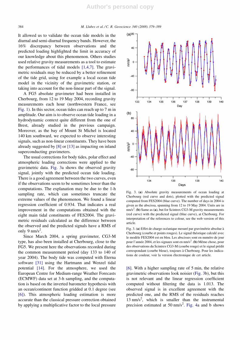
A FG5 absolute gravimeter had been installed inCherbourg, from 12 to 19 May 2004, recording gravitymeasurements each hour (northwestern France, seeFig. 1). In this sector, ocean tides can reach up to 7 m inamplitude. Our aim is to observe ocean tide loading in ahydrodynamic context quite different from the one ofBrest, already studied in the previous campaign.Moreover, as the bay of Mount St Michel is located140 km southward, we expected to observe interestingsignals, such as non-linear constituents. They have beenalready suggested by [8] or [13] as impacting on inlandsuperconducting gravimeters.

The usual corrections for body tides, polar effect andatmospheric loading corrections were applied to thegravimetric data. Fig. 3a shows the observed gravitysignal, jointly with the predicted ocean tide loading.There is a good agreement between the two curves, evenif the observations seem to be sometimes lower than thecomputations. The explanation may be due to the 1-hsampling rate, which can sometimes truncate theextreme values of the phenomenon. We found a linearregression coefficient of 0.934. That indicates a realimprovement in the computations obtained with theeight main tidal constituents of FES2004. The gravi-metric residuals calculated as the difference betweenthe observed and the predicted signals have a RMS ofonly 9 nm/s2.

Since March 2004, a spring gravimeter, CG3-Mtype, has also been installed at Cherbourg, close to theFG5. We present here the observations recorded duringthe common measurement period (day 133 to 140 ofyear 2004). The body tide was computed with Eternasoftware [31] using the Hartmann and Wenzel tidalpotential [14]. For the atmosphere, we used theEuropean Centre for Medium-range Weather Forecasts(ECMWF) data set at 3-h sampling, and the computa-tion is based on the inverted barometer hypothesis withan ocean/continent function gridded at 0.1 degree (see[6]). This atmospheric loading estimation is moreaccurate than the classical pressure correction obtainedby applying a multiplicative factor to the local pressure

[6]. With a higher sampling rate of 5 min, the relativegravimetric observations look noisier (Fig. 3b), but thisis not relevant and the linear regression coefficientcomputed without filtering the data is 1.013. Theobserved signal is in excellent agreement with thepredicted one, and the RMS of the residuals reaches13 nm/s2, which is smaller than the instrumentalprecision estimated at 50 nm/s2. Fig. 4a and b shows


Fig. 3. (a) Absolute gravity measurements of ocean loading atCherbourg (red curve and dots), plotted with the predicted signalcomputed from FES2004 (blue curve). The number of days in 2004 isgiven as the abscissa, spanning from 12 to 19 May 2004. Units are innm/s2. (b) Same as (a), but for Scintrex CG3-M gravity measurements(red curve) with the predicted signal (blue curve), at Cherbourg. Forinterpretation of the references to colour, see the web version of thisarticle.

Fig. 3. (a) Effet de charge océanique mesuré par gravimétrie absolue àCherbourg (courbe et points rouges). Le signal théorique calculé avecle modèle FES2004 est en bleu. Les abscisses sont en numéro de jourpour l’année 2004, et les signaux sont en nm/s2. (b)Même chose, pourdes observations du Scintrex CG3-M (courbe rouge) et le signal préditcorrespondant (courbe bleue), toujours à Cherbourg. Pour les indica-tions de couleur, voir la version électronique de cet article.


the gravimetric residues computed for the absolute andrelative observations.

High-precision microgravimetric studies are alwaysa useful tool to validate tidal models and loading theoryin coastal regions. The actual residuals are very small,and the remaining noise comes from the instrumental

measurements, from the applied corrections (such as theatmospheric loading), from other environmental fea-tures such as higher (or lower) sea tidal height due toweather conditions, or even, from the predicted loading.

5. Tilt experiment

Inclinometry is a high-performance tool, andprobably the most sensitive and least expensive onefor studying ocean tide loading deformation near thecoast (e.g., [21,23]). It consists in measuring the angulartime variation between the normal to the instant geoid(plumb line or local vertical) and an initial state of thisdirection. The instruments devoted to this kind ofmeasurement can resolve up to 10–9 rad (with a compactBlum’s pendulum based on a Zöllner suspension beam,[3,27]) or even 10–10 rad (using a long hydrostatictiltmeter, see, e.g., [2]).

Although hydrostatic devices show better long-termbehaviour (less drift), smaller temperature dependenceand better sensitivity, they must be installed inunperturbed, long (say > 30 m) and horizontal tunnels,which is not feasible everywhere in our study area. Forour study, we installed two Blum’s pendulums in thenorth–south and east–west directions, in an under-ground depository in Cherbourg (France).

The appropriate Green’s function provides, byconvolution, the tilt response to the load. An importantproperty of this Green’s function is that it behaves like1/r2, r being the distance to the point load. This leads toan invariance of scale: a 1-kg load at 1 m produces(more or less, depending on the Earth model) the sametilt as 1 tonne at 1 km and so on. In the framework of ourstudy, this confers a higher dependence on the closestloads with respect to gravity or displacement responses.

The pendulum signals have been recorded using a22-bit ADC at a 30-s initial sampling rate, from March2004 to July 2005. Two steps have been addressed toensure the calibration. Firstly, an electronic calibrationis made in the laboratory, to determine the voltageresponse to a displacement of the beam. Secondly, themechanical gain of the tiltmeter-pendulum is derivedfrom its eigenperiod, which is adjusted when thependulum is settled. We estimated that a final accuracyof a few percent is hard to reach and actually considerthat 5% is realistic. This limitation complicates thecomparison between models and records. A procedurethat uses the ratio between waves may be more suitablethan the direct comparisons reported here.

The extract of the raw data presented in Fig. 5ashows a clear tidal signal. The seismic noise level isvery low, confirming that the tunnel is a quiet place,


Fig. 4. (a) Gravimetric residues computed between the FG5 signaland the predicted one. In fact, they are the differences between the twocurves, red and blue, of Fig. 3. (b) Same as (a), but for the Scintrexdata. For interpretation of the references to colour, see the web versionof this article.

Fig. 4. (a) Résidus calculés à partir des observations de gravimétrieabsolue (FG5) et des effets de charge prédits. Il s’agit simplement de ladifférence entre les courbes rouge et bleue de la Fig. 3. (b) Mêmechose avec les observations de gravimétrie relative (Scintrex CG3-M).Pour les indications de couleur, voir la version électronique de cetarticle.


with very few temperature fluctuations. To compare theobservations with the ocean tide loading prediction, wefirst remove the theoretical Earth tide contribution asprovided by the ETERNA package, involving a Wahr–Dehant model [10]. The comparison between the EWde-tided observations (red curve) and ocean tide loadingpredictions (blue curve) can be seen in Fig. 5b. To makethis plot, tilt data have been decimated to a 5-minsampling rate. The agreement between the two curves isquite good, with no phase shift and very closeamplitudes. The observed curve is very clean, andcompared to the relative observations, the signal-to-noise ratio is much better. Instrumental noise cannot be

estimated within a period range between a few minutesto one week, since the natural oceanic and atmosphericground-roll generates a stronger signal, which obscuresthis noise. Except during earthquake occurrences, thestandard deviation of the 30-s sampling varies between0.001 mrad and a maximum of 0.005 mrad, dependingon the state of the closer sea disturbances.

6. FTLRS experiment

Satellite Laser Ranging (SLR) is one of the spacegeodetic techniques used for establishing and monitor-ing the International Terrestrial Reference Frame(ITRF). Today, the laser network consists of 40 fixedlaser stations that are distributed all around the world;two main geodynamical satellites (LAGEOS-1&2, at6000 km high) are used as primary geodetic targets forcomputing the station coordinates together with Earthrotation parameters. Due to the high quality of thenetwork (see the ILRS requirements, 1998), the orbitalmotion of these two satellites is computed with aprecision of roughly 1 cm (rms) over a tracking periodof one week.

In addition to this permanent frame, some mobilelaser systems have been developed. Among them, theFrench Transportable Laser Ranging System (FTLRS)is the only mobile laser station that is able to bedeployed quickly (within 2–3 days), due to its technicalfeatures [24].

Thus, for the first time in 2004, a laser rangingsystem has been used to detect the signal due to oceantidal loading in northern France (from 13 September to26 October). The challenge was to estimate a periodicvertical station motion by tracking geodetic satellitepasses just over the Brest site (Fig. 1), and byconsidering their orbits as spatial vertical references.During this tracking campaign, we observed 203 passesproviding 3090 normal points (see Table 1 for theavailable ranging data per satellite). Due to the lack ofLAGEOS data, we focused our analysis on the threesatellites Jason-1, Starlette and Stella, whose globalorbits can be computed to the level of 1.5–2 cm (rms)over a few days [9].

Fig. 6 presents an extract of the dataset obtainedduring 7 days from the total observation period.Because of the heterogeneous data set around the Brestsite, it was not possible to directly adjust a set of stationcoordinates every 6 h, especially when accumulatingthe range data of three satellites.

Theoretically, as the accuracy of the FTLRS reaches0.5 cm RMS, the instantaneous vertical positioning ofthe ground will mainly depend on the accuracy of the


Fig. 5. East–west tilt observations from silica pendulum tiltmeter atCherbourg, during the same period as gravimetric plots: (a) raw signal,(b) signal corrected from all constituents, except loading tide (redcurve), and predicted curve using FES2004 tide model (blue curve).Units are in microradians. For interpretation of the references tocolour, see the web version of this article.

Fig. 5. Observations inclinométriques dans la direction est–ouest àpartir d’un pendule horizontal en silice, faites à Cherbourg pendant lamême période : (a) signal brut, (b) signal corrigé de tous les effetsconnus, excepté l’effet de charge océanique (courbe rouge) ; la courbeprédite à partir du modèle de marée FES2004 est en bleu. Les unitéssont des microradians. Pour les indications de couleur, voir la versionélectronique de cet article.


satellite altitude at the same time of measurement, andof the whole orbit computation. The latter can beestimated to be close to 1.5 cm (RMS) for LAGEOS,which leads to a total error of 1.6 cm for theinstantaneous positioning. Repeating the experimentN times would decrease the error bar a HN factor.

However, in reality, various other factors have to beincluded to estimate the total error in the instantaneousmeasurement: the horizontal positioning error of thestation at Brest (around 1 cm), the bias of the verticalityof the laser and also the non-repeatability in time of theobservations (because the ground is never at the samegeocentric distance). So, we have estimated the morerealistic instantaneous error to 2.9 cm by using the truedata (date and orientation of the laser shooting) and bytaking into account for the over error sources.As there arefew number of passes observed for each computation of

the altitude at Brest, this error decreases to about 1 cm. Ifwe cumulate the entire data set obtained during thecampaign, the total error reduces to a few millimetres.

However, some observations looked at individuallycan present a higher error. Aberrant-looking pointspresented in Fig. 6 are just usual outliners, assuming aGaussian law.

Finally, we aim to estimate the amplitude of theloading effect of the main M2 tidal constituent byconsidering primarily the very high elevation passes, i.e.from range data acquired at 65 degrees or more abovethe Brest horizon. When fixing the frequency of the M2tide to its nominal value, we estimated its amplitude at3.731 � 0.5 cm compared to 3.730 cm for the FES2004tide model.

7. Conclusion

This monitoring campaign provides an overview ofthe techniques that can be employed in ocean tideloading surveys, and also for others geodetic studieswhere high-quality measurements are needed.

The GPS results are very good. Several dataprocessing software have been tested, and the bestone gives mean RMS values between observed GPS andthe computed positions equal to 2.5, 3.1 and 4.5 mm, foreastward, northward and upward components, respec-tively. A future comparison with the other geodetictechniques deployed in Cherbourg and Brest shouldhelp us to discriminate between the sources of theresidual discrepancies: instrumental, processing pro-blems or problems in the tidal models. If the dataanalyses reveal problems in the models, the spatialdistribution of the GPS stations should allow us toquantify the spatial variations of the misfits and to helpidentify their origins (imprecise tide models, impreciseloading modelling, spatially non linear effects,unknown Earth local rheology. . .)

Relative and absolute gravimeters also provide goodcomparisons with the tidal models and loadingcomputations. After compensating for the differences


Table 1Number of passes and number of normal points for each tracked satellite during the campaign (Ajis, Champ, Envisat, ERS2, GFO1, Grace A andGrace B, Jason1, Lageos1, Lageos 2, Starlette, Stella, and Topex)

Tableau 1Nombre de passages et de points normaux pour chaque satellite suivi au cours de la campagne (Ajis, Champ, Envisat, ERS2, GFO1, Grace A andGrace B, Jason1, Lageos1, Lageos 2, Starlette, Stella and Topex)

Satellite ajis cham env1 ers2 gfo1 grca grcb jas1 lag1 lag2 star stel topx Total

Passes 8 1 6 4 5 3 1 38 1 2 51 25 58 203Normal pts 119 5 62 61 77 27 9 804 1 12 475 218 1220 3090

Fig. 6. Zoom over seven days of observation during the FTLRSoperation. Black dots are vertical coordinates of the station computedevery 6 h. The load vertical displacement from M2 wave is plotted inred. For interpretation of the references to colour, see the web versionof this article.

Fig. 6. Extrait de sept jours de mesures réalisés pendant la périoded’observation avec la FTLRS. Les coordonnées verticales calculéestoutes les 6 h sont représentées par des points noirs. Le déplacementvertical sous la charge de la marée est la courbe rouge. Pour lesindications de couleur, voir la version électronique de cet article.


between the corresponding sampling rates, the twotechniques show similar accuracy, and the maximumRMS gravimetric residuals are only 13 nm/s2. To obtainfurther improvements, a finer tuning needs beperformed, since residuals can come from numerousorigins (tidal model, rheology, theory, gridding effects).

This campaign has highlighted the usefulness ofsilica tiltmeters for ocean tide loading studies. The dataare acquired with an exceptional quality in terms ofsignal-to-noise ratio, but their calibration must beimproved. It is important to install the instruments in avery quiet site, with weak thermal variations. Actually,tilt measurements provide the cleanest signal of allthose recorded, with a noise level of 0.005 mrad withinthe diurnal and semi-diurnal bands (the amplitude of thephenomena being between 0.3 and 0.5 mrad, and theeffects induced by non-linear tides, not included in thismodel, have an amplitude of about 0.05 mrad, whichcould explain the observed residual RMS of the sameamount). The advantage of the tiltmeter observationsalso lies in the fact that near the coasts, the ocean loadtilt becomes higher than the solid earth tide tilt.

For the first time, a mobile SLR system has beendeployed to detect loading displacement at tidalfrequencies. The amplitude of the loading effect ofM2 tide has been determined accurately from the rangedata set, accumulated during five weeks using threelow-earth-orbit satellites. Our campaign has demon-strated that very rapid ground displacements can beestimated from SLR measurements. Now, with rangedata from the LAGEOS satellites, which orbit at a muchhigher altitude and with a lower mean motion, we canexpect a much better capability to calibrate the tidalloading effects using space geodetic techniques.

In this paper, we chose not to refine the land-seamask of FES2004 using a smaller spatial samplingwhen computing the ocean loading, even though alarger resolution may cause significant errors [5]. Theimprovement of the coastline resolution imposes aresampling of the ocean tide model, which may not bevalid for coastal regions. A better way consists in usinga local ocean tide model, computed on a smaller grid,and to complete it with a global model outside thecovered zone. The fine resolution of the local modelallows a better description of the coastline. We testedthis computational scheme during a comparison withGPS data, but we did not obtain any noticeablereduction of the residues. As mentioned before, othercauses of errors may be invoked.

However, this multidata campaign has allowed us tovalidate ocean tide models through the loadingcomputation, and to estimate the error budget for each

geodetic device. In a future work, long time series andinstrumental collocation will be exploited. When asked,full data sets will be provided via a ftp site.

Acknowledgments

We are grateful to all of the technical staff andscientists who contributed to this campaign, withspecial thanks to C. Batany, H. Delorme, B. Luck, K.Mahiouz, F., M. Pierron, D. Feraudy for the time theyspent to care for the instruments. We also thank theEPSHOM for their help with the FTLRS measurements,the French navy, who provided a quiet place to installthe inclinometers, the IUT of Cherbourg and others,who let us fix a GPS antenna on their roof. Finally, wethank F. Lyard who provided us with several versions ofhis tide model. This campaign has been supported byGDR–G2 (INSU/CNRS – CNES).

References

[1] T.F. Baker, M.S. Bos, Validating, Earth and ocean tide modelsusing tidal gravity measurements, Geophys. J. Int. 152 (2003)468–485.

[2] P. Bernard, F. Boudin, S. Sacks, A. Linde, P.A. Blum,C. Courteille, M.-F. Esnoult, H. Castarede, S. Felikis, H. Billiris,Continuous strain and tilt monitoring on the Trizonia island, Riftof Corinth, Greece, C. R. Geoscience 336 (4–5) (2004) 313–323.

[3] P.A. Blum, Contribution à l’étude des variations de la verticaleen un lieu, Ann. Geophys. 19 (1963) 215–243.

[4] M.S. Bos, T.F. Baker, K. Rothing, H.P. Plag, Testing ocean tidemodels in the Nordic seas with tidal gravity observations,Geophys. J. Int. 150 (2002) 687–694.

[5] M.S. Bos, T.F. Baker, An estimate of the errors in gravity oceantide loading computations, J. Geod. 79 (2005) 50–63.

[6] J.P. Boy, P. Gegout, J. Hinderer, Reduction of Surface GravityData from Global Atmospheric Loading, Geophys. J. Int. 149(2002) 534–545.

[7] J.P. Boy, M. Llubes, J. Hinderer, N. Florsch, A comparison oftidal ocean loading models using superconducting gravimeterdata, J. Geophys. Res. 108 (2003) 2193, doi:10.1029/2002JB002050.

[8] J.P. Boy, M. Llubes, R. Ray, J. Hinderer, S. Rosat, F. Lyard, Th.Letellier, Non-Linear Oceanic Tides Observed by Superconduct-ing Gravimeters in Europe, J. Geodyn. 38 (2004) 391–405.

[9] D. Coulot, Télémétrie Laser sur Satellites et Combinaisons deTechniques Géodésiques, Contribution au système de référenceterrestre et applications, PhD thesis, ED d’île de France, Obser-vatoire de Paris, France, 2005.

[10] V. Dehant, P. Defraigne, J.M.Wahr, Tides for a convective Earth,J. Geophys. Res. 104 (B1) (1999) 1035–1058.

[11] W.E. Farrell, Deformation of the Earth by surface loads, Rev.Geophys. 10 (1972) 761–797.

[12] Ferland R, IGS MAIL 4642: IGS00 (v2), 2003.[13] N. Florsch, J. Hinderer, H. Legros, Identification of quarter

diurnal waves in superconducting gravimeter data, Bull. Inf.Mar. Terr. 122 (1995) 8189–9198.



[14] T. Hartmann, H.G. Wenzel, The HW95 tidal potential catalogue,Geophys. Res. Lett. 22 (24) (1995) 3553–3556.

[15] U. Hugentobler, S. Schaer, P. Fridez, Bernese GPS Software,Version 4.2, Astronomical Institute, University of Berne,Switzerland, 2001.

[16] R.W. King, Y. Bock, Documentation for the GAMIT GPSanalysis software, release 10.1, Massachusetts Institute of Tech-nology, Cambridge, MA, USA, 2004.

[17] F. Lefèvre, F. Lyard, Ch. Le Provost, E.J.O. Schrama, FES99:A global tide finite element solution assimilating tide gauge andaltimetric information, J. Atmos. Oceanic Technol. 19 (2002)1345–1356.

[18] M. Llubes, N. Florsch, M. Amalvict, J. Hinderer, M.-F. Lalan-cette, D. Orseau, B. Simon, Observation gravimétrique dessurcharges océaniques : premières expériences en Bretagne,C. R. Acad. Sci. Paris, Ser. IIa 332 (2001) 77–82.

[19] M. Llubes, N. Florsch, L. Longuevergne, J. Hinderer, M. Amal-vict, Local Hydrology, Global Geodynamics Project andCHAMP/GRACE Perspectives: some case studies, J. Geodyn.38 (2004) 355–374.

[20] F. Lyard, Th. Letellier, F. Lefèvre, Modelling the global oceantides: a modern insight from FES2004, Ocean Dyn 56 (5–6)(2006) 394–415.

[21] J.-M.Marthelot, E. Coudert, B.L. Isacks, Tidal tilt from localizedocean loading in the New Hebrides Arc, Bull. Seismol. Soc. Am.70 (1) (1980) 283–292.

[22] S.A. Melachroinos, R. Biancale, M. Llubes, F. Perosanz, F.Lyard, M. Vergnolle, M.N. Bouin, F. Masson, J. Nicolas, L.Morel, S. Durand, Ocean tide loading (OTL) displacements from

global and local grids: comparisons to GPS estimates over theshelf of Brittany, France, J Geod. 82 (2008) 357–371.

[23] P. Melchior, B. Ducarme, Tidal loading computations for tilt inEurope, Bull. Inf. Mar. Terr. 99 (1987) 6897–6901.

[24] J. Nicolas, F. Pierron, M. Kasser, P. Exertier, P. Bonnefond,F. Barlier, J. Haase, French transportable Laser Ranging Station:Scientific objectives, technical features, and performance, Appl.Opt. 39 (3) (2000) 402–410.

[25] A. Niell, Global mapping functions for the atmosphere delay atradio wavelengths, J. Geophys. Res. 101 (1996) 3227–3246.

[26] S. Pagiatakis, The response of a realistic Earth to ocean tideloading, Geophys. J. Int. 103 (1990) 541–560.

[27] B. Saleh, P.A. Blum, H. Delorme, New silica compact tiltmeterfor deformations measurements, J. Surv. Eng. 117 (1991) 27–35.

[28] M. Vergnolle, M.N. Bouin, L. Morel, F. Masson, S. Durand, J.Nicolas, S.A. Melachroinos, GPS estimates of ocean tide loadingin NW-France: Determination of ocean tide loading constituentsand comparison with a recent ocean tide model, Geophys. J. Int.173 (2008) 444–458.

[29] S. Vey, E. Calais, M. Llubes, N. Florsch, G. Woppelmann,J. Hinderer, M. Amalvict, M.-F. Lalancette, B. Simon,F. Duquenne, J.S. Haase, GPS measurements of ocean loadingand its impact on zenith tropospheric delay estimates: a casestudy in Brittany, France, J. Geod. 76 (8) (2002) 419–427.

[30] F.H. Webb, J.F. Zumberge, An Introduction to GIPSY/OASIS,JPL D-11088, 1995.

[31] H.G. Wenzel, The nanogal software: Earth Tide data processingpackage ETERNA 3.30, Bull. Inf. Mar. Terr. 124 (1996) 9425–9439.


Multi-technique monitoring of ocean tide loading in northern France

Documents

Transcript of Multi-technique monitoring of ocean tide loading in northern France