University of Rhode Island University of Rhode Island

DigitalCommons@URI DigitalCommons@URI

Open Access Dissertations

2016

Multi-Phase Multi-Physics Finite Element Model Updating of Multi-Phase Multi-Physics Finite Element Model Updating of

Piezoelectric Transducer Piezoelectric Transducer

Liang Su University of Rhode Island, suliang.leo@gmail.com

Follow this and additional works at: https://digitalcommons.uri.edu/oa_diss

Recommended Citation Recommended Citation Su, Liang, "Multi-Phase Multi-Physics Finite Element Model Updating of Piezoelectric Transducer" (2016). Open Access Dissertations. Paper 491. https://digitalcommons.uri.edu/oa_diss/491

This Dissertation is brought to you for free and open access by DigitalCommons@URI. It has been accepted for inclusion in Open Access Dissertations by an authorized administrator of DigitalCommons@URI. For more information, please contact digitalcommons@etal.uri.edu.

MULTI-PHASE MULTI-PHYSICS FINITE ELEMENT MODEL UPDATING

OF PIEZOELECTRIC TRANSDUCER

BY

LIANG SU

A DISSERTATION SUBMITTED IN PARTIAL FULFILLMENT OF THE

REQUIREMENTS FOR THE DEGREE OF

DOCTOR OF PHILOSOPHY

IN

OCEAN ENGINEERING

UNIVERSITY OF RHODE ISLAND

2016

DOCTOR OF PHILOSOPHY DISSERTATION

OF

LIANG SU

APPROVED:

Dissertation Committee:

Major Professor Sau-Lon James Hu

Harold Vincent

George Tsiatas

Nasser H. Zawia

DEAN OF THE GRADUATE SCHOOL

UNIVERSITY OF RHODE ISLAND

2016

ABSTRACT

The overall objective of this dissertation is to propose a quick and accurate

method of updating transducer models. When one makes measurements on a

piezoelectric transducer, oftentimes only the impedance function is measured as

the experimental data. Thus, to perform model updating for transducers, two

major tasks will be covered: (i) developing and verifying an efficient method for

estimating the electric impedance function of a transducer, and (ii) developing and

testing a FE model updating method for piezoelectric transducers.

The proposed method to estimate the impedance function of a transducer

is a Laplace domain method. It expresses both the voltage and current in their

partial-fraction forms in the Laplace domain, and obtains the impedance function

of the transducer from the ratio of the voltage and current. The Prony-SS method

is employed to extract the poles and residues of the voltage and current signals.

Compared with traditional methods, the proposed method uses the transient sig-

nals, and will not suffer any leakage problems or resolution issues. In addition, this

method requires only very short signals to obtain the impedance function, and is

excellent for rejecting noise.

This proposed model-updating method is a multi-physics FE model-updating

method, including the correction of the elastic material properties based on a

short-circuit model, and the correction of dielectric and piezoelectric parameters

based on an open-circuit model. The fundamental updating algorithm employed

in both steps is the cross-model cross-mode (CMCM) method. In addition to its

accuracy and efficiency, this method has the advantages of both the direct matrix

methods and indirect physical property-adjustment methods. Implementing the

CMCM algorithm requires a knowledge of both the measured modal frequencies

and the corresponding mode shapes, but a measured impedance function could

provide only modal frequencies for short- and open-circuit transducers. When

dealing with the incomplete modal information, an iterative procedure is taken. In

each iteration, the “measured” mode shapes are approximated by the mode shapes

obtained from the previous iteration’s updated FE model.

In this study, we employed a tube transducer, which is made of piezoceramic

material, to develop and test new methods of estimating the impedance function

and updating piezoelectric constitutive properties. Both computer simulations and

lab experiments have been conducted to verify the accuracy and efficiency of the

proposed methods.

ACKNOWLEDGMENTS

None of the work in the following dissertation would have been possible with-

out the help of many people. I would first like to express my sincere gratitude to

my advisor, Dr. Sau-Lon James Hu. His guidance and mentoring has helped me to

grow as a scientist and individual through the few years. Without his support and

patient guidance, I cannot finish my Ph.D. study and this dissertation would not

have been possible. I would like to acknowledge Dr. Huajun Li for his persistent

help in my research and Dr. Harold (Bud) Vincent for guiding me to experimental

research. And I’d also like to thank Dr. George Tsiatas, Dr. Stephen Licht, and

Dr. Haibo He for agreeing to serve as my committee members and giving me useful

instructions.

Much of my success would not have been possible without the help of my

colleagues: Bin Gao, Zhongben Zhu, Fushun Liu, Haocai Huang and the ocean

engineering department faculty and staff. Finally, I must also thank my friends

and family for their constant love and support through all of the small victories,

daunting challenges, and moments of doubt.

iv

PREFACE

This dissertation follows the University of Rhode Island Graduate School

guidelines for the preparation of a dissertation in standard format. The mate-

rial presented in this thesis is divided into eight chapters.

• Chapter 1 serves to provide an introduction to the studies within this disser-

tation, as well as a review of the relevant research in FE model updating.

• Chapter 2 is an introduction to piezoelectric transducers, especially tube

transducers. We begin with a brief overview of transducers and piezoelec-

tric material. Both full and reduced constitutive equations are introduced to

explain the performance of thin-tube transducers, and elaborate the relation-

ship between piezoelectric constitutive properties. In addition, we address

the analytical solution for ring (single DOF vibrators) and the FE solution

for tube (multi DOF vibrators), and their electrical representations, i.e., e-

quivalent circuits, are extended from those solutions.

• Chapter 3 presents the electromechanically coupled FE formulations and the

procedures for modeling tube transducers with 2D and 3D elements using a

commercial package. Furthermore, we present numerical verifications of the

FE model, including comparisons with an approximate analytical solution,

among two commercial FE packages, and with physical measurements.

• Chapters 4 and 5 show techniques and numerical studies for the estimation of

impedance functions. In addition to a review of the traditional methods for

estimating the impedance function of a piezoelectric transducer, in Chapter

4, we also newly propose an improved method using the Laplace domain. The

newly proposed method decomposes the signals into their complex exponen-

tial components using the Prony-SS method, and it is particularly effective

v

for handling measured voltage and current signals that have been contami-

nated by noise. In Chapter 5, we discuss a numerical study of the estimation

of the impedance function. To test the effectiveness of the proposed Laplace

domain method, both numerical simulations and lab experiment are includ-

ed. The impedance function that was estimated from the proposed method

is compared with those obtained using traditional methods. The effective-

ness of noise cancellation for both the proposed and traditional Fourier-based

method is also investigated.

• In Chapter 6, we describe procedures for updating piezoelectric transducers.

Besides a brief review of traditional model updating methods, a new approach

which is based on the extended cross-model cross-mode method is proposed.

The proposed model-updating method is a two-step method, including the

correction of the elastic material properties based on a short-circuit model

in the first step, and the correction of dielectric and piezoelectric parame-

ters based on an open-circuit model in the second step. Chapter 7 includes

two examples of the numerical demonstration of model-updating methods:

a simulated transducer and a real transducer. The simulated transducer is

employed to test the accuracy of the proposed method, and ultimately, the

effectiveness of the proposed method is tested on a real transducer, with the

impedance function of the transducer being estimated from the experiment.

• Conclusions and suggestions for further work are given in Chapter 8.

vi

TABLE OF CONTENTS

ABSTRACT . . . . . . . . . . . . . . . . . . . . . . . . . . . . . . . . . . ii

ACKNOWLEDGMENTS . . . . . . . . . . . . . . . . . . . . . . . . . . iv

PREFACE . . . . . . . . . . . . . . . . . . . . . . . . . . . . . . . . . . . . v

TABLE OF CONTENTS . . . . . . . . . . . . . . . . . . . . . . . . . . vii

LIST OF FIGURES . . . . . . . . . . . . . . . . . . . . . . . . . . . . . . xi

LIST OF TABLES . . . . . . . . . . . . . . . . . . . . . . . . . . . . . . . xiii

CHAPTER

1 Introduction . . . . . . . . . . . . . . . . . . . . . . . . . . . . . . . 1

1.1 Statement of the Problem . . . . . . . . . . . . . . . . . . . . . 1

1.2 Methodology and Procedures . . . . . . . . . . . . . . . . . . . . 3

2 Piezoelectric Transducers . . . . . . . . . . . . . . . . . . . . . . 7

2.1 Introduction . . . . . . . . . . . . . . . . . . . . . . . . . . . . . 7

2.1.1 Tube Transducers . . . . . . . . . . . . . . . . . . . . . 8

2.1.2 Piezoelectric Material . . . . . . . . . . . . . . . . . . . . 10

2.2 Constitutive Equations . . . . . . . . . . . . . . . . . . . . . . . 11

2.2.1 Full Constitutive Equations . . . . . . . . . . . . . . . . 11

2.2.2 Reduced Constitutive Equations for a Thin Cylinder . . 15

2.3 Piezoelectric Vibrators . . . . . . . . . . . . . . . . . . . . . . . 16

2.3.1 Ring Vibrator . . . . . . . . . . . . . . . . . . . . . . . . 17

2.3.2 Thin Tube Vibrator . . . . . . . . . . . . . . . . . . . . . 22

vii

Page

viii

3 Finite Element Model of Piezoelectric Structure . . . . . . . . 27

3.1 Finite Element Formulation . . . . . . . . . . . . . . . . . . . . 28

3.1.1 Piezoelectric Element . . . . . . . . . . . . . . . . . . . . 28

3.1.2 Assembled System Equation . . . . . . . . . . . . . . . . 30

3.1.3 Open- and Short-circuited Electrical Boundary Conditions 31

3.2 Cylindrical Transducer Modelling and Analysis . . . . . . . . . . 33

3.2.1 Modelling and Analysis of 2D Element Model . . . . . . 33

3.2.2 Modelling and Analysis of 3D Element Model . . . . . . 39

3.2.3 Constitutive Equations of 2D and 3D Models . . . . . . . 41

3.3 Numerical Verifications . . . . . . . . . . . . . . . . . . . . . . . 45

3.3.1 Comparison with Analytical Solution . . . . . . . . . . . 46

3.3.2 Verification by ABAQUS Model . . . . . . . . . . . . . . 48

3.3.3 Comparison with Experimental Data . . . . . . . . . . . 48

4 Methods of Estimating Impedance Function . . . . . . . . . . . 50

4.1 Traditional Methods . . . . . . . . . . . . . . . . . . . . . . . . 50

4.2 Proposed Method . . . . . . . . . . . . . . . . . . . . . . . . . . 51

4.3 Complex Exponential Decomposition . . . . . . . . . . . . . . . 52

4.3.1 Prony’s method . . . . . . . . . . . . . . . . . . . . . . . 53

4.3.2 Prony-SS method . . . . . . . . . . . . . . . . . . . . . . 54

4.4 Noise Rejection and Damping Modelling . . . . . . . . . . . . . 62

4.4.1 Noise-cancelling Methods Statement . . . . . . . . . . . . 62

4.4.2 Damping Estimation . . . . . . . . . . . . . . . . . . . . 64

5 Numerical Study of Estimating Impedance Function . . . . . 66

Page

ix

5.1 Simulation Study . . . . . . . . . . . . . . . . . . . . . . . . . . 66

5.1.1 Estimation with Laplace- and Fourier-based Methods . . 66

5.1.2 Estimating Impedance Function in Noisy Environment . 70

5.2 Laboratory Test . . . . . . . . . . . . . . . . . . . . . . . . . . . 74

6 Finite Element Model Updating of Piezoelectric Structure . 78

6.1 Introduction . . . . . . . . . . . . . . . . . . . . . . . . . . . . . 78

6.2 Traditional Model Updating Methods . . . . . . . . . . . . . . . 78

6.2.1 Direct Methods . . . . . . . . . . . . . . . . . . . . . . . 78

6.2.2 Iterative Methods . . . . . . . . . . . . . . . . . . . . . . 79

6.3 Cross-model Cross-mode (CMCM) Method . . . . . . . . . . . . 80

6.3.1 Procedure of CMCM Method . . . . . . . . . . . . . . . 81

6.3.2 Extended CMCM Method . . . . . . . . . . . . . . . . . 84

6.4 Model Updating of Piezoceramic Tube by CMCM Method . . . 85

6.4.1 Multi-physics Model Updating . . . . . . . . . . . . . . 85

6.4.2 Model Updating Based on Reduced Constitutive Equations 87

6.4.3 Model Updating Based on 3D Constitutive Equations . . 92

7 Numerical Study of Model Updating for Tube Transducer . . 101

7.1 Model Updating of Simulated Tube Transducer . . . . . . . . . 101

7.1.1 Updating of Material Parameters . . . . . . . . . . . . . 102

7.1.2 Summary of the Updating of Model Parameters . . . . . 107

7.2 Model Updating of Real Tube Transducer . . . . . . . . . . . . . 108

8 Conclusions . . . . . . . . . . . . . . . . . . . . . . . . . . . . . . . 115

APPENDIX

Page

x

A Simple 33- and 31-mode Vibrators . . . . . . . . . . . . . . . . . 119

B Modeling and Interfacing with ANSYS . . . . . . . . . . . . . . 122

B.1 Modeling for Piezoelectric Structures with ANSYS . . . . . . . . 122

B.2 Interfacing with ANSYS . . . . . . . . . . . . . . . . . . . . . . 124

C Parameter Sensitivity of Piezoelectric Tube Transducer . . . 126

C.1 Sensitivity of d-form Parameters . . . . . . . . . . . . . . . . . . 126

C.2 Sensitivity of e-form Parameters . . . . . . . . . . . . . . . . . . 130

D Model Updating with Measured Mode Shapes . . . . . . . . . 133

D.1 Model Updating of Elastic Parameters . . . . . . . . . . . . . . 133

D.2 Model Updating of Electric-coupling Parameters . . . . . . . . . 133

D.3 Numerical Study . . . . . . . . . . . . . . . . . . . . . . . . . . 135

BIBLIOGRAPHY . . . . . . . . . . . . . . . . . . . . . . . . . . . . . . . 136

LIST OF FIGURES

Figure Page

1 Real transducer (Left), Finite element model of transducer (Right) 3

2 Three possible modes of cylindrical shell transducers . . . . . . 9

3 Illustration of (a) whole ring vibrator, (b) an incremental segment 18

4 Simple equivalent circuit . . . . . . . . . . . . . . . . . . . . . . 21

5 Equivalent circuit of ceramic ring . . . . . . . . . . . . . . . . . 22

6 Thin-wall tube transducer . . . . . . . . . . . . . . . . . . . . . 23

7 Three finite element vibration modes of a tube transducer . . . 24

8 The impedance function of a tube transducer . . . . . . . . . . 25

9 Modes driven equivalent circuit . . . . . . . . . . . . . . . . . . 26

10 Sketch of PLANE13 element . . . . . . . . . . . . . . . . . . . . 33

11 Finite element model of a tube transducer . . . . . . . . . . . . 34

12 Mode shapes and modal frequencies of the short-circuit model . 36

13 Mode shapes and modal frequencies of the open-circuit model . 37

14 The impedance function of the tube transducer (harmonic analysis) 38

15 Sketch of SOLID226 element . . . . . . . . . . . . . . . . . . . . 40

16 3D tube model built by SOLID226 element . . . . . . . . . . . . 40

17 Impedance functions obtained from 2D and 3D models . . . . . 42

18 Impedance functions of analytical and FE models . . . . . . . . 47

19 Impedance functions of analytical and constrained FE models . 47

20 Impedance functions obtained from ANSYS and ABAQUS . . . 48

21 Impedance functions obtained from ANSYS and lab measurement 49

xi

Figure Page

xii

22 Measurement system with noise sources . . . . . . . . . . . . . 62

23 The impedance function from ANSYS . . . . . . . . . . . . . . 67

24 The voltage and charge signals . . . . . . . . . . . . . . . . . . 68

25 The comparison of the estimated impedance functions . . . . . 69

26 Impedance functions estimated from noisy signals by FFT methods 70

27 Singular Values of Hankel Matrix . . . . . . . . . . . . . . . . . 71

28 The impedance function using 1000 data points (proposed method) 72

29 The impedance function using 3000 data points (proposed method) 73

30 The experiment setup for estimating the impedance function . . 74

31 The circuit diagram of the experiment . . . . . . . . . . . . . . 75

32 Transient input and the corresponding output signals . . . . . . 76

33 The comparison of the impedance functions using experimental data 77

34 Flowchart of the iterative extended CMCM method . . . . . . . 86

35 The impedance functions of the original and target models . . . 103

36 Iteration procedure of α1 and α2 on simulation model . . . . . . 105

37 Iteration procedure of α3 on simulation model . . . . . . . . . . 107

38 The impedance functions of the target and updated models . . 109

39 The impedance functions of the original model and the experiment110

40 Iteration procedure of α1 and α2 on experiment model . . . . . 111

41 Iteration procedure of α3 on experiment model . . . . . . . . . . 112

42 The impedance functions of the updated model and the experiment114

A.1 The piezoelectric longitudinal vibrator in 33 mode . . . . . . . . 119

A.2 The piezoelectric longitudinal vibrator in 31 mode . . . . . . . . 121

LIST OF TABLES

Table Page

1 Independent parameters of PZT . . . . . . . . . . . . . . . . . . 14

2 Properties of PZT5A material . . . . . . . . . . . . . . . . . . . 35

3 The comparison of modal frequencies between 2D and 3D models 41

4 Material properties of the original and target models . . . . . . 102

5 Properties of original, target and updated simulation models . . 109

6 Properties of original and updated experiment models . . . . . . 114

B.1 Tensor indices notations . . . . . . . . . . . . . . . . . . . . . . 124

C.1 Elastic parameters sensitivity in the d-form . . . . . . . . . . . 127

C.2 Elastic parameters sensitivity in the d-form (engineering parameters)128

C.3 Dielectric and piezoelectric parameters sensitivity in the d-form 129

C.4 Elastic parameters sensitivity in the e-form . . . . . . . . . . . . 131

C.5 Dielectric and piezoelectric parameters sensitivity in the e-form 132

D.1 Properties of original, target and updated models . . . . . . . . 135

xiii

CHAPTER 1

Introduction

1.1 Statement of the Problem

The accuracy of the finite-element (FE) model of a piezoelectric transducer

depends on the accuracy of the material’s constitutive properties, but the values

provided in the manufacturer’s specification sheets for piezoelectric materials are

often incomplete or inaccurate (Abboud et al., 1998). Because of the polycrys-

talline nature of piezoceramics and the statistical variations in their composition

and production-related influences, the standard tolerance range of piezoelectric

material is ±20% (Ltd, 2011). In addition, depolarization influences the accura-

cy of the material properties, which may result from operating temperatures that

are too near the Curie temperature, high static-pressure cycling in deep-water ap-

plications, high alternating electric fields, or a slight extent from the passage of

time (Sherman and Butler, 2007). Therefore, the properties of different transduc-

ers made with the same piezoelectric material may vary, and it is necessary to

obtain a quick and accurate method of updating transducer models.

FE model updating has been defined as the systematic adjustment of FE mod-

els using the experimental data. When one makes measurements on a piezoelectric

transducer, oftentimes only the impedance function is measured as the experimen-

tal data. Thus, to perform model updating for transducers, two major tasks will

be covered: (i) developing and verifying an efficient method for estimating the

electric impedance function of a transducer, and (ii) developing and testing a FE

model updating method for piezoelectric transducers.

The electrical impedance function is a function of frequency, and it is gener-

ally defined as the total resistance offered by a device or circuit to the flow of an

alternating current at specific frequencies. As an electrical feature, it is relatively

1

easy to be estimated, and includes many important transducer properties such

as the resonance frequency, capacitance, bandwidth, and damping. Traditionally,

there are two methods for estimating the impedance function: (i) stepped harmon-

ic analysis (i.e., single frequency) method, and (ii) Fourier-based analysis method

using transient signals. The stepped harmonic analysis involves repeatedly ap-

plying a harmonic input signal to obtain the corresponding steady-state response,

then computing the impedance of the given frequency. The Fourier-based method

computes the impedance function from the complex ratio of the Fast Fourier Trans-

form (FFT) of the input and output time-domain signals. However, both methods

above have drawbacks. The stepped harmonic analysis method is time consuming

and requires specialized equipment, while the Fourier-based analysis method suffers

from problems related to frequency leakage and resolution (Lis and Schmidt, 2004;

Lis et al., 2005; Su et al., 2014).

In terms of model-updating technologies, the traditional methods have been

classified into two major types: direct matrix methods and indirect physical prop-

erty adjustment methods (Friswell and Mottershead, 1995). The first of these two

groups generally involves non-iterative methods, all of which are based on com-

puting changes that are made directly to the mass and stiffness matrices. Such

changes may have succeeded in generating modified models that have properties

close to those measured in the tests, but the resulting models become abstract

“representation” models, and cannot be interpreted in a physical way. The sec-

ond group comprises methods that are in many ways more acceptable in that the

parameters that they adjust are much closer to physically realizable quantities.

The methods in this second group, which seek to find correction factors for each

individual FE or for each design parameter related to each FE, have generally been

viewed as the main hope for the development of updating technology. The pub-

2

lished model-updating methods that were implemented for ultrasound transducers

belong to the second group of methods (Piranda et al., 1998; Piranda et al., 2001).

Because these methods are all iterative, a much greater computation effort is re-

quired, and the solutions for the physical properties are often prone to diverge

(Hu et al., 2007).

1.2 Methodology and Procedures

In this study, we employed a tube transducer, which is made of piezoceramic

material, to develop and test new methods of estimating the impedance function

and updating piezoelectric constitutive properties. The effect of the backing layer

and the transducer housing is not involved in this study, and the general procedure

is also applicable to other types of piezoelectric transducers.

Figure 1. Real transducer (Left), Finite element model of transducer (Right)

Figure. 1 shows a real tube transducer and its FE model, which is built using

the commercial FE package, ANSYS. Because the FE model is axially symmetric,

we can build it using either a three-dimensional (3D) element or by revolving its

two-dimensional (2D) element radial cross section (a rectangle in the x-y plane)

around the z-axis. In this study, we conduct modal, harmonic, and transien-

t (dynamic response) analyses based on this FE model. The modal analysis is

employed to obtain the modal frequencies and mode shapes of the piezoelectric

3

tube transducer under both open- and short-circuit electric boundary conditions;

the harmonic analysis is used to obtain the standard impedance function, and the

transient analysis is to obtain the electric-charge time signal, while the piezoelec-

tric tube transducer is subjected to an input electric-potential time signal. The

ultimate purpose of the transient analysis is to obtain the impedance function of

the transducer.

The newly developed method to estimate the impedance function of a trans-

ducer is a Laplace domain method. It expresses both the voltage and current

in their partial-fraction forms in the Laplace domain, and obtains the impedance

function of the transducer from the ratio of the voltage and current. The Prony-SS

method is employed to extract the poles and residues of the voltage and current sig-

nals (Hu et al., 2013). Compared with traditional methods, the proposed Prony-

based method uses the transient signals, and will not suffer any leakage problems

or resolution issues. In addition, this method requires only very short signals to

obtain the impedance function, and is excellent for rejecting noise. Both computer

simulations and lab experiment have been conducted to verify the accuracy and

efficiency of this Laplace domain method.

The proposed model-updating method is the multi-physics FE model-updating

method. This method is a two-step method, including the correction of the elastic

material properties based on a short-circuit model in the first step, and the correc-

tion of dielectric and piezoelectric parameters based on an open-circuit model in

the second step. The fundamental updating algorithm employed in both steps is

the CMCM method (Hu et al., 2007; Hu and Li, 2008). In addition to its accuracy

and efficiency, this method has the advantages of both the direct matrix method-

s and indirect physical property-adjustment methods. Implementing the CMCM

algorithm requires a knowledge of both the measured modal frequencies and the

4

corresponding mode shapes, but a measured impedance function could provide on-

ly modal frequencies for short- and open-circuit transducers. When dealing with

the incomplete modal information, an iterative procedure is taken. In each itera-

tion, the “measured” mode shapes are approximated by the mode shapes obtained

from the previous iteration’s updated FE model.

Specific to piezoelectric tube transducers poling in the radial direction, which

obeys the thin-tube assumption, elastic material parameters associated with a

tube’s thickness direction would not affect the functionality of the piezoelectric

tube. In turn, the corresponding impedance function depends only on four in-

dependent material parameters: two elastic parameters Y E11 and ν12 (or sE11 and

sE12), the permittivity under constant stress εT33, and the piezoelectric parameter

d31. Specifically, only the values of Y E11 and ν12 (or sE11 and sE12) determine the

resonance frequencies of the impedance function, which are the modal frequencies

of the transducer in the short-circuit situation, the value of εT33 determines the

unclamped capacitance, and the value of d31 affects the anti-resonant frequencies

of the impedance function, which are the modal frequencies of the transducer in

the open-circuit condition. Likewise, one could update those two elastic properties

Y E11 and ν12 (or sE11 and sE12) in the short-circuit model, then update εT33 and d31 in

the open-circuit model.

However, with respect to References.(Hu et al., 2007; Piefort, 2001), the

piezoelectric material’s parameters that meet the requirements of the CMCM

method are e-form group parameters. Therefore, the d-form parameters, Y E11 , ν12

(or sE11, sE12), ε

T33, and d31 need to be converted to e-form parameters to finish the

updating procedure. For most commercial FE method (FEM) packages such as

ANSYS, the input e-form parameters of models (for both 2D and 3D models) are

the e-form parameters of full constitutive equations, but are not reduced equations.

5

The 10 independent parameters in e-form that are used to fully characterize the

constitutive equations of PZT-type materials are cE11, cE33, c

E12, c

E13, c

E44, ε

S33, ε

S11, e31,

e33, and e15. We can easily determine that it is not possible to obtain these 10

e-form parameters with only four d-form parameters. Thus, to keep only those

four parameters while using a commercial package, this study employs two simple

ways to manipulate the situation: (1) a mathematical simplification that involves

setting all insensitive parameters to be equal to zero, and (2) a physical simpli-

fication by using an isotropic material model. One must recognize that setting

insensitive coefficients equal to zero may easily violate the underlying physics and

cause singularity in mathematics.

6

CHAPTER 2

Piezoelectric Transducers

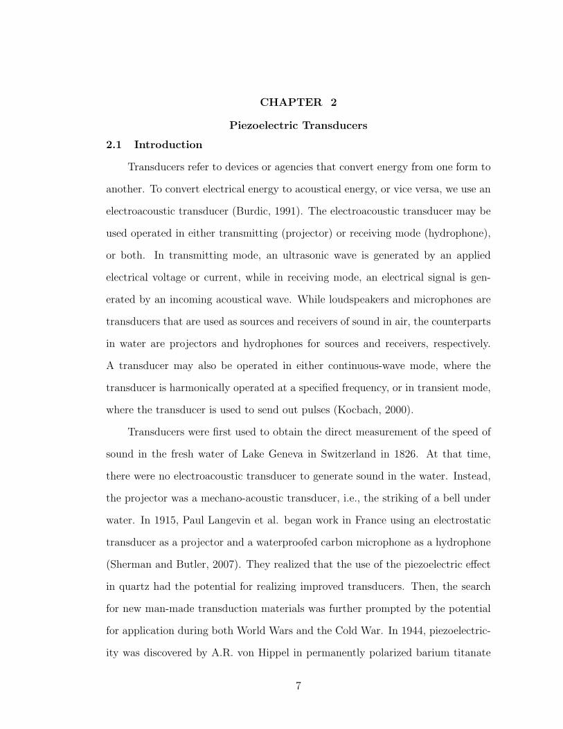
2.1 Introduction

Transducers refer to devices or agencies that convert energy from one form to

another. To convert electrical energy to acoustical energy, or vice versa, we use an

electroacoustic transducer (Burdic, 1991). The electroacoustic transducer may be

used operated in either transmitting (projector) or receiving mode (hydrophone),

or both. In transmitting mode, an ultrasonic wave is generated by an applied

electrical voltage or current, while in receiving mode, an electrical signal is gen-

erated by an incoming acoustical wave. While loudspeakers and microphones are

transducers that are used as sources and receivers of sound in air, the counterparts

in water are projectors and hydrophones for sources and receivers, respectively.

A transducer may also be operated in either continuous-wave mode, where the

transducer is harmonically operated at a specified frequency, or in transient mode,

where the transducer is used to send out pulses (Kocbach, 2000).

Transducers were first used to obtain the direct measurement of the speed of

sound in the fresh water of Lake Geneva in Switzerland in 1826. At that time,

there were no electroacoustic transducer to generate sound in the water. Instead,

the projector was a mechano-acoustic transducer, i.e., the striking of a bell under

water. In 1915, Paul Langevin et al. began work in France using an electrostatic

transducer as a projector and a waterproofed carbon microphone as a hydrophone

(Sherman and Butler, 2007). They realized that the use of the piezoelectric effect

in quartz had the potential for realizing improved transducers. Then, the search

for new man-made transduction materials was further prompted by the potential

for application during both World Wars and the Cold War. In 1944, piezoelectric-

ity was discovered by A.R. von Hippel in permanently polarized barium titanate

7

ceramics, and in 1954, even stronger piezoelectricity was achieved in polarized

lead zirconate titanate ceramics (PZT), which are still being used in most un-

derwater sound transducers (Jaffe et al., 1955). The development of underwater

electroacoustic transducers expanded rapidly during the twentieth century, and it

continued to be a growing field of knowledge (Sherman and Butler, 2007).

The various applications of transducers over a wide frequency range (from

about 1 Hz to over 1 MHz) requires many different transducer designs. In naval

applications, acoustic communication, echo ranging, and passive listening all re-

quire different projectors to transmit sound, and different hydrophones to receive

sound. Generally, hydrophones and projectors are used in large groups of up to

1000 or more transducers closely packed in planar, cylindrical, or spherical arrays

mounted on naval ships. Transducers also play an important role in other applica-

tions. For example, in oceanography, transducers help to finish seafloor mapping

and determinate seafloor characteristics. In ocean engineering, they help to iden-

tify the locations of oil and gas deposits under the oceans, and with the laying of

underwater cables or pipelines. Several research projects employ transducers to

acquire data related to a wide variety of topics such as the Acoustic Thermometry

of Ocean Climate project (ATOC) and the Sound Surveillance System, which has

been used to study the behavior of sperm whales, and to detect earthquakes and

volcanic eruptions under the sea (Sherman and Butler, 2007).

2.1.1 Tube Transducers

The cylindrical shell is the basic shape of transducers that are widely used

in many engineering applications. Three possible modes of cylindrical transducers

are shown in Figure. 2.

Figure. 2(a) shows a cylindrical shell that operates in the radial mode. The

inner and outer cylindrical surfaces are coated with conducting material, and the

8

Figure 2. Three possible modes of cylindrical shell transducers

poling field is applied between these surfaces. This geometry is characterized by

moderate sensitivity and high output capacitance. Because of the large capaci-

tance, the design is capable of driving long cables directly without suffering much

loss in sensitivity.

Figure. 2(b) shows the tangential mode of operation. Conducting stripes that

are formed longitudinally on the ceramic cylindrical surface divide the cylinder into

an even number of curved segments. Alternate stripes are electrically connected

and a poling field applied in the circumferential direction. The cylindrical segments

are thus electrically in parallel but mechanically in series. This configuration is

characterized by high sensitivity and low capacitance, and is an excellent design

where high sensitivity is required, and where suitable electronic isolation from the

cable can be provided close to the hydrophone element.

The configuration shown in Figure. 2(c) operates in the longitudinal mode.

The ends of the ceramic cylinder are made to conduct electrically and the poling

field is applied in the direction parallel to the cylindrical axis. This configuration

has a somewhat higher sensitivity than the radial mode, and as with the tangential

mode, the electrical impedance of the device is high (Burdic, 1991).

The present study focuses on the radial mode transducer. Only the active

9

element (thin piezoelectric tube) which is sandwiched between a front layer and a

backing layer is considered, and the effect of assembling and the transducer housing

is not involved in the analysis. As a varying voltage is applied over the electrodes,

the cylindrical transducer will begin to vibrate. This vibration is related to the

geometry of this tube and the material parameters.

The present study focuses on the radial-mode transducer. We consider only

the active element (thin piezoelectric tube), which is sandwiched between a front

layer and a backing layer, and the effects of the assembly and the transducer

housing were not considered in the analysis. As a varying voltage is applied over

the electrodes, the cylindrical transducer will begin to vibrate. This vibration is

related to the geometry of the tube and the material parameters.

2.1.2 Piezoelectric Material

At present, piezoelectric materials are the most commonly used material when

developing transducers. When mechanical stresses are applied to a piezoelectric

material solid, a voltage is produced between its surfaces, called a piezoelectric

effect. Conversely, when a voltage is applied across certain surfaces of the solid, the

solid undergoes a mechanical distortion, which is called the inverse piezoelectric

effect. Most of the piezoelectric materials are crystalline solids. They can be

single crystals, which are either formed naturally or by synthetic processes, or

polycrystalline materials such as ferroelectric ceramics, which can be rendered

piezoelectric in any chosen polar direction by the poling treatment. During the

manufacture of piezoceramics, a suitable ferroelectric material is first fabricated

into the desired shape. The piezoceramic element is then heated to an elevated

temperature (the Curie point) while in the presence of a strong DC field.

The best known piezoelectric material is lead zirconate titanate (PZT) which

is an intermetallic inorganic compound. It is a white solid that is insoluble in

10

all solvents, and it has a perovskite-type structure. The remanent polarization

gives PZT an approximately linear response to an alternating electric field. It is

very stable and large enough to give a strong piezoelectric effect. However, this

also causes depolarization to significantly affect the performance of PZT trans-

ducers. This depolarization may result from operating temperatures that are too

near the Curie temperature, high static pressure cycling in deep-water applica-

tions, high alternating electric fields, or a slight extent from the passage of time.

Thus, while the properties of true piezoelectrics are determined by their internal

crystal structure and cannot be changed, the piezoelectric properties of polarized

electrostrictive materials depend on the level of remanence achieved during the

polarization process, and may be changed by the operating conditions. Therefore,

although PZT material has many advantages compared to other materials for un-

derwater transducer applications, its limitations must also be considered during

the design process (Piefort, 2001).

2.2 Constitutive Equations2.2.1 Full Constitutive Equations

The linear piezoelectric effect in a piezoelectric medium can be described using

a set of constitutive equations. When it is expressed in the so-called e-form, one

has:

T = cES− etE (1)

D = eS+ εSE (2)

where T ∈ R6×1 is stress vector, S ∈ R6×1 strain vector, E ∈ R3×1 electric field

vector, D ∈ R3×1 electric displacement vector, cE ∈ R6×6 elastic stiffness matrix,

e ∈ R3×6 piezoelectric stress matrix (superscript t stands for the transpose) and

εS ∈ R3×3 permittivity matrix. The superscript of cE indicates that the elastic

compliance coefficients matrix is obtained with E being held constant, and the

11

superscript of εS indicates that the permittivity coefficients matrix is obtained

with S being held constant (Sherman and Butler, 2007; Piefort, 2001).

Generally, the coefficient matrices in Eqs. 1 and 2 include 45 independent coef-

ficients. However, for polarized piezoelectric ceramic material (such as PZT) which

belongs to the 4 mm (C4V) crystal class (IEE, 1987) , many of the coefficients are

zero or related, leaving only 10 independent coefficients, and the corresponding

equations are explicitly expressed in the e-form as:

T1

T2

T3

T4

T5

T6

=

cE11 cE12 cE13 0 0 0cE12 cE11 cE13 0 0 0cE13 cE13 cE33 0 0 00 0 0 cE44 0 00 0 0 0 cE44 00 0 0 0 0 cE66

S1

S2

S3

S4

S5

S6

−

0 0 e310 0 e310 0 e330 e15 0e15 0 00 0 0

E1

E2

E3

(3)

D1

D2

D3

=

0 0 0 0 e15 00 0 0 e15 0 0e31 e31 e33 0 0 0

S1

S2

S3

S4

S5

S6

+

εS11 0 00 εS11 00 0 εS33

E1

E2

E3

(4)

where cE66 = (cE11 − cE12)/2. The subscript 3 is the direction in which ceramic ele-

ment is polarized. Subscripts 1 and 2 represent directions perpendicular to poling

direction, and 4, 5 and 6 refer to shear directions that follow IEEE convention,

namely, 23→ 4, 13→ 5, and 12→ 6 (Wik, 2015).

A widely used alternative and equivalent representation consists in writing

the constitutive equations in the so-called d-from:

S = sE T+ dt E (5)

D = dT+ εT E (6)

where sE ∈ R6×6 is elastic compliance matrix, d ∈ R3×6 piezoelectric strain ma-

trix and εT ∈ R3×3 permittivity matrix at constant stress. Combined into one

12

equation, the expanded form for 4 mm crystal class is explicitly expressed as

(Balmes and Deraemaeker, 2013):

S1

S2

S3

S4

S5

S6

D1

D2

D3

=

sE11 sE12 sE13 0 0 0 0 0 d31sE12 sE11 sE13 0 0 0 0 0 d31sE13 sE13 sE33 0 0 0 0 0 d330 0 0 sE44 0 0 0 d15 00 0 0 0 sE44 0 d15 0 00 0 0 0 0 sE66 0 0 00 0 0 0 d15 0 εT11 0 00 0 0 d15 0 0 0 εT11 0d31 d31 d33 0 0 0 0 0 εT33

T1

T2

T3

T4

T5

T6

E1

E2

E3

(7)

From the constitutive equations of d-form and e-form, it is straightforward to

obtain the following relationships:

cE = (sE)−1

(8)

e = d (sE)−1

(9)

and

εS = εT − edt (10)

Furthermore, Eq.10 can also be expressed as either

εS = εT − dcEdt (11)

or

εS = εT − esEet (12)

For quantifying the elastic parameters, many people prefer to use engineering

parameters, instead of the compliance or stiffness parameters. For a transverse

isotropic material whose properties are the same in the plane perpendicular to the

poling direction, the compliance matrix sE can be expressed in terms of engineering

13

parameters as:

sE =

1Y E11− ν12

Y E11− ν13

Y E33

0 0 0

− ν12Y E11

1Y E11− ν13

Y E33

0 0 0

− ν13Y E33− ν13

Y E33

1Y E33

0 0 0

0 0 0 1G

0 00 0 0 0 1

G0

0 0 0 0 0 2(1+ν12)

Y E11

(13)

where Y E11 and Y E

33 are the Young’s modulus in 1-direction and 3-direction, re-

spectively; G is the shear modulus on the plane whose normal is in 1-direction

(or 2-direction); and ν12 and ν13 are the Poisson’s ratios that correspond to the

contraction in 2-direction and 3-direction when the extension is in 1-direction.

In summary, the material parameters of PZT include 2 independent dielectric

permittivities, 3 independent piezoelectric constants and 5 independent elastic

constants. These material parameters are listed in Table.1

Table 1. Independent parameters of PZT

e-form d-formElastic Stiffness Elastic Compliance Engineering Parameter

cE11 sE11 Y E11

cE12 sE12 Y E33

cE13 sE13 νE12

cE33 sE33 νE13

cE44 sE44 GPiezoelectric stress constant Piezoelectric strain constant

e31 d31e33 d33e15 d15

Dielectric permittivity at constant strain Dielectric permittivity at constant stressεS11 εT11εS33 εT33

14

2.2.2 Reduced Constitutive Equations for a Thin Cylinder

When the piezoceramic transducer polarized in the thickness direction is

modeled as a very thin cylinder, the normal stress in the thickness (radial)

direction and the respective transverse shear stress components are negligible

(Erturk and Inman, 2011):

T3 = T4 = T5 = 0 (14)

If the electric field components in the axis-1 and axis-2 are zero,

E1 = E2 = 0 (15)

then Eq.7 becomes the reduced constitutive equationsS1

S2

S6

D3

=

sE11 sE12 0 d31sE12 sE11 0 d310 0 sE66 0d31 d31 0 εT33

T1

T2

T6

E3

(16)

From the above equation, there are only four independent material parameters

which will affect the dynamic characteristics of a piezoceramic thin tube trans-

ducer: s11, s12, εT33 and d31, noting that sE66 = 2(sE11 − sE12) is not an independent

parameter. Since sE11 = 1/Y E11 and sE12 = −ν12/Y E

11 , the four independent material

parameters can also be: Y E11 , ν12, ε

T33 and d31.

In an attempt to show the corresponding e-form, one can first rearrange Eq.16

into: sE11 sE12 0 0sE12 sE11 0 00 0 sE66 0−d31 −d31 0 1

T1

T2

T6

D3

=

1 0 0 −d310 1 0 −d310 0 1 00 0 0 εT33

S1

S2

S6

E3

(17)

Let the e-form of the reduced constitutive equations be denoted byT1

T2

T6

D3

=

cE11 cE12 0 −e31cE12 cE11 0 −e310 0 cE66 0e31 e31 0 εS33

S1

S2

S6

E3

(18)

15

From the above two equations, one hascE11 cE12 0 −e31cE12 cE11 0 −e310 0 cE66 0e31 e31 0 εS33

=

sE11 sE12 0 0sE12 sE11 0 00 0 sE66 0−d31 −d31 0 1

−1

1 0 0 −d310 1 0 −d310 0 1 00 0 0 εT33

(19)

After some algebra, one obtains the reduced e-form parameters to be:

cE11 =sE11

(sE11 + sE12)(sE11 − sE12)

=Y E11

(1 + ν12)(1− ν12)(20)

cE12 =−sE12

(sE11 + sE12)(sE11 − sE12)

=Y E11ν12

(1 + ν12)(1− ν12)(21)

cE66 =1

sE66=

Y E11

2(1 + ν12)(22)

eE31 =d31

sE11 + sE12=

d31YE11

1− ν12(23)

εS33 = εT33 −2d231

sE11 + sE12= εT33 −

2d231YE11

1− ν12(24)

It is realized that the reduced d-form parameters are identical to those of the

original constitutive equations, but the reduced e-form parameters are completely

different from those of the original constitutive equations. For the finite element

model updating in this study, the purpose is to update the material parameters

based on the experimentally obtained impedance function of a piezoceramic thin

tube transducer. Only four independent material parameters are necessary, or

could be updatable, for a piezoceramic thin tube transducer; and it would be

better to update the d-form parameters for the obvious reason mentioned above.

2.3 Piezoelectric Vibrators

The piezoceramic transducer to be studied is a thin tube type, where the

length and diameter of the tube is much larger than its thickness. If the length of

this transducer is also very small, then it becomes a piezoceramic “ring” transducer.

Traditionally, a ring transducer has been treated as a SDOF (single-degree-of-

freedom) system in the analytical derivation for its impedance (or admittance)

function.

16

2.3.1 Ring Vibrator

A ring vibrator has been often treated as a 3-1 SDOF vibrator (see Appendix

A), where the only strain/stress occurs in the circumference direction (also 1-

direction) and the poling direction (3-direction) could be the radial direction (or

longitudinal direction). One can refer its detailed derivation for the impedance (or

admittance) function to Reference.(Mason, 2013), while the following presentation

provides a brief review.

Analytical Impedance Function for a Ring Transducer

The ring transducer poling in radial direction is treated as a 3-1 SDOF vibrator

which has the reduced constitutive equation in its d-form to be:

S1 = sE11T1 + d31E3 (25)

D3 = d31T1 + εT33E3 (26)

and its corresponding e-form is shown to be:

T1 =1

sE11S1 −

d31sE11

E3 (27)

D3 =d31sE11

S1 +

(εT33 −

d231sE11

)E3 (28)

Thus, the laterally clamped (in one dimension) permittivity

εS33 = εT33(1− k2

31

)(29)

where the coupling coefficient k231 = d231/s

E11ε

T33.

With the assumptions of negligibly small cross-sectional dimensions, the equa-

tion of motion for a ring transducer (see Figure.3) can be derived from Newton’s

second law applied to a segment. This incremental segment which is not balanced

by external radial forces causes a radial acceleration as a whole. The resultant

force on this incremental segment is

Fr = Fδθ = T1ℓ t δθ (30)

17

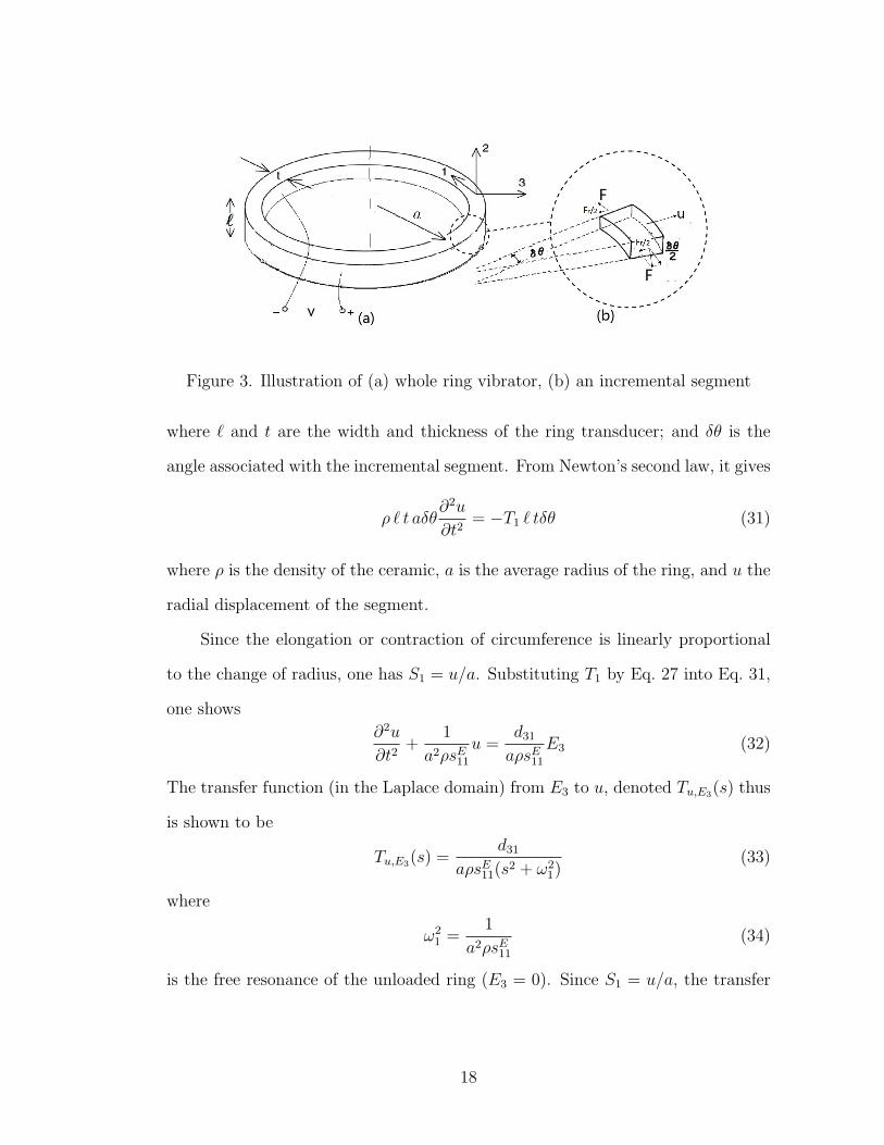
Figure 3. Illustration of (a) whole ring vibrator, (b) an incremental segment

where ℓ and t are the width and thickness of the ring transducer; and δθ is the

angle associated with the incremental segment. From Newton’s second law, it gives

ρ ℓ t aδθ∂2u

∂t2= −T1 ℓ tδθ (31)

where ρ is the density of the ceramic, a is the average radius of the ring, and u the

radial displacement of the segment.

Since the elongation or contraction of circumference is linearly proportional

to the change of radius, one has S1 = u/a. Substituting T1 by Eq. 27 into Eq. 31,

one shows

∂2u

∂t2+

1

a2ρsE11u =

d31aρsE11

E3 (32)

The transfer function (in the Laplace domain) from E3 to u, denoted Tu,E3(s) thus

is shown to be

Tu,E3(s) =d31

aρsE11(s2 + ω2

1)(33)

where

ω21 =

1

a2ρsE11(34)

is the free resonance of the unloaded ring (E3 = 0). Since S1 = u/a, the transfer

18

function from E3 to S1, denoted TS1,E3(s), thus is

TS1,E3(s) = TS1,u(s)Tu,E3(s) =d31

a2ρsE11(s2 + ω2

1)(35)

From Eq. 28, one shows the transfer function from E3 to D3 to be

TD3,E3(s) =d31sE11

TS1,E3(s)+εT33(1− k2

31

)=

d231a2ρ(sE11)

2(s2 + ω21)

+εT33(1− k2

31

)(36)

From E3 = V/t where V is the electric potential and the current, I = 2π a ℓ D3,

one has the corresponding transfer functions

TE3,V (s) = 1/t (37)

and

TI,D3(s) = 2π a ℓ s (38)

From Eqs. 36, 37 and 38, one obtains

TI,V (s) =2π a ℓ s

t

[d231

a2ρ(sE11)2(s2 + ω2

1)+ εT33

(1− k2

31

)](39)

The admittance function Y (ω), in the frequency domain, of the ring transducer is

defined as the transfer function TI,V (s) while substituting s by jω:

Y (ω) =I(ω)

V (ω)= j ω

(2π a ℓ

t

)[d231

a2ρ(sE11)2(ω2

1 − ω2)+ εT33

(1− k2

31

)](40)

Substituting for ω1 (see Eq. 34) and k31 (see Eq. 29), Eq. 40 becomes

Y (ω) = j ω

(2π a ℓ

t

)[k231ε

T33ω

21

ω21 − ω2

+ εT33(1− k231)

](41)

The reciprocal of the admittance function Y (ω) is the impedance function Z(ω).

Resonance frequency ωr and antiresonance frequency ωa are obtained from

the pole and zero of the admittance, given by (Mason, 2013; Wilson, 1988)

ω2r = ω2

1 =1

a2ρsE11(42)

19

and

ω2a =

ω2r

1− k231

(43)

respectively. Conversely, the coupling coefficient k31 is given by

k231 = 1−

(ωr

ωa

)2

(44)

Single-degree-of-freedom Equivalent Circuits

Eq. 41 can be expressed as the sum of the blocked electrical admittance YE(ω)

and the motional admittance YM(ω):

Y (ω) = YE(ω) + YM(ω) (45)

The blocked electrical admittance is

YE(ω) = j ω

(2π a ℓ

t

)[εT33(1− k2

31)]= j ω C0 (46)

where C0 is the clamped capacitance

C0 = Cf (1− k231) (47)

and the free (or total) capacitance of the ring is

Cf =2π a ℓ εT33

t(48)

The motional admittance YM(ω) is

YM(ω) = j ω

(2π a ℓ

t

)k231ε

T33ω

21

ω21 − ω2

= j ω C1

(ω21

ω21 − ω2

)(49)

where the motional capacitance C1 is

C1 = Cfk231 (50)

or

C1 =

(2π a ℓ εT33

t

)d231

sE11εT33

=asE112πℓt

(2π ℓ d31sE11

)2

= CmN2 (51)

20

in which the mechanical compliance of the ring Cm is

Cm =asE112πℓt

(52)

and the turns ratio N is

N =2πℓd31sE11

(53)

Referring to the simple equivalent circuit of Figure. 4, using Eq. 51 for C1,

the motional inductance L1 can be derived from ω21 = (1/L1C1) as:

L1 =1

ω21C1

=1

ω21CmN2

(54)

Substituting Eq. 34 for ω21 and Eq. 52 for Cm into Eq. 54, one obtains

L1 =M

N2(55)

where M = 2πatℓρ is the total mass of the ring.

Figure 4. Simple equivalent circuit

From Cm and M and the turns ratio N , an equivalent electrical circuit is

illustrated in Figure. 5, where the elements on the right side of the idealized trans-

former are the components of the mechanical impedance Zm for the unloaded ring,

where liberty has been taken to insert a damping factor Rm.

21

Figure 5. Equivalent circuit of ceramic ring

The equivalent circuit is an electrical alternative representation of transducer

that can be combined with power amplifier circuits, and other electrical circuits. It

is sometimes more convenient to fit the impedance plots to lumped circuit models

in order to predict the electrical behaviour of the transducer.

2.3.2 Thin Tube Vibrator

This dissertation focuses on the study of a thin-wall tube transducer (see

Figure. 6). The main difference of a tube transducer from a ring transducer is the

axial length ℓ of the tube is not small relative to its diameter. There is no simple

analytical solution for the admittance function of the tube transducer because

multiple complex vibration modes will contribute to the admittance function. In

practice, finite element models are often built to obtain the vibration modes, as

well as the admittance (or impedance) function.

Finite-element Results for Tube Transducers

Figure. 7 displays three vibration modes of a tube transducer that are com-

puted from an axisymmetrical FE model. The figure on the right shows the 3D

mode shapes, and the corresponding cross section is shown on the left. Figure. 8

is the corresponding impedance function obtained from the FE model. There are

22

Figure 6. Thin-wall tube transducer

multiple local maxima and minima in the impedance function, indicating that

multiple vibration modes contribute to the impedance function. In theory, the

frequencies associated with the local minima and maxima should agree well with

the modal frequencies that correspond to the short-circuit model and open-circuit

model, respectively (Piefort, 2001).

Mode-driven Equivalent Circuit

For a SDOF ring vibrator, one rewrites the admittance function Eq. 45 as:

Y (ω) = Y0(ω) + Y1(ω) (56)

From Eq. 46 and Eq. 49, one has

Y0(ω) = j ω C0 (57)

and

Y1(ω) = j ω C1

(ω21

ω21 − ω2

)(58)

Since ω21 = 1/(L1C1), Eq. 58 can also be written as

Y1(ω) = j ω C1

(1

1− C1L1 ω2

)(59)

23

Figure 7. Three finite element vibration modes of a tube transducer

24

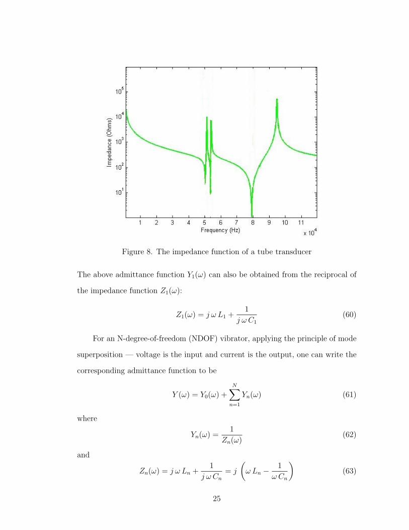
Figure 8. The impedance function of a tube transducer

The above admittance function Y1(ω) can also be obtained from the reciprocal of

the impedance function Z1(ω):

Z1(ω) = j ω L1 +1

j ω C1

(60)

For an N-degree-of-freedom (NDOF) vibrator, applying the principle of mode

superposition — voltage is the input and current is the output, one can write the

corresponding admittance function to be

Y (ω) = Y0(ω) +N∑

n=1

Yn(ω) (61)

where

Yn(ω) =1

Zn(ω)(62)

and

Zn(ω) = j ω Ln +1

j ω Cn

= j

(ω Ln −

1

ω Cn

)(63)

25

in which Cn and Ln are the nth motional capacitance and nth motional inductance,

respectively. They are related to the nth modal (resonant) frequency ωn of a

transducer through ω2n = 1/(LnCn).

Eq. 61 to Eq. 63 implies that the transducer can be represented by an equiva-

lent circuit, which includes N parallel modal branches, as shown in Figure. 9. This

equivalent circuit is often called a mode-driven equivalent circuit (Ballato, 1990).

Each branch represents one mechanical mode, and C0 is the clamped capacitance,

which is equal to the capacitance of the transducer without the piezoelectric effect.

Figure 9. Modes driven equivalent circuit

26

CHAPTER 3

Finite Element Model of Piezoelectric Structure

The mathematical model of a physical system often results in partial differ-

ential equations that cannot be solved analytically because of the complexity of

the boundary conditions or domain. To study a complex model, the FE method is

often employed. The FE method subdivides a complex system into its individual

components or elements whose behavior is readily understood, and it then rebuilds

the original system by assembling such components. Nowadays, the FE method

has become one of the most important analysis tools in engineering.

Since the late 1960s, the work by Eer Nisse (1967) and Tiersten (1967) have

established variational principles for piezoelectric media. Allik & Hughes (1970),

who proposed a tetrahedral element that accounted for piezoelectricity, contribut-

ed greatly to the FE modelling of structures with embedded piezoelectricity. In

1986, piezoelectric elements were for the first time included in the commercial

FE program ANSYS. Later, piezoelectric finite elements have also been includ-

ed in other commercially available FE packages such as ABAQUS and COMSOL

(Kocbach, 2000; Manual, 2005; Multiphysics and Module, 2014). These commer-

cial software packages provide a wide range of simulation options that control the

complexity of both the modelling and analysis of a system. It allows users to easily

build an FE model with piezoelectric elements, and simplifies the analysis proce-

dure. In the present study, we adopted primarily ANSYS to perform FE modelling

using piezoelectric media.

Many studies have focused on the FE analysis for various piezoelectric struc-

tures (Hwang and Park, 1993; Kim and Lee, 2007; Lewis et al., 2009). In this s-

tudy, we focus only on piezoelectric tube transducers that were polarized in the

27

radial direction. The specific analyses included in this study are modal and tran-

sient (dynamic response) analysis. We employed modal analysis to obtain the

modal frequencies and mode shapes of the piezoelectric tube transducer under

both open- and short-circuit electric boundary conditions. We used the transient

analysis to obtain the electric charge time signal while the piezoelectric tube trans-

ducer is subjected to an input electric-potential time signal. The ultimate purpose

of the transient analysis is to obtain the impedance function of the transducer.

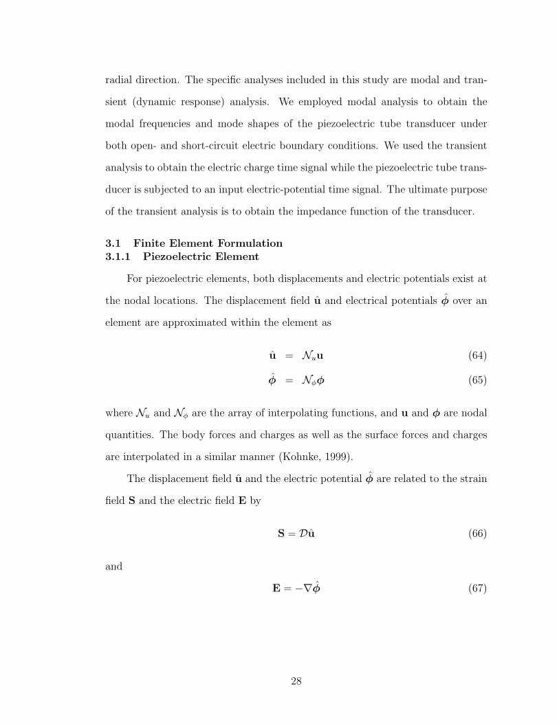
3.1 Finite Element Formulation3.1.1 Piezoelectric Element

For piezoelectric elements, both displacements and electric potentials exist at

the nodal locations. The displacement field u and electrical potentials ϕ over an

element are approximated within the element as

u = Nuu (64)

ϕ = Nϕϕ (65)

where Nu and Nϕ are the array of interpolating functions, and u and ϕ are nodal

quantities. The body forces and charges as well as the surface forces and charges

are interpolated in a similar manner (Kohnke, 1999).

The displacement field u and the electric potential ϕ are related to the strain

field S and the electric field E by

S = Du (66)

and

E = −∇ϕ (67)

28

where ∇ is the gradient operator and D is the derivation operator defined as:

D =

∂x 0 00 ∂y 00 0 ∂z0 ∂z ∂y∂z 0 ∂x∂y ∂x 0

(68)

Therefore, the strain field S and the electric field E are related to the nodal dis-

placements and potential by the shape-functions derivatives Bu and Bϕ, which are

defined by

S = DNuu = Buu (69)

E = −∇Nϕϕ = −Bϕϕ (70)

The dynamic equations of a piezoelectric continuum can be derived from

the Hamilton principle, in which the Lagrangian and the virtual work are prop-

erly adapted to include the electrical contributions as well as the mechanical

ones (Piefort, 2001; Allik and Hughes, 1970; Lerch, 1990; Tzou and Tseng, 1990).

Without further elaboration, for a piezoelectric element, the resulting mechanical

equilibrium equation and the electric-flux conservation equation can be written in

the form

Muuu+Kuuu+Kuϕϕ = f (71)

and

Kϕuu+Kϕϕϕ = g (72)

respectively, where

Muu =

∫V

ρN tuNudV (73)

is the element mass matrix (no inertia terms exist for the electrical flux conservation

equation), ρ is the mass density,

Kuu =

∫V

Btuc

EBudV (74)

29

is the element displacement stiffness matrix,

Kuϕ = Ktϕu =

∫V

Btue

tBϕdV (75)

is the element piezoelectric coupling matrix,

Kϕϕ = −∫V

Btϕε

SBϕdV (76)

is the element dielectric “stiffness” matrix, f is the element mechanical force vector,

and g is the element electric charge vector. In addition, V denotes the volume of

the element (Allik and Hughes, 1970).

3.1.2 Assembled System Equation

In the present study, the total volume Vp is divided into P volumes V(j)p ,

j = 1, · · · , P . Any variable A defined in element j will be written as A(j) as

follows. The relation between the local node-displacement vector u(j) and the

global node-displacement vector U is given through a transformation matrix L(j)u ,

such that

u(j) = L(j)u U (77)

and the relation between the local potential vector ϕ(j) and the global potential

vector Φ is given through a transformation matrix L(j)ϕ , such that

ϕ(j) = L(j)ϕ Φ (78)

The system equations for the whole structure are obtained by the summation of

the contribution from each FE, which can be written in terms of nodal quantities:[M 00 0

]U

Φ

+

[KUU KUΦ

KΦU KΦΦ

]UΦ

=

FG

(79)

where the assembled matrices are given by:

M =P∑

j=1

L(j)u

tM(j)

uu L(j)u (80)

30

KUU =P∑

j=1

L(j)u

tK(j)

uu L(j)u (81)

KUΦ =P∑

j=1

L(j)u

tK

(j)uϕL

(j)ϕ (82)

KΦU =P∑

j=1

L(j)ϕ

tK

(j)ϕu L

(j)u (83)

KΦΦ =P∑

j=1

L(j)ϕ

tK

(j)ϕϕ L

(j)ϕ (84)

F =P∑

j=1

L(j)u

tf (j) (85)

and

G =P∑

j=1

L(j)ϕ

tg(j) (86)

Eq. 79 couples the mechanical variables U and the electrical potentials Φ; F rep-

resents the external forces applied to the structure, and G represents the electric

charges brought to the electrodes (Piefort, 2001).

3.1.3 Open- and Short-circuited Electrical Boundary Conditions

If the electric potential Φ is controlled, the governing equations become

MU+KUUU = F−KUΦΦ (87)

where the second term in the right hand side represents the equivalent piezoelectric

loads. From Eq. 87, one sees that the eigenvalues problem of the system with short-

circuited electrodes, namely Φ = 0, is

(KUU − ω2M)U = 0 (88)

31

It can be seen from Eq. 87 that the modal frequencies, ω, and mode shapes of the

short-circuit model are the same as if there was no piezoelectric electromechanical

coupling.

Conversely, open electrodes correspond to a charge condition G = 0. In this

case, from Eq.79, one writes

Φ = −(K−1ΦΦKΦU)U (89)

Upon substituting Eq. 89 into Eq. 87, it yields

MU+ (KUU −KUΦK−1ΦΦKΦU)U = F (90)

which shows that the global stiffness matrix depends on the electrical boundary

conditions. From Eq. 90, one sees that the eigenvalues problem of the system with

open-circuited electrodes is

(KUU − ω2aM)U = 0 (91)

where

KUU = KUU −KUΦK−1ΦΦKΦU (92)

and ωa denotes the modal frequencies of the open-circuit model. Note that KUU is

the condensed electro-elastic stiffness matrix which amounts to performing a static

condensation to eliminate the degrees of freedom associated with Φ. In physics,

the piezoelectric electromechanical coupling increases the overall stiffness of the

system if the electrodes are left open as additional electric potential energy has

been stored. For a tube transducer, the corresponding modal frequencies of an

open-circuited electrodes, ωa, are the anti-resonant frequencies of the transducer

(Piefort, 2001).

32

3.2 Cylindrical Transducer Modelling and Analysis

The commercial FE packages such as ANSYS have the capability to perform

a fully coupled piezoelectric analysis. In this study, both 2D axisymmetric plane

piezoelectric elements and 3D solid piezoelectric elements are suitable for modeling

the axisymmetric piezoelectric tube.

3.2.1 Modelling and Analysis of 2D Element Model

A specific 2D coupled-field plane element of ANSYS is the PLANE13 element

which will be utilized in this study for modeling axisymmetric transducers. Shown

in Figure. 10 is the PLANE13 element which is defined by four nodes, with three

degrees of freedom per node for piezoelectric analysis, including x-direction dis-

placement, y-direction displacement and voltage (Kohnke, 1999). Please refer to

Appendix B for more detailed ANSYS information about element settings, prop-

erties assignment, piezoelectric analysis and data extraction.

Figure 10. Sketch of PLANE13 element

Throughout this dissertation, the specific numerical model to be studied is a

simple tube transducer with the inner diameter Di = 16× 10−3 m, outer diameter

Do = 19× 10−3 m and length ℓ = 20× 10−3 m. While using axial symmetric plane

elements, one can conveniently build this tube transducer model by revolving its

cross section (a rectangle in the x-y plane) around the z-axis (see Figure. 11).

The poling direction is radially outwards from the axis of symmetry, namely z-

33

axis. Since the order of the stresses in ANSYS differs from those typically used

in electrical applications (IEEE standard), care must be taken while inputting the

corresponding coefficients matrices for the tube transducer model.

Figure 11. Finite element model of a tube transducer: (a) 3D model, and (b) crosssection

The material properties could be specified in either e-form or d-form. The

10 parameters in the e-form are cE11, cE33, c

E12, c

E13, c

E44, ε

S33, ε

S11, e31, e33 and e15,

and the 10 material properties given in the d-form are sE11, sE33, s

E12, s

E13, s

E44, ε

T33,

εT11, d31, d33 and d15. ANSYS allows the user to choose either e-form or d-form

to build piezoelectric FE models. In the present numerical example, the material

properties of APC850 (Navy II) has been chosen, and its d-form parameters are

listed in Table 2, where ε0 = 8.854187817× 10−12 F/m.

Modal properties, including modal frequencies and mode shapes, are impor-

tant dynamic characteristics of a transducer. For a piezoelectric tube transducer,

we are interested in knowing its modal properties for both short-circuit and open-

circuit models. For the open-circuit FE modelling, the potentials on the inner

surface are limited to zero, but are unspecified on the outer surface. For the

34

Table 2. Properties of PZT5A materialMaterial constant Symbol ValueElastic compliance sE13 −5.74× 10−12 m2/N

sE33 18.5× 10−12 m2/NsE44 46× 10−12 m2/NsE11 15.8× 10−12 m2/NsE12 −4.9× 10−12 m2/N

Piezoelectric strain constant d31 −175× 10−12 C/Nd33 400× 10−12 C/Nd15 590× 10−12 C/N

Permittivity εT11/ε0 1851(under constant stress) εT33/ε0 1594

short-circuit model, the potentials on both the inner and outer surfaces are set

to zero. Let z = 0 be the location at the middle of the tube in the axial direc-

tion. The mechanical boundary conditions are considered to be free at both ends,

i.e., at z = −L/2 and z = L/2. First, we performed the modal analysis for the

short-circuit model. The obtained mode shapes are classified into two particular

groups: symmetric and anti-symmetric to z = 0. The symmetric mode shapes

and their corresponding modal frequencies are shown in Figure. 12(a), and the

antisymmetric mode shapes and their corresponding modal frequencies are shown

in Figure. 12(b). In addition, we performed the modal analysis for the open-

circuit model. The resulting mode shapes are also symmetric and anti-symmetric

to z = 0. Figure. 13(a) and Figure. 13(b) show the symmetric and antisymmetric

modes, respectively.

ANSYS has a built-in capability to compute the impedance function of a

transducer by using the harmonic analysis. In the harmonic analysis, we applied

a unit amplitude voltage having a frequency sweeping from 0 to 120 KHz with

an increment of 200 Hz in the radial direction, and Figure. 14 shows the obtained

impedance function. From the impedance function plot, the frequencies corre-

35

Figure 12. The mode shapes and modal frequencies of the short-circuit model: (a)symmetric modes, and (b) antisymmetric modes.

36

Figure 13. The mode shapes and modal frequencies of the open-circuit model: (a)symmetric modes, and (b) antisymmetric modes.

37

Figure 14. The impedance function of the tube transducer by using the harmonicanalysis

38

sponding to the local minima and local maxima are commonly referred to as the

resonance frequencies and anti-resonance frequencies, respectively, of multi-mode

transducers. In theory, the resonance and anti-resonance frequencies should a-

gree well with the modal frequencies obtained from the short- and open-circuit

models, respectively. Only the modal frequencies corresponding to the symmetric

modes of the short- and open-circuit models (see Figure. 12 and 13) are plotted

as the vertical lines in Figure. 14. Clearly, they are in line with the resonance and

anti-resonance frequencies of the impedance function.

Because the axially uniform voltage input is symmetric to z = 0, only sym-

metric modes can be excited. Consequently, only symmetric modes “participate”

in the mechanical vibration and the associated electrical impedance function. Fur-

thermore, because of the axially uniform nature of the input, the mode that has

the most uniform mode shape would dominate the mechanical vibration. In fact,

the most uniform mode shape for the short-circuit model has a modal frequency

of 79.35 KHz (see Figure. 12), which is the global minimum of the impedance

function, and the most uniform mode shape for the open-circuit model has the

modal frequency 95.09 KHz (see Figure. 13), which is the global maximum of the

impedance function.

3.2.2 Modelling and Analysis of 3D Element Model

In this study, the specific 3D element type employed to build up the piezoelec-

tric cylinder is SOLID226 of ANSYS, as shown in Figure. 15. This type of element

contains 20 nodes with four degrees-of-freedom (DoFs) per node, including the

x-direction displacement, y-direction displacement, z-direction displacement, and

voltage (Kohnke, 1999). Please refer to Appendix B for more detailed ANSYS

information about element settings, properties assignment, piezoelectric analyses,

and data extraction.

39

Figure 15. Sketch of SOLID226 element

1

X

Y

Z

APR 14 201513:11:03

PLOT NO. 1

ELEMENTS

Figure 16. 3D tube model built by SOLID226 element

The 3D tube model that was built using SOLID226 element is shown in Fig-

ure.16. Because building the 3D model follows the same geometry, boundary con-

ditions, and material properties, as utilized for the 2D model, similar modal fre-

quencies are expected from the 2D and 3D models. A comparison of the first three

40

modal frequencies between the 2D and 3D models for both short- and open-circuit

models is presented in Table 3, which shows an excellent agreement between these

two models. In Table 3, the relative error was defined as the 2D result minus the

3D result, and it was then normalized by the 3D result. Furthermore, Figure. 17

shows the excellent agreement of impedance functions obtained from the 2D and

3D models.

Table 3. The comparison of modal frequencies between 2D and 3D models

Circuit Mode number Modal frequency (Hz.) Relative error2D model 3D model

Short 1 50290.60 50293.68 -0.006%2 53409.10 53470.08 -0.114%3 79350.58 79355.57 -0.006%

Open 1 51149.01 51147.52 0.003%2 53992.38 54054.97 -0.116%3 95087.15 95134.09 -0.049%

3.2.3 Constitutive Equations of 2D and 3D Models

The distinction of the constitutive equations for 2D (axisymmetrical) and 3D

models is very important, as it is often not well understood and many errors can

arise from the confusion between 2D and 3D properties of piezoelectric materials.

Note however that the dij, sEij and εTii coefficients are equal for 2D and 3D con-

stitutive equations. It is therefore preferable to handle the material properties of

piezoelectric materials in the d-form.

In calculations for axisymmetric structures, it is preferable to use a cylindrical

coordinate system where the symmetry of the problem can be exploited. Let the

three-dimensional cylindrical coordinate system be denoted by (R, θ, Z), where R

is in the radial direction, θ the circumferential direction, and Z axial direction.

41

2 4 6 8 10 12

x 104

10−1

100

101

102

103

104

105

Frequency (Hz)

Impe

danc

e (O

hms)

2−D Model3−D Model

Figure 17. Comparison of impedance functions obtained from 2D and 3D models

42

The strain vector for the cylindrical coordinate system is given by:

S =

S1

S2

S3

S4

S5

S6

=

SR

Sθ

SZ

2SθZ

2SRZ

2SRθ

= Luu (93)

where

Lu =

∂∂R

0 01R

1R

∂∂θ

00 0 ∂

∂Z

0 ∂∂Z

1R

∂∂θ

∂∂Z

0 ∂∂R

1R

∂∂θ

∂∂R− 1

R0

(94)

and

u =

uR

uθ

uZ

(95)

The electric field vector for a cylindrical coordinate system is defined by

E =

E1

E2

E3

=

ER

Eθ

EZ

= −

∂∂R1R

∂∂θ∂∂Z

ϕ = −Lϕϕ (96)

where Lϕ is defined by the last transition.

When only axially symmetric vibrations are considered, this axisymmetrical

constraint suggests

∂

∂θ= 0 (97)

Additionally, let axially symmetric torsional (circumferential) vibrations be ex-

cluded, i.e.,

uθ = 0 (98)

Thus, only two coordinates are needed to describe the problem in the axisym-

metric case: R and Z. This class of problems has been often referred to as 2D

axisymmetric problems.

43

Imposing Eqs. 97 and 98 on Eqs. 93 and 96 yields

S4 = SθZ = 0 (99)

S6 = SRθ = 0 (100)

E2 = Eθ = 0 (101)

Only four of the six strain components and two of the three components of the

electric field need to be included in the analysis. This results in the following

definition for the strain vector and the electric field vector in the two-dimensional

axisymmetric case:

S =

SR

Sθ

SZ

2SRZ

=

∂∂R

01R

00 ∂

∂Z∂∂Z

∂∂R

uR

uZ

= Luu (102)

and

E =

ER

EZ

= −

∂∂R∂∂Z

ϕ = −Lϕϕ (103)

The derivation operator matrices Lu and Lϕ therefore have the following definitions

in this case

Lu =

∂∂R

01R

00 ∂

∂Z∂∂Z

∂∂R

(104)

and

Lϕ =

∂∂R∂∂Z

(105)

In terms of the d-form, the reduced constitutive equations for the axisymmet-

ric 2D element become

S1

S2

S3

S5

D1

D3

=

sE11 sE12 sE13 0 0 d31sE12 sE11 sE13 0 0 d31sE13 sE13 sE33 0 0 d330 0 0 sE44 d15 00 0 0 d15 εT11 0d31 d31 d33 0 0 εT33

T1

T2

T3

T5

E1

E3

(106)

44

To derive the corresponding e-form, one can first rearrange Eq. 106 into:sE11 sE12 sE13 0 0 0sE12 sE11 sE13 0 0 0sE13 sE13 sE33 0 0 00 0 0 sE44 0 00 0 0 −d15 1 0−d31 −d31 −d33 0 0 1

T1

T2

T3

T5

D1

D3

=

1 0 0 0 0 −d310 1 0 0 0 −d310 0 1 0 0 −d330 0 0 1 −d15 00 0 0 0 εT11 00 0 0 0 0 εT33

S1

S2

S3

S5

E1

E3

(107)

Let the e-form of the reduced constitutive equations be denoted by

T1

T2

T3

T5

D1

D3

= A

S1

S2

S3

S5

E1

E3

(108)

From the above two equations, one has

A =

sE11 sE12 sE13 0 0 0sE12 sE11 sE13 0 0 0sE13 sE13 sE33 0 0 00 0 0 sE44 0 00 0 0 −d15 1 0−d31 −d31 −d33 0 0 1

−1 1 0 0 0 0 −d310 1 0 0 0 −d310 0 1 0 0 −d330 0 0 1 −d15 00 0 0 0 εT11 00 0 0 0 0 εT33

(109)

The resulting stiffness matrix cE is a 4× 4 matrix:

cE =

cE11 cE12 cE13 0cE12 cE11 cE13 0cE13 cE13 cE33 00 0 0 cE44

(110)

Note that the stiffness coefficient cij of the 2D formulation differs from the stiffness

coefficient cij of the 3D constitutive equations.

3.3 Numerical Verifications

While using finite element models to conduct research, the numerical verifi-

cation of them is always essential. In the following presentation, the verification

process includes: (1) the comparison with an approximate analytical solution, (2)

the comparison among two commercial finite element packages, and (3) the com-

parison with physical measurements.

45

3.3.1 Comparison with Analytical Solution

One can compare the impedance function of the FE model with the analyt-

ical impedance function based on a ring transducer which has been presented in

Chapter 2. While using the analytical formula, Eq. 40, the following parameters

are utilized: radius a = Do+Di

4= 8.75×10−3 m, length ℓ = 20×10−3 m, permittiv-

ity εT33 = 1.594 × 10−8 (F/m), density ρ = 7600 (kg/m3), piezoelectric coefficient

d31 = −175× 10−12 (C/N) and compliance sE11 = 15.8× 10−12 (m2/N).

Shown in Figure. 18 is the analytical impedance function, comparing to the

impedance function from the finite element model. The analytical impedance

function, which has been derived from a mathematical model of a single-degree-

of-freedom vibrator, contains only a “breathing” vibration mode. In contrast,

the impedance function from the finite element model has been contributed by

multiple vibration modes. Due to the imposed simplifications for the derivation of

the analytical impedance function, the significant discrepancy between these two

impedance functions is not surprising.

For better matching the impedance function computed from a finite element

model to the analytical impedance function, a “constrained” finite element model

has been built. This constrained model does not allow movements in the axial

direction for all elements. The resulting impedance function of the constrained

model — contributed only by a uniformly breathing mode as well — is shown in

Figure. 19. Although there is still discrepancy between the analytical impedance

function and the impedance function from the constrained finite element model,

the difference has become much smaller.

46

Figure 18. Comparison of the impedance function of the FE model with theanalytical impedance function based on a ring transducer

Figure 19. Comparison of the impedance function of the constrained FE modelwith the analytical impedance function based on a ring transducer

47

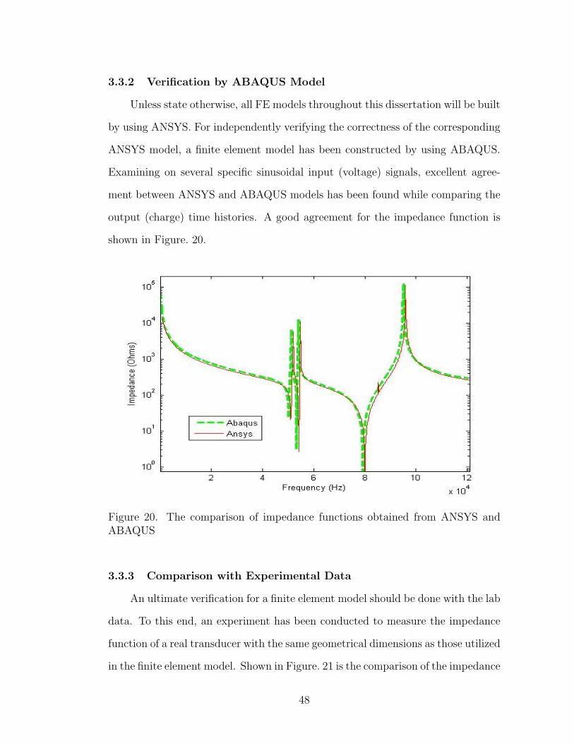
3.3.2 Verification by ABAQUS Model

Unless state otherwise, all FE models throughout this dissertation will be built

by using ANSYS. For independently verifying the correctness of the corresponding

ANSYS model, a finite element model has been constructed by using ABAQUS.

Examining on several specific sinusoidal input (voltage) signals, excellent agree-

ment between ANSYS and ABAQUS models has been found while comparing the

output (charge) time histories. A good agreement for the impedance function is

shown in Figure. 20.

Figure 20. The comparison of impedance functions obtained from ANSYS andABAQUS

3.3.3 Comparison with Experimental Data

An ultimate verification for a finite element model should be done with the lab

data. To this end, an experiment has been conducted to measure the impedance

function of a real transducer with the same geometrical dimensions as those utilized

in the finite element model. Shown in Figure. 21 is the comparison of the impedance

48

functions obtained from ANSYS and the lab measurement. By and large, they

match reasonably well with each other. One obvious reason for the discrepancy

between the impedance functions obtained from ANSYS and the lab measurement

is that the piezoelectric material properties used in ANSYS model could not be the

same as those of the real transducer. In fact, the ultimate goal of this dissertation is

to perform FE model updating on the piezoelectric material properties so that the

impedance functions obtained from ANSYS and the lab measurement can match

better. The algorithm and procedure to carry out the multi-physics FE model

updating on the piezoelectric material properties will be addressed in Chapter 6.

Figure 21. The comparison of impedance functions obtained from ANSYS and labmeasurement

49

CHAPTER 4

Methods of Estimating Impedance Function

One of the most important characteristics of transducers is its impedance

function, which is usually obtained from processing the measured voltage and

current signals. In addition to a review of the traditional methods for estimat-

ing the impedance function of a piezoelectric transducer (Lis and Schmidt, 2004;

Umchid et al., 2009), in this chapter, we newly propose an improved method. This

newly proposed method, which is operated in the Laplace domain, is particularly

effective for handling measured voltage and current signals that have been con-

taminated by noise.

4.1 Traditional Methods

Traditionally, there are two kinds of methods for estimating the impedance

function: (i) stepped harmonic analysis (i.e. single frequency) method, and (i-

i) Fourier-based analysis method using transient signals. The stepped harmonic

analysis is to repeatedly apply a harmonic input signal to get the correspond-

ing steady state response, then compute the impedance of the given frequency

(Lis and Schmidt, 2004). The Fourier method computes the impedance function

from the complex ratio of the FFT of the input and output time domain signals.

Both methods have drawbacks. The stepped harmonic analysis method is very

time consuming; and the Fourier-based analysis method always suffers from the

problems related to the periodic assumption of both input and output signals, such

as frequency leakage and resolution.

50

4.2 Proposed Method

This study proposes a new method to estimate the impedance function via the

Laplace domain in order to overcome the drawbacks of the traditional methods.

The first step of the proposed method is to decompose both input and output time

domain signals into complex exponential components. Because the input voltage

signal v(tk) can be controlled, one can choose to use an exponentially decayed

voltage signal:

v(tk) = γv eλvtk (111)

where λv, γv = constants. For the sake of a clear presentation, let the output signal

(from FE model) be a transient charge signal, c(tk). Decomposed into complex

exponential components, c(tk) can be written into

c(tk) =

p∑n=1

γneλn tk (112)

where p is the number of the decomposition terms, and the complex exponentials

λn and complex amplitudes γn are computed coefficients. Because c(tk) is a real

signal, λn and γn must either be real numbers or occur in complex conjugate pairs.

Let λn = −an + jωn, then an is the damping factor in seconds−1 and ωn is the

frequency in radians. Since the Laplace property L(eλv t) = 1/(s−λv), the Laplace

transform of the input voltage v(t) = γv eλvt is shown to be

V (s) ≡ L(v(t)) = γvs− λv

(113)

Similarly, the Laplace transform of the output charge c(t) is:

C(s) ≡ L(c(t)) =p∑

n=1

γns− λn

(114)

One can find the complex amplitudes and exponentials of a signal in the time

domain are really the poles and residues in the Laplace domain associated with

51

the signal. In turn, both input and output signals in the Laplace domain can be

readily established in a partial fraction form.

To calculate the impedance function, one needs to get the current signal, i(t),

from the derivative of the charge with respect time, that is i(t) = dc(t)/dt. By

using the Laplace property L(df(t)/dt) = sF (s)− f(0), the Laplace transform of

the current i(t) becomes

I(s) = sC(s) =P∑

n=1

sγns− λn

(115)

if the initial charge c(0) is equal to 0.

The impedance function in the s domain can be readily obtained from Eqs. 113

and 115:

Z(s) =V (s)

I(s)(116)

Finally, substituting s by jω in the above equation, one obtains the impedance

function of ω.

4.3 Complex Exponential Decomposition

To implement the proposed method, an essential task is to decompose the sig-

nal into its complex exponential components. An arbitrary signal y(t) can always

be decomposed into a finite number of complex exponential components, called

Prony’s series.

y(t) =

p∑n=1

γneλnt 0 ≤ t < T (117)

where p is the number of terms. For digital signal analysis, the continuous y(t) is

not known and usually equally spaced samples are available. Denoting sampling

interval ∆t, tk = k∆t and yk ≡ y(tk), where k = 0, . . . ,m, one writes the discrete

Prony’s series as

yk =

p∑n=1

γnzkn (118)

52

where zn = eλn∆t.

In Eq. 117, the exponential functions eλnt, n = 1, · · · , p form a basis on the

open interval 0 ≤ t < T . Clearly, the Prony series (Eq. 117) can also be viewed as

the general solution of a pth-order homogenous linear ordinary differential equation

with constant real-valued coefficients an:

p∑n=0

any(n)(t) = 0, for 0 ≤ t < T (119)

where y(n)(t) = dny/dtn. And the exponents λn (n = 1, · · · , p) in Eq. 117 are the

roots of the characteristic equation associated with Eq. 119:

p∑n=0

anλn = 0 (120)

If only the equally-spaced sampled data yk (k = 0, 1, · · · , N − 1) are given,

then Eq. 119 becomes a pth-order difference equation:

p∑n=0

bnyk+n = 0, for k = 0, 1, · · · , N − p− 1 (121)

where bn are real-valued constants. Without losing the generality, let bp = 1.

From Eqs. 118 and 121, the characteristic equation associated with Eq. 121 can be

obtained to be:p∑

n=0

bnzn = 0 (122)

Note that the linear difference equation and its characteristic equation have the

same coefficients bn.

4.3.1 Prony’s method

Traditionally, Prony’s method has often been utilized to decompose a signal

into complex exponential components. In brief, Prony’s method is a technique

for fitting an exponential model to a few equally spaced measured data points

(Prony, 1795). While the original Prony’s method presented a method that exactly

53

fits as many purely damped exponentials as required to fit the available data points,

the modern version of Prony’s method generalizes to damped sinusoidal models. In

addition, it utilizes the least-squares analysis to approximately fit an exponential

model for cases where there are more data points than needed to fit the assumed

number of exponential terms. However, because Prony’s method suffers from an

ill-conditioned problem with respect to determining the roots of the high-order

polynomial that is encountered, the estimation of Prony’s method may have a

significant error (Hu et al., 2013).

4.3.2 Prony-SS method

To avoid dealing with the ill-conditioned problem, in this study, we employed

an alternative approach that uses a first-order matrix homogenous difference equa-

tion (state-space model) to replace the high-order homogenous difference equation,

and the approach is called the Prony-SS method (Hu et al., 2013). Although the

Prony-SS method and Prony’s method appear to be theoretically identical, they

are drastically different with respect to crucial numerical issues, including condi-

tioning and stability. While Prony’s method is very sensitive to the sampling rate

and round-off error, the Prony-SS method is not. While Prony’s method has trou-

ble dealing with noise embedded in the signal, the Prony-SS method can handle

noisy signals properly because it has a built-in noise-rejection mechanism that uses

truncated singular-value decomposition. While root-finding of a high-order poly-

nomial, which is a classical ill-conditioned problem, is a required step in Prony’s

method, the Prony-SS method completely avoids it (Hu et al., 2013).

The Prony-SS method begins with a first-order matrix difference equation,

which is a state-space model, to replace a high-order difference equation used

in Prony’s method. The three steps of the Prony-SS method are: (1) obtain a

realization for the state matrix of the first-order matrix difference equation from

54

the Hankel matrices composed by the sampled data; (2) compute the eigenvalues of

the realization matrix, and then obtain the estimates of the frequency and damping

factor of each exponential term, and (3) solve for a set of linear equations to yield

the estimates of the exponential amplitude and sinusoidal initial phase of each

component (Hu et al., 2013).

By introducing

x1 = y(0), x2 = y(1), · · · , xp = y(p−1) (123)

and assuming ap = 1, Eq. 117 is converted into a first-order matrix differential

equation as

x(t) = Fx(t) (124)

where x(t) = dx(t)/dt,

F =

0 1 0 0 · · · 0 00 0 1 0 · · · 0 00 0 0 1 · · · 0 0...

......

.... . .

......

0 0 0 0 · · · 0 1−a0 −a1 −a2 −a3 . . . −ap−2 −ap−1

∈ Rp×p (125)

and

x(t) =

x1

x2...xp

∈ Rp (126)

The solution of Eq. 124 has the form x(t) = veλt where λ is a constant and v is a

time-independent p-element column vector. When x(t) = veλt is substituted into

Eq. 124, it yileds the algebraic eigenvalue equation:

Fv = λv (127)

Theoretically, the p eigenvalues of the matrix F are exactly the p roots of the

characteristic equation of Eq. 120. Instead of determining the roots of Eq. 120,

the Prony-SS method is to compute the eigenvalues of the matrix F.

55

The elements of vector x in Eq. 126 are often termed the state variables of the

linear dynamic system, and they serve as the “coordinates” of the system. However,

there are an infinite number of ways of selecting the coordinates. Denoting an

arbitrary nonsingular transformation matrix by Φ ∈ Rp×p, and another set of

coordinates by q ∈ Rp, one can formulate the transformation relationship between

x and q as:

x(t) = Φq(t) (128)

Now, substitute x(t) = Φq(t) and x(t) = Φq(t) into Eq. 124 and premultiply both

sides by Φ−1, the resulting equation becomes

q(t) = Gq(t) (129)

where G = Φ−1FΦ. Note that Eq. 129 and Eq. 124 share the same form. Because

G is a similarity transformation of F, they must have the same eigenvalues.

Let the eigenvalues and the corresponding eigenvectors of G be denoted by

λ1, λ2, · · · , λp and u(1), u(2), · · · , u(p), respectively. Because u(1)eλ1t, u(2)e

λ2t, · · · ,

u(p)eλpt form a basis for solutions of Eq. 129, the general solution of Eq. 129 can

be written as:

q(t) =

p∑n=1

gnu(n)eλnt (130)

where gn are arbitrary constants. In Eq. 130, each element of q(t) is a linear

combination of eλnt, n = 1, . . . , p, so is y(t) in Eq. 117. Therefore, y(t) is a linear

combination of the elements of q(t), that is,

y(t) =

p∑n=1

cnqn(t) (131)

or

y(t) = ctq (132)

where qn(t) is the nth element of q(t) and c ∈ Rp is a column vector.

56

The discrete version of Eq. 129 is a first-order homogeneous matrix difference

equation which can be written as:

qk+1 = Aqk (133)

where qk ≡ q(tk) and A = exp(Gt). From Eq. 132, at t = tk, one has

yk = ctqk = ctAkq0 (134)

Here, the specific goal is using the given discrete signal yk, k = 0, · · · , N − 1, to

obtain a realization of A. Next, the eigenvalues of A, and those of F (i.e. λn, n =

1, · · · , p), can be computed without going through the procedure of determining

polynomial coefficients and zeros (Hu et al., 2013).

The Hankel matrix H(k) ∈ Rξ×η was defined as

H(k) =

yk yk+1 · · · yk+η−1

yk+1 yk+2 · · · yk+η...

.... . .

...yk+ξ−1 yk+ξ · · · yk+ξ+η−2

(135)

Upon substituting Eq. 134 into Eq. 135, it can be shown that H(k) is the product

of three matrices:

H(k) = PξAkQη (136)

where

Pξ =

ct

ctActA2

· · ·ctAξ−1

∈ Rξ×p (137)

and

Qη = [ q0 Aq0 A2q0 · · · Aη−1q0 ] ∈ Rp×η (138)

57

A realization of A can be obtained from H(0) and H(1). Substituting k = 0

and k = 1 into Eq. 136 yields

H(0) = PξQη (139)

and

H(1) = PξAQη (140)

Applying the singular value decomposition of H(0), one writes

(Zhou and Doyle, 1996):

H(0) = [ U1 U2 ]

[Σ1 00 0

] [VT

1

VT2

]= U1Σ1V

T1 (141)

In theory, the model order of the dynamic system, p, is equal to the number of

non-zero singular values in Eq. 141, that is, U1 ∈ Rξ×p, Σ1 ∈ Rp×p and V1 ∈ Rp×η,

and the rank of H(0) is p. The singular values should go to zero when the rank

of the matrix is exceeded, but for measured data due to random errors and small

inconsistencies in the data, the singular values will not become zero but will become

very small. While choosing the size of H(0), both ξ and η must be greater than p.

A direct comparison between Eqs. 139 and 141 suggests that Pξ is related

to U1, and Qη to VT1 . A possible “balanced” choice is Pξ = U1Σ

1/21 and Qη =

Σ1/21 VT

1 . Substituting Pξ = U1Σ1/21 and Qη = Σ

1/21 VT

1 into Eq. 140, one obtains:

H(1) = U1Σ1/21 AΣ

1/21 VT

1 (142)

Premultipling Σ−1/21 UT

1 and postmultiplying V1Σ−1/21 at Eq. 142 yields a realiza-

tion of A as:

A = Σ−1/21 UT

1H(1)V1Σ−1/21 (143)

While the computed eigenvalues of A are zn, n = 1, · · · , p, the corresponding λn in

Eq. 117 are λn = ln(zn)/∆t. Finally, the complex coefficients γn can be computed

58

by solving a second set of linear equations (Hu et al., 2013):z01 z02 · · · z0pz11 z12 · · · z1p...

.... . .

...zK−11 zK−1

2 · · · zK−1p

γ1γ2...γp

=

c0c1...

cK−1

(144)

Multi-signal Prony-SS method

While the above Prony-SS method has been derived to deal with a single

signal decomposition, it can also be extended to perform the multiple signals

(Hu et al., 2016). We denote the column vector yk ∈ RN×1 for the signal da-

ta, where N is the number of signals. The multiple-signal vector can be written

as:

yk =

p∑n=1

Γnzkn (145)

where

Γn =

γn,1γn,2...

γn,N

∈ RN (146)

The extension from the single-signal Prony-SS method to multiple signals is

quite straightforward. The first two steps of the proposed method are the same as

the single-signal Prony-SS’s step described above. We first obtained a realization

for the state matrix of a first-order matrix difference equation, and we then compute

the eigenvalues of the realization matrix to obtain the estimates of the frequency

and damping factor of each exponential term. The distinction between the single-

signal and multiple-signal Prony-SS method is that the elements in Eq. 135 are

replaced by corresponding block matrices, that is,

H(k) =

yk yk+1 · · · yk+η−1

yk+1 yk+2 · · · yk+η...

.... . .

...yk+ξ−1 yk+ξ · · · yk+ξ+η−2

∈ Rξ×η (147)

59

Further, when considering multiple signals, Eq. 134 becomes

yk = CtAkq0 (148)

where Ct is ∈ RN×p with ctn ∈ R1×P , n = 1, · · · , N as its rows and ctn is the row

vector corresponding to the nth signal. Upon substituting Eq. 148 into Eq. 147, it

can be shown that H(k) is the product of three matrices:

H(k) = PξAkQη (149)

where

Pξ =

Ct

CtACtA2

· · ·CtAξ−1

∈ RNξ×p (150)

and Qη stay the same as Eq. 138.

Then using the same step illustrated in single signal, a realization of A can

be obtained from H(0) and H(1):

A = Σ−1/21 Ut

1H(1)V1Σ−1/21 (151)

where

H(0) = PξQη (152)

and

H(1) = PξAQη (153)

UT1 , V1 and Σ1 can be obtained by applying the singular value decomposition

of H(0), one writes (Zhou and Doyle, 1996):

H(0) = [ U1 U2 ]

[Σ1 00 0

] [Vt

1

Vt2

]= U1Σ1V

t1 (154)

60

In theory, the model order of the dynamic system, p, is equal to the number

of non-zero singular values in Eq. (154), that is, U1 ∈ Rξ×p, Σ1 ∈ Rp×p and

V1 ∈ Rp×η, and the rank of H(0) is p. While choosing the size of H(0), both ξ and

η must be greater than p. The computed eigenvalues of A are zn, n = 1, · · · , p,

and the corresponding λn in Eq. 112 are λn = ln(zn)/∆t.

Once zn, n = 1, · · · , p, have been computed, the next step involves the solution

of a second set of linear equations. The matrix form of equations is written as:z01 z02 · · · z0pz11 z12 · · · z1p...

.... . .

...zK−11 zK−1

2 · · · zK−1p

Γt1

Γt2...Γt

p

=

yt0

yt1...

ytK−1

(155)

where

Γ =

γ1,1 γ1,2 · · · γ1,Nγ2,1 γ2,2 · · · γ2,N...

.... . .

...γp,1 γp,2 · · · γp,N

(156)

The residues Γn, n = 1, · · · , p can be calculated using Eq. 155 and , consequently,

the amplitudes and phase angles.

When estimating the impedance function, it has been theoretically proven

that the poles of the output signal of a linear system will contain the poles of

the input signal (Hu et al., 2016). To guarantee that the estimated poles of the

output (current) signal contain the input (voltage) poles, it is necessary to process

both input and output signals simultaneously by using the multi-signal Prony-SS

method. An intended feature of the multi-signal Prony-SS method is that all input

and output signals share the same model – a pth-order difference equation. With

this feature, a consistent set of “global” poles (natural frequencies and damping

factors) exists among all signals.

61

4.4 Noise Rejection and Damping Modelling

It is inevitable that the measured input and output signals must contain var-

ious noises, and a realistic transducer must include damping (energy dissipation)

mechanism. This section addresses the noise handling by using the traditional

frequency domain method and the proposed method. As the proposed method has

the capability of estimating the damping ratios associated with multiple vibration

modes, this section also includes using a Rayleigh damping for the finite element

model based on the estimated damping ratios of dominant vibration modes.

4.4.1 Noise-cancelling Methods Statement

Figure. 22 shows a schematic representation of a measurement system to both

input and output noise.

Figure 22. Measurement system with noise sources

To remove the noise, the traditional frequency-domain method used to esti-

mate the frequency-response function (reciprocal of impedance function) of a linear

system is based on the calculation of the averaged auto-power spectra

GP P (ω) =1

N

N∑n=1

Pn(ω)P∗n(ω) (157)

and

GUU(ω) =1

N

N∑n=1

Un(ω)U∗n(ω) (158)

62

together with the cross-power spectra

GU P (ω) =1

N

N∑n=1

Un(ω)P∗n(ω) (159)

and

GP U(ω) =1

N

N∑n=1

Pn(ω)U∗n(ω) (160)

where N is the number of segments, and Pn and Un are the Fourier transforms

of measured time-domain signals of a segment pn and un, respectively, while ( . )∗

denotes the complex conjugate. Using the averaged spectra of the measured input

and output signals, the frequency-response function (reciprocal of the impedance

function) of the system can be estimated by the following estimator:

H(ω) =1

Z(ω)=

√√√√GU P (ω)

GP P (ω)

GP U(ω)

GUU(ω)(161)

Note that because of limitations of the Fourier transform, this Fourier-based de-

noising method suffers from the problems related to the periodic assumption, such

as frequency leakage and resolution. In principle, the averaging procedure usually

requires the amount of data to be very large (Craig and Kurdila, 2006).

Noise Cancellation of Laplace Method

The noise cancellation of the proposed method is based on neglecting the

insignificant exponential components of the signal. Assume that sk (k = 1, · · · , i+

1) is a singular value of the Hankel matrix, sorted from high to low, Eq. 141 can

be written as

U1Σ1Vt1 =

[u1 u2 · · · u(i+1)

]·

s1

s2. . .

si+1

·

vt1

vt2...

vtm−i

= u1s1v

t1 + u2s2v

t2 + · · ·+ ui+1si+1v

ti+1 (162)

where m is the amount of data and i is the number of rows of Hanker matrix. We

can find the value of sk that determines the effect of a component on the entire

63

signal. Because the noisy components are much smaller relative to the system

components, one can take the first n components as the response from the system,

and the rest are from noise. Therefore, Eq. 162 can be written into

U1Σ1Vt1 = [Usystem|Unoise]

[Ssystem 0

0 Snoise

] [Vt

system

Vtnoise

]= u1s1v

t1 + · · ·+ unsnv

tn + · · ·+ ui+1si+1v

ti+1 (163)

We can neglect the components ranked after n to achieve noise cancelling. It is

important to note that the number of rows should not be too small, as that will

affect the rank of system, while the number should not be too big as that will affect

the efficiency of noise cancelling. Therefore, the noise cancelling of the proposed

method depends on the choice of the noise threshold n, which is the number of

exponential components produced by the system but noise. A conventional way of

choosing the noise threshold is to find a significant gap in the normalized singular

values. Generally, there is a sharp drop between the system and noise components,

and therefore, we should take the n, which is the number of singular values before

the sharp drop, as the rank of the system.

4.4.2 Damping Estimation

The proposed method is capable of estimating the damping ratio, ξn, of the

impedance function at resonance frequencies. After computing the eigenvalues zn

of the transition matrix A using Eq. 143, the corresponding λn can be calculated

by

λn =ln(zn)

∆t(164)

and the damping ratio

ξn =an|λn|

(165)

where an is the real part of λn.

64

When using FE commercial packages, we often cannot specify damping coef-

ficients directly, but employ them while setting the harmonic analysis or transient

analysis. The Rayleigh damping matrix, C, is a widely used damping model, and

is defined as (Cai et al., 2002):

C = αM+ βK (166)

where M is the system mass matrix, K is the system stiffness matrix, and α and

β are two coefficients that are related to the damping ratios by

ξn =1

2(α

ωn

+ βωn) (167)

where ωn is the nth modal frequency of the system. When the two damping ratios,

ξ1 and ξ2, which are associated with frequencies ω1 and ω2, are estimated using

the proposed method, the values of α and β can be calculated by

α =2ξ1ω1ω

22 − 2ξ2ω

21ω2

ω22 − ω2

1

(168)

and

β =2ξ1ω1 − 2ξ2ω2

ω21 − ω2

2

(169)

respectively.

65

CHAPTER 5

Numerical Study of Estimating Impedance Function

In this chapter, we present a numerical study of the estimation of the

impedance function of a piezoelectric transducer. To test the effectiveness of the

proposed Laplace domain method, both the numerical simulation and the lab ex-

periment are included. The impedance functions estimated from the proposed

method are compared to those obtained from traditional methods. In addition,

the effectiveness of noise cancelation for both the proposed and the traditional

Fourier-based methods is also investigated.

5.1 Simulation Study

The simulation model is a 2D FE model, shown in Figure. 11. The impedance

function estimated by the stepped single-frequency method which repeats hundreds

or thousands of single-frequency analysis is considered to be accurate. Some com-

mercial FE packages, including ANSYS, have the built-in capability to compute the

impedance function of a transducer using the stepped harmonic (single-frequency)

analysis (Moaveni, 2003). By using ANSYS with the frequencies ranged from 0

to 120 KHz with an increment 200 Hz, the impedance function of the present FE

model from the harmonic analysis is shown in Figure. 23.

5.1.1 Estimation with Laplace- and Fourier-based Methods

The drawback of the stepped single-frequency method is that it is very time-

consuming, especially compared to traditional Fourier-based methods. Fourier-

based methods usually carry out the FFT of the transient signals of voltage and

current (or charge) that are obtained from a single test. In this study, the pro-

posed Laplace domain method is to be evaluated against both the stepped single-

66

Figure 23. The impedance function from ANSYS

frequency and a Fourier-based method.

For the numerical simulation study, the transient time signals of the voltage

and charge are generated by the transient dynamic analysis of ANSYS. The sam-

pling rate of the time signals is taken to be fs = 104 KHz, or the time interval

∆t = 1 × 10−7 s. Thus, the present analysis targets modal frequencies below the

Nyquist frequency 5 × 103 KHz. The input (voltage) signal was generated with

the form v(t) = γv eλvt, with γv = 500 V and λv = −1× 10−3, for a total duration

of 5 × 10−3 s. The output signal is the electric charge response on the outer sur-

face of the transducer. The time histories of the voltage and charge are shown in

Figure. 24.

To properly estimate the impedance function, Fourier-based methods and the

proposed Laplace method have significantly different requirements with respect to

the duration of the output signal. While applying a Fourier-based method, the

67

Figure 24. The voltage and charge signals

68

input and output signals must be long enough to achieve the desired frequency

resolution. To achieve the frequency resolution of 200 Hz in the Fourier analysis,

the duration of both voltage and charge signals must be 5×10−3 s long. In contrast,

to extract the poles and residues associated with the charge signal, the proposed

Laplace-domain method would employ the initial segment from 0 to 1 × 10−4 s

only for the charge signal.

Figure 25. The comparison of the estimated impedance functions

Figure. 25 shows the comparison of the estimated impedance functions from

the proposed method and the Fourier-based method, against that from the stepped

harmonic method. One can easily conclude the following:

1. The impedance function estimated from the proposed method agrees well

with that from the stepped single frequency method.

2. The proposed method significantly outperforms the Fourier-based method,

especially at the region of high frequency. Note that the damping factor for

this FE model has been set to be equal to 0.

69

In summary, the proposed method significantly outperforms the Fourier-based

method. Furthermore, the signal required for the proposed method is much shorter

than that for the Fourier-based method. The impedance function estimated by the

proposed method also has a much higher resolution than that of the Fourier-based

method.

5.1.2 Estimating Impedance Function in Noisy Environment

To simulate a more realistic environment, we included the Rayleigh damping

with α = 0 and β = 1× 10−7 for the FE model, and added 10% random Gaussian

white noise to the clean signals. The level of the additive white noise is quantified

by a stated percentage, which is defined as the ratio of the standard deviation of

the Gaussian white noise (σn) to that of the noise-free signal (σs): σn/σs × 100%.

Let the signal-to-noise ratio be defined as S/N = 20log10(σs/σn). A 10% noisy

signal corresponds to S/N = 20.

Figure 26. Impedance functions estimated from noisy signals by FFT methods

70

Shown in Figure. 26 are two impedance functions estimated from noisy signals,

including: (1) direct FFT approach which obtains the impedance function based on

the ratio of the FFT of the voltage to that of the current, and (2) auto/cross power

spectra approach, i.e. Eq. 161. For comparison purpose, Figure. 26 also shows the

impedance function that is obtained from the stepped harmonic analysis. While

using the power spectra approach, we use 20 signals, each having 5 × 104 data

points, to calculate the averaged impedance function.

Next, the noise rejection of the proposed method by using a truncated singular

value decomposition technique is carried out. The first 100 singular values of

H(0)500×500 for the charge signal, which are normalized by the first singular value,

are shown in Figure. 27.

Figure 27. Singular Values of Hankel Matrix

71

Clearly, the singular value curve in Figure. 27 has a significant gap between its

26th and 27th singular values. As the gap may represent the separation between

the true signal and noise, the model order for this signal is set equal to 26. By

implementing the proposed method with model order 26, we obtain the impedance

function of the simulation model shown in Figure. 28. One notices that a good

agreement has been achieved between the stepped single-frequency method and

the proposed method using only 1000 data points. When 3000 data points are em-

ployed in the proposed method, it results in an even better match (see Figure. 29).

Figure 28. The impedance function using 1000 data points (proposed method)

72

Figure 29. The impedance function using 3000 data points (proposed method)

73

5.2 Laboratory Test

Ultimately, the effectiveness of the proposed method must be tested for a real

transducer (see Figure. 6). The laboratory test was setup (see Figure. 30) for

estimating the impedance function of a real piezoelectric tube. In this experiment,

the transducer tube was mounted on a “soft” base (a sponge pad) to simulate a

free-free mechanical boundary condition.

Figure 30. The experiment setup for estimating the impedance function

The key components of the hardware system include:

1. Source of excitation input: Arbitrary Waveform Signal Generator

(AWG5000B);

2. Data-acquisition hardware: Multifunction I/O Boards for PCI Bus Comput-

ers (PCI-6110E);

3. Dynamic analyzer: a computer with the signal analysis software (MATLAB)

and FE software (ANSYS).

For detailed information about these pieces of equipment, one can refer to

References.(Mul, 1998; Tektronix, 2008).

74

The corresponding circuit diagram of the experiment is shown in Figure. 31,

where the resistance R1 = 3140 ohm, V1 is the input voltage generated by the

Figure 31. The circuit diagram of the experiment

signal generator, and V2 is the response voltage on the piezoelectric tube. The

impedance Z of the piezoelectric tube can be calculated by

Z =V2

V1 − V2

×R1 (170)

The experimental procedure requires three steps to estimate the impedance

function:

1. Generate the input signal V1 on a computer and download it to the generator

(AWG5000);

2. Conduct the experiment and collect the response signal V2;

3. Perform the necessary signal-processing tasks to obtain the impedance func-

tion.

Both the stepped harmonic signals and transient signals have been utilized as the

input V1. The harmonic input signals were generated repeatedly at uniformly

75

spaced frequencies with intervals of 0.24 KHz. The transient signal was an ex-

ponential decay signal with a maximum of 1V and a decay ratio of −3 × 103.

Figure. 32 shows the transient input and its corresponding output.

Figure 32. Transient input and the corresponding output signals

Using the transient signals, the impedance functions estimated by the di-

rect FFT and proposed methods are shown in Figure. 33. Also included is the

impedance function estimated by the stepped harmonic method. It is clear that

the proposed method outperforms the traditional Fourier-based method.

76

Figure 33. The comparison of the impedance functions using experimental data

77

CHAPTER 6

Finite Element Model Updating of Piezoelectric Structure

6.1 Introduction

Model updating is defined as the process of correcting the numerical values of

individual parameters in a mathematical model using data obtained from an asso-

ciated experimental model such that the updated model more correctly describes

the dynamic properties of the subject structure. This chapter briefly reviews tra-

ditional finite element model updating methods for elastic systems. In particular,

the CMCM method is presented and extended to apply for the finite element mod-

el updating when only modal frequencies are available. Based on the extended

CMCM method, this chapter newly develops an approach for the multi-physics

FE model updating of piezoelectric systems. In this chapter, the newly devel-

oped method is limited to update the material parameters of a piezoelectric tube

transducer while the only information available is the impedance function of the

transducer.

6.2 Traditional Model Updating Methods

Traditionally, model updating methods can be classified into two major group-

s: direct methods and iterative methods.

6.2.1 Direct Methods

Direct methods are generally of non-iterative methods, all of which are based

on computing changes made directly to the mass and stiffness matrices. Typical

direct methods include Lagrange multiplier methods, matrix mixing methods and

control theory methods (Friswell and Mottershead, 1995). These methods have

the advantage of not requiring any iterations, thus eliminating the possibilities

of divergence and excessive computation. And abstract “representation” models

78

could be built up to reproduce the measured data exactly.

One major drawback of direct methods is that the updated mass and stiffness

matrices have little physical meaning and cannot be related to physical parameters

to the finite elements in the original model. Another drawback of direct methods

is the need to expand the mode shape vectors to the full set of finite element model

degrees of freedom. Because the quality of mode shape measurements generally

cannot be considered to be completely accurate using current measurement tech-

nology, this expansion will introduce errors in the data required by the updating

algorithm (Friswell and Mottershead, 1995).

6.2.2 Iterative Methods

In many ways, iterative methods are more acceptable in that the parameters

they adjust are much closer to physically realizable quantities, and have generally

been viewed as the main hope for updating technology. In the iterative method-

s, the basic procedure consists of solving an optimization problem, in which the

discrepancies between the analytical (numerical) and measured dynamic charac-

teristics are minimized by adjusting the unknown model properties.

Typically, the dynamic characteristics that are employed are modal parame-

ters (denoted as z), including both modal frequencies and mode shapes, and the

unknown model properties are the updating parameters (denoted as θ), which are

commonly the dimensionless correction factors for each element. Suppose there

are more measured modal parameters than unknown updating parameters, then

the estimate for the updating parameters can be obtained using a least-squares

method. Because the modal parameters are always non-linear functions of the

updating parameters, the least-squares problem is solved in an iterative way.

The iterative methods are generally based on the use of a Taylor series of the

modal parameters that are expanded as a function of the updating parameters,

79

and this series is often truncated to produce a linear approximation of the form

δz = Senδθ (171)

where δθ is the perturbation in the updating parameters, δz is the error in the

analytical and measured modal parameters, and Sen is the sensitivity matrix. The

sensitivity matrix Sen, which contains the first derivatives of the modal parameters

with respect to the updating parameters, is calculated analytically with formulas

based on the equation of motion. The calculation of these derivatives is computa-

tionally intensive. In principle, the sensitivity matrix, Sen, must be reevaluated at

each iteration based on the latest estimate of the updating parameters. Consider-

ing Eq. 171, the use of δz indicates that the measured and analytical modes must

be paired correctly. Because the mass distribution of the analytical model and

that of the actual structure may be different, the measured and analytical mode

shapes must be scaled consistently. Furthermore, because of the iterative proce-

dure and a possible ill-conditioned Sen, the solutions are often prone to diverge

(Hu et al., 2007).

Up to the present, most published model updating methods for ultra-

sound transducers belong to the category of iterative methods in the tra-

ditional sense (Piranda et al., 1998; Piranda et al., 2001; Araujo et al., 2009;

Kwok et al., 1997).

6.3 Cross-model Cross-mode (CMCM) Method

The model updating method employed in this study is the cross-model cross-

mode (CMCM) method, which involves solving a set of linear simultaneous equa-

tions for the physically meaningful correction factors. Each linear equation of the

CMCM method is formulated based on the product terms from two same/different

modes associated with the mathematical and experimental models, respectively.

In addition to its accuracy and efficiency, the CMCM method has several other

80

advantages over traditional model updating methods, including: (1) it is a direct,

as well as a physical property adjustment, model updating method. While it is

a non-iterative method and therefore very cost-effective in computational time, it

also has the advantage of preserving the initial model configuration and physical

connectivity of the updated model; (2) it uses both the mode shapes and modal fre-

quencies for the simultaneous updating of the mass and stiffness matrices, whereas

it does not require the measured mode be paired with the same mode of the ana-

lytical model; (3) the implementation of the new updating approach needs only the

first few measured modes being arbitrarily scaled; (4) the method is a systematic

approach and theoretically it is readily applicable to various kinds of structural or

mechanical systems (Hu et al., 2007).

6.3.1 Procedure of CMCM Method

In the development of the CMCM method, it is assumed that the stiffness

and mass matrices of the structure, denoted by K and M, are obtained from the

finite-element model. It is intended to “correct” or “update” the stiffness and mass

matrix coefficients by modal measurements, including a few mode shapes and their

corresponding frequencies.

The ith eigenvalue and eigenvector associated with K and M is expressed as

KΦi = λiMΦi (172)

Assume that the stiffness matrix K∗ of the actual (experimental) model is a mod-

ification of K to be formulated as

K∗ = K+Ne∑n=1

αnKn (173)

where Kn is the stiffness matrix corresponding to the nth element; Ne is the

number of “elements”; and αn are correction factors to be determined. Herein, for

simplicity in presentation, it is assumed that each element involves a parameter

81

to be updated, such as the Youngs modulus of each element. A more general

formulation of Eq. 173 can have the number of unknowns, or correction terms, to

be less, or greater, than Ne.

Likewise, one writes the corresponding expression for a corrected mass matrix

M∗ as

M∗ = M+Ne∑n=1

βnMn (174)

in which Mn is the mass matrix corresponding to the nth element; and βn are

correction coefficients to be determined. Again, it is assumed that each element

involves a mass quantity to be corrected, such as the mass density of each element.

Clearly, Eqs. 173 and 174 are applicable to general finite-element formulations with

any element type where individual mass and stiffness matrices may be very large.

Express the jth eigenvalue and eigenvector associated with K∗ and M∗ as

K∗Φ∗j = λ∗

jM∗Φ∗

j (175)

In the following development, it is assumed that a few of λ∗j and Φ∗

j are known

measurements available from modal testing.

Premultiplying Eq. 172 by Φ∗jt and Eq. 175 by Φi

t yields

Φ∗jtKΦi = λiΦ

∗jtMΦi (176)

and

ΦitK∗Φ∗

j = λ∗jΦi

tM∗Φ∗j (177)

respectively. Because M is a symmetric matrix, one has [Φ∗jtMΦi]

t = ΦtiMΦ∗

j .

Also noting the transpose of a scalar equals to itself, i.e. [Φ∗jtMΦi]

t = Φ∗jtMΦi.

One thus has

Φ∗jtMΦi = Φt

iMΦ∗j (178)

Similarly, since K is a symmetric matrix, one shows that

Φ∗jtKΦi = Φt

iKΦ∗j (179)

82

Dividing Eq. 177 by Eq. 176, and using the scalar identities of Eqs. 178 and 179,

one obtainsΦt

iK∗Φ∗

j

ΦtiKΦ∗

j

=λ∗j

λi

ΦitM∗Φ∗

j

ΦtiMΦ∗

j

(180)

Substituting Eqs. 173 and 174 into the above equation yields

1 +Ne∑n=1

αnAn,ij =λ∗j

λi

(1 +Ne∑n=1

βnBn,ij) (181)

where

An,ij =Φi

tKnΦ∗j

ΦitKΦ∗

j

(182)

and

Bn,ij =Φi

tMnΦ∗j

ΦitMΦ∗

j

(183)

Using a new index m to replace ij, Eq. 181 becomes

1 +Ne∑n=1

αnAn,ij = bm(1 +Ne∑n=1

βnBn,ij) (184)

where

bm =λ∗j

λi

(185)

Rearranging Eq. 184, one obtains

Ne∑n=1

αnAn,m − bm

Ne∑n=1

βnBn,m = bm − 1 (186)

orNe∑n=1

αnAn,m +Ne∑n=1

βnEn,m = fm (187)

where En,m = −bmBn,m, fm = bm − 1. When Ni reliable modes are available from

the finite-element model, and Nj modes are measured from the corresponding real

structure, totally Nm = Ni × Nj CMCM equations can be formed from Eq. 187.

Written in a matrix form, one has

αA+ βE = f (188)

83

in which A and E are Nm × Ne matrix; α and β are column vectors of size Ne;

and f is a column vector of size Nm. Furthermore, one can rewrite Eq. 188 as

Gγ = f (189)

where

G =[A E

],γ =

[αβ

](190)

A singular value decomposition (SVD) approach can be used to solve forGγ =

f where the system can be just-determined, under-determined, over-determined, or

mixed-determined. Decompose the rectangular matrix G as the product of three

matrices

G = UΣVt (191)

where the matrices U and V, real or complex unitary matrices with UtU = I,

VtV = I, and the matrix Σ, a diagonal matrix whose diagonal elements are

singular values. These singular values are usually arranged in order of deceasing

size. Some of the singular values may be zero. One can partitionΣ into a submatrix

Σp of p nonzero singular values and zero matrices as

Σ =

[Σp 00 0

](192)

where Σp is a p × p diagonal matrix. The decomposition then becomes G =

UpΣpVtp, where Up and Vp consist of the first p columns of U and V. The

natural solution of the inverse problem has been shown to be (Hu et al., 2007;

Hu and Li, 2008)

γ = G−1f = VpΣ−1p Ut

pf (193)

6.3.2 Extended CMCM Method

In dealing with spatially incomplete situations, one usually applies either mod-

el reduction or modal expansion schemes. The case of no mode shapes at all is

84

an extreme case of incompleteness. A possible approach to deal with the extreme

incompleteness case — only measured modal frequencies available — is to extend

the original CMCM method involving an iterative procedure (see the flowchart

in Figure.34) (Li et al., 2008). It involves repeatedly applying the following two

steps:

1. When no measured mode shapes are available, a plausible approximation for

a measured mode shape is the corresponding analytical mode shape form the

FE model.

2. Using the measured modal frequencies and the corresponding approximated

measured mode shapes (from Step 1), one can proceed the original CM-

CM method to compute correction coefficients, and rebuild the updated FE

model.

The iteration will continue until a converged solution with a preset tolerance is

achieved.

6.4 Model Updating of Piezoceramic Tube by CMCM Method

This section develops a procedure to apply the extended CMCM method to

perform the multi-physics model updating for piezoceramic tube transducers. It

is assumed that the mass density and geometry of a piezoceramic tube transducer

could be measured accurately, and thus do not need to be corrected. The quantities

require to be updated are the constitutive material properties of the piezoelectric

tube. The only modal information available to perform the model updating is the

measured impedance function of the piezoelectric tube transducer.

6.4.1 Multi-physics Model Updating

The term multi-physics model updating indicates that the parameters to be

updated belong to more than one category of physics. For a piezoelectric transduc-

85

Figure 34. Flowchart of the iterative extended CMCM method with measuredmodal frequencies only

86

er, there are three groups of parameters, elastic parameters, dielectric parameters

and piezoelectric parameters. Referring to a measured impedance function, elas-

tic parameters would solely decide the resonance frequencies which are the modal

frequencies of the transducer in short circuit situation; dielectric parameters (per-

mittivity) determine the unclamped capacitance; and all three groups of param-

eters affect the anti-resonance frequencies which are the modal frequencies of the

transducer in open circuit condition. Therefore, one can proceed the multi-physics

parameter updating as follows:

1. From the resonant frequencies of the measured impedance function, update

the elastic parameters based on a short-circuit FE model.

2. From the measured impedance value at a very low frequency region, update

the dielectric parameters (permittivity) in the poling direction.

3. From the anti-resonant frequencies of the measured impedance function, up-

date the piezoelectric parameters based on a open-circuit FE model.

6.4.2 Model Updating Based on Reduced Constitutive Equations

Theoretically, the equations of motion for a specific piezoelectric structure,

such as a thin tube transducer, can be derived by applying either the reduced

constitutive equations or the 3D full constitutive equations. Also, the extended

CMCM method can perform the multi-physics model updating for piezoelectric

transducers based on the equations of motion derived from either of the constitutive

equations. However, one should not update the parameters associated with the

reduced constitutive equations while the equations of motion of the finite element

models have been formulated based on the 3D full constitutive equations, vice

versa.

87

Updating of Elastic Parameters

This section presents the implementation of the extended CMCM method on

a thin cylinder transducer based on the reduced constitutive equations. The first

step is to update the elastic parameters from a short-circuit model. From Eqs. 74

and 81, the global stiffness matrix of a short-circuit model KUU could be written

as

KUU =P∑

j=1

L(j)u

t[∫

V

Btuc

EBudV

]j

L(j)u (194)

where P is the number of elements, L(j)u is the localization matrix of the jth

element, and the term within the brackets is the stiffness matrix associated with

the jth element.

For a thin cylindrical transducer polarized in the radial direction, its reduced

constitutive equations have been shown previously in Eq. 18 to be in a form of

coefficients cE11 and cE12. Considering that all the elements are made of the same

polarized piezoelectric PZT material, since the operation of Eq. 194 is linear in

terms of the stiffness coefficients, one shows

KUU = K1 +K2 (195)

where K1 = cE11 KcE11, K2 = cE12 KcE12

, KcE11and KcE12

are the change of KUU due

to the unit changes of cE11 and cE11, respectively. Sequentially, in the finite element

model updating formulation for the stiffness coefficients cE11 and cE12, the updated

global stiffness matrix of a short circuit model K∗UU can be written as

K∗UU = (1 + α1)c

E11 KcE11

+ (1 + α2)cE12 KcE12

= KUU +2∑

i=1

αiKi (196)

where α1 and α2 are the correction coefficient of cE11 and cE12 respectively. The form

of Eq. 196 is consistent with Eq. 173 that has been formulated for the development

of the CMCM method, thus one can proceed the extended CMCM method to

88

compute α1 and α2 when two or more resonant frequencies are extractable from

the measured impedance function. After obtaining α1 and α2, the updated elastic

parameters cE11∗and cE12

∗are

cE11∗= (1 + α1)c

E11 (197)

and

cE12∗= (1 + α2)c

E12 (198)

respectively.

Updating of Dielectric Parameters (Permittivity)

When a piezoceramic transducer is excited at a very low frequency fL, it can

be treated as a capacitor. Thus, the electrical impedance function Z(f) at the

frequency fL is completely determined by the capacitance, C, at the electrical

terminals:

ZL =1

2πfLC(199)

where ZL ≡ Z(fL). With the inner and outer surfaces fully covered by con-

ducting electrodes, the capacitance of cylinder in the radial direction is given by

(Burdic, 1991)

C =2πε33ℓ

ln(Do/Di)(200)

where Di is the inner diameter, Do the outer diameter, ℓ the axial length and ε33

the permittivity in the poling direction.

If the mechanical boundary condition is free-free during the experiment of

estimating the impedance function of a transducer, the related permittivity of this

unclamped transducer is the permittivity at constant stress, noted by εT33. From

Eqs. 199 and 200, the permittivity at constant stress of cylinder transducer is

estimated by

εT33∗=

ln(Do/Di)

4π2ℓZLfL(201)

89

Note that Eqs. 201 is valid for updating the permittivity εT33 regardless of the

equations of motion of the finite element model having been formulated based on

the reduced constitutive equations or the 3D full constitutive equations.

Updating of Piezoelectric Parameters

After the elastic parameters cE11∗and cE12

∗and the permittivity parameter εT33

∗

have been obtained, the open-circuited FE model, together with the anti-resonant

frequencies of the measured impedance function, can be employed to update the

piezoelectric parameter d31 (or e31) of a thin-walled cylindrical transducer poling

in the 3-direction. As shown in Eq. 92, the global stiffness matrix of an open-

circuited FE model consists of displacement stiffness matrix, KUU , piezoelectric

coupling matrix, KΦU and dielectric “stiffness” matrix, KΦΦ. Considering that all

the elements are made of the same polarized piezoelectric PZT material, one writes

KUΦ = KtΦU =

P∑j=1

L(j)u

t[∫

V

Btue

tBϕdV

]j

L(j)ϕ (202)

and

KΦΦ =P∑

j=1

L(j)ϕ

t[∫

V

Btϕε

SBϕdV

]j

L(j)ϕ (203)

For a thin-wall tube transducer, since the operations of Eq. 202 and 203 are linear

in e31 and εS33, respectively, one can express

KUΦ = KtΦU = e31 Ke31 (204)

and

KΦΦ = εS33 KεS33(205)

where Ke31 is the change of KUΦ due to the unit change of e31, and KεS33is the

change of KΦΦ due to the unit change of εS33.

Consequently, the condensed electro-elastic stiffness matrix in Eq. 92 becomes

KUU = KUU +K3 (206)

90

where

K3 = −aKe31(KεS33)−1Kt

e31(207)

in which

a =(e31)

2

εS33(208)

In the finite element model updating formulation for the condensed electro-elastic

stiffness matrix, one writes

K∗UU = K∗

UU + (1 + α3)K3 (209)

where α3 is the correction coefficient of a, i.e. the correction coefficient for

(e31)2/εS33.

As the form of Eq. 209 is consistent with Eq. 173, one can proceed the ex-

tended CMCM method to compute α3 when one or more modal frequencies of an

open-circuit model (anti-resonant frequencies of the transducer) are available. The

updated a is calculated by

a∗ = (1 + α3) a (210)

Although α3 can be used to update (e31)2/εS33, updating e31 and εS33 individually

requires at least one more equation.

For a unclamped thin cylindrical transducer polarized in the radial direction,

from e31 = d31/(sE11 + sE12) (see Eq. 23) and εS33 = εT33−2d231/(sE11 + sE12) (see Eq. 24),

one writes

εS33 = εT33 − 2(sE11 + sE12)(e31)2 (211)

Furthermore, from cE11 = sE11/((sE11 + sE12)(s

E11 − sE12)) (see Eq. 20) and cE12 =

−sE12/((sE11 + sE12)(sE11 − sE12)) (see Eq. 21), one writes

sE11 + sE12 =1

cE11 + cE12(212)

91

After the updated quantities εT33∗, cE11

∗, cE12

∗and a∗ have been obtained, from

Eqs. 208, 211 and 212, one shows the updated εS33 and e31 to be

εS33∗=

(cE11∗+ cE12

∗)εT33

∗

cE11∗+ cE12

∗+ 2a∗

(213)

and

e∗31 = −√a∗ εS33

∗(214)

respectively.

6.4.3 Model Updating Based on 3D Constitutive Equations

Because most commercial finite element packages do not use the reduced con-

stitutive equations to generate the equations of motion for piezoelectric structures,

one can not update the parameters associated with the reduced constitutive equa-

tions: cE11, cE12, e31 and εS33, while using commercial finite element packages. When

a finite element model for a piezoceramic structure is built by a commercial pack-

age based on full 3D constitutive equations, the user must input all 10 material

parameters of piezoceramic associated with the 3D constitutive equations.

As described in Chapter 2, while using the d-form constitutive equations, only

4 parameters, namely sE11, sE12, d31 and εT33, among the 10 independent material pa-

rameters are sensitive to the impedance function of a thin-wall tube piezoceramic

transducer. In other words, parameters sE33, sE13, s

E44, ε

T11, d33 and d15 will not affect

the impedance function of a thin-wall tube piezoceramic transducer. On the one

hand, while using the impedance function of a thin-wall tube piezoceramic trans-

ducer, it is not possible to update all 10 material parameters. On the other hand,

only 4 sensitive parameters are required to be updated for accurately obtaining its

impedance function.

While using the commercial package ANSYS to build a finite element model

for a thin-wall tube piezoceramic transducer, the user must input sE11, sE12, d31 and

92

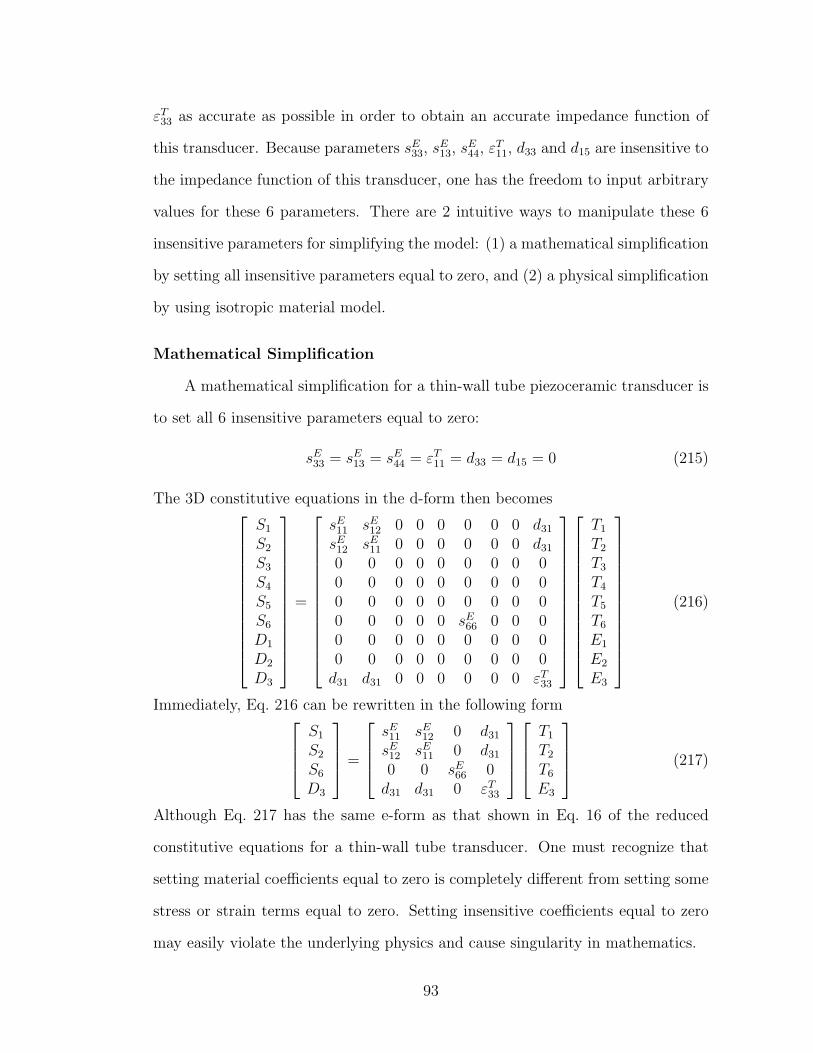
εT33 as accurate as possible in order to obtain an accurate impedance function of

this transducer. Because parameters sE33, sE13, s

E44, ε

T11, d33 and d15 are insensitive to

the impedance function of this transducer, one has the freedom to input arbitrary

values for these 6 parameters. There are 2 intuitive ways to manipulate these 6

insensitive parameters for simplifying the model: (1) a mathematical simplification

by setting all insensitive parameters equal to zero, and (2) a physical simplification

by using isotropic material model.

Mathematical Simplification

A mathematical simplification for a thin-wall tube piezoceramic transducer is

to set all 6 insensitive parameters equal to zero:

sE33 = sE13 = sE44 = εT11 = d33 = d15 = 0 (215)

The 3D constitutive equations in the d-form then becomes

S1

S2

S3

S4

S5

S6

D1

D2

D3

=

sE11 sE12 0 0 0 0 0 0 d31sE12 sE11 0 0 0 0 0 0 d310 0 0 0 0 0 0 0 00 0 0 0 0 0 0 0 00 0 0 0 0 0 0 0 00 0 0 0 0 sE66 0 0 00 0 0 0 0 0 0 0 00 0 0 0 0 0 0 0 0d31 d31 0 0 0 0 0 0 εT33

T1

T2

T3

T4

T5

T6

E1

E2

E3

(216)

Immediately, Eq. 216 can be rewritten in the following formS1

S2

S6

D3

=

sE11 sE12 0 d31sE12 sE11 0 d310 0 sE66 0d31 d31 0 εT33

T1

T2

T6

E3

(217)

Although Eq. 217 has the same e-form as that shown in Eq. 16 of the reduced

constitutive equations for a thin-wall tube transducer. One must recognize that

setting material coefficients equal to zero is completely different from setting some

stress or strain terms equal to zero. Setting insensitive coefficients equal to zero

may easily violate the underlying physics and cause singularity in mathematics.

93

Physical Simplification

One physical simplification for a thin-wall tube transducer is to assign those

6 insensitive parameters sE13, sE33, s

E44, ε

T11, d33 and d15 as follows:

sE13 = sE12, sE33 = sE11, s

E44 = sE66 (218)

and

εT11 = d33 = d15 = 0 (219)

Eq. 218 implies the related engineering parameters as

Y E33 = Y E

11 , ν13 = ν12, G =Y E11

2(1 + ν12)(220)

From the physical point of view, Eq. 218 suggests that the elastic material prop-

erties are characterized as an isotropic material. The conditions in Eq. 219 imply

the following: (1) εT11 = 0, there is no current caused by the electric field in the

non-poling directions (i.e., 1- and 2-direction); (2) d33 = 0, there is no electrical

polarization in the poling direction caused by the stress applied in the poling direc-

tion; and (3) d15 = 0, there is no electrical polarization in the non-poling direction

caused by the shear stress applied in the non-poling directions (Ltd, 2011).

In the remaining part of this section, it intends to show the corresponding

e-form parameters based on the above physical simplification. For a isotropic

material, the stiffness matrix is written as:

c =

cE11 cE12 cE12 0 0 0cE12 cE11 cE12 0 0 0cE12 cE12 cE11 0 0 00 0 0 cE66 0 00 0 0 0 cE66 00 0 0 0 0 cE66

(221)

where cE66 = (cE11 − cE12)/2. The relationships among the stiffness, engineering and

compliance parameters for isotropic material are as follows (Vignjevic et al., 2008):

cE11 =(1− ν12)Y

E11

(1 + ν12)(1− 2ν12)=

sE11 + sE12(sE11 − sE12)(s

E11 + 2sE12)

(222)

94

cE12 =ν12Y

E11

(1 + ν12)(1− 2ν12)= − sE12

(sE11 − sE12)(sE11 + 2sE12)

(223)

cE66 =Y E11

2(1 + ν12)=

1

2(sE11 − sE12)(224)

With εT11 = d33 = d15 = 0, the piezoelectric strain matrix and dielectric matrix

at constant stress become

d =

0 0 0 0 0 00 0 0 0 0 0d31 d31 0 0 0 0

(225)

and

εT =

0 0 00 0 00 0 εT33

(226)

Using e = d (sE)−1

(see Eq. 9):

0 0 0 0 e15 00 0 0 e15 0 0e31 e31 e33 0 0 0

=

0 0 0 0 0 00 0 0 0 0 0d31 d31 0 0 0 0

cE11 cE12 cE12 0 0 0cE12 cE11 cE12 0 0 0cE12 cE12 cE11 0 0 00 0 0 cE66 0 00 0 0 0 cE66 00 0 0 0 0 cE66

(227)

one shows

e31 = d31(cE11 + cE12) (228)

and

e33 = 2d31cE12 (229)

From Eqs. 228 and 229, it yields

e33 =2cE12

cE11 + cE12e31 (230)

95

Applying εS = εT − edt (see Eq. 10),

εS11 0 00 εS11 00 0 εS33

=

0 0 00 0 00 0 εT33

− 0 0 0 0 e15 0

0 0 0 e15 0 0e31 e31 e33 0 0 0

0 0 d310 0 d310 0 00 0 00 0 00 0 0

(231)

one obtains the following dielectric permittivity relationship

εS33 = εT33 − 2e31d31 (232)

Substituting Eq. 228 into Eq. 232 yields

εS33 = εT33 − 2d231(cE11 + cE12) (233)

The above physical simplification satisfies the general physics of a tube trans-

ducer, and requires only four independent sensitive parameters: sE11, sE12, d31 and

εT33, in the finite element modeling based on the full 3D constitutive equations.

In the finite element model formulation for the equations of motion, the stiffness

matrix of the dynamic structure is needed. The CMCM model updating method

also updates the stiffness matrix of the structure. Thus, one must update the

e-form material coefficients. There are 6 non-zero e-form parameters in the above

physical simplification, including: cE11, cE12, c

E66, e31, e33 and εS33.

Updating of Elastic Parameters

Considering that all the elements are made of the same polarized piezoelectric

PZT material, since the operation of Eq. 194 is linear in terms of the stiffness

coefficients cE11, cE12, c

E13, c

E33 and cE44, any 3D structure shows

KUU = cE11KcE11+ cE12 KcE12

+ cE13KcE13+ cE33 KcE33

+ cE44 KcE44(234)

where KcEijcan be interpreted as the change of KUU due to the unit change of cEij.

96

Imposing the physical simplification in Eq. 218 yields:

cE44 =1

2(cE11 − cE12) (235)

cE11 = cE33 (236)

and

cE12 = cE13 (237)

Therefore, Eq. 234 can be rewritten as

KUU = cE11KcE11+ cE12KcE12

(238)

where

KcE11= KcE11

+KcE33+

1

2KcE44

(239)

and

KcE12= KcE12

+KcE13− 1

2KcE44

(240)

In the finite element model updating formulation, the updated global stiffness

matrix of a short circuit model K∗UU then can be written as

K∗UU = (1 + α1)c

E11KcE11

+ (1 + α2)cE12KcE12

= KUU +2∑

i=1

αiKi (241)

where α1 and α2 are the correction coefficient of cE11 and cE12 respectively. The form

of Eq. 241 is consistent with Eq. 173 that has been formulated for the development

of the CMCM method, thus one can proceed the extended CMCM method to

compute α1 and α2.

Updating of Piezoelectric Parameters

From Eqs. 202, the linear operations on the piezoelectric stress matrix e for

full 3D constitutive equations yields

KUΦ = KtΦU = e31Ke31 + e33Ke33 + e15Ke15 (242)

97

where Ke31 , Ke33 and Ke15 are the changing of global stiffness due to the unit

change of e31, e33 and e15, respectively. According to the the proposed physical

simplification, e15 = 0 and e33 = [2cE12/(cE11 + cE12)] e31, Eq.242 becomes

KUΦ = e31KeE31(243)

where

KeE31= Ke31 +

(2cE12

cE11 + cE12

)Ke33 (244)

Similarly, from Eq. 203, the linear operations on the permittivity matrix ε for

full 3D constitutive equations yields

KΦΦ = εS11KεS11+ εS33KεS33

(245)

where KεS11and KεS33

are the changing of global stiffness due to the unit change of

εS11 and εS33, respectively. Since εS11 = 0 due to the imposed physical simplification,

Eq. 245 becomes

KΦΦ = εS33 KεS33(246)

Consequently, the condensed eletro-elastic stiffness matrix in Eq. 92 becomes

KUU = KUU +K3 (247)

where

K3 = −aKe31(KεS33)−1Kt

e31(248)

in which

a =(e31)

2

εS33(249)

After the updated global stiffness matrix of a short-circuit model K∗UU has been

obtained, the finite element model updating formulation for the updated global

stiffness matrix of an open-circuit model K∗UU then can be written as

K∗UU = K∗

UU + (1 + α3)K3 (250)

98

where α3 are the correction coefficients of a. The form of Eq. 250 agrees with

Eq. 173, thus the extended CMCM method can be employed to compute α3.

Summary of Updating Material Parameters

In summary, the values of cE11∗, cE12

∗, εT33

∗and a∗ were first updated at the

three phases of the proposed multi-physics finite element model updating method.

Next, similar to the derivation of Eqs. 213 and 214, εS33∗and e31

∗ can be calculated

by

εS33∗=

(cE11∗+ cE12

∗)εT33

∗

cE11∗+ cE12

∗+ 2a∗

(251)

and

e∗31 = −√a∗ εS33

∗(252)

respectively.

For completeness, also presented below are the updated d-form coefficients

and engineering parameters which are related to the updated e-form coefficients.

Directly from Eq. 228 that e31 = d31(cE11 + cE12), the updated piezoelectric strain

constant, d∗31, can be calculated by

d∗31 =e∗31

cE11∗+ cE12

∗ (253)

Recalling cE11 = (1− ν12)YE11/[(1 + ν12)(1− 2ν12)] (see Eq. 222) and cE12 =

ν12YE11/[(1 + ν12)(1− 2ν12)] (see Eq. 223), one gets cE11/c

E12 = (1− ν12)/ν12. From

this ratio relationship, one writes the updated Poisson ratio in terms of cE11∗and

cE12∗as

ν∗12 =

cE12∗

cE11∗+ cE12

∗ (254)

Furthermore, one obtains the updated Young’s modulus Y E11

∗in terms of ν∗

12 and

cE12∗as

Y E11

∗=

cE12∗

ν∗12

(1 + ν∗12)(1− 2ν∗

12) (255)

99

Once Y E11

∗and ν∗

12 are available, one writes

sE11∗=

1

Y E11

∗ (256)

and

sE12∗= − ν∗

12

Y E11

∗ (257)

100

CHAPTER 7

Numerical Study of Model Updating for Tube Transducer

Chosen for the numerical demonstration are two examples: a simulated trans-

ducer and a real transducer. Because the target values of parameters are known

for the simulated transducer and can be compared with the updated values, the

simulated transducer is employed to test the accuracy of the proposed method.

Ultimately, the effectiveness of the proposed method must be tested on a real

transducer, with the impedance function of the transducer being estimated ex-

perimentally. Theoretically, one can use either a 2D or 3D FE model for model

updating using the extended multi-physics CMCM method. However, the allowed

input for the material property in most commercial softwares is for the 3D con-

stitutive equations, not corresponding to the 2D reduced constitutive equations

under the axisymmetric assumption; therefore, this study focuses on using the 3D

constitutive equations for the model updating of tube transducer.

7.1 Model Updating of Simulated Tube Transducer

In the first example, both the original analytical model and the target model

are generated from using the same FE model, but with different sets of material

coefficients. It is assumed that the analytical model is with a set of “wrong” coef-

ficients. The goal is to correct those wrong coefficients from the measured modal

information which is simulated from the same FE model with “right” coefficients.

The ANSYS FE models in this example are built using the 3D solid element

type: SOLID226. These models have the same geometry and poling direction as

the transducer shown in Figure. 16. Because engineering parameters are more

commonly provided in manufacture specification sheets, they are utilized as the

intended updating quantities for the elastic material properties. According to

101

the theoretical derivation in Chapter 2, as well as the sensitivity study shown in

Appendix C, the four parameters that are sensitive to the impedance function of

a tube transducer are: Y E11 , ν12, ε

T33, and d31. The original and target values of

these four parameters are listed in Table 4. The relative error provided in Table 4

is defined as the difference between the original value and the target value, and

it is then normalized by the target value. Figure. 35 shows a comparison of the

impedance function of the original model and that of the target model. There are

three modes that significantly contributing to the impedance functions. For the

impedance function of the target model, the three major resonant frequencies are

51.4, 55, and 82.6 KHz, and the three anti-resonant frequencies are 52.4, 55.8, and

101.6 KHz.

Table 4. Material properties of the original and target modelsParameter Unit Original Value Target Value Relative Error

Y E11 1010 (N/m2) 6.3 6.66 5.4054%ν12 — 0.31 0.3333 6.9907%d31 10−12 (C/N) −175 −210 16.6667%

εT33/ε0 — 1576 2294 31.2990%

7.1.1 Updating of Material Parameters

Given the three modal frequencies of the target short-circuit model: 51.4, 55

and 82.6 KHz, and those of the target open-circuit model: 52.4, 55.8 and 101.6

KHz, the task is to apply the extended CMCM method to perform the multi-

physics model updating for the analytical piezoceramic tube transducer model.

Updating of Elastic Parameters

The first step is to update the elastic parameters of the analytical piezoceramic

tube transducer model, using the short-circuit model (or pure mechanical model).

As described in Chapter 6, a physical simplification is to assume an isotropic

102

0 2 4 6 8 10 12

x 104

10−1

100

101

102

103

104

105

106

Frequency (Hz)

Impe

danc

e (O

hms)

OriginalTarget

Figure 35. The comparison of the impedance function between the original andtarget models

103

material in the finite element formulation. Given the Young’s modulus Y E11 =

6.3 × 1010N/m2 and Poisson’s ratio ν12 = 0.31, the following stiffness parameters

are computed:

cE11 = cE33 =(1− ν12)Y

E11

(1 + ν12)(1− 2ν12)= 8.73× 1010N/m2

cE12 = cE13 =ν12Y

E11

(1 + ν12)(1− 2ν12)= 3.92× 1010N/m2

cE44 = cE66 =Y E11

2(1 + ν12)= 2.415× 1010N/m2

For formulating the CMCM equations in Eq. 241, one first needs to extract

KcE11and KcE12

. The ways to extract KcE11and KcE12

are basically identical. Eq. 239

shows that KcE11is a linear combination of KcE11

, KcE33and KcE44

. While using

ANSYS, a possible way of extracting KcE11is the same as that of extracting KcE33

or KcE44.

The following presents a way of obtaining KcE11numerically. First, build a

short-circuit FE model with distinct values of the five stiffness parameters: cE11,

cE12, cE13, c

E33 and cE44, and denote the corresponding numerical global stiffness matrix

to be K(1)UU . Second, build another short-circuit FE model with the same values

for these stiffness parameters, except doubling the value of cE11, and denote the

corresponding numerical global stiffness matrix to be K(2)UU . Recall that KcE11

is

defined as the change of KUU (global stiffness matrix for the short-circuit model)

due to the unit change of cE11. Thus one possible way of obtaining KcE11numerically

is by performing the following operation:

KcE11=

K(2)UU −K

(1)UU

cE11(258)

Given the three modal frequencies of the target short-circuit model: 51.4, 55

and 82.6 KHz, and two submatrices: KcE11and KcE12

, the extended CMCM method

is applied to estimate α1 and α2 which are the correction coefficients of cE11 and

cE12, respectively.

104

10 20 30 40 50 60 70 80 90 1000.14

0.16

0.18

0.2

0.22

0.24

0.26

0.28

0.3

Number of iterations

Cor

rect

ion

coef

ficie

nt

α

1

Target α1

α2

Target α2

Figure 36. Iteration procedure of α1 and α2 on simulation model

Figure. 36 shows the convergence of α1 and α2. After 14 iteration steps, these

values converge to 0.1455 and 0.2755, respectively, and match the target values

accurately. The updated elastic parameters cE11∗and cE12

∗can be calculated by

cE11∗= (1 + α1)c

E11 = 10× 1010N/m2

and

cE12∗= (1 + α2)c

E12 = 5.0004× 1010N/m2

respectively.

Updating of Permittivity

Because the mechanical boundary condition is free-free, the related permittiv-

ity of this unclamped transducer is the permittivity at constant stress. According

105

to Eq. 201, with the impedance, ZL = 26804Ω, from the impedance function at

400 Hz, the permittivity at constant stress is

εT33∗=

ln(Do/Di)

4π2ℓZLfL= 2293.3ε0

where the vacuum permittivity ε0 = 8.854187817× 10−12C/m.

Updating of Piezoelectric Parameters

After updating the elastic parameters and permittivity, the open-circuited FE

model, together with the anti-resonant frequencies of the target model, can be

employed to update the piezoelectric parameter d31 (or e31). Given the original

piezoelectric constant d31 = −175× 10−12C/N and permittivity at constant stress

εT33 = 1576ε0, the original e-form parameters are computed:

e31 = (cE11∗+ cE12

∗)d31 = −26.25N/V ·m

e33 = 2cE12∗d31 = −17.5N/V ·m

εS33 = εT33 − 2d231(cE11

∗+ cE12

∗) = 538ε0

For formulating the CMCM equations in Eq. 250, one needs to compute the

original linear variable

a =(e31)

2

εS33= 1.2808/ε0

and extract submatrices Ke31 and KεS33. Eq. 244 shows that Ke31 is a linear com-

bination of Ke33 and Ke31 . While using ANSYS, the way of extracting KεS33, Ke31

and Ke31 is the same as that of extracting KcE11.

Given the three modal frequencies of the target open-circuit model: 52.4, 55.8,

and 101.6 KHz, and two submatrices: Ke31 and KεS33, the extended CMCM method

is applied to estimate α3, which is the correction coefficient of a, i.e., the correction

coefficient for (e31)2/εS33.

Figure. 37 shows the convergence of the correction coefficient of α3. During

this procedure, the value of the coefficient drops sharply to the point of −0.0284

106

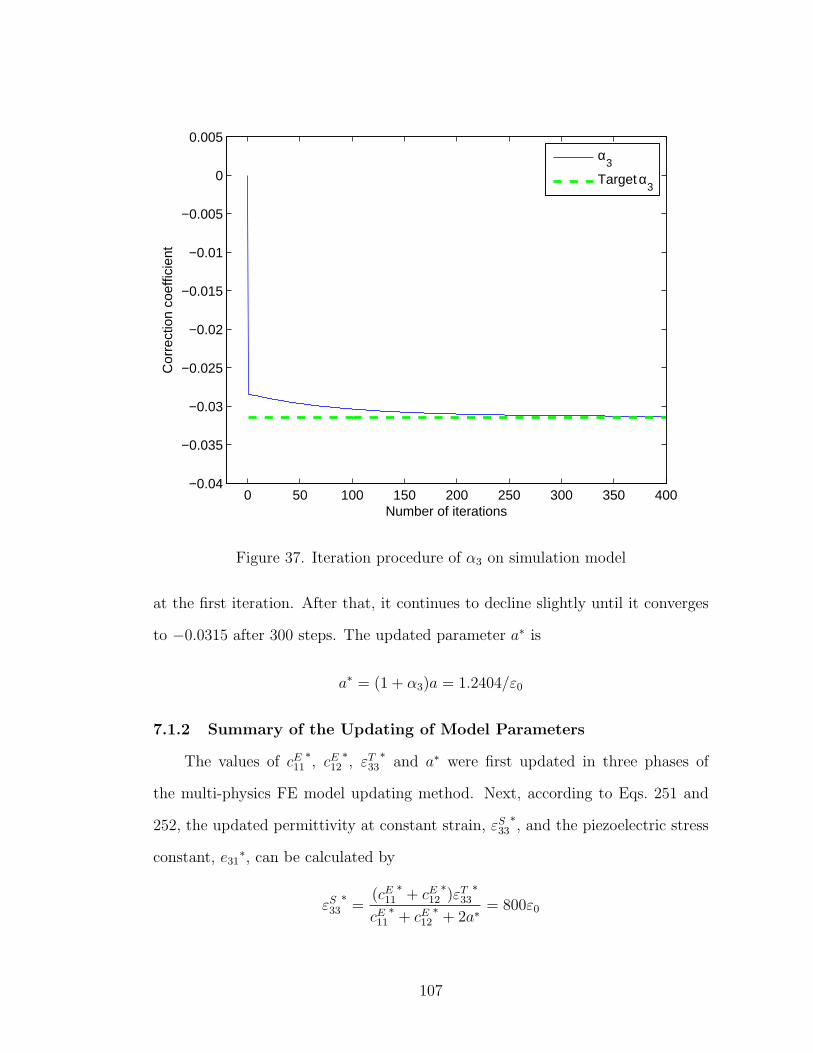
0 50 100 150 200 250 300 350 400−0.04

−0.035

−0.03

−0.025

−0.02

−0.015

−0.01

−0.005

0

0.005

Number of iterations

Cor

rect

ion

coef

ficie

nt

α

3

Target α3

Figure 37. Iteration procedure of α3 on simulation model

at the first iteration. After that, it continues to decline slightly until it converges

to −0.0315 after 300 steps. The updated parameter a∗ is

a∗ = (1 + α3)a = 1.2404/ε0

7.1.2 Summary of the Updating of Model Parameters

The values of cE11∗, cE12

∗, εT33

∗and a∗ were first updated in three phases of

the multi-physics FE model updating method. Next, according to Eqs. 251 and

252, the updated permittivity at constant strain, εS33∗, and the piezoelectric stress

constant, e31∗, can be calculated by

εS33∗=

(cE11∗+ cE12

∗)εT33

∗

cE11∗+ cE12

∗+ 2a∗

= 800ε0

107

and

e∗31 = −√a∗ εS33

∗= −31.5N/V ·m

respectively.

For completeness, also presented below are the updated d-form coefficients

and engineering parameters which are related to the updated e-form coefficients.

According to Eq. 253, the updated piezoelectric strain constant, d∗31, can be calcu-

lated by

d∗31 =e∗31

cE11∗+ cE12

∗ = −209.96× 10−12C/N

Furthermore, the updated Poisson ratio, ν∗12, and Young’s modulus, Y E

11∗, can be

calculated by

ν∗12 =

cE12∗

cE11∗+ cE12

∗ = 0.3333

and

Y E11

∗=

cE12∗

ν∗12

(1 + ν∗12)(1− 2ν∗

12) = 6.66× 1010N/m2

respectively.

In summary, the comparison between the original values, target values, and

updated values is given in Table 5. The relative error provided in Table 5 is defined

as the difference between the updated value and the target value, normalized by the

target value. The corresponding impedance functions obtained from the target and

updated models are shown in Figure. 38. We found that the updated parameters

from the proposed method match perfectly with the target values, and the proposed

method can handle well the model updating of cylinder transducers.

7.2 Model Updating of Real Tube Transducer

In the second example, the real transducer, shown in Figure. 6, is employed

which has the same geometry and boundary conditions as utilized for the simula-

tion example. Lab experiment of estimating impedance function for it was con-

108

Table 5. The comparison of properties between original, target and updated sim-ulation modelsParameters Unit Original Value Target Value Updated Value Relative error

Y E11 (1010N/m2) 6.3 6.66 6.66 0%ν12 — 0.31 0.3333 0.3333 0%d31 (10−12C/N) −175 −209.96 −210 0.019%

εT33/ε0 — 1576 2293.3 2294 0.0305%

0 2 4 6 8 10 12

x 104

10−1

100

101

102

103

104

105

106

107

Frequency (Hz)

Impe

danc

e (O

hms)

TargetUpdated

Figure 38. The comparison of the impedance functions between the target andupdated models

ducted in Chapter 5. And the original material properties of its FE model were

obtained from the manufacturer’s specification sheet of APC material 850 (Navy

Equivalent Navy II, APC International, Ltd (Ltd, 2011)): Y E11 = 6.3× 1010N/m2,

ν12 = 0.31, d31 = −175× 10−12 C/N, εT33 = 1900ε0.

109

0 2 4 6 8 10 12

x 104

100

101

102

103

104

105

Frequency (Hz)

Impe

danc

e (O

hms)

OriginalExperiment

Figure 39. The comparison of the impedance functions between the original modeland the experiment

110

Figure. 39 shows the impedance functions that were obtained from the original

FE model and experiment. With the frequencies at the local minimum of the

impedance function for the experiment being 49.89, 52.99, and 78.75 KHz, the

elastic parameters for the real transducer can be updated using the same procedure

as in the simulation example.

10 20 30 40 50 60 70 80 90 100

0.03

0.04

0.05

0.06

0.07

0.08

0.09

0.1

0.11

0.12

Number of iterations

Cor

rect

ion

coef

ficie

nt

α

1

Target α1

α2

Target α2

Figure 40. Iteration procedure of α1 and α2 on experiment model

Figure. 40 shows the convergence of the correction coefficients of α1 and α2.

After 14 iteration steps, these values converge to 0.025 and 0.1013, respectively.

Then, the updated elastic parameters cE11∗and cE12

∗can be calculated by

cE11∗= (1 + α1)c

E11 = 8.9503× 1010N/m2

and

cE12∗= (1 + α2)c

E12 = 4.3209× 1010N/m2

111

respectively.

Because the transducer in the experiment is placed on the sponge (free-free

mechanical boundary condition), the permittivity is the permittivity at constant

stress. According to Eq. 201, with the impedance, ZL = 9617Ω, from impedance

function at 1 KHz, the permittivity at constant stress is

εT33∗=

ln(Do/Di)

4π2ℓZLfL= 2556ε0

With the frequencies at the local maximum of the impedance function of the

experiment being 50.8, 53.94, and 94.7 KHz, the piezoelectric parameter for the

real transducer can also be updated using the same procedure as in the simulation

example.

0 5 10 15 200

0.05

0.1

0.15

0.2

0.25

0.3

0.35

0.4

0.45

0.5

Number of iterations

Cor

rect

ion

coef

ficie

nt

α

3

Target α3

Figure 41. Iteration procedure of α3 on experiment model

Figure. 41 shows the convergence of the correction coefficient α3. After five

112

iterations, α3 converges to 0.4556, and the updated parameter a∗ = 0.7996/ε0.

According to Eqs. 251 and 252, after updating cE11∗, cE12

∗, εT33

∗, and a∗, the

updated permittivity at constant strain, εS33∗, and the piezoelectric stress constant,

e31∗, can be calculated by

εS33∗=

(cE11∗+ cE12

∗)εT33

∗

cE11∗+ cE12

∗+ 2a∗

= 1082ε0

and

e∗31 = −√

a∗ εS33∗= −29.42N/V ·m

respectively.

By converting to d-form coefficients and engineering parameters, the updated

piezoelectric strain constant, d∗31, Poisson ratio, ν∗12, and Young’s modulus, Y E

11∗,

can be calculated by

d∗31 =e∗31

cE11∗+ cE12

∗ = −221.7× 10−12C/N

,

ν∗12 =

cE12∗

cE11∗+ cE12

∗ = 0.3256

and

Y E11

∗=

cE12∗

ν∗12

(1 + ν∗12)(1− 2ν∗

12) = 6.1367× 1010N/m2

respectively. A comparison of the original values and updated values is shown in

Table 6. The relative error presented in Table 6 is defined as the difference between

the original value and the updated value, then normalized by the updated value.

Figure. 42 shows the resulting impedance function of the updated model vs. the

experimental estimation. We obtained the Rayleigh damping coefficients α ≈ 0

and β = −3.996 from the experiment using Eqs.168 and 169. Again, this result

suggests that the proposed method can also handle the model updating of real

transducers.

113

Table 6. The comparison of properties between original and updated experimentmodels

Parameters Unit Original Updated Relative errorY E11 1010N/m2 6.3 6.1367 −2.66%ν12 — 0.31 0.3256 4.7912%d31 10−12C/N −175 −221.7 21.0645%

εT33/ε0 — 1900 2556 25.67%

0 2 4 6 8 10 12

x 104

100

101

102

103

104

105

Frequency (Hz)

Impe

danc

e (O

hms)

ExperimentUpdated

Figure 42. The comparison of the impedance function between the updated modeland the experiment

114

CHAPTER 8

Conclusions

Finite element model updating has been defined as the systematic adjustment

of finite element models using experimental data. In this study, for the finite ele-

ment model updating of a piezoelectric tube transducer, the experimental data has

been limited to be the measured electric impedance function of the tube transduc-

er. This study covered two major tasks: (i) developing and verifying an efficient

method for estimating the electric impedance function of a transducer, and (ii)

developing and testing a finite element model updating method for piezoelectric

tube transducers. Although this study has focused on the correction of the mate-

rial parameters of tube type of piezoelectric transducers, the general procedure is

also applicable to other types of piezoelectric transducers. The newly developed

method on estimating the impedance function of a transducer is a Laplace domain

method. The proposed model updating method is a two-step method, including

the correction of the elastic material properties based on a short circuit model in

the first step, and the correction of dielectric and piezoelectric parameters based

on an open-circuit model in the second step. The fundamental updating algorithm

employed in both steps is the CMCM method. Both computer simulations and

lab experiments have been conducted to verify the correctness and accuracy of the

proposed methods on the two tasks mentioned above.

Major findings and contributions are summarized as follows:

Modal analysis of the finite element models This study shed new light on

the modal analysis of the short- and open-circuit finite element models as-

sociated with piezoelectric tube transducers. It has been demonstrated that

the resonant and anti-resonant frequencies of an impedance function matched

115

well with the modal frequencies of the short- and open-circuit models, respec-

tively. Mode shapes of a piezoelectric tube transducer could not be measured

at lab, but they are necessary information to conduct the CMCM model

updating method. Due to the uniform voltage (electromotive force) along

the axial direction, only symmetric modes (to the axial center of the tube

transducer) would “participate” in the mechanical vibration. In turn, only

symmetric modes would affect the impedance function of the tube transduc-

er. This study verified that the most dominant mode identified from the

impedance function was the mode with axially uniform mode shape. Basi-

cally, three symmetric modes would participate in the impedance function

of piezoelectric tube transducer: breathing mode, bending mode and axi-

al mode. These three mode forms did not have deformation in the tube’s

thickness direction (i.e., poling direction or 3-direction). Consequently, elas-

tic material parameters associated with the 3-direction would not affect the

impedance function of piezoelectric tube transducers.

Estimating the impedance function Processing both the input (voltage) and

output (charge or current) signals simultaneously, the proposed multi-signal

Prony-SS method was able to extract the poles and residues of the input

and output signals. After expressing both the voltage and current in their

partial fraction forms in the Laplace domain, the impedance function of

the transducer was obtained from the ratio of the voltage and current as a

function of frequency, ω, per substituting the Laplace variable s by jω. In

comparison to traditional Fourier-based methods, the proposed Prony-based

method did not suffer any leakage problems or resolution issues. Another

advantage of the proposed method is that it requires only very short signals to

obtain the impedance function. The accuracy and efficiency of the proposed

116

method has been demonstrated by using both computer simulation and lab

experiment data. This study also demonstrated the excellent capability of

the proposed method on rejecting noise.

Reduced constitutive equations There are ten material parameters to fully

character the constitutive equations of PZT-type material. However, the re-

duced constitutive equations associated with piezoelectric tube transducers

contains only four independent material parameters: two elastic parameter-

s Y E11 and ν12 (or sE11 and sE12), the permittivity in constant stress εT33, and

the piezoelectric parameter d31. In other words, the impedance function of

a piezoelectric tube transducer should depend only on these four material

parameters. Through the sensitivity study for each material parameter, this

study also numerically verified that the impedance function of a piezoelectric

tube transducer depends only on those four material parameters. Specifi-

cally, the values of Y E11 and ν12 determined the resonant frequencies in the

impedance function; the value of εT33 decided the impedance at the low fre-

quency region; and the value of d31 determined the anti-resonant frequencies

in the impedance function.

Implementation of ANSYS finite element models This study adopted the

commercial finite element software ANSYS to build piezoelectric tube trans-

ducers. However, ANSYS would not allow the user to build a finite element

model based on the reduced constitutive equations. In other words, one

must specify all 10 material parameters in the d-form or e-form for the full

3-dimensional constitutive equations. For using the CMCM method, it is

required to express the global stiffness matrix as a linear combination of only

those parameters to be updated, and those parameters must be associated

with the e-form. Thus, particular steps have been taken to formulate the

117

global stiffness matrix from ANSYS to be a linear form of elastic parameters

cE11 and cE12. In this study, the submatrices associated with cE11 and cE12 were

successfully extracted while using ANSYS. Similarly, submatrices associated

with εS33 and e31 were extracted as well.

Multi-physics finite element model updating Although there have been

many papers conducting the finite element model updating for civil and

mechanical systems, only a few articles addressed the model updating for

piezoelectric transducers. This study has been the literature to conduct the

multi-physics finite element model updating using a two-step approach. Be-

cause a short-circuit transducer is equivalent to a pure mechanical oscillator,

it was reasonable to update the elastic parameters of a piezoelectric trans-

ducer in the first step based on a short-circuit finite element model. In the

second step for updating the electric and piezoelectric parameters, it was

necessary to employ an open-circuit finite element model. Implementing the

CMCM algorithm required the knowledge of both the measured modal fre-

quencies and the corresponding mode shapes, but a measured impedance

function could provide only modal frequencies for short- and open-circuit

transducers. In dealing with the incomplete modal information, an iterative

procedure was taken. In each iteration, the “measured” mode shapes were

approximated by the mode shapes obtained from the previous iteration’s

updated finite element model. After a sufficient number of iterations, a con-

verged solution (model) was always obtained. The high performance of the

proposed two-step approach has been demonstrated through both computer

simulations and lab experiment.

118

APPENDIX A

Simple 33- and 31-mode Vibrators

If DC voltages are externally applied, the transducer responds with a me-

chanical deformation. Similarly, an AC field will cause the transducer to vi-

brate as a vibrator. To better understand piezoelectric vibrators, we intro-

duced two typical one-dimensional vibrators, 33-mode and 31-mode vibrators

(Sherman and Butler, 2007).

Shown in Figure. A.1 is an idealized 33-mode vibrator. A piezoelectric ceramic

Figure A.1. The piezoelectric longitudinal vibrator in 33 mode

bar of length L is fixed at one end, and is attached to a mass M at the other end.

This piezoelectric bar is polarized using electrodes on the ends to establish the

polar axis parallel to the length of the bar. An alternating voltage, V , is applied

between the same electrodes, creating an alternating electric field, E3, which is

parallel to the polarization. Assume that the stresses T1, T2 and electric fields E1,

E2 in no poling directions are both neglected, and the purely longitudinal electric

field does not excite shear stresses, (i.e., T4 = T5 = T6 = 0). Therefore, the

119

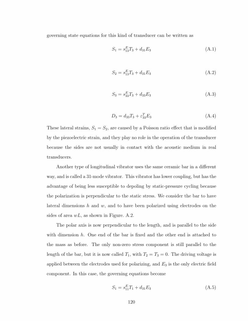
governing state equations for this kind of transducer can be written as

S1 = sE13T3 + d31E3 (A.1)

S2 = sE13T3 + d31E3 (A.2)

S3 = sE33T3 + d33E3 (A.3)

D3 = d33T3 + εT33E3 (A.4)

These lateral strains, S1 = S2, are caused by a Poisson ratio effect that is modified

by the piezoelectric strain, and they play no role in the operation of the transducer

because the sides are not usually in contact with the acoustic medium in real

transducers.

Another type of longitudinal vibrator uses the same ceramic bar in a different

way, and is called a 31-mode vibrator. This vibrator has lower coupling, but has the

advantage of being less susceptible to depoling by static-pressure cycling because

the polarization is perpendicular to the static stress. We consider the bar to have

lateral dimensions h and w, and to have been polarized using electrodes on the

sides of area wL, as shown in Figure. A.2.

The polar axis is now perpendicular to the length, and is parallel to the side

with dimension h. One end of the bar is fixed and the other end is attached to

the mass as before. The only non-zero stress component is still parallel to the

length of the bar, but it is now called T1, with T2 = T3 = 0. The driving voltage is

applied between the electrodes used for polarizing, and E3 is the only electric field

component. In this case, the governing equations become

S1 = sE11T1 + d31E3 (A.5)

120

Figure A.2. The piezoelectric longitudinal vibrator in 31 mode

S2 = sE12T1 + d31E3 (A.6)

S3 = sE13T1 + d33E3 (A.7)

D3 = d31T1 + εT33E3 (A.8)

121

APPENDIX B

Modeling and Interfacing with ANSYS

B.1 Modeling for Piezoelectric Structures with ANSYS

ANSYS is one of the most commonly used commercial FE packages in many

engineering fields. It is used to simplify the development of FE models as users

can operate step-by-step to determine whether a specific process is relevant to

the problem being addressed. There are six main steps in the development of FE

models using ANSYS:

1. Define the element types;

2. Define the material properties;

3. Define the model geometry;

4. Generate the mesh;

5. Apply the constraints;

6. Start the analysis.

In terms of the piezoelectric analysis, ANSYS provides several powerful ele-

ments to improve the efficiency of engineering designs. Some important elements

and their key options for piezoelectric material are as follows:

2-D Axial Symmetric Elements:

• Plane13, KEYOPT(1) = 7, coupled-field quadrilateral solid;

• Plane223, KEYOPT(1) = 1001, coupled-field 8-node quadrilateral.

3-D Elements:

122

• Solid5, KEYOPT(1) = 0 or 3 coupled-field brick;

• Solid98, KEYOPT(1) = 0 or 3 coupled-field tetrahedron;

• Solid226, KEYOPT(1) = 1001, coupled-field 20-node brick;

• Solid227, KEYOPT(1) = 1001, coupled-field 10-node tetrahedron.

Note that the permittivity of Plane223, Solid226, and Solid227 can be specified

either as PERX, PERY, and PERZ on the MP command, respectively, or by

specifying the terms of the anisotropic permittivity matrix using the TB, DPER,

and TBDATA commands, respectively. If we use the MP command to specify

the permittivity, the permittivity input will be interpreted as the permittivity at

constant strain. If we use the TB, DPER command, we can specify the permittivity

matrix either at constant strain εS (TBOPT = 0) or at constant stress εT (TBOPT

= 1). The latter input will be internally converted to the permittivity at constant

strain εS using the piezoelectric strain and stress matrices. The values that are

inputted on either MP, PERX or TB, DPER will always be interpreted as relative

permittivity values.

It is important to note the difference between the notation standards of AN-

SYS and IEEE. For most published piezoelectric materials, the order used for the

piezoelectric matrix is x, y, z, yz, xz, xy, based on IEEE standards (Voigt nota-

tion) (IEE, 1987; Helnwein, 2001), while the ANSYS input order is x, y, z, xy,

yz, xz. This means that we need to transform the IEEE standards matrix to the

ANSYS input order by switching the row data for the shear terms. A comparison

of notations used by ANSYS and IEEE for tensor indices is given in Table B.1.

Therefore, we can obtain the ANSYS parameter matrix from the IEEE standard

matrix by switching 4(yz) and 6(xy) (4←→ 6), and then switching 5(xz) and new

6(yz) (5←→ 6) (Kohnke, 1999).

123

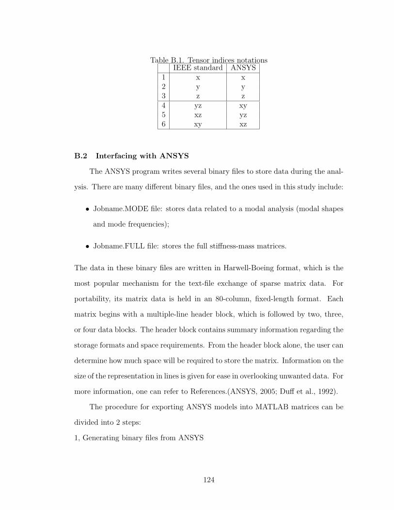
Table B.1. Tensor indices notationsIEEE standard ANSYS

1 x x2 y y3 z z4 yz xy5 xz yz6 xy xz

B.2 Interfacing with ANSYS

The ANSYS program writes several binary files to store data during the anal-

ysis. There are many different binary files, and the ones used in this study include:

• Jobname.MODE file: stores data related to a modal analysis (modal shapes

and mode frequencies);

• Jobname.FULL file: stores the full stiffness-mass matrices.

The data in these binary files are written in Harwell-Boeing format, which is the

most popular mechanism for the text-file exchange of sparse matrix data. For

portability, its matrix data is held in an 80-column, fixed-length format. Each

matrix begins with a multiple-line header block, which is followed by two, three,

or four data blocks. The header block contains summary information regarding the

storage formats and space requirements. From the header block alone, the user can

determine how much space will be required to store the matrix. Information on the

size of the representation in lines is given for ease in overlooking unwanted data. For

more information, one can refer to References.(ANSYS, 2005; Duff et al., 1992).

The procedure for exporting ANSYS models into MATLAB matrices can be

divided into 2 steps:

1, Generating binary files from ANSYS

124

A modal analysis must be launched if a mass matrix is needed. Otherwise, a

simple static analysis is sufficient for writing the stiffness matrix into a binary file.

The command WRFULL makes the analysis stop after writing the files, meaning

that ANSYS will not actually do the analysis. This command can be useful and

help to avoid long calculations.

2, Reading and converting Harwell-Boeing format with MATLAB

The matrices written by ANSYS are compatible with the Harwell-Boeing (H-

B) format, and must be converted into MATLAB format. A library and stand-

alone utility developed by the Berkeley Benchmarking and Optimization (BeBOP)

Group can be used to convert between the Harwell-Boeing, Matrix Market, and

MATLAB sparse matrix formats. A version for complex matrices is also available

(Tex, 2013).

125

APPENDIX C

Parameter Sensitivity of Piezoelectric Tube Transducer

There are 10 independent parameters for piezoelectric materials (such as

PZT), which can be divided into three groups: five elastic parameters, two di-

electric parameters, and three piezoelectric parameters.

C.1 Sensitivity of d-form Parameters

In d-form, the five elastic parameters are sE11, sE12, s

E13, s

E33, and sE44, while the

two dielectric parameters are εT11 and εT33, and the three piezoelectric parameters

are d31, d33, and d15. Of the five elastic parameters, as proven in Eq. 16, only

two parameters, i.e., sE11 and sE12, theoretically affect the mechanical and electric

behaviors of tube transducers. We can use the sensitivity study of the FE model

to prove this theoretical deduction. When the elastic parameters (sE11, sE33, s

E12, s

E13

and sE44) are doubled respectively, Table C.1 shows the sensitivity of the impedance

function to elastic parameters. Using the engineering parameters Y E11 , Y

E33 , ν12, ν13,

and G to substitute sE11, sE33, s

E12, s

E13, and sE44 as elastic parameters, respectively,

the sensitivity study of the impedance function is as shown in Table C.2. Then, we

verified numerically the theoretical deduction, i.e., that only two elastic parameters

Y E11 , ν12 or sE11, s

E12 in d-form can affect the impedance function.

In terms of the dielectric and piezoelectric parameters, in theory, only one

dielectric parameter εT33 and one piezoelectric parameter d31 affect the electric be-

haviors of transducers. Dividing the parameters by two respectively, the sensitivity

study of the impedance function is as shown in Table C.3. We can easily see that

the sensitivity study result agrees well with the theoretical deduction. The permit-

tivity at constant stress εT33 determines the impedance at the low-frequency region,

and the piezoelectric strain constant d31 influences the anti-resonance frequencies.

126

Table C.1. Elastic parameters sensitivity in the d-form

sE11 sE12

0 0.5 1 1.5 2

x 105

101

102

103

104

105

Frequency (Hz)

Impe

danc

e (O

hms)

OriginalChanged

0 0.5 1 1.5 2

x 105

101

102

103

104

105

Frequency (Hz)

Impe

danc

e (O

hms)

OriginalChanged

sE33 sE44

0 0.5 1 1.5 2

x 105

101

102

103

104

105

Frequency (Hz)

Impe

danc

e (O

hms)

OriginalChanged

0 0.5 1 1.5 2

x 105

101

102

103

104

105

Frequency (Hz)

Impe

danc

e (O

hms)

OriginalChanged

sE13

0 0.5 1 1.5 2

x 105

101

102

103

104

105

Frequency (Hz)

Impe

danc

e (O

hms)

OriginalChanged

127

Table C.2. Elastic parameters sensitivity in the d-form (engineering parameters)

Y E11 ν12

0 2 4 6 8 10 12

x 104

101

102

103

104

105

Frequency (Hz)

Impe

danc

e (O

hms)

OriginalChanged

0 2 4 6 8 10 12

x 104

100

101

102

103

104

105

Frequency (Hz)

Impe

danc

e (O

hms)

OriginalChanged

Y E33 ν13

0 2 4 6 8 10 12

x 104

101

102

103

104

105

Frequency (Hz)

Impe

danc

e (O

hms)

OriginalChanged

0 2 4 6 8 10 12

x 104

101

102

103

104

105

Frequency (Hz)

Impe

danc

e (O

hms)

OriginalChanged

G

0 2 4 6 8 10 12

x 104

101

102

103

104

105

Frequency (Hz)

Impe

danc

e (O

hms)

OriginalChanged

128

Table C.3. Dielectric and piezoelectric parameters sensitivity in the d-form

εT33 d31

0 0.5 1 1.5 2

x 105

101

102

103

104

105

Frequency (Hz)

Impe

danc

e (O

hms)

OriginalChanged

0 0.5 1 1.5 2

x 105

101

102

103

104

105

Frequency (Hz)

Impe

danc

e (O

hms)

OriginalChanged

εT11 d33

0 0.5 1 1.5 2

x 105

101

102

103

104

105

Frequency (Hz)

Impe

danc

e (O

hms)

OriginalChanged

0 0.5 1 1.5 2

x 105

101

102

103

104

105

Frequency (Hz)

Impe

danc

e (O

hms)

OriginalChanged

d15

0 0.5 1 1.5 2

x 105

101

102

103

104

105

Frequency (Hz)

Impe

danc

e (O

hms)

OriginalChanged

129

C.2 Sensitivity of e-form Parameters

In contrast, we can also choose e-form parameters, cE11, cE33, c

E12, c

E13, c

E44, ε

S33,

εS11, e31, e33, and e15, to develop the FE models. Tables C.4 and C.5 show the

results of the sensitivity study when we double the elastic parameters and divide

the dielectric and piezoelectric parameters by two, respectively.

We can easily find that e-form parameters, cE11, cE12, c

E13, c

E33, e31, e33, and εS33

all affect the impedance function of transducers. Because only four parameters

determine the vibration of a thin-tube transducer in the d-form, we can use an

infinite number of e-form parameter groups to develop FE models that share the

same impedance function.

130

Table C.4. Elastic parameters sensitivity in the e-form

cE11 cE12

cE13 cE33

cE44

131

Table C.5. Dielectric and piezoelectric parameters sensitivity in the e-form

e33 e31

e15 εT33

εT11

132

APPENDIX D

Model Updating with Measured Mode Shapes

While the CMCMmethod can achieve the model updating for thin-tube trans-

ducers using the impedance function through an iteration procedure, it can also

update all independent parameters directly with mode shapes that are difficult to

measure experimentally but easy to obtain from FE models. Although this method

cannot currently be used in model updating for real transducers, in future, it will

enable model updating without iterations.

D.1 Model Updating of Elastic Parameters

The global stiffness matrix of a short-circuit model in linear combination form

with coefficients cE11, cE12, c

E13, c

E33, and cE44 is shown in Eq. 234. Consistent with the

formulation for the development of the CMCMmethod, the updated global stiffness

matrix can be written as

K∗UU = (1 + α1)c

E11KcE11

+ (1 + α2)cE12 KcE12

+ (1 + α3)cE13 KcE13

+ (1 + α4)cE33 KcE33

+ (1 + α5)cE44KcE44

= KUU +5∑

i=1

αiKi

(D.1)

where α1, α2, α3, α4, and α5 are the correction coefficients of cE11,cE12,c

E13,c

E33, and

cE44 respectively. Therefore, we can perform the CMCM method using target mode

shapes to compute the correction coefficients (α1, α2, α3, α4, and α5) directly.

D.2 Model Updating of Electric-coupling Parameters

Assuming εS11 to be zero and substituting Eq. 242 and 245 into 92, the global

stiffness matrix in the open-circuit model can be written as

KUU = KUU +K3 (D.2)

133

where

K3 = b1K6 + b2K7 + b3K8 +√b1b2K9 +

√b1b3K10 +

√b2b3K11 (D.3)

in which b1 = e231/εS33, b2 = e233/ε

S33, b3 = e215/ε

S33, and the submatrices are

K6 = −Ke31K−1εS33

Kte31

(D.4)

K7 = −Ke33K−1εS33

Kte33

(D.5)

K8 = −Ke15K−1εS33

Kte15

(D.6)

K9 = −Ke31K−1εS33

Kte33−Ke33K

−1εS33

Kte31

(D.7)

K10 = −Ke15K−1εS33

Kte33−Ke33K

−1εS33

Kte15

(D.8)

K11 = −Ke31K−1εS33

Kte15−Ke15K

−1εS33

Kte15

(D.9)

.

Consistent with the formulation for the development of the CMCM method,

the updated global stiffness matrix in the open-circuit model can be written as

K∗UU = K∗

UU + (1 + α6)b1K6 + (1 + α7)b2K7 + (1 + α8)b3K8

+√

(1 + α6)b1(1 + α7)b2K9 +√(1 + α6)b1(1 + α8)b3K10 +

√(1 + α7)b2(1 + α8)b3K11

(D.10)

where α6, α7, and α8 are the correction coefficients of b1, b2, and b3 respectively.

The form of Eq. D.10 agrees with Eq. 173; thus, we can perform the CMCM

method to compute α6, α7, and α8. Although α6, α7, and α8 can be used to

update e231/εS33, e

233/ε

S33, and e215/ε

S33, respectively, updating e31, e33, e15, and εS33

individually requires at least one more equation. For an unclamped thin cylindrical

transducer polarized in the radial direction, from εS = εT − esEet (see Eq. 12),

the additional equation is

εS33∗= εT33

∗ − 2(s∗11 + s∗12)(e∗31)

2 + 4s∗13e∗33e

∗31 + s∗33(e

∗33)

2

ε0(D.11)

where εT33∗is the permittivity at constant stress, which can be calculated from the

measured capacitance of the transducer at low frequencies.

134

D.3 Numerical Study

We performed a simulation example to test the accuracy of the proposed

method. In this example, both the original model and the target model are gen-

erated by using the same 3D FE model with different sets of coefficients. Using

d-form parameters (cE11, cE12, c

E13, c

E33, c

E44, ε

S33, e33, e31, and e15) to build FE models,

the result of model updating is as shown in Table D.1. This result suggests that

the proposed method can handle well the model updating of tube transducers.

Table D.1. The comparison of properties between original, target and updatedmodels

Parameters Original Target UpdatedcE11 9.2e10 11.04e10 11.0399e10cE12 4.4e10 5.104e10 5.1041e10cE13 4.2e10 4.62e10 4.62e10cE33 8e10 8.48e10 8.4798e10cE44 2.2e10 2.53e10 2.5302e10εS33 538 800 799.393e33 17.3 30 30.0132e31 -5.363 -10 -9.989e15 12.8 15 15.013

135

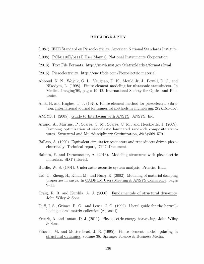
BIBLIOGRAPHY

(1987). IEEE Standard on Piezoelectricity. American National Standards Institute.

(1998). PCI-6110E/6111E User Manual. National Instruments Corporation.

(2013). Text File Formats. http://math.nist.gov/MatrixMarket/formats.html.

(2015). Piezoelectricity. http://enc.tfode.com/Piezoelectric material.

Abboud, N. N., Wojcik, G. L., Vaughan, D. K., Mould Jr, J., Powell, D. J., andNikodym, L. (1998). Finite element modeling for ultrasonic transducers. InMedical Imaging’98, pages 19–42. International Society for Optics and Pho-tonics.

Allik, H. and Hughes, T. J. (1970). Finite element method for piezoelectric vibra-tion. International journal for numerical methods in engineering, 2(2):151–157.

ANSYS, I. (2005). Guide to Interfacing with ANSYS. ANSYS, Inc.

Araujo, A., Martins, P., Soares, C. M., Soares, C. M., and Herskovits, J. (2009).Damping optimization of viscoelastic laminated sandwich composite struc-tures. Structural and Multidisciplinary Optimization, 39(6):569–579.

Ballato, A. (1990). Equivalent circuits for resonators and transducers driven piezo-electrically. Technical report, DTIC Document.

Balmes, E. and Deraemaeker, A. (2013). Modeling structures with piezoelectricmaterials. SDT tutorial.

Burdic, W. S. (1991). Underwater acoustic system analysis. Prentice Hall.

Cai, C., Zheng, H., Khan, M., and Hung, K. (2002). Modeling of material dampingproperties in ansys. In CADFEM Users Meeting & ANSYS Conference, pages9–11.

Craig, R. R. and Kurdila, A. J. (2006). Fundamentals of structural dynamics.John Wiley & Sons.

Duff, I. S., Grimes, R. G., and Lewis, J. G. (1992). Users’ guide for the harwell-boeing sparse matrix collection (release i).

Erturk, A. and Inman, D. J. (2011). Piezoelectric energy harvesting. John Wiley& Sons.

Friswell, M. and Mottershead, J. E. (1995). Finite element model updating instructural dynamics, volume 38. Springer Science & Business Media.

136

Helnwein, P. (2001). Some remarks on the compressed matrix representationof symmetric second-order and fourth-order tensors. Computer Methods inApplied Mechanics and Engineering, 190(22):2753–2770.

Hu, S.-L. J. and Li, H. (2008). A systematic linear space approach to solving par-tially described inverse eigenvalue problems. Inverse Problems, 24(3):035014.

Hu, S.-L. J., Li, H., and Wang, S. (2007). Cross-model cross-mode method formodel updating. Mechanical Systems and Signal Processing, 21(4):1690–1703.

Hu, S.-L. J., Liu, F., Gao, B., and Li, H. (2016). Pole-residue method for numericaldynamic analysis. Journal of Engineering Mechanics, page 04016045.

Hu, S.-L. J., Yang, W.-L., and Li, H.-J. (2013). Signal decomposition and recon-struction using complex exponential models. Mechanical Systems and SignalProcessing, 40(2):421–438.

Hwang, W.-S. and Park, H. C. (1993). Finite element modeling of piezoelectricsensors and actuators. AIAA journal, 31(5):930–937.

Jaffe, B., Roth, R., and Marzullo, S. (1955). Properties of piezoelectric ceramicsin the solid-solution series lead titanate-lead zirconate-lead oxide: tin oxideand lead titanate-lead hafnate. Journal of research of the National Bureau ofStandards, 55(5):239–254.

Kim, J. O. and Lee, J. G. (2007). Dynamic characteristics of piezoelectric cylin-drical transducers with radial polarization. Journal of sound and vibration,300(1):241–249.

Kocbach, J. (2000). Finite element modeling of ultrasonic piezoelectric transducers.PhD, University of Bergen.

Kohnke, P. (1999). ANSYS theory reference. Ansys.

Kwok, K. W., Chan, H. L. W., and Choy, C. L. (1997). Evaluation of the ma-terial parameters of piezoelectric materials by various methods. Ultrasonics,Ferroelectrics, and Frequency Control, IEEE Transactions on, 44(4):733–742.

Lerch, R. (1990). Simulation of piezoelectric devices by two-and three-dimensionalfinite elements. Ultrasonics, Ferroelectrics, and Frequency Control, IEEETransactions on, 37(3):233–247.

Lewis, R., Bowen, C., Dent, A., and Jonas, K. (2009). Finite element and ex-perimental analysis of the vibration response of radially poled piezoceramiccylinders. Ferroelectrics, 389(1):95–106.

Li, H., Wang, J., and Hu, S.-L. J. (2008). Using incomplete modal data for damagedetection in offshore jacket structures. Ocean Engineering, 35(17):1793–1799.

137

Lis, W. and Schmidt, J. (2004). Measuring the impedance of ultrasonic transducers.Hydroacoustics, 7:143–148.

Lis, W., Schmidt, J., and Wojan, Z. (2005). Determining the impedance of ultra-sonic transducers by the added elements method. Hydroacoustics, 8:99–104.

Ltd, A. I. (2011). PIEZOELECTRIC CERAMICS: PRINCIPLES ANDAPPLICATIONS. APC International, Ltd.

Manual, A. U. (2005). Version 6.5.

Mason, W. P. (2013). Physical acoustics. Elsevier Science.

Moaveni, S. (2003). Finite element analysis: theory and application with ANSYS.Pearson Education India.

Multiphysics, C. and Module, C. M. H. T. (2014). Comsol multiphysics user’sguide.

Piefort, V. (2001). Finite element modelling of piezoelectric active structures. PhDthesis, Universite Libre de Bruxelles.

Piranda, B., Ballandras, S., Steichen, W., and Hecart, B. (2001). A model-updatingprocedure to simulate piezoelectric transducers accurately. Ultrasonics,Ferroelectrics, and Frequency Control, IEEE Transactions on, 48(5):1321–1331.

Piranda, B., Steichen, W., and Ballandras, S. (1998). Model updating appliedto ultrasound piezoelectric transducers. In Ultrasonics Symposium, 1998.Proceedings., 1998 IEEE, volume 2, pages 1057–1060. IEEE.

Prony, R. (1795). Essai experimental et analytique sur les lois de la dilatabilite desfluides elastiques et sur celles de la force expansive de la vapeur de leau et dela vapeur de lalkool, r differentes temperatures. J. de lEcole Polytechnique.

Sherman, C. H. and Butler, J. L. (2007). Transducers and arrays for underwatersound. Springer.

Su, L., Huang, H., Gao, B., Vincent, H. T., and Hu, S.-L. J. (2014). Estimat-ing impedance function of piezoelectric transducer via laplace domain. InThe 2014 World Congress on Advances in Civil, Environmental and MaterialsResearch (ACEM-2014), Busan Korea.

Tektronix (2008). AWG5000B Series Arbitrary Waveform Generators ServiceManual.

Tzou, H. and Tseng, C. (1990). Distributed piezoelectric sensor/actuator designfor dynamic measurement/control of distributed parameter systems: a piezo-electric finite element approach. Journal of sound and vibration, 138(1):17–34.

138

Umchid, S., Gopinath, R., Srinivasan, K., Lewin, P., Daryoush, A., Bansal, L., andEl-Sherif, M. (2009). Development of calibration techniques for ultrasonichydrophone probes in the frequency range from 1 to 100mhz. Ultrasonics,49(3):306–311.

Vignjevic, R., Campbell, J. C., Bourne, N. K., and Djordjevic, N. (2008). Model-ing shock waves in orthotropic elastic materials. Journal of Applied Physics,104(4):044904.

Wilson, O. B. (1988). Introduction to theory and design of sonar transducers,volume 3. Peninsula Publishing Los Altos, CA.

Zhou, K. and Doyle, J. C. (1996). Robust and optimal control, volume 40. Prenticehall New Jersey.

139