
GIS Based Multi-Criteria Land Suitability Assessment for ...
Upload
khangminh22Category
view
0download
0
DISSERTATION
MULTI-CRITERIA ANALYSIS IN MODERN INFORMATION MANAGEMENT
Submitted by
Rinku Dewri
Department of Computer Science
In partial fulfillment of the requirements
for the Degree of Doctor of Philosophy
Colorado State University
Fort Collins, Colorado
Summer 2010

COLORADO STATE UNIVERSITY
June 17, 2010
WE HEREBY RECOMMEND THAT THE DISSERTATION PREPARED UNDER
OUR SUPERVISION BY RINKU DEWRI ENTITLED MULTI-CRITERIA ANALYSIS IN
MODERN INFORMATION MANAGEMENT BE ACCEPTED AS FULFILLING IN PART
REQUIREMENTS FOR THE DEGREE OF DOCTOR OF PHILOSOPHY.
Committee on Graduate work
Indrakshi Ray
Howard J. Siegel
Advisor: L. Darrell Whitley
Co-Advisor: Indrajit Ray
Department Chair: L. Darrell Whitley
ii

ABSTRACT OF DISSERTATION
MULTI-CRITERIA ANALYSIS IN MODERN INFORMATION MANAGEMENT
The past few years have witnessed an overwhelming amount of research in the field
of information security and privacy. An encouraging outcome of this research is the vast
accumulation of theoretical models that help to capture the various threats that persis-
tently hinder the best possible usage of today’s powerful communication infrastructure.
While theoretical models are essential to understanding the impact of any breakdown in
the infrastructure, they are of limited application if the underlying business centric view
is ignored. Information management in this context is the strategic management of the
infrastructure, incorporating the knowledge about causes and consequences to arrive at
the right balance between risk and profit.
Modern information management systems are home to a vast repository of sensitive
personal information. While these systems depend on quality data to boost the Quality
of Service (QoS), they also run the risk of violating privacy regulations. The presence of
network vulnerabilities also weaken these systems since security policies cannot always
be enforced to prevent all forms of exploitation. This problem is more strongly grounded
in the insufficient availability of resources, rather than the inability to predict zero-day
attacks. System resources also impact the availability of access to information, which in
itself is becoming more and more ubiquitous day by day. Information access times in
such ubiquitous environments must be maintained within a specified QoS level. In short,
modern information management must consider the mutual interactions between risks,
resources and services to achieve wide scale acceptance.
This dissertation explores these problems in the context of three important domains,
namely disclosure control, security risk management and wireless data broadcasting. Re-
iii

search in these domains has been put together under the umbrella of multi-criteria deci-
sion making to signify that “business survival” is an equally important factor to consider
while analyzing risks and providing solutions for their resolution. We emphasize that
businesses are always bound by constraints in their effort to mitigate risks and therefore
benefit the most from a framework that allows the exploration of solutions that abide by
the constraints. Towards this end, we revisit the optimization problems being solved in
these domains and argue that they oversee the underlying cost-benefit relationship.
Our approach in this work is motivated by the inherent multi-objective nature of the
problems. We propose formulations that help expose the cost-benefit relationship across
the different objectives that must be met in these problems. Such an analysis provides
a decision maker with the necessary information to make an informed decision on the
impact of choosing a control measure over the business goals of an organization. The
theories and tools necessary to perform this analysis are introduced to the community.
Rinku DewriDepartment of Computer Science
Colorado State UniversityFort Collins, CO 80523
Summer 2010
iv

Acknowledgments
I consider myself privileged to have Dr. Darrell Whitley as my advisor and Dr. Indrajit
Ray as my co-advisor. Dr. Whitley took me as his PhD student back when I had very
little idea of how I would frame my research career. His objective advice inspired me
to become an independent thinker and have focused goals. I could not have evolved
as a researcher without his support and experience. It was his constant motivation that
brought me in touch with another great advisor, Dr. Ray. Dr. Ray introduced me to
the world of security and privacy, and effectively taught me the essence of collaborative
research. He turned my undergraduate background into a skill set, and helped me lay
down a research plan that I would have never visioned on my own. He helped me grow
not only as a researcher but as a person as well. Thank you Dr. Whitley and Dr. Ray for
shaping my life so perfectly.
I am equally fortunate to have had the opportunity to work with Dr. Indrakshi Ray.
She has been both a mentor and a collaborator to me. Her valuable feedback goes a
long way in improving the quality of my work, my writing skills and my perception of a
complete person. Thank you Dr. Ray for the encouraging discussions and helping me get
in touch with the research community. I will always remember the wonderful conference
trips around the world that you made possible.
I have not had as much fun as I did while taking Dr. Wim Böhm’s course on Embed-
ded Systems. I can only try to become a teacher as good as him. Drawing inspiration
from his cheerful disposition, I always managed to get past the toughest of times. Thank
you Dr. Bohm.
It has been a wonderful experience working with Dr. Sanjay Rajopadhye. I learned the
basics of parallel computing from him, and subsequently worked under him for a research
paper. His enthusiasm in his work is something to draw energy from for everyone. Thank
v

you Dr. Rajopadhye.
I learned the principles of research-oriented teaching while taking Dr. H. J. Siegel’s
course on Heterogeneous Computing. His approach incites the very motivation that
every graduate student needs. The concepts I learned in his course are spread out across
a good part of this dissertation. His presentation guidelines have helped me get through
a number of research talks. Thank you Dr. Siegel for teaching the qualities of a good
academician, and agreeing to be a part of my graduate committee.
I thank Nayot Poolsappasit for making me a part of his work and the interesting
discussions we had together. I thank Manachai Toahchoodee for being such a wonderful
cube-mate.
I thank the Colorado Assamese community for making me a part of their families.
I thank Ashish Mehta, Alodeep Sanyal, Animesh Banerjea, Lakshminarayanan Ren-
ganarayanan, Manjukumar Harthikote-Matha, Rajat Agrawal and Sudip Chakraborty for
being such wonderful friends. My stay at CSU would not have been the same without
you all.
I thank Dr. Bugra Gedik for providing his source code for one of the simulation
studies in this dissertation.
I thank Carol Calliham, Kim Judith, Sharon Van Gorder and the rest of the department
staff for all the administrative support they provided.
I thank my fiancée Saonti for her love and understanding. Much of what I have
accomplished today would not have been possible without her.
I shall always be grateful to Maa and Deuta, my parents, for bringing me up to the
person I am today. I dedicate this dissertation to them. I shall also always cherish the
moments with my siblings Moni, Pinku and Dolly.
vi

Dedicated to
Maa and Deuta
vii

Table of Contents
List of Figures xvii
List of Tables xxvi
1 Multi-Criteria Information Management 1
I Disclosure Control 7
2 Managing Data Privacy and Utility 8
2.1 Related Work . . . . . . . . . . . . . . . . . . . . . . . . . . . . . . . . . . . . 12
2.2 Multi-objective Optimization . . . . . . . . . . . . . . . . . . . . . . . . . . . 20
2.3 Preliminaries . . . . . . . . . . . . . . . . . . . . . . . . . . . . . . . . . . . . . 23
2.3.1 k–Anonymity . . . . . . . . . . . . . . . . . . . . . . . . . . . . . . . . 25
2.3.2 ℓ–Diversity . . . . . . . . . . . . . . . . . . . . . . . . . . . . . . . . . 25
2.3.3 (k,ℓ)–Safe . . . . . . . . . . . . . . . . . . . . . . . . . . . . . . . . . . 27
2.3.4 Optimal generalization . . . . . . . . . . . . . . . . . . . . . . . . . . 27
2.4 Problem Formulation . . . . . . . . . . . . . . . . . . . . . . . . . . . . . . . . 28
2.4.1 Generalization loss . . . . . . . . . . . . . . . . . . . . . . . . . . . . . 29
2.4.2 Suppression loss . . . . . . . . . . . . . . . . . . . . . . . . . . . . . . 29
2.4.3 The multi-objective problems . . . . . . . . . . . . . . . . . . . . . . . 30
2.4.4 Illustrative example . . . . . . . . . . . . . . . . . . . . . . . . . . . . 36
2.5 Solution Methodology . . . . . . . . . . . . . . . . . . . . . . . . . . . . . . . 37
2.5.1 Solution encoding . . . . . . . . . . . . . . . . . . . . . . . . . . . . . 38
2.5.2 NSGA-II . . . . . . . . . . . . . . . . . . . . . . . . . . . . . . . . . . . 39
2.5.3 Crossover for constrained attributes . . . . . . . . . . . . . . . . . . . 40
viii
2.5.4 Population initialization . . . . . . . . . . . . . . . . . . . . . . . . . . 41
2.5.5 Experimental setup . . . . . . . . . . . . . . . . . . . . . . . . . . . . . 41
2.6 Results and Discussion . . . . . . . . . . . . . . . . . . . . . . . . . . . . . . . 42
2.6.1 Problem A: Zero suppression . . . . . . . . . . . . . . . . . . . . . . . 43
2.6.2 Problem B: Maximum allowed suppression . . . . . . . . . . . . . . . 44
2.6.3 Problem C: Any suppression . . . . . . . . . . . . . . . . . . . . . . . 45
2.6.4 Problem D: (k,ℓ)–safety . . . . . . . . . . . . . . . . . . . . . . . . . . 46
2.6.5 Resolving the dilemma . . . . . . . . . . . . . . . . . . . . . . . . . . 49
2.7 Conclusions . . . . . . . . . . . . . . . . . . . . . . . . . . . . . . . . . . . . . 50
3 Pareto Optimization on a Generalization Lattice 53
3.1 Preliminaries . . . . . . . . . . . . . . . . . . . . . . . . . . . . . . . . . . . . . 54
3.1.1 Domain generalization lattice . . . . . . . . . . . . . . . . . . . . . . . 55
3.1.2 Pareto-optimal generalization . . . . . . . . . . . . . . . . . . . . . . . 57
3.2 Pareto Search . . . . . . . . . . . . . . . . . . . . . . . . . . . . . . . . . . . . 58
3.2.1 Ground nodes . . . . . . . . . . . . . . . . . . . . . . . . . . . . . . . . 59
3.2.2 Height search . . . . . . . . . . . . . . . . . . . . . . . . . . . . . . . . 60
3.2.3 Depth search . . . . . . . . . . . . . . . . . . . . . . . . . . . . . . . . 61
3.3 POkA Algorithm . . . . . . . . . . . . . . . . . . . . . . . . . . . . . . . . . . 64
3.3.1 POkA . . . . . . . . . . . . . . . . . . . . . . . . . . . . . . . . . . . . . 65
3.3.2 Improvements . . . . . . . . . . . . . . . . . . . . . . . . . . . . . . . . 67
3.4 Performance Analysis . . . . . . . . . . . . . . . . . . . . . . . . . . . . . . . 67
3.4.1 Convergence . . . . . . . . . . . . . . . . . . . . . . . . . . . . . . . . 68
3.4.2 Impact of the depth parameter d . . . . . . . . . . . . . . . . . . . . . 70
3.4.3 Node pruning efficiency . . . . . . . . . . . . . . . . . . . . . . . . . . 72
3.4.4 Summary . . . . . . . . . . . . . . . . . . . . . . . . . . . . . . . . . . 73
3.5 Conclusions . . . . . . . . . . . . . . . . . . . . . . . . . . . . . . . . . . . . . 73
4 Incorporating Data Publisher Preferences 75
4.1 Preliminaries . . . . . . . . . . . . . . . . . . . . . . . . . . . . . . . . . . . . . 77
4.1.1 Normalized weighted penalty . . . . . . . . . . . . . . . . . . . . . . 77
ix
4.1.2 Normalized equivalence class dispersion . . . . . . . . . . . . . . . . 78
4.2 Objective Scalarization . . . . . . . . . . . . . . . . . . . . . . . . . . . . . . . 79
4.2.1 Efficient points . . . . . . . . . . . . . . . . . . . . . . . . . . . . . . . 80
4.2.2 Necessary and sufficient conditions . . . . . . . . . . . . . . . . . . . 83
4.3 Scalarizing Bias and Loss . . . . . . . . . . . . . . . . . . . . . . . . . . . . . 85
4.4 Reference Direction Approach . . . . . . . . . . . . . . . . . . . . . . . . . . 89
4.5 Minimizing the Achievement Function . . . . . . . . . . . . . . . . . . . . . 93
4.5.1 A modified selection operator . . . . . . . . . . . . . . . . . . . . . . 94
4.5.2 Solution to OP . . . . . . . . . . . . . . . . . . . . . . . . . . . . . . . 96
4.6 Empirical Results . . . . . . . . . . . . . . . . . . . . . . . . . . . . . . . . . . 96
4.6.1 Solution efficiency . . . . . . . . . . . . . . . . . . . . . . . . . . . . . 98
4.6.2 Impact of population size . . . . . . . . . . . . . . . . . . . . . . . . . 98
4.6.3 Effect of weight vector . . . . . . . . . . . . . . . . . . . . . . . . . . . 99
4.6.4 Impact of bias preference . . . . . . . . . . . . . . . . . . . . . . . . . 100
4.6.5 Efficiency . . . . . . . . . . . . . . . . . . . . . . . . . . . . . . . . . . 101
4.7 Conclusions . . . . . . . . . . . . . . . . . . . . . . . . . . . . . . . . . . . . . 102
5 Comparing Disclosure Control Algorithms 104
5.1 Anonymization Bias . . . . . . . . . . . . . . . . . . . . . . . . . . . . . . . . 108
5.2 Preliminaries . . . . . . . . . . . . . . . . . . . . . . . . . . . . . . . . . . . . . 110
5.3 Strict Comparisons . . . . . . . . . . . . . . . . . . . . . . . . . . . . . . . . . 114
5.4 ◮-better Comparators . . . . . . . . . . . . . . . . . . . . . . . . . . . . . . . 121
5.4.1 ◮rank-better . . . . . . . . . . . . . . . . . . . . . . . . . . . . . . . . . 121
5.4.2 ◮cov-better . . . . . . . . . . . . . . . . . . . . . . . . . . . . . . . . . 123
5.4.3 ◮spr-better . . . . . . . . . . . . . . . . . . . . . . . . . . . . . . . . . 124
5.4.4 ◮hv-better . . . . . . . . . . . . . . . . . . . . . . . . . . . . . . . . . . 125
5.4.5 ◮WTD-better . . . . . . . . . . . . . . . . . . . . . . . . . . . . . . . . 127
5.4.6 ◮LEX-better . . . . . . . . . . . . . . . . . . . . . . . . . . . . . . . . . 128
5.4.7 ◮GOAL-better . . . . . . . . . . . . . . . . . . . . . . . . . . . . . . . . 128
5.5 Conclusions . . . . . . . . . . . . . . . . . . . . . . . . . . . . . . . . . . . . . 129
x

6 Data Privacy Through Property Based Generalizations 131
6.1 Property Based Generalization . . . . . . . . . . . . . . . . . . . . . . . . . . 133
6.1.1 Quality Index functions . . . . . . . . . . . . . . . . . . . . . . . . . . 134
6.1.2 Anonymizing with multiple properties . . . . . . . . . . . . . . . . . 136
6.2 Representative PBGs . . . . . . . . . . . . . . . . . . . . . . . . . . . . . . . . 138
6.2.1 Box-dominance . . . . . . . . . . . . . . . . . . . . . . . . . . . . . . . 139
6.2.2 An updator using �box . . . . . . . . . . . . . . . . . . . . . . . . . . 140
6.3 An Evolutionary Generator . . . . . . . . . . . . . . . . . . . . . . . . . . . . 143
6.3.1 Population initialization and evaluation . . . . . . . . . . . . . . . . . 144
6.3.2 Fitness assignment . . . . . . . . . . . . . . . . . . . . . . . . . . . . . 144
6.3.3 Selection . . . . . . . . . . . . . . . . . . . . . . . . . . . . . . . . . . . 144
6.3.4 Recombination . . . . . . . . . . . . . . . . . . . . . . . . . . . . . . . 144
6.4 Performance Analysis . . . . . . . . . . . . . . . . . . . . . . . . . . . . . . . 145
6.4.1 Performance metrics . . . . . . . . . . . . . . . . . . . . . . . . . . . . 146
6.4.2 Worst case privacy . . . . . . . . . . . . . . . . . . . . . . . . . . . . . 147
6.4.3 Measuring privacy with spread function . . . . . . . . . . . . . . . . 148
6.4.4 Using multiple loss metrics . . . . . . . . . . . . . . . . . . . . . . . . 149
6.4.5 Efficiency in finding representative minimal PBGs . . . . . . . . . . 150
6.4.6 Node evaluation efficiency . . . . . . . . . . . . . . . . . . . . . . . . 151
6.5 Conclusions . . . . . . . . . . . . . . . . . . . . . . . . . . . . . . . . . . . . . 151
7 Disclosures in a Continuous Location-Based Service 153
7.1 Protecting Privacy in a Continuous LBS . . . . . . . . . . . . . . . . . . . . . 154
7.2 Related Work . . . . . . . . . . . . . . . . . . . . . . . . . . . . . . . . . . . . 156
7.3 Location Anonymity in Continuous LBS . . . . . . . . . . . . . . . . . . . . . 160
7.3.1 System architecture . . . . . . . . . . . . . . . . . . . . . . . . . . . . . 160
7.3.2 Historical k-anonymity . . . . . . . . . . . . . . . . . . . . . . . . . . 161
7.3.3 Implications . . . . . . . . . . . . . . . . . . . . . . . . . . . . . . . . . 165
7.4 The CANON Algorithm . . . . . . . . . . . . . . . . . . . . . . . . . . . . . . 167
7.4.1 Handling defunct peers . . . . . . . . . . . . . . . . . . . . . . . . . . 169
xi

7.4.2 Deciding a peer set . . . . . . . . . . . . . . . . . . . . . . . . . . . . . 170
7.4.3 Handling a large MBR . . . . . . . . . . . . . . . . . . . . . . . . . . . 174
7.5 Empirical Study . . . . . . . . . . . . . . . . . . . . . . . . . . . . . . . . . . . 175
7.5.1 Experimental setup . . . . . . . . . . . . . . . . . . . . . . . . . . . . . 176
7.5.2 Comparative performance . . . . . . . . . . . . . . . . . . . . . . . . . 178
7.5.3 Impact of parameters . . . . . . . . . . . . . . . . . . . . . . . . . . . 180
7.5.4 Summary . . . . . . . . . . . . . . . . . . . . . . . . . . . . . . . . . . 184
7.6 Preventing Query Disclosures . . . . . . . . . . . . . . . . . . . . . . . . . . . 184
7.6.1 System architecture . . . . . . . . . . . . . . . . . . . . . . . . . . . . . 186
7.6.2 Query associations in a continuous LBS . . . . . . . . . . . . . . . . . 187
7.6.3 Query m-invariance . . . . . . . . . . . . . . . . . . . . . . . . . . . . 192
7.7 A Cloaking Algorithm . . . . . . . . . . . . . . . . . . . . . . . . . . . . . . . 194
7.8 Empirical Study . . . . . . . . . . . . . . . . . . . . . . . . . . . . . . . . . . . 197
7.8.1 Experimental setup . . . . . . . . . . . . . . . . . . . . . . . . . . . . . 198
7.8.2 Simulation results . . . . . . . . . . . . . . . . . . . . . . . . . . . . . 198
7.9 Conclusions . . . . . . . . . . . . . . . . . . . . . . . . . . . . . . . . . . . . . 201
II Security Risk Management 203
8 Security Hardening on Attack Tree Models 204
8.1 Related Work . . . . . . . . . . . . . . . . . . . . . . . . . . . . . . . . . . . . 206
8.2 A Simple Network Model . . . . . . . . . . . . . . . . . . . . . . . . . . . . . 207
8.3 Attack Tree Model . . . . . . . . . . . . . . . . . . . . . . . . . . . . . . . . . 208
8.4 Cost Model . . . . . . . . . . . . . . . . . . . . . . . . . . . . . . . . . . . . . . 213
8.4.1 Evaluating Potential Damage . . . . . . . . . . . . . . . . . . . . . . . 214
8.4.2 Evaluating Security Cost . . . . . . . . . . . . . . . . . . . . . . . . . 216
8.5 Problem Formulation . . . . . . . . . . . . . . . . . . . . . . . . . . . . . . . . 217
8.6 Empirical Results . . . . . . . . . . . . . . . . . . . . . . . . . . . . . . . . . . 219
8.7 Conclusions . . . . . . . . . . . . . . . . . . . . . . . . . . . . . . . . . . . . . 224
xii
9 Security Hardening on Pervasive Workflows 225
9.1 Related Work . . . . . . . . . . . . . . . . . . . . . . . . . . . . . . . . . . . . 227
9.2 The Pervasive Workflow Model . . . . . . . . . . . . . . . . . . . . . . . . . . 227
9.2.1 A pervasive health care environment . . . . . . . . . . . . . . . . . . 228
9.2.2 Computing and communication infrastructure . . . . . . . . . . . . . 229
9.2.3 Workflow . . . . . . . . . . . . . . . . . . . . . . . . . . . . . . . . . . 230
9.2.4 Context . . . . . . . . . . . . . . . . . . . . . . . . . . . . . . . . . . . . 230
9.3 Security Provisioning . . . . . . . . . . . . . . . . . . . . . . . . . . . . . . . . 233
9.4 Cost Computation . . . . . . . . . . . . . . . . . . . . . . . . . . . . . . . . . 234
9.5 Problem Formulation . . . . . . . . . . . . . . . . . . . . . . . . . . . . . . . . 236
9.6 Empirical Results . . . . . . . . . . . . . . . . . . . . . . . . . . . . . . . . . . 238
9.7 Conclusions . . . . . . . . . . . . . . . . . . . . . . . . . . . . . . . . . . . . . 242
10 Security Hardening on Bayesian Attack Graphs 243
10.1 A Test Network . . . . . . . . . . . . . . . . . . . . . . . . . . . . . . . . . . . 245
10.2 Modeling Network Attacks . . . . . . . . . . . . . . . . . . . . . . . . . . . . 246
10.3 Security Risk Assessment with BAG . . . . . . . . . . . . . . . . . . . . . . . 252
10.3.1 Probability of vulnerability exploitation . . . . . . . . . . . . . . . . . 253
10.3.2 Local conditional probability distributions . . . . . . . . . . . . . . . 255
10.3.3 Unconditional probability to assess security risk . . . . . . . . . . . . 256
10.3.4 Posterior probability with attack evidence . . . . . . . . . . . . . . . 257
10.4 Security Risk Mitigation with BAG . . . . . . . . . . . . . . . . . . . . . . . . 259
10.4.1 Assessing security outcomes . . . . . . . . . . . . . . . . . . . . . . . 261
10.4.2 Assessing the security mitigation plan . . . . . . . . . . . . . . . . . 263
10.4.3 Genetic algorithm . . . . . . . . . . . . . . . . . . . . . . . . . . . . . 264
10.5 Empirical Results . . . . . . . . . . . . . . . . . . . . . . . . . . . . . . . . . . 266
10.6 Conclusions . . . . . . . . . . . . . . . . . . . . . . . . . . . . . . . . . . . . . 271
11 Revisiting the Optimality of Security Policies 273
11.1 Exploring Defense Strategies . . . . . . . . . . . . . . . . . . . . . . . . . . . 275
11.2 Defense and Attack Strategy . . . . . . . . . . . . . . . . . . . . . . . . . . . 278
xiii
11.3 Payoff Model . . . . . . . . . . . . . . . . . . . . . . . . . . . . . . . . . . . . . 280
11.4 Problem Statement . . . . . . . . . . . . . . . . . . . . . . . . . . . . . . . . . 283
11.5 Competitive Co-Evolution . . . . . . . . . . . . . . . . . . . . . . . . . . . . . 284
11.6 Empirical Results . . . . . . . . . . . . . . . . . . . . . . . . . . . . . . . . . . 287
11.7 Conclusions . . . . . . . . . . . . . . . . . . . . . . . . . . . . . . . . . . . . . 291
III Wireless Data Broadcasting 294
12 Utility Driven Data Broadcast Scheduling 295
12.1 Related Work . . . . . . . . . . . . . . . . . . . . . . . . . . . . . . . . . . . . 300
12.2 Broadcast Scheduling . . . . . . . . . . . . . . . . . . . . . . . . . . . . . . . . 302
12.2.1 Broadcast model . . . . . . . . . . . . . . . . . . . . . . . . . . . . . . 303
12.2.2 Utility metric . . . . . . . . . . . . . . . . . . . . . . . . . . . . . . . . 304
12.2.3 Problem statement . . . . . . . . . . . . . . . . . . . . . . . . . . . . . 305
12.2.4 Scheduling transaction data . . . . . . . . . . . . . . . . . . . . . . . . 306
12.3 Solution Methodology . . . . . . . . . . . . . . . . . . . . . . . . . . . . . . . 307
12.3.1 Heuristics . . . . . . . . . . . . . . . . . . . . . . . . . . . . . . . . . . 308
12.3.2 Heuristics with local search . . . . . . . . . . . . . . . . . . . . . . . . 308
12.3.3 (2 + 1)-ES . . . . . . . . . . . . . . . . . . . . . . . . . . . . . . . . . . 309
12.3.4 Heuristics for transaction scheduling . . . . . . . . . . . . . . . . . . 312
12.4 Experimental Setup . . . . . . . . . . . . . . . . . . . . . . . . . . . . . . . . . 314
12.5 Empirical Results . . . . . . . . . . . . . . . . . . . . . . . . . . . . . . . . . . 316
12.5.1 Data-item level scheduling . . . . . . . . . . . . . . . . . . . . . . . . 316
12.5.2 Transaction level scheduling . . . . . . . . . . . . . . . . . . . . . . . 324
12.5.3 Scheduling time . . . . . . . . . . . . . . . . . . . . . . . . . . . . . . 332
12.6 Conclusions . . . . . . . . . . . . . . . . . . . . . . . . . . . . . . . . . . . . . 332
13 Scheduling Ordered Data Broadcasts 334
13.1 Ordered Data Broadcasts . . . . . . . . . . . . . . . . . . . . . . . . . . . . . . 335
13.2 Solution Methodology . . . . . . . . . . . . . . . . . . . . . . . . . . . . . . . 337
13.3 Empirical Results . . . . . . . . . . . . . . . . . . . . . . . . . . . . . . . . . . 338
xiv
13.4 Conclusions . . . . . . . . . . . . . . . . . . . . . . . . . . . . . . . . . . . . . 343
14 Scheduling in Multi-Layered Broadcast Systems 345
14.1 Problem Modeling . . . . . . . . . . . . . . . . . . . . . . . . . . . . . . . . . 348
14.1.1 Broadcast server model . . . . . . . . . . . . . . . . . . . . . . . . . . 348
14.1.2 Data server model . . . . . . . . . . . . . . . . . . . . . . . . . . . . . 350
14.1.3 Formal statement . . . . . . . . . . . . . . . . . . . . . . . . . . . . . . 351
14.1.4 Performance metrics . . . . . . . . . . . . . . . . . . . . . . . . . . . . 352
14.2 Schedule Generation . . . . . . . . . . . . . . . . . . . . . . . . . . . . . . . . 353
14.2.1 RxW . . . . . . . . . . . . . . . . . . . . . . . . . . . . . . . . . . . . . 354
14.2.2 MAX . . . . . . . . . . . . . . . . . . . . . . . . . . . . . . . . . . . . . 355
14.2.3 SIN-α . . . . . . . . . . . . . . . . . . . . . . . . . . . . . . . . . . . . 355
14.2.4 NPRDS . . . . . . . . . . . . . . . . . . . . . . . . . . . . . . . . . . . 356
14.3 Scheduling with Stochastic Information . . . . . . . . . . . . . . . . . . . . . 357
14.3.1 MDMP . . . . . . . . . . . . . . . . . . . . . . . . . . . . . . . . . . . 357
14.3.2 MBSP . . . . . . . . . . . . . . . . . . . . . . . . . . . . . . . . . . . . . 358
14.4 Experimental Setup . . . . . . . . . . . . . . . . . . . . . . . . . . . . . . . . . 360
14.4.1 Data item popularity . . . . . . . . . . . . . . . . . . . . . . . . . . . . 361
14.4.2 Relating data item size to popularity . . . . . . . . . . . . . . . . . . 361
14.4.3 Assigning deadlines to requests . . . . . . . . . . . . . . . . . . . . . 363
14.4.4 Varying workloads . . . . . . . . . . . . . . . . . . . . . . . . . . . . . 363
14.4.5 Generating requests at data servers . . . . . . . . . . . . . . . . . . . 363
14.4.6 Estimating data server response time distributions . . . . . . . . . . 364
14.4.7 Software implementation . . . . . . . . . . . . . . . . . . . . . . . . . 364
14.4.8 Convolution time . . . . . . . . . . . . . . . . . . . . . . . . . . . . . . 365
14.4.9 Other specifics . . . . . . . . . . . . . . . . . . . . . . . . . . . . . . . 366
14.5 Empirical Results . . . . . . . . . . . . . . . . . . . . . . . . . . . . . . . . . . 366
14.5.1 Effectiveness of using distributions . . . . . . . . . . . . . . . . . . . 366
14.5.2 Comparative performance . . . . . . . . . . . . . . . . . . . . . . . . . 368
14.5.3 Impact of broadcast utilization factor . . . . . . . . . . . . . . . . . . 368
xv

14.5.4 Impact of slack deviation on MBSP . . . . . . . . . . . . . . . . . . . 371
14.5.5 Effect of scheduling by size . . . . . . . . . . . . . . . . . . . . . . . . 373
14.5.6 Stretch and performance . . . . . . . . . . . . . . . . . . . . . . . . . 374
14.5.7 Broadcast policies . . . . . . . . . . . . . . . . . . . . . . . . . . . . . 376
14.6 Conclusions . . . . . . . . . . . . . . . . . . . . . . . . . . . . . . . . . . . . . 379
15 Dissertation Summary 381
Bibliography 384
xvi

List of Figures
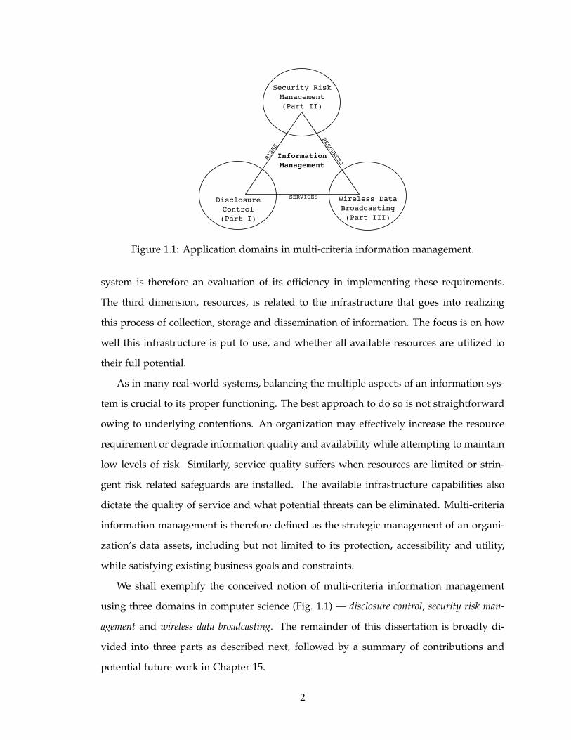
1.1 Application domains in multi-criteria information management. . . . . . . 2
2.1 Pareto-front for a hypothetical two-objective problem. . . . . . . . . . . . . 22
2.2 Hierarchy tree for the marital status attribute. Numbering on the leaf nodes
indicate their ordering in Σmarital status. . . . . . . . . . . . . . . . . . . . . . . 24
2.3 Example generalization encoding for the workclass constrained attribute. . . 38
2.4 One generation of NSGA-II. . . . . . . . . . . . . . . . . . . . . . . . . . . . . 39
2.5 Usual single point crossover (left) and special crossover for constrained
attributes (right). . . . . . . . . . . . . . . . . . . . . . . . . . . . . . . . . . . 40
2.6 Solutions to Problem A found by NSGA-II. Inset figures show cumulative
distribution of |Ei| as i increases. . . . . . . . . . . . . . . . . . . . . . . . . . 43
2.7 Solutions to Problem B (η = 10%) found by NSGA-II. Top-leftmost plot
shows all obtained solutions. Each subsequent plot (follow arrows) is a
magnification of a region of the previous plot. . . . . . . . . . . . . . . . . . 45
2.8 Solutions to Problem C found by NSGA-II. Read x-axis label for a plot from
the text-box along the same column and y-axis label from the text-box along
the same row. Trade-off characteristics are visible across different pairs of
the objective functions. . . . . . . . . . . . . . . . . . . . . . . . . . . . . . . . 46
2.9 Problem C solutions for (a) %SL < 0.2 and (b) %GL < 0.3. Encircled solu-
tions can be of interest to a user. . . . . . . . . . . . . . . . . . . . . . . . . . 47
2.10 Problem D solutions for η = 0.1 and %loss < 0.3. (a) k–anonymity is more
desired and (b) ℓ–diversity is more desired. . . . . . . . . . . . . . . . . . . 47
xvii

2.11 Problem D solutions for η = 0.1 and k ≪ ℓ. (a) Maximum loss allowed is
20%. (b) Maximum loss is increased to 21%. The quality of solutions as
well as the number of choices available increase considerably for a slight
increase in the loss limit. . . . . . . . . . . . . . . . . . . . . . . . . . . . . . 48
3.1 (a) Example domain generalization hierarchies of attributes ZIP, SEX and
SALARY. (b) Domain generalization lattice using example DGHs. (c) Gen-
eralization and specialization graphs of node (1,0,1) in the lattice. . . . . . 54
3.2 Depiction of Pareto-optimal nodes. . . . . . . . . . . . . . . . . . . . . . . . . 57
3.3 Use of depth search and height search to reach node M from node N
through a ground node. . . . . . . . . . . . . . . . . . . . . . . . . . . . . . . 59
3.4 Top row shows the search space and true Pareto-optimal nodes while using
different loss metrics. Bottom row shows the Pareto-optimal nodes found
by exhaustive search and the nodes obtained by POkA. . . . . . . . . . . . . 69
3.5 Comparison of Pareto-optimal nodes identified using depths of 1, 2 and 3
(=davg). . . . . . . . . . . . . . . . . . . . . . . . . . . . . . . . . . . . . . . . . 71
3.6 Percentage of nodes evaluated for varying lattice sizes. Results are gen-
erated by using the DCN metric. Varying lattice sizes are generated by
considering varying number of attributes to anonymize. . . . . . . . . . . . 72
4.1 Strong and weak efficiency. Weak efficiency implies one of the objective
values may be improved without changing the other. . . . . . . . . . . . . . 81
4.2 (a) Geometrical interpretation of solution procedure to Chebyshev min-max
problem. (b) Geometrical interpretation of reference direction approach. . . 91
4.3 NWP and NECD values of non-dominated solutions returned by NSGA-II
for different kpre f (effective k value obtained is highlighted). . . . . . . . . . 97
4.4 Impact of population size (Npop) on solution quality for kpre f = 5 and pref-
erence point NWPpre f = 0.2; NECDpre f = 1.0. . . . . . . . . . . . . . . . . . 99
4.5 Effect of the weight vector on attainable NWP and NECD. Also shown are
the corresponding number of groupings in the attribute domains. . . . . . 100
4.6 Impact of bias preference on solutions obtained with weights wv2. . . . . . 101
xviii

5.1 The size of equivalence class to which a tuple in T1 belongs to for different
anonymizations. Two different anonymizations with the same collective
privacy level can have different privacy levels for individual tuples. . . . . 109
5.2 The rank-based ◮rank-better comparator assigns ranks to property vectors
based on the distance from a point of interest Dmax. . . . . . . . . . . . . . . 122
5.3 Computation of the quality index functions based on the ◮cov and ◮spr
comparators. Icov is based on the number of tuples with better property
value while Ispr is based on the actual difference in magnitude of the mea-
sured property value. . . . . . . . . . . . . . . . . . . . . . . . . . . . . . . . . 123
5.4 The hypervolume comparator ◮hv gives preference to property vectors that
solely outperform more property vectors – D2 in this case since volume of
region B > volume of region A. . . . . . . . . . . . . . . . . . . . . . . . . . 126
6.1 Schematic of an iterative search process. . . . . . . . . . . . . . . . . . . . . . 138
6.2 Non-dominated boxes and representative minimal PBGs for a hypothetical
two property anonymization. . . . . . . . . . . . . . . . . . . . . . . . . . . . 140
6.3 Single point crossover and single-step mutation in the recombination process.145
6.4 PBG-EA solutions for the two property (k-GLM) and three property (k-ℓ-
GLM) problems. . . . . . . . . . . . . . . . . . . . . . . . . . . . . . . . . . . . 148
6.5 PBG-EA solutions for the two property (Sk-GLM) and three property (Sk-
Sℓ-GLM) problems using spread based quality. . . . . . . . . . . . . . . . . . 148
6.6 PBG-EA solutions with a single privacy property (k-anonymity) and two
loss metrics (GLM-CM). . . . . . . . . . . . . . . . . . . . . . . . . . . . . . . 149
6.7 Partial (k ∈ [1,100]) representative set of solutions for the two property (k-
GLM) problem with ǫk = 5 and ǫGLM = 5000. . . . . . . . . . . . . . . . . . . 151
7.1 Schematic of the system architecture. . . . . . . . . . . . . . . . . . . . . . . 161
7.2 Conventional k-anonymity and historical k-anonymity. Size of historically
k-anonymous MBR is influenced by movement of objects in O1’s anonymity
set at time t1. . . . . . . . . . . . . . . . . . . . . . . . . . . . . . . . . . . . . 163
xix

7.3 Risk of partial disclosure for varying anonymity levels k > (N + 1)/2. N =
100 and n is the number of cloaking regions for which adversary has full
location information. . . . . . . . . . . . . . . . . . . . . . . . . . . . . . . . 165
7.4 Peer set partitioning into groups over which multiple range queries are
issued with the same identifier. . . . . . . . . . . . . . . . . . . . . . . . . . 169
7.5 Trace data generated on Chamblee region of Georgia, USA. The mean
speed, standard deviation and traffic volume on the three road types used
are shown. . . . . . . . . . . . . . . . . . . . . . . . . . . . . . . . . . . . . . . 176
7.6 Comparative performance of CANON with ProvidentHider (PH) for dif-
ferent anonymity requirements (k) and oversize factors (τ). (a) Average
number of requests served in a session. (b) Percentage of requests sup-
pressed (anonymity requirement could not be satisfied). (c) Average size of
requesting object’s peer group. . . . . . . . . . . . . . . . . . . . . . . . . . . 179
7.7 Impact of different neighborhood step size θ on CANON. (a) Average num-
ber of requests served in a session. (b) Average size of requesting object’s
peer group. (c) Average number of folds increase in requesting object’s
MBR area over a session. . . . . . . . . . . . . . . . . . . . . . . . . . . . . . . 181
7.8 Impact of spatial resolution parameters on CANON – top: sub-MBR area
αsub and bottom: full-MBR area α f ull with θ = 15◦. (a) Average number of
requests served in a session. (b) Average size of requesting object’s peer
group. (c) Percentage of suppressed requests. . . . . . . . . . . . . . . . . . 183
7.9 Schematic of the system architecture for query privacy. . . . . . . . . . . . . 186
7.10 Example showing movement of users during a particular session registered
to U. Values within the circles signify service attribute values of the users.
Each cloaking region generated for U is 2-diverse and 3-anonymous. . . . 187
7.11 Comparative performance of location k-anonymity, query ℓ-diversity and
query m-invariance. . . . . . . . . . . . . . . . . . . . . . . . . . . . . . . . . 199
7.12 Impact of spatial resolution αsub. . . . . . . . . . . . . . . . . . . . . . . . . . 201
8.1 Example network model. . . . . . . . . . . . . . . . . . . . . . . . . . . . . . 207
xx

8.2 Example attack tree. . . . . . . . . . . . . . . . . . . . . . . . . . . . . . . . . 212
8.3 Attack tree of example network model. . . . . . . . . . . . . . . . . . . . . . 213
8.4 SGA solutions to Problem 8.1 with α varied from 0 to 1 in steps of 0.05. . . 220
8.5 NSGA-II solutions to Problem 8.2 and sensitivity of a solution to optimum
settings. . . . . . . . . . . . . . . . . . . . . . . . . . . . . . . . . . . . . . . . . 221
8.6 NSGA-II solutions to Problem 8.3 with D = 0 and r = 1. Problem 8.2 solu-
tions are also shown for comparison. . . . . . . . . . . . . . . . . . . . . . . . 222
8.7 Compressed attack tree showing residual damage computation with R3 as
security control set. . . . . . . . . . . . . . . . . . . . . . . . . . . . . . . . . . 223
9.1 Component interactions in a pervasive environment. . . . . . . . . . . . . . 229
9.2 (a) Context-based probability estimates. (b) Workflow probability calculation.232
9.3 (a) NSGA-II solutions in Scenario A. (b) Ratio of uncovered and covered
damage cost for solutions obtained for Scenarios A and B. The line of shift
shows the point beyond which the uncovered damage is more than the
covered damage. . . . . . . . . . . . . . . . . . . . . . . . . . . . . . . . . . . 239
9.4 NSGA-II solutions in Scenario B. (a) Solutions when maintenance cost of
the devices are comparable. (b) Solutions when some devices have com-
paratively higher maintenance cost. . . . . . . . . . . . . . . . . . . . . . . . 240
9.5 (a) NSGA-II solutions in Scenario C. Inset figure shows the sensitivity of a
solution to security mechanism failures. (b) Solutions for failure radius = 1. 241
10.1 Test-bed network model. . . . . . . . . . . . . . . . . . . . . . . . . . . . . . . 246
10.2 BAG of test network with unconditional probabilities. . . . . . . . . . . . . 250
10.3 Simple BAG illustrating probability computations. . . . . . . . . . . . . . . 256
10.4 Posterior probabilities in test network after attack incidents (marked by E©). 259
10.5 Augmented-BAG of test network with 13 security controls. . . . . . . . . . 264
10.6 Schematic of the genetic algorithm used to solve SOOP and MOOP. . . . . 265
10.7 Augmented-BAG of test network under two attack incidents. The expected
loss/gain (Vj) is shown at each node. . . . . . . . . . . . . . . . . . . . . . . 267
xxi

10.8 Genetic algorithm solutions to single objective problem obtained by using
different weights. . . . . . . . . . . . . . . . . . . . . . . . . . . . . . . . . . . 269
10.9 Genetic algorithm solutions to multi-objective problem with static risk as-
sessment. . . . . . . . . . . . . . . . . . . . . . . . . . . . . . . . . . . . . . . . 270
10.10Genetic algorithm solutions to MOOP with dynamic risk assessment. . . . 270
11.1 A hypothetical payoff matrix showing defender and attacker payoffs. . . . 276
11.2 Payoff for different attack strategies in hypothetical attack tree. Circles
denote nodes of the attack tree and the rectangle denote a defense. Value
within a circle signify a payoff value that the attacker receives if it succeeds
in reaching the node. Value within the rectangle is the cost that the attacker
incurs to bypass the defense. . . . . . . . . . . . . . . . . . . . . . . . . . . . 279
11.3 Schematic of competitive co-evolution of attack and defense strategies. . . 287
11.4 Fitness of best defense and attack strategies in every iteration of the co-
evolutionary process. . . . . . . . . . . . . . . . . . . . . . . . . . . . . . . . . 288
11.5 Average fitness of defender and attacker strategies showing “arms race”
population dynamics between the 100th and the 200th generations. . . . . . 289
11.6 Payoffs when an independent GA is run for each best host strategy from
every generation to find the best opponent strategy for it. o/+ represent
the payoffs when the defender/attacker is the host. . . . . . . . . . . . . . . 290
11.7 Defense and attack strategy of equilibrium solution. . . . . . . . . . . . . . . 291
12.1 Typical on-demand broadcast architecture in a pervasive environment. . . 303
12.2 Utility of serving a request. . . . . . . . . . . . . . . . . . . . . . . . . . . . . 304
12.3 2-exchange operator example. . . . . . . . . . . . . . . . . . . . . . . . . . . . 309
12.4 Solution encoding for multiple channels. . . . . . . . . . . . . . . . . . . . . 310
12.5 Syswerda recombination. . . . . . . . . . . . . . . . . . . . . . . . . . . . . . 311
12.6 Mutation using the insertion operator. . . . . . . . . . . . . . . . . . . . . . . 312
12.7 Percentage of maximum total utility obtained by the solution methods. The
utility obtainable suffers when the most requested data item is the largest
in size. . . . . . . . . . . . . . . . . . . . . . . . . . . . . . . . . . . . . . . . . 317
xxii

12.8 Utility derived by using EDF and HUF with INC data size distribution.
Top: Utility obtained from each of the request for EDF (left) and HUF
(right). Bottom: Utility of requests served during a broadcast for EDF (left)
and HUF (right). . . . . . . . . . . . . . . . . . . . . . . . . . . . . . . . . . . 318
12.9 Improvements obtained by doing 50000 iterations of the 2-exchange opera-
tor for the EDF schedule generated during the 3000th scheduling instance.
The DEC data size distribution is used here. A newly obtained solution is
considered better only if it exceeds the utility of the current solution by at
least 20. . . . . . . . . . . . . . . . . . . . . . . . . . . . . . . . . . . . . . . . . 320
12.10Empirical cumulative density function of the % success rates of performing
100 independent iterations of the 2-exchange operation in each scheduling
instance with EDF (left) and HUF (right). A success means the operation
resulted in a better schedule. . . . . . . . . . . . . . . . . . . . . . . . . . . . 321
12.11Top: Broadcast frequency of the N data items for ES (left) and HUF/LS
(right). Bottom: Fraction of maximum utility obtained from the different
broadcasts for ES (left) and HUF/LS (right). The DEC distribution is used
with a 80 KB/s bandwidth. . . . . . . . . . . . . . . . . . . . . . . . . . . . . 323
12.12Percentage of maximum total utility obtained by the solution methods for
transaction level scheduling. Local search results in substantial improve-
ment in the heuristic generated schedules. . . . . . . . . . . . . . . . . . . . 324
12.13Whisker plots of response time for earliest deadline and highest utility
heuristics on transaction level scheduling with the INC distribution. T-
EDF fails to distinguish between requests of different priority levels. T-
HUF makes the distinction on the average but response times are often
high. Local search suitably modifies the schedules in both cases. . . . . . . 325
12.14Broadcast frequency of the N data items for transaction level scheduling
in the DEC distribution. Distribution of average and below-average sized
data items reaches an uniform trend for high utility solution methods. . . 328
xxiii
12.15Improvements obtained by local search in T-EDF/LS during the 5000th
scheduling instance. Improvements are minor when the T-EDF schedule
is already “good" (INC distribution). Utility shows an increasing trend at
the end of the 1000th iteration of the local search for the DEC distribution. 330
12.16Improvements obtained by local search and ES in the schedule generated by
T-EDF during the 5000th scheduling instance. For transaction level schedul-
ing, local search performs better in avoiding local optima compared to
(2 + 1)-ES. . . . . . . . . . . . . . . . . . . . . . . . . . . . . . . . . . . . . . . 331
13.1 A counter example for the Syswerda order-based crossover operator. Or-
dering constraints are {a,b, c}, {d, e, f , g} and {h, i, j}; constraint {d, e, f , g}is violated in the offspring. . . . . . . . . . . . . . . . . . . . . . . . . . . . . 338
13.2 Percentage global utility for the different λ values in the ES. For the INC
assignment, a high utility level is obtainable with λ = 1. For the DEC
assignment, increasing the sampling rate λ and the number of generations
results in improvement of the global utility. . . . . . . . . . . . . . . . . . . . 339
13.3 Mean difference between time of request arrival and time of first data item
broadcast for data groups of different sizes in the DEC assignment. . . . . 340
13.4 (a) Schedule utility progress during the 5000th scheduling instance with
DEC. Utilities are also plotted for 100 points sampled around the parent of
every generation. (b) Percentage global utility for (2 + 1)-ES and a genetic
algorithm. . . . . . . . . . . . . . . . . . . . . . . . . . . . . . . . . . . . . . . 342
14.1 Broadcast server architecture in non-local data model. . . . . . . . . . . . . 349
14.2 Data server architecture following a M/G/1-PS model. . . . . . . . . . . . 351
14.3 Data item size distribution and rank assignment. . . . . . . . . . . . . . . . 362
14.4 Comparative deadline miss rates of identical algorithms in their stochastic
(using probability distributions) and non-stochastic (using expected values)
versions. . . . . . . . . . . . . . . . . . . . . . . . . . . . . . . . . . . . . . . . 367
14.5 Performance metric values for different heuristics under different workloads.369
14.6 Impact of Sdev on scheduling decisions. . . . . . . . . . . . . . . . . . . . . . 372
xxiv

14.7 Broadcast frequencies of data items by rank at UFbs = 0.75. . . . . . . . . . 374
14.8 Cumulative probability distribution of stretch values at UFbs = 1.0. . . . . 375
14.9 Cumulative probability distribution of dlnQ − ctQ (positive slack) for re-
quests which are served within their deadlines (dlnQ > ctQ); UFbs = 1.0. . 376
14.10Broadcast frequency of different data items by their ranks using MBSP
and NPRDS. Top: Low utilization (UFbs = 0.75). Bottom: High utilization
(UFbs = 4.0). The dotted lines signify the better performing heuristic. . . . 377
xxv

List of Tables
2.1 Original data set T. . . . . . . . . . . . . . . . . . . . . . . . . . . . . . . . . . 36
2.2 2-anonymous generalization of original data set T. . . . . . . . . . . . . . . 37
3.1 3-anonymous version (right) of a table. . . . . . . . . . . . . . . . . . . . . . 56
3.2 Attributes and DGH lengths used from the adult census data set. . . . . . . 68
3.3 Number of nodes evaluated when using different depth limits. Results are
generated by using the GLM metric. The total number of nodes is 17920.
Number of true Pareto-optimal nodes is 45. . . . . . . . . . . . . . . . . . . 70
4.1 Example data set and its 2–anonymous generalized version. . . . . . . . . . 77
4.2 Efficiency and ach values for different generalizations of the data set in Ta-
ble 4.1. q1 = (0.3,0.08);q2 = (0.2,0.15);q3 = (0.15,0.05);q4 = (0.25,0.05);q5 =
(0.1,0.5). wemp = 0.3;wsal = 0.7. . . . . . . . . . . . . . . . . . . . . . . . . . . 82
4.3 Attributes and domain size from the adult census data set. . . . . . . . . . . 96
5.1 Hypothetical microdata. . . . . . . . . . . . . . . . . . . . . . . . . . . . . . . 105
5.2 Two 3-anonymous generalizations of T1. Real values of marital status are
shown in italics. Left table is denoted as T3a and right table as T3b. . . . . . 106
5.3 A 4-anonymous generalization of T1. . . . . . . . . . . . . . . . . . . . . . . 108
5.4 Strict comparators based on dominance relationships. . . . . . . . . . . . . 115
6.1 CE and RR values in PBG-EA anonymization with different sets of proper-
ties. Values are shown as meanvariance from the 20 runs. . . . . . . . . . . . . . . . 147
6.2 CE and RR values in PBG-EA anonymization with different discretization
vectors. . . . . . . . . . . . . . . . . . . . . . . . . . . . . . . . . . . . . . . . . 150
xxvi
6.3 Average number of nodes evaluated in PBG-EA for different sets of prop-
erties. Total number of nodes in the first four sets is 17920 and that in the
last set is 8960. . . . . . . . . . . . . . . . . . . . . . . . . . . . . . . . . . . . . 152
7.1 Successive query 3-diverse cloaking regions. . . . . . . . . . . . . . . . . . . 156
7.2 Session profile SP(U) and background knowledge BK(U) used during a
query association attack on U. . . . . . . . . . . . . . . . . . . . . . . . . . . 188
7.3 Associating service attribute values using query association attacks. (a)
Condition 2c in Def. 7.4 not met for Alice. (b) All possible query association
attacks w.r.t. Table 7.2. . . . . . . . . . . . . . . . . . . . . . . . . . . . . . . . 190
8.1 Initial vulnerability per host in example network. . . . . . . . . . . . . . . . 208
8.2 Connectivity in example network. . . . . . . . . . . . . . . . . . . . . . . . . 208
8.3 Security controls for example network model. . . . . . . . . . . . . . . . . . 217
8.4 Fully robust solutions obtained by NSGA-II with r = 1. . . . . . . . . . . . . 222
10.1 Initial list of vulnerabilities in test network. . . . . . . . . . . . . . . . . . . . 247
10.2 CVSS attributes used for estimation of attack likelihood. . . . . . . . . . . . 254
10.3 Expanded LCPD of node A (in Fig. 10.3) under the presence of security
control M0. . . . . . . . . . . . . . . . . . . . . . . . . . . . . . . . . . . . . . . 260
10.4 Security outcome assessment for each individual control in augmented-
BAG of test network. Net benefit is (B −A− 622.0). . . . . . . . . . . . . . 268
12.1 Experiment parameters. . . . . . . . . . . . . . . . . . . . . . . . . . . . . . . 314
14.1 Performance metric values for MBSP with UFbs = 2 and varying Sdev. . . . 372
14.2 Relative broadcast frequencies of data items according to access types. Each
entry signifies if the frequency in the better performing heuristic is lower,
similar, or higher than that in the other heuristic. . . . . . . . . . . . . . . . 378
xxvii

CHAPTER 1
Multi-Criteria Information Management
Information management is the process of collecting information from one or more
sources, followed by its dissemination to one or more consumers. This process also im-
plicitly assumes the transient storage of the collected data prior to its distribution. The
term “information” is not bound to a specific form or media, but instead generalizes to
any data asset in which the managing organization has a stake. This perception is used to
differentiate information management from data management where the latter typically
involves management of the data needs within an organization. The former, however,
also includes preserving the enterprise motives during and after the data transits from a
source to a consumer.
Any modern information management system entails three broad dimensions – risk,
resources, and services. Risk manifests itself when the data that is collected and then dis-
tributed is potentially sensitive, or deemed sensitive by the primary source of collection.
In this case, the management system must have some safety guarantees associated with
them. Risk also encapsulates the case where data assets may be improperly accessed
either during storage or after distribution. The second dimension, services, involves the
guarantees of access to data by a legitimate consumer. This factor is commonly known as
“availability” of a system. However, a system must also try to assure that the information
is received in a state that is usable to the consumer. The quality of service offered by the
1
Information
Management
RISKS
RESOURCES
SERVICES
Security Risk
Management
(Part II)
Disclosure
Control
(Part I)
Wireless Data
Broadcasting
(Part III)
Figure 1.1: Application domains in multi-criteria information management.
system is therefore an evaluation of its efficiency in implementing these requirements.
The third dimension, resources, is related to the infrastructure that goes into realizing
this process of collection, storage and dissemination of information. The focus is on how
well this infrastructure is put to use, and whether all available resources are utilized to
their full potential.
As in many real-world systems, balancing the multiple aspects of an information sys-
tem is crucial to its proper functioning. The best approach to do so is not straightforward
owing to underlying contentions. An organization may effectively increase the resource
requirement or degrade information quality and availability while attempting to maintain
low levels of risk. Similarly, service quality suffers when resources are limited or strin-
gent risk related safeguards are installed. The available infrastructure capabilities also
dictate the quality of service and what potential threats can be eliminated. Multi-criteria
information management is therefore defined as the strategic management of an organi-
zation’s data assets, including but not limited to its protection, accessibility and utility,
while satisfying existing business goals and constraints.
We shall exemplify the conceived notion of multi-criteria information management
using three domains in computer science (Fig. 1.1) — disclosure control, security risk man-
agement and wireless data broadcasting. The remainder of this dissertation is broadly di-
vided into three parts as described next, followed by a summary of contributions and
potential future work in Chapter 15.
2

Part I: Disclosure Control
Privacy violations emanating from the public sharing of personally identifying infor-
mation have raised serious concerns over the past few years. The nature of these viola-
tions indicate that information privacy is difficult to guarantee even after the removal of
unique identification data. Multiple real world instances have exemplified this aspect in
recent years.
• 35% of victims were re-identified in Chicago’s de-identified homicide database by
comparing the records with those in the Social Security Death Index [137].
• The health records of the Governor of Massachusetts were re-identified from Group
Insurance Commission’s anonymized data by using a voter registration list [165].
• Unique identification is possible for approximately 70% of the population from fa-
milial database records using genealogies extracted from newspaper obituaries and
death records [122].
• Users were uniquely identified based on their search queries released as part of an
anonymized Web queries data set (contained over twenty million search keywords)
by AOL for research purposes [14].
• A person’s date of birth, gender and ZIP code forms a unique identifier for 63% of
the US population reported in the 2000 census [76].
• Researchers uniquely identified Netflix R© users from an anonymized movie ratings
data set (contained nearly half million records) released by the rental firm to facili-
tate research to improve its movie-recommendation engine [134].
• Public availability of the Social Security Administration’s Death Master File and the
widespread accessibility of personal information from sources such as data brokers
or profiles on social networking sites enable researchers to fully predict the social
security number [4].
The seriousness of these violations is well-understood in the research community and
has generated significant interest in the field of disclosure control. This field of research
3
has looked into the formulation of data modification techniques and privacy models that
can prevent possible unique linkage between a person and the corresponding informa-
tion contained in a database record. However, the challenge lies in the enforcement of
these techniques, predominantly due to the fact that the quality of the shared data often
determines its usefulness for the legitimate purpose for which it is intended. The privacy
primitives can reduce the risk of re-identification, but at the same time degrades the ser-
vice quality that an organization can guarantee based on the data quality. We shall look
into the limitations of the current decision making framework used in this domain, and
present our formulations that implicitly assume the existence of reciprocal interactions
between risks and services in disclosure control.
Part I of this dissertation is organized as follows. Chapter 2 introduces the privacy
versus utility problem in disclosure control and provides an extensive survey of currently
known solution techniques for solving this problem. This chapter also discusses the
multi-objective nature of the problem and presents our decision making model based on
multi-criteria analysis [55, 57]. Chapter 3 continues the discussion in the context of a data
modification representation widely used by current techniques [59]. Chapter 4 extends
the multi-criteria analysis by enabling the inclusion of data publisher preferences in the
optimization process [53, 65]. Inclusion of these preferences allows a data publisher to
focus on solutions that meet certain pre-specified requirements in terms of risk mitigation
and quality achievement. Chapter 5 discusses the methodology that should be adopted
for a comparative study in this domain, given that an algorithm cannot cater to both
the privacy and utility objectives simultaneously [58]. Chapter 6 collects our observa-
tions and presents a unified framework to perform multi-criteria decision making in data
anonymization [61]. Chapter 7 looks at some of the privacy issues in the management of
information originating from the ubiquitous usage of mobile services [60, 62].
Part II: Security Risk Management
Networked systems constantly run under the risk of compromise. The security in
these systems is only as good as the availability of known exploits and corresponding
mitigation controls. Modern systems also have an extensive degree of inter-connectivity
4

that complicates the identification of contributions made by an existing vulnerability to-
wards system compromise. Significant research has therefore gone into the formulation
of security models for networked systems using paradigms like attack graphs and attack
trees. These models help identify the cause-consequence relationship between system
states, and enumerate the different attack paths that can lead to a compromised state.
They also allow a system administrator to identify the minimum set of control measures
necessary to prevent known exploits.
While risk assessment is vital to the security of any networked system, risk mitigation
is often constrained by the availability of sufficient resources. Efficiency in risk mitigation
is therefore also dependent on what control measures are chosen within given cost con-
straints. Security risk management encompasses this decision making paradigm where
resource availability impacts the extent of risk to which a networked system will always
be exposed. However, existing techniques deviate from this core principle and assume
that the system administrator has the resources required to effectuate a “completely se-
cure” system. We argue that this is an impractical assumption and the decision to achieve
a certain level of security can only be made after obtaining a comprehensive understand-
ing of the risks–resources trade-offs.
Part II of this dissertation is organized as follows. Chapter 8 looks at how security
hardening is typically approached in existing works, and highlights the requirement for
a multi-criteria analysis [51]. This analysis is crucial to any organization that operates
under tight budget constraints, but at the same time, must make a best effort to pro-
tect its network assets. Chapter 9 discusses a similar problem in the domain of pervasive
systems, where resource constraints are imposed by the heterogeneous nature of the envi-
ronment [52]. Chapter 10 discusses how the hardening process can be made more robust
by including attack probabilities in a cause-consequence model. These probabilities in-
dicate an attack’s difficulty level and are used to identify system states that have a high
likelihood of compromise. Chapter 11 introduces the evolving attacker model and po-
sitions the efficacy of the static approach to security risk management under constantly
changing attacker-defender dynamics.
5

Part III: Wireless Data Broadcasting
Fast access to information is becoming increasingly vital to support today’s mobile
infrastructures. As mobile devices gain more and more compute power, the variety of
applications that can be supported by these devices are also becoming diverse. One of
the implications of this trend for modern information management systems is to have the
ability to provide clients fast access to the vast repository of data over a wireless medium.
Challenges in doing so arise from the fact that wireless bandwidth is a limited resource.
Wireless data broadcasting is becoming a popular mechanism in this scenario due to its
scalability properties. Broadcasting reduces the amount of data to be transferred over
a wireless channel when multiple clients are interested in the same information. Exten-
sive research have therefore been carried out to determine optimal broadcast schedules
satisfying a variety of access time constraints.
Since the broadcast schedules are built in real time, the QoS criteria must be well
represented in order to minimize access delays and maximize resource utilization. The
QoS criteria must encapsulate the possibility that access time constraints cannot always
be met, in which case, the data should be made available based on its possible utility.
We shall look at a practical perception of information availability in terms of the utility
derived from it by the consumers. A number of utility driven optimization problems are
explored here.
Part III of this dissertation is organized as follows. Chapter 12 discusses the design
of broadcast schedulers that attempt to maximize the utility of broadcast data given the
bandwidth limitations of a system [56]. Chapter 13 considers the additional constraint
of ordering in the data items [63, 64]. Chapter 14 introduces a stochastic variant of the
broadcasting problem in the context of a non-local data storage model [54].
6

Part I
Disclosure Control
7

CHAPTER 2
Managing Data Privacy and Utility
Various scientific studies, business processes and legal procedures depend on qual-
ity data. Large companies have evolved whose sole business is gathering data from vari-
ous sources, building large data repositories, and then selling the data or their statistical
summary for profit. Examples of such large data publishers are credit reporting agen-
cies, financial companies, demographic data providers and so on. These data reposito-
ries often contain sensitive personal information, including medical records and financial
profiles, which if disclosed and/or misused, can have alarming ramifications. Thus, not
only the storage of this data done with strong security controls, but the dissemination
is also frequently governed by various privacy requirements and subjected to disclosure
control. For privacy protection, the data need to be sanitized of personally identifying
attributes before it can be shared. Anonymizing the data, however, is quite challenging.
Re-identifying the values in sanitized attributes is not impossible when other publicly
available information or an adversary’s background knowledge can be linked with the
shared data. A classic example of such linking attacks was demonstrated by Sweeney [163],
in which the author used a readily purchased voter list to re-identify medical records. In
fact, a recent study on the year 2000 census data of the U.S. population reveals that 53%
of the individuals can be uniquely identified by their gender, city and date of birth; 63%
if the ZIP code is known in addition [76].
8
Database researchers have worked hard over the past several years to address such
privacy concerns. Earlier techniques such as scrambling and adding noise to the data
values [5] address the inference problem in statistical databases without reducing the
value of the data. More recently, Samarati and Sweeney proposed the concept of k–
anonymity to address the privacy problem. k–anonymity reduces the chances of a linking
attack being successful [151, 152, 165]. The anonymization process involves transforming
the original data set into a form unrecognizable in terms of the exact data values by using
generalization and suppression schemes. A generalization performs a one-way mapping
of the values of personally identifiable attributes, called quasi-identifiers, to a form non
differentiable from the original values or to a form that induces uncertainty in recognizing
them. An example of this is replacing a specific age by an age range. More often than not,
it may be impossible to enforce a chosen level of privacy due to the presence of outliers in
the data set. Outliers are not pre-defined in a given data set. Rather they depend on the
generalization scheme that one is applying on the data. Given a particular generalization,
outliers may emerge, making it difficult to achieve a desired level of privacy. In such a
situation, a suppression scheme gets rid of the outliers. Suppression works by removing
entire tuples making them no longer existent in the data set. A transformed data set of
this nature is said to be k–anonymous if each record in it is same as at least k − 1 other
records with respect to the quasi-identifiers. The higher the value of k, the stronger the
privacy that the model offers.
An unavoidable consequence of performing such anonymization is a loss in the qual-
ity of the information content of the data set. Statistical inferences suffer as more and
more diverse data are recoded to the same value, or records are deleted by a suppression
scheme. A summary statistic relying on accurate individual information automatically
deteriorates when stronger privacy is implemented. Researchers have therefore looked
at different methods to obtain an optimal anonymization that results in a minimal loss
of information [16, 89, 92, 150, 164, 178]. Since deciding on an anonymization for k–
anonymity is NP-hard [127], most studies so far have focused on algorithms to minimize
the information loss for a fixed value of k.
As research in this front progressed, other types of attacks have also been identified
9
— homogeneity attack, background knowledge attack, skewness attack and similarity attack [112,
120]. Models beyond k–anonymity have been proposed to counter these new forms of
attacks on anonymized data sets and the hidden sensitive attributes. Two of the more
well known models in this class are the ℓ–diversity model [120] and the t–closeness model
[112]. While these models enable one to better guarantee the preservation of privacy in
the disseminated data, they still come at a cost of reduced quality of the information.
The (possibly) unavoidable loss in data quality due to anonymizing techniques presents
a dilemma to the data publisher. Since the information they provide forms the basis of
their revenue, its whole purpose would be lost if the privacy controls prohibit any kind
of fruitful inferences being made from the distributed data. In other words, although
the organization needs to use some anonymization technique when disseminating the
data, it also needs to maintain a pre-determined level of utility in the published data.
Proper anonymization thus involves weighing the risk of publicly disseminated infor-
mation against the statistical utility of the content. In such a situation, it is imperative
that the data publisher understands the implications of setting a parameter in a privacy
model (for example, k in k–anonymity or ℓ in ℓ–diversity) to a particular value. There
is clearly a trade-off involved. Setting the parameter to a “very low” value impacts the
privacy of individuals in the database. Picking a “very high” value disrupts the inference
of any significant statistical information from the anonymized data set. Furthermore, a
data publisher may at times be confronted with a choice of several values of a parame-
ter. This will arise in situations where individuals are allowed an opportunity to specify
their desired privacy levels. For example, some users may be content with k = 2 (in the
k–anonymity model) while others may want k = 4. In such cases, the publisher needs
to determine if some higher parameter value than initially selected is (or is not) possible
with the same level of information loss. If a higher value is possible it will do a bonafide
service to the individuals whose personal data are in the repository.
We believe that in order to understand the impact of setting the relevant parameters,
a data publisher needs to answer questions similar to the following.
1. What level of privacy can one assure given that one may not suppress any record in
the data set and can only tolerate an information loss of 25% (say)?
10

2. What is a good value for k (assuming the k–anonymity model) when one may sup-
press 10% (say) of the records and be able to tolerate an information loss of (maybe)
25%?
3. Under the “linking attacks” threat model and assuming that the users of the pub-
lished data sets are likely to have background knowledge about some of the indi-
viduals represented in the data set, is it possible to combine the k–anonymity and
the ℓ–diversity models to obtain a generalization that protects against the privacy
problems one is worried about?
4. Is there a generalization that gives a high k and a high ℓ value if one is ready to
suppress (maybe) 10% of the records and tolerate (say) 20% of information loss?
Unfortunately, answering these questions using existing techniques will require us to
try out different k (or ℓ) values to determine what is suitable. Additionally, since the
k–anonymity and ℓ–diversity models have been developed to address different types of
attacks on privacy, one may want to combine the two models. This will require more
possibilities to be tried out. Further, such a methodology does not guarantee that better
privacy results cannot be obtained without incurring any or an acceptable increase in
the information loss. Although recent studies have looked into the development of fast
algorithms to minimize the information loss for a particular anonymization technique
with a given value for the corresponding parameter, very few of them explore the data
publisher’s dilemma – given an acceptable level of information loss, determine the best k
and/or ℓ value that satisfy the privacy requirements of the data set.
This chapter introduces the multi-objective nature of data anonymization and pro-
poses the requisite formulations to address the data publisher’s dilemma. First, we dis-
cuss the formulation of a series of multi-objective optimization problems, the solutions
to which provide an in-depth understanding of the trade-off present between the level of
privacy and the quality of the anonymized data set. We note that one important feature
often overlooked in the specification of a privacy model is the distribution of the pri-
vacy parameter across the anonymized data set. The privacy parameter reported on an
anonymized data set, for example k in k-anonymity, is a quantifier of the least property
11
satisfied by all tuples in the data set. Very often, this quantity is an inexact characteriza-
tion of the privacy level, for it may be the case that a majority of the tuples in the data set
actually satisfy a higher privacy property – a higher k value for example. Failure to cap-
ture the distribution of the parameter values thereby makes differentiating between two
equivalent (in the sense of a privacy model parameter value and utility) anonymizations
a difficult task. Techniques are therefore required to capture (or specify) this distribution
and make it a part of the optimization process. As our second contribution, we build on
the concept of weighted-k anonymity and include it in one of the multi-objective problem
formulations. Third, we provide an analytical discussion on the formulated problems to
show how information on this trade-off behavior can be utilized to adequately answer
the data publisher’s questions. Fourth, we exemplify our approach by using a popu-
lar evolutionary algorithm to solve the multi-objective optimization problems relevant to
this study. Our last contribution is the design of a multi-objective formulation that can
be used to search for generalizations that result in acceptable adherence to more than
one privacy property within acceptable utility levels. Towards this end, we show how
decision making is affected when trying to use the k–anonymity and ℓ-diversity models
simultaneously.
The remainder of the chapter is organized as follows: Section 2.1 reviews some of
the existing research in disclosure control. The required background on multi-objective
optimization is presented in Section 2.2. We introduce the terminology used in the chapter
in Section 2.3. Section 2.4 provides a description of the four multi-objective problems we
formulate and the underlying motivation behind them. The specifics of the solution
methodology with respect to solving the problems using an evolutionary algorithm is
given in Section 2.5, and a discussion of the results so obtained is presented in Section
2.6. Finally, Section 2.7 summarizes and concludes the chapter.
2.1 Related Work
Several algorithms have been proposed to find effective k–anonymization. The µ-argus
algorithm is based on the greedy generalization of infrequently occurring combinations
of quasi-identifiers and suppresses outliers to meet the k–anonymity requirement [89].
12
µ-argus suffers from the shortcoming that larger combinations of quasi-identifiers are not
checked for k–anonymity and hence the property is not always guaranteed [164].
Sweeney’s Datafly approach uses a heuristic method to generalize the attribute con-
taining the most distinct sequence of values for a provided subset of quasi-identifiers
[164]. Sequences occurring less than k times are suppressed. Samarati’s algorithm [150]
can identify all k–minimal generalizations, out of which an optimal generalization can be
chosen based on certain preference information provided by the data recipient. A similar
full-domain generalization is also proposed in Incognito [109]. The basic Incognito algorithm
starts with the generalization lattice of a single attribute and performs a modified bottom-
up breadth-first search to determine the possible generalized domains of the attribute that
satisfy k–anonymity. Thereafter, the generalization lattice is updated to include more and
more number of attributes.
Iyengar proposes a flexible generalization scheme and uses a genetic algorithm to per-
form k–anonymization on the larger search space that resulted from it [92]. Although the
method can maintain a good solution quality, it has been criticized for being a slow iter-
ative process. In this context, Lunacek et al. introduce a new crossover operator that can
be used with a genetic algorithm for constrained attribute generalization, and effectively
show that Iyengar’s approach can be made faster [118]. As another stochastic approach,
Winkler proposes using simulated annealing to do the optimization [178].
On the more theoretical side, Sweeney proposes the MinGen algorithm [164] that ex-
haustively examines all potential generalizations to identify the generalization that min-
imally satisfies the anonymity requirement, acknowledging that the approach is imprac-
tical even on modest sized data sets. Meyerson and Williams have recently proposed an
approximation algorithm that achieves an anonymization with O(k logk) of optimal [127].
However, the method is not suitable when larger values of k is desired.
Most of the previous approaches start from the original data set and systematically
or greedily generalize it into one that is k–anonymous. Bayardo and Agrawal propose a
complete search method that iteratively constructs less generalized solutions starting from
a completely generalized data set [16]. The algorithm starts with a fully generalized data
set and systematically specializes it into one that is minimally k–anonymous. It uses a tree
13
search strategy exploiting both cost-based pruning and dynamic search rearrangement
[17]. The idea of a “solution cut” is presented by Fung et al. in their approach to top
down specialization [72]. A generalization is visualized as a “cut” through the taxonomy
tree of each attribute. A cut of a tree is a subset of values in the tree that contains exactly
one value on each root-to-leaf path. A solution cut is a cut that satisfies the anonymity
requirement.
A more general view of k-anonymization is clustering with a constraint on the mini-
mum number of objects in every cluster [6, 32, 67, 111]. Clustering techniques use metrics
that quantify the distance between tuples and distance between equivalence classes. The
basic idea for the algorithm is to find an arbitrary equivalence class of size smaller than
k and merge it with the closest equivalence classes to form a larger equivalence class
with the smallest distortion. The process is repeated recursively until each equivalence
class contains at least k tuples. Minimum distortion is enforced by choosing the closest
common generalizations of attributes.
LeFevre et al. extend the notion of generalizations on attributes to generalization on
tuples in the data set [110]. The authors argue that such multidimensional partition-
ing of the generalization domain show better performance in capturing the underlying
multivariate distribution of the attributes, often advantageous in answering queries with
predicates on more than just one attribute.
The drawbacks of using k–anonymity are first described by Machanavajjhala et al.
[120]. They identify that k–anonymized data sets are susceptible to privacy violations
when there is little diversity in the sensitive attributes of a k–anonymous equivalence
class. In order to alleviate such privacy breaches, they propose the model of ℓ–diversity
which obtains anonymizations with an emphasis on the diversity of sensitive attribute
values on a k–anonymous equivalence class. Further work presented by Li et al. show that
the ℓ–diversity model is also susceptible to certain types of attacks [112]. To this effect,
they emphasize having the t–closeness property that maintains the same distribution of
sensitive attribute values in an equivalence class as is present in the entire data set, with
a tolerance level of t. They realize that t–closeness does not deal with identity disclosure
scenarios and propose that it should be used in conjunction with k–anonymity.
14
The k–anonymity model assumes an adversary with full knowledge about the public
information (quasi-identifiers) of all individuals in the microdata. This is an unrealistic
assumption and is often not required. Variations have thus been proposed with relax-
ations on the knowledge of an adversary. If an adversary knows the public information
of a single individual, then we may generalize the table so that the original public data
of every individual maps to the generalized public data of at least k tuples. This is a
relaxation of the k–anonymity requirement since the k tuples are not required to form an
equivalence class. Such an anonymization results in (1,k)–anonymity. Another notion is
that of (k,1)–anonymity where any tuple in the anonymized data set maps to at least k
tuples in the original data. When both forms of anonymity are satisfied, it is called (k,k)–
anonymity [74]. Every k–anonymous table is (k,k)–anonymous, but the reverse is not
necessarily true. (k,k)–anonymizations are secure if an adversary has knowledge on a
limited number of individuals in the data set, but can be insecure if the adversary has full
knowledge on all individuals. Quantified notions of adversarial knowledge is also used
in skyline privacy [36]. A vector (ℓ,k,m) is used to say that the adversary knows ℓ sensitive
values that a target individual does not have, the sensitive values of k individuals other
than the target, and m individuals such that if any one has a specific sensitive value then
the target also has it. Given such a representation of adversarial knowledge, a released
table must guarantee multidimensional privacy such that the adversary’s confidence that
an individual has a certain sensitive value should not exceed a given threshold.
Combination of different privacy characteristics have also been attempted in certain
models. The (α,k)–anonymity model extends k–anonymity such that the confidence of
associating quasi-identifiers to sensitive values is limited to within α [181]. Under this
model, any k–anonymization must also satisfy the α-deassociation requirement, i.e. the
relative frequency of a given value of a sensitive attribute in an equivalence class must
be less than or equal to a user-defined threshold α, where 0 < α < 1. However, the
model has limitations similar to ℓ–diversity. When the frequency of sensitive values in the
whole data set is not well-proportioned, the presence of some highly sensitive values with
lower frequency will force α to be very close to one. Therefore a generic model, called
the complete (α,k)–anonymity, uses different α values for different sensitive values [95].
15
Another model proposed to protect against attribute disclosure is p–sensitive k–anonymity
[173]. A data set satisfies p–sensitive k–anonymity if it satisfies k–anonymity and the
number of distinct values for each sensitive attribute is at least p in each equivalence class.
Extended p–sensitive k–anonymity further enforces the requirement that no two values of a
sensitive attribute in an equivalence class are descendants of a common protected node
in a hierarchy tree specified over the sensitive attribute domain [34]. The hierarchy tree
captures semantic relationships between possible values. A similar approach to combine
k–anonymity and ℓ–diversity is adopted in the (k,ℓ)–anonymity model [113].
Most anonymity models focus on an universal approach to privacy where the same
amount of preservation is sought for all individuals. As a consequence, such models
may be offering insufficient protection to a subset of individuals while applying exces-
sive privacy control to another subset. The notion of personalized anonymity eliminates
such problems by performing generalizations that satisfy personal requirements [185].
Personal preferences on sensitive attributes are captured as “guarding nodes”. For exam-
ple, a personal preference may allow “flu” to be disclosed as the illness of a patient but
no disclosure of a “lung cancer” patient or the inference that the illness is “cancer” may
be allowed. In such cases, the released microdata must limit the probability of inference
of information beyond what is allowed within a threshold.
A different approach to data generalization is adopted in Anatomy [184]. It is a data
dissemination method designed on top of ℓ–diversity with the difference that quasi-
identifiers are not generalized and released in their original form. The quasi-identifiers
and the sensitive attribute are released in two different tables, called the QIT and ST re-
spectively. The tuples in a microdata are first partitioned (without generalizing the quasi-
identifiers) into groups such that the ℓ–diversity property holds in every group. QIT
comprises of only the quasi-identifier values of the tuples along with the group number
to which a tuple belongs. ST lists, for every group, the distinct values of the sensitive
attribute in the group along with a count of the number of tuples in the group that has a
specific value. Since no generalization is performed on the quasi-identifiers, anatomy pre-
serves any distributions/correlations in the attributes. Enforcing the ℓ–diversity property
while grouping the tuples protects ST against homogeneity and background knowledge
16
attacks. Besides such fragmentation, perturbation (addition of noise) is another technique
that is used to anonymize data. Although data perturbation is slowly being discarded
in microdata anonymization, these methods are still used in statistical disclosure control
where answers to summary queries on a statistical database should not reveal individ-
ual values. However, under the light of recent results by Dwork and Yekhanin [68], the
efficacy of the technique even for statistical disclosure control has become questionable.
Quantification of data utility has been approached from different perspectives by re-
searchers. Early notion of information loss is based on the number of generalization steps
one has to perform to achieve a given privacy requirement [150]. Such a method assumes
that attribute domains can be progressively generalized and a partial order can be im-
posed on the domain of all generalizations for an attribute. For instance, ZIP codes can
be generalized by dropping a digit from right to left at each generalization step. Postal
addresses can be generalized to the street, then to the city, to the county, to the state, and
so on. Given that such orderings can be imposed, a distance can be computed for each
attribute between the microdata and a generalized version of it. The result is a distance
vector with an entry for each attribute. Dominance relationships are used to determine if
one distance vector is better than other – a better distance vector will have lower distance
values for each attribute.
Information loss is also measured in terms of the amount of distortion in a generalized
table. In a cell of a generalized table, the ratio of the domain of the value found in the cell
to the height of the attribute’s hierarchy reports the amount of generalization and thereby
measures the cell’s distortion [164]. Precision of a generalized table is then computed as
one minus the sum of all cell distortions (normalized by the total number of cells). Gen-
eralizations based on attributes with longer generalization hierarchies typically maintain
precision better than generalizations based on attributes with shorter hierarchies. Further,
hierarchies with different heights can provide different precision measures for the same
table. A similar distortion measure is also used in [111].
Similar estimation of information loss is used in the general loss metric [92]. The general
loss metric computes a normalized information loss for each data value in the generalized
data set. The requirement here is that information in every column is potentially impor-
17
tant and hence a flexible scheme to compute the loss for both numeric and categorical
data is required. Consider an attribute containing categorical information that is general-
ized based on a hierarchy tree (e.g. Fig. 2.2). The generalized value of this attribute for a
certain tuple corresponds to node P in the tree. If the total number of leaf nodes in the
tree is M and the number of leaf nodes in the subtree rooted at node P is MP, then loss
for this data value is computed as (MP − 1)/(M − 1). Similarly, if Ui and Li are the upper
and lower bounds of the interval to which a numerical attribute value gets mapped to, the
loss is (Ui − Li)/(U − L), where U and L are the upper and lower bounds of the attribute.
The general loss is the sum of loss over all data values. In some attempts, a summation
of losses computed by these methods (interval based and tree based) is instead used [32].
A widely used loss metric, called the discernibility metric, assigns a penalty to each
tuple based on the number of tuples in the anonymized data set that are indistinguishable
to each other [16]. Thus, a tuple belonging to an equivalence class of size j is assigned
a penalty of j. A suppressed tuple is assigned a penalty equal to the number of tuples
in the data set. The idea behind using the size of the equivalence class as a measure of
information loss is to penalize generalizations that result in equivalence classes bigger
than what is required to enforce a given privacy requirement. A variant of this is to use
the normalized average cluster size [110].
Data utility is often measured in conjunction with privacy in an attempt to combine
both objectives into a single metric. A metric of such nature favors generalizations that
result in maximum gain in the information entropy for each unit of anonymity loss result-
ing from the generalization. Methods employing such a metric progressively increase the
amount of generalization, called a bottom up generalization approach [176], or decrease it,
called a top down specialization approach [72], with the objective of maximizing the metric
without violating the anonymity requirement. Utility assessment in these methods are
motivated by the ability to perform correct classification tasks as typical in data mining
applications. A classification metric is also proposed by Iyengar where a tuple is pe-
nalized if it gets suppressed or of its class label does not match the majority class label
[92].
Another metric, called usefulness, measures utility as the average diversity in the tuples
18
belonging to an equivalence class [117]. This measurement is similar to the general loss
metric, with differences being in the treatment of interval based attribute domains. For
such domains, the loss is assigned as the normalized distance between the maximum
and minimum values of the attribute in the equivalence class. A complementary metric,
called protection, uses the inverse of the tuple diversities as a measure of the privacy factor.
The two metrics inherently exhibit a reciprocal relationship, useful when a data publisher
wants to modulate the anonymization process towards one objective or the other.
Preliminary metrics to evaluate the effectiveness of anonymized data in answering
aggregate queries have also been proposed. Quality here is derived from a normalized
difference between the result of evaluating a query on the anonymous data and the result
on the original data [110]. Given a totally ordered set of sensitive attribute values, these
metrics measure the range of values that is encompassed in a query result [193]. The
smaller the range, the higher is the query answering accuracy.
Loss metrics should not only capture the information loss caused by the generaliza-
tion but also account for the importance of the different attributes. For example, given
a disease analysis data set, an “age” attribute may be considered more critical than a
“ZIP code” attribute. In such a case, generalizations that are able to maintain the “age”
attribute more accurately should be favored. The weighted normalized certainty penalty met-
ric uses a weighted sum of the loss measurements in different attributes of the data set
[187]. The loss measurement is similar as in the general loss metric and the usefulness
metric. The introduction of such preference characteristics indicates that the measurement
of utility can be a very subjective matter after all.
The first known attempt of exploring the privacy and utility trade-offs is undertaken
by Dewri et al. [55]. The work focuses on a multi-objective optimization formulation
based on a model called weighted-k anonymity. A similar trade-off analysis is presented
by Huang and Du in the problem of optimizing randomized response schemes for privacy
protection [88].
The potential problem in using the above approaches is that they are targeted to-
wards obtaining an optimal generalization for a fixed value of k, ℓ, or t, sometimes in
conjunction. Besides running the algorithms multiple times with different values of the
19

parameter(s), no attempt is known to have been made to understand how the general-
izations and the related cost metrics change with changes in the parameter values. Our
work seeks to fill this gap.
2.2 Multi-objective Optimization
In real world scenarios, often a problem is formulated to cater to several criteria or
design objectives, and a decision choice to optimize these objectives is sought for. An opti-
mum design problem must then be solved with multiple objectives in consideration. This
type of decision making falls under the broad category of multi-criteria, multi-objective,
or vector optimization problems.
Multi-objective optimization differs from single-objective ones in the cardinality of
the optimal set of solutions. Single-objective optimization techniques are aimed towards
finding the global optima. In case of multi-objective optimization, there is no such concept
of a single optimum solution. This is due to the fact that a solution that optimizes one
of the objectives may not have the desired effect on the others. As a result, it is not
always possible to determine an optimum that corresponds in the same way to all the
objectives under consideration. Decision making under such situations thus require some
domain expertise to choose from multiple trade-off solutions depending on the feasibility
of implementation.
Formally we can state a multi-objective optimization problem (MOOP) in microdata
disclosure control (MDC) as follows.
Definition 2.1 MDC MOOP. Let f1, . . . , fM denote M objective functions to maximize
while performing a modification of a given table T. Find a generalized table T′ of T
which optimizes the M-dimensional vector function
f (T∗) = [ f1(T∗), f2(T
∗), . . . , fM(T∗)], (2.1)
where T∗ is a generalized version of T.
The objective functions in this case are either related to the privacy or utility level
maintained in an anonymized table. Note that the privacy level can be inferred with
20
respect to different privacy models. Hence the number of objectives can be more than
two. In order to find an optimal solution to the MDC MOOP, we must be able to com-
pare anonymizations with respect to all the objectives in hand. However, due to the
conflicting nature of the objective functions, a simple objective value comparison between
two anonymizations cannot be performed. Most multi-objective algorithms thus use the
concept of dominance to compare feasible solutions.
Definition 2.2 DOMINANCE AND PARETO-OPTIMAL SET. Given a table T and M ob-
jectives to maximize, a generalized table T1 of T is said to dominate another generalized
table T2 of T if
1. ∀i ∈ {1,2, . . . , M} fi(T1) ≥ fi(T2), and
2. ∃j ∈ {1,2, . . . , M} f j(T1) > f j(T2).
T2 is then said to be dominated by T1, denoted by T2 � T1. If the two conditions
do not hold, T1 and T2 are said to be non-dominated w.r.t. each other, denoted by the
� symbol. Further, all generalized tables of T which are not dominated by any possible
generalized version of T constitutes the Pareto-optimal set.
In other words, a Pareto-optimal solution is as good as other solutions in the Pareto-
optimal set, and not worse than other feasible solutions outside the set. The surface
generated by these solutions in the objective space is called the Pareto-front or Pareto-
surface. Fig. 2.1 shows the Pareto-front for a hypothetical two-objective problem, with the
dominance relationships between three feasible solutions.
In the context of the k–anonymity problem, the Pareto-front for the two objectives –
maximize k and minimize loss – provides the decision maker an understanding of the
changes in the information loss when k is varied. Consider two anonymized versions T1
and T2 of a data set, with corresponding k and loss as (k1, loss1) and (k2, loss2) respectively.
Let us assume that k1 < k2 and loss1 = loss2. A decision maker using T1, and unaware
of T2, misses on the fact that a higher k value is possible without incurring any increase
in the loss. A multi-objective algorithm using the dominance concept can expose this
relationship between T1 and T2, namely T1 � T2. As another example, consider the
21
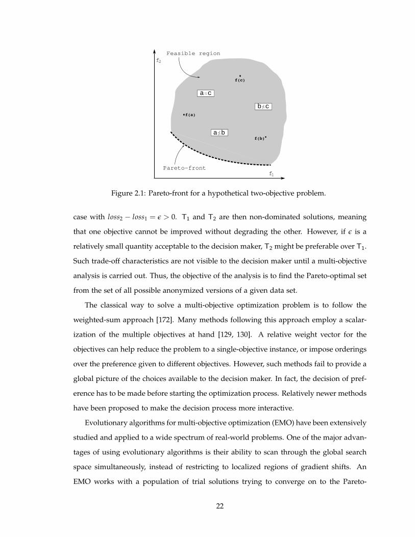
Feasible region
Pareto-front
f(a)
f(b)
f(c)
f
f
a b
b c
a c
2
1
Figure 2.1: Pareto-front for a hypothetical two-objective problem.
case with loss2 − loss1 = ǫ > 0. T1 and T2 are then non-dominated solutions, meaning
that one objective cannot be improved without degrading the other. However, if ǫ is a
relatively small quantity acceptable to the decision maker, T2 might be preferable over T1.
Such trade-off characteristics are not visible to the decision maker until a multi-objective
analysis is carried out. Thus, the objective of the analysis is to find the Pareto-optimal set
from the set of all possible anonymized versions of a given data set.
The classical way to solve a multi-objective optimization problem is to follow the
weighted-sum approach [172]. Many methods following this approach employ a scalar-
ization of the multiple objectives at hand [129, 130]. A relative weight vector for the
objectives can help reduce the problem to a single-objective instance, or impose orderings
over the preference given to different objectives. However, such methods fail to provide a
global picture of the choices available to the decision maker. In fact, the decision of pref-
erence has to be made before starting the optimization process. Relatively newer methods
have been proposed to make the decision process more interactive.
Evolutionary algorithms for multi-objective optimization (EMO) have been extensively
studied and applied to a wide spectrum of real-world problems. One of the major advan-
tages of using evolutionary algorithms is their ability to scan through the global search
space simultaneously, instead of restricting to localized regions of gradient shifts. An
EMO works with a population of trial solutions trying to converge on to the Pareto-
22
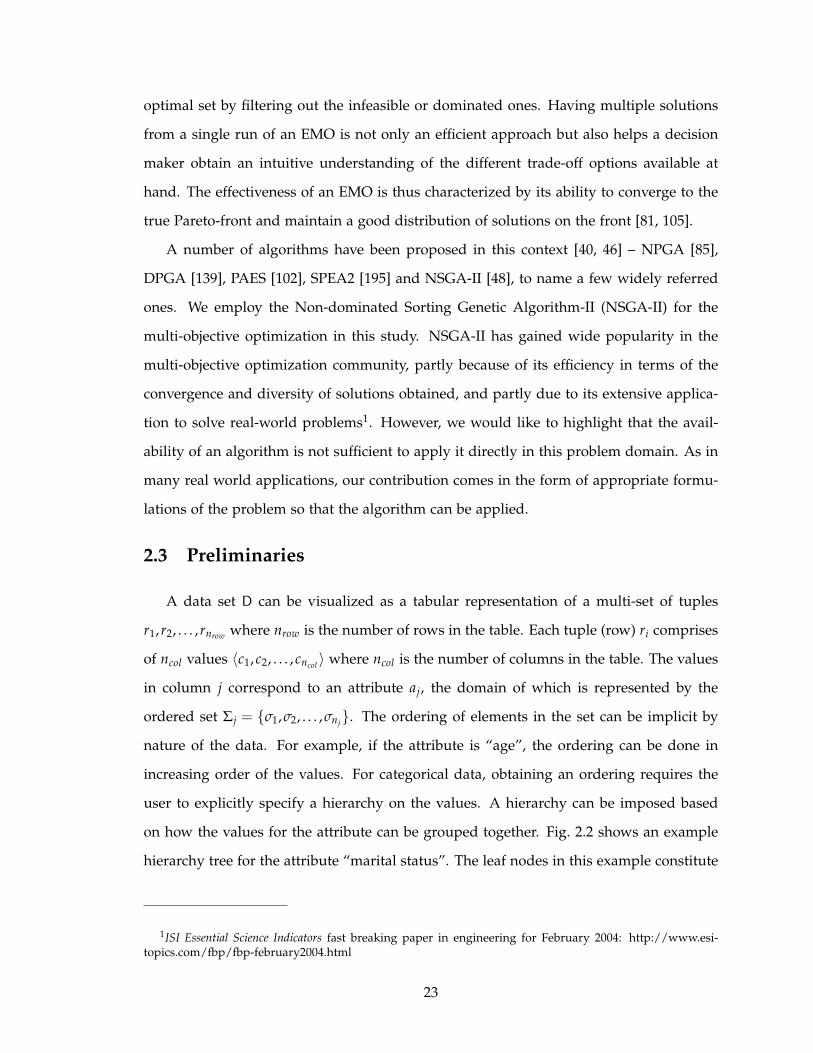
optimal set by filtering out the infeasible or dominated ones. Having multiple solutions
from a single run of an EMO is not only an efficient approach but also helps a decision
maker obtain an intuitive understanding of the different trade-off options available at
hand. The effectiveness of an EMO is thus characterized by its ability to converge to the
true Pareto-front and maintain a good distribution of solutions on the front [81, 105].
A number of algorithms have been proposed in this context [40, 46] – NPGA [85],
DPGA [139], PAES [102], SPEA2 [195] and NSGA-II [48], to name a few widely referred
ones. We employ the Non-dominated Sorting Genetic Algorithm-II (NSGA-II) for the
multi-objective optimization in this study. NSGA-II has gained wide popularity in the
multi-objective optimization community, partly because of its efficiency in terms of the
convergence and diversity of solutions obtained, and partly due to its extensive applica-
tion to solve real-world problems1. However, we would like to highlight that the avail-
ability of an algorithm is not sufficient to apply it directly in this problem domain. As in
many real world applications, our contribution comes in the form of appropriate formu-
lations of the problem so that the algorithm can be applied.
2.3 Preliminaries
A data set D can be visualized as a tabular representation of a multi-set of tuples
r1,r2, . . . ,rnrow where nrow is the number of rows in the table. Each tuple (row) ri comprises
of ncol values 〈c1, c2, . . . , cncol〉 where ncol is the number of columns in the table. The values
in column j correspond to an attribute aj, the domain of which is represented by the
ordered set Σj = {σ1,σ2, . . . ,σnj}. The ordering of elements in the set can be implicit by
nature of the data. For example, if the attribute is “age”, the ordering can be done in
increasing order of the values. For categorical data, obtaining an ordering requires the
user to explicitly specify a hierarchy on the values. A hierarchy can be imposed based
on how the values for the attribute can be grouped together. Fig. 2.2 shows an example
hierarchy tree for the attribute “marital status”. The leaf nodes in this example constitute
1ISI Essential Science Indicators fast breaking paper in engineering for February 2004: http://www.esi-topics.com/fbp/fbp-february2004.html
23
Marital
Status
Not Married Married
Once
Married
Never
Married
Spouse
Absent
Spouse
Present
AF−spouseCiv−spouseDivorced Widowed Separated
1 2 3
4 5
6 7
Figure 2.2: Hierarchy tree for the marital status attribute. Numbering on the leaf nodesindicate their ordering in Σmarital status.
the actual values that the attribute can take. The ordering for these values can be assigned
based on the order in which the leaf nodes are reached in a pre-order traversal of the
hierarchy tree [92].
A generalization Gj for an attribute aj is a partitioning of the set Σj into ordered sub-
sets 〈Σj1 ,Σj2 , . . . ,ΣjP〉 which preserves the ordering in Σj, i.e. if σa appears before σb in
Σj then, for σa ∈ Σjl and σb ∈ Σjm , l ≤ m. Further, every element in Σj must appear in
exactly one subset and the elements in the subsets maintain the same ordering as in Σj.
For the “age” attribute having values in the range of [10,90], a possible generalization
can be 〈{[10,30]},{(30,50]},{(50,70]},{(70,90]}〉. A possible generalization for the “mar-
ital status” attribute can be 〈{Not Married}, {spouse-absent}, {civ-spouse}, {AF-spouse}〉. It is
important to note that generalizations for categorical data is dependent on how the hier-
archy is specified for it. Further, generalizations are restricted to only those that respect
the hierarchy. The generalization is said to be constrained in such a case. For example,
the generalization 〈{Never Married, Divorced}, {Widowed, Separated}, {Married}〉 is not valid
for “marital status” since the hierarchy tree specifies that the values {Divorced, Widowed,
Separated} can only be generalized as Once-Married, if at all.
Note that the number of partitions (or groups) of an attribute domain, i.e. P, signifies
the extent of generalization that will be performed for the attribute. If P = 1 then all values
of the attribute will be represented by the same subset, in which case all information in
24

that attribute is lost. On the other extreme, if P = |Σj| for attribute aj then every value
will map to its own unique subset (no generalization) and all information in the attribute
will be maintained in the original form.
Given the generalizations G1, G2, . . . , Gncol, the data set D can be transformed to the
anonymized data set D′ by replacing each value v at row i and column j in D by Gj(v),
where Gj(v) gives the index of the subset to which v belongs to in the generalization Gj.
Note that if a particular generalization Gj is equal to the domain of values Σj, all values
of the corresponding attribute will be transformed to the same subset index 1, in which
case all information in that attribute is lost and the cell is suppressed.
2.3.1 k–Anonymity
Tuples in D whose subset indices are equal in every column of D′ can be grouped
together into QI-groups or equivalence classes. In other words, a QI-group collects all tu-
ples in D that has the same generalized form for the quasi-identifiers. The k–anonymity
problem is then defined as follows.
Definition 2.3 k–ANONYMITY PROBLEM. Given a data set D, find a set of generaliza-
tions for the attributes in D such that the QI-groups induced by anonymizing D using the
generalizations are all of size at least k.
The problem can also be explained as obtaining the generalizations under which every
tuple in D′ is same as at least k − 1 other tuples. Thus, a higher value of k evaluates to a
lower chance of privacy breach.
2.3.2 ℓ–Diversity
The set of attributes can be divided into sensitive and non-sensitive classes. A sensitive
attribute is one whose value must not be revealed (or get revealed) for any tuple in the
data set. All other attributes are considered non-sensitive. Then, the ℓ–diversity principle
says that every QI-group should contain at least ℓ “well-represented” values for a sensitive
attribute [120]. The principle can be instantiated in many different forms depending on
the meaning of “well-represented”.
25

Let as be a sensitive attribute in a data set with the domain of values Σs = {σ1,σ2, . . . ,σns}.
Further, let Q1, . . . , Qp be the QI-groups induced by a generalization. If c(σ)j,where σ ∈Σs, denotes the count of the number of tuples with the sensitive attribute value σ in Qj,
then one possible instantiation of the ℓ–diversity problem can be stated as follows.
Definition 2.4 ℓ–DIVERSITY PROBLEM. Given a data set D, find a set of generalizations
for the attributes in D such that for each QI-group induced by anonymizing D using the
generalizations, the relation
c(σ)j
|Qj|≤ 1
ℓ(2.2)
holds for all σ ∈ Σs and j = 1, . . . , p.
In other words, the ℓ–diversity property guarantees that a sensitive attribute value
cannot be associated with a particular tuple with a probability more than 1/ℓ. The higher
the value of ℓ, the better is the privacy. Although this instantiation underlines the essence
of the ℓ–diversity principle, two other formulations have been suggested in the original
work. One of them is to assure that the entropy of each QI-group, defined as
Entropy(Qj) = − ∑σ∈Σs
c(σ)j
|Qj|log
(
c(σ)j
|Qj|
)
, (2.3)
is at least logℓ. This requires that the entropy of the whole table is at least logℓ which
may be difficult to ensure when a few values appear more frequently than others. Hence,
another instantiation makes sure that the most frequent sensitive values do not appear too
frequently in a QI-group and the less frequent values do not occur rarely. This is called
recursive (c,ℓ)–diversity. If m is the number of sensitive attribute values in a QI-group and
ri is the count of the ith most frequent value in the QI-group, then the QI-group is said
to be recursive (c,ℓ)–diverse if r1 < c(rℓ,rℓ+1, . . . ,rm). Every QI-group must be recursive
(c,ℓ)–diverse for a table to have recursive (c,ℓ)–diversity. The nature of the instantiation is
not the focus of this work but the parameters involved in it. We shall use the instantiation
given in Def. 2.4 to demonstrate our methodology.
26
2.3.3 (k,ℓ)–Safe
At this stage, we introduce the concept of a (k,ℓ)–safe anonymization. Along the
lines of models such as general (α,k)–anonymity [181] and p–sensitive k–anonymity
[173], a (k,ℓ)–safe data set incorporates the benefits of k–anonymity and ℓ–diversity in
an anonymization. From a data publisher’s perspective, it is meaningful since it allows
one to ascertain the presence of the privacy guards obtainable from both k–anonymity
and ℓ–diversity. A high k value in this case prohibits the likelihood of linking attacks,
while a high ℓ value prohibits the likelihood of homogeneity and background knowledge
attacks. When multiple types of attacks are possible on a data set, a data publisher would
most certainly want to safeguard the published data against as many of them as possible.
Definition 2.5 (k,ℓ)–SAFE. An anonymized data set is (k,ℓ)–safe if it is k–anonymous
and ℓ–diverse.
The distinction between (α,k)–anonymity and (k,ℓ)–safety lies in the representation
of attribute disclosure risks. (α,k)–Anonymity requires that a possible value of a sensi-
tive attribute should appear with a relative frequency not greater than α in a QI-group,
also called the α-deassociation property. The motivation behind this representation is to
prohibit the frequent occurrence of certain highly sensitive values in a QI-group, such
as “HIV” in a disease data set, and hence control the inference probability on these val-
ues. (k,ℓ)–Safe, on the other hand, uses an instantiation of ℓ–diversity that specifies the
minimum number of distinct values of a sensitive attribute that must appear in a QI-
group. This is very much similar to p–sensitive k–anonymity. Nonetheless, ℓ–diversity
can very well be instantiated in conformation to α-deassociation or any of the other forms
mentioned in the original work. Hence, we use the generic name (k,ℓ)–safe.
2.3.4 Optimal generalization
The trivial generalization Gj = 〈Σj〉, where j = 1, . . . , ncol , can provide the highest
k and the highest ℓ value. However, such a generalization results in an anonymized
data set with little or no statistically significant information. It is often desired that the
anonymized data set be useful for some level of statistical analysis. In such a case, the
27
decision on the value of k (or ℓ) is subjected to a loss measurement of the information
content in the anonymized data set, usually done using some metric. An optimization
problem defined for a given value of k (or ℓ) tries to find the generalizations that result in
a minimal loss given by the metric.
Depending on the distribution of data values in a data set, obtaining a generalization
with an acceptable loss for a given value of k (or ℓ) may or may not be possible. This
happens when the data set has outliers that cannot be anonymized without overly gener-
alizing the remaining data points. Therefore, it becomes a requirement that such outliers
be suppressed completely in order to avoid an over-generalization. A suppressed tuple
is usually considered nonexistent in the data set. The loss metric can account for this
suppression in its loss measurement.
When suppression is allowed, an anonymized data set can be made k–anonymous by
suppressing all tuples that belong to QI-groups of size less than k. Similar suppression
methods can be used to enforce the ℓ–diversity property. The case without suppression
can be modeled into the earlier scenario (with suppression) by assigning an infinite loss
when suppression is performed [16]. However, it should be noted that the presence of
outliers will always force the requirement for suppression, in which case the loss measure-
ment will always become infinite. Furthermore, even though suppression is not allowed,
such an approach enforces the k–anonymity (or ℓ–diversity) property by suppressing out-
liers. If all the data points in the data set must stay in the anonymized data set as well,
the desired privacy properties cannot be ascertained even after adopting such modeling.
We now proceed to formulate a set of four problems, the solutions to which provide an
in-depth understanding of the publisher’s dilemma. This is accompanied by an example
that illustrates the scope of the problem and the corresponding analysis we envisage to
help alleviate the problem.
2.4 Problem Formulation
As stated in the previous section, an optimization algorithm requires a numeric repre-
sentation of the information loss associated with a particular generalization. A quantified
loss value enables the optimization algorithm to compare two generalizations for their
28

relative effectiveness. Loss (cost) metrics assign some notion of penalty to each tuple
whose data values get generalized or suppressed, thereby reflecting the total information
lost in the anonymization process. In this work, we use the general loss metric proposed
by Iyengar [92]. The general loss metric computes a normalized information loss for each
of the data values in an anonymized data set. Note that our use of the general loss metric
is only a matter of choice. The optimization process we use is a black box method and is
not affected by how information loss is measured.
2.4.1 Generalization loss
Consider the data value vi,j at row i and column j in the data set D. The general loss
metric assigns a penalty to this data value based on the extent to which it gets generalized
during anonymization. Let gi,j = Gj(vi,j) be the index of the subset to which vi,j belongs
in the generalization Gj, i.e. vi,j ∈ Σjgi,j. The penalty for information loss associated with
vi,j is then given as follows.
loss(vi,j) =|Σjgi,j
| − 1
|Σj| − 1(2.4)
For categorical data, the loss for a cell is proportional to the number of leaf nodes
rooted at an internal node (the generalized node) of the hierarchy tree. The loss attains
a maximum value of one when the cell is suppressed (Gj = 〈Σj〉), or in other words,
when the root of the tree is the generalized node. Subtracting one ensures that a non-
generalized value incurs zero loss since the cardinality of the subset to which it belongs
would be one. The generalization loss is then obtained as the total loss over all the data
values in the data set.
GL =nrow
∑i=1
ncol
∑j=1
loss(vi,j) (2.5)
2.4.2 Suppression loss
Although the loss due to suppression can be incorporated into the generalization loss,
we decide to separate it out for the purpose of our study. When a row is suppressed, all
cells in the row are suppressed irrespective of the generalization. Each cell thereby incurs
29
a loss of one (consequence of Eq. (2.4)). Let nsup be the number of rows to be suppressed
in the data set. The suppression loss for the data set is then given as
SL = ncol × nsup. (2.6)
2.4.3 The multi-objective problems
The multi-objective problems we formulate in this chapter are intended to analyze
and understand the trade-off nature of the generalization and suppression losses when
k (or ℓ) is varied. A single objective optimization problem to minimize the generaliza-
tion loss with a fixed k (or ℓ) will require multiple runs of the algorithm to understand
this trade-off. By adopting a multi-objective approach, we can generate a fairly good
approximation of the Pareto-front in a single run of the algorithm, which in turn pro-
vides us with the requisite information to make a better decision on the choice of k (or
ℓ) for anonymization. In this context, we formulate a series of multi-objective problems
for our analysis. Although, Problems A, B, and C are described for the k–anonymity
problem, similar analysis can be carried out for ℓ–diversity as well. Problem D caters to
(k,ℓ)–safety.
Also note that the problems under study are not intended to provide the data pub-
lisher a “best” value for the parameter(s) involved in the anonymization technique. Rather,
we put forward a methodology to understand the implications of choosing a particular
value for the parameter(s) in terms of the resulting privacy and the data utility. Hence,
we shall often find that one or more solutions returned by the optimization process are
trivially not acceptable either in terms of privacy or utility, or in some cases, both. It is not
our objective to consider such solutions as degenerate and prohibit them from appearing
in the solution set. After all, they are also a manifestation of the privacy-utility trade-off,
which would likely be never selected as a choice by the data publisher, but still possible.
For example, an extreme solution will correspond to a situation where every tuple in
the data set belongs to its own QI-group, thereby resulting in no privacy and maximum
utility. Another extremity is the case where all tuples are grouped together in a single
QI-group resulting in maximum privacy but no utility. One cannot deny the fact that in
the case of privacy versus utility, both of these are possible solutions. The multi-objective
30
optimization formulations do not incorporate the required domain knowledge to identify
these extremities (or other such solutions) as being impractical. Only the data publisher
has the requisite knowledge to make such identification and disregard such solutions.
This is often a post-optimization process. Hence, the focus in the solution set should be
concentrated on the practical solutions reported by the method. Quite often there will be
more than one, and the methodology provides the data publisher a distinctive picture of
the differences arising between privacy and utility when it makes a decision to choose
one solution over another.
2.4.3.1 Problem A: Zero suppression
The presence of outliers in a data set makes it difficult to find a suitable value of k
when suppression of data is not allowed. In the first problem formulation, we strictly
adhere to the requirement that no tuple in the data set can be deleted. Intuitively, such
a strict requirement makes the k–anonymity problem insensible to solve for a given k as
the optimization algorithm will be forced to overly generalize the data set in its effort to
ensure k–anonymity. The outliers usually belong to very small QI-groups and the only
way to merge them into a bigger one is by having more generalization.
Although solving the k–anonymity problem is not possible in terms of its strict defi-
nition, it is worth noting that a generalization can still affect the distribution of the size of
the QI-groups even when suppression is not allowed.
Let us define an equi-privacy class Ei as the set of all tuples in QI-groups of size i.
Hence an arbitrary equi-privacy class Ei shall contain all tuples that are i–anonymous.
For brevity, we shall use the term “small equi-privacy class” or “equi-privacy class with
lower i” to mean equi-privacy classes Eis with relative smaller i than that used in the term
“large equi-privacy class” or “equi-privacy class with high i”. An ideal generalization
would then maintain an acceptable level of loss and also keep the number of rows in
equi-privacy classes with lower i relatively fewer than in equi-privacy classes with higher
i. Although this does not guarantee complete k–anonymity, the issue of privacy breach
can be solved to a limited extent by reducing the probability that a randomly chosen row
would belong to a small QI-group.
31
With this motivation, we define the weighted-k–anonymity multi-objective problem to
find generalizations that produce a high weighted-k value and low generalization loss.
Each equi-privacy class Ei defines a privacy level for its member tuples – every tuple in
the equi-privacy class is the same as exactly i − 1 other tuples in the same class and has
a probability of breach equal to 1/i. For an intuitive comparison, the k in k–anonymity is
the smallest value of i such that Ei is non-empty.
The weighted-k for a particular generalization inducing the equi-privacy classes E1, E2,
. . . , Enrow on the anonymized data set is then obtained as follows.
kweighted =∑
nrowi=1 (i · |Ei|)∑
nrowi=1 |Ei|
(2.7)
Refer to the concept of local recoding [168] in this context. A local recoding scheme
produces a k–anonymization by using an individual generalization function (instead of
a global one) for each tuple in the data set. This is a more powerful scheme compared
to having a single generalization function since outliers can be easily suppressed without
the drawbacks of an over generalization. Hence, data utility can be maintained. The
weighted-k–anonymity based generalization is orthogonal to this concept in certain ways.
Local recoding explores the domain of generalization functions and uses multiple points
in this domain to recode different subsets of the data set differently. This puts outliers in
their own subset(s), thereby making it easy to enforce a given minimum QI-group size.
Weighted-k–anonymity, on the other hand, works with a single generalization function
and, instead of trying to enforce a fixed minimum QI-group size, it flexibly creates QI-
groups of different sizes with no minimum size constraint. The outliers then must lie
in smaller QI-groups in order to maximize data utility. The similarity between the two
methods is that the outliers get treated differently than the rest of the data set.
The weighted-k is an estimation of the QI-group size distribution, and hence, although
the chances are very rare, a high value need not always indicate that there exists no
tuple in the anonymized data set appearing in its original form, i.e. in QI-groups of size
one. Since the method results in an average case analysis, rather than worst case, such
generalizations can appear. We present three justifications to the use of average privacy
in multi-objective analysis, rather than worst case privacy.
32

First, the use of minimum privacy induces a very dense search space for the purpose
of multi-objective optimization. Let us assume that an encoding for a candidate general-
ization is represented by n bits, resulting in a search space of size 2n. Given that a data
set of size N can be generalized to have possible k values in the range of 1 (no general-
ization) to N (all suppressed), on the average, there are 2n/N points on the search space
that will map to the same k value, i.e. these points will not be distinguishable from each
other on measures of privacy. Even with the modest assumption of n = 50 and N = 106,
this average number is in the magnitude of 109. In addition, this average estimate is only
wishful thinking. The mapping will be much denser for smaller k values. On one side,
most points in the search space will induce very similar (and low) privacy levels, while
on the other, finding one with significantly higher values of k will be extremely difficult.
We can say that there is very little diversity in the search points when using minimum
privacy as an objective to maximize. This diversity is a desired property to analyze trade-
offs. Using average privacy introduces diversity since the distribution of QI-group sizes
have significant avenues to be different for different possible generalizations.
Second, in the context of multi-objective optimization, we cannot exclude solutions
with QI-group sizes of one since they just represent an aspect of the privacy-utility trade-
off. Ideally, if another generalization with the same (or better) level of utility but without
the isolated tuples exists, i.e. the tuples are embedded in QI-groups of size more than
one, then it would result in a higher value of weighted-k. Moreover, such a generalization
will dominate the previous one and replace it from the solution set.
Third, conformation to worst-case privacy requirements can be achieved once the
trade-off front is approximated. Enforcements of worst-case requirements such as min-
imum QI-group size is essential during optimization in a single objective framework.
However, when performing a multi-objective analysis, these enforcements are part of the
post-optimization strategy. The requirement essentially helps filter out solutions from the
Pareto-front approximated in the analysis. In fact, a minimum utility level can also be
one such requirement.
Note that in most cases not all QI-groups with all possible sizes will be generated.
Hence, certain equi-privacy classes will be empty. The weighted-k value provides a suffi-
33

ciently good estimate of the distribution of the QI-group sizes. A high weighted-k value
implies that QI-groups with bigger sizes are relatively more abundant than those with
very few tuples. The multi-objective problem is then formulated as finding the general-
ization that maximizes the weighted-k and minimizes the generalization loss for a given
data set.
2.4.3.2 Problem B: Maximum allowed suppression
In this problem, we enable suppression and allow the user to specify an acceptable
fraction η of the maximum suppression loss possible (nrow · ncol). Such an approach im-
poses a hard limit on the number of suppressions allowed [16]. However, unlike earlier
approaches, by allowing the user to specify a suppression loss limit independent of k, the
optimization procedure can be made to explore the trade-off properties of k and general-
ization loss within the constraint of the imposed suppression loss limitation.
When suppression is allowed within a user specified limit, all tuples belonging to the
equi-privacy classes E1, . . . , Ed can be suppressed, where d satisfies the relation
d
∑i=1
(|Ei| · ncol) ≤ η · nrow · ncol <
d+1
∑i=1
(|Ei| · ncol). (2.8)
Thereafter, the resulting data set becomes (d + 1)–anonymous and also satisfies the
suppression loss constraint. We can now define our optimization problem as finding the
generalization that maximizes d and minimizes the generalization loss. The problem can
also be viewed as the maximization of k and minimization of GL satisfying the constraint
SL ≤ η · nrow · ncol . Note that the problem formulation allows the optimization procedure
to find generalizations that create equi-privacy classes with lower i’s of smaller size and
thereby increase d.
2.4.3.3 Problem C: Any suppression
The third problem is formulated as an extension of the second one where the user
does not provide a maximum limit on the suppression loss. The challenge here is the
computation of k, GL and SL for a generalization without having a baseline from which
to start. Since the three quantities are dependent on each other for their computation,
it is important that we have some base k value to proceed. We adopt the weighted-k
34
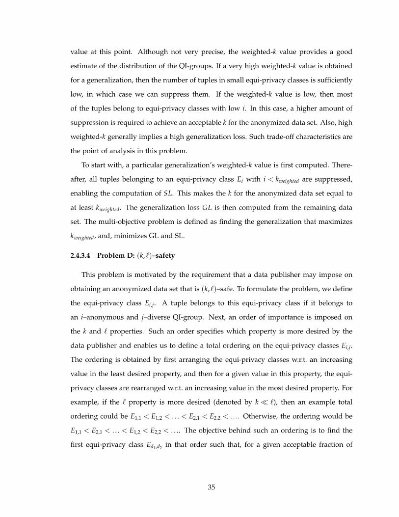
value at this point. Although not very precise, the weighted-k value provides a good
estimate of the distribution of the QI-groups. If a very high weighted-k value is obtained
for a generalization, then the number of tuples in small equi-privacy classes is sufficiently
low, in which case we can suppress them. If the weighted-k value is low, then most
of the tuples belong to equi-privacy classes with low i. In this case, a higher amount of
suppression is required to achieve an acceptable k for the anonymized data set. Also, high
weighted-k generally implies a high generalization loss. Such trade-off characteristics are
the point of analysis in this problem.
To start with, a particular generalization’s weighted-k value is first computed. There-
after, all tuples belonging to an equi-privacy class Ei with i < kweighted are suppressed,
enabling the computation of SL. This makes the k for the anonymized data set equal to
at least kweighted. The generalization loss GL is then computed from the remaining data
set. The multi-objective problem is defined as finding the generalization that maximizes
kweighted, and, minimizes GL and SL.
2.4.3.4 Problem D: (k,ℓ)–safety
This problem is motivated by the requirement that a data publisher may impose on
obtaining an anonymized data set that is (k,ℓ)–safe. To formulate the problem, we define
the equi-privacy class Ei,j. A tuple belongs to this equi-privacy class if it belongs to
an i–anonymous and j–diverse QI-group. Next, an order of importance is imposed on
the k and ℓ properties. Such an order specifies which property is more desired by the
data publisher and enables us to define a total ordering on the equi-privacy classes Ei,j.
The ordering is obtained by first arranging the equi-privacy classes w.r.t. an increasing
value in the least desired property, and then for a given value in this property, the equi-
privacy classes are rearranged w.r.t. an increasing value in the most desired property. For
example, if the ℓ property is more desired (denoted by k ≪ ℓ), then an example total
ordering could be E1,1 < E1,2 < . . . < E2,1 < E2,2 < . . .. Otherwise, the ordering would be
E1,1 < E2,1 < . . . < E1,2 < E2,2 < . . .. The objective behind such an ordering is to find the
first equi-privacy class Ed1,d2in that order such that, for a given acceptable fraction of
35

Table 2.1: Original data set T.
Tuple ID Age Marital Status
1 15 Never Married
2 17 Never Married
3 20 Civ-Spouse
4 26 AF-Spouse
5 28 AF-Spouse
6 30 Civ-Spouse
7 30 AF-Spouse
suppression loss η,
k ≪ ℓ : ncol · (d1−1
∑i=1
L∑j=1
|Ei,j| +d2
∑j=1
|Ed1,j|) > η · nrow · ncol (2.9)
ℓ ≪ k : ncol · (K∑i=1
d2−1
∑j=1
|Ei,j| +d1
∑i=1
|Ei,d2|) > η · nrow · ncol , (2.10)
where L and K are the maximum obtainable values for ℓ and k respectively for the
given data set. In other words, all tuples belonging to equi-privacy classes prior to Ed1,d2
in the order can be suppressed without violating the suppression loss constraint. The
data set then becomes (d1,d2)–safe and satisfies the suppression loss constraint. The
multi-objective optimization problem is then defined as finding the generalization that
maximizes d1, maximizes d2, and minimizes GL.
2.4.4 Illustrative example
Before discussing the solution methodology, we present a small example that illus-
trates the scope of these problems and type of analysis that we envisage to evolve from
our solution. Consider the data tuples shown in Table 2.1. Obtaining a 3-anonymous
generalization would require tuples 1 and 2 to be in an equi-privacy class with one or
more of the other tuples. Given the hierarchy tree of the “marital status” attribute (see
Fig. 2.2), such a generalization would result in the suppression of the attribute, since the
only ancestor node common to the values is the root node of the hierarchy tree. Tuples
1 and 2 act as outliers in this case which prohibit obtaining 3-anonymity without overly
generalizing the “marital status” attribute.
36
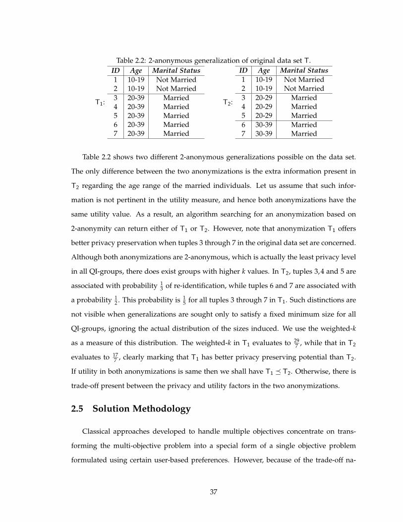
Table 2.2: 2-anonymous generalization of original data set T.
T1:
ID Age Marital Status
1 10-19 Not Married2 10-19 Not Married
3 20-39 Married4 20-39 Married5 20-39 Married6 20-39 Married7 20-39 Married
T2:
ID Age Marital Status
1 10-19 Not Married2 10-19 Not Married
3 20-29 Married4 20-29 Married5 20-29 Married
6 30-39 Married7 30-39 Married
Table 2.2 shows two different 2-anonymous generalizations possible on the data set.
The only difference between the two anonymizations is the extra information present in
T2 regarding the age range of the married individuals. Let us assume that such infor-
mation is not pertinent in the utility measure, and hence both anonymizations have the
same utility value. As a result, an algorithm searching for an anonymization based on
2-anonymity can return either of T1 or T2. However, note that anonymization T1 offers
better privacy preservation when tuples 3 through 7 in the original data set are concerned.
Although both anonymizations are 2-anonymous, which is actually the least privacy level
in all QI-groups, there does exist groups with higher k values. In T2, tuples 3,4 and 5 are
associated with probability 13 of re-identification, while tuples 6 and 7 are associated with
a probability 12 . This probability is 1
5 for all tuples 3 through 7 in T1. Such distinctions are
not visible when generalizations are sought only to satisfy a fixed minimum size for all
QI-groups, ignoring the actual distribution of the sizes induced. We use the weighted-k
as a measure of this distribution. The weighted-k in T1 evaluates to 297 , while that in T2
evaluates to 177 , clearly marking that T1 has better privacy preserving potential than T2.
If utility in both anonymizations is same then we shall have T1 � T2. Otherwise, there is
trade-off present between the privacy and utility factors in the two anonymizations.
2.5 Solution Methodology
Classical approaches developed to handle multiple objectives concentrate on trans-
forming the multi-objective problem into a special form of a single objective problem
formulated using certain user-based preferences. However, because of the trade-off na-
37
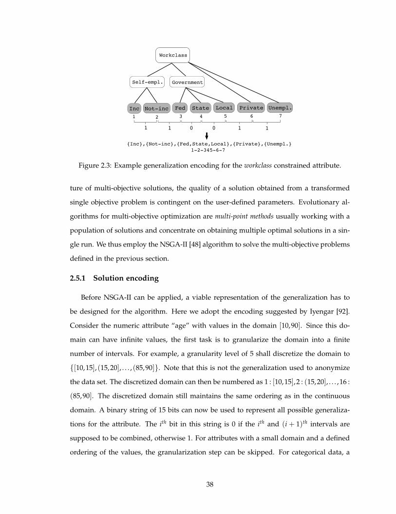
Figure 2.3: Example generalization encoding for the workclass constrained attribute.
ture of multi-objective solutions, the quality of a solution obtained from a transformed
single objective problem is contingent on the user-defined parameters. Evolutionary al-
gorithms for multi-objective optimization are multi-point methods usually working with a
population of solutions and concentrate on obtaining multiple optimal solutions in a sin-
gle run. We thus employ the NSGA-II [48] algorithm to solve the multi-objective problems
defined in the previous section.
2.5.1 Solution encoding
Before NSGA-II can be applied, a viable representation of the generalization has to
be designed for the algorithm. Here we adopt the encoding suggested by Iyengar [92].
Consider the numeric attribute “age” with values in the domain [10,90]. Since this do-
main can have infinite values, the first task is to granularize the domain into a finite
number of intervals. For example, a granularity level of 5 shall discretize the domain to
{[10,15], (15,20], . . . , (85,90]}. Note that this is not the generalization used to anonymize
the data set. The discretized domain can then be numbered as 1 : [10,15],2 : (15,20], . . . ,16 :
(85,90]. The discretized domain still maintains the same ordering as in the continuous
domain. A binary string of 15 bits can now be used to represent all possible generaliza-
tions for the attribute. The ith bit in this string is 0 if the ith and (i + 1)th intervals are
supposed to be combined, otherwise 1. For attributes with a small domain and a defined
ordering of the values, the granularization step can be skipped. For categorical data, a
38
Figure 2.4: One generation of NSGA-II.
similar encoding can be obtained once an ordering on the domain values is imposed as
discussed in Section 2.3. Fig. 2.3 shows an example generalization encoding for a “work-
class” attribute. The individual encoding for each attribute is concatenated to create the
overall encoding for a generalization involving all attributes.
2.5.2 NSGA-II
Similar to a simple genetic algorithm, NSGA-II starts with a population P0 of Npop ran-
dom generalizations. A generation index t = 0,1, . . . , GenMAX keeps track of the number
of iterations of the algorithm. Each trial generalization is used to create the anonymized
data set and the corresponding values of the quantities to be optimized are calculated.
Each generation of NSGA-II then proceeds as follows. An offspring population Qt is
first created from the parent population Pt by applying the usual genetic operations of
selection, crossover and mutation [75]. For constrained attributes, a special crossover op-
erator is used as discussed in the next subsection. The offspring population also gets
evaluated. The parent and offspring populations are then combined to form a popula-
tion Rt = Pt ∪ Qt of size 2Npop. A non-dominated sorting is applied to Rt to rank each
solution based on the number of solutions that dominate it. Rank 1 solutions are all non-
dominated solutions in the population. A rank r solution is only dominated by solutions
of lower ranks.
39
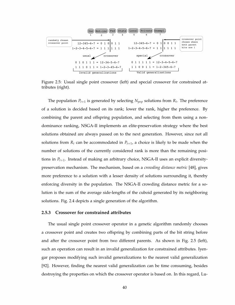
Figure 2.5: Usual single point crossover (left) and special crossover for constrained at-tributes (right).
The population Pt+1 is generated by selecting Npop solutions from Rt. The preference
of a solution is decided based on its rank; lower the rank, higher the preference. By
combining the parent and offspring population, and selecting from them using a non-
dominance ranking, NSGA-II implements an elite-preservation strategy where the best
solutions obtained are always passed on to the next generation. However, since not all
solutions from Rt can be accommodated in Pt+1, a choice is likely to be made when the
number of solutions of the currently considered rank is more than the remaining posi-
tions in Pt+1. Instead of making an arbitrary choice, NSGA-II uses an explicit diversity-
preservation mechanism. The mechanism, based on a crowding distance metric [48], gives
more preference to a solution with a lesser density of solutions surrounding it, thereby
enforcing diversity in the population. The NSGA-II crowding distance metric for a so-
lution is the sum of the average side-lengths of the cuboid generated by its neighboring
solutions. Fig. 2.4 depicts a single generation of the algorithm.
2.5.3 Crossover for constrained attributes
The usual single point crossover operator in a genetic algorithm randomly chooses
a crossover point and creates two offspring by combining parts of the bit string before
and after the crossover point from two different parents. As shown in Fig. 2.5 (left),
such an operation can result in an invalid generalization for constrained attributes. Iyen-
gar proposes modifying such invalid generalizations to the nearest valid generalization
[92]. However, finding the nearest valid generalization can be time consuming, besides
destroying the properties on which the crossover operator is based on. In this regard, Lu-
40

nacek et al. propose a special crossover operator that always creates a valid offspring for
constrained attributes [118]. Instead of randomly choosing a crossover point, their opera-
tor forces the crossover point to be chosen at a location where the bit value is one for both
parents. By doing so, both parts (before and after the crossover point) of both parents
can be guaranteed to be valid generalizations individually, which can then be combined
without destroying the hierarchy requirement. Fig. 2.5 (right) shows an instance of this
operator.
2.5.4 Population initialization
In order to be able to use Lunacek et al.’s crossover operator, the validity of the parent
solutions must be guaranteed. This implies that the initial population that NSGA-II starts
with must contain all valid generalizations for the constrained attributes. For a given
hierarchy tree, we use the following algorithm to generate valid generalizations for the
constrained attributes in the initial population.
Starting from the root node, a node randomly decides if it would allow its subtrees to
be distinguishable. If it decides not to then all nodes in its subtrees are assigned the same
identifier. Otherwise the root of each subtree receives a unique identifier. The decision is
then translated to the root nodes of its subtrees and the process is repeated recursively.
Once all leaf nodes are assigned an identifier, two adjacent leaf nodes in the imposed
ordering are combined only if they have the same identifier. Since a parent node always
make the decision if child nodes will be combined or not, all generalizations so produced
will be valid.
2.5.5 Experimental setup
We apply our methodology to the “adult.data” benchmark data set available from the
UCI machine learning repository [103]. The data was extracted from a census bureau
database and has been extensively used in studies related to k–anonymization. We pre-
pared the data set as described in [16, 92]. All rows with missing values are removed
from the data set to finally have a total of 30162 rows. The attributes “age”, “education”,
“race”, “gender” and “salary class” are kept unconstrained, while the attributes “work-
41
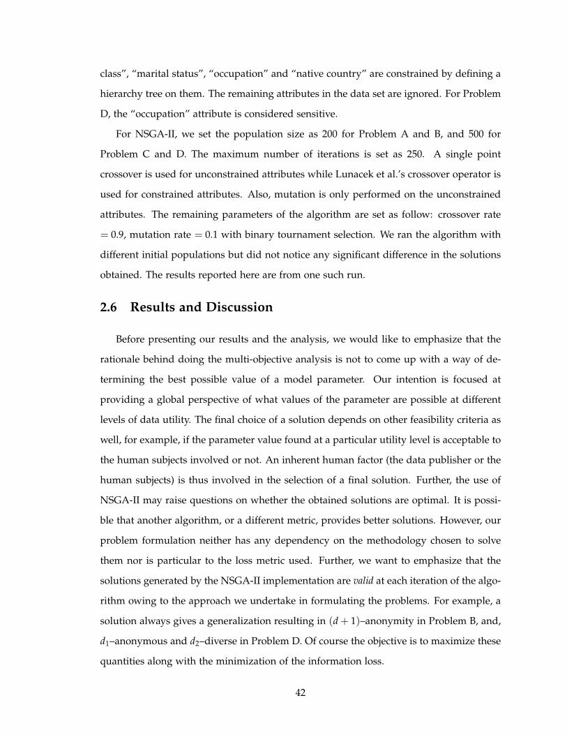
class”, “marital status”, “occupation” and “native country” are constrained by defining a
hierarchy tree on them. The remaining attributes in the data set are ignored. For Problem
D, the “occupation” attribute is considered sensitive.
For NSGA-II, we set the population size as 200 for Problem A and B, and 500 for
Problem C and D. The maximum number of iterations is set as 250. A single point
crossover is used for unconstrained attributes while Lunacek et al.’s crossover operator is
used for constrained attributes. Also, mutation is only performed on the unconstrained
attributes. The remaining parameters of the algorithm are set as follow: crossover rate
= 0.9, mutation rate = 0.1 with binary tournament selection. We ran the algorithm with
different initial populations but did not notice any significant difference in the solutions
obtained. The results reported here are from one such run.
2.6 Results and Discussion
Before presenting our results and the analysis, we would like to emphasize that the
rationale behind doing the multi-objective analysis is not to come up with a way of de-
termining the best possible value of a model parameter. Our intention is focused at
providing a global perspective of what values of the parameter are possible at different
levels of data utility. The final choice of a solution depends on other feasibility criteria as
well, for example, if the parameter value found at a particular utility level is acceptable to
the human subjects involved or not. An inherent human factor (the data publisher or the
human subjects) is thus involved in the selection of a final solution. Further, the use of
NSGA-II may raise questions on whether the obtained solutions are optimal. It is possi-
ble that another algorithm, or a different metric, provides better solutions. However, our
problem formulation neither has any dependency on the methodology chosen to solve
them nor is particular to the loss metric used. Further, we want to emphasize that the
solutions generated by the NSGA-II implementation are valid at each iteration of the algo-
rithm owing to the approach we undertake in formulating the problems. For example, a
solution always gives a generalization resulting in (d + 1)–anonymity in Problem B, and,
d1–anonymous and d2–diverse in Problem D. Of course the objective is to maximize these
quantities along with the minimization of the information loss.
42
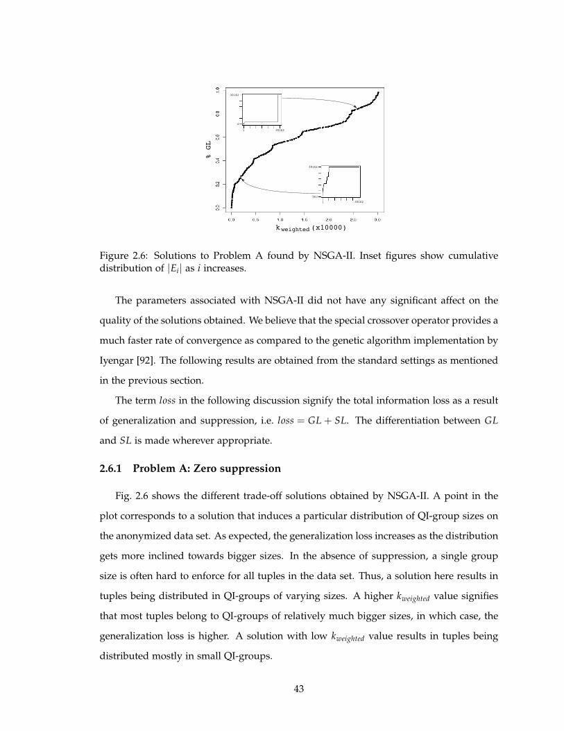
k (x10000)
% GL
weighted
1 30162
4
30162
1 30162
563
30162
Figure 2.6: Solutions to Problem A found by NSGA-II. Inset figures show cumulativedistribution of |Ei| as i increases.
The parameters associated with NSGA-II did not have any significant affect on the
quality of the solutions obtained. We believe that the special crossover operator provides a
much faster rate of convergence as compared to the genetic algorithm implementation by
Iyengar [92]. The following results are obtained from the standard settings as mentioned
in the previous section.
The term loss in the following discussion signify the total information loss as a result
of generalization and suppression, i.e. loss = GL + SL. The differentiation between GL
and SL is made wherever appropriate.
2.6.1 Problem A: Zero suppression
Fig. 2.6 shows the different trade-off solutions obtained by NSGA-II. A point in the
plot corresponds to a solution that induces a particular distribution of QI-group sizes on
the anonymized data set. As expected, the generalization loss increases as the distribution
gets more inclined towards bigger sizes. In the absence of suppression, a single group
size is often hard to enforce for all tuples in the data set. Thus, a solution here results in
tuples being distributed in QI-groups of varying sizes. A higher kweighted value signifies
that most tuples belong to QI-groups of relatively much bigger sizes, in which case, the
generalization loss is higher. A solution with low kweighted value results in tuples being
distributed mostly in small QI-groups.
43

The inset figures in the plot depict the cumulative distribution of the number of tuples
belonging to an equi-privacy class Ei (y-axis) with respect to different i values (x-axis).
The distributions of two extreme solutions corroborate the speculation that a higher gen-
eralization loss must be incurred to assure a greater level of privacy for a larger section
of the data set. Low generalization losses are only possible when most tuples belong to
equi-privacy classes of lower i value.
However, it should be noted that the distributions for the two example solutions are
not complementary in nature. For the solution with lower generalization loss, the distri-
bution has a continuously increasing trend, implying that equi-privacy classes of different
i values exist for the solution. The other solution shows an abrupt increase signifying that
the tuples either belong to equi-privacy classes with very small i or ones with very large
i. The sought balance in the distribution may therefore exist with an acceptable level of
generalization loss.
2.6.2 Problem B: Maximum allowed suppression
Fig. 2.7 shows the trade-off between k and loss in Problem B when a maximum of
10% suppression loss is allowed. Recall that the k value in this problem is d + 1. The
top-leftmost plot shows all the solutions obtained for the problem. Each subsequent plot
(follow arrows) is a magnification of the steepest part in the previous plot. Each plot
shows the presence of locally flat regions where a substantial increase in the k value
does not have a comparatively high increase in the loss. These regions can be of interest
to a data publisher since it allows one to provide higher levels of data privacy without
compromising much on the information content. Also, since the solutions corresponding
to these flat regions evaluate to distantly separated k values, an analysis based on a single
objective formulation with a fixed k shall require a much higher number of runs of the
algorithm to identify such trade-off characteristics.
Interestingly, the trend of the solutions is similar in each plot. The existence of such re-
peated characteristics on the non-dominated front suggests that a data publisher’s choice
of a specific k, no matter how big or small, can have avenues for improvement, specially
when the choice falls in the locally flat regions. A choice of k made on the rising parts
44
k (x10000)
% loss
Figure 2.7: Solutions to Problem B (η = 10%) found by NSGA-II. Top-leftmost plot showsall obtained solutions. Each subsequent plot (follow arrows) is a magnification of a regionof the previous plot.
of the front is seemingly not a good choice since the user would then be paying a high
cost in degraded data quality without getting much improvement on the privacy factor.
The rational decision choice in such a case would be to lower the k value to a flat region
of the front. We observed similar trends in the solutions when the suppression loss was
reduced to a low 1%.
2.6.3 Problem C: Any suppression
The trade-off characteristics in Problem C are depicted in Fig. 2.8. Preliminary obser-
vations from the plot indicate that an increase in generalization loss results in a decrease
in the suppression loss. A similar trend is observed when the k value increases. Since the
k values in this case are computed directly from the weighted-k, an explanation for these
observations is possible. A high generalization loss signifies that most tuples in the data
set belong to large equi-privacy classes, thereby inducing a high weighted-k. This implies
a low accumulation in suppression loss resulting from the deletion of tuples in equi-
privacy classes with i < kweighted. Also, as kweighted increases, the equi-privacy class size
distribution incline more towards the ones with high i values resulting in lesser number
45
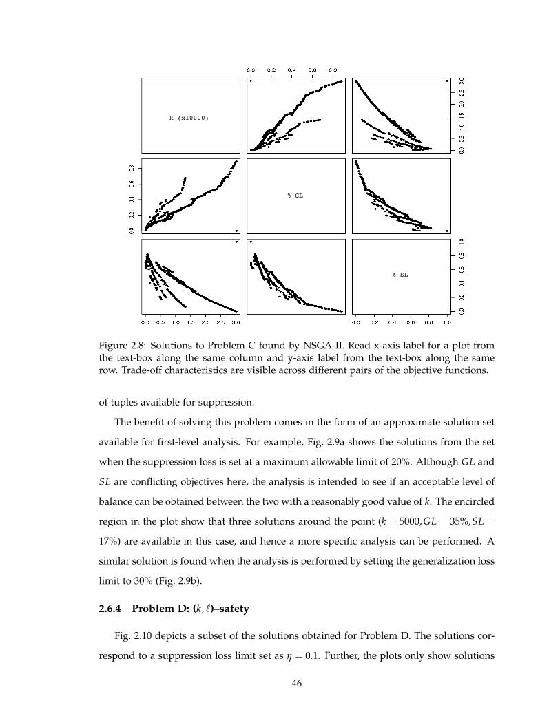
k (x10000)
% GL
% SL
Figure 2.8: Solutions to Problem C found by NSGA-II. Read x-axis label for a plot fromthe text-box along the same column and y-axis label from the text-box along the samerow. Trade-off characteristics are visible across different pairs of the objective functions.
of tuples available for suppression.
The benefit of solving this problem comes in the form of an approximate solution set
available for first-level analysis. For example, Fig. 2.9a shows the solutions from the set
when the suppression loss is set at a maximum allowable limit of 20%. Although GL and
SL are conflicting objectives here, the analysis is intended to see if an acceptable level of
balance can be obtained between the two with a reasonably good value of k. The encircled
region in the plot show that three solutions around the point (k = 5000, GL = 35%,SL =
17%) are available in this case, and hence a more specific analysis can be performed. A
similar solution is found when the analysis is performed by setting the generalization loss
limit to 30% (Fig. 2.9b).
2.6.4 Problem D: (k,ℓ)–safety
Fig. 2.10 depicts a subset of the solutions obtained for Problem D. The solutions cor-
respond to a suppression loss limit set as η = 0.1. Further, the plots only show solutions
46
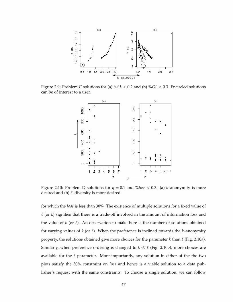
k (x10000)
% SL
% GL
(a) (b)
Figure 2.9: Problem C solutions for (a) %SL < 0.2 and (b) %GL < 0.3. Encircled solutionscan be of interest to a user.
ℓ
k
(a) (b)
Figure 2.10: Problem D solutions for η = 0.1 and %loss < 0.3. (a) k–anonymity is moredesired and (b) ℓ–diversity is more desired.
for which the loss is less than 30%. The existence of multiple solutions for a fixed value of
ℓ (or k) signifies that there is a trade-off involved in the amount of information loss and
the value of k (or ℓ). An observation to make here is the number of solutions obtained
for varying values of k (or ℓ). When the preference is inclined towards the k–anonymity
property, the solutions obtained give more choices for the parameter k than ℓ (Fig. 2.10a).
Similarly, when preference ordering is changed to k ≪ ℓ (Fig. 2.10b), more choices are
available for the ℓ parameter. More importantly, any solution in either of the the two
plots satisfy the 30% constraint on loss and hence is a viable solution to a data pub-
lisher’s request with the same constraints. To choose a single solution, we can follow
47
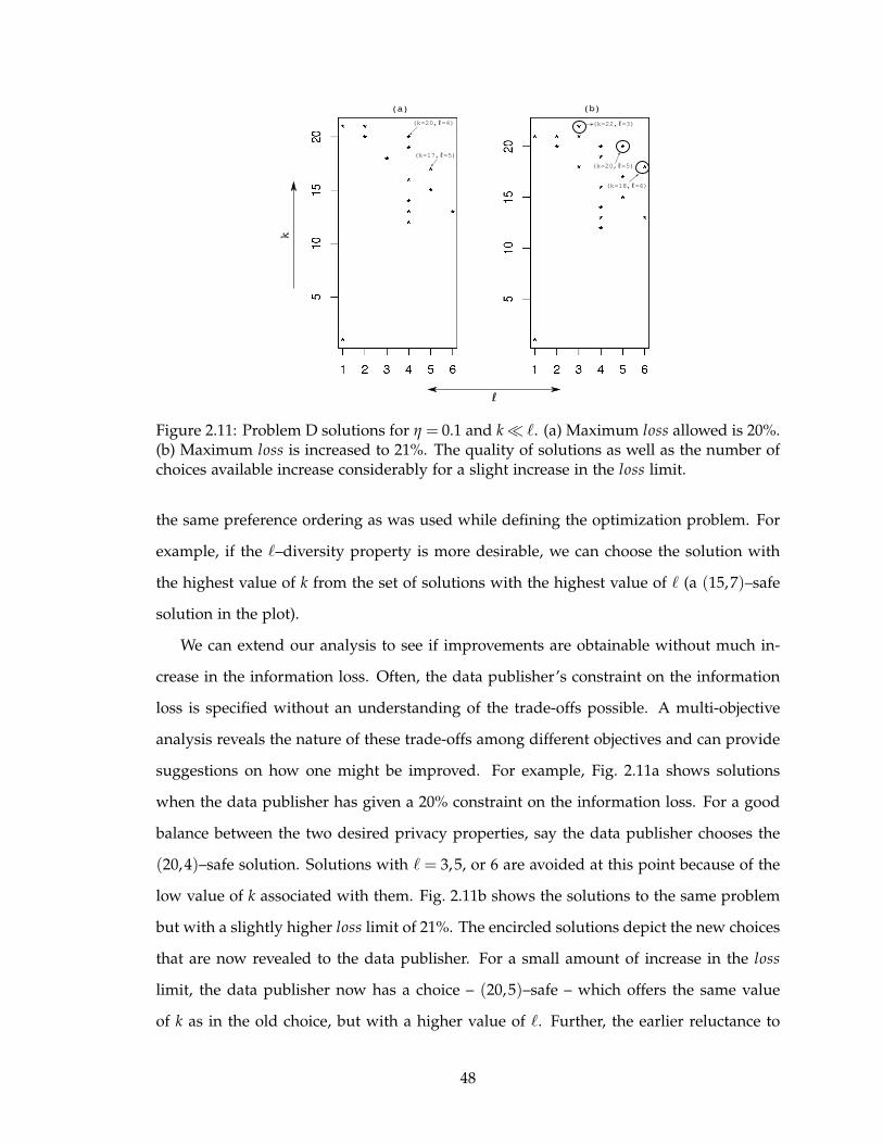
ℓ
k
(k=20,ℓ=4)
(k=17,ℓ=5)
(k=22,ℓ=3)
(k=20,ℓ=5)
(k=18,ℓ=6)
(a) (b)
Figure 2.11: Problem D solutions for η = 0.1 and k ≪ ℓ. (a) Maximum loss allowed is 20%.(b) Maximum loss is increased to 21%. The quality of solutions as well as the number ofchoices available increase considerably for a slight increase in the loss limit.
the same preference ordering as was used while defining the optimization problem. For
example, if the ℓ–diversity property is more desirable, we can choose the solution with
the highest value of k from the set of solutions with the highest value of ℓ (a (15,7)–safe
solution in the plot).
We can extend our analysis to see if improvements are obtainable without much in-
crease in the information loss. Often, the data publisher’s constraint on the information
loss is specified without an understanding of the trade-offs possible. A multi-objective
analysis reveals the nature of these trade-offs among different objectives and can provide
suggestions on how one might be improved. For example, Fig. 2.11a shows solutions
when the data publisher has given a 20% constraint on the information loss. For a good
balance between the two desired privacy properties, say the data publisher chooses the
(20,4)–safe solution. Solutions with ℓ = 3,5, or 6 are avoided at this point because of the
low value of k associated with them. Fig. 2.11b shows the solutions to the same problem
but with a slightly higher loss limit of 21%. The encircled solutions depict the new choices
that are now revealed to the data publisher. For a small amount of increase in the loss
limit, the data publisher now has a choice – (20,5)–safe – which offers the same value
of k as in the old choice, but with a higher value of ℓ. Further, the earlier reluctance to
48
choose a solution with ℓ = 3 is reduced after the revelation of the (22,3)–safe solution. In
fact, there is even a candidate solution with ℓ = 6 and a much better value in k. With this
information, the data publisher now has some idea about the trade-offs possible between
privacy and information loss. In fact, the trade-off analysis in this case may motivate the
data publisher to relax the loss constraint, which is not a big relaxation in itself, and reap
the benefits of better privacy.
2.6.5 Resolving the dilemma
It is possible to analyze the trade-off surface generated for a particular data set and
provide the data publisher with an analytical form for it. Given that an approximation of
the Pareto-front is known, an analytical form can be derived through a polynomial curve
fitting approach. However, it must be noted that analyzing the privacy-utility trade-off
in this manner is rather problem specific. It cannot be ascertained that the Pareto-front
always has a definitive structure for all data sets. Any theoretical analysis motivated
from Pareto behavior in a data set is limited to that particular data set, and is not directly
extensible to another. We cannot say for sure if the Pareto front will be similar for different
data sets with similar distributions. Understanding the trade-off is rather empirical in
this work, represented directly in terms of the parameter values and the resulting utility
(represented by the value of the utility metric of choice). Nonetheless, it is not always
true that empirical results are just tuples of 〈privacy,utility〉 values without providing
much insight into the trade-off involved. Observing the Pareto-front on a graphical plot
can reveal underlying traits. A classic case of this is seen in Fig. 2.7. Our observations
indicate here that a major part of the Pareto-front is flat, or steep, in this data set. This
signify that the data publisher has more flexibility in choosing a k value for a given level
of utility. The steep jumps in utility signify that there exist points for which utility can
often be improved significantly with a slight deterioration in privacy.
To summarize the above discussion, we go back to the questions asked by the data
publisher in the beginning of this chapter, and try to provide answers to them w.r.t. the
benchmark data set.
1. We can generalize the data set in such a way that more number of tuples have a
49
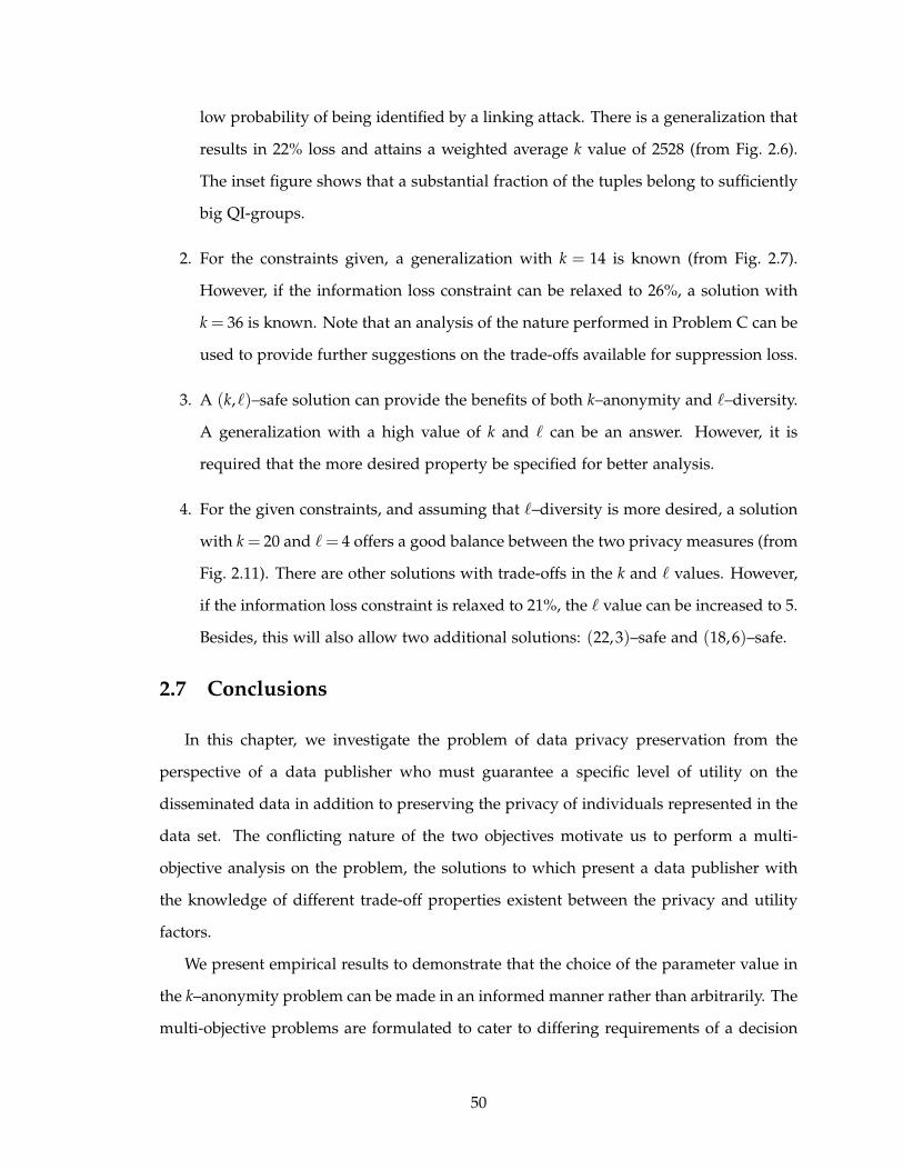
low probability of being identified by a linking attack. There is a generalization that
results in 22% loss and attains a weighted average k value of 2528 (from Fig. 2.6).
The inset figure shows that a substantial fraction of the tuples belong to sufficiently
big QI-groups.
2. For the constraints given, a generalization with k = 14 is known (from Fig. 2.7).
However, if the information loss constraint can be relaxed to 26%, a solution with
k = 36 is known. Note that an analysis of the nature performed in Problem C can be
used to provide further suggestions on the trade-offs available for suppression loss.
3. A (k,ℓ)–safe solution can provide the benefits of both k–anonymity and ℓ–diversity.
A generalization with a high value of k and ℓ can be an answer. However, it is
required that the more desired property be specified for better analysis.
4. For the given constraints, and assuming that ℓ–diversity is more desired, a solution
with k = 20 and ℓ = 4 offers a good balance between the two privacy measures (from
Fig. 2.11). There are other solutions with trade-offs in the k and ℓ values. However,
if the information loss constraint is relaxed to 21%, the ℓ value can be increased to 5.
Besides, this will also allow two additional solutions: (22,3)–safe and (18,6)–safe.
2.7 Conclusions
In this chapter, we investigate the problem of data privacy preservation from the
perspective of a data publisher who must guarantee a specific level of utility on the
disseminated data in addition to preserving the privacy of individuals represented in the
data set. The conflicting nature of the two objectives motivate us to perform a multi-
objective analysis on the problem, the solutions to which present a data publisher with
the knowledge of different trade-off properties existent between the privacy and utility
factors.
We present empirical results to demonstrate that the choice of the parameter value in
the k–anonymity problem can be made in an informed manner rather than arbitrarily. The
multi-objective problems are formulated to cater to differing requirements of a decision
50
maker, primarily focused on the maximization of the k value and minimization of the
losses.
For generalizations without suppression, a unique k may not be available. However,
the analysis indicates that generalizations are possible that provide a higher level of pri-
vacy for a higher fraction of the data set without compromising much on its information
content. When suppression is allowed up to a hard limit, the user’s choice of k should be
based on an analysis similar to that performed in Problem B. Typically, the nature of the
non-dominated solution set provides invaluable information on whether an anonymiza-
tion exists to improve a particular value of the model parameter without much degrada-
tion in quality of the data. First-level explorations in this context can begin with gaining
an overall understanding of the trade-off characteristics in the search space.
Our results also indicate that different privacy models can be combined and optimized
to result in minimal information loss. However, the trade-off picture is better portrayed
in cases when the model parameters are kept separated and formulated as multiple ob-
jectives. We use (k,ℓ)–safety as the combination of k–anonymity and ℓ–diversity models
with the objective of demonstrating how a multi-objective formulation can be devised to
search for generalizations that result in acceptable adherence to more than one privacy
property and within acceptable utility levels. Trade-off analysis lends credence to the
fact that often a data publisher’s choice of a particular solution can be augmented with
information to suggest possible improvements on one or more objectives.
The formulations presented in the chapter also address the data publisher’s dilemma.
They provide a methodology to analyze the problem of data anonymization in manners
that appeal to the actual entity that disseminates the data. We believe that such an analysis
not only reinstates the data publisher’s confidence in its choice of a particular privacy
model parameter, but also identifies ways of examining if the level of privacy requested
by a human subject is achievable within the acceptable limits of perturbing data quality.
Future work in this direction can start with examination of the framework with other
models of privacy preservation. Real valued parametrization of t makes the t–closeness
model an interesting subsequent candidate. Hybrid models catering to different forms
of attacks are also required. Work on this can begin with an exploration of what trade-
51

offs are generated when looking for the existence of two, or more, privacy properties
simultaneously. We believe that transitioning these different models into the real world
would require us to synchronize our perspective of the problem with those that actually
deal with it.
52
CHAPTER 3
Pareto Optimization on a Generalization Lattice
Representation of the generalization space plays a crucial role in the design of algo-
rithms attempting to maximize the data utility. Although Iyengar’s bit vector representa-
tion is one of the most flexible schemes to represent the search space, it does not readily
provide a known structure that algorithms can exploit during the search. Therefore, a ma-
jority of the anonymization algorithms [16, 72, 89, 92, 109, 110, 117, 150, 176] are known
to work with a generalization space arranged in the form of a graph, called the domain
generalization lattice, where every node is a vector signifying the amount of generalization
for each quasi-identifier. Efficient traversal of the lattice has been particularly explored so
that the number of nodes that undergo evaluation (determining equivalence classes and
computing loss) can be reduced.
In this chapter, we extend our analysis based on the Pareto concept to identify optimal
generalizations on a domain generalization lattice. Our principle contribution, the Pareto-
Optimal k-Anonymization (POkA) algorithm, utilizes a combination of depth first traversals
of the lattice to efficiently move from one Pareto-optimal node to another. Two key prop-
erties, namely height boundary property and ground node property, have been proposed to
guide the search in a manner that requires minimal node evaluations while assuring that
all Pareto-optimal nodes are identified. Performance analysis on a benchmark data set
shows that POkA can prune a large number of sub-optimal nodes from being evaluated
53
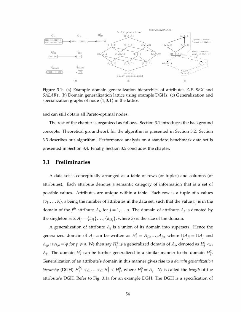
(2,1,1)
(2,0,1)(1,1,1) (2,1,0)
(0,1,1) (1,0,1) (1,1,0) (2,0,0)
(0,0,1) (0,1,0) (1,0,0)
(0,0,0)
(2,1,1)
(2,0,1)(1,1,1)
(1,0,1)
(0,0,1) (1,0,0)
(0,0,0)
(ZIP,SEX,SALARY)
{12345},{12346}
{12355},{12356}{1234*},{1235*} {123**}
HZIP0
HZIP1 HZIP
2
HSEX0 HSEX
1
HSALARY0 HSALARY
1
{M},{F} {*}
{<50K},{>=50K} {*}
fully generalized
fully specialized
generalization
graph of (1,0,1)
specialization
graph of (1,0,1)
(b) (c)(a)
Figure 3.1: (a) Example domain generalization hierarchies of attributes ZIP, SEX andSALARY. (b) Domain generalization lattice using example DGHs. (c) Generalization andspecialization graphs of node (1,0,1) in the lattice.
and can still obtain all Pareto-optimal nodes.
The rest of the chapter is organized as follows. Section 3.1 introduces the background
concepts. Theoretical groundwork for the algorithm is presented in Section 3.2. Section
3.3 describes our algorithm. Performance analysis on a standard benchmark data set is
presented in Section 3.4. Finally, Section 3.5 concludes the chapter.
3.1 Preliminaries
A data set is conceptually arranged as a table of rows (or tuples) and columns (or
attributes). Each attribute denotes a semantic category of information that is a set of
possible values. Attributes are unique within a table. Each row is a tuple of s values
〈v1, . . . ,vs〉, s being the number of attributes in the data set, such that the value vj is in the
domain of the jth attribute Aj, for j = 1, . . . , s. The domain of attribute Aj is denoted by
the singleton sets Aj = {aj1}, . . . ,{ajSj}, where Sj is the size of the domain.
A generalization of attribute Aj is a union of its domain into supersets. Hence the
generalized domain of Aj can be written as H1j = Aj1, . . . , Ajm where ∪
iAji = ∪Aj and
Ajp ∩ Ajq = φ for p 6= q. We then say H1j is a generalized domain of Aj, denoted as H1
j <G
Aj. The domain H1j can be further generalized in a similar manner to the domain H2
j .
Generalization of an attribute’s domain in this manner gives rise to a domain generalization
hierarchy (DGH) HNj
j <G . . . <G H1J < H0
j , where H0j = Aj. Nj is called the length of the
attribute’s DGH. Refer to Fig. 3.1a for an example DGH. The DGH is a specification of
54
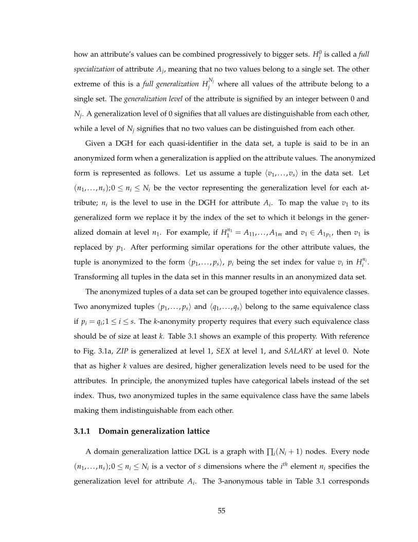
how an attribute’s values can be combined progressively to bigger sets. H0j is called a full
specialization of attribute Aj, meaning that no two values belong to a single set. The other
extreme of this is a full generalization HNj
j where all values of the attribute belong to a
single set. The generalization level of the attribute is signified by an integer between 0 and
Nj. A generalization level of 0 signifies that all values are distinguishable from each other,
while a level of Nj signifies that no two values can be distinguished from each other.
Given a DGH for each quasi-identifier in the data set, a tuple is said to be in an
anonymized form when a generalization is applied on the attribute values. The anonymized
form is represented as follows. Let us assume a tuple 〈v1, . . . ,vs〉 in the data set. Let
(n1, . . . ,ns);0 ≤ ni ≤ Ni be the vector representing the generalization level for each at-
tribute; ni is the level to use in the DGH for attribute Ai. To map the value v1 to its
generalized form we replace it by the index of the set to which it belongs in the gener-
alized domain at level n1. For example, if Hn11 = A11, . . . , A1m and v1 ∈ A1p1
, then v1 is
replaced by p1. After performing similar operations for the other attribute values, the
tuple is anonymized to the form 〈p1, . . . , ps〉, pi being the set index for value vi in Hnii .
Transforming all tuples in the data set in this manner results in an anonymized data set.
The anonymized tuples of a data set can be grouped together into equivalence classes.
Two anonymized tuples 〈p1, . . . , ps〉 and 〈q1, . . . ,qs〉 belong to the same equivalence class
if pi = qi;1 ≤ i ≤ s. The k-anonymity property requires that every such equivalence class
should be of size at least k. Table 3.1 shows an example of this property. With reference
to Fig. 3.1a, ZIP is generalized at level 1, SEX at level 1, and SALARY at level 0. Note
that as higher k values are desired, higher generalization levels need to be used for the
attributes. In principle, the anonymized tuples have categorical labels instead of the set
index. Thus, two anonymized tuples in the same equivalence class have the same labels
making them indistinguishable from each other.
3.1.1 Domain generalization lattice
A domain generalization lattice DGL is a graph with ∏i(Ni + 1) nodes. Every node
(n1, . . . ,ns);0 ≤ ni ≤ Ni is a vector of s dimensions where the ith element ni specifies the
generalization level for attribute Ai. The 3-anonymous table in Table 3.1 corresponds
55

Table 3.1: 3-anonymous version (right) of a table.
ZIP SEX SALARY DISEASE
12345 M <50K Cancer
12346 M <50K Gastritis
12345 F <50K HIV
12355 F ≥50K Cancer
12355 M ≥50K HIV
12356 M ≥50K Cancer
ZIP SEX SALARY DISEASE
1234* * <50K Cancer1234* * <50K Gastritis1234* * <50K HIV
1235* * ≥50K Cancer1235* * ≥50K HIV1235* * ≥50K Cancer
to the node (1,1,0). An edge exists between two nodes (n1, . . . ,ns) and (m1, . . . ,ms) if
and only if the vectors differ in exactly one element and the difference is one. To put it
formally, ∑i |ni − mi| = 1. The node (0, . . . ,0) (s times) is the fully specialized node of the
lattice and corresponds to the un-anonymized data set. The node (N1, . . . , Ns) is the fully
generalized node and corresponds to no disclosure of the data. Fig. 3.1b illustrates these
terms.
In a typical k-anonymization algorithm, a node is sought in this lattice such that it
satisfies k-anonymity and results in minimum information loss for the specified value of
k. An exhaustive search is often not desired since evaluation of equivalence class sizes on
a moderately sized data set can be computationally intensive. Most algorithms therefore
perform some form of pruning of the lattice. Note that the algorithms we refer to here are
meant to find optimal generalization levels for a given value of k. Pruning of the lattice
when no k value is specified is an unresolved problem until now.
Given a domain generalization lattice and a node (n1, . . . ,ns), we can also define a
specialization graph which contains the nodes (p1, . . . , ps) such that pi ≤ ni;1 ≤ i ≤ s. Edges
between nodes in this graph are drawn similar to as in a DGL. The node (n1, . . . ,ns) is
called the root node of the specialization graph. Along similar lines, we can also define
a generalization graph if nodes instead satisfy pi ≥ ni;1 ≤ i ≤ s. Fig. 3.1c highlights the
specialization and generalization graph of the node (1,0,1). Intuitively, the specialization
graph of a node contains all other nodes which are more specialized in one or more
attributes, and in effect induce comparatively smaller k and lower loss. Contrary to that,
a generalization graph of a node contains all other nodes which are more generalized
in one or more attributes, and in effect induce comparatively larger k and higher loss.
56

2 3 4 5 6 7
Pareto-optimal
Sub-optimal
kinformation loss
Figure 3.2: Depiction of Pareto-optimal nodes.
Hence, we shall often use the term “move down” and “move up” while traversing a
specialization and generalization graph respectively. These two graphs will be used later
while performing the search for optimal nodes.
3.1.2 Pareto-optimal generalization
Let kN and LN signify the k and information loss associated with a node N in the
domain generalization lattice. The node N is a Pareto-optimal generalization if there is
no other node M in the lattice such that one of the following two conditions hold.
• kM ≥ kN and LM < LN , or
• kM > kN and LM ≤ LN .
If one of the conditions is true, then M is said to dominate N. Therefore, a Pareto-
optimal node is one whose k value cannot be improved upon by another node without
increasing the information loss, and the information loss at the induced k value is min-
imal. Note that Pareto-optimal nodes need not always exist at every possible value of
k. For example, in Fig. 3.2, no Pareto-optimal node appears with k = 4 since the node
with k = 5 offers a higher value of k but with lower information loss. As is evident from
the figure, trade-off behavior becomes clear when all Pareto-optimal solutions are known.
The advantage of finding Pareto-optimal nodes is two fold. First, the minimal informa-
tion loss at relevant k values is computed. Second, the choice of a particular solution can
be based on the change of information loss rather than on arbitrary selection of k. In
57
the figure, the choice of k = 5 can perhaps be made since there is not much difference in
information loss from the k = 3 node. Therefore, our objective is to search the DGL in an
efficient manner and identify the Pareto-optimal nodes. Note that this process does not
require the specification of a k value by the data publisher. Instead, optimal k values are
reported as part of the set of Pareto-optimal generalizations.
3.2 Pareto Search
The basic search strategy we adopt is to start from an already known Pareto-optimal
node and prune nodes that cannot be Pareto-optimal. We shall start with the Pareto-
optimal node with the highest possible k value and then use it as a starting step to find
the next Pareto-optimal node. The next Pareto-optimal node is the one with a k value closest
to that of the previous one but with lower loss. Hence, given a Pareto-optimal node N =
(n1, . . . ,ns), the next Pareto-optimal node M is the one with minimum (kN − kM);kM < kN
and LM < LN . We shall call the node N a base node. In Fig. 3.2, the next Pareto-optimal
node for the node with k = 5 is the node with k = 3. The node M is found by combining
a depth-first search (DFS) traversal of the specialization graph of N with a DFS traversal
of the generalization graph of another node.
The first step in this process is to have a known Pareto-optimal node to begin with –
the first base node. This is not difficult since the node (N1, . . . , Ns) is bound to be Pareto-
optimal. This node induces a k value equal to the size of the data set since all tuples get
transformed to the same anonymized form. No other node can produce a k value higher
than this. Once the next Pareto-optimal node is found, the process is repeated using this
newly found node as the base node.
The next step is to assure that the node M can be reached from the base node N. Note
that kM < kN . Hence, M will not be present in the generalization graph of N. Recall
that all nodes in the generalization graph of N will have more generalization in one or
more attributes and will result in a higher k value. This observation results in the first
level of pruning of the DGL. Given the Pareto-optimal node N, the number of nodes
pruned by not searching the generalization graph of N is ∏i(Ni − ni + 1). At first glance
it may seem that the node M should be somewhere in the specialization graph of N and
58

(2,1,1)
(2,0,1)(1,1,1) (2,1,0)
(0,1,1) (1,0,1) (1,1,0) (2,0,0)
(0,0,1) (0,1,0) (1,0,0)
(0,0,0)
ground node
depth search height search
N
M
Figure 3.3: Use of depth search and height search to reach node M from node N througha ground node.
is hence directly reachable from N. In fact, if the node M is in the specialization graph
of N, then it would be the one with the highest k value in the set {(n1, . . . ,nj−1,nj −1,nj+1, . . . ,ns)|1 ≤ j ≤ s;nj 6= 0} – immediate neighbors of N in the graph. Since other
nodes in the specialization graph are indeed specializations of a node in this set, they
would have k values lower than the highest possible k in these immediate neighbors.
However, there is still a set of nodes that are not present in the specialization graph of
N but can potentially include M. These nodes are the ones that can be generated from N
by performing generalization in some attributes, specialization in some and no change in
others. A positive observation in this context is that the node M can still be reached from
N through a node common in the specialization graph of M and N, called a ground node.
3.2.1 Ground nodes
A ground node is a node common in the specialization graphs of two nodes in the
domain generalization lattice. A trivial ground node for any two nodes is the fully spe-
cialized node (0, . . . . ,0). Other non-trivial nodes also do exist. Given the nodes N and
M, any node in the set G = {(g1, . . . , gs)|0 ≤ gi ≤ min(ni,mi)} is a ground node for N and
M. M can then be reached from N by first moving down the specialization graph of N
to a ground node and then moving up in the generalization graph of the ground node.
The first phase of this process, i.e. moving down to the ground node, is called a depth
search rooted at N. The phase of moving up from the ground node is called a height search
rooted at the ground node. Fig. 3.3 illustrates this process.
59

Note that although a depth search is essential to find a ground node, nodes traversed
in the process need not be evaluated if they are not immediate neighbors of the base
node. This follows from the earlier observation that if M resides in the specialization
graph of N, then it will be one of the immediate neighbors. This observation leads to the
second level of pruning in node evaluation. However, nodes in the height search are to
be evaluated since k values will increase progressively. The only exception are nodes that
are also part of the depth search but not immediate neighbors of the base node. A brute
force method to perform the searches would mean traversing the specialization graph of
N all the way down to the fully specialized node and then traversing the generalization
graph of the trivial ground node. Clearly, this is an exhaustive search. The following two
sections discuss the theoretical properties that bound the extent of search to be performed
in both phases. Efficiently determining the minimum extent to search will further reduce
the number of nodes to be evaluated.
3.2.2 Height search
Height search from a ground node is a DFS traversal of the generalization graph with
the ground node as the root. To clarify any ambiguity in language, we say that height
search is a height first traversal of the graph. The search is said to be at height h when
the current node H is h steps away from the ground node G, i.e ∑i |hi − gi| = h. The
height h is a dynamically chosen parameter in our approach. The assumption we make
is that both k and information loss are non-decreasing quantities when performing more
generalization in an attribute. Based on this assumption, the following property states
how “high” should the height search proceed before coming back to its parent node.
Theorem 3.1 Height Boundary Property. Let A = {A1, . . . , As} be a set of attributes.
Given a Pareto-optimal node N = (n1, . . . ,ns), the next Pareto-optimal node M can be
found by a height search of a node in the specialization graph of N, further search up a
node H being terminated whenever kH ≥ kN or LH ≥ LN .
Proof The node to start the height search from is a ground node G present in the spe-
cialization graph of N. Since M is the next Pareto-optimal node, we have kM < kN and
60

LM < LN . Based on the aforementioned assumption, if M is in the generalization graph
of G, then it must be reached in a height search before a node H with kH ≥ kN or LH ≥LN
is reached. Hence, whenever such a node is encountered, we have reached the maximum
height along that path. �
The height to search is therefore bounded by the k and loss values of the base node.
We shall start with the ground node and choose a child for subsequent search only if it has
k and loss lower than that of N. Child nodes that are common to the specialization graph
of N (and not immediate neighbors of N) are not evaluated and are always selected.
All selected child nodes are subjected to the same evaluation for further search. Exact
specification of how the next Pareto-optimal node is identified from height searches is
presented in Section 3.3. The further down the ground node is from the base node, the
greater will be the number of nodes that will require evaluation in the height search.
We therefore need a good estimate of the ground node closest to the next Pareto-optimal
node. This is achieved by the depth search.
3.2.3 Depth search
Depth search from a base node N is a DFS traversal of the specialization graph with
N as the root. The depth d of the search is the maximum total difference in generalization
levels from the base node to an internal node. Therefore, a depth search of depth d
implies the traversal of nodes D such that ∑i |ni − di| ≤ d. Under this specification, an
internal node is searched further only if its maximum total difference in generalization
levels from the base node is less than d. Each node at depth d in the specialization graph
of N is considered a candidate ground node and is subjected to a height search. Note that
the DGL is a graph (not a tree) and hence the general intuition that the number of nodes
subjected to height search will increase exponentially with larger d is not true. In the
following, we deduce the depth at which a ground node (not necessarily the closest one)
for the next Pareto-optimal node is bound to exist and derive an estimate of the depth to
actually search.
Lemma 3.1 The minimum equivalence class size of a data set with s attributes A =
61

{A1, . . . , As} is the same as the minimum equivalence class size of a data set with two
attributes A1 and A2, where A1 = Aj and A2 = A1 × . . . × Aj−1 × Aj+1 × . . . × As.
Proof The proof follows from the fact that A2 is simply a concatenated version of the
values of the attributes A1, . . . , Aj−1, Aj+1, . . . , As. Determining the equivalence class sizes
in a data set with s attributes require finding the frequency of occurrence of every possi-
ble combination of values for s − 1 attributes. In the case with two attributes, this step is
performed while finding the equivalence class sizes for the attribute A2. Hence in both
cases, a tuple with a particular sequence of values for A1, . . . , As will belong to an equiv-
alence class of the same size. This means that the minimum equivalence class size will
also be same. �
Lemma 3.2 Let A1 and A2 be two attributes with DGH lengths of N1 and N2 respectively.
If N = (n1,n2), such that 0 ≤ n1 ≤ N1 and 0 ≤ n2 ≤ N2, is a Pareto-optimal node, then one
of G1 = (n1,0) and G2 = (0,n2) is a ground node for the next Pareto-optimal node.
Proof The next Pareto-optimal node M is the one with kM closest to kN satisfying the
constraints kM < kN and LM < LN , i.e. there is no other node M′ such that kM < kM′ < kN
and LM′ < LN . The first set of possibilities are the immediate descendants of N, i.e.
D1 = (n1 − 1,n2) or D2 = (n1,n2 − 1). Other descendant nodes of N, i.e. nodes of the form
L = (l1, l2);0 ≤ li < ni, have k values lower than max(kD1,kD2
) and hence do not satisfy the
requirements for the next Pareto-optimal node. If one of D1 or D2 is Pareto-optimal then
G2 or G1 respectively is a ground node for it.
If none of D1 and D2 is the next Pareto-optimal node then nodes of the form (l1, h2) or
(h1, l2), where ni < hi ≤ Ni, must dominate them (after satisfying the required constraints)
and are likely candidates. Since G1 is a ground node for any node of the form (h1, l2) and
G2 for nodes of the form (l1, h2), the result still holds. �
Theorem 3.2 Ground Node Property. Let A = {A1, . . . , As} be a set of attributes with Ni
as the DGH length of Ai. If N = (n1, . . . ,ns);0 ≤ ni ≤ Ni is a Pareto-optimal node, then one
or more nodes in the set Gbest ∪Gworst, where Gbest = {(n1, . . . ,nj−1,0,nj+1, . . . ,ns)|1 ≤ j ≤ s}and Gworst = {(0, . . . ,nj, . . . ,0)|1 ≤ j ≤ s}, are ground nodes of the next Pareto-optimal
node.
62

Proof The proof follows from the observation that the problem of finding Pareto-optimal
nodes for s properties can be transformed to the case of finding Pareto-optimal nodes for
two properties. To do so, we map the attribute set A to two attributes A1 and A2 such
that A1 = Aj and A2 = A1 × . . .× Aj−1 × Aj+1 × . . .× As. A tuple 〈v1, . . . ,vs〉 in the original
data set is transformed to the form 〈vj,v1; . . . ;vj−1;vj+1; . . . ;vs〉. Any anonymized version
of a tuple is mapped in a similar manner. By Lemma 3.1, both data sets (generalized or
not) will induce the same value of k. The loss metric can be modified so that the loss
associated with a tuple in the data set with s attributes is proportional to that of the tuple
in the data set with two attributes.
The step that remains is a specification for the DGH of A2. Nodes in the DGH of A2
are formed by taking every possible combination of nodes from the DGHs of the s − 1
attributes. A node is therefore of the form Nj = (n1; . . . ;nj−1;nj+1; . . . ;ns);0 ≤ ni ≤ Ni. The
total ordering of these nodes is obtained by first sorting them in ascending order of the
k value they induce and then in ascending order of the loss (if k is same for two nodes).
This follows the general notion of a DGH where k (and then loss) increases as we step
from one node to the next. The domain generalization lattice for two attributes contains
nodes of the form (nj,Nj).
Therefore, there is a bijective mapping between the set of nodes in the domain gener-
alization lattice with s attributes and the set of nodes in the domain generalization lattice
with two attributes. Since, the k and loss values of two corresponding nodes are also
same, any Pareto-optimal node in the lattice with s attributes will also be Pareto-optimal
in the lattice with two attributes, and vice versa.
Hence by Lemma 3.2, given N and a particular value for j, the ground nodes for
the next Pareto-optimal node are one or both of (0,Nj) or (nj,0). This translates to
nodes of the form (n1, . . . ,nj−1,0,nj+1, . . . ,ns) and (0, . . . ,nj, . . . ,0) in the lattice for s at-
tributes. Since the transformation into the case with two attributes can be performed
in s different ways (1 ≤ j ≤ s), the set of such possible ground nodes is given as Gbest =
{(n1, . . . ,nj−1,0,nj+1, . . . ,ns)|1 ≤ j ≤ s} and Gworst = {(0, . . . ,nj, . . . ,0)|1 ≤ j ≤ s}. �
63

Assuring that nodes in Gworst are covered while performing a depth search, i.e. d =
maxj
(∑i ni − nj), ensures all possible Pareto-optimal nodes before N (ones with k and loss
lower than that of N) will be discovered. This is achieved by allowing the discovery of
nodes that require specialization in all (but one) attributes. However, this is often not
required if only the immediately next Pareto-optimal node has to be found. Covering
nodes in Gbest, i.e. d = maxi
(ni), is sufficient for this purpose. Depth search that covers
nodes in Gbest allows the discovery of nodes that may require full specialization in at
most one attribute. To be precise, it allows finding nodes that have full specialization in
the attribute with the longest DGH length. A longer DGH is typically specified for an
attribute with a bigger domain size. Hence, full specialization in such an attribute has the
tendency to induce small equivalence classes, thereby a small value of k. The immediately
next Pareto-optimal node is more likely to have a k value closer to kN .
A good strategy to adopt here is to ensure that attributes which are close to full
specialization in N get a chance to become so while attributes that are far away from
being fully specialized are explored in less depth. Consider the nature of nodes that
get covered in a depth search of davg = ⌈∑i Ni
s ⌉ depth, davg being the average number of
steps required for an attribute to become fully specialized from a fully generalized state.
First, depth search to davg depth ensures that half of the number of attributes will have a
chance to become fully specialized. Second, in davg number of steps, the attributes which
are closer to being fully specialized stand a higher chance of becoming so. Third, taking
davg steps allows combination of different levels of specialization for different attributes
without making any of them fully specialized (if not already). Performance analysis
in Section 3.4 corroborates that this strategy indeed provides the best balance between
exploration of nodes and discovery of Pareto-optimal ones.
3.3 POkA Algorithm
The Pareto-Optimal k-Anonymization (POkA) algorithm is an iterative search method
to identify the Pareto-optimal generalizations for a given data set. The attributes in the
data set that are subjected to generalization (conventionally called quasi-identifiers) are
specified and a DGH is defined for every such attribute. The algorithm is iterative be-
64

Procedure 3.1 HeightSearch(Node P, boolean useNode)
Input: A node P and a boolean value (true or false) useNode. N is the base node.Output: (M,kM,LM): M is a node in GG(P) with the highest k value such that kM < kN
and LM < LN , or NULL if no such node exists.1: if (useNode = true) then
2: No = (P,kP,LP)3: else
4: No = (NULL,0,0)5: end if
6: for all (child node C of P in GG(P)) do
7: if (C ∈ SG(N) and ∑i |ni − ci| > 1) then
8: Q = HeightSearch(C, f alse)9: else
10: Evaluate(C)11: if (kC < kN and LC < LN) then
12: Q = HeightSearch(C, true)13: else
14: Q = (NULL,0,0)15: end if
16: end if
17: if (kQ > kNo or (kQ = kNo and LQ < LNo )) then
18: No = (Q,kQ,LQ)19: end if
20: end for
21: return No
cause one combination of depth search and height search, and a base node, is required
to identify one Pareto-optimal node. The process is applied repeatedly to identify subse-
quent nodes. We implicitly assume that outliers are handled using the maximum allowed
suppression method as described in Section 2.4.3.2.
3.3.1 POkA
Height search and depth search are the two crucial components of POkA. We use
the notation SG(P) and GG(P) to signify the set of nodes in the specialization graph
and generalization graph of a node P respectively. Let N be the base node. kP and LP
signify the k and information loss value associated with node P. Further, we assume the
existence of a function Evaluate which takes as input a node P in the DGL and returns
kP and LP. These returned values are computed after using the suppression strategy
mentioned earlier.
65

Procedure 3.2 DepthSearch(Node P)
Input: A node P in SG(N), N being the base node.Output: (M,kM,LM): M is a node reachable by height search of some node in SG(P) and
with the highest k value such that kM < kN and LM < LN .1: No = (NULL,0,0)2: for all (child node C of P in SG(P)) do
3: if (∑i |ni − ci| = d) then
4: if (d = 1) then
5: Evaluate(C)6: Q = HeightSearch(C, true)7: else
8: Q = HeightSearch(C, f alse)9: end if
10: else
11: Q = DepthSearch(C)12: end if
13: if (kQ > kNo or (kQ = kNo and LQ < LNo )) then
14: No = (Q,kQ,LQ)15: end if
16: end for
17: return No
Procedure 3.1 presents the pseudo-code for a height search implementation. Height
search initiated at a node therefore returns the node in its generalization graph with the
highest k and one which satisfies the constraints on the k and loss. Any node that belongs
to SG(N) and is not an immediate neighbor of N is not evaluated and height search
proceeds without considering the k and loss of such a node. Otherwise, the node is
evaluated to determine if further search is required as determined by the height boundary
property. The method is initiated at a candidate ground node decided in the depth search.
d signifies the depth to search in the following.
Procedure 3.2 shows the pseudo-code for a depth search implementation. The imple-
mentation is a simple DFS traversal with a height search being initiated when nodes at
depth d are encountered. The best M found in these height searches is translated upwards
towards the root of the specialization graph. Hence, the node M returned from a call to
DepthSearch(N) is the next identified Pareto-optimal node.
POkA starts by a call to DepthSearch with the fully generalized node. For every new
Pareto-optimal node identified, DepthSearch is iteratively called until the Pareto-optimal
node with k ≤ 2 is found. Procedure 3.3 shows the pseudo-code of this process.
66

Procedure 3.3 POkA()
Output: The set P of Pareto-optimal nodes in the DGL.1: N = (N1, . . . , Ns)2: P = {N}3: while (kN > 2) do
4: (N,kN ,LN) = DepthSearch(N)5: P = P ∪ {N}6: end while
7: return P
3.3.2 Improvements
Node traversal in DepthSearch and HeightSearch can be further reduced by taking into
account the structure of the DGL. Since the structure is that of a graph, nodes in the spe-
cialization graph and generalization graph will share nodes as children. This structure
results in repeated visits to a node during a depth/height search initiated by multiple
parent nodes that share the node as a child. Although repeated visits to the same node
do not increase the number of unique node evaluations required, there is redundancy
involved as the results from searching the node further have already been taken into ac-
count. We therefore perform some bookkeeping at every visited node to prevent repeated
visits.
The output from every node visited during a height search, i.e. the return values, is
separately stored in a list HBest. Whenever a height search is to be initiated at a node,
the list HBest is first checked to find if an entry corresponding to the node exists. If it
does, then the node (and subsequent nodes) has already been searched and the stored
values are returned. If not, the height search is done as usual. Similar to HBest, a list
DBest is created for every node visited during a depth search. Depth search at a node
is not performed if results for the node already exist in the list. Both lists are emptied
before calling DepthSearch in Procedure 3.3. Procedures 3.1 and 3.2 can be easily modified
to maintain and use these lists.
3.4 Performance Analysis
We applied our methodology to the “adult.data” benchmark data set. The attributes
used in this study along with their DGH lengths are listed in Table 3.2. Attributes with
67
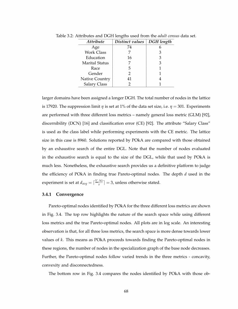
Table 3.2: Attributes and DGH lengths used from the adult census data set.
Attribute Distinct values DGH length
Age 74 6Work Class 7 3Education 16 3
Marital Status 7 3Race 5 1
Gender 2 1Native Country 41 4
Salary Class 2 1
larger domains have been assigned a longer DGH. The total number of nodes in the lattice
is 17920. The suppression limit η is set at 1% of the data set size, i.e. η = 301. Experiments
are performed with three different loss metrics – namely general loss metric (GLM) [92],
discernibility (DCN) [16] and classification error (CE) [92]. The attribute “Salary Class”
is used as the class label while performing experiments with the CE metric. The lattice
size in this case is 8960. Solutions reported by POkA are compared with those obtained
by an exhaustive search of the entire DGL. Note that the number of nodes evaluated
in the exhaustive search is equal to the size of the DGL, while that used by POkA is
much less. Nonetheless, the exhaustive search provides us a definitive platform to judge
the efficiency of POkA in finding true Pareto-optimal nodes. The depth d used in the
experiment is set at davg = ⌈∑i Nis ⌉ = 3, unless otherwise stated.
3.4.1 Convergence
Pareto-optimal nodes identified by POkA for the three different loss metrics are shown
in Fig. 3.4. The top row highlights the nature of the search space while using different
loss metrics and the true Pareto-optimal nodes. All plots are in log scale. An interesting
observation is that, for all three loss metrics, the search space is more dense towards lower
values of k. This means as POkA proceeds towards finding the Pareto-optimal nodes in
these regions, the number of nodes in the specialization graph of the base node decreases.
Further, the Pareto-optimal nodes follow varied trends in the three metrics - concavity,
convexity and disconnectedness.
The bottom row in Fig. 3.4 compares the nodes identified by POkA with those ob-
68
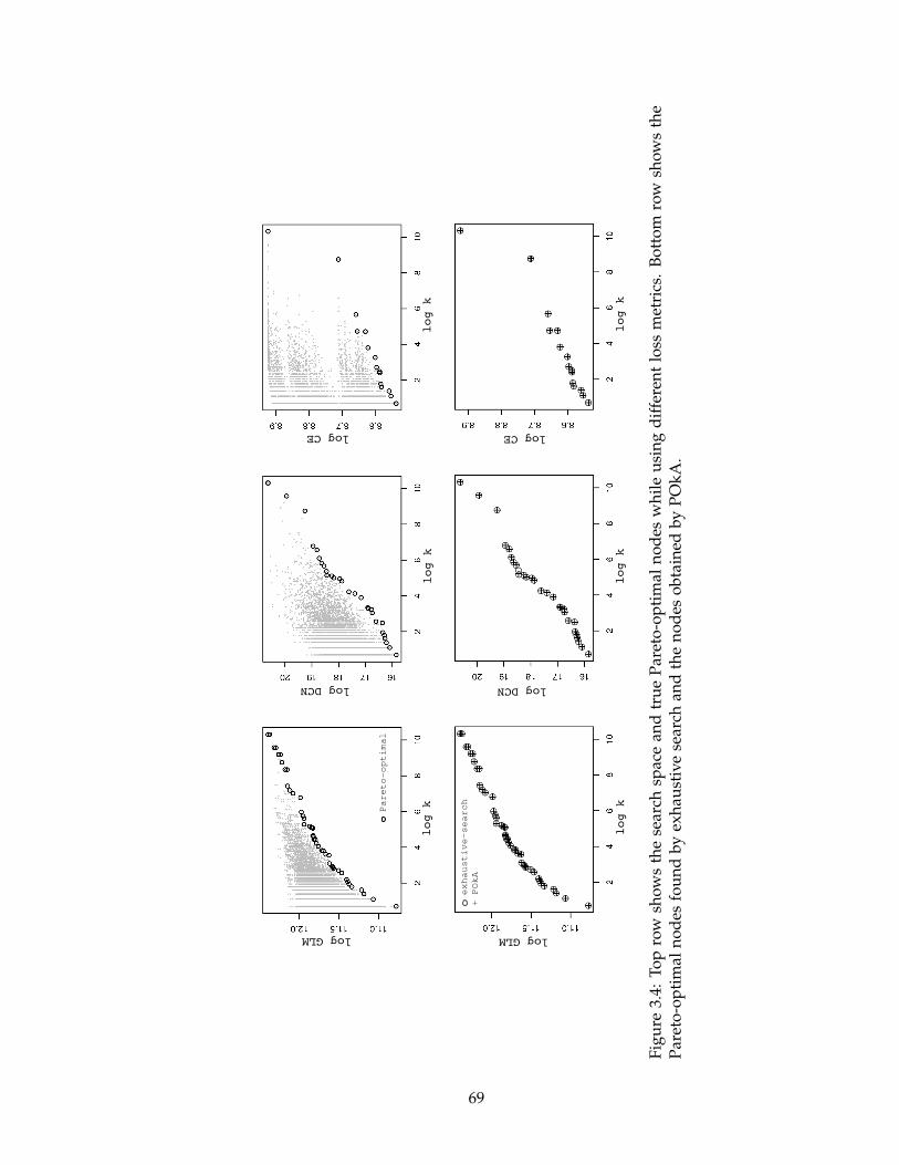
Pareto-optimal
log GLM
exhaustive-search
+ POkA
log k
log k
log k
log k
log k
log k
log GLM
log DCN log DCN
log CE log CE
Fig
ure
3.4:
To
pro
wsh
ow
sth
ese
arch
spac
ean
dtr
ue
Par
eto
-op
tim
aln
od
esw
hil
eu
sin
gd
iffe
ren
tlo
ssm
etri
cs.
Bo
tto
mro
wsh
ow
sth
eP
aret
o-o
pti
mal
no
des
fou
nd
by
exh
aust
ive
sear
chan
dth
en
od
eso
bta
ined
by
PO
kA
.
69
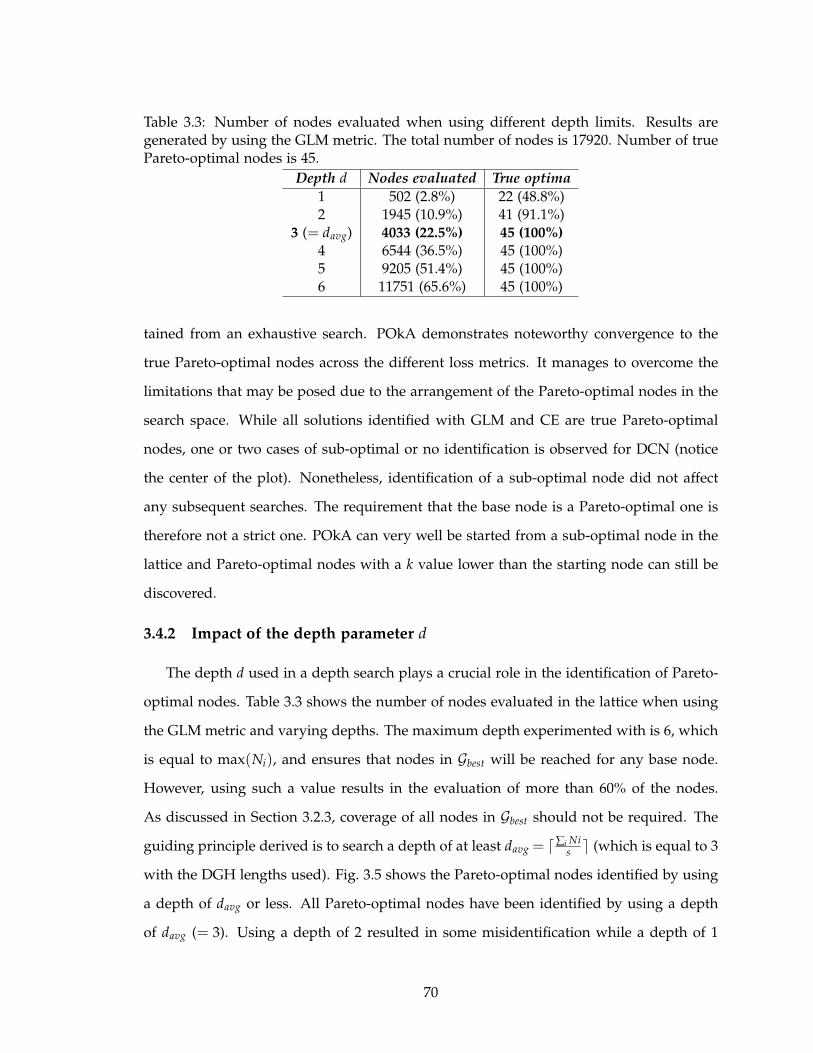
Table 3.3: Number of nodes evaluated when using different depth limits. Results aregenerated by using the GLM metric. The total number of nodes is 17920. Number of truePareto-optimal nodes is 45.
Depth d Nodes evaluated True optima
1 502 (2.8%) 22 (48.8%)2 1945 (10.9%) 41 (91.1%)
3 (= davg) 4033 (22.5%) 45 (100%)
4 6544 (36.5%) 45 (100%)5 9205 (51.4%) 45 (100%)6 11751 (65.6%) 45 (100%)
tained from an exhaustive search. POkA demonstrates noteworthy convergence to the
true Pareto-optimal nodes across the different loss metrics. It manages to overcome the
limitations that may be posed due to the arrangement of the Pareto-optimal nodes in the
search space. While all solutions identified with GLM and CE are true Pareto-optimal
nodes, one or two cases of sub-optimal or no identification is observed for DCN (notice
the center of the plot). Nonetheless, identification of a sub-optimal node did not affect
any subsequent searches. The requirement that the base node is a Pareto-optimal one is
therefore not a strict one. POkA can very well be started from a sub-optimal node in the
lattice and Pareto-optimal nodes with a k value lower than the starting node can still be
discovered.
3.4.2 Impact of the depth parameter d
The depth d used in a depth search plays a crucial role in the identification of Pareto-
optimal nodes. Table 3.3 shows the number of nodes evaluated in the lattice when using
the GLM metric and varying depths. The maximum depth experimented with is 6, which
is equal to max(Ni), and ensures that nodes in Gbest will be reached for any base node.
However, using such a value results in the evaluation of more than 60% of the nodes.
As discussed in Section 3.2.3, coverage of all nodes in Gbest should not be required. The
guiding principle derived is to search a depth of at least davg = ⌈∑i Nis ⌉ (which is equal to 3
with the DGH lengths used). Fig. 3.5 shows the Pareto-optimal nodes identified by using
a depth of davg or less. All Pareto-optimal nodes have been identified by using a depth
of davg (= 3). Using a depth of 2 resulted in some misidentification while a depth of 1
70
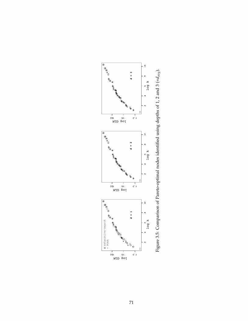
log GLM
log k
log k
log k
log GLM
log GLM
d = 1
d = 2
d = 3
exhaustive-search
+ POkA
Fig
ure
3.5:
Co
mp
aris
on
of
Par
eto
-op
tim
aln
od
esid
enti
fied
usi
ng
dep
ths
of
1,2
and
3(=
dav
g).
71
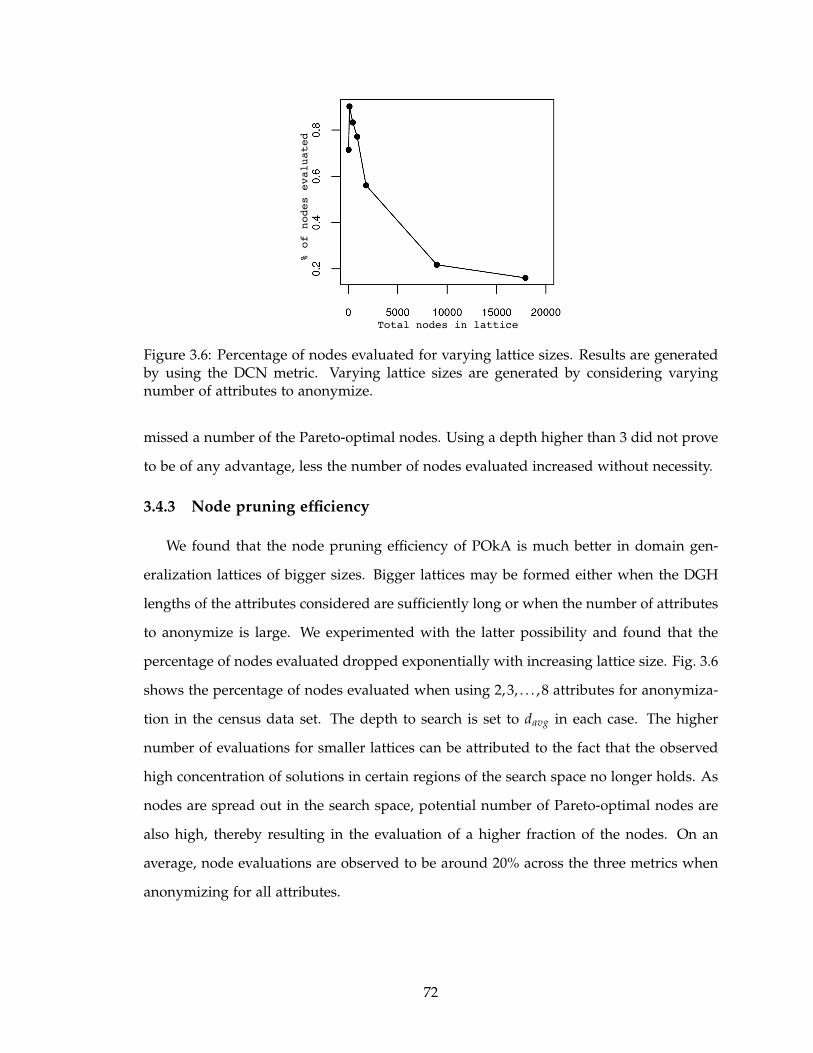
Total nodes in lattice
% of nodes evaluated
Figure 3.6: Percentage of nodes evaluated for varying lattice sizes. Results are generatedby using the DCN metric. Varying lattice sizes are generated by considering varyingnumber of attributes to anonymize.
missed a number of the Pareto-optimal nodes. Using a depth higher than 3 did not prove
to be of any advantage, less the number of nodes evaluated increased without necessity.
3.4.3 Node pruning efficiency
We found that the node pruning efficiency of POkA is much better in domain gen-
eralization lattices of bigger sizes. Bigger lattices may be formed either when the DGH
lengths of the attributes considered are sufficiently long or when the number of attributes
to anonymize is large. We experimented with the latter possibility and found that the
percentage of nodes evaluated dropped exponentially with increasing lattice size. Fig. 3.6
shows the percentage of nodes evaluated when using 2,3, . . . ,8 attributes for anonymiza-
tion in the census data set. The depth to search is set to davg in each case. The higher
number of evaluations for smaller lattices can be attributed to the fact that the observed
high concentration of solutions in certain regions of the search space no longer holds. As
nodes are spread out in the search space, potential number of Pareto-optimal nodes are
also high, thereby resulting in the evaluation of a higher fraction of the nodes. On an
average, node evaluations are observed to be around 20% across the three metrics when
anonymizing for all attributes.
72
3.4.4 Summary
To summarize the results, POkA can identify true Pareto-optimal nodes for a wide
range of loss metrics that structure the search space in different ways. The experimental
results corroborate the theoretical motivation behind using the average number of steps
for full specialization of an attribute as the depth to search. The performance of POkA
does not deteriorate even if certain nodes identified by it are not Pareto-optimal and
used as base nodes. Finally, the number of nodes evaluated is a small percentage of
the total number of nodes when the lattice is significantly bigger than the number of
Pareto-optimal nodes it contain.
3.5 Conclusions
Privacy preserving data dissemination has to minimize the information loss in the
anonymized data set while protecting the identity of underlying individuals to the max-
imum extent possible. In the context of k-anonymity, existing approaches address these
aspects only partially by concentrating only on the issue of minimum information loss.
Specifically, these approaches do not provide any information on the trade-off behavior
between privacy and data utility.
In this chapter, we propose the POkA algorithm to find generalization schemes that
are Pareto-optimal with respect to k-anonymity and a loss metric. By identifying Pareto-
optimal nodes in a domain generalization lattice we can guarantee that no other gen-
eralization can improve on the privacy aspect without deteriorating data utility. POkA
uses a combination of depth first traversals of the lattice to efficiently find the Pareto-
optimal nodes. Theoretical groundwork behind efficiently performing these traversals is
presented. Results on a benchmark data set show that POkA has the potential to identify
all Pareto-optimal nodes with a small percentage of node evaluations. They also demon-
strate that the algorithm is applicable for a number of commonly used loss metrics.
Node evaluation can be further reduced if a better heuristic to stop the depth search
can be found. An initial step in this direction is to investigate more stringent properties
for the ground node. Another research direction is to extend the algorithm to other
73

models of privacy. Pareto-optimality is used here as a two dimensional concept between
privacy and data utility, while there exists privacy models that require the specification
of more than a single parameter. Investigating Pareto-optimal anonymization with such
models is a challenging area as well.
74
CHAPTER 4
Incorporating Data Publisher Preferences
A standard approach in microdata anonymization is to progressively generalize the
data until it is k–anonymous. However, such an approach cannot guarantee optimality
if different attributes carry different levels of significance. For example, in a medical
data set, attributes such as age and disease are more important than the ZIP code of the
underlying patient. This opens up the possibility that a minimum information loss can
be sustained even for higher values of k, thereby providing better privacy than speci-
fied. Searching for higher privacy generalizations is also fruitful if the data publisher can
tolerate an information loss higher than the minimum possible. Existing optimization
attempts do not embrace such preference criteria.
Further, k–anonymity is only a minimalistic measure of the privacy level. The actual
privacy levels of two individuals in a k–anonymous data set can be very different. For
example, consider a 3–anonymous data set. If record A is same as 2 other records while
record B is same as 9 other records, the privacy level of individual B is much higher (9/10)
than that of individual A (2/3). This characteristic, which we call the anonymization bias
[58], is induced by the nature of the k–anonymity model since it only helps to identify
the worst case privacy level. Given the subjective nature of information loss, we cannot
ignore the possibility of a reciprocal relationship between privacy bias and information
loss.
75
In this chapter, we first propose an adaptation of a goal programming based interac-
tive procedure to resolve the problem of choosing a generalization scheme that meets a
privacy property along with minimum bias and information loss. We build on the idea of
anonymization bias to provide a quantitative measurement of the feature. This enables us
to define a precise vector optimization problem for minimizing the privacy bias and infor-
mation loss. We provide a formal characterization of an optimal solution to the problem
in terms of solutions to an achievement-scalarizing function that is based on tolerable bias
and loss values specified by the data publisher. Next, a possible formulation of a scalar-
izing function to minimize bias and information loss is presented. Finally, an interactive
procedure is discussed to help explore the set of optimal solutions based on feedback
received from the data publisher. Such feedback-based search is necessary when the so-
lution generated with specified preferences is not acceptable. The procedure employs a
reference direction approach in order to generate multiple solutions in the neighborhood of
the data publisher’s preferences.
The second contribution is an approach to obtain data generalizations satisfying the
k–anonymity property given preference values on the information loss and privacy bias.
As part of the reference direction approach, the scalarizing function formulated in the
first contribution is subjected to a constrained minimization. We show how the proposed
evolutionary multi-objective approach solves the minimization problem and helps resolve
the issue of finding better privacy levels than specified (by the parameter k), in the pres-
ence of varying data attribute significance and data publisher preferences.
The remainder of the chapter is organized as follows. Section 4.1 provides a prelimi-
nary background on the problem. Section 4.2 provides a formal definition of an efficient
solution to the problem and presents the requisite properties that a scalarizing function
must possess to guarantee such efficiency. A possible scalarizing function for our prob-
lem is discussed in Section 4.3. Section 4.4 discusses the interactive reference direction
approach designed on top of a minimax problem. Section 4.5 presents our multi-objective
algorithm to solve the minimax problem. Empirical results on a benchmark data set are
presented in Section 4.6. Finally, Section 4.7 summarizes and concludes the chapter.
76

Table 4.1: Example data set and its 2–anonymous generalized version.
Employee Code (emp) Salary Class (sal)
81521 C1
81522 C1
81523 C1
82635 C2
82636 C2
82647 C2
82648 C2
81634 C3
81631 C3
81632 C3
81639 C3
81630 C3
emp sal
8152* C18152* C18152* C1
8263* C28263* C2
8264* C28264* C2
8163* C38163* C38163* C38163* C38163* C3
4.1 Preliminaries
We shall use Iyengar’s bit vector representation of a generalization (Section 2.5.1)
to demonstrate the concepts in this chapter. We further associate a value eci to each
tuple in the anonymized data set D′ to signify the size of the equivalence class to which
the tuple belongs. k-anonymity then requires that min(ECD′) ≥ k, where ECD′ is the
vector (ec1, . . . , ecnrow) for D′. Consider the data set in Table 4.1 (left). The data set has
12 entries of 5-digit employee codes and the corresponding salary class. The right table
is a generalized version of this data set where the last digit of the employee code is
removed. As a result, the entries can be grouped together into equivalence classes and
the corresponding equivalence class vector is (3,3,3,2,2,2,2,5,5,5,5,5). The data set then
becomes 2–anonymous since the minimum value in this vector is 2. Since, k–anonymity
satisfies the monotonicity property, i.e. a k–anonymous data set is also (k − 1)–anonymous,
we shall refer to the parameter k in k–anonymity as kpre f and min(ECD′) as the effective
k resulting from the generalizations. In addition, we define the following loss and bias
metrics for our experimental analysis.
4.1.1 Normalized weighted penalty
Let (w1, . . . ,wncol) be a vector of weights where weight 0 ≤ wi ≤ 1 reflects the impor-
tance of the attribute ai. The sum of weights is fixed at 1.0. The penalty for information
77
loss associated with a value vi,j is then given as follows.
penalty(vi,j) = wjloss(vi,j), (4.1)
where loss refers to the generalization loss defined in Eq. (2.4). The penalty attains a
maximum value (equal to the weight of the attribute) when the number of partitions of
an attribute’s domain is one. An entire tuple can thus have a penalty of at most 1.0. The
normalized weighted penalty in D′ is then obtained as the fractional penalty over all tuples
in the data set.
NWP(D′) =∑
nrowi=1 ∑
ncolj=1 penalty(vij)
nrow(4.2)
4.1.2 Normalized equivalence class dispersion
The k–anonymity model is only representative of the worst case privacy measurement.
As a result, it is possible that two anonymized versions of a data set, both satisfying k–
anonymity, result in very different equivalence class sizes for the tuples. The privacy level
of a tuple is directly related to its eci value – the higher the value, lower is the probability
of privacy breach. Since the k–anonymity definition does not enforce any requirement on
how eci values should be distributed, it is often possible that an anonymization is biased
towards a set of tuples (eci ≫ kpre f ) while providing minimalistic privacy (eci = kpre f )
for others. Our attempt here is to control the occurrence of such biased privacy within
acceptable limits.
The value of eci for a tuple can range from 1 to the number of tuples in the data set,
i.e. nrow. This range reflects the maximum bias that can be present in the anonymized
data set. The normalized equivalence class dispersion measures the bias as the maximum
dispersion present in the eci values relative to the maximum possible dispersion.
NECD(D′) =max(ECD′) − min(ECD′)
nrow − 1(4.3)
Note that tighter privacy constraints can implicitly satisfy relaxed ones owing to the
monotonicity property. Hence, if the privacy constraint is 2−anonymity, then any gen-
eralization that achieves k−anonymity with k ≥ 2 is a privacy preserving generalization.
78

In this case, a 2−anonymous and a 3−anonymous table are both privacy preserving but
with the possibility that the latter induces lower bias than the former. Under such condi-
tions, trade-offs can exist between the amount of bias and the utility of the data.
4.2 Objective Scalarization
A typical vector optimization problem involves decision making under the presence
of multiple conflicting objectives. The most important characteristic of these problems is
the non-existence of a single optima, but rather a set of “incomparable” solutions with
respect to the objectives. In the context of data privacy, these solutions embody the trade-
off characteristics in the two objectives – minimum bias (for e.g., minimum NECD) and
minimum information loss (for e.g., minimum NWP) – and are the points for analysis
by a data publisher. Further, while multiple such trade-off solutions may exist, a data
publisher is only interested in those that induce NECD and NWP values close to some
preference levels. We ask the following questions in this regard.
1. What is an efficient solution in the multi-objective minimization of NECD and
NWP?
2. Can such a solution be obtained by minimizing a scalar function that also incorpo-
rates preferences on NECD and NWP?
3. What guarantees that a minimum of the scalar function will be an efficient solution
of the multi-objective problem?
4. Will it be possible to generate different efficient solutions by minimizing the scalar
function?
5. Can we find a scalar function whose minimum is an efficient solution in the neigh-
borhood of the data publisher’s preferred NECD and NWP values?
The answer to the first question is grounded in the dominance based comparison of
points in a multi-objective space. We provide the definition of a trade-off solution in this
space using the principle of dominance, also called an efficient point. The second question
is answered by introducing the concept of scalar achievement functions that combine the
79
two objectives into one and take the data publisher preferences as one of its parameters.
The issues raised in the third and fourth questions are resolved by enforcing the strictly
order preserving and strictly order representing properties in the scalar function. Finally, such
a function will be formulated in the next section as an answer to the fifth question.
4.2.1 Efficient points
Let F be the set of privacy preserving generalizations given the privacy constraint
PCON . In other words, all generalizations in F satisfy the privacy constraint PCON . A
generic privacy constraint is considered in order to emphasize that this approach is not
limited to k–anonymity alone. Other models such as ℓ–diversity or t–closeness may as
well be used to specify PCON . Further, the following discussion is free from any intrinsic
characteristic of the privacy constraint, other than the fact that the set of generalizations
considered (the set F ) satisfy the constraint. We shall later see in Section 4.5 how the
search algorithm stays focused on this set. Due to the same reason, the privacy guar-
antees provided by a resulting generalization will also be same as that provided by the
underlying privacy model.
Let ∆ : F → R be a privacy bias function that assigns a privacy preserving generaliza-
tion a real number signifying the privacy bias induced by it. Similarly, let Π : F → R be
an information loss function signifying the amount of information lost due to a privacy
preserving generalization. NECD and NWP are examples of ∆ and Π respectively.
Consider the set of points in Q = {(δ,π)|δ = ∆(F),π = Π(F), F ∈ F}. The set Q con-
tains the points signifying the bias and information loss for each possible privacy pre-
serving generalization and shall be called the efficiency space. Hence, each point in Q can
be associated with a privacy preserving generalization in F . The following discussion is
presented in terms of the points in Q given the understanding that a solution is actually
represented by the associated point in F . A partial order can be imposed on the points
in Q as follows.
Definition 4.1 DOMINANCE. q1 = (δ1,π1) weakly dominates q2 = (δ2,π2), denoted by
q1 ≺W q2, iff δ1 < δ2 and π1 < π2. Further, q1 = (δ1,π1) strongly dominates q2 = (δ2,π2) 6= q1,
denoted by q1 ≺S q2, iff δ1 ≤ δ2 and π1 ≤ π2.
80
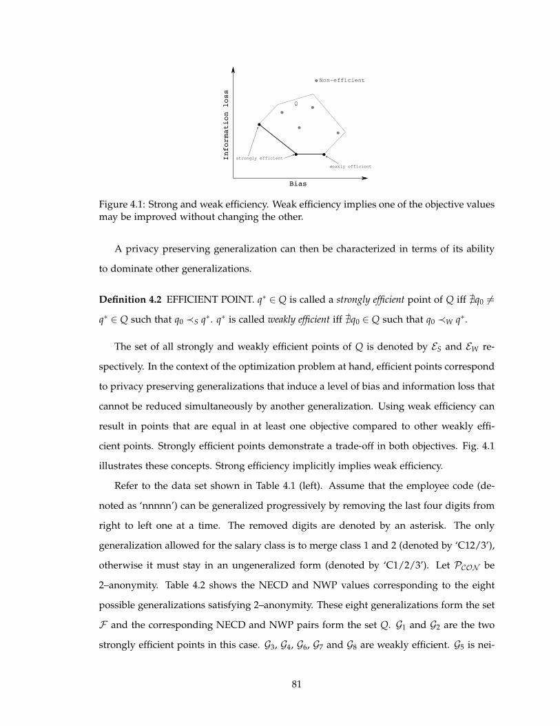
Non-efficient
Q
Bias
Information loss
weakly efficient
strongly efficient
Figure 4.1: Strong and weak efficiency. Weak efficiency implies one of the objective valuesmay be improved without changing the other.
A privacy preserving generalization can then be characterized in terms of its ability
to dominate other generalizations.
Definition 4.2 EFFICIENT POINT. q∗ ∈ Q is called a strongly efficient point of Q iff ∄q0 6=q∗ ∈ Q such that q0 ≺S q∗. q∗ is called weakly efficient iff ∄q0 ∈ Q such that q0 ≺W q∗.
The set of all strongly and weakly efficient points of Q is denoted by ES and EW re-
spectively. In the context of the optimization problem at hand, efficient points correspond
to privacy preserving generalizations that induce a level of bias and information loss that
cannot be reduced simultaneously by another generalization. Using weak efficiency can
result in points that are equal in at least one objective compared to other weakly effi-
cient points. Strongly efficient points demonstrate a trade-off in both objectives. Fig. 4.1
illustrates these concepts. Strong efficiency implicitly implies weak efficiency.
Refer to the data set shown in Table 4.1 (left). Assume that the employee code (de-
noted as ‘nnnnn’) can be generalized progressively by removing the last four digits from
right to left one at a time. The removed digits are denoted by an asterisk. The only
generalization allowed for the salary class is to merge class 1 and 2 (denoted by ‘C12/3’),
otherwise it must stay in an ungeneralized form (denoted by ‘C1/2/3’). Let PCON be
2–anonymity. Table 4.2 shows the NECD and NWP values corresponding to the eight
possible generalizations satisfying 2–anonymity. These eight generalizations form the set
F and the corresponding NECD and NWP pairs form the set Q. G1 and G2 are the two
strongly efficient points in this case. G3, G4, G6, G7 and G8 are weakly efficient. G5 is nei-
81
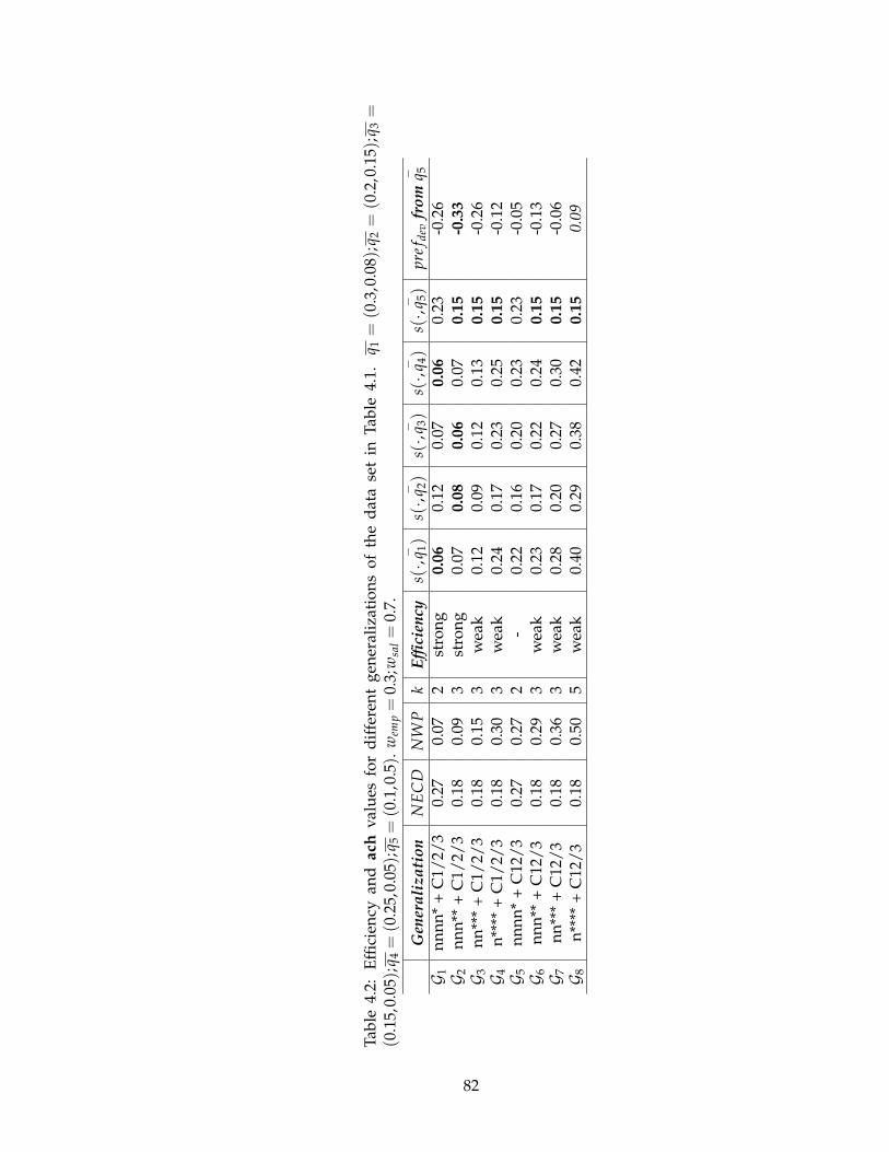
Tab
le4.
2:E
ffici
ency
and
ach
val
ues
for
dif
fere
nt
gen
eral
izat
ion
so
fth
ed
ata
set
inT
able
4.1.
q 1=
(0.3
,0.0
8);
q 2=
(0.2
,0.1
5);
q 3=
(0.1
5,0.
05);
q 4=
(0.2
5,0.
05);
q 5=
(0.1
,0.5
).w
emp=
0.3;
wsa
l=
0.7.
Gen
era
liza
tio
nN
EC
DN
WP
kE
ffici
ency
s(·,
− q 1)
s(·,
− q 2)
s(·,
− q 3)
s(·,
− q 4)
s(·,
− q 5)
pre
f dev
fro
m− q 5
G 1n
nn
n*
+C
1/2/
30.
270.
072
stro
ng
0.0
60.
120.
070.0
60.
23-0
.26
G 2n
nn
**+
C1/
2/3
0.18
0.09
3st
ron
g0.
070.0
80.0
60.
070.1
5-0
.33
G 3n
n**
*+
C1/
2/3
0.18
0.15
3w
eak
0.12
0.09
0.12
0.13
0.1
5-0
.26
G 4n
****
+C
1/2/
30.
180.
303
wea
k0.
240.
170.
230.
250.1
5-0
.12
G 5n
nn
n*
+C
12/
30.
270.
272
-0.
220.
160.
200.
230.
23-0
.05
G 6n
nn
**+
C12
/3
0.18
0.29
3w
eak
0.23
0.17
0.22
0.24
0.1
5-0
.13
G 7n
n**
*+
C12
/3
0.18
0.36
3w
eak
0.28
0.20
0.27
0.30
0.1
5-0
.06
G 8n
****
+C
12/
30.
180.
505
wea
k0.
400.
290.
380.
420.1
50.
09
82

ther weakly nor strongly efficient since G2 weakly dominates and G1 strongly dominates
G5.
4.2.2 Necessary and sufficient conditions
Multiple techniques exist to solve a vector optimization problem. These techniques
may focus on approximating the set of efficient points using ǫ–dominance [3, 66, 105, 174]
or concentrate on parts of the set using reference points [49, 119, 170, 177, 192]. A standard
approach in the latter category is to associate a scalar problem to the original vector
problem and generate efficient points by a single objective optimization of the scalar
function [129, 130]. A typical scalarizing function s : R2 → R defined over R
2 depends
on an arbitrary parameter−q ∈ R
2, the functional form being denoted as s(·,−q). Such
functions must possess certain properties so that a minimum of the function can imply
an efficient point of Q and vice versa.
Definition 4.3 STRICTLY ORDER PRESERVING. Let s : R2 → R be a scalarizing function
with respect to−q ∈ R
2. s is strictly order preserving in Q iff
P1. ∀q1,q2 ∈ Q,q1 ≺S q2 ⇒ s(q1,−q) ≤ s(q2,
−q), and
P2. ∀q1,q2 ∈ Q,q1 ≺W q2 ⇒ s(q1,−q) < s(q2,
−q).
These two properties enforce the monotonicity requirements on s so that a minimum
of the function is an efficient point of Q. This provides a sufficient optimality condition.
The function s must satisfy another property so that any efficient solution of Q can be
obtained by minimization of s parametrized by−q.
Definition 4.4 STRICTLY ORDER REPRESENTING. Let s : R2 → R be a scalarizing func-
tion with respect to−q ∈ R
2. s is strictly order representing in Q iff
R1. ∀q0 ∈ S0 = {q ∈ Q|s(q,−q) ≤ wc}, we also have q0 ≺S
−q, where wc = s(
−q,
−q), and
R2. ∀q0 ∈ S′0 = {q ∈ Q|s(q,
−q) < wc}, we also have q0 ≺W
−q.
The strictly order representing properties help us prove that each efficient solution
of Q has a corresponding value of the parameter−q so that the minimum of s is the
efficient solution. The scalarization thus provides the necessary optimality conditions.
83

The following propositions provide a characterization of the efficient points of Q in terms
of the solutions to a strictly order preserving and strictly order representing function s.
Proposition 4.1 If q∗ is a global minimum point of s(q,−q) on Q, then q∗ ∈ EW .
Proposition 4.2 If q∗ is a unique global minimum point of s(q,−q) on Q, then q∗ ∈ ES.
Proposition 4.3 If q∗ ∈ EW , then q∗ is a global minimum of s(q,−q) on Q for
−q = q∗.
Proposition 4.4 If q∗ ∈ ES, then q∗ is a unique global minimum of s(q,−q) on Q for
−q = q∗.
A global minimum of the scalar achievement function should not be confused as a
global minimum in the NWP vs. NECD objective space. In fact, a global minimum is not
defined in a multi-objective case. Following Propositions 4.1 and 4.2, a global minimum
of s(·,−q) (a single objective function) only implies that the resulting solution is an efficient
point of the two-objective space. Further, by Propositions 4.3 and 4.4, one can arrive at
different efficient points by modifying the parameter−q in the achievement function.
With reference to Table 4.2, Propositions 4.1 and 4.2 guarantee that the global min-
imum of a strictly order preserving and strictly order representing function will never
appear at generalization G5. Further, if the parameter−q of the function is set to the
corresponding NECD and NWP values of a generalization, then the global minimum
is guaranteed to appear at that generalization (Propositions 4.3 and 4.4). Hence, every
efficient point is reachable by the function.
Note that minimal points of a scalarizing function does not correspond to the final
solution of choice by the data publisher. They are rather used to locally approximate
the preferences of the data publisher with the guarantee that the generated solutions
are efficient. Data publisher preferences are typically embodied in the parameter−q of
the function (also called a preference point, reference objective or aspiration level) with the
idea that an efficient solution minimizing some sort of distance from−q is sought. This
is followed by an interaction with the data publisher to inquire if the reported solution
is satisfactory. Order preserving and order representing properties guarantee that the
reported solution (generated by a minimization of the scalarizing function) is efficient,
or is the best one possible within the specification of the aspiration levels. Therefore, in
84
this framework, an optimal solution from the perspective of the data publisher is not the
generalization that results in minimum information loss (as assumed in existing works),
but the generalization that meets the preference levels in the best possible way. The next
section dwells into the formulation of a scalar achievement function that integrates these
requirements.
4.3 Scalarizing Bias and Loss
The typical constrained optimization problem explored in disclosure control is to find
an anonymized version of a data set, or effectively a set of generalizations resulting in
the anonymized version, that induce minimum information loss subject to the constraint
that the anonymized data set is k–anonymous. Given the NP-hard nature of the problem
[127], heuristic based approaches in this context progressively increase the amount of
generalization for the attributes until the k–anonymity constraint is satisfied [16, 72, 176].
The anonymized data set at this point is assumed to incur minimum information loss.
These approaches have two major drawbacks.
First, the information loss metric is assumed to have a monotonic relationship with
the amount of generalization. In other words, as more generalization is performed (no
matter for which attribute), the information loss increases. Only under this assumption
can one claim that by performing generalization only to the extent necessary to satisfy
the k–anonymity constraint, we shall also be minimizing the information loss. However,
the assumption is not valid when all attributes do not carry the same significance.
Second, these approaches do not provide the framework to explore the possibility of
attaining higher effective k values. Owing to the monotonicity property, an effective k
value higher than kpre f will also satisfy the anonymity constraint, but comes with the
added advantage of better privacy. Further, existing approaches do not take into account
any preference specified on information loss. There are some successful attempts to obtain
all possible k–anonymized versions of a data set [109, 150], out of which the optimal one
can be chosen based on preference criteria. Nonetheless, the set of solutions obtained
with those approaches still remains exponentially large, making the search for an optimal
choice equally difficult to perform. The issue of privacy bias remains unexplored in all
85
these attempts.
The objective behind the scalarization of bias and utility is to arrive at privacy pre-
serving generalizations that correspond to efficient solutions that are close to a reference
objective. The reference objective is a point that signifies a tolerable level of bias and
information loss to the data publisher. Depending on whether the reference objective lies
inside or outside the efficiency space, the specified bias and information loss constraint
may or may not be satisfied. If solutions better than the reference objective exist, then an
efficient solution as far as possible from the reference point will provide the best possible
improvements beyond the aspirations of the data publisher. On the other hand, if the
reference objective is unachievable, then the data publisher can at best have a solution
which is efficient and closest to the reference point.
We seek a scalarizing function that embeds these two requirements. In addition, the
strictly order preserving and strictly order representing properties must be satisfied so
that efficient points can be generated by a minimization of the scalar function. We present
here one possible formulation for such a function.
Let qideal = (δideal ,πideal) denote the ideal point in R2, the components of which are
obtained by individual minimization of the bias and loss functions, i.e. δideal = min ∆(·)and πideal = min Π(·). If a unique F ∈ F minimizes both the bias and loss functions,
then qideal is the optimal solution. However, under the presence of trade-off behavior
in the two functions, such a generalization will not exist. Hence, the ideal point is of
theoretical importance only. For most cases in data privacy, the ideal point is the point
(0,0). Next, let qutp = (δutp,πutp) be an utopian point computed as δutp = δideal − ǫδ and
πutp = πideal − ǫπ where ǫδ and ǫπ are small positive numbers. The scalarizing function
ach := s(q,−q) for q = (δ,π) ∈ R
2 and−q = (
−δ,
−π) ∈ R
2 is then formulated as
s(q,−q) = max
[
w(δ − δutp), (1 − w)(π − πutp)]
, (4.4)
where w =
1−δ − δutp
/
1−δ − δutp
+1
−π − πutp
.
This scalarization of bias and loss provides a maximal over-achievement of the ob-
jectives if the reference point is feasible. Otherwise, the function provides a minimal
underachievement. The parameter w allows us to vary the weights on the two objectives,
86

thereby providing a mechanism to explore the neighborhood of a solution. The precise
impact of w is discussed in Section 4.4.
Consider the preference point−q1 = (0.3,0.08) in Table 4.2. The minimum of the ach
function in this case appears at G1 since the corresponding NECD and NWP values of
0.27 and 0.07 can over-achieve the preferred ones. However, G1 cannot provide the same
improvements for the preference point−q2 = (0.2,0.15). The minimum in this case appears
at G2 since it can provide the best over-achievement in the two objectives.−q3 = (0.15,0.05)
and−q4 = (0.25,0.05) are infeasible preferences. The minima here are obtained at the gen-
eralizations that produce minimal underachievement, i.e. G2 and G1 respectively. Further,
the minimum point in all cases is also an efficient point in the NECD vs. NWP objective
space. This is due to the strictly order preserving property of ach.
Theorem 4.1 The scalarizing function ach is strictly order preserving.
Proof To prove property P1, consider the distinct points q1 = (δ1,π1),q2 = (δ2,π2) ∈ Q
such that q1 ≺S q2.
Hence, we have δ1 ≤ δ2 and π1 ≤ π2. Assuming that−q > qutp (a valid assumption since
the reference point will at best be qideal), we have 0 < w < 1, giving us (1 − w) > 0. We
can thus obtain the following two relations.
w(δ1 − δutp) ≤ w(δ2 − δutp)
(1 − w)(π1 − πutp) ≤ (1 − w)(π2 − πutp)
Using the observation that a ≤ b and c ≤ d implies max(a, c) ≤ max(b,d), we obtain
s(q1,−q) ≤ s(q2,
−q), thus proving property P1.
To prove property P2, let q1 ≺W q2. We then have δ1 < δ2 and π1 < π2. The remainder
of the proof follows in a manner similar to above, giving us s(q1,−q) < s(q2,
−q). Thus ach
is strictly order preserving. �
Theorem 4.2 The scalarizing function ach is strictly order representing for
wc = 1/
1−δ − δutp
+1
−π − πutp
. (4.5)
87

Proof To prove property R1, let q1 = (δ1,π1) ∈ S0. Hence s(q1,−q) ≤ wc = s(
−q,
−q), i.e.
max[
w(δ1 − δutp), (1 − w)(π1 − πutp)]
≤ wc.
Rewriting the expression in terms of wc we get
max
wc
(
δ1 − δutp
−δ − δutp
)
,wc
(
π1 − πutp
−π − πutp
)
≤ wc
i.e. wc
(
δ1 − δutp
−δ − δutp
)
≤ wc and wc
(
π1 − πutp
−π − πutp
)
≤ wc.
After simplification we get,−δ − δ1 ≥ 0 and
−π − π1 ≥ 0. Hence, q1 ≺S
−q. This proves
property R1.
To prove property R2, let q1 ∈ S′0. Hence s(q1,
−q) < wc. By proceeding in a manner as
above we get−δ − δ1 > 0 and
−π − π1 > 0. Therefore, q1 ≺W
−q. Thus ach is strictly order
representing. �
Based on Propositions 4.1 and 4.2, minimization of ach (a minimax problem) over Q
will therefore result in an efficient privacy preserving generalization. However, solutions
to the minimax problem can return either weakly or strongly efficient solutions. Ideally, a
strongly efficient solution is more desirable since weakly efficient solutions cannot guar-
antee that one of the objective values cannot be reduced by keeping the other constant.
Strongly efficient solutions are indicated by a unique global minimum of ach. For the case
when multiple global minima exists, inference of strong efficiency is difficult. As a resolu-
tion to this problem, we choose a solution that provides the maximum over-achievement
or minimum underachievement with respect to the reference objective, i.e. choose the so-
lution q = (δ,π) ∈ Qg with minimum preference deviation, pre fdev = (δ + π −−δ − −
π), where
Qg ⊆ Q is the set of global minima points of ach. Thus, if an unachievable reference
objective is specified by the data publisher, an efficient solution as close as possible to the
reference point will be returned. However, if the reference objective is suboptimal (lower
bias and loss possible), then an efficient solution as far away as possible from the refer-
ence point is returned. Further, Propositions 4.3 and 4.4 guarantee that if the reference
objective chosen by the data publisher is an efficient point in itself, then a minimum of
ach will exist exactly at the desired solution.
88

Consider the preference point−q5 = (0.1,0.5) in Table 4.2. Multiple minima points exist
for ach in this case. These points provide the least underachievement in NECD while
satisfying the NWP preference of 0.5. The minimum preference deviation is obtained in
G2 as it best over-achieves the NWP preference. G2 is also the strongly efficient point in
the set of minima.
Incorporating data publisher preferences in the optimization procedure can also po-
tentially hinder minimality attacks [180]. Minimality attacks exploit the knowledge that
most data generalization algorithms attempt to enforce the privacy requirement with as
less generalization as possible (minimum information loss). Hence, most existing meth-
ods are prone to this attack. However, the ach function subjected to minimization in this
work is parametrized by the data publisher preferences. Therefore, a minimum of this
function is not necessarily the generalization that induces the minimal information loss.
In other words, the extent of generalization performed is not guided by the minimality
principle (as assumed in minimality attacks), but is rather dependent on what the data
publisher specifies as tolerable information loss. This can void the efficacy of minimal-
ity attacks since the preferences of the data publisher are most likely unknown to the
attacker. However, a more extensive analysis is required to validate this claim.
4.4 Reference Direction Approach
While a solution obtained by minimizing the ach function is efficient, a data publisher
may not find the reported solution satisfactory enough with respect to the reference objec-
tives in mind. This is because the initial knowledge of the data publisher on the feasibility
of a solution inducing the aspired bias and loss is limited. Once a solution is generated,
the data publisher obtains additional knowledge on what levels of bias and loss are pos-
sible around the neighborhood of the preference point. This prompts for an interactive
method that allows the data publisher to progressively explore efficient solutions until a
satisfactory one is found. We adapt a method based on reference directions to facilitate this
exploration [47, 128].
Definition 4.5 REFERENCE DIRECTION. Let q be a point in R2 and
−q ∈ R
2 be a prefer-
89

Procedure 4.1 ReferenceDirectionApproach(Point q1, Point−q, integer n)
Input: Initial point q1 ∈ R2 and a preference point
−q > qutp. n is the number of efficient
solutions to generate along the reference direction.1: t = 12: repeat
3: Qe f f = φ
4: dt =−q − qt {vector arithmetic}
5: for all (m in {1, . . . ,n}) do
6:−
qm = qt + (m/n)dt
7: Obtain q∗m as the solution to the problem of minimizing ach := s(q,−
qm)8: Qe f f = Qe f f ∪ {q∗m}9: end for
10: if (no solution in Qe f f is satisfactory) then
11: Choose a point in Qe f f as qt+1 to define a new reference direction12: t = t + 113: end if
14: until (a satisfactory solution is found)
ence point. The reference direction d is then defined as the vector d =−q − q.
The basic approach here is to generate a number of efficient points along the projection
of a reference direction on the efficiency space. This gives the data publisher an idea of
the trade-off characteristics of solutions in the neighborhood where the data publisher’s
interest lies in the first place. If a satisfactory solution is found, then the process stops.
Otherwise, one of the generated solutions is chosen to define a new reference direction
for the next iteration of the process. This procedure of specifying a new search direc-
tion enables a data publisher to control how much deviation from the aspiration levels
is tolerable in a certain objective. The reference direction approach computes what pa-
rameter value needs to be passed to the scalar achievement function to generate solutions
in this new direction of interest. A new set of solutions is then generated and the pro-
cess continues. By doing so, the data publisher can extensively explore the neighborhood
surrounding the preference point until a solution is in agreement with the publisher’s
requirements. We shall first provide the basic steps of the method (Procedure 4.1) and
then provide a geometrical perspective of the procedure.
Refer to the data set in Table 4.1. Assume that the data publisher starts with a pref-
erence point−q = (0.1,0.1). Based on the extent of NECD and NWP values to explore,
90
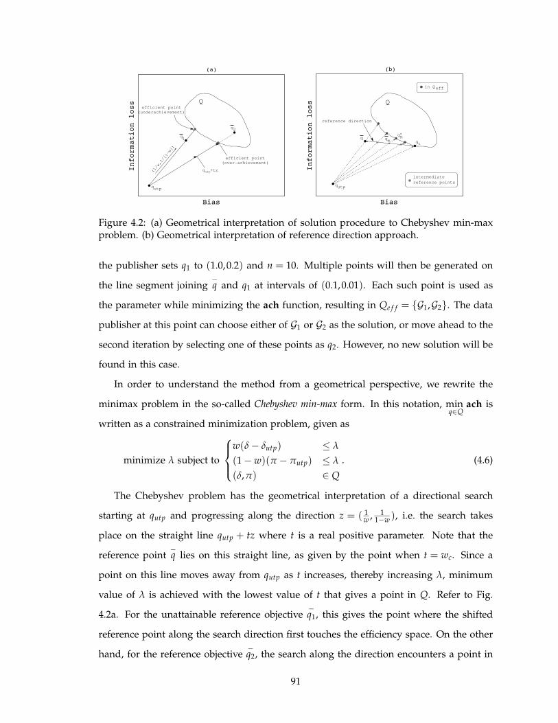
Bias
Information loss
Information loss
Bias
q1
q2
qutp
efficient point
efficient point
Q
q +tzutp(1/w,1/[1-w])
qutp
reference direction
qqt
qm
qm*
Q
(a) (b)
intermediate
reference points
(over-achievement)
(underachievement)
in Qeff
Figure 4.2: (a) Geometrical interpretation of solution procedure to Chebyshev min-maxproblem. (b) Geometrical interpretation of reference direction approach.
the publisher sets q1 to (1.0,0.2) and n = 10. Multiple points will then be generated on
the line segment joining−q and q1 at intervals of (0.1,0.01). Each such point is used as
the parameter while minimizing the ach function, resulting in Qe f f = {G1,G2}. The data
publisher at this point can choose either of G1 or G2 as the solution, or move ahead to the
second iteration by selecting one of these points as q2. However, no new solution will be
found in this case.
In order to understand the method from a geometrical perspective, we rewrite the
minimax problem in the so-called Chebyshev min-max form. In this notation, minq∈Q
ach is
written as a constrained minimization problem, given as
minimize λ subject to
w(δ − δutp) ≤ λ
(1 − w)(π − πutp) ≤ λ
(δ,π) ∈ Q
. (4.6)
The Chebyshev problem has the geometrical interpretation of a directional search
starting at qutp and progressing along the direction z = ( 1w , 1
1−w ), i.e. the search takes
place on the straight line qutp + tz where t is a real positive parameter. Note that the
reference point−q lies on this straight line, as given by the point when t = wc. Since a
point on this line moves away from qutp as t increases, thereby increasing λ, minimum
value of λ is achieved with the lowest value of t that gives a point in Q. Refer to Fig.
4.2a. For the unattainable reference objective−q1, this gives the point where the shifted
reference point along the search direction first touches the efficiency space. On the other
hand, for the reference objective−q2, the search along the direction encounters a point in
91

the efficiency space before encountering the reference point, i.e. t < wc, thereby providing
an over-achievement.
Note that the direction of search is decided by w, which in turn is parametrized by the
reference objective. It is therefore possible to change the direction of search by providing
different reference objectives. The interactive procedure does so by generating interme-
diate reference objectives−
qm on the reference direction. Refer to Fig. 4.2b. At iteration t,
a current solution qt and the reference objective−q defines the reference direction. Inter-
mediate reference points are then generated along this direction. For each such point, a
search is performed along the straight line joining qutp and the reference point. In other
words, solutions to the Chebyshev problem is found taking different search directions,
each returning an efficient solution in the neighborhood of qt and−q. For example, the
solution q∗m is found as the shifted intersection of the reference direction and straight line
defined by the vector ( 1w , 1
1−w ) with w being computed using the reference objective−
qm.
Recall that since ach is strictly order representing, all efficient solutions are minima of
some representation of the function (parametrized by the reference objective). This in turn
implies that there exists some value of w (again, parametrized by the reference objective)
corresponding to every efficient point, such that the solution to ach is the efficient point.
Theorem 4.3 Let q∗ ∈ Q be an efficient solution. There exists a value of w such that
0 < w < 1 and q∗ is a unique global minimum of ach.
Proof Let q∗ = (δ∗,π∗) ∈ Q be an efficient solution (weakly or strongly). To the contrary,
let us assume that there exists no positive value of w such than q∗ is a unique global
minimum of ach.
Let us set−q = q∗. This gives us
w =
[
1
δ∗ − δutp
]
/
[
1
δ∗ − δutp+
1
π∗ − πutp
]
.
Note that w is greater than zero (since for any q ∈ Q, q > qutp) and less than one. In
the Chebyshev formulation of ach, q∗ will be a feasible solution. In other words, we can
find a λ∗ such that w(δ∗ − δutp) ≤ λ∗ and (1 − w)(π∗ − πutp) ≤ λ∗. After simplification,
the least value of such a λ∗ is found to be wc.
92
However, since q∗ is not a unique global minimum, there must exist another point
q0 = (δ0,π0) ∈ Q with a corresponding λ = λ0 such that λ∗ ≥ λ0 ≥ w(δ0 − δutp) and λ∗ ≥λ0 ≥ (1 − w)(π0 − πutp). By substituting λ∗ with wc, and the value of w in the two
relations, we arrive at the following two expressions: δ∗ ≥ δ0 and π∗ ≥ π0, or in other
words, q0 ≺S q∗. Hence, q∗ cannot be an efficient solution unless q0 = q∗. Hence, q∗ is
a unique global minimum of the Chebyshev problem. Therefore, there exists a value
0 < w < 1 such that q∗ is a unique global minimum of ach. �
Thus, ach can be used to generate any efficient point by varying its parameters. How-
ever, unlike a typical weighted sum approach, parameter specification in this approach
is more intuitive to the data publisher, namely the aspiration levels of the publisher. Ar-
tificial parameters like weights are often difficult to specify, with the drawback that they
can sometimes be inconsistent with intuition. Further, convergence in the interactive pro-
cedure is completely guided by the data publisher. Hence, although the finally chosen
solution may be very different from the initial aspiration levels, it is guaranteed to be a
satisfactory one.
4.5 Minimizing the Achievement Function
A crucial step in the reference direction approach is finding a privacy preserving
generalization that minimizes ach (a solution q∗m in Step 7). This optimization problem is
repeatedly solved as part of the approach. With respect to k−anonymity and the metrics
NWP and NECD, the problem can be stated in the following manner. Here,−π = NWPpre f
and−δ = NECDpre f .
Problem 4.1 Optimization Problem (OP). Given a data set D, kpre f , NWPpre f and NECDpre f ,
find the anonymized data set D′ that minimizes the achievement function ach subject to
the constraint kpre f − min(ECD′) ≤ 0.
The optimization problem at hand is a constrained single objective problem. In this
section we propose an approach based on evolutionary multi-objective optimization to
find a solution to the problem. The method involves transforming the constraint into a
93
separate objective giving us a bi-objective vector optimization problem [40]. The multi-
objective variant of OP is formulated as follows.
Problem 4.2 Multi-Objective Optimization Problem (MOOP). Given a data set D, kpre f ,
NWPpre f and NECDpre f , find the anonymized data set D′ that minimizes the achievement
function f1(D′) : ach(D′) and the function f2(D′) : kpre f − min(ECD′).
Solutions to the MOOP are characterized by the Pareto-dominance concept. Under
such a characterization, an anonymized data set D′ found by the solution methodology is
a non-dominated solution to the MOOP if it cannot find another solution D′′ such that
• f1(D′′) ≤ f1(D
′) and f2(D′′) < f2(D′), or
• f1(D′′) < f1(D
′) and f2(D′′) ≤ f2(D′).
A direct and positive consequence of using this formulation is the exposure of higher
effective k solutions, if any. Note that a solution to OP only needs to satisfy the constraint
kpre f − min(ECD′) ≤ 0. In the multi-objective formulation, the solutions undergo further
filtering based on non-dominance – for two solutions with equal value of ach, the one
with higher effective k (lower f2) gets preference. Thus, if multiple solutions to OP exists
at different effective k values, the multi-objective approach directs the search towards the
one providing the highest level of privacy.
Recall the case when multiple minima are obtained with−q5 = (0.1,0.5) as the prefer-
ence point in Table 4.2. All points except G8 will be filtered out by the multi-objective
optimizer since it provides a comparatively higher value for k. Given that a NWP value
of 0.5 can be tolerated, G8 leverages it to improve the privacy level. Note that if the NWP
preference is changed to say 0.2, then G8 will no longer be a minimum point of ach. In
that case, there will be multiple solutions with same k and ach values. The preference
deviation metric will then be used to choose a solution.
4.5.1 A modified selection operator
We use the Non-dominated Sorting Genetic Algorithm-II (NSGA-II) with Iyengar’s
bit vector representation to obtain solutions to the MOOP. While most components of
94

NSGA-II are retained in the original form, a modification is proposed for the selection
procedure in order to direct solutions towards the feasible region of OP [65]. NSGA-II
employs a crowded comparison operator as part of its binary tournament selection scheme.
This operator gives preference to solutions with lower ranks (in accordance with the non-
dominated ranking scheme of the algorithm). For the case when the compared solutions
are of the same rank, the crowding distance metric is used to choose the solution with
least diversity. Our modification involves distinguishing between feasible ( f2(D′) ≤ 0)
and infeasible ( f2(D′) > 0) solutions of OP during the selection procedure. The procedure
is outlined as follows for two solutions x and y.
1. If both x and y are feasible, select based on crowded comparison operator.
2. If x is feasible and y is not, or vice versa, select the feasible one.
3. If both x and y are infeasible:
(a) select one with minimum f2.
(b) if f2 is equal, select one with minimum f1.
(c) if f1 is also equal, use crowding distance metric.
4. Use arbitrary selection for any unresolved case.
Using this selection procedure, we can initially direct the search towards the feasible
region of OP and thereafter concentrate on exploring the trade-off characteristics. Step
3 of the procedure uses a lexicographic approach to selection. Note that the space of
possible solutions to the problem is increasingly dense as the effective k approaches 1,
i.e. a relatively higher number of solutions are feasible for lower kpre f . Step 3b and 3c are
particularly useful in such settings. Also, the feasibility check here involves determining
the size of the smallest equivalence class and whether it is at least kpre f . This check must
be appropriately modified when considering a privacy model different from k–anonymity.
This involves determining the value of the privacy parameter (e.g. k in k–anonymity or
ℓ in ℓ–diversity) resulting from using a generalization, and checking whether it satisfies
the minimum threshold set by the data publisher.
95

Table 4.3: Attributes and domain size from the adult census data set.
Attribute Domain Size
Age (age) 20 (granularity=5)Work Class (wkc) 7Education (edc) 16
Marital Status (mst) 7Occupation (occ) 14
Race (rac) 5Gender (gen) 2
Native Country (ncy) 41Salary Class (slc) 2
4.5.2 Solution to OP
Once the final non-dominated solution set ND to MOOP is obtained, the solution
to OP is chosen as the point D′ such that D
′ = argminD′′∈ND f
f1(D′′), where ND f = {Di ∈
ND| f2(Di) ≤ 0}. The case of multiple such solutions is resolved using the preference
deviation metric. Since the minimum of ach obtained in this manner is only justifiable
w.r.t. ND f , we shall say that D′ is an efficient solution only w.r.t. the non-dominated solu-
tions generated by NSGA-II. Hence, although a global minimum of ach is guaranteed to
be an efficient solution (w.r.t. the entire efficiency space) in theory, the NP-hard nature of
the problem prevents us from claiming that the solution found is indeed a true minimum.
The statement is just a cautious side note to indicate that the effectiveness of the approach
is as good as the convergence and diversity preservation abilities of the multi-objective
optimizer.
4.6 Empirical Results
We applied the NSGA-II methodology to the “adult.data” benchmark data set. The
attributes used in this study along with their domain size are listed in Table 4.3. Recall
that each attribute requires (domain size - 1) bits to represent all possible generalizations.
This gives us a chromosome of length 105 bits representing a solution. For NSGA-II, the
population size Npop is set at 100 with a maximum of 50,000 function evaluations. Binary
crossover is performed on the entire chromosome with rate 0.8. Mutation is performed
on the individual encodings of every attribute with a rate of 0.001. The modified selection
96
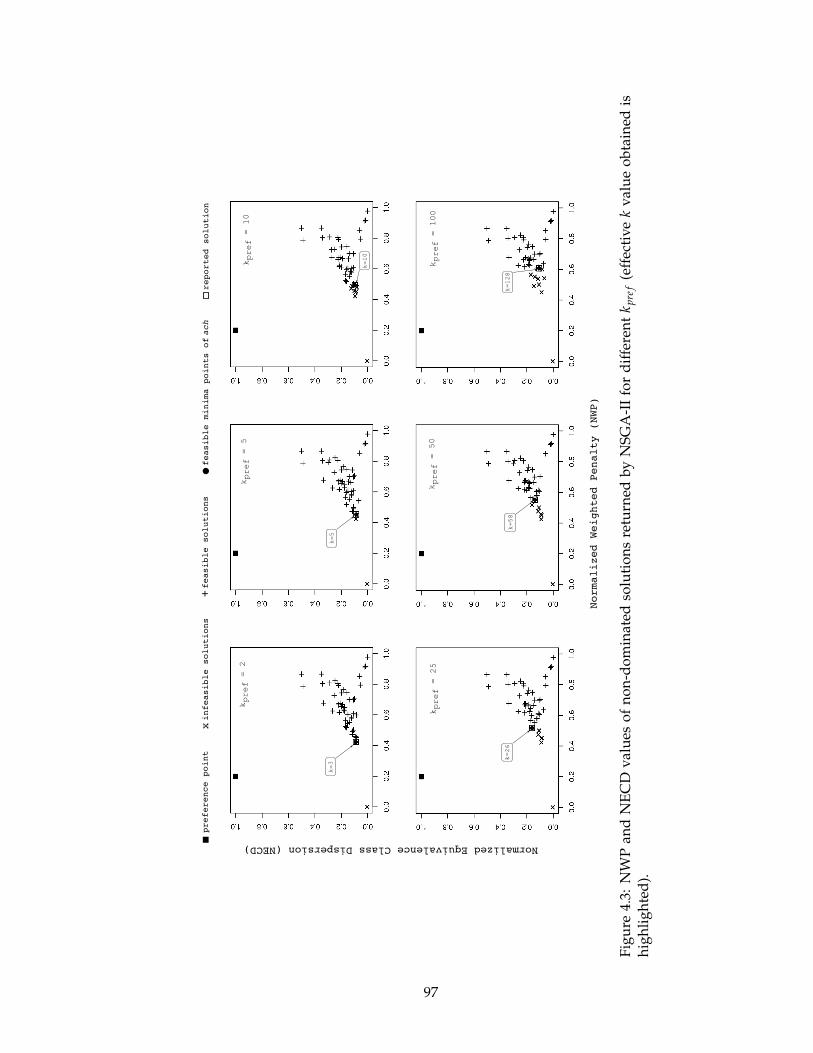
Normalized Weighted Penalty (NWP)
Normalized Equivalence Class Dispersion (NECD)preference point
feasible solutions
+xinfeasible solutions
feasible minima points of ach
reported solution
k = 2
pref
k = 5
pref
k = 10
pref
k = 100
pref
k = 50
pref
k = 25
pref
k=3
k=5
k=10
k=26
k=58
k=128
Fig
ure
4.3:
NW
Pan
dN
EC
Dv
alu
eso
fn
on
-do
min
ated
solu
tio
ns
retu
rned
by
NS
GA
-II
for
dif
fere
nt
kp
ref
(eff
ecti
ve
kv
alu
eo
bta
ined
ish
igh
lig
hte
d).
97

operator is used for binary tournament selection. Weights on the attributes are assigned
equally (1/9), unless otherwise stated.
4.6.1 Solution efficiency
Fig. 4.3 illustrates the NWP and NECD values of the non-dominated solutions re-
turned by NSGA-II for different values of kpre f . The preference point of NWPpre f = 0.2
and NECDpre f = 1.0 is used in these experiments. Choosing a NECD preference of 1.0
effectively allows NSGA-II to look for low NWP solutions irrespective of the privacy bias
they induce. As higher values of kpre f are used, the number of feasible solutions obtained
decreases. This is likely to happen since the search space is known to be very dense for
low values of kpre f , while solutions become rare as higher privacy requirements are en-
forced. Consequently, while reported solutions for kpre f = 2,5 and 10 have an effective
k close to kpre f , higher values are obtained for kpre f = 25,50 and 100. However, higher
information loss has to be sustained for stronger privacy requirements. A unique feasible
minimum of ach is obtained in all the cases. In confirmation to our theoretical observa-
tion, the minimum point is a non-dominated point in the NWP vs. NECD objective space
w.r.t other feasible solutions returned by NSGA-II. Further, the existence of solutions at
effective k values higher than kpre f (for example k = 3 for kpre f = 2) strengthens our claim
that the optimal solution need not always have effective k value equal to kpre f . Once again,
the concept of Pareto-dominance helps here in discovering these solutions.
4.6.2 Impact of population size
Fig. 4.4 shows the reported solutions for three different settings of population size,
Npop = 100,250 and 500. Notice that increasing the population size, while keeping the
number of function evaluations fixed, seems to have only marginal impact on the overall
solution quality. Solutions are slightly less effective in terms of the preference deviation
metric for larger population size, albeit there is no logical pattern in the behavior. Larger
populations typically have the potential to explore more parts of the search space. How-
ever, the absence of a uniform distribution of solutions in the search space makes this
exploration difficult. We also notice that the number of unique solutions obtained is sim-
98

k = 5
unique sols. = 55
pref = -0.6609831 dev
N = 100pop
k = 5
unique sols. = 54
pref = -0.648858 dev
N = 500pop
k = 7
unique sols. = 52
pref = -0.610092 dev
N = 250popk = 5pref
0.3 0.4 0.5 0.6
NECD
NWP
0.06 0.10 0.14
Figure 4.4: Impact of population size (Npop) on solution quality for kpre f = 5 and prefer-ence point NWPpre f = 0.2; NECDpre f = 1.0.
ilar irrespective of the population size used. Large populations have more duplicates that
affect the convergence rate of the population. This is primarily due to the higher selective
pressure of duplicate solutions, which limits the exploratory capabilities of the popula-
tion. Small populations and higher number of iterations is a key element in solving this
problem.
4.6.3 Effect of weight vector
Fig. 4.5 illustrates the solutions obtained for different assignment of weights to the
attributes. As is evident from the solutions, the assignment of equal weights (wv1) in
this problem results in a much higher NWP and NECD. Weight assignments impact the
amount of generalization that may be performed for an attribute, which in turn influence
the information content of the anonymized data set. Even when all attributes are equally
important, higher weights can be assigned to attributes with larger domain sizes to re-
tain as much information as possible. For example, while most solutions in the figure
completely suppress (number of partitions = 1) the “native country” attribute, assigning
a higher weight to the attribute (as in wv2 and wv5) return solutions with more number of
partitions. In general, NSGA-II is seemingly effective in generating solutions with higher
number of partitions in accordance with the weight assignments. The “age” attribute
seems to have some correlation with the other attributes as the generalization performed
99
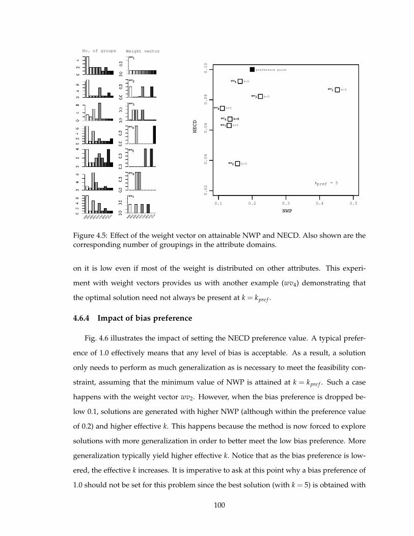
No. of groups Weight vector
age
wkc
edc
mst
occ
rac
gen
ncy
slc
age
wkc
edc
mst
occ
rac
gen
ncy
slc
wv1
wv2
wv3
wv4
wv5
wv6
wv7
wv3
wv5
wv6
wv4
wv7
wv2
wv1
preference point
k = 5pref
0.1 0.2 0.3 0.4 0.50.02 0.04 0.06 0.08 0.10
NECD
NWP
k=5
k=5
k=5
k=5
k=5
k=5
k=8
Figure 4.5: Effect of the weight vector on attainable NWP and NECD. Also shown are thecorresponding number of groupings in the attribute domains.
on it is low even if most of the weight is distributed on other attributes. This experi-
ment with weight vectors provides us with another example (wv4) demonstrating that
the optimal solution need not always be present at k = kpre f .
4.6.4 Impact of bias preference
Fig. 4.6 illustrates the impact of setting the NECD preference value. A typical prefer-
ence of 1.0 effectively means that any level of bias is acceptable. As a result, a solution
only needs to perform as much generalization as is necessary to meet the feasibility con-
straint, assuming that the minimum value of NWP is attained at k = kpre f . Such a case
happens with the weight vector wv2. However, when the bias preference is dropped be-
low 0.1, solutions are generated with higher NWP (although within the preference value
of 0.2) and higher effective k. This happens because the method is now forced to explore
solutions with more generalization in order to better meet the low bias preference. More
generalization typically yield higher effective k. Notice that as the bias preference is low-
ered, the effective k increases. It is imperative to ask at this point why a bias preference of
1.0 should not be set for this problem since the best solution (with k = 5) is obtained with
100
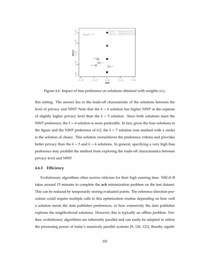
Solid - preference point
Hollow - reported solution
k=7
k=7
k=6
k=5
k = 5pref
0.10 0.15 0.20 0.25 0.30
NWP
0.02 0.04 0.06 0.08 0.10
NECD
Figure 4.6: Impact of bias preference on solutions obtained with weights wv2.
this setting. The answer lies in the trade-off characteristic of the solutions between the
level of privacy and NWP. Note that the k = 6 solution has higher NWP at the expense
of slightly higher privacy level than the k = 5 solution. Since both solutions meet the
NWP preference, the k = 6 solution is more preferable. In fact, given the four solutions in
the figure and the NWP preference of 0.2, the k = 7 solution (one marked with a circle)
is the solution of choice. This solution overachieves the preference criteria and provides
better privacy than the k = 5 and k = 6 solutions. In general, specifying a very high bias
preference may prohibit the method from exploring the trade-off characteristics between
privacy level and NWP.
4.6.5 Efficiency
Evolutionary algorithms often receive criticism for their high running time. NSGA-II
takes around 15 minutes to complete the ach minimization problem on the test dataset.
This can be reduced by temporarily storing evaluated points. The reference direction pro-
cedure could require multiple calls to this optimization routine depending on how well
a solution meets the data publisher preferences, or how extensively the data publisher
explores the neighborhood solutions. However, this is typically an offline problem. Fur-
ther, evolutionary algorithms are inherently parallel and can easily be adapted to utilize
the processing power of today’s massively parallel systems [9, 126, 121], thereby signifi-
101
cantly improving the run time. As a rough estimate, evolutionary algorithms in today’s
multi-core systems can perform 5000 function evaluations in the same amount of time
it took to perform one evaluation on a uni-core system ten years ago. The proliferation
of grid-based systems can increase this factor by twenty folds in a short span of time.
Nonetheless, the evolutionary algorithm is just one technique to minimize the ach func-
tion. It is worth investigating if existing search methods proposed for loss minimization
in a generalization lattice can be adapted to minimize an achievement function instead.
This would make existing methods equally suitable for finding privacy preserving gener-
alizations that also adhere to data publisher preferences.
4.7 Conclusions
In this chapter, we explore the problem of privacy bias minimization along with data
utility maximization in the space of data generalizations that satisfy a particular privacy
property. In addition, we also emphasize that data publisher preferences are an important
component in this optimization problem. As a possible solution methodology, we pro-
pose using scalarizing functions based on preferences of the data publisher to transform
the vector optimization problem to a scalar one. Strictly order preserving and strictly
order representing properties in such a function guarantee that a solution obtained by
minimizing the scalar function is also efficient in terms of the vector problem.
Minimization of the scalar function is performed by transforming the privacy con-
straint into a second objective, thereby providing a method to improve upon the specified
privacy levels, if possible. The multi-objective problem is solved using an evolutionary al-
gorithm. Moreover, a reference direction based interactive procedure iteratively uses this
algorithm to help a data publisher explore efficient solutions until a satisfactory one is
found. Results on a benchmark data set demonstrate the effectiveness of the evolutionary
algorithm in finding solutions that best achieve the preferences of the data publisher. The
method is also able to find higher effective k values depending on the weights assigned
to different attributes.
It would be interesting to see how different notions of homogeneity in privacy levels
can be used to define bias metrics, and what impact they have on the information preser-
102

vation efficiency of a generalization. The efficacy of minimality attacks when generaliza-
tions are based on preferences is also a direction worth exploring. Given the advantages
of the proposed concepts, it will be important to reduce the runtime complexity of the
approach. Currently, most of the overhead is imposed by the evolutionary algorithm.
It is not yet clear if a more guided heuristic search can be performed on the space of
generalizations.
103
CHAPTER 5
Comparing Disclosure Control Algorithms
A typical disclosure control algorithm searches over the space of anonymizations
satisfying a particular privacy model, seeking the one with highest utility. An implicit as-
sumption in such optimization attempts is that all anonymizations satisfying a particular
privacy property fare equally well in preserving the privacy of individuals. For example,
in the k-anonymity model where the measure of privacy is given by the size of the mini-
mum equivalence class in the anonymized data set, two anonymizations of the same data
set achieving the same value of k will be considered equally good with respect to privacy
protection. Comparative studies based on such an assumption ignore the fact that an
anonymization can introduce unwanted bias towards a certain fraction of the individuals
represented in the data set. This bias stems from the fact that current privacy models
offer only a collective representation of the level of privacy, resulting in higher privacy
for some individuals and minimalistic for others. Under such a scenario, the results of
comparing the effectiveness of various anonymizations can be misleading.
Let us consider the data set T1 shown in Table 5.1. The data set contains 10 tuples with
3 attributes in each. Table 5.2 show two possible 3-anonymous (T3a and T3b) generaliza-
tions of T1. The level of privacy inferred from T3a and T3b is based on 3-anonymity which
is essentially the minimum size of an equivalence class. The notion of privacy assumed
here is in a minimalistic sense, meaning that every tuple has at most a 13 probability of
104
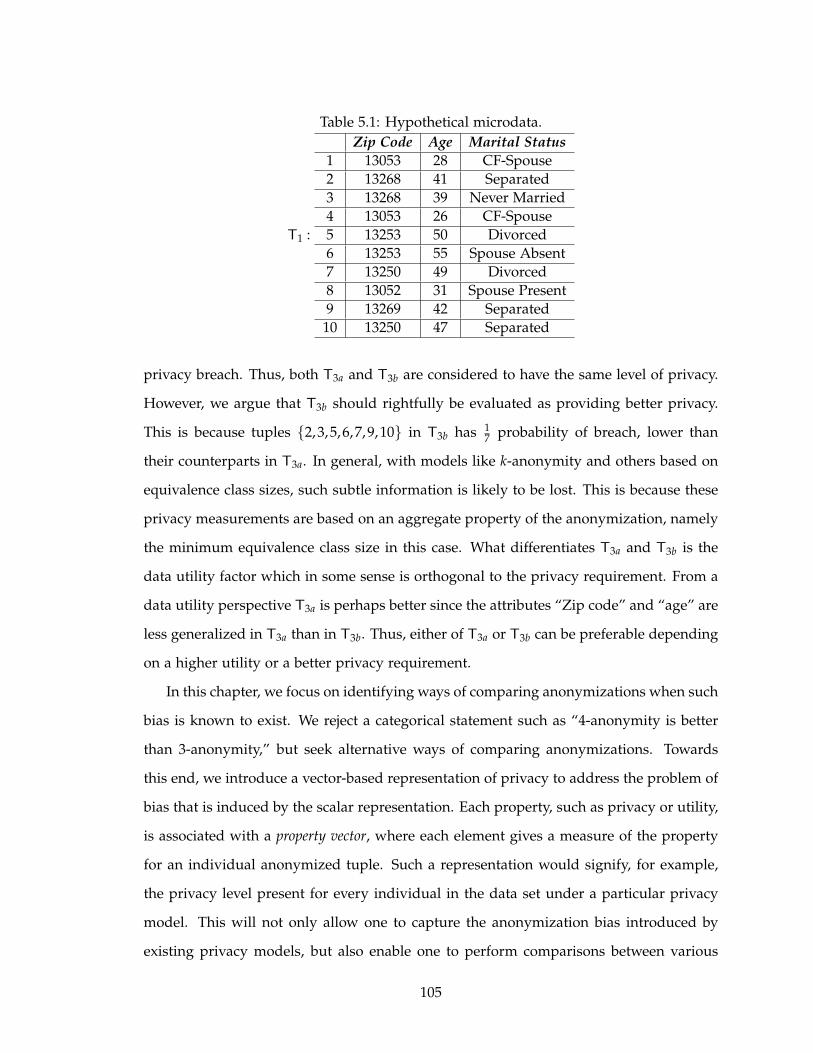
Table 5.1: Hypothetical microdata.
T1 :
Zip Code Age Marital Status
1 13053 28 CF-Spouse
2 13268 41 Separated
3 13268 39 Never Married
4 13053 26 CF-Spouse
5 13253 50 Divorced
6 13253 55 Spouse Absent
7 13250 49 Divorced
8 13052 31 Spouse Present
9 13269 42 Separated
10 13250 47 Separated
privacy breach. Thus, both T3a and T3b are considered to have the same level of privacy.
However, we argue that T3b should rightfully be evaluated as providing better privacy.
This is because tuples {2,3,5,6,7,9,10} in T3b has 17 probability of breach, lower than
their counterparts in T3a. In general, with models like k-anonymity and others based on
equivalence class sizes, such subtle information is likely to be lost. This is because these
privacy measurements are based on an aggregate property of the anonymization, namely
the minimum equivalence class size in this case. What differentiates T3a and T3b is the
data utility factor which in some sense is orthogonal to the privacy requirement. From a
data utility perspective T3a is perhaps better since the attributes “Zip code” and “age” are
less generalized in T3a than in T3b. Thus, either of T3a or T3b can be preferable depending
on a higher utility or a better privacy requirement.
In this chapter, we focus on identifying ways of comparing anonymizations when such
bias is known to exist. We reject a categorical statement such as “4-anonymity is better
than 3-anonymity,” but seek alternative ways of comparing anonymizations. Towards
this end, we introduce a vector-based representation of privacy to address the problem of
bias that is induced by the scalar representation. Each property, such as privacy or utility,
is associated with a property vector, where each element gives a measure of the property
for an individual anonymized tuple. Such a representation would signify, for example,
the privacy level present for every individual in the data set under a particular privacy
model. This will not only allow one to capture the anonymization bias introduced by
existing privacy models, but also enable one to perform comparisons between various
105
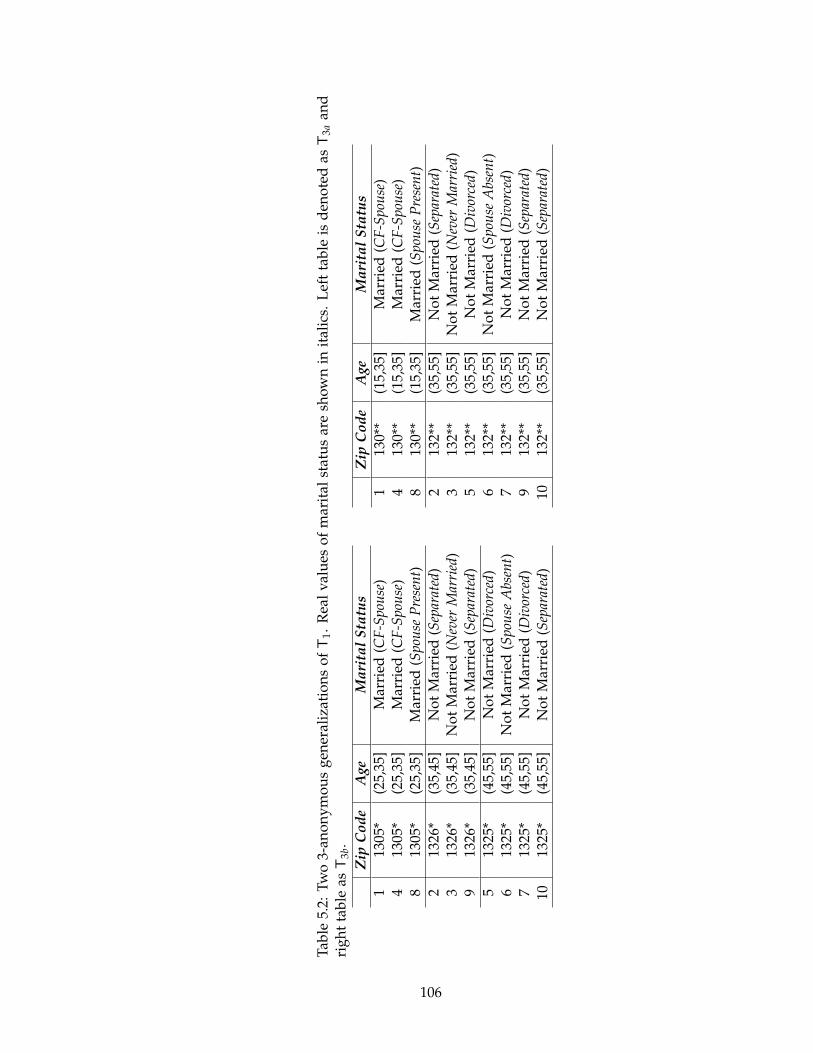
Tab
le5.
2:T
wo
3-an
on
ym
ou
sg
ener
aliz
atio
ns
of
T1.
Rea
lv
alu
eso
fm
arit
alst
atu
sar
esh
ow
nin
ital
ics.
Lef
tta
ble
isd
eno
ted
asT
3a
and
rig
ht
tab
leas
T3
b.
Zip
Co
de
Age
Ma
rita
lS
tatu
s
113
05*
(25,
35]
Mar
ried
(CF
-Spo
use
)4
1305
*(2
5,35
]M
arri
ed(C
F-S
pou
se)
813
05*
(25,
35]
Mar
ried
(Spo
use
Pre
sen
t)
213
26*
(35,
45]
No
tM
arri
ed(S
epar
ated
)3
1326
*(3
5,45
]N
ot
Mar
ried
(Nev
erM
arri
ed)
913
26*
(35,
45]
No
tM
arri
ed(S
epar
ated
)
513
25*
(45,
55]
No
tM
arri
ed(D
ivor
ced)
613
25*
(45,
55]
No
tM
arri
ed(S
pou
seA
bsen
t)7
1325
*(4
5,55
]N
ot
Mar
ried
(Div
orce
d)10
1325
*(4
5,55
]N
ot
Mar
ried
(Sep
arat
ed)
Zip
Co
de
Age
Ma
rita
lS
tatu
s
113
0**
(15,
35]
Mar
ried
(CF
-Spo
use
)4
130*
*(1
5,35
]M
arri
ed(C
F-S
pou
se)
813
0**
(15,
35]
Mar
ried
(Spo
use
Pre
sen
t)
213
2**
(35,
55]
No
tM
arri
ed(S
epar
ated
)3
132*
*(3
5,55
]N
ot
Mar
ried
(Nev
erM
arri
ed)
513
2**
(35,
55]
No
tM
arri
ed(D
ivor
ced)
613
2**
(35,
55]
No
tM
arri
ed(S
pou
seA
bsen
t)7
132*
*(3
5,55
]N
ot
Mar
ried
(Div
orce
d)9
132*
*(3
5,55
]N
ot
Mar
ried
(Sep
arat
ed)
1013
2**
(35,
55]
No
tM
arri
ed(S
epar
ated
)
106

anonymizations based on the difference in distribution of the privacy levels.
We propose the notion of quality index functions that can be used to evaluate the ef-
fectiveness of an anonymization and then formally analyze the characteristics of such
functions. An m-ary quality index function assigns a real number to a combination of
m property vectors. This quantitative estimate is useful in measuring the quality of the
property vector. If the quality index value for one instance of a property vector produced
by an anonymization is better than another instance produced by a different anonymiza-
tion, we will say that the first anonymization is preferred over the second. Unary quality
index functions are limited in their ability in performing comparisons and can measure
only the aggregate properties of the anonymizations. Towards this end, we explore other
methods of comparison that allows one to quantify the differences in the values of the
property measured across the tuples instead of a minimalistic estimate. We also present
various preference based techniques when comparisons are to be made across multiple
properties.
Problems similar to the ones encountered here are known to exist in the multi-objective
optimization community as well. Quality assessment of solution sets in this community
is often difficult because of the existence of non-dominance relationships between one or
more members of two different sets. Hansen and Jaszkiewicz propose the use of qual-
ity measures that induce a linear ordering on the space of all possible solution sets [81].
Knowles and Corne [101] provide a critical overview of existing quality measures and
show that most existing measures do not cater to the “ordering” requirement proposed
by Hanse and Jaszkiewicz. Later work presented by Zitzler et al. explore the limitations of
a comparative study done under the light of quality indicators [196]. We have found that a
principle theorem proved in their work is equally applicable in the case of anonymization
comparisons. The analysis presented in their work serves as a backbone for this study.
The remainder of the chapter is organized as follows. The idea of anonymization
bias is elaborated upon in Section 5.1. Section 5.2 defines the concepts pertinent to the
remaining discussion. Section 5.3 explores the limitations of performing a comparative
study using strict comparisons. The requirement for other methods of comparison follows
from this in Section 5.4. A number of comparators are suggested in this section. Finally,
107
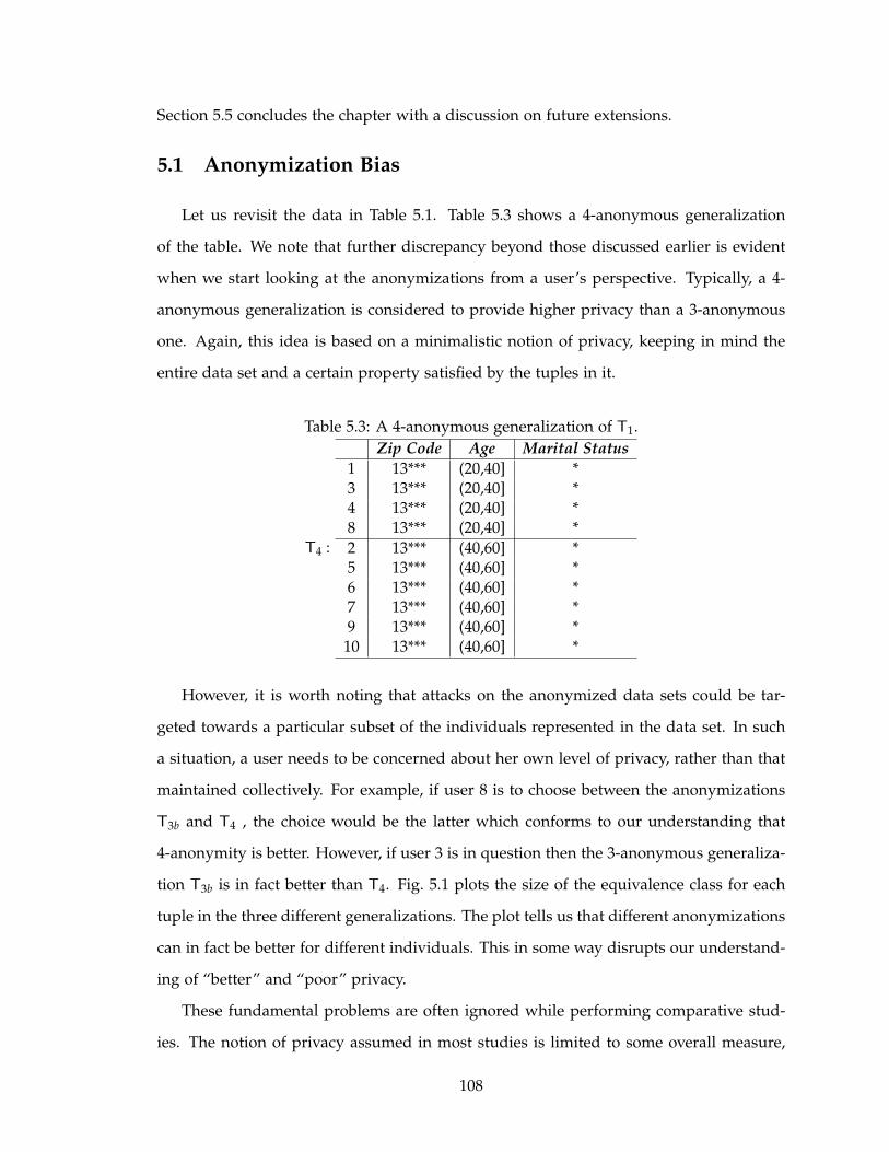
Section 5.5 concludes the chapter with a discussion on future extensions.
5.1 Anonymization Bias
Let us revisit the data in Table 5.1. Table 5.3 shows a 4-anonymous generalization
of the table. We note that further discrepancy beyond those discussed earlier is evident
when we start looking at the anonymizations from a user’s perspective. Typically, a 4-
anonymous generalization is considered to provide higher privacy than a 3-anonymous
one. Again, this idea is based on a minimalistic notion of privacy, keeping in mind the
entire data set and a certain property satisfied by the tuples in it.
Table 5.3: A 4-anonymous generalization of T1.
T4 :
Zip Code Age Marital Status
1 13*** (20,40] *3 13*** (20,40] *4 13*** (20,40] *8 13*** (20,40] *
2 13*** (40,60] *5 13*** (40,60] *6 13*** (40,60] *7 13*** (40,60] *9 13*** (40,60] *10 13*** (40,60] *
However, it is worth noting that attacks on the anonymized data sets could be tar-
geted towards a particular subset of the individuals represented in the data set. In such
a situation, a user needs to be concerned about her own level of privacy, rather than that
maintained collectively. For example, if user 8 is to choose between the anonymizations
T3b and T4 , the choice would be the latter which conforms to our understanding that
4-anonymity is better. However, if user 3 is in question then the 3-anonymous generaliza-
tion T3b is in fact better than T4. Fig. 5.1 plots the size of the equivalence class for each
tuple in the three different generalizations. The plot tells us that different anonymizations
can in fact be better for different individuals. This in some way disrupts our understand-
ing of “better” and “poor” privacy.
These fundamental problems are often ignored while performing comparative stud-
ies. The notion of privacy assumed in most studies is limited to some overall measure,
108
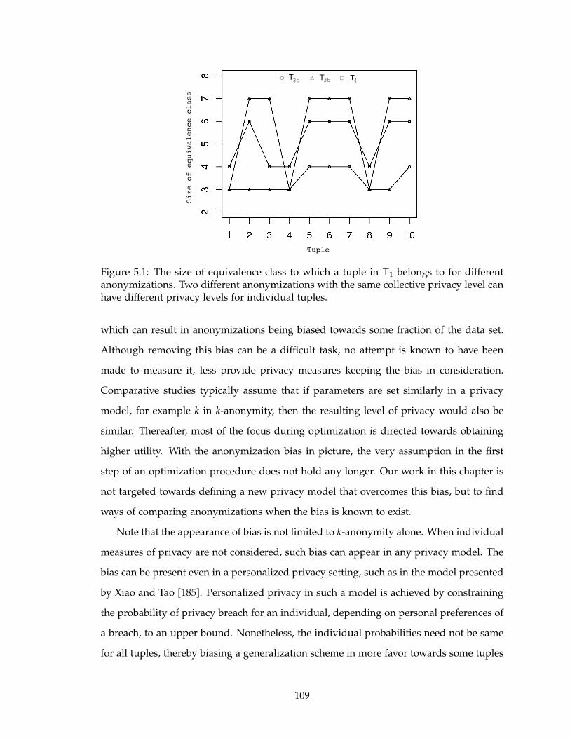
Tuple
Size of equivalence class
TT T3a 3b 4
Figure 5.1: The size of equivalence class to which a tuple in T1 belongs to for differentanonymizations. Two different anonymizations with the same collective privacy level canhave different privacy levels for individual tuples.
which can result in anonymizations being biased towards some fraction of the data set.
Although removing this bias can be a difficult task, no attempt is known to have been
made to measure it, less provide privacy measures keeping the bias in consideration.
Comparative studies typically assume that if parameters are set similarly in a privacy
model, for example k in k-anonymity, then the resulting level of privacy would also be
similar. Thereafter, most of the focus during optimization is directed towards obtaining
higher utility. With the anonymization bias in picture, the very assumption in the first
step of an optimization procedure does not hold any longer. Our work in this chapter is
not targeted towards defining a new privacy model that overcomes this bias, but to find
ways of comparing anonymizations when the bias is known to exist.
Note that the appearance of bias is not limited to k-anonymity alone. When individual
measures of privacy are not considered, such bias can appear in any privacy model. The
bias can be present even in a personalized privacy setting, such as in the model presented
by Xiao and Tao [185]. Personalized privacy in such a model is achieved by constraining
the probability of privacy breach for an individual, depending on personal preferences of
a breach, to an upper bound. Nonetheless, the individual probabilities need not be same
for all tuples, thereby biasing a generalization scheme in more favor towards some tuples
109
than others.
It is imperative to ask if an anonymization can be strictly better than another. It is
known that privacy and utility are two conflicting facets of an anonymization, indicat-
ing that an anonymization better in one aspect (privacy or utility) is likely to suffer on
the other. However, even if utility is not considered as a criteria for obtaining a better
generalization, how easy is it to establish that one anonymization is better than another?
The answer could be subjective depending on how one defines a “better” anonymiza-
tion. We shall explore the limitations and alternatives to establish the superiority of an
anonymization for various definitions in this context.
5.2 Preliminaries
Let Φ1,Φ2, . . . ,Φa represent the domains of a attributes. A data set of size N de-
fined over these attributes is a collection of N tuples of the form (φ1,φ2, . . . ,φa) ∈ Φ1 ×Φ2 × . . . × Φa. An anonymization of a data set is achieved by performing generaliza-
tion/suppression of the tuples, resulting in an anonymized data set unidentifiable from
the original one. Since suppression of tuples can be represented as a special case of gener-
alization, we adhere to the term “generalization” to mean both. Further, although tuples
suppressed during an anonymization are usually eliminated, we assume that they still ex-
ist in the anonymized data set in an overly generalized form. This enables us to say that
both the original data set and the anonymized one are of the same size. An anonymized
data set is then subjected to a variety of property measurements. A property here refers to
a scalar quantity signifying a privacy, utility or any other measurable feature of a tuple in
the anonymized data set. This gives us a vector of values representing the property value
for every tuple of the anonymized data set.
Definition 5.1 PROPERTY VECTOR. A property vector D for a data set of size N is an
N -dimensional vector (d1,d2, . . . ,dN ) with di ∈ R;1 ≤ i ≤ N specifying a measure of a
property for the ith tuple of the data set.
A property signifies the grounds under which a comparison is made between two
anonymizations. Consider that we are performing k-anonymization on a data set. A
110

generalization scheme to do so results in multiple equivalence classes, the desired prop-
erty being that all such equivalence classes are of size at least k. If we pick our privacy
property to be the “size of the equivalence class to which a tuple belongs,” then each tuple
will have an associated integer. This results in a property vector D = (d1,d2, . . . ,dN ) for a
data set of size N . For example, the equivalence class property vector induced in T3a is
(3,3,3,3,4,4,4,3,3,4). Another example of a property could be the contribution made by a
tuple to the total information loss. If measurements on the diversity of sensitive attributes
in an equivalence class is desired, then the property can be the number of times the sen-
sitive attribute value of a tuple appears in its equivalence class. Considering “marital
status” as a sensitive attribute, such a property vector for T3a will be (2,2,1,2,2,1,2,1,2,1).
Ideally, any number of properties can be studied on a given anonymization. An
anonymization is only a representation of the generalization scheme, inducing different
property vectors for different properties. For example, one may be interested in ana-
lyzing an anonymization w.r.t. both k-anonymity and ℓ-diversity. In such a case, the
property vectors to consider are the ones generated by the properties - size of equivalence
class of a tuple and count of the sensitive attribute value of a tuple in its equivalence class. For
an anonymization, a property vector due to the first property relates to k-anonymity,
while that from the latter one relates to ℓ-diversity. We thus use the notion of r-property
anonymization to indicate that the set of properties decided upon for a comparison pro-
cess is restricted to a pre-specified set of r properties. The objective of a comparison is to
decide if one anonymization is better than another w.r.t. the specified properties.
Definition 5.2 r–PROPERTY ANONYMIZATION. Let ∆ be the set of all data sets of size
N . Let Υ be the set of all elements υ ∈ 2RN
such that |υ| = r. A r–property anonymization
G is a function G : ∆ → Υ which induces a set of r N -dimensional property vectors G(δ)
on a data set δ ∈ ∆.
Note that an r-property anonymization does not mean that there are restrictions on
how an anonymization is done. It only indicates that, for a given anonymization, r dif-
ferent property vectors are chosen to proceed with the comparison. The idea is to project
an anonymized data set into a set of N -dimensional vectors with regard to r proper-
111

ties, and then compare the resulting vectors for different anonymization schemes. For
example, the aforementioned example of analyzing the size of equivalence class and the
number of sensitive attribute values of a tuple in its equivalence class will be referred to
as 2–property anonymization.
Comparisons between anonymizations is done by defining a comparator, denoted by
⊲. A comparator is an ordering operation defined on sets of property vectors. An ex-
ample is the dominance-based comparator � – under a 1-property anonymization, say
Υ1 = {(d11, . . . ,d1
N )} and Υ2 = {(d21, . . . ,d2
N )}, then Υ1 � Υ2 iff ∀1 ≤ i ≤N ,d1i ≥ d2
i . In other
words, comparators are user-defined ways of evaluating the superiority of a property
vector. An anonymization is better than another only w.r.t. the comparator used in com-
paring the induced set of property vectors. Therefore, given a comparator ⊲, the relation
G1 ⊲ G2 ⇐⇒ Υ1 ⊲ Υ2 is implicitly assumed to be true. Note that the definition of a com-
parator need not always be explicitly made in terms of the values in a property vector.
For example, a comparator may be defined just to check if more values in one property
vector are higher than the corresponding values in another vector. Hence, we use quality
index functions on property vectors to quantitatively measure the competence of a set of
property vectors.
Definition 5.3 m-ARY QUALITY INDEX. Let Π be the set of all property vectors w.r.t a
particular property. An m-ary quality index I is a function I : Πm → R which assigns a
combination of m property vectors D1, . . . ,Dm a real value I(D1, . . . ,Dm).
Since comparisons are usually performed by applying an anonymization on the same
data set, we shall restrict Π to be the set of all property vectors of the same size, i.e. the
size N of the data set. Based on the same reasoning, a quality index may also use the
original data set while mapping property vectors to real numbers.
A commonly used method of performing comparisons is through unary quality in-
dex functions (1-ary). Unary quality indices are functions applied independently on
anonymizations. They measure one or more feature (privacy/utility) of an anonymiza-
tion, and the quantitative value is considered representative of the measured feature of
the anonymization. For example, k-anonymity is an unary quality index on the equiv-
112

alence class size property vector, given as Ik−anon(D) = mindi
(D) (= 3 for T3a). Another
possible quality index could be the average size of the equivalence class maintained in
the anonymized data set, i.e. Iavg(D) = ∑ di/N (= 3 × 3 + 3 × 3 + 4 × 4/10=3.4 for T3a).
Other models like ℓ-diversity and t-closeness result in other property vectors depending
on the property being measured, for example ℓ-diversity uses a count of the number of
times the sensitive attribute value of a tuple is represented in an equivalence class. With
this property, we shall have a unary quality index ℓ = Iℓ−div((2,2,1,2,2,1,2,1,2,1)) value
of 1 for T3a (considering “marital status” as the sensitive attribute). Once again, the ℓ
or t values for an anonymization is a quality measurement on the property vectors, the
minimum values in these models. Certain forms of utility measurements can also be cap-
tured from property vectors. A loss measurement, such as the general loss metric [92],
computes a normalized loss quantity for every tuple of the data set. For such metrics, a
property vector specifies the loss resulting from each tuple in the data set. Thereafter, the
quality index is some form of aggregation of the individual losses.
Note that unary indices only allow the measurement of an aggregate property of an
anonymization. This limits any kind of comparison against the bias that may be present
across anonymizations. More specifically, comparisons are not possible across the prop-
erty values maintained by a tuple in two different anonymizations. This problem is elim-
inated by binary indices (2-ary) since both anonymizations are now available to allow
comparison of individual components of the induced property vectors. A binary quality
index has two anonymizations as input and the real-valued output signifies a relative
measure of one anonymization’s effectiveness over another. For example, a binary qual-
ity index such as Ibinary(s, t) = |{si|si > ti}| counts the number of entries in the property
vector s that has higher property values than the corresponding entries in t. Note that
s and t in this case are property vectors measuring the same property in two different
anonymizations. For the size of equivalence class property in T3a, with property vec-
tor s = (3,3,3,3,4,4,4,3,3,4), and T3b, with property vector t = (3,7,7,3,7,7,7,3,7,7), we
have Ibinary(s, t) = 0 and Ibinary(t, s) = 7. These index values indicate that if an 1-property
anonymization is analyzed w.r.t. the size of equivalence class property, then anonymiza-
tion T3b inducing the property vector t is preferable over T3a.
113
Quality estimation based on index functions stresses on the fact that a particular
anonymization can be interpreted with respect to many different privacy properties and
utility measurements. The superiority of one anonymization to another is thus dependent
on what privacy properties are taken into consideration while performing the compari-
son. If quality indices are used to establish this superiority, then our concern is how many
of them are needed to do so.
5.3 Strict Comparisons
Most algorithms in disclosure control are designed to obtain anonymizations that
can maximize the utility of the anonymized data while satisfying a pre-specified privacy
property. An anonymization is considered to be better than another if it provides higher
utility within the constraints of the privacy requirement. Privacy, as given by a model, and
utility are two properties induced by an anonymization. A disclosure control algorithm
scans through the space of anonymizations satisfying a privacy property to find the one
with maximum utility. Performance of one algorithm is said to be better than another if
it is able to find an anonymization with higher utility.
This form of comparison suffers from the fact that the privacy level measured from
an anonymization is a scalar quantity. It is known that maximum privacy and maximum
utility are orthogonal objectives that cannot be achieved at the same time. Hence, it is
imperative that when an anonymization with a better utility is found by an algorithm,
the privacy factor must suffer. However, this facet may not be exposed if scalar measures
are used to represent privacy. The anonymization bias plays an important role here in
explaining a degraded performance in privacy from high utility anonymizations. Further,
optimization attempts are also rare where emphasis is laid on obtaining anonymizations
that satisfy more than one privacy property.
Discrepancies of the above nature prompts us to consider vector based measurements
of the properties induced by an anonymization. Our perspective of an anonymization is
that of a source that induces various properties, both in terms of privacy and utility, and
more importantly, the properties can be measured on each tuple in the data set. There-
after, methods to compare these property vectors (one or more) are devised to evaluate
114
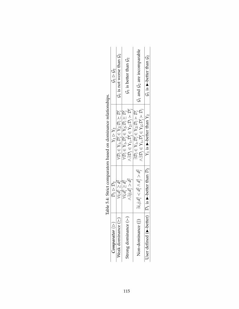
Tab
le5.
4:S
tric
tco
mp
arat
ors
bas
edo
nd
om
inan
cere
lati
on
ship
s.
Co
mp
ara
tor
(⊲)
D1⊲
D2
Υ1⊲
Υ2
G 1⊲
G 2W
eak
do
min
ance
(�)
∀i;d
1 i≥
d2 i
∀Di∈
Υ1,D
′ i∈
Υ2;D
i�
D′ i
G 1is
no
tw
ors
eth
anG 2
Str
on
gd
om
inan
ce(≻
)∀i
;d1 i≥
d2 i
∧∃j;
d1 j>
d2 j
∀Di∈
Υ1,D
′ i∈
Υ2;D
i�
D′ i
∧∃D
j∈
Υ1,D
′ j∈
Υ2;D
j≻
D′ j
G 1is
bet
ter
than
G 2
No
n-d
om
inan
ce(‖
)∃i
,j;d
1 i<
d2 i∧
d1 j>
d2 j
∃Di∈
Υ1,D
′ i∈
Υ2;D
i≻
D′ i
∧∃D
j∈
Υ1,D
′ j∈
Υ2;D
′ j≻
Dj
G 1an
dG 2
are
inco
mp
arab
le
Use
rd
efin
ed(◮
-bet
ter)
D1
is◮
-bet
ter
than
D2
Υ1
is◮
-bet
ter
than
Υ2
G 1is
◮-b
ette
rth
anG 2
115

the competence of an anonymization.
The first question we ask is the feasibility of performing strict comparisons. A strict
comparison between property vectors follows from the concept of dominance, widely
used in the multi-objective optimization community. The notions of weak and strong dom-
inance enables us to make strong statements about the superiority of an anonymization.
Weak dominance says that every measured value of a property on every tuple of the
data set after an anonymization must be at least as good as the value measured from the
corresponding tuples with another anonymization. This establishes a “not worse than”
relationship between vectors. Strong dominance offers a stricter notion and establishes
the “better than” relationship (Table 5.4). The non-dominance relationship signifies in-
comparable vectors. We are interested in strict comparisons based on dominance because
they provide a framework to undoubtedly justify why an anonymization is better than
another. It can potentially eliminate the effects of anonymization bias during a compar-
ative study. However, the following discussion shows that adopting a dominance based
comparative method could be rather impractical.
Theorem 5.1 Let D1 and D2 be two property vectors measuring the same property and
induced by the 1–property anonymizations G1 and G2 respectively on a data set of size
N . If (I1,I2, . . . ,In) be a vector of n unique unary quality indices such that
∀1 ≤ i ≤ n : Ii(D1) ≥ Ii(D2) ⇐⇒ D1 � D2, (5.1)
then the number of indices is at least equal to the size of the data set, i.e. n ≥N .
Proof The proof follows from the fact that the number of open hypercubes required to
cover RN is finite. We shall show that if n < N , then infinite such open hypercubes
can be defined. The proof is by induction. Consider the two non-comparable property
vectors D1 = (a,b) and D2 = (b, a) with a,b ∈ R and n = 1. Then either I1(D1) ≥ I1(D2)
or I1(D1) < I1(D2). This implies that either D1 � D2 or D2 � D1, which leads to a
contradiction since D1 ‖ D2. Hence the theorem holds for N = 2.
Let us suppose that the theorem holds for data sets of size N − 1. Consider the two
property vectors D1 = (a, a, . . . , a, c) and D2 = (b,b, . . . ,b, c) with a,b ∈ R and a < b on a
116
data set of size N . Further, let us assume that there exists a combination of n < N unary
quality indices satisfying the relation in the theorem.
We first show that ∀1 ≤ i ≤ n : Ii(D1) < Ii(D2).
If ∃j such that Ij(D1) > Ij(D2) then D2 � D1 which results in a contradiction.
Next, consider a property vector D ∈ Dc = {(d1,d2, . . . ,dN−1, c)|∀1 ≤ i ≤ N − 1 : a <
di < b}; c ∈ R. We then have D2 �D �D1 leading to ∀1 ≤ i ≤ n : Ii(D2) ≥ Ii(D) ≥ Ii(D1).
If ∃j such that Ij(D2) = Ij(D1), then Ij(D2) = Ij(D) = Ij(D1). With this we can now
prove that the number of indices required for data sets of size N − 1 can be less than
N − 1, contrary to the hypothesis assumed. To do so, we consider two property vectors
Dp = (p1, p2, . . . , pN−1) and Dq = (q1,q2, . . . ,qN−1) on a data set of size N − 1, such that
∀1 ≤ i ≤ N − 1 : a < pi ≤ qi < b. Hence, Dq � Dp. Next, we expand the two vectors by
concatenating the same arbitrary element c ∈ R, the concatenated vectors being denoted
by Dp|c and Dq|c respectively. Since ∀1 ≤ i ≤ n : Ii(Dq|c) ≥ Ii(Dp|c) ⇐⇒ Dq|c � Dp|c and
(Dq � Dp) ⇐⇒ (Dq|c � Dp|c), we have ∀1 ≤ i ≤ n : Ii(Dq|c) ≥ Ii(Dp|c) ⇐⇒ Dq � Dp.
Also, using the result that Ij(D2) = Ij(D) = Ij(D1) for any D ∈ Dc, we have Ij(Dq|c) =
Ij(Dp|c). Hence the result of Ij can be ignored and one can write ∀1≤ i 6= j ≤ n : Ii(Dq|c)≥Ii(Dp|c) ⇐⇒ Dq � Dp, which means that less than N − 1 (recall n < N ) quality indices
can be used to compare Dp and Dq. Since this is contrary to the assumed hypothesis, the
existence of such j is not possible.
Thus, ∀1 ≤ i ≤ n : Ii(D1) < Ii(D2).
Let us now consider the open hyperrectangle Ic = {(r1,r2, . . . ,rn) ∈ Rn|∀1 ≤ i ≤ n :
Ii(D1) < ri < Ii(D2)}. Also, for f > c, Ic ∩I f = φ; if ∃(r1,r2, . . . ,rn) ∈ Ic ∩I f then ∀1 ≤ i ≤n : [Ii((a, a, . . . , a, c)) < ri < Ii((b,b, . . . ,b, c))] ∧ [Ii((a, a, . . . , a, f )) < ri < Ii((b,b, . . . ,b, f ))],
giving ∀1 ≤ i ≤ n : I((a, a, . . . , a, f )) < Ii((b,b, . . . ,b, c)), and implying that (b,b, . . . ,b, c) �(a, a, . . . , a, f ) which is absurd. Hence, since R is uncountable and c is chosen arbitrarily
in R, there are uncountably many disjoint open hyperrectangles in the n-dimensional
quality index space Rn. This is in contradiction to the fact that R
n contains countably
many disjoint open hyperrectangles. Therefore, n ≮ N which implies n ≥N . �
A similar proof can be given for the case when strong dominance has to be inferred
between two property vectors, i.e. for the equivalence relation [∀1 ≤ i ≤ n : Ii(D1) ≥
117

Ii(D2) ∧ ∃j ∈ {1, . . . ,n}|Ij(D1) > Ij(D2)] ⇐⇒ D1 ≻ D2 to hold, n must be at least N .
An important question here is whether all possible N -dimensional property vectors
are valid given a specific privacy measurement and a specific data set. The answer is
a strict no. For example, if we consider the size of the equivalence class as the privacy
property, one commonly used in models like k-anonymity and ℓ-diversity, we would find
that the measurements are dependent. In other words, if a tuple belongs to an equivalence
class of size s, then there exists s− 1 other tuples that belong to the same equivalence class.
Hence the measurement (size of equivalence class) will be the same for all s tuples. This
restricts us from attaining all possible property vectors. This then raises the question if
Theorem 5.1 is valid when the set of possible property vectors is actually a subset of the
set of all possible property vectors. We show that the theorem in fact holds for such a
subset as well.
Corollary 5.1 Let Π be the set of all property vectors that can be defined for a data set of
size N . Let D ⊆ Π be a set of property vectors measuring a particular property such that
∀D1,D2 ∈ D,
∀1 ≤ i ≤ n : Ii(D1) ≥ Ii(D2) ⇐⇒ D1 � D2. (5.2)
Then, n ≥N .
Proof Let us assume that n <N . The proof is given by constructing the maximal superset
DM of D on which the relationship holds. Let a = (a1, a2, . . . , aN ),b = (b1,b2, . . . ,bN ) ∈ D.
Hence we can say, ∀1 ≤ i ≤ n : Ii(a)≥ Ii(b) ⇐⇒ a � b. Also then a,b ∈ DM. Now consider
the following vectors.
• x ∈ X = {(a1c1, a2c2, . . . , aN cN )|∀1 ≤ i ≤N ; ci ≥ 1}
• y ∈ Y = {(b1 + (a1 − b1)e1, . . . ,bN + (aN − bN )eN )|∀1 ≤ i ≤N ;0 ≤ ei ≤ 1}
• z ∈ Z = {(b1/d1,b2/d2, . . . ,bN /dN )|∀1 ≤ i ≤N ;di ≥ 1}
We have the following relation on these vectors: a � b ⇐⇒ x � a � y � b � z. Hence,
by applying the quality indices Ii’s on a and b one can compare two property vectors
belonging to two different sets from X , Y and Z . Note that one can still not assert that
118

two vectors belonging to the same set (X ,Y or Z) can be compared in the same manner.
Thus, we arbitrarily choose three vectors, one each from X ,Y and Z , and include it in
DM, i.e. DM = {x, a,y,b,z}. Hence, given two vectors in DM, we can find at least three
other vectors that satisfy the relationship, thereby increasing the cardinality of DM. Since
the choice of the new vectors is arbitrary, we can continue the process as many times as
possible, every time increasing the cardinality of DM. Then, in the limit, DM will become
equal to Π. This contradicts the result from Theorem 5.1 saying that n ≥N quality indices
are required to compare two property vectors in Π. Therefore, the assumed hypothesis
n < N is incorrect, implying n ≥N . �
The situation becomes worse if comparisons are to be made against multiple proper-
ties. On first thought, it is possible to map a set of property vectors to an unique property
vector of size N and Theorem 5.1 could suggest that the lower bound on n is therefore N .
Let Υp = {Dp1,Dp2, . . . ,Dpr} be a set of r property vectors, where Dpi = (dpi1,d
pi2, . . . ,d
piN );
1 ≤ i ≤ r. Consider the vector dj ∈ Dj = {(dp1j,d
p2j, . . . ,d
prj) ∈ R
r} for some j ∈ {1, ...,N}.
Note that |Dj| = Rr and since the cardinality of R
r and R is the same, there exists a bijec-
tive function f j : Dj → R. Now define the function F : Υ → RN which maps each set of r
property vectors to a vector of size N as F (Υp ∈ Υ) = ( f1(d1), f2(d2), . . . , fN (dN )). Since
every f j is a bijective function, F is bijective too. However, a bijective mapping is not
sufficient to imply the equivalence relation F (Υ1) � F (Υ2) ⇐⇒ Υ1 � Υ2 and hence the
lower bound (n ≥ N ) given by Theorem 5.1 would be incorrect. It can be shown that for
the relation to hold, n should at least be equal to rN . The following corollary gives this
lower bound on the number of quality indices required to compare two sets of property
vectors. Note that the corollary uses notions of quality index functions extended to sets
of property vectors.
Corollary 5.2 Let Υ1 = {D11,D12, . . . ,D1r} and Υ2 = {D21,D22, . . . ,D2r} be two sets of
property vectors induced by the r–property anonymizations G1 and G2 respectively on
a data set of size N . If (I1,I2, . . . ,In) be a vector of n unary quality indices such that
∀1 ≤ i ≤ n : Ii(Υ1) ≥ Ii(Υ2) ⇐⇒ Υ1 � Υ2, (5.3)
then n ≥ rN .
119
Proof Let us assume that there exists quality indices Ii;1 ≤ i < rN such that the equiva-
lence relation holds. Now, Υ1 � Υ2 ⇐⇒ ∀1 ≤ j ≤ r;D1j � D2j. If Dpj = (dpj1,d
pj2, . . . ,d
pjN )
then D1j � D2j ⇐⇒ ∀1 ≤ z ≤ N ;d1jz ≥ d2
jz. Therefore, Υ1 � Υ2 ⇐⇒ ∀1 ≤ j ≤ r;∀1 ≤ z ≤N ;d1
jz ≥ d2jz. By transitivity, we then have ∀1 ≤ i < rN : Ii(Υ1) ≥ Ii(Υ2) ⇐⇒ ∀1 ≤ j ≤
r;∀1 ≤ z ≤N ;d1jz ≥ d2
jz.
Let us now consider a data set of size rN . For two property vectors D1 and D2
defined on this data set, D1 � D2 if and only if every component of D1 is greater than
or equal to the corresponding component of D2. We first divide a property vector on
this data set into r equal sections, thereby resulting in r N -dimensional vectors. The
quality indices Ii can then be applied to these resulting vectors. The equivalence relation
∀1 ≤ i < rN : Ii(Υ1) ≥ Ii(Υ2) ⇐⇒ ∀1 ≤ j ≤ r;∀1 ≤ z ≤ N ;d1jz ≥ d2
jz can then be used
to state that less than rN quality indices can be used to establish a dominance relation
between D1 and D2. This contradicts the result from Theorem 5.1 which states that we
would require at least rN quality indices to compare any two property vectors on a data
set of size rN . Hence, no such combination of quality indices with n < rN can exist. �
The results till this point indicate that it is rather impractical to determine the supe-
riority of an anonymization based on notions of weak or strong dominance, and with
unary quality indices. This prompts us to consider other methods of representing the
quality of anonymizations relative to one another by defining ◮-better (read as metric
better) comparators. For example, we can define a ◮cov-better comparator such that, given
two equivalence size property vectors D1 and D2, D1◮covD2 if more tuples in D1 have a
higher equivalence class size than the corresponding number in D2. Another example is
the ◮min-better comparator typically used in models such as k-anonymity – D1 ◮min D2
if mind1
i
(D1) > mind2
i
(D2). In fact, current methods of comparison are all based on some
◮-better comparator.
◮-better comparators may naturally induce the quality indices to be used to infer
the relationship, for example Ik−anon is the quality index to be used to infer ◮min-better.
However, as mentioned earlier, comparators such as ◮min are limited by the fact that they
are based on some aggregate property of the vectors, ignoring the anonymization bias
altogether. On the other hand, ◮cov is a rational candidate since the relationship is based
120

on the output from comparing multiple tuples in the two property vectors. Note that ◮cov
in fact induces a binary quality index as presented in the next section.
5.4 ◮-better Comparators
Comparisons with dominance based comparators suffer from the drawback that the
number of unary quality indices required is impractically large. This also follows from
our intuition that comparison of two N -dimensional vectors cannot be accomplished with
less than N scalar quantities without losing information. Besides this difficulty, domi-
nance based comparison is a rather strict way of evaluating the quality of an anonymiza-
tion. It is not unlikely that a property vector is not able to dominate another vector
because of low property values for a minor fraction of the tuples. This effectuates to say-
ing that the anonymization bias could be present negligibly resulting in a non-dominance
relationship.
Although removing the effects of anonymization bias is hard (or perhaps impossible),
methods can be devised to keep it in consideration during a comparative study. We
therefore seek other comparators, called ◮-better comparators, that can capture the quality
of anonymizations together with the bias they introduce. ◮-better comparators provide
a weaker notion of superiority than dominance-based ones, nonetheless their objective is
also targeted towards identifying anonymizations with better utilization of the bias.
In the following discussion, we introduce a number of ◮-better comparators and the
corresponding unary/binary quality index they induce. All expressions below are in
terms of two property vectors D1 = (d11,d1
2, . . . ,d1N ) and D2 = (d2
1,d22, . . . ,d2
N ) measuring a
given property when induced by two different anonymizations on a data set of size N .
Without loss of generality, we assume that a higher value of a property measurement for
a tuple is better.
5.4.1 ◮rank-better
Consider the N -dimensional space of all property vectors for a given property. Let
Dmax be a point of interest and all points are assigned a rank based on their distance
from Dmax. We then say D1 ◮rank D2 if the rank of D1 is lower than the rank of D2. A
121
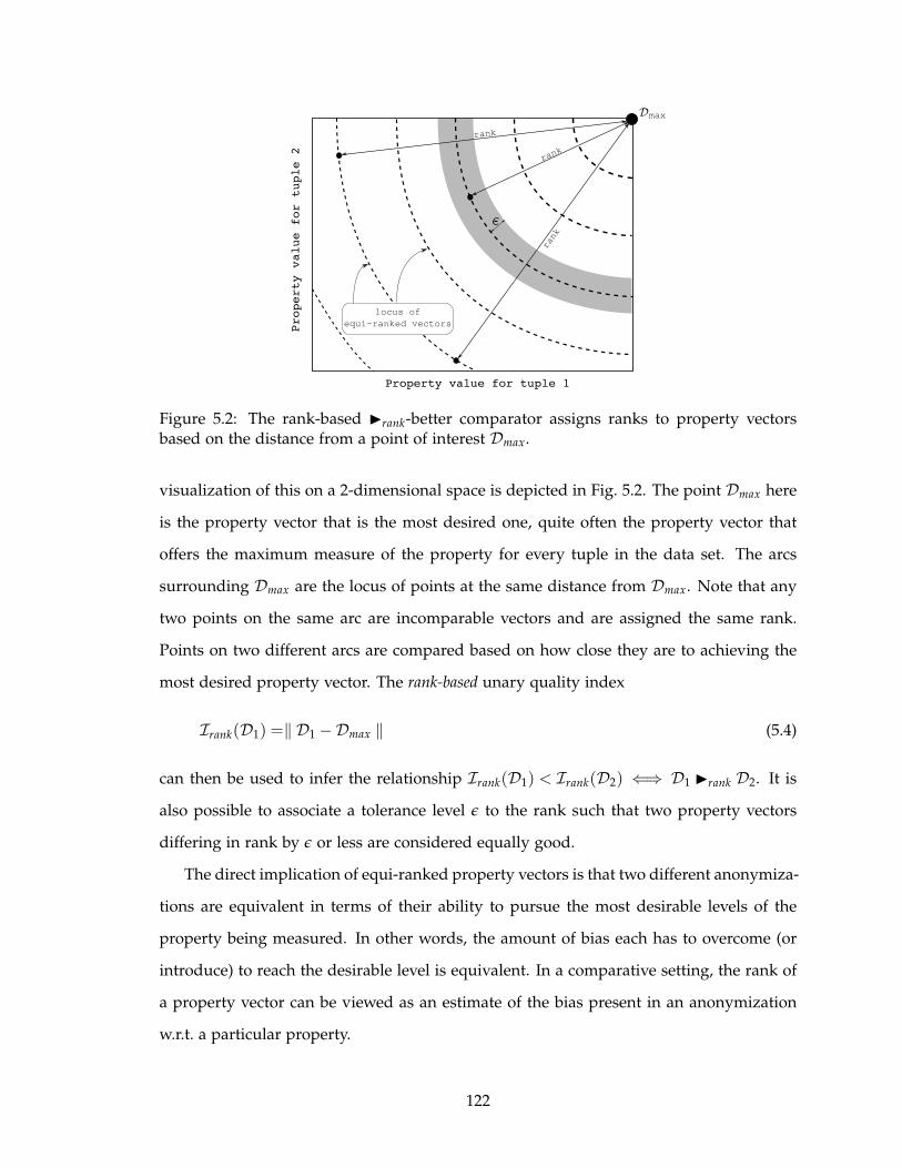
Property value for tuple 1
Property value for tuple 2
D
rank
rank
rank
locus of
equi-ranked vectors
max
C
Figure 5.2: The rank-based ◮rank-better comparator assigns ranks to property vectorsbased on the distance from a point of interest Dmax.
visualization of this on a 2-dimensional space is depicted in Fig. 5.2. The point Dmax here
is the property vector that is the most desired one, quite often the property vector that
offers the maximum measure of the property for every tuple in the data set. The arcs
surrounding Dmax are the locus of points at the same distance from Dmax. Note that any
two points on the same arc are incomparable vectors and are assigned the same rank.
Points on two different arcs are compared based on how close they are to achieving the
most desired property vector. The rank-based unary quality index
Irank(D1) =‖ D1 −Dmax ‖ (5.4)
can then be used to infer the relationship Irank(D1) < Irank(D2) ⇐⇒ D1 ◮rank D2. It is
also possible to associate a tolerance level ǫ to the rank such that two property vectors
differing in rank by ǫ or less are considered equally good.
The direct implication of equi-ranked property vectors is that two different anonymiza-
tions are equivalent in terms of their ability to pursue the most desirable levels of the
property being measured. In other words, the amount of bias each has to overcome (or
introduce) to reach the desirable level is equivalent. In a comparative setting, the rank of
a property vector can be viewed as an estimate of the bias present in an anonymization
w.r.t. a particular property.
122
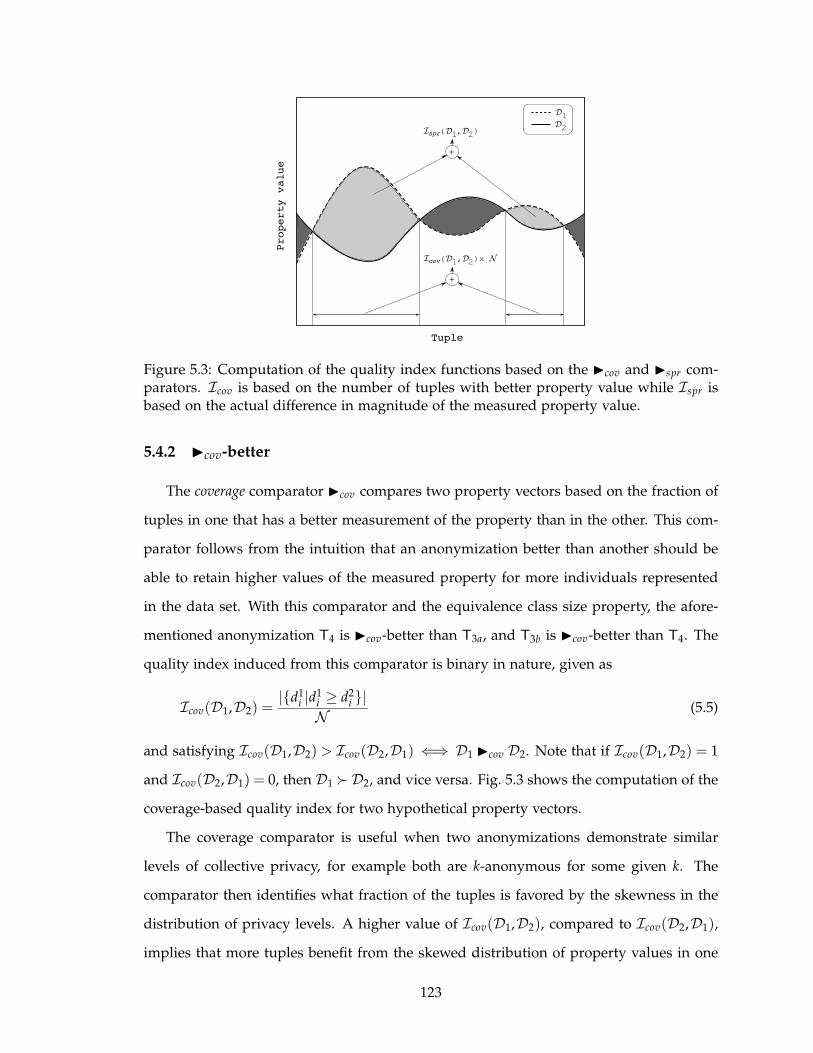
Tuple
Property value
+
I Dcov( 1, 2)x ND
D1
D2
+
I Dspr( 1, 2)D
Figure 5.3: Computation of the quality index functions based on the ◮cov and ◮spr com-parators. Icov is based on the number of tuples with better property value while Ispr isbased on the actual difference in magnitude of the measured property value.
5.4.2 ◮cov-better
The coverage comparator ◮cov compares two property vectors based on the fraction of
tuples in one that has a better measurement of the property than in the other. This com-
parator follows from the intuition that an anonymization better than another should be
able to retain higher values of the measured property for more individuals represented
in the data set. With this comparator and the equivalence class size property, the afore-
mentioned anonymization T4 is ◮cov-better than T3a, and T3b is ◮cov-better than T4. The
quality index induced from this comparator is binary in nature, given as
Icov(D1,D2) =|{d1
i |d1i ≥ d2
i }|N (5.5)
and satisfying Icov(D1,D2) > Icov(D2,D1) ⇐⇒ D1 ◮cov D2. Note that if Icov(D1,D2) = 1
and Icov(D2,D1) = 0, then D1 ≻D2, and vice versa. Fig. 5.3 shows the computation of the
coverage-based quality index for two hypothetical property vectors.
The coverage comparator is useful when two anonymizations demonstrate similar
levels of collective privacy, for example both are k-anonymous for some given k. The
comparator then identifies what fraction of the tuples is favored by the skewness in the
distribution of privacy levels. A higher value of Icov(D1,D2), compared to Icov(D2,D1),
implies that more tuples benefit from the skewed distribution of property values in one
123

anonymization than in the other. Such a comparison helps justify that the bias introduced
by an anonymization can be useful in providing better property values for a larger fraction
of the data set.
5.4.3 ◮spr-better
The coverage comparator does not take into consideration the difference in magnitude
of a measured property for a given tuple when comparing it across two different property
vectors. It is possible that for two vectors D1 and D2 with Icov(D1,D2) ≈ Icov(D2,D1) (the
quality index values are close), D1 maintains much better values in the property for the
tuples on which it is superior than D2, compared to those on which D2 is superior. For ex-
ample, consider the hypothetical property vectors D1 = (2,2,3,4,5) and D2 = (3,2,4,2,3).
In this case, Icov(D1,D2) = Icov(D2,D1) = 35 . However, one can argue that D1 is a supe-
rior vector since the difference in magnitude of the measured property is higher (a value
of 2) in the two tuples where it is better than D2. This difference is only 1 in the two
tuples where D2 is better. The spread comparator ◮spr is based on the total amount of
variation (or spread) present between tuples w.r.t. a property. The quality index based on
this comparator is given as
Ispr(D1,D2) =N∑i=1
max(d1i − d2
i ,0) (5.6)
and measures the total difference in magnitude of the measured property for the tuples
on which D1 performs better than D2. We then say Ispr(D1,D2) > Ispr(D2,D1) ⇐⇒D1 ◮spr D2. We also have Ispr(D1,D2) = 0 ⇐⇒ D2 � D1. Fig. 5.3 shows the difference in
computation of the coverage-based and spread-based quality indices.
The spread comparator uses a quantification of the leverage availed by individual
tuples from the skewed distribution of property values. This is crucial when the frac-
tion of tuples benefited, as given by the Icov quality index, are equivalent. The Ispr
quality index quantifies the utilization of the bias in terms of differences in observed
property values. Even for the case when two anonymizations have different collective
privacy levels, this quantification differentiates them further, often counter to established
preferential norms. For example, consider the equivalence class size property vector
(3,3,3,5,5,5,5,5,3,3,3,4,4,4,4) from a 3-anonymous generalization and (2,2,6,6,6,6,6,6,3,
124
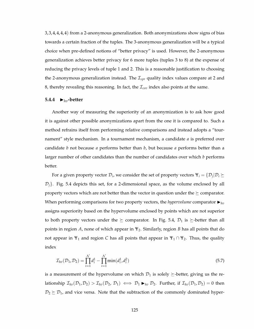
3,3,4,4,4,4) from a 2-anonymous generalization. Both anonymizations show signs of bias
towards a certain fraction of the tuples. The 3-anonymous generalization will be a typical
choice when pre-defined notions of “better privacy” is used. However, the 2-anonymous
generalization achieves better privacy for 6 more tuples (tuples 3 to 8) at the expense of
reducing the privacy levels of tuple 1 and 2. This is a reasonable justification to choosing
the 2-anonymous generalization instead. The Ispr quality index values compare at 2 and
8, thereby revealing this reasoning. In fact, the Icov index also points at the same.
5.4.4 ◮hv-better
Another way of measuring the superiority of an anonymization is to ask how good
it is against other possible anonymizations apart from the one it is compared to. Such a
method refrains itself from performing relative comparisons and instead adopts a “tour-
nament” style mechanism. In a tournament mechanism, a candidate a is preferred over
candidate b not because a performs better than b, but because a performs better than a
larger number of other candidates than the number of candidates over which b performs
better.
For a given property vector Di, we consider the set of property vectors Ψi = {Dj|Di �Dj}. Fig. 5.4 depicts this set, for a 2-dimensional space, as the volume enclosed by all
property vectors which are not better than the vector in question under the � comparator.
When performing comparisons for two property vectors, the hypervolume comparator ◮hv
assigns superiority based on the hypervolume enclosed by points which are not superior
to both property vectors under the � comparator. In Fig. 5.4, D1 is �-better than all
points in region A, none of which appear in Ψ2. Similarly, region B has all points that do
not appear in Ψ1 and region C has all points that appear in Ψ1 ∩ Ψ2. Thus, the quality
index
Ihv(D1,D2) =N∏i=1
d1i −
N∏i=1
min(d1i ,d2
i ) (5.7)
is a measurement of the hypervolume on which D1 is solely �-better, giving us the re-
lationship Ihv(D1,D2) > Ihv(D2, D1) ⇐⇒ D1 ◮hv D2. Further, if Ihv(D1,D2) = 0 then
D2 � D1, and vice versa. Note that the subtraction of the commonly dominated hyper-
125
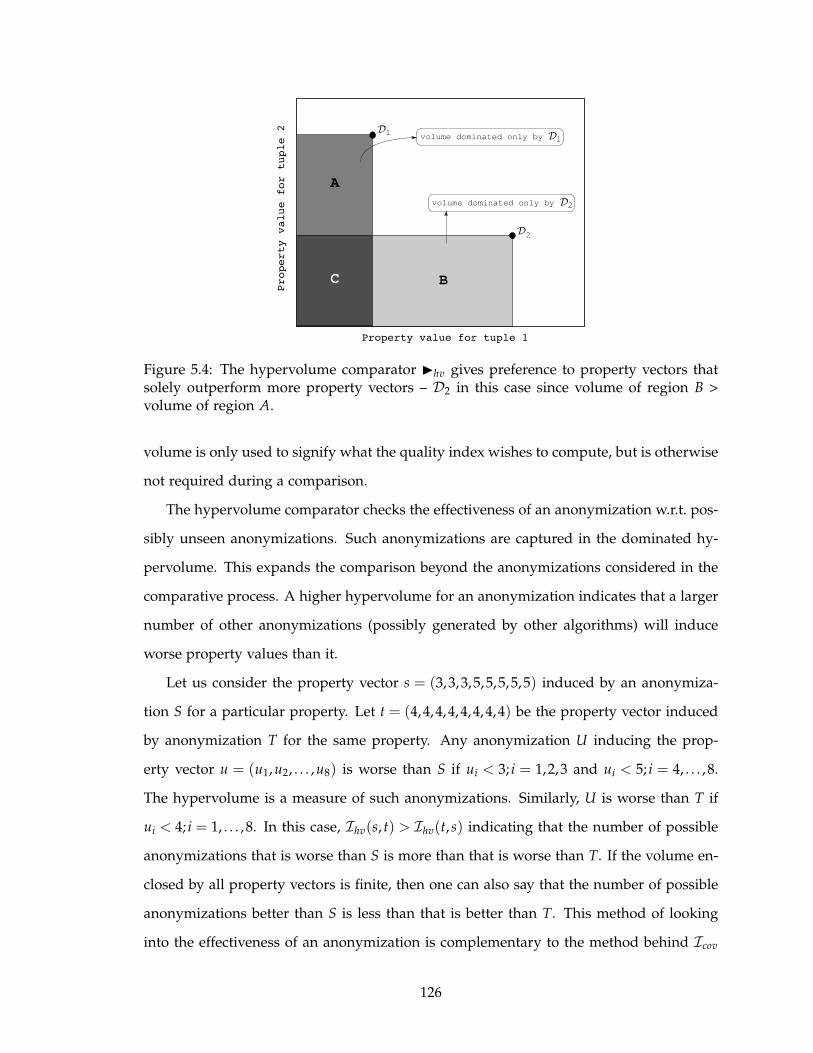
Property value for tuple 1
Property value for tuple 2
A
BC
D
D
1
2
volume dominated only by D1
volume dominated only by D2
Figure 5.4: The hypervolume comparator ◮hv gives preference to property vectors thatsolely outperform more property vectors – D2 in this case since volume of region B >volume of region A.
volume is only used to signify what the quality index wishes to compute, but is otherwise
not required during a comparison.
The hypervolume comparator checks the effectiveness of an anonymization w.r.t. pos-
sibly unseen anonymizations. Such anonymizations are captured in the dominated hy-
pervolume. This expands the comparison beyond the anonymizations considered in the
comparative process. A higher hypervolume for an anonymization indicates that a larger
number of other anonymizations (possibly generated by other algorithms) will induce
worse property values than it.
Let us consider the property vector s = (3,3,3,5,5,5,5,5) induced by an anonymiza-
tion S for a particular property. Let t = (4,4,4,4,4,4,4,4) be the property vector induced
by anonymization T for the same property. Any anonymization U inducing the prop-
erty vector u = (u1,u2, . . . ,u8) is worse than S if ui < 3; i = 1,2,3 and ui < 5; i = 4, . . . ,8.
The hypervolume is a measure of such anonymizations. Similarly, U is worse than T if
ui < 4; i = 1, . . . ,8. In this case, Ihv(s, t) > Ihv(t, s) indicating that the number of possible
anonymizations that is worse than S is more than that is worse than T. If the volume en-
closed by all property vectors is finite, then one can also say that the number of possible
anonymizations better than S is less than that is better than T. This method of looking
into the effectiveness of an anonymization is complementary to the method behind Icov
126
and Ispr. While the latter two facilitates a comparison on a one-to-one basis, comparisons
via Ihv involves a broader extent of the space of property vectors.
These four quality indices can be used to compare property vectors measuring a sin-
gle property only. It is true that an anonymization evaluated as being better w.r.t. a
particular property can be worse in the context of another. Hence, for the case when
more than one property is being measured on an anonymization, other mechanisms are
required to weigh the importance of the different properties when making comparisons.
We now consider sets of property vectors, instead of a single one, and suggest three in-
dices to compare two such sets. Let us assume that comparisons are to be made across
the sets Υ1 = {D11,D12, . . . ,D1r} and Υ2 = {D21,D22, . . . ,D2r} induced by two r–property
anonymizations G1 and G2 respectively. In the following expressions, we use the notation
I(X,Y) to indicate a binary quality index defined to compare two property vectors X
and Y. Note that different quality indices can be used to compare different properties.
Also, without any loss of generality, we assume that a higher value of the quality index
is desirable; otherwise we can negate the index value.
5.4.5 ◮WTD-better
The first method to compare sets of property vectors is based on the classical weighted
sum approach. Weight assignments are useful when the properties analyzed are orthog-
onal in nature, such as privacy and utility. The weight-based comparator ◮WTD requires a
vector W = (w1, . . . wr) such that the weight wi signifies the importance of the ith property
being measured. Typically the weights are chosen such that, for 1 ≤ i ≤ r, 0 < wi < 1 and
∑ri=1 wi = 1. The quality index is given as
IWTD(Υ1,Υ2) =r
∑i=1
[wi · I(D1i,D2i)] (5.8)
and comparisons are made using the relationship IWTD(Υ1, Υ2) > IWTD(Υ2,Υ1) ⇐⇒Υ1 ◮WTD Υ2. It is advisable to normalize the I values before computing the weighted
sum.
Consider the 3-anonymous generalizations in T3a and T3b. The size of equivalence
class property vectors for the two generalizations are pa = (3,3,3,3,4,4,4,3,3,4) and pb =
(3,7,7,3,7,7,7,3,7,7) respectively. Using Iyengar’s data utility metric [92], the utility
127
property vectors for them are ua = (2.03,1.7,1.7,2.03,1.6,1.6,1.6,2.03,1.7,1.6) and ub =
(2.03,0.97,0.97,2.03,0.97,0.97,0.97,2.03,0.97,0.97) respectively. Using the coverage com-
parator we have, Icov(pa, pb) = 0.3 < 1 = Icov(pb, pa) and Icov(ua,ub) = 1 > 0.3 = Icov(ub,ua).
Thus, if equal weights are assigned to both privacy and utility, then generalizations T3a
and T3b are equally good.
5.4.6 ◮LEX-better
The weight-based comparator suffers from the drawback that it may sometimes be
difficult to assign weight values specifying the preference of a property. An alternative to
this is to instead specify a lexicographic ordering of the different properties. For example,
when privacy levels depicted by different privacy models are to be used in conjunction to
decide on an anonymization, the property vectors induced from different privacy proper-
ties can be ordered in descending order of relevance. Such a method orders the elements
of a set of property vectors such that the most desirable property is the first element, the
second most desirable property as the second element, and so on. With this ordering in
place, we define the following quality index.
ILEX(Υ1,Υ2) = mini
{1 ≤ i ≤ r|I(D1i,D2i) − I(D2i,D1i) > ǫi} (5.9)
Here, ǫ = (ǫ1, . . . ,ǫr) is a significance vector where ǫi gives the maximum tolerable
difference in the I values for the ith property. Thus, two property vectors D1i and D2i
are considered to be equally good if |I(D1i,D2i) − I(D2i,D1i)| ≤ ǫi. The ǫ-lexicographic
comparator ◮LEX assigns superiority to a set of property vectors based on the property on
which it is more superior, given the ordering on the properties and the significance vector.
ILEX(Υ1,Υ2) thereby computes the first property on the ordering where Υ1 is superior. If
ILEX(Υ1,Υ2) < ILEX(Υ2,Υ1), then Υ1 has a more desirable property where it is superior
to Υ2, i.e. ILEX(Υ1,Υ2) < ILEX(Υ2,Υ1) ⇐⇒ Υ1 ◮LEX Υ2.
5.4.7 ◮GOAL-better
The goal-based comparator ◮GOAL is useful when the competence of an anonymization
can be measured in terms of its closeness to a desirable level (or goal). In such a situation,
128
a goal vector G = (g1, . . . , gr) specifies the values desired in the quality indices used – the
I functions. The quality index
IGOAL(Υ1,Υ2) =r
∑i=1
[I(D1i,D2i) − gi]2 (5.10)
then computes the sum-of-squares error of the quality indices from the goal values.
The comparison is performed with the relationship IGOAL(Υ1,Υ2) < IGOAL(Υ2,Υ1) ⇐⇒Υ1 ◮GOAL Υ2. We can also use unary performance indices as replacements for the binary
functions I . The use of unary indices simplifies the specification of the goal vector in
terms of the goal property vectors instead. If Dg1, . . . ,Dgr are the goal property vectors,
then the goal vector can be formulated as G = (I1(Dg1), . . . ,Ir(Dgr)), where Iis are unary
quality indices.
5.5 Conclusions
In this chapter, we explore an often ignored factor in the comparison of anonymiza-
tions reported by microdata disclosure control algorithms. This factor, which we call the
anonymization bias, results in anonymizations being skewed towards a fraction of the
data set w.r.t. a privacy property. Hence, the attainment of a collective privacy level is
not sufficient to conclude that two anonymizations offer the same level of privacy. We
therefore introduce property vectors as an alternate representation of a property (pri-
vacy/utility) measured on an anonymization. This representation helps indicate the pri-
vacy level of every individual in the data set separately. Further, the issue of comparing
anonymizations is addressed by the usage of quality index functions that give an ab-
solute or a relative quantitative estimate of the quality of property vectors. Our initial
conclusion on such a comparative method is that unary quality indices are limited in
their ability to perform comparisons, specifically when strict inferences like “not worse
than” or “better than” are to be made between anonymizations. As a result, we explore
alternative methods of comparison, keeping in mind that comparators defined on such
grounds should make adequate effort to quantify the differences in values of the prop-
erty measured across the tuples of the entire data set instead of a minimalistic estimate.
Estimates based on rank, spread and hypervolume are thus suggested. We also present
129
various preference based techniques when comparisons are to be made across multiple
properties induced by anonymizations.
An immediate extension of this work is the identification of privacy measures that ad-
dress the anonymization bias. Moreover, vector-based representations of privacy would
require a rethinking of the utility optimization problem since trade-offs between privacy
and utility now becomes more apparent. The currently adopted optimization framework
in disclosure control is single objective in nature. The scalar quantification of privacy en-
ables the framework to direct its search for higher utility anonymization while satisfying
a privacy constraint. If vector representations of privacy are adopted, then the framework
has to undergo changes. This is primarily because the vector representation allows one to
distinguish between anonymizations even when a typical privacy constraint is satisfied
by both. Note that the current framework only makes this distinction based on utility,
whereas the vector representation enables the distinction to be made at the privacy front
as well. Finding “good” anonymizations thus converts into a multi-objective problem.
Although the multi-objective nature of the privacy versus utility problem is well under-
stood in the community, it has remained irrelevant under the pretext of scalar privacy
representations. However, under the light of vector representations, privacy should no
longer be imposed only as a constraint in the framework but rather handled directly as
an objective to maximize.
130
CHAPTER 6
Data Privacy Through Property Based Generalizations
Most algorithms in disclosure control are designed to obtain anonymizations (gen-
eralization with or without suppression) that can maximize the utility of the anonymized
data while satisfying a pre-specified privacy property. A specific generalization is there-
fore considered to be better than another if it provides higher utility within the constraints
of the privacy requirement. The adoption of such an optimization framework brings forth
pertinent practical issues that have been ignored for long. We have independently identi-
fied and sought resolution to three such issues in the previous chapters.
(1) The data publisher’s dilemma: ([55, 88]) Data utility and respondent privacy are two
equally important facets of data publishing. Proper anonymization thus involves weigh-
ing the risk of publicly disseminated information against the statistical utility of the con-
tent. In such a situation, it is imperative that the data publisher understands the impli-
cations of setting a parameter in a privacy model to a particular value. There is clearly a
trade-off involved. Setting the parameter to a “very low” value impacts the privacy of in-
dividuals. Picking a “very high” value disrupts the inference of any significant statistical
information.
(2) Anonymity model correlations: The k–anonymity model is prone to other forms of
attacks on privacy. As a result, a multitude of other privacy models have been proposed
over time [112, 120, 173, 191], quite often followed by newer forms of privacy attacks.
131

The inclusion of multiple models in the anonymization process is desirable since a single
comprehensive model is yet to be developed. However, the correlation between these
models is not well studied making the task of parameter selection a difficult one. Data
generalization algorithms will also find it difficult to satisfy multiple privacy constraints
when existing correlations are inverse in nature.
(3) Biased privacy: ([58]) Consider the k−anonymity model where the measure of pri-
vacy (the value of k) is given by the minimum size of an equivalence class. Thus, two
anonymizations inducing the same value of k will be considered equally good with re-
spect to privacy protection. However, it is quite possible that for one of the anonymiza-
tions a majority of the individual tuples have lesser probabilities of privacy breaches than
their counterparts in the other anonymization. Individual privacy levels as depicted by
such a model can therefore be misleading – higher for some, minimalistic for others.
Resolution of the first issue is a difficult task within the existing optimization frame-
work. Any attempt to find the “best level of privacy” will require an enumeration across
different parameter values to determine what is suitable. The second issue makes pa-
rameter selection further difficult owing to a larger combination of possible choices. The
decision maker is also required to have an understanding of the feasibility of combining
different models. The third issue is a resultant of the worst case representation of privacy.
Such a representation identifies the minimum privacy present for all individuals but is in-
adequate to capture the amount of skewness (homogeneity or heterogeneity) introduced
in individual privacy levels. Thus, the level of privacy guaranteed by a generalization can
become questionable.
In this chapter, we propose resolutions to these issues using the notion of property
based generalizations. First, inclusion of multiple objectives in the anonymization process
is captured using properties as anonymization objectives. A generalization here is viewed
as a source which can be independently subjected to evaluation in terms of different
privacy or utility properties. Second, evaluation of a generalization with respect to a
privacy property is performed using both worst case and vector based measurements.
The overall effectiveness of a generalization is then measured with a dominance operator.
The dominance relationship analyzes a generalization in terms of its achievement and
132

trade-offs in the different properties. The concept of a single optimal solution is therefore
discarded and a representative subset of the minimal solution set is sought. Towards
this end, our third contribution is in terms of an evolutionary algorithm that can be
used to efficiently search the domain generalization lattice to identify such representative
solutions. The algorithm uses a modified dominance operator to select these solutions.
The remainder of the chapter is organized as follows. Section 6.1 introduces prop-
erty based generalizations, followed by a description of the modified dominance operator
in Section 6.2. The evolutionary algorithm is presented in Section 6.3. Section 6.4 dis-
cusses the results of applying the algorithm on a benchmark data set. Finally, Section 6.5
concludes the chapter.
6.1 Property Based Generalization
Multiple objectives to meet during data anonymization are captured in the form of
properties [58]. Formally, a property is defined as follows.
Definition 6.1 PROPERTY. A property is a function P that maps a table T to a vector of
size equal to the number of tuples in the table. The vector is called a property vector and
denoted by P(T).
A property refers to a privacy, utility or any other measurable feature of a tuple.
It signifies the grounds under which a comparison is made between two nodes in the
domain generalization lattice. Our perspective of a node is that of a source inducing
multiple properties that can be measured on each tuple in the data set. For example, ap-
plying the generalization levels corresponding to a node results in multiple equivalence
classes. If we pick our property to be the “size of the equivalence class to which a tuple be-
longs,” then each tuple will have an associated integer. This results in a property vector
Pequiv(T) = (k1,k2, . . . ,kN ) for a data set of size N , where ki is the equivalence class size
of the ith tuple. If measurements on the diversity of sensitive attributes is required, the
property can be the number of times the sensitive attribute value of a tuple appears in its
equivalence class. A property is therefore a vector based measurement. The motivation
behind using such vector based measurements is two folded. First, it fits the conventional
133

“worst case” method of measuring privacy. Second, it allows us to determine the effi-
ciency of a node with consideration to the distribution of privacy levels across the data
set. These two methods of assessing a node are jointly represented through the use of
quality index functions.
6.1.1 Quality Index functions
Comparison between generalizations with respect to a single property can be done
by defining an ordering operation on the co-domain of the property. Towards this end,
quality index functions map a node to the set of real numbers. The underlying idea is to
quantify quality differences between generalizations by applying common metrics.
Definition 6.2 QUALITY INDEX. Let T be the collection of all possible generalized ver-
sions of a table T. Given a property P , a quality index IP is a function IP : T × T → R
which assigns an ordered pair of two tables Tl ,Tm ∈ T a real value IP (Tl ,Tm).
The value IP (Tl ,Tm) signifies the quality of table Tl relative to table Tm and with
respect to the property P . We would therefore say that Tl is preferable over Tm with
respect to P if IP (Tl ,Tm) > IP (Tm,Tl), assuming that a higher value signifies better
achievement of the property. Otherwise, the relationship is IP (Tl ,Tm) < IP (Tm,Tl).
6.1.1.1 Worst case measurements
A quality index function in the definition requires two tables as input. However,
a commonly used method of evaluating a generalization is through unary quality in-
dex functions. Unary quality indices are functions applied independently on general-
izations, i.e. they have a single table as input. For example, the k-anonymity property
is a unary quality index based on the equivalence class size property Pequiv, given as
IPequiv(T) = min
i(Pequiv(T)). Unary indices only allow the measurement of an aggregate
property of a generalization. This prohibits any kind of comparison of individual prop-
erty values maintained by tuples in a generalization with that maintained in another.
Having said so, we do not specify any restriction on the formulation of a quality index
function. This is because data utility functions are typically unary in nature, i.e. they
are absolute estimates of the information content of the anonymized data. We keep the
134
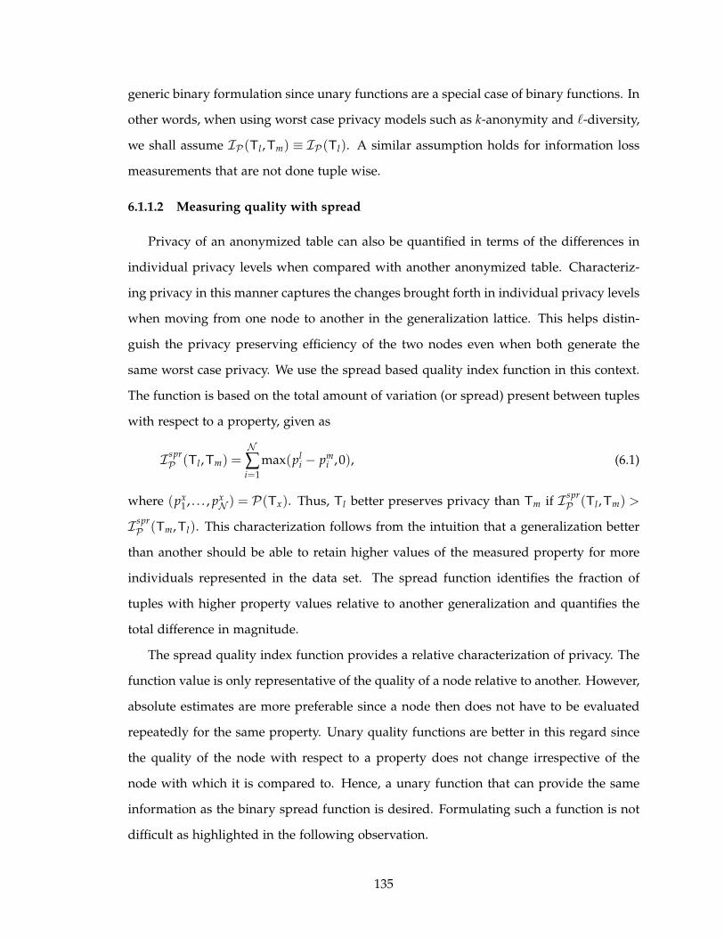
generic binary formulation since unary functions are a special case of binary functions. In
other words, when using worst case privacy models such as k-anonymity and ℓ-diversity,
we shall assume IP (Tl ,Tm) ≡ IP (Tl). A similar assumption holds for information loss
measurements that are not done tuple wise.
6.1.1.2 Measuring quality with spread
Privacy of an anonymized table can also be quantified in terms of the differences in
individual privacy levels when compared with another anonymized table. Characteriz-
ing privacy in this manner captures the changes brought forth in individual privacy levels
when moving from one node to another in the generalization lattice. This helps distin-
guish the privacy preserving efficiency of the two nodes even when both generate the
same worst case privacy. We use the spread based quality index function in this context.
The function is based on the total amount of variation (or spread) present between tuples
with respect to a property, given as
I sprP (Tl ,Tm) =
N∑i=1
max(pli − pm
i ,0), (6.1)
where (px1 , . . . , px
N ) = P(Tx). Thus, Tl better preserves privacy than Tm if I sprP (Tl ,Tm) >
I sprP (Tm,Tl). This characterization follows from the intuition that a generalization better
than another should be able to retain higher values of the measured property for more
individuals represented in the data set. The spread function identifies the fraction of
tuples with higher property values relative to another generalization and quantifies the
total difference in magnitude.
The spread quality index function provides a relative characterization of privacy. The
function value is only representative of the quality of a node relative to another. However,
absolute estimates are more preferable since a node then does not have to be evaluated
repeatedly for the same property. Unary quality functions are better in this regard since
the quality of the node with respect to a property does not change irrespective of the
node with which it is compared to. Hence, a unary function that can provide the same
information as the binary spread function is desired. Formulating such a function is not
difficult as highlighted in the following observation.
135

Observation: Let SP (Tx) denote the sum of the property values in the property vector
P(Tx). Then I sprP (Tl ,Tm) > I spr
P (Tm,Tl) if and only if SP (Tl) > SP (Tm).
The observation is also valid if the “greater than” relationship is replaced with an
“equal to” or “less than” relationship. Comparing nodes under the light of the spread
function can therefore be performed using the sum of the property values, i.e. I sprP (Tl ,Tm)≡
IP (Tl) = SP (Tl). Hence, in the subsequent sections, we shall use the notation IP (Tl) to
denote the quality of Tl with respect to P , keeping in mind that IP is either a unary
function (as used in worst case measurements and loss assessments) or the sum function
SP (sufficient to infer the quality according to the binary spread function).
6.1.2 Anonymizing with multiple properties
Ideally, any number of properties can be studied on a generalized table. In the
presence of multiple properties, quality with respect to each property must be weighed
in appropriately before choosing one generalization over another. Let us consider an
anonymization with respect to the set of properties P = {P1, . . . ,Pr}. Assessing the qual-
ity of a generalization Tl with respect to the properties P will result in a vector of values
IP(Tl) = [IP1(Tl), . . . ,IPr
(Tl)] where the ith element represents the quality of Tl with re-
spect to the property Pi. The dominance relation � is then specified over the set of
such vectors to characterize the efficiency of a generalization with respect to P, such that
IP(Tl) � IP(Tm) if
1. ∀i = 1 . . . r : IPi(Tl) ≥ IPi
(Tm), and
2. ∃j ∈ {1, . . . ,r} : IPj(Tl) > IPj
(Tm).
This relation states that for a table to be better than another, it must not have worse
quality across all the properties while maintaining better quality with respect to at least
one property. Once again, the notion of better quality can be in terms of a lower quality
index value, implying the use of a “less than” relationship for comparing across such
properties. Note that the dominance relation is transitive in nature, i.e if IP(T1) � IP(T2)
and IP(T2) � IP(T3), then IP(T1) � IP(T3). Using dominance to evaluate a generalization
introduces the concept of a property based generalization (PBG).
136
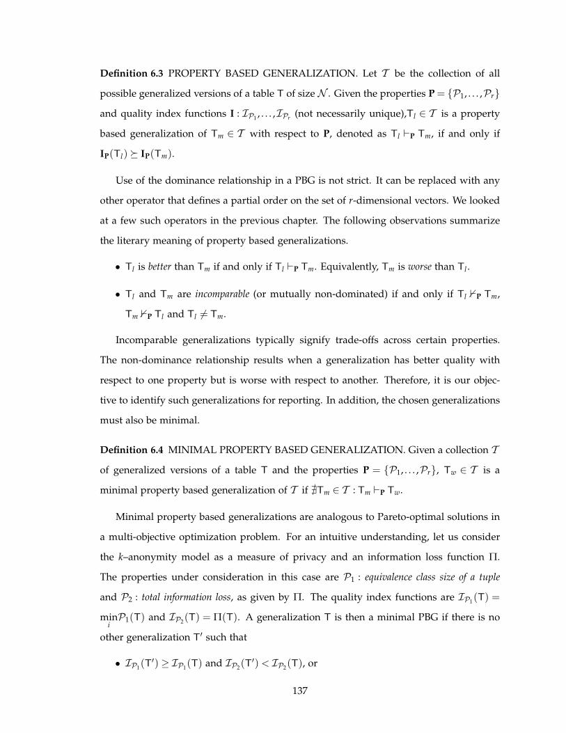
Definition 6.3 PROPERTY BASED GENERALIZATION. Let T be the collection of all
possible generalized versions of a table T of size N . Given the properties P = {P1, . . . ,Pr}and quality index functions I : IP1
, . . . ,IPr(not necessarily unique),Tl ∈ T is a property
based generalization of Tm ∈ T with respect to P, denoted as Tl ⊢P Tm, if and only if
IP(Tl) � IP(Tm).
Use of the dominance relationship in a PBG is not strict. It can be replaced with any
other operator that defines a partial order on the set of r-dimensional vectors. We looked
at a few such operators in the previous chapter. The following observations summarize
the literary meaning of property based generalizations.
• Tl is better than Tm if and only if Tl ⊢P Tm. Equivalently, Tm is worse than Tl .
• Tl and Tm are incomparable (or mutually non-dominated) if and only if Tl 0P Tm,
Tm 0P Tl and Tl 6= Tm.
Incomparable generalizations typically signify trade-offs across certain properties.
The non-dominance relationship results when a generalization has better quality with
respect to one property but is worse with respect to another. Therefore, it is our objec-
tive to identify such generalizations for reporting. In addition, the chosen generalizations
must also be minimal.
Definition 6.4 MINIMAL PROPERTY BASED GENERALIZATION. Given a collection Tof generalized versions of a table T and the properties P = {P1, . . . ,Pr}, Tw ∈ T is a
minimal property based generalization of T if ∄Tm ∈ T : Tm ⊢P Tw.
Minimal property based generalizations are analogous to Pareto-optimal solutions in
a multi-objective optimization problem. For an intuitive understanding, let us consider
the k–anonymity model as a measure of privacy and an information loss function Π.
The properties under consideration in this case are P1 : equivalence class size of a tuple
and P2 : total information loss, as given by Π. The quality index functions are IP1(T) =
miniP1(T) and IP2
(T) = Π(T). A generalization T is then a minimal PBG if there is no
other generalization T′ such that
• IP1(T′) ≥ IP1
(T) and IP2(T′) < IP2
(T), or
137
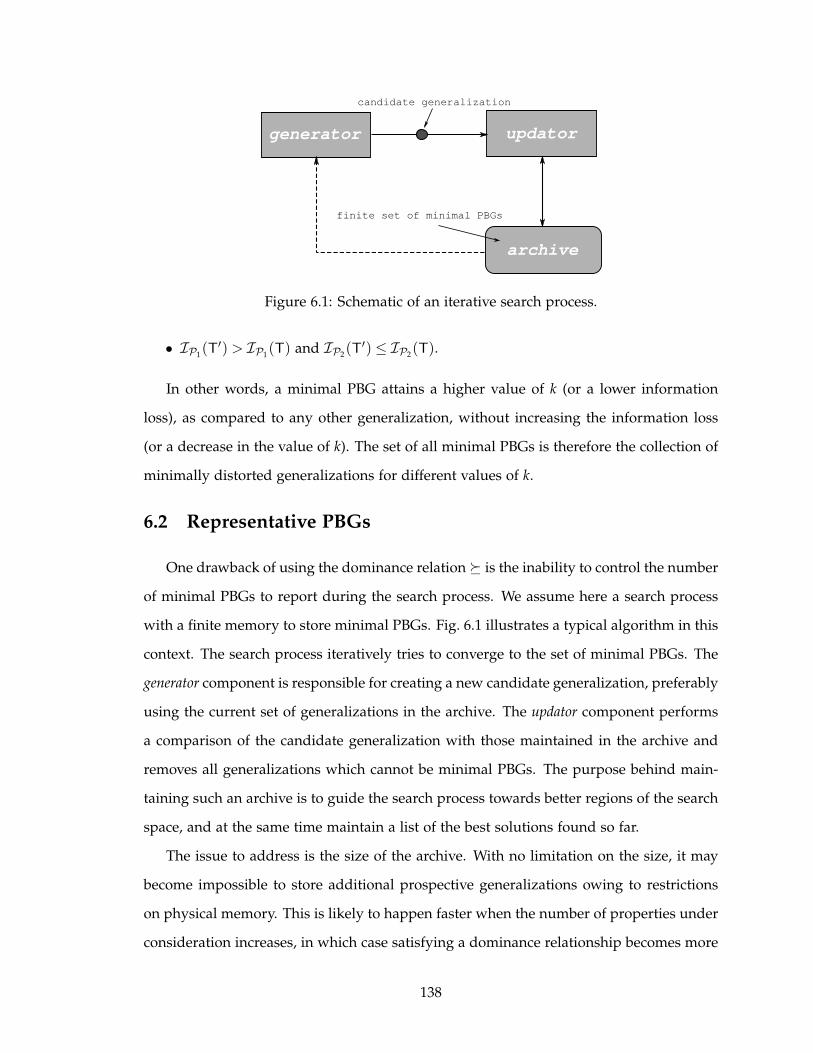
generator updator
archive
candidate generalization
finite set of minimal PBGs
Figure 6.1: Schematic of an iterative search process.
• IP1(T′) > IP1
(T) and IP2(T′) ≤ IP2
(T).
In other words, a minimal PBG attains a higher value of k (or a lower information
loss), as compared to any other generalization, without increasing the information loss
(or a decrease in the value of k). The set of all minimal PBGs is therefore the collection of
minimally distorted generalizations for different values of k.
6.2 Representative PBGs
One drawback of using the dominance relation � is the inability to control the number
of minimal PBGs to report during the search process. We assume here a search process
with a finite memory to store minimal PBGs. Fig. 6.1 illustrates a typical algorithm in this
context. The search process iteratively tries to converge to the set of minimal PBGs. The
generator component is responsible for creating a new candidate generalization, preferably
using the current set of generalizations in the archive. The updator component performs
a comparison of the candidate generalization with those maintained in the archive and
removes all generalizations which cannot be minimal PBGs. The purpose behind main-
taining such an archive is to guide the search process towards better regions of the search
space, and at the same time maintain a list of the best solutions found so far.
The issue to address is the size of the archive. With no limitation on the size, it may
become impossible to store additional prospective generalizations owing to restrictions
on physical memory. This is likely to happen faster when the number of properties under
consideration increases, in which case satisfying a dominance relationship becomes more
138

and more difficult (a consequence of the curse of dimensionality). A generator using the
current archive in creating new candidate generalizations will also use more computation
time if the archive size is allowed to grow unbounded. Further, it is sufficient that a data
disseminator obtains a finite representative subset of minimal PBGs for the purpose of
decision making. The primary criteria to fulfill is that the archive maintain generalizations
that are minimal PBGs and at the same time have enough diversity to represent the trade-
off behavior across the multiple properties.
6.2.1 Box-dominance
Let M denote the set of all minimal PBGs corresponding to a given data set. The
objective is to obtain a polynomially bounded sized subset of M. Let (ǫ1, . . . ,ǫr);ǫi > 0
denote a discretization vector, r being the number of properties considered. The quality
index space Rr is then discretized by placing a hypergrid with the co-ordinates 0,ǫi,2ǫi, . . .
along each of the r dimensions. This divides the space into boxes with side lengths same
as the discretization vector. Assuming the quality index functions are bounded on both
sides, i.e. 0 < IPi(T) ≤ Ki, the box of a generalization Tl is given by the vector
B(Tl) =
[⌊IP1(Tl)
ǫ1
⌋
, . . . ,
⌊IPr(Tl)
ǫr
⌋]
. (6.2)
A modified dominance relation, called box-dominance and denoted by �box, is then
formulated as
IP(Tl) �box IP(Tm) ⇐⇒{
B(Tl) � B(Tm) , if B(Tl) 6= B(Tm)
IP(Tl) � IP(Tm) ,otherwise. (6.3)
The box-dominance relation first places the quality index value vectors (IP(Tl) and
IP(Tm)) in their boxes. If the vectors are on different boxes, then Tl cannot be a PBG
of Tm if the box of Tl does not dominate the box of Tm. Otherwise, for the case when
boxes are the same, the dominance is checked on the quality index values. Further,
every box is allowed to hold only one generalization. Choice between two incomparable
generalizations belonging to the same box is made arbitrarily. Fig. 6.2 illustrates this
modified dominance relation.
Non-dominated boxes signify regions where a minimal PBG exists. By allowing the
existence of a single generalization per non-dominated box, the modified dominance rela-
139
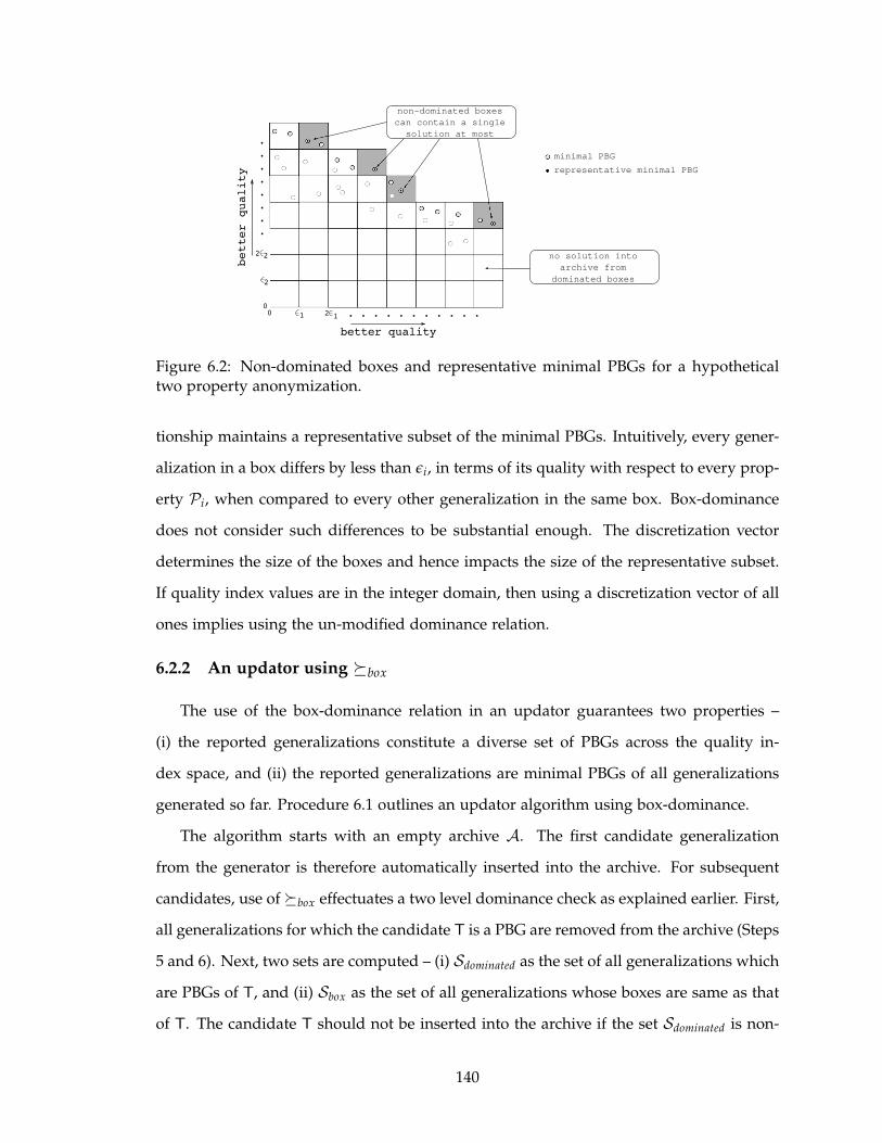
. . . . . . . . . . .2
2
2 . . . . . . . .
1 10
2
0
better quality
better quality
minimal PBG
representative minimal PBG
non-dominated boxes
can contain a single
solution at most
no solution into
archive from
dominated boxes
Figure 6.2: Non-dominated boxes and representative minimal PBGs for a hypotheticaltwo property anonymization.
tionship maintains a representative subset of the minimal PBGs. Intuitively, every gener-
alization in a box differs by less than ǫi, in terms of its quality with respect to every prop-
erty Pi, when compared to every other generalization in the same box. Box-dominance
does not consider such differences to be substantial enough. The discretization vector
determines the size of the boxes and hence impacts the size of the representative subset.
If quality index values are in the integer domain, then using a discretization vector of all
ones implies using the un-modified dominance relation.
6.2.2 An updator using �box
The use of the box-dominance relation in an updator guarantees two properties –
(i) the reported generalizations constitute a diverse set of PBGs across the quality in-
dex space, and (ii) the reported generalizations are minimal PBGs of all generalizations
generated so far. Procedure 6.1 outlines an updator algorithm using box-dominance.
The algorithm starts with an empty archive A. The first candidate generalization
from the generator is therefore automatically inserted into the archive. For subsequent
candidates, use of �box effectuates a two level dominance check as explained earlier. First,
all generalizations for which the candidate T is a PBG are removed from the archive (Steps
5 and 6). Next, two sets are computed – (i) Sdominated as the set of all generalizations which
are PBGs of T, and (ii) Sbox as the set of all generalizations whose boxes are same as that
of T. The candidate T should not be inserted into the archive if the set Sdominated is non-
140

Procedure 6.1 BoxDominanceUpdator(Archive A, Generalization T)
Input: Archive A, candidate generalization T.Output: Updated archive A.
1: if (A = φ) then
2: A = {T}3: goto Line 124: end if
5: Sdominate = {T′ ∈ A|IP(T) �box IP(T′)}
6: A = A− Sdominate
7: Sdominated = {T′ ∈ A|IP(T′) �box IP(T)}
8: Sbox = {T′ ∈ A|B(T) = B(T′)}
9: if (Sdominated = φ and Sbox = φ) then
10: A = A∪ {T}11: end if
12: return A
empty, i.e. there exists a generalization in the archive which is a PBG of T. Further, if
Sbox is not empty then inclusion of T in the archive will result in the presence of two
different generalizations which are positioned in the same box. Step 9 checks for these
two conditions, thereby guaranteeing that only non-dominated boxes contain a solution
and only one solution is contained in a non-dominated box. The following two theorems
prove that the archive maintained in this manner will only contain minimal PBGs from
the set of candidates generated so far and will be of bounded size.
Theorem 6.1 Let Mg denote the set of all generalizations produced by a generator un-
til iteration t and M∗g denote the set of minimal PBGs of Mg. Then the archive A as
maintained by Procedure 6.1 contains only minimal PBGs of Mg, i.e. A ⊆M∗g.
Proof We assume that Procedure 6.1 is incorrect, implying A * M∗g. Therefore there
exists Ts ∈ A generated at iteration s such that Ts /∈M∗g.
If Ts /∈M∗g then there exists Tq ∈Mg discovered at iteration q 6= s such that IP(Tq) �
IP(Ts). Also, either B(Tq) = B(Ts) or B(Tq) � B(Ts). We can merge these cases and say
IP(Tq) �box IP(Ts).
Case (i): q < s
If Tq is present in A at iteration s then Ts will not be included in the archive since
Sdominated for Ts contains at least Tq.
141

If Tq is not present in A at iteration s then it must have been removed by a gen-
eralization Tr in A such that IP(Tr) �box IP(Tq). We therefore have IP(Tr) � IP(Tq)
or B(Tr) � B(Tq). Using the transitivity of the � relation, we have IP(Tr) � IP(Ts) or
B(Tr) � B(Ts), which implies IP(Tr) �box IP(Ts). Hence in this case as well Sdominated 6= φ
for Ts. Note that Tr itself might have got removed from the archive between iteration
q and iteration s. However, owing to the transitivity, the generalization which removes
it will instead appear in Sdominated for Ts. Hence Ts will never appear in A, i.e. Ts /∈ A,
which is a contradiction.
Case (ii): q > s
In this case, if Ts exists in A at iteration q then it would be removed from the archive
as it belongs to the set Sdominate of Tq. Further, if Tq gets removed and Ts gets re-generated
at a later iteration, the transitivity property would assure that Ts does not get re-inserted
into the archive. Thus, Ts /∈ A which is again a contradiction.
Therefore, Ts can never be a member of the archive at iteration t if it is not a mini-
mal PBG. We can therefore say Procedure 6.1 is correct and the archive A contains only
minimal PBGs of Mg. �
Theorem 6.2 The archive A as maintained by Procedure 6.1 is of bounded size, given as
|A| ≤r−1
∏i=1
bi, (6.4)
where bi is the ith largest element of the vector (K1ǫ1
, . . . , Krǫr
).
Proof Recall that K1, . . . ,Kr are the upper bounds of the quality index functions for r prop-
erties. These values can very well be equal. By using box co-ordinates at 0,ǫi,2ǫi, . . . along
each dimension i, we have divided the quality index value space into ∏ri=1
Kiǫi
boxes and
only one node in each box can be included in A. We now cluster these boxes into groups
of br boxes, giving us a total of ∏r−1i=1 bi clusters. A cluster is formed by grouping together
boxes that have the same co-ordinates in all but one dimension. Note that choosing br as
the parameter to decide the number of boxes in a cluster gives us the smallest possible
cluster size and hence the largest number of clusters. This is required if an upper bound
on the archive size is to be computed. Next, in a cluster, the box having the maximum
142

Procedure 6.2 PBG-EA()
Output: Archive A of representative minimal PBGs.1: A = φ; t = 02: Initialize population Pt
3: Evaluate Pt
4: Update A with nodes in Pt
5: repeat
6: Assign fitness to nodes in Pt and A7: Perform selection in Pt ∪A8: Generate Pt+1 by performing recombination on selected nodes9: Update A with nodes in Pt+1
10: t = t + 111: until (t ≥ maximum number of iterations allowed)12: return A
co-ordinate value in the differing dimension will dominate all other boxes in the cluster.
Therefore, only such a box will contain a minimal PBG. Each cluster can therefore con-
tribute only one minimal PBG, bounding the archive size to the number of such clusters,
i.e. |A| ≤ ∏r−1i=1 bi. �
Note that the specific upper bounds on the quality index functions are not used by the
updator but is only required to show that the size of the archive depends on these bounds
and the chosen discretization vector. Given a specific size for the representative subset of
minimal PBGs, the discretization vector can be adjusted accordingly if the upper bounds
on the quality index functions are known.
6.3 An Evolutionary Generator
An efficient generator is required not only to find new candidate PBGs, but also to
minimize the number of node evaluations performed during the search process. The
generator evaluates each node that it explores and provides it to the updator. Discov-
ering nodes that can converge quickly (without involving too many intermediate node
evaluations) to a minimal PBG is therefore the primary objective of the generator. We
propose here an evolutionary algorithm for this purpose, henceforth called PBG-EA. The
algorithm follows the structure described in Procedure 6.2.
The update method from Procedure 6.1 is used iteratively in steps 4 and 9. Specifics
of the other steps are described next.
143

6.3.1 Population initialization and evaluation
A population Pt is a collection of Npop nodes in the lattice and undergoes changes as
the algorithm progresses. Recall that every node is a vector of s dimensions where s is the
number of quasi-identifiers. The population P0 is created by randomly selecting nodes in
the lattice. The fully generalized and fully specialized nodes are always inserted into this
initial population as they are trivially minimal PBGs. Evaluation of a population means
computing the quality index values for each node in the population. Outliers in the data
set must be handled in this step and is done using a maximum allowed suppression
scheme.
6.3.2 Fitness assignment
Fitness signifies the potential of a node to be a minimal PBG relative to the current
population and archive. The fitness assignment we use is adapted from the one used in
the SPEA2 algorithm [195]. Let domP be the number of nodes in Pt ∪ A dominated by
P ∈ Pt ∪A. The fitness of a node P is then computed as the sum of the dominance counts
of the nodes which dominate P, or
FitnessP = ∑P′∈Pt∪A and P′�P
domP′ . (6.5)
All non-dominated generalizations will therefore have a fitness of zero. Hence, lower
fitness implies better generalizations. The fitness of a node not only reflects the number of
nodes that dominate it but also takes into account the dominance power of those nodes.
6.3.3 Selection
Selection of nodes for recombination is performed by using a binary tournament strat-
egy in Pt ∪ A. Under this strategy, two nodes are randomly chosen from Pt ∪ A and the
one with the lower fitness is selected. The process is repeated for Npop times, giving a
selected population of size Npop.
6.3.4 Recombination
Recombination is a two step process involving the crossover and mutation opera-
tors, the resulting nodes from which are used as the next population Pt+1. A single
144
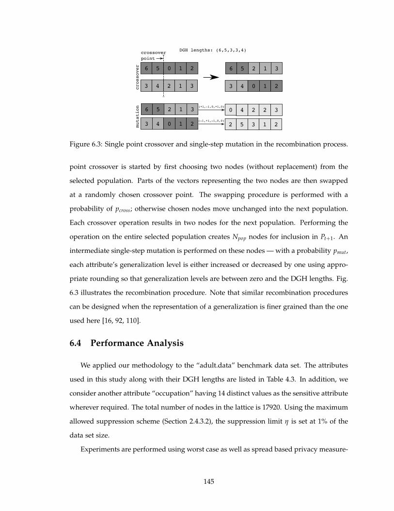
6 5 0 1 2
3 4 2 1 3
6 5 2 1 3
3 4 0 1 2
6 5 2 1 3
3 4 0 1 2
0 4 2 2 3
2 5 3 1 2
(+1,-1,0,+1,0)
(-1,+1,-1,0,0)
DGH lengths: (6,5,3,3,4)crossover
point
crossover
mutation
Figure 6.3: Single point crossover and single-step mutation in the recombination process.
point crossover is started by first choosing two nodes (without replacement) from the
selected population. Parts of the vectors representing the two nodes are then swapped
at a randomly chosen crossover point. The swapping procedure is performed with a
probability of pcross; otherwise chosen nodes move unchanged into the next population.
Each crossover operation results in two nodes for the next population. Performing the
operation on the entire selected population creates Npop nodes for inclusion in Pt+1. An
intermediate single-step mutation is performed on these nodes — with a probability pmut,
each attribute’s generalization level is either increased or decreased by one using appro-
priate rounding so that generalization levels are between zero and the DGH lengths. Fig.
6.3 illustrates the recombination procedure. Note that similar recombination procedures
can be designed when the representation of a generalization is finer grained than the one
used here [16, 92, 110].
6.4 Performance Analysis
We applied our methodology to the “adult.data” benchmark data set. The attributes
used in this study along with their DGH lengths are listed in Table 4.3. In addition, we
consider another attribute “occupation” having 14 distinct values as the sensitive attribute
wherever required. The total number of nodes in the lattice is 17920. Using the maximum
allowed suppression scheme (Section 2.4.3.2), the suppression limit η is set at 1% of the
data set size.
Experiments are performed using worst case as well as spread based privacy measure-
145

ments. k-anonymity and ℓ-diversity are used as the privacy objectives for experiments
using worst case privacy. For experiments with spread based measurements, we consider
the two properties P1 : size of equivalence class of a tuple and P2 : count of sensitive attribute
value of a tuple in its equivalence class. Sum of the property values in the respective property
vectors are denoted by Sk and Sℓ respectively in the plots.
Information loss estimates are obtained using the general loss metric (GLM) and clas-
sification error (CM) [92]. GLM computes a normalized information loss using the sizes
of the generalized domains to which values of an attribute belong. The attribute “salary
class” is used as the class label while performing experiments with the CM metric. The
metric assigns zero error to a tuple if its class label is same as the majority class label;
otherwise one. The lattice size in this case is 8960. Solutions reported by PBG-EA are
compared with those obtained by an exhaustive search of the entire generalization lattice.
Note that the number of nodes evaluated in the exhaustive search is equal to the size
of the lattice, while that used by PBG-EA is much less. Further, an exhaustive search
may not always be computationally feasible. Nonetheless, an exhaustive search in this
study provides us a definitive platform to judge the efficiency of PBG-EA in finding true
minimal PBGs.
An instance of PBG-EA is run with a population size Npop = 25 and for 100 iterations,
pcross = 0.8 and pmut = 1/number of quasi-identifiers = 0.125. Each experiment is run 20
times to compute the mean and variance of the performance metrics (discussed below).
The discretization vector is set to all ones, unless otherwise indicated.
6.4.1 Performance metrics
Efficiency of PBG-EA is measured in terms of its ability to converge to the true min-
imal PBGs (as found by the exhaustive search) and how well the solutions represent the
set of all minimal PBGs. Two metrics are used to quantify these two aspects.
6.4.1.1 Convergence Error (CE)
Let M be the set of all minimal PBGs for a data set and M′ be the solutions in the
archive at the end of the final iteration. Quality index values of all nodes in M and
146

Table 6.1: CE and RR values in PBG-EA anonymization with different sets of properties.Values are shown as mean
variance from the 20 runs.
Objectives CE RR
k, GLM 3.7×10⁻⁴
6.5×10−90.94
8×10⁻⁴
k,ℓ, GLM 3.3×10⁻⁴
1.1×10−70.93
1.1×10⁻³
Sk, GLM 5.7×10⁻⁴
2.5×10−70.84
1.7×10⁻³
Sk,Sℓ, GLM 6.6×10⁻⁴
2.0×10−70.83
1.4×10⁻³
M′ are normalized by dividing the values by the corresponding maximum in M. The
convergence error (CE) is then given as
CE = ∑M′∈M′
minM∈M
[
dist(
IP(M), IP(M′))]
, (6.6)
where dist is the euclidean distance between two vectors. A CE value of zero means all
solutions in the archive have converged to some minimal PBG.
6.4.1.2 Representation Ratio (RR)
The representation ratio is the fraction of non-dominated boxes in M that are occu-
pied by a solution in M′. Given a discretization vector, solutions in M are assigned their
respective boxes and the non-dominated boxes are marked. RR signifies how many of
these marked boxes are occupied by a solution in the archive. A value of one signifies
that a solution in each non-dominated box exists in the archive.
6.4.2 Worst case privacy
Fig. 6.4 compares the PBG-EA solutions with those obtained from an exhaustive search
for worst case privacy measurements as in k-anonymity and ℓ-diversity. Trade-offs be-
tween the k value and the loss are evident from the two property (k-GLM) solutions. The
convergence efficiency of PBG-EA is worth mentioning as 94% of all minimal PBGs are
discovered by the algorithm (Table 6.1). Although the algorithm utilizes random numbers
in a number of places, this performance of the algorithm is more or less persistent (low
variance across the 20 runs). The trade-offs in the three property (k-ℓ-GLM) seem to be
more in terms of loss, rather than between k and ℓ. Nonetheless, a few points do exist
that demonstrate that alternative ℓ values can be obtained for a fixed value of k at the
147
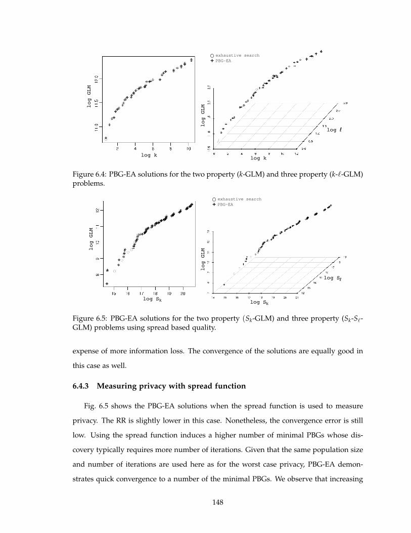
log k
log GLM
log GLM
log k
log ℓ
exhaustive search
PBG-EA+
Figure 6.4: PBG-EA solutions for the two property (k-GLM) and three property (k-ℓ-GLM)problems.
log S
log GLM
log GLM
exhaustive search
PBG-EA
k log Sk
log Sℓ
+
Figure 6.5: PBG-EA solutions for the two property (Sk-GLM) and three property (Sk-Sℓ-GLM) problems using spread based quality.
expense of more information loss. The convergence of the solutions are equally good in
this case as well.
6.4.3 Measuring privacy with spread function
Fig. 6.5 shows the PBG-EA solutions when the spread function is used to measure
privacy. The RR is slightly lower in this case. Nonetheless, the convergence error is still
low. Using the spread function induces a higher number of minimal PBGs whose dis-
covery typically requires more number of iterations. Given that the same population size
and number of iterations are used here as for the worst case privacy, PBG-EA demon-
strates quick convergence to a number of the minimal PBGs. We observe that increasing
148
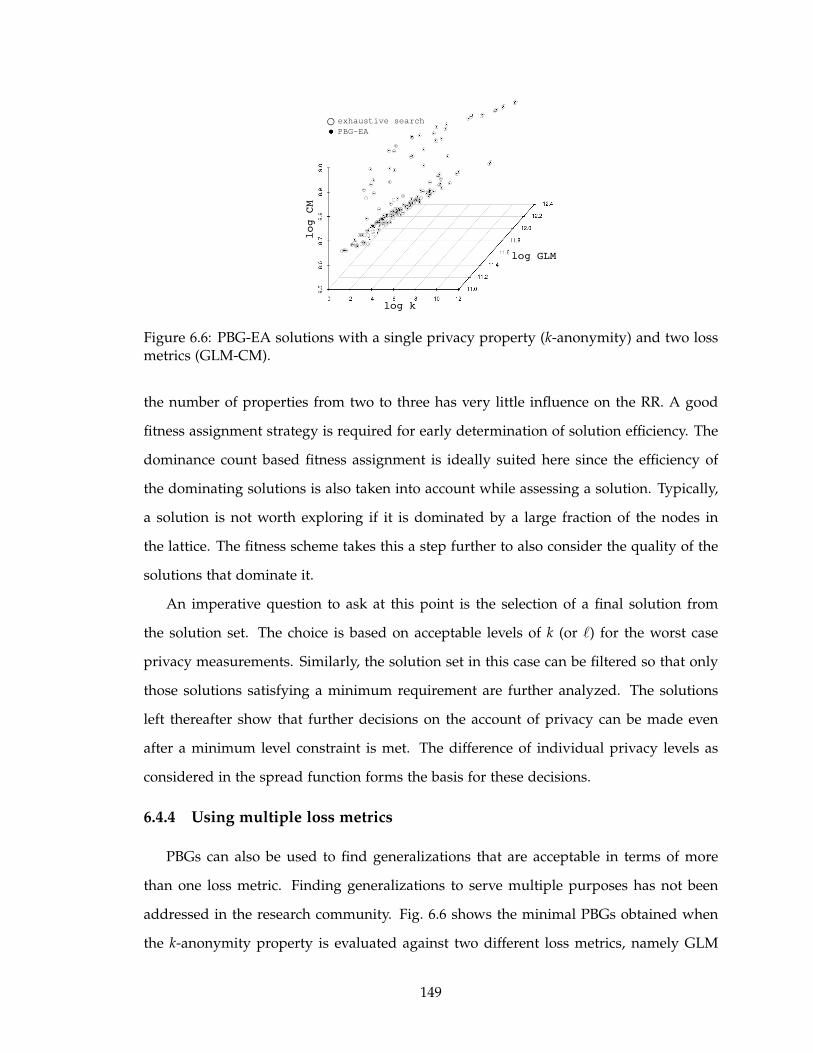
log k
log GLM
log CM
exhaustive search
PBG-EA
Figure 6.6: PBG-EA solutions with a single privacy property (k-anonymity) and two lossmetrics (GLM-CM).
the number of properties from two to three has very little influence on the RR. A good
fitness assignment strategy is required for early determination of solution efficiency. The
dominance count based fitness assignment is ideally suited here since the efficiency of
the dominating solutions is also taken into account while assessing a solution. Typically,
a solution is not worth exploring if it is dominated by a large fraction of the nodes in
the lattice. The fitness scheme takes this a step further to also consider the quality of the
solutions that dominate it.
An imperative question to ask at this point is the selection of a final solution from
the solution set. The choice is based on acceptable levels of k (or ℓ) for the worst case
privacy measurements. Similarly, the solution set in this case can be filtered so that only
those solutions satisfying a minimum requirement are further analyzed. The solutions
left thereafter show that further decisions on the account of privacy can be made even
after a minimum level constraint is met. The difference of individual privacy levels as
considered in the spread function forms the basis for these decisions.
6.4.4 Using multiple loss metrics
PBGs can also be used to find generalizations that are acceptable in terms of more
than one loss metric. Finding generalizations to serve multiple purposes has not been
addressed in the research community. Fig. 6.6 shows the minimal PBGs obtained when
the k-anonymity property is evaluated against two different loss metrics, namely GLM
149

Table 6.2: CE and RR values in PBG-EA anonymization with different discretization vec-tors.
ǫk ǫℓ ǫGLM CE RR
5 - 100 4.3×10⁻⁴
2.6×10−70.95
1.6×10⁻³
10 - 1000 1.6×10⁻⁴
8.0×10−80.98
8.2×10⁻⁴
50 - 10000 1.7×10⁻⁴
1.1×10−81.00.0
5 2 100 4.9×10⁻³
2.5×10−70.92
1.2×10⁻³
10 4 1000 7.4×10⁻³
9.3×10−70.92
7.0×10⁻⁴
50 6 10000 1.8×10⁻²
8.2×10−60.88
1.7×10⁻³
and CM. The heavily scattered points across the entire space signify the existence of re-
ciprocal relationships between GLM and CM. Ideally, for a given k value, the convention
is to choose the generalization with the lowest GLM. However, the multi-loss metric ex-
periment indicates that choosing a generalization with a comparatively higher GLM can
serve the dual purpose of making the anonymized data set also suitable for classification
tasks.
6.4.5 Efficiency in finding representative minimal PBGs
Although the set of minimal PBGs for the data set used in the study is not unbounded
in size, we experimented with several discretization vectors to demonstrate the efficiency
of PBG-EA in finding a representative subset. Table 6.2 shows the performance measures
for some vectors. The high representation ratio is indicative of the fact that PBG-EA so-
lutions cover most of the non-dominated boxes generated by the use of the discretization
vectors. For two property (k-GLM) anonymization, as higher ǫ values are used for the ob-
jectives, the efficiency of PBG-EA improves in terms of RR. However, using more number
of properties tend to slightly affect the performance owing mostly to the limited number
of iterations.
Fig. 6.7 shows a part of the boxed quality index space for ǫk = 5 and ǫGLM = 5000
in the range of k = 1 to 100. The archive in this case contains only one solution from
each non-dominated box. The representative solution set is characterized by the property
that, for any other solution, there is a solution in the archive whose k or GLM is within
a difference less than the corresponding discretized level. Choosing larger discretizations
150

k
GLM (x10000)
+
minimal PBG
PBG-EA solution
non-dominated box
Figure 6.7: Partial (k ∈ [1,100]) representative set of solutions for the two property (k-GLM) problem with ǫk = 5 and ǫGLM = 5000.
therefore mean a smaller representative subset. Choice of the vector to use is at the
discretion of the data publisher, determined by the number of solutions to analyze in the
first place.
6.4.6 Node evaluation efficiency
Efficiency of PBG-EA in converging quickly to a minimal PBG is evaluated by counting
the number of unique nodes that are evaluated by it during the search process. Although
the evolutionary algorithm can potentially explore 2500 (25 × 100) distinct nodes in the
lattice, a much smaller number is actually evaluated. Table 6.3 lists the average (out of the
20 runs) number of unique node evaluations performed for different problem instances.
We consider this low percentage of node evaluations to be a positive indication of the
convergence efficiency of PBG-EA. This is particularly promising since the entire set of
minimal PBGs (all one discretization vector) is found by exploring a small 5% of nodes in
the lattice. The nodes evaluated is slightly higher for three property problems. This is not
surprising since the number of minimal PBGs is also comparatively higher in such cases.
6.5 Conclusions
In this chapter, we have argued that the use of existing notions of a minimal gen-
eralization burdens a data publisher with the task of model parameter selection, quite
often without knowing its impact on the utility of the data. The task becomes further
151

Table 6.3: Average number of nodes evaluated in PBG-EA for different sets of properties.Total number of nodes in the first four sets is 17920 and that in the last set is 8960.
Objectives Avg. node evaluations
k, GLM 916 (5.1%)k,ℓ, GLM 946 (5.3%)Sk, GLM 1136 (6.3%)
Sk,Sℓ, GLM 1197 (6.7%)k, GLM, CM 1073 (11.9%)
complicated when the data publisher has to include multiple privacy models or account
for more than one possible data usage scenario.
In our approach, we propose identifying the basic properties that provide the req-
uisite protection from a privacy breach, and then measuring them for each underlying
individual. This generates a property vector for every generalization. Comparison of gen-
eralizations with respect to a single property is performed using quality index functions.
Apart from the conventional worst case measures of privacy, a binary index function is
presented which measures privacy using the variations in individual privacy levels. In
the presence of multiple properties, a dominance based partial order relationship is used
to define a property based generalization. Optimality in such generalizations is signi-
fied by non-dominated generalizations (minimal PBGs) under the dominance relation.
The objective of our approach is to gather a representative subset of generalizations that
demonstrate trade-offs in quality while trying to attain the different properties. The rep-
resentative subset is maintained by using a box-dominance operator which guarantees
that the solutions generated are optimal and the number of such solutions do not grow
unbounded in size. An evolutionary algorithm is suggested to explore the generalization
lattice and identify the optimal nodes. Application on a benchmark data set shows that
the algorithm can quickly discover a diverse set of minimal PBGs with a small number of
node evaluations.
Observations from our multi-loss experiment suggest that the problem of microdata
anonymization to serve multiple usages needs to be explored in more details. No study
has yet tried to understand the correlation between the multitude of loss metrics that exist
in the literature.
152
CHAPTER 7
Disclosures in a Continuous Location-Based Service
Technological advances in location tracking and its growing embedment in mobile
devices have opened up a new spectrum of on-demand services. These services deliver
customized information based on the location of a mobile object. A location-based service
(LBS) may simply provide information on the nearest gas station, perform targeted mar-
keting by location-based advertising, or enhance emergency response services, among
others. A mobile object can receive up-to-date and precise information by revealing its
location accurately to the LBS provider. The services are classified into two types based
on how frequently a mobile object communicates its location to the provider. The first
one is a snapshot LBS where the current location of the mobile object is sufficient to deliver
the service. For example, an emergency response service such as E-911 in North America
acquires the location of the caller to dispatch emergency services at the precise location.
The second one is a continuous LBS where the mobile object must periodically commu-
nicate its location as part of the service agreement. For example, a Pay-As-You-Drive
insurance service must receive location updates from the mobile object to bill the con-
sumer accurately. A real time friend finder service such as Loopt R© is another example in
this category.
Application domains are potentially endless with location-tracking technology. How-
ever, a serious concern surrounding their acceptance is the potential usage of the location
153
data to infer sensitive personal information about the mobile users. Privacy in location-
based services has been studied from two different perspectives – location anonymity and
query privacy. Location anonymity is related to the disclosure of exact locations that a
user has visited. This knowledge can in turn reveal personal lifestyles, places of frequent
visits, or even the medical problems of the involved user. With access to exact location
data, sender anonymity can be violated without the capability to track a mobile user. We
refer to this class of adversaries as location-unaware adversaries. Such adversaries use exter-
nal information to perform attacks resulting in restricted space identification, observation
identification and location tracking [77].
Query privacy is related to the disclosure of sensitive information in the query itself
and its association to a user. Consider a marketing agency such as CellFire R© that delivers
mobile coupons to users based on their location and category of interest. The retail part-
ners sponsoring such an agency are spread out across multiple categories, ranging from
apparels, groceries, automotives, entertainment, electronics to insurance, telecommuni-
cation, marketing and fitness. Each category in itself can be sub-divided; apparels, for
example, can be divided into men’s, women’s or children’s. Users therefore use service at-
tribute identifiers that specify their interest category. More often than not, a user’s service
attribute value is considered sensitive since it directly reveals personal preferences (or
requirements) of the user. Addressing the sensitivity is more important in a service like
GoogleTM Adwords that can perform location-based marketing on virtually any area of
interest. Query privacy is therefore an essential requirement. It has a more direct impact
on user privacy than location anonymity.
7.1 Protecting Privacy in a Continuous LBS
Location obfuscation is one of the widely researched approaches to safeguard location
anonymity. This technique guarantees that the location data received at the LBS provider
can be associated back to more than one object – to at least k objects under the location
k-anonymity model [77]. For this, a cloaking region is communicated to the service provider
instead of the actual location. A k-anonymous cloaking region contains at least k− 1 other
mobile objects besides the service user. However, this approach is not sufficient to pre-
154
serve privacy in a continuous LBS. In the continuous case, an object maintains an ongoing
session with the LBS, and successive cloaking regions may be correlated to associate the
session back to the object. Such session associations reveal the trajectory of the involved
object, and any sensitive information thereof. Cloaking regions may be susceptible to cor-
relation attacks due to their close proximity in time or movement restriction of objects in
those regions [188]. Assuring that every cloaking region contains k objects is not sufficient
since the absence of an object in one of the regions eliminates the possibility that it is the
session owner. Performing such elimination is much easier for a location-aware adversary
who has the capability to monitor users. This class of adversaries has exact location infor-
mation on one or more objects and uses it to eliminate possibilities and probabilistically
associate the session to consistently existing objects. It may seem that these attacks can
be avoided by using a different identifier for every cloaking region. However, location
data can still be correlated using techniques such as multi-target tracking [147]. Besides,
the provider needs to be able to distinguish updates from the same object in order to
maintain service quality [18].
Session association attacks can be avoided if it can be assured that every cloaking re-
gion in a session contains k common objects. This is referred to as historical k-anonymity
[20]. However, as a result of the movement of objects, a historically k-anonymous cloaking
region is very likely to grow in size over time, thereby deteriorating service quality. With-
out the proper strategies to control the size of the cloaking region, historical k-anonymity
is only a theoretical extension of k-anonymity for continuous LBS.
Preservation of query privacy in a LBS is similar to protection against attribute dis-
closures in data privacy. A typical principle used in this context is query ℓ-diversity [114].
A cloaking region conforming to query ℓ-diversity contains users with at least ℓ “well-
represented” service attribute values. One way of enforcing the principle is to ascertain
that there are users with at least ℓ distinct interest categories. Henceforth, any reference
to query ℓ-diversity implies this particular enforcement. Query ℓ-diversity ensures that
a user cannot be linked to less than ℓ distinct service attribute values, thereby prevent-
ing homogeneity attacks [120]. However, this approach is not sufficient to prevent query
disclosures in a continuous location-based service.
155
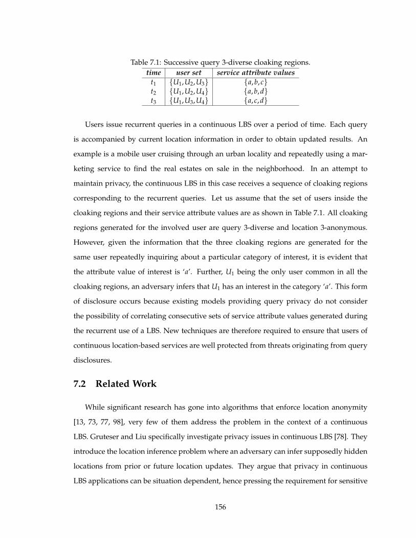
Table 7.1: Successive query 3-diverse cloaking regions.
time user set service attribute values
t1 {U1,U2,U3} {a,b, c}t2 {U1,U2,U4} {a,b,d}t3 {U1,U3,U4} {a, c,d}
Users issue recurrent queries in a continuous LBS over a period of time. Each query
is accompanied by current location information in order to obtain updated results. An
example is a mobile user cruising through an urban locality and repeatedly using a mar-
keting service to find the real estates on sale in the neighborhood. In an attempt to
maintain privacy, the continuous LBS in this case receives a sequence of cloaking regions
corresponding to the recurrent queries. Let us assume that the set of users inside the
cloaking regions and their service attribute values are as shown in Table 7.1. All cloaking
regions generated for the involved user are query 3-diverse and location 3-anonymous.
However, given the information that the three cloaking regions are generated for the
same user repeatedly inquiring about a particular category of interest, it is evident that
the attribute value of interest is ‘a’. Further, U1 being the only user common in all the
cloaking regions, an adversary infers that U1 has an interest in the category ‘a’. This form
of disclosure occurs because existing models providing query privacy do not consider
the possibility of correlating consecutive sets of service attribute values generated during
the recurrent use of a LBS. New techniques are therefore required to ensure that users of
continuous location-based services are well protected from threats originating from query
disclosures.
7.2 Related Work
While significant research has gone into algorithms that enforce location anonymity
[13, 73, 77, 98], very few of them address the problem in the context of a continuous
LBS. Gruteser and Liu specifically investigate privacy issues in continuous LBS [78]. They
introduce the location inference problem where an adversary can infer supposedly hidden
locations from prior or future location updates. They argue that privacy in continuous
LBS applications can be situation dependent, hence pressing the requirement for sensitive
156
and insensitive areas. Their base algorithm releases location updates only if an object is
in an insensitive area. Other variants try to preserve privacy by controlling the frequency
of updates. Hoh and Gruteser propose a perturbation algorithm to cross paths of objects
(by exchanging their pseudonyms) when they are close to each other [83]. However, the
approach does not safeguard against location-unaware adversaries as actual location data
is communicated to the LBS. Kido et al. use false dummies to simulate the movement
of mobile nodes in order to hide the trace of an actual object [99]. An object submits
k − 1 false locations along with the true one during an update. Such a technique fails
to guarantee privacy in the presence of location-aware adversaries. Xu and Cai propose
using historical traces of objects to derive a spatio-temporal cloaking region that provides
trajectory protection [189]. However, the approach requires that an object specifies its
entire path before using the service.
Bettini et al. introduce historical k-anonymity and propose a spatio-temporal general-
ization algorithm to enforce it [20]. The generalization algorithm enlarges the area and
time interval of the request to increase the uncertainty about the real location, and at the
same time include k common objects. The generalization is accepted only if the area and
time interval satisfy specified tolerance constraints. The method fails to account for mo-
bility of the objects, without which the generalized area can easily become larger than the
tolerance if it were to satisfy historical k-anonymity. Uninterrupted sessions will therefore
become very difficult.
Chow and Mokbel argue that spatial cloaking algorithms should satisfy the k-sharing
and memorization properties to be robust against session associations [39]. They focus on
a cloaking mechanism that allows users to specify different privacy levels for location
anonymity and query privacy. The two properties together imply historical k-anonymity.
Their algorithm maintains groups of objects based on the two properties, along with
query types involved with the objects. Unlike previous approaches, the method does not
have any tolerance to satisfy in terms of the cloaking region’s area. In fact, the cloaking
region in this case can be much larger since a group can include objects involved in a
number of different sessions. A query may also not be equally significant at all locations
occupied by a group’s members. Query privacy is preserved by ensuring that more than
157
one user in the cloaked region is interested in the same service attribute value as the
issuer. We later refer to this as many-to-one queries. Given the restriction that the cloaking
region must memorize and maintain a fixed set of users, the size of the induced cloaking
region becomes an issue with this technique.
Xu and Cai propose an information theoretic measure of anonymity for continuous
LBS [188]. They define a k-anonymity area as the cloaking region whose entropy is at
least k. Although not all k-anonymity areas are historically k-anonymous, their particular
implementation called plainKAA satisfies the property. However, the algorithm is prone
to inversion attacks where an adversary uses knowledge of the anonymizing algorithm to
breach privacy. The algorithm also fails when some objects stop using the service. The
authors propose modifications to plainKAA to resolve the issue of increasing cloaking
area, although that may no longer preserve historical k-anonymity.
The most recent of algorithms in this domain is ProvidentHider [124]. It uses a max-
imum perimeter constraint to ensure that cloaking regions are not too large, and the
starting set of objects is as big as possible (to take care of leaving objects). This algorithm
is later used in our comparative study.
Riboni et al. argue that an adversary may derive an association between a user and a
service attribute value based on the distribution of service attribute values in the cloaking
regions generated for the user [41]. Therefore, they propose generalizing service attribute
values so that the distance between the distribution of service attribute values in cloaking
regions for the user and that in regions generated for other users is below a threshold.
Besides the fact that generalizing service attributes adversely affects service quality, it is
also not clear if performing such generalizations can prevent disclosures emerging from
correlations in consecutive cloaking regions. The t-closeness model [112] on which their
algorithm is based upon is itself known to be sensitive to the distance metric.
The drawbacks present in the above algorithms point out three issues that must be
addressed before historical k-anonymity can be efficiently enforced, namely defunct peers,
diverging trajectories and locality of requests. Defunct peers are objects that become unavail-
able in time. As a result, any object dependent on a defunct peer to preserve historical
k-anonymity can no longer do so. Also, if objects in a historically k-anonymous cloaking
158

region diverge from each other, the cloaking region would finally become too large for
any reasonable service guarantee. Such divergence also allows an adversary infer crucial
associations between the mobile objects and the request. Our primary contribution is
therefore an anonymization algorithm, called Continuous ANONymizer (CANON), that
implements explicit strategies to resolve each of the three identified issues. In particular,
we argue that a cloaking region should be determined using direction information of the
objects and show how this restricts the inferences that can be made about the issuer of
the request. Large cloaking regions are also avoided by this process. Further, we propose
using multiple cloaking regions while issuing a query in order to maintain better service
quality.
This chapter also presents a formal analysis of privacy attacks leading to query dis-
closures in a continuous LBS. We explicitly characterize the privacy threats under consid-
eration and state the background knowledge required to execute the underlying attacks.
We model the attacks that can lead to query disclosures and formally show how a tech-
nique such as query ℓ-diversity fails to provide query privacy in a continuous LBS. While
the threats analyzed here are new in the context of location-based services, similar prob-
lems have been explored for privacy protection during the re-publication of dynamic
microdata. The principal of m-invariance [186] is of particular interest here because of
the similarity in privacy issues it helps resolve and those present in a continuous LBS.
m-Invariance infuses counterfeit entries into a data set so that a particular individual is
always associated with a fixed set of sensitive parameter values irrespective of the ad-
dition or deletion of entries. Drawing upon the privacy guarantees of m-invariance, we
formulate the principle of query m-invariance and show how it can be used to control the
amount of risk present in the use of a continuous LBS. We further propose a cloaking
algorithm to efficiently enforce the principle.
The remainder of the chapter is organized as follows. Section 7.3 presents the system
architecture and highlights the issues related to historical k-anonymity. The CANON al-
gorithm is presented next in Section 7.4. Section 7.5 presents results from an experimental
analysis using the algorithm. The issue of query privacy in a continuous LBS is discussed
next in Section 7.6. It presents the system architecture and highlights the requirement
159

for query m-invariance. A cloaking algorithm that preserves this privacy property is pre-
sented in Section 7.7. Section 7.8 details a comparison of this privacy model to location
k-anonymity and query ℓ-diversity. Finally, Section 7.9 concludes the chapter.
7.3 Location Anonymity in Continuous LBS
Research in database privacy has shown that formal evaluation of privacy attacks and
preservation techniques is difficult without explicitly stating the extent of an adversary’s
knowledge. Similar arguments have also been made in the context of privacy in snapshot
LBS [123]. A continuous LBS susceptible to location-unaware adversaries only can usu-
ally preserve privacy by implementing the conventional k-anonymity model. A mobile
object’s position can be concealed by using an arbitrary cloaking region instead of the
actual location. In the presence of location-aware adversaries only, exact object locations
can be sent to the LBS as long as there is a many-to-one mapping from mobile objects
to request identifiers. However, the snapshot k-anonymity model is not sufficient in this
case. New privacy preserving algorithms are needed that will protect against both types
of adversaries. We shall discuss our system architecture and then show how historical
k-anonymity is preserved in the presence of both types of adversaries.
7.3.1 System architecture
Our system consists of interactions between three layers – (i) mobile objects, (ii) a trusted
anonymity server, and (iii) a continuous LBS provider. Fig. 7.1 depicts a schematic of the
architecture. The trusted anonymity server acts as a channel for any communication be-
tween mobile objects and continuous LBS providers. All privacy guarantees are therefore
enforced at the trusted anonymity server. A mobile object O initiates a service session
by registering itself with the anonymity server. The registration process includes the
exchange of current location information (O.loc) and service parameters. The service pa-
rameters collectively signify the request to forward to the LBS provider, as well as the
anonymity level (O.k) to enforce while doing so. The anonymity server issues a pseudo-
identifier and uses it both as a session identifier (O.sid) with the mobile object and as an
object identifier when communicating with the LBS provider. A set of cloaking regions
160

continuous LBS provider
mobile objects
anonymizer
query processor
location
+
request
O.sid
suppressed
multiple cloaking regionsmultiple
range
queries
O.sid
candidate
result
set
filtered
result(s)
trusted anonymity server
Figure 7.1: Schematic of the system architecture.
is then generated for the requesting object and multiple range queries are issued to the
LBS provider for these regions. Communication between the anonymity server and the
LBS provider is always referenced using the object identifier so that the LBS can maintain
service continuity. The candidate results retrieved from the LBS provider are filtered at
the anonymity server and then communicated to the mobile object. Subsequent location
updates from the mobile object is handled in a similar fashion (with the pre-assigned
session identifier) until the anonymity level cannot be satisfied or the service session is
terminated. A request is suppressed (dropped) when the anonymity requirements can no
longer be met within the same service session. A new identifier is then used if the mobile
object re-issues the same request. Therefore, the number of consecutive requests served
with a single identifier serves as a metric to evaluate the efficiency of the anonymizing
algorithm. Higher values signify longer continuity, implying better quality of service. We
further assume that an object does not change its service parameters during a session. A
separate session is started if a request with different service parameters is to be made.
Therefore, an object can have multiple sessions running at the same time, each with a
different session identifier. Without any loss of generality, we assume that a mobile object
O has a single running session at most; identified by O.sid.
7.3.2 Historical k-anonymity
The primary purpose of a cloaking region is to make a given mobile object O indistin-
guishable from a set of other objects. This set of objects, including O, forms the anonymity
set of O. Objects in the anonymity set shall be referred to as peers of O and denoted
by O.peers. A cloaking region for O is usually characterized by the minimum bounding
161

rectangle (MBR) of the objects in O.peers. A range query is defined over such an MBR.
Therefore, the cloaking region is typically required to satisfy two properties in order to
achieve an acceptable balance between privacy and service quality.
• Sufficient anonymity: The degree of anonymity of a cloaking region is characterized
by the ambiguity introduced in differentiating one object from another with respect
to the actual issuer of the request. Under the conventional k-anonymity model, this
is achieved by ensuring that the anonymity set of a mobile object contains at least
k − 1 other objects. The value of k determines the level of privacy, and can either be
a user-specific or a system parameter.
• Sufficient quality: Since the result set of a range query caters to every mobile object
possibly present inside the cloaking region’s MBR, a bigger candidate set is more
likely for a larger MBR. Bigger candidate sets mean longer durations of time com-
municating the result with the anonymity server, longer computational overhead
filtering the results, as well as, possibly higher service costs owing to I/O over-
heads. Therefore, a smaller cloaking region is preferred over larger ones. This is
typically enforced by specifying a maximum spatial resolution as a constraint for
MBR sizes. In addition, a maximum temporal resolution can also be specified to de-
lay service requests so that smaller cloaking regions can be generated by watching
the location of moving objects over a longer duration of time.
As demonstrated in a number of prior works, achieving reasonable levels of anonymity
and service quality is not difficult in the case of a snapshot LBS. Since snapshot services
consider every request to be mutually independent, service quality does not depend on
the ability to correlate consecutive requests from the same mobile object. However, in our
assumed architecture for a continuous LBS, maintaining the two properties is significantly
difficult.
Consider the movement pattern of the objects depicted in Fig. 7.2. A 3-anonymous
MBR is computed for O1 during three consecutive location updates. If O1’s requests at
the three time instances are mutually independent from each other (as in a snapshot
LBS), then privacy level of O1 is maintained at 3-anonymity across the different MBRs.
162
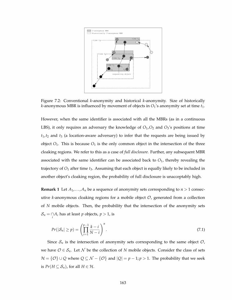
requesting object
time t1
time t2
time t3
3-anonymous MBR
Historically 3-anonymous MBR
O3
O1
O2
time t2
time t3
Figure 7.2: Conventional k-anonymity and historical k-anonymity. Size of historicallyk-anonymous MBR is influenced by movement of objects in O1’s anonymity set at time t1.
However, when the same identifier is associated with all the MBRs (as in a continuous
LBS), it only requires an adversary the knowledge of O1,O2 and O3’s positions at time
t1, t2 and t3 (a location-aware adversary) to infer that the requests are being issued by
object O1. This is because O1 is the only common object in the intersection of the three
cloaking regions. We refer to this as a case of full disclosure. Further, any subsequent MBR
associated with the same identifier can be associated back to O1, thereby revealing the
trajectory of O1 after time t3. Assuming that each object is equally likely to be included in
another object’s cloaking region, the probability of full disclosure is unacceptably high.
Remark 1 Let A1, . . . , An be a sequence of anonymity sets corresponding to n > 1 consec-
utive k-anonymous cloaking regions for a mobile object O, generated from a collection
of N mobile objects. Then, the probability that the intersection of the anonymity sets
Sn = ∩i
Ai has at least p objects, p > 1, is
Pr(|Sn| ≥ p) =
(
p−1
∏i=1
k − i
N − i
)n
. (7.1)
Since Sn is the intersection of anonymity sets corresponding to the same object O,
we have O ∈ Sn. Let N be the collection of N mobile objects. Consider the class of sets
H = {O} ∪ Q where Q ⊆ N − {O} and |Q| = p − 1; p > 1. The probability that we seek
is Pr(H ⊆ Sn), for all H ∈ H.
163

Consider a set Aj. We assume that each cloaking region minimally satisfies k-anonymity,
i.e. ∀j, |Aj| = k. Hence, Aj has k − 1 objects other than O. The number of ways such sets
can be formed is (N−1k−1 ). Further, the number of such sets that has H as a subset is
(N−pk−p ). Therefore, Pr(H ⊆ Aj) = (N−p
k−p )/(N−1k−1 ) = ∏
p−1i=1
k−iN−i . Also, for H ⊆ Sn, we have
∀j, H ⊆ Aj and which implies Sn has at least as many objects as in H, i.e. p. The proba-
bility Pr(|Sn| ≥ p) is therefore
Pr(∀H ∈ H,∀j, H ⊆ Aj) =
(
p−1
∏i=1
k − i
N − i
)n
. (7.2)
Remark 2 If k ≤ N+12 then the probability of full disclosure is at least 3
4 . The full disclosure
risk is given as D f ull = Pr(|Sn| = 1) = Pr(|Sn| ≥ 1) − Pr(|Sn| ≥ 2). Since intersection of
the anonymity sets contain at least one object, we have Pr(|Sn| ≥ 1) = 1. Hence, D f ull =
1 − ( k−1N−1)n. With k ≤ N+1
2 , or k−1N−1 ≤ 1
2 , we have
D f ull ≥ 1 − 1
2n≥ 1 − 1
22=
3
4. (7.3)
We also observe in Fig. 7.2 that it does not require knowledge on the objects’ locations
at all three time instances in order to breach O1’s privacy. In fact, location knowledge at
time instances t1 and t2 is sufficient to lower O1’s privacy to 2-anonymity. This is referred
to as a partial disclosure. Such disclosures occur when the intersection of anonymity sets
(corresponding to the same object) contains less than the desired number of peers (the
anonymity level k).
Remark 3 Although the likelihood of full disclosure reduces as k approaches N, partial
disclosures can still render an anonymization algorithm ineffective. Fig. 7.3 shows the
probability of partial disclosure for N = 100 and various anonymity levels. The partial
disclosure typically increases as k increases from (N + 1)/2. For the case when the ad-
versary’s location knowledge extends beyond two cloaking regions, the situation is much
worse as full disclosures are more likely for a larger range of anonymity levels.
A straightforward extension of the conventional k-anonymity model that can counter
risks of full and partial disclosures in a continuous LBS is to ensure that all anonymity sets
within a service session contain at least k common objects. In other words, k-anonymity
164

k
Probability of disclosure
n=2
n=5n=10
n=2
n=5n=10
full
partial
Figure 7.3: Risk of partial disclosure for varying anonymity levels k > (N + 1)/2. N = 100and n is the number of cloaking regions for which adversary has full location information.
should be satisfied on the intersection of anonymity sets, referred to as historical k-
anonymity.
Definition 7.1 HISTORICAL k–ANONYMITY. Let A1, . . . , An be a sequence of anonymity
sets corresponding to the cloaking regions with the same identifier and at time instants
t1, . . . , tn, ti > tj for i > j, respectively. The anonymity set Ai is then said to satisfy historical
k-anonymity if |A1 ∩ . . . ∩ Ai| ≥ k.
In other words, the sequence of anonymity sets preserve historical k-anonymity if all
subsequent sets after A1 contain at least k same objects from A1. Therefore, even an
adversary with complete location knowledge of all the mobile objects in all the cloaking
regions can not associate the object identifier to less than k objects. This prohibits both
cases of full and partial disclosures. Fig. 7.2 depicts how the cloaking regions should
change over time in order to ensure that object O1 always has historical 3-anonymity.
7.3.3 Implications
Since anonymity sets under historical k-anonymity also satisfy the conventional k-
anonymity model, privacy breaches involving restricted space identification, observation
identification and location tracking by location-unaware adversaries are implicitly im-
peded. In addition, historical k-anonymity also impedes session association attacks by
165

location-aware adversaries. Hence, the privacy guarantees of historical k-anonymity in
a continuous LBS is similar to that of k-anonymity in a snapshot LBS. However, main-
taining acceptable levels of service can become increasingly difficult in case of historical
k-anonymity. We have identified three issues for consideration that impact the practical
usage of historical k-anonymity.
(1) Defunct peers: A defunct peer in an anonymity set is an object that is no longer
registered with the anonymity server. As a result, it can no longer be ascertained that a
cloaking region includes the peer. If the first cloaking region generated during a particular
session contains exactly k objects, then every other anonymity set in that session must
contain the same k objects for it be historically k-anonymous. A defunct peer in this
case does not allow subsequent cloaking regions to satisfy historical k-anonymity and
introduces possibilities of partial disclosure. Such possibilities can be reduced either
by suppressing the requests that fail to meet historical k-anonymity, or by reducing the
impact of a defunct peer on the achievement of a desired anonymity level. The latter
is achieved in ProvidentHider by generating the first cloaking region to include as many
peers as possible within a MBR of fixed perimeter. It is expected that more than k objects
will get included in the first anonymity set, thereby providing some flexibility for peers
to defunct before influencing the minimum required anonymity set size. However, this
approach cannot account for the varying density of objects across time and space. A
highway, for example, can be very sparsely populated with cars during off-peak hours,
but can be heavily occupied during rush hour. Using a fixed perimeter can also lead to a
high percentage of suppressed requests where object distribution is relatively sparse.
(2) Diverging peer trajectories: The trajectories of peers influence the size of a cloaking
region (satisfying historical k-anonymity) over time. Refer to Fig. 7.2. The MBR for object
O1 becomes increasingly larger owing to the trajectory of object O3. Bigger cloaking
regions have a negative impact on service quality. In general, the more divergent the
trajectories are, the worse is the effect. Algorithms that use a maximum spatial resolution
will not be able to facilitate service continuity as spatial constraints will not be met. In
the worst case, trying to satisfy historical k-anonymity will unwantedly result in requests
being serviced on a snapshot basis.
166

(3) Locality of requests: The significance of a particular service request can often be
correlated with the locality where it originated. For instance, let us assume that the
region shown in Fig. 7.2 corresponds to a urban locality. Further, object O1 issues a
request to periodically update itself with information (availability, price, etc.) on the
nearest parking garage. At time instance t1, an adversary cannot infer which object (out
of O1,O2 and O3) is the actual issuer of the request. All objects in this case are in a locality
where the request holds equal significance. However, as O3 moves away from the urban
locality (suspiciously ignoring the high concentration of garages if it were the issuer), an
adversary can infer that the issuer of the request is more likely to be O1 or O2. We say
that these two objects are still in the locality of the request. If historical k-anonymity is
continued to be enforced, O3 (and most likely O2 as well) will be positioned in different
localities, thereby allowing an adversary infer with high confidence that O1 is the issuer
of the request. The significance of requests and the locality of peers can also help an
adversary infer a non-uniform distribution of request issuer likelihoods. Peers ought to
have some level of directional similarity in order to avoid such inferences.
Note that these three issues are primarily applicable in the context of a continuous
LBS, more specifically when working in conjunction with an anonymity server enforcing
historical k-anonymity. Defunct peers is not an issue in snapshot LBS since the set of
peers can be decided on a per request basis. Further, since the same peers need not be
present in subsequent anonymity sets, their trajectories do not influence the size of the
next privacy preserving cloaking region. Differences in locality also do not provide addi-
tional inferential power to an adversary. However, in a continuous LBS, these three issues
are direct residues of providing privacy by historical k-anonymity. Our attempt in this
work is to find an effective technique to enforce historical k-anonymity in a way that pro-
duces minimal impact on the service quality. The CANON (Continuous ANONymizer)
algorithm presented in the next section highlight the strategies adopted to do so.
7.4 The CANON Algorithm
CANON is an anonymization algorithm that enforces historical k-anonymity for use
with a continuous LBS. The algorithm defines explicit procedures to handle each of the
167

Procedure 7.1 CANON(Object O)
Input: Mobile object O (includes all associated data).Output: A set of peer groups (one of them includes O); null if request is suppressed
(cannot satisfy anonymity).1: if (O.sid = null) then
2: O.peers = CreatePeerSet(O)3: O.sid = new session identifier4: else
5: Remove defunct objects in O.peers6: end if
7: if (|O.peers| < O.k) then
8: O.sid = null
9: return null
10: end if
11: peerGroups = PartitionPeerSet(O)12: if (∃g ∈peerGroups such that |g| < 2) then
13: O.sid = null
14: return null
15: end if
16: return peerGroups
three potential issues identified in the previous section. An overview of the algorithm is
shown in Procedure 7.1.
CANON is initiated by the anonymity server whenever it receives a request from a
mobile object O. The algorithm starts by first checking if O has an open session with
respect to the current request. If it finds one then the set of peers is updated by removing
all defunct peers from the set. Otherwise, a peer set is generated for O through the proce-
dure CreatePeerSet and a session identifier is assigned. The newly generated (or updated)
peer set must have at least O.k objects in order to continue to the next step; otherwise
the request is suppressed and the session is terminated. Historical k-anonymity is en-
sured at the end of Line 10 since at least k objects inserted into O.peers by CreatePeerSet
is still registered with the anonymity server. The next step is to divide the peer set into
groups over which the range queries will be issued. A peer group is defined as a subset
of O.peers. PartitionPeerSet divides O.peers into disjoint peer groups. We shall often use
the term “object’s peer group” to signify the group that contains O. Each peer group
defines a smaller cloaking region than that defined by the entire peer set and reduces the
impact of diverging trajectories on service quality. The peer groups returned by CANON
168

MBR of peer set
O.sid=xyz
peer group
peer group
peer grouppeer group
xyz
xyz
xyz
continuous LBS provider
query processor
xyz
xyz
Figure 7.4: Peer set partitioning into groups over which multiple range queries are issuedwith the same identifier.
are used to issue multiple range queries (one for each) with the same object identifier.
Fig. 7.4 depicts this process. Line 12 checks that each peer group contains at least two
objects in order to avoid the disclosure of exact location information (of any object) to
location-unaware adversaries.
All object agglomerations, namely into peer sets and then into peer groups, are per-
formed so that the reciprocity property is satisfied. This property states that the inclusion
of any two objects in a peer set (group) is independent of the location of the object for
which the peer set (groups) is being formed. Reciprocity prevents inversion attacks where
knowledge of the underlying anonymizing algorithm can be used to identify the actual
object. The Hilbert Cloak algorithm [98] was first proposed in this context for the con-
ventional k-anonymity model. Hilbert Cloak orders the objects according to their Hilbert
indices (index on a space filling curve) and then groups them into buckets of size k. The
peer set of an object is the bucket that contains the object. The peer set is the same for
any object in the same bucket. CreatePeerSet and PartitionPeerSet thus use Hilbert-sorted
lists to incorporate these properties.
7.4.1 Handling defunct peers
As mentioned earlier, defunct peers can influence the lifetime of a service session
by reducing the peer set size to below the limit that satisfies historical k-anonymity. The
resolution is to include more than k objects in the first peer set. An indirect way to achieve
169

this is to specify a maximum spatial boundary around the requesting object’s location
and then include all objects within that boundary into the peer set. However, this method
suffers from object distribution problems as in ProvidentHider. It may be possible to adapt
the spatial boundary according to available traffic information. Even so, determining the
adjustments could be a difficult task. Using spatial boundaries also cannot account for the
relative differences in MBR sizes corresponding to varying anonymity requirements. For
example, an area of 1 km2 may be sufficient to have enough peers to satisfy a historical 2-
anonymity requirement, but may not be so to satisfy a stronger requirement (say historical
50-anonymity).
A more direct method to resolve the issue is to specify the desired peer set size ex-
plicitly. This removes any dependency on how the objects are distributed and the area
required to cover a reasonable number of them. We can specify the size as a sufficiently
big constant. However, this strategy favors objects with weaker anonymity requirements
as their peer sets are allowed a comparatively higher number of peers to defunct. For
instance, a constant peer set size of 20 would allow the anonymizer to tolerate up to 18
defunct peers to preserve historical 2-anonymity, but only 5 defuncts to preserve histor-
ical 15-anonymity. Therefore, the strategy adopted in CANON uses an oversize factor τ
that relatively specifies the number of extra peers that must be included in the peer set.
The minimum initial size of the peer set of an object O is equal to (1 + τ)×O.k with this
strategy. We say “minimum” because other parameters introduced later can allow more
peers to be included. Use of an oversize factor prevents the problem associated with con-
stant peer set sizes. Note that since CANON partitions the peer set into further groups
before issuing a query, the area of the cloaking region defined by the enlarged peer set
has little or no influence on service quality. However, we would still not want the area to
expand extensively in order to curb the issue of request locality.
7.4.2 Deciding a peer set
The CreatePeerSet procedure determines the initial peer set for an object. This is a
crucial step since anonymity for subsequent requests in the session will be evaluated on
the basis of the initial peer set. We have introduced the oversize factor to reduce the
170

chances of a peer set failing to meet anonymity requirements due to defunct peers. In
addition, we also need to ensure that majority of the objects in the peer set are in the
locality of the request. There are two requirements to address in this regard.
1. Objects in the peer set should define an area where the request is equally significant
to all the peers.
2. Objects in the peer set should move so that the defined area does not expand “too
much”.
The first requirement will prohibit the inclusion of peers that are positioned in a local-
ity where the issued request is unlikely to be made. The second requirement addresses
locality of requests in the dynamic scenario where the trajectories of the peers could be
such that they are positioned in very different localities over time. Preventing the MBR
of the peer set from expanding prohibits peers from being too far away from each other.
The first requirement can be fulfilled by choosing peers according to the Hilbert Cloak
algorithm. Peers chosen according to Hilbert indices will induce a small MBR, thereby en-
suring that they are more likely to be in the same locality. However, a peer set generated
by this process cannot guarantee that the second requirement will be fulfilled for long.
This is because the neighbors of an object (according to Hilbert index) may be moving in
very different directions.
It is clear from the above observation that the direction of travel of the objects should
be accounted for when selecting peers. The direction of travel is calculated as a vector
from the last known location of the object to its current location, i.e. if O.loc1 = (x1,y1)
and O.loc2 = (x2,y2) are the previously and currently known positions of O respectively,
then the direction of travel is given as O.dir = O.loc2 −O.loc1 = (x2 − x1,y2 − y1). O.dir
is set to (0,1) (north) for newly registered objects. A θ-neighborhood for O is then defined
as the set of all objects whose direction of travel is within an angular distance θ (say in
degrees) from O.dir. Therefore, a 0◦-neighborhood means objects traveling in the same
direction, while a 180◦-neighborhood contains all objects. If all peers are chosen within a
0◦-neighborhood then it is possible that the area defined by the initial peer set will more
or less remain constant over time. However, the initial area itself could be very large due
171

Procedure 7.2 CreatePeerSet(Object O)
Input: Mobile object O (includes all associated data), and system globals τ, θ and α f ull .Output: A set of peer objects (including O).
1: L = set of available mobile objects sorted by their Hilbert index2: ko f = (1 + τ) ×O.k; P = φ
3: repeat
4: Lc = φ
5: for all (l ∈ L in order) do
6: if (|Lc| ≥ ko f and AreaMBR(Lc ∪ {l})> α f ull) then
7: break
8: end if
9: Lc = Lc ∪ {l}10: end for
11: Pprev = P ; f = 1;Opivot = first object in Lc
12: repeat
13: P = ( f θ)-neighbors of Opivot in Lc
14: f = f + 115: until (|P| ≥ min(ko f , |Lc|))16: L = L−P17: until (O ∈ P)18: if (|P| < ko f ) then
19: P = P ∪ Pprev
20: else if (|L| < ko f ) then
21: P = P ∪ L22: end if
23: return P
to the non-availability of such peers within a close distance. On the other hand, using a
180◦-neighborhood essentially allows all objects to be considered and hence the area can
be kept small by including close objects. Of course, the area may increase unwantedly
over time. Peer set generation is therefore guided by two system parameters in CANON
- the neighborhood step size θ and the full-MBR resolution α f ull . The neighborhood step size
specifies the resolution at which the θ-neighborhood is incremented to include dissimilar
(in terms of travel direction) peers. The full-MBR resolution specifies some area within
which the issued request is equally likely to have originated from any of the included
objects, thereby making it difficult for an adversary to eliminate peers based on position
and request significance. For small values of θ and some α f ull , all objects in a peer set
would ideally move in a group, in and out of a locality. Procedure 7.2 outlines the pseudo-
code of CreatePeerSet. We assume the existence of a function AreaMBR that returns the
area of the minimum bounding rectangle of a set of objects.
172

CreatePeerSet first creates a sorted list L of all registered objects according to their
Hilbert indices. It then continues to divide them into buckets (starting from the first one
in the sorted list) until the one with O is found (Lines 3-17). Every time a bucket is
formed, L is updated by removing all objects in the bucket from the list (Line 16). Lines
5-10 determine a set Lc of candidate objects that can potentially form a bucket. Starting
from the first available object in L, we continue to include objects in Lc as long as the
minimum peer set size (denoted by ko f and decided by the oversize factor) is not met, or
the area of the MBR of included objects is within the full-MBR resolution. Note that, as a
result of this condition (Line 6), the minimum required size of the peer set receives more
prominence than the resulting area. Hence, the full-MBR resolution is only a guiding
parameter and not a constraint. Next, Lines 12-15 select ko f objects from the candidate
set to form a bucket. The first object in Lc is chosen as a pivot and all objects in the
θ-neighborhood of the pivot are included in the bucket. If the bucket is not full up to its
capacity (ko f ) and more objects are present in Lc, then the neighborhood is increased by
the step size θ. By the end of this process, the bucket would either contain ko f objects or
there are less than ko f objects in Lc. The latter is only possible when list L contains less
than ko f objects, i.e. the last bucket is being created. Note that object O is not explicitly
used anywhere to decide the buckets, thereby guaranteeing reciprocity. Once the bucket
with O is found, two more checks are required (Lines 18-22). First, if O’s bucket has less
than ko f objects (possible if it is the last one), then it is merged with the previous bucket.
Second, if the number of objects remaining in L is less than ko f (implying O’s bucket
is second to last), then the remaining objects are included into O’s bucket to maintain
reciprocity.
CreatePeerSet uses θ-neighborhoods and the full-MBR resolution to balance between
dissimilar peers and the resulting MBR area. While the step size θ allows incremental
selection of dissimilar peers, α f ull guides the extent of increment admissible to generate a
localized peer set. Note that the creation of a peer set is a one time procedure every service
session. Hence, a good estimation of the direction of travel is required to avoid diverging
trajectories. One possibility is to obtain destination points of objects and generate an
average direction of travel. An average direction can also be calculated based on the
173

displacement vector of the object from its starting position. One can also estimate a
direction of travel based on a set of last known locations. CANON uses an instantaneous
direction vector. We believe this method performs reasonably well in road networks,
although the efficacy of other techniques remains to be determined.
7.4.3 Handling a large MBR
The full-MBR resolution parameter is used to control breaches related to request lo-
calities. Typical values are in the range of 10 to 50 km2. The parameter is therefore
not intended to help generate cloaking regions with small MBRs. A continuous LBS
would require a much finer resolution to deliver any reasonable service. Further, de-
pending on variations in velocity and the underlying road network, some extent of ex-
pansion/contraction of the MBR is very likely. The MBR of a peer set is therefore not
a good candidate to issue the range queries. Instead, the peer set is partitioned into
multiple disjoint groups by PartitionPeerSet. Partitioning of the peer set eliminates empty
spaces between peers (introduced in the first place if trajectories diverge) and produces
smaller MBRs for the range queries [169]. This partitioning can be done either in a way
such that each peer group has a minimum number of objects or each peer group has a
maximum spatial resolution. The former approach cannot guarantee that the resulting
MBR will have an acceptable area. The latter method is adopted in CANON where the
maximum spatial resolution of a peer group is specified as the sub-MBR resolution αsub.
αsub is relatively much smaller than α f ull . Procedure 7.3 outlines the partitioning method.
The partitioning is performed in a manner similar to Hilbert Cloak, with the difference
that each bucket now induces an area of at most αsub instead of a fixed number of objects.
Starting from the first object in the Hilbert-sorted peer set, an object is added to a bucket as
long as the sub-MBR resolution is met (Line 6); otherwise the current bucket is a new peer
group (Line 8) and the next bucket is created (Line 9). Reciprocity is preserved as before.
Note that the pseudo-code in Procedure 7.3 does not handle the case when a peer group
contains only one object. Procedure 7.1 checks that such groups do not exist (safeguard
against location-unaware adversaries); otherwise the request is suppressed. However, the
partitioning algorithm itself can relax the sub-MBR resolution when a peer group with
174

Procedure 7.3 PartitionPeerSet(Object O)
Input: Mobile object O (includes all associated data) and system global αsub.Output: A set of peer groups.
1: Sort objects in O.peers by their Hilbert index2: peerGroups = φ
3: bucket = φ
4: for all (l ∈ O.peers in order) do
5: if (AreaMBR(bucket∪{l}) ≤ αsub) then
6: bucket = bucket∪{l}7: else
8: peerGroups = peerGroups ∪ {bucket}9: bucket = {l}
10: end if
11: end for
12: peerGroups = peerGroups ∪ {bucket}13: return peerGroups
a single object is found. One possible modification is to merge any peer group having a
single object with the group generated prior to it. Another parameter-less technique is to
create partitions that result in the minimum average peer group MBR with the constraint
that each group must have at least two objects. We have kept these possibilities for future
exploration.
7.5 Empirical Study
The experimental evaluation compares the performance of CANON with the Providen-
tHider algorithm. For every new request, ProvidentHider first groups all available objects
from a Hilbert-sorted list such that each bucket holds O.k objects; more if adding them
does not violate a maximum perimeter (Pmax) constraint. The peer set of an object is the
bucket that contains the object. A range query is issued over the area covered by the
objects in the peer set only if the maximum perimeter constraint is satisfied; otherwise
the request is suppressed. As the peers move, the assigned peer set is partitioned as
before and the bucket containing the issuing object is assigned as the new peer set. The
new peer set must satisfy the perimeter constraint, as well as have at least O.k objects.
ProvidentHider also differentiates between objects based on their location. We assume that
all objects are in the visible domain with respect to such differentiation. We measure a
number of statistics to evaluate the performance.
175

Figure 7.5: Trace data generated on Chamblee region of Georgia, USA. The mean speed,standard deviation and traffic volume on the three road types used are shown.
• service continuity: average number of requests served in a session.
• service failures: percentage of suppressed requests.
• safeguard against location-unaware adversaries: average size of the peer group to which
the issuing object belongs.
• request localization: average factor of increase in MBR area of an object’s first peer
set.
7.5.1 Experimental setup
We have generated trace data using a simulator [73] that operates multiple mobile ob-
jects based on real-world road network information available from the National Mapping
Division of the US Geological Survey. We have used an area of approximately 168 km2
in the Chamblee region of Georgia, USA for this study (Fig. 7.5). Three road types are
identified based on the available data – expressway, arterial and collector. Real traffic vol-
ume data is used to determine the number of objects in the different road types [77]. The
total number of objects on a road type vary proportionate to the total length and traffic
volume of the road type, and reciprocally to the average speed of the objects. The mean
176
speed, standard deviation and traffic volumes on the road types are shown in the figure.
Using the number of objects on each road type, the simulator randomly places them on
the network and moves them around. The objects move with a speed drawn from a nor-
mal distribution, randomly making turns and changing speed at junctions. The simulator
maintains the traffic volume statistics while moving the objects.
The used traffic volume information results in 8,558 objects with 34% on expressways,
8% on arterial roads and 58% on collector roads. The trace data consists of multiple
records spanning one hour of simulated time. A record is made up of a time stamp,
object number, x and y co-ordinates of object’s location, and a status indicator. The status
indicator signifies if the object is registered at the anonymity server. An object’s status
starts off randomly as being active or inactive. The object remains in the status for a time
period drawn from a normal distribution with mean 10 minutes and standard deviation
5 minutes. The status is randomly reset at the end of the period and a new time period
is assigned. The granularity of the data is maintained such that the Euclidean distance
between successive locations of the same object is approximately 100 meters. Each object
has an associated k value drawn from the range [2,50] by using a Zipf distribution favor-
ing higher values and with the exponent 0.6. The trace data is sorted by the time stamp
of records.
During evaluation, the first minute of records is used only for initialization. Subse-
quently, the status of each record is used to determine if the object issues a request. Only
an active object is considered for anonymization. If the object was previously inactive or
its prior request was suppressed, then it is assumed that a new request has been issued.
Otherwise, the object is continuing a service session. The anonymizer is then called to
determine the cloaking region(s), if possible. The process continues until the object enters
an inactive (defunct) state. Over 2,000,000 anonymization requests are generated during
a pass of the entire trace data.
Default values of other algorithm parameters are set as follows: τ = 0.0, α f ull = 25 km2,
αsub = 1 km2, θ = 180◦ and Pmax = 5000 m. All parameters take their default values unless
stated otherwise. A 5000 m perimeter constraint for ProvidentHider is approximately an
area of 1.6 km2. Compared to that, αsub has a smaller default value. The precision is
177

around 1000 m (assuming a square area) which serves reasonably well for a Pay-As-You-
Drive insurance service. We also study how CANON performs for services that require a
higher precision. The full-MBR resolution of 25 km2 evaluates to a locality about 132
ththe
size of New York City. The entire map is assumed to be on a grid of 214 × 214 cells (a cell
at every meter) while calculating the Hilbert indices [116]. Objects in the same cell have
the same Hilbert index.
7.5.2 Comparative performance
Fig. 7.6a shows the average number of requests served in a session for different
anonymity requirements. ProvidentHider demonstrates poor performance for higher k
values, almost to the extent of one request per session. Comparatively, CANON main-
tains much better service continuity. As mentioned earlier, using a fixed area for varying
anonymity requirements makes it difficult for ProvidentHider to keep the peer set within
the required size. The task is much difficult for bigger peer sets as the algorithm does not
consider the issue of diverging trajectories. In fact, a high percentage of the requests is
suppressed for higher values of k (Fig. 7.6b). CANON’s performance also seems to fluctu-
ate depending on the oversize factor. In general, a maximum peer set size slightly larger
than the minimum required (for example τ = 0.25) gives the best performance, while any
further increase degrades it. While a few extra peers is useful to handle defunct peers,
having a much larger peer set implies having objects over a larger area and often far away
from each other (over time). Therefore, it is possible that some peer groups are formed
with a single object owing to the sub-MBR constraint. Requests are then suppressed in
the absence of a strategy to handle such peer groups. This is also corroborated by the
similar trend in request suppression.
Fig. 7.6c shows the average size of the peer group to which the requesting object
belonged. Bigger sizes imply more ambiguity for a location-unaware adversary while
trying to identify the actual object. While the sizes are larger for higher k (implying that
safeguard against location-unaware adversaries scale as more safeguard against location-
aware adversaries is desired), there does not seem to be any observable trend due to
changes in the oversize factor.
178
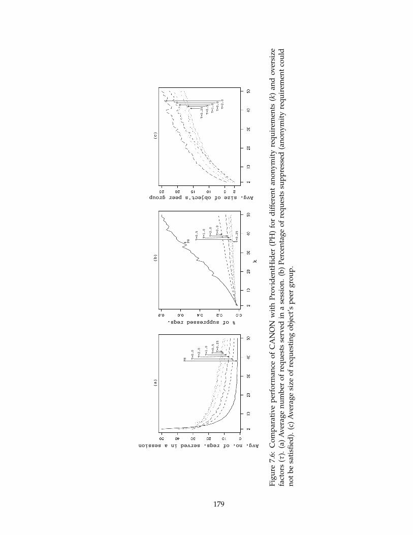
Avg. no. of reqs. served in a session
% of suppressed reqs.
Avg. size of object's peer group
k
τ=0.25
τ=0.5
τ=1.0
τ=2.0
τ=0.0
PH
τ=0.0
τ=2.0
τ=1.0
τ=0.5
τ=0.25
PH
τ=0.25
τ=0.5
τ=1.0
τ=0.0
τ=2.0
(a) (b) (c)
Fig
ure
7.6:
Co
mp
arat
ive
per
form
ance
of
CA
NO
Nw
ith
Pro
vid
entH
ider
(PH
)fo
rd
iffe
ren
tan
on
ym
ity
req
uir
emen
ts(k
)an
do
ver
size
fact
ors
(τ).
(a)
Av
erag
en
um
ber
of
req
ues
tsse
rved
ina
sess
ion
.(b
)P
erce
nta
ge
of
req
ues
tssu
pp
ress
ed(a
no
ny
mit
yre
qu
irem
ent
cou
ldn
ot
be
sati
sfied
).(c
)A
ver
age
size
of
req
ues
tin
go
bje
ct’s
pee
rg
rou
p.
179

7.5.3 Impact of parameters
Each parameter in CANON is intended to address a specific issue with the use of
historical k-anonymity. We perform some parametric studies to demonstrate the con-
sequences of varying these parameters. The neighborhood step size is varied between
1◦ and 180◦, and performance is observed for three different settings of the sub-MBR
(αsub = 0.25,1.0 and 4 km2) and full-MBR (α f ull = 10,25 and 50 km2) resolutions. Note
that increasing/decreasing the full-MBR resolution will have no impact on peer sets if
the required number of objects is always present within a small area. Hence, studies on
α f ull with θ = 180◦ produces same results. We therefore use a neighborhood step size
of 15◦ while observing the impact of α f ull . Having a small θ forces CANON to consider
more similar/dissimilar peers depending on whether we have a large/small α f ull . All
parameters other than the ones mentioned take their default values.
7.5.3.1 Neighborhood step size θ
Performance in terms of service continuity does not differ a lot for varying step size
(Fig. 7.7a). Some differences are observed for lower ranges of k (2 − 15) where larger step
sizes show a better performance. Differences are more prominent in terms of peer group
size where a bigger neighborhood improves the safeguard against location-unaware ad-
versaries (Fig. 7.7b). This behavior is expected since bigger neighborhood sizes allow
the inclusion of more dissimilar peers, thereby inducing bigger peer groups due to the
possibly close proximity of objects. The statistic of interest is the size of the MBR area
defined by the objects in the peer set. Fig. 7.7c indicates that this area remains almost con-
stant for the smaller step sizes, specifically for the more frequently requested anonymity
levels (higher k), implying that the objects in a peer set move together as a group. We
are not concerned about the high increase in area for lower k values (2 − 15) because the
initial area defined by the peer sets in this range is not too large to begin. We believe
the instantaneous calculation of direction vectors impact performance in this range. The
area increases by more than two folds (across different anonymity requirements) when
direction of travel is ignored (θ = 180◦), while it is contained within a two factor increase
for the other experimented values. For the sake of perception, a four times increase in
180
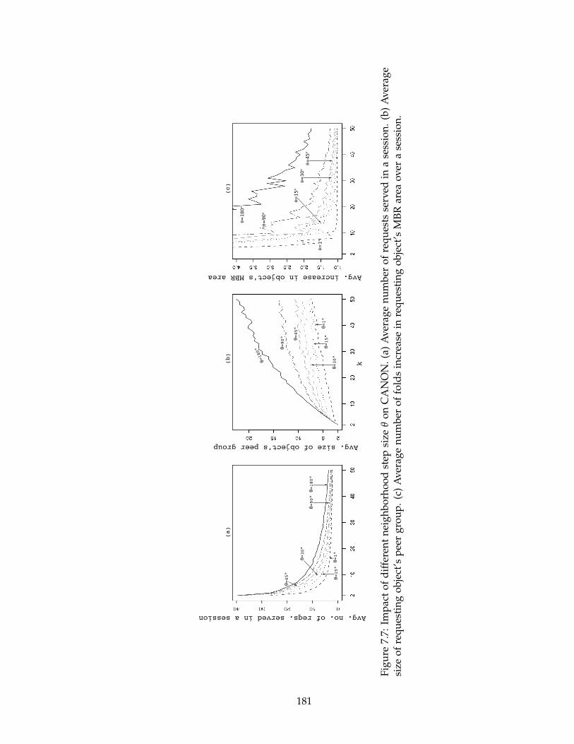
Avg. no. of reqs. served in a session
Avg. size of object's peer group
Avg. increase in object's MBR area
θ=1°
θ=15°
θ=180°
θ=90°
θ=30°
θ=45°
k
θ=180° θ=90° θ=45°
θ=30°
θ=15°
θ=1°
θ=180
°
θ=90
°
θ=1
°
θ=45
°
θ=15
°
θ=30
°
(a) (b) (c)
Fig
ure
7.7:
Imp
act
of
dif
fere
nt
nei
gh
bo
rho
od
step
size
θo
nC
AN
ON
.(a
)A
ver
age
nu
mb
ero
fre
qu
ests
serv
edin
ase
ssio
n.
(b)
Av
erag
esi
zeo
fre
qu
esti
ng
ob
ject
’sp
eer
gro
up
.(c
)A
ver
age
nu
mb
ero
ffo
lds
incr
ease
inre
qu
esti
ng
ob
ject
’sM
BR
area
ov
era
sess
ion
.
181

the area of a square doubles the distance between diagonally opposite points. Therefore,
most peers can be maintained in the locality of the request by using θ-neighborhoods.
Even a step size of 90◦ provides considerable benefits in this regard without severely
affecting the other performance measures.
7.5.3.2 Sub-MBR resolution αsub
Smaller sub-MBR resolutions mean higher precision in the range queries. However,
they also mean higher chances of smaller peer groups, often ones with a single object.
With reference to Fig. 7.8 (top row), a smaller αsub results in a higher rate of failures,
inducing shorter service sessions. Services requiring high location precision will therefore
fail to provide longer service continuity. An object’s peer group size is also comparatively
smaller. Improvements in service continuity is more prominent for weaker anonymity
requirements as αsub is increased. However, improvements in peer group size is more
noticeable in higher k values. In effect, finding a suitably balanced αsub can help achieve
good overall performance. αsub is decided by the service requirements in most cases.
Nonetheless, depending on how stringent the requirement is, both privacy (from location-
unaware adversaries) and service quality may have scope for improvement.
7.5.3.3 Full-MBR resolution α f ull
The full-MBR resolution is observed to have little or no influence on the average num-
ber of requests served in a session (Fig. 7.8 bottom row). However, larger areas tend to
have higher percentage of failures. A possible explanation is as follows. A larger area
with a small step size means similar objects are preferred over the proximity of objects.
As a result, a peer set includes objects distributed far apart. This leads to the suppression
of requests when the sub-MBR constraint is imposed on the formation of peer groups.
Objects far apart cannot be grouped without violating the constraint. This also results
in a comparatively smaller peer group size. On the other hand, a smaller area allows
inclusion of close proximity objects at the expense of similarity. The sub-MBR constraint
is therefore easier to meet and suppression rate is lower.
182
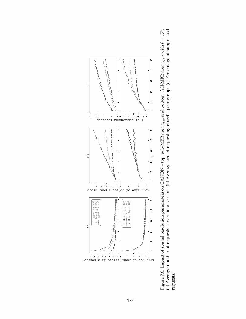
Avg. size of object's peer group
Avg. no. of reqs. served in a session
k
% of suppressed requests
α =0.25 km
sub
2
α =1.00 km
sub
2
α =4.00 km
sub
2
(a) (b) (c)
α =10.0 km
full
2
α =25.0 km
full
2
α =50.0 km
full
2
Fig
ure
7.8:
Imp
act
of
spat
ial
reso
luti
on
par
amet
ers
on
CA
NO
N–
top
:su
b-M
BR
area
αsu
ban
db
ott
om
:fu
ll-M
BR
area
αfu
llw
ith
θ=
15◦ .
(a)
Av
erag
en
um
ber
of
req
ues
tsse
rved
ina
sess
ion
.(b
)A
ver
age
size
of
req
ues
tin
go
bje
ct’s
pee
rg
rou
p.
(c)
Per
cen
tag
eo
fsu
pp
ress
edre
qu
ests
.
183
7.5.4 Summary
The following points summarize the results from the experimental study.
• CANON has a superior performance compared to ProvidentHider in maintaining
longer service sessions across a wide range of anonymity requirements. More re-
quests are also successfully anonymized by CANON.
• Including a small number of extra objects in a peer set is advantageous in handling
defunct peers. However, extremely large peer sets can be detrimental.
• Use of direction information during the formation of a peer set does help avoid
peers drifting away from each other over time. Choice of a too small neighborhood
affects service quality, but is not necessary to balance performance across different
measures.
• Performance is better with larger sub-MBR resolutions. However, performance in
high precision services may be improved with a good strategy to relax the con-
straint.
• Service continuity is marginally different for different full-MBR resolutions. How-
ever, failure to serve new requests is much lower with smaller resolutions.
7.6 Preventing Query Disclosures
No single privacy model can yet prevent all underlying threats. Hence, the types
of privacy attacks considered under an adversary model should also be explicitly men-
tioned. Earlier studies have identified two attack categories – identity inferencing (associ-
ation of a user with the location(s) it has visited) and query association (inference of the
sensitive attribute(s) involved in a user’s request). The extent of success while execut-
ing attacks in these categories is decided by the adversary’s background knowledge. In
this study, we assume that the adversary’s background knowledge is in terms of location
information of one or more users. Note that the background knowledge can also be in
terms of query parameters. Such forms of knowledge enable an adversary to eliminate
possibilities in query association attacks.
184

Location-unaware adversaries do not posses knowledge of exact user locations. How-
ever, identity inferencing by such adversaries is possible when the revealed location data
corresponds to a private address (restricted space identification) or can be associated to a
user based on observed evidence (observation identification). If the location data is from
a continuous LBS, then trajectories can also be linked to a user. Location k-anonymity
prevents such inferencing by cloaking the exact location data inside a bounding box con-
taining at least k users. Query association is the next step of identity inferencing where
an adversary tries to determine what service attributes are interesting to an identified
user. However, a k-anonymous cloaking region can implicitly reveal service attributes if
all users in it specify the same (or similar) values. Query ℓ-diversity prevents such attacks
by ensuring that a cloaking region contains users with at least ℓ distinct attribute values.
On the other hand, a location-aware adversary has exact location information on one
or more users, and possibly at multiple time instances. User identities are therefore
assumed to be known to the adversary. Hence, exact location data may be communicated
to the LBS. However, location-aware adversaries cannot infer service attributes from the
location knowledge as long as every location communicated to the LBS is query ℓ-diverse.
In other words, a service request should involve a set of ℓ distinct attribute values (one of
which is the real one) for every location update. Note that one cannot dismiss the absence
of location-unaware adversaries in a given setting. Hence, cloaking regions are still used
instead of exact locations.
A continuous LBS introduces other threats in the presence of location-aware adver-
saries. A continuous LBS allows an adversary to obtain the successive cloaking regions of
a particular user. Given that both types of adversaries may be present, a LBS may adopt
one of the following two methods to prevent query association.
• Many-to-one queries: In this method, a k-anonymous cloaking region communicated
to the LBS is associated with a single service attribute (the one belonging to the
actual user). Therefore, there are at least k potential users who may be the owner of
the service attribute. However, if only one user is common across all the cloaking
regions, then the attribute value must be associated with that user.
185
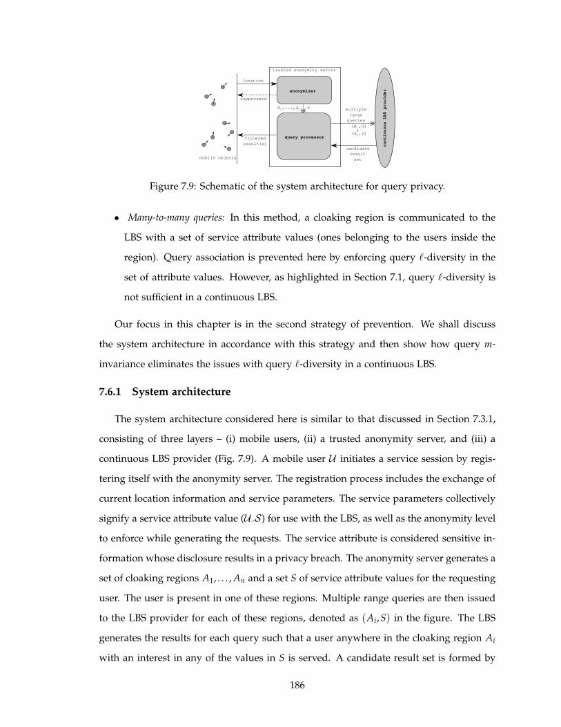
continuous LBS provider
mobile objects
anonymizer
query processor
location
suppressed
A ,...,A multiple
range
queries
candidate
result
set
filtered
result(s)
trusted anonymity server
S1 n
(A ,S)1
(A ,S)n
Figure 7.9: Schematic of the system architecture for query privacy.
• Many-to-many queries: In this method, a cloaking region is communicated to the
LBS with a set of service attribute values (ones belonging to the users inside the
region). Query association is prevented here by enforcing query ℓ-diversity in the
set of attribute values. However, as highlighted in Section 7.1, query ℓ-diversity is
not sufficient in a continuous LBS.
Our focus in this chapter is in the second strategy of prevention. We shall discuss
the system architecture in accordance with this strategy and then show how query m-
invariance eliminates the issues with query ℓ-diversity in a continuous LBS.
7.6.1 System architecture
The system architecture considered here is similar to that discussed in Section 7.3.1,
consisting of three layers – (i) mobile users, (ii) a trusted anonymity server, and (iii) a
continuous LBS provider (Fig. 7.9). A mobile user U initiates a service session by regis-
tering itself with the anonymity server. The registration process includes the exchange of
current location information and service parameters. The service parameters collectively
signify a service attribute value (U .S) for use with the LBS, as well as the anonymity level
to enforce while generating the requests. The service attribute is considered sensitive in-
formation whose disclosure results in a privacy breach. The anonymity server generates a
set of cloaking regions A1, . . . , An and a set S of service attribute values for the requesting
user. The user is present in one of these regions. Multiple range queries are then issued
to the LBS provider for each of these regions, denoted as (Ai,S) in the figure. The LBS
generates the results for each query such that a user anywhere in the cloaking region Ai
with an interest in any of the values in S is served. A candidate result set is formed by
186
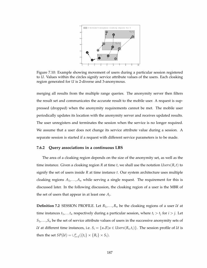
R ,t1
2-diverse/3-anonymous cloaking regions for U
c
a
b
a
a
b
b
d
d
a
a
a
1
R ,t22
R ,t33
U
1 2 3 4 5 6 7 8 9 10
1
2
3
4
5
6
7
Figure 7.10: Example showing movement of users during a particular session registeredto U. Values within the circles signify service attribute values of the users. Each cloakingregion generated for U is 2-diverse and 3-anonymous.
merging all results from the multiple range queries. The anonymity server then filters
the result set and communicates the accurate result to the mobile user. A request is sup-
pressed (dropped) when the anonymity requirements cannot be met. The mobile user
periodically updates its location with the anonymity server and receives updated results.
The user unregisters and terminates the session when the service is no longer required.
We assume that a user does not change its service attribute value during a session. A
separate session is started if a request with different service parameters is to be made.
7.6.2 Query associations in a continuous LBS
The area of a cloaking region depends on the size of the anonymity set, as well as the
time instance. Given a cloaking region R at time t, we shall use the notation Users(R, t) to
signify the set of users inside R at time instance t. Our system architecture uses multiple
cloaking regions A1, . . . , An while serving a single request. The requirement for this is
discussed later. In the following discussion, the cloaking region of a user is the MBR of
the set of users that appear in at least one Ai.
Definition 7.2 SESSION PROFILE. Let R1, . . . , Rn be the cloaking regions of a user U at
time instances t1, . . . tn respectively during a particular session, where ti > tj for i > j. Let
S1, . . . ,Sn be the set of service attribute values of users in the successive anonymity sets of
U at different time instances, i.e. Si = {u.S|u ∈ Users(Ri, ti)}. The session profile of U is
then the set SP(U ) = ∪ni=1({ti} × {Ri} × Si).
187

Table 7.2: Session profile SP(U) and background knowledge BK(U) used during a queryassociation attack on U.
t R S1 t1 R1 a2 t1 R1 b3 t1 R1 c4 t2 R2 a5 t2 R2 b6 t3 R3 a7 t3 R3 b
(a) SP(U)
t x y u
1 t1 5.1 2.3 Alice2 t1 6.4 1.8 Bob3 t2 5.8 3.6 Alice4 t2 6.9 3.5 Bob5 t3 5.9 5.8 Alice6 t3 9.2 5.5 Bob
(b) BK(U)
An entry in a session profile is therefore of the form 〈t,R,S〉. For an e ∈ SP(U ), we
shall use e.t, e.R and e.S to denote the corresponding terms. We shall also refer to U as
the owner of the session profile. Consider the movement of the users shown in Fig. 7.10.
Let us assume that a session for U lasted for three time stamps t1, t2 and t3, during which
the 2-diverse cloaking regions R1, R2 and R3 are generated. Note that users other than
U may terminate their session while U’s session is in progress. As a result, their service
attribute value may change during U’s session. Table 7.2a lists the session profile of U
w.r.t. this session.
Ideally, no knowledge on the owner of the session is required to form a session profile.
A continuous LBS can improve service quality if successive requests from the same user
can be distinguished from others [18]. Hence, the anonymity server typically maintains
some session identifier with the continuous LBS. All cloaking regions with the same
identifier belong to the same user. This information, along with the request logs (time
stamp and attribute values) accumulated at the LBS, is sufficient to build the session
profile. The objective is to accurately associate a service attribute value to the owner
of the profile. Note that, under a location-aware adversary model, identification of the
owner of the profile implies a successful query association only when the anonymity
server uses the many-to-one system of querying the LBS. In a many-to-many system, the
adversary will still have to associate one of the many attribute values to the owner. Next,
we formally state the background knowledge of the location-aware adversary that can be
used to link the owner to its service attribute value.
188
Definition 7.3 BACKGROUND KNOWLEDGE. The background knowledge of an adver-
sary is a set BK of tuples of the form 〈t, x,y,u〉 which implies that the user u is known to
have been at the location (x,y) at time instance t.
We shall only consider a subset of the background knowledge possessed by an ad-
versary. This subset corresponds to the information that is relevant to perform a query
association along with the data in a session profile. Given a session profile SP(U ), the
background knowledge corresponding to the session is given as BK(U ) = {b ∈ BK|i ∈{1, . . . ,n},b.u ∈ ∩
iUsers(Ri, ti),b.t = ti}. We make the worst case assumption that the ad-
versary is aware of the location of every user present in the cloaking regions of U at all
time instances when the queries are issued. In other words, for every ti when a query
is issued, there exists | ∩i
Users(Ri, ti)| entries in BK(U ). These entries correspond to the
users that are present in all the cloaking regions generated during a session, and can
potentially be the owner of the session. Table 7.2b lists the background knowledge used
for U. The cloaking regions contain two potential owners, complete location information
on whom is listed in BK(U). Background knowledge associates users to locations while
a session profile associates locations to service attribute values. The adversary relates the
location data in BK(U ) and SP(U ) to link users to attribute values. We call this a query
association attack.
Definition 7.4 QUERY ASSOCIATION ATTACK. Given a session profile SP(U ) and the
background knowledge BK(U ), a query association attack on user U is a mapping f :
BK(U ) → SP(U ) such that
1. every b ∈ BK(U ) is mapped to exactly one e ∈ SP(U ),
2. every b ∈ BK(U ) with f (b) = e satisfies
(a) (b.x,b.y) is inside e.R
(b) b.t = e.t
(c) for all b′ ∈ {bo ∈ BK(U )|bo.u = b.u}, f (b′).S = e.S .
The first condition states that a user can be associated with only one attribute value
in a given time instance. The second condition prohibits the adversary from arbitrarily
189
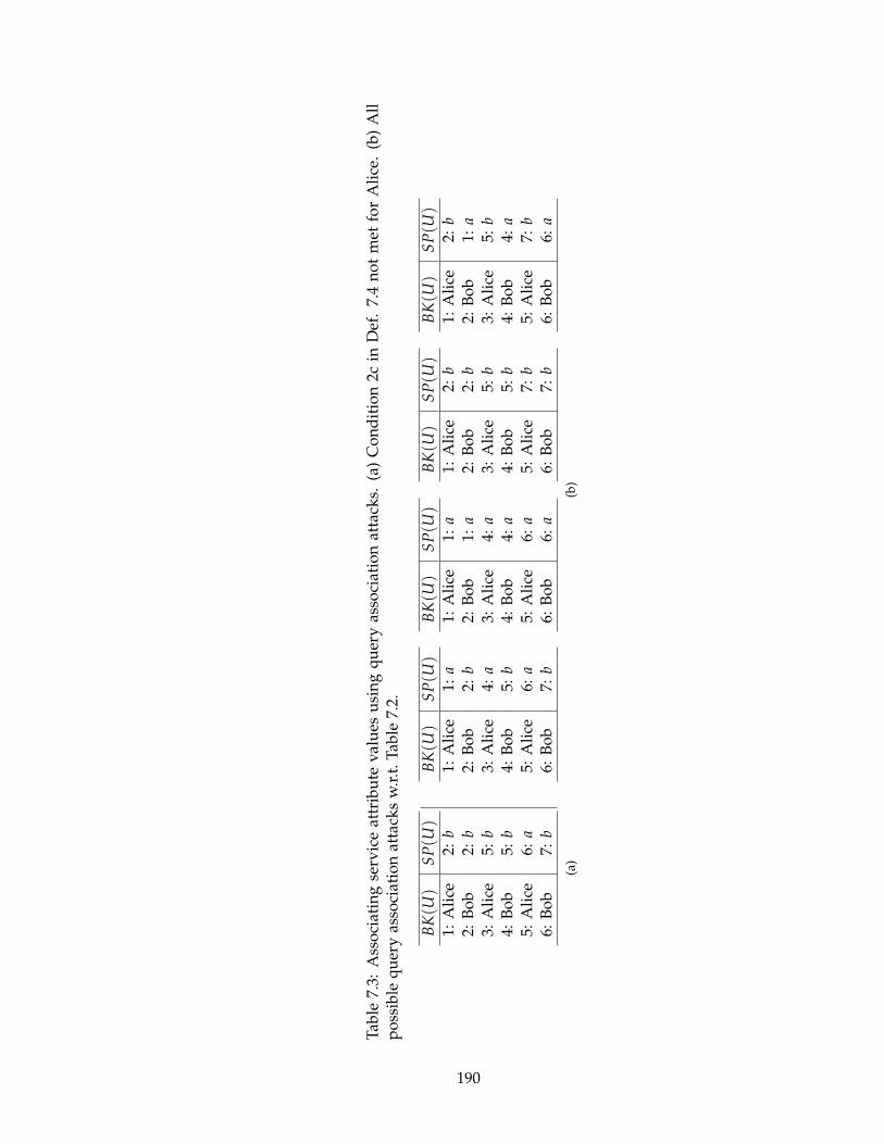
Tab
le7.
3:A
sso
ciat
ing
serv
ice
attr
ibu
tev
alu
esu
sin
gq
uer
yas
soci
atio
nat
tack
s.(a
)C
on
dit
ion
2cin
Def
.7.
4n
ot
met
for
Ali
ce.
(b)
All
po
ssib
leq
uer
yas
soci
atio
nat
tack
sw
.r.t
.T
able
7.2.
BK
(U)
SP(U
)1:
Ali
ce2:
b2:
Bo
b2:
b3:
Ali
ce5:
b4:
Bo
b5:
b5:
Ali
ce6:
a6:
Bo
b7:
b
(a)
BK
(U)
SP(U
)1:
Ali
ce1:
a2:
Bo
b2:
b3:
Ali
ce4:
a4:
Bo
b5:
b5:
Ali
ce6:
a6:
Bo
b7:
b
BK
(U)
SP(U
)1:
Ali
ce1:
a2:
Bo
b1:
a3:
Ali
ce4:
a4:
Bo
b4:
a5:
Ali
ce6:
a6:
Bo
b6:
a
BK
(U)
SP(U
)1:
Ali
ce2:
b2:
Bo
b2:
b3:
Ali
ce5:
b4:
Bo
b5:
b5:
Ali
ce7:
b6:
Bo
b7:
b
BK
(U)
SP(U
)1:
Ali
ce2:
b2:
Bo
b1:
a3:
Ali
ce5:
b4:
Bo
b4:
a5:
Ali
ce7:
b6:
Bo
b6:
a
(b)
190
mapping tuples between BK(U ) and SP(U ). Conditions 2a and 2b state that a user must
be inside the cloaking region (and at the specific time instance) corresponding to the entry
to which it is mapped to. Condition 2c requires that a user be associated with a single
attribute value across all time instances. This condition forms the basis for a successful
attack since it is known that the owner of the session profile will always have the same
service attribute value within the session. Consider the mapping between BK(U) and
SP(U) shown in Table 7.3a. This mapping associates Alice with the value ‘b’ at time t1
(1 → 2) and t2 (3 → 5), but with ‘a’ at time t3 (5 → 6). If Alice is the owner of the profile,
then she must be associated with the same value at all time instances. In other words, the
mapping fails to satisfy condition 2c and is not considered a possible query association
attack. The mappings shown in Table 7.3b are the only possible query association attacks
in this case. Privacy is then measured as the probability that a query association attack
accurately associates a user with its service attribute value.
Definition 7.5 DISCLOSURE RISK. Given a session profile SP(U ), let QAA(U ) be the
set of all possible query association attacks on user U . Consider the subset QAAb(U )
of query association attacks that accurately identifies the service attribute value of U ,
i.e. given b ∈ BK(U ) with b.u = U , QAAb(U ) = { f ∈ QAA(U )|∀b, f (b).S = U .S}. The
disclosure risk for U is the fraction of query association attacks on U that accurately
maps it with its service attribute value, given as DR(U ) = |QAAb(U )||QAA(U| .
With reference to Table 7.3b, we have |QAA(U)| = 4, out of which two mappings
accurately associate U (i.e. Alice) with the service attribute value used by her during the
session (i.e. ‘a’). Therefore, |QAAb(U)| = 2 and disclosure risk of Alice is 0.5.
Theorem 7.1 Let R1, . . . , Rn be the cloaking regions of a user U at time instances t1, . . . tn
respectively during a particular session, where ti > tj for i > j. Let S1, . . . ,Sn be the set of
service attribute values of users in the successive anonymity sets of U at different time
instances, i.e. Si = {u.S|u ∈ Users(Ri, ti)}. The disclosure risk of U is 1.0 if | ∩i
Si| = 1.
Proof Let f : BK(U ) → SP(U ) be any query association attack. Consider a tuple b ∈BK(U ) such that b.u = U and let f (b) = e. Hence, for any tuple b′ ∈ BK(U ) with b′.u = U ,
191

we have f (b′).S = e.S (from Def. 7.4, condition 2c). Note that e.S is the service attribute
value that the adversary has associated with U under the attack f . We show that e.S is in
fact U .S for any f , and hence all possible query association attacks accurately associate
U with its service attribute value, i.e. QAA(U ) = QAAb(U ) =⇒ DR(U ) = 1.0.
By definition of BK(U ), every b′ has a different time stamp (b′.t) and is therefore
mapped to a different f (b′). Further, only one cloaking region is associated with a time
stamp in a session profile. Hence, every f (b′) has a different cloaking region depending
on the time stamp. Since there is a b′ for t1, . . . , tn, there is a f (b′) for every t1, . . . , tn. Si
is the set of service attribute values associated to users in the cloaking region at time ti.
Therefore, any Si includes the value f (b′).S = e.S , implying e.S ∈ ∩iSi. Also, e.S must be
the only element in ∩iSi as the size of this set is given to be one. Given that U belongs to
all cloaking regions in the session profile and U .S is the parameter with which it issues
its query, U .S must also be in ∩iSi. This gives us e.S = U .S. �
7.6.3 Query m-invariance
Theorem 7.1 underlines why location k-anonymity and query ℓ-diversity are not suf-
ficient to prevent query association attacks. Location k-anonymity only guarantees that
the number of users in every cloaking region is at least k. However, the same users may
not be present across all the cloaking regions, thereby requiring a much smaller BK(U ).
Historical k-anonymity guarantees that background knowledge must be available on at
least k users. Nonetheless, query association attacks can still reveal the service attribute
value if only one such value is consistently present across all queries. Query ℓ-diversity
guarantees that there are at least ℓ distinct values in every query, but does not try to
invariably maintain the same set of values across queries. The requirement for such an
invariant property motivates us to consider the principle of query m-invariance.
Definition 7.6 QUERY m-INVARIANCE. Let R1, . . . , Rn be the cloaking regions of a user
U at time instances t1, . . . tn respectively during a particular session, where ti > tj for
i > j. A cloaking region Rj is query m-invariant if | ∩ji=1 Si| ≥ m where Si = {u.S|u ∈
Users(Ri, ti)}.
192
Query m-invariance implicitly implies location m-anonymity and query m-diversity.
The principle draws upon the observation that the number of possible query association
attacks will increase if a user can be associated with more number of service attribute
values. However, this would require multiple values to be present at all time stamps in
the session profile. Query m-invariance guarantees that the number of such values is
not less than m. With reference to Fig. 7.10, there are two values (‘a’ and ‘b’) that are
invariably present across all cloaking regions. The disclosure risk in this case is 12 . In
general, the following theorem provides the upper bound on the disclosure risk for query
m-invariant cloaking regions.
Theorem 7.2 Let R1, . . . , Rn be query m-invariant cloaking regions of a user U at time
instances t1, . . . tn respectively during a particular session, where ti > tj for i > j. The
disclosure risk of U is then at most 1m .
Proof Since U is present inside every Ri;1 ≤ i ≤ n, BK(U ) contains a tuple for U at each
time instance t1, . . . , tn. Let b1, . . . ,bn denote these tuples, i.e. bi.u = U and bi.t = ti, for
1 ≤ i ≤ n. Given a query association attack f : BK(U ) → SP(U ), we have f (b1).S = . . . =
f (bn).S by Def. 7.4, condition 2c. Consider an arbitrary bk. Note that if f maps bk such
that f (bk).S = U .S , then every bi; i 6= k will also be mapped such that f (bi).S = U .S . By
definition, such a query association attack then belongs to QAAb(U ). Hence, we need a
count of the number of attacks that map an arbitrarily chosen bk in {b1, . . . ,bn} to a session
entry such that f (bk).S = U .S .
Since bk.u must be associated with the same service attribute value at all time stamps,
it must be one that is present in all Si, for 1 ≤ i ≤ n. Let p = | ∩i
Si|. Further, let q be the
number of users in ∩iUsers(Ri, ti). The same users are present in BK(U ) at time stamp tk.
The function f associates the q users with one of the p service attribute values. This can
be done in pq ways, out of which pq−1 is the number of ways where a particular user is
fixed to a specific value. Hencepq−1
pq = 1p is the fraction of attacks that associate bk.u (or
U ) with a particular value in ∩iSi (which can be U .S since it belongs to all Si). Since all
cloaking regions are query m-invariant, we have p ≥ m, implying that the fraction is at
most 1m . �
193
Note that, by symmetry, any user in ∩iUsers(Ri, ti) has a disclosure risk of at most 1
m .
Further, the number of users in ∩iUsers(Ri, ti) does not affect the disclosure risk as far as
query association attacks are concerned. There is no restriction on the size of common
users set (as in historical k-anonymity) since, under the location-aware adversary model,
user identities are already assumed to be known. As far as location aware-adversaries are
concerned, it is sufficient to have k-anonymous cloaking regions.
7.7 A Cloaking Algorithm
A trivial implementation of query m-invariance is to randomly decide m distinct ser-
vice attribute values (one of them must be the user’s attribute value) and use it as the
invariant set of values (we call it S in Fig. 7.9) across all cloaking regions in the session.
However, this implementation is vulnerable to other inference attacks. Consider the user
U who consistently uses the service attribute value ‘a’. Hence, the set S in all sessions
belonging to U will have ‘a’. Given that other values in S will be generated randomly,
an adversary can observe that the value ‘a’ is present with a high frequency in the set S
across all sessions whenever user U is in the common users set. This allows the adver-
sary make a highly confident association between U and ‘a’. The method to prevent such
inference attacks is to preserve reciprocity in the set S, i.e. the set S should be the same
no matter which user in ∩iUsers(Ri, ti) is the owner of the session. Ideally, such a set is
{u.S|u ∈ ∩iUsers(Ri, ti)}. However, forming this set is not possible without clairvoyant
knowledge about the users that will be present in every cloaking region generated in the
session.
Our approach considers a m-diverse set of users in the first time stamp t1 and uses
their service attribute values as the set S. In successive instances, the cloaking region is
adjusted so that each value in S is the service attribute value of at least one user inside the
region. All cloaking regions then have users with service attribute values in S, thereby
making ∩iSi equal to S. Since the first cloaking region is m-diverse, S has at least m
elements and every cloaking region is query m-invariant. Further, reciprocity in the user
set is preserved by using Hilbert Cloak to determine the anonymity sets. Procedure 7.4
outlines this approach.
194

Procedure 7.4 m-InvariantCloak(User U )
Input: Mobile user U .Output: A set of peer groups (one of them includes U ).
1: L = set of available mobile users sorted by their Hilbert index2: Dprev = φ;D = φ
3: if (U .invSet = φ) then
4: D = m-DiverseCloak(L,U )5: params = U .invSet = {u.S|u ∈ D}6: else
7: repeat
8: Dprev = D;D = φ; params = φ
9: for all (l ∈ L in order) do
10: D = D ∪ {l}11: params = params ∪ {l.S}12: if (|params ∩ U .invSet| = U .m) then
13: break
14: end if
15: end for
16: L = L−D17: until (U ∈ D)18: end if
19: if (|params ∩ U .invSet| < U .m) then
20: if (Dprev = φ) then
21: return null
22: else
23: D = Dprev ∪D24: end if
25: end if
26: U .invSet = U .invSet ∩ {u.S|u ∈ D}27: return PartitionSet(D)
m-InvariantCloak starts with a list L of all registered users sorted by their Hilbert index.
For every registered user U , it maintains: (i) a set of service attribute values (U .invSet)
that has invariably been present in every cloaking region generated for U in the current
session, (ii) the anonymity requirement (U .m) for U and (iii) the service attribute value
(U .S) used by U in the current session. The set of users in the first cloaking region is
generated by m-DiverseCloak (Lines 3-5). This function returns a m-diverse set of users
using the Hilbert Cloak algorithm. Hilbert Cloak partitions the set of users into buckets
such that each bucket is m-diverse. The algorithm returns the set of users in the bucket
that contains U . The invariant set for U is the set of service attribute values of the returned
users (Line 5). For subsequent cloaking requests in the same session, the buckets are
195

formed such that each contains U .m service attribute values from U .invSet (Lines 7-17).
New buckets are formed until the one with U is found. Note that if U is in the last
bucket, then there may be less than U .m distinct attribute values in it. In such a case, U ’s
bucket is merged with the previous one (Line 23) if it exists; otherwise the request must
be suppressed (Line 21). Request suppression is not likely as long as U .m is not higher
than the number of possible service attribute values. Once the bucket of U is decided, its
invariant set is updated. The update is required because the first invariant set may contain
more than U .m diverse values out of which only U .m fixed values are to be retained from
the second instance onwards. The merging of buckets is the only reason why an invariant
set may have more than U .m elements. The following theorem summarizes the effect of
the pseudo-code.
Theorem 7.3 Let R be the minimum bounding rectangle of the users in D, where Dis generated by m-InvariantCloak(U ) at the end of Line 25 in Procedure 7.4. Then, R
preserves query m-invariance with m = U .m.
Users in the set D at the end of Line 25 can be used to issue point queries along with
the service attribute set U .invSet. This will be a case of one-to-many queries. As men-
tioned earlier, we discourage such queries because of the possible presence of location-
unaware adversaries. m-InvariantCloak therefore partitions D into peer groups using Par-
titionSet. Similar to the partitioning approach in the CANON algorithm, the objective
of PartitionSet is to partition a m-invariant user set into peer groups. Every group then
defines its own minimum bounding rectangle (called the sub-MBR) over which a range
query is issued. Results to such a query are formed such that any user anywhere inside
the rectangle is served. Procedure 7.5 restates the partitioning approach, with the differ-
ence that each bucket now must include at least 2 users. If the last group has less than 2
users then it is merged with the group formed prior to it (Lines 12-14). The partitioning
can also be performed so that every group has a fixed number of users. We avoid this
approach since user densities vary across time and space, as a result of which, the area of
cloaking regions may be beyond acceptable levels. Note that the invariant set of service
attribute values is not changed by the partitioning scheme. In fact, the same set is used for
196

Procedure 7.5 PartitionSet(Set L)
Input: A set L of users and system global αsub.Output: A set of peer groups.
1: Sort objects in L by their Hilbert index2: peerGroups = φ
3: bucket = φ
4: for all (l ∈ L in order) do
5: if (AreaMBR(bucket∪{l}) ≤ αsub or |bucket| < 2) then
6: bucket = bucket∪{l}7: else
8: peerGroups = peerGroups ∪ {bucket}9: bucket = {l}
10: end if
11: end for
12: if (|bucket| < 2) then
13: Remove last bucket entered into peerGroups and merge it with bucket14: end if
15: peerGroups = peerGroups ∪ {bucket}16: return peerGroups
the range queries corresponding to each cloaking region. Hence the following theorem
holds.
Theorem 7.4 Let G1, . . . , Gn be the peer groups returned by m-InvariantCloak for a mobile
user U . With reference to the system architecture in Section 7.6.1, we define S = {g.S|g ∈∪iGi} and Ai = the minimum bounding rectangle of users in Gi. The anonymity server
then preserves query m-invariance for U .
7.8 Empirical Study
This empirical study compares the effectiveness of location k-anonymity, query ℓ-
diversity and query m-invariance in limiting the privacy risks in a continuous LBS. Hilbert
Cloak is used to create the location k-anonymous and query ℓ-diverse cloaking regions,
while m-InvariantCloak is used for query m-invariance. The cloaking region returned by
Hilbert Cloak for k-anonymity and ℓ-diversity is partitioned similar to as in Procedure
7.5. The following statistics are used to evaluate the performance.
• safeguard against query disclosures: number of vulnerable sessions extracted using
Theorem 7.1.
197

• service quality: area of a sub-MBR.
• safeguard against location-unaware adversaries: number of users inside a sub-MBR.
• anonymization time: time required to compute a privacy preserving cloaking region.
7.8.1 Experimental setup
Trace data for this experiment is generated using the same simulator as described in
Section 7.5.1. A record in this case is made up of a time stamp, user identifier, and x and
y co-ordinates of the user’s location. Duration of a session for a user is determined from
a normal distribution with mean 10 minutes and standard deviation 5 minutes. A new
duration is assigned at the end of a session. Each user has an associated k/ℓ/m value
drawn from the range [2,50] by using a Zipf distribution favoring higher values. Service
attribute values are assigned from a set of 100 values using another Zipf distribution.
Both distributions have an exponent of 0.6. The trace data is sorted by the time stamp of
records.
The session duration time is used to determine if a request is a new one or a continuing
one. The anonymizer is then called to determine the cloaking region(s), if possible. The
process continues until the session ends; a new session is started when the user issues
the next request. A new service attribute value is assigned to a user at the beginning of
every session. The anonymizer receives over 4,000,000 anonymization requests during a
pass of the entire trace data. The default spatial resolution is set to αsub = 0.0625 km2. The
precision is around 250 m (assuming a square area) with this setting.
7.8.2 Simulation results
Fig. 7.11 compares the effectiveness of location k-anonymity, query ℓ-diversity and
query m-invariance. Query m-invariance is most effective in preventing query association
attacks (Fig. 7.11a). Query ℓ-diversity can prevent query disclosures in more number of
sessions compared to location k-anonymity. This is anticipated since ℓ-diverse cloaking
regions are required to have at least ℓ distinct service attribute values. The invariance
property in query m-invariance further prevents the possibility of only one attribute value
198
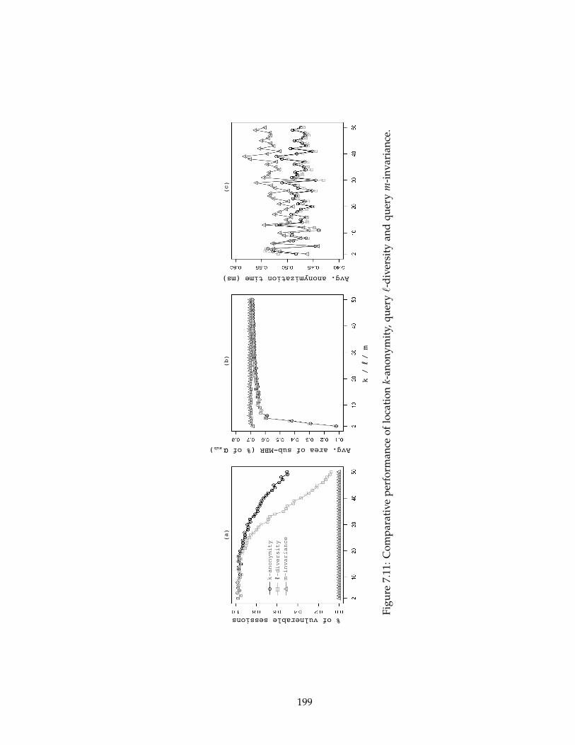
% of vulnerable sessions
Avg. area of sub-MBR (% of α )
Avg. anonymization time (ms)
k / ℓ / m
(a) (b) (c)
k-anonymity
ℓ-diversity
m-invariance
sub
Fig
ure
7.11
:C
om
par
ativ
ep
erfo
rman
ceo
flo
cati
on
k-an
on
ym
ity,
qu
ery
ℓ-d
iver
sity
and
qu
ery
m-i
nv
aria
nce
.
199

being common across the cloaking regions. Both k-anonymity and ℓ-diversity have almost
100% vulnerability for weaker anonymity requirements. In general, the fewer the number
of service attribute values in the first cloaking region, the higher are the chances of not
having any of those values in subsequently generated regions. However, by definition,
such chances are reduced to zero in the query m-invariance model.
We also observe that query ℓ-diversity manages to reduce the number of vulnerable
sessions to impressive lows for cases with higher anonymity requirements. This is not un-
likely since the probability of a particular value being in a subset of all possible attribute
values is higher when larger subsets are to be formed. However, the performance is not
indicative of similar behavior. Query m-invariance guarantees that the invariant set has
a size of at least m. On the other hand, the low percentage of vulnerable sessions with
query ℓ-diversity only means that the invariant set is not of size one. The actual size of
the set can very well be less than ℓ. Hence, the disclosure risk is not guaranteed to be less
than 1ℓ, resulting in partial disclosures.
Sub-MBR areas are typically smaller with k-anonymity and ℓ-diversity (Fig. 7.11b).
Query m-invariance generates comparatively larger areas for weaker anonymity require-
ments. This is because the users that satisfy the invariant set requirement may often be
far away from each other. This is specifically true if the invariant set has values that are
not frequently requested. Nevertheless, the sub-MBR area is within the spatial resolution,
implying that peer groups could be formed without violating the spatial constraint (the
‘or’ condition in Line 5 of Procedure 7.5). Further, the service quality is consistent across
all anonymity requirements. Fig. 7.11c illustrates the average time required to anonymize
a request. The query m-invariance requirement does not impose any significant overhead
in terms of computation time.
Fig. 7.12a depicts the impact of αsub on service quality. A very small spatial resolu-
tion (such as αsub = 0.0025 km2) is difficult to satisfy irrespective of the anonymity level
required. Given that each peer group must contain at least 2 users, the spatial constraint
is easily violated and the sub-MBR area is consequently larger than specified. The area
is large enough to accommodate 2 users. Fig. 7.12b corroborates this observation since
the average number of users inside a sub-MBR is 2 for such an αsub. A cloaking region
200
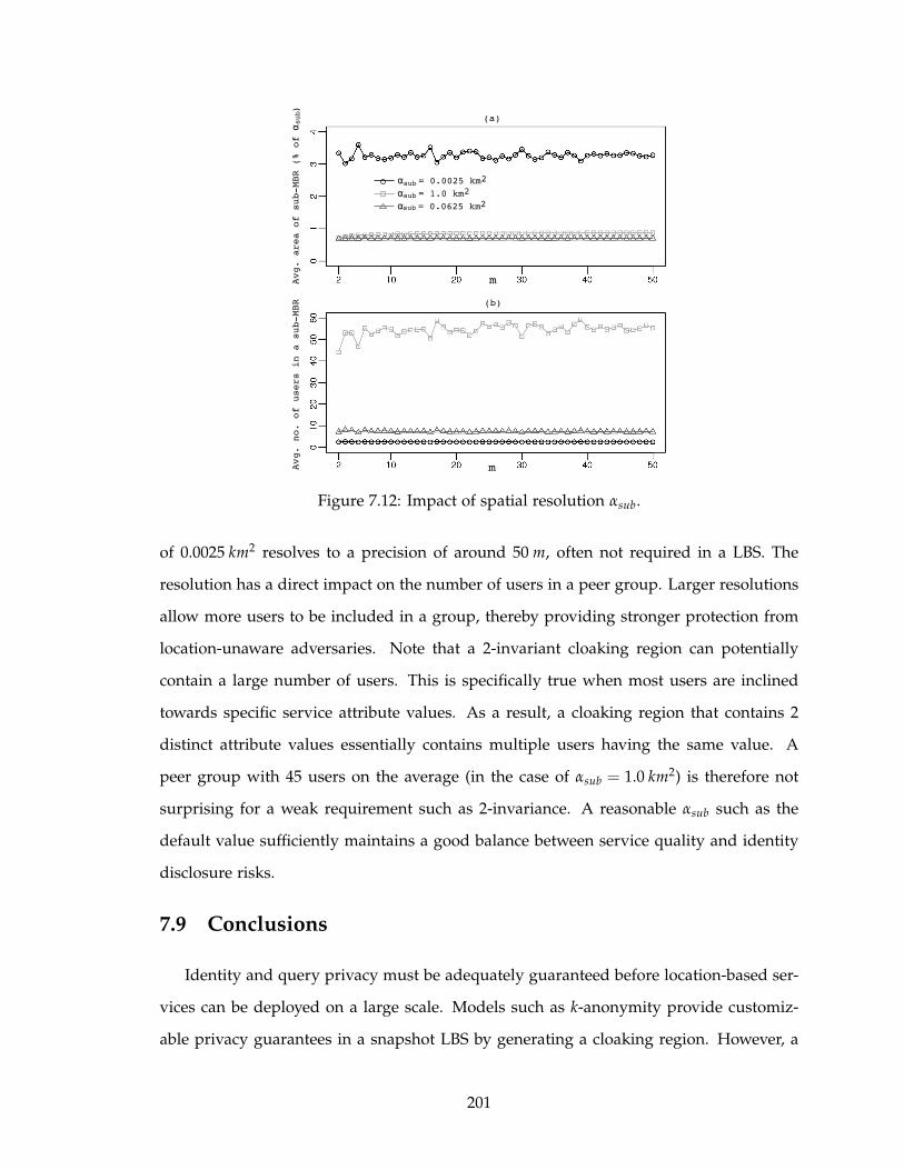
Avg. no. of users in a sub-MBR
Avg. area of sub-MBR (% of α
)
m
α = 0.0025 km
α = 1.0 km
α = 0.0625 km
(a)
m
(b)
2
2
2
sub
sub
sub
sub
Figure 7.12: Impact of spatial resolution αsub.
of 0.0025 km2 resolves to a precision of around 50 m, often not required in a LBS. The
resolution has a direct impact on the number of users in a peer group. Larger resolutions
allow more users to be included in a group, thereby providing stronger protection from
location-unaware adversaries. Note that a 2-invariant cloaking region can potentially
contain a large number of users. This is specifically true when most users are inclined
towards specific service attribute values. As a result, a cloaking region that contains 2
distinct attribute values essentially contains multiple users having the same value. A
peer group with 45 users on the average (in the case of αsub = 1.0 km2) is therefore not
surprising for a weak requirement such as 2-invariance. A reasonable αsub such as the
default value sufficiently maintains a good balance between service quality and identity
disclosure risks.
7.9 Conclusions
Identity and query privacy must be adequately guaranteed before location-based ser-
vices can be deployed on a large scale. Models such as k-anonymity provide customiz-
able privacy guarantees in a snapshot LBS by generating a cloaking region. However, a
201

k-anonymous cloaking region is not sufficient to guarantee privacy in a continuous LBS.
An extended notion called historical k-anonymity has been proposed for such services.
However, all known methods of enforcing historical k-anonymity significantly affects the
quality of service that the service provider can deliver. In this chapter, we have identified
the factors that contribute towards deteriorated service quality and suggested resolutions.
We propose the CANON algorithm that delivers reasonably good service quality across
different anonymity requirements. The algorithm uses tunable parameters to adjust the
size of a peer set, trajectories of peers and cloaking regions over which range queries are
issued. Immediate future work includes optimizing the performance of CANON in terms
of better usage of directional information. We believe this optimization is crucial in order
to have similar performance across all levels of anonymity requirements.
Association of service parameters to users cannot be prevented in a continuous LBS
by simply assuring that a cloaking region contains k or more users, or ℓ distinct service
attribute values. Assuming a location-aware adversary model, we have provided a formal
analysis to show that service attributes risk disclosure if the privacy model does not guar-
antee that an invariant set of attribute values is present in all cloaking regions generated
for the continuous LBS. We therefore propose using the principle of query m-invariance
where all cloaking regions are required to contain users with a fixed set of service attribute
values. We have shown that this requirement limits the involved risk, which in itself can
be controlled by the parameter m. We further propose a cloaking algorithm to enforce the
principle and have shown its effectiveness compared to location k-anonymity and query
ℓ-diversity. Results on trace data generated on a real-world road network show that query
m-invariance can be enforced without significantly affecting service quality or imposing
computational overhead. Further, the approach can be used to safeguard against both
location-aware and location-unaware adversaries. Future work can be directed towards
understanding the risks from query association attacks under alternative forms of back-
ground knowledge. Specifically, we are interested in exploring the privacy guarantees
required to tackle adversaries with limited knowledge on user locations.
202

Part II
Security Risk Management
203
CHAPTER 8
Security Hardening on Attack Tree Models
Network-based computer systems form an integral part of any information tech-
nology infrastructure today. The different levels of connectivity between these systems
directly facilitate the circulation of information within an organization, thereby reducing
invaluable wait time and increasing the overall throughput. As an organization’s opera-
tional capacity becomes more and more dependent on networked computing systems, the
need to maintain accessibility to the resources associated with such systems has become
a necessity. Any weakness or vulnerability that could result in the breakdown of the net-
work has direct consequences on the amount of yield manageable by the organization.
This, in turn, requires the organization to not only consider the advantages of utilizing a
networked system, but also consider the costs associated with managing the system.
With cost-effectiveness occurring as a major factor in deciding the extent to which
an organization would secure its network, it is not sufficient to detect the presence or
absence of a vulnerability and implement a security measure to rectify it. Further analysis
is required to understand the contribution of the vulnerabilities towards any possible
damage to the organization’s assets. Often, vulnerabilities are not exploited in isolation,
but rather used in groups to compromise a system. Similarly, security policies can have a
coverage for multiple vulnerabilities. Thus, cost-effective security management requires
researchers to evaluate the different scenarios that can lead to the damage of a secured
204

asset, and then come up with an optimal set of security policies to defend such assets.
Researchers have proposed building security models for networked systems using
paradigms like attack graphs [10, 94, 141, 156, 166] and attack trees [43, 131, 145, 155],
and then finding attack paths in these models to determine scenarios that could lead to
damage. However, determining possible attack paths, although useful, does not help the
system administrators much. They are more interested in determining the best possible
way of defending their network in terms of an enumerated set of hardening options [136].
Moreover, the system administrator has to work within a given set of budget constraints
which may preclude her from implementing all possible hardening measures or even
measures that cover all the weak spots. Thus, the system administrator needs to find
a trade-off between the cost of implementing a subset of security hardening measures
and the damage that can potentially happen to the system if certain weak spots are left
unpatched. In addition, the system administrator may also want to determine optimal
robust solutions. These are sets of security hardening measures with the property that
even if some of the measures within a set fail, the system is still not compromised.
We believe that the problem should be addressed in a more systematic manner, utiliz-
ing the different tools of optimization at hand. A decision maker would possibly make a
better choice by successively exploring the different levels of optimization possible, rather
than accepting a solution from an “off-the-shelf” optimizer. Towards this end, this chapter
discusses our four major contributions. First, we refine and formalize the notion of attack
trees so as to encode the contribution of different security conditions leading to system
compromise. Next, we develop a model to quantify the potential damage that can occur
in a system from the attacks modeled by the system attack tree. We also quantify the
security control cost incurred to implement a set of security hardening measures. Third,
we model the system administrator’s decision problem as three successively refined op-
timization problems on the attack tree model of the system. We progressively transform
one problem into the next to cater to more cost-benefit information as may be required
by the decision maker. Last but not least, we discuss our thoughts and observations
regarding the solutions, in particular the robust solutions identified by our optimization
process, with a belief that such discussion will help the system administrator decide what
205
methodology to adopt.
The rest of the chapter is organized as follows. We discuss some of the previous works
related to determining optimum security hardening measures in Section 8.1. In Section
8.2, we describe a simple network that we use to illustrate our problem formulation and
solution. The attack tree model formalism and the cost model are presented in Sections
8.3 and 8.4 respectively. The three optimization problems are presented in Section 8.5
with some empirical results and discussion following in Section 8.6. Finally, we conclude
in Section 8.7.
8.1 Related Work
Network vulnerability management has been previously addressed in a variety of
ways. Noel et al. use a data structure called exploit dependency graphs [136] to compute
minimum cost-hardening measures. Given a set of initial conditions in the graph, they
compute Boolean assignments to these conditions, enforced by some hardening measure,
so as to minimize the total cost of those measures. As pointed out in their work, these
initial conditions are the only type of network security conditions under our strict control.
Hardening measures applied to internal nodes can potentially be bypassed by an attacker
by adopting a different attack path. Jha et al. [94] on the other hand do not consider any
cost for the hardening measures. Rather, their approach involves finding the minimal set
of atomic attacks critical for reaching the goal and then finding the minimal set of security
measures that cover the minimal set of atomic attacks.
Such analysis is meant for providing solutions that guarantee complete network safety.
However, the hardening measures provided may still not be feasible within the financial
or other business constraints of an organization. Under such circumstances, a decision
maker must perform a cost-benefit analysis to understand the trade-off between hard-
ening costs and network safety. Furthermore, a minimum cost hardening measure set
only means that the root goal is safe, and some residual damage may still remain in the
network. Owing to these real-world concerns, network vulnerability management should
not always be considered as a single-objective optimization problem.
A multi-objective formulation of the problem is presented by Gupta et al. [79]. They
206
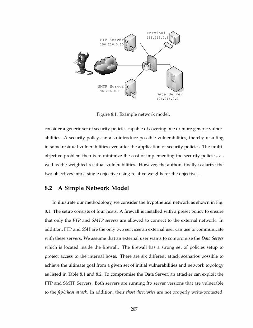
Terminal
196.216.0.3
Data Server
196.216.0.2
SMTP Server
196.216.0.1
FTP Server
196.216.0.10
Figure 8.1: Example network model.
consider a generic set of security policies capable of covering one or more generic vulner-
abilities. A security policy can also introduce possible vulnerabilities, thereby resulting
in some residual vulnerabilities even after the application of security policies. The multi-
objective problem then is to minimize the cost of implementing the security policies, as
well as the weighted residual vulnerabilities. However, the authors finally scalarize the
two objectives into a single objective using relative weights for the objectives.
8.2 A Simple Network Model
To illustrate our methodology, we consider the hypothetical network as shown in Fig.
8.1. The setup consists of four hosts. A firewall is installed with a preset policy to ensure
that only the FTP and SMTP servers are allowed to connect to the external network. In
addition, FTP and SSH are the only two services an external user can use to communicate
with these servers. We assume that an external user wants to compromise the Data Server
which is located inside the firewall. The firewall has a strong set of policies setup to
protect access to the internal hosts. There are six different attack scenarios possible to
achieve the ultimate goal from a given set of initial vulnerabilities and network topology
as listed in Table 8.1 and 8.2. To compromise the Data Server, an attacker can exploit the
FTP and SMTP Servers. Both servers are running ftp server versions that are vulnerable
to the ftp/.rhost attack. In addition, their rhost directories are not properly write-protected.
207
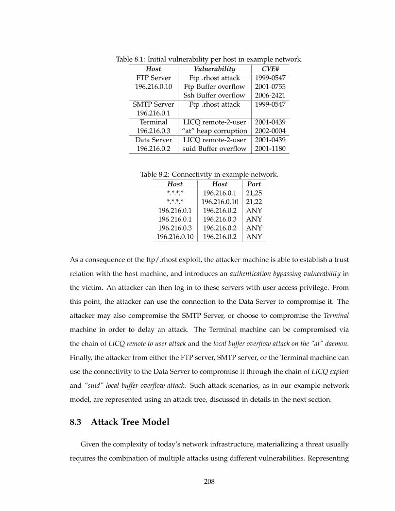
Table 8.1: Initial vulnerability per host in example network.
Host Vulnerability CVE#
FTP Server Ftp .rhost attack 1999-0547196.216.0.10 Ftp Buffer overflow 2001-0755
Ssh Buffer overflow 2006-2421
SMTP Server Ftp .rhost attack 1999-0547196.216.0.1
Terminal LICQ remote-2-user 2001-0439196.216.0.3 “at” heap corruption 2002-0004
Data Server LICQ remote-2-user 2001-0439196.216.0.2 suid Buffer overflow 2001-1180
Table 8.2: Connectivity in example network.
Host Host Port
*.*.*.* 196.216.0.1 21,25*.*.*.* 196.216.0.10 21,22
196.216.0.1 196.216.0.2 ANY196.216.0.1 196.216.0.3 ANY196.216.0.3 196.216.0.2 ANY196.216.0.10 196.216.0.2 ANY
As a consequence of the ftp/.rhost exploit, the attacker machine is able to establish a trust
relation with the host machine, and introduces an authentication bypassing vulnerability in
the victim. An attacker can then log in to these servers with user access privilege. From
this point, the attacker can use the connection to the Data Server to compromise it. The
attacker may also compromise the SMTP Server, or choose to compromise the Terminal
machine in order to delay an attack. The Terminal machine can be compromised via
the chain of LICQ remote to user attack and the local buffer overflow attack on the “at” daemon.
Finally, the attacker from either the FTP server, SMTP server, or the Terminal machine can
use the connectivity to the Data Server to compromise it through the chain of LICQ exploit
and “suid” local buffer overflow attack. Such attack scenarios, as in our example network
model, are represented using an attack tree, discussed in details in the next section.
8.3 Attack Tree Model
Given the complexity of today’s network infrastructure, materializing a threat usually
requires the combination of multiple attacks using different vulnerabilities. Representing
208

different scenarios under which an asset can be damaged thus becomes important for
preventive analysis. Such representations not only provide a picture of the possible ways
to compromise a system, but can also help determine a minimal set of preventive actions.
Given the normal operational state of a network, including the vulnerabilities present, an
attack can possibly open up avenues to launch another attack, thereby taking the attacker
a step closer to its goal. A certain state of the network in terms of access privileges or
machine connectivity can be a prerequisite to be able to exploit a vulnerability. Once the
vulnerability is exploited, the state of the network can change enabling the attacker to
launch the next attack in the sequence. Such a pre-thought sequence of attacks gives rise
to an attack scenario.
It is worth noting that such a notion of a progressive attack induces a transitive rela-
tionship between the vulnerabilities present in the network and can be exploited while de-
ciding on the security measures. Attack graph [10, 94, 136, 156] and attack tree [145, 155]
representations have been proposed in network vulnerability management to demon-
strate such cause-consequence relationships. The nodes in these data structures usually
represent a certain network state of interest to an attacker, with edges connecting them
to indicate the cause-consequence relationship. Although different attack scenarios are
easily perceived in attack graphs, they can potentially suffer from a state space explo-
sion problem. Ammann et al. [10] identified this problem and propose an alternative
formulation, with the assumption of monotonicity. The monotonicity property states that
the consequence of an attack is always preserved once achieved. Such an assumption
can greatly reduce the number of nodes in the attack graph, although at the expense of
further analysis required to determine the viable attack scenarios. An exploit-dependency
graph can be extracted from their representation to indicate the various conjunctive and
disjunctive relationships between different nodes. For the purpose of this study, we adopt
the attack tree representation since it presents a much clearer picture of the different hi-
erarchies present between attacker sub-goals. An attack tree uses explicit conjunctive and
disjunctive branch decomposition to reduce the visualization complexity of a sequence of
operations. The representation also helps us efficiently calculate the cost factors that are
of interest to us.
209

Different properties of the network effectuate different ways for an attacker to com-
promise a system. We first define an attribute-template that lets us generically categorize
these network properties for further analysis.
Definition 8.1 ATTRIBUTE-TEMPLATE. An attribute-template is a generic property of
the hardware or software configuration of a network which includes, but is not limited
to, the following.
• system vulnerabilities (which are often reported in vulnerability databases such as
BugTraq, CERT/CC, or NetCat).
• network configuration such as open port, unsafe firewall configuration, etc.
• system configuration such as data accessibility, unsafe default configuration, or
read-write permission in file structures.
• access privilege such as user account, guest account, or root account.
• connectivity.
An attribute-template lets us categorize most of the atomic properties of the network
that might be of some use to an attacker. For example, “running SSH1 v1.2.23 on FTP
Server” can be considered as an instance of the system vulnerabilities template. Similarly,
“user access on Terminal” is an instance of the access privilege template. Such templates
also let us specify the properties in propositional logic. We define an attribute with such
a concept in mind.
Definition 8.2 ATTRIBUTE. An attribute is a propositional instance of an attribute-template.
It can take either a true or false value.
The success or failure of an attacker reaching its goal depends mostly on what truth
values the attributes in a network take. Its also lays the foundations for a security manager
to analyze the effects of falsifying some of the attributes using some security policies. We
formally define an attack tree model based on such attributes. Since we consider an
attribute as an atomic property of a network, taking either a true or false value, most of
the definitions are written in propositional logic involving these attributes.
210
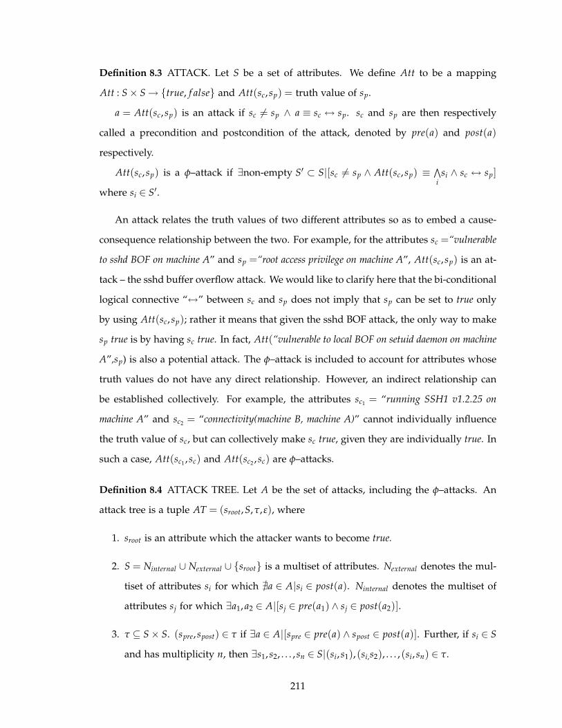
Definition 8.3 ATTACK. Let S be a set of attributes. We define Att to be a mapping
Att : S × S → {true, f alse} and Att(sc, sp) = truth value of sp.
a = Att(sc, sp) is an attack if sc 6= sp ∧ a ≡ sc ↔ sp. sc and sp are then respectively
called a precondition and postcondition of the attack, denoted by pre(a) and post(a)
respectively.
Att(sc, sp) is a φ–attack if ∃non-empty S′ ⊂ S|[sc 6= sp ∧ Att(sc, sp) ≡ ∧
isi ∧ sc ↔ sp]
where si ∈ S′.
An attack relates the truth values of two different attributes so as to embed a cause-
consequence relationship between the two. For example, for the attributes sc =“vulnerable
to sshd BOF on machine A” and sp =“root access privilege on machine A”, Att(sc, sp) is an at-
tack – the sshd buffer overflow attack. We would like to clarify here that the bi-conditional
logical connective “↔” between sc and sp does not imply that sp can be set to true only
by using Att(sc, sp); rather it means that given the sshd BOF attack, the only way to make
sp true is by having sc true. In fact, Att(“vulnerable to local BOF on setuid daemon on machine
A”,sp) is also a potential attack. The φ–attack is included to account for attributes whose
truth values do not have any direct relationship. However, an indirect relationship can
be established collectively. For example, the attributes sc1= “running SSH1 v1.2.25 on
machine A” and sc2 = “connectivity(machine B, machine A)” cannot individually influence
the truth value of sc, but can collectively make sc true, given they are individually true. In
such a case, Att(sc1, sc) and Att(sc2 , sc) are φ–attacks.
Definition 8.4 ATTACK TREE. Let A be the set of attacks, including the φ–attacks. An
attack tree is a tuple AT = (sroot,S,τ, ε), where
1. sroot is an attribute which the attacker wants to become true.
2. S = Ninternal ∪ Nexternal ∪ {sroot} is a multiset of attributes. Nexternal denotes the mul-
tiset of attributes si for which ∄a ∈ A|si ∈ post(a). Ninternal denotes the multiset of
attributes sj for which ∃a1, a2 ∈ A|[sj ∈ pre(a1) ∧ sj ∈ post(a2)].
3. τ ⊆ S × S. (spre, spost) ∈ τ if ∃a ∈ A|[spre ∈ pre(a) ∧ spost ∈ post(a)]. Further, if si ∈ S
and has multiplicity n, then ∃s1, s2, . . . , sn ∈ S|(si, s1), (si,s2), . . . , (si, sn) ∈ τ.
211
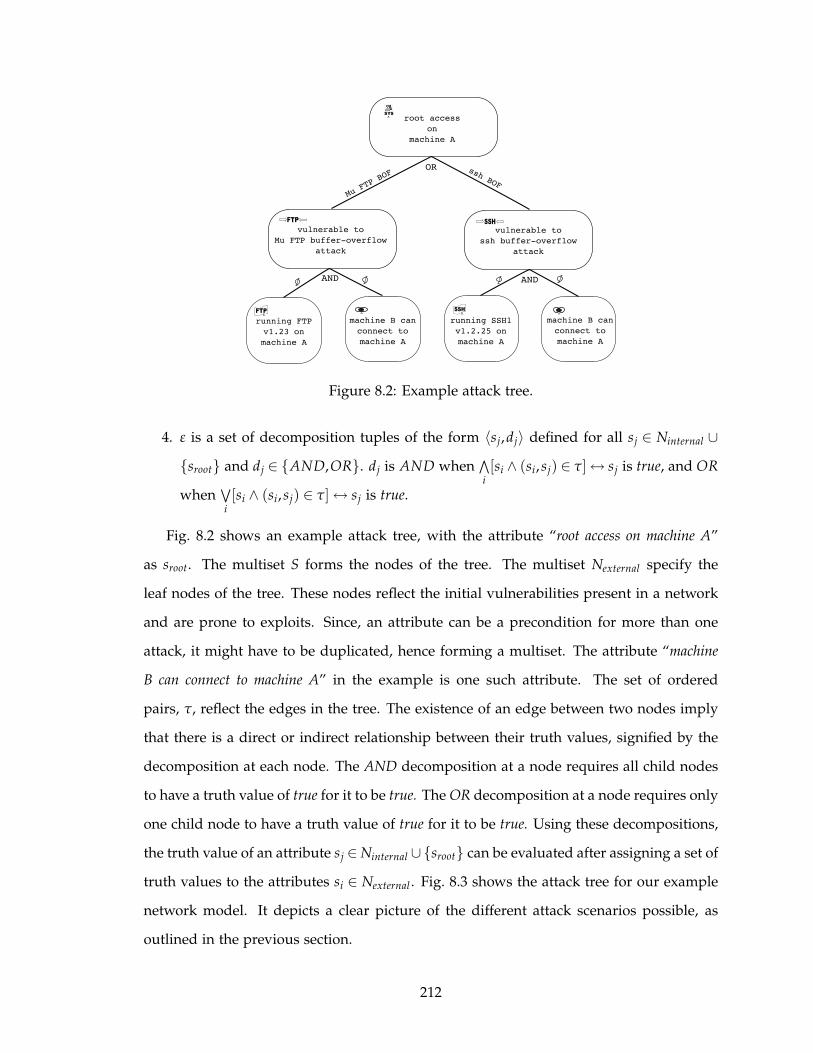
Figure 8.2: Example attack tree.
4. ε is a set of decomposition tuples of the form 〈sj,dj〉 defined for all sj ∈ Ninternal ∪{sroot} and dj ∈ {AND,OR}. dj is AND when
∧
i[si ∧ (si, sj) ∈ τ] ↔ sj is true, and OR
when∨
i[si ∧ (si, sj) ∈ τ] ↔ sj is true.
Fig. 8.2 shows an example attack tree, with the attribute “root access on machine A”
as sroot. The multiset S forms the nodes of the tree. The multiset Nexternal specify the
leaf nodes of the tree. These nodes reflect the initial vulnerabilities present in a network
and are prone to exploits. Since, an attribute can be a precondition for more than one
attack, it might have to be duplicated, hence forming a multiset. The attribute “machine
B can connect to machine A” in the example is one such attribute. The set of ordered
pairs, τ, reflect the edges in the tree. The existence of an edge between two nodes imply
that there is a direct or indirect relationship between their truth values, signified by the
decomposition at each node. The AND decomposition at a node requires all child nodes
to have a truth value of true for it to be true. The OR decomposition at a node requires only
one child node to have a truth value of true for it to be true. Using these decompositions,
the truth value of an attribute sj ∈ Ninternal ∪{sroot} can be evaluated after assigning a set of
truth values to the attributes si ∈ Nexternal . Fig. 8.3 shows the attack tree for our example
network model. It depicts a clear picture of the different attack scenarios possible, as
outlined in the previous section.
212
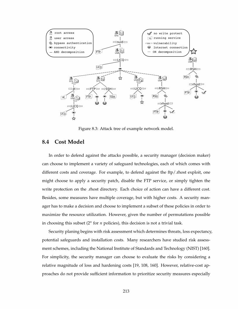
SYS
suid
USR
LICQ
FTP2
SYS
USR
LICQ2
SYS USR
at
at3
LICQ
LICQ3
USR
LICQ
LICQ3
FTP SSH
FTP10
SSH10
RSH
RSH10
rhost
FTP10
10
USR
RSH
RSH 1
rhost
FTP 1
1
SYS
USR
XXX
xxx
root access
user access
bypass authentication
connectivity
no write protect
running service
vulnerability
Internet connection
AND decomposition OR decomposition
x
Figure 8.3: Attack tree of example network model.
8.4 Cost Model
In order to defend against the attacks possible, a security manager (decision maker)
can choose to implement a variety of safeguard technologies, each of which comes with
different costs and coverage. For example, to defend against the ftp/.rhost exploit, one
might choose to apply a security patch, disable the FTP service, or simply tighten the
write protection on the .rhost directory. Each choice of action can have a different cost.
Besides, some measures have multiple coverage, but with higher costs. A security man-
ager has to make a decision and choose to implement a subset of these policies in order to
maximize the resource utilization. However, given the number of permutations possible
in choosing this subset (2n for n policies), this decision is not a trivial task.
Security planing begins with risk assessment which determines threats, loss expectancy,
potential safeguards and installation costs. Many researchers have studied risk assess-
ment schemes, including the National Institute of Standards and Technology (NIST) [160].
For simplicity, the security manager can choose to evaluate the risks by considering a
relative magnitude of loss and hardening costs [19, 108, 160]. However, relative-cost ap-
proaches do not provide sufficient information to prioritize security measures especially
213

when the organization faces resource constraints. We adapt Butler’s multi-attribute risk
assessment framework [29, 30] to develop quantitative risk assessments for our security
optimization. Butler’s framework enables an aggregated representation of the various
factors dominating the business model of an organization. First we define the notion of a
security control in the context of the attack tree definition.
Definition 8.5 SECURITY CONTROL. Given an attack tree (sroot,S,τ, ε), the mapping
SC : Nexternal → {true, f alse} is a security control if ∃si ∈ Nexternal |SC(si) = f alse.
In other words, a security control is a preventive measure to falsify one or more
attributes in the attack tree, so as to stop an attacker from reaching its goal. Further, in
the presence of multiple security controls SCk, the truth value of an attribute si ∈ Nexternal
is taken as∧
kSCk(si). Given a security control SC, the set of all si ∈ Nexternal |SC(si) = f alse
is called the coverage of SC. Hence, for a given set of security controls we can define
the coverage matrix specifying the coverage of each control. For a given set of m security
controls, we use the Boolean vector ~T = (T1,T2, . . . , Tm) to indicate if a security control
is chosen by a security manager. Note that the choice of this vector indirectly specifies
which attributes in the attack tree (leaf nodes) would be false.
8.4.1 Evaluating Potential Damage
The potential damage, Pj, represents a unit-less damage value that an organization
may have to incur in the event that an attribute sj becomes true. Based on Butler’s frame-
work, we propose four steps to calculate the potential damage for an attribute sj.
Step1: Identify potential consequences of having a true value for the attribute, induced
by some attack. In our case, we have identified five outcomes – lost revenue (mon-
etary), non-productive downtime (time), damage recovery (monetary), public em-
barrassment (severity) and law penalty (severity) – denoted by x1j, x2j, x3j, x4j and
x5j.
Step2: Estimate the expected number of attack occurrence, Freqj, resulting in the conse-
quences. A security manager can estimate the expected number of attack from the
214

organization-based historical data or public historical data1.
Step3: Assess a single value function, Vij(xij), for each possible consequence. The pur-
pose of this function is to normalize different unit measures so that the values can
be summed together under a single standard scale.
Vij(xij) =xij
Maxj
xij× 100 ,1 ≤ i ≤ 5 (8.1)
Step4: Assign a preference weight factor, Wi, to each possible consequence. A security
manager can rank each outcome on a scale of 1 to 100. The outcome with the most
concern would receive 100 points. The manager ranks the other attributes relative
to the first. Finally, the ranks are normalized and set as Wi.
The potential damage for the attribute can then be calculated as given by the following
equation.
Pj = Freqj ×5
∑i=1
WiVij(xij) (8.2)
When using an attack tree, a better quantitative representation of the cost is obtained
by considering the residual damage once a set of security policies are implemented.
Hence, we augment each attribute in the attack tree with a value signifying the amount
of potential damage residing in the subtree rooted at the attribute and the attribute itself.
Definition 8.6 AUGMENTED-ATTACK TREE. Given an attack tree AT = (sroot,S,τ, ε), an
augmented-attack tree ATaug = AT|〈I,V〉 is obtained by associating a tuple 〈Ii,Vi〉 to each
si ∈ S, where
1. Ii is an indicator variable for the attribute si, where
Ii =
{
0 , i f si is f alse
1 , i f si is true. (8.3)
2. Vi is a value associated with the attribute si.
1Also known as an incident report published annually in many sites such as CERT/CC or SANS.ORG.
215

In this work, all attributes si ∈ Nexternal are given a zero value. The value associated
with sj ∈ Ninternal ∪ {sroot} is then computed recursively as follows.
Vj =
∑ Vkk|(sk ,sj)∈τ
+ IjPj , i f dj is AND
max Vkk|(sk ,sj)∈τ
+ IjPj , i f dj is OR(8.4)
Ideally, Pj is same for all identical attributes in the multiset. We took a “panic ap-
proach” in calculating the value at each node, meaning that given multiple subtrees are
rooted at an attribute with an OR decomposition, we choose the maximum value. We do
so because an attacker’s capabilities and preferences cannot be known in advance. The
residual damage of the augmented tree is then defined as follows.
Definition 8.7 RESIDUAL DAMAGE. Given an augmented-attack tree (sroot,S,τ, ε)|〈I,V〉and a vector ~T = (Ti), Ti ∈ {0,1};1 ≤ i ≤ m, the residual damage is defined as the value
associated with sroot, i.e.
RD(~T) = Vroot. (8.5)
8.4.2 Evaluating Security Cost
Similar to the potential damage, the security manager first lists possible security costs
for the implementation of a security control, assigns the weight factor on them, and
computes the normalized value. The only difference is that there is no expected number of
occurrence needed in the evaluation of security cost. In this study, we have identified five
different costs of implementing a security control – installation cost (monetary), operation
cost (monetary), system downtime (time), incompatibility cost (scale), and training cost
(monetary). The overall cost Cj, for the security control SCj, is then computed in a similar
manner as for potential damage, with an expected frequency of one. The total security
cost for a set of security controls implemented is then defined as follows.
Definition 8.8 TOTAL SECURITY CONTROL COST. Given a set of m security controls,
each having a cost Ci;1 ≤ i ≤ m, and a vector ~T = (Ti), Ti ∈ {0,1};1 ≤ i ≤ m, the total
216
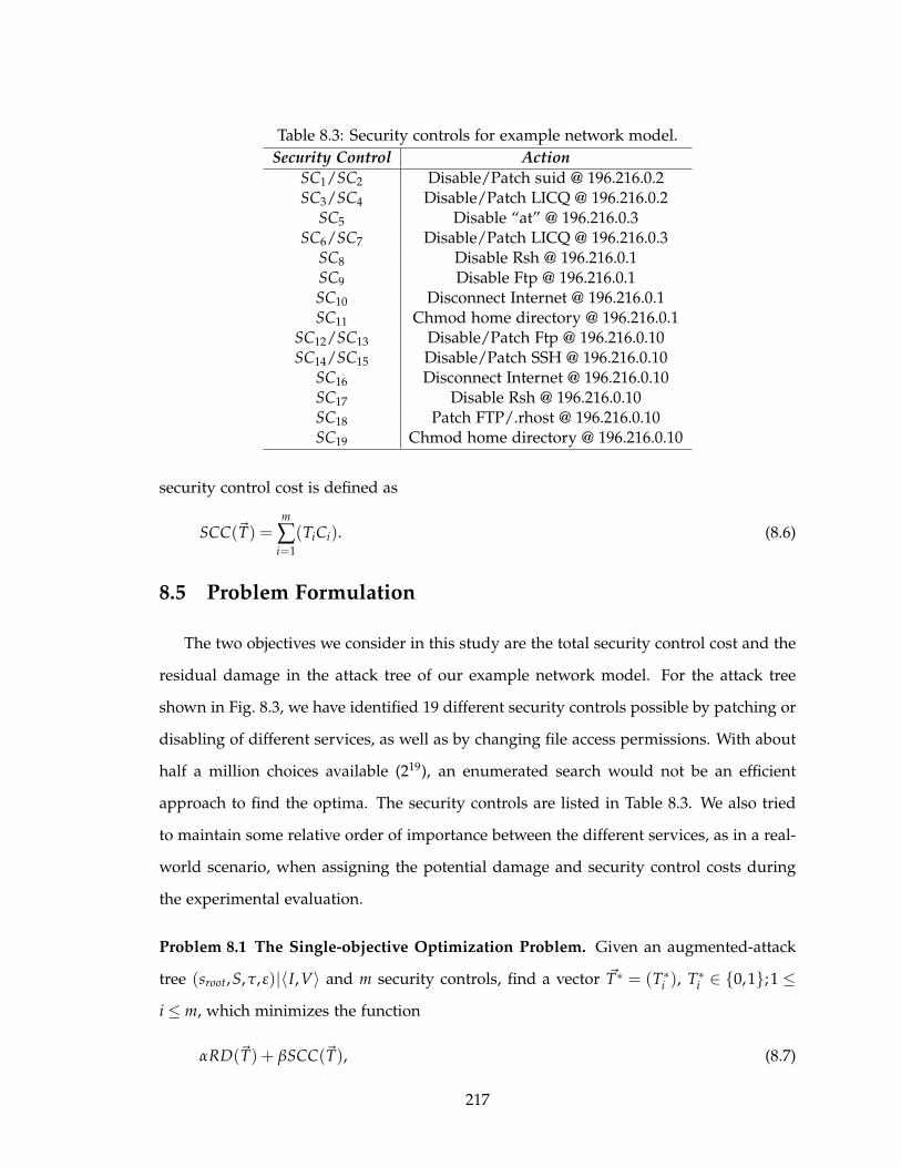
Table 8.3: Security controls for example network model.
Security Control Action
SC1/SC2 Disable/Patch suid @ 196.216.0.2SC3/SC4 Disable/Patch LICQ @ 196.216.0.2
SC5 Disable “at” @ 196.216.0.3SC6/SC7 Disable/Patch LICQ @ 196.216.0.3
SC8 Disable Rsh @ 196.216.0.1SC9 Disable Ftp @ 196.216.0.1SC10 Disconnect Internet @ 196.216.0.1SC11 Chmod home directory @ 196.216.0.1
SC12/SC13 Disable/Patch Ftp @ 196.216.0.10SC14/SC15 Disable/Patch SSH @ 196.216.0.10
SC16 Disconnect Internet @ 196.216.0.10SC17 Disable Rsh @ 196.216.0.10SC18 Patch FTP/.rhost @ 196.216.0.10SC19 Chmod home directory @ 196.216.0.10
security control cost is defined as
SCC(~T) =m
∑i=1
(TiCi). (8.6)
8.5 Problem Formulation
The two objectives we consider in this study are the total security control cost and the
residual damage in the attack tree of our example network model. For the attack tree
shown in Fig. 8.3, we have identified 19 different security controls possible by patching or
disabling of different services, as well as by changing file access permissions. With about
half a million choices available (219), an enumerated search would not be an efficient
approach to find the optima. The security controls are listed in Table 8.3. We also tried
to maintain some relative order of importance between the different services, as in a real-
world scenario, when assigning the potential damage and security control costs during
the experimental evaluation.
Problem 8.1 The Single-objective Optimization Problem. Given an augmented-attack
tree (sroot,S,τ, ε)|〈I,V〉 and m security controls, find a vector ~T∗ = (T∗i ), T∗
i ∈ {0,1};1 ≤i ≤ m, which minimizes the function
αRD(~T) + βSCC(~T), (8.7)
217

where α and β are preference weights for the residual damage and the total cost of security
control respectively, 0 ≤ α, β ≤ 1 and α + β = 1.
The single-objective problem is the most likely approach to be taken by a decision
maker. Given only two objectives, a preference based approach might seem to provide
a solution in accordance with general intuition. However, as we find in the case of our
example network model, the quality of the solution obtained can be quite sensitive to the
assignment of the weights. To demonstrate this affect, we run multiple instances of the
problem using different combination of values for α and β. α is varied in the range of
[0,1] in steps of 0.05. β is always set to 1 − α.
Problem 8.2 The Multi-objective Optimization Problem. Given an augmented-attack
tree (sroot,S,τ, ε)|〈I,V〉 and m security controls, find a vector ~T∗ = (T∗i ), T∗
i ∈ {0,1};1 ≤i ≤ m, which minimizes the total security control cost and the residual damage.
The next level of sophistication is added by formulating the minimization as a multi-
objective optimization problem. The multi-objective approach alleviates the requirement
to specify any weight parameters and hence a better global picture of the solutions can
be obtained.
Problem 8.3 The Multi-objective Robust Optimization Problem. Let ~T = (Ti) be a
Boolean vector. A perturbed assignment of radius r, ~Tr, is obtained by inverting the
value of at most r elements of the vector ~T. The robust optimization problem can then be
defined as follows.
Given an augmented-attack tree (sroot,S,τ, ε)|〈I,V〉 and m security controls, find a
vector ~T∗ = (T∗i ), T∗
i ∈ {0,1};1 ≤ i ≤ m, which minimizes the total security control cost
and the residual damage, satisfying the constraint
max~Tr
RD(~Tr) − RD(~T) ≤ D, (8.8)
where D is the maximum perturbation allowed in the residual damage.
The third problem is formulated to further strengthen the decision process by deter-
mining robust solutions to the problem. Robust solutions are less sensitive to failures in
218

security controls and hence subside any repeated requirements to re-evaluate solutions
in the event of a security control failure.
We use a simple genetic algorithm (SGA) [75] to solve Problem 8.1. NSGA-II is used to
solve Problems 8.2 and 8.3. The algorithm parameters are set as follows: population size
= 100, number of generations = 250, crossover probability = 0.9, and mutation probability
= 0.1.
8.6 Empirical Results
We first present the sensitivity results of NSGA-II and SGA to their parameters. In-
creasing the population size from 100 to 500 gives us a faster convergence rate, although
the solutions reported still remains the same. The effect of changing the crossover prob-
ability in the range of 0.7 to 0.9 does not lead to any significant change of the solutions
obtained. Similar results were observed when changing the mutation probability from
0.1 to 0.01. The solutions also do not change when the number of generations is changed
from 250 to 500. Since we did not observe any significant change in the solutions by vary-
ing the algorithm parameters, the following results are presented as obtained by setting
the parameters as chosen in the previous section.
It is usually suggested that the preference based approach should normalize the func-
tions before combining them into a single function. However, we did not see any change
in the solutions of the normalized version of Problem 8.1. Fig. 8.4 shows the solutions
obtained from various runs of SGA in Problem 8.1 with varying α. A decision maker, in
general, may want to assign equal weights to both the objective functions, i.e. set α = 0.5. It
is clear from the figure that such an assignment does not necessarily provide the desired
balance between the residual damage and the total security control cost. Furthermore,
such balance is also not obtainable by assigning weight values in the neighborhood of 0.5.
The solutions obtained are quite sensitive to the weights, and in this case, much higher
preference must be given to the total security control cost to find other possible solutions.
Since the weights do not always influence the objectives in the desired manner, under-
standing their effect is not a trivial task for a decision maker. It is also not possible to
always do an exhaustive analysis of the affect of the weights on the objectives. Given such
219
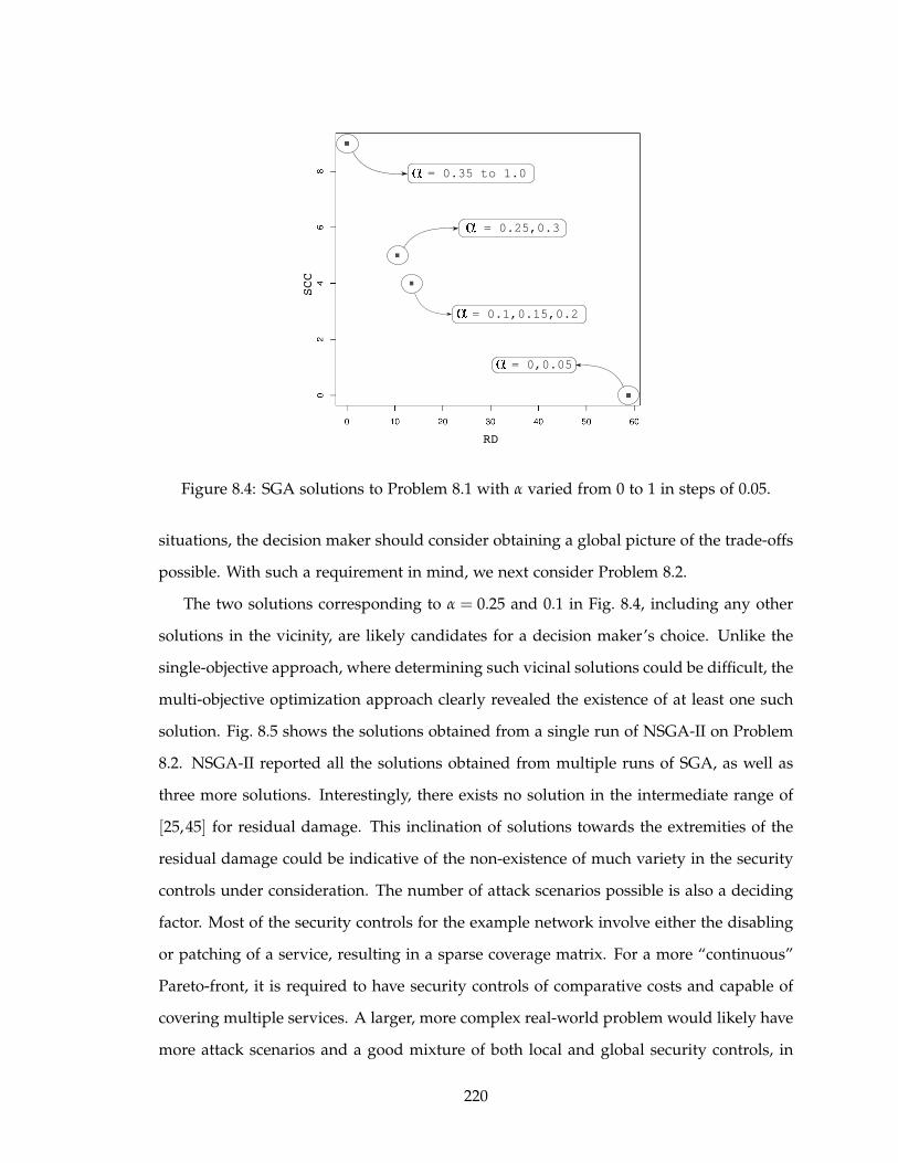
RD
SCC
= 0.25,0.3
= 0.1,0.15,0.2
= 0,0.05
= 0.35 to 1.0
Figure 8.4: SGA solutions to Problem 8.1 with α varied from 0 to 1 in steps of 0.05.
situations, the decision maker should consider obtaining a global picture of the trade-offs
possible. With such a requirement in mind, we next consider Problem 8.2.
The two solutions corresponding to α = 0.25 and 0.1 in Fig. 8.4, including any other
solutions in the vicinity, are likely candidates for a decision maker’s choice. Unlike the
single-objective approach, where determining such vicinal solutions could be difficult, the
multi-objective optimization approach clearly revealed the existence of at least one such
solution. Fig. 8.5 shows the solutions obtained from a single run of NSGA-II on Problem
8.2. NSGA-II reported all the solutions obtained from multiple runs of SGA, as well as
three more solutions. Interestingly, there exists no solution in the intermediate range of
[25,45] for residual damage. This inclination of solutions towards the extremities of the
residual damage could be indicative of the non-existence of much variety in the security
controls under consideration. The number of attack scenarios possible is also a deciding
factor. Most of the security controls for the example network involve either the disabling
or patching of a service, resulting in a sparse coverage matrix. For a more “continuous”
Pareto-front, it is required to have security controls of comparative costs and capable of
covering multiple services. A larger, more complex real-world problem would likely have
more attack scenarios and a good mixture of both local and global security controls, in
220
RD
SCC
RD10 20 30 40 50
SC4
SC11
SC4
SC11
SC4
SC11
sensitivity
Figure 8.5: NSGA-II solutions to Problem 8.2 and sensitivity of a solution to optimumsettings.
which case, such gaps in the Pareto-front will be unlikely.
Once the decision maker has a better perspective of the solutions possible, further
analysis of the solutions may be carried out in terms of their sensitivity to security control
failures. Such sensitivity analysis is helpful in not only reducing valuable decision making
time, but also to guarantee some level of fault tolerance in the network. Fig. 8.5 shows the
sensitivity of one of the solutions to a failure in one of the security controls corresponding
to the solution. This solution, with security controls SC4 and SC11, will incur a high
residual damage in the event of a failure of SC4. Thus, a decision maker may choose
to perform a sensitivity analysis on each of the solutions and incorporate the results
thereof in making the final choice. However, the decision maker then has no control
on how much of additional residual damage would be incurred in the event of failure.
Problem 8.3 serves the requirements of this decision stage by allowing the decision maker
to specify the maximum allowed perturbation in the residual damage. It is also possible to
specify the scope of failure – the radius r – within which the decision maker is interested
in analyzing the robustness of the solutions. For this study, we are mostly interested
in obtaining solutions that are fully robust, meaning the residual damage should not
221
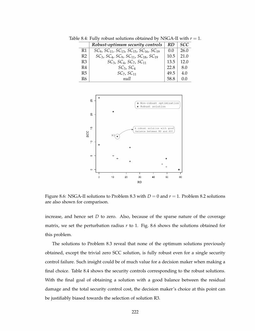
Table 8.4: Fully robust solutions obtained by NSGA-II with r = 1.
Robust-optimum security controls RD SCC
R1 SC9, SC11, SC13, SC15, SC16, SC19 0.0 26.0R2 SC3, SC4, SC9, SC11, SC18, SC19 10.5 21.0R3 SC3, SC4, SC7, SC11 13.5 12.0R4 SC3, SC4 22.8 8.0R5 SC7, SC11 49.5 4.0R6 null 58.8 0.0
RD
SCC
Non-robust optimization
Robust solution
A robust solution with good
balance between RD and SCC
R3
Figure 8.6: NSGA-II solutions to Problem 8.3 with D = 0 and r = 1. Problem 8.2 solutionsare also shown for comparison.
increase, and hence set D to zero. Also, because of the sparse nature of the coverage
matrix, we set the perturbation radius r to 1. Fig. 8.6 shows the solutions obtained for
this problem.
The solutions to Problem 8.3 reveal that none of the optimum solutions previously
obtained, except the trivial zero SCC solution, is fully robust even for a single security
control failure. Such insight could be of much value for a decision maker when making a
final choice. Table 8.4 shows the security controls corresponding to the robust solutions.
With the final goal of obtaining a solution with a good balance between the residual
damage and the total security control cost, the decision maker’s choice at this point can
be justifiably biased towards the selection of solution R3.
222
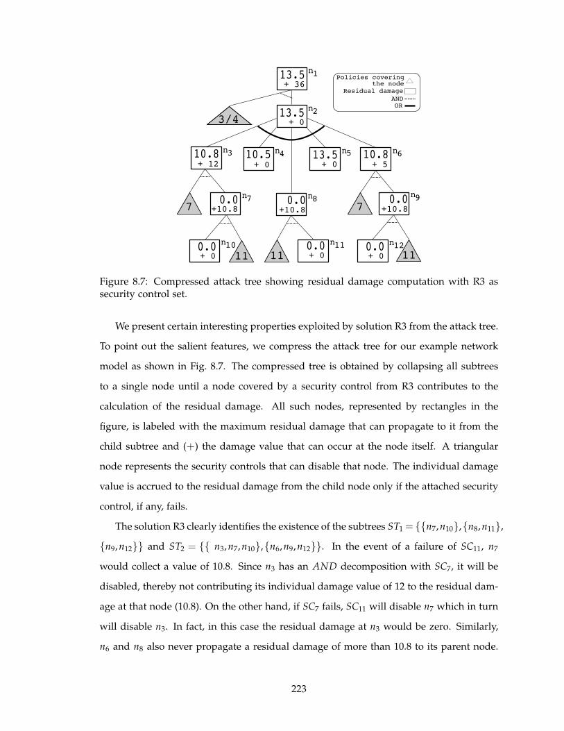
Figure 8.7: Compressed attack tree showing residual damage computation with R3 assecurity control set.
We present certain interesting properties exploited by solution R3 from the attack tree.
To point out the salient features, we compress the attack tree for our example network
model as shown in Fig. 8.7. The compressed tree is obtained by collapsing all subtrees
to a single node until a node covered by a security control from R3 contributes to the
calculation of the residual damage. All such nodes, represented by rectangles in the
figure, is labeled with the maximum residual damage that can propagate to it from the
child subtree and (+) the damage value that can occur at the node itself. A triangular
node represents the security controls that can disable that node. The individual damage
value is accrued to the residual damage from the child node only if the attached security
control, if any, fails.
The solution R3 clearly identifies the existence of the subtrees ST1 = {{n7,n10},{n8,n11},
{n9,n12}} and ST2 = {{ n3,n7,n10},{n6,n9,n12}}. In the event of a failure of SC11, n7
would collect a value of 10.8. Since n3 has an AND decomposition with SC7, it will be
disabled, thereby not contributing its individual damage value of 12 to the residual dam-
age at that node (10.8). On the other hand, if SC7 fails, SC11 will disable n7 which in turn
will disable n3. In fact, in this case the residual damage at n3 would be zero. Similarly,
n6 and n8 also never propagate a residual damage of more than 10.8 to its parent node.
223
Consequently, n2 never propagates a value more than 13.5. The individual cost of 36 at
n1 is never added to this residual damage value of 13.5 from n2 since, owing to the AND
decomposition, n1 is always falsified by security controls SC3 and SC4, only one of which
is assumed to fail at a time. The solution wisely applies security controls covering mul-
tiple attack scenarios, and at multiple points in those scenarios to keep the damage to a
minimum.
8.7 Conclusions
In this chapter, we address the system administrator’s dilemma, namely, how to se-
lect a subset of security hardening measures from a given set so that the total cost of
implementing these measures is not only minimized but also within budget and, at the
same time, the cost of residual damage is also minimized. One important contribution of
our approach is the use of an attack tree model of the network to drive the solution. By
using an attack tree in the problem, we are able to better guide the optimization process
by providing the knowledge about the attributes that make an attack possible. Further, a
systematic analysis enables us to approach the problem in a modular fashion, providing
added information to a decision maker to form a concrete opinion about the quality of
the different trade-off solutions possible.
The cost model that we adopt in this chapter is somewhat simplistic. We assume
that, from a cost of implementation perspective, the security measures are independent
of each other, where in real life they may not be so. In addition, we have assumed that the
system administrator’s decision is in no way influenced by an understanding of the cost
to break the system. Furthermore, the possible decomposition of an attack tree to divide
the problem into sub-problems is an interesting alternative to explore. Finally, there is
a dynamic aspect to the system administrator’s dilemma. During run time the system
administrator may need to revise her decision based on emerging security conditions.
224
CHAPTER 9
Security Hardening on Pervasive Workflows
Pervasive computing aims at making the presence of computing machinery so trans-
parent that their very presence becomes imperceptible to the end user. These applications
involve interacting with heterogeneous devices having various capabilities under the con-
trol of different entities. Such applications make use of workflows that are mostly auto-
mated and do not require much human intervention. For critical applications, the work-
flows pass on sensitive information to the various devices and make crucial decisions.
Failure to protect such information against security breaches may cause irreparable dam-
ages.
Pervasive computing applications impose a number of unique constraints that make
choosing the appropriate security mechanisms difficult. Interoperability of the heteroge-
neous devices must be taken into account while selecting security mechanisms. Resource
consumption is a very important consideration as this directly relates to the up-time
and maintainability of the application. The cost of deployment must also be considered.
Thus, an overall picture illustrating the cost-benefit trade-offs in the presence of these
constraints is needed before a final decision can be made.
Unfortunately, security threats in a pervasive environment are very application de-
pendent. Thus, it is not possible to give a solution that is satisfactory for all pervasive
applications. For example, if a communication is between a mobile device and a base
225

station, then a particular type of authentication protocol may be appropriate, whereas if
the communication is of an ad-hoc nature, the same protocol may be inappropriate. Fur-
ther, the communication between two devices can be deemed sensitive or non-sensitive
depending on the context under which the communication is taking place. Finally, the
resource constraints varies for different scenarios and prohibit the usage of the same se-
curity measures even for the same class of threats.
Context based security provisioning has earlier been proposed to adapt the secu-
rity level of a communication to the sensitivity of the information being exchanged
[97, 132, 133]. Nonetheless, exploring the aforementioned trade-off options becomes diffi-
cult when contexts are introduced. Contexts are dynamic in nature and proactive analysis
do not always capture all possible scenarios. However, it is important to realize that per-
vasive environments set up with a specific application in mind have predefined ways of
handling the different scenarios that can appear during the lifetime of the environment.
It is therefore possible that these scenarios be represented in a concise way and subjected
to security evaluation techniques. This is a good beginning since an organization has a
concrete understanding of the assets it has and the points of immediate interest usually
involve the likelihood of potential damages to these known assets.
In this chapter, we formalize these issues and identify possible resolutions to some of
the decision making problems related to securing a pervasive environment. We propose
the use of workflow profiles to represent the business model of a pervasive environment
and compute the cost associated with the maintenance of the workflow. We then perform
a multi-objective analysis to maximize the security level of the workflow and minimize
the cost incurred thereof. The multi-objective formulations take into account the energy
constraints imposed by devices in the environment. We demonstrate our methodology
using an evolutionary algorithm in a pervasive healthcare domain.
The rest of the chapter is organized as follows. Section 9.1 presents the related work in
this field. An example healthcare pervasive environment along with the concept of work-
flow representations is presented in Section 9.2. Security provisioning in the workflow is
discussed in Section 9.3. Section 9.4 presents the cost model for the workflow. Section 9.5
discusses the multi-objective problems, some empirical results on which are presented in
226
Section 9.6. Finally, Section 9.7 concludes the chapter.
9.1 Related Work
Security provisioning in pervasive environments is an open field for research. Camp-
bell et al. present an overview of the specific security challenges that are present in this
field [33] and describe their prototype implementation of a component-based middleware
operating system. A more specific formulation for security provisioning in wireless sen-
sor networks is presented by Chigan et al. [37]. Their framework has an offline security
optimization module targeted towards maximizing a security provision index. Ranganathan
et al. propose some meta-level metrics to gauge the ability of different security services
in a pervasive environment [143].
Dependability issues related to the application of pervasive computing to the health-
care domain is discussed by Bohn et al. [26]. They argue that the healthcare domain can
serve as a benchmark platform for pervasive computing research. They point out the
security issues relevant to the setup of such a platform. Similar practical issues are also
investigated by Black et al. [25].
An example usage of context information in pervasive applications is presented by
Judd and Steenkiste [97]. Their approach allows proactive applications to obtain con-
text information on an user’s current environment and adapt their behavior accordingly.
The use of context information for security provisioning is proposed by Mostéfaoui and
Brézillon [132]. They propose using contextual graphs to appropriately decide on the
security policies to enforce. Further reasoning on the contributions of combining context
and security is provided by the same authors in [133]. Sanchez et al. propose a Monte
Carlo based framework to model context data and evaluate context based security policies
[153].
9.2 The Pervasive Workflow Model
Security threats in a pervasive environment are application dependent. Consequently,
business models investing in any kind of a pervasive computing paradigm will highly
benefit if formalisms are derived to enable a “case-by-case” study of the problem of se-
227

curity provisioning. We therefore discuss our approach using an example healthcare
application.
9.2.1 A pervasive health care environment
The pervasive healthcare environment consists of devices that measure the vital signs
of patients, location sensors that locate mobile resources, location-aware PDAs carried by
health-care personnel, and back-end systems storing and processing records of patient
data. The devices are connected through wired or wireless medium. The application con-
sists of different workflows that get triggered by various events. The following example
specifies the workflow that handles the situation when an unanticipated change occurs in
a patient’s vital signs (VS) monitor.
Case1: The VS monitor tries to detect the presence of the doctor within a wireless com-
municable distance. If the doctor is present, she can make suggestions which may
or may not be based on the patient report stored at the back-end. She may also de-
cide to request the assistance of a nurse, who is located with the help of the network
infrastructure. In case of an emergency, the same infrastructure is used to notify the
emergency service.
Case2: If a doctor cannot be located nearby, there is a search for a nurse. The nurse
may have the requisite skills to take care of the situation, perhaps with information
obtained from the back-end system. If not, the nurse requests the network infras-
tructure to locate a remote doctor. The remote doctor can then make suggestions to
the nurse or directly interact with the monitoring devices using the network. Pos-
sibilities are also that the doctor feels the need to be immediately with the patient
and informs the emergency service on her way.
Case3: If a nearby doctor or a nurse cannot be located, the VS monitor communicates
with the network infrastructure to locate a remote doctor. The doctor, once located,
can remotely interact with the monitoring equipments, or decide to attend to the
situation physically, often asking for assistance from a nurse. Emergency services
are notified on a need basis. Also, on the event that the network is unable to locate
228
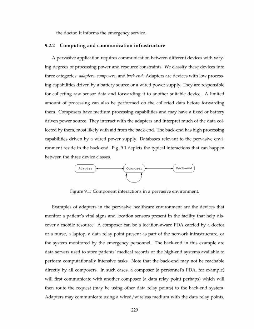
the doctor, it informs the emergency service.
9.2.2 Computing and communication infrastructure
A pervasive application requires communication between different devices with vary-
ing degrees of processing power and resource constraints. We classify these devices into
three categories: adapters, composers, and back-end. Adapters are devices with low process-
ing capabilities driven by a battery source or a wired power supply. They are responsible
for collecting raw sensor data and forwarding it to another suitable device. A limited
amount of processing can also be performed on the collected data before forwarding
them. Composers have medium processing capabilities and may have a fixed or battery
driven power source. They interact with the adapters and interpret much of the data col-
lected by them, most likely with aid from the back-end. The back-end has high processing
capabilities driven by a wired power supply. Databases relevant to the pervasive envi-
ronment reside in the back-end. Fig. 9.1 depicts the typical interactions that can happen
between the three device classes.
Figure 9.1: Component interactions in a pervasive environment.
Examples of adapters in the pervasive healthcare environment are the devices that
monitor a patient’s vital signs and location sensors present in the facility that help dis-
cover a mobile resource. A composer can be a location-aware PDA carried by a doctor
or a nurse, a laptop, a data relay point present as part of the network infrastructure, or
the system monitored by the emergency personnel. The back-end in this example are
data servers used to store patients’ medical records or the high-end systems available to
perform computationally intensive tasks. Note that the back-end may not be reachable
directly by all composers. In such cases, a composer (a personnel’s PDA, for example)
will first communicate with another composer (a data relay point perhaps) which will
then route the request (may be using other data relay points) to the back-end system.
Adapters may communicate using a wired/wireless medium with the data relay points,
229
which in turn communicate over an infrastructure network to the back-end system. The
composer class comprising mainly of handheld PDAs and similar devices communicate
wirelessly with adapters and other composers.
9.2.3 Workflow
A workflow captures the various relationships between the participating nodes and
provides a concise representation of the different contexts under which the different nodes
communicate with each other.
Definition 9.1 WORKFLOW. A workflow is a tuple 〈N, E,n〉 representing one or more
execution paths of a business model, where N is a multiset of nodes representing the
devices in the application, E is a set of ordered pairs of the form (ns,nd)∈ N × N denoting
the communication links, and n ∈ N is a source node that triggers the workflow.
A workflow can also be visualized in terms of transfer of work between devices. A
workflow is a meta-level representation of the order in which different devices participate
to achieve one or more business goals. A feasible execution path in such a representation
resembles the order of participation of the nodes to achieve one of the goals. For exam-
ple, to find the nearest doctor, transfer of work progresses as VS Monitor→Data Relay
Point→Location Sensor→Data Relay Point→ . . . →Doctor, and signifies an execution path.
Although this transfer of work involves multiple location sensors and multiple data re-
lay points, the workflow representation does not make a distinction among them. This
is primarily because the objective behind the usage of a communication link between a
data relay point and a location sensor is fixed (find a doctor) and hence all such links are
assumed to exchange information with the same level of sensitivity.
9.2.4 Context
Although a workflow helps identify the different communication links used as part
of different execution paths, it does not provide any information on the frequency with
which a particular channel is used. This frequency estimate is required to determine the
rate of power consumption of the two participating devices in the link. When security
230

measures are placed in these links, the rate of power consumption will increase depend-
ing on the computational requirements of the algorithms. Here we have an inherent
conflict. Heavily used communication channels should ideally have security measures
with low computing requirements in order to reduce the power consumption at the two
participating devices. At the same time, strong security measures are perhaps required
to safeguard the huge amount of information flowing through the channel. Quite often
this is hard to achieve since strong security measures typically are computation intensive
algorithms.
Definition 9.2 CONTEXT. A context is a prefix of some execution path through a work-
flow. It is associated with a probability estimate vector that gives the likelihood of the
context changing into other contexts.
A context specifies the different nodes that are traversed when following a particular
execution path. We use the notation Cv to represent a context with the current node v. In
some cases, we use a more informal notation and describe contexts by just concatenating
the names of the nodes. For example, for the context ABCDC, the current node is C and
the node has been reached by following the path A → B → C → D → C. We use ‘|’ to de-
note the operator to concatenate a node to a context, resulting in a new context. Note that
a context may be a part of multiple execution paths. Context-based probability estimates
will help capture the likelihood with which a context can change. This is described next.
Consider Fig. 9.2a; let Cv be the context and let t be its probability of occurrence. We
assign a probability on each outgoing edge signifying the chances with which the current
context changes. The context becomes Cv|x with probability p1 and Cv|y with probability
p2.
For a node v with k outgoing edges numbered in a particular order, the context-based
probability vector (p1, p2, . . . , pk)Cvgives the probabilities on the outgoing edges in the
same order when the current context is Cv. The probability values for a given context can
be obtained from audit logs collected over a period of time signifying how often did v
act as an intermediate node in the communication between two neighbor nodes under a
particular communication sequence.
231

vt
p1
p2
x
xv
v
context
yv
y
D B
C
A
1
1
1
0.5
0.2 0.15
0.05
0.25+0.15
0.20.3
2
3
2
3
(0.5,0.3,0.2)
(0.4,0.5.0.1)
(0.75,0.25)
(0,1,0)
A
AB
ABC
ABCB
0.05
Context probabilities
2
(a) (b)
Figure 9.2: (a) Context-based probability estimates. (b) Workflow probability calculation.
It is important to realize that a workflow by itself does not reveal the feasible execution
paths. It is only by including context information that the feasible execution paths get
defined. Context-based probability estimates tell us if an adjacent node can become a part
of a particular execution path. If all probabilities on the outgoing edges of a particular
node are zero, then the execution does not proceed and the current context at that point
terminates as a feasible execution path. Hence, by defining a set of possible contexts,
along with their context-based probability estimates, we have a precise way of defining
which execution paths are feasible. We call this set the context set of the workflow.
Definition 9.3 CONTEXT SET. A context set for a workflow is a set of contexts that are
all possible prefixes of all feasible execution paths.
The context set contains only those contexts for which there is non-zero probability
of transitioning into another context. To infer the feasible execution paths from a given
context set, we start at the source node and check to see if the current context (the source
node alone at this point) is present in the context set. We can move onto an adjacent node
if the probability on the edge to it is non-zero. The current context then changes to a
different one for each reachable node. The process is repeated for all such nodes until a
node is reached where the current context is not present in the context set. Such a context
is then a feasible execution path.
Note that context-based probability estimates provide the probability with which an
outgoing edge will be used in the current context. This probability does not, as yet, pro-
232

vide an estimate of the overall frequency with which the edge is used in the workflow. We
shall show in Section 9.4 how the context set is used to compute the effective probability
with which a particular communication link in the workflow gets used.
9.3 Security Provisioning
The problem of security provisioning in a workflow involves the identification of po-
tentially damaging attacks and the security mechanisms that can be adopted to protect
against such attacks. Depending on the nature of communication between two nodes,
a subset of the known attacks can be more prominent than others in a communication
channel. Besides the ability to defend against one or more attacks, the choice of a security
mechanism is also dependent on the resources it consumes during execution.
Definition 9.4 SECURITY MECHANISM. Given a set of A attacks, denoted by a1, a2, . . . , aA,
a security mechanism Si is a Boolean vector [Si1,Si2, . . . ,SiA], where Sij is 1 if it defends
against attack aj, 0 otherwise.
An attack in this definition refers to the consequence of a malicious activity. A se-
curity mechanism is capable of preventing one or more attacks. For a given set of NS
security mechanisms, we have a coverage matrix defining which attacks are covered by
which mechanisms. Further, each mechanism has an associated power consumption rate,
denoted by SMCi, where 1 ≤ i ≤ NS.
To facilitate the enforcement of different security mechanisms along different commu-
nication links, we augment each edge on the workflow with an attack vector specifying the
attacks which are of concern in the link.
Definition 9.5 ATTACK VECTOR. An attack vector on an edge of the workflow is a
Boolean vector of size A with the jth component being either 1 or 0 based on whether
attack aj is plausible on the edge or not.
Given an attack vector, it is possible that no single security mechanism can provide
the required defenses against all attacks of concern on the edge. Multiple mechanisms
have to be selected such that they can collectively provide the coverage for the attacks.
233

Definition 9.6 SECURITY CONTROL VECTOR. A security control vector SVe = [SVe1,
SVe2, . . . ,SVeNS] on the edge e is a Boolean vector, where SVei is 1 if the security mechanism
Si is chosen, 0 otherwise.
For a particular security control vector SVe, the attacks collectively covered by SVe
is computed from the expression∨
i(SVei · Si), for i = 1, . . . , Ns. The ‘dot’ operator here
indicates scalar multiplication with a vector and ‘∨’ signifies the Boolean OR operation.
The resultant of this expression is a Boolean vector of size A and signifies which attacks
are covered by the combination of the security mechanisms. We shall call this vector the
covered attack vector of the edge on which the security control vector operates.
If AVe and CAVe are the attack vector and covered attack vector on an edge e, then
the Hamming distance between the zero vector and the vector AVe ∧ ¬CAVe, ‘∧’ and
‘¬’ signifying the boolean AND and NOT operators respectively, computes the number
of attacks initially specified as plausible on the edge but not covered by any security
mechanism in the control vector. We shall denote this quantity by H(AVe,CAVe).
9.4 Cost Computation
In this study, we are interested in the cost that an organization has to incur to keep a
particular workflow running. To this effect, we consider the cost of maintenance. The cost
of maintenance relates to the expenses that an organization has to incur to hire personnel
for regular maintenance rounds, purchase supplies and hardware support equipments, or
may be due to losses arising from downtime in services during maintenance. A reduction
in the cost is possible if the workflow can be engineered to run for a longer time between
two maintenance rounds. We realize that the contributing factors appear with different
magnitudes and in different dimensions, often with different levels of impact, and are
hence difficult to combine into one cost measure. We can adapt Butler’s Multi-attribute
Risk Assessment model [29, 30] to cater to these difficulties.
Maintenance cost estimates obtained using Butler’s method is used along with fre-
quency estimates obtained from the workflow to determine the total maintenance cost
incurred to keep the workflow running. Before we can do so, the probability estimates on
234

Procedure 9.1 EffectiveProbability(Context c, Probability t)
Input: Context c and probability t. {context set C, context based probability estimates andworkflow graph are assumed global data}
Output: Effective probability of edges. {initialized to 0.0 on all edges}1: if (c ∈ C) then
2: h = current node in context c3: for all (edge e outgoing to a node g from h) do
4: pe = probability of going to g from h in the context c5: Add pet to effective probability of edge e6: E f f ectiveProbability(c|g, pet)7: end for
8: end if
the communication links have to be aggregated to determine the overall frequency with
which the link is used. This is done by calculating the effective probability of usage of a
communication link on the event the workflow gets triggered.
Refer to Fig. 9.2a. Since the probabilities on the outgoing edges are decided indepen-
dent of each other, the effective probability on the two outgoing edges can be calculated
as p1t and p2t respectively. Also, since the probabilities on an outgoing edge are only
dependent on the current context, effective probabilities accumulating on an edge from
different contexts can be summed together to give the probability with which the edge is
used. Fig. 9.2b shows the calculation of the effective probabilities for a small workflow.
The workflow has node A as the source node. The outgoing edges from the source node
capture all possible situations that can occur when the workflow is triggered. The given
context probabilities are ordered according to the numbering on the outgoing edge at
the current node. Procedure 9.1 when instantiated with arguments (A,1.0) recursively
computes the effective probabilities on the edges of the workflow given the context prob-
abilities shown in the figure. We denote the effective probability on an edge e by pe.
Once the effective probabilities on each edge of the workflow are calculated, the number
of times a particular edge is used can be found by multiplying the number of times the
workflow is triggered with the effective probability on the edge.
Let Pi and MCi be the power capacity and total maintenance cost of the ith unique
device respectively. Let {e1, e2, . . . , ek} be the set of edges that connect the nodes corre-
sponding to this device with other nodes. Let Ti be a constant power consumption by the
235

device and PCij = ∑NS
l=1(SVej l × SMCl) the power consumption rate of the device because
of the security mechanisms in place on edge ej; j = 1, . . . ,k. If the workflow is triggered F
times, then edge ej with effective probability pejwill be used f = F × pej
times. Hence, the
total power consumed at device i after the security provisioning on edge ej is expressed
as (Ti + PCij) × f . A maintenance will be required for the device every ∑kj=1
(Ti+PCij)× f
Pi
times of usage. The total maintenance cost for the workflow is
TMC = ∑i
(
MCi ×k
∑j=1
(Ti + PCij) × f
Pi
)
. (9.1)
9.5 Problem Formulation
The multi-objective formulations presented here are intended to help analyze the
trade-offs resulting from the selection of a particular set of security control vectors for
the different communication links in a workflow and the corresponding cost of mainte-
nance. To begin with, we decide on a subset Ep ⊆ E of edges on the workflow that are
subjected to the security provisioning procedure.
The first optimization problem we consider is the determination of security control
vectors for each edge in Ep in order to minimize the cost of maintenance and the total
number of attacks left uncovered on the edges of the workflow, i.e. minimize ∑e∈EpH(AVe,
CAVe).
Problem 9.1 Scenario A. Find security control vectors for each edge e ∈ Ep that minimizes
TMC and minimizes ∑e∈EpH(AVe,CAVe).
Although the total number of uncovered attacks provide a good idea about the po-
tential exploits still remaining in the workflow, the damages that can result from the
exploitation of the uncovered attacks can be more than that could have resulted from the
covered attacks. The choice of security control vectors based on the number of covered
attacks can thus be a misleading indicator of the assets that the employed security mech-
anisms helped protect. To this effect, instead of minimizing the number of uncovered
attacks, the second formulation incorporates the minimization of the total potential dam-
age that can result from the uncovered attacks. To facilitate the computation of the total
236
potential damage, we modify the attack vector to indicate the damages possible instead
of just a Boolean indicator of whether an attack is plausible in an edge or not. The jth
component of the attack vector is then a real valued quantity signifying the potential dam-
age cost if attack aj is not covered by a security mechanism on the edge. The quantity can
be zero if the corresponding attack is not of concern on the particular edge. We do not
focus on the cost models that can be adopted to estimate such damage levels. Butler’s
framework is a good starting point in this direction.
Problem 9.2 Scenario B. Find security control vectors for each edge e ∈ Ep that minimizes
TMC and minimizes ∑e∈Ep〈AVe,¬CAVe〉, where 〈, 〉 signifies the scalar product operation.
An assumption implicit in the above two formulations is that every security mecha-
nism is capable of running in all the devices present in the workflow. This is not true
when there exists devices with very low power capabilities and not all security mecha-
nisms can be supported by them. The existence of such devices impose the constraint that
certain security mechanisms can never be placed on certain communication links. Thus,
we extend Problem 9.2 to generate solutions that are feasible within such constraints. Let
ns,e and nd,e denote the two communicating devices on the edge e. For the security mech-
anisms to be able to execute, the total power consumed by the mechanisms in place on
this edge has to be less than the minimum of the power capacities of the two participating
devices. The optimization problem is then formulated as follows.
Problem 9.3 Scenario C. Find security control vectors SVe for each edge e ∈ Ep which
minimizes TMC and minimizes ∑e∈Ep〈AVe,¬CAVe〉, satisfying the constraints ∑
NSi=1(SVei ×
SMCi) ≤ min(Pns,e , Pnd,e), for all edges e ∈ Ep.
For the final problem, we explore the scenario when the adopted security mechanisms
are not robust enough and are prone to failures. Non-robust security control vectors suffer
from the drawback that a failure in one of the security mechanisms can heavily increase
the number of uncovered attacks or the total potential damage in the workflow. Robust
solutions, on the other hand, are able to contain such increases within a pre-specified
acceptable level. We use the notion of a failure radius r which signifies the number of
237
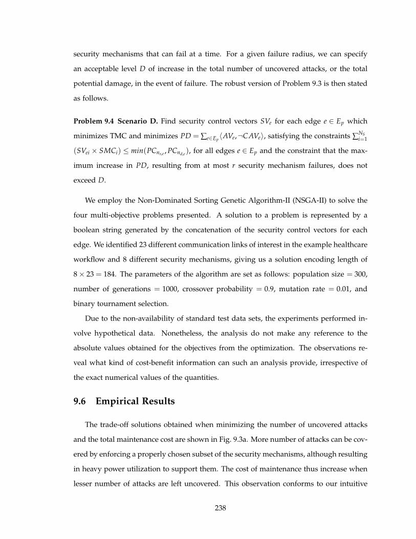
security mechanisms that can fail at a time. For a given failure radius, we can specify
an acceptable level D of increase in the total number of uncovered attacks, or the total
potential damage, in the event of failure. The robust version of Problem 9.3 is then stated
as follows.
Problem 9.4 Scenario D. Find security control vectors SVe for each edge e ∈ Ep which
minimizes TMC and minimizes PD = ∑e∈Ep〈AVe,¬CAVe〉, satisfying the constraints ∑
NSi=1
(SVei × SMCi) ≤ min(PCns,e , PCnd,e), for all edges e ∈ Ep and the constraint that the max-
imum increase in PD, resulting from at most r security mechanism failures, does not
exceed D.
We employ the Non-Dominated Sorting Genetic Algorithm-II (NSGA-II) to solve the
four multi-objective problems presented. A solution to a problem is represented by a
boolean string generated by the concatenation of the security control vectors for each
edge. We identified 23 different communication links of interest in the example healthcare
workflow and 8 different security mechanisms, giving us a solution encoding length of
8 × 23 = 184. The parameters of the algorithm are set as follows: population size = 300,
number of generations = 1000, crossover probability = 0.9, mutation rate = 0.01, and
binary tournament selection.
Due to the non-availability of standard test data sets, the experiments performed in-
volve hypothetical data. Nonetheless, the analysis do not make any reference to the
absolute values obtained for the objectives from the optimization. The observations re-
veal what kind of cost-benefit information can such an analysis provide, irrespective of
the exact numerical values of the quantities.
9.6 Empirical Results
The trade-off solutions obtained when minimizing the number of uncovered attacks
and the total maintenance cost are shown in Fig. 9.3a. More number of attacks can be cov-
ered by enforcing a properly chosen subset of the security mechanisms, although resulting
in heavy power utilization to support them. The cost of maintenance thus increase when
lesser number of attacks are left uncovered. This observation conforms to our intuitive
238
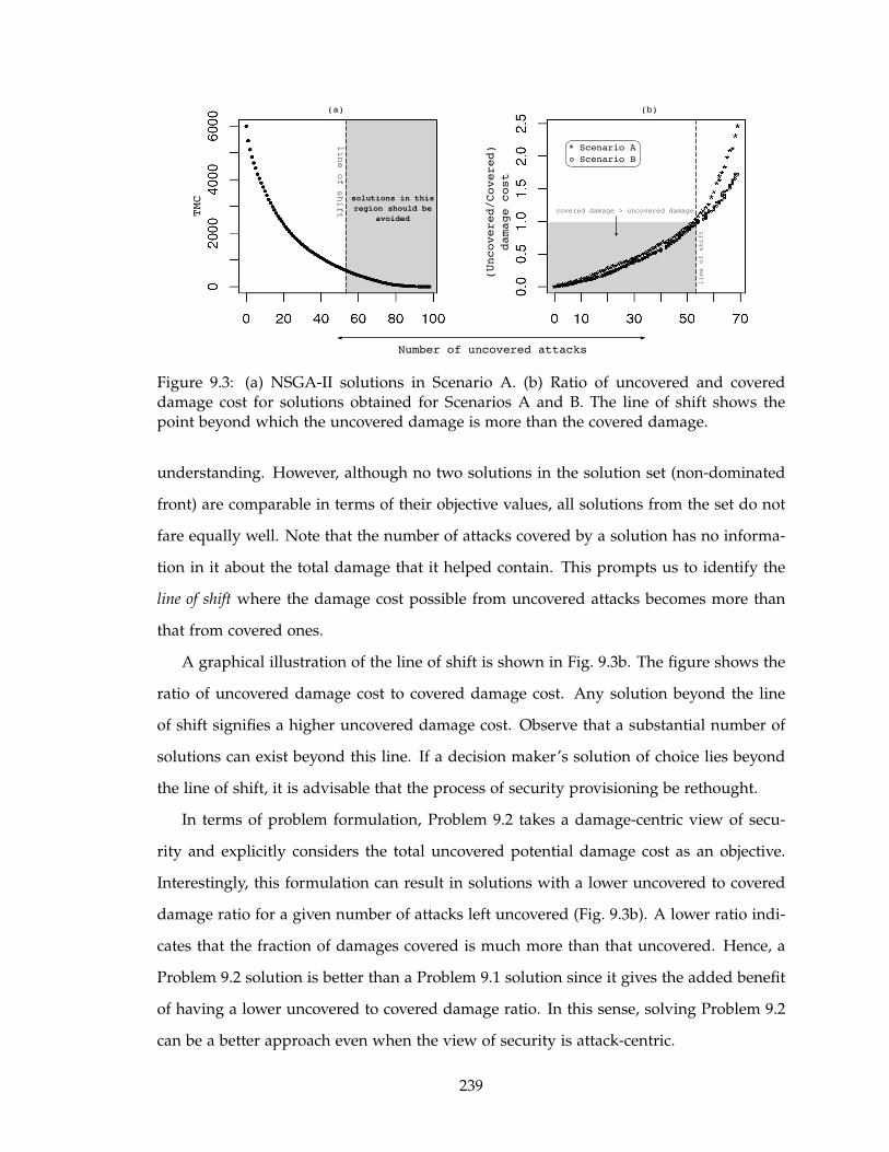
Number of uncovered attacks
TMC
(Uncovered/Covered)
damage cost
* Scenario A
Scenario B
covered damage > uncovered damage
line of shift
line of shift
solutions in this
region should be
avoided
(a) (b)
Figure 9.3: (a) NSGA-II solutions in Scenario A. (b) Ratio of uncovered and covereddamage cost for solutions obtained for Scenarios A and B. The line of shift shows thepoint beyond which the uncovered damage is more than the covered damage.
understanding. However, although no two solutions in the solution set (non-dominated
front) are comparable in terms of their objective values, all solutions from the set do not
fare equally well. Note that the number of attacks covered by a solution has no informa-
tion in it about the total damage that it helped contain. This prompts us to identify the
line of shift where the damage cost possible from uncovered attacks becomes more than
that from covered ones.
A graphical illustration of the line of shift is shown in Fig. 9.3b. The figure shows the
ratio of uncovered damage cost to covered damage cost. Any solution beyond the line
of shift signifies a higher uncovered damage cost. Observe that a substantial number of
solutions can exist beyond this line. If a decision maker’s solution of choice lies beyond
the line of shift, it is advisable that the process of security provisioning be rethought.
In terms of problem formulation, Problem 9.2 takes a damage-centric view of secu-
rity and explicitly considers the total uncovered potential damage cost as an objective.
Interestingly, this formulation can result in solutions with a lower uncovered to covered
damage ratio for a given number of attacks left uncovered (Fig. 9.3b). A lower ratio indi-
cates that the fraction of damages covered is much more than that uncovered. Hence, a
Problem 9.2 solution is better than a Problem 9.1 solution since it gives the added benefit
of having a lower uncovered to covered damage ratio. In this sense, solving Problem 9.2
can be a better approach even when the view of security is attack-centric.
239
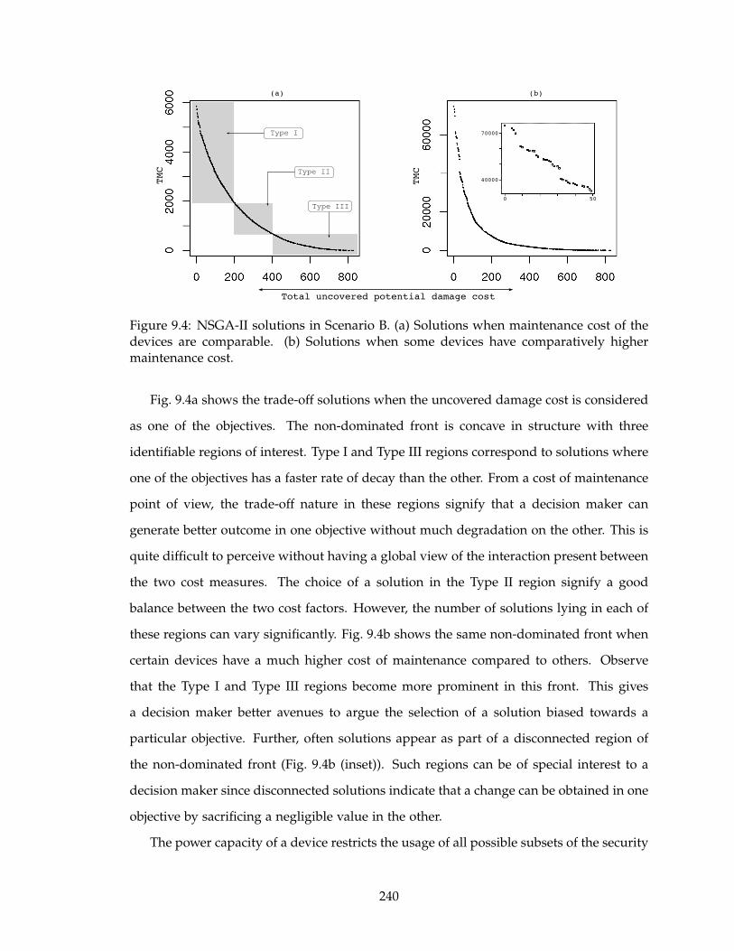
Type I
Type II
Type III
0 50
70000
40000
Total uncovered potential damage cost
TMC
TMC
(a) (b)
Figure 9.4: NSGA-II solutions in Scenario B. (a) Solutions when maintenance cost of thedevices are comparable. (b) Solutions when some devices have comparatively highermaintenance cost.
Fig. 9.4a shows the trade-off solutions when the uncovered damage cost is considered
as one of the objectives. The non-dominated front is concave in structure with three
identifiable regions of interest. Type I and Type III regions correspond to solutions where
one of the objectives has a faster rate of decay than the other. From a cost of maintenance
point of view, the trade-off nature in these regions signify that a decision maker can
generate better outcome in one objective without much degradation on the other. This is
quite difficult to perceive without having a global view of the interaction present between
the two cost measures. The choice of a solution in the Type II region signify a good
balance between the two cost factors. However, the number of solutions lying in each of
these regions can vary significantly. Fig. 9.4b shows the same non-dominated front when
certain devices have a much higher cost of maintenance compared to others. Observe
that the Type I and Type III regions become more prominent in this front. This gives
a decision maker better avenues to argue the selection of a solution biased towards a
particular objective. Further, often solutions appear as part of a disconnected region of
the non-dominated front (Fig. 9.4b (inset)). Such regions can be of special interest to a
decision maker since disconnected solutions indicate that a change can be obtained in one
objective by sacrificing a negligible value in the other.
The power capacity of a device restricts the usage of all possible subsets of the security
240
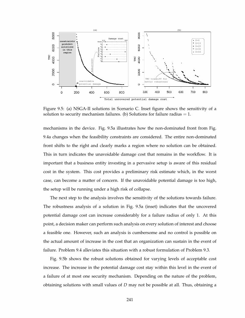
TMC
constraints
prohibit
solutions
in this
region
unavoidable
potential damage
410 560None
S1S2S3S4S5S6S7S8
Damage cost
Failure
Robustness
TMC
D=0
* D=10
+ D=20
D=30
x D=50
TMC tradeoff for
better robustness
Total uncovered potential damage cost
(a) (b)
Figure 9.5: (a) NSGA-II solutions in Scenario C. Inset figure shows the sensitivity of asolution to security mechanism failures. (b) Solutions for failure radius = 1.
mechanisms in the device. Fig. 9.5a illustrates how the non-dominated front from Fig.
9.4a changes when the feasibility constraints are considered. The entire non-dominated
front shifts to the right and clearly marks a region where no solution can be obtained.
This in turn indicates the unavoidable damage cost that remains in the workflow. It is
important that a business entity investing in a pervasive setup is aware of this residual
cost in the system. This cost provides a preliminary risk estimate which, in the worst
case, can become a matter of concern. If the unavoidable potential damage is too high,
the setup will be running under a high risk of collapse.
The next step to the analysis involves the sensitivity of the solutions towards failure.
The robustness analysis of a solution in Fig. 9.5a (inset) indicates that the uncovered
potential damage cost can increase considerably for a failure radius of only 1. At this
point, a decision maker can perform such analysis on every solution of interest and choose
a feasible one. However, such an analysis is cumbersome and no control is possible on
the actual amount of increase in the cost that an organization can sustain in the event of
failure. Problem 9.4 alleviates this situation with a robust formulation of Problem 9.3.
Fig. 9.5b shows the robust solutions obtained for varying levels of acceptable cost
increase. The increase in the potential damage cost stay within this level in the event of
a failure of at most one security mechanism. Depending on the nature of the problem,
obtaining solutions with small values of D may not be possible at all. Thus, obtaining a
241
certain level of robustness for a given level of security is not always feasible. However,
there could be areas where experimenting with different values of D can be beneficial in
understanding how the cost of maintenance changes with changing levels of robustness.
As is seen in this example, the increase in the cost of maintenance is much higher when
moving from a robustness level of D = 30 to 20 than moving from D = 50 to 30.
9.7 Conclusions
In this chapter, we address the problem of optimal security provisioning in pervasive
environments under the presence of energy constraints. We adopt a workflow model
to represent the different contexts under which a communication is established between
two devices. We provide a formal statement of the problem of security provisioning
and define a series of multi-objective optimization problems to understand the trade-offs
involved between the cost of maintenance and the security of a pervasive setup.
Our analysis reveals important parameters that a business entity should be aware of
before investing in the setup. First, the definition of “security” in the formulated prob-
lems plays an important role. Often, an attack-centric view of security is not enough
and emphasis must be paid rather to a damage-centric view. Good solutions protecting
against more attacks do not necessarily protect higher asset values. Also, the distribution
of these solutions on the objective space provide invaluable clues to a decision maker
on the amount of security gains possible across different levels of cost. The presence of
energy constraints results in an unavoidable potential damage always residual in the sys-
tem, early estimates on which can help the business entity invest better in risk mitigation
strategies. Risk estimates also depend on the robustness of a chosen solution. Our robust
formulation enables one to control the changes that can occur in the event of security
mechanism failure and explore the costs involved.
We acknowledge that the presented work involves various other areas of research that
require equal attention. The modeling of the different cost factors is a crucial aspect
without which optimization formulations are difficult to transition to the real world. We
can also explore the possibility of modifying the optimization framework to work on
workflow models that can be broken down into sub-workflows for scalability.
242
CHAPTER 10
Security Hardening on Bayesian Attack Graphs
Traditionally, information security planning and management for an organization
begins with risk assessment that determines threats to critical resources and the corre-
sponding loss expectancy. A number of researchers have proposed risk assessment meth-
ods by building security models of network systems, using paradigms like attack graphs
[10, 94, 141, 156, 166] and attack trees [43, 131, 145, 155], and then finding attack paths in
these models to determine scenarios that could lead to damage. However, a majority of
these models fail to consider the attacker’s capabilities and, consequently, the likelihood
of a particular attack being executed. Without these considerations, threats and their
impact can be easily misjudged.
To alleviate such drawbacks, Dantu et al. [42] propose a probabilistic model to as-
sess network risks. They model network vulnerabilities using attack graphs and applied
Bayesian logic to perform risk analysis. In a similar effort, Liu and Man [115] use Bayesian
networks to model potential attack paths in a system, and develop algorithms to compute
an optimal subset of attack paths based on background knowledge of attackers and attack
mechanisms. In both Dantu et al.’s and Liu and Man’s works, nodes in the attack graph
are assigned a probability value that describes the likelihood of attack on a node. They
compute the likelihood of system compromise by chaining Bayesian belief rules on top
of the assigned probabilities. The organizational risk is then computed as the product of
243

the likelihood of system compromise and the value of expected loss. The major problem
with both these works is that they do not specify how the conditional probability value
of an attack on each node is computed. Further, these works do not consider the problem
of optimal risk mitigation.
System administrators are often interested in assessing the risk to their systems and
determining the best possible way to defend their network in terms of an enumerated set
of hardening options. Risk assessment methods such as those discussed earlier have been
adopted by researchers to determine a set of potential safeguards, and related security
control installation costs. There is however a dynamic aspect to the security planning
process as well. For every attack, there is a certain probability of occurrence that can
change during the life time of a system depending on what the contributing factors for
the attack are and how they are changing. During run time, the system administrator
may need to revise her decision based on such emerging security conditions. The attack
tree model discussed in Section 8.3 does not allow such dynamic security planning.
Frigault et al. propose Bayesian network based attack graphs to incorporate temporal
factors, such as availability of exploit codes or security patches, in order to facilitate a
dynamic security planning process [71]. We can extend such concepts by encompassing
the influence of ongoing attack incidents as well. In particular, we can use forward and
backward probability inference techniques to assess the dynamic network security risk,
given one or more nodes have been compromised by ongoing attacks.
Collectively, this chapter attempts to address the limitations highlighted above. First,
we propose an alternative method of security risk assessment that we call Bayesian At-
tack Graphs (BAGs). In particular, we adapt the notion of Bayesian belief networks so as
to encode the contribution of different security conditions during system compromise.
Our model incorporates the usual cause-consequence relationships between different net-
work states (as in attack graphs and attack trees) and, in addition, takes into account the
likelihoods of exploiting such relationships. Second, we propose a method to estimate an
organization’s risk from different vulnerability exploitations based on the metrics defined
in the Common Vulnerability Scoring System (CVSS) [154]. CVSS is designed to be an
open and standardized method to rate IT vulnerabilities based on their base, temporal
244
and environmental properties. We also develop a model to quantify the expected return
on investment based on a user specified cost model and likelihoods of system compro-
mise. Third, we model the risk mitigation stage as a discrete reasoning problem and
propose a genetic algorithm to solve it. The algorithm can identify optimal mitigation
plans in the context of both single and multi-objective analysis. We also discuss how
the above contributions collectively provide a platform for static and dynamic analysis of
risks in networked systems.
The rest of the chapter is organized as follows. The test network used to illustrate
our problem formulation and solution is described in Section 10.1. Section 10.2 presents
the formalism for a Bayesian Attack Graph model. The likelihood estimation method in
static and dynamic scenarios is discussed in Section 10.3. The risk mitigation process
along with the expected cost computations is presented in Section 10.4. Empirical results
are presented in Section 10.5. Finally, we conclude Section 10.6.
10.1 A Test Network
Fig. 10.1 depicts the test network used in this study. The network consists of eight
hosts located within two sub-nets. A DMZ tri-homed firewall is installed with preset
policies to ensure that the Web server, Mail server and the DNS server, located in the
DMZ network, are separated from the local network so that the damage will only be
limited to the DMZ zone if one of these servers is compromised. The firewall has a
strong set of policies (shown in the inset table) to prevent remote access to the internal
hosts. In particular, all machines in the DMZ zone passively receive service requests and
only respond to the sender as needed. However, in order to accommodate Web service’s
transactions, the Web server is allowed to send SQL queries to the SQL server located
in the trusted zone on a designated channel. Local machines are located behind a NAT
firewall so that all communications to external parties are delivered through the Gateway
server. In addition, all local desktops, including the administrator machine, have remote
desktop enabled to facilitate remote operations for company employees working from
remote sites. The remote connections are monitored by SSHD installed in the Gateway
server.
245
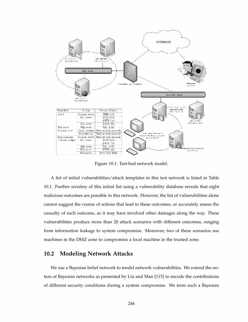
Figure 10.1: Test-bed network model.
A list of initial vulnerabilities/attack templates in this test network is listed in Table
10.1. Further scrutiny of this initial list using a vulnerability database reveals that eight
malicious outcomes are possible in this network. However, the list of vulnerabilities alone
cannot suggest the course of actions that lead to these outcomes, or accurately assess the
casualty of each outcome, as it may have involved other damages along the way. These
vulnerabilities produce more than 20 attack scenarios with different outcomes, ranging
from information leakage to system compromise. Moreover, two of these scenarios use
machines in the DMZ zone to compromise a local machine in the trusted zone.
10.2 Modeling Network Attacks
We use a Bayesian belief network to model network vulnerabilities. We extend the no-
tion of Bayesian networks as presented by Liu and Man [115] to encode the contributions
of different security conditions during a system compromise. We term such a Bayesian
246
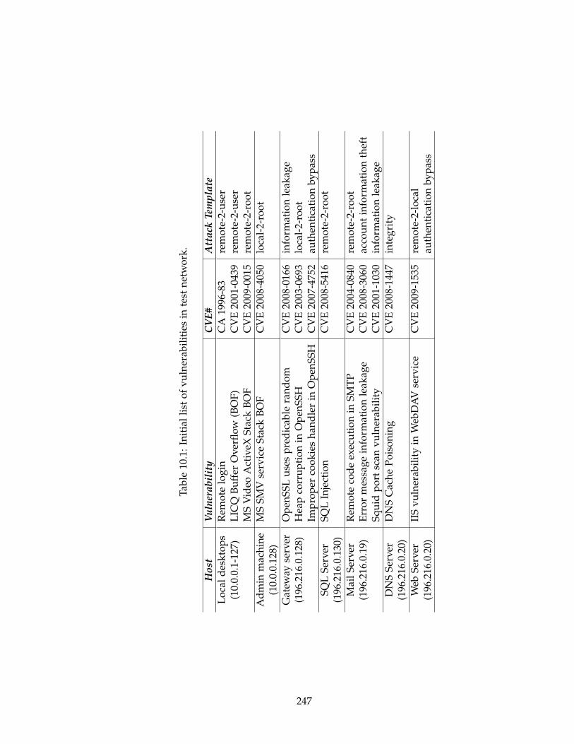
Tab
le10
.1:
Init
ial
list
of
vu
lner
abil
itie
sin
test
net
wo
rk.
Ho
stV
uln
era
bil
ity
CV
E#
Att
ack
Tem
pla
te
Lo
cal
des
kto
ps
Rem
ote
log
inC
A19
96-8
3re
mo
te-2
-use
r(1
0.0.
0.1-
127)
LIC
QB
uff
erO
ver
flo
w(B
OF
)C
VE
2001
-043
9re
mo
te-2
-use
rM
SV
ideo
Act
iveX
Sta
ckB
OF
CV
E20
09-0
015
rem
ote
-2-r
oo
t
Ad
min
mac
hin
eM
SS
MV
serv
ice
Sta
ckB
OF
CV
E20
08-4
050
loca
l-2-
roo
t(1
0.0.
0.12
8)
Gat
eway
serv
erO
pen
SS
Lu
ses
pre
dic
able
ran
do
mC
VE
2008
-016
6in
form
atio
nle
akag
e(1
96.2
16.0
.128
)H
eap
corr
up
tio
nin
Op
enS
SH
CV
E20
03-0
693
loca
l-2-
roo
tIm
pro
per
coo
kie
sh
and
ler
inO
pen
SS
HC
VE
2007
-475
2au
then
tica
tio
nb
yp
ass
SQ
LS
erv
erS
QL
Inje
ctio
nC
VE
2008
-541
6re
mo
te-2
-ro
ot
(196
.216
.0.1
30)
Mai
lS
erv
erR
emo
teco
de
exec
uti
on
inS
MT
PC
VE
2004
-084
0re
mo
te-2
-ro
ot
(196
.216
.0.1
9)E
rro
rm
essa
ge
info
rmat
ion
leak
age
CV
E20
08-3
060
acco
un
tin
form
atio
nth
eft
Sq
uid
po
rtsc
anv
uln
erab
ilit
yC
VE
2001
-103
0in
form
atio
nle
akag
e
DN
SS
erv
erD
NS
Cac
he
Po
iso
nin
gC
VE
2008
-144
7in
teg
rity
(196
.216
.0.2
0)
Web
Ser
ver
IIS
vu
lner
abil
ity
inW
ebD
AV
serv
ice
CV
E20
09-1
535
rem
ote
-2-l
oca
l(1
96.2
16.0
.20)
auth
enti
cati
on
by
pas
s
247

network as a Bayesian Attack Graph (BAG).
Using the notion of an attribute-template as defined in Section 8.3, we define an at-
tribute in a BAG as follows.
Definition 10.1 ATTRIBUTE. An attribute is a Bernoulli random variable representing
the state of an instance of an attribute-template.
An attribute S is therefore associated with a state – True (S = 1/T) or False (S = 0/F) –
and a probability Pr(S). The state signifies the truth value of the proposition underlined
by the instance of the attribute template. For example, the instance S :“user access on
Local machine” is an attribute when associated with a truth value signifying whether an
attacker has user access on the local machine. We shall also use the term “compromised”
to indicate the true (or S = 1) state of an attribute. Further, Pr(S) is the probability of the
attribute being in state S = 1. Consequently, Pr(¬S) = 1 − Pr(S) is the probability of the
state being S = 0. The success or failure of an attacker reaching its goal depends mostly
on the states of the attributes in a network. It also lays the foundations for a security
manager to analyze the effects of forcing some attributes to the false state using security
measures. We formally define a BAG to capture the cause-consequence relationships
between such attributes.
Definition 10.2 ATOMIC ATTACK. Let S be a set of attributes. We define A, a conditional
dependency between a pair of attributes, as a mapping A : S × S → [0,1]. Then, given
Spre,Spost ∈ S, a : Spre 7→ Spost is called an atomic attack if
1. Spre 6= Spost,
2. given Spre = 1, we also have Spost = 1 with probability A(Spre,Spost) > 0, and
3. ∄S1, . . . ,Sj ∈ S−{Spre,Spost} such that A(Spre,S1) > 0,A(S1,S2) > 0, . . . , and A(Sj,Spost)
> 0.
Therefore, an atomic attack allows an attacker to compromise the attribute Spost from
Spre with a non-zero probability of success. Although, given a compromised attribute,
another attribute can be compromised with positive probability using a chain of other
248

attributes, the third condition in the definition does not allow such instances to be consid-
ered as atomic attacks. Instead, each step in such a chain is an atomic attack. Informally,
an attack is associated with a vulnerability exploitation, denoted by ei, which takes the
attacker from one network state (Spre) to another (Spost). The probability of an exploita-
tion, Pr(ei), states the ease with which an attacker can perform the exploitation. Hence,
we say that A(Spre,Spost) = Pr(ei), and Spre and Spost are respectively called a precondition
and postcondition of the attack a, denoted by pre(a) and post(a) respectively.
An attack relates the states of two different attributes so as to embed a cause-consequence
relationship between the two. For example, for the attributes Spre =“sshd BOF vulnerabil-
ity on machine A” and Spost =“root access privilege on machine A”, the attack Spre 7→ Spost is
associated with the ei =“sshd buffer overflow” exploit. Using this exploit, an attacker can
achieve root privilege on a machine provided the machine has the sshd BOF vulnerability.
A(Spre,Spost) is the probability of success of the exploit, i.e. A(Spre,Spost) = Pr(ei).
Definition 10.3 BAYESIAN ATTACK GRAPH. Let S be a set of attributes and A be the
set of atomic attacks defined on S. A Bayesian Attack Graph is a tuple BAG = (S,τ, ε,P),
where
1. S = Ninternal ∪ Nexternal ∪ Nterminal . Nexternal denotes the set of attributes Si for which
∄a ∈ A|Si = post(a). Ninternal denotes the set of attributes Sj for which ∃a1, a2 ∈A|[Sj = pre(a1) and Sj = post(a2)]. Nterminal denotes the set of attributes Sk for which
∄a ∈ A|Sk = pre(a).
2. τ ⊆ S × S. An ordered pair (Spre,Spost) ∈ τ if Spre 7→ Spost ∈ A. Further, for Si ∈ S,
the set Pa[Si] = {Sj ∈ S|(Sj,Si) ∈ τ} is called the parent set of Si.
3. ε is a set of decomposition tuples of the form 〈Sj,dj〉 defined for all Sj ∈ Ninternal ∪Nterminal and dj ∈ {AND,OR}. dj is AND if Sj = 1 ⇒ ∀Si ∈ Pa[Sj],Si = 1. dj is OR if
Sj = 1 ⇒ ∃Si ∈ Pa[Sj],Si = 1.
4. P is a set of discrete conditional probability distribution functions. Each attribute
Sj ∈ Ninternal ∪ Nterminal has a discrete local conditional probability distribution (LCPD)
representing the values of Pr(Sj | Pa[Sj]).
249
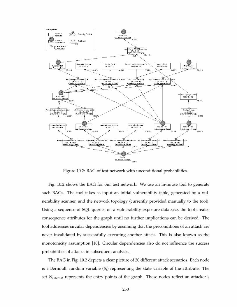
Figure 10.2: BAG of test network with unconditional probabilities.
Fig. 10.2 shows the BAG for our test network. We use an in-house tool to generate
such BAGs. The tool takes as input an initial vulnerability table, generated by a vul-
nerability scanner, and the network topology (currently provided manually to the tool).
Using a sequence of SQL queries on a vulnerability exposure database, the tool creates
consequence attributes for the graph until no further implications can be derived. The
tool addresses circular dependencies by assuming that the preconditions of an attack are
never invalidated by successfully executing another attack. This is also known as the
monotonicity assumption [10]. Circular dependencies also do not influence the success
probabilities of attacks in subsequent analysis.
The BAG in Fig. 10.2 depicts a clear picture of 20 different attack scenarios. Each node
is a Bernoulli random variable (Si) representing the state variable of the attribute. The
set Nexternal represents the entry points of the graph. These nodes reflect an attacker’s
250

capability as discovered in a threat-source model. Nterminal resemble the end points in the
graph. These nodes reflect casualty at the end of each attack scenario. The set of ordered
pair, τ, reflects the edges in the graph. The existence of an edge between two nodes imply
that there is a causal dependency between their states, signified by the decomposition at
each node. AND-decomposition signifies that the compromised state of a node implies
that all nodes in its parent set have also been compromised. Similarly, OR-decomposition
signifies that at least one parent node is in the true state. Note that these decompositions
are uni-directional. For instance, under AND-decomposition, compromising all nodes in
the parent set does not necessarily imply the node itself has been compromised. This is
because the attacks relating the node with its parents can have varying levels of difficulty,
or in other words, different probabilities of success. Hence, although the preconditions
of the attacks have been met, there can still be a non-zero probability that the attacker
is unable to carry out all the exploits successfully. The existence of this probability is
what primarily differentiates a BAG from a classical attack graph. The probabilities are
captured in the local conditional probability distribution of the node. The LCPD is a set of
probability values specifying the chances of the node being compromised, given different
combination of states of its parents.
Definition 10.4 LOCAL CONDITIONAL PROBABILITY DISTRIBUTION. Let (S,τ, ε,P)
be a BAG and Sj ∈ Ninternal ∪ Nterminal . For Si ∈ Pa[Sj], let ei be the vulnerability ex-
ploitation associated with the attack Si 7→ Sj. A local conditional probability distribution
(LCPD) function of Sj, mathematically equivalent to Pr(Sj | Pa[Sj]), is defined as follows.
1. dj = AND
Pr(Sj | Pa[Sj]) =
0, ∃Si ∈ Pa[Sj] | Si = 0
Pr(⋂
Si=1ei), otherwise (10.1)
2. dj = OR
Pr(Sj | Pa[Sj]) =
0, ∀Si ∈ Pa[Sj],Si = 0
Pr(⋃
Si=1ei), otherwise (10.2)
To compute the local conditional probabilities when multiple exploits are involved, we
proceed as follows. For AND-decomposition, each vulnerability exploitation is a distinct
251
event. The chance of compromising the target node depends on the success of each
individual exploit. Therefore, we use the product rule in probability to derive Pr(⋂
Si=1ei)
as
Pr(⋂
Si=1
ei) = ∏Si=1
Pr(ei). (10.3)
For OR-decomposition, Liu et al. observed that the joint probability is equivalent to the
noisy-OR operator [115], given as
Pr(⋃
Si=1
ei) = 1 − ∏Si=1
[1 − Pr(ei)] . (10.4)
10.3 Security Risk Assessment with BAG
Security risk management consists of threat analysis, risk assessment, loss expectancy,
potential safeguards and risk mitigation analysis. A BAG positions itself between threat
analysis and risk assessment. Threat sources and the list of initial vulnerabilities are used
to build the BAG threat model. Once the graph is built, the administrator can expect
better results in risk assessment and risk mitigation analysis as follows.
Static Risk Assessment: Risk assessment begins with the identification of system char-
acteristics, potential threat sources and attacker capabilities. Threat sources are
represented as the external nodes in a BAG, along with their impact on other net-
work attributes. One set of attributes act as preconditions to an exploit, which when
successfully executed by an attacker, can make the network state favorable for sub-
sequent exploits. Estimating the amount of risk at each node therefore requires
some judgment on attacker capabilities. Often this judgment is indirectly stated
as the system administrator’s subjective belief on the likelihood of a threat source
becoming active and the difficulty of an exploit. The former is represented by the
probabilities Pr(Si) for all Si ∈ Nexternal , also called the prior probabilities, and is sub-
jectively assigned by the administrator. The latter is incorporated into an internal
node’s LCPD. Thereafter, given the prior probability values and the LCPDs, we can
compute the unconditional probability Pr(Sj) for any node Sj ∈ Ninternal ∪ Nterminal .
252
These risk estimates can be used to help locate weak spots in the system design and
operations.
Dynamic Risk Assessment: A deployed system may experience first hand attack inci-
dents during its life cycle. Formally, an attack incident is evidence that an attribute
is in the true state. A security administrator may then want to investigate how these
incidents impact the risk estimates initially derived solely based on subjective be-
liefs. Knowledge about attack incidents is therefore used to update the probabilities
using the Bayesian inference techniques of forward and backward propagation. For-
ward propagation updates the probability on successor attributes that are directly
influenced by the evidences. Backward propagation corrects/adjusts the initial hy-
pothesis on all prior attributes. Thereafter, the posterior probabilities (updated uncon-
ditional probabilities) reflect the likelihoods of other potential outcomes under the
light of detected events.
Risk Mitigation Analysis: Risk assessment paves the way for efficient decision making
targeted at countering risks either in a proactive or reactive manner. Given a set
of security measures (e.g. firewall, access control policy, cryptography, etc.), we can
design the security plan which is the most resource efficient in terms of reducing
risk levels in the system. This can be done before the deployment (static mitigation)
or in response to attack incidents (dynamic mitigation).
10.3.1 Probability of vulnerability exploitation
In order to compute the local conditional probability distribution (LCPD) of an at-
tribute, the administrator needs to estimate the probability of success when an attacker
exploits a known vulnerability exploitation. We propose a method to estimate this at-
tack likelihood using publicly available risk exposure data sources. In particular, we are
interested in deriving attack likelihoods using the metrics defined in NIST’s Common
Vulnerability Scoring System (CVSS) [154].
A CVSS score is a decimal number on a scale of 0 to 10. It is composed of three groups
– base, temporal and environmental. The base metrics quantify the intrinsic characteristics
of a vulnerability with two sub-scores – (i) the exploitability sub-score, composed of the
253
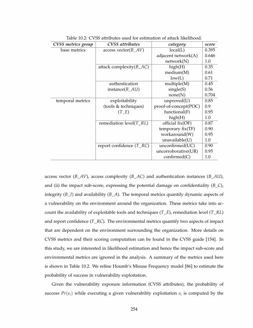
Table 10.2: CVSS attributes used for estimation of attack likelihood.
CVSS metrics group CVSS attributes category score
base metrics access vector(B_AV) local(L) 0.395adjacent network(A) 0.646
network(N) 1.0attack complexity(B_AC) high(H) 0.35
medium(M) 0.61low(L) 0.71
authentication multiple(M) 0.45instance(B_AU) single(S) 0.56
none(N) 0.704
temporal metrics exploitability unproved(U) 0.85(tools & techniques) proof-of-concept(POC) 0.9
(T_E) functional(F) 0.95high(H) 1.0
remediation level(T_RL) official fix(OF) 0.87temporary fix(TF) 0.90workaround(W) 0.95unavailable(U) 1.0
report confidence (T_RC) unconfirmed(UC) 0.90uncorroborative(UR) 0.95
confirmed(C) 1.0
access vector (B_AV), access complexity (B_AC) and authentication instances (B_AU),
and (ii) the impact sub-score, expressing the potential damage on confidentiality (B_C),
integrity (B_I) and availability (B_A). The temporal metrics quantify dynamic aspects of
a vulnerability on the environment around the organization. These metrics take into ac-
count the availability of exploitable tools and techniques (T_E), remediation level (T_RL)
and report confidence (T_RC). The environmental metrics quantify two aspects of impact
that are dependent on the environment surrounding the organization. More details on
CVSS metrics and their scoring computation can be found in the CVSS guide [154]. In
this study, we are interested in likelihood estimation and hence the impact sub-score and
environmental metrics are ignored in the analysis. A summary of the metrics used here
is shown in Table 10.2. We refine Houmb’s Misuse Frequency model [86] to estimate the
probability of success in vulnerability exploitation.
Given the vulnerability exposure information (CVSS attributes), the probability of
success Pr(ei) while executing a given vulnerability exploitation ei is computed by the
254
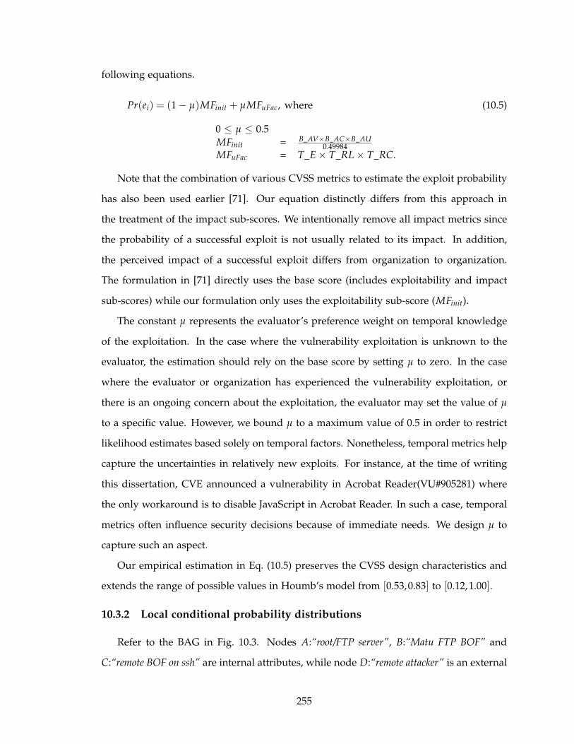
following equations.
Pr(ei) = (1 − µ)MFinit + µMFuFac, where (10.5)
0 ≤ µ ≤ 0.5
MFinit = B_AV×B_AC×B_AU0.49984
MFuFac = T_E × T_RL × T_RC.
Note that the combination of various CVSS metrics to estimate the exploit probability
has also been used earlier [71]. Our equation distinctly differs from this approach in
the treatment of the impact sub-scores. We intentionally remove all impact metrics since
the probability of a successful exploit is not usually related to its impact. In addition,
the perceived impact of a successful exploit differs from organization to organization.
The formulation in [71] directly uses the base score (includes exploitability and impact
sub-scores) while our formulation only uses the exploitability sub-score (MFinit).
The constant µ represents the evaluator’s preference weight on temporal knowledge
of the exploitation. In the case where the vulnerability exploitation is unknown to the
evaluator, the estimation should rely on the base score by setting µ to zero. In the case
where the evaluator or organization has experienced the vulnerability exploitation, or
there is an ongoing concern about the exploitation, the evaluator may set the value of µ
to a specific value. However, we bound µ to a maximum value of 0.5 in order to restrict
likelihood estimates based solely on temporal factors. Nonetheless, temporal metrics help
capture the uncertainties in relatively new exploits. For instance, at the time of writing
this dissertation, CVE announced a vulnerability in Acrobat Reader(VU#905281) where
the only workaround is to disable JavaScript in Acrobat Reader. In such a case, temporal
metrics often influence security decisions because of immediate needs. We design µ to
capture such an aspect.
Our empirical estimation in Eq. (10.5) preserves the CVSS design characteristics and
extends the range of possible values in Houmb’s model from [0.53,0.83] to [0.12,1.00].
10.3.2 Local conditional probability distributions
Refer to the BAG in Fig. 10.3. Nodes A:“root/FTP server”, B:“Matu FTP BOF” and
C:“remote BOF on ssh” are internal attributes, while node D:“remote attacker” is an external
255
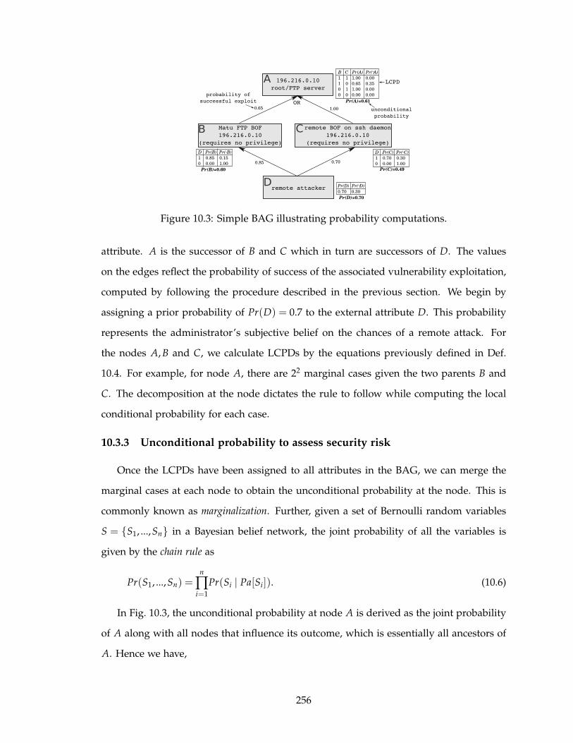
A
B C
D
196.216.0.10
root/FTP server
Matu FTP BOF
196.216.0.10
(requires no privilege)
remote BOF on ssh daemon
196.216.0.10
(requires no privilege)
remote attacker
B C Pr(A) Pr( A)
1 1 1.00 0.00
1 0 0.65 0.35
0 1 1.00 0.00
0 0 0.00 0.00
D Pr(C) Pr( C)
1 0.70 0.30
0 0.00 1.00
D Pr(B) Pr( B)
1 0.85 0.15
0 0.00 1.00
Pr(D) Pr( D)
0.70 0.30
0.85 0.70
1.000.65
Pr(D)=0.70
Pr(C)=0.49Pr(B)=0.60
Pr(A)=0.61
LCPD
unconditional
probability
probability of
successful exploit OR
Figure 10.3: Simple BAG illustrating probability computations.
attribute. A is the successor of B and C which in turn are successors of D. The values
on the edges reflect the probability of success of the associated vulnerability exploitation,
computed by following the procedure described in the previous section. We begin by
assigning a prior probability of Pr(D) = 0.7 to the external attribute D. This probability
represents the administrator’s subjective belief on the chances of a remote attack. For
the nodes A, B and C, we calculate LCPDs by the equations previously defined in Def.
10.4. For example, for node A, there are 22 marginal cases given the two parents B and
C. The decomposition at the node dictates the rule to follow while computing the local
conditional probability for each case.
10.3.3 Unconditional probability to assess security risk
Once the LCPDs have been assigned to all attributes in the BAG, we can merge the
marginal cases at each node to obtain the unconditional probability at the node. This is
commonly known as marginalization. Further, given a set of Bernoulli random variables
S = {S1, ...,Sn} in a Bayesian belief network, the joint probability of all the variables is
given by the chain rule as
Pr(S1, ...,Sn) =n
∏i=1
Pr(Si | Pa[Si]). (10.6)
In Fig. 10.3, the unconditional probability at node A is derived as the joint probability
of A along with all nodes that influence its outcome, which is essentially all ancestors of
A. Hence we have,
256

Pr(A) = Pr(A, B,C, D)= Pr(A | B,C) × Pr(B | D) × Pr(C | D) × Pr(D) (chain rule)= ∑
B,C,D∈{T,F}[Pr(A | B,C) × Pr(B | D) × Pr(C | D) × Pr(D)] (marginalization)
= (1.0 × 0.85 × 0.7 × 0.7)TTT + (0.65 × 0.85 × 0.3 × 0.7)TFT+(1.0 × 0.15 × 0.7 × 0.7)FTT (after simplification)
= 0.6060 ≈ 61%.
Similarly, unconditional probabilities at nodes B and C can be computed by consider-
ing the sub-network rooted at the corresponding nodes. The unconditional probabilities
are shown under the LCPD table of each node. Fig. 10.2 shows the unconditional proba-
bilities of the nodes in our test network. It exposes the weak spots of the system where
the likelihood of attack is higher than others. The security administrator can use this
threat model to prioritize risk and derive an effective security hardening plan so as to
reduce the risk to a certain level (e.g. < 50%) before deploying the system. The model can
also be used to assess what-if scenarios, for e.g. while deploying new machines, services,
or operations of interest.
10.3.4 Posterior probability with attack evidence
The BAG can also be used to address dynamic aspects of the security planning pro-
cess. Every network state has a certain probability of occurrence. This probability can
change during the life time of the system due to emerging security conditions, changes
in contributing factors or the occurrence of attack incidents. The BAG can then be used
to calculate the posterior probabilities in order to evaluate the risk from such emerging
conditions.
Let S = {S1, ...,Sn} be the set of attributes in a BAG and E = {S′1, ...,S′
m} ⊂ S be a
set of attributes where some evidence of exploit have been observed. We can say that
attributes in E are in the true state, i.e. S′i = 1 for all S′
i ∈ E. Let Sj ∈ S − E be an attribute
whose posterior probability has to be determined. The probability we are interested in is
Pr(Sj | E) and can be obtained by using the Bayes Theorem, given as
Pr(Sj | E) = Pr(E | Sj) × Pr(Sj)/Pr(E). (10.7)
Pr(E | Sj) is the conditional probability of joint occurrence of S′1, ...,S′
m given the states
257

of Sj. Pr(E) and Pr(Sj) are the prior unconditional probability values of the correspond-
ing attributes. Since evidence attributes in E are mutually independent, Pr(E | Sj) =
∏i Pr(S′i | Sj) and Pr(E) = ∏i Pr(S′
i). For example, in Fig. 10.3, assume that the system
administrator detects an attack incident on A (attacker compromises FTP server). The
posterior probability of C is then computed as follows.
Pr(C | A) = Pr(A | C)Pr(C)/Pr(A)= 0.81, where
Pr(A | C) = ∑B∈{T,F} [Pr(A | B,C = T)Pr(B)]= (1.0 × 0.6)T + (1.0 × 0.4)F
= 1.0Pr(A) = 0.61Pr(C) = 0.49
Similarly, the posterior probability at node B can be computed in the same manner.
Note that the unconditional probability of node C was originally 0.49. After taking into
account the attack incident at node A, the posterior probability becomes 0.81. Further,
computation of posterior probabilities for successor nodes of A (forward propagation)
remain the same as described in the previous sub-section, with the change that the LCPDs
at those nodes only account for the A = 1 case while marginalization. In this manner, the
security administrator can revise the probability of occurrence of every node of the graph
in response to an emerging attack incident. Fig. 10.4 shows the posterior probabilities
in response to two hypothetical evidences (denoted by the label E©) in the Mail server
of our test network. Note that the parent (“root access @ 196.216.0.19”) of the evidence
node “squid port scan” has a posterior probability of less than 1.0. Ideally, given the
evidence that the port scan has been executed, the attacker must have had root access
on the machine. Hence, the parent node should also have an updated probability of
1.0. However, this inference assumes that the squid port scan is only executable after
gaining root access on the machine. The system administrator may decide to relax such
an assumption in order to account for uncertainties (e.g. zero-day attacks), achieved by
replacing the zero values in Def. 10.4 with non-zero values. Such a relaxation will reduce
the impact of the evidence nodes on their parents.
As can be seen in Fig. 10.4, most of the unconditional probabilities increase after the
attack incidents, but not at the same rate. It is possible to have nodes with decreased
258
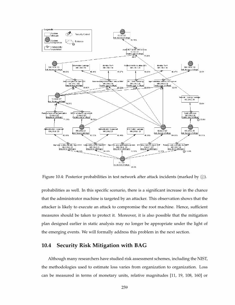
Figure 10.4: Posterior probabilities in test network after attack incidents (marked by E©).
probabilities as well. In this specific scenario, there is a significant increase in the chance
that the administrator machine is targeted by an attacker. This observation shows that the
attacker is likely to execute an attack to compromise the root machine. Hence, sufficient
measures should be taken to protect it. Moreover, it is also possible that the mitigation
plan designed earlier in static analysis may no longer be appropriate under the light of
the emerging events. We will formally address this problem in the next section.
10.4 Security Risk Mitigation with BAG
Although many researchers have studied risk assessment schemes, including the NIST,
the methodologies used to estimate loss varies from organization to organization. Loss
can be measured in terms of monetary units, relative magnitudes [11, 19, 108, 160] or
259
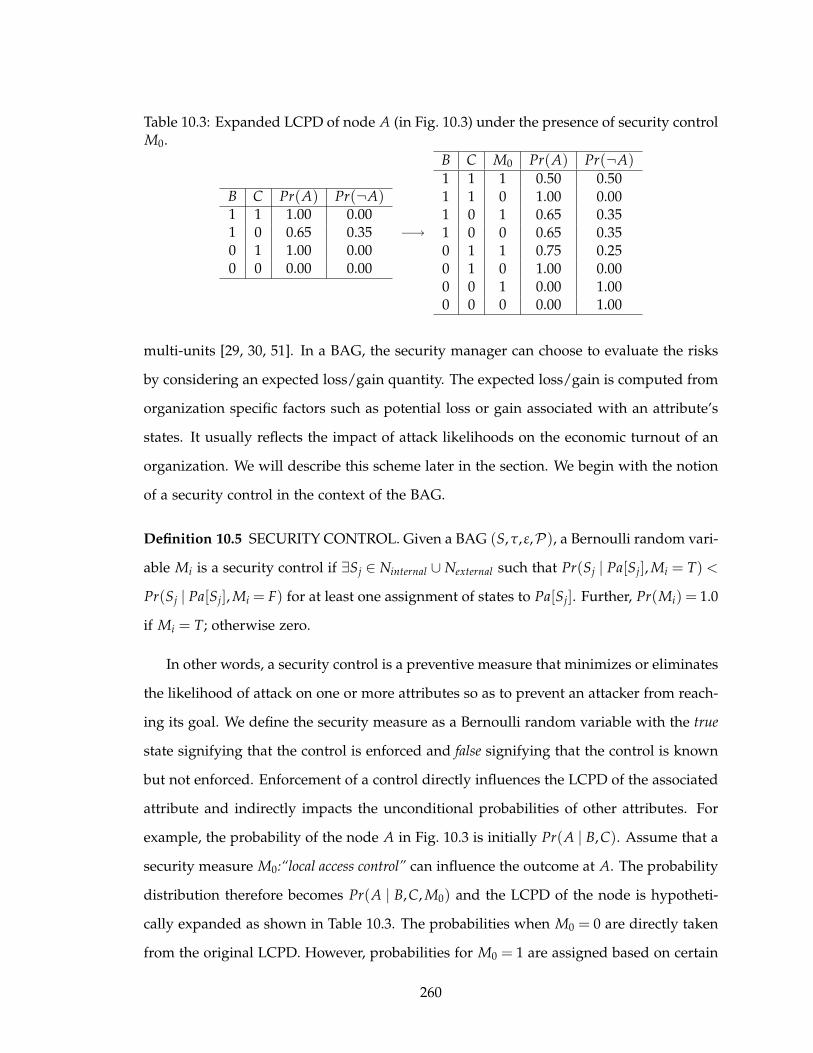
Table 10.3: Expanded LCPD of node A (in Fig. 10.3) under the presence of security controlM0.
B C Pr(A) Pr(¬A)1 1 1.00 0.001 0 0.65 0.35 −→0 1 1.00 0.000 0 0.00 0.00
B C M0 Pr(A) Pr(¬A)1 1 1 0.50 0.501 1 0 1.00 0.001 0 1 0.65 0.351 0 0 0.65 0.350 1 1 0.75 0.250 1 0 1.00 0.000 0 1 0.00 1.000 0 0 0.00 1.00
multi-units [29, 30, 51]. In a BAG, the security manager can choose to evaluate the risks
by considering an expected loss/gain quantity. The expected loss/gain is computed from
organization specific factors such as potential loss or gain associated with an attribute’s
states. It usually reflects the impact of attack likelihoods on the economic turnout of an
organization. We will describe this scheme later in the section. We begin with the notion
of a security control in the context of the BAG.
Definition 10.5 SECURITY CONTROL. Given a BAG (S,τ, ε,P), a Bernoulli random vari-
able Mi is a security control if ∃Sj ∈ Ninternal ∪ Nexternal such that Pr(Sj | Pa[Sj], Mi = T) <
Pr(Sj | Pa[Sj], Mi = F) for at least one assignment of states to Pa[Sj]. Further, Pr(Mi) = 1.0
if Mi = T; otherwise zero.
In other words, a security control is a preventive measure that minimizes or eliminates
the likelihood of attack on one or more attributes so as to prevent an attacker from reach-
ing its goal. We define the security measure as a Bernoulli random variable with the true
state signifying that the control is enforced and false signifying that the control is known
but not enforced. Enforcement of a control directly influences the LCPD of the associated
attribute and indirectly impacts the unconditional probabilities of other attributes. For
example, the probability of the node A in Fig. 10.3 is initially Pr(A | B,C). Assume that a
security measure M0:“local access control” can influence the outcome at A. The probability
distribution therefore becomes Pr(A | B,C, M0) and the LCPD of the node is hypotheti-
cally expanded as shown in Table 10.3. The probabilities when M0 = 0 are directly taken
from the original LCPD. However, probabilities for M0 = 1 are assigned based on certain
260

subjective belief on the security measure’s capacity to prevent the attribute’s compromise.
The modified LCPDs are used to compute the unconditional probability of nodes in the
graph. It is not difficult to see that the unconditional probability of a node (and its suc-
cessors) influenced by a control will reduce when the control is enforced. Note that, by
definition, the unconditional probability of the control itself is 1.0 if its state is true.
Definition 10.6 SECURITY MITIGATION PLAN. Given set M = {M1, . . . , Mm} of m secu-
rity controls, a security mitigation plan is represented by a boolean vector ~T = (T1,T2, . . . , Tm)
where Mi = Ti.
Therefore, the mitigation plan is a specification of which controls have been chosen for
enforcement as part of the hardening process. Further, for a given control Mi, consider the
set I of all Sj ∈ Ninternal ∪ Nterminal such that Pr(Sj | Pa[Sj], Mi = T) < Pr(Sj | Pa[Sj], Mi = F)
(for some assignment of states to Pa[Sj]). Then, the subset {Sk ∈ I|Pa[Sk] ∩ I = φ} is the
coverage of Mi. With reference to Fig. 10.3, a control such as M0:“disconnect from Internet”
directly changes the probability Pr(D) (equal to zero if M0 = 1). This in effect changes
the LCPD tables at nodes B, C and D. Therefore, the set I contains all four nodes for M0.
However, only node D is in the coverage of M0 since, for all other nodes, one or more
parent nodes are also present in I . Intuitively, the coverage nodes are those whose LCPDs
are directly affected by a security control, rather than by indirect inference. For a given
security mitigation plan ~T, we can define the plan coverage by collecting the coverage
of each enforced control in the plan. Each control Mi also has an associated cost Ci of
implementation, giving us the total plan cost as
SCC(~T) =m
∑i=1
(TiCi). (10.8)
10.4.1 Assessing security outcomes
When using a BAG, a better quantitative representation of the loss/gain is obtained
by considering the expected loss/gain once a set of security measures have been imple-
mented. Hence, we augment the BAG with a value signifying the amount of potential
loss/gain at each node, and account for the security decision during evaluation.
261

Definition 10.7 AUGMENTED-BAYESIAN ATTACK GRAPH. Let BAG = (S,τ, ε,P) be a
Bayesian attack graph. An augmented-Bayesian attack graph (augmented-BAG) BAGaug =
BAG|(M,γ,V) is obtained by adding a node set M, edge set γ and by associating a value
Vj to each Sj ∈ S, where
1. M is the set of security controls.
2. γ ⊆ M × S. An ordered pair (Mi,Sj) ∈ γ if Sj is in the coverage of Mi.
3. Vj is the expected loss/gain associated with the attribute Sj ∈ S.
The set M extends the BAG with additional nodes representing hardening measures.
The set γ represents the new edges between the controls and attributes of the graph. A
new edge is inserted if a control directly influences the state of an attribute. In this work,
all external attributes are given a zero cost, i.e. Vj = 0 for all Sj ∈ Nexternal . The value
associated with Sj ∈ Ninternal ∪ Nterminal is computed as
Vj =[
1 − Pr(Sj)]
× Gj − Pr(Sj) × Lj, (10.9)
where Lj is the potential loss representing the damage value that an organization might
have to pay when the attribute Sj is compromised, Gj is the potential gain if Sj is not
compromised and Pr(Sj) is the unconditional probability of Sj. If there exists (Mi,Sj) ∈ γ,
Pr(Sj) is computed as a conditional probability Pr(Sj | Mi) where the state of Mi depends
on the security plan ~T = (Ti). The expected loss/gain w.r.t. the security plan ~T, denoted
by LG(~T), is computed as the cumulative sum of all node values, i.e.
LG(~T) = ∑Sj∈S
Vj. (10.10)
A positive value of LG signifies gain, while a negative value signifies loss. Note that
we do not assume any particular cost model in our formulations, both for control cost
and loss/gain evaluation. The cost model is usually subjective to organizational policies
and hence can differ from one institution to another. The cost factors considered here
(security control cost, potential loss and potential gain) are standard quantities that any
organization must be able to determine in order to perform risk analysis.
262

10.4.2 Assessing the security mitigation plan
In order to defend against the attacks possible, a security manager (as a decision
maker) can choose to implement a variety of safeguard technologies, each of which comes
with different cost and coverage. For example, to defend against the “ftp/.rhost” exploit,
one might choose to apply a security patch, firewall, or simply disable the FTP service.
Each choice of action has a different cost and different outcome. A security administrator
has to assess the technologies and make a decision towards maximum resource utilization.
The two objectives we consider in this study are the total security control cost and the
expected loss/gain. The single-objective problem is the most likely approach to be taken
by a decision maker. The problem is stated as follows.
Problem 10.1 The Single-Objective Optimization Problem (SOOP). Given an augmented-
BAG (S,τ, ε,P) | (M,γ,V), find a vector ~T∗ = (T∗i ), T∗
i ∈ {0,1};1 ≤ i ≤ |M|, which max-
imizes the function αLG( ~T∗) − βSCC( ~T∗), where α and β are preference weights for the
expected loss/gain and the total cost of security control respectively, 0 ≤ α, β ≤ 1 and
α + β = 1.
The method for assessing a security plan is as follows. First, the security analyst
chooses a subset of security controls to construct a security plan ~T∗. She then updates
the unconditional probability of all attributes using the plan coverage information. She
computes the expected loss/gain associated with every attribute Sj ∈ S using Eq. (10.9).
Finally, the total expected loss/gain of the entire graph is taken as an assessment of the
security plan’s outcome. The best security plan is the one that maximizes the function
αLG( ~T∗) − βSCC( ~T∗).
The next level of sophistication is added by formulating the optimization as a multi-
objective problem. The multi-objective approach alleviates the requirement to specify any
weight parameters and hence a better global picture of the solutions can be obtained.
Problem 10.2 The Multi-Objective Optimization Problem (MOOP). Given an augmented-
BAG (S,τ, ε,P) | (M,γ,V), find a vector ~T∗ = (T∗i ), T∗
i ǫ{0,1};1 ≤ i ≤ |M|, which mini-
mizes SCC and maximizes LG.
263
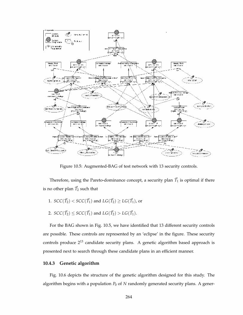
Figure 10.5: Augmented-BAG of test network with 13 security controls.
Therefore, using the Pareto-dominance concept, a security plan ~T1 is optimal if there
is no other plan ~T2 such that
1. SCC(~T2) < SCC(~T1) and LG(~T2) ≥ LG(~T1), or
2. SCC(~T2) ≤ SCC(~T1) and LG(~T2) > LG(~T1).
For the BAG shown in Fig. 10.5, we have identified that 13 different security controls
are possible. These controls are represented by an ‘eclipse’ in the figure. These security
controls produce 213 candidate security plans. A genetic algorithm based approach is
presented next to search through these candidate plans in an efficient manner.
10.4.3 Genetic algorithm
Fig. 10.6 depicts the structure of the genetic algorithm designed for this study. The
algorithm begins with a population P0 of N randomly generated security plans. A gener-
264
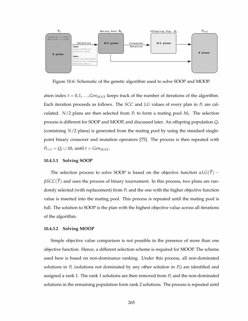
Pt Pt+1Mating Pool M
Selection Crossover
Mutation
(1,0,1,1,....,1,1)
(0,1,1,0,....,1,0)
.
.
.
N plans
N/2 plans N/2 plans
N plans
SOOP:
using objective
function value
MOOP:
using non-dominated
ranking and crowding
distance metric
Offspring Pop. Qtt
Figure 10.6: Schematic of the genetic algorithm used to solve SOOP and MOOP.
ation index t = 0,1, . . . , GenMAX keeps track of the number of iterations of the algorithm.
Each iteration proceeds as follows. The SCC and LG values of every plan in Pt are cal-
culated. N/2 plans are then selected from Pt to form a mating pool Mt. The selection
process is different for SOOP and MOOP, and discussed later. An offspring population Qt
(containing N/2 plans) is generated from the mating pool by using the standard single-
point binary crossover and mutation operators [75]. The process is then repeated with
Pt+1 = Qt ∪ Mt until t = GenMAX.
10.4.3.1 Solving SOOP
The selection process to solve SOOP is based on the objective function αLG(~T) −βSCC(~T) and uses the process of binary tournament. In this process, two plans are ran-
domly selected (with replacement) from Pt and the one with the higher objective function
value is inserted into the mating pool. This process is repeated until the mating pool is
full. The solution to SOOP is the plan with the highest objective value across all iterations
of the algorithm.
10.4.3.2 Solving MOOP
Simple objective value comparison is not possible in the presence of more than one
objective function. Hence, a different selection scheme is required for MOOP. The scheme
used here is based on non-dominance ranking. Under this process, all non-dominated
solutions in Pt (solutions not dominated by any other solution in Pt) are identified and
assigned a rank 1. The rank 1 solutions are then removed from Pt and the non-dominated
solutions in the remaining population form rank 2 solutions. The process is repeated until
265

all solutions are assigned a rank. Selection of N/2 solutions for the mating pool is then
performed according to increasing rank. The crowding distance metric [48] is used if the
number of solutions required to fill the mating pool is lower than the available solutions
in the rank being considered. The crowding distance of a solution is the perimeter of the
rectangle formed by its two neighbors of the same rank; the distance is infinite for points
having less than two neighbors (e.g. extreme points). Choice of solutions within a rank
is done in decreasing order of crowding distance, thereby giving preference to solutions
that are not at close proximity to others. The set of solutions to MOOP are the rank 1
solutions of PGenMAX.
10.5 Empirical Results
In the preparation phase, we conduct risk assessment analysis to initially compute
the static risk. Fig. 10.2 shows the unconditional probabilities at the nodes of the test
network. We identify 13 security controls that can be used to reduce the risk. We assign a
security control cost to each individual control and link each control to the attribute(s) in
the BAG that are covered by it. The augmented-BAG resulting from this process is shown
in Fig. 10.5. Next, we assign different damage costs and revenue to every attribute in the
graph. Although we do not assume any particular cost model and values are assigned
hypothetically for the purpose of demonstration, we maintain some relative difference in
magnitude to account for the relative importance of different services.
In the first experiment, we assess the expected loss/gain on top of the static risk anal-
ysis results (Fig. 10.2) using Eq. (10.9). When using no security control, i.e. a mitigation
plan signified by the zero vector, we have an overall expected gain of 622.0 units. Then
we assess the cost on the dynamic environment where we assume that two attack inci-
dents have been detected. Fig. 10.4 and Fig. 10.7 show the posterior probabilities and
the expected loss/gain at the nodes under this situation. Note that these attack incidents
quickly change the business scenario. The total expected loss/gain (LG) changes from
622.0 to −398.17 units. We also notice a change in the momentum of risk. In particular,
the posterior probabilities indicate a significant change in risk level at the Administra-
tive server owing to the two attack incidents. This change influences the priority of risks
266
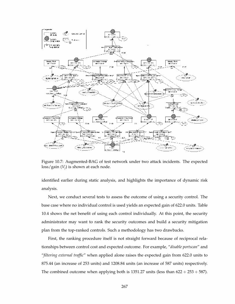
Figure 10.7: Augmented-BAG of test network under two attack incidents. The expectedloss/gain (Vj) is shown at each node.
identified earlier during static analysis, and highlights the importance of dynamic risk
analysis.
Next, we conduct several tests to assess the outcome of using a security control. The
base case where no individual control is used yields an expected gain of 622.0 units. Table
10.4 shows the net benefit of using each control individually. At this point, the security
administrator may want to rank the security outcomes and build a security mitigation
plan from the top-ranked controls. Such a methodology has two drawbacks.
First, the ranking procedure itself is not straight forward because of reciprocal rela-
tionships between control cost and expected outcome. For example, “disable portscan” and
“filtering external traffic” when applied alone raises the expected gain from 622.0 units to
875.44 (an increase of 253 units) and 1208.84 units (an increase of 587 units) respectively.
The combined outcome when applying both is 1351.27 units (less than 622 + 253 + 587).
267

Table 10.4: Security outcome assessment for each individual control in augmented-BAGof test network. Net benefit is (B −A− 622.0).
Security Control Cost (A) Outcome (B) Net benefit
apply OpenSSH security patch 63 1407.89 722.89apply MS work around 14 1202.45 566.45filtering external traffic 70 1208.84 516.84limit DNS access 53 1000.65 325.65disable portscan 11 875.44 242.44disable WebDAV 250 1095.90 223.90apply MS09-004 work around 31 861.10 208.10add Network IDS 102 858.91 134.91add Firewall 205 881.15 54.15encryption 34 681.75 25.75digital signature 33 673.28 18.28query restriction 84 681.00 −25.00use POP3 instead 153 704.67 −70.33
On the other hand, combining “add Firewall” (individual increase from 622.0 to 881.15
units) and “apply MS work around” (individual increase from 622.0 to 1202.45 units) can
raise the outcome to 1735.6 units (greater than 622 + 259 + 580). The latter two are better
choices based on expected outcome, but the former two incurs a lower cost of imple-
mentation. This makes the ranking of controls, based on a specific cost factor, a difficult
process. Second, even if a ranking has been established, greedy selection can lead to
sub-optimal plans. Assume that controls are ranked based on the net benefit they incur
individually. The security controls are ordered in this manner in Table 10.4. Given a
control cost constraint of say 200.0 units, and a selection scheme based on the ranks, an
administrator will choose the first four controls in the table. These controls have a com-
bined cost of 200.0 units and results in an expected gain of 2673.96 units (a net benefit
of 2473.96 units collectively). However, selecting the 5th and the 7th controls, instead of
the 4th one, effectuates an expected gain of 2809.28 units at the cost of 189.0 units (a net
benefit of 2620.28 units). This shows that the security administrator should not choose
the security controls based on their individual outcomes or by greedy selection. Instead,
a more sophisticated decision making platform is required. This motivates the next three
experiments with single and multi-objective optimization.
We conduct three risk mitigation analysis experiments on the test network. The ge-
268
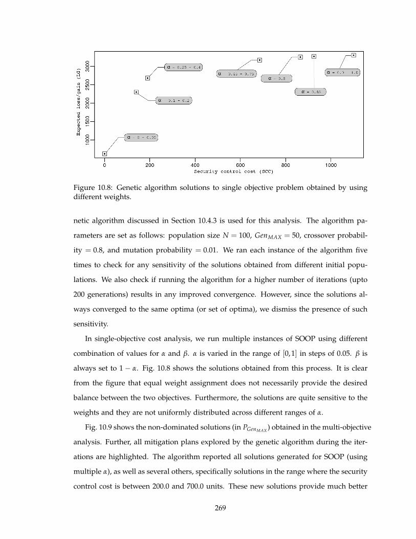
Figure 10.8: Genetic algorithm solutions to single objective problem obtained by usingdifferent weights.
netic algorithm discussed in Section 10.4.3 is used for this analysis. The algorithm pa-
rameters are set as follows: population size N = 100, GenMAX = 50, crossover probabil-
ity = 0.8, and mutation probability = 0.01. We ran each instance of the algorithm five
times to check for any sensitivity of the solutions obtained from different initial popu-
lations. We also check if running the algorithm for a higher number of iterations (upto
200 generations) results in any improved convergence. However, since the solutions al-
ways converged to the same optima (or set of optima), we dismiss the presence of such
sensitivity.
In single-objective cost analysis, we run multiple instances of SOOP using different
combination of values for α and β. α is varied in the range of [0,1] in steps of 0.05. β is
always set to 1 − α. Fig. 10.8 shows the solutions obtained from this process. It is clear
from the figure that equal weight assignment does not necessarily provide the desired
balance between the two objectives. Furthermore, the solutions are quite sensitive to the
weights and they are not uniformly distributed across different ranges of α.
Fig. 10.9 shows the non-dominated solutions (in PGenMAX) obtained in the multi-objective
analysis. Further, all mitigation plans explored by the genetic algorithm during the iter-
ations are highlighted. The algorithm reported all solutions generated for SOOP (using
multiple α), as well as several others, specifically solutions in the range where the security
control cost is between 200.0 and 700.0 units. These new solutions provide much better
269
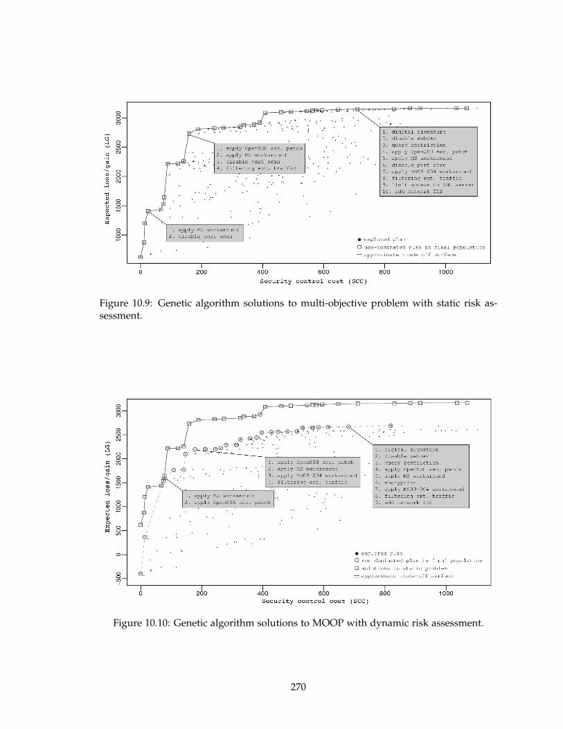
Figure 10.9: Genetic algorithm solutions to multi-objective problem with static risk as-sessment.
Figure 10.10: Genetic algorithm solutions to MOOP with dynamic risk assessment.
270
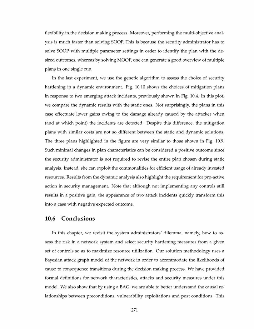
flexibility in the decision making process. Moreover, performing the multi-objective anal-
ysis is much faster than solving SOOP. This is because the security administrator has to
solve SOOP with multiple parameter settings in order to identify the plan with the de-
sired outcomes, whereas by solving MOOP, one can generate a good overview of multiple
plans in one single run.
In the last experiment, we use the genetic algorithm to assess the choice of security
hardening in a dynamic environment. Fig. 10.10 shows the choices of mitigation plans
in response to two emerging attack incidents, previously shown in Fig. 10.4. In this plot,
we compare the dynamic results with the static ones. Not surprisingly, the plans in this
case effectuate lower gains owing to the damage already caused by the attacker when
(and at which point) the incidents are detected. Despite this difference, the mitigation
plans with similar costs are not so different between the static and dynamic solutions.
The three plans highlighted in the figure are very similar to those shown in Fig. 10.9.
Such minimal changes in plan characteristics can be considered a positive outcome since
the security administrator is not required to revise the entire plan chosen during static
analysis. Instead, she can exploit the commonalities for efficient usage of already invested
resources. Results from the dynamic analysis also highlight the requirement for pro-active
action in security management. Note that although not implementing any controls still
results in a positive gain, the appearance of two attack incidents quickly transform this
into a case with negative expected outcome.
10.6 Conclusions
In this chapter, we revisit the system administrators’ dilemma, namely, how to as-
sess the risk in a network system and select security hardening measures from a given
set of controls so as to maximize resource utilization. Our solution methodology uses a
Bayesian attack graph model of the network in order to accommodate the likelihoods of
cause to consequence transitions during the decision making process. We have provided
formal definitions for network characteristics, attacks and security measures under this
model. We also show that by using a BAG, we are able to better understand the causal re-
lationships between preconditions, vulnerability exploitations and post conditions. This
271

is facilitated by computing the likelihoods of different outcomes possible as a result of
the cause-consequence relationships. We have demonstrated how the BAG can be used to
revise these likelihoods in the event of attack incidents. Using empirical results on a test
network, we show that such a dynamic analysis helps the system administrator identify
evolving weak spots in a network. We also provide the necessary optimization formula-
tions required to build a mitigation plan that reduces the risk levels. Towards this end,
we propose a genetic algorithm capable of performing both single and multi-objective
optimization of the administrator’s objectives. While single objective analysis uses ad-
ministrator preferences to identify the optimal plan, multi-objective analysis provides a
complete trade-off information before a final plan is chosen.
As immediate future work, we can improve the efficiency of our evaluation algorithm.
The evaluation algorithm is used to compute the unconditional probabilities and is cur-
rently implemented using a brute force DFS traversal. Posterior probability computation
is expensive using this implementation and therefore impacts the decision making time
in a dynamic scenario. In particular, we wish to revise the evaluation algorithm to include
heuristic based update mechanisms in order to reduce the time required to complete the
mitigation analysis, without scarifying the quality of results obtainable. Furthermore,
the mitigation process in dynamic situations needs to be improved so that a security ad-
ministrator can quickly identify the best security response that accounts for all former
investments made as part of the static analysis stage.
It is worth mentioning that some security controls have been found to be commonly
included in the optimal solutions. It is possible that security hardening is more critical in
certain areas of the attack graph. Such areas could be nodes that have multiple fan outs.
In other words, these critical areas are at-risk junctions that can be used by an attacker
to cause multiple outcomes. Security controls that can reduce risk in such areas are
likely to be parts of the optimal solutions. Therefore, it is worth investigating how such
controls can be identified efficiently so as to reduce the search space for the optimization
algorithm.
272

CHAPTER 11
Revisiting the Optimality of Security Policies
Over the past several years, researchers have shown considerable interest in the
problem of optimal security hardening. Work in this area range from identifying the
minimal set of attacks that can break a system [94], to finding the set of security measures
with minimum cost that can protect a given system [136], to identifying the optimal set
of security controls under a given cost assumption [51]. These works use attack models
such as attack graphs and attack trees to statically enumerate a system’s vulnerabilities
and suggest optimal defenses based on these models.
While these works provide valuable insights into the problem of optimal security
hardening, the approaches provide only a static perspective to the problem. They assume
that the end goal is to identify a set of security controls that can prevent a particular
security breach from occurring. Once a security control is in place, they are done. Since
the administrator has to operate within fixed budgetary restrictions it often prevents her
from implementing defenses at all the weak spots in the system [51]. Rather, she has to
perform a tradeoff analysis between the cost of security control and residual damage for
not covering some weak spots. An attacker, meanwhile, continues to explore alternative
attack scenarios to inflict maximum damage possible to a system, despite the security
controls that are in place. Many a times, the attacker’s goal may be just to cause some
damage, and not necessarily cause the specific security breach that the defender is trying
273

to protect against. The attacker may be aided by several factors in this quest. Defenses
may have unknown vulnerabilities that can be exploited as a system evolves with time.
Misconfiguration of defenses can render them susceptible to attacks. If the attacker has
insider knowledge about system configuration, weak spots and defenses (or lack thereof),
such knowledge can be used to increase the probability of a defense failing. Such a
situation may not be acceptable to the higher ups in the organization. Their perspective
may be to not only prevent a specific security breach but also accept minimal collateral
damage. This may require a continual updating of the defense strategy based on attacker
activities. Thus, one important objective of security hardening, often missed by existing
works, is to make life as difficult for the attacker as possible by adjusting security controls.
It seems worth investigating if such an arms race between the attacker and the defender
will be perpetual or there exists a state involving security controls in which the defender
is guaranteed that unexpected damages will never be inflicted no matter how the attacker
changes its strategies.
Bistarelli et al. propose defense trees as an extension to attack trees to analyze the
economic profitability of security measures and their deterrent effects on attackers [24]. A
game theoretic perspective of the problem is presented by the same authors in an attempt
to discover Nash equilibrium points between the security provider and the attacker [23].
An implicit assumption in their work is the existence of a payoff matrix that can be used
by a software tool to deduce the points of equilibrium. However, as we explain later, the
payoff matrix can be too large to be computed for a given problem.
In this chapter, we revisit the optimal security hardening problem keeping in view
the attacker’s perspective, namely, defenses can be broken. Our goal is to identify how
security controls can be decided to maximize the return on investment for a defender,
under the scenario that an attacker is actively engaged in maximizing its return on at-
tacks. We make three major contributions to this effect. First, we show that keeping
the attacker’s perspective in deciding security controls may often appear to be counter-
intuitive but nonetheless provides a better return on investment for an organization. This
is because such an approach can lead to an equilibrium condition in which even if the
attacker adapts to the installed controls, he cannot expect to cause damages that the de-
274

fender has not already foreseen and accounted for. From the attacker’s point of view, he
is better off not trying to breach any of these installed defenses. Our second contribution
is that we explore the optimal security control placement problem as a dynamic engage-
ment between the defender and the attacker. We model the problem as an “arms race”.
We allow both the attacker and defender to start with poor quality strategies and then
improve them depending on perceived payoffs. Finally, we solve the optimization prob-
lem using the competitive co-evolution paradigm and show how the constant engagement
between a defender and an attacker drives the solution towards a state of equilibrium.
Optimal solution is reached when no further increase in payoff is noticed by either side.
The rest of the chapter is organized as follows. Section 11.1 introduces a motivating
example to show how the attacker’s perspective may help in choosing optimal security
controls. Section 11.2 formalizes the notion of defense and attack strategies. Next, in
Section 11.3 we define the payoff models for the attacker as well as the defender. This
is followed by the formalization of the optimization problem in Section 11.4. A brief
background of competitive co-evolution is provided in Section 11.5 to help understand
the solution methodology which is discussed later in the same Section. Empirical results
and discussions are presented in Section 11.6. Finally, we conclude in Section 11.7.
11.1 Exploring Defense Strategies
Incorporating the attacker’s perspective in the optimal security hardening problem is
not easy. We consider a hypothetical example to illustrate how a defender’s decision to
employ a particular strategy is influenced when the attacker’s gains are kept in consid-
eration. Consider the payoff matrix shown in Fig. 11.1. The example assumes that the
defender has two possible defense strategies d1 and d2, and the attacker has two different
attack strategies a1 and a2 to try out. The objective of the defender is to decide on one
defense strategy to adopt. The first value in a cell (i, j) is a measure of some payoff that
the defender derives by adopting strategy di under the situation when the attacker uses
strategy aj. Given that the defender is only interested in its payoff value, it uses an aver-
age case analysis and finds that strategy d1 can maintain a higher average payoff than d2
– 7.5 compared to 5.5. The defender will arrive at the same strategy even with a best case
275

Figure 11.1: A hypothetical payoff matrix showing defender and attacker payoffs.
analysis. The defender therefore installs the defense d1. However, the decision on d1 can
reveal itself to be flawed when the attacker’s payoffs are introduced.
The second value in a cell (i, j) is a measure of the payoff that the attacker derives by
adopting attack aj when defense di is in place. With d1 in place, the attacker sees that its
payoff is more (6 compared to 2) by adopting strategy a1. Hence, it will always employ
a1, in which case the defender will always derive a payoff of 5. This value is not only less
than the average payoff of d1, but is also less than the average payoff of d2. The value is
not even better than the individual payoffs possible with d2, i.e. 6 when a1 occurs and 5
when a2 occurs. Further, if we consider the situation where the attacker does not know
which defense is in place and wants to choose a strategy using an average or best case
analysis, strategy a1 is the favorable choice. This is because strategy a1 always provides
a higher payoff than a2 no matter which defense is in place. In the light of this analysis,
the defender should thus be choosing strategy d2. Since the attacker’s choice is inclined
towards using a1, the defender now derives a payoff of 6, compared to 5 when choosing
d1.
Another interesting facet of d2 is the equilibrium it maintains with a1. Let us assume
that the defender does a best case analysis, as in the case when the attacker’s payoffs
are not known, and chooses d1. The attacker then employs a1 to maximize its payoff.
The defender notices that its payoff is not optimal when a1 occurred and so switches to
d2 to increase it. Hereafter, although the defense strategy has changed, the attacker’s
best strategy is to stick to a1. In other words, the defender and the attacker enters a
state of equilibrium where none benefits any further from changes in strategy. Hence,
276

even though d1 appears to be the optimal strategy at first glance, over time the defender
changes policies to finally settle down with d2 – the equilibrium strategy.
One may ask what is the equilibrium solution’s relation to the notion of optimal secu-
rity hardening. Consider the scenario where a defender installs defenses based on some
optimality criteria on a system. Over time, an attacker finds the best possible way to
exploit the system under the defensive configuration. The defender notices the attacker’s
exploitation mechanism and modifies its policies keeping in consideration the optimal-
ity criteria. The attacker adapt to the changes and the process continues. When the
defense policies corresponding to the equilibrium condition are instantiated and the at-
tacker adapts to it, the defender is already running the optimal set of policies possible for
the attacker’s adaption and does not need to change it. Thus, in the long run, the notion
of optimal security hardening converges towards security in equilibrium with attacks.
Performing an analysis of the nature shown in the example is relatively more difficult
on a larger scale. First, the payoff matrix can be very large in a real scenario. For d defense
controls and a attack points, this matrix can be as large as 2d × 2a. Filling the matrix
can thus involve an immense number of evaluations. Second, even if the matrix can be
computed, performing the analysis to decide on the best strategy can be impractical. Note
that a best (or equilibrium) defense strategy as depicted in the example may not exist at
all. For example, if the values at cell (2,1) are replaced by (4,10), then the best strategy
for the attacker varies depending on the defense. Nonetheless, we can argue that d1 is a
better defense strategy in this case since the payoff is better than from d2 – 5 with a1 as
the strategy of choice for the attacker compared to 4 with a2 as the attacker’s choice.
Ideally, it would be sufficient to decide on a defense strategy by comparing it against
others under the light of attack strategies resulting in higher payoffs for the attacker. One
may visualize the attack strategies as test cases to measure the competence of a defense
strategy. Better test cases are those which are more difficult to solve, or in other words,
results in inferior performance of the defense strategy. Similarly, an attack strategy should
only be analyzed against defense strategies that result in higher payoffs for the defender.
The presence of such cyclic dependencies in the evaluation process makes the analysis
hard to conduct. Moreover, the optimal defense strategy will most likely have to be
277

changed over time to maintain maximum payoff depending on what strategy is chosen
by the attacker. Hence we believe it is worth investigating if an equilibrium strategy exists
for the security hardening problem.
11.2 Defense and Attack Strategy
We adopt the network and attack tree model described in Chapter 8 to demonstrate
the concepts. Recall that nodes of an attack tree are defined as propositions and edges
relate the truth value of a node with that of its children. Leaf nodes on the tree represent
propositions related to the different network and system states, which may be true or false
depending on what defenses are in place. The truth values of the leaf nodes progressively
define if the propositions on the internal nodes would be true or false. If no defense (also
called a security control) is installed, all leaf nodes would be true, which would finally
lead to the root node to become true as well. In such a case, the attacker is assumed to
have successfully met its objective. Due to the presence of the AND-OR decompositions,
the root node may become true even if all leaf nodes are not true. Similarly, all leaf nodes
need not be false for the root to become false.
A defender installs defenses on the network (makes some or all leaf nodes false) so as
to prevent the root node from becoming true. The defender’s choice of defenses may be
determined by factors such as the installation cost and the potential damage residual after
making the choice. From an attacker’s perspective, the attack tree is a model showing the
different ways it can compromise the root node. However, we do not restrict our focus to
the root node alone. An attacker’s strategy might as well be directed towards inflicting
the most damage in the presence of defenses, rather than just compromising the root
node. The choice of such a strategy is also influenced by the difficulty that the attacker
has to overcome in order to bypass any installed defenses.
In order to defend against the attacks possible, the defender can choose to implement a
variety of safeguard technologies (or defenses). Each choice of action can have a different
cost involved. Besides, some measures have multiple coverages, but with higher costs.
The defender has to make a decision and choose to implement a subset of these policies
in order to maximize the resource utilization.
278
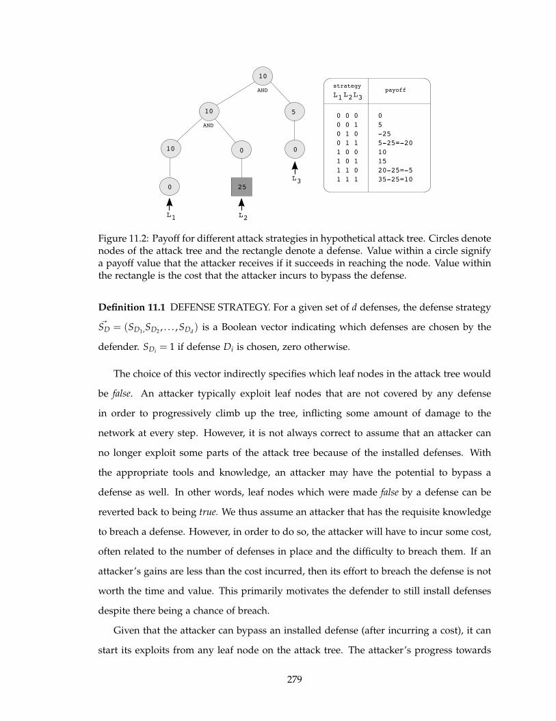
Figure 11.2: Payoff for different attack strategies in hypothetical attack tree. Circles denotenodes of the attack tree and the rectangle denote a defense. Value within a circle signifya payoff value that the attacker receives if it succeeds in reaching the node. Value withinthe rectangle is the cost that the attacker incurs to bypass the defense.
Definition 11.1 DEFENSE STRATEGY. For a given set of d defenses, the defense strategy
~SD = (SD1,SD2, . . . ,SDd
) is a Boolean vector indicating which defenses are chosen by the
defender. SDi= 1 if defense Di is chosen, zero otherwise.
The choice of this vector indirectly specifies which leaf nodes in the attack tree would
be false. An attacker typically exploit leaf nodes that are not covered by any defense
in order to progressively climb up the tree, inflicting some amount of damage to the
network at every step. However, it is not always correct to assume that an attacker can
no longer exploit some parts of the attack tree because of the installed defenses. With
the appropriate tools and knowledge, an attacker may have the potential to bypass a
defense as well. In other words, leaf nodes which were made false by a defense can be
reverted back to being true. We thus assume an attacker that has the requisite knowledge
to breach a defense. However, in order to do so, the attacker will have to incur some cost,
often related to the number of defenses in place and the difficulty to breach them. If an
attacker’s gains are less than the cost incurred, then its effort to breach the defense is not
worth the time and value. This primarily motivates the defender to still install defenses
despite there being a chance of breach.
Given that the attacker can bypass an installed defense (after incurring a cost), it can
start its exploits from any leaf node on the attack tree. The attacker’s progress towards
279

the root is then decided by the leaf nodes it chooses. Note that choosing all leaf nodes that
can collectively make an intermediate node true need not always be the best approach for
the attacker. For instance, given that defenses will be in place at different levels of the tree
and the attacker will have to incur a cost to bypass them, it is possible that the attacker
derives more payoff by inflicting damages at different parts of the attack tree rather than
continuing along a single scenario all the way up to the root. An example of this situation
is depicted in Fig. 11.2. With the given values and the defense in place, the strategy
101 generates a higher payoff than trying to reach the root node with strategy 111. This
happens because the cost to breach the installed defense nullifies any gains derived from
breaching it. An attack strategy is thus defined as follows.
Definition 11.2 ATTACK STRATEGY. Let a denote the number of unique leaf nodes in an
attack tree. An attack strategy ~SA = (SA1,SA2, . . . ,SAa
) is a Boolean vector indicating which
leaf nodes in the tree are chosen by the attacker for exploit. SAi= 1 if node Ai ∈ Nexternal
is chosen, zero otherwise.
Thus, an attack strategy specifies the path(s) that the attacker pursues to an intermedi-
ate or the top level of the attack tree. The success of the strategy depends on the defense
strategy adopted by the defender, as well as the number of levels it can move up on the
tree. Another way to visualize an attack strategy is the set of leaf nodes that the attacker
assumes to be true, or will make true by breaching the defenses protecting them.
11.3 Payoff Model
An augmented-attack tree (Section 8.4.1) extends an attack tree by associating a value
Vi to every node. The value associated with a node signifies the sum of the total potential
damage present in the child subtree(s) and the potential damage of the node itself. If
no defense is installed, i.e. all leaf nodes are true, then Vroot gives the maximum damage
possible on the attack tree. When a defender decides on a defense strategy, it essentially
sets the truth values of the covered leaf nodes to false. Uncovered leaf nodes are set to
true. An attacker reverts any falsified leaf node to true if the node is chosen as part of the
attack strategy. With this configuration, we can then find out the damage inflicted on the
280

attack tree as a result of an attack strategy.
Definition 11.3 DAMAGE INFLICTED. For a given defense strategy ~SD and an attack
strategy ~SA on an augmented-attack tree ATaug, the damage inflicted DI is given by the
value of the root node of the tree, i.e.
DI( ~SD, ~SA) = Vroot. (11.1)
The payoff for a defender and an attacker is an estimate of the gain it receives by
adopting a particular strategy and after incurring the corresponding costs associated with
the implementation of the strategy. For a defender, the cost of implementation relates to
factors such as operations cost, training cost, system downtime, incompatibility cost and
installation cost.
Definition 11.4 DEFENSE STRATEGY COST. Given a set of d defenses, each having a
cost Ci;1 ≤ i ≤ d and a defense strategy ~SD, the defense strategy cost DSC is defined as
DSC( ~SD) =d
∑i=1
(SDiCi). (11.2)
For an attacker, the cost of realizing an attack strategy is related to the effort it has to
put forward in overcoming any defenses on its way. We model this cost under a simplistic
assumption that stronger defenses are likely to have a higher cost of implementation.
Under this assumption, we measure the relative difficulty to breach a defense – a value in
[0,1] – and assign the cost to breach it, BC(·), as a fraction (given by the difficulty value)
of the cost of implementation of the defense, i.e.
BC(Di) =Ci
Maxi
Ci× Ci. (11.3)
Definition 11.5 ATTACK STRATEGY COST. Given a set of d defenses, a defense strategy
~SD and an attack strategy ~SA on an attack tree AT, the attack strategy cost ASC is defined
as
ASC( ~SD, ~SA) =d
∑i=1
∑j|Di(Aj)= f alse
[BC(Di)SDiSAj
]. (11.4)
281

The expression above iterates through the leaf nodes covered by a particular defense.
Thereafter, the cost to breach the defense is added to the attack strategy cost if the defense
is part of the defense strategy and the leaf node is part of the attack strategy. When a
breach occurs, the cost paid by the defender to install it (Ci) is a loss, called the breach
loss BL(·) and expressed in a manner similar to the above equation.
BL( ~SD, ~SA) =d
∑i=1
∑j|Di(Aj)= f alse
[CiSDiSAj
] (11.5)
We then define the defender and attacker payoffs as follows.
Definition 11.6 PAYOFF FOR DEFENDER AND ATTACKER. For a given defense strat-
egy ~SD and an attack strategy ~SA on an augmented-attack tree ATaug, the defender’s
payoff POD is given as
POD( ~SD, ~SA) = DI(~0,~1) + DSC( ~SD) − DI( ~SD, ~SA) − BL( ~SD, ~SA), (11.6)
and the attacker’s payoff POA is given as
POA( ~SD, ~SA) = DI( ~SD, ~SA) − ASC( ~SD, ~SA). (11.7)
Here, DI(~0,~1) signify the maximum damage possible on the attack tree, which hap-
pens when there are no defenses installed and the attacker exploits all leaf nodes. ~0
represent the all zero vector and ~1 is the all one vector. Note that both payoff functions
employ the same DI value derived from the attack tree. One can argue that the attacker’s
knowledge on the damages sustained by the defender when compromising a node is
rather limited, and thus cannot be same as that of the defender. Further, the attacker
need not have the complete knowledge about the cost of implementing a defense and
hence will not know the exact value of ASC. We understand that both are rational argu-
ments. Our justification to them is based on the fact that the POA function need not be
an exact estimate of the actual payoff derived by the attacker. The optimization process
only needs to compare payoff values to determine the relative effectiveness of two attack
strategies, in which case it suffices to have a value proportional to the actual payoff. The
POA function satisfies this requirement since the attacker’s actual payoff is likely to be
proportional to the damage it inflicts on the tree. Moreover, the cost paid by the attacker
to overcome a defense will likely be proportional to the sustainability of the defense.
282

11.4 Problem Statement
We first normalize the POD and POA functions in order to account for differences
arising in the magnitude of the values. The POA function is in the range of [−ASC( ~SD, ~SA),
DI(~0,~1)] which is remapped to [0, ASC( ~SD, ~SA) + DI(~0,~1)] by adding ASC(~SD, ~SA) to the
value. POD function is in the non-negative range [0, DSC( ~SD) + DI(~0,~1)]. The normal-
ized functions for POD and POA – in the range of [0,1] – are then given as follows.
PODnorm( ~SD, ~SA) =POD( ~SD, ~SA)
DSC( ~SD) + DI(~0,~1)(11.8)
POAnorm( ~SD, ~SA) =POA( ~SD, ~SA) + ASC( ~SD, ~SA)
ASC( ~SD, ~SA) + DI(~0,~1)(11.9)
The normalized versions are more intuitive in understanding what the payoff func-
tions model. The defender has an investment worth DSC( ~SD) + DI(~0,~1) on the attack
tree. PODnorm gives the fraction of this investment protected by the defender’s strategy
for a particular attack strategy. In other words, PODnorm gives the fractional return on
investment for the defender. From an attacker’s perspective, the best it can do is gather-
ing the payoff from maximum damage and also retain the cost incurred while doing so
to itself. DI( ~SD, ~SA) is the amount that it actually derives. POAnorm is thus the fractional
return on attack to the attacker.
The defender’s optimization problem is to find a defense strategy ~SD that gives max-
imum PODnorm under all possible attack strategies. The attacker’s optimization problem
is to find an attack strategy ~SA that gives maximum POAnorm under all possible defense
strategies. However, such a strategy may not exist. Besides, as argued earlier, evaluating
a host strategy with all opponent strategies is often impractical. We introduce here the
terms host and opponent to refer to the party whose strategy is being tested and the party
against whom it is being tested respectively. In order to compare two host strategies, it
is sufficient to evaluate them against their respective best opponent strategy (one gener-
ating the highest payoff for the opponent with the host strategy in place). Hence, a more
suitable statement of the optimization problem is as follows.
283

Problem 11.1 Defender’s Optimization Problem. Given an augmented attack tree ATaug
and d defenses, find the defense strategy ~SD∗
that maximizes PODnorm( ~SD, ~SA∗), where
~SA∗
satisfies the relation POAnorm( ~SD, ~SA∗)≥ POAnorm( ~SD, ~SA) for any attack strategy ~SA.
Problem 11.2 Attacker’s Optimization Problem. Given an augmented attack tree ATaug
and d defenses, find the attack strategy ~SA∗
that maximizes POAnorm( ~SD∗, ~SA), where
~SD∗
satisfies the relation PODnorm( ~SD∗, ~SA) ≥ PODnorm( ~SD, ~SA) for any defense strategy
~SD.
The brute force method to solve each problem is to first generate the payoff matrix and
then mark the cell, for every host strategy, with the highest opponent payoff. The solution
is the host strategy which has the highest payoff in the marked cells. If, given the host
strategy in the solution, the opponent’s payoff is also the highest, and vice versa, then
the solution admits a Nash equilibrium [135]. We want to emphasize here that solving
just one problem is not sufficient. For example, assume that the defender has found the
optimal solution to its problem. The PODnorm reported by the solution implicitly assumes
that the attacker will launch the strategy ~SA∗
that gives the highest attacker payoff –
established in the optimization problem by the relation. If the attacker also solves its own
optimization problem, there is no guarantee that the best strategy found by it is the same
~SA∗
as found in solving the defender’s optimization problem. The outcome in this case
could be that both the attacker and the defender get sub-optimal payoffs. The desired
solution is the defense and attack strategy pair ~SD∗
and ~SA∗
that satisfy the conditions
1. PODnorm( ~SD∗, ~SA
∗) > PODnorm( ~SD, ~SA
∗), and
2. POAnorm( ~SD∗, ~SA
∗) > POAnorm( ~SD
∗, ~SA),
for any given defense strategy ~SD( 6= ~SD∗) and attack strategy ~SA( 6= ~SA
∗).
11.5 Competitive Co-Evolution
Competitive co-evolution refers to the concurrent evolution of two distinct species
in which the fitness of an individual in one species is based on its competitive abilities
284

against the individuals of the other species. Fitness evaluation with such reciprocal ac-
tions are hypothesized to occur in nature. Game theory based models of such interactions
is first presented in Axelrod’s Prisoners’ Dilemma [12]. The evolution of species in such
a competitive habitat usually leads to a evolutionary stable strategy [157] which cannot be
invaded by the process of natural selection. In other words, the species reverts back to
the stable strategy over time.
Competitive co-evolution has been successfully applied to the evolution of strategies
for games such an Tic-Tac-Toe and Nim [148]. The range of potential opponent strategies
is typically very big in such games, thereby making it difficult to determine an exoge-
nous fitness evaluation function. Other domains such as software reliability testing faces
a similar problem. The solution using competitive co-evolution involves using two popu-
lations, one representing the software solutions and the other representing the test cases,
each taking turns in testing and being tested against the other [82]. A survey of other real
world applications is available in [28].
Success of competitive co-evolution is attributable to the emergence of an evolutionary
“arms race” [44]. Consider two populations of defense strategies and attack strategies.
To begin with, both populations are likely to have strategies of poor quality. Most of the
host strategies will have low payoffs brought forth by one or two good strategies existing
in the opponent population. However, since defense strategies are evolving based on
their competitive abilities against attack strategies, the success of the defender implies
the failure of the attacker. When the attacker finds strategies to improve its payoff by
overcoming the failure, it helps the defender identify gaps previously unthought of in
its previous strategies. The same idea drives the attacker’s strategies. New opponent
strategies drive hosts towards better counter strategies, improving host performance by
forcing it to respond to a wider range of more challenging test cases.
The next question that comes to mind is whether a good host strategy of the cur-
rent generation can prove its competence against opponent strategies that are lost in the
evolution of the opponent population. This is referred to as the memory property in co-
evolution. To handle such situations, co-evolutionary algorithms employ a “hall of fame”
[149] sub-population which keeps track of the best opponent solutions found from earlier
285
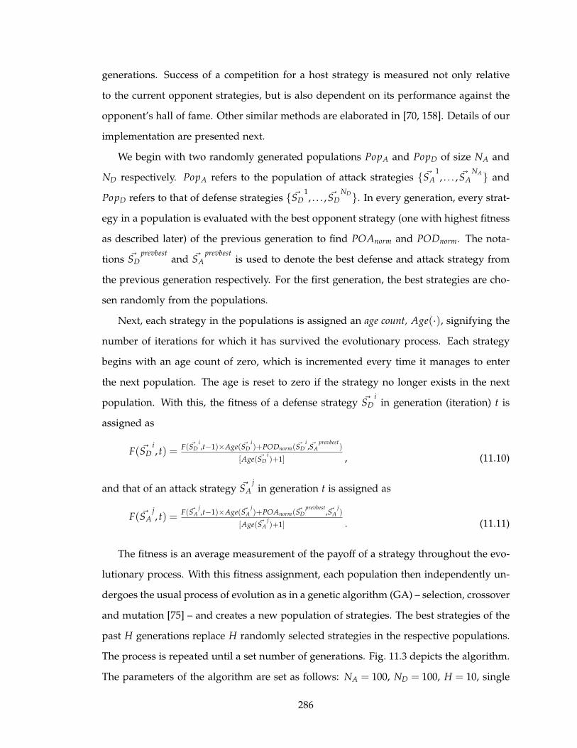
generations. Success of a competition for a host strategy is measured not only relative
to the current opponent strategies, but is also dependent on its performance against the
opponent’s hall of fame. Other similar methods are elaborated in [70, 158]. Details of our
implementation are presented next.
We begin with two randomly generated populations PopA and PopD of size NA and
ND respectively. PopA refers to the population of attack strategies { ~SA1, . . . , ~SA
NA} and
PopD refers to that of defense strategies { ~SD1, . . . , ~SD
ND}. In every generation, every strat-
egy in a population is evaluated with the best opponent strategy (one with highest fitness
as described later) of the previous generation to find POAnorm and PODnorm. The nota-
tions ~SDprevbest
and ~SAprevbest
is used to denote the best defense and attack strategy from
the previous generation respectively. For the first generation, the best strategies are cho-
sen randomly from the populations.
Next, each strategy in the populations is assigned an age count, Age(·), signifying the
number of iterations for which it has survived the evolutionary process. Each strategy
begins with an age count of zero, which is incremented every time it manages to enter
the next population. The age is reset to zero if the strategy no longer exists in the next
population. With this, the fitness of a defense strategy ~SDi
in generation (iteration) t is
assigned as
F( ~SDi, t) = F( ~SD
i,t−1)×Age( ~SD
i)+PODnorm( ~SD
i, ~SA
prevbest)
[Age( ~SDi)+1] , (11.10)
and that of an attack strategy ~SAj
in generation t is assigned as
F( ~SAj, t) = F( ~SA
j,t−1)×Age( ~SA
j)+POAnorm( ~SD
prevbest, ~SA
j)
[Age( ~SAj)+1] . (11.11)
The fitness is an average measurement of the payoff of a strategy throughout the evo-
lutionary process. With this fitness assignment, each population then independently un-
dergoes the usual process of evolution as in a genetic algorithm (GA) – selection, crossover
and mutation [75] – and creates a new population of strategies. The best strategies of the
past H generations replace H randomly selected strategies in the respective populations.
The process is repeated until a set number of generations. Fig. 11.3 depicts the algorithm.
The parameters of the algorithm are set as follows: NA = 100, ND = 100, H = 10, single
286
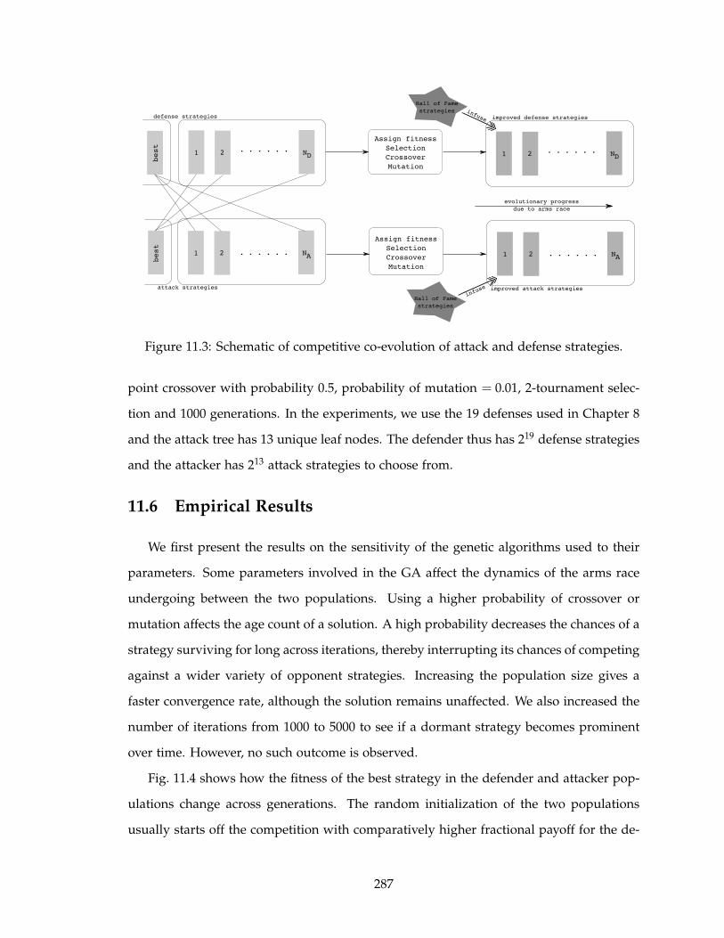
Figure 11.3: Schematic of competitive co-evolution of attack and defense strategies.
point crossover with probability 0.5, probability of mutation = 0.01, 2-tournament selec-
tion and 1000 generations. In the experiments, we use the 19 defenses used in Chapter 8
and the attack tree has 13 unique leaf nodes. The defender thus has 219 defense strategies
and the attacker has 213 attack strategies to choose from.
11.6 Empirical Results
We first present the results on the sensitivity of the genetic algorithms used to their
parameters. Some parameters involved in the GA affect the dynamics of the arms race
undergoing between the two populations. Using a higher probability of crossover or
mutation affects the age count of a solution. A high probability decreases the chances of a
strategy surviving for long across iterations, thereby interrupting its chances of competing
against a wider variety of opponent strategies. Increasing the population size gives a
faster convergence rate, although the solution remains unaffected. We also increased the
number of iterations from 1000 to 5000 to see if a dormant strategy becomes prominent
over time. However, no such outcome is observed.
Fig. 11.4 shows how the fitness of the best strategy in the defender and attacker pop-
ulations change across generations. The random initialization of the two populations
usually starts off the competition with comparatively higher fractional payoff for the de-
287
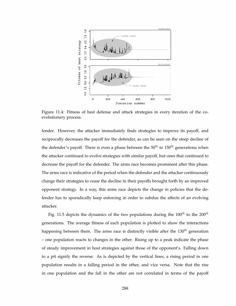
Iteration number
Fitness of best strategy
Defender
Attacker
arms race
arms race
Figure 11.4: Fitness of best defense and attack strategies in every iteration of the co-evolutionary process.
fender. However, the attacker immediately finds strategies to improve its payoff, and
reciprocally decreases the payoff for the defender, as can be seen on the steep decline of
the defender’s payoff. There is even a phase between the 50th to 150th generations when
the attacker continued to evolve strategies with similar payoff, but ones that continued to
decrease the payoff for the defender. The arms race becomes prominent after this phase.
The arms race is indicative of the period when the defender and the attacker continuously
change their strategies to cease the decline in their payoffs brought forth by an improved
opponent strategy. In a way, this arms race depicts the change in policies that the de-
fender has to sporadically keep enforcing in order to subdue the affects of an evolving
attacker.
Fig. 11.5 depicts the dynamics of the two populations during the 100th to the 200th
generations. The average fitness of each population is plotted to show the interactions
happening between them. The arms race is distinctly visible after the 130th generation
– one population reacts to changes in the other. Rising up to a peak indicate the phase
of steady improvement in host strategies against those of the opponent’s. Falling down
to a pit signify the reverse. As is depicted by the vertical lines, a rising period in one
population results in a falling period in the other, and vice versa. Note that the rise
in one population and the fall in the other are not correlated in terms of the payoff
288
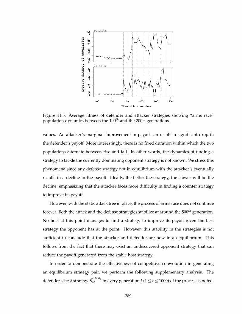
Figure 11.5: Average fitness of defender and attacker strategies showing “arms race”population dynamics between the 100th and the 200th generations.
values. An attacker’s marginal improvement in payoff can result in significant drop in
the defender’s payoff. More interestingly, there is no fixed duration within which the two
populations alternate between rise and fall. In other words, the dynamics of finding a
strategy to tackle the currently dominating opponent strategy is not known. We stress this
phenomena since any defense strategy not in equilibrium with the attacker’s eventually
results in a decline in the payoff. Ideally, the better the strategy, the slower will be the
decline; emphasizing that the attacker faces more difficulty in finding a counter strategy
to improve its payoff.
However, with the static attack tree in place, the process of arms race does not continue
forever. Both the attack and the defense strategies stabilize at around the 500th generation.
No host at this point manages to find a strategy to improve its payoff given the best
strategy the opponent has at the point. However, this stability in the strategies is not
sufficient to conclude that the attacker and defender are now in an equilibrium. This
follows from the fact that there may exist an undiscovered opponent strategy that can
reduce the payoff generated from the stable host strategy.
In order to demonstrate the effectiveness of competitive co-evolution in generating
an equilibrium strategy pair, we perform the following supplementary analysis. The
defender’s best strategy ~SDbestt
in every generation t (1 ≤ t ≤ 1000) of the process is noted.
289
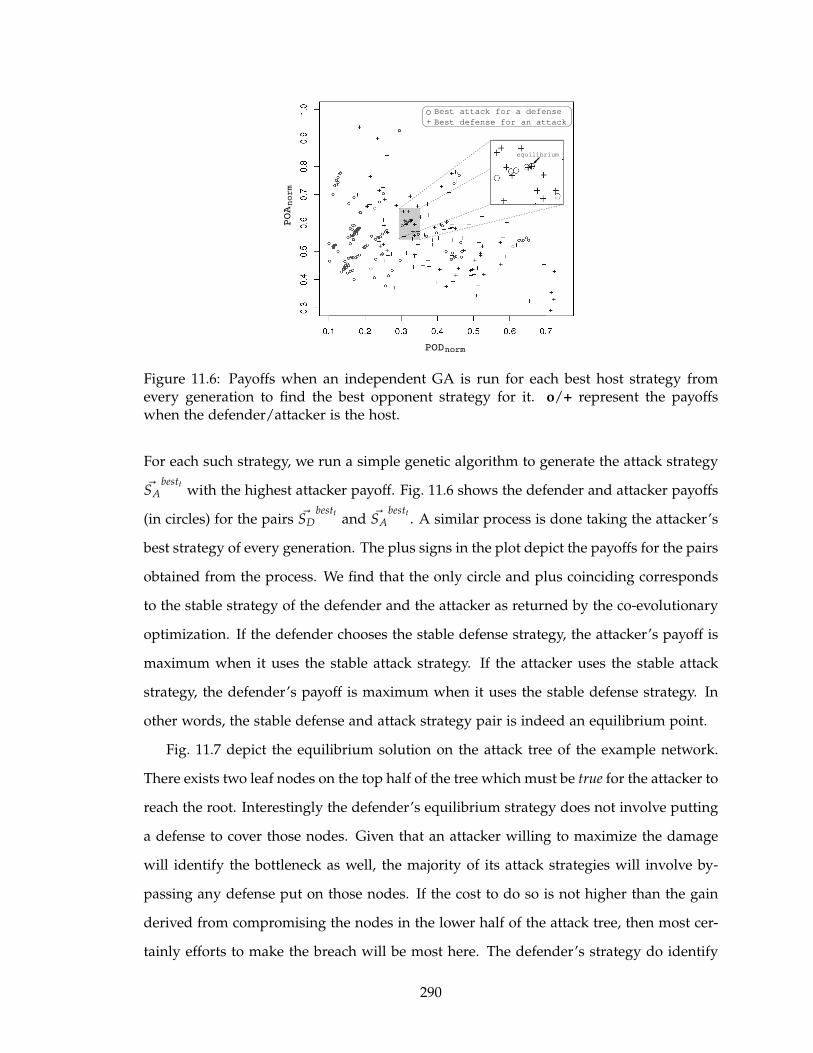
equilibrium
Best attack for a defense
Best defense for an attack+
PODnorm
POAnorm
Figure 11.6: Payoffs when an independent GA is run for each best host strategy fromevery generation to find the best opponent strategy for it. o/+ represent the payoffswhen the defender/attacker is the host.
For each such strategy, we run a simple genetic algorithm to generate the attack strategy
~SAbestt
with the highest attacker payoff. Fig. 11.6 shows the defender and attacker payoffs
(in circles) for the pairs ~SDbestt
and ~SAbestt
. A similar process is done taking the attacker’s
best strategy of every generation. The plus signs in the plot depict the payoffs for the pairs
obtained from the process. We find that the only circle and plus coinciding corresponds
to the stable strategy of the defender and the attacker as returned by the co-evolutionary
optimization. If the defender chooses the stable defense strategy, the attacker’s payoff is
maximum when it uses the stable attack strategy. If the attacker uses the stable attack
strategy, the defender’s payoff is maximum when it uses the stable defense strategy. In
other words, the stable defense and attack strategy pair is indeed an equilibrium point.
Fig. 11.7 depict the equilibrium solution on the attack tree of the example network.
There exists two leaf nodes on the top half of the tree which must be true for the attacker to
reach the root. Interestingly the defender’s equilibrium strategy does not involve putting
a defense to cover those nodes. Given that an attacker willing to maximize the damage
will identify the bottleneck as well, the majority of its attack strategies will involve by-
passing any defense put on those nodes. If the cost to do so is not higher than the gain
derived from compromising the nodes in the lower half of the attack tree, then most cer-
tainly efforts to make the breach will be most here. The defender’s strategy do identify
290
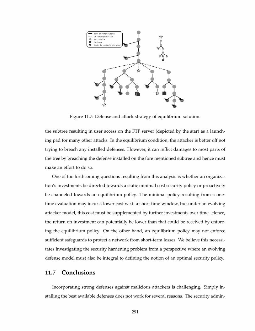
AND decomposition
OR decomposition
Attribute
Defense
Node in attack strategy
Figure 11.7: Defense and attack strategy of equilibrium solution.
the subtree resulting in user access on the FTP server (depicted by the star) as a launch-
ing pad for many other attacks. In the equilibrium condition, the attacker is better off not
trying to breach any installed defenses. However, it can inflict damages to most parts of
the tree by breaching the defense installed on the fore mentioned subtree and hence must
make an effort to do so.
One of the forthcoming questions resulting from this analysis is whether an organiza-
tion’s investments be directed towards a static minimal cost security policy or proactively
be channeled towards an equilibrium policy. The minimal policy resulting from a one-
time evaluation may incur a lower cost w.r.t. a short time window, but under an evolving
attacker model, this cost must be supplemented by further investments over time. Hence,
the return on investment can potentially be lower than that could be received by enforc-
ing the equilibrium policy. On the other hand, an equilibrium policy may not enforce
sufficient safeguards to protect a network from short-term losses. We believe this necessi-
tates investigating the security hardening problem from a perspective where an evolving
defense model must also be integral to defining the notion of an optimal security policy.
11.7 Conclusions
Incorporating strong defenses against malicious attackers is challenging. Simply in-
stalling the best available defenses does not work for several reasons. The security admin-
291

istrator has to work within fixed budgetary constraints and has to explain the return on
investment of security controls to the management. However, any convincing argument
explaining the return on investment must take the attacker’s benefits into consideration.
Our first contribution in this chapter is the identification of this fact in order to motivate
the pursuance of security hardening keeping both the defender and attacker payoffs into
account.
We argue that the notion of optimal security hardening is often dictated by the con-
stant interaction between the defender and the attacker. What is perceived as the optimal
return on investment would cease to be so once the attacker’s strategy to exploit the de-
fensive configuration is understood. We justify this with the argument that the system
administrator would more than likely be approached by the management to re-evaluate
its defenses under the light of the attacker’s strategy. Our second contribution highlights
that the dynamic engagement between the attacker and the defender is a continuous
process ending only when both enter a state of equilibrium. We thus emphasize that
identifying such equilibrium conditions, if any, is where the true sense of optimal secu-
rity hardening is buried. To this end, we formulate the requisite optimization problems
and present the notion of equilibrium in terms of the formulated problems.
As a viable methodology, we propose the use of competitive co-evolution to generate
the aforementioned equilibrium strategies. The method involves an algorithm that in-
trinsically models the arms race undergoing between the attacker and the defender, with
the ability to effectively find the equilibrium solutions. Solutions from the hypothetical
example demonstrate that keeping the attackers’ perspective in consideration for secu-
rity administration can result in placing security controls in places that may appear non
intuitive but provide a better return on investment for an organization.
In this work, we assume the existence of a single attacker owning any generated pay-
off. However, the problem can be more interesting when payoff models can be designed
to incorporate multiple attackers working in conjunction to achieve a particular objective
and sharing the payoff so generated. Further work can be directed towards designing
algorithms that can identify the existence of multiple equilibrium points simultaneously.
We believe that Pareto analysis intended towards generation of such solutions is a promis-
292

ing avenue to explore. Formal analysis to determine if equilibrium solutions exist at all
would be a major contribution as well.
293

Part III
Wireless Data Broadcasting
294

CHAPTER 12
Utility Driven Data Broadcast Scheduling
Recent advances in wireless communication technology are increasingly making
the dream of pervasive computing a reality. Pervasive computing involves a network of
portable computing devices so thoroughly embedded in our day-to-day work and per-
sonal life that their existence becomes difficult to perceive altogether. The devices interact
with each other and with other computing devices by exchanging rapid and continuous
streams of data. To facilitate almost imperceptible human-computer interaction, data ac-
cess times in such environments must be maintained within a specified Quality of Service
(QoS) level. Challenges in doing so arise from the fact that wireless bandwidth is typically
a limited resource, and thus it is not always possible to meet the quality requirements of
every device. This constraint not only makes pervasive data access a challenging problem,
but also identifies “optimal resource allocation” as one of the major research problems in
this domain.
A pervasive environment encompasses both peer-to-peer and client-server modes of
data dissemination. For example, a typical pervasive health care system may involve
multiple sensor nodes disseminating data on the monitored vital signs of a patient to a
personal digital assistant carried by the attending health care personal. Data communica-
tion follows a peer-to-peer architecture in such a setting. On the other hand, a pervasive
environment designed to serve queries on flight information in an airport is based on
295

a client-server mode of communication. Flight information usually reside in a database
server from where data is disseminated based on the incoming queries. For an envi-
ronment like an airport, it is appropriate to assume that the database will be queried
more frequently for certain types of data. Similar situations can be imagined in a stock
trading center, a pervasive traffic management system, or a pervasive supermarket. Such
scenarios open up possibilities of adopting a broadcast based architecture to distribute
data in a way that multiple queries for the same data item get served by a single broad-
cast. The focus of this chapter is directed towards data access issues in such pervasive
environments.
Quality of service is an important facet in such pervasive data access. Consider the
following example application - a traffic management system for a big city. The city gov-
ernment implements a traffic pricing policy for all vehicles on all roads based on factors
such as the distance traveled, the type of road traveled on, the time of day, vehicle cate-
gory and customer type (for example, special fee paying, traveling salesman, paramedic
on-call etc.) The system gathers real time traffic data via thousands of sensors, such as
traffic cameras, magneto-resistive traffic sensors and radars spread throughout the city.
To help drivers optimize their travel costs, the traffic management system provides vari-
ous routing services to drivers to avoid roadblocks, construction delays, congestion, and
accidents.1
A driver requests and gets routing services using smart GPS equipped devices as
follows. A device periodically uploads the vehicle’s current location (based on GPS in-
formation), intended destination, time willing to spend for traveling to destination, a
prioritized list of routing restrictions (for example, waypoints that the driver would like
to visit if possible, rest stops, scenic byways etc.), vehicle category and customer type,
and current speed. In response, the server replies with a set of route information. Each
route information contains among other things information about road segments to travel
on this route and traffic patterns on these road segments. The GPS equipped device uses
1Such an application is not very far-fetched. The Dutch government is in the process of introducing asimilar electronic traffic management system and pricing model. See [45].
296
this information and uses other parameters set by the driver to compute a good route
to take. Note that since the response to many drivers will no doubt contain overlapping
route segments and traffic information, it makes sense broadcasting this data.
The requests arrive at the server with various priority levels and soft deadlines. For
example, a higher fee paying customer gets a higher priority than a lesser fee paying
customer. A VIP’s convoy may get a still higher priority. Emergency responders get the
highest priority. A routing request that comes associated with a set of routing restrictions
automatically gets associated with a set of soft deadlines based on the speed of the driver.
The requests from different drivers may also get re-prioritized at the server so as to meet
a broader goal of reducing congestion and enabling smoother traffic flows.
Let us assume that at some point there is a major traffic gridlock within the city and the
traffic server gets thousands of re-routing requests from users. While these requests are
queued up at the server, another request comes from a VIP’s convoy with a high priority
and deadline. At this time, the server needs to determine how to schedule this request.
Pre-empting others may enable the server to meet the timeliness of this latest request.
However, serving some or all of the earlier requests has the advantage of clearing up the
gridlock earlier.
In this example, the different data that the server needs to serve is associated with
different utility values. Owing to the dynamic nature of the utility of responses to queries,
the time criticality factor cannot be ignored altogether when disseminating data. The
server would like to satisfy as many queries in a timely manner as possible. However,
some queries may be delayed beyond their specified deadlines (for example, the query
from the VIP’s convoy). The users, who hardly realize the broader goals of the traffic
management system and various bottlenecks in the information infrastructure, would
like to have their requests served at the earliest; however, it is reasonable to assume that
delayed data still provide some utility even if received after a specified deadline. For
example, a delayed route information may prevent a driver from visiting a particular
waypoint en route or may require the driver to use the next gas station. Nonetheless, it
may still allow the driver to choose a good route to the destination. An assumption of
reduced data utility in the face of missed deadline, enables data broadcasts to be tailored
297
in such a way that total utility associated with a broadcast is maximized. This helps
maintain a certain QoS level in the underlying infrastructure.
Note that the specific problem we are trying to address is, by no means, restricted
only to the example application outlined above. Similar scenarios are witnessed in en-
vironments such as Stock Exchanges. Here stock brokers on the floor seek and receive
periodic market data on wireless hand-held devices and notebooks and analyze them to
determine which stocks are hot. They also buy and sell stocks using such devices. Pop-
ularity of stocks change throughout the day, and it is important to analyze such trends
along multiple dimensions in order to buy and sell stocks. Thus, although queries from
brokers are implicitly associated with deadlines, these can be considered soft. The over-
all goal of the Stock Exchange is still to satisfy as many requests as possible in a timely
manner. To wrap up the scope of the problem domain, we would like to point out that
in order to make useful decisions, the stock broker may make a request for a group of
data from the Stock Exchange (for example, stock prices of three different oil companies).
A typical constraint on such requests is that all these data items must be received (not
necessarily in any particular order) before the stock broker can perform the relevant local
analysis of the market trends. Such a request can be considered a transactional request (or
simply a transaction). For scheduling in such cases, additional constraints must be placed
for ensuring the validity of data received.
Wireless broadcast mechanisms have been extensively investigated earlier. However,
very few of these research give attention to the effective utility involved in the timely
servicing of a request. Time criticality has been earlier addressed in a number of con-
texts with the assumption of a hard deadline [69, 96, 100, 104, 107, 183, 187]. Broadcast
scheduling in these works mostly focus on the timely servicing of a request to minimize
the number of missed deadlines. When the assumption of a soft deadline is appropriate,
a broadcast schedule should not only try to serve as many requests as possible, but also
make a “best effort” in serving them with higher utility values. Often, heuristics are em-
ployed in a dynamic setting to determine these schedules. However, their designs do not
involve the QoS criteria explicitly. Heuristic based methods make local decisions w.r.t. a
request or a broadcast, and often fail to capture the sought global QoS requirement. Much
298

of this is due to the fact that real time decision making cannot span beyond an acceptable
time limit, thereby restricting the usage of “full length” optimization techniques to the
domain. It does become imperative to design hybrid strategies that can combine the fast
real time performance of heuristics and the better solution qualities obtained from search
based optimization.
In this chapter, we propose a dynamic scheduler that tries to maximize the overall
utility of servicing requests and at the same time tries to serve as many requests in a
timely manner as possible. The setup is a wireless broadcast environment as in perva-
sive computing applications. For this work, we choose to ignore the problem of power
constraints of wireless devices. We acknowledge that this is serious problem because the
entire time a wireless device is waiting to receive a broadcast, it has to keep its power
status in active mode rather than reverting to a power saving doze mode. However, this
can be addressed by packaging the transmitted data appropriately. A number of works
have been done in air indexes [91, 194] that try to facilitate power saving by broadcasting
index information along with the data. From the air index information, the receiver can
predict the arrival time of its data and can accordingly switch its power level to doze or
active mode. Such a strategy can very well be incorporated in our model.
We begin with an attempt to understand the nature of the underlying search space,
and argue that traditional heuristics usually generate solutions in a worse part of this
space w.r.t a given global utility measurement. We explore “local search” as an option to
boost the performance of these solutions and provide arguments as to why the option is
viable in a real time setting. The observations allow us to propose a light weight stochastic
hill climber that surpasses the performance of a heuristic, and explicitly searches the space
of schedules to maximize utility. We believe that the proposed method provides insights
into better broadcast mechanisms which often clear our understanding for better heuristic
design.
The rest of the chapter is organized as follows. Section 12.1 summarizes the related
work in this domain. The broadcast model and the scheduling problem are discussed in
Section 12.2. The explored solution methods and the experimental setup are described in
Section 12.3 and Section 12.4 respectively. Results and discussions from the experiments
299
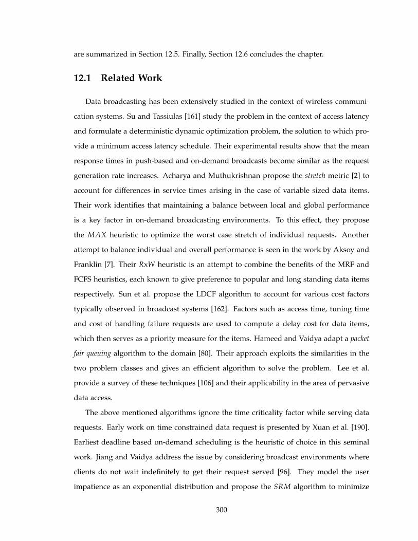
are summarized in Section 12.5. Finally, Section 12.6 concludes the chapter.
12.1 Related Work
Data broadcasting has been extensively studied in the context of wireless communi-
cation systems. Su and Tassiulas [161] study the problem in the context of access latency
and formulate a deterministic dynamic optimization problem, the solution to which pro-
vide a minimum access latency schedule. Their experimental results show that the mean
response times in push-based and on-demand broadcasts become similar as the request
generation rate increases. Acharya and Muthukrishnan propose the stretch metric [2] to
account for differences in service times arising in the case of variable sized data items.
Their work identifies that maintaining a balance between local and global performance
is a key factor in on-demand broadcasting environments. To this effect, they propose
the MAX heuristic to optimize the worst case stretch of individual requests. Another
attempt to balance individual and overall performance is seen in the work by Aksoy and
Franklin [7]. Their RxW heuristic is an attempt to combine the benefits of the MRF and
FCFS heuristics, each known to give preference to popular and long standing data items
respectively. Sun et al. propose the LDCF algorithm to account for various cost factors
typically observed in broadcast systems [162]. Factors such as access time, tuning time
and cost of handling failure requests are used to compute a delay cost for data items,
which then serves as a priority measure for the items. Hameed and Vaidya adapt a packet
fair queuing algorithm to the domain [80]. Their approach exploits the similarities in the
two problem classes and gives an efficient algorithm to solve the problem. Lee et al.
provide a survey of these techniques [106] and their applicability in the area of pervasive
data access.
The above mentioned algorithms ignore the time criticality factor while serving data
requests. Early work on time constrained data request is presented by Xuan et al. [190].
Earliest deadline based on-demand scheduling is the heuristic of choice in this seminal
work. Jiang and Vaidya address the issue by considering broadcast environments where
clients do not wait indefinitely to get their request served [96]. They model the user
impatience as an exponential distribution and propose the SRM algorithm to minimize
300
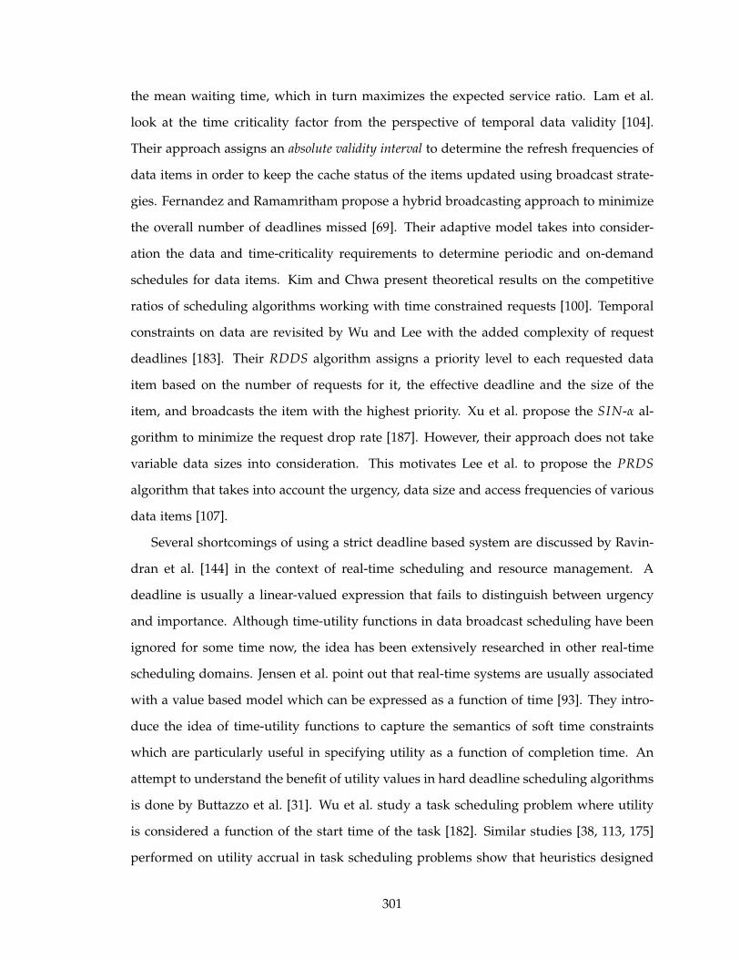
the mean waiting time, which in turn maximizes the expected service ratio. Lam et al.
look at the time criticality factor from the perspective of temporal data validity [104].
Their approach assigns an absolute validity interval to determine the refresh frequencies of
data items in order to keep the cache status of the items updated using broadcast strate-
gies. Fernandez and Ramamritham propose a hybrid broadcasting approach to minimize
the overall number of deadlines missed [69]. Their adaptive model takes into consider-
ation the data and time-criticality requirements to determine periodic and on-demand
schedules for data items. Kim and Chwa present theoretical results on the competitive
ratios of scheduling algorithms working with time constrained requests [100]. Temporal
constraints on data are revisited by Wu and Lee with the added complexity of request
deadlines [183]. Their RDDS algorithm assigns a priority level to each requested data
item based on the number of requests for it, the effective deadline and the size of the
item, and broadcasts the item with the highest priority. Xu et al. propose the SIN-α al-
gorithm to minimize the request drop rate [187]. However, their approach does not take
variable data sizes into consideration. This motivates Lee et al. to propose the PRDS
algorithm that takes into account the urgency, data size and access frequencies of various
data items [107].
Several shortcomings of using a strict deadline based system are discussed by Ravin-
dran et al. [144] in the context of real-time scheduling and resource management. A
deadline is usually a linear-valued expression that fails to distinguish between urgency
and importance. Although time-utility functions in data broadcast scheduling have been
ignored for some time now, the idea has been extensively researched in other real-time
scheduling domains. Jensen et al. point out that real-time systems are usually associated
with a value based model which can be expressed as a function of time [93]. They intro-
duce the idea of time-utility functions to capture the semantics of soft time constraints
which are particularly useful in specifying utility as a function of completion time. An
attempt to understand the benefit of utility values in hard deadline scheduling algorithms
is done by Buttazzo et al. [31]. Wu et al. study a task scheduling problem where utility
is considered a function of the start time of the task [182]. Similar studies [38, 113, 175]
performed on utility accrual in task scheduling problems show that heuristics designed
301
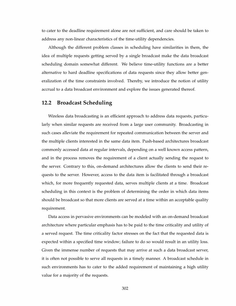
to cater to the deadline requirement alone are not sufficient, and care should be taken to
address any non-linear characteristics of the time-utility dependencies.
Although the different problem classes in scheduling have similarities in them, the
idea of multiple requests getting served by a single broadcast make the data broadcast
scheduling domain somewhat different. We believe time-utility functions are a better
alternative to hard deadline specifications of data requests since they allow better gen-
eralization of the time constraints involved. Thereby, we introduce the notion of utility
accrual to a data broadcast environment and explore the issues generated thereof.
12.2 Broadcast Scheduling
Wireless data broadcasting is an efficient approach to address data requests, particu-
larly when similar requests are received from a large user community. Broadcasting in
such cases alleviate the requirement for repeated communication between the server and
the multiple clients interested in the same data item. Push-based architectures broadcast
commonly accessed data at regular intervals, depending on a well known access pattern,
and in the process removes the requirement of a client actually sending the request to
the server. Contrary to this, on-demand architectures allow the clients to send their re-
quests to the server. However, access to the data item is facilitated through a broadcast
which, for more frequently requested data, serves multiple clients at a time. Broadcast
scheduling in this context is the problem of determining the order in which data items
should be broadcast so that more clients are served at a time within an acceptable quality
requirement.
Data access in pervasive environments can be modeled with an on-demand broadcast
architecture where particular emphasis has to be paid to the time criticality and utility of
a served request. The time criticality factor stresses on the fact that the requested data is
expected within a specified time window; failure to do so would result in an utility loss.
Given the immense number of requests that may arrive at such a data broadcast server,
it is often not possible to serve all requests in a timely manner. A broadcast schedule in
such environments has to cater to the added requirement of maintaining a high utility
value for a majority of the requests.
302
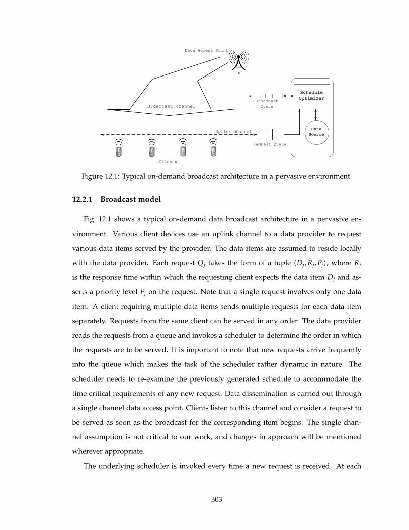
Data
Source
Request Queue
Schedule
OptimizerBroadcast
QueueBroadcast channel
Uplink channel
Data Access Point
Clients
Figure 12.1: Typical on-demand broadcast architecture in a pervasive environment.
12.2.1 Broadcast model
Fig. 12.1 shows a typical on-demand data broadcast architecture in a pervasive en-
vironment. Various client devices use an uplink channel to a data provider to request
various data items served by the provider. The data items are assumed to reside locally
with the data provider. Each request Qj takes the form of a tuple 〈Dj, Rj, Pj〉, where Rj
is the response time within which the requesting client expects the data item Dj and as-
serts a priority level Pj on the request. Note that a single request involves only one data
item. A client requiring multiple data items sends multiple requests for each data item
separately. Requests from the same client can be served in any order. The data provider
reads the requests from a queue and invokes a scheduler to determine the order in which
the requests are to be served. It is important to note that new requests arrive frequently
into the queue which makes the task of the scheduler rather dynamic in nature. The
scheduler needs to re-examine the previously generated schedule to accommodate the
time critical requirements of any new request. Data dissemination is carried out through
a single channel data access point. Clients listen to this channel and consider a request to
be served as soon as the broadcast for the corresponding item begins. The single chan-
nel assumption is not critical to our work, and changes in approach will be mentioned
wherever appropriate.
The underlying scheduler is invoked every time a new request is received. At each
303

P
R 2R
j
j j
0.5Pj
3Rj
0.25Pj
Response time
Utility
Figure 12.2: Utility of serving a request.
invocation, the scheduler first determines the requests that are being currently served and
removes them from the request queue. The data items required to serve the remaining
requests are then determined and a schedule is generated to serve them. The scheduler
tries to make a “best effort” at generating a schedule that respects the response time
requirements of the requesting devices.
12.2.2 Utility metric
The utility of a data item broadcast is measured from the response time and priority
level of the requests served by it. The response time rj of a request Qj arriving at time
tj,arr and served at time tj,ser is given by (tj,ser − tj,arr). We assume that the utility of a
data item received by a client decreases exponentially if not received within the expected
response time (Fig. 12.2) [93]. For a given request Qj, the utility generated by serving it
within a response time rj is given as
uj =
{
Pj ,rj ≤ Rj
Pje−αj(rj−Rj) ,rj > Rj
. (12.1)
The utility of broadcasting a data item d is then given as
Ud = ∑j|d serves Qj
uj. (12.2)
For a given schedule S that broadcasts the data items D1, D2, . . . , Dk in order, the utility
of the schedule is given as
US =Dk
∑d=D1
Ud. (12.3)
304
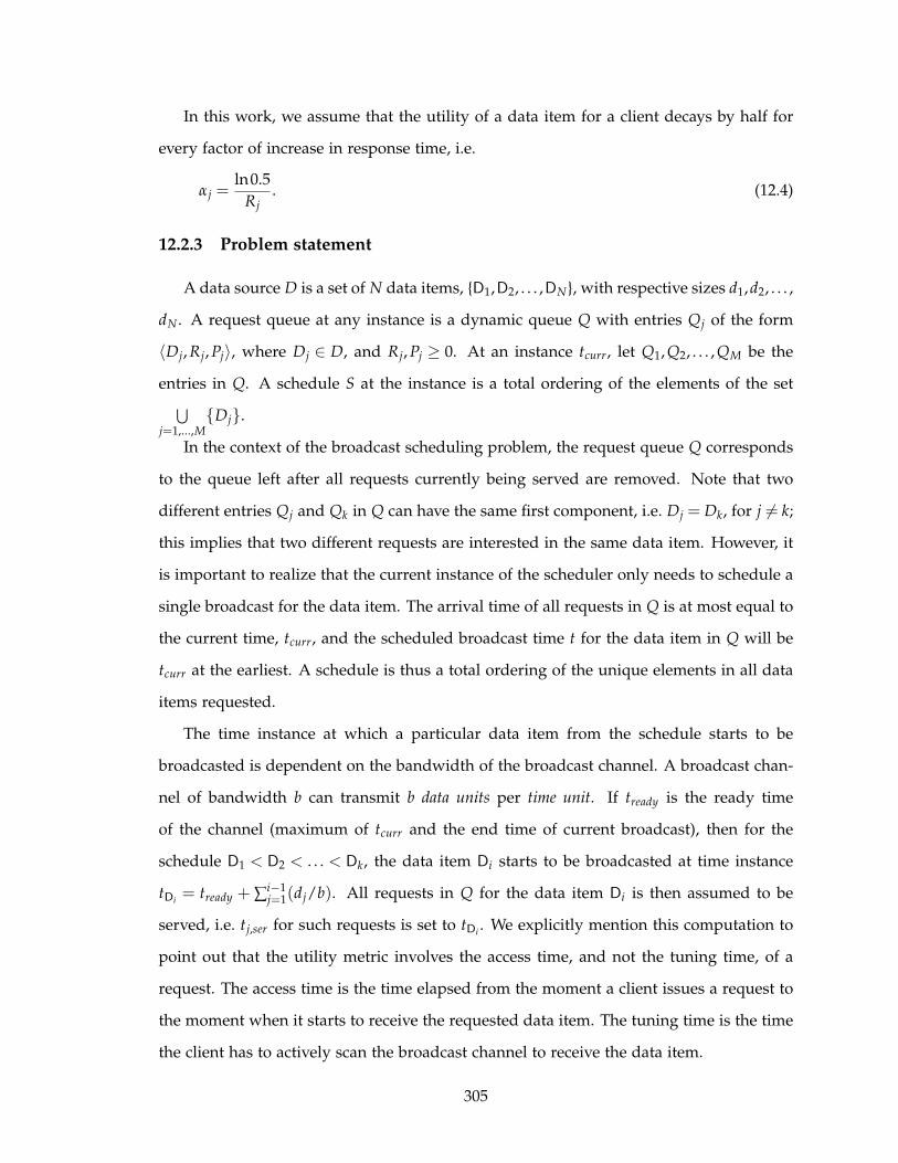
In this work, we assume that the utility of a data item for a client decays by half for
every factor of increase in response time, i.e.
αj =ln0.5
Rj. (12.4)
12.2.3 Problem statement
A data source D is a set of N data items, {D1,D2, . . . ,DN}, with respective sizes d1,d2, . . . ,
dN . A request queue at any instance is a dynamic queue Q with entries Qj of the form
〈Dj, Rj, Pj〉, where Dj ∈ D, and Rj, Pj ≥ 0. At an instance tcurr, let Q1, Q2, . . . , QM be the
entries in Q. A schedule S at the instance is a total ordering of the elements of the set
⋃
j=1,...,M{Dj}.
In the context of the broadcast scheduling problem, the request queue Q corresponds
to the queue left after all requests currently being served are removed. Note that two
different entries Qj and Qk in Q can have the same first component, i.e. Dj = Dk, for j 6= k;
this implies that two different requests are interested in the same data item. However, it
is important to realize that the current instance of the scheduler only needs to schedule a
single broadcast for the data item. The arrival time of all requests in Q is at most equal to
the current time, tcurr, and the scheduled broadcast time t for the data item in Q will be
tcurr at the earliest. A schedule is thus a total ordering of the unique elements in all data
items requested.
The time instance at which a particular data item from the schedule starts to be
broadcasted is dependent on the bandwidth of the broadcast channel. A broadcast chan-
nel of bandwidth b can transmit b data units per time unit. If tready is the ready time
of the channel (maximum of tcurr and the end time of current broadcast), then for the
schedule D1 < D2 < . . . < Dk, the data item Di starts to be broadcasted at time instance
tDi= tready + ∑
i−1j=1(dj/b). All requests in Q for the data item Di is then assumed to be
served, i.e. tj,ser for such requests is set to tDi. We explicitly mention this computation to
point out that the utility metric involves the access time, and not the tuning time, of a
request. The access time is the time elapsed from the moment a client issues a request to
the moment when it starts to receive the requested data item. The tuning time is the time
the client has to actively scan the broadcast channel to receive the data item.
305

While Eq. (12.3) can be used to measure the instantaneous utility of a schedule, it
is not suitable in determining the performance level of a solution method in a dynamic
setting. We thus use the utility generated from the queries already served as the yardstick
to compare performance. In other words, the performance of a solution methodology at
an instance where queries Q1, . . . , QK are already served is measured by ∑Kj=1 uj. In effect,
we are interested in the global utility generated by the method. The aforementioned QoS
criteria could be a specification in terms of this global utility. The objective behind the
design of a solution methodology is to then maximize this global utility measured at any
instance.
12.2.4 Scheduling transaction data
The aforementioned problem assumes that requests are made at the data item level.
A client interested in multiple data items would make independent requests for the in-
dividual items. As an extension of this problem, we also consider the case of transaction
level requests. A transaction level request differs from a data item level request in the
sense that a request involves more than one data item. The order of retrieval of the data
items is not important, but processing at the client end cannot start until all data items
are received.
The difference in problem formulation appears here in the definition of a query Qj. An
entry Qj in the request queue now takes the form 〈Dj, Rj, Pj〉, where Dj = {Dj1 , . . . , Djn} ⊆D and Rj, Pj ≥ 0. The request is considered to be served at tj,served, which is the time
instance when the last remaining data item in Dj is broadcast. The utility generated
by serving the request then follows from Eq. (12.2). Note that, with this formulation,
scheduling at the transaction level is not a simple extension of the problem of scheduling
an aggregation of multiple requests from the same client. The following factors highlight
the differences in data item and transaction level scheduling.
1. Multiple data item level requests made from the same client can have different
deadlines associated with different data items. However, the deadline specified in
a transaction level request is specific to the transaction and not the individual data
items required to complete it.
306
2. Each request made at the data item level would accrue some utility, irrespective of
whether it came from the same client or not. The notion of dependency between the
data items (to complete a transaction) is not embedded in the requests. A request at
the transaction level specifies this dependency by collecting the required data items
into a set and making a request for the entire set. Utility is accrued in this case only
when all items in the set are served.
3. When requests are made independently, the scheduler is not required to maintain
low levels of latency between broadcasts of data items requested by the same client.
However, at the transaction level, the schedules generated must take the latency into
consideration since the utility will keep reducing until all requested data items are
retrieved by the client.
12.3 Solution Methodology
In the previous section, we identified that a solution methodology which can maxi-
mize the global utility is desired for the broadcast problem under study. However, it is
often difficult to anticipate the incoming data access requests in a dynamic environment.
Besides, an ongoing broadcast cannot be interrupted to accommodate higher utility from
new requests. This restricts a solution methodology to focus on the current request queue
only and make scheduling decisions that yield higher utility from the generated sched-
ule. It can only be expected that a higher global utility measure would be obtained in the
process.
Another constraint is the time factor involved in making a scheduling decision. Data
requests usually arrive more frequently than they can be served, which in turn lead to
the generation of a long request queue. Any scheduling method must be fast enough to
generate a good schedule without adding much to the access time of requests. Latencies
induced between broadcasts because of the scheduling time is also a detrimental factor
to resource utilization. Heuristics are often used as fast decision makers, but may result
in degraded solution quality. Hybrid approaches in this context can provide a suitable
trade-off between solution quality and decision time.
307
Moreover, the assumption that a heuristic driven method is most appropriate in real
time decision making can be flawed. This is specially true when the search space involved
is well understood and specialized optimization methods can be devised to exploit the
dynamics of the search space. In such situations, even a suboptimal solution generated by
a carefully crafted optimization technique could be better than a heuristic based solution.
12.3.1 Heuristics
For the purpose of this study, we use two heuristics – Earliest Deadline First (EDF) and
Highest Utility First (HUF) – which takes into account the time critical nature of a data
request.
EDF starts off by first scheduling the data item which corresponds to a request with
the minimum tcurr − (tarr + Rj). All requests in Q that get served by this broadcast are
removed (all requests for the scheduled data item) and the process is repeated on the
remaining requests. For multiple channels, the heuristic can be combined with best local
earliness to map the data item to a channel that becomes ready at the earliest. EDF gives
preference to data items that have long been awaited by some request, thereby having
some level of impact on the utility that can be generated by the requests. However, it
does not take into account the actual utility generated.
HUF alleviates this problem by first considering the data item that can generate the
highest amount of utility. The strategy adopted by HUF may seem like a good approach
particularly when the overall utility is the performance metric. However, HUF generated
schedules may not be flexible enough in a dynamic environment. For example, if the
most requested data item in the current request queue generates the highest utility, HUF
would schedule the item as the next broadcast. If this data item requires a high broadcast
time, not only will the subsequent broadcasts in the schedule suffer in utility, but new
requests will also have to wait for a long time before getting served.
12.3.2 Heuristics with local search
As mentioned earlier, the emphasis in this work is understanding the performance
of heuristics when coupled with local search techniques. We therefore introduce some
308
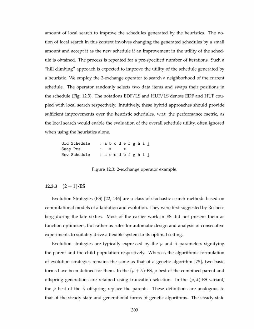
amount of local search to improve the schedules generated by the heuristics. The no-
tion of local search in this context involves changing the generated schedules by a small
amount and accept it as the new schedule if an improvement in the utility of the sched-
ule is obtained. The process is repeated for a pre-specified number of iterations. Such a
“hill climbing” approach is expected to improve the utility of the schedule generated by
a heuristic. We employ the 2-exchange operator to search a neighborhood of the current
schedule. The operator randomly selects two data items and swaps their positions in
the schedule (Fig. 12.3). The notations EDF/LS and HUF/LS denote EDF and HUF cou-
pled with local search respectively. Intuitively, these hybrid approaches should provide
sufficient improvements over the heuristic schedules, w.r.t. the performance metric, as
the local search would enable the evaluation of the overall schedule utility, often ignored
when using the heuristics alone.
Old Schedule : a b c d e f g h i j
Swap Pts : * *
New Schedule : a e c d b f g h i j
Figure 12.3: 2-exchange operator example.
12.3.3 (2 + 1)-ES
Evolution Strategies (ES) [22, 146] are a class of stochastic search methods based on
computational models of adaptation and evolution. They were first suggested by Rechen-
berg during the late sixties. Most of the earlier work in ES did not present them as
function optimizers, but rather as rules for automatic design and analysis of consecutive
experiments to suitably drive a flexible system to its optimal setting.
Evolution strategies are typically expressed by the µ and λ parameters signifying
the parent and the child population respectively. Whereas the algorithmic formulation
of evolution strategies remains the same as that of a genetic algorithm [75], two basic
forms have been defined for them. In the (µ + λ)-ES, µ best of the combined parent and
offspring generations are retained using truncation selection. In the (µ,λ)-ES variant,
the µ best of the λ offspring replace the parents. These definitions are analogous to
that of the steady-state and generational forms of genetic algorithms. The steady-state
309

Procedure 12.1 (2+1)-ES()
1: Generate two initial solutions x and y2: Evaluate x and y3: repeat
4: Recombine x and y to generate an offspring z5: Mutate z with probability p6: Evaluate z7: Replace x and y by the two best solutions from {x,y,z}8: until (termination criteria is met)
variant of genetic algorithms explicitly maintains the best solution found so far, while the
generational variant blindly replaces the current population with the offspring population
generated.
For our experimentation, we employ the (µ + λ)-ES variant with µ = 2 and λ = 1. This
simple form of the ES is chosen to keep the dynamic scheduling time within an acceptable
limit without sacrificing on the solution quality. Also, a (2 + 1)-ES can be seen as a type
of greedy stochastic local search. It is stochastic because there is no fixed neighborhood
and therefore the neighborhood does not define a fixed set of local optima. Otherwise,
the method is very much a local search technique: sample the neighborhood and move to
the best point. The pseudo code for the algorithm is given in Procedure 12.1.
12.3.3.1 Solution encoding and evaluation
For the data broadcasting problem mentioned in the previous section, a typical sched-
ule can be represented by a permutation of the unique data item numbers in Q. Thus,
for n unique data items, the search spans over a space of n! points. In the presence of
multiple channels (T say), a similar encoding can be obtained by using −1 as a delimiter
between the schedules in different channels (Fig. 12.4) [140]. The evaluation of a solution
involves finding the utility of the represented schedule as given by Eq. (12.3). The higher
the utility, the better is the solution.
Channel: |--1--| |-2-| .... |--T--|
Encoding: 3 1 4 -1 2 6 -1 .... -1 8 5 9
Figure 12.4: Solution encoding for multiple channels.
310
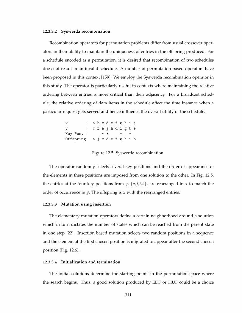
12.3.3.2 Syswerda recombination
Recombination operators for permutation problems differ from usual crossover oper-
ators in their ability to maintain the uniqueness of entries in the offspring produced. For
a schedule encoded as a permutation, it is desired that recombination of two schedules
does not result in an invalid schedule. A number of permutation based operators have
been proposed in this context [159]. We employ the Syswerda recombination operator in
this study. The operator is particularly useful in contexts where maintaining the relative
ordering between entries is more critical than their adjacency. For a broadcast sched-
ule, the relative ordering of data items in the schedule affect the time instance when a
particular request gets served and hence influence the overall utility of the schedule.
x : a b c d e f g h i j
y : c f a j h d i g b e
Key Pos. : * * * *
Offspring: a j c d e f g h i b
Figure 12.5: Syswerda recombination.
The operator randomly selects several key positions and the order of appearance of
the elements in these positions are imposed from one solution to the other. In Fig. 12.5,
the entries at the four key positions from y, {a, j, i,b}, are rearranged in x to match the
order of occurrence in y. The offspring is x with the rearranged entries.
12.3.3.3 Mutation using insertion
The elementary mutation operators define a certain neighborhood around a solution
which in turn dictates the number of states which can be reached from the parent state
in one step [22]. Insertion based mutation selects two random positions in a sequence
and the element at the first chosen position is migrated to appear after the second chosen
position (Fig. 12.6).
12.3.3.4 Initialization and termination
The initial solutions determine the starting points in the permutation space where
the search begins. Thus, a good solution produced by EDF or HUF could be a choice
311
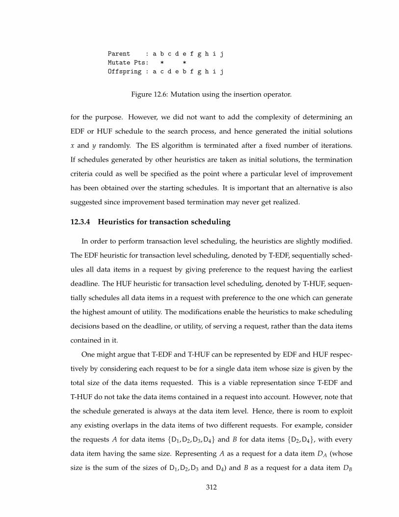
Parent : a b c d e f g h i j
Mutate Pts: * *
Offspring : a c d e b f g h i j
Figure 12.6: Mutation using the insertion operator.
for the purpose. However, we did not want to add the complexity of determining an
EDF or HUF schedule to the search process, and hence generated the initial solutions
x and y randomly. The ES algorithm is terminated after a fixed number of iterations.
If schedules generated by other heuristics are taken as initial solutions, the termination
criteria could as well be specified as the point where a particular level of improvement
has been obtained over the starting schedules. It is important that an alternative is also
suggested since improvement based termination may never get realized.
12.3.4 Heuristics for transaction scheduling
In order to perform transaction level scheduling, the heuristics are slightly modified.
The EDF heuristic for transaction level scheduling, denoted by T-EDF, sequentially sched-
ules all data items in a request by giving preference to the request having the earliest
deadline. The HUF heuristic for transaction level scheduling, denoted by T-HUF, sequen-
tially schedules all data items in a request with preference to the one which can generate
the highest amount of utility. The modifications enable the heuristics to make scheduling
decisions based on the deadline, or utility, of serving a request, rather than the data items
contained in it.
One might argue that T-EDF and T-HUF can be represented by EDF and HUF respec-
tively by considering each request to be for a single data item whose size is given by the
total size of the data items requested. This is a viable representation since T-EDF and
T-HUF do not take the data items contained in a request into account. However, note that
the schedule generated is always at the data item level. Hence, there is room to exploit
any existing overlaps in the data items of two different requests. For example, consider
the requests A for data items {D1,D2,D3,D4} and B for data items {D2,D4}, with every
data item having the same size. Representing A as a request for a data item DA (whose
size is the sum of the sizes of D1,D2,D3 and D4) and B as a request for a data item DB
312
loses the fact that the data items in B are a subset of those in A. Further, exploiting
the existence of such subsets is also not trivial. This is specifically true for T-EDF which
makes decisions based solely on the deadline. If A has an earlier deadline than B then
the schedule generated will be D1 < D2 < D3 < D4; otherwise D2 < D4 < D1 < D3. Ob-
serve that, in the former case, both requests A and B will be served at the same time
instance (the instance when D4 starts broadcasting), while in the latter case, B will get
served earlier. Hence, irrespective of the deadlines, the latter schedule is always equal to
or better than the former. It is possible that even T-HUF fails to exploit the relationship.
If serving A first generates higher utility than serving B first, T-HUF would generate the
former schedule, thereby pushing the finish time of B further in the time line. It misses
the observation that by serving B first it can still maintain the same utility for A. The
situation is further complicated when the data items have varying sizes. Given such ob-
servations, augmenting the heuristics with local search would allow for an interesting
exploration at the data item level. Recall that the local search would attempt to improve
on the heuristic generated schedule by swapping data items at different positions. The
corresponding local search variants for T-EDF and T-HUF are denoted by T-EDF/LS and
T-HUF/LS respectively.
The (2 + 1)-ES does not make a distinction between data item level and transaction
level requests. It always operates at the data item level irrespective of how the request
was made. Similar to the earlier case, the (2 + 1)-ES here first determines the set of data
items to be scheduled in order to serve all requests in the queue –⋃Dj. It then generates
a schedule with these items to maximize the utility. Since requests are served only when
all requested data items are received by a client, random initial solutions are likely to
disperse dependent data items (belonging to the same transaction). Hence, we modify the
initialization strategy to direct the search from a favorable region in the search space. The
modification creates the initial solutions by choosing random requests from the queue
and sequentially laying out the data items contained in the requests on the schedule.
For example, if D1 = {D1,D2,D3} and D2 = {D3,D2} are two transactions on the request
queue, and transaction 1 is randomly chosen under this process, then data items D1,D2
and D3 will be consecutive on the initial schedule. The process generates a favorable
313

Table 12.1: Experiment parameters.
Parameter Value Comment
N 300 Number of data itemsdmin 5KB Minimum data item sizedmax 1000KB Maximum data item size
b 120 KB/s Broadcast channel bandwidthm 60s/180s Request response time meanσ 20s/40s Request response time std. dev.r 5 Request arrival rate
rT 5 Transaction size Poisson rates 0.8 Zipf’s law characterizing exponentP Low(1), Medium(2), High(4) Priority levelsp 0.5 Mutation probability
Gen 1000 Iterations for local search and ES
arrangement of the data items for some of the requests. The remaining functionality of
the ES is maintained as described in Section 12.3.3.
12.4 Experimental Setup
The data sets used in our experiments are generated using various popular distri-
butions that are known to capture the dynamics of a public data access system. The
different parameters of the experiment are tabulated in Table 12.1 and discussed below.
We generate two different data sets with these parameter settings, one involving data
item level requests and another involving transaction level requests. Experiments are run
independently on the two data sets using the corresponding heuristics and the (2 + 1)-ES.
Each data set contains 10,000 requests generated using a Poisson distribution with
an arrival rate of r requests per second. Each request consists of an arrival time, data
item number (or set of data item numbers for transaction level requests), an expected
response time, and a priority level. For transaction level requests, the number of data
items contained in a transaction is drawn from another Poisson distribution with rate rT
items per transaction.
We would like to point here that the number of data items (N) to be handled by
a scheduler need not be very big in a pervasive setup. Each broadcast station would
314
typically be responsible for catering requests involving a sub-domain of the entire setup,
in which case its data domain would also be comparatively smaller. The data items
requested are assumed to follow the commonly used Zipf -like distribution [27] with the
characterizing exponent of 0.8. Under this assumption, the first data item becomes the
most requested item, while the last one is the least requested. Broadcast schedules can
be heavily affected by the size of the most requested data item. Hence, we consider two
different assignments of sizes to the data items from existing literature [80, 107]. The
INC distribution makes the most requested data item the smallest in size, while the DEC
distribution makes it the largest in size.
INC : di = dmin +(i − 1)(dmax − dmin + 1)
N, i = 1, . . . , N (12.5)
DEC : di = dmax −(i − 1)(dmax − dmin + 1)
N, i = 1, . . . , N (12.6)
Expected response times are assigned from a normal distribution with mean m and
standard deviation σ. The particular settings of these parameters in our data item level
experiment results in expected response times to be generated in the range of [0,120]s
with a probability of 0.997. For transaction level requests, the mean and standard devia-
tion are changed so that the interval changes to [60,300]s. Any value generated outside
the range of the intervals is changed to the lower bound of the corresponding interval.
We use three different priority levels for the requests – low, medium, and high. Numeric
values are assigned to these levels such that the significance of a level is twice that of the
previous one. Since the total utility is related to the priority of the requests, we make
assignments from these levels in such a way that the maximum utility obtainable by
serving requests from each priority level is probabilistically equal. To do so, we use a
roulette-wheel selection [75] mechanism which effectively sets the probability of selecting
a priority level as: P(Low) = 47 , P(Medium) = 2
7 , and P(High) = 17 . Such a scheme restricts
the scheduler from favoring high priority requests unless the utility generated by them is
in fact higher than the cumulative utility from low priority requests.
Workloads on the scheduler can be varied by either changing the request arrival rate,
or the channel bandwidth. We use the latter approach and specify the bandwidth used
315

wherever different from the default.
The local search for EDF/LS, HUF/LS, T-EDF/LS and T-HUF/LS are run for Gen
number of iterations. For (2 + 1)-ES, the same number of iterations is chosen as the
termination criteria. The number of iterations has been fixed such that the scheduling
time is not more than 0.01s (on a 2.4 GHz Pentium 4 with 512 MB memory running
Fedora Core 7) when the request queue contains requests for around 150 unique data
items on the average. This is critical so that the runtime of the iterative algorithms do not
impose high latencies in the decision making process. The performance of each method
is measured at the time instance when all the requests get served. In other words, the
performance of each method is given by the sum of the utilities generated by serving each
of the requests in the data set.
12.5 Empirical Results
We first present the overall performance results obtained for the five different solution
methodologies on the data item level data set. Although, the data item level scheduling
problem can be viewed as a special case of the transaction level scheduling, we observed
that a method’s performance can be quite different in these two problem classes.
12.5.1 Data-item level scheduling
Fig. 12.7 shows the performance in terms of the percentage of maximum total utility
returned by using each of the methods. The maximum total utility is obtained when
every request is served within its expected response time, in which case it attains an
utility equal to its priority level. Thus, summing up the priorities of all requests gives the
maximum total utility that can be obtained.
For the INC data size distribution, HUF, HUF/LS and ES have similar performance.
Although, EDF and EDF/LS have a slightly lower performance, both the methods do
reasonably well. A major difference is observed in the amount of improvement gained
by EDF by using local search, as compared to that of HUF. This is because EDF does not
take into consideration the utility factor of requests and hence performing a local search
based on utility results in a substantial level of improvement. HUF does reasonably well
316
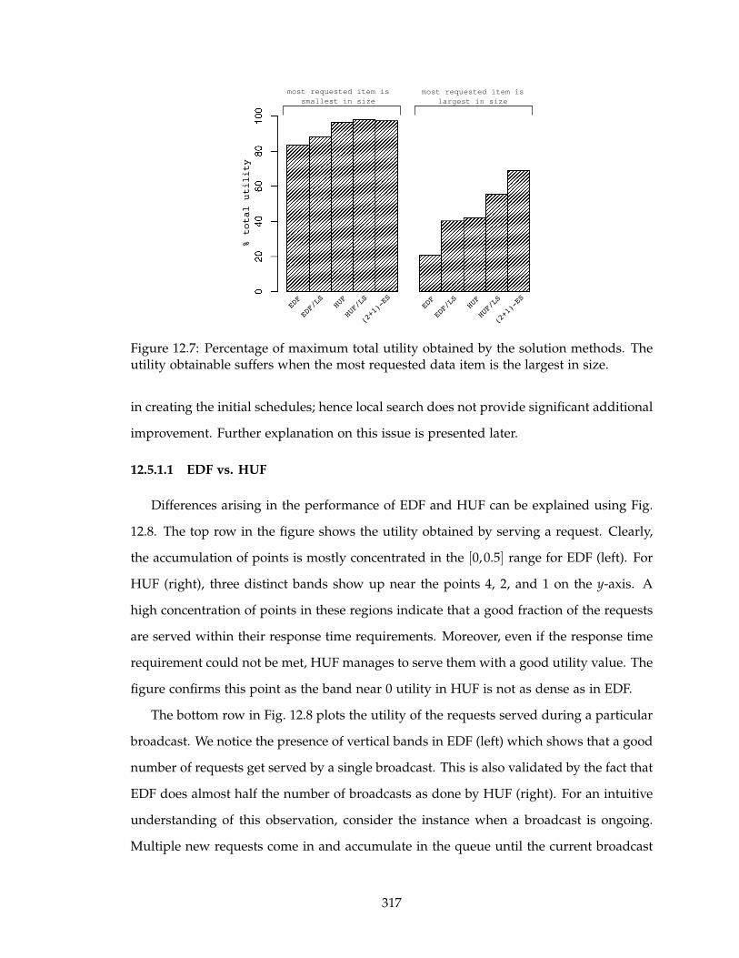
EDF
EDF/LS
HUF
HUF/LS
(2+1)-ES
EDF
EDF/LS
HUF
HUF/LS
(2+1)-ES
most requested item is
smallest in size
most requested item is
largest in size
% total utility
Figure 12.7: Percentage of maximum total utility obtained by the solution methods. Theutility obtainable suffers when the most requested data item is the largest in size.
in creating the initial schedules; hence local search does not provide significant additional
improvement. Further explanation on this issue is presented later.
12.5.1.1 EDF vs. HUF
Differences arising in the performance of EDF and HUF can be explained using Fig.
12.8. The top row in the figure shows the utility obtained by serving a request. Clearly,
the accumulation of points is mostly concentrated in the [0,0.5] range for EDF (left). For
HUF (right), three distinct bands show up near the points 4, 2, and 1 on the y-axis. A
high concentration of points in these regions indicate that a good fraction of the requests
are served within their response time requirements. Moreover, even if the response time
requirement could not be met, HUF manages to serve them with a good utility value. The
figure confirms this point as the band near 0 utility in HUF is not as dense as in EDF.
The bottom row in Fig. 12.8 plots the utility of the requests served during a particular
broadcast. We notice the presence of vertical bands in EDF (left) which shows that a good
number of requests get served by a single broadcast. This is also validated by the fact that
EDF does almost half the number of broadcasts as done by HUF (right). For an intuitive
understanding of this observation, consider the instance when a broadcast is ongoing.
Multiple new requests come in and accumulate in the queue until the current broadcast
317
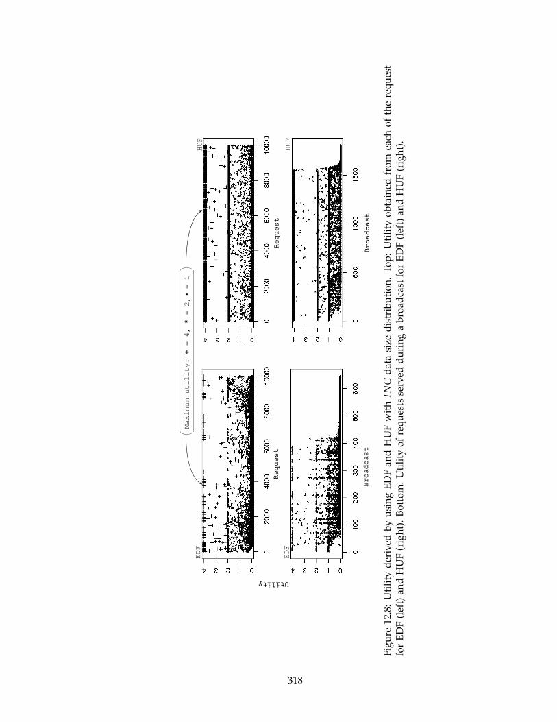
Broadcast
Request
Request
Broadcast
Utility
Maximum utility: + = 4, * = 2, = 1
.
EDF
EDF
HUF
HUF
Fig
ure
12.8
:U
tili
tyd
eriv
edb
yu
sin
gE
DF
and
HU
Fw
ith
INC
dat
asi
zed
istr
ibu
tio
n.
To
p:
Uti
lity
ob
tain
edfr
om
each
of
the
req
ues
tfo
rE
DF
(lef
t)an
dH
UF
(rig
ht)
.B
ott
om
:U
tili
tyo
fre
qu
ests
serv
edd
uri
ng
ab
road
cast
for
ED
F(l
eft)
and
HU
F(r
igh
t).
318
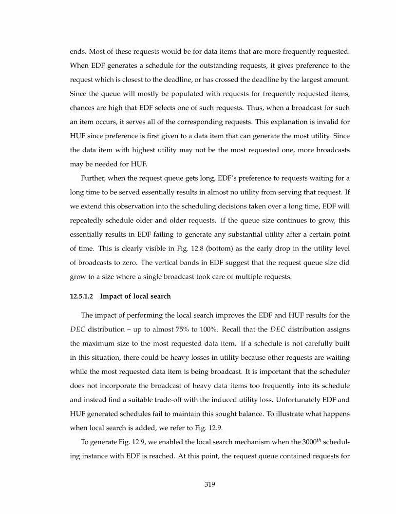
ends. Most of these requests would be for data items that are more frequently requested.
When EDF generates a schedule for the outstanding requests, it gives preference to the
request which is closest to the deadline, or has crossed the deadline by the largest amount.
Since the queue will mostly be populated with requests for frequently requested items,
chances are high that EDF selects one of such requests. Thus, when a broadcast for such
an item occurs, it serves all of the corresponding requests. This explanation is invalid for
HUF since preference is first given to a data item that can generate the most utility. Since
the data item with highest utility may not be the most requested one, more broadcasts
may be needed for HUF.
Further, when the request queue gets long, EDF’s preference to requests waiting for a
long time to be served essentially results in almost no utility from serving that request. If
we extend this observation into the scheduling decisions taken over a long time, EDF will
repeatedly schedule older and older requests. If the queue size continues to grow, this
essentially results in EDF failing to generate any substantial utility after a certain point
of time. This is clearly visible in Fig. 12.8 (bottom) as the early drop in the utility level
of broadcasts to zero. The vertical bands in EDF suggest that the request queue size did
grow to a size where a single broadcast took care of multiple requests.
12.5.1.2 Impact of local search
The impact of performing the local search improves the EDF and HUF results for the
DEC distribution – up to almost 75% to 100%. Recall that the DEC distribution assigns
the maximum size to the most requested data item. If a schedule is not carefully built
in this situation, there could be heavy losses in utility because other requests are waiting
while the most requested data item is being broadcast. It is important that the scheduler
does not incorporate the broadcast of heavy data items too frequently into its schedule
and instead find a suitable trade-off with the induced utility loss. Unfortunately EDF and
HUF generated schedules fail to maintain this sought balance. To illustrate what happens
when local search is added, we refer to Fig. 12.9.
To generate Fig. 12.9, we enabled the local search mechanism when the 3000th schedul-
ing instance with EDF is reached. At this point, the request queue contained requests for
319
0 1000
1.0
2.5
Iteration
Utility improvement factor
Figure 12.9: Improvements obtained by doing 50000 iterations of the 2-exchange operatorfor the EDF schedule generated during the 3000th scheduling instance. The DEC datasize distribution is used here. A newly obtained solution is considered better only if itexceeds the utility of the current solution by at least 20.
127 unique data items. The local search mechanism use the 2-exchange operator to gener-
ate a new schedule. To start with, the 2-exchange operator is applied to the EDF schedule
to generate a new one. If the utility improves by more than 20, the new schedule is con-
sidered for any further 2-exchange operation. The process is repeated for 50000 iterations.
The plot shows the factor of improvement obtained from the EDF schedule at each itera-
tion of the local search. The factor of improvement is computed as utility of solution/utility
of EDF solution. A gray point (x,y) in the plot illustrates that the factor of improvement
for the solution obtained in the xth iteration of the search is y. The solid line joins the
points where a generated schedule had an utility improvement of 20, or more, over the
current one.
The horizontal bands in the figure illustrate the fact that the schedule space is mostly
flat in structure. For a given schedule, most of its neighboring schedules (obtained by
the 2-exchange operator) have, more or less, equal amounts of utility associated with
them. Hence the improvement factor values accumulate around a region to generate the
bands. A more interesting observation is the amount of improvement obtained across the
different iterations. We see that the schedule utility improves to a factor of 2.5 within
the first 1000 iterations of the local search (inset Fig. 12.9), after which the progress slows
320
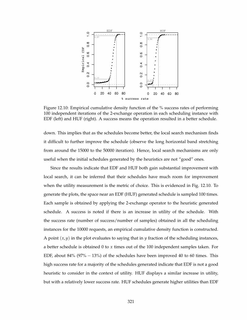
% success rate
Empirical CDF
0.13
0.97
0.92
0.07
HUFEDF
Figure 12.10: Empirical cumulative density function of the % success rates of performing100 independent iterations of the 2-exchange operation in each scheduling instance withEDF (left) and HUF (right). A success means the operation resulted in a better schedule.
down. This implies that as the schedules become better, the local search mechanism finds
it difficult to further improve the schedule (observe the long horizontal band stretching
from around the 15000 to the 50000 iteration). Hence, local search mechanisms are only
useful when the initial schedules generated by the heuristics are not “good” ones.
Since the results indicate that EDF and HUF both gain substantial improvement with
local search, it can be inferred that their schedules have much room for improvement
when the utility measurement is the metric of choice. This is evidenced in Fig. 12.10. To
generate the plots, the space near an EDF (HUF) generated schedule is sampled 100 times.
Each sample is obtained by applying the 2-exchange operator to the heuristic generated
schedule. A success is noted if there is an increase in utility of the schedule. With
the success rate (number of success/number of samples) obtained in all the scheduling
instances for the 10000 requests, an empirical cumulative density function is constructed.
A point (x,y) in the plot evaluates to saying that in y fraction of the scheduling instances,
a better schedule is obtained 0 to x times out of the 100 independent samples taken. For
EDF, about 84% (97% − 13%) of the schedules have been improved 40 to 60 times. This
high success rate for a majority of the schedules generated indicate that EDF is not a good
heuristic to consider in the context of utility. HUF displays a similar increase in utility,
but with a relatively lower success rate. HUF schedules generate higher utilities than EDF
321
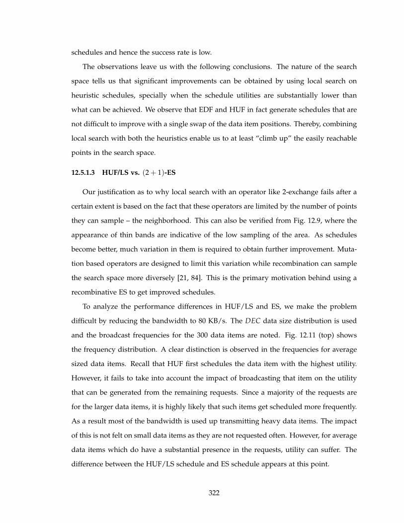
schedules and hence the success rate is low.
The observations leave us with the following conclusions. The nature of the search
space tells us that significant improvements can be obtained by using local search on
heuristic schedules, specially when the schedule utilities are substantially lower than
what can be achieved. We observe that EDF and HUF in fact generate schedules that are
not difficult to improve with a single swap of the data item positions. Thereby, combining
local search with both the heuristics enable us to at least “climb up” the easily reachable
points in the search space.
12.5.1.3 HUF/LS vs. (2 + 1)-ES
Our justification as to why local search with an operator like 2-exchange fails after a
certain extent is based on the fact that these operators are limited by the number of points
they can sample – the neighborhood. This can also be verified from Fig. 12.9, where the
appearance of thin bands are indicative of the low sampling of the area. As schedules
become better, much variation in them is required to obtain further improvement. Muta-
tion based operators are designed to limit this variation while recombination can sample
the search space more diversely [21, 84]. This is the primary motivation behind using a
recombinative ES to get improved schedules.
To analyze the performance differences in HUF/LS and ES, we make the problem
difficult by reducing the bandwidth to 80 KB/s. The DEC data size distribution is used
and the broadcast frequencies for the 300 data items are noted. Fig. 12.11 (top) shows
the frequency distribution. A clear distinction is observed in the frequencies for average
sized data items. Recall that HUF first schedules the data item with the highest utility.
However, it fails to take into account the impact of broadcasting that item on the utility
that can be generated from the remaining requests. Since a majority of the requests are
for the larger data items, it is highly likely that such items get scheduled more frequently.
As a result most of the bandwidth is used up transmitting heavy data items. The impact
of this is not felt on small data items as they are not requested often. However, for average
data items which do have a substantial presence in the requests, utility can suffer. The
difference between the HUF/LS schedule and ES schedule appears at this point.
322
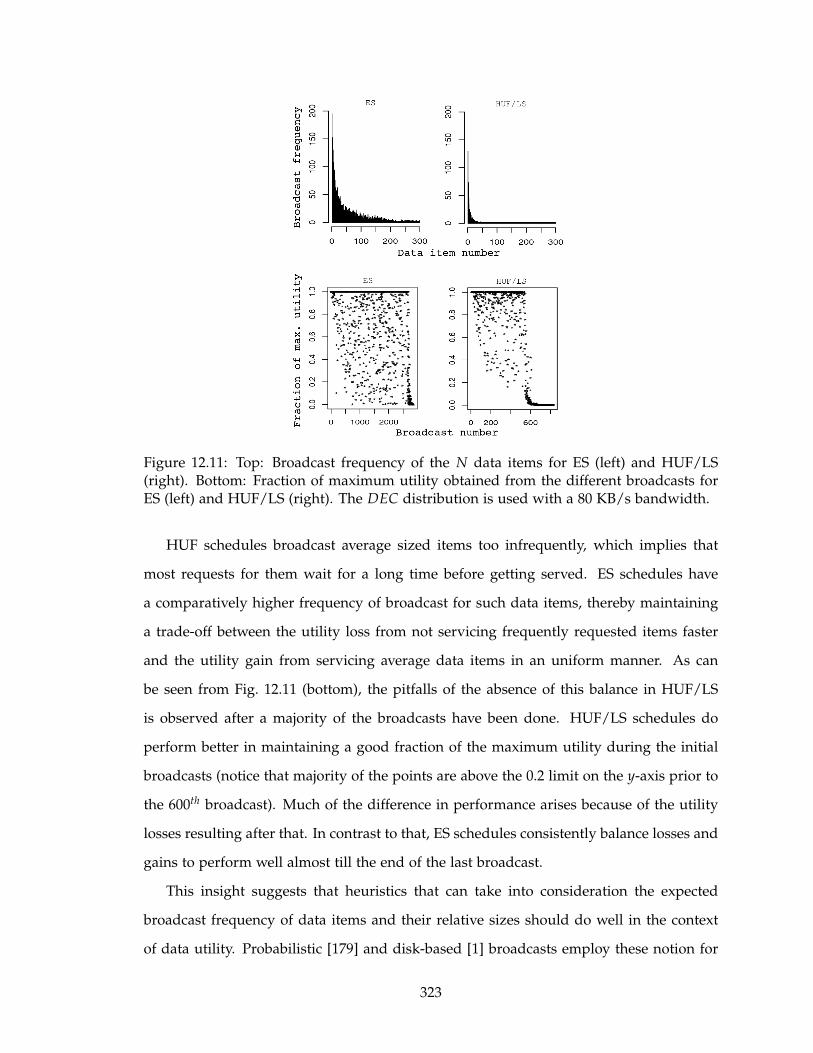
Figure 12.11: Top: Broadcast frequency of the N data items for ES (left) and HUF/LS(right). Bottom: Fraction of maximum utility obtained from the different broadcasts forES (left) and HUF/LS (right). The DEC distribution is used with a 80 KB/s bandwidth.
HUF schedules broadcast average sized items too infrequently, which implies that
most requests for them wait for a long time before getting served. ES schedules have
a comparatively higher frequency of broadcast for such data items, thereby maintaining
a trade-off between the utility loss from not servicing frequently requested items faster
and the utility gain from servicing average data items in an uniform manner. As can
be seen from Fig. 12.11 (bottom), the pitfalls of the absence of this balance in HUF/LS
is observed after a majority of the broadcasts have been done. HUF/LS schedules do
perform better in maintaining a good fraction of the maximum utility during the initial
broadcasts (notice that majority of the points are above the 0.2 limit on the y-axis prior to
the 600th broadcast). Much of the difference in performance arises because of the utility
losses resulting after that. In contrast to that, ES schedules consistently balance losses and
gains to perform well almost till the end of the last broadcast.
This insight suggests that heuristics that can take into consideration the expected
broadcast frequency of data items and their relative sizes should do well in the context
of data utility. Probabilistic [179] and disk-based [1] broadcasts employ these notion for
323
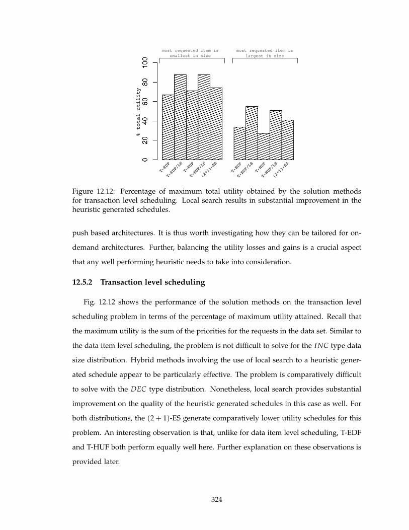
T-EDF
T-EDF/LS
T-HUF
T-HUF/LS
(2+1)-ES
T-EDF
T-EDF/LS
T-HUF
T-HUF/LS
(2+1)-ES
most requested item is
smallest in size
most requested item is
largest in size
% total utility
Figure 12.12: Percentage of maximum total utility obtained by the solution methodsfor transaction level scheduling. Local search results in substantial improvement in theheuristic generated schedules.
push based architectures. It is thus worth investigating how they can be tailored for on-
demand architectures. Further, balancing the utility losses and gains is a crucial aspect
that any well performing heuristic needs to take into consideration.
12.5.2 Transaction level scheduling
Fig. 12.12 shows the performance of the solution methods on the transaction level
scheduling problem in terms of the percentage of maximum utility attained. Recall that
the maximum utility is the sum of the priorities for the requests in the data set. Similar to
the data item level scheduling, the problem is not difficult to solve for the INC type data
size distribution. Hybrid methods involving the use of local search to a heuristic gener-
ated schedule appear to be particularly effective. The problem is comparatively difficult
to solve with the DEC type distribution. Nonetheless, local search provides substantial
improvement on the quality of the heuristic generated schedules in this case as well. For
both distributions, the (2 + 1)-ES generate comparatively lower utility schedules for this
problem. An interesting observation is that, unlike for data item level scheduling, T-EDF
and T-HUF both perform equally well here. Further explanation on these observations is
provided later.
324
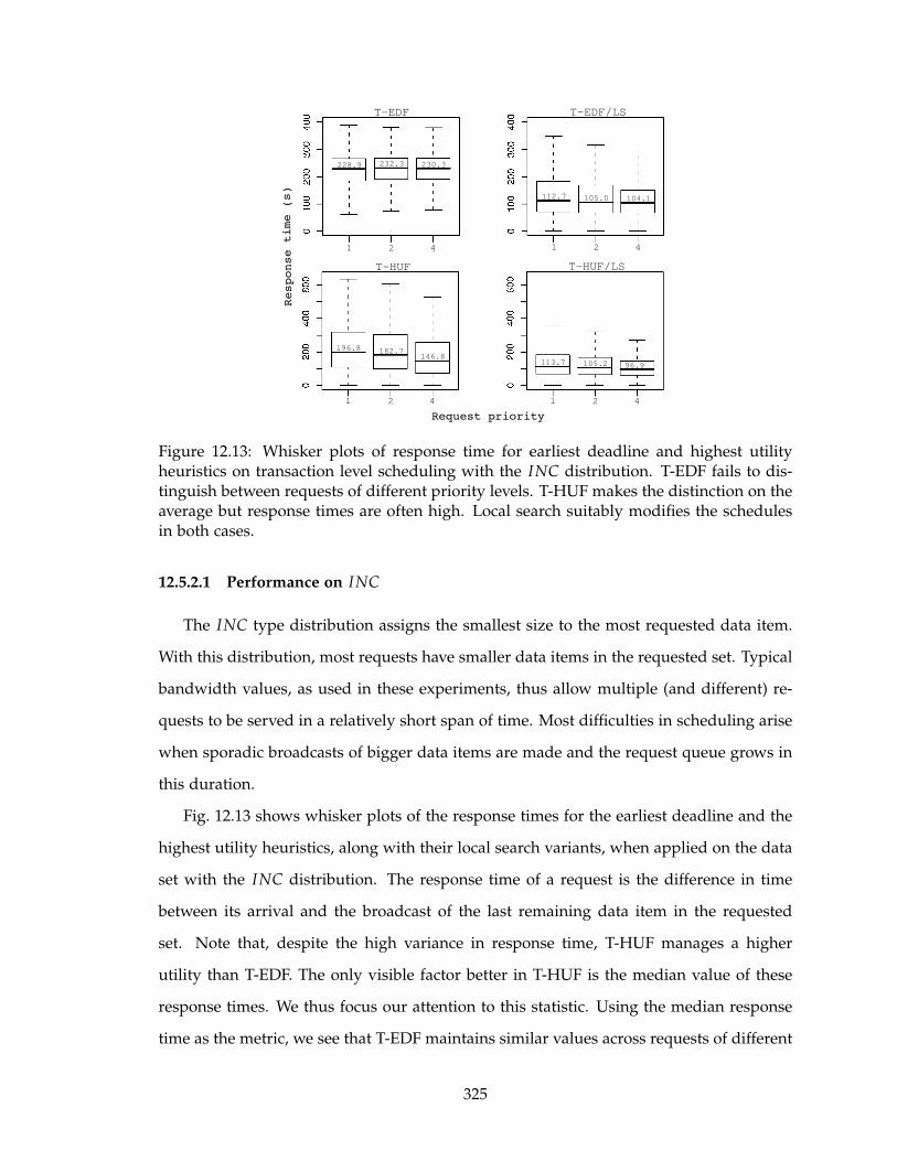
1 2 4 1 2 4
1 2 4 1 2 4
228.9 232.3 230.3
112.7 105.0 104.1
196.8 182.7146.8
113.7 105.2 96.9
T-EDF T-EDF/LS
T-HUF T-HUF/LS
Request priority
Response time (s)
Figure 12.13: Whisker plots of response time for earliest deadline and highest utilityheuristics on transaction level scheduling with the INC distribution. T-EDF fails to dis-tinguish between requests of different priority levels. T-HUF makes the distinction on theaverage but response times are often high. Local search suitably modifies the schedulesin both cases.
12.5.2.1 Performance on INC
The INC type distribution assigns the smallest size to the most requested data item.
With this distribution, most requests have smaller data items in the requested set. Typical
bandwidth values, as used in these experiments, thus allow multiple (and different) re-
quests to be served in a relatively short span of time. Most difficulties in scheduling arise
when sporadic broadcasts of bigger data items are made and the request queue grows in
this duration.
Fig. 12.13 shows whisker plots of the response times for the earliest deadline and the
highest utility heuristics, along with their local search variants, when applied on the data
set with the INC distribution. The response time of a request is the difference in time
between its arrival and the broadcast of the last remaining data item in the requested
set. Note that, despite the high variance in response time, T-HUF manages a higher
utility than T-EDF. The only visible factor better in T-HUF is the median value of these
response times. We thus focus our attention to this statistic. Using the median response
time as the metric, we see that T-EDF maintains similar values across requests of different
325
priorities. It fails to identify that high priority requests can generate more utility and
hence the data items in such requests should receive some level of preference over low
priority requests. The observation is not surprising since T-EDF’s efforts are restricted
to the deadline requirement only. In effect, there is no distinction between two requests
with the same amount of time remaining to their deadlines, but with different priorities.
T-HUF makes the distinction clear and further differentiates between such requests with
the added advantage of being able to identify broadcasts that might serve multiple low
priority requests instead of just a single high priority request.
Although T-EDF and T-HUF’s differences come from the ability to distinguish between
priority levels of requests, it does not seem to be the only factor affecting the utility. Local
search on these methods result in substantial improvement. The contributing factor to
this is the low median response time maintained along with the priority demarcations.
Note that T-EDF/LS and T-HUF/LS generate very similar distributions in the response
times. As described in the hypothetical example in Section 12.3.4, both T-EDF and T-
HUF do not take into account the effect of intermingling data items on the schedule
utility. Often it is possible to defy the logic behind a heuristic to some extent without
degrading the utility of the heuristic generated schedule. In certain cases, this can in
fact result in a better schedule. By swapping data items across the schedule, local search
effectuates better exploitation of the fact that commonly requested data items are present
in a significant fraction of the requests in the queue. What is uncertain is whether the
similar distributions in the response times is indicative of a local or a global optima.
12.5.2.2 Performance on DEC
A major difference between data item level scheduling and transaction level schedul-
ing is in the number of data items that has to be broadcasted to serve the requests in
the data set. With an average transaction size of 5 data items in each request, transac-
tion level scheduling has to make 5 different broadcasts before a single request is served.
Thus, heuristics in this problem must be able to exploit any overlaps between requests to
be effective in utility. The problem is further complicated with the DEC type distribution.
All requests in this case will contain at least one or more big data items as a result of
326
the Zipf distribution. If broadcast of such items (taking a long time to broadcast) serves
a very small fraction of the requests, then utility will most likely suffer in the long run.
Further, average or smaller sized data items will be requested with a less frequency, often
by requests separated far apart in the time line. Once again, utility will suffer if a heuris-
tic waits for a long time to accumulate requests for such data items with the objective of
serving multiple such requests with a single broadcast. Thus, a heuristic must be able to
balance these two aspects of broadcasting when working on transaction level scheduling
with the DEC distribution.
Fig. 12.14 shows the broadcast frequency of the different data items on this problem.
The frequency distribution is very dissimilar than in the case of data item level scheduling.
T-EDF, which performs better than T-HUF here, manages to maintain an almost uniform
distribution. In fact, if the first 20% of the bigger data items is not considered, all methods
show a similar trend. The uniform distribution is an extreme form of the balance we seek
as indicated above. T-HUF encounters a problem when seeking this balance and results
in a marginal drop in performance as compared to T-EDF. In transaction level scheduling,
requests which overlap significantly with parts of other requests are the ones that can
generate the highest utility. The overlap mostly occurs in the frequently requested data
items. T-HUF schedules such requests first without taking into account that delaying
a broadcast for a commonly requested item can actually help accumulate more requests
interested in the same data item. Unless a new request has better overlap features than the
ones already existing in the queue, the T-HUF schedule undergoes very small changes and
virtually remains consistent, specially in the first few data items in the broadcast queue,
for a certain period of time. What disrupts the consistency is the accumulation of enough
new requests to change the overlap features altogether. However, multiple data items
(often the bigger ones) have already been broadcast by this time and T-HUF is needed
to schedule another broadcast for them. In the case of T-EDF, this effect is overpowered
to some extent by the deadline requirement. Whenever a new request with a smaller
deadline and a lesser overlap with the existing requests arrive, T-EDF immediately gives
preference to it. As a result, broadcast times of data items in the existing schedule is
delayed, which helps serve more requests now. The frequency of broadcast of commonly
327
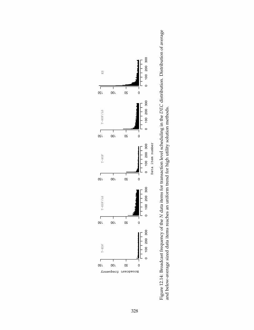
Data item number
Broadcast frequency
T-EDF
T-EDF/LS
T-HUF
T-HUF/LS
ES
Fig
ure
12.1
4:B
road
cast
freq
uen
cyo
fth
eN
dat
ait
ems
for
tran
sact
ion
lev
elsc
hed
uli
ng
inth
eD
EC
dis
trib
uti
on
.D
istr
ibu
tio
no
fav
erag
ean
db
elo
w-a
ver
age
size
dd
ata
item
sre
ach
esan
un
ifo
rmtr
end
for
hig
hu
tili
tyso
luti
on
met
ho
ds.
328
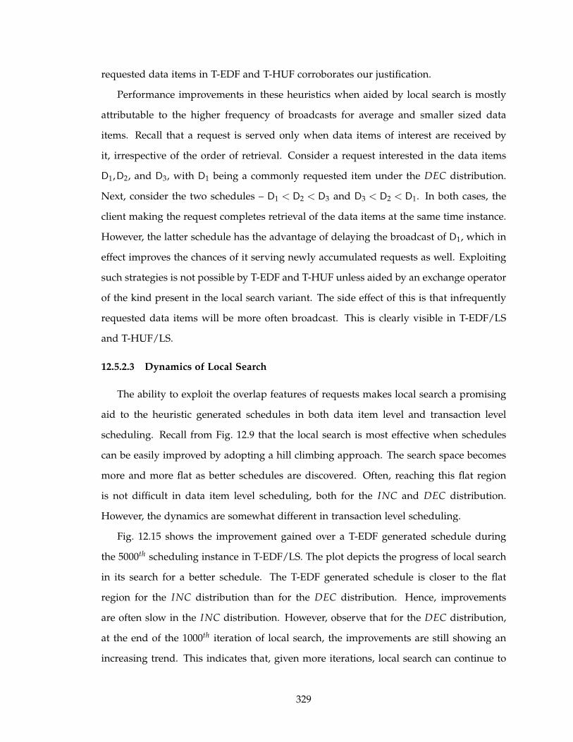
requested data items in T-EDF and T-HUF corroborates our justification.
Performance improvements in these heuristics when aided by local search is mostly
attributable to the higher frequency of broadcasts for average and smaller sized data
items. Recall that a request is served only when data items of interest are received by
it, irrespective of the order of retrieval. Consider a request interested in the data items
D1,D2, and D3, with D1 being a commonly requested item under the DEC distribution.
Next, consider the two schedules – D1 < D2 < D3 and D3 < D2 < D1. In both cases, the
client making the request completes retrieval of the data items at the same time instance.
However, the latter schedule has the advantage of delaying the broadcast of D1, which in
effect improves the chances of it serving newly accumulated requests as well. Exploiting
such strategies is not possible by T-EDF and T-HUF unless aided by an exchange operator
of the kind present in the local search variant. The side effect of this is that infrequently
requested data items will be more often broadcast. This is clearly visible in T-EDF/LS
and T-HUF/LS.
12.5.2.3 Dynamics of Local Search
The ability to exploit the overlap features of requests makes local search a promising
aid to the heuristic generated schedules in both data item level and transaction level
scheduling. Recall from Fig. 12.9 that the local search is most effective when schedules
can be easily improved by adopting a hill climbing approach. The search space becomes
more and more flat as better schedules are discovered. Often, reaching this flat region
is not difficult in data item level scheduling, both for the INC and DEC distribution.
However, the dynamics are somewhat different in transaction level scheduling.
Fig. 12.15 shows the improvement gained over a T-EDF generated schedule during
the 5000th scheduling instance in T-EDF/LS. The plot depicts the progress of local search
in its search for a better schedule. The T-EDF generated schedule is closer to the flat
region for the INC distribution than for the DEC distribution. Hence, improvements
are often slow in the INC distribution. However, observe that for the DEC distribution,
at the end of the 1000th iteration of local search, the improvements are still showing an
increasing trend. This indicates that, given more iterations, local search can continue to
329
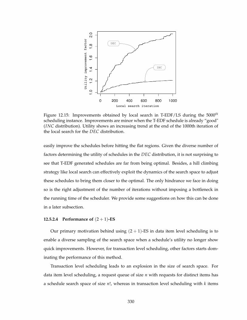
INC
DEC
Local search iteration
Utility improvement factor
Figure 12.15: Improvements obtained by local search in T-EDF/LS during the 5000th
scheduling instance. Improvements are minor when the T-EDF schedule is already “good"(INC distribution). Utility shows an increasing trend at the end of the 1000th iteration ofthe local search for the DEC distribution.
easily improve the schedules before hitting the flat regions. Given the diverse number of
factors determining the utility of schedules in the DEC distribution, it is not surprising to
see that T-EDF generated schedules are far from being optimal. Besides, a hill climbing
strategy like local search can effectively exploit the dynamics of the search space to adjust
these schedules to bring them closer to the optimal. The only hindrance we face in doing
so is the right adjustment of the number of iterations without imposing a bottleneck in
the running time of the scheduler. We provide some suggestions on how this can be done
in a later subsection.
12.5.2.4 Performance of (2 + 1)-ES
Our primary motivation behind using (2 + 1)-ES in data item level scheduling is to
enable a diverse sampling of the search space when a schedule’s utility no longer show
quick improvements. However, for transaction level scheduling, other factors starts dom-
inating the performance of this method.
Transaction level scheduling leads to an explosion in the size of search space. For
data item level scheduling, a request queue of size n with requests for distinct items has
a schedule search space of size n!, whereas in transaction level scheduling with k items
330
Iteration number
Utility improvement factor
Local search Local search
ESES
INC DEC
Figure 12.16: Improvements obtained by local search and ES in the schedule generatedby T-EDF during the 5000th scheduling instance. For transaction level scheduling, localsearch performs better in avoiding local optima compared to (2 + 1)-ES.
per transaction, the search space can become as big as (kn)!. A bigger search space not
only requires more exploration, but can also inject a higher possibility of prematurely
converging to a local optima. Fig. 12.16 depicts the exploration with local search and
the (2 + 1)-ES. In order to generate the plots, we ran T-EDF until the 5000th request
arrives. A schedule for the requests in the queue at this point is then generated by
running T-EDF/LS and (2 + 1)-ES for 5000 iterations each. This guarantees that both
methods are operating on the same queue (same search space) and for sufficient number
of iterations. Utility improvements by the ES starts stagnating after the 2000th iteration,
suggesting convergence towards a local optima. Local search, on the other hand, has a
better rate of improvement before starting to stagnate. This is visible for both INC and
DEC distributions.
The premature convergence in (2 + 1)-ES is mostly due to the loss in genetic diversity of
the solutions. As more and more recombination takes place, the two parents involved in
the method starts becoming more and more similar, and finally being unable to generate
a diverse offspring. This phenomenon is what typically identifies the convergence of
the method. However, given the bigger search space and the small population (two)
involved in exploring it, the phenomenon results in the method getting trapped in the
local optima present across the space. It is suggestive from the broadcast frequency of
different data items (Fig. 12.14) that, on the overall, the method failed to balance the
broadcast of different sized data items for the DEC distribution. Changing the µ and λ
331

parameters, as well as the mutation probability, of the method usually helps resolve such
premature convergence. However, one should keep the real time runtime constraints into
consideration while experimenting with the parameters. Local search, on the other hand,
does not face such a problem. Ideally, given enough number of iterations with random
restarts, a hill climbing approach is more resilient in this regard.
12.5.3 Scheduling time
The number of generations allowed to local search, or ES, can affect the quality of so-
lutions obtained and the time required to make scheduling decisions. In our experiments,
this value is set so that an average request queue can be handled in a small amount of
time. However, the average queue size will greatly vary from problem to problem, often
depending on the total number of data items served by the data source. In such situa-
tions, it may seem difficult to determine what a good value for the number of iterations
should be. Further, in a dynamic environment, the average queue length itself may be a
varying quantity. Nonetheless, one should keep in mind that scheduling decisions need
not always be made instantaneously. The broadcast time of data items vary considerably
from one to the other. The broadcast scheduled immediately next cannot start until the
current one finishes. This latency can be used by a scheduler to continue its search for
better solutions, specially with iterative methods like a local search or an ES.
12.6 Conclusions
In this chapter, we address the problem of time critical data access in pervasive en-
vironments where the time criticality can be associated with a QoS requirement. To this
end, we formulate a utility metric to evaluate the performance of different scheduling
methods. The earliest deadline first (EDF) and highest utility first (HUF) heuristics are
used in two problem domains – data item level scheduling and transaction level schedul-
ing. In the data item level domain, our initial observation on their performance conforms
to the speculation that HUF performs better since it takes into consideration the utility of
requests while making scheduling decisions. Further analysis of the nature of the schedul-
ing problem shows that EDF and HUF generated schedules can be greatly improved by
332
introducing a minor amount of local search to them. The impact of the local search is
found to be a direct consequence of the schedules generated by these heuristics which are
found to belong to a region of the search space from where obtaining improvements is
not difficult.
The observations drawn from this understanding of the behavior of local search aided
heuristics enable us to propose an evolution strategy based search technique that provides
more variance to a simple local search. The utility induced by such a technique surpasses
that of both EDF and HUF, and their local search variants. This result also shows that
search based optimization techniques are a viable option in real time broadcast scheduling
problems, and often suboptimal solutions generated by such a technique can be better
than those obtained from a heuristic.
The transaction level domain appear to be a relatively harder problem to solve. Bal-
ancing the broadcast frequency of data items is important here and we observe that T-EDF
performs better in doing so as compared to T-HUF. Local search still remains a promising
candidate to boost the performance of these heuristics. For certain data size distributions,
local search improvements can continue if allowed to run outside the runtime restrictions
set in our experiments. Better strategies to trigger the scheduler is thus required. Trans-
action level scheduling also has different search space dynamics, often with an explosive
size and the presence of local optima. The evolution strategy method is affected by this,
often leading to lower utility schedules than local search. Further experimentation is re-
quired in this direction to see how the parameters of the ES can be changed to avoid
susceptibility towards such situations.
Future work in this context may be inspired from the insights obtained from the
analysis conducted on the (2 + 1)-ES. From an utility standpoint, we intend to explore the
option of designing heuristics that pay special attention to factors like broadcast frequency
and loss-gain trade-off during scheduling decisions. Also, when requests involve multiple
data items which may undergo regular updates, the validity of a broadcast must also be
taken into account. Timely delivery of a data item then has to consider a validity deadline
as well.
333

CHAPTER 13
Scheduling Ordered Data Broadcasts
Many pervasive application domains involve clients interested in groups of related
data items that can be processed one at a time following some order. Consider the traffic
management system example introduced in the previous chapter. The system gathers
current traffic information using sensors and disseminates it to drivers in real time on
demand. Drivers use smart GPS navigation units to request road conditions so that they
can be routed and re-routed along the best possible roads. The GPS unit periodically
requests traffic information for the roads that are still remaining in its route plan. The
traffic service needs to provide the road conditions in the same order that the roads are in
the route plan. That is, if the current route plan is 〈r1,r2,r3,r4〉, where ri is a road identifier,
then the traffic service should provide the information as 〈rc1,rc2,rc3,rc4〉, where rci is the
road condition for ri. A scheduling problem occurs in such an application when the
number of data access requests is larger than the bandwidth capacity of the server.
Various soft deadlines may also be imposed on the requested data items, which if
not served within a specific time window may result in the data item having near zero
utility when finally received. For example, from the time that a driver makes a request
for traffic information on road ri to the time the monitoring service reports back with a
gridlock on ri, the driver may already have missed a more convenient exit for an alternate
route. Given the resource limitations, it is not always possible that the time constraints
334

of every incoming request be satisfied. Thus, a broadcast schedule is sought which can
serve clients with as much utility as possible. The scheduling problem is more difficult
in a real-time setting where generation of a high utility schedule has to respect run time
constraints as well.
Although ordered queries have been studied in the mobile computing paradigm
[35, 90, 87], schedule evaluation is rarely based on the utility of responses. In this chap-
ter, we first propose an utility accrual method for data requests involving constraints
on the order of the requested data items. Second, we define a modified version of the
Syswerda recombination operator for use in methods with recombination. Finally, the
utility function is used by an evolution strategy based schedule optimizer to evaluate the
effectiveness of the schedules. We pay particular attention to the run time constraint of
the scheduler and argue that simple variants of an evolution strategy can be employed to
satisfy this requirement.
The remainder of the chapter is organized as follows. Section 13.1 presents the util-
ity function and a formal statement of the problem. Section 13.2 discusses the search
algorithms. Some empirical results are presented in Section 13.3. Finally, Section 13.4
concludes the chapter.
13.1 Ordered Data Broadcasts
A data source D = {D1, D2, . . . , DN} is a set of N ordered sets (or data groups), where
Dj = {d1j,d2j, . . . ,dNj j} with Nj being the cardinality of Dj and j = 1, . . . , N. All data items
dij are assumed to be unique and are of equal size dsize. A request is considered to be “fully
served” when the last data item in the requested data group is retrieved, otherwise it is
considered “partially served”. A request queue at any instance is a dynamic queue Q with
entries Qj of the form 〈Dj, Rj〉, Dj ∈ D and Rj ≥ 0. At an instance tcurr, let Q1, Q2, . . . , QM
be the entries in Q. We define the notation Wait[Qj] to denote the data item that the
request Qj is currently waiting for. Further, we define Rem[Qj] as the ordered subset
of data items that has been requested in Qj but not yet received, i.e. Rem[Qj] ⊆ Dj. A
schedule is a total ordering of the elements in the multi-set⋃
j=1,...,MRem[Qj].
The time instance at which a particular data item from the schedule starts to be broad-
335
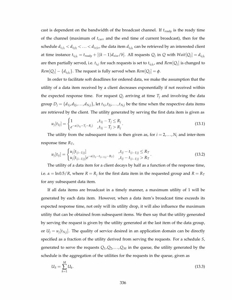
cast is dependent on the bandwidth of the broadcast channel. If tready is the ready time
of the channel (maximum of tcurr and the end time of current broadcast), then for the
schedule di1 j1 < di2 j2 < . . . < diP jP , the data item dik jk can be retrieved by an interested client
at time instance tik jk = tready + [(k − 1)dsize/b]. All requests Qj in Q with Wait[Qj] = dik jk
are then partially served, i.e. tik j for such requests is set to tik jk , and Rem[Qj] is changed to
Rem[Qj] − {dik jk}. The request is fully served when Rem[Qj] = φ.
In order to facilitate soft deadlines for ordered data, we make the assumption that the
utility of a data item received by a client decreases exponentially if not received within
the expected response time. For request Qj arriving at time Tj and involving the data
group Dj = {d1j,d2j, . . . ,dNj j}, let t1j, t2j, . . . , tNj j be the time when the respective data items
are retrieved by the client. The utility generated by serving the first data item is given as
uj[t1j] =
{
1 , t1j − Tj ≤ Rj
e−α(t1j−Tj−Rj) , t1j − Tj > Rj
. (13.1)
The utility from the subsequent items is then given as, for i = 2, . . . , Nj and inter-item
response time RT,
uj[tij] =
{
uj[t(i−1)j] , tij − t(i−1)j ≤ RT
uj[t(i−1)j]e−α(tij−t(i−1)j−RT) , tij − t(i−1)j > RT
. (13.2)
The utility of a data item for a client decays by half as a function of the response time,
i.e. α = ln0.5/R, where R = Rj for the first data item in the requested group and R = RT
for any subsequent data item.
If all data items are broadcast in a timely manner, a maximum utility of 1 will be
generated by each data item. However, when a data item’s broadcast time exceeds its
expected response time, not only will its utility drop, it will also influence the maximum
utility that can be obtained from subsequent items. We then say that the utility generated
by serving the request is given by the utility generated at the last item of the data group,
or Uj = uj[tNj j]. The quality of service desired in an application domain can be directly
specified as a fraction of the utility derived from serving the requests. For a schedule S,
generated to serve the requests Q1, Q2, . . . , QM in the queue, the utility generated by the
schedule is the aggregation of the utilities for the requests in the queue, given as
US =M
∑k=1
Uk. (13.3)
336
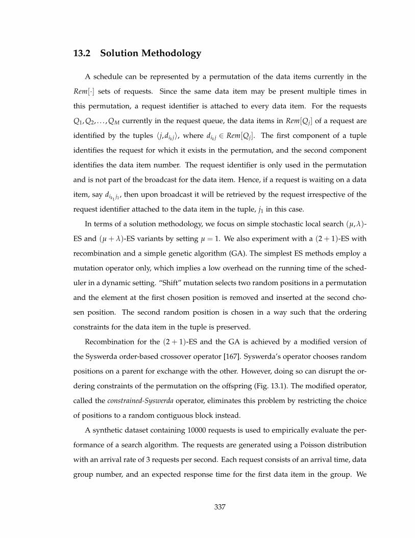
13.2 Solution Methodology
A schedule can be represented by a permutation of the data items currently in the
Rem[·] sets of requests. Since the same data item may be present multiple times in
this permutation, a request identifier is attached to every data item. For the requests
Q1, Q2, . . . , QM currently in the request queue, the data items in Rem[Qj] of a request are
identified by the tuples 〈j,dik j〉, where dik j ∈ Rem[Qj]. The first component of a tuple
identifies the request for which it exists in the permutation, and the second component
identifies the data item number. The request identifier is only used in the permutation
and is not part of the broadcast for the data item. Hence, if a request is waiting on a data
item, say dik1j1 , then upon broadcast it will be retrieved by the request irrespective of the
request identifier attached to the data item in the tuple, j1 in this case.
In terms of a solution methodology, we focus on simple stochastic local search (µ,λ)-
ES and (µ + λ)-ES variants by setting µ = 1. We also experiment with a (2 + 1)-ES with
recombination and a simple genetic algorithm (GA). The simplest ES methods employ a
mutation operator only, which implies a low overhead on the running time of the sched-
uler in a dynamic setting. “Shift” mutation selects two random positions in a permutation
and the element at the first chosen position is removed and inserted at the second cho-
sen position. The second random position is chosen in a way such that the ordering
constraints for the data item in the tuple is preserved.
Recombination for the (2 + 1)-ES and the GA is achieved by a modified version of
the Syswerda order-based crossover operator [167]. Syswerda’s operator chooses random
positions on a parent for exchange with the other. However, doing so can disrupt the or-
dering constraints of the permutation on the offspring (Fig. 13.1). The modified operator,
called the constrained-Syswerda operator, eliminates this problem by restricting the choice
of positions to a random contiguous block instead.
A synthetic dataset containing 10000 requests is used to empirically evaluate the per-
formance of a search algorithm. The requests are generated using a Poisson distribution
with an arrival rate of 3 requests per second. Each request consists of an arrival time, data
group number, and an expected response time for the first data item in the group. We
337

Valid Parent 1 : a b c d e f g h i j
Valid Parent 2 : a d e b c h i f g j
Cross Positions : * * *
Invalid Offspring : a b e d c f g h i j
Figure 13.1: A counter example for the Syswerda order-based crossover operator. Order-ing constraints are {a,b, c}, {d, e, f , g} and {h, i, j}; constraint {d, e, f , g} is violated in theoffspring.
consider 100 different data groups, the number of data items in each drawn from an ex-
ponential distribution with rate parameter 10. The bandwidth for the broadcast channel
is set at 200KB/s.
The data groups requested are assumed to follow the commonly used Zipf distribu-
tion [27] with the characterizing exponent of 0.8. Under this assumption, the first data
group becomes the most requested one, while the last one is the least requested. Broad-
cast schedules can be heavily affected by the size of the most requested data group. Thus,
we consider the two different assignments: INC – most requested data group has the
smallest number of data items, and DEC – most requested data group is the largest in
size [80, 107]. Each data item is of size 50KB.
Expected response times for the first data item are assigned from a normal distribution
with mean 60s and standard deviation 20s. Any negative value is replaced by zero.
Response time for intermediate data items is set at 1s.
For different variants of the (1 + λ)-ES and (1,λ)-ES, we fixed the maximum number
of function evaluations to 15000. The number of function evaluations is fixed at 5000 for
the (2 + 1)-ES. The parameters for the GA is set as follows: population size = 100, number
of function evaluations = 15000, crossover probability = 0.8, mutation probability = 0.05,
and 2-tournament selection.
13.3 Empirical Results
We present the results obtained from different variants of the ES on the two different
data group assignments – INC and DEC. The results are averaged for 20 runs for each
variant. Fig. 13.2 shows the percentage global utility obtained by running (1 + λ)-ES
338
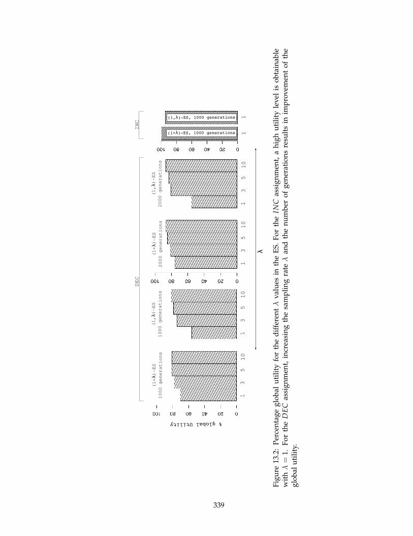
13
510
13
510
13
510
13
510
11
% global Utility
(1+λ)-ES
1000 generations
(1,λ)-ES
1000 generations
(1+λ)-ES
2000 generations
(1,λ)-ES
2000 generations
(1+λ)-ES, 1000 generations
(1,λ)-ES, 1000 generations
DEC
INC
λ
Fig
ure
13.2
:P
erce
nta
ge
glo
bal
uti
lity
for
the
dif
fere
nt
λv
alu
esin
the
ES
.F
or
the
INC
assi
gn
men
t,a
hig
hu
tili
tyle
vel
iso
bta
inab
lew
ith
λ=
1.F
or
the
DE
Cas
sig
nm
ent,
incr
easi
ng
the
sam
pli
ng
rate
λan
dth
en
um
ber
of
gen
erat
ion
sre
sult
sin
imp
rov
emen
to
fth
eg
lob
alu
tili
ty.
339
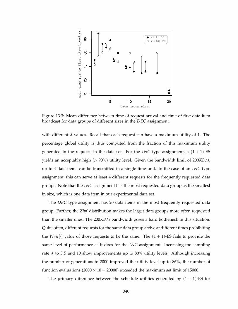
(1+1)-ES
(1+10)-ES
Data group size
Mean time (s) to first item broadcast
Figure 13.3: Mean difference between time of request arrival and time of first data itembroadcast for data groups of different sizes in the DEC assignment.
with different λ values. Recall that each request can have a maximum utility of 1. The
percentage global utility is thus computed from the fraction of this maximum utility
generated in the requests in the data set. For the INC type assignment, a (1 + 1)-ES
yields an acceptably high (> 90%) utility level. Given the bandwidth limit of 200KB/s,
up to 4 data items can be transmitted in a single time unit. In the case of an INC type
assignment, this can serve at least 4 different requests for the frequently requested data
groups. Note that the INC assignment has the most requested data group as the smallest
in size, which is one data item in our experimental data set.
The DEC type assignment has 20 data items in the most frequently requested data
group. Further, the Zipf distribution makes the larger data groups more often requested
than the smaller ones. The 200KB/s bandwidth poses a hard bottleneck in this situation.
Quite often, different requests for the same data group arrive at different times prohibiting
the Wait[·] value of those requests to be the same. The (1 + 1)-ES fails to provide the
same level of performance as it does for the INC assignment. Increasing the sampling
rate λ to 3,5 and 10 show improvements up to 80% utility levels. Although increasing
the number of generations to 2000 improved the utility level up to 86%, the number of
function evaluations (2000 × 10 = 20000) exceeded the maximum set limit of 15000.
The primary difference between the schedule utilities generated by (1 + 1)-ES for
340

1000 generations and (1 + 10)-ES for 2000 generations is attributable to the latency that
the scheduler puts in between the time of arrival of a request and the time when the first
data item for the request is broadcast. Fig. 13.3 shows the mean values of this latency for
data groups of different sizes. The (1 + 10)-ES maintains a higher mean latency for the
larger data groups, whereas the (1 + 1)-ES maintains a higher value for the smaller data
groups. Given that most requests are for the larger data groups in the DEC assignment,
postponing the first data item broadcast for such requests provides gaps in the schedule
to serve pending (or partially served) requests. Recall that the expected response time
is the highest for the first data item (between 0 and 120s). Once a client has received
the first data item, the expected response time drops to RT = 1s. Hence, by delaying the
first data item broadcast for the most requested data groups, the (1 + 10)-ES maintains a
better flexibility in serving pending requests.
For the experimental data set, a simple (1 + 1)-ES for 1000 generations is sufficient
when the QoS requirement is not too high (< 75%). For the case when the utility require-
ment is higher, a higher sampling rate is desired. However, note that results obtained
from running the different variants for 2000 generations (more function evaluations) do
not always yield a high difference in the utility levels as compared to those from running
the same variants for 1000 generations. This is observed in both the comma and plus
variants of the ES.
Fig. 13.4a shows the changes in the objective function (schedule utility given by (13.3))
value during the scheduling instance when the 5000th request arrives. The scheduler is
working with DEC and λ = 5. Further, at each iteration, the plot shows the utilities of 100
randomly sampled points (using shift mutation) near the current parent. Note that the
rise in the utility of the schedule is faster during the first 250 generations and then slows
down considerably. In other words, as better schedules are obtained, improvements are
harder to find. This in turn makes the progress slower. Moreover, the randomly sampled
points around the parent of the current generation show very small differences in the
utility values. This makes it difficult for the ES to maintain a steady increase in the
schedule utility.
Fig. 13.4b shows the percentage global utility generated by the (2 + 1)-ES and the
341

Generation
Objective function (schedule utility)
(1+5)-ES
(1,5)-ES
(a)
(b)
INC
DEC
% global Utility
(2+1)-ES
(2+1)-ES
GA
GA
Fig
ure
13.4
:(a
)S
ched
ule
uti
lity
pro
gre
ssd
uri
ng
the
5000
thsc
hed
uli
ng
inst
ance
wit
hD
EC
.U
tili
ties
are
also
plo
tted
for
100
po
ints
sam
ple
dar
ou
nd
the
par
ent
of
ever
yg
ener
atio
n.
(b)
Per
cen
tag
eg
lob
alu
tili
tyfo
r(2
+1)-
ES
and
ag
enet
ical
go
rith
m.
342
GA. Performance of both methods is on a par with the stochastic search variants for the
INC size distribution. The GA’s performance on the DEC distribution is easily overpow-
ered by a (1 + 3)-ES. Further, the GA does a maximal utilization of the allowed function
evaluations of 15000. The (2 + 1)-ES achieves an utility of 83%, equivalent to that of the
(1 + 5)-ES with 2000 generations. An important factor to consider here is the number of
function evaluations used in the two methods – 5000 in (2 + 1)-ES compared to 10000
in the (1 + 5)-ES. Although this performance is marginally better (about 3%) than the
(1 + 5)-ES with 1000 generations, we stress that even obtaining such marginal improve-
ments is difficult with the DEC distribution.
The enhanced performance of (2 + 1)-ES is attributable to the additional exploration
brought forth by the recombination operator. Local search methods do not display enough
exploratory capabilities when stuck in a plateau of the search space. Recombination
allows for a more diverse sampling in such cases, thereby resulting in a faster exploration
through plateaus. The GA is expected to benefit from this as well. The cause of its poor
performance is not well understood.
13.4 Conclusions
Pervasive computing applications often need to broadcast grouped data objects such
that the elements in the group satisfy a user specified ordering constraint. In addition,
objects not served within a specific window may end up having near zero utility. In this
chapter, we introduce a method of utility accrual for grouped data objects and use it
to evaluate the effectiveness of a schedule. We argue that evolution strategy is a viable
methodology to maximize the utility of broadcasts given the run time constraints of the
application. We investigate three different methods – a simple stochastic local search
using (1 + λ)-ES and (1,λ)-ES, a (2 + 1)-ES with a modified Syswerda recombination
operator, and a genetic algorithm. Our experiments suggest that the generation of an
optimal schedule when the most requested group has the highest number of data items
is a difficult problem to solve, often requiring a longer duration of search. However,
recombination based ES appears to be particularly effective. The (2 + 1)-ES with the
proposed recombination operator demonstrates the potential to generate better schedules
343

without engaging in too many function evaluations, thereby providing a fair trade-off
between the run time and utility objectives of a scheduler.
The problem considered in this chapter assumes that data items are unique across
different data groups. However, there exists other problems in pervasive environments
where the data groups can have common data items. We can investigate if the scheduling
strategy identified here works equally well in such problem domains.
344

CHAPTER 14
Scheduling in Multi-Layered Broadcast Systems
Most of the earlier works in designing broadcast schedulers assume a centralized
system where the broadcast server has local access to the data items [2, 7, 55, 107, 187].
This simplifies the problem since the broadcast scheduler need not take into consideration
the time required to retrieve the data item while making scheduling decisions. However,
a number of application domains exist where such centralized storage of data are not
possible. Consider the example of a company that provides investment consulting and
management services to its clients (a company like Morningstar R©). One service provided
by such a company is real-time, on-demand information on stocks, mutual funds etc., in
the form of market indices. Typically, such a company does not generate this information
itself but fetches it from other companies (Morningstar R©, for example, gets a significant
portion of this data from the company Interactive Data CorporationSM). With the current
ubiquity of wireless computing devices, we can imagine that clients of the company seek
and receive periodic market data on their mobile phones, PDAs and notebooks, and
analyze the data to determine which investments are rewarding. Since multiple clients
may seek the same data, it makes good business sense for the company to broadcast this
data. The clients also perform financial transactions using such devices. Market indices
change throughout the day and it is important to analyze such trends along multiple
dimensions in order to perform trading. Thus, although queries from clients are implicitly
345
associated with deadlines, these can be considered soft. Even if the queries are served
after their deadline, they still have some value. The overall goal of the company will be
to satisfy as many requests as possible in a timely manner, keeping in mind that the data
may need to be fetched from other sources.
Decentralized storage of data introduces a novel problem to the broadcast scheduler,
specifically if the data items must be retrieved from a data server prior to broadcast.
Typically, the scheduler has complete knowledge on the time required to broadcast an
item and uses this information in deciding a schedule. However, when data have to be
fetched from a data server, this knowledge assumes a stochastic form. A data server
will usually be serving multiple broadcast servers following its own request management
policy. Thus, the time required to fetch a data item is not known apriori. A broadcast
scheduler then has to build a schedule based on stochastic information available about
the retrieval time of data items.
In this chapter, we visit the problem of data broadcast scheduling under such a sce-
nario. We model the problem as a case of stochastic scheduling and explore the performance
of a number of heuristic based schedulers. We argue that heuristics used in deterministic
scheduling may not perform well in a stochastic problem of this nature. We show how
probability estimates on a data server’s response times can be used in the design of better
schedulers. To this end, we propose two heuristics – the Minimum Deadline Meet Probabil-
ity and the Maximum Bounded Slack Probability heuristics – that are based on the request
completion time distributions rather than their exact values. Further, we augment our ob-
servations with an analysis to understand the underlying principles of a good scheduler.
Our results demonstrate that a better performing broadcast policy exploits factors such
as bandwidth utilization, data sizes and access frequencies. This is often as a result of
how the specific heuristic has been formulated.
While considerable attention has been paid to designing heuristics for broadcast schedul-
ing in centralized data systems, heuristics for non-local data models are rare to find. Data
staging concerns in broadcast scheduling were first highlighted by Aksoy et al. [8]. The
authors focus on a decision problem where the data items are not readily available for
broadcast. An opportunistic scheduling mechanism is introduced where data items avail-
346
able for broadcast are chosen instead. Further, hint-based cache management and prefetching
techniques are proposed in order to decrease the fetch latency of a data item. However,
these techniques do not utilize any information available on the fetch time of data items
while determining the broadcast schedule. The focus in our work is to supplement such
data staging mechanisms by informing the scheduler on the workload present on a data
server and make decisions accordingly.
Traintafillou et al. study a similar problem in the context of disk access latencies [171].
The primary objective of their work is to study the interplay among different components
of a broadcast system, namely the broadcast scheduler, disk scheduler, cache manager
and the transmission scheduler. However, disk access latencies are typically much smaller
than data retrieval latencies from a secondary source. In effect, the impact of data fetch
times is amplified in decentralized storage systems. Further, unlike as in non-local data
systems, the heuristics proposed in their work assume that disk service times are known
apriori.
Hierarchical data dissemination is used by Omotayo et al. in the context where data
updates are frequently pushed from one server to another [138]. The scheduling prob-
lem is explored at the primary server which needs to decide how frequently to broadcast
updated data items to secondary servers. Since the primary server does not maintain
any incoming request queue, there is no stochasticity involved on part of the secondary
servers. Notably, stochastic scheduling has been explored in depth for job shop schedul-
ing problems where execution time of jobs are not known apriori [50, 125].
The remainder of the chapter is organized as follows. Section 14.1 presents the broad-
cast architecture used in this study. The formal statement of the problem is also outlined
here. The heuristics experimented with are discussed in Section 14.2. Section 14.3 in-
troduces the two heuristics proposed in this chapter for stochastic broadcast scheduling.
Section 14.4 outlines the details of the experimental setup and the synthetic data set used
to evaluate the performance of the heuristics. Section 14.5 presents the results obtained
and provides an extensive discussion on the performance of the heuristics. Finally, Sec-
tion 14.6 summarizes the chapter.
347

14.1 Problem Modeling
Stochastic scheduling refers to the class of scheduling problems where the time re-
quired to complete a particular task is modeled as a random variable. Compared to
deterministic scheduling where the time of completion of a task can be computed before
it begins execution, the actual completion time in the stochastic case is known only after
the task finishes execution. However, a probability distribution of the completion time is
known (or can be computed) for such tasks. Data broadcast scheduling transforms into
a stochastic problem when the data items to be broadcast are not available locally at the
broadcast server. In such a scenario, the broadcast server has to retrieve the data items
prior to initiating the broadcast, from data servers distributed over a network. The data
servers on the other hand will be receiving multiple requests from other broadcast servers
and will have their own policy to manage the serving of accumulating data requests. The
serving of requests on part of the data server may be accomplished by a unicast, multicast
or a broadcast mechanism. Hence, the time required by a broadcast server to fetch a data
item will not be known until the item is actually fetched. Scheduling decisions on the
broadcast server that must be made prior to fetching any data item will therefore be in-
accurate. As an alternative, a broadcast server can use response time probability estimates
of the data servers. The response time is the time elapsed between making a request and
getting the request served. The probability estimates would present a broadcast server
with likely durations of time it would require to retrieve a data item, thereby introducing
the stochastic broadcast scheduling problem. A stochastic scheduler can use the probabil-
ity estimates as prior knowledge on the problem instance, but does not utilize anticipated
information from the future (such as a possible value for the response time) while gen-
erating a scheduling policy. Often times, the policy itself may undergo revisions as data
items are actually fetched and their response times are known.
14.1.1 Broadcast server model
Fig. 14.1 depicts the broadcast architecture used in this study. Clients request different
data items from a broadcast server using the uplink channel. Each request Q has an ar-
rival time, a data item index and an absolute deadline, given by the tuple 〈arrQ,dQ,dlnQ〉.
348
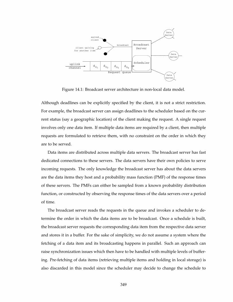
uplink
channel
Request queue
Broadcast
Server
Scheduler
broadcast
dQ1dQ2
dQ3dQ4
served
client
client waiting
for another item
Data
Server
Data
Server
Data
Server
Figure 14.1: Broadcast server architecture in non-local data model.
Although deadlines can be explicitly specified by the client, it is not a strict restriction.
For example, the broadcast server can assign deadlines to the scheduler based on the cur-
rent status (say a geographic location) of the client making the request. A single request
involves only one data item. If multiple data items are required by a client, then multiple
requests are formulated to retrieve them, with no constraint on the order in which they
are to be served.
Data items are distributed across multiple data servers. The broadcast server has fast
dedicated connections to these servers. The data servers have their own policies to serve
incoming requests. The only knowledge the broadcast server has about the data servers
are the data items they host and a probability mass function (PMF) of the response times
of these servers. The PMFs can either be sampled from a known probability distribution
function, or constructed by observing the response times of the data servers over a period
of time.
The broadcast server reads the requests in the queue and invokes a scheduler to de-
termine the order in which the data items are to be broadcast. Once a schedule is built,
the broadcast server requests the corresponding data item from the respective data server
and stores it in a buffer. For the sake of simplicity, we do not assume a system where the
fetching of a data item and its broadcasting happens in parallel. Such an approach can
raise synchronization issues which then have to be handled with multiple levels of buffer-
ing. Pre-fetching of data items (retrieving multiple items and holding in local storage) is
also discarded in this model since the scheduler may decide to change the schedule to
349
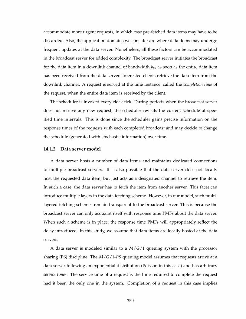
accommodate more urgent requests, in which case pre-fetched data items may have to be
discarded. Also, the application domains we consider are where data items may undergo
frequent updates at the data server. Nonetheless, all these factors can be accommodated
in the broadcast server for added complexity. The broadcast server initiates the broadcast
for the data item in a downlink channel of bandwidth bbs as soon as the entire data item
has been received from the data server. Interested clients retrieve the data item from the
downlink channel. A request is served at the time instance, called the completion time of
the request, when the entire data item is received by the client.
The scheduler is invoked every clock tick. During periods when the broadcast server
does not receive any new request, the scheduler revisits the current schedule at spec-
ified time intervals. This is done since the scheduler gains precise information on the
response times of the requests with each completed broadcast and may decide to change
the schedule (generated with stochastic information) over time.
14.1.2 Data server model
A data server hosts a number of data items and maintains dedicated connections
to multiple broadcast servers. It is also possible that the data server does not locally
host the requested data item, but just acts as a designated channel to retrieve the item.
In such a case, the data server has to fetch the item from another server. This facet can
introduce multiple layers in the data fetching scheme. However, in our model, such multi-
layered fetching schemes remain transparent to the broadcast server. This is because the
broadcast server can only acquaint itself with response time PMFs about the data server.
When such a scheme is in place, the response time PMFs will appropriately reflect the
delay introduced. In this study, we assume that data items are locally hosted at the data
servers.
A data server is modeled similar to a M/G/1 queuing system with the processor
sharing (PS) discipline. The M/G/1-PS queuing model assumes that requests arrive at a
data server following an exponential distribution (Poisson in this case) and has arbitrary
service times. The service time of a request is the time required to complete the request
had it been the only one in the system. Completion of a request in this case implies
350

bds
insufficient quanta requests
completed
requests
service
time
remaining service time
quanta to
requests
Figure 14.2: Data server architecture following a M/G/1-PS model.
transmission of the entire data item from the data server to the broadcast server. The
bandwidth available at the data server is distributed uniformly to serve requests in a
round-robin fashion. Hence, if there are n requests ready to be served in the queue and
bds is the bandwidth available at the data server, then each request receives a quanta bdsn of
the bandwidth every clock tick. A request that gets completely served in the quanta leaves
the system; otherwise it is cycled back into the queue for another quanta in the next clock
tick. Fig. 14.2 depicts this architecture. Note that the quanta received by a request will
vary every clock tick as new requests keep entering the system and completed requests
leave.
14.1.3 Formal statement
A data server DSi is a collection of Ni data items Di = {di1,di
2, . . . ,diNi} such that
D = ∪iDi and Di ∩ Dj = φ for i 6= j. The null intersection enforces the condition that the
same data item is not hosted by two different data servers, i.e., no replication. A broad-
cast server maintains a dynamic queue with requests arriving as a tuple 〈arrQ,dQ,dlnQ〉,where arrQ is the arrival time of a request Q, dQ ∈ D is the data item requested and
dlnQ > arrQ is the absolute deadline for the request. Further, let bbs and bds be the band-
width available at the broadcast and data server respectively.
At each scheduling instance, the scheduler first removes all requests from the queue
that will be served by the current broadcast and generates a schedule for all remaining
requests Q′. A schedule is thus a total ordering of the data items in ∪Q′{dQ′}. Let f t(d)
be the time required to fetch the data item d from the corresponding data server. If
tready is the ready time of the broadcast channel (the time instance when any ongoing
351

broadcast ends), di1 → di2 → ·· · → diPthe broadcast schedule and sd be the size of data
item d, then the broadcast of an item dikends at time tdik
= tready + ∑kj=1[ f t(dij
) +sdij
bbs]. All
requests Q′ served by this broadcast then has a completion time ctQ′ = tdikand response
time rtQ′ = (ctQ′ − arrQ′). The objective of the scheduler is to generate a schedule such
that the response time of the requests do not exceed the limit set by the deadline, i.e.,
rtQ′ ≤ (dlnQ′ − arrQ′), or ctQ′ ≤ dlnQ′ .
14.1.4 Performance metrics
We shall use three metrics – deadline miss rate, average stretch and utility – to evaluate
the performance of different schedulers. Measurements are taken when all requests in
the experimental data set have been served.
14.1.4.1 Deadline Miss Rate (DMR)
Let Q be the set of all requests served by the broadcast server at an instance of time.
The deadline miss rate (DMR) is the fraction of requests in Q which missed their dead-
lines, given as
DMR =|{Q ∈ Q|rtQ > (dlnQ − arrQ)}|
|Q| . (14.1)
14.1.4.2 Average Stretch (ASTR)
The stretch of a request is the ratio of its response time to its service time. Recall that
the service time of a request is the time it would take to serve the request had it been the
only one in the system. In a non-local data model, the service time should also include
the retrieval time of the data item requested. Hence, if the request Q involves a data item
of size s, to be retrieved from a data server with bandwidth bds and broadcasted over a
channel with bandwidth bbs, then the service time of Q is given by stQ = s( 1bds
+ 1bbs
). The
stretch of the request is then given as STRQ =rtQ
stQ. A low stretch value indicates closer
proximity of the response time to the minimum time needed to serve the request.
Intuitively, it seems that the response time of a request can never be less than the
service time. Hence, the stretch of a request should always be greater than or equal to 1.0.
However, when data fetching times are significant, the stretch can be less than one. This
352

can happen when a new request for a data item next scheduled for broadcast, and being
currently retrieved from a data server, enters the broadcast server. In such a situation, the
request realizes a retrieval time less than sbds
and gets served as soon as the retrieval ends.
Therefore, the response time becomes less than the service time. The average stretch
(ASTR) is given as
ASTR =∑Q∈Q STRQ
|Q| =1
|Q| ∑Q∈Q
rtQ
stQ. (14.2)
Ideally, a low ASTR signifies that most requests are served with minimal deviation
from their service times. Hence, most requests will meet their deadlines as well, resulting
in a lower DMR.
14.1.4.3 Utility (UT)
The performance level depicted by DMR is useful when the deadlines imposed are
hard. However, when soft deadlines are in place, a request being served after its deadline
still holds some utility. Thus, the utility (UT) metric uses a function that maps the re-
sponse time of a request to a real number. We use the following function in this context.
UQ =
{
1 ,rtQ ≤ (dlnQ − arrQ)
e−αQ(rtQ−dlnQ+arrQ) ,otherwise, (14.3)
where αQ = ln0.5/(dlnQ − arrQ). Thus, the utility of a request is 1.0 if served by its
deadline, otherwise decreases exponentially depending on the relative deadline of the
request. The fractional utility attained in the system is then given as
UT =∑Q∈Q UQ
|Q| . (14.4)
An UT value of 1.0 indicates that all requests are served by their deadline; otherwise
the closer it is to 1.0, the lesser is the time by which requests overshot their respective
deadlines. Note that a high UT does not necessarily indicate a low DMR.
14.2 Schedule Generation
A major challenge in the generation of optimal schedules for data broadcasting is the
lack of a formal theory underpinning the statistical characteristics of a “good” broad-
cast schedule. While queuing theory provides preliminary grounds for such analysis, no
353
attempt is known to have been made to understand a broadcast system that reflects a
one-to-many relationship between servings and arrivals in the queue. Hence, a signifi-
cant amount of focus is concentrated in designing heuristic methods that employ intuitive
perceptions of good broadcast mechanisms. Much of this is also due to the additional con-
straint of scheduling time imposed by the real time requirement in on-demand systems.
A typical workload condition may prohibit the use of time consuming methods in or-
der to avoid long accumulation of requests and increases in their response times. Long
scheduling times may also keep valuable broadcast bandwidth idle, resulting in ineffi-
cient utilization of available resources. To this end, heuristic driven schedulers are often
preferred as fast decision makers.
Most of the existing heuristics in broadcast scheduling have been evaluated assuming
systems with local data availability. For this study, we adopted four well-performing
heuristics – RxW, MAX, SIN-α and PRDS – proposed for such systems and observe
their performance in non-local data availability systems. While no intrinsic property in
these heuristics prohibit them from use in our problem model, modifications are made if
required.
14.2.1 RxW
The RxW heuristic [7] combines the benefits of the MRF (Most Requested First) and
FCFS (First Come First Serve) heuristics in order to provide sufficient weight to both
heavily requested and long awaited data items. Owing to its simplicity, the RxW heuristic
has a low overhead in terms of scheduling time. RxW schedule data items in decreasing
order of their R × W values, where R is the number of pending requests for a data item
and W is the time for which the oldest pending request for the data item has been waiting.
Such a broadcast mechanism gives preference to data items which are either frequently
requested or has not been broadcast in a long time (with at least one request waiting
for it). This approach aims at balancing popularity and accumulation of requests for
unpopular items. Hence, although the heuristic does not have any implicit factor that
considers the deadline of requests, deadlines can be met by not keeping a request too
long in the request queue.
354

14.2.2 MAX
The MAX heuristic [2] first assigns a hypothetical deadline to each request based on
the maximum stretch value observed in the already served requests. For a request Q
arriving at time arrQ and with a service time stQ, the hypothetical deadline is calculated
as (arrQ + stQ × Smax), where Smax is the maximum stretch observed till now in the served
requests. Once the hypothetical deadline for all outstanding requests have been assigned,
the MAX heuristic uses EDF (Earliest Deadline First) – the closer the hypothetical deadline
to the current time, the higher the preference – to generate the schedule. Following the
suggestions in the original work, the hypothetical deadline for a request is not changed
once assigned even if the maximum stretch Smax is updated over time.
The MAX heuristic effectuates a scheduling mechanism that is targeted towards mini-
mizing the maximum stretch value in the system. By doing so, MAX tries to maintain an
optimal response time for requests, taking into account that different requests typically
involve data items of different sizes. Note that the hypothetical deadline is not related
to the actual deadline imposed on a request. Nevertheless, if MAX manages to generate
schedules that prohibit the maximum stretch from increasing drastically, then requests
will be served with minimal deviations from the minimum time required to serve them.
Assuming that actual deadlines are imposed reasonably, the requests are then likely to
complete within their deadlines.
14.2.3 SIN-α
The SIN-α (Slack time Inverse Number of pending requests) heuristic [187] integrates
the “urgency” and “productivity” factors into a single metric called sin.α. The intuition
behind the heuristic is explained by the authors using the following two arguments.
• Given two items with the same number of pending requests, the one with a closer
deadline should be broadcast first to reduce request drop rate;
• Given two items with the same deadline, the one with more pending requests
should be broadcast first to reduce request drop rate.
355

Based on these two arguments, the sin.α value for a data item (requested for by at
least one client) is given as
sin.α =slack
numα=
1stDeadline − clock
numα, (14.5)
where slack represents the urgency factor, given as the duration from the current time
(clock) to the absolute deadline of the most urgent outstanding request (1stDeadline) for
the data item, and num (≥ 1) represents the productivity factor, given as the number of
pending requests for the data item. The parameter α (≥ 0) can amplify or reduce the
significance of the productivity factor while making scheduling decisions. With sin.α
values assigned to the data items, the schedule is created in increasing order of the sin.α
values. Note that the SIN-α heuristic does not take into account the different sizes of the
data items involved in the requests. Hence, the heuristic does not differentiate between
equi-probable data items with very different sizes. The α value in our experiments is set
at 2 based on overall performance assessment presented in the original work. We shall
henceforth refer to this heuristic as SIN2.
14.2.4 NPRDS
Apart from the two arguments provided for SIN-α, the PRDS (Preemptive Request
count, Deadline, Size) heuristic [107] incorporates a third factor based on data sizes.
• Given two data items with the same deadline and number of pending requests, the
one with a smaller data size should be broadcast first.
We modify PRDS into a non-preemptive version and call it NPRDS. Preemptive sched-
ules are usually expected to perform better than non-preemptive ones. However, preemp-
tion has been discarded in this study to facilitate a fair comparison. Besides, preemptive
scheduling in a non-local data model would either require the broadcast server to repeat-
edly request the same data item for the same set of requests (thus adding to the response
time of the requests), or has to buffer all preempted data items. NPRDS works by first as-
signing a priority value to each data item (with at least one request for it), given as Rdln×s ,
where R is the number of pending requests for the data item, dln is the earliest feasible
absolute deadline (the broadcast of the item can serve the request before its deadline) of
356

Procedure 14.1 MDMP()
Output: A broadcast schedule.1: tcb = time when the currently ongoing broadcast started2: scur = size of the item being broadcast3: Initialize Xbdst such that Pr(Xbdst = tcb + scur
bbs) = 1. If no broadcast is currently taking
place, then the initial PMF for Xbdst contains a single impulse at the current time, i.e.Pr(Xbdst = current time) = 1
4: repeat
5: for all (pending request Q) do
6: XQ = (Xbdst ⊙ XDS(dQ)) ⊕sdQ
bbs
7: end for
8: Choose the request Q∗ such that Pr(XQ∗ ≤ dlnQ∗) = minQ
Pr(XQ ≤ dlnQ) {ties are
broken by selecting the request which involves a data item that can serve a higher numberof requests}
9: Schedule dQ∗ as the next broadcast item10: Mark all requests that would be served by dQ∗ as “served”.11: until (all pending requests are marked “served”)
outstanding requests for the data item, and s is the size of the item. A higher value of this
priority estimate indicates that the data item is waited for by more number of requests,
can help attain a tighter deadline and will not take much time to broadcast. Hence, the
NPRDS schedule is generated in decreasing order of the priority values. The NPRDS
heuristic aims at providing a fair treatment to different data sizes, access frequency of
data items and the deadline of requests.
14.3 Scheduling with Stochastic Information
The heuristics outlined in the previous section do not utilize any information available
on the response times of the data server. This information is assumed to be available in
the form of a probability distribution. Next, we propose two novel heuristics that utilize
such stochastic information to compute a completion time distribution for data items.
Thereafter, scheduling decisions are made based on the probability of serving a request
within its deadline.
14.3.1 MDMP
The MDMP (Minimum Deadline Meet Probability) heuristic can be considered a
stochastic version of EDF. Under MDMP, the highest preference is given to the data item
357
corresponding to the request that has the minimum probability of meeting its deadline. In
order to compute this probability, we first have to determine the completion time distribu-
tion of broadcasting a data item. In a situation where the response time of fetching a data
item is deterministic, the completion time of a broadcast would simply be the addition of
the ready time of the broadcast channel, the response time of fetching the data item and
the time required to broadcast the item over the channel. A similar method is used for the
case when the response time of fetching an item is stochastic. We begin with the response
time PMF of the data server where the data item resides and combine it with the ready
time distribution of the broadcast channel. Let DS(d) denote the data server where the
data item d resides and Xk denote the random variable representing the response time
of fetching a data item from data server k. If Xbdst denote the random variable repre-
senting the ready time distribution of the broadcast channel, then the completion time
distribution of broadcasting data item d of size sd is given by Xbdst + XDS(d) + sdbbs
. Hence,
determining the completion time distribution requires us to find a way of adding random
variables. This can be achieved by the convolution, denoted by ⊙, of the PMFs of the cor-
responding random variables. Addition of a scalar to a random variable, denoted by ⊕,
is equivalent to shifting the time axis of the random variable’s PMF by the scalar amount.
With these two operations, we can define the MDMP heuristic as shown in Procedure
14.1.
Note that the convolution of Xbdst with the data server response time PMFs can be
precomputed before step 6 in order to reduce the time complexity of the heuristic. Also,
proper resolution of ties may serve to be crucial when there exists multiple requests in
the queue that have already missed their respective deadlines, i.e. Pr(XQ ≤ dlnQ) = 0.
Hence, instead of arbitrarily choosing a data item from equal deadline meet probability
requests, we choose the one that can serve a higher number of requests and reduce request
accumulation.
14.3.2 MBSP
The MBSP (Maximum Bounded Slack Probability) heuristic can be visualized as the
dual of MDMP with slight modifications. Slack in this case is defined as the duration from
358

Procedure 14.2 MBSP()
Output: A broadcast schedule.1: Initialize Xbdst as in Procedure 14.12: repeat
3: for all (pending request Q) do
4: XQ = dlnQ ⊖ [(Xbdst ⊙ XDS(dQ)) ⊕sdQ
bbs]
5: end for
6: Choose the request Q∗ such that Pr(XQ∗ ≤ Sdev · [dlnQ∗ − arrQ∗ ]) = maxQ
Pr(XQ ≤Sdev · [dlnQ − arrQ]) {ties are broken by selecting the request which involves a data itemthat can serve a higher number of requests}
7: Schedule dQ∗ as the next broadcast item8: Mark all requests that would be served by dQ∗ as “served”9: until ( all pending requests are marked “served”.)
the deadline of a request to the time when it gets served. This slack value is positive if
the request is served before the deadline, otherwise negative. MBSP schedules data items
based on a lower bound for the slack value of requests. Since negative slack requests have
already missed their deadlines, it might seem reasonable to give preference to ones which
can still meet their deadlines. However, such a strategy can result in certain requests being
pushed too far away from their imposed deadlines. Hence, MBSP employs a slack deviation
parameter Sdev to extend the deadline of a request by a variable amount and measures
the slack from this extended deadline. This is equivalent to imposing a lower bound on
the slack value of requests. If a request misses this extended deadline too, then one can
say that the request has been ignored for a long duration of time (after it missed the
deadline) and should now be served. Thus, MBSP gives preference to requests with the
maximum probability of missing the deadline extended by the slack deviation parameter,
or in other words, to requests with the maximum probability of going below the lower
bounded slack value. The heuristic can be computed as shown in Procedure 14.2.
The ⊖ operator in step 4 signifies the subtraction of a random variable X from a scalar
quantity qscalar. This operation results in a random variable X′ = qscalar ⊖ X, such that
Pr(X′ = qscalar − x) = Pr(X = x). Note that if Sdev = 0, then MBSP simply chooses the
request with the maximum probability of missing its deadline. We have used the relative
deadline of a request as the factor to scale in deciding the extended deadline. This is
primarily based on an understanding of the utility derived from serving a request that
359
has already missed its deadline. Since we have assumed here that the drop in utility
is related to the time overshot from the deadline, we adhere to this value in calculating
the extended deadline as well. Other representations of utility may signify a different
formulation to be more appropriate.
The novelty in MDMP and MBSP lies in the treatment of the stochastic information
available about retrieval times of data items. A typical scheduler can compute the ex-
pected value from the response time distribution and use it as the time required to fetch
any data item from the data server. Therefore, the scheduler assumes that a data item
of any size can be fetched in the same amount of time, and ignores the varying work-
load in the data server. MDMP and MBSP work directly with the probability distribution
and hence utilize convolution, instead of direct sums of broadcast and expected retrieval
times, to find completion time distributions. The potential advantage of obtaining this
completion time distribution lies in the fact that a scheduler can now compute the exact
probability with which a particular request will be completely served within a given time
period. To our knowledge, using the probability of successfully completing a broadcast
to build a schedule has not been attempted earlier, and is an approach that diverges from
typical deterministic methods.
14.4 Experimental Setup
The experimental setup used in this study consists of a single broadcast server and
four data servers. Requests at the broadcast server arrive at a rate of λbs = 5 requests per
second following a Poisson distribution. Each request consists of an arrival time, a data
item number and an absolute deadline. A total of 100,000 such requests are generated for
inclusion in a synthetic data set. A data item is chosen for a request based on its size and
popularity, as discussed in Sections 14.4.1 and 14.4.2.
We have written our custom tool to simulate the broadcast and data server interac-
tions. The tool is a sequential control flow program that switches between a broadcast
server module and a data server module, and measures the various time related statistics
required in the performance metrics. Note that although our implementation has a se-
quential control flow, the execution of the data server module is designed in a way that
360
the data servers appear to be running in parallel to the broadcast server. Details of this
implementation is given in Section 14.4.7. Owing to the nature of the implementation, a
single machine is sufficient as a host for the tool to measure the relevant time statistics
(completion time of requests). Different data servers are only instantiations of the data
server module.
14.4.1 Data item popularity
Data items are requested following the Zipf-like distribution with a characterizing
exponent of β = 0.8. A larger exponent means that more requests are concentrated on
a few hot items. Breslau et. al found that the distribution of web requests from a fixed
group of users can be characterized by a Zipf-like distribution with the exponent ranging
from 0.64 to 0.83 [27]. They also found that the exponent centers around 0.8 for traces
from homogeneous environments. In order to use such a distribution, data items are first
assigned ranks which are then used in deciding the probability of requesting a data item
of a particular rank. The probability of choosing a data item of rank k is given as
Pr(Rank = k) =1/kβ
∑Nn=1(1/nβ)
, (14.6)
where N is the total number of data items. A total of 400 data items is used here. Ranks
are assigned to these data items and the probability distribution is used to determine
which item is requested as part of a request. The rank 1 item is the most frequently
requested, while the rank 400 item is least requested. Note that we still need to assign a
size to each data item.
14.4.2 Relating data item size to popularity
Data item sizes vary from 5KB to 1MB in increments of 50KB. The data sizes are set
based on the assumption that most data items appearing in relevant application domains
will typically contain raw data or encoded using some markup language. A data item of
500KB in itself can contain significant amounts of information in this case. We do assume
that some large files may exist and hence set the upper limit at 1MB. These values
also reflect the numbers used in related literature. Assignment of sizes to data items of
different ranks is done using a hybrid distribution [15]. The body of this distribution
361

Data item size (KB)
Frequency
255
1255
rank assignment
256 400
Figure 14.3: Data item size distribution and rank assignment.
follows lognormal characteristics while the tail follows a heavy tailed Pareto distribution,
given as
Pr(Size = s) =
{
1sσ√
2πe−(ln s−µ)2/2σ2
, s ≤ sbreak
αkαs−(α+1) , s > sbreak
, (14.7)
where the parameters are set as follows: µ = 5.5, σ = 0.6, α = 1.4, k = 175 and sbreak = 500.
The parameters are set so that the lognormal distribution spans over the 0− 500KB range
and smoothly transitions into the Pareto distribution from 500KB onwards. Fig. 14.3
shows the data item size distribution and the rank assignment scheme on the items. As
also observed in web traces used by Barford and Crovella, about 82% of the data items lie
in the body of the distribution with the used parameter settings [15]. Note that an actual
workload may demonstrate slightly different values for these parameters depending on
the number of items, minimum and maximum data size, access frequencies of items, etc.
However, the overall distribution is expected to remain consistent with the one used here.
The performance results are therefore not restricted to the used parameter settings, but
are rather dependent on the effectiveness of the underlying distributions in capturing real
workload characteristics.
Each unique data item with size from 5KB to 255KB are assigned ranks from 1 to 255
in descending order of the sizes. This ranking scheme continues from 256 to 400 with data
items of size higher than 255KB in ascending order. The rank assignment makes sizes in
the range [5KB,255KB] more frequently requested, while bigger sizes get a below average
362

request frequency. The average file size under this distribution is savg = 205KB. This
setup follows the general observation made by Breslau et. al that the average size of less
frequently accessed data items is comparatively larger than that of frequently accessed
items [27].
14.4.3 Assigning deadlines to requests
Expected response times are assigned to requests from a normal distribution with
mean 60s and standard deviation 20s. This response time is added to the arrival time of
a request to get the absolute deadline for the request.
14.4.4 Varying workloads
One way to simulate different workload conditions is by changing the request arrival
rate. Higher request rates result in a larger number of pending requests to schedule
at a given time instance. The scheduler’s performance is then gauged by how fast the
request queue can be cleared by the schedule built by it. This assessment assumes a
fixed (and reasonable) bandwidth available for broadcast. An alternative to this, and the
one adopted here, is to modulate the bandwidth utilization factor of the broadcast server
(UFbs) and keep the request rate fixed. By changing the utilization factor we can effectuate
different bandwidths available at the broadcast server. This in turn changes the rate at
which a particular schedule can be executed, thereby modulating the number of pending
requests and simulating different workload conditions. The bandwidth is thus assigned
as bbs = λbssavg/UFbs KB/s. Given a fixed bandwidth bbs, the request rate is directly
proportional to the utilization factor.
14.4.5 Generating requests at data servers
The data servers are simulated as M/G/1-PS systems running in parallel with the
broadcast server. The bandwidth available at a data server is fixed at bds = 5760KB/s (a
T3 connection). The 400 data items are randomly assigned to the four data servers. Every
request coming to a data server has an associated service time (time required to serve the
request had it been the only one in the system). For requests originating at the broadcast
server, this service time is equal to the size of the data item to be retrieved divided by
363

the total bandwidth at the data server. The data servers are also accessed by clients other
than the broadcast server in our simulation setup. Service times for requests from such
clients are generated as follows. First, a sample of 10 million requests is generated for the
broadcast server. For each data server, the sizes of data items in the sample that would
be served by this server are then used to generate a size distribution for the server. The
service time distribution for the server follows this size distribution, with service times
given as the size values divided by the bandwidth. Every time a new request is to be
generated at the server, the service time distribution is sampled and the value is used as
the service time of the request. The size distribution also lets us calculate an expected
data item size that is requested at the server. Requests arrive at a data server at the rate of
λds = 16 requests per second according to a Poisson distribution. This, coupled with the
expected data item size information, generates a 70% bandwidth utilization in the data
servers.
14.4.6 Estimating data server response time distributions
A data server distributes its available bandwidth equally to all pending requests in a
round-robin fashion. Hence, depending on the number of requests pending at a server,
the time required to retrieve a data item from the server, i.e. the response time of the data
server, would typically be higher than the service time of the request. Application of the
proposed methods will require an approximation of the probability distribution of data
retrieval times. We do not assume any known probability distribution. Rather, we suggest
that the approximation be obtained by sampling the data server, and representative points
be used to obtain the approximated PMF. In order to generate the response time PMFs of
the data servers, each server is run independently and the response times of 10 million
requests are noted. This gives us an estimate of the response time distribution at the
server, from which 100 points are chosen uniformly to construct the PMF.
14.4.7 Software implementation
The broadcast server requests an item from a data server only when the current broad-
cast ends and there is an item waiting for broadcast next in the schedule. We pay nec-
364
essary attention to maintain the dynamics of the data server during the time when the
broadcast server is in the process of broadcasting an item. Our implementation achieves
this using sequential programming of two components - (i) the broadcast server module
(BSM) and (ii) the data server module (DSM). A system global Clock keeps track of the
current time (initialized to zero). The BSM reads the data set file and inserts all requests
having an arrival time equal to Clock into a request queue. The scheduling algorithm is
then invoked to generate a schedule to serve the requests in the queue. Clock is incre-
mented by one and portions of the schedule that would get executed within this time
period (between the old and new value of Clock) is updated. The update is performed
as follows. The data server hosting the data item next scheduled for broadcast is deter-
mined. The DSM for the corresponding data server is called to compute the retrieval time
for the data item. It executes by infusing its request queue according to a Poisson distri-
bution, with service times drawn as described in Section 14.4.5. Each DSM maintains its
own local clock that runs at 1000 ticks per Clock tick. The data item request of BSM is
inserted into the queue only when the DSM’s local clock is at the time when the previous
broadcast (at the broadcast server) ended. This guarantees that the data server is running
even when no request was made by the broadcast server. The DSM returns back to the
BSM as soon as the requested data item is completely served. In addition, it saves its cur-
rent state (queue and local clock) if the local clock time did not surpass Clock. Similarly,
the BSM considers the broadcast of the data item complete only if the retrieval of the item
did not overshoot into the next clock tick. A completed broadcast implies removal of all
requests in the queue waiting for the data item. The BSM reads the next set of requests
in the data file and repeats the process. DSMs corresponding to the four data servers are
initialized by running them for at least 50000 clock ticks before starting the BSM.
14.4.8 Convolution time
Convolution is implemented using an O(n logn) algorithm with Fast Fourier Transforms
[142]. Iterative convolution, as in MDMP and MBSP, can increase the convolution time
as the number of samples in the generated PMF (Xbdst) increases. In general, if PMF f
has N f samples and PMF g has Ng samples, then their convolution contains N f + Ng − 1
365
samples. When applied iteratively, the PMF size can increase considerably, thereby in-
creasing the convolution time as well. Hence, in order to keep the scheduling time within
acceptable limits, we direct the algorithm to generate resulting PMFs with a maximum of
100 samples.
14.4.9 Other specifics
The slack deviation parameter Sdev is set at 0.25, unless otherwise stated. The sched-
uler is invoked every second until the last request in the data set enters the queue;
thereafter, it is invoked every five seconds until the request queue becomes empty. The
scheduler is invoked every second since the schedule built by it is based on probabilistic
estimates of retrieval times of data items (especially for MDMP and MBSP). The actual
retrieval time is known only after a data item is fetched completely from the data server,
in which case, the scheduler may require to rearrange the remaining part of the schedule
for a better QoS. This is also the reason why the scheduler is repeatedly invoked even if
no new request enters the queue. Our implementation operates in a batch mode, mean-
ing, the current schedule is revisited (and reorganized if required) after a few data items
(more precisely, as much as that can be fetched and broadcasted in one tick) have been
fetched and broadcasted.
14.5 Empirical Results
Performance measurement is taken once all 100,000 requests in the data set are served.
The total time spent in scheduling instances between a request’s arrival and completion
is added to the response time of the request while taking the measurements.
14.5.1 Effectiveness of using distributions
In order to demonstrate the effectiveness of using data server response time distri-
butions in scheduling, we compare the performance of MDMP and MBSP to their non-
stochastic versions. The non-stochastic versions use the expected value of the response
time distributions as an estimate of the time required to fetch a data item from a server.
The non-stochastic version of MDMP serves requests in ascending order of their close-
366
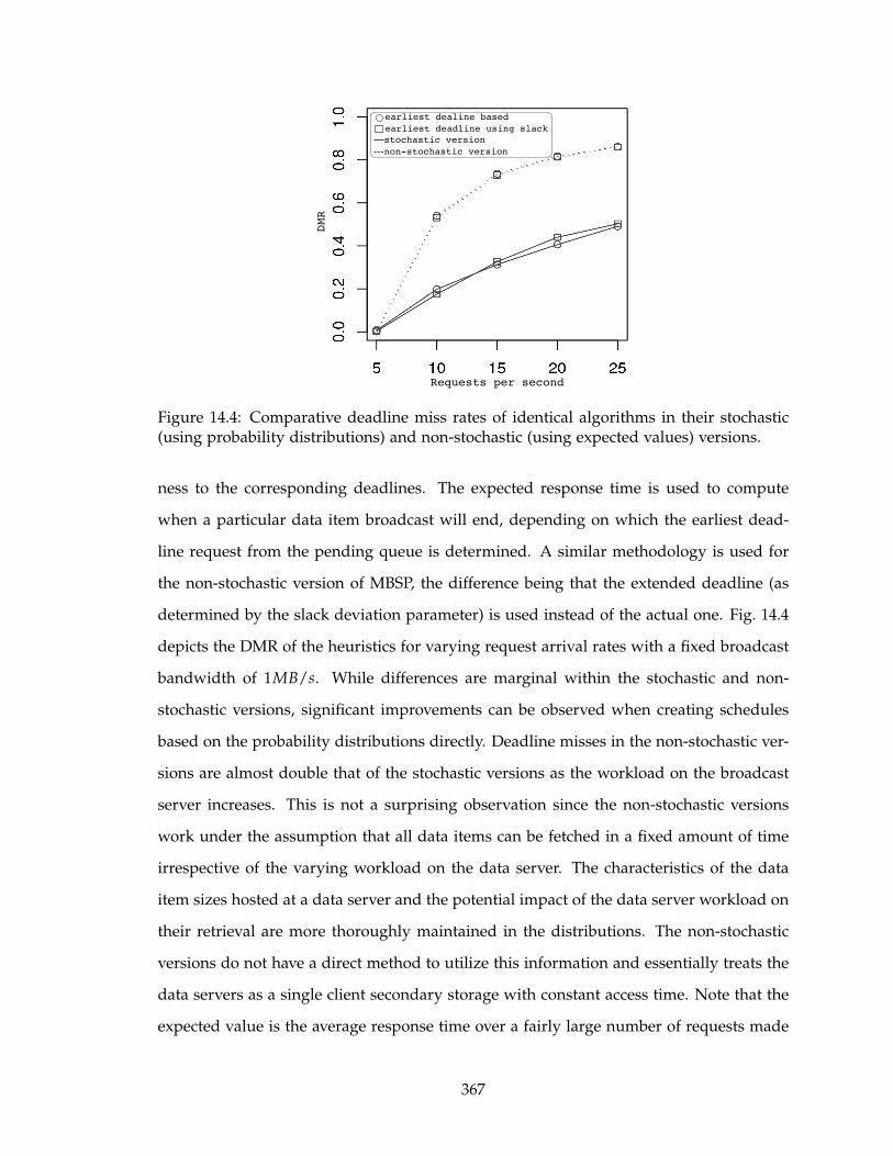
Requests per second
DMR
earliest dealine based
earliest deadline using slack
stochastic version
non-stochastic version
Figure 14.4: Comparative deadline miss rates of identical algorithms in their stochastic(using probability distributions) and non-stochastic (using expected values) versions.
ness to the corresponding deadlines. The expected response time is used to compute
when a particular data item broadcast will end, depending on which the earliest dead-
line request from the pending queue is determined. A similar methodology is used for
the non-stochastic version of MBSP, the difference being that the extended deadline (as
determined by the slack deviation parameter) is used instead of the actual one. Fig. 14.4
depicts the DMR of the heuristics for varying request arrival rates with a fixed broadcast
bandwidth of 1MB/s. While differences are marginal within the stochastic and non-
stochastic versions, significant improvements can be observed when creating schedules
based on the probability distributions directly. Deadline misses in the non-stochastic ver-
sions are almost double that of the stochastic versions as the workload on the broadcast
server increases. This is not a surprising observation since the non-stochastic versions
work under the assumption that all data items can be fetched in a fixed amount of time
irrespective of the varying workload on the data server. The characteristics of the data
item sizes hosted at a data server and the potential impact of the data server workload on
their retrieval are more thoroughly maintained in the distributions. The non-stochastic
versions do not have a direct method to utilize this information and essentially treats the
data servers as a single client secondary storage with constant access time. Note that the
expected value is the average response time over a fairly large number of requests made
367
to a data server. However, requests from a broadcast server to a given data server may be
sporadic depending on the popularity of the data items hosted by the server.
14.5.2 Comparative performance
Fig. 14.5 shows the performance metric values for the six heuristics under different
workload conditions. Variable workload conditions are simulated by changing the band-
width of the downlink channel, as given by the different bandwidth utilization factors
UFbs = 0.5,0.75,1.0,2.0,3.0,4.0,5.0. An utilization factor greater than 1.0 means data re-
quests arrive at a rate higher than that can be handled by the broadcast server band-
width. With the fixed bandwidth model, these factors translate to workloads generated
by more than 5 requests per second with bbs = 1MB/s. MDMP and MBSP maintain a
DMR of less than 1% as the bandwidth utilization approaches 100%. On the other hand,
the DMR of NPRDS increases to 8%. In general, deadline miss rates are less than 10%
for utilization factors of less than 1.0. Similarly, all heuristics can generate schedules with
more than 95% utility at such utilization factors. All heuristics show an exponential in-
crease in the number of deadlines missed when the utilization factor goes above 1.0. The
drop in utility and increase in the average stretch follow similar trends. Both stochastic
heuristics, MDMP and MBSP, perform better in DMR and UT over a wider range of band-
width utilization. MDMP and NPRDS have around 20% deadline misses at UFbs = 2.0,
compared to 34% of MAX. The utility metric is between 82% (MAX) and 93% (MDMP)
at this point. However, as mentioned earlier, the average stretch metric does not reflect
this performance. MAX and NPRDS are the better performing ones according to ASTR.
We also notice an improvement in the comparative performance of NPRDS as bandwidth
utilization goes beyond 300%. The NPRDS heuristic displays better sustenance in all three
metrics at such utilizations.
14.5.3 Impact of broadcast utilization factor
Heuristic performance is heavily affected by the workload conditions and bandwidth
available at the broadcast server. In conditions of heavy workload, or low bandwidth, the
accumulation of requests at the broadcast server dominates the rate at which requests get
368
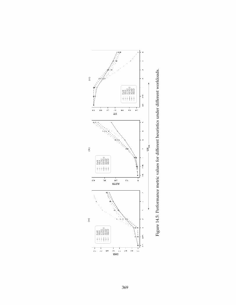
RxW
MAX
SIN2
NPRDS
MDMP
MBSP
UFbs
DMR
ASTR
UT
(a)
(b)
(c)
RxW
MAX
SIN2
NPRDS
MDMP
MBSP
RxW
MAX
SIN2
NPRDS
MDMP
MBSP
Fig
ure
14.5
:P
erfo
rman
cem
etri
cv
alu
esfo
rd
iffe
ren
th
euri
stic
su
nd
erd
iffe
ren
tw
ork
load
s.
369
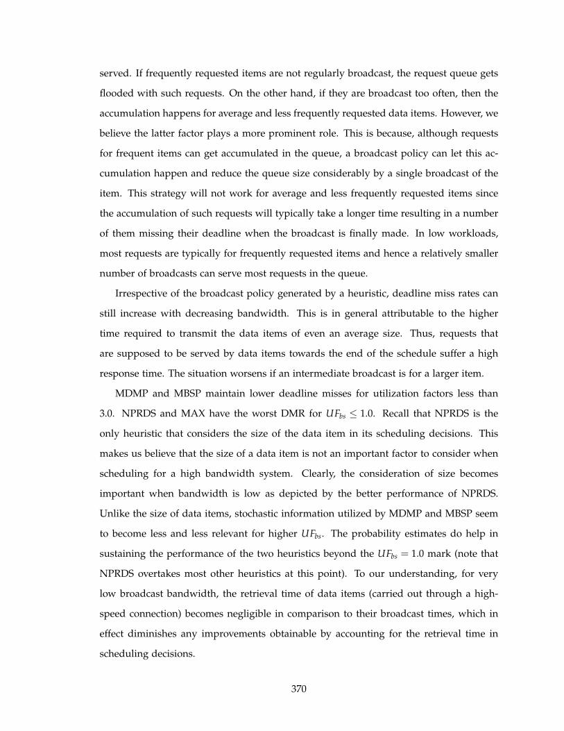
served. If frequently requested items are not regularly broadcast, the request queue gets
flooded with such requests. On the other hand, if they are broadcast too often, then the
accumulation happens for average and less frequently requested data items. However, we
believe the latter factor plays a more prominent role. This is because, although requests
for frequent items can get accumulated in the queue, a broadcast policy can let this ac-
cumulation happen and reduce the queue size considerably by a single broadcast of the
item. This strategy will not work for average and less frequently requested items since
the accumulation of such requests will typically take a longer time resulting in a number
of them missing their deadline when the broadcast is finally made. In low workloads,
most requests are typically for frequently requested items and hence a relatively smaller
number of broadcasts can serve most requests in the queue.
Irrespective of the broadcast policy generated by a heuristic, deadline miss rates can
still increase with decreasing bandwidth. This is in general attributable to the higher
time required to transmit the data items of even an average size. Thus, requests that
are supposed to be served by data items towards the end of the schedule suffer a high
response time. The situation worsens if an intermediate broadcast is for a larger item.
MDMP and MBSP maintain lower deadline misses for utilization factors less than
3.0. NPRDS and MAX have the worst DMR for UFbs ≤ 1.0. Recall that NPRDS is the
only heuristic that considers the size of the data item in its scheduling decisions. This
makes us believe that the size of a data item is not an important factor to consider when
scheduling for a high bandwidth system. Clearly, the consideration of size becomes
important when bandwidth is low as depicted by the better performance of NPRDS.
Unlike the size of data items, stochastic information utilized by MDMP and MBSP seem
to become less and less relevant for higher UFbs. The probability estimates do help in
sustaining the performance of the two heuristics beyond the UFbs = 1.0 mark (note that
NPRDS overtakes most other heuristics at this point). To our understanding, for very
low broadcast bandwidth, the retrieval time of data items (carried out through a high-
speed connection) becomes negligible in comparison to their broadcast times, which in
effect diminishes any improvements obtainable by accounting for the retrieval time in
scheduling decisions.
370

An interesting observation to note is at UFbs = 2.0. Although, the DMRs of NPRDS,
MDMP and MBSP are quite similar at this point, there is still a significant difference in
their UT values. NPRDS and MDMP display a DMR of about 20% and MBSP has a DMR
of 17.5%. However, MDMP maintains a higher utility than NPRDS (93% compared to
87%). The requests which missed their deadlines in MDMP did so by smaller durations
than in NPRDS. Hence, equivalent deadline misses need not always correlate to similar
utilities. Broadcast schedules can be generated that, although misses equal number of
deadlines, can maintain closer proximity of the response time of requests to their service
times. MBSP, on the other hand, displays a trade-off characteristic where lower DMR has
been achieved by a slight reduction in the utility (89.6%).
Based on these observations, MDMP and MBSP are probable choices for low and
marginally higher workloads, while NPRDS is the likely candidate for very heavy work-
loads. One should note that deadline misses will increase exponentially when bandwidth
utilization goes higher than 100%. Marginal increases in the utilization factor are accept-
able owing to bursts in traffic. However, the range of utilization factors where heuristics
such as NPRDS performs better in this problem are very unlikely settings for a realistic
broadcast system (a system having almost 50% deadline misses). If a situation does occur
where the utilization surpasses the expected range, then the network design is revisited
or additional resources are installed to bring down the utilization to the sought range.
In this regard, MDMP and MBSP both sustain their better performance up to 300% uti-
lization. The observation helps conclude that MDMP and MBSP are also suitable for
handling occasional bursts in traffic.
14.5.4 Impact of slack deviation on MBSP
The MBSP heuristic first schedules the request with the maximum probability of miss-
ing the extended deadline decided by the slack deviation parameter Sdev. The extended
deadline for a request Q is given as dlnQ + Sdev(dlnQ − arrQ). Table 14.1 shows the varia-
tion in the performance metrics across five different slack deviations. Recall that Sdev = 0
corresponds to the heuristic that prefers the request with maximum probability of missing
the deadline and shows very similar performance to the dual heuristic MDMP (minimum
371
Table 14.1: Performance metric values for MBSP with UFbs = 2 and varying Sdev.
Sdev DMR ASTR UT
0.00 0.198 93.0 0.9220.25 0.175 97.0 0.8960.50 0.236 111.8 0.8660.75 0.263 124.9 0.841.00 0.266 132.5 0.833
arrQ timedlnQ
data items
insufficient to
broadcast any item
sufficient to
broadcast small items
sufficient to
broadcast large items
Figure 14.6: Impact of Sdev on scheduling decisions.
probability of meeting the deadline). While ASTR and UT show consistent degradation
as Sdev is increased from 0.0 to 1.0, DMR displays a change in gradient around Sdev = 0.25.
The intuition behind MBSP is to provide “sufficient” slack to the scheduler to satisfy
other requests at the expense of ones which are likely to or have already missed their
deadlines. This is achieved by informing a longer deadline for requests to the scheduler,
instead of the actual one. The slack deviation parameter helps modulate the amount of
slack so that exploited requests do not remain in the system for ever. The key to setting
the parameter is understanding what serves as “sufficient”.
Refer to Fig. 14.6. When the slack deviation is too small, the slack is of little or no
help since no data item (to serve other requests) can be broadcast between the actual
and the extended deadline. The performance of MBSP would thus be equivalent to that
of MDMP. The reason why a value such as 0.25 works best for the tested workloads
can be attributed to the size of the most frequently requested items (an item of around
200KB in the experimental setup). Assume that a request Q has already missed its actual
deadline t = dlnQ. Further, let its extended deadline be t + x, where x is determined by
the slack deviation parameter as x = Sdev(dlnQ − arrQ). Let the current time be t + 1.
Since MBSP sees the deadline for Q as t + x, it would try to schedule other requests first
372
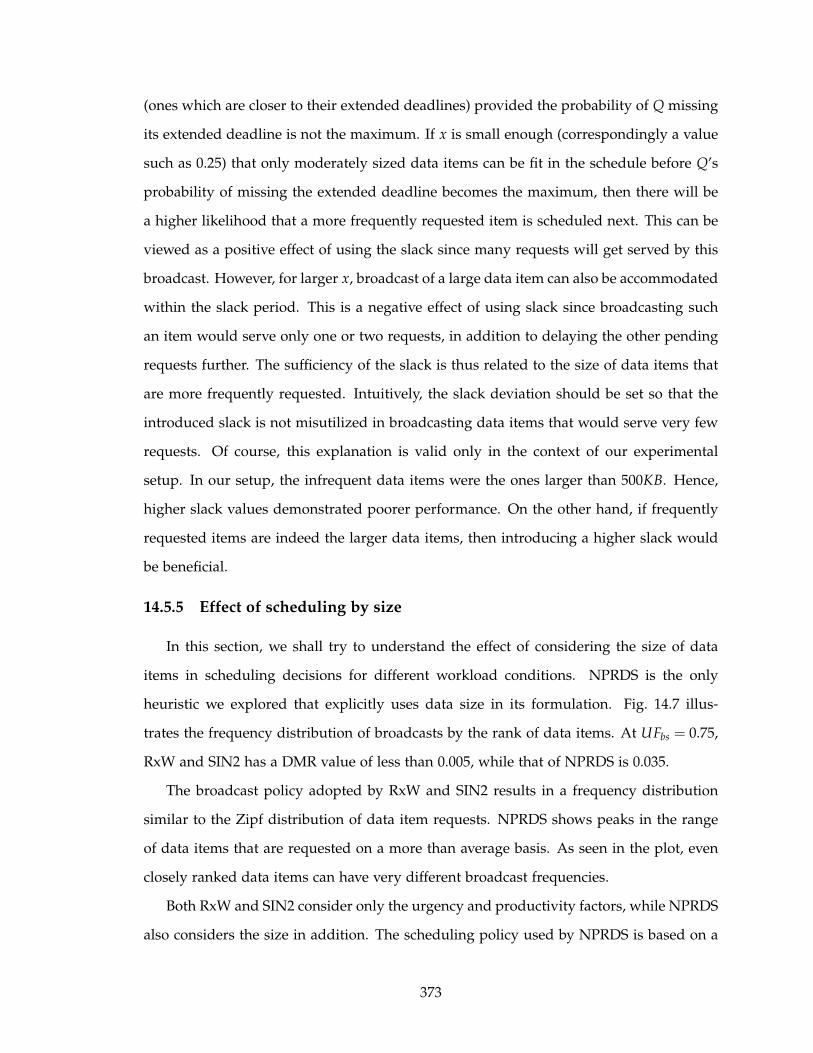
(ones which are closer to their extended deadlines) provided the probability of Q missing
its extended deadline is not the maximum. If x is small enough (correspondingly a value
such as 0.25) that only moderately sized data items can be fit in the schedule before Q’s
probability of missing the extended deadline becomes the maximum, then there will be
a higher likelihood that a more frequently requested item is scheduled next. This can be
viewed as a positive effect of using the slack since many requests will get served by this
broadcast. However, for larger x, broadcast of a large data item can also be accommodated
within the slack period. This is a negative effect of using slack since broadcasting such
an item would serve only one or two requests, in addition to delaying the other pending
requests further. The sufficiency of the slack is thus related to the size of data items that
are more frequently requested. Intuitively, the slack deviation should be set so that the
introduced slack is not misutilized in broadcasting data items that would serve very few
requests. Of course, this explanation is valid only in the context of our experimental
setup. In our setup, the infrequent data items were the ones larger than 500KB. Hence,
higher slack values demonstrated poorer performance. On the other hand, if frequently
requested items are indeed the larger data items, then introducing a higher slack would
be beneficial.
14.5.5 Effect of scheduling by size
In this section, we shall try to understand the effect of considering the size of data
items in scheduling decisions for different workload conditions. NPRDS is the only
heuristic we explored that explicitly uses data size in its formulation. Fig. 14.7 illus-
trates the frequency distribution of broadcasts by the rank of data items. At UFbs = 0.75,
RxW and SIN2 has a DMR value of less than 0.005, while that of NPRDS is 0.035.
The broadcast policy adopted by RxW and SIN2 results in a frequency distribution
similar to the Zipf distribution of data item requests. NPRDS shows peaks in the range
of data items that are requested on a more than average basis. As seen in the plot, even
closely ranked data items can have very different broadcast frequencies.
Both RxW and SIN2 consider only the urgency and productivity factors, while NPRDS
also considers the size in addition. The scheduling policy used by NPRDS is based on a
373
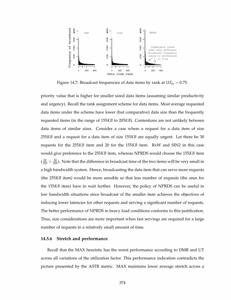
Data item rank
Frequency of broadcast
RxW SIN2 NPRDS
comparable ranks
have very different
broadcast frequency
owing to difference
in size
Figure 14.7: Broadcast frequencies of data items by rank at UFbs = 0.75.
priority value that is higher for smaller sized data items (assuming similar productivity
and urgency). Recall the rank assignment scheme for data items. Most average requested
data items under the scheme have lower (but comparative) data size than the frequently
requested items (in the range of 155KB to 205KB). Contentions are not unlikely between
data items of similar sizes. Consider a case where a request for a data item of size
255KB and a request for a data item of size 155KB are equally urgent. Let there be 30
requests for the 255KB item and 20 for the 155KB item. RxW and SIN2 in this case
would give preference to the 255KB item, whereas NPRDS would choose the 155KB item
( 20155 >
30255 ). Note that the difference in broadcast time of the two items will be very small in
a high bandwidth system. Hence, broadcasting the data item that can serve more requests
(the 255KB item) would be more sensible so that less number of requests (the ones for
the 155KB item) have to wait further. However, the policy of NPRDS can be useful in
low bandwidth situations since broadcast of the smaller item achieves the objectives of
inducing lower latencies for other requests and serving a significant number of requests.
The better performance of NPRDS in heavy load conditions conforms to this justification.
Thus, size considerations are more important when fast servings are required for a large
number of requests in a relatively small amount of time.
14.5.6 Stretch and performance
Recall that the MAX heuristic has the worst performance according to DMR and UT
across all variations of the utilization factor. This performance indication contradicts the
picture presented by the ASTR metric. MAX maintains lower average stretch across a
374
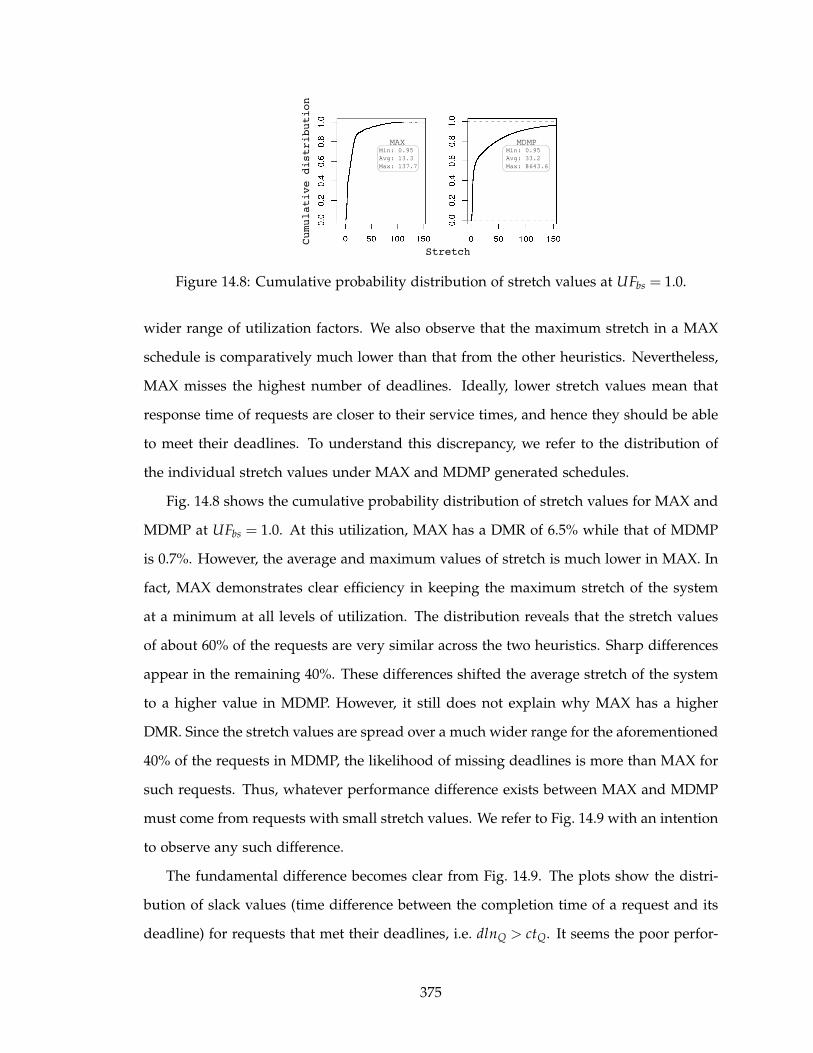
Stretch
Cumulative distribution
MAX MDMPMin: 0.95
Avg: 13.3
Max: 137.7
Min: 0.95
Avg: 33.2
Max: 8643.6
Figure 14.8: Cumulative probability distribution of stretch values at UFbs = 1.0.
wider range of utilization factors. We also observe that the maximum stretch in a MAX
schedule is comparatively much lower than that from the other heuristics. Nevertheless,
MAX misses the highest number of deadlines. Ideally, lower stretch values mean that
response time of requests are closer to their service times, and hence they should be able
to meet their deadlines. To understand this discrepancy, we refer to the distribution of
the individual stretch values under MAX and MDMP generated schedules.
Fig. 14.8 shows the cumulative probability distribution of stretch values for MAX and
MDMP at UFbs = 1.0. At this utilization, MAX has a DMR of 6.5% while that of MDMP
is 0.7%. However, the average and maximum values of stretch is much lower in MAX. In
fact, MAX demonstrates clear efficiency in keeping the maximum stretch of the system
at a minimum at all levels of utilization. The distribution reveals that the stretch values
of about 60% of the requests are very similar across the two heuristics. Sharp differences
appear in the remaining 40%. These differences shifted the average stretch of the system
to a higher value in MDMP. However, it still does not explain why MAX has a higher
DMR. Since the stretch values are spread over a much wider range for the aforementioned
40% of the requests in MDMP, the likelihood of missing deadlines is more than MAX for
such requests. Thus, whatever performance difference exists between MAX and MDMP
must come from requests with small stretch values. We refer to Fig. 14.9 with an intention
to observe any such difference.
The fundamental difference becomes clear from Fig. 14.9. The plots show the distri-
bution of slack values (time difference between the completion time of a request and its
deadline) for requests that met their deadlines, i.e. dlnQ > ctQ. It seems the poor perfor-
375

dln -ct
Cumulative distribution
Q Q
MAX MDMP
served very close
to the deadlines
Figure 14.9: Cumulative probability distribution of dlnQ − ctQ (positive slack) for requestswhich are served within their deadlines (dlnQ > ctQ); UFbs = 1.0.
mance of MAX is attributable to its inability to utilize the time gaps between a request’s
arrival and its imposed deadline to serve other pending requests. 20% of the requests in
MDMP are served very close to their deadlines (near zero positive slack). This indicates
that MDMP manages to utilize the slack between a request’s arrival and its deadline in
serving more urgent requests. Requests far away from their deadlines will have higher
probabilities of meeting their deadlines and hence can be pushed back in the schedule
to accommodate requests with lower probabilities of meeting their deadlines. The hypo-
thetical deadline created by MAX cannot capture this logic since it attempts to service a
request as close as possible to its service time. An important conclusion from this anal-
ysis is that the stretch of a request, at least in its defined form, is not an accurate factor
to include in deciding scheduling policies. This is particularly true for deadline based
systems where using any introduced slack may be advantageous.
14.5.7 Broadcast policies
The final analysis presented in this section is on the broadcast policies generated by
heuristics that result in additional performance improvement. For this we observe the
policies generated by MBSP and NPRDS. The performance difference between the two
heuristics diminish as the utilization factor increases, with NPRDS gaining at very high
utilization. The policies are observed in terms of the request and broadcast frequency of
data items. To do so, we divided the data items into four access types: frequent (ranks 1
to 20), above average (ranks 21 to 45), average (ranks 46 to 255) and infrequent (ranks 256 to
400). We then observed how the broadcast frequency of data items in the four categories
376
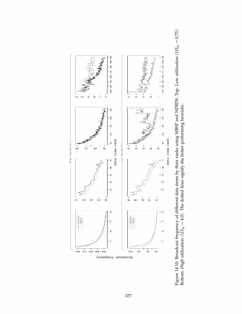
Data item rank
Broadcast frequency
NPRDS
MBSP
NPRDS
MBSP
Data item rank
High bandwidth
Low bandwidth
Fig
ure
14.1
0:B
road
cast
freq
uen
cyo
fd
iffe
ren
td
ata
item
sb
yth
eir
ran
ks
usi
ng
MB
SP
and
NP
RD
S.
To
p:
Lo
wu
tili
zati
on
(UF b
s=
0.75
).B
ott
om
:H
igh
uti
liza
tio
n(U
F bs=
4.0).
Th
ed
ott
edli
nes
sig
nif
yth
eb
ette
rp
erfo
rmin
gh
euri
stic
.
377
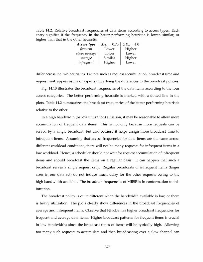
Table 14.2: Relative broadcast frequencies of data items according to access types. Eachentry signifies if the frequency in the better performing heuristic is lower, similar, orhigher than that in the other heuristic.
Access type UFbs = 0.75 UFbs = 4.0
frequent Lower Higherabove average Lower Lower
average Similar Higherinfrequent Higher Lower
differ across the two heuristics. Factors such as request accumulation, broadcast time and
request rank appear as major aspects underlying the differences in the broadcast policies.
Fig. 14.10 illustrates the broadcast frequencies of the data items according to the four
access categories. The better performing heuristic is marked with a dotted line in the
plots. Table 14.2 summarizes the broadcast frequencies of the better performing heuristic
relative to the other.
In a high bandwidth (or low utilization) situation, it may be reasonable to allow more
accumulation of frequent data items. This is not only because more requests can be
served by a single broadcast, but also because it helps assign more broadcast time to
infrequent items. Assuming that access frequencies for data items are the same across
different workload conditions, there will not be many requests for infrequent items in a
low workload. Hence, a scheduler should not wait for request accumulation of infrequent
items and should broadcast the items on a regular basis. It can happen that such a
broadcast serves a single request only. Regular broadcasts of infrequent items (larger
sizes in our data set) do not induce much delay for the other requests owing to the
high bandwidth available. The broadcast frequencies of MBSP is in conformation to this
intuition.
The broadcast policy is quite different when the bandwidth available is low, or there
is heavy utilization. The plots clearly show differences in the broadcast frequencies of
average and infrequent items. Observe that NPRDS has higher broadcast frequencies for
frequent and average data items. Higher broadcast patterns for frequent items is crucial
in low bandwidths since the broadcast times of items will be typically high. Allowing
too many such requests to accumulate and then broadcasting over a slow channel can
378
introduce deadline misses for a higher number of requests. On the other hand, accumu-
lation of average items should not be allowed since it would usually take a long time for
a significant accumulation to happen. This will only keep such requests pending in the
system for a long duration of time. The request accumulation of above average items are
somewhere in between frequent and average ones. NPRDS decides to allow the accumu-
lation of these requests more than MBSP to utilize the broadcast bandwidth for frequent
and average items. Infrequent items are ignored the most owing to their high broadcast
time.
Understanding the broadcast policies in this manner not only reveals what factors are
more important in different utilization, but also paves the way to transform a pull-based
system to a push-based one with similar performance. However, in addition to relative
measurements, such conversions will also require the estimation of absolute frequency in
a probabilistic manner.
14.6 Conclusions
In this chapter, we introduce the problem of stochastic scheduling in broadcast sys-
tems where data items must be retrieved from different data servers prior to broadcasts.
We model the data servers as M/G/1 − PS systems where the available bandwidth is
equally divided among pending requests. Schedules are then generated at the broad-
cast server to serve requests within their imposed deadlines. Two novel heuristics are
proposed that use the probability distribution of response times in the data servers to
generate schedules. The Minimum Deadline Meet Probability (MDMP) heuristic sched-
ules requests based on their probability of meeting the deadline. The Maximum Bounded
Slack Probability (MBSP) heuristic defines an extended deadline for requests as given by
a slack deviation parameter, with an intention to use any negative slack for serving other
pending requests. The performance of these heuristics is compared to that of four other
heuristics – RxW, MAX, SIN2 and NPRDS – that have been proposed for deterministic
broadcast scheduling. Performance is evaluated using three metrics - deadline miss rate,
average stretch, and utility.
Empirical results on a synthetic data set reveals that both MDMP and MBSP show
379
superior performance in conditions of both low and high broadcast utilization. In very
heavy workloads, the response time of data retrieval is observed to become negligible
compared to the broadcast time. NPRDS provides a better performance under such sit-
uations. However, such load conditions are often not realistic. Further analysis on the
impact of various factors on broadcasting policies reveals that size of data items can often
be ignored in scheduling decisions when the broadcast bandwidth is high. The stretch of
requests, as typically defined, is also found to be an inaccurate factor to consider while
scheduling in deadline based systems. Finally, good broadcast policies can have very
different characteristics depending on workload conditions. Request accumulation, data
item access frequencies and their broadcast times assume different levels of prominence
in different situations, thereby affecting the performance of the heuristics. We also ex-
plore the effect of the slack deviation parameter on MBSP and found correspondence of
its performance to the amount of negative slack that the heuristic is allowed to exploit.
Typically, very low values do not enable any slack utilization, while high values provide
too much of it to make the broadcast of larger data items feasible.
In future, we need to explore the scenario when multiple servers can host the same
data item. The scheduler then has to build a fetching schedule based on perceived re-
sponse times and evaluate its effectiveness in combination with the broadcast sched-
ule. Interactions between the broadcast and data server can be made more complex
by including concepts such as parallel/pre-fetching and data replication. In general,
parallel/pre-fetching will change the probabilities of retrieval times of the data items.
The final scheduling approach can therefore remain the same. Data replication will have
a deeper impact since the probabilities of fetching the same item within a specific period
will be different for different data servers. Increasing the number of data servers and
distributing frequently accessed data items across them can also provide lower data re-
trieval times and can correspondingly impact heuristic performance. These issues require
a much extensive analysis and thus forms the basis for our future work.
380
CHAPTER 15
Dissertation Summary
Modern information management systems are required to satisfy multiple goals in
their implementation. Simultaneous adherence to these goals is often found to be difficult
owing to their conflicting nature. This dissertation explores three goals laid down for any
such system, namely risk minimization, maximal resource utilization and service quality
maximization.
Multi-criteria analysis is proposed as a flexible tool to obtain the best balance along
the three dimensions – risks, resources and services. Balancing these dimensions is chal-
lenging due to the presence of inherent reciprocal influences. We explore three domains
in computer science that exhibit the requirement for a multi-criteria analysis. Extensive
empirical studies are provided to establish our propositions.
We use disclosure control as the first platform to demonstrate how controlling the
exposure of sensitive personal information can negatively impact the service goals of a
data broker. Our extensive survey of existing techniques indicate that the current trend is
to determine data modifications that preserve a pre-specified level of privacy and induce
a minimum loss in information within the constraint. Contrary to this trend, we propose
evaluating privacy and data utility within a multi-objective optimization framework. This
provides a data publisher the trade-off information required to make an informed deci-
sion on what level of privacy can be enforced for a certain level of data utility, and vice
381
versa. Our proposed techniques also allow a data publisher to limit the exploration of
solutions to a subset that closely matches the preferences of the publisher. One of the
important outcomes of the multi-criteria analysis is the identification of bias in individual
privacy levels. This bias is introduced primarily due to the minimalistic nature of existing
privacy models. Towards this end, we redefine the characteristics of an optimal solution
and propose a multi-criteria framework capable of identifying solutions with user-defined
properties.
The second domain we explore, security risk management, highlights how limited
resource availability often becomes a deciding factor while protecting the assets in a net-
work. We move beyond the assumption that an organization has all necessary resources
to protect its network, and argue that sections of a network will always remain exposed
to an attacker. Towards this end, we propose using cause-consequence attack models to
obtain a global picture of residual risks and involved hardening costs. The methodology
can also be used to determine optimal points of hardening under other resource con-
straints such as energy consumption and computational power of a node. We also show
that knowledge about the attack difficulties can help identify where resources need to be
spent predominantly. This can be done by mitigating vulnerabilities with a high probabil-
ity of being exploited. Game theory based extensions of the security hardening problem
reveal that attacker-defender dynamics cannot be ignored since an optimal solution in the
long run is very different from one that provides short term optimality.
Wireless data broadcasting is used as the third domain to exemplify the impact of lim-
ited resources on the quality of service that can be delivered by an information system.
The QoS criteria to satisfy while maximally utilizing the wireless bandwidth is predom-
inantly based on hard deadlines. We provide justifications to use soft deadlines as an
alternative since it allows a broadcast scheduler to relatively determine the utility of a
broadcast data item. We explore broadcast systems supporting different data dependen-
cies (single data, transaction data and ordered data) and data retrieval schemes.
Specific future directions have been highlighted at the end of individual chapters. We
outline below the general directions for each of the explored domains.
• There is an abundance of privacy models proposed for data anonymization. How-
382
ever, privacy issues extend much beyond databases. The rapid growth of mobile
communication systems, and the application domains thereof, have started to reveal
disclosure problems usually unseen in databases. However, a majority of existing
models can be transitioned to address these problems. The question that remains
open is how these models will affect the usability of a mobile application. Address-
ing the privacy versus usability problem is an immediate requirement for these
mobile information systems.
• Optimal security hardening has been researched with a static perspective for a long
time now. Interesting approaches have originated out of this research. Nonetheless,
the optimality of a security policy is very easily invalidated by the changing dy-
namics of a network and growth of attacker capabilities. Given that policy decisions
cannot change as easily as the network itself, there is the need to revisit the defi-
nition of an optimal security solution. Research is required to tightly integrate the
possible evolution of the network and the attacker into this definition. Resource uti-
lization cannot be maximized in this domain without an evolving defender model.
• A number of generic heuristics exist to build broadcast schedules for efficient data
broadcasting. However, application requirements are often very diverse in mobile
environments. Although utility functions can capture the global characteristics of
data usefulness, the quality of service would be sub-optimal unless data utility can
be expressed as a function of the underlying application usage. Custom represen-
tations of data utility will further influence a number of decisions on where data
items should be stored, what replication frequencies should be used, and what up-
date policies will be best for transient data, among others.
383
Bibliography
[1] Acharya, S., Alonso, R., Franklin, M., and Zdonik, S. Broadcast Disks: DataManagement for Asymmetric Communication Environments. In Proceedings of the1995 ACM SIGMOD International Conference on Management of Data (1995), pp. 199–210.
[2] Acharya, S., and Muthukrishnan, S. Scheduling On-Demand Broadcasts: NewMetrics and Algorithms. In Proceedings of the 4th Annual ACM/IEEE InternationalConference on Mobile Computing and Networking (1998), pp. 43–54.
[3] Ackermann, H., Newman, A., Röglin, H., and Vöcking, B. Decision-makingBased on Approximate and Smoothed Pareto Curve. Theoretical Computer Science378, 3 (2007), 253–270.
[4] Acquisti, A., and Gross, R. Predicting Social Security Numbers from Public Data.Proceedings of the National Academy of Sciences 106, 27 (2009), 10975–10980.
[5] Adam, N. R., and Worthmann, J. C. Security-Control Methods for StatisticalDatabases: A Comparative Study. ACM Computing Survey 21, 4 (1989), 515–556.
[6] Aggarwal, G., Feder, T., Kenthapadi, K., Khuller, S., Panigrahy, R., Thomas,D., and Zhu, A. Achieving Anonymity Via Clustering. In Proceedings of the 25thACM SIGMOD-SIGACT-SIGART Symposium on Principles of Database Systems (2006),pp. 153–162.
[7] Aksoy, D., and Franklin, M. RxW: A Scheduling Approach for Large-Scale On-Demand Data Broadcast. IEEE/ACM Transactions on Networking 7, 6 (1999), 846–860.
[8] Aksoy, D., Franklin, M., and Zdonik, S. Data Staging for On-Demand Broadcast.In Proceedings of the 27th International Conference on Very Large Data Bases (2001),pp. 571–580.
[9] Alba, E., and Tomassini, M. Parallelism and Evolutionary Algorithms. IEEETransactions on Evolutionary Computation 6, 5 (2002), 443–462.
[10] Ammann, P., Wijesekera, D., and Kaushik, S. Scalable, Graph-Based NetworkVulnerability Analysis. In Proceedings of the 9th Conference on Computer and Commu-nications Security (2002), pp. 217–224.
[11] Arora, A., Hall, D., Piato, C., Ramsey, D., and Telang, R. Measuring the Risk-based Value of IT Security Solutions. IT Professional 6, 6 (2004), 35–42.
[12] Axelrod, R. Evolution of Strategies in the Iterated Prisoner’s Dilemma. In GeneticAlgorithms and Simulated Annealing. Morgan Kaufmann, 1987, pp. 32–41.
384

[13] Bamba, B., Liu, L., Pesti, P., and Wang, T. Supporting Anonymous LocationQueries in Mobile Environments with Privacy Grid. In Proceedings of the 17th In-ternational World Wide Web Conference (2008), pp. 237–246.
[14] Barbaro, M., and Zeller, T. A Face is Exposed for AOL Searcher No. 4417749:New York Times. http://www.nytimes.com/2006/08/09/technology/09aol.html,2006.
[15] Barford, P., and Crovella, M. Generating Representative Web Workloads forNetwork and Server Performance Evaluation. ACM SIGMETRICS Performance Eval-uation Review 26, 1 (1998), 151–160.
[16] Bayardo, R. J., and Agrawal, R. Data Privacy Through Optimal k-Anonymization.In Proceedings of the 21st International Conference on Data Engineering (2005), pp. 217–228.
[17] Bayardo, R. J., Agrawal, R., and Gunopulos, D. Constraint-Based Rule Miningin Large, Dense Databases. In Proceedings of the 15th International Conference on DataEngineering (1999), pp. 188–197.
[18] Beresford, A. R., and Stajano, F. Location Privacy in Pervasive Computing. IEEESecurity and Privacy 2 (2003), 46–55.
[19] Berger, B. Data-centric Quantitative Computer Security Risk Assessment. Informa-tion Security Reading Room, SANS (2003).
[20] Bettini, C., Wang, X. S., and Jajodia, S. Protecting Privacy Against Location-Based Personal Identification. In Proceedings of the 2nd VLDB Workshop on SecureData Management (2005), pp. 185–199.
[21] Beyer, H. G. An Alternative Explanation for the Manner in which Genetic Algo-rithms Opearate. BioSystems 41 (1997), 1–15.
[22] Beyer, H. G., and Schwefel, H. P. Evolution Strategies: A Comprehensive Intro-duction. Natural Computing 1 (2002), 3–52.
[23] Bistarelli, S., Dall’Aglio, M., and Perretti, P. Strategic Games on Defense Trees.In Formal Aspects in Security and Trust. Springer, 2006, pp. 1–15.
[24] Bistarelli, S., Fioravanti, F., and Perretti, P. Defense Tree for Economic Eval-uations of Security Investment. In Proceedings of the 1st International Conference onAvailability, Reliability and Security (2006), pp. 416–423.
[25] Black, J. P., Segmuller, W., Cohen, N., Leiba, B., Misra, A., Ebling, M. R., and
Stern, E. Pervasive Computing in Health Care: Smart Spaces and Enterprise Infor-mation Systems. In MobiSys 2004 Workshop on Context Awareness (2004).
[26] Bohn, J., Gärtner, F., and Vogt, H. Dependability Issues in Pervasive Computingin a Healthcare Environment. In SPC 2003 (2003), pp. 53–70.
[27] Breslau, L., Cao, P., Fan, L., Phillips, G., and Shenker, S. Web Caching and Zipf-Like Distributions: Evidence and Implications. In Proceedings of the IEEE INFOCOM’99 (1999), pp. 126–134.
385
[28] Bull, L. Coevolutionary Computation: An Introduction. http://www.cems.uwe.ac.uk/˜lbull/intro.pdf, 1998.
[29] Butler, S., and Fischbeck, P. Multi-attribute Risk Assessment. In Proceedings ofSREIS02 in conjunction of 10th IEEE International Requirements Engineering Conference(2002).
[30] Butler, S. A. Security Attribute Evaluation Method: A Cost-benefit Approach. InProceedings of the 24rd International Conference on Software Engineering (2002), pp. 232–240.
[31] Buttazzo, G., Spuri, M., and Sensini, F. Value vs. Deadline Scheduling in Over-load Conditions. In Proceedings of the 16th IEEE Real-Time Systems Symposium (1995),pp. 90–99.
[32] Byun, J. W., Karma, A., Bertino, E., and Li, N. Advances in Databases: Con-cepts, Systems and Applications. Springer Berlin/Heidelberg, 2007, ch. Efficient k-Anonymization Using Clustering Techniques, pp. 188–200.
[33] Campbell, R. H., Al-Muhtadi, J., Naldurg, P., Sampemane, G., and Mickunas,M. D. Towards Security and Privacy for Pervasive Computing. In Proceedings of theInternational Symposium on Software Security (2002), pp. 1–15.
[34] Campman, A., and Truta, T. M. Extended p-Sensitive k-Anonymity. Studia Uni-versitatis Babes-Bolyai Informatica 51, 2 (2006), 19–30.
[35] Chehadeh, Y., Hurson, A., and Kavehrad, M. Object Organization on a SingleBroadcast Channel in the Mobile Computing Environment. Multimedia Tools andApplications 9, 1 (1999), 69–94.
[36] Chen, B., LeFevre, K., and Ramakrishnan, R. Privacy Skyline: Privacy withMultidimensional Adversarial Knowledge. In Proceedings of the 33rd InternationalConference on Very Large Data Bases (2007), pp. 770–781.
[37] Chigan, C., Ye, Y., and Li, L. Balancing Security Against Performance in Wire-less Ad Hoc and Sensor Networks. In Proceedings of the IEEE Vehicular TechnologyConference (2004), vol. 7, pp. 4735–4739.
[38] Cho, H., Wu, H., Ravindran, B., and Jensen, E. D. On Multiprocessor UtilityAccrual Real-Time Scheduling With Statistical Timing Assurances. In Proceedingsof the IFIP International Conference on Embedded and Real-Time Ubiquitous Computing(2006), pp. 274–286.
[39] Chow, C.-Y., and Mokbel, M. Enabling Private Continuous Queries for RevealedUser Locations. In Proceedings of the 10th International Symposium on Spatial andTemporal Databases (2007), pp. 258–275.
[40] Coello, C. A. C. An Updated Survey of GA-Based Multiobjective OptimizationTechniques. ACM Computing Surveys 32, 2 (2000), 109–143.
[41] D. Riboni, L. Pareschi, C. B., and Jajodia, S. Preserving Anonymity of Recur-rent Location-Based Queries. In Proceedings of the 16th International Symposium onTemporal Representation and Reasoning (2009).
386
[42] Dantu, R., Loper, K., and Kolan, P. Risk Management Using Behavior BasedAttack Graphs. In Proceedings of the International Conference on Information Technology:Coding and Computing (2004), vol. 1, p. 445.
[43] Dawkins, J., Campbell, C., and Hale, J. Modeling Network Attacks: Extending theAttack Tree Paradigm. In Proceedings of the Workshop on Statistical Machine LearningTechniques in Computer Intrusion Detection (2002).
[44] Dawkins, R. The Blind Watchmaker. Norton & Company, Inc., 1986.
[45] de Jonge, W. Kilometerheffing op basis van elektronische aangifte. Informatie(2003), 22–27.
[46] Deb, K. Multi-objective Optimization Using Evolutionary Algorithms. John Wiley &Sons Inc., 2001.
[47] Deb, K., and Kumar, A. Interactive Evolutionary Multi-objective Optimization andDecision-Making Using Reference Direction Method. In Proceedings of the Geneticand Evolutionary Computation Conference (2007), pp. 781–788.
[48] Deb, K., Pratap, A., Agarwal, S., and Meyarivan, T. A Fast and Elitist Multiob-jective Genetic Algorithm: NSGA–II. IEEE Transactions on Evolutionary Computation6, 2 (2002), 182–197.
[49] Deb, K., and Sundar, J. Reference Point Based Multi-objective Optimization UsingEvolutionary Algorithms. In Proceedings of the Genetic and Evolutionary ComputationConference (2006), vol. 1, pp. 635–642.
[50] Dempster, M. A. H., Lenstra, J. K., and Kan, A. H. G. R. Deterministic and Stochas-tic Scheduling. D. Reidel Publishing Company, 1982.
[51] Dewri, R., Poolsappasit, N., Ray, I., and Whitley, D. Optimal Security Hard-ening Using Multi-objective Optimization on Attack Tree Models of Networks. InProceedings of the 14th Conference on Computer and Communications Security (2007),pp. 204–213.
[52] Dewri, R., Ray, I., Ray, I., and D.Whitley. Security Provisioning in Pervasive En-vironments Using Multi-objective Optimization. In Proceedings of the 13th EuropeanSymposium on Research in Computer Security (2008), pp. 349–363.
[53] Dewri, R., Ray, I., Ray, I., and Whitley, D. k-Anonymization in the Presenceof Publisher Preferences. IEEE Transactions on Knowledge and Data Engineering, toappear.
[54] Dewri, R., Ray, I., Ray, I., and Whitley, D. Real Time Stochastic Scheduling inBroadcast Systems with Decentralized Data Storage. Real-Time Systems, to appear.
[55] Dewri, R., Ray, I., Ray, I., and Whitley, D. On the Optimal Selection of k in thek-Anonymity Problem. In Proceedings of the 24th International Conference on DataEngineering (2008), pp. 1364–1366.
[56] Dewri, R., Ray, I., Ray, I., and Whitley, D. Optimizing On-Demand Data Broad-cast Scheduling in Pervasive Environments. In Proceedings of the 11th InternationalConference on Extending Database Technology (2008), pp. 559–569.
387

[57] Dewri, R., Ray, I., Ray, I., and Whitley, D. Advances in Artificial Intelligence forPrivacy Protection and Security. World Scientific Publishing, 2009, ch. Multi-ObjectiveEvolutionary Optimization in Statistical Disclosure Control.
[58] Dewri, R., Ray, I., Ray, I., and Whitley, D. On the Comparison of MicrodataDisclosure Control Algorithms. In 12th International Conference on Extending DatabaseTechnology (2009), pp. 240–251.
[59] Dewri, R., Ray, I., Ray, I., and Whitley, D. POkA: Identifying Pareto-Optimal k-Anonymous Nodes in a Domain Hierarchy Lattice. In Proceedings of the 18th ACMConference on Information and Knowledge Management (2009), pp. 1037–1046.
[60] Dewri, R., Ray, I., Ray, I., and Whitley, D. On the Formation of Historicallyk-Anonymous Anonymity Sets in a Continuous LBS. In 6th International ICST Con-ference on Security and Privacy in Communication Networks (2010), p. to appear.
[61] Dewri, R., Ray, I., Ray, I., and Whitley, D. On the Identification of Property BasedGeneralizations in Microdata Anonymization. In Proceedings of the 24th Annual IFIPWG 11.3 Working Conference on Data and Applications Security (2010), pp. 81–96.
[62] Dewri, R., Ray, I., Ray, I., and Whitley, D. Query m-Invariance: Preventing QueryDisclosures in Continuous Location-Based Services. In Proceedings of the 11th Inter-national Conference on Mobile Data Management (2010), pp. 95–104.
[63] Dewri, R., Whitley, D., Ray, I., and Ray, I. Evolution Strategy Based Optimizationof On-Demand Dependent Data Broadcast Scheduling. In Proceedings of the Geneticand Evolutionary Computation Conference (2008), pp. 1699–1700.
[64] Dewri, R., Whitley, D., Ray, I., and Ray, I. Optimizing Real-Time Ordered-DataBroadcasts in Pervasive Environments Using Evolution Strategy. In Proceedingsof the 10th International Conference on Parallel Problem Solving from Nature (2008),pp. 991–1000.
[65] Dewri, R., Whitley, D., Ray, I., and Ray, I. A Multi-Objective Approach to DataSharing with Privacy Constraints and Preference Based Objectives. In Proceedings ofthe 11th Annual Conference on Genetic and Evolutionary Computation (2009), pp. 1499–1506.
[66] Diakonikolas, I., and Yannakakis, M. Small Approximate Pareto Sets for Bi-objective Shortest Paths and Other Problems. In Approximation, Randomization, andCombinatorial Optimization. Algorithms and Techniques. Springer Berlin/Heidelberg,2007, pp. 74–88.
[67] Domingo-Ferrer, J., and Mateo-Sanz, J. M. Practical Data-Oriented Microaggre-gation for Statistical Disclosure Control. IEEE Transactions on Knowledge and DataEngineering 14, 1 (2002), 189–201.
[68] Dwork, C., and Yekhanin, S. New Efficient Attacks on Statistical Disclosure Con-trol Mechanisms. In Proceedings of the 28th Annual Conference on Cryptology (2008),pp. 469–480.
388

[69] Fernandez, J., and Ramamritham, K. Adaptive Dissemination of Data in Time-Critical Asymmetric Communication Environments. Mobile Networks and Applica-tions 9, 5 (2004), 491–505.
[70] Ficici, S. G., and Pollack, J. B. A Game-Theoretic Memory Mechanism for Coevo-lution. In Proceedings of the Genetic and Evolutionary Computation Conference (2003),pp. 286–297.
[71] Frigault, M., Wang, L., Singhal, A., and Jajodia, S. Measuring Network Secu-rity Using Dynamic Bayesian Network. In Proceedings of the 4th ACM Workshop onQuality of Protection (2009), pp. 23–30.
[72] Fung, B. C. M., Wang, K., and Yu, P. S. Top-Down Specialization for Informationand Privacy Preservation. In Proceedings of the 21st International Conference in DataEngineering (2005), pp. 205–216.
[73] Gedik, B., and Liu, L. Protecting Location Privacy with Personalized k-Anonymity:Architecture and Algorithms. IEEE Transactions on Mobile Computing 7, 1 (2008), 1–18.
[74] Gionis, A., Mazza, A., and Tassa, T. k-Anonymization Revisited. In Proceedings ofthe 24th International Conference on Data Engineering (2008), pp. 744–753.
[75] Goldberg, D. E. Genetic Algorithms in Search, Optimization, and Machine Learning.Addison-Wesley, 1989.
[76] Golle, P. Revisiting the Uniqueness of Simple Demographics in the US Population.In Proceedings of the 5th ACM Workshop on Privacy in Electronic Society (2006), pp. 77–80.
[77] Gruteser, M., and Grunwald, D. Anonymous Usage of Location-Based ServicesThrough Spatial and Temporal Cloaking. In Proceedings of the 1st International Con-ference on Mobile Systems, Applications, and Services (2003), pp. 31–42.
[78] Gruteser, M., and Liu, X. Protecting Privacy in Continuous Location-TrackingApplications. IEEE Security and Privacy 2, 2 (2004), 28–34.
[79] Gupta, M., Rees, J., Chaturvedi, A., and Chi, J. Matching Information SecurityVulnerabilities to Organizational Security Policies: A Genetic Algorithm Approach.Decision Support Systems 41, 3 (2006), 592–603.
[80] Hameed, S., and Vaidya, N. H. Efficient Algorithms for Scheduling Data Broadcast.Wireless Networks 5, 3 (1999), 183–193.
[81] Hanse, M. P., and Jaszkiewicz, A. Evaluating the Quality of Approximationsof the Non-dominated Set. IMM Technical Report IMM-REP-1998-7, Institute ofMathematical Modeling, Technical University of Denmark, 1998.
[82] Hillis, W. D. Co-evolving Parasites Improve Simulated Evolution as an Optimiza-tion Procedure. In Artificial Life II. Addison-Wesley, 1991.
[83] Hoh, B., and Gruteser, M. Protecting Location Privacy Through Path Confusion.In Proceedings of the 1st International Conference on Security and Privacy for EmergingAreas in Communication Networks (2005), pp. 194–205.
389
[84] Holland, J. Hidden Order: How Adaptation Build Complexity. Basic Books, 1995.
[85] Horn, J., Nafploitis, N., and Goldberg, D. A Niched Pareto Genetic Algorithmfor Multiobjective Optimization. In Proceedings of the 1st IEEE Conference on Evolu-tionary Computation (1994), pp. 82–87.
[86] Houmb, S. H., and Franqueira, V. N. Estimating ToE Risk Level Using CVSS. InProceedings of the 4th International Conference on Availability, Reliability and Security(2009), pp. 718–725.
[87] Huang, J.-L., and Chen, M.-S. Dependent Data Broadcasting for UnorderedQueries in a Multiple Channel Mobile Environment. IEEE Transactions on Knowl-edge and Data Engineering 16, 9 (2004), 1143–1156.
[88] Huang, Z., and Du, W. OptRR: Optimizing Randomized Response Schemes forPrivacy-Preserving Data Mining. In Proceedings of the 24th International Conferenceon Data Engineering (2008), pp. 705–714.
[89] Hundepool, A., and Willenborg, L. Mu and Tau Argus: Software for Statisti-cal Disclosure Control. In Proceedings of the 3rd International Seminar on StatisticalConfidentiality (1996).
[90] Hurson, A. R., Chehadeh, Y. C., and Hannan, J. Object Organization on ParallelBroadcast Channels in a Global Information Sharing Environment. In Proceedings ofthe 19th International Performance, Computing, and Communications Conference (2000),pp. 347–353.
[91] Imielinski, T., Viswanathan, S., and Badrinath, B. Data on Air: Organizationand Access. IEEE Transactions on Knowledge and Data Engineering 9, 3 (1997), 353–372.
[92] Iyengar, V. S. Transforming Data to Satisfy Privacy Constraints. In Proceedingsof the 8th ACM SIGKDD International Conference on Knowledge Discovery and DataMining (2002), pp. 279–288.
[93] Jensen, E., Locke, C., and Tokuda, H. A Time Driven Scheduling Model for Real-Time Operating Systems. In Proceedings of the 6th IEEE Real-Time Systems Symposium(1985), pp. 112–122.
[94] Jha, S., Sheyner, O., and Wing, J. M. Two Formal Analysis of Attack Graphs. InProceedings of the 15th IEEE Computer Security Foundations Workshop (2002), pp. 49–63.
[95] Jian-min, H., Hui-qun, Y., Juan, Y., and Ting-ting, C. A Complete (α,k)-Anonymity Model for Sensitive Values Individuation Preservation. In Proceedings ofthe International Symposium on Electronic Commerce and Security (2008), pp. 318–323.
[96] Jiang, S., and Vaidya, N. H. Scheduling Data Broadcasts to “Impatient" Users. InProceedings of the 1st ACM International Workshop on Data Engineering for Wireless andMobile Access (1999), pp. 52–59.
[97] Judd, G., and Steenkiste, P. Providing Contextual Information to Pervasive Com-puting Applications. In Proceedings of the 1st IEEE Annual Conference on PervasiveComputing and Communications (2003), pp. 133–142.
390
[98] Kalnis, P., Ghinita, G., Mouratidis, K., and Papadias, D. Preventing Location-Based Identity Inference in Anonymous Spatial Queries. IEEE Transactions onKnowledge and Data Engineering 19, 12 (2007), 1719–1733.
[99] Kido, H., Yanagisawa, Y., and Satoh, T. An Anonymous Communication Tech-nique Using Dummies for Location-Based Services. In Proceedings of the IEEE Inter-national Conference on Pervasive Services (2005), pp. 88–97.
[100] Kim, J.-H., and Chwa, K.-Y. Scheduling Broadcasts with Deadlines. TheoreticalComputer Science 325, 3 (2004), 479–488.
[101] Knowles, J. D., and Corne, D. W. On Metrics for Comparing Non-DominatedSets. In Proceedings of the Congress on Evolutionary Computation (2002), pp. 711–716.
[102] Knowles, J. D., Corne, D. W., and Oates, M. J. On the Assessment of Multiob-jective Approaches to the Adaptive Distributed Database Management Problem. InProceedings of the Parallel Problem Solving from Nature VI (2000), pp. 869–878.
[103] Kohavi, R., and Becker, B. UCI Machine Learning Repository - Adult Database.ftp://ftp.ics.uci.edu/pub/machine-learning-databases/adult/.
[104] Lam, K., Chan, E., and Yuen, J. C. Approaches for Broadcasting Temporal Data inMobile Computing Systems. Journal of Systems and Software 51, 3 (2000), 175–189.
[105] Laumanns, M., Thiele, L., Deb, K., and Zitzler, E. Combining Convergence andDiversity in Evolutionary Multiobjective Optimization. Evolutionary Computation 10,3 (2002), 263–282.
[106] Lee, K. C. K., Lee, W., and Madria, S. Pervasive Data Access in Wireless andMobile Computing Environments. Wireless Communications and Mobile Computing(2008), 25–44.
[107] Lee, V. C., Wu, X., and Ng, J. K. Scheduling Real-Time Requests in On-DemandData Broadcast Environments. Real-Time Systems 34, 2 (2006), 83–99.
[108] Lee, W. Toward Cost-sensitive Modeling for Intrusion Detection and Response.Journal of Computer Security 10, 1 (2002), 5–22.
[109] LeFevre, K., DeWitt, D. J., and Ramakrishnan, R. Incognito: Efficient Full-Domain k-Anonymity. In Proceedings of the 2005 ACM SIGMOD International Con-ference on Management of Data (2005), pp. 49–60.
[110] LeFevre, K., DeWitt, D. J., and Ramakrishnan, R. Mondrian MultidimensionalK-Anonymity. In Proceedings of the 22nd International Conference in Data Engineering(2006), p. 25.
[111] Li, J., Wong, R. C., Fu, A. W., and Pei, J. Achieving k-Anonymity by Clusteringin Attribute Hierarchical Structures. In Proceedings of 8th International Conference onData Warehousing and Knowledge Discovery (2006), pp. 405–416.
[112] Li, N., Li, T., and Venkatasubramanian, S. t–Closeness: Privacy Beyond k–Anonymity and ℓ–Diversity. In Proceedings of the 23rd International Conference onData Engineering (2007), pp. 106–115.
391
[113] Li, P. A Utility Accrual Scheduling Algorithm for Real-Time Activities with MutualExclusion Resource Constraints. IEEE Transactions on Computers 55, 4 (2006), 454–469.
[114] Liu, F., Hua, K. A., and Cai, Y. Query l-Diversity in Location-Based Services. InProceedings of the 10th International Conference on Mobile Data Management: Systems,Services and Middleware (2009), pp. 436–442.
[115] Liu, P., Zang, W., and Yu, M. Incentive-Based Modeling and Inference of AttackerIntent, Objectives, and Strategies. ACM Transactions on Information and System Secu-rity 8, 1 (2005), 78–118.
[116] Liu, X., and Schrack, G. Encoding and Decoding the Hilbert Order. Software-Practice and Experience 26, 12 (1996), 1335–1346.
[117] Loukides, G., and Shao, J. Capturing Data Usefulness and Privacy Protection ink-Anonymisation. In Proceedings of the 2007 ACM Symposium on Applied Computing(2007), pp. 370–374.
[118] Lunacek, M., Whitley, D., and Ray, I. A Crossover Operator for the k-AnonymityProblem. In Proceedings of the 8th Annual Conference on Genetic and Evolutionary Com-putation (2006), pp. 1713–1720.
[119] Luque, M., Miettinen, K., Eskelinen, P., and Ruiz, F. Incorporating Preference In-formation in Interactive Reference Point Methods for Multiobjective Optimization.Omega 37, 2 (2009), 450–462.
[120] Machanavajjhala, A., Gehrke, J., Kifer, D., and Venkitasubramaniam, M. ℓ–Diversity: Privacy Beyond k–Anonymity. In Proceedings of the 22nd InternationalConference on Data Engineering (2006), p. 24.
[121] Maitre, O., Baumes, L. A., Lachiche, N., Corma, A., and Collet, P. CoarseGrain Parallelization of Evolutionary Algorithms on GPGPU cards with EASEA.In Proceedings of the 11th Annual Conference on Genetic and Evolutionary Computation(2009), pp. 1403–1410.
[122] Malin, B. Re-identification of Familial Database Records. In AMIA Annual Sympo-sium Proceedings (2006), pp. 524–528.
[123] Mascetti, S., Bettini, C., Freni, D., and Wang, X. S. Spatial Generalisation Al-gorithms for LBS Privacy Preservation. Journal of Location Based Services 1, 3 (2007),179–207.
[124] Mascetti, S., Bettini, C., Wang, X. S., Freni, D., and Jajodia, S. ProvidentHider:An Algorithm to Preserve Historical k-Anonymity in LBS. In Proceedings of the 10thInternational Conference on Mobile Data Management: Systems, Services and Middleware(2009), pp. 172–181.
[125] Megow, N., Uetz, M., and Vredeveld, T. Models and Algorithms for StochasticOnline Scheduling. Mathematics of Operations Research 31, 3 (2006), 513–525.
[126] Melab, N., Cahon, S., and Talbi, E. G. Grid Computing for Parallel BioinspiredAlgorithms. Journal of Parallel and Distributed Computing 66, 8 (2006), 1052–1061.
392
[127] Meyerson, A., and Williams, R. On the Complexity of Optimal k-Anonymity. InProceedings of the 23rd ACM Symposium on the Principles of Database Systems (2004),pp. 223–228.
[128] Miettinen, K., and Kirilov, L. Interactive Reference Direction Approach Us-ing Implicit Parametrization for Nonlinear Multiobjective Optimization. Journalof Multi-Criteria Decision Analysis 13, 2-3 (2005), 115–123.
[129] Miettinen, K., and Mäkelä, M. M. On Scalarizing Functions in MultiobjectiveOptimization. OR Spectrum 24, 2 (2002), 193–213.
[130] Miglierina, E., and Molho, E. Scalarization and Stability in Vector Optimization.Journal of Optimization Theory and Applications 114, 3 (2002), 657–670.
[131] Moore, A. P., Ellison, R. J., and Linger, R. C. Attack Modeling for InformationSurvivability. Technical Note CMU/SEI-2001-TN-001, Carnegie Melon University/ Software Engineering Institute, 2001.
[132] Mostéfaoui, G. K., and Brézillon, P. Modeling Context-Based Security Policieswith Contextual Graphs. In Proceedings of the 2nd IEEE Annual Conference on Perva-sive Computing and Communications (2004), pp. 28–32.
[133] Mostéfaoui, G. K., and Brézillon, P. Context-Based Constraints in Security: Mo-tivation and First Approach. Electronic Notes in Theoretical Computer Science 146, 1(2006), 85–100.
[134] Narayanan, A., and Shmatikov, V. How To Break Anonymity of the Netflix PrizeDataset. Computing Research Repository arXiv:cs/0610105v2 (2006).
[135] Nash, J. Non-Cooperative Games. The Annals of Mathematics 54, 2 (1950), 286–295.
[136] Noel, S., Jajodia, S., O’Berry, B., and Jacobs, M. Efficient Minimum-cost Net-work Hardening via Exploit Dependency Graphs. In Proceedings of the 19th AnnualComputer Security Applications Conference (2003), pp. 86–95.
[137] Ochoa, S., Rasmussen, J., Robson, C., and Salib, M. Reidentification of Individ-uals in Chicago’s Homicide Database: A Technical and Legal Study. Tech. rep.,Massachusetts Institute of Technology, 2001.
[138] Omotayo, A., Hammad, M. A., and Barker, K. Update-Aware Scheduling Al-gorithms for Hierarchical Data Dissemination Systems. In Proceedings of the 7thInternational Conference on Mobile Data Management (2006), p. 18.
[139] Osyczka, A., and Kundu, S. A New Method to Solve Generalized Multicriteria Op-timization Problems Using the Simple Genetic Algorithm. Structural Optimization10, 2 (1995), 94–99.
[140] Page, A. J., and Naughton, T. J. Framework for Task Scheduling in HeterogeneousDistributed Computing Using Genetic Algorithms. Artificial Intelligence Review 24,3-4 (2005), 415–429.
[141] Phillips, C., and Swiler, L. P. A Graph-Based System for Network-VulnerabilityAnalysis. In Proceedings of the 1998 New Security Paradigms Workshop (1998), pp. 71–79.
393

[142] Press, W. H., Vetterling, W. T., Teukolsky, S. A., and Flannery, B. P. NumericalRecipes in C: The Art of Scientific Computing, second ed. Cambridge University Press,1992, pp. 538–545.
[143] Ranganathan, A., Al-Muhtadi, J., Biehl, J., Ziebart, B., Campbell, R., and Bai-ley, B. Towards a Pervasive Computing Benchmark. In Proceedings of the 3rd IEEEAnnual Conference on Pervasive Computing and Communications 2005 (2005), pp. 194–198.
[144] Ravindran, B., Jensen, E. D., and Li, P. On Recent Advances in Time/UtilityFunction Real-Time Scheduling and Resource Management. In Proceedings of the8th IEEE International Symposium on Object-Oriented Real-Time Distributed Computing(2005), pp. 55–60.
[145] Ray, I., and Poolsappasit, N. Using Attack Trees to Identify Malicious Attacksfrom Authorized Insiders. In Proceedings of the 10th European Symposium on Researchin Computer Security (2005), pp. 231–246.
[146] Rechenberg, I. Evolutionsstrategie: Optimierung technischer Systemenach Prinzipiender biologischen Evolution. PhD thesis, Technical University of Berlin, 1970.
[147] Reid, D. An Algorithm for Tracking Multiple Targets. IEEE Transactions on Auto-matic Control 24, 6 (1979), 843–854.
[148] Rosin, C. D., and Blew, R. K. Methods for Competitive Co-Evolution: FindingOpponents Worth Beating. In Proceedings of the 6th International Conference on GeneticAlgorithms (1995), pp. 373–381.
[149] Rosin, C. D., and Blew, R. K. New Methods for Competitive Coevolution. Evolu-tionary Computation 5, 1 (1997), 1–29.
[150] Samarati, P. Protecting Respondents’ Identities in Microdata Release. IEEE Trans-actions on Knowledge and Data Engineering 13, 6 (2001), 1010–1027.
[151] Samarati, P., and Sweeney, L. Generalizing Data to Provide Anonymity whenDisclosing Information. In Proceedings of the 17th ACM Symposium on Principles ofDatabase Systems (1998), p. 188.
[152] Samarati, P., and Sweeney, L. Protecting Privacy when Disclosing Information:k–Anonymity and its Enforcement through Generalization and Suppression. Tech.rep., Computer Science Laboratory, SRI International, 1998.
[153] Sanchez, C., Gruenwald, L., and Sanchez, M. A Monte Carlo Framework toEvaluate Context Based Security Policies in Pervasive Mobile Environments. InProceedings of the 6th International ACM Workshop on Data Engineering for Wireless andMobile Access (2007), pp. 41–48.
[154] Schiffman, M. Common Vulnerability Scoring System (CVSS). http://www. first.org/cvss/cvss-guide. html.
[155] Schneier, B. Attack Trees. Dr. Dobb’s Journal (1999).
394

[156] Sheyner, O., Haines, J., Jha, S., Lippmann, R., and Wing, J. M. Automated Gen-eration and Analysis of Attack Graphs. In Proceedings of the IEEE Symposium onSecurity and Privacy (2002), pp. 273–284.
[157] Smith, J. M. Evolution and the Theory of Games. Cambridge University Press, 1982.
[158] Stanley, K. O., and Miikkulainen, R. The Dominance Tournament Method ofMonitoring Progress in Coevolution. In Proceedings of the Genetic and EvolutionaryComputation Conference Workshop Program (2002), pp. 242–248.
[159] Starkweather, T., McDaniel, S., Whitley, C., Mathias, K., and Whitley, D. AComparison of Genetic Sequencing Operators. In Proceedings of the 4th InternationalConference on Genetic Algorithms (1991), pp. 69–76.
[160] Stoneburner, G., Goguen, A., and Feringa, A. Risk Management Guide forInformation Technology Systems. NIST Special Publication 800–30 (2002).
[161] Su, C., and Tassiulas, L. Broadcast Scheduling for Information Distribution. InProceedings of the INFOCOM ’97 (1997), pp. 109–117.
[162] Sun, W., Shi, W., Shi, B., and Yu, Y. A Cost-Efficient Scheduling Algorithm ofOn-Demand Broadcasts. Wireless Networks 9, 3 (2003), 239–247.
[163] Sweeney, L. Weaving Technology and Policy Together to Maintain Confidentiality.Journal of Law, Medicine and Ethics 26, 2-3 (1997), 98–110.
[164] Sweeney, L. Achieving k–Anonymity Privacy Protection Using Generalization andSuppression. International Journal on Uncertainty, Fuzziness and Knowledge-based Sys-tems 10, 5 (2002), 571–588.
[165] Sweeney, L. k–Anonymity: A Model for Protecting Privacy. International Journal onUncertainty, Fuzziness and Knowledge-based Systems 10, 5 (2002), 557–570.
[166] Swiler, L., Phillips, C., Ellis, D., and Chakerian, S. Computer-Attack GraphGeneration Tool. In Proceedings of the DARPA Information Survivability Conference andExposition II (2001), pp. 307–321.
[167] Syswerda, G. Schedule Optimization Using Genetic Algorithms. In The GeneticAlgorithms Handbook, L. Davis, Ed. Van Nostrand Reinhold, 1990.
[168] Takemura, A. Local Recoding by Maximum Weight Matching for Disclosure Con-trol of Microdata Sets. CIRJE F-Series CIRJE-F-40, CIRJE, Faculty of Economics,University of Tokyo, 1999.
[169] Tan, K. W., Lin, Y., and Mouratidis, K. Spatial Cloaking Revisited: Distinguish-ing Information Leakage from Anonymity. In Proceedings of the 11th InternationalSymposium on Spatial and Temporal Databases (2009), pp. 117–134.
[170] Thiele, L., Miettinen, K., Korhonen, P. J., and Molina, J. A Preference-BasedEvolutionary Algorithm for Multi-Objective Optimization. Evolutionary Computa-tion 17, 3 (2009), 411–436.
[171] Triantafillou, P., Harpantidou, R., and Paterakis, M. High Performance DataBroadcasting Systems. Mobile Networks and Applications 7, 4 (2002), 279–290.
395
[172] Triantaphllou, E. Multi-Criteria Decision Making Methods. Springer, 2000.
[173] Truta, T. M., and Vinay, B. Privacy Protection: p-Sensitive k-Anonymity Prop-erty. In Proceedings of the 22nd International Conference on Data Engineering Workshops(2006), p. 94.
[174] Vassilvitskii, S. and Yannakakis, M. Efficiently Computing Succinct Trade-offCurves. Theoretical Computer Science 348, 2 (2005), 334–356.
[175] Vengerov, D., Mastroleon, L., Murphy, D., and Bambos, N. Adaptive Data-Aware Utility-Based Scheduling in Resource-Constrained Systems. Tech. Rep. TR-2007-164, Sun Labs, 2007.
[176] Wang, K., Yu, P., and Chakraborty, S. Bottom-Up Generalization: A Data MiningSolution to Privacy Protection. In Proceedings of the 4th IEEE International Conferenceon Data Mining (2004), pp. 249–256.
[177] Wierzbicki, A. P. The Use of Reference Objectives in Multiobjective Optimization.In Multiple Criteria Decision Making Theory and Applications. Springer, 1980, pp. 468–486.
[178] Winkler, W. Using Simulated Annealing for k–Anonymity. Tech. rep., US CensusBureau Statistical Research Division, 2002.
[179] Wong, J. W. Broadcast Delivery. Proceedings of the IEEE 76, 12 (1988), 1566–1577.
[180] Wong, R. C., Fu, A. W., Wang, K., and Pei, J. Minimality Attack in Privacy Pre-serving Data Publishing. In Proceedings of the 33rd International Conference on VeryLarge Data Bases (2007), pp. 543–554.
[181] Wong, R. C., Li, J., Fu, A., and Wang, K. (α,k)-Anonymity: An Enhanced k-Anonymity Model for Privacy Preserving Data Publishing. In Proceedings of the12th ACM SIGKDD International Conference on Knowledge Discovery and Data Mining(2006), pp. 754–759.
[182] Wu, H., Balli, U., Ravindran, B., and Jensen, E. D. Utility Accrual Real-TimeScheduling Under Variable Cost Functions. In Proceedings of the 11th IEEE Conferenceon Embedded and Real-Time Computing Systems and Applications (2005), pp. 213–219.
[183] Wu, X., and Lee, V. C. Wireless Real-Time On-Demand Data Broadcast Schedulingwith Dual Deadlines. Journal of Parallel and Distributed Computing 65, 6 (2005), 714–728.
[184] Xiao, X., and Tao, Y. Anatomy: Simple and Effective Privacy Preservation. In Pro-ceedings of the 32nd International Conference on Very Large Data Bases (2006), pp. 139–150.
[185] Xiao, X., and Tao, Y. Personalized Privacy Preservation. In Proceedings of the 2006ACM SIGMOD International Conference on Management of Data (2006), pp. 229–240.
[186] Xiao, X., and Tao, Y. m-Invariance: Towards Privacy Preserving Re-publication ofDynamic Datasets. In Proceedings of the 2007 ACM SIGMOD International Conferenceon Management of Data (2007), pp. 689–700.
396

[187] Xu, J., Wang, W., Pei, J., Wang, X., Shi, B., and Fu, A. Utility-Based Anonymiza-tion Using Local Recodings. In Proceedings of the 12th Annual SIGKDD InternationalConference on Knowledge Discovery and Data Mining (2006), pp. 785–790.
[188] Xu, T., and Cai, Y. Location Anonymity in Continuous Location-Based Services. InProceedings of the 15th International Symposium on Advances in Geographic InformationSystems (2007), p. 39.
[189] Xu, T., and Cai, Y. Exploring Historical Location Data for Anonymity Preservationin Location-Based Services. In IEEE INFOCOM 2008 (2008), pp. 1220–1228.
[190] Xuan, P., Sen, S., Gonzalez, O., Fernandez, J., and Ramamritham, K. Broadcaston Demand: Efficient and Timely Dissemination of Data in Mobile Environments.In Proceedings of the 3rd IEEE Real-Time Technology and Applications Symposium (1997),pp. 38–48.
[191] Ye, X., Zhang, Y., and Liu, M. A Personalized (α,k)-Anonymity Model. In Pro-ceedings of the International Conference on Web-Age Information Management (2008),pp. 341–348.
[192] Y.Yun, Nakayama, H., and Yoon, M. Sequential Approximation Method inMulti-objective Optimization Using Aspiration Level Approach. Evolutionary Multi-Criterion Optimization 4403 (2007), 317–329.
[193] Zhang, Q., Koudas, N., Srivastava, D., and Yu, T. Aggregate Query Answeringon Anonymized Tables. In Proceedings of the 23rd International Conference on DataEngineering (2007), pp. 116–125.
[194] Zheng, B., Lee, W., and Lee, D. Spatial Index on Air. In Proceedings of the 1st IEEEInternational Conference on Pervasive Computing and Communications (2003).
[195] Zitzler, E., Laumanns, M., and Thiele, L. SPEA2: Improving the Strength ParetoEvolutionary Algorithm. In Evolutionary Methods for Design, Optimization and Controlwith Applications to Industrial Problems (2002), pp. 95–100.
[196] Zitzler, E., Thiele, L., Laumanns, M., Fonseca, C. M., and da Fonseca, V. G.Performance Assessment of Multiobjective Optimizers: An Analysis and Review.IEEE Transactions on Evolutionary Computation 7, 2 (2003), 117–132.
397
Copyright © 2022 FDOKUMEN