ARTICLE IN PRESS

0097-8493/$ - se

doi:10.1016/j.ca

�CorrespondE-mail addr

oscardavid.robl

arodri@dtf.fi.u

Computers & Graphics 32 (2008) 293–306

www.elsevier.com/locate/cag

Technical Section

MSRS: A fast linear solver for the real-time simulationof deformable objects

Marcos Garcıaa, Oscar D. Roblesa, Luis Pastora, Angel Rodrıguezb,�

aDpto. de Arquitectura y Tecnologıa de Computadores, Ciencia de la Computacion e Inteligencia Artificial, Escuela Superior de Ingenierıa Informatica,

Universidad Rey Juan Carlos (URJC), C/ Tulipan, s/n. 28933 Mostoles, Madrid, SpainbDpto. Tecnologıa Fotonica, Facultad de Informatica, Universidad Politecnica de Madrid (UPM), Campus de Montegancedo s/n,

28660 Boadilla del Monte, Madrid, Spain

Received 11 October 2007; received in revised form 18 December 2007; accepted 22 January 2008

Abstract

Nowadays many interactive computer graphics applications deal with soft-bodies. These applications are always demanding higher

and higher levels of realism, increasing the complexity of the animated scenarios. Therefore, the techniques used to animate the objects

should be very efficient to grant interactivity. Most often, an accurate answer is not needed and a visually plausible one is enough. One of

the most important issues in physically based simulations is to keep the model stable under all simulation conditions. In this paper we

present a technique called matrix system reduction solver (MSRS) to highly accelerate the real-time simulation of a finite element-based

technique. Our method is fast, visually plausible and robust. In the first stage of the algorithm an initial solution is estimated. Then, only

those equations showing a large error are solved using a more precise technique. In the final stage the linear and angular momenta are

corrected. Experimental results show the feasibility of this new approach from the point of view of performance compared to the results

provided by the stiffness warping method.

r 2008 Elsevier Ltd. All rights reserved.

Keywords: Real-time simulation; Deformable objects; Robust linear FEM

1. Introduction

A lot of effort has been devoted to the task of achieving ahigher level of realism in physically based animation ofdeformable objects during the last two decades. Thetechnological improvements introduced both in graphicshardware and general purpose processors have allowed totackle challenges like the real-time simulation of deform-able entities such as cloth and hair for characters in gamesand animation, soft tissue in surgical simulators, etc. Theseapplications constantly demand higher degrees of accuracyand visual realism, which affect the interactivity of thesimulations. In such applications, only a small percentageof the computation time is devoted to physical simulation,since most of the available time has to be spent in other

e front matter r 2008 Elsevier Ltd. All rights reserved.

g.2008.01.008

ing author. Tel.: +34913367371; fax: +34913367372.

esses: marcos.garcia@urjc.es (M. Garcıa),

es@urjc.es (O.D. Robles), luis.pastor@urjc.es (L. Pastor),

pm.es (A. Rodrıguez).

tasks like rendering, character’s behaviors, etc. Therefore,the computations associated to physical simulations sufferfrom strong time restrictions, demanding the developmentof efficient solutions.To keep the interaction realistic between the users and

the virtual worlds created for these applications, two mainobjectives must be pursued:

�

To grant the simulation stability. � To reach near real-time responses (around 30 frames per

second) [1].

For the first objective, robust environments must bedesigned to provide the user with complete freedom toperform any action compatible with the applications. Thisrequires developing physical models that are always stable,independently of external events. Implicit integration hasproven its value for keeping the simulations stable [2–6].For the second objective, a compromise between accuracy

ARTICLE IN PRESSM. Garcıa et al. / Computers & Graphics 32 (2008) 293–306294

and speed has to be reached. The final objective thenbecomes to produce plausible responses rather than theexact one as long as that approach allows getting close toreal time.

This work deals with deformable models using a finiteelement method (FEM) approach. FEM is physically moreaccurate than most methods, although solving its govern-ing equations is computationally expensive and its use inreal-time simulations has been limited. Nevertheless, due tothe performance of the latest computers and the avail-ability of simplified approaches, FEM is experiencing agrowing use in real-time applications where visuallyplausible results are considered to be good enough.

This paper presents matrix system reduction solver(MSRS), a new technique to accelerate the solution ofthe warped stiffness finite element approach [7] using theglobal rotation of the mesh while granting the simulationrobustness. An initial solution is first computed combininga precalculated solver and the global mesh rotation. Then,the nodes that show large errors are solved separately usinga matrix smaller than the whole system matrix. Finally, thelinear and angular momenta are corrected to grant theirconservation. Summarizing, the main contribution of thiswork is a technique to accelerate the real-time simulationof deformable objects using a stable finite element method.The initial solution given by the system would be goodenough when the object is under small deformations. Whenthe object is highly deformed extra time is needed to give amore plausible answer. This extra time depends on themagnitude of the deformation.

Even though in this paper the proposed technique hasbeen applied to accelerate the finite element stiffnesswarping method, it can also be easily modified in orderto accelerate other finite element methods.

The paper is structured as follows. First, a brief overviewof previous works is given in Section 2. Section 3 presents asummary of the stiffness warping finite element formula-tion, since it was chosen as the starting point for themethod presented here, given its advantages in terms ofspeed and stability. Section 4 describes the techniqueproposed in this paper and how it can speed upsimulations. Section 5 presents the experimental results,comparing the proposed technique with previous methodsboth in terms of velocity and accuracy. Also, this sectionanalyzes the results achieved while modifying several of themethod’s parameters. Last, Section 6 is devoted toconclusions and ongoing work.

2. Previous work

Nowadays there is a wide variety of physical models thatcan be used to simulate deformable objects, but few ofthem are able to deal with real-time simulations. Forexample, the following techniques can be pointed out:mass-spring systems [2,8–13]; mesh free methods [14–16];finite elements [17–19]; finite differences [20]; finite volumes[21,22]; boundary element methods [23]; and finally,

position-based methods [24–26]. None of them can beconsidered the best, since they depend on specific featuresof both the applications and the deformable objects. Forexample, a system like ArtiSynth that simulates the vocaltract and upper airway combines in a open-source librarysupport for particle–spring systems, splines, finite elementmodels and PCA driven point clouds [27]. Extensivesurveys for deformable models can be found in [28], andmore recently, in [29].Many approaches for the real-time simulation of

deformable objects use simplified and/or precomputedmodels of the finite element method. An excellent andcomplete treatment of the FEM theory can be found in[30]. We will discuss some recent papers that proposesimulating deformable objects in real time using finiteelements techniques.Bro-Nielsen and Cotin were among the first researchers

to present detailed work to simulate real-time deformationsof a volumetric linear elastic object using finite elements[31]. They reduced the computation time required by thevolumetric model preprocessing the responses and usingonly the surface nodes of the mesh. However, it wasnot possible to simulate dynamic behaviors due to thequasi-static nature of their model (a succession of staticpose solutions). Modal analysis [32] is another option toreduce the computational load precomputing a set ofdeformation modes. Choi and Ko apply this technique topropose a real-time simulation technique to constraineddeformable objects attached to rigid supports [33]. Huanget al. [34] propose a similar technique to the modalapproach. They manually decompose the object intoseveral sub-domains to apply a linear elastic model.A better accuracy is achieved in this case because onlylocal rotation estimation is computed in each sub-domain.Complex objects make the manual task of decomposingthe objects difficult, although they propose to run acluster principal component analysis to obtain a gooddecomposition without user interaction. Huang et al.reduce the matrix system dimension in the frequencydomain and perform an adaptive computation of therotations in the spatial domain [35], but the preservation ofthe angular momenta is not granted in their simulationtechnique.Further reduction of the computation time can be

obtained introducing a general multiresolution adaptiveapproach to produce ‘‘conforming, hierarchical, adaptiverefinement methods (CHARMS)’’ based on the refinementof base functions [36]. Unfortunately, the improvementachieved by this method is limited because it must still dealwith the inherent problems resulting from the nonlinea-rities. Multigrid has also been used to accelerate theanimation of deformable models. Wu and Tendick apply amultigrid integration scheme to simulate deformablemodels in surgical training systems [37], improving stabilityand convergence over one single level explicit integrator.Georgii and Westermann integrate linear, corotationallinear and nonlinear Green strain into a multigrid-based

ARTICLE IN PRESSM. Garcıa et al. / Computers & Graphics 32 (2008) 293–306 295

solution to construct an interactive implicit solver fordeformable volumetric objects [38]. Otaduy et al. [39] detectcollisions using an adaptivity-aware hierarchical algorithmcombined with multiscale bounding hierarchies representa-tions together with an adaptive multigrid algorithm forunstructured meshes. Previously, Aksoylu et al. [40] alsodesigned multigrid solvers to simplify irregular meshesimplementing vertex removal through half-edge contrac-tions. Shi et al. [41] mainly focus on a mesh editingenvironment to manipulate large meshes, but they alsoanimate deformable models with a multigrid solver [41].The main drawbacks of multigrid solutions are the higherdemanding memory needs and the numerical artifacts thatmay appear when changes in the different levels of thehierarchy are required.

Debunne et al. [42] used a Green strain tensor, asO’Brien and Hodgins [18], to deal with nonlinearities. Thisallowed to simulate large deformations since the Greentensor is invariant to rigid body movements. To obtainreal-time simulations they partitioned the object into amultiresolution hierarchy of tetrahedral meshes andapplied an adaptive automatic technique based on spaceand time level of detail. To increase stability, they applied asemi-implicit integration scheme [3]. In a similar way, Wuet al. used a dynamic progressive mesh to simulate both thestrain tensor and material nonlinearities of differentsubdomains of the object [43]. Picinbono et al. [44] havealso simulated material nonlinearities using a set of localstress tensors, referring to their model as a nonlinear tensor-

mass model. They decoupled the motion of all of the nodesusing a mass-lumping approach so that the force could becomputed for each vertex. For each tetrahedron, the forceat its vertices depended on the force created by the vertexdisplacement and the force produced by the displacementsof its neighbors. They used an explicit integration schemeto solve the dynamics of the model. Trying to furtherimprove the stability of the models, it must be remarkedthe work of Irving et al. for detecting invertible tetrahedra[45,46]. Later, Irving et al. mixed time discretization (forcorrecting positions and velocities) and spatial discretiza-tion to enforce local incompressibility in deformableobjects over one-rings around nodes instead of individualtetrahedra [47].

Lately, implicit integration schemes have been imple-mented in different model approaches in order to providerobustness to the simulations. However, due to thecomputational cost of the implicit integration scheme,most work performed so far assumes linear elasticity tosimplify the model governing equations and use acombination of different techniques to realistically simulatelarge deformations.

Muller et al. [48] precomputed the stiffness matrix ofeach mesh element using a linear strain model. Thesematrices were warped via the mesh node rotations at everystep simulation to compute elastic forces in the localunrotated coordinate frame of each vertex. However, therotation of each vertex had to be computed from the

location of its adjacent vertices which constitutes anambiguous problem. Additionally, some ghost forces mayappear since the sum of the momentum could be differentof zero. In a similar approach, Etzmuss et al. [49] extractedthe rotations of the triangle elements rather than therotation of vertices. At each time step the rotations wererecalculated before computing the deformation forcesusing the polar decomposition of the deformation gradient.The polar decomposition gave a unique rotation foreach element that was used to move back the triangleto its unrotated configuration, where the forces arecomputed, and then moved it again to its rotatedconfiguration. Later, Muller and Gross extended the ideaof extracting rotations from elements rather than fromvertices, and applied the stiffness warping method to(SWM) simulate elasto-plastic materials [7]. This way, theyavoided any ambiguity problem and guaranteed no ghostforces since the sum of the momenta at each vertex of thetetrahedral mesh is zero. Garcıa et al. [50] optimized thetechnique of Muller and Gross constructing a precondi-tioner matrix for thecoefficient matrix of the implicitintegration scheme based on the global rotation matrix ofthe object, and applied this solution to objects with smalldeformations or to objects that appear outside of the users’interest zone.Although constraint techniques have been largely

applied for different interactive applications (e.g. [51–53]),focusing in computer animation, constraint-based ap-proaches are recently emerging again as a way to avoiditerative solvers and stabilization techniques on the under-lying numerical integration methods. Jakobsen focusedmainly in distance constraints combined with a Verletintegrator [24]. Lenoir and Fonteneau [54] offered a mixedsolution for rigid and deformable objects using Lagrangemultipliers. Following the work of Weinstein et al. [55] witharticulated rigid objects and using iterative solvers, Gissleret al. [56] presented a local scheme to enforce non-conflicting geometric constraints for dynamically deform-ing mass-point systems. Muller et al. [26] presented aconstraint-based approach that omits the velocity layer anddirectly works with vertex positions in the explicitintegration method to compute internal and externalforces. This method has been applied to build a real-timecloth simulator.

3. Background

Since this model has to be used for animating elasticobjects in interactive applications, it should be easy tosolve. Mainly, this paper will be devoted to discussing thesimplifications proposed in order to keep the mathematicalmodel linear.The Cauchy tensor was used to measure the strain. The

main advantage of this tensor is that it is linear, but it onlymeasures correctly small deformations. To make thistensor suitable also for large deformations, the stiffnesswarping method proposed in [7] will be used here. To keep

ARTICLE IN PRESSM. Garcıa et al. / Computers & Graphics 32 (2008) 293–306296

the model as simple as possible, a linear constitutiveequation was also used.

3.1. Finite element method

To solve the system numerically still without SWM, theset of partial differential equations established by con-tinuum mechanics are space discretizated using the FEM.The first step is to discretize the object into a finite numberof disjoint elements, in our case, tetrahedra.

The dynamic behavior of the object can be described as

M €xþD _xþ Kðx� x0Þ ¼ f ext, (1)

whereM is the mass matrix, D the damping matrix, K is thestiffness matrix, f ext a vector of externally applied forces, xis the current position of the mesh nodes, _x and €x the firstand second derivatives of the position x with respect totime, and x0 is the initial position. Since in our case we areusing linearized elastic forces, the stiffness matrix K isconstant and can be precomputed.

At each instant t, the model state will be defined by boththe position and velocity ðvÞ of the nodes. In our case, thisstate is computed using an implicit integration scheme sinceit is advisable to give more significance to stability than tonumerical accuracy in order to achieve a stable animationin any situation.

The response of implicit integrators is much more stablethan the explicit integrators’ response, although from acomputational point of view, implicit integrators are muchmore expensive too. The results are computed by solving asystem of equations.

The following equation shows the system solved everyintegration step h:

f inðtÞ ¼ Kðxð0Þ � xðtÞÞ, (2)

S ¼Mþ hDþ h2K, (3)

Svðtþ hÞ ¼MvðtÞ þ hðf inðtÞ � f ext

ðtÞÞ. (4)

It should be remarked that S is constant and S�1 could beprecomputed.

3.2. Global rotation method

This model is only valid to compute small deformationsbecause a linear deformation tensor is used. Furthermore,if the object is not immobilized in R3 with some vertices,their rotations are interpreted as deformations, which willresult in fictitious forces. On the other hand, in spite of thefact that S is sparse, S�1 is not, and a vector multiplicationis an expensive operation for solving the system.

Some authors, like Terzopoulos et al. [57] or Capell et al.[58], separate deformations and rigid body motions(translation and rotation). In order to prevent the rotationproblem, the approach presented here uses the globalobject rotation matrix RgðtÞ for computing the internalforces in a non-rotated configuration, avoiding therefore

the fictitious forces problem:

f ine ðtÞ ¼ RG;12�12ðt� hÞðKeðR

�1G;12�12ðt� hÞxeðtÞ � xeð0ÞÞÞ

¼ RG;12�12ðt� hÞðKeðRtG;12�12ðt� hÞxeðtÞ � xeð0ÞÞÞ,

(5)

where xeðtÞ is a vector that contains the locations of thenodes of the elements at instant t and

RG;12�12ðtÞ ¼

RgðtÞ 03�3 03�3 03�3

03�3 RgðtÞ 03�3 03�3

03�3 03�3 RgðtÞ 03�3

03�3 03�3 03�3 RgðtÞ

266664

377775, (6)

where 03�3 is a 3� 3 zero matrix.Since all the stiffness matrix elements are multiplied by

the same rotation matrix, the vector f inðtÞ that collects the

internal forces applied over all the elements may beobtained as

f inðtÞ ¼ RG;3n�3nðtÞKðR

tG;3n�3nðtÞxðtÞ � xðt0ÞÞ. (7)

Several works have previously used the polar decomposi-tion for computing the global object rotation [59,60]. Masslumping is a well known technique in the standard FEMliterature [30]. Recently, Garcıa et al. lump the mass andthe damping matrix [50] rewriting the linear equationsystem (Eq. (4)) as:

RGSR�1G vðtþ hÞ ¼MvðtÞ þ hðf inðtÞ � f ext

ðtÞÞ. (8)

It should be remembered that S is constant and S�1 can beprecomputed. RG is orthogonal and it is easy to computeR�1G in real time. The solution obtained solving Eq. (8) isplausible when the rotations of the mesh elements Re aresimilar to the global object rotation Rg; in other cases, it isunrealistic. Therefore, to achieve a higher degree of realismit is necessary to combine this technique with others.Garcıa et al. use RGS

�1R�1G as a precomputable precondi-tioner or to solve the system directly for objects with smalldeformations or for objects that appear outside of theusers’ interest zone [50].

3.3. Stiffness warping method

The previous method leads to an unrealistic result if therotation of the mesh elements differ too much from theglobal rotation. For solving this problem, Muller et al. usea method where forces are computed using the localrotation of the nodes of tetrahedral meshes [48]. The maindrawback of this technique is that momenta conservation isnot preserved anymore, thus appearing unrealistic forces inthe animation. This effect is more noticeable when theobjects lack movement restrictions and may freely move.Also, Etzmuss et al. [49] present a method where forces arecomputed using the local rotation of mesh elements rathermesh nodes.Muller et al. [7] extend the technique proposed by

Etzmuss et al. to tetrahedral meshes using the element

ARTICLE IN PRESSM. Garcıa et al. / Computers & Graphics 32 (2008) 293–306 297

warping, a technique that uses the elements’ rotationsinstead of the nodes’ rotations from triangular meshes.With this formulation, the following system must be solvedat each integration step:

SwvðtÞ ¼Mvðt� hÞ þ hðf inðt� hÞ � f ext

ðt� hÞÞ, (9)

where

Sw ¼Mþ hDþ h2Krðt� hÞ, (10)

KrðtÞ ¼

Pe

ReðtÞKe;1;1R�1e ðtÞ . . .

Pe

ReðtÞKe;1;nR�1e ðtÞ

..

. . ..

Pe

ReðtÞKe;n;1R�1e ðtÞ . . .

Pe

ReðtÞKe;n;nR�1e ðtÞ

2666664

3777775.

(11)

The rotation Re of each element e may be computed withthe method described by Muller et al. [60]. Using thismethod, the matrix system becomes sparse, symmetric,definite positive and non-constant. Taking into accountthese features, the most common option is to solve thesystem using the conjugate gradient method (CGM)[61–63].

4. MSRS: matrix system reduction solver

This section presents MSRS, a new method for reducingthe size of the matrix system in order to accelerate theanimation of deformable objects without affecting nega-tively the stability of the dynamic simulation.

As it was mentioned in the introduction, the algorithmpresented here is divided into three stages. First, an initialsolution is computed obtaining an approximation of thefinal velocities. Then, the error of this solution is estimated.Finally, a more accurate solver is used to obtain a bettersolution just for those nodes showing high errors.Unfortunately this method does not ensure momentaconservation; therefore, in the last stage, the momentahave to be corrected, which can be done using acomputationally non-demanding algorithm. All these stepswill be studied in this section.

Dropping elements from the system matrix reduces theconjugate gradient method’s computational requirementsin two different ways: First, the decrease in the number ofelements taken into consideration reduces the number ofarithmetic operations required in each algorithm iteration.Second, the reduction of the matrix system size speeds upthe CGM.1

4.1. Initial solution generation

The dynamic model proposed in Eq. (4) may be easilysolved by precomputing the inverse of the matrix systemusing a factorization technique and then computing at each

1Remember that the CGM finds a right solution after n iterations, being

n the matrix dimension.

iteration the global mesh rotation as explained inSection 3.2. The main drawback of this simple solution isthat noticeable errors appear at those nodes where localforces are applied, producing local element rotations thatare significatively different from the global object rotation.In the proposed optimization method, we suppose thatmost of the local elements that compose the deformableobjects experience rotations which are very similar to theglobal object rotation. Therefore, we assume that theresults given by this technique could be used as initialsolutions. In subsequent stages, those nodes that belong toelements where the local rotation is similar to the globalrotation are removed from the system matrix.In MSRS, the matrix proposed in Eq. (4) is precom-

puted as

S ¼ LsLts (12)

using the Cholesky factorization for positive definitematrices. In consequence, any generic system

Sx ¼ b (13)

may be computed just using the Gauss elimination method.It should be noticed that S is a sparse matrix, but Ls is notnecessarily sparse. To minimize the number of non-zeroelements in Ls, the nodes are reordered using theapproximate minimum degree ordering algorithm [64,65].The Cholesky factorization is precomputed instead of theinverse because if those elements closer to zero are removedfrom Ls, the system matrix is still symmetric and positivedefinite. Even more, the reordering process increases thenumber of zero elements in the Cholesky factorization.Fig. 1 shows the results of applying the reordering andfactorization process to one of the models presented in theresults section.Combining the matrix S and the global object rotation

RG;3n�3n, computed following the technique proposed byMuller et al. [60], an estimated solution vðiÞ is achieved bysolving the equation

RG;3n�3nSRtG;3n�3nvðtÞ ¼ f , (14)

where

f ¼Mvðt� hÞ þ hðf inðt� hÞ � f ext

ðt� hÞÞ. (15)

4.2. Accurate solver

Sometimes, vðiÞ is good enough, but in other cases it willbe necessary to obtain a more accurate solution. For thosecases, the nodes where the error is greater can be extracted.Next, it is possible to solve a reduced system, made up ofjust those nodes, using the CGM.The error is estimated using the residual values

(measured in the same units as velocity) directly obtainedfrom the CGM.2 After applying the SWM to calculate the

2A further discussion about residuals and linear systems can be found in

the work of Saad and van der Vorst [66].

ARTICLE IN PRESS

Fig. 1. Reordering and factorization of the original matrix elements’ distribution using a Cholesky factorization. (a), (e), (i) Original element distribution.

(b), (f), (j) Matrix factorization. (c), (g), (k) Reordered distribution. (d), (h), (l) Reordered matrix factorization.

M. Garcıa et al. / Computers & Graphics 32 (2008) 293–306298

system matrix Sw, the residual vector is obtained using

SwvðtÞ � f ¼ r (16)

and the residual values ri are obtained for each systemequation. The next step is to analyze these values to build anew system

S0v0ðtÞ ¼ f 0. (17)

The dimension of S0 is much lower than the dimension ofSw. Scanning the residual vector r, those equations thatprovide higher residual values will remain in the matrix S0,while those showing lower values will become candidates tobe eliminated from S0. For the elimination criteria, athreshold can be fixed taking into consideration therequirements of the simulation behavior about animationrate and visual realism. All those equations involving onlyvariables labeled as ‘‘removable’’ are eliminated from thesystem. Next, the variables that are removed are consideredconstant, being introduced in the system as boundaryconditions, using a simple elimination technique to finallyremove the corresponding equations from S0 and f 0ðtÞ. Itshould be noticed that the remaining values of f 0ðtÞ aremodified to meet the boundary conditions. Although the

removing stage may suggest that some connectivity amongthe elements may be lost, no disconnected componentsappear because updating the boundary conditions grantsthis fact.

Algorithm 1. S0 and f 0 reconstruction algorithm.

{Initialization}

S0 ¼ Sw

for all node j do {Read the node list}

if node j is ‘‘removable’’ then Remove row j from S0

Remove element j from f 0

else

for all neighbor nodes of node j {Access to neighbornodes}

i f neighbor node k is ‘‘removable’’ then R e-move element Sj;k

S

ubtract the contribution the corresponding node

f 0j0 ¼ f j � Sj;k vðtÞ from f j.

e

nd if

end for

end if

end for

ARTICLE IN PRESSM. Garcıa et al. / Computers & Graphics 32 (2008) 293–306 299

The following sequence resumes the steps described

above:

(1)

Estimate the initial velocity v with Eq. (14). (2) Compute the initial residual value r with Eq. (16). (3) Label all nodes as ‘‘removable’’. (4) Scan r: if rj4a being a a threshold parameter, then

toggle element j as ‘‘non removable’’.

(5) Label also all neighbor nodes of the ‘‘non remova-

ble’’ nodes as ‘‘non removable’’.

(6) Reconstruct S0 and f 0 with the algorithm described in

Algorithm 1 and solve the new system.

The initial value of v0 for the CGM may be generated bydeleting all removable nodes from vðtÞ or from vðt� hÞ.

Labeling node j as ‘‘non removable’’ at step no. 4makes sure that system equation j will not be removedfrom the matrix Sw. Additionally, step no. 5 ensuresthat no node that appears in an equation with a residualvalue greater than a will be eliminated. This way, S0

will keep all the equations with residual values greater thana and not many equations with low residual values,effectively discarding a large percentage of them. Inthe experiments carried out, the possibility of suppressingstep no. 5 to exclusively store those equations with aresidual value greater than the threshold in matrix S0 hasalso been tested. In this case, some nodes that belong toequations with high residuals are removed from the matrix.Suppressing step no. 5 decreases the dimension of S0 andthe computation time, but increases also the errormagnitude.

The following section presents some considerations to betaken into account for defining the final dynamic systemmodel.

4.3. Momenta preservation

There are some issues that the deformable model musthandle correctly in order to have the simulation lookrealistic, such as preserving the object’s volume. In ourframework, the volume preservation is considered throughthe Poisson ratio (n ¼ 0:49), one of the two Lame constantsof the material. Other feature that must be satisfied by thetheoretical model is the momenta preservation. If this isnot granted, some accelerations would appear without theinfluence of any external force making the simulation looknon-plausible. In consequence, it is essential that thetheoretical model used in MSRS grants linear and angularmomenta preservation, which implies that momenta onlyvary due to the application of external forces. If Dpint andDl int are, respectively, the internal linear and angularmomenta increments, the following conditions must besatisfied:

Dpint ¼X

i

miDvinti ¼ 0, (18)

Dl int¼X

i

qi ^miDvinti ¼ 0, (19)

where Dvinti is the speed increment generated by the internal

forces f int in a time interval h at node i and qi is the vectorthat joins node i with the object’s center of mass. If weconsider the first order Taylor approximation of viðtÞ wecan assume that

Dpint ¼ hX

i

f inti ¼ 0 8h40, (20)

Dl int¼ h

Xi

qi ^ f inti ¼ 0 8h40. (21)

The integration scheme that computes the object state ineach simulation step, described by Eq. (4), grants thepreservation of both momenta although it introduces afictitious damping that assures the simulation stability.Unfortunately, solving the equation system generated bythis integrator following the method described in Section4.1 does not grant any momenta preservation.To cope with this problem, different approaches have

been taken. For example, Desbrun et al. propose a simplesolution that requires the correction of the angularmomentum [3]. This technique assumes that

(1)

The inertia tensor is the identity matrix. (2) The rotations can be linearly approximated.

The algorithm presented here (MSRS) does not make thesame assumptions; the following sections present analternative technique that achieves the preservation oflinear and angular momenta.

4.3.1. Linear momentum preservation

In order to correct the linear momentum it will beassumed that only the external forces f ext have influence onthis value. Let Dp be the momentum increment after theintegration step. Dp may be decomposed in two compo-nents

�

Dpext, originated by the external forces. � Dpvir, originated by the fictitious linear moment intro-duced by the technique used to solve the matrix systemwith the implicit integrator.

Let us suppose that Dpvir is generated by the application ofa virtual force f vir over the center of gravity. Therefore, f vir

generates a speed variation Dvvir

Dp ¼ Dpext þ Dpvir ¼X

i

f exti hþ f virh

¼X

i

f exti hþmtDvvir, (22)

where mt is the total object mass and h is the size of theintegration step.To rectify the linear momentum, Dvvir can be computed

and subtracted from the nodes’ velocities.

ARTICLE IN PRESSM. Garcıa et al. / Computers & Graphics 32 (2008) 293–306300

Considering all these ideas, the algorithm to rectify thelinear momentum will be

(1)

Compute the virtual force f vir:

f vir¼X

i

miðviðtþ hÞ � viðtÞÞ

h� f ext

i

� �, (23)

where viðtÞ and viðtþ hÞ are, respectively, the velocitiesof the node i obtained before and after the integrationstep and mi is the mass of the node i. It must beremarked that the proposed model allocates mass in thenodes.

(2)

Compute the velocity caused by the fictitious force overthe center of gravity:

Dvvir ¼f virh

mt

. (24)

(3)

Subtract the velocity Dvvir from the velocity values of allthe nodes:

viðtþ hÞ ¼ viðtþ hÞ � Dvvir for all i. (25)

4.3.2. Angular momentum preservation

Similarly to linear momentum, the increment of theangular momentum depends only on the torque generatedby the external forces text, and just like in the previous case,the angular momentum increment after the integration stepDl is decomposed in the momentum produced by theexternal forces Dlext and the virtual momentum Dlvir

that appears after the integration stage. Let us assumethat Dlvir is generated by the introduction of a virtualtorque svir. To correct the momentum, the increment of theangular velocity Dxvir generated by svir will be considerednull:

Dl ¼ Dlextþ Dlvir

¼X

qi ^ f exti hþ svirh ¼ sexthþ IDxvir,

(26)

where I is the inertia tensor of the object.Putting everything together, the angular momentum can

be corrected using the following algorithm:

(1)

Compute the center of mass c:

c ¼

Pmixi

mt

, (27)

where xi is the position of node i.

(2) Compute the inertia tensor I :

Ixx ¼X

i

miððxi;y � cyÞ2þ ðxi;z � czÞ

2Þ,

Iyy ¼X

i

miððxi;z � czÞ2þ ðxi;x � cxÞ

2Þ,

I zz ¼X

i

miððxi;y � cyÞ2þ ðxi;x � cxÞ

2Þ,

Ixy ¼X

i

�miðxi;x � cxÞðxi;y � cyÞ,

Ixz ¼X

i

�miðxi;x � cxÞðxi;z � czÞ,

Iyz ¼X

i

�miðxi;y � cyÞðxi;z � czÞ. (28)

(3)

Compute the virtual torque svir:

svir ¼X

i

ðxi � ciÞ ^miðviðtþ hÞ � viðtÞÞ

h� f ext

i

� �. (29)

(4)

Compute the angular velocity increment Dxvir:

Dxvir ¼ I�1svirh. (30)

(5)

Correct the velocity of each node:

viðtþ hÞ ¼ viðtþ hÞ � ðDxvir ^ ðxi � cÞÞ for all i. (31)

4.3.3. Additional remarks

First, it is worth mentioning that the proposed opera-tions to correct both momenta may be implemented with anegligible computational overload, in particular if it iscompared with the cost of solving the equation systemassociated to the implicit integrator.Furthermore, since the proposed method to preserve the

linear momentum has no influence in the angularmomentum computation and vice versa, both methodsmay be computed at the same time without any dependenceand the computations may be reused. Algorithm 2 gathersthe fusion of both momenta computation. In the testsperformed, it looks that this solution does not introduce amore noticeable damping than the SWM.

4.4. The final algorithm

Based on the contents of the previous sections, Algo-rithm 3 details the main stages of the new optimizationtechnique based on matrix system reduction.This technique can be easily modified for being used in

other existing FEMs adapting the global rotation matrixfor computing the internal forces in a non-rotatedconfiguration and solving the system matrix using MSRS.

5. Results and discussion

This section presents the experiments performed forevaluating MSRS, the proposed method. As a generalcomment, MSRS achieves computation times which areremarkably faster than those provided by the stiffnesswarping method, with simulation errors low enough to beconsidered also as admissible.Three different object models have been used in the tests

(Fig. 2). Two of them, the Happy Buddha (587 nodes and1579 elements) and the Venus (110 nodes and 266 elements)

ARTICLE IN PRESS

Fig. 2. Geometrical models used in the simulation, together with several frames extracted from the interactive simulations carried out. (a) Owl in rest

position. (b) Happy Buddha in rest position. (c) Venus. (d) Compressing the owl. (e) Bending Happy Buddha. (f) Shaking Venus.

M. Garcıa et al. / Computers & Graphics 32 (2008) 293–306 301

were taken from the Stanford 3D Scanning Repository[67]. The third one (Owl) was created by scanning an owlmodel (259 nodes and 706 elements).

Algorithm 2. Algorithm pseudocode for merging thecomputation of the linear and angular momenta.

{Initialization}

I ¼ 0; c ¼ 0;mt ¼ 0 for all node i do {Center of gravity computation}

cþ ¼ mixi

mtþ ¼ mi

end for

c ¼c

mt

for all node i do {Inertia tensor computation}

Ixxþ ¼ miððxi;y � cyÞ2þ ðxi;z � czÞ

2Þ

Iyyþ ¼ miððxi;z � czÞ2þ ðxi;x � cxÞ

2Þ

Izzþ ¼ miððxi;y � cyÞ2þ ðxi;x � cxÞ

2Þ

Ixy� ¼ miðxi;x � cxÞðxi;y � cyÞ

Ixz� ¼ miðxi;x � cxÞðxi;z � czÞ

Iyz� ¼ miðxi;y � cyÞðxi;z � czÞ

end for

Iyx ¼ Ixy

Izx ¼ Ixz

Izy ¼ Iyz

for all node i do {Ghost forces computation}

f aux¼

miðviðtþ hÞ � viðtÞÞ

f� f ext

i

f virþ ¼ f aux

svirþ ¼ ðxi � ciÞ ^ f aux

end for

{Virtual linear velocity computation}

Dvvir ¼f virh

mt

{Virtual angular velocity computation}

Dxvir ¼ I�1svirh

for all node i do {Correction of the linear velocity}

viðtþ hÞ� ¼ Dvvir þ Dxvir ^ ðxi � cÞ

end for

Algorithm 3. Matrix system reduction algorithm

1: Estimate the initial velocity v using Eq. (14) 2: Compute the initial residual value r using Eq. (16) 3: Label all nodes as ‘‘removable’’ 4: for all j 2 r do {Scan r elements} 5: if rj4a then

6:

Element j is labeled as ‘‘non removable’’ 7: end if

8:

end for

9:

Label also as ‘‘non removable’’ all neighbor nodes ofthose obtained in step 6

10:

Build S0 y f 0 following Algorithm #1 11: Grant the linear and angular momenta preservation

according to Algorithm #2.

These three models present different geometrical andmechanical features, which result in different behavior and

ARTICLE IN PRESS

Table 1

Relative error (in terms of volume conservation) for different methods and

threshold values a in the MSRS. The values are given in %

GRM SWM a ¼ 10 a ¼ 50 a ¼ 100 a ¼ 150

Buddha

Average 20.38 2.26 4.06 4.57 4.98 7.04

Std. Dev. 25.08 1.50 5.48 6.53 7.39 8.21

Owl

Average 20.23 17.98 17.03 16.70 17.65 17.60

Std. Dev. 3.15 2.72 3.79 4.25 3.61 3.64

Venus

Average 15.17 1.93 2.23 3.41 6.08 8.07

Std. Dev. 12.40 2.46 2.10 1.80 3.12 4.32

Table 2

Average iteration time in milliseconds for solving the system

GRM SWM MSRS(10) MSRS(50) MSRS(100) MSRS(150)

Buddha 3.929 78.026 65.217 46.696 38.770 35.731

Owl 1.505 28.503 19.576 17.167 13.251 12.681

Venus 0.465 7.669 6.220 4.245 3.997 3.898

Table 3

Percentage of nodes removed from the system matrix using different

threshold values a

MSRS(10) MSRS(50) MSRS(100) MSRS(150)

Buddha 32.58 59.00 72.81 79.59

M. Garcıa et al. / Computers & Graphics 32 (2008) 293–306302

deformations during the experiments. For example, theVenus is very flexible around its waist, presenting duringthe tests strong element rotations (relative to the wholemesh) in many areas of the model. The Happy Buddha doesnot have this feature, but the legs which link the base withthe rest of the body are thin, and therefore this relativelysmall part of the model experience very strong deforma-tions. Last, the Owl model has an overall spherical shape.There are not any extensive parts of the model which areeasily rotated with respect to the object’s global motion. Inall cases, the Poisson’s ratio used has been n ¼ 0:49.

The experiments carried out and summarized here werebasically performed by having an operator executingdifferent actions on each of the models, recording theexternal forces associated to these actions, and simulatingeach model’s behavior using all of the consideredtechniques. This way, all of the methods can be comparedboth in terms of accuracy and speed. Collision detectioncan be processed using some of the collision detectiontechniques available for deformable models. In theapplication presented here, a solution based on boundingvolume hierarchies (BVHs) using sphere trees has beenapplied [68,69]. Other techniques can be easily introducedin the simulation engine thanks to the software architec-ture. The computer used in the tests was a 2.4GHzPentium IV CPU with 1GB of main memory; the timesgiven in the figures and tables below were obtained withthis machine.

In this section, the results provided by the MSRSmethod are compared with two others, selected forbenchmarking purposes:

Owl 41.30 51.59 80.13 85.76

Venus 37.48 80.16 91.04 95.92

� the global rotation method (GRM) [50]; � the stiffness warping method (SWM) [48].

The choice of these two reference methods can beexplained because MSRS is based on both the methods.

MSRS uses a conjugate gradient approach precondi-tioned with a Jacobi matrix. Several issues have beenconsidered in this section; the most relevant are errors,performance (in terms of execution time), thresholdinfluence on the simulation results and how the orderingalgorithm affects the number of zero elements in the systemmatrix (this last issue was already mentioned in Section 4.1and Fig. 1). With respect to errors, it has to be pointed outthat they have been measured in terms of volume variation,as proposed by Muller et al. [48].

Table 1 shows the simulation error results for differentmethods and threshold values (for MSRS), measured aschanges in volume. As it was explained in the previoussection, this threshold is used for deciding which nodesshould be removed from the system matrix.

Table 2 lists the average time spent by each method andthreshold settings while solving a simulation iteration. Justlike before, Table 2 displays results for the GRM, SWMand MSRS methods (with threshold values of 10, 50, 100and 150 for the last case).

Table 3 presents the percentage of nodes removedfrom the system matrix for threshold values of 10, 50,100 and 150.Studying in detail the results gathered in Tables 1 and 2,

some conclusions can be reached:

(1)

In the MSRS method, the threshold a has a noticeableimpact both on the response error and in the executiontime. As usual, there is not a ‘‘best’’ value: Increasingthe threshold magnitude improves the method’s speedbut decreases its accuracy. Depending on each specificapplication it will be advisable to choose a larger orsmaller threshold. Given the results presented in Tables1 and 2, a threshold magnitude of 50 could give a goodcompromise on both factors.

(2)

The GRM method produces errors unacceptably largewhenever some of the mesh elements experiencerotations that are strongly different from the globalmesh rotations. This is shown in the large error averageand standard deviations presented in Table 2 forthe Buddha and Venus cases. In particular, thelarge standard deviations show that extremely largevolume variations are quite possible; this is particularly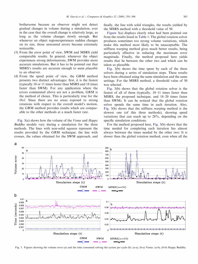

ARTICLE IN PRESS

Fig

M. Garcıa et al. / Computers & Graphics 32 (2008) 293–306 303

bothersome because an observer might not detectgradual changes in volume during a simulation, everin the case that the overall change is relatively large, aslong as the volume changes slowly enough. Butwhenever an object regionexperiences sudden changeson its size, those unwanted errors become extremelynoticeable.

(3)

From the error point of view, SWM and MSRS yieldcomparable results. In general, whenever the objectexperiences strong deformations, SWM provides moreaccurate simulations. But it has to be pointed out thatMSRS’s results are accurate enough to seem plausible

to an observer.

(4) From the speed point of view, the GRM method

presents two distinct advantages: first, it is the fastest(typically 10 or 11 times faster than MSRS and 18 timesfaster than SWM). For any application where theerrors commented above are not a problem, GRM isthe method of choice. This is particularly true for theOwl. Since there are no areas exposed to strongrotations with respect to the overall model’s motion,the GRM method provides results which are compar-able to the other methods at a much faster rate.

Fig. 3(a) shows how the volume of the Venus and Happy

Buddha models vary during a simulation for the threemethods. The lines with non-solid squares represent theresults provided by the GRM technique; the line withcrosses, the values obtained for the SWM approach, and

. 3. Figures showing the volume error (a) and the time consumed solving

finally, the line with solid triangles, the results yielded bythe MSRS method with a threshold value of 50.Figure 3(a) displays clearly what had been pointed out

from the results listed in Table 1: The global rotation solverproduces sometimes too strong volume variations, whichmake this method most likely to be unacceptable. Thestiffness warping method gives much better results, beingparticularly effective in reducing the maximum errormagnitude. Finally, the method proposed here yieldsresults that lie between the other two and which can betaken as plausible.Fig. 3(b) shows the time spent by each of the three

solvers during a series of simulation steps. These resultshave been obtained using the same simulation and the samesettings. For the MSRS method, a threshold value of 50was selected.Fig. 3(b) shows that the global rotation solver is the

fastest of all of them (typically, 10–11 times faster thanMSRS, the proposed technique, and 18–20 times fasterthan SWM). It can be noticed that the global rotationsolver spends the same time in each iteration. Also,Fig. 3(b) shows that the stiffness warping method is theslowest one (of this three methods), showing speedvariations that can reach up to 28%, depending on thespecific simulation conditions.For the method proposed here, Fig. 3(b) shows that the

time needed for completing each iteration lies almostalways between the times needed by the other two: It isslower than the global rotation method, even when all the

the system per cycle (b). (a-a), (b-a) Venus. (a-b), (b-b) Happy Buddha.

ARTICLE IN PRESS

Table 4

Number of non-zero elements in the matrix system performing a Cholesky

factorization and combining a reordering stage plus a Cholesky

factorization

Original Cholesky

factorization

Reordered data

plus Cholesky

factorization

Buddha 54 639 588 306 78 951

Owl 23 787 140 946 30 894

Venus 9 558 29 208 9 093

M. Garcıa et al. / Computers & Graphics 32 (2008) 293–306304

elements are removed from the system matrix, because itneeds to compute the elements’ rotation for the whole meshin order to compute the local error. Also, the time spent ateach simulation step may suffer from variations higherthan 55%.

It was mentioned in Section 4.1 that the matrix S isprecomputed using a Cholesky factorization in order todecrease the complexity of the system solving process. Ithas to be noted that it is important not only to perform theCholesky factorization, but also to reorder the matrix inorder to maximize the number of zero elements.

Fig. 1 showed the non-zero elements’ distributions of thesystem matrix for the owl model applying a Choleskyfactorization to the original data and to the reordered data.As it can be noticed, using the Cholesky factorization overthe reordered data greatly reduces the number of non-zeroelements. The number of non-zero elements is much higherboth on the inverse matrix system and on the Choleskyfactorization without reordering than in the reorderedCholesky-factorized matrix. For this reason, the reorderedCholesky factorization is less sensitive to the elimination ofthose elements very close to zero. In this work severalreordering algorithms have been tested, such as the reverseCuthill-McKee or the approximate minimum degree[64,65], being the latter the one that has yielded best results.

Table 4 presents the number of non-zero elements for thefactorized system matrix, with and without reorderingthe non-zero elements. The reordering stage reduces thenumber of non-zero elements one order of magnitudeapproximately.

6. Conclusions and future work

This paper presents a new method for solving thedynamics of deformable objects. The proposed technique isbased on the finite elements’ rotational formulation,solving the constitutive equations in an efficient way anddevoting more time to control the error whenevernecessary. The new solver provides very fast, visuallyplausible responses (the increment of the relative error inMSRS with respect SWM is always around jDj ¼ 2:3 foralpha ¼ 50, improving its performance in the case of theowl), spending more time in those situations whenthe deformations are more noticeable, for example, whenthe user interacts with the model.

Looking at the results achieved by the method presentedin this paper, the time needed to obtain each answer isnever below the threshold given by the time required forcomputing the rotation of each element and for estimatingthe introduced error. Therefore, these stages constrain themethod’s maximum velocity.Nevertheless, the MSRS method attains a good error-

computational speed tradeoff, giving a much higheraccuracy than the global rotation method, and an almosttwice as fast speed when compared with the stiffnesswarping method.Given the proposed method’s strong and weak points, it

is possible to combine it with the GRM so that the systemglobal response is optimized. For example, it is possible todynamically select the global rotation method whenever theobject is out of the user’s region of interest, or the objecthas a compact shape like the Owl model in theseexperiments. Otherwise, the MSRS technique can be used.Regarding the proposed technique, the main problem

from the implementation point of view is selecting anappropriate threshold which provides efficient and visuallyplausible answers in all cases. This threshold should dependon different issues such as the object’s volume, itsmechanical behavior, its geometry, the restrictions whichapply to a specific application, etc. Nowadays this thresholdis selected manually; future work will focus on developingmethods for adaptive threshold updating, taking intoconsideration the issues mentioned above and others suchas the relative significance of each object within the scene.Also, future work will include decreasing the MSRS

method’s overhead, looking for faster alternative techni-ques to compute each element’s rotation and estimate theintroduced error. Another option will be to find connectedcomponents after vertex removal and solving a fewseparate and smaller linear systems.

Acknowledgments

This work has been partially funded by the the SpanishMinistry of Education and Science (Grant TIN2007-67188)and Government of the Community of Madrid (GrantS-0505/DPI/0235; GATARVISA).

Appendix A. Supplementary data

Supplementary data associated with this article can befound in the online version at doi:10.1016/j.cag.2008.01.008.

References

[1] Burdea GC, Coiffet P. Virtual reality technology. 2nd ed. with

CD-ROM. NY, EEUU: Wiley-IEEE Press; 2003.

[2] Baraff D, Witkin A. Large steps in cloth simulation. In:

SIGGRAPH’98: Proceedings of the 25th annual conference on

computer graphics and interactive techniques. New York, NY,

EEUU: ACM Press; 1998. p. 43–54.

ARTICLE IN PRESSM. Garcıa et al. / Computers & Graphics 32 (2008) 293–306 305

[3] Desbrun M, Schroder P, Barr A. Interactive animation of structured

deformable objects. In: Proceedings of the 1999 conference on

graphics interface ’99. San Francisco, CA, EEUU: Morgan Kauf-

mann; 1999. p. 1–8.

[4] Debunne G, Desbrun M, Barr AH, Cani M-P. Interactive multi-

resolution animation of deformable models. In: Eurographics workshop

on computer animation and simulation (EGCAS), 1999. p. 133–44. URL

hhttp://www-evasion.imag.fr/Publications/1999/DDBC99i.

[5] Volino P, Thalmann NM. Implementing fast cloth simulation with

collision response. In: CGI ’00: Proceedings of the international

conference on computer graphics. Washington, DC, EEUU: IEEE

Computer Society; 2000. p. 257–66.

[6] Hilde L, Meseure P, Chaillou C. A fast implicit integration method

for solving dynamic equations of movement. In: Proceedings of

the ACM symposium on virtual reality software and technology.

New York, NY, EEUU: ACM Press; 2001. p. 71–6.

[7] Muller M, Gross M. Interactive virtual materials. In: Proceedings of

graphics interface (GI 2004), Ontario, Canada, 2004. p. 239–46.

[8] Waters K. A muscle model for animation three-dimensional facial

expression. In: Proceedings of the 14th annual conference on

computer graphics and interactive techniques, SIGGRAPH’87,

annual conference. ACM, New York: ACM Press; 1987. p. 17–24.

[9] Terzopoulos D, Waters K. Physically-based facial modelling,

analysis, and animation. The Journal of Visualization and Computer

Animation 1990;1(2):73–80.

[10] Waters K, Terzopoulos D. Modeling and animating faces using

scanned data. The Journal of Visualization and Computer Animation

1991;2(4):123–8.

[11] Breen DE, House DH, Wozny MJ. Predicting the drape of woven

cloth using interacting particles. In: Proceedings of the 21st annual

conference on computer graphics and interactive techniques, SIG-

GRAPH’94, vol. 28 of annual conference. ACM. New York: ACM

Press; 1994. p. 365–72.

[12] Mosegaard J, Herborg P, Sørensen TS. A GPU accelerated spring

mass system for surgical simulation. In: Proceedings of medicine

meets virtual reality, California, EEUU, 2005. p. 342–8.

[13] Garcıa M, Pastor L, Rodrıguez A. An adaptive multiresolution mass-

spring model. In: Li S, Pereira F, Shum H-Y, Tescher AG, editors.

Proceedings of visual communications and image processing 2005,

vol. 5960. Beijing, China: IEEE and SPIE, SPIE; 2005. p. 480–91.

[14] Liu GR. Mesh-free methods. Boca Raton, FL, EEUU: CRC Press;

2002.

[15] Muller M, Keiser R, Nealen A, Pauly M, Gross M, Alexa M. Point

based animation of elastic, plastic and melting objects. In: SCA ’04:

proceedings of the 2004 ACM SIGGRAPH/eurographics symposium

on computer animation, eurographics association, Aire-la-Ville,

Switzerland, Switzerland; 2004. p. 141–51.

[16] Pauly M, Keiser R, Adams B, Dutre P, Gross M, Guibas LJ. Meshless

animation of fracturing solids. In: SIGGRAPH ’05: ACM SIG-

GRAPH 2005 Papers. New York, NY, USA: ACM; 2005. p. 957–64.

[17] Picinbono G. Modeles geometriques et physiques pour la simulation

d’interventions chirurgicales. PhD thesis, INRIA, Sophia-Antipolis

Francia; 2001.

[18] O’Brien JF, Hodgins JK. Graphical modeling and animation of

brittle fracture. In: Proceedings of ACM SIGGRAPH 1999. New York:

ACM Press/Addison-Wesley Publishing Co.; 1999. p. 137–46.

[19] Nesme M, Payan Y, Faure F. Efficient, physically plausible finite

elements. In: Dingliana J, Ganovelli F, editors. Eurographics (short

papers); 2005. p. 77–80 hhttp://www-evasion.imag.fr/Publications/

2005/NPF05i.

[20] Terzopoulos D, Platt J, Barr A, Fleischer K. Elastically deformable

models. In: Proceedings of the 14th annual conference on computer

graphics and interactive techniques, SIGGRAPH’87, annual con-

ference. ACM, Anaheim, CA: ACM Press; 1987. p. 205–14.

[21] Teran J, Blemker S, Hing VNT, Fedkiw R. Finite volume methods

for the simulation of skeletal muscle. In: ACM SIGGRAPH/

eurographics symposium on computer animation, annual conference.

ACM: ACM Press; 2003. p. 68–74.

[22] Teran J, Sifakis E, Blemker SS, Ng-Thow-Hing V, Lau C, Fedkiw R.

Creating and simulating skeletal muscle from the visible human data

set. IEEE Transactions on Visualization and Computer Graphics

2005;11(3):317–28.

[23] James DL, Pai DK, Artdefo: accurate real time deformable objects.

In: Proceedings of SIGGRAPH, 1999. p. 65–72.

[24] Jakobsen T. Advanced character physics—the Fysix engine hwww.

gamasutra.comi. Date: 21-1-2003 Retrieved February 22, 2008, from

source.

[25] Fedor M. Fast character animation using particle dynamics. In:

Aboshosha A, et al., editors. Proceedings of the first ICGST

international conference on graphics, vision and image processing,

vol. 05, ICGST. Cairo, Egypt, 2005. p. 393–400.

[26] Muller M, Heidelberger B, Hennix M, Ratcliff J. Position based

dynamics. In: Mendoza C, Navazo I, editors. Proceedings of the 3rd

international workshop in virtual reality interactions and physical

simulation ‘‘VRIPHYS’06’’. Eurographics. Madrid, Spain: Euro-

graphics Association; 2006. p. 71–80.

[27] Fels S, Vogt F, van den Doel K, Lloyd J, Stavness I, Vatikiotis-

Bateson E. Artisynth: a biomechanical simulation platform for the

vocal tract and upper airway. Technical Report TR-2006-10,

Computer Science Department, University of British Columbia;

2006. URL hhttp://hct.ece.ubc.ca/publications/pdf/TR-2006-10.pdfi.

[28] Gibson SFF, Mirtich B. A survey of deformable modeling in

computer graphics, Technical Report 97-19, MERL—a Mitsubishi

Electric Research Laboratory; 1997.

[29] Nealen A, Muller M, Keiser R, Boxerman E, Carlson M. Physically

based deformable models in computer graphics. In: Eurographics

state-of-the-art report (EG-STAR). Eurographics Association; 2005.

p. 71–94.

[30] Bathe K. Finite element procedures. Englewood Cliffs, NJ: Prentice-

Hall; 1996.

[31] Bro-Nielsen M, Cotin S. Real-time volumetric deformable models

for surgery simulation using finite elements and condensation.

Computer Graphics Forum 1996;15(3):57–66 hciteseer.ist.psu.edu/

bro-nielsen96realtime.htmli.

[32] Pentland A, Williams J. Good vibrations: model dynamics for

graphics and animation. In: SIGGRAPH ’89: Proceedings of the 16th

annual conference on computer graphics and interactive techniques.

New York, NY, USA: ACM Press; 1989. p. 215–22.

[33] Choi MG, Ko H-S. Modal warping: real-time simulation of large

rotational deformation and manipulation. IEEE Transactions on

Visualization and Computer Graphics 2005;11(1):91–101.

[34] Huang J, Liu X, Bao H, Guo B, Shum H-Y. An efficient large

deformation method using domain decomposition. Computer Gra-

phics 2006;30(6):927–35.

[35] Huang J, Shi X, Liu X, Zhou K, Guo B, Bao H. Geometrically based

potential energy for simulating deformable objects. Visual Computer

2006;22(9):740–8.

[36] Grinspun E, Krysl P, Schroder P. Charms: a simple framework for

adaptive simulation. In: SIGGRAPH ’02: proceedings of the 29th

annual conference on computer graphics and interactive techniques.

New York, NY, USA: ACM Press; 2002. p. 281–90.

[37] Wu X, Tendick F. Multigrid integration for interactive deformable

body simulation. In: Cotin S, Metaxas DN, editors. ISMS, vol. 3078.

In: Lecture notes in computer science. Berin: Springer; 2004.

p. 92–104.

[38] Georgii J, Westermann R. A multigrid framework for real-time

simulation of deformable bodies. Computers & Graphics 2006;30(3):

408–15.

[39] Otaduy MA, Germann D, Redon S, Gross M. Adaptive deforma-

tions with fast tight bounds. In: SCA ’07: proceedings of the 2007

ACM SIGGRAPH/eurographics symposium on computer anima-

tion. Aire-la-Ville, Switzerland: Eurographics Association; 2007.

p. 181–90.

[40] Aksoylu B, Khodakovsky A, Schroder P. Multilevel solvers for

unstructured surface meshes. SIAM Journal of Scientific Computing

2005;26(4):1146–65.

ARTICLE IN PRESSM. Garcıa et al. / Computers & Graphics 32 (2008) 293–306306

[41] Shi L, Yu Y, Bell N, Feng W-W. A fast multigrid algorithm for mesh

deformation. In: SIGGRAPH ’06: ACM SIGGRAPH 2006 papers.

New York, NY, USA: ACM Press; 2006. p. 1108–17.

[42] Debunne G, Desbrun M, Cani M-P, Barr AH. Dynamic real-time

deformations using space and time adaptive sampling. In: Fiume E,

editor. SIGGRAPH ’01: proceedings of the 28th annual conference on

computer graphics and interactive techniques, annual conference series.

New York, NY, USA: ACM Press; 2001. p. 31–6 ISBN 1-58113-374-X

hhttp://www-imagis.imag.fr/Publications/2001/DDCB01i.

[43] Wu X, Downes S, Goktekin T, Tendick F. Adaptive nonlinear finite

elements for deformable body simulation using dynamic progressive

meshes. In: Chalmers A, Rhyne T-M, editors. EG 2001 proceedings,

vol. 20(3). Blackwell Publishing; 2001. p. 349–358 hciteseer.ist.psu.

edu/wu01adaptive.htmli.

[44] Picinbono G, Delingette N, Ayache N. Non-linear and anisotropic

elastic soft tissue models for medical simulation. In: Proceedings of

the IEEE international conference in robotics and automation

ICRA2001, vol. 2, Seoul, Korea, 2001. p. 1370–75.

[45] Irving G, Teran J, Fedkiw R. Invertible finite elements for robust

simulation of large deformation. In: Boulic R, Pai D, editors.

Proceedings of eurographics/ACM SIGGRAPH symposium on

computer animation (SCA). Aire-la-Ville, Switzerland: Eurographics

Association; 2004. p. 131–40.

[46] Irving G, Teran J, Fedkiw R. Tetrahedral and hexahedral invertible

finite elements. Graphical Models 2006;68(2):66–89.

[47] Irving G, Schroeder C, Fedkiw R. Volume conserving finite element

simulations of deformable models. In: SIGGRAPH ’07: ACM

SIGGRAPH 2007 papers, vol. 26. New York, NY, USA: ACM;

2007. p. 13-1–6.

[48] Muller M, Dorsey J, McMillan L, Jagnow R, Cutler B. Stable real-

time deformations. In: Proceedings of ACM SIGGRAPH symposium

on computer animation (SCA), 2002. p. 49–54.

[49] Etzmuss O, Keckeisen M, Strasser W. A fast finite element solution

for cloth modelling. In: Proceedings of 11th Pacific conference on

computer graphics and applications (PG’03), 2003. p. 244–251.

[50] Garcıa M, Mendoza C, Pastor L, Rodrıguez A. Optimized linear

FEM for modeling deformable objects. Computer Animation and

Virtual Worlds 2006;17(3–4):393–402.

[51] Sutherland I. Sketchpad: a man machine graphical communication

system. PhD thesis, Massachusetts Institute of Technology; 1963.

[52] Gleicher M, Witkin A. Supporting numerical computations in

interactive contexts. In: Graphics interface ’93, 1993. p. 138–145.

[53] Gleicher M. A differential approach to graphical interaction. PhD

dissertation, Carnegie Mellon University, School of Computer

Science; November 1994. URL hhttp://www.cs.wisc.edu/graphics/

Papers/Gleicher/Thesis/i.

[54] Lenoir J, Fonteneau S. Mixing deformable and rigid-body mechanics

simulation. In: CGI ’04: proceedings of the computer graphics

international (CGI’04). Washington, DC, EEUU: IEEE Computer

Society; 2004. p. 327–34.

[55] Weinstein R, Teran J, Fedkiw R. Dynamic simulation of articulated

rigid bodies with contact and collision. IEEE Transactions on

Visualization and Computer Graphics 2006;12(3):365–74.

[56] Gissler M, Becker M, Teschner M. Local constraint methods for

deformable objects. In: Mendoza C, Navazo I, editors. Proceedings

of 3rd international workshop in virtual reality interactions and

physical simulation ‘‘VRIPHYS’06’’. Madrid, Spain: Eurographics

Association; 2006. p. 25–32.

[57] Terzopoulos D, Witkin A, Kass M. Symmetry-seeking models and

3D object reconstruction. International Journal of Computer Vision

1987;1:211–21.

[58] Capell S, Green S, Curless B, Duchamp T, Popovic Z. Interactive

skeleton-driven dynamic deformations. In: SIGGRAPH ’02: Proceed-

ings of the 29th annual conference on computer graphics and interactive

techniques. New York, NY, USA: ACM Press; 2002. p. 586–93.

[59] Hauth M, StraXer W. Corotational simulation of deformable solids.

In: Proceedings of WSCG 2004, 2004. p. 137–45.

[60] Muller M, Heidelberger B, Teschner M, Gross M. Meshless

deformations based on shape matching. ACM Transactions on

Graphics 2005;24(3):471–8.

[61] Press WH, Flannery BP, Teukolsky SA, Vetterling WT. Numerical

recipes. 2nd ed. Cambridge, UK: Cambridge University Press; 1993.

[62] Shewchuk JR. An introduction to the conjugate gradient method

without the agonizing pain. Technical report Carnegie Mellon

University, Pittsburgh, PA, EEUU; 1994.

[63] Krızek M, Neittaanmaki P, Glowinski R, Korotov S, editors.

Conjugate gradient algorithms and finite element methods. Berlin:

Springer; 2003 ISBN 3-540-21319-8.

[64] Markowitz HM. The elimination form of the inverse and its

application. Management Science 1957;3:257–69.

[65] Amestoy PR, Davis TA, Duff IS. An approximate minimum degree

ordering algorithm. SIAM Journal onMatrix Analysis and Applications

1996;17(4):886–905 URL hhttp://link.aip.org/link/?SML/17/886/1i.

[66] Saad Y, van der Vorst HA. Iterative solution of linear systems in the

20th century. Journal of Computer Applications and Mathematics

2000;123(1–2):1–33.

[67] Computer Graphics Laboratory. The Stanford 3D scanning reposi-

tory hhttp://graphics.stanford.edu/data/3Dscanrep/i;2007 (accessed

31.10.2007).

[68] Garcıa M, Bayona S, Toharia P, Mendoza C. Comparing sphere-tree

generators and hierarchy updates for deformable objects collision

detection. In: Bebis G, Boyle R, Koracin D, Parvin B, editors.

International symposium on visual computing (ISVC05), vol. 3804.

In: Lecture notes in computer science. Nevada, EEUU: Springer;

2005. p. 167–74 ISBN 3-540-30750-8, ISSN 0302-9743.

[69] Spillmann J, Becker M, Teschner M. Efficient updates of bounding

sphere hierarchies for geometrically deformable objects. In: Mendoza

C, Navazo I, editors. Proceedings of 3rd international workshop in

virtual reality interactions and physical simulation ‘‘VRIPHYS’06’’.

Madrid, Spain: Eurographics Association; 2006. p. 53–60.