MSC.Marc Volume A
648
Theory and User Information MSC.Marc Version 2001 Volume A
-
Upload
khangminh22 -
Category
Documents
-
view
0 -
download
0
Transcript of MSC.Marc Volume A

Theory and User Information
MSC.Marc
Version 2001
Volume A

Copyright 2001 MSC.Software CorporationPrinted in U. S. A.This notice shall be marked on any reproduction of this data, in whole or in part.
Corporate Europe
MSC.Software Corporation MSC.Software GmbH2 MacArthur Place Am MoosfeldSanta Ana, CA 92707 81829 München, GERMANYTelephone: (714) 540-8900 Telephone: (49) (89) 431 987 0Fax: (714) 784-4056 Fax: (49) (89) 436 1716
Asia Pacific Worldwide WebMSC Japan Ltd. www.mscsoftware.comEntsuji-Gadelius Building2-39, Akasaka 5-chomeMinato-ku, Tokyo 107-0052, JAPANTelephone: (81) (3) 3505 0266Fax: (81) (3) 3505 0914
Document Title: MSC.Marc Volume A: Theory and User Information, Version 2001
Part Number: MA*2001*Z*Z*Z*DC-VOL-A
Revision Date: April, 2001
Proprietary NoticeMSC.Software Corporation reserves the right to make changes in specifications and other information contained in this document without prior notice.
ALTHOUGH DUE CARE HAS BEEN TAKEN TO PRESENT ACCURATE INFORMATION, MSC.SOFTWARE CORPORATION DISCLAIMS ALL WARRANTIES WITH RESPECT TO THE CONTENTS OF THIS DOCUMENT (INCLUDING, WITHOUT LIMITATION, WARRANTIES OR MERCHANTABILITY AND FITNESS FOR A PARTICULAR PURPOSE) EITHER EXPRESSED OR IMPLIED. MSC.SOFTWARE CORPORATION SHALL NOT BE LIABLE FOR DAMAGES RESULTING FROM ANY ERROR CONTAINED HEREIN, INCLUDING, BUT NOT LIMITED TO, FOR ANY SPECIAL, INCIDENTAL OR CONSEQUENTIAL DAMAGES ARISING OUT OF, OR IN CONNECTION WITH, THE USE OF THIS DOCUMENT.
This software documentation set is copyrighted and all rights are reserved by MSC.Software Corporation. Usage of this documentation is only allowed under the terms set forth in the MSC.Software Corporation License Agreement. Any reproduction or distribution of this document, in whole or in part, without the prior written consent of MSC.Software Corporation is prohibited.
TrademarksAll products mentioned are the trademarks, service marks, or registered trademarks of their respective holders.

MSC.Marc Volume A: Theory and User Information
Contents
C O N T E N T SMSC.Marc Volume A: Theory and User Information
Preface About This Manual, xvii
Purpose of Volume A, xviii
Contents of Volume A, xviii
How to Use This Manual, xix
Chapter 1The Marc System Marc Programs, 1-3
Marc, 1-3 Mentat, 1-3
Structure of Marc, 1-5 Procedure Library, 1-5 Material Library, 1-5 Element Library, 1-5 Program Function Library, 1-5
Features and Benefits of Marc, 1-6
Chapter 2Program Initiation Marc Host Systems, 2-2
Workspace Requirements, 2-3 Marc Workspace Requirements, 2-3
File Units, 2-5
Program Initiation, 2-7
Examples of Running Marc Jobs, 2-10

MSC.Marc Volume A: Theory and User InformationContents
vi
Chapter 3Data Entry Input Conventions, 3-2
Input of List of Items, 3-3 Examples of Lists, 3-5
Parameters, 3-6
Model Definition Options, 3-7
History Definition Options, 3-8
REZONE Option, 3-10
Chapter 4Introduction to Mesh Definition
Direct Input, 4-3 Element Connectivity Data, 4-3 Nodal Coordinate Data, 4-7 Activate/Deactivate, 4-7
User Subroutine Input, 4-8
MESH2D, 4-9 Block Definition, 4-9 Merging of Nodes, 4-10 Block Types, 4-10 Symmetry, Weighting, and Constraints, 4-14 Additional Options, 4-15
Mentat, 4-16
FXORD Option, 4-17 Major Classes of the FXORD Option, 4-17 Recommendations on Use of the FXORD Option, 4-22
Incremental Mesh Generators, 4-23
Bandwidth Optimization, 4-24
Rezoning, 4-25
Substructure, 4-26 Technical Background, 4-27 Scaling Element Stiffness, 4-29
BEAM SECT Parameter, 4-30 Orientation of the Section in Space, 4-30 Definition of the Section, 4-30

viiMSC.Marc Volume A: Theory and User InformationContents
Error Analysis, 4-33
Local Adaptivity, 4-34 Number of Elements Created, 4-34 Boundary Conditions, 4-35 Location of New Nodes, 4-36 Adaptive Criteria, 4-38
Global Remeshing, 4-41 Remeshing Criteria, 4-43 Remeshing Techniques, 4-44
Chapter 5Structural Procedure Library
Linear Analysis, 5-3 Accuracy, 5-5 Error Estimates, 5-5 Adaptive Meshing, 5-5 Fourier Analysis, 5-6
Nonlinear Analysis, 5-10 Geometric Nonlinearities, 5-15 Updated Lagrangian Procedure, 5-22 Nonlinear Boundary Conditions, 5-27 Buckling Analysis, 5-29 Perturbation Analysis, 5-31 Computational Procedures for Elastic-Plastic Analysis, 5-38 CREEP, 5-50 AUTO THERM CREEP (Automatic Thermally Loaded
Elastic-Creep/Elastic-Plastic-Creep Stress Analysis), 5-54 Viscoelasticity, 5-55 Viscoplasticity, 5-56
Fracture Mechanics, 5-58 Linear Fracture Mechanics, 5-58 Nonlinear Fracture Mechanics, 5-60 Numerical Evaluation of the J-integral, 5-62 Modeling Considerations, 5-64 Dynamic Crack Propagation, 5-65 Dynamic Fracture Methodology, 5-66
Dynamics, 5-67 Eigenvalue Analysis, 5-67 Transient Analysis, 5-71

MSC.Marc Volume A: Theory and User InformationContents
viii
Harmonic Response, 5-80 Spectrum Response, 5-84
Rigid-Plastic Flow, 5-86 Steady State Analysis, 5-87 Transient Analysis, 5-87 Technical Background, 5-87
Superplasticity, 5-89
Soil Analysis, 5-92 Technical Formulation, 5-93 Evaluation of Soil Parameters for the Critical State
Soil Model, 5-96
Design Sensitivity Analysis, 5-110 Theoretical Considerations, 5-112
Design Optimization, 5-114 Approximation of Response Functions Over the
Design Space, 5-115 Improvement of the Approximation, 5-118 The Optimization Algorithm, 5-118 Marc User Interface for Sensitivity Analysis
and Optimization, 5-119
Considerations for Nonlinear Analysis, 5-123 Behavior of Nonlinear Materials, 5-124 Scaling the Elastic Solution, 5-124 Load Incrementation, 5-124 Selecting Load Increment Size, 5-126 Automatic Load Incrementation, 5-127 Residual Load Correction, 5-130 Restarting the Analysis, 5-131
Data Transfer from Axisymmetric Analysis to 3-D Analysis, 5-133 Load and Displacement Boundary Conditions Transfer from
Axisymmetric Analysis to 3-D using Table Curve Shift, 5-133
References, 5-136
Chapter 6Nonstructural Procedure Library
Heat Transfer, 6-3 Steady State Analysis, 6-5

ixMSC.Marc Volume A: Theory and User InformationContents
Transient Analysis, 6-5 Convergence Control, 6-7 Temperature Effects, 6-8 Initial Conditions, 6-9 Boundary Conditions, 6-9 Radiation Viewfactors, 6-10 Radiation-Gap, 6-19 Channel, 6-20 Output, 6-21
Hydrodynamic Bearing, 6-23 Technical Background, 6-25
Electrostatic Analysis, 6-28 Technical Background, 6-29
Magnetostatic Analysis, 6-31 Technical Background, 6-32
Electromagnetic Analysis, 6-37 Technical Background, 6-38
Acoustic Analysis, 6-42 Rigid Cavity Acoustic Analysis, 6-42 Technical Background, 6-42 Coupled Acoustic-Structural Analysis, 6-44 Technical Background, 6-44
Fluid Mechanics, 6-49 Finite Element Formulation, 6-52 Penalty Method, 6-55 Steady State Analysis, 6-56 Transient Analysis, 6-56 Solid Analysis, 6-56 Solution of Coupled Problems in Fluids, 6-57 Degrees of Freedom, 6-57 Element Types, 6-58
MSC.Marc Volume A: Theory and User InformationContents
x
Coupled Analyses, 6-60 Fluid/Solid Interaction – Added Mass Approach, 6-62 Coupled Thermal-Electrical Analysis (Joule Heating), 6-64 Thermal Mechanically Coupled Analysis, 6-67
References, 6-70
Chapter 7Material Library Linear Elastic Material, 7-3
Composite Material, 7-6 Layered Materials, 7-7 Material Preferred Direction, 7-10 Material Dependent Failure Criteria, 7-14 Interlaminar Shear for Thick Shell and Beam Elements, 7-20 Interlaminar Stresses for Continuum
Composite Elements, 7-21 Progressive Composite Failure, 7-22
Gasket, 7-23 Constitutive Model, 7-23
Nonlinear Hypoelastic Material, 7-29
Elastomer, 7-30 Updated Lagrange Formulation for Nonlinear Elasticity, 7-41
Time-Independent Inelastic Behavior, 7-43 Yield Conditions, 7-46 von Mises Yield Condition, 7-46 Mohr-Coulomb Material (Hydrostatic Stress
Dependence), 7-50 Buyukozturk Criterion (Hydrostatic Stress Dependence), 7-52 Powder Material, 7-52 Workhardening Rules, 7-55 Flow Rule, 7-61 Constitutive Relations, 7-62
Time-Dependent Inelastic Behavior, 7-67 Creep (Maxwell Model), 7-72 Oak Ridge National Laboratory Laws, 7-76 Swelling, 7-78 Viscoplasticity (Explicit Formulation), 7-78 Creep (Implicit Formulation), 7-79

xiMSC.Marc Volume A: Theory and User InformationContents
Viscoelastic Material, 7-80 Narayanaswamy Model, 7-93
Temperature Effects and Coefficient of Thermal Expansion, 7-99 Piecewise Linear Representation, 7-99 Temperature-Dependent Creep, 7-101 Coefficient of Thermal Expansion, 7-101
Time-Temperature-Transformation, 7-103
Low Tension Material, 7-106 Uniaxial Cracking Data, 7-106 Low Tension Cracking, 7-107 Tension Softening, 7-107 Crack Closure, 7-108 Crushing, 7-108 Analysis, 7-108
Soil Model, 7-109 Elastic Models, 7-109 Cam-Clay Model, 7-110
Damage Models, 7-113 Ductile Metals, 7-113 Elastomers, 7-116
Nonstructural Materials, 7-120 Heat Transfer Analysis, 7-120 Thermo-Electrical Analysis, 7-120 Hydrodynamic Bearing Analysis, 7-120 Fluid/Solid Interaction Analysis – Added Mass
Approach, 7-120 Electrostatic Analysis, 7-121 Magnetostatic Analysis, 7-121 Electromagnetic Analysis, 7-121 Acoustic Analysis, 7-121 Fluid Analysis, 7-121
References, 7-122
Chapter 8Contact Numerical Procedures, 8-3
Lagrange Multipliers, 8-3 Penalty Methods, 8-3

MSC.Marc Volume A: Theory and User InformationContents
xii
Hybrid and Mixed Methods, 8-4 Direct Constraints, 8-4
Definition of Contact Bodies, 8-5
Numbering of Contact Bodies, 8-8
Motion of Bodies, 8-9 Initial Conditions, 8-11
Detection of Contact, 8-12 Shell Contact, 8-14 Neighbor Relations, 8-15
Implementation of Constraints, 8-17
Friction Modeling, 8-20 Glue Model, 8-27
Separation, 8-28 Release, 8-28
Coupled Analysis, 8-29
Element Considerations, 8-31 2-D Beams, 8-31 3-D Beams, 8-32 Shell Elements, 8-32
Dynamic Impact, 8-33
Rezoning, 8-34
Adaptive Meshing, 8-35
Result Evaluation, 8-36
Tolerance Values, 8-37
Workspace Reservation, 8-39

xiiiMSC.Marc Volume A: Theory and User InformationContents
Mathematical Aspects of Contact, 8-40 Lagrange Multiplier Procedure, 8-40 Direct Constraint Procedure, 8-41 Solution Strategy for Deformable Contact, 8-52 Friction Modeling, 8-54 Automatic Penetration Checking Procedure, 8-56
References, 8-58
Chapter 9Boundary Conditions Loading, 9-3
Loading Types, 9-3 Fluid Drag and Wave Loads, 9-6 Mechanical Loads, 9-8 Thermal Loads, 9-9 Initial Stress and Initial Plastic Strain, 9-10 Heat Fluxes, 9-11 Mass Fluxes and Restrictors, 9-12 Electrical Currents, 9-13 Electrostatic Charges, 9-13 Acoustic Sources, 9-14 Magnetostatic Currents, 9-14 Electromagnetic Currents and Charges, 9-15
Kinematic Constraints, 9-16 Boundary Conditions, 9-16 Transformation of Degree of Freedom, 9-17 Shell Transformation, 9-17 Tying Constraint, 9-21 Rigid Link Constraint, 9-29 Shell-to-Solid Tying, 9-30 Support Conditions, 9-31
Cyclic Symmetry, 9-32
Cross Section, 9-35

MSC.Marc Volume A: Theory and User InformationContents
xiv
Chapter 10Element Library Truss Elements, 10-17
Membrane Elements, 10-18
Continuum Elements, 10-19
Beam Elements, 10-20
Plate Elements, 10-21
Shell Elements, 10-22
Heat Transfer Elements, 10-23 Acoustic Analysis, 10-23 Electrostatic Analysis, 10-23 Fluid/Solid Interaction, 10-23 Hydrodynamic Bearing Analysis, 10-23 Magnetostatic Analysis, 10-24 Electromagnetic Analysis, 10-24 Soil Analysis, 10-24 Fluid Analysis, 10-24
Special Elements, 10-25
Incompressible Elements, 10-26 Large Strain Elasticity, 10-26 Large Strain Plasticity, 10-27 Rigid-Plastic Flow, 10-27
Constant Dilatation Elements, 10-28
Reduced Integration Elements, 10-29
Continuum Composite Elements, 10-30
Fourier Elements, 10-31
Semi-infinite Elements, 10-32
Assumed Strain Formulation, 10-33
Follow Force Stiffness Contribution, 10-34
Explicit Dynamics, 10-35
Adaptive Mesh Refinement, 10-36
References, 10-37

xvMSC.Marc Volume A: Theory and User InformationContents
Chapter 11Solution Procedures for Nonlinear Systems
Full Newton-Raphson Algorithm, 11-3
Modified Newton-Raphson Algorithm, 11-5
Strain Correction Method, 11-6
The Secant Method, 11-8
Direct Substitution, 11-10 Load Correction, 11-10
Arc-Length Methods, 11-11
Remarks, 11-19
Convergence Controls, 11-20
Singularity Ratio, 11-23
Solution of Linear Equations, 11-25 Direct Methods, 11-25 Iterative Methods, 11-26 Preconditioners, 11-26 Storage Methods, 11-27 Nonsymmetric Systems, 11-28 Complex Systems, 11-28 Iterative Solvers, 11-28 Basic Theory, 11-29
Flow Diagram, 11-31
References, 11-32
Chapter 12Output Results Workspace Information, 12-3
Direct Solution Procedure, 12-4
Increment Information, 12-5 Summary of Loads, 12-5 Timing Information, 12-5 Singularity Ratio, 12-5 Convergence, 12-5
Selective Printout, 12-7 Options, 12-7 User Subroutines, 12-9

MSC.Marc Volume A: Theory and User InformationContents
xvi
Restart, 12-10
Element Information, 12-11 Solid (Continuum) Elements, 12-12 Shell Elements, 12-13 Beam Elements, 12-14 Heat Transfer Elements, 12-15 Gap Elements, 12-15 Linear Springs, 12-15 Hydrodynamic Bearing, 12-15
Nodal Information, 12-16 Stress Analysis, 12-16 Reaction Forces, 12-16 Residual Loads, 12-16 Dynamic Analysis, 12-16 Heat Transfer Analysis, 12-17 Rigid-Plastic Analysis, 12-17 Hydrodynamic Bearing Analysis, 12-17 Electrostatic Analysis, 12-17 Magnetostatic Analysis, 12-17 Electromagnetic Analysis, 12-17 Acoustic Analysis, 12-17 Contact Analysis, 12-17
Post File, 12-18
Program Messages, 12-19
Marc HyperMesh Results Interface, 12-20
Marc SDRC I-DEAS Results Interface, 12-21
Status File, 12-22
Appendix AFinite Element Technology in Marc
Governing Equations of Various Structural Procedures, A-1
System And Element Stiffness Matrices, A-5
Load Vectors, A-7
References, A-8
Index

xviiMSC.Marc Volume A: Theory and User InformationContents

MSC.Marc Volume A: Theory and User InformationContents
xviii

Preface
About This Manual
This manual is MSC.Marc Volume A, the first in a series of six volumes documenting the MSC.Marc (Marc) Finite Element program. The documentation of Marc is summarized below. You will find references to these documents throughout this manual.
Preface
About This Manual
Purpose of Volume A
Contents of Volume A
How to Use This Manual

MSC.Marc Volume A: Theory and User InformationAbout This Manual Preface
xviii
Purpose of Volume AThe purpose of this volume is:
1. To help you define your finite element problem by describing Marc’s capabilities to model physical problems.
2. To identify and describe complex engineering problems and introduce Marc’s scope and capabilities for solving these problems.
3. To assist you in accessing Marc features that are applicable to your particular problems and to provide you with references to the rest of the Marc literature.
4. To provide you with the theoretical basis of the computational techniques used to solve the problem.
Contents of Volume AThis volume describes how to use Marc. It explains the capabilities of Marc and gives pertinent background information. The principal categories of information are found under the following titles:
Chapter 1 The Marc System
Chapter 2 Program Initiation
Chapter 3 Data Entry
Chapter 4 Introduction to Mesh Definition
Chapter 5 Structural Procedure Library
Chapter 6 Nonstructural Procedure Library
Marc Documentation
TITLE VOLUME
Theory and User Information Volume A
Element Library Volume B
Program Input Volume C
User Subroutines and Special Routines Volume D
Demonstration Problems Volume E
Background Papers Volume F

xixMSC.Marc Volume A: Theory and User InformationPreface About This Manual
Chapter 7 Material Library
Chapter 8 Contact
Chapter 9 Boundary Conditions
Chapter 10 Element Library
Chapter 11 Solution Procedures for Nonlinear Systems
Chapter 12 Output Results
The information in this manual is both descriptive and theoretical. You will find engineering mechanics discussed in some detail. You will also find specific instructions for operating the various options offered by Marc.
How to Use This ManualVolume A organizes the features and operations of the Marc program sequentially. This organization represents a logical approach to problem solving using Finite Element Analysis. First, the database is entered into the system, as described in Chapter 3. Next, a physical problem is defined in terms of a mesh overlay. Techniques for mesh definition are described in Chapter 4. Chapters 5 and 6 describe the various structural analyses that can be performed by Marc, while Chapter 7 describes the material models that are available in Marc. Chapter 8 describes the contact capabilities. Chapter 9 discusses constraints, in the form of boundary conditions. Chapter 10 explains the type of elements that can be used to represent the physical problem. Chapter 11 describes the numerical procedures for solving nonlinear equations. Finally, the results of the analysis, in the form of outputs, are described in Chapter 12.
This volume is also designed as a reference source. This means that all users will not need to refer to each section of the manual with the same frequency or in the same sequence.

MSC.Marc Volume A: Theory and User InformationPreface
xx

Chapter 1 The Marc System
The Marc system contains a series of integrated programs that facilitate analysis of engineering problems in the fields of structural mechanics, heat transfer, and electromagnetics. The Marc system consists of the following programs:
• Marc
• Mentat
These programs work together to:
• Generate geometric information that defines your structure (Marc and MSC.Marc Mentat (Mentat))
• Analyze your structure (Marc)
• Graphically depict the results (Marc and Mentat)
CHAPTER
1 The Marc System
Marc Programs
Structure of Marc
Features and Benefits of Marc

MSC.Marc Volume A: Theory and User InformationChapter 1 The Marc System
1-2
MSC.Patran also supports nonlinear analysis with Marc. For a detailed description of the supported functionalities, refer to MSC.Patran Marc Preference Guide.
Figure 1-1 shows the interrelationships among these programs. Marc Programs discusses the Marc component programs.
Figure 1-1 The Marc System
Marc
Mentat
MentatPreprocessing
Analysis
Postprocessing

1-3MSC.Marc Volume A: Theory and User InformationChapter 1 The Marc System Marc Programs
Marc Programs
Marc
You can use Marc to perform linear or nonlinear stress analysis in the static and dynamic regimes and to perform heat transfer analysis. The nonlinearities may be due to either material behavior, large deformation, or boundary conditions. An accurate representation accounts for these nonlinearities.
Physical problems in one, two, or three dimensions can be modeled using a variety of elements. These elements include trusses, beams, shells, and solids. Mesh generators, graphics, and postprocessing capabilities, which assist you in the preparation of input and the interpretation of results, are all available in Marc. The equations governing mechanics and implementation of these equations in the finite element method are discussed in Chapters 5, 6, 7, 8, and 11.
Mentat
Mentat is an interactive computer program that prepares and processes data for use with the finite element method. Interactive computing can significantly reduce the human effort needed for analysis by the finite element method. Graphical presentation of data further reduces this effort by providing an effective way to review the large quantity of data typically associated with finite element analysis.
An important aspect of Mentat is that you can interact directly with the program. Mentat verifies keyboard input and returns recommendations or warnings when it detects questionable input. Mentat checks the contents of input files and generates warnings about its interpretation of the data if the program suspects that it may not be processing the data in the manner in which you, the user, have assumed. Mentat allows you to graphically verify any changes the input generates.
Mentat can process both two- and three-dimensional meshes to do the following:
Generate and display a mesh
Generate and display boundary conditions and loadings
Perform postprocessing to generate contour, deformed shape, and time history plots

MSC.Marc Volume A: Theory and User InformationMarc Programs Chapter 1 The Marc System
1-4
The data that is processed includes:
Nodal coordinates
Element connectivity
Nodal boundary conditions
Nodal coordinate systems
Element material properties
Element geometric properties
Element loads
Nodal loads/nonzero boundary conditions
Element and nodal sets

1-5MSC.Marc Volume A: Theory and User InformationChapter 1 The Marc System Structure of Marc
Structure of Marc
Marc has four comprehensive libraries, making the program applicable to a wide range of uses. These libraries contain structural procedures, materials, elements, and program functions. The contents of each library are described below.
Procedure Library
The structural procedure library contains procedures such as static, dynamic, creep, buckling, heat transfer, fluid mechanics, and electromagnetic analysis.
The procedure library conveniently relates these various structural procedures to physical phenomena while guiding you through modules that allow, for example, nonlinear dynamic and heat-transfer analyses.
Material Library
The material library includes many material models that represent most engineering materials. Examples are the inelastic behavior of metals, soils, and rubber material. Many models exhibit nonlinear properties such as plasticity, viscoelasticity, and hypoelasticity. Linear elasticity is also included. All properties may depend on temperature.
Element Library
The element library contains 157 elements. This library lets you describe any geometry under any linear or nonlinear loading conditions.
Program Function Library
The program functions such as selective assembly, user-supplied subroutines, and restart, are tailored for user-friendliness and are designed to speed up and simplify analysis work. Marc allows you to combine any number of components from each of the four libraries and, in doing so, puts at your disposal the tools to solve almost any structural mechanics problem.

MSC.Marc Volume A: Theory and User InformationFeatures and Benefits of Marc Chapter 1 The Marc System
1-6
Features and Benefits of Marc
Since the mid-1970s, Marc has been recognized as the premier general purpose program for nonlinear finite element analysis. The program’s modularity leads to its broad applicability. All components of the structural procedure, material, and element libraries are available for use, allowing virtually unlimited flexibility and adaptability.
Marc has helped analyze and influence final design decisions on
Marc’s clients gained the following benefits not attainable through other numerical or experimental techniques. These benefits include:
Accurate results for both linear and nonlinear analysis
Better designs, which result in improved performance and reliability
The ability to model complex structures and to incorporate geometric and material nonlinear behavior
Documentation, technical support, consulting, and education provided by MSC.Software Corporation
Availability of Marc on most computers from workstations to supercomputers
Efficient operation
Automotive parts
Nuclear reactor housings
Biomedical equipment
Offshore platform components
Coated fiberglass fabric roof structures
Rocket motor casings
Ship hulls
Elastomeric motor mounts
Space vehicles
Electronic components
Steam-piping systems
Engine pistons
Tires
Jet engine rotors
Welding, casting, and quenching processes
Large strain metal extrusions

Chapter 2 Program Initiation
Chapter 2 explains how to execute Marc on your computer. Marc runs on many types of machines. All Marc capabilities are available on each type of machine; however, program execution can vary among machine types. The allocation of computer memory depends on the hardware restrictions of the machine you are using. There is no limit to the size of the analysis that can be performed by Marc other than the limit imposed by your computing resources.
CHAPTER
2 Program Initiation
Marc Host Systems
Workspace Requirements
File Units
Program Initiation
Examples of Running Marc Jobs

MSC.Marc Volume A: Theory and User InformationMarc Host Systems Chapter 2 Program Initiation
2-2
Marc Host Systems
Marc runs on most computers. Table 2-1 summarizes the types of machines and operating systems on which Marc currently runs.
Table 2-1 Marc Computer Versions
Computer Machine Type Operating System
CRAY YMP, C90, J90 UNICOS
DEC/ALPHA All machines DEC OSF or Windows-NT
Hewlett-Packard HP9000 HP-UX, SPP-UX
IBM RS6000 AIX
Silicon Graphics All machines IRIX
SUN All machines Polaris
Intel Based Pentium (etc.) Windows-NT

2-3MSC.Marc Volume A: Theory and User InformationChapter 2 Program Initiation Workspace Requirements
Workspace Requirements
Computing the amount of workspace required by Marc is a complex function of many variables. The most efficient method is to select a large enough workspace to handle a variety of runs, without sacrificing efficiency or wasting core memory. The program dynamically acquires memory if necessary and if memory is available. The following sections discuss workspace requirements for Marc.
Marc Workspace Requirements
Both in-core and out-of-core data storage schemes are available in Marc. Elements can also be stored out-of-core if you use the ELSTO parameter. Therefore, this program presents some unique complications in the estimation of sizing. The program has both an in-core and out-of-core solver. Marc chooses the solution type automatically.
There are two out-of-core storage options in Marc. These options are:
• Out-of-Core Element Data storage • Out-of-Core Solution
The Out-of-Core Element Data option stores element arrays (strains, stresses, temperatures, etc.) on an auxiliary device. Data connected with storage of all element quantities occupy a large amount of space for the more complex shell or three-dimensional elements. Putting this data in secondary storage does not cause long I/O times and allows a savings of core storage. To use this option, set the ELSTO parameter. This information is written to Unit 3.
The Out-of-Core Solution is invoked automatically, as required. Data related to the master stiffness matrix occupy the most space and have significant effect on the I/O time. In many problems, there is insufficient memory to store the complete stiffness matrix in the core memory. In such cases, the program automatically selects the out-of-core solution procedure. When the direct solver is used, Marc uses a Gaussian elimination procedure with a blocked skyline storage technique for solving the stiffness matrix. The program tries to fit as much of the full system as possible into the core memory. The minimal necessary workspace equals
2*HBW*NDEG*IF
where HBW is the maximum nodal half-bandwidth and NDEG is the maximum number of degrees of freedom per node. The IF value varies depending on your system:
IF = 1 for CRAYIF = 2 for all other machines

MSC.Marc Volume A: Theory and User InformationWorkspace Requirements Chapter 2 Program Initiation
2-4
If the program uses the out-of-core solution, the output includes a graphical representation of the profile of the stiffness matrix.
You should optimize the nodal bandwidth for all nontrivial problems. The stiffness matrix requires approximately the following amount of memory:
NUMNP*NDEG*AHBW*NDEG*IF
where:
NUMNP = number of nodes in the structureNDEG = number of degrees-of-freedom per node AHBW = average nodal half-bandwidth IF = 1 for CRAY IF = 2 for all other machines
For large problems, you may want to see the exact workspace requirements for running a job, without actually executing the analysis. To do this, insert the STOP parameter to exit the program normally after the workspace is allocated. The allocated workspace is based on the optimized bandwidth if you request the OPTIMIZE option in the model definition section.

2-5MSC.Marc Volume A: Theory and User InformationChapter 2 Program Initiation File Units
File Units
Marc uses auxiliary files for data storage in various ways. Particular FORTRAN unit numbers are used for certain program functions (for example, ELSTO, RESTART). Table 2-2 lists these file unit numbers.
Note: On most systems, these files are references by file names, as well as by the file unit numbers.
Several of these files are necessary for solving most problems. The program input file and program output file are always required.
On most computer systems, you do not need to allocate file space, because the operating system does this automatically.
Table 2-2 File Units
FORTRANUnit
NumberPurpose Format
1 Mesh generation input/output Card image
2 Out-of-core solution Unformatted
3 ELSTO Unformatted
4 Plot output file Unformatted
5 Input file Card image
6 Output file Line printer
7 Dummy/logfile (HP only) Formatted
8 Restart output Unformatted
9 Restart input Unformatted
10 Dummy
11 Out-of-core solution Unformatted
12 Out-of-core solution Unformatted
13 Out-of-core solution Unformatted
14 Out-of-core solution Unformatted
15 Out-of-core solution - Lanczos Unformatted

MSC.Marc Volume A: Theory and User InformationFile Units Chapter 2 Program Initiation
2-6
16 Post output Unformatted
17 Post input Unformatted
18 Optimization Formatted
19 Post output Formatted
20 Post input Formatted
21 Dummy
22 Fluid/solid interaction - Lanczos Unformatted
23 Lanczos Unformatted
24 Temperature input Formatted
25 Temperature input Unformatted
31 Substructures Data Base Unformatted
41 Post output for domain decomposition Unformatted
42 Post output for domain decomposition Formatted
45 Design Optimization Formatted
46 Design Sensitivity or Optimization Unformatted
49 Defaults File Formatted
50 Radiation Viewfactor Formatted
51 Post File Lock File Formatted
52 Dynamic Control FIle Formatted
97 Exit Messages Formatted
98 Global Default File Formatted
99 Material Data Base Formatted
Table 2-2 File Units (Continued)
FORTRANUnit
NumberPurpose Format

2-7MSC.Marc Volume A: Theory and User InformationChapter 2 Program Initiation Program Initiation
Program Initiation
Procedures (shell script) are set up that facilitate the execution of Marc on most computers. These procedures invoke machine-dependent control or command statements. These statements control files associated with a job.
This shell script submits a job and automatically takes care of all file assignments. This command must be executed at the directory where all input and output files concerning this Marc job are available. To use this shell script, every Marc job should have a unique name qualifier and all Marc output files connected to that job uses this same qualifier. For restart, post, change state, all default Marc Fortran units should be used.
To actually submit a Marc job, the following command should be used:
run_marc -prog prog_name -jid job_name -rid rid_name -pid pid_name \-sid sid_name -queue queue_name -user user_name -back back_value \-ver verify_value -save save_value -vf view_name -def def_name \-nprocd number_of_processors -nthread number_of_threads \-dir directory_where_job_is_processed -itree message_passing_type \-host hostfile (for running over the network) -pq queue_priority \-at date_time -comp compatible_machines_on_network -cpu time_limit \-autorst autorestart_value
where the \ provides for continuation of the command line.
Table 2-3 Keyword Description
Keyword Possible Names or Values Description
-prog marc Run marc with or without user subroutinesRun saved module “progname.marc”
-jid jidname job/input file identification-rid ridname Identification of previous job for restart.-pid pidname Identification of job that created temperature
file.-sid sidname Identification of database file for
substructures.* Default value if keyword is not used.

MSC.Marc Volume A: Theory and User InformationProgram Initiation Chapter 2 Program Initiation
2-8
-queue (-q)
background*foregroundqueue name
Run the program in the background.Run the program in the foreground.Submit to batch queue the queue name. Only available for machines with batch queue; for example, Convex, Cray. Queue names and submit command syntax may differ from site to site, adjust run_marc if necessary.
-user username User subroutine username.f will be used to generate a new load module.
-back yes*no
Run program in background.Run program in foreground.
-ver yes*no
Verify the input syntax.Don’t verify the input syntax.
-save yesno*
Save the generated or existing module.Don’t save the generated or existing module.
-vf viewname Identification of viewfactor file created by Mentat.
-def defname Data file name for setting user defaults.-nprocd number Number of domains.-nthread number Level of parallelism for solver type 6.-itree number Messages passing tree type for domain
decomposition.-dir directory name Directory where the job I/O should take
place.-host hostfile name Host file for running over the network.-comp yes
no
The executable located on the machine from which Marc is started will be used on all machines.A separate executable is created for each machine on the network. Defaults to no if O/S versions different on machines.
-pq 0,1,2,etc Batch queue only: queue priority
-at date/time Batch queue only: delay time for start of job.Syntax: January,1,1998,12:30or: today,5pm
Table 2-3 Keyword Description (Continued)
Keyword Possible Names or Values Description
* Default value if keyword is not used.

2-9MSC.Marc Volume A: Theory and User InformationChapter 2 Program Initiation Program Initiation
-cpu sec Batch queue only: cpu time limit
-autorst 0 or 1 If 0 when remeshing is required, the analysis program goes into a wait state until meshing is complete. If 1 when remeshing is required, the analysis program stops, the mesher begins, and the analysis program automatically restarts.Using the default procedure (0) uses more memory, but less I/O.Using the restart procedure (1), invokes the RESTART LAST model definition option.
Table 2-3 Keyword Description (Continued)
Keyword Possible Names or Values Description
* Default value if keyword is not used.

MSC.Marc Volume A: Theory and User InformationExamples of Running Marc Jobs Chapter 2 Program Initiation
2-10
Examples of Running Marc Jobs
Example 1:
run_marc -jid e2x1
This runs the job e2x1 in the background using a single processor.
The input file is e2x1.dat in the current working directory.
Example 2:
run_marc -jid e2x14 -user u2x14 -sav y -nproc 4
This runs the job e2x14 in the background with four processors. The user subroutine is linked with the Marc library and a new executable module is created as u2x14.marc and saved in the current working directory after completion of the job.
Example 3:
run_marc -jid e2x14a -prog u2x14 -nproc 4
Use the above saved module u2x14.marc to run the job e2x14a in the background with four processors.
Example 4:
run_marc -jid e3x2a -v no -b no -nproc 2
Run the job e3x2a in the foreground with two processors. The job runs immediately without verifying any arguments interactively. If there are any input errors in the arguments, the job does not run and the error message is sent to the screen.
Example 5:
run_marc -jid e3x2b -rid e3x2a
Run the job e3x2b in the background using a single processor. The job uses e3x2a.t08, which is created from Example 4, as restart file.
Example 6:
run_marc -jid e2x1 -nproc 2
Runs a two processor job on a single parallel machine.
Example 7:
run_marc -jid e2x1 -nproc 2 -host hostfile
Runs a two-processor job over a network. The hosts are specified in the file hostfile.

Chapter 3 Data Entry
The input data structure is made up of three logically distinct sections:
1. Parameters describe the problem type and size.2. Model definition options give a detailed problem description.3. History definition options define the load history.
Input data is organized in (optional) blocks. Key words identify the data for each optional block. This form of input enables you to specify only the data for the optional blocks that you need to define your problem. The various blocks of input are “optional” in the sense that many have built-in default values which can be used by Marc in the absence of any explicit input from you.
CHAPTER
3 Data Entry
Input Conventions
Parameters
Model Definition Options
History Definition Options
REZONE Option

MSC.Marc Volume A: Theory and User InformationInput Conventions Chapter 3 Data Entry
3-2
Input Conventions
Marc performs all data conversion internally so that the system does not abort because of data errors made by you. The program reads all input data options alphanumerically and converts them to integer, floating point, or keywords, as necessary. Marc issues error messages and displays the illegal option image if it cannot interpret the option data field according to the specifications given in the manual. When such errors occur, the program attempts to scan the remainder of the data file and ends the run with an exit error message at the END OPTION option or at the end of the input file.
Two input format conventions can be used: fixed and free format. You can mix fixed and free format options within a file, but you can only enter one type of format on a single option.
The syntax rules for fixed fields are as follows:
• You must right-justify integers in their fields. (The right blanks are filled with zeroes).
• Give floating point numbers with or without an exponent. If you give an exponent, it must be preceded by the character E or D and must be right-justified.
The syntax rules for free fields are as follows:
• Check that each option contains the same number of data items that it would contain under standard fixed-format control. This syntax rule allows you to mix fixed-field and free-field options in the data file because the number of options you need to input any data list are the same in both cases.
• Separate data items on a option with a comma. The comma can be surrounded by any number of blanks. Within the data item itself, no embedded blanks can appear.
• Give floating point numbers with or without an exponent. If you use an exponent, it must be preceded by the character E or D and must immediately follow the mantissa (no embedded blanks).
• Give keywords exactly as they are written in the manual. Embedded blanks do not count as separators here (for example, BEAM SECT is one word only).
• If a option contains only one free-field data item, follow that item with a comma. For example, the number “1” must be entered as “1,” if it is the only data item on a option. If the comma is omitted, the entry is treated as fixed format and may not be properly right-justified.

3-3MSC.Marc Volume A: Theory and User InformationChapter 3 Data Entry Input Conventions
• If the EXTENDED parameter is used, integer data is given using 10 fields as opposed to 5 fields. This allows very large models to be included in Marc. Additionally, real numbers are entered using 20 or 30 fields as opposed to 10 or 15. This allows increased accuracy when reading in data.
• All data can be entered as uppercase or lowercase text.
Input of List of Items
Marc often requests that you enter a list of items in association with certain program functions. As an example, these items can be a set of elements as in the ISOTROPIC option, or a set of nodes as in the POINT LOAD option. Six types of items can be requested:
Element numbersNode numbersDegree-of-freedom numbersIntegration point numbers Layer numbers Increment numbers
This list can be entered using either the OLD format (compatible with the G, H, and J versions of Marc) or the NEW format (the K version).
Using the OLD format, you can specify the list of items in three different forms. You can specify:
1. A range of items as: m n p
which implies items m through n by p. If p is not specified, the program assumes it is 1. Note that the range can either increase or decrease.
2. A list of items as: -n a1 a2 a3 ... an
which implies that you should give n items, and they are a ,...a.
3. A set name as: MYSET
which implies that all items previously specified in the set MYSET are used. Specify the items in a set using the DEFINE model definition option.
Using the NEW format, you can express the list of items as a combination of one or more sublists. These sublists can be specified in three different forms. The following operations can be performed between sublists:
ANDINTERSECTEXCEPT

MSC.Marc Volume A: Theory and User InformationInput Conventions Chapter 3 Data Entry
3-4
When you form a list, subsets are combined in binary operations (from left to right). The following lists are examples.
1. SUBLIST1 and SUBLIST2
This list implies all items in subsets SUBLIST1 and SUBLIST2. Duplicate items are eliminated and the resulting list is sorted.
2. SUBLIST1 INTERSECT SUBLIST2
This list implies only those items occurring both in subsets SUBLIST1 and SUBLIST2; the resulting list is sorted.
3. SUBLIST1 EXCEPT SUBLIST2
This list implies all items in subset SUBLIST1 except those which occur in subset SUBLIST2; the resulting list is sorted.
4. SUBLIST1 AND SUBLIST2 EXCEPT SUBLIST3 INTERSECT SUBLIST4
This list implies the items in subsets SUBLIST1 and SUBLIST2 minus those items that occur in subset SUBLIST3. Then, if the remaining items also occur in subset SUBLIST4, they are included in the list.
Sublists can have several forms. You can specify:
1. A range of items as:
m TO n BY p
orm THROUGH n BY p
which implies items m through n by p. If “BY p” is not included, the program assumes “BY 1”. Note that the range can either increase or decrease.
2. A string of items as:
a1 a2 a3 ... an
which implies that n items are to be included. If continuation options are necessary, then either a C or CONTINUE should be the last item on the option.
3. A set name as: MYSET
which implies that all items you previously specified to be in the set MYSET are used. You specify the items in a set using the DEFINE option.
Note: INTERSECT or EXCEPT cannot be used when defining lists of degrees of freedom.

3-5MSC.Marc Volume A: Theory and User InformationChapter 3 Data Entry Input Conventions
Examples of Lists
This section presents some examples of lists and entry formats.
Use the DEFINE model definition option to associate a list of items with a set name with items. Three sets are defined below: FLOOR, NWALL, and WWALL.
• DEFINE NODE SET FLOOR contains:1 TO 15 (1,2,3,4,5,6,7,8,9,10,11,12,13,14,15)
• DEFINE NODE SET NWALL contains:
5 TO 15 BY 5 AND 20 TO 22 (5,10,15,20,21,22)
• DEFINE NODE SET WWALL contains:11 TO 20 (11,12,13,14,15,16,17,18,19,20)
Some possible lists are:
• NWALL AND WWALL, which would contain nodes:5 10 11 12 13 14 15 16 17 18 19 20 21 22
• NWALL INTERSECT WWALL, which would contain nodes:15 20
• NWALL AND WWALL EXCEPT FLOOR, which would contain nodes:16 17 19 20 21 22

MSC.Marc Volume A: Theory and User InformationParameters Chapter 3 Data Entry
3-6
Parameters
This group of parameters allocates the necessary working space for the problem and sets up initial switches to control the flow of the program through the desired analysis, This set of input must be terminated with an END parameter. The input format for these parameters is described in MSC.Marc Volume C: Program Input.

3-7MSC.Marc Volume A: Theory and User InformationChapter 3 Data Entry Model Definition Options
Model Definition Options
This set of data options enters the initial loading, geometry, and material data of the model and provides nodal point data, such as boundary conditions. Model definition options are also used to govern the error control and restart capability. Model definition options can also specify print-out and postprocessing options. The data you enter on model definition options provides the program with the necessary information for determining an initial elastic solution (zero increment solution). This group of options must be terminated with the END OPTION option. The input format for these options is described in MSC.Marc Volume C: Program Input.

MSC.Marc Volume A: Theory and User InformationHistory Definition Options Chapter 3 Data Entry
3-8
History Definition Options
This group of options provides the load incrementation and controls the program after the initial elastic analysis. History definition options also include blocks which allow changes in the initial model specifications. Each set of load sets must be terminated with a CONTINUE option. This option requests that the program perform another increment or series of increments if you request the auto-incrementation features. The input format for these options is described in MSC.Marc Volume C: Program Input.
A typical input file setup for the Marc program is shown below.
• Marc ParameterTerminated by an END parameter
• Marc Model Definition Options (Zero Increment) Terminated by an END OPTION option
• Marc History DefinitionData for the First Increment Terminated by a CONTINUE option
• (Additional History Definition Option for the second, third, ..., Increments)
Figure 3-1 is a dimensional representation of the Marc input data file.

3-9MSC.Marc Volume A: Theory and User InformationChapter 3 Data Entry History Definition Options
Figure 3-1 The Marc Input Data File
LoadIncrementation
ModelDefinition
Parameter
ProportionalIncrementAuto LoadEtc.
ConnectivityCoordinatesFixed DisplacementsEtc.
TitleSizingEtc.
Line
ar a
nd N
onlin
ear
Ana
lysi
sR
equi
ring
Incr
emen
tatio
n
Line
ar A
naly
sis

MSC.Marc Volume A: Theory and User InformationREZONE Option Chapter 3 Data Entry
3-10
REZONE Option
When the REZONE option is inserted into the input file, the program reads additional data options to control the rezoning steps. These options must immediately follow the END OPTION option or a CONTINUE history definition option.
You can select as many rezoning steps in one increment as you need. Every rezoning step is defined by the data, starting with the REZONE option and ending with the CONTINUE option. The END REZONE option terminates the complete set of rezoning steps that form a complete rezoning increment. Follow the rezoning input with normal history definition data, or again by rezoning data. The input format for these options is described in MSC.Marc Volume C: Program Input.

Chapter 4 Introduction to Mesh Definition
CHAPTER
4 Introduction to Mesh Definition
Direct Input
User Subroutine Input
MESH2D
Mentat
FXORD Option
Incremental Mesh Generators
Bandwidth Optimization
Rezoning
Substructure
BEAM SECT Parameter
Error Analysis
Local Adaptivity
Global Remeshing

MSC.Marc Volume A: Theory and User InformationChapter 4 Introduction to Mesh Definition
4-2
This chapter describes the techniques for mesh definition available internally in Marc. Mesh definition is the process of converting a physical problem into discrete geometric entities for the purpose of analysis. Before a body can undergo finite element analysis, it must be modeled into discrete physical elements. An example of mesh definition is shown in Figure 4-1.
Figure 4-1 Structure with Finite Element Mesh
Mesh definition encompasses the placement of geometric coordinates and the grouping of nodes into elements. For Marc to have a valid mesh definition, the nodes must have geometric coordinates and must be connected to an element.
First, describe the element by entering the element number, the element type, and the node numbers that make up the element.
Next, enter the physical coordinates of the nodal points.
Note: You do not need to enter element numbers and node numbers sequentially or consecutively

4-3MSC.Marc Volume A: Theory and User InformationChapter 4 Introduction to Mesh Definition Direct Input
Direct Input
You must enter two types of data into Marc for direct mesh definition: connectivity data, which describes the nodal points for each element, and coordinate data which gives the spatial coordinates of each nodal point. This section describes how to enter this data.
Element Connectivity Data
You can enter connectivity data from either the input option file (FORTRAN unit 5) or from an auxiliary file. Several blocks of connectivity can be input. For example, the program can read one block from tape and subsequently read a block from the input option file. Each block must begin with the word CONNECTIVITY. In the case of duplicate specification, Marc always uses the data that was input last for a particular element.
Enter the nodal points of two-dimensional elements in a counterclockwise order. Figure 4-2 illustrates correct and incorrect numbering of element connectivity data.
Figure 4-2 Correct/Incorrect Numbering of Two-Dimensional Element Connectivity of 4-Node Elements
When there are eight nodal points on a two-dimensional element, number the corner nodes 1 through 4 in counterclockwise order. The midside nodes 5 through 8 are subsequently numbered in counterclockwise order. Figure 4-3 illustrates the correct numbering of element connectivity of 8-node elements.
Y,R
X,Z
Correct Numbering Incorrect Numbering
1 2
34
1
2 3
4

MSC.Marc Volume A: Theory and User InformationDirect Input Chapter 4 Introduction to Mesh Definition
4-4
Figure 4-3 Numbering of Two-Dimensional Element Connectivity for 8-Node Quadrilateral Elements
Lower-order triangular elements are numbered using the counterclockwise rule.
Figure 4-4 Numbering of 3-Node Triangular Element
Note that quadrilateral elements can be collapsed into triangular elements by repeating the last node.
The higher order triangular elements have six nodes, the corner nodes are numbered first in a counterclockwise direction. The midside nodes 4 through 6 are subsequently numbered as shown in Figure 4-5.
Y,R
X,Z
1 2
34
5
8 6
7
1 2
3X,R
X,Z

4-5MSC.Marc Volume A: Theory and User InformationChapter 4 Introduction to Mesh Definition Direct Input
Figure 4-5 Numbering of 6-Node Triangular Element
Number three-dimensional elements in the same order as two-dimensional elements for each plane. Enter nodes for an 8-node brick in counterclockwise order as viewed from inside the element. First, enter nodes comprising the base; then enter ceiling nodes as shown in Figure 4-6.
Figure 4-6 Numbering of Element Connectivity for 8-Node Brick
A 20-node brick contains two 8-node planes and four nodes at the midpoints between the two planes. Nodes 1 through 4 are the corner nodes of one face, given in counterclockwise order as viewed from within the element. Nodes 5 through 8 are on the opposing face; nodes 9 through 12 are midside nodes on the first face, while nodes
1 2
3
6 5
4
8 7
65
4 3
21
Z
Y
X

MSC.Marc Volume A: Theory and User InformationDirect Input Chapter 4 Introduction to Mesh Definition
4-6
13 through 16 are their opposing midside nodes. Finally, nodes 17 through 20 lie between the faces with node 17 between 1 and 5. Figure 4-7 illustrates the numbering of element connectivity for a 20-node brick.
Figure 4-7 Numbering of Three-Dimensional Element Connectivity for 20-Node Brick
The four node tetrahedral is shown in Figure 4-8.
Figure 4-8 Numbering of Four-Node Tetrahedral
The ten-node tetrahedral is shown in Figure 4-9. The corner nodes 1-4 are numbered first. The first three midside nodes occur on the first face. Nodes 8, 9, and 10 are between nodes 1 and 4, 2 and 4, and 3 and 4, respectively.
8 7
65
4 3
21
Z
Y
X9
1210
17 1811
13 20 19
16 14
15
4
3
21

4-7MSC.Marc Volume A: Theory and User InformationChapter 4 Introduction to Mesh Definition Direct Input
Figure 4-9 Numbering of Ten-Node Tetrahedral
Nodal Coordinate Data
You can enter nodal coordinates directly from the input option file (FORTRAN unit 5) or from an auxiliary file. You can enter several blocks of nodal coordinate data in a file. In the case of duplicate specifications, the program uses data entered last for a particular nodal point in the mesh definition.
Direct nodal input can be used to input local corrections to a previously generated set of coordinates. These options give the modified nodal coordinates.
The CYLINDRICAL option can be used to transform coordinates given in a cylindrical system to a Cartesian system.
Note: requires the final coordinate data in terms of a single Cartesian system. Refer to MSC.Marc Volume B: Element Library to determine the required coordinate data for a particular element type.
Activate/Deactivate
You have the ability to turn on and off elements using this option, which is useful when modeling ablation or excavation. When you enter the mesh connectivity, the program assumes that all elements are to be included in the analysis unless they are deactivated. This effectively removes this material from the model. These elements can be reinstated later by using the ACTIVATE option. The previously calculated level of stress is also reinstated. The use of these options results in nonlinear behavior and have an effect upon convergence.
4
3
21
9
5
6
8
7
10

MSC.Marc Volume A: Theory and User InformationUser Subroutine Input Chapter 4 Introduction to Mesh Definition
4-8
User Subroutine Input
User subroutines can be used to generate or modify the data for mesh definition. User subroutine UFCONN generates or modifies element connectivity data. The UFCONN model definition option activates this subroutine. The user subroutine is called once for each element requested. Refer to Volume D: User Subroutines and Special Routines for a description of user subroutine UFCONN and instructions for its use.
User subroutine UFXORD generates or modifies the nodal coordinates. The UFXORD model definition option activates this subroutine. The user subroutine is called once for each node requested. Refer to Volume D: User Subroutines and Special Routines for a description of user subroutine UFXORD and instructions for its use.

4-9MSC.Marc Volume A: Theory and User InformationChapter 4 Introduction to Mesh Definition MESH2D
MESH2D
MESH2D generates a mesh of quadrilateral or triangular elements for a two-dimensional body of any shape. The generated mesh is written to a separate file and must be read with the CONNECTIVITY, COORDINATES, and FIXED DISP, etc., options.
Block Definition
In MESH2D, a physical object or domain is divided into quadrilateral and/or triangular parts, called “blocks”. Quadrilateral blocks are created by Marc by mapping with polynomials of the third order from a unit square. These blocks can, therefore, be used to approximate curved boundaries. The geometry of a quadrilateral block is defined by the coordinates on 12 nodes shown in Figure 4-10. If the interior nodes on an edge of the block are equal to zero or are not specified, the edge of the block is straight.
Triangular blocks have straight edges. The geometry of a triangular block is defined by the coordinates of the three vertices.
Figure 4-10 Typical Quadrilateral Block
x ξ η,( ) x P1( )Φii 1=
12
∑= ξ η,( )
y ξ η,( ) y P1( )Φii 1=
12
∑= ξ η,( )
1 2
34
5 6
7
8
910
11
12
2
2
h
xP1
P2
P3
P4
P5
P6
P7
P8
P9P10
P11
P12

MSC.Marc Volume A: Theory and User InformationMESH2D Chapter 4 Introduction to Mesh Definition
4-10
Merging of Nodes
Marc creates each block with a unique numbering scheme. The MERGE option fuses all nodes that lie within a small circle, renumbers the nodes in sequence, and then removes all gaps in the numbering system. You can select which blocks are to be merged together, or you can request that all blocks be merged. You must give the closeness distance for which nodes will be merged.
Block Types
MESH2D generates two types of quadrilateral blocks. Block Type 1 is a quadrilateral block that is covered by a regular grid. The program obtains this grid by dividing the block edge into M by N intervals. Figure 4-11 illustrates the division of block edges into intervals with M=4, N=3.
The P1 P4 face of the block is the 1-4 face of triangular elements and the P1 P2 face of the block becomes the 1-2 face of quadrilateral elements.
Block Type 2 is a quadrilateral block that allows the transition of a coarse mesh to a finer one. In one direction, the block is divided into M, 2M, 4M ...; while in the other direction, the block is divided into N intervals. Figure 4-12 illustrates the division of Block Type 2 edges into intervals.

4-11MSC.Marc Volume A: Theory and User InformationChapter 4 Introduction to Mesh Definition MESH2D
Figure 4-11 Block Type 1
17
24
9
2
1 3 6 7
4 5 8
16
7 8 9
1 2 3 4 5
10
15
6
11
16 17 18 19 20
12 13 14
P2
P3
P1
P4
ξ
2/3
2/3
2/3
N = 3
1/2 1/2 1/2 1/2
M = 4
η
9 12
ξ
η
2/3
2/3
2/3
N = 3
1/2 1/2 1/2 1/2
M = 4
16 17 18 19 20
11 12 13 14 15
106 7 8 9
1 2 3 4 5
1110
5 6 7 8
1 2 3 4
Triangular
Quadrilateral

MSC.Marc Volume A: Theory and User InformationMESH2D Chapter 4 Introduction to Mesh Definition
4-12
Figure 4-12 Block Type 2
The P1 P2 face of the block becomes the 1-2 face of quadrilateral elements, and the P2 P3 face of the block is the 2-3 face of triangular elements.
8
7
6
5
43
2
1
1 2 3
45 6 7
8
910 11 12 13 14 15 16
17
1819
342/7
4/7
3/7
M = 2
N = 3
P4
h
x
P3
P2P11 1
Triangular
1 1
Quadrilateral
6
5
43
2
1
1/2
1 2 3
4 5 6
7 8 9 10 11
2
h
x
1/21/21/2

4-13MSC.Marc Volume A: Theory and User InformationChapter 4 Introduction to Mesh Definition MESH2D
Block Type 3 is a triangular block. The program obtains the mesh for this block by dividing each side into N equal intervals. Figure 4-13 illustrates Block Type 3 for triangular and quadrilateral elements.
Figure 4-13 Block Type 3
Block Type 4 is a refine operation about a single node of a block. The values of N and M are not used.
Figure 4-14 Block Type 4
If quadrilateral elements are used in a triangular block, the element near the P2 P3 face of the block is collapsed by MESH2D in every row. The P1 P2 face of the block is the 1-2 face of the generated elements.
6
8
7
43
21
16
1
2
3
4
5
6
7
8
9
10
11
12
13
14
15
P1
N = 4
Triangular Quadrilateral
P2
P3
5
4
P2
10
P3
1
P1
2 3
5 6 7
8 9
4
321
1 2
34
1 2
75
4
6
3

MSC.Marc Volume A: Theory and User InformationMESH2D Chapter 4 Introduction to Mesh Definition
4-14
Symmetry, Weighting, and Constraints
MESH2D contains several features that facilitate the generation of a mesh: use of symmetries, generation of weighted meshes, and constraints. These features are discussed below.
MESH2D can use symmetries in physical bodies during block generation. An axis of symmetry is defined by the coordinates of one nodal point, and the component of a vector on the axis. One block can be reflected across many axes to form the domain. Figure 4-15 illustrates the symmetry features of MESH2D.
Figure 4-15 Symmetry Option Example
A weighted mesh is generated by the program by spacing the two intermediate points along the length of a boundary. This technique biases the mesh in a way that is similar to the weighting of the boundary points. This is performed according to the third order isoparametric mapping function.
Note: If a weighted mesh is to be generated, be cautious not to move the interior boundary points excessively. If the points are moved more than 1/6 of the block length from the 1/3 positions, the generated elements can turn inside-out.
1
Original Block
1
One Symmetry Axis
2
1
Two Symmetry Axes
2
4
3
1
Three Symmetry Axes
2
4
3
8
7
5
6

4-15MSC.Marc Volume A: Theory and User InformationChapter 4 Introduction to Mesh Definition MESH2D
The CONSTRAINT option generates boundary condition restraints for a particular degree of freedom for all nodes on one side of a block. The option then writes the constraints into the file after it writes the coordinate data. The FIXED DISP, etc., option must be used to read the boundary conditions generated from the file.
Additional Options
Occasionally, you might want to position nodes at specific locations. The coordinates of these nodes are entered explicitly and substituted for the coordinates calculated by the program. This is performed using the SPECIFIED NODES option. Some additional options in MESH2D are:
• MESH2D can be used several times within one input file.
• The START NUMBER option gives starting node and element numbers.
• The CONNECT option allows forced connections and/or disconnections with other blocks. This option is useful when the final mesh has cracks, tying, or gaps between two parts.
• The MANY TYPES option specifies different element types.

MSC.Marc Volume A: Theory and User InformationMentat Chapter 4 Introduction to Mesh Definition
4-16
Mentat
Mentat is an interactive program which facilitates mesh definition by generating element connectivity and nodal coordinates. Some of the Mentat capabilities relevant to mesh generation are listed below.
• Prompts you for connectivity information and nodal coordinates. Accepts input from a keyboard or mouse.
• Accepts coordinates in several coordinate systems (Cartesian, cylindrical, or spherical).
• Translates and rotates (partial) meshes.
• Combines several pre-formulated meshes.
• Duplicates a mesh to a different physical location.
• Generates a mirror image of a mesh.
• Subdivides a mesh into a finer mesh.
• Automatic mesh generation in two- and three-dimensions.
• Imports geometric and finite element data from CAD systems.
• Smooths nodal point coordinates to form a regular mesh
• Converts geometric surfaces to meshes.
• Refines a mesh about a point or line.
• Expands line mesh into a surface mesh, or a surface mesh into a solid mesh.
• Calculates the intersection of meshes.
• Maps nodal point coordinates onto prescribed surfaces.
• Writes input data file for connectivity and coordinates in Marc format for use in future analyses.
• Apply boundary conditions to nodes and elements.
• Define material properties.
• Submit Marc jobs.
Use the CONNECTIVITY and COORDINATES options to read the information generated by Mentat into Marc. These options are discussed in Direct Input.

4-17MSC.Marc Volume A: Theory and User InformationChapter 4 Introduction to Mesh Definition FXORD Option
FXORD Option
The FXORD model definition option (Volume C: Program Input) generates doubly curved shell elements of element type 4, 8, or 24 for the geometries most frequently found in shell analysis. Since the mathematical form of the surface is well-defined, the program can generate the 11 or 14 nodal coordinates needed by element type 8, 24, or 4 to fit a doubly curved surface from a reduced set of coordinates. For example, you can generate an axisymmetric shell by entering only four coordinates per node. The FXORD option automatically generates the complete set of coordinates required by the elements in the program from the mathematical form of the surface.
A rotation and translation option is available for all components of the surface to give complete generality to the surface generation. The input to FXORD consists of the reduced set of coordinates given in a local coordinate system and a set of coordinates which orient the local system with respect to the global system used in the analysis. The program uses these two sets of coordinates to generate a structure made up of several shell components for analysis.
The FXORD option allows for the generation of several types of geometries. Because you may need to analyze shells with well-defined surfaces not available in this option, you can use the UFXORD user subroutine to perform your own coordinate generation (Volume D: User Subroutines and Special Routines). The FXORD option can also be used to convert cylindrical coordinates or spherical coordinates to Cartesian coordinates for continuum elements.
Major Classes of the FXORD Option
The following cases are considered:
• Shallow Shell (Type I) • Axisymmetric Shell (Type 2)• Cylindrical Shell Panel (Type 3)• Circular Cylinder (Type 4)• Plate (Type 5) • Curved Circular Cylinder (Type 6)• Convert Cylindrical to Cartesian (Type 7) • Convert Spherical to Cartesian (Type 8)
Shallow Shell (Type I)
Type 1 is a shallow shell with
(4-1)θ1 x1 θ2, x2= =

MSC.Marc Volume A: Theory and User InformationFXORD Option Chapter 4 Introduction to Mesh Definition
4-18
The middle surface of Figure 4-16 (Type 1) is defined by an equation of the form
(4-2)
and the surface is determined when the following information is given at each node.
(4-3)
The last coordinate is only necessary for Element Type 4.
Figure 4-16 Classification of Shells
x3 x3 x1 x, 2( )=
x1 x2 x3
∂x3
∂x1--------
∂x3
∂x2--------
∂2x3
∂x1∂x2-----------------, , , , ,
X3
R
f
q
Type 2
X2
Type 1
X1
X2
X3
X3
X1
X2
X3
X1
X2X3
Type 3 Type 4
3R
φ

4-19MSC.Marc Volume A: Theory and User InformationChapter 4 Introduction to Mesh Definition FXORD Option
Axisymmetric Shell (Type 2)
The middle surface symmetric to the axis (Figure 4-16, Type 2) is defined as:
(4-4)
where and are the angles shown in Figure 4-16. In this case, the surface is defined by
(4-5)
The angles and are given in degrees.
Cylindrical Shell Panel (Type 3)
The middle surface is the cylinder defined by Figure 4-16.
(4-6)
The nodal geometric data required is
(4-7)
Circular Cylinder (Type 4)
This is the particular case of Type 3 where the curve
(4-8)
is the circle given by Figure 4-16 (Type 4).
(4-9)
x3
x1 R φ( ) φ θcoscos=
x2 R φ( ) φ θsincos=
x3 R φ( ) φsin=
φ θ
θ φ RdRdφ-------, , ,
θ φ
x1 x1 s( )=
x2 x2 s( )=
x3 x3=
s x3 x1 x2
dx1
ds--------
dx2
ds--------, , , , ,
x1 s( ) x2, s( )
x1 R θcos=
x2 R θsin=

MSC.Marc Volume A: Theory and User InformationFXORD Option Chapter 4 Introduction to Mesh Definition
4-20
The only nodal information is now
(4-10)
Note that is given in degrees and, because is constant, it needs to be given for the first nodal point only.
Plate (Type 5)
The shell is degenerated into the plate
(4-11)
The data is reduced to
(4-12)
Curved Circular Cylinder (Type 6)
Figure 4-17 illustrates this type of geometry.
Figure 4-17 Curved Circular Cylinder
θ x3 R, ,
θ R
x3 0=
x1 x2,
Shell Middle Surface
Type 6
X1
R
q
X2
X3
q1
f
q2

4-21MSC.Marc Volume A: Theory and User InformationChapter 4 Introduction to Mesh Definition FXORD Option
4Introduction to Mesh Definition
FXORD Option
The middle surface of the shell is defined by the equations
(4-13)
The Gaussian coordinates on the surface are
(4-14)
and form an orthonormal coordinate system. The nodal point information is
(4-15)
and in degrees. You need to specify the radii and only for the first nodal point.
Convert Cylindrical to Cartesian (Type 7)
Type 7 allows you to enter the coordinates for continuum elements in cylindrical coordinates, which are converted by Marc to Cartesian coordinates. In this way, you can enter , , and obtain x, y, z where is given in degrees and
(4-16)
Convert Spherical to Cartesian (Type 8)
Type 8 allows you to enter the coordinates for continuum elements in spherical coordinates, which are converted by Marc to Cartesian coordinates. In this way, you can enter , , and obtain x, y, z where and are given in degrees and
(4-17)
x1 r θcos=
x2 r θ φ R 1 φcos–( )+cossin=
x3 R r θsin– r φsin+( ) φsin=
θ1 rθ=
θ2 Rφ=
θ φ r R, , ,
θ φ r R
R θ Z θ
x R θcos=
y R θsin=
z Z=
R θ φ θ φ
x R θ φsincos=
y R θ φcossin=
z R φcos=

MSC.Marc Volume A: Theory and User InformationFXORD Option Chapter 4 Introduction to Mesh Definition
4-22
Recommendations on Use of the FXORD Option
When a continuous surface has a line of discontinuity, for example, a complete
cylinder at , you must place two nodes at each nodal location on the line to allow the distinct coordinate to be input. You must use tying element type 100 to join the degrees of freedom. Generally, when different surfaces come together, you must use the intersecting shell tyings.
The FXORD option cannot precede the COORDINATES option, because it uses input from that option.
θ 0° 360°= =

4-23MSC.Marc Volume A: Theory and User InformationChapter 4 Introduction to Mesh Definition Incremental Mesh Generators
Incremental Mesh Generators
Incremental mesh generators are a collection of options available in Marc to assist you in generating the mesh. Incremental mesh generators generate connectivity lists by repeating patterns and generate nodal coordinates by interpolation. Use these options directly during the model definition phase of the input.
During the model definition phase, you can often divide the structure into regions, or blocks, for which a particular mesh pattern can be easily generated. This mesh pattern is established for each region and is associated with a single element connectivity list. Use the CONNECTIVITY option to input this element connectivity list. The incremental mesh generators then generate the remainder of the connectivity lists.
Critical nodes define the outline of the regions to be analyzed. Use the COORDINATES option to enter the critical nodes. The incremental mesh generators complete the rest and join the regions by merging nodes.
A special connectivity interpolator option generates midside nodes for elements where these nodes have not been specified in the original connectivity. A separate mesh generation run is sometimes required to determine the position of these nodes. This run can be followed by mesh display plotting.
The incremental mesh generators are listed below:
Element Connectivity Generator – The CONN GENER option repeats the pattern of the connectivity data for previously defined master elements. One element can be removed for each series of elements, allowing the program to generate a tapered mesh. Two elements can be removed for each series with triangular elements.
Element Connectivity Interpolator – The CONN FILL option completes the connectivity list by generating midside nodes. You first generate the simpler quadrilateral or brick elements without the midside nodes. You can then fill in the midside nodes with this option.
Coordinate Generator – The NODE GENER option creates a new set of nodes by copying the spacing of another specified set of nodes.
Coordinate Interpolator – The NODE FILL generates intermediate nodes on a line defined by two end nodes. The spaces between the nodes can be varied according to a geometric progression.
Coordinate Generation for Circular Arcs – The NODE CIRCLE option generates the coordinates for a series of nodes which lie on a circular arc.
Nodal Merge – The NODE MERGE option merges all nodes which are closer than a specified distance from one another and it eliminates all gaps in the nodal numbers.

MSC.Marc Volume A: Theory and User InformationBandwidth Optimization Chapter 4 Introduction to Mesh Definition
4-24
Bandwidth Optimization
Marc can minimize the nodal bandwidth of a structure in several ways. The amount of storage is directly related to the size of the bandwidth, and the computation time increases in proportion to the square of the average bandwidth.
The OPTIMIZE option allows you to choose from several bandwidth optimization algorithms. The minimum degree algorithm should only be used if the direct sparse solver is used.
The three available OPTIMIZE options are listed in Table 4-1.
Note: This option creates an internal node numbering that is different from your node numbering. Use your node numbering for all inputs. All output appears with your node numbering. The occurrence of gap or Herrmann elements can change the internal node numbers. On occasion, this change can result in a nonoptimal node numbering system, but this system is necessary for successful solutions.
The nodal correspondence table obtained through this process can be saved and then used in subsequent analyses. This eliminates the need to go through the optimization step in later analyses. The correspondence table is used to relate the user-defined node (external) numbers to the program-optimized (internal) node numbers and vice versa.
Table 4-1 Bandwidth Optimization Options
Option Number
Remarks
2 Cuthill-McKee algorithm
9 Sloan
10 Minimum Degree Algorithm

4-25MSC.Marc Volume A: Theory and User InformationChapter 4 Introduction to Mesh Definition Rezoning
Rezoning
The REZONING parameter defines a new mesh and transfers the state of the old mesh to the new mesh. Elements or nodes can be either added to or subtracted from the new mesh. This procedure requires a subincrement to perform the definition of the new mesh. The rezoning capability can be used for two- and three-dimensional continuum elements and for shell elements 22, 75, 138, 139, and 140. See Figure 4-18 for an example of rezoning.
Figure 4-18 Mesh Rezoning
Before Rezoning After Rezoning
MSC.Marc Volume A: Theory and User InformationSubstructure Chapter 4 Introduction to Mesh Definition
4-26
Substructure
Marc is capable of multilevel substructuring that includes:
• Generation of superelements
• Use of superelements in subsequent Marc analyses
• Recovery of solutions (displacements, stresses, and strains) in the individual substructures
The Marc multilevel procedure allows superelements to be used. One self-descriptive database stores all data needed during the complete analysis. You only have to ensure this database is saved after every step of the analysis.
The advantages of substructuring are the following:
• Separates linear and nonlinear parts of the model
• Allows repetition of symmetrical or identical parts of the model for linear elastic analysis
• Separates large models into multiple, moderate-size models
• Separates fixed model parts from parts of the model that may undergo design changes
A disadvantage of substructuring is the large amount of data that must be stored on the database.
Three steps are involved in a substructuring run.
• The superelement generation step is done for every superelement at a certain level.
• The use of superelements in subsequent Marc runs is done at the highest level, or is incorporated into Step 1 for the intermediate levels.
• Recovery of solutions within a certain superelement can or cannot be done for every superelement.
Substructuring in Marc is only possible for static analysis. Nonlinearities are not allowed with a superelement. You, as a user, must ensure that nonlinearities are not present.
The maximum number of levels in a complete analysis is 26. The maximum number of substructures in the complete analysis is 676.
Each step can be done in an individual run, or an unlimited number of steps can be combined into a single run.

4-27MSC.Marc Volume A: Theory and User InformationChapter 4 Introduction to Mesh Definition Substructure
During superelement generation in Marc, you can generate a complete new superelement or you can copy a previously defined superelement with identical or newly defined external load conditions. Any number of superelements can be formed in a generation run.
Marc offers flexibility in the use of superelements by allowing rotation or mirroring of a superelement. If a run is nonlinear, superelements are treated as linear elastic parts. At every increment, you can perform a detailed analysis of certain substructures by descending down to the desired superelements. Use the normal Marc control algorithm (AUTO INCREMENT, AUTO LOAD, PROPORTIONAL INCREMENT) to control the load on the superelements.
Use parameter SUBSTRUC to declare the formation of a substructure. Use the SUBSTRUCTURE model definition option to define the nodes and degrees of freedom that belong to the substructure. Use the SUPER parameter combined with the SUPERINPUT model definition data to use the substructure in a later run. Use the user subroutine SSTRAN to rotate or mirror a substructure.
Technical Background
The system of equations for a linear static structure is
(4-18)
When local degrees of freedom (subscripted ) and external degrees of freedom
(subscripted ) are considered, this can be rewritten as
(4-19)
To obtain both the stiffness matrix and the load vector of the substructure, it is necessary to eliminate and rewrite the above system with as the only unknown
splitting the above equation.
(4-20)
The first equation can be written as
(4-21)
Ku P=
l
e
Kll Kel
Kle Kee
ul
ue Pl
Pe
=
u1 ue
Kllul Kelue+ Pl=
Kleul Keeue+ Pe=
and
ul K– ll1–= Kelue Kll
1– Pl+•

MSC.Marc Volume A: Theory and User InformationSubstructure Chapter 4 Introduction to Mesh Definition
4-28
Substituting this equation into the second
(4-22)
This can be rewritten as
(4-23)
where
(4-24)
and
(4-25)
and are solved by the triangularization of , the forward and backward
substitution of and , respectively, and premultiplication with , ,
and are used in the next part of the analysis with other substructures or with
another element mesh. That analysis results in the calculation of ue.
You can now calculate the local degrees of freedom and/or the stresses using the following procedure:
(4-26)
which can be written as
(4-27)
where
(4-28)
The displacement of the substructure is, therefore, known, and stresses and strains can be calculated in the normal way.
KleKll1– Kelue– KleKll
1– Pl Keeue++ Pe=
Kee* ue Pe
*=
Kee* Kee KleKll
1– Kel–=
Pe* Pe KleKll
1–Pl–=
Kee* Pe
* Kll
Kel Pl Kle Kee*
Pe*
Kll ul• Pl Kelue–=
ul Kll1–
Pl*•=
Pl* Pe Kelue–=

4-29MSC.Marc Volume A: Theory and User InformationChapter 4 Introduction to Mesh Definition Substructure
Scaling Element Stiffness
Occasionally, it is desirable to perform a scalar multiplication of the stiffness, mass, and load matrix to represent a selective duplication of the finite element mesh.
The STIFSCALE option can be used to enter the scaling factor for each element. In this case, the global stiffness, mass, and load matrices are formed as follows:
(4-29)
Note that no transformation of the stiffness matrix occurs and that point loads are not scaled.
Kg ΣsiKiel Mg, ΣsiMi
el and Fg, Σsifiel= = =

MSC.Marc Volume A: Theory and User InformationBEAM SECT Parameter Chapter 4 Introduction to Mesh Definition
4-30
BEAM SECT Parameter
The BEAM SECT parameter inputs data to define the sectional properties for three-dimensional beam elements. Include this option if you are using element types 13, 77, or 79 or element types 14, 25, 76, or 78 with a noncircular section, or if you are using element types 52 or 98 and torsional and shear stiffness must be defined independently.
The convention adopted for the local (beam) coordinate system is: the first and second director (local X and Y) at a point are normal to the beam axis; the third director (local Z) is tangent to the beam axis and is in the direction of increasing distances along the beam. The director set forms a right-handed system.
Orientation of the Section in Space
The beam axis in an element is interpolated from the two nodes of the element.
(4-30)
where the last three coordinates are only used for element 13.
The beam section orientation in an element is defined by the direction of the first director (local X) at a point, and this direction is specified via the coordinates of an additional node or through the GEOMETRY option (see MSC.Marc Volume C: Program Input).
Definition of the Section
You can include any number of different beam sections in any problem. Data options following the BEAM SECT parameter of the Marc input (see MSC.Marc Volume C: Program Input) define each section. The program numbers the sections in the order they are entered. To use a particular section for a beam element, set EGEOM2 (GEOMETRY option, Option 2, Columns 11-20) to the floating-point value of the section number, for example, 1, 2, or 3. The program uses the default circular section for the closed section beam elements (14, 25, 76, 78) if EGEOM1 is nonzero. The program uses the default solid rectangular cross section for elements 52 or 98 if EGEOM1 is nonzero. Figure 4-19 shows how the thin-walled section is defined using input data.
x y zdxds------
dyds------
dzds-----, , , , ,

4-31MSC.Marc Volume A: Theory and User InformationChapter 4 Introduction to Mesh Definition BEAM SECT Parameter
The rules and conventions for defining a section are listed below:
1. An coordinate system defines the section, with the first director
at a point of the beam. The origin of the system represents the location of the node with respect to the section.
2. Enter the section as a series of branches. Branches can have different geometries, but they must form a complete traverse of the section in the input sequence so that the endpoint of one branch is the start of the next branch. It is often necessary for the traverse of the section to double back on itself. To cause the traverse to do this, specify a branch with zero thickness.
3. You must divide each branch into segments. The stress points of the section are the branch division points. The stress points are the points used for numerical integration of a section’s stiffness and for output for stress results. Branch endpoints are always stress points. There must always be an even number of divisions (nonzero) in any branch. Not counting branches of zero thickness, you can use a maximum of 31 stress points (30 divisions) in a complete section.
4. Branch thickness varies linearly between the values given for branch endpoint thickness. The thickness can be discontinuous between branches. A branch is assumed to be of constant thickness equal to the thickness given at the beginning of the branch if the thickness at the end of the branch is given as an exact zero.
5. The shape of a branch is interpolated as a cubic based on the values of
and and their directions, in relation to distance along the branch. The
data is input at the two ends of the branch. If both and are given as exact zeros at both ends of the branch, the branch is assumed to be straight. The section can have a discontinuous slope at the branch ends. The beginning point of one branch must coincide with the endpoint of the
previous branch. As a result, and for the beginning of a branch need to be given only for the first branch of a section.
6. Stress points are merged into one point if they are separated by a distance less than , where is a thickness at one of these points.
x1
y1
– x1
x1
y1
–
x1
y1
dx1
ds⁄ dy1
ds⁄
x1
y1
t 10⁄ t

MSC.Marc Volume A: Theory and User InformationBEAM SECT Parameter Chapter 4 Introduction to Mesh Definition
4-32
Figure 4-19 shows three sections of a beam. Notice the use of zero thickness branches in the traverse of the I section. The program provides the following data: the location of each stress point in the section, the thickness at that point, the weight associated with each point (for numerical integration of the section stiffness), and the warping function at each section.
Figure 4-19 Beam Section Definition Examples
Branch Divisions Thickness
1-2 8 0.52-3 4 0.53-4 8 0.54-5 4 0.55-6 8 0.5
Branch Divisions Thickness
1-2 10 1.02-3 10 1.03-4 10 1.0
Section 1
12
3
45 6
10
20
xl
yl
1 2
3 4
8
8
16
xl
yl
Section 2
Branch Divisions Thickness
1-2 8 1.02-3 4 0.03-4 8 0.34-5 4 0.05-6 8 1.0
60°2
3 4
5
1 6
R=517.85
10
xl
yl
Section 3

4-33MSC.Marc Volume A: Theory and User InformationChapter 4 Introduction to Mesh Definition Error Analysis
Error Analysis
You can determine the quality of the analysis by using the ERROR ESTIMATE option.
The ERROR ESTIMATE option can be used to determine the mesh quality (aspect ratio, and skewness), and how they change with deformation. While all of the Marc elements satisfy the patch test, the accuracy of the solution often depends on having regular elements. In analyses where the updated Lagrangian method is used, the mesh often becomes highly distorted during the deformation process. This option tells you when it would be beneficial to perform a rezoning step.
This option can also be used to examine the stress discontinuity in the analysis. This is a measure of the meshes ability to represent the stress gradients in the problem. Large stress discontinuities are an indication that the mesh is not of sufficient quality. This can be resolved by increasing the number of elements or choosing a higher order element.

MSC.Marc Volume A: Theory and User InformationLocal Adaptivity Chapter 4 Introduction to Mesh Definition
4-34
Local Adaptivity
The adaptive mesh generation capability increases the number of elements and nodes to improve the accuracy of the solution. The capability is applicable for both linear elastic analysis and for nonlinear analysis. The capability can be used for lower-order elements, 3-node triangles, 4-node quadrilaterals, 4-node tetrahedrals, and 8-node hexahedral elements.
When used in conjunction with the ELASTIC parameter for linear analysis, the mesh is adapted and the analysis repeated until the adaptive criteria is satisfied. When used in a nonlinear analysis, an increment is performed. If necessary, this increment is followed by a mesh adjustment which is followed by the analysis of the next increment in time. While this can result in some error, as long as the mesh is not overly coarse, it should be adequate.
Number of Elements Created
The adaptive meshing procedure works by dividing an element and internally tying nodes to insure compatibility. Figure 4-20 shows the process for a single quadrilateral element.
Figure 4-20 Single Quadrilateral Element Process
A similar process occurs for the triangles, tetrahedrons, and hexahedrons elements. You can observe that for quadrilaterals the number of elements expands by four with each subdivision; similarly, the number of elements increases by eight for hexahedrals. If full refinement occurs, you observe that the number of elements is
for quadrilaterals and for hexahedrons elements. The number of levels also limits the amount of subdivisions that may occur.
Original Element Level 1 Refinement Level 2 Refinement Level 3 Refinement
2levelx2( )
2levelx3( )

4-35MSC.Marc Volume A: Theory and User InformationChapter 4 Introduction to Mesh Definition Local Adaptivity
For this reason, it is felt that the number of levels should, in general, be limited to three.
When adaptive meshing occurs, you can observe that discontinuities are created in the mesh as shown below:
To ensure compatibility node B is effectively tied to nodes A and C, and node D is effectively tied to nodes C and E. All of this occurs internally and does not conflict with other user-defined ties or contact.
Boundary Conditions
When mesh refinement occurs, boundary conditions are automatically adjusted to reflect the change in mesh. The rules listed below are followed:
1. Fixed Displacement
For both 2-D and 3-D, if both corner nodes on an edge have identical boundary conditions, the new node created on that edge has the same boundary conditions. For 3-D, if all four nodes on a face have identical boundary conditions, the new node created in the center of the face has the same boundary conditions. Note that identical here means the same in the first degree of freedom, second degree of freedom, etc. independently of one another.
LevelNumber of Elements
Quadrilaterals Hexahedrals
0 1 1
1 4 8
2 16 64
3 64 512
4 256 4096
AB C
D
E

MSC.Marc Volume A: Theory and User InformationLocal Adaptivity Chapter 4 Introduction to Mesh Definition
4-36
2. Point Loads
The point loads remain unchanged on the original node number.
3. Distributed Loads
Distributed loads are automatically placed on the new elements. Caution should be used when using user subroutine FORCEM as the element numbers can be changed due to the new mesh process.
4. Contact
The new nodes generated on the exterior of a body are automatically treated as potential contact nodes. The elements in a deformable body are expanded to include the new elements created. After the new mesh is created, the new nodes are checked to determine if they are in contact. It should be noted that new nodes on the bounding surfact that are completely ties to the corresponding edge nodes are not checked for contact.
CAUTION: None of the nodes of an element being subdivided should have a local coordinate system defined through the TRANSFORMATION option.
Location of New Nodes
When an element is refined, the default is that the new node on an edge is midside to the two corner nodes. As an alternative, the SURFACE and ATTACH NODE options can be used or user subroutine UCOORD can be used. The SURFACE option can be used to describe the mathematical form of the surface. If the corner nodes of an edge are attached to the surface, the new node is placed upon the actual surface.
This is illustrated in Figure 4-21 and Figure 4-22, where initially a single element is used to represent a circle. The circle is defined with the SURFACE option and the original four nodes are placed on it using the ATTACH NODE option. Notice that the new nodes are placed on the circle.

4-37MSC.Marc Volume A: Theory and User InformationChapter 4 Introduction to Mesh Definition Local Adaptivity
Figure 4-21 Original Mesh and Surface
Figure 4-22 Levels of Refinement
Level 1 Refinement Level 2 Refinement
Level 2 and 3 Refinement

MSC.Marc Volume A: Theory and User InformationLocal Adaptivity Chapter 4 Introduction to Mesh Definition
4-38
Adaptive Criteria
The adaptive meshing subdivision occurs when a particular adaptive criteria is satisfied. Multiple adaptive criteria can be selected using the ADAPTIVE model definition option. These include:
Mean Strain Energy Criterion
The element is refined if the strain energy of the element is greater than the average strain energy in a chosen set of elements times a given factor, .
(4-31)
Zienkiewicz-Zhu Criterion
The error norm is defined as either
(4-32)
The stress error and strain energy errors are
and (4-33)
where is the smoothed stress and is the calculated stress. Similarly, is for energy.
An element is subdivided if
and
or
and
where NUMEL is the number of elements in the mesh. If , , , and are input
as zero, then .
f1
element strain energytotal strain energy
number of elements----------------------------------------------- * f1>
π2σ∗ σ–( )2
dV∫σ2
dV σ∗ σ–( )2dV∫+∫
--------------------------------------------------------= γ2E∗ E–( )2
dV∫E
2dV E∗ E–( )2
dV∫+∫---------------------------------------------------------=
X σ∗ σ–( )2dV∫= Y E∗ E–( )2
dV∫=
σ* σ E
π f1>
Xel f2 * X/NUMEL f3 * X * f1 π NUMEL⁄⁄+>
γ f1>
Yel f4 * Y/NUMEL f5 * Y * f1 γ NUMEL⁄⁄+>
f2 f3 f4 f5
f2 1.0=

4-39MSC.Marc Volume A: Theory and User InformationChapter 4 Introduction to Mesh Definition Local Adaptivity
Zienkiewicz – Zhu Plastic Strain Criterion
The plastic strain error norm is defined as .
The plastic strain error is . The allowable element plastic strain
error is . The element will
be subdivided when and . NUMEL is the number of elements in
the mesh.
Zienkiewicz-Zhu Creep Strain Criterion
Zienkiewicz-Zhu creep strain error norm is defined as
. The creep strain error is . The
allowable element creep strain error is
.
The element will be subdivided when and . NUMEL is the number
of elements in the mesh.
Equivalent Values Criterion
This method is based upon either relative or absolute testing using either the equivalent von Mises stress, the equivalent strain, equivalent plastic strain or equivalent creep strain. An element is subdivided if the current element value is a given fraction of the maximum (relative) or above a given absolute value.
or
or
α2εp* εp
–( )2dV∫
εp2dV εp* εp
–( )2dV∫+∫
-----------------------------------------------------------=
A εp* εp–( )
2dV∫=
AEPS f2 * A NUMEL f3 * A * f1 α NUMEL⁄⁄+⁄=
α f1> Ael AEPS>
β2εc* εc
–( )2dV∫
εc2dV εc* εc
–( )2dV∫+∫
----------------------------------------------------------= B εc* εc–( )
2dV∫=
AECS f2 * B NUMEL f3 * B * f1 β NUMEL⁄⁄+⁄=
β f1> Bel AECS>
σvm f1σmax
vm> σvm f2>
εvm f3σmax
vm> εvm f4>

MSC.Marc Volume A: Theory and User InformationLocal Adaptivity Chapter 4 Introduction to Mesh Definition
4-40
Node Within A Box Criterion
An element is subdivided if it falls within the specified box. If all of the nodes of the subdivided elements move outside the box, the elements are merged back together.
Nodes In Contact Criterion
An element is subdivided if one of its nodes is associated with a new contact condition. In the case of a deformable-to-rigid contact, this implies that the node has touched a rigid surface. For deformable-to-deformable contact, the node can be either a tied or retained node. Note that if chattering occurs, there can be an excessive number of elements generated. Use the level option to reduce this problem.
Temperature Gradient Criterion
An element is subdivided if the gradient in the element is greater than a given fraction of the maximum gradient in the solution. This is the recommended method for heat transfer.
User-defined Criterion
User subroutine UADAP can be used to prescribe a user-defined adaptive criteria.
Previously Refined Mesh Criterion
Use the refined mesh from a previous analysis as the starting point to this analysis. The information from the previous adapted analysis is read in.

4-41MSC.Marc Volume A: Theory and User InformationChapter 4 Introduction to Mesh Definition Global Remeshing
Global Remeshing
In the analysis of metal or rubber, the materials may be deformed from some initial (maybe simple) shape to a final, very often, complex shape. During the process, the deformation can be so large that the mesh used to model the materials may become highly distorted, and the analysis cannot go any further without using some special techniques. Remeshing/rezoning in Marc is a useful feature to overcome the difficulties.
In a contact analysis, the basic steps of global remeshing/rezoning are:
1. When the mesh becomes too distorted because of the large deformation to continue the analysis, the analysis is stopped.
2. A new mesh is created based on the deformed shape of the contact body to be rezoned.
3. A data mapping is performed to transfer necessary data from the old, deformed mesh to the new mesh.
4. The contact tolerance is recalculated (if not specified by you) and the contact conditions are redefined.
5. The analysis continues.
Prior to MSC.Marc 2000, the global remeshing/rezoning had to be done manually. With MSC.Marc 2000, the above steps can be done automatically (see Figure 4-23). Based on the different remeshing criteria specified, the program determines when remeshing/rezoning is required. The automatic remeshing can be controlled through the ADAPT GLOBAL option. When remeshing/rezoning in 2-D, the program finds the outline of the body to be rezoned and repairs the outline to remove possible penetrations. The program then calls the mesher to create a new mesh based on the clean outline. The program also performs data transfer from the old mesh to the new mesh, redetermines the contact conditions, and continues the analysis.
The automatic remeshing/rezoning feature uses the updated Lagrange formulation by default. The automatic remeshing/rezoning feature can be activated using REZONING,1 parameter. Remeshing/rezoning can be carried out for one or more contact bodies at one increment. Different bodies can use different remeshing/rezoning criteria. The remeshing/rezoning criteria, the bodies to be rezoned, the element target length and other remeshing control parameters for the new meshes are specified by you or by the program via the ADAPT GLOBAL model definition option.Notes: Automatic remeshing/rezoning feature only works for two-dimensional continuum
elements in the current release of Marc.
Only mechanical and thermal boundary conditions transferred through contact are preserved by the automatic remeshing/rezoning feature in the current release of Marc.
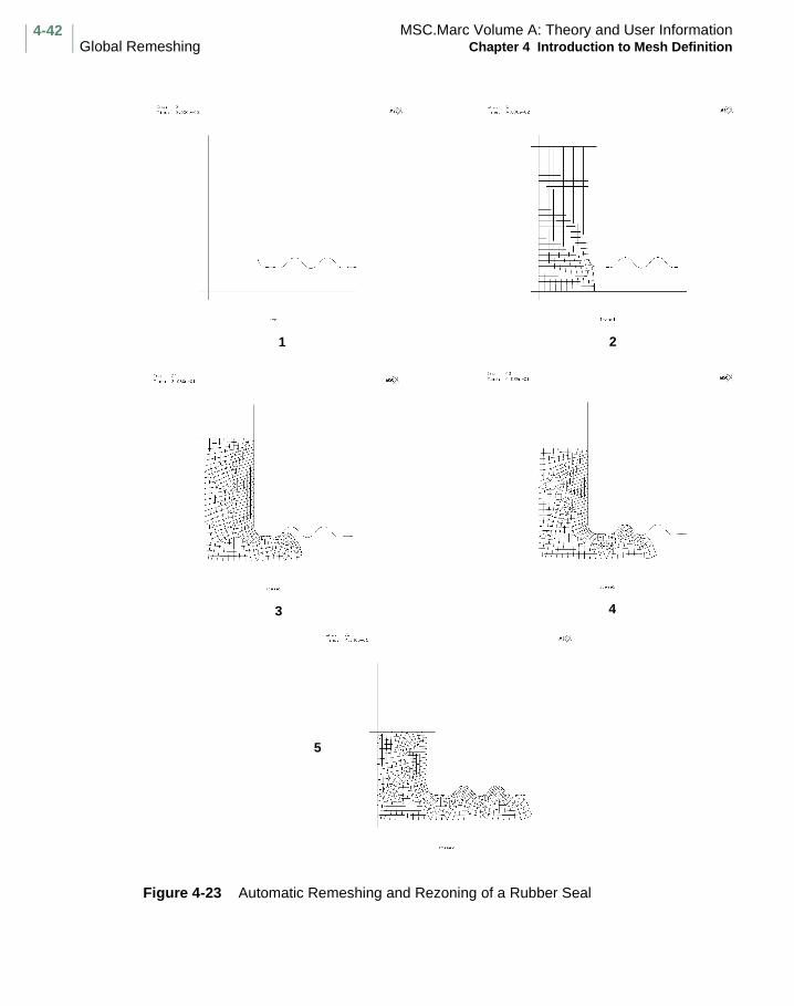
MSC.Marc Volume A: Theory and User InformationGlobal Remeshing Chapter 4 Introduction to Mesh Definition
4-42
Figure 4-23 Automatic Remeshing and Rezoning of a Rubber Seal
1 2
3 4
5

4-43MSC.Marc Volume A: Theory and User InformationChapter 4 Introduction to Mesh Definition Global Remeshing
Remeshing Criteria
It is possible to choose any combination of the following remeshing criteria: Element Distorsion, Contact Penetration, Increment, Angle Deviation or Immediate.
Element Distortion
The identified body is remeshed when the distortion in the elements becomes large, or it is anticipated that the distortion will become large.
The element distortion criteria is based upon examining the angles of the elements at the end of the increment and an estimate of the change in the angle in the next increment.
Given that is the coordinates in the beginning of the step and that are the
displacements in the increment, then:
and
If and , remesh, or if and , remesh which is equivalent to
and remesh or
and remesh or
and or
and .
Contact Penetration
The identified body is remeshed when the curvature of the contact body is such that the current mesh cannot accurately detect penetration.
The penetration remeshing criteria is based upon examining the distance between the edge of an element and the contacted body.
Xn ∆Un
Xn 1+ Xn ∆Un+= Xn 2+est Xn 1+ ∆Un+=
Xn Xn + 1 Xn + 2est
α β
α 0.8>cos β 0.9>cos α 0.9>cos β αcos>cos
0 α 36°< < 0 β 25°< <144° α 180°< < 155° β 180°< <0 α 25°< < β α<155° α 180°< < β α<
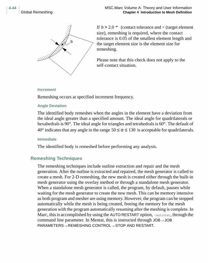
MSC.Marc Volume A: Theory and User InformationGlobal Remeshing Chapter 4 Introduction to Mesh Definition
4-44
If (contact tolerance and < (target element size), remeshing is required, where the contact tolerance is 0.05 of the smallest element length and the target element size is the element size for remeshing.
Please note that this check does not apply to the self-contact situation.
Increment
Remeshing occurs at specified increment frequency.
Angle Deviation
The identified body remeshes when the angles in the element have a deviation from the ideal angle greater than a specified amount. The ideal angle for quadrilaterals or hexahedrals is 90°. The ideal angle for triangles and tetrahedrals is 60°. The default of 40° indicates that any angle in the range is acceptable for quadrilaterals.
Immediate
The identified body is remeshed before performing any analysis.
Remeshing Techniques
The remeshing techniques include outline extraction and repair and the mesh generation. After the outline is extracted and repaired, the mesh generator is called to create a mesh. For 2-D remeshing, the new mesh is created either through the built-in mesh generator using the overlay method or through a standalone mesh generator. When a standalone mesh generator is called, the program, by default, pauses while waiting for the mesh generator to create the new mesh. This can be memory intensive as both program and mesher are using memory. However, the program can be stopped automatically while the mesh is being created, freeing the memory for the mesh generation with the program automatically resuming after the meshing is complete. In Marc, this is accomplished by using the AUTO RESTART option, -autorst, through the command line parameter. In Mentat, this is instructed through JOB→JOB PARAMETERS→REMESHING CONTROL→STOP AND RESTART.
b
b 2.0 * >
50 α 130≤ ≤

4-45MSC.Marc Volume A: Theory and User InformationChapter 4 Introduction to Mesh Definition Global Remeshing
Mesh Generation
There are various mesh generators available in Marc based on Advancing front, Overlay, and Delauney Triangulation techniques.
Advancing front meshing: This mesher creates either triangular, quadrilateral, or mixed triangular and quadrilateral mesh. For a given outline boundary, it starts by creating the elements along the boundary. The new boundary front is then formed when the layer of elements is created. This front advances inward until the complete region is meshed. Some smoothing technique is used to improve the quality of the elements. In general, this mesher works with any enclosed geometry and for geometry that has holes inside. The element size can be changed gradually from the boundary to the interior allowing smaller elements near the boundary with no tying constraints necessary (see Figure 4-24).
Figure 4-24 Advanced Front Meshing
Overlay meshing: This is a quadrilateral mesh generator. The 2-D overlay mesher is included within Marc. It creates a quadrilateral mesh by forming a regular grid covering the center area of a body. A projection is then used to project all

MSC.Marc Volume A: Theory and User InformationGlobal Remeshing Chapter 4 Introduction to Mesh Definition
4-46
boundary nodes onto the real surface and form the outer layer elements. For the surface that is not in contact with other bodies, a cubic spline line is used to make the outline points smoother. This mesher also allows up to two level refinements on boundary where finer edges are needed to capture the geometry detail, and one level of coarsening in the interior where small elements are not necessary. This refinement and coarsening are performed using the tying constraints (see Figure 4-25).
Figure 4-25 Local Refinement and Coarsening
In general, overlay meshing produces good quality elements. However, it does not take geometry with holes inside. It may not create a good mesh with geometry that has a very thin region or very irregular shape. Also, because the regular grid is created based on the global coordinate system, it may create a poor mesh if the geometry is not aligned with the global coordinate system.

4-47MSC.Marc Volume A: Theory and User InformationChapter 4 Introduction to Mesh Definition Global Remeshing
Delaunay Triangulation: This mesher creates only the triangular mesh. All the triangles satisfy the Delaunay triangulation property. It takes all the seed points on the improved outlines as initial triangulation points. The triangulation is implemented by sequential insertion of new points into the triangulation until all the triangles satisfy the local density and quality requirement. Delaunay triangulation algorithm assures the triangular mesh created has the best quality possible for the given set of points. The mesher also allows geometry to have holes inside the body and a variation of the elements with different sizes (Figure 4-26).
Figure 4-26 Meshing with Delaunay Triangulation
Outline Extraction and Repair
The outline consists of all the boundary edges of the contact body. Once the outline is extracted from the mesh, it is checked against other contacting bodies. The penetration from other contacting bodies is marked and the outline is corrected according to the penetration. If the outline is to be used for the advancing front or Delaunay mesher, some refinement and corrections are required to obtain better outline points. These

MSC.Marc Volume A: Theory and User InformationGlobal Remeshing Chapter 4 Introduction to Mesh Definition
4-48
outline points become boundary nodes in the new mesh and cannot be altered during the meshing process. The following procedures are taken by the program to prepare the new outline for the remeshing:
Step 1: Marking the hard points: The hard points are those points that represent important features of the original outline. Hard points are points that mark the beginning or end of the boundary portion of the mesh that is in contact, and the points that represent a sharp corner (such as 90° angle).
Step 2: Marking the points with target element size and minimum element size: The outline points are placed based on the target element size. The refinements and the user-defined outline points are allowed to change this control. However, the minimum element size is used to make sure the outline segment is not too small for the mesh generation.
Step 3: Marking the points with curvature consideration: The curvature control is used to allow small outline segments to be used on the boundary where curvature radii are small. three neighboring outline points are used to calculate the curvature radius. The associate curvature circle can then be formed by a number of line segments. With the same number of line segments used to approximate a circle, smaller outline segments for smaller curvature circles can be had (Figure 4-27).
Figure 4-27 Curvature Consideration
l2πR
n----------=

4-49MSC.Marc Volume A: Theory and User InformationChapter 4 Introduction to Mesh Definition Global Remeshing
Step 4: Marking the points with thin region consideration: In the area where a thin region is formed, small elements are preferred. This can be done by detecting the thin region and using smaller outline segments in the area. The segment length used for the thin area is to allow at least three elements to be presented across the thin area.
Step 5: Smoothing the outline points: Smoothing is required on the outline so that the segment length can gradually vary.
Step 6: Interpolations: Interpolation is the actual process to create a new outline based on the extracted outline and the marking of the outline points. Linear interpolation is used on the contact area to prevent penetration into the other contact bodies. Cubic spline line interpolation is used for the free surfaces.
Remeshing Based on the Target Number of Elements
Instead of giving the element size, you can give the target number of elements for the remeshing. The number of elements in the new mesh can also be controlled by using a percentage tolerance to ensure that the new mesh does not have too many or too few elements. However, this tolerance control requires remeshing trials and it cannot be used with the AUTO RESTART option.

MSC.Marc Volume A: Theory and User InformationChapter 4 Introduction to Mesh Definition
4-50

Chapter 5 Structural Procedure Library
CHAPTER
5 Structural Procedure Library
Linear Analysis
Nonlinear Analysis
Fracture Mechanics
Dynamics
Rigid-Plastic Flow
Superplasticity
Soil Analysis
Design Sensitivity Analysis
Design Optimization
Considerations for Nonlinear Analysis
Data Transfer from Axisymmetric Analysis to 3-D Analysis
References

MSC.Marc Volume A: Theory and User InformationChapter 5 Structural Procedure Library
5-2
This chapter describes the analysis procedures in Marc applicable to structural problems. These procedures range from simple linear elastic analysis to complex nonlinear analysis. A large number of options are available, but you need to consider only those capabilities that are applicable to your physical problem. This chapter provides technical background information as well as usage information about these capabilities.
5-3MSC.Marc Volume A: Theory and User InformationChapter 5 Structural Procedure Library Linear Analysis
Linear Analysis
Linear analysis is the type of stress analysis performed on linear elastic structures. Because linear analysis is simple and inexpensive to perform and generally gives satisfactory results, it is the most commonly used structural analysis. Nonlinearities due to material, geometry, or boundary conditions are not included in this type of analysis. The behavior of an isotropic, linear, elastic material can be defined by two material constants: Young’s modulus , and Poisson’s ratio .
Marc allows you to perform linear elastic analysis using any element type in the program. Various kinematic constraints and loadings can be prescribed to the structure being analyzed; the problem can include both isotropic and anisotropic elastic materials.
The principle of superposition holds under conditions of linearity. Therefore, several individual solutions can be superimposed (summed) to obtain a total solution to a problem.
Linear analysis does not require storing as many quantities as does nonlinear analysis; therefore, it uses the core memory more sparingly. The ELASTIC parameter uses the assembled and decomposed stiffness matrices to arrive at repeated solutions for different loads.
Note: Linear analysis is always the default analysis type in the Marc program.
Linear analysis in Marc requires only the basic input. Table 5-1 shows a subset of the Marc options and parameters which are often used for linear analysis.
E v

MSC.Marc Volume A: Theory and User InformationLinear Analysis Chapter 5 Structural Procedure Library
5-4
More complex linear analyses require additional data blocks.
1. Parameter ELASTIC allows solutions for the same structural system with different loadings (multiple loading analysis). When using the ELASTIC parameter, you must apply total loads, rather than incremental quantities (for example., total force, total moment, total temperature) in subsequent increments.
2. The RESTART option, used with the ELASTIC parameter and/or CASE COMBIN option, stores individual load cases in a restart file. You can also store the decomposed stiffness matrix for later analyses.
3. Model definition option CASE COMBIN combines the results obtained from different loading cases previously stored in a restart file.
4. The ADAPTIVE option can be used to improve the accuracy of the analysis.
5. The J-INTEGRAL option allows the study of problems of linear fracture mechanics.
6. The FOURIER option allows the analysis of axisymmetric structures subjected to arbitrary loadings.
Table 5-1 Basic Input
Type Name
Parameter TITLESIZINGELEMENTSELASTICALL POINTSCENTROIDADAPTIVEFOURIEREND
Model Definition CONNECTIVITYCOORDINATESGEOMETRYISOTROPICFIXED DISPDIST LOADSPOINT LOADCASE COMBINEND OPTION

5-5MSC.Marc Volume A: Theory and User InformationChapter 5 Structural Procedure Library Linear Analysis
7. Model definition option ORTHOTROPIC or ANISOTROPIC activates the anisotropic behavior option. In addition, user subroutines ANELAS, HOOKLW, ANEXP, and ORIENT define the mechanical and thermal anisotropy and the preferred orientations.
8. You can use both the linear SPRINGS and FOUNDATION options in a linear stress analysis.
Accuracy
It is difficult to predict the accuracy of linear elastic analysis without employing special error estimation techniques. An inaccurate solution usually exhibits itself through one or more of the following phenomena:
• Strong discontinuities in stresses between elements
• Strong variation in stresses within an element
• Stresses that oscillate from element to element
Error Estimates
The ERROR ESTIMATE option can also be used to obtain an indication of the quality of the results. You can have the program evaluate the geometric quality of the mesh by reporting the aspect ratios and skewness of the elements. In a large deformation updated Lagrange analysis, you can also observe how these change during the analysis, which indicates mesh distortion. When the mesh distortion is large, it is a good idea to do a rezoning step.
The ERROR ESTIMATE option can also be used to evaluate the stress discontinuity between elements. Marc first calculates a nodal stress based upon the extrapolated integration point values. These nodal values are compared between adjacent elements and reported. Large discrepancies indicate an inability of the mesh to capture high stress gradients, in which case you should refine the mesh and rerun the analysis.
The ERROR ESTIMATE option can be used for either linear or nonlinear analysis.
Adaptive Meshing
The ADAPTIVE option can be used to insure that a certain level of accuracy is achieved. The elastic analysis is repeated with a new mesh until the level of accuracy requested is achieved.

MSC.Marc Volume A: Theory and User InformationLinear Analysis Chapter 5 Structural Procedure Library
5-6
Fourier Analysis
Through Fourier expansion, Marc analyzes axisymmetric structures that are subjected to arbitrary loading. The FOURIER option is available only for linear analysis.
During Fourier analysis, a three-dimensional analysis decouples into a series of independent two-dimensional analyses, where the circumferential distribution of displacements and forces are expressed in terms of the Fourier series. Both mechanical and thermal loads can vary arbitrarily in the circumferential direction. You can determine the structure’s total response from the sum of the Fourier components.
The Fourier formulation is restricted to axisymmetric structures with linear elastic material behavior and small strains and displacements. Therefore, conditions of linearity are essential and material properties must remain constant in the circumferential direction.
To use Fourier expansion analysis in Marc, the input must include the following information:
• The FOURIER parameter allocates storage for the series expansion.
• Fourier model definition blocks for as many series as are needed to describe tractions, thermal loading, and boundary conditions. Number the series sequentially in the order they occur during the FOURIER model definition input. Three ways to describe the series are listed below:
• Specify coefficients on the Fourier model definition blocks.
• Describe (where is the angle in degrees about the circumference) in
point-wise fashion with an arbitrary number of pairs given on the blocks. Marc forms the corresponding series coefficients.
• Generate an arbitrary number of pairs using the user subroutine UFOUR and let the program calculate the series coefficients.
You can obtain the total solution at any position around the circumference by superposing the components already calculated after completion of all increments required by the analysis. The CASE COMBIN option calculates this total solution by summing the individual harmonics which are stored in the restart file.
The number of steps or increments needed for analysis depends on the number of harmonics that are chosen. For a full analysis with symmetric and antisymmetric load cases, the total number of increments equals twice the number of harmonics. Table 5-2 shows which Fourier coefficients are used for a given increment.
a0 a1 b1…, ,
F θ( ) θθ F θ( ),[ ]
θ F θ( ),[ ]

5-7MSC.Marc Volume A: Theory and User InformationChapter 5 Structural Procedure Library Linear Analysis
The magnitude of concentrated forces should correspond to the value of the ring load integrated around the circumference. Therefore, if the Fourier coefficients for a varying ring load are found from the distribution, where has the units of force per unit length, the force magnitude given in the point load block should equal the circumference of the loaded ring. If is in units of force per
radian, the point load magnitude should be .
The Fourier series can be found for varying pressure loading from input
with expressed in force per unit area. Marc calculates the equivalent nodal forces and integrates them around the circumference. The distributed load magnitude in the distributed loads block should be 1.0.
Table 5-3 shows the elements in the program that can be used for Fourier analysis.
Table 5-2 Fourier Coefficients – Increment Number
LOAD TERMS
INC. 1st DOF,Z 2nd DOF,R 3rd DOF,θ
0 0
1 0 0
2
3
‡ ⋅ ⋅ ⋅
‡ ⋅ ⋅ ⋅
‡ ⋅ ⋅ ⋅
Table 5-3 Elements Used for Fourier Analysis
Element Type Description
62 8-node73 8-node with reduced integration63 8-node for incompressible behavior74 8-node for incompressible behavior with reduced integration90 3-node shell
a0 a0
a0
a1 a1 b1
b1 b1 a1
2n an an bn
2n 1+ bn bn an
p θ( ) θ p θ( ),[ ] p θ( )
p θ( )2π
θ p θ( ),[ ]p

MSC.Marc Volume A: Theory and User InformationLinear Analysis Chapter 5 Structural Procedure Library
5-8
Technical Background
The general form of the Fourier series expansion of the function is shown in the equation below.
(5-1)
This expression expands the displacement function in terms of sine and cosine terms. A symmetric and an antisymmetric problem are formulated for each value of .
The displacements for the symmetric case, expressed in terms of their nodal values, are
(5-2)
Nodal forces are
(5-3)
The value is a special case in Fourier analysis. If only the symmetric expansion terms are used, the formulation defaults to the fully axisymmetric two-dimensional analysis. The antisymmetric case for yields a solution for the variable that corresponds to loading in the tangential direction. Analyze axisymmetric solids under pure torsion in this way.
F θ( )
F θ( ) a0 an nθcos bn nθsin+( )n 1=
∞
∑+=
n
un N1 N2 …, ,[ ] nθ un ecos=
vn N1 N2 …, ,[ ] nθ vn ecos=
wn N1 N2 …, ,[ ] nsin θ wn e=
Z Z0 Zn nθcos
1
n
∑+=
R R0 Rn nθcos
1
n
∑+=
T T0 Tn nθsin
1
n
∑+=
n 0=
n 0= θ

5-9MSC.Marc Volume A: Theory and User InformationChapter 5 Structural Procedure Library Linear Analysis
Modal Shapes and Buckling Load Estimations During a Fourier Analysis
During a Fourier analysis, Marc can be asked to estimate both the modal shapes and buckling loads for each harmonic in the analysis. In either case, the program performs a Fourier analysis first and then estimates the modal shapes/buckling load at prescribed harmonic numbers. In addition to the input data required for a Fourier analysis (FOURIER parameter and FOURIER model definition option), the following must also be added: DYNAMIC parameter and MODAL INCREMENT model definition option; BUCKLE parameter and BUCKLE INCREMENT model definition option, for Fourier modal shape and Fourier buckling load estimations, respectively.
In the Fourier modal analysis, the mass matrix in the eigenvalue equation is a constant matrix. The stiffness matrix in the eigenvalue equation is the one associated with a prescribed harmonic of the Fourier analysis. The expression of the eigenvalue equation is:
(5-4)
where is the stiffness matrix associated with the mth harmonic of the Fourier
analysis and is a constant matrix. Multiple modes for each harmonic can be extracted.
Similarly, in a Fourier buckling analysis, the stiffness matrices in the eigenvalue equation are (respectively); the linear elastic stiffness matrix and the geometric stiffness matrix associated with the prescribed harmonic of the Fourier analysis.
The eigenvalue equation is expressed
(5-5)
where is the linear elastic stiffness matrix and is the geometric stiffness
matrix, associated with the mth harmonic of the Fourier analysis. The stresses used in the calculation of the geometric stiffness matrix are those associated with the symmetric load case, . Multiple buckling load estimations for each harmonic are also available.
Km[ ]φ ω2 M0[ ]φ– 0=
Km[ ]
M0[ ]
Km[ ]φ λ Kg
m[ ]φ– 0=
Km[ ] Kg
m[ ]
m 0=

MSC.Marc Volume A: Theory and User InformationNonlinear Analysis Chapter 5 Structural Procedure Library
5-10
Nonlinear Analysis
The finite element method can be used for nonlinear, as well as linear, problems. Early development of nonlinear finite element technology was mostly influenced by the nuclear and aerospace industries. In the nuclear industry, nonlinearities are mainly due to the nonlinear, high-temperature behavior of materials. Nonlinearities in the aerospace industry are mainly geometric in nature and range from simple linear buckling to complicated post-bifurcation behavior. Nonlinear finite element techniques have become popular in metal forming manufacturing processes, fluid-solid interaction, and fluid flow. In recent years, the areas of biomechanics and electromagnetics have seen an increasing use of finite elements.
A problem is nonlinear if the force-displacement relationship depends on the current state (that is, current displacement, force, and stress-strain relations). Let be a
generalized displacement vector, a generalized force vector, and the stiffness matrix. The expression of the force-displacement relation for a nonlinear problem is
(5-6)
Linear problems form a subset of nonlinear problems. For example, in classical linear elastostatics, this relation can be written in the form
(5-7)
where the stiffness matrix is independent of both and . If the matrix depends on other state variables that do not depend on displacement or loads (such as temperature, radiation, moisture content, etc.), the problem is still linear.
Similarly, if the mass matrix is a constant matrix, the following undamped dynamic problem is also linear:
(5-8)
There are three sources of nonlinearity: material, geometric, and nonlinear boundary conditions. Material nonlinearity results from the nonlinear relationship between stresses and strains. Considerable progress has been made in attempts to derive the continuum or macroscopic behavior of materials from microscopic backgrounds, but, up to now, commonly accepted constitutive laws are phenomenological. Difficulty in obtaining experimental data is usually a stumbling block in mathematical modeling of material behavior. A plethora of models exist for more commonly available materials like elastomers and metals. Other material model of considerable practical importance are: composites, viscoplastics, creep, soils, concrete, powder, and foams. Figure 5-1
u
P K
P K P u,( )u=
P Ku=
K u P K
P Mu·· Ku+=

5-11MSC.Marc Volume A: Theory and User InformationChapter 5 Structural Procedure Library Nonlinear Analysis
shows the elastoplastic, elasto-viscoplasticity, and creep. Although the situation of strain hardening is more commonly encountered, strain softening and localization has gained considerable importance in recent times.
Geometric nonlinearity results from the nonlinear relationship between strains and displacements on the one hand and the nonlinear relation between stresses and forces on the other hand. If the stress measure is conjugate to the strain measure, both sources of nonlinearity have the same form. This type of nonlinearity is mathematically well defined, but often difficult to treat numerically. Two important types of geometric nonlinearity occur:
a. The analysis of buckling and snap-through problems (see Figure 5-2 and Figure 5-3).
b. Large strain problems such as manufacturing, crash, and impact problems. In such problems, due to large strain kinematics, the mathematical separation into geometric and material nonlinearity is nonunique.
Figure 5-1 Material Nonlinearity
σ
εElasto-Plastic Behavior
σ
εElasto-Viscoplastic Behavior
ε
εc
tCreep Behavior
σ

MSC.Marc Volume A: Theory and User InformationNonlinear Analysis Chapter 5 Structural Procedure Library
5-12
Figure 5-2 Buckling
Figure 5-3 Snap-Through
Boundary conditions and/or loads can also cause nonlinearity. Contact and friction problems lead to nonlinear boundary conditions. This type of nonlinearity manifests itself in several real life situations; for example, metal forming, gears, interference of mechanical components, pneumatic tire contact, and crash (see Figure 5-4). Loads on a structure cause nonlinearity if they vary with the displacements of the structure. These loads can be conservative, as in the case of a centrifugal force field (see Figure 5-5); they can also be nonconservative, as in the case of a follower force on a cantilever beam (see Figure 5-6). Also, such a follower force can be locally nonconservative, but represent a conservative loading system when integrated over the structure. A pressurized cylinder (see Figure 5-7) is an example of this.
P
u
Linear
Stable
Neutral
Unstable
P
Pc
u
P
u
P

5-13MSC.Marc Volume A: Theory and User InformationChapter 5 Structural Procedure Library Nonlinear Analysis
Figure 5-4 Contact and Friction Problem
Figure 5-5 Centrifugal Load Problem (Conservative)

MSC.Marc Volume A: Theory and User InformationNonlinear Analysis Chapter 5 Structural Procedure Library
5-14
Figure 5-6 Follower Force Problem (Nonconservative)
Figure 5-7 Pressurized Cylinder (Globally Conservative)
P
P

5-15MSC.Marc Volume A: Theory and User InformationChapter 5 Structural Procedure Library Nonlinear Analysis
The three types of nonlinearities are described in detail in the following sections.
Geometric Nonlinearities
Geometric nonlinearity leads to two types of phenomena: change in structural behavior and loss of structural stability.
There are two natural classes of large deformation problems: the large displacement, small strain problem and the large displacement, large strain problem. For the large displacement, small strain problem, changes in the stress-strain law can be neglected, but the contributions from the nonlinear terms in the strain displacement relations cannot be neglected. For the large displacement, large strain problem, the constitutive relation must be defined in the correct frame of reference and is transformed from this frame of reference to the one in which the equilibrium equations are written.
The collapse load of a structure can be predicted by performing an eigenvalue analysis. If performed after the linear solution (increment zero), the Euler buckling estimate is obtained. An eigenvalue problem can be formulated after each increment of load; this procedure can be considered a nonlinear buckling analysis even though a linearized eigenvalue analysis is used at each stage.
The kinematics of deformation can be described by the following approaches:
A. Lagrangian Formulation
B. Eularian Formulation
C. Arbitrary Eularian-Lagrangian (AEL) Formulation
The choice of one over another can be dictated by the convenience of modeling physics of the problem, rezoning requirements, and integration of constitutive equations.
A. Lagrangian Formulation
In the Lagrangian method, the finite element mesh is attached to the material and moves through space along with the material. In this case, there is no difficulty in establishing stress or strain histories at a particular material point and the treatment of free surfaces is natural and straightforward.
The Lagrangian approach also naturally describes the deformation of structural elements; that is, shells and beams, and transient problems, such as the indentation problem shown in Figure 5-8.

MSC.Marc Volume A: Theory and User InformationNonlinear Analysis Chapter 5 Structural Procedure Library
5-16
Figure 5-8 Indentation Problem with Pressure Distribution on Tool
This method can also analyze steady-state processes such as extrusion and rolling. Shortcomings of the Lagrangian method are that flow problems are difficult to model and that the mesh distortion is as severe as the deformation of the object. Severe mesh degeneration is shown in Figure 5-9b. However, recent advances in adaptive meshing and rezoning have alleviated the problems of premature termination of the analysis due to mesh distortions as shown in Figure 5-9c.
The Lagrangian approach can be classified in two categories: the total Lagrangian method and the updated Lagrangian method. In the total Lagrangian approach, the equilibrium is expressed with the original undeformed state as the reference; in the updated Lagrangian approach, the current configuration acts as the reference state. The kinematics of deformation and the description of motion is given in Figure 5-10 and Table 5-4.
Depending on which option you use, the stress and strain results are given in different form as discussed below. If none of the following parameters, LARGE DISP, UPDATE, or FINITE, are used, the program uses and prints “engineering” stress and strain measures. These measures are suitable only for analyses without large incremental or total rotation or large incremental or total strains.
Using only the LARGE DISP parameter, Marc uses the total Lagrangian method. The program uses and prints second Piola-Kirchhoff stress and Green-Lagrange strain. These measures are suitable for analysis with large incremental rotations and large incremental strains.
With the combination of LARGE DISP and UPDATE, Marc uses Cauchy stresses and true strains. This combination of parameters is suitable for analyses with small incremental rotations and small incremental strains. Stress and strain components are printed with respect to the current state.
sz
∆u

5-17MSC.Marc Volume A: Theory and User InformationChapter 5 Structural Procedure Library Nonlinear Analysis
Figure 5-9 Rezoning Example
Figure 5-10 Description of Motion
(a) Original (b) Deformed Mesh (Undeformed Mesh) Before Rezoning
(c) Deformed MeshAfter Rezoning
Reference
t = 0
Current
t = n + 1
Previous
t = n
un + 1
F
f
∆u
Fn
un
Fn+1 = fFn

MSC.Marc Volume A: Theory and User InformationNonlinear Analysis Chapter 5 Structural Procedure Library
5-18
The combination of LARGE DISP, UPDATE, and FINITE (with constant dilatation used on the GEOMETRY option) or PLASTICITY (option 3) results in a complete large strain plasticity formulation with B-Bar method to satisfy incompatibility using the updated Lagrange procedure. The use of PLASTICITY (option 3) parameter obviates the need of the CONSTANT DILATATION parameter. The program internally uses true (Cauchy) stress and rotation neutralized strains. In the case of proportional straining, this method leads to logarithmic strains.
Note: For materials exhibiting large strain plasticity with volumetric changes (for example, soils, powder, snow, wood) only LARGE DISP, FINITE, and UPDATE should be used. Use of CONSTANT DILATATION or PLASTICITY parameters will enforce the incompressibility condition and, in such materials, yield incorrect and nonphysical behavior.
The use of PLASTICITY,5 results in a complete large strain plasticity formulation in mixed framework using the updated Lagrange. The program uses the multiplicative decomposition of deformation gradient. The results are given in true (Cauchy) stress and logarithmic strains.
Large strain rubber elasticity can be modeled in either total Lagrange (ELASTICITY,1 : second Piola-Kirchhoff stress, Green Lagrange strain) or updated Lagrange (ELASTICITY,2 : Cauchy stress, Logarithmic strain) framework.
PLASTICITY,5 and ELASTICITY,2 parameters can be used with either displacement or Herrmann elements.
Table 5-4 Kinematics and Stress-Strain Measures in Large Deformation
ConfigurationMeasures
Reference (t = 0 or n) Current (t = n + 1)
Coordinates
Deformation Tensor
Strain Measure
Stress Measure
X
C (Right Cauchy-Green)
E (Green-Lagrange)F (Deformation Gradient)
S (second Piola-Kirchhoff)P (first Piola-Kirchhoff)
x
b (Left Cauchy-Green)
e (Logarithmic)
σ (Cauchy)
Parameter Kinematics FormulationPLASTICITY,1 Total Lagrange Small strain, mean normal, additive decomposition
of strain rates.PLASTICITY,3 Updated Lagrange Large strain, mean normal, additive decomposition
of strain rates. Equivalent to: LARGE DISP, FINITE, UPDATE, and CONSTANT DILATATION.

5-19MSC.Marc Volume A: Theory and User InformationChapter 5 Structural Procedure Library Nonlinear Analysis
Theoretically and numerically, if formulated mathematically correct, the two formulations yield exactly the same results. However, integration of constitutive equations for certain types of material behavior (for example, plasticity) make the implementation of the total Lagrange formulation inconvenient. If the constitutive equations are convected back to the original configuration and proper transformations are applied, then both formulations are equivalent. However, for deformations involving excess distortions, ease of rezoning favors the updated Lagrangian formulation. This is reflected in the fact that a rezoned mesh in the current state is mapped back to excessively distorted mesh leading to negative Jacobian in the total Lagrangian formulation.
The terminology total and updated Lagrangian has been used with some vagueness [1, 2]. In this document, for a sequence of incremental motions at and , the total Lagrangian formulation entails the use of configuration as reference; while in the updated Lagrangian configuration, the (unequilibriated) configuration is the reference.
Total Lagrangian Procedure
The total Lagrangian procedure can be used for linear or nonlinear materials, in conjunction with static or dynamic analysis. Although this formulation is based on the initial element geometry, the incremental stiffness matrices are formed to account for previously developed stress and changes in geometry.
This method is particularly suitable for the analysis of nonlinear elastic problems (for instance, with the Mooney or Ogden material behavior or the user subroutine HYPELA). The total Lagrangian approach is also useful for problems in plasticity and creep, where moderately large rotations but small strains occur. A case typical in problems of beam or shell bending. However, this is only due to the approximations involved.
To activate the large displacement (total Lagrangian approach) option in Marc, use the LARGE DISP parameter. Include the FOLLOW FOR parameter for follower force (for example, centrifugal or pressure load) problems. This parameter forms all distributed loads on the basis of the current geometry. Do not use the CENTROID parameter with this parameter. Always use residual load corrections with this parameter. To input control tolerances for large displacement analysis, use model definition option CONTROL.
PLASTICITY,5 Updated Lagrange Large strain, radial return multiplicative decomposition of deformation gradient.
ELASTICITY,1 Total Lagrange Large strain.ELASTICITY,2 Updated Lagrange Large strain.
Parameter Kinematics Formulation
t 0 1 2 …n, , ,=n 1+ t 0=
t n 1+=
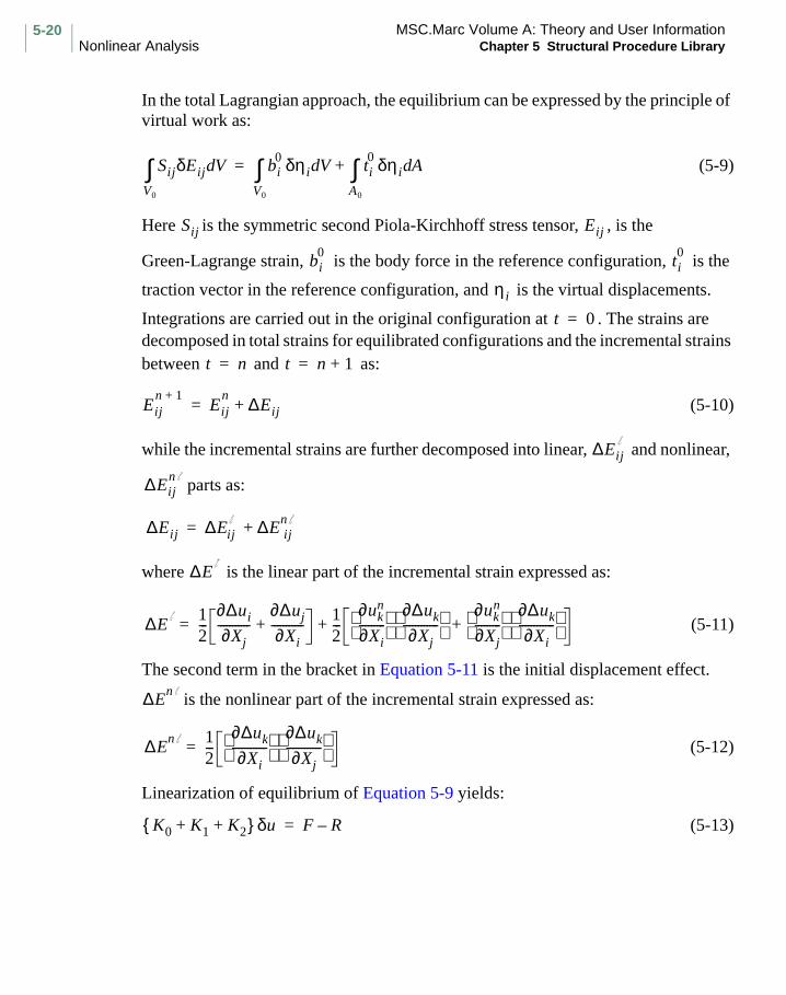
MSC.Marc Volume A: Theory and User InformationNonlinear Analysis Chapter 5 Structural Procedure Library
5-20
In the total Lagrangian approach, the equilibrium can be expressed by the principle of virtual work as:
(5-9)
Here is the symmetric second Piola-Kirchhoff stress tensor, , is the
Green-Lagrange strain, is the body force in the reference configuration, is the
traction vector in the reference configuration, and is the virtual displacements.
Integrations are carried out in the original configuration at . The strains are decomposed in total strains for equilibrated configurations and the incremental strains between and as:
(5-10)
while the incremental strains are further decomposed into linear, and nonlinear,
parts as:
where is the linear part of the incremental strain expressed as:
(5-11)
The second term in the bracket in Equation 5-11 is the initial displacement effect. is the nonlinear part of the incremental strain expressed as:
(5-12)
Linearization of equilibrium of Equation 5-9 yields:
(5-13)
SijδEij VdV0
∫ bi0 δηi V ti
0 δηi AdA0
∫+dV0
∫=
Sij Eij
bi0
ti0
η i
t 0=
t n= t n 1+=
Eijn 1+
Eijn ∆Eij+=
∆Eij
∆Eijn
∆Eij ∆Eij ∆Enij+=
∆E
∆E12---
∂∆ui
∂Xj-----------
∂∆uj
∂Xi-----------+
12---
∂ukn
∂Xi---------
∂∆uk
∂Xj------------
∂ukn
∂Xj---------
∂∆uk
∂Xi------------
++=
∆En
∆En 1
2---
∂∆uk
∂Xi------------
∂∆uk
∂Xj------------
=
K0 K1 K2+ + δ u F R–=
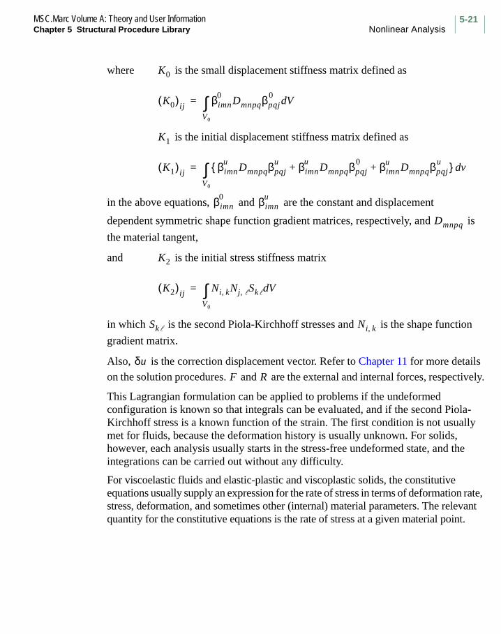
5-21MSC.Marc Volume A: Theory and User InformationChapter 5 Structural Procedure Library Nonlinear Analysis
5Structural Procedure Library
Nonlinear Analysis
where is the small displacement stiffness matrix defined as
is the initial displacement stiffness matrix defined as
in the above equations, and are the constant and displacement
dependent symmetric shape function gradient matrices, respectively, and is
the material tangent,
and is the initial stress stiffness matrix
in which is the second Piola-Kirchhoff stresses and is the shape function
gradient matrix.
Also, is the correction displacement vector. Refer to Chapter 11 for more details
on the solution procedures. and are the external and internal forces, respectively.
This Lagrangian formulation can be applied to problems if the undeformed configuration is known so that integrals can be evaluated, and if the second Piola-Kirchhoff stress is a known function of the strain. The first condition is not usually met for fluids, because the deformation history is usually unknown. For solids, however, each analysis usually starts in the stress-free undeformed state, and the integrations can be carried out without any difficulty.
For viscoelastic fluids and elastic-plastic and viscoplastic solids, the constitutive equations usually supply an expression for the rate of stress in terms of deformation rate, stress, deformation, and sometimes other (internal) material parameters. The relevant quantity for the constitutive equations is the rate of stress at a given material point.
K0
K0( )ij βimn0
Dmnpqβpqj0
VdV0
∫=
K1
K1( )ij βimnu
Dmnpqβpqju βimn
uDmnpqβpqj
0 βimnu Dmnpqβpqj
u+ + vd
V0
∫=
βimn0 βimn
u
Dmnpq
K2
K2( )ij Ni k, Nj , Sk VdV0
∫=
Sk Ni k,
δu
F R

MSC.Marc Volume A: Theory and User InformationNonlinear Analysis Chapter 5 Structural Procedure Library
5-22
It, therefore, seems most obvious to differentiate the Lagrangian virtual work equation with respect to time. The rate of virtual work is readily found as
(5-14)
This formulation is adequate for most materials, because the rate of the second Piola-Kirchhoff stress can be written as
(5-15)
For many materials, the stress rate is even a linear function of the strain rate
(5-16)
Equation 5-14 supplies a set of linear relations in terms of the velocity field. The velocity field can be solved noniteratively and the displacement can be obtained by time integration of the velocities.
The second Piola-Kirchhoff stress for elastic and hyperelastic materials is a function of the Green-Lagrange strain defined below:
(5-17)
If the stress is a linear function of the strain (linear elasticity)
(5-18)
the resulting set of equations is still nonlinear because the strain is a nonlinear function of displacement.
Updated Lagrangian Procedure
The updated Lagrange formulation takes the reference configuration at . True or Cauchy stress and an energetically conjugate strain measure, namely the true strain, are used in the constitutive relationship.
The updated Lagrangian approach is useful in:
a. analysis of shell and beam structures in which rotations are large so that the nonlinear terms in the curvature expressions may no longer be neglected, and
b. large strain plasticity analysis, for calculations which the plastic deformations cannot be assumed to be infinitesimal.
S·ijδEij Sij
∂vk
∂Xi--------
∂δηk
∂Xj------------+ dV
V0
∫ b· iδηidV t·iδηidAA0
∫+V0
∫=
S·ij S
·ij E
·kl Smn Epq, ,( )=
S·ij Dijkl Smn Epq,( )E
·kl=
Sij Sij Ekl( )=
Sij DijkEk=
t n 1+=

5-23MSC.Marc Volume A: Theory and User InformationChapter 5 Structural Procedure Library Nonlinear Analysis
In general, this approach can be used to analyze structures where inelastic behavior (for example, plasticity, viscoplasticity, or creep) causes the large deformations. The (initial) Lagrangian coordinate frame has little physical significance in these analyses since the inelastic deformations are, by definition, permanent. For these analyses, the Lagrangian frame of reference is redefined at the last completed iteration of the current increment.
You can use the updated procedure with or without the LARGE DISP parameter. When you use the LARGE DISP parameter, Marc takes into account the effect of the internal stresses by forming the initial stress stiffness. Marc also calculates the strain increment to second order accuracy to allow large rotation increments. It is recommended that the LARGE DISP parameter be used in conjunction with the UPDATE parameter.
The UPDATE parameter in Marc (used with or without the LARGE DISP parameter) defines a new (Lagrangian) frame of reference at the beginning of each increment. This option is suitable for analysis of problems of large total rotation but small strain. If analysis of large plastic strain is required, use the FINITE parameter in addition to the UPDATE parameter. Marc uses true stress (σ) and logarithmic strains. Hence, you must input your stress-strain curves as true stress versus logarithmic strain.
The PLASTICITY parameter with options 3 or 5 utilize the updated Lagrange procedure for elastic-plastic analysis. The ELASTICITY parameter with option 2 utilizes the updated Lagrange procedure for large strain elasticity (Mooney or Ogden).
It is instructive to derive the stiffness matrices for the updated Lagrangian formulation starting from the virtual work principle in Equation 5-9.
Direct linearization of the left-hand side of Equation 5-9 yields:
(5-19)
where ∆u and η are actual incremental and virtual displacements respectively, and σkj is Cauchy stress tensor.
(5-20)
Sij δEij( )d( ) VdV0
∫ ∇η ikσkj∇∆ uij vdVn 1+
∫=
SijδEijd Vd
V0
∫ ∇ sη ijLijk∇s ∆uk( ) vd
Vn 1+
∫=

MSC.Marc Volume A: Theory and User InformationNonlinear Analysis Chapter 5 Structural Procedure Library
5-24
denotes the symmetric part of , which represents the gradient operator in the current configuration. Also, in Equation 5-19 and Equation 5-20, three identities are used:
(5-21)
in which represents the material moduli tensor in the reference configuration
which is convected to the current configuration, . This yields:
(5-22)
where is the material stiffness matrix written as
in which is the symmetric gradient operator-evaluated in the current
configuration and is the Cauchy stresses
and is the geometric stiffness matrix written as
while and are the external and internal forces, respectively.
Keeping in view that the reference state is the current state, a rate formulation analogous to Equation 5-14 can be obtained by setting:
(5-23)
∇ s ∇
σij1J---FimSmnFjn=
δEij Fmi∇sηmnFnj=
Lijk1J---FimFjnFkpFqDmnpq=
and
Dmnpq
Lijk
K1 K2+ δ u F R–=
K1
K1( )ij βimnLmnpqβpqj
Vn 1+
∫=
βimn
σkl
K2
K2( )ij σkNi k, Nj , vd
Vn 1+
∫=
F R
Fij δij δEij, δdij ∂
∂Xi--------, ∂
∂xi------- Sij, σij= = = =
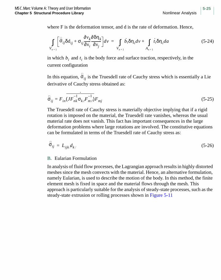
5-25MSC.Marc Volume A: Theory and User InformationChapter 5 Structural Procedure Library Nonlinear Analysis
where F is the deformation tensor, and d is the rate of deformation. Hence,
(5-24)
in which and is the body force and surface traction, respectively, in the
current configuration
In this equation, is the Truesdell rate of Cauchy stress which is essentially a Lie
derivative of Cauchy stress obtained as:
(5-25)
The Truesdell rate of Cauchy stress is materially objective implying that if a rigid rotation is imposed on the material, the Truesdell rate vanishes, whereas the usual material rate does not vanish. This fact has important consequences in the large deformation problems where large rotations are involved. The constitutive equations can be formulated in terms of the Truesdell rate of Cauchy stress as:
(5-26)
B. Eularian Formulation
In analysis of fluid flow processes, the Lagrangian approach results in highly distorted meshes since the mesh convects with the material. Hence, an alternative formulation, namely Eularian, is used to describe the motion of the body. In this method, the finite element mesh is fixed in space and the material flows through the mesh. This approach is particularly suitable for the analysis of steady-state processes, such as the steady-state extrusion or rolling processes shown in Figure 5-11
∇σijδdij σij
∂vk
∂xi--------
∂δηk
∂xj------------+ dv
Vn 1+
∫ b· iδηidvVn 1+
∫ t·iδηidaAn 1+
∫+=
bi ti
∇σij
σij∇
Fin JFnk1–σkFm
1–( )
·= Fmj
∇σij Lijk dk=

MSC.Marc Volume A: Theory and User InformationNonlinear Analysis Chapter 5 Structural Procedure Library
5-26
Figure 5-11 Rolling Analysis
The governing differential equations of equilibrium for fluid flow through an enclosed volume are now written as:
(5-27)
where, is the material time derivative of a quantity. For an incompressible fluid,
Equation 5-27 along with continuity equation (mass conservation) yields:
(5-28)
The left-hand side of Equation 5-28 represents the local rate of change augmented by the convection effects. The same principle can be called to physically explain the material time derivative of Cauchy stress; that is, Truesdell rate of Cauchy stress. It can be seen from Equation 5-25 that:
(5-29)
The second and third terms on the right-hand side represent the convection effects. The last term vanishes for a completely incompressible material; a condition enforced in the rigid-plastic flow of solids.
D ρvi( )Dt
----------------- ρbi
∂σij
∂xj---------+=
DDt------
ρ∂vi
∂t------- ρvj
∂vi
∂xj-------+ ρbi
∂σij
∂xj---------+=
∇σij σ· ij∂vi
∂xk-------- σkj– σik
∂vj
∂xk--------– σij
∂vk
∂xk--------+=

5-27MSC.Marc Volume A: Theory and User InformationChapter 5 Structural Procedure Library Nonlinear Analysis
C. Arbitrary Eularian-Lagrangian (AEL) Formulation
In the AEL formulation referential system, the grid moves independently from the material, yet in a way that is spans the material at any time. Hence, a relationship between derivative with respect to the material and grid derivative is expressed as:
(5-30)
where is the relative velocity between the material particle, and the mesh
velocity, ; for example,
(5-31)
The second or latter term represents the convective effect between the grid and the
material. Note that for , a purely Eularian formulation is obtained. The equation of momentum, for instance, can be represented as:
(5-32)
Due to its strong resemblance to the pure Eularian formulation, AEL is also called quasi-Eularian formulation.
Nonlinear Boundary Conditions
There are three types of problems associated with nonlinear boundary conditions: contact, nonlinear support, and nonlinear loading. The contact problem might be solved through the use of special gap elements of the CONTACT option. Nonlinear support might involve nonlinear springs and/or foundations. Sometimes nonlinearities due to rigid links that become activated or deactivated during an analysis can be modeled through adaptive linear constraints. Nonlinear loading is present if the loading system is nonconservative, as is the case with follower forces or frictional slip effects.
Discontinuities are inherent in the nature of many of these nonlinearities, making the solution by means of incremental linear approximations difficult. Some of the most severe nonlinearities in mechanics are introduced by nonlinear boundary conditions. It is, therefore, very important to be aware of potential problem areas and to have a good understanding of the underlying principles. This awareness and understanding enables you to validate numerical answers and to take alternative approaches if an initial attempt fails.
·( ) *( ) ci( ) i,+=
ci vip
vim
ci vip
vim–=
vip
vim=
ρvi* ρ v
j
pv
jm–( )
∂vi
∂xj-------+
∂σij
∂xj--------- bi+=

MSC.Marc Volume A: Theory and User InformationNonlinear Analysis Chapter 5 Structural Procedure Library
5-28
Contact Problems
Contact problems are commonly encountered in physical systems. Some examples of contact problems are the interface between the metal workpiece and the die in metal forming processes, pipe whip in piping systems, and crash simulation in automobile designs.
Contact problems are characterized by two important phenomena: gap opening and closing and friction. As shown in Figure 5-12, the gap describes the contact (gap closed) and separation (gap open) conditions of two objects (structures). Friction influences the interface relations of the objects after they are in contact. The gap condition is dependent on the movement (displacement) of the objects, and friction is dependent on the contact force as well as the coefficient of (Coulomb) friction at contact surfaces. The analysis involving gap and friction must be carried out incrementally. Iterations can also be required in each (load/time) increment to stabilize the gap-friction behavior.
Figure 5-12 Normal Gap Between Potentially Contacting Bodies
Two options are available in Marc for the simulation of a contact problem. A detailed description of these options (gap-friction element and the CONTACT option) is given in Chapter 8, Contact.
Nonlinear Support
Marc provides two options for the modeling of support conditions: springs and elastic foundations. In a nonlinear problem, the spring stiffness and the equivalent spring stiffness of the elastic foundation can be modified through a user subroutine. In the nonlinear spring option, the incremental force in the spring is
(5-33)
AB
n
∆F K ∆u2 ∆u1–( )=
5-29MSC.Marc Volume A: Theory and User InformationChapter 5 Structural Procedure Library Nonlinear Analysis
where is the spring stiffness, is the displacement increment of the degree of
freedom at the second end of the spring, and is the displacement increment of the
degree of freedom at the first end of the spring.
Use the SPRINGS model definition option for the input of spring data. User subroutine USPRNG may be used to specify the value of based on the amount of previous deformation for nonlinear springs. In dynamic analysis, the SPRINGS option can also be used to define a dashpot.
In the elastic nonlinear FOUNDATION option, the elements in Marc can be specified as being supported on a frictionless (nonlinear) foundation. The foundation supports the structure with an increment force per unit area given by
(5-34)
where is the equivalent spring stiffness of the foundation (per unit surface area),
and is the incremental displacement of the surface at a point in the same direction
as .
To input nonlinear foundation data, use the FOUNDATION model definition option.
To specify the value of for the nonlinear equivalent spring stiffness based on the amount of previous deformation of the foundation, use the user subroutine USPRNG.
Nonlinear Loading
When the structure is deformed, the directions and the areas of the surface loads are changed. For most deformed structures, such changes are so small that the effect on the equilibrium equation can be ignored. But for some structures such as flexible shell structure with large pressure loads, the effects on the results can be quite significant so that the surface load effects have to be included in the finite element equations.
Marc forms both pressure stiffness and pressure terms based on current deformed configuration with the FOLLOW FOR parameter. The FOLLOW FOR parameter should be used with the LARGE DISP parameter and the CENTROID parameter should not be included due to the use of the residual load correction.
Buckling Analysis
Buckling analysis allows you to determine at what load the structure will collapse. You can detect the buckling of a structure when the structure’s stiffness matrix approaches a singular value. You can extract the eigenvalue in a linear analyses to obtain the linear buckling load. You can also perform eigenvalue analysis for buckling load in a nonlinear problem based on the incremental stiffness matrices.
K ∆u2
∆u1
K
∆Pn K un( )∆un=
K
∆un
∆Pn
K

MSC.Marc Volume A: Theory and User InformationNonlinear Analysis Chapter 5 Structural Procedure Library
5-30
The buckling option estimates the maximum load that can be applied to a geometrically nonlinear structure before instability sets in. To activate the buckling option in the program, use the parameter BUCKLE. If a nonlinear buckling analysis is performed, also use the parameter LARGE DISP.
Use the history definition option BUCKLE to input control tolerances for buckling load estimation (eigenvalue extraction by a power sweep or Lanczos method). You can estimate the buckling load after every load increment. The BUCKLE INCREMENT option can be used if a collapse load calculation is required at multiple increments.
The linear buckling load analysis is correct when you take a very small load step in increment zero, or make sure the solution has converged before buckling load analysis (if multiple increments are taken). Linear buckling (after increment zero) can be done without using the LARGE DISP parameter, in which case the restriction on the load step size no longer applies.
In a buckling problem that involves material nonlinearity (for example, plasticity), the nonlinear problem must be solved incrementally. During the analysis, a failure to converge in the iteration process or nonpositive definite stiffness signals the plastic collapse.
For extremely nonlinear problems, the BUCKLE option cannot produce accurate results. In that case, the history definition option AUTO INCREMENT allows automatic load stepping in a quasi-static fashion for both geometric large displacement and material (elastic-plastic) nonlinear problems. The option can handle elastic-plastic snap-through phenomena. Therefore, the post-buckling behavior of structures can be analyzed.
The buckling option solves the following eigenvalue problem by the inverse power sweep method:
(5-35)
where is assumed to be a linear function of the load increment to cause
buckling. The geometric stiffness used for the buckling load calculation is based
on the stress and displacement state change at the start of the last increment. However, the stress and strain states are not updated during the buckling analysis. The buckling load is therefore estimated by:
(5-36)
where for increments greater than 1, is the load applied at the beginning
of the increment prior to the buckling analyses, and is the value obtained by the power sweep or Lanczos method.
K λ∆KG ∆u u ∆σ, ,( )+[ ]φ 0=
∆KG ∆P
∆KG
P beginning( ) λ∆P+
P beginning( )λ

5-31MSC.Marc Volume A: Theory and User InformationChapter 5 Structural Procedure Library Nonlinear Analysis
The control tolerances for the inverse power sweep method are the maximum number of iterations in the power sweep and the convergence tolerance. The power sweep terminates when the difference between the eigenvalues in two consecutive sweeps divided by the eigenvalue is less than the tolerance. The Lanczos method concludes when the normalized difference between all eigenvalues satisfies the tolerance. The maximum number of iterations and the tolerance are specified through the BUCKLE history definition option.
Perturbation Analysis
The buckling mode can be used to perform a perturbation analysis of the structure. In the manual mode, a buckling increment is performed upon request and the coordinates are perturbed by a fraction of the buckling mode or eigenvector. You enter the eigenvector number and the fraction. In the subsequent increments, the coordinates are:
(5-37)
The manual mode can be activated by using the BUCKLE INCREMENT model definition, or BUCKLE load incrementation option. In the automatic mode, the program checks for a nonpositive definite system during the solution phase. When this occurs, it automatically performs a buckle analysis during the next increment and updates the coordinates. The automatic mode can be activated by using the BUCKLE INCREMENT option. Also, be sure to force the solution of the nonpositive definite system through the CONTROL option or PRINT parameter.
Material Nonlinearities
In a large strain analysis, it is usually difficult to separate the kinematics from the material description. Table 5-5 lists the characteristics of some common materials.
Table 5-5 Common Material Characteristics
Material Characteristics Examples Models
Composites Anisotropic:1) layered,
21 constants2) Fiber reinforced,
one-dimensional strain in fibers
Bearings, aircraft panels
Tires, glass/epoxy
Composite continuum elements
Rebars
X X fφφ------+=
dsij Cijk dεk=
SE2--- T
tCT 1–( )=

MSC.Marc Volume A: Theory and User InformationNonlinear Analysis Chapter 5 Structural Procedure Library
5-32
A complete description of the material types mentioned in the table is given in Chapter 7. However, some notable characteristics and procedural considerations of some commonly encountered materials behavior are listed next.
Inaccuracies in experimental data, misinterpretation of material model parameters and errors in user-defined material law are some common sources of error in the analysis from the materials viewpoint. It is useful to check the material behavior by running a single element test with prescribed displacement and load boundary conditions in uniaxial tension and shear.
Creep Strains increasing with time under constant load.Stresses decreasing with time under constant deformations. Creep strains are non-instantaneous.
Metals at high temperatures, polymide films
ORNLNorton
Maxwell
Elastic Stress functions of instantaneous strain only. Linear load-displacement relation.
Small deformation (below yield) for most materials: metals, glass, wood
Hookes Law
Elasto-plasticity
Yield condition flow rule and hardening rule necessary to calculate stress, plastic strain. Permanent deformation upon unloading.
MetalsSoils
von Mises IsotropicCam -ClayHill’s Anisotropic
Hyperelastic Stress function of instantaneous strain. Nonlinear load-displacement relation. Unloading path same as loading.
Rubber MooneyOgden
Hypoelastic Rate form of stress-strain law Concrete
Viscoelastic Time dependence of stresses in elastic material under loads. Full recovery after unloading.
RubberGlass
Simo ModelNarayanaswamy
Viscoplastic Combined plasticity and creep phenomenon
MetalsPowder
Walker ModelPower lawShima Model
Table 5-5 Common Material Characteristics (Continued)
Material Characteristics Examples Models

5-33MSC.Marc Volume A: Theory and User InformationChapter 5 Structural Procedure Library Nonlinear Analysis
Large Strain Elasticity
Structures composed of elastomers, such as tires and bushings, are typically subjected to large deformation and large strain. An elastomer is a polymer, such as rubber, which shows a nonlinear elastic stress-strain behavior. The large strain elasticity capability in Marc deals primarily with elastomeric materials. These materials are characterized by the form of their elastic strain energy function. For a more detailed description of elastomeric material, see Elastomer in Chapter 7.
For the finite element analysis of elastomers, there are some special considerations which do not apply for linear elastic analysis. These considerations, discussed below, include:
• Large Deformations
• Incompressible Behavior
• Instabilities
• Existence of Multiple Solutions
Large Deformations
The formulation is complete for arbitrarily large displacements and strains.
When extremely large deformations occur, the element mesh should be designed so that it can follow these deformations without complete degeneration of elements. For problems involving extreme distortions, rezoning must be done. Rezoning can be used with the formulation in the updated Lagrangian framework using conventional displacement based elements.
Incompressible Behavior
One of the most frequent causes of problems analyzing elastomers is the incompressible material behavior. Lagrangian multipliers (pressure variables) are used to apply the incompressibility constraint. The result is that the volume is kept constant in a generalized sense, over an element.
Both the total, as well as updated Lagrange formulations, are implemented with appropriate constraint ratios for lower- and higher-order elements in 2-D and 3-D. For many practical analysis, the LBB (Ladyszhenskaya-Babuska-Brezzi) condition does not have to be satisfied in the strictest sense; for example, four node quadrilateral based on Herrmann principle.
For elements that satisfy the LBB condition, error estimates of the following form can be established
(5-38)uh
u– 1 ph
p– 0+ O hmin k 1+, ( )=
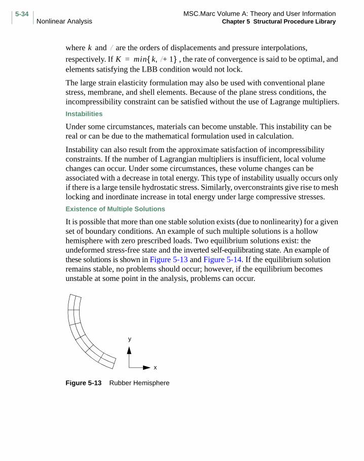
MSC.Marc Volume A: Theory and User InformationNonlinear Analysis Chapter 5 Structural Procedure Library
5-34
where and are the orders of displacements and pressure interpolations,
respectively. If , the rate of convergence is said to be optimal, and elements satisfying the LBB condition would not lock.
The large strain elasticity formulation may also be used with conventional plane stress, membrane, and shell elements. Because of the plane stress conditions, the incompressibility constraint can be satisfied without the use of Lagrange multipliers.
Instabilities
Under some circumstances, materials can become unstable. This instability can be real or can be due to the mathematical formulation used in calculation.
Instability can also result from the approximate satisfaction of incompressibility constraints. If the number of Lagrangian multipliers is insufficient, local volume changes can occur. Under some circumstances, these volume changes can be associated with a decrease in total energy. This type of instability usually occurs only if there is a large tensile hydrostatic stress. Similarly, overconstraints give rise to mesh locking and inordinate increase in total energy under large compressive stresses.
Existence of Multiple Solutions
It is possible that more than one stable solution exists (due to nonlinearity) for a given set of boundary conditions. An example of such multiple solutions is a hollow hemisphere with zero prescribed loads. Two equilibrium solutions exist: the undeformed stress-free state and the inverted self-equilibrating state. An example of these solutions is shown in Figure 5-13 and Figure 5-14. If the equilibrium solution remains stable, no problems should occur; however, if the equilibrium becomes unstable at some point in the analysis, problems can occur.
Figure 5-13 Rubber Hemisphere
k
K min k 1+, =
y
x

5-35MSC.Marc Volume A: Theory and User InformationChapter 5 Structural Procedure Library Nonlinear Analysis
Figure 5-14 Inverted Rubber Hemisphere
When incompressible material is being modeled, the basic linearized incremental procedure is used in conjunction with mixed variational principles similar in form to the Herrmann incompressible elastic formulation. These formulations are incorporated in plane strain, axisymmetric, generalized plane strain, and three-dimensional elements. These mixed elements may be used in combination with other elements in the library (suitable tying may be necessary) and with each other. Where different materials are joined, the pressure variable at the corner nodes must be uncoupled to allow for mean pressure discontinuity. Tying must be used to couple the displacements only.
Large Strain Plasticity
In recent years there has been a tremendous growth in the analysis of metal forming problems by the finite element method. Although an Eularian flow-type approach has been used for steady-state and transient problems, the updated Lagrangian procedure, pioneered by McMeeking and Rice, is most suitable for analysis of large strain plasticity problems. The main reasons for this are: (a) its ability to trace free boundaries, and (b) the flexibility of taking elasticity and history effects into account. Also, residual stresses can be accurately calculated.
y
x

MSC.Marc Volume A: Theory and User InformationNonlinear Analysis Chapter 5 Structural Procedure Library
5-36
The large strain plasticity capability in Marc allows you to analyze problems of large-strain, elastic-plastic material behavior. These problems can include manufacturing processes such as forging, upsetting, extension or deep drawing, and/or large deformation of structures that occur during plastic collapse. The analysis involves both material, geometric and boundary nonlinearities.
In addition to the options required for plasticity analysis, the LARGE DISP, UPDATE, and FINITE parameters are needed for large strain plasticity analysis.
In performing finite deformation elastic-plastic analysis, there are some special considerations which do not apply for linear elastic analysis. These considerations include:
• Choice of Finite Element Types
• Nearly Incompressible Behavior
• Treatment of Boundary Conditions
• Severe Mesh Distortion
• Instabilities
Choice of Finite Element Types
Accurate calculation of large strain plasticity problems depends on the selection of adequate finite element types. In addition to the usual criteria for selection, two aspects need to be given special consideration: the element types selected need to be insensitive to (strong) distortion; for plane strain, axisymmetric, and three-dimensional problems, the element mesh must be able to represent nondilatational (incompressible) deformation modes.
Nearly Incompressible Behavior
Most finite element types tend to lock during fully plastic (incompressible) material behavior. A remedy is to introduce a modified variational principle which effectively reduces the number of independent dilatational modes (constraints) in the mesh. This procedure is successful for plasticity problems in the conventional “small” strain formulation. Zienkiewicz pointed out the positive effect of reduced integration for this type of problem and demonstrates the similarity between modified variational procedures and reduced integration. MSC.Software Corporation recommends the use of lower-order elements, invoking the constant dilatation option. The lower-order elements, which use reduced integration and hourglass control, also behave well for nearly incompressible materials.

5-37MSC.Marc Volume A: Theory and User InformationChapter 5 Structural Procedure Library Nonlinear Analysis
Treatment of Boundary Conditions
In many large strain plasticity problems, specifically in the analysis of manufacturing processes, the material slides with or without friction over curved surfaces. This results in a severely nonlinear boundary condition. The Marc gap-friction element and CONTACT option can model such sliding boundary conditions.
Severe Mesh Distortion
Because the mesh is attached to the deforming material, severe distortion of the element mesh often occurs, which leads to a degeneration of the results in many problems. The ERROR ESTIMATE option can be used to monitor this distortion. To avoid this degeneration, generate a new finite element mesh for the problem and then transfer the current deformation state to the new finite element mesh. The rezoning procedure in the program is specifically designed for this purpose.
Instabilities
Elastic-plastic structures are often unstable due to necking phenomena. Consider a rod of a rigid-plastic incompressible workhardening material. With the current true uniaxial strain rate and the current workhardening, the rate of true uniaxial stress is equal to
(5-39)
The applied force is equal to , where is the current area of the rod. The rate of the force is therefore equal to
(5-40)
On the other hand, conservation of volume requires that
(5-41)
Hence, the force rate can be calculated as
(5-42)
Instability clearly occurs if . For applied loads (as opposed to applied boundary conditions), the stiffness matrix becomes singular (nonpositive definite).
For the large strain plasticity option, the workhardening slope for plasticity is the rate of true stress versus the true plastic strain rate. The workhardening curve must, therefor, be entered as the true stress versus the logarithmic plastic strain in a uniaxial tension test.
ε·
h σ
σ· Hε·=
F σA= A
F·
σ· A σA·
+=
Aε· A·
+ 0=
F·
H σ–( )Aε·=
σ H>

MSC.Marc Volume A: Theory and User InformationNonlinear Analysis Chapter 5 Structural Procedure Library
5-38
With the updated Lagrangian option, you cannot use the anisotropic plasticity formulation, but you can use anisotropic elastic properties.
Computational Procedures for Elastic-Plastic Analysis
Three basic procedures for plasticity exist in Marc. In this section, the variational form of equilibrium equations and constitutive relations, and incompressibility are summarized. Issues regarding return mapping procedures for stress calculation in three-dimensional and plane-stress conditions are also discussed.
For notational purpose, three configurations are considered at any point, original ( ), previous ( ) and current ( ). An iterative procedure, full or modified Newton-Raphson, secant, or arc-length is used to solve for the equilibrium at .
1. Small Strain Plasticity (reference configuration: ):In this approach, the basis of variational formulation are 2nd Piola-Kirchhoff stress, and Green-Lagrange strain, . Equilibrium of the current state can thus be represented by the following virtual work principle:
(5-43)
During the increment, all state variables are defined with respect to the state at and are updated at the end of increment upon convergence.
The linearized form of constitutive equations is given as:
(5-44)
in which is the second Piola-Kirchhoff stress, is the Cauchy stress, and
is the elasto-plastic moduli. This linearization has the advantage that it is fully independent of the rotation increment, but the disadvantage is that the linearization causes errors equal to the square of the strain increment. Moreover, imposing the incompressibility condition in terms of the trace of Green-Lagrange strains leads to errors in the form of fictitious volume changes in fully developed plastic flow.
The above procedure works well in the context of small strain plasticity. However, in many large deformation problems including metal forming processes, the plastic strain increments can be very large and the above
t 0= t n= t n 1+=
t n 1+=
t 0=
S E
S : δE Vd
Vn
∫ t : δη dA b : δη Vd
Vn
∫+An
∫=
t n=
dS Lep
: dE σ.dE– dE.σ–=
S σ
Lep
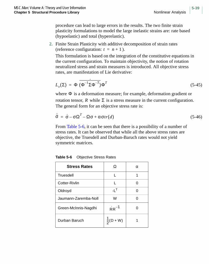
5-39MSC.Marc Volume A: Theory and User InformationChapter 5 Structural Procedure Library Nonlinear Analysis
procedure can lead to large errors in the results. The two finite strain plasticity formulations to model the large inelastic strains are: rate based (hypoelastic) and total (hyperelastic).
2. Finite Strain Plasticity with additive decomposition of strain rates (reference configuration: ).
This formulation is based on the integration of the constitutive equations in the current configuration. To maintain objectivity, the notion of rotation neutralized stress and strain measures is introduced. All objective stress rates, are manifestation of Lie derivative:
(5-45)
where is a deformation measure; for example, deformation gradient or
rotation tensor, while is a stress measure in the current configuration. The general form for an objective stress rate is:
(5-46)
From Table 5-6, it can be seen that there is a possibility of a number of stress rates. It can be observed that while all the above stress rates are objective, the Truesdell and Durban-Baruch rates would not yield symmetric matrices.
Table 5-6 Objective Stress Rates
Stress Rates Ω α
Truesdell L 1
Cotter-Rivlin L 0
Oldroyd -LT 0
Jaumann-Zaremba-Noll W 0
Green-McInnis-Nagdhi 0
Durban Baruch 1
t n 1+=
Lv Σ( ) Φ Φ 1– ΣΦ T–( )·
ΦT=
ΦR Σ
∇σ σ· σΩT– Ωσ– ασ tr d( )+=
R·R
1–
12--- D W+( )

MSC.Marc Volume A: Theory and User InformationNonlinear Analysis Chapter 5 Structural Procedure Library
5-40
Marc’s implementation of rate formulation involves the use of Jaumann rate of Cauchy stress which is obtained as an average of the Oldroyd and Cotter-Rivlin stress rates. Thus, the Jaumann rate can be written as:
(5-47)
(5-48)
where ( ) is the ordinary rate and ( ) is the objective rate with is the spin
or the antisymmetric part of the velocity gradient, . The last term is neglected because of the incompressible nature of plasticity.
The equilibrium in the current state is given by the virtual work principle at :
(5-49)
Linearization of the above form leads to the variational statement:
(5-50)
where,
(5-51)
Within the context of rotation neutralized form of constitutive relations,
is defined as:
(5-52)
where, . Also, the rotation neutralized strain can be calculated by:
(5-53)
with being the mid-increment strain, a good approximation for incremental logarithmic strain measure.
∇σ σ· Wσ– σW+=
∇σ σ· ΩT σ σ Ω tr dε( )σ+⋅+⋅+=
∇W
L
t n 1+=
σ : δε vd
Vn+1
∫ t . δηda b . δη vd
Vn+1
∫+An+1
∫=
dσ : δε 2 dε σ⋅( ) : δε– tr dε( )σ : δε σ : ∇ u( ) ∇ η( )T⋅ ]+ +[ vdVn+1
∫ =
d b . δη v t . δη adAn+1
∫+dVn+1
∫
σVn+1
∫ : δε dv–
dσ R dσRNR
T⋅ ⋅=
dσRN
dσRNL
RN : dεRN
=
dεRNR
Tdε R⋅⋅=
εRNU I+( ) T–
F I+( )εMIDF I+( ) U I+( ) 1–
=
εMID

5-41MSC.Marc Volume A: Theory and User InformationChapter 5 Structural Procedure Library Nonlinear Analysis
Where is the engineering strain and is the stretch tensor
obtained by the polar decomposition of . Admitting an error of the order of in the approximation of the logarithmic strain, one obtains:
(5-54)
where (5-55)
During computations, the third term of Equation 5-50, , is neglected due to its nonsymmetric nature.
In a fully developed plastic flow, the volumetric part of the energy can become extremely large and lead to volumetric locking. Hence, a special treatment of incompressibility is done to relax the volumetric constraint in an assumed strain format. The volumetric part of deformation gradient is modified such that, the assumed deformation gradient is:
(5-56)
Linearization of in the original state relates it to the displacement gradients in the current state as:
(5-57)
where,
(5-58)
where the first two terms are evaluated at each integration point and the last term is averaged over the element.
For a lower order element, the procedure leads to mean or constant dilatation approach. Considering Equation 5-50 to Equation 5-58 the resulting system can be expressed as:
(5-59)
e U I–= U
Fe.e
dσ Lep
: dε=
Lep
R R LRN
RT⋅ ⋅( ) R
T⋅ ⋅=
tr dε( ) σ : δε⋅
J
13---
J
13---–
F=
F
DF ∇ ∆ u( ) F=
∇ ∆ u( ) ∆u( )i j,13--- div ∆u( ) δij–
13--- div ∆u( ) δij+=
∇ s
η : Lep
: ∇ s
∆u( ) 2∇ s
η σ : ∇ s
∆u( )⋅ σ : ∇ ∆ u( ) ∇η( )T
⋅+–[ ] vd
Vn+1
∫ =
d b . δη v t . δη adAn+1
∫+dVn+1
∫
∇ s
η[ ]T : σ vd
Vn 1+
∫–

MSC.Marc Volume A: Theory and User InformationNonlinear Analysis Chapter 5 Structural Procedure Library
5-42
5Structural Procedure Library
Nonlinear Analysis
In the event, the elastic strains become large in an elastic-plastic analysis the rate based constitutive equations do not accurately model the material response. This results from the fact that the elasticity matrix are assumed to have constant coefficients in the current deformed configuration.
In the next formulation, the rate of deformation tensor is decomposed multiplicatively into the elastic and plastic parts to resolve these problems.
3. Finite strain plasticity with multiplicative decomposition of deformation gradient.
An alternative formulation, based on the multiplicative decomposition of the deformation gradient has been implemented in Marc, namely:
(5-60)
where , , and are (elastic, thermal, and plastic) deformation gradients, respectively. The thermo-mechanical coupling is implemented using the staggered approach.
The above decomposition has a physical basis to it as the stresses are derived from quadratic - logarithmic strain energy density function:
(5-61)
This function has been chosen due to the availability of the material coefficients from material testing in a small strain case.
In the metal forming applications, the elastic strains are negligible and the rate-based (or hypoelastic) as well as the total (or hyperelastic) form of constitutive equations give virtually the same results. However, many polymers, metals subjected to large hydrostatic pressures, high velocity impact loading of metals and processes, where shape changes after deformation need to be evaluated precisely, the hyperelastic formulation yields physically more meaningful results.
The return mapping procedure for the calculation of stresses is based on the radial return procedure. With the use of exponential mapping algorithm, the incompressibility condition is imposed exactly:
(5-62)
F FeF
θF
p=
Fe
Fθ
Fp
W12---λ J
eln( )
2µ tr
12--- b
eln
2+=
det Fp
1=

5-43MSC.Marc Volume A: Theory and User InformationChapter 5 Structural Procedure Library Nonlinear Analysis
The strain energy is separated into deviatoric and volumetric parts in the framework of mixed formulation. The general form of three-field variational principle is:
(5-63)
where, (5-64)
and are the deviatoric and elastic volumetric parts of the free
energy, p is the pressure, and are elastic pointwise and average elastic Jacobian of the element, respectively. The volumetric free energy can be of any form in Equation 5-62. However, if the incompressibility is enforced in a pointwise fashion and the volumetric free energy is assumed to be of the form:
(5-65)
the perturbed Lagrangian form of the variational principle can be cast in a two-field framework as:
(5-66)
Note that , hence, P is not the true pressure in Equation 5-66. Choice of the volumetric free energy in Equation 5-65 is not arbitrary and is described in more detail in Chapter 7 in the Elastomer section.
Linearization of the equilibrium condition arising from the stationary of the variational principle Equation 5-66, yields:
π u p J, ,( ) [WV0
∫ b( ) U J e
( ) p Je
J e
–( )]+ += dV
b J
23---–
b=
W b( ) U J e
( )
Je
J e
U Je( ) 9
2---K J
e( )
13---
1–
2
=
π u P,( ) W b( ) 3P Je( )
13---
1– P
2
2K-------–+ Vd
V0
∫=
P p Je( )
23---
=

MSC.Marc Volume A: Theory and User InformationNonlinear Analysis Chapter 5 Structural Procedure Library
5-44
(5-67)
The linearization of the constraint equation defines the term in Equation 5-67.
The derivation of the spatial tangent follows by a push forward of the material tangent into the current configuration:
Hence, (5-68)
where S is the pull back of the deviatoric Kirchhoff stress tensor. Assuming the entire incremental deformation to be elastic, a symmetric stress tensor,
can be defined with respect to a fixed plastic intermediate configuration
as:
(5-69)
also noting that,
where (5-70)
(5-71)
where (5-72)
and (5-73)
∇ sη : 1J--- Cdev P J
e( )
13---
13---1 1 2I–⊗
+
: ∇ su +
Vn+1
∫
σ : ∇ ∆ u( )( ). ∇η( )T dPJ
------- Je( )
13---
1 : ∇η+ dv =
d bVn+1
∫ . δη v tAn+1
∫ . δη ad+d
∇ sη( )T
Vn+1
∫ : σ vd–
dP
Cdev
S F1– τdev
FT–
=
S
Fnp
S Fetr( )
1–τdev
Fetr( )
T–=
S SANA NA⊗A 1=
3
∑= SAβA
λAetr( )
2---------------=
dS dSA NA NA SB SA–( ) ΩBA NA NB⊗B A≠
3
∑A 1=
3
∑+⊗A 1=
3
∑=
dSA1
λAetr( )
2λBe
tr( )2
-------------------------------- ∂βA
∂εBetr
----------- 2βA δAB–
λBetr
dλBetr
=
dNA ΩAB NB=

5-45MSC.Marc Volume A: Theory and User InformationChapter 5 Structural Procedure Library Nonlinear Analysis
similarly, with (5-74)
(5-75)
The algorithmic elasto-plastic tangent can be obtained as:
(5-76)
Combining Equation 5-71, Equation 5-76, and Equation 5-77, the spatial form of deviatoric part of the tangent as:
(5-77)
The singularity for two- or three-equal stretch ratios is removed by repeated application of L’Hospital’s rule. Due to separate interpolation of the pressure, a larger system of equations needs to be solved. A static condensation of the element variables is carried out before going in the solver. This step renders the singularity of the system to be inversely proportional to the bulk modulus of the material. Due to the multiplicative split of the deformation gradient and an additive split of the free energy into deviatoric and volumetric parts, this framework is eminently suitable for implementation of general nonlinear elastic as well as inelastic material models. Besides, compressible and nearly incompressible material response can be naturally handled.
C Fetr( )
TFe
tr= Fe
tr λAetr
nA NA⊗A 1=
3
∑=
dC 2λBetr
dλBetr
NB NB +⊗B 1=
3
∑=
λBetr( )
2λBe
tr( )2
–
ΩBA NA NB⊗B A≠
3
∑A 1=
3
∑
Cdev 2F F∂S∂C-------F
T
F
T2 Fe
tr( ) Fetr( ) ∂S
∂C------- Fe
tr( )TFe
tr( )T= =
Cdev
∂βA
∂εBetr
----------- 2βAδAB–
nA nA nB nB⊗ ⊗ ⊗B A≠
3
∑A 1=
3
∑=
λAetr( )
2βB λBe
tr( )2βA–
λBetr( )
2λAe
tr( )2
–--------------------------------------------------- nA( nB nA nB +⊗ ⊗ ⊗
B A≠
3
∑A 1=
3
∑+
nA nB nB nA )⊗ ⊗ ⊗

MSC.Marc Volume A: Theory and User InformationNonlinear Analysis Chapter 5 Structural Procedure Library
5-46
Finally, the stress calculation is done via return mapping to the yield surface. There are several methods to return the stress. Among them, the popular ones include:
Closest point projection (which reduces to radial return for von Mises), mean normal approach, midpoint rule, trapezoidal rule, and tangent cutting plane algorithm.
Krieg and Krieg (1977) investigated the radial return algorithm which has been proposed by Wilkins (1964). The third algorithm analyzed was the so-called secant stiffness method proposed by Rice and Tracy (1973) which represented a special case of the generalized Trapezoidal rule for nonhardening materials algorithm in contrast to the fully implicit radial return algorithm and the fully explicit tangent stiffness approach. The radial return method (shown in Figure 5-15) was found to be the most accurate among the three analyzed, particularly when large strain increments were used. The radial return and mean normal method are available in Marc and are described next.
Figure 5-15 Radial Return Method
σfinal σ*
σ3′σ2
′
σ1′
∆σe

5-47MSC.Marc Volume A: Theory and User InformationChapter 5 Structural Procedure Library Nonlinear Analysis
1. Closest Point Projection procedure:
The closest point projection or the backward Euler algorithm reduces to a radial return scheme for cases where there is no anisotropy or plane stress condition. The trial stress is determined as:
(5-78)
The final stress state is obtained by simply scaling the trial stress by a scale factor,
where, (5-79)
the plastic consistency parameter , is obtained by solving for consistency condition iteratively.
An explicit form of the material tangent for the isotropic, von Mises yield surface can be given as:
(5-80)
where, (5-81)
Here is the return direction normal to the current yield surface. For the plane stress case, the zero normal stress condition is explicitly imposed in the yield condition. Since the yield surface is not a circle in the plane, the return direction is not radial anymore.
2. Mean-Normal method:
Assuming the entire deformation to be elastic in nature, the trial stress is evaluated as:
(5-82)
Due to the use of pressure independent yield function, only the deviatoric stresses are evaluated. As shown in Figure 5-16, represents the fraction of strain increment for which the plastic flow occurs.
σdrr σd 2G∆εd+=
β
β 12G∆λ
σdrr
---------------–=
∆λ
Lep
2G β I13---1 1⊗–
2G γ N N⊗–=
γ 1
1H
3G-------+
----------------- 1– β+=
N
σdmn σd 2αG∆εd 1 α–( )G∆εd++=
1 α–( )

MSC.Marc Volume A: Theory and User InformationNonlinear Analysis Chapter 5 Structural Procedure Library
5-48
Figure 5-16 Mean-Normal Method
includes the deviatoric stresses at the previous increment scaled such
that it satisfies the yield condition. The yield criterion might not be exactly satisfied due to temperature effects, numerical integration of elastic-plastic relationships, or accumulated numerical inaccuracy.
indicates that the stress state is exactly on the yield surface. If
, scale by a factor such that:
(5-83)
The equivalent plastic strain, plastic strain tensor and the elasto-plastic moduli are obtained as:
(5-84)
(5-85)
(5-86)
σfinal
σo
σ*
∆σe
σ* + σo + ∆σe
σ′1
σ′2 σ′3
σd
F σ( ) 0=
F σ( ) 0> σ λ
F λσ( ) 0 0 λ 1< <=
∆εp Ce : N : ∆ε 1 α–( )
N : C : N H+---------------------------------------------=
∆εp ∆εp N=
Lep
Ce
1 α–( ) C
e : N( ) C
e : N( )⊗
N : Ce : N H+
------------------------------------------------–=

5-49MSC.Marc Volume A: Theory and User InformationChapter 5 Structural Procedure Library Nonlinear Analysis
where, is the mean-normal direction to the yield surface, is the
hardening modulus and is the elastic tangent moduli.
Ortiz and Popov (1985) introduced two rather general classes of return algorithms – the generalized midpoint and the generalized trapezoidal rules (shown in Figure 5-17). The stability and accuracy analysis of these two classes of algorithms yielded the result that either method is unconditionally stable for values of the algorithmic parameter ,
while being second-order accurate for . The parameter can vary from 0 to 1 and indicates to which degree the return algorithm is based on information from the previous stress state (explicit) or the stress state to be determined (implicit). For a value of , the resulting algorithm would be the fully explicit member of the algorithm family; while for
, the fully implicit variant is recovered. For nonhardening materials, the mean normal algorithm is a special case of trapezoidal rule. Numerical examples, however, indicated that, for large time steps, larger values for yielded more accurate and stable results. This finding is in general agreement with earlier analyses determining the radial return method, a fully implicit algorithm, to be more accurate than other explicit ( ) or
midpoint algorithms.
Figure 5-17 Generalized Trapezoidal Rule with Isotropic Hardening for Plane Stress
N H
Ce
α 1 2⁄≤α 1 2⁄= α
α 0=
α 1=
α
α 0=
α 12---=
σ2Ni
σi
σt
1 α–( )Ni
σi 1+αNi 1+
σ1

MSC.Marc Volume A: Theory and User InformationNonlinear Analysis Chapter 5 Structural Procedure Library
5-50
Marc plasticity algorithms are unconditionally stable and accurate for moderate strain increments. However, overall global stability of the system can be dictated by other considerations like contact, buckling which then guide the selection of appropriate load increment size. It should also be recognized that the algorithmically consistent tangent in the closest point projection algorithm is based on the current state, and a lack of embedded directionality (unlike secant methods) in the tangent can lead to divergent solutions unless line search or automatic time stepping algorithms are used. However, when it converges it shows quadratic convergence as compared to linear convergence for the mean-normal scheme.
CREEP
Creep is a time-dependent inelastic behavior that can occur at any stress level, either below or above the yield stress of a material. Creep is an important factor at elevated temperatures.
Marc offers the following options to be used in conjunction with creep analysis:
• Creep data can be entered directly through data input or user subroutine.
• Creep behavior can be either isotropic or anisotropic.
• The Oak Ridge National Laboratory (ORNL) rules on creep can be activated.
• An automatic time stepping scheme maximizes the time step size in the analysis.
• Eigenvalues can be extracted for the estimation of creep buckling time.
• Use parameter CREEP to activate the CREEP analysis option in Marc.
Input the creep time period and control tolerance information through the history definition option AUTO CREEP. This option can be used repeatedly to define a new creep time period and new tolerances.
Creep analysis is often carried out in several runs using the RESTART option. Save restart files for continued analysis. The REAUTO option allows you to reset the parameters defined in the AUTO CREEP option upon restart.
Adaptive Time Control
The AUTO CREEP option takes advantage of the diffusive characteristics of most creep solutions. Specifically, this option controls the transient creep analysis. You specify a period of creep time and a suggested time increment. The program automatically selects the largest possible time increment that is consistent with the tolerance set on stress and strain increments (see Creep Control Tolerances in this chapter).

5-51MSC.Marc Volume A: Theory and User InformationChapter 5 Structural Procedure Library Nonlinear Analysis
The algorithm is: for a given time step , a solution is obtained. Marc then finds the
largest values of stress change per stress, , and creep strain change per elastic
strain, . It compares these values to the tolerance values, (stress change
tolerance) and (strain change tolerance), for this period.
The value is calculated as the larger of
(5-87)
If , the program resets the time step as
(5-88)
The time increment is repeated until convergence is obtained or the maximum recycles control is exceeded. In the latter case, the run is ended.
If the first repeat does not satisfy tolerances, the possible causes are:
• excessive residual load correction
• strong additional nonlinearities such as creep buckling-creep collapse
• incorrect coding in user subroutine CRPLAW, VSWELL, or UVSCPL.
Appropriate action should be taken before the solution is restarted.
If , the solution is stepped forward to and the next step is begun. The time step used in the next increment is chosen as
(5-89)
(5-90)
(5-91)
Since the time increment is adjusted to satisfy the tolerances, it is impossible to predetermine the total number of time increments for a given total creep time.
∆t
∆σ σ⁄
∆εcr εel⁄ Ts
Te
p
∆σ σ⁄( ) Tσ⁄
∆εcr εel⁄( ) Tε⁄or
p 1>
∆tnew 0.8 ∆told p⁄=
p 1< t ∆t+
∆tnew ∆told= if 0.8 < p < 1
∆tnew 1.25 ∆told= if 0.65 < p< 0.8
∆tnew 1.5 ∆told= if p < 0.65

MSC.Marc Volume A: Theory and User InformationNonlinear Analysis Chapter 5 Structural Procedure Library
5-52
Creep Control Tolerances
Marc performs a creep analysis under constant load or displacement conditions on the basis of a set of tolerances and controls you provide.These are as follows:
1. Stress change tolerance – This tolerance controls the allowable stress change per time step during the creep solution, as a fraction of the total stress at a point. Stress change tolerance governs the accuracy of the transient creep response. If you need accurate tracking of the transient response, specify a tight tolerance of 1 percent or 2 percent stress change per time step. If you need only the steady-state solution, supply a relatively loose tolerance of 10-20 percent. It is also possible to check the absolute rather than the relative stress.
2. Creep strain increment per elastic strain – Marc uses either explicit or implicit integration of the creep rate equation. When the explicit procedure is used, the creep strain increment per elastic strain is used to control stability. In almost all cases, the default of 50 percent represents the stability limit, so that you need not provide any entry for this value. It is also possible to check the absolute rather than the relative strain.
3. Maximum number of recycles for satisfaction of tolerances – During AUTO CREEP, Marc chooses its own time step. In some cases, the program recycles to choose a time step that satisfies tolerances, but recycling rarely occurs more than once per step. Excessive recycling can be caused by physical problems such as creep buckling, poor coding of user subroutine CRPLAW, VSWELL, or UVSCPL or excessive residual load correction that can occur when the creep solution begins from a state that is not in equilibrium.
The maximum number of recycles allows you to avoid wasting machine time under such circumstances. If there is no satisfaction of tolerances after the attempts at stepping forward, the program stops. The default of five recycles is conservative in most cases.
4. Low stress cut-off – Low stress cut-off avoids excessive iteration and small time steps caused by tolerance checks that are based on small (round off) stress states. A simple example is a beam in pure bending. The stress on the neutral axis is a very small roundoff-number, so that automatic time stepping scheme should not base time step choices on tolerance satisfaction at such points. The default of five percent of the maximum stress in the structure is satisfactory for most cases.

5-53MSC.Marc Volume A: Theory and User InformationChapter 5 Structural Procedure Library Nonlinear Analysis
5. Choice of element for tolerance checking – Creep tolerance checking occurs as a default for all integration points in all elements. You might wish to check tolerances in only 1 element or in up to 14 elements of your choice. Usually, the most highly stressed element is chosen.
When you enter the tolerances and controls, the following conventions apply:
• All stress and strain measures in tolerance checks are second invariants of the deviatoric state (that is, equivalent von Mises uniaxial values).
• You can reset all tolerances and controls upon the completion of one AUTO CREEP sequence.
Background Information
Creep behavior is based on a von Mises creep potential with isotropic behavior described by the equivalent creep law:
(5-92)
The material behavior is therefore described by:
(5-93)
where is the outward normal to the current von Mises stress surface and is
the equivalent creep strain rate.
There are two numerical procedures used in implementing creep behavior. The default is an explicit procedure in which the above relationship is implemented in the program by an initial strain technique. In other words, a pseudo-load vector due to the creep strain increment is added to the right-hand side of the stiffness equation.
(5-94)
where is the stiffness matrix, and and are incremental displacement and incremental nodal force vectors, respectively. The integral
(5-95)
ε· cr
f σ εcr T t, , ,( )=
∆εcr ε· cr ∂σ
∂σ′--------=
∂σ∂σ′-------- ε· cr
K∆u ∆P βTD∆εcrdvV∫+=
K ∆u ∆P
βTD∆εcrdvV∫

MSC.Marc Volume A: Theory and User InformationNonlinear Analysis Chapter 5 Structural Procedure Library
5-54
is the pseudo-load vector due to the creep strain increment in which is the strain
displacement relation and is the stress-strain relation.
As an alternative, an implicit creep procedure can be requested with the CREEP parameter. In this case, the effect inelastic strain rate has an influence on the stiffness matrix. Using this technique, significantly larger steps in strain space can be used.
Creep Buckling
Marc also predicts the creep time to buckling due to stress redistribution under given load or repeated cyclic load.
The buckling option solves the following equation for the eigenvalue
(5-96)
The geometric stiffness matrix, , is a function of the increments of stress and
displacement. These increments are calculated during the last creep time step increment. To determine the creep time to buckle, perform a buckle step after a converged creep increment. Note that the incremental time must be scaled by the calculated eigenvalue, and added to the total (current) time to get an estimate as to when buckling occurs.
AUTO THERM CREEP (Automatic Thermally Loaded Elastic-Creep/Elastic-Plastic-Creep Stress Analysis)
The AUTO THERM CREEP option is intended to allow automatic, thermally loaded elastic-creep/elastic-plastic-creep stress analysis, based on a set of temperatures defined throughout the mesh as a function of time. The temperatures and transient times are presented to the program through the CHANGE STATE option, using input option 3 (post file), and the program creates its own set of temperature steps (increments) based on a temperature change tolerance provided in this option. The times at all temperature steps are calculated by the program for creep analyses.
At each temperature step (increment), an elastic/elastic-plastic analysis is carried out first to establish stress levels in the structure. A creep analysis is performed next on the structure for the time period between current and previous temperature steps (increments). Both the elastic/elastic-plastic stress and the creep analyses are repeated until the total creep time provided in this option is reached. Convergence controls are provided on the CONTROL option for elastic-plastic analysis and in the AUTO THERM CREEP option for creep analysis. The analysis can be restarted at temperature steps (increments) or at creep steps (subincrements). The results can be saved on a post file (POST option) for postprocessing.
βD
K λKG+( )Φ 0=
KG

5-55MSC.Marc Volume A: Theory and User InformationChapter 5 Structural Procedure Library Nonlinear Analysis
If no DIST LOADS, POINT LOAD, or PROPORTIONAL INCREMENT option appears with the AUTO THERM CREEP set, all mechanical loads and kinematic boundary conditions are held constant during the AUTO THERM CREEP. However, DIST LOADS, POINT LOAD, PROPORTIONAL INCREMENT, or DISP CHANGE can be included in the set – the mechanical loads and kinematic boundary conditions which are then defined are assumed to change in proportion to the time scale of the temperature history defined by the CHANGE STATE option and are applied accordingly. This is based on the fact that the increments of load and displacement correspond to the end of the transient time of the AUTO THERM CREEP input.
Viscoelasticity
In a certain class of problems, structural materials exhibit viscoelastic behavior. Two examples of these problems are quenching of glass structures and time-dependent deformation of polymeric materials. The viscoelastic material retains linearity between load and deformation; however, this linear relationship depends on time. Consequently, the current state of deformation must be determined from the entire history of loading. Different models consisting of elastic elements (spring) and viscous elements (dashpot) can be used to simulate the viscoelastic material behavior described in Chapter 7. A special class of temperature dependence known as the Thermo-Rheologically Simple behavior (TRS) is also applicable to a variety of thermal viscoelastic problems. Both the equation of state and the hereditary integral approaches can be used for viscoelastic analysis.
To model the thermo-rheologically simple material behavior, the SHIFT FUNCTION model definition option can be used to choose the Williams-Landel-Ferry equation or the power series expression or Narayanaswamy model.
In Marc, two options are available for small strain viscoelastic analysis. The first option uses the equation of state approach and represents a Kelvin model. The second option is based on the hereditary integral approach and allows the selection of a generalized Maxwell model. The thermo-rheologically simple behavior is also available in the second option for thermal viscoelastic analysis. The Time-Independent Inelastic Behavior section in Chapter 7 discusses these models in detail. Automatic time stepping schemes AUTO CREEP and AUTO TIME can be used in a viscoelastic analysis for first and second options, respectively.
The first option for viscoelastic analysis uses the Kelvin model. To activate the generalized Kelvin model in Marc, use the VISCO ELAS or CREEP parameter. To input the matrices [A] and [B] for the Kelvin strain rate computations, use the user subroutine CRPVIS. To input creep time period and the tolerance control for the maximum strain in an increment, use the history definition option AUTO CREEP.
MSC.Marc Volume A: Theory and User InformationNonlinear Analysis Chapter 5 Structural Procedure Library
5-56
Simo model for large strain viscoelasticity can be used in conjunction with the damage and hyperelastic Mooney or Ogden material model. The large strain viscoelastic material behavior can be simulated by incorporating the model definition option VISCELMOON or VISCELOGDEN. Viscoelasticity for hyperelastic materials is available only in the total Lagrangian framework.
Nonlinear structural relaxation behavior of materials can be modeled by the Narayanaswamy model which accounts for memory effect. This model allows simulation of evolution of physical properties of glass subjected to complex time temperature histories. The thermal expansion behavior for the Narayanaswamy model is controlled via the model definition option VISCEL EXP.
Viscoplasticity
There are two procedures in Marc for viscoplastic analysis: explicit and implicit. A brief description of each procedure follows:
Explicit Method
The elasto-viscoplasticity model in Marc is a modified creep model to which a plastic element is added. The plastic element is inactive when the stress is less than the yield stress of the material. You can use the elasto-viscoplasticity model to solve time-dependent plasticity and creep as well as plasticity problems with a nonassociated flow law.
The CREEP option in Marc has been modified to enable solving problems with viscoplasticity. The method is modified to allow solving elastic-plastic problems with nonassociated flow rules which result in nonsymmetric stress-strain relations if the tangent modulus method is used.
The requirements for solving the viscoplastic problem are:
• CREEP parameter and creep controls
• Load incrementation immediately followed by a series of creep increments specified by AUTO CREEP
• Use of user subroutine CRPLAW and/or user subroutine NASSOC
The following load incrementation procedure enables you solve a viscoplastic problem:
1. Apply an elastic load increment that exceeds the steady-state yield stress.2. Relieve the high yield stresses by turning on the AUTO CREEP option.
You may repeat steps 1 and 2 as many times as necessary to achieve the required load history.

5-57MSC.Marc Volume A: Theory and User InformationChapter 5 Structural Procedure Library Nonlinear Analysis
Note: The size of the load increments are not altered during the AUTO CREEP process so that further load increments can be effected by using the PROPORTIONAL INCREMENT option.
The viscoplastic approach converts an iterative elastic-plastic method to one where a fraction of the initial force vector is applied at each increment with the time step controls. The success of the method depends on the proper use of the automatic creep time step controls. This means that it is necessary to select an initial time step that will satisfy the tolerances placed on the allowable stress change.
The allowable stress change is specified in the creep controls. The most highly stressed element usually yields the maximum strain rate. It is also important to select a total time that gives sufficient number of increments to work off the effects of the initial force vector. A total time of 30 times the estimated ∆t is usually sufficient.
Marc does not distinguish between viscoplastic and creep strains. A user subroutine NASSOC allows you to specify a nonassociated flow rule for use with the equivalent creep strains (viscoplastic) that are calculated by subroutine CRPLAW. A flag is set in the CREEP parameter in order to use the viscoplastic option with a nonassociated flow rule.
The viscoplasticity feature can be used to implement very general constitutive relations with the aid of user subroutines ZERO and YIEL.
Since the viscoplasticity model in Marc is a modified creep model, you should familiarize yourself with the creep analysis procedure (see Nonlinear Analysis at the beginning of this chapter).Implicit Method
A general viscoplastic material law can be implemented through user subroutine UVSCPL. When using this method, you are responsible for defining the inelastic strain increment and the current stress.
The initial time step ∆t =allowable stress change x 0.7
Maximum viscoplastic strain rate x Young’s modulus

MSC.Marc Volume A: Theory and User InformationFracture Mechanics Chapter 5 Structural Procedure Library
5-58
Fracture Mechanics
Linear Fracture Mechanics
Linear fracture mechanics presupposes existence of a crack and examines the conditions under which crack growth occurs. In particular, it determines the length at which a crack propagates rapidly for specified load and boundary conditions. The concept of linear fracture mechanics stems from Griffith’s work on purely brittle materials. Griffith stated that, for crack propagation, the rate of elastic energy release should at least equal the rate of energy needed for creation of a new crack surface. This concept was extended by Irwin to include limited amounts of ductility. In Irwin’s considerations, the inelastic deformations are confined to a very small zone near the tip of a crack.
The basic concept presented by Griffith and Irwin is an energy balance between the strain energy in the structure and the work needed to create a new crack surface. This energy balance can be expressed using the energy release rate as
(5-97)
is defined as
(5-98)
where is the strain energy and is the crack length. depends on the geometry
of the structure and the current loading. is called the fracture toughness of the
material. It is a material property which is determined from experiments. Note that the energy release rate is not a time derivative but a rate of change in potential energy with crack length. An important feature of Equation 5-97 is that it can be used as a fracture criterion; a crack starts to grow when reaches the critical value .
The stress and strain fields near the tip of a crack are singular for a linear elastic material model. The stresses and strains have the principal form
(5-99)
G
G Gc=
G
GdΠda-------–=
Π a G
Gc
G Gc
σ K
r------ f θ( )=
ε K
r------g θ( )=

5-59MSC.Marc Volume A: Theory and User InformationChapter 5 Structural Procedure Library Fracture Mechanics
in a polar coordinate system centered at the crack tip. Thus, a linear elastic material is
said to have a singularity near a crack tip. It is easy to demonstrate that in both Griffith’s and Irwin’s considerations, the elastic energy release rate is determined by a single parameter: the strength of the singularity in the elastic stress field at the crack tip. This is the so-called stress intensity factor, and is usually denoted by capital .
The magnitude of depends on the crack length, the distribution and intensity of applied loads, and the geometry of the structure. Crack propagation occurs when any combination of these factors causes a stress intensity factor to be equal to or greater
than the experimentally determined material property , which is equivalent to
Equation 5-97. Hence, the objective of linear fracture mechanics calculations is to determine the value of .
There are three possible modes of crack extension in linear elastic fracture mechanics: the opening mode, sliding mode, and tearing mode (see Figure 5-18).
Figure 5-18 Irwin’s Three Basic Modes of Crack Extension
1 r⁄
K
K
K
Kc
K
(a) Mode I: Opening
x
z
y
(b) Mode II: Sliding
x
z
y
(c) Mode III: Tearing
x
z
y

MSC.Marc Volume A: Theory and User InformationFracture Mechanics Chapter 5 Structural Procedure Library
5-60
The opening mode (see Figure 5-18a), Mode I, is characterized by the symmetric separation of the crack surfaces with respect to the plane, prior to extension (symmetric with respect to the X-Y and X-Z planes).
The sliding mode, Mode II, is characterized by displacements in which the crack surfaces slide over one another perpendicular to the leading edge of the crack (symmetric with respect to the X-Y plane and skew-symmetric with respect to the X-Z plane).
The tearing mode, Mode III, finds the crack surfaces sliding with respect to one another parallel to the leading edge (skew-symmetric with respect to the X-Y and X-Z planes).
It is customary to associate a stress intensity factor with each of these mode: , ,
and . There is also an associated fracture toughness associated with each mode:
, , and . The most critical mode is usually mode I and in many cases the
other modes are not considered. The connection between the energy release rate and the stress intensity factors is given by
(5-100)
where
for plane stress (5-101)
and
for plane strain (5-102)
MSC.Marc uses the so-called J-integral for evaluating the energy release rate, see below. The J-integral is similar to G but is more general and is also used for nonlinear applications. J is equivalent to G when a linear elastic material model is used.
Nonlinear Fracture Mechanics
Nonlinear fracture mechanics is concerned with determining under which conditions crack propagation (growth) occurs. In this sense, nonlinear fracture mechanics is similar to linear fracture mechanics. However, there are additional questions addressed in nonlinear fracture mechanics. Is the crack propagation stable or unstable? If it is stable, at which speed does it occur? After some propagation, is the crack arrested?
KI KII
KIII
KIc KIIc KIIIc
GKI
2
E’------
KIII2
E’---------
1 ν+E
------------KIII2+ +=
E’ E=
E’E
1 ν2–--------------=
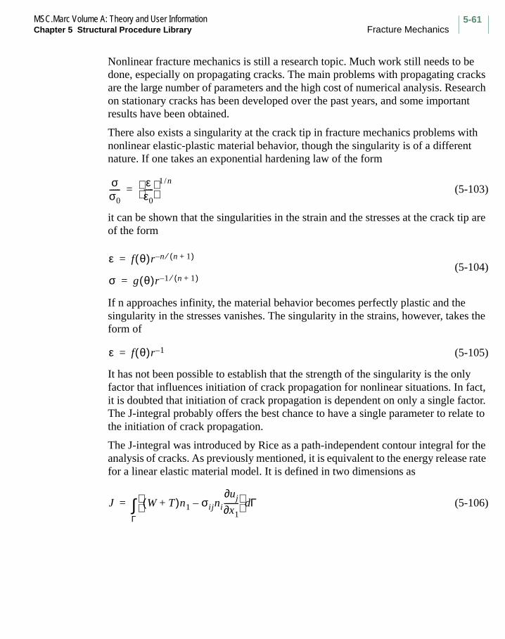
5-61MSC.Marc Volume A: Theory and User InformationChapter 5 Structural Procedure Library Fracture Mechanics
Nonlinear fracture mechanics is still a research topic. Much work still needs to be done, especially on propagating cracks. The main problems with propagating cracks are the large number of parameters and the high cost of numerical analysis. Research on stationary cracks has been developed over the past years, and some important results have been obtained.
There also exists a singularity at the crack tip in fracture mechanics problems with nonlinear elastic-plastic material behavior, though the singularity is of a different nature. If one takes an exponential hardening law of the form
(5-103)
it can be shown that the singularities in the strain and the stresses at the crack tip are of the form
(5-104)
If n approaches infinity, the material behavior becomes perfectly plastic and the singularity in the stresses vanishes. The singularity in the strains, however, takes the form of
(5-105)
It has not been possible to establish that the strength of the singularity is the only factor that influences initiation of crack propagation for nonlinear situations. In fact, it is doubted that initiation of crack propagation is dependent on only a single factor. The J-integral probably offers the best chance to have a single parameter to relate to the initiation of crack propagation.
The J-integral was introduced by Rice as a path-independent contour integral for the analysis of cracks. As previously mentioned, it is equivalent to the energy release rate for a linear elastic material model. It is defined in two dimensions as
(5-106)
σσ0------
εε0-----
1 n/=
ε f θ( )r n n 1+( )⁄–=
σ g θ( )r 1 n 1+( )⁄–=
ε f θ( )r 1–=
J W T+( )n1 σijni
uj∂x1∂
--------– Γd
Γ∫=

MSC.Marc Volume A: Theory and User InformationFracture Mechanics Chapter 5 Structural Procedure Library
5-62
5Structural Procedure Library
Fracture Mechanics
where is the strain energy density, is the kinetic energy density, is the stress
tensor and is the displacement vector. The integration path is a curve
surrounding the crack tip, see Figure 5-19.The J-integral is independent of the path as long as it starts and ends at the two sides of the crack face and no other singularities are present within the path. This is an important feature for the numerical evaluation since the integral can be evaluated using results away from the crack tip.
Figure 5-19 Definition of the J-integral
Numerical Evaluation of the J-integral
The J-integral evaluation in MSC.Marc is based upon the domain integration method as described in reference [1]. A direct evaluation of Equation 5-106 is not very practical in a finite element analysis due to the difficulties in defining the integration path . In the domain integration method for two dimensions, the line integral is
converted into an area integration over the area inside the path . This conversion is exact for the linear elastic case and also for the nonlinear case if the loading is proportional, that is, if no unloading occurs. By choosing this area as a set of elements, the integration is straightforward using the finite element solution. In two dimensions, the converted expression is
(5-107)
W T σij
ui Γ
Γ
Γ
ni
x
y
ΓΓ
J σij
uj∂x1∂
-------- Wδ1i– q1δ
xiδ-------- Ad
A∫=

5-63MSC.Marc Volume A: Theory and User InformationChapter 5 Structural Procedure Library Fracture Mechanics
for the simplified case of no thermal strains, body forces or pressure on the crack faces. For the general expression, see reference [Ref. 1]. A is the area inside and
is a function introduced in the conversion into an area integral. The function can
be chosen pretty generally, as long it is equal to one at the crack tip and zero on . The form of the function chosen in Marc is that it has the constant value of one at all nodes inside , and decreases to zero over the outermost ring of elements in . It can
be interpreted as a rigid translation of the nodes inside while the nodes on remain fixed. Thus, the contribution to Equation 5-107 comes only from the elements in a ring away from the crack tip. This interpretation is that of virtual crack extension and this method can be seen as a variant of such a technique, although it is extended with the effects of thermal strains, body forces, and pressure on the crack faces.The set of nodes moved rigidly is referred to as the rigid region and the function as the shift
function or shift vector.
In three dimensions, the line integral becomes an area integral where the area is surrounding a part of the crack front. In this case, the selection of the area is even more cumbersome than in two dimension. The converted integral becomes a volume integral which is evaluated over a set of elements. The rigid region is a set of nodes which contains a part of the crack front, and the contribution to the integral comes from the elements which have at least one but not all its nodes in the rigid region.
Determination of the rigid region and the shift vector
For the evaluation of the J-integral, Marc requires the nodes along the crack front, the shift vector, and the nodes of the rigid region. Marc allows three ways of defining the rigid region. The first is direct input; the nodes in the rigid region are listed explicitly. With this variant, the shift vector is also specified directly. The second and third variants use an automatic search for the nodes of the rigid region. The second variant is based on the mesh topology (connectivity) where a number of regions of increasing size are found by Marc. The first region for two dimensions consists of the nodes of all elements connected to the crack tip node. The second region consists of all nodes in the first region and the nodes of all elements connected to any node in the first region and so on for a given number of regions. This way, contours of increasing size are determined. In the third way of determining the rigid region, a radius is given and all nodes within that radius are part of the rigid region. For the automatic search methods the shift vector can also be determined automatically. It is then determined using the first element edge on the crack face (for meshes with notches see below). Symmetry at the crack face is automatically detected by Marc, also for the case that the symmetry condition is applied by means of a rigid contact body.
Γq1 q1
Γ
Γ A
Γ Γ
q1

MSC.Marc Volume A: Theory and User InformationFracture Mechanics Chapter 5 Structural Procedure Library
5-64
In three dimensions, it is a bit more complicated. The crack front is defined by an unsorted list of nodes. In order to obtain the variation of the J-integral along the crack front, a disk of nodes with the normal of the disk directed along the tangent to the crack front can be determined. This type of disk can readily be defined if the mesh around the crack front consists of brick elements in a regular mesh. This mesh is typically created from a two-dimensional mesh which is extruded along the crack front. The topology based determination of the rigid region assumes such a mesh and creates disks of increasing size at each crack front node from element faces. The shift vector at each crack front node is automatically determined to be perpendicular to both the tangent to the crack front and the normal to the crack face at each crack front node. At the first and last crack front node, where a free surface is assumed to exist, the shift direction is projected to the tangent to the free surface. This is important since the shift must not change the outer boundary of the model. The geometry based search method here works with a cylinder with the axis aligned with the tangent of the crack front and centered at the crack front node. The length of the cylinder is given as a fraction of the distance to the neighboring crack front nodes. All nodes within the cylinder are part of the rigid region. This method is useful if, for instance, the mesh around the crack front is created with an automatic mesh generator. The shift vector is determined in the same way as for the topology based search method.
In, for instance, elasto-plastic analyses, it is often advantageous to use a mesh where there are several (multiple) nodes at the crack tip. If collapsed elements are used at the crack tip, the nodes are kept separate and a notch is formed as the crack tip deforms. For this kind of mesh, a “multiple nodes” distance is given, which should be smaller than the smallest element at the crack tip. All nodes within that distance are then considered part of the crack tip, and the first contour for the topology based search will consist of all elements connected to any of these nodes (in three-dimensions of element faces connected to any of these nodes). The normal to the crack face used for determining the shift vector is taken as the first face outside the crack tip nodes. Thus, it is also possible to model the crack with an initial notch.
Modeling Considerations
The main difficulty in the finite element analysis of linear elastic fracture mechanics is representing the solution near the crack front. Typically, a focused mesh is used with the elements in a spider web shape. This gives a mesh with rings of elements in a radial fashion and is particularly useful for studying the variation of the values of with contour radius. If higher order elements are used for an elastic analysis, it is advantageous to use so-called quarter point elements at the crack tip. These are regular elements where the midside nodes at element sides for which one node is part of the
J

5-65MSC.Marc Volume A: Theory and User InformationChapter 5 Structural Procedure Library Fracture Mechanics
crack tip are shifted towards the crack tip to the quarter point location along the side. This gives a more accurate description of the singularity at the crack tip and is important to use if a coarse mesh is used.
In three-dimensions, the mesh along the crack front is typically created from a planar mesh which is extruded along the crack front as mentioned above. This allows the rigid regions to be created in a regular manner which is advantageous for accuracy. Note that Marc allows rigid contact surfaces to be used for applying symmetry conditions. For a three-dimensional example, see the New Features Manual, Chapter 5.
Dynamic Crack Propagation
The concepts of fracture mechanics discussed in previous sections have been applied to the prediction of crack initiation, as well as slow stable crack growth of statically loaded structures and for the prediction of fatigue crack growth in cyclically loaded structures. In problems where inertial effects cannot be ignored, application of quasi-static fracture mechanics techniques can lead to erroneous conclusions. The use of dynamic fracture mechanics concepts for these problems is clearly of necessity. The main emphasis on dynamic fracture mechanics is to predict the initiation of stationary cracks in structures, which are subjected to impact loading. It also focuses on the conditions for the continuous growth of fast propagating cracks, and on the conditions under which a crack is arrested.
The problem of predicting the growth rate and the possible crack arrest point is quite complicated. It is often treated by means of a so-called dynamic fracture methodology, which requires the combined use of experimental measurements and of detailed finite element analyses. An essential step in this approach is formed by the numerical simulation of propagating cracks by means of the finite element method.
The J-integral as implemented in Marc takes into account the effect of inertial and body forces, thermal and mechanical loading and initial strains.
The use of the DYNAMIC parameter and the LORENZI model definition option allows for the calculation of dynamic energy release rates for cracked bodies which are subjected to arbitrary thermal and mechanical loadings including initial stresses.
MSC.Marc Volume A: Theory and User InformationFracture Mechanics Chapter 5 Structural Procedure Library
5-66
Dynamic Fracture Methodology
In complete similarity with static fracture mechanics concepts, it is assumed that dynamic crack growth processes for linear materials are governed by the following condition:
(5-108)
where is the dynamic stress intensity factor for mode I, is the crack velocity,
and is the dynamic crack propagation toughness, which is assumed to be a
material parameter that in general depends on crack velocity , temperature , and
specimen thickness .
The dynamic stress intensity factor depends on crack length ( ), applied loading ( ),
time ( ), specimen dimensions ( ), temperature ( ) and initial stress fields ( )
caused by residual stresses or by an initial strain field. The prediction of the crack propagation history and crack arrest event demands complete knowledge of the
vs. relation. The Dynamic Fracture Methodology procedure consists of the following two phases:
1. Generation phase – in this phase, a crack arrest experiment is performed, yielding a crack propagation-versus-time curve. In addition, a numerical simulation of the experiment is carried out by using the measured crack propagation curve. This is used as input for the numerical model. This allows the calculation of dynamic stress intensity factors as a function of time. Combination of the latter relation with the measured crack propagation curve results in a curve, which can be considered the dynamic crack propagation toughness-versus-crack velocity relation.
2. Application phase – in order to predict the crack growth and possible crack arrest point in a structural component, the inverse problem is solved. Now, the actual stress intensity factors are calculated for the structural component, that is subjected to a particular loading history, by means of a dynamic finite element analysis. These calculated values are compared to the fracture toughness curve obtained during the generation phase, Equation 5-108, and from this the crack growth is predicted.
KI t( ) RID a· T B, ,( )= a· 0≥
KI t( ) a·
RID
a· T
B
a σt D T σi
RID
a·

5-67MSC.Marc Volume A: Theory and User InformationChapter 5 Structural Procedure Library Dynamics
Dynamics
Marc’s dynamic analysis capability allows you to perform the following calculations:
• Eigenvalue Analysis
• Transient Analysis
• Harmonic Response
• Spectrum Response
The program contains two methods for eigenvalue extraction and three time integration operators. Nonlinear effects, including material nonlinearity, geometric nonlinearity, and boundary nonlinearity, can be incorporated.
Linear problems can be analyzed using modal superposition or direct integration. All nonlinear problems should be analyzed using direct integration methods.
In addition to distributed mass, you can also attach concentrated masses associated with each degree of freedom of the system. You can include damping in either the modal superposition or the direct integration methods. You can also include (nonuniform) displacement and/or velocity as an initial condition, and apply time-dependent forces and/or displacements as boundary conditions.
Eigenvalue Analysis
Marc uses either the inverse power sweep method or the Lanczos method to extract eigenvalues and eigenvectors. The DYNAMIC parameter is used to determine which procedure to use, and how many modes are to be extracted. The inverse power sweep method is typically used for extracting a few modes while the Lanczos method is optimal for several modes. After the modes are extracted, they can be used in a transient analysis or spectrum response calculation.
In dynamic eigenvalue analysis, we find the solution to an undamped linear dynamics problem:
where is the stiffness matrix, is the mass matrix, are the eigenvalues
(frequencies) and are the eigenvectors. In Marc, if the extraction is performed after
increment zero, is the tangent stiffness matrix, which can include material and geometrically nonlinear contributions. The mass matrix is formed from both distributed mass and point masses.
K ω2M–( )φ 0=
K M ωφ
K

MSC.Marc Volume A: Theory and User InformationDynamics Chapter 5 Structural Procedure Library
5-68
Inverse Power Sweep
Marc creates an initial trial vector. To obtain a new vector, the program multiplies the initial vector by the mass matrix and the inverse (factorized) stiffness matrix. This process is repeated until convergence is reached according to either of the following criteria: single eigenvalue convergence or double eigenvalue convergence. In single eigenvalue convergence, the program computes an eigenvalue at each iteration. Convergence is assumed when the values of two successive iterations are within a prescribed tolerance. In double eigenvalue convergence, the program assumes that the trial vector is a linear combination of two eigenvectors.
Using the three latest vectors, the program calculates two eigenvalues. It compares these two values with the two values calculated in the previous step; convergence is assumed if they are within the prescribed tolerance.
When an eigenvalue has been calculated, the program either exits from the extraction loop (if a sufficient number of vectors has been extracted) or it creates a new trial vector for the next calculation. If a single eigenvalue was obtained, Marc uses the double eigenvalue routine to obtain the best trial vector for the next eigenvalue. If two eigenvalues were obtained, the program creates an arbitrary trial vector orthogonal to the previously obtained vectors.
After Marc has calculated the first eigenvalue, it orthogonalizes the trial vector at each iteration to previously extracted vectors (using the Gram-Schmidt orthogonalization procedure). Note that the power shift procedure is available with the inverse power sweep method.
To select the power shift, set the following parameters:
• Initial shift frequency – This is normally set to zero (unless the structure has rigid body modes, preventing a decomposition around the zeroth frequency).
• Number of modes to be extracted between each shift – A value smaller than five is probably not economical because a shift requires a new decomposition of the stiffness matrix.
• Auto shift parameter – When you decide to do a shift, the new shift point is set to
Highest frequency2 + scalar x (highest frequency - next highest frequency)2
You can define the value of the scalar through the MODAL SHAPE option.

5-69MSC.Marc Volume A: Theory and User InformationChapter 5 Structural Procedure Library Dynamics
The Lanczos Method
The Lanczos algorithm converts the original eigenvalue problem into the determination of the eigenvalues of a tri-diagonal matrix. The method can be used either for the determination of all modes or for the calculation of a small number of modes. For the latter case, the Lanczos method is the most efficient eigenvalue extraction algorithm. A simple description of the algorithm is as follows.
Consider the eigenvalue problem:
(5-109)
Equation 5-109 can be rewritten as:
(5-110)
Consider the transformation:
(5-111)
Substituting Equation 5-111 into Equation 5-110 and premultiplying by the matrix
on both sides of the equation, we have
(5-112)
The Lanczos algorithm results in a transformation matrix such that:
(5-113)
(5-114)
where the matrix is a symmetrical tri-diagonal matrix of the form:
(5-115)
ω2 M u K u+– 0=
1ω2------ M u M K 1– M u=
u Q η=
QT
1ω2------ QT M Q η QT M K 1– M Q η=
Q
QT M Q I=
QT M K 1– MQ T=
T
T
α1 β2 0
β2 α2 β3
βm
0 βm αm
=

MSC.Marc Volume A: Theory and User InformationDynamics Chapter 5 Structural Procedure Library
5-70
Consequently, the original eigenvalue problem, Equation 5-110, is reduced to the following new eigenvalue problem:
(5-116)
The eigenvalues in Equation 5-116 can be calculated by the standard QL-method.
Through the MODAL SHAPE option, you can either select the number of modes to be extracted, or a range of modes to be extracted. The Sturm sequence check can be used to verify that all of the required eigenvalues have been found. In addition, you can select the lowest frequency to be extracted to be greater than zero.
The Lanczos procedure also allows you to restart the analysis at a later time and extract additional roots. It is unnecessary to recalculate previously obtained roots using this option.
Convergence Controls
Eigenvalue extraction is controlled by:
a. The maximum number of iterations per mode in the power sweep method; or the maximum number of iterations for all modes in the Lanczos iteration method,
b. an eigenvalue has converged when the difference between the eigenvalues in two consecutive sweeps divided by the eigenvalue is less than the tolerance, and
c. the Lanczos iteration method has converged when the normalized difference between all eigenvalues satisfies the tolerance. The maximum number of iterations and the tolerance are specified through the MODAL SHAPE history definitions.
Modal Stresses and Reactions
After the modal shapes (and frequencies) are extracted, the RECOVER history definition option allows for the recovery of stresses and reactions at a specified mode. This option can be repeated for any of the extracted modes. The stresses are computed from the modal displacement vector ; the nodal reactions are calculated from
. The RECOVER option is also used to place eigenvectors on the post file.
1ω2------η T η=
φ
F Kφ ω2Mφ–=

5-71MSC.Marc Volume A: Theory and User InformationChapter 5 Structural Procedure Library Dynamics
Transient Analysis
Transient dynamic analysis deals with an initial-boundary value problem. In order to solve the equations of motion of a structural system, it is important to specify proper initial and boundary conditions. You obtain the solution to the equations of motion by using either modal superposition (for linear systems) or direct integration (for linear or nonlinear systems). In direct integration, selecting a proper time step is very important. For both methods, you can include damping in the system.
The following sections discuss the six aspects of transient analysis listed below.
• Modal Superposition• Direct Integration• Time Step Definition• Initial Conditions• Time-Dependent Boundary Conditions• Damping
Modal Superposition
The modal superposition method predicts the dynamic response of a linear structural system. In using this method, we assume that the dynamic response of the system can be expressed as a linear combination of the mode shapes of the system. For the principle of superposition to be valid, the structural system must be linear. Damping can be applied to each mode used in the superposition procedure.
To select the eigenvalue extraction method and the number of modal shapes, use the parameter DYNAMIC. To select a fraction of critical damping for each mode, use the DAMPING model definition option. The history definition option DYNAMIC CHANGE can be used to select the time step.
Marc obtains the transient response on the basis of eigenmodes extracted. The number of modes extracted (rather than the choice of time step) governs the accuracy of the solution.
Consider the general linear undamped problem
(5-117)
and suppose that n eigenvectors are known.
(5-118)
M u·· K u+ f t( )=
φ1 … φn, ,
u Σφiui t( )=

MSC.Marc Volume A: Theory and User InformationDynamics Chapter 5 Structural Procedure Library
5-72
The eigenmodes are orthogonal with respect to the and matrices. After substitution in Equation 5-117, we find a set of uncoupled dynamic equations
(5-119)
where:
(5-120)
(5-121)
(5-122)
We can introduce damping on each mode as a fraction of critical damping ( ) for that
mode. We can rewrite Equation 5-119 in the form
(5-123)
Equation 5-119 or Equation 5-123 can be solved exactly for . The response of
the structure is obtained by use of Equation 5-118.
Direct Integration
Direct integration is a numerical method for solving the equations of motion of a dynamic system. It is used for both linear and nonlinear problems. In nonlinear problems, the nonlinear effects can include geometric, material, and boundary nonlinearities. For transient analysis, Marc offers three direct integration operators listed below.
• Newmark-beta Operator
• Houbolt Operator
• Central Difference Operator
To select the direct integration operator, use the DYNAMIC parameter. Specify the time step size through the DYNAMIC CHANGE, AUTO TIME, or AUTO STEP option. Direct integration techniques are imprecise; this is true regardless of which technique you use. Each technique exhibits at least one of the following problems: conditional stability, artificial damping, and phase errors.
Newmark-beta Operator
This operator is probably the most popular direct integration method used in finite element analysis. For linear problems, it is unconditionally stable and exhibits no numerical damping. The Newmark-beta operator can effectively obtain solutions for
M K
miu··
i kiui+ fi t( )=
mi φiTMφi=
ki φiTKφi=
fi t( ) φiT f t( )=
µi
miu··
i 2miωiµiu·i kiui+ + fi t( )=
ui t( )

5-73MSC.Marc Volume A: Theory and User InformationChapter 5 Structural Procedure Library Dynamics
linear and nonlinear problems for a wide range of loadings. The procedure allows for change of time step, so it can be used in problems where sudden impact makes a reduction of time step desirable. This operator can be used with adaptive time step control. Although this method is stable for linear problems, instability can develop if nonlinearities occur. By reducing the time step and/or adding (stiffness) damping, you can overcome these problems.
Houbolt Operator
This operator has the same unconditional stability as the Newmark-beta operator. In addition, it has strong numerical damping characteristics, particularly for higher frequencies. This strong damping makes the method very stable for nonlinear problems as well. In fact, stability increases with the time step size. The drawback of this high damping is that the solution can become inaccurate for large time steps. Hence, the results obtained with the Houbolt operator usually have a smooth appearance, but are not necessarily accurate. The Houbolt integration operator, implemented in Marc as a fixed time step procedure, is particularly useful in obtaining a rough scoping solution to the problem.
Single Step Houbolt Operator
Two computational drawbacks of the Houbolt operator are the requirement of a special starting procedure and the restriction to fixed time steps. In [Ref. 30], a Single Step Houbolt procedure has been presented, being unconditionally stable, second order accurate and asymptotically annihilating. In this way, the algorithm is computationally more convenient compared to the standard Houbolt method, but because of its damping properties, the time steps have to be chosen carefully. This algorithm is recommended for implicit dynamic contact analyses.
Central Difference Operators
These explicit operators for IDYN = 4 and IDYN = 5 are only conditionally stable. The program automatically calculates the maximum allowable time step. This method is not very useful for shell or beam structures because the high frequencies result in a very small stability limit. This method is particularly useful for analysis of shock-type phenomena. In this procedure, since the operator matrix is a diagonal mass matrix, no inverse of operator matrix is needed. However, this fact also implies that you cannot use this method in problems having degrees of freedom with zero mass. This restriction precludes use of the Herrmann elements, gap-friction elements, the pipe bend element, and Elements 49 and 72. Elements 49 and 72 are precluded because they have a rotational degree of freedom, which does not have an associated mass. The mass is updated only if the UPDATE

MSC.Marc Volume A: Theory and User InformationDynamics Chapter 5 Structural Procedure Library
5-74
parameter or the CONTACT option is used. The elastomer capability can be used with explicit dynamics in an updated Lagrange framework where the pressure variables are condensed out before going into the solver.
Technical Background
Consider the equations of motion of a structural system:
(5-124)
where , , and are mass, damping, and stiffness matrices, respectively, and ,
, , and are acceleration, velocity, displacement, and force vectors. Various direct integration operators can be used to integrate the equations of motion to obtain the dynamic response of the structural system. The technical background of the three direct integration operators available in Marc is described below.
Newmark-beta Operator
The generalized form of the Newmark-beta operator is
(5-125)
(5-126)
where superscript denotes a value at the nth time step and , , and take on their usual meanings.
The particular form of the dynamic equations corresponding to the trapezoidal rule
results in
(5-127)
where the internal force is
(5-128)
Equation 5-127 allows implicit solution of the system
(5-129)
Ma Cv Ku+ + F=
M C K a
v u F
un 1+ un ∆tvn 1 2⁄ β–( )∆t2an β∆t2an 1++ + +=
vn 1+ vn 1 γ–( )∆tan γ∆tan 1++ +=
nu v a
γ 1 2⁄= β 1 4⁄=,
4∆t2--------M
2∆t-----C K+ +
∆u Fn 1+ Rn
– M an 4∆t-----vn+
Cvn+ +=
R
R βTσdvV∫=
n 1+ un ∆u+=

5-75MSC.Marc Volume A: Theory and User InformationChapter 5 Structural Procedure Library Dynamics
Notice that the operator matrix includes , the tangent stiffness matrix. Hence, any nonlinearity results in a reformulation of the operator matrix. Additionally, if the time step changes, this matrix must be recalculated because the operator matrix also depends on the time step. It is possible to change the values of and through the PARAMETERS option.
Houbolt Operator
The Houbolt operator is based on the use of a cubic fitted through three previous points and the current (unknown) in time. This results in the equations
(5-130)
and
(5-131)
Substituting this into the equation of motion results in
(5-132)
This equation provides an implicit solution scheme. By solving Equation 5-129 for
, you obtain Equation 5-133, and so obtain and .
(5-133)
Equation 5-132 is based on uniform time steps – errors occur when the time step is
changed. Also, a special starting procedure is necessary since and appear in Equation 5-132.
K
γ β
vn 1+ 116------un 1+ 3un–
32---un 1– 1
3---un 2––+
∆t⁄=
an 1+ 2un 1+ 5un– 4un 1– un 2––+( ) ∆t2⁄=
2∆t2--------M
116∆t---------C K+ +
∆u Fn 1+ Rn–1
∆t2-------- 3un 4un 1–– un 2–+( )M + +=
1∆t-----
76---un 3
2---un 1––
13---un 2–+
C
∆u vn 1+
an 1+
n 1+ un ∆u+=
un 1–
un 2–

MSC.Marc Volume A: Theory and User InformationDynamics Chapter 5 Structural Procedure Library
5-76
Single Step Houbolt Operator
The Single Step Houbolt operator according to [Ref. 30] starts with the following equilibrium equation and expressions for the velocity and acceleration:
(5-134)
(5-135)
(5-136)
Notice that in contrast to the Newmark and the standard Houbolt method, the equilibrium equation also contains terms corresponding to the beginning of the
increment. Without loss of generality, the parameter can be set to 1. Based on asymptotic annihilation and second order accuracy, the remaining parameters can be shown to fulfill:
, , , , ,
, , ,
In this way, the number of unknown parameters has been reduced to two. Based on a
Taylor series expansion of the displacement about the nth time step, and should
be related by , which finally yields . According to
[Ref. 30], should be set to 3/2 (with ) to minimize the velocity error and
to 1/2 (with ) to avoid velocity overshoot. The default values in Marc are
and , but the user can modify and using the PARAMETERS model definition and history definition option.
αm1Ma
n 1+ αc1Cv
n 1+ αk1Ku
n 1+ αmMa
n αcCv
n αkKu
n+ + + + + =
α f1F
n 1+a
fF
n+
un 1+
un ∆tv
n β∆t2a
n β1∆t2a
n 1++ + +=
vn 1+
vn γ∆ta
n γ1∆tan 1+
+ +=
αm1
αk0= β γ= β1 γ γ1
+= αm1 2⁄–= αk1
1 2β1⁄=
αc2β β1
+( ) 4β12⁄–= αc1
2β 3β1+( ) 4β12
⁄= α f αk= α f1 αk1
=
β β1
β β1+ 1 2⁄= γ 1 2⁄ 1 2⁄ γ1
–( )=
γ1 γ 1 2⁄–=
γ 0=
γ13 2⁄= γ 1– 2⁄= γ1 γ
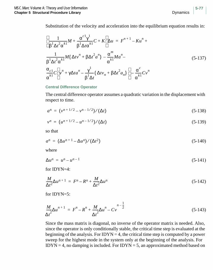
5-77MSC.Marc Volume A: Theory and User InformationChapter 5 Structural Procedure Library Dynamics
Substitution of the velocity and acceleration into the equilibrium equation results in:
(5-137)
Central Difference Operator
The central difference operator assumes a quadratic variation in the displacement with respect to time.
(5-138)
(5-139)
so that
(5-140)
where
(5-141)
for IDYN=4:
(5-142)
for IDYN=5:
(5-143)
Since the mass matrix is diagonal, no inverse of the operator matrix is needed. Also, since the operator is only conditionally stable, the critical time step is evaluated at the beginning of the analysis. For IDYN = 4, the critical time step is computed by a power sweep for the highest mode in the system only at the beginning of the analysis. For IDYN = 4, no damping is included. For IDYN = 5, an approximated method based on
1
β1∆t2αk1
-----------------------Mαc1γ1
β1∆tαk1--------------------C K+ +
∆u Fn 1+
Kun
–
1
β1∆t2αk1
-----------------------M ∆tvn β∆t
2a
n+ αm
αk1--------Ma
n
αc1
αk1--------C v
n γ∆tan γ1
β1∆t----------- ∆tvn β∆t
2an+ –+
–
αc
αk1--------Cv
n–
–
+=
an vn 1 2⁄+ vn 1 2⁄––( ) ∆t( )⁄=
vn un 1 2⁄+ un 1 2⁄––( ) ∆t( )⁄=
an ∆un 1+ ∆un–( ) ∆t2( )⁄=
∆un un un 1––=
M∆t2--------∆un 1+ Fn Rn–
M∆t2--------∆un+=
M
∆t2
-------∆un 1+
Fn
Rn
–M
∆t2
--------∆un
Cvn
12---–
–+=

MSC.Marc Volume A: Theory and User InformationDynamics Chapter 5 Structural Procedure Library
5-78
element geometry is used to compute the highest eigenvalue. The critical time step is calculated for each time step whenever the UPDATE parameter is used in the analysis. The variable time step can be used only for IDYN = 5. Unless there is significant distortion in an element, the change of critical time step is not significant.
Time Step Definition
In a transient dynamic analysis, time step parameters are required for integration in time. The DYNAMIC CHANGE option can be used for either the modal superposition or the direct integration procedure. The AUTO TIME option can be used for the Newmark-beta operator and the Single Step Houbolt operator to invoke the adaptive time control. Enter parameters to specify the time step size and period of time for this set of boundary conditions.
When using the Newmark-beta operator, decide which frequencies are important to the response. The time step in this method should not exceed 10 percent of the period of the highest relevant frequency in the structure. Otherwise, large phase errors will occur. The phenomenon usually associated with too large a time step is strong oscillatory accelerations. With even larger time steps, the velocities start oscillating. With still larger steps, the displacement eventually oscillates. In nonlinear problems, instability usually follows oscillation. When using adaptive dynamics, you should prescribe a maximum time step.
As in the Newmark-beta operator, the time step in Houbolt integration should not exceed 10 percent of the period of the highest frequency of interest. However, the Houbolt method not only causes phase errors, it also causes strong artificial damping. Therefore, high frequencies are damped out quickly and no obvious oscillations occur. It is, therefore, completely up to the engineer to determine whether the time step was adequate.
In nonlinear problems, the mode shapes and frequencies are strong functions of time because of plasticity and large displacement effects, so that the above guidelines can be only a coarse approximation. To obtain a more accurate estimate, repeat the analysis with a significantly different time step (1/5 to 1/10 of the original) and compare responses.
The central difference integration method is only conditionally stable; the program automatically calculates the stable time step. This step size yields accurate results for all practical problems.

5-79MSC.Marc Volume A: Theory and User InformationChapter 5 Structural Procedure Library Dynamics
Initial Conditions
In a transient dynamic analysis, you can specify initial conditions such as nodal displacements and/or nodal velocities. To enter initial conditions, use the following model definition options: INITIAL DISP for specified nodal displacements, and INITIAL VEL for specified nodal velocities. As an alternative, you can use the user subroutine USINC.
Time-Dependent Boundary Conditions
Simple time-dependent load or displacement histories can be entered on data blocks. However, in general cases with complex load histories, it is often more convenient to enter the history through a user subroutine. Marc allows the use of subroutines FORCDT and FORCEM for boundary conditions. Subroutine FORCDT allows you to specify the time-dependent incremental point loads and incremental displacements. Subroutine FORCEM allows you to specify the time-dependent magnitude of the distributed load.
Damping
In a transient dynamic analysis, damping represents the dissipation of energy in the structural system. It also retards the response of the structural system.
Marc allows you to enter two types of damping in a transient dynamic analysis: modal damping and Rayleigh damping. Use modal damping for the modal superposition method and Rayleigh damping for the direct integration method. For modal superposition, you can include damping associated with each mode. To do this, use the DAMPING option to enter the fraction of critical damping to be used with each mode.
During time integration, Marc associates the corresponding damping fraction with each mode. The program bases integration on the usual assumption that the damping matrix of the system is a linear combination of the mass and stiffness matrices, so that damping does not change the modes of the system.
For direct integration damping, you can specify the damping matrix as a linear combination of the mass and stiffness matrices of the system. You can specify damping coefficients on an element basis.
Stiffness damping should not be applied to either Herrmann elements or gap elements because of the presence of Lagrangian multipliers.
Numerical damping is used to damp out unwanted high-frequency chatter in the structure. If the time step is decreased (stiffness damping might cause too much damping), use the numerical damping option to make the damping (stiffness) coefficient proportional to the time step. Thus, if the time step decreases, high-frequency response can still be accurately represented. This type of damping is

MSC.Marc Volume A: Theory and User InformationDynamics Chapter 5 Structural Procedure Library
5-80
particularly useful in problems where the characteristics of the model and/or the response change strongly during analysis (for example, problems involving opening or closing gaps).
Element damping uses coefficients on the element matrices and is represented by the equation:
(5-144)
where
is the global damping matrix
is the mass matrix of ith element
is the stiffness matrix of the ith element
is the mass damping coefficient on the ith element
is the usual stiffness damping coefficient on the ith element
is the numerical damping coefficient on the ith element
is the time increment
If the same damping coefficients are used throughout the structure, Equation 5-144 is equivalent to Rayleigh damping.
The damping coefficients associated with springs (stiffness and numerical damping) and with mass points (mass damping) are zero. The damping on elastic foundations is the same as the damping on the element on which the foundation is applied. For springs, a dashpot can be added for nonlinear analysis.
Harmonic Response
Harmonic response analysis allows you to analyze structures vibrating around an equilibrium state. This equilibrium state can be unstressed or statically prestressed. Statically prestressed equilibrium states can include material and/or geometric nonlinearities. You can compute the damped response for prestressed structures at various states.
C α iMi βi γi∆tπ-----+
Ki+
i 1=
n
∑=
C
Mi
Ki
ai
βi
γi
∆t

5-81MSC.Marc Volume A: Theory and User InformationChapter 5 Structural Procedure Library Dynamics
In many practical applications, components are dynamically excited. These dynamic excitations are often harmonic and usually cause only small amplitude vibrations. Marc linearizes the problem around the equilibrium state. If the equilibrium state is a nonlinear, statically prestressed situation, Marc considers all effects of the nonlinear deformation on the dynamic solution. These effects include the following:
• initial stress
• change of geometry
• influence on constitutive law
The vibration problem can be solved as a linear problem using complex arithmetic.
The analytical procedure consists of the following steps:
1. Marc calculates the response of the structure to a static preload (which can be nonlinear) based on the constitutive equation for the material response. In this portion of the analysis, the program ignores inertial effects.
2. Marc calculates the complex-valued amplitudes of the superimposed response for each given frequency, and amplitude of the boundary tractions and/or displacements. In this portion of the analysis, the program considers both material behavior and inertial effects.
3. You can apply different loads with different frequencies or change the static preload at your discretion. All data relevant to the static response is stored during calculation of the complex response.
To initiate a harmonic response analysis, use the HARMONIC parameter. To define the excitation frequency, use the HARMONIC history definition option. If you enter the HARMONIC history definition option with a set of incremental data, Marc assumes those incremental data apply only for the harmonic excitation. This is true for applied boundary conditions as well as loads.
The small amplitude vibration problem can be written with complex arithmetic as follows
(5-145)
where
complex response vector
complex load vector
The notation is further defined below:
(5-146)
K iωD ω2M–+[ ] u P=
u ure iuim+=
P Pre iPim+=
K ΣKel ΣKsp+=

MSC.Marc Volume A: Theory and User InformationDynamics Chapter 5 Structural Procedure Library
5-82
5Structural Procedure Library
Dynamics
where
are element stiffness matrices
are the spring stiffness matrices
(5-147)
where
are element mass matrices
are masspoint contributions
(5-148)
where
are element damping matrices
are damper contributions
stiffness damping coefficient
mass damping coefficient
numerical damping coefficient
=
= excitation frequencies
= complex response vector
= complex load vector
If all external loads and forced displacements are in phase and the system is undamped, this equation reduces to
(5-149)
which could be solved without activating the complex arithmetic on the HARMONIC parameter.
The values of the damping coefficients ( , , ) are entered via the DAMPING model definition option. The spring and damper contributions are entered in the SPRINGS model definition option and mass points are specified in the MASSES model definition option.
Kel
Ksp
M ΣMel ΣMmp+=
Mel
Mmp
D ΣDel ΣDd Σ αK βM 2ωγK+ +( )+ +=
Del
Dd
αβγi 1–
ωu ure iuim+
p Pre iPim+
K ω2M–( )ure Pre=
α β γ
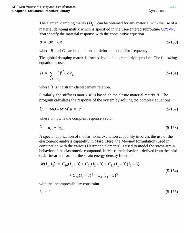
5-83MSC.Marc Volume A: Theory and User InformationChapter 5 Structural Procedure Library Dynamics
The element damping matrix ( ) can be obtained for any material with the use of a
material damping matrix which is specified in the user-entered subroutine UCOMPL. You specify the material response with the constitutive equation.
(5-150)
where and can be functions of deformation and/or frequency.
The global damping matrix is formed by the integrated triple product. The following equation is used:
(5-151)
where is the strain-displacement relation.
Similarly, the stiffness matrix is based on the elastic material matrix . The program calculates the response of the system by solving the complex equations:
(5-152)
where now is the complex response vector
(5-153)
A special application of the harmonic excitation capability involves the use of the elastomeric analysis capability in Marc. Here, the Mooney formulation (used in conjunction with the various Herrmann elements) is used to model the stress-strain behavior of the elastomeric compound. In Marc, the behavior is derived from the third order invariant form of the strain energy density function.
(5-154)
with the incompressibility constraint
(5-155)
Del
σ Bε Cε·+=
B C
D βTC Veld
vel
∫el∑=
β
K B
K iωD ω2M–+[ ] u P=
u
u ure iuim+=
W I1 I2,( ) C10 I1 3–( ) C01 I2 3–( ) C11 I1 3–( ) I2 3–( )+ +=
C20+ I1 3–( )2 C30 I1 3–( )3+
I3 1=

MSC.Marc Volume A: Theory and User InformationDynamics Chapter 5 Structural Procedure Library
5-84
where , , and are the invariants of the deformation. For the harmonic
excitation, the constitutive equation has the specific form
(5-156)
with as the quasi-static moduli following form the Mooney strain energy density
function and
(5-157)
The output of Marc consists of stresses, strains, displacements and reaction forces, all of which may be complex quantities. The strains are given by
(5-158)
and the stresses by
(5-159)
The reaction forces are calculated with
(5-160)
where is only included if requested on the HARMONIC parameter.
The printout of the nodal values consists of the real and imaginary parts of the complex values, but you can request that the amplitude and phase angle be printed. You do this with the PRINT CHOICE model definition option.
Spectrum Response
The spectrum response capability allows you to obtain maximum response of a structure subjected to known spectral base excitation response. This is of particular importance in earthquake analysis and random vibration studies. You can use the spectrum response option at any point in a nonlinear analysis and, therefore, ascertain the influence of material nonlinearity or initial stress.
I1 I2 I3
∆Sij Dijkl 2iωφijkl+[ ]∆ Ekl=
Dijkl
φijkl φ0 Cik1– Cjl
1– Cil1– Cjk
1–+[ ] φ1 δikCjl1– Cil
1– δjk+[ ]φ2 CikCjl
1– Cil1– Cjk+[ ] φ0δijCkl
1– φ11δijδkl
φ12δijCkl φ20+ CijCkl1– φ21+ Cijδkl φ22CijCkl
+ +
+ + +
+
=
ε β u=
σ Bε C+= ε·
R Ku ω2Mu– iωΣDelu iωΣDdu+ +=
ω2Mu–

5-85MSC.Marc Volume A: Theory and User InformationChapter 5 Structural Procedure Library Dynamics
The spectrum response capability technique operates on the eigenmodes previously extracted to obtain the maximum nodal displacements, velocities, accelerations, and reaction forces. You can choose a subset of the total modes extracted by either specifying the lowest n modes or by selecting a range of frequencies.
Enter the displacement response spectrum for a particular digitized value of
damping through user subroutine USSD. Marc performs the spectrum analysis based on the latest set of modes extracted. The program lumps the mass matrix to produce
. It then obtains the projection of the inertia forces onto the mode
(5-161)
The spectral displacement response for the jth mode is
(5-162)
Marc then calculates the root-mean-square values as
(5-163)
(5-164)
(5-165)
(5-166)
SD ω( )
M φj
Pj M φj=
α j SD ωj( ) Pj=
u α jφj( )2
j∑
1 2⁄= DISPLACEMENT
v α jωjφj( )2
j∑
1 2⁄= VELOCITY
a α jωjφj( )2
j∑
1 2⁄= ACCELERATION
f α jωj2Mφj( )2
j∑
1 2⁄= FORCE

MSC.Marc Volume A: Theory and User InformationRigid-Plastic Flow Chapter 5 Structural Procedure Library
5-86
Rigid-Plastic Flow
The rigid-plastic flow analysis is an approach to large deformation analysis which can be used for metal forming problems. Two formulations are available: an Eulerian (steady state) and Lagrangian (transient) approach. The effects of elasticity are not included. If these effects are important, this option should not be used.
In the steady state approach, the velocity field (and stress field) is obtained as the solution of a steady-state flow analysis. The time period is considered as 1.0 and, hence, the velocity is equal to the deformation. In the transient formulation, the incremental displacement is calculated.
The R-P FLOW parameter invokes the rigid-plastic procedure. This procedure needs to enforce the incompressibility condition, which is inherent to the strictly plastic type of material response being considered.
Incompressibility can be imposed in three ways:
1. by means of Lagrange multipliers. Such procedure requires Herrmann elements which have a pressure variable as the Lagrange multiplier.
2. by means of penalty functions. This procedure uses regular solid elements, and adds penalty terms to any volumetric strain rate that develops. It is highly recommended that the constant dilatation formulation be used – by entering a nonzero value in the second field of the GEOMETRY model definition option.
Penalty factor can be treated as constant or variable through the R-P FLOW parameter. The penalty value is entered through the PARAMETERS option.
3. in plane stress analysis (shell and membrane elements), the incompressibility constraint is satisfied exactly by updating the thickness. This capability is not available for steady state analysis.
In R-P flow analysis, several iterations are required at any given increment, the greatest number occurring in the first increment. Subsequent increments require fewer iterations, since the initial iteration can make use of the solution from the previous increment.
Due to the simplicity of the rigid-plastic formulation, it is possible to bypass stress recovery for all iterations but the last in each increment, provided that displacement control is used. In such cases, considerable savings in execution time are achieved. If nodal based friction is used in a contact analysis, then a stress recovery is always performed after each iteration.

5-87MSC.Marc Volume A: Theory and User InformationChapter 5 Structural Procedure Library Rigid-Plastic Flow
Steady State Analysis
The steady state R-P flow formulation is based on an Eulerian reference system. For problems in which a steady-state solution is not appropriate, an alternative method is available to update the coordinates. User subroutine UPNOD is used to update the nodal coordinates at the end of a step according to the relationship.
(5-167)
where n refers to the step number, vn is the nodal velocity components, and ∆t is an arbitrary time step. ∆t is selected in such a way as to allow only a reasonable change in mesh shape while ensuring stability with each step.
Updating the mesh requires judicious selection of a time step. This requires some knowledge of the magnitude of the nodal velocities that will be encountered. The time step should be selected such that the strain increment is never more than one percent for any given increment.
The quantities under the title of ENGSTN in the printouts actually refer to the strain rate at an element integration point. The reaction forces output by the program gives the limit loads on the structure.
Transient Analysis
In the transient procedure, there is an automatic updating of the mesh at the end of each increment. During the analysis, the updated mesh can exhibit severe distortion and the solution might be unable to converge. Mesh rezoning can be used to overcome this difficulty.
Technical Background
The rigid-plastic flow capability is based on iteration for the velocity field in an incompressible, non-Newtonian fluid. The normal flow condition for a nonzero strain rate can be expressed as:
(5-168)
where
(5-169)
xin xi
n 1– vn∆t+=
σ′ ij23---
σ
ε·---
ε· ij µ ε·
( ) ε· ij= =
ε· 2
3---ε· ijε
·ij=

MSC.Marc Volume A: Theory and User InformationRigid-Plastic Flow Chapter 5 Structural Procedure Library
5-88
is the equivalent strain rate, is the yield stress (which may be rate-dependent) and
(5-170)
gives the deviatoric stress. The effective viscosity is evaluated as:
(5-171)
Note that as . A cutoff value of strain rate is used in the program to
avoid this difficulty. An initial value for is necessary to start the iterations. These values can be specified in the PARAMETERS option. The default cut-off value is 10-6, and the default initial strain rate value is 10-4.
The value of the flow stress is dependent upon both the equivalent strain, the equivalent strain rate, and the temperature. This dependence can be given through the WORK HARD, STRAIN RATE, and TEMPERATURE EFFECTS options, respectively. For steady state analysis, user subroutine UNEWTN can be used to define a viscosity. In this manner, a non-Newtonian flow analysis can be performed. For the transient procedure, user subroutine URPFLO can be used to define the flow stress.
σ
σ′ ij σij13---δijσkk–=
µ 23---
σ
ε·---=
ε·
0 µ ∞→,→
ε·

5-89MSC.Marc Volume A: Theory and User InformationChapter 5 Structural Procedure Library Superplasticity
Superplasticity
Superplasticity is the ability of a material to undergo extensive deformation such as strains of 1000% without necking. Superplastic behavior has been reported in numerous metal, alloys and ceramics. Every instance of superplasticity is associated with: (1) A fine grain size ( ), (2) deformation temperatures , and
(3) a strain-rate sensitivity factor .
Using finite element analysis to simulate superplastic fabrication of complex parts used in the aerospace and automotive industries requires this material behavior and contact with friction. Furthermore, the process pressure needs to be automatically adjusted to keep the material within a target strain rate. The simulation can be used to predict thinning, forming time, areas of void formation, and can ultimately be employed in shape optimization; thus, reducing the number of prototypes of forming trials required to product an acceptable part.
Three mechanisms have been proposed to account for the high strain-rate sensitivity found in superplastic materials: (1) Vacancy creep, (2) creep by grain boundary diffusion, and (3) grain boundary sliding. According to Ghosh and Hamilton, the strain-rate sensitivity of metals arises from the viscous nature of the deformation process. The viscosity is a result of the resistance offered by internal obstacles within the material. In dislocation glide and climb processes, the obstacles are a fine dispersion of second phase particles within the grain interior, between which the dislocations are bent around and moved. At high homologous temperatures ( ; where is the melting temperature), the high diffusivities around grain
boundary regions can lead to grain boundary sliding. The overall rate sensitivity of a material is then a result of the rate sensitivities of the grain boundary and the grain interior. The more the material behaves as a viscous liquid, the greater its superplasticity.
The superplastic behavior is characterized by the dependence of the flow stress upon the strain-rate, which is usually depicted by the logarithmic relationship shown in Figure 5-20.
As indicated in Figure 5-20, the stress-strain rate behavior of a superplastic material can be divided into three regions. Values of strain-rate sensitivity, (the slope of flow stress versus strain-rate curve) which is a measure of resistance to localized necking, are relatively low in both the low stress-low strain rate region I and the high stress-high strain rate region III and superplasticity is not manifested. Rather, superplasticity is found only in region II, a transition region in which stress increases rapidly with
1 10 µm– 0.4Tm>
m 0.3>
T 0.4Tm> Tm
m

MSC.Marc Volume A: Theory and User InformationSuperplasticity Chapter 5 Structural Procedure Library
5-90
increasing strain-rate. As temperature increases and/or grain size decreases, region II is displaced to higher strain-rates. Moreover, the maximum observed values of increase with similar changes in these parameters.
Figure 5-20 (a) Flow stress and (b) Strain-rate Sensitivity as a Function of Strain-rate
Certainly the forming process innovations evoked will need to be carefully studied and developed. Forming times are slow, and there will be a critical need for optimizing forming pressures, stress strain-rate and deflection in sheet forming. Based on the schematic flow stress-strain rate relationships given above, it is apparent that high values of are requisite for superplastic materials. Since, for a given material and
forming temperature, , usually varies with strain-rate, it is desirable to control strain-rate during forming so that optimum or at least adequate strain-rate sensitivity is exhibited. Ductility is also dependent upon forming temperature, which must lie within a narrow range. If forming temperatures and pressure cycle are optimum, then
m
Decreasing grain size orincreasing temperature
Region III
Region II
Region I
ln σ
ln ε
(a)
.
Decreasing grain size orincreasing temperature
Region IIIRegion II
Region I
(b)
m = d σln
d ε·
ln------------
ln ε.
m
m

5-91MSC.Marc Volume A: Theory and User InformationChapter 5 Structural Procedure Library Superplasticity
unlike conventional ductile materials, superplastic materials are much less susceptible to localized necking. Additionally, under such conditions, the flow stress occurring during forming is much lower than the mechanical yield stress.
Thus, the superplastic materials may be viewed as exhibiting time-dependent inelastic behavior with the yield stress as a function of time, temperature, strain-rate, total stress and total strain. Typical materials used in commercial superplastic forming applications include Ti-6A1-4V titanium alloy and 5083 aluminium alloy.
The form of constitutive equation used to simulate superplasticity is given as:
(5-172)
The form in Equation 5-172 can be recovered by using appropriate constants in the ISOTROPIC model definition option to define power law or rate power law. Thus,
Power Law Model: (5-173)
Rate Power Law Model: (5-174)
The superplastic forming process requires the use of the SPFLOW parameter. The use of this parameter automatically activates the FOLLOW FOR and PROCESSOR parameters. The process parameters are controlled by the use of the SUPERPLASTIC history definition option.
σy ε· m
=
σy A εo ε·
+( )m
Bε· n
+=
σy Aεmε· n
B+=

MSC.Marc Volume A: Theory and User InformationSoil Analysis Chapter 5 Structural Procedure Library
5-92
Soil Analysis
This section has the solution procedure for fluid-soil analysis. In the current formulation, it is assumed that the fluid is of a single phase, and only slightly compressible. This formulation will not be adequate if steam-fluid-solid analysis is required. The dry soil can be modeled using one of the three models: linear elasticity, nonlinear elasticity and the modified Cam-Clay model.
There are three types of soil analysis available in Marc. In the first type, you perform an analysis to calculate the fluid pressure in a porous medium. In such analyses, heat transfer elements 41, 42, or 44 are used. The SOIL model definition option is used to define the permeability of the solid and the bulk modulus and dynamic viscosity of the fluid. The porosity is given either through the INITIAL POROSITY or the INITIAL VOID RATIO options and does not change with time. The prescribed pressures can be defined using the FIXED PRESSURE option, while input mass flow rates are given using either the POINT FLUX or DIST FLUXES option.
In the second type of soil analysis, the pore (fluid) pressure is directly defined, and the structural analysis is performed. Element types 27, 28, or 21 are available. In such analyses, the pore pressure is prescribed using the INITIAL PORE and CHANGE PORE options. The characteristics of the soil material are defined using the SOIL option. If an elastic model is used, the Young’s moduli and Poison’s ratio are important. If the Cam-Clay model is used, the compression ratios and the slope of the critical state line is important. For the Cam-Clay model, the preconsolidation pressure is defined using the INITIAL PC option. For this model, it is also important to define an initial (compressive stress) to ensure a stable model.
In the third type of soil analysis, a fully-coupled approach is used. Element types 32, 33, or 35 are available. These elements are “Herrmann” elements, which are conventionally used for incompressible analysis. In this case, the extra variable represents the fluid pressure. The SOIL option is now used to define both the soil and fluid properties. The porosity is given through the INITIAL POROSITY or the INITIAL VOID RATIO option. The prescribed nodal loads and mass flow rates are given through the POINT LOAD option, while distributed loads and distributed mass flow rates are given through the DIST LOADS option. The FIXED DISP option is used to prescribe either nodal displacements or pore pressures.

5-93MSC.Marc Volume A: Theory and User InformationChapter 5 Structural Procedure Library Soil Analysis
Technical Formulation
In soil mechanics, it is convenient to decompose the total stress σ into a pore pressure component and effective stress .
(5-175)
Note the sign convention used; a positive pore pressure results in a compressive stress. The momentum balance (equilibrium) equations are with respect to the total stresses in the system.
(5-176)
where is the density, and , are the body force and the acceleration. The equilibrium equation can then be expressed as
(5-177)
The fluid flow behavior can be modeled using Darcy’s law, which states that the fluid’s velocity, relative to the soil’s skeleton, is proportional to the total pressure gradient.
(5-178)
where
is the fluid’s bulk velocity
is the soil permeability
is the fluid viscosity
is the fluid density
is the gravity vector.
The fluid is assumed to be slightly compressible.
(5-179)
where is the bulk modulus of the fluid.
p σ′
σ σ′ pI–=
∇σ f+ ρu··=
ρ f u··
∇σ′ ∇ p– f+ ρu··=
u· fK–µ
------- ∇ p ρfg+( )=
u· f
K
µρf
g
p· Kfρ· f
ρf----=
Kf

MSC.Marc Volume A: Theory and User InformationSoil Analysis Chapter 5 Structural Procedure Library
5-94
However, the compressibility is assumed small enough such that the following holds:
(5-180)
It is also assumed that the bulk modulus of the fluid is constant, introducing the fluid’s compressibility .
(5-181)
The solid grains are assumed to be incompressible. Under these assumptions, the governing equations for fluid flow is
(5-182)
where is the medium’s porosity.
It is important to note that the medium’s porosity is only dependent upon the original porosity and the total strains. Letting and stand for the fluid and solid’s volume
(5-183)
where is the determinant of the deformation gradient and is the original porosity,
both with respect to the reference configuration.
Introducing the weighting function and , the weak form, which is the basis for
the finite element system, then becomes
(5-184)
where and are the conventional volumes and surface area and is the applied tractions. Note that the applied tractions is the combined tractions from both the effective stress and the pore pressure .
and
(5-185)
∇ ρ fKµ---- ∇ p ρfg+( )⋅ ρf∇
Kµ---- ∇ p ρfg+( )⋅≈
βf
βf 1 Kf⁄=
∇ Kµ---- ∇ p ρfg+( )⋅ φβf p
· ∇ u·+=
σ
Vf Vs
φ dVf dVf dVs+( )⁄ 1 J 1– 1 φ0–( )–= =
J φ0
ηu ηp
ηu f ρηu u··– ∇η u σ′– ∇η up+[ ] dvVn 1+
∫ ηu t daA∫+ 0=
V A t
σ′ p
∇η p Kµ---- ∇ p ρfg+( ) φβfηpp·+ ηp ∇ u·( )+ dv
Vn 1+
∫ ηpqndaAn 1+
∫– 0=

5-95MSC.Marc Volume A: Theory and User InformationChapter 5 Structural Procedure Library Soil Analysis
where the normal volumetric inflow, , is:
(5-186)
The weak form of equilibrium can be written as:
(5-187)
(5-188)
Application of the directional derivative formula yields:
(5-189)
Hence,
(5-190)
Similarly,
(5-191)
(5-192)
(5-193)
qn
qnkµ--- ∇ p ρfg+( ) n⋅=
ru ∇ η up⋅[ ] vdVn 1+
∫=
rp ∇η pKµ---- ∇ p ρfg+( ) φβfηpp· ηp∇ u·⋅+ +⋅ vd
Vn 1+
∫=
Du ru( ) δu⋅ ddε----- ru u εδu+( )
ε 0==
Du ru( ) δu⋅ ∇ ∆ u ∇ η up⋅( ) ∇η uT ∇∆ up⋅+⋅[ ] vd
Vn 1+
∫=
Dp ru( ) δp⋅ ∇ η u∆p⋅ vdVn 1+
∫=
Du rp( ) δu⋅ ∇η pKµ---- ∇ p ρfg+( ) φβfηpp· ηp∇ u·⋅+ +⋅ ∇ ∆ u ηp∇ u·
T ⋅–⋅
Vn 1+
∫=
∇∆ u ηp+ ∇ ∆ u·⋅ ∇∆ u∇η pKµ---- ∇ p ρfg+( ) ∇η p
Kµ---- ∇∆ u( )∇ p dv⋅–⋅–
Dp rp( ) δp⋅ ∇η pKµ---- ∇∆ p φβfηp∆p·+⋅ vd
Vn 1+
∫=

MSC.Marc Volume A: Theory and User InformationSoil Analysis Chapter 5 Structural Procedure Library
5-96
with the displacement and pressures interpolated independently as:
(5-194)
we get a linearized system of equilibrium equation,
(5-195)
The resulting system of equations is highly nonlinear and nonsymmetric, and is solved by full Newton-Raphson solution scheme.
Note that it is assumed that the permeability, porosity, viscosity, and the bulk modulus of the fluid are considered independent of the state variables and . It is evident that, in general, this is not the case; however, in the analysis that follows, these dependencies are ignored for tangent purposes. Note that they are included in the calculation of the residuals and ; hence, convergence is always achieved at the
true solution.
Three types of analyses can be performed. The simplest is a solution for only the fluid pressure based upon the porosity of the soil. In this case, a simple Poisson type analysis is performed and element types 41, 42, or 44 are used. In the second type of analysis, the pore pressures are explicitly defined and the structural analysis is performed. In this case, the element types 21, 27, and 28 should be used. Finally, a fully-coupled analysis is performed; in which case, you should use element types 32, 33, or 35. Of course, the soil can be combined with any other element types, material properties to represent the structure, such as the pilings.
Evaluation of Soil Parameters for the Critical State Soil Model
To illustrate how to extract soil parameters, namely , , and , a hypothetical data set for a normally consolidated clay in presented in Figures 5-21 to 5-29. Now we shall use these data to show the procedure of determination of parameters for the critical state model. The data presented here pertain to conventional triaxial conditions.
∆u Ni∆ui∑=
and
p Njpj∑=
Kuu Kup
Kpu Kpp
δu
δp
FRu
Rp
–=
u p
Ru Rp
M κ λ

5-97MSC.Marc Volume A: Theory and User InformationChapter 5 Structural Procedure Library Soil Analysis
Figures 5-21 to 5-23 show the stress-strain relations for constant pressure tests under different initial conditions p0=10 (69), 20 (139), and 30 (207) psi (kPa), respectively. Here the mean effective pressure of the soil sample is kept constant throughout the test. The last data point shown on the deviatoric stress (q) versus axial strain (ε1) plot for any test is considered as the ultimate condition for that test. The void ratio values at the beginning and the end of each test are given in Table 5-7.
Table 5-7 Test Values for Cam Clay Model
Test
InitialPressure, p0
(effective)(psi)
Initialvoid Ratio,
e0
FinalPressure, pf(effective)
(psi)
FinalVoid Ratio,
e1
p-constant 10 1.080 10 0.980
p-constant 20 0.959 20 0.860
p-constant 30 0.889 30 0.787
Drained 10 1.080 15 0.908
Drained 20 0.959 30 0.787
Drained 30 0.889 45 0.716
Undrained 10 1.080 05.55 1.080
Undrained 20 0.959 11.09 0.959
Undrained 30 0.889 16.64 0.889

MSC.Marc Volume A: Theory and User InformationSoil Analysis Chapter 5 Structural Procedure Library
5-98
Figure 5-21 Constant Pressure Test: p0 = 10 psi
Figure 5-22 Constant Pressure Test: p0 = 20 psi
Dev
iato
ric s
tress
, qσ 1
σ 3–
=(p
si)
10
8
6
4
2
0 0.10 0.20
Axial strain, ε1
0.05
0.04
0.03
0.02
0.01
0.10 0.20
Volu
met
ric s
train
,εν
Dev
iato
ric s
tress
, qσ 1
σ 3–
=(p
si)
25
20
15
10
5
0 0.10 0.20
Axial strain, ε1
0.05
0.04
0.03
0.02
0.01
0.10 0.20
Volu
met
ric s
train
,εν

5-99MSC.Marc Volume A: Theory and User InformationChapter 5 Structural Procedure Library Soil Analysis
Figure 5-23 Constant Pressure Test: p0 = 30 psi
Figures 5-24 to 5-26 show stress-strain relation plots for three fully drained tests performed at initial pressures 10, 20, and 30 psi. Here, there is no pore pressure development, and the effective mean pressure increases during the test. The void ratio values at the beginning and end of each test are given in Table 5-7.
Dev
iato
ric s
tress
, qσ 1
σ 3–
=(p
si) 30
20
15
10
5
0.10 0.20
Axial strain, ε1
0.05
0.04
0.03
0.02
0.01
0.10 0.20
Volu
met
ric s
train
,εν
25

MSC.Marc Volume A: Theory and User InformationSoil Analysis Chapter 5 Structural Procedure Library
5-100
Figure 5-24 Drained Test: p0 = 10 psi
Dev
iato
ric s
tress
, qσ 1
σ 3–
=(p
si)
16
8
6
4
2
0.10 0.20
Axial strain, ε1
0.10
0.08
0.06
0.04
0.02
0.10 0.20
Volu
met
ric s
train
,εν
10
12
14

5-101MSC.Marc Volume A: Theory and User InformationChapter 5 Structural Procedure Library Soil Analysis
Figure 5-25 Drained Test: p0 = 20 psi
Dev
iato
ric s
tress
, qσ 1
σ 3–
=(p
si)
20
15
10
5
0.10 0.20
Axial strain, ε1
0.10
0.08
0.06
0.04
0.02
0.10 0.20
Vol
umet
ric s
train
,εν
25
30

MSC.Marc Volume A: Theory and User InformationSoil Analysis Chapter 5 Structural Procedure Library
5-102
5Structural Procedure Library
Soil Analysis
Figure 5-26 Drained Test: p0 = 30 psi
Figures 5-27 to 5-29 show stress-strain behavior under undrained conditions. Here there is no change in volume of the sample. However, fluid pore pressure are developed during the test, thereby reducing the effective stresses until the ultimate (failure) state is reached.
Dev
iato
ric s
tress
, qσ 1
σ 3–
=(p
si)
40
30
20
10
0.10 0.20
Axial strain, ε1
0.10
0.08
0.06
0.04
0.02
0.10 0.20
Vol
umet
ric s
trai
n,ε ν
50

5-103MSC.Marc Volume A: Theory and User InformationChapter 5 Structural Procedure Library Soil Analysis
Figure 5-27 Undrained Test: p0 = 10 psi
Dev
iato
ric s
tress
, qσ 1
σ 3–
=(p
si)4
3
2
1
0.01 0.02
Axial strain, ε1
Pore
pre
ssur
e, u
(psi
)
5
6
0.03 0.04
4
3
2
1
0.01 0.02
5
6
0.03 0.04
Axial strain, ε1

MSC.Marc Volume A: Theory and User InformationSoil Analysis Chapter 5 Structural Procedure Library
5-104
Figure 5-28 Undrained Test: p0 = 20 psi
Devia
toric
stre
ss, q
σ 1σ 3
–=
(psi)
8
6
4
2
0.01 0.02
Axial strain, ε1
Pore
pre
ssur
e, u
(psi)
10
12
0.03 0.04
8
6
4
2
0.01 0.02
10
0.03 0.04
Axial strain, ε1

5-105MSC.Marc Volume A: Theory and User InformationChapter 5 Structural Procedure Library Soil Analysis
Figure 5-29 Undrained Test: p0 = 30 psi
Figure 5-30 shows the variation of void ratio with mean pressure which is obtained from a hydrostatic compression (HC) test with three load reversals (that is, unloading-reloading cycles). In this figure, void ratio is plotted to a linear scale while the hydrostatic stress is plotted to a logarithmic (base 10) scale. In fact, this is the usual way of presenting one-dimensional consolidation or hydrostatic test results in geotechnical engineering practices.
Devia
toric
stre
ss, q
σ 1σ 3
–=
(psi)
8
6
4
2
0.01 0.02
Axial strain, ε1
Pore
pre
ssur
e, u
(psi)
10
16
0.03 0.04
14
12
10
8
0.01 0.02
16
0.03 0.04
Axial strain, ε1
0
12
14
6
4
2

MSC.Marc Volume A: Theory and User InformationSoil Analysis Chapter 5 Structural Procedure Library
5-106
Figure 5-30 Hydrostatic Compression Test: Cc = 0.04, Cs = 0.06
Determination of parameter, M: The parameter M is the slope of the critical state line on a p-q plot. To determine its value, the values of p and q at ultimate conditions for each test are plotted as shown in Figure 5-31; the ultimate condition for each test is assumed to be the last point plotted in Figures 5-21 to 5-29. At the ultimate conditions, the sample undergoes excessive deformations under constant deviatoric stress, and hence it could be taken as the asymptotic stress to the curve. The slope of the critical state line (Figure 5-31) is calculated as 1.0 for the soil above. That is,
.
Voi
d ra
tio, e 1.0
0.9
0.8
20 30Pressure, p (psi) (logarithmic scale with base 10)
A
40 500.7
1.1
1.2
Cc
Cs
10
BC
M 1.0=

5-107MSC.Marc Volume A: Theory and User InformationChapter 5 Structural Procedure Library Soil Analysis
Figure 5-31 Critical State Line in q-p (psi)
Determination of parameters λ and κ: The values of gamma and kappa can be related to the commonly known quantities such as compression index ( ) and
swelling index ( ). The compression index, , is defined as the slope of virgin
loading line on e-log10p plot while the swelling index, , is defined as the unloading-
reloading curves on the same plot. Usually, the compression index and swelling index are defined with respect to a one-dimensional consolidation test. However, it can be shown that the e-ln(p) curve for any constant stress ratio test, that is, for constant q/p ratio, is parallel to that obtained from a hydrostatic test, (Figure 5-32).
Dev
iato
ric s
tres
s, q
(ps
i)
30
20
10
5020
Mean Pressure, p (psi)
30 400
40
45
10
Slope = M = 1.0
DrainedConstant pressureUndrained
M
Cc
Cs Cc
Cs

MSC.Marc Volume A: Theory and User InformationSoil Analysis Chapter 5 Structural Procedure Library
5-108
Figure 5-32 Isotropic Consolidation (Data from Table 5-8)
In fact, one-dimensional hydrostatic test is parallel to that obtained under critical state conditions. The values of gamma and kappa can be related to and as follows.
The virgin compression line can be expressed as
(5-196)
or
(5-197)
and the swelling line (unloading-reloading) can be expressed as
(5-198)
or
(5-199)
Voi
d ra
tio, e 1.0
0.9
0.8
6030Pressure (psi) (logarithmic scale with base 10)
40 500.7
1.1
1.2
20
Hydrostatic loading
At critical state
70 80 90
e0 vs. p0
ef vs. pf
Cc Cs
e e0– Cclog10pp0-----
=
e e0– λ pp0-----
ln=
e e0– Cslog10pp0-----
=
e e0– κ pp0-----
ln=
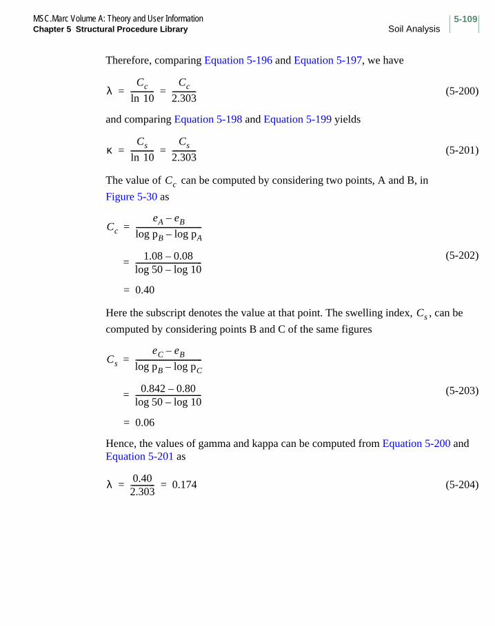
5-109MSC.Marc Volume A: Theory and User InformationChapter 5 Structural Procedure Library Soil Analysis
Therefore, comparing Equation 5-196 and Equation 5-197, we have
(5-200)
and comparing Equation 5-198 and Equation 5-199 yields
(5-201)
The value of can be computed by considering two points, A and B, in
Figure 5-30 as
(5-202)
Here the subscript denotes the value at that point. The swelling index, , can be
computed by considering points B and C of the same figures
(5-203)
Hence, the values of gamma and kappa can be computed from Equation 5-200 and Equation 5-201 as
(5-204)
λCc
10ln-------------
Cc
2.303-------------= =
κCs
10ln-------------
Cs
2.303-------------= =
Cc
Cc
eA eB–
log pB log pA–------------------------------------=
1.08 0.08–log 50 log 10–------------------------------------=
0.40=
Cs
Cs
eC eB–
log pB log pC–------------------------------------=
0.842 0.80–log 50 log 10–------------------------------------=
0.06=
λ 0.402.303------------- 0.174= =

MSC.Marc Volume A: Theory and User InformationDesign Sensitivity Analysis Chapter 5 Structural Procedure Library
5-110
Design Sensitivity Analysis
Design sensitivity analysis is used to obtain the sensitivity of various aspects of a design model with respect to changes in design parameters in order to facilitate structural modifications. The design parameters that are amenable to change are called “design variables”. The two major aspects of the design model for which design sensitivity is considered herein are:
a. Design objective
b. Design model response
As a result, the design sensitivity analysis capability in Marc is currently limited to finite element models of structures with linear response in the computation of
1. Gradients for
a. An objective function (or the design objective), if one is defined by you (for example, minimizing the material volume in the model).
b. Various types of design model responses under multiple cases of static mechanical loading, or free vibration, in linear behavior.
2. Element contributions to the responses of the model.
The gradient of the objective function or of a response function is simply the set of derivatives of such a function with respect to each of the design variables, at a given point in the design space (that is, for a given design).
For sensitivity analysis to proceed, the design model, the analysis requirements, the design variables, and the functions for which the gradients are to be found have to be specified by you.
The existing design sensitivity analysis capability in Marc can be applied in one of two ways:
1. As a stand-alone feature, where you are concerned only with obtaining sensitivity analysis results. Such an application is completed with the output of the sensitivity analysis results.
2. Within a design optimization process, where you are concerned mainly with the optimization of a design objective related to a finite element model. This type of an application of sensitivity analysis is transparent to you. The design optimization process is completed with the output of design optimization related data, such as the optimized objective function, related values of the design variables, and the analysis results for the optimized design.

5-111MSC.Marc Volume A: Theory and User InformationChapter 5 Structural Procedure Library Design Sensitivity Analysis
These two procedures are described below.
1. Sensitivity analysis as a stand-alone feature
This type of solution usually aims at obtaining the derivatives of user prescribed response quantities at a given design, with respect to each of multiple design variables specified by the user. This set of derivatives is therefore the gradient of the response function at the given design in the design variable space (or, in short, in the design space). For example, for a prescribed response function r, given the design variables , , and ,
the gradient is defined as
(5-205)
The number of response quantities for which gradients are computed is limited either by the program default or by a user-specified number. If you are interested in obtaining the sensitivity analysis results in order of criticality, the option to sort them in this order is also available. The responses are currently prescribed as constraints with user-defined bounds. If sorting is not required, the bounds can be mostly arbitrary, although they still have to conform to the type of constraint prescribed. However, if sorting is required and is to be meaningful, it is important for you to give realistic bounds on the response.
Element contributions to each response quantity are obtained as a by-product of the type of response sensitivity analysis capability in Marc. Thus, the response r can be represented as a sum of these element contributions:
(5-206)
where the second term, , involves work done elsewhere, such as in support settlement, if any.
This is helpful for a visual understanding of which regions of the model contribute in what manner to each of the response quantities at the given design, since it can be plotted in a manner similar to, say stress contours.
x1 x2 x3
∇ r˜
drdx1--------
drdx2--------
drdx3--------
T=
r re C+
e 1=
N
∑=
C

MSC.Marc Volume A: Theory and User InformationDesign Sensitivity Analysis Chapter 5 Structural Procedure Library
5-112
Finally, as an option, if you also prescribe an objective function, the gradient of the objective function with respect to the design variables is also computed at the given design. Thus, for the objective function , Marc obtains
(5-207)
2. Sensitivity analysis within a design optimization process:
The design optimization algorithm in Marc requires the utilization of gradients of the objective function and of the constraint functions, which are very closely related to the response functions. The current algorithm, described under “design optimization”, ignores your initial prescribed design, but instead begins by generating other designs within the prescribed bounds for the design variables. Once the optimization algorithm is completed and the optimized design is available, if a sensitivity analysis is required at the optimized state, it will be necessary for you to modify the model accordingly and to use sensitivity analysis as a stand alone feature.
During design optimization, sensitivity analysis is performed for a maximum number of constraints either indicated by the program default or prescribed by you.
Theoretical Considerations
The method currently employed in Marc for response sensitivity analysis is the “virtual load” method. For sensitivity analysis of the objective function, finite differencing on the design variables is performed directly.
In the virtual load method, first a design is analyzed for the user-prescribed load cases, and, if also prescribed, for eigenfrequency response. The response of the structure having been evaluated for each of these analyses, the response quantities for which sensitivity analysis is to be performed are then decided upon and collected in a database. In sequence, a virtual load case is generated for each such response quantity. Reanalysis for a virtual load case leads to virtual displacements.
The principle of virtual work is then invoked. This defines the element contributed part of the response quantity, for which the virtual load was applied, as a dot product of the structural displacement vector, for the actual load case with which the response is associated, and the virtual load vector itself.
W
∇ W˜
dWdx1--------
dWx2
-------- … dWdxn--------
T=

5-113MSC.Marc Volume A: Theory and User InformationChapter 5 Structural Procedure Library Design Sensitivity Analysis
The jth response can be expressed as the dot product of the actual load vector with
the virtual displacement vector as
(5-208)
By differentiation of this expression, you can show that the derivative of the response with respect to a given design variable is given by
where is the stiffness matrix of the structure. The response derivative above is evaluated on the element basis as:
(5-209)
where the vectors and are the vector of element nodal displacements due to the
actual load case and the vector of element nodal forces due to the virtual load, respectively. The case of eigenfrequencies follows the same logic except that an explicit solution for the virtual load case is not necessary. The derivatives are now evaluated at the element level via finite differencing. This is known as the semi-analytical approach.
Note that the derivative expression for the virtual load method is quite similar to that for the Adjoint Variable method. In fact, while they are conceptually different approaches, for certain cases they reduce to exactly the same expressions. However, for certain other cases, the terms take on different meanings although the end result is the same.
rj
rj pTuv=
rj xi
drj
dxi-------
dpvT
dxi---------u uv
T dpdxi-------
dKdxi-------u–
+=
K
drj
dxi-------
dpvT
dxi---------u uv
T dpdxi-------
dKdxi-------u–
+ee
∑=
u pv

MSC.Marc Volume A: Theory and User InformationDesign Optimization Chapter 5 Structural Procedure Library
5-114
Design Optimization
Design optimization refers to the process of attempting to arrive at certain ideal design parameters, which, when used within the model, satisfy prescribed conditions regarding the performance of the design and at the same time minimize (or maximize) a measurable aspect of the design. In Marc, you can ask to minimize
1. total material volume
2. total material mass
3. total material cost.
When there is more than one material in the finite element model, the specification of different mass densities and unit costs are taken into account in the computation of the objective function.
The performance requirements might not necessarily have to be related to response, but also to different concepts such as packaging, design envelope, even maintenance. The current capability is based on optimization with constraints on response. Also, the lower and upper bounds on the design variables themselves define the limits of design modifications. Hence, the design optimization problem can be posed mathematically in the following format:
Minimize
Subject to
where is the objective function, and is the jth constraint function, either
specified as an inequality related to a response quantity or as a limit on a design variable. For example, to limit the x-direction translation component at a node k, the constraint can first be written as
Assuming that the displacement is constrained for positive values, the normalized constraint expression (dropping the subscript ) becomes:
(5-210)
with its derivatives as:
(5-211)
W
cj 0.0≥ j 1 … m, ,=
W cj
ux( )k uxk*≤
c j
u∗ u–( ) u∗ 0.0≥⁄
dcdx------
1–u∗------
dudx------=
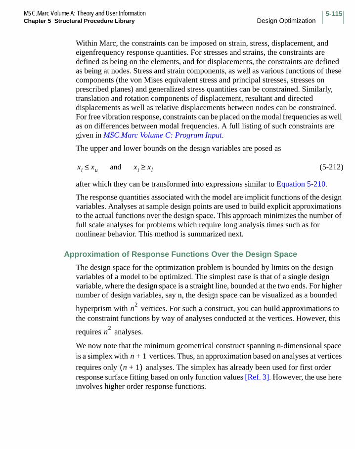
5-115MSC.Marc Volume A: Theory and User InformationChapter 5 Structural Procedure Library Design Optimization
Within Marc, the constraints can be imposed on strain, stress, displacement, and eigenfrequency response quantities. For stresses and strains, the constraints are defined as being on the elements, and for displacements, the constraints are defined as being at nodes. Stress and strain components, as well as various functions of these components (the von Mises equivalent stress and principal stresses, stresses on prescribed planes) and generalized stress quantities can be constrained. Similarly, translation and rotation components of displacement, resultant and directed displacements as well as relative displacements between nodes can be constrained. For free vibration response, constraints can be placed on the modal frequencies as well as on differences between modal frequencies. A full listing of such constraints are given in MSC.Marc Volume C: Program Input.
The upper and lower bounds on the design variables are posed as
(5-212)
after which they can be transformed into expressions similar to Equation 5-210.
The response quantities associated with the model are implicit functions of the design variables. Analyses at sample design points are used to build explicit approximations to the actual functions over the design space. This approach minimizes the number of full scale analyses for problems which require long analysis times such as for nonlinear behavior. This method is summarized next.
Approximation of Response Functions Over the Design Space
The design space for the optimization problem is bounded by limits on the design variables of a model to be optimized. The simplest case is that of a single design variable, where the design space is a straight line, bounded at the two ends. For higher number of design variables, say n, the design space can be visualized as a bounded
hyperprism with vertices. For such a construct, you can build approximations to the constraint functions by way of analyses conducted at the vertices. However, this
requires analyses.
We now note that the minimum geometrical construct spanning n-dimensional space is a simplex with vertices. Thus, an approximation based on analyses at vertices
requires only analyses. The simplex has already been used for first order response surface fitting based on only function values [Ref. 3]. However, the use here involves higher order response functions.
xi xu and xi xl≥≤
n2
n2
n 1+
n 1+( )
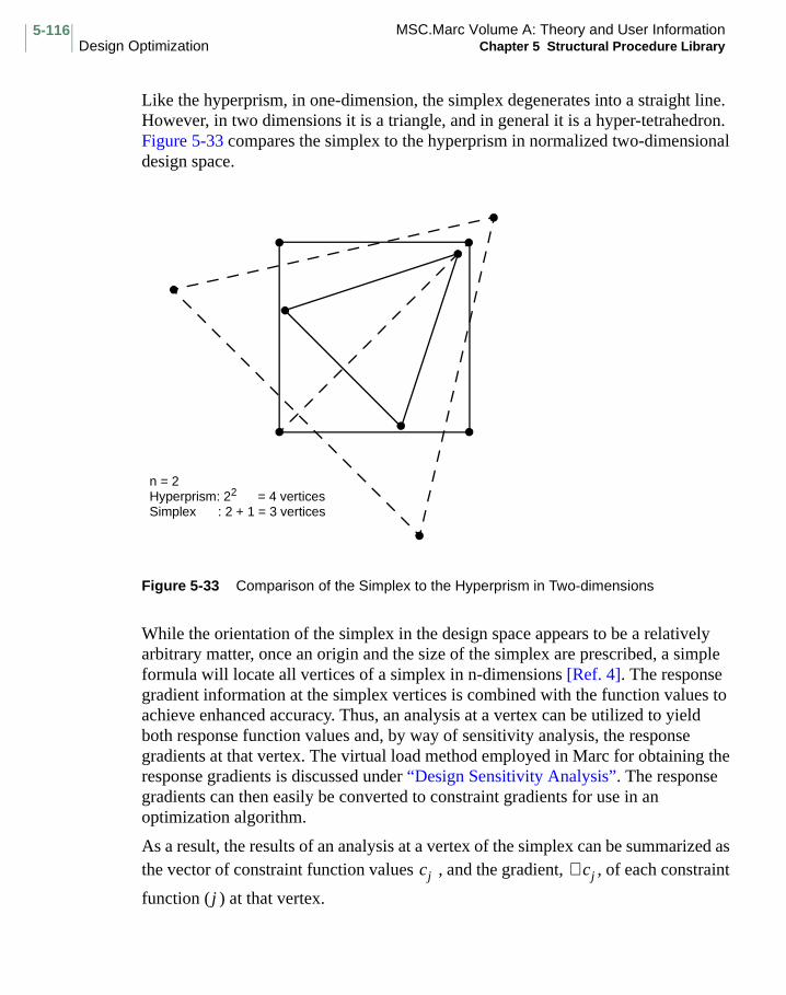
MSC.Marc Volume A: Theory and User InformationDesign Optimization Chapter 5 Structural Procedure Library
5-116
Like the hyperprism, in one-dimension, the simplex degenerates into a straight line. However, in two dimensions it is a triangle, and in general it is a hyper-tetrahedron. Figure 5-33 compares the simplex to the hyperprism in normalized two-dimensional design space.
Figure 5-33 Comparison of the Simplex to the Hyperprism in Two-dimensions
While the orientation of the simplex in the design space appears to be a relatively arbitrary matter, once an origin and the size of the simplex are prescribed, a simple formula will locate all vertices of a simplex in n-dimensions [Ref. 4]. The response gradient information at the simplex vertices is combined with the function values to achieve enhanced accuracy. Thus, an analysis at a vertex can be utilized to yield both response function values and, by way of sensitivity analysis, the response gradients at that vertex. The virtual load method employed in Marc for obtaining the response gradients is discussed under “Design Sensitivity Analysis”. The response gradients can then easily be converted to constraint gradients for use in an optimization algorithm.
As a result, the results of an analysis at a vertex of the simplex can be summarized as the vector of constraint function values , and the gradient, , of each constraint
function ( ) at that vertex.
n = 2Hyperprism: 22 = 4 verticesSimplex : 2 + 1 = 3 vertices
cj ∇ cj
j

5-117MSC.Marc Volume A: Theory and User InformationChapter 5 Structural Procedure Library Design Optimization
For the case of a one variable problem, the results of analyses at the two vertices are symbolized in Figure 5-34, for a hypothetical constraint .
Figure 5-34 Vertex Results for One-dimensional Design Space
From Figure 5-34, it appears almost natural to fit a cubic function to the four end conditions (two function values and two slopes) depicted in the figure. However, this approach is too rigid, and is not easily generalizable to higher dimensions. On the other hand, the use of two quadratics, which are then merged in a weighted manner gives higher flexibility and potential for increased accuracy.
It can be seen that the two equations, and , are designed such that they both
satisfy the function values at the two vertices, but satisfies the slope at vertex 1
only, and satisfies the slope at vertex 2 only. Finally, at any design point , the
response function can be approximated as
(5-213)
where the weight functions and are normally functions of and possibly some other parameters.
This type of approach has the further advantage that it is consistent with the use of the simplex for determining analysis points and approximating constraint functions in the higher dimensional cases. Therefore, for an n-dimensional problem, the simplex
cj
cj1
dcj1dx
-----------
cj2
dcj2dx
-----------x
Possible Actual Function
1
2
E2
E1
E1 E2
E1
E2 x
cj
cj W1 E1 W2 E1+( ) W1 W2+( )⁄=
W1 W2 x

MSC.Marc Volume A: Theory and User InformationDesign Optimization Chapter 5 Structural Procedure Library
5-118
having vertices, each equation needs to have unknown parameters. The general quadratic polynomial without the cross-coupling terms satisfies this condition for all .
Improvement of the Approximation
When approximations are used, the results of an optimization process need to be checked by means of a detailed analysis. As a result, the approximations can be adjusted and the optimization algorithm can be reapplied. Depending on how accurate the approximations prove to be and how many more detailed analyses are acceptable to you, this process can be applied for a number of cycles in order to improve upon the results.
The Optimization Algorithm
The optimization algorithm implemented in Marc is the Sequential Quadratic Programming method [Ref. 5]. This method is employed using the approximation described above. By obtaining response function and gradient values from the approximate equations, the need for full scale analyses is reduced. The method is summarized below.
The quadratic programming technique is based on the approximation of the objective function by a quadratic function. When nonlinear constraints exist, as is the case in most practical design optimization problems, the second order approximation concept is extended to the Lagrangian which is a linear combination of the objective function and the constraint functions. The solution method for a quadratic programming problem with nonlinear constraints can be summarized as the following:
At each step, modify the design variables vector by adding a scaled vector
(5-214)
where is a search direction and is the scale factor along the search direction. If the search direction has been determined, the scale factor can be found by some type of line search along the search direction. The determination of the search direction constitutes the major undertaking in the quadratic programming method. If is the
Hessian of the Lagrangian and is the gradient of the objective function, then the
search direction is that which minimizes the function
(5-215)
n 1+ n 1+( ) n+ 2n 1+=
n
x
x x qs+←
s q
H
g
s
gTs s
THs( ) 2⁄+

5-119MSC.Marc Volume A: Theory and User InformationChapter 5 Structural Procedure Library Design Optimization
subject to the linearized constraints
(5-216)
where is the Jacobian matrix of the constraints and is the vector of constraint functions at the current iteration. Due to lack of knowledge about which constraints will be active at the optimum, the Hessian of the Lagrangian is not always readily available. Thus, some iterations take the form of a gradient projection step.
The coefficients of the constraint functions in the Lagrangian are the Lagrange multipliers which are unknown before solution has started. At the optimum these multipliers are zero for inactive constraints. Normally, the above problem is solved using only those constraints which appear to be active at or close to the current design point, with the assumption that these constraints will be active at the optimum. The selection of these active constraints is done within the framework of an active set strategy, the set being modified appropriately with the progression of the iterations. Similarly, the arrays , , and are also modified as the iterations proceed.
Marc User Interface for Sensitivity Analysis and Optimization
This is discussed below under input, output, and postprocessing.
Input
Input features related to design sensitivity and design optimization are similar. However, they differ in the parameter data blocks and in the optional specification of an objective function for the case of sensitivity analysis. Therefore, other than these two items, all discussion of input should be construed to refer to both procedures equally. All design sensitivity and design optimization related parameters and options in a Marc input file start with the word DESIGN.
All load cases and any eigenfrequency analysis request associated with sensitivity analysis or optimization should be input as load increments in the history definition section after the END OPTION line. The maximum number of nodes with point loads or the maximum number of distributed load cases should be defined in the DIST LOADS parameter.
The type of solution requested from Marc can simply be indicated by the parameter input DESIGN SENSITIVITY or DESIGN OPTIMIZATION. Only one of these lines can appear in the input. These parameters also let you change the sorting of constraints, the maximum number of constraints in the active set, and the maximum number of cycles of design optimization. The first two items are discussed in previous sections. A cycle of design optimization refers to a complete solution employing the sequential quadratic programming technique followed by a detailed finite element analysis to
Js c–≥
J c
g H J

MSC.Marc Volume A: Theory and User InformationDesign Optimization Chapter 5 Structural Procedure Library
5-120
accurately evaluate the new design point reached by way of approximate solution. If required, the approximation is improved using the results of the last finite element analysis, and a new cycle is started.
The specification of an objective function, being optional for design sensitivity, is made by use of the model definition option DESIGN OBJECTIVE. This allows you to choose from one of the available design objectives.
The DESIGN VARIABLES option allows you to specify the design variables associated with the finite element model. You have a choice of three major types of design variables:
1. Element cross-sectional properties as given by way of the GEOMETRY option.
2. Material properties as given by ISOTROPIC or ORTHOTROPIC options.
3. Composite element properties of layer thickness and ply angle, as given by the COMPOSITE option.
The properties which are supported are listed under the DESIGN VARIABLES option. The relevant elements, for which cross-sectional properties can be specified as design variables, each has a section in Volume B: Element Library, describing which properties, if any, can be posed as design variables for that element.
Similarly, the list of material properties (currently all related to linear behavior) that can be design variables is given under the DESIGN VARIABLES option. For composite groups, the layer thicknesses and ply angles can be given as design variables for composite groups.
Design variables can be linked across finite element entities such that a given design variable controls several entities. An example is the linking of the thicknesses of several plane stress elements by means of a single design variable. Thus, when this variable changes, the thicknesses of all linked elements reflect this change. On the other hand, for the unlinked case, all thicknesses are associated with separate design variables. This feature is controlled by the LINKED and UNLINKED commands.
Response quantities, or constraints on response quantities, are specified by means of the DESIGN DISPLACEMENT CONSTRAINTS, DESIGN STRAIN CONSTRAINTS, DESIGN STRESS CONSTRAINTS, and DESIGN FREQUENCY CONSTRAINTS options. There is no limit to the number of constraints. Displacement constraints are posed at nodes or groups of nodes, while the strain and stress constraints are posed over elements or groups of elements, and frequency constraints are posed for free vibration modes. A complete list can be found under the above mentioned options in Volume C: Program Input.

5-121MSC.Marc Volume A: Theory and User InformationChapter 5 Structural Procedure Library Design Optimization
When strain or stress constraints are prescribed, it is useful to know that the program evaluates such constraints at all integration points of all layers of an element and proceeds to consider the most critical integration point at the related layer for the element. Thus, a strain or stress constraint on an element normally refers to the most critical value the constraint can attain within the element. During optimization, the most critical location within the element may change and any necessary adjustment takes place internally.
For certain responses, the limiting values can be the same in absolute value for both the positive and negative values of the response. For constraints on such response functions, you have the choice of prescribing either separate constraints on the positive and negative values, or a combined constraint on the absolute value. The first approach is more accurate albeit at a higher computational cost.
Output
For sensitivity analysis, the output file contains the following information:
• Echo of input, any warnings or error messages.
• A table of numbers and definitions for your prescribed design variables. It is important to note that the variable values are always output in the internal numbering sequence which is defined in this table. Search for the words ‘Design variable definitions’ to reach this table in the output file.
• Analysis results for your prescribed design.
• The value of the objective function and its gradient with respect to the design variables prescribed by you.
• Sensitivity analysis results for the response functions in the default or user-defined set, sorted in order of criticalness (if specified). It should be noted that although the responses are sorted across multiple load cases, the sensitivity results are output for each load case. The related output file consists of a check on the actual response value (obtained by sensitivity analysis) and the gradient of the response with respect to the design variables. For eigenfrequency results, the check values on the response can be somewhat more accurate than the results from eigenfrequency analysis since the latter is iterative, but the check uses the Rayleigh quotient on top of the iteration results. A constraint reference number allows you to track the sensitivity analysis results plots when postprocessing. Search for the word ‘Sensitivity’ to reach this output.
For design optimization, the following is written into the output file:
• Echo of input, any warnings or error messages.
• Certain indications that some analyses are being done, but no analysis results except for the ‘best’ design reached during optimization.

MSC.Marc Volume A: Theory and User InformationDesign Optimization Chapter 5 Structural Procedure Library
5-122
5Structural Procedure Library
Design Optimization
• The objective function values and the vector of design variable values:• At each of the simplex vertices.
• For the starting simplex vertex (from this point on, the information also includes whether the design is feasible or not).
• At the end of each cycle of optimization.
• For the ‘best’ design found.
• Analysis results for the ‘best’ design.
Postprocessing
This requires that you ask the program to create a post file. The following plots can be obtained by way of postprocessing.
For sensitivity analysis:
• Bar charts for gradients of response quantities with respect to the design variables.
• Contour plots of element contributions to response quantities. Thus, a finite element model contour plot gives the element contributions to a specific response quantity which was posed in the form of a constraint in the input file.
The increment number of the sensitivity analysis results is the highest increment number available in the post file. The information for each response quantity is written out as for a subincrement. The zeroth subincrement corresponds to the objective function information. Numbers for the other subincrements correspond to the constraint reference number(s) in the output file.
For design optimization:
• Path plots showing the variation of the objective function and of the design variables over the history of the optimization cycles. The best design (feasible or not) is not necessarily the last design point in the plot. The values at the starting vertex are considered as belonging to the zeroth subincrement. Each optimization cycle is then another subincrement. The increment number corresponding to these subincrements is taken as zero. The analysis results for the ‘best’ design start from increment one.
• Bar charts where each chart gives the values of the design variables at the optimization cycle corresponding to that bar chart.

5-123MSC.Marc Volume A: Theory and User InformationChapter 5 Structural Procedure Library Considerations for Nonlinear Analysis
Considerations for Nonlinear Analysis
Nonlinear analysis is usually more complex and expensive than linear analysis. Also, a nonlinear problem can never be formulated as a set of linear equations. In general, the solutions of nonlinear problems always require incremental solution schemes and sometimes require iterations (or recycles) within each load/time increment to ensure that equilibrium is satisfied at the end of each step. Superposition cannot be applied in nonlinear problems.
The four iterative procedures available in Marc are: Newton-Raphson, Modified Newton-Raphson, Newton-Raphson with strain correction modification, and a secant procedure. If the R-P flow contribution model is chosen, a direction substitution is used. See the appendix for a discussion of these iterative procedures.
A nonlinear problem does not always have a unique solution. Sometimes a nonlinear problem does not have any solution, although the problem can seem to be defined correctly.
Nonlinear analysis requires good judgment and uses considerable computing time. Several runs are often required. The first run should extract the maximum information with the minimum amount of computing time. Some design considerations for a preliminary analysis are:
• Minimize degrees of freedom whenever possible.• Halve the number of load increments by doubling the size of each load
increment.• Impose a coarse tolerance on convergence to reduce the number of iterations. A
coarse run determines the area of most rapid change where additional load increments might be required. Plan the increment size in the final run by the following rule of thumb: there should be as many load increments as required to fit the nonlinear results by the same number of straight lines.
Marc solves nonlinear static problems according to one of the following two methods: tangent modulus or initial strain. Examples of the tangent modulus method are elastic-plastic analysis, nonlinear springs, nonlinear foundations, large displacement analysis and gaps. This method requires at least the following three controls:
• A tolerance on convergence • A limit to the maximum allowable number of recycles• Specification of a minimum number of recycles

MSC.Marc Volume A: Theory and User InformationConsiderations for Nonlinear Analysis Chapter 5 Structural Procedure Library
5-124
An example of the initial strain method is creep or viscoelastic analysis. Creep analysis requires the following tolerance controls:
• Maximum relative creep strain increment control• Maximum relative stress change control• A limit to the maximum allowable number of recycles
To input control tolerances, use the model definition option CONTROL. These values can be reset upon restart or through the CONTROL history definition option. See “Convergence Controls” in Chapter 11 for further discussion on tolerance controls.
Behavior of Nonlinear Materials
Nonlinear behavior can be time- (rate-) independent, or time- (rate-) dependent. For example, plasticity is time-independent and creep is time-dependent. Both viscoelastic and viscoplastic materials are also time-dependent. Nonlinear constitutive relations must be modeled correctly to analyze nonlinear material problems. A comprehensive discussion of constitutive relations is given in Chapter 7.
Scaling the Elastic Solution
The parameter SCALE causes scaling of the linear-elastic solution to reach the yield stress in the highest stressed element. Scaling takes place for small displacement elastic-plastic analysis, where element properties do not depend on temperature. The SCALE parameter causes all aspects of the initial solution to be scaled, including displacements, strains, stresses, temperature changes, and loads. Subsequent incrementation is then based on the scaled solution.
Load Incrementation
Several history definition options are available in Marc to input mechanical and thermal load increments (see Table 5-8). The choice is between a fixed and an automatic load stepping scheme. For a fixed scheme, the load step size remains constant during a load case. The fixed schemes are AUTO LOAD for static mechanical, CREEP INCREMENT for creep, DYNAMIC CHANGE for dynamic mechanical and TRANSIENT NON AUTO for thermal/thermo-mechanically coupled. For an adaptive scheme, the load step size changes from one increment to the other and also within an increment depending on convergence criteria and/or user-defined criteria. The adaptive schemes are AUTO STEP and AUTO INCREMENT for static mechanical, AUTO CREEP and AUTO STEP for creep, AUTO STEP and TRANSIENT for dynamic mechanical and AUTO STEP and TRANSIENT for thermal/thermo-mechanically coupled.

5-125MSC.Marc Volume A: Theory and User InformationChapter 5 Structural Procedure Library Considerations for Nonlinear Analysis
The main automatic scheme is AUTO STEP, which has been greatly enhanced in the 2001 release. Previously, one or more criteria based upon strain, stress, displacement, or temperature increments had to be given for controlling the time step. Besides these criteria, there is a new criterion for automatically controlling the load step based upon the number of recycles. This allows the option to be used directly with default settings for mechanical, thermal and thermo-mechanically coupled analysis problems. More details on the AUTO STEP option are given in the next section.
While the improved AUTO STEP option is designed as the default adaptive stepping procedure, it may still be advantageous to use one of the other available adaptive time-stepping options. This is the case for the following analysis types:
• Post buckling or snap-through analyses require the so-called arclength method which is available through the AUTO INCREMENT option. This option can only be used in static mechanical analyses and the applied load is automatically increased or decreased in order to maintain a certain arclength
Note: AUTO INCREMENT can also be used for general situations without instabilities, but, in general, the AUTO STEP option is preferred for these situations.
• For creep analysis, the available adaptive options are AUTO CREEP and AUTO STEP. The AUTO CREEP option supports some features which are not available through AUTO STEP (see the descriptions in Volume C). If AUTO STEP is used for creep problems, it may be advisable to use a creep strain increment criterion and a stress increment criterion as additional user-defined criteria in combination with the default recycle criterion. AUTO STEP is usually more reliable in cases involving creep and contact.
• For the case of automatic load stepping for a thermally loaded elastic-creep/elastic-plastic-creep stress analysis, the only available scheme is AUTO THERM CREEP (see Volume C).
• For thermally driven mechanical problems, the AUTO THERM option can be used. The thermal loads derived from a thermal analysis are applied using the CHANGE STATE option in a mechanical analysis. The load step of the mechanical analysis is automatically adjusted based upon user-specified (allowed) changes in temperature from the thermal analysis per increment. For example, if there is a change of 50° in the thermal analysis in one increment and you only allowed a change of 10° per increment in the mechanical analysis, AUTO THERM splits up the thermal increment into five mechanical increments.

MSC.Marc Volume A: Theory and User InformationConsiderations for Nonlinear Analysis Chapter 5 Structural Procedure Library
5-126
Selecting Load Increment Size
Selecting a proper load step increment is an important aspect of a nonlinear solution scheme. Large steps often lead to many recycles per increment and, if the step is too large, it can lead to inaccuracies and nonconvergence. On the other hand, using too small steps is inefficient.
When a fixed load stepping scheme is used, it is important to select an appropriate load step size that captures the loading history and allows for convergence within a reasonable number of recycles. For complex load histories, it is often necessary to break up the analysis into separate load cases with different step sizes. For fixed stepping, there is an option to have the load step automatically cut back in case of failure to obtain convergence. When an increment diverges, the intermediate deformations after each recycle can show large fluctuations and the final cause of program exit can be any of the following: maximum number of recycles reached (exit 3002), elements going inside out (exit 1005 or 1009) or, in a contact analysis, nodes sliding off a rigid contact body (exit 2400). These deformations are normally not visible as post results (there is a feature to allow for the intermediate results to be available on the post file, see the POST option). If the cutback feature is activated and one of these failures occurs, the state of the analysis at the end of the previous increment is restored from a copy kept in memory, and the increment is subdivided into a number of subincrements. The step size is halved until convergence is obtained or the user-specified number of cutbacks has been performed. Once a subincrement is converged, the analysis continues to complete the rest of the original increment. No results are written to the post file during subincrementation. When the original increment is finished, the calculation continues to the next increment with the original increment count maintained. No results are written to the post file during subincrementation, and the original increment count is preserved. If the global
Table 5-8 History Definition Options for Load Incrementation
Load Type Fixed Adaptive
Mechanical AUTO LOADDYNAMIC CHANGECREEP INCREMENT
AUTO STEPAUTO INCREMENTAUTO TIME*AUTO THERMAUTO CREEPAUTO THERM CREEP
Thermal TRANSIENT NON AUTO AUTO STEPTRANSIENT
* The option is obsolete, use AUTO STEP instead.

5-127MSC.Marc Volume A: Theory and User InformationChapter 5 Structural Procedure Library Considerations for Nonlinear Analysis
remeshing option is activated in conjunction with the cutback feature, then for exit 1005 or 1009, the chosen contact body is remeshed and the analysis is repeated with the original time step before the first cutback.
Automatic Load Incrementation
In many nonlinear analyses, it is useful to have Marc figure out the appropriate load step size automatically. The AUTO INCREMENT option is a so-called arc-length method and is designed for applications like post buckling and snap-through analysis. This method is described in detail in Chapter 11, Arc-Length Methods on page 11.
Any automatic load incrementation method is currently limited to input histories that only have linear variations in load or displacement since all of the automatic load incrementation methods only require the total load or displacement at the end of the load case. For example, one may not use a rigid body with a linearly changing velocity, since the resulting displacement of the rigid body would give parabolically changing displacements. In this case, one would need to use a constant velocity for the automatic load incrementation methods to work properly.
For any automatic load incrementation, care must be taken to approriately define the loading history in each loadcase. The load case should be defined between appropriate break points in the load history curve. For example, in Figure 5-35, correct results would be obtained upon defining three distinct loadcases between times ,
, and during the model preparation. However, if only one load case is
defined for the entire load history between , the the total applied load for the
loadcase is zero.
Figure 5-35 Defining Loadcases for Automatic Load Incrementation
0 t1–
t1 t2– t2 t3–
0 t3–
P (
Load
)
P2
P1
t1 t2 t3
t (Time)
P (
Load
)
P2
P1
t3
t (Time)0 0
a. Three Defined Loadcases b. One Defined Loadcase

MSC.Marc Volume A: Theory and User InformationConsiderations for Nonlinear Analysis Chapter 5 Structural Procedure Library
5-128
AUTO STEP
The scheme appropriate for most other applications is AUTO STEP. The primary control of the load step is based upon the number of recycles needed to obtain convergence. There are a number of optional user-specified physical criteria that can be used to additionally control the load step. For the recycle based option the user specifies a desired number of recycles. This number is used as a target value for the load stepping scheme. If the number of recycles needed to obtain convergence exceeds the desired number, the load step size is reduced, the recycle counter is reset to zero and the increment is performed again with the new load step. The factor with which the time step is cut back defaults to 1.2 and can be specified by you. The load step for the next increment is increased if the number of recycles required in the current increment is less than the desired number. The same factor that is used for decreasing the time step is used for increasing it. The load step is never increased during an increment. In addition, the same type of cut-back feature for fixed load stepping, as described in the Selecting Load Increment Size section, is available for this scheme as well.
There are some exceptions to the basic scheme outlined above. If an increment is consistently converging with the original load step and the number of recycles exceeds the desired number, the number of recycles is allowed to go beyond the desired number until convergence or up to the user specified maximum number. The time step is then decreased for the next increment. An increment is determined to be converging if the convergence ratio was decreasing in three previous recycles.
Special rules also apply in a contact analysis. For quasi-static problems, the AUTO STEP option is designed to only use the automated penetration check option (see CONTACT option, 7th field of 2nd data block; option 3 is always used). Even if you flag the increment splitting penetration check option, Marc internally converts it to the automated penetration check. During the recycles, the contact status can keep changing (new nodes come in contact, nodes slide to new segments, separate etc.). Whenever the contact status changes during an increment, a new set of contact constraints are incorporated into the equilibrium equations and more recycles are necessary in order to find equilibrium. These extra recycles, which are solely due to contact changes, are not counted when the comparison is made to the desired number for determining if the load step needs to be decreased within the increment. Thus, only true Newton-Raphson iterations are taken into account. For the load step of the next increment, the accumulated number of recycles during the previous increment is used. This ensures that the time step is not increased when there are many changes in contact during the previous increment.

5-129MSC.Marc Volume A: Theory and User InformationChapter 5 Structural Procedure Library Considerations for Nonlinear Analysis
In addition to allowing Marc to use the number of recycles for automatically controlling the step size for AUTO STEP, user-specified physical criteria can be used for controlling the step size. You can specify the maximum allowed incremental change within certain ranges for specific quantities during an increment. The quantities available are displacements, rotations, stresses, strains, strain energy, and temperature (in thermal or thermomechanically coupled analyses). These criteria can be utilized in two ways. By default, they are used as limits, which means that the load step is decreased if a criterion is violated during the current increment, but they do not influence the decision to change the load step for the next increment (that is, only the actual number of recycles versus desired number of recycles controls the load step for the next increment). The criteria can also be used as targets; in which case, they are used as the main means for controlling the time step for the current and next increments. If the calculated values of the criteria are higher than the user specified values the time step is scaled down. If the obtained values for a converged increment are less than the user specified, the time step is scaled up. The scale factor used is the ratio between the actual value and the target value and this factor is limited by user-specified minimum and maximum factors (defaults to 0.1 and 10 respectively). If this type of load step control is used together with the recycle based control, the time step can be reduced due to whichever criterion that is violated. The decision to increase the step size for the next increment is based upon the physical criteria.
In many analyses it is convenient to obtain post file results at specified time intervals. This is naturally obtained with a fixed load stepping scheme but not with an automatic
scheme. Traditionally, the post output frequency is given as every nth increment. With the AUTO STEP procedure, you can request post output to be obtained at equally spaced time intervals. In this case, the time step is temporarily modified to exactly reach the time for output. The time step is then restored in the following increment.
The AUTO STEP option also has an artificial damping feature available for mechanical statics analyses. If the time step is decreased to below the user-specified minimum time step, Marc normally stops with exit number 3015; but if the artificial damping feature is activated, the analysis is continued with a smaller time step. The solution is stabilized by adding a factored lumped mass matrix to the stiffness matrix and modifying the force vector consistently. This artificial stabilization is turned off once the time step increases above the minimum time step. If the feature is used, it might be useful to write post file results at fixed time intervale; otherwise, many increments might appear on the post file even for a small time period. The critical parameter for this feature is the (artificial) mass density, which needs to be specified with an appropriate value for all materials in the model.

MSC.Marc Volume A: Theory and User InformationConsiderations for Nonlinear Analysis Chapter 5 Structural Procedure Library
5-130
The defaults of the AUTO STEP optin are carefully chosen to be adequate in a wide variety of applications. There are cases, however, when the settings may need to be modified. Assume that the default settings are used, which means that the recycle based control is active with an initial load of one per cent of the total. If the structure is weakly nonlinear, convergence is obtained in just a few recycles and the time steps for successive increments get progressively larger. This can lead to problems if the initially weakly nonlinear structure suddenly exhibits stronger nonlinearities; for instance, occurrence of plasticity or parts coming into contact. Possible remedies to this problem include:
(i) decrease the time step scale factor from 1.2 to a smaller number so the step size does not grow so rapidly;
(ii) use a physical criterion like maximum increment of displacements to limit the load step;
(iii)use the maximum time step to limit large steps;
(iv)decrease the desired and maximum number of recycles to make the scheme more prone to decrease the load step if more recycles are needed.
Another situation is if the structure is highly nonlinear and convergence is slow. In this case, it may be necessary to increase the desired number and maximum number of recycles. In general, there is a close connection between the convergence tolerances used and the desired number and maximum number of recycles. In many cases, it may be beneficial to use one or more physical criteria; for example, the increment of plastic strain as targets for controlling the load step.
Residual Load Correction
The residual load is applied as a correcting force to ensure that equilibrium is maintained and, hence, that an accurate solution is obtained for nonlinear problems.
The residual load correction enforces global equilibrium at the start of each new increment. This prevents the accumulation of out-of-equilibrium forces from increment to increment and makes the solution less sensitive to the step size. Figure 5-36 shows how stiffness is based on the state at the start of a step. The variables are defined below for increments i = 1,2,3:
• applied forces for i = 1,2,3
• calculated displacements for i = 1,2,3
• residual loads for i = 1,2,3
Fi
ui
Ri

5-131MSC.Marc Volume A: Theory and User InformationChapter 5 Structural Procedure Library Considerations for Nonlinear Analysis
Figure 5-36 Stiffness Based on State at Start of Step
The residual load correction is the difference between the internal forces and the externally applied loads. The residual load correction is expressed as
(5-217)
where is the differential operator which transforms displacements to strains, is
the current generalized stresses, is the total applied load vector, and is the residual load correction.
In order to evaluate the residual load correction accurately, evaluate the integral by summing the contributions from all integration points. The residual load correction feature requires that stresses be stored at all the integration points. Data storage at all integration points is the default in Marc, but can be overridden in linear analysis by use of the CENTROID parameter.
Note: The ALL POINTS parameter should be used for all nonlinear analysis. In the K3 version and all subsequent versions, this is the default.
Restarting the Analysis
The model definition option RESTART creates a restart file for the current analysis which can be used in subsequent analyses. It can also be used to read in a previously generated file to continue the analysis. The RESTART option is very important for any multi-increment analysis because it allows you to continue the analysis at a later time. The default situation writes the restart information to unit 8 and reads a previously generated file from unit 9. For post processing, option RESTART can be used to plot
Φ2 + ∆Φ2
Φ1 + ∆Φ1
Φ1Ρ1
Ρ2
Ρ3
Υ1 Υ2 Υ3
Ρ1
R P βTσdV∫–=
β σP R

MSC.Marc Volume A: Theory and User InformationConsiderations for Nonlinear Analysis Chapter 5 Structural Procedure Library
5-132
or combine load cases (see CASE COMBIN). Upon restart, you can use the model definition REAUTO option to redefine parameters associated with an automatic load sequence.
To save storage space, it is not necessary to store each increment of analysis. The frequency can be set using the RESTART option, and subsequently modified using the RESTART INCREMENT option. It is also possible to store only the last converged solution by using the RESTART LAST option. This should not be used with elastic analysis because the stiffness matrix is not stored.

5-133MSC.Marc Volume A: Theory and User InformationChapter 5 Structural Procedure Library Data Transfer from Axisymmetric Analysis to 3-D Analysis
Data Transfer from Axisymmetric Analysis to 3-D Analysis
In many cases, it is possible to begin the numerical simulations as a two-dimensional axisymmetric problem even though the final problem is fully three-dimensional. This is advantageous because of the large computational savings. For this to be useful, the first stage of the problem should be truly axisymmetric. The second stage of the problem can be fully three-dimensional. The AXITO3D model definition option is used in the input file of the 3-D problem to transfer results from an axisymmetric analysis into a 3-D analysis. The data from the axisymmetric analysis is stored on the post file. In the 3-D analysis, the results from axisymmetric analysis are used as initial conditions.
There are three steps in performing an axisymmetric to 3-D analysis.
1. Run axisymmetric analysis.
2. Expand axisymmetric model to 3-D model and transfer data from axisymmetric model to 3-D model. (Axisymmetric model file is used for expansion of loads and boundary conditions besides the mesh. Exception is remeshing where the model file is not used.)
3. Run 3-D analysis.
Most quadrilateral axisymmetric elements (in 3-D case, hexahedral elements), including Herrmann elements, and most available materials, such as metal and rubber, can be used in the axisymmetric to 3-D analysis. For problems involving large deformation, either total or updated Lagrangian formulation must be used. Thermal and dynamic effects are considered.
For more detailed information on this feature, see the model definition option, AXITO3D, in MSC.Marc Volume C: Program Input.
Note: This feature is not supported by the MARC preference in Patran 2001.
Load and Displacement Boundary Conditions Transfer from Axisymmetric Analysis to 3-D using Table Curve Shift
Because the externally applied loads and displacement boundary conditions are not fully available in the post file, it is, generally, not possible to complete an AXITO3D analysis based solely on the information in the post file. Mentat is used to achieve the load and displacement boundary conditions data transfer from axisymmetric to 3-D analysis by means of shifting load table curves.

MSC.Marc Volume A: Theory and User InformationData Transfer from Axisymmetric Analysis to 3-D Analysis Chapter 5 Structural Procedure Library
5-134
The entire history of the load and the displacement boundary conditions for a complete axisymmetric to 3-D analysis must be defined using the table curves. Once the axisymmetric part of the analysis is finished, Mentat is used to expand the axisymmetric model to a 3-D model. During the model expansion, you are required to define if the table curves need to be shifted and how much the curves are to be shifted. For this purpose, either an increment number (converts internally to time) for the axisymmetric analysis or time value (which is the starting point of the 3-D analysis) has to be defined. If the table curve shift is performed, the increment number or time value is defined under:
MESH GENERATION→EXPAND→AXISYMMETRIC MODEL TO 3D.
This definition is copied to:
INITIAL CONDITIONS→MECHANICAL→AXISYMMETRIC TO 3D
and no modification is allowed. If the table curve shift is not performed, the increment number or time value is defined under:
INITIAL CONDITIONS→MECHANICAL→AXISYMMETRIC TO 3D
After the table curve shift is completed, you can delete or modify existing table curves or add new table curves depending on the specific requirement.
The table curves used with external loads are shifted differently from those associated with displacement boundary conditions. Examples are shown in Figure 5-37. The curve is A is a typical table curve used to define load or displacement boundary conditions, where t is the time at which the 3-D analysis starts. If the curve in A is associated with external loads, B shows the shifted table curve, where the total load at the end of the axisymmetric analysis is applied at the start of the 3-D analysis. If the curve in A is associated with displacement boundary conditions, C shows the shifted table curve, where the new curve for 3-D analysis starts at the zero.
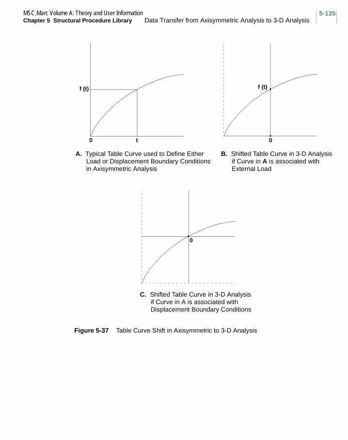
5-135MSC.Marc Volume A: Theory and User InformationChapter 5 Structural Procedure Library Data Transfer from Axisymmetric Analysis to 3-D Analysis
Figure 5-37 Table Curve Shift in Axisymmetric to 3-D Analysis
f (t)
0 t
f (t)
A. Typical Table Curve used to Define Either Load or Displacement Boundary Conditionsin Axisymmetric Analysis
B. Shifted Table Curve in 3-D Analysisif Curve in A is associated with External Load
0
0
C. Shifted Table Curve in 3-D Analysisif Curve in A is associated with Displacement Boundary Conditions

MSC.Marc Volume A: Theory and User InformationReferences Chapter 5 Structural Procedure Library
5-136
References
1. Key, S. W. and R. D. Krieg, 1982, “On the Numerical Implementation of Inelastic Time-Dependent, Finite Strain Constitutive Equations in Structural Mechanics”, Computer Methods in Applied Mechanics in Engineering, V.33, pp. 439–452, 1982.
2. Bathe, K. J., E. Ramm, and E. L. Wilson. “Finite Element formulation for Large Deformation Dynamic Analyses”, International Journal for Numerical Methods in Engineering, V. 9, pp. 353–386, 1975.
3. Montgomery, D. C., Design and Analysis of Experiments, (2nd ed.) John Wiley and Sons, 1984.
4. Spendley, W., Hext, G. R., Himsworth, F. R., “Sequential Application of Simplex Designs in Optimisation and Evolutionary Operation”, Technometrics, Vol. 4, No. 4, pp. 441-461 (1962).
5. Gill, P. E., Murray, W., Saunders, M. A., Wright, M. H., “Sequential Quadratic Programming Methods for Nonlinear Programming”, NATO-NSF-ARO, Advanced Study Inst. on Computer Aided Analysis and Optimization of Mechanical System Dynamics, Iowa City, IA, Aug. 1-2, 1983, pp. 679-700.
6. Bathe, K. J. Finite Element Procedures Prentice-Hall, 1996.
7. MARC Reference Manual Volume F.
8. Wilkinson, J. H. The Algebraic Eigenvalue Problem. Oxford: Clarendon Press, 1965.
9. Zienkiewicz, O. C., and Taylor, L. C. The Finite Element Method. Fourth Ed., Vol. 1 & 2. London: McGraw-Hill, 1989.
10. Barsoum, R. S. “On the Use of Isoparametric Finite Elements in Linear Fracture Mechanics.” Int. J. Num. Methods in Engr. 10, 1976.
11. Dunham, R. S. and Nickell, R. E. “Finite Element Analysis of Axisymmetric Solids with Arbitrary Loadings.” No. 67-6. Structural Engineering Laboratory, University of California at Berkeley, June, 1967.
12. Hibbitt, H. D., Marcal, P. V. and Rice, J. R. “A Finite Element Formulation for Problems of Large Strain and Large Displacement.” Int. J. Solids Structures 6 1069-1086, 1970.

5-137MSC.Marc Volume A: Theory and User InformationChapter 5 Structural Procedure Library References
13. Houbolt, J. C. “A Recurrence Matrix Solution for the Dynamic Response of Elastic Aircraft.” J. Aero. Sci. 17, 540-550, 1950.
14. McMeeking, R. M., and Rice, J. R. “Finite-Element Formulations for Problems of Large Elastic-Plastic Deformation.” Int. J. Solids Structures 11, 601-616, 1975.
15. MARC Update. “The Inverse Power Sweep Method in MARC.” U.S. Ed., vol. 3, no. 1, February, 1984.
16. Simo, J. C., Taylor, R. L., and Pister, K. S. “Variational and Projection Methods for the Volume Constraint in Finite Deformation Elasto-Plasticity,” Comp. Meth. in App. Mech. Engg., 51, 1985.
17. Simo, J. C. and Taylor, R. L. “A Return Mapping Algorithm for Plane Stress Elasto-Plasticity,” Int. J. of Num. Meth. Engg., V. 22, 1986.
18. Wriggers, P., Eberlein, R., and Reese, S. “A Comparison of Three-Dimensional Continuum and Shell Elements for Finite Plasticity,” Int. J. Solids & Structures, V. 33, N. 20-22, 1996.
19. Simo, J. C. and Taylor, R. L. “Quasi-Incompressible Finite Elasticity in Principal Stretches, Continuum Basis and Numerical Algorithms,” Comp. Meth. App. Mech. Engg., 85, 1991.
20. Marcal, P. V. “Finite Element Analysis of Combined Problems of Nonlinear Material and Geometric Behavior.” in Proceedings of the ASME Computer Conference, Computational Approaches in Applied Mechanics, Chicago, 1969.
21. Melosh, R. J., and Marcal, P. V. “An Energy Basis for Mesh Refinement of Structural Continua.” Int. J. Num. Meth. Eng. 11, 1083-1091, 1971.
22. Morman, K. N., Jr., Kao, B. G., and Nagtegaal, J. C. “Finite Element Analysis of Viscoelastic Elastomeric Structures Vibrating about Nonlinear Statically Stressed Configurations.” SAE Technical Papers Series 811309, presented at 4th Int. Conference on Vehicle Structural Mechanics, Detroit, November 18-20, 1981.
23. Morman, K. N., Jr., and Nagtegaal, J. C. “Finite Element Analysis of Small Amplitude Vibrations in Pre-Stressed Nonlinear Viscoelastic Solids.” Int. J. Num. Meth. Engng, 1983.
24. Nagtegaal, J. C. “Introduction in Geometrically Nonlinear Analysis.” Int. Seminar on New Developments in the Finite Element Method, Santa Marherita Ligure, Italy, 1980.

MSC.Marc Volume A: Theory and User InformationReferences Chapter 5 Structural Procedure Library
5-138
25. Nagtegaal, J. C., and de Jong, J. E. “Some Computational Aspects of Elastic-Plastic Large Strain Analysis.” in Computational Methods in Nonlinear Mechanics, edited by J. T. Oden. North-Holland Publishing Company, 1980.
26. Newmark, N. M. “A Method of Computation for Structural Dynamics.” ASCE of Eng. Mech. 85, 67-94, 1959.
27. Parks, D. M. “A Stiffness Derivative Finite Element Technique for Determination of Elastic Crack Tip Stress Intensity Factors.” International Journal of Fractures 10, (4), 487-502, December 1974.
28. Timoshenko, S., Young, D. H., and Weaver, Jr., W. Vibration Problems in Engineering. John Wiley, New York: 1979.
29. Wilkinson, J. H. The Algebraic Eigenvalue Problem. Oxford: Clarendon Press, 1965.
30. Chung, J. and Hulbert, G.M., “A family of single-step Houbolt time integration algorithms for structural dynamics”, Comp. Meth. in App. Mech. Engg., 118, 1994.
31. Shih, C.F., Moran B. and Nakamura K., “Energy release rate along a three-dimensional crack front in a thermally stressed body”, International Journal of Fracture, vol. 30, pp. 79–102, 1986.
32. Anderson, T.L., Fracture Mechanics: Fundamentals and Applications (2nd ed.) CRC Press, 1995.

Chapter 6 Nonstructural Procedure Library
CHAPTER
6 Nonstructural Procedure Library
Heat Transfer
Hydrodynamic Bearing
Electrostatic Analysis
Magnetostatic Analysis
Electromagnetic Analysis
Acoustic Analysis
Fluid Mechanics
Coupled Analyses
References

MSC.Marc Volume A: Theory and User InformationChapter 6 Nonstructural Procedure Library
6-2
This chapter describes the nonstructural analysis procedures available in Marc. These are comprised of several areas including heat transfer, hydrodynamic bearing, electrostatics, magnetostatics, electromagnetics, fluid mechanics, and coupled analysis. This chapter provides the technical background information as well as usage information about these capabilities.

6-3MSC.Marc Volume A: Theory and User InformationChapter 6 Nonstructural Procedure Library Heat Transfer
Heat Transfer
Marc contains a solid body heat transfer capability for one-, two-, and three-dimensional, steady-state and transient analyses. This capability allows you to obtain temperature distributions in a structure for linear and nonlinear heat transfer problems. The nonlinearities in the problem may include temperature-dependent properties, latent heat (phase change) effect, heat convection in the flow direction, and nonlinear boundary conditions (convection and radiation). The temperature distributions can, in turn, be used to generate thermal loads in a stress analysis.
Marc can be applied to solve the full range of two- and three-dimensional transient and steady-state heat conduction and heat convection problems. Marc provides heat transfer elements that are compatible with stress elements. Consequently, the same mesh can be used for both the heat transfer and stress analyses. Transient heat transfer is an initial- boundary value problem, so proper initial and boundary conditions must be prescribed to the problem in order to obtain a realistic solution. Marc accepts nonuniform nodal temperature distribution as the initial condition, and can handle temperature/time-dependent boundary conditions. Both the thermal conductivity and the specific heat in the problem can be dependent on temperature; however, the mass density remains constant at all times. The thermal conductivity can also be anisotropic. Latent heat effects (solid-to-solid, solid-to-liquid phase changes) can be included in the analysis. A time-stepping procedure is available for transient heat transfer analysis. Temperature histories can be stored on a post file and used directly as thermal loads in subsequent stress analysis. User subroutines are available for complex boundary conditions such as nonlinear heat flux, convection, and radiation.
A summary of Marc capabilities for transient and steady-state analysis is given below.
• Selection of the following elements that are compatible with stress analysis:
1-D: three-dimensional link (2-node, 3-node)2-D: planar and axisymmetric element (3-, 4-, and 8-node)3-D: solid elements (4-, 8-, 10-, and 20-node)shell elements (4- and 8-node)
• Specification of temperature-dependent materials (including latent heat effects) is performed with the model definition options ISOTROPIC, ORTHOTROPIC, TEMPERATURE EFFECTS, and ORTHO TEMP.
• Selection of initial conditions is done using the INITIAL TEMP option.

MSC.Marc Volume A: Theory and User InformationHeat Transfer Chapter 6 Nonstructural Procedure Library
6-4
• Selection of the temperature and time-dependent boundary conditions (prescribed temperature history, volumetric flux, surface flux, film coefficients, radiation, change of prescribed temperature boundary conditions during analyses) is done using the FIXED TEMPERATURE, TEMP CHANGE, DIST FLUXES, POINT FLUX, and FILMS options.
• Import of viewfactors calculated by Mentat for radiation analyses.
• Selection of time steps using history definition option TRANSIENT.
• Application of a tying constraints on nodal temperatures using model definition option TYING.
• Generation of a thermal load (temperature) file using the POST option, which can be directly interfaced with the stress analysis using model definition option CHANGE STATE.
• Use of user subroutines ANKOND for anisotropic thermal conductivity, FILM for convective and radiative boundary conditions or FLUX for heat flux boundary conditions.
• Selection of nodal velocity vectors for heat convection is done using VELOCITY and VELOCITY CHANGE options.
• Use of user subroutines UVELOC for heat convection.
In addition, a number of thermal contact gap and fluid channel elements are available in Marc. These elements can be used for heat transfer problems involving thermal contact gap and fluid channel conditions.
The thermal contact elements provide perfect conduction or radiation/convection between surfaces of the thermal contact gap, depending on the surface temperatures. The perfect conduction capability in the elements allows for the enforcement of equal temperatures at nodal pairs and the radiation/convection capability allows for nonlinear heat conduction between surfaces, depending on film coefficient and emissivity. The perfect conduction is simulated by applying a tying constraint on temperatures of the corresponding nodal points. An automatic tying procedure has been developed for such elements. The radiation/convection capabilities in the elements are modeled by one-dimensional heat transfer in the thickness direction of the elements with variable thermal conductivity.
For the purpose of cooling, channels allowing coolant to flow through often appear in the solid. The fluid channel elements are designed for the simulation of one-dimensional fluid/solid convection conditions based on the following assumptions:
1. Heat conduction in the flow direction can be neglected compared to heat convection;
2. The heat flux associated with transient effects in the fluid (changes in fluid temperature at a fixed point in space) can be neglected.

6-5MSC.Marc Volume A: Theory and User InformationChapter 6 Nonstructural Procedure Library Heat Transfer
For high velocity air flow, these assumptions are reasonable and the following approach is used:
Each cooling channel is modeled using channel elements. On the sides of the channel elements, convection is applied automatically. The film coefficient is equal to the film coefficient between fluid and solid, whereas the sink temperature represents the temperature of the fluid. A two-step staggered solution procedure is used to solve for the weakly coupled fluid and solid temperatures.
Steady State Analysis
For steady state problems, use the STEADY STATE history definition option. If the problem is nonlinear, use the tolerance for property recycling on the CONTROL model definition set to obtain an accurate solution.
You must distinguish between two cases of nonlinearity in steady-state solutions: mild nonlinearities and severe nonlinearities. In the case of mild nonlinearities, variations are small in properties, film coefficients, etc., with respect to temperatures. The steady-state solution can be obtained by iteration. After a small number of iterations, the solution should converge.
The technique described above is not suitable for severe nonlinearities. Examples of severe nonlinearities are radiation boundary conditions and internal phase-change boundaries. In these cases, you must track the transient with a sufficiently small time step ( ) to retain stability until the steady-state solution is reached. Clearly, the
choice of is dependent on the severity of the nonlinearity. The number of steps necessary to obtain the steady-state solution can often be reduced by judicious choice of initial conditions. The closer the initial temperatures are to the steady-state, the fewer the number of increments necessary to reach steady-state.
Transient Analysis
An automatic time stepping scheme can be used to adjust the time step for each increment. Use the TRANSIENT history definition option. The automatic time stepping scheme is based on a maximum allowable temperature change per step which is given on the CONTROL option. The scheme is as follows:
1. After the program obtains a solution for a step, it calculates the maximum temperature change in the step and checks this value against the specified control value.
∆t
∆t

MSC.Marc Volume A: Theory and User InformationHeat Transfer Chapter 6 Nonstructural Procedure Library
6-6
2. If the actual maximum change exceeds the specified value, the program repeats the step with a smaller time step and continues repeating this step until the maximum temperature change is smaller than the specified value or until the maximum number of recycles given on the control option is reached (in which case the program stops).
3. If the actual maximum temperature change is:
a. between 80 percent and 100 percent of the specified value, the program goes on to the next step, using the same time step.
b. between 65 percent and 80 percent of the specified value, the program tries the next step with a time step of 1.25 times the current step.If the actual maximum is below 65 percent of the specified value, the program tries the next step with a time step that is 1.5 times the current step.
The purpose of the scheme is to increase the time step as the analysis proceeds.
You can switch off the automatic time stepping scheme, and force the program to step through the transient with a fixed time step you specify.
Technical Background
Let the temperature within an element be interpolated from the nodal values
of the element through the interpolation functions ,
(6-1)
The governing equation of the heat transfer problem is
(6-2)
In Equation 6-2, and are the temperature-dependent heat capacity and
thermal conductivity matrices, respectively, is the nodal temperature vector, is
the time derivative of the temperature vector, and is the heat flux vector.
The selection of the backward difference scheme for the discretization of the time variable in Equation 6-2 yields the following expression:
(6-3)
Equation 6-3 computes nodal temperatures for each time increment .
T x( ) T
N x( )
T x( ) N x( )T=
C T( )T·
K T( )T+ Q=
C T( ) K T( )
T T·
Q
1∆t-----C T( ) K T( )+ Tn Qn
1∆t-----C T( )Tn 1–+=
∆ t( )

6-7MSC.Marc Volume A: Theory and User InformationChapter 6 Nonstructural Procedure Library Heat Transfer
For the evaluation of temperature-dependent matrices, the temperatures at two previous steps provide a linear (extrapolated) temperature description over the desired interval
(6-4)
This temperature is then used to obtain an average property of the material over the interval to be used in Equation 6-3, such that
(6-5)
During iteration, the average property is obtained based on the results of the previous iteration:
(6-6)
are the results of the previous iteration.
Convergence Control
Use model definition option CONTROL along with the automatic time stepping scheme to input convergence controls in transient heat transfer analysis. These options are:
1. Maximum number of time steps in this run.
2. Maximum allowable nodal temperature change. This is used only if the automatic time stepping scheme is used.
3. Maximum allowable nodal temperature change before properties are re-evaluated and matrices reassembled.
4. Maximum error in temperature estimate used for property evaluation. This control provides a recycling capability to improve accuracy in highly nonlinear heat transfer problems (for instance, for latent heat or radiation boundary conditions).
T τ( ) T t ∆t–( )=τ∆t----- T t ∆t–( ) T t 2∆t–( )–( )+
f
f1∆t----- f T τ( )[ ] dτ
t ∆t–
t
∫=
T τ( ) T t ∆t–( ) τ∆t----- T* t( ) T t ∆t–( )–( )+=
T* t( )

MSC.Marc Volume A: Theory and User InformationHeat Transfer Chapter 6 Nonstructural Procedure Library
6-8
Temperature Effects
The thermal conductivity, specific heat, and emissivity in a heat transfer analysis can depend on temperatures; however, the mass density remains constant. Specify reference temperature values of thermal conductivity, specific heat, mass density, and emissivity with the ISOTROPIC option. Enter temperature variations of both the thermal conductivity and specific heat using the TEMPERATURE EFFECTS option. This option also allows input of latent heat information. The temperature-dependent data can be entered using either the slope-break point representation or the property versus temperature representation. During analysis, an extrapolated/interpolated averaging procedure is used for the evaluation of temperature-dependent properties.
Latent heat can be induced because of a phase change that can be characterized as solid-to-solid, solid-to-fluid, fluid-to-solid, or a combination of the above, depending on the nature of the process.
Phase change is a complex material behavior. Thus, a detailed modeling of this change of material characteristic is generally very difficult. The use of numerical models to simulate these important phenomena is possible; several major factors associated with phase change of certain materials have been studied numerically.
The basic assumption of the latent heat option in Marc is that the latent heat is uniformly released in a temperature range between solidus and liquidus temperatures of the materials (see Figure 6-1). Marc uses a modified specific heat to model the latent heat effect. If the experimental data is sufficient and available, a direct input of the temperature-dependent specific heat data (see Figure 6-2) can be used. Results of both approaches are comparable if the temperature increments are relatively small.
Figure 6-1 Modeling Phase Changes with the Latent Heat Option
Sp
ecif
ic H
eat
Temperature
Latent Heat Uniformly ReleaseBetween ST and LT
ST – Solidus TemperatureLT – Liquidus Temperature
ST LT

6-9MSC.Marc Volume A: Theory and User InformationChapter 6 Nonstructural Procedure Library Heat Transfer
Figure 6-2 Modeling Phase Changes with the Specific Heat Option
Initial Conditions
In a transient heat transfer analysis, Marc accepts nonuniform nodal temperature distribution as the initial condition. Enter the initial condition through the model definition option INITIAL TEMP or through user subroutine USINC. Initial conditions are not required in steady-state heat transfer analysis, even though they can improve convergence when temperature-dependent properties are included.
Boundary Conditions
There are two types of boundary conditions in transient/steady-state heat transfer analysis: prescribed nodal temperatures and nodal/element heat fluxes. These boundary conditions are entered directly through input or through user subroutines.
Prescribe nodal temperatures at boundary nodes using the model definition option FIXED TEMPERATURE. Prescribe time-dependent nodal temperatures through user subroutine FORCDT. You can change prescribed nodal temperatures with the TEMP CHANGE option.
The model definition option POINT FLUX allows you to enter constant concentrated (nodal) heat fluxes such as heat source and heat sink. Use the user subroutine FORCDT for time and/or temperature-dependent nodal fluxes.
Use the model definition option DIST FLUXES and the user subroutine FLUX for constant and time/temperature-dependent distributed (surface or volumetric) heat fluxes.
Note: In heat transfer analysis, you must always specify total values; for example, total temperature boundary conditions or total fluxes. This specification is to be used consistently for the heat transfer portion of analysis on coupled thermal-mechanical (thermal-solid), fluid-thermal, and fluid-thermal-solid.
Sp
ecif
ic H
eat
Temperature

MSC.Marc Volume A: Theory and User InformationHeat Transfer Chapter 6 Nonstructural Procedure Library
6-10
Use the model definition option FILMS to input the constant film coefficient and the ambient temperature associated with the convective boundary conditions. Use the user subroutine FILM for time/temperature-dependent convective boundary conditions. The expression of the convective boundary condition is
(6-7)
where , , , and are heat flux, film coefficient, unknown surface temperature,
and ambient temperature, respectively.
The radiative boundary condition can be expressed as
(6-8)
where is the heat flux, is the Stefan-Boltzmann coefficient, is emissivity, and
and are unknown surface and ambient temperatures, respectively. The
radiative boundary condition can be rewritten as
(6-9)
This shows that the radiative boundary condition is equivalent to a nonlinear convective boundary condition, in which the equivalent film coefficient
depends on the unknown surface temperature . This case requires
the user subroutine FILM.
Radiation Viewfactors
One important element in radiation is the viewfactor calculations which are generally tedious and nontrivial. In many analyses, the radiative transfer of heat between surfaces plays a significant role. To properly model this effect, it is necessary to compute the proportion of one surface which is visible from a second surface known as the formfactor or viewfactor. The viewfactor, defined by a fourth order integral, presents many difficulties in its computation. Primary among these is the large amount of computing power needed, especially when shadowing effects are included.
The radiative flow of hear from surface 1 to surface 2 is given by:
(6-10)
q H Ts T∞–( )=
q H Ts T∞
q σε Ts4 T∞
4–( )=
q σ εTs T∞
q σε Ts3 Ts
2T∞ TsT∞2 T∞
3+ + +( ) Ts T∞–( )=
= H σ ε Ts T∞, , ,( ) Ts T∞–( )
H σ ε Ts T∞, , ,( ) Ts
q12 σF12 T14
T24
–( )=

6-11MSC.Marc Volume A: Theory and User InformationChapter 6 Nonstructural Procedure Library Heat Transfer
in which, is the viewfactor and is calculated as:
(6-11)
Computational Approach
There are several methods available for the viewfactor calculation, namely, the Direct Adaptive Integration, Adaptive Contour Integration, and the Monte Carlo Method method. A brief description of these methods is given below.
Direct Adaptive Integration
This approach computes viewfactors by directly computing a fourth order integral between every pair of surfaces. This means that there are N squared integrations to be performed, a quadratic scaling.
Besides being quadratic, to achieve reasonable accuracy, this approach requires a huge number computations for surfaces which are close together; a situation which frequently occurs.
Using the direct integration approach, Marc calculates the viewfactors automatically for you in each cavity of an axisymmetric body involving radiative heat transfer. This capability is not available for two-dimensional plane and three-dimensional bodies. The parameter RADIATION is used to activate this viewfactor calculation capability; the model definition option RADIATING CAVITY allows you to input outlines of each cavity in terms of nodal numbers.
You must subdivide the radiative boundary in this heat transfer problem into one or more unconnected cavities. For each cavity, you define the outline of the cavity in terms of an ordered sequence of nodes. Usually, the nodes coincide with the nodes of the finite element mesh. You can add extra nodes, provided you also give the appropriate boundary conditions.
The nodes must be given in counterclockwise order with respect to an axis orthogonal to the plane of the figure and pointing to the viewer (see Figure 6-3). If the cavity is not closed, the program adds the last side by connecting the last node with the first one. This side is treated as a black body as far as radiation is concerned; its temperature is taken as the average between the temperatures of the adjacent nodes.
Marc internally computes the viewfactor between every side of the cavity and all other sides. The matrix with the viewfactors can be stored into a file, and read in again during a subsequent analysis, thus avoiding a new computation. During a transient heat transfer analysis, for every time step, the program estimates the temperature reached at the end of the step. From the estimated temperature, the emissivity
F12
F121
A1------
φ1 φ2coscos
πr2
----------------------------- A2d A1dA2
∫A1
∫=

MSC.Marc Volume A: Theory and User InformationHeat Transfer Chapter 6 Nonstructural Procedure Library
6-12
(temperature dependent) is computed. In addition, the radiating heat fluxes are computed. The temperatures at the end of the step are computed by solving the finite element equations.
At every node, the difference between estimated and computed temperature is obtained. If the tolerance allowed by the model definition option CONTROL is exceeded, iterations within the time step take place. Otherwise, the computation of the step is concluded.
The cavity is defined by its boundary defined by a list of nodes ordered counterclockwise.
Figure 6-3 Radiating Cavity (Approach II: Valid for Axisymmetric Capability Only)
Insulated boundary condition (for example, symmetry boundaries) requires that the sum of the heat fluxes at a node be zero. This requirement is satisfied automatically. Therefore, no input is required for this type of boundary condition.
As previously mentioned, in a heat transfer analysis of axisymmetric body involving radiative boundary conditions, Marc automatically calculates viewfactors for radiation. A description of the viewfactor calculation follows.
Visibility
ϑV
1 2
3
4
5
6
78
9
10
11
R
Z

6-13MSC.Marc Volume A: Theory and User InformationChapter 6 Nonstructural Procedure Library Heat Transfer
The amount of radiation exchanged between two surfaces will depend upon what fraction of the radiation from each surface impinges the other surfaces. Referring to Figure 6-3, the radiation propagating from surface i to surface j will be:
(6-12)
It is noted that the viewfactor, , is solely geometrical in nature. From the definition of , we see that
(6-13)
We are now ready to derive the heat transfer radiation equation. Steady-state (equilibrium) energy conservation requires:
(6-14)
Two independent expressions for can be formed.
1. The incoming radiation on a surface must equal the radiation emitted by all other surfaces which strike this surface,
(6-15)
where is the number of surfaces involved in the computations.
2. The other expression for is
(6-16)
where
is the emissive poweris the emissivityis the reflectance.
qij JiAi
φi φjAjcoscos
r2--------------------------------
JiAiFij= =
FijFij
AjFji AiFij=
qi Ai Ji Gi–( )=
Gi
AiGi Jj
j 1=
N
∑ AjFji JjAiFij
j 1=
N
∑= =
Gi Jj
j 1=
N
∑ Fij=
or
N
Gi
Gi
Ji εiEni–
ρi---------------------
Ji εiEni–
1 εi–---------------------= =
Enερ

MSC.Marc Volume A: Theory and User InformationHeat Transfer Chapter 6 Nonstructural Procedure Library
6-14
Substituting Equation 6-16 into Equation 6-14 and rearranging it gives
(6-17)
This expression for can be inserted into Equation 6-15. After regrouping terms, you get the governing equation for gray body diffuse radiation problems
(6-18)
For the problem of black bodies, that is, ε = 1, we have,
(6-19)
This equation states the obvious; net radiation heat flow from a black surface is the difference between radiation given off and received; that is, there is no reflection.
Figure 6-4 Viewfactor Definition
The heat flux radiating from to is computed as
(6-20)
Ji Eni
1 εi–
Aiεi-------------qi–=
Ji
Aiδij 1 εj–( )AiFij–
Ajεj----------------------------------------------- qj Aiδij AiFij–[ ] Eni
=
qj Aiδij AiFij–[ ] Eni =
Ai
θi
r
Aj
θj
Ai Aj
qij Ji Ai θicos( )Aj θjcos
πr2-------------------
=
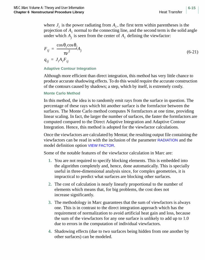
6-15MSC.Marc Volume A: Theory and User InformationChapter 6 Nonstructural Procedure Library Heat Transfer
where is the power radiating from , the first term within parentheses is the projection of normal to the connecting line, and the second term is the solid angle under which is seen from the center of defining the viewfactor:
(6-21)
Adaptive Contour Integration
Although more efficient than direct integration, this method has very little chance to produce accurate shadowing effects. To do this would require the accurate construction of the contours caused by shadows; a step, which by itself, is extremely costly.
Monte Carlo Method
In this method, the idea is to randomly emit rays from the surface in question. The percentage of these rays which hit another surface is the formfactor between the surfaces. The Monte Carlo method computes N formfactors at one time, providing linear scaling. In fact, the larger the number of surfaces, the faster the formfactors are computed compared to the Direct Adaptive Integration and Adaptive Contour Integration. Hence, this method is adopted for the viewfactor calculations.
Once the viewfactors are calculated by Mentat; the resulting output file containing the viewfactors can be read in with the inclusion of the parameter RADIATION and the model definition option VIEW FACTOR.
Some of the notable features of the viewfactor calculation in Marc are:
1. You are not required to specify blocking elements. This is embedded into the algorithm completely and, hence, done automatically. This is specially useful in three-dimensional analysis since, for complex geometries, it is impractical to predict what surfaces are blocking other surfaces.
2. The cost of calculation is nearly linearly proportional to the number of elements which means that, for big problems, the cost does not increase significantly.
3. The methodology in Marc guarantees that the sum of viewfactors is always one. This is in contrast to the direct integration approach which has the requirement of normalization to avoid artificial heat gain and loss, because the sum of the viewfactors for any one surface is unlikely to add up to 1.0 due to errors in the computation of individual viewfactors.
4. Shadowing effects (due to two surfaces being hidden from one another by other surfaces) can be modeled.
Ji AiAiAj Ai
Fij
θi θjcoscos
πr2
---------------------------Aj=
qij JiAiFij=

MSC.Marc Volume A: Theory and User InformationHeat Transfer Chapter 6 Nonstructural Procedure Library
6-16
For a surface to participate in the computations, it must participate in the following operations:
1. Ray Emission: The surface should be able to randomly emit a ray from its surface. The origin of the ray should be randomly distributed over the area of the surface (see Figure 6-5). The direction of the ray should be distributed according to the cosine of the angle between the ray and the normal to the surface at the origin of the ray, thereby emitting more rays normal to the surface than tangent to it.
2. Ray Intersection: Given an origin, direction, and length of a ray, the surface should be able to determine whether it is hit by that ray, and if hit, the length of the ray at the point of intersection.
Determination of viewfactors involves consideration of several desired properties like speed, accuracy, shadowing, translucence, absorption, nonuniform emission, reciprocity, and efficiency. In light of the properties listed above, the Monte Carlo approach is adapted in conjunction with the ray tracing and boxing algorithms.
Figure 6-5 Random Ray Emission in Monte Carlo Method
Figure 6-6 depicts the formation of shadows which essentially involves the computation of incident light by tracing rays from the light source to the point of incidence of the eye rays. These rays do not reflect or refract. Shadows are formed when light source rays are obstructed, either partially or fully, from reaching an object. Refraction and reflection of light from light sources is not computed.
Finally, to compute the viewfactors, it is not necessary to check the intersection of incident rays with all objects under consideration. Such a method would be prohibitively computationally expensive and preclude a large scale three dimensional analysis. An effective technique for fast calculation of intersections is employed.
1
2

6-17MSC.Marc Volume A: Theory and User InformationChapter 6 Nonstructural Procedure Library Heat Transfer
The method relies on sorting the objects before any intersections are computed. The information computed is used to eliminate most of the intersection computations. The technique requires that each object to be sorted have a bounding box which entirely encloses it.
Figure 6-6 Shadowing Effects in Ray Tracing
The sorting relies on creation of a binary tree of bounding boxes. Thus, a bounding box is computed for all objects. The objects are then sorted by the coordinate of the longest dimension of the bounding box. This list of objects is then divided into two sets, each having an equal number of objects. This process is repeated recursively until each set contains no more than a given maximum number of objects. This recursive sorting process is depicted in Figure 6-7.
Point Light
Eye Ray
Light Source Rays
Shadow

MSC.Marc Volume A: Theory and User InformationHeat Transfer Chapter 6 Nonstructural Procedure Library
6-18
Figure 6-7 Fast Intersection Technique for Sorting Objects
21
6
9
8
543
7

6-19MSC.Marc Volume A: Theory and User InformationChapter 6 Nonstructural Procedure Library Heat Transfer
Ray intersections are performed by searching the binary bounding box tree which involves determining whether the ray hits the bounding box of all the objects. If the intersection with one bounding box is not found, then another bounding box is considered. In the event an intersection does exist, each object in the node is intersected with the ray if the intersection is a bottom node of the tree. Otherwise, the bounding boxes of both subtrees are intersected with the search in the closest subtree conducted first. The process continues until all rays are exhausted.
Radiation-Gap
For the thermal contact gap element, in the gap open condition, two surface temperatures and at the centroid of the surfaces of a thermal contact element are obtained by interpolation from the nodal temperatures. These two surface temperatures are used for the computation of an equivalent conductivity for the radiation/convection link. The expression of the equivalent thermal conductivity is:
(6-22)
where is the emissivity, is the Stefan-Boltzmann constant, is the length of the element (distance between a and b), , are absolute temperatures at a and b converted from and ; and is the constant film coefficient.
The equivalent thermal conductivity for the thermal contact element is assumed to be in the gap direction. The thermal conductivities in other two local directions are all set to zero. A coordinate transformation from the local to the global coordinate system allows the generation of the thermal conductivity matrix of the thermal contact element in the global system for assembly.
Similarly, in the gap closed condition, tying constraints are automatically generated by the program for thermal contact elements. The constraint equation for each pair of nodes can be expressed as:
(6-23)
where
= nodal temperatures at nodes I and J
= gap closure temperature.
Ta Tb
k1
k1 εσL Tka Tkb+( ) Tka2
Tkb2
+( ) H L+=
ε σ LTka Tkb
Ta Tb H
k1
TI TJ+ if Tgap Tclose>( )
Tgap12--- TI TJ+( )=
TI TJ,
Tclose

MSC.Marc Volume A: Theory and User InformationHeat Transfer Chapter 6 Nonstructural Procedure Library
6-20
Channel
For the fluid channel element, the one-dimensional, steady-state, convective heat transfer in the fluid channel can be expressed as:
(6-24)
where is mass flow rate, is specific heat, is fluid temperature, is solid temperature, is streamline coordinate, is circumference of channel, is film coefficient, and is inlet temperature.
Similarly, the conductive heat transfer in the solid region is governed by the following equation:
(6-25)
subjected to given initial condition and fixed temperature and/or flux boundary conditions. At the interface between the fluid and solid, the heat flux estimated from convective heat transfer is
(6-26)
In Equation 6-25, is the heat capacity matrix, is the conductivity matrix and is the heat flux vector. Equation 6-25 and Equation 6-26 are coupled equations. The coupling is due to the unknown solid temperature appearing in Equation 6-24 and unknown fluid temperature in Equation 6-26 for the solution of Equation 6-25.
The solutions for Equation 6-24 and Equation 6-25 are obtained from the introduction of a backward difference for the discretization of time variable in Equation 6-25 and of streamline distance in Equation 6-24. Let
(6-27)
we obtain
(6-28)
where = time-step in transient analysis. Similarly, let
(6-29)
m· c∂Tf
∂s-------- Γh Tf Ts–( )+ 0=
Tf 0( ) Tinlet=
m· c Tf Tss Γ h
Tinlet
CTs·
KTs+ Q=
q h Ts Tf–( )=
C K Q
TsTf
Ts·
Tsi
Tsi 1–
–[ ] ∆ t( )⁄=
1∆t-----C K+
Tsi
Qi 1∆t-----CTs
i 1–+=
∆t
dTf
ds-------- Tf Tf
j 1––[ ] ∆ s( )⁄=

6-21MSC.Marc Volume A: Theory and User InformationChapter 6 Nonstructural Procedure Library Heat Transfer
6Nonstructural Procedure Library
Heat Transfer
we obtain
(6-30)
where is the streamline increment,
(6-31)
Output
Marc prints out both the nodal temperatures and the temperatures at the element centroid when the CENTROID parameter is used, or at the integration points if the ALL POINTS parameter is invoked. You can also indicate on the HEAT parameter for the program to print out the temperature gradients and the resulting nodal fluxes.
To create a file of element and nodal point temperatures, use the POST model definition option. This file can be used as temperature input for performing a thermal stress analysis. This file is processed using the CHANGE STATE option in the subsequent thermal stress analysis. This post file can also interface with Mentat to plot temperature as a function of time.
Heat Transfer with Convection
Marc has the capability to perform heat transfer with convection if the velocity field is known. The numerical solutions of the convection-diffusion equation have been developed in recent years. The streamline-upwind Petro-Galerkin (SUPG) method has been implemented into the Marc heat transfer capability.
The elements which are available are described in Table 6-1.
Table 6-1 Heat Transfer Convection Elements
Element Type Description
36, 65 2-, 3-node link
37, 39, 41, 50, 69, 85, 86 3-, 4-, 8-node planar
38, 40, 42, 70, 87, 88, 122 4-, 4-, 8-node axisymmetric
43, 44, 71, 123, 133 8-, 20-node hexahedron
135 4-node tetrahedral
133 10-node tetrahedron
131, 132 6-node triangular
Tfj ∆sβ Tf
j 1–+[ ] 1 ∆sα+( )⁄=
∆s
α Γ h m· c( )⁄ ;= β ΓhTsj 1–
m· c( )⁄=and

MSC.Marc Volume A: Theory and User InformationHeat Transfer Chapter 6 Nonstructural Procedure Library
6-22
To activate the convection contribution, use the HEAT parameter and set the fifth field to 2. Due to the nonsymmetric nature of the convection term, the nonsymmetric solver is used automatically. Specify the nodal velocity vectors using the VELOCITY option. To change velocity, use VELOCITY CHANGE. If nonuniform velocity vectors are required, user subroutine UVELOC is used. This capability can be used in conjunction with the Rigid-Plastic Flow on page 86 to perform a coupled analysis, in which the velocity fields are obtained.
Technical Background
The general convection-diffusion equation is:
(6-32)
The perturbation weighting functions are introduced as:
(6-33)
is the standard interpolation function in Equation 6-1. The upwinding parameter, , is the weighting used to eliminate artificial diffusion of the solution; while the beta
term, , is to avoid numerical dispersion. is the magnitude of local velocity vectors. is the temperature, is the diffusion tensor. is the source term and is the time increment.
The optimal choice for α and β are:
where is the local Peclet number in the local element and is the local Courant number:
Peclet = density ∗ specific heat ∗ characteristic length ∗ magnitude of the fluid velocity/conductivity
Peclet =
and
where is the time increment.
The characteristic length is defined in [Ref. 12] where is required for numerical stability. When , the is set to be zero and a large time step is recommended to avoid numerical dispersion.Note: The interpolation function N is not the time-space functions defined in [Ref. 6], so that most
Marc heat transfer elements can be used. The convection contribution of heat transfer shell elements is limited due to the definitions of the perturbation weighting function and the interpolation function.
∂T∂t------ v ∇ T⋅+ ∇ κ∇ T( ) Q+⋅=
W N α h2 v-------- v ∇ N⋅( )
β h4 v--------∆t v ∇ N⋅( )
+ +=
Nα
β vT κ Q ∆t
α Peclet 2⁄( ) 2 Peclet⁄( )–coth=
β C 3 2 Peclet⁄( )–⁄ * α C⁄( )=
Peclet C
ρ*c*h* v k⁄
C v * ∆t( ) h⁄= ∆t( )h C 1≤C 1> β

6-23MSC.Marc Volume A: Theory and User InformationChapter 6 Nonstructural Procedure Library Hydrodynamic Bearing
Hydrodynamic Bearing
Marc has a hydrodynamic bearing analysis capability, which enables you to solve lubrication problems. This capability makes it possible to model a broad range of practical bearing geometries and to calculate various bearing characteristics such as load carrying capability, stiffness, and damping properties. It can also be used to analyze elasto-hydrodynamic problems.
The lubricant flow in hydrodynamic bearing is governed by the Reynolds equation. The bearing analysis capability has been implemented into Marc to determine the pressure distribution and mass flow in bearing systems.
Marc is capable of solving steady-state lubrication problems; the incremental procedure analyzes a sequence of different lubricant film profiles. Marc also can be used to solve coupled elasto-hydrodynamic problems. This analysis requires a step-by-step solution for both the lubrication and the stress problems using separate runs. Because the finite element meshes for each problem are different, the program does not contain an automated coupling feature.
Only one-dimensional or two-dimensional lubricant flow needs to be modeled, since no pressure gradient exists across the film height. This modeling is done with the available heat transfer elements. The library elements listed in Table 6-2 can be used for this purpose.
Marc computes and prints the following elemental quantities: lubricant thickness, pressure, pressure gradient components, and mass flux components. Each of these is printed at the element integration point.
Table 6-2 Hydrodynamic Bearing Elements
Element Description
36 2-node, three dimensional link
37 3-node, planar triangle
39 4-node, bilinear quadrilateral
41 8-node, planar biquadratic quadrilateral
65 3-node, three-dimensional link
69 8-node, biquadratic quadrilateral with reduced integration
121 4-node bilinear quadrilateral with reduced integration
131 6-node triangle

MSC.Marc Volume A: Theory and User InformationHydrodynamic Bearing Chapter 6 Nonstructural Procedure Library
6-24
The nodal point data consists of pressures, equivalent nodal mass flux at fixed boundary points, or residuals at points where no boundary conditions are applied. In addition, the program automatically integrates the calculated pressure distribution over the entire region to obtain consistent equivalent nodal forces. This integration is only performed in regions where the pressure exceeds the cavitation pressure.
The output includes the load carrying capacity (the total force on the bearing). This capacity is calculated by a vectorial summation of the nodal reaction forces. In addition, the bearing moment components with respect to the origin of the finite element mesh can be calculated and printed.
To activate the bearing analysis option, use the BEARING parameter. If the analysis requires modeling of flow restrictors, also include the RESTRICTOR parameter.
The values of the viscosity, mass density, and cavitation pressure must be defined in the ISOTROPIC option. Specify temperature-dependent viscosity values via TEMPERATURE EFFECTS. If thermal effects are included, the STATE VARS parameter is also required. In hydrodynamic bearing analyses, temperature is the second state variable. Pressure is the first state variable.
The fluid thickness field can be strongly position-dependent. A flexible specification of the film profile is allowed by using either the nodal thickness or elemental thickness option. Define nodal thickness values in the THICKNESS option. You may also redefine the specified values via the user subroutine UTHICK. Elemental values of lubricant thicknesses can be defined in the GEOMETRY option.
Marc also enables the treatment of grooves. Constant groove depth magnitudes can be specified in the GEOMETRY option. If the groove depth is position-dependent, the contribution to the thickness field can be defined in user subroutine UGROOV.
The relative velocity of the moving surfaces is defined on a nodal basis in the VELOCITY option. In addition, you can redefine the specified nodal velocity components in user subroutine UVELOC.
Specify prescribed nodal pressure values in the FIXED PRESSURE option. Define restrictor type boundary conditions in the RESTRICTOR option. To specify nonuniform restrictor coefficients, use user subroutine URESTR.
Input nodal point mass fluxes using the POINT FLUX option. Specify distributed mass fluxes in the DIST FLUXES option. If nonuniform fluxes are necessary, apply this via user subroutine FLUX.
Define variations of the previously specified lubrication film thickness field through the THICKNS CHANGE option. The program adds this variation to the current thickness values and solves the lubrication problem.

6-25MSC.Marc Volume A: Theory and User InformationChapter 6 Nonstructural Procedure Library Hydrodynamic Bearing
Activate the calculation of bearing characteristics (that is, damping and stiffness properties) through the DAMPING COMPONENTS or STIFFNS COMPONENTS options. Marc evaluates these properties based on the specified change in film thickness. This evaluation requires the formation of a new right-hand-side, together with a matrix back substitution. This is performed within so-called subincrements. The bearing force components calculated within these subincrements represent the bearing characteristics (that is, the change in load carrying capacity for the specified thickness change or thickness rate). The previously specified total thickness is not updated within subincrements. The calculated bearing characteristics are passed through to user subroutine UTHICK. This allows you to define an incremental thickness change as a function of the previously calculated damping and/or stiffness properties. This procedure can be applied when analyzing the dynamic behavior of a bearing structure. Mechanical problems can often be represented by simple mass-damper-spring systems if the bearing structure is nondeformable. A thickness increment can be derived based on the current damping and stiffness properties by investigating the mechanical equilibrium at each point in time.
The bearing analysis capability deals with only steady-state solution and does not include the analysis of transient lubrication phenomena. Note that the incrementation procedure is only meant to analyze a sequence of film profiles. No nonlinearities are involved; each increment is solved in a single step without iteration.
To calculate the reaction forces that act on the bearing structure, Marc requires information about the spatial orientation of the lubricant. This information is not contained in the finite element model because of the planar representation of the lubricant. Therefore, it is necessary to define the direction cosines of the unit normal vector that is perpendicular to the lubricant on a nodal basis in user subroutine UBEAR. The resulting nodal reaction forces are printed.
Marc requires a step-by-step solution of both the lubrication problem and the stress problem in separate runs. The thickness changes need to be defined within the lubrication analysis based upon the displacements calculated in the stress analysis. The stress analysis post file and user subroutine UTHICK can be used for this purpose. The tractions to be applied in the stress analysis can be read from the bearing analysis post file in subroutine FORCDT.
Technical Background
The flow of a lubricant between two surfaces that move relative to each other is governed by the Reynolds equation
(6-34)∇ ρh3
12η--------- ∇ p
⋅ ∂ ρh( )∂t
--------------–12--- ∇ ρ hu( )– M+ 0=

MSC.Marc Volume A: Theory and User InformationHydrodynamic Bearing Chapter 6 Nonstructural Procedure Library
6-26
where:
is lubricant pressureis mass densityis film thickness is viscosity is time is the relative velocity vector between moving surfaces is the mass flux per unit area added to the lubricant
The following assumptions are involved in the derivation of this equation:
• The lubricant is a Newtonian fluid; that is, the viscosity is constant. • There is no pressure gradient across the film height.• There is laminar flow.• Inertial effects are negligible. • The lubricant is incompressible; that is, mass density is constant. • Thermal effects are absent.
By introducing the film constant
(6-35)
Equation 6-35 can be written as
(6-36)
where is the reduced mass flux given by
(6-37)
In case of a stationary bearing, the transient term in Equation 6-37 vanishes.
Three different kinds of boundary conditions can be distinguished for the lubrication problem: prescribed pressure on boundary, prescribed mass flux normal to the boundary, and mass flux proportional to pressure.
Prescribed pressure on boundary is specified as
(6-38)
where is the value of the prescribed pressure.
pρhηtuM
λ ρh3
12η---------=
∇ λ∇ p( )⋅ Mr+ 0=
Mr
Mr M∂ ρh( )
∂t--------------–
12--- ∇ ρ hu( )–=
p p=
p

6-27MSC.Marc Volume A: Theory and User InformationChapter 6 Nonstructural Procedure Library Hydrodynamic Bearing
Prescribed mass flux normal to the boundary has the form
(6-39)
where is the reduced inward mass flux. Here, refers to the inward normal on the
boundary, and and are the inward components of total mass flux and relative velocity, respectively.
If a restrictor is used (as in hydrostatic bearings), the total mass flux is a linear function of the pressure on the boundary. This condition is specified as
(6-40)
or, written in a slightly different form
(6-41)
where c is the restriction coefficient and
(6-42)
is the reduced pressure.
The differential Equation 6-34, together with the boundary conditions (Equation 6-39, Equation 6-40, and Equation 6-42) completely describe the lubrication problem. This is analogous to a heat conduction problem as shown in Table 6-3.
Table 6-3 Comparison of Lubrication and Heat Conduction
Lubrication Heat Conduction
Pressure Temperature
Film constant Conductivity
Reduced body mass flux Body heat flux
Reduced boundary mass flux Boundary heat flux
Restriction coefficient Film coefficient
Reduced reference pressure Reference temperature
λ∂p∂n------– mn
12---ρhun– mn
r= =
mnr n
mn un
mn λ–∂p∂n------
12---ρhun+ c p p–( )= =
λ∂p∂n------– c pr p–( )=
pr pρhun
2c------------–=
p T
λ k
Mr Q
mn qn
c h
pr Tr

MSC.Marc Volume A: Theory and User InformationElectrostatic Analysis Chapter 6 Nonstructural Procedure Library
6-28
Electrostatic Analysis
Marc has the capability to perform electrostatic analysis. This allows the program to evaluate the electric fields in a body or media, where electrical charges are present. This can be solved for one-, two-, or three-dimensional fields. The semi-infinite elements can be used to represent an infinite domain. The electrostatic problem is governed by the Poisson equation for a scalar potential. This analysis is purely linear and has been implemented in Marc analogously to the steady state heat transfer problem. The available elements are described in Table 6-4 below.
Marc computes and prints the following quantities: electric potential field vector ( )
and electric displacement vector ( ) at the element integration points. The nodal
point data consists of the potential and the charge .
Table 6-4 Element Types for Electrostatic Analysis
Element Type Description
37, 39, 131, 41 3-, 4-, 6-, 8-node planar
69 8-node reduced integration planar
121 4-node reduced integration planar
101, 103 6-, 9-node semi-infinite planar
38, 40, 132, 42 3-, 4-, 6-, 8-node axisymmetric
70 8-node reduced integration axisymmetric
122 4-node reduced integration axisymmetric
43, 44 8-, 20-node 3-dimensional brick
71 20-node reduced integration brick
105, 106 12-, 27-node semi-infinite brick
123 8-node reduced integration brick
133 10-node tetrahedral
50, 85, 86 3-, 4-, 8-node shell
87, 88 2-, 3-node axisymmetric shell
135 4-node tetrahedral
E
D
φ Q

6-29MSC.Marc Volume A: Theory and User InformationChapter 6 Nonstructural Procedure Library Electrostatic Analysis
To activate the electrostatic option, use the ELECTRO parameter. The value of the isotropic permittivity constant is given in the ISOTROPIC option, orthotropic constants can be specified using the ORTHOTROPIC option. Optionally, user subroutine UEPS can be used.
Specify nodal constraints using the FIXED POTENTIAL option. Input nodal charges using the POINT CHARGE option. Specify distributed charges by using the DIST CHARGES option. If nonuniform charges are required, user subroutine FLUX can be used for distributed charges and user subroutine FORCDT for point charges.
The electrostatic capability deals with linear, steady-state problems only. The STEADY STATE option is used to begin the analysis. The resultant quantities can be stored on the post file for processing with Mentat.
Technical Background
The Maxwell equations to govern electrostatics are written in terms of the electric displacement vector and the electric field vector such that
(6-43)
and
(6-44)
where is a given volume charge density.
The constitutive law is typically given in a form as:
(6-45)
where is the dielectric constant.
Introducing the scalar potential such that
(6-46)
which satisfied the constraint Equation 6-44 exactly.
Denoting the virtual scalar potential by , the variational formulation is
(6-47)
D E
∇ D⋅ ρ=
∇ E× 0=
ρ
D εE=
ε
φ
E ∇φ–=
ψ
∇ψ ε∇φ( )dV⋅V∫ ψρdV
V∫ ψ ε∇φ n–( )da⋅
A∫+=

MSC.Marc Volume A: Theory and User InformationElectrostatic Analysis Chapter 6 Nonstructural Procedure Library
6-30
The natural boundary condition is applied through the surface integral in terms of the normal electric displacement using
(6-48)
Consider a material interface , separating two materials 1 and 2, and as is continuous over the material interface, the tangential electric field constraint is automatically satisfied.
(6-49)
If charges are present on the interface, these are applied as distributed loads as follows:
(6-50)
Using the usual finite element interpolation functions and their derivatives , we obtain
(6-51)
(6-52)
and finally
(6-53)
ε∇φ n⋅– D n⋅ Dn= =
A12 φ
n E1 E2–( )× 0= on A12
n D1 D2–( )⋅ ρs= on A12
N β
ψ NΨ= φ NΦ=
K βTε βdVV∫=
F NTρNdVV∫ NTNDnda
A∫ NTNρsda
A12
∫+ +=
KΦ F=

6-31MSC.Marc Volume A: Theory and User InformationChapter 6 Nonstructural Procedure Library Magnetostatic Analysis
Magnetostatic Analysis
Marc has the capability to perform magnetostatic analysis. This allows Marc to calculate the magnetic field in a media subjected to steady electrical currents. This can be solved for two- or three-dimensional fields. Semi-infinite elements can be used to represent an infinite domain.
The magnetostatic analysis for two-dimensional analysis is solved using a scalar potential, while for three-dimensional problems, a full vector potential is used. The magnetic permeability can be a function of the magnetic field, hence, creating a nonlinear problem. Only steady-state analyses are performed. The available elements which are described in Table 6-5.
Marc computes and prints magnetic induction ( ), the magnetic field vector ( ), and the vector potential at the element integration points. The nodal point data consist of the potential ( ) and the current ( ).
To activate the magnetostatic option, use the MAGNETO parameter. The value of the isotropic permeability (µ) is given on the ISOTROPIC option; orthotropic constants can be specified using the ORTHOTROPIC option. Optionally, user subroutine UEPS can be used. Often, it is easier to specify (1/µ), which is also available through these options. A nonlinear permeability can be defined using the B-H relation.
Table 6-5 Elements Types for Magnetostatic Analysis
Element Type Description
37, 39, 131, 41 3-, 4-, 6-, 8-node planar
69 8-node reduced integration planar
121 4-node reduced integration planar
101, 103 6-, 9-node semi-infinite planar
102, 104 6-, 9-node semi-infinite axisymmetric
38, 40, 132, 42 3-, 4-, 6-, 8-node axisymmetric
70 8-node reduced integration axisymmetric
122 4-node axisymmetric reduced integration
109 8-node brick
110 12-node semi-infinite brick
B H
A J

MSC.Marc Volume A: Theory and User InformationMagnetostatic Analysis Chapter 6 Nonstructural Procedure Library
6-32
Specify nodal constraints using the FIXED POTENTIAL option. Input nodal currents using the POINT CURRENT option. Specify distributed currents by using the DIST CURRENT option. Permanent magnets can be introduced by using the PERMANENT option for isotropic materials, or by entering a remanence vector via the B-H RELATION option for orthotropic materials. In addition, user subroutine FLUX can be used for nonuniform distributed current and user subroutine FORCDT for fixed nodal potentials or point current.
The magnetostatic capability is linear unless a nonlinear B-H relation is defined. In such problems, convergence is reached when the residual current satisfies the tolerance defined in the CONTROL option. The STEADY STATE option is used to begin the analysis. The resultant quantities can be stored on the post file for processing with Mentat.
Technical Background
The Maxwell equations for magnetostatics are written in terms of the magnetic flux density vector B such that
(6-54)
and
(6-55)
where J is the current density vectors.
For magnetic materials, the following relation between , , and , the magnetization vector, holds:
(6-56)
with being the permeability of vacuum. Denoting the magnetic susceptibility by and the permanent magnet vector by , we have
(6-57)
which can be substituted into Equation 6-56 to yield
(6-58)
in which µ is the permeability, given by
(6-59)
∇ H× J=
∇ B⋅ 0=
B H M
B µ0 H M+( )=
µ0χm M0
M χm H M0+=
B µ H Br+=
µ µ0 1 χm+( )=

6-33MSC.Marc Volume A: Theory and User InformationChapter 6 Nonstructural Procedure Library Magnetostatic Analysis
and Br is the remanence, given by
(6-60)
Notice that is usually called the relative permeability .
Figure 6-8 Nonlinear B-H Relationship
For isotropic linear material, and are scalar constants. If the material is
orthotropic, and change into tensors. For real ferromagnetic material, and
µ are never constant. Instead, they depend on the strength of the magnetic field. Usually this type of material nonlinearity is characterized by a so-called magnetization curve or B-H relation specifying the magnitude of (a component of) B as a function of (a component of) H.
In Marc, the magnetization curve can be entered via the B-H RELATION option. For isotropic material, only one set of data points, representing the magnitude of the magnetic induction, , as a function of , the magnitude H, needs to be given. For orthotropic material, multiple curves are needed with each curve relating a component of B to the corresponding component of H.
From Equation 6-58 and Equation 6-60, it can be seen that for orthotropic materials, a permanent magnetization or remanence can be entered through the B-H RELATION option, by putting in a nonzero B value for H = Q. For isotropic material, this does not work since the direction of the remanence vector is still indeterminate. Therefore, in the isotropic case, the only possibility is to supply the magnetization vector through the PERMANENT option. Any offset of the -curve, implying
Br µ0M0=
1 χm+( ) µr
B
Br
H
χm M0
χm M χm
B H
B H( )

MSC.Marc Volume A: Theory and User InformationMagnetostatic Analysis Chapter 6 Nonstructural Procedure Library
6-34
will be disregarded in this case. For orthotropic material, it is not allowed to use the PERMANENT option. In this case, the magnetization can exclusively be specified through the B-H RELATION option.
It is emphasized that the magnetization curve specified under B-H RELATION must be monotone and uniquely defined.
Introducing the vector potential A such that
(6-61)
which automatically satisfies the constraint, Equation 6-55, and we then have the final form
(6-62)
The vector potential ( ) is not uniquely defined by Equation 6-61. In 2-D magnetostatic simulations, this indeterminacy is removed by the reduction of to a scalar quantity. In 3-D situations, Marc uses the Coulomb gauge for this purpose:
(6-63)
Denote the virtual potential by ; then, the variational formulation is
(6-64)
where is the outward normal to at the boundary .
In the three-dimensional case, the Coulomb gauge, Equation 6-63, is enforced with a penalty formulation. The resulting term added to the variational formulation, Equation 6-64 reads:
(6-65)
The default value used for is:
(6-66)
B 0 at H(≠ 0 )=
∇ A× B=
∇ µ 1– ∇ A×( )× J µ 1–Br+=
AA
∇ A• 0=
W
µ 1– ∇ W×( ) ∇ A×( )dV•
V∫ W JdV• W ∇ µ 1–
Br×( )dV• W H n×( )dA•
Γ∫+
V∫+
V∫=
n V Γ
µ 1– ∇ W×( ) ∇ A×( )dV•
V∫ W JdV• W ∇ µ 1–
Br×( )dV• W H n×( )dA•
Γ∫+
V∫+
V∫=
r ∇ W•( ) ∇ A•( ) VdV∫+
r
r 104– µ 1–
=

6-35MSC.Marc Volume A: Theory and User InformationChapter 6 Nonstructural Procedure Library Magnetostatic Analysis
Using the usual finite element interpolation functions , the discrete curl operator ,
and the weighting function .
(6-67)
Leads to the resulting system of algebraic equations
(6-68)
where
(6-69)
(6-70)
The Coulomb gauge is based upon the principle of conservation of electric charge which in its steady state form reads:
(6-71)
In Marc, it is up to you to specify the current distribution. When doing so, it is recommended to ensure that this distribution satisfies Equation 6-70. Otherwise, condition Equation 6-63 could be violated. As a consequence, the results could become less reliable.
From the third term on the right-hand side of Equation 6-70, it becomes clear that the natural boundary condition in this magnetostatic formulation is , the tangential component of the magnetic field intensity. Consequently, if no other condition is specified by you, by default a zero tangential magnetic field intensity at the boundaries is assumed.
Besides, when there are no currents present on a material interface separating two
materials 1 and 2, the tangential magnetic field intensity is assumed to be continuous:
(6-72)
N G
W N=
G ∂N ∂y⁄∂N ∂x⁄
=for two-dimensional problems
G∂N ∂y⁄ ∂N ∂z⁄–
∂N ∂z⁄ ∂N ∂x⁄–
∂N ∂x⁄ ∂N ∂y⁄–
=for three-dimensional problems
KA F=
K GTµ 1–
G Vd
V∫=
F NTN J( ) V G
TM
1–Br V N
TN H n×( )
Γ∫+d
V∫+d ad
V∫=
∇ J• 0=
H n×
Γ12
n H1 H2–( )× 0 on Γ12=

MSC.Marc Volume A: Theory and User InformationMagnetostatic Analysis Chapter 6 Nonstructural Procedure Library
6-36
With and , the magnetic field intensities in material 1 and 2, respectively. A
discontinuous tangential magnetic field intensity can be modeled by assigning an appropriate distributed “shear” current density to the interface. This (surface) current density is related to and by:
(6-73)
H1 H2
J H1 H2
n H1 H2–( )× J on Γ12=

6-37MSC.Marc Volume A: Theory and User InformationChapter 6 Nonstructural Procedure Library Electromagnetic Analysis
Electromagnetic Analysis
Marc has the capability to perform both transient (dynamic) and harmonic fully coupled electromagnetic analysis. This allows Marc to calculate the electrical and magnetic fields subjected to external excitation. This can be solved for both two- or three-dimensional fields. A vector potential for the magnetic field is augmented with a scalar potential for the electrical field. If a transient analysis is performed, the magnetic permeability can be a function of the magnetic field; hence, a nonlinear problem. The elements available for electromagnetic analysis are described in Table 6-6.
Marc prints the magnetic flux density ( ), the magnetic field vector ( ), electric flux density ( ), and the electrical field intensity at the integration points. In a harmonic analysis, these have real and imaginary components. The nodal point data consists of the vector potential , the scalar potential , the charge , and current .
To activate the electromagnetic option, use the EL-MA parameter. The values of the isotropic permittivity ( ), permeability ( ), and conductivity ( ) are given in the ISOTROPIC option. Orthotropic constants can be specified using the ORTHOTROPIC option. User subroutines UEPS, UMU, and USIGMA can be optionally used. A nonlinear permeability can be defined using the B-H relation.
Specify nodal constraints using the FIXED POTENTIAL option. Input nodal currents and charge using the POINT CURRENT option. Specify distributed currents by using the DIST CURRENT option and distributed charges by using the DIST CHARGES option. Nonuniform distributed currents and charges can also be specified by user subroutine FORCEM.
The electromagnetic capability is linear, unless a nonlinear B-H relation is defined. In such problems, convergence is reached when the residual satisfies the tolerance defined in the CONTROL option. The transient capability is only available with a fixed time step; use the DYNAMIC CHANGE option to activate this option. The resultant quantities can be stored on the post file for processing with Mentat.
Table 6-6 Element Types for Electromagnetic Analysis
Element Type Description
111 4-node planar
112 4-node axisymmetric
113 8-node brick
B HD
A V Q I
ε µ σ

MSC.Marc Volume A: Theory and User InformationElectromagnetic Analysis Chapter 6 Nonstructural Procedure Library
6-38
In electromagnetic analysis, you can enter the current and/or the charge. In a harmonic analysis, you can enter both the real and imaginary components.
Technical Background
Technical Formulation
Electromagnetic analysis is based upon the well-known Maxwell’s equations. This has been implemented in Marc for both transient and harmonic analyses.
Transient Formulation
The Maxwell’s equations are:
(6-74)
(6-75)
(6-76)
(6-77)
where the constitutive relations are
Table 6-7 Input Options for Electromagnetic Analysis
Load DescriptionInput Options
Model Definition History Definition User Subroutine
Nodal CurrentNodal Charge
POINT CURRENT POINT CURRENT FORCDT
Distributed Current DIST CURRENT DIST CURRENT FORCEM
Distributed Charge DIST CHARGES DIST CHARGE FORCEM
∇ E× B·
+ 0=
∇ H εE·
– σ–× E 0=
∇ ε E·
σE+( )⋅ 0=
∇ B⋅ 0=
D εE=
B µ0 H M+( )=
J σE=

6-39MSC.Marc Volume A: Theory and User InformationChapter 6 Nonstructural Procedure Library Electromagnetic Analysis
and
is the electric field intensityis the electric flux densityis the magnetic field intensityis the magnetic flux densityis the current densityis the magnetization
and
is the permittivityis the permeabilityis the conductivityis the permeability of free space.
Additionally, we have the conservation of charge:
(6-78)
where is the charge density.
We assume that the magnetization vector is given by
(6-79)
where is the strength of the permanent magnet and is the susceptibility. The magnetic field can be defined as
(6-80)
in which is the permeability, given by
(6-81)
and is the remanence, given by
(6-82)
Notice that is usually called the relative permeability .
A vector magnetic potential and a scalar potential are introduced, such that
(6-83)
(6-84)
EDHBJM
εµσµ0
ρ· ∇ J⋅+ 0=
ρ
M χH M0+=
M0 χ
B µ H Br+=
µ
µ µ0 1 χm+( )=
Br
Br µ0M0=
1 χm+( ) µr
A V
B ∇ A×=
E ∇ V A·
+( )–=

MSC.Marc Volume A: Theory and User InformationElectromagnetic Analysis Chapter 6 Nonstructural Procedure Library
6-40
Note that since only the curl of is required, an arbitrary specification of the divergence can be made. The Coulomb gage is then introduced.
(6-85)
This is implemented using a penalty condition. It is important to note that depends not only on the scalar potential, but also upon the vector potential. Hence, interpretation of as the usual voltage can lead to erroneous results.
Substituting into Maxwell’s equations results in:
(6-86)
(6-87)
It has been assumed that ; in that, the permittivity has a zero time derivative.
Due to the hyperbolic nature of the above system (similar to dynamics), a Newmark-beta algorithm is employed in the discretization.
The general form is
(6-88)
(6-89)
The particular form of the dynamic equations corresponding to the trapezoidal rule:
(6-90)
results in a symmetric formulation, which is unconditionally stable for linear systems.
In the current formulation, a fixed time step procedure must be used. The time step is defined through the DYNAMIC CHANGE option.
Harmonic Formulation
In harmonic analysis, it is assumed that the excitation is a sinusoidal function, and the resultant also has a sinusoidal behavior. This results in the solution of a complex system of equations. In this case, Maxwell’s equations become
(6-91)
(6-92)
A
∇ A⋅ 0=
E
V
∇ µ 1– ∇ A× µ0M0–( )[ ]× ε ∇ V·
A··
+( ) σ ∇ V A·
+( )+ + 0=
∇– ε ∇ V·
A··
+( )[ ]⋅ σ ∇ V A·
+( )+ 0=
ε· 0=
An 1+ An ∆tA· n 1
2--- β–
∆t2A··n
β∆t2An 1++ + +=
A· n 1+
A· n
1 γ–( )∆tA··n
γ∆tA··n 1+
++=
γ 12---= β 1
4---=
∇ E× iωB+ 0=
∇ H× iεωE– σE– 0=

6-41MSC.Marc Volume A: Theory and User InformationChapter 6 Nonstructural Procedure Library Electromagnetic Analysis
6Nonstructural Procedure Library
Electromagnetic Analysis
(6-93)
(6-94)
where is the excitation angular frequency and .
Additionally, we have the conservation of charge
(6-95)
where all symbols are the same as in the discussion above regarding transient behavior. Again, a vector potential and a scalar potential are introduced. In this case, these are complex potentials. Substituting into the Maxwell’s equations results in
(6-96)
(6-97)
where
With a little manipulation, a symmetric complex formulation may be obtained. The excitation frequency is prescribed using the HARMONIC option.
Note that the capability to extract the natural frequencies of a complex system by modal analysis does not exist in Marc. The harmonic formulation is assumed to be linear; therefore, you should not include the B-H RELATION option.
∇ D⋅ ρ– 0=
∇ B⋅ 0=
ω i 1–=
iωρ ∇ J⋅+ 0=
A V
∇ µ 1– ∇ A× µoMo–( )[ ]× σ ∇ V iωA+( )+ 0=
∇– σ ∇ V iωA+( )[ ]⋅ 0=
σ σ iωε+=

MSC.Marc Volume A: Theory and User InformationAcoustic Analysis Chapter 6 Nonstructural Procedure Library
6-42
Acoustic Analysis
Marc has the capability to perform acoustic analysis in a rigid as well as a deformable cavity. This allows the program to calculate the fundamental frequencies of the cavity, as well as the pressure distribution in the cavity. This can be solved for two- or three-dimensional fields.
Rigid Cavity Acoustic Analysis
The acoustic problem with rigid reflecting boundaries is a purely linear problem analogous to dynamic analysis, but using the heat transfer elements.
The elements which are available for acoustic analysis of a rigid cavity are described in Table 6-8.
Marc computes and prints the following quantities: pressure and pressure gradient at the integration points. The nodal point data consists of the pressure and the source.
Technical Background
The wave equation in an inviscid fluid can be expressed in terms of the pressure as
(6-98)
Table 6-8 Element Types for Rigid Cavity Acoustic Analysis
Element Type Description
37, 39, 131, 41 3-, 4-, 6-, 8-node planar
69 8-node reduced integration planar
121 4-node reduced integration planar
101, 103 6-, 9-node semi-infinite planar
38, 40, 132, 42 3-, 4-, 6-, 8-node axisymmetric
70 8-node reduced integration axisymmetric
122 4-node reduced integration axisymmetric
133 10-node tetrahedral
135 4-node tetrahedral
p
c
12--- ∂2
p
∂t2
-------- ∇ 2p=

6-43MSC.Marc Volume A: Theory and User InformationChapter 6 Nonstructural Procedure Library Acoustic Analysis
where is the sonic velocity
(6-99)
where is the bulk modulus and is the density.
Equation 6-98 can be rewritten as
(6-100)
Where the source terms are neglected, note that this is analogous to the dynamic equation of motion.
The modeling of rigid reflecting boundaries can be done as follows.
Mathematically, a reflecting boundary is described by:
(6-101)
where is the pressure gradient normal to the reflecting surface.
This is analogous to an insulated boundary in heat transfer. Hence, a reflecting boundary can be modeled by a set of nodes at the outer surface of the area which are not connected to another part of the medium. A reflecting plate in the middle of an acoustic medium can be modeled by double nodes at the same location
Note: Where there are no boundary conditions applied, there is a zero-valued eigenvalue, corresponding to a constant pressure mode. Hence, you need to have a nonzero initial shift point.
To activate the acoustic option, use the ACOUSTIC parameter. The number of modes to be extracted should also be included on this parameter. The bulk modulus and the density of the fluid are given in the ISOTROPIC option.
Specify nodal constraints using the FIXED PRESSURE option. Input nodal sources using the POINT SOURCE option. Specify distributed sources using the DIST SOURCES option. If nonuniform sources are required, apply these via user subroutine FLUX.
To obtain the fundamental frequencies, use the MODAL SHAPE option after the END OPTION. The nodes can be used in a transient analysis by invoking the DYNAMIC CHANGE option. The point and distributed sources could be a function of time.
c
c K ρ⁄=
K ρ
K∇ 2p ρ∂2
p
∂t2
--------– 0=
∂p∂n------ 0=
∂p∂n------

MSC.Marc Volume A: Theory and User InformationAcoustic Analysis Chapter 6 Nonstructural Procedure Library
6-44
Coupled Acoustic-Structural Analysis
In a coupled acoustic-structural analysis, both the acoustic medium and the structure are modeled. In this way, the effect of the acoustic medium on the dynamic response of the structure and of the structure on the dynamic response of the acoustic medium can be taken into account. Such a coupled analysis is especially important when the natural frequencies of the acoustic medium and the structure are in the same range. In Marc, only a harmonic coupled acoustic-structural analysis can be performed. Since the interface between the acoustic medium and the structure is determined automatically by Marc based on the CONTACT option, setting up the finite element model is relatively easy since the meshes do not need to be identical at the interface.
Technical Background
The acoustic medium will be called the fluid, although it might also be a gas, and is considered to be inviscid and compressible. The equilibrium equation is given by:
(6-102)
in which is the pressure, is the fluid density, is the displacement vector and a
superposed dot indicates differentiation with respect to time.
Using the bulk modulus of the fluid , the constitutive behavior can be written as:
(6-103)
The Equations (6-102) and (6-103) can be combined to:
(6-104)
It is also possible to add a damping term to Equation (6-102), with the resistivity or fluid drag:
(6-105)
p∇ ρ fu··
+ 0=
p ρf u
Kf
p Kf u∇–=
1Kf-----p
·· 1ρf---- p∇ 2– 0=
ru·
r
p∇ ru· ρfu
··+ + 0=

6-45MSC.Marc Volume A: Theory and User InformationChapter 6 Nonstructural Procedure Library Acoustic Analysis
Since we restrict the discussion to harmonic analyses, we can write , with
the excitation frequency and the imaginary unit, so that Equation (6-105) reduces to:
(6-106)
in which the complex density is given by:
(6-107)
The weak form of Equation (6-106) is obtained in a standard way by introducing the variational field and integrating over the fluid volume :
(6-108)
Applying the divergence theorem of Green to this expression yields:
(6-109)
in which represents the boundary of the fluid with an inward normal .
Along the boundary, various conditions can occur:
• The pressure is prescribed on the boundary .
• The normal acceleration is prescribed to be on the accelerating boundary .
• The normal acceleration of the fluid equals the normal acceleration of the solid, , on the fluid-structure interface .
• Nonreflecting or reactive boundary conditions are introduced using a spring-
dashpot analogy on as . In this way, a spring and a
dashpot are placed in series between the acoustic medium and its boundary, with the spring and the dashpot parameter, both per unit area. Some
classical conditions can be modeled by this expression:
1. Free surfaces waves in a gravity field: , with the gravity acceleration;
u·
iωu=
ω i
1Kf-----p
·· 1ρ
f
---- p∇ 2– 0=
ρf
ρf ρf
irω----–
=
δp V
δp1Kf-----p
·· 1ρf
---- p∇ 2– Vd
V∫ 0=
δp1Kf-----p
·· 1ρf
---- δp p∇∇+ Vd
V∫ 1
ρf
----δpp∂n∂
----- ΓdΓ∫+ 0=
Γ n
p Γp
anΓa
u··
fn u··
sn= Γ fs
Γ fn1ρ---
p∂n∂
----- p·
cI⁄ p··
kI⁄+=
kI cI
p∂n∂
----- p··
g⁄= g

MSC.Marc Volume A: Theory and User InformationAcoustic Analysis Chapter 6 Nonstructural Procedure Library
6-46
2. The plane wave radiation boundary condition: , with the wave velocity;
3. Using the complex admittance of the boundary, with the impedance, the normal velocity can be related to the pressure by
, so that a given can be modeled
by setting and .
Upon discretizing the fluid and the solid using finite elements, the fluid pressure and the displacements of the solid can be approximated in a standard way, so that Equation (6-109) yields:
(6-110)
where and contain the pressure and displacement degrees of freedom, contains
the interpolation functions and is a transformation matrix to relate the displacements in normal direction to the global displacement components. Since Equation (6-110) must be valid for arbitrary admissible values of , evaluating the
various integrals and using , and , results in:
(6-111)
In order to end up with a set of coupled equations, we need to consider the solid as well. The effect of the fluid on the solid originates from the fluid pressure at the fluid-solid interface. This can be easily included by evaluating the virtual work corresponding to the fluid pressure:
(6-112)
p∂n∂
----- p·
c⁄= c
1 z ω( )⁄ z ω( )
u· fn p z ω( )⁄ 1 cI⁄ iω kI⁄+( )p= = z ω( )
1 cI⁄ 1 kI⁄
δpT Np 1cI----NpTp
·Np 1
kI----NpTp
··+
ΓdΓ fn
∫+ 0=
δpTNp 1Kf-----NpTp·· δpT Np∇( ) 1
ρf
---- N∇ pT( )p+
Vd
V∫ δpTNp
an Γ δpTNpNuTGu·· Γd
Γ fs
∫–d
Γa
∫–
p u NG
δp
p·
iωp= p··
ω2p–= u··
ω2u–=
Kf iωCf ω2Mf–+ p ω2Sfsu+ Ff=
δWp δ– unsp Γd
Γ fs
∫ δ– uTGTNuNpTp ΓdΓ fs
∫ δuTSfsT
– p= = =
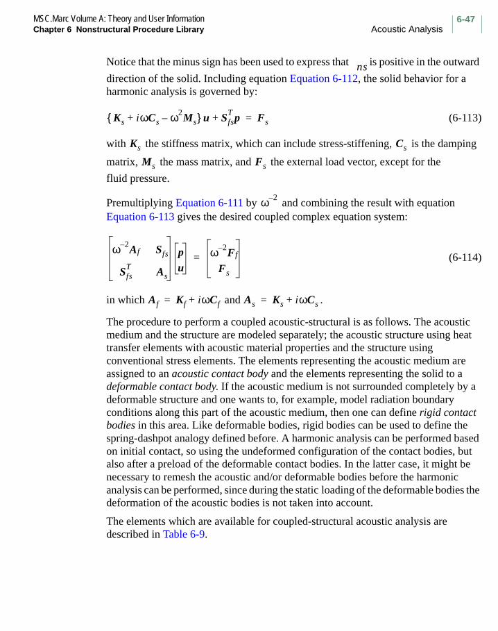
6-47MSC.Marc Volume A: Theory and User InformationChapter 6 Nonstructural Procedure Library Acoustic Analysis
Notice that the minus sign has been used to express that is positive in the outward
direction of the solid. Including equation Equation 6-112, the solid behavior for a harmonic analysis is governed by:
(6-113)
with the stiffness matrix, which can include stress-stiffening, is the damping
matrix, the mass matrix, and the external load vector, except for the
fluid pressure.
Premultiplying Equation 6-111 by and combining the result with equation Equation 6-113 gives the desired coupled complex equation system:
(6-114)
in which and .
The procedure to perform a coupled acoustic-structural is as follows. The acoustic medium and the structure are modeled separately; the acoustic structure using heat transfer elements with acoustic material properties and the structure using conventional stress elements. The elements representing the acoustic medium are assigned to an acoustic contact body and the elements representing the solid to a deformable contact body. If the acoustic medium is not surrounded completely by a deformable structure and one wants to, for example, model radiation boundary conditions along this part of the acoustic medium, then one can define rigid contact bodies in this area. Like deformable bodies, rigid bodies can be used to define the spring-dashpot analogy defined before. A harmonic analysis can be performed based on initial contact, so using the undeformed configuration of the contact bodies, but also after a preload of the deformable contact bodies. In the latter case, it might be necessary to remesh the acoustic and/or deformable bodies before the harmonic analysis can be performed, since during the static loading of the deformable bodies the deformation of the acoustic bodies is not taken into account.
The elements which are available for coupled-structural acoustic analysis are described in Table 6-9.
ns
Ks iωCs ω2Ms–+ u SfsT p+ Fs=
Ks Cs
Ms Fs
ω 2–
ω 2– Af Sfs
SfsT
As
pu
ω 2– Ff
Fs
=
Af Kf iωCf+= As Ks iωCs+=

MSC.Marc Volume A: Theory and User InformationAcoustic Analysis Chapter 6 Nonstructural Procedure Library
6-48
Marc computes and prints the following quantities: pressure and pressure gradient at the integration points. The nodal point data consists of the pressure and the source.
The ACOUSTIC parameter is used to indicate that a coupled acoustic-structural analysis is performed. In addition to the CONTACT option, the model definition options ACOUSTIC and REGION are used to define the material properties of the acoustic medium and to set which elements correspond to the solid and the fluid region. Typical boundary conditions for the acoustic medium can be entered using the FIXED PRESSURE model definition and PRESS CHANGE history definition option. The DIST SOURCES and POINT SOURCE model definition and DIST SOURCES and POINT SOURCE history definition options are used to define the load on the acoustic medium. The HARMONIC history definition option is used to define the excitation frequencies.
Table 6-9 Element Types for Coupled-Structural Acoustic Analysis
Element Type Description
37, 39 3-, 4-node planar
121 4-node reduced integration planar
38, 40 3-, 4-node axisymmetric
122 4-node reduced integration axisymmetric
135 4-node tetrahedral

6-49MSC.Marc Volume A: Theory and User InformationChapter 6 Nonstructural Procedure Library Fluid Mechanics
Fluid Mechanics
Marc has the capability to perform fluid flow analysis. Marc solves the Navier-Stokes equations in the fluid under the restrictions that the fluid is considered to be nonreactive, incompressible, single phases, and laminar. The capabilities in Marc can be applied to four different problems listed below:
Fluid behavior onlyFluid-thermal coupled behaviorFluid-solid coupled behaviorFluid-thermal-solid coupled behavior
Mass Conservation
The principle of mass conservation for a single-phase fluid can be expressed in differential form as:
(6-115)
where is the mass density, is the Eulerian fluid velocity, and is the time.
Momentum Conservation
The principle of conservation of linear momentum results in:
(6-116)
where is the stress tensor and is the body force per unit mass.
In general, the stress tensor can be written as the sum of the hydrostatic stress and
the deviatoric stress .
(6-117)
(6-118)
DρDt------- ρ∇ v⋅+ 0=
ρ v t
ρ ∂v∂t----- v ∇ v⋅+
ρf ∇ σ⋅+=
σ f
σσ′
σ 13---σijδij=
σ′ σ ij13---σijδij– σij σδij–= =

MSC.Marc Volume A: Theory and User InformationFluid Mechanics Chapter 6 Nonstructural Procedure Library
6-50
In fluid mechanics, the fluid pressure is introduced as the negative hydrostatic pressure:
(6-119)
Energy Conservation
For incompressible fluids, the principle of conservation of thermal energy is expressed by:
(6-120)
where is the temperature, is the specific heat at constant pressure, is the
thermal flux, and is the internal heat generated.
Equation of State
The equation of state for a homogeneous, single-phase gas is:
(6-121)
m is the mass of the fluid, is the molecular weight of the gas, is the universal gas
constant, is the volume that the gas occupies.
The gas constant is often expressed as for each substance. The equation of state is then written as:
(6-122)
In Marc, it is assumed that the fluid is incompressible. In such cases, the density is constant
Constitutive Relations
The shear strain rate tensor is defined:
(6-123)
p σ–=
ρCp∂T∂t------ vi
∂T∂xi-------+
∂qi
∂xi-------– H+=
T Cp qi
H
pVmRT
M------------=
M R
V
R R M⁄=
ρ PRT-------=
ρ ρo=
εij12---
∂vi
∂xj-------
∂vj
∂xi-------+
=

6-51MSC.Marc Volume A: Theory and User InformationChapter 6 Nonstructural Procedure Library Fluid Mechanics
For viscous incompressible fluids, it is assumed that there is an expression:
(6-124)
where is the dynamic viscosity.
If the viscosity is not a function of the strain rate, the material is considered Newtonian. Viscous fluid flow is usually characterized by the Reynolds number :
(6-125)
where is a typical velocity and is the characteristic length.
Viscosity for common fluids like air and water is fairly constant over a broad range of temperatures. However, many materials have viscosity which is strongly dependent on the shear strain rate. These materials include glass, concrete, oil, paint, and food products. There are several non-Newtonian fluid models in Marc to describe the viscosity as described below.
Piecewise Non-Newtonian Flow
is the equivalent strain rate = (6-126)
, where is a piecewise linear function.
Bingham Fluid
A Bingham fluid behaves as a “rigid” fluid if the stress is below a certain level, labeled the yield stress, and behaves in a nonlinear manner at higher stress levels.
if (6-127)
if (6-128)
The effective viscosity is and
The materials that can be simulated with this model are cement, slurries, and pastes.
σij ′ 2µε· ij µγ· ij= =
µ
Re
ReρLvµ
----------=
v L
ε·
ε· 2
3---ε· ijε
·ij
1 2⁄=
µ µ ε·
( )= µ
σij ′ µoγ· ij gγ· ij γ·
⁄+= σ g≥
γ· ij 0= σ g<
µ µo g γ·
⁄+= γ· 1
2---γ· ijγ
·ij
12---
=

MSC.Marc Volume A: Theory and User InformationFluid Mechanics Chapter 6 Nonstructural Procedure Library
6-52
Power Law Fluid
The fluid is represented as:
(6-129)
where is a nondimensional constant.
This model is useful for simulating flow of rubber solutions, adhesives, and biological fluids.
Carreau Model
This model alleviates the difficulties associated with the power law model and accounts for the lower and upper limiting viscosities for an extreme value of the equivalent shear strain rate.
(6-130)
where and µ• are the viscosity at time equals zero and infinity, respectively.
The thermal flux is governed by the Fourier law.
(6-131)
Finite Element Formulation
In the procedures developed, the fluid-thermal coupling can be treated as weak or strong. In the weak formulation, the solution of the fluid and thermal equilibrium equations are solved in a staggered manner. In the strongly coupled approach, a simultaneous solution is obtained.
This section cannot cover all of the details of the finite element formulation. It does discuss the final form of the linearized set of equations and some of the consequences. Beginning with degrees of freedom in a system – namely, v, p, and T for the mixed method – we utilize the traditional finite element interpolation functions to relate the values within the element to the nodal values.
σij ′ µoK γ·
( )n 1–
γ· ij=
K
µ µ∞ µo µ∞–( ) 1 τ2γ· 2
+( )n 1–( ) 2⁄
+=
µo
qi kij∂T∂xj-------=

6-53MSC.Marc Volume A: Theory and User InformationChapter 6 Nonstructural Procedure Library Fluid Mechanics
Because the pressure stabilizing Petrov-Galerkin (PSPG) method is employed in Marc, equal order interpolation functions can be used for the velocity and the pressure. The method of weighted residuals is used to solve the coupled Navier-Stokes equations. Based upon the conservation laws of momentum (mass and energy), we obtain first order differential equations in the form:
(6-132)
(6-133)
(6-134)
where the first equation is obtained from momentum, the second from mass, and the third from energy conservation, respectively. This is expressed in matrix form as:
(6-135)
if the penalty method is employed
(6-136)
resulting in
(6-137)
The introduction of the streamline upwinding technique (SUPG) developed by Brooks and Hughes is a major improvement for the stability of the fluid equations. This procedure controls the velocity oscillations induced by the advection terms. Effectively, this procedure adds artificial viscosity to the true viscosity. The second stabilization method, PSPG, allows equal order velocity and pressure interpolation functions to be used without inducing oscillations in the pressure field. The PSPG term is not included when using the penalty formulation. The details of these
Mv· A v( )v K T v,( )v Cp– B T( )T+ + + F t( )=
CTv 0=
NT·
D v( )T L T( )T+ + Q v t,( )=
M 0 0
0 N 0
0 0 0
v·
T·
p·
A K+ B C–
0 D L+ 0
CT
– 0 0
v
T
p
+F
Q
0
=
p χMP1–C
Tv=
M 0
0 N
v·
T·
A K χCMP1–C
T+ + B
0 D L+
v
T
+ F
Q
=
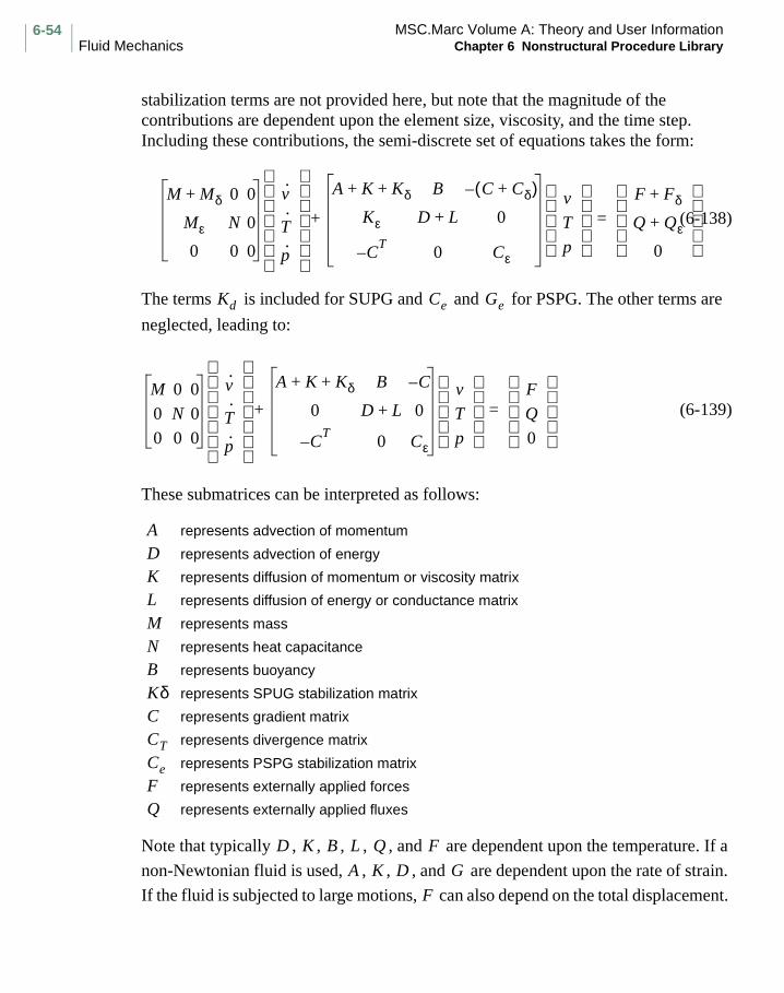
MSC.Marc Volume A: Theory and User InformationFluid Mechanics Chapter 6 Nonstructural Procedure Library
6-54
stabilization terms are not provided here, but note that the magnitude of the contributions are dependent upon the element size, viscosity, and the time step. Including these contributions, the semi-discrete set of equations takes the form:
(6-138)
The terms is included for SUPG and and for PSPG. The other terms are
neglected, leading to:
(6-139)
These submatrices can be interpreted as follows:
Note that typically , , , , , and are dependent upon the temperature. If a
non-Newtonian fluid is used, , , , and are dependent upon the rate of strain.
If the fluid is subjected to large motions, can also depend on the total displacement.
represents advection of momentum
represents advection of energy
represents diffusion of momentum or viscosity matrix
represents diffusion of energy or conductance matrix
represents mass
represents heat capacitance
represents buoyancy
represents SPUG stabilization matrix
represents gradient matrix
represents divergence matrix
represents PSPG stabilization matrix
represents externally applied forces
represents externally applied fluxes
M Mδ+ 0 0
Mε N 0
0 0 0
v·
T·
p·
A K Kδ+ + B C Cδ+( )–
Kε D L+ 0
CT
– 0 Cε
v
T
p
+F Fδ+
Q Qε+
0
=
Kd Ce Ge
M 0 0
0 N 0
0 0 0
v·
T·
p·
A K Kδ+ + B C–
0 D L+ 0
CT
– 0 Cε
v
T
p
+F
Q
0
=
ADKLMNBKδCCT
CeFQ
D K B L Q F
A K D G
F
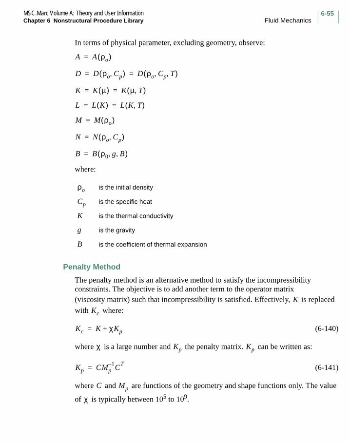
6-55MSC.Marc Volume A: Theory and User InformationChapter 6 Nonstructural Procedure Library Fluid Mechanics
In terms of physical parameter, excluding geometry, observe:
where:
Penalty Method
The penalty method is an alternative method to satisfy the incompressibility constraints. The objective is to add another term to the operator matrix (viscosity matrix) such that incompressibility is satisfied. Effectively, is replaced
with where:
(6-140)
where is a large number and the penalty matrix. can be written as:
(6-141)
where and are functions of the geometry and shape functions only. The value
of is typically between 105 to 109.
is the initial density
is the specific heat
is the thermal conductivity
is the gravity
is the coefficient of thermal expansion
A A ρo( )=
D D ρo Cp,( ) D ρo Cp T, ,( )= =
K K µ( ) K µ T,( )= =
L L K( ) L K T,( )= =
M M ρo( )=
N N ρo Cp,( )=
B B ρ0 g B, ,( )=
ρo
Cp
K
g
B
K
Kc
Kc K χKp+=
χ Kp Kp
Kp CMp1–C
T=
C Mp
χ

MSC.Marc Volume A: Theory and User InformationFluid Mechanics Chapter 6 Nonstructural Procedure Library
6-56
The penalty method should not be used for three-node planar elements, or four-node tetrahedral elements.
Steady State Analysis
It is possible to simplify the equations governing fluid flow by assuming that the time derivatives of the velocity and temperature are zero. This is achieved by using the STEADY STATE option. For thermally coupled, non-Newtonian flows, you still have a highly nonlinear system and multiple iterations are required.
Transient Analysis
The equations discussed above are still differential equations because of the presence of time derivatives of velocity and temperature. The conversion of the equations to fully discrete linear equations requires an assumption of the behavior during the increment. The approximations inevitably result in problems with accuracy, artificial damping, and/or stability problems.
Marc uses the first order backward Euler procedure such that:
(6-142)
This is substituted into the equations to yield:
(6-143)
Marc allows either fixed time step or adaptive time step procedure.
The equations of fluid flow are highly nonlinear even for Newtonian behavior because of the inclusion of the advection terms. The Newton-Raphson and direct substitution procedures are available to solve these problems.
Solid Analysis
Solid can be modeled in two ways:
• The first is to model them as a fluid with a very large viscosity. In such cases, an Eularian procedure is used throughout the model. The constitutive laws are limited to the fluid relationships.
• The second is to model them as true solids. In such cases, a Lagrangian or updated Lagrangian approach is used in the solid.
v·n 1+ vn 1+ vn–( ) ∆t⁄=
A K Kδ M ∆t⁄+ + + B C–
0 D L N ∆t⁄+ + 0
CT
– 0 Cε
v
T
p F M ∆t vn⋅⁄–
Q Qε N ∆t Tn⋅⁄–+
0
=

6-57MSC.Marc Volume A: Theory and User InformationChapter 6 Nonstructural Procedure Library Fluid Mechanics
The complete Marc constitutive routines are available for representing the solid behavior.
An important consideration is the interface between the fluid and solid. In the case of large motion at the interface, it might be necessary to remesh the fluid region. This is not supported in the K7 release. For small changes in the structural deformation, the nodes at the interface are updated. The pressure is transmitted between the fluid and the solid.
Solution of Coupled Problems in Fluids
The coupled fluid-thermal problem can be solved using either a tightly coupled procedure as shown above or in a staggered manner. Problems such as free convection are inherently coupled and are best solved using the tightly coupled procedure.
The fluid-solid interaction problem is solved in a weakly coupled manner. Every attempt has been made to maximize the computational efficiency. It should be noted that, while the staggered procedure can result in more global iterations, there are several motivating factors for solving the system in this manner.
• In solving fluid problems, especially in three dimensions, very large systems of equations are obtained. Any procedure that reduces the number of equations (for example, excluding the solid) is potentially beneficial.
• The fluid flow solution always requires the solution of a nonsymmetric system. In a weakly staggered analysis, the structural problem can still be solved with a symmetric solver.
• When using an iterative solver, the solution of the strongly coupled system will result in an ill-conditioned system, which results in poor convergence. This is because the terms associated with the fluid, thermal, and structural operator are of several different orders of magnitude.
The problem can be divided into two regions (fluid and solid) to accommodate these requirements. In each region, a different solver can be invoked; different nodal optimizers can be used; and a different memory allocation can be performed. Often, the fluid uses an out-of-core nonsymmetric solver while the structure uses an in-core symmetric solver.
Degrees of Freedom
The degrees of freedom in a fluid analysis are the velocities or, for the mixed method, the velocity and the pressure. When the pressure is not included explicitly as a degree of freedom, the incompressibility constraint is imposed using a penalty approach.

MSC.Marc Volume A: Theory and User InformationFluid Mechanics Chapter 6 Nonstructural Procedure Library
6-58
If a strongly coupled fluid-thermal problem is solved, the degrees of freedom are either the velocities and temperatures or the velocities, pressure, and temperature. For a three dimensional problem, the number of degrees of freedom could be 5.
The degrees of freedom associated with the solid are the conventional displacements or the displacements and temperatures.
Element Types
The fluid region can be represented using the conventional displacement elements in Marc. When using the mixed method, the pressure has the same order and interpolation functions as the velocity. In a coupled fluid-thermal analysis, the temperature also has the same order as the velocity. Hence, the element types available are:
Planar
Axisymmetric
Three Dimensional
The three-node triangular elements or the four-node tetrahedral element give poor results when used with the penalty formulation.
Type3-node linear 34-node isoparametric bilinear 114-node isoparametric bilinear reduced integration 1156-node isoparametric triangle 1258-node isoparametric biquadratic 278-node isoparametric biquadratic reduced integration 54
Type3-node linear 24-node isoparametric bilinear 104-node isoparametric bilinear reduced integration 1166-node isoparametric triangle 1268-node isoparametric biquadratic 288-node isoparametric biquadratic reduced integration 55
Type4-node tetrahedron 1348-node trilinear brick 78-node trilinear brick with reduced integration 11720-node brick 2120-node brick with reduced integration 57

6-59MSC.Marc Volume A: Theory and User InformationChapter 6 Nonstructural Procedure Library Fluid Mechanics
The shape functions used are identical to those used for structural analyses and can be found in any finite element textbook.
All of the mesh generation capabilities in Mentat can be used to generate the fluid mesh. Furthermore, Mentat can be used to visualize the results in a manner consistent with structural analyses.
Marc’s implementation of the Navier-Stokes equations utilizes the natural boundary condition.
At nodal points, you can prescribe the time dependent values of the velocity and temperature. This can be achieved by using the FIXED VELOCITY, FIXED TEMPERATURE, VELOCITY CHANGE, and/or TEMP CHANGE options. User subroutine FORCDT can be used for complex time-dependent behavior.
The excitation can be prescribed at the nodes as either time-dependent force or flux. This can be achieved using POINT FLUX. Again, user subroutine FORCDT can be used for complex time-dependent behavior. Additionally, for two-dimensional problems, edge pressures. or edge fluxes can be defined; for three-dimensional problems, surface fluxes or surface pressures can be defined. These quantities are numerically integrated using the shape functions.
Gravity and centrifugal loads can also be applied.
For coupled fluid-solid interaction problems, the pressure of the fluid is automatically applied to the structure. The resultant deformation of the structure is applied to the fluid boundaries. In the current release, only small deformations of the solid are permitted.
The viscosity, mass density, conductivity, and specific head are defined through the ISOTROPIC option. The STRAIN RATE option is used to define non-Newtonian viscous behavior. The penalty parameter can be entered through the PARAMETERS option.
Note: In fluid analysis, data for POINT LOAD and DIST LOADS should be prescribed as total rather than incremental quantity (as used in mechanical analysis). Similarly, POINT FLUX and DIST FLUXES for heat transfer analysis are also given as total quantity. This specification is to be used consistently for the fluid and/or heat transfer portion of analysis in coupled fluid-solid, fluid-thermal, and fluid-thermal-solid.

MSC.Marc Volume A: Theory and User InformationCoupled Analyses Chapter 6 Nonstructural Procedure Library
6-60
Coupled Analyses
The definition of coupled systems includes the multiple domains and independent or dependent variables describing different physical systems. In the situation with multiple domains, the solution for both domains is obtained simultaneously. Similarly, the dependent variables cannot be condensed out of the equilibrium equations explicitly.
Coupled systems can be classified into two categories:
1. Interface variables coupling: In this class of problems, the coupling occurs through the interfaces of the domain. The domains can be physically different (for example, fluid-solid interaction) or physically the same but with different discretization (for example, mesh partition with explicit/implicit procedures in different domains).
Figure 6-9 Fluid-structure Interaction (Physically Different Domains)
2. Field variables coupling: In this, the domain can be the same or different. The coupling occurs through the governing differential equations describing different physical phenomenon; for example, coupled thermo-mechanical problems.
Figure 6-10 Metal Extrusion with Plastic Flow Coupled with Thermal Field

6-61MSC.Marc Volume A: Theory and User InformationChapter 6 Nonstructural Procedure Library Coupled Analyses
6Nonstructural Procedure Library
Coupled Analyses
Marc can solve seven types of coupled problems: fluid-solid, fluid-thermal, fluid-solid-thermal interaction, coupled thermo-electrical (Joule heating), coupled thermo-mechanical, fluid-soil (pore pressure), and electromagnetic. The type of coupling is summarized in Table 6-10.
There are two approaches for solving fluid-solid interaction problems. In the first approach, the fluid is assumed to be inviscid and incompressible. The effect of the fluid is to augment the mass matrix of a structure. Modal shapes can be obtained for a fluid/solid system; the modal superposition procedure predicts the dynamic behavior of the coupled fluid/solid system. This prediction is based on extracted modal shapes. This method is discussed below.
The general fluid-solid capability models nonlinear transient behavior and is discussed in the fluid mechanics section.
There are two approaches for solving fluid-thermal interaction problems. The first is for a fluid constricted to move through thin areas and is implemented using the CHANNEL option. This is discussed earlier in this chapter. The second approach solves the coupled Navier-Stokes equations and is discussed in the fluid mechanics section.
The fluid-thermal-mechanical capability is described in more detail in the fluid mechanics section.
Table 6-10 Summary of Coupled Procedures
Interaction Category Coupling
Fluid-Solidadded mass approachgeneral approach
InterfaceInterface
WeakWeak
Fluid-Thermalchannel approachgeneral approach
InterfaceField
WeakStrong or Weak
Fluid-Thermal-Solid Field/Interface Strong or Weak/Weak
Thermal-Electric (Joule) Field Weak
Thermal- Mechanical Field Weak
Fluid-Pore Field Strong
Electromagnetic Field Strong

MSC.Marc Volume A: Theory and User InformationCoupled Analyses Chapter 6 Nonstructural Procedure Library
6-62
In the coupled thermo-electrical problem, the coupling takes place through the temperature-dependent electrical conductivity in the electrical problem and the internal heat generation caused by electrical flow in the thermal problem. The program solves for the voltage and temperature distribution.
Similarly, the coupling between the thermal and mechanical problems takes place through the temperature-dependent material properties in the mechanical (stress) problem and the internal heat generation in the mechanical problem caused by plastic work, which serves as input for the heat transfer problem. The temperature distribution and displacements are obtained.
In each of the coupled problems described above, two analyses are performed in each load/time increment. Iterations can also be carried out within each increment to improve the convergence of the coupled thermo-electrical and thermo-mechanical solutions.
In the coupled fluid-soil model, the fluid is assumed to be inviscid and incompressible. The effect of the fluid is to augment the stress in the soil material to satisfy equilibrium, and to influence the soil’s material behavior.
In the electromagnetic analysis, the fully coupled Maxwell’s equations are solved.
In the latter two analyses, the equations (fluid flow/structural or electrical/magnetic) are solved simultaneously.
Fluid/Solid Interaction – Added Mass Approach
The fluid/solid interaction procedure investigates structures that are either immersed in, or contain a fluid. Examples of problems that make use of this feature are vibration of dams, ship hulls, and tanks containing liquids.
Marc is capable of predicting the dynamic behavior of a structural system that is subject to the pressure loading of fluid. The fluid is assumed to be inviscid and incompressible; for example, water.
In Marc, the fluid is modeled with heat transfer elements (potential theory) and the structure is modeled with normal stress or displacement elements. The element choice must ensure that the interface between the structural and fluid models has compatible interpolation; that is, both solid and fluid elements are either first order or second order. The TYING option can be used to achieve compatibility if necessary. To identify the interfaces between the fluid and the structure, the FLUID SOLID model definition set is necessary.

6-63MSC.Marc Volume A: Theory and User InformationChapter 6 Nonstructural Procedure Library Coupled Analyses
During increment zero, Marc calculates the stiffness matrix for the structure and the mass matrix for the structure augmented by the fluid effect. Marc then extracts the eigenvalues of the coupled system using the MODAL SHAPE option. The modal superposition procedure can then be used to predict the time response of the coupled system. DYNAMIC CHANGE can be used to perform modal superposition.
To input properties of solids and the mass density of the fluid elements, use the model definition option ISOTROPIC.
The calculation of the structural mass augmentation requires triangularization of the fluid potential matrix: this matrix is singular, unless the fluid pressure is fixed at least at one point with the FIXED DISP option.
Technical Background
In a fluid/solid interaction problem, the equations of motion can be expressed as
(6-144)
The pressure vector p can be calculated from
(6-145)
The matrices in Equation 6-144 and Equation 6-145 are defined as
(6-146)
(6-147)
(6-148)
(6-149)
Msa Ku+1ρf----S
Tp=
Sa– Hp=
Ms Niβ
Niα ρs Vd
V∫=
K βijβ
Dijkl βklα
VdV∫=
S RβρfniNi
αAd
AT
∫=
H∂R
β
∂xi---------
∂Rα
∂xi---------- Vd
Vf
∫=

MSC.Marc Volume A: Theory and User InformationCoupled Analyses Chapter 6 Nonstructural Procedure Library
6-64
where
and are mass densities of the fluid and solid, respectively
is the acceleration vector
is the displacement vector
is the strain displacement relation
is the material constitutive relation
is the displacement interpolation function
is the pressure interpolation function
is the outward normal to the surface with fluid pressure
is the surface on which the fluid pressure acts
In the present case, the fluid is assumed to be incompressible and inviscid. Only infinitesimal displacements are considered during the fluid vibration, so that the Eulerian and material coordinates coincide.
Substituting Equation 6-145 into Equation 6-144, we obtain
(6-150)
This equation now allows the modes and frequencies of the solid structure immersed in the fluid to be obtained by conventional eigenvalue methods.
Coupled Thermal-Electrical Analysis (Joule Heating)
The coupled thermal-electrical analysis procedure can be used to analyze electric heating problems. The coupling between the electrical problem and the thermal problem in a Joule heating analysis is due to the fact that the resistance in the electric problem is dependent on temperatures, and the internal heat generation in the thermal problem is a function of the electrical flow.
Marc analyzes coupled thermo-electrical (Joule heating) problems. Use the parameter JOULE to initiate the coupled thermo-electrical analysis. This capability includes the analysis of the electrical problem, the associated thermal problem, and the coupling between these two problems.
The electrical problem is a steady-state analysis and can involve current and/or voltage boundary conditions as well as temperature-dependent resistivity.
ρf ρs
a
u
βij
Dijkl
Ni
R
ni p
AT
Ms STH 1– S ρf⁄+( )a Ku+ 0=or
Ma Ku+ 0=

6-65MSC.Marc Volume A: Theory and User InformationChapter 6 Nonstructural Procedure Library Coupled Analyses
The thermal analysis is generally a transient analysis with temperature-dependent thermal properties and time/temperature-dependent boundary conditions.
Use the model definition options ISOTROPIC, ORTHOTROPIC, TEMPERATURE EFFECTS, and ORTHO TEMP to input reference values of thermal conductivity, specific heat, mass density, and electrical resistivity, as well as their variations with temperatures. The mass density must remain constant throughout the analysis.
Use the model definition option VOLTAGE for nodal voltage boundary conditions, and the model definition options POINT CURRENT and/or DIST CURRENT for current boundary conditions. No initial condition is required for the electrical problem, since a steady-state solution is obtained.
In the thermal problem, you can use the model definition options INITIAL TEMP, FILMS, POINT FLUX, DIST FLUXES, and FIXED TEMPERATURE to prescribe the initial conditions and boundary conditions. Use the user subroutines FILM and FLUX for complex convective and flux boundary conditions. To enter the unit conversion factor between the electrical and thermal problems, use the model definition option JOULE. Marc uses this conversion factor to compute heat flux generated from the current flow in the structure.
Use the history definition options STEADY STATE, TRANSIENT, POINT CURRENT, DIST CURRENT, VOLTAGE CHANGE, POINT FLUX, DIST FLUXES, and TEMP CHANGE for the incrementation and change of boundary conditions.
A weak coupling between the electrical and thermal problems is assumed in the coupled thermo-electrical analysis, such that the distributions of the voltages and the temperatures of the structure can be solved separately within a time increment. A steady-state solution of the electrical problem (in terms of nodal voltages) is calculated first within each time step.
The heat generation due to electrical flow is included in the thermal analysis as an additional heat input.
The temperature distribution of the structure (obtained from the thermal analysis) is used to evaluate the temperature-dependent resistivity, which in turn is used for the electrical analysis in the next time increment.

MSC.Marc Volume A: Theory and User InformationCoupled Analyses Chapter 6 Nonstructural Procedure Library
6-66
Technical Background
In the coupled thermo-electrical analysis, the matrix equation of the electrical problem can be expressed as
(6-151)
and the governing equation of the thermal problem is
(6-152)
In Equation 6-151 and Equation 6-152:
is the temperature-dependent electrical conductivity matrix
is the nodal current vector
is the nodal voltage vector
and are the temperature-dependent heat capacity and thermal conductivity matrices, respectively
is the nodal temperature vector
is the time derivative of the temperature vector
is the heat flux vector
is the internal heat generation vector caused by the current flow.
The coupling between the electrical and thermal problems is through terms and
in Equation 6-151 and Equation 6-152.
The selection of the backward difference scheme for the discretization of the time variable in Equation 6-152 yields the following expression:
(6-153)
Equation 6-153 is used for the computation of nodal temperatures in each time increment .
ρ T( )V I=
C T( )T·
K T( )T+ Q QE
+=
ρ T( )I
V
C T( ) K T( )
T
T.
Q
QE
ρ T( )
QE
1∆t----- C T( )[ ] K T( )Tn+ Qn Qn
E 1∆t-----C T( )Tn 1–+ +=
∆t
6-67MSC.Marc Volume A: Theory and User InformationChapter 6 Nonstructural Procedure Library Coupled Analyses
The internal heat generation vector is computed from
(6-154)
(6-155)
where and are the current and electrical resistance, respectively.
The controls for the heat transfer option allow input of parameters that govern the convergence solution and accuracy of heat transfer analysis.
Thermal Mechanically Coupled Analysis
Many operations performed in the metal forming industry (such as casting, extrusion, sheet rolling, and stamping) can require a coupled thermo-mechanical analysis. The observed physical phenomena must be modeled by a coupled analysis if the following conditions pertain:
• The body undergoes large deformations such that there is a change in the boundary conditions associated with the heat transfer problem.
• Deformation converts mechanical work into heat through an irreversible process which is large relative to other heat sources.
In either case, a change in the temperature distribution contributes to the deformation of the body through thermal strains and influences the material properties.
Marc has a capability that allows you to perform mechanically coupled analysis. This capability is available for all stress elements and for small displacement, total Lagrangian, updated Lagrangian, or rigid plastic analysis.
Use the COUPLE parameter to invoke this option. When defining the mesh, if you specify the element as a stress type through the CONNECTIVITY option, Marc generates an associated heat transfer element, if possible. The region having an associated heat transfer element has coupled behavior. If you specify the element as a heat transfer type through the CONNECTIVITY option, that region is considered rigid. Only heat transfer is performed in that region.
Marc uses a staggered solution procedure in coupled thermo-mechanical analysis. It first performs a heat transfer analysis, then a stress analysis. Use the CONTROL option to enter the control tolerances used in the analysis.
Load control and time step control are intimately coupled in these analyses. These controls can be specified in either of two ways.
QE
QE
BTq
EVd
V∫=
qE
i2R=
i R

MSC.Marc Volume A: Theory and User InformationCoupled Analyses Chapter 6 Nonstructural Procedure Library
6-68
• A fixed time step/load size can be specified by using either the DYNAMIC CHANGE option or the TRANSIENT NON AUTO option. In these cases, mechanical loads and deformations are incremental quantities that are applied to each step. Fluxes are total quantities.
• An adaptive time step/load size can be specified by using the AUTO TIME option. In this case, mechanical loads and deformations are entered as the total quantities that are applied over the load set. Fluxes are total quantities.
Exercise caution when applying boundary conditions. Use the FIXED DISP or FIXED TEMPERATURE options as well as DISP CHANGE or TEMP CHANGE for mechanical or thermal boundary conditions, respectively.
There are two primary causes of coupling. First, coupling occurs when deformations result in a change in the associated heat transfer problem. Such a change can be due to either large deformation or contact. Large deformation effects are coupled into the heat transfer problem only if the UPDATE parameter is invoked. The gap element in Marc (Type 12) has been modified so that if no contact occurs, the gap element acts as a perfect insulator. When contact does occur, the gap element acts as a perfect conductor.
The second cause of coupling is heat generated due to inelastic deformation. The irreversibility of plastic flow causes an increase in the amount of entropy in the body. This can be expressed as
(6-156)
where is the fraction of the rate of plastic work dissipated into heat. Farren and Taylor measure f as approximately 0.9 for most metals. Using the mechanical equivalent of heat ( ), the rate of specific volumetric flux is
(6-157)
Use the CONVERT model definition option to define .
Of course, all mechanical and thermal material properties can be temperature dependent. The governing matrix equations can be expressed as
(6-158)
(6-159)
TS·
fW· p
=
fW· p
M
R MfW· p
ρ⁄=
Mf
Mu·· D T( )u· K T( )u+ + f=
C T( )T·
K T( )T+ Q Q1+=

6-69MSC.Marc Volume A: Theory and User InformationChapter 6 Nonstructural Procedure Library Coupled Analyses
In Equation 6-159, represents the amount of heat generated due to plastic work.
The specific heat matrix and conductivity matrix can be evaluated in the current configuration if the updated Lagrange option is used.
Note: All terms except can be temperature dependent.
Q1
C K
M
MSC.Marc Volume A: Theory and User InformationReferences Chapter 6 Nonstructural Procedure Library
6-70
References
1. T. J. R. Hughes, L. P. France, and M. Becestra, “A New Finite Element Formulation for Computational Fluid Dynamics, V. Circumventing the Babuska-Brezzi Conduction, A Stable Petrov-Galerkin Formulation of the Stokes Problem Accommodating Equal-Order Interpolations”, Comp. Meth. in Applied Mech. and Eng., p. 85-90, Vol. 59, 1986.
2. G. Hauke and T. J. R. Hughes, “A unified approach to compressible and incompressible flow”, Comput. Methods Appl. Mech. Eng., p. 389-395, 113, (1994).
3. T. E. Tezduyar, S. Mittal, S. E. Ray, and R. Shih, “Incompressible Flow computations with stabilized bilinear and linear equal order-interpolation velocity-pressure elements”, Comput. Methods. Appl. Mech. Eng., p. 221-242, 95, (1992).
4. B. Ramaswaymy, T. C. Jue, “Some Recent Trends and Developments in Finite Element Analysis for Incompressible Thermal Flows”, Int. J. Num. Meth. Eng., p. 671-707, 3, (1992).
5. A. N. Brooks and T. J. R. Hughes, “Streamline upwind/Petrov-Galerkin formulations for convection dominated flows with particular emphasis on the incompressible Navier-Stokes equations”, Comp. Meth. Appl. Eng., 30, (1982).
6. Codina, R. “Finite element formulation for the numerical solution of the convection-diffusion equation” 1993.
7. Cornfield, G. C., and Johnson, R. H. “Theoretical Predictions of Plastic Flow in Hot Rolling Including the Effect of Various Temperature Distributions.” Journal of Iron and Steel Institute 211, pp. 567-573, 1973.
8. Hsu, M. B. “Modeling of Coupled Thermo-Electrical Problems by the Finite Element Method.” Third International Symposium on Numerical Methods for Engineering, Paris, March, 1983.
9. MARC Reference manual Volume F.
10. Peeters, F. J. H. “Finite Element Analysis of Elasto-Hydrodynamic Lubrication Problems.” in Proceedings of the XIth Int. Finite Element Kongress, edited by IKOSS GmbH. Baden- Baden, Germany, Nov. 15-16, 1982.

6-71MSC.Marc Volume A: Theory and User InformationChapter 6 Nonstructural Procedure Library References
11. Yu, C C. and Heinrich, J. C. “Petro-Galerkin methods for the time-dependent convective transport equation.” Int. J. Numer. Meth. Engrg., Vol. 23 (1986), 883-901.
12. Yu, C C. and Heinrich, J. C. “Petro-Galerkin methods for multidimensional time-dependent convective transport equation.” Int. J. Numer. Meth. Engrg., Vol. 24 (1987), 2201-2215.
13. Zienkiewicz, O. C. The Finite Element Method in Engineering Science. Third Ed. London: McGraw-Hill, 1978.
14. Zienkiewicz, O. C., and Godbole, P. N. “A Penalty Function Approach to Problems of Plastic Flow of Metals with Large Surface Deformations.” Journal of Strain Analysis 10, 180-183, 1975.
15. Zienkiewicz, O. C., and Godbole, P. N. “Flow of Plastic and viscoPlastic Solids with Special Reference to Extrusion and Forming Processes.” Int. Num. Methods in Eng. 8, 1974.
16. Zienkiewicz, O. C., Loehner, R., Morgan, K., and Nakazawa, S. Finite Elements in Fluid Mechanics – A Decade of Progress, John Wiley & Sons Limited, 1984.

MSC.Marc Volume A: Theory and User InformationChapter 6 Nonstructural Procedure Library
6-72

Chapter 7 Material Library
CHAPTER
7 Material Library
Linear Elastic Material
Composite Material
Nonlinear Hypoelastic Material
Elastomer
Time-Independent Inelastic Behavior
Time-Dependent Inelastic Behavior
Temperature Effects and Coefficient of Thermal Expansion
Time-Temperature-Transformation
Low Tension Material
Soil Model
Damage Models
Nonstructural Materials
References

MSC.Marc Volume A: Theory and User InformationChapter 7 Material Library
7-2
This chapter describes the material models available in Marc. The models range from simple linear elastic materials to complex time- and temperature-dependent materials. This chapter provides basic information on the behavior of various types of engineering materials and specifies the data required by the program for each material. For example, to characterize the behavior of an isotropic linear elastic material at constant temperatures, you need only specify Young’s modulus and Poisson’s ratio. However, much more data is required to simulate the behavior of material that has either temperature or rate effects. References to more detailed information are cited in this chapter.
The material models included in this chapter are:
• Linear Elastic Material
• Composite Material
• Nonlinear Hypoelastic Material
• Elastomer
• Time-Independent Inelastic Behavior
• Time-Dependent Inelastic Behavior
• Temperature Effects and Coefficient of Thermal Expansion
• Time-Temperature-Transformation
• Low Tension Material
• Soil Model
• Damage Models
• Nonstructural Materials
Data for the materials is entered into Marc either directly through the input file or by user subroutines. Each section of this chapter discusses various options for organizing material data for input. Each section also discusses the constitutive (stress-strain) relation and graphic representation of the models and includes recommendations and cautions concerning the use of the models.

7-3MSC.Marc Volume A: Theory and User InformationChapter 7 Material Library Linear Elastic Material
Linear Elastic Material
Marc is capable of handling problems with either isotropic linear elastic material behavior or anisotropic linear elastic material behavior.
The linear elastic model is the model most commonly used to represent engineering materials. This model, which has a linear relationship between stresses and strains, is represented by Hooke’s Law. Figure 7-1 shows that stress is proportional to strain in a uniaxial tension test. The ratio of stress to strain is the familiar definition of modulus of elasticity (Young’s modulus) of the material.
E (modulus of elasticity) = (axial stress)/(axial strain) (7-1)
Figure 7-1 Uniaxial Stress-Strain Relation of Linear Elastic Material
Experiments show that axial elongation is always accompanied by lateral contraction of the bar. The ratio for a linear elastic material is:
= (lateral contraction)/(axial elongation) (7-2)
This is known as Poisson’s ratio. Similarly, the shear modulus (modulus of rigidity) is defined as:
(shear modulus) = (shear stress)/(shear strain) (7-3)
Str
ess
Strain
E
1
v
G

MSC.Marc Volume A: Theory and User InformationLinear Elastic Material Chapter 7 Material Library
7-4
It can be shown that for an isotropic material
(7-4)
The shear modulus can be easily calculated if the modulus of elasticity and
Poisson’s ratio are known.
Most linear elastic materials are assumed to be isotropic (their elastic properties are the same in all directions). Anisotropic material exhibits different elastic properties in different directions. The significant directions of the material are labeled as preferred directions, and it is easiest to express the material behavior with respect to these directions.
The stress-strain relationship for an isotropic linear elastic method is expressed as
(7-5)
where is the Lame constant and (the shear modulus) is expressed as
(7-6)
The material behavior can be completely defined by the two material constants
and .
Use the model definition option ISOTROPIC for the input of isotropic linear elastic material constants (Young’s modulus) and (Poisson’s ratio).
The effects of these parameters on the design can be determined by using the DESIGN SENSITIVITY parameter. The optimal value of the elastic properties for linear elastic analysis can be determined using the DESIGN OPTIMIZATION parameter.
The stress-strain relationship for an anisotropic linear elastic material can be expressed as
(7-7)
The values of (the stress-strain relation) and the preferred directions (if
necessary) must be defined for an anisotropic material. For example, the orthotropic stress-strain relationship for a plane stress element is
G E 2 1 v+( )( )⁄=
G E
v
σij λδijεkk 2Gεij+=
λ G
λ νE 1 ν+( ) 1 2ν–( )( )⁄= and
G E 2 1 ν+( )( )⁄=
E
v
E v
σij Cijklεkl=
Cijkl
7-5MSC.Marc Volume A: Theory and User InformationChapter 7 Material Library Linear Elastic Material
(7-8)
There are only four independent constants in Equation 7-8.
To input anisotropic stress-strain relations, use the model definition options ORTHOTROPIC or ANISOTROPIC and user subroutine ANELAS or HOOKLW. The ORTHOTROPIC option allows as many as 9 elastic constants to be defined. The ANISOTROPIC option allows as many as 21 elastic constants to be defined. If the anisotropic material has a preferred direction, use the model definition option ORIENTATION or the user subroutine ORIENT to input a transformation matrix. Refer to MSC.Marc Volume D: User Subroutines and Special Routines for information on user subroutines.
A Poisson’s ratio of 0.5, which would be appropriate for an incompressible material, can be used for the following elements: Herrmann, plane stress, shell, truss, or beam. A Poisson’s ratio which is close (but not equal) to 0.5 can be used for constant dilation elements and reduced integration elements in situations which do not include other severe kinematic constraints. Using a Poisson’s ratio close to 0.5 for all other elements usually leads to behavior that is too stiff. A Poisson’s ratio of 0.5 can also be used with the updated Lagrangian formulation in the multiplicative decomposition framework using the standard displacement elements. In these elements, the treatment for incompressibility is transparent to you.
11 ν12ν21–( )
-----------------------------
E1 ν21E1 0
ν12E2 E2 0
0 0 1 ν12ν21–( )G
=

MSC.Marc Volume A: Theory and User InformationComposite Material Chapter 7 Material Library
7-6
Composite Material
Composite materials are composed of layers of different materials (or layers of the same anisotropic material) with various layer thicknesses and different orientations. The material in each layer may be either linear or nonlinear. Tightly bonded layers (layered materials) are often stacked in the thickness direction of beam, plate, shell structures, or solids.
Figure 7-2 identifies the locations of integration points through the thickness of beam and shell elements with/without the COMPOSITE option.
Note that when the COMPOSITE option is used, as shown on the left, the layer points are positioned midway through each layer. When the COMPOSITE option is not used, the layer points are equidistantly spaced between the top and bottom surfaces. Marc forms a stress-strain law by performing numerical integration through the thickness. If the COMPOSITE option is used, the trapezoidal method is employed; otherwise, Simpson’s rule is used.
Figure 7-2 Integration Points through the Thickness of Beam and Shell Elements
Figure 7-3 shows the location of integration points through the thickness of continuum elements. Marc forms the element stiffness matrix by performing numerical integration based on the standard isoparametric concept.
****
*****Beams or Shells with
Composite OptionBeams or Shells without
Composite Option
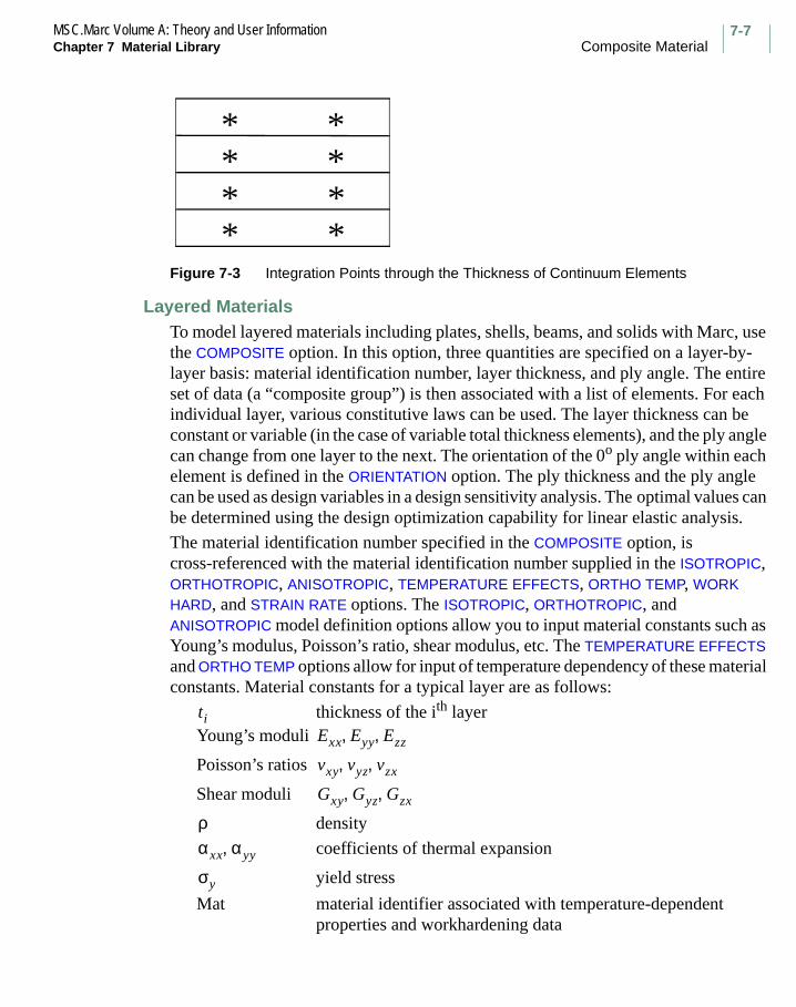
7-7MSC.Marc Volume A: Theory and User InformationChapter 7 Material Library Composite Material
Figure 7-3 Integration Points through the Thickness of Continuum Elements
Layered MaterialsTo model layered materials including plates, shells, beams, and solids with Marc, use the COMPOSITE option. In this option, three quantities are specified on a layer-by-layer basis: material identification number, layer thickness, and ply angle. The entire set of data (a “composite group”) is then associated with a list of elements. For each individual layer, various constitutive laws can be used. The layer thickness can be constant or variable (in the case of variable total thickness elements), and the ply angle can change from one layer to the next. The orientation of the 0o ply angle within each element is defined in the ORIENTATION option. The ply thickness and the ply angle can be used as design variables in a design sensitivity analysis. The optimal values can be determined using the design optimization capability for linear elastic analysis.
The material identification number specified in the COMPOSITE option, is cross-referenced with the material identification number supplied in the ISOTROPIC, ORTHOTROPIC, ANISOTROPIC, TEMPERATURE EFFECTS, ORTHO TEMP, WORK HARD, and STRAIN RATE options. The ISOTROPIC, ORTHOTROPIC, and ANISOTROPIC model definition options allow you to input material constants such as Young’s modulus, Poisson’s ratio, shear modulus, etc. The TEMPERATURE EFFECTS and ORTHO TEMP options allow for input of temperature dependency of these material constants. Material constants for a typical layer are as follows:
thickness of the ith layerYoung’s moduli
Poisson’s ratios
Shear moduli
density
coefficients of thermal expansion
yield stress
Mat material identifier associated with temperature-dependent properties and workhardening data
**** *
***
tiExx Eyy Ezz, ,
vxy vyz vzx, ,
Gxy Gyz Gzx, ,
ραxx αyy,
σy

MSC.Marc Volume A: Theory and User InformationComposite Material Chapter 7 Material Library
7-8
User subroutines ANELAS, HOOKLW, ANEXP, and ANPLAS can be used for the anisotropic behavior of elastic constants, coefficient of thermal expansion, and yield condition.
There are seven given classes of strain-stress relations. The class of a particular element depends on the number of direct (NDI) and shear (NSHEAR) components of stress. Table 7-1 lists the eight classes of elements.
Table 7-1 Classes of Stress-Strain Relations
Class 1 NDI = 1,NSHEAR = 0Beam Elements 5, 8, 13, 16, 23, 46, 47, 48, 52, 64, 77, 79,142-148
Class 2 NDI = 2,NSHEAR = 0Axisymmetric Shells 15 and 17
Class 3 NDI = 1,NSHEAR = 1Beam Elements 14, 45, 76, 78
Class 4 NDI = 2,NSHEAR = 1Plane Stress, Plates and Thin Shells 49 and 72
ε 1 Exx⁄ σ [=
εxx
εyy 1 Exx⁄ νyx Eyy⁄–
νxy Exx⁄– 1. Eyy⁄
σxx
σyy
=
νyx νxyEyy Exx⁄=
εγ
1 Exx⁄ 0
0 1 Gxy⁄
στ
=
εxx
εyy
γxy
1 Exx⁄ νyx Eyy⁄– 0
νxy Exx⁄– 1 Eyy⁄ 0
0 0 1 Gxy⁄
σxx
σyy
τxy
=
νyx νxy Eyy Exx⁄( )=

7-9MSC.Marc Volume A: Theory and User InformationChapter 7 Material Library Composite Material
Class 5 NDI = 2,NSHEAR = 1Thick Axisymmetric Shells 1 and 89
Class 6 NDI = 3,NSHEAR = 1Plane Strain, Axisymmetric with No Twist, Elements 151-154.
Class 7 NDI = 2,NSHEAR = 3Thick Shell, Elements 22, 75
Table 7-1 Classes of Stress-Strain Relations (Continued)
εmm
εθθ
γT 1 Emm⁄ νθm Eθθ⁄– 0
νmθ Emm⁄– 1 Eθθ⁄ 0
0 0 1 Gmθ⁄
σmm
σθθ
τT
=
εxx
εyy
εzz
γxy 1 Exx⁄ νyx Eyy⁄– νzx Ezz⁄– 0
νxy Exx⁄– 1 Eyy⁄ νzy Ezz⁄– 0
νxz Exx⁄– νyz Eyy⁄– 1 Ezz⁄ 0
0 0 0 1 Gxy⁄
σxx
σyy
σzz
τxy
=
νyx νxyEyy Exx⁄= νzy νyzEzz Eyy⁄= νxz νzxExx Ezz⁄=
εxx
εyy
γxy
γyz
γzx 1 Exx⁄ νyx Eyy⁄– 0 0 0
νxy Exx⁄– 1 Eyy⁄ 0 0 0
0 0 1 Gxy⁄ 0 0
0 0 0 1 Gyz⁄ 0
0 0 0 0 1 Gzx⁄
σxx
σyy
τxy
τyz
τxy
=
νyx νxyEyy Exx⁄=

MSC.Marc Volume A: Theory and User InformationComposite Material Chapter 7 Material Library
7-10
Material Preferred Direction
Every element type in Marc has a default orientation (that is, a default coordinate system) within which element stress-strain calculations take place. This system is also assumed to be the coordinate system of material symmetry. This is especially important for non-isotropic materials (orthotropic, anisotropic, or composite materials). With the ORIENTATION option, you specify the orientation of the material axes of symmetry (relationship between the element coordinate system and the global
coordinate system, or the 0o ply angle line, if composite) in one of four different ways:
1. as a specific angle offset from an element edge,2. as a specific angle offset from the line created by two intersecting planes,3. as a particular coordinate system specified by user-supplied unit vectors, or 4. as specified by user subroutine ORIENT. This is accomplished by the
specification of an orientation type, an orientation angle, or one or two user-defined vectors.
For the first option (EDGE I-J orientation type), the intersecting plane is defined by the surface normal vector and a vector parallel to the vector pointing from element node I to element node J. The intersection of this plane with the surface tangent plane
defines the 0o orientation axis. (See Figure 7-4.) The orientation angle is measured in the tangent plane positive about the surface normal.
For the second option (global plane orientation type), the intersecting plane is the chosen global coordinate plane. The intersection of this plane with the surface tangent
plane defines the 0o orientation axis. (See Figure 7-5.)
For continuum composite elements (types 149-154), use of the default orientation (coordinate system) is recommended.
Class 8 NDI = 3,NSHEAR = 3Three-Dimensional Brick Elements, Elements 149, 150
Table 7-1 Classes of Stress-Strain Relations (Continued)
εxx
εyy
εzz
γxy
γyz
γzx 1 Exx⁄ νyx Eyy⁄– νzx Ezz⁄– 0 0 0
νxy Exx⁄– 1 Eyy⁄ νzy Ezz⁄– 0 0 0
νxz Exx⁄– νyz Eyy⁄– 1. Ezz⁄ 0 0 0
0 0 0 1 Gxy⁄ 0 0
0 0 0 0 1 Gyz⁄ 0
0 0 0 0 0 1 Gzx⁄
σxx
σyy
σzz
τxy
τyz
τzx
=

7-11MSC.Marc Volume A: Theory and User InformationChapter 7 Material Library Composite Material
Figure 7-4 Edge I-J Orientation Type
Ω
α
Direction 1 ofpreferred coordinate system (fiber direction
n = Normal to SurfaceTangent Plane
Element Surface
Z
Y
X
Ω = Orientation Angle (Positive
α = ply angle (if COMPOSITE)
Right-hand Rotation About n)
Node I
Node J
Vector Parallel to EdgeI-J Projected ontoSurface Tangent Plane
Integration Point
in the ply)
00 Ply Angle

MSC.Marc Volume A: Theory and User InformationComposite Material Chapter 7 Material Library
7-12
Figure 7-5 Global ZX Plane Orientation Type
The third option (user-defined plane orientation type) makes use of one or two user-defined vectors to define the intersecting plane. Using a single vector, the intersecting plane is that plane which contains the user vector and the chosen coordinate axis. Using two user vectors, the intersecting plane is that plane which contains both of them. (See Figure 7-6.)
Ωα
Direction 1 ofpreferred coordinate system
Elem
ent S
urfa
ce
Surface
Global ZX Plane
n - Normal to SurfaceTangent Plane
Intersection of
Two Planes
Z
Y
X
Ω = Orientation Angle (Positive
α = ply angle (if COMPOSITE)
Right-hand Rotation About n)
TangentPlane

7-13MSC.Marc Volume A: Theory and User InformationChapter 7 Material Library Composite Material
Figure 7-6 User Defined XU Plane Orientation Type
Orientation type 3-D ANISO also makes use of two user-defined vectors, but in this case, the first vector defines the first (1) principal direction and the second vector defines the second (2) principal direction. (See Figure 7-7.)
Finally, in the fourth option, the user subroutine ORIENT must be used for the definition of the orientation of the material axis of symmetry.
Ωα
Direction 1 ofPreferred Coordinate System
u = user-defined vector
n = Normal to SurfaceTangent Plane
Surface TangentPlane
Intersection of Two Planes
Element SurfaceZ
Y
X α = Ply Angle (if composite)
globalX
Ω = Orientation Angle (PositiveRight-hand Rotation About n)

MSC.Marc Volume A: Theory and User InformationComposite Material Chapter 7 Material Library
7-14
Figure 7-7 3-D ANISO Orientation Type
Material Dependent Failure Criteria
Calculations of user specified failure criteria on a layer by layer basis are available in Marc. They are maximum stress (MX STRESS), maximum strain (MX STRAIN), TSAI-WU, HOFFMAN, HILL or user subroutine UFAIL. During each analysis, up to three failure criteria can be selected; failure indices are calculated and printed for every integration point. The model definition option FAIL DATA is used for the input of failure criteria data.
A simple description of these failure criteria is given below:
1. Maximum Stress Criterion
At each integration point, Marc calculates six quantities:
(7-9)
Z
Y
X
= Direction 1 of Preferred Coordinate System
= Direction 2 of Preferred Coordinate System
= User Vector 1
= User Vector 2
U1
U2
U2
U1
U3 U1 U2×=
σ1
Xt------
F⁄
σ1
Xc------–
F⁄
σ1 0>
σ1 0<
if
if
1.

7-15MSC.Marc Volume A: Theory and User InformationChapter 7 Material Library Composite Material
(7-10)
(7-11)
(7-12)
(7-13)
(7-14)
where
is the failure index (F =1.0).
are the maximum allowable stresses in the 1-direction in tension
and compression.
are maximum allowable stresses in the 2-direction in tension
and compression.
are maximum allowed stresses in the 3-direction in tension
and compression.
maximum allowable in-plane shear stress.
maximum allowable 23 shear stress.
maximum allowable 31 shear stress.
σ2
Yt------
F⁄
σ2
Yc------–
F⁄
σ2 0>
σ2 0<
if
if
2.
σ3
Zt------
F⁄
σ3
Zc------–
F⁄
σ3 0>
σ3 0<
if
if
3.
σ12
S12--------
F⁄4.
σ23
S23--------
F⁄5.
σ31
S31--------
F⁄6.
F
Xt Xc,
Yt Yc,
Zt Zc,
S12
S23
S31

MSC.Marc Volume A: Theory and User InformationComposite Material Chapter 7 Material Library
7-16
2. Maximum Strain Failure Criterion
At each integration point, calculates six quantities:
(7-15)
(7-16)
(7-17)
(7-18)
(7-19)
(7-20)
where
is the failure index ( F=1.0).
are the maximum allowable strains in the 1 direction in tension
and compression.
are the maximum allowable strains in the 2 direction in tension
and compression.
are the maximum allowable strains in the 3 direction in tension
and compression.
ε1
e1t------
F⁄
ε1
e1c-------–
F⁄
ε1 0>
ε1 0<
if
if
1.
ε2
e2t------
F⁄
ε2
e2c-------–
F⁄
ε2 0>
ε2 0<
if
if
2.
ε3
e3t------
F⁄
ε3
e3c-------–
F⁄
ε3 0>
ε3 0<
if
if
3.
γ12
g12-------
F⁄4.
γ23
g23-------
F⁄5.
γ31
g31-------
F⁄6.
F
1t e1c,
e2t e2c,
e3t e3c,

7-17MSC.Marc Volume A: Theory and User InformationChapter 7 Material Library Composite Material
is the maximum allowable shear strain in the 12 plane.
is the maximum allowable shear strain in the 23 plane.
is the maximum allowable shear strain in the 31 plane.
3. Hill Failure Criterion
Assumptions:
a. Orthotropic materials only
b. Incompressibility during plastic deformation
c. Tensile and compressive behavior are identical
At each integration point, Marc calculates:
(7-21)
For plane stress condition, it becomes
(7-22)
where
is the maximum allowable stress in the 1 direction
is the maximum allowable stress in the 2 direction
is the maximum allowable stress in the 3 direction
are as before
g12
g23
g31
σ12
X2
------σ2
2
Y2
------σ3
2
Z2
------1
X2
------1
Y2
-----1
Z2
-----–+ σ1σ2–
1
X2
------1
Z2
-----1
Y2
-----–+ σ1σ3–+ +
1
Y2
-----1
Z2
-----1
X2
------–+ σ2σ3–
σ122
S122
--------σ13
2
S132
--------σ23
2
S232
-------- F⁄+ + +
σ12
X2------
σ1σ2
X2------------–
σ22
Y2------
σ122
S122
--------+ +
F⁄
X
Y
Z
S12 S23 S31 F, , ,
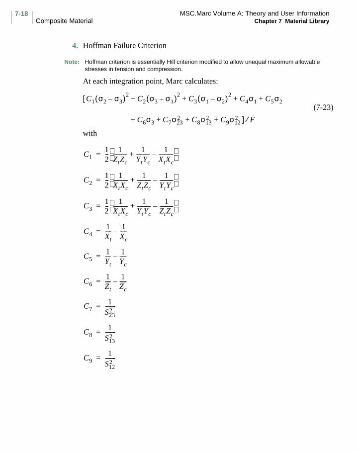
MSC.Marc Volume A: Theory and User InformationComposite Material Chapter 7 Material Library
7-18
4. Hoffman Failure Criterion
Note: Hoffman criterion is essentially Hill criterion modified to allow unequal maximum allowable stresses in tension and compression.
At each integration point, Marc calculates:
(7-23)
with
C1 σ2 σ3–( )2C2 σ3 σ1–( )2
C3 σ1 σ2–( )2C4σ1 C5σ2+ + + +[
C6σ3 C7σ232 C8σ13
2 C9σ122 ] F⁄+ + + +
C112---
1ZtZc----------
1YtYc----------
1XtXc-----------–+
=
C212---
1XtXc-----------
1ZtZc----------
1YtYc----------–+
=
C312---
1XtXc-----------
1YtYc----------
1ZtZc----------–+
=
C41Xt-----
1Xc-----–=
C51Yt----
1Yc-----–=
C61Zt----
1Zc-----–=
C71
S232
--------=
C81
S132
--------=
C91
S122
--------=

7-19MSC.Marc Volume A: Theory and User InformationChapter 7 Material Library Composite Material
For plane stress condition, it becomes
(7-24)
where: are as before.
Note: For small ratios of, for example, , the Hoffman criteria can become negative due to the
presence of the linear terms.
5. Tsai-Wu Failure Criterion
Tsai-Wu is a tensor polynomial failure criterion. At each integration point, Marc calculates:
(7-25)
where are as before.
Interactive strength constant for the 12 plane
Interactive strength constant for the 23 plane
Interactive strength constant for the 31 plane
For plane stress condition, it becomes
(7-26)
Note: In order for the Tsai-Wu failure surface to be closed,
See Wu, R.Y. and Stachurski, 2, “Evaluation of the Normal Stress Interaction Parameter in the Tensor Polynomial Strength Theory for Anisotropic Materials”, Journal of Composite Materials, Vol. 18, Sept. 1984, pp. 456-463.
1Xt-----
1Xc-----–
σ11Yt----
1Yc-----–
σ2
σ12
XtXc-----------
σ22
YtYc----------
σ122
S122
--------σ1σ2
XtXc------------–+ + + +
F⁄
Xt Xc Yt Yc Zt Zc S12 S23 S31 F, , , , , , , , ,
σ1Xt-----
1Xt-----
1Xc-----–
σ11Yt----
1Yc-----–
σ21Zt----
1Zc-----–
σ3
σ12
XtXc-----------
σ22
YtYc----------
σ32
ZtZc----------+ + + + +
τ122
S122
--------τ23
2
S232
--------τ13
2
S132
-------- 2F12σ1σ2 2F23σ2σ3 2F13σ1σ3 ] F⁄+ + + + + +
Xt Xc Yt Yc Zt Zc S12 S23 S31 F, , , , , , , , ,
F12
F23
F13
1Xt-----
1Xc-----–
σ11Y2-----
1Yc-----–
σ2
σ12
XtXc-----------
σ22
YtYc----------
σ122
S12-------- 2F12σ1σ2+ + + + +
F⁄
F122 1
XtXc-----------
1YtYc----------•< F23
2 1YtYc----------
1ZtZc----------•< F31
2 1XtXc-----------
1ZtZc----------•<

MSC.Marc Volume A: Theory and User InformationComposite Material Chapter 7 Material Library
7-20
6. User-defined Failure Criteria
Using the user subroutine UFAIL, you can evaluate your own failure criterion as a function of stresses and strains at each integration point.
Interlaminar Shear for Thick Shell and Beam Elements
Another addition made for composite analysis is the calculation of interlaminar shears (a parabolic distribution through the thickness direction) for thick shells, elements 22, 75, and 140 and for thick beam element 45. These interlaminar shears are printed in the local coordinate system above and below each layer selected for printing by PRINT CHOICE or PRINT ELEMENT. These values are also available for postprocessing. The TSHEAR parameter must be used for activating the parabolic shear distribution calculations.
In Marc, the distribution of transverse shear strains through the thickness for thick shell and beam elements was assumed to be constant. From basic strength of materials and the equilibrium of a beam cross section, it is known that the actual distribution is more parabolic in nature. As an additional option, the formulations for elements 22, 75, 140, and 45 have been modified to include a parabolic distribution of transverse shear strain. The formulation is exact for beam element 45, but is approximate for the thick shell elements 22, 75, and 140. Nevertheless, the approximation is expected to give improved results from the previous constant shear distribution. Furthermore, interlaminar shear stresses for composite beams and shells can now be easily calculated.
With the assumption that the stresses in the and direction are uncoupled, the equilibrium condition through the thickness is given by
(7-27)
where is the layer axial stress; is the layer shear stress. From beam theory, we have
(7-28)
where is the section bending moment and is the shear force. Assuming that
(7-29)
V1
V2
∂τ z( )∂z
-------------∂σ z( )
∂x--------------+ 0=
σ z( ) τ t( )
V∂M∂x--------+ 0=
M V
σ z( ) f z( )M=

7-21MSC.Marc Volume A: Theory and User InformationChapter 7 Material Library Composite Material
7Material Library
Composite Material
by taking the derivative of Equation 7-29 with respect to x, substituting the result into Equation 7-27, using Equation 7-28 and integrating, we obtain
(7-30)
The function is given from beam theory as
(7-31)
where is the layer initial Young’s modulus, is the location of the neutral axis
and is the section bending moment of inertia. Equation 7-31 and Equation 7-29 express the usual bending relation
(7-32)
except that these two equations are written so that the axis is not necessarily the neutral axis of bending. With respect to this axis, membrane and bending action is, in general, coupled. Note that
(7-33)
and stress at the top and bottom surface of the shell.
Interlaminar Stresses for Continuum Composite Elements
In Marc, the interlaminar shear and normal stresses are calculated by averaging the stresses in the stacked two layers. The stresses are transformed into a component tangent to the interface and a component normal to the interface. The two components, considered as shear stress and normal stress, respectively, are printed out in the output file.
By using POST code 501 or 511 (see MSC.Marc Volume C: Program Input) representing interlaminar normal and shear stresses respectively, the interlaminar normal or shear stress can be written into a post file in the form of a stress tensor
τ z( ) f z( )dz V•
z∫=
f z( )
f z( )E0 z( )
EI------------- z z–( )=
E0 z( ) z
EI
σ z( ) MzI
-------–=
z 0=
z
zE z( )dzz∫
E z( )dzz∫----------------------=
τ z( ) 0=

MSC.Marc Volume A: Theory and User InformationComposite Material Chapter 7 Material Library
7-22
defined in the global coordinate directions. Mentat can be used to plot the principal directions of the stress tensor which show the magnitude and the direction of the stress, and the changes based on deformation.
Progressive Composite Failure
A model has been put into Marc to allow the progressive failure of certain types of composite materials. The aspects of this model are defined below:
1. Failure occurs when any one of the failure criteria is satisfied.
2. The behavior up to the failure point is linear elastic.
3. Upon failure, the material moduli for orthotropic materials at the integration points are changed such that all of the moduli have the lowest moduli entered.
4. Upon failure, for isotropic materials, the failed moduli are taken as 10% of the original moduli.
5. If there is only one modulus, such as in a beam or truss problem, the failed modulus is taken as 10% of the original one.
6. There is no healing of the material.
This is flagged through the FAIL DATA model definition option.

7-23MSC.Marc Volume A: Theory and User InformationChapter 7 Material Library Gasket
Gasket
Engine gaskets are used to seal the metal parts of the engine to prevent steam or gas from escaping. They are complex (often multi-layer) components, usually rather thin and typically made of several different materials of varying thickness. The gaskets are carefully designed to have a specific behavior in the thickness direction. This is to ensure that the joints remain sealed when the metal parts are loaded by thermal or mechanical loads. The through-thickness behavior, usually expressed as a relation between the pressure on the gasket and the closure distance of the gasket, is highly nonlinear, often involves large plastic deformations, and is difficult to capture with a standard material model. The alternative of modeling the gasket in detail by taking every individual material into account in the finite element model of the engine is not feasible. It requires a lot of elements which makes the model unacceptably large. Also, determining the material properties of the individual materials might be cumbersome.
The gasket material model addresses these problems by allowing gaskets to be modeled with only one element through the thickness, while the experimentally or analytically determined complex pressure-closure relationship in that direction can be used directly as input for the material model. The material must be used together with the first-order solid composite element types 149 (three-dimensional solid element), 151 (two-dimensional plane strain element) or 152 (two-dimensional axi-symmetric element). In that case, these elements consists of one layer and have only one integration point in the thickness direction of the element.
Constitutive Model
The behavior in the thickness direction, the transverse shear behavior, and the membrane behavior are fully uncoupled in the gasket material model. In subsequent sections, these three deformation modes are discussed.
Local Coordinate System
The material model is most conveniently described in terms of a local coordinate system in the integration points of the element (see Figure 7-8). For three-dimensional elements, the first and second directions of the coordinate system are tangential to the midsurface of the element at the integration point. The third direction is the thickness direction of the gasket and is perpendicular to the midsurface. For two-dimensional elements, the first direction of the coordinate system is the direction of the midsurface at the integration point, the second direction is the thickness direction of the gasket and is perpendicular to the midsurface, and the third direction coincides with the global 3-direction.

MSC.Marc Volume A: Theory and User InformationGasket Chapter 7 Material Library
7-24
In a total Lagrange formulation, the orientation of the local coordinate system is determined in the undeformed configuration and is fixed. In an updated Lagrange formulation, the orientation is determined in the current configuration and is updated during the analysis.
Figure 7-8 The Location of the Integration Points and the Local Coordinate Systems in Two- and Three-dimensional Gasket Elements
Thickness Direction - Compression
In the thickness direction, the material exhibits the typical gasket behavior in compression, as depicted in Figure 7-9. After an initial nonlinear elastic response (section AB), the gasket starts to yield if the pressure p on the gasket exceeds the initial yield pressure py0. Upon further loading, plastic deformation increases, accompanied by (possibly nonlinear) hardening, until the gasket is fully compressed (section BD). Unloading occurs in this stage along nonlinear elastic paths (section FG, for example). When the gasket is fully compressed, loading and unloading occurs along a new nonlinear elastic path (section CDE), while retaining the permanent deformation built up during compression. No additional plastic deformation is developed once the gasket is fully compressed.
The loading and unloading paths of the gasket are usually established experimentally by compressing the gasket, unloading it again, and repeating this cycle a number of times for increasing pressures. The resulting pressure-closure data can be used as input for the material model. The user must supply the loading path and may specify up to ten unloading paths. In addition, the initial yield pressure py0 must be given. The loading path should consist of both the elastic part of the loading path and the hardening part, if present. If no unloading paths are supplied or if the yield pressure is not reached by the loading path, the gasket is assumed to be elastic. In that case, loading and unloading occurs along the loading path.
1
2
Midsurface
Integration Point
1
2
3
Midsurface
Integration Point

7-25MSC.Marc Volume A: Theory and User InformationChapter 7 Material Library Gasket
The loading and unloading paths must be defined using the TABLE model definition option (see MSC.Marc Volume C: Program Input) and must relate the pressure on the gasket to the gasket closure. The unloading paths specify the elastic unloading of the gasket at different amounts of plastic deformation; the closure at zero pressure is taken as the plastic closure on the unloading path. If unloading occurs at an amount of plastic deformation for which no path has been specified, the unloading path is constructed automatically by linear interpolation between the two nearest user supplied paths. The unloading path, supplied by the user, with the largest amount of plastic deformation is taken as the elastic path at full compression of the gasket.
For example, in Figure 7-9, the loading path is given by the sections AB (elastic part) and BD (hardening part) and the initial yield pressure is the pressure at point B. The (single) unloading path is curve CDE. The latter is also the elastic path at full compression of the gasket. The amount of plastic closure on the unloading path is cp1. The dashed curve FG is the unloading path at a certain plastic closure cp that is constructed by interpolation from the elastic part of the loading path (section AB) and the unloading path CD.
Figure 7-9 Pressure-closure Relation of a Gasket
py0
py1
py
cp0 cp1cp cy0 cy1cy
A
B
C
D
E
F
G
Gasket Closure Distance c
Gas
ket
Pre
ssu
rep
loading path
unloading path

MSC.Marc Volume A: Theory and User InformationGasket Chapter 7 Material Library
7-26
The compressive behavior in the thickness direction is implemented by decomposing the gasket closure rate into an elastic and a plastic part:
(7-34)
Of these two parts, only the elastic part contributes to the pressure. The constitutive equation is given by the following rate equation:
. (7-35)
Here, Dc is the consistent tangent to the pressure-closure curve.
Plastic defomation develops when the pressure p equals the current yield pressure py. The latter is a function of the amount of plastic deformation developed so far and is given by the hardening part of the loading path (section BD in Figure 7-9).
Initial Gap
The thickness of a gasket can vary considerably throughout the sealing region. Since the gasket is modeled with only one element through the thickness, this can lead to meshing difficulties at the boundaries between thick regions and thin regions. The initial gap parameter can be used to solve this. The parameter basically shifts the loading and unloading curves in the positive closure direction. As long as the closure distance of the gasket elements is smaller than the initial gap, no pressure is built up in the gasket. The sealing region can thus be modeled as a flat sheet of uniform thickness and the initial gap parameter can be set for those regions where the gasket is actually thinner than the elements of the finite element mesh used to model it.
Thickness Direction - Tension
The tensile behavior of the gasket in the thickness direction is linear elastic and is governed by a tensile modulus Dt. The latter is defined as a pressure per unit closure distance (that is, length).
Transverse Shear and Membrane Behavior
The transverse shear is defined in the 2-3 and 3-1 planes of the local coordinate system (for three-dimensional elements) or the 1-2 plane (for two-dimensional elements). It is linear elastic and characterized by a transverse shear modulus Gt.
The membrane behavior is defined in the local 1-2 plane (for three-dimensional elements) or the local 3-1 plane (for two-dimensional elements) and is linear elastic and isotropic. Young’s modulus Em and Poisson’s ratio νm that govern the membrane behavior are taken from an existing material that must be defined using the
c· c·e
c·p
+=
p· Dcc·e
Dc c· c·p
–( )= =

7-27MSC.Marc Volume A: Theory and User InformationChapter 7 Material Library Gasket
ISOTROPIC model definition option. Multiple gasket material can refer to the same isotropic material for their membrane properties (see also the GASKET model definition option in MSC.Marc Volume C: Program Input).
Thermal Expansion
Since the solid composite element types currently do not have a associated heat transfer element, gasket materials cannot be used in coupled thermo-mechanical analysis. However, thermal expansion of the elements by means of a FIXED TEMPERATURE boundary condition is supported. The thermal expansion of the gasket material is isotropic and the thermal expansion coefficient are taken from the isotropic material that also describes the membrane behavior.
Constitutive Equations
As mentioned above, the behavior in the thickness direction of the gasket is formulated as a relation between the pressure p on the gasket and the gasket closure distance c. In order to formulate the constitutive equations of the gasket material, this relation (Equation 7-35) must first be written in terms of stresses and strains. This depends heavily on the stress and strain tensor employed in the analysis. For small strain analyses, for example, the engineering stress and strain are used. In that case, the gasket closure rate and the pressure rate are related to the strain rate and the stress rate by
and (7-36)
in which h is the thickness of the gasket.
The resulting constitutive equation for three-dimensional elements, expressed in the local coordinate system of the integration, now reads
(7-37)
c· hε·–= p· σ·–=
σ· 11
σ· 22
σ· 33
σ· 12
σ· 23
σ· 31
Em
1 νm2
–---------------
νmEm
1 νm2
–--------------- 0 0 0 0
νmEm
1 νm2
–---------------
Em
1 νm2
–--------------- 0 0 0 0
0 0 C 0 0 0
0 0 0Em
2 1 νm+( )------------------------ 0 0
0 0 0 0 Gt 0
0 0 0 0 0 Gt
ε· 11
ε· 22
ε· 33 ε· 33p
–
γ· 12
γ· 23
γ· 31
=

MSC.Marc Volume A: Theory and User InformationGasket Chapter 7 Material Library
7-28
in which C = hDc. For two-dimensional elements, the equation is given by
(7-38)
For large deformations in a total Lagrange formulation, in which the Green-Lagrange strains and the second Piola-Kirchhoff stresses are employed (as well as in an updated Lagrange environment) in which the logarithmic strains and and Cauchy stresses are being used, similar but more complex relations can be derived.
σ· 11
σ· 22
σ· 33
σ· 12
Em
1 νm2
–--------------- 0
νmEm
1 νm2
–--------------- 0
0 C 0 0
νmEm
1 νm2
–--------------- 0
Em
1 νm2
–--------------- 0
0 0 0 Gt
ε· 11
ε· 22 ε· 22p
–
ε· 33
γ· 12
=

7-29MSC.Marc Volume A: Theory and User InformationChapter 7 Material Library Nonlinear Hypoelastic Material
Nonlinear Hypoelastic Material
The hypoelastic model is able to represent a nonlinear elastic (reversible) material behavior. For this constitutive theory, Marc assumes that
(7-39)
where is a function of the mechanical strain and is a function of the temperature.
The stress and strains are true stresses and logarithmic strains, respectively, when used in conjunction with the UPDATE, FINITE, and LARGE DISP.
When used in conjunction with the LARGE DISP option only, Equation 7-39 is expressed as
(7-40)
where are the Green-Lagrangian strain and second Piola-Kirchhoff stress, respectively.
The HYPOELASTIC model definition option is necessary to invoke this model. This model can be used with any stress element, including Herrmann formulation elements.
The tensors and are defined by you in the user subroutine HYPELA. In order to
provide an accurate solution, should be a tangent stiffness evaluated at the beginning of the iteration. In addition, the total stress should be defined as its exact value at the end of the increment. This allows the residual load correction to work effectively.
In HYPELA2, besides the functionality of HYPELA, additional information is available regarding the kinematics of deformation. In particular, the deformation gradient ( ),
rotation tensor ( ), and the eigenvalues ( ) and eigenvectors ( ) to form the stretch
tensor ( ) are also provided. This information is available only for the continuum elements namely: plane strain, generalized plane strain, plane stress, axisymmetric, axisymmetric with twist, and three-dimensional cases.
For more information on the use of user subroutines, see MSC.Marc Volume D: User Subroutines and Special Routines.
σ· ij Lijklε· klgij+=
L g
S·ij LijklE
·kl
gij+=
E S,
L g
L
F
R λ N
U

MSC.Marc Volume A: Theory and User InformationElastomer Chapter 7 Material Library
7-30
Elastomer
An elastomer is a polymer which shows nonlinear elastic stress-strain behavior. The term elastomer is often used to refer to materials which show a rubber-like behavior, even though no rubbers exist which show a purely elastic behavior. Depending upon the type of rubber, elastomers show a more or less strongly pronounced viscoelastic behavior. Marc considers both the viscous effects and the elastic aspects of the materials behavior. These materials are characterized by their elastic strain energy function.
Elastomeric materials are elastic in the classical sense. Upon unloading, the stress-strain curve is retraced and there is no permanent deformation. Elastomeric materials are initially isotropic. Figure 7-10 shows a typical stress-strain curve for an elastomeric material.
Figure 7-10 A Typical Stress-Strain Curve for an Elastomeric Material
Calculations of stresses in an elastomeric material requires an existence of a strain energy function which is usually defined in terms of invariants or stretch ratios. Significance and calculation of these kinematic quantities is discussed next.
In the rectangular block in Figure 7-11, , , and are the principal stretch ratios
along the edges of the block defined by
(7-41)
σ, S
tres
s
ε, Strain
100%
λ1 λ2 λ3
λ i Li ui+( ) Li⁄=
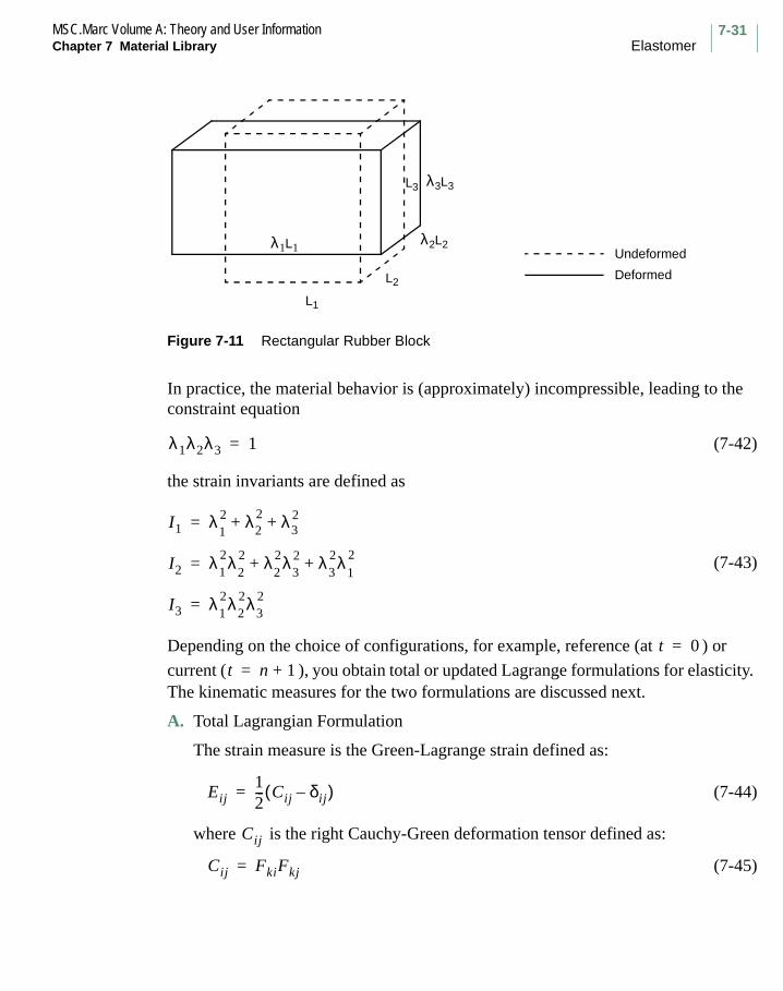
7-31MSC.Marc Volume A: Theory and User InformationChapter 7 Material Library Elastomer
Figure 7-11 Rectangular Rubber Block
In practice, the material behavior is (approximately) incompressible, leading to the constraint equation
(7-42)
the strain invariants are defined as
(7-43)
Depending on the choice of configurations, for example, reference (at ) or
current ( ), you obtain total or updated Lagrange formulations for elasticity. The kinematic measures for the two formulations are discussed next.
A. Total Lagrangian Formulation
The strain measure is the Green-Lagrange strain defined as:
(7-44)
where is the right Cauchy-Green deformation tensor defined as:
(7-45)
L3
λ2L2
L2
L1
λ1L1 Undeformed
Deformed
λ3L3
λ1λ2λ3 1=
I1 λ12 λ2
2 λ32+ +=
I2 λ12λ
22 λ
22λ
32 λ
32λ
12
+ +=
I3 λ12λ
22λ
32=
t 0=
t n 1+=
Eij12--- Cij δij–( )=
Cij
Cij FkiFkj=

MSC.Marc Volume A: Theory and User InformationElastomer Chapter 7 Material Library
7-32
in which is the deformation gradient (a two-point tensor) written as:
(7-46)
The Jacobian is defined as:
(7-47)
Thus, the invariants can be written as:
(7-48)
in which is the permutation tensor. Also, using spectral decomposition theorem,
(7-49)
in which the stretches are the eigenvalues of the right Cauchy-Green
deformation tensor, and the eigenvectors are .
B. Updated Lagrange Formulation
The strain measure is the true or logarithmic measure defined as:
(7-50)
where the left Cauchy-Green or finger tensor is defined as:
(7-51)
Thus, using the spectral decomposition theorem, the true strains are written as:
(7-52)
Fkj
Fkj
∂xk
∂Xj--------=
J
J λ1λ2λ3 det Cij( )12---
= =
I1 Cii=
I2
CijCij Cii( )2–( )2
---------------------------------------=
I316--- eijkepqrCipCjqCkr det Cij( )= =
(implied sum on i)
eijk
Cij λA2
NiA
NjA
=
λA2
Cij NiA
εij12--- ln bij=
bij
bij FikFjk=
εij12--- λAln( )ni
A njA=

7-33MSC.Marc Volume A: Theory and User InformationChapter 7 Material Library Elastomer
where is the eigenvectors in the current configuration. It is noted that the
true strains can also be approximated using first Padé approximation, which is a rational expansion of the tensor, as:
(7-53)
where a polar decomposition of the deformation gradient is done into the left stretch tensor and rotation tensor as:
The Jacobian is defined as:
(7-54)
and the invariants are now defined as:
(7-55)
It is noted that either Equation 7-48 or Equation 7-55 gives the same strain energy since it is scalar and invariant. Also, to account for the incompressibility condition, in both formulations, the strain energy is split into deviatoric and volumertic parts as:
(7-56)
Thus, the generalized Mooney-Rivlin (gmr) and the Ogden models for nearly-incompressible elastomeric materials are written as:
(7-57)
where and are the first and second deviatoric invariants.
A particular form of the generalized Mooney-Rivlin model, namely the third order deformation (tod) model, is implemented in Marc.
niA
εij 2 Vij δij–( ) Vij δij+( ) 1–=
FijVij Rij
Fij VikRkj=
J
J λ1λ2λ3 det bij( )12---
= =
I1 bii=
I212--- bijbij bii( )2
–( )=
I316--- eijkepqrbipbjqbkr det bij( )= =and
W Wdeviatoric Wvolumetric+=
Wdeviatoricgmr
Cmn I1 3–( )m
I2 3–( )n
n 1=
N
∑m 1=
N
∑=
I1 I2

MSC.Marc Volume A: Theory and User InformationElastomer Chapter 7 Material Library
7-34
(7-58)
where
is the deviatoric third order deformation form strain
energy function,
are material constants obtained from
experimental data
Simpler and popular forms of the above strain energy function are obtained as:
(7-59)
Use the MOONEY model definition option to activate the elastomeric material option in Marc and enter the material constants .
The TEMPERATURE EFFECTS model definition option can be used to input the temperature dependency of the constants and . The user subroutine UMOONY
can be used to modify all five constants , , , , and . For
viscoelastic, the additional model definition option VISCELMOON must be included.
The form of strain energy for the Ogden model in Marc is,
(7-60)
where are the deviatoric stretch ratios while , , and are the
material constants obtained from the curve fitting of experimental data. This capability is available in Mentat.
If no bulk modulus is given, it is taken to be virtually incompressible. This model is different from the Mooney model in several respects. The Mooney material model is with respect to the invariants of the right or left Cauchy-Green strain tensor and implicitly assumes that the material is incompressible. The Ogden formulation is with
Wdevratorictod
C10 I1 3–( ) C01 I2 3–( ) C11 I1 3–( ) I2 3–( ) C20 I1 3–( )2+ + + +=
C30 I1 3–( )3
Wdeviatorictod
C10 C01 C11 C20 C30, , , ,
Wdeviatoricmr
C10 I1 3–( ) C01 I2 3–( )+= Mooney-Rivlin
Wdeviatoricnh
C10 I1 3–( )= Neo-Hookean
C10 C01 C11 C20 C30, , , ,
C10 C01
C01 C10 C11 C20 C30
Wdeviatoricogden
µk
αk------ λ1
αk λ2αk λ3
α k3–+ +( )
k 1=
N
∑=
λ iαk J
αk
3-----–
λ iαk= Cmn µk αk

7-35MSC.Marc Volume A: Theory and User InformationChapter 7 Material Library Elastomer
respect to the eigenvalues of the right or left Cauchy-Green strain, and the presence of the bulk modulus implies some compressibility. Using a two-term series results in identical behavior as the Mooney mode if:
and and and
The material data is given through the OGDEN model definition option or the user subroutine UOGDEN. For viscoelastic behavior, the additional model definition option VISCELOGDEN must be included.
In the Arruda-Boyce strain energy model, the underlying molecular structure of elastomer is represented by an eight-chain model to simulate the non-Gaussian behavior of individual chains in the network. The two parameters, and ( is
the chain density, is the Botzmann constant, is the temperature, and is the number of statistical links of length in the chain between chemical crosslinks) representing initial modules and limiting chain extensibility and are related to the molecular chain orientation thus representing the physics of network deformation.
As evident in most models describing rubber deformation, the strain energy function constructed by fitting experiment data obtained from one state of deformation to another fails to accurately describe that deformation mode. The Arruda-Boyce model ameliorates this defect and is unique since the standard tensile test data provides sufficient accuracy for multiple modes of deformation.
Figure 7-12 Eight Chain Network in Stretched Configuration
µ1 2C10= α1 2= µ2 2C01–= α2 2–=
nkΘ N n
k Θ N
λ2α0
λ3α0
λ1α0
C1
k
j
i

MSC.Marc Volume A: Theory and User InformationElastomer Chapter 7 Material Library
7-36
The model is constructed using the eight chain network as follows [Ref. 1]:
Consider a cube of dimension with an unstretched network including eight chains
of length , where the fully extended chain has an approximate length of N.
A chain vector from the center of the cube to a corner can be expressed as:
(7-61)
Using geometrical considerations, the chain vector length can be written as:
(7-62)
and
(7-63)
Using statistical mechanics considerations, the work of deformation is proportional to the entropy change on stretching the chains from the unstretched state and may be written in terms of the chain length as:
(7-64)
where is the chain density and is a constant. is an inverse Langevin function correctly accounts for the limiting chain extensibility and is defined as:
(7-65)
where Langevin is defined as:
(7-66)
α0
r0 N=
C1
α0
2------ λ1 i
α0
2------ λ2 j
α0
2------ λ3 k+ +=
rchain1
3------- N λ1
2 λ22 λ3
2+ +( )1 2⁄=
λchain
rchain
r0------------
1
3------- I1( )1 2⁄
= =
W nkΘNrchain
N------------
β nβ
βsinh--------------
ΘC–+=
n C β
β L 1–rchain
N------------
=
ℑ β( ) β 1β---–coth=

7-37MSC.Marc Volume A: Theory and User InformationChapter 7 Material Library Elastomer
With Equation 7-63 through Equation 7-66, the Arruda-Boyce model can be written
(7-67)
Also, using the notion of limiting chain extensibility, Gent [Ref. 3] proposed the following constibutive relation:
(7-68)
where
(7-69)
The constant is independent of molecular length and, hence, of degree of
crosslinking. The model is attractive due to its simplicity, but yet captures the main behavior of a network of extensible molecules over the entire range of possible strains.
The Arruda-Boyce and Gent model can be invoked by using the ARRUDBOYCE and GENT model definition options, respectively.
The volumetric part of the strain energy is for all the rubber models in Marc:
(7-70)
when is the bulk modulus.
WdevArruda-Boyce nkΘ 1
2--- I1 3–( ) 1
20N---------- I1
29–( ) 11
1050N2
------------------ I13
27–( )+ +=
19
7000N3
------------------ I14
81–( ) 519
673750N4
------------------------ I15
243–( ) ]+ +
WdevGent EIm–
6------------
Im
Im I1*–
----------------log=
I1* I1 3–=
EIm
Wvolumetric9K2
------- J
13---
1–
2
=
K

MSC.Marc Volume A: Theory and User InformationElastomer Chapter 7 Material Library
7-38
It can be noted that the particular form of volumetric strain energy is chosen such that:
(i) The constraint condition is satisfied for incompressible deformations only; for example:
(7-71)
(ii) The constraint condition does not contribute to the dilatational stiffness.
This yields the constraint function as:
(7-72)
upon substitution of Equation 7-74 in Equation 7-70 and taking the first variation of the variational principle, you obtain the pressure variable as:
(7-73)
The equation has a physical significance in that for small deformations, the pressure is linearly related to the volumetric strains by the bulk modulus .
The discontinuous or continuous damage models discussed in the models section on damage can be included with the generalized Mooney-Rivlin, Ogden, Arruda-Boyce, and Gent models to simulate Mullins effect or fatigue of elastomers when using the updated Lagrangian approach. In the total Lagrangian framework however, this is available for the Ogden model only.
The rubber foam model which is based on Ogden formulation has a strain energy form as follows:
(7-74)
f I3( )> 0 if I3 0>
0= if I3 1=
< 0 if I3 0<
f I3( ) 3 I3
16---
1–
=
p 3K J
13---
1–
=
K
Wµn
αn------ λ1
αn λ2αn λ3
αn 3–+ +( )µn
βn----- 1 J
βn–( )n 1=
N
∑+
n 1=
N
∑=

7-39MSC.Marc Volume A: Theory and User InformationChapter 7 Material Library Elastomer
where , , are material constants. The model reduces to incompressible
Ogden model when equals zero.
You can define any other invariant based models through the use of the user subroutine UENERG when using the MOONEY option in model definition for elasticity in total or updated Lagrangian framework. A principal stretch-based strain energy function can also be defined through the user subroutine UPSTRECH when using the OGDEN option in the model definition for elasticity in the updated Lagrangian framework.
Once the strain energy function is defined, the stresses and material tangent can be evaluated for the total and updated Lagrangian formulations as:
A. Total Lagrangian Formulation:
The stress measure in the total Lagrangian formulation is the symmetric second Piola-Kirchhoff stress , calculated as:
(7-75)
The material elasticity tangent is:
(7-76)
B. Updated Lagrangian Formulation:
The stress measure in the updated Lagrangian formulation is the Cauchy or true stress calculated as:
(7-77)
The spatial elasticity tangent is:
(7-78)
The material constants for the Mooney-Rivlin form can be obtained from experimental data. The Mooney-Rivlin form of the strain energy density function is
(7-79)
µn αn βn
βn
Sij
Sij∂W∂Eij--------- 2
∂W∂Cij----------= =
Dijkl∂2
W∂Eij∂Ekl--------------------- 4
∂2W
∂Cij∂Ckl---------------------= =
σij2J---
∂W∂bik---------- ∂bkj=
Lijkl4J--- ∂bim
∂2W
∂bmj∂bkn---------------------- ∂bnl=
Wdeviatoricmooney-rivlin
C10 I1 3–( ) C01 I2 3–( )+=

MSC.Marc Volume A: Theory and User InformationElastomer Chapter 7 Material Library
7-40
For the Mooney-Rivlin model, the force and deformation for a uniaxial test specimen can be related as
(7-80)
which can be written in the form:
(7-81)
where is the force of the specimen, is the original area of the specimen, and
is the uniaxial stretch ratio. This equation provides a simple way to determine the Mooney-Rivlin constants. The Mooney-Rivlin constitutive equation is applicable if
the plot of versus should yield a straight line of slope and
intercept ( ) on the vertical axis as shown in Figure 7-13.
If only the Young’s modulus is supplied, and full uniaxial data are not available then
(7-82)
is a reasonable assumption. The constants then follow from the relation:
(7-83)
The material coefficients for the models can be obtained from Mentat. This allows you to select which model is most appropriate for your data.
P 2A0 11
λ3
------– λ1C10 C01+( )=
P
2A0 λ11
λ12
------–
--------------------------------- C10
C01
λ1--------+=
P A0 λ1
P 2A0 λ11
λ12
------– ⁄ 1
λ1----- C01
C01 C10+1λ1----- 1=
E
C01 0.25C10≅
6 C10 C01+( ) E≅

7-41MSC.Marc Volume A: Theory and User InformationChapter 7 Material Library Elastomer
Figure 7-13 Plots for Various Rubbers in Simple Extension for Mooney-Rivlin Model
Updated Lagrange Formulation for Nonlinear Elasticity
The total Lagrange nonlinear elasticity models in Marc have been augmented with a formulation in an Updated Lagrange framework. Hence, Rezoning can be used for elastomeric materials based upon the current configuration. This is specially useful in large deformation analysis since typically excessive element distortion in elastomeric materials can lead to premature termination of analysis. The new formulation accommodates the generalized Mooney-Rivlin and Ogden material models preserving the same format and strain energy functions as the total Lagrange formulation. In addition, the Arruda-Boyce and the Gent models are only available in the updated Lagrange framework.
The updated Lagrangian rubber elasticity capability can be used in conjunction with both continuous as well as discontinuous damage models. Thermal, as well as viscoelastic, effects can be modeled with the current formulation. While the Mooney model can account for the temperature dependent material properties, the Ogden model does not support the temperature dependence at this time. The singularity ratio of the system is inversely proportional to the order of bulk modulus of the material due to the condensation procedure.
0.50.1
0.6 0.7 0.8 0.9 1.01/λ
B0.2
0.3
0.4
σ/2(
λ-1/
λ2 ) (
N/m
n2 )
A
CD
E
F
G

MSC.Marc Volume A: Theory and User InformationElastomer Chapter 7 Material Library
7-42
A consistent linearization has been carried out to obtain the tangent modulus. The singularity for the case of two- or three-equal stretch ratios is analytically removed by application of L’Hospital’s rule. The current framework with an exact implementation of the finite strain kinematics along with the split of strain energy to handle compressible and nearly incompressible response is eminently suitable for implementation of any nonlinear elastic as well as inelastic material models. In fact, the finite deformation plasticity model based on the multiplicative decomposition,
is implemented in the same framework.
To simulate elastomeric materials, incompressible element(s) are used for plane strain, axisymmetric, and three-dimensional problems for elasticity in total Lagrangian framework. These elements can be used with each other or in combination with other elements in the library. For plane stress, beam, plate or shell analysis, conventional elements can be used. For updated Lagrangian elasticity, both conventional elements (as well as Hermann elements) can be used for plane strain, axisymmetric, and three-dimensional problems.
F FeFθF
p=

7-43MSC.Marc Volume A: Theory and User InformationChapter 7 Material Library Time-Independent Inelastic Behavior
Time-Independent Inelastic Behavior
In uniaxial tension tests of most metals (and many other materials), the following phenomena can be observed. If the stress in the specimen is below the yield stress of the material, the material behaves elastically and the stress in the specimen is proportional to the strain. If the stress in the specimen is greater than the yield stress, the material no longer exhibits elastic behavior, and the stress-strain relationship becomes nonlinear. Figure 7-14 shows a typical uniaxial stress-strain curve. Both the elastic and inelastic regions are indicated.
Figure 7-14 Typical Uniaxial Stress-Strain Curve (Uniaxial Test)
Within the elastic region, the stress-strain relationship is unique. As illustrated in Figure 7-15, if the stress in the specimen is increased (loading) from zero (point 0) to
(point 1), and then decreased (unloading) to zero, the strain in the specimen is also
increased from zero to , and then returned to zero. The elastic strain is completely
recovered upon the release of stress in the specimen.
The loading-unloading situation in the inelastic region is different from the elastic behavior. If the specimen is loaded beyond yield to point 2, where the stress in the specimen is and the total strain is , upon release of the stress in the specimen
the elastic strain, , is completely recovered. However, the inelastic (plastic) strain,
, remains in the specimen. Figure 7-15 illustrates this relationship. Similarly, if the
Note: Stress and strain are total quantities.
Stress InelasticRegion
Elastic Region
YieldStress
Strain
σ1
ε1
σ2 ε2
ε2e
ε2p

MSC.Marc Volume A: Theory and User InformationTime-Independent Inelastic Behavior Chapter 7 Material Library
7-44
specimen is loaded to point 3 and then unloaded to zero stress state, the plastic strain
remains in the specimen. It is obvious that is not equal to . We can conclude
that in the inelastic region:
• Plastic strain permanently remains in the specimen upon removal of stress.
• The amount of plastic strain remaining in the specimen is dependent upon the stress level at which the unloading starts (path-dependent behavior).
The uniaxial stress-strain curve is usually plotted for total quantities (total stress versus total strain). The total stress-strain curve shown in Figure 7-14 can be replotted as a total stress versus plastic strain curve, as shown in Figure 7-16. The slope of the total stress versus plastic strain curve is defined as the workhardening slope (H) of the material. The workhardening slope is a function of plastic strain.
Figure 7-15 Schematic of Simple Loading - Unloading (Uniaxial Test)
ε3p ε
2p ε
3p
Stress
Total Strain = Strain and Elastic Strain
Yield Stress
Strain
∆ε3p
ε2 ε2p ε2
e+=
ε3 ε3p ε3
e+=
σy
σ3
σ2
σ1
ε3ε2ε1
ε3p ε
3e
ε2eε
2p
0
1
2
3

7-45MSC.Marc Volume A: Theory and User InformationChapter 7 Material Library Time-Independent Inelastic Behavior
Figure 7-16 Definition of Workhardening Slope (Uniaxial Test)
The stress-strain curve shown in Figure 7-14 is directly plotted from experimental data. It can be simplified for the purpose of numerical modeling. A few simplifications are shown in Figure 7-17 and are listed below:
1. Bilinear representation – constant workhardening slope
2. Elastic perfectly-plastic material – no workhardening
3. Perfectly-plastic material – no workhardening and no elastic response
4. Piecewise linear representation – multiple constant workhardening slopes
5. Strain-softening material – negative workhardening slope
In addition to elastic material constants (Young’s modulus and Poisson’s ratio), it is essential to include yield stress and workhardening slopes when dealing with inelastic (plastic) material behavior. These quantities can vary with parameters such as temperature and strain rate. Since the yield stress is generally measured from uniaxial tests, and the stresses in real structures are usually multiaxial, the yield condition of a multiaxial stress state must be considered. The conditions of subsequent yield (workhardening rules) must also be studied.
Plastic Strain
H = tan θ (Workhardening Slope)
= dσ/dεp
θ
εp
σTotal Stress

MSC.Marc Volume A: Theory and User InformationTime-Independent Inelastic Behavior Chapter 7 Material Library
7-46
Figure 7-17 Simplified Stress-Strain Curves (Uniaxial Test)
Yield Conditions
The yield stress of a material is a measured stress level that separates the elastic and inelastic behavior of the material. The magnitude of the yield stress is generally obtained from a uniaxial test. However, the stresses in a structure are usually multiaxial. A measurement of yielding for the multiaxial state of stress is called the yield condition. Depending on how the multiaxial state of stress is represented, there can be many forms of yield conditions. For example, the yield condition can be dependent on all stress components, on shear components only, or on hydrostatic stress. A number of yield conditions are available in Marc, and are discussed in this section.
von Mises Yield Condition
Although many forms of yield conditions are available, the von Mises criterion is the most widely used. The success of the von Mises criterion is due to the continuous nature of the function that defines this criterion and its agreement with observed behavior for the commonly encountered ductile materials. The von Mises criterion
σ
ε(1) Bilinear Representation
σ
ε(3) Perfectly Plastic
σ
ε(5) Strain Softening
σ
ε(2) Elastic-Perfectly Plastic
σ
ε(4) Piecewise Linear Representation

7-47MSC.Marc Volume A: Theory and User InformationChapter 7 Material Library Time-Independent Inelastic Behavior
states that yield occurs when the effective (or equivalent) stress (σ) equals the yield stress (σy) as measured in a uniaxial test. Figure 7-18 shows the von Mises yield surface in two-dimensional and three-dimensional stress space.
Figure 7-18 von Mises Yield Surface
1. For an isotropic material
(7-84)
where σ1, σ2, and σ3 are the principal Cauchy stresses.
σ can also be expressed in terms of nonprincipal Cauchy stresses.
(7-85)
The yield condition can also be expressed in terms of the deviatoric stresses as:
(7-86)
where is the deviatoric Cauchy stress expressed as
(7-87)
For isotropic material, the von Mises yield condition is the default condition in Marc. The initial yield stress is defined in the ISOTROPIC and ORTHOTROPIC options. A user-defined finite strain, isotropic plasticity material model can be implemented through the user subroutine UFINITE.
YieldSurface
ElasticRegion
(b) π-Plane
YieldSurface
ElasticRegion
(a) Two-dimensional Stress Space
σ′3
σ′2σ′1
σ1
σ2
σ σ1 σ2–( )2 σ2 σ3–( )2 σ3 σ1–( )2+ +[ ] 1 2⁄ 2⁄=
σ σx σy–( )2 σy σz–( )2 σz σx–( )2 6 τxy2 τyz
2 τzx2+ +( )+ + +[ ] 1 2⁄=( ) 2⁄
σ 32---σ′
ijσ′
ij=
σ′ij
σ′ij
σij13---σkkδij–=
σy
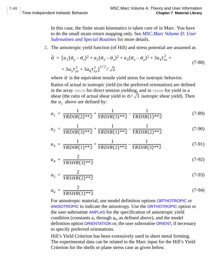
MSC.Marc Volume A: Theory and User InformationTime-Independent Inelastic Behavior Chapter 7 Material Library
7-48
In this case, the finite strain kinematics is taken care of in Marc. You have to do the small strain return mapping only. See MSC.Marc Volume D: User Subroutines and Special Routines for more details.
2. The anisotropic yield function (of Hill) and stress potential are assumed as
(7-88)
where is the equivalent tensile yield stress for isotropic behavior.
Ratios of actual to isotropic yield (in the preferred orientation) are defined in the array YRDIR for direct tension yielding, and in YRSHR for yield in a shear (the ratio of actual shear yield to isotropic shear yield). Then the above are defined by:
(7-89)
(7-90)
(7-91)
(7-92)
(7-93)
(7-94)
For anisotropic material, use model definition options ORTHOTROPIC or ANISOTROPIC to indicate the anisotropy. Use the ORTHOTROPIC option or the user subroutine ANPLAS for the specification of anisotropic yield condition (constants a1 through a6, as defined above), and the model definition option ORIENTATION or, the user subroutine ORIENT, if necessary to specify preferred orientations.
Hill’s Yield Criterion has been extensively used in sheet metal forming. The experimental data can be related to the Marc input for the Hill’s Yield Criterion for the shells or plane stress case as given below.
σ a[ 1 σy σz–( )2 a2 σz σx–( )2 a3 σx σy–( )2 3a4τzx2+ + + +=
3a5τyz2 3a6τxy
2 ]1 2⁄2⁄+ +
σ
σ 3⁄a1
a11
YRDIR 2( )**2------------------------------------
1YRDIR 3( )**2------------------------------------
1YRDIR 1( )**2------------------------------------–+=
a21
YRDIR 3( )**2------------------------------------
1YRDIR 1( )**2------------------------------------
1YRDIR 2( )**2------------------------------------–+=
a31
YRDIR 1( )**2------------------------------------
1YRDIR 2( )**2------------------------------------
1YRDIR 3( )**2------------------------------------–+=
a42
YRSHR 3( )**2-------------------------------------=
a52
YRSHR 2( )**2-------------------------------------=
a62
YRSHR 1( )**2-------------------------------------=

7-49MSC.Marc Volume A: Theory and User InformationChapter 7 Material Library Time-Independent Inelastic Behavior
7Material Library
Time-Independent Inelastic Behavior
Figure 7-19 Axes of Anisotropy
The sample of tensile coupon cut from a sheet in the three directions, (rolling), 45° and 90° (transverse) is tested to obtain
, respectively. Similarly, the anisotropy parameter defined as:
(7-95)
is obtained for the 0°, 45°, and 90° directions. The yield stress in the third (thickness) direction can be written as:
(7-96)
The direct stress coefficients are now:
(7-97)
(7-98)
(7-99)
where in the average of all directions. Similarly, the shear coefficients can be evaluated at:
N (Thickness Direction)R (Rolling Direction)
T (Transverse Direction)
θ
θ 0=σ σ0, σ45, and σ90=
rεwidth
εthickness-------------------=
σN σ0
r90 1 r0+( )r0 r90+
-------------------------- σ90
r0 1 r90+( )r0 r90+
--------------------------= =
YRDIR 1( )σ0
σav--------=
YRDIR 2( )σ90
σav--------=
YRDIR 3( )σN
σav--------=
σav σ

MSC.Marc Volume A: Theory and User InformationTime-Independent Inelastic Behavior Chapter 7 Material Library
7-50
(7-100)
(7-101)
It is noted that the transverse direction is usually considered isotropic which is reasonable on physical grounds. Also, notice that for complete isotropy, and , which yields the von Mises yield criterion.
Mohr-Coulomb Material (Hydrostatic Stress Dependence)
Marc includes options for elastic-plastic behavior based on a yield surface that exhibits hydrostatic stress dependence. Such behavior is observed in a wide class of soil and rock-like materials. These materials are generally classified as Mohr-Coulomb materials (generalized von Mises materials). Ice is also thought to be a Mohr-Coulomb material. The generalized Mohr-Coulomb model developed by Drucker and Prager is implemented in Marc. There are two types of Mohr-Coulomb materials: linear and parabolic. Each is discussed on the following pages.
Linear Mohr-Coulomb Material
The deviatoric yield function, as shown in Figure 7-20, is assumed to be a linear function of the hydrostatic stress.
(7-102)
where
(7-103)
(7-104)
Analysis of linear Mohr-Coulomb material based on the constitutive description above is available in Marc through the ISOTROPIC model definition option. Through the ISOTROPIC option, the values of and are entered. Note that, throughout the program, the convention that the tensile direct stress is positive is maintained, contrary to its use in many soil mechanics texts.
YRSHR 1( ) YRDIR 3( ) 32r45 1+-------------------=
YRSHR 2( ) YRSHR 3( ) 1.0= =
σ0 σ45 σ90 σ= = = YRDIR 3( ) 1=
f αJ1 J21 2⁄ σ
3-------–+ 0= =
J1 σii=
J212---σ′
ijσ′
ij=
σ α

7-51MSC.Marc Volume A: Theory and User InformationChapter 7 Material Library Time-Independent Inelastic Behavior
The constants and can be related to and by
(7-105)
where is the cohesion and is the angle of friction.
Figure 7-20 Yield Envelope of Plane Strain (Linear Mohr-Coulomb Material)
Parabolic Mohr-Coulomb Material
The hydrostatic dependence is generalized to give a yield envelope which is parabolic in the case of plane strain (see Figure 7-21).
(7-106)
The parabolic yield surface is obtained in Marc through the ISOTROPIC model definition option. Enter the values and through the model definition option ISOTROPIC.
(7-107)
where is the cohesion.
α σ c φ
cσ
3 1 12α2–( )[ ] 1 2⁄------------------------------------------ 3α
1 3α2–( )1 2⁄-------------------------------; φsin= =
c φ
Yield Envelope
c
σφ
R
σx + σy2
τ
f 3J2 3βσJ1+( )1 2⁄ σ– 0= =
σ β
β α3 3c2 α2–( )( )1 2⁄-----------------------------------------=σ2
3 c2 α2
3------–
=
c
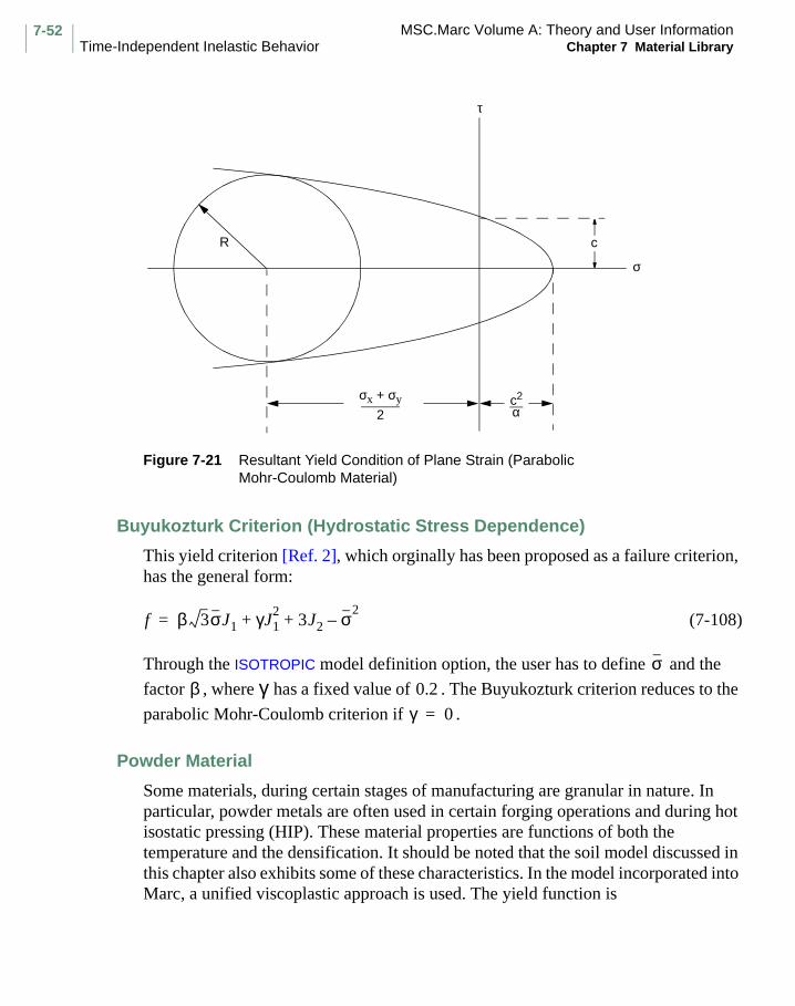
MSC.Marc Volume A: Theory and User InformationTime-Independent Inelastic Behavior Chapter 7 Material Library
7-52
Figure 7-21 Resultant Yield Condition of Plane Strain (Parabolic Mohr-Coulomb Material)
Buyukozturk Criterion (Hydrostatic Stress Dependence)
This yield criterion [Ref. 2], which orginally has been proposed as a failure criterion, has the general form:
(7-108)
Through the ISOTROPIC model definition option, the user has to define and the
factor , where has a fixed value of . The Buyukozturk criterion reduces to the
parabolic Mohr-Coulomb criterion if .
Powder Material
Some materials, during certain stages of manufacturing are granular in nature. In particular, powder metals are often used in certain forging operations and during hot isostatic pressing (HIP). These material properties are functions of both the temperature and the densification. It should be noted that the soil model discussed in this chapter also exhibits some of these characteristics. In the model incorporated into Marc, a unified viscoplastic approach is used. The yield function is
c2
c
σ
R
σx + σy2 α
τ
f β 3σJ1 γJ12
3J2 σ2–+ +=
σβ γ 0.2
γ 0=

7-53MSC.Marc Volume A: Theory and User InformationChapter 7 Material Library Time-Independent Inelastic Behavior
(7-109)
where is the uniaxial yield stress, is the deviatoric stress tensor, and is the
hydrostatic pressure. , are material parameters.
can be a function of temperature and relative density, , are functions only of
relative density.
Typically, we allow:
(7-110)
where is the relative density.
As the powder becomes more dense, approaches 1 and the classical von Mises model is recovered.
It should be noted that the elastic properties are also functions of relative density. In particular, as the material becomes fully dense, the Poisson’s ratio approaches 0.5.
As most processes involving powder materials are both pressure and thermally driven, it can be necessary to perform a coupled analysis. Marc also allows you to specify density effects for the thermal properties, conductivity and specific heat. The basic input data is entered through the POWDER option. In addition to the TEMPERATURE EFFECTS option, there is a DENSITY EFFECTS option. The initial relative density is entered through the RELATIVE DENSITY option.
Note that this material can undergo both large shear and volumetric strains. The LARGE DISP, UPDATE, and FINITE parameters should also be used. In HIP processes, the can would typically be modeled using a conventional elastic plastic material law. Additionally, the FOLLOW FOR parameter would be used to ensure that the pressure remain normal to the deformed material.
F1γ---
32---σ′
ijσ′
ijp2
β2-----+
1 2⁄σy–=
σy σ′ij
p
γ β
σy γ β
β q1 q2+ ρq3( )q4=
γ b1 b2ρb3+( )b4=
ρ
ρ

MSC.Marc Volume A: Theory and User InformationTime-Independent Inelastic Behavior Chapter 7 Material Library
7-54
The necessary experiments required for determination of the constants for the Shima Model are as follows:
1. To determine the parameter , a uniaxial compression test is performed:
(7-111)
By measuring the incremental strain during a period of time, can be obtained
(7-112)
2. The second parameter, , can be obtained by performing a triaxial (uniform) compression test:
(7-113)
By neglecting the elastic strains, you obtain:
(7-114)
or
(7-115)
For thermo-mechanically coupled problems, the temperature dependent functions are obtained by repeating the above test procedures at different temperatures.
Figure 7-22 Yield Function of Shima Model
p
σ11 p, σ22 σ33, σij 0 as i j≠= = =
β
β 23---
dε11p
dε22p
–
dεiip
---------------------------- +0.5
=
γ
σ11 σ22 σ33 σeq→ pγβ------= = =
dεii 0 σy→ pγβ------= =
γ pσyβ---------=
σ′ :σ′23---γ2σy
2-----------------
p2
β2γ2
σ y2
--------
--------
-

7-55MSC.Marc Volume A: Theory and User InformationChapter 7 Material Library Time-Independent Inelastic Behavior
Oak Ridge National Laboratory Options
In Marc, the ORNL options are based on the definitions of ORNL-TM- 3602 [1] for stainless steels and ORNL recommendations [2] for 2 1/4 Cr-1 Mo steel.
The initial yield stress should be used for the initial inelastic loading calculations for both the stainless steels and 2 1/4 Cr-1 Mo steel. The 10th-cycle yield stress should be used for the hardened material. The 100th-cycle yield stress must be used in the following circumstances:
1. To accommodate cyclic softening of 2 1/4 Cr-1 Mo steel after many load cycles
2. After a long period of high temperature exposure
3. After the occurrence of creep strain
To enter initial and 10th-cycle yield stresses, use the model definition option ISOTROPIC or ORTHOTROPIC.
Effects of Temperature and Strain Rates on Yield Stress
This section describes Marc capabilities with respect to the effect of temperature and strain rate.
Marc allows you to input a temperature-dependent yield stress. To enter the yield stress at a reference temperature, use the model definition options ISOTROPIC or ORTHOTROPIC. To enter variations of yield stress with temperatures, use the model definition options TEMPERATURE EFFECTS and ORTHO TEMP. Repeat the model definition options TEMPERATURE EFFECTS and ORTHO TEMP for each material, as necessary. The effect of temperatures on yielding is discussed further in Constitutive Relations on page 62.
Marc allows you to enter a strain rate dependent yield stress, for use in dynamic and flow (for example, extrusion) problems. To use the strain rate dependent yield stress in static analysis, enter a fictitious time using the TIME STEP option. The zero-strain-rate yield stress is given on the ISOTROPIC or ORTHOTROPIC options. Repeat the model definition option STRAIN RATE for each different material where strain rate data are necessary. Refer to Constitutive Relations on page 62 for more information on the strain-rate effect on yielding.
Workhardening Rules
In a uniaxial test, the workhardening slope is defined as the slope of the stress-plastic strain curve. The workhardening slope relates the incremental stress to incremental plastic strain in the inelastic region and dictates the conditions of subsequent yielding. A number of workhardening rules (isotropic, kinematic, and combined) are available

MSC.Marc Volume A: Theory and User InformationTime-Independent Inelastic Behavior Chapter 7 Material Library
7-56
in Marc. A description of these workhardening rules is given below. The uniaxial stress-plastic strain curve can be represented by a piecewise linear function through the WORK HARD option. As an alternative, you can specify workhardening through the user subroutine WKSLP.
There are two methods to enter this information, using the WORK HARD option. In the first method, you must enter workhardening slopes for uniaxial stress data as a change in stress per unit of plastic strain (see Figure 7-23) and the plastic strain at which these slopes become effective (breakpoint).
Figure 7-23 Workhardening Slopes
and so on.
Note: The slopes of the workhardening curves should be based on a plot of the stress versus plastic strain for a tensile test. The elastic strain components of the stress-strain curve should not be included. The first breakpoint of the workhardening curve should be 0.0.
E E E E
Strain
Stress
∆ε1p
σ
∆σ3∆σ2
∆σ1
∆ε2p ∆ε
3p
∆σ1
∆ε1p
----------
∆σ2
∆ε2p
----------
∆σ3
∆εp----------
0.0
∆ε1p
∆ε1p ∆ε
2p+
Slope Breakpoint

7-57MSC.Marc Volume A: Theory and User InformationChapter 7 Material Library Time-Independent Inelastic Behavior
In the second method, you enter a table of yield stress, plastic strain points. This option is flagged by adding the word DATA to the work hard statement.
Note: The data points should be based on a plot of the stress versus plastic strain for a tensile test. The elastic strain components should not be included. The first plastic strain should equal 0.0 and the first stress should agree with that given as the yield stress in the ISOTROPIC or ORTHOTROPIC options.
The yield stress and the workhardening data must be compatible with the procedure used in the analysis. For small strain analyses, the engineering stress and engineering strain are appropriate. If only the LARGE DISP parameter is used, the yield stress should be entered as the second Piola-Kirchhoff stress, and the workhard data be given with respect to plastic Green-Lagrange strains. If the LARGE DISP, UPDATE, FINITE parameters or PLASTICITY 3, 4, or 5 are used, the yield stress must be defined as a true or Cauchy stress, and the workhardening data with respect to logarithmic plastic strains.
Isotropic Hardening
The isotropic workhardening rule assumes that the center of the yield surface remains stationary in the stress space, but that the size (radius) of the yield surface expands, due to workhardening. The change of the von Mises yield surface is plotted in Figure 7-24b.
A review of the load path of a uniaxial test that involves both the loading and unloading of a specimen will assist in describing the isotropic workhardening rule. The specimen is first loaded from stress free (point 0) to initial yield at point 1, as shown in Figure 7-24a. It is then continuously loaded to point 2. Then, unloading from 2 to 3 following the elastic slope E (Young’s modulus) and then elastic reloading from 3 to 2 takes place. Finally, the specimen is plastically loaded again from 2 to 4 and elastically unloaded from 4 to 5. Reverse plastic loading occurs between 5 and 6.
It is obvious that the stress at 1 is equal to the initial yield stress and stresses at
points 2 and 4 are larger than , due to workhardening. During unloading, the stress
state can remain elastic (for example, point 3), or it can reach a subsequent (reversed) yield point (for example, point 5). The isotropic workhardening rule states that the reverse yield occurs at current stress level in the reversed direction. Let be the
stress level at point 4. Then, the reverse yield can only take place at a stress level of (point 5).
The isotropic workhardening model (with a work slope of 0) is the default option in Marc. To explicitly specify the isotropic hardening option in Marc, use the model definition options ISOTROPIC or ORTHOTROPIC. To input workhardening slope data, use the WORK HARD option or WKSLP user subroutine.
σy
σy
σ4
σ4–

MSC.Marc Volume A: Theory and User InformationTime-Independent Inelastic Behavior Chapter 7 Material Library
7-58
For many materials, the isotropic workhardening model is inaccurate if unloading occurs (as in cyclic loading problems). For these problems, the kinematic hardening model or the combined hardening model represents the material better.
Figure 7-24 Schematic of Isotropic Hardening Rule (Uniaxial Test)
6
5
12
65
4
3
2 1
0
E
E
E
+σ4
σ
σy
−σ4
4
30
(a) Loading Path
(b) von Mises Yield Surface
σ′3
σ′2σ′1

7-59MSC.Marc Volume A: Theory and User InformationChapter 7 Material Library Time-Independent Inelastic Behavior
Kinematic Hardening
Under the kinematic hardening rule, the von Mises yield surface does not change in size or shape, but the center of the yield surface can move in stress space. Figure 7-25b illustrates this condition. Ziegler’s law is used to define the translation of the yield surface in the stress space.
The loading path of a uniaxial test is shown in Figure 7-25a. The specimen is loaded in the following order: from stress free (point 0) to initial yield (point 1), 2 (loading), 3 (unloading), 2 (reloading), 4 (loading), 5 and 6 (unloading). As in isotropic hardening, stress at 1 is equal to the initial yield stress , and stresses at 2 and 4 are
higher than , due to workhardening. Point 3 is elastic, and reverse yield takes place
at point 5. Under the kinematic hardening rule, the reverse yield occurs at the level of , rather than at the stress level of . Similarly, if the specimen is
loaded to a higher stress level (point 7), and then unloaded to the subsequent yield
point 8, the stress at point 8 is . If the specimen is unloaded from a
(tensile) stress state (such as point 4 and 7), the reverse yield can occur at a stress state in either the reverse (point 5) or the same (point 8) direction.
To invoke the kinematic hardening in Marc, use the model definition options ISOTROPIC or ORTHOTROPIC. To input workhardening slope data, use the WORK HARD option or WKSLP user subroutine.
For many materials, the kinematic hardening model gives a better representation of loading/unloading behavior than the isotropic hardening model. For cyclic loading, however, the kinematic hardening model can represent neither cyclic hardening nor cyclic softening.
Combined Hardening
Figure 7-26 shows a material with highly nonlinear hardening. Here, the initial hardening is assumed to be almost entirely isotropic, but after some plastic straining, the elastic range attains an essentially constant value (that is, pure kinematic hardening). The basic assumption of the combined hardening model is that such behavior is reasonably approximated by a classical constant kinematic hardening constraint, with the superposition of initial isotropic hardening. The isotropic hardening rate eventually decays to zero as a function of the equivalent plastic strain measured by
(7-116)
σy
σy
σ5 σ4 2σy–( )= σ4–
σ7
σ8 σ7 2σy–( )=
εp ε· p
dt∫ 23---ε· ij
pε· ij
p
1 2⁄
dt∫= =

MSC.Marc Volume A: Theory and User InformationTime-Independent Inelastic Behavior Chapter 7 Material Library
7-60
This implies a constant shift of the center of the elastic domain, with a growth of elastic domain around this center until pure kinematic hardening is attained. In this model, there is a variable proportion between the isotropic and kinematic
contributions that depends on the extent of plastic deformation (as measured by ).
Figure 7-25 Schematic of Kinematic Hardening Rule (Uniaxial Test)
εp
(b) von Mises Yield Surface
12
3
4
56
7
8
0
σy
2σy
(a) Loading Path
σ4
σ7
σ8
σ5
σ
2σy
σ′3
σ′2σ′
1
ε

7-61MSC.Marc Volume A: Theory and User InformationChapter 7 Material Library Time-Independent Inelastic Behavior
Figure 7-26 Basic Uniaxial Tension Behavior of the Combined Hardening Model
Use the model definition options ISOTROPIC or ORTHOTROPIC to activate the combined workhardening option in Marc. Use the WORK HARD option or WKSLP user subroutine to input workhardening slope data.
The workhardening data at small strains governs the isotropic behavior, and the data at large strains governs the kinematic hardening behavior. If the last workhardening slope is zero, the behavior is the same as the isotropic hardening model.
Flow Rule
Yield stress and workhardening rules are two experimentally related phenomena that characterize plastic material behavior. The flow rule is also essential in establishing the incremental stress-strain relations for plastic material. The flow rule describes the
differential changes in the plastic strain components as a function of the current stress state.
Fully HardenedPure KinematicRange
CombinedHardeningRange
InitialElasticRange
InitialYield
One-half CurrentElastic Range
σ
ε
32
dαdεpKinematic Slope,
Stress
Strain
dεp
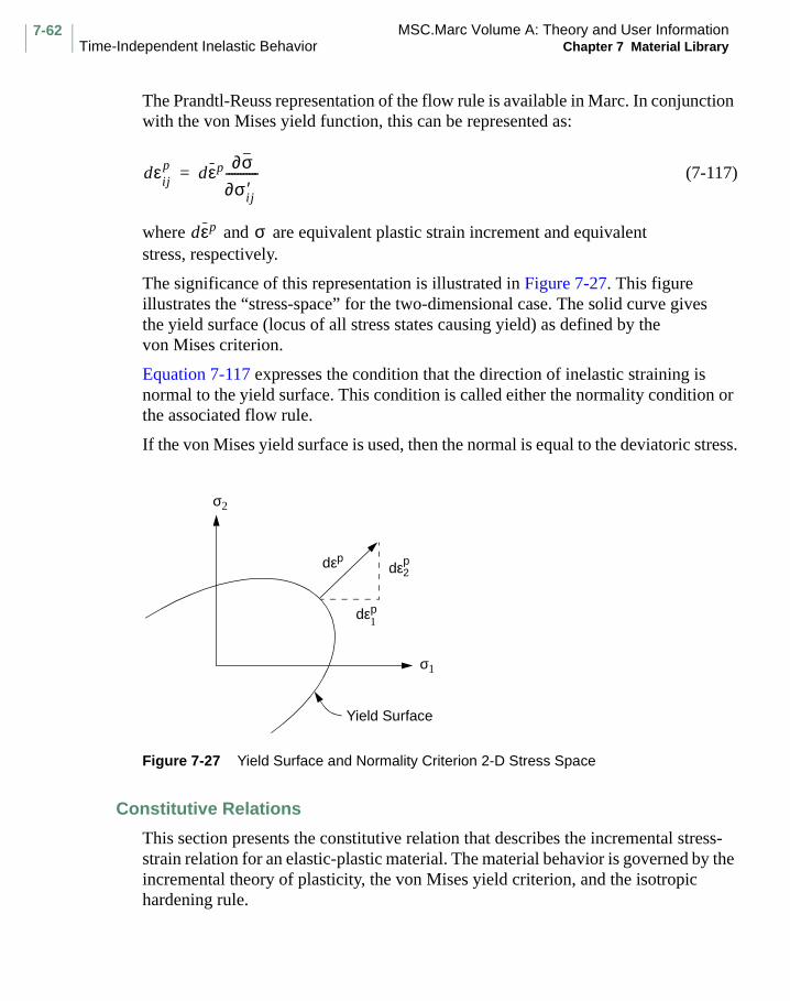
MSC.Marc Volume A: Theory and User InformationTime-Independent Inelastic Behavior Chapter 7 Material Library
7-62
The Prandtl-Reuss representation of the flow rule is available in Marc. In conjunction with the von Mises yield function, this can be represented as:
(7-117)
where and are equivalent plastic strain increment and equivalent stress, respectively.
The significance of this representation is illustrated in Figure 7-27. This figure illustrates the “stress-space” for the two-dimensional case. The solid curve gives the yield surface (locus of all stress states causing yield) as defined by the von Mises criterion.
Equation 7-117 expresses the condition that the direction of inelastic straining is normal to the yield surface. This condition is called either the normality condition or the associated flow rule.
If the von Mises yield surface is used, then the normal is equal to the deviatoric stress.
Figure 7-27 Yield Surface and Normality Criterion 2-D Stress Space
Constitutive Relations
This section presents the constitutive relation that describes the incremental stress-strain relation for an elastic-plastic material. The material behavior is governed by the incremental theory of plasticity, the von Mises yield criterion, and the isotropic hardening rule.
dεijp dεp ∂σ
∂σij′
-----------=
dεp σ
Yield Surface
σ2
dε2dεp
dεp1
σ1
p

7-63MSC.Marc Volume A: Theory and User InformationChapter 7 Material Library Time-Independent Inelastic Behavior
Let the workhardening coefficient be expressed as
(7-118)
and the flow rule be expressed as
(7-119)
Consider the differential form of the familiar stress-strain law, with the plastic strains interpreted as initial strains
(7-120)
where is the elasticity matrix defined by Hooke’s law.
After substitution of Equation 7-119, this becomes
(7-121)
Contracting Equation 7-121 by
(7-122)
and recognizing that
(7-123)
with use of Equation 7-118 in place of the left-hand side,
(7-124)
H
H dσ dεp⁄=
dεpdεp dσ
dσ------
=
dσ C : dε C : dεp–=
C
dσ C : dε C : ∂σ∂σ------dεp–=
∂σ∂σ------
∂σ∂σ------
: dσ ∂σ∂σ------
: C : dε ∂σ∂σ------
: C : ∂σ∂σ------
dεp–=
dσ ∂σ∂σ------ : dσ=
Hdεp ∂σ∂σ------
: C : dε ∂σ∂σ------
: C : ∂σ∂σ------
dεp–=
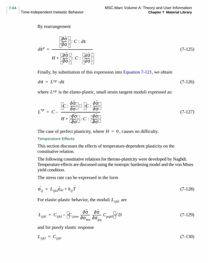
MSC.Marc Volume A: Theory and User InformationTime-Independent Inelastic Behavior Chapter 7 Material Library
7-64
By rearrangement
(7-125)
Finally, by substitution of this expression into Equation 7-121, we obtain
(7-126)
where is the elasto-plastic, small strain tangent moduli expressed as:
(7-127)
The case of perfect plasticity, where , causes no difficulty.
Temperature Effects
This section discusses the effects of temperature-dependent plasticity on the constitutive relation.
The following constitutive relations for thermo-plasticity were developed by Naghdi. Temperature effects are discussed using the isotropic hardening model and the von Mises yield condition.
The stress rate can be expressed in the form
(7-128)
For elastic-plastic behavior, the moduli are
(7-129)
and for purely elastic response
(7-130)
dεp
∂σ∂σ------
: C : dε
H∂σ∂σ------
: C : dσdσ------
+
-----------------------------------------------------=
dσ Lep :dε=
Lep
Lep
C C :
∂σ∂σ------
C : ∂σ∂σ------
⊗
H∂σ∂σ------
: C : ∂σ∂σ------
+
---------------------------------------------------–=
H 0=
σij·
Lijklε·
kl hijT·
+=
Lijkl
Lijkl Cijkl Cijmn ∂σ
∂σmn------------
∂σ∂σpq----------- Cpqkl
D⁄–=
Lijkl Cijkl=

7-65MSC.Marc Volume A: Theory and User InformationChapter 7 Material Library Time-Independent Inelastic Behavior
The term that relates the stress increment to the increment of temperature for elastic-plastic behavior is
(7-131)
and for purely elastic response
(7-132)
where
(7-133)
and
(7-134)
and are the coefficients of thermal expansion.
Strain Rate Effects
This section discusses the influence of strain rate on the elastic-plastic constitutive relation.
Strain rate effects cause the structural response of a body to change because they influence the material properties of the body. These material changes lead to an instantaneous change in the strength of the material. Strain rate effects become more pronounced for temperatures greater than half the melting temperature ( ). The
following discussion explains the effect of strain rate on the size of the yield surface.
Using the von Mises yield condition and normality rule, we obtain an expression for the stress rate of the form
(7-135)
hij Xij Cijklαkl– Cijkl∂σ
∂σkl---------- σpqXpq
23---σ∂σ
∂T------–
D⁄–=
Hij Xij Cijklαkl–=
D49--- σ2
∂σ∂εp--------
∂σ∂σij--------- Cijkl
∂σ∂σkl----------+=
Xij
∂Cijkl
∂T--------------εkl
e=
αkl
Tm
σ· ij Lijklε·
kl rijε·· p
+=

MSC.Marc Volume A: Theory and User InformationTime-Independent Inelastic Behavior Chapter 7 Material Library
7-66
For elastic-plastic response
(7-136)
and
(7-137)
where
(7-138)
Lijkl Cijkl Cijmn ∂σ
∂σmn------------
∂σ∂σpq----------- Cpqkl
D⁄–=
rij Cijmn ∂σ
∂σmn------------
23--- σ
∂σ
∂ε· p
-------- D⁄=
D49--- σ2
∂σ∂εp--------
∂σ∂σij--------- Cijkl
∂σ∂σkl----------+=

7-67MSC.Marc Volume A: Theory and User InformationChapter 7 Material Library Time-Dependent Inelastic Behavior
Time-Dependent Inelastic Behavior
Force-displacement relationships vary in different material models. A perfectly elastic material and a perfectly viscous material can be represented by a spring and a dashpot, respectively (as shown in Figure 7-28). In a perfectly elastic material, the deformation is proportional to the applied load. In a perfectly viscous material, the rate of change of the deformation over time is proportional to the load.
Figure 7-28 Perfectly Elastic (Spring) and Viscous (Dashpot) Materials
In the class of viscoelastic and creeping materials, the application of a constant load is followed by a deformation, which can be made up of an instantaneous deformation (elastic effect) followed by a continual deformation with time (viscous effect). Eventually, it can become pure viscous flow. Continued deformation under constant load is termed creep (see Figure 7-29).
A viscoelastic material can be subjected to sudden application of a constant deformation. This results in an instantaneous proportional load (elastic effect), followed by a gradual reduction of the required load with time, until a limiting value of the load is attained. The decreasing of load for a constant deformation, is termed relaxation (see Figure 7-30).
Viscoelastic and creeping materials can be represented by models consisting of both springs and dashpots because the material displays both elastic effects and viscous effects. This implies that the material either continues to flow for a given stress, or the stress decreases with time for a given strain. The measured relation between stress and strain is generally very complex.
DASHPOTSPRING
f = ku f =
f = Force f = Force
u = Displacement = Velocity (Time Rate of Change of Displacement)
k = Spring Stiffness η = Viscosity of the Dashpot
ηu·
u·

MSC.Marc Volume A: Theory and User InformationTime-Dependent Inelastic Behavior Chapter 7 Material Library
7-68
Figure 7-29 The Creep Curve
Figure 7-30 The Relaxation Curve
Two models that are commonly used to relate stress and strain are the Maxwell and Kelvin (Voigt or Kelvin-Voigt) models. A description of these models is given below.
The mathematical relation which holds for the Maxwell solid is
(7-139)
ε (Strain)
t (Time)0
A
B
C
OA – Instantaneous Elastic EffectAB – Delayed Elastic EffectBC – Viscous Flow
σ (Stress)
t (Time)0
ε· ασ·= βσ+

7-69MSC.Marc Volume A: Theory and User InformationChapter 7 Material Library Time-Dependent Inelastic Behavoir
7Material Library
Time-Dependent Inelastic Behavoir
In the one-dimensional case for normal stress
(7-140)
This relation can be depicted as a spring and dashpot in series, as shown in Figure 7-31. The integration of Equation 7-139 yields
(7-141)
Figure 7-31 Maxwell Solid
The strain and stress responses of the Maxwell Solid model are shown in Figure 7-32 and Figure 7-33, respectively.
Figure 7-32 Strain Response to Applied Constant Stress (Maxwell Solid)
α 1E---=
β 1η---=
ε σE---
ση---dt∫+=
σσ
σ
t
Constant Stress Applied
ε
t
Response to Constant Stress
σ0E

MSC.Marc Volume A: Theory and User InformationTime-Dependent Inelastic Behavoir Chapter 7 Material Library
7-70
Figure 7-33 Stress Response to Applied Constant Strain (Maxwell Solid)
The mathematical relation which holds for the Kelvin (Voigt or Kelvin-Voigt) solid is
(7-142)
This equation is depicted as a spring and dashpot in parallel. (See Figure 7-34). When (no dashpot), the system is a linearly elastic system in which , the
elastic modulus.
When (no spring), the “solid” obeys Newton’s equation for a viscous fluid and
, the viscous coefficient. Thus, we can rewrite Equation 7-142 in the form
(7-143)
In the above relation, we have considered one-dimensional normal stress and strain. The relation holds equally well for shear stress and shear strain in which ,
the shear modulus, and , the viscous coefficient. Equation 7-142 can be rewritten as
(7-144)
Figure 7-34 Kelvin (Voigt or Kelvin-Voigt) Solid
ε
t
Constant Strain Applied
ε
t
Response to Constant Strain
σ
τ
σ αε βε·+=
β 0= α E=
E 0=
β η=
σ Eε ηε·+=
τ γ α G=
β η=
τ Gγ ηγ·+=
E
σ
η
σ

7-71MSC.Marc Volume A: Theory and User InformationChapter 7 Material Library Time-Dependent Inelastic Behavoir
The strain responses of the Kelvin Solid model are depicted in Figure 7-35. For multiaxial situations, these equations can be generalized to tensor quantities.
Figure 7-35 Strain Response to Applied Stress (Kelvin Solid)
To invoke the Maxwell model, use the CREEP parameter. The creep strain can be specified as either deviatoric creep strain (conventional creep) or dilatational creep strain (swelling). To invoke the Kelvin model, also use the CREEP parameter and CRPVIS user subroutine.
(a) Stress Pulse
σ
σ0
t1t
(b) Strain Response to Stress of Infinite Domain
ε
t
t
(c) Strain Response to Stress Pulse of Finite Length
ε
t1
σ0E
t

MSC.Marc Volume A: Theory and User InformationTime-Dependent Inelastic Behavoir Chapter 7 Material Library
7-72
Creep (Maxwell Model)
Creep is an important factor in elevated-temperature stress analysis. In Marc, creep is represented by a Maxwell model. Creep is a time-dependent, inelastic behavior, and can occur at any stress level (that is, either below or above the yield stress of a material). The creep behavior can be characterized as primary, secondary, and tertiary creep, as shown in Figure 7-36. Engineering analysis is often limited to the primary and secondary creep regions. Tertiary creep in a uniaxial specimen is usually associated with geometric instabilities, such as necking. The major difference between the primary and secondary creep is that the creep strain rate is much larger in the primary creep region than it is in the secondary creep region. The creep strain rate is the slope of the creep strain-time curve. The creep strain rate is generally dependent on stress, temperature, and time.
The creep data can be specified in either an exponent form or in a piecewise linear curve. To specify creep data, use the model definition option CREEP. Subroutine CRPLAW allows alternative forms of creep behavior to be programmed directly.
(7-145)
Figure 7-36 Creep Strain Versus Time (Uniaxial Test at Constant Stress and Temperature)
ε· c dεc
dt--------=
Note: Primary Creep: Fast decrease in creep strain rate Secondary Creep: Slow decrease in creep strain rate Tertiary Creep: Fast increase in creep strain rate
SecondaryCreep
PrimaryCreep
TertiaryCreep
Creep StrainεC
Time (t)

7-73MSC.Marc Volume A: Theory and User InformationChapter 7 Material Library Time-Dependent Inelastic Behavoir
There are four possible modes of input for creep constitutive data.
1. Express the dependence of equivalent creep strain rate on any independent parameter through a piecewise linear relationship. The equivalent creep strain rate is then assumed to be a piecewise linear approximation to
(7-146)
where A is a constant; is equivalent creep strain rate; and , , , and
are equivalent stress, equivalent creep strain, temperature and time,
respectively. The functions , , , and are piecewise linear and entered in the form as either slope-break point data or function-variable data. This representation is shown in Figure 7-37. Enter functions , , , and
through the model definition option CREEP. (Any of the functions ( , , ,
or ) can be set to unity by setting the number of piecewise linear slopes for that relation to zero on the input data.)
2. The dependence of equivalent creep strain rate on any independent parameter can be given directly in power law form by the appropriate exponent. The equivalent creep strain rate is
(7-147)
Enter the constants , , , , and directly through the model definition option CREEP. This is often adequate for engineering metals at constant temperature where Norton’s rule is a good approximation.
(7-148)
3. Define the equivalent creep strain rate directly with the user subroutine CRPLAW.
4. Use the ISOTROPIC option to activate the ORNL (Oak Ridge National Laboratory rules) capability of the program.
Isotropic creep behavior is based on a von Mises creep potential described by the equivalent creep law
(7-149)
ε· c
A f σ( ) g εc( ) h T( ) dk t( )dt
------------••••=
ε· c
σ εcT
t
f g h k
f g h k
f g h
k
ε· c Aσm εc( )n
Tp qtq 1–( )•••=
A m n p q
ε· c
A= σn
ε·
f σ εc T t, , ,( )=

MSC.Marc Volume A: Theory and User InformationTime-Dependent Inelastic Behavoir Chapter 7 Material Library
7-74
Figure 7-37 Piecewise Linear Representation of Creep Data
The material creep behavior is described by
(7-150)
During creep, the creep strain rate usually decreases. This effect is called creep hardening and can be a function of time or creep strain. The following section discusses the difference between these two types of hardening.
(1) Slope-Break Point Data
Slope Break Point
S1 X1
S2 X2S3 X3
(2) Function-Variable Data
Function Variable
F1 X1F2 X2
F3 X3F4 X4
Function F (X)
[Such as t ,
g , h (T),
k (t)]
σ( )
εc( )
X1
F1
X2
F2
X3
F3
X4
F4
S1
S2
S3
Variable X (Such as σ, εC, T, t)
ε·
ijc ε
· c ∂σ∂σij---------
=

7-75MSC.Marc Volume A: Theory and User InformationChapter 7 Material Library Time-Dependent Inelastic Behavoir
Consider a simple power law that illustrates the difference between time and strain-hardening rules for the calculation of the creep strain rate.
(7-151)
where is the creep strain, and are values obtained from experiments and t is
time. The creep rate can be obtained by taking the derivative with respect to time
(7-152)
However, being greater than 0, we can compute the time as
(7-153)
Substituting Equation 7-152 into Equation 7-151 we have
(7-154)
Equation 7-152 shows that the creep strain rate is a function of time (time hardening). Equation 7-154 indicates that the creep strain rate is dependent on the creep strain (strain hardening). The creep strain rates calculated from these two hardening rules generally are different. The selection of a hardening rule in creep analysis must be based on data obtained from experimental results. Figure 7-38 and Figure 7-39 show time and strain hardening rules in a variable state of stress. It is assumed that the stress in a structure varies from to to ; depending upon the model chosen, different
creep strain rates are calculated accordingly at points 1, 2, 3, and 4. Obviously, creep strain rates obtained from the time hardening rule are quite different from those obtained by the strain hardening rule.
εc βtn=
εc β n
εc
ε·c dεc
dt-------- nβtn 1–= =
t t
tεc
β----
1 n/
=
ε·c
nβtn 1– n β1 n⁄ εc( ) n 1–( ) n⁄( )( )= =
σ1 σ2 σ3

MSC.Marc Volume A: Theory and User InformationTime-Dependent Inelastic Behavoir Chapter 7 Material Library
7-76
Figure 7-38 Time Hardening
Figure 7-39 Strain Hardening
Oak Ridge National Laboratory Laws
Oak Ridge National Laboratory (ORNL) has performed a large number of creep tests on stainless and other alloy steels. It has also set certain rules that characterize creep behavior for application in nuclear structures. A summary of the ORNL rules on creep is given below. The references listed at the end of this section offer a more detailed discussion of the ORNL rules.
εcσ1
0
1
2
3
4
t
σ2
σ3
εc
σ1
0
12
3
4
t
σ2
σ3

7-77MSC.Marc Volume A: Theory and User InformationChapter 7 Material Library Time-Dependent Inelastic Behavoir
1. Auxiliary Rules for Applying Strain-Hardening to Situations Involving Stress Reversals
The Blackburn Creep Law is required as user subroutine CRPLAW. The parameter EQCP (first parameter in CRPLAW) is defined as
(7-155)
when the ORNL constitutive option is flagged through use of the ISOTROPIC option. In all other cases, the definition
(7-156)
is retained. The equivalent primary creep strain passes into CRPLAW in EQCPNC, the second parameter. The second parameter must be redefined in that routine as the equivalent (total) creep strain increment. The first parameter (EQCP) must be redefined as the equivalent primary creep strain increment when the ORNL constitutive option is flagged. During analysis with the ORNL option, equivalent creep strain stores the distance between the two shifted origins in creep strain space ( in ORNL-TM-3602). The sign on this value indicates which origin is currently active, so that a negative sign indicates use of the “negative” origin ( ).
2. Plasticity Effect on Creep
The effect of plastic strains on creep must be accommodated for the time-dependent creep behavior of 2 1/4 Cr -1 Mo Steel. Since plastic strains in one direction reduce the prior creep strain hardening accumulated in the reverse direction, ORNL recommends that the softening influence due to plastic strains be treated much the same as when reversed creep strain occurs. The following quantities are defined:
(7-157)
(7-158)
where is instantaneous creep strain components
(7-159)
εc 23---Σ∆εij
c Σ∆εijc
1 2/
=
εc Σ 23---∆εc
ij ∆εijc
1 2/
=
ε
εij–
Nij εijI ε
ij–( ) G⁄=+ + +
Nij– ε
ijI ε
ij––( ) G–⁄=
εijI
εij
εij–; = positive and negative strain origins+

MSC.Marc Volume A: Theory and User InformationTime-Dependent Inelastic Behavoir Chapter 7 Material Library
7-78
and
(7-160)
(7-161)
Swelling
Marc allows pure swelling (dilatational creep) effect in a creep analysis. To use the swelling option, perform a regular creep analysis as discussed earlier. Use the user
subroutine VSWELL to define the increment of volumetric swelling . The
increment of volumetric swelling is generally a function of neutron flux, time, and temperatures.
For example, radiation-induced swelling strain model for 20% C. W. Stainless Steel 316 can be expressed as:
(7-162)
where , , and are functions of temperature, is neutron flux, and is time.
Viscoplasticity (Explicit Formulation)
The creep (Maxwell) model can be modified to include a plastic element (as shown in Figure 7-40). This plastic element is inactive when the stress ( ) is less than the yield
stress ( ) of the material. The modified model is an elasto-viscoplasticity model and
is capable of producing some observed effects of creep and plasticity. In addition, the viscoplastic model can be used to generate time-independent plasticity solutions when stationary conditions are reached. At the other extreme, the viscoplastic model can reproduce standard creep phenomena. The model allows the treatment of nonassociated flow rules and strain softening which present difficulties in conventional (tangent modulus) plasticity analyses.
The viscoplasticity option can be used to implement very general constitutive relations with the aid of the following user subroutines: ZERO, YIEL, NASSOC, and CRPLAW. See Nonlinear Analysis in Chapter 5 for details on how to use these procedures.
It is recommended that you use the implicit formulation described in the following paragraphs to model general viscoplastic materials.
G G εijI ε
ij–( ) 2 3⁄ ε
ijI ε
ij–( ) ε
ijI ε
ij–( )[ ] 1 2⁄= =+ + + +
G– G εijI ε
ij––( ) 2 3⁄ ε
ijI ε
ij––( ) ε
ijI ε
ij––( )[ ] 1 2⁄= =
∆VV
-------
∆VV
------- RφtRα--- ln
1 exp α τ φt–( )( )+1 expτ+
----------------------------------------------+=
R t α φ t
σσy

7-79MSC.Marc Volume A: Theory and User InformationChapter 7 Material Library Time-Dependent Inelastic Behavoir
Figure 7-40 Uniaxial Representation of Viscoplastic Material
Creep (Implicit Formulation)
This formulation, as opposed to that described in the previous section, is fully implicit. A fully implicit formulation is unconditionally stable for any choice of time step size; hence, allowing a larger time step than permissible using the explicit method. Additionally, this is more accurate than the explicit method. The disadvantage is that each increment may be more computationally expensive. This model is activated using the CREEP parameter. There are two methods for defining the inelastic strain rate. The CREEP model definition option can be used to define a Maxwell creep model. The back stress must be specified through the field reserved for the yield stress in the ISOTROPIC or ORTHOTROPIC options. There is no creep strain when the stress is less than the back stress. The equivalent creep strain increment is expressed as
and the inelastic deviatoric strain components are
where is the deviatoric stress at the end of the increment and is the back stress.
is a function of temperature, time, etc. An algorithmic tangent is used to form the stiffness matrix.
ee
evp
σ
Plastic ElementInactive if σ < σy
εp εvp=
∆ε i A σn 1+ σy–( )m∆t=
∆εiji 3
2---∆εiσ′ ij
σ--------=
σ′ij σy
A

MSC.Marc Volume A: Theory and User InformationTime-Dependent Inelastic Behavoir Chapter 7 Material Library
7-80
To allow for the implementation of general unified creep-plasticity or viscoplastic models, user subroutine UVSCPL is available. This routine requires you to define only the inelastic strain rate. The program automatically calculates a tangent stiffness matrix. This option is activated by indicating that the material is VISCO PLAS in the ISOTROPIC or ORTHOTROPIC option.
Based on a parameter defined in the CREEP parameter, one of three tangent matrices is formed. The first is using an elastic tangent, which requires more iterations, but can be computationally efficient because re-assembly might not be required. The second is an algorithmic tangent that provides the best behavior for small strain power law creep. The third is a secant (approximate) tangent that gives the best behavior for general viscoplastic models.
Viscoelastic Material
Marc has two models that represent viscoelastic materials. The first can be defined as a Kelvin-Voigt model. The latter is a general hereditary integral approach.
Kelvin-Voigt Model
The Kelvin model allows the rate of change of the inelastic strain to be a function of the total stress and previous strain. To activate the Kelvin model in Marc, use the CREEP parameter.
The Kelvin material behavior (viscoelasticity) is modeled by assuming an additional
creep strain , governed by
(7-163)
where and are defined in the user subroutine CRPVIS and the total strain is
(7-164)
(7-165)
(7-166)
(7-167)
(7-168)
εijk
ddt-----ε
ijk Aijklσ′kl Bijklεkl
k–=
A B
εij εije ε
ijp ε
ijc ε
ijk ε
ijth+ + + +=
εijth
= thermal strain components
εije = elastic strain components (instantaneous response)
εijp
= plastic strain components
εijc
= creep strains defined via the CRPLAW and VSWELL user subroutines

7-81MSC.Marc Volume A: Theory and User InformationChapter 7 Material Library Time-Dependent Inelastic Behavoir
(7-169)
The CRPVIS user subroutine is called at each integration point of each element when the Kelvin model is used.
Use the AUTO CREEP option to define the time step and to set the tolerance control for the maximum strain in any increment.
The CREEP option allows Maxwell models to be included in series with the Kelvin model.
Hereditary Integral Model
The stress-strain equations in viscoelasticity are not only dependent on the current stress and strain state (as represented in the Kelvin model), but also on the entire history of development of these states. This constitutive behavior is most readily expressed in terms of hereditary or Duhamel integrals. These integrals are formed by considering the stress or strain build-up at successive times. Two equivalent integral forms exist: the stress relaxation form and the creep function form. In Marc, the stress relaxation form is used.
The viscoelasticity option in Marc can be used for both the small strain and large strain Mooney or Ogden material (total Lagrange formulation) stress-relaxation problems. A description of these models is as follows:
Small Strain Viscoelasticity
In the stress relaxation form, the constitutive relation can be written as a hereditary integral formulation
(7-170)
The functions are called stress relaxation functions. They represent the
response to a unit applied strain and have characteristic relaxation times associated with them. The relaxation functions for materials with a fading memory can be expressed in terms of Prony or exponential series.
(7-171)
εijk = Kelvin model strain components as defined above
σij t( ) Gijkl t τ–( )dεkl τ( )
dτ-----------------dτ
0
t
∫ Gijkl t( )εkl 0( )+=
Gijkl
Gijkl t( ) Gijkl∞ Gijkl
n exp t λn⁄–( )
n 1=
N
∑+=

MSC.Marc Volume A: Theory and User InformationTime-Dependent Inelastic Behavoir Chapter 7 Material Library
7-82
in which is a tensor of amplitudes and is a positive time constant
(relaxation time). In the current implementation, it is assumed that the time
constant is isotropic. In Equation 7-171, represents the long term
modulus of the material.
The short term moduli (describing the instantaneous elastic effect) are then given by
(7-172)
The stress can now be considered as the summation of the stresses in a generalized Maxwell model (Figure 7-41)
(7-173)
where
(7-174)
(7-175)
Figure 7-41 The Generalized Maxwell or Stress Relaxation Form
Gijkl
n λn
Gijkl∞
Gijkl0
Gijkl 0( ) Gijkl∞
Gijkln
n 1=
N
∑+= =
σij t( ) σij∞ t( ) σij
n t( )n 1=
N
∑+=
σij∞ Gijkl
∞ εkl t( )=
σijn
Gijkln
exp t τ–( ) λn
⁄–[ ]dεkl τ( )
dτ-----------------dτ
0
t
∫=
E1
η1
q1
ε
E0
τi = ηi/Ei
E2
η2
q2
Ei
ηi
qiηE

7-83MSC.Marc Volume A: Theory and User InformationChapter 7 Material Library Time-Dependent Inelastic Behavoir
For integration of the constitutive equation, the total time interval is subdivided into a number of subintervals ( ) with time-step
. A recursive relation can now be derived expressing the stress
increment in terms of the values of the internal stresses at the start of the
interval. With the assumption that the strain varies linearly during the time interval h, we obtain the increment stress-strain relation as
(7-176)
where
(7-177)
and
(7-178)
In Marc, the incremental equation for the total stress is expressed in terms of the short term moduli (See Equation 7-172).
(7-179)
In this way, the instantaneous elastic moduli can be specified through the ISOTROPIC or ORTHOTROPIC options. Moreover, since the TEMPERATURE EFFECTS option acts on the instantaneous elastic moduli, it is more straightforward to use the short term values instead of the long term ones. Note that the set of equations given by Equation 7-179 can directly be used for both anisotropic and isotropic materials.
Isotropic Viscoelastic Material
For an isotropic viscoelastic material, Marc assumes that the deviatoric and volumetric behavior are fully uncoupled and that the behavior can be described by a time dependent shear and bulk modules. The bulk moduli is generally assumed to be time independent; however, this is an unnecessary restriction of the general theory.
tm 1– tm,
h tm tm 1––=
σijn
∆σij tm( ) Gijkl
∞β
nh( )Gijkl
n
n 1=
N
∑+ ∆εkl αn h( )σijn
tm h–( )n 1=
N
∑–=
αn h( ) 1 exp h λn
⁄–( )–=
βn
h( ) αnh( )λn
h⁄=
∆σij tm( ) Gijkl0
1 βn
h( )– Gijkln
n 1=
N
∑– ∆εkl tm( ) αnh( )σij
n
n 1=
N
∑–= tm h–( )

MSC.Marc Volume A: Theory and User InformationTime-Dependent Inelastic Behavoir Chapter 7 Material Library
7-84
Both the shear and bulk moduli can be expressed in a Prony series
(7-180)
(7-181)
with short term values given by
(7-182)
(7-183)
Let the deviatoric and volumetric component matrices and be given by
(7-184)
G t( ) G∞
Gn exp t λd
n⁄–( )
n 1=
N
∑+=
K t( ) K∞
Kn exp t λv
n⁄–( )n 1=
N
∑+=
G0 G∞ Gn
n 1=
N
∑+=
K0 K∞ Kn
n 1=
N
∑+=
πd πv
πd
4 3⁄ 2 3⁄– 2 3⁄– 0 0 0
2 3⁄– 4 3⁄ 2 3⁄– 0 0 0
2 3⁄– 2 3⁄– 4 3⁄ 0 0 0
0 0 0 1 0 0
0 0 0 0 1 0
0 0 0 0 0 1
=
πv
1 1 1 0 0 0
1 1 1 0 0 0
1 1 1 0 0 0
0 0 0 0 0 0
0 0 0 0 0 0
0 0 0 0 0 0
=

7-85MSC.Marc Volume A: Theory and User InformationChapter 7 Material Library Time-Dependent Inelastic Behavoir
The increment set of equations is then given by
(7-185)
and
(7-186)
Note that the deviatoric and volumetric response are fully decoupled.
The instantaneous moduli need to be given in the ISOTROPIC option. Time
dependent values (shear moduli and time constants ; bulk moduli
and time constants ) need to be entered in the VISCELPROP option.
Time-stepping is performed using the TIME STEP, AUTO TIME, or AUTO STEP option in the history definition block.
Note that the algorithm is exact for linear variations of the strain during the increment. The algorithm is implicit; hence, for each change in time-step, a new assembly of the stiffness matrix is required.
Anisotropic Viscoelastic Material
Equation 7-179 can be used for the analysis of anisotropic viscoelastic
materials. The tensor of amplitudes must be entered through the
ORTHOTROPIC option. However, both the and the must be entered
using the VISCELORTH option.
∆σ tm( ) G0
1 βdn
h( )–[ ] Gn
n 1=
Nd
∑–
πd∆ε tm( )=
αdn h( )σd
n tm h–( )n 1=
Nd
∑ αvn h( )σv
n tm h–( )n 1=
Nv
∑––
K0 1 βvn
h( )–[ ] Kn
n 1=
Nv
∑–
πv∆ε tm( )
∆σdn
tm( ) βdn
h( )Gnπd∆ε tm( ) αdn
h( )σdn
tm h–( )–=
∆σvn
tm( ) βvn
h( )Knπv∆ε tm( ) αvn
h( )σvn
tm h–( )–=
Gn λd
nK
n
λv
n
Gijkl0
Gijkln λn

MSC.Marc Volume A: Theory and User InformationTime-Dependent Inelastic Behavoir Chapter 7 Material Library
7-86
Alternatively, a complete set of moduli (21 components) can be specified in the HOOKVI user subroutine.
The ORIENTATION option or ORIENT user subroutine can be used to define a
preferred orientation both for the short time moduli and the amplitude
functions .
Incompressible Isotropic Viscoelastic Materials
Incompressible elements in Marc allow the analysis of incompressible and nearly incompressible materials in plane strain, axisymmetric and three-dimensional problems. The incompressibility of the element is simulated through the use of an perturbed Lagrangian variational principle based on the Herrmann formulation.
The constitutive equation for a material with no time dependence in the volumetric behavior can be expressed as
(7-187)
(7-188)
The hydrostatic pressure term is used as an independent variable in the variational principle. The Herrmann pressure variable is now defined in the same way as in the formulation for time independent elastic materials.
(7-189)
The constitutive Equation 7-187 and Equation 7-188 can then be rewritten
(7-190)
Gijkl0
Gijkln
∆σij tm( ) 2 Gijkl0
1 βnh( )–[ ] Gijkl
n
n 1=
N
∑–
∆εkl tm( ) 13---∆εpp tm( )δkl–=
αnh( ) σ′ij( )n
tm( )n 1=
N
∑–13---σkkδij+
∆σpp tm( ) 3K0∆εpp tm( )=
Hσpp
2G0 1 ν0+( )------------------------------=
∆σij tm( ) 2Ge ∆εij ν∗ Hδij+( ) αn h( ) σ′ ij( )n
tm h–( )n 1=
N
∑–=

7-87MSC.Marc Volume A: Theory and User InformationChapter 7 Material Library Time-Dependent Inelastic Behavoir
where
(7-191)
(7-192)
Thermo-Rheologically Simple Behavior
The rate processes in many viscoelastic materials are known to be highly sensitive to temperature changes. Such temperature-dependent properties cannot be neglected in the presence of any appreciable temperature variation. For example, there is a large class of polymers which are adequately represented by linear viscoelastic laws at uniform temperature. These polymers exhibit an approximate translational shift of all the characteristic response functions with a change of temperature, along a logarithmic time axis. This shift occurs without a change of shape. These temperature-sensitive viscoelastic materials are characterized as Thermo-Rheologically Simple.
A “reduced” or “pseudo” time can be defined for the materials of this type and for a given temperature field. This new parameter is a function of both time and space variables. The viscoelastic law has the same form as one at constant temperature in real time. If the shifted time is used, however, the transformed viscoelastic equilibrium and compatibility equations are not equivalent to the corresponding elastic equations.
In the case where the temperature varies with time, the extended constitutive law implies a nonlinear dependence of the instantaneous stress state at each material point of the body upon the entire local temperature history. In other words, the functionals are linear in the strains but nonlinear in the temperature.
The time scale of experimental data is extended for Thermo-Rheologically Simple materials. All characteristic functions of the material must obey the same property. The shift function is a basic property of the material and must be determined experimentally. As a consequence of the shifting of the mechanical properties data parallel to the time axis (see Figure 7-42), the values of the zero and infinite frequency complex moduli do not change due to shifting. Hence, elastic materials with temperature-dependent characteristics neither belong to nor are consistent with the above hypothesis for the class of Thermo-Rheologically Simple viscoelastic solids.
Ge G0 1 βn h( )Gn–[ ]n 1=
N
∑–=
ν∗ G0
1 ν0+( ) G
e1 2ν0
–( )–
3Ge
---------------------------------------------------------------=

MSC.Marc Volume A: Theory and User InformationTime-Dependent Inelastic Behavoir Chapter 7 Material Library
7-88
Figure 7-42 Relaxation Modulus vs. Time at Different Temperatures
Let be the relaxation modulus as a function of at uniform
temperature, . Then
(7-193)
where is measured relative to some arbitrary temperature . The modulus curve shifts towards shorter times with an increase of temperature;
is a positive increasing function for . If denotes the
relaxation modulus as a function of time at uniform temperature , so that,
(7-194)
then
(7-195)
The relaxation modulus (and the other characteristic functions) at an arbitrary uniform temperature is thus expressed by the base temperature behavior related to a new time scale that depends on that temperature.
There is some mapping of the time coordinate for nonuniform, nonconstant temperature, , which depends on the position
For a nonuniform, nonconstant temperature, the shift function is and the rate of change of reduced time can be written as:
GT
T0
f(T1)
ln t
T1T2
f(T2)
E ln t( ) ln t
T
ET ln t( ) ET0ln t+f T( )[ ] * ρT ρ0T0⁄( )=
f T( ) T
f T( ) T T0> GT t( )
T
GT t( ) ET ln t( )=
GT t( ) GT0ξ( )=
T x t,( )
a T x t,( )( )
dξ aT T x t,( )[ ] dt=

7-89MSC.Marc Volume A: Theory and User InformationChapter 7 Material Library Time-Dependent Inelastic Behavior
7Material Library
Time-Dependent Inelastic Behavior
Marc offers two explicit forms for entering the shift function. The first is based on the familiar Williams-Landel-Ferry (WLF) equation. Rewriting the above expression for reduced time as
(7-196)
then the WLF form state that
(7-197)
and
(7-198)
Typically, the glassy transition point is taken as the reference temperature in the above relation. The logarithmic shift can also be expressed in a polynomial expansion about the arbitrary reference point as
(7-199)
Enter the shift function parameters associated with Thermo-Rheologically Simple behavior through the SHIFT FUNCTION model definition option. As an alternative to the WLF function, Marc allows use of series expansion or specification via the TRSFAC user subroutine.
In addition to the Thermo-Rheologically Simple material behavior variations
of initial stress-strain moduli , the temperature of the other mechanical properties (coefficient of thermal expansion, etc.) due to changes in temperature can be specified via the TEMPERATURE EFFECTS option.
Note, however, that only the instantaneous moduli are effected by the TEMPERATURE EFFECTS option. Hence, the long term moduli given by
(7-200)
can easily become negative if the temperature effects are not defined properly.
ξ x t,( ) dt ′aT T x t ′,( )[ ]----------------------------
0
t∫=
a10 T T( )logC1 T T0–( )–
C2 T T0–( )+-------------------------------- h T( )–= =
ξ t( ) 10h T t′( )[ ]
dt ′0
t∫=
10AT T( )log ai T T0–( )i
i 0=
m
∑=
Gijkl0
Gijkl∞
Gijkl0
t( ) Gijkln
n 1=
N
∑–=

MSC.Marc Volume A: Theory and User InformationTime-Dependent Inelastic Behavior Chapter 7 Material Library
7-90
Large Strain Viscoelasticity
For an elastomeric time independent material, the constitutive equation is expressed in terms of an energy function . For a large strain viscoelastic material, Simo generalized the small strain viscoelasticity material behavior to a large strain viscoelastic material. The energy functional then becomes
(7-201)
where are the components of the Green-Lagrange strain tensor,
internal variables and the elastic strain energy density for instantaneous
deformations. In Marc, it is assumed that , meaning that the energy density for instantaneous deformations is given by the third order James Green and Simpson form or the Ogden form.
The components of the second Piola-Kirchhoff stress then follow from
(7-202)
The energy function can also be written in terms of the long term moduli
resulting in a different set of internal variables
(7-203)
where is the elastic strain energy for long term deformations. Using this energy definition, the stresses are obtained from
(7-204)
Observing the similarity with the equations for small strain viscoelasticity the internal variables can be obtained from a convolution expression
(7-205)
W
ψ EijQijn( ) ψ0
Eij( ) Qijn
Eij
n 1=
N
∑– ψIn
Qijn( )
n 1=
N
∑+=
Eij Qijn
ψ0
ψ0W=
Sij∂ψ∂Eij---------
∂ψ0
∂Eij--------- Qij
n
n 1=
N
∑–= =
Tijn
ψ Eij Tijn,( ) ψ∞ Eij( ) Tij
nEij
n 1=
N
∑+=
ψ∞
Sij∂ψ∞ E( )
∂Eij------------------- Tij
n
n 1=
N
∑+=
Tijn
S·ijn
0
t∫ τ( )exp t τ–( ) λn⁄–[ ] dτ=

7-91MSC.Marc Volume A: Theory and User InformationChapter 7 Material Library Time-Dependent Inelastic Behavior
where are internal stresses obtained from energy functions.
(7-206)
Let the total strain energy be expressed as a Prony series expansion
(7-207)
If, in the energy function, each term in the series expansion has a similar form, Equation 7-197 can be rewritten
(7-208)
where is a scalar multiplier for the energy function based on the short term values.
The stress-strain relation is now given by
(7-209)
(7-210)
(7-211)
Analogue to the derivation for small strain viscoelasticity, a recursive relation can be derived expressing the stress increment in terms of values of the internal stresses at the start of the increment.
Sijn
Sijn ∂ψn
∂Eij---------=
ψ ψ∞ ψnexp t λn⁄–( )n 1=
N
∑+=
ψ ψ∞ δnψ0exp t λn⁄–( )n 1=
N
∑+=
δn
Sij t( ) Sij∞
t( ) Tijn
n 1=
N
∑ t( )+=
Sij∂ψ∞
∂Eij---------- 1 δn
n 1=
N
∑–
∂ψ0
∂Eij---------= =
Tijn δn
Sij0
t( )exp t τ–( ) λn⁄–[ ] dτ0
t
∫=

MSC.Marc Volume A: Theory and User InformationTime-Dependent Inelastic Behavior Chapter 7 Material Library
7-92
In Marc, the instantaneous values of the energy function are always given on the MOONEY or OGDEN option, the equations are reformulated in terms of the short time values of the energy function
(7-212)
(7-213)
It is assumed that the viscoelastic behavior in Marc acts only on the deviatoric behavior. The incompressible behavior is taken into account using special Herrmann elements.
At this time, the large strain viscoelastic model is only available using the total Lagrange procedure. Large strain viscoelasticity is invoked by use of the VISCELMOON or VISCELOGDEN option in the constitutive option of the model
definition block. The time dependent multipliers and associated relaxation
times as defined by Equation 7-198 are given in the VISCELMOON or VISCELOGDEN option. For the Ogden model, both deviatoric and dilatational relaxation behavior is allowed.
Viscoelasticity can be modeled with Arruda-Boyce and Gent models using VISCELMOON option.
Time-stepping can be performed using the TIME STEP with AUTO LOAD, AUTO TIME, or AUTO STEP option of the history definition block.
The free energy function versus time data being used for large strain viscoelasticity can be generated by fitting the experimental data in Mentat provided the following two tests are done:
1. Standard quasi-static tests (tensile, planar-shear, simple-shear, equi-biaxial tension, volumertic) to determine the elastomer free energy
constants.
2. Standard relaxation tests to obtain stress versus time.
∆Sij tm( ) 1 1 βn h( )–
n 1=
N
∑– δn
Sij0
tm( ) Sij0 tm h–( )– =
αnSijn
tm h–( )n 1=
N
∑–
∆Sij tm( ) βn h( )δn Sij0
tm( ) Sijn
tm h–( )–[ ] α n h( )Sijn
tm h–( )–=
δn
λn
W0

7-93MSC.Marc Volume A: Theory and User InformationChapter 7 Material Library Time-Dependent Inelastic Behavior
Narayanaswamy Model
The annealing of flat glass requires that the residual stresses be of an acceptable magnitude, while the specification for optical glass components usually includes a homogenous refractive index. The design of heat treated processes (for example, annealing) can be accomplished using the Narayanaswamy model. This allows you to study the time dependence of physical properties (for example, volumes) of glass subjected to a change in temperature.
The glass transition is a region of temperature in which molecular rearrangements occur on a scale of minutes or hours, so that the properties of a liquid change at a rate that is easily observed. Below the glass transition temperature , the material is
extremely viscous and a solidus state exists. Above , the equilibrium structure is
arrived at easily and the material is in liquidus state. Hence, the glass transition is revealed by a change in the temperature dependence of some property of a liquid during cooling. If a mechanical stress is applied to a liquid in the transition region, a time-dependent change in dimensions results due to the phenomenon of visco-elasticity.
If a liquid in the transition region is subjected to a sudden change in temperature, a time-dependent change in volume occurs as shown in Figure 7-43. The latter process is called structural relaxation. Hence, structural relaxation governs the time-dependent response of a liquid to a change of temperature.
Suppose a glass is equilibrated at temperature , and suddenly cooled to at .
The instantaneous change in volume is , followed by relaxation towards
the equilibrium value . The total change in volume due to the temperature
change is as shown in Figure 7-43b. The rate of volume change depends
on a characteristic time called the relaxation time.
Tg
Tg
T1 T2 t0
αg T2 T1–( )
V ∞ T2,( )
α1 T2 T1–( )

MSC.Marc Volume A: Theory and User InformationTime-Dependent Inelastic Behavior Chapter 7 Material Library
7-94
Figure 7-43 Structural Relaxation Phenomenon
The slope of changes from the high value characteristic of the fluid to the
low characteristic of the glass as shown in Figure 7-44. The glass transition
temperature is a point in the center of the transition region. The low-temperature
slope represents the change in volume caused by vibration of the atoms in their
potential wells. In the (glassy) temperature range, the atoms are frozen into a particular configuration. As the temperature increases, the atoms acquire enough energy to break bonds and rearrange into new structures. That allows the volume to increase more rapidly, so . The difference represents the
structural contribution to the volume.
T1
T2
t0
T(t)
t(a) Step Input for Temperature
V(0,T1)
V(∞,T2)
V(0,T2)
t0 t
αg(T2-T1)
αl(T2-T1)
(b) Volume Change as Function of Temperature
dV dT⁄ α1
αg
Tg
αg V
T
α1 αg> α α1 αg–=

7-95MSC.Marc Volume A: Theory and User InformationChapter 7 Material Library Time-Dependent Inelastic Behavior
Figure 7-44 Property (Volume) – Temperature Plot
When a liquid is cooled and reheated, a hysteresis is observed as shown in Figure 7-45
Figure 7-45 Volume Change During Cyclic Temperature History
Unfortunately, the notion of a glass transition temperature is insufficient as real glassy materials generally exhibit a temperature regime, called a transition range, across which their bulk properties gradually change from being solid-like to liquid-like in nature.
V(T)
V(T1)
T2 Tg Tf(T1)
αg
αl
SolidusState
LiquidState
Transition Range
Tf (T1) : Fictive Temperature
V(T0)
T0
T1
Tg T
V
Nonequilibrium
Equilibrium

MSC.Marc Volume A: Theory and User InformationTime-Dependent Inelastic Behavior Chapter 7 Material Library
7-96
As discussed earlier, properties have a time dependence in the transition range. An explanation for the strong time dependence lies in that the material resides at a nonequilibrium temperature which lags behind the applied temperature during the heating-cooling cycle. The nonequilibrium temperature is called the fictive temperature, , as shown in Figure 7-44. The fictive temperature at is
found by extrapolating a line from with slope to intersect a line
extrapolated from with slope (see Figure 7-44). For (well below the
glass transition), reaches a limiting value that is called . If the material were
equilibrated at , then instantaneously cooled to , it would change along the
line with slope because no structural rearrangement could occur. Therefore, it
would have the same volume as the continuously cooled sample.
The response of the volume change can be described by:
(7-214)
where is the current value of the fictive temperature. The response function,
, which dictates the value of the fictive temperature is assumed to be linear in its
argument and governs both the value of the fictive temperature as well as the material property of interest.
(7-215)
By virtue of its linearity, Boltzmann’s superposition principle can be invoked to calculate the fictive temperature at any time:
(7-216)
The concept of reduced time, , is introduced in the spirit of Thermo-Rheologically Simple materials to capture the disparate nonlinear response curves on a single master curve.
Tf T1 Tf T1( ),
V T1( ) αg
V T0( ) α1 T T2≤
Tf Tg
Tf T1( ) T1
αg
V T2 t,( ) V T1 ∞,( ) αg T2 T1–( ) α l αg–( ) Tf t( ) T2–( )+ +=
Tf t( )
Mv
V t( ) V ∞( )–V 0( ) V ∞( )–------------------------------- Mv ξ t( )( )
Tf t( ) T ∞( )–
T 0( ) T ∞( )–------------------------------= =
Tf t( ) T t( ) Mv ξ t( ) ξ t′( )–( ) ddt′------ T t ′( )( ) t'd( )
∞–
t
∫–=
ξ t( )

7-97MSC.Marc Volume A: Theory and User InformationChapter 7 Material Library Time-Dependent Inelastic Behavior
The reduced time used in Marc is given by the following expression:
(7-217)
Here is the reference relaxation time of the material evaluated at a suitable reference
temperature, . The relaxation time at the given time and temperature can be
represented as:
(7-218)
The parameter allows you to dictate how much of the fictive temperature participates in the prescription of the relaxation time, and must, therefore, range between 0 and 1.
is the activation energy for the particular process and is the gas constant. A typical response function is:
(7-219)
Multiple structural relaxation times can exist. The response function has, therefore, been implemented as:
ξ t( )τref
τ T t ′( )( )------------------- t ′d
∞–
t
∫=
τ ref
Tref τ
τ τ refHR----
1Tref---------
xT---–
1 x–( )Tf
----------------–– exp⋅=
x
H R
Mv ξ( ) ξτ--–
exp=
Mv ξ( ) Wg( )iξτ i----–
exp⋅i 1=
n
∑=

MSC.Marc Volume A: Theory and User InformationTime-Dependent Inelastic Behavior Chapter 7 Material Library
7-98
For a complete description of the model, it is necessary to prescribe the following:
1. The weight for each term in the series (usually ).
2. The reference relaxation times .
3. The fraction parameter and the activation energy-gas constant ratio.
4. The solid and liquid coefficients of thermal of expansion, and through the VISCEL EXP option.
A stable algorithm is employed to calculate the convolution integrals. For improved accuracy it is recommended that the time steps used during the simulation be sufficiently small.
In Figure 7-46, the volume of cube of material, which is allowed to contract freely and
is experiencing a 100oC quench, is displayed.
Figure 7-46 Volume-Temperature-Time Plot
Wg( )i Wg( )i 1≈∑τ i ref,
x
αg α1
Temperature
Vol
ume
Time
∆T=100
αg∆T
αl∆T

7-99MSC.Marc Volume A: Theory and User InformationChapter 7 Material Library Temperature Effects and Coefficient of Thermal Expansion
Temperature Effects and Coefficient of Thermal Expansion
Experimental results indicate that a large number of material properties vary with temperatures. Marc accepts the temperature-dependent material properties shown in Table 7-2 in the form of piecewise linear functions for different types of analysis.
Please note that is temperature in the above expressions. With the exception of heat transfer or Joule heating, the temperature is a state variable.
Piecewise Linear Representation
In Marc, the temperature variation of a material constant is assumed to be a piecewise linear function of temperature. Figure 7-47 illustrates this function. Input the piecewise linear function of temperature using the ISOTROPIC, ORTHOTROPIC, TEMPERATURE EFFECTS, and ORTHO TEMP model definition options. Enter the base value or value at reference temperature (the lowest temperature that will occur during
Table 7-2 Temperature-Dependent Material Properties
Analysis Type Material Properties
Stress Analysis Modulus of elasticity (Young’s Modulus)
Poisson’s Ratio
Yield Stress
Workhardening Slope
Coefficient of Thermal Expansion
Mooney Constants
Heat Transfer Analysis Thermal Conductivity
Specific Heat
Emissivity
Couples Thermo-Electrical (Joule Heating Analysis)
Electric Resistivity
Hydrodynamic Heating Viscosity
E T( )
ν T( )
σy T( )
h T( )
α T( )
C01 T( ) C10 T( ),
C11 T( ) C20 T( ),
C30 T( )
K T( )
C T( )
ε T( )
π T( )
µ T( )
T
F T( )

MSC.Marc Volume A: Theory and User InformationTemperature Effects and Coefficient of Thermal Expansion Chapter 7 Material Library
7-100
your analysis), through the ISOTROPIC, and ORTHOTROPIC model definition options. Input either the slope-breakpoint data or the function-temperature data through the TEMPERATURE EFFECTS and ORTHO TEMP model definition options.
Figure 7-47 Piecewise Linear Representation of Temperature-Dependent Material Properties
(1) Slope-Break Point Data
Slope Break Point
S1 = (F2 - F1)/(T2 - T1) T1
S2 = (F3 - F2)/(T3 - T2) T2
S3 = (F4 - F3)/(T4 - T3) T3
(2) Function-Variable Data
Function Variable
F1 T1
F2 T2
F3 T3
F4 T4
Temperature (T)T1
BaseValue
F1
TemperatureDependent
PropertyF(T)
F1
T2
F2
T3
F3
T4
F4
S1
S2
S3

7-101MSC.Marc Volume A: Theory and User InformationChapter 7 Material Library Temperature Effects and Coefficient of Thermal Expansion
Temperature-Dependent Creep
In Marc, the temperature dependency of creep strain can be entered in two ways. The
creep strain rate may be entered as a piecewise linear function. If the creep strain can be expressed in the form of a power law
(7-220)
where and are two experimental constants, input the experimental constants through the CREEP model definition option.
For other temperature dependency, you must use the CRPLAW user subroutine to input the variation of creep strain with temperature.
Coefficient of Thermal Expansion
Marc always uses an instantaneous thermal expansion coefficient definition
(7-221)
or
(7-222)
In many cases, the thermal expansion data is given with respect to a reference temperature
(7-223)
where is a function of temperature:
(7-224)
Clearly, in this case
(7-225)
ε· c
ε· c
ATm=
A m
dεijth α ijdT= in general
dεijth α dT δij= for the isotropic case
εth α= T T0–( )
a
α α T( )=
dεth α dαdT------- T T0–( )+ dT=

MSC.Marc Volume A: Theory and User InformationTemperature Effects and Coefficient of Thermal Expansion Chapter 7 Material Library
7-102
so the necessary conversion procedure is:
1. Compute and plot Equation 7-223 in the form Equation 7-225
(7-226)
as a function of temperature.
2. Model Equation 7-226 in user subroutine ANEXP, or with piecewise linear slopes and breakpoints in the TEMPERATURE EFFECTS option.
The anisotropic coefficient of thermal expansion can be input through either the ORTHOTROPIC model definition option or the ANEXP user subroutine.
α α dαdT------- T T0–( )+=

7-103MSC.Marc Volume A: Theory and User InformationChapter 7 Material Library Time-Temperature-Transformation
Time-Temperature-Transformation
Certain materials, such as carbon steel, exhibit a change in mechanical or thermal properties when quenched or air cooled from a sufficiently high temperature. At any stage during the cooling process, these properties are dependent on both the current temperature and the previous thermal history. The properties are influenced by the internal microstructure of the material, which in turn depends on the rate at which the temperature changes. Only in instances where the temperature is changed very gradually does the material respond in equilibrium, where properties are simply a function of the current temperature. In addition, during the cooling process certain solid-solid phase transformations can occur. These transformations represent another form of change in the material microstructure which can influence the mechanical or thermal properties. These transformations can be accompanied by changes in volume.
The occurrence of phase change is also dependent on the rate of cooling of the material. This relationship is shown in a typical cooling diagram (see Figure 7-48). The curves A, B, and C in Figure 7-48 represent the temperature history of a structure that has been subjected to a different cooling rate. It is obvious that the structural material experiences phase changes at different times and temperatures, depending on the rate of cooling. Under cooling rate A, the material changes from phase 1 to phase 4 directly. The material undergoes three phase changes (phase 1 to phase 2 to phase 3 to phase 4) for both cooling rates B and C. However, the phase changes take place at different times and temperatures.
The Time-Temperature-Transformation (TIME-TEMP) option allows you to account for the time-temperature-transformation interrelationships of certain materials during quenching or casting analyses.
Use the T-T-T parameter to invoke the time-temperature-transformation. Input all the numerical data required for this option through the TIME-TEMP model definition option.
In a transient heat transfer analysis, the thermal properties which can be defined as a function of time and temperature are the thermal conductivity and the specific heat per unit reference mass. Here, the effects of latent heat or phase transformation can be included through the definition of the specific heat.
In a thermal stress analysis, the mechanical properties which can be defined as a function of time and temperature are the Young’s modulus, Poisson’s ratio, yield stress, workhardening slope, and coefficient of thermal expansion. The effects of volumetric change due to phase transformation can be included through the definition of the coefficient of thermal expansion.

MSC.Marc Volume A: Theory and User InformationTime-Temperature-Transformation Chapter 7 Material Library
7-104
Figure 7-48 Simplified Cooling Transformation Diagram
Test data must be available in a tabular form for each property of each material group. For a given cooling rate, the value of a property must be known at discrete points over a range of temperatures. There can be several sets of these discrete points corresponding to measurements at several different cooling rates. The cooling tests must be of a specific type known as Newton Cooling; that is, the temperature change in the material is controlled such that
(7-227)
In addition, a minimum and a maximum temperature that bracket the range over which the TIME-TEMP option is meant to apply must also be given.
For the simulation of the cooling rate effect in finite element analysis, material properties of a structure can be assumed as a function of two variables: time and temperature. Two-dimensional interpolation schemes are used for the interpolation of properties.
Line of Phase Change –Change in Volume
Tem
pera
ture
(T
)
A
B C
T1
Time (t)
T3
T2
T4
T5
T1
T3
T2
t1 t2
T t( ) A exp at–( ) B+=

7-105MSC.Marc Volume A: Theory and User InformationChapter 7 Material Library Time-Temperature-Transformation
Interpolation is based on making the time variable discrete. Stress analysis is carried out incrementally at discrete time stations and material properties are assumed to vary piecewise linearly with temperature at any given time. These temperature-dependent material properties are updated at each increment in the analysis. For illustration, at time , the material is characterized by the phase 1 and phase 4 behaviors at temperature ranges to , and to , respectively (see Figure 7-48). Similarly, at time , the material behavior must be characterized by all four phases, each in a different temperature range (that is, phase 1, to ; phase 2, to ; phase 3,
to ; phase 4, to ). The selection of an interpolation scheme is generally dependent on the form of the experimental data. A linear interpolation procedure can be effectively used where the properties are expressed as a tabulated function of time and temperature.
During time-temperature-transformation, the change in volume in a stress analysis is assumed to take place in a temperature range . The change in volume is also assumed to be uniform in space, such that the effect of the volume change can be represented by a modification of the coefficient of thermal expansion. For a triangular distribution of in the temperature range , the value of the modified coefficient of thermal expansion is
(7-228)
where is the change in volume. A schematic of the modified is shown in Figure 7-49.
Figure 7-49 Modified Coefficient of Thermal Expansion for Short-Time Change in Volume
t1T1 T3 T3 T2
t2T1 T4 T4 T5
T5 T3 T3 T2
∆T
α T( ) ∆T
αm2
∆T------- 1 φ+3 1–[ ]=
φ α T( )
Temperature (T)
Coe
ffici
ent o
f the
rmal
Exp
ansi
on (
α)
∆T
αm

MSC.Marc Volume A: Theory and User InformationLow Tension Material Chapter 7 Material Library
7-106
Low Tension Material
Marc can handle concrete and other low tension material. The CRACK DATA option assists in predicting crack initiation and in simulating tension softening, plastic yielding and crushing. This option can be used for the following:
• Elements with a one-dimensional stress-strain relation (beam and truss elements)
• Elements with a two-dimensional stress-strain relation (plane stress, plane strain, and shell elements)
• Three-dimensional elements (bricks)
Analytical procedures that accurately determine stress and deformation states in concrete structures are complicated by several factors. Two such factors are the following:
• The low strength of concrete in tension that results in progressive cracking under increasing loads
• The nonlinear load-deformation response of concrete under multiaxial compression
Because concrete is mostly used in conjunction with steel reinforcement, an accurate analysis requires consideration of the components forming the composite structure. Steel reinforcement bars are introduced as rebar elements.
Each rebar element must be input with a separate element number, and the same connectivity as the filler element. The REBAR model definition option or REBAR user subroutine is used to define the orientation of the reinforcement rods.
Uniaxial Cracking Data
The cracking option is accessed through the ISOTROPIC option. Uniaxial cracking data can be specified using the CRACK DATA option or the UCRACK user subroutine. When the CRACK DATA option is used to specify uniaxial cracking data, the following must be specified: the critical cracking stress, the modulus of the linear strain softening behavior, and the strain at which crushing occurs. Material properties, such as Young’s modulus and Poisson’s ratio, are entered using the ISOTROPIC option and the WORK HARD option. This model is for a material which is initially isotropic; if the model is initially orthotropic, see FAIL DATA for an alternative cracking model. A typical uniaxial stress-strain diagram is shown in Figure 7-50.

7-107MSC.Marc Volume A: Theory and User InformationChapter 7 Material Library Low Tension Material
Figure 7-50 Uniaxial Stress-Strain Diagram
Low Tension Cracking
A crack develops in a material perpendicular to the direction of the maximum principal stress if the maximum principal stress in the material exceeds a certain value (see Figure 7-51). After an initial crack has formed at a material point, a second crack can form perpendicular to the first. Likewise, a third crack can form perpendicular to the first two. The material loses all load-carrying capacity across the crack unless tension softening is included.
Tension Softening
If tension softening is included, the stress in the direction of maximum stress does not go immediately to zero; instead the material softens until there is no stress across the crack. At this point, no load-carrying capacity exists in tension (see Figure 7-51). The softening behavior is characterized by a descending branch in the tensile stress-strain diagram, and it may be dependent upon the element size.
E Young’s ModulusEs Tension-Softening Modulus
σy Yield Stress
σcr Critical Cracking Stress
εcrush Crushing StrainWorkhardening
εcrush
σcr
Es
E
σy
ε

MSC.Marc Volume A: Theory and User InformationLow Tension Material Chapter 7 Material Library
7-108
Figure 7-51 Crack Development
Crack Closure
After a crack forms, the loading can be reversed; therefore, the opening distance of a crack must be considered. In this case, the crack can close again, and partial mending occurs. When mending occurs, it is assumed that the crack has full compressive stress-carrying capability and that shear stresses are transmitted over the crack surface, but with a reduced shear modulus.
Crushing
As the compressive stress level increases, the material eventually loses its integrity, and all load-carrying capability is lost; this is referred to as crushing. Crushing behavior is best described in a multiaxial stress state by a crushing surface having the same shape as the yield surface. The failure criterion can be used for a two-dimensional stress state with reasonable accuracy. For many materials, experiments indicate that the crushing surface is roughly three times larger than the initial yield surface.
Analysis
The evolution of cracks in a structure results in the reduction of the load carrying capacity. The internal stresses need to be redistributed through regions that have not failed. This is a highly nonlinear problem and can result in the ultimate failure of the structure. The AUTO INCREMENT or AUTO STEP option should be used to control the applied load on the structure.
y
x
σ2
θ
σ1
σ1 σ
2

7-109MSC.Marc Volume A: Theory and User InformationChapter 7 Material Library Soil Model
7Material Library
Soil Model
Soil material modeling is considerably more difficult than conventional metals, because of the nonhomogeneous characteristics of soil materials. Soil material usually consists of a large amount of random particles. Soils show unique properties when tested. The bulk modulus of soil increases upon pressing. Also, when the preconsolidation stress is exceeded, the stiffness reduces dramatically while the stiffness increases upon unloading. At failure, there is no resistance to shear, and stiff clays or dense sands are dilatant. Over the years, many formulations have been used, including linear elastic, nonlinear elastic, Drucker-Prager or Mohr Coulomb, and Cam-Clay and variations thereof. In Marc, the material models for available soil modeling are linear elasticity, nonlinear elasticity, and the Cam-Clay model.
Elastic Models
Linear elasticity is defined in the conventional manner, defining the Young’s moduli and the Poisson’s ratio in the SOIL option. The nonlinear elasticity model is implemented through the HYPELA or HYPELA2 user subroutine. Some of the simplest models include the bilinear elasticity, where a different moduli is used during the loading and unloading path, or to represent total failure when a critical stress is obtained.
A more sophisticated elastic law is the hyperbolic model, where six constants are used. In this model, the tangent moduli are
(7-229)
Two of the elastic models are the E-ν and K-G variable elastic models. In the E-ν model, Poisson’s ratio is considered constant and
(7-230)
while, in the K-G model
(7-231)
(7-232)
The key difficulty with the elastic models is that dilatancy cannot be represented.
E 1Rf 1 φsin–( ) σ1 σ3–( )
2c φcos 2σ3 φsin+-----------------------------------------------------–
2 σ3
pa------
n
=
E E0 αEp βEτ+ +=
K K0 αKp+=
G G0 αGp βGτ+ +=

MSC.Marc Volume A: Theory and User InformationSoil Model Chapter 7 Material Library
7-110
Cam-Clay Model
The Cam-Clay model was originally developed by Roscoe, and then evolved into the modified Cam-Clay model of Roscoe and Burland. This model, which is also called the critical state model, is implemented in Marc.
The yield surface is an ellipse in the p,τ plane as shown in Figure 7-52, and is defined by
(7-233)
where is the preconsolidation pressure, and is the slope of the critical
state line.
The Cam-Clay model has the following notable properties. At the intersection of the critical state line and the ellipse, the normal to the ellipse is vertical. Because an associated flow rule is used, all plastic strain at failure is distortional; the soil deforms at constant volume (Figure 7-52). The strain hardening and softening behavior are shown in Figure 7-53. Also, if the preconsolidation pressure is large, the soil remains elastic for large stresses. The evolution of the preconsolidation pressure is
(7-234)
where
(7-235)
where
is the void ratio
is the virgin compression index (see Figure 7-54)
is the recompression index (see Figure 7-54)
Fτ2
Mcs2
--------- 2ppc– p2+ 0= =
pc Mcs
p·c θpctr ε· pl( )–=
θ 1 e+λ κ–------------=
e
λ
κ

7-111MSC.Marc Volume A: Theory and User InformationChapter 7 Material Library Soil Model
Figure 7-52 Modified Cam-Clay Yield Surface
Figure 7-53 Strain Hardening and Softening Behavior
Figure 7-54 Response of Idealized Soil to Hydrostatic Pressure
Critical State Line Strain HardeningCeasesStrain Softening
Ceases
Regionoriginallyelastic
1
2
3
4
τ(εq)
PCOεv( )p
q
1
2
q2
εq
q
3
4
q4
εq
1 1λ
κ
e
p–( )ln

MSC.Marc Volume A: Theory and User InformationSoil Model Chapter 7 Material Library
7-112
The void ratio and the porosity are related by the expression
(7-236)
In the modified Cam-Clay model, it is also assumed that the behavior is nonlinear elastic with a constant Poisson’s ratio, the bulk modulus behave as:
(7-237)
Note that this implies that at zero hydrostatic stress, the bulk modulus is also zero. To avoid computational difficulties, a cutoff pressure of one percent of the preconsolidation pressure is used.
This constitutive law is implemented in Marc using a radial return procedure. It is available for either small or large strain analysis.When large displacements are anticipated, you should use the UPDATE parameter.
The necessary parameters for the Cam-Clay soil model can be obtained by the following experiments:
1. Hydrostatic test: determines volumetric elastic bulk modulus, yield stress, and the virgin and recompression ratio of soils.
2. Shear-box test: determines the slope of critical state line and shear modulus of the soil. However, the tests have to be calibrated with numerical simulations to get the necessary constants.
3. Triaxial shear test: the most comprehensive experimental information and obviates the need for the first two tests and obtains all the necessary constants listed above.
φ e1 e+------------=
K1 e+
κ------------p–=

7-113MSC.Marc Volume A: Theory and User InformationChapter 7 Material Library Damage Models
Damage Models
In many structural applications, the finite element method is used to predict failure. This is often performed by comparing the calculated solution to some failure criteria, or by using classical fracture mechanics. Previously, we discussed two models where the actual material model changed due to some failure, see Progressive Composite Failure on page 22 and the previous section on Low Tension Material on page 106. In this section, the damage models appropriate for ductile metals and elastomeric materials will be discussed.
Ductile Metals
In ductile materials given the appropriate loading conditions, voids will form in the material, grow, then coalesce, leading to crack formation and potentially, failure. Experimental studies have shown that these processes are strongly influenced by hydrostatic stress. Gurson studied microscopic voids in materials and derived a set of modified constitutive equations for elastic-plastic materials. Tvergaard and Needleman modified the model with respect to the behavior for small void volume fractions and for void coalescence.
In the modified Gurson model, the amount of damage is indicated with a scalar parameter called the void volume fraction f. The yield criterion for the macroscopic assembly of voids and matrix material is given by:
(7-238)
as seen in Figure 7-55.
The parameter was introduced by Tvergaard to improve the Gurson model at
small values of the void volume fraction. For solids with periodically spaced voids, numerical studies [10] showed that the values of and were
quite accurate.
The evolution of damage as measured by the void volume fraction is due to void nucleation and growth. Void nucleation occurs by debonding of second phase particles. The strain for nucleation depends on the particle sizes. Assuming a normal distribution of particle sizes, the nucleation of voids is itself modeled as a normal distribution in the strains, if nucleation is strain controlled. If void nucleation is assumed to be stress controlled in the matrix, a normal distribution is assumed in the stresses. The original Gurson model predicts that ultimate failure occurs when the
Fσσy-----
22q1f∗
q2σkk
2σy-------------
1 q1f∗( )2+[ ]–cosh+ 0= =
q1
q1 1.5= q2 1=

MSC.Marc Volume A: Theory and User InformationDamage Models Chapter 7 Material Library
7-114
void volume fraction f, reaches unity. This is too high a value and, hence, the void
volume fraction f is replaced by the modified void volume fraction in the yield function.
The parameter is introduced to model the rapid decrease in load carrying capacity if void coalescence occurs.
(7-239)
where fc is the critical void volume fraction, and is the void volume at failure,
and . A safe choice for would be a value greater than namely,
. Hence, you can control the void volume fraction, , at which the solid loses all stress carrying capability.
Numerical studies show that plasticity starts to localize between voids at void volume fractions as low as 0.1 to 0.2. You can control the void volume fraction , beyond which void-void interaction is modeled by Marc. Based on the classical studies, a value of can be chosen.
The existing value of the void volume fraction changes due to the growth of existing voids and due to the nucleation of new voids.
(7-240)
The growth of voids can be determined based upon compressibility of the matrix material surrounding the void.
(7-241)
f∗
f∗
f∗ f= if f ≤ fc
f∗ fc
fu* fc–
fF fc–--------------
f fc–( )+= if f > fc
fF
fu* 1 q1⁄= fF 1 q1⁄( )
fF 1.1 q1⁄= fF
fc
fc 0.2=
f· f·growth f·nucleation+=
f·growth 1 f–( )ε· kk
p=

7-115MSC.Marc Volume A: Theory and User InformationChapter 7 Material Library Damage Models
Figure 7-55 Plot of Yield Surfaces in Gurson Model
As mentioned earlier, the nucleation of new voids can be defined as either strain or stress controlled. Both follow a normal distribution about a mean value.
In the case of strain controlled nucleation, this is given by
(7-242)
where is the volume fraction of void forming particles, the mean strain for void
nucleation and the standard deviation.
In the case of stress controlled nucleation, the rate of nucleation is given by:
(7-243)
If the second phase particle sizes in the solid are widely varied in size, the standard deviation would be larger than in the case when the particle sizes are more uniform. The Marc user can also input the volume fraction of the nucleating second phase void nucleating particles in the input deck, as the variable .
1.0
0.5
00 1 2 3 4
σe σM⁄
f* 0=
f* fu*⁄ 0.01=
σkk 3σM⁄
0.90.6
0.30.1
f·nucleationfN
S 2π-------------- exp
12---
εmp εn–
S-----------------
2
– ε· mp=
fN εn
S
f·nucleationfN
S 2π-------------- exp
12---
σ 13---σkk σn–+
S---------------------------------
2
– * σ· 1
3---σ· kk+=
fN

MSC.Marc Volume A: Theory and User InformationDamage Models Chapter 7 Material Library
7-116
A typical set of values for an engineering alloy is given by Tvergaard for strain controlled nucleation as
. (7-244)
It must be remarked that the determination of the three above constants from experiments is extremely difficult. The modeling of the debonding process must itself be studied including the effect of differing particle sizes in a matrix. It is safe to say that such an experimental study is not possible. The above three constants must necessarily be obtained by intuition keeping in mind the meaning of the terms.
When the material reaches 90 percent of , the material is considered to be failed. At this point, the stiffness and the stress at this element are reduced to zero.
Elastomers
Under repeated application of loads, elastomers undergo damage by mechanisms involving chain breakage, multi-chain damage, micro-void formation, and micro-structural degradation due to detachment of filler particles from the network entanglement. Two types of phenomenological models namely, discontinuous and continuous, exists to simulate the phenomenon of damage.
1. Discontinuous Damage:
The discontinuous damage model simulates the “Mullins’ effect” as shown in Figure 7-56.
Figure 7-56 Discontinuous Damage
εn 0.30 ; fN 0.04 ; S 0.01= = =
fF

7-117MSC.Marc Volume A: Theory and User InformationChapter 7 Material Library Damage Models
This involves a loss of stiffness below the previously attained maximum strain. The higher the maximum attained strain, the larger is the loss of stiffness. Upon reloading, the uniaxial stress-strain curve remains insensitive to prior behavior at strains above the previously attained maximum in a cyclic test. Hence, there is a progressive stiffness loss with increasing maximum strain amplitude. Also, most of the stiffness loss takes place in the few earliest cycles provided the maximum strain level is not increased. This phenomenon is found in both filled as well as natural rubber although the higher levels of carbon black particles increase the hysteresis and the loss of stiffness. The free energy, W, can be written as:
(7-245)
where is the nominal strain energy function, and
(7-246)
determines the evolution of the discontinuous damage. The reduced form of Clausius-Duhem dissipation inequality yields the stress as:
(7-247)
Mathematically, the discontinuous damage model has a structure very similar to that of strain space plasticity. Hence, if a damage surface is defined as:
(7-248)
The loading condition for damage can be expressed in terms of the Kuhn-Tucker conditions:
(7-249)
The consistent tangent can be derived as:
(7-250)
W K α β,( )W0
=
W0
α max W0( )=
S 2K α β,( ) ∂W
0
∂C----------=
Φ W α 0≤–=
Φ 0≤ α· 0≥ α· Φ 0=
C 4 K ∂2
W0
∂C∂C---------------
∂K
∂W0
---------- ∂W
0
∂C----------
∂W0
∂C----------⊗+=

MSC.Marc Volume A: Theory and User InformationDamage Models Chapter 7 Material Library
7-118
2. Continuous Damage:
The continuous damage model can simulate the damage accumulation for strain cycles for which the values of effective energy is below the maximum attained value of the past history as shown in Figure 7-57.
Figure 7-57 Continuous Damage
This model can be used to simulate fatigue behavior. More realistic modeling of fatigue would require a departure from the phenomenological approach to damage. The evolution of continuous damage parameter is governed by the arc length of the effective strain energy as:
(7-251)
Hence, β accumulates continuously within the deformation process.
β ∂∂s ′-------W
0s ′( ) s′d
0
t
∫=

7-119MSC.Marc Volume A: Theory and User InformationChapter 7 Material Library Damage Models
The Kachanov factor is implemented in Marc through both an additive as well as a multiplicative decomposition of these two effects as:
(7-252)
(7-253)
You specify the phenomenological parameters and
. If is not defined, it is automatically determined such that, at zero
values of and , the Kachanov factor . If, according to
Equation 7-252 or Equation 7-253 the value of exceeds 1, is set back to 1.
The above damage model is available for deviatoric behavior and is flagged by means of the OGDEN and DAMAGE model definition options. If, in addition, viscoelastic behavior is desired, the VISCELOGDEN option can be included. Finally, the user subroutine, UELDAM, can be used to define damage functions different from Equation 7-249 to Equation 7-253.
The parameters required for the continuous or discontinuous damage model can be obtained using the experimental data fitting option in Mentat.
K α β,( )
K α β,( ) d∞
dnα
αηn------–
dnβ
βλn-----–
exp
n 1=
2
∑+exp
n 1=
2
∑+=
K α β,( ) d∞
dn α δnβ+
ηn-------------------–
exp
n 1=
2
∑+=
dnα
dnβ ηn λn dn δn, , , , ,
d∞
d∞
α β K 1=
K K
MSC.Marc Volume A: Theory and User InformationNonstructural Materials Chapter 7 Material Library
7-120
Nonstructural Materials
In addition to stress analysis, Marc can be used for heat transfer, coupled thermo-electrical heating (Joule heating), hydrodynamic bearing, fluid/solid interaction, electrostatic, magnetostatic, electromagnetic, acoustic, and fluid problems. Material properties associated with these analyses and Marc options that control these analyses are described below.
Heat Transfer Analysis
In heat transfer analysis, use model definition options, ISOTROPIC and ORTHOTROPIC, to input values of thermal conductivity, specific heat, and mass density. If the latent heat effect is to be included in the analysis, the value of latent heat and associated solidus and liquidus temperatures must be entered through the TEMPERATURE EFFECTS model definition option. Both the thermal conductivity and specific heat can be dependent on temperatures. The mass density must be constant throughout the analysis. In addition, the ANKOND user subroutine can be used for the input of anisotropic thermal conductivity. For radiation analysis, you must enter the Stefain-Boltzmann constant in the RADIATION parameter and the emissivity through the ISOTROPIC option. The emissivity can be temperature dependent.
Thermo-Electrical Analysis
In addition to thermal conductivity, specific heat and mass density, the value of electric resistivity must be entered using the model definition options, ISOTROPIC, and ORTHOTROPIC, in a coupled thermo-electrical analysis. Input the variation of electric resistivity with temperature through the TEMPERATURE EFFECTS option.
Hydrodynamic Bearing Analysis
In a hydrodynamic bearing analysis, the model definition options, ISOTROPIC and ORTHOTROPIC, can be used for entering both the viscosity and specific mass. Define the temperature dependency of viscosity through the TEMPERATURE EFFECTS option.
Fluid/Solid Interaction Analysis – Added Mass Approach
In a fluid/solid analysis, the density of a fluid is given in the first field of the ISOTROPIC option. The fluid is assumed to be nonviscous and incompressible.

7-121MSC.Marc Volume A: Theory and User InformationChapter 7 Material Library Nonstructural Materials
Electrostatic Analysis
In an electrostatic analysis, the permittivity can be defined through either the ISOTROPIC or ORTHOTROPIC options. In addition, the UEPS user subroutine can be used for the input of anisotropic permittivity.
Magnetostatic Analysis
In a magnetostatic analysis, the permeability can be defined through either the ISOTROPIC or ORTHOTROPIC options. A nonlinear relationship can be entered via the B-H RELATION option. The UMU user subroutine can be used for the input of isotropic permeability.
Electromagnetic Analysis
In an electromagnetic analysis, the permittivity, permeability and conductivity can be defined using either the ISOTROPIC or ORTHOTROPIC options. An assumption made is that the permittivity is a constant (does not vary with time) in the analysis. A nonlinear permeability can be entered via the B-H RELATION option. The user subroutines, UEPS, UMU, and USIGMA, can be used for the input of anisotropic permittivity, permeability, and conductivity, respectively. Both the dependent and harmonic analysis can be performed.
Acoustic Analysis
In an acoustic analysis of a cavity with rigid boundaries, the bulk modulus and the relative density of the medium can be entered through the ISOTROPIC option.
The ACOUSTIC parameter is used to indicate that a coupled acoustic-structural analysis is performed. In addition to the CONTACT option, the model definition options ACOUSTIC and REGION are used to define the material properties of the acoustic medium and to set which elements correspond to the solid and the fluid region.
Fluid Analysis
In the fluid analysis, viscosity and density can be defined using the ISOTROPIC option. In addition, conductivity and specific heat are defined for coupled fluid-thermal analysis. Non-Newtonian fluid behavior can be defined using the STRAIN RATE option. The TEMPERATURE EFFECTS option can be used to define the temperature dependence of the properties above.

MSC.Marc Volume A: Theory and User InformationReferences Chapter 7 Material Library
7-122
References
1. Arruda, E. M. and Boyce, M. C. “A three-dimensional constitutive model for the large stretch behaviour of rubber elastic materials”, J. Mech. Phys. Solids, Vol.41, No. 2, 1993.
2. Buyukozturk, O., "Nonlinear Analysis of Reinforced Concrete Structures", Computers and Structures, 7, 149-156 (1977).
3. Gent, A. N. “A new constitutive relation for rubber”, Rubber Chem. Tech., 69, 1996.
4. “Current Recommended Constitutive Equations for Inelastic Design Analysis of FFTF Components.” ORLN-TM-360Z, October 1971.
5. “Finite Element Calculation of Stresses in Glass Parts Undergoing Viscous Relaxation”, J.Am.Ceram.Soc. Vol. 70[2], pp. 90-95, 1987.
6. Mooney, M. J. Appl Phys., Vol. II, p. 582, 1940.
7. Naghdi, P. M. “Stress-Strain Relations in Plasticity and Thermoplasticity.” In Plasticity, Proceedings of the Second Symposium on Naval Structural Mechanics, edited by E. H. Lee and P. S. Symonds. Pergamon Press, 1960.
8. Narayanaswamy, O.S., “A Model of Structural Relaxation in Glass”, J.Am.Ceram.Soc., Vol. 54[10], pp. 491-498, 1971.
9. Prager, W. Introduction to Mechanics to Continua. New York: Dover Press, 1961.
10. “Proposed Modification to RDT Standard F9-5T Inelastic Analysis Guidelines.” ORNL, October 1978.
11. Rivlin, R. S. Phil Trans Roy Soc (A), Vol. 240, 459, 1948.
12. Rivlin, R. S. Phil Trans Roy Soc (A), Vol. 241, 3-79, 1948.
13. Timoshenko, S. P., and J. N. Goodier. Theory of Elasticity. Third Ed. New York: McGraw-Hill, 1970.
14. Simo, J. C. “On a Fully Three-dimensional Finite Strain Viscoelastic Damage Model: Formulation and Computational Aspects,” Computer Methods in Applied Mechanics and Engineering, Vol. 60, 1987, pp. 153-173.

7-123MSC.Marc Volume A: Theory and User InformationChapter 7 Material Library References
15. Tvergaard, V., Influence of Voids on Shear Band Instabilities under Plane Strain Conditions, Int. J. Fracture, Vol. 17, pp. 389-407, 1981.
16. Tvergaard, V., Material Failure by Void Coalescence in Localized Shear Bands, in Int. J. Solids Struct., Vol. 18, No. 8, pp. 652-672, 1982.

MSC.Marc Volume A: Theory and User InformationChapter 7 Material Library
7-124

Chapter 8 Contact
CHAPTER
8 Contact
Numerical Procedures
Definition of Contact Bodies
Numbering of Contact Bodies
Motion of Bodies
Detection of Contact
Implementation of Constraints
Friction Modeling
Separation
Coupled Analysis
Element Considerations
Dynamic Impact
Rezoning

MSC.Marc Volume A: Theory and User InformationChapter 8 Contact
8-2
The simulation of many physical problems requires the ability to model the contact phenomena. This includes analysis of interference fits, rubber seals, tires, crash, and manufacturing processes among others. The analysis of contact behavior is complex because of the requirement to accurately track the motion of multiple geometric bodies, and the motion due to the interaction of these bodies after contact occurs. This includes representing the friction between surfaces and heat transfer between the bodies if required. The numerical objective is to detect the motion of the bodies, apply a constraint to avoid penetration, and apply appropriate boundary conditions to simulate the frictional behavior and heat transfer. Several procedures have been developed to treat these problems including the use of Perturbed or Augmented Lagrangian methods, penalty methods, and direct constraints. Furthermore, contact simulation has often required the use of special contact or gap elements. Marc allows contact analysis to be performed automatically without the use of special contact elements. A robust numerical procedure to simulate these complex physical problems has been implemented in Marc.
Adaptive Meshing
Result Evaluation
Tolerance Values
Workspace Reservation
Mathematical Aspects of Contact
References

8-3MSC.Marc Volume A: Theory and User InformationChapter 8 Contact Numerical Procedures
Numerical Procedures
Lagrange Multipliers
In performing contact analysis, you are solving a constrained minimization problem where the constraint is the ‘no penetration’ constraint. The Lagrange multiplier technique is the most elegant procedure to apply mathematical constraints to a system. Using this procedure, if the constraints are properly written, overclosure or penetration does not occur. Unfortunately, Lagrange multipliers lead to numerical difficulties with the computational procedure as their inclusion results in a nonpositive definite mathematical system. This requires additional operations to insure an accurate, stable solution which leads to high computational costs. Another problem with this method is that there is no mass associated with the Lagrange multiplier degree of freedom. This results in a global mass matrix which cannot be inverted. This precludes the used of Lagrange multiplier techniques in explicit dynamic calculations which are often used in crash simulations. The Lagrange multiplier technique has often been implemented in contact procedures using special interface elements such as the Marc gap element (type 12). This facilitates the correct numerical procedure, but puts a restriction on the amount of relative motion that can occur between bodies. The use of interface elements requires an apriori knowledge of where contact occurs. This is unachievable in many physical problems such as crash analysis or manufacturing simulation.
Penalty Methods
The penalty method or its extension, the Augmented Lagrangian method, is an alternative procedure to numerically implement the contact constraints. Effectively, the penalty procedure constrains the motion by applying a penalty to the amount of penetration that occurs. The penalty approach can be considered as analogous to a nonlinear spring between the two bodies. Using the penalty approach, some penetration occurs with the amount being determined by the penalty constant or function. The choice of the penalty value can also have a detrimental effect on the numerical stability of the global solution procedure. The penalty method is relatively easy to implement and has been extensively used in explicit dynamic analysis although it can result in an overly stiff system for deformable-to-deformable contact since the contact pressure is assumed to be proportional to the pointwise penetration. The pressure distribution is generally oscillatory.

MSC.Marc Volume A: Theory and User InformationNumerical Procedures Chapter 8 Contact
8-4
Hybrid and Mixed Methods
In the hybrid method, the contact element is derived from a complementary energy principle by introducing the continuity on the contact surface as a constraint and treating the contact forces as additional elements. Mixed methods, based on perturbed Lagrange formulation, usually consist of pressure distribution interpolation which is an order less than the displacement field, have also been used to alleviate the difficulties associated with the pure Lagrange method.
Direct Constraints
Another method for the solution of contact problems is the direct constraint method. In this procedure, the motion of the bodies is tracked, and when contact occurs, direct constraints are placed on the motion using boundary conditions – both kinematic constraints on transformed degrees of freedom and nodal forces. This procedure can be very accurate if the program can predict when contact occurs. This is the procedure that is implemented in Marc through the CONTACT option. No special interference elements are required in this procedure and complex changing contact conditions can be simulated since no apriori knowledge of where contact occurs is necessary. The details of the implementation are presented in an appendix.

8-5MSC.Marc Volume A: Theory and User InformationChapter 8 Contact Definition of Contact Bodies
Definition of Contact Bodies
There are two types of contact bodies in Marc – deformable and rigid. Deformable bodies are simply a collection of finite elements as shown below.
Figure 8-1 Deformable Body
This body has three key aspects to it:
1. The elements which make up the body.
2. The nodes on the external surfaces which might contact another body or itself. These nodes are treated as potential contact nodes.
3. The edges (2-D) or faces (3-D) which describe the outer surface which a node on another body (or the same body) might contact. These edges/faces are treated as potential contact segments.
Note that a body can be multiply connected (have holes in itself). It is also possible for a body to be composed of both triangular elements and quadrilateral elements in 2-D or tetrahedral elements and brick elements in 3-D. Beam elements and shells are also available for contact.
Each node and element should be in, at most, one body. The elements in a body are defined using the CONTACT option. It is not necessary to identify the nodes on the exterior surfaces as this is done automatically. The algorithm used is based on the fact that nodes on the boundary are on element edges or faces that belong to only one element. Each node on the exterior surface is treated as a potential contact node. In many problems, it is known that certain nodes never come into contact; in such cases, the CONTACT NODE option can be used to identify the relevant nodes. As all nodes on free surfaces are considered contact nodes, if there is an error in the mesh generation such that internal holes or slits exist, undesirable results can occur.
Note: These problems can be visualized by using Mentat to create an outline plot and fixed by using the sweep command in Mentat.

MSC.Marc Volume A: Theory and User InformationDefinition of Contact Bodies Chapter 8 Contact
8-6
The potential segments composed of edges or faces are treated in potentially two ways. The default is that they are considered as piece-wise linear (PWL). As an alternative, a cubic spline (2-D) or a Coons surface (3-D) can be placed through them. The SPLINE option is used to activate this procedure. This improves the accuracy of the calculation of the normal. This is discussed further in the appendix.
Rigid bodies are composed of curves (2-D) or surfaces (3-D) or meshes with only thermal elements in coupled problems. The most significant aspect of rigid bodies is that they do not distort. Deformable bodies can contact rigid bodies, but contact between rigid bodies is not considered.
They can be created either in CAD systems and transferred through Mentat into Marc, created within Mentat, or created directly through the Marc input. There are several different types of curves and surfaces that can be entered including:
Within the Mentat GUI, all curves or surfaces are mathematically treated as NURB surfaces. This allows the greatest level of generality. Within the analysis, these rigid surfaces can be treated in two ways – discrete piecewise linear lines (2-D) or patches (3-D), or as analytical NURB surfaces. When the discrete approach is used, all geometric primitives are subdivided into straight segments or flat patches. You have control over the density of these subdivisions to approximate a curved surface within a desired degree of accuracy. This subdivision is also relevant when determining the corner conditions (see section on page 12). The treatment of the rigid bodies as NURB surfaces is advantageous because it leads to greater accuracy in the representation of the geometry and a more accurate calculation of the surface normal. Additionally, the variation of the surface normal is continuous over the body which leads to a better calculation of the friction behavior and a better convergence.
Table 8-1 Geometrical Entities Used in Modeling Contact
2-D 3-D
line 4-node patch
circular arc ruled surface
spline surface of revolution
NURB Bezier
poly-surface
cylinder
sphere
NURB
trimmed NURB

8-7MSC.Marc Volume A: Theory and User InformationChapter 8 Contact Definition of Contact Bodies
To create a rigid body, you can either read in the curve and surface geometry created from a CAD system or create the geometry in Mentat or directly enter it in Marc. You then use the CONTACT option to select which geometric entities are to be a part of the rigid body. An important consideration for a rigid body is the definition of the interior side and the exterior side. For two-dimensional analysis, the interior side is formed by the right-hand rule when moving along the body.
This is easily visualized with Mentat by activating ID CONTACT (2-D).
Figure 8-2 Orientation of Rigid Body Segments
For three-dimensional analysis, the interior side is formed by the right-hand rule along a patch. The interior side is visualized in Mentat as the front surface (pink); whereas, the exterior side is visualized in Mentat as the back surface (gold).
It is not necessary for rigid bodies to define the complete body. Only the bounding surface needs to be specified. You should take care, however, that the deforming body cannot slide out of the boundary curve in 2-D (Figure 8-3). This means that it must always be possible to decompose the displacement increment into a component normal and a component tangential to the rigid surface.
Figure 8-3 Deformable Surface Sliding Out of Rigid Surface
123
Interior1
4
3
2
Interior Side
Side
Incorrect Correct

MSC.Marc Volume A: Theory and User InformationNumbering of Contact Bodies Chapter 8 Contact
8-8
Numbering of Contact Bodies
When defining contact bodies for a deformable-to-deformable analysis, it is important to define them in the proper order. As a general rule, a body with a finer mesh should be defined before a body with a coarser mesh.
Note: For problems involving adaptive meshing or automated remeshing, care must be taken to satisfy this rule before as well as after the mesh change.
If one has defined a body numbering which violates the general rule, or if the rule is violated upon remeshing, then a CONTACT TABLE model or history definition option can be used to modify the order in which contact will be established. This order can be directly user-defined or decided by the program. In the latter case, the order is based on the rule that if two deformable bodies might come into contact, searching is done for nodes of the body having the smallest element edge length. It should be noted that this implies single-sided contact for this body combination, as opposed to the default double-sided contact.

8-9MSC.Marc Volume A: Theory and User InformationChapter 8 Contact Motion of Bodies
Motion of Bodies
The motion of deformable bodies is prescribed using the conventional methods of applying displacements, forces, or distributed loads to the bodies. It is advantageous to not apply displacements or point loads to nodes which might come into contact with other rigid bodies. If a prescribed displacement is to be imposed, it is better to introduce another rigid body and apply the motion to the rigid body. Symmetry surfaces are treated as a special type of bodies which have the property of being frictionless and where the nodes are not allowed to separate.
There are three ways to prescribe the motion of rigid surfaces:
Prescribed velocityPrescribed positionPrescribed load
Associated with the rigid body is a point labeled the centroid. When the first two methods are chosen, you define the translational motion of this point, and the angular motion about an axis through this point. The direction of the axis can be defined for three-dimensional problems. For two-dimensional problems, it is a line normal to the plane. For complex time-dependent behavior, the MOTION user subroutine can be used to prescribe the motion as an alternative to the input. The motion during a time increment is considered to be linear. The position is determined by an explicit, forward integration of the velocities based upon the current time step. A time increment must always be defined even if a static, rate-independent analysis is performed.
When load controlled rigid bodies are used, two additional nodes, called the control nodes, are associated with each rigid body. In 2-D problems, the first node has two translational degrees of freedom (corresponding to the global x- and y-direction) and the second node has one rotational degree of freedom (corresponding to the global z-direction). In 3-D problems, the first node has three translational degrees of freedom (corresponding to global x-, y-, and z-direction) and the second node has three rotational degrees of freedom (corresponding to the global x-, y-, and z-direction). In this way, both forces and moments can be applied to a body by using the POINT LOAD option for the control nodes. Alternatively, one may prescribe one or more degrees of freedom of the control nodes by using the FIXED DISP or DISP CHANGE options. Generally speaking, load-controlled bodies can be considered as rigid bodies with three (in 2-D) or six (in 3-D) degrees of freedom. The prescribed position and prescribed velocity methods (see Figure 8-4) have less computational costs than the prescribed load method (see Figure 8-5).

MSC.Marc Volume A: Theory and User InformationMotion of Bodies Chapter 8 Contact
8-10
Figure 8-4 Velocity Controlled Rigid Surface
Figure 8-5 Load Controlled Rigid Surface
If the second control node is not specified, the rotation of the body is prescribed to be zero.
It should be noted that, irrespective of the coordinates of the control nodes, Marc will position the control nodes in the center of rotation of the body.
1
2
3
1
2
V ω
Centroid
Extra NodeFx
Fy
Mz

8-11MSC.Marc Volume A: Theory and User InformationChapter 8 Contact Motion of Bodies
Initial Conditions
At the beginning of the analysis, bodies should either be separated from one another or in contact. Bodies should not penetrate one another unless the objective is to perform an interference fit calculation. Rigid body profiles are often complex, making it difficult for you to determine exactly where the first contact is located. Before the analysis begins (increment zero), if a rigid body has a nonzero motion associated with it, the initialization procedure brings it into first contact with a deformable body. No motion or distortion occurs in the deformable bodies during this process. In a coupled thermal mechanical analysis, no heat transfer occurs during this process. If more than one rigid body exists in the analysis, each one with a nonzero initial velocity is moved until it comes into contact. Because increment zero is used to bring the rigid bodies into contact only, you should not prescribe any loads (distributed or point) or prescribed displacements initially. For multistage contact analysis (often needed to simulate manufacturing processes), the APPROACH and SYNCHRONIZED options in conjunction with the CONTACT TABLE and MOTION CHANGE options allow you to model contact bodies so that they just come into contact with the workpiece.

MSC.Marc Volume A: Theory and User InformationDetection of Contact Chapter 8 Contact
8-12
Detection of Contact
During the incremental procedure, each potential contact node is first checked to see whether it is near a contact segment. The contact segments are either edges of other 2-D deformable bodies, faces of 3-D deformable bodies, or segments from rigid bodies. By default, each node could contact any other segment including segments on the body that it belongs to. This allows a body to contact itself. To simplify the computation, it is possible to use the CONTACT TABLE option to indicate that a particular body will or will not contact another body. This is often used to indicate that a body will not contact itself. During the iteration process, the motion of the node is checked to see whether it has penetrated a surface by determining whether it has crossed a segment.
Because there can be a large number of nodes and segments, efficient algorithms have been developed to expedite this process. A bounding box algorithm is used so that it is quickly determined whether a node is near a segment. If the node falls within the bounding box, more sophisticated techniques are used to determine the exact status of the node.
During the contact process, it is unlikely that a node exactly contacts the surface. For this reason, a contact tolerance is associated with each surface.
Figure 8-6 Contact Tolerance
If a node is within the contact tolerance, it is considered to be in contact with the segment. The contact tolerance is calculated by the program as the smaller of 5% of the smallest element side or 25% of the smallest (beam or shell) element thickness. It is also possible for you to define the contact tolerance through the input.
2 x Tolerance

8-13MSC.Marc Volume A: Theory and User InformationChapter 8 Contact Detection of Contact
During an increment, if node A moves from to , where
is beyond the contact tolerance, the node is considered to have penetrated. In such a case, either the increment is divided into subincrements as discussed in “Mathematical Aspects of Contact” or the increment is reduced in size.
Figure 8-7 Trial Displacement with Penetration
The size of the contact tolerance has a significant impact on the computational costs and the accuracy of the solution. If the contact tolerance is too small, detection of contact is difficult, leading to higher costs. Also many nodes are more likely to be considered penetrating leading to increase in increment splitting, therefore, increasing the computational costs. If the contact tolerance is too large, nodes are considered in contact prematurely, resulting in a loss of accuracy. Furthermore, nodes might “penetrate” the surface by a large amount.
An effective compromise is to bias the tolerance area so that a smaller distance is on the outside surface than on the inside surface. This is done by entering a bias factor. The bias factor should have its value between 0.0 and 1.0. The default is 0.0 or no bias.This results in good accuracy and reasonable computational costs. In analyses involving frictional contact, a bias (recommended value: 0.95 - 0.99) to the contact core is found beneficial to facilitate convergence.
In some instances, you might wish to influence the decision regarding the deformable segment a node contacts (or does not contact). This can be done using the EXCLUDE option.
At( )
Atrial( )
t ∆t+( )
Atrial( )
t ∆t+( )
A(t)
Atrial (t + ∆t)

MSC.Marc Volume A: Theory and User InformationDetection of Contact Chapter 8 Contact
8-14
Figure 8-8 Biased Contact Tolerance
Shell Contact
A node on a shell makes contact when the position of the node plus or minus half the thickness projected with the normal comes into contact with another segment. In 2-D, this can be shown as:
Figure 8-9 Default Shell Contact
If point x or y falls within the contact tolerance distance of segment S, node A is considered in contact with the segment S. Here and are the position vectors of
a point on the surfaces 1 and 2 on the shell, A is the position vector of a point (node in a discretized model) on the midsurface of the shell, is the normal to the
midsurface, and is the shell thickness.
(1 - Bias)∗ tolerance
(1 + Bias)∗ tolerance
x
x2x tolerance A
S
ShellMidsurface
t
1
2
x1 A n t 2⁄+=
x2 A n t 2⁄–=
x1 x2
n
t

8-15MSC.Marc Volume A: Theory and User InformationChapter 8 Contact Detection of Contact
As the shell has finite thickness, the node (depending on the direction of motion) can physically contact either the top surface, bottom surface, or mathematically contact can be based upon the midsurface. You can control whether detection occurs with either both surfaces, the top surface, the bottom surface, or the middle surface. In such cases, either two or one segment will be created at the appropriate physical location. Note that these segments will be dependent, not only on the motion of the shell, but also the current shell thickness.
Figure 8-10 Selective Shell Contact
are segments associated with shell consisting of node 1 and 2.
Neighbor Relations
When a node is in contact with a rigid surface, it tends to slide from one segment to another. In 2-D, the segments are always continuous and so are the segment numbers. Hence, a node in contact with segment n slides to segment or to segment . This simplifies the implementation of contact.
n 2
S1
S2
1
n
2
S1
S2
2
1
n
1
S12
Include Both Segments Top Segment Only
Bottom Segments Only Ignore Shell Thickness
S1 S2,
n 1– n 1+

MSC.Marc Volume A: Theory and User InformationDetection of Contact Chapter 8 Contact
8-16
Figure 8-11 Neighbor Relationship (2-D)
In 3-D, the segments are often discontinuous. This can be due to the subdivision of matching surfaces or, more likely, the CAD definition of the under lying surface geometry.
Figure 8-12 Neighbor Relationship (3-D)
Continuous surface geometry is highly advantageous as a node can slide from one segment to the next with no interference (assuming the corner conditions are satisfied). Discontinuous surface geometry results in additional operations when a node slides off a patch and cannot find an adjacent segment. Hence, it is advantageous to use geometry clean-up tools to eliminate small sliver surfaces and make the surfaces both physically continuous and topologically contiguous.
n - 1n n + 1
Nonmatching Segments
Continuous Surface Segments Discontinuous Surface Geometry

8-17MSC.Marc Volume A: Theory and User InformationChapter 8 Contact Implementation of Constraints
Implementation of Constraints
For contact between a deformable body and a rigid surface, the constraint associated with no penetration is implemented by transforming the degrees of freedom of the contact node and applying a boundary condition to the normal displacement. This can be considered solving the problem:
where represents the nodes in contact which have a local transformation, and represents the nodes not in contact and, hence, not transformed. Of the nodes transformed, the displacement in the normal direction is then constrained such that
is equal to the incremental normal displacement of the rigid body at the
contact point.
Figure 8-13 Transformed System (2-D)
As a rigid body can be represented as either a piecewise linear or as an analytical (NURB) surface, two procedures are used. For piecewise linear representations, the normal is constant until node P comes to the corner of two segments as shown in Figure 8-14. During the iteration process, one of three circumstances occur. If the angle is small , the node P slides to the next segment. In
such a case, the normal is updated based upon the new segment. If the angle α is large ( or ) the node separates from the surface if it is a convex
corner, or sticks if it is a concave corner. The value of is important in
Kaa
Kab
Kba
Kbb
ua
ub fa
fb
=
a b
δuan
n
tP
α α smooth α α smooth< <–( )
α α smooth> α α smooth–<
α smooth

MSC.Marc Volume A: Theory and User InformationImplementation of Constraints Chapter 8 Contact
8-18
controlling the computational costs. A larger value of reduces the
computational costs, but might lead to inaccuracies. The default values are 8.625° for 2-D and 20° for 3-D. These can be reset using the PARAMETERS option in the model definition or history definition section.
Figure 8-14 Corner Conditions (2-D)
In 3-D, these corner conditions are more complex. A node (P) on patch A slides freely until it reaches the intersection between the segments. If it is concave, the node first tries to slide along the line of intersection before moving to segment B. This is the natural (lower energy state) of motion.
These corner conditions also exist for deformable-to-deformable contact analysis. Because the bodies are continuously changing in shape, the corner conditions (sharp convex, smooth or sharp concave) are continuously being re-evaluated.
When a rigid body is represented as an analytical surface, the normal is recalculated at each iteration based upon the current position. This leads to a more accurate solution, but can be more costly because of the NURB evaluation.
Figure 8-15 Corner Conditions (3-D)
α smooth
αΠα
Convex Corner Concave Corner
A
B
P
P

8-19MSC.Marc Volume A: Theory and User InformationChapter 8 Contact Implementation of Constraints
When a node of a deformable body contacts a deformable body, a multipoint constraint (called tying) is automatically imposed. Recalling that the exterior edges (2-D) or faces (3-D) of the other deformable bodies are known, a constraint expression is formed. For 2-D analysis, the number of retained nodes is three – two from the edge and the contacting node itself. For 3-D analysis, the number of retained nodes is five – four from the patch and the contacting node itself. The constraint equation is such that the contacting node should be able to slide on the contacted segment, subject to the current friction conditions. This leads to a nonhomogeneous, nonlinear constraint equation. In this way, a contacting node is forced to be on the contacted segment. This might introduce undesired stress changes, since a small gap or overlap between the node and the contacted segment will be closed (note that using the Single Step Houbolt operator in dynamics, forcing a node to be on the contacted segment is switched off by default, but can be activated via the PARAMETERS option). During initial detection of contact (increment 0), the stress-free projection option avoids those stress changes for deformable contact by adapting the coordinates of the contacting nodes such that they are positioned on the contacted segment. This stress-free projection can be activated using a CONTACT TABLE. A similar option exists for glued contact; however, in this case, overlap will not be removed.
During the iteration procedure, a node can slide from one segment to another, changing the retained nodes associated with the constraint. A recalculation of the bandwidth is automatically made. Because the bandwidth can radically change, the bandwidth optimization is also automatically performed.
A node is considered sliding off a contacted segment if is passes the end of the segment over a distance more than the contact tolerance. As mentioned earlier, the node separates from the contacted body if this happens at a convex corner. For deformable contact, this tangential tolerance at convex corners can be enlarged by using the delayed sliding off option activated via a CONTACT TABLE.

MSC.Marc Volume A: Theory and User InformationFriction Modeling Chapter 8 Contact
8-20
Friction Modeling
Friction is a complex physical phenomena that involves the characteristics of the surface such as surface roughness, temperature, normal stress, and relative velocity. The actual physics of friction continues to be a topic of research. Hence, the numerical modeling of the friction has been simplified to two idealistic models.
The most popular friction model is the Adhesive Friction or Coulomb Friction model. This model is used for most applications with the exception of bulk forming such as forging. The Coulomb model is:
where
is the normal stress
is the tangential (friction) stress
is the friction coefficient
is the tangential vector in the direction of the relative velocity
is the relative sliding velocity.
The Coulomb model is also often written with respect to forces
where
is the tangential force
is the normal reaction
Quite often in contact problems, neutral lines develop. This means that along a contact surface, the material flows in one direction in part of the surface and in the opposite direction in another part of the surface. Such neutral lines are, in general, not known a priori.
σfr µ– σn t⋅≤
σn
σfr
µ
t
tvr
vr
-------=
vr
ft µfn t⋅–≤
ft
fn

8-21MSC.Marc Volume A: Theory and User InformationChapter 8 Contact Friction Modeling
8Contact
Friction Modeling
For a given normal stress, the friction stress has a step function behavior based upon the value of or .
Figure 8-16 Coulomb Friction Model
This discontinuity in the value of can result in numerical difficulties so a modified
Coulomb friction model is implemented:
Physically, the value of RVCNST is the value of the relative velocity when sliding occurs. The value of RVCNST is important in determining how closely the mathematic model represents the step function. A very large value of RVCNST results in a reduced value of the effective friction. A very small value results in poor convergence. It is recommended that the value of RVCNST be 1% or 10% of a typical relative sliding velocity, . Because of this smoothing procedure, a node in contact
always has some slipping.
Besides the numerical reasons, this ‘ever slipping node’ model has a physical basis. Oden and Pires pointed out that for metals, there is an elasto-plastic deformation of asperities at the microscopic level (termed as ‘cold weld’) which leads to a nonlocal and nonlinear frictional contact behavior. The arctan representation of the friction model is a mathematical idealization of this nonlinear friction behavior.
vr ∆u
vr
ft or σfr
Stick
Slip
σfr
σfr µ– σn 2π---arctan
vr
RVCNST-----------------------
t⋅≤
vr

MSC.Marc Volume A: Theory and User InformationFriction Modeling Chapter 8 Contact
8-22
When the Coulomb model is used with the stress based model, the integration point stresses are first extrapolated to the nodal points and then transformed so a direct component is normal to the contacted surface. The tangential stress is then evaluated and a consistent nodal force is calculated.
For shell elements, since a nodal force based Coulomb model is used:
Figure 8-17 Stick-slip Approximation ( )
This nodal forced based model should not be used if a nonlinear friction coefficient is to be used, as this nonlinearity is, in general, dependent upon the stress, not the force. This model can also be used for continuum elements.
The Coulomb friction model can also be utilized as a true stick-slip model. In this procedure, a node completely sticks to a surface until the tangential force reaches the critical value . Also, to model the differences in static versus dynamic friction
coefficients, an overshoot parameter, , can be used in the calculations.
σn 0≡
ft µfn2π---arctan
vr
RVCNST-----------------------
t⋅⋅–=
ft
1C = 0.01
C = 0.1C = 1
C = 10
C = 100
-10ϖr
10
fn 1 C, RVCNST= =
µfn
α

8-23MSC.Marc Volume A: Theory and User InformationChapter 8 Contact Friction Modeling
The stick-slip model is always based upon the nodal forces.
When using the stick-slip procedure, the program flow is:
Note that this procedure requires additional testing to determine if the stick-slip condition has converged. It requires that
where is the tangential force in the previous iteration.
Initial Contact
∆ut 0≈
Assume SlippingMode
Assume StickingMode
Determine Solutionof Next Iteration
Remain in Slipping Mode if:ft ∆ut 0<• and ∆ut β>
Remain in Sticking Mode if:ft αµ fn≤
Change to Sticking Mode if:ft ∆ut 0>• and ∆ut β>
or if ∆ut εβ≈
Change to Slipping Mode if:ft αµ fn>
No Yes
1 eft
ftp
---- 1 e+≤ ≤–
ftp

MSC.Marc Volume A: Theory and User InformationFriction Modeling Chapter 8 Contact
8-24
This additional testing on the convergence of the friction forces is not required when the smooth/continuous model is used.
The friction model can be represented as shown in Figure 8-18.
Figure 8-18 Stick-Slip Friction Parameters
µfnαµ
f n
ft
2β
2εβ
∆υt
α = 1.05 (default; can be user-defined)β = 1 x 10⁻⁶ (default; can be user-defined)
ε = 1 x 10⁻⁶ (fixed; so that εβ ≈ 0)e = 5 x 10⁻² (default; can be user-defined)

8-25MSC.Marc Volume A: Theory and User InformationChapter 8 Contact Friction Modeling
Coulomb friction is a highly nonlinear phenomena dependent upon both the normal force and relative velocity. Because the Coulomb friction model is an implicit function of the velocity or displacement increment, the numerical implementation of friction has two components: a force contribution and a contribution to the stiffness matrix. The stiffness is calculated based upon:
This later contribution, if fully implemented would lead to a nonsymmetric system. Because of the additional computational costs – both in terms of memory and CPU costs, the contribution to the stiffness matrix is symmetrized.
When the stress based friction model is used, the following steps are taken.
1. Extrapolate the physical stress, equivalent stress, and temperature from the integration points to the nodes using the conventional element shape functions.
2. Calculate the normal stress.
3. Calculate the relative sliding velocity. At the beginning of an increment, the previously calculated relative sliding velocity is used as the starting point. When a node first comes into contact, it is assumed that it is first sticking, so the relative sliding velocity is zero.
4. Numerically integrate the friction forces and the stiffness contribution.
For the case of deformable-deformable contact, loads equal in magnitude and opposite in direction are applied to the body that is contacted. Each of these loads is extrapolated to the closest boundary nodes. With this procedure, it is guaranteed that all friction forces applied are in self equilibrium.
The Coulomb friction model often does not correlate well with experimental observations when the normal force/stress becomes large. If the normal stress becomes large, the Coulomb model might predict that the frictional shear stresses increase to a level that can exceed the flow stress or the failure stress of the material. As this is not physically possible, the choices are either to have a nonlinear coefficient of friction or to use the cohesive, shear based friction model.
Kij
∂fti
∂vrj
--------=
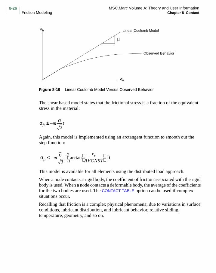
MSC.Marc Volume A: Theory and User InformationFriction Modeling Chapter 8 Contact
8-26
Figure 8-19 Linear Coulomb Model Versus Observed Behavior
The shear based model states that the frictional stress is a fraction of the equivalent stress in the material:
Again, this model is implemented using an arctangent function to smooth out the step function:
This model is available for all elements using the distributed load approach.
When a node contacts a rigid body, the coefficient of friction associated with the rigid body is used. When a node contacts a deformable body, the average of the coefficients for the two bodies are used. The CONTACT TABLE option can be used if complex situations occur.
Recalling that friction is a complex physical phenomena, due to variations in surface conditions, lubricant distribution, and lubricant behavior, relative sliding, temperature, geometry, and so on.
σfr
µ
Linear Coulomb Model
Observed Behavior
σn
σfr mσ3
-------t–≤
σfr mσ3
-------2π---arctan
vr
RVCNST-----------------------
t⋅⋅–≤

8-27MSC.Marc Volume A: Theory and User InformationChapter 8 Contact Friction Modeling
It was decided to implement the above two friction models, and to allow you to extend them, if necessary, by means of user the UFRIC subroutine. In such a routine, you provide the friction coefficient or the friction factor as
or
– position of the point at which friction is being calculated
– normal force at the point at which friction is being calculated
– temperature at the point at which friction is being calculated
– relative sliding velocity between point at which friction is being calculated and surface
– flow stress of the material
Glue Model
A special type of friction model is the glue option, which imposes that there is no relative tangential motion. The glue motion is activated through the CONTACT TABLE option.
A novel application of contact is to join two dissimilar meshes. In such a case, by specifying a very large separation force and that the glue motion is activated, the constraint equations are automatically written between the two meshes.
µ µ x fn T vr σy, , , ,( )=
m m x fn T vrσy, , ,( )=
x
fn
T
vr
σy

MSC.Marc Volume A: Theory and User InformationSeparation Chapter 8 Contact
8-28
Separation
After a node comes into contact with a surface, it is possible for it to separate in a subsequent iteration or increment. Mathematically, a node should separate when the reaction force between the node and surface becomes tensile or positive. Physically, you could consider that a node should separate when the tensile force or normal stress exceeds the surface tension. Rather than use an exact mathematical definition, you can enter the force or stress required to cause separation.
Separation can be based upon either the nodal forces or the nodal stresses. The use of the nodal stress method is recommended as the influence of element size is eliminated.
In many analysis, contact occurs but the contact forces are small; for example, laying a piece of paper on a desk. Because of the finite element procedure, this could result in numerical chattering. Marc has some additional contact control parameters that can be used to minimize this problem. As separation results in additional iterations (which leads to higher costs), the appropriate choice of parameters can be very beneficial.
When contact occurs, a reaction force associated with the node in contact balances the internal stress of the elements adjacent to this node. When separation occurs, this reaction force behaves as a residual force (as the force on a free node should be zero). This requires that the internal stresses in the deformable body be redistributed. Depending on the magnitude of the force, this might require several iterations.
You should note that in static analysis, if a deformable body is constrained only by other bodies (no explicit boundary conditions) and the body subsequently separates from all other bodies, it would then have rigid body motion. For static analysis, this would result in a singular or nonpositive definite system. This problem can be avoided by appropriate boundary conditions.
Release
A special case of separation is the intentional release of all nodes from a rigid body. This is often used in manufacturing analysis to simulate the removal of the workpiece from the tools. After the release occurs in such an analysis, there might be a large redistribution of the loads. It is possible to gradually reduce the residual force to zero, which improves the stability, and reduces the number of iterations required. The RELEASE history definition option allows the release (separation) of all the nodes in contact with a particular surface at the beginning of the increment. The rigid body should be moved away using the MOTION CHANGE option or deactivated using the CONTACT TABLE option to ensure that the nodes do not inadvertently recontact the surface they were released from.

8-29MSC.Marc Volume A: Theory and User InformationChapter 8 Contact Coupled Analysis
Coupled Analysis
Contact analysis has several consequences on performing a coupled analysis. When performing a coupled contact analysis between multiple deformable bodies, each body deforms due to mechanical and thermal loads and undergoes heat conduction. When the bodies come into contact, there is heat flux across the surfaces. You need to provide a coefficient of heat transfer between the surfaces. This is often quite significant as a hot workpiece might come into contact with a cold tool set. Additionally, if friction is present, heat is generated based upon:
where is the mechanical equivalent of heat. Half of the heat generated due to
friction is contributed to each body. If the model allows a body to be rigid, two options are available. In the first case, the rigid body is considered to have a constant temperature (heat source or heat sink). Heat flux is exchanged between the rigid body and the deformable body. In the second case, it is required to perform a heat transfer analysis in the rigid body. In this case, the rigid body must be constructed of finite elements, but they are chosen as heat transfer types. Deformation does not occur in this body, but a heat transfer analysis is performed. This is computationally more efficient than performing a coupled analyses where all bodies are deformable.
Symmetry bodies have different characteristics as they are frictionless (hence, no heat generated) and because there is no heat flux across a symmetry plane.
Heat fluxes (FILMS) are automatically created on all the boundaries of the deformable-bodies. Two film coefficients are assigned to each body. One corresponds to free convection and is used whenever the boundary is free. The other is a contact film, and is used whenever the boundary is in contact with another body. In these cases, the heat flux across the interface is given by:
where
is the surface temperature
is the film coefficient between the two surfaces
is the temperature of the same contact location, as obtained from interpolation of nodal temperatures of the body being contacted.
q ffr vr Meq⋅ ⋅=
Meq
q HD TD T–( )=
T
HD
TD

MSC.Marc Volume A: Theory and User InformationCoupled Analysis Chapter 8 Contact
8-30
When a deformable-body contacts a rigid-body, the coefficients associated with the rigid-body are used. When two deformable bodies are in contact, the average value of the film coefficient specified for the bodies is used. The CONTACT TABLE option can also be used to specify the film coefficient. As with all other coupled problems, heat generated by plastic deformation can be calculated and applied as a volumetric flux. The heat generated by friction is also calculated and applied as a surface flux.
Two user subroutines are available to facilitate the creation of more sophisticated boundary flux definitions (such as radiation and convections with variations in space, temperature, pressure, etc.). UHTCON allows you to specify a film coefficient while the surface is in contact, and UHTCOE allows you to specify a film coefficient while the surface is free.

8-31MSC.Marc Volume A: Theory and User InformationChapter 8 Contact Element Considerations
Element Considerations
Marc allows contact with almost all of the available elements, but the use of certain elements has a consequence on the analysis procedure. Contact analysis can be performed with all of the structural continuum elements, either lower order or higher order, including those of the Hermann (incompressible) formulation, except axisymmetric elements with twist. Friction modeling is available in all of these elements except the semi-infinite elements. Higher order iso parametric shape functions have interpolation functions which lead to the equivalent nodal forces that oscillate between the corner and midside nodes. As this has a detrimental effect on both contact detection and determining contact separation, a procedure has been implemented to eliminate this problem. On the exterior surfaces, the midside nodes are constrained (tied) to the corner nodes automatically. This effectively results in a linear variation of the displacement along this edge. Hence, the element does not behave as a full bi-quadratic (2-D) or tri-quadratic element (3-D). All elements in the interior of the body behave in the conventional higher-order manner. In many manufacturing and rubber analyses, the lower-order elements behave better than the higher-order elements because of their ability to represent the large distortion; hence, these lower-order elements are recommended.
The constraints imposed on the nodal degrees of freedom are dependent upon the type of element.
1. When a node of a continuum element comes into contact, the translational degrees of freedom are constrained.
2. When a node of a shell element comes into contact, the translational degrees of freedom are constrained and no constraint is places on the rotational degrees of freedom. The exception to this is when a shell contacts a symmetry surface. In this case, the rotation about the element edge is also constrained.
Additionally, beams and shells contact is governed by the rules outlined below.
2-D Beams
All nodes on beams are potential contact nodes. Beam elements can be used in contact in two modes.
1. The two-dimensional beams can come into contact with rigid bodies composed of curves in the same x-y plane. The normal is based upon the normal of the rigid surface.

MSC.Marc Volume A: Theory and User InformationElement Considerations Chapter 8 Contact
8-32
2. The two-dimensional beams can come into contact with deformable bodies either of continuum elements or other beam elements. As the beams are in two dimensions, they do not intersect one another.
3-D Beams
Three-dimensional beam elements can be used in contact in three modes.
1. The nodes of the beams can come into contact with rigid bodies composed of surfaces. The normal is based upon the normal of the rigid surface.
2. Nodes of the three-dimensional beams can also come into contact with the faces of three-dimensional continuum elements or shell elements.
3. The three-dimensional elastic beams can also contact other elastic beams. In this case, we can consider beams crossing one another. In such cases, the beams are automatically subdivided such that four beams are created. As the beams slide upon each other, they are adaptively changed in length.
Figure 8-20 Beam-to-Beam Contact
Shell Elements
All nodes on shell elements are potential contact nodes. As the midside nodes of shell elements are automatically tied, the high-order shell element (type 22) has no benefit. Shell elements can contact either rigid bodies, continuum elements, or other shell elements. Shell-shell contact involves a more complex analysis because it is necessary to determining which side of the shell contact occurs.
Contact Occurs New Beams Created Adaptive Meshing of Sliding Beams

8-33MSC.Marc Volume A: Theory and User InformationChapter 8 Contact Dynamic Impact
Dynamic Impact
The capability is available for both implicit time integration via the Newmark-beta or Houbolt operators, and the explicit time integration via the (fast) central difference operator.
The Newmark-beta and the Single Step Houbolt procedure have the capability to allow variable time steps and, when using the user-defined fixed time step procedure, the time step is split by the algorithm to satisfy the contact conditions. Since the central difference operator is constrained to small time steps by the stability requirement, time splitting is not used by the contact algorithm.
For most dynamic impact problems, the Single Step Houbolt method is recommended, as this procedure possesses high-frequency dissipation. This is often necessary to avoid numerical problems by contact-induced high-frequency oscillations. If the other dynamic operators are used, it is recommended that numerical damping be used during the analysis.
In dynamic analysis, the requirement of energy conservation is supplemented with the requirement of momentum conservation. In addition to the constraints placed upon the displacements, additional constraints are placed on the velocity and acceleration of the nodal points in contact, except for the Single Step Houbolt method.
When a node contacts a rigid surface, it is given the velocity and acceleration of the rigid surface in the normal direction. The rigid surfaces are treated as if they have infinite mass, hence, infinite momentum.

MSC.Marc Volume A: Theory and User InformationRezoning Chapter 8 Contact
8-34
Rezoning
In manufacturing simulations the objective is to deform the workpiece from some initial (simple) shape to a final, often complex shape. This deformation of the material, results in mesh distortion. For this reason, it is often required to perform a rezoning/remeshing step. At this point, the analysis is stopped. A new mesh is created; the current state of deformation, strains, stresses, etc. is transferred to the new mesh, and the analysis is continued. This has several consequences for contact analysis.
1. It is necessary to redefine the elements associated with the deformable body that is being rezoned. This is done through the CONTACT CHANGE option.
2. If a contact tolerance was not defined by you, a new contact tolerance is calculated based upon the new mesh. This distance can be smaller than the previously calculated tolerance, leading to more iterations.
3. After the new mesh is created, the program redetermines the potential contact nodes and the number of contact segments. In the current release of Marc, it is necessary to give an upper bound to this number to insure sufficient memory allocation. Additionally, as a rezoning analysis increases the number of nodes, elements, and boundary conditions, it is necessary to reserve space for these features from the beginning of the analysis. This is done through the SIZING parameter.
4. At the first increment after remeshing, Marc determines which nodes are in contact. If the new mesh does not reflect the exterior surface of the old model, it is possible that a region that was previously in contact is no longer in contact. This is usually not so serious; as most likely, the node subsequently comes into contact. A more significant problem is if a node in the new mesh is created which, in fact, has penetrated another body. If the newly created node is beyond another body’s surface by more than the contact tolerance, it is possible that a poor contact analysis results.
If rezoning occurs, rigid surfaces must be kept the same and cannot be changed.
Marc auto-rezoning feature, activated by REZONING,1 for 2-D problems, automatically creates new meshes and performs rezoning to resolve mesh distortion problems. In such cases, points (1) and (4) are treated automatically.

8-35MSC.Marc Volume A: Theory and User InformationChapter 8 Contact Adaptive Meshing
Adaptive Meshing
Contact between a deformable-body and a rigid body is insured such that the nodes do not penetrate the rigid surface. It is possible that an edge of an element penetrates a rigid surface, especially where high curvature is present because of the finite element discretization. The use of the adaptive mesh generation procedure can be used to reduce these problems.
In addition to the traditional error criteria such as Zienkiewicz-Zhu or maximum stress, etc., you can request that the mesh be adaptively refined due to contact. In such a case, when a node comes into contact, the elements associated with that node are refined. This results in a greater number of elements and nodes on the exterior region where contact occurs. This can lead to a substantial improvement in the accuracy of the solution.
Figure 8-21 Contact Closure Condition
The adaptive meshing procedure has consequences to the contact procedure similar to the rezoning procedure.
1. If a contact tolerance was not defined by you, a new contact tolerance is calculated based upon the new mesh. This distance can be smaller than the previously calculated tolerance, leading to more iterations.
2. After the new mesh is created, the program redetermines the potential contact nodes and the number of contact segments. In the current release of Marc, it is necessary to give an upper bound to this number to insure sufficient memory allocation. Additionally, as a rezoning analysis increases the number of nodes, elements, and boundary conditions, it is necessary to reserve space for these features from the beginning of the analysis. This is done through the ADAPTIVE parameter.
Penetration of Element Edge due to Mesh Discretization Result of Adaptive Meshing

MSC.Marc Volume A: Theory and User InformationResult Evaluation Chapter 8 Contact
8-36
Result Evaluation
The Marc post file contains the results for both the deformable bodies and the rigid bodies. In performing a contact analysis, you can obtain three types of results. The first is the conventional results from the deformable body. This includes the deformation, strains, stresses, and measures of inelastic behavior such as plastic and creep strains. In addition to reaction forces at conventional boundary conditions, you can obtain the contact forces and friction forces imparted on the body by rigid or other deformable bodies. By examining the location of these forces, you can observe where contact has occurred, but Marc also allows you to select the contact status as a post file variable (a value of zero means that a node is not in contact; a value of one means that a node is in contact).
It is also possible to obtain the resultant force following from contact on the deformable bodies and the resultant force and moment on the rigid bodies. The moment is taken about the user-defined centroid of the rigid body. The time history of these resultant forces are of significant issues in many engineering analysis. Of course, if there is no resultant force on a rigid body, it implies that body is not in contact with any deformable body.
Finally, if the additional print is requested, the output file reflects information on when a node comes into contact, what rigid body/segment is contacted, when separation occurs, when a node contacts a sharp corner, the displacement in the local coordinate system, and the contact force in the local coordinate system. For large problems, this can result in a significant amount of output.
The motion of the rigid bodies can be displayed as well as the deformable bodies. Rigid bodies which are modeled using the piecewise linear approach are displayed as line segments for flat patches. When the rigid surfaces are modeled as analytical surfaces, the visualization appears as piecewise linear in older versions (pre-K7/Mentat 3.1) or as trimmed NURBS in subsequent versions.

8-37MSC.Marc Volume A: Theory and User InformationChapter 8 Contact Tolerance Values
Tolerance Values
On the third data block for contact, five tolerances can be set for determination of the contact behavior. Not entering any values here means that Marc calculates values based on the problem specification.
Relative Sliding Velocity Between Surfaces Below Which Friction Forces Drop
As discussed in the Friction Modeling section, the equations of friction are smoothed internally in the program to avoid numerical instabilities. The equations are inequalities whenever two contacting surfaces stick to each other and equalities whenever the surfaces slide (or slip). Thus, the character of contact constraints change depending on whether there is sticking or slipping. The smoothing procedure consist of modifying it in such a way, that there is always slip; the amount is a function of the relative velocity and a constant RVcnst. The value of this constant must be specified here. It actually means, that if we specify a small value in comparison to the relative velocity, the jump behavior is better approximated, but numerical instabilities can be expected. A large value means, that we need a large relative velocity before we get the force at which the slip occurs.
It is suggested to use values between 0.1 and 0.01 times a typical surface velocity.
Distance Below Which a Node is Considered Touching a Surface
In each step, it is checked whether a (new) node is in contact with other surfaces. This is determined by the distance between the nodes and the surfaces. Since the distance is a calculated number, there are always roundoff errors involved. Therefore, a contact tolerance is provided such that if the distance calculated is below this tolerance, a node is considered in contact. A too large value means that a high number of body nodes are considered to be in contact with the surface and are consequently all moved to the surface, which can be unrealistic in some applications. A too small value of this number means that the applied deformation increment is split into a high number of increments, thus increasing the cost of computation.
The tolerance must be provided by the analyst or can be calculated by Marc. In general, the contact tolerance should be a small number compared to the geometrical features of the configuration being analyzed. The value calculated by Marc is determined as 1/20 of the smallest element size for solid elements or 1/4 of the thickness of shell elements. If both shell and continuum elements are present, the default is based upon the smaller of the two values.

MSC.Marc Volume A: Theory and User InformationTolerance Values Chapter 8 Contact
8-38
Tolerance on Nodal Reaction Force on Nodal Stress Before Separation Occurs
If a tensile force occurs at a node which is in contact with a surface, the node should separate from the surface. Rather than using any positive value, a threshold value can be specified. This number should theoretically be zero. However, because a small positive reaction might be due only to errors in equilibrium, this threshold value avoids unnecessary separations. A too small value of this force results in alternating separation and contact between the node and the surface. A too large value, of course, results in unrealistic contact behavior.
Marc calculates this value as the maximum residual force in the structure. Note that the maximum residual force can be specified in the CONTROL option. Default for this value, a 10 percent of the maximum reaction force is used. Consequently, if locally high reaction forces at a particular point are present, the separation force is large as well. In most cases, however, the default value is a good measure.
If you indicate that separation is to be based upon stresses, a value of the separation stress should be entered. The default value is the maximum residual force at node n divided by the contact area of node n.

8-39MSC.Marc Volume A: Theory and User InformationChapter 8 Contact Workspace Reservation
Workspace Reservation
In the definition of the contact behavior, a number of maximum workspace numbers must be set for the workspace reservation in Marc. It would, theoretically, be possible to automate this as well, but since in a restart analysis with mesh rezoning or adaptive meshing for instance, it might be necessary to increase the number of elements of the deforming body, this is not possible for all cases. Therefore, you must specify some numbers here. Too large values of the numbers means that the internal workspace for Marc is not optimally used. Too small numbers are indicated at the start of the analysis by Marc, but if it occurs in a restart, it can mean that the complete analysis has to be repeated.
The numbers which have to be set are the following:
– number of bodiesThis is immediately clear from the surface definition.
– maximum number of entities for any surfaceThis number is easily determined by looking at each surface and counting the number of straight segments to be created. For deformable surfaces, this depends on the element mesh; for rigid surfaces, it is easily determined for straight lines and circle segments (these are by default divided into 10 segments), for splines, it is a little more difficult since it depends on the value of the error control.
– upper bound to the number of boundary nodes of any deformable surfaceThis number is, of course, closely related to the previous number for deformable surfaces.
In cases where the maximums are difficult to determine beforehand, it is always possible to perform the analysis with a STOP parameter. Marc tells you the numbers which are to be used. Again, be careful for possible restarts with mesh rezoning or adaptive meshing.

MSC.Marc Volume A: Theory and User InformationMathematical Aspects of Contact Chapter 8 Contact
8-40
Mathematical Aspects of Contact
Contact can be defined as finding the displacement of points A and B such that
where A is on one body and B is on another body, n is the direction cosine of a vector between the two points, and TOL is the closure distance.
Figure 8-22 Normal Gap Between Potentially Contacting Bodies
Lagrange Multiplier Procedure
In the Lagrange Multiplier Procedure, the variational procedure is augmented by the constraint. The virtual work principle leads to the traditional systems equation:
The constraint conditions can be expressed as
Through the minimization of the augmented functional
you obtain
uA uB–( ) n TOL<•
AB
n
Ku f=
Cu 0=
Ψ 12---u
TKu u
Tf– λT
Cu+=
K CT
C 0
u
λ f
0
=

8-41MSC.Marc Volume A: Theory and User InformationChapter 8 Contact Mathematical Aspects of Contact
8Contact
Mathematical Aspects of Contact
This equation can be solved simultaneously for both the displacement ( ) and the
Lagrange multiplier ( ). You observe the introduction of Lagrange multipliers results in a zero on the diagonal. Hence, even well posed physical problems no longer have positive definite systems. This often results in numerical difficulties and restricts the type of linear equation solver that can be used.
Direct Constraint Procedure
Marc divides contact problems into two domains; the first is when a deformable body makes contact with a rigid surface and the second is when a deformable body makes contact with another deformable body or itself.
Two-dimensional or three-dimensional bodies are treated conceptually in the same manner.
Deformable-Rigid Contact
In such a problem, a target node on the deformable body has no constraint while contact does not occur. Once contact is detected, the degrees of freedom are transformed to a local system and a constraint is imposed such that
where v is the prescribed velocity of the rigid surface. This local transformation is continuously updated to reflect sliding of point A along the rigid surface.
If the glue option is activated, an additional displacement constraint is formed as
u
λ
∆unormal v n⋅=
∆u gentialtan v t⋅=

MSC.Marc Volume A: Theory and User InformationMathematical Aspects of Contact Chapter 8 Contact
8-42
Figure 8-23 Contact Coordinate System
Chapter8
Contact
The determination of when contact occurs and the calculation of the normal vector are critical to the numerical simulation. In Marc, three procedures are used for detecting penetration and imposing contact. In Figure 8-24, node A is not in contact with the rigid body at the beginning of the increment ( ). After time step , node A
penetrates rigid surface if no constraint is imposed in step .
a. This is clearly not an acceptable solution. The first two procedures discussed below are used when the fixed time step procedure is used. In the first procedure, the time step is divided into two periods or subincrements. In the first subincrement, node A is unconstrained such that its motion is unimpeded. In the second subincrement, the motion is constrained. The numerical procedure now needs to find the time period such that contact first occurs. This is a nonlinear mathematical problem and only an approximate solution can be obtained. The time step chosen is obtained by linearizing the displacement increment. This results in potential penetration or only approximately reaching the contact surface.
A
n
t
y
x
z
Before Contact After Contact
B
A
B
n ∆t
n 1+
∆t
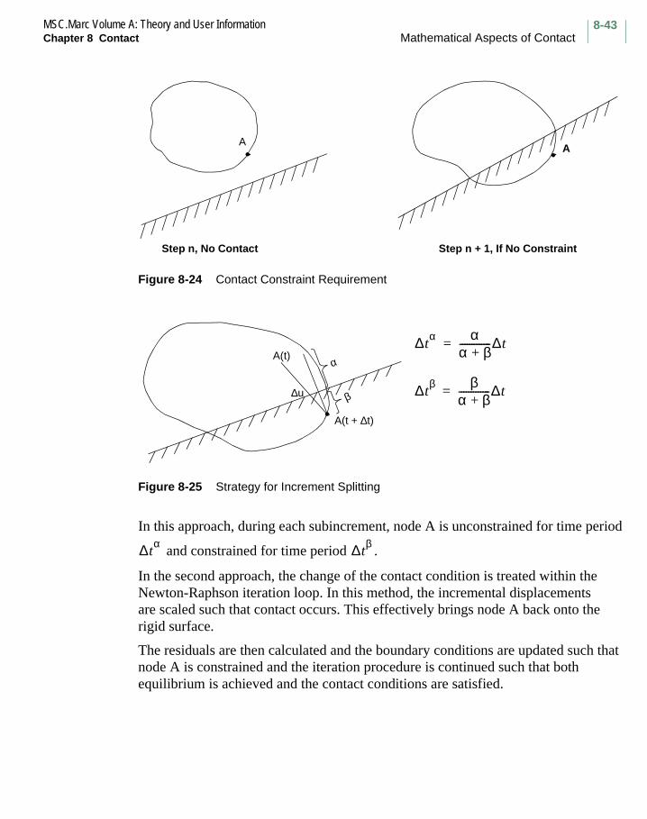
8-43MSC.Marc Volume A: Theory and User InformationChapter 8 Contact Mathematical Aspects of Contact
Figure 8-24 Contact Constraint Requirement
Figure 8-25 Strategy for Increment Splitting
In this approach, during each subincrement, node A is unconstrained for time period
and constrained for time period .
In the second approach, the change of the contact condition is treated within the Newton-Raphson iteration loop. In this method, the incremental displacements are scaled such that contact occurs. This effectively brings node A back onto the rigid surface.
The residuals are then calculated and the boundary conditions are updated such that node A is constrained and the iteration procedure is continued such that both equilibrium is achieved and the contact conditions are satisfied.
A
Step n, No Contact
A
Step n + 1, If No Constraint
∆u
A(t)
β
A(t + ∆t)
α
∆tα α
α β+-------------∆t=
∆tβ β
α β+-------------∆t=
∆tα ∆t
β

MSC.Marc Volume A: Theory and User InformationMathematical Aspects of Contact Chapter 8 Contact
8-44
The third procedure is used when the adaptive time stepping procedure is used (AUTO TIME or AUTO STEP). Marc then reduces the time step in the increment such that the node just comes into contact. In the next increment, the node is given the appropriate contact constraint and a new time step is determined based upon the convergence criteria.
Analytical Contact
Utilizing the analytical representation of rigid surfaces influences the numerical procedure in several ways:
1. The rigid surface is represented by a nonuniform rational B-spline surface (NURB) which provides a precise mathematical form capable of representing the common analytical shapes – circle, conic curve, free-form curves, surfaces of revolution, and sculptured surfaces.
The surface can be expressed in simple mathematical form to model complex multiple surfaces with advantage of continuity in first and second derivative. Those analytical forms are expressed in four-dimensional homogeneous coordinate space by:
For curves, it simplifies to:
where the B are 4-D homogeneous defining polygon vertices, and are nonrational B-spline basis functions, hi,j is homogeneous
coordinates. For given parameters and in local system, the location (x, y, z) in three-dimensional space, first derivative and second derivative (if required), are calculated. Given a point with x, y and z Cartesian
P u v,( )
Bi j,
j 1=
m 1+
∑ hi j, Ni k, u( )Mj l, v( )i 1=
n 1+
∑
hi j, Ni k, u( )Mj l, v( )j 1=
m 1+
∑i 1=
n 1+
∑--------------------------------------------------------------------------------=
P u( )
BihiNi k, u( )i 1=
n 1+
∑
hiNi k, u( )i 1=
n 1+
∑--------------------------------------=
Ni k,Mj l,
u v

8-45MSC.Marc Volume A: Theory and User InformationChapter 8 Contact Mathematical Aspects of Contact
coordinates, there is no explicit mathematical form to find out the parameters u and v in the local space, so they are obtained using an iterative procedure.
2. The location of the closest point on the contact surface corresponding to node A needs to be determined. This process, determined analytically when using flat patches, requires an iterative approach for rigid bodies modeled with NURBS.
Figure 8-26 Closest Point Projection Algorithm
3. Once the point P is known, the normal is calculated based upon the NURB. This normal is used in a manner consistent with the PWL procedure.
4. Because the normal can change from iteration to iteration, the imposition of the kinematic boundary conditions is continuously changing.
A
P

MSC.Marc Volume A: Theory and User InformationMathematical Aspects of Contact Chapter 8 Contact
8-46
In the PWL approach:
In the analytical approach:
where the subscripts represent the iteration number.
5. In the PWL approach, when a node slides from one segment to another, the corner condition logic is activated. The advantages of analytical surfaces is that this logic is not necessary until you come to the end of the spline. This reduces the amount of iterations required.
6. The friction calculation is dependent upon the surface normal and tangent. When using the analytical approach, the friction calculation includes the effect of changes in the direction of the normal vector from iteration to iteration. This improves the accuracy and convergence behavior.
7. Because the normal is continuous, the calculation of nodal forces is more accurate. This allows for the determination of nodal separation to occur beginning with the second iteration as opposed to when equilibrium convergence has been achieved using the PWL approach.
Solution Strategy for Rigid Contact
1. At the start of an increment, all boundary nodes are checked for contact with surfaces and flagged if so.
2. Next, transformations and imposed displacements are determined for each touching node. With the knowledge of the time increment and surface velocity, the configuration of the surface at the end of the increment is found. Then, the distance from the node starting position to the current surface segment is determined and is the probable normal displacement to be imposed. If there is a previous solution for displacement increments, these are used to estimate the tangential displacement increment (Figure 8-27). If this estimate still puts the node at the end of the increment in the same surface segment, then this one is used to determine the
∆un( )0v n⋅=
δun( )i0=
∆un( )0v n0⋅=
δun( )iv n1 v– n0⋅ ⋅=

8-47MSC.Marc Volume A: Theory and User InformationChapter 8 Contact Mathematical Aspects of Contact
transformation matrix between local and global coordinates, and the normal displacement is accepted. Otherwise, the procedure is repeated for the adjacent segment. If a concave corner is hit, the boundary node is fixed to such corner. If the node goes out of a sharp convex corner, it is immediately released from the surface.
3. One increment of the problem is solved iteratively and values for displacement increments are calculated. Step 2 is repeated at each iteration for possible changes in surface segment.
4. Once convergence is obtained, nodal forces are checked. Whenever a positive normal force (or stress) is detected which is larger than the tolerance, a node is released from the surface segment at which such force (or stress) corresponds and Step 3 is repeated. This tolerance can be modified using the user subroutine SEPFOR (or SEPSTR).
5. A check is made on all free boundary nodes to determine whether the newly calculated displacement increments puts them inside any surface (Figure 8-28). If that is the case and the fixed time step procedure is used, the increment is reduced in such a way, that the first node is barely in contact. The process is restarted at Step 3 whenever there is a reduction in increment size.
6. Whenever there is a reduction in increment size and the loading history parameters request fixed increments, the current increment is considered split into two and the remainder is executed next.
7. Go to next increment (Step 1).

MSC.Marc Volume A: Theory and User InformationMathematical Aspects of Contact Chapter 8 Contact
8-48
Figure 8-27 Node P Already In Contact (2-D)
Figure 8-28 New Node in Contact P
SEGBP
β
∆u
∆utest
∆un
SEGE
SEGB - Die segment at beginningof increment
SEGE - Die segment at end ofincrement
∆u - Displacement incrementof previous increment
∆un - Imposed normal displacement
∆utest - Estimate of tangentialdisplacement
β - Angle used in transformationmatrix
SEGB
SEGEA
B
∆u
P
SEGB - Die segment at beginningof increment
SEGE - Die segment at end ofincrement
∆u - Displacement incrementcalculated
PB - Factor to scale incrementPA

8-49MSC.Marc Volume A: Theory and User InformationChapter 8 Contact Mathematical Aspects of Contact
Figure 8-29 Node P Already in Contact (3-D)
Deformable-Deformable Contact
When a node contacts a deformable body, a tying relation is formed between the contacting nodes and the nodes on the other body. This constraint relationship uses information regarding the normal to the surface. This normal is calculated based upon the piecewise linear representation of the element face. This has the consequences that the constraint relation is not accurate because it is constant over the complete segment. As a node slides from one face to another, there is a discontinuity in the normal which leads to potential numerical difficulties.
PATB Patch at beginning of increment
PATE Patch at end of increment
∆u Previous displacement increment of node P
∆un Imposed normal displacement increment (local direction 3)
∆utest Estimated tangential displacement
PATB
PATE
P
∆u
∆un
∆utest
2
31

MSC.Marc Volume A: Theory and User InformationMathematical Aspects of Contact Chapter 8 Contact
8-50
Figure 8-30 Deformable Contact; Piecewise Linear Geometry Description
As an alternative, you can fit a smooth surface through the finite elements. For 2-D, a cubic spline is used. This spline is calculated based upon the tangent and position of the nodes on the segment. This gives a more accurate representation of the actual physical geometry and a more accurate calculation of the normal. You must identify where actual discontinuities exists. You can use the SPLINE option to define the area of the deformable body in 2-D or 3-D where the smoothness is required.
Figure 8-31 Improved Geometry Description of Contacted Deformable Body (2-D case)
Actual Geometry
Finite Element Approximation
4
3
2
1
Contacting Body
Contacted Body
2 – 3: Contacted Segment

8-51MSC.Marc Volume A: Theory and User InformationChapter 8 Contact Mathematical Aspects of Contact
Figure 8-32 Contacted Body
Figure 8-33 Extracted Faces
For 3-D problems, a Coons surface is used to improve the geometric representation in calculating the normal.
12
3
4
5
6
7
8
9
10
11
12
1-2-3-4: Contacted Segment

MSC.Marc Volume A: Theory and User InformationMathematical Aspects of Contact Chapter 8 Contact
8-52
Figure 8-34 Internal Representation Based on Coons Surfaces
Solution Strategy for Deformable Contact
1. Upon initiation, the program determines the boundary nodes on each body. For 2-D, these nodes are ordered in sequence in order to describe the boundary in a counterclockwise manner. Linear geometrical entities are then created out of subsequent pairs of nodes, to define a surface profile as in a rigid surface. For 3-D, 4-node patches are created.
2. Once contact between a node and a deformable surface is detected, a tie is activated. The tying matrix is such that the contacting node follows the surface of the surface (Figure 8-35); it can slide along it or be stuck according to the general contact conditions.
3. Contact occurs between all deformable bodies unless the CONTACT TABLE option is used. In deformable contact, there is no master or slave body; each body is checked against every other body.
4. During the iteration process of finding an incremental solution, a node can slide from one segment to another, changing the retained nodes of its tie. A recalculation of the bandwidth is, therefore, made every iteration. From increment (or subincrement) to increment, the number of nodes in contact can change. In such cases, an optimization of the bandwidth is automatically available to cope with the possible drastic changes in bandwidth that a new tie produces.

8-53MSC.Marc Volume A: Theory and User InformationChapter 8 Contact Mathematical Aspects of Contact
Figure 8-35 Tyings in Deformable Contact (2-D)
Figure 8-36 Tying in Deformable Contact (3-D)
When the glue option is used between two deformable bodies, a simpler tying relationship is formed, such that no relative motion occurs.
segt+Dt
segt
∆UB ∆UA ∆UC
A
B
C
Tied NodeRetained Nodes
AA B C
Tied node TRetained nodes T, R2, R3, R4, R5
T/R1
R2
R5R3
R4
t
t+ ∆t

MSC.Marc Volume A: Theory and User InformationMathematical Aspects of Contact Chapter 8 Contact
8-54
Friction Modeling
The regularized form of the Coulomb friction model can be written as:
is a nonlinear relation between the relative sliding velocity and the friction force. Implementation in Marc has been done using a nonlinear spring model. Noting that the behavior of a nonlinear spring, as shown in Figure 8-37, is given by the equation:
Figure 8-37 Spring Model
in which is the spring stiffness and , , , and are displacements and
forces of points 1 and 2, the equivalent in terms of velocities is readily seen to read
Since is a nonlinear function of the relative velocity, the above equation is solved incrementally, where within each increment a number of iterations may be necessary. For a typical iteration , the equation to be solved looks like
(8-1)
ft
2µfn
π-----------arctanvr
RVCNST-----------------------
=
K K–
K– K
u1
u2
F1
F2
=
u, F u, F
1 2
K u1 u2 F1 F2
K K–
K– K
v1
v2
F1t
F2t
=
K
i
Ki
Ki
–
Ki
– Ki
δv1i
δv2i
∆F1ti
∆F2ti
=

8-55MSC.Marc Volume A: Theory and User InformationChapter 8 Contact Mathematical Aspects of Contact
where and are used to update and by
(8-2)
Notice that and correspond to the beginning of the iteration. For
deformable-rigid contact, it is easy to see that
, (8-3)
since the motion of a rigid body (to which node 2 belongs) is exactly prescribed by you. In a static analysis, Marc provides no direct information about velocities, so they have to be calculated from the displacement and time increments. Denoting a time increment by , we can write
, (8-4)
in which represents the correction of the incremental displacement for
iteration like (see also Equation 8-2).
(8-5)
Substituting Equation 8-3 and Equation 8-4 into Equation 8-1 yields
(8-6)
For the first iteration of an increment, an improvement of equation Equation 8-6 can
be achieved by taking into account the velocity at the end of the previous
increment. Then equation Equation 8-4 can be rewritten as
, (8-7)
δv1i δv2
iv1
iv2
i
v1i
v1i 1– δv1
i+=
v2i
v2i 1–
= δv2i
+
v1i 1–
v2i 1–
δv2i
0=
∆t
δv1i δu1
i
∆t---------=
δu1i ∆u1
i 1–
i
∆u1i ∆u1
i 1–= δ+
1∆t-----K
iδu1i ∆F1
i=
v1p
δv11 ∆u1
1
∆t--------- v1
p–=

MSC.Marc Volume A: Theory and User InformationMathematical Aspects of Contact Chapter 8 Contact
8-56
so that Equation 8-6 can be modified like
(8-8)
For the subsequent iterations,
(8-9)
In equation Equation 8-8, denotes the relative velocity between the points 1 and 2
at the end of the previous increment. It must be noted that the additional term in Equation 8-8 is especially important if the velocity of the rigid body differs much from the relative velocity. This is usually the case in rolling processes, when the roll has been modeled as a rigid body. For this reason, this improved friction model is called friction for rolling.
Automatic Penetration Checking Procedure
To detect contact between bodies whose boundaries are moving towards each other, an automatic penetration checking procedure is available. This procedure significantly increases accuracy and stability for models in which boundary nodes are displacing significantly. Typical examples include metal forming processes (sheet forming and forging), highly deformable elastomeric models (rubber boots), and snap-fit problems (inserting a key into a lock).
The automatic penetration checking procedure is available under the CONTACT option. It is automatically activated if the adaptive loading procedure is selected. If the automatic penetration checking procedure is selected for these two options, a different procedure, as described below, is used instead.
From a computational perspective, the automatic penetration checking procedure detects penetration each time displacements are updated.
For implicit analysis, this typically happens after a matrix solution which produces a change in the displacements due to a change in applied loads and internal forces. The procedure detects nodes traversing a contact boundary due to the change in displacements. If at least one node penetrates a contact surface, a scale factor is applied to the change in displacements such that the penetrating nodes are moved back to the contact surface.
The automatic penetration checking procedure can, therefore, be considered to be a type of a line search. The procedure also looks at the magnitude of the change in displacement of nodes which already are contacting and not necessarily penetrating.
1∆t-----K
1δu11 ∆F1
1K vr
pv2
p–[ ]–=
1∆t-----K
iδu1i ∆F1
i=
vri

8-57MSC.Marc Volume A: Theory and User InformationChapter 8 Contact Mathematical Aspects of Contact
Using stability considerations, the scale factor calculated above may be further modified. In addition, for nodes on a contact boundary which are not yet contacting, a similar procedure is followed to enhance stability.
Because the procedure can reduce the change in displacements, it may require more iterations to complete an increment. It is important to ensure that the maximum allowable number of iterations to complete an increment is set to a sufficiently large value. When the adaptive loading procedure is used, or when the fixed time stepping procedure is used with automatic restarting, the increment automatically restarts if the maximum allowable number of iterations is exceeded. In the case of the adaptive loading procedure, the time step is modified.
When dynamics or the arc length control method is used, the above procedure is not available. Instead, penetration is checked for when convergence is achieved, usually after multiple iterations.
Note: The automatic penetration checking procedure is always used with the enhanced AUTO STEP time stepping procedure in MSC.Marc 2001.

MSC.Marc Volume A: Theory and User InformationReferences Chapter 8 Contact
8-58
References
1. Oden, J. T. and Pires, E. B. “Nonlocal and Nonlinear Friction Laws and Variational Principles for Contact Problems in Elasticity,” J. of Applied Mechanics, V. 50, 1983.
2. Ju, J. W. and Taylor, R. L. “A perturbed Lagrangian formulation for the finite element solution of nonlinear frictional contact problems,” J. De Mechanique Theorique et Appliquee, Special issue, Supplement, 7, 1988.
3. Simo, J. C. and Laursen, T. A. “An Augmented Lagranian treatment of contact problems involving friction,” Computers and Structures, 42, 1002.
4. Peric, D. J. and Owen, D. R. J. “Computational Model for 3-D contact problems with friction based on the Penalty Method,” Int. J. of Meth. Engg., V. 35, 1992.
5. Taylor, R. L., Carpenter, N. J., and Katona, M. G. “Lagrange constraints for transient finite element surface contact,” Int. J. Num. Meth. Engg., 32, 1991.
6. Wertheimer, T. B. “Numerical Simulation Metal Sheet Forming Processes,” VDI BERICHET, Zurich, Switzerland, 1991.

Chapter 9 Boundary Conditions
Marc is based on the stiffness method and deals primarily with force-displacement relations. In a linear elastic system, force and displacement are related through the constant stiffness of the system; the governing equation of such a system can be expressed as
(9-1)
where is the stiffness matrix and and are nodal displacement and nodal force vectors, respectively. Equation 9-1 can be solved either for unknown displacements subjected to prescribed forces or for unknown forces (reactions) subjected to prescribed displacements. In general, the system is subjected to mixed (prescribed displacement and force) boundary conditions, and Marc computes both the unknown displacements and reactions. Obviously, at any nodal point, the nodal forces and nodal displacements cannot be simultaneously prescribed as boundary conditions for the same degree of freedom.
CHAPTER
9 Boundary Conditions
Loading
Kinematic Constraints
Ku F=
K u F

MSC.Marc Volume A: Theory and User InformationChapter 9 Boundary Conditions
9-2
Note: You must prescribe at least a minimum number of boundary conditions to insure that rigid body motion does not occur.
The prescribed force boundary conditions are often referred to as loads and the prescribed displacement boundary conditions as boundary conditions.
Note: Boundary conditions can be prescribed in either the global or a local coordinate system. A nodal transformation between the global and the local coordinate systems must be carried out if the boundary condition is prescribed in a local system.
In a nonlinear stress analysis problem, Marc carries out the analysis incrementally and expresses the governing equation in an incremental form in terms of the incremental displacement vector and the incremental force vector .
(9-2)
Consequently, you must also define both the loads and the prescribed nodal displacements incrementally.
In addition to the prescribed displacement boundary conditions, constraint relations can exist among the nodal displacements. For example, the first degree of freedom of node i is equal to that of node j at all times. The expression of this constraint relation is
(9-3)
Generally, a homogenous linear constraint equation can be expressed as
(9-4)
where represents the degrees of freedom to be constrained, are other
retained degrees of freedom in the structure, and are constants.
You can enter constraints through either the TYING option or the SERVO LINK option.
You can use linear/nonlinear springs and foundations to provide special support to the structure and the gap and friction element (or CONTACT option) to simulate the contact problem.
∆u ∆F
Kdu df=
ui uj=
ut a1u1 a2u2 … anun+ + +=
u u1 … un, ,
a1 … an, ,

9-3MSC.Marc Volume A: Theory and User InformationChapter 9 Boundary Conditions Loading
Loading
Different types of analyses require different kinds of loading. For example, the loads in stress analysis are forces; those in heat transfer analysis are heat fluxes. Force is a vector quantity defined by magnitude and direction; heat flux is a scalar quantity defined by magnitude only. Loading can be time invariant (constant value) or time dependent.
Loading Types
You can categorize a particular type of load as either a point (concentrated) load or surface/volumetric (distributed) load, depending on application conditions. The spatial distribution of the load can be uniform or nonuniform. Special loading types also exist in various analyses. For example, centrifugal loading exists in stress analysis, and convection and radiation exist in heat transfer analysis. You can add point loads directly to the nodal force vector, but equivalent nodal forces first must be calculated by Marc from distributed loads and then added to the nodal force vector. These distinguishing features are described below.
A point (or nodal) load of either a vector (force, moment) or a scalar (heat flux) quantity is a concentrated load that is applied directly to a nodal point (see Figure 9-1). In a global or local coordinate system, a force must be defined in terms of vector components (see Figure 9-2). If the force vector is defined in a local coordinate system, then a global-to-local coordinate transformation matrix must be defined for the nodal point (see Figure 9-3 and Figure 9-4). For axisymmetric elements, the magnitude of the point load must correspond to the ring load integrated around the circumferences.
Figure 9-1 Schematic of a Point Load
y
x
Point (a)Heat Flux Q (Scalar)
Q
y
x
Point (b)Force F (Vector)
F
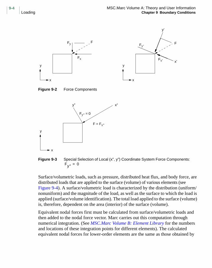
MSC.Marc Volume A: Theory and User InformationLoading Chapter 9 Boundary Conditions
9-4
Figure 9-2 Force Components
Figure 9-3 Special Selection of Local (x”, y”) Coordinate System Force Components:
Surface/volumetric loads, such as pressure, distributed heat flux, and body force, are distributed loads that are applied to the surface (volume) of various elements (see Figure 9-4). A surface/volumetric load is characterized by the distribution (uniform/nonuniform) and the magnitude of the load, as well as the surface to which the load is applied (surface/volume identification). The total load applied to the surface (volume) is, therefore, dependent on the area (interior) of the surface (volume).
Equivalent nodal forces first must be calculated from surface/volumetric loads and then added to the nodal force vector. Marc carries out this computation through numerical integration. (See MSC.Marc Volume B: Element Library for the numbers and locations of these integration points for different elements). The calculated equivalent nodal forces for lower-order elements are the same as those obtained by
y
x
F
Fx
Fy
y
x
F
Fx’
Fy’
y’
x’
y
x
Fy” = 0
y” x”
F = Fx”
Fy’’ 0=

9-5MSC.Marc Volume A: Theory and User InformationChapter 9 Boundary Conditions Loading
equally lumping the uniformly distributed loads onto the nodes. However, for high-order elements, the lumping is no longer simple (see Figure 9-5). As a result, the surface/volumetric loads should not be lumped arbitrarily.
Figure 9-4 Schematic of Surface/Volumetric Load
y
x
1
P2
4 3
2
Px
Q
(a) Distributed Mechanical Load (b) Distributed Heat Flux
Py
P1
Py
x
1
P2
4 3
2
P1
q
Surface 2-3:Uniform Normal Pressure p Uniform Heat flux q
Surface 3-4:Nonuniform Normal Pressure p1 - p2 Nonuniform Heat flux q1 = q2
Whole Volume:Volumetric Loads Px’Py Volumetric Heat Flux Q

MSC.Marc Volume A: Theory and User InformationLoading Chapter 9 Boundary Conditions
9-6
Figure 9-5 Allocation of a Uniform Body Force to Nodes for a Rectangular Element Family
Fluid Drag and Wave Loads
Marc provides a fluid drag and wave load capabilities that can be applied on beam type structures that are partially or fully submerged in fluid (see Figure 9-6). Morison’s equation is used to evaluate the fluid drag loads that are associated with steady currents. Only distributed drag and buoyancy effects are considered. Marc employs Airy wave theory to evaluate wave velocities that can be invoked for dynamic analysis option.
Fluid drag and wave loads are invoked using the DIST LOADS model definition with an IBODY load type of 11. These loads also require the FLUID DRAG model definition to input the relevant information regarding the fluid elevation and its flow. Table 9-2 lists input options for fluid drag and wave loads.
1/4
1/41/4
1/4
1/21/2 1/4
1/4
1/4
1/4
-1/121/3
1/3
1/3
-1/12
-1/12
-1/12
1/3
1/61/6 2/3-1/12-1/12
-1/12-1/12 1/3
1/3
1/31/3

9-7MSC.Marc Volume A: Theory and User InformationChapter 9 Boundary Conditions Loading
Figure 9-6 Fluid Drag and Wave Loads
Table 9-1 Input Options for Fluid Drag and Wave Loads
Load DescriptionInput Options
Model Definition History Definition User Subroutine
Fluid Drag Load DIST LOADSFLUID DRAG
DIST LOADS
Wave Load DIST LOADSFLUID DRAG
DIST LOADS
Steady VelocityWave Load
Pipe
OutsideFluid
InsideFluid
Sea Bed
Flow VelocityDistribution
VelocityGradient
BuoyancyForce
Fluid DragForce

MSC.Marc Volume A: Theory and User InformationLoading Chapter 9 Boundary Conditions
9-8
Mechanical Loads
Marc allows you to enter mechanical loads in various forms for stress analysis. These loads can be concentrated forces and moments, uniformly and nonuniformly distributed pressures, body forces, gravity or centrifugal loads. Table 9-2 lists input options for mechanical loads.
Application of centrifugal and Coriolis loadings require the ROTATION A model definition option, which defines the data corresponding to the axis of rotation. The actual load can be invoked by specifying an IBODY load types 100 or 103 for
centrifugal and Coriolis loadings, respectively. The square of rotation speed, , is entered in radians per time, for the magnitude of the distributed load. The mass density must also be defined in the ISOTROPIC or ORTHOTROPIC options.
Table 9-2 Input Options for Mechanical Loads
Load DescriptionInput Options
Model Definition History Definition User Subroutine
Point Load: Concentrated Force/Moment
POINT LOAD POINT LOAD FORCDT
Surface Load Pressure Shearing Forces, and Distributed Moment (Uniform/Nonuniform Distribution)
DIST LOADS DIST LOADS FORCEM
Volumetric Load Body Forces and Acceleration Forces
DIST LOADS DIST LOADS FORCEM
Centrifugal Loading
DIST LOADSROTATION A
DIST LOADS
Coriolis Loading DIST LOADSROTATION A
DIST LOADS
Fluid Loading DIST LOADSFLUID DRAG
ω2

9-9MSC.Marc Volume A: Theory and User InformationChapter 9 Boundary Conditions Loading
Application of gravity load is achieved by using IBODY load type 102. The mass density must be defined in the ISOTROPIC or ORTHOTROPIC options. The acceleration can be given independently in the x, y, and z direction through the DIST LOADS option.
Use of the FOLLOW FOR parameter results in the equivalent nodal loads due to pressures being calculated based on the current geometry. When this option is used, any change of surface area or orientation results in a change of load. FOLLOW FOR automatically invokes the LOAD COR parameter, so stresses should be stored at all integration points. The FOLLOW FOR parameter is typically used when a shell structure, which can undergo large deformation and rotations, is subjected to a pressure load. You can also specify that the follower force stiffness matrix can be included.
A number of history definition options are available for input of multiple load increments. For example, the AUTO LOAD option generates a specified number of increments, all having the same load increment, and is useful for nonlinear analysis with proportional loads; the PROPORTIONAL INCREMENT option allows the previous load increment to be scaled up or down for use in the current load increment. The AUTO INCREMENT option allows automatic load stepping in a quasi-static analysis and is useful for both geometrically and materially nonlinear problems.
Thermal Loads
Element integration point temperatures are used in a thermal stress analysis to generate thermal load. The AUTO THERM history definition option allows automatic application of temperature increments based on a set of temperatures defined throughout the mesh as a function of time. The CHANGE STATE option presents the temperatures to Marc, and Marc then creates its own set of temperature steps based on a temperature change tolerance provided through this option. Table 9-3 lists input options for thermal loads. You can input either the incremental temperature or the total temperatures as thermal loads.
The thermal strain increment is defined as
(9-5)
where is thermal strain increment, is the coefficient of thermal expansion, and
is the temperature increment. Equivalent nodal forces are calculated from the thermal strain increment and then added to the nodal force vector for the solution of the problem.
∆εth α∆T∫=
∆εth α∆T

MSC.Marc Volume A: Theory and User InformationLoading Chapter 9 Boundary Conditions
9-10
You can input the coefficient of thermal expansion through the ISOTROPIC or ORTHOTROPIC model definition options and the temperature increment through various options.
Initial Stress and Initial Plastic Strain
Marc allows you to enter a set of initial stresses that simulate the stress state in the structure at the beginning of an analysis. A typical example is prestress in a tensioned fabric roof. The set of initial stresses must be self-equilibrating and should not exceed the yield stress of the material. Table 9-4 shows the input options for initial stress.
Table 9-3 Input Options for Thermal Loads
Load Description
Input Options
ParameterModel
DefinitionHistory
DefinitionUser
Subroutine
Incremental Temperatures*
THERMALTHERMAL
LOADSTHERMAL
LOADSCREDE
Total Temperatures*
THERMALCHANGE
STATECHANGE
STATENEWSV
Initial Temperature*
INITIAL STATE
INITSV
Total Nodal Temperatures
POINT TEMP POINT TEMP
Initial Nodal Temperature
INITIAL TEMP USINC
*Temperatures must be specified at each integration point (or at the centroid if the CENTROID parameter is used) of each element in the mesh.
Table 9-4 Input Options for Initial Stress and Initial Plastic Strain
Load Description
Input Options
Parameter Model Definition User Subroutine
Initial Stress Prestress
ISTRESS INIT STRESS UINSTR
Initial Plastic Strain
INITIAL PLASTIC STRAIN
INITPL

9-11MSC.Marc Volume A: Theory and User InformationChapter 9 Boundary Conditions Loading
Marc also provides various ways of initializing the equivalent plastic strain throughout the model. This is useful in metal forming analysis in which the previous amount of equivalent plastic strain is often required. This history dependent variable represents the amount of plastic deformation that the model was subjected to, and is used in the work (strain) hardening model. The input option is shown in Table 9-4.
Heat Fluxes
In a heat transfer analysis, you can enter heat fluxes in various forms. Unlike stress analysis, heat transfer analysis requires entering the total values of flux. Table 9-5 lists the input options for heat fluxes.
There are three special heat flux conditions representing insulation, convection, and radiation.
1. Insulation
(9-6)
No input is required for the insulated case.
2. Convection
(9-7)
You must enter the film coefficient H and ambient temperature through the FILMS option or the FILM user subroutine. You can also directly input the heat flux using the FLUX user subroutine.
Table 9-5 Input Options for Heat Fluxes
Load DescriptionInput Options
Model Definition History Definition User Subroutine
Point Heat Flux (Sink or Source)
POINT FLUX POINT FLUX FORCDT
Surface Heat Flux, Convection, Radiation
DIST FLUXESFILMS
DIST FLUXESFILMS
FLUX*FILM*
Volumetric Flux Load Body Flux
DIST FLUXES DIST FLUXESFILMS
FLUX*
* Can be used for complicated flux loadings, convection, and radiation, allowing the input of nonuniform temperature- and time-dependent boundary conditions.
q 0=
q H Ts T–( )=
T
q

MSC.Marc Volume A: Theory and User InformationLoading Chapter 9 Boundary Conditions
9-12
3. Radiation
(9-8)
You must enter either the heat flux using the FLUX user subroutine or the temperature dependent film coefficient and ambient temperature using the FILM user subroutine. These relationships are shown in Equation 9-9. The use of FILM is recommended to ensure a stable solution.
(9-9)
where is the Stefan-Boltzmann constant, is emissivity, and are unknown surface and ambient temperatures, respectively.
An an alternative, the VIEW FACTOR option can be used to read in viewfactors calculated by Mentat. The RADIATION parameter is also required.
Mass Fluxes and Restrictors
In a hydrodynamic bearing analysis, you can enter mass fluxes, restrictors, and pump pressures as loads. Table 9-6 lists input options for these quantities.
Table 9-6 Input Options for Mass Fluxes and Restrictors
Load Description
Input Options
ParameterModel
DefinitionHistory
DefinitionUser
Subroutine
Nodal Mass Fluxes
BEARING POINT FLUX POINT FLUX
Distributed Mass Fluxes
BEARING DIST FLUXES DIST FLUXES FLUX*
Restrictors BEARINGRESTRICTOR
RESTRICTOR URESTR**
* Can be used for nonuniform mass fluxes** Can be used for nonuniform restrictions or pump pressures.
q σ ε Ts4
T∞4
–( )⋅=
qH Ts T σ ε, , ,( )
T
q σε Ts4
T∞4
–( )=
σ ε Ts3
Ts2T∞ TsT∞
2T∞
3+ + +( ) Ts T∞–( )⋅=
H Ts T∞,( ) Ts T∞–( )=
σ ε Ts T∞

9-13MSC.Marc Volume A: Theory and User InformationChapter 9 Boundary Conditions Loading
Electrical Currents
In coupled thermo-electrical (Joule heating) analysis, you can prescribe electrical currents as loads for the calculation of unknown nodal voltages. In magnetostatic analysis, you can also define the current. In such cases, as a steady state analysis is performed, there is no time variation of the currents. Table 9-7 lists input options for electrical currents.
Electrostatic Charges
In an electrostatic analysis, the charge can be entered, noting that a steady state analysis is performed so there is no time variation of charge. Table 9-8 summarized the input options.
Table 9-7 Input Options for Electrical Currents
Load DescriptionInput Options
Model Definition History Definition User Subroutine
Nodal Current POINT CURRENT POINT CURRENT FORCDT
Surface and Body Currents
DIST CURRENT DIST CURRENT FLUX
Table 9-8 Input Options for Electrostatic Charge
Load DescriptionInput Options
Model Definition History Definition User Subroutine
Nodal Charge POINT CHARGE
Distributed and Body Charges
DIST CHARGES FLUX

MSC.Marc Volume A: Theory and User InformationLoading Chapter 9 Boundary Conditions
9-14
Acoustic Sources
In acoustic analysis, you can enter a source pressure if a transient analysis by modal superposition is being performed. Table 9-9 summarized the input options.
Magnetostatic Currents
In a magnetostatic analysis, the current can be entered, noting that a steady state analysis is performed so there is no time variation of current. Table 9-10 summarizes the input options.
Table 9-9 Input Options for Acoustic Sources
Load DescriptionInput Options
Model Definition History Definition User Subroutine
Nodal Source POINT SOURCE POINT SOURCE FORCDT
Distributed Source DIST SOURCES DIST SOURCES FLUX
Nodal Source FIXED PRESSURE PRESS CHANGE FORCDT
Table 9-10 Input Options for Magnetostatic Current
Load DescriptionInput Options
Model Definition History Definition User Subroutine
Nodal Current POINT CURRENT POINT CURRENT
Distributed and Body Current
DIST CURRENT DIST CURRENT FLUX

9-15MSC.Marc Volume A: Theory and User InformationChapter 9 Boundary Conditions Loading
Electromagnetic Currents and Charges
In an electromagnetic analysis, the current can be entered. These values can have time variation if a transient analysis is performed or a harmonic excitation can be applied. Table 9-11 summarizes the input options.
Table 9-11 Input Options for Currents and Charges
Load DescriptionInput Options
Model Definition History Definition User Subroutine
Nodal Current POINT CURRENT POINT CURRENT
Distributed and Body Current
DIST CURRENT DIST CURRENT FLUX
Nodal Charge POINT CURRENTPOINT CHARGE
POINT CURRENT
Distributed and Body Charge
DIST CHARGES DIST CHARGES

MSC.Marc Volume A: Theory and User InformationKinematic Constraints Chapter 9 Boundary Conditions
9-16
Kinematic Constraints
Marc allows you to input kinematic constraints through various options that include
• Boundary Conditions (prescribed nodal values)
• Transformation of Degree of Freedom
• Shell Transformation
• Tying Constraint
• Rigid Link Constraint
• Shell-to-Solid Tying
• Cyclic Symmetry
• Support Conditions
Boundary Conditions
Marc allows you to specify the nodal value for a particular degree of freedom. If you do not give a nodal value when you specify the boundary condition, Marc sets the fixed nodal value to zero. An option allows boundary conditions to be specified at the time of two-dimensional mesh generation with MESH2D. You can apply a different set of boundary conditions for each load increment.
Table 9-12 gives the nodal values for the various analyses, and Table 9-13 lists the input options for boundary conditions in different analyses.
Table 9-12 Analyses with Corresponding Nodal Values
Analysis Nodal Values
Acoustics Pressure
Coupled Fluid Thermal Velocity, Pressure, and Temperature
Coupled Thermo-electrical Voltage and Temperature
Coupled Thermo-mechanical Displacement and Temperature
Electrostatic Potential
Fluid Velocity and Pressure
Heat transfer Temperature
Hydrodynamic Bearing Pressure
Magnetostatic Potential
Rigid Plastic Flow Velocity
Stress Displacements

9-17MSC.Marc Volume A: Theory and User InformationChapter 9 Boundary Conditions Kinematic Constraints
Transformation of Degree of Freedom
Marc allows transformation of individual nodal degrees of freedom from the global direction to a local direction through an orthogonal transformation that facilitates the application of boundary conditions and the tying together of shell and solid elements.
Transformations are assumed to be orthogonal. Once you invoke a transformation on a node, you must input all loads and kinematic conditions for the node in the transformed system.Nodal output is in the transformed system. This option is invoked using the TRANSFORMATION option.
The UTRANFORM option allows transformations to be entered via the UTRANS user subroutine. This allows you to transform the degrees of freedom at an individual node from global directions to a local direction through an orthogonal transformation. UTRANFORM allows you to change the transformation with each increment. When you invoke this option, the nodal output is in both the local and the global system.
Shell Transformation
The SHELL TRANSFORMATION option allows you to transform the global degree of freedom of doubly curved shells to shell degrees of freedom in order to facilitate application of forces in the shell directions, edge moments, and clamped or simply supported boundary conditions. There are four types of shell transformations.
The SHELL TRANSFORMATION model definition option specifies information on the shell transformation. For Types 1 and 3, only the node number has to be specified. For Types 2 and 4, a boundary direction (the direction cosine of t as shown in Figure 9-7) also has to be specified in the surface.
Table 9-13 Input Options for Boundary Conditions
Load DescriptionInput Options
Model Definition History Definition User Subroutine
Displacement FIXED DISP DISP CHANGE FORCDT
Temperature FIXED TEMPERATURE
TEMP CHANGE FORCDT
Voltage VOLTAGE VOLTAGE CHANGE
Pressure FIXED PRESSURE PRESS CHANGE FORCDT
Potential FIXED POTENTIAL
Velocity FIXED VELOCITY VELOCITY CHANGE
FORCDT
θ1 θ2,

MSC.Marc Volume A: Theory and User InformationKinematic Constraints Chapter 9 Boundary Conditions
9-18
Figure 9-7 Boundary Directions in Shell Transformation
After transformation, the following definitions apply.
Type 1: Transformation for two-dimensional beams and shell nodes (Element Types 15, 16, and 17). The transformation defines the degrees of freedom with respect to a local coordinate system (s, n) (see Figure 9-8). The four degrees of freedom after transformation are:
1 = tangential displacement
2 = normal displacement
3 = rotation
4 = Meridional stretch
Figure 9-8 Type 1: Shell Transformation
1
θ1
θ2
us
un
φε
x2
x1
sPositiveDirection
n

9-19MSC.Marc Volume A: Theory and User InformationChapter 9 Boundary Conditions Kinematic Constraints
Type 2: Transformations for doubly curved shell nodes with nine degrees of freedom (Element Type 4 corner nodes of Element Type 24). The transformation defines a local coordinate system ( ). (See Figure 9-9).
The nine degrees of freedom after transformation are:
1 = displacement in specified (boundary) direction
2 = displacement normal to (boundary) direction but tangential to
shell surface
3 = displacement normal to shell surface
4 = rotation of shell around boundary
5 = rotation of shell around normal to boundary tangential to the
shell surface
6 = rotation of boundary around normal to shell surface
7 = stretch tangential to specified (boundary) direction
8 = stretch normal to specified (boundary) direction
9 = shear stretch in t-s direction
Type 3: Transformations at midside nodes for doubly curved shell nodes with three degrees of freedom (Element Type 24). The transformation defines a local coordinate system ( ), (see Figure 9-10). The degrees of freedom after transformation are:
1 = rotation of normal to boundary around normal to shell
2 = stretch normal to boundary
3 = rotation around boundary
t s n, ,
ut
us
un
φt
φs
φn
εt
εs
γts
t s n, ,
∂ut ∂s⁄
∂us ∂s⁄
∂un ∂s⁄

MSC.Marc Volume A: Theory and User InformationKinematic Constraints Chapter 9 Boundary Conditions
9-20
Figure 9-9 Types 2 and 4: Shell Transformations
Figure 9-10 Type 3: Shell Transformation
Type 4: Transformation for doubly curved nodes with 12 degrees of freedom (Element Type 4). The transformation defines a local coordinate system ( ). The first 9 degrees of freedom after transformation are the same as 1 through 9 in Type 2 (Figure 9-9), and the remaining three are:
variation of g along the boundary (9-10)
variation of e along the boundary (9-11)
variation of f along the boundary (9-12)
sn t
θ2
x3
θ1
x2
x1
s
n t
x3x2
x1
t s n, ,
10 ∂2ut ∂Θ1∂Θ2⁄=
11 ∂2us ∂Θ1∂Θ2⁄=
12 ∂2un ∂Θ1∂Θ2⁄=

9-21MSC.Marc Volume A: Theory and User InformationChapter 9 Boundary Conditions Kinematic Constraints
When using the SHELL TRANSFORMATION option, the displacement increments and reaction forces are output in the local directions immediately after solution of the equations. At the end of the increment, you can print out the global displacement increments and total displacements in the global coordinate directions.
If you invoke the FOLLOW FOR parameter, the SHELL TRANSFORMATION option defines a local coordinate system in the current (updated) geometry of the structure. This additional feature is especially useful with the UPDATE parameter, because you can then specify edge moments and/or large edge rotations of shells and beams.
CAUTION: If you apply a shell transformation to a node, do not apply a standard transformation or shell tying type to that node.
Tying Constraint
Marc contains a generalized tying (constraint) condition option. Any constraint involving linear dependence of nodal degrees of freedom can be included in the stiffness equations.
A tying constraint involves one tied node and one or more retained nodes, and a tying (constraint) condition between the tied and retained nodes. The degrees of freedom (for example, displacements, temperatures) of the tied node are dependent on the degrees of freedom of the retained nodes through the tying condition. In some special tying conditions, the tied node can also be a retained node. The tying condition can be represented by a tying (constraint) matrix. Note that if the tying constraint involves only one retained node, the choice of which node is to be tied to retained is arbitrary.
As a simple example, impose the constraint that the first degree of freedom of node I be equal to that of node J at all times (see Figure 9-11).
Figure 9-11 Simple Tying Constraint
2,V
1,U
UJ
UII
J
Constraint Equation:UI = UJ
Tied node I, retained node J, orTied node J, retained node I

MSC.Marc Volume A: Theory and User InformationKinematic Constraints Chapter 9 Boundary Conditions
9-22
As a second example, the simulation of a sliding boundary condition requires the input of both the boundary conditions and the tying constraints (see Figure 9-12).
Figure 9-12 Tying Constraint Illustration (Sliding Boundary Conditions)
The example illustrated in Figure 9-12 enforces rigid sliding on the boundary in the local coordinates defined above.
(9-13)
(9-14)
The first equation is a set of fixed boundary conditions. The second equation is a constraint equation and can be rewritten as three constraint equations:
(9-15)
(9-16)
(9-17)
These equations express all the displacements in terms of . In this example, node
j is chosen to be the retained node; nodes i, k, and l are tied nodes. You can use the TYING option to enter this information.
Marc has a number of standard tying constraints that can be used for mesh refinement, shell-to-shell, shell-to-beam, beam-to-beam, and shell-to-solid intersections. Table 9-14 through Table 9-17 describe these options. Table 9-18 through Table 9-20 show the tying constraints for pipe elements, shell stiffeners, and nodal degrees of freedom. Table 9-21 summarizes the rigid link constraint.
Y (v)
X (u)
Local axes
XYi
jk
l
vi vj vk v1 0= = = =
ui uj uk u1= = =
ui uj=
uk uj=
u1 uj=
u uj

9-23MSC.Marc Volume A: Theory and User InformationChapter 9 Boundary Conditions Kinematic Constraints
The SERVO LINK option uses the homogeneous linear constraint capability (tying) to input simple constraints of the form
(9-18)
where is a degree of freedom to be constrained; are the other
retained degrees of freedom in this structure; and are constants provided
in this option.
You can use the TYING or SERVO LINK model definition option to enter standard tying constraint information, and the TYING CHANGE option to change tying constraints during load incrementation.
The UFORMS user subroutine is a powerful method to specify a user-defined constraint equation. This constraint can be nonlinear; for example, it can be dependent on time or previous deformation.
Table 9-14 Tying Constraints for Mesh Refinement
Tying Code
Number of Retained Nodes
Purpose Remarks
31 2 Refine mesh of first order (linear displacement) elements in two dimensions
Tie interior nodes on refined side to corner nodes in coarse side (see Figure 9-13)
32 3 Refine mesh of second order (quadratic displacement in two dimensions
Tie interior nodes on refined side to edge of element of coarse side (see Figure 9-14)
33 4 Refine mesh of 8-node bricks
Tie interior node on refined side to four corner nodes of an element face on coarse side (see Figure 9-15)
34 8 Refine mesh of 20-node bricks
Tie interior nodes on refined side to eight (four corner, four midside) nodes of element face on coarse side (see Figure 9-16)
ut a1ur1 a2ur2 …+ +=
ut ur1 ur2 …, ,
a1 a2 …, ,

MSC.Marc Volume A: Theory and User InformationKinematic Constraints Chapter 9 Boundary Conditions
9-24
Figure 9-13 Mesh Refinement for 4-Node Quad
Figure 9-14 Mesh Refinement for 8-Node Quad
Figure 9-15 Mesh Refinement for 8-Node Brick
T – Tied NodeR – Retained Node
R
T
R
T – Tied NodeR – Retained Node
T
T
T
T
R
R
R
R
T
R
R

9-25MSC.Marc Volume A: Theory and User InformationChapter 9 Boundary Conditions Kinematic Constraints
Figure 9-16 Mesh Refinement for 20-Node Brick
Table 9-15 Tying Constraints for Shell-to-Shell Intersection
Tying Code
Number of Retained Nodes
Purpose Remarks
22 2 Join intersecting shells, Element Type 4, 8, or 24; fully moment-carrying joint
Tied node is also the second retained node*
18 2 Join intersecting shells, Element Type 4, 8, or 14; fully moment-carrying joint
Tied node is also the second retained node
28 2 Join intersecting shells, Element Type 4, 8, or 24; pinned point
Tied node is also the second retained node
24** 2 Join intersecting shells or beams, Element Types 15-17
Tied node is also the second retained node
* Thickness vector must be specified at tied nodes and retained nodes.** See Figure 9-17.
R
T
T
T
T
R
R
R
R

MSC.Marc Volume A: Theory and User InformationKinematic Constraints Chapter 9 Boundary Conditions
9-26
Figure 9-17 Standard Tying Type 24, Tie Shell-to-Shell or Beam-to-Beam; Moment-Carrying
Table 9-16 Tying Constraints for Beam-to-Beam Intersection
Tying Code
Number of Retained Nodes
Purpose Remarks
13 2 Join Two Elements Type 13 under an arbitrary angle; full moment-carrying joint
Tied node also the second retained node
52 1 Pin joint for Beam Type 14, 25, 52, 76-79, 98
53 1 Full moment-carrying joint for Beam Types 14, 25, 52, 76-79, 98
Tie interior node on refined side to four corner nodes of an element face on coarse side (see Figure 9-15)
S
A B
S
2
1

9-27MSC.Marc Volume A: Theory and User InformationChapter 9 Boundary Conditions Kinematic Constraints
Figure 9-18 Standard Tying Type 23, Tie Solid-to-Shell (Element Type 1)
Figure 9-19 Standard Tying Type 25, Tie Solid-to-Shell (Element Type 15)
Table 9-17 Tying Constraints for Shell-to-Solid Intersections
Tying Code
Number of Retained Nodes
Purpose Remarks
23 1 Tie axisymmetric solid node to axisymmetric shell(Element Type 1) node
Tied and retained nodes must be transformed to local system and TRANSFORMATION option invoked (see Figure 9-18).
25 2 Join solid mesh to shell or beam (Type 15 or 16)
Similar to 23 but no transformation needed. Tied node also second retained node. (see Figure 9-19)
T2
T1
R
x’
y’
B
A
ε
α
T1
T2
RT3
T4
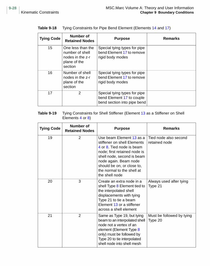
MSC.Marc Volume A: Theory and User InformationKinematic Constraints Chapter 9 Boundary Conditions
9-28
Table 9-18 Tying Constraints for Pipe Bend Element (Elements 14 and 17)
Tying CodeNumber of
Retained NodesPurpose Remarks
15 One less than the number of shell nodes in the z-r plane of the section
Special tying types for pipe bend Element 17 to remove rigid body modes
16 Number of shell nodes in the z-r plane of the section
Special tying types for pipe bend Element 17 to remove rigid body modes
17 2 Special tying types for pipe bend Element 17 to couple bend section into pipe bend
Table 9-19 Tying Constraints for Shell Stiffener (Element 13 as a Stiffener on Shell Elements 4 or 8)
Tying CodeNumber of
Retained NodesPurpose Remarks
19 2 Use beam Element 13 as a stiffener on shell Elements 4 or 8. Tied node is beam node; first retained node is shell node, second is beam node again. Beam node should be on, or close to, the normal to the shell at the shell node
Tied node also second retained node
20 3 Create an extra node in a shell Type 8 Element tied to the interpolated shell displacements with tying Type 21 to tie a beam Element 13 or a stiffener across a shell element
Always used after tying Type 21
21 2 Same as Type 19, but tying beam to an interpolated shell node not a vertex of an element (Element Type 8 only) must be followed by Type 20 to tie interpolated shell node into shell mesh
Must be followed by tying Type 20

9-29MSC.Marc Volume A: Theory and User InformationChapter 9 Boundary Conditions Kinematic Constraints
Rigid Link Constraint
Tying type 80 can be used to define a rigid link between nodes. This capability can be used for both small deformation and large deformation, large rotation problems. In small deformations, a linear constraint equation is used. In addition to the end points of the link, a second retained node must be given. This node is used to calculate and store the rigid body rotations. For two-dimensional problems, this represents a rotation about the Z-axis.
A complete rigid region can be modeled by using multiple tying type 80’s. In this case, the same two nodes are used for the retained nodes in all of the constraints.
The rigid links can be used with all elements except types 4, 8, 24, 15, 16, and 17. In addition, it should not be used in rigid plastic analysis.
Table 9-20 Tying constraints for Nodal Degrees of Freedom
Tying Code
Number of Retained Nodes
Purpose Remarks
I≤NDEG 1 Tie the Ith degree of freedom at the tied node to the Ith degree of freedom at the retained node
NDEG = number of degrees of freedom per node
100 1 Tie all degrees of freedom at the tied node to the corresponding degrees of freedom at the retained node
>100 1 Generate several tyings of type ≤NDEG
Tying code is first degree of freedom multiplied by 100 added to last degree of freedom (209 means tie second through ninth degree of freedom at tied node to respective second through ninth degree of freedom at retained node)
<0(negative integer)
User-defined User-generated tying type through the UFORMS user subroutine

MSC.Marc Volume A: Theory and User InformationKinematic Constraints Chapter 9 Boundary Conditions
9-30
Shell-to-Solid Tying
In many problems, a region exists that is modeled with both brick elements and shell elements. A particular case of this is shown is Figure 9-20 and Figure 9-21.
In the first case, an 8-node brick which has been reduced to a triangular prism is connected to a 4-node shell. In the second case, a 20-node brick is connected to an 8-node shell. An automatic constraint equation is developed between the elements. Note that the thickness of the shell must be entered as the brick thickness.
Figure 9-20 4-Node Shell-to-Solid Automatic Constraint
Figure 9-21 8-Node Shell-to-Solid Automatic Constraint
Table 9-21 Rigid Link Constraint
Tying Code
Number of Retained Nodes
Purpose Remarks
80 2 Define a rigid link between nodes
The second retained node is an unattached node which contains the rotation

9-31MSC.Marc Volume A: Theory and User InformationChapter 9 Boundary Conditions Kinematic Constraints
Support Conditions
Marc provides linear and nonlinear springs and foundations for the modeling of support conditions. For dynamic analysis, a dashpot can also be included.Table 9-22 lists input options for linear springs and elastic foundations.
The force in the spring is
(9-19)
where is the spring stiffness, is the displacement of the degree of freedom at the
second end of the spring, and is the displacement of the degree of freedom at the
first end of the spring. In a dynamic analysis, is the damping factor and and
are the velocities of the nodes.
You can specify the elements in Marc to be supported on a frictionless, elastic foundation. The foundation supports the structure with a force per unit area (force per unit length, for beams) given by
(9-20)
where is the equivalent spring stiffness of the foundation, and is the normal
displacement of the surface at a point in the same direction as .
The same conventions apply to the elastic foundation specification as for pressure specification, in terms of the face of the element that is used. The force is applied whether the displacement is tensile or compressive.
The USPRNG user subroutine allows you to supply a nonlinear spring stiffness or a nonlinear foundation stiffness as a function of prior displacement and force.
Table 9-22 Input Options for Linear Springs and Elastic Foundations
Load DescriptionInput Options
Model Definition History Definition User Subroutine
Linear Springs SPRINGS USPRNG
Elastic Foundation FOUNDATION FOUNDATION USPRNG
F K u2 u1–( ) D v2 v1–( )+=
K u2
u1
D v2 v1
pn Kun=
K un
pn

MSC.Marc Volume A: Theory and User InformationKinematic Constraints Chapter 9 Boundary Conditions
9-32
Cyclic SymmetryA special set of tying constraints for continuum elements can be automatically generated by the Marc program to effectively analyze structures with a geometry and a loading varying periodically about a symmetry axis. Figure 9-22 shows an example where, on the left-hand side, the complete structure is given and, on the right-hand side, a sector to be modeled.
Figure 9-22 Cyclic symmetric structure: complete model (left) and modeled sector (right)
Looking at points and on this segment, the displacement vectors should fulfil:
(9-21)
which can also be written as:
(9-22)
where the transformation matrix depends on the symmetry axis (which, in the
example above, coincides with the global Z-axis) and the sector angle (see Figure 9-22). In Marc, the input for the option CYCLIC SYMMETRY consists of the direction vector of the symmetry axis, a point on the symmetry axis and the sector angle . The following items should be noted:
X
Y
X
Y
x’y’
A
B
α
A B
u’B uA=
uB RuA=
Rα
α
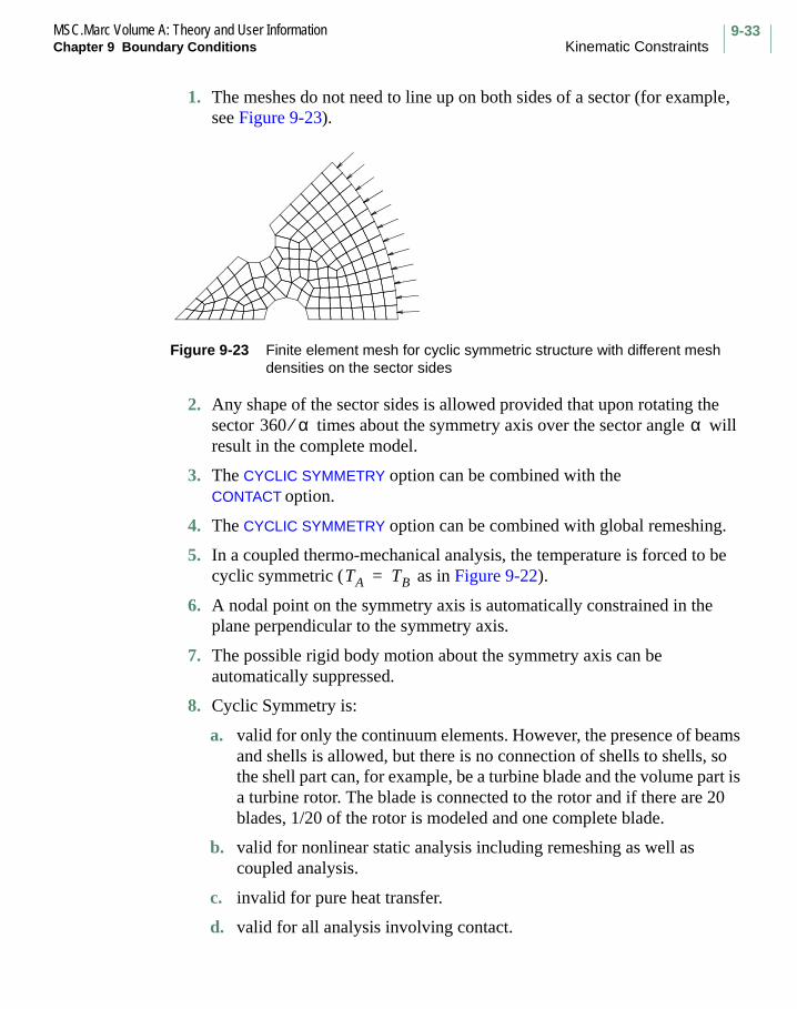
9-33MSC.Marc Volume A: Theory and User InformationChapter 9 Boundary Conditions Kinematic Constraints
1. The meshes do not need to line up on both sides of a sector (for example, see Figure 9-23).
Figure 9-23 Finite element mesh for cyclic symmetric structure with different mesh densities on the sector sides
2. Any shape of the sector sides is allowed provided that upon rotating the sector times about the symmetry axis over the sector angle will result in the complete model.
3. The CYCLIC SYMMETRY option can be combined with the CONTACT option.
4. The CYCLIC SYMMETRY option can be combined with global remeshing.
5. In a coupled thermo-mechanical analysis, the temperature is forced to be cyclic symmetric ( as in Figure 9-22).
6. A nodal point on the symmetry axis is automatically constrained in the plane perpendicular to the symmetry axis.
7. The possible rigid body motion about the symmetry axis can be automatically suppressed.
8. Cyclic Symmetry is:
a. valid for only the continuum elements. However, the presence of beams and shells is allowed, but there is no connection of shells to shells, so the shell part can, for example, be a turbine blade and the volume part is a turbine rotor. The blade is connected to the rotor and if there are 20 blades, 1/20 of the rotor is modeled and one complete blade.
b. valid for nonlinear static analysis including remeshing as well as coupled analysis.
c. invalid for pure heat transfer.
d. valid for all analysis involving contact.
360 α⁄ α
TA TB=

MSC.Marc Volume A: Theory and User InformationKinematic Constraints Chapter 9 Boundary Conditions
9-34
e. valid also for: eigenvalue analysis such as buckling or modal analysis, harmonic analysis, and transient dynamic analysis. However, there are restrictions in the case of modal analysis which are described in more detail in the following paragraphs.
To prevent confusion, it must be emphasized that the cyclic symmetry feature described above is different than linear cyclic symmetry commonly used in modal analysis where physical quantities such as, , displacements, forces, stresses and
temperature in the n-th segment are expanded in a Fourier series with terms of the
cyclic components, , in the fundamental region, like:
(9-23)
where k is the harmonic order; N is the total number of sectors; is the fundamental
inter-sector phase shift defined as ; and K is defined as:
(9-24)
There are considerable savings in both computing time and data storage associated with the use of the linear cyclic symmetry concept. Assuming a finite element model with a sector size of m degrees of freedom, a real-valued cyclic symmetry approach leads, in the worst case, to one eigenvalue problem of size m and
eigenvalue problems of size ; a complex approach leads to eigenvalue problems of size m; while the full analysis leads to a single, but very costly, eigenvalue problem
of size .
Although linear cyclic symmetry can reduce the problem size greatly, it is restricted to linear analysis, and the sector must have its surface mesh on the symmetry planes to be identical on each side of the sector. The nonlinear cyclic symmetry implemented in Marc can be used for nonlinear problems, such as contact, and the nodes do not need to line up on both symmetry planes of the sector (for example, see Figure 9-23).
xn
uk
xn1N----u0 2
N---- uk c,
n 1–( )kαcos uk s,n 1–( )sin kα+[ ] 1–( )n 1–
N--------------------u
N2----
+
k 1=
K
∑+=
α2π N⁄
K
N 1–2
------------- if N is odd
N 2–2
------------- if N is even
=
N 1–( ) 2⁄2m N
Nm

9-35MSC.Marc Volume A: Theory and User InformationChapter 9 Boundary Conditions Kinematic Constraints
Cross SectionIn various engineering applications, it is necessary to define a pre-stress in for example bolts or rivets before applying any other structural loading. Although such a pre-stressed state is often simulated using a temperature loading, it is rather difficult to arrive at a desired net force in the bolt or rivet. An easier way is to use the option CROSS-SECTION.
Generally speaking, a cross section in a model is defined by (see Figure 9-24):
1. All the nodes in the cross section;
2. The normal vector to the cross section;
3. All the elements sharing nodes in the cross section and lying on the side of the cross section corresponding to the opposite normal vector.
Figure 9-24 Cross section examples: regular mesh (left) and irregular mesh (right)
Notice that this option can be used for continuum as well as for beam and shell stress elements.
An additional node, called nc, has to be assigned to every cross section defined in a model. Such a node has only one degree of freedom, namely the displacement in the direction of the cross section normal vector, which is indicated as . Elements
corresponding to the cross section definition now get a modified displacement field,
1 2 3 4 12 3
45
6
Normal Normal
Cross Section Cross Section
Vector Vector
unc

MSC.Marc Volume A: Theory and User InformationKinematic Constraints Chapter 9 Boundary Conditions
9-36
depending on which nodes of the elements are part of the cross section. If the third and fourth node of a 4-node element are part of the cross section, the element displacement vector is changed according to (see Figure 9-25):
(9-25)
Similarly, if only the fourth node is part of the cross section, the element displacement vector is given by:
(9-26)
:
Figure 9-25 Cross section with 4-node elements: two nodes in cross section (left), one node in cross section (right)
As a result, the following is possible:
1. A force in the cross section can be defined by specifying a POINT LOAD on the first degree of freedom of node nc. Notice that this force works in the direction of the cross section normal vector. The resulting displacement of node nc can be seen as the shortening of the cross section elements.
2. A constant overclosure in the cross section can be obtained by specifying the first degree of freedom of node nc via the FIXED DISP or DISP CHANGE option. Then, the reaction force in node nc is the section force in the direction of the cross section normal vector.
UeT
u1T
, u2T
, u3T
uncnT+ , u4
TuncnT
+=
UeT
u1T
, u2T
, u3T
, u4T
uncnT+=
1
Cross Section
4 3
2
n
1
Cross Section
4
3
2
n

9-37MSC.Marc Volume A: Theory and User InformationChapter 9 Boundary Conditions Kinematic Constraints
During an analysis, you can switch from one of the above options to the other. So, to simulate the behavior of a pre-stressed bolt under additional loading conditions, you should first define the pre-tension force via the POINT LOAD option and subsequently use the DISP CHANGE option to "lock" the bolt by setting the incremental displacement to zero.
If you are only interested in the total force in the cross section, the displacement
should be set to zero. Then, the total force in the cross section is given by the reaction force in node nc.
∆unc
unc

MSC.Marc Volume A: Theory and User InformationChapter 9 Boundary Conditions
9-38

Chapter 10 Element Library
CHAPTER
10 Element Library
Truss Elements
Membrane Elements
Continuum Elements
Beam Elements
Plate Elements
Shell Elements
Heat Transfer Elements
Special Elements
Incompressible Elements
Constant Dilatation Elements
Reduced Integration Elements
Continuum Composite Elements
Fourier Elements

MSC.Marc Volume A: Theory and User InformationChapter 10 Element Library
10-2
Marc includes an extensive element library. The element library allows you to model various types of one-, two-, and three-dimensional structures, such as plane stress and plane strain structures, axisymmetric structures, full three-dimensional solid structures, and shell-type structures. Table 10-1 lists the element types in the library. Table 10-2 shows the structural classification of elements. (See MSC.Marc Volume B: Element Library for a detailed description of each element, a reference to the use of each element, and recommendations concerning the selection of element types for analysis).
After you select an element type or a combination of several element types for your analysis with the ELEMENTS or SIZING parameter, you must prepare the necessary input data for the element(s). In general, the data consist of element connectivity, thickness for two-dimensional beam, plate and shell elements, cross section for three-dimensional beam elements, coordinates of nodal points, and face identifications for distributed loadings.
You can choose different element types to represent various parts of the structure in an analysis. If there is an incompatibility between the nodal degrees of freedom of the elements, you have to provide appropriate tying constraints to ensure the compatibility of the displacement field in the structure. Marc assists you by providing many standard tying constraint options, but you are responsible for the consistency of your analysis.
You can use almost all of the Marc elements for both linear and nonlinear analyses, with the following exceptions.
• No plasticity or cracking is allowed in the elastic beams, the shear-panel, the Fourier, and the Herrmann (incompressible) elements.
• The updated Lagrange and finite strain plasticity features are not available for all elements.
Semi-infinite Elements
Assumed Strain Formulation
Follow Force Stiffness Contribution
Explicit Dynamics
Adaptive Mesh Refinement
References

10-3MSC.Marc Volume A: Theory and User InformationChapter 10 Element Library
• Only heat links and two-dimensional heat transfer elements can be used for hydrodynamic bearing analysis.
• Fourier analysis can be carried out only for a limited number of axisymmetric elements.
Marc defines all continuum elements in the global coordinate system. Truss, beam, plate, and shell elements are defined in a local coordinate system and the resulting output must be interpreted accordingly. You should give special attention to the use of these elements if the material properties have preferred orientations. The ORIENTATION option is available to define the preferred directions.
All Marc elements are numerically integrated. Element quantities, such as stresses, strains, and temperatures, are calculated at each integration point of the element if you use the ALL POINTS parameter. This is the default in Marc. These quantities are computed only at the centroid of the element, if the CENTROID parameter is used.
Table 10-1 Element Library
ElementUpdated LagrangeAvailable
Code
2-node axisymmetric shell element Yes (1)
Axisymmetric triangular ring element Yes (2)
Two-dimensional (plane stress) 4-node, isoparametric quadrilateral Yes (3)
Curved quadrilateral thin-shell element Yes (4)
Beam column No (5)
Two-dimensional plane strain, constant stress triangle Yes (6)
8-node isoparametric three-dimensional hexahedron Yes (7)
3-node triangular arbitrary shell Yes (8)
Three-dimensional truss element Yes (9)
Axisymmetric quadrilateral element (isoparametric) Yes (10)
Plane strain quadrilateral element (isoparametric) Yes (11)
Gap and friction element No (12)
Open-section beam No (13)
Closed-section beam Yes (14)
Isoparametric 2-node axisymmetric shell Yes (15)
Isoparametric 2-node curved beam Yes (16)
Pipe-bend element No (17)
4-node isoparametric membrane No (18)

MSC.Marc Volume A: Theory and User InformationChapter 10 Element Library
10-4
Generalized plane-strain quadrilateral Yes (19)
Axisymmetric torsional quadrilateral Yes (20)
Three-dimensional 20-node brick Yes (21)
Curved quadrilateral thick-shell element Yes (22)
Three-dimensional, 20-node rebar element No (23)
Curved quadrilateral shell element Yes (24)
Closed-section beam in three dimensions Yes (25)
Plane stress, 8-node distorted quadrilateral Yes (26)
Plane strain, 8-node distorted quadrilateral Yes (27)
Axisymmetric, 8-node distorted quadrilateral Yes (28)
Generalized plane strain distorted quadrilateral Yes (29)
Membrane 8-node distorted quadrilateral No (30)
Elastic Curved Pipe (Elbow)/Straight Beam Element No (31)
Plane strain, 8-node distorted quadrilateral, for incompressible behavior
Yes (32)
Axisymmetric 8-node distorted quadrilateral, for incompressible behavior
Yes (33)
Generalized plane strain 8-node distorted quadrilateral for incompressible behavior
No (34)
Three-dimensional 20-node brick for incompressible behavior Yes (35)
Heat transfer element (three-dimensional link) No (36)
Heat transfer element (arbitrary planar triangle) No (37)
Heat transfer element (arbitrary axisymmetric triangle) No (38)
Heat transfer element (planar bilinear quadrilateral) No (39)
Heat transfer element (axisymmetric bilinear quadrilateral No (40)
Heat transfer element (8-node planar biquadratic quadrilateral No (41)
Heat transfer element (8-node axisymmetric biquadratic quadrilateral)
No (42)
Heat transfer element (three-dimensional 8-node brick) No (43)
Heat transfer element (three-dimensional 20-node brick) No (44)
Curved Timoshenko beam element in a plane Yes (45)
Plane strain rebar element No (46)
Generalized plane strain rebar element No (47)
Table 10-1 Element Library (Continued)
ElementUpdated LagrangeAvailable
Code

10-5MSC.Marc Volume A: Theory and User InformationChapter 10 Element Library
Axisymmetric rebar element No (48)
Triangular thin shell element Yes (49)
Triangular heat transfer shell element No (50)
Cable Element No (51)
Elastic beam Yes (52)
Plane stress 8-node quadrilateral with reduced integration Yes (53)
Plane strain 8-node distorted quadrilateral with reduced integration Yes (54)
Axisymmetric 8-node distorted quadrilateral with reduced integration
Yes (55)
Generalized plane strain 10-node distorted quadrilateral with reduced integration
Yes (56)
Three-dimensional 20-node brick with reduced integration Yes (57)
Plane strain 8-node distorted quadrilateral for incompressible behavior with reduced integration
Yes (58)
Axisymmetric 8-node distorted quadrilateral for incompressible behavior with reduced integration
Yes (59)
Generalized plane strain 10-node distorted quadrilateral incompressible behavior with reduced integration
No (60)
Three-dimensional 20-node brick for incompressible behavior with reduced integration
Yes (61)
Axisymmetric 8-node quadrilateral for arbitrary loading No (62)
Axisymmetric 8-node quadrilateral for arbitrary loading, and incompressible behavior
No (63)
Isoparametric 3-node truss element Yes (64)
Heat transfer element 3-node truss (three-dimensional link) No (65)
8-node axisymmetric with twist, for incompressible behavior No (66)
8-node axisymmetric with twist No (67)
Elastic 4-node shear panel No (68)
Heat transfer element (8-node, planar biquadratic quadrilateral with reduced integration)
No (69)
Heat transfer element (8-node, axisymmetric biquadratic quadrilateral with reduced integration)
No (70)
Heat transfer element (three-dimensional 20-node brick with reduced integration)
No (71)
Table 10-1 Element Library (Continued)
ElementUpdated LagrangeAvailable
Code
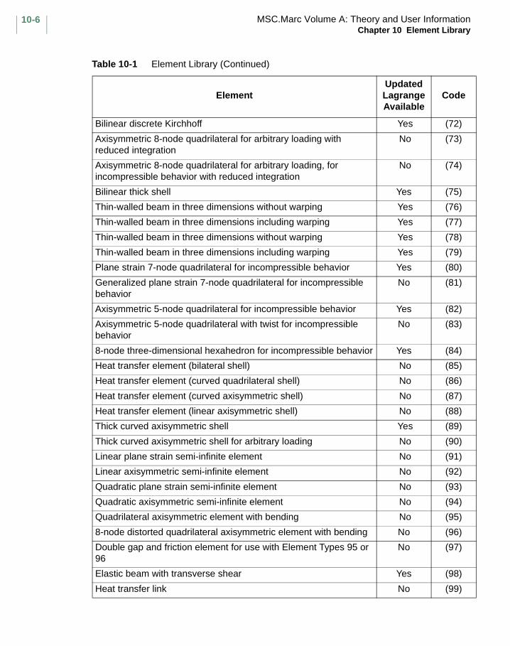
MSC.Marc Volume A: Theory and User InformationChapter 10 Element Library
10-6
Bilinear discrete Kirchhoff Yes (72)
Axisymmetric 8-node quadrilateral for arbitrary loading with reduced integration
No (73)
Axisymmetric 8-node quadrilateral for arbitrary loading, for incompressible behavior with reduced integration
No (74)
Bilinear thick shell Yes (75)
Thin-walled beam in three dimensions without warping Yes (76)
Thin-walled beam in three dimensions including warping Yes (77)
Thin-walled beam in three dimensions without warping Yes (78)
Thin-walled beam in three dimensions including warping Yes (79)
Plane strain 7-node quadrilateral for incompressible behavior Yes (80)
Generalized plane strain 7-node quadrilateral for incompressible behavior
No (81)
Axisymmetric 5-node quadrilateral for incompressible behavior Yes (82)
Axisymmetric 5-node quadrilateral with twist for incompressible behavior
No (83)
8-node three-dimensional hexahedron for incompressible behavior Yes (84)
Heat transfer element (bilateral shell) No (85)
Heat transfer element (curved quadrilateral shell) No (86)
Heat transfer element (curved axisymmetric shell) No (87)
Heat transfer element (linear axisymmetric shell) No (88)
Thick curved axisymmetric shell Yes (89)
Thick curved axisymmetric shell for arbitrary loading No (90)
Linear plane strain semi-infinite element No (91)
Linear axisymmetric semi-infinite element No (92)
Quadratic plane strain semi-infinite element No (93)
Quadratic axisymmetric semi-infinite element No (94)
Quadrilateral axisymmetric element with bending No (95)
8-node distorted quadrilateral axisymmetric element with bending No (96)
Double gap and friction element for use with Element Types 95 or 96
No (97)
Elastic beam with transverse shear Yes (98)
Heat transfer link No (99)
Table 10-1 Element Library (Continued)
ElementUpdated LagrangeAvailable
Code

10-7MSC.Marc Volume A: Theory and User InformationChapter 10 Element Library
Heat transfer link No (100)
6-node planar semi-infinite heat transfer No (101)
6-node axisymmetric semi-infinite heat transfer No (102)
9-node planar semi-infinite heat transfer No (103)
9-node axisymmetric semi-infinite heat transfer No (104)
12-node 3-D semi-infinite heat transfer No (105)
27-node 3-D semi-infinite heat transfer No (106)
12-node 3-D semi-infinite No (107)
27-node 3-D semi-infinite No (108)
8-node 3-D magnetostatic No (109)
12-node 3-D semi-infinite magnetostatic No (110)
4-Node Quadrilateral Planar Electromagnetic No (111)
4-Node Quadrilateral Axisymmetric Electromagnetic No (112)
8-Node Quadrilateral Three-Dimensional Electromagnetic No (113)
4-Node Quadrilateral Plane Stress, Reduced Integration with Hourglass Control
Yes (114)
4-Node Quadrilateral Plane Strain, Reduced Integration with Hourglass Control
Yes (115)
4-Node Quadrilateral Axisymmetric, Reduced Integration with Hourglass Control
Yes (116)
8-Node Three-Dimensional Brick, Reduced Integration with Hourglass Control
Yes (117)
Incompressible 4+1-Node, Quadrilateral, Plane Strain, Reduced Integration with Hourglass Control
No (118)
Incompressible 4+1-Node, Quadrilateral, Axisymmetric, Reduced Integration with Hourglass Control
No (119)
Incompressible 8+1-Node, Three-Dimensional Brick, Reduced Integration with Hourglass Control
No (120)
4-Node, Heat Transfer Planar, Reduced Integration with Hourglass Control
No (121)
4-Node, Heat Transfer Axisymmetric, Reduced Integration with Hourglass Control
No (122)
8-Node, Heat Transfer Three-Dimensional Brick, Reduced Integration with Hourglass Control
No (123)
Table 10-1 Element Library (Continued)
ElementUpdated LagrangeAvailable
Code

MSC.Marc Volume A: Theory and User InformationChapter 10 Element Library
10-8
6-Node, Plane Stress Triangle Yes (124)
6-Node, Plane Strain Triangle Yes (125)
6-Node, Axisymmetric Triangle Yes (126)
10-Node, Tetrahedron Yes (127)
Incompressible, 6-Node Triangle Yes (128)
Incompressible, 6-Node Triangle Yes (129)
Incompressible, 10-Node Tetrahedral Yes (130)
6-Node, Heat Transfer Planar No (131)
6-Node, Heat Transfer Plane Axisymmetric No (132)
10-Node, Heat Transfer Tetrahedral No (133)
Four-node, Tetrahedral Yes (134)
Four-node, Heat Transfer Tetrahedral No (135)
Three-node, Thin Shell Yes (138)
Four-node, Thin Shell Yes (139)
Four-Node, Thick Shell, Reduced Integration with Hourglass Control
Yes (140)
Eight-node Axisymmetric Rebar with Twist No (142)
Four-node Plane Strain Rebar No (143)
Four-node Axisymmetric Rebar No (144)
Four-node Axisymmetric Rebar with Twist No (145)
Eight-node Brick Rebar No (146)
Four-node Membrane Rebar No (147)
Eight-node Membrane Rebar No (148)
Eight-node Composite Brick Yes (149)
Twenty-node Composite Brick Yes (150)
Four-node Plane Strain Composite Yes (151)
Four-node Axisymmetric Composite Yes (152)
Eight-node Plane Strain Composite Yes (153)
Eight-node Axisymmetric Composite Yes (154)
3 + 1-node Incompressible Plane Strain Triangle Yes (155)
3 + 1-node Incompressible Axisymmetric Triangle Yes (156)
4 + 1-node Incompressible Tetrahedron Yes (157)
Table 10-1 Element Library (Continued)
ElementUpdated LagrangeAvailable
Code

10-9MSC.Marc Volume A: Theory and User InformationChapter 10 Element Library
Table 10-2 Structural Classification of Elements
Element Structural Type
Element Number
Function Remarks
Three-dimensional truss 9 Linear 2-node straight
12 Linear 4-node straight gap and friction
51 Analytic 2-node cable element
64 Quadratic 3-node curved
97 Linear 4-node straight double gap and friction
Two-dimensional beam column
5 Linear/cubic 2-node straight
16 Cubic 2-node curved
45 Cubic 3-node curved Timoshenko theory
Three-dimensional beam column
13 Cubic 2-node curved open section
14 Linear/cubic 2-node straight closed section
25 Cubic 2-node straight closed section
31 Analytic 2-node elastic
52 Linear/cubic 2-node straight elastic
76 Linear/cubic 2 + 1-node straight closed section; use with Element 72
77 Linear/cubic 2 + 1-node straight open section; use with Element 72
78 Linear/cubic 2-node straight closed section; use with Element 75
79 Linear/cubic 2-node straight open section
98 Linear 2-node straight Timoshenko theory
Axisymmetric shell 1 Linear/cubic 2-node straight
15 Cubic 2-node curved
89 Quadratic 3-node curved thick shell theory
90 Quadratic 3-node curved with arbitrary loading; thick shell theory
Plane stress 3 Linear 4-node quadrilateral
26 Quadratic 8-node quadrilateral
53 Quadratic 8-node reduced integration quadrilateral
114 Linear/Assumed strain 4-node quadrilateral, reduced integration, with hourglass control
124 Quadratic 6-node triangle

MSC.Marc Volume A: Theory and User InformationChapter 10 Element Library
10-10
Plane strain 6 Linear 3-node triangle
11 Linear 4-node quadrilateral
27 Quadratic 8-node quadrilateral
54 Quadratic 8-node reduced integration quadrilateral
91 Linear/special 6-node semi-infinite
93 Quadratic/special 9-node semi-infinite
115 Linear/Assumed strain 4-node quadrilateral, reduced integration, with hourglass control
125 Quadratic 6-node triangle
Generalized plane strain
19 Linear 4 + 2-node quadrilateral
29 Quadratic 8 + 2-node quadrilateral
56 Quadratic 8 + 2-node reduced integration quadrilateral
Axisymmetric solid 2 Linear 3-node triangle
10 Linear 4-node quadrilateral
20 Linear 4-node quadrilateral with twist
28 Quadratic 8-node quadrilateral
55 Quadratic 8-node reduced integration quadrilateral
62 Quadratic 8-node quadrilateral with arbitrary loading
67 Quadratic 8-node quadrilateral with twist
73 Quadratic 8-node reduced integration quadrilateral and arbitrary loading
92 Linear/special 6-node semi-infinite
94 Quadratic/special 9-node semi-infinite
95 Linear 4-node quadrilateral with bending
96 Quadratic 8-node quadrilateral with bending
116 Linear/Assumed strain 4-node quadrilateral, reduced integration, with hourglass control
126 Quadratic 6-node triangle
Membrane three-dimensional
18 Linear 4-node quadrilateral
30 Quadratic 8-node quadrilateral
Table 10-2 Structural Classification of Elements (Continued)
Element Structural Type
Element Number
Function Remarks

10-11MSC.Marc Volume A: Theory and User InformationChapter 10 Element Library
Doubly-curved thin shell 4 Cubic 4-node curved quadrilateral
8 Fractional cubic 3-node curved triangle
24 Cubic patch 4 + 4-node curved quadrilateral
49 Linear 3 + 3-node curved triangle discrete Kirchhoff
72 Linear 4 + 4-node twisted quadrilateral discrete Kirchhoff
138 Linear 3-node triangle discrete Kirchhoff
139 Linear 4-node twisted quadrilateral discrete Kirchhoff
Doubly-curved thick shell
22 Quadratic 8-node curved quadrilateral with reduced integration
75 Linear 4-node twisted quadrilateral
140 Linear 4-node twisted quadrilateral, reduced integration with hourglass control
Three-dimensional solid 7 Linear 8-node hexahedron
21 Quadratic 20-node hexahedron
57 Quadratic 20-node reduced integration hexahedron
107 Linear/special 12-node semi-infinite
108 Quadratic 27-node semi-infinite special
117 Linear/Assumed strain 8-node hexahedron, reduced integration with hourglass control
127 Quadratic 10-node tetrahedron
134 Linear 4-node tetrahedron
Incompressible plane strain
32 Quadratic 8-node quadrilateral
58 Quadratic 8-node reduced integration quadrilateral
80 Linear 4 + 1-node quadrilateral
118 Linear/Assumed strain 4 + 1-node quadrilateral, reduced integration with hourglass control
128 Quadratic 6-node triangle
155 Linear 3 + 1-node triangle
Incompressible generalized plane strain
34 Quadratic 8 + 2-node quadrilateral
60 Quadratic 8 + 2-node with reduced integration quadrilateral
81 Linear 4 + 3-node quadrilateral
Table 10-2 Structural Classification of Elements (Continued)
Element Structural Type
Element Number
Function Remarks

MSC.Marc Volume A: Theory and User InformationChapter 10 Element Library
10-12
Incompressible axisymmetric
33 Quadratic 8-node quadrilateral
59 Quadratic 8-node with reduced integration quadrilateral
63 Quadratic 8-node quadrilateral with arbitrary loading
66 Quadratic 8-node quadrilateral with twist
74 Quadratic 8-node reduced integration quadrilateral with arbitrary loading
82 Linear 4 + 1-node quadrilateral
83 Linear 4 + 1-node quadrilateral with twist
119 Linear/Assumed strain 4 + 1-node quadrilateral reduced integration, with hourglass control
129 Quadratic 6-node triangle
156 Linear 3 + 1-node triangle
Incompressible three-dimensional solid
35 Quadratic 20-node hexahedron
61 Quadratic 20-node with reduced integration hexahedron
84 Linear 8 + 1-node hexahedron Node 9
120 Linear/Assumed strain 8 + 1-node hexahedron, reduced integration with hourglass control
130 Quadratic 10-node tetrahedron
157 Linear 4 + 1-node tetrahedron
Pipe bend 17 Cubic 2-nodes in-section; 1-node out-of-section
31 Special 2-node elastic
Table 10-2 Structural Classification of Elements (Continued)
Element Structural Type
Element Number
Function Remarks

10-13MSC.Marc Volume A: Theory and User InformationChapter 10 Element Library
Rebar Elements 23 Quadratic 20-node hexahedron
46 Quadratic 8-node quadrilateral plane strain
47 Quadratic 8 + 2-node quadrilateral generalized plane strain
48 Quadratic 8-node quadrilateral axisymmetric
142 Quadratic 8-node axisymmetric with twist
143 Linear 4-node plane strain
144 Linear 4-node axisymmetric
145 Linear 4-node axisymmetric with twist
146 Linear 8-node hexahedron
147 Linear 4-node membrane
148 Quadratic 8-node membrane
Continuum Composite 149 Linear 8-node brick
150 Quadratic 20-node brick
151 Linear 4-node quadrilateral plane strain
152 Linear 4-node quadrilateral axisymmetric
153 Quadratic 8-node quadrilateral plane strain
154 Quadratic 8-node quadrilateral axisymmetric
Three-dimensional shear panel
68 Linear 4-node quadrilateral
Heat conduction three-dimensional link
36 Linear 2-node straight
65 Quadratic 3-node curved
Heat conduction planar 37 Linear 3-node triangle
39 Linear 4-node quadrilateral
41 Quadratic 8-node quadrilateral
69 Quadratic 8-node reduced integration quadrilateral
101 Linear/special 6-node semi-infinite
103 Linear/special 9-node semi-infinite
121 Linear 4-node quadrilateral, reduced integration, with hourglass control
131 Quadratic 6-node triangular
Table 10-2 Structural Classification of Elements (Continued)
Element Structural Type
Element Number
Function Remarks

MSC.Marc Volume A: Theory and User InformationChapter 10 Element Library
10-14
Heat conduction axisymmetric
38 Linear 3-node triangle
40 Linear 4-node quadrilateral
42 Quadratic 8-node quadrilateral
70 Quadratic 8-node reduced integration quadrilateral
102 Linear/special 6-node semi-infinite
104 Quadratic/special 9-node semi-infinite
122 Linear 4-node quadrilateral, reduced integration, with hourglass control
132 Quadratic 6-node triangular
Heat conduction solids 43 Linear 8-node hexahedron
44 Quadratic 20-node hexahedron
71 Quadratic 20-node reduced integration hexahedron
105 Linear/special 12-node semi-infinite
106 Quadratic/special 27-node semi-infinite
123 Linear 8-node hexahedron, reduced integration, with hourglass control
133 Quadratic 10-node tetrahedron
135 Linear 4-node tetrahedron
Heat conduction shell 50 Linear 3-node triangle
85 Linear 4-node quadrilateral
86 Quadratic 8-node quadrilateral
Heat conduction axisymmetric shell
87 Quadratic 3-node curved
88 Linear 2-node straight
Magnetostatic three-dimensional solids
109 Linear 8-node hexahedron
110 Linear/special 12-node semi-infinite
Electromagnetic Planar 111 Linear 4-node quadrilateral
Electromagnetic Axisymmetric
112 Linear 4-node quadrilateral
Electromagnetic Solid 113 Linear 8-node hexahedron
Table 10-2 Structural Classification of Elements (Continued)
Element Structural Type
Element Number
Function Remarks

10-15MSC.Marc Volume A: Theory and User InformationChapter 10 Element Library
Distributed loads can be applied along element edges, over element surfaces, or in the volume of the element. Marc automatically evaluates consistent nodal forces through numerical integration. (See MSC.Marc Volume B: Element Library for details on this process). Concentrated forces must be applied at the nodal points.
All plate and shell elements can be used in a composite analysis. You can have a variable thickness shell, and control the thickness and material property and orientation for each layer. For the thick shell elements (types 22, 45, or 75), the interlaminar shear can also be calculated.
Five concepts differentiate the various elements types. These concepts are summarized in Table 10-1 and Table 10-2 and are listed below.
1. The type of geometric domain that the element is modeling. These geometric domains are:
TrussMembraneBeamPlateShellPlane stressPlane strainGeneralized plane strainAxisymmetricThree-dimensional solidSpecial
2. The type of interpolation (shape) functions used in the element. These functions are:
Linear QuadraticCubicHermitian Special
The interpolation function is used to describe the displacement at an arbitrary point in the body.
(10-1)
where is the displacement at x, are the interpolation (shape)
functions, and are the generalized nodal displacements.
ui x( ) Ni x( )ui=
u x( ) N
u

MSC.Marc Volume A: Theory and User InformationChapter 10 Element Library
10-16
Engineering strain is
(10-2)
Therefore, the computational evaluation is
(10-3)
Hence,
(10-4)
3. The number of nodes in a particular element.
4. The number of degrees of freedom associated with each node, and the type of degrees of freedom.
5. The integration method used to evaluate the stiffness matrix. Marc contains elements which use full integration and reduced integration.
εij x( ) 1 2∂ui x( )
∂xj---------------
∂uj x( )∂xi
---------------+ ⁄=
εij x( ) 1 2⁄∂Niui
∂xj-------------
∂Njuj
∂xi-------------+
βijui= =
βij
∂Ni
∂xj--------=

10-17MSC.Marc Volume A: Theory and User InformationChapter 10 Element Library Truss Elements
Truss Elements
Marc contains 2- and 3-node isoparametric truss elements that can be used in three dimensions. These elements have only displacement degrees of freedom.
Since truss elements have no shear resistance, you must ensure that there are no rigid body modes in the system.

MSC.Marc Volume A: Theory and User InformationMembrane Elements Chapter 10 Element Library
10-18
Membrane Elements
Marc contains 4- and 8-node isoparametric membrane elements that can be used in three dimensions. These elements have only displacement degrees of freedom.
Since membrane elements have no bending resistance, you must ensure that there are no rigid body modes in the system.
Membrane elements are often used in conjunction with beam or truss elements.

10-19MSC.Marc Volume A: Theory and User InformationChapter 10 Element Library Continuum Elements
Continuum Elements
Marc contains continuum elements that can be used to model plane stress, plane strain, generalized plane strain, axisymmetric and three-dimensional solids. These elements have only displacement degrees of freedom. As a result, solid elements are not efficient for modeling thin structures dominated by bending. Either beam or shell elements should be used in these cases.
The solid elements that are available in Marc have either linear or quadratic interpolation functions.
They include
• 4-, 6-, and 8-node plane stress elements
• 3-, 4-, 6-, and 8-node plane strain elements
• 6 (4 plus 2)- and 10 (8 plus 2)-node generalized plane strain elements
• 3-, 4-, 6-, and 8-node axisymmetric ring elements
• 8-, 10-, and 20-node brick elements
• 4- and 10-node tetrahedron
In general, the elements in Marc use a full-integration procedure. Some elements use reduced integration. The lower-order reduced integration elements include an hourglass stabilization procedure to eliminate the singular modes.
Continuum elements are widely used for thermal stress analysis. For each of these elements, there is a corresponding element available for heat transfer analysis in Marc. As a result, you can use the same mesh for the heat transfer and thermal stress analyses.
Marc has no singular element for fracture mechanics analysis. However, the simulation of stress singularities can be accomplished by moving the midside nodes of 8-node quadrilateral and 20-node brick elements to quarter-point locations near the crack tip. Many fracture mechanics analyses have used this quarter-point technique successfully.
The 4- and 8-node quadrilateral elements can be degenerated into triangles, and the 8-and 20-node solid brick elements can be degenerated into wedges and tetrahedra by collapsing the appropriate corner and midside nodes. The number of nodes per element is not reduced for degenerated elements. The same node number is used repeatedly for collapsed sides or faces. When degenerating incompressible elements, exercise caution to ensure that a proper number of Lagrange multipliers remain. You are advised to use the higher-order triangular or tetrahedron elements wherever possible, as opposed to using collapsed quadrilaterals and hexahedra.

MSC.Marc Volume A: Theory and User InformationBeam Elements Chapter 10 Element Library
10-20
Beam Elements
Marc’s beam elements are 2- and 3-node, two- and three-dimensional elements that can model straight and curved-beam structures and framed structures and can serve as stiffeners in plate and shell structures. A straight beam of a circular cross section can be used for modeling the straight portion of piping systems. Translational and rotational degrees of freedom are included in beam elements. The cross-section of the beam can be standard rectangular, circular sections, or arbitrarily closed or open sections. The BEAM SECT parameter is used to define an arbitrary closed or open cross section.
The beam elements are numerically integrated along their axial direction using Gaussian integration. The stress strain law is integrated through the cross section using Simpson’s rule. Stresses and strains are evaluated at each integration point through the thickness. This allows an accurate calculation if nonlinear material behavior is present. In elastic beam elements, only the total axial force and moments are computed at the integration points.

10-21MSC.Marc Volume A: Theory and User InformationChapter 10 Element Library Plate Elements
Plate Elements
The linear shell elements (Types 49, 72, 75, 138, 139, or 140) or the quadratic element (Type 22) can be used effectively to model plates and have the advantage that tying is unnecessary. For element type 49, you can indicate on the GEOMETRY option that the flat plate formulation is to be used. This reduces computational costs. To further reduce computational costs for linear elastic plate analysis, the number of points through the thickness can be reduced to one by use of the SHELL SECT parameter.

MSC.Marc Volume A: Theory and User InformationShell Elements Chapter 10 Element Library
10-22
Shell Elements
Marc contains three isoparametric, doubly curved, thin shell elements: 3-, 4-, and 8-node elements (Types 4, 8, and 24, respectively) based on Koiter-Sanders shell theory.
These elements are C1 continuous and exactly represent rigid-body modes. The program defines a mesh of these elements with respect to a surface curvilinear coordinate system. You can use the FXORD model definition option to generate the nodal coordinates. Tying constraints must be used at shell intersections.
Thin shell analysis can be performed using either the 3-node discrete Kirchhoff theory (DKT) based element (Type 138), the 4-node bilinear DKT element (Type 139), the 6-node bilinear semi-loof element (Type 49), or the 8-node bilinear semi-loof element (Type 72). Thick shell analysis can be performed using the 4-node bilinear Mindlin element (Type 75), the 4-node reduced integration with hourglass Mindlin element (Type 140), or the 8-node quadratic Mindlin element (Type 22). The thick shell elements have been developed so that there is no locking when used for thin shell applications.
The global coordinate system defines the nodal degrees of freedom of these elements. These elements are convenient for modeling intersecting shell structures since tying constraints at the shell intersections are not needed.
Marc contains three axisymmetric shell elements: 2-node straight, 2-node curved, and 3-node curved. You can use these elements to model axisymmetric shells; combined with axisymmetric ring elements, they can be used to simulate the thin and thick portions of the structure. The program provides standard tying constraints for the transition between shell and axisymmetric ring elements.

10-23MSC.Marc Volume A: Theory and User InformationChapter 10 Element Library Heat Transfer Elements
Heat Transfer Elements
The heat transfer elements in Marc consist of the following:
• 2- and 3-node three-dimensional links
• 3-, 4-, 6-, and 8-node planar and axisymmetric elements
• 6- and 9-node planar and axisymmetric semi-infinite elements
• 8-, 10-, and 20-node solid elements
• 12- and 27-node semi-infinite brick elements
• 2-, 3-, 4-, 6-, and 8-node shell elements.
For each heat transfer element, there is at least one corresponding stress element, enabling you to use the same mesh for both the heat transfer and thermal stress analyses. Heat transfer elements are also employed to analyze coupled thermo-electrical (Joule heating) problems.
In heat transfer elements, temperature is the only nodal degree of freedom. In heat transfer shell elements, two or three temperatures through the thickness are used as nodal degrees of freedom. In Joule heating, the voltage and temperature are the nodal degrees of freedom.
Acoustic Analysis
Heat transfer elements are also used to model the compressible media in acoustic analysis. In this case, the pressure is the single nodal degree of freedom.
Electrostatic Analysis
Heat transfer elements are also used for electrostatic analysis. The scalar potential is the degree of freedom.
Fluid/Solid Interaction
Heat transfer elements are used to model the inviscid, incompressible fluid/solid interaction problems. The hydrostatic pressure is the degree of freedom.
Hydrodynamic Bearing Analysis
The three-dimensional heat transfer links and planar elements are used to model the lubricant film. As no variation occurs through the thickness of the film, two-dimensional problems are reduced to one-dimensional, and three-dimensional problems are reduced to two-dimensional. The pressure is the degree of freedom.

MSC.Marc Volume A: Theory and User InformationHeat Transfer Elements Chapter 10 Element Library
10-24
Magnetostatic Analysis
For two-dimensional problems, a scalar potential can be used; hence, the heat transfer planar and axisymmetric elements are employed. The single degree of freedom is the potential. For three-dimensional analyses, magnetostatic elements are available. In such cases, there are three degrees of freedom to represent the vector potential.
Electromagnetic Analysis
In electromagnetic problems, a vector potential, augmented with a scalar potential, is used. There are lower-order elements available for these analyses.
Soil Analysis
There are three types of soil/pore pressure analysis. If a pore pressure analysis only is performed, “heat transfer” elements (41, 42, or 44) are used. If an uncoupled soil analysis is performed, the standard elements (21, 27, or 28) are used. If a coupled analysis is performed, the Herrmann elements (32, 33, or 35) are used. In this case, the last degree of freedom is the pore pressure.
Fluid Analysis
When performing fluid analysis, any planar, axisymmetric or solid continuum element can be used. These elements either used a mixed formulation or a penalty formulation based upon the value of the FLUID parameter. For the mixed formulation, each node of lower- or higher-order continuum element has velocities as well as pressure degrees of freedom. The penalty method yields elements with only the velocities as the nodal variables.

10-25MSC.Marc Volume A: Theory and User InformationChapter 10 Element Library Special Elements
Special Elements
Marc contains a gap-and-friction element, a pipe bend element, a shear-panel element, and several rebar elements. All are unique features in the program.
The gap-and-friction element (12, 97) is based on the imposition of gap closure constraint and frictional-stick or frictional-slip through Lagrange multipliers. This element provides frictional and gapping connection between any two nodes of a structure; it can be used in several variations, depending on the application. In the default formulation, the element simulates a gap in a fixed direction, such that a body does not penetrate a given flat surface. Using the optional formulation, you can constrain the true distance between two end-points of the gap to be greater than some arbitrary distance. This ability is useful for an analysis in which a body does not penetrate a given two-dimensional circular or three-dimensional spherical surface. Finally, you can update the gap direction and closure distance during analysis for the modeling of sliding along a curved surface.
The pipe-bend (3-node elbow) element 17 is designed for linear and nonlinear analysis of piping systems. It is a modified axisymmetric shell element for modeling the bends in a piping system. The element has a beam mode superposed on the axisymmetric shell modes so that ovalization of the cross-section is admitted. The twisting of a pipe-bend section is ignored because the beam has no flexibility in torsion. Built-in tying constraints are used extensively for coupling the pipe-bend sections to each other and to straight beam elements.
The curved-pipe (2-node) element 31 is designed for linear analysis only. The stiffness matrix is based upon the analytic elastic solution of a curved pipe.
The shear panel (element 68) is a 4-node, elastic element of arbitrary shape. It is an idealized model of an elastic sheet. This element only provides shearing resistance. It must be used with beam stiffeners to ensure any normal or bending resistance. The shear-panel element is restricted to linear material and small displacement analysis.
The cable element (51) is an element which exactly represents the catenary behavior of a cable. It is an elastic element only.
The rebar elements (23, 46, 47, 48, 142, 143, 144, 145, 146, 147, and 148) are hollow elements in which you can place single-direction strain members (reinforcing cords or rods). A rebar element is used in conjunction with another solid element (filler) to represent a reinforced material such as reinforced concrete. The reinforcing members and the filler are accurately represented by the superposition of rebar and solid elements. The rebar elements can be used for small as well as large strain behavior of the reinforcing cords. Also, any kind of material behavior can be simulated by the rebar elements in Marc.

MSC.Marc Volume A: Theory and User InformationIncompressible Elements Chapter 10 Element Library
10-26
Incompressible Elements
Incompressible and nearly incompressible materials can be modeled by using a special group of elements in the program. These elements, based on modified Hermann variational principles, are capable of handling large deformation effects as well as creep and thermal strains. The incompressibility constraint is imposed by using Lagrange multipliers. Generally, the low (linear) order elements have a single additional node which contains the Lagrange multiplier, while the high-order (quadratic) elements have Lagrange multipliers at each corner node.
Elements 155 (plane strain triangle), 156 (axisymmetric triangle), and 157 (3-D tetrahedron) are low-order elements and are exceptions within the incompressible element group. They have an additional node located at the center of the elements and have Lagrange multipliers at each corner node. The shape function of the center node is a bubble function. See Figure 10-1 for an element 155 case. The degrees of freedom of the center node is condensed out on the element level before the assembly of the global matrix.
Figure 10-1 Element 155
Large Strain Elasticity
The incompressible elements based on Hermann formulations can be used for large strain analysis of rubber-like materials, using either total Lagrangian formulation or updated Lagrangian formulation.
x
1
2
3
4
Nodes with both displacements and pressure as degrees of freedom
Center node with only displacement degrees of freedom. The shape function for this node is a bubble function.
x

10-27MSC.Marc Volume A: Theory and User InformationChapter 10 Element Library Incompressible Elements
Large Strain Plasticity
The incompressible elements can be used for large strain analysis of elasto-plastic materials using updated Lagrangian formulation, based on multiplicative decomposition of deformation gradient.
Rigid-Plastic Flow
In rigid-plastic flow analysis, with effectively no elasticity, incompressible elements must be used. For such analyses, you have a choice of using either the elements with Lagrange multipliers discussed above, or standard displacement continuum elements. In the latter case, a penalty function is used to satisfy the incompressibility constraint.

MSC.Marc Volume A: Theory and User InformationConstant Dilatation Elements Chapter 10 Element Library
10-28
Constant Dilatation Elements
You can choose an integration scheme option, which makes the dilatational strain constant throughout the element. This can be accomplished using the CONSTANT DILATATION parameter or by setting the second field of the GEOMETRY option to one. Constant dilatational elements are recommended for use in approximately incompressible, inelastic analysis, such as large strain plasticity, because conventional elements can produce volumetric locking due to overconstraints for nearly incompressible behavior. This option is only available for elements of lower order (Types 7, 10, 11, 19, and 20). For the lower-order reduced integration elements (114 to 117) with hourglass control, as only one integration point is used, these elements do not lock, and effectively, a constant dilatation formulation is used. (The constant dilatation approach has also been referred to mean dilatation and B-bar approach in literature.)

10-29MSC.Marc Volume A: Theory and User InformationChapter 10 Element Library Reduced Integration Elements
Reduced Integration Elements
Marc uses a reduced integration scheme to evaluate the stiffness matrix or the thermal conductivity matrix for a number of isoparametric elements. The mass matrix and the specific heat matrix of the element are always fully integrated.
For lower-order, 4-node quadrilateral elements, the number of numerical integration points is reduced from 4 to 1; in 8-node solid elements, the number of numerical integration points is reduced from 8 to 1. For 8-node quadrilateral elements, the number of numerical integration points is reduced from 9 to 4; for 20-node solid elements, the number of numerical integration points is reduced from 27 to 8.
The energy due to the higher-order deformation mode(s) associated with high-order elements is not included in the analysis. Reduced integration elements and fully integrated elements can be used together in an analysis. Reduced integration elements are more economical than fully integrated elements and they can improve analysis accuracy. However, with near singularities and in regions of high-strain gradients, the use of reduced integration elements can lead to oscillations in the displacements and produce inaccurate results. Using reduced integration elements results in zero-energy modes, or breathing nodes. In the lower-order elements, an additional stabilization stiffness is added which eliminates these so-called “hourglass” modes.

MSC.Marc Volume A: Theory and User InformationContinuum Composite Elements Chapter 10 Element Library
10-30
Continuum Composite Elements
There is a group of isoparametric elements in Marc which can be used to model composite materials. Different material properties can be used for different layers within these elements. The number of continuum layers within an element, the thickness of each layer, and the material identification number for each layer are input via the COMPOSITE option. A maximum number of five layers can be used in one element.
These elements are available as both lower- and higher-order and can be used for plane strain, axisymmetric, or 3-D solid analysis. No compatible heat transfer elements are associated with these elements in the current version of Marc.

10-31MSC.Marc Volume A: Theory and User InformationChapter 10 Element Library Fourier Elements
Fourier Elements
A special class of elements exists which allows the analysis of axisymmetric structures with nonaxisymmetric loads. The geometry and material properties of these structures do not change in the circumferential direction, and the displacement can be represented by a Fourier series. This representation allows a three-dimensional problem to be decoupled into a series of two-dimensional problems. Both solid and shell Fourier elements exist in Marc. These elements can only be used for linear elastic analyses.

MSC.Marc Volume A: Theory and User InformationSemi-infinite Elements Chapter 10 Element Library
10-32
Semi-infinite Elements
This group of elements can be used to model unbounded domains. In the semi-infinite direction, the interpolation functions are exponential, such that the function (displacement) is zero at the far domain. The rate of decay of the function is dependent upon the location of the midside nodes. The interpolation function in the non semi-infinite directions are either linear or quadratic.
These elements can be used for static plane strain, axisymmetric, or 3-D solid analysis. They can also be used for heat transfer, electrostatic, and magnetostatic analyses.

10-33MSC.Marc Volume A: Theory and User InformationChapter 10 Element Library Assumed Strain Formulation
Assumed Strain Formulation
Conventional isoparametric four-node plane stress and plane strain, and eight-node brick elements behave poorly in bending. The reason is that these elements do not capture a linear variation in shear strain which is present in bending when a single element is used in the bending direction. For three elements (namely, 3, 7, and 11) the interpolation functions have been modified such that shear strain variation can be better represented. For the lower-order reduced integration elements (114 to 123), an assumed strain formulation written with respect to the natural coordinates is used. For elastic isotropic bending problems, this allows the exact displacements to be obtained with only a single element through the thickness. This is invoked by using the ASSUMED STRAIN parameter or by setting the third field of the GEOMETRY option to one.

MSC.Marc Volume A: Theory and User InformationFollow Force Stiffness Contribution Chapter 10 Element Library
10-34
Follow Force Stiffness Contribution
When activating the FOLLOW FOR parameter, the distributed loads are calculated based upon the current deformed configuration. It is possible to activate an additional contribution which goes into the stiffness matrix. This improves the convergence. This capability is available for element types 3, 7, 10, 11, 18, 72, 75, 80, 81, 82, 83, 84, 114, 115, 116, 117, 118, 119, 120, 139, 140, 149, 151, and 152. Inclusion of the follower force stiffness can result in nonsymmetric stiffness for nonenclosed volumes, thereby, resulting in increased computational times. You can flag the nonsymmetric solver in the SOLVER option.

10-35MSC.Marc Volume A: Theory and User InformationChapter 10 Element Library Explicit Dynamics
Explicit Dynamics
The explicit dynamics formulation IDYN=5 model is restricted to the following elements:
1, 2, 3, 5, 6, 7, 9, 10, 11, 18, 19, 20, 52, 64, 75, 89, 98, 114, 115, 116, 117, 118, 119, 120, 130, 139, and 140.
When using this formulation, the mass matrix is defined semi-analytically; for example, no numerical integration is performed. In addition, a quick method is used to calculate the Courant stability limit associated with each element. For these reasons, this capability is limited to the elements mentioned above.

MSC.Marc Volume A: Theory and User InformationAdaptive Mesh Refinement Chapter 10 Element Library
10-36
Adaptive Mesh Refinement
Marc has a capability to perform adaptive mesh refinement to improve the accuracy of the solution. This capability is invoked by using the ADAPTIVE parameter and model definition option. The adaptive meshing is available for the following 2-D and 3-D elements:
2, 3, 6, 7, 10, 11, 18, 19, 20, 37, 38, 39, 40, 43, 75, 80, 81, 82, 83, 84, 111, 112, 113, 114, 115, 116, 117, 118, 119, 120, 121, 122, 123, 138, 139, and 140

10-37MSC.Marc Volume A: Theory and User InformationChapter 10 Element Library References
References
1. Herrmann, L.R. “Elasticity Equations for Incompressible and Nearly Incompressible Materials by a Variational Theorem.” AIAA Journal, 3 (10): 1896-2000, 1965.
2. Nagtegaal, J.C., Parks, D.M., and Rice, J.R. “On Numerically Accurate Finite Element Solutions in the Fully Plastic Range.” Computer Methods in Applied Mechanics and Engineering, 4, 153-178, 1974.
3. Zienkiewicz, O.C. The Finite Element Method. 3rd ed., London: McGraw-Hill, 1977.

MSC.Marc Volume A: Theory and User InformationChapter 10 Element Library
10-38

Chapter 11 Solution Procedures for Nonlinear Systems
CHAPTER
11 Solution Procedures for Nonlinear Systems
Full Newton-Raphson Algorithm
Modified Newton-Raphson Algorithm
Strain Correction Method
The Secant Method
Direct Substitution
Arc-Length Methods
Remarks
Convergence Controls
Singularity Ratio
Solution of Linear Equations
Flow Diagram
References

MSC.Marc Volume A: Theory and User InformationChapter 11 Solution Procedures for Nonlinear Systems
11-2
This chapter discusses the solution schemes in Marc for nonlinear problems. Issues of convergence controls, singularity ratio, and available solvers for linearized system of equations are also discussed. In a nonlinear problem, a set of equations must be solved incrementally. The governing equation of the linearized system can be expressed, in an incremental form, as
(11-1)
where and are the correction to the incremental displacements and residual force vectors, respectively.
There are several solution procedures available in Marc for the solution of nonlinear equations:
• Full Newton-Raphson Algorithm
• Modified Newton-Raphson Algorithm
• Strain Correction Method
• The Secant Method
• Direct Substitution
• Arc-Length Methods
Kδu r=
δu r

11-3MSC.Marc Volume A: Theory and User InformationChapter 11 Solution Procedures for Nonlinear Systems Full Newton-Raphson Algorithm
Full Newton-Raphson Algorithm
The basis of the Newton-Raphson method in structural analysis is the requirement that equilibrium must be satisfied. Consider the following set of equations:
(11-2)
where is the nodal-displacement vector, is the external nodal-load vector, is
the internal nodal-load vector (following from the internal stresses), and is the tangent-stiffness matrix. The internal nodal-load vector is obtained from the internal stresses as
(11-3)
In this set of equations, both and are functions of . In many cases, is also a
function of (for example, if follows from pressure loads, the nodal load vector is a function of the orientation of the structure). The equations suggest that use of the full Newton-Raphson method is appropriate.
Suppose that the last obtained approximate solution is termed , where indicates the iteration number. Equation 11-2 can then be written as
(11-4)
This equation is solved for and the next appropriate solution is obtained by
and (11-5)
Solution of this equation completes one iteration, and the process can be repeated. The subscript denotes the increment number representing the state . Unless
stated otherwise, the subscript is dropped with all quantities referring to the current state.
The full Newton-Raphson method is the default in Marc (see Figure 11-1). The full Newton-Raphson method provides good results for most nonlinear problems, but is expensive for large, three-dimensional problems, when the direct solver is used. The computational problem is less significant when the iterative solvers are used.
K u( )δu F R u( )–=
u F R
K
R βTσ vdV∫
elem∑=
R K u F
u F
δui i
K un 1+i 1–( )δu F R un 1+
i 1–( )–=
δui
∆ui ∆u
i 1– δui
+= un 1+i un 1+
i 1– δui
+=
n t n=
n 1+

MSC.Marc Volume A: Theory and User InformationFull Newton-Raphson Algorithm Chapter 11 Solution Procedures for Nonlinear Systems
11-4
Figure 11-1 Full Newton-Raphson
δu1
∆u1 ∆u2 ∆u3
r1
Solution Converged
Incremental Displacements
0
Fn + 1
Fn
Force

11-5MSC.Marc Volume A: Theory and User InformationChapter 11 Solution Procedures for Nonlinear Systems Modified Newton-Raphson Algorithm
Modified Newton-Raphson Algorithm
The modified Newton-Raphson method is similar to the full Newton-Raphson method, but does not reassemble the stiffness matrix in each iteration.
(11-6)
Figure 11-2 Modified Newton-Raphson
The process is computationally inexpensive because the tangent stiffness matrix is formed and decomposed once. From then on, each iteration requires only forming the right-hand side and a backward substitution in the solution process. However, the convergence is only linear, and the potential for a very large number of iterations, or even nonconvergence, is quite high.
If contact or sudden material nonlinearities occur, reassembly cannot be avoided. The modified Newton-Raphson method is effective for large-scale, only mildly nonlinear problems. When the iterative solver is employed, simple back substitution is not possible, making this process ineffective. In such cases, the full Newton-Raphson method should be used instead.
If the load is applied incrementally, Marc recalculates the stiffness matrix at the start of each increment or at selected increments, as specified.
K u0( )δu
iF R u
i 1–( )–=
r1
δu1
Solution Converged
Incremental Displacements
Force
Fn + 1
Fn
0 ∆u1 ∆u2 ∆u5

MSC.Marc Volume A: Theory and User InformationStrain Correction Method Chapter 11 Solution Procedures for Nonlinear Systems
11-6
Strain Correction Method
The strain correction method is a variant of the full Newton method. This method uses a linearized strain calculation, with the nonlinear portion of the strain increment applied as an initial strain increment in subsequent iterations and recycles. This method is appropriate for shell and beam problems in which rotations are large, but membrane stresses are small.
In such cases, rotation increments are usually much larger than the strain increments, and, hence, the nonlinear terms can dominate the linear terms. After each
displacement update, the new strains are calculated from and
which yield
(11-7)
This expression is linear except for the last term. Since the iteration procedures start with a fully linearized calculation of the displacement increments, the nonlinear contributions yield strain increments inconsistent with the calculated displacement increments in the first iteration. These errors give rise to either incorrect plasticity calculations (when using small strain plasticity method), or, in the case of elastic material behavior, yields erroneous stresses. These stresses, in their turn, have a dominant effect on the stiffness matrix for subsequent iterations or increments, which then causes the relatively poor performance.
The remedy to this problem is simple and effective. The linear and nonlinear part of the strain increments are calculated separately and only the linear part of
(11-8)
is used for calculation of the stresses. The nonlinear part
(11-9)
is used as an “initial strain” in the next iteration or increment, which contributes to the residual load vector defined by
(11-10)
Eαβi 1+ u
i δu δ= ui( )
Eαβi 1+ Eαβ
i=12--- δ( uα β, δuβ α, ) uκ α,
i δuκ β, δuκ α, uκβi δuκ α, δuκ α,+ + + ++
Elαβ( ) Eαβ
i=
12--- δuα β, δuβ α,+( ) uκ α,
i δuκ β, δuκ α, uκβi+ ++
Eαβnl( )i 1+ 1
2---δuκ α, δuκ β,=
RC δκ β, Xκ α, L
αβγδ∆Eγδnl
Vd
V0
∫=

11-7MSC.Marc Volume A: Theory and User InformationChapter 11 Solution Procedures for Nonlinear Systems Strain Correction Method
This “strain correction” term is defined by
(11-11)
Since the displacement and strain increments are now calculated in a consistent way, the plasticity and/or equilibrium errors are greatly reduced. The performance of the strain correction method is not as good if the displacement increments are (almost) completely prescribed, which is not usually the case. Finally, note that the strain correction method can be considered as a Newton method in which a different stiffness matrix is used.
K un 1+i( )δu F R un 1+
i( )– RC
–=

MSC.Marc Volume A: Theory and User InformationThe Secant Method Chapter 11 Solution Procedures for Nonlinear Systems
11-8
The Secant Method
The secant method used by Marc is based on the Davidon-rank one, quasi-Newton update. The secant method is similar to the modified Newton-Raphson method in that the stiffness matrix is calculated only once per increment. The residual is modified to improve the rate of convergence. When the iterative solver is employed, simple back substitution is not possible, making this process ineffective. Use the full Newton-Raphson method instead.
Figure 11-3 Secant Newton
The quasi-Newton requirement is that a stiffness matrix for iteration could be found
based on the right-hand sides of iterations, and , as follows
(11-12)
This problem does not uniquely determine . The Davidon-rank one update uses an
additive form on the inverse of the tangent stiffness matrix as follows:
(11-13)
r1
Fn + 1
Fn
Force
δu1
∆u1 ∆u4
Incremental Displacements
i
i i 1–
Kiδu
iF R un 1+
i( )–[ ] F R un 1+i 1–( )–[ ]– r
ir
i 1––= =
Ki
Ki( )
1–K
0( )1– δu
i 1–K
0( )1–
ri
ri 1–
–( )–[ ] δui 1–
K0( )
1–r
ir
i 1––( )–[ ]
T
δui 1–
K0( )
1–r
ir
i 1––( )–[ ]
Tr
ir
i 1––( )
-----------------------------------------------------------------------------------------------------------------------------------------+=

11-9MSC.Marc Volume A: Theory and User InformationChapter 11 Solution Procedures for Nonlinear Systems The Secant Method
At every iteration, a modified Newton-Raphson solution is obtained first:
(11-14)
Substitution in Equation 11-12 allows the direct calculation of by means of
several vector operations. First, a coefficient is obtained
(11-15)
and finally, a correction to incremental displacements is calculated as:
(11-16)
δu*( )
iK
1( )1–r
i=
δui
C
Cδu
i 1– δu*( )i δu*( )i 1––+[ ]
Tr
i
δui 1– δu*( )i δu*( )i 1–
–+[ ]T
r ri 1–
–( )-----------------------------------------------------------------------------------------------=
δui
1 C–( ) δu*( )iCδu
i 1–– C δu*( )i 1–
+=

MSC.Marc Volume A: Theory and User InformationDirect Substitution Chapter 11 Solution Procedures for Nonlinear Systems
11-10
Direct Substitution
In the Eulerian formulation (R-P FLOW parameter), the governing equation of the system can be expressed as
(11-17)
where is a velocity vector, and is a force vector.
This equation is very nonlinear because is a nonlinear function of . By default, a
direct substitution method is used to solve the problem. If is the velocity at iteration
, the result of iteration is
(11-18)
If this method does not converge in 10 iterations, it is possible to switch into a full Newton-Raphson method.
Load Correction
You usually stop iterating whenever the solution reaches a certain precision; this can be measured, for instance, by how close
(11-19)
is from zero, or a variety of other measurements (convergence on energy or generalized displacements).
In the solution of linearized set of equations, there is always a residual error, , in a solution. The best way not to let it creep up during incrementation is to carry this error into the next increment. This procedure is known as Residual Load Correction.
The solution of the system of equations for which the solution needs to be obtained is:
(11-20)
Kv F=
v F
K v
vi
i i 1+
K vi( ) v
i 1+F=
r F R–=
r
K un 1+i( )δu
irn 1+
irn+=

11-11MSC.Marc Volume A: Theory and User InformationChapter 11 Solution Procedures for Nonlinear Systems Arc-Length Methods
Arc-Length Methods
The solution methods described above involve an iterative process to achieve equilibrium for a fixed increment of load. Besides, none of them have the ability to deal with problems involving snap-through and snap-back behavior. An equilibrium path as shown in Figure 11-4 displays the features possibly involved.
Figure 11-4 Snap-through Behavior
The issue at hand is the existence of multiple displacement vectors, , for a given
applied force vector, . This method provides the means to ensure that the correct displacement vector is found by Marc. If you have a load controlled problem, the solution tends to jump from point 2 to 6 whenever the load increment after 2 is applied. If you have a displacement controlled problem, the solution tends to jump from 3 to 5 whenever the displacement increment after 3 is applied. Note that these problems appear essentially in quasi-static analyses. In dynamic analyses, the inertia forces help determine equilibrium in a snap-through problem.
Thus, in a quasi-static analysis sometimes it is impossible to find a converged solution for a particular load (or displacement increment):
u
5
4
3
26
F
Force
Displacements
u
F
λn 1+ F λnF– ∆λF=

MSC.Marc Volume A: Theory and User InformationArc-Length Methods Chapter 11 Solution Procedures for Nonlinear Systems
11-12
This is illustrated in Figure 11-4 where both the phenomenon of snap-through (going from point 2 to 3) and snap-back (going from point 3 to 4) require a solution procedure which can handle these problems without going back along the same equilibrium curve.
As shown in Figure 11-5, assume that the solution is known at point A for load level . For arriving at point B on the equilibrium curve, you either reduce the step size
or adapt the load level in the iteration process. To achieve this end, the equilibrium equations are augmented with a constraint equation expressed typically as the norm of incremental displacements. Hence, this allows the load level to change from iteration to iteration until equilibrium is found.
Figure 11-5 Intersection of Equilibrium Curve with Constraining Surface
The augmented equation, , describes the intersection of the equilibrium curve
with an auxiliary surface for a particular size of the path parameter :
(11-21)
Variations of the parameter moves the surface whose intersection with the
equilibrium curve generates a sequence of points along the curve. The distance
between two intersection points, denoted with and , denoted by l is the so-called
arc-length.
λnF
F
λnF
λn 1+ F
A
B
r
u
g
c u λ,( )g η
r u λ,( ) λF R u( )– 0= =
c u λ,( ) g u λ,( ) ∆η– 0= =
ηr
η0 η

11-13MSC.Marc Volume A: Theory and User InformationChapter 11 Solution Procedures for Nonlinear Systems Arc-Length Methods
Linearization of Equation 11-21 around point A in Figure 11-5 yields:
(11-22)
where:
(11-23)
(11-24)
(11-25)
(11-26)
It can be noted that a standard Newton-Raphson solution procedure is obtained if the constraint condition is not imposed. The use of the constraint equation causes a loss of the banded system of equations which would have been obtained if only the
matrix was used. Instead of solving the set of equations iteratively, the block elimination process is applied.
Consider the residual at iteration to which the fraction of load level corresponds
(11-27)
The residual for some variation of load level, , becomes
(11-28)
which can be written as:
(11-29)
where (11-30)
and (11-31)
K P
nT
n0
δu
δλ r–
r0–
=
K∂r∂u------ : P
∂r∂λ------= =
nT ∂c
∂u------ : n0
∂c∂λ------= =
r λF R–=
r0 g u λ,( ) ∆η–=
K
N 1+
i λ i 1–
ri λ i 1–( ) λ i 1–
F Ri
ui 1–( )–=
δλi
ri λ i 1– δλi
+( ) δλiF r
i λ i 1–( )+=
δui λ i 1– δλi
+( ) δui λ i 1–( ) δλiδu
*i
+=
δui λ i 1–( ) K
i( )1–r=
δu*i
Ki( )
1–F=

MSC.Marc Volume A: Theory and User InformationArc-Length Methods Chapter 11 Solution Procedures for Nonlinear Systems
11-14
Notice that does not depend on the load level. The equation above essentially
establishes the influence of a change in the load level during one iteration on the change in displacement increment for that iteration. After one iteration is solved, this equation is used to determine the change in the load level such that the constraint is followed. There are several arc-length methods corresponding to different constraints.
Among them, the most well-known arc-length method is one proposed by Crisfield, in which the iterative solution in displacement space follows a spherical path centered around the beginning of the increment. This requirement is translated in the formula:
(11-32)
where l is the arc length. The above equation with the help of Equation 11-29 and Equation 11-5 is applied as:
(11-33)
The equation above is interpreted with and in the prediction phase while retaining the full form of Equation 11-33 in the correction phase. Two solutions for are available. We choose the one that maintains a positive angle of the displacement increment from one iteration to the next.
The two roots of this scalar equation are and . To avoid going back on the original load-deflection curve, the angle between the incremental displacement
vectors, and (before and after the current iteration, respectively) should
be positive. Two alternative values of (namely, and corresponding
to and are obtained and the cosine of two corresponding angles (
and ) are given by
(11-34)
and (11-35)
δui
δλi
c l2 ∆u
i∆ui
= =
δu*i( )Tδu
*i[ ] δλ i( )
22 ∆u
i 1– δui λ i 1–( )+( )
Tδu
*i[ ] δλ i( )+ +
∆ui 1– δu
i λ i 1–( )+( )T
∆ui 1– δu
i λ i 1–( )+( ) l2
–[ ] 0=
i 1= δu1
0=
δλ
δλi( )1 δλi( )2
∆ui 1– ∆u
i
∆ui ∆u
i( )1 ∆ui( )2
δλi( )1 δλi( )2 φ1
φ2
φ1cos∆u
n 1+i( )
1[ ] T∆un 1+
i 1–
l------------------------------------------------=
φ2cos∆u
n 1+i( )2[ ]
T∆un 1+
i 1–
l-------------------------------------------------=

11-15MSC.Marc Volume A: Theory and User InformationChapter 11 Solution Procedures for Nonlinear Systems Arc-Length Methods
Once again, the prediction phase is interpreted with and , while
Equation 11-34 and Equation 11-35 retain their full form in the correction phase.
As mentioned earlier, the appropriate root, or is that which gives a
positive . In case both the angles are positive, the appropriate root is the one closest to the linear solution given as:
(11-36)
Crisfield’s solution procedure, generalized to an automatic load incrementation process, has been implemented in Marc as one of the options under the AUTO INCREMENT model definition option. Various components of this process are shown in Figure 11-6.
Figure 11-6 Crisfield’s Constant Arc Length
The constraints in Equation 11-32 and Equation 11-33 are imposed at every iteration. Disadvantage of the quadratic equation suggested by Crisfield is the introduction of an equation with two roots and thus the need for an extra equation to solve the system for the calculated roots if two real roots exists. This situation arises when the
i 1= ∆un 1+0 ∆un=
δλi( )1 δλi( )2
φcos
δλi ∆ui 1– δu
i+( ) ∆u
i 1– δui
+( ) l2
–
2 ∆ui 1– δu
i+( )δu
*i
-------------------------------------------------------------------------------=
δu*2
( )
∆u*1
( )λ0 ∆u*1
( )
r1
δu2 λ1( ) K2
1–f2
=
F
Force
Incremental Displacement

MSC.Marc Volume A: Theory and User InformationArc-Length Methods Chapter 11 Solution Procedures for Nonlinear Systems
11-16
contribution (or ) is very large in comparison to the arc-length. This can be avoided in most cases by setting sufficiently small values of the error tolerance on the residual force. In case the above situation still persists despite the reduction of error tolerance, Marc has two options to proceed:
a. To attempt to continue the analysis with the load increment used in the initial step of auto increment process.
b. Use the increment resulting from the linear constraint for the load.
This is circumvented in Ramm’s procedure due to the linearization.
Another approach to impose the constraint is due to Ramm, who also makes use of a quadratic equation to impose the constraint giving rise to the Riks-Ramm method. The difference is that while Crisfield imposes the constraint as a quadratic equation, Ramm linearized the constraint.
Geometrically, the difference between the two methods is that the Crisfield method enforces the correction on the curve of the augmented equation introducing no residual for the augmented equation. Ramm takes the intersection between the linearizations of the curves which gives a residual of the augmented equation for the next step. Both methods converge to the same solution, the intersection of the two curves, unless approximations are made.
The Riks-Ramm constraint is linear, in that:
which results in a linear equation for :
Thus, the load parameter predictor is calculated as:
(11-37)
while during the corrector phase it is:
(11-38)
∆u1 δu
1
c l2 ∆un∆un 1+= =
δλ
∆unT δu
i δλ δu*i
+( ) l2
=
δλn 1+1 ∆un l ∆un( )T
Ki( )
1–r
i[ ]–
∆unT δu*
1( )-----------------------------------------------------------------=
δλn 1+i
∆un 1+
i( )TK
i( )1–r
i[ ]
∆un 1+i( )T δu*
i( )-------------------------------------------------–=

11-17MSC.Marc Volume A: Theory and User InformationChapter 11 Solution Procedures for Nonlinear Systems Arc-Length Methods
It is noted that in the definition of the constraint, the normalized displacement of the
previous step is used for the normal to the auxiliary surface . Thus, problems
can arise if the step size is too big. In situations with sharp curvatures in the solution path, the normal to the prediction may not find intersections with the equilibrium curve. Note that the norm of the displacement increment during the iterations is not constant in Riks-Ramm method.
In contact problems, sudden changes of the stiffness can be present (due to two bodies which are initially not in contact suddenly make contact). Hence, a potential problem exists in the Riks-Ramm method if the inner-product of the displacement due to the
load vector and the displacement increment is small. This could result in a
very large value of the load increment for which convergence in the subsequent iterations is difficult to achieve. Therefore, a modified predictor can be used resulting in a modified Riks-Ramm procedure as:
(11-39)
where
(11-40)
This method effectively scales the load increment to be applied in the prediction and is found to be effective for contact problems.
Refinements and Controls
The success of the methods depend on the suitable choice of the arc-length:
The initial value of the arc-length is calculated from the initial fraction of the load specified by you in the following fashion:
(11-41)
(11-42)
∂c∂u------ n=
δu*i ∆un
∆λ1 ln 1– δu*1 αδu
*1[ ] Tδu
1–
αδ∆u*1[ ]∆ u
*1
-------------------------------------------------------------=
α∆un
Tδu*i
∆unTδu
*i
------------------------=
C l2
=
β
Kδu βF R–=
lini2 ∆u=

MSC.Marc Volume A: Theory and User InformationArc-Length Methods Chapter 11 Solution Procedures for Nonlinear Systems
11-18
In subsequent steps the arc-length can be reduced or increased at the start of a new load step depending on the number of iterations in the previous step. This number
of iterations in compared with the desired number of iterations which is typically
set to 3 or 5. The new arc-length is then given by:
(11-43)
Two control parameters exist to limit the maximum enlargement or the minimum reduction in the arc-length.
(11-44)
In addition, the maximum value can be set to the load multiplier during a particular iteration. In general, control on the limiting values with respect to the arc-length multiplier is preferred in comparison with the maximum fraction of the load to be applied in the iteration since a solution is sought for a particular value of the arc-length.
Also, attention must be paid to the following:
1. In order to tract snap-through problems, the method of allowing solution if the stiffness matrix becomes nonpositive needs to be set.
2. The maximum number of iterations must be set larger than the desired number of iterations.
I0
Id
lnew2 Id
I0---- lprev
2=
minl2
lini2
------ max< <

11-19MSC.Marc Volume A: Theory and User InformationChapter 11 Solution Procedures for Nonlinear Systems Remarks
Remarks
Which solution method to use depends very much on the problem. In some cases, one method can be advantageous over another; in other cases, the converse might be true.
Whether a solution is obtainable or not with a given method, usually depends on the character of the system of equations being solved, especially on the kind on nonlinearities that are involved.
As an example in problems which are linear until buckling occurs, due to a sudden development of nonlinearity, it is necessary for you to guide the arc-length algorithm by making sure that the arc length remains sufficiently small prior to the occurrence of buckling.
Even if a solution is obtainable, there is always the issue of efficiency. The pros and cons of each solution procedure, in terms of matrix operations and storage requirements have been discussed in the previous sections. A very important variable regarding overall efficiency is the size of the problem. The time required to assemble a stiffness matrix, as well as the time required to recover stresses after a solution, vary roughly linearly with the number of degrees of freedom of the problem. On the other hand, the time required to go through the solver varies roughly quadratically with the bandwidth, as well as linearly with the number of degrees of freedom.
In small problems, where the time spent in the solver is negligible, you can easily wipe out any solver gains, or even of assembly gains, with solution procedures such as a line search which requires a double stress recovery. Also, for problems with strong material or contact nonlinearities, gains obtained in assembly in modified Newton-Raphson can be nullified by increased number of iterations or nonconvergence.
There are some developments widely covered in the literature and available in Marc which have not been covered in the chapter. Namely, iterative methods and element-by-element iterative solution schemes, which completely avoid the assembly of a global stiffness matrix and the subsequent direct solution of a system of equations. The development of new solution procedures is still an active field of research in the academic community.

MSC.Marc Volume A: Theory and User InformationConvergence Controls Chapter 11 Solution Procedures for Nonlinear Systems
11-20
Convergence Controls
The default procedure for convergence criterion in Marc is based on the magnitude of the maximum residual load compared to the maximum reaction force. This method is appropriate since the residuals measure the out-of-equilibrium force, which should be minimized. This technique is also appropriate for Newton methods, where zero-load iterations reduce the residual load. The method has the additional benefit that convergence can be satisfied without iteration.
The basic procedures are outlined below.
1. RESIDUAL CHECKING
(11-45)
(11-46)
(11-47)
(11-48)
Where is the force vector, and is the moment vector. and
are control tolerances. indicates the component of with the
highest absolute value. Residual checking has two drawbacks. First, if the CENTROID parameter is used, the residuals and reactions are not calculated accurately. Second, in some special problems, such as free thermal expansion, there are no reaction forces. The program uses displacement checking in either of these cases.
2. DISPLACEMENT CHECKING
(11-49)
(11-50)
(11-51)
(11-52)
Fresidual ∞Freaction ∞
---------------------------- TOL1<
Fresidual ∞Freaction ∞
---------------------------- TOL1 and<Mresidual ∞Mreaction ∞
------------------------------ TOL2<
Fresidual ∞ TOL1<
Fresidual ∞ TOL1 and Mresidual ∞ TOL2<<
F M TOL1
TOL2 F ∞ F
δu ∞∆u ∞
--------------- TOL1<
δu ∞∆u ∞
--------------- TOL1 and<δφ ∞∆φ ∞
--------------- TOL2<
δu ∞ TOL1<
δu ∞ TOL1 and δφ ∞ TOL2<<

11-21MSC.Marc Volume A: Theory and User InformationChapter 11 Solution Procedures for Nonlinear Systems Convergence Controls
where is the displacement increment vector, is the correction to incremental displacement vector, is the correction to incremental rotation vector, and is the rotation iteration vector. With this method, convergence is satisfied if the maximum displacement of the last iteration is small compared to the actual displacement change of the increment. A disadvantage of this approach is that it results in at least one iteration, regardless of the accuracy of the solution.
Figure 11-7 Displacement Control
3. STRAIN ENERGY CHECKING
This is similar to displacement testing where a comparison is made between the strain energy of the latest iteration and the strain energy of the increment. With this method, the entire model is checked.
(11-53)
where is the strain energy of the increment and is the correction to incremental strain energy of the iteration. These energies are the total energies, integrated over the whole volume. A disadvantage of this approach is that it results in at least one iteration, regardless of the accuracy of the solution. The advantage of this method is that it evaluates the global accuracy as opposed to the local accuracy associated with a single node.
Different problems require different schemes to detect the convergence efficiently and accurately. To do this, the following combinations of residual checking and displacement checking are also available.
∆u δu∆φ
δφ
F
u
δk
δ1δ0
Correction to incremental displacements of ith iterationδi
Displacements at increment nun
δi
δjj 0=
i
∑-------------- ≤ Tolerance
un 1+0
un 1+k 1+
δE∆E------- TOL1<
∆E δE

MSC.Marc Volume A: Theory and User InformationConvergence Controls Chapter 11 Solution Procedures for Nonlinear Systems
11-22
4. RESIDUAL OR DISPLACEMENT CHECKING
This procedure does convergence checking on both residuals (Procedure 1) and displacements (Procedure 2). Convergence is obtained if one converges.
5. RESIDUAL AND DISPLACEMENT CHECKING
This procedure does a convergence check on both residuals and displacements (Procedure 4). Convergence is achieved if both criteria converge simultaneously.
For problems where maximum reactions or displacements are extremely small (even close to the round-off errors of computers), the convergence check based on relative values could be meaningless if the convergence criteria chosen is based on these small values. It is necessary to check the convergence with absolute values; otherwise, the analysis is prematurely terminated due to a nonconvergent solution. Such situations are not predicable and usually happen at certain stages of an analysis. For example, problems with stress free motion (rigid body motion or free thermal expansion) and small displacements (springback or constraint thermal expansion) may need to check absolute value at some stage of the analysis, as shown in Table 11-1. However, it is also difficult to determine when to check the absolute value and how small the absolute criterion value should be. In order to improve the robustness of an FE analysis, Marc allows you to use the AUTO SWITCH option to switch the convergence check scheme automatically if the above mentioned situation occurs during the analysis. Using the AUTO SWITCH option allows Marc to automatically change the convergence check scheme to Procedure 4 if small reactions or displacements are detected. This function can be deactivated by specifying an absolute value check as before.
.
Table 11-1 Effectiveness of various Relative Tolerance Convergence Testing Criterion
Analysis TypeConvergence Variable
Displacement/Rotation
Residual Force/Torque
Strain Energy
Stress-free motion Yes No No
Springback No Yes No
Free Thermal Expansion Yes No No
Constraint Thermal Expansion No Yes Yes
Yes – relative tolerance testing works.No – relative tolerance testing doesn’t work.
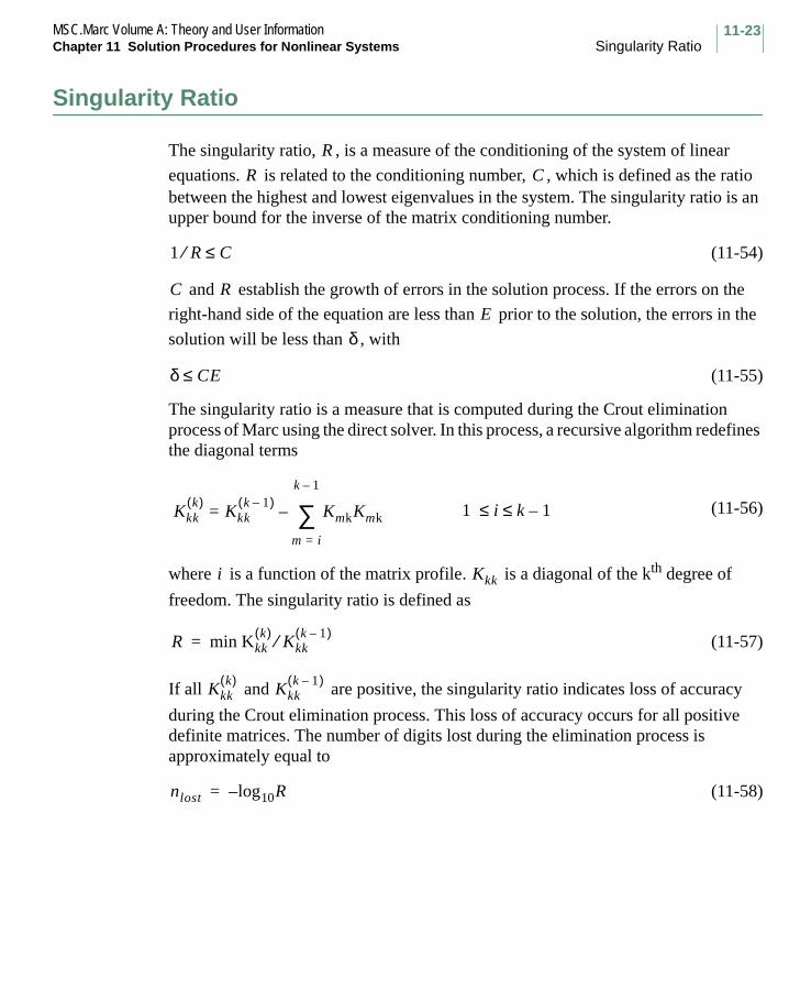
11-23MSC.Marc Volume A: Theory and User InformationChapter 11 Solution Procedures for Nonlinear Systems Singularity Ratio
Singularity Ratio
The singularity ratio, , is a measure of the conditioning of the system of linear
equations. is related to the conditioning number, , which is defined as the ratio between the highest and lowest eigenvalues in the system. The singularity ratio is an upper bound for the inverse of the matrix conditioning number.
(11-54)
and establish the growth of errors in the solution process. If the errors on the
right-hand side of the equation are less than prior to the solution, the errors in the
solution will be less than , with
(11-55)
The singularity ratio is a measure that is computed during the Crout elimination process of Marc using the direct solver. In this process, a recursive algorithm redefines the diagonal terms
(11-56)
where is a function of the matrix profile. is a diagonal of the kth degree of
freedom. The singularity ratio is defined as
(11-57)
If all and are positive, the singularity ratio indicates loss of accuracy
during the Crout elimination process. This loss of accuracy occurs for all positive definite matrices. The number of digits lost during the elimination process is approximately equal to
(11-58)
R
R C
1 R C≤⁄
C R
E
δ
δ CE≤
Kkkk( )
Kkkk 1–( )
Kmk
m i=
k 1–
∑–= Kmk 1 i k 1–≤ ≤
i Kkk
R min Kkkk( )
Kkkk 1–( )⁄=
Kkkk( )
Kkkk 1–( )
nlost log10R–=

MSC.Marc Volume A: Theory and User InformationSingularity Ratio Chapter 11 Solution Procedures for Nonlinear Systems
11-24
The singularity ratio also indicates the presence of rigid body modes in the structure.
In that case, the elimination process produces zeros on the diagonal . Exact
zeros never appear because of numerical error; therefore, the singularity ratio is of the order
(11-59)
where is the accuracy of floating-point numbers used in the calculation. For
most versions of Marc, . If rigid body modes are present, is very small
or negative. If either a zero or a negative diagonal is encountered, execution of Marc is terminated because the matrix is diagnosed as being singular.
You can force the solution of a nonpositive definite or singular matrix. In this case,
Marc does not stop when it encounters a negative or small term on the diagonal.
If you use Lagrangian multiplier elements, the matrix becomes nonpositive definite
and Marc automatically disables the test on the sign of . However, it still tests on
singular behavior.
Note: The correctness of a solution obtained for a linearized set of equations in a nonpositive definite system is not guaranteed.
Kkkk( )
0≅
R O 10ndigit–
( )=
ndigit
ndigit 12> Kkkk( )
Kkkk( )
Kkkk( )

11-25MSC.Marc Volume A: Theory and User InformationChapter 11 Solution Procedures for Nonlinear Systems Solution of Linear Equations
Solution of Linear Equations
The finite element formulation leads to a set of linear equations. The solution is obtained through numerically inverting the system. Because of the wide range of problems encountered with Marc, there are several solution procedures available.
Most analyses result in a system which is real, symmetric, and positive definite. While this is true for linear structural problems, assuming adequate boundary conditions, it is not true for all analyses. Marc has two main modes of solvers – direct and iterative. Each of these modes has two families of solvers, based upon the storage procedure. While all of these solvers can be used if there is adequate memory, only a subset uses spill logic for an out-of-core solution. Finally, there are classifications based upon nonsymmetric and complex systems. This is summarized below:
The choice of the solution procedure is made through the SOLVER option.
Direct Methods
Traditionally, the solution of a system of linear equations was accomplished using direct solution procedures, such as Cholesky decomposition and the Crout reduction method. These methods are usually reliable, in that they give accurate results for virtually all problems at a predictable cost. For positive definite systems, there are no computational difficulties. For poorly conditioned systems, however, the results can degenerate but the cost remains the same. The problem with these direct methods is that a large amount of memory (or disk space) is required, and the computational costs become very large.
Direct Profile
Direct Sparse
Iterative Sparse
Multifrontal Sparse
Vendor Provided Sparse*
Solver Option 0 4 2 8 6
Real Symmetric Yes Yes Yes Yes Yes
Real Nonsymmetric Yes No No Yes No
Complex Symmetric Yes No No Yes SUN only
Complex nonsymmetric No No No Yes No
Out-of-core Yes Yes No Yes SGI only
Possible problem with poorly conditioned systems
No No Yes No No
*Available for SGI, HP, and SUN platforms only.

MSC.Marc Volume A: Theory and User InformationSolution of Linear Equations Chapter 11 Solution Procedures for Nonlinear Systems
11-26
Iterative Methods
The K5 release of Marc introduced iterative solvers as a viable alternative for the solution of large systems. These iterative methods are based on preconditioned conjugate gradient methods. The single biggest advantage of these iterative methods is that they allow the solution of very large systems at a reduced computational cost. This is true regardless of the hardware configuration. The disadvantage of these methods is that the solution time is dependent not only upon the size of the problem, but also the numerical conditioning of the system. A poorly conditioned system leads to slow convergence – hence increased computation costs.
When discussing iterative solvers, two related concepts are introduced: fractal dimension, and conditioning number. Both are mathematical concepts, although the fractal dimension is a simpler physical concept. The fractal dimension, the range of which is between 1 and 3, is a measure of the “chunkiness” of the system. For instance, a beam has a fractal dimension of 1, while a cube has a fractal dimension of 3.
The conditioning number is related to the ratio of the lowest to the highest eigenvalues of the system. This number is also related to the singularity ratio, which has been traditionally reported in the Marc output when using a direct solution procedure. In problems involving beams or shells, the conditioning number is typically small, because of the large differences between the membrane and bending stiffnesses.
Preconditioners
The choice of preconditioner can substantially improve the conditioning of the system, which in turn reduces the number of iterations required. While all positive definite systems with degrees of freedom converges in iterations, a well
conditioned system typically converges in less than the square root of iterations.
The available preconditioners available in the sparse iterative solver are
Preconditioner Sparse
None No
Diagonal Yes
Scaled Diagonal Yes
Incomplete Cholesky Yes
Element Cholesky No
N N
N

11-27MSC.Marc Volume A: Theory and User InformationChapter 11 Solution Procedures for Nonlinear Systems Solution of Linear Equations
The sparse iterative solver requires an error criteria to determine when convergence occurs. The default is to use an error criteria based upon the ratio between the residuals in the solution and the reaction force. After obtaining the solution of the
linear equations evaluate:
(11-60)
The residual from the solution procedure is:
(11-61)
If the system is linear ( does not change) and exact numerics are preformed, then
.
Because this is an iterative method the residual is nonzero, but reduces in size with further iterations. Convergence is obtained when
(11-62)
The tolerance is specified through the SOLVER option.
Storage Methods
In general, a system of linear equations with N unknowns is represented by a matrix
of size N by , or variables. Fortunately, in finite element or finite difference analyses, the system is “banded” and not all of the entries need to be stored. This substantially reduces the memory (storage) requirements as well as the computational costs.
In the finite element method, additional zeroes often exist in the system, which results in a partially full bandwidth. Hence, the profile (or skyline) method of storage is advantageous. This profile storage method is used in Marc to store the stiffness matrix. When many zeroes exist within the bandwidth, the sparse storage methods can be quite advantageous. Such techniques do not store the zeroes, but require additional memory to store the locations of the nonzero values. You can determine the “sparsity” of the system (before decomposition) by examining the statements:
“Number of nodal entries excluding fill in” x“Number of nodal entries including fill in” y
If the ratio ( ) is large, then the sparse matrix storage procedure is advantageous.
uc
KuC
FC
=
Res FA
FC
– FA
KuC
–= =
K
Res 0=
Res Reac TOL<⁄
N N2
x y⁄

MSC.Marc Volume A: Theory and User InformationSolution of Linear Equations Chapter 11 Solution Procedures for Nonlinear Systems
11-28
Nonsymmetric Systems
The following analyses types result in nonsymmetric systems of equations:
Inclusion of convective terms in heat transfer analysisCoriolis effects in transient dynamic analysisFluid mechanicsSoil analysisFollower force stiffnessFrictional contact
The first three always result in a nonsymmetric system. The last three can be solved either fully using the nonsymmetric solver, or (approximately) using a symmetric solver. The nonsymmetric problem uses twice as much memory for storing the stiffness matrix.
Complex Systems
Marc utilizes a complex operator matrix for dynamic harmonic analyses when the damping matrix is present or for transient electromagnetic analyses. The matrix is always symmetric.
Iterative Solvers
In Marc, an iterative sparse solver is available using a sparse matrix technique. This method is advantageous for different classes of problems.
There exist certain types of analyses for which the sparse iterative solver is not appropriate. These types include:
elastic analysisexplicit creep analysiscomplex harmonic analysissubstructurescentral difference techniqueseigenvalue analysisuse of gap elements
Elastic or explicit creep analysis involves repeated solutions using different load vectors. When a direct solver is used, this is performed very efficiently using back substitution. However, when an iterative solver is used, the stiffness matrix is never inverted, and the solution associated with a new load vector requires a complete re-solution.
The sparse iterative solver can exhibit poor convergence when shell elements or Herrmann incompressible elements are present.

11-29MSC.Marc Volume A: Theory and User InformationChapter 11 Solution Procedures for Nonlinear Systems Solution of Linear Equations
Basic Theory
A linear finite element system is expressed as:
(11-63)
And a nonlinear system is expressed as:
(11-64)
where is the elastic stiffness matrix, is the tangent stiffness matrix in a
nonlinear system, is the displacement vector, is the applied load vector, and is the residual.
The linearized system is converted to a minimization problem expressed as:
(11-65)
For linear structural problems, this process can be considered as the minimization of the potential energy. The minimum is achieved when
(11-66)
The function decreases most rapidly in the direction of the negative gradient.
(11-67)
The objective of the iterative techniques is to minimize function, , without inverting the stiffness matrix. In the simplest methods,
(11-68)
where
(11-69)
The problem is that the gradient directions are too close, which results in poor convergence.
An improved method led to the conjugate gradient method, in which
(11-70)
(11-71)
Ku F=
KT∆u F R– r= =
K KT
∆u F r
ψ u( ) 1 2uT⁄ Ku u
TF–=
u K1–F=
ψ
∇ψ u( ) F Ku– r= =
ψ
uk 1+ uk αkrk+=
αk rkTrk rk
T⁄ Krk=
uk 1+ uk αkPk+=
αk PkTrk 1– Pk
T⁄ KPk=

MSC.Marc Volume A: Theory and User InformationSolution of Linear Equations Chapter 11 Solution Procedures for Nonlinear Systems
11-30
The trick is to choose to be conjugate to . Hence, the name
“conjugate gradient methods. Note the elegance of these methods is that the solution may be obtained through a series of matrix multiplications and the stiffness matrix never needs to be inverted.
Certain problems which are ill-conditioned can lead to poor convergence. The introduction of a preconditioner has been shown to improve convergence. The next key step is to choose an appropriate preconditioner which is both effective as well as computationally efficient. The easiest is to use the diagonal of the stiffness matrix. The incomplete Cholesky method has been shown to be very effective in reducing the number of required iterations.
Pk K P1 P2 … Pk 1–, , ,

11-31MSC.Marc Volume A: Theory and User InformationChapter 11 Solution Procedures for Nonlinear Systems Flow Diagram
Flow Diagram
Figure 11-8 is a diagram showing the flow sequence of Marc. This diagram shows the input phase, equivalent nodal load vector calculation, matrix assembly, matrix solution, stress recovery, and output phase. It also indicates load incrementation and iteration within a load increment.
Figure 11-8 Marc Flow Diagram
No
No
Yes
Yes
Equivalent NodalLoad Vector
Matrix Assembly
Input Phase:Read Input DataSpace Allocation
Data Check
Matrix Solution
Stress Recovery
Convergence
Output Phase
Adapt Mesh
NextIncrement
Stop
IncrementalLoads
Tim
e S
tep
Loop
Itera
tion
Loop

MSC.Marc Volume A: Theory and User InformationReferences Chapter 11 Solution Procedures for Nonlinear Systems
11-32
References
1. Bathe, K. J. Finite Element Procedures, Prentice Hall, Englewood Cliffs, NJ, 1996.
2. Riks, E. “An incremental approach to the solution of solution and buckling problems”, Int. J. of Solids and Structures, V. 15, 1979.
3. Riks, E. “Some Computational Aspects of the Stability Analysis of Nonlinear Structures”, Comp. Methods in Appl. Mech. and Eng., 47, 1984.
4. Crisfield, M. A. “A fast incremental iterative procedure that handles snapthrough”, Comput. & Structures, V. 13, 1981.
5. Ramm, E. “Strategies for tracing the nonlinear response near limit points,” in K. J. Bathe et al (eds), Europe-US Workshop on Nonlinear Finite Element Analysis in Structural Mechanics, Ruhr University Bochum, Germany, Springer-Verlag, Berlin, pp/ 63-89. Berlin, 1985.

Chapter 12 Output Results
CHAPTER
12 Output Results
Workspace Information
Increment Information
Selective Printout
Restart
Element Information
Nodal Information
Post File
Program Messages
Marc HyperMesh Results Interface
Marc SDRC I-DEAS Results Interface
Status File

MSC.Marc Volume A: Theory and User InformationChapter 12 Output Results
12-2
This chapter summarizes the information that Marc provides in the output. In addition to reviewing your input, Marc provides information about the procedures the program uses and the workspace allocation. All calculated results are automatically written to the output file unless the user specifically requests otherwise.

12-3MSC.Marc Volume A: Theory and User InformationChapter 12 Output Results Workspace Information
Workspace Information
Marc reports several aspects of workspace information, specifically, the allocation of memory workspace and the size of the work files.
First, Marc gives the workspace needed for the input and stiffness assembly. This number tells how much memory workspace is needed to store the user-supplied data, the program-calculated data, and two-element stiffness matrices. Each set of data comprises three parts: overhead, element information, and nodal information. Element information consists of properties, geometries, strains, and stresses, and nodal information consists of coordinates, displacements, and applied forces.
Note: You must input a number (an amount of memory) on the SIZING parameter greater than the number (amount of memory) requested by Marc.
Next, Marc specifies the internal core allocation parameters. These values are useful in user subroutines and are often provided to the user subroutines. The values provided here are:
• the number of degrees of freedom per node (NDEG) • the number of coordinates per node (NCRD) • the number of generalized strains per integration point (NGENS) • the number of stresses per integration point (NSTRMX) • the number of invariants per integration point (NEQST)
Note the following:
• The number of degrees of freedom per node indicates the number of boundary conditions necessary to eliminate rigid body modes.
• The number of generalized strains per integration point for beams and shells include both membrane and curvature strains.
• The number of stresses per integration point is the number of stresses per layer multiplied by the number of layers.
• The number of invariants per integration point is the number of layers for either shell or beam elements.
The ELSTO parameter stores element information on an auxiliary storage device, rather than in main memory. You can invoke this option, or Marc invokes it automatically. In this option, Marc:
• sets a flag for element storage (IELSTO) • specifies how many words are used per element (NELSTO) • specifies the number of elements per buffer (MXELS) • specifies the total amount of space needed to store this information

MSC.Marc Volume A: Theory and User InformationWorkspace Information Chapter 12 Output Results
12-4
The number of elements per buffer should be at least two, and you can change the buffer size in the ELSTO parameter option to increase the number of elements which will be in the buffer.
Marc states how much workspace is needed for the MESH2D option and any of the bandwidth optimizers. In each case, the number you prescribe in the SIZING parameter must be larger than the number given by Marc.
Direct Solution Procedure
Marc offers two direct solver options. The default direct solver uses a variable bandwidth (also known as profile) storage scheme. Since the required storage space and the solution time depend on the cumulative profile length, a nodal renumbering that minimizes the profile length can give rise to considerable savings in storage and solution time. Several renumbering schemes are available in Marc and they can be requested using the OPTIMIZE option. These optimization procedures are described in the Bandwidth Optimization section of Chapter 4. The other direct solver option available in Marc uses a sparse storage scheme. A nodal renumbering based on minimum degree algorithm is done automatically to minimize the fill after factorization.
After Marc has determined the total profile length or the total fill after factorization depending on the requested solver option, it reports the total workspace needed for in-core matrix storage. If the workspace specified on SIZING is larger than the total workspace needed for the in-core matrix solution, the in-core matrix storage will be employed. In the case when the required storage exceeds the workspace specified in SIZING, the out-of-core solver is invoked. In which case, Marc reports the required workspace for each nodal row, the number of nodal rows per buffer, and the size of each auxiliary file. The more nodal rows per buffer, the more efficient the solution procedure is. The buffer size can be increased only by increasing the allocation in SIZING. Marc terminates unless the number of nodal rows per buffer is two or greater. If the out-of-core option is invoked, Marc reports the structure of the global stiffness matrix indicating the nonzero values in the stiffness matrix.

12-5MSC.Marc Volume A: Theory and User InformationChapter 12 Output Results Increment Information
Increment Information
A variety of information is given for each increment, and often for each iteration, of the analysis. This information is useful in determining the accuracy and the stability of the analysis.
Summary of Loads
The printout entitled “Load Increments Associated with Each Degree of Freedom” allows you to check the load input quickly. It represents the sum, over all nodes in the mesh, of the point loads and the equivalent forces obtained after distributed loads (pressures, body forces) are applied. For example, you can easily check a pressure because the total force in a global coordinate direction would be the projected area normal to that direction of the surface upon which the pressure is applied, multiplied by the pressure magnitude.
Timing Information
The amount of CPU necessary to reach the given location in the analysis is indicated by the following output:
• start of increment• start of assembly• start of matrix solution• end of matrix solution• end of increment
As an example, subtract the time associated with the start of the matrix solution from the time associated with the end of the matrix solution to determine how much time was spent in the equation solver.
Singularity Ratio
The singularity ratio is a measure of the conditioning of the matrix (see the Appendix A for further details). This ratio is printed each time there is a solution of the matrix equations. You can measure the influence of the nonlinearities in the structure by examining the change in singularity ratios between increments.
Convergence
Several messages are printed that concern the convergence of the solution. These messages indicate the displacement, velocity, or residual error and are very important because they provide information concerning the accuracy of the solution procedure.

MSC.Marc Volume A: Theory and User InformationIncrement Information Chapter 12 Output Results
12-6
These messages also indicate the ratio of the error and its relative quantity. This ratio must be less than that given in the CONTROL option for convergence to occur. See Appendix A for details on convergence testing.
When the iterative solver is used, additional messages are printed regarding the convergence of the solution procedures.

12-7MSC.Marc Volume A: Theory and User InformationChapter 12 Output Results Selective Printout
Selective Printout
Marc gives you several options and user subroutines for the control of the Marc output.
Options
PRINT CHOICE allows you to select how much of the element and nodal information is to be printed. The possible selections are
• group of elements
• group of nodes
• which layers (form beam and shell elements)
• which integration points
• increment frequency between printouts
The data entered through this option remain in control until you insert a subsequent PRINT CHOICE set. You can include such a set with either the model definition or with the history definition set. To obtain the default printout after a previous PRINT CHOICE, invoke PRINT CHOICE using blank entries.
Note: The PRINT CHOICE option has no effect on the restart or post file.
You can use the PRINT ELEMENT capability as a replacement for, or in conjunction with, the PRINT CHOICE option. The enhancements this option offers over the PRINT CHOICE option are the following:
1. You have a choice of integration and layer points for each element to be printed, which is especially useful when several different element types are used in one analysis.
2. You have a choice of the type of quantity to be printed, for instance, stresses could be printed for all elements, but strains for only a few.
3. The types of output quantities that can be selected are stresses, strains, creep strain, thermal strain, cracking strain, Cauchy stress, state variables, strain energy, or all nonzero quantities.
4. The output can be placed in a file other than the standard output file.
5. The PRINT NODE option can be used to obtain element quantities such as stresses and strains at the nodal points of each element. These are obtained by extrapolating the integration point values to the nodes.

MSC.Marc Volume A: Theory and User InformationSelective Printout Chapter 12 Output Results
12-8
The PRINT NODE option is an alternative to the PRINT CHOICE option for controlling the output of nodal quantities. The additional capabilities of this option compared to the PRINT CHOICE are as follows:
1. You can choose which of the following nodal quantities are to be printed:
incremental displacementstotal displacements velocitiesaccelerationsreaction forcesgeneralized stresses
2. Different quantities can be printed for different nodal points.
3. The output can be placed in a file other than the standard output file.
Note: All quantities are saved on the restart file, and you can obtain them at a later time by using the RESTART option. Quantities that were not printed out are available for later use.
The SUMMARY option allows you to get a quick summary of the results obtained in the analysis. This option prints the maximum and minimum quantities in tabular form. The table is designed for direct placement into reports. You control the increment frequency of summary information and the file unit to which the information is written.
The SUMMARY option reports on the physical components and the Tresca, von Mises, and mean values of stress, plastic strain, and creep strain. It also reports on such nodal quantities as displacements, velocities, accelerations, and reaction forces.
The sort options (ELEM SORT and NODE SORT) allow you to sort calculated quantities in either ascending or descending order. These quantities may either be sorted by their real magnitude or their absolute magnitude. The sort options also allow you to control the type of quantity to be sorted, for example, equivalent stress and the number of items to be sorted. The sort options print the sorted values in tabular form. The table is designed for direct placement into reports. You may control the increment frequency of sorted values and the file unit to which these values are written.
The PRINT VMASS option allows you to selectively choose which elements and associated volumes and masses to be printed. In order to have correct mass computations, mass density for each element must be given. The volumes and masses can be written on either standard output file unit 6, or user specified unit.

12-9MSC.Marc Volume A: Theory and User InformationChapter 12 Output Results Selective Printout
User Subroutines
User subroutines can be used to obtain additional output, which can be accessed at each time/load increment. The available subroutines are the following:
• IMPD – obtains nodal quantities, such as displacements, coordinates, reaction forces, velocities, and accelerations
• ELEVAR – obtains element quantities such as strains, stresses, state variables, and cracking information
• ELEVEC – outputs element quantities during harmonic subincrements
• INTCRD – obtains the integration point coordinates used for forming the stiffness matrix

MSC.Marc Volume A: Theory and User InformationRestart Chapter 12 Output Results
12-10
Restart
One capability of the RESTART option allows you to recover the output at increments where printout was suppressed in previous runs. This option can be used to print time/load increments for a number of consecutive increments. Under this option, Marc does not do any analysis.
In conjunction with the RESTART option, you can use either the PRINT CHOICE or PRINT ELEMENT, or PRINT NODE option to select a region of the model for which you want to obtain results.

12-11MSC.Marc Volume A: Theory and User InformationChapter 12 Output Results Element Information
Element Information
The main output from an increment includes element information followed by nodal information. The system provides the element data at each integration point. If you use the CENTROID parameter, the system provides the element data at the centroidal point. You can control the amount of printed output by using either the PRINT CHOICE or PRINT ELEMENT option. All quantities are total values at the current state (at the end of the current increment), and the physical components are printed for each tensor quantity (stress, strain, and generalized stress and strain). The orientation of these physical components is generally in the global coordinate system; however, their orientation depends on the element type. (MSC.Marc Volume B: Element Library explains the output for each particular element type.) Also, the physical components may be printed with respect to a user defined preferred system.
In addition to the physical components, certain invariants are given, as follows:
1. Tresca intensity - the maximum difference of the principal values, and the measure of intensity usually required for ASME code analysis
von Mises intensity - defined for stress as
(12-1)
where is a stress tensor and s is the deviatoric stress tensor. For beam and truss elements, , and additional shears are zero; for plane stress elements, including plates and shells, .
2. von Mises intensity - calculated for strain type quantities as
(12-2)
Marc uses these measures in the plasticity and creep constitutive theories. For example, incompressible metal creep and plasticity are based on the equivalent von Mises stress. For beam, truss, and plane stress elements, an incompressibility assumption is made regarding the noncalculated strain components.
a. For beam and truss elements, this results in
(12-3)
Sij σ 13---δijσkk–=σ 3
2---SijSij=
σσ22 σ33 0= =
σ33 0=
ε 23---εijεij=
ε22 ε3312---ε11–= =

MSC.Marc Volume A: Theory and User InformationElement Information Chapter 12 Output Results
12-12
b. For plane stress elements
(12-4)
c. For beam and plane stress elements taken as a whole
(12-5)
3. Mean normal intensity - calculated as
(12-6)
Equation 12-6 represents the negative hydrostatic pressure for stress quantities. For strain quantities, the equation gives the dilatational magnitude. This measurement is important in hydrostatically dependent theories (Mohr-Coulomb or extended von Mises materials), and for materials susceptible to void growth.
4. The principal values are calculated from the physical components. Marc solves the eigenvalue problem for the principal values using the Jacobi transformation method. Note that this is an iterative procedure and may give slightly different results from those obtained by solving the cubic equation exactly.
5. State variables are given at any point where they are nonzero.
Solid (Continuum) Elements
For solid (continuum) elements, stress, strain, and state variables are the only element quantities given. Marc prints out stresses and total strain for each integration point. In addition, it prints out thermal, plastic, creep, and cracking strains, if they are applicable. Note that the total strains include the thermal contribution.
ε33 ε11 ε22+( )–=
εkk 0=
σ11 σ22 σ33+ +( ) 3⁄
or
ε11 ε22 ε33+ +( ) 3⁄

12-13MSC.Marc Volume A: Theory and User InformationChapter 12 Output Results Element Information
Shell Elements
Marc prints generalized stresses and generalized total strains for each integration point. For thick shell (Type 22, 72, 75) elements interlaminar shear stresses are printed at the interface of two laminated layers.
The generalized stresses printed out for shell elements are
(12-7)
(12-8)
The generalized strains printed are
(12-9)
(12-10)
Physical stress values are output only for the extreme layers unless you invoke either PRINT CHOICE or PRINT ELEMENT. In addition, thermal, plastic, creep, and cracking strains are printed for values at the layers, if applicable. Although the total strains are not output for the layers, you can calculate them using the following equations.
(12-11)
(12-12)
(12-13)
where h is the directed distance from the midsurface to the layer; are the stretches;
and are the curvatures as printed. You can obtain these quantities by using the
ELEVAR subroutine.
1t--- σij yd
t 2⁄–
+ t 2⁄
∫
Section Force per Unit Thickness( )
Section moment per Unit Thickness( )
1t--- yσij yd
t 2⁄–
+ t 2⁄
∫
α β, 1 2,=Eαβ ;
Stretch( )
α β, 1 2,=καβ ;
Curvature( )
ε11 E11 hκ11+=
ε22 E22 hκ22+=
γ12 E12 hκ12+=
Eij
κ ij

MSC.Marc Volume A: Theory and User InformationElement Information Chapter 12 Output Results
12-14
Beam Elements
The printout for beam elements is similar to shell elements, except that the section values are force, bending and torsion moment, and bimoment for open section beams. For beam element type 45, interlaminar shear stresses are printed at the interface of laminated layers if the TSHEAR parameter is used.
These values are given relative to the section axes (X, Y, Z) which are defined in the COORDINATES or the GEOMETRY option.
Before a beam member can be designed, it is necessary to understand the section forces distribution along the axial direction of the beam. For example, if variations of shear force and moment along axial direction are plotted, the graphs are termed shear diagram and moment diagram, respectively. To postprocess these diagrams, post code 261 needs to be specified along with the post codes (shown in Table 12-1) which define the corresponding section forces of the beam element.
Table 12-1 Post Codes for Beam Section Forces
Element Type
2-D/3-D
Post Code
264(Axial Force)
265(Moment xx or Moment
ip)
266(Moment yy or Moment
op)
267(Shear xz or
Shear ip)
268(Shear yz or
Shear op)269
(Torque)270
(Bimoment)
5 2-D X X
16 2-D X X
45 2-D X X X
13 3-D X X X X X
14 3-D X X X X
25 3-D X X X X
31 3-D X X X X X X
52 3-D X X X X
76 3-D X X X X
77 3-D X X X X
78 3-D X X X X
79 3-D X X X X
98 3-D X X X X X X

12-15MSC.Marc Volume A: Theory and User InformationChapter 12 Output Results Element Information
Heat Transfer Elements
Marc prints the element temperatures and temperature gradients. In the coupled thermo-electric (Joule heating) analysis, the program also prints the element voltage, current, and heat fluxes.
Gap Elements
Marc prints the gap contact force, friction forces, and the amount of slip.
Linear Springs
Marc prints the spring forces.
Hydrodynamic Bearing
Marc prints the pressure in the lubricant.

MSC.Marc Volume A: Theory and User InformationNodal Information Chapter 12 Output Results
12-16
Nodal Information
Marc also prints out the following quantities at each nodal point.
Stress Analysis
• Incremental displacements - the amount of deformation that occurred in the last increment
• Total displacements - the summation of the incremental displacements
• Total equivalent nodal forces (distributed plus point loads) - the total force applied to the model through distributed loads (pressures) and point loads
• Reaction forces at fixed boundary conditions
• Residual loads at nodal points that are not fixed by boundary conditions
Note: Each value listed above is given at each nodal point, unless you invoke the PRINT CHOICE or PRINT NODE option. If you invoke the TRANSFORMATION option, Marc prints the nodal information relative to the user-defined system, rather than the global coordinate system.
Reaction Forces
Marc computes reaction forces based on the integration of element stresses. This is the only way to compute total reaction forces in a nonlinear analysis. Since such integration is only exact if the stresses are known at each integration point, the reaction forces are not printed if you use the CENTROID parameter.
In a nonlinear analysis, you should check that the reaction forces are in equilibrium with the external forces. If they are not in equilibrium, the analysis will be inaccurate, usually due to excessively large incremental steps. In most cases, the equilibrium is automatically ensured due to the convergence testing in Marc.
Residual Loads
The residual loads are a measure of the accuracy of the equilibrium in the system during analysis. This measure is very important in a nonlinear analysis and should be several orders of magnitude smaller than the reaction forces.
Dynamic Analysis
In a dynamic analysis, Marc prints out the total displacement, velocity, and acceleration at each time increment.

12-17MSC.Marc Volume A: Theory and User InformationChapter 12 Output Results Nodal Information
Heat Transfer Analysis
In a heat transfer analysis, Marc prints out nodal temperatures and nodal heat fluxes. If a thermo-electrical analysis is performed, Marc prints nodal voltages as well.
Rigid-Plastic Analysis
In steady-state rigid-plastic analysis, Marc prints nodal velocities.
Hydrodynamic Bearing Analysis
In a hydrodynamic bearing analysis, Marc gives the mass flux at the nodal points.
Electrostatic Analysis
In an electrostatic analysis, Marc prints the scalar potential and the charge.
Magnetostatic Analysis
In a magnetostatic analysis, Marc prints the vector potential and the current.
Electromagnetic Analysis
In an electromagnetic analysis, Marc prints out the vector and scalar potential, the current, and the charge.
Acoustic Analysis
In an acoustic analysis, Marc prints the pressure and the source.
Contact Analysis
The standard output includes, at the end of each increment, a summary of information regarding each body. This information reports the increment’s rigid body velocity, the position of the center of rotation, and the total loads on the body. These last values are obtained by adding the contact forces of all nodes in contact with the rigid body in cause. Deformable bodies being in equilibrium have no load reported.
Additional information can be obtained by means of the PRINT,5 parameter. In such cases, all the contact activity is reported. Namely, every time a new node touches a surface, or separates from a surface, a corresponding message is issued.
Contact with rigid surfaces entails an automatic transformation. Displacement increments and reactions in the transformed coordinates - tangent and normal to the contact interface - are also reported for every node that is in contact in the usual Marc manner.

MSC.Marc Volume A: Theory and User InformationPost File Chapter 12 Output Results
12-18
Post File
The post file contains results of the analysis performed. This information can be viewed using Mentat to observe the displaced mesh, contours of element quantities, principal quantities, time history behavior, response gradients, design variables, etc. The post file contains the finite element mesh and any changes to the finite element mesh due to either rezoning or adaptive mesh refinement. Basic nodal quantities (such as displacements, velocities, acceleration, applied loads, and reaction forces) are automatically placed on the post file. It is also possible to include user-defined nodal vectors by use of the UPOSTV user subroutine. Element quantities, such as stress, strain, plastic strain) must be explicitly requested by using the POST model definition option. It is possible to have user-defined element quantities placed on the post file for subsequent display by using the UPOSTV user subroutine.

12-19MSC.Marc Volume A: Theory and User InformationChapter 12 Output Results Program Messages
Program Messages
The messages provided by Marc at various points in the output show the current status of the problem solution. Several of these messages are listed below.
• START OF INCREMENT x indicates the start of increment number x.
• START OF ASSEMBLY indicates Marc is about to enter the stiffness matrix assembly.
• START OF MATRIX SOLUTION indicates the start of the solution of the linear system.
• SINGULARITY RATIO prints yyy, where yyy is an indication of the conditioning of the matrix. This value is typically in the range 10-6 to 1. If yyy is of the order of machine accuracy (10-6 for most machines), the equations might be considered singular and the solution unreliable.
• END OF MATRIX SOLUTION indicates the end of matrix decomposition.
• END OF INCREMENT x indicates the completion of increment number x.
• RESTART DATA at INCREMENT x ON UNIT 8 indicates that the restart data for increment number x has been written (saved) on Unit 8.
• POST DATA at INCREMENT x on UNIT y indicates that the post data for increment number x has been written (saved) on Unit y.
In addition to these Marc messages, exit messages indicate normal and abnormal exists from Marc. Table 12-2 shows the most common exit messages.
Table 12-2 Marc Exit Messages
Message Meaning
MARC EXIT 3001 Normal exit.
MARC EXIT 3004 Normal exit.
MARC EXIT 12 End of plotting (normal exit).
MARC EXIT 13 Input data errors were detected by the program.
MARC EXIT 2004 Operator matrix (for example, stiffness matrix in stress analysis) has become non-positive definite and the analysis terminated.
MARC EXIT 3002 Convergence has not occurred within the allowable number of recycles.

MSC.Marc Volume A: Theory and User InformationMarc HyperMesh Results Interface Chapter 12 Output Results
12-20
Marc HyperMesh Results Interface
Marc now outputs results for postprocessing with HyperMesh. The writing of the HyperMesh results file is invoked by the HYPERMESH model definition option described in detail in MSC.Marc Volume C: Program Input. Mentat can also be used to write the necessary commands into the Marc data file. The related button can be found one level below each of the ANALYSIS CLASS buttons within the JOBS menu.The binary file created as a result has the title jobid.hmr where jobid is the name of the data file for the job.
The geometry data may be imported into HyperMesh from a Marc data file. Alternatively, it can be created by HyperMesh or read in from other formats via the HyperMesh import capability.
The types of data that may be selected for writing into the HyperMesh results file are listed in MSC.Marc Volume C: Program Input under the HYPERMESH model definition option. It is important to note that, in case eigenvectors for buckling or eigenfrequency analysis are to be written into the results file, the corresponding Marc file should have the BUCKLE INCREMENT or MODAL INCREMENT model definition option, as appropriate. The BUCKLE, MODAL SHAPE, and RECOVER history definition options are not to be used in these cases.
Since HyperMesh allows only one deformed shape plot per simulation, each eigenvector of an eigenvalue analysis is saved as a separate simulation. Thus, when using HyperMesh, these eigenvectors can be plotted by skipping to the next simulation rather than skipping to the next data type of a simulation. The contour plots can be obtained for all data types including eigenvectors.
In case the number of requested eigenvalues is more than the number extracted, the data type in the HyperMesh “deformed” screen will inform you for those modes that are not extracted. The “next” button may need to be clicked to see the data type in the “deformed” mode of plotting.

12-21MSC.Marc Volume A: Theory and User InformationChapter 12 Output Results Marc SDRC I-DEAS Results Interface
Marc SDRC I-DEAS Results Interface
A facility exists in Marc to write out an SDRC I-DEAS universal file of the analysis results, in order for postprocessing by the I-DEAS program. The writing of the universal file is invoked by the SDRC model definition option described in detail in MSC.Marc Volume C: Program Input. Mentat can also be used to write the necessary commands into the Marc data file. The related button can be found one level below each of the ANALYSIS CLASS buttons within the JOBS menu. The formatted ASCII file created as a result has the title jobid.unv, where jobid is the name of the data file for the job.
The model data is imported into I-DEAS by way of the universal file as well.
The types of data that may be selected for writing into the I-DEAS universal file are listed in MSC.Marc Volume C: Program Input under the SDRC model definition option.

MSC.Marc Volume A: Theory and User InformationStatus File Chapter 12 Output Results
12-22
Status File
The status file contains summarized information of the analysis. Each line within this file includes the load case number, the associated increment number, and the number of cycles, contact separations, and cutbacks associated with that increment; the accumulated total cycles, increment splittings, separations, cutbacks, and remeshing times numbers in the analysis as well as the time step size of each increment and the overall time achieved by the analysis. Marc reports all this information on one line upon completion of each increment. If the increment is partially completed (for example, the completion of one part of a split increment or one part of the whole increment due to cutback), Marc also reports one line for each part of the increment.

Appendix A Finite Element Technology in Marc
Governing Equations of Various Structural Procedures
This section describes the basic concepts of finite element technology. For more information, you are urged to refer to the finite element text [1-5]. Marc was developed on the basis of the displacement method. The stiffness methodology used in Marc addresses force-displacement relations through the stiffness of the system. The force-displacement relation for a linear static problem can be expressed as
(A-1)
APPENDIX
A Finite Element Technology in Marc
Governing Equations of Various Structural Procedures
System And Element Stiffness Matrices
Load Vectors
References
Ku f=
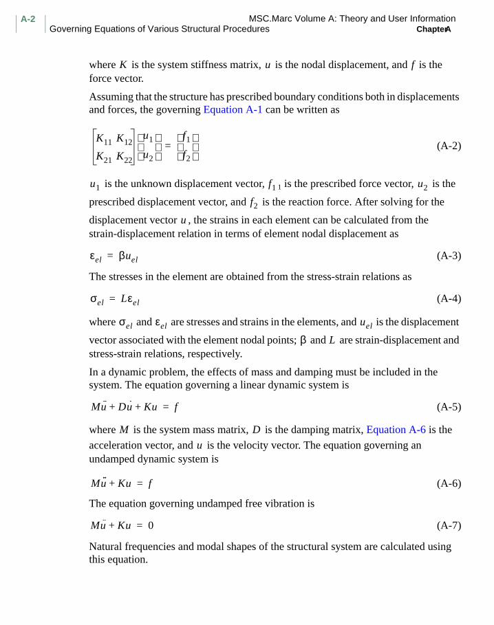
MSC.Marc Volume A: Theory and User InformationGoverning Equations of Various Structural Procedures Chapter A
A-2
where is the system stiffness matrix, is the nodal displacement, and is the force vector.
Assuming that the structure has prescribed boundary conditions both in displacements and forces, the governing Equation A-1 can be written as
(A-2)
is the unknown displacement vector, 1 is the prescribed force vector, is the
prescribed displacement vector, and is the reaction force. After solving for the
displacement vector , the strains in each element can be calculated from the strain-displacement relation in terms of element nodal displacement as
(A-3)
The stresses in the element are obtained from the stress-strain relations as
(A-4)
where and are stresses and strains in the elements, and is the displacement
vector associated with the element nodal points; and are strain-displacement and stress-strain relations, respectively.
In a dynamic problem, the effects of mass and damping must be included in the system. The equation governing a linear dynamic system is
(A-5)
where is the system mass matrix, is the damping matrix, Equation A-6 is the
acceleration vector, and is the velocity vector. The equation governing an undamped dynamic system is
(A-6)
The equation governing undamped free vibration is
(A-7)
Natural frequencies and modal shapes of the structural system are calculated using this equation.
K u f
K11 K12
K21 K22
u1
u2 f1
f2
=
u1 f1 u2
f2
u
εel βuel=
σel Lεel=
σel εel uel
β L
Mu·· Du· Ku+ + f=
M D
u
Mu·· Ku+ f=
Mu·· Ku+ 0=

A-3MSC.Marc Volume A: Theory and User InformationChapter A Governing Equations of Various Structural Procedures
(A-8)
The equations governing some other procedures are similar. For example, the governing equation of transient heat transfer analysis is
(A-9)
where is the heat capacity matrix, is the thermal conductivity matrix, is the
thermal load vector (flux), is the nodal temperature vector, and is the time derivative of the temperature. Equation A-9 reduces to
(A-10)
for the steady-state problem. Note that the equation governing steady-state heat transfer (Equation A-10) and the equation of static stress analysis (Equation A-1) take the same form. Similarly, the hydrodynamic bearing problem is analogous to a steady-state heat transfer problem. This problem is governed by an equation similar to Equation A-10.
The matrix equation of the electrical problem in coupled thermo-electrical analysis is
(A-11)
The equation governing the thermal problem is:
(A-12)
in both Equation A-11 and Equation A-12, is the voltage, is the temperature-dependent electrical-conductivity matrix, I is the nodal-current vector,
is the temperature-dependent, heat-capacity matrix, and is the
thermal-conductivity matrix. is the nodal temperature vector, is the heat-flux
vector, and is the internal heat-generation vector that results from the electrical
current. Electrical and thermal problems are coupled through and .
The matrix equations for the thermal-mechanical problem are as follows:
(A-13)
(A-14)
Kφ ω2Mφ– 0=
CT·
HT+ Q=
C H Q
T t
HT Q=
ρ T( )v I=
C T( )T·
H T( )T+ Q Qe
+=
v ρ T( )
C T( ) H T( )T Q
Qe
ρ T( ) Qe
Mu·· D T( )u· K T( )u+ + f=
C T( )T·
H T( )T+ Q QI
+=

MSC.Marc Volume A: Theory and User InformationGoverning Equations of Various Structural Procedures Chapter A
A-4
In Equation A-13 and Equation A-14 the damping matrix , stiffness matrix ,
heat-capacity matrix and thermal-conductivity matrix are all dependent on
temperature. is the internal heat generated due to inelastic deformation. The coupling between the heat transfer problem and the mechanical problem is due to the temperature-dependent mechanical properties and the internal heat generated. If an updated Lagrangian analysis is performed, and are dependent upon prior displacement.
The governing equations described above are either sets of algebraic equations (Equation A-1, Equation A-10, and Equation A-11), or sets of ordinary differential equations (Equation A-5 through Equation A-8 and all equations through Equation A-4). The time variable is a continuous variable for the ordinary differential equations. Select an integration operator (for example, Newmark-Beta, Houbolt, or central difference for dynamic problems, and backward difference for heat transfer) to reduce the set of differential equations to a set of algebraic equations. The final form of governing equations of all analysis procedures is, therefore, a set of algebraic equations.
D K
C H
QI
K H

A-5MSC.Marc Volume A: Theory and User InformationChapter A System And Element Stiffness Matrices
System And Element Stiffness Matrices
The previous section presented system matrices assembled from element matrices in the system. For example, the system stiffness matrix is expressed in terms of the
element stiffness matrix as
(A-15)
where is the number of elements in the system. The system stiffness matrix is a symmetric-banded matrix. See Figure A-1 for a schematic of the assemblage of element matrices. When the element-by-element iterative solver is used, the total stiffness matrix is never assembled.
The element stiffness matrix can be expressed as
(A-16)
where is the volume of the element, is the strain-displacement relation, and is the stress-strain relation.
(A-17)
(A-18)
The mass matrix can be expressed as
(A-19)
The integration in Equation A-16 is carried out numerically in Marc, and is dependent on the selection of integration points. The element stiffness matrix can be fully or under integrated. The mass matrix is always fully integrated.
Note: The β matrix is directly associated with the shape functions and geometry of each element. Shape functions associated with different element types are explained in MSC.Marc Volume B: Element Library. Stress-strain relations L are discussed in Chapter 7 of this manual.
K
Kiel
K Kiel
N
∑=
N
Kel βT
Lβdvel
vel
∫=
vel β L
ε βu=
σ Lε=
Mel
NTρNdv
vel
∫=

MSC.Marc Volume A: Theory and User InformationSystem And Element Stiffness Matrices Chapter A
A-6
Figure A-1 Schematic of Matrix Assemblage
1 2
3 4 5
67
8
(a)
(b)
(c)
1 2 3 4 5
F[K]
Band
δ
δ
1
4 5
2 3

A-7MSC.Marc Volume A: Theory and User InformationChapter A Load Vectors
Load Vectors
The nodal force vector f in Equation A-1 includes the contributions of various types of loading.
(A-20)
where is the point load vector, is the surface load vector, is the body
(volumetric) load vector, and represents all other types of load vectors (for example, thermal and creep strains, and initial stress).
The point load is associated with nodal degrees-of-freedom and can be added to the nodal force vector directly. Equivalent nodal force vectors , y must be
calculated from the distributed (surface/volumetric) load first and then added to the nodal force vector. In Marc, the computation of equivalent nodal forces is carried out through numerical integration of the distributed load over the surface area of volume to which the load is applied. This can be expressed as
(A-21)
(A-22)
where is the pressure.
Figure A-1 shows the assemblage of the nodal force vector.
f fpoint fsurface fbody f∗+ + +=
fpoint fsurface fbody
f*
fsurface fbody
fsurface NTpdA
A∫=
fbody NTpdV
V∫=
p

MSC.Marc Volume A: Theory and User InformationReferences Chapter A
A-8
References
1. Zienkiewicz, O. C. and R. L. Taylor. The Finite Element Method (4th ed.) Vol. 1. Basic Formulation and Linear Problems (1989),) Vol. 2. Solid and Fluid Mechanics, Dynamics, and Nonlinearity (1991) McGraw-Hill Book Co., London, U. K.
2. Bathe, K. J. Finite Element Procedures, Prentice-Hall, Englewood Cliffs, NJ, 1995.
3. Hughes, T. J. R. The Finite Element Method–Linear Static and Dynamic Finite Element Analysis, Prentice-Hall, Englewood Cliffs, NJ. 1987.
4. Ogden, R. W. “Large Deformation Isotropic Elasticity: On The Correlation of Theory and Experiment for Incompressible Rubberlike Solids,” Proceedings of the Royal Society, Vol. A (326), pp. 565-584, 1972.
5. Cook, R. D., D. S. Malkus, and M. E. Plesha, Concepts and Applications of Finite Element Analysis (3rd ed.), John Wiley & Sons, New York, NY, 1989.

A B C D E F G H
Index
I N D E XMSC.Marc Volume A: Theory and User Information
I J K L M N O P Q R S T U V W X Y Z
Aacoustic
analysis 6-42, 7-121, 9-14, 10-23, 12-17element types 6-42, 6-48input options 9-14
ACOUSTIC (parameter) 6-43ACTIVATE (history definition option) 4-7ADAPTIVE (model definition option) 4-38, 5-4,
5-5, 10-36ADAPTIVE (parameter) 8-35, 10-36adaptive mesh
contact 8-35refinement 10-36
adaptive time control 5-50additional node, cross section 9-35ALL POINTS (parameter) 5-131, 6-21, 10-3analysis 7-120
acoustic 6-42, 7-121, 9-14, 10-23, 12-17contact 12-17coupled 6-60coupled acoustic-structural 6-44coupled contact 8-29coupled thermo-electrical (Joule heating)
6-64coupled thermo-mechanical 6-67crack 5-58design sensitivity 5-110dynamic 12-16eigenvalue 5-67electrical 9-13electromagnetic 6-37, 7-121, 9-15, 10-24,
12-17electrostatic 7-121, 9-13, 10-23, 12-17error 4-33
fluid 6-49, 7-121, 10-24fluid/solid interaction 6-62, 7-120, 10-23Fourier 5-6harmonic 6-40heat transfer 6-3, 7-120, 9-11, 12-17hydrodynamic bearing 6-23, 7-120, 9-12,
10-23, 12-17linear 5-3magnetostatic 6-31, 7-121, 10-24, 12-17nonlinear 5-10perturbation 5-31rigid-plastic 5-86, 12-17soil 5-92, 7-109, 10-24stress 12-16thermo-electrical 7-120viscoplastic 5-56
analytical contact 8-44ANELAS (user subroutine) 5-5, 7-5, 7-8ANEXP (user subroutine) 5-5, 7-8, 7-102angle deviation criteria, remeshing 4-44ANISOTROPIC (model definition option) 5-5, 7-5,
7-7, 7-48anisotropic viscoelastic material 7-85ANKOND (user subroutine) 6-4, 7-120ANPLAS (user subroutine) 7-8, 7-48application phase 5-66APPROACH (history definition option) 8-11Arbitrary Eularian-Lagrangian (AEL)
formulation 5-27arc-length methods 11-11ASSUMED STRAIN (parameter) 10-33assumed strain formulation 10-33ATTACH NODE (model definition option) 4-36

A B C D E F G H I J K L M N O P Q R S T U V W X Y Z
I-2MSC.Marc Volume A: Theory and User InformationIndex
AUTO CREEP (history definition option) 5-50, 5-52, 5-53, 5-55, 5-56, 5-57, 7-81
AUTO INCREMENT (history definition option) 4-27, 5-30, 7-108, 9-9
AUTO LOAD (history definition option) 4-27, 7-92, 9-9
AUTO STEP (history definition option) 5-72, 7-85, 7-92, 7-108, 8-44
AUTO THERM (history definition option) 9-9AUTO THERM CREEP (history definition option)
5-54, 5-55AUTO TIME (history definition option) 5-55, 5-72,
5-78, 6-68, 7-85, 7-92, 8-44Automatic Thermally Loaded Elastic-Creep/
Elastic-Plastic-Creep Stress Analysis (AUTO THERM CREEP) 5-54
AXITO3D (model definition option) 5-133
Bbandwidth optimization 4-24beam elements 10-20, 12-14BEAM SECT (parameter) 4-30, 10-20beam-to-beam intersection tying constraints 9-26BEARING (parameter) 6-24behavior
incompressible 5-33nearly incompressible 5-36nonlinear 5-124
B-H RELATION (electromagnetic, model definition option) 6-41, 7-121
B-H RELATION (magnetostatic, model definition option) 6-32, 6-33, 6-34, 7-121
Bingham fluid 6-51block definition 4-9body motion 8-9boundary conditions
input options 9-17time-dependent 5-79treatment of 5-37
BUCKLE (history definition option) 5-30, 5-31BUCKLE (parameter) 5-9, 5-30BUCKLE INCREMENT (model definition option)
5-9, 5-30, 5-31buckling analysis 5-29
CCam-Clay model 7-110Carreau model 6-52CASE COMBIN (model definition option) 5-4, 5-6,
5-132central difference operator 5-73, 5-77CENTROID (parameter) 5-19, 5-29, 5-131, 6-21,
9-10, 10-3, 11-20, 12-11, 12-16CHANGE PORE (model definition option) 5-92CHANGE STATE (history definition option) 5-54,
5-55CHANGE STATE (model definition option) 6-4,
6-21, 9-9CHANNEL (model definition option) 6-61closest point projection procedure 5-47combined hardening 7-59common material characteristics 5-31COMPOSITE (model definition option) 5-120,
7-6, 7-7composite material 7-6computers 2-2conditioning number 11-26CONN FILL (model definition option) 4-23CONN GENER (model definition option) 4-23CONNECT (model definition option) 4-15CONNECTIVITY (model definition option) 4-9,
4-16, 4-23, 6-67CONSTANT DILATATION (parameter) 5-18, 10-28constant dilatation elements 10-28constitutive relations 7-62CONSTRAINT (model definition option) 4-15

A B C D E F G H I J K L M N O P Q R S T U V W X Y Z
MSC.Marc Volume A: Theory and User InformationIndex
I-3
contactanalysis 12-17bodies 8-5constraint implementation 8-17deformable 8-49detection 8-12friction modeling 8-20mathematical aspects 8-40neighbor relations 8-15shell 8-14
CONTACT (model definition option) 5-27, 5-28, 5-37, 5-74, 8-4, 8-5, 8-7, 9-2, 9-33
CONTACT CHANGE (rezoning option) 8-34CONTACT NODE (model definition option) 8-5contact penetration criteria, remeshing 4-43CONTACT TABLE (history definition option) 8-11,
8-12, 8-28CONTACT TABLE (model definition option) 8-19,
8-26, 8-27, 8-30, 8-52CONTINUE (history definition option) 3-4, 3-8,
3-10continuum elements 10-19CONTROL (electromagnetic, model definition
option) 6-37CONTROL (heat transfer, model definition
option) 6-67CONTROL (history definition option) 5-54,
5-124, 6-5CONTROL (magnetostatic, model definition
option) 6-32CONTROL (model definition option) 5-19, 5-31,
5-124, 6-5, 6-7, 6-12, 8-38, 12-6control algorithm 4-27convergence controls 5-70CONVERT (model definition option) 6-68COORDINATES (model definition option) 4-9,
4-16, 4-22, 4-23, 12-14Coulomb model, friction 8-20COUPLE (parameter) 6-67
coupled acoustic-structural analysis 6-44divergence theorem of Green 6-45fluid pressure 6-46harmonic analyses 6-45
coupled acoustic-structural snalysisacoustic medium 6-47
coupled analysis 6-60coupled contact analysis 8-29coupled thermo-electrical analysis (Joule
heating) 6-64coupled thermo-mechanical analysis 6-67crack analysis 5-58CRACK DATA (model definition option) 7-106cracking
closure 7-108low tension 7-107uniaxial 7-106
creep 5-50buckling 5-54control tolerances 5-52implicit formulation 7-79Maxwell model 7-72
CREEP (model definition option) 5-50, 5-56, 7-72, 7-73, 7-79, 7-81, 7-101
CREEP (parameter) 5-50, 5-54, 5-55, 5-56, 5-57, 7-71, 7-79, 7-80
Crisfield 11-14, 11-16, 11-32criteria
equivalent values 4-39mean strain energy 4-38node within a box 4-40nodes in contact 4-40previously refined mesh 4-40remeshing 4-43temperature gradient 4-40user-defined 4-40Zienkiewicz-Zhu 4-38Zienkiewicz-Zhu creep strain 4-39
cross section 9-35

A B C D E F G H I J K L M N O P Q R S T U V W X Y Z
I-4MSC.Marc Volume A: Theory and User InformationIndex
CRPLAW (user subroutine) 5-51, 5-52, 5-56, 5-57, 7-72, 7-73, 7-77, 7-78, 7-80, 7-101
CRPVIS (user subroutine) 5-55, 7-71, 7-80, 7-81crushing 7-108cyclic symmetry 9-32CYCLIC SYMMETRY (model definition option)
9-33cyclic symmetry tying constraints 9-32CYLINDRICAL (model definition option) 4-7
DDAMAGE (model definition option) 7-119damage models 7-113damping 5-79DAMPING (model definition option) 5-71, 5-79,
5-82DAMPING COMPONENTS (history definition
option) 6-25data transfer, axisymmetric analysis to 3-D
analysis 5-133DEFINE (model definition option) 3-3, 3-4, 3-5deformable contact, solution strategy 8-52deformable-deformable contact 8-49degree of freedom transformation 9-17DENSITY EFFECTS (model definition option)
7-53DESIGN DISPLACEMENT CONSTRAINTS (model
definition option) 5-120DESIGN FREQUENCY CONSTRAINTS (model
definition option) 5-120DESIGN OBJECTIVE (model definition option)
5-120design optimization 5-114DESIGN OPTIMIZATION (parameter) 5-119, 7-4DESIGN SENSITIVITY (parameter) 5-119, 7-4design sensitivity analysis 5-110design space 5-115
DESIGN STRAIN CONSTRAINTS (model definition option) 5-120
DESIGN STRESS CONSTRAINTS (model definition option) 5-120
DESIGN VARIABLES (model definition option) 5-120
dilatational creep 7-78direct
constraints 8-4integration 5-72mesh definition input 4-3methods 11-25solution 12-4
DISP CHANGE (history definition option) 5-55, 6-68
DIST CHARGE (electromangetic, model definition option) 6-37
DIST CHARGES (electrostatic, model definition option) 6-29
DIST CURRENT (electromagnetic, model definition option) 6-37
DIST CURRENT (Joule, history definition option) 6-65
DIST CURRENT (Joule, model definition option) 6-65
DIST CURRENT (magnetostatic, model definition option) 6-32
DIST FLUXES (history definition option) 6-65DIST FLUXES (model definition option) 5-92,
6-4, 6-9, 6-24, 6-65DIST LOADS (history definition option) 5-55DIST LOADS (model definition option) 5-92, 9-6,
9-9DIST LOADS (parameter) 5-119DIST SOURCE (model definition option) 6-43ductile metals 7-113

A B C D E F G H I J K L M N O P Q R S T U V W X Y Z
MSC.Marc Volume A: Theory and User InformationIndex
I-5
dynamicanalysis 12-16crack propagation 5-65fracture methodology 5-66impact 8-33
DYNAMIC (parameter) 5-9, 5-65, 5-67, 5-71, 5-72DYNAMIC CHANGE (dynamic, history definition
option) 6-68DYNAMIC CHANGE (electromagnetic, history
definition option) 6-37, 6-40DYNAMIC CHANGE (history definition option)
5-71, 5-72, 5-78, 6-43, 6-63
EEdge I-J orientation 7-11effects of temperature and strain rates on yield
stress 7-55eigenvalue analysis 5-67ELASTIC (parameter) 4-34, 5-3, 5-4elastic models 7-109ELASTICITY (parameter) 5-4, 5-23elastomeric material 7-30elastomers 7-116electrical
analysis 9-13input options 9-13
ELECTRO (parameter) 6-29electromagnetic
analysis 6-37, 7-121, 9-15, 10-24, 12-17element types 6-37input options 6-38, 9-15
electrostaticanalysis 7-121, 9-13, 10-23, 12-17element types 6-28input options 9-13
ELEM SORT (model definition option) 12-8element distortion criteria, remeshing 4-43
elementsacoustic analysis 6-42, 6-48beam 12-14classes of stress-strain relations 7-8connectivity data 4-3electromagnetic 6-37electrostatic 6-28fluid 6-58Fourier analysis 5-7gap-and-friction 10-25, 12-15heat transfer 12-15heat transfer convection 6-21hydrodynamic bearing 6-23magnetostatic 6-31membrane 10-18plate 10-21quarter point 5-64semi-infinite 10-32shell 10-22special 10-25structural classification 10-9truss 10-17types library 10-3
ELEMENTS (parameter) 10-2ELEVAR (user subroutine) 12-9, 12-13ELEVEC (user subroutine) 12-9EL-MA (parameter) 6-37ELSTO (parameter) 2-3, 2-5, 12-3, 12-4END (parameter) 3-6, 3-8END OPTION (model definition option) 3-2, 3-7,
3-8, 3-10, 5-119, 6-43END REZONE (rezoning option) 3-10Equivalent Values Criterion 4-39error analysis 4-33ERROR ESTIMATE (model definition option)
4-33, 5-5, 5-37Eularian formulation 5-25

A B C D E F G H I J K L M N O P Q R S T U V W X Y Z
I-6MSC.Marc Volume A: Theory and User InformationIndex
examples of lists input 3-5EXCLUDE (history definition option) 8-13EXTENDED (parameter) 3-3
FFAIL DATA (model definition option) 7-22, 7-106file units 2-5FILM (user subroutine) 6-4, 6-10, 6-65, 9-11, 9-12FILMS (model definition option) 6-4, 6-10, 6-65,
9-11FINITE (parameter) 5-16, 5-18, 5-23, 5-36, 7-29,
7-53, 7-57FIXED DISP (model definition option) 4-9, 4-15,
5-92, 6-63, 6-68FIXED POTENTIAL (electromagnetic, model
definition option) 6-37FIXED POTENTIAL (electrostatic, model
definition option) 6-29FIXED POTENTIAL (magnetostatic, model
definition option) 6-32FIXED PRESSURE (model definition option)
5-92, 6-24, 6-43FIXED TEMPERATURE (model definition option)
6-4, 6-9, 6-59, 6-65, 6-68FIXED TERMPERATURE (model definition
option) 7-27FIXED VELOCITY (model definition option) 6-59flow
diagram 11-31rule 7-60
fluidanalysis 6-49, 7-121, 10-24elements 6-58
FLUID (parameter) 10-24FLUID DRAG (model definition option) 9-6fluid drag and wave
input options 9-7loads 9-6
fluid mechanics 6-49Bingham fluid 6-51Carreau model 6-52element types 6-58piecewise non-Newtonian flow 6-51power law fluid 6-52
FLUID SOLID (model definition option) 6-62fluid/solid interaction analysis 6-62, 7-120,
10-23FLUX (user subroutine) 6-4, 6-9, 6-24, 6-29, 6-32,
6-43, 6-65, 9-11, 9-12FOLLOW FOR (parameter) 5-19, 5-29, 7-53, 9-9,
9-21, 10-34FORCDT (user subroutine) 5-79, 6-9, 6-25, 6-29,
6-32, 6-59Force components 9-4FORCEM (user subroutine) 4-36, 5-79, 6-37FOUNDATION (model definition option) 5-5, 5-29Fourier
coefficients 5-7FOURIER (model definition option) 5-4, 5-6, 5-9FOURIER (parameter) 5-6, 5-9Fourier analysis 5-6
elements 10-31elements used 5-7
fractal dimension 11-26fracture mechanics 5-58friction modeling 8-20FXORD (model definition option) 4-17, 4-22,
10-22
Ggap-and-friction element 10-25, 12-15gasket 7-23GASKET (model definition option) 7-27generation phase 5-66geometric domains 10-15
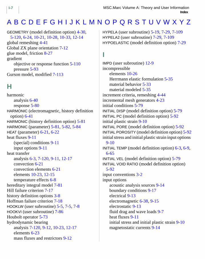
A B C D E F G H I J K L M N O P Q R S T U V W X Y Z
MSC.Marc Volume A: Theory and User InformationIndex
I-7
GEOMETRY (model definition option) 4-30, 5-120, 6-24, 10-21, 10-28, 10-33, 12-14
global remeshing 4-41Global ZX plane orientation 7-12glue model, friction 8-27gradient
objective or response function 5-110pressure 5-93
Gurson model, modified 7-113
Hharmonic
analysis 6-40response 5-80
HARMONIC (electromagnetic, history definition option) 6-41
HARMONIC (history definition option) 5-81HARMONIC (parameter) 5-81, 5-82, 5-84HEAT (parameter) 6-21, 6-22heat fluxes 9-11
(special) conditions 9-11input options 9-11
heat transferanalysis 6-3, 7-120, 9-11, 12-17convection 6-21convection elements 6-21elements 10-23, 12-15temperature effects 6-8
hereditary integral model 7-81Hill failure criterion 7-17history definition options 3-8Hoffman failure criterion 7-18HOOKLW (user subroutine) 5-5, 7-5, 7-8HOOKVI (user subroutine) 7-86Houbolt operator 5-73hydrodynamic bearing
analysis 7-120, 9-12, 10-23, 12-17elements 6-23mass fluxes and restrictors 9-12
HYPELA (user subroutine) 5-19, 7-29, 7-109HYPELA2 (user subroutine) 7-29, 7-109HYPOELASTIC (model definition option) 7-29
IIMPD (user subroutine) 12-9incompressible
elements 10-26Herrmann elastic formulation 5-35material behavior 5-33material modeled 5-35
increment criteria, remeshing 4-44incremental mesh generators 4-23initial conditions 5-79INITIAL DISP (model definition option) 5-79INITIAL PC (model definition option) 5-92initial plastic strain 9-10INITIAL PORE (model definition option) 5-92INITIAL POROSITY (model definition option) 5-92initial stress and initial plastic strain input options
9-10INITIAL TEMP (model definition option) 6-3, 6-9,
6-65INITIAL VEL (model definition option) 5-79INITIAL VOID RATIO (model definition option)
5-92input conventions 3-2input options
acoustic analysis sources 9-14boundary conditions 9-17electrical 9-13electromagnetic 6-38, 9-15electrostatic 9-13fluid drag and wave loads 9-7heat fluxes 9-11initial stress and initial plastic strain 9-10magnetostatic currents 9-14

A B C D E F G H I J K L M N O P Q R S T U V W X Y Z
I-8MSC.Marc Volume A: Theory and User InformationIndex
mass fluxes and restrictors 9-12mechanical loads 9-8thermal loads 9-10
input, mechanical and thermal load increments 5-124
INTCRD (user subroutine) 12-9interpolation (shape) functions, type of 10-15inverse power sweep 5-68ISOTROPIC (acoustic, model definition option)
6-43, 7-121ISOTROPIC (electromagnetic, model definition
option) 6-37, 7-121ISOTROPIC (electrostatic, model definition
option) 6-29, 7-121ISOTROPIC (fluid, model definition option) 6-63,
7-120, 7-121ISOTROPIC (heat transfer, model definition
option) 6-65, 7-120, 9-10ISOTROPIC (hydrodynamic, model definition
option) 7-120ISOTROPIC (magnetostatic, model definition
option) 6-31, 7-121ISOTROPIC (model definition option) 3-3, 5-120,
6-3, 6-8, 6-24, 6-59, 7-4, 7-7, 7-27, 7-47, 7-50, 7-51, 7-55, 7-57, 7-59, 7-61, 7-73, 7-77, 7-79, 7-80, 7-83, 7-85, 7-99, 7-100, 7-106, 9-8, 9-9
isotropic hardening 7-57
JJ-INTEGRAL (model definition option) 5-4JOULE (model definition option) 6-65JOULE (parameter) 6-64Joule heating 6-64
KKachanov factor 7-119Kelvin-Voigt model 7-80kinematic
constraints 9-16hardening 7-59
LLagrange multipliers 8-3Lagrangian formulation 5-15Lanczos method 5-69large deformations 5-33LARGE DISP (parameter) 5-16, 5-18, 5-19, 5-23,
5-29, 5-30, 5-36, 7-29, 7-53, 7-57large strain
elasticity 5-33plasticity 5-35
linear analysis 5-3linear elastic material 7-3linear fracture mechanics 5-58linear springs and elastic foundations input
options 9-31linked/unlinked 5-120list of items, input 3-3load
automatic incrementation 5-127fluid drag and wave 9-6history definition options 5-126increment size 5-126mechanical 9-8surface/volumetric 9-4thermal 9-9types 9-3
LOAD COR (parameter) 9-9LORENZI (model definition option) 5-65

A B C D E F G H I J K L M N O P Q R S T U V W X Y Z
MSC.Marc Volume A: Theory and User InformationIndex
I-9
MMAGNETO (parameter) 6-31magnetostatic
analysis 7-121, 9-14, 10-24, 12-17current input options 9-14elements types 6-31
MANY TYPES (model definition option) 4-15Marc
host systems 2-2overview 1-3
mass fluxes and restrictors 9-12mass fluxes and restrictors input options 9-12MASSES (model definition option) 5-82material
dependent failure criteria 7-14instabilities 5-37low tension 7-106powder 7-52preferred direction 7-10
material modelcomposite 7-6elastomers 7-30gasket 7-23linear elastic 7-3Mohr-Coulomb (hydrostatic yield
dependence) 7-50nonlinear hypoelastic 7-29time-independent inelastic 7-43
maximumstrain failure criterion 7-16stress criterion 7-14
Mean Strain Energy Criterion 4-38mean-normal method 5-47mechanical
loads 9-8loads input options 9-8
membrane elements 10-18MERGE (model definition option) 4-10
meshdefinition 4-2refinement tying constraints 9-23severe distortion 5-37
mesh generation, remeshing techniques 4-45advancing front meshing 4-45Delaunay Triangulation 4-47overlay meshing 4-45
MESH2D 4-9MESH2D (model definition option) 4-15, 12-4modal
stresses and reactions 5-70superposition 5-71
MODAL INCREMENT (model definition option) 5-9
MODAL SHAPE (history definition option) 5-68, 5-70, 6-43, 6-63
model definition options 3-7Mohr-Coulomb
linear material 7-50parabolic material 7-51
Monte Carlo method 6-15MOONEY (model definition option) 7-34, 7-39,
7-92Mooney-Rivlin 7-34, 7-40MOTION (2-D, user subroutine) 8-9MOTION CHANGE (history definition option)
8-11, 8-28Mullin’s effect 7-116multiplicative decomposition 5-18, 5-42, 7-42
NNarayanaswamy model 5-55, 7-93NASSOC (user subroutine) 5-56, 5-57, 7-78Navier-Stokes 6-49, 6-53, 6-59, 6-61nearly incompressible behavior 5-36neighbor relations 8-15Neo-Hookean 7-34

A B C D E F G H I J K L M N O P Q R S T U V W X Y Z
I-10MSC.Marc Volume A: Theory and User InformationIndex
Newmark-beta operator 5-72, 5-74Newton Cooling 7-104Newton-Raphson method
full 11-3modified 11-5
nodal degrees of freedom tying constraints 9-29NODE CIRCLE (model definition option) 4-23NODE FILL (model definition option) 4-23NODE GENER (model definition option) 4-23NODE MERGE (model definition option) 4-23NODE SORT (model definition option) 12-8Node Within A Box Criterion 4-40Nodes In Contact Criterion 4-40nodes, merging of 4-10nonlinear
analysis 5-10fracture mechanics 5-60
nonlinearities, three types 5-15non-Newtonian 6-51nonstructural materials 7-120NURB 8-6, 8-17, 8-18, 8-44, 8-45
trimmed 8-6, 8-36
OOak Ridge National Laboratory (ORNL) 5-50,
7-55, 7-76objective function 5-110, 5-112, 5-118, 5-119,
5-121, 5-122objective stress rates 5-39OGDEN (model definition option) 7-35, 7-39,
7-92, 7-119operating systems 2-2operator
central difference 5-73Houbolt 5-73Newmark-beta 5-72single step Houbolt 5-73
OPTHOTROPIC (model definition option) 7-61
optimization algorithm 5-118OPTIMIZE (model definition option) 2-4, 4-24,
12-4Option
ACTIVATE (history definition) 4-7ADAPTIVE (model definition) 4-38, 5-4, 5-5,
10-36ANISOTROPIC (model definition) 5-5, 7-5,
7-7, 7-48APPROACH (history definition) 8-11ATTACH NODE (model definition) 4-36AUTO CREEP (history definition) 5-50, 5-52,
5-53, 5-55, 5-56, 5-57, 7-81AUTO INCREMENT (history definition) 4-27,
5-30, 7-108, 9-9AUTO LOAD (history definition) 4-27, 7-92,
9-9AUTO STEP (history definition) 5-72, 7-85,
7-92, 7-108, 8-44AUTO THERM (history definition) 9-9AUTO THERM CREEP (history definition)
5-54, 5-55AUTO TIME (history definition) 5-55, 5-72,
5-78, 6-68, 7-85, 7-92, 8-44AXITO3D (model definition) 5-133B-H RELATION (electromagnetic, model
definition) 6-41, 7-121B-H RELATION (magnetostatic, model
definition) 6-32, 6-33, 6-34, 7-121BUCKLE (history definition) 5-30, 5-31BUCKLE INCREMENT (model definition) 5-9,
5-30, 5-31CASE COMBIN (model definition) 5-4, 5-6,
5-132CHANGE PORE (model definition) 5-92CHANGE STATE (history definition) 5-54,
5-55CHANGE STATE (model definition) 6-4, 6-21,
9-9

A B C D E F G H I J K L M N O P Q R S T U V W X Y Z
MSC.Marc Volume A: Theory and User InformationIndex
I-11
CHANNEL (model definition) 6-61COMPOSITE (model definition) 5-120, 7-6,
7-7CONN FILL (model definition) 4-23CONN GENER (model definition) 4-23CONNECT (model definition) 4-15CONNECTIVITY (model definition) 4-9, 4-16,
4-23, 6-67CONSTRAINT (model definition) 4-15CONTACT (model definition) 5-27, 5-28,
5-37, 5-74, 8-4, 8-5, 8-7, 9-2, 9-33CONTACT CHANGE (rezoning) 8-34CONTACT NODE (model definition) 8-5CONTACT TABLE (history definition) 8-11,
8-12, 8-28CONTACT TABLE (model definition option)
8-19CONTACT TABLE (model definition) 8-19,
8-26, 8-27, 8-30, 8-52CONTINUE (history definition) 3-4, 3-8, 3-10CONTROL (electromagnetic, model
definition) 6-37CONTROL (heat transfer, model definition)
6-67CONTROL (history definition) 5-54, 5-124,
6-5CONTROL (magnetostatic, model definition)
6-32CONTROL (model definition) 5-19, 5-31,
5-124, 6-5, 6-7, 6-12, 8-38, 12-6CONVERT (model definition) 6-68COORDINATES (model definition) 4-9, 4-16,
4-22, 4-23, 12-14CRACK DATA (model definition) 7-106CREEP (model definition) 5-50, 5-56, 7-72,
7-73, 7-79, 7-81, 7-101CYCLIC SYMMETRY (model definition) 9-33CYLINDRICAL (model definition) 4-7DAMAGE (model definition) 7-119
DAMPING (model definition) 5-71, 5-79, 5-82DAMPING COMPONENTS (history definition)
6-25DEFINE (model definition) 3-3, 3-4, 3-5DENSITY EFFECTS (model definition) 7-53DESIGN DISPLACEMENT CONSTRAINTS
(model definition) 5-120DESIGN FREQUENCY CONSTRAINTS (model
definition) 5-120DESIGN OBJECTIVE (model definition) 5-120DESIGN STRAIN CONSTRAINTS (model
definition) 5-120DESIGN STRESS CONSTRAINTS (model
definition) 5-120DESIGN VARIABLES (model definition) 5-120DISP CHANGE (history definition) 5-55, 6-68DIST CHARGE (electromangetic, model
definition) 6-37DIST CHARGES (electrostatic, model
definition) 6-29DIST CURRENT (electromagnetic, model
definition) 6-37DIST CURRENT (Joule, history definition)
6-65DIST CURRENT (Joule, model definition)
6-65DIST CURRENT (magnetostatic, model
definition) 6-32DIST FLUXES (history definition) 6-65DIST FLUXES (model definition) 5-92, 6-4,
6-9, 6-24, 6-65DIST LOADS (history definition) 5-55DIST LOADS (model definition) 5-92, 9-6, 9-9DIST SOURCE (model definition) 6-43DYNAMIC CHANGE (history definition) 5-71,
5-72, 5-78, 6-43, 6-63DYNAMIC CHANGE (history definition,
dynamic) 6-68

A B C D E F G H I J K L M N O P Q R S T U V W X Y Z
I-12MSC.Marc Volume A: Theory and User InformationIndex
DYNAMIC CHANGE (history definition, electromagnetic) 6-37, 6-40
ELEM SORT (model definition) 12-8END OPTION (model definition) 3-2, 3-7, 3-8,
3-10, 5-119, 6-43END REZONE (rezoning) 3-10ERROR ESTIMATE (model definition) 4-33,
5-5, 5-37EXCLUDE (history definition) 8-13FAIL DATA (model definition) 7-22, 7-106FILMS (model definition) 6-4, 6-10, 6-65,
9-11FIXED DISP (model definition) 4-9, 4-15,
5-92, 6-63, 6-68FIXED POTENTIAL (electromagnetic, model
definition) 6-37FIXED POTENTIAL (electrostatic, model
definition) 6-29FIXED POTENTIAL (magnetostatic, model
definition) 6-32FIXED PRESSURE (model definition) 5-92,
6-24, 6-43FIXED TEMPERATURE (model definition)
6-4, 6-9, 6-59, 6-65, 6-68, 7-27FIXED VELOCITY (model definition) 6-59FLUID DRAG (model definition) 9-6FLUID SOLID (model definition) 6-62FOUNDATION (model definition) 5-5, 5-29FOURIER (model definition) 5-4, 5-6, 5-9FXORD (model definition) 4-17, 4-22, 10-22GASKET (model definition) 7-27GEOMETRY (model definition) 4-30, 5-120,
6-24, 10-21, 10-28, 10-33, 12-14HARMONIC (electromagnetic, history
definition) 6-41HARMONIC (history definition) 5-81history definition 3-8HYPOELASTIC (model definition) 7-29INITIAL DISP (model definition) 5-79
INITIAL PC (model definition) 5-92INITIAL PORE (model definition) 5-92INITIAL POROSITY (model definition) 5-92INITIAL TEMP (model definition) 6-3, 6-9,
6-65INITIAL VEL (model definition) 5-79INITIAL VOID RATIO (model definition) 5-92ISOTROPIC (acoustic, model definition) 6-43,
7-121ISOTROPIC (electromagnetic, model
definition) 6-37, 7-121ISOTROPIC (electrostatic, model definition)
6-29, 7-121ISOTROPIC (fluid, model definition) 6-63,
7-120, 7-121ISOTROPIC (heat transfer, model definition)
6-65, 7-120, 9-10ISOTROPIC (hydrodynamic, model
definition) 7-120ISOTROPIC (magnetostatic, model definition)
6-31, 7-121ISOTROPIC (model definition) 3-3, 5-120,
6-3, 6-8, 6-24, 6-59, 7-4, 7-7, 7-27, 7-47, 7-50, 7-51, 7-55, 7-57, 7-59, 7-61, 7-73, 7-77, 7-79, 7-80, 7-83, 7-85, 7-99, 7-100, 7-106, 9-8, 9-9
J-INTEGRAL (model definition) 5-4JOULE (model definition) 6-65LORENZI (model definition) 5-65MANY TYPES (model definition) 4-15MASSES (model definition) 5-82MERGE (model definition) 4-10MESH2D (model definition) 4-15, 12-4MODAL INCREMENT (model definition) 5-9MODAL SHAPE (history definition) 5-68,
5-70, 6-43, 6-63model definition 3-7MOONEY (model definition) 7-34, 7-39, 7-92

A B C D E F G H I J K L M N O P Q R S T U V W X Y Z
MSC.Marc Volume A: Theory and User InformationIndex
I-13
MOTION CHANGE (history definition) 8-11, 8-28
NODE CIRCLE (model definition) 4-23NODE FILL (model definition) 4-23NODE GENER (model definition) 4-23NODE MERGE (model definition) 4-23NODE SORT (model definition) 12-8OGDEN (model definition) 7-35, 7-39, 7-92,
7-119OPTIMIZE (model definition) 2-4, 4-24, 12-4ORIENTATION (model definition) 7-5, 7-7,
7-10, 7-48, 7-86, 10-3ORTHO TEMP (model definition) 6-3, 6-65,
7-7, 7-55, 7-99, 7-100ORTHOTROPIC (electrical, model definition)
7-121ORTHOTROPIC (electromagnetic, model
definition) 6-37, 7-121ORTHOTROPIC (electrostatic, model
definition) 6-29ORTHOTROPIC (magnetostatic, model
definition) 6-31, 7-121ORTHOTROPIC (model definition) 5-5,
5-120, 6-3, 7-5, 7-7, 7-47, 7-48, 7-55, 7-57, 7-59, 7-61, 7-79, 7-80, 7-83, 7-85, 7-99, 7-100, 7-102, 9-8, 9-9
ORTHOTROPIC (thermal, model definition) 6-65, 7-120, 9-10
PARAMETERS (history definition) 5-75PARAMETERS (model definition) 5-86, 5-88,
6-59, 8-18, 8-19PERMANENT ((magnetostatic, model
definition) 6-33, 6-34PERMANENT (magnetostatic, model
definition) 6-32POINT CHARGE (model definition) 6-29POINT CURRENT (electromagnetic, history
definition) 6-37
POINT CURRENT (Joule, history definition) 6-65
POINT CURRENT (Joule, model definition) 6-65
POINT CURRENT (magnetostatic, model definition) 6-32
POINT FLUX (history definition) 6-65POINT FLUX (model definition) 5-92, 6-4,
6-9, 6-24, 6-59, 6-65POINT LOAD (history definition) 5-55POINT LOAD (model definition) 3-3, 5-92, 8-9POINT SOURCE (model definition) 6-43POST (model definition) 5-54, 6-4, 6-21,
12-18POWDER (model definition) 7-53PRINT CHOICE (model definition) 5-84, 7-20,
12-7, 12-8, 12-10, 12-11, 12-13, 12-16PRINT ELEMENT (model definition) 7-20,
12-7, 12-10, 12-11, 12-13PRINT NODE (model definition) 12-7, 12-8,
12-10, 12-16PRINT VMASS (model definition) 12-8PROPORTIONAL INCREMENT (history
definition) 4-27, 5-55, 5-57, 9-9RADIATING CAVITY (model definition) 6-11REAUTO (model definition) 5-50, 5-132REBAR (model definition) 7-106RECOVER (history definition) 5-70RELATIVE DENSITY (model definition) 7-53RELEASE (history definition) 8-28RESTART (model definition) 2-5, 5-4, 5-50,
5-131, 5-132, 12-8, 12-10RESTART INCREMENT (history definition)
5-132RESTART LAST (model definition) 5-132RESTRICTOR (model definition) 6-24REZONE (rezoning) 3-10ROTATION A (model definition) 9-8SERVO LINK (model definition) 9-2, 9-23

A B C D E F G H I J K L M N O P Q R S T U V W X Y Z
I-14MSC.Marc Volume A: Theory and User InformationIndex
SHELL TRANSFORMATION (model definition) 9-17, 9-21
SHIFT FUNCTION (model definition) 5-55, 7-89
SOIL (model definition) 5-92, 7-109SOLVER (model definition) 10-34, 11-25,
11-27SPECIFIED NODES (model definition) 4-15SPLINE (model definition) 8-6, 8-50SPRINGS (model definition) 5-5, 5-29, 5-82START NUMBER (model definition) 4-15STEADY STATE (electrostatic, history
definition) 6-29STEADY STATE (history definition) 6-5, 6-56,
6-65STEADY STATE (magnetostatic, history
definition) 6-32STIFFNS COMPONENTS (history definition)
6-25STIFFSCALE (model definition) 4-29STRAIN RATE (model definition) 5-88, 6-59,
7-7, 7-55STRAIN RATE (model definition, fluid) 7-121SUBSTRUCTURE (model definition) 4-27SUMMARY (model definition) 12-8SUPERINPUT (model definition) 4-27SURFACE (model definition) 4-36SYNCHRONIZED (history definition) 8-11TABLE (model definition) 7-25TEMP CHANGE (history definition) 6-4, 6-9,
6-59, 6-65, 6-68TEMPERATURE EFFECTS (coupled thermal-
stress, model definition) 7-120TEMPERATURE EFFECTS (heat transfer,
model definition) 6-65, 7-120TEMPERATURE EFFECTS (hydrodynamic,
model definition) 7-120
TEMPERATURE EFFECTS (model definition) 5-88, 6-3, 6-8, 6-24, 7-7, 7-34, 7-53, 7-55, 7-83, 7-89, 7-99, 7-100, 7-102, 7-121
THICKNESS (model definition) 6-24THICKNS CHANGE (history definition) 6-24TIME STEP (history definition) 7-55, 7-85,
7-92TIME-TEMP (model definition) 7-103, 7-104TRANSFORMATION (model definition) 9-17,
9-27, 12-16TRANSIENT (history definition) 6-4, 6-5, 6-65TYING (model definition) 6-4, 6-62, 9-2,
9-22, 9-23TYING CHANGE (history definition) 9-23UFCONN (model definition) 4-8UFXORD (model definition) 4-8UTRANFORM (model definition) 9-17VELOCITY (model definition) 6-4, 6-22, 6-24VELOCITY CHANGE (history definition) 6-4,
6-22, 6-59VIEW FACTOR (model definition) 6-15, 9-12VISCEL EXP (model definition) 5-56, 7-98VISCELMOON (model definition) 5-56, 7-34,
7-92VISCELOGDEN (model definition) 5-56, 7-35,
7-92, 7-119VISCELORTH (model definition) 7-85VISCELPROP (model definition) 7-85VOLTAGE (model definition) 6-65VOLTAGE CHANGE (history definition) 6-65WORK HARD (model definition) 5-88, 7-7,
7-56, 7-57, 7-59, 7-61ORIENT (user subroutine) 5-5, 7-5, 7-10, 7-13,
7-48, 7-86ORIENTATION (model definition option) 7-5, 7-7,
7-10, 7-48, 7-86, 10-3ORTHO TEMP (model definition option) 6-3,
6-65, 7-7, 7-55, 7-99, 7-100

A B C D E F G H I J K L M N O P Q R S T U V W X Y Z
MSC.Marc Volume A: Theory and User InformationIndex
I-15
ORTHOTROPIC (electrical, model definition option) 7-121
ORTHOTROPIC (electromagnetic, model definition option) 6-37, 7-121
ORTHOTROPIC (electrostatic, model definition option) 6-29
ORTHOTROPIC (magnetostatic, model definition option) 6-31, 7-121
ORTHOTROPIC (model definition option) 5-5, 5-120, 6-3, 7-5, 7-7, 7-47, 7-48, 7-55, 7-57, 7-59, 7-79, 7-80, 7-83, 7-85, 7-99, 7-100, 7-102, 9-8, 9-9
ORTHOTROPIC (thermal, model definition option) 6-65, 7-120, 9-10
out-of-core storage options 2-3
PParameter
ACOUSTIC 6-43ADAPTIVE 8-35, 10-36ALL POINTS 5-131, 6-21, 10-3ASSUMED STRAIN 10-33BEAM SECT 4-30, 10-20BEARING 6-24BUCKLE 5-9, 5-30CENTROID 5-19, 5-29, 5-131, 6-21, 9-10,
10-3, 11-20, 12-11, 12-16CONSTANT DILATATION 5-18, 10-28COUPLE 6-67CREEP 5-50, 5-54, 5-55, 5-56, 5-57, 7-71,
7-79, 7-80DESIGN OPTIMIZATION 5-119, 7-4DESIGN SENSITIVITY 5-119, 7-4DIST LOADS 5-119DYNAMIC 5-9, 5-65, 5-67, 5-71, 5-72ELASTIC 4-34, 5-3, 5-4ELASTICITY 5-4, 5-23ELECTRO 6-29
ELEMENTS 10-2EL-MA 6-37ELSTO 2-3, 2-5, 12-3, 12-4END 3-6, 3-8EXTENDED 3-3FINITE 5-16, 5-18, 5-23, 5-36, 7-29, 7-53,
7-57FLUID 10-24FOLLOW FOR 5-19, 5-29, 7-53, 9-9, 9-21,
10-34FOURIER 5-6, 5-9HARMONIC 5-81, 5-82, 5-84HEAT 6-21, 6-22JOULE 6-64LARGE DISP 5-16, 5-18, 5-19, 5-23, 5-29,
5-30, 5-36, 7-29, 7-53, 7-57LOAD COR 9-9MAGNETO 6-31PLASTICITY 5-18, 5-23, 7-57PRINT 5-31, 12-17RADIATION 6-11, 6-15, 7-120, 9-12RESTRICTOR 6-24REZONING 4-25R-P FLOW 5-86, 11-10SCALE 5-124SHELL SECT 10-21SIZING 8-34, 10-2, 12-3, 12-4STATE VARS 6-24STOP 2-4, 8-39SUBSTRUC 4-27SUPER 4-27TSHEAR 7-20, 12-14T-T-T 7-103UPDATE 5-16, 5-18, 5-23, 5-36, 5-73, 5-78,
6-68, 7-29, 7-53, 7-57, 7-112, 9-21VISCO ELAS 5-55
parameters 3-6PARAMETERS (history definition option) 5-75

A B C D E F G H I J K L M N O P Q R S T U V W X Y Z
I-16MSC.Marc Volume A: Theory and User InformationIndex
PARAMETERS (model definition option) 5-86, 5-88, 6-59, 8-18, 8-19
penalty 5-86, 6-55methods 8-3
PERMANENT ((magnetostatic, model definition option) 6-34
PERMANENT (magnetostatic, model definition option) 6-32, 6-33
perturbation analysis 5-31piecewise linear representation 7-99pipe bend element tying constraints 9-28PLASTICITY (parameter) 5-18, 5-23, 7-57plate elements 10-21POINT CHARGE (model definition option) 6-29POINT CURRENT (electromagnetic, history
definition option) 6-37POINT CURRENT (Joule, history definition
option) 6-65POINT CURRENT (Joule, model definition
option) 6-65POINT CURRENT (magnetostatic, model
definition option) 6-32POINT FLUX (history definition option) 6-65POINT FLUX (model definition option) 5-92, 6-4,
6-9, 6-24, 6-59, 6-65POINT LOAD (history definition option) 5-55POINT LOAD (model definition option) 3-3, 5-92,
8-9POINT SOURCE (model definition option) 6-43Poisson’s 5-3, 7-3, 7-4, 7-5, 7-7, 7-53, 7-99,
7-103, 7-106, 7-109, 7-112POST (model definition option) 5-54, 6-4, 6-21,
12-18post file 12-18POWDER (model definition option) 7-53powder material 7-52Power Law Fluid 6-52preconditioners, iterative solvers 11-26pre-stress in bolts 9-35
Previously Refined Mesh Criterion 4-40PRINT (parameter) 5-31, 12-17PRINT CHOICE (model definition option) 5-84,
7-20, 12-7, 12-8, 12-10, 12-11, 12-13, 12-16PRINT ELEMENT (model definition option) 7-20,
12-7, 12-10, 12-11, 12-13PRINT NODE (model definition option) 12-7,
12-8, 12-10, 12-16PRINT VMASS (model definition option) 12-8program
initiation 2-7messages 12-19
progressive composite failure 7-22PROPORTIONAL INCREMENT (history definition
option) 4-27, 5-55, 5-57, 9-9PSPG 6-53PWL (piece-wise linear) 8-6
Qquarter point elements 5-64
Rradial return 5-46RADIATING CAVITY (model definition option)
6-11RADIATION (parameter) 6-11, 6-15, 7-120, 9-12radiation viewfactors 6-10radiation-gap 6-19REAUTO (model definition option) 5-50, 5-132REBAR (model definition option) 7-106REBAR (user subroutine) 7-106RECOVER (history definition option) 5-70reduced integration elements 10-29RELATIVE DENSITY (model definition option)
7-53RELEASE (history definition option) 8-28

A B C D E F G H I J K L M N O P Q R S T U V W X Y Z
MSC.Marc Volume A: Theory and User InformationIndex
I-17
remeshingcriteria 4-43global 4-41
remeshing techniques 4-44mesh generation 4-45outline extraction and repair 4-47target number of elements 4-49
Residual Load Correction 5-130, 11-10RESTART (model definition option) 2-5, 5-4,
5-50, 5-131, 5-132, 12-8, 12-10restart analysis 5-131RESTART INCREMENT (history definition option)
5-132RESTART LAST (model definition option) 5-132RESTRICTOR (model definition option) 6-24RESTRICTOR (parameter) 6-24result evaluation, contact 8-36REZONE (rezoning option) 3-10rezoning 4-25REZONING (parameter) 4-25rigid contact, solution strategy 8-46rigid link constraint 9-30rigid-plastic analysis 5-86, 10-27, 12-17Riks-Ramm 11-16, 11-17ROTATION A (model definition option) 9-8R-P FLOW (parameter) 5-86, 11-10rubber foam model 7-38RVCNST 8-21, 8-22
SSCALE (parameter) 5-124scaling, linear-elastic solution 5-124Secant method 11-8semi-infinite elements 10-32sensitivity 5-110separation, contact 8-28SEPFOR (user subroutine) 8-47SEPSTR (user subroutine) 8-47
Sequential Quadratic Programming 5-118SERVO LINK (model definition option) 9-2, 9-23shell
contact 8-14elements 10-22stiffener tying constraints 9-28transformation 9-17
SHELL SECT (parameter) 10-21shell stiffener tying constraints 9-28SHELL TRANSFORMATION (model definition
option) 9-17, 9-21shell-to-shell intersection tying constraints 9-25shell-to-solid intersections tying constraints 9-27SHIFT FUNCTION (model definition option) 5-55,
7-89single step Houbolt operator 5-73SIZING (parameter) 8-34, 10-2, 12-3, 12-4SOIL (model definition option) 5-92, 7-109soil analysis 5-92, 7-109, 10-24SOLVER (model definition option) 10-34, 11-25,
11-27special elements 10-25SPECIFIED NODES (model definition option)
4-15spectrum response 5-84SPLINE (model definition option) 8-6, 8-50SPRINGS (model definition option) 5-5, 5-29,
5-82SSTRAN (user subroutine) 4-27START NUMBER (model definition option) 4-15STATE VARS (parameter) 6-24status file 12-22STEADY STATE (electrostatic, history definition
option) 6-29STEADY STATE (history definition option) 6-5,
6-56, 6-65STEADY STATE (magnetostatic, history definition
option) 6-32Stefan-Boltzmann 9-12

A B C D E F G H I J K L M N O P Q R S T U V W X Y Z
I-18MSC.Marc Volume A: Theory and User InformationIndex
stick-slip model, friction 8-23STIFFNS COMPONENTS (history definition
option) 6-25STIFFSCALE (model definition option) 4-29STOP (parameter) 2-4, 8-39storage methods 11-27strain correction method 11-6STRAIN RATE (model definition option) 5-88,
6-59, 7-7, 7-55STRAIN RATE (model definition, fluid option)
7-121strain rate effects on elastic-plastic constitutive
relation 7-65stress
analysis 12-16intensity factors 5-59
stress intensity factor defined 5-59SUBSTRUC (parameter) 4-27SUBSTRUCTURE (model definition option) 4-27substructuring 4-26SUMMARY (model definition option) 12-8SUPER (parameter) 4-27SUPERINPUT (model definition option) 4-27SUPG 6-53SURFACE (model definition option) 4-36symmetries 4-14SYNCHRONIZED (history definition option) 8-11
TTABLE (model definition option) 7-25TEMP CHANGE (history definition option) 6-4,
6-9, 6-59, 6-65, 6-68TEMPERATURE EFFECTS (coupled thermal-
stress, model definition option) 7-120TEMPERATURE EFFECTS (heat transfer, model
definition option) 6-65, 7-120TEMPERATURE EFFECTS (hydrodynamic, model
definition option) 7-120
TEMPERATURE EFFECTS (model definition option) 5-88, 6-3, 6-8, 6-24, 7-7, 7-34, 7-53, 7-55, 7-83, 7-89, 7-99, 7-100, 7-102, 7-121
Temperature Gradient Criterion 4-40temperature-dependent
creep 7-101material properties 7-99
tension softening 7-107thermal
loads 9-9loads input options 9-10
thermo-electrical 7-120Thermo-Rheologically Simple material 7-87THICKNESS (model definition option) 6-24THICKNS CHANGE (history definition option)
6-24TIME STEP (history definition option) 7-55, 7-85,
7-92time step definition 5-78time-dependent
boundary conditions 5-79inelastic behavior 7-67
time-independent, inelastic behavior 7-43TIME-TEMP (model definition option) 7-103,
7-104Time-Temperature-Transformation (T-T-T)
7-103tolerance values, contact 8-37total Lagrangian procedure 5-19TRANSFORMATION (model definition option)
9-17, 9-27, 12-16TRANSIENT (history definition option) 6-4, 6-5,
6-65TRSFAC (user subroutine) 7-89truss elements 10-17Tsai-Wu failure criterion 7-19TSHEAR (parameter) 7-20, 12-14T-T-T (parameter) 7-103

A B C D E F G H I J K L M N O P Q R S T U V W X Y Z
MSC.Marc Volume A: Theory and User InformationIndex
I-19
TYING (model definition option) 6-4, 6-62, 9-2, 9-22, 9-23
TYING CHANGE (history definition option) 9-23tying constraints
beam-to-beam intersection 9-26cyclic symmetry 9-32mesh refinement 9-23nodal degrees of freedom 9-29pipe bend element 9-28shell stiffener 9-28shell-to-shell intersection 9-25shell-to-solid intersections 9-27
UUADAP (user subroutine) 4-40UBEAR (user subroutine) 6-25UCOMPL (user subroutine) 5-83UCOORD (user subroutine) 4-36UCRACK (user subroutine) 7-106UELDAM (user subroutine) 7-119UENERG (user subroutine) 7-39UEPS (user subroutine) 6-29, 6-31, 6-37, 7-121UFAIL (user subroutine) 7-14, 7-20UFCONN (model definition option) 4-8UFCONN (user subroutine) 4-8UFINITE (user subroutine) 7-47UFORMS (user subroutine) 9-23, 9-29UFOUR (user subroutine) 5-6UFOXORD (user subroutine) 4-17UFRIC (user subroutine) 8-27UFXORD (model definition optiion) 4-8UFXORD (user subroutine) 4-8UGROOV (user subroutine) 6-24UHTCOE (user subroutine) 8-30UHTCON (user subroutine) 8-30UMOONY (user subroutine) 7-34UMU (user subroutine) 6-37, 7-121UNEWTN (user subroutine) 5-88uniaxial cracking data 7-106
UOGDEN (user subroutine) 7-35UPDATE (parameter) 5-16, 5-18, 5-23, 5-36,
5-73, 5-78, 6-68, 7-29, 7-53, 7-57, 7-112, 9-21updated Lagrange Formulation, nonlinear
elasticity 7-41updated Lagrangian Procedure 5-22UPNOD (user subroutine) 5-87UPOSTV (user subroutine) 12-18UPSTRECH (user subroutine) 7-39URESTR (user subroutine) 6-24URPFLO (user subroutine) 5-88User subroutine
ANELAS 5-5, 7-5, 7-8ANEXP 5-5, 7-8, 7-102ANKOND 6-4, 7-120ANPLAS 7-8, 7-48CRPLAW 5-51, 5-52, 5-56, 5-57, 7-72, 7-73,
7-77, 7-78, 7-80, 7-101CRPVIS 5-55, 7-71, 7-80, 7-81ELEVAR 12-9, 12-13ELEVEC 12-9FILM 6-4, 6-10, 6-65, 9-11, 9-12FLUX 6-4, 6-9, 6-24, 6-29, 6-32, 6-43, 6-65,
9-11, 9-12FORCDT 5-79, 6-9, 6-25, 6-29, 6-32, 6-59FORCEM 4-36, 5-79, 6-37HOOKLW 5-5, 7-5, 7-8HOOKVI 7-86HYPELA 5-19, 7-29, 7-109HYPELA2 7-29, 7-109IMPD 12-9INTCRD 12-9MOTION (2-D) 8-9NASSOC 5-56, 5-57, 7-78ORIENT 5-5, 7-5, 7-10, 7-13, 7-48, 7-86REBAR 7-106SEPFOR 8-47SEPSTR 8-47SSTRAN 4-27TRSFAC 7-89

A B C D E F G H I J K L M N O P Q R S T U V W X Y Z
I-20MSC.Marc Volume A: Theory and User InformationIndex
UADAP 4-40UBEAR 6-25UCOMPL 5-83UCOORD 4-36UCRACK 7-106UELDAM 7-119UENERG 7-39UEPS 6-29, 6-31, 6-37, 7-121UFAIL 7-14, 7-20UFCONN 4-8UFINITE 7-47UFORMS 9-23, 9-29UFOUR 5-6UFRIC 8-27UFXORD 4-8, 4-17UGROOV 6-24UHTCOE 8-30UHTCON 8-30UMOONY 7-34UMU 6-37, 7-121UNEWTN 5-88UOGDEN 7-35UPNOD 5-87UPOSTV 12-18UPSTRECH 7-39URESTR 6-24URPFLO 5-88USIGMA 6-37, 7-121USINC 5-79, 6-9USPRNG 5-29, 9-31USSD 5-85UTHICK 6-24, 6-25UTRANS 9-17UVELOC 6-4, 6-22, 6-24UVSCPL 5-51, 5-52, 5-57, 7-80VSWELL 5-51, 5-52, 7-78, 7-80WKSLP 7-56, 7-57, 7-59, 7-61YIEL 5-57, 7-78ZERO 5-57, 7-78
user subroutine input 4-8User-defined Criterion 4-40user-defined failure criteria 7-20USIGMA (user subroutine) 6-37, 7-121USINC (user subroutine) 5-79, 6-9USPRNG (user subroutine) 5-29, 9-31USSD (user subroutine) 5-85UTHICK (user subroutine) 6-24, 6-25UTRAN (user subroutine) 9-17UTRANFORM (model definition option) 9-17UVELOC (user subroutine) 6-4, 6-22, 6-24UVSCPL (user subroutine) 5-51, 5-52, 5-57, 7-80
VVELOCITY (model definition option) 6-4, 6-22,
6-24VELOCITY CHANGE (history definition option)
6-4, 6-22, 6-59VIEW FACTOR (model definition option) 6-15,
9-12viewfactor calculation
Adaptive Contour Integration 6-15Direct Adaptive Integration 6-11Monte Carlo Method 6-15
VISCEL EXP (model definition option) 5-56, 7-98VISCELMOON (model definition option) 5-56,
7-34, 7-92VISCELOGDEN (model definition option) 5-56,
7-35, 7-92, 7-119VISCELORTH (model definition option) 7-85VISCELPROP (model definition option) 7-85VISCO ELAS (parameter) 5-55viscoelastic material
incompressible isotropic 7-86isotropic 7-83Thermo-Rheologically Simple 7-87
viscoelasticity 5-55viscoplastic analysis 5-56

A B C D E F G H I J K L M N O P Q R S T U V W X Y Z
I-21MSC.Marc Volume A: Theory and User InformationIndex
viscoplasticityexplicit formulation 7-78explicit method 5-56implicit method 5-57
VOLTAGE (model definition option) 6-65VOLTAGE CHANGE (history definition option)
6-65von Mises 5-46, 5-47, 5-53, 5-115, 7-46, 7-50,
7-53, 7-57, 7-58, 7-59, 7-62, 7-64, 7-65, 7-73, 12-8, 12-11, 12-12
VSWELL (user subroutine) 5-51, 5-52, 7-78, 7-80
Wweighted mesh 4-14Williams-Landel-Ferry (WLF) 5-55, 7-89WKSLP (user subroutine) 7-56, 7-57, 7-59, 7-61WORK HARD (model definition option) 5-88, 7-7,
7-56, 7-57, 7-59, 7-61workhardening
isotropic 7-57rules 7-55slope 7-44
workspace allocation 2-3, 8-39
YYIEL (user subroutine) 5-57, 7-78Young’s 7-2, 7-3, 7-7, 7-21, 7-40, 7-45, 7-57,
7-99, 7-103, 7-106, 7-107, 7-109
ZZERO (user subroutine) 5-57, 7-78Zienkiewicz-Zhu Creep Strain Criterion 4-39Zienkiewicz-Zhu Criterion 4-38

MSC.Marc Volume A: Theory and User InformationIndex
I-22