Effects of Air Pollution from Biomass Burning in Amazon: A Panel Study of Schoolchildren
Upload
independentCategory
view
3download
0
Environmental Fluid Mechanics (2005) 5: 135–167
Monitoring the Transport of Biomass BurningEmissions in South America
© Springer 2005
SAULO R. FREITASa,∗, KARLA M. LONGOa, MARIA A.F. SILVA DIASb,PEDRO L. SILVA DIASb, ROBERT CHATFIELDc, ELAINE PRINSd, PAULOARTAXOb, GEORG A. GRELLe and FERNANDO S. RECUEROb
aCenter for Weather Prediction and Climate Studies - CPTEC/INPE, Brazil; bUniversity of SãoPaulo, Brazil; cNASA Ames Research Center, U.S.A.; dNOAA/NESDIS/ORA, Madison, WI, U.S.A.;eCooperative Institute for Research in Environmental Science (CFRES), University at Colorado,and NOAA Research – Forecast Systems Laboratory, Boulder, CO, U.S.A.
Received 16 June 2003; accepted in revised form 3 May 2004
Abstract. The atmospheric transport of biomass burning emissions in the South American andAfrican continents is being monitored annually using a numerical simulation of air mass motions;we use a tracer transport capability developed within RAMS (Regional Atmospheric Modeling Sys-tem) coupled to an emission model. Mass conservation equations are solved for carbon monoxide(CO) and particulate material (PM2.5). Source emissions of trace gases and particles associatedwith biomass burning activities in tropical forest, savanna and pasture have been parameterized andintroduced into the model. The sources are distributed spatially and temporally and assimilated dailyusing the biomass burning locations detected by remote sensing. Advection effects (at grid scale)and turbulent transport (at sub-grid scale) are provided by the RAMS parameterizations. A sub-grid transport parameterization associated with moist deep and shallow convection, not explicitlyresolved by the model due to its low spatial resolution, has also been introduced. Sinks associatedwith the process of wet and dry removal of aerosol particles and chemical transformation of gasesare parameterized and introduced in the mass conservation equation. An operational system has beenimplemented which produces daily 48-h numerical simulations (including 24-h forecasts) of CO andPM2.5, in addition to traditional meteorological fields. The good prediction skills of the model aredemonstrated by comparisons with time series of PM2.5 measured at the surface.
Key words: aerosol transport, air pollution, atmospheric modeling, biomass burning, climate change,long-distance transport, weather forecast
1. Introduction
The high concentration of aerosol particles and trace gases observed in the Amazonand Central Brazilian atmosphere during the dry season is associated with intenseanthropogenic biomass burning activity (vegetation fires). A widely cited estimate∗Corresponding author, E-mail: [email protected]
136 SAULO R. FREITAS ET AL.
suggests that biomass burning in South America is responsible for the emissionof 30 Tg year−1 of aerosol particles to the atmosphere [1]. Most of the particlesare in the fine particle fraction of the size distribution, which can remain in theatmosphere for approximately a week [2]. Estimates of biomass burning emissionsas high as these are disputed by those making detailed studies of subtropical land-scapes [3], and are thought to vary widely from year to year [4]. Consequently,annual monitoring is an important effort. In addition to aerosol particles, biomassburning produces water vapor and carbon dioxide, and is a major source of othercompounds such as carbon monoxide (CO), volatile organic compounds, nitrogenoxides (NOx = NO + NO2), and organic halogen compounds. In the presence ofabundant solar radiation and high concentrations of NOx, the oxidation of CO andhydrocarbons is followed by ozone (O3) formation.
In GOES-8 visible imagery Prins et al. [5] have observed immense regionalsmoke plumes in South America covering an area of approximately 4 to 5 millionkm2 during the biomass-burning season. Inhalable aerosol particles (dp < 10 µm)with concentrations as high as 400 µg m−3 have been measured near the surfacelevel and the vertically integrated smoke aerosol optical thickness column risesas high as 4.0 (440 nm) in Central Brazil [6–8]. The biomass burning particles,made up primarily of partially oxidized organic matter mixed with black-carbon,are highly efficient scatterers and absorbers of solar radiation; a single scatteringalbedo as low as 0.82 has been estimated for these particles [9].
On a regional and global scale, a persistent and heavy smoke layer over anextensive tropical region may alter the radiation balance and hydrologic cycling.Modeling efforts of Jacobson [10] and Sato et al. [11] have suggested that black-carbon radiative forcing could balance the cooling effects of the global anthro-pogenic sulfate emissions. The direct global radiative forcing of black-carbon isestimated to be 0.55 Wm−2, corresponding to 1/3 of the CO2 forcing. In termsof direct radiative forcing, this would elevate black-carbon to one of the mostimportant elements in global warming, second only to CO2 [12].
The presence of biomass burning particles in the atmosphere may also modifythe solar radiative balance by changing cloud microphysics. These particles act ascloud condensation and ice nuclei, promoting changes in the cloud drops spectrumand so altering the cloud albedo and precipitation [13, 14]. This suggests that bio-mass burning effects may extrapolate from the local scale and be determinant inthe pattern of planetary redistribution of energy from the tropics to medium andhigh latitudes via convective transport processes.
Several atmospheric pollutant transport models on regional or global scales havebeen used. Grell et al. [15] describe a multiscale complex chemistry model coupledto the Penn State/NCAR nonhydrostatic mesoscale model (MM5). Chatfield et al.[16] use the Global-Regional Atmospheric Chemistry Event Simulator (GRACES)to introduce a conceptual model of how fire emissions and chemistry produce theAfrican/Oceanic plumes. Chatfield et al. [17] present a connection between trop-ical emissions and an observed subtropical plume of carbon monoxide at remote
MONITORING THE TRANSPORT OF BIOMASS BURNING EMISSIONS IN SOUTH AMERICA 137
areas over the Pacific Ocean, using the GRACES and MM5 models. The GeorgiaTech/Goddard Global Ozone Chemistry Aerosol Radiation and Transport (GO-CART) model is an example of a global transport model. Chin et al. [18] employedGOCART to simulate the atmospheric global sulfur cycle. MOZART (Model ofOzone And Related Tracers) is another “off-line” global chemical transport modelappropriate for simulating the three-dimensional distribution of chemical speciesin the atmosphere [19, 20]. The term ‘off-line’ indicates the transport model isdriven using outputs from an atmospheric model previously run or by atmosphericanalysis data assimilation. ‘On-line’ transport models have considerable benefitssince they can use the same temporal and spatial resolution of the atmosphericmodel, avoiding errors associated to numerical interpolation. More significantly,they are suitable for feedback studies between the tracers and the atmosphere (e.g.the effects of aerosol on the radiative transfer).
In this paper a tracer transport model coupled to the Regional AtmosphericModeling System – RAMS [21] will be described. The tracer transport simulationis made simultaneously, or ‘on-line’, with the atmospheric state evolution. As aresult, a real time monitoring transport system has been implemented using thecoupled transport-atmospheric model. This operational system was designed toforecast and study the transport of biomass burning aerosol and gaseous speciesin the South American and African continents with an application during to the2002 dry season.
The specification of the biomass burning description and the source emissionparameterization will be described in Section 2. The coupled transport-atmosphericmodel will be presented in Sections 3 and 4. Results described in the context ofour description of the transport of aerosol and gases as well as some comparisonswith observations are shown in Section 4. Conclusions and recommendations arepresented in Section 5.
2. Overview of Biomass Burning Emissions and Transport in South America
The ignition, evolution and behavior of a biomass fire and its emissions depend onmany factors which are ultimately controlled by the environment. Local climateis extremely important in the determination of the amount and characteristics ofthe biomass available. For a given type of biomass, the local weather, includingtemperature, precipitation, humidity and wind, controls the conditions required forthe fire ignition and maintenance.
Biomass burning can be described in four basic stages: ignition, flaming, smol-dering and extinction [22]. The flaming stage is a pyrolitic process, with elevatedtemperatures as high as 1800 K, that acts to break apart the biomass molecules anddecompose compounds of high molecular weight mostly into lower molecular-weight species, but also producing soot and tar along with the principle product.Nitrogen oxides, hydrocarbons and an abundance of aerosol particles are also emit-ted during the flaming stage. CO and other compounds characterized by incomplete
138 SAULO R. FREITAS ET AL.
oxidation as well as aerosol particles are emitted primarily during the smolderingphase at temperatures typically below 1000 K [23]. The amount of water in thebiomass is one of the most important biomass burning control factors and candetermine which stage, flaming or smoldering, will be more significant and definesthe ratio between the emitted CO and CO2.
Ward et al. [23] estimated the amount of biomass over the ground for savanna(campo Limpo, campo Sujo, campo cerrado and cerrado stricto sensu) and primaryand secondary-growth tropical forests, ranging from 0.71 to 29.24 kg m−2. The as-sociated standard errors ranged between 0.05 to 0.08 kg m−2 for the savanna classesand 1.68 to 3.58 kg m−2 for the primary and second-growth forests, respectively.The combustion factors (percentile of biomass effectively burned) ranged from52 to 100%, depending on the vegetation type and the phase of combustion andshowed standard errors ranging between 0 and 8.2% for the savanna classes andfrom 2.93 and 3.61% for the primary and second-growth forests, respectively. Thehigher values for the amount of biomass and lower values for combustion factorwere observed for the forest sites.
The emission factor gives the total amount of generic compound emitted interms of the total biomass consumed. Ward et al. [23] estimate that a cerradofire emits on average 1700 g[CO2]/kg[biomass burned] and 60 g[CO]/kg[biomassburned], while for the forest sites the emission factors were on average 1600 and125 g/kg for the CO2 and CO, respectively. In the cerrado fuel biomass is primarilyconsumed during the flaming phase. However, in forested sites the fraction of fuelconsumed during the flaming and smoldering phases was observed to be approx-imately equal. These results are comparable with the estimates of Ferek et al. [24],based on aircraft measurements conducted during the SCAR-B (Smoke, Cloudsand Radiation-Brazil, 1995) field campaign. Average values of CO2 and CO emis-sion factors of 1700 and 66.5 g/kg were reported for the cerrado areas, respectively.For forest areas, during the flaming phase, emission factors of 1670 and 70 g/kgwere estimated for CO2 and CO, respectively, contrasting with 1524 and 140 g/kgfor the smoldering phase. Andreae and Merlet [25] compiled emission factors fromthe literature and produced estimates for several species. For CO the numbers were65 ± 20 g/kg for savanna and grassland and 104 ± 20 g/kg for tropical forest.PM2.5 ranged from 5.4 ± 1.5 g/kg for savanna and grassland and 9.1 ± 1.5 g/kgfor tropical forest.
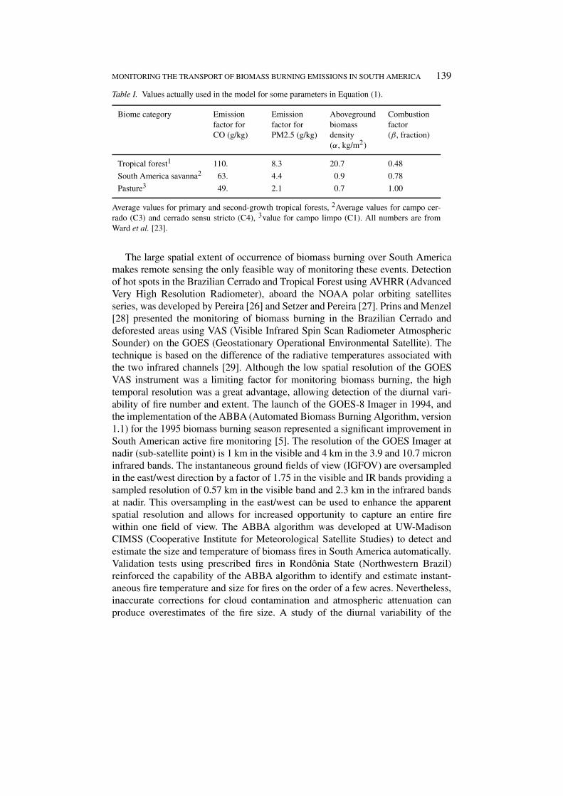
Based on the estimated values of the amount of biomass over the ground (α),the combustion factor (β) and the emission factor (EF ), it is possible to estimatethe quantity emitted of a certain species [η] during a burning event if the burningarea (afire) and the type of vegetation can be determined. This can be accomplishedusing the following equation.
M [η] = αveg · βveg · EF [η]veg · afire. (1)
Here the unit for M [η] is kg. For use in the model, we have selected the followingset of parameters described in Table I.
MONITORING THE TRANSPORT OF BIOMASS BURNING EMISSIONS IN SOUTH AMERICA 139
Table I. Values actually used in the model for some parameters in Equation (1).
Biome category Emissionfactor forCO (g/kg)
Emissionfactor forPM2.5 (g/kg)
Abovegroundbiomassdensity(α, kg/m2)
Combustionfactor(β, fraction)
Tropical forest1 110. 8.3 20.7 0.48
South America savanna2 63. 4.4 0.9 0.78
Pasture3 49. 2.1 0.7 1.00
Average values for primary and second-growth tropical forests, 2Average values for campo cer-rado (C3) and cerrado sensu stricto (C4), 3value for campo limpo (C1). All numbers are fromWard et al. [23].
The large spatial extent of occurrence of biomass burning over South Americamakes remote sensing the only feasible way of monitoring these events. Detectionof hot spots in the Brazilian Cerrado and Tropical Forest using AVHRR (AdvancedVery High Resolution Radiometer), aboard the NOAA polar orbiting satellitesseries, was developed by Pereira [26] and Setzer and Pereira [27]. Prins and Menzel[28] presented the monitoring of biomass burning in the Brazilian Cerrado anddeforested areas using VAS (Visible Infrared Spin Scan Radiometer AtmosphericSounder) on the GOES (Geostationary Operational Environmental Satellite). Thetechnique is based on the difference of the radiative temperatures associated withthe two infrared channels [29]. Although the low spatial resolution of the GOESVAS instrument was a limiting factor for monitoring biomass burning, the hightemporal resolution was a great advantage, allowing detection of the diurnal vari-ability of fire number and extent. The launch of the GOES-8 Imager in 1994, andthe implementation of the ABBA (Automated Biomass Burning Algorithm, version1.1) for the 1995 biomass burning season represented a significant improvement inSouth American active fire monitoring [5]. The resolution of the GOES Imager atnadir (sub-satellite point) is 1 km in the visible and 4 km in the 3.9 and 10.7 microninfrared bands. The instantaneous ground fields of view (IGFOV) are oversampledin the east/west direction by a factor of 1.75 in the visible and IR bands providing asampled resolution of 0.57 km in the visible band and 2.3 km in the infrared bandsat nadir. This oversampling in the east/west can be used to enhance the apparentspatial resolution and allows for increased opportunity to capture an entire firewithin one field of view. The ABBA algorithm was developed at UW-MadisonCIMSS (Cooperative Institute for Meteorological Satellite Studies) to detect andestimate the size and temperature of biomass fires in South America automatically.Validation tests using prescribed fires in Rondônia State (Northwestern Brazil)reinforced the capability of the ABBA algorithm to identify and estimate instant-aneous fire temperature and size for fires on the order of a few acres. Nevertheless,inaccurate corrections for cloud contamination and atmospheric attenuation canproduce overestimates of the fire size. A study of the diurnal variability of the
140 SAULO R. FREITAS ET AL.
detected number of fire pixels for the 1995 burning season showed that the peak ofburning occurs around 17:45 UTC and ranged between 1500 and 3500 fire pixels.The number of fires detected at 17:45 UTC is from 3 to 4 times larger than thenumber of fires at 14:45 and 20:45 UTC and about 20 times greater than the numberof fires detected at 11:45 UTC [30]. A new version of the GOES-8 ABBA wasdeveloped for fire detection and monitoring throughout the Western Hemisphere.The Wildfire ABBA (WF_ABBA) enables fire monitoring in most ecosystems andwas streamlined to allow for rapid processing of half-hourly GOES Imager datafor hazards applications and model data assimilation activities. Version 6.0 of theWF_ABBA was implemented during the 2002 fire season in South America.
Biomass burning emits hot gases and particles which are transported upwarddue to positive buoyancy. The interaction between the smoke and the environmentproduces eddies that entrain colder environmental air into the smoke plume, whichdilutes the plume and reduces buoyancy. The daily turbulent transport in the planet-ary boundary layer (PBL) produces a well-mixed layer; while horizontal advectiontransports the plume downwind in the PBL. Dry and wet convective processes andtopographic forcing transport tracers into the middle and upper troposphere. In thetroposphere, the pollutants are advected away from the source region. Removalprocesses are more efficient in the PBL; when the pollutants are transported tothe troposphere their residence time increases. Several authors [16, 17, 31–39]have been working on the transport of biomass burning emissions in the SouthAmerican and African continents, mainly focusing on the transport due to wet anddeep convective circulations. They have shown the importance of this mechanismon the vertical distribution of the biomass burning pollutants from the PBL to thehigh troposphere with possible implications for regional and global climate change.
3. The Atmospheric and the Coupled On-Line Eulerian Tracers TransportModels
The on-line 3-D model transport follows the Eulerian approach coupled to theRAMS 4.3 parallel version [21]. RAMS is a numerical model designed to simulateatmospheric circulations at many scales. RAMS solves the fully compressible non-hydrostatic equations described by Tripoli and Cotton [40], and is equipped witha multiple grid nesting scheme which allows the model equations to be solvedsimultaneously on any number of interacting computational meshes of differentspatial resolution. It has a sophisticated set of packages to simulate processes suchas: radiative transfer, surface-air water, heat and momentum exchanges, turbulentplanetary boundary layer transport and cloud microphysics. The initial conditionscan be defined from various observational data sets that can be combined and pro-cessed with a mesoscale isentropic data analysis package [41]. As for the boundaryconditions, there is a 4DDA (four-dimensional data assimilation) scheme allowingthe atmospheric fields to be nudged towards the large-scale data.
MONITORING THE TRANSPORT OF BIOMASS BURNING EMISSIONS IN SOUTH AMERICA 141
During the dry season, South America and Africa have a large number of ve-getation fires throughout much of the continent. The effects of these fires on thelower-middle and upper troposphere are expressed very discretely by cloud trans-ports. The computational limitation constrains the model runs to low spatial res-olution (on the order of a few tens of kilometers). At this resolution, a cumulusscheme parameterization needs to be introduced because the model is not capableof resolving convection explicitly. New deep and shallow convective parameteriz-ation schemes based on a mass flux approach [42, 43] have been implemented inRAMS 4.3. The Grell scheme includes moist convective-scale downdrafts and usesas closure the quasi-equilibrium hypothesis for the determination of the updraftmass flux on the cloud base. This cumulus scheme is suitable for mesoscale runs(horizontal grid spacing about 20 km) and so is adequate for regional transportstudies.
The tracer mixing ratio, s(= ρ/ρair), is calculated using the mass conservationequation
∂s
∂t=
(∂s
∂t
)adv
+(
∂s
∂t
)PBLturb
+(
∂s
∂t
)shallowconv
+(
∂s
∂t
)deepconv
+ WPM2.5 + R + Q, (2)
where the symbols are defined as follows:
• ∂s
∂t, the local tendency,
• adv, the grid-scale advection,
• PBL turb, the sub-grid turbulent transport in the PBL,
• deep conv, the sub-grid transport associated with the moist deep convection,
• shallow conv, the sub-grid transport associated with the moist shallow convec-tion,
• WPM2.5, the convective wet removal for PM2.5 (particulate matter with dp <
2.5µm),
• R, the sink term associated with generic dry removal and/or chemical transform-ation,
• Q, the source emission associated with the biomass burning process.
The tracer mixing ratio is updated in time using the total tendency given by Equa-tion (2) and a constant inflow is applied as a tracer boundary condition. The nextsections will discuss other terms on the right hand side of Equation (2) in moredetail.
142 SAULO R. FREITAS ET AL.
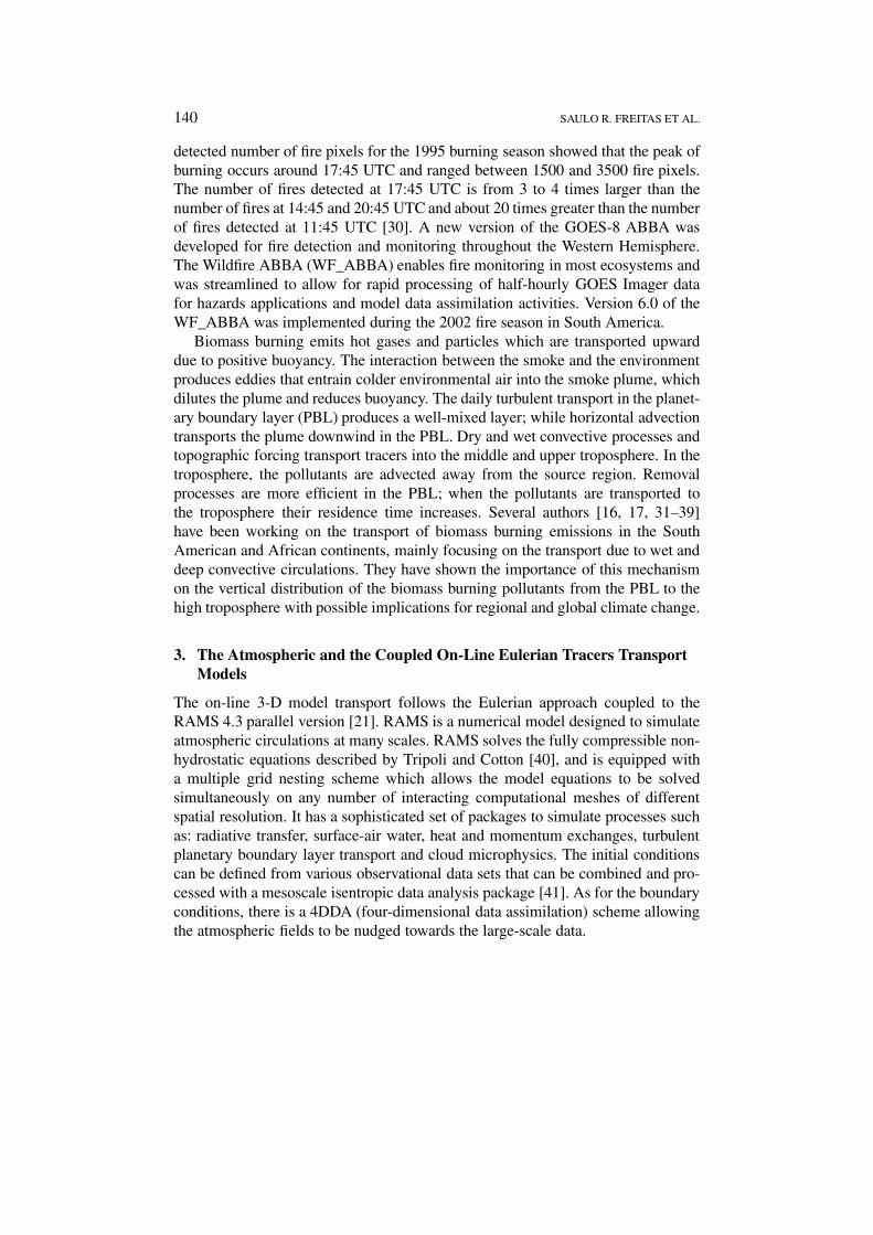
Figure 1. Biomass burning source emission parameterization. Fires are sub-grid processesburning different types of vegetation. The total amount of emitted mass is obtained and dilutedin the air contained in each model grid box.
3.1. THE PARAMETERIZATION OF THE SOURCE EMISSION Q
The source emission parameterization is based on the half-hourly GOES-8 WF_ABBA fire product and field observations. Figure 1 illustrates the technique. In-side of each model grid box there may be several observed sub-grid fires eachburning a different type of vegetation. For each fire pixel detected by the GOES-8WF_ABBA, the mass of the emitted tracer is calculated using Equation (1) wherethe type of vegetation burning is determined by merging the fire map with the1 km IGBP 2.0 vegetation map [44], thus allowing an appropriate selection of thevegetation-dependent factors in Equation (1). We estimate the burned area by theinstantaneous fire size given by the GOES-8 WF_ABBA for each non-saturatedand non-cloudy fire pixel, where it is possible to retrieve sub-pixel fire character-istics. For GOES-8 WF_ABBA detected fires that have no information about theinstantaneous fire size, the mean instantaneous fire size of 0.14 km2 (calculatedfrom the GOES-8 ABBA database of the previous years) is used. The emissionin the model follows the diurnal burning cycle described in Section 2. The emis-sion diurnal cycle is defined by a Gaussian function r(t) centered at 17:45 UTC,normalized to 1, and 8 h wide. In this way, the source emission term is given by
Q[η] = r(t)
ρ0�V
∑fires_∈Grid_Box
M [η], (3)
where ρ0 is the basic state air density, �V is the volume of the first physical gridcell (corresponding to the vertical level k = 2) and the mass is calculated overall fires inside the grid cell. The sources are spatially and temporally distributed
MONITORING THE TRANSPORT OF BIOMASS BURNING EMISSIONS IN SOUTH AMERICA 143
and daily assimilated by the model according to the biomass burning hotspotsidentified in the GOES 3.9 micron band by the WF_ABBA processing system.Presently, the source emissions for CO and PM2.5 have been parameterized, butseveral significant species could be added, e.g., CO2, NO, HCN.
3.2. THE SINK TERM r
The generic process of removal/transformation of tracers (dry deposition and sedi-mentation for PM2.5 and chemical transformation for CO) is summarized throughthe term R given by
R = − s
λ, (4)
where the lifetime λ is approximated as 30 days for CO [45] and 6 days for PM2.5[2]. Since the lifetime of CO is long, from 50 to occasionally a minimum of 15days [46], CO acts essentially as a passive tracer in the simulation. The CO in thesimulations tends to flow out of the model, especially above the boundary layer,and boundary conditions control the concentration more than the linearized chem-ical removal. Similarly, within the boundary layer, it is true that the transport timefrom the major sources to major vertical transport regions is shorter than 15 days,and so the exact lifetime assigned is of secondary importance. The PM2.5 tracerquantity represents a monomodal submicron aerosol not significantly affected bycoalescence or condensation of further material. This seems to be an adequatedescription for smoke starting a few hours after emission through the point ofsignificant interaction with cloud and a high probability of removal. Within theboundary layer, the 6-day lifetime for PM2.5 corresponds to a deposition velocityof ∼0.35 km/day within the approximately 2 km mixed layer. This value is perhapsthree times the commonly used deposition velocity for small particles, and approx-imately correct for larger particles which have less mass efficiency in affectinglight. Above the mixed layer, the suggested lifetime is too short, but here aerosolis dispersed more rapidly by winds, as with CO. The general effect should be thatour removal is too rapid. More realistic dry deposition and sedimentation schemeswill be implemented for operational monitoring during the next dry season. Themajor uncertainties in the mass loading and optical effects that we are addressingconcern emission strength and wet removal efficiency, and these have the greatestimpact on our model performance.
144 SAULO R. FREITAS ET AL.
3.3. THE PARAMETERIZED DEEP CONVECTIVE TRANSPORT AND ASSOCIATED
WET REMOVAL
The deep and moist convection effects on the tracers’ distribution are based on theGrell mass flux cumulus scheme. This sub-grid transport tendency on the tracermixing ratio is given by(
∂s
∂t
)deepconv
= mb
ρ0
[δuηu (su − s) + εδdηd (sd − s) + η
∂s
∂z
], (5)
where mb is the updraft mass flux at cloud base, δ is the mass detrainment rate andη is the normalized mass flux, with the subscripts u and d standing for updraftand downdrafts, respectively. ε is the ratio between the downdraft and updraftmass fluxes, η is the environment normalized mass flux, su, sd and s stand fortracers mixing ratio for the in-cloud updraft, downdraft and environment, respect-ively. The first term on the right side of Equation (5) corresponds to updraft massdetrainment, the second, to downdraft mass detrainment, and the last, to envir-onmental subsidence (advection). For biomass burning tracers usually the PBL ismore polluted than the troposphere, so the typical role of the updraft transport is tovent the polluted air from the PBL to the high troposphere where the smoke-ladenair is detrained. Conversely, the downdraft brings more pristine air from the midtroposphere into the PBL.
The in-cloud tracer mixing ratio is determined from
dsu/d
dz= −µu/d
(su/d − s
), (6)
where µu/d is the up/downdraft entrainment rate and the following boundary con-dition is used
s(zu/d
) = s(zu/d
), (7)
zu is the updraft cloud base height, and zd is the height level where the downdraftstarts. The coupled convective tracers transport model utilizes mb, δu/d , ηu/d , η,ε, µu/d , zu and zd diagnosed from the cumulus scheme to determine the value ofEquation 5.
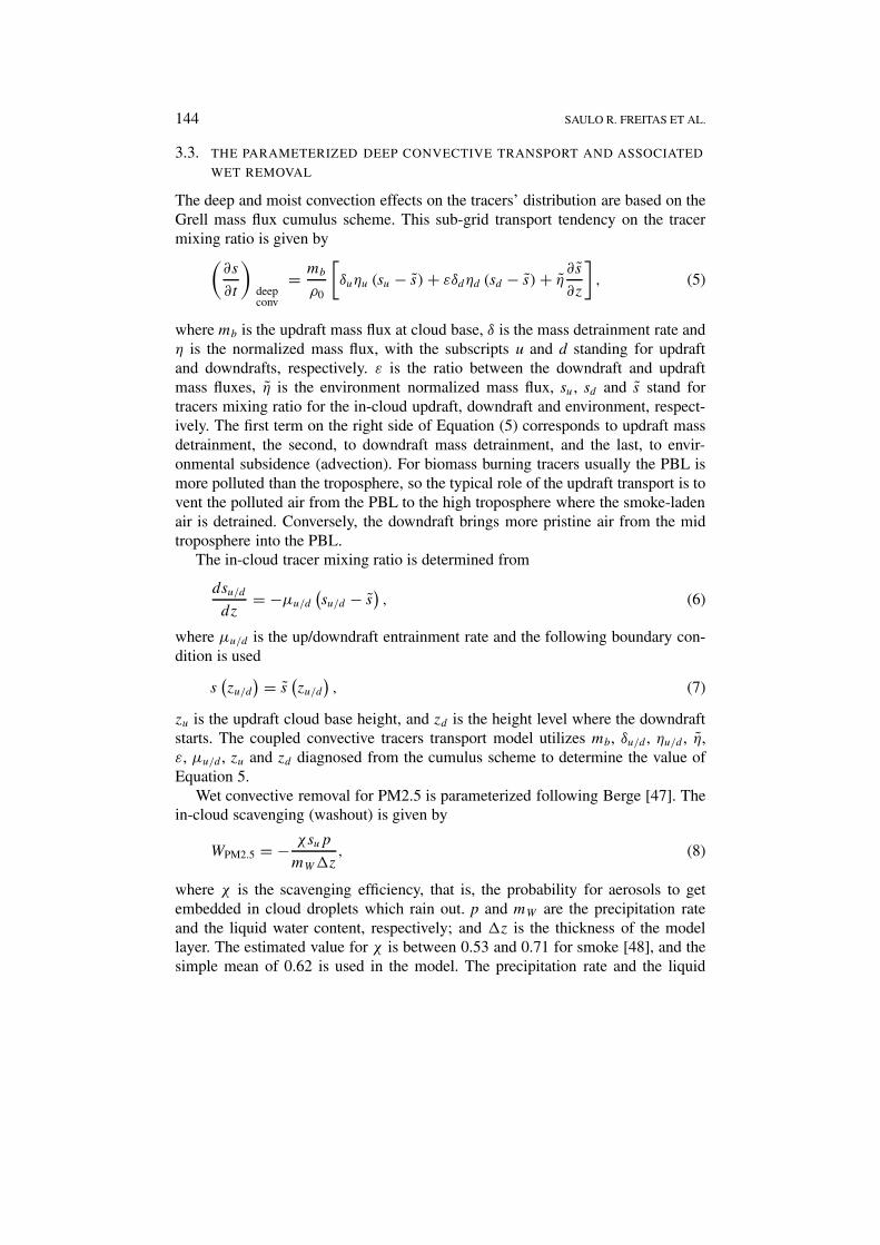
Wet convective removal for PM2.5 is parameterized following Berge [47]. Thein-cloud scavenging (washout) is given by
WPM2.5 = − χsup
mW�z, (8)
where χ is the scavenging efficiency, that is, the probability for aerosols to getembedded in cloud droplets which rain out. p and mW are the precipitation rateand the liquid water content, respectively; and �z is the thickness of the modellayer. The estimated value for χ is between 0.53 and 0.71 for smoke [48], and thesimple mean of 0.62 is used in the model. The precipitation rate and the liquid
MONITORING THE TRANSPORT OF BIOMASS BURNING EMISSIONS IN SOUTH AMERICA 145
water content are both diagnosed by the Grell cumulus scheme and in-cloud tracerconcentration is obtained through Equation (6) after the washout. The sub-cloudprecipitation scavenging (rainout) is estimated from
WPM2.5 = −AMEsu, (9)
where M is the concentration of precipitation water (kg [water]/m3), E is the meancollection efficiency averaged over all raindrop sizes and A is an empirical coeffi-cient [47].
3.4. THE PARAMETERIZED SHALLOW CONVECTIVE TRANSPORT
The shallow convective transport follows the same approach described in Equa-tion (5), but disregards the transport by downdrafts and the wet removal process. Itis coupled to the Grell shallow convection scheme. Here, shallow cumuli act onlyin venting the aerosol particles and gases from the PBL to the low troposphere.
3.5. THE GRID SCALE ADVECTION AND SUB-GRID TURBULENT TRANSPORT
The grid scale advection and the sub-grid diffusional transport are calculated us-ing existing RAMS parameterizations. The horizontal diffusion is based on theSmagorinsky [49] formulation. The vertical diffusion is parameterized according tothe Mellor and Yamada [50] scheme, which employs a prognostic of the turbulentkinetic energy. The advection is a forward–upstream scheme of second-order [51].
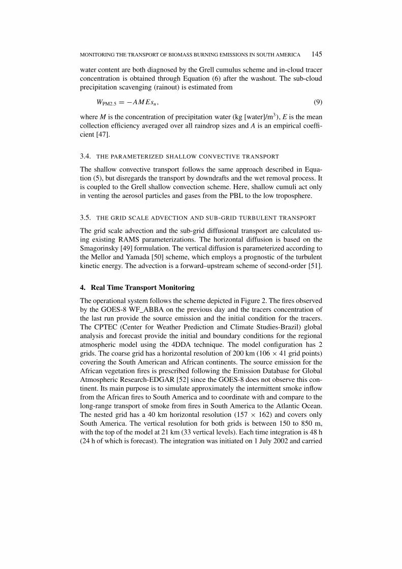
4. Real Time Transport Monitoring
The operational system follows the scheme depicted in Figure 2. The fires observedby the GOES-8 WF_ABBA on the previous day and the tracers concentration ofthe last run provide the source emission and the initial condition for the tracers.The CPTEC (Center for Weather Prediction and Climate Studies-Brazil) globalanalysis and forecast provide the initial and boundary conditions for the regionalatmospheric model using the 4DDA technique. The model configuration has 2grids. The coarse grid has a horizontal resolution of 200 km (106 × 41 grid points)covering the South American and African continents. The source emission for theAfrican vegetation fires is prescribed following the Emission Database for GlobalAtmospheric Research-EDGAR [52] since the GOES-8 does not observe this con-tinent. Its main purpose is to simulate approximately the intermittent smoke inflowfrom the African fires to South America and to coordinate with and compare to thelong-range transport of smoke from fires in South America to the Atlantic Ocean.The nested grid has a 40 km horizontal resolution (157 × 162) and covers onlySouth America. The vertical resolution for both grids is between 150 to 850 m,with the top of the model at 21 km (33 vertical levels). Each time integration is 48 h(24 h of which is forecast). The integration was initiated on 1 July 2002 and carried
146 SAULO R. FREITAS ET AL.
Figure 2. General flow of the real time system for monitoring the transport of biomass burningemissions in South America.
through successive 48-h integrations through 30 November 2002. This system hasbeen running on a pc-Linux cluster with 13 processors (Intel-pentium III, 1 GHz)and takes about 5 h of computation time.
5. Discussion
Climatologically, from June to September, central Brazil is dominated by a high-pressure area with little precipitation and light winds in the lower troposphere[53] and with convection in the Amazon basin shifted to the northwest part ofSouth America. These conditions are associated with the westward displacementof the South Atlantic Subtropical High (SASH) and the northward motion of theIntertropical Convergence Zone (ITCZ) during the austral winter. However, on aday-to-day basis several transient systems may change this picture, thereby alteringthe typical pattern of the smoke transport. The position of the SASH determ-ines the entrance of the clean maritime air to the biomass burning area playingan important role in defining the shape of the regional smoke plume as it is theprimary mechanism responsible for the dilution of the polluted air. Approachingcold frontal systems from the south are responsible for disturbances in atmosphericstability and in the wind fields. These changes define the main corridors of smokeexport to oceanic areas. The typical model output representing the tracers (CO and
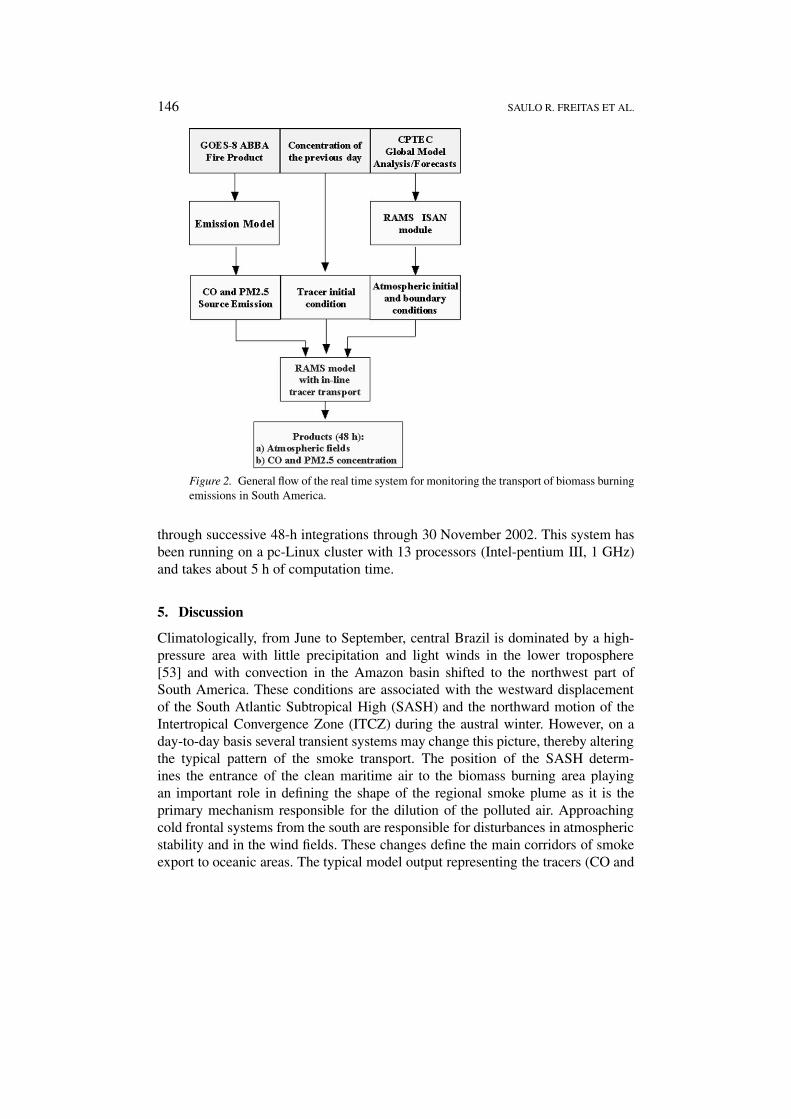
MONITORING THE TRANSPORT OF BIOMASS BURNING EMISSIONS IN SOUTH AMERICA 147
Figure 3. Example of the transport model output. (a) Shows the plume of CO (ppb) for theregional model grid (40 km horizontal resolution) at 1800Z on 25 August 2002 at 1100 mabove surface. (b) Depicts the coarse model grid (200 km) covering South America and partsof Africa.
148 SAULO R. FREITAS ET AL.
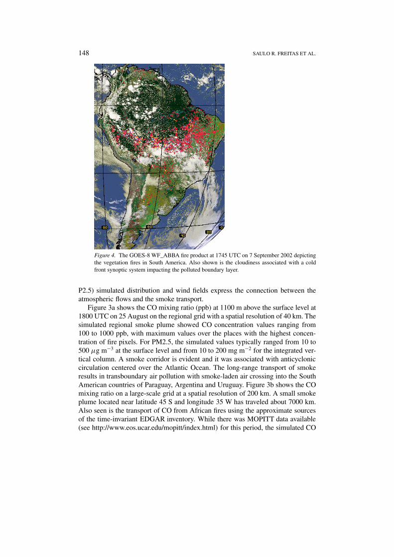
Figure 4. The GOES-8 WF_ABBA fire product at 1745 UTC on 7 September 2002 depictingthe vegetation fires in South America. Also shown is the cloudiness associated with a coldfront synoptic system impacting the polluted boundary layer.
P2.5) simulated distribution and wind fields express the connection between theatmospheric flows and the smoke transport.
Figure 3a shows the CO mixing ratio (ppb) at 1100 m above the surface level at1800 UTC on 25 August on the regional grid with a spatial resolution of 40 km. Thesimulated regional smoke plume showed CO concentration values ranging from100 to 1000 ppb, with maximum values over the places with the highest concen-tration of fire pixels. For PM2.5, the simulated values typically ranged from 10 to500 µg m−3 at the surface level and from 10 to 200 mg m−2 for the integrated ver-tical column. A smoke corridor is evident and it was associated with anticycloniccirculation centered over the Atlantic Ocean. The long-range transport of smokeresults in transboundary air pollution with smoke-laden air crossing into the SouthAmerican countries of Paraguay, Argentina and Uruguay. Figure 3b shows the COmixing ratio on a large-scale grid at a spatial resolution of 200 km. A small smokeplume located near latitude 45 S and longitude 35 W has traveled about 7000 km.Also seen is the transport of CO from African fires using the approximate sourcesof the time-invariant EDGAR inventory. While there was MOPITT data available(see http://www.eos.ucar.edu/mopitt/index.html) for this period, the simulated CO
MONITORING THE TRANSPORT OF BIOMASS BURNING EMISSIONS IN SOUTH AMERICA 149
was primarily in the boundary layer or hidden by cloud and largely invisible tothe MOPITT sensor. MOPITT depends upon thermal emission of radiation fromCO molecules, and is most sensitive in the mid troposphere. Estimates for lowertropospheric levels (below 2–3 km tend to represent a standard initial profile usedfor the retreival. The MOPITT estimate at 1.5 km suggests around 250 ppb forthe portion of South America seen. In Africa, where climatological fire emissionshad to be used, the comparison was of course not quite as good. More intensivecomparisons between model and MOPITT results are in development.
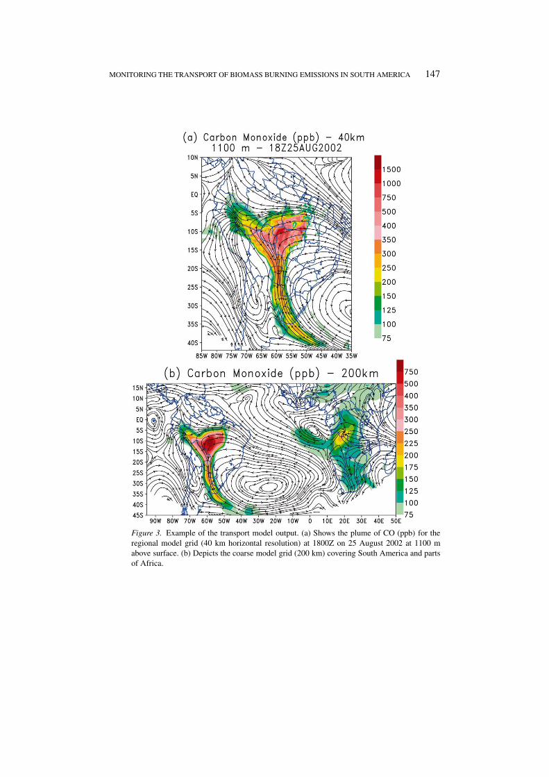
5.1. A COLD FRONT CASE STUDY
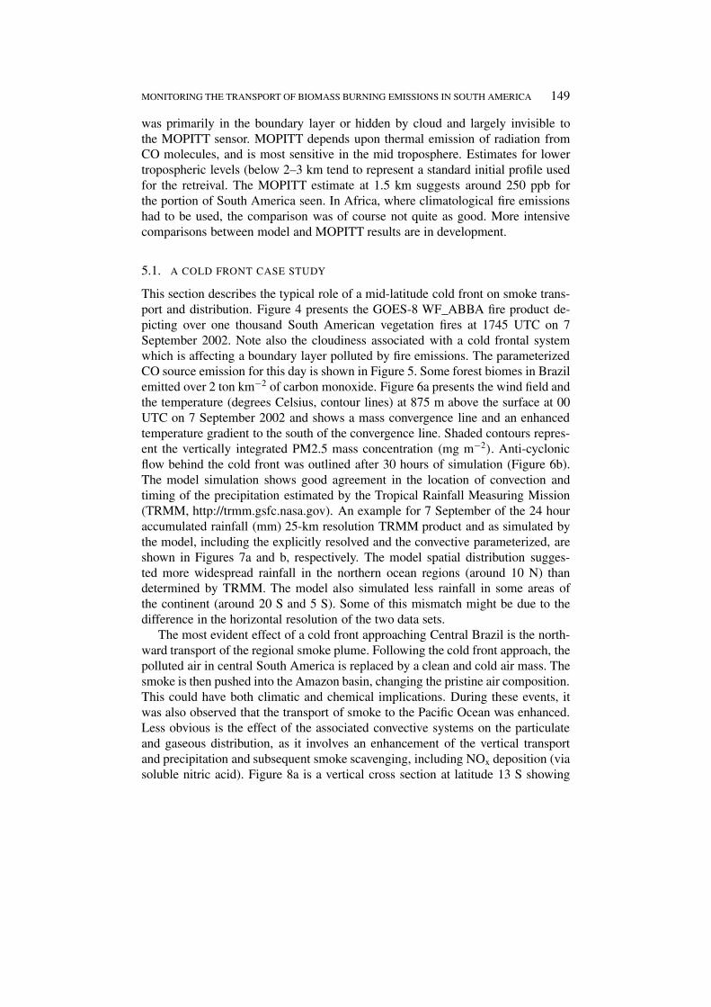
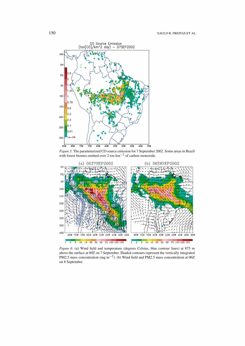
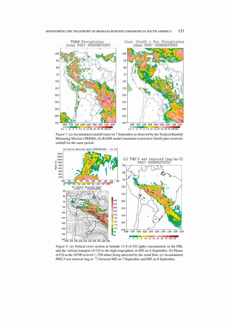
This section describes the typical role of a mid-latitude cold front on smoke trans-port and distribution. Figure 4 presents the GOES-8 WF_ABBA fire product de-picting over one thousand South American vegetation fires at 1745 UTC on 7September 2002. Note also the cloudiness associated with a cold frontal systemwhich is affecting a boundary layer polluted by fire emissions. The parameterizedCO source emission for this day is shown in Figure 5. Some forest biomes in Brazilemitted over 2 ton km−2 of carbon monoxide. Figure 6a presents the wind field andthe temperature (degrees Celsius, contour lines) at 875 m above the surface at 00UTC on 7 September 2002 and shows a mass convergence line and an enhancedtemperature gradient to the south of the convergence line. Shaded contours repres-ent the vertically integrated PM2.5 mass concentration (mg m−2). Anti-cyclonicflow behind the cold front was outlined after 30 hours of simulation (Figure 6b).The model simulation shows good agreement in the location of convection andtiming of the precipitation estimated by the Tropical Rainfall Measuring Mission(TRMM, http://trmm.gsfc.nasa.gov). An example for 7 September of the 24 houraccumulated rainfall (mm) 25-km resolution TRMM product and as simulated bythe model, including the explicitly resolved and the convective parameterized, areshown in Figures 7a and b, respectively. The model spatial distribution sugges-ted more widespread rainfall in the northern ocean regions (around 10 N) thandetermined by TRMM. The model also simulated less rainfall in some areas ofthe continent (around 20 S and 5 S). Some of this mismatch might be due to thedifference in the horizontal resolution of the two data sets.
The most evident effect of a cold front approaching Central Brazil is the north-ward transport of the regional smoke plume. Following the cold front approach, thepolluted air in central South America is replaced by a clean and cold air mass. Thesmoke is then pushed into the Amazon basin, changing the pristine air composition.This could have both climatic and chemical implications. During these events, itwas also observed that the transport of smoke to the Pacific Ocean was enhanced.Less obvious is the effect of the associated convective systems on the particulateand gaseous distribution, as it involves an enhancement of the vertical transportand precipitation and subsequent smoke scavenging, including NOx deposition (viasoluble nitric acid). Figure 8a is a vertical cross section at latitude 13 S showing
150 SAULO R. FREITAS ET AL.
Figure 5. The parameterized CO source emission for 7 September 2002. Some areas in Brazilwith forest biomes emitted over 2 ton km−2 of carbon monoxide.
Figure 6. (a) Wind field and temperature (degrees Celsius, blue contour lines) at 875 mabove the surface at 00Z on 7 September. Shaded contours represent the vertically integratedPM2.5 mass concentration (mg m−2). (b) Wind field and PM2.5 mass concentration at 06Zon 8 September.
MONITORING THE TRANSPORT OF BIOMASS BURNING EMISSIONS IN SOUTH AMERICA 151
Figure 7. (a) Accumulated rainfall (mm) on 7 September as observed by the Tropical RainfallMeasuring Mission (TRMM), (b) RAMS model simulated (convective (Grell) plus resolved)rainfall for the same period.
Figure 8. (a) Vertical cross section at latitude 13 S of CO (ppb) concentration in the PBLand the vertical transport of CO to the high troposphere at 00Z on 8 September. (b) Plumeof CO at the 10700 m level (∼250 mbar) being advected by the zonal flow. (c) AccumulatedPM2.5 wet removal (mg m−2) between 00Z on 7 September and 00Z on 8 September.
152 SAULO R. FREITAS ET AL.
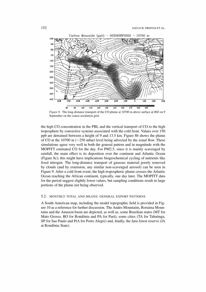
Figure 9. The long-distance transport of the CO plume at 10700 m above surface at 00Z on 9September on the coarse resolution grid.
the high CO concentration in the PBL and the vertical transport of CO to the hightroposphere by convective systems associated with the cold front. Values over 150ppb are detrained between a height of 9 and 13.5 km. Figure 8b shows the plumeof CO at the 10700 m (∼250 mbar) level being advected by the zonal flow. Thesesimulations agree very well in both the general pattern and in magnitude with theMOPITT estimated CO for the day. For PM2.5, since it is mainly scavenged byrainfall, the main effect is its deposition over the continent and Atlantic Ocean(Figure 8c); this might have implications biogeochemical cycling of nutrients likefixed nitrogen. The long-distance transport of gaseous material poorly removedby clouds (and by extension, any similar non-scavenged aerosol) can be seen inFigure 9. After a cold front event, the high tropospheric plume crosses the AtlanticOcean reaching the African continent, typically, one day later. The MOPITT datafor the period suggest slightly lower values, but sampling conditions result in largeportions of the plume not being observed.
5.2. MONTHLY TOTAL AND MEANS: GENERAL EXPORT PATTERNS
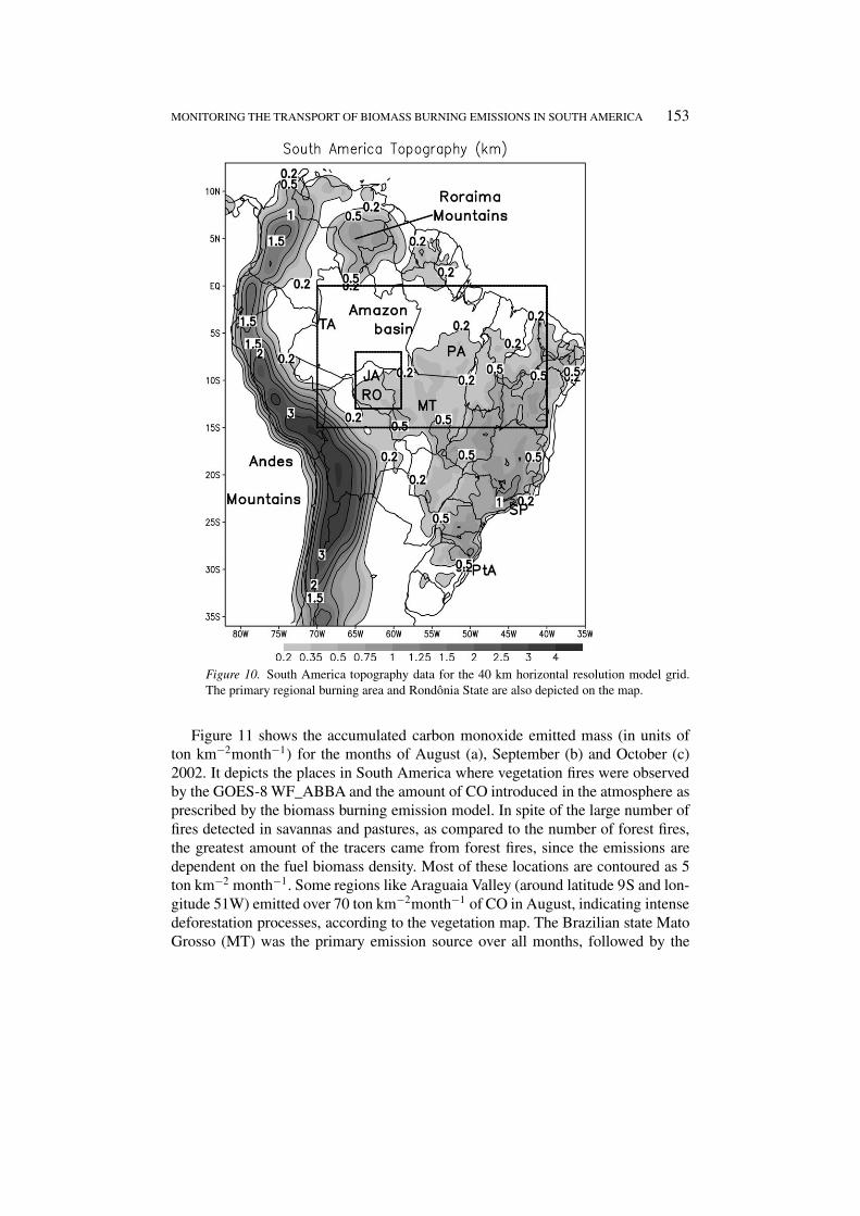
A South American map, including the model topographic field is provided in Fig-ure 10 as a reference for further discussion. The Andes Mountains, Roraima Moun-tains and the Amazon basin are depicted, as well as, some Brazilian states (MT forMato Grosso, RO for Rondônia and PA for Pará), some cities (TA for Tabatinga,SP for Sao Paulo and PtA for Porto Alegre) and, finally, the Jaru forest reserve (JAat Rondônia State).
MONITORING THE TRANSPORT OF BIOMASS BURNING EMISSIONS IN SOUTH AMERICA 153
Figure 10. South America topography data for the 40 km horizontal resolution model grid.The primary regional burning area and Rondônia State are also depicted on the map.
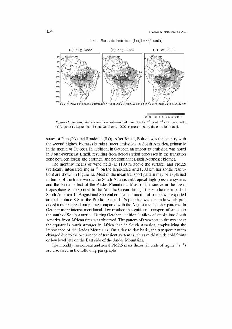
Figure 11 shows the accumulated carbon monoxide emitted mass (in units ofton km−2month−1) for the months of August (a), September (b) and October (c)2002. It depicts the places in South America where vegetation fires were observedby the GOES-8 WF_ABBA and the amount of CO introduced in the atmosphere asprescribed by the biomass burning emission model. In spite of the large number offires detected in savannas and pastures, as compared to the number of forest fires,the greatest amount of the tracers came from forest fires, since the emissions aredependent on the fuel biomass density. Most of these locations are contoured as 5ton km−2 month−1. Some regions like Araguaia Valley (around latitude 9S and lon-gitude 51W) emitted over 70 ton km−2month−1 of CO in August, indicating intensedeforestation processes, according to the vegetation map. The Brazilian state MatoGrosso (MT) was the primary emission source over all months, followed by the
154 SAULO R. FREITAS ET AL.
Figure 11. Accumulated carbon monoxide emitted mass (ton km−2month−1) for the monthsof August (a), September (b) and October (c) 2002 as prescribed by the emission model.
states of Para (PA) and Rondônia (RO). After Brazil, Bolívia was the country withthe second highest biomass burning tracer emissions in South America, primarilyin the month of October. In addition, in October, an important emission was notedin North-Northeast Brazil, resulting from deforestation processes in the transitionzone between forest and caatinga (the predominant Brazil Northeast biome).
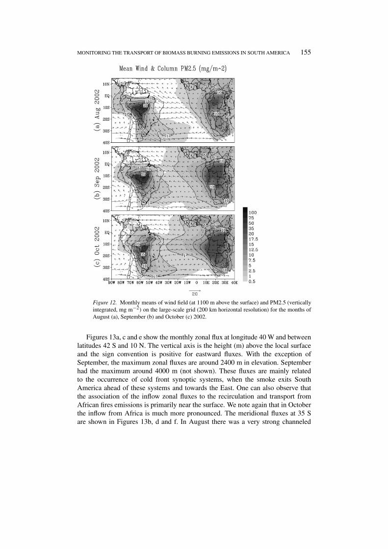
The monthly means of wind field (at 1100 m above the surface) and PM2.5(vertically integrated, mg m−2) on the large-scale grid (200 km horizontal resolu-tion) are shown in Figure 12. Most of the mean transport pattern may be explainedin terms of the trade winds, the South Atlantic subtropical high pressure system,and the barrier effect of the Andes Mountains. Most of the smoke in the lowertroposphere was exported to the Atlantic Ocean through the southeastern part ofSouth America. In August and September, a small amount of smoke was exportedaround latitude 8 S to the Pacific Ocean. In September weaker trade winds pro-duced a more spread out plume compared with the August and October patterns. InOctober more intense meridional flow resulted in significant transport of smoke tothe south of South America. During October, additional inflow of smoke into SouthAmerica from African fires was observed. The pattern of transport to the west nearthe equator is much stronger in Africa than in South America, emphasizing theimportance of the Andes Mountains. On a day to day basis, the transport patternchanged due to the occurrence of transient systems such as mid-latitude cold frontsor low level jets on the East side of the Andes Mountains.
The monthly meridional and zonal PM2.5 mass fluxes (in units of µg m−2 s−1)
are discussed in the following paragraphs.
MONITORING THE TRANSPORT OF BIOMASS BURNING EMISSIONS IN SOUTH AMERICA 155
Figure 12. Monthly means of wind field (at 1100 m above the surface) and PM2.5 (verticallyintegrated, mg m−2) on the large-scale grid (200 km horizontal resolution) for the months ofAugust (a), September (b) and October (c) 2002.
Figures 13a, c and e show the monthly zonal flux at longitude 40 W and betweenlatitudes 42 S and 10 N. The vertical axis is the height (m) above the local surfaceand the sign convention is positive for eastward fluxes. With the exception ofSeptember, the maximum zonal fluxes are around 2400 m in elevation. Septemberhad the maximum around 4000 m (not shown). These fluxes are mainly relatedto the occurrence of cold front synoptic systems, when the smoke exits SouthAmerica ahead of these systems and towards the East. One can also observe thatthe association of the inflow zonal fluxes to the recirculation and transport fromAfrican fires emissions is primarily near the surface. We note again that in Octoberthe inflow from Africa is much more pronounced. The meridional fluxes at 35 Sare shown in Figures 13b, d and f. In August there was a very strong channeled
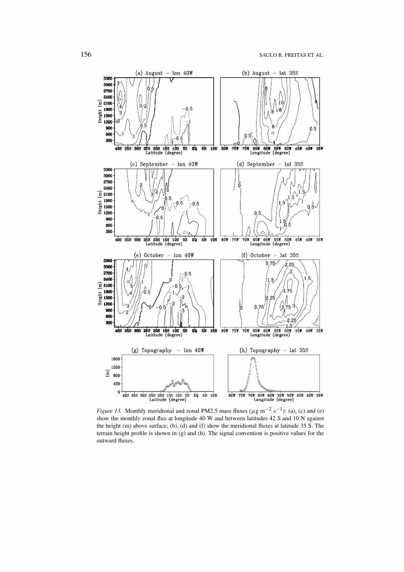
156 SAULO R. FREITAS ET AL.
Figure 13. Monthly meridional and zonal PM2.5 mass fluxes (µg m−2 s−1): (a), (c) and (e)show the monthly zonal flux at longitude 40 W and between latitudes 42 S and 10 N againstthe height (m) above surface; (b), (d) and (f) show the meridional fluxes at latitude 35 S. Theterrain height profile is shown in (g) and (h). The signal convention is positive values for theoutward fluxes.
MONITORING THE TRANSPORT OF BIOMASS BURNING EMISSIONS IN SOUTH AMERICA 157
mean flux up to 10 µg m−2 s−1 around 55 W and at a height of 2400 m, largelyrelated to the Andes low level jets as shown in Figure 3. The other months hadlower meridional fluxes which were more spread out.
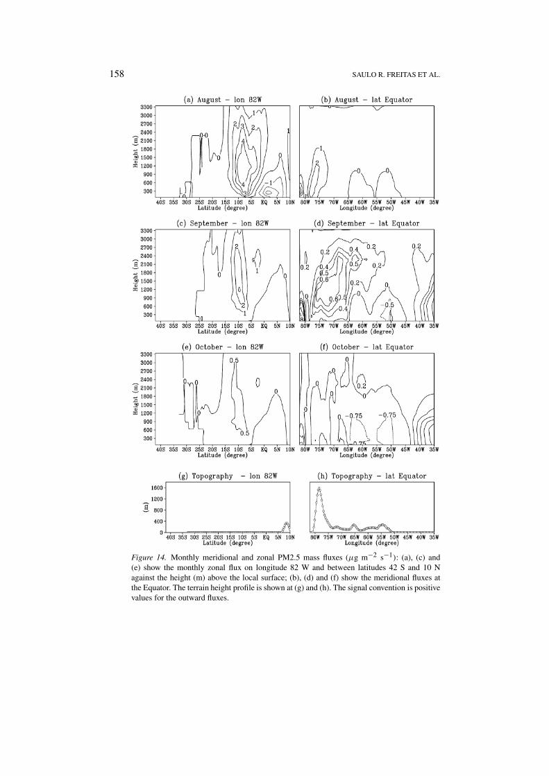
Figure 14 shows the same fluxes as described in the last paragraph, but atlongitude 82 W and the Equator. The transport to the Pacific Ocean took placepredominantly around latitude 8 S (Figures 14a, c and e) and during the month ofAugust. The meridional outward fluxes crossing the Equator (Figures 14b, d and f)are due to the channeling of the trade winds Northwest of the Amazon Basin by theAndes Mountains to the West and the Roraima Mountains to the East (as shown inFigure 3).
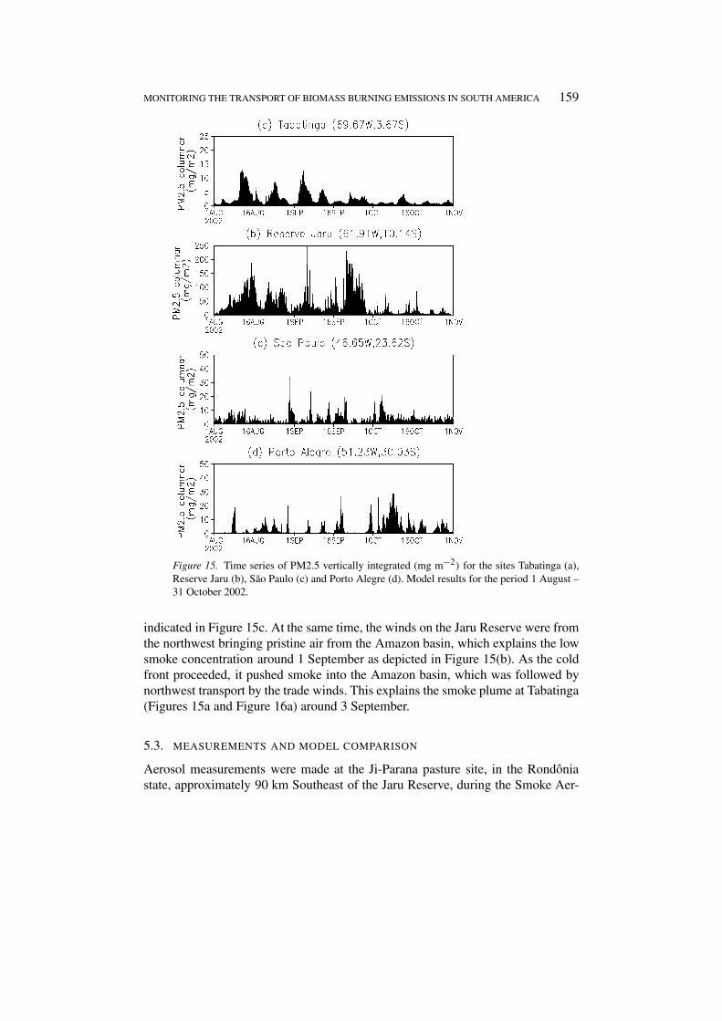
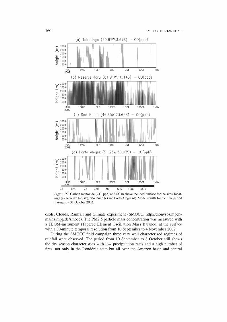
A different view of model performance is given by observations made at thesurface. Time series of vertically integrated (mg m−2) PM2.5 and CO (ppb) below3300 m, as simulated by the model, are shown in Figures 15 and 16 for the sitesTabatinga (a), Jaru Reserve (b), São Paulo (c) and Porto Alegre (d) (see Figure 10for their locations). Tabatinga is in the northwest Amazon and is used to monitorthe incursion of smoke into the pristine areas of the Amazon basin. The smokeintrusion is well defined by the spikes of the PM2.5 column (Figure 15a) and thevertical profiles of CO (Figure 16a). Jaru Reserve is located within a burning regionand serves as a local air quality indicator. Very strong boundary layer pollution wasobserved during August and September, reaching 250 mg m−2 and 2000 ppb forthe particulate and CO concentrations, respectively (Figure 15b and Figure 16b). InOctober, with the onset of the rain season, the smoke was sharply reduced, showingonly short-duration smoke bursts, mainly related to the local emissions. The citiesof São Paulo and Porto Alegre (Figures 15 and 16c, d) are included to illustratethe South American smoke outflows and the effects of the regional smoke plumeon the air quality of these cities. The narrow spikes of smoke passing over thesecities are evident and were primarily associated with the convergence flows due toapproaching cold fronts. The smoke plumes typically passed over the cities almostuncoupled from the surface and may have had insignificant effects on the local airquality. A strong outflow passing over Porto Alegre during October is shown inFigure 12c.
The connection between the narrow spikes of smoke in the time series for theNorthwest and Southeast sites, which describes the continental export of smoke,can be envisioned by studying a sequence of events from 25 August to 3 Septem-ber. Starting on 25 August (Figure 3a), the corridor of smoke was pushed towardsthe Andes Mountains due to a westward motion of the anti-cyclonic circulation,bringing clean oceanic air to the East and most of Central Brazil. On 28 August,a mid-latitude cold frontal system approached from the Pacific Ocean, pushingthe smoke corridor back to the Atlantic Ocean (not shown). At 0600 UTC on29 August the smoke corridor crossed the lower troposphere over Porto Alegre,as is indicated by the narrow spike preceding September 1 in Figure 15d. As thecold frontal system moved northward, the smoke corridor at the flow convergenceregion was pushed to the northeast and, one day later, was crossing São Paulo, as
158 SAULO R. FREITAS ET AL.
Figure 14. Monthly meridional and zonal PM2.5 mass fluxes (µg m−2 s−1): (a), (c) and(e) show the monthly zonal flux on longitude 82 W and between latitudes 42 S and 10 Nagainst the height (m) above the local surface; (b), (d) and (f) show the meridional fluxes atthe Equator. The terrain height profile is shown at (g) and (h). The signal convention is positivevalues for the outward fluxes.
MONITORING THE TRANSPORT OF BIOMASS BURNING EMISSIONS IN SOUTH AMERICA 159
Figure 15. Time series of PM2.5 vertically integrated (mg m−2) for the sites Tabatinga (a),Reserve Jaru (b), São Paulo (c) and Porto Alegre (d). Model results for the period 1 August –31 October 2002.
indicated in Figure 15c. At the same time, the winds on the Jaru Reserve were fromthe northwest bringing pristine air from the Amazon basin, which explains the lowsmoke concentration around 1 September as depicted in Figure 15(b). As the coldfront proceeded, it pushed smoke into the Amazon basin, which was followed bynorthwest transport by the trade winds. This explains the smoke plume at Tabatinga(Figures 15a and Figure 16a) around 3 September.
5.3. MEASUREMENTS AND MODEL COMPARISON
Aerosol measurements were made at the Ji-Parana pasture site, in the Rondôniastate, approximately 90 km Southeast of the Jaru Reserve, during the Smoke Aer-
160 SAULO R. FREITAS ET AL.
Figure 16. Carbon monoxide (CO, ppb) at 3300 m above the local surface for the sites Tabat-inga (a), Reserve Jaru (b), São Paulo (c) and Porto Alegre (d). Model results for the time period1 August – 31 October 2002.
osols, Clouds, Rainfall and Climate experiment (SMOCC, http://dionysos.mpch-mainz.mpg.de/smocc). The PM2.5 particle mass concentration was measured witha TEOM-instrument (Tapered Element Oscillation Mass Balance) at the surfacewith a 30-minute temporal resolution from 10 September to 4 November 2002.
During the SMOCC field campaign three very well characterized regimes ofrainfall were observed. The period from 10 September to 8 October still showsthe dry season characteristics with low precipitation rates and a high number offires, not only in the Rondônia state but all over the Amazon basin and central
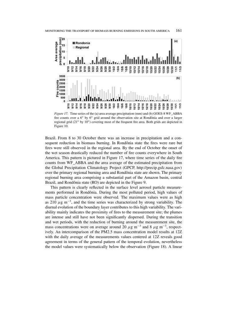
MONITORING THE TRANSPORT OF BIOMASS BURNING EMISSIONS IN SOUTH AMERICA 161
Figure 17. Time series of the (a) area average precipitation (mm) and (b) GOES-8 WF_ABBAfire counts over a 6◦ by 6◦ grid around the observation site at Rondônia and over a largerregional grid (21◦ by 10◦) covering most of the frequent fire area. Both grids are depicted inFigure 10.
Brazil. From 8 to 30 October there was an increase in precipitation and a con-sequent reduction in biomass burning. In Rondônia state the fires were rare butfires were still observed in the regional area. By the end of October the onset ofthe wet season drastically reduced the number of fire counts everywhere in SouthAmerica. This pattern is pictured in Figure 17, where time series of the daily firecounts from WF_ABBA and the area average of the estimated precipitation fromthe Global Precipitation Climatology Project (GPCP, http://precip.gsfc.nasa.gov)over the primary regional burning area and Rondônia state are shown. The primaryregional burning area comprising a substantial part of the Amazon basin, centralBrazil, and Rondônia state (RO) are depicted in the Figure 9.
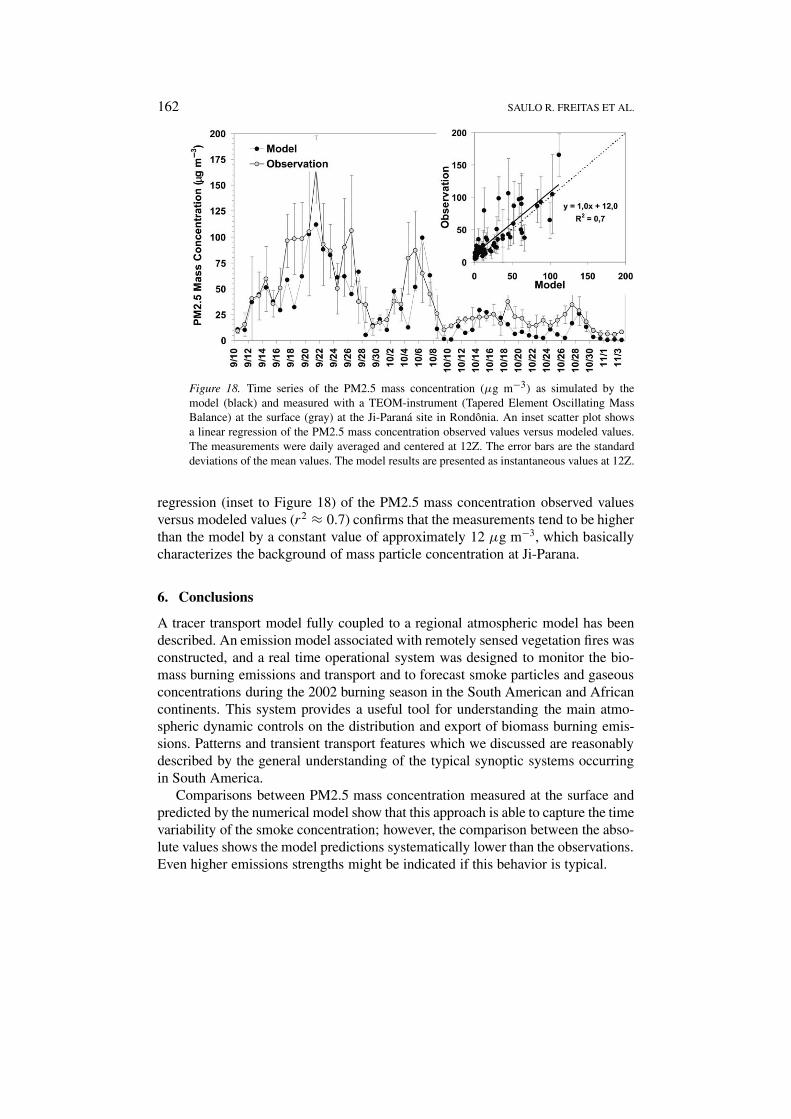
This pattern is clearly reflected in the surface level aerosol particle measure-ments performed in Rondônia. During the most polluted period, high values ofmass particle concentration were observed. The maximum values were as highas 210 µg m−3, and the time series was characterized by strong variability. Thediurnal evolution of the boundary layer contributes to this high variability. The vari-ability mainly indicates the proximity of fires to the measurement site; the plumesare intense and still have not been significantly dispersed. During the transitionand wet periods, with the reduction of burning around the measurement site, themass concentrations were on average around 20 µg m−3 and 8 µg m−3, respect-ively. An intercomparison of the PM2.5 mass concentration model results at 12Zwith the daily average of the measurements values centered at 12Z reveals goodagreement in terms of the general pattern of the temporal evolution, neverthelessthe model values were systematically below the observation (Figure 18). A linear
162 SAULO R. FREITAS ET AL.
Figure 18. Time series of the PM2.5 mass concentration (µg m−3) as simulated by themodel (black) and measured with a TEOM-instrument (Tapered Element Oscillating MassBalance) at the surface (gray) at the Ji-Parana site in Rondônia. An inset scatter plot showsa linear regression of the PM2.5 mass concentration observed values versus modeled values.The measurements were daily averaged and centered at 12Z. The error bars are the standarddeviations of the mean values. The model results are presented as instantaneous values at 12Z.
regression (inset to Figure 18) of the PM2.5 mass concentration observed valuesversus modeled values (r2 ≈ 0.7) confirms that the measurements tend to be higherthan the model by a constant value of approximately 12 µg m−3, which basicallycharacterizes the background of mass particle concentration at Ji-Parana.
6. Conclusions
A tracer transport model fully coupled to a regional atmospheric model has beendescribed. An emission model associated with remotely sensed vegetation fires wasconstructed, and a real time operational system was designed to monitor the bio-mass burning emissions and transport and to forecast smoke particles and gaseousconcentrations during the 2002 burning season in the South American and Africancontinents. This system provides a useful tool for understanding the main atmo-spheric dynamic controls on the distribution and export of biomass burning emis-sions. Patterns and transient transport features which we discussed are reasonablydescribed by the general understanding of the typical synoptic systems occurringin South America.
Comparisons between PM2.5 mass concentration measured at the surface andpredicted by the numerical model show that this approach is able to capture the timevariability of the smoke concentration; however, the comparison between the abso-lute values shows the model predictions systematically lower than the observations.Even higher emissions strengths might be indicated if this behavior is typical.
MONITORING THE TRANSPORT OF BIOMASS BURNING EMISSIONS IN SOUTH AMERICA 163
The disagreement regarding emissions may be due to several factors. One im-portant factor is that there is a lack of information on the input parameters to theemission model. The biomass loading and the emission factors available in theliterature were determined only for a few sites in South America and those numberswere scaled up using a vegetation map. This unavoidable procedure, with the data-set available to date, certainly is not consistent with the high heterogeneity of theAmazon biomes. Remote sensing of fires also has a number of difficulties. Cloudcover acts to reduce the number of fire pixels observed by the GOES WF_ABBA,along with other factors such as the size and intensity of the fire and satellite viewangle. The ability of the GOES WF_ABBA to monitor fires every half hour is ex-tremely helpful in being able to give the best opportunity to catch a glimpse of fireactivity between the clouds. To date detailed studies to estimate the effect of cloudcoverage on fire detection have not been performed. Since the GOES WF_ABBAfire product provides estimates of instantaneous fire size and not total burned area,comparisons with ground truth observations and estimates of fire size at the time ofthe GOES observation are difficult to determine. Comparisons with 3 fires duringthe SCAR-C and SCAR-B field programs indicated that the instantaneous GOESABBA estimates were typically 20–50% greater than the estimated instantaneouslyobserved fire size at a given time [5]. The fires in Brazil were from 8 to 25 acresin size. Considering a pixel size is over 2 orders of magnitude larger than this, itprovides a much better estimate than simply assuming that the entire pixel is onfire. As for the number of fires detected by the GOES, recent ground truth studiesin Acre have shown that throughout a day the GOES WF_ABBA observed roughly70–80% of the fires that were identified on the ground [54]. Of course a fire mayburn for a number of hours, but the GOES WF_ABBA may only be able to see it inone or two time periods due to cloud coverage or low intensity burning at the othertime periods. Furthermore there is a distinct diurnal signature to the occurrence ofanthropogenic fire activity in Brazil. The advantage of GOES is the ability to havenumerous opportunities to detect a given fire throughout the day.
An alternative to this emission model would be the use of climatological bio-mass burning emission datasets [4, 52]. Model results using these cited datasetspresent more disagreements with observation, not only in the absolute values butalso with regards to the time variability.
The Amazon basin does not have a dense meteorological observational networkand this is reflected in the quality of the atmospheric analysis used as initial andboundary conditions for the atmospheric model integration. In addition, the pres-ence of the smoke in the atmosphere results in strong radiative forcing as theseparticles are very efficient solar radiation scatterers and absorbers. The atmosphereresponds to this forcing through a cooling of the low levels and a heating of theupper levels of the PBL. The net effect is an increase in the atmospheric thermody-namical stabilization. This will affect the aerosol vertical distribution by trappingthe smoke, resulting in high concentrations near the ground where the observationswere made. Ongoing model development includes coupling of this monitoring
164 SAULO R. FREITAS ET AL.
system with an aerosol model which will be able to resolve the direct radiativeeffects of the smoke aerosol particles and improve the description of the boundarylayer diurnal cycle. Finally, the model results represent an ensemble average ina 40 km grid cell while the observation is local and might not be representativeof the model scale. Overall, the model is a powerful tool in understanding thesynoptic controls on the biomass burning plume transport and has demonstratedgood prediction skills.
Acknowledgements
This work was supported by Fundação de Amparo à Pesquisa do Estado de SãoPaulo (FAPESP), the Millennium Institute ’Global and Integrated Advancement ofthe Mathematics in Brazil’ and Projects and Studies Financing Agency (FINEP),Brazil. A substantial part of the model development for this work was done byS. Freitas and R. Chatfield under a grant from US NASA’s component of LBA-ECO, RTOP 622-94-13-10. The GOES WF_ABBA fire product was producedwith funding from NOAA (NA07EC0676) and the NASA ESE IDS program. Theviews, opinions, and findings contained in this article are those of the author(s) andshould not be construed as an official NOAA or US Government position, policy, ordecision. The authors also thank Alexandre Correia and the anonymous reviewersfor their very constructive comments.
References
1. Andreae, M.: 1991, Biomass burning: its history, use and distribution and its impact on environ-mental quality and global climate. In: J.S. Levine (ed.), Global Biomass Burning: Atmospheric,Climatic and Biospheric Implications, pp. 3–21, MIT Press, Cambridge, Mass.
2. Kaufman, Y.: 1995, Remote sensing of direct and indirect aerosol forcing. In: R.J. Charlsonand J. Heintzenberg (eds.), Aerosol Forcing of Climate, pp. 297–332, John Wiley & Sons Ltd.,Chichester.
3. Scholes, R., Ward, D. and Justice, C.: 1996, Emissions of trace gases and aerosols particlesdue to vegetation burning in southern hemisphere Africa, J. Geophys. Res. 101 (D19), 23667–23676.
4. Duncan, B., Martin, R., Staudt, A., Yevich, R. and Logan, J.: 2003, Interannual and seasonalvariability of biomass burning emissions constrained by satellite observations, J. Geophys. Res.108 (D2), 4100.
5. Prins, E., Feltz, J., Menzel, W. and Ward, D.: 1998, An overview of GOES-8 diurnal fire andsmoke results for SCAR-B and 1995 fire season in South America, J. Geophys. Res. 103 (D24),31821–31835.
6. Artaxo P., Gerab, F., Yamasoe, M. and Martins, J.: 1994, Fine mode aerosol composition inthree long-term atmospheric monitoring sampling stations in the Amazon basin, J. Geophys.Res. 99, 22857–22867.
7. Artaxo P., Fernandes, E., Martins, J. , Yamasoe, M., Hobbs, P., Maenhaut, W., Longo K. andCastanho, A.: 1998, Large-scale aerosol source apportionment in Amazonia, J. Geophys. Res.103, 31837–31847.

MONITORING THE TRANSPORT OF BIOMASS BURNING EMISSIONS IN SOUTH AMERICA 165
8. Echalar, F., Artaxo, P., Martins, J., Yamasoe M. and Gerab, F.: 1998, Long-term monitoringof atmospheric aerosols in the Amazon basin: Source identification and apportionment, J.Geophys. Res. 103, 31849–31864.
9. Reid, J., Hobbs, P., Ferek, R., Blake, D., Martins, J., Dunlap, M. and Liousse, C.: 1998,Physical, chemical and optical properties of regional hazes dominated by smoke in Brazil,J. Geophys. Res. 103, 32059–32080.
10. Jacobson, M.: 2001, Global direct radiative forcing due to multicomponent anthropogenic andnatural aerosols, J. Geophys. Res. 106 (D2), 1551–1568.
11. Sato, M., Hansen, J., Koch, D., Lacis, A., Ruedy, R., Dubovik, O., Holben, B., Chin, M. andNovakov, T..: 2003, Global atmospheric black carbon inferred from AERONET, Proc. Natl.Acad. Sci. USA, 100, 6319–6324.
12. Andreae, M.: 2001, The dark side of aerosols, Nature, 409, 671–672.13. Cotton, W. and Pielke, R.: 1996, Human Impacts on Weather and Climate, Cambridge
University Press, New York.14. Rosenfeld, D.: 1999, TRMM observed first direct evidence of smoke from forest fires inhibiting
rainfall, Geophys. Res. Lett. 26, 3101.15. Grell, G., Emeis, S., Stockwell, W., Schoenemeyer, T., Forkel, R., Michalakes, J., Knoche,
R. and Seidl, W.: 2000, Application of a multiscale, coupled MM5/chemistry model to thecomplex terrain of the VOTALP valley campaign, Atmos. Env. 34, 1435–1453.
16. Chatfield, R., Vastano, J., Singh, H. and Sachse, G.: 1996, A general model of how fire emis-sions and chemistry produce African/oceanic plumes (O3, CO, PAN, smoke), J. Geophys. Res.101 (D19), 24279–24306.
17. Chatfield, R., Guo, Z., Sachse, G., Blake, D. and Blake, N.: 2002, The subtropical global plumein the Pacific Exploratory Mission-Tropics A (PEM-Tropics A), PEM-Tropics B and the GlobalAtmospheric Sampling Program (GASP): How tropical emissions affect the remote Pacific. J.Geophys. Res., 107 (D16), 4278.
18. Chin, M., Rood, R., Lin, S.-J., Muller, J.-F. and Thompson, A.: 2000, Atmospheric sulfur cyclesimulated in the global model GOCART: Model description and global properties, J. Geophys.Res. 105 (D20), 24671–24687.
19. Brasseur, G., Hauglustaine, D., Walters, S., Rasch, P., Müller, J.-F., Granier, C. and Tie, X.:1998, MOZART, a global chemical transport model for ozone and related chemical tracers, 1:Model description, J. Geophys. Res. 103 (D21), 28265–28289.
20. Horowitz, L., Walters, S., Mauzerall, D., Emmons, L., Rasch, P., Granier, C., Tie, X., Lamarque,J.-F., Schultz, M. and Brasseur, G.: 2003, A global simulation of tropospheric ozone and relatedtracers: Description and evaluation of MOZART, version 2, J. Geophys. Res. 108 (D24), 4784.
21. Walko, R., Band, L., Baron J., Kittel, F., Lammers, R., Lee, T., Ojima, D., Pielke, R., Taylor,C., Tague, C., Tremback, C. and Vidale, P.: 2000, Coupled atmosphere-biophysics-hydrologymodels for environmental modeling, J. Appl. Meteorol. 39, 931–944.
22. Lobert, J.M. and Warnatz, J.: 1993, Emissions from the combustion process in vegetation. In:P.J. Crutzen and J. Goldamner (eds.), Fire in the Environment: Its Ecological, Atmospheric andClimatic Importance, pp. 15–38, John Wiley & Sons Ltd., Chichester.
23. Ward, E., Susott, R., Kaufman, J., Babbit, R., Cummings, D., Dias, B., Holben, B., Kauf-man, Y., Rasmussen, R. and Setzer, A.: 1992, Smoke and fire characteristics for cerrado anddeforestation burns in Brazil: BASE-B Experiment, J. Geophys. Res. 97 (D13), 14601–14619.
24. Ferek, J., Reid, J. and Hobbs, P.: 1996, Emission factors of hydrocarbons, halocarbons, tracegases and particles from biomass burning in Brazil. In: V. Kirchhoff (ed.), Smoke/Sulfate,Clouds and Radiation – Brazil (SCAR-B) Proceedings, pp. 35–39, Transtec Editorial, Fortaleza.
25. Andreae, M. and Merlet, P.: 2001, Emission of trace gases and aerosols from biomass burning,Global Biogeochem. Cycles, 15, 955–966.
26. Pereira, M.: 1988, Detecção, Monitoramento e Análises de alguns Impactos Ambientais deQueimadas na Amazônia Usando Dados de Avião e dos Satélites NOAA e LANDSAT. Disser-
166 SAULO R. FREITAS ET AL.
tação de mestrado, INPE-4503-TDL/326, 268 p., Instituto Nacional de Pesquisas Espaciais (inPortuguese).
27. Setzer, A. and Pereira, M.: 1991, Amazonia biomass burnings in 1987 and an estimate of theirtropospheric emissions, Ambio, 20, 19–22.
28. Prins, E. and Menzel, W.: 1992, Geostationary satellite detection of biomass burning in SouthAmerica, Int. J. Remote Sens., 13, 2783–2799.
29. Matson, M. and Dozier, J.: 1981, Identification of sub-resolution high temperature sourcesusing a thermal IR sensor, Photogram. Eng. Remote Sens., 47, 1311–1318.
30. Prins, E., Menzel, W. and Ward, D.: 1996, GOES-8 ABBA diurnal fire monitoring duringSCAR-B. In: V. Kirchhoff (ed.), Smoke/Sulfate, Clouds and Radiation – Brazil (SCAR-B)Proceedings, pp. 153–157, Transtec Editorial, Fortaleza.
31. Chatfield, R. and Crutzen, P.: 1984, Sulfur dioxide in remote oceanic air: Cloud transport ofreactive precursors, J. Geophys. Res., 89 (D5), 7111–7132.
32. Pickering, K., Dickerson, R., Huffman, G., Boatman. J. and Schanot, A.: 1988, Trace gastransport in the vicinity of frontal convective clouds, J. Geophys. Res. 93 (D1), 759–773.
33. Chatfield, R. and Delany, A.: 1990, Convection links biomass burning to increased tropicalozone: However, models will tend to overpredict O3, J. Geophys. Res. 95 (D12), 18473–18488.
34. Thompson, A., Pickering, K., Dickerson, R., Ellis, Jr. W., Jacob, D., Scala, J., Tao, W.-K.,McNamara, D. and Simpson, J.: 1994, Convective transport over the Central United States andits role in regional CO and ozone budgets, J. Geophys. Res. 99 (D09), 18703–18711.
35. Freitas, S., Silva Dias, M., Silva Dias, P., Longo, K., Artaxo, P., Andreae, M. and Fischer, H.:2000, A convective kinematic trajectory technique for low-resolution atmospheric models, J.Geophys. Res. 105 (D19), 24375–24386.
36. Longo, K., Thompson, A., Kirchhoff, V., Remer, L., Freitas S., Silva Dias, M., Artaxo, P., Hart,W., Spinhirne, J. and Yamasoe, M.: 1999, Correlation between smoke and tropospheric ozoneconcentration in Cuiabá during Smoke, Clouds and Radiation-Brazil (SCAR-B), J. Geophys.Res. 104 (D10), 12113.
37. Freitas, S., Silva Dias, M. and Silva Dias, P.: 2000, Modeling the convective transport of tracegases by deep and moist convection, Hybrid Meth. Eng., 2 (3), 317–330.
38. Galanter, M., Levy, II H. and Carmichael, G.: 2000, Impacts of biomass burning on troposphericCO, NOx, and O3, J. Geophys. Res. 105 (D5), 6633–6653.
39. Andreae, M., Artaxo, P., Fischer, H., Freitas, S., Grégoire, J.-M., Hansel, A., Hoor, P., Kor-mann, R., Krejci, R., Lange, L., Lelieveld, J., Lindinger, W., Longo, K., Peters, W., Reus, M.,Scheeren, B., Silva Dias, M. A. F., Ström, J., Velthoven, P. F. J. and Williams, J.: 2001, Trans-port of biomass burning smoke to the upper troposphere by deep convection in the equatorialregion, Geophys. Res. Lett. 28 (6), 951.
40. Tripoli, G. and Cotton, W.: 1982, The Colorado State University three-dimensionalcloud/mesoscale model. Part I: General theoretical framework and sensitivity experiments, J.Res. Atmos. 16, 185–219.
41. Tremback, C.: 1990, Numerical Simulation of a Mesoscale Convective Complex: Model Devel-opment and Numerical Results. Ph.D. Dissertation, Atmos. Sci. Paper No. 465, Colorado StateUniversity, Dept. of Atmospheric Science, Fort Collins, CO.
42. Grell, G.: 1993, Prognostic evaluation of assumptions used by cumulus parameterization, Mon.Wea. Rev. 121 764–787.
43. Grell, G. and Devenyi, D.: 2002, A generalized approach to parameterizing convectioncombining ensemble and data assimilation techniques, Geophys. Res. Lett. 29, 1693.
44. Belward, A.: 1996, The IGBP-DIS global 1 km land cover data set (DISCover)-proposal andimplementation plans, IGBP-DIS Working Paper No. 13, Toulouse, France.
45. Seinfeld, J. and Pandis, S.: 1998, Atmospheric Chemistry and Physics, John Wiley & Sons Inc.,New York.
MONITORING THE TRANSPORT OF BIOMASS BURNING EMISSIONS IN SOUTH AMERICA 167
46. Mauzerall, D., Logan, J., Jacob, D., Anderson, B., Blake, D., Bradshaw, J., Heikes, B., Sachse,G., Singh, H. and Talbot, B.: 1998, Photochemistry in biomass burning plumes and implicationsfor tropospheric ozone over the tropical South Atlantic, J. Geophys. Res. 103 (D7), 8401–8423.
47. Berge, E.: 1993, Coupling of wet scavenging of sulphur to clouds in a numerical weatherprediction model, Tellus 45B, 1–22.
48. Chuang, C., Penner, J. and Edwards, L.: 1992, Nucleation scavenging of smoke particles andsimulated drop size distributions over large biomass fires, J. Atmos. Sci. 14, 1264–1275.
49. Smagorinsky, J.: 1963, General circulation experiments with the primitive equations. Part I:The basic experiment, Mon. Wea. Rev. 91, 99–164.
50. Mellor, G. and Yamada, T.: 1974, A hierarchy of turbulence closure models for planetaryboundary layers, J. Atmos. Sci. 31, 1791–1806.
51. Tremback, C., Powell, J., Cotton, W. and Pielke, R.: 1987, The forward in time upstreamadvection scheme: Extension to higher orders, Mon. Wea. Rev. 115, 540–555.
52. Olivier, J., Bouwman, A., van der Maas, C., Berdowski, J., Veldt, C., Bloos, J., Visschedijk,A., Zandveld, P. and Haverlag, J.: 1996, Description of EDGAR Version 2.0: A Set of GlobalEmission Inventories of Greenhouse Gases and Ozone-Depleting Substances for All Anthro-pogenic and Most Natural Sources on a per Country Basis and on a 1x1 Degree Grid, RIVMReport 771060 002/TNO-MEP Report R96/119, National Institute of Public Health and theEnvironment, Bilthoven, the Netherlands.
53. Satyamurty, P., Nobre, C. and Silva Dias, P.: 1998, South America. In: D. Karoly and VincentD., (eds.), Meteorology of the Southern Hemisphere, Meteorological Monographs 27 No. 49,pp. 119–139, American Meteorological Society, Boston.
54. McClaid-Cook, K., Selhorst, D., Widson, J., Pantoja, N., Brown, I., Prins, E., Feltz, J. andFonseca Duarte, A. A.: 2003, Estimation of Amazon biomass burning events in Acre, Brazilusing GOES-8 and AVHRR hot pixel data. In: The 99th Annual Meeting of the Association ofAmerican Geographers, New Orleans, Lousiania, March 5–8.
Copyright © 2022 FDOKUMEN