Inclusion of biomass burning in WRF-Chem: impact of wildfires on weather forecasts

ACPD10, 1–36, 2010

Inclusion of biomassburning inWRF-Chem

G. Grell et al.

Title Page

Abstract Introduction

Conclusions References

Tables Figures

J I

J I

Back Close

Full Screen / Esc

Printer-friendly Version

Interactive Discussion

Discussion

Paper

|D

iscussionP

aper|

Discussion

Paper

|D

iscussionP

aper|

Atmos. Chem. Phys. Discuss., 10, 1–36, 2010www.atmos-chem-phys-discuss.net/10/1/2010/doi:10.5194/acpd-10-1-2010© Author(s) 2010. CC Attribution 3.0 License.

AtmosphericChemistry

and PhysicsDiscussions

This discussion paper is/has been under review for the journal Atmospheric Chemistryand Physics (ACP). Please refer to the corresponding final paper in ACP if available.

Inclusion of biomass burning inWRF-Chem: impact of wildfires onweather forecastsG. Grell1, S. R. Freitas2, M. Stuefer3, and J. Fast4

1Earth Systems Research Laboratory of the National Oceanic and AtmosphericAdministration (NOAA), and Cooperative Institute for Research in Environmental Sciences(CIRES), Boulder, CO 80305-3337, USA2Center for Weather Forecasting and Climate Studies, INPE, Cachoeira Paulista, Brazil3University of Alaska, Fairbanks, Alaska, USA4Pacific Northwest National Laboratory, USA

Received: 9 September 2010 – Accepted: 25 October 2010 – Published:

Correspondence to: G. Grell ([email protected])

Published by Copernicus Publications on behalf of the European Geosciences Union.

1

http://www.atmos-chem-phys-discuss.net

http://www.atmos-chem-phys-discuss.net/10/1/2010/acpd-10-1-2010-print.pdf

http://www.atmos-chem-phys-discuss.net/10/1/2010/acpd-10-1-2010-discussion.html

http://creativecommons.org/licenses/by/3.0/

ACPD10, 1–36, 2010


G. Grell et al.

Title Page



Tables Figures

J I

J I

Back Close

Full Screen / Esc



Discussion

Paper

|D

iscussionP

aper|

Discussion

Paper

|D

iscussionP

aper|

Abstract

A plumerise algorithm for wildfires was included in WRF-Chem, and applied to lookat the impact of intense wildfires during the 2004 Alaska wildfire season on weatherforecasts using model resolutions of 10 km and 2 km. Biomass burning emissions wereestimated using a biomass burning emissions model. In addition a 1-D time dependent5

cloud model is used online in WRF-Chem to estimate injection heights as well as thefinal emission rates. It is shown that with the inclusion of the intense wildfires of the2004 fire season in the model simulations the interaction of the aerosols with the at-mospheric radiation leads to significant modifications of vertical profiles of temperatureand moisture in cloud free areas. On the other hand, when clouds are present, the10

high concentrations of fine aerosol (PM2.5) and the resulting large numbers of CloudCondensation Nuclei (CCN) have a strong impact on clouds and microphysics, withdecreased precipitation coverage and precipitation amounts during the first 12 h of theintegration, but significantly stronger storms during the afternoon hours.

1 Introduction15

It is well known that Alaska wildfires have a strong impact on air pollution from the localup to the hemispheric scale. Although wildfires occur throughout the US, the largestfires and greatest number of fires occur in Alaska, the Southeastern United States,and the West. The climate of Alaska’s Interior favors annually recurring wildfires due tothe available fuels and the common occurrence of thunderstorms. Wildfires burn vast20

areas almost every summer, and are a significant agent of change in the boreal forestecosystem. Highly flammable material like dry tundra and leaves and needles at thefloor of the boreal forests are well preserved during cold and dry seasons. As a result,both lightning- and human-caused wildfires burn an average of 400 000 hectares annu-ally. Alaska wildfires have gained a lot of attention as fires in remote areas sometimes25

burn over several months without human suppression (in contrast to fires in most other

2





ACPD10, 1–36, 2010


G. Grell et al.

Title Page



Tables Figures

J I

J I

Back Close

Full Screen / Esc



Discussion

Paper

|D

iscussionP

aper|

Discussion

Paper

|D

iscussionP

aper|

more populated areas of the globe). Even small Alaska fires may contribute signifi-cantly to air pollution.

Extreme fire seasons occurred in 2004 and 2005. The 2004 season was the warmestand third driest summer on record for Interior Alaska. By the end of summer 2004,a total of 701 wildfires burned 6.6 millions of acres (26 670 km2) of mostly boreal forest.5

The 2004 fire season broke the 1957 record for the most acres burned in one year.The largest fire was the “Boundary Fire” near Fairbanks, which consumed 537 627acres. Particulate matter threatened human health for weeks. For example, high fineparticulate matter (PM2.5) concentration was measured in Fairbanks during the 2004fire season, when 41 days were reported as unhealthy to hazardous; 16 (of the 41)10

days were classified as clearly hazardous to human health.While the impact of fires on air quality has long been realized, much less is known

about the impact of fires on weather. Many of the current environmental challenges inweather, climate, and air quality involve strongly coupled systems. It is well acceptedthat chemical species will influence the weather by changing the atmospheric radiation15

budget as well as through cloud formation. Inegrated modeling systems have been de-veloped and used by the atmospheric chemistry research community since the 1990’s(Jacobson, 1994, 1997a,b). However, traditionally aerosol feedbacks have been ne-glected in NWP modeling, due to the necessity to make approximations required bylimited computing resources. Although increased attention has recently been given to20

the impact of chemical constituents (in particular aerosols) on medium range weatherforecasts, this attention is still mostly focused on the interaction of aerosols with atmo-spheric radiation, with less emphasis on the interaction of aerosol with cloud microph-syics. Both feedback processes may either directly improve the forecasts or lead to anindirect improvement through better meteorological data assimilation (Hollingsworth25

et al., 2008).The objectives of our study are two fold. First, a wildfire algorithm is included into

the community version of the Weather Research and Forecast Modeling system (WRF,Skamarock et al., 2008) as it is coupled with Chemistry (WRF-Chem, Grell et al., 2005).

3





ACPD10, 1–36, 2010


G. Grell et al.

Title Page



Tables Figures

J I

J I

Back Close

Full Screen / Esc



Discussion

Paper

|D

iscussionP

aper|

Discussion

Paper

|D

iscussionP

aper|

Second, because of the capabilities of this modeling system to look at the interactionof aerosols with radiation and microphsyics, we tested this implementation on cloudresolving scales to study the impact of the fires on the simulations of weather. Be-cause of the very intense wildfires, the Alaska 2004 season represented an excellentopportunity to look at these interaction processes. In the following subsection we will5

first describe some aspects of WRF-Chem, in particular the coupling of chemistry, radi-ation, and microphysics. Next, in Sect. 3, we will explain some aspects of the biomassburning emissions model. Section 4 will discuss the plumerise model that is used toestimate injection heights and final emission rates. Section 5 will give details on the ex-perimental setup. Results will be presented in Sect. 6, with some concluding remarks10

in Sect. 7.

2 Model description

The Weather Research and Forecasting (WRF) model includes various options for dy-namic cores and physical parameterizations (Skamarock et al., 2008) so that it canbe used to simulate atmospheric processes over a wide range of spatial and tempo-15

ral scales. WRF-Chem, the chemistry version of the WRF model (Grell et al., 2005),simulates trace gases and particulates interactively with the meteorological fields usingseveral treatments for photochemistry and aerosols developed by the user community.In this study, the RADM2 photochemical mechanism (Stockwell et al., 1997) coupledwith the MADE/SORGAM aerosol model (Ackermann et al., 1998; Schell et al., 2001)20

is used to simulate aerosol evolution over Alaska. MADE/SORGAM employs a modalapproach (Aiken, accumulation, and coarse modes) to represent the aerosol size dis-tribution. An aerosol optical property module (Barnard et al., 2010) has been added toWRF-Chem that treats bulk, modal, and sectional aerosol size distribution using a sim-ilar methodology for refractive indices and multiple mixing rules. Three-dimensional25

distributions of aerosol optical thickness, single scattering albedo, and asymmetry pa-rameters computed by the aerosol optical property module are passed into the God-

4





ACPD10, 1–36, 2010


G. Grell et al.

Title Page



Tables Figures

J I

J I

Back Close

Full Screen / Esc



Discussion

Paper

|D

iscussionP

aper|

Discussion

Paper

|D

iscussionP

aper|

dard shortwave radiation scheme to represent the aerosol direct effect (Fast et al.,2006; Barnard et al., 2010). The impact of aerosols on longwave radiation is currentlyneglected.

The interactions between aerosols and clouds, such as the first and second indi-rect effects, activation/resuspension, wet scavenging, and aqueous chemistry are de-5

scribed in more detail by Gustafson et al. (2007) and Chapman et al. (2009). Whilethese processes were originally implemented for the MOSAIC aerosol sectional model,they recently have been coupled to MADE/SORGAM in a similar manner.

Following Ghan and Easter (2006), aerosols and gases associated with (i.e. dis-solved or suspended in) cloud drops are treated as “cloud borne”. Aerosols not asso-10

ciated with any microphysical quantities are treated as “interstitial” as they exist in airbetween cloud and precipitation particles. In clear air that contains no cloud or precip-itation particles, all aerosols are interstitial. The mixing ratios of interstitial and cloud-borne aerosols are treated as separate, fully prognostic species. Aerosols associatedwith other microphysical categories (i.e. precipitation) are treated diagnostically. The15

treatment of cloud-aerosol interactions in WRF-Chem is therefore an intermediate rep-resentation; more complex than diagnostic methods employed by climate models andyet simpler than fully prognostic approaches. Cloud-aerosol interactions are treatedonly for liquid clouds and do not treat ice-aerosol interactions, therefore some cautionis warranted for conclusions drawn from simulating mixed-phase and ice clouds.20

Aerosol activation is based on the methodology used in the MIRAGE global aerosolclimate model (Abdul-Razaak and Ghan, 2000, 2002; Ghan et al., 1997, 2001a,b;Zhang et al., 2002). Bulk hygroscopicity of each size mode, equivalent to k in Pet-ters and Kreidenweis (2007), is based on the volume-weighted average of the hygro-scopicity of each aerosol component. Aerosols and trace gases in cloud and rain25

drops can be modified by aqueous-phase chemical reactions. In WRF-Chem, cloud-chemistry uses the bulk approach of Fahey and Pandis (2001) for cloud drops only. Ascloud drops are collected by precipitation particles, the cloud-borne aerosols and tracegases are also collected. The cloud-borne aerosols are calculated explicitly, while the

5





ACPD10, 1–36, 2010


G. Grell et al.

Title Page



Tables Figures

J I

J I

Back Close

Full Screen / Esc



Discussion

Paper

|D

iscussionP

aper|

Discussion

Paper

|D

iscussionP

aper|

cloud chemistry module provides the fraction of each trace gas that is cloud-borne,or dissolved in cloud water. Aerosols and trace gases that become associated withprecipitation within a cloud are assumed to immediately deposit (or fall out) to the sur-face. Their release back to atmosphere due to precipitation evaporation below cloud iscurrently not treated. Below-cloud wet removal of trace gases by rain is treated using5

the approach of Easter et al. (2004), and is limited to several highly soluble gases plusSO2 and H2O2.

The treatments for activation, resuspension, and wet removal require a microphysicsscheme that has a prognostic cloud drop number capability. Therefore, a prognostictreatment of cloud drop number was added to the Lin microphysics scheme. The pa-10

rameterization of Liu et al. (2005) was also added to make autoconversion of clouddrops to rain dependent on cloud drop number. The interactions of clouds and in-coming solar radiation was added to WRF-Chem by making the simulated cloud dropnumber an input parameter to the Goddard shortwave radiation scheme. Thus, dropnumber will affect the calculated drop mean radius and cloud optical depth, thereby15

treating the first indirect effect. Since aerosols have been coupled to only grid-resolvedclouds and precipitation, the use of cloud-aerosol interaction in WRF-Chem is not idealfor grid spacings greater than ∼10 km.

3 The biomass burning emissions model

Biomass burning emissions are estimated using the Brazilian Biomass Burning Emis-20

sions Model (3BEM) which is based on near real-time remote sensing fire productsto determine fire emissions and plume rise characteristics (Freitas et al., 2005, 2007;Longo et al., 2007). In 3BEM fire emissions are updated as they become available andare spatially and temporally distributed according to the fire count locations obtainedby remote sensing (mainly from the sensors AVHRR, MODIS and GOES-12). For our25

study the same type of data were used in retro mode.

6





ACPD10, 1–36, 2010


G. Grell et al.

Title Page



Tables Figures

J I

J I

Back Close

Full Screen / Esc



Discussion

Paper

|D

iscussionP

aper|

Discussion

Paper

|D

iscussionP

aper|

We also use a hybrid remote sensing fire product to minimize missing remote sensingobservations. The fire database actually utilized is a combination of the GeostationaryOperational Environmental Satellite - Wildfire Automated Biomass Burning Algorithm(GOES WF ABBA product (cimss.ssec.wisc.edu/goes/burn/wfabba.html; Prins et al.,1998), the INPE fire product, which is based on the Advanced Very High Resolution5

Radiometer (AVHRR), aboard the NOAA polar orbiting satellites series (www.cptec.inpe.br/queimadas; Setzer and Pereira, 1987) and the Moderate Resolution ImagingSpectroradiometer (MODIS) fire product (modis-fire.umd.edu; Giglio et al., 2003). Thethree fire products databases are combined using a filter algorithm to avoid doublecount of the same fire, by eliminating additional fires within a circle of 1 km radius. The10

fire detection maps are merged with 1 km resolution land use (Belward, 1996; Sestiniet al., 2003) and carbon in live vegetation (Olson et al., 2000) datasets to provide theassociated emission factor, combustion factor and carbon density. The emission andcombustion factors for each biome are based on the work of Ward et al. (1992) andAndreae and Merlet (2001). The burnt area is estimated by the instantaneous fire size15

retrieved by remote sensing, when available, or by statistical properties of the scars(see Longo et al., 2007, for more details). Emission rates are estimated using thetraditional bottom-up approach (Seiler and Crutzen, 1980). Basically, for each fire pixeldetected, the mass of the emitted tracer (m) is calculated by

m[η] =αvegβvegξ[η]vegafire , (1)20

which takes into consideration the estimated values for the amount of above-groundbiomass (α) available for burning (on a dry mass basis), the combustion factor (β)and the emission factor (ξ) for a certain species [η], taking into account the type ofvegetation, and the burning area (afire) for each burning event.

7





cimss.ssec.wisc.edu/goes/burn/wfabba.html

www.cptec.inpe.br/queimadas



modis-fire.umd.edu

ACPD10, 1–36, 2010


G. Grell et al.

Title Page



Tables Figures

J I

J I

Back Close

Full Screen / Esc



Discussion

Paper

|D

iscussionP

aper|

Discussion

Paper

|D

iscussionP

aper|

4 Plumerise and online estimation of injection heights

Biogenic and anthropogenic emissions are, in general, released into the atmospherewith temperatures which are very close to the ambient air and, so, with negligible buoy-ancy. In this case, in numerical models they can be treated as surface fluxes. However,biomass burning emits hot gases and particles, which are transported upward by the5

positive buoyancy generated by the fire. Due to radiative cooling and the efficient heattransport by convection, there is a rapid decay of temperature above the burning area.Also, the interaction between the smoke and the environment produces eddies thatentrain colder environmental air into the smoke plume, which dilutes the plume and re-duces buoyancy. The dominant characteristic is a strong upward flow with a moderate10

temperature excess compared to the ambient air. The final height that is reached bythe plume is controlled by the thermodynamic stability of the atmospheric environmentand the surface heat flux released from the fire. Additional buoyancy may be gainedfrom latent heat release of condensation, which plays an important role in determin-ing the effective injection height of the plume, that is, its terminal height. In that way,15

emissions from biomass burning can have a direct and rapid transport into the plan-etary boundary layer, the free troposphere, and even the stratosphere (e.g., Frommet al., 2000), developing pyro-convection. This convective scale transport mechanismis simulated by embedding a 1-D time-dependent cloud model with appropriate lowerboundary conditions in each column of WRF-Chem (the host model). In this technique,20

WRF-Chem feeds the plume model with the ambient conditions. Remote-sensing fireproducts are used in combination with a land use dataset for selection of appropriatefire properties and determine which columns the fires are located, and the plume riseis simulated explicitly. The final height of the plume is then used in the source emis-sion field of the host model to determine the effective injection height where material25

emitted during the flaming phase will be released and then transported and dispersedby the prevailing winds (Freitas et al., 2006, 2007).

8





ACPD10, 1–36, 2010


G. Grell et al.

Title Page



Tables Figures

J I

J I

Back Close

Full Screen / Esc



Discussion

Paper

|D

iscussionP

aper|

Discussion

Paper

|D

iscussionP

aper|

5 WRF-Chem setup

5.1 Experimental domains and initial conditions

WRF-Chem has the ability to look at both, the aerosol direct and indirect effect. Whilethe direct effect may be studied on coarser scales as well as on high resolution, theindirect effect is best looked at on cloud resolving scales. The indirect effect involves the5

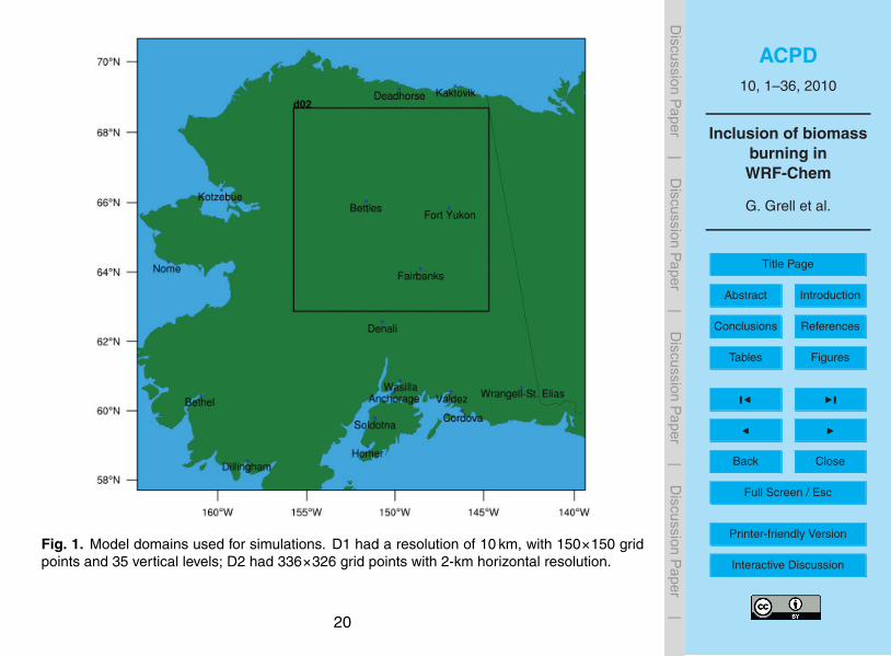
microphysical parameterizations and cloud dynamics, which is usually not well handledby coarser scale simulations. For this reason, we chose two nested domains withregional (dx=10 km) and cloud resolving (dx=2 km) resolutions. Figure 1 shows thedomain setup.

To provide realistic initial conditions a 10-day spin-up period was applied with and10

without biomass burning emissions on domain D1. D1 was initialized on 26 June 2004and WRF-Chem was run to produce 24 h simulations. The North American RegionalReanalysis (NARR) from the National Center for Environmental Prediction (NCEP) wasused to provide meteorological initial and boundary conditions. Initial conditions on 26June for the prognostic gas-phase and aerosol variables are based on those of Mc-15

Keen et al. (2002). These consist of laterally invariant vertical profiles representingclean, oceanic, midlatitude conditions from measurements collected onboard previousNASA-sponsored aircraft missions. Subsequently every 24 h a new simulation wasperformed on D1, with new meteorological fields from NARR. The chemistry for allsubsequent runs was initialized with the previous 24 h forecast. Anthropognic emis-20

sions and biomass burning emissions were provided by 3BEM. The identical proce-dure was repeated for runs without fires (the biomass burning emissions from 3BEMwere excluded in this second set of runs). Physical parameterizations on the regionalscale domain include the Mellor Yamda Boundary layer scheme, the NOAH Land Sur-face model, a version of the Grell-Devenyi Convection parameterization, the Lin et al.25

microphysics scheme, coupled to the model aerosol parameterization and modifiedby Fast et al. (2006) to include second moment effects. The 24 h simulations from 2July 2004 provided the chemical initial fields for the WRF-Chem simulations described

9





ACPD10, 1–36, 2010


G. Grell et al.

Title Page



Tables Figures

J I

J I

Back Close

Full Screen / Esc



Discussion

Paper

|D

iscussionP

aper|

Discussion

Paper

|D

iscussionP

aper|

below.

5.2 The cloud resolving domain

Initial meteorological fields for domain D2 also come from NARR. However, higherresolution terrain was added. The location and size of the domain was chosen to covera large part of the smoky area, and to include the Fairbanks sounding. Additionally5

the integration period (3 July, 00:00 UTC to 5 July, 00:00 UTC) includes sunny anddry weather periods as well as convectively active wet periods. Boundary conditionsfor both, meteorology and chemistry come from domain D1 (3-hourly). The chemicalfields are also initialized from domain D1, to make use of the 10 day spin up period.Physical parameterizations as well as chemical modules are identical to the larger10

domain, except that no convective parameterization is used for the integration over D1.

6 Results

MODIS Satellite pictures over Alaska from 3 July, 21:23 UC and model predicted in-tegrated and vertically averaged PM2.5 (b) for 3 July, 21:00 UTC are shown in Fig. 2.Indicated is also the domain boundary for the cloud resolving nest. The model predicts15

high concentrations of smoke over D2, with highest concentrations South-East of Fair-banks and north of Fort Yukon. The model also correctly simulates the smoke in thewestern part of the domain, which must have originated from the Alaska fires, since noboundary conditions were available for the large domain (D1). Smoke must have beentransported from Alaska out over the Pacific Ocean, before being returneds in shifting20

wind conditions. Note that at the same time there were also significant fires in Canada,outside of D1, leading to a significant underprediction of aerosol concentrations in theeastern part of D1, but outside of domain D2.

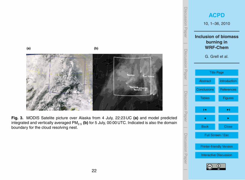
24 h later (Fig. 3), the weather situation is changed significantly with much convectionand rain over large parts of the domain and south-westerlies bringing smoke free and25

10





ACPD10, 1–36, 2010


G. Grell et al.

Title Page



Tables Figures

J I

J I

Back Close

Full Screen / Esc



Discussion

Paper

|D

iscussionP

aper|

Discussion

Paper

|D

iscussionP

aper|

much cleaner air to Fairbanks.While the main goal of this paper is not a verification with observations, but rather

a process study with a newly implemented parameterization, it is gratifying to be ableto show some improvements in weather predictions. This should be expected, sincefor our cases there was a very strong signal provided by the intense and large fires5

of the 2004 fire season. While it usually maybe difficult to predict aerosol concen-trations with enough accuracy to show an improvement in weather prediction, this isdifferent for our study. This is shown in Fig. 4 which compares model predicted and ob-served soundings for 00:00 UTC, 4 July and runs with and without fires (cloud resolvingsimulations). The runs with fires produce much closer agreement with observations.10

Boundary Layer temperatures are cooler, the air is dryer, CAPE is almost identical toobservations for the runs with fires. In general. The simulated soundings represent theobserved atmosphere are in much closer agreement in the lowest 5 km of the atmo-sphere. We also compared soundings at 12:00 UTC on 4 July, and at 00:00 UTC on5 July. While the 12:00 UTC soundings were almost identical for the two simulations15

(very little impact of the fires), the 00:00 UTC soundings on 5 July also showed someimprovements, indicating that the radiative impact was probably the largest positiveeffect on the simulations.

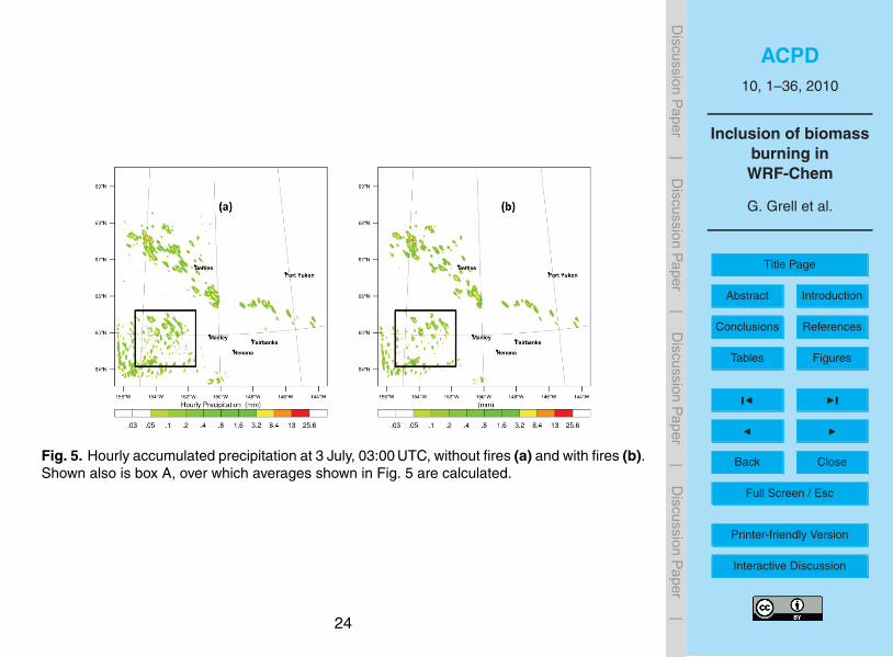
Next we will first focus on comparing the cloud resolving simulations with and withoutthe effect of the wildfires. Figure 5 shows hourly precipitation rates at 03:00 UTC on20

3 July for runs with and without fire, early in the forecast and over domain D2. At thispoint most of the fire impacts are caused by the interactions of the aerosols with themicrophysics. Radiative impacts are still small (see also discussion below and Fig. 8).High aerosol concentrations caused by the wildfires and the responding high numbersof Cloud Condensation Nuclei (CCN) have lead to an increase of cloud water mixing25

ratio, a decrease in rainwater mixing ratio, and in increase in droplet numbers. Thiscan be seen in Fig. 6, which displays mixing ratios of hydrometeors averaged overbox A. Box A was chosen to cover an area representative for the rain fall differencesin the south west of domain D2 at 03:00 UTC (the location of box A can be seen in

11





ACPD10, 1–36, 2010


G. Grell et al.

Title Page



Tables Figures

J I

J I

Back Close

Full Screen / Esc



Discussion

Paper

|D

iscussionP

aper|

Discussion

Paper

|D

iscussionP

aper|

Fig. 4). Droplet number density is sharply increased as is the sum of cloud-waterand ice mixing ratio, while rain-water, snow and graupel mixing ratios are decreased.Figure 6 also shows the averaged total PM2.5 concentration (solid line) for the runwith fires. Note also that the increase in droplet number density and the decreasein rain/snow mixing ratio peak at the same level (approximately at 1.5 km above the5

surface), while the increase in cloud water/ice mixing ratio peaks somewhat higherat about 2 km above the surface. The highest PM2.5 concentrations are found nearthe surface, with a second maximum at about 5 km. This second maximum PM2.5appeared to be related to the smoke entering D2 from the south-west.

By 12:00 UTC results are still qualitatively very similar, as shown in Fig. 7. There is10

less precipitation in the simulations that include the effects of fires. Although short waveradiation is still active in Alaska at night, it’s impact is small and differences in radiativetendencies may also have been caused by difference in cloud fields. Figure 8 showsthe averaged temperature tendency from the atmospheric radiation routine for box Bas well as averaged fine aerosol concentrations. Tendencies are in general very small,15

and should not be the reason for the difference in predicted precipitation tendencies.Domain averaged (D2) precipitation rates as well as fractional coverage of precipi-

tating grid points over the first 18 h of the simulation are shown in Fig. 9 and indicateconsistently lower precipitation as well as less coverage when the impact of fires isconsidered. This is expected because of the extremely high aerosol concentrations in20

the smoky areas, resulting in large CCN numbers, high droplet concentrations, smalldroplets and less conversion to rain.

During the day time results qualitatively change drastically. Storms become moreintense and precipitation becomes more widespread in the runs with fires. This can beseen in Fig. 9, which shows the fractional coverage of grid points with precipitation and25

domain averaged precipitation rate over area D2 and the second 18 h of the simulation.The largest domain averaged differences are in the late afternoon and evening whenconvective activity is the strongest. Towards the morning, the results almost flip again,although the fractional coverage remains higher for the runs that include the effects of

12





ACPD10, 1–36, 2010


G. Grell et al.

Title Page



Tables Figures

J I

J I

Back Close

Full Screen / Esc



Discussion

Paper

|D

iscussionP

aper|

Discussion

Paper

|D

iscussionP

aper|

fires. We attribute the much increased precipitation to both, the radiative feedback aswell as the microphysical feedback. In the eastern part of the domain it may be moststraightforward to try to separate these effects, since before 00:00 UTC on 4 July, largeparts of the domain were cloud free. Fig. 11 shows temperature and dew point differ-ences for cross section A (shown in Fig. 13) before any precipitation formed (3 July,5

22:00 UTC). Temperatures are significantly higher (up to 3 ◦C), especially near the topof the boundary layer. Dew points are higher in the boundary layer, but significantlylower just above. This is caused by a shallower boundary layer in the runs with fires.Aerosols appear to heat the atmosphere strongest at the top of the boundary layer,leading to a more stable and shallower PBL. Since the dew points are also somewhat10

higher in the lowest levels, CAPE is increased slightly. This holds for most of the areain the north eastern cloud free region part of the domain. Figure 12 shows that theincrease in temperature is well collocated with intense PM2.5 plumes. Biomass burn-ing has large black carbon emissions, which leads to much absorption in addition todecreased short wave radiation near the surface.15

Next we look at the differences in some convective storms in the same area a fewhours later. Storms form in approximately the same positions at the same time(00:00 UTC, 4 July). Figure 13 displays simulated echo intensity (maximum DBZ) forthe runs with and without fires indicating the location of the storms in domain D2. Fromthis figure it can be seen that the intensity of the storms in the run with fires is signifi-20

cantly stronger. The hydrometeor fields and the PM2.5 concentrations in cross sectionB for both runs are shown in Fig. 14, the differences in hydrometeor fields and windsin the cross section are shown in Fig. 15. Convection is much stronger this time for theruns with fires, with stronger updraft velocities, and higher cloud and rainwater concen-trations. Only in the umbrella and in newly forming convection ahead of the system did25

we find higher cloud water/ice mixing ratios in the runs without fires.Finally we take a look at domain D1. At 10 km resolution we are using a convective

parameterization that is based on the Grell-Devenyi (2002) approach. However, theoriginal scheme was modified to include a flag to allow for spreading of the subsidence

13





ACPD10, 1–36, 2010


G. Grell et al.

Title Page



Tables Figures

J I

J I

Back Close

Full Screen / Esc



Discussion

Paper

|D

iscussionP

aper|

Discussion

Paper

|D

iscussionP

aper|

to neighboring grid points, as well as including neighboring grid points in determiningthe forcing for the convection, which make this scheme more suited for higher resolutionwhen this flag is turned on. However, at this point aerosol effects had not been includedin this parameterization. The indirect effect only comes in through the interaction ofaerosols with the resolved scale microphysics. In Fig. 16 we again show fractional5

coverage and domain averaged precipitation rates averaged over domain D2, but fromthe coarser resolution simulation (part of D1). Qualitatively the results are somewhatsimilar to the cloud resolving simulation for domain D2. However, fractional coverage issomewhat higher for the runs with fires almost throughout the simulation, except for themorning of 4 July, where both, fractional coverage and domain averaged precipitation10

are smaller for the runs with fires. However, compared to domain D2, the increase inprecipitation in the afternoon and evening is much more pronounced for domain D1. Anexample is shown in Fig. 17, displaying hourly precipitation rates at 04:00 UTC, 4 July2004. Both resolved and non-resolved precipitation (not shown here) had significantlyincreased precipitation rates during afternoon and evening hours. However, while the15

convective parameterization produced a diurnal oscillation in fractional coverage, theresolved precipitation was steadily increasing in coverage throughout the period, withsome local maximum in the afternoon and evening.

7 Conclusions

A plumerise algorithm for wildfires was successfully added to WRF-Chem. Biomass20

burning emissions were estimated using a biomass burning emissions model whichcan be based on near real-time remote sensing fire products or historic fire data todetermine fire emissions and plume rise characteristics (Freitas et al., 2005, 2007;Longo et al., 2007). Fire emissions are updated as they become available and arespatially and temporally distributed according to the fire count locations obtained by25

remote sensing. A 1-D time dependent cloud model is then used in WRF-Chem toestimate injection heights as well as the final emission rates. This wildfire algorithm

14





ACPD10, 1–36, 2010


G. Grell et al.

Title Page



Tables Figures

J I

J I

Back Close

Full Screen / Esc



Discussion

Paper

|D

iscussionP

aper|

Discussion

Paper

|D

iscussionP

aper|

was then applied to look at the impact of intense wildfires on weather forecasts.In general, a strong direct effect is apparent during the daytime. Interaction of the

aerosols with atmospheric radiation through scattering and absorption is very signifi-cant in and just above the boundary layer, coinciding with the largest aerosol concen-trations. In cloud free areas this leads to somewhat cooler surface temperatures. The5

warming above the surface layers then was causing a shallower and moister boundarylayer as well as slightly increased CAPE in the clear areas. The impact of the interac-tion of aerosols with microphsyics in the presence of intense nearby wildfires maybemore difficult to categorize, since the radiative impacts cannot be completely excluded.In our studies the initial impact of the smoke appears to be to decrease the precipi-10

tation (coverage and intensity), but increase the cloud water mixing ratio and dropletnumbers. This seems especially apparent during the first 12 h of the integration (Alaskanight time) when there is only a small effect from the interaction of the aerosols withatmospheric radiation. During the afternoons precipitation activity is increased signif-icantly in amount and coverage when smoke from fires is considered. The stronger15

storms are most likely caused by both the interaction of aerosols with the atmosphericradiation as well as the interaction with the microphsyics.

Qualitatively similar results are seen in the larger domain that still employs a convec-tive parameterization. However, the afternoon increase in precipitation amounts andcoverage is much more pronounced.20

References

Abdul-Razzak, H. and Ghan, S. J.: A parameterization of aerosol activation. 2. Multiple aerosoltypes, J. Geophys. Res., 105, 6837–6844, 2000.

Abdul-Razzak, H. and Ghan, S. J.: A parameterization of aerosol activation. 3. Sectional rep-resentation, J. Geophys. Res., 107, article no.?, doi:10.1029/2001JD000483, 2002.25

Ackermann, I. J., Hass, H., Memmesheimer, M., Ebel, A., Binkowski, F. S., and Shankar, U.:Modal aerosol dynamics model for Europe: development and first applications, Atmos. Envi-ron., 32, 2981–2999, 1998.

15





ACPD10, 1–36, 2010


G. Grell et al.

Title Page



Tables Figures

J I

J I

Back Close

Full Screen / Esc



Discussion

Paper

|D

iscussionP

aper|

Discussion

Paper

|D

iscussionP

aper|

Andreae, M., and Merlet, P.: Emission of trace gases and aerosols from biomass burning,Global Biogeochem. Cy., 15(4), 955–966, 2001.

Barnard, J. C., Fast, J. D., Paredes-Miranda, G., Arnott, W. P., and Laskin, A.: Technical Note:Evaluation of the WRF-Chem “Aerosol Chemical to Aerosol Optical Properties” Module usingdata from the MILAGRO campaign, Atmos. Chem. Phys., 10, 7325–7340, doi:10.5194/acp-5

10-7325-2010, 2010.Belward, A.: The IGBP-DIS global 1 km land cover data set (DISCover)-proposal and imple-

mentation plans, IGBP-DIS Working Paper No. 13, Toulouse, France, 1996.Chapman, E. G., Gustafson Jr., W. I., Easter, R. C., Barnard, J. C., Ghan, S. J., Pekour, M. S.,

and Fast, J. D.: Coupling aerosol-cloud-radiative processes in the WRF-Chem model: In-10

vestigating the radiative impact of elevated point sources, Atmos. Chem. Phys., 9, 945–964,doi:10.5194/acp-9-945-2009, 2009.

Easter, R. C., Ghan, S. J., Zhang, Y., Saylor, R. D., Chapman, E. G., Laulainen, N. S.,Abdul-Razzak, H., Leung, L. R., Bian, X., and Zaveri, R. A.: MIRAGE: model de-scription and evaluation of aerosols and trace gases, J. Geophys. Res., 109, D20210,15

doi:10.1029/2004JD004571, 2004.Fahey, K. M. and Pandis, S. N.: Optimizing model performance: variable size resolution in cloud

chemistry modeling, Atmos. Environ., 35, 4471–4478, 2001.Fast, J. D., Gustafson, W. I., Easter, R. C., Zaveri, R. A., Barnard, J. C., Chapman, E. G.,

Grell, G. A., and Peckham, S. E.: Evolution of ozone, particulates, and aerosol direct radiative20

forcing in the vicinity of Houston using a fully coupled meteorology, chemistry, and aerosolmodel. J. Geophys. Res., 111, article no.?, doi:10.1029/2005JD006721, 2006.

Freitas, S. R., Longo, K. M., Silva Dias, M., Silva Dias, P., Chatfield, R., Prins, E., Artaxo, P.,Grell, G., and Recuero, F.: Monitoring the transport of biomass burning emissions in SouthAmerica, Environ. Fluid Mech., 5(1–2), 135–167, doi:10.1007/s10652-005-0243-7, 2005.25

Freitas, S. R., Longo, K. M., and Andreae, M. O.: Impact of including the plume rise of vegeta-tion fires in numerical simulations of associated atmospheric pollutants, Geophys. Res. Lett.,33, L17808, doi:10.1029/2006GL026608, 2006.

Freitas, S. R., Longo, K. M., Chatfield, R., Latham, D., Silva Dias, M. A. F., Andreae, M. O.,Prins, E., Santos, J. C., Gielow, R., and Carvalho Jr., J. A.: Including the sub-grid scale30

plume rise of vegetation fires in low resolution atmospheric transport models, Atmos. Chem.Phys., 7, 3385–3398, doi:10.5194/acp-7-3385-2007, 2007.

Fromm, M., Alfred, J., Hoppel, K., Hornstein, J., Bevilacqua, R., Shettle, E., Servranckx, R.,

16





ACPD10, 1–36, 2010


G. Grell et al.

Title Page



Tables Figures

J I

J I

Back Close

Full Screen / Esc



Discussion

Paper

|D

iscussionP

aper|

Discussion

Paper

|D

iscussionP

aper|

Li, Z., and Stocks, B.: Observations of boreal forest fire smoke in the stratosphere by POAMIII, SAGE II, and lidar in 1998, Geophys. Res. Lett., 27, 1407–1410, 2000.

Ghan, S. J. and Easter, R. C.: Impact of cloud-borne aerosol representation on aerosol di-rect and indirect effects, Atmos. Chem. Phys., 6, 4163–4174, doi:10.5194/acp-6-4163-2006,2006.5

Ghan, S. J., Easter, R. C., Chapman, E. G., Abdul-Razzak, H., Zhang, Y., Leung, L. R.,Laulainen, N. S., Saylor, R. D., and Zaveri, R. A.: A physically based estimate of radiativeforcing by anthropogenic sulfate aerosol, J. Geophys. Res., 106, 5279–5293, 2001a.

Ghan, S. J., Easter, R. C., Hudson, J., and Breon, F.-M.: Evaluation of aerosol indirect radiativeforcing in MIRAGE, J. Geophys. Res., 106, 5317–5334, 2001b.10

Ghan, S. J., Leung, L. R., Easter, R. C., and Abdul-Razzak, H.: Prediction of droplet number ina general circulation model, J. Geophys. Res., 102, 21777–21794, 1997.

Giglio, L., Descloitres, J., Justice, C. O., and Kaufman, Y. J.: An enhanced contextual firedetection algorithm for MODIS, Remote Sens. Environ., 87, 273–282, 2003.

Grell, G. A., Peckham, S. E., McKeen, S., Schmitz, R., Frost, G., Skamarock, W. C., and15

Eder, B.: Fully coupled “online” chemistry within the WRF model, Atmos. Environ., 39, 6957–6975, 2005.

Grell, G. A. and Devenyi, D.: A generalized approach to parameterizing convectioncombining ensemble and data assimilation techniques, Geophys. Res. Lett., 29(14),doi:10.1029/2002GL015311, 2002.20

Gustafson Jr., W. I., Chapman, E. G., Ghan, S. J., and Fast, J. D.: Impact on modeledcloud characteristics due to simplified treatment of uniform cloud condensation nuclei duringNEAQS 2004, Geophys. Res. Lett., 34, L19809, doi?, 2007.

Hollingsworth, A., Engelen, R. J., Textor, C., Benedetti, A., Boucher, O., Chevallier, F., De-thof, A., Elbern, H., Eskes, H., Flemming, J., Granier, C., Kaiser, J. W., Morcrette, J. J.,25

Rayner, P., Peuch, V.-H., Rouil, L., Schultz, M., Simmons, A., and the GEMS consortium: To-ward a monitoring and forecasting system for atmospheric composition. The GEMS Project,Bull. Am. Meteor. Soc., 89, 1147–1164, doi:10.1175/2008BAMS2355.1, 2008.

Jacobson, M. Z.: Developing, coupling, and applying a gas, aerosol, transport, and radiationmodel to study urban and regional air pollution. PhD. Dissertation, Dept. of Atmospheric30

Sciences, UCLA, 436 pp., 1994.Jacobson, M. Z.: Development and application of a new air pollution modeling system. Part II:

Aerosol module structure and design, Atmos. Environ., 31A, 131–144, 1997a.

17





ACPD10, 1–36, 2010


G. Grell et al.

Title Page



Tables Figures

J I

J I

Back Close

Full Screen / Esc



Discussion

Paper

|D

iscussionP

aper|

Discussion

Paper

|D

iscussionP

aper|

Jacobson, M. Z.: Development and application of a new air pollution modeling system. Part III:Aerosol-phase simulations, Atmos. Environ., 31A, 587–608, 1997b.

Liu, Y., Daum, P. H., and McGraw, R. L.: Size truncation effect, threshold behavior,and a new type of autoconversion parameterization, Geophys. Res. Lett., 32, L11811,doi:10.1029/2005GL022636, 2005.5

Longo, K. M., Freitas, S. R., Andreae, M. O., Setzer, A., Prins, E., and Artaxo, P.: The Cou-pled Aerosol and Tracer Transport model to the Brazilian developments on the RegionalAtmospheric Modeling System (CATT-BRAMS) – Part 2: Model sensitivity to the biomassburning inventories, Atmos. Chem. Phys., 10, 5785–5795, doi:10.5194/acp-10-5785-2010,2010. Please notice: ACP update inserted!10

Olson, J. S., Watts, J. A., and Allison, L. J.: Major World Ecosystem Complexes Ranked byCarbon in Live Vegetation: A Database (Revised November 2000). NDP-017, available at:http://cdiac.esd.ornl.gov/ndps/ndp017.html from Carbon Dioxide Information Analysis Cen-ter, Oak Ridge National Laboratory, Oak Ridge, Tennessee, USA, 2000.

Petters, M. D. and Kreidenweis, S. M.: A single parameter representation of hygroscopic15

growth and cloud condensation nucleus activity, Atmos. Chem. Phys., 7, 1961–1971,doi:10.5194/acp-7-1961-2007, 2007.

Prins, E., Feltz, J., Menzel, W., and Ward, D.: An overview of GOES-8 diurnal fire and smokeresults for SCAR-uuand 1995 fire season in South America, J. Geophys. Res., 103(D24),31821–31835, 1998.20

Schell, B., Ackermann, I. J., Hass, H., Binkowski, F. S., and Ebel, A.: Modeling the formation ofsecondary organic aerosol within a comprehensive air quality modeling system, J. Geophys.Res., 106, 28275–28293, 2001.

Seiler, W. and Crutzen, P. J.: Estimates of gross and net fluxes of carbon between the biosphereand the atmosphere from biomass burning, Climatic Change, 2, 207–247, 1980.25

Setzer, A. and Pereira, M.: Amazonia biomass burnings in 1987 and an estimate of their tropo-spheric emissions, Ambio, 20, 19–22, 1991.

Skamarock, W. C., Klemp, J. B., Dudhia, J., Gill, D. O., Barker, D. M., Wang, W., and Pow-ers, J. G.: A description of the advanced research WRF version 2. NCAR Technical Note,NCAR/TN-468+STR, 8 pp., 2005.30

Stockwell, W. R., Kirchner, F., Kuhn, M., and Seefeld, S.: A new mechanism for regional atmo-pheric modeling, J. Geophys. Res., 102, 25874–25879, 1997.

18





http://cdiac.esd.ornl.gov/ndps/ndp017.html

ACPD10, 1–36, 2010


G. Grell et al.

Title Page



Tables Figures

J I

J I

Back Close

Full Screen / Esc



Discussion

Paper

|D

iscussionP

aper|

Discussion

Paper

|D

iscussionP

aper|

Ward, E., Susott, R., Kaufman, J., Babbit, R., Cummings, D., Dias, B., Holben, B., Kaufman, Y.,Rasmussen, R., and Setzer, A.: Smoke and fire characteristics for cerrado and deforestationburns in Brazil: BASE-B Experiment, J. Geophys. Res., 97(D13), 14601–14619, 1992.

Zhang, Y., Easter, R. C., Ghan, S. J., and Abdul-Razzak, H.: Impact of aerosol sizerepresentation on modeling aerosol-cloud interactions, J. Geophys. Res., 107, 4558,5

doi:10.1029/2001JD001549, 2002.

19





ACPD10, 1–36, 2010


G. Grell et al.

Title Page



Tables Figures

J I

J I

Back Close

Full Screen / Esc



Discussion

Paper

|D

iscussionP

aper|

Discussion

Paper

|D

iscussionP

aper|

Fig. 1. Model domains used for simulations. D1 had a resolution of 10 km, with 150×150 gridpoints and 35 vertical levels; D2 had 336×326 grid points with 2-km horizontal resolution.

20





ACPD10, 1–36, 2010


G. Grell et al.

Title Page



Tables Figures

J I

J I

Back Close

Full Screen / Esc



Discussion

Paper

|D

iscussionP

aper|

Discussion

Paper

|D

iscussionP

aper|

(a) (b)

Fig. 2. MODIS Satellite picture over Alaska from 3 July, 21:23 UC (a) and model predictedintegrated and vertically averaged PM2.5 (b) for 3 July, 21:00 UTC. Indicated is also the domainboundary for the cloud resolving nest.

21





ACPD10, 1–36, 2010


G. Grell et al.

Title Page



Tables Figures

J I

J I

Back Close

Full Screen / Esc



Discussion

Paper

|D

iscussionP

aper|

Discussion

Paper

|D

iscussionP

aper|

(a) (b)

Fig. 3. MODIS Satelite picture over Alaska from 4 July, 22:23 UC (a) and model predictedintegrated and vertically averaged PM2.5 (b) for 5 July, 00:00 UTC. Indicated is also the domainboundary for the cloud resolving nest.

22





ACPD10, 1–36, 2010


G. Grell et al.

Title Page



Tables Figures

J I

J I

Back Close

Full Screen / Esc



Discussion

Paper

|D

iscussionP

aper|

Discussion

Paper

|D

iscussionP

aper|

Fig. 4. Observed (black) and predicted (blue) sounding for Fairbanks, Alaska, an 4 July,00:00 UTC. Shawn is temperature (solid), dew points (dashed-dotted), and wind barbs for runswithout fires (a) and runs with fires (b). A malst adiabat based an a mixed parcel for the lowest100 mb of the observed (simulated) sounding 15 dashed in red (magenta). if possible,please provide higher quality

23





ACPD10, 1–36, 2010


G. Grell et al.

Title Page



Tables Figures

J I

J I

Back Close

Full Screen / Esc



Discussion

Paper

|D

iscussionP

aper|

Discussion

Paper

|D

iscussionP

aper|

Fig. 5. Hourly accumulated precipitation at 3 July, 03:00 UTC, without fires (a) and with fires (b).Shown also is box A, over which averages shown in Fig. 5 are calculated.

24





ACPD10, 1–36, 2010


G. Grell et al.

Title Page



Tables Figures

J I

J I

Back Close

Full Screen / Esc



Discussion

Paper

|D

iscussionP

aper|

Discussion

Paper

|D

iscussionP

aper|

Fig. 6. Hydrometeor properties averaged over box A (shown in Fig. 4). Displayed is the dif-ference (dashed line) in droplet number density (a), the sum of rain water, snow, and graupelmixing ratio (b) and the sum of cloud water and ice mixing ratio (c) for the run with fires minusthe run without fires. Shown also on all 3 panels is the total PM2.5 concentration (solid line) forthe run with fires.

25





ACPD10, 1–36, 2010


G. Grell et al.

Title Page



Tables Figures

J I

J I

Back Close

Full Screen / Esc



Discussion

Paper

|D

iscussionP

aper|

Discussion

Paper

|D

iscussionP

aper|

Fig. 7. Hourly precipitation at 3 July, 12:00 UTC, without fires (a) and with fires (b). Shown alsois box B, over which averages shown in Fig. 8 are calculated.

26





ACPD10, 1–36, 2010


G. Grell et al.

Title Page



Tables Figures

J I

J I

Back Close

Full Screen / Esc



Discussion

Paper

|D

iscussionP

aper|

Discussion

Paper

|D

iscussionP

aper|

Fig. 8. Radiative temperature tendency differences (dashed line) averaged over box B (shownin Fig X Please define which figure is meant.) for the run with fires minus the run withoutfires. The solid line is the total averaged PM2.5 concentration for the runs with fires.

27





ACPD10, 1–36, 2010


G. Grell et al.

Title Page



Tables Figures

J I

J I

Back Close

Full Screen / Esc



Discussion

Paper

|D

iscussionP

aper|

Discussion

Paper

|D

iscussionP

aper|

Fig. 9. Fractional coverage (a) of grid points with precipitation and domain averaged precipita-tion rate in mm/h (b) over area D2 for the first 18 h of the simulabon. The solid line indicatesrun without fires, dashed line is for the runs with fires. The horizontal axis is the simulation timein hours.

28





ACPD10, 1–36, 2010


G. Grell et al.

Title Page



Tables Figures

J I

J I

Back Close

Full Screen / Esc



Discussion

Paper

|D

iscussionP

aper|

Discussion

Paper

|D

iscussionP

aper|

Fig. 10. Fractional coverage (a) of grid points with precipitation and domain averaged precip-itation rate in mm/h (b) over area D2 from 3 July, 18:00 UTC to 12:00 UTC, 4 July. The solidline indicates run without fires, dashed line is for the runs with fires. The horizontal axis is thesimulation time in hours.

29





ACPD10, 1–36, 2010


G. Grell et al.

Title Page



Tables Figures

J I

J I

Back Close

Full Screen / Esc



Discussion

Paper

|D

iscussionP

aper|

Discussion

Paper

|D

iscussionP

aper|

Fig. 11. Temperature (a) differences in ◦C and water vapor mixing ratio (b) differences (g/kg)from the runs with fires minus the run without fires for cross section A at 22:00 UTC, 3 July2004. Fields are averaged along a line that extends 5 grid points into and out of the crosssection.

30





ACPD10, 1–36, 2010


G. Grell et al.

Title Page



Tables Figures

J I

J I

Back Close

Full Screen / Esc



Discussion

Paper

|D

iscussionP

aper|

Discussion

Paper

|D

iscussionP

aper|

Fig. 12. Temperature (a) Please check. differences in ◦C overlayed with PM2.5 concen-trations (in red) for cross section A. Fields are averaged along a line that extends 5 grid pointsinto and out of the cross section.

31





ACPD10, 1–36, 2010


G. Grell et al.

Title Page



Tables Figures

J I

J I

Back Close

Full Screen / Esc



Discussion

Paper

|D

iscussionP

aper|

Discussion

Paper

|D

iscussionP

aper|

Fig. 13. Maximum dbz for storms at around 02:00 UTC, 4 July without (b) and with (c) firesin the eastern part of the domain (a). Terrain is shaded. Cross section A is shown in (a) witha dashed line, cross section B is marked in (b) and (c) with a solid line.

32





ACPD10, 1–36, 2010


G. Grell et al.

Title Page



Tables Figures

J I

J I

Back Close

Full Screen / Esc



Discussion

Paper

|D

iscussionP

aper|

Discussion

Paper

|D

iscussionP

aper|

Fig. 14. Cloudwater/ice mixing ratio (calor), rain water, snow and graupel mixing ratio (blacklines) and PM2.5 concentrations (gray shades) for cross section B (shown in Fig. 13) and runswithout (a) and with (b) fires. Fields are averaged along a line that extends 5 grid points intoand out of the cross section.

33





ACPD10, 1–36, 2010


G. Grell et al.

Title Page



Tables Figures

J I

J I

Back Close

Full Screen / Esc



Discussion

Paper

|D

iscussionP

aper|

Discussion

Paper

|D

iscussionP

aper|

Fig. 15. Differences fields (runs with fires – runs without fires) of the sum of cloudwater andice mixing ratio (color), the sum of rain water, snow and graupel mixing ratios (black lines,)and winds in the cross section (arrows) for cross section b (shown in Fig. 13) and runs without(a) Please check. and with (b) Please check. fires. Fields are averaged along a linethat extends 5 grid points into and out of the cross section.

34





ACPD10, 1–36, 2010


G. Grell et al.

Title Page



Tables Figures

J I

J I

Back Close

Full Screen / Esc



Discussion

Paper

|D

iscussionP

aper|

Discussion

Paper

|D

iscussionP

aper|

Fig. 16. Fractional coverage (a) of grid points with precipitation and precipitation rate in mm/h(b) from simulation over large domain (dx 10 km) averaged over area D2. The solid line indi-cates run without fires, dashed line is for the runs with fires. Results include both resolved andnon-resolved precipitation.

35





ACPD10, 1–36, 2010


G. Grell et al.

Title Page



Tables Figures

J I

J I

Back Close

Full Screen / Esc



Discussion

Paper

|D

iscussionP

aper|

Discussion

Paper

|D

iscussionP

aper|

Fig. 17. Total hourly precipitation accumulation from 03:00 UTC to 04:00 UTC an 4 July 2004as simulated over domain D1 without the effect of fires (a) and including the effect of fires (b).

36





Inclusion of biomass burning in WRF-Chem: impact of wildfires on weather forecasts

Documents

Transcript of Inclusion of biomass burning in WRF-Chem: impact of wildfires on weather forecasts