NBER WORKING PAPER SERIES

MONEY STOCK TARGETING, BASE ORIFF ANO PRICE-LEVEL PREOICTABILITY: LESSONS FROM THE U.K. EXPERIENCE

Michael D. Bordo

Ehsan U. Choudhri

Anna J. Schwartz

Working Paper No. 2825

NATIONAL BUREAU OF ECONOMIC RESEARCH 1050 Massachusetts Avenue

Cambridge, MA 02138

January 1989

For helpful comments and suggestions, we would like to thank Michael Ootaey, Charles Evans, Marvin Goodfriend, Bennett McCalluzn, Carl Walsh and partici- pants at aeminara held at the Federal Reserve Bank of Richmond, Carleton

University, Texas A and M University, Rice University and the Univeraity of South Carolina. This research is part of NBER's research programs in Economic Fluctuations, Financial Markets and Monetary Economics, and in International Studies. Any opinions expressed are those of the authors not those of the National Bureau of Economic Research.

NBER Working Paper #2825 January 1989

MONEY STOCK TARGETING, BASE DRIFT AND PRICE-LEVEL PREDICTABILITY: LESSONS FROM THE U.K. EXPERIENCE

ABSTRACT

It is controversial whether money stock targeting without base

drift (i.e. following a trend—stationary growth path) makes the price

level more predictable in the presence of permanent shocks to money

demand. Developing a procedure that does not run into the Lucas

critique, and applying this procedure to the case of the U.K., the paper

finds that the variance of the trend inflation rate in the U.K. would

have been reduced by more than one half if the Bank of England had not

allowed base drift.

Michael D. Bordo Ehsan U. Choudhri Department of Economics Department of Economics College of Business Administration Carleton University University of South Carolina Ottawa, Ontario Columbia, SC 29212 K1S 5B6

CANADA

Anna J. Schwartz National Bureau of Economic Research 269 Mercer Street New York, NY 10003

I. Introduction

During the 1970's, a number of countries attempted to control

inflation and promote price stability by targeting monetary aggregates.

In setting monetary targets, a general practice has been to calculate

next period's target level on the basis of the actual rather than the

(previously-announced) target level for the current period. According to

this practice (hereafter referred to as base drift), when the money stock

diverges from its target growth path, the divergence does not tend to be

reversed later and thus results in a permanent change in the money stock.

In other words, the money stock series would contain a unit root under

base drift.

One popular criticism of the base drift policy is that it would

introduce greater uncertainty about the long—run behavior of the money

stock, and thus monetary targeting with base drift would not succeed in

achieving long-run price stability.' Indeed, if the arguments of and

shocks to the money demand function are trend stationary (so that the

real money stock is trend stationary), the price level series has a unit

root if and only if the money stock series has a unit root. In this

case, the price level is clearly less predictable over long periods under

base drift.

An interesting issue in this context is why a targeting policy whose

major goal is long—run price stability would allow base drift under these

circumstances. Goodfriend (1987) has suggested the explanation that base

drift is induced by a tension arising between the price level smoothing

and interest rate smoothing objectives of a central bank. Although base

drift makes the price level less predictable over long periods (by

introducing a unit root into the price level series), it is allowed

because it also helps reduce the variability of interest rates.

An alternative view has been suggested by Walsh (1986, 1987), who

has pointed out that if the demand for money is subject to permanent

shifts, the price level would not be trend stationary even without base

drift. Indeed, base drift would offset the effect of permanent shocks to

money demand on the price level, and as Walsh (1986) has shown an optimal

policy would involve some (between zero and full) base drift. It is thus

possible that full base drift, as compared to no base drift, would make

the price level more predictable over long periods. The goal of price

stability alone would suffice in this case to explain why central banks

follow the base drift policy.

The two views on the effect of base drift on the stochastic

behavior of the price level can only be resolved by an examination of the

empirical evidence. Such evidence is difficult to obtain because

satisfactory structural models of price dynamics are lacking, and

therefore, the econometric estimation of price behavior often relies on

reduced—form equat.ions. For reasons discussed in the well—known Lucas

(1976) critique, reduced—form equations estimated for a regime of base

drift cannot be used to predict the behavior of the price level under a

counter—factual regime of no base drift.

To avoid this problem, the present paper focuses on the influence of

base drift on the behavior of the permanent component of the price level

(the trend price level). It can be shown that the forecast variance of

the trend price level would dominate the forecast variance of the actual

3

price level over long time horizons and hence provide useful information

about long—term uncertainty about the price level. It is possible,

moreover, to estimate the hypothetical behavior of the trend price level

under no base drift (on the basis of data available from a base drift

regime) using a procedure developed in this paper. The procedure

exploits the widely accepted proposition that money is neutral in the

long run. Empirical implementation of our procedure requires estimation

of the long—run components of both the price level and money stock. We

estimate these components using an approach that has its roots in the

Beveridge and Nelson (1981) method for decomposing univariate series into

permanent and transitory components.2

Our empirical work focuses on the monetary experience of the United

Kingdom since 1976. The Bank of England has allowed full base drift in

setting targets for sterling M3, and has implemented its target policy by

using interest rate control. Although other countries have also pursued

monetary targeting with base drift, the United Kingdom's experience with

this policy represents one of the longest periods of targeting without a

change in the control procedure. In addition, the United Kingdom has

been less successful than most other countries [e.g.,

the U.S., Canada

and Germany] in hitting its targets and has experienced greater

variability in its price level than most other countries. Thus the U.K.

experience with monetary targeting provides a good case study of the

influence of base drift on price stability.

Section II of the paper uses a model with flexible prices and

rational expectations to provide a simple example of conditions under

which base drift may either increase or decrease the forecast variance of

the price level. Section III paves the way for our empirical analysis by

4

introducing a framework in which each variable is decomposed into

permanent and transitory components. Using this framework, we then

explain our procedure for estimating the behavior of the trend price

level in the absence of base drift, making use of the data available from

a targeting regime in its presence. Applying this procedure to the case

of the United Kingdom in section IV, we examine whether the trend price

level in the United Kingdom would have been less predictable if the Bank

of England had not allowed any base drift. Our results show that the

policy of no base drift would have reduced the forecast variance of the

trend price level by slightly more than one half. Interestingly, this

substantial reduction in the variance occurs even though the demand for £

M3 in the United Kingdom has exhibited permanent shifts. Thus our

evidence is consistent with the view that base drift increases price

level uncertainty.

II. Base Drift and Price—Level Variability: A Simple Model

To explore the influence of base drift on the behavior of the price

level, we begin with a simple stochastic model that assumes flexible

prices and rational expectations. As is the case in the United Kingdom,

we assume that the. central bank uses an interest rate control procedure

to achieve its money stock targets. We also assume that information on

the money stock and the price level becomesavilable (to both the

central bank and the public) after a one-period lag. Our set—up is a

modified version of the (1981) model that McCallum used to analyze the

implications of an interest rate policy rule for price level determinacy.

The key differences between our model and McCallum's are that we allow

for the possibility of base drift and include a permanent shock in the

5

ironey demand function. In McCallum's rrodel, the central bank pursues the

objective of interest-rate smoothing. Goodfriend (1981) has suggested

that this objective induces central banks to incorporate base drift in

setting their targets. To keep our theoretical example simple, however,

we assume that the central bank is concerned only with keeping the money

stock on target (our more general empirical model in section III,

however, does allow for other goals such as interest—rate smoothing).

Our model is described by the following equations:

m = Pt a + e , (1)

at at_l + a , (2)

Pt =

EtiPt+i - r + ' (3)

ot + d ' (4)

= (i.e )m1 (5)

= -(l/s)[u — Et i(Pt+at+ e)J , (6)

where m and represent the logarithms of the money stock and the price

level, r is the nominal rate of interest, e. a and dt are white noise

disturbances, and the operator Eti denotes the expectation of the

indicated variable conditional on information on all variables in the

model up to period t—1.

6

Equations (1) and (2) represent the money market. The demand for

money is assumed to depend on a permanent shock as well as a temporary

shock et.

For simplicity, we assume that the permanent shock is a random

walk while the temporary shock is serially uncorrelated. Equations (3)

and (4) summarize the goods market. The variable in these equations

is the real rate of interest, and like is assumed to follow a random

walk. Following McCallum (1981), we assume that an island' model

underlies the determination of p in such a model would

represent an average of local' real rates (that utilize global

information on the nominal interest rate but only local information n prices), we use Etipt+i rather than

Etpt+i to express the expected value

of the next period's price level in (3). Note that shocks to the real

interest rate (dr)

may be correlated with those to the demand for money

(aand/or e) but we cannot be sure about the signs of these correlations

without further specification of the underlying model. Finally, (5) and

(6) provide a simple characterization of money-stock targeting with

interest rate control. In these equations, prepresents the target level

of mt.

To simplify the discussion, we assume that the target rate of

money growth equals zero. The setting of the target stock in (5) allows

for full base drift when e = 0 and no base drift when a 1. As our

concern here is to highlight the difference between two widely—discussed

policy alternatives of zero or full base drift, we do not attempt to

derive an optimal policy rule. Assuming that the central bank pursues no

other goal, the interest rate is set in (6) such that the expected stock

of money equals the target stock. Note that given the one—period

information lag, m can diverge from because of unanticipated changes

in money demand and the price level.

7

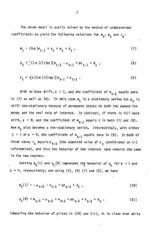
The above model is easily solved by the method of undetermined

coefficients to yield the following solutions for m, Pt and

= (1-e )mi + a + e + d ' (7)

[ (1 )/(14e )] m1 - a + + d , (8)

-[e (i.e )/(1496 + 6t_i (9)

With no base drift, a = 1, and the coefficient of mi equals zero

in (7) as well as (8). In this case m is a stationary series but is

still non—stationary because of permanent shocks to both the demand for

money and the real rate of interest. In contrast, if there is full base

drift, a = 0, and the coefficient of mi equals 1 in both (7) and (8). Now m also becomes a non—stationary series. Interestingly, with either

o = 1 or e = 0, the coefficient of rn1 equals zero in (9). In both of

these cases rt equals (the expected value of conditional on t—i

information), and thus the behavior of the interest rate remains the same

in the two regimes.

Letting and represent the behavior of Pt fore = 1 and

o = 0, respectively, and using (2), (4) (7) and (8), we have

= - a t-2 - ati + + dt , (10)

= m2 - a t-2 + e1 + t_i + d1 + dt . (11)

Comparing the behavior of prices in (10) and (11), it is clear that while

8

the policy of full base drift, as compared to no drift, eliminates the

shock a1 from the price equation, at the same time it introduces new

shocks e1 and dt_i. To explore the influence of base drift on price variability, we let

FV(e ) Et{pt+k(o ) — Ep.(o)}2, e

= 1, 0, denote the k-period forecast

variance of p, and use (2), (4) (10) and (11) to obtain

FV(1) = (k-i)

2 + + (k-1)0

- 2(kl)oad (12)

FV(0) = (k-1)(14 )2a + + (k-1) + 2(kl)(l4)oed (13)

where 2 and 2 are the variances of a and e while a and are the

a e ad ed

covariances between a and d, and e and d. According to (12) and (13),

the one—period forecast variances are the same (and equal to o) with or

without base drift. However, for longer forecast intervals, the two

regimes imply different variances. For k > 2, it follows from (12) and

(13) that

FV(0) -

FV(I) (k1)[a2 + (j+28)a (14)

Thus, when k > 2 the difference between the full—drift and no—drift

k—period forecast variances increases with variances of shocks e and d

but decreases with that of shock a. This difference is also influenced

by the covariances between shocks a and d, and e and d, but the direction

of the influence would depend on whether these covariances are positive

or negative.

9

As the above simple analysis illustrates, which targeting regime

would lead to a lower variability of the price level is essentially an

empirical question. In the next section, we develop a procedure that can

be used to estimate forecast variances of the trend price level for the

two regimes, using data generated under the base—drift regime.

III. A Methodology for Estimating the Influence of Base Drift on the

Trend Price Level

Reduced—form equations [(7) — (9)] for

rn. Pt and r in the previous

section were derived from a particular model. In this section, we

consider reduced—form equations for these variables of a very general

form that would be consistent with a broad class of models of assets and

goods markets and of monetary policy rules. We only require that the

underlying structure obey certain minimal restrictions on the behavior of

the permanent components of these variables. To incorporate these

restrictions into the analysis, each variable is decomposed into a trend

or a permanent component and a cyclical or a transitory component as

follows:

+ Ut., (15)

where is a 3 x 1 vector of variables mt, P1 r;

= [t a

vector of permanent components of these variables; and

u = [ u1 u2 u3] a vector of transitory components. The permanent

components are assumed to evolve as

=1 + V , (16)

10

where y = [y 12131 is a vector of constants and v = [ v1 v2 v] a

vector of shocks to the permanent components. Both u and v at-c

covariance stationary.

We assume that money is neutral in the long run in the sense that

the distribution of permanent components of real variables is independent

of the behavior of the money stock. In this context, permanent

components could be viewed as representing values in the long run or' the

"natural" equilibrium. The concept of the long—run equilibrium, however,

is often not well defined and its meaning differs from one model to

another. For example, deviations of variables from their long—run values

are explained in terms of price stickiness by one approach, and

information lags by another. The length of time required to reach the

long—run equilibrium could thus depend on what type of short—run friction

is assumed.

To avoid identifying the long run with a specific period of time, it

'is appealing to use the concept of the permanent component suggested by

Beveridge and Nelson (1981). According to this concept

= im (Etyt - ky ) . (17)

The permanent components defined by (17) represent forecasts (after

adjusting for deterministic trends) of corresponding variables in the

future far enough to eliminate the influence of all types of short-run

frictions. These forecasts, moreover, utilize all current information

available in the model. As discussed below, an immediate implication of

(17) is that the shocks to permanent components (vt) are white noise

disturbances. Also note that one or more components of Vt can be set

11

equal to zero. In such special cases, the corresponding permanent

component(s) would simply follow a deterministic trend line over time.

Having defined our measure of permanent components, we next discuss

two relations that link the permanent components of the two real

variables in our model, the real stock of money and the real rate of

interest. First, we assume a "long—run demand for money of the form:

(18)

where at is a random variable that represents shifts in the long-run

demand. Second, we express the permanent component of the nominal

interest rate as

t t + E(pt, — (19)

where is the permanent component of the real interest rate (i.e., the

natural rate of interest). In conformity with (17), we use Et as the

expectation operator but our analysis would not be affected if (as in our

model in the previous section) we used Ei instead. Note that since

v2is a white noise, (16) implies that the second term in (19) is a

constant. Although our analysis in this section makes use of only the

long—run demand for money it is interesting to note that (15) and (18)

imply the following 'short—run money demand:

- Pt = - 8 rt

+ e, (20)

where e = u1 — u2 +u3, and is thus a stationary random variable.

12

Using (16) and (18), moreover, = + + v1 — -

v2t + 8(y3

+

v3), and thus it represents either a random walk or a deterministic

trend (in the special case where v = 0). t4e can, therefore, consider at

as representing permanent shocks and e temporary shocks to money

demand in (20).

Now our assumption that money is neutral in the long run can be

restated as that does not affect the distributions of both at and

An important implication of this assumption that we exploit below is that

the behavior of both rand ct

will be the same under regimes of full and

no base drift. Note that we need not assume superneutrality as the

deterministic trend rates of money growth and inflation and are

assumed below to be the same in both regimes.5 The behavior of would

differ between the two regimes, however, as this series would be a trend

stationary process under no base drift but non—stationary under base

drift.

To examine the behavior of under different regimes, let the

money stock target be set as follows:

Ut =

11 + (1—g )m1 + o . (21)

The setting of the money stock target in (21) is more general than (5) in

that it allows for a deterministic trend rate of money growth equal to

y. We also now consider the possibility that the central bank might be

concerned with goals (such as interest—rate smoothing) other than

targeting of the money stock. In the theoretical model of the previous

section, the money stock deviated from the target path because of the

one—period information lag. The deviation, moreover, was a white noise

13

disturbance. The pursuit of other goals would now provide another reason

why the money stock would deviate from the target path. The deviations

of m frornu for this reason could be serially correlated. The central

bank policy is assumed, however, to ensure that the money stock reverts

to its targeted path in the long run. The difference (mt..

),

therefore, would represent a stationary series.

In the discussion below, we use the notation x(o ), e = 0, 1, to

represent the value of a variable x under regimes of full and no base

drift, respectively. The behavior of the money stock under the two

regimes can be derived from (21) as

mt(l) = +y1t + z(l) , (22)

mt(O) =

1 + mt_i(O) + z(0) , (23)

where t is a time trend, is the value of 1t

for t = 0, and z m - - Since z is a stationary series, mt(l) is generated by a

trend—stationary process while mt(O) is generated by a

difference—stationary process.

Now suppose that for a certain period, the central bank of a country

follows a targeting policy with full base drift. We could use the data

for this regime to estimate (0). We discuss below our econometric

procedure for estimating permanent components. Here, we first explain

how the data for the base—drift regime can also be used to estimate

t(1). Our assumption of long—run neutrality of money implies that at(1)

= (O) and t(1) = (0). Our model in this section also implies that

the expected rate of trend inflation , E(p÷1_p), equals 2 (the drift

14

term in the equation for Given that 2 is the same under the two regimes, (1)

= t(0) according to (19). In view of (18). it follows

that the real stock of money would be the same under the two regimes, and

hence

- iL,(O) + (O) . (24)

As (1) =o according to (22), (24) shows that we need estimates

of only rnt(O) and in order to obtain estimates of

To estimate the permanent component of the money stock and the price

level under base drift, we use a measure that is based on a rnultivariate

version of the Beveridge—Nelson (1981) methodology. To explain this

measure, we first note that since is covariance stationary, it will

have the following Wold representation:

+ C(L)€ , (25)

where CCL) C0 +

C1L + C2L2 + ....) is a 3 x 3 matrix of polynomials in

the lag operator L, and = a vector of innovations in

Pt and r. Using (17) and (25), it can be shown that

= +j + Et , (26)

where 0 = z C. is the matrix of long—run multipliers. The measure of

i=0 given by (26) always exists. Also comparing (26) with (16), it is clear

that since each element of v is a linear function of the components of

it represents a white noise process.

15

It is important to emphasize that while the long—run neutrality of

money may have implications about how structural disturbances affect

permanent components, it does not imply any restrictions on the effects

of reduced-form shocks c on (i.e., on the elements of matrix 0). For

example, given a constant expected trend inflation rate, a nominal shock

would not affect or — p1 according to the neutrality proposition.

However, as the shock to the reduced—form equation for m(i) would in

general be a combination of both nominal and real structural

disturbances, its effects on or — are not restricted.

In the above discussed Beveridge—Nelson decomposition, innovations

in both the permanent and transitory components are the same. Other

models of the decomposition of a variable into permanent and transitory

components allow innovations in the two components to be different and

introduce a priori restrictions on correlations between the two

innovations. As Cochrane (1988) has demonstrated (in terms of a

univariate process), however, the innovation variance of the permanent

component is the same regardless of what decomposition is used. Thus,

although we use (26) to estimate the forecast variances of (O) and

our estimates of these variances would not change if another model

of the permanent—transitory decomposition were chosen.

As discussed in the next section, innovation variances of p under

the two regimes can be calculated using estimates of 0 and of the

covariance matrix of derived from the base drift regime. To obtain

these estimates, our strategy is to identify and estimate an appropriate

VAR system for the United Kingdom. The VAR system is then used to obtain

estimates of 0 and the covariance matrix of c.

16

IV. Empirical Results for the United Kingdom

Before presenting evidence on the effect of base drift in the United

Kingdom, we briefly describe the targeting policy followed by the Bank of

England. The Bank began announcing monetary growth targets for dates

from July 1976. The decision to adopt explicit monetary targets was

apparently taken in recognition of the need for monetary control to limit

inflation and sterling depreciation. The Bank chose to target the broad

aggregate sterling M3 (M3 rather than the narrower Ml aggregate

followed by the U.S. and Canada for several reasons. First, econometric

studies undertaken in the early 1970's indicated that the demand for £M3

was more stable than that for Ml. Second, £M3 corresponds more closely

to items on the asset side of the consolidated Banking sector balance

sheet which the Bank believes it can directly influence through its

policy [ see Goodhart (1983)] . Since 1982, the Bank has also started

declaring targets for other monetary aggregates. But as the experience

with these other targets is not very long, this paper focuses on the

Bank's targeting of £M3.

Each year since 1976, the Bank has announced a target range for the

rate of growth of £M3. The target range normally applies to a 12—month

period and the rate of growth is calculated using the actual (rather than

the previously—announced) stock of £M3 in a specific month of the year as

the base.l This procedure thus allows a base drift to occur every year.

Figure 1 shows the behavior of both the actual and the target levels of

£M3. The target levels are calculated using the mid—points of the

announced target ranges for the rates of £M3 growth. As the figure shows

actual £M3 rose significantly above the target path during 1980-82.

Given the base drift policy, however, the target levels were adjusted

17

upwards in this period. This adjustment made it possible for £M3 to stay

close to the target path from the middle of 1982 to the beginning of

1985. In Figure 1 we also show the hypothetical target path that would

have obtained if the Bank allowed no base drift and used a rate of money

growth equal to the average of announced rates. It is clear from the

figure that without base drift the target levels would have been much

lower since 1980 and would have induced a very different monetary policy

than actually followed.

To hit its monetary targets, the Bank uses an interest rate control

procedure. For several years after the Competition and Credit Control

Act of 1971, the Bank followed a procedure similar to that of the Federal

Reserve before 1979 and the Bank of Canada before 1982, that is, interest

rates were set to make the demand for £M3 equal to what the Bank wished

to supply. Disillusioned with the margin of error surrounding the money

demand function in 1972—73, the Bank switched to a policy focused

directly on the asset counterparts to £M3. According to an accounting

identity based on consolidating the balance sheets of the Bank of

England's banking department and the commercial banks, the Bank links

changes in £M3 to asset counterparts including as principal components:

changes in bank lending to the private sector; the Public Sector

Borrowing Requirement (PSBR) less private lending to the government i.e.

the sale of government securities (gilts) to the public. Based on this

identity and information about the PSBR and forecasts of bank lending,

market interest rates (such as the rate on 3-month Treasury bills) are

set to sell the required amounts of gilts necessary to hit the £M3

target.8

18

We next discuss the data used to estimate an empirical model for the

United Kingdom based on the methodology of section III. We considered

both monthly and quarterly data. The variable r was measured by the

3—month Treasury bill rate expressed as a fraction, and m by the

logarithm of £M3.9 Two different price indexes, logarithms of the

Consumer Price Index (known as the retail price index in the U.K.) and

the GDP deflator (available only on a quarterly basis), were used to

measure p on a monthly and quarterly basis.10 A month (as compared to a

quarter) appears to be a more appropriate unit of time for the purpose of

representing the Bank of England's policy of interest—rate control.

However, since the quarterly data includes a more satisfactory price

index, this paper focuses on estimates based on quarterly data. The

results derived from the monthly model are not reported but are similar.

To facilitate the selection of an appropriate form of the VR

system, Table 1 tests the three series, m, p and r, for stationarity and

cointegration for the period 1977:2 to 1985:4.'' Panel A of this table

presents two types of tests of the unit—root hypothesis for a univariate

series: one based on Dickey and Fuller (1979) and the other on Stock and

Watson (forthcoming). According to both tests, the results do not reject

the hypothesis that the series in levels of rn, p and r all contain a unit

root. The indication of a unit root in the ni series, moreover, is fully

consistent with our interpretation that the Bank's targeting procedure

involves full base drift. In the case of first—differenced series, the

unit—root hypothesis is rejected at the conventional levels for t,r

according to both tests and for t.m according to the Stock—Watson test.

The case for rejecting the hypothesis for p is less strong. The

Stock—Watson statistic rejects the hypothesis that a unit root is present

19

in p only at the 17% level. The Dickey—Fuller statistic also does riot

reject the hypothesis at the conventional levels but the standard error

of p (the coefficient of the lagged dependent variable) for p is large and the power of the test is not high in this case.12 Thus we do not

consider this evidence to provide strong indication of non—stationarity

in Ap.

Panel B of Table 1 provides Stock-Watson tests of common trends in

m, p and r. As the results show, the hypothesis that these series have

three distinct unit roots is clearly not rejected against the alterna-

tives of one or two unit roots. The absence of common trends in rn, p and

r is consistent with the view that the demand for money is subject to

permanent shocks (the shift variable at contains a unit root).'3 In view

of the above evidence, we assume that m, p and r are first—difference

stationary and are not cointegrated with each other. We thus estimate a

VAR system where each of the three variables is entered in the first

difference form.

Before describing our results further, we note that as emphasized

recently by Cochrane (1988), tests of unit roots have a low power in the

sense that it is difficult to distinguish a stationary series from a

stationary series plus a small random walk. It is thus instructive to

examine how big the random walk component is in the series. Cochrane

(1988) suggests that the variance of the shock to the random walk

component relative to the variance of the first difference of the series

provides a good measure of the size of the random walk component. He

uses the variance of the long difference of the series (i.e., the

difference between values over long periods) to estimate the variance of

the shock to the random walk component. The targeting regime in the UK

20

is not long enough to provide a satisfactory estimate of this statistic.

However, as discussed below we do estimate the variance of A(t) from

the VAR model and this variance is large in relation to the variance of

p(m). Thus, at least on the basis of the VAR estimates, the random

walk components do not appear to be small in these series.

The VAR model is estimated over the period 1976:2 to 1985:4 and

includes four lags for each variable (the first observation for the

dependent variable is thus 1977:2). The estimation period was not long

enough to explore additional lags. We did consider models with two or

three lags but these were rejected against the alternative of a model

with four lags. We also introduced a time trend in (each equation of)

the system but as this variable was found to be insignificant, it was

dropped from the model.

The Thatcher administration which began in 1979 introduced a number

of programs including the Medium Term Financial Strategy, in which an-

nounced money growth targets were to be reduced over a sequence of years.

This strategy was intended to give financial markets some indication of

the government's objectives. One issue is whether the monetary policy

regime actually changed after Thatcher took office. Ag4in, we did not

have sufficient degrees of freedom to examine whether VAR coefficients

were significantly different before and after Thatcher. As a crude

attempt to explore the influence of Thatcher, however, we did try a dummy

variable (equal to one after 1979:2, zero otherwise) in each equation but

this variable also turned out to be insignificant.

As the trend price level is a random walk, the one—period forecast

variance of is the same as the variance of tp.11 This variance is

estimated from the VAR system as follows: letting \hsp(O) and Vp(1)

21

denote variances of Ap under full and no base drift, noting that

= 1

+ t(0) — r(O) according to (24), and using (26) to

estimatep(O) and ni(O), we obtain

Vs(O) = D2z (27)

Vip(1) =

(D2—D1) (02-D1)', (28)

where D1

and 02

are the first two rows of matrix 0 under base drift, and

is the covariance matrix of shocks c under the same regime. As

discussed below, estimates of D, and are readily obtained from a

VAR systetn.

One general problem associated with the use of a VAR model is that

impulse response functions generated from VAR residuals do not generally

provide meaningful information about the effect of structural

disturbances. For our present purpose, however, it is easy to show that

the variance ofp remains unchanged regardless of whether it is estimated in terms of VAR residuals or structural disturbances. For

instance, let the structural model be

= , + B(Ly1 + (29)

where is a vector of constants, 8(L) is a matrix of polynomials in the

lag operator L, and is a vector of structural disturbances.

Premultiplying both sides of (29) with A1, we obtain the following VAR

form (that we estimate in this section):

= + F(Ly1 + (30)

22

wheree = A F(L) = A1B(L) and = A. Given that (30) can be

inverted to obtain the moving average process (25), (29) will imply a

moving average representation in terms of the structural disturbances as

follows:

+ C(L)At. (31)

Using (31) it is straightforward to show that the variance of p in terms

of structural disturbances is exactly the same as that in terms of VAR

residuals It can similarly be shown that any Choleski

orthogonalization of shocks to the VAR system would not make any

difference to the variance ofp.

In Table 2 we show certain results from the VAR model that are

needed to estimate the variance of p. Panel A of this table shows the

correlation/covariance matrix of the residuals in the three equations.

Panel B displays the accumulated responses (over 10, 20, 30 and 40

quarters) of both m and p to a unit shock to each of the three equations. The accumulated responses do not tend to change much beyond

20 quarters. We use the sums of responses over 40 quarters to

approximate the long—run multipliers that correspond to the elements of

and

Using the above estimates, rows 1 and 2 of Table 3 show the

variances of the trend inflation rate with and without base drift [i.e.,

Va(0) and '(1)] calculated according to (27) and (28). As can be seen

from the ratio of the two variances in row 3 of this table, the variance

of under no base drift is less than one—half of that under base drift.

Our estimates thus imply that a targeting policy without base drift would

23

have brought about a large reduction in the variability of the trend inflation rate. To illustrate this result, we construct the series

and according to (24) and (26), using estimates of and

£ 2t available from the VAR model. These series are exhibited in Figure

2. As the figure clearly demonstrates,the variability of the trend

inflation rate would have been much smaller under a policy of no base

drift.

As our empirical work is concerned with estimating the effect of

base drift only on the behavior of the permanent component of the price

level, it is interesting to examine how big the permanent or the random

walk component is in this series. As discussed above, Cochrane (1988)

has suggested that one way to answer this question is to compare the

variance of with that of p. The variance of A estimated for the

period 1977:2 to 1988:4 is shown in row 4 of Table 3. Comparing this

variance with our estimate of the variance of Ap under base drift, row 5

shows that the latter is about seven times as large as the former.'5 The

size of the permanent component thus seems to be very prominent in the

case of the UK price level.'6

V. Conclusions — If the real stock of nney includes a random walk component, the

price level would not be trend stationary even if targeting policy allows

no base drift. In this case, it is not clear whether the presence of

base drift would make the price level more or less predictable. Our

theoretical analysis suggests that the answer to this question depends on

the relative strength of different types of shocks. According to our

analysis in section II the price level would be more predictable with

24

than without base drift if permanent shocks to money demand dominate.

The model yields the opposite result, however, if shocks to the real rate

of interest (and/or temporary shocks to money demand) domi nate.

To obtain empirical evidence on this issue, the paper develops a

procedure for estimating the effect of base drift on the forecast

variance of the trend price level or equivalently the variance of the

trend inflation rate (which is an indicator of the predictability of the

actual price level over long periods). We find that the practice of base

drift in the U.K. was responsible for lower predictability of the trend

price level. The case in favor of base drift made by Walsh (1986) relies

on the argument that money demand is subject to permanent shifts. For

the U.K., the eri'or term in money demand is indeed non—stationary but

despite this evidence of permanent shifts in the U.K.'s money demand we

estimate that a policy of allowing no base drift would have decreased the

forecast variance of the trend price level in the U.K. by more than one

half.

This paper does not explore the issue of why the Bank of England

permitted base drift to reduce the predictability of the price level over

long periods. The reason may well lie in Goodfriend's (1987) explanation

that base drift is induced by the objective of smoothing interest rates.

Such a goal may have been followed by the Bank to ensure orderly

financial markets, to aid the government in meeting its fiscal objectives

and to stabilize the exchange rate.

The empirical analysis in this paper is based on a general model

that restricts the underlying structure essentially in requiring that

money be neutral in the long—run -— that is, the behavior of permanent

components of real variables be the same under different monetary

25

regimes. Although this paper focuses on the influence of base drift, the

empirical methodology can clearly be used to examine the effect of other

types of changes in monetary regimes on the long—run predictability of

the price level.

26

Footnotes

1. For this and other criticisms of the base drift policy, see, for

instance, Poole (1976), Friedman (1982), and Broaddus and Goodfriend

(1984). Also see the (1985) report of the Shadow Open Market

Committee and the (1985) Economic Report of the President.

2. For an extention of the Beveridge—Nelson methodology to multivariate

models, see, for example, Huizinga (1987) and King, Plosser, Stock

and Watson (1987).

3. An equation similar to (3) is derived by McCallum using a model where

the IS function depends on the real interest rate and output is

constant. Such an equation is also implied by Barro's (1981, Chapter

2) model in which both the demand and supply of output in each local

market are a stochastic function of a locally perceived real rate of

interest.

4. For example, if a Barro (1981, Chapter 2) type model underlies the

determination of and at(and/or et) depends positively on output,

then a positive economy-wide shock to the supply of output would

decrease tbut increase czt(and/or et) via its effect on Output. Both

of these variables would increase, however, in the case of a positive

economy—wide shock to the demand for output.

5. It may be argued that a change in the average inflation rate may

cause financial innovations which would alter the behavior of

However, our assumption below that 12 is the same in the two regimes

implies that the average inflation rates would also tend to be the

same over long periods (e.g., see Figure 2).

6. The Bank first announced a monetary target for M3 in 1976 and then

shifted in 1977 to a target for sterling M3 that excludes

non—sterling balances from M3.

27

7. The base month was April for each year from 1976 through 1978, June

for 1979 and February for subsequent years. The announced target

ranges were as follows:

Year Target Year Target Year Target

1976 9.&-13.0 1977 9.0—13.0 1978 8.0—12.0

1919 8.0—12.0 1980 7.0—11.0 1981 6.0-10.0

1982 8.0—12.0 1983 7.0-11.0 1984 6.0—10.0

1985 5.0— 9.0

8. To affect the Treasury bill rate, the Bank has used its short—term

interest rate (originally the Bank Rate, subsequently the Minimum

Lending Rate and recently the clearing rate for bills [see Walters

(1986), p. 115]).

9. The source of both series is Bank of England, Quarterly Bulletin.

The series on€M3 is seasonally adjusted by the Bank. Quarterly data

represent averages of monthly data.

10. The source of both series is OECD, Main Economic Indicators. The

series on the GDP deflator is seasonally adjusted.

11. With four lags used in these tests as well as the VAR model estimated

below, the first observation for the data is 1976:2 which represents

roughly the starting date for announced targets in the U.K.

12. For p, the standard error of p equals .216. Thus, for example, the

t—valuefpr the hypothesis that p = .3 would be 1.64. Also note that

since the standard error of p is high in the case of am as well, the

test of stationarity also does not have much pow" for this series.

13. Since + e = mt —

Pt +

rt, according to (20), stationarity of

twould imply that m, p and r are cointegrated.

28

14. Moreover the n—period forecast variance simply equals n times the

one—period forecast variance in this case.

15. Mote that according to (15), the ratio of the variance ofpt to that

afApt will lie between zero and one if the covariance between

andu2t is zero. This ratio can exceed one if, as in the case of

our model, the covariance between Apt and

Au2t is negative, and two

times the absolute value of the covariance is greater than the

variance ofAu2t.

16. It may also be of interest to examine the size of the permanent

component in £M3. Using the estimate of the variance of AI derived

from our VAR model, we find that this variance is 1.2 times the

sample variance of m.

29

Table 1

Tests of Stationarity and Cointegration

A. Univariate Series

Series p [ (p )] g(1,0) [p—value(%)] m .865 [—1.498] -5.418 [79.50] p .948 [—1.631] —2.825 [94.50 r .778 [—2.211] -6.086 [73.75

.186 [—2.978] -24.195 [ 2.75]

.654 [—1.605] -15.377 [17.00] —.077 [—4.107] —28.385 [ 1.00]

B. Multivariate Series

g(3,2) [p—value(%)] g(3,1) [p—value(%)]

m, p and r —12.159 [91.00] -1.929 [99.75]

NOTE: p is the coefficient on the lagged value of the dependent variable in a regression that also includes 3 lagged first differences of the dependent variable, a constant and a time trend. (p) is the Dickey-Fuller (1979) Statistic that tests the null hypothesis that p = 1. According to the distribution tabulated by Fuller (1976), the critical value (corresponding to approximately the same

degrees of freedom as in our test) for -r (p ) is —3.24 at the 10%, and —3.60 at the 5% level. q(1,O) is the Stock—Watson Statistic

(forthcoming) that tests the null hypothesis of one unit root against the alternative of no unit root; q(3,2) and q(3,1) are the Stock—Watson Statistics testing for 3 unit roots against the alternatives of 2 and 1 unit roots. All of these statistics use linear detrending and four lags.

30

Table 2

Selected Results from the VAR Model

A. Correlation/Covariance Matrix of VAR Residuals

.149 * io — .069 - .336

-.634 * 1o 573 * 1o .411

£ 3 459 * .348 * 10 .125 * 10

B. Selected Long—Run Multipliers

The Response to a Unit Shock Suirmied Over

Variable Innovation 10 Quarters 20 Quarters 30 Quarters 40 Quarters

C 1

.709 .494 .486 .489

C 2 1.189 1.749 1.749 1.743

.679 .780 .792 .790

—.857 —1.026 —1.022 —1.020

2 3.097 3.434 3.421 3.418

.949 1.077 1.074 1.073

NOTE: Innovations, €, and €3 represent, respectively, residuals in

the equations explaining m, p and r. In panel A, the values

above the diagonal represent correlation coefficients while those

on and below the diagonal represent variances and covariances.

In panel B, values represent responses to shocks equal to 1.0 in

the case of each innovation.

31

Table 3

Estimates of Selected Variances

Value

1. The variance of tj with base drift .13695 * iü_2

2. The variance of a1 without base drift .06143 *

3. Row 2 divided by Row 1 .44852

4. The variance ofp with base drift .01906 * 102 5. Row 1 divided by Row 4 7.1856

32

FIGURE 1

The Behavior of M3 (in logarithms) Compared to Target Levels With and Without Base Drift

Actual 1M3

£M3 target (with base drift)

Hypothetical £M3 target (without base drift)

— — — — — —

232 23 - 3 2

33

FI(;uRE 2 -

Trend lnfl ation Rates (Percent Per Year) With and Without Base Drift

y ), ' (

30

Trend inflation rate with base drift Trend inflation rate without base drift

20

C:

23 :2 23 23 12 3 123 :2 3 23 1239 7 7a 81 92 03 E 35

34

References

Barro, Robert 3., Money, Expectations and Business Cycles: Essays in

Macroeconomics (New York: Academic Press), 1981.

Beveridge, Stephen, and Charles R. Nelson, "A New Approach to

Decomposition of Economic Time Series into Permanent and Transitory

Components with Particular Attention to Measurement of the Business

Cycle'', Journal of Monetary Economics 7 (1981), 151—74.

Broaddus, Alfred, and Marvin Goodfriend, "Base Drift and the Longer Run

Growth of Ml: Experience from a Decade of Monetary Targeting',

Federal Reserve Bank of Richmond, Economic Review 70

(November/December 1984), 3—14.

Cochrane, John H., 'How Big is the Random Walk in GNP?", Journal of

Political Economy 96 (October 1988), 893—920.

Dickey, D.A., and W.A. Fuller, "Distribution of the Estimators for Auto

Regressive Time Series with a Unit Root', Journal of the American

Statistical Association 74 (1979), 427—31.

Friedman, Milton, "Monetary Policy: Theory and Practice", Journal of

Money, Credit and Banking 85 (February 1982), 191—205.

Fuller, Wayne A., Introduction to Statistical Time Series (New York:

Wiley), 1976.

Goodfriend, Marvin, "Interest Rate Smoothing and Price Level

Trend—Stationarity", Journal of Monetary Economics 19 (May 1987),

335—348.

Goodhart, Charles A.E., Monetary Theory and Practice (London), 1983.

35

Huizinga, John, An Empirical Investigation of the Long—Run Behavior of

Real Exchange Rates, Carnegie Rochester Conference Series on Public

PoLIcy 27 (Autumn 1987).

King, Robert, Charles Plosser, dames Stock and Mark Watson, "Stochastic

Trends and Economic Fluctuations", NBER Working Paper No. 2229

(April 1987).

Lucas, Robert E., Econometric Policy Evaluation: A Critique, Carnegie

Rochester Conference Series on Public Policy 1 (1976), 19—46.

McCallum, Bennett 1., Price Level Determinacy with an Interest Rate

Policy Rule and Rational Expectations', Journal of Monetary

Economics 8 (1981), 319—29.

Poole, William, "Interpreting the Feds Monetary Targets", Brookin9s

Papers on Economic Activity (1976 No. 1) 247—59.

Shadow Open Market Cormsittee, "Policy Statement', Center for Research in

Government Policy and Business, Graduate School of Management,

University of Rochester, March 1985.

Stock, James, and Mark Watson, "Testing for Common Trends', Journal of

the American Statistical Association (forthcoming).

Walsh, Carl E., 'In Defence of Base Drift", Anierican Economic Review" 76

(September 1986), 692—700.

Walsh, Carl E., "The Impact of Monetary Targeting in the United States:

1976—84', NBER Working Paper no. 2384, (September 1987).

Walters, Alan A., Britain's Economic Renaissance: Margaret Thatcher's

Reforms 1979—1984 (Oxford: Oxford University Press), 1986.

U.S. Council of Economic Advisers, Economic Report of the President

(Washington), 1985.