Molecular Genetic Analysis of Durable Adult Plant Leaf Rust ...
320
Universität für Bodenkultur Wien Department für Agrarbiotechnologie, IFA-Tulln Institut für Biotechnologie in der Pflanzenproduktion Molecular Genetic Analysis of Durable Adult Plant Leaf Rust Resistance of the Austrian Winter Wheat Cultivar “Capo” Dissertation zur Erlangung des Doktorgrades an der Universität für Bodenkultur Eingereicht von: Dipl.-Ing. Lydia MATIASCH Matrikelnummer: 9940095 Betreuer: Univ. Prof. Dipl.-Ing. Dr. nat. techn. Hermann BÜRSTMAYR Gutachter: Ao. Univ. Prof. Dipl.-Ing. Dr. nat. techn. Marc LEMMENS Ao. Univ. Prof. Dipl.-Ing. Dr. nat. techn. Karl MODER Wien, März 2014
-
Upload
khangminh22 -
Category
Documents
-
view
0 -
download
0
Transcript of Molecular Genetic Analysis of Durable Adult Plant Leaf Rust ...

Universität für Bodenkultur Wien Department für Agrarbiotechnologie, IFA-Tulln
Institut für Biotechnologie in der Pflanzenproduktion
Molecular Genetic Analysis of Durable Adult Plant Leaf Rust Resistance of the Austrian
Winter Wheat Cultivar “Capo”
Dissertation zur Erlangung des Doktorgrades an der Universität für Bodenkultur
Eingereicht von:
Dipl.-Ing. Lydia MATIASCH
Matrikelnummer: 9940095
Betreuer:
Univ. Prof. Dipl.-Ing. Dr. nat. techn. Hermann BÜRSTMAYR
Gutachter:
Ao. Univ. Prof. Dipl.-Ing. Dr. nat. techn. Marc LEMMENS Ao. Univ. Prof. Dipl.-Ing. Dr. nat. techn. Karl MODER
Wien, März 2014

Herzlich bedanken möchte ich mich bei... ...allen, deren Verständnis und Unterstützung zum Gelingen dieser Arbeit beigetragen haben. ...meinem Betreuer Prof. Hermann Bürstmayr, der mir das Thema der Dissertation zur Verfügung gestellt und eine Finanzierung der wissenschaftlichen Arbeit ermöglicht hat. Die zugrunde liegenden Daten wurden im Rahmen von Projekten erhoben, die vom FWF (Translational Research Program TRP, Projektnummer L182-B06), INTERREG IIIA Österreich – Slowakei und dem Land Niederösterreich gefördert wurden. ...Mag.a Katharina Herzog für ihre hervorragende Unterstützung bei allen Arbeiten im Labor und auf dem Feld, sowie ihre Freundschaft. ...allen Mitarbeiterinnen und Mitarbeitern am Institut für Biotechnologie in der Pflanzen-produktion der Universität für Bodenkultur für wertvolle Hilfe bei den Versuchen am Feld und im Labor. ...allen Studierenden, die durch ihren Einsatz bei den Braunrostinokulationen und die Unterstützung bei den Bonituren die zeitgerechte Datenerhebung bei den Feldversuchen gesichert haben. ...den Projektpartnerinnen und -partnern, die Versuche in Piešťany, Probstdorf, Aumühle, Fundulea, Martonvásár, Nyon, Reichersberg, Rust und Schmida ermöglicht und betreut haben. ...allen, die durch interessante Diskussionen und wertvolle Anmerkungen mich im wissenschaftlichen Arbeiten vorangebracht haben. Danke!

i
Kurzfassung Titel: Molekulargenetische Analyse der dauerhaften Resistenz der österreichischen Winterweizensorte „Capo“ gegenüber Braunrost im Erwachsenenstadium Braunrost ist eine durch Puccinia triticina (früher Puccinia recondita f. sp. tritici) hervor-gerufene, weit verbreitete Pilzkrankheit von Weizen, die zu beträchtlichen Ertragsverlusten führt. Capo ist eine wichtige österreichische Winterweizensorte, die kaum anfällig für P. recondita ist, obwohl sie seit mehr als 20 Jahren großflächig angebaut und häufig in Zuchtprogrammen verwendet wird. Frühere Tests haben gezeigt, dass Capo das Resistenzgen Lr13 (Lr für ’leaf rust’) enthält, das allein aber in großen Teilen Europas nicht mehr länger wirksam ist. Ziel der vorliegenden Untersuchung war es, genauere Kenntnisse über die Vererbung der quantitativen und dauerhaften Resistenz im Erwachsenenstadium von Capo zu erlangen. Drei von Capo abgeleitete Populationen wurden in künstlich inokulierten Feldversuchen auf mehreren Standorten in Mittel- und Osteuropa in drei bis sechs Jahren auf Braunrost-resistenz getestet. Darüber hinaus wurden von diesen drei Populationen Entwicklungs- und Wuchsmerkmale sowie weitere auftretende Krankheiten erhoben. Die Population Isengrain/Capo wurde mit fast 700 molekularen Markern genetisch charakterisiert und eine Kopplungskarte erstellt. In einem ersten Validierungsschritt wurden einige Marker auch für eine zweite Population eingesetzt. Zusätzlich wurden die in wiederholten Bonituren gesammelten Daten zum Braunrostbefall dazu verwendet, die Wiederholbarkeit von Bewertungen durch dieselbe bzw. durch verschiedene Personen zu beurteilen. In der Population Isengrain/Capo wurden mehrere quantitativ wirkende Effekte (QTL für ’quantitative trait loci’) entdeckt. Der wirksamste von Capo vererbte QTL wurde am kurzen Arm von Chromosom 3B kartiert und erklärte bis zu 15 % der phänotypischen Varianz. Dieser QTL konnte auch in der zweiten Population gefunden werden und war eng mit dem Marker Xbarc75 gekoppelt. Der wirksamste QTL stammte von der anfälligen Sorte Isengrain und erklärte bis zu 50 % der phänotypischen Varianz. Die wahrscheinlichste Position ist das Markerintervall XS26M14_4–Xwmc557.1 am langen Arm von Chromosom 7B. In einer nachfolgenden Haplotypenanalyse konnte nicht eindeutig geklärt werden, ob der Effekt auf 7B dem Gen Lr14a entspricht. Außerdem wurden mehrere QTL für andere Merkmale gefunden. Der QTL auf Chromosom 3B war auch gegenüber Gelbrost (Puccinia striiformis f. sp. tritici) wirksam. Die entdeckten genetischen Marker für diese neuen Resistenz-QTL gegen Braunrost sind die ersten, die für mitteleuropäisches Zuchtmaterial geeignet sind. Markergestützte Selektion beschleunigt die Resistenzzüchtung und ermöglicht somit die Entwicklung von Sorten mit kombinierter und dadurch dauerhafter Braunrostresistenz.

ii

iii
Abstract Leaf rust caused by Puccinia triticina (formerly Puccinia recondita f. sp. tritici) is a commonly occurring fungal wheat disease and leads to significant yield loss. Capo is an important Austrian winter wheat cultivar hardly susceptible to P. recondita despite extensive cultivation and wide use in breeding programs for more than 20 years. Previous tests have shown that Capo carries Lr13, a leaf rust resistance (Lr) gene which on its own is no longer effective against leaf rust in large parts of Europe. The aim of the study at hand was to elucidate the genetics of Capo’s quantitative and durable adult plant resistance by means of molecular mapping. Three Capo derived populations were tested for leaf rust resistance in artificially inoculated field experiments at several Middle and Eastern European locations during three to six seasons. These three populations were also assessed for developmental and morphological traits and further occurring diseases. The Isengrain/Capo population was genotyped with almost 700 molecular markers and a linkage map was calculated. In a first validation step some of the markers were also applied to a second population. Furthermore leaf rust data collected from repeated assessments were used to evaluate the inter-rater and intra-rater reproducibility. In the Isengrain/Capo population several quantitative trait loci (QTL) for leaf rust were identified. The most effective Capo derived QTL was located on the short arm of chromosome 3B and accounted for up to 15 % of the phenotypic variance. This QTL was also detected in the second population and tightly linked to marker Xbarc75. The most effective QTL originated from the susceptible parent Isengrain and contributed up to 50 % of the phenotypic variance. The most likely position is the marker interval XS26M14_4–Xwmc557.1 on the long arm of chromosome 7B. A subsequent haplotype analysis did not definitely clarify whether the effect on 7B corresponds to the gene Lr14a. Furthermore QTL for several other traits were identified. Notably the QTL on chromosome 3B was also effective against yellow rust (Puccinia striiformis f. sp. tritici). The identified genetic markers for tagging these new leaf rust resistance QTL are the first suitable for Central European breeding material. Marker-assisted selection accelerates resistance breeding and enables the development of lines with combined and thus durable leaf rust resistance.

iv

v
Contents
MOLECULAR GENETIC ANALYSIS OF DURABLE ADULT PLANT LEAF RUST RESISTANCE OF THE AUSTRIAN WINTER WHEAT CULTIVAR “CAPO” I
KURZFASSUNG I
ABSTRACT III
CONTENTS V
LIST OF FIGURES VII
LIST OF TABLES XI
ABBREVIATIONS XV
1 INTRODUCTION AND PROBLEM DESCRIPTION 1
2 SPECIFIC AIMS AND EXPERIMENTAL APPROACHES 3 2.1 Specific Aims 3 2.2 Experimental Approaches 3
3 STATE OF THE ART 5 3.1 Wheat 5 3.2 Leaf Rust of Wheat 9 3.2.1 Symptoms of Leaf Rust 9 3.2.2 Epidemiology 10 3.2.3 Control of Leaf Rust 12 3.3 Breeding Wheat for Leaf Rust Resistance 15 3.3.1 Sources of Resistance 15 3.3.2 Genetics of Resistance 15 3.3.3 Disease Assessment 18 3.3.4 Mapping Disease Resistance in Wheat 27
4 MATERIALS AND METHODS 35 4.1 Plant Material 35 4.1.1 Parental Lines 35 4.1.2 Thatcher Near Isogenic Lines 38 4.2 Field Experiments 38 4.3 Artificial Leaf Rust Inoculation 41 4.3.1 Collection and Storage of Spores 41 4.3.2 Inocula Preparation 41 4.3.3 Inoculation Techniques 42 4.4 Leaf Rust Assessment 43 4.5 Other Traits 45 4.5.1 Molecular Markers 47 4.6 Statistical Analysis 53 4.6.1 Reproducibility of Disease Assessment 53 4.6.2 Field Data 56 4.6.3 Marker Data 62 4.6.4 QTL Analysis 63

vi
5 RESULTS 65 5.1 Field Experiments 65 5.1.1 Leaf Rust Assessment 65 5.1.2 Heading 93 5.1.3 Plant Height 101 5.1.4 Other Traits 106 5.1.5 Trait Correlations 117 5.2 Genetic Map Population Isengrain/Capo 121 5.2.1 Microsatellite (SSR) Markers 121 5.2.2 Amplified Fragment Length Polymorphism (AFLP) Markers 121 5.2.3 Linkage Map 122 5.3 Genetic Map Population Arina/Capo 122 5.4 Quantitative Trait Mapping 145 5.4.1 Population Isengrain/Capo 145 5.4.2 Population Arina/Capo 160 5.4.3 Comparison of QTL Detected in Isengrain/Capo and Arina/Capo 170 5.5 Epistatic Interactions 175 5.6 SSR Marker Haplotype Comparison 175
6 DISCUSSION 179 6.1 Leaf Rust Resistance 179 6.1.1 Inter-rater and Intra-rater Reproducibility 180 6.1.2 Field Experiments 183 6.1.3 Detection of Leaf Rust Resistance QTL 185 6.1.4 SSR Marker Haplotype Comparison 199 6.1.5 Epistatic Interactions 201 6.2 Heading, Plant Height and Other Traits 202 6.2.1 Field Experiments 202 6.2.2 QTL Detection 203 6.3 Trait Associations 213 6.4 Estimation Methods for the Coefficient of Heritability 215 6.5 Genetic Map 216 6.6 Conclusion 217
7 LITERATURE 219

vii
List of Figures Fig. 1 Origination of wheat: Evolutionary hybridization, domestication and selection steps .... 6 Fig. 2 Life cycle of leaf rust................................................................................................... 10 Fig. 3 The principles of SSR markers................................................................................... 29 Fig. 4 The principles of AFLP markers ................................................................................. 30 Fig. 5 Layout of the field plots .............................................................................................. 39 Fig. 6 Leaf rust inoculation with hand sprayer and covering over night with plastic bags...... 43 Fig. 7 Symptoms of leaf rust on infected plants .................................................................... 44 Fig. 8 Scoring aid for estimating the percentage of diseased leaf area................................. 45 Fig. 9 Polymorphism pattern of the SSR primer Barc340 producing three fragments ........... 48 Fig. 10 Polymorphism pattern of the AFLP primer combination S11M23................................ 49 Fig. 11 Scatterplots of all repeated assessments of leaf rust severity (% infected leaf area) .. 77 Fig. 12 Frequency distributions of leaf rust severity (% infected leaf area) of the population
Isengrain/Capo........................................................................................................... 79 Fig. 13 Scatterplots for the correlation of leaf rust severity between experiments................... 81 Fig. 14 Frequency distributions of leaf rust severity (% infected leaf area) of the population
Arina/Capo ................................................................................................................. 83 Fig. 15 Frequency distributions of leaf rust severity (% infected leaf area) of the population
Furore/Capo............................................................................................................... 85 Fig. 16 Frequency distributions of leaf rust severity (relative AUDPC) of the population
Isengrain/Capo........................................................................................................... 88 Fig. 17 Frequency distributions of leaf rust severity (relative AUDPC) of the population
Arina/Capo ................................................................................................................. 89 Fig. 18 Frequency distribution of leaf rust severity (relative AUDPC) of the population
Furore/Capo............................................................................................................... 90 Fig. 19 Frequency distribution of seedling resistance (0-4) of the population Arina/Capo....... 90 Fig. 20 Frequency distributions of heading (day of the year) of the pop. Isengrain/Capo........ 94 Fig. 21 Frequency distributions of heading (day of the year) of the population Arina/Capo..... 98 Fig. 22 Frequency distributions of heading (day of the year) of the population Furore/Capo 100 Fig. 23 Frequency distributions of plant height (cm) of the population Isengrain/Capo ......... 102 Fig. 24 Frequency distributions of plant height (cm) of the population Arina/Capo ............... 104 Fig. 25 Frequency distributions of plant height (cm) of the population Furore/Capo ............. 105 Fig. 26 Bar charts of the population Arina/Capo for awnedness ........................................... 107 Fig. 27 Frequency distribution of leaf blotch severity (1-9) of the pop. Isengrain/Capo ......... 108 Fig. 28 Frequency distributions of Septoria leaf blotch severity (1-9) of the populations
Arina/Capo and Furore/Capo ................................................................................... 109 Fig. 29 Frequency distributions of powdery mildew severity (1-9) of the populations
Isengrain/Capo, Arina/Capo and Furore/Capo.......................................................... 110 Fig. 30 Frequency distribution of yellow rust severity (1-9) of the population Arina/Capo ..... 111 Fig. 31 Frequency distribution of glaucousness (1-5) of the population Arina/Capo ............. 111 Fig. 32 Frequency distributions of frost heaving severity (1-9) of the populations
Isengrain/Capo and Furore/Capo ............................................................................. 112 Fig. 33 Frequency distributions of leaf chlorosis severity (0-9) of the populations
Isengrain/Capo and Arina/Capo ............................................................................... 113

viii
Fig. 34 Frequency distributions of leaf tip necrosis severity (0-9) of the populations Isengrain/Capo and Arina/Capo ............................................................................... 115
Fig. 35 Scatterplots of the traits (a) leaf rust severity measured by the percentage of infected leaf area versus rel. AUDPC, (b) leaf rust severity versus heading, (c) leaf rust severity versus plant height and (d) heading versus plant height for the population Isengrain/Capo......................................................................................................... 117
Fig. 36 Bar charts of the RIL populations Isengrain/Capo and Furore/Capo for the different classes of leaf rust severity comparing the plants without and with teliospores ........ 118
Fig. 37 Scatterplots depicting the correlation of the three single assessments of the trait leaf rust severity in 2008 Tulln and the resulting relative AUDPC for the population Isengrain/Capo......................................................................................................... 119
Fig. 38 Linkage groups assigned to chromosome 1A........................................................... 123 Fig. 39 Linkage groups assigned to chromosome 1B........................................................... 124 Fig. 40 Linkage groups assigned to chromosome 1D........................................................... 125 Fig. 41 Linkage groups assigned to chromosome 2A........................................................... 126 Fig. 42 Linkage groups assigned to chromosome 2B........................................................... 127 Fig. 43 Linkage groups assigned to chromosome 2D........................................................... 128 Fig. 44 Linkage groups assigned to chromosome 3A........................................................... 129 Fig. 45 Linkage groups assigned to chromosome 3B........................................................... 130 Fig. 46 Linkage groups assigned to chromosome 3D........................................................... 131 Fig. 47 Linkage groups assigned to chromosome 4A........................................................... 132 Fig. 48 Linkage groups assigned to chromosome 4B........................................................... 133 Fig. 49 Linkage groups assigned to chromosome 4D........................................................... 134 Fig. 50 Linkage groups assigned to chromosome 5A........................................................... 135 Fig. 51 Linkage groups assigned to chromosome 5B........................................................... 136 Fig. 52 Linkage groups assigned to chromosome 5D........................................................... 137 Fig. 53 Linkage groups assigned to chromosome 6A........................................................... 138 Fig. 54 Linkage groups assigned to chromosome 6B........................................................... 139 Fig. 55 Linkage groups assigned to chromosome 6D........................................................... 140 Fig. 56 Linkage groups assigned to chromosome 7A........................................................... 141 Fig. 57 Linkage groups assigned to chromosome 7B........................................................... 142 Fig. 58 Linkage groups assigned to chromosome 7D........................................................... 143 Fig. 59 Linkage groups of the population Isengrain/Capo not definitely assigned to a certain
chromosome ............................................................................................................ 144 Fig. 60 Unassigned linkage groups of the population Isengrain/Capo .................................. 144 Fig. 61 Comparative diagram of the leaf rust severity QTL on chromosomes 3B and 7B ..... 149 Fig. 62 Leaf rust severity: Boxplots of the different allele groups of the QTL markers........... 150 Fig. 63 Frequency distributions of leaf rust severity (% infected leaf area) of the population
Isengrain/Capo (calculated mean over three, six and eleven experiments). ............. 151 Fig. 64 Comparative diagram of the leaf rust severity QTL on chromosomes 3B and 7B ..... 151 Fig. 65 Leaf rust severity, mean over eleven exp.: Boxplots of the different allele groups .... 152 Fig. 66 Leaf rust severity, mean over two exp.: Boxplots of the different allele groups ......... 152 Fig. 67 Disease progress curves for leaf rust severity of the population Isengrain/Capo ...... 153 Fig. 68 Heading: Boxplots of the different allele groups........................................................ 154 Fig. 69 Plant height: Boxplots of the different allele groups .................................................. 155 Fig. 70 Leaf blotch severity: Boxplots of the different allele groups ...................................... 156

ix
Fig. 71 Powdery mildew severity: Boxplots of the different allele groups .............................. 156 Fig. 72 Leaf chlorosis severity: Boxplots of the different allele groups.................................. 158 Fig. 73 Leaf tip necrosis severity: Boxplots of the different allele groups .............................. 159 Fig. 74 Leaf rust severity, mean over eleven exp.: Boxplots of the different allele groups .... 161 Fig. 75 Leaf rust severity, mean over three exp.: Boxplots of the different allele groups....... 162 Fig. 76 Disease progress curves for leaf rust severity of the population Arina/Capo............. 163 Fig. 77 Plant height: Boxplots of the different allele groups .................................................. 164 Fig. 78 Yellow rust severity: Boxplots of the different allele groups ...................................... 165 Fig. 79 Glaucousness: Boxplots of the different allele groups .............................................. 166 Fig. 80 Lodging seveverity: Boxplots of the different allele groups ....................................... 167 Fig. 81 Leaf chlorosis severity: Boxplots of the different allele groups.................................. 167 Fig. 82 Leaf tip necrosis severity: Boxplots of the different allele groups .............................. 168 Fig. 83 Interval analysis of a QTL for leaf tip necrosis severity on chromosome 2A.............. 170 Fig. 84 Interval analysis of QTL for heading and leaf chlorosis severity on chrom. 2D ......... 170 Fig. 85 Interval analysis of QTL for glaucousness and leaf chlorosis severity on chr. 3A ..... 170 Fig. 86 Interval analysis of QTL for leaf rust severity, relative AUDPC, yellow rust severity and
leaf tip necrosis severity on chromosome 3B............................................................ 171 Fig. 87 Interval analysis of QTL for plant height, leaf blotch severity, powdery mildew severity,
glaucousness, leaf chlorosis severity and leaf tip necrosis severity on chrom. 4B .... 171 Fig. 88 Interval analysis of QTL for plant height, lodging severity and leaf tip necrosis severity
on chromosome 5A .................................................................................................. 172 Fig. 89 Interval analysis of a QTL for leaf tip necrosis severity on chromosome 5B.............. 172 Fig. 90 Interval analysis of a QTL for lodging severity on chromosome 6B........................... 172 Fig. 91 Interval analysis of QTL for leaf rust severity, relative AUDPC, the appearance of
teliospores and leaf chlorosis severity on chromosome 7B....................................... 173 Fig. 92 Interval analysis of a QTL for heading on a linkage group not definitely assigned to
chromosomes 2B, 2D, 6A, 6B or 7B......................................................................... 173 Fig. 93 Interval analysis of a QTL for plant height on a linkage group not definitely assigned to
chromosomes 2B, 4B, 5A or 7B ............................................................................... 174 Fig. 94 Interval analysis of a QTL for plant height on a linkage group not definitely assigned to
chromosomes 6A or 6B............................................................................................ 174 Fig. 95 Haplotype comparison of SSR marker Xgwm132.1. ................................................. 177


xi
List of Tables Table 1 Classification of cultivated wheats, closely related wild species (Triticum sp.) and the
ancestors of hexaploid bread wheat. ............................................................................ 6 Table 2 Triticum and Aegilops species discussed in this monograph ........................................ 7 Table 3 Pedigree of the parental lines..................................................................................... 36 Table 4 Overview on all experiments for all three tested populations and all evaluated traits .. 40 Table 5 Microsatellite markers/ primers used for haplotype analysis of the QTL for leaf rust
resistance on linkage groups 3B and 7B_2................................................................. 50 Table 6 Parental and standard lines with known Lr genes used for allele comparison............. 52 Table 7 Results of the repeated scoring on the first day of leaf rust assessment in 2008 by rater
one............................................................................................................................. 66 Table 8 Results of the repeated scoring on the first day of leaf rust assessment in 2008 by rater
one and two................................................................................................................ 67 Table 9 Results of the repeated scoring on the second day of leaf rust assessment in 2008 by
rater one..................................................................................................................... 67 Table 10 Results of the repeated scoring on the second day of leaf rust assessment in 2008 by
rater one and two ....................................................................................................... 68 Table 11 Results of the repeated scoring on the second day of leaf rust assessment in 2008 by
rater two ..................................................................................................................... 68 Table 12 Results of the repeated scoring on the second day of leaf rust assessment in 2008 by
rater one and two together and rater one alone.......................................................... 69 Table 13 Results of the repeated scoring on the third day of leaf rust assessment in 2008 by
rater one..................................................................................................................... 69 Table 14 Results of the repeated scoring on the third day of leaf rust assessment in 2008 by
rater one and two ....................................................................................................... 70 Table 15 Results of the repeated scoring on the third day of leaf rust assessment in 2008 by
rater two ..................................................................................................................... 70 Table 16 Results of the repeated leaf rust assessment in 2007 by rater two and three together
and rater three alone .................................................................................................. 71 Table 17 Results of the repeated leaf rust assessment in 2009 by rater three and four............. 71 Table 18 Overall results of the repeated scoring of leaf rust assessment in 2008 by rater one.. 72 Table 19 Overall results of the repeated scoring of leaf rust assessment in 2008 by rater one
and two ...................................................................................................................... 72 Table 20 Overall results of the repeated scoring of leaf rust assessment in 2008 by rater two .. 73 Table 21 Differences in classes between compared assessments in 2008 (number of scored
lines) .......................................................................................................................... 73 Table 22 Differences in classes between all compared assessments (percentage of scored
lines) .......................................................................................................................... 73 Table 23 Results of all repeated leaf rust assessments (percentage of identically scored lines) 74 Table 24 Statistics for absolute class differences of all repeated assessments of leaf rust
severity....................................................................................................................... 75 Table 25 Statistics for absolute differences (% infected leaf area), including regression and
correlation parameters and test results of all repeated assessments of leaf rust sev.. 76 Table 26 Leaf rust severity (% infected leaf area) of the population Isengrain/Capo ................. 78

xii
Table 27 Spearman’s rho for leaf rust severity (% infected leaf area) of the population Isengrain/Capo........................................................................................................... 80
Table 28 Analysis of variance for leaf rust severity (% infected leaf area) of the population Isengrain/Capo........................................................................................................... 81
Table 29 Leaf rust severity (% infected leaf area) of the population Arina/Capo........................ 82 Table 30 Analysis of variance for leaf rust severity (% infected leaf area) of the population
Arina/Capo ................................................................................................................. 82 Table 31 Spearman’s rho for leaf rust severity (% infected leaf area) of the population
Arina/Capo ................................................................................................................. 84 Table 32 Leaf rust severity (% infected leaf area) of the population Furore/Capo...................... 85 Table 33 Spearman’s rho for leaf rust severity (% infected leaf area) of the population
Furore/Capo............................................................................................................... 86 Table 34 Analysis of variance for leaf rust severity (% infected leaf area) of the population
Furore/Capo............................................................................................................... 86 Table 35 Leaf rust severity (relative AUDPC) of the population Isengrain/Capo........................ 87 Table 36 Spearman’s rho for leaf rust severity (relative AUDPC) of the population
Isengrain/Capo........................................................................................................... 88 Table 37 Analysis of variance for leaf rust severity (relative AUDPC) of the population
Isengrain/Capo........................................................................................................... 88 Table 38 Leaf rust severity (relative AUDPC) of the population Arina/Capo .............................. 88 Table 39 Spearman’s rho for leaf rust severity (relative AUDPC) of the pop. Arina/Capo.......... 89 Table 40 Analysis of variance for leaf rust severity (relative AUDPC) of the population
Arina/Capo ................................................................................................................. 89 Table 41 Leaf rust severity (relative AUDPC) of the population Furore/Capo ............................ 89 Table 42 Seedling resistance (0-4) of the population Arina/Capo.............................................. 90 Table 43 Analysis of covariance for leaf rust severity (% infected leaf area) of the population
Isengrain/Capo........................................................................................................... 91 Table 44 Analysis of variance for leaf rust severity (% infected leaf area) of the population
Isengrain/Capo........................................................................................................... 91 Table 45 Analysis of covariance for leaf rust severity (% infected leaf area) of the population
Arina/Capo ................................................................................................................. 92 Table 46 Analysis of variance for leaf rust severity (% infected leaf area) of the population
Arina/Capo ................................................................................................................. 92 Table 47 Analysis of covariance for leaf rust severity (% inf. leaf area) of the standard lines .... 92 Table 48 Analysis of variance for leaf rust severity (% inf. leaf area) of the standard lines ........ 93 Table 49 Heading (day of the year) of the population Isengrain/Capo ....................................... 93 Table 50 Spearman’s rho for heading (day of the year) of the population Isengrain/Capo......... 95 Table 51 Analysis of variance for heading (day of the year) of the population Isengrain/Capo .. 96 Table 52 Heading (day of the year) of the population Arina/Capo ............................................. 96 Table 53 Spearman’s rho for heading (day of the year) of the population Arina/Capo............... 97 Table 54 Analysis of variance for heading (day of the year) of the population Arina/Capo ........ 97 Table 55 Heading (day of the year) of the population Furore/Capo ........................................... 99 Table 56 Analysis of variance for heading (day of the year) of the population Furore/Capo ...... 99 Table 57 Spearman’s rho for heading (day of the year) of the population Furore/Capo........... 101 Table 58 Plant height (cm) of the population Isengrain/Capo .................................................. 101 Table 59 Analysis of variance for plant height (cm) of the population Isengrain/Capo ............. 102

xiii
Table 60 Spearman’s rho for plant height (cm) of the population Isengrain/Capo.................... 103 Table 61 Plant height (cm) of the population Arina/Capos....................................................... 103 Table 62 Spearman’s rho for plant height (cm) of the population Arina/Capo.......................... 104 Table 63 Analysis of variance for plant height (cm) of the population Arina/Capo ................... 104 Table 64 Plant height (cm) of the population Furore/Capo ...................................................... 105 Table 65 Spearman’s rho for plant height (cm) of the population Furore/Capo........................ 106 Table 66 Analysis of variance for plant height (cm) of the population Furore/Capo ................. 106 Table 67 Values of the population Isengrain/Capo for all other traits....................................... 107 Table 68 Values of the population Arina/Capo for all other traits ............................................. 108 Table 69 Values of the population Furore/Capo for all other traits........................................... 109 Table 70 Spearman’s rho for powdery mildew severity (1-9) of the population Furore/Capo ... 110 Table 71 Analysis of variance for powdery mildew severity (1-9) of the pop. Furore/Capo ...... 110 Table 72 Spearman’s rho for lodging severity (1-5 or 0-5) of the population Isengrain/Capo... 112 Table 73 Spearman’s rho for lodging severity (0-5) of the population Arina/Capo ................... 113 Table 74 Spearman’s rho for lodging severity (1-5 or 0-5) of the population Furore/Capo....... 113 Table 75 Spearman’s rho for leaf chlorosis severity (0-9) of the population Isengrain/Capo.... 114 Table 76 Analysis of variance for leaf chlorosis severity (0-9) of the pop. Isengrain/Capo....... 114 Table 77 Spearman’s rho for leaf chlorosis severity (0-9) of the population Arina/Capo .......... 114 Table 78 Analysis of variance for leaf chlorosis severity (0-9) of the population Arina/Capo.... 115 Table 79 Spearman’s rho for leaf tip necrosis severity (0-9) of the population Isengrain/Capo 116 Table 80 Analysis of variance for leaf tip necrosis severity (0-9) of the pop. Isengrain/Capo... 116 Table 81 Spearman’s rho for leaf tip necrosis severity (0-9) of the population Arina/Capo ...... 116 Table 82 Analysis of variance for leaf tip necrosis severity (0-9) of the pop. Arina/Capo ......... 116 Table 83 Cramér’s V for the correlation of the appearance of teliospores and the other traits
assessed in the experiments in Tulln 2004............................................................... 118 Table 84 Cramér’s V for the correlation of awnedness and the other traits in the population
Arina/Capo assessed in four experiments and for mean values ............................... 120 Table 85 AFLP primer combinations applied........................................................................... 121 Table 86 Detected QTL in the population Isengrain/Capo (interval mapping).......................... 146 Table 87 Overview on all detected QTL of the population Isengrain/Capo .............................. 147 Table 88 Overview on all detected QTL of the population Arina/Capo..................................... 148 Table 89 Markers not assigned to linkage groups with significant effects on traits detected in
single point ANOVA in the population Arina/Capo. ................................................... 148 Table 90 Detected QTL in the population Arina/Capo (interval mapping) ................................ 160 Table 91 Results of the haplotype comparison with lines carrying Lr27................................... 176 Table 92 Results of the haplotype comparison with lines carrying Lr14a and Lr19.................. 177 Table 93 Studies on the virulence distribution of Puccinia triticina in different regions............. 187 Table 94 Studies on the effectiveness of leaf rust resistance (Lr) genes in different regions ... 188 Table 95 Studies on leaf rust resistance (Lr) genes of hexaploid wheat grown in diff. regions. 189 Table 96 Comparative view on the QTL detected in the populations Isengrain/Capo and
Arina/Capo ............................................................................................................... 204 Table 97 Estimated coefficient of heritability calculated after the simplified formula by Nyquist
(1991) and by the means of variance components ................................................... 216

xiv

xv
Abbreviations α type I error probability or risk of the first kind (rejecting a true null hypothesis) AFLP amplified fragment length polymorphism AGES Österreichische Agentur für Gesundheit und Ernährungssicherheit (Austrian Agency for Health
and Food Safety) ANOVA analysis of variance APR adult plant resistance AUDPC area under the disease progress curve
β type II error probability or risk of the second kind (rejecting a true alternative hypothesis) BAES Bundesamt für Ernährungssicherheit (Federal Office for Food Safety) BARC Beltsville Agricultural Research Centre BBCH coding system for plant growth stages (Maier 2001) cM centiMorgan CTAB cetyltrimethylammoniumbromide CV coefficient of variation DArT diversity arrays technology df degrees of freedom DNA deoxyribonucleic acid DON deoxynivalenol FAO Food and Agriculture Organization of the United Nations Fx x. filial-generation Fx:y Fx derived Fy generation GWM Gatersleben-Wheat-Microsatellite IFA-Tulln Department for Agrobiotechnology in Tulln kb kilo-base pair (1 kb = 1,000 bp) LOD logarithm of odds LR leaf rustLr leaf rust resistance gene LSD least significant difference NIL near isogenic line PCR polymerase chain reaction Pm powdery mildew resistance gene QTL quantitative trait loci RFLP restriction fragment length polymorphism R-gene race-specific resistance gene RIL recombinant inbred line SSR simple sequence repeat (or microsatellite) Sr stem (black) rust resistance gene Stb Septoria tritici blotch resistance gene Yr yellow (stripe) rust resistance gene

xvi

Introduction and Problem Description
1
1 Introduction and Problem Description Leaf rust caused by the fungus Puccinia triticina (formerly Puccinia recondita f. sp. tritici) is a regularly occurring cereal disease throughout the world. It can not just infect hexaploid or bread wheat (Triticum aestivum ssp. aestivum), but also durum wheat (T. turgidum ssp. durum) and triticale (x Triticosecale) and the wheat’s immediate ancestors (Roelfs et al. 1992). Yield losses of 50 % and higher are possible if infection occurs at an early developmental stage (Huerta-Espino et al. 2011). In Austria losses of up to 20% are possible, especially in the eastern region due to the dry Pannonian climate (Cate and Besenhofer 2009). Development and cultivation of less susceptible wheat varieties is an economically – and moreover environmentally – sound method to reduce yield losses. More than 70 genes conferring resistance to leaf rust (Lr) have been identified (McIntosh et al. 2013), but just a few have shown to provide longer lasting protection despite intensive cultivation on large acreage and are still effective in (Central) Europe (Mesterházy et al. 2002, Vida et al. 2009). Ideally a cultivar’s resistance should be durable. Durable or stable resistance keeps effective for a long period of time as no physiologic races of the pathogen have emerged that are able to overcome the resistance (Birch 2001b). The Austrian winter wheat cultivar Capo was registered in 1989 and is still the most important Austrian quality winter wheat variety regarding the certified area for the seed production and the amount of produced seeds (BAES 2012b, 2013a). A reason is its unique combination of above average yield, good bread making quality and low to medium susceptibility to various diseases. It seems to possess durable resistance to leaf rust. Since its registration more than 20 year ago, the official rating by the Austrian Agency for Health and Food Safety (AGES) dropped just from 2 to 4 in 2012 on a 1 (= absent/ very low) to 9 (= very strong) scale (BAES 2013b). Anyhow, it has been difficult if not impossible to find this resistance again in the offspring. Furore, a near relative of Capo (see Table 3), was scored with 6 in 2010 (BAES 2011), only two registered relatives were rated better than Capo: Peppino (registered in 2008) was rated with 3, Philipp (2005) with 2 (BAES 2013b). The genetic of Capo’s resistance is yet not well understood. In seedling tests Capo was susceptible, indicating that it possesses adult plant resistance only (Winzeler et al. 2000). It was postulated that Capo has Lr13 and some additional yet unknown Lr gene(s), as Lr13 on its own is not effective in Europe (Mesterházy et al. 2002). Several combinations of Lr13 with other leaf rust resistance genes have been reported to be more effective than the individual genes alone (Kolmer 1992a, 1996, Kolmer and Liu 2001, Park et al. 2002). The combination of Lr13 with Lr34 was reported to provide the most durable resistance throughout the world (Kolmer 1996). In a preceding diploma project it was not verified definitely, whether Capo carries Lr34, but it is clearly not the exclusive source of resistance (Matiasch 2005). Markers linked to the traits of interest facilitate breeding. Morphological markers have only limited availability, whereas molecular markers (DNA markers) are numerous (Jones et al.

Introduction and Problem Description
2
1997). Especially in the case of resistance breeding molecular markers are a very powerful tool. On the one hand it is often difficult to establish reliable inoculation and scoring methods and for some diseases natural infection does not occur regularly. On the other hand molecular markers allow the fast screening of large plant numbers at an early seedling stage (Young 1999). Whether a breeding line contains just one effective resistance allele or a combination of desired alleles which increases the durability of resistance can not be determined on the field, but with molecular markers. Thus, molecular markers enable the so-called “gene pyramiding”.

Specific Aims and Experimental Approaches
3
2 Specific Aims and Experimental Approaches
2.1 Specific Aims The objectives of this study were:
• To detect the chromosomal regions of the Austrian winter wheat cultivar Capo that are responsible for its long lasting adult plant resistance against leaf rust by means of molecular mapping.
• To quantify the additive and non-additive effects of these regions involved in leaf rust resistance.
• To identify molecular markers tightly linked to these regions.
• To find possible relationships between leaf rust resistance and other traits such as day of heading and plant height.
• To analyze whether the loci responsible for leaf rust resistance are only effective in the detected crossing population or in other Capo offspring, too.
2.2 Experimental Approaches To achieve these aims, 240 recombinant inbred lines (RILs) from a cross of Capo and the susceptible French winter wheat cultivar Isengrain were evaluated for leaf rust resistance in replicated field experiments with artificial inoculation at several locations in the years 2004 to 2009. In addition, 233 RILs from an Arina/Capo and 201 RILs from a Furore/Capo cross were tested in some of these years. Day of heading, plant height and – if occurring – other plant diseases (e.g. powdery mildew severity, Septoria leaf blotch severity) or environmental influences such as lodging severity or frost heaving severity were evaluated. The population Isengrain/Capo was used for the identification of those chromosomal regions that contribute to leaf rust resistance or other evaluated plant characters (quantitative trait loci, QTL). Therefore the RILs were in parallel genotyped with molecular markers: A genetic map was constructed with microsatellite (simple sequence repeats, SSR) and amplified fragment length polymorphism markers (AFLP). The joint analysis of the phenotypic data of the field experiments and these marker data by simple interval mapping enabled the detection of QTL for several traits including leaf rust resistance in the population Isengrain/Capo. Additionally the population Arina/Capo was characterized with some SSR, preferably in the region of a detected QTL for leaf rust severity inherited from Capo. As far as possible due to the very low number of markers, a linkage map was also constructed for this RIL population. The combined analysis of field and marker data was performed by single point analysis of variance and simple interval mapping. The main research in the lab was carried out between December 2005 and November 2009.

Specific Aims and Experimental Approaches
4

State of the Art
5
3 State of the Art
3.1 Wheat The term “wheat” comprises grain crops from the genera Triticum and Aegilops. Five biological species belong to the genus Triticum: T. monococcum, T. urartu, T. turgidum, T. timopheevii, T. aestivum (Zohary et al. 2012). T. aestivum and T. turgidum are most important in present-day agriculture, T. monococcum was historically a wheat species of great importance (Feuillet et al. 2008). Several different classifications of wheat exist. Tables of current and historical classifications of Triticum and Aegilops as well as comparisons between the most frequently used classifications are available at the Wheat Genetic and Genomic Resources Center of the Kansas State University (http://www.k-state.edu/wgrc/Taxonomy/taxintro.html). This monograph uses the names according to the classification by van Slageren (1994). Names of other genera of the Poaceae family are used according to the USDA classification (http://plants.usda.gov/classification.html). Table 2 provides a compilation of the Triticum and Aegilops species mentioned in the monograph. The common names are taken from the GRIN Taxonomy of Plants (http://www.ars-grin.gov/cgi-bin/npgs/html/queries.pl?language=en). Wheat (Triticum aestivum ssp. aestivum and T. turgidum ssp. durum) is among the three most important cereals worldwide. In 2011 wheat was grown on more than 220 million hectares, accounting for almost 32 % of the world’s cereal production area, being more than the area for the cultivation of maize and rice (24 %). Due to the lower average yield, the produced quantity of more than 704 million tons lagged behind that of maize (883 m. t) and rice (723 m. t). In the European Union wheat was grown in 2011 on 26 million hectares corresponding to 46 % of the total area for cereal cultivation, giving 140 million tons of grain or 48 % of the gross cereal production. In Austria wheat covered 42 % of the cereal growing area, giving 31 % of the total cereal production, but according to yield lagged with 1.8 million tons behind maize with 2.5 million tons. The world’s main wheat producing countries according to the produced quantities are China, India, the Russian Federation, the United States of America and France; according to the area of cultivation India, the Russian Federation, China, the United States of America, Kazakhstan and Australia (FAOSTAT 2013). The oldest archeological evidence comes from the Fertile Crescent and confirms the domestication of wheat for more than 10,000 years. The hexaploid bread wheat most likely originated from the south-western corner of the Caspian Belt about 8,000 to 7,000 years ago (Zohary et al. 2012). In Fig. 1 and Table 1 the origination of wheat is displayed. Triticum urartu with the genomic constitution AuAu and a yet unknown Aegilops species from the Sitopsis section closely related to Ae. speltoides with the genomic constitution SS hybridized and formed the first polyploid wheat T. turgidum (genomic constitution BBAA). Domestication and selection resulted in emmer and durum wheat. A further hybridization step between T. turgidum ssp. dicoccum and Ae. tauschii having the genomic constitution DD gave rise to the hexaploid T. aestivum bread wheat (Feuillet et al. 2008).

State of the Art
6
Fig. 1 Origination of wheat: Evolutionary hybridization (black), domestication (grey) and
selection steps (white arrows) (modified after Feuillet et al. 2008 and van Slageren 1994)
Table 1 Classification of cultivated wheats, closely related wild species ( Triticum sp.) and the
ancestors of hexaploid bread wheat (modified after van Slageren 1994 and Zohary et al. 2012). For the common names see Table 2.
chromosome number
species genomic constitution
wild brittle, hulled
domesticated non-brittle, hulled
domesticated free-threshing
diploid (2n = 14)
Ae. speltoides Ae. tauschii T. monococcum T. urartu
SS DD AbAb AuAu
all all
ssp. aegilopoides all
- -
ssp. monococcum -
- - - -
tetraploid (2n = 28)
T. turgidum BBAA ssp. dicoccoides ssp. dicoccum ssp. paleocolchicum
ssp. carthlicum ssp. durum ssp. polonicum ssp. turanicum ssp. parvicoccum [extinct] ssp. turgidum
hexaploid (2n = 42)
T. aestivum
BBAADD
-
ssp. spelta ssp. macha
ssp. aestivum ssp. compactum ssp. sphaerococcum
Aegilops/Triticum
T. monococcum ssp. aegilopoides (AbAb)
T. urartu (AuAu)
Aegilops “Sitopsis” Ae. speltoides (SS)
T. turgidum (BBAA)
dom. einkorn (AbAb)
durum/ macaroni wheat (BBAA)
ssp. aestivum bread/ common wheat
(BBAADD)
T. monococcum ssp. monococcum wild einkorn (AbAb)
T. turgidum ssp. durum (BBAA)
T. aestivum (BBAADD)
T. turgidum ssp. dicoccoides wild emmer wheat (BBAA)
T. turgidum ssp. dicoccum dom. emmer wheat (BBAA)
Ae. tauschii (DD)

State of the Art
7
Table 2 Triticum and Aegilops species discussed in this monograph: classification by van Slageren (1994) vs. classification by Kimber and Sears (1987) and their common names
van Slageren (1994) Kimber and Sears (1987) common name genome
Ae. geniculata T. ovatum ovate goat grass UUMM Ae. kotschyi T. kotschyi UUSS Ae. neglecta T. neglectum three-awn goat grass UUMM Ae. peregrina T. peregrinum SSUU Ae. sharonensis T. sharonense SshSsh Ae. speltoides var. ligustica T. speltoides goat grass DD Ae. speltoides var. speltoides T. speltoides goat grass DD Ae. tauschii T. tauschii Tausch's goat grass DD Ae. triuncialis T. triunciale barbed/ jointed goat grass UUCC Ae. umbellulata T. umbellulatum UU Ae. ventricosa T. ventricosum belly-shape hard grass DDNN T. aestivum ssp. aestivum T. aestivum bread/ common wheat BBAADD T. aestivum ssp. compactum T. aestivum club wheat BBAADD T. aestivum ssp. macha T. aestivum macha wheat BBAADD T. aestivum ssp. spelta T. aestivum spelt/ dinkel wheat BBAADD T. aestivum ssp. sphaerococcum T. aestivum Indian dwarf wheat BBAADD T. monococcum ssp. aegilopoides T. monococcum wild einkorn AbAb T. monococcum ssp. monococcum T. monococcum domesticated einkorn AbAb
T. timopheevii ssp. armeniacum T. timopheevii Timopheev's wheat GGAA T. timopheevii ssp. timopheevii T. timopheevii Timopheev's wheat GGAA T. turgidum ssp. carthlicum T. turgidum Persian wheat BBAA T. turgidum ssp. dicoccoides T. turgidum wild emmer BBAA T. turgidum ssp. dicoccum T. turgidum domesticated emmer BBAA T. turgidum ssp. durum T. turgidum durum/ macaroni wheat BBAA T. turgidum ssp. paleocolchicum T. turgidum Georgian emmer BBAA T. turgidum ssp. polonicum T. turgidum Polish wheat BBAA T. turgidum ssp. turanicum T. turgidum Khorossan/ Oriental wheat BBAA T. turgidum ssp. turgidum T. turgidum rivet/ poulard wheat BBAA T. urartu T. monococcum red wild einkorn AuAu
All of the about 500 species in 30 genera from the Triticeae tribe listed in the NCBI Taxonomy Browser (http://www.ncbi.nlm.nih.gov/Taxonomy/Browser/wwwtax.cgi) belong to the gene pool of wheat. Depending on the closeness of the genomic relationship, they are either part of the primary, secondary or tertiary gene pool of polyploid wheats. The primary gene pool is most easily to exploit as the species hybridize directly with cultivated wheat. It comprises hexaploid and tetraploid cultivars and landraces, early domesticated species and wild species with a polyploid BBAA genome as well as the diploid ancestors with the AA and the DD genome. Species sharing at least one homologous genome with cultivated wheat are classed among the secondary gene pool. If the gene of interest is located on one of the homologous genes, it can be introgressed into wheat by means of homologous recombination. Polyploid Triticum and Aegilops species such as T. timopheevii with the GGAA genome and diploid Aegilops species from the Sitopsis section with the SS genome are part of the secondary gene pool of wheat. For gene transfer from non-homologous chromosomes or species of the tertiary gene pool special methods such

State of the Art
8
as irradiation, callus culture mediated translocation or gametocidal chromosomes are necessary. Species of the tertiary gene pool – diploids as well as polyploids – share none of the genomes with wheat. In the case of wheat important species belong to the genera Secale (RR) and Thinopyrum (EE), also including important perennials (Mujeeb-Kazi and Rajaram 2002, Feuillet et al. 2008). The gene centers of these species are the regions of choice when searching for interesting traits to be introgressed into wheat such as disease resistance. Dvorak et al. (2011) performed molecular studies of wild and domesticated emmer, hexaploid wheat and Aegilops tauschii. Their results indicate today’s center of diversity of domesticated emmer in the Mediterranean and of wheat in Turkey, which do not coincide with Vavilov’s centers of crop origin, due to gene flow from the ancestors subsequent to crop origin.

State of the Art
9
3.2 Leaf Rust of Wheat The causal organism for leaf rust of wheat (Triticum aestivum ssp. aestivum and T. turgidum ssp. durum) is the fungus Puccinia triticina. Formerly it was named Puccinia recondita (Poelt 1985) with the forma specialis (f. sp.) tritici infecting wheat, durum, triticale (x Triticosecale) and the immediate ancestors of wheat (Roelfs et al. 1992). Further details of the taxonomic history are given in Bolton et al. (2008) and of the genus Puccinia in Poelt (1985) and Poelt and Zwetko (1997). Taxonomy of Puccinia triticina (Bolton et al. 2008):
• kingdom: Fungi • phylum: Basidiomycota
• class: Urediniomycetes
• order: Uredinales • family: Pucciniaceae • genus: Puccinia
Leaf rust occurs wherever wheat is grown. It is the most common and the most widely distributed rust disease of wheat, more frequent than stem rust (P. graminis f. sp. tritici) and yellow rust (P. striiformis f. sp. tritici) of wheat (Knott 1989 and Bolton et al. 2008). Its importance depends on the resistance of the predominant cultivars, the climate and the weather in the particular year (Knott 1989). Serious infection before tillering can result under extreme conditions in yield reductions of up to 90 %. Epidemics of the 20th century with yield reductions of up to 50 % have been reported from the United States of America, Canada, Mexico, Chile, South Africa and Egypt. In North-Western Europe the importance of leaf rust increased with the growing intensity (McIntosh et al. 1995, Hoffmann and Schmutterer 1999). In Austria leaf rust occurs especially in the eastern region with Pannonian climate. In years with warm weather losses of late varieties can reach 20 % (Cate and Besenhofer 2009).
3.2.1 Symptoms of Leaf Rust
Throughout the whole vegetation period, but intensified after stem elongation, symptoms of leaf rust infection develop (Cate and Besenhofer 2009). Preferably on the upper surface of the leaves circularly shaped small (about 1-2 mm in diameter) orange-brown to orange-red randomly scattered pustules, rarely arranged in rings, appear that can be wiped off (Fig. 7 on page 44). These are the uredia. Frequently these pustules are surrounded by a chlorotic halo (Knott 1989, Parry 1990, Hoffmann and Schmutterer 1999, Kolmer 2009). In the case of severe infection, pustules can cover almost the entire leaf surface (Knott 1989), and not only leaf blades and leaf sheaths (Hoffmann and Schmutterer 1999), indeed the cereal head can become infected (Murray et al. 1998). Later in the season black elongated telia appear on the lower leaf surface (Hoffmann and Schmutterer 1999).

State of the Art
10
Infection with leaf rust increases transpiration and reduces photosynthetic activity because of chlorosis, withering starting from the leaf tips, and premature defoliation, thus resulting in a decreased number of kernels per head as well as a lower thousand kernel and hectoliter weight due to shriveling of kernels. Furthermore protein content can be negatively affected (Knott 1989, Hoffmann and Schmutterer 1999, Bolton et al. 2008). If plants are heavily infested early in the season, the rooting system develops badly, growth can lag behind and tillering is reduced. Winter wheat infected in autumn can be more prone to frost heaving (Roelfs et al. 1992, Hoffmann and Schmutterer 1999). According to estimations from the United States regarding infections at the early dough stage, an increase in leaf rust severity by 1 % results in a yield loss growth of 0.42 % (Murray et al. 1998).
3.2.2 Epidemiology
Puccinia triticina is an obligate parasite that can grow on host plants only (Börner 2009). The mycelium grows in the intercellular space and haustoria take nutrients from the plant cells. Frequently the infected tissue remains green, whereas the surrounding tissue ages prematurely due to the loss of nutrients (Hoffmann and Schmutterer 1999). The fungus is macrocyclic and heteroecious (McIntosh et al. 1995). Macrocyclic fungi have five spore types: urediniospores, teliospores, basidiospores, pycniospores and aeciospores. Heteroecious means that there is an alternate host. In regions too cold for overwintering as mycelium or in the urediniospores stage, but sufficient for the teliospores, the alternate hosts are important (Knott 1989). The alternate hosts do not only provide local inoculum for infection of adjacent wheat crops, but by hosting the sexual stage of the life cycle they facilitate the development of new pathotypes. Amongst the alternate hosts of Puccinia triticina are species of Thalictrum, Anchusa, Isopyrum and Clematis (McIntosh et al. 1995). Fig. 2 gives the life cycle of leaf rust.
Fig. 2 Life cycle of leaf rust (left: Roelfs et al. 1992, right: Bolton et al. 2008)

State of the Art
11
Urediniospores can be carried by wind over long distances, up to several thousand kilometers. Depending on the temperature the dikaryotic urediniospores (two genetically different nuclei) can survive on stubble and dry plant parts between one to several weeks. In temperate to subtropical climate leaf rust can overwinter in the urediniospore stage. They are resistant to temperature and remain alive for months under snow. Urediniospores deposited by the wind from distant areas cause initial infections in the spring. At temperatures of 10-28°C and if free water, e.g. because of dew development, is available for about three hours, germination of the urediniospores is possible. The optimal temperature for the infection process is 16°C. In this case germination happens within one hour. Within three hours the germ tube grows until it reaches a stoma and an appressorium develops pushing an infection peg through the stoma. In the substomatal cavity vesicle develop within eight hours. From the vesicle infection hyphae grow producing haustoria mother cells. Then penetration pegs push into cells of the host and haustoria form within twelve hours. In the darkness infection develops faster. About one third of germinated urediniospores result in an infection. After about 5-8 days pustules – the uredia – become visible. In case of optimal conditions sporulation – the production of urediniospores – starts after 7-14 days. Increasing temperatures decrease latency time with an optimum at 25°C. Over a period of about three weeks one uredinium can produce about 3,000 spores per day. Thus, within two weeks heavy infestation can occur especially high in the crop canopy, spreading rapidly horizontally. Volunteer grain can be an infection reservoir and winter wheat can already be infected in the autumn. Frequently infections late in the autumn are not visible as no urediniospores are produced, but the fungus overwinters as mycelium being the reason for endemic occurrence. Puccinia triticina does not necessarily require an alternate host, but can survive and proliferate with the urediniospores producing asexual life cycle only, if the conditions allow survival of urediniospores. Later in the season when leaf senescence starts or under unfavorable conditions brown to black two-celled dikaryotic teliospores appear. In cold climates this is the overwintering stage of the fungus and in the Mediterranean climate the stage surviving the hot and dry summers. Generally after a dormancy period of several weeks with alternate periods of freezing and thawing, or wetting and drying, the teliospores germinate forming a basidium at temperatures of 7-27°C with an optimum at 10-16°C. In the mature teliospores the two nuclei have undergone karyogamy and fused to a diploid nucleus. Now undergoing meiosis four haploid basidiospores develop on a sterigma. After mitosis each basidiospore contains two identical haploid nuclei. The basidiospores are distributed by the air but just for short distances of a few meters. They can only infect very young plants or organs of the alternate host. The various species of possible alternate hosts differ in susceptibility. Germinating rapidly, the produced infection peg penetrates directly into epidermal cells. On the upper surface of the leaves bottle-shaped pycnia develop under the epidermis. Approximately 7-14 days after the infection, the pycnia open and honeydew leaks that contains the pycniospores. They are the male gametes of which two different mating types (+ and -) exist. Thus, this

State of the Art
12
fungus is heterothallic. Furthermore the pycnia contain flexuous hyphae that are the female gametes. For a successful fertilization the opposite mating types are required. The pycniospores can be transferred to other pycnia by rain splash, dew, direct contact (e.g. leaves rubbing together in the wind), or by insects attracted by the honeydew. The developing mycelium is dikaryotic and culminates as an aecium which becomes visible further 7-10 days later on the lower leaf surface directly below the pycnium. The dikaryotic aeciospores are produced in long chains in the aecial horns. One aecium can contain several aecial horns, the number depending on the number of fertilizations occurred in the pycnium. Thus, the aeciospores of a single aecium differ genetically between different aecial horns, but within one aecial horn they are genetically identical. The aeciospores – when wetted and dried – are forcibly discharged and can be carried by the wind over relatively short distances and infect adjacent wheat fields. On infected wheat leaves urediniospores are produced, thus the lifecycle is completed (Knott 1989, Roelfs et al. 1992, Hoffmann and Schmutterer 1999).
3.2.3 Control of Leaf Rust
3.2.3.1 Agronomic Measures
Control of leaf rust can be achieved by cultural methods, but just to a lesser extent than the use of resistant varieties or chemicals (Knott 1989). One aspect is the appropriate use of fertilizers. Excessive application of nitrogen fertilizer and the use of plant growth regulators (CCC compounds) increase susceptibility to leaf rust (BFL 2000). Too dense wheat stands should be avoided (Hoffmann and Schmutterer 1999). Controlling the timing, frequency and amount of irrigation can help decrease leaf rust infections in some regions. Furthermore, the green bridge ought to be removed to reduce the chance of epidemics due to endogenous inoculum (Roelfs et al. 1992). Disposal of crop debris (Murray et al. 1998), thorough stubble working and tillage to control volunteer plants – in some areas several times – minimizes leaf rust survival between the wheat-growing seasons (Roelfs et al. 1992, Cate and Besenhofer 2009). Delayed planting of winter wheat reduces inoculum transfer from nearby fields of spring or late winter wheat cultivars. On the other hand, in areas where wind transported inoculum arrives late in the season, early planting allows the plants to mature before leaf rust infections can become serious (Knott 1989). Spring and winter wheat should be spatially divided. Regarding the prevailing wind direction, fields of early maturing cultivars should be placed downwind of late varieties. The eradication of alternate hosts generally is economically not feasible. They rather give the possibility of sexual reproduction and thus occurrence of new pathotypes than being a reservoir for epidemics causing inoculum (Roelfs et al. 1992).

State of the Art
13
3.2.3.2 Chemical Control
In areas with intense production and high yields (70 dt/ha and above), the application of chemicals can be economically reasonable (Knott 1989, Hoffmann and Schmutterer 1999). In Austria the economic threshold for an application of rust fungicides in wheat is generally reached if the infected leaf area of the three uppermost leaves exceeds 2 % or more than 30 % of the plants show symptoms of leaf rust. The most susceptible developmental stage and thus the time of application starts with the formation of the second node (BBCH 32) and lasts until after the end of heading (BBCH 59) (BFL 2000). Registered fungicides include different agents from the substance groups triazole, strobilurin and pyrazole (BAES 2013c, PPDB 2013). One to several applications are necessary, depending on the weather, the length of the growing season and the fungicide (Knott 1989). Fungicides need to be sprayed immediately after the development of the first leaf rust symptoms to ensure success. Usually fungicides have a combined action against several leaf pathogens. Frequently the “secondary effect” of a fungicide application against powdery mildew, Septoria or head diseases is sufficiently controlling a development of leaf rust later in the season (Meinert and Mittnacht 1992, Hoffmann and Schmutterer 1999). Disadvantages of chemical rust control are not only the costs and possible environmental hazards, but also the potential development of fungicide resistant rusts as has occurred with other fungal pathogens. Besides, if environmental conditions are favorable for the development of leaf rust, fungicides may provide inadequate protection (Roelfs et al. 1992).
3.2.3.3 Biological Control
From different species (insects, bacteria, fungi and plants) suppressing effects on the development of Puccinia triticina has been reported, but there has not been any large-scale utilization yet. In several studies Mycodiplosis larvae were observed feeding on spores of rust fungi, among other, of the Uredinales order (e.g. Powell 1971, Henk et al. 2011). The saprophytic bacterium Erwinia herbicola provided nearly complete protection to Puccinia triticina due to antibiosis (Kempf and Wolf 1989). Strains of the bacteria Pseudomonas can suppress leaf rust of wheat by producing antibiotics, hydrogen cyanide and siderophores (Levy et al. 1989, Flaishman et al. 1996). An isolate of Bacillus velezensis showed a control of Puccinia triticina of more than 70 % compared to solely spraying the detergent (Roh et al. 2009). Endophytic fungi (Chaetomium sp. A, Chaetomium sp. B and Phoma sp.) reduced the density of rust pustules. In this study it was impossible to fully elucidate the mechanisms (Dingle and McGee 2003). The authors suggested that most probably the endophytes induced defense mechanisms in the wheat plants. In another experiment Park et al. (2005) revealed that Chaetomium globosum produces antifungal substances. Spencer and Atkey (1981) found evidence for the parasitism of Verticillium lecanii on spores of Puccinia triticina.

State of the Art
14
Yoon et al. (2010) studied the one-day protective activities of Prunella vulgaris (common self heal) extracts against several fungal diseases. In the greenhouse the methanol extract had 83 % of the effect against Puccinia triticina compared to the fungicide flusilazole. Some further predators preying on the urediniospores are listed by Fleming (1980). He tried to model the influence on rust development by an effective natural enemy complex and specifies the identified priorities for research.
3.2.3.4 Genetic Resistance
The most effective method of biological rust control is the cultivation of resistant varieties (Knott 1989). For breeding leaf rust resistant spring bread wheat varieties by CIMMYT (International Maize and Wheat Improvement Center) since 1973, Marasas et al. (2003) estimated that the benefit-cost ratio was 27:1. Genetic resistance is an ecologically and for the farmer furthermore economically sound strategy of rust control. In organic farming the use of resistant cultivars is – apart from agronomic measures and biological control – the only possibility for reducing leaf rust infection.

State of the Art
15
3.3 Breeding Wheat for Leaf Rust Resistance Breeding wheat for resistance to leaf rust requires the identification of resistance sources, determining the components of resistance and their phenotypic and genetic characteristics such as the plant developmental stage at which they are effective and whether they are useful against a wide range of leaf rust isolates. In order to enhance the chance of durable resistance either the future development of the rust population needs to be predicted or several genetically diverse resistance sources need to be combined which can be facilitated by molecular mapping. Seeking for genetic diversity in resistance is not just important in breeding of a new cultivar, but perhaps even more important in selecting cultivars for cultivation in a certain region (McIntosh et al. 1995).
3.3.1 Sources of Resistance
Puccinia triticina can infect hexaploid wheat (Triticum aestivum ssp. aestivum), tetraploid durum wheat (T. turgidum ssp. durum), wild emmer wheat (T. turgidum ssp. dicoccoides), domesticated emmer wheat (T. turgidum ssp. dicoccum), triticale (x Triticosecale), Aegilops speltoides and Ae. cylindrica. It seems that leaf rust infecting T. aestivum, T. turgidum and Aegilops are different formae speciales (Bolton et al. 2008). These plant species belong to the primary or secondary gene pool of wheat, but also resistances from the tertiary gene pool can be introgressed (Feuillet et al. 2008). All these species are possible sources of leaf rust resistance. More than 70 genes for leaf rust resistance (Lr) have been identified. Most of them have been found in T. aestivum cultivars. Some have been obtained from other Triticum as well as from Aegilops (goat grass), Secale (rye), Thinopyrum and Elymus (wheat grass) species (Roelfs et al. 1992, McIntosh et al. 1995, Kolmer 2007, McIntosh et al. 2013):
• Aegilops geniculata • Ae. kotschyi
• Ae. neglecta
• Ae. peregrina
• Ae. sharonensis • Ae. speltoides
• Ae. tauschii
• Ae. triuncialis
• Ae. umbellulata • Ae. ventricosa
• Elymus trachycaulis
• Secale cereale • Triticum aestivum ssp. spelta
• T. monococcum
• T. monococcum ssp. monococcum.
• T. timopheevii ssp. armeniacum • T. timopheevii ssp. viticulosum
• T. turgidum ssp. dicoccoides
• T. turgidum ssp. dicoccum
• T. turgidum ssp. durum • Thinopyrum intermedium
• Thinopyrum ponticum
3.3.2 Genetics of Resistance
Leaf rust can infect wheat if it has the particular gene(s) for virulence corresponding to the Lr gene(s) of the cultivar. This gene-for-gene relationship has first been established for flax and flax rust (Melampsora lini) by Harold H. Flor, who conducted his studies already in

State of the Art
16
the 1940s. Several exceptions from the existence of two possible alleles in leaf rust (either for virulence or for avirulence) for each resistance gene in the host have been detected: For the Lr2 locus three alleles exist (Lr2a, Lr2b and Lr2c), but it seems that virulence/ avirulence to them can not segregate independently. The Lr3 locus has likewise three different possible alleles (Lr3, Lr3bg and Lr3ka), but leaf rust races can be virulent to one, two or three of them. Similar virulence/ avirulence to the two alleles of the Lr14 locus (Lr14a and Lr14b) are inherited independently (Kolmer 1996). Whether Lr14a and Lr14b can be considered as true alleles, has not been definitely clarified as it was possible to combine both in one single line (Dyck and Samborski 1970). Furthermore, the expression of avirulence in leaf rust as well as the expression of resistance in wheat can range from completely dominant to recessive, depending on the genotype (homozygous or hetero-zygous) of the corresponding resistance and avirulence gene (Bolton et al. 2008). Whether an Lr gene is expressed dominantly or recessively can also depend on the genetic background. This has been observed e.g. for Lr2b and Lr2c. The dominance of Lr23 was furthermore temperature dependent (Kolmer 1996). Virulence genes in the rust population can disappear if Lr genes are not present in the wheat population, but occur in high frequencies if extensively used in agriculture. Frequently resistance from alien sources is present in just a small population. Thus, there is little contact with leaf rust and the selection pressure low, and initially these sources of resistance are effective against a wide range of rust races. But resistance in the wheat’s wild relatives is genetically and physiologically similar to resistance of cultivated wheat and thus not necessarily more useful or durable (Knott 1989, Roelfs et al. 1992). Whether or not virulence genes disappear from the rust population as they become unnecessary when no longer present in the grown cultivars, depends on the penalty on fitness associated with the particular virulence (Wilde et al. 2002, Agrios 2005). Most of the already identified Lr genes confer race-specific resistance (R-genes) (Bolton et al. 2008). Thus, by definition, these genes do not provide durable resistance as at least one physiological race of P. triticina has emerged that was able to infect wheat carrying these genes (Birch 2001b). Race-specific leaf rust resistance frequently results in a rapid cell death around the point of infection, known as hypersensitive response, causing characteristic infection types (Bolton et al. 2008). McIntosh et al. (2001) described the infection types of more than 40 Lr genes. Race-specific Lr genes are effective from the seedling to the adult plant stage, although the effectiveness can vary with the develop-mental stage: Two examples are Lr12 and Lr13. Whereas Lr13 is already effective at the stage of leaf development (about three leaf stage), Lr12 is most effective at the end of stem elongation (flag leaf stage) (Knott 1989). One of just a few race non-specific Lr genes is Lr34. Regardless of the tested leaf rust isolates the resistance was the same and did not involve hypersensitive reactions (Bolton et al. 2008). Resistance associated with Lr34 is characterized by fewer numbers of uredinia also being smaller in size, and a longer latent period compared to susceptible cultivars, thus meeting the definition of slow rusting or partial resistance (Kolmer 1996). Lr34 is an adult plant resistance gene, expressed during the grain-filling stage. It is most

State of the Art
17
effective in the flag leaf and stimulates senescence-like processes. Despite extensive cultivation of cultivars carrying Lr34, virulence toward Lr34 has not increased and the resistance has remained durable for more than 50 years (Krattinger et al. 2009). Other slow rusting resistance genes are Lr46 (Singh et al. 1998), Lr67 (Herrera-Foessel et al. 2011; Hiebert et al. 2010) and LrP (Singh RP et al. 2011). The effectiveness of Lr genes can not just be influenced by the inoculum density and the plant developmental stage, but also by temperature. Whereas infection of plants carrying certain Lr genes increases with increasing temperatures (e.g. Lr11, Lr18), it decreases if plants have others (e.g. Lr3, Lr16, Lr17, Lr23), but temperature sensitivity is often dependent on leaf rust isolate and plant developmental stage. Additionally interactions between temperature and light influencing the expression of resistance have been observed. Modifiers, inhibitors (e.g. for Lr23) and suppressors are further possible influences on Lr genes. Sometimes it is rather the whole genetic background that affects resistance than just a single modifier. In the case of Lr27 and Lr31 both genes need to be present to condition resistance, being the only clear example of complementary genes. More frequently interactions between resistance genes are observed: The combination of several resistance alleles results in a higher level of resistance than is conditioned by the most effective individual gene. Examples are combinations of the adult plant resistance genes Lr13 and Lr34 either with one another or with other Lr genes such as Lr33 (Roelfs 1988, Kolmer 1996). Nevertheless, even the resistance of some varieties carrying Lr13 and a second R-gene broke down just a few years after their release in northwestern Mexico in the 1970s and 1980s as virulent races emerged. The still improper use of R-genes results in “boom-and-bust” cycles and the necessity of cultivar replacement frequently even shortly after release. To enhance resistance durability, at least two effective R-genes need to be combined (Singh 2012). Two leaf rust resistance genes have proven to be durable till date: Lr34 and Lr46 (Priyamvada et al. 2011). Both are conferring slow rusting or partial resistance, expressed at the adult plant stage without hypersensitive reaction (Kolmer 1996, Singh et al. 1998, Martínez et al. 2001, Krattinger et al. 2009). This is mostly in congruence with McIntosh’s general concept of a durable (or race non-specific) source of rust resistance already stated in 1992: “that it may be controlled by more than a single gene; that it is more likely to operate at the adult-plant stage rather than at both the juvenile (seedling) and adult stages; and that it confers a non-hypersensitive response to infection” (McIntosh 1992, p. 523). Latest by the 1980s there was evidence that most likely gene combinations of several genes all having small, additive effects provide durable resistance, whereas single genes conferring durable resistance are rare (Roelfs 1988, Knott 1989). If 4-5 genes conferring slow rusting or partial resistance are combined, acceptable levels of long lasting resistance can be achieved, even if the single genes provide insufficient protection. Although breeding for partial resistance is – especially at the beginning – more laborious for various reasons, it should be preferred as this kind of resistance is considered to be less likely to be overcome by virulent races und thus durable and less prone to “boom-and-bust” cycles compared to an improper usage of R-genes. Pyramiding several partial

State of the Art
18
resistance genes (and possibly additional R-genes) is facilitated by the identification of tightly linked molecular markers and genomic selection (Singh 2012). Components of quantitative resistance are the infection efficiency (the number of lesions per deposited spores), the latent period (frequently measured by the number of days from inoculation to sporulation), the lesion size and the spore production per lesion. Azzimonti et al. (2013) were the first to consider several components of quantitative resistance (infection efficiency, latent period, lesion size, sporulation rate per lesion, sporulation rate per unit of sporulating tissue) altogether. Combining factors for different components of quantitative resistance makes it more difficult for the pathogen to adapt. The terms race non-specific, general, horizontal, partial, minor gene, quantitative, polygenic, adult-plant, field and durable resistance have often been used interchangeably. Likewise race-specific, differential, vertical, strong, major/ R gene, qualitative, and mono-/ oligogenic have synonymously been used for the second kind of true resistance, i.e. genetically controlled resistance of a host to a pathogen (Agrios 2005). Although this appears to be generally correct, exceptions have been detected: Partial (or slow rusting) resistance is not necessarily non-specific (Knott 1989). Lr34 is a major gene, but conferring quantitative resistance (Kolmer 1996). The review about durable resistance in wheat by Priyamvada et al. (2011) also focuses on the various terms used to characterize resistance. The opposite of true resistance is apparent resistance, plants appearing to be resistant due to disease escape or tolerance. Wheat can escape rust infection e.g. because of stomata opening that late in the day that germ tubes of rust spores have already desiccated. A possibility also used in wheat breeding is to select for earliness, helping to escape rust diseases (Agrios 2005). Tolerant plants show no harmful physiologic effects despite infection. The pathogen can multiply, but neither disease symptoms nor yield or quality losses are observed, thus it can be regarded as a kind of disease resistance without pathogen resistance. Selecting for tolerance has to be regarded with caution as tolerant plants provide a reservoir of inoculum and thus increase disease pressure on other varieties (Birch 2001a+c). Different levels of tolerance to leaf rust have been observed e.g. by Andenow et al. (1997) in Ethiopian landraces and by Herrera-Foessel et al. (2006) in CIMMYT genotypes of Triticum turgidum.
3.3.3 Disease Assessment
Disease assessment or phytopathometry is the process of measuring disease intensity quantitatively. It is always aimed at having a quantitative measure that is related to yield losses. Disease assessment can be done on a single sample unit (a plant or part of a plant) or on a population of plants; at one point in time during plant development or at several time points. As disease is the result of an interaction between a host and a pathogen, there are two populations that can be assessed: In pathogen assessment numbers of pathogens (e.g. spores) per unit (area or volume) are measured. Disease

State of the Art
19
assessment in the narrower sense is the observation of visible symptoms caused by the pathogen. Results and the correlation to yield losses may be different. The term scoring is defined as the activity of assigning each item of the sample to the appropriate class (Zadoks and Schein 1979, Nutter and Schultz 1995, Nutter 2001). Response is a qualitative measure for describing symptoms. A lesion can be classified as necrotic, chlorotic, poorly sporulating, or richly sporulating. Disease intensity is a quantitative measure for the amount of disease in a population. Three terms have to be distinguished: disease prevalence, incidence and severity (often used synonymously with intensity). Disease prevalence is the proportion of geographic sampling units (e.g. regions, fields) where a disease has been detected, divided by the total number of sampling units observed. Disease incidence is the number of plant units (e.g. whole plants, leaves) with disease symptoms, expressed as a proportion of the total number of sampling units assessed. Disease severity is the term for the quantification of the amount of disease symptoms on a single sampling unit, e.g. percentage of infected leaf area (Horsfall and Cowling 1978, Zadoks and Schein 1979, Nutter and Schultz 1995, Nutter 2001).
3.3.3.1 Keys for Disease Assessment
Various keys have been developed for scoring disease severity. They can be divided into two classes: Descriptive keys (in some cases with pictures) for different types of disease symptoms and levels, and standard area diagrams. Field or descriptive keys are verbal and numerical descriptions of disease severity classes. They aim at fast visual assessment of diseases on whole plants, plots, or fields (Zadoks and Schein 1979). Standard area diagrams or diagrammatic scales are pictorial representations consisting of a set of schemes that depict the true value of disease severity on individual sampling units, expressed as a percentage of the total surface area (Lindow 1983, Nutter and Esker 2001). They differ in the number of classes and whether these classes are equally distributed over the total range or unequally because of other assumptions. Either intermediate values are interpolated (Sherwood et al. 1983) or only values shown by the key are “allowed” ratings. The first scale to measure disease severity was developed by Cobb (1892 cited in Horsfall and Cowling 1978). His sketches showed five degrees of rust infection from 1 to 50 % of diseased leaf area. A still widely used key for assessment of leaf rust severity is the modified Cobb scale. The maximum of tissue area that can be covered by pustules is arbitrarily set to 37 % as only about one third of leaf area can be occupied by rust uredinia. Therefore there are two sets of numbers for disease severity: One for the actual percentage (up to 37 %) or true severity and a second for the relative severity as the percentage of maximum tissue covered by rust pustules (up to 100 %) (Peterson et al. 1948 cited in Zadoks and Schein 1979 and Roelfs et al. 1992). James (1971) published similar standard area diagrams in black and white for various diseases of cereal and forage crops including leaf rust of cereals together with detailed description of their usage.

State of the Art
20
Horsfall and Heuberger (1942 cited in Horsfall and Cowling 1978) were using the McKinney index for assessing disease severity caused by Alternaria solani on tomatoes (Solanum lycopersicum) for many years. The McKinney index is a quantitative, numerical rating: 0.00 = no disease, 0.75 = very slight, 1.00 = slight, 2.00 = moderate, 3.00 = abundant. They found out that their data assessed with the McKinney index fitted well to the counts of stem end rot and dead leaves, that loss was linear with disease grade and that the agreement between observers was good. When Horsfall and Barratt (1945 cited in Horsfall and Cowling 1978) wanted to improve the McKinney index, they came across the Weber-Fechner law. It states that an observed intensity is proportional to the logarithm of the intensity of the stimulus (true intensity) (Horsfall and Cowling 1978, Lindow 1983, Forbes and Jeger 1987). Horsfall and Barratt were confident that this law can also be applied to visual assessment of disease severity (Nita et al. 2003). Thus, Horsfall and Barratt (1945 cited in Horsfall and Cowling 1978) developed a scale with disease grades placed logarithmically instead of arithmetically. In addition they realized that it is always the smaller amount that is observed: Below 50 % infection it is the proportion of diseased area, beyond 50 % the proportion of healthy tissue. Therefore grades downwards and onwards from 50 % were set in that way that they covered half the range of the previous class. On a double-logarithmic scale with 50 % as median, these twelve classes (0, 0-3, 3-6, 6-12, 12-25, 25-50, 50-75, 75-88, 88-94, 94-100, 100 %) are equally distributed (Lindow 1983). That means, whereas the classes in the mid range cover 25 % (50-25 and 50-75 %), classes at both ends of the scale cover just a few percent difference. Hau et al. (1989) pointed out that experienced assessors would use finer grades in direct assessments than the Horsfall-Barratt scale. Other scales are used for assessing disease response/ reaction types (Zadoks and Schein 1979). A widely used scale was developed by McNeal et al. (1971 cited in Zadoks and Schein 1979 and Roelfs et al. 1992). Disease symptoms are described for 10 levels of infection types from immune to very susceptible and these classes are either coded with symbols or numbers.
3.3.3.2 Suitability of Assessment Keys
Large (1966 cited in Zadoks and Schein 1979, p. 253) stated that “No standard diagram can show all the differing distributions of lesions that can make up a percentage cover. What the observer really has to do is to visualize what area the lesions would cover if he could gather them all together, and then to estimate this area as a percentage of the total area of the leaf.” This is the problem of all field keys and rating scales: How well can they mirror disease severities occurring in the experiments, are there sufficient intervals to represent all of the disease developmental stages? Furthermore are they easy and fast to use and applicable to a wide range of different conditions (Godoy et al. 1997)? Which one(s) is (are) the best with regard to repeatability of disease assessment, negligible differences in scoring

State of the Art
21
between raters, and foremost, results of which scoring aid approach are next to the true severity values and – in the end – are the best prediction of yield losses? Baird and Noma (1978 cited in Hebert 1982 and Hau et al. 1989) proposed four different types of stimulus-response curves:
• linear function: Response (R) and stimulus (S) increase linearly. R = a S
• logarithmic function or Weber-Fechner law: Linear increase of response due to a logarithmic increase of the stimulus. R = a log S
• exponential function: The response increases logarithmically as the stimulus increases linearly. R = eaS
• power function or Stevens’ law: The stimulus and response increase logarithmically. R = Sa, log R = a log S
Hebert (1982) urged to compare different scales for these assumptions in the same experiment to find out the best and to determine whether the use of a scale can improve the accuracy of estimates at all. In addition it must be tested, whether the scale can be used for assessing actual disease severity or rather for classifying into disease severity categories only. Several studies have been conducted in order to find the most suitable scales or diagrammatic keys for the assessment of disease severity in various host-pathogen systems. Hau et al. (1989) tested data from a previous experiment (Kranz 1970 cited in Hau et al. 1989) for the four possible stimulus-response curves. They proved a linear relationship only for untransformed data or for the logarithmic transformation of both stimulus and response, i.e. power function or Steven’s law. The Weber-Fechner law was not valid for these data. Redman and Brown (1964) tested raters’ abilities to distinguish percentages in disease severity. Their experiments substantiated the Horsfall-Barratt rating system. Between 0-5 % and 95-100 % disease severity the amount of accurate estimates was largest, whereas between 40-60 % it was lowest. But they regarded percentages determined from the rating numbers as more meaningful and developed a series of tables for the easy transformation. Others who tested the raters’ abilities to distinguish differences in disease severity were Hau et al. (1989). Assessors had to estimate the severity level of two schematic leaves at one time. The left picture had a lower, higher or the same level as the right one. In the latter case, it was only rotated by 180°. The highest severity levels in the experiment were 30 %, differences between the leaves to be compared varied between 0 and 8 %. As they observed that the distribution pattern of points on the schematic leaves influenced discriminability, they summarized severity levels to pairs of three. Hau et al. (1989) showed that the ability to distinguish minor differences in disease severity decreased with increasing disease level. As the least necessary difference did not further increase with disease severity from 8 % infected leaf area onwards, they assumed a proportional relationship only below a constant threshold, thus rejecting the validity of the Weber law in the case of disease assessment at least when regarding the total range of infection levels.

State of the Art
22
Koch and Hau (1980) discovered in their direct assessment studies without the use of severity scales that certain values were preferred by raters. They are primarily dependent on the ability to differentiate levels of disease severity, but also based on the decimal system. These values, which they call “knots”, are obviously best suitable to be used in standard diagrams. Hau et al. (1989) proved these knots with data from a previous experiment by Kranz (1970 cited in Hau et al. 1989). As Koch and Hau (1980) detected furthermore that with growing disease severity differences between values used for estimates became larger, they tested whether the knots fit with the Weber-Fechner law. With logit (logistic) and logarithmic transformations they showed that their knots were placed well upon a straight line, thus corroborating the Weber-Fechner law. Koch and Hau (1980) assumed that minor deviations can be explained with the familiarity to the decimal system. This fact should obviously not be ignored when constructing a scoring scheme. Having used the Horsfall-Barratt scale for 35 years, Hollis (1984, p. 145) declared that “the contention of Horsfall and Barratt that the eye sees in logarithms remains a valid perception of the Weber-Fechner law”. Lipps and Madden (1989) compared different assessment systems for their ability to predict yield losses of winter wheat (Triticum aestivum) caused by powdery mildew (Erysiphe graminis). Correlation between the estimates gained by the different systems was high. Correlation between estimated disease severity and yield loss was good, although r2 was not the same for all tested cultivars. A 0-10 scale that accounts for the leaf position and the percentage of infected leaf area was found to be most practicable for assessments in field tests at various growth stages. They also compared the area under the disease progress curve (AUDPC) and data from a single assessment and proved that AUDPC does not necessarily improve yield loss prediction compared to a one-time assessment at an optimal growth stage. O’Brien and van Bruggen (1992) did a similar experiment for corky root (Rhizomonas suberifaciens) of lettuce (Lactuca sativa). Two of the three compared scales were developed for qualitatively estimating corky root of lettuce: one for seedlings (10 levels), and the other for mature plants (7 levels). The seedling scale was illustrated by line drawings, the mature plant scale just as the third one, a 12 level quantitative Horsfall-Barratt scale for the taproot area, was based on photographs. They did not identify one of these three scales to be the best in all terms. For the particular situation – developmental stage, average disease severity level and question (precision, accuracy or correlation to yield loss) – another scale proved to be the best. The lower precision at moderate disease levels (20-80 %) was not improved when using the Horsfall-Barratt scale compared to the others. Thus they concluded that at best the high variability of the estimates at medium disease levels can partly be explained by the Weber-Fechner law.

State of the Art
23
3.3.3.3 Correctness of Disease Assessment
The different terms related to correctness of disease assessment used in this thesis are defined as follows: Accuracy is the measure of the closeness/ the degree of conformity of an estimate to the supposed true value (Read 1982, Everitt 1998, Nutter 2001). Precision is the relative measure of the reproducibility (reliability and/or repeatability) of disease assessments (Sherwood et al. 1983, Nutter and Schultz 1995, Nutter 2001). Reproducibility is the closeness of estimates obtained on the same sampling units under changes of methods, raters and so on (Everitt 1998). Reliability is the extent to which estimates for the same sampling units assessed with the same method by different raters yield similar results (Everitt 1998, Nutter 2001). Repeatability is the closeness of observations over short intervals of time by the same rater on the same sampling units using the same method (Everitt 1998). Thus Nutter et al. (1993) and Nutter and Schultz (1995) used the terms intra-rater repeatability for the linear relationship between assessments of the same sampling units repeated by the same person, and inter-rater reliability between assessments performed by different raters. Sherwood et al. (1983) were among the first to study accuracy and precision of disease assessment. In their experiment they used the key diagrams of James (1971) for leaf rust (Puccinia triticina), stem rust (P. graminis) and powdery mildew (Erysiphe graminis) of cereals for the assessment of purple leaf spot (Stagnospora arenaria) of orchardgrass (Dactylis glomerata) as “leaves”. One of their additional questions was, whether there was a difference if raters were used to this scoring scheme or only had experience in disease scoring of other forage crops (two groups). Another question was whether there are differences in scoring errors depending on the size of the symptoms. To know the true value of diseased area, the area of enlarged photographs of the assessed leaves covered with spots was determined by weighing the paper copies. Repeated determinations showed little differences, thus being a good method for estimating true disease severity. With analysis of variance (ANOVA) for testing accuracy they detected significant effects of group, scorer within group, leaf and scorer x leaf effects. In general, disease severity was overestimated. The error was largest at low infection levels. If the diseased area was the same, the score for leaves with more but smaller spots was higher. The mean coefficient of variation (CV) as a measure for precision for each three repeated estimates per leaf per scorer was more than 20 % in this experiment. Significant differences in CV among leaves were not correlated to disease severity, number or size of spots, and there was no effect of the scorer. Correlations between estimated and true disease severity was 0.92-0.97 for the ten participating scorers and 0.85-0.99 between their estimates. Sherwood et al. (1983) referred the differences between groups of scorers to differences in previous disease assessment training. Different scores for leaves with the same disease severity, but different numbers because of different sized spots were due to the different ability of the eye to distinguish areas: If a double amount of diseased area is solely caused by

State of the Art
24
doubling the area of each lesion, the difference is just a change of 1.4 x diameter compared to a doubling in number of spots if their size remains unchanged. Based on these results, Sherwood et al. (1983) recommend additional diagrams with respect to low infection levels and different spot sizes together with training. Recalculating the data of Amant (1977 cited in Hau et al. 1989), Hau et al. (1989) got similar results of the value of CV. For higher disease severity levels they detected a negative correlation between CV and disease severity that was not found by Sherwood et al. (1983) due to a lower level of maximum disease severity in their experiment. The experiments of Forbes and Jeger (1987) went even further. Aware of the results of Amant (1977 cited in Forbes and Jeger 1987) and Sherwood et al. (1983) they extended their experiments to different object characteristics such as plant structures (not only restricted to various leaf shapes) and lesion sizes. Disease assessment was done without the use of standard area diagrams. But the drawings to be assessed were standard area diagrams taken from different assessment keys. Thus there were limited combinations of plant structures, lesion sizes and shapes and disease severities. In general as in the experiment by Sherwood et al. (1983) disease severity was overestimated. Variances of the estimates were largest in the range 25 to 75 % diseased area. This is in accordance with the Weber-Fechner law. Estimation error was calculated as different relations of observed and true severity. Effects of rater, plant structure, and severity on estimation error were tested by means of ANOVA and found to be significant for all methods of error calculation as well as the interactions intensity-by-rater and intensity-by-plant-structure. Whereas overall accuracy (mean value of the average deviation between estimated and true values) was good (3.9 % severity), values of assessors and plant structures varied within a broad range (-1.5 to 16.2 and 0.3 to 16.0 % severity). Precision of raters (measured by the standard deviation of repeated estimates) was more consistent, but even worse (11.2 to 16.7 % severity). Precision and accuracy with regard to disease severity levels were only partly in accordance with the Horsfall-Barratt hypothesis: Severity levels below 25 % were assessed with greatest precision and accuracy, but largest deviations between true and estimated disease severity and biggest differences between repeated assessments occurred at 25 % diseased area and not at 50 %. At the 75 % level, only accuracy was better compared to 50 %. Plant structures with larger symptoms were estimated more accurately. Different transformations of the observed disease severity and the same relations of observed and true severity as in ANOVA were used in simple linear and logarithmic regression analysis. The simplest model (observed
severity = β0 + β1 true severity) was fitting best (r2 = 0.70). For the logit transformation of the observed severity, the logarithmic model was fitting better than the simple linear one. Correction for observed values (100 minus observed value) if true severity was beyond 50 % did not improve r2 of the models. Hau et al. (1989) used the data of Amant (1977) furthermore for testing the influence of leaf shape, leaf color, leaf size, lesion size, and lesion color. They used a weighted regression analysis between the observed differences in disease severity for different leaf shapes etc. vs. the true value of disease severity. The weight was the inverse of the

State of the Art
25
calculated variances to account for growing observed differences with growing disease levels. Disease severity of an oval apple leaf (Malus domestica) was estimated higher than of a linear barley (Hordeum vulgare) leaf, with larger differences for growing disease level (intercept and slope about 1). Neither leaf nor lesion color seemed to have an effect on the estimates. On smaller leaves disease severity was estimated higher, but there was little change with severity level (intercept and slope about 0.2). The effect of lesion size was stronger. The same disease level due to smaller lesions was estimated higher compared to bigger lesions. With growing level of disease severity, differences became slighter (intercept -0.74, slope -0.95). Furthermore Hau et al. (1989) compared the results of assessments with and without the use of standard area diagrams. The diagrams were labeled with roman numbers and depicted true disease severities of 0.5, 2, 4.5, 8, 15, 30 and 50 % infected leaf area. In a first step wheat leaf schemes with simulated Septoria infection had to be classified according to the standard area diagrams. Although raters were not experienced only one of 860 classifications differed more than one level from the true class. Estimates of the same leaf schemes without any scoring aid in the second step were more variable. Moreover the mean derived from direct assessments was always higher than the true value. Hau et al. (1989) recommended proving whether their results were also true for experienced assessors. O’Brien and van Bruggen (1992) did not only test correlation between estimated disease severity and yield loss, but also precision and accuracy of the assessments done with the three different scales. As estimate of accuracy they used the absolute difference between estimated and “correct” score (recorded by the originator of the particular scale). The measure of precision was the standard deviation of the estimates of one assessor for each root and each of the three scales divided by a correction factor depending on the scale. O’Brien and van Bruggen (1992) did not find a general improvement in accuracy and precision using the Horsfall-Barratt scale compared to the others. Experienced raters were able to score more accurately with the Horsfall-Barratt scale than inexperienced ones. They assumed that perhaps for this scale more training would be required. Godoy et al. (1997) developed diagrammatic scales for four different leaf diseases of bean. They considered minimum and maximum values of disease severity observed in the fields and determined intermediate levels according to the Weber-Fechner law. Specific characteristics of the particular diseases such as chlorotic halo surrounding pustules at higher disease severity levels or necrotic tissue on the veins and borders were taken into account. Using these scales, estimates of all five raters were accurate with intercepts of zero and slopes of one of the linear regression line between actual and estimated disease severity and a coefficient of determination of r2 > 0.80 for 90 % of the assessments. Even for the worst rater the absolute error (actual severity minus estimated severity) was lower
than ± 15 %. Inter-rater reliability measured by the coefficient of determination was different for the diseases. For rust it was about r2 = 0.80, for anthracnose about 0.90 and for angular leaf spot even beyond 0.90. For Alternaria spot inter-rater reliability varied between 0.43 – 0.95 due to a low scoring precision of one rater for this particular disease.

State of the Art
26
Two different assessment methods for estimating Cercospora leaf spot (Cercospora beticola) on sugar beet (Beta vulgaris) were compared by Vereijssen et al. (2003). Accuracy and reproducibility were higher for the whole plant scale with detailed description of the characteristics of the particular severity level than for a single leaf scale with predefined levels of diseased leaf area for each leaf of a plant. Class width was narrowest at low severity levels and broadest in the mid range. Nita et al. (2003) compared estimates using the Horsfall-Barratt scale with direct visual estimates of percentage of infected leaflet area caused by Phomopsis leaf blight (Phomopsis obscurans) on strawberry (Fragaria x ananassa). Four repetitions were done on prepared leaflets in the lab; the fifth was conducted in the field with leaflets still attached to the plants. In all repetitions 25 leaflets were assessed twice (once directly and once using the Horsfall-Barratt scale) by six raters (three with limited and three with substantial experience), in three repetitions two times with both methods. Actual disease severity of each leaflet was estimated by repeated cutting and weighing of the total and the diseased area on photographs. Additionally leaflet and lesion size, lesion number and type were recorded. For determining accuracy, Nita et al. (2003) used Lin’s concordance correlation coefficient. This reproducibility index evaluates the agreement between two repeated assessments. It is measuring the variation from a linear regression line with intercept zero and slope one. Thus, it compensates for the detection failures of Pearson’s correlation coefficient, paired t-test and least square regression (Lin 1989). The concordance correlation coefficient was not generally higher for either direct estimates or assessments using the Horsfall-Barratt scale, the relationship between actual and estimated severity was linear and there was no strong association between estimation error and severity level. Because of the observed linear relationship Nita et al. (2003) tested a new scale with equal intervals of 5 % and the additional class 1 %. Assessing the data from the direct estimation to the appropriate class, results from this scale were better in terms of accuracy and reliability than using the Horsfall-Barratt scale. Thus results of Nita et al. (2003) did not support the principles underlying the Horsfall-Barratt scale; there was little evidence of the validity of the Weber-Fechner law or the Horsfall-Barratt type of stimulus-response relationship. Intra-rater reliability was high for all raters with 89 % of the correlation coefficients greater than r = 0.90 for direct assessment and 81 % when using the Horsfall-Barratt scale. Generally with only a few exceptions, values were higher for direct assessment. Values of inter-rater reliability were a little bit lower. The assessment of plants in the field revealed similar results. Differences between raters with little vs. substantial experience were slight, but both intra- and inter-rater reliability were higher for the latter. With increasing range of disease severity, correlation coefficients were increasing. Using a linear stepwise regression analysis the influence of leaflet size, number of lesions, lesion size and type were determined. Lesion number and leaflet size were significant regression parameters, lesion size and type did not influence severity estimates (Nita et al. 2003). Nutter and Schultz (1995) gave a good overview on different tests and measures of precision: With analysis of variance (ANOVA) differences between raters and assessment

State of the Art
27
methods and disease severity x rater interactions can be tested. If the latter are significant, differences between raters cannot be removed by using rater as a factor, because they respond differently to different disease levels. With simple linear regression the degree of error due to raters or assessment methods can be quantified. A slope different from one indicates a systematic bias proportional to the level of disease severity, whereas an intercept different from zero indicates a constant bias. The coefficient of determination (r2) gives the amount of one assessment explained by another. The product moment correlation coefficient (r) is only a measure of the strength of the linear relationship between two assessments. Neither can it be used for the prediction of the second assessment by the first one nor for estimating systematic and constant bias. The coefficient of variation (CV) calculated as 100 times the square root of the error mean square divided by the grand mean is a measure of the precision of compared assessments (i.e. intra-rater repeatability and intra-rater reliability or different assessment methods). As the experimental error is expressed as a percentage of the mean, values of different assessment methods are normalized and can be compared. The standard error of the estimate for y (SEy) is another index of precision. Though being a measure similar to the CV, the SEy provides additional information about the relative precision of the disease estimates predicted by the linear regression. As for the coefficient of variation, the higher the values of the standard error, the lower the precision. As it is beyond doubt that training improves precision and accuracy of estimates, various computer training programs have been developed, e.g. DISTRAIN (Tomerlin and Howell 1988), Disease.Pro (Nutter and Schultz 1995) or SeverityPro (Nutter et al. 1998). Training with the latter, users can choose between a training mode with feedback after each estimate and a testing mode which calculates parameters for accuracy and precision. Additionally type of disease and lesion size can be selected. Computer based methods for assessing disease severity have gained importance. Automated disease assessments based on computer assisted image analysis as described by Lindow and Webb (1983) are more accurate than visual estimation, but limited to potted plants or detached leaves. If it is used for determining disease severity of whole field plots, selection of the “average” leaves is restricted to the subjective decision of the rater and likely to be as error prone as direct visual assessment of disease severity.
3.3.4 Mapping Disease Resistance in Wheat
Due to its polyploid genome, hexaploid wheat has a very large genome size: about 16 (Gill and Friebe 2002) to 17 billion base pairs (Brenchley et al. 2012), comprising an estimated number of 164,000 to 334,000 protein-encoding genes, including pseudogenes (Devos et al. 2008). Choulet et al. (2010) found one gene per 87 kb in the distal and one per 184 kb in the proximal contigs. Brenchley et al. 2012 identified about 95,000 genes. Approximately 80 % of the genome is repetitive sequence (Smith and Flavell 1975 cited in Choulet et al. 2010). Thus, a genome-wide study of hexaploid is a challenging task.

State of the Art
28
3.3.4.1 Molecular Markers
Molecular markers are identifiable DNA sequences. They can be conceived as constant landmarks in a genome, located at specific genome positions and showing Mendelian inheritance (FAO 2003, Griffiths AJF et al. 2012). Thus, molecular markers detect variation in the DNA sequence. The first ones developed were the restriction fragment length polymorphism (RFLP) markers in the 1970s. They belong to the group of markers based on the hybridization between a DNA or RNA probe and genomic DNA. The second group comprises markers based on PCR (polymerase chain reaction) amplification of genomic DNA, e.g. SSR (simple sequence repeats) or AFLP (amplified fragment length polymorphism) markers (Doveri et al. 2008). These authors provide a chronological listing of the different molecular markers. Already young plants can be characterized with molecular markers and results are independent from environmental influences. Generally, the DNA sequence of a certain trait is unknown and the marker need not be the trait’s sequence. But the marker must be located in close proximity to be inherited together with the trait (Becker 2011). For QTL analysis (3.3.4.3) SSR and AFLP markers are used most frequently (Becker 2011). Another application is marker-assisted selection (3.3.4.4). Desirable properties of an ideal marker system as listed by Doveri et al. (2008):
• high level of polymorphism and reproducibility,
• co-dominant inheritance (allowing discrimination between homo- and heterozygotes in diploid organisms),
• clear designation of alleles,
• frequent occurrence in the genome, • even distribution throughout the genome,
• selective neutrality,
• straightforward and cheap development of assay,
• easy/ rapid procedure (amenable to automation if required), • possibility of exchange between laboratories,
• contained costs in routine analyses (following marker development). Microsatellites or Simple Sequence Repeats (SSR) Simple sequence repeats are defined as DNA regions consisting of one to six tandemly repeated nucleotides and a length of 12 to 100 base pairs. It was estimated that microsatellites occur with an average frequency of one every 6-7 kb in the Triticeae (Paux and Sourdille 2009). Genotypes differ in the number of repeats (Becker 2011). Microsatellites are highly polymorphic, loci are discrete and alleles generally co-dominant (Doveri et al. 2008). Fig. 3 illustrates the principles of SSR markers. A disadvantage of SSR markers are the high costs for their development as sequencing is necessary. Despite, they are the most widely used marker types and almost four thousand

State of the Art
29
microsatellites have been published for Triticeae species in the last ten years (Paux and Sourdille 2009). Sequences of primers for WMS (wheat microsatellites), later named GWM (Gatersleben wheat microsatellites), and GDM (Gatersleben D-genome micro-satellites) have been developed and published by the Institute for Plant Genetics and Crop Research in Gatersleben, Germany (Korzun et al. 1997, Röder et al. 1998, Pestsova et al. 2000). The Beltsville Agricultural Research Center in Maryland, USA, has developed and published the BARC (Song et al. 2002), the Wheat Microsatellite Consortium the WMC markers (Gupta et al. 2002). Among the others, less frequently used markers are the PSP developed by the John Innes Centre in Norwich, UK (Stephenson et al. 1998) and the CFA, CFD and GPW markers developed by the UMR Amélioration et Santé des plantes in Clermont-Ferrand, France (Sourdille et al. 2001 cited in Sourdille et al. 2004, Guyomarc’h et al. 2002).
Fig. 3 The principles of SSR markers (Prince and Ogundiwin 2004)
Amplified Fragment Length Polymorphism (AFLP) In the mid 1990s the AFLP marker technique was developed. It combines restriction fragment length polymorphism with PCR. The genomic DNA is cut using two different enzymes: A so-called rare cutter and a frequent cutter. Then adapters are ligated to the sequences of the restriction sites of the enzymes. The primers for PCR reaction are based on the sequences of the adapters. The number of amplified fragments can be reduced by adding selective nucleotides to the PCR primers. The number of visible fragments can be reduced by labeling the primers amplifying the rare cutter’s sequence. Polymorphisms are due to changes in the sequence of the restriction sites or the selective nucleotides of the PCR primer or caused by insertions or deletions in the fragments. AFLP markers are generally dominant, bands are detected as present or absent. In a single reaction several different genetic loci can be screened. Sequence data of the species is not necessary for primer development (Doveri et al. 2008). Thus, costs of development and application of AFLP markers are comparatively low. A disadvantage of AFLP markers is that they lack – in contrast to SSR markers – locus specificity (Somers 2004). Fig. 4 illustrates the principles of AFLP markers.

State of the Art
30
Fig. 4 The principles of AFLP markers (Prince and Ogundiwin 2004)
The map positions of numerous SSR markers have already been published, thus they can be used for identifying the chromosomal position and forming the backbone. To achieve sufficient map coverage, anonymous multi-loci markers, such as AFLP are used (Doveri et al. 2008).
3.3.4.2 Construction of Genetic Linkage Maps
Genetic linkage maps describe the order of loci within linkage groups. Loci can comprise morphological, isozyme and DNA markers. The relative distance between markers is determined by the recombination frequency. Recombination can occur between the alleles at any two loci of the homologous chromosomes. The closer two loci are located on a chromosome, the lower is the likelihood of recombination. The distance between markers is measured in centimorgans (cM). One centimorgan corresponds to a chance of one percent that two loci will be separated by recombination during meiosis. The relationship between recombination frequency and genetic distance is not directly linear. Thus, mapping functions are used to correct the departure from the linear relationship. The two most commonly used are the Haldane (1919) and the Kosambi (1943) function. There is no specific relationship between the physical and the genetic distance of loci. One centimorgan corresponds to a distance of about ten thousand to one million nucleotides (10-1,000 kb). Variation does not only exist between species, but even between regions of a single chromosome. In some regions of the genome recombination occurs more frequently than usual, causing a proportional expansion of these regions of the map. Also regions with the opposite effect are known. Another reason is the so-called interference, the effect of a recombination inhibiting a further recombination in an adjacent region. An area with severely suppressed recombination is the centromeric region. For the construction of a genetic linkage map several steps are necessary: selection of parents; production of a mapping population; identification of polymorphic markers between the parental lines; genotyping of the population with these polymorphic markers and statistical analysis. The selection of the parental lines for producing the segregating population is a crucial step as they need to exhibit sufficient genetic polymorphism. Suitable mapping populations can, amongst others, consist of F2 plants, backcrosses,

State of the Art
31
recombinant inbred or double haploid lines. The latter two are most commonly used for genetic mapping in the Triticeae (Mihovilovich et al. 2008, Lehmensiek et al. 2009, Griffiths AJF et al. 2012). The construction of genetic linkage maps is facilitated by software such as MAPMAKER/EXP© (Lander et al. 1987, Lincoln et al. 1993a), JoinMap® (Stam 1993), Map Manager QTX© (Manly and Olson 1999, Manly et al. 2001), Carte Blanche© (Buntjer 2002), R/qtl© (Broman et al. 2003), CAR
HTA GÈNE
© (de Givry et al. 2005) and RECORD© (van Os et al. 2005). For hexaploid wheat numerous maps have been published. From the GrainGenes database (USDA 2014) 28 maps with SSR markers, including 18 maps comprising all 21 chromosomes, are available.
3.3.4.3 QTL Analysis
In crop plants several important traits related to yield, quality, efficiency of nutrient uptake, resistance and tolerance to abiotic stress show quantitative variation. There are two possible reasons for a continuous distribution: The trait is influenced by the environment or the trait is controlled by several different genes, termed quantitative trait loci (QTL). Each of these loci has a more or less small effect on the trait, segregates according to Mendel’s laws, and can be affected by environmental factors to varying degrees. The genes can act in an additive, dominant or epistatic way. Molecular markers allow to map and identify QTL (Liu 1998, Zeng et al. 2008, Becker 2011, Griffiths AJF et al. 2012). Studying size differences in beans, Sax (1923) discovered a genetic linkage between a factor for pigmentation and bean size, i.e. between a marker and a quantitative trait. The simplest method to detect QTL is the joint analysis of marker and phenotypic data, the so-called single point or single marker analysis. A genetic linkage map is not required (Lehmensiek et al. 2009). Single point analysis can be based on a simple t-test, an analysis of variance (ANOVA), a linear regression or a likelihood approach. Liu (1998) provides an extensive discussion of the statistics behind these methods. Single point analysis suffers from several disadvantages: It cannot be distinguished between a QTL with a small effect and tight linkage, and a QTL with large effect and loose linkage. The effect of QTL not lying at the marker locus may be underestimated and a higher progeny number is required (Lander and Botstein 1989). Therefore, several methods for interval mapping to locate QTL that make use of linkage maps have been developed. Interval mapping considers the joint frequencies of an adjacent marker pair and a putative QTL in between them (Liu 1998). Lander and Botstein (1989) used the maximum likelihood method for interval mapping. The logarithm of odds (LOD) score is the ratio of the probability of observing the data if there is a QTL near the marker locus to the probability without existence of a QTL (Griffiths AJF et al. 2012). Further approaches are nonlinear and linear regression analysis. Liu (1998) also discusses these statistical methods. Zeng (1993, 1994) improved sensitivity and efficiency of QTL mapping by combining interval mapping with multiple regression, known as composite interval mapping. Also other methods such as cross validation (Utz et al. 2000), jack-knifed partial least squares

State of the Art
32
regression (Bjørnstad et al. 2004), bootstrapping and Bayesian methods (Melchinger et al. 2004), outlier detection (Verbyla et al. 2007), Bayesian interval mapping (Yandell et al. 2007) and machine learning (Bedo et al. 2008) were introduced to improve the power of QTL detection as well as estimated effects and positions. As an accurate map is one of the most important prerequisites for QTL mapping, Lehmensiek et al. (2005) reported a method for map curation. Other factors influencing the accuracy of QTL detection are the experimental design, the type and size of segregating population, the heritability of the trait, the number and effects of QTL, their interactions and distribution over the genome, the number of markers and their distance in between and the percentage of codominant markers. A recombinant inbred line or double haploid population has – for a given heritability of a quantitative trait – a higher power compared to an F2 or backcross population and requires a smaller number of lines to be phenotyped, especially if replication is possible (Asíns 2002). The optimal marker density is about one every 10 cM. A further increase has little effect on the power of QTL detection. Piepho (2000) confirmed these simulation results by other authors for interval mapping in a backcross population. Last but not least, the accuracy of QTL mapping depends on the ability of the statistical method to determine the location and to estimate the genetic effect of the QTL (Asíns 2002). Several computer programs have been developed that facilitate QTL mapping, e.g. MAPMAKER/QTL© (Paterson et al. 1988, Lincoln et al. 1993b), QTL Cartographer© (Basten et al. 1994, Wang et al. 2007), PLABQTL© (Utz and Melchinger 1996), QGeneTM (Nelson 1997, Joehanes and Nelson 2008), Map Manager QTX© (Manly and Olson 1999, Manly et al. 2001), MapQTL® (van Ooijen 2009), Multimapper© (Silanpää and Arjas 1998, Silanpää 2004), R/qtl© (Broman et al. 2003) and R/qtlbim© (Yandell et al. 2007). Semagn et al. (2010) provide a list of mapping software, Liu (1998) gives a list of the key references for methodology, computer software and experiments for QTL mapping.
3.3.4.4 Marker-assisted Selection (MAS)
Marker-assisted selection is the term for the usage of DNA markers in plant breeding (Collard and Mackill 2008). It is a kind of indirect selection. The big advantage of molecular markers is that they directly show the variability at the DNA level (Becker 2011). Markers have to be reliable; this implies that they need to be tightly linked to the target locus. At best the marker is located within the target gene. To reduce the chance of crossover, two flanking markers or at least markers within a genetic distance of less than 5 cM should be preferred (Collard and Mackill 2008). Amongst the advantages of marker-assisted selection is the possibility to screen already at the seedling stage. Furthermore some marker types allow distinguishing between hetero- and homozygous plants. Thus, selection can start at an early generation. The results are not biased by environmental conditions. If traits have a low heritability because of environmental interactions, marker-assisted selection is more efficient than phenotypic selection. Marker-assisted selection furthermore enables the screening for resistance to

State of the Art
33
diseases not present in the region and can also be useful for other traits associated with phenotypes expensive, technically difficult or even impossible to evaluate (Reece and Haribabu 2007, Collard and Mackill 2008, Lübberstedt and Bhattacharyya 2008). Important applications of marker-assisted selection:
• Marker-assisted evaluation of breeding material: On the one hand it allows getting information about the genetic diversity of the breeding material, on the other hand it enables to confirm the genetic purity of individual plants and thus support the selection of parental lines in breeding programs.
• Marker-assisted backcrossing: If genetic sources from agronomically poorly adapted donors are transferred to elite genotypes, genetic markers can not just help to identify genotypes with the target alleles, but also to reduce the amount of surrounding DNA sequence (brake the “linkage drag”) from the donor, and identify individuals of the backcross population homozygous for a very high percentage of the alleles of the recurrent parent in an early generation.
• Marker-assisted gene pyramiding: If several genes, e.g. conferring rust resistance, are to be combined in a single plant, these genes usually show the same phenotype. DNA markers enable to determine the number of involved resistance genes or confirm the presence of multiple alleles related to a single trait.
• Combined marker-assisted selection: In case of large QTL numbers, combining phenotypic assessment and marker-assisted selection can increase efficiency. Furthermore DNA markers can be used to reduce the number of individuals for phenotypic assessment.
(Holland 2004, Reece and Haribabu 2007, Collard and Mackill 2008, Lightfoot and Iqbal 2008, Kumar et al. 2011) A potential drawback of marker-assisted selection is the favored usage of genes with high phenotypic effect and tightly linked to molecular markers in breeding and hence a reduction in genetic diversity (Singh 2012). Whether marker-assisted selection is superior to direct selection by than direct selection by phenotyping depends on the inheritance pattern of the trait (mono- to polygenic), the heritability, and the possibility and complexity of phenotypic assessment (Lightfoot and Iqbal 2008, Becker 2011).


Material and Methods
35
4 Materials and Methods
4.1 Plant Material The tested plant material belonged to recombinant inbred line (RIL) populations (single-seed descents). For the development of the plant material the parental line Capo was used for all crossings:
• Isengrain/Capo: 240 lines, F6:7 (341 lines in the field experiments 2004-2006)
• Furore/Capo: 201 lines, F6:7 • Arina/Capo: 233 lines, F6:7
4.1.1 Parental Lines
4.1.1.1 Capo
Capo is an Austrian high-quality winter wheat cultivar brought to market in 1989. Despite the long time it has been cultivated, it is still the most important high-quality wheat cultivar in the eastern part of Austria with Pannonian climate. Capo is an awned early ripening cultivar of tall plant type that combines yield stability with good bread making quality (BAES 2013b). Out of 5843.94 ha of the certified area for the production of all winter wheat seeds, 984.76 ha (> 16 %) was for the variety Capo only. This is more than two fold the area of the second most important variety Antonius (BAES 2012b). In Lower Austria, the most important region for seeds production, Capo is covering almost a quarter of the total area for production of certified seeds. This is just slightly lower than the total area of Astardo, Element and Energo (BAES 2012c). Also in organic farming Capo is the most important variety with seeds being produced on nearly 30 % of the total area. This is almost the amount of Antonius and Astardo together (BAES 2012a). One reason is Capo’s stable adult plant resistance to leaf rust. While it was scored with 2 on a 1 (= absent/ very low) to 9 (= very strong) scale in the year 1989, it was scored with 4 in 2012 – more than 20 years later (BAES 2013b). Therefore Capo’s resistance to leaf rust seems to be durable. It does not show an immune reaction, but a typical slow rusting type of resistance. Capo’s origin and pedigree is given in Table 3. The parents Pokal and Martin possess good and moderate leaf rust resistance. Capo carries Lr13 (Winzeler et al. 2000, Mesterházy et al. 2002, Park et al. 2001) which is only effective in a few regions of Europe (Mesterházy et al. 2000, 2002, Błaszczyk et al. 2004, Lind and Gultyaeva 2007, Martínez et al. 2007, Akin et al. 2008, Vida et al. 2009). As Capo was classified as resistant in field tests at all 25 European locations, where it was evaluated over a period of two years at the end of the 1990s together with 71 other European cultivars, it was postulated that it must contain additional yet unknown resistance factors. In more than 80 % of the seedling tests conducted in the course of the same project Capo was rated as susceptible (Winzeler et al. 2000), clearly indicating that Capo possesses adult plant resistance only. Similar results were also obtained by Pathan and Park (2006).

Material and Methods
36
Furthermore Capo is very resistant to yellow rust caused by Puccinia striiformis f. sp. tritici. To all other diseases tested for the Austrian list of all registered cultivars Capo is moderately susceptible (BAES 2013b). The parents Pokal and Martin are slightly more resistant to Fusarium spp. (Bürstmayr et al. 1996). Capo has been crossed with several leaf rust susceptible cultivars to analyze the leaf rust resistance in the offspring. Table 3 shows the origin and pedigree of all four parents used for developing the testing populations presented in this study. In a preceding diploma project (Matiasch 2005) the Isengrain/Capo (341 lines), Furore/Capo (201 lines) and five other Capo derived populations from past studies at IFA-Tulln were evaluated for leaf rust severity in the year 2004: SVP72017 – 272 lines (Bürstmayr et al. 2000), Mv17 – 87 lines, Bankuti 1201 – 66 lines, Tiszataj – 17 lines and Korona – 16 lines (Grausgruber-Gröger 2000). Table 3 Pedigree of the parental lines
line origin pedigree and comments
Capo Probstdorfer Saatzucht®, Austria Diplomat/Purdue5517//Extrem/HP3517 (= Pokal//Martin)
Isengrain Florimond Desprez®, France Apollo/Soissons
Furore Probstdorfer Saatzucht®, Austria Carolus//Pokal/Martin (sisterline of Capo)
Arina Federal Research Station for Agronomy, Switzerland
Moisson/Zenith
4.1.1.2 Isengrain
The awned French cultivar Isengrain was released in 1997 (Martynov et al. 2006). It is very early maturing and combines very high yield and good bread making quality (Elsoms 2008). The National Association of British & Irish Millers (NABIM) classified Isengrain into group 2: varieties that exhibit bread making potential, but are not suited to all kinds of grist (NABIM 2008). It shows good disease resistance, especially to yellow rust, mildew and Septoria tritici. Until the beginning of the 2000s it was on the Home-Grown Cereals Authority (HGCA) Recommended List® in the UK (Elsoms 2008). Isengrain carries Lr14a (Błaszczyk et al. 2004, Rimé et al. 2005). The effectiveness of this gene is low, not only in Europe but throughout the world virulence is widespread (Table 93, Table 94, McIntosh et al. 1995, Mesterházy et al. 2002). Isengrain’s parent Soissons, which was already released ten years before Isengrain (Martynov et al. 2006) has been on the HGCA Recommended List® until the season 2009/2010 (HGCA 2009). Similar to Isengrain it combines unique quality characteristics for specialized bread grist and medium to high disease resistance, especially against yellow rust, mildew and Septoria tritici (Elsoms 2010).

Material and Methods
37
4.1.1.3 Arina
Arina was released in 1981 (Martynov et al. 2006). It is an awnless Swiss winter wheat variety late in heading (Šíp et al. 2007) and susceptible to leaf rust although it carries Lr13 (Winzeler et al. 2000, Park et al. 2001, Pathan and Park 2006). It was selected as a parental line in this project as it has been used for various studies before, and there is already plenty of information about the phenotype, physiology and genetics of this cultivar. A genetic map of a population Arina/Forno had been constructed with SSR and RFLP markers (Paillard et al. 2003) and used for the detection of QTL for Stagnospora glume blotch caused by Stagnospora nodorum, against which Arina has a highly effective and durable quantitative resistance (Schnurbusch et al. 2003). As Arina is moderately resistant to Fusarium head blight – low disease severity, high yield and relatively low content of the mycotoxin deoxynivalenol (DON) (Jenny et al. 2000) –, extensive studies of the genetic reasons have also been conducted with the same mapping population. Several QTL for the resistance to Fusarium head blight inherited from Arina were detected (Paillard et al. 2004). A detailed study to identify QTL for resistance to Fusarium head blight and associated traits such as plant height was also done with a population Arina/Riband with participation of the working group at IFA-Tulln (Draeger et al. 2007). Amongst others, Arina and lines of the populations Arina/Forno and Arina/Riband were evaluated in a multi-environment test for their level and stability of Fusarium head blight resistance (Bürstmayr et al. 2008). Arina was also included as a resistant standard line in various physiological studies about the development of Fusarium infection (e.g. Doohan et al. 2000, Kang and Buchenauer 2002, 2003, Browne et al. 2006, Šrobárová et al. 2009), mycotoxin accumulation (e.g. Lemmens et al. 2004, Chrpová et al. 2007, Šíp et al. 2007, 2008) and inheritance and genetic architecture of Fusarium resistance (e.g. Bürstmayr et al. 1999, Zwart et al. 2008, Löffler et al. 2009). In several leaf rust studies Arina was used as the susceptible parent (e.g. Fried and Winzeler 1990, Schachermayr et al. 1994, 1995, Ortelli et al. 1996a, 1996b, 1996c), and the mapping population Arina/Forno was also used to study the genetics of Forno’s leaf rust resistance (Schnurbusch et al. 2004) and the development for SSR markers specific for the Lr34 region (Bossolini et al. 2006). In a study on the suitability of endopeptidase markers for Lr19 Arina was used as the recurrent parent for developing testing lines (Winzeler et al. 1995). The population Arina/Forno was furthermore used for mapping seedling and adult plant stem rust resistance. Both parents showed intermediate adult plant stem rust response. (Bansal et al. 2008a). A host-toxin interaction in the wheat-Stagnospora nodorum pathosystem was studied in this population with Arina being the susceptible parent (Abeysekara et al. 2009). The relationship between a gene for yellow rust resistance inherited from Forno and for stem rust resistance inherited from Arina was also investigated using this population. The stem rust resistance gene was located on chromosome 2AL and designated Sr48 (Bansal et al. 2009).

Material and Methods
38
Arina is among the most Septoria tritici blotch resistant cultivars (Brown et al. 2001, Chartrain et al. 2004a) and a map based on SSR and AFLP markers was constructed for a population Arina/Riband in order to detect QTL for Septoria tritici blotch (Chartrain et al. 2004b). Arina carries the resistance gene Stb6 (Chartrain et al. 2005). In the population Arina/Forno (Paillard et al. 2003) on 6AS a resistance gene was identified and named Stb15 and on 7DS a further QTL inherited from Arina (Arraiano et al. 2007). The very first map containing DArT, AFLP and SSR markers was based on a crossing of Arina with the Norwegian spring wheat breeding line NK93604 (Semagn et al. 2006). QTL for low DON content inherited from Arina were detected in the same mapping population (Semagn et al. 2007). Furthermore various physiological studies were done on the cultivar Arina about the uptake and distribution of seed treatments (Simmen and Gisi 1996), influences on senescence of leaves (Crafts-Brandner et al. 1998, Herrmann and Feller 1998), or the transport of different metal ions in wheat (Zeller and Feller 1999, 2000, Minder and Feller 2003, Page and Feller 2005, Riesen and Feller 2005).
4.1.1.4 Furore
Furore is a quality winter wheat with good baking and excellent milling quality released in 1998 (BAES 2011). Although it is a relative of Capo (one parent was a sisterline of Capo), it is moderately to heavily susceptible to leaf rust and heavily susceptible to yellow rust. It is only recommended for regions with dry Pannonian climate (BAES 2011).
4.1.2 Thatcher Near Isogenic Lines
In 2007 Thatcher near isogenic lines (NILs) with the genes Lr1, 2a, 2b, 2c, 3a, 3bg, 3ka, 9-13, 14a, 14b, 15-26, 28-30, 32-35, 37, 38, 44, B, W=52 and Thatcher were tested at a farmer’s field near IFA-Tulln.
4.2 Field Experiments The three populations Isengrain/Capo, Furore/Capo and Arina/Capo were tested across several years (2004-2009) and different trial sites not only in Austria (Aumühle, Probstdorf, Reichersberg, Schmida/Hausleiten, Tulln), but also in other European countries (Hungary, Romania, Slovakia and Switzerland). Detailed information about all conducted experiments is given in Table 4. All but eleven experiments had a randomized complete block design with two replications. In 2007 an experiment with only one replication was cut in April to prolong vegetation period in order to have more time for the build up of leaf rust infection and for scoring (FM7 and IM7). IVm5, AT7 and ARe8 had just one replication; the others (IS6, IS7, ARo8, AU8, ASw8, AS8) had two replications, but were not randomized. About 4 g of seeds were used for sowing double rows, 1 m in length and with a space of 17 cm. With a distance of 29 cm left and right to each testing plot, a mix of lines susceptible to leaf rust (mainly Arina and Ritmo), was grown as a single row (see Fig. 5).

Material and Methods
39
This “spreader row” aimed at provoking an even disease pressure over the whole experimental area. Furthermore this layout offered the opportunity to check uniformity of leaf rust infection across the site (see 5.1.1.3 Analysis of Covariance). Several standard lines with reported susceptibility or resistance to leaf rust and partly known Lr genes were included for comparison in all field experiments.
Testing lines Spreader rows
17 cm 29 cm
1 m
Testing lines Spreader rowsTesting lines Spreader rows
17 cm 29 cm
1 m
17 cm 29 cm
1 m
Fig. 5 Layout of the field plots
Fertilizing and weed control was done as common in the particular growing area. At the Austrian trial sites in the years 2005-2009 some fungicides against Septoria nodorum were applied:
• Mirage® 45 EC (Prochloraz; Makhteshim Agan, Cologne, DE): 1.2l /ha, BBCH 59-69,
• Sportak® 45 EC (Prochloraz; BASF SE, Limburgerhof, DE): 1 l/ha, BBCH 59-69 or
• Pugil® 75 WG (Chlorthalonil; Vischim srl, Pero, IT): 1.4 kg/ha, BBCH 51-61 As an example, the experiment in Tulln 2007 is described in detail:
Planting: 2006-10-18 Seed treatment with Rovral® TS (Carbendazim + Iprodion; BASF SE, Limburgerhof, DE) 1 ml/100 g seed
Rovral® TS: Kwizdaplast® (adhesive, Kwizda Agro GmbH): Water = 1 : 1 : 2
Fertilizer: 1st application: 2007-03-04 Vollkorn plus 20.8.8 60 kg N/ha 2nd application: 2007-05-14 NAC (27% N) 30 kg N/ha Weed control: 2007-04-13 Express® SX (Tribenuron; Du Pont de Nemous GmbH, Neu-Isenburg, DE) 15 g/ha Platform® S (Carfentrazone-ethyl; TBH Agrochemie GmbH, Allerheiligen, AT) 0.7 l/ha Fungicide: 2007-05-16 Mirage® 45 EC (Prochloraz; Makhteshim Agan, Cologne, DE) 1.2 l/ha
Thatcher NILs were only tested in 2007 in Tulln in 1 m2-plots in one not-randomized replication. Table 4 lists all experiments from 2004 to 2009 with the RIL populations Isengrain/Capo, Arina/Capo and Furore/Capo: experimental locations, tested populations, the abbrevia-tions of the experiments, the number of leaf rust assessments (LR) and other evaluated traits. If the layout was not a randomized complete block design with two replications (rep.), it is mentioned in the last column “comments”. All evaluated traits are described in
testing lines spreader rows

Material and Methods
40
detail in 4.4 and 4.5. “LR spreader” means that the leaf rust infection of the spreader row plants was scored a few days before the first rating of the experimental plots. Table 4 Overview on all experiments for all three tested populations and all evaluated traits
year location population exp LR other traits comments
2004 Aumühle/AT Furore FA4 1 flowering 2004 Aumühle/AT Isengrain IA4 1 flowering, leaf blotch severity 2004 Tulln/AT Furore FT4 2 flowering, plant height, crop density, teliospores 2004 Tulln/AT Isengrain IT4 2 flowering, plant height, crop density, teliospores 2005 Tulln/AT Furore FVm5 0 heading 2005 Tulln/AT Isengrain IVm5 0 heading 1 rep. 2005 Tulln/AT Isengrain IVs5 1 2006 Piešťany/SK Isengrain IS6 3 heading not random. 2006 Probstdorf/AT Furore FP6 2 heading, powdery mildew sev., frost heaving sev. 2006 Probstdorf/AT Isengrain IP6 2 heading, powdery mildew sev., frost heaving sev. 2006 Tulln/AT Furore FT6 0 flowering, plant height 2006 Tulln/AT Isengrain IT6 0 flowering, plant height 2007 Piešťany/SK Isengrain IS7 3 heading not random. 2007 Probstdorf/AT Furore FP7 2 heading, lodging severity 2007 Probstdorf/AT Isengrain IP7 2 heading, lodging severity 2007 Schmida/AT Isengrain IH7 3 heading 2007 Tulln/AT Arina AT7 3 heading, plant height, awnedness 1 rep. 2007 Tulln/AT Furore FT7 1 heading, plant height 2007 Tulln/AT Furore FM7 1 heading, plant height 1 rep. 2007 Tulln/AT Isengrain IM7 1 heading, plant height 1 rep. 2007 Tulln/AT Isengrain IT7 0 heading, plant height 2008 Fundulea/RO Arina ARo8 3 heading, infection type, seedling resistance rep. beside
each other 2008 Martonvásár/HU Arina AU8 1 infection type not random. 2008 Nyon/CH Arina ASw8 2 heading, powdery mildew severity, Septoria leaf
blotch severity, yellow rust severity, infection type not random.
2008 Piešťany/SK Arina AS8 3 heading not random. 2008 Probstdorf/AT Arina AP8 1 lodging severity, LR spreader 2008 Probstdorf/AT Furore FP8 0 heading, powdery mildew severity, Septoria leaf
blotch severity, lodging severity, LR spreader
2008 Probstdorf/AT Isengrain IP8 1 lodging severity, LR spreader 2008 Reichersberg/AT Arina ARe8 1 heading 1 rep. 2008 Rust/AT Arina ARu8 1 heading, awnedness, lodging severity, LR spreader 2008 Rust/AT Furore FRu8 0 heading 2008 Rust/AT Isengrain IRu8 1 heading, lodging severity, LR spreader 2008 Schmida/AT Arina AH8 1 heading, awnedness, LR spreader 2008 Schmida/AT Furore FH8 0 heading, LR spreader 2008 Schmida/AT Isengrain IH8 1 heading, LR spreader 2008 Tulln/AT Arina AT8 3 heading, plant height, awnedness, LR spreader 2008 Tulln/AT Furore FT8 3 heading, plant height, LR spreader 2008 Tulln/AT Isengrain IT8 3 heading, plant height, LR spreader 2009 Rust/AT Arina ARu9 5 heading, leaf chlorosis severity, leaf tip necrosis
severity, glaucousness
2009 Rust/AT Isengrain IRu9 2 leaf chlorosis severity, leaf tip necrosis severity 2009 Tulln/AT Arina AT9 4 heading, leaf chlorosis sev., leaf tip necrosis sev. 2009 Tulln/AT Isengrain IT9 0 heading, leaf chlorosis sev., leaf tip necrosis sev.

Material and Methods
41
4.3 Artificial Leaf Rust Inoculation Collection and storage of spores, inoculum preparation and inoculation techniques were based on the methods described by Browder (1971), McIntosh et al. (1995), Walther (1996), Singh and Huerta-Espino (2003) and Cherukuri et al. (2005).
4.3.1 Collection and Storage of Spores
• Infected leaves were collected at different trial sites and in different experimental units, not only in the leaf rust trials. With a special adaptor for the vacuum cleaner, the spores were sucked directly into 50 ml plastic tubes. Bigger leaf particles were removed with tweezers. Spores with less contamination were harvested from our trousers at the very beginning of the scoring time. Collecting spores by the use of draperies would be a good possibility if this can be done at another location than the experiments to be scored.
• The open tubes were either dried with a lyophilizer for one day or left in an exsiccator with Silica Gel Orange® (2-5 mm, Indicator, Perlform, Carl Roth GmbH + Co. KG, Karlsruhe, DE, #P077.2) for about two weeks.
• Spores were stored in the tubes, additionally packed into a vacuum sealed plastic bag at -80°C.
4.3.2 Inocula Preparation
• To reactivate spores, the tube was put immediately after taking out of the -80°C freezer, in a water bath with 42°C for 5 minutes (modified after McIntosh et al. 1995).
• For a water based suspension (≈ 10 Mio/ml), about 0.2 g spores were suspended in 100 ml dest. H2O. 75 µl Tween20® (Sigma-Aldrich CHEMIE Gmbh, Steinheim, DE, #P1379) were added to improve moistening and suspending of the spores as described by Cherukuri et al. (2005). The suspension was left on a magnetic stirrer for at least one hour to ensure even concentration.
• For a mineral oil suspension (Light white oil®, Sigma-Aldrich #M-3516), 2.5 g spores were dissolved in 1 l oil.
• Due to the harvesting method, spores were always mixed with small plant particles. Therefore the resulting spore concentration was always checked using a Bürker-Türk counting chamber. As the suspension was – despite mixing well – always rather inhomogeneous, all 16 small squares were counted in both parts of the chamber and it was repeated two times.

Material and Methods
42
4.3.3 Inoculation Techniques
Four different inoculation techniques were applied over the intervening years of the project:
• Planting of infected seedlings
• Inoculation into the leaf sheaths
• Spraying with a hand sprayer and covering over night
• Spraying with Micron Sprayer
• Brushing with Silica To control the effectiveness of the inoculum used for spraying the field trials, two multi plates with seedlings were inoculated in the climate chamber (≈ 15 hours, 100% humidity, room temperature). In parallel susceptible wheat plants grown next to the laboratory were inoculated in two replications with the normal, double- and three-fold amount of the inoculum and covered over night with a plastic bag in the same way as the inoculated plants on the trial sites. Doing this it was possible to know which inoculation maybe failed. Planting of Infected Seedlings Seedlings at about BBCH 12 – 13 (two to three leaves unfolded) were inoculated with water based inoculum (sprayed several times) and left for about one day in a climate chamber with almost 100% humidity and room temperature. Afterwards they were placed back into the greenhouse until leaf rust symptoms developed. At tillering or latest at about BBCH 30 (beginning of stem elongation) when the weather forecast promised warm and rainy weather one infected seedling was planted in every second spreader row. One or two weeks later planting was repeated for the other spreader rows. Inoculation into the Leaf Sheaths: At a rainy day at the beginning of stem elongation 25 µl of water based inoculum were injected with a mechanical Stepper (Handy Step®, Brand GmbH + Co KG, Wertheim, DE) directly into the leaf sheaths of the flag leaf of two plants per spreader row. Spraying with a Hand Sprayer and Covering over Night: In the afternoon (between about 14 and 17 o’clock) at tillering (BBCH 2) or beginning of stem elongation one plant in every second spreader row was inoculated by means of a hand sprayer with 2 ml of water based inoculum. Then it was covered over night with a plastic bag (see Fig. 6). The next morning between 8:30 and 10 o’clock the bags were removed. The longer the coverage the better, but too much heating of the covered plants should be avoided. About one week later, inoculations were repeated for the other spreader rows. This method seemed to be the most effective one.

Material and Methods
43
Fig. 6 Leaf rust inoculation with hand sprayer and covering over night with plastic bags
Spraying with Micron Sprayer In the late afternoon at the end of tillering (BBCH 29) the whole experiment was inoculated with an oil based inoculum. Using ULVA+® (Micron Sprayer Ltd., Bromyard, Herefordshire, UK) with a flow rate of 10 ml/min and a walking speed of 1 plot/sec, each plot was inoculated with about 150 µl. The little effect of this inoculation method was probably caused by the small amount of spores and the very late application in the growing season (just a few days before heading). Brushing with Silica 400 mg spores were mixed with 1.5 g silica (Celite® 545, particle size 0.02-0.1 mm, Merck KgaA, Darmstadt, DE, #1.02693.0250). This mixture was diluted 10-fold and 100-fold. Flag leaves were rubbed with one of these three concentrations of spore-silica mixture. The amount of spores per leaf was 5.5 Mio spores for the highest concentration. The leaves were sprayed with aqua dest. immediately afterwards. This was only tried out on some plants at about the end of stem elongation outside the experiments and in the greenhouse.
4.4 Leaf Rust Assessment Leaf rust severity was visually scored in each plot according to the scale described by Bartels and Backhaus. (2000). On infected leaves brown colored pustules of urediniospores are visible (see Fig. 7). The average percentage of covered area of the upper leaves of all plants in each plot was estimated according to Fig. 8. Unfortunately some experiments failed to yield data due to late or too weak infection with leaf rust despite artificial inoculation. Table 4 shows, in which experiments and how often leaf rust severity data were collectable. If possible, scoring was repeated several times.

Material and Methods
44
Fig. 7 Symptoms of leaf rust on infected plants
Leaf rust severity measured by the area under the disease progress curve (AUDPC) was calculated for each plot according to the modified formula of Shaner and Finney (1977) if leaf rust severity was scorable at least three times for one experiment.
)]x(x2)/y[(yAUDPC i1i
1n
1ii1i −∗+= +
−
=+∑
yi .......... leaf rust severity (% diseased leaf area) at the ith observation xi .......... day of the ith observation n........... total number of observations
As the period between scorings was different in each experiment, the relative AUDPC was calculated for comparing data:
)*x100/()]x(x2)/y[(y*100AUDPCrel. ni1i
1n
1ii1i −∗+= +
−
=+∑
Its dimension is time in days beginning from the first rating by disease score (% infected leaf area). The appearance of teliospores on the lower leaf surface was noted (0 = no visible teliospores, 1 = teliospores visible). Infection type was scored by the three project partners in Fundulea, Nyon and Martonvásár in 2008. The scoring schemes used in Fundulea and Martonvásár are different modifications (additional levels) of the scheme described by Roelfs et al. (1992): R = resistance, MR = moderate resistance, MS = moderate susceptibility, S = full susceptibility. In Nyon infection type was scored after McIntosh et al. (1995). The scoring schemes are hardly comparable and these data have not yet been used for any statistical analysis.

Material and Methods
45
Fig. 8 Scoring aid for estimating the percentage of diseased leaf area (Moll et al. 1996 in Bartels
and Backhaus 2000)
Seedling resistance: This experiment was sown and inoculated separately in the greenhouse in one replication. Infection type was scored on a 0 (= immune) to 4 (= susceptible) scale described by Roelfs (1984). LR infection of spreader row plants was scored a few days before it was possible to score LR infection of the experimental plots, too. The average infection of the whole row was scored on a 1 (= very few pustules) to 5 (= heavily diseased) scale.
4.5 Other Traits Heading: Generally the day was noted, when about half of the plants were heading or flowering. Plots were checked every second or third day. For further calculations this value was converted to “day of the year”. If flowering was scored instead of heading, five days were subtracted. The experiments P6, S6, FT6, H7, S7 and S8, were scored on another scale (e.g. 1 = early to 9 = late), too late or not often enough to be easily comparable with the others. As there were plenty of data for this trait, data of these experiments were not used for further calculations except trait correlations of single experiments. Plant height was measured by the distance in cm from the ground level to the top of the heads, not taking awns into account, and approximated to ± 5 cm. Awnedness was scored for the population Arina/Capo with the levels “no” (= all plants awnless), “partly” (= some plants awnless, others awned) and “yes” (= all plants awned).

Material and Methods
46
Crop density was scored on a 1 (= no missing plants) to 5 (= more than half of the plants missing) scale, if there were big differences caused by bad germination, frost heaving or bird damage. Leaf blotch severity caused among other factors by the fungus Septoria sp. was scored on a 1 (= no visible symptoms) to 9 (= completely diseased) scale. Septoria leaf blotch (Septoria sp.) severity was scored on a 1 (= no visible symptoms) to 9 (= completely diseased) scale. Powdery mildew severity caused by the fungus Erysiphe graminis was scored on a 1 (= no visible symptoms) to 9 (= completely diseased) scale. Yellow rust (Puccinia striiformis f. sp. tritici) severity was scored on a 1 (= no visible symptoms) to 9 (= completely diseased) scale. Glaucousness was scored on a 1 (= no wax) to 5 scale. Frost heaving severity was scored on a 1 to 9 scale. 1 = no damage, 2 = leaf (tips) slightly damaged, 3 = (outer) leaves partly dead, 4 = single tillers frozen, 5 = definite frostbites of single plants… 9 = all plants frozen. Lodging severity was scored either on a 1-5 (P7), 0-5 (P8, Ru8) or 1-9 (FP8) scale with 0 or 1 = no lodging and 5 or 9 = complete lodging. Leaf chlorosis severity was scored on a 0 (= no visible symptoms) to 9 (= extremely chlorotic) scale. Leaf tip necrosis severity was scored on a 0 (= no visible symptoms) to 9 (= heavy symptoms) scale.

Material and Methods
47
4.5.1 Molecular Markers
For construction of genetic linkage maps and detection of genomic regions linked to phenotypic traits, two different molecular marker techniques were used: microsatellites or simple sequence repeats (SSR) and amplified fragment length polymorphism markers (AFLP). Genotyping was carried out on 240 lines of the population Isengrain/Capo and the whole population Arina/Capo. The 120 lines most susceptible and most resistant to leaf rust were selected based on the phenotypic data of the 2004 and 2005 field experiments, but those exhibiting severe symptoms of other leaf diseases were discarded.
4.5.1.1 DNA Extraction
For isolation of genomic DNA lyophilized young leaves were used, following a modification of the CTAB extraction method described by Hoisington et al. (1994). For details see Appendix A: Lab Instructions and Protocols.
4.5.1.2 SSR Markers
For amplification of directly labeled SSR primers a modification of the PCR protocol described by Röder et al. (1998) was used. In this case the 5’ end of the forward primer was directly labeled with a fluorochrome, either IRD700 or IRD800. Alternatively forward primers that had a M13-tail and a modification of the protocol of Steiner et al. (2004) were used. Then a M13-30 oligonucleotide (5’ CCC AGT CAC GAC GTT G 3’) labeled with the fluorochrome had to be added as a third primer to the reaction mix. Fragments were
separated and detected on a LI-COR 4200 DNA Analyzer (LI-COR Biosciences GmbH, Bad Homburg, DE). DNA bands were detected with a laser, and a digital image was collected on a PC. On a dual dye machine samples labeled with the two different fluorochrome s could be recorded simultaneously. For details see Appendix A: Lab Instructions and Protocols. Almost 300 SSR primers were tested for polymorphic markers between the parental lines: 82 BARC (Beltsville Agricultural Research Center, P. Cregan, USDA-ARS, USA), 188 GWM (Gatersleben wheat microsatellite, M.S. Röder, Institut für Pflanzengenetik und Kulturpflanzenforschung, Germany) and GDM (Gatersleben D-genome microsatellite) and 21 WMC (Wheat Microsatellite Consortium, P. Isaac, Agrogene, France). 129 SSR primers were applied on the population Isengrain/Capo, 36 on the population Arina/Capo. Information about primer sequences was taken from Korzun et al. (1997), Röder et al. (1998), Pestsova et al. (2000), Gupta et al. (2002), Song et al. (2002), and the GrainGenes database (USDA 2014). Unpublished microsatellites were kindly provided by M.S. Röder (IPK Gatersleben), and P. Cregan and Q.J. Song (BARC, USDA-ARS). If a primer produced more than one polymorphic fragment, they were numbered starting from the shortest fragment. As an example, the pattern of the primer Barc340 is shown in Fig. 9. This primer produces a codominant fragment (Xbarc340.1), a polymorphic fragment (but monomorphic for the parents, Xbarc340.2) and a dominant fragment for Isengrain

Material and Methods
48
(Xbarc340.3). Fragments like Xbarc340.2 were only used for mapping if the population segregated almost 50 : 50 for the two alleles.
Fig. 9 Polymorphism pattern of the SSR primer Barc340 producing three fragments for 60 lines
of the population Isengrain/Capo. I = Isengrain allele, C = Capo allele
4.5.1.3 AFLP Markers
The protocol for AFLP was a modification of the one described by Hartl et al. (1999).
Fragments were analyzed on a LI-COR machine (if labeled with IRD700 or IRD800) or
separated on C.B.S. Vertical Electrophoresis System (Sequencer) (C.B.S. Scientific Company, Del Mar, US) and detected on Typhoon TrioTM Variable Mode Imager (Amersham Biosciences, Buckinghamshire, GB). In the latter case depending on the used dyes up to three samples could be analyzed simultaneously. For details see Appendix A: Lab Instructions and Protocols. From 42 AFLP primer combinations with two selective nucleotides at the 3’ end of both primers tested, 30 were applied on the population Isengrain/Capo. Table 85 on page 121 gives the number of polymorphic loci for each combination. The loci were named depending on the used primer combination according to the list by KeyGene (2010). The numbering of all polymorphic fragments resulting from one primer combination was done beginning with the shortest one. As an example, the pattern of primer combination
S11M23 is shown in Fig. 10. C.B.S. gels were scanned at least two times. The shown picture was collected after four hours, when short fragments were no longer visible because of the shorter time for passing the whole gel.
Xbarc340.3 Xbarc340.2 Xbarc340.1
I I C

Material and Methods
49
Fig. 10 Polymorphism pattern of the AFLP primer combination S11M23 for 80 lines of the
population Isengrain/Capo. Whether the fragment results from the resistant line Capo or the susceptible line Isengrain is indicated by dr (dominant res.) and ds (d. susceptible)
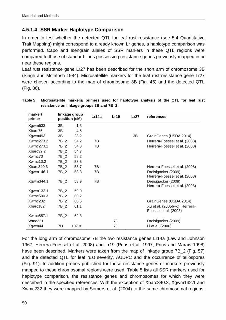
Material and Methods
50
4.5.1.4 SSR Marker Haplotype Comparison
In order to test whether the detected QTL for leaf rust resistance (see 5.4 Quantitative Trait Mapping) might correspond to already known Lr genes, a haplotype comparison was performed. Capo and Isengrain alleles of SSR markers in these QTL regions were compared to those of standard lines possessing resistance genes previously mapped in or near these regions. Leaf rust resistance gene Lr27 has been described for the short arm of chromosome 3B (Singh and McIntosh 1984). Microsatellite markers for the leaf rust resistance gene Lr27 were chosen according to the map of chromosome 3B (Fig. 45) and the detected QTL (Fig. 86). Table 5 Microsatellite markers/ primers used for haplotype analysis of the QTL for leaf rust
resistance on linkage groups 3B and 7B_2
marker/ primer
linkage group position (cM) Lr14a Lr19 Lr27 references
Xgwm533 3B 1.3 Xbarc75 3B 4.5 Xgwm493 3B 23.2 3B GrainGenes (USDA 2014) Xwmc273.2 7B_2 54.2 7B Herrera-Foessel et al. (2008) Xwmc273.1 7B_2 54.3 7B Herrera-Foessel et al. (2008) Xbarc32.2 7B_2 54.7 Xwmc70 7B_2 58.2 Xwmc10.2 7B_2 58.5 Xbarc340.3 7B_2 58.7 7B Herrera-Foessel et al. (2008) Xgwm146.1 7B_2 58.8 7B Dreisigacker (2009),
Herrera-Foessel et al. (2008) Xgwm344.1 7B_2 58.9 7B Dreisigacker (2009)
Herrera-Foessel et al. (2008) Xgwm132.1 7B_2 59.0 Xwmc500.3 7B_2 60.2 Xwmc232 7B_2 60.6 GrainGenes (USDA 2014) Xbarc182 7B_2 61.1 Xu et al. (2005b+c), Herrera-
Foessel et al. (2008) Xwmc557.1 7B_2 62.8 Wmc221 7D Dreisigacker (2009) Xgwm44 7D 107.8 7D Li et al. (2006)
For the long arm of chromosome 7B the two resistance genes Lr14a (Law and Johnson 1967, Herrera-Foessel et al. 2008) and Lr19 (Prins et al. 1997, Prins and Marais 1998) have been described. Markers were taken from the map of linkage group 7B_2 (Fig. 57) and the detected QTL for leaf rust severity, AUDPC and the occurrence of teliospores (Fig. 91). In addition probes published for these resistance genes or markers previously mapped to these chromosomal regions were used. Table 5 lists all SSR markers used for haplotype comparison, the resistance genes and chromosomes for which they were described in the specified references. With the exception of Xbarc340.3, Xgwm132.1 and Xwmc232 they were mapped by Somers et al. (2004) to the same chromosomal regions.

Material and Methods
51
Ten other markers published for the down end of chromosome 7BL by Somers et al. (2004), Herrera-Foessel et al. (2008) or the GrainGenes database (USDA 2014) either produced no fragments, fragments of the same length for Isengrain and Capo or a polymorphic pattern too difficult to be scored for the population and were therefore not considered for haplotype analysis. For allele comparison 25 varieties and standard lines carrying Lr14a, Lr27 (or both) or Lr19 were selected. Parents of all three tested populations and the parents of the cultivar Isengrain were included in haplotype analysis. All lines and the described Lr genes are given in Table 6. If a line carries two or more Lr genes different from Lr13, Lr14a, Lr19 or Lr27, they are not specified (i.a.). The cultivars Cranbrook, Shortim, Timgalen, Gatcher, Karl, Kalkee, Rescue, Warigo, Agatha, Agrus, Hand, Kawfars and Transfer found in the Germplasm Resources Information Network (GRIN) database were kindly provided by National Small Grain Collection, Agricultural Research Service, United States Department of Agriculture (NSGC); Apollo by Volker Lindt, PhD; F4 34/1/1/98, F4 34-9, F4 34-10, F4/8, F4 1/27/2 by Doc. RNDr. Ján Kraic, PhD (Director of Research Institute of Plant Production Piešťany, Slovakia) and Fundulea-29 by Mariana Ittu, PhD (Senior scientist wheat breeding team, National Agricultural Research and Development Institute Fundulea, Romania). The cultivar Transfer was confounded with Transfer-12 which carries Lr19 and included into the analysis although it has only Lr9. Fragments were scored with C (same length as the Capo allele), I (same length as the Isengrain allele), N (neither the length of C or I) or 0 (no visible fragment in the considered size interval).

Material and Methods
52
Table 6 Parental and standard lines with known Lr genes used for allele comparison
line resistance gene parent of references
Cranbrook Lr27 (i.a.) Martynov et al. 2006 Shortim Lr27+ Lr1 Martynov et al. 2006 Timgalen Lr27 (i.a.) McIntosh et al. 1995, Martynov et
al. 2006 Hope Lr14a+ Lr27+ Lr22b McIntosh et al. 1995, Martynov et
al. 2006 Gatcher Lr14a+Lr27 (i.a.) McIntosh et al. 1995, Park et al.
2002, Martynov et al. 2006 Karl Lr14a+Lr27 (i.a.) Martynov et al. 2006 Kalkee Lr14a+Lr27 Martynov et al. 2006 Rescue Lr14a+Lr27 Martynov et al. 2006 Warigo Lr14a+Lr27 Martynov et al. 2006 Courtot Lr14a Martynov et al. 2006 Inia-66 Lr14a, Lr13 (i.a.) McIntosh et al. 1995, Martynov et
al. 2006 Récital Lr14a, Lr13 Park et al. 2001 Forno Lr14a Winzeler et al. 2000, Park et al.
2001 Pathan and Park 2006 Renan Lr14a+Lr37 Winzeler et al. 2000, Błaszczyk et
al. 2004, Pathan and Park 2006 Soissons Lr14a Isengrain Park et al. 2001, Błaszczyk et al.
2004, Rimé et al. 2005 Apollo Lr13+Lr26 Isengrain Park et al. 2001, Singh D et al.
2001, Pathan and Park 2006 Isengrain Lr14a the population Isengrain/Capo Błaszczyk et al. 2004, Rimé et al.
2005 Capo Lr13+ all three tested populations Winzeler et al. 2000, Park et al.
2001, Pathan and Park 2006 Furore the population Furore/Capo Arina Lr13 the population Arina/Capo Winzeler et al. 2000, Park et al.
2001, Pathan and Park 2006 F4 34/1/1/98 Lr19 Kraic (2006) F4 34-9 Lr19 Kraic (2006) F4 34-10 Lr19 Kraic (2006) F4/8 Lr19 Kraic (2006) F4 1/27/2 Lr19 Kraic (2006) Agatha Lr19 Martynov et al. 2006 Agrus Lr19 Martynov et al. 2006 Hand Lr19 Martynov et al. 2006 Kawfars Lr19 Martynov et al. 2006 Transfer Lr9 Martynov et al. 2006 Fundulea-29 Lr19 (i.a.) Martynov et al. 2006

Material and Methods
53
4.6 Statistical Analysis
4.6.1 Reproducibility of Disease Assessment
In the years 2006 and 2007 it was possible that always the same two persons scored the trait leaf rust severity in all experiments in Austria together. Because of more populations and more experiments in 2008, these two persons had to split up populations. Even though using the scoring aid shown in Fig. 8, the standard lines distributed over the three populations at one experimental site were assessed by both raters independently to ensure comparable scores: the first time one part together with the population in which they were planted and in the second run all standards separately. The resulting data should be checked if there were differences between the two scores of one rater and if scores of the two raters fit together. Additionally data of two ratings for the same plants done by two different persons on the same day from one replication of an experiment in 2007 and one experiment in 2009 ought to be analyzed to see how well these repeated scorings fit. Comparison of Reproducibility for the Unequally Fine Graded Classes of the Scoring Aid The scoring aid used for assessing leaf rust severity (% infected leaf area) is finer graded in the area of low leaf rust infection than in the part of higher infection: Between zero and ten percent infected leaf area there are additionally the classes one, three and five percent. Furthermore the classes 20 and 30 percent are shown and 50 and 70 percent. Additionally the classes 40, 60 and above 70 percent in steps of 10 percent were used in assessments. For each repeated assessment the proportion of lines assigned to the same class in the second scoring/ by the second rater was determined to see, whether reproducibility differs with the range of disease severity, e.g. due to the very fine graded classes beyond ten percent, or in the mid range as would be expected if the Weber-Fechner law was valid. Test of the Absolute Differences of Repeated Assessments In the optimal case, all plants get the same score at both times and by both raters. The mean of these absolute differences was tested, null hypothesis H0: µ|d| = 0 against the one-sided alternative hypothesis HA: µ|d| > 0. The required optimal sample size was determined iteratively from
( )
δσ∗+
= β−−α−−2
1;1n1;1n ttn (modified after Rasch et al. 1999, pp. 78-79)
with: n........... sample size (total number of observed plants)
α .......... type I error probability (rejecting a valid null hypothesis)
β........... type II error probability (rejecting a valid alternative hypothesis) tn-1; 1-p .... quantile of the t-distribution

Material and Methods
54
σ2 ......... residual variance
δ........... minimal distance to be detected
This is implemented in CADEMO® Modul LIGHT Version 3.27 (BioMath GmbH
16.11.2006): Fallzahl → Einstichprobenproblem → Mittelwert Test…
Precision requirements were set to α = 0.05 (risk of the first kind: mistaken rejection of a
valid null hypothesis) and β = 0.01 (risk of the second kind: mistaken acceptance of a wrong null hypothesis and rejection of a valid alternative hypothesis). For the particular problem, the error probability for acceptance of H0 should be small, whereas error
probability for rejection of H0 can be larger. s2 = 100 was the estimate for σ2 and a minimal
difference of δ = 7 should be detected. An optimal sample size of n = 35 would be necessary. As sample sizes were consistently larger – the number of plants scored two times resulted out of the necessity to have all standard lines scored by one rater and was not based on considerations about precision requirements – and variances differed due to varying maximum disease severity level, the detectable difference d was estimated for each test. The test statistic was:
nµ
t 0 ∗−
=s
x
with: x ......... mean of the absolute differences µ0 ......... given value of the mean (= zero) s........... sample standard deviation of the absolute differences
The null hypothesis H0: µ|d| = 0 was accepted if |t| ≤ tn-1;1-α, otherwise it was rejected (modified after Rasch et al. 1999, p. 77). This test is implemented in R©:
t.test(variable, mu=0, alternative=“greater”, conf.level=0.95)
To account for narrower class width at low disease severity levels, additionally to leaf rust severity measured by the percentage of infected leaf area the absolute class differences were calculated. Model II Regression Analysis Regression analysis was used to test whether there was systematic and/or constant bias
in the reproducibility of assessments. In the case of no bias the intercept β0 would be zero
and the slope β1 one in the linear regression model yi = β0 + β1x i. These two hypotheses were tested as follows (modified after Rasch et al. 1999, pp. 156-157, 143):
Test of the intercept: H0: β0 = 0 against the two-sided alternative HA: β0 ≠ 0
The test statistic was 0
tβ = (β0 - 00β ) /
0βs and H0 was rejected if |
0tβ | > tn-2; 1-α/2 with:
00β ....... given value of β0 (= zero)
n........... sample size (total number of observed plants)
α .......... type I error probability (rejecting a valid null hypothesis)

Material and Methods
55
tn-2; 1-α/2 .. quantile of the t-distribution
0βs ........ standard deviation of β0, calculated as:
∑
∑∑
=
==
−−
−=
n
1i
2i
n
1i
2i
n
1i
2ii
2β
)x(xn*
x*
2n
)y(ys
0
with:
iy ......... score of the ith plant in the second assessment/ by the second person
iy ......... estimated value of the y variable according to the regression model
ix ........ score of the ith plant in the first assessment/ by the first person
x ......... mean value of the x variable
This test is implemented in R©: model <- lm(assessment2 ~ assessment1) summary(model)
Test of the slope: H0: β1 = 1 against the two-sided alternative HA: β1 ≠ 1
The test statistic was 1
tβ = (β1 – 01β ) /
1βs and H0 was rejected if |
1tβ | > tn-2; 1-α/2 with
01β ....... given value of β1 (= one)
n........... sample size
α .......... type I error probability (rejecting a valid null hypothesis)
1βs ........ standard deviation of β1, calculated as:
∑
∑
=
=
−−
−=
n
1i
2i
n
1i
2ii
2β
)x(x
1*
2n
)y(ys
1
The optimal sample size was determined iteratively from:
( )
∗δ∗+
= −−−−2
*
β1;2n2α/1;2n
s
σttn (modified after Rasch et al. 1998, p. 285)
with: β........... type II error probability (rejecting a valid alternative hypothesis)
σ .......... residual standard deviation
δ........... minimal distance to be detected s* .......... (xmax – xmin) / 2
This is implemented in CADEMO® Modul REA Version 3.27 (BioMath GmbH 16.11.2006):
Test → Vergleich des Anstiegs mit einer Konstanten As the error probability for acceptance of H0 should be small, whereas error probability for
rejection of H0 can be larger, the risk of the first kind α was set to 0.2 and type II error
probability β to 0.01. With σ = 10, δ = 0.2 and s* = 30 the resulting optimal sample size would be n = 39. This was beyond the sample size of all but one of the compared assessments.

Material and Methods
56
The coefficient of determination (r2) is a measure for the variation of the results of the second assessment that are explained by the first ones. It is included in the output of the R© code given above. The underlying formula is given by Rasch et al. 1999 (pp. 171-172). Test of Correlation Coefficients Pearson’s product moment correlation coefficient is a measure of the linear relationship. Spearman’s rho is a rank correlation coefficient and thus a measure of the strength of the monotone relationship of two repeated assessments. The tested null hypothesis was
H0: 0 < |ρ| ≤ 0.8. Type I error probability was α = 0.05. In 4.6.2.1 Trait Correlations the details about estimating and testing the correlation coefficient are given. As sample size was lower than required, in case of acceptance of H0 precision requirements are not met.
4.6.2 Field Data
Because of the different scoring methods, the traits used for further statistical analysis can be divided into the following classes based on their type of scale:
• ordinal scale: − appearance of teliospores (no, yes)
− awnedness (no, partly, yes)seedling resistance (0-4)
− heading (1-9)
− crop density (1-5)
− leaf blotch severity (1-9)
− Septoria leaf blotch severity (1-9)
− powdery mildew severity (1-9)
− yellow rust severity (1-9)
− glaucousness (1-5)
− frost heaving severity (1-9)
− lodging severity (0-5, 1-5, 1-9)
− leaf chlorosis severity (0-9)
− leaf tip necrosis severity (0-9)
• ratio/ interval scale: − leaf rust severity (% infected leaf area, AUDPC)
− heading (day of the year)
− plant height (cm)
Means over the two replications of an experiment were calculated for all traits except appearance of teliospores. If the scoring scheme was the same for different experiments, the mean over experiments was calculated too, but only for lines assessable in all experiments. Thus sample size of mean values can be below those of single experiments. The trait awnedness was treated similarly: If scores were different for different replications or experiments, the level “partly” was applied as it can be explained by genetic segregation in the population. In the histograms always the means are shown. They are the basis for most of the further statistical analysis.

Material and Methods
57
Not all scorings were usable for all further descriptive statistics and statistical tests due to large numbers of missing lines, or scoring schemes that were not comparable. R© version 2.8.0 (R© Development Core Team 2008) was used for drawing diagrams, and for calculating correlation coefficients. For the fast generation of histograms of the main traits (leaf rust severity, heading and plant height) of all experiments, an R© function was developed (see Appendix B: R© Functions and SAS® Codes). Contingency tables (chi-squared tests of independence) were analyzed with SPSS© 15.0.1 für Windows Version 15.0.1 (SPSS Inc., 1989-2006). The software package SAS® for Windows version 9.2 TS Level 1M0 was used for calculating analysis of variance (ANOVA) tables and estimating variance components. The procedure therefore was GLM (general linear model) with type III sum of squares. Due to different experimental locations in different years, the factor “experiment” was introduced for year–location combinations.
4.6.2.1 Trait Correlations
For estimating and testing trait correlations between proportionally scaled traits, Pearson’s product moment correlation coefficient was calculated and tested as a measure of the
linear relationship. In SAS®, SPSS© and R© only the test of the null hypothesis H0: ρ = 0
against the two-sided alternative hypothesis HA: ρ ≠ 0 is implemented. As the information whether a correlation coefficient is significantly different from zero or not is of few practical
relevance (Kubinger et al. 2007), the composite null hypothesis H0: 0 < |ρ| ≤ |ρ0| was
tested against the one sided alternative hypothesis HA: |ρ| > |ρ0|. The square root of the
coefficient of determination ρ2 explaining a relevant amount of variance for the particular
question was chosen as the value of ρ0. The correlation coefficients calculated with R© cor.test(assessment1, assessment2, method = c(“pearson”))
were tested according to Rasch et al. (1998, p. 326). For testing the null hypothesis
H0: ρ = ρ0 (ρ0 ≠ 0), r had to be transformed as follows:
rr
z−+=
11
ln21
The testing value ρ0 had to be transformed in the same way, therefore it would not be
possible to test H0: ρ = 1:
0
00 1
1ln
21
zρ−ρ+=
The test statistic was
3n)z(u 0 −−= z .
The null hypothesis was rejected if u > u1-α with: r ........... estimated correlation coefficient
ρ0 ......... testing value n........... sample size
u1-α ....... quantile of the normal distribution
α .......... type I error probability (rejecting a valid null hypothesis)

Material and Methods
58
The optimal sample size was determined from
[ ] 3)zz/()uu(n 20111 +−+= β−α− (modified after Rasch et al. 1998, p. 325)
with: z1.......... transformation as above with ρ1 = ρ0 + δ
δ........... minimal distance to be detected
β........... type II error probability (rejecting a valid alternative hypothesis)
This is implemented in CADEMO® Modul LIGHT Version 3.27 (BioMath GmbH
16.11.2006): Fallzahl → Einstichprobenproblem → Korrelationskoeffizient Test… Additionally Spearman’s rho was calculated and tested. It is a measure of the strength of the monotone dependence of the traits. It corresponds to Pearson’s product moment correlation coefficient calculated with the ranks (Rasch et al. 1996, pp. 598-600). This correlation coefficient can be used for ordinally scaled traits too. Spearman’s rho can be tested in the same way as Pearson’s product moment coefficient if the sample size
exceeds n ≥ 30 (Kubinger 1990). Spearman’s rho was calculated using R©:
cor.test(trait1, trait2, alternative = c(“two.sided”), method = c(“spearman”))
The interdependency between appearance of teliospores, awnedness and other traits was analyzed with contingency tables (chi-squared tests of independence). The null hypothesis is that both traits are independent. H0: The probability of a certain trait combination is the product of the single trait occurrences. The alternative hypothesis is that this is not valid
HA: pij ≠ pi. p.j for at least one pair (i, j). The underlying formulas and test statistics are given in Rasch et al. (1998, pp. 199-200). R© code for chi-squared test of independence:
chisq.test(traitcombination) chisq.test(traitcombination)$expected
gives the expected observation for every combination. It should be beyond 5 as the chi-squared distribution is only valid asymptotically. In addition Cramér’s V was calculated as a measure of dependence according to the formula
)1b;1amin(nV
2
−−∗Χ= (Rasch et al. 1998, pp. 193-194) with:
Χ2......... chi-squared test statistics (calculated with R©) n........... sample size a........... number of rows (number of levels of trait A) b........... number of columns (number of levels of trait B)

Material and Methods
59
Correlation of Traits Assessed in the Same Experiment In the case of proportionally scaled traits, Pearson’s product moment correlation coefficient and Spearman’s rho were estimated and tested, in the case of ordinally scaled traits only the latter. As correlations with a coefficient of determination r2 less 0.35 – meaning that less than 35 % of the variability of the y-variable can be explained by the x-variable – are of no
practical relevance, the tested null hypothesis was H0: 0 < |ρ| ≤ 0.59. Type I error
probability was α = 0.05. Due to population sizes of n = 201 for Furore/Capo and larger for
Isengrain/Capo and Arina/Capo, the other precision requirements could be set to β = 0.1
(type II error probability) and δ = 0.12 (minimal effect of relevance) requiring an optimal sample size of n = 199. To test correlations of the ordinally scaled traits appearance of teliospores of P. triticina or awnedness with the other traits by means of contingency tables, the proportionally scaled traits were categorized as follows: The classes of leaf rust severity measured by the percentage of infected leaf area were 0-10, > 10-20, > 20-30 and > 30-50. As no telio-spores can be produced if there is no infection with leaf rust (no visible urediniospores), all plants without symptoms were in this case excluded from analysis. Data of the trait heading were categorized to groups spanning two days, plant height to groups of ten centimeters. In some cases classes at the end of the range had to be merged in order to meet the assumption that the frequencies expected under validity of the null hypothesis are not less than two and for at least 50 % of the cells not less than five. Due to the small differences between the RILs of the population Furore/Capo, data of the trait heading were categorized to groups spanning only one day, plant height to groups of five centimeters. These tests were performed for all traits within one experiment and also for the means over experiments. Correlation Between Experiments To obtain estimates of the reproducibility of the assessments, Spearman’s rho between the same trait assessed in different experiments was estimated and tested. In this case
the tested null hypothesis was H0: 0 < |ρ| ≤ 0.71. The precision requirements for these
tests were set to α = 0.05 (type I error probability), β = 0.05 (type II error probability) and
δ = 0.1 (minimal effect of relevance), requiring an optimal sample size of n = 192.
4.6.2.2 Estimating the Coefficient of Broad Sense Heritability
As a further measure of the reproducibility of evaluations the coefficient of broad sense heritability was estimated according to Hallauer and Miranda (1981 cited in Klahr et al. 2007), Nyquist (1991) and Becker (2011). The notation is following Rasch et al. (1999). The heritability h2 is defined as the proportion of genotypic (g) variance of the total phenotypic (p) variance:

Material and Methods
60
2p
2g2
σ
σh =
The variance of the phenotype comprises the variance of the genotype and the environment (experiment) and the error variance:
er
σ
e
σσσ
22ge2
g2p ++=
These variance components were calculated from the ANOVA table after Nyquist (1991):
source of variation df MS expected mean square
experiments (E) e-1 MSE
replications (R) within E e(r-1) MSR
genotypes (G) g-1 MSG 2g
2ge
2 erσrσσ ++
interaction G x E (g-1)(e-1) MSGE 2ge
2 rσσ +
experimental error (ε) e(r-1)(g-1) MSε 2σ
total (T) erg-1 MST
e.......... number of experiments
r........... number of replications
g .......... number of genotypes 2gσ ........ variance of genotypic values of genotypes in the population (total genotypic var.) 2geσ ....... variance of interaction effects between genotypes and experiments 2σ ........ variance of total effect(s) of experimental unit(s) within a replication
As Nyquist (1991) demonstrated for the case of several experiments with a randomized complete block design and the same number of replications that the exact formular for estimating the coefficient of heritability
2p
2g2
s
sh =
can be simplified:
G
GE2
MSMS
1h −=
because
erMSMS
s GEG2g
−=
erMS
erMS
erMSMS
erMSMS
er
s
e
sss GGEGEG
22ge2
g2p =+−+−=++= εε .
ANOVA tables were calculated with SAS®. The main effects of the levels of E, R and G and the interaction G x E were considered random:
proc GLM data=… outsat=…; class R G E; model trait = R(E) G E G*E / SS3; random R(E) G E G*E / test; run;
As the number of replications was varying between experiments or data were otherwise missing, the presumptions were not met and the coefficient r (averaged number of

Material and Methods
61
replications) was different for each variance component. Therefore estimates of the coefficient of heritability were calculated exactly on the basis of variance components and in addition after the simplified formula despite missing data to compare differences in the results. As the effects of the main factors and the interaction were considered random, the F-values are calculated by dividing the mean squares (MS) of the factor (or the interaction) by the MS of the particular error. Another question was whether information about the leaf rust infection of the spreader rows next to each plot can help improving data and results. Therefore ANOVA were calculated for the two populations Isengrain/Capo and Arina/Capo for the four experiments in Probstdorf, Rust, Schmida and Tulln in 2008. In a second step the mean value of the spreader rows next to each plot was included in an analysis of covariance. Coefficients of heritability were estimated for each population with the exact and the simplified method. For covariance analysis in SAS® the covariate simply has to be added to the code line for the model:
model LR = R(E) G E G*E mSpreader / SS3;
4.6.2.3 Least Significant Difference (LSD)
If the difference between the mean values of lines is lower than the LSD, they are said to
be equal. The type I error probability α was set to 0.05. The values of LSD5% were estimated according to the formula
975.0,df%5 trMS2
LSDε
∗∗= ε
with MSε ...... mean square error r ........... number of replications (two) tdf,γ ........ quantile of the t-distribution (α = 0.05, γ = 0.975)
dfε......... degrees of freedom for the error
In SAS® the model was specified as model trait = R G / SS3;

Material and Methods
62
4.6.3 Marker Data
For constructing linkage maps JoinMap® 4 (van Ooijen 2006) with evaluation license was used. Default values of all parameters were not changed with the exception of using Haldane’s mapping function instead of Kosambi’s. The resulting linkage groups were checked with MAPMAKER/EXP© 3.0b (Lincoln et al. 1993a). With JoinMap® 4 genotype frequencies for all loci were tested whether segregation is different from the Mendelian ratio, considering the particular classification (dominant for the Capo allele, codominant or dominant for the allele of the other parent). The underlying test is a chi-squared test of independence. To preclude wrong marker data, particularly AFLP markers often were not scored for the following reasons:
- very weak - badly separated from other fragments - pattern just “weak” – “strong” - seemingly varying fragment sizes due to different neighboring bands for the different
parts of the population - not polymorphic between the parental lines and segregation vastly diverging from
the Mendelian ratio In some cases marker data were only available for a part of the population due to scoring difficulties. If these markers were mapped to different linkage groups, whether JoinMap® 4 or MAPMAKER/EXP© 3.0b was used, they were retrospectively excluded from linkage analysis. Maps were drawn using MapChart© 2.1 (Voorrips 2002). To assign linkage maps to certain chromosomes or chromosomal arms, they were compared to microsatellite maps of wheat published by Röder et al. (1998), Pestsova et al. (2000), Gupta et al. (2002), and the genetic markers information and the following maps available from the GrainGenes database (USDA 2014):
- Wheat, Consensus SSR, 2004 (Somers et al. 2004) - Wheat, Composite, 2004 - T. boeoticum x monococcum [modern grouping: T. monococcum ssp. aegilopoides x
T. monococcum ssp. monococcum] (Singh et al. 2007) - Wheat, Arina x Forno (Paillard et al. 2003) - Wheat, Chinese Spring x SQ1 (Quarrie et al. 2005) - Wheat, Physical, SSR (Sourdille et al. 2004) - Wheat, Synthetic x Opata, BARC (Song et al. 2005) - T. turgidum [modern grouping: T. turgidum ssp. turgidum], Langdon x G18-16 (Peleg
et al. 2008) - T. turgidum [modern grouping: T. turgidum ssp. turgidum], Messapia x dicoccoides,
SSR (Korzun et al. 1999)

Material and Methods
63
4.6.4 QTL Analysis
4.6.4.1 Interval Mapping
For the populations Isengrain/Capo and Arina/Capo LOD values (logarithm of odds) were calculated with QTL Cartographer© Version 2.5 (Basten et al. 1994, Brown 2005, Wang et al. 2007) using “Interval Mapping” and 1.0 cM as “Walk speed”. The threshold for each trait was estimated by permutations (1000 permutation times, significance level 0.05). All QTL with a likelihood ratio value ≥ the threshold were said to be significant
(LOD = 0.217 ∗ likelihood ratio, Basten et al. 2005). In order to detect solely additive effects as only homozygous lines are valuable in plant breeding, all heterozygous marker data were treated as “missing values” in QTL analysis. Results were checked with PLABQTL© Version 1.2 (Utz and Melchinger 1996, 2006). QTL analysis was done for the following traits:
- leaf rust severity: population Isengrain/Capo and Arina/Capo - relative AUDPC (leaf rust severity): population Isengrain/Capo and Arina/Capo - appearance of teliospores: population Isengrain/Capo - seedling resistance: population Arina/Capo - heading: population Isengrain/Capo and Arina/Capo - plant height: population Isengrain/Capo and Arina/Capo - awnedness: population Arina/Capo - crop density: population Isengrain/Capo - leaf blotch severity: population Isengrain/Capo - Septoria leaf blotch severity: population Arina/Capo - powdery mildew severity: population Isengrain/Capo and Arina/Capo - yellow rust severity: population Arina/Capo - glaucousness: population Arina/Capo - frost heaving severity: population Isengrain/Capo - lodging severity: population Isengrain/Capo and Arina/Capo - leaf chlorosis severity: population Isengrain/Capo and Arina/Capo - leaf tip necrosis severity: population Isengrain/Capo and Arina/Capo
4.6.4.2 Single Point ANOVA
Analysis of variance (ANOVA) for all single markers (not only those in linkage groups) was done for all traits assessed in the population Arina/Capo. As markers with significant LOD values detected by interval mapping (see 4.6.4.1 Interval Mapping) had a p-value less
than 0.01 in the single point ANOVA, this value was used for the type I error probability α. ANOVA was calculated with the SAS® procedure GLM. The program for the trait mheading (heading, mean over experiments) is given as an example in Appendix B: R© Functions and SAS® Codes.

Material and Methods
64
4.6.4.3 Additive Effects
Additive effects were calculated as half of the difference of the mean values of the homozygous lines for the corresponding marker:
2mm
effectadditive IC −=
with mc ........ mean over all lines with the same allele as the parental line Capo mI ......... mean over all lines with the same allele as the parental line Isengrain
4.6.4.4 Epistatic Interactions
If resistance genes are combined in cultivars, they can either act additively or epistatic interactions can occur. In quantitative genetics epistasis is defined as the interaction of genes with the exception of additive interaction. Epistatic interactions can produce a particularly favorable or unfavorable effect, e.g. with regard to disease resistance (Kolmer 1992a, Becker 2011). For calculation of epistatic interactions with the SAS® program written by Holland and Ingle (2001) a framework map of the population Isengrain/Capo with not more than one locus every 2 to 3 cM was used. As the number of heterozygous plants in a F6 population is almost negligible, this group is prone to be the outlier. Therefore – if it was possible because of more than one locus within 2 to 3 cM – codominant loci and also those markers that were scorable on just a small part of the population were removed. To avoid type I error (mistaken detection of epistatic interactions), the risk of the first kind was set to α = 0.0001. Mean over three, six and eleven experiments (see Table 26), all single assessments of leaf rust severity measured by the percentage of infected leaf area, leaf rust severity measured by AUDPC (single experiments and the mean over them) and the appearance of teliospores were used as traits. To ensure finding all epistatic interactions between Capo and Isengrain QTL calculation was repeated with the original map for the relevant linkage groups assigned to the chromosomes 3B, 7B and all possibly assigned to 2B, where Lr13 described for Capo is located. A further ANOVA (SAS® procedure GLM) was calculated without and with the marker1*marker2 interaction term. Data of the eleven leaf rust assessments (see Table 26), the mean over these eleven as well as over three and six experiments and AUDPC in the experiments Piešťany 2006 and Tulln 2008 and the mean over these two were used as traits. The risk of the first kind was set to α = 0.05. In the case of significant interactions the improvement of the model measured by R2 was determined.

Results
65
5 Results
5.1 Field Experiments
5.1.1 Leaf Rust Assessment
First the results of the reproducibility of disease assessment are presented as reproducibi-lity is a prerequisite for reliable data analyses.
5.1.1.1 Inter-rater and Intra-rater Reproducibility
For assessing leaf rust severity measured by the percentage of infected leaf area, all raters were using the scoring aid given in Fig. 8. In addition to the classes shown, all raters used the scores 40, 60 and 80 %. In a few cases two raters used scores even finer than these classes. For evaluating reproducibility based on the classes, these values were randomly assigned to one of the neighboring classes. On the other hand, one rater did not use the score three percent. Comparison of Reproducibility for the Unequally Fine Graded Classes of the Scoring Aid In Table 7 to Table 17 the results of the comparisons of leaf rust severity scoring (% infected leaf area) repeated by one rater or by different raters are given. The number of lines assigned to the same or a deviating class are shown. Additionally the percentage of identically scored plants was calculated for each class separately, for all classes i.e. for all lines, for all but the zero percent class, for all classes lower than ten percent without and with the class zero percent, and the classes ten percent and beyond. In the repeated ratings of standard lines in 2008 by rater one 56-58 % of lines got the same score. Reproducibility was almost 10 % lower for rater two. The amount of the same scores given by rater one and two was smallest on the third day of assessment (30 %) and highest (68 %) on the second day. On this day 52 lines were scored in the morning by the two raters together to compare and adjust rating again after one day (about 500 to 1000 plots) of separate assessment. On the third day of scoring the overall reproducibility of the scores of rater one by rater two was only 30 %, whereas for the classes < 10 % it was over 60 % that is higher than on the first two days. If scores for the class with zero infection were not taken into account, intra-rater and inter-rater reproducibility differed much: values ranged from 23 to 66 % and were with no exception lower compared to the results including the zero scores. The difference of overall reproducibility was slightest for the repeated scoring by person two. In five out of the nine comparisons of assessments in 2008, all lines with no detected infection in the first scoring got the same score in the second rating. The lowest level of identically scored plants in the class zero infection were 2 out of 3 lines scored by rater one again in the second rating and 9 out of 13 scored by rater one compared to the assessment of rater one and two together (both on the second day of assessment). On the first and second day reproducibility for the range below 10 % (not taking the zero class into account) was well (more than 20 %) below the reproducibility for the classes 10 % and more. Only on the third day of assessment, the difference was below 10 %; for rater two it was even reverse.

Results
66
For single classes there was neither a clear trend towards higher or lower scores in the second assessment or by a specific rater, nor was there a range that was assessed with a definitely higher or lower reproducibility. In most of the compared assessments well beyond 90 % of the lines were assessed to the same or a neighboring class in the second rating. Only on the third day assessments repeated by rater two showed larger deviations. Scores differing by three classes occurred rarely with the exception of these two repeated assessments. The detailed results are given in Table 21. As counts for each disease level were rather low, overall sums for the experiments in 2008 were calculated and are given in Table 18 to Table 20. The amount of identically scored plots by rater one was higher than for rater two. In the assessment of rater one repeated by rater two, the percentage of identical scored plants was well below 50 %. In the leaf rust assessment by rater two and three together in 2007 and repeated by rater three alone, values of percentage of identically scored lines were 48 % for the range below ten percent infected leaf area, and 34 % for the range ten percent and higher. The values of these ranges were 36 % and 33 % in the comparison of rater three and four in 2009. This is in contrast to the compared assessments by rater one and two in 2008. Table 22 lists the differences in classes (percentage of all scores) for the comparisons rater one first scoring vs. rater one second scoring, rater one vs. rater two, rater two first scoring vs. rater two second scoring (mean over all disease assessments in 2008), rater two and three together vs. rater three alone and rater three vs. rater four. Table 23 gives the percentage of identically rated plots for these comparisons. Table 7 Results of the repeated scoring on the first day of leaf rust assessment in 2008 by rater one
lr class 1 st scoring deviation in lr classes 2 nd scoring %
(% infected leaf area) -3 -2 -1 0 +1 +2 +3 total identical
0 11 3 14 79 1 4 1 8 1 14 7 3 1 8 2 11 73 5 1 1 2 50
10 4 3 1 8 38 20 1 8 7 16 50 30 1 1 18 4 24 75 40 1 1 100 50 60 70 80 90
100
total 0 ≤ x ≤ 100 % 1 2 10 51 25 1 90 57 classes 0 < x ≤ 100 % 1 2 10 40 22 76 53 classes 0 < x < 10 % 1 5 10 10 1 27 37 classes x < 10 % 1 5 21 13 1 41 51 classes x ≥ 10 % 1 5 30 12 49 61

Results
67
Table 8 Results of the repeated scoring on the first day of leaf rust assessment in 2008 by rater one and two
lr class rater 1 deviation in lr classes rater 2 %
(% infected leaf area) -3 -2 -1 0 +1 +2 +3 total identical
0 14 1 15 93 1 3 2 1 6 33 3 7 5 4 1 17 29 5 2 2 2 2 8 25
10 1 1 2 4 25 20 1 5 4 10 50 30 5 13 6 1 25 52 40 1 1 3 5 60 50 60 70 80 90
100
total 0 ≤ x ≤ 100 % 1 20 45 20 4 90 50 classes 0 < x ≤ 100 % 1 20 34 19 4 75 45 classes 0 < x < 10 % 12 9 7 3 31 29 classes x < 10 % 12 23 8 3 46 50 classes x ≥ 10 % 1 8 22 12 1 44 50
Table 9 Results of the repeated scoring on the second day of leaf rust assessment in 2008 by
rater one
lr class 1 st scoring deviation in lr classes 2 nd scoring %
(% infected leaf area) -3 -2 -1 0 +1 +2 +3 total identical
0 2 1 3 67 1 3 1 1 0 5 1 1 2 50
10 3 3 100 20 2 1 3 33 30 2 2 1 1 6 17 40 3 3 6 50 50 1 9 2 12 75 60 2 2 100 70 80 90
100
total 0 ≤ x ≤ 100 % 3 5 22 8 38 58 classes 0 < x ≤ 100 % 3 5 20 7 35 57 classes 0 < x < 10 % 1 1 1 3 33 classes x < 10 % 1 3 2 6 50 classes x ≥ 10 % 2 5 19 6 32 59

Results
68
Table 10 Results of the repeated scoring on the second day of leaf rust assessment in 2008 by rater one and two
lr class rater 1 deviation in lr classes rater 2 %
(% infected leaf area) -3 -2 -1 0 +1 +2 +3 total identical
0 4 4 100 1 3 1 4 75 3 1 1 0 5 1 3 4 8 38
10 5 5 10 50 20 2 3 1 6 50 30 10 1 11 91 40 3 4 1 8 50 50 22 6 28 79 60 3 1 4 75 70 80 90
100
total 0 ≤ x ≤ 100 % 6 57 20 1 84 68 classes 0 < x ≤ 100 % 6 53 20 1 80 66 classes 0 < x < 10 % 1 6 5 1 13 46 classes x < 10 % 1 10 5 1 17 59 classes x ≥ 10 % 5 47 15 67 70
Table 11 Results of the repeated scoring on the second day of leaf rust assessment in 2008 by
rater two
lr class 1 st scoring deviation in lr classes 2 nd scoring %
(% infected leaf area) -3 -2 -1 0 +1 +2 +3 total identical
0 1 1 100 1 1 1 2 50 3 1 1 0 5 1 1 2 4 25
10 1 1 3 1 6 50 20 1 1 2 4 0 30 1 7 1 9 78 40 1 2 6 9 22 50 8 8 100 60 2 2 0 70 80 90
100
total 0 ≤ x ≤ 100 % 3 7 23 13 46 50 classes 0 < x ≤ 100 % 3 7 22 13 45 49 classes 0 < x < 10 % 1 1 2 3 7 29 classes x < 10 % 1 1 3 3 8 38 classes x ≥ 10 % 2 6 20 10 38 53

Results
69
Table 12 Results of the repeated scoring on the second day of leaf rust assessment in 2008 by rater one and two together and rater one alone
lr class rater 1+2 deviation in lr classes rater 1 %
(% infected leaf area) -3 -2 -1 0 +1 +2 +3 total identical
0 9 4 13 69 1 1 1 0 3 1 1 0 5 1 1 0
10 1 1 1 1 4 25 20 2 2 2 6 33 30 6 1 7 86 40 2 1 3 33 50 7 2 9 78 60 5 2 7 29 70 80 90
100
total 0 ≤ x ≤ 100 % 11 28 11 2 52 54 classes 0 < x ≤ 100 % 11 19 7 2 39 49 classes 0 < x < 10 % 1 0 1 1 3 0 classes x < 10 % 1 9 5 1 16 56 classes x ≥ 10 % 10 19 6 1 36 53
Table 13 Results of the repeated scoring on the third day of leaf rust assessment in 2008 by
rater one
lr class 1 st scoring deviation in lr classes 2 nd scoring %
(% infected leaf area) -3 -2 -1 0 +1 +2 +3 total identical
0 8 8 100 1 4 4 8 50 3 5 1 1 0
10 1 1 0 20 1 3 3 7 43 30 2 1 1 4 25 40 1 9 7 1 18 39 50 1 2 8 3 14 57 60 4 15 4 23 65 70 2 4 6 67 80 90
100
total 0 ≤ x ≤ 100 % 3 25 50 12 90 56 classes 0 < x ≤ 100 % 3 25 42 12 82 51 classes 0 < x < 10 % 1 4 4 9 44 classes x < 10 % 1 4 12 17 71 classes x ≥ 10 % 2 21 38 12 73 52

Results
70
Table 14 Results of the repeated scoring on the third day of leaf rust assessment in 2008 by rater one and two
lr class rater 1 deviation in lr classes rater 2 %
(% infected leaf area) -3 -2 -1 0 +1 +2 +3 total identical
0 12 12 100 1 5 2 7 29 3 1 1 2 0 5 1 1 2 0
10 1 1 2 50 20 2 2 1 2 7 29 30 1 6 9 5 1 22 41 40 3 7 12 22 32 50 5 8 7 5 25 20 60 2 9 16 27 7 70 1 7 8 13 80 90
100
total 0 ≤ x ≤ 100 % 3 17 41 43 26 6 136 30 classes 0 < x ≤ 100 % 3 17 29 43 26 6 124 23 classes 0 < x < 10 % 2 6 2 1 11 18 classes x < 10 % 2 6 14 1 23 61 classes x ≥ 10 % 1 11 27 42 26 6 113 24
Table 15 Results of the repeated scoring on the third day of leaf rust assessment in 2008 by
rater two
lr class 1 st scoring deviation in lr classes 2 nd scoring %
(% infected leaf area) -3 -2 -1 0 +1 +2 +3 total identical
0 1 1 100 1 2 2 100 3 5 1 1 2 0
10 20 1 2 1 4 25 30 3 2 5 40 40 1 5 1 7 71 50 1 1 2 4 2 10 40 60 3 3 2 8 38 70 4 2 6 67 80 1 1 0 90
100
total 0 ≤ x ≤ 100 % 2 2 9 22 9 2 46 48 classes 0 < x ≤ 100 % 2 2 9 21 9 2 45 47 classes 0 < x < 10 % 1 2 1 4 50 classes x < 10 % 1 3 1 5 60 classes x ≥ 10 % 1 2 9 19 8 2 41 46

Results
71
Table 16 Results of the repeated leaf rust assessment in 2007 by rater two and three together and rater three alone
lr class rater 2+3 deviation in lr classes rater 3 %
(% infected leaf area) -3 -2 -1 0 +1 +2 +3 total identical
0 2 2 100 1 8 18 10 36 22 3 5 20 9 34 59 5 1 28 40 5 74 54
10 3 28 19 4 54 35 20 1 14 12 10 37 32 30 8 4 3 1 16 25 40 4 2 4 10 20 50 1 6 1 8 75 60 2 1 1 4 25 70 1 1 0 80 1 1 0 90
100
total 0 ≤ x ≤ 100 % 8 90 114 54 11 277 41 classes 0 < x ≤ 100 % 8 90 112 54 11 275 41 classes 0 < x < 10 % 1 33 68 32 10 144 47 classes x < 10 % 1 33 70 32 10 146 48 classes x ≥ 10 % 7 57 44 22 1 131 34
Table 17 Results of the repeated leaf rust assessment in 2009 by rater three and four
lr class rater 3 deviation in lr classes rater 4 %
(% infected leaf area) -4 -3 -2 -1 0 +1 +2 +3 +4 +5 total identical
0 2 2 100 1 9 8 5 1 23 39 3 5 30 26 49 29 7 1 1 143 34
10 1 5 2 27 39 32 8 3 117 33 20 3 11 37 30 7 88 42 30 1 2 8 24 18 20 1 7 81 30 40 3 8 14 1 6 2 34 24 50 1 2 1 4 8 25 60 1 1 0 70 80 90
100
total 0 ≤ x ≤ 100 % 1 6 38 75 170 131 50 15 10 1 497 34 classes 0 < x ≤ 100 % 1 6 38 75 168 131 50 15 10 1 495 34 classes 0 < x < 10 % 30 26 58 37 12 1 1 1 166 35 classes x < 10 % 30 26 60 37 12 1 1 1 168 36 classes x ≥ 10 % 1 6 8 49 110 94 38 14 9 9 33

Results
72
Table 18 Overall results of the repeated scoring of leaf rust assessment in 2008 by rater one
lr class 1 st scoring deviation in lr classes 2 nd scoring %
(% infected leaf area) -3 -2 -1 0 +1 +2 +3 total identical
0 21 4 25 84 1 8 5 8 1 22 23 3 1 8 3 12 67 5 3 2 5 40
10 5 6 1 12 50 20 1 3 12 10 26 46 30 3 5 20 6 34 59 40 1 9 11 4 25 44 50 1 3 17 5 26 65 60 4 17 4 25 68 70 2 4 6 67 80 90
100
total 0 ≤ x ≤ 100 % 1 8 40 123 45 1 218 56 classes 0 < x ≤ 100 % 1 8 40 102 41 1 193 53 classes 0 < x < 10 % 3 9 15 11 1 39 38 classes x < 10 % 3 9 36 15 1 64 56 classes x ≥ 10 % 1 5 31 87 30 154 56
Table 19 Overall results of the repeated scoring of leaf rust assessment in 2008 by rater one and
two
lr class rater 1 deviation in lr classes rater 2 %
(% infected leaf area) -3 -2 -1 0 +1 +2 +3 total identical
0 30 1 31 97 1 8 7 1 1 17 41 3 1 7 5 6 1 20 25 5 1 4 5 6 2 18 28
10 1 7 7 1 16 44 20 5 10 6 2 23 43 30 1 11 32 12 2 58 55 40 1 7 14 13 35 40 50 27 14 7 5 53 51 60 5 10 16 31 16 70 1 7 8 13 80 90
100
total 0 ≤ x ≤ 100 % 4 43 143 83 30 7 310 46 classes 0 < x ≤ 100 % 4 43 113 82 30 7 279 41 classes 0 < x < 10 % 2 19 17 13 3 1 55 31 classes x < 10 % 2 19 47 14 3 1 86 55 classes x ≥ 10 % 2 24 96 69 27 6 224 43

Results
73
Table 20 Overall results of the repeated scoring of leaf rust assessment in 2008 by rater two
lr class 1 st scoring deviation in lr classes 2 nd scoring %
(% infected leaf area) -3 -2 -1 0 +1 +2 +3 total identical
0 2 2 100 1 1 3 4 75 3 1 1 0 5 1 1 1 3 6 17
10 1 1 3 1 6 50 20 2 3 1 2 8 13 30 4 9 1 14 64 40 2 7 7 16 44 50 1 1 2 12 2 18 67 60 2 3 3 2 10 30 70 4 2 6 67 80 1 1 0 90
100
total 0 ≤ x ≤ 100 % 2 5 16 45 22 2 92 49 classes 0 < x ≤ 100 % 2 5 16 43 22 2 90 48 classes 0 < x < 10 % 1 1 1 4 4 11 36 classes x < 10 % 1 1 1 6 4 13 46 classes x ≥ 10 % 1 4 15 39 18 2 79 49
Table 21 Differences in classes between compared assessments in 2008 (number of scored lines)
day 1 2 3 1 2 3 2 3 over all over all over all comparison 1-1 1-1 1-1 1-2 1-2 1-2 2-2 2-2 1-1 1-2 2-2
-3 1 2 1 2 -2 2 3 3 1 3 3 2 8 4 5 -1 10 5 25 20 6 17 7 9 40 43 16 0 51 22 50 45 57 41 23 22 123 143 45
+1 25 8 12 20 20 43 13 9 45 83 22 +2 1 4 26 2 1 30 2 +3 1 6 7
total 90 38 90 90 84 136 46 46 218 310 92
Table 22 Differences in classes between all compared assessments (percentage of scored lines)
comparison 1-1 1-2 2-2 1+2-1 2+3-3 3-4
-5 - - - - - - -4 - - - - - < 1 -3 < 1 - 2 - - 1 -2 4 1 5 - 3 8 -1 18 14 17 21 32 15 0 56 46 49 54 41 34
+1 21 27 24 21 19 26 +2 < 1 10 2 4 4 10 +3 - 2 - - - 3 +4 - - - - - 2 +5 - - - - - < 1

Results
74
Table 23 Results of all repeated leaf rust assessments (percentage of identically scored lines)
lr score percentage of identically scored lines
(% infected leaf area) rater 1-1 rater 1-2 rater 2-2 rater 1+2-1 rater 2+3-3 rater 3-4
0 84 97 100 69 100 100 1 23 41 75 0 22 39 3 67 25 0 0 59 5 40 28 17 0 54 34
10 50 44 50 25 35 33 20 46 43 13 33 32 42 30 59 55 69 86 25 30 40 44 40 50 33 20 24 50 65 51 65 78 75 25 60 68 16 30 29 25 0 70 67 13 67 0 80 0 0 90
100
x = 0 84 97 100 69 100 100 10 ≤ x ≤ 30 53 51 46 53 33 35 40 ≤ x ≤ 60 59 39 50 58 41 23 70 ≤ x ≤ 90 67 13 57 0 x = 100
1 ≤ x ≤ 30 48 43 44 45 41 35
0 ≤ x ≤ 100 56 46 49 54 41 34 0 < x < 10 38 31 36 0 47 35 x < 10 56 55 46 56 48 36 x ≥ 10 56 40 49 53 34 33
Test of the Absolute Difference of Repeated Assessments Leaf rust severity of the standards compared in 2008 was increasing between the first and the third day of scoring. The number of lines scored by different raters or two times by the same rater was varying. Compared to rater one, rater two assigned the most diseased plants on the second and third day to a higher disease severity class. The mean of the absolute differences of repeated assessments by rater one was lowest at the first day of scoring (2.5 %) and increased to 4.1 % with increasing leaf rust severity. The coefficient of variation (CV) of the absolute differences was decreasing from 171.1 % on the first to 127.9 % on the third day. Rater two did no repeat assessment on the first day. Mean value was slightly larger compared to rater one and also increasing (from 4.0 to 6.2 %), CV was lower and did not change much. CV for the repeated assessments by rater one and rater two was declining from 143.7 % on the first day to 91.8 % on the third day and thus below the values of rater one. From the first to the second day the mean absolute difference was dropping from 3.5 to 3.1 % and was highest on the last day (9.3 %) like for the other comparisons. Modus (most frequent value) for the absolute difference was 0 % except for the repeated scoring for rater one and two on the third assessment day in 2008 (10 %). In half of the comparisons, including all repeated assessments by rater one, the median of the absolute

Results
75
differences was 0 %, indicating that at least 50 % of the plots were rated identically in the two assessments. For the repeated assessment by rater one and two on the first day, median was 0.5 % and on the third day 10 %. In the repeated assessments by rater two, median was 1.5 % on the second and 5 % on the third day of assessment. Maximum value of the difference of two scorings for the same plot was in most of the comparisons 20 %. It was higher (30 %) for the repeated assessments by rater two on the third day and lower (15 %) on the second day. The lowest value was 10 % for the repeated assessments by rater one and two on the second day. Sample size for the repeated assessments of RILs and standard lines by rater two and three together and by rater three alone was a multiple of that in 2008. Therefore the risk of the second kind is much smaller. Values of mean and CV of absolute differences were similar: 3.4 % and 123.7 %, the median was 2 %. Mean value of the comparison of rater three and four was 7.2 %, CV 120.8 %, and median 5 %. Sample size was almost doubled. The null hypothesis of no difference between the two repeated assessments was rejected in all cases. The detailed results are given in Table 25. In Table 24 the statistic measures for the class differences are shown. Table 24 Statistics for absolute class differences of all repeated assessments of leaf rust severity
day in 2008 1 2 3 1 2 3 2 3 2 2007 2009
comparison 1-1 1-1 1-1 1-2 1-2 1-2 2-2 2-2 1+2-1 2+3-3 3-4
sample size 90 38 90 90 84 136 46 46 52 277 497 mean value (class) 0.5 0.5 0.5 0.6 0.3 1.0 0.6 0.7 0.5 0.7 1.0 median (class) 0 0 0 0.5 0 1 0.5 1 0 1 1 modus (class) 0 0 0 0 0 1 0 0 0 1 1 standard dev. (class) 0.6 0.6 0.6 0.6 0.5 0.8 0.6 0.8 0.6 0.6 1.0 variance 0.4 0.4 0.3 0.4 0.3 0.7 0.4 0.6 0.3 0.4 0.9 coefficient of variation 127.3 129.4 118.3 108.3 158.9 83.4 109.7 113.0 115.5 91.8 96.6 minimum value (class) 0 0 0 0 0 0 0 0 0
maximum value (cl.) 3 2 2 2 3 3 2 3 2 2 5
Intra-rater and inter-rater reproducibility: model II regression analysis Scatterplots of all repeated assessments of leaf rust severity (% infected leaf area) either by the same or by a different rater are shown in Fig. 11a-k. The diameters of the circles are directly proportional to the number of lines with the same scores. To see better whether there is a trend to higher or lower scores in the second rating, a line with slope 1 and intercept 0 is given too. Values of the regression parameters are given in Table 25. Acceptance of the null hypothesis proves a good reproducibility of the disease assessment. Rejection of the null hypothesis for beta 0 (intercept) indicates a constant bias, for beta 1 (slope) a systematic bias proportional to the level of disease severity. The value of the coefficient of determination (r2) was between 0.72 and 0.94.

Results
76
Test of Correlation Coefficients The linear relationship, tested by Pearson’s product moment correlation coefficient, and the monotonous relationship, tested by Spearman’s rho, was in all cases significantly beyond 0.8 (Table 25). Table 25 Statistics for absolute differences (% infected leaf area), including regression and
correlation parameters and test results of all repeated assessments of leaf rust severity
day in 2008 1 2 3 1 2 3 2 3 2 2007 2009
comparison 1-1 1-1 1-1 1-2 1-2 1-2 2-2 2-2 1+2-1 2+3-3 3-4
sample size 90 38 90 90 84 136 46 46 52 277 497 mean value 2.5 4.1 4.1 3.5 3.1 9.3 4.0 6.2 3.8 3.4 7.2 median 0 0 0 0.5 0 10 1.5 5 0 2 5 modus 0 0 0 0 0 10 0 0 0 0 0 standard deviation 4.3 5.9 5.3 5.0 4.3 8.5 4.6 7.2 5.3 4.3 8.7 variance 18.1 34.4 28.1 25.2 18.3 72.4 20.8 51.3 27.7 18.1 76.1 coefficient of variation 171.1 141.9 127.9 143.7 136.5 91.8 113.9 115.6 138.9 123.7 120.8 minimum value 0 0 0 0 0 0 0 0 0 0 0 maximum value 20 20 20 20 10 20 15 30 20 20 45
t-test H0 rej. rej. rej. rej. rej. rej. rej. rej. rej. rej. rej. min. detectable diff. 2.0 3.3 2.0 2.0 1.1 1.6 2.2 4.4 2.7 1.1 1.9
beta 0 0.48 -2.81 -0.89 1.37 2.10 -2.08 1.13 -5.64 2.46 0.42 -0.23 H0 acc. acc. acc. rej. rej. rej. acc. rej. rej. acc. acc. beta 1 1.02 1.06 0.98 0.97 0.99 1.24 0.98 1.11 0.91 0.90 1.28 H0 acc. acc. acc. acc. acc. rej. acc. rej. rej. rej. rej. r2 0.86 0.89 0.92 0.83 0.94 0.90 0.89 0.87 0.92 0.86 0.72
Pearson’s corr. coeff. 0.93 0.94 0.96 0.91 0.97 0.95 0.95 0.93 0.96 0.93 0.85 H0 rej. rej. rej. rej. rej. rej. rej. rej. rej. rej. rej.
Spearman’s rho 0.93 0.94 0.95 0.93 0.97 0.94 0.94 0.94 0.96 0.85 0.85
H0 rej. rej. rej. rej. rej. rej. rej. rej. rej. rej. rej.

Results
77
Fig. 11a-k Scatterplots of all repeated assessments of leaf rust severity (% infected leaf area). a-c: rater one on day one (a), two (b) and three (c) in 2008; d-f: rater one and two on day one (d), two (e) and three (f) in 2008; g-h: rater two on day two (g) and three (h) in 2008; i: rater one and two together and rater one alone on day two in 2008; j: rater 2 and 3 together and rater 3 alone in 2007; k: rater 3 and rater 4 in 2009. The diameters of the circles are directly proportional to the number of lines with the same scores.
0 20 40 60 80 100
020
4060
8010
0
rater 1
rate
r 1
0 20 40 60 80 100
020
4060
8010
0
rater 1
rate
r 1
0 20 40 60 80 100
020
4060
8010
0
rater 1
rate
r 1
0 20 40 60 80 100
020
4060
8010
0
rater 1
rate
r 2
0 20 40 60 80 100
020
4060
8010
0
rater 1
rate
r 2
0 20 40 60 80 100
020
4060
8010
0
rater 1
rate
r 2
0 20 40 60 80 100
020
4060
8010
0
rater 2
rate
r 2
0 20 40 60 80 100
020
4060
8010
0
rater 2
rate
r 2
0 20 40 60 80 100
020
4060
8010
0
rater 1 and 2
rate
r 1
0 20 40 60 80 100
020
4060
8010
0
rater 2 and 3
rate
r 3
0 20 40 60 80 100
020
4060
8010
0
rater 3
rate
r 4
a b c
d e f
g h i
j k

Results
78
5.1.1.2 Leaf Rust Infection
For the population Isengrain/Capo the trait leaf rust severity measured by the percentage of infected leaf area was assessed in 14 experiments, in some of them several times. Data resulting from eleven of these experiments were used for testing correlations between experiments and estimating the coefficient of broad sense heritability (h2). The detailed results of the parental lines Isengrain (susceptible) and Capo (resistant) and the population are given in Table 26. Table 26 Leaf rust severity (% infected leaf area): scoring day, mean values of the parents Isengrain
and Capo and the population Isengrain/Capo, population standard deviation, population range, least significant difference (LSD 5%) and number of assessed lines
experiment sc. day Isengrain Capo pop. x ± s pop. range LSD 5% n
Tulln/AT 20041,2,3) 1 17.3 3.9 12.6 ± 11.6 0.0 – 45.0 12.3 234
Piešťany/SK 20061,2) 3 25.0 20.0 18.8 ± 7.4 5.0 – 50.0 8.5 240
Probstdorf/AT 20061,2,3) 1 45.0 27.5 38.1 ± 20.1 0.0 – 80.0 23.3 239
Probstdorf/AT 20071) 2 38.8 37.8 31.6 ± 16.9 0.0 – 65.0 36.9 232
Schmida/AT 20071,3) 2 40.0 45.0 37.4 ± 14.5 4.0 – 70.0 16.5 234
Tulln/AT (M) 20071) 1 40.0 20.0 26.7 ± 17.5 1.0 – 70.0 1 rep. 213
Probstdorf/AT 20081) 1 52.5 47.5 47.0 ± 7.7 1.5 – 60.0 9.5 213
Rust/AT 20081,3) 1 25.0 28.5 29.1 ± 15.1 1.0 – 50.0 19.9 234
Schmida/AT 20081,3) 1 21.9 9.5 18.6 ± 13.8 0.5 – 50.0 20.1 240
Tulln/AT 20081,3) 3 45.0 32.5 33.3 ± 15.5 0.0 – 65.0 13.4 240 Rust/AT 20091) 2 40.0 21.9 32.9 ± 21.2 0.0 – 80.0 26.3 192
mean over 11 experiments1) 35.5 26.7 29.9 ± 10.9 3.7 – 52.3 5.6 158
mean over 3 experiments2) 29.1 17.1 23.2 ± 11.1 2.5 – 48.3 9.7 233 mean over 6 experiments3) 32.4 24.5 28.4 ± 12.8 2.1 – 55.8 7.5 224 1) used for calculating “mean over 11 experiments”, h2: 0.90 (simpl. formula), 0.91 (variance comp.) 2) used for calculating “mean over 3 experiments”, h2: 0.70 (simpl. formula), 0.70 (variance comp.) 3) used for calculating “mean over 6 experiments”, h2: 0.91 (simpl. formula), 0.91 (variance comp.)
The recombinant inbred line (RIL) population showed continuous variation for leaf rust severity. In Fig. 12a-l the frequency distributions of these eleven experiments and the mean over them are illustrated. In seven out of the eleven experiments Capo was clearly less infected with leaf rust than Isengrain, as would be expected. In the two experiments Probstdorf 2007 and Probstdorf 2008 there were minor differences in leaf rust severity between the two parental lines with Capo being the less susceptible one. But in the two experiments Schmida 2007 and Rust 2008 Capo was more diseased than Isengrain. Hence positive alleles for leaf rust resistance inherited from both parents (5.4.1.1 QTL for Leaf Rust Resistance) seemed to be more effective in different experiments. Therefore these eleven experiments were divided into those three in which resistance inherited from Capo was seen best and those six in which resistance inherited from Isengrain was detectable. Partly these experiments overlap.

Results
79
no
. of R
ILs
Isen
grai
n/C
apo
no
. of R
ILs
Isen
grai
n/C
apo
no
. of R
ILs
Isen
grai
n/C
apo
no
. of R
ILs
Isen
grai
n/C
apo
Fig. 12a-l Frequency distributions of leaf rust severity (% infected leaf area) of the RIL population
Isengrain/Capo in the experiments 2004 Tulln (a), 2006 Pieš ťany (b), 2006 Probstdorf (c), 2007 Probstdorf (d), 2007 Schmida (e), 2007 Tulln (M) (f), 2008 Probstdorf (g), 2008 Rust (h), 2008 Schmida (i), 2008 Tulln (j), 2009 Rust (k) and the mean over these eleven experiments (l). Values of the parental lines are indicated by arrows, number of lines according to Table 26.
d
0 20 40 60 80 100 0
50
100
150
CI ↓
a
0 20 40 60 80 100
0
50
100
150
I ↓
b
0 20 40 60 80 100 0
50
100
150 C ↓
I ↓
c
0 20 40 60 80 100 0
50
100
150
I ↓
C ↓
j
0 20 40 60 80 100 0
50
100
150
C ↓ I ↓
k
0 20 40 60 80 100 0
50
100
150
I ↓
C ↓
e
0 20 40 60 80 100 0
50
100
150
C ↓ I
↓
f
0 20 40 60 80 100 0
50
100
150
C ↓
I ↓
g
0 20 40 60 80 100 0
50
100
150 C ↓
I ↓
h
0 20 40 60 80 100 0
50
100
150
IC ↓
i
0 20 40 60 80 100 0
50
100
150
I ↓
C ↓
l
0 20 40 60 80 100 0
50
100
150
C ↓ I ↓
leaf rust severity (% infected leaf area)
leaf rust severity (% infected leaf area)
leaf rust severity (% infected leaf area)
C ↓

Results
80
Table 27 Sample size (n) for Spearman’s rho (r) between the eleven assessments of leaf rust severity (% infected leaf area) of the population Isengrain/Capo. Additionally acceptance (acc.) or rejection (rej.) of the H 0: 0 < ρ ≤ 0.71 is given. α = β = 0.05, not t. = not tested
IS6 IP6 IP7 IH7 IM7 IP8 IRu8 IH8 IT8 IRu9
IT4 n 234 233 227 228 208 211 230 234 234 189 r 0.51 0.63 0.32 0.52 0.40 0.33 0.59 0.59 0.69 0.42 H0 acc. acc. acc. acc. acc. acc. acc. acc. acc. not t. IS6 n 239 232 234 213 213 234 240 240 192 r 0.53 0.35 0.37 0.35 0.29 0.42 0.50 0.53 0.45 H0
acc. acc. acc. acc. acc. acc. acc. acc. acc. IP6 n 231 233 213 213 234 239 239 192 r 0.51 0.70 0.50 0.48 0.65 0.67 0.76 0.60 H0
acc. acc. acc. acc. acc. acc. rej. acc. IP7 n 228 207 206 226 232 232 187 r 0.43 0.26 0.36 0.44 0.44 0.47 0.43 H0
acc. acc. acc. acc. acc. acc. not t. IH7 n 211 208 228 234 234 189 r 0.56 0.49 0.65 0.69 0.76 0.51 H0
acc. acc. acc. acc. acc. not t. IM7 n 191 209 213 213 176 r 0.32 0.43 0.50 0.58 0.39 H0
not t. acc. acc. acc. not t. IP8 n 212 213 213 182 r 0.44 0.39 0.50 0.56 H0
acc. acc. acc. not t. IRu8 n 234 234 190 r 0.67 0.71 0.47 H0
acc. acc. not t. IH8 n 240 192 r 0.78 0.54 H0
rej. acc. IT8 n 192 r 0.66 H0
acc.
A comparative view of the frequency distributions of the population Isengrain/Capo for the calculated means over eleven, three and six experiments are shown in Fig. 63. The values of Spearman’s rho between these eleven experiments and whether the null hypothesis H0: 0 < ρ ≤ 0.71 was accepted (acc.) or rejected (rej.) are presented in Table 27. If sample size (n) was below 192, the correlation coefficient was not tested (not t.). The lowest value of r was 0.26 (between the experiments Probstdorf and Tulln (M) 2007), the highest 0.78 (Schmida and Tulln 2008). Scatterplots of these two are shown in Fig. 13.

Results
81
Solely the correlation coefficients between the experiments Probstdorf 2006 and Tulln 2008 plus Schmida and Tulln 2008 were significantly beyond 0.71.
0 10 20 30 40 50 60 70
010
2030
4050
6070
Probstdorf 2007: leaf rust severity (% infected leaf area)
Tul
ln (
M)
2007
: le
af r
ust
seve
rity
(% in
fect
ed le
af a
rea)
populationIsengrainCapo
r = 0.26
0 10 20 30 40 50 60 70
010
2030
4050
6070
Schmida 2008: leaf rust severity (% infected leaf area)
Tul
ln 2
008:
leaf
rus
t se
verit
y (%
infe
cted
leaf
are
a)
populationIsengrainCapo
r = 0.78
Fig. 13 Scatterplots for the correlation of leaf rust severity between the experiments Probstdorf
and Tulln (M) 2007 (left) and Schmida and Tulln 2008 (right). The diameters of the circles are directly proportional to the number of lines with the same scores.
Analysis of variance (ANOVA) with experiments, replications within experiments, genotypes as main factors and the interaction term genotype x experiment revealed statistically significant effects for all these four random factors on leaf rust severity. Table 28 gives the degrees of freedom (df), the mean squares (MS), the F-values and the
decisions about the null hypotheses based on a type I error rate of α = 0.05. Additionally the compositions of the mean squares are shown for the estimation of the coefficient of heritability (h2) by means of variance components. The value of the coefficient of broad sense heritability over all eleven experiments was 0.90 (calculated using the simplified formula) and 0.91 (calculated by means of variance components). The estimated coefficients of heritability were for both calculation methods 0.70 for the three experiments in which the QTL inherited from Capo was seen best and 0.91 for the six experiments in which the QTL inherited from Isengrain was seen best. Table 28 Analysis of variance for leaf rust severity (% infected leaf area) of the population
Isengrain/Capo across eleven experiments
source of variation df MS F-value αααα = 0.05
experiments (E) 10 36484.2 13.75 significant (p < 0.0001) replications (R) within E 10 2538.3 24.18 significant (p < 0.0001) genotypes (G) 239 2091.0 10.84 significant (p < 0.0001) interaction G x E 2261 199.1 1.90 significant (p < 0.0001) experimental error (ε) 1979 105.0
2ge
2GE s782.1sMS ∗+=
2g
2ge
2G s434.17s666.1sMS ∗+∗+=
h2: 0.90 (using the simplified formula), 0.91 (using variance components)

Results
82
For the population Arina/Capo leaf rust severity (measured by the percentage of infected leaf area) was assessed in twelve experiments, in some of them several times. Data from all but the experiment in Reichersberg 2008 (infection too low) were used for further statistical analysis. The detailed results of the parental lines Arina (susceptible) and Capo (resistant) and the population are presented in Table 29. The frequency distributions of the single experiments and the mean over these eleven experiments showing continuous variation are illustrated in Fig. 14a-l. In all experiments Capo was the less susceptible parent, as would be expected. Population mean and maximum were higher compared to the population Isengrain/Capo. As for the population Isengrain/Capo ANOVA (results presented in Table 30) revealed statistically significant effects for all three main factors and the interaction term on leaf rust severity. The estimated coefficient of broad sense heritability was 0.89 (calculated using the simplified formula) and 0.90 (calculated by means of variance components) – slightly lower than for Isengrain/Capo. Table 29 Leaf rust severity (% infected leaf area): scoring day, mean values of the parents Arina
and Capo and the population Arina/Capo, population standard deviation, population range, least significant difference (LSD 5%) and number of assessed lines
experiment sc. day Arina Capo pop. x ± s pop. range LSD 5% n
Tulln/AT 2007 2 70.0 56.7 68.0 ± 10.0 30.0 - 90.0 1 rep. 230 Fundulea/RO 2008 3 90.0 3.0 50.7 ± 22.5 0.0 – 100.0 0.0*) 230 Martonvásár/HU 2008 1 90.0 20.0 60.1 ± 25.3 0.0 – 100.0 26.0 228 Nyon/CH 2008 2 50.0 5.0 21.8 ± 16.5 0.0 - 80.0 26.9 226 Piešťany/SK 2008 3 30.0 10.0 25.6 ± 10.8 4.0 - 50.0 8.1 229 Probstdorf/AT 2008 1 58.8 47.5 51.4 ± 4.3 30.0 - 65.0 9.0 231 Rust/AT 2008 1 60.0 16.9 45.3 ± 14.2 5.0 - 70.0 21.0 226 Schmida/AT 2008 1 53.8 17.3 31.8 ± 14.4 0.0 - 60.0 25.1 233 Tulln/AT 2008 2 63.8 37.5 36.8 ± 11.4 1.0 - 60.0 12.2 233 Rust/AT 2009 4 82.5 21.3 46.7 ± 23.6 2.0 - 90.0 26.1 227 Tulln/AT 2009 4 80.0 21.9 44.7 ± 24.2 3.0 - 90.0 23.5 231
mean over 11 experiments 66.3 23.4 44.3 ± 12.1 9.1 - 68.2 5.5 206 *) identical scores in both replications
h2: 0.89 Table 30 Analysis of variance for leaf rust severity (% infected leaf area) of the population
Arina/Capo across eleven experiments
source of variation df MS F-value αααα = 0.05
experiments (E) 10 66815.3 72.70 significant (p < 0.0001) replications (R) within E 10 711.8 7.54 significant (p < 0.0001) genotypes (G) 232 2755.7 9.92 significant (p < 0.0001) interaction G x E 2281 290.4 3.08 significant (p < 0.0001) experimental error (ε) 2014 94.4
2ge
2GE s793.1sMS ∗+=
2g
2ge
2G s181.18s677.1sMS ∗+∗+=
h2: 0.89 (using the simplified formula), 0.90 (using variance components)

Results
83
no
. of R
ILs
Arin
a/C
apo
no
. of R
ILs
Arin
a/C
apo
no
. of R
ILs
Arin
a/C
apo
no
. of R
ILs
Arin
a/C
apo
Fig. 14a-l Frequency distributions of leaf rust severity (% infected leaf area) of the RIL population
Arina/Capo in the experiments 2007 Tulln (a), 2008 Fundulea (b), 2008 Martonvásár (c), 2008 Nyon (d), 2008 Pieš ťany (e), 2008 Probstdorf (f), 2008 Rust (g), 2008 Schmida (h), 2008 Tulln (i), 2009 Rust (j), 2009 Tulln (k) and the mean over these eleven experiments (l). Values of the parental lines are indicated by arrows, number of lines according to Table 29.
The values of Spearman’s rho ranged from 0.19 (between the experiments Tulln 2007 and Probstdorf 2008) to 0.78 (Rust and Tulln 2009) with the latter being the only one significantly beyond 0.71. Values and sample sizes of all pairwise correlation coefficients are presented in Table 31.
a
0 20 40 60 80 100 0
50
100
150
C ↓
A ↓
b
0 20 40 60 80 100 0
50
100
150
A ↓
C ↓
c
0 20 40 60 80 100 0
50
100
150
A ↓
C ↓
d
0 20 40 60 80 100 0
50
100
150
A ↓
C ↓
e
0
50
100
150 A ↓
C ↓
g
0 20 40 60 80 100 0
50
100
150
A ↓
C ↓
h
0 20 40 60 80 100 0
50
100
150
A ↓
C ↓
i
0 20 40 60 80 100 0
50
100
150
A ↓
C ↓
j
0 20 40 60 80 100 0
50
100
150
A ↓
C ↓
k
0 20 40 60 80 100 0
50
100
150
A ↓ C
↓
f
0 20 40 60 80 100 0
50
100
150
A ↓
l
0 20 40 60 80 100 0
50
100
150
A ↓
C ↓
leaf rust severity (% infected leaf area)
leaf rust severity (% infected leaf area)
leaf rust severity (% infected leaf area)
C ↓
0 20 40 60 80 100

Results
84
Table 31 Sample size (n) for Spearman’s rho (r) between the eleven assessments of leaf rust severity (% infected leaf area) of the population Arina/Capo. Additionally acceptance (acc.) or rejection (rej.) of the H 0: 0 < ρ ≤ 0.71 is given. α = β = 0.05
ARo8 AU8 ASw8 AS8 AP8 ARu8 AH8 AT8 ARu9 AT9
AT7 n 227 225 223 226 228 223 230 230 224 228 r 0.35 0.37 0.34 0.32 0.19 0.43 0.42 0.43 0.39 0.41 H0 acc. acc. acc. acc. acc. acc. acc. acc. acc. acc. ARo8 n 228 226 228 230 225 230 230 224 228 r 0.57 0.47 0.33 0.39 0.54 0.52 0.56 0.60 0.61 H0
acc. acc. acc. acc. acc. acc. acc. acc. acc. AU8 n 224 226 228 223 228 228 222 226 r 0.39 0.37 0.46 0.59 0.55 0.62 0.63 0.61 H0
acc. acc. acc. acc. acc. acc. acc. acc. ASw8 n 224 226 221 226 226 220 224 r 0.26 0.35 0.41 0.35 0.45 0.53 0.51 H0
acc. acc. acc. acc. acc. acc. acc. AS8 n 229 224 229 229 223 227 r 0.25 0.26 0.33 0.43 0.34 0.36 H0
acc. acc. acc. acc. acc. acc. AP8 n 226 231 231 225 229 r 0.43 0.53 0.56 0.61 0.58 H0
acc. acc. acc. acc. acc. ARu8 n 226 226 220 224 r 0.56 0.61 0.67 0.69 H0
acc. acc. acc. acc. AH8 n 233 227 231 r 0.69 0.68 0.64 H0
acc. acc. acc. AT8 n 227 231 r 0.74 0.73 H0
acc. acc. ARu9 n 225 r 0.78 H0
rej.
Data from five out of the seven experiments of the population Furore/Capo in which leaf rust severity (measured by the percentage of infected leaf area) was assessed were used for further statistical analysis. In all experiments except Probstdorf 2007 Capo was less infected than Furore. The frequency distributions of the five experiments showing continuous variation and the mean values over them are illustrated in Fig. 15a-g. The detailed results of the parental lines Furore (susceptible) and Capo (resistant) and the population are given in Table 32. Due to small sample sizes it was not possible to test all

Results
85
Table 32 Leaf rust severity (% infected leaf area): scoring day, mean values of the parents Furore and Capo and the population Furore/Capo, population standard deviation, population range, least significant difference (LSD 5%) and number of assessed lines
experiment sc. day Furore Capo pop. x ± s pop. range LSD 5% n
Tulln/AT 2004 1 33.3 7.0 22.0 ± 10.5 1.0 – 45.0 15.2 200 Probstdorf/AT 2006 1 57.5 47.5 53.5 ± 12.6 4.0 – 80.0 12.4 201 Probstdorf/AT 2007 2 23.6 50.0 41.7 ± 15.2 0.0 – 70.0 33.7 189 Tulln/AT 2007 1 27.5 25.0 24.2 ± 9.8 5.0 – 50.0 22.3 201 Tulln/AT (M) 2007 1 22.5 10.0 17.3 ± 11.5 1.0 – 50.0 1 rep. 194 Tulln/AT 2008 3 47.5 27.5 38.8 ± 11.9 4.0 – 60.0 16.1 201
mean over 6 experiments 35.3 27.8 33.0 ± 8.5 9.8 – 51.7 9.3 181
h2: 0.79
no
. of R
ILs
Fur
ore/
Cap
o
no. o
f RIL
s F
uror
e/C
apo
no
. of R
ILs
Fur
ore/
Cap
o
Fig. 15a-g Frequency distributions of leaf rust severity (% infected leaf area) of the RIL population
Furore/Capo in the experiments 2004 Tulln (a), 2006 Probstdorf (b), 2007 Probstdorf (c), 2007 Tulln (d), 2007 Tulln (M) (e), 2008 Tulln (f) and the mean over these six experiments (g). Values of the parental lines are indicated by arrows, number of lines according to Table 32.
a
0 20 40 60 80 100 0
50
100
150
F ↓
C ↓
b
0 20 40 60 80 100 0
50
100
150
C ↓
F ↓
c
0 20 40 60 80 100 0
50
100
150
C ↓
F ↓
d
0 20 40 60 80 100 0
50
100
150
CF ↓
e
0 20 40 60 80 100 0
50
100
150
C ↓
F ↓
f
0 20 40 60 80 100
0
50
100
C ↓
F ↓
150
g
0 20 40 60 80 100
0
50
100
150
C ↓
F ↓
leaf rust severity (% infected leaf area)
leaf rust severity (% infected leaf area)
leaf rust severity (% infected leaf area)

Results
86
correlations between these five experiments. The values of Spearman’s rho ranged from 0.17 (between Probstdorf and Tulln 2007) to 0.71 (Probstdorf 2006 and Tulln 2008), none being statistically significantly beyond 0.71. All values and the corresponding sample sizes are presented in Table 33. In Table 34 results of the ANOVA are given. In contrast to the populations Isengrain/Capo and Arina/Capo no significant effect of the factor experiment on leaf rust severity was detected. The estimated coefficient of broad sense heritability was 0.79 (calculated using the simplified formula) and 0.80 (calculated by means of variance components), thus being lower than for the two other populations. Table 33 Sample size (n) for Spearman’s rho (r) between the five assessments of leaf rust severity
(% infected leaf area) of the population Furore/Capo. Additionally acceptance (acc.) or rejection (rej.) of the H 0: 0 < ρ ≤ 0.71 is given. α = β = 0.05, not t. = not tested
FP6 FP7 FT7 FM7 FT8
FT4 n 200 188 200 193 200 r 0.68 0.34 0.40 0.38 0.63 H0 acc. not t. acc. acc. acc. FP6 n 189 200 194 200 r 0.40 0.48 0.41 0.71 H0
not t. acc. acc. acc. FP7 n 189 181 189 r 0.17 0.19 0.41 H0
not t. not t. not t. FT7 n 193 200 r 0.26 0.43 H0
acc. acc. FM7 n 194 r 0.37 H0
acc.
Table 34 Analysis of variance for leaf rust severity (% infected leaf area) of the population
Furore/Capo across six experiments
source of variation df MS F-value αααα = 0.05
experiments (E) 5 64868.7 4.23 not significant (p = 0.0694) replications (R) within E 5 15040.8 145.37 significant (p < 0.0001) genotypes (G) 200 692.1 4.90 significant (p < 0.0001) interaction G x E 980 143.8 1.39 significant (p < 0.0001) experimental error (ε) 914 103.5
2ge
2GE s755.1sMS ∗+=
2g
2ge
2G s684.9s644.1sMS ∗+∗+=
h2: 0.79 (using the simplified formula), 0.80 (using variance components)

Results
87
In several experiments it was possible to assess leaf rust severity measured by the percentage of infected leaf area three times of (almost) all lines: Piešťany 2006, Fundulea 2008, Piešťany 2008 and Tulln 2008. Scoring in Piešťany (2006) was done the second time 10 days and the third time 17 days after the first assessment. In Fundulea (2008) leaf rust assessment was repeated after 20 and 36 days, in Piešťany (2008) after 6 and 18 days and in Tulln (2008) after 4 and 6 days. To make results better comparable, AUDPC was calculated as relative AUDPC (percentage of AUDPC compared to the highest possible AUDPC in the experiment). Results of the population Isengrain/Capo (Piešťany 2006 and Tulln 2008) are presented in Table 35 (population characteristics and values of the parents), Fig. 16a-b (frequency distributions), Table 36 (Spearman’s rho) and Table 37 (results of the ANOVA). In both experiments all lines were assessed three times. For the three experiments of the population Arina/Capo (Fundulea, Piešťany and Tulln 2008), the corresponding results are shown in Table 38, Fig. 17a-c, Table 39 and Table 40. The detailed results of the population Furore/Capo (Tulln 2008) are presented in Table 41 and illustrated in Fig. 18. Values of AUDPC differed more between different locations and years than between the three populations in Tulln 2008. Considering the population Isengrain/Capo, all main factors and the interaction term had statistically significant effects on AUDPC; in Arina/Capo replications were not significant. Spearman’s rho was 0.57 between the two experiments of the population Isengrain/Capo and ranged from 0.31 to 0.53 between the three experiments of the population Arina/Capo. Coefficients of broad sense heritability estimated for Isengrain/Capo were 0.55 for both calculation methods, and for Arina/Capo 0.61 (calculated using the simplified formula) and 0.62 (calculated by means of variance components). In Fig. 67 disease progress curves are illustrated for the different alleles of the two markers most tightly associated with leaf rust severity of the RILs and the parental lines. Table 35 Leaf rust severity (relative AUDPC): mean values of the parents Isengrain and Capo and
the population Isengrain/Capo, population standard deviation, population range, least significant difference (LSD 5%) and number of assessed lines
experiment Isengrain Capo pop. x ± s pop. range LSD 5% n
Piešťany/SK 2006 13.0 7.0 9.6 ± 5.1 1.0 – 27.9 6.4 240 Tulln/AT 2008 30.2 15.0 18.5 ± 12.0 0.0 – 47.0 8.2 240 h2: 0.55

Results
88
no
. of R
ILs
Isen
grai
n/C
apo
Fig. 16a-b Frequency distributions of leaf rust severity (relative AUDPC) of the RIL population
Isengrain/Capo in the experiments 2006 Pieš ťany (a) and 2008 Tulln (b). Values of the parental lines are indicated by arrows, number of lines according to Table 35.
Table 36 Sample size (n) for Spearman’s rho (r) between the two assessments of leaf rust severity
(relative AUDPC) of the population Isengrain/Capo. Additionally acceptance (acc.) or rejection (rej.) of the H 0: 0 < ρ ≤ 0.71 is given. α = β = 0.05
IT8
IS6 n 240 r 0.57 H0 acc.
Table 37 Analysis of variance for leaf rust severity (relative AUDPC) of the population
Isengrain/Capo across two experiments
source of variation df MS F-value αααα = 0.05
experiments (E) 1 19091.52 49.22 significant (p = 0.0039) replications (R) within E 2 297.59 20.58 significant (p < 0.0001) genotypes (G) 239 234.36 2.24 significant (p < 0.0001) interaction G x E 239 104.81 7.25 significant (p < 0.0001) experimental error (ε) 477 14.46
2ge
2GE s997.1sMS ∗+=
2g
2ge
2G s994.3s997.1sMS ∗+∗+=
h2: 0.55 (using the simplified formula), 0.55 (using variance components)
Table 38 Leaf rust severity (relative AUDPC): mean values of the parents Arina and Capo and the
population Arina/Capo, population standard deviation, population range, least significant difference (LSD 5%) and number of assessed lines
experiment Arina Capo pop. x ± s pop. range LSD 5% n
Fundulea/RO 2008 46.5 1.6 27.1 ± 14.3 0.8 – 54.6 0.5 229 Piešťany/SK 2008 14.9 4.3 11.5 ± 5.3 1.6 – 31.8 4.4 229 Tulln/AT 2008 47.0 17.8 33.6 ± 10.0 1.0 – 56.0 9.8 233
h2: 0.61
a
0 20 40 60 80 100 0
50
100
150
I ↓
b
0 20 40 60 80 100 0
50
100
150
I ↓
C ↓
leaf rust severity (relative AUDPC)
leaf rust severity (relative AUDPC)
C ↓

Results
89
Table 39 Sample size (n) for Spearman’s rho (r) between the three assessments of leaf rust severity (relative AUDPC) of the population Arina/Capo. Additionally acceptance (acc.) or rejection (rej.) of the H 0: 0 < ρ ≤ 0.71 is given. α = β = 0.05
AS8 AT8
ARo8 n 228 230 r 0.31 0.53 H0 acc. acc. AS8 n 229 r 0.38 H0
acc.
no
. of R
ILs
Arin
a/C
apo
Fig. 17a-c Frequency distributions of leaf rust severity (relative AUDPC) of the RIL population
Arina/Capo in the experiments 2008 Fundulea (a), 2008 Pieš ťany (b) and 2008 Tulln (c). Values of the parental lines are indicated by arrows, number of lines according to Table 38.
Table 40 Analysis of variance for leaf rust severity (relative AUDPC) of the population Arina/Capo
across three experiments
source of variation df MS F-value αααα = 0.05
experiments (E) 2 59654.05 438.77 significant (p < 0.0001) replications (R) within E 3 0.81 0.08 not significant (p = 0.9704) genotypes (G) 232 376.07 2.59 significant (p < 0.0001) interaction G x E 456 145.14 14.45 significant (p < 0.0001) experimental error (ε) 688 10.05
2ge
2GE s2sMS ∗+=
2g
2ge
2G s931.5s2sMS ∗+∗+=
h2: 0.61 (using the simplified formula), 0.62 (using variance components)
Table 41 Leaf rust severity (relative AUDPC): mean values of the parents Furore and Capo and the
population Furore/Capo, population standard deviation, population range, least significant difference (LSD 5%) and number of assessed lines
experiment Furore Capo pop. x ± s pop. range LSD 5% n
Tulln/AT 2008 26.4 10.0 18.0 ± 7.8 1.9 – 40.5 9.6 201
a
0 20 40 60 80 100
0
50
100
150
A ↓ C
↓
b
0 20 40 60 80 100
0
50
100
150 A ↓
C ↓
c
0 20 40 60 80 100
0
50
100
150
A ↓
C ↓
leaf rust severity (relative AUDPC)
leaf rust severity (relative AUDPC)
leaf rust severity (relative AUDPC)

Results
90
no
. of R
ILs
Fur
ore/
Cap
o
Fig. 18 Frequency distribution of leaf rust severity (relative AUDPC) of the 201 RILs of the
population Furore/Capo in the experiment 2008 Tulln. Values of the parental lines are indicated by arrows.
Seedling resistance (measured on a 0 to 4 scale) was only assessed for the population Arina/Capo in a single replicated greenhouse experiment in Fundulea in the year 2008. The mean value 2.7 was the same for both parents and the population. The frequency distribution showing continuous variation is illustrated in Fig. 19, the corresponding values are presented in Table 42. Table 42 Seedling resistance (0-4): mean values of the parents Arina and Capo and the population
Arina/Capo, population standard deviation, population range, least significant difference (LSD5%) and number of assessed lines
experiment Arina Capo pop. x ± s pop. range LSD 5% n
Fundulea/RO 2008 2.7 2.7 2.7 ± 0.4 2.0 – 4.0 1 rep. 220
no
. of R
ILs
Arin
a/C
apo
Fig. 19 Frequency distribution of seedling resistance (0-4) of the 220 RILs of the population
Arina/Capo in the experiment 2008 Fundulea. Values of the parental lines are indicated by arrows.
0 1 2 3 4 0
20
40
60
80
100
CA ↓
0 20 40 60 80 100
0
50
100
150
F ↓
C ↓
leaf rust severity (relative AUDPC)
seedling resistance (0-4)

Results
91
5.1.1.3 Analysis of Covariance
Plants of the spreader rows were artificially inoculated to provoke leaf rust infection. From these infection points the disease spread over the whole area. At the optimal scoring date, leaf rust severity of the plants of a particular line is not dependent on the proximity to initially inoculated spreader row plants (or other environmental influences) but solely on their susceptibility. It was tested, whether data of leaf rust infection of the spreader row plants next to each plot assessed a few days earlier improved results in terms of the estimated coefficient of broad sense heritability. These tests were conducted in 2008 in the four experiments Probstdorf, Rust, Schmida and Tulln of the populations Isengrain/Capo and Arina/Capo and for standard lines distributed among the experiments of all three populations. Spreader row data were included as a covariate in an analysis of covariance. Results of Isengrain/Capo are presented in Table 43, of Arina/Capo in Table 45 and of the standard lines in Table 47. For comparison of estimated coefficients of heritability ANOVA were calculated for the same experiments. Results are presented in Table 44, Table 46 and Table 48. The value of the population Isengrain/Capo increased by 1.2 % if spreader row data were included calculated after the simplified formula and by 1.4 % for the value based on variance components. The increase of the population Arina/Capo was 0.4 % for both procedures. In the case of the standard lines the value decreased by 0.4 and 0.2 %.
Table 43 Analysis of covariance for leaf rust severity (% infected leaf area) of the population Isengrain/Capo across four experiments
source of variation df MS F-value αααα = 0.05
experiments (E) 3 32665.94 83.18 significant (p < 0.0001) replications (R) within E 4 453.64 6.44 significant (p < 0.0001) genotypes (G) 239 877.23 6.63 significant (p < 0.0001) interaction G x E 661 134.18 1.90 significant (p < 0.0001) covariate (S) 1 4635.08 65.78 significant (p < 0.0001) experimental error (ε) 766 70.46
2ge
2GE s828.1sMS ∗+=
2g
2ge
2G s659.6s776.1sMS ∗+∗+=
h2: 0.85 (using the simplified formula), 0.85 (using variance components)
Table 44 Analysis of variance for leaf rust severity (% infected leaf area) of the population Isengrain/Capo across four experiments
source of variation df MS F-value αααα = 0.05
experiments (E) 3 44016.17 70.04 significant (p = 0.0002) replications (R) within E 4 577.18 7.70 significant (p < 0.0001) genotypes (G) 239 862.22 6.21 significant (p < 0.0001) interaction G x E 684 140.67 1.88 significant (p < 0.0001) experimental error (ε) 798 74.96
2ge
2GE s845.1sMS ∗+=
2g
2ge
2G s913.6s793.1sMS ∗+∗+=
h2: 0.84 (using the simplified formula), 0.84 (using variance components)

Results
92
Table 45 Analysis of covariance for leaf rust severity (% infected leaf area) of the population Arina/Capo across four experiments
source of variation df MS F-value αααα = 0.05
experiments (E) 3 34353.80 64.00 significant (p = 0.0003) replications (R) within E 4 672.32 8.69 significant (p < 0.0001) genotypes (G) 232 676.71 6.09 significant (p < 0.0001) interaction G x E 687 111.62 1.44 significant (p < 0.0001) covariate (S) 1 4143.35 53.57 significant (p < 0.0001) experimental error (ε) 846 77.35
2ge
2GE s910.1sMS ∗+=
2g
2ge
2G s436.7s878.1sMS ∗+∗+=
h2: 0.84 (using the simplified formula), 0.84 (using variance components)
Table 46 Analysis of variance for leaf rust severity (% infected leaf area) of the population
Arina/Capo across four experiments
source of variation df MS F-value αααα = 0.05
experiments (E) 3 34584.47 52.71 significant (p = 0.0006) replications (R) within E 4 619.15 7.58 significant (p < 0.0001) genotypes (G) 232 703.59 5.98 significant (p < 0.0001) interaction G x E 687 118.13 1.45 significant (p < 0.0001) experimental error (ε) 864 81.72
2ge
2GE s932.1sMS ∗+=
2g
2ge
2G s551.7s907.1sMS ∗+∗+=
h2: 0.83 (using the simplified formula), 0.83 (using variance components)
Table 47 Analysis of covariance for leaf rust severity (% infected leaf area) of the standard lines
across four experiments
source of variation df MS F-value αααα = 0.05
experiments (E) 3 3056.67 17.64 significant (p < 0.0001) replications (R) within E 4 148.87 2.06 not significant (p = 0.0852) genotypes (G) 26 4546.66 21.31 significant (p < 0.0001) interaction G x E 48 253.28 3.51 significant (p < 0.0001) covariate (S) 1 745.77 10.34 significant (p = 0.0014) experimental error (ε) 337 72.13
2ge
2GE s882.4sMS ∗+=
2g
2ge
2G s577.12s806.3sMS ∗+∗+=
h2: 0.94 (using the simplified formula), 0.96 (using variance components)

Results
93
Table 48 Analysis of variance for leaf rust severity (% infected leaf area) of the standard lines across four experiments
source of variation df MS F-value αααα = 0.05
experiments (E) 3 3406.08 18.20 significant (p < 0.0001) replications (R) within E 4 150.74 2.05 not significant (p = 0.0856) genotypes (G) 26 4710.68 22.43 significant (p < 0.0001) interaction G x E 49 243.51 3.32 significant (p < 0.0001) experimental error (ε) 345 73.39
2ge
2GE s945.4sMS ∗+=
2g
2ge
2G s244.13s971.3sMS ∗+∗+=
h2: 0.95 (using the simplified formula), 0.96 (using variance components)
5.1.2 Heading
For the population Isengrain/Capo the trait heading was assessed in 15 experiments. In the experiment Schmida 2007 the scoring period did not cover the whole heading period, therefore it was impossible to use these data for any further statistical analysis. In the experiments Probstdorf 2006 instead of monitoring the day of the year a 1 to 9 scale was used for heading. In Piešťany those plants that had already started heading were determined on three days. Thus, these data were not useable for comparisons with the other experiments. If flowering was assessed instead of heading, data were converted by subtracting five days. Table 49 gives the detailed results of the parental lines and the population. With the exception of the experiment Tulln 2006 Capo was heading one to five days later than Isengrain. The population showed continuous variation as illustrated in Fig. 20a-l. Table 49 Heading (day of the year): mean values of the parents Isengrain and Capo and the
population Isengrain/Capo, population standard deviation, population range, least significant difference (LSD 5%) and number of assessed lines
experiment Isengrain Capo pop. x ± s pop. range LSD 5% n
Aumühle/AT 2004 154.9 155.9 153.8 ± 3.2 148.0 – 159.5 2.5 240 Tulln/AT 2004 156.4 157.3 154.5 ± 3.2 149.5 – 162.5 2.7 240 Tulln/AT (Vm) 2005 148.5 150.5 150.3 ± 2.5 144.0 – 155.0 1 rep. 240 Tulln/AT 2006 163.0 162.3 162.0 ± 2.6 156.0 – 167.0 2.3 240 Probstdorf/AT 2007 139.0 142.0 140.1 ± 3.4 131.0 – 145.0 2.8 239 Tulln/AT (M) 2007 137.0 142.0 139.5 ± 2.8 134.0 – 146.0 1 rep. 227 Tulln/AT 2007 134.8 138.0 136.5 ± 3.6 128.5 – 143.0 2.6 240 Rust/AT 2008 148.0 151.4 150.1 ± 2.8 144.0 – 156.0 1.9 240 Schmida/AT 2008 150.4 152.9 152.0 ± 2.1 148.0 – 156.5 1.6 216 Tulln/AT 2008 148.1 150.0 149.4 ± 2.2 144.5 – 154.0 1.4 240 Tulln/AT 2009 141.9 144.3 143.9 ± 2.9 137.0 – 150.0 1.9 240
mean over 11 experiments 147.5 149.7 148.8 ± 2.3 143.6 – 153.3 0.7 204
h2: 0.98

Results
94
no
. of R
ILs
Isen
grai
n/C
apo
no
. of R
ILs
Isen
grai
n/C
apo
no
. of R
ILs
Isen
grai
n/C
apo
no
. of R
ILs
Isen
grai
n/C
apo
Fig. 20a-l Frequency distributions of heading (day of the year) of the RIL population Isengrain/Capo
in the experiments 2004 Aumühle (a), 2004 Tulln (b), 2005 Tulln (Vm) (c), 2006 Tulln (d), 2007 Probstdorf (e), 2007 Tulln (M) (f), 2007 Tulln (g), 2008 Rust (h), 2008 Schmida (i), 2008 Tulln (j), 2009 Tulln (k) and the mean over these eleven experiments (l). Values of the parental lines are indicated by arrows, number of lines according to Table 49.
The values of Spearman’s rho were statistically significantly beyond 0.71 for most of these eleven comparisons. Exceptions were the comparisons between Tulln 2004 and all other experiments except Aumühle 2004. Four out of ten comparisons with Aumühle 2004 and the comparison Tulln (Vm) 2005 and Schmida 2008 were neither significant. The
h
130 140 150 160 170 0
50
100
150
C ↓ I
↓
a
130 140 150 160 170 0
50
100
150
IC ↓
b
130 140 150 160 170 0
50
100
150
IC ↓
c
130 140 150 160 170 0
50
100
150
C ↓
I ↓
d
130 140 150 160 170 0
50
100
150
CI ↓
e
130 140 150 160 170 0
50
100
150
C ↓
I ↓
f
130 140 150 160 170 0
50
100
150
C ↓
I ↓
g
130 140 150 160 170 0
50
100
150
C ↓
I ↓
i
130 140 150 160 170 0
50
100
150
C ↓
I ↓
j
130 140 150 160 170 0
50
100
150
IC ↓
k
130 140 150 160 170 0
50
100
150
C ↓ I
↓
l
130 140 150 160 170 0
50
100
150
C ↓ I ↓
heading (day of the year) heading (day of the year) heading (day of the year)

Results
95
estimated correlation coefficients and whether the null hypothesis H0: 0 < ρ ≤ 0.71 was accepted (acc.) or rejected (rej.) are presented in Table 50. Table 50 Sample size (n) for Spearman’s rho (r) between the eleven assessments of heading (day of
the year) of the population Isengrain/Capo. Additionally acceptance (acc.) or rejection (rej.) of the H 0: 0 < ρ ≤ 0.71 is given. α = β = 0.05
IT4 IVm5 IT6 IP7 IM7 IT7 IRu8 IH8 IT8 IT9
IA4 n 240 240 240 239 227 240 240 216 240 240 r 0.92 0.73 0.71 0.76 0.76 0.79 0.77 0.72 0.76 0.77 H0 rej. acc. acc. rej. acc. rej. rej. acc. rej. rej. IT4 n 240 240 239 227 240 240 216 240 240 r 0.68 0.68 0.72 0.71 0.75 0.73 0.68 0.74 0.73 H0
acc. acc. acc. acc. acc. acc. acc. acc. acc. IVm5 n 240 239 227 240 240 216 240 240 r 0.80 0.81 0.77 0.78 0.79 0.75 0.80 0.81 H0
rej. rej. rej. rej. rej. acc. rej. rej. IT6 n 239 227 240 240 216 240 240 r 0.83 0.84 0.84 0.84 0.80 0.87 0.85 H0
rej. rej. rej. rej. rej. rej. rej. IP7 n 227 239 239 215 239 239 r 0.89 0.91 0.91 0.90 0.90 0.90 H0
rej. rej. rej. rej. rej. rej. IM7 n 227 227 204 227 227 r 0.94 0.90 0.88 0.93 0.92 H0
rej. rej. rej. rej. rej. IT7 n 240 216 240 240 r 0.91 0.87 0.92 0.92 H0
rej. rej. rej. rej. IRu8 n 216 240 240 r 0.91 0.93 0.92 H0
rej. rej. rej. IH8 n 216 216 r 0.92 0.91 H0
rej. rej. IT8 n 240 r 0.94 H0
rej.
ANOVA with experiments, replications within experiments, genotypes as main factors and the interaction term genotype x experiment revealed statistically significant effects for all these four random factors on the date of heading. Table 51 gives the degrees of freedom (df), the mean squares (MS), the F-values and the decisions about the null hypotheses

Results
96
based on a type I error rate of α = 0.05. Additionally the compositions of the mean squares are shown for the estimation of the coefficient of heritability by the means of variance components. The value of the coefficient of broad sense heritability (h2) over all eleven experiments was 0.98 for both calculation methods. Table 51 Analysis of variance for heading (day of the year) of the population Isengrain/Capo across
eleven experiments
source of variation df MS F-value αααα = 0.05
experiments (E) 10 25166.528 4447.81 significant (p < 0.0001) replications (R) within E 9 4.052 3.11 significant (p = 0.0010) genotypes (G) 239 122.586 43.54 significant (p < 0.0001) interaction G x E 2352 2.925 2.25 significant (p < 0.0001) experimental error (ε) 2080 1.303
2ge
2GE s794.1sMS ∗+=
2g
2ge
2G s133.18s673.1sMS ∗+∗+=
h2: 0.98 (using the simplified formula), 0.98 (using variance components)
For the population Arina/Capo data of all heading assessments except from the experiment Piešťany 2008 were used for further statistical analysis. The detailed results of the parental lines and the population are given in Table 52. The corresponding frequency distributions showing continuous variation are illustrated in Fig. 21a-j. In all experiments Capo was heading a few days earlier than Arina. Table 52 Heading (day of the year): mean values of the parents Arina and Capo and the population
Arina/Capo, population standard deviation, population range, least significant difference (LSD5%) and number of assessed lines
experiment Arina Capo pop. x ± s pop. range LSD 5% n
Tulln/AT 2007 139.3 137.7 138.0 ± 2.4 130.0 – 144.0 1 rep. 232 Fundulea/RO 2008 143.8 142.8 142.0 ± 1.9 139.0 – 149.0 1 rep. 230 Nyon/CH 2008 147.5 145.5 146.6 ± 1.8 142.5 – 150.5 1.2 228 Reichersberg/AT 2008 154.0 151.0 152.1 ± 1.9 149.0 – 161.0 1 rep. 230 Rust/AT 2008 152.9 150.8 152.0 ± 1.6 148.5 – 155.5 1.5 230 Schmida/AT 2008 153.5 151.4 152.3 ± 1.5 149.5 – 156.0 1.6 232 Tulln/AT 2008 150.4 149.9 150.5 ± 1.2 148.0 – 156.0 1.4 233 Rust/AT 2009 147.3 145.0 146.7 ± 2.2 142.5 – 154.0 2.1 232 Tulln/AT 2009 146.8 145.0 146.4 ± 2.0 142.0 – 157.5 1.8 233
mean over 9 experiments 148.4 146.6 147.4 ± 1.6 143.9 – 151.4 0.6 228
h2: 0.96 The values of Spearman’s rho (Table 53) between these nine experiments ranged from 0.54 (between the experiments Tulln 2007 and Reichersberg 2008) to 0.89 (Nyon and Rust 2008). Two third of the correlations had a coefficient statistically significantly beyond 0.71. Mainly correlations with the experiment Tulln 2007 were lower. As for the population Isengrain/Capo ANOVA (results presented in Table 54) revealed statistically

Results
97
Table 53 Sample size (n) for Spearman’s rho (r) between the nine assessments of heading (day of the year) of the population Arina/Capo. Additionally acceptance (acc.) or rejection (rej.) of the H 0: 0 < ρ ≤ 0.71 is given. α = β = 0.05
ARo8 ASw8 ARe8 ARu8 AH8 AT8 ARu9 AT9
AT7 n 229 228 229 230 232 232 232 232 r 0.58 0.78 0.54 0.74 0.71 0.73 0.73 0.72 H0 acc. rej. acc. acc. acc. acc. acc. acc. ARo8 n 228 230 229 229 230 229 230 r 0.76 0.81 0.76 0.75 0.73 0.79 0.72 H0
rej. rej. rej. acc. acc. rej. acc. ASw8 n 228 228 228 228 228 228 r 0.76 0.89 0.85 0.82 0.85 0.79 H0
rej. rej. rej. rej. rej. rej. ARe8 n 229 229 230 229 230 r 0.79 0.76 0.71 0.79 0.72 H0
rej. rej. acc. rej. acc. ARu8 n 230 230 230 230 r 0.85 0.81 0.86 0.80 H0
rej. rej. rej. rej. AH8 n 231 231 231 r 0.80 0.83 0.77 H0
rej. rej. rej. AT8 n 231 232 r 0.81 0.80 H0
rej. rej. ARu9 n 232 r 0.82 H0
rej.
Table 54 Analysis of variance for heading (day of the year) of the population Arina/Capo across
nine experiments
source of variation df MS F-value αααα = 0.05
experiments (E) 8 6073.550 259.96 significant (p < 0.0001) replications (R) within E 6 25.682 37.31 significant (p < 0.0001) genotypes (G) 232 35.406 26.37 significant (p < 0.0001) interaction G x E 1838 1.408 2.04 significant (p < 0.0001) experimental error (ε) 1382 0.688
2ge
2GE s651.1sMS ∗+=
2g
2ge
2G s395.13s502.1sMS ∗+∗+=
h2: 0.96 (using the simplified formula), 0.96 (using variance components)

Results
98
significant effects for all main factors (experiments, replications and genotypes) and the interaction term experiment x genotype on the date of heading. The estimated coefficient of broad sense heritability (h2) was for both calculation methods 0.96, thus being slightly lower than for Isengrain/Capo.
no
. of R
ILs
Arin
a/C
apo
no
. of R
ILs
Arin
a/C
apo
no
. of R
ILs
Arin
a/C
apo
no
. of R
ILs
Arin
a/C
apo
Fig. 21a-j Frequency distributions of heading (day of the year) of the RIL population Arina/Capo in
the experiments 2007 Tulln (a), 2008 Fundulea (b), 2008 Nyon (c), 2008 Reichersberg (d), 2008 Rust (e), 2008 Schmida (f), 2008 Tulln (g), 2009 Rust (h), 2009 Tulln (i) and the mean over these nine experiments (j). Values of the parental lines are indicated by arrows, number of lines according to Table 52.
a
130 140 150 160 170 0
50
100
150
C ↓
A ↓
b
130 140 150 160 170 0
50
100
150
CA ↓
c
130 140 150 160 170 0
50
100
150
C ↓
A ↓
d
130 140 150 160 170
0
50
100
150
C ↓
A ↓
e
130 140 150 160 170 0
50
100
150
C ↓
A ↓
f
130 140 150 160 170 0
50
100
150 C ↓
A ↓
g
130 140 150 160 170 0
50
100
150
A ↓
C ↓
h
130 140 150 160 170
0
50
100
150
C ↓
A ↓
i
130 140 150 160 170 0
50
100
150
C ↓ A ↓
j
130 140 150 160 170 0
50
100
150
A ↓
C ↓
heading (day of the year)
heading (day of the year) heading (day of the year)

Results
99
For the population Furore/Capo the trait heading was assessed of all lines in twelve experiments of which two had only one replication. In the experiments Probstdorf 2006 and 2008 heading was scored on a 1 to 9 scale, thus data were not comparable with those of the other experiments. In Tulln 2006 the majority of RILs were flowering within a period of a few days between two scoring dates, thus data fit badly to those of other experiments. If flowering was assessed instead of heading, data were converted by subtracting five days. The detailed results of the parental lines and the population are given in Table 55. The corresponding frequency distributions showing continuous variation are illustrated in Fig. 22a-j. The values of Spearman’s rho between these nine assessments of heading ranged from 0.25 (between the experiments Aumühle 2004 and Tulln (Vm) 2005) to 0.67 (Probstdorf and Tulln (M) 2007), none being statistically significantly beyond 0.71. These results are presented in Table 57. Table 55 Heading (day of the year): mean values of the parents Furore and Capo and the population
Furore/Capo, population standard deviation, population range, least significant difference (LSD5%) and number of assessed lines
experiment Furore Capo pop. x ± s pop. range LSD 5% n
Aumühle/AT 2004 156.3 157.0 156.0 ± 1.0 153.0 – 158.0 2.4 201 Tulln/AT 2004 157.5 156.3 156.7 ± 1.0 151.0 – 158.5 1.6 201 Tulln/AT (Vm) 2005 150.5 150.5 151.3 ± 0.9 147.5 – 155.0 1 rep. 201 Probstdorf/AT 2007 140.0 142.2 141.1 ± 1.3 137.5 – 144.0 1.7 201 Tulln/AT 2007 135.0 138.5 136.6 ± 1.6 134.0 – 141.0 2.9 201 Tulln/AT (M) 2007 139.5 140.0 140.2 ± 1.0 138.0 – 142.0 1 rep. 201 Rust/AT 2008 150.8 151.6 151.6 ± 1.0 149.5 – 154.5 1.7 201 Schmida/AT 2008 152.1 152.3 152.4 ± 0.9 150.0 – 155.5 1.6 201 Tulln/AT 2008 150.1 150.0 150.3 ± 0.6 149.0 – 153.0 1.1 201
mean over 9 experiments 148.0 148.7 148.5 ± 0.8 146.8 – 150.6 0.7 201
h2: 0.86 Table 56 Analysis of variance for heading (day of the year) of the population Furore/Capo across
nine experiments
source of variation df MS F-value αααα = 0.05
experiments (E) 8 19321.582 2746.67 significant (p < 0.0001) replications (R) within E 7 6.848 7.06 significant (p < 0.0001) genotypes (G) 200 8.436 7.41 significant (p < 0.0001) interaction G x E 1600 1.152 1.19 significant (p = 0.0005) experimental error (ε) 1395 0.970
2ge
2GE s763.1sMS ∗+=
2g
2ge
2G s697.14s633.1sMS ∗+∗+=
h2: 0.86 (using the simplified formula), 0.87 (using variance components)

Results
100
no
. of R
ILs
Fur
ore/
Cap
o
no. o
f RIL
s F
uror
e/C
apo
no
. of R
ILs
Fur
ore/
Cap
o
no. o
f RIL
s F
uror
e/C
apo
Fig. 22a-j Frequency distributions of heading (day of the year) of the 201 RILs of the population
Furore/Capo in the experiments 2004 Aumühle (a), 2004 Tulln (b), 2005 Tulln (Vm) (c), 2007 Probstdorf (d), 2007 Tulln (e), 2007 Tulln (M) (f), 2008 Rust (g), 2008 Schmida (h), 2008 Tulln (i) and the mean over these nine experiments (j). Values of the parental lines are indicated by arrows.
As for the two other populations ANOVA revealed statistically significant effects for all main factors and the interaction term on the date of heading. The estimated coefficient of broad sense heritability (h2) was 0.86 (calculated using the simplified formula) and 0.87 (calculated by means of variance components), thus being clearly lower than for the two other populations.
a
130 140 150 160 170 0
50
100
150
C ↓
F
b
0
50
100
150
130 140 150 160 170
c
130 140 150 160 170 0
50
100
150
d
0
50
100
150
130 140 150 160 170
F ↓
C ↓
e
0
50
100
150
130 140 150 160 170
F ↓
C ↓
f
130 140 150 160 170 0
50
100
150 FC ↓
g
0
50
100
150
130 140 150 160 170
h
0
50
100
150
130 140 150 160 170
C ↓
F
i
0
50
100
150
130 140 150 160 170
F ↓
C ↓
j
0
50
100
150
130 140 150 160 170
F ↓
heading (day of the year)
heading (day of the year) heading (day of the year)
CF ↓
F ↓
C
C ↓
FC ↓

Results
101
Table 57 Sample size (n) for Spearman’s rho (r) between the nine assessments of heading (day of the year) of the population Furore/Capo. Additionally acceptance (acc.) or rejection (rej.) of the H 0: 0 < ρ ≤ 0.71 is given. α = β = 0.05
FT4 FVm5 FP7 FT7 FM7 FRu8 FH8 FT8
FA4 n 201 201 201 201 201 201 201 201 r 0.50 0.25 0.46 0.34 0.36 0.41 0.37 0.32 H0 acc. acc. acc. acc. acc. acc. acc. acc. FT4 n 201 201 201 201 201 201 201 r 0.34 0.40 0.35 0.39 0.34 0.41 0.38 H0
acc. acc. acc. acc. acc. acc. acc. FVm5 n 201 201 201 201 201 201 r 0.35 0.34 0.37 0.39 0.39 0.32 H0
acc. acc. acc. acc. acc. acc. FP7 n 201 201 201 201 201 r 0.66 0.67 0.59 0.60 0.49 H0
acc. acc. acc. acc. acc. FT7 n 201 201 201 201 r 0.57 0.58 0.61 0.48 H0
acc. acc. acc. acc. FM7 n 201 201 201 r 0.56 0.55 0.57 H0
acc. acc. acc. FRu8 n 201 201 r 0.65 0.61 H0
acc. acc. FH8 n 201 r 0.60 H0
acc.
5.1.3 Plant Height Table 58 Plant height (cm): mean values of the parents Isengrain and Capo and the population
Isengrain/Capo, population standard deviation, population range, least significant difference (LSD 5%) and number of assessed lines
experiment Isengrain Capo pop. x ± s pop. range LSD 5% n
Tulln/AT 2004 71.9 100.6 88.3 ± 9.5 65.0 – 110.0 6.8 240 Tulln/AT 2006 70.0 93.8 86.2 ± 9.0 65.0 – 110.0 9.7 240 Tulln/AT (M) 2007 80.0 107.5 94.5 ± 8.7 75.0 – 115.0 1 rep. 227 Tulln/AT 2007 81.3 106.3 101.8 ± 9.4 75.0 – 122.5 9.0 240 Tulln/AT 2008 71.9 90.6 86.3 ± 8.1 67.5 – 107.5 8.5 240
mean over 5 experiments 75.0 99.8 91.7 ± 8.0 71.0 – 108.0 4.0 227
h2: 0.95
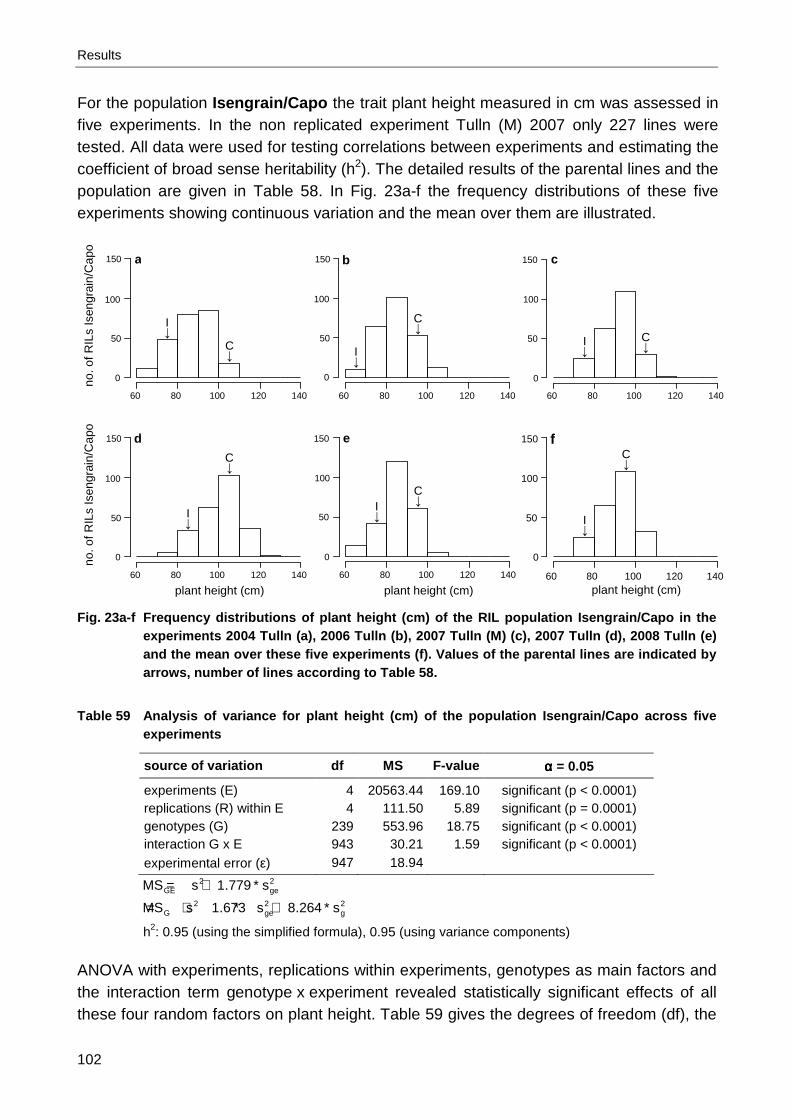
Results
102
For the population Isengrain/Capo the trait plant height measured in cm was assessed in five experiments. In the non replicated experiment Tulln (M) 2007 only 227 lines were tested. All data were used for testing correlations between experiments and estimating the coefficient of broad sense heritability (h2). The detailed results of the parental lines and the population are given in Table 58. In Fig. 23a-f the frequency distributions of these five experiments showing continuous variation and the mean over them are illustrated.
no
. of R
ILs
Isen
grai
n/C
apo
no
. of R
ILs
Isen
grai
n/C
apo
Fig. 23a-f Frequency distributions of plant height (cm) of the RIL population Isengrain/Capo in the
experiments 2004 Tulln (a), 2006 Tulln (b), 2007 Tulln (M) (c), 2007 Tulln (d), 2008 Tulln (e) and the mean over these five experiments (f). Values of the parental lines are indicated by arrows, number of lines according to Table 58.
Table 59 Analysis of variance for plant height (cm) of the population Isengrain/Capo across five
experiments
source of variation df MS F-value αααα = 0.05
experiments (E) 4 20563.44 169.10 significant (p < 0.0001) replications (R) within E 4 111.50 5.89 significant (p = 0.0001) genotypes (G) 239 553.96 18.75 significant (p < 0.0001) interaction G x E 943 30.21 1.59 significant (p < 0.0001) experimental error (ε) 947 18.94
2ge
2GE s779.1sMS ∗+=
2g
2ge
2G s264.8s673.1sMS ∗+∗+=
h2: 0.95 (using the simplified formula), 0.95 (using variance components)
ANOVA with experiments, replications within experiments, genotypes as main factors and the interaction term genotype x experiment revealed statistically significant effects of all these four random factors on plant height. Table 59 gives the degrees of freedom (df), the
d
60 80 100 120 140 0
50
100
150
C ↓
I ↓
a
60 80 100 120 140 0
50
100
150
C ↓
I ↓
c
60 80 100 120 140 0
50
100
150
C ↓ I
↓
b
60 80 100 120 140
0
50
100
150
C ↓
I ↓
e
60 80 100 120 140 0
50
100
150
C ↓ I
↓
f
60 80 100 120 140 0
50
100
150 C ↓
I ↓
plant height (cm) plant height (cm) plant height (cm)

Results
103
mean squares (MS), the F-values and the decisions about the null hypotheses based on a
type I error rate of α = 0.05. Additionally the compositions of the mean squares are shown for the estimation of the coefficient of heritability by the means of variance components. The value of the coefficient of broad sense heritability over all five experiments was 0.95 for both calculation methods. The values of Spearman’s rho between these five experiments and whether the null hypothesis H0: 0 < ρ ≤ 0.71 was accepted (acc.) or rejected (rej.) are presented in Table 60. Values of r ranged from 0.68 (between the experiments Tulln 2006 and 2008), to 0.84 (Tulln 2006 and 2007 (M)). Correlations with the experiment Tulln 2008 were consistently lower and not statistically significantly beyond 0.71. Table 60 Sample size (n) for Spearman’s rho (r) between the five assessments of plant height (cm)
of the population Isengrain/Capo. Additionally acceptance (acc.) or rejection (rej.) of the H0: 0 < ρ ≤ 0.71 is given. α = β = 0.05
IT6 IM7 IT7 IT8
IT4 n 240 227 240 240 r 0.83 0.81 0.77 0.70 H0 rej. rej. rej. acc. IT6 n 227 240 240 r 0.84 0.78 0.68 H0
rej. rej. acc. IM7 n 227 227 r 0.80 0.75 H0
rej. acc. IT7 n 240 r 0.76 H0
acc.
For all lines of the population Arina/Capo plant height was assessed in two experiments (the first with only one replication). The detailed results of the parental lines and the population are given in Table 61, the corresponding frequency distributions are illustrated in Fig. 24a-c. Table 61 Plant height (cm): mean values of the parents Arina and Capo and the population
Arina/Capo, population standard deviation, population range, least significant difference (LSD5%) and number of assessed lines
experiment Arina Capo pop. x ± s pop. range LSD 5% n
Tulln/AT 2007 106.7 111.7 110.7 ± 9.4 75.0 – 130.0 1 rep. 233 Tulln/AT 2008 95.6 92.5 93.0 ± 7.9 72.5 – 112.5 9.8 233
mean over 2 experiments 101.2 102.1 101.9 ± 8.0 73.8 – 121.3 9.4 233
h2: 0.83
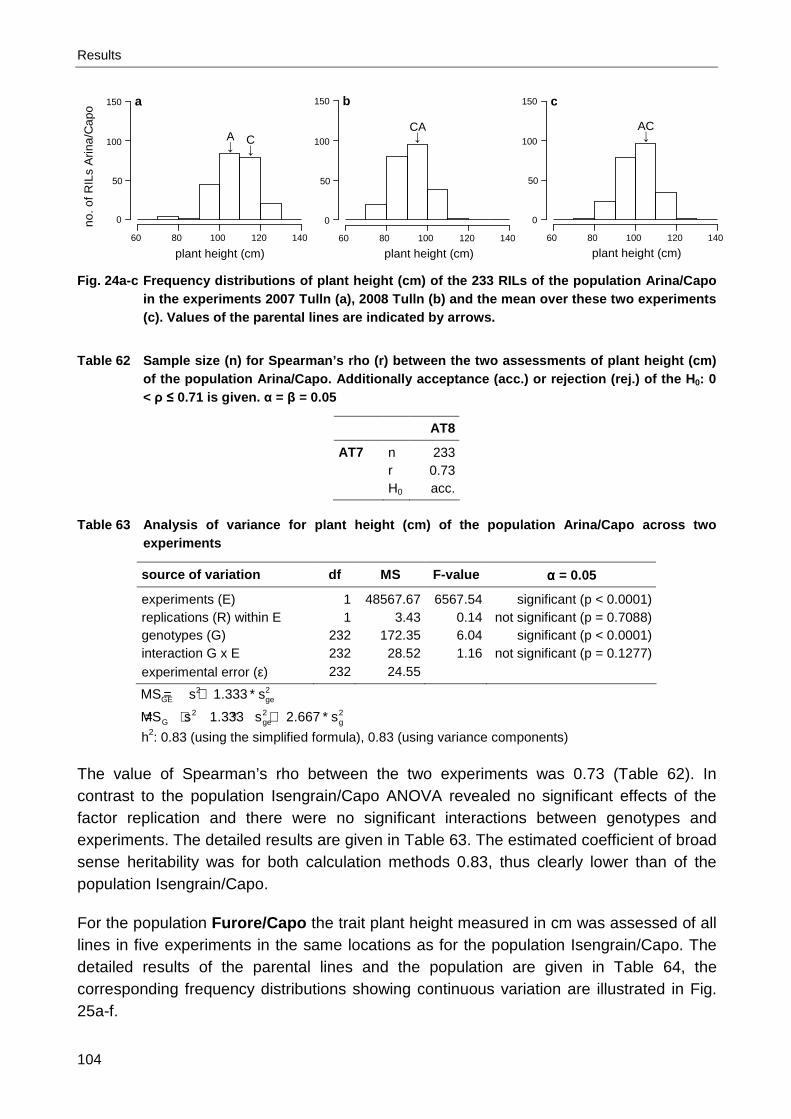
Results
104
no
. of R
ILs
Arin
a/C
apo
Fig. 24a-c Frequency distributions of plant height (cm) of the 233 RILs of the population Arina/Capo
in the experiments 2007 Tulln (a), 2008 Tulln (b) and the mean over these two experiments (c). Values of the parental lines are indicated by arrows.
Table 62 Sample size (n) for Spearman’s rho (r) between the two assessments of plant height (cm)
of the population Arina/Capo. Additionally acceptance (acc.) or rejection (rej.) of the H 0: 0 < ρ ≤ 0.71 is given. α = β = 0.05
AT8
AT7 n 233 r 0.73 H0
acc.
Table 63 Analysis of variance for plant height (cm) of the population Arina/Capo across two
experiments
source of variation df MS F-value αααα = 0.05
experiments (E) 1 48567.67 6567.54 significant (p < 0.0001) replications (R) within E 1 3.43 0.14 not significant (p = 0.7088) genotypes (G) 232 172.35 6.04 significant (p < 0.0001) interaction G x E 232 28.52 1.16 not significant (p = 0.1277) experimental error (ε) 232 24.55
2ge
2GE s333.1sMS ∗+=
2g
2ge
2G s667.2s333.1sMS ∗+∗+=
h2: 0.83 (using the simplified formula), 0.83 (using variance components)
The value of Spearman’s rho between the two experiments was 0.73 (Table 62). In contrast to the population Isengrain/Capo ANOVA revealed no significant effects of the factor replication and there were no significant interactions between genotypes and experiments. The detailed results are given in Table 63. The estimated coefficient of broad sense heritability was for both calculation methods 0.83, thus clearly lower than of the population Isengrain/Capo. For the population Furore/Capo the trait plant height measured in cm was assessed of all lines in five experiments in the same locations as for the population Isengrain/Capo. The detailed results of the parental lines and the population are given in Table 64, the corresponding frequency distributions showing continuous variation are illustrated in Fig. 25a-f.
a
60 80 100 120 140 0
50
100
150
C ↓
A ↓
b
60 80 100 120 140 0
50
100
150
CA ↓
c
60 80 100 120 140 0
50
100
150
AC ↓
plant height (cm) plant height (cm) plant height (cm)

Results
105
Table 64 Plant height (cm): mean values of the parents Furore and Capo and the population Furore/Capo, population standard deviation, population range, least significant difference (LSD5%) and number of assessed lines
experiment Furore Capo pop. x ± s pop. range LSD 5% n
Tulln/AT 2004 92.5 105.0 97.2 ± 5.4 85.0 – 110.0 5.4 201 Tulln/AT 2006 86.7 96.3 93.0 ± 4.8 80.0 – 105.0 6.4 201 Tulln/AT 2007 102.5 113.8 109.3 ± 5.0 97.5 – 120.0 8.6 201 Tulln/AT (M) 2007 92.5 100.0 96.8 ± 4.0 85.0 – 105.0 1 rep. 201 Tulln/AT 2008 86.9 91.9 89.3 ± 4.5 77.5 – 100.0 8.5 201
mean over 5 experiments 92.2 101.4 97.1 ± 3.8 87.5 – 106.0 3.3 201
h2: 0.84
no
. of R
ILs
Fur
ore/
Cap
o
no. o
f RIL
s F
uror
e/C
apo
Fig. 25a-f Frequency distributions of plant height (cm) of the 201 RILs of the population Furore/Capo
in the experiments 2004 Tulln (a), 2006 Tulln (b), 2007 Tulln (c), 2007 Tulln (M) (d), 2008 Tulln (e) and the mean over these five experiments (f). Values of the parental lines are indicated by arrows.
The values of Spearman’s rho between these five experiments ranged from 0.46 (between the experiments Tulln 2004 and 2008) to 0.66 (Tulln 2004 and 2006), thus the same correlations being lowest and highest as for the population Isengrain/Capo. But in contrast, for the Furore/Capo no single coefficient was statistically significantly beyond 0.71. Results of the ANOVA (presented in Table 66) were similar to the population Isengrain/Capo: All main factors and the interaction term had significant effects on plant height. The estimated coefficient of broad sense heritability was for both calculation methods 0.84, thus being clearly below the values of the population Isengrain/Capo, but slightly beyond those of Arina/Capo.
a
60 80 100 120 140 0
50
100
150
C ↓
b
60 80 100 120 140 0
50
100
150
F ↓
c
60 80 100 120 140 0
50
100
150 F ↓
C ↓
d
60 80 100 120 140 0
50
100
150 FC ↓
e
60 80 100 120 140 0
50
100
150
C ↓
f
60 80 100 120 140 0
50
100
150
C ↓
F ↓
plant height (cm) plant height (cm) plant height (cm)
C ↓
F ↓
F ↓

Results
106
Table 65 Sample size (n) for Spearman’s rho (r) between the five assessments of plant height (cm) of the population Furore/Capo. Additionally acceptance (acc.) or rejection (rej.) of the H0: 0 < ρ ≤ 0.71 is given. α = β = 0.05
FT6 FT7 FM7 FT8
FT4 n 201 201 201 201 r 0.66 0.60 0.54 0.46 H0 acc. acc. acc. acc. FT6 n 201 201 201 r 0.58 0.62 0.47 H0
acc. acc. acc. FT7 n 201 201 r 0.56 0.48 H0
acc. acc. FM7 n 201 r 0.49 H0
acc.
Table 66 Analysis of variance for plant height (cm) of the population Furore/Capo across five
experiments
source of variation df MS F-value αααα = 0.05
experiments (E) 4 22870.29 224.17 significant (p < 0.0001) replications (R) within E 4 96.72 6.97 significant (p < 0.0001) genotypes (G) 200 120.90 6.41 significant (p < 0.0001) interaction G x E 800 19.18 1.38 significant (p < 0.0001) experimental error (ε) 800 13.88
2ge
2GE s778.1sMS ∗+=
2g
2ge
2G s333.8s667.1sMS ∗+∗+=
h2: 0.84 (using the simplified formula), 0.84 (using variance components)
5.1.4 Other Traits
In addition to the traits leaf rust severity, heading and plant height, several other traits were assessed in some experiments. The detailed results of the parental lines and the populations are given in Table 67 (Isengrain/Capo), Table 68 (Arina/Capo) and Table 69 (Furore/Capo). As Capo is an awned cultivar, whereas Arina awnless, the trait awnedness was assessed in the population Arina/Capo in five experiments. If some plants of a particular line were awned, whereas others were not, they were classified as “partly”. No single line was classified “awned” in one and “awnless” in another experiment. In Fig. 26a-e bar charts illustrate the distributions of awned, partly awned and awnless lines in these five experiments and the mean over them.

Results
107
Table 67 Mean values of the parents Isengrain and Capo and the population Isengrain/Capo, population standard deviation, population range, least significant difference (LSD 5%), heritability (h 2) and number of assessed lines for all other traits
trait experiment Isengrain Capo pop. x ± s pop. range LSD 5% h2 n
leaf blotch severity (1-9) Aumühle/AT 2004
8.4 5.1 6.1 ± 1.3 4.0 – 9.0 1 rep. 239
powdery mildew sev. (1-9) Probstdorf/AT 2006
3.3 3.3 3.1 ± 1.0 2.0 – 6.5 1.3 240
frost heaving severity (1-9) Probstdorf/AT 2006
4.3 2.8 3.7 ± 1.2 1.0 – 7.0 3.0 240
lodging severity (1-5) Probstdorf/AT 2007
1.0 2.5 1.8 ± 1.0 1.0 – 5.0 1.9 239
lodging severity (0-5) Probstdorf/AT 2008
0.5 3.1 1.9 ± 1.8 0.0 – 5.0 3.0 240
lodging severity (0-5) Rust/AT 2008
0.0 0.5 0.2 ± 0.5 0.0 – 2.5 1.5 240
lodging severity (0-5) Rust/AT 2008 0.0 1.0 0.5 ± 1.0 0.0 – 4.5 2.1 240
leaf chlorosis severity (0-9) Rust/AT 2009
0.0 0.5 1.1 ± 1.7 0.0 – 8.0 1.3 240
leaf chlorosis severity (0-9) Tulln/AT 2009
0.3 0.4 1.3 ± 1.6 0.0 – 7.0 1.8 240
leaf chlorosis severity (0-9) mean over 2 experiments
0.2 0.5 1.2 ± 1.6 0.0 – 7.5 1.1 0.93 240
leaf tip necrosis sev. (0-9) Rust/AT 2009
2.1 1.0 2.5 ± 1.7 0.0 – 8.0 1.7 240
leaf tip necrosis sev. (0-9) Tulln/AT 2009
2.0 0.5 2.6 ± 1.9 0.0 – 8.5 2.0 240
leaf tip necrosis sev. (0-9) mean over 2 experiments
2.1 0.8 2.6 ± 1.7 0.0 – 8.3 1.3 0.92 240
no
. of R
ILs
Arin
a/C
apo
Fig. 26a-e Bar charts of the 233 RILs of the population Arina/Capo for awnedness in the experiments
2007 Tulln (a), 2008 Rust (b), 2008 Schmida (c), 2008 Tulln (d) and the mean over these four experiments (e). Capo: awned, Arina: awnless.
no partly yes
a
0
20
40
60
80
100
no partly yes
b
0
20
40
60
80
100
no partly yes
c
0
20
40
60
80
100
no partly yes
d
0
20
40
60
80
100
no partly yes
e
0
20
40
60
80
100
awnedness awnedness awnedness awnedness awnedness
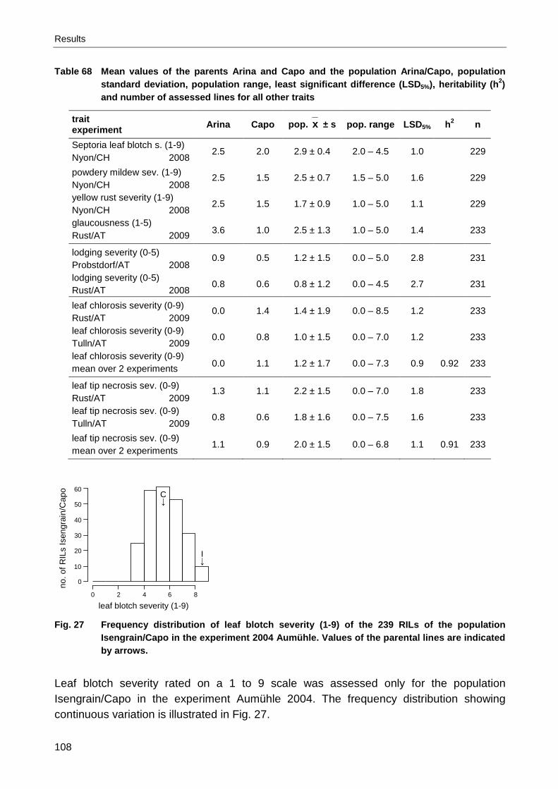
Results
108
Table 68 Mean values of the parents Arina and Capo and the population Arina/Capo, population standard deviation, population range, least significant difference (LSD 5%), heritability (h 2) and number of assessed lines for all other traits
trait experiment Arina Capo pop. x ± s pop. range LSD 5% h2 n
Septoria leaf blotch s. (1-9) Nyon/CH 2008
2.5 2.0 2.9 ± 0.4 2.0 – 4.5 1.0 229
powdery mildew sev. (1-9) Nyon/CH 2008
2.5 1.5 2.5 ± 0.7 1.5 – 5.0 1.6 229
yellow rust severity (1-9) Nyon/CH 2008
2.5 1.5 1.7 ± 0.9 1.0 – 5.0 1.1 229
glaucousness (1-5) Rust/AT 2009
3.6 1.0 2.5 ± 1.3 1.0 – 5.0 1.4 233
lodging severity (0-5) Probstdorf/AT 2008
0.9 0.5 1.2 ± 1.5 0.0 – 5.0 2.8 231
lodging severity (0-5) Rust/AT 2008
0.8 0.6 0.8 ± 1.2 0.0 – 4.5 2.7 231
leaf chlorosis severity (0-9) Rust/AT 2009
0.0 1.4 1.4 ± 1.9 0.0 – 8.5 1.2 233
leaf chlorosis severity (0-9) Tulln/AT 2009
0.0 0.8 1.0 ± 1.5 0.0 – 7.0 1.2 233
leaf chlorosis severity (0-9) mean over 2 experiments 0.0 1.1 1.2 ± 1.7 0.0 – 7.3 0.9 0.92 233
leaf tip necrosis sev. (0-9) Rust/AT 2009
1.3 1.1 2.2 ± 1.5 0.0 – 7.0 1.8 233
leaf tip necrosis sev. (0-9) Tulln/AT 2009
0.8 0.6 1.8 ± 1.6 0.0 – 7.5 1.6 233
leaf tip necrosis sev. (0-9) mean over 2 experiments
1.1 0.9 2.0 ± 1.5 0.0 – 6.8 1.1 0.91 233
no
. of R
ILs
Isen
grai
n/C
apo
Fig. 27 Frequency distribution of leaf blotch severity (1-9) of the 239 RILs of the population
Isengrain/Capo in the experiment 2004 Aumühle. Values of the parental lines are indicated by arrows.
Leaf blotch severity rated on a 1 to 9 scale was assessed only for the population Isengrain/Capo in the experiment Aumühle 2004. The frequency distribution showing continuous variation is illustrated in Fig. 27.
0 2 4 6 8
0
10
20
30
40
50
60 C ↓
I ↓
leaf blotch severity (1-9)

Results
109
Table 69 Mean values of the parents Furore and Capo and the population Furore/Capo, population standard deviation, population range, least significant difference (LSD 5%), heritability (h 2) and number of assessed lines for all other traits
trait experiment Furore Capo pop. x ± s pop. range LSD 5% h2 n
Septoria leaf blotch s. (1-9) Probstdorf/AT 2008
5.4 5.0 4.7 ± 0.5 3.5 – 6.0 1.4 201
powdery mildew sev. (1-9) Probstdorf/AT 2006
3.8 3.5 3.3 ± 0.7 2.0 – 5.0 1.5 201
powdery mildew sev. (1-9) Probstdorf/AT 2008
4.8 4.0 3.8 ± 0.6 2.5 – 5.5 1.6 201
powdery mildew sev. (1-9) mean over 2 experiments
4.3 3.8 3.6 ± 0.5 2.5 – 5.3 1.1 0.02 201
frost heaving severity (1-9) Probstdorf/AT 2006
2.8 3.0 3.0 ± 0.8 1.0 – 5.5 2.0 201
lodging severity (1-5) Probstdorf/AT 2007
1.2 4.3 2.4 ± 1.1 1.0 – 5.0 2.8 201
lodging severity (0-5) Probstdorf/AT 2008
0.5 1.3 1.0 ± 1.3 0.0 – 5.0 2.8 201
lodging severity (1-9) Probstdorf/AT 2008 1.0 1.0 2.7 ± 1.4 1.0 – 7.0 4.9 201
no
. of R
ILs
Arin
a/C
apo
no
. of R
ILs
Fur
ore/
Cap
o
Fig. 28a-b Frequency distributions of Septoria leaf blotch severity (1-9) of the RIL populations. 229
lines Arina/Capo 2008 Nyon (a), 201 lines Furore/Capo 2008 Probstdorf (b). Values of the parental lines are indicated by arrows.
Infection with Septoria leaf blotch rated on a 1 to 9 scale was assessed for the population Arina/Capo in the experiment Nyon 2008 and for Furore/Capo in Probstdorf 2008. The frequency distributions showing continuous variation are illustrated in Fig. 28a-b. Infection was more severe in the latter experiment than in the first.
0 2 4 6 8 0
50
100
150
F ↓
C ↓ b
0 2 4 6 8 0
50
100
150
C ↓
A ↓ a
Septoria leaf blotch severity (1-9) Septoria leaf blotch severtity (1-9)

Results
110
no
. of R
ILs
Isen
grai
n/C
apo
no
. of R
ILs
Arin
a/C
apo
no
. of R
ILs
Fur
ore/
Cap
o
Fig. 29a-e Frequency distributions of powdery mildew severity (1-9) of the RIL populations. 240 lines
Isengrain/Capo 2006 Probstdorf (a), 229 lines Arina/Capo 2008 Nyon (b); 201 lines Furore/Capo: 2006 Probstdorf (c), 2008 Probstdorf (d) and the mean over these two experiments (e). Values of the parental lines are indicated by arrows.
Table 70 Sample size (n) for Spearman’s rho (r) between the two assessments of powdery mildew
severity (1-9) of the population Furore/Capo. Additionally acceptance (acc.) or rejection (rej.) of the H 0: 0 < ρ ≤ 0.71 is given. α = β = 0.05
FP8
FP6 n 201 r 0.02 H0
acc.
Table 71 Analysis of variance for powdery mildew severity (1-9) of the population Furore/Capo
across two experiments
source of variation df MS F-value αααα = 0.05
experiments (E) 1 64.0908 24.55 significant (p = 0.0306) replications (R) within E 2 2.4689 4.07 significant (p = 0.0178) genotypes (G) 200 0.7613 1.02 not significant (p = 0.4516) interaction G x E 200 0.7483 1.23 significant (p = 0.0403) experimental error (ε) 400 0.6064
2ge
2GE s2sMS ∗+=
2g
2ge
2G s4s2sMS ∗+∗+=
h2: 0.02 (using the simplified formula), 0.02 (using variance components)
c
0 2 4 6 8 0
50
100
150
CF ↓
d
0 2 4 6 8 0
50
100
150
F ↓
e
0 2 4 6 8
0
50
100
150
F ↓
0 2 4 6 8
0
50
100
150
C ↓
A ↓
b
0 2 4 6 8 0
50
100
150
IC ↓
a
C ↓
C ↓
powdery mildew severity (1-9) powdery mildew severity (1-9)
powdery mildew severity (1-9) powdery mildew severity (1-9) powdery mildew severity (1-9)

Results
111
Powdery mildew severity was assessed on a 1 to 9 scale in the experiments Probstdorf 2006 (Isengrain/Capo and Furore/Capo), Nyon 2008 (Arina/Capo) and Probstdorf 2008 (Furore/Capo). The frequency distributions of the single experiments and the mean values over the Furore/Capo experiments showing continuous variation are illustrated in Fig. 29a-e. The value of Spearman’s rho between the two experiments of the population Furore/Capo (Table 70) was very low. ANOVA (Table 71) revealed no significant effect of the factor genotypes on powdery mildew infection. As all lines were rated in both replications of these experiments, the coefficient of broad sense heritability (h2) 0.02 was identical for both calculation methods. The difference between the two Furore/Capo experiments was larger than the difference between the two populations Isengrain/Capo and Furore/Capo in the experiment Probstdorf 2006. Yellow rust severity rated on a 1 to 9 scale was assessed only for the population Arina/Capo in the experiment Nyon 2008. The frequency distribution showing continuous variation is illustrated in Fig. 30.
no
. of R
ILs
Arin
a/C
apo
Fig. 30 Frequency distribution of yellow rust severity (1-9) of the 229 RILs of the population
Arina/Capo in the experiment 2008 Nyon. Values of the parental lines are indicated by arrows.
no
. of R
ILs
Arin
a/C
apo
Fig. 31 Frequency distribution of glaucousness (1-5) of the 233 RILs of the population Arina/Capo
in the experiment 2009 Rust. Values of the parental lines are indicated by arrows.
Glaucousness rated on a 1 to 5 scale was assessed only for the population Arina/Capo in the experiment Rust 2009. The frequency distribution showing continuous variation is illustrated in Fig. 31.
0 1 2 3 4 5
0
10
20
30
40
50
60 A ↓
0 2 4 6 8 0
20
40
60
80
100 C ↓
A ↓
yellow rust severity (1-9)
glaucousness (1-5)
C ↓

Results
112
no
. of R
ILs
Isen
grai
n/C
apo
no
. of R
ILs
Fur
ore/
Cap
o
Fig. 32a-b Frequency distributions of frost heaving severity (1-9) of the RIL populations in the
experiment 2006 Probstdorf: 240 lines Isengrain/Capo (a), 201 lines Furore/Capo (b). Values of the parental lines are indicated by arrows.
Frost heaving severity measured on a 1 to 9 scale was assessed in the experiment Probstdorf 2006. The frequency distribution of the population Isengrain/Capo is illustrated in Fig. 32a, of the population Furore/Capo in Fig. 32b. Both showed continuous variation. Furore and Capo were almost equally susceptible; Isengrain was clearly more prone to frost heaving. Thus, mean value, range and LSD were higher for the population Isengrain/Capo than for the population Furore/Capo. Lodging severity rated on different scales was assessed in three experiments of the population Isengrain/Capo, two of Arina/Capo and three of Furore/Capo. In the experiment Rust 2008 lodging severity of the population Isengrain/Capo was assessed twice. Due to the different scales, results are hardly comparable. It seems that variability between experiments was equal to variability between different populations at the same trial site. The values of Spearman’s rho ranged from 0.18 to 0.59 for the population Isengrain/Capo, from 0.04 to 0.39 for Furore/Capo and was 0.32 for Arina/Capo, none being significantly beyond 0.71. The detailed results are presented in Table 72, Table 73 and Table 74. Table 72 Sample size (n) for Spearman’s rho (r) between the four assessments of lodging severity
(1-5 or 0-5) of the population Isengrain/Capo. Additionally acceptance (acc.) or rejection (rej.) of the H 0: 0 < ρ ≤ 0.71 is given. α = β = 0.05
IP8 IRu8_1 IRu8_2
IP7 n 239 239 239 r 0.52 0.18 0.41 H0 acc. acc. acc. IP8 n 240 240 r 0.22 0.43 H0
acc. acc. IRu8_1 n 240 r 0.59 H0
acc.
0 2 4 6 8
0
20
40
60
80 b
0 2 4 6 8 0
20
40
60
80
I ↓
a C ↓
FC ↓
frost heaving severity (1-9) frost heaving severity (1-9)

Results
113
Table 73 Sample size (n) for Spearman’s rho (r) between the two assessments of lodging severity (0-5) of the population Arina/Capo. Additionally acceptance (acc.) or rejection (rej.) of the H0: 0 < ρ ≤ 0.71 is given. α = β = 0.05
ARu8
AP8 n 231 r 0.32 H0
acc.
Table 74 Sample size (n) for Spearman’s rho (r) between the three assessments of lodging severity
(1-5 or 0-5) of the population Furore/Capo. Additionally acceptance (acc.) or rejection (rej.) of the H 0: 0 < ρ ≤ 0.71 is given. α = β = 0.05
FP8_1 FP8_2
FP7 n 201 201 r 0.39 0.05 H0 acc. acc. FP8_1 n 201 r 0.04 H0
acc.
no
. of R
ILs
Isen
grai
n/C
apo
no
. of R
ILs
Arin
a/C
apo
Fig. 33a-f Frequency distributions of leaf chlorosis severity (0-9) of the RIL populations. 240 lines
Isengrain/Capo 2009 Rust (a), 2009 Tulln (b) and the mean over these two experiments (c); 233 lines Arina/Capo 2009 Rust (d), 2009 Tulln (e) and the mean over these two experiments (f). Values of the parental lines are indicated by arrows.
d
0 2 4 6 8 10 0
50
100
150
C ↓
e
0 2 4 6 8 10
0
50
100
150 f
0 2 4 6 8 10 0
50
100
150
C ↓
a
0 2 4 6 8 10 0
50
100
150 b
0 2 4 6 8 10 0
50
100
150 c
0 2 4 6 8 10
0
50
100
150
A ↓
IC ↓ IC
↓ IC ↓
A ↓
AC ↓
leaf chlorosis severity (0-9) leaf chlorosis severity (0-9) leaf chlorosis severity (0-9)

Results
114
Symptoms of leaf chlorosis rated on a 0 to 9 scale were assessed in the experiments Rust and Tulln 2009 for the populations Isengrain/Capo and Arina/Capo. The frequency distributions of the single experiments and the mean over them showing continuous variation are illustrated in Fig. 33a-f. In the experiment Rust 2009 Isengrain and Arina showed no symptoms, in Tulln 2009 Isengrain was about as susceptible as Capo. Both populations showed similar variation. Due to the very slight differences there was no clear tendency which population was more or less susceptible and in which experiment symptoms were more severe. Capo was rated highest in the experiment Rust 2009 of the population Arina/Capo. The values of Spearman’s rho of both populations were statisti-cally significantly beyond 0.71. The detailed results are presented in Table 75 and Table 77. For both populations ANOVA revealed no significant effect of the experiments on leaf chlorosis severity. In the case of Isengrain/Capo there were no significant interactions either (Table 76 and Table 78). The values of the coefficient of broad sense heritability were 0.93 for Isengrain/Capo and 0.92 for Arina/Capo. Despite missing values in the first population, results of both populations were independent from the calculation method. Table 75 Sample size (n) for Spearman’s rho (r) between the two assessments of leaf chlorosis
severity (0-9) of the population Isengrain/Capo. Additionally acceptance (acc.) or rejection (rej.) of the H 0: 0 < ρ ≤ 0.71 is given. α = β = 0.05
IT9
IRu9 n 240 r 0.81 H0
rej.
Table 76 Analysis of variance for leaf chlorosis severity (0-9) of the population Isengrain/Capo
across two experiments
source of variation df MS F-value αααα = 0.05
experiments (E) 1 5.6916 0.82 not significant (p = 0.4583) replications (R) within E 2 6.8354 11.15 significant (p < 0.0001) genotypes (G) 239 10.2727 14.29 significant (p < 0.0001) interaction G x E 239 0.7188 1.17 not significant (p = 0.0741) experimental error (ε) 477 0.6128
2ge
2GE s997.1sMS ∗+=
2g
2ge
2G s994.3s997.1sMS ∗+∗+=
h2: 0.93 (using the simplified formula), 0.93 (using variance components)
Table 77 Sample size (n) for Spearman’s rho (r) between the two assessments of leaf chlorosis
severity (0-9) of the population Arina/Capo. Additionally acceptance (acc.) or rejection (rej.) of the H 0: 0 < ρ ≤ 0.71 is given. α = β = 0.05
AT9
ARu9 n 233 r 0.84 H0
rej.

Results
115
Table 78 Analysis of variance for leaf chlorosis severity (0-9) of the population Arina/Capo across two experiments
source of variation df MS F-value αααα = 0.05
experiments (E) 1 25.7779 7.37 not significant (p = 0.0806) replications (R) within E 2 2.9882 8.18 significant (p = 0.0003) genotypes (G) 232 10.9366 12.53 significant (p < 0.0001) interaction G x E 232 0.8727 2.39 significant (p < 0.0001) experimental error (ε) 464 0.3654
2ge
2GE s2sMS ∗+=
2g
2ge
2G s4s2sMS ∗+∗+=
h2: 0.92 (using the simplified formula), 0.92 (using variance components)
no
. of R
ILs
Isen
grai
n/C
apo
no
. of R
ILs
Arin
a/C
apo
Fig. 34a-f Frequency distributions of leaf tip necrosis severity (0-9) of the RIL populations. 240 lines
Isengrain/Capo 2009 Rust (a), 2009 Tulln (b) and the mean over these two experiments (c); 233 lines Arina/Capo 2009 Rust (d), 2009 Tulln (e) and the mean over these two experiments (f). Values of the parental lines are indicated by arrows.
Leaf tip necrosis severity rated on a 0 to 9 scale was assessed in the same experiments as leaf chlorosis severity. The frequency distributions of the single experiments and the mean over them showing continuous variation are illustrated in Fig. 34a-f. Arina showed more severe leaf tip necrosis than Capo, but clearly less than Isengrain. Thus, mean value, standard deviation and maximum value of the population Isengrain/Capo was higher than of the population Arina/Capo. For both populations differences between the two experiments were low. The values of Spearman’s rho of both populations were about the same as for leaf chlorosis severity and statistically significantly beyond 0.71. The detailed results are presented in Table 79 and Table 81. For both populations ANOVA
d
0 2 4 6 8 10
0
20
40
60
80
100
CA ↓
0 2 4 6 8 10 0
20
40
60
80
100 f
0 2 4 6 8 10 0
20
40
60
80
100 C ↓
A ↓
a
0 2 4 6 8 10 0
20
40
60
80
100
C ↓
I ↓
b
0 2 4 6 8 10 0
20
40
60
80
100
C ↓
I ↓
c
0 2 4 6 8 10
0
20
40
60
80
100
C ↓
I ↓
CA ↓ e
leaf tip necrosis severity (0-9) leaf tip necrosis severity (0-9) leaf tip necrosis severity (0-9)

Results
116
revealed no significant effect of the experiments on leaf tip necrosis severity and no significant interactions (Table 80 and Table 82). The values of the coefficient of broad sense heritability were 0.92 for Isengrain/Capo and 0.91 for Arina/Capo, thus being a little bit lower than for leaf chlorosis severity. Table 79 Sample size (n) for Spearman’s rho (r) between the two assessments of leaf tip necrosis
severity (0-9) of the population Isengrain/Capo. Additionally acceptance (acc.) or rejection (rej.) of the H 0: 0 < ρ ≤ 0.71 is given. α = β = 0.05
IT9
IRu9 n 240 r 0.86 H0
rej.
Table 80 Analysis of variance for leaf tip necrosis severity (0-9) of the population Isengrain/Capo
across two experiments
source of variation df MS F-value αααα = 0.05
experiments (E) 1 7.6722 2.05 not significant (p = 0.2805) replications (R) within E 2 3.6092 4.16 significant (p = 0.0161) genotypes (G) 239 12.1634 12.24 significant (p < 0.0001) interaction G x E 239 0.9939 1.15 not significant (p = 0.1080) experimental error (ε) 476 0.8672
2ge
2GE s994.1sMS ∗+=
2g
2ge
2G s989.3s994.1sMS ∗+∗+=
h2: 0.92 (using the simplified formula), 0.92 (using variance components)
Table 81 Sample size (n) for Spearman’s rho (r) between the two assessments of leaf tip necrosis
severity (0-9) of the population Arina/Capo. Additionally acceptance (acc.) or rejection (rej.) of the H 0: 0 < ρ ≤ 0.71 is given. α = β = 0.05
AT9
ARu9 n 233 r 0.81 H0
rej.
Table 82 Analysis of variance for leaf tip necrosis severity (0-9) of the population Arina/Capo
across two experiments
source of variation df MS F-value αααα = 0.05
experiments (E) 1 33.0940 4.88 not significant (p = 0.1578) replications (R) within E 2 6.7840 8.65 significant (p = 0.0002) genotypes (G) 232 8.8519 11.26 significant (p < 0.0001) interaction G x E 232 0.7859 1.00 not significant (p = 0.4885) experimental error (ε) 462 0.7845
2ge
2GE s994.1sMS ∗+=
2g
2ge
2G s989.3s994.1sMS ∗+∗+=
h2: 0.91 (using the simplified formula), 0.91 (using variance components)

Results
117
5.1.5 Trait Correlations
Pearson’s product moment coefficient and/or Spearman’s rho were calculated and tested to find possible correlations between leaf rust severity, heading, plant height and other proportionally or ordinally scaled traits. If possible, these tests were not only done for a particular experiment but also for the mean over experiments. All results (number of lines
n, correlation coefficient r and whether the null hypothesis H0: 0 < |ρ| ≤ 0.59 was accepted or rejected are given in Table 9 – 47 in Appendix C.
0 10 20 30 40 50
05
1015
2025
3035
leaf rust severity (% infected leaf area)
leaf
rus
t se
verit
y (r
elat
ive
AU
DP
C)
populationIsengrainCapo
r = 0.96
0 10 20 30 40
142
144
146
148
150
152
leaf rust severity (% infected leaf area)
head
ing
(day
in t
he y
ear)
populationIsengrainCapo
r = -0.17
0 10 20 30 40 50 60
7080
9010
0
leaf rust severity (% infected leaf area)
plan
t he
ight
(cm
)
populationIsengrainCapo
r = -0.01
144 146 148 150 152
7080
9010
0
heading (day in the year)
plan
t he
ight
(cm
)
populationIsengrainCapo
r = 0.44
Fig. 35a-d Scatterplots of the traits (a) leaf rust severity measured by the percentage of infected leaf
area versus rel. AUDPC (mean over two experiments), (b) leaf rust severity versus heading (mean over six experiments), (c) leaf rust severity versus plant height (mean over three experiments) and (d) heading versus plant height (mean over five experiments) for the RIL population Isengrain/Capo. The positions of the parental lines are indicated. The dia-meters of the circles are directly proportional to the number of lines with the same scores.
a b
c d

Results
118
In none of the three populations Isengrain/Capo, Arina/Capo or Furore/Capo a relevant correlation (r2 > 0.35 or r > |0.59|) between different traits was detected. For an example, the scatterplots of the population Isengrain/Capo and the parental lines for the trait leaf rust severity versus heading and plant height are shown in Fig. 35b-d. The value of Spearman’s rho is also given there. Means were calculated over those experiments in which both traits were assessed. The diameters of the circles are directly proportional to the number of observations. The only exceptions of correlations with coefficients r > |0.59| were detected between the repeated assessments of leaf rust severity (measured by the percentage of infected leaf area and the relative AUDPC). Exemplarily the scatterplots of the population Isengrain/ Capo of the experiment Tulln 2008 are presented in Fig. 37a-f. In Fig. 35a the scatterplot of leaf rust severity measured by the percentage of infected leaf area versus relative AUDPC for the mean over the experiments Piešťany 2006 and Tulln 2008 is shown. Interdependencies between the traits appearance of teliospores and awnedness were analyzed by means of contingency tables and chi-squared tests of independence. The appearance of teliospores was significantly correlated with the leaf area exhibiting symptoms of leaf rust. In the population Isengrain/Capo as well as Furore/Capo the proportion of plants with teliospores increased with leaf rust severity. The bar charts are presented in Fig. 36. Correlations with the traits heading and plant height were not significant, though lines with later heading dates were less likely to have teliospores. Values of Cramér’s V are given in Table 83.
no yes
>0-10>10-20>20-30>30-50
Isengrain/Capo
appearance of teliospores
no.
of R
ILs
Isen
grai
n/C
apo
050
100
150
200
no yes
>0-10>10-20>20-30>30-50
Furore/Capo
appearance of teliospores
no.
of R
ILs
Fur
ore/
Cap
o
050
100
150
200
Fig. 36 Bar charts of the RIL populations Isengrain/Capo (left) and Furore/Capo (right) for the
different classes of leaf rust severity comparing the plants without and with teliospores
Table 83 Cramér’s V for the correlation of the appearance of teliospores and the other traits assessed in the experiments in Tulln 2004
population heading plant height leaf rust severity
Isengrain/Capo 0.09 0.10 0.45 Furore/Capo 0.10 0.10 0.42

Results
119
0 10 20 30 40 50 60 70
010
2030
4050
6070
leaf rust severity first scoring (% infected leaf area)
leaf
rus
t se
verit
y se
cond
sco
ring
(% in
fect
ed le
af a
rea)
populationIsengrainCapo
r = 0.92
0 10 20 30 40 50 60 70
010
2030
4050
6070
leaf rust severity first scoring (% infected leaf area)
leaf
rus
t se
verit
y (A
UD
PC
)
populationIsengrainCapo
r = 0.94
0 10 20 30 40 50 60 70
010
2030
4050
6070
leaf rust severity second scoring (% infected leaf area)
leaf
rus
t se
verit
y th
ird s
corin
g (%
infe
cted
leaf
are
a)
populationIsengrainCapo
r = 0.94
0 10 20 30 40 50 60 70
010
2030
4050
6070
leaf rust severity second scoring (% infected leaf area)
leaf
rus
t se
verit
y (A
UD
PC
)
populationIsengrainCapo
r = 0.99
0 10 20 30 40 50 60 70
010
2030
4050
6070
leaf rust severity first scoring (% infected leaf area)
leaf
rus
t se
verit
y th
ird s
corin
g (%
infe
cted
leaf
are
a)
populationIsengrainCapo
r = 0.90
0 10 20 30 40 50 60 70
010
2030
4050
6070
leaf rust severity third scoring (% infected leaf area)
leaf
rus
t se
verit
y (A
UD
PC
)
populationIsengrainCapo
r = 0.97
Fig. 37a-f Scatterplots depicting the correlation of the three single assessments of the trait leaf rust
severity in 2008 Tulln and the resulting relative AUDPC for the RIL population Isengrain/ Capo. The positions of the parental lines are indicated. The diameters of the circles are directly proportional to the number of lines with the same scores.
a b
c d
f e

Results
120
Table 84 Cramér’s V for the correlation of awnedness and the other traits in the population Arina/Capo assessed in four experiments and for mean values
experiment heading plant height leaf rust sev. lodging sev. AUDPC
Tulln 2007 0.10 0.11 0.10 Rust 2008 0.01 0.17 0.15 Schmida 2008 0.15 0.14 Tulln 2008 0.08 0.15 0.07 0.08
mean 0.08 0.13 0.10
No significant correlation was detected between awnedness and any other trait in the population Arina/Capo. The values of Cramér’s V are presented in Table 84.

Results
121
5.2 Genetic Map Population Isengrain/Capo
5.2.1 Microsatellite (SSR) Markers
290 SSR primer pairs were analyzed on the two parental lines Isengrain and Capo. Exactly half of them revealed clearly polymorphic bands, 91 (31 %) produced solely monomorphic bands and for 10 % no fragments were detectable. Bands of the remaining 25 primer pairs (9 %) were either very difficult to score because of small fragment size differences or might be dominant. 129 SSR primer pairs were applied to the population Isengrain/Capo, generating 165 different polymorphic marker bands. As an example the polymorphism pattern of the SSR primer Barc340 is given in Fig. 9 on page 48. The primer pair producing maximum polymorphic bands was Wmc500 with five distinct markers that were assigned to four different chromosomes of the B-genome. 17 markers were excluded from map calculation.
5.2.2 Amplified Fragment Length Polymorphism (AFLP) Markers
30 AFLP primer combinations were applied to the population Isengrain/Capo. Out of the 673 generated polymorphic bands, 39 were excluded from mapping (15 of them being monomorphic for the parents) and 98 polymorphisms were not be scorable at all. There-fore some numbered AFLP loci are missing in the map. The list of the used selective nucleotides, the name according to the list by KeyGene (2010), the number of detected polymorphic fragments and the number of mapped loci are given in Table 85. As an example the polymorphism pattern of the AFLP primer combination S11M23 is given in Fig. 10 on page 49. Table 85 AFLP primer combinations applied
sel. nucleotides Sse8387I-MseI name polym.
fragments mapped
loci sel. nucleotides Sse8387I-MseI name polym.
fragments mapped
loci
AA-AT S11M14 23 18 GA-TA S19M23 29 20 AA-CG S11M17 15 12 GC-AA S20M11 14 12 AA-CT S11M18 10 7 GC-AT S20M14 15 4 AA-TA S11M23 29 25 GC-TA S20M23 42 24 AA-TT S11M26 7 6 GT-AG S22M13 27 24 AC-AG S12M13 38 28 GT-CG S22M17 28 25 AC-CT S12M18 23 17 GT-GC S22M20 11 8 AG-GC S13M20 13 11 TA-AG S23M13 36 27 AT-AC S14M12 28 15 TA-AT S23M14 41 24 AT-CT S14M18 26 15 TA-CA S23M15 30 23 CC-CC S16M16 23 19 TA-CG S23M17 20 15 CG-CT S17M18 12 12 TC-GA S24M19 3 2 CT-AT S18M14 14 12 TT-AT S26M14 28 19 CT-GC S18M20 15 8 TT-CT S26M18 27 16 GA-CG S19M17 14 9 TT-GG S26M21 32 25

Results
122
5.2.3 Linkage Map
In total data of 684 molecular markers were used for map construction in the population Isengrain/Capo. 83 % of these markers segregated according to the Mendelian ratio
(α = 0.05). 619 markers were mapped into 49 linkage groups covering a total genetic distance of 2,150 cM: 137 SSR markers (34 BARC, 86 GWM and 17 WMC) and 482 AFLP markers with an average marker distance of 3.5 cM. 33 linkage groups were unambiguously assigned to a chromosome based on the SSR markers with known chromosomal position, covering a total genetic distance of 1,873 cM. To all 21 chromosomes of the hexaploid wheat genome at least one linkage group was assigned. The obtained genetic linkage maps of the population Isengrain x Capo are presented in Fig. 38 to Fig. 58 with their short arm at the top. On the left-hand side the genetic distance in cM is indicated, on the right-hand side the corresponding marker used for map construction (AFLP – black, SSR in color: Xbarc – blue, Xgwm – green, Xwmc – red). On the very left the wheat consensus reference map of Somers et al. (2004) is shown, in the right part linkage groups detected in the population Arina x Capo and the Arina x Forno reference map of Paillard et al. (2003). In the reference maps only SSR markers assigned to comparable linkage groups in at least one mapping population are highlighted in the same colors and connected by a straight line. All distances are cM (Haldane) with the exception of the wheat consensus map (Kosambi). Markers clustered at certain chromosomal regions and were not evenly distributed across the whole genome. Therefore, marker coverage varied between the A, B and D genome and within as well as between chromosomes: 146 loci were mapped to the A genome (covering 652 cM), 302 to the B genome (796 cM) and 78 to the D genome (405 cM). Eight linkage groups (covering 189 cM) that were not definitely assigned to a certain chromosome are shown in Fig. 59. Further eight linkage groups (covering 108 cM) comprised solely of AFLP markers (presented in Fig. 60), 11 SSR and 54 AFLP markers remained yet unlinked.
5.3 Genetic Map Population Arina/Capo 32 SSR primer pairs were applied to the population Arina/Capo, generating 36 different polymorphic marker bands, out of which 22 were mapped to nine linkage groups. Comparing the Capo alleles with those detected in the population Isengrain/Capo, all linkage groups were assigned to seven different chromosomes, covering a total genetic distance of 140 cM. All linkage groups and single markers that matched to loci mapped in the population Isengrain/Capo by comparing Capo alleles are presented in Fig. 38 to Fig. 58 in comparison to the Isengrain/Capo map and two reference maps as described in 5.2.3 Linkage Map.

Results
123
75
Glu-A30,0Xgdm336,1Xgwm13611,6Lr1022,2Xcfa222623,8Xcfd1524,6Xgwm3327,4Xwmc81828,9Xwmc33635,2Xwmc9540,5Xgdm13643,0Xbarc8347,6Xwmc2448,4Xgwm35751,6Xbarc11953,6Xgwm16456,3Xbarc14856,8Xcfd5957,0Xwmc74457,5Xcfd3057,7Xbarc2858,2Xgwm13560,7Xwmc27861,7Xwmc63062,1Xwmc82662,6Xwmc61162,7Xwmc1162,8Xwmc46963,8Xwmc183 Xbarc24064,5Xcfd2264,7Xwmc31268,5Xwmc9368,8Xcfa212970,8Xwmc971,5Xgwm49785,5Xwmc67387,9Xwmc5190,0Xwmc71691,0Xwmc5998,0
Xbarc158113,8Xbarc17114,8Xbarc145116,0
Xcfa2219124,1Xgwm99126,0
1A
Xbarc2630,0XS13M20_68,4XS22M13_189,4XS26M21_612,3XS13M20_414,1XS22M17_1414,4XS26M14_2114,6XS23M13_414,9XS22M13_2017,0Xgwm13625,6
XS23M14_6 XS19M23_280,0
XS23M15_1011,9XS16M16_1014,0
Xgwm13527,4
XS11M23_2932,5
XS11M23_1848,2
1A
Xgwm13527,4
1A
Xcfd58.20,0Xcfa2153 Xgdm33Xpsp29991,0
Xsfr2(Lrk10)3,7XgbxG5646,0Xwmc3296,3XksuE1810,4
Xsfr.AtB5.1b46,8Xpsr94151,3Xcfd58.152,9Xgwm35754,6Xgwm135.257,7Centromere60,0Xgwm135.164,7
1A
Fig. 38 Linkage groups assigned to chromosome 1A
Wheat Consensus Isengrain x Capo Arina x Capo Arina x Forno
0,0

Results
124
Gli-B10,0Glu-B35,0Xgwm60811,7Xgwm55014,3Xwmc81816,8Xwmc5117,8Xwmc4918,6Xwmc79819,0Xbarc12819,5Xwmc61920,7Xgwm26421,2Xbarc6023,3Xwmc406 Xwmc500.123,5Xbarc824,9Xgwm41325,9Xgdm3626,8Xgwm13327,8Xgwm3328,0Xwmc500.229,2Xwmc12829,8Xgdm28 Xgdm33Xgwm494 Xwmc3129,9
Xgwm13130,7Xgwm49831,1Xbarc18731,5Xwmc41931,8Xwmc61131,9Xcfd5932,4Xcfd232,5Xwmc26932,8Xwmc59733,2Xgwm27333,4Xgwm1833,6Xcfd65 Xgdm13634,2Xgwm11 Xbarc13734,3Xwmc62634,8Xwmc21635,1Xwmc21335,8Xwmc81335,9Xwmc69436,7Xwmc15637,0Xgwm58237,3Xgwm374.137,8Xbarc24038,0Xbarc18138,3Xcfa212939,3Xcfd4839,8Xgdm10141,9Xwmc41643,5Glu-B144,3Xwmc13447,3Xgwm40349,6Xwmc20660,2Xgwm27460,7Xgwm15361,4Xbarc8161,7Xwmc631 Xwmc76662,7Xwmc67362,8Xbarc18863,0Xgwm26863,5Xgwm12464,1Xcfa214774,9Xwmc83090,3Xwmc71990,4Xwmc4491,5Xwmc367102,6Xbarc80106,3Xgwm259106,8Xwmc728109,5Xgwm140110,9
1B
XS11M23_160,0XS22M13_108,8XS20M14_210,0XS23M13_2913,6XS23M13_1914,4XS23M17_520,7XS23M15_520,9XS11M26_521,2XS18M14_721,7XS24M19_122,4XS18M14_622,8XS14M12_1123,2XS23M13_2523,3Xwmc500.523,4XS14M12_17 XS26M14_1823,6XS11M18_1023,7XS20M11_823,8XS26M14_1724,0XS23M15_1624,1XS11M17_1324,3XS17M18_424,5XS23M14_2924,6Xbarc32.124,7XS23M17_624,8Xgwm26424,9XS23M14_4025,0XS19M23_1025,4XS20M23_4125,9XS26M21_1326,2Xgwm146.226,6XS22M13_1231,1XS13M20_831,6XS18M20_234,6Xgwm41336,9XS18M20_1139,7Xwmc500.440,9XS16M16_2041,3XS26M18_442,0XS18M20_542,7XS26M14_1143,9Xgwm1144,2XS11M14_345,7XS26M14_1047,8XS26M21_1152,3XS11M23_90,0XS23M17_163,6XS23M17_86,2
XS20M23_3310,9
XS20M23_4022,6Xgwm26823,1
XS23M17_136,1
Xgwm25960,6XS22M13_1662,4XS22M20_162,5XS14M18_2162,7XS14M18_2662,9
1B
Xgwm110,0
XS11M23_90,0XS23M17_163,6XS23M17_86,2
XS20M23_3310,9
XS20M23_4022,6Xgwm26823,1
XS23M17_136,1
Xgwm25960,6XS22M13_1662,4XS22M20_162,5XS14M18_2162,7XS14M18_2662,9
1B
Xgwm5500,0
Xsfr2(Lrk10)4,0
Xglk3018,5
Xgwm60442,6Xpsr64246,3Xgwm1146,7Centromere48,0OA9348,9Xgwm13155,6Xglk13656,8Xwmc21657,0
Xcfd4867,9
Xgwm153111,1
Xgwm268121,5
Xwmc44159,2Xgdm38159,4Xbcd1261161,1Xcdo105 Xcdo460161,6Xpsr143165,0Xgwm259171,0
XksuE11175,9Xcfa2292177,0Xgwm140179,7
1B
Fig. 39 Linkage groups assigned to chromosome 1B
Wheat Consensus Isengrain x Capo Arina x Capo Arina x Forno

Results
125
Xgwm1470,0Glu-D33,4Gli-D14,3Xgdm338,3Xbarc14913,7Xwmc67315,4Xwmc14716,4Xgdm12618,8Xgwm3322,0Xwmc43222,5Xcfd15 Xwmc33623,2Xcfd6126,4Xcfd2128,0Xwmc22229,7Xcfd9233,1Xgwm10635,5Xbarc11944,2Xgwm19145,4Xgwm33748,4Xwmc48948,5Xcfd5950,4Xbarc9950,5Xcfd7250,6Xcfd6552,3Xwmc42952,7Xbarc14853,9Xgwm60854,1Xbarc22954,3Xgwm45855,3Xbarc24055,7Xwmc33956,1Xwmc59056,8Xbarc16958,4Xwmc21659,2Xcfd1959,5Xwmc3672,8Xcfa212973,0Xcfd4873,1Xgwm64275,4Xwmc9376,6Xwmc26177,1Xwmc73277,3Xcfd6384,1Xwmc81386,9Xbarc6692,2Xgwm232107,0Xcfd282108,0Xcfa2147112,0Xwmc609113,0Xwmc405115,0Xgdm111116,0Xbarc62117,0
1D
XS23M14_50,0
XS22M17_316,1
XS11M14_1224,7Xgwm33725,3
XS18M14_1331,6
1D
nix0,0
1D
Xcfd580,0
Xcfd1519,5
XksuE1841,3Centromere Xcfd9242,0
Xpsr16859,0Xgwm5559,9Xgwm45861,9Xgdm1963,6
Xcfd1969,2Xwmc21672,4
Xgwm64291,9Xcfd4892,4Xgdm1496,7
Xcfd63104,5
1D
Fig. 40 Linkage groups assigned to chromosome 1D
Wheat Consensus Isengrain x Capo Arina x Forno

Results
126
Xbarc2120,0Xwmc3826,0Xwmc4077,7Xgwm4979,0Xgwm61410,4Xgwm63611,0Xwmc66712,3Xgwm29613,3Xbarc12414,5Xgwm51216,0Xcfd3617,6Xgwm35924,1Xwmc72827,8Xwmc17728,3Xwmc59828,5Xgwm71.129,5Xwmc60229,9Xwmc14930,5Xwmc82740,6Xwmc45341,2Xwmc52245,0Xwmc47448,4Xwmc29648,8Xwmc79249,3Xgwm12251,1Xgwm33951,4Xgwm51551,7Xgwm10 Xgwm42551,9Xgwm44852,0Xgwm27552,1Xgwm249 Xgwm9552,5Xgwm71.253,5Xgwm55854,0Xwmc6355,1Xwmc70255,2Xwmc64455,7Xgdm10156,1Xgwm47356,6Xwmc79457,1Xwmc63258,0Xgwm32858,3Xwmc45559,3Xgwm37259,5Xwmc81960,7Xwmc26162,3Xbarc563,1Xcfd665,0Xgwm4766,1Xgwm44568,2Xwmc10970,7Xgwm31273,7Xgwm29476,3Xcfd16885,2Xcfd8691,1Xwmc181103,1Xgwm356126,0Xbarc76131,0Xwmc658139,9Xgwm382140,2Xgwm311142,5
2A
XS23M15_120,0XS20M23_100,9Xgwm6362,0
Xgwm3590,0
XS11M23_175,4
XS22M13_1321,0
XS14M18_944,0XS12M18_545,1XS22M13_349,0XS22M13_450,4Xgwm37252,9Xgwm55853,5XS16M16_2154,8XS12M18_2357,3XS12M13_3859,6
2A
Xgwm3590,0
XS11M23_175,4
XS22M13_1321,0
XS14M18_944,0XS12M18_545,1XS22M13_349,0XS22M13_450,4Xgwm37252,9Xgwm55853,5XS16M16_2154,8XS12M18_2357,3XS12M13_3859,6
Isengrain
Xpsr649 Xpsr9330,0Xgwm2100,7Xgwm6140,9Xgwm4974,9
Xgwm35948,5
Xgwm7155,7XgbxG36.2 XgbxG36.159,2
pox38181,5
Xgwm372104,2Centromere105,0Xcfa2263 Xpsr919105,9
Xpsr630119,2
sfr.BE590525130,0
Xgwm312136,6
Xglk610142,9
Xglk653151,0
Xcfd276157,2
Xpsr934 Xgwm526186,3
Xcfa2086192,2
Xgwm382 Xgwm311200,7
Xfba8204,4
2A
Fig. 41 Linkage groups assigned to chromosome 2A
Wheat Consensus Isengrain x Capo Arina x Forno

Results
127
Lr160,0Xwmc7641,3Xbarc453,7Xbarc353,8Xwmc6615,1Xgwm2105,9Xwmc4896,4Xwmc3827,7Xgwm61411,6Xbarc12414,9Xwmc2525,0Xwmc15428,5Xwmc24330,0Xwmc21334,5Xbarc20037,2Xgwm25737,4Xwmc59738,4Xwmc25739,1Xgwm42940,4Xwmc77042,6Xbarc1042,7Xgwm14846,5Xgwm41048,7Xwmc43449,8Xbarc1350,2Xbarc750,7Xbarc18352,0Xbarc5554,8Xwmc26155,4Xwmc27256,6Xgwm63057,9Xbarc9859,0Xwmc47459,3Xbarc1859,8Xwmc34460,2Xwmc2760,4Xgwm37460,7Xbarc16761,1Xwmc26561,7Xwmc17962,0Xcfa227862,1Xgwm132 Xgwm40362,8Xgwm31963,2Xwmc47763,4Xwmc24563,6Xwmc59263,9Xwmc49864,1Xgwm27164,5Xgwm5565,8Xbarc12867,2Xgwm12969,2Xgwm38871,9BM134420-23972,5Xbarc10175,5Xwmc44176,8Xcfd7077,1Xwmc50077,6Xwmc5177,8Xgwm12078,7Xgwm19179,1Xcfd7382,4Xgwm1682,8Xgwm4783,0Xgwm50185,4Xwmc17586,7Xwmc33293,4Xwmc62794,1Xwmc14999,6Xwmc361100,8Xwmc317105,6Xwmc817106,3Xbarc159109,0Xgwm382114,2Xwmc356117,0Xgwm526120,1Xwmc602123,1
2B
Xwmc25.20,0
Xbarc10.38,6Xgwm2579,9Xbarc20012,6Xgwm68220,5XS20M23_527,6Xgwm14835,4XS19M23_1749,9XS20M23_1254,3Xgwm12059,1XS23M17_1961,5XS11M23_1962,7Xwmc500.264,0XS12M18_765,3XS22M17_2275,5XS11M17_9 XS23M14_2077,1XS26M21_777,3XS22M17_2177,5XS11M18_477,6XS22M17_1877,8XS11M14_1978,0XS22M17_778,1XS23M14_15 XS23M14_22XS26M21_2178,3
XS16M16_1478,5XS13M20_1078,8XS11M23_2878,9XS11M14_1879,0XS19M23_1179,3XS19M23_2979,6XS19M23_880,8
XS14M18_200,0
Xbarc1143,9
2B
Xwmc25.20,0
Xgwm2570,0
Xgwm14825,5
Xgwm1200,0
2B
OA1020,0
Xpsr93312,6Xpsr56615,2
OA10138,0
Xgwm7171,9Xgwm25772,4
Xgwm42994,1CaM_SF395,5Xgwm410 pox38197,6Xgwm14899,2Xglk407103,8Centromere104,0
Xgwm120125,1
sfr.BE590525131,3Xpsr681132,3Xpsr331132,6Xpsr540138,2Xglk632 Xglk653139,2Xcfd276142,8Xfba8143,1
Xglk600154,2
Xpsr934159,4Xgwm526161,8
Xpsr644177,9
2B
Fig. 42 Linkage groups assigned to chromosome 2B
Wheat Consensus Isengrain x Capo Arina x Capo Arina x Forno

Results
128
Xbarc1240,0Xwmc5744,3Xcfd56 Xcfd656,6Xcfd519,3Xbarc9010,2Xcfd3610,7Xwmc11111,0Xwmc2518,4Xwmc50320,5Xgwm26123,2Xgwm29623,8Xgwm21026,0Xwmc11228,0Xgwm45532,1Xwmc47037,1Xgwm48440,7Xwmc45342,9Xcfd4343,1Xbarc16846,7Xgwm10248,2Xcfd259,5BE497718-26060,5Xgwm51562,5Xgwm24963,6Xwmc1863,7Xgwm3064,0Xcfd1765,2Xgwm35865,5Xbarc14565,6Xcfd11665,8Xwmc63066,4Xwmc24567,0Xwmc14467,1Xcfd19368,6Xcfd16068,8Xwmc60168,9Xwmc79771,2Xgwm15773,1Xcfd7377,6Xcfd23378,7Xcfd6280,1Xbarc22881,0Xwmc4182,8Xwmc18184,6Xcfd1684,9Xgwm60887,7Xcfd16888,4Xwmc24390,0Xgwm53990,9Xgwm34993,2Xcfd23994,2Xcfd16194,9Xwmc16797,1Xwmc17599,2Xgwm382100,4Xgwm320100,9Xbarc59101,4Xbarc159101,8Xwmc817103,8Xgwm301107,0
2D
XS18M14_90,0XS12M13_321,4XS16M16_174,5XS23M15_276,4XS26M18_137,1XS26M21_37,6XS11M23_208,3XS19M23_2610,2Xgwm48414,4
Xgwm53949,8Xgwm60862,9XS23M13_3671,8XS13M20_175,1XS23M15_675,8XS11M23_1576,0XS17M18_1076,2XS14M18_876,3XS12M18_276,4XS12M18_1576,5XS23M15_2976,6XS19M23_7 XS19M23_1876,7XS20M23_477,2XS12M13_2877,3XS23M17_1477,5XS14M18_16 XS20M23_177,7XS19M17_877,9XS17M18_178,1XS19M23_1978,3XS22M13_878,5XS14M18_678,8XS11M26_479,7Xgwm34992,6
XS20M23_19132,1
Isengrain
Xpsr5660,0
Xgdm354,7Xgwm2967,5Xgwm26110,8
Xcfd5316,8
Xgwm7141,7
Xgwm48477,4
Xgwm10294,3
Xglk30299,4
Centromere125,0
Xgwm539138,0
(Break)163,0
OA104188,0
Xgwm349194,0
Xgwm301225,0
Xcfd50268,0
2D
Fig. 43 Linkage groups assigned to chromosome 2D
Wheat Consensus Isengrain x Capo Arina x Forno

Results
129
Xwmc110,0
Xwmc5325,7
Xcfd799,5
Xgwm36913,8Xbarc4536,7Xgwm237,0Xgwm13340,2Xwmc50541,7Xgwm3243,7Xwmc64043,8Xwmc66444,5Xgwm544,9Xgwm445,0Xgwm666.145,3Xgwm67445,6Xgwm3046,1Xwmc65146,2Xbarc6747,1Xwmc388.147,3Xcfd19347,6Xwmc627 Xwmc489Xgwm40348,9
Xcfa213450,5Xcfa223451,6Xwmc52752,5Xwmc69553,2Xwmc26954,4Xwmc42855,7Xwmc26461,2Xcfa226264,4Xgwm49465,6Xgwm16266,8Xwmc9671,5Xbarc6972,9Xgwm49773,0Xcfa219373,8Xwmc17381,1Xcfd281,8Xwmc55983,3Xgwm15584,9Xwmc15387,4Xwmc21589,2Xcfa207697,7Xwmc16999,3Xwmc388.299,9Xwmc594105,0Xgwm666.2106,0Xgwm480115,8
3A
Xgwm7790,0
XS11M23_14 XS19M23_165,9
XS26M18_124,7
Xbarc1241,3XS16M16_245,1XS16M16_348,9XS23M14_150,0XS22M20_457,7XS16M16_858,3XS12M13_2358,7XS12M18_2159,2XS22M17_2059,6XS22M17_968,4XS22M17_2577,9XS22M17_2678,2XS22M17_1991,1XS22M17_892,2XS17M18_892,5XS20M23_1492,8XS12M18_1392,9XS11M14_20 XS11M23_25XS14M12_2393,0
XS22M13_24 XS12M13_3493,1XS26M14_1393,2XS20M11_1093,4XS23M13_793,7XS17M18_1194,0XS26M18_2294,4XS23M14_2195,7
XS23M15_20118,4
Xgwm133.20,0Xgwm7201,8
XS11M26_66,7XS11M26_77,5Xgwm112111,2Xgwm63815,3
Xgwm111020,8
Xgwm1550,0
Xgwm66621,5XS11M23_323,9Xgwm75124,9XS19M23_325,3XS11M23_226,5
XS19M23_2138,2XS19M23_2039,3XS26M21_1941,7
3A
Xgwm7790,0
Xgwm72022,9
Xgwm111027,5Xgwm112129,7
Xgwm1550,0
Xgwm7510,0
3A
Xbcd9070,0
Xtam6113,8Xcfd7917,2
Xgwm36921,5
(Break)26,5
CaM_SF271,5Centromere72,0
Xcfa213480,5Xpsr57082,3Xglk48582,9
OA09196,1Xcfa226297,5Xwmc264100,0
Xgwm155139,9
Xcfa2170.1145,3Xcfa2170.2145,6
Xgwm666174,0
3A
Fig. 44 Linkage groups assigned to chromosome 3A
Wheat Consensus Isengrain x Capo Arina x Capo Arina x Forno

Results
130
Xbarc750,0Xbarc1800,2Xgwm3890,7Xwmc4303,0Xwmc6744,4Xgwm533.15,9Xbarc1477,2Xgwm49311,8Xbarc8714,2Xwmc754 Xcfd7914,5Xbarc9215,4Xwmc59729,7Xgwm533.230,2Xwmc50032,3Xcfd2834,9Xwmc62335,8Xwmc80839,1Xwmc67942,0Xwmc4348,7Xwmc5149,0Xwmc7850,7Xwmc54052,1Xgwm56654,1Xbarc17354,2Xgwm26455,6Xwmc23155,9Xgwm28456,2Xbarc68 Xgwm7256,9Xwmc81557,0Xwmc67557,1Xwmc50557,3Xwmc777 Xcfd657,7Xwmc61258,2Xwmc62559,4Xbarc7359,8Xwmc69360,1Xwmc695 Xwmc54460,6Xgwm285 Xwmc44660,9Xgwm27461,1Xwmc61561,4Xwmc36661,5Xwmc161,6Xwmc53362,1Xwmc76262,2Xwmc75162,4Xgwm64462,6Xgwm37663,2Xcfd463,4Xgwm7765,1Xwmc30765,4Xwmc65367,6Xgwm10768,0Xwmc47168,7Xwmc18269,0Xbarc16470,3Xwmc52771,2Xwmc41872,4Xwmc82773,7Xcfa213475,4Xbarc14576,0Xgwm13177,5Xwmc78778,7Xgwm480,5Xcfd28382,4Xbarc22989,3Xwmc29189,5Xgwm10894,4Xcfa217094,7Xbarc8497,1Xbarc20697,2Xwmc687105,4Xwmc326107,4Xbarc77111,2Xwmc206114,3Xgwm299122,5Xgwm114125,4Xgwm547137,7Xgwm181139,3Xgwm247141,5Xwmc261142,1Xwmc274142,2Xwmc632142,9Xgwm340147,6
3B
XS23M15_30,0Xgwm533 XS26M18_191,3XS16M16_6 XS23M13_212,5XS12M13_332,8XS26M18_203,1Xbarc754,5XS17M18_34,9XS26M14_15,0XS26M18_215,2XS13M20_96,0Xgwm49323,2XS23M15_1744,3XS22M13_2144,4XS22M17_244,5XS22M17_144,7XS23M15_2845,0XS12M13_148,8XS12M13_249,5XS16M16_1149,9XS23M14_2852,2XS22M20_257,6XS12M18_2258,3XS11M23_2359,0XS19M23_2459,1XS11M14_1459,3Xbarc6864,6XS12M13_2467,0XS16M16_1970,9XS23M13_2 XS23M13_1771,1XS22M13_1571,3XS23M14_2371,4Xgwm68572,0Xgwm28572,3XS16M16_973,3XS20M23_974,9XS20M11_575,2XS23M15_475,6XS26M21_2092,2Xbarc11596,6XS22M20_3102,9XS26M18_14104,2XS12M18_11105,0XS12M18_12105,4Xgwm108105,8XS20M14_11107,1XS11M17_12107,5XS23M15_9108,1XS23M17_18109,3
XS23M15_7142,7XS23M13_34143,3XS19M17_1 XS23M17_3143,6XS26M18_15143,9XS11M17_1144,5XS23M13_24156,1XS11M14_10159,8XS17M18_9161,1XS16M16_4161,3XS14M12_4161,7XS14M12_3161,8Xgwm299163,6
XS26M18_10179,7
Xgwm340187,7XS12M13_35187,9XS23M15_25188,0Xgwm247188,9
3B
Xgwm5330,0
Xbarc750,0Xgwm389.13,1
Xgwm3892.220,7
Xgwm2850,0
Xgwm10841,7
Xgwm3400,0Xgwm2470,5
3B
Xgwm3890,0Xbcd9070,4
Xcfd79.218,0
Xcfd79.121,9
Xtam6128,3
Xgwm7762,0Xgwm26465,0Xpsr90265,9Xwmc18267,0Xcfd470,4Centromere71,0Xcfa213472,7
Xgwm13187,4
Xgwm383102,5
Xcfa2170143,5Xbcd131143,7
Xpsr386168,0Xwmc326169,2
(Break)195,0
Xgwm181220,0Xgwm340221,2
Xmwg11232,7
3B
Fig. 45 Linkage groups assigned to chromosome 3B
Wheat Consensus Isengrain x Capo Arina x Capo Arina x Forno

Results
131
Xcfd350,0Xgwm217,6Xgwm31418,3Xgwm38319,7Xgwm66421,1Xgwm11422,7Xbarc4222,9Xbarc5223,1Xwmc49223,5Xcfd20124,8Xgdm13626,8Xgdm9927,7Xcfd22327,9Xbarc6828,7Xgwm49728,9Xgwm5229,8Xgwm45630,1Xgwm341 Xgwm19130,3Xwmc74130,9Xwmc50531,5Xcfd231,7Xcfd6232,0Xcfd70.232,2Xwmc533 Xwmc65632,8Xcfd19333,4Xbarc12533,8Xcfd434,0Xgwm64534,6Xwmc43534,9Xcfd935,7Xwmc52935,8Xwmc41838,2Xwmc63138,7Xgwm342,7Xwmc54942,8Xcfd21143,6Xwmc55246,3Xgdm7261,5Xbarc7178,6
3D
XS17M18_20,0
Xgwm38321,4
Xbarc4235,6
3D
Xgwm5330,0
Xgwm3830,0
3D
Xbcd907.10,0Xpsr13274,1Xglk355,1Xbcd907.2 Xpsr12007,7Xgwm16110,4Xcfd5512,2Xgwm53314,3
Xcfd14123,7
Xglk53850,3
Centromere62,0
Xcfd477,3
(Break)102,3
Xgwm645127,3
Xgwm383137,5Xcfd152139,1
Xcfd223156,4
Xcfd211172,5
Xgwm760177,2
Xcfd9204,8
Xpsr931208,6
Xgwm114222,0
3D
Fig. 46 Linkage groups assigned to chromosome 3D
Wheat Consensus Isengrain x Capo Arina x Capo Arina x Forno

Results
132
Xgwm40,0Xwmc5161,9Xgwm1652,4Xbarc2063,6Xbarc1386,4Xwmc4207,1Xwmc897,3Xwmc491 Xwmc6807,6Xwmc487,8Xcfd718,4Xwmc1738,5Xgwm6018,9Xwmc15 Xgwm48Xwmc4469,1
Xgwm449,9Xcfa225610,0Xwmc75710,3Xwmc9610,5Xgwm61012,1Xwmc61713,3Xgwm39718,4Xwmc51322,2Xwmc65024,9Xbarc17026,6Xgwm63736,5Xwmc46837,7Xwmc25838,9Xwmc70739,5Xwmc16146,0Xgwm56546,6Xgwm49449,1Xcfd25751,3Xwmc71857,0Xgwm16257,4Xwmc76058,2Xwmc59758,3Xwmc28359,0Xcfd8860,3Xwmc26260,9Xwmc69861,8Xwmc50067,4Xwmc23268,1Xcfd3069,8Xbarc7070,6Xbarc7870,9GBSS75,8Xgwm16078,9Xcfd281,0Xwmc77682,4Xwmc31382,9Xwmc72283,9Xwmc49785,1Xwmc21987,6
4A
XS11M14_220,0
Xgwm6108,2
XS26M18_824,9
XS23M17_1032,2XS23M14_3932,9XS23M14_2733,0
XS14M12_2558,8
XS16M16_1263,2XS11M17_566,2
4A
nix0,0
4A
Centromere0,0
Xgwm39710,0
XksuH916,8
XgbxG3623,0Xgwm26525,4
XgbxR52252,0Xwg83456,8Xglk12859,2Xgbx348059,6
Xbcd90784,6Xglk30287,0Xcdo54587,6
Xgwm160105,7Xpsr573 Xpsr119Xpsr618107,2
Xpsr160112,8Xgwm350113,5WCI-1115,2
4A
Fig. 47 Linkage groups assigned to chromosome 4A
Wheat Consensus Isengrain x Capo Arina x Forno

Results
133
Xwmc6170,0Xwmc71011,2Rht117,0Xwmc51120,3Xwmc49121,0Xbarc2021,6Xgwm54021,7Xgwm36822,3Xwmc82623,0Xwmc4823,1Xwmc89 Xcfd223,2Xwmc25423,3Xgwm10724,1Xwmc695 Xwmc41924,4Xgwm113 Xwmc1624,5Xwmc238 Xbarc2525,0Xgwm6625,2Xwmc54626,3Xwmc65726,7BF484674-29726,9Xgwm51327,4Xgwm16527,6Xgwm11227,8Xgwm19228,9Xcfd28329,4Xgwm14930,9Xgwm49531,4Xcfd2233,4Xgwm25135,7Xwmc69235,9Xwmc31037,3Xbarc163 Xwmc65238,6Xwmc34940,6Xwmc67941,2Xgwm66441,5Xwmc41341,7Xbarc6042,8Xbarc6842,9Xgwm643,4Xcfd3943,8Xbarc10945,9Xwmc4748,8Xgwm53849,3Xbarc1053,7Xwmc12559,4
4B
Xgwm107.20,0XS19M23_53,1Xbarc340.15,5Xgwm4959,2XS18M14_1010,3
Xgwm25115,5XS11M18_616,5XS23M15_1118,9
4B
Xgwm107.20,0Xbarc251,8Xgwm1495,9
Xgwm2510,0
4B
Xgwm3680,0
Centromere5,0Xgwm5406,0Xgwm16510,0
Xgwm25114,9Xpsr91415,2
Xglk33528,1Xgwm629,7Xgwm53831,2
Xglk34873,0
Xbcd143179,5
4B
Fig. 48 Linkage groups assigned to chromosome 4B
Wheat Consensus Isengrain x Capo Arina x Capo Arina x Forno

Results
134
Xwmc6170,0
Xwmc2859,9Rht212,3
Xwmc57424,8Xwmc8926,7Xwmc72027,2Xwmc4828,3Xcfd106 Xgwm21330,2Xgwm60830,8Xwmc5231,0Xbarc9831,8Xcfd19332,0Xbarc9132,3Xwmc47332,5Xcfd2332,9Xgwm13333,1Xcfd7133,2Xwmc18233,7Xwmc48934,1Xgwm192 Xwmc45734,5Xgwm16538,3Xwmc33142,9Xwmc20653,9Xwmc39954,0Xcfd3956,8Xcfd8466,7Xwmc62270,0Xgwm19482,0Xwmc7484,7Xwmc82586,7Xgwm62489,1Xgwm60991,3
4D
Xgwm6240,0Xgwm6092,1XS23M13_34,7
4D
Xgwm6240,0Xgwm6091,1
4D
Centromere0,0
Xcfd8410,0Xgwm26511,4Xcfd5414,2
Xglk34824,3Xbcd143125,2Xgwm62427,0
4D
Fig. 49 Linkage groups assigned to chromosome 4D
Wheat Consensus Isengrain x Capo Arina x Capo Arina x Forno

Results
135
Xbarc100,0
Xgwm44323,7Xwmc4724,0Xwmc71328,2Xgwm20532,8Xgdm10934,0Xgwm15434,3Xwmc65435,3Xcfa210437,2BF202040-16440,7Xwmc48942,4Xcfa219044,0Xgwm29352,1Xbarc19753,2Xgwm415 Xwmc75254,7Xgwm12954,8Xcfa225056,2Xwmc15056,7Xwmc70557,6Xbarc11758,0Xbarc18659,1Xbarc5660,7Xwmc80562,9Xbarc18063,3Xgwm30463,5Xbarc14163,9Xgwm18664,4Xbarc165 Xwmc44664,9Xcfa212165,4Xwmc79565,9Xgwm9666,4Xwmc49267,1Xbarc4069,9Xgwm15672,2Xgwm63974,0Xgwm61776,3Xwmc41579,4Xcfd280,5Xwmc63082,5Xwmc47583,7Xgwm66690,3Xwmc38891,8Xbarc15195,3Xwmc9699,2Xcfa2155103,1Xcfa2163104,3Xcfa2141106,4Xwmc445107,9Xbarc232110,7Xcfa2185113,5Xwmc110127,2Xgwm126138,7Xgwm179139,8Xcfd39142,0Xwmc577142,2Xgwm595150,5Xwmc524152,0Xwmc727154,8Xgwm291164,0Xgwm410166,7B1168,5
5A
Xbarc10.20,0XS16M16_70,8
XS22M13_179,3
Xgwm44327,7
Xgwm20534,2
Xgwm105751,7Xbarc5653,2XS20M11_754,9XS20M23_1155,1Xbarc11756,0Xbarc18656,6Xbarc18058,6
Xgwm15668,5Xbarc10071,8XS13M20_1376,7Xbarc36078,2XS23M13_3079,2XS12M13_1779,4XS12M13_1979,8Xwmc32282,1Xbarc19787,4XS23M14_290,5
XS26M21_1497,5
XS23M13_1121,5
XS26M14_24134,6XS12M13_8134,8XS12M13_6135,5
Xbarc319.2160,4
5A
Xgwm4430,0
Xgwm10570,0
Xbarc36029,7
Xbarc319.20,0
5A
Xgwm4430,0
Centromere20,0
Xpsr94527,7
Xglk62932,3Xwmc9633,4
Xgwm15647,1Xpsr091250,2
Xglk31757,7
Xpsr38668,4
Xgwm63976,4
Xpsr12087,4
Xgwm66695,3
Xfbb166104,5
Xpsr426115,3
Xpsr145135,0Xcfa2141136,4Xcfa2163 Xcdo584137,2
Xcdo1312163,5
XgbxG276169,6
Xgwm595180,5
sfr.BE404610186,1
Xgwm291191,7
Xglk348198,3
5A
Fig. 50 Linkage groups assigned to chromosome 5A
Wheat Consensus Isengrain x Capo Arina x Capo Arina x Forno

Results
136
Xcfd50,0BE404594-1753,2Xwmc7738,2Xwmc63011,6Xbarc24012,2Xbarc2113,1Xcfd6014,3Xwmc4723,9Xgwm44331,6Xwmc72837,4Xcfd2038,0Xgwm23438,1Xwmc14939,3Xgdm14653,5Xwmc81354,7Xwmc74055,6Xgwm15956,8Xgwm13356,9Xbarc458,2Xgwm6658,7Xgwm54059,0Xgwm19159,3Xwmc376 Xwmc68260,0Xwmc38660,1Xbarc10960,9Xgwm54461,2Xwmc61662,1Xwmc7362,5Xcfa207062,7Xwmc36363,2Xgwm27463,6Xgwm6864,3Xgwm6765,2Xbarc8966,2Xgwm33567,6Xgwm21367,9Xwmc43568,7Xwmc74570,8Xgwm37172,6Xcfd274,3Xgwm49975,1Xgwm63977,1Xwmc40577,5Xwmc75978,8Xwmc41580,3Xwmc53784,0Xgwm55488,5BQ237037-3088,7Xcfd794,1Xwmc289112,1Xgwm271112,3Xwmc326113,1Xwmc75113,7Xgwm408117,2Xwmc810121,1Xgwm604123,7Xwmc500126,1Xbarc140127,2Xwmc99128,1Xcfa2121.2129,0Xbarc142129,6Xwmc734131,9Xgdm116132,8Xwmc160133,1Xbarc232133,6Xwmc235138,7Xcfd86139,2Xwmc28139,4Xwmc118140,2Xwmc508140,9Xwmc640148,3Xbarc59153,9Xwmc430154,0Xwmc783156,7Xgwm497164,4Xwmc258173,0
5B
XS12M18_170,0XS12M18_190,4XS11M18_70,8XS12M18_182,2
XS12M18_614,1XS23M17_1219,1XS20M11_120,0Xgwm133.421,9XS11M14_823,4XS11M17_424,6Xgwm33524,9XS11M14_925,9XS23M15_1328,0Xgwm371.129,5XS11M18_534,1Xgwm1191.139,0Xgwm1191.240,2
XS26M14_220,0XS11M23_101,8XS19M23_92,0XS26M14_153,5XS23M13_105,8XS26M21_229,0
XS23M14_721,2
XS19M17_1630,9Xgwm60432,1XS19M17_1433,3Xwmc500.134,0XS20M14_334,5XS20M23_339,6
XS22M17_452,5XS12M13_2053,1XS11M18_953,8
5B
XS12M18_170,0XS12M18_190,4XS11M18_70,8XS12M18_182,2
XS12M18_614,1XS23M17_1219,1XS20M11_120,0Xgwm133.421,9XS11M14_823,4XS11M17_424,6Xgwm33524,9XS11M14_925,9XS23M15_1328,0Xgwm371.129,5XS11M18_534,1Xgwm1191.139,0Xgwm1191.240,2
Xbarc319.10,0
Xgwm6049,2
5B
Xgwm2340,0
Xgwm4438,1
Xpsr94526,3Xgwm54029,2Xgwm27431,0Xpsr906 XgbxG16131,3Centromere34,0Xgwm33536,1Xpsr57437,1Xpsr120138,0
Xgwm37146,9
Xgwm63962,0Xpsr12064,1Xcfd7b65,8Xgwm104366,0
(Break)91,0
Xglk165116,0Xgwm1246119,4Xpsr145120,2
XksuH9148,5
Xglk354160,5
5B
Fig. 51 Linkage groups assigned to chromosome 5B
Wheat Consensus Isengrain x Capo Arina x Capo Arina x Forno

Results
137
Xwmc2330,0Xbarc130 Xbarc1403,5Xcfd183,7Xgwm1908,9Xcfa210413,7Xcfd18914,6Xgwm20516,4Xcfd7819,6Xwmc15021,6Xbarc14323,4Xwmc31824,7Xcfd3725,5Xcfd6725,7Xgwm35826,2Xgwm1626,8Xgwm15927,5Xwmc60827,6Xcfd8128,0Xwmc80529,9Xcfd4031,1Xgdm15333,0Xwmc79934,0Xcfd26634,4Xbarc4936,5Xgdm13837,8Xcfd842,5Xwmc40542,7Xgwm58344,0Xgdm13646,8Xgwm63948,1Xgwm18249,9Xwmc63050,7Xcfd2650,8Xcfd753,7Xcfd354,0Xwmc57454,3Xcfd1254,9Xcfd57 Xcfd10256,2Xgwm17457,8Xwmc28960,2Xgwm12161,3Xgwm27161,7Xwmc21563,3Xwmc26465,3Xgwm29265,4Xwmc9566,6Xgwm21266,7Xwmc43467,2Xcfd15669,3Xcfd2971,1Xcfd1976,1Xwmc78876,8Xwmc63677,6Xwmc9778,1Xcfa214179,4Xcfd18380,4Xbarc23281,4Xwmc35781,7Xgdm13384,1Xcfd285,5Xgdm6388,0Xwmc20688,9Xcfd28390,2Xcfd8691,0Xwmc64093,1Xcfd1098,4Xwmc161106,5Xwmc96109,7Xgwm469110,3Xwmc765112,7Xbarc144115,7Xgwm269118,4Xgwm565118,6Xgwm272119,1Xwmc443119,7Xgwm654121,3Lr1123,0
5D
Xgwm174.10,0Xgwm174.20,8
Xgwm29231,2Xgwm21234,6
XS22M20_640,2
Xgwm2720,0XS11M14_111,2XS23M14_381,6
XS18M14_512,3
5D
Xgwm1900,0
Xgwm1740,0
Xgwm2920,0
5D
Xgwm1900,0
Xgwm20514,4
Xcfd8121,0
Xcfd4031,8
Centromere40,0
Xcfd26658,9
Xgwm58375,6
Xgwm17492,9Xcfd2696,5
Xcfd7106,9
Xgwm292144,0
Xgdm116191,2
Xgdm63202,6
(Break)227,0
Xgwm654 Xgwm269252,6Xglk621256,5Xgwm272257,3
5D
Fig. 52 Linkage groups assigned to chromosome 5D
Wheat Consensus Isengrain x Capo Arina x Capo Arina x Forno

Results
138
Xgwm4590,0Xgwm3341,8Xbarc20613,0Xbarc2322,7Xwmc18228,8Xbarc3734,9Xbarc4836,6Xbarc146 Xwmc753Xwmc24336,7
Xbarc19536,9Xcfd80 Xcfd19037,1Xwmc39837,2Xwmc67238,2Xwmc14538,7Xwmc74839,8Xwmc78639,9Xwmc256 Xwmc15040,4Xwmc80741,0Xbarc343,9Xwmc68445,8Xwmc20146,4Xgwm13247,9Xgwm57050,5Xwmc55352,0Xwmc17953,9
Xgwm16982,6Xwmc41786,2
Xwmc58091,0Xgwm42793,2Xgwm61795,3
Xwmc621114,5Xwmc206114,6
Xwmc254148,2
Xwmc59156,3
6A
XS26M21_90,0
XS11M17_1413,3XS23M15_2316,1
Xgwm16944,9
6A
XS26M21_90,0
XS11M17_1413,3XS23M15_2316,1
Xgwm16944,9
Isengrain
Xpsr1190,0
XgbxG564.27,6Xbcd18218,5XgbxG369,4Xgwm4599,6
Xpsr56348,5
Xpsr90484,3
OA09790,6
Centromere102,0
Xsfr.AtB5.1137,3Xgwm570140,5XgbxG564.1141,0
Xgwm169156,5
sfr.BE404610191,5Xpsr966b192,4
6A
Fig. 53 Linkage groups assigned to chromosome 6A
Wheat Consensus Isengrain x Capo Arina x Forno

Results
139
Xgwm6130,0Xwmc4191,8Xwmc4862,9Xbarc765,2Xwmc4879,2Xcfd1313,8Xcfd115,3Xgwm13216,8Xwmc104 Xgwm70517,0Xgdm11326,6Xgwm51827,3Xwmc59728,7Xwmc49429,2Xgwm50832,2Xgwm19133,7Xwmc73735,1Xwmc39836,1Xgwm19336,3Xgwm13337,1Xgwm36137,7Xgwm64438,7Xwmc397 Xwmc75640,1Xwmc10540,2Xgwm8841,0Xwmc473 Xgwm273Xwmc179 BF202619-8641,5
Xgwm7042,2Xbarc14643,4Xwmc18243,8Xbarc19844,1Xcfa211044,4Xwmc72644,6Xwmc7944,8Xgwm31145,1Xgwm60845,4Xwmc74845,6Xwmc78646,3Xbarc12747,1Xwmc53947,4Xgwm62647,7Xwmc15249,1Xgwm10751,8Xbarc2455,3Xgwm21959,3Xbarc17859,7Xwmc41764,4Xbarc13482,4
6B
XS22M13_110,0XS14M12_51,1XS22M13_11,5XS23M13_272,1XS22M13_22,2XS20M23_262,4XS23M14_112,7XS11M23_133,9
XS19M23_424,9XS11M23_525,6XS24M19_230,6Xgwm132.232,7XS12M18_2033,0XS11M14_534,6
Xgwm518.142,9Xgwm518.243,3
XS26M21_1557,9Xgwm133.358,4Xwmc39759,2XS11M17_861,4
Xbarc2473,8
XS23M14_3079,3
Xgwm21992,3
XS12M13_2798,0XS20M23_699,0
Xbarc134116,1XS26M21_31126,4XS14M18_24127,5XS12M13_16128,2XS12M18_9128,3XS26M21_25128,5XS12M13_9129,2XS23M14_16129,5XS23M17_13131,2XS22M13_23133,0
6B
Xgwm518.10,0Xgwm518.21,9
Xgwm133.358,4Xwmc39759,2XS11M17_861,4
Xbarc2473,8
XS23M14_3079,3
Xgwm21992,3
XS12M13_2798,0XS20M23_699,0
Xbarc134116,1XS26M21_31126,4XS14M18_24127,5XS12M13_16128,2XS12M18_9128,3XS26M21_25128,5XS12M13_9129,2XS23M14_16129,5XS23M17_13131,2XS22M13_23133,0
6B
Xpsr09640,0Xcfd13.13,4Xcfd13.26,2XgbxG411 XgbxG1618,5XgbxR86610,2XksuH411,8
Xpsr106 Xgwm51819,1Xcdo270 Xsfr.AtB224,0Xcfd19026,1Xgwm13327,7sfr.BE49811928,4Xwmc18230,4Xfba8133,2Centromere35,0
Xgwm21947,7Xpsr92449,5
6B
Fig. 54 Linkage groups assigned to chromosome 6B
Wheat Consensus Isengrain x Capo Arina x Capo Arina x Forno

Results
140
Xcfd490,0Xbarc1833,2Xcfd1355,2
Xbarc17315,6Xcfd7519,1Xgdm13219,7Xcfd1321,3Xcfd122,9Xcfd4223,5Xgwm46925,2Xwmc74926,6
Xcfd13234,6
Xbarc5446,9Xcfd1949,7Xbarc19651,4Xgwm32552,9Xcfd19054,9Xgwm5557,0Xgwm13357,7Xbarc5 Xwmc82258,2Xcfd80 Xcfd37Xcfd18859,5
Xwmc75361,1Xcfd76 Xwmc46961,2Xcfd21961,3Xcfd28767,9Xwmc78668,9Xwmc74869,9Xbarc20472,8Xbarc17579,1
Xbarc9691,7
Xwmc773109,7
6D
Xgwm4690,0
Xbarc540,0
Xbarc1964,8
Xgwm32512,0XS18M14_217,6XS18M14_1 XS26M14_618,4XS18M14_421,0Xbarc146.121,1
XS18M14_327,2
Xbarc27331,4
6D
Xgwm4690,0
6D
Xcfd490,0
Xgdm13230,8
Xgwm46935,5
Xcfd1341,8
Xgdm10884,7
Xcfd19.295,1
Xgdm14108,4Xgwm55109,8Centromere112,0Xpsr915114,4Xcfd19.1116,1Xcfd47120,0
6D
Fig. 55 Linkage groups assigned to chromosome 6D
Wheat Consensus Isengrain x Capo Arina x Capo Arina x Forno

Results
141
Xgwm6660,0Xwmc3884,0Xgwm2334,8Xwmc1585,4Xgwm6357,2Xbarc707,9Xgwm35011,3Xbarc15112,4Xwmc49712,6Xwmc64614,0Xgwm47117,2Xwmc47922,1Xwmc16826,0Xgwm6029,6Xcfd24231,9Xcfa204932,0Xwmc17933,6Xwmc59334,7Xwmc28337,3Xbarc15440,6Xcfa202841,7Xbarc12743,6Xwmc8354,3Xwmc40557,6Xwmc82659,1Xbarc17464,0Xcfd666,6Xbarc2367,4Xgwm57368,2Xwmc1769,6Xgwm26070,4Xbarc10871,1Xwmc9 Xwmc182Xwmc69571,8
Xwmc59672,2Xwmc42272,5Xwmc60372,9Xwmc6573,2Xbarc12176,0Xgwm1076,6Xbarc4976,7Xwmc60777,0Xwmc13977,6Xwmc48877,9Xgwm478,1Xbarc19579,1Xcfd19380,6Xgwm27683,6Xcfa225791,5Xcfd2091,8Xgwm28299,8Xgwm332100,2Xwmc790102,2Xgwm63103,9Xwmc633106,5Xcfa2019106,6Xgwm554107,4Xwmc525112,6Xcfa2040118,8Xwmc809131,2
7A
XS23M13_230,0XS26M18_172,8XS26M18_113,5XS26M21_304,2Xgwm6814,9XS23M15_305,6XS26M21_266,0XS23M13_316,6XS16M16_16,9XS16M16_157,7XS14M12_97,9XS23M15_218,2XS12M13_58,6XS26M21_188,7XS13M20_39,2XS12M13_49,4
XS11M23_240,0
Xbarc10824,8Xgwm87026,5
XS22M17_130,0
XS14M12_1912,7XS11M23_2212,8XS11M23_2113,0
Xgwm6327,8
7A
Xgwm8700,0
7A
Xgwm3500,0Xpsr1193,0Xgwm2334,1Xgwm6358,4XgbxG56412,6Xcdo545 Xpsr38612,9Xbcd90714,7
Xgbx348050,5
Xcfa204956,1Xwg83458,7Xfbb16659,2Xcdo47562,7
Xpsr95281,7
Xcfa217497,7
OA85103,3Xgwm573104,8
Xglk356111,6Xgdm14114,1Xgwm260118,5sfr.BF475036119,4
Xgwm276139,1
Centromere160,0
XgbxG411181,2
Xgwm332 Xgwm282185,0
Xmwg938197,8
XgbxG218234,7
Xpsr687 pwir232242,0
7A
Fig. 56 Linkage groups assigned to chromosome 7A
Wheat Consensus Isengrain x Capo Arina x Capo Arina x Forno

Results
142
Xwmc6060,0Xwmc3231,2Xgwm5697,9Xwmc7633,1Xgwm53735,2Xcfa210637,9Xgwm40040,0Xgwm6841,2BE499017-17447,4Xwmc546.147,5Xbarc8549,0Xwmc18251,9Xgwm57352,7Xwmc42652,8Xgwm4653,5Xbarc7254,2Xwmc75856,0Xwmc546.256,4Xgwm4356,9Xwmc33557,9Xgwm1658,1Xgwm29758,3Xwmc47558,6Xwmc66259,0Xgwm64459,1Xwmc69659,3Xwmc476 Xwmc36460,0Xwmc47160,2Xbarc26760,6Xwmc21860,9Xbarc9561,6Xgwm33362,5Xwmc43564,8Xwmc39667,3Xwmc65367,4Xgwm21368,2Xbarc17668,7Xgwm11273,9Xgwm27476,7Xcfd2280,4Xgwm13180,5Xwmc5183,9Xgwm30286,0Xwmc72386,6Xwmc54086,8Xwmc51792,5Xwmc792110,3Xwmc311118,0Xwmc613135,2Xgwm611136,1Xgwm577136,7Xwmc581137,9Xbarc10139,6Xwmc166141,8Xwmc276141,9Xbarc32142,0Xwmc273142,7Xcfa2040143,4Xbarc182143,7BG262689-071144,9Xwmc557146,0Xwmc10147,2Xwmc526147,5Xwmc500147,8Xbarc123148,5Xwmc70148,6Xgwm146149,9Xgwm344151,4Xbarc94155,4
7B
Xgwm5370,0
XS18M20_128,2XS20M23_810,4XS23M14_1310,8XS20M11_411,5
Xgwm33335,9
XS17M18_655,6XS14M12_160,0XS22M17_151,2XS22M17_162,7XS12M13_3022,6XS22M13_2223,7XS20M23_2833,0XS20M11_1333,2XS16M16_1634,8XS26M14_451,7Xwmc273.254,2Xwmc273.154,3Xbarc32.254,7XS22M17_2455,1XS18M20_955,5XS11M26_256,8XS11M26_357,5XS26M14_2558,1Xwmc7058,2Xwmc10.258,5XS17M18_7 XS13M20_12Xbarc340.358,7
Xgwm146.158,8Xgwm344.158,9Xgwm132.1 XS19M23_1359,0XS18M20_1059,2XS23M13_33 Xwmc500.360,2XS11M14_160,3Xwmc23260,6XS11M17_1160,9Xbarc18261,1XS26M21_561,8XS19M17_1162,6Xwmc557.162,8XS23M13_2274,9XS20M23_3990,2XS20M11_691,1XS14M12_1494,2XS23M15_1596,6XS26M18_2497,8XS23M13_3598,7XS12M18_499,4XS23M17_20100,8XS22M13_7101,8XS18M14_11102,9XS11M14_23103,2XS12M13_26104,5XS12M13_12105,8
Isengrain
Xcdo560,0
Xgwm53711,3
sfr.BE42746118,6
Xcfa217424,7
Xgwm573 Xpsr10830,4
Xgwm4640,4Xgwm13343,9Centromere45,0Xpsr95546,8Xgwm64447,6Xpsr95849,0Xglk549 Xpsr92752,5
Xpsr35066,7
Xpsr12971,7
Xmwg97577,3XgbxG41179,2
XksuD2102,7
Xgwm146135,0Xgwm344135,4pwir232136,2Xpsr593136,5Xpsr687137,0Xwmc232138,0XgbxG35140,7XgbxG218141,0
7B
Fig. 57 Linkage groups assigned to chromosome 7B
Wheat Consensus Isengrain x Capo Arina x Forno

Results
143
Xgwm3500,0Xwmc6466,0Xwmc50621,0Xbarc18428,2Xwmc45030,5Xgwm63531,2Xbarc7041,1Xcfd4144,0Xgdm88 Xgdm14550,9Xcfd3151,7Xcfd2651,9Xcfd6653,1Xwmc62953,3Xwmc69853,7Xwmc60655,2Xgwm13058,9Xbarc15462,4Xcfd3064,6Xwmc82765,6BE418437-19568,3Xbarc8769,3Xbarc569,7Xwmc46371,7Xwmc40573,8Xbarc12674,9Xgwm29576,5Xgwm4478,4Xcfd2179,8Xwmc702 Xwmc43883,8Xcfd4684,9Xwmc12185,9Xwmc4287,5Xgwm11188,8Xbarc12889,2Xgwm473 Xwmc65390,3Xwmc182 Xcfd291,4Xgwm437 Xwmc48991,5Xwmc63091,6Xwmc22191,7Xcfd1492,7Xwmc47394,8Xcfd19396,0Xwmc48898,4Xbarc17298,8Xgwm121101,6Xwmc94101,7Xwmc150105,2Xbarc121106,6Xgdm67106,9Xwmc797108,1Xcfd25110,7Xwmc671114,5Xbarc111114,8Xwmc824124,2Xbarc53129,9Xgwm428135,9Xgwm37140,9Xwmc273142,5Xwmc634142,8Xcfa2040144,0Xbarc76144,3Xcfd69144,8Xwmc166146,5Xwmc14152,6Xcfd175154,3
7D
XS19M23_20,0
XS26M18_36,6XS14M18_187,8XS14M18_178,8
XS11M23_114,6
XS14M18_2337,5
Xgwm88547,6
Xgwm29576,6Xgwm13079,1
Xgwm44107,8
Xwmc273.30,0
Xbarc76.18,2Xbarc76.29,3
7D
Xgwm8850,0
Xgwm29576,6Xgwm13079,1
Xgwm44107,8
7D
Xpsr1600,0Xgwm3501,4
Xpsr5637,0
Xgwm63512,6
Xcfd6634,1
Xgwm29562,1
Xgwm100294,7
Xgwm44108,1
Xcfa2174116,8Xcfd46120,9Centromere121,0
Xcfd68129,4XgbxG161133,2Xgwm437135,4
Xpsr350158,0
Xgdm67165,7
Xgdm150213,3
Xgwm37236,4
Xfba8243,0
7D
Fig. 58 Linkage groups assigned to chromosome 7D
Wheat Consensus Isengrain x Capo Arina x Capo Arina x Forno

Results
144
Fig. 59 Linkage groups of the population Isengrain/Capo not definitely assigned to a certain chromosome
Fig. 60 Unassigned linkage groups of the population Isengrain/Capo
XS19M17_2 0,0 XS11M17_3 0,5 Xgwm133.1 2,7 XS22M13_9 4,2
XS18M20_6 18,3 XS26M21_28 27,0
1B3A4D5B6B6D7B?
XS17M18_5 0,0 XS23M15_22 3,5 XS13M20_2 3,6 XS26M14_3 3,7 XS26M21_10 3,9 XS26M14_16 4,8 Xgwm382 13,5 XS12M13_7 15,4 Xgwm265 25,5 XS11M23_27 30,7 XS23M14_25 33,3
2AD?
Xwmc25.1 0,0 Xgwm132.3 XS26M21_24 3,5 XS26M14_8 3,9 XS22M20_7 6,7 XS22M20_8 7,5
XS23M14_19 32,7
2BD6AB7B?
Xbarc10.1 0,0 XS26M21_23 11,1 XS22M17_5 13,9 XS22M17_6 14,0 XS20M11_14 15,0 XS20M23_31 18,2
2B4B5A7B?
Xgwm190 0,0
Xgwm959 20,6
4A5D?
XS23M13_14 0,0 XS23M15_18 7,9 XS14M12_24 10,6
Xbarc146.2 29,0
6AB?
XS20M23_16 0,0 XS17M18_12 4,3 XS18M20_13 4,4 XS16M16_18 4,6 XS26M21_2 5,0 XS11M14_21 5,3 Xgwm344.2 8,1
7AB?
Xwmc557.2 0,0 XS12M13_3 XS11M23_26 10,7 XS14M18_22 11,0 XS22M13_14 18,3 XS14M12_8 18,6 XS18M14_12 18,9 XS11M18_2 20,3
7B?
XS12M13_13 0,0 XS12M13_25 0,6
XS23M13_18 13,0 XS26M14_23 19,6 XS13M20_5 26,9
XS26M18_16 0,0 XS19M17_13 5,4 XS20M11_11 7,8 XS20M23_17 8,1 XS20M11_9 8,2 XS20M23_15 8,8 XS20M23_13 8,9 XS14M12_10 9,2 XS14M12_15 10,2 XS26M14_2 26,1
XS23M13_5 XS23M17_11 0,0
XS23M13_12 0,0 XS11M17_10 4,6 XS22M17_12 4,8 XS23M17_4 5,1 XS22M17_11+12 5,4 XS22M17_11 5,6 XS19M17_9+10 5,8 XS19M17_4+5 6,1 XS23M13_26 6,8 XS12M13_37 11,0 XS11M14_7 11,2 XS11M14_17 12,3 XS23M14_17 12,6
XS26M14_20 0,0
XS11M17_2 23,5
XS26M21_8 0,0 XS23M13_6 0,4 XS14M18_4 0,6 XS22M13_26 3,8 XS23M14_12 3,9 XS20M11_3 4,0 XS14M18_10 4,5 XS22M17_17 5,4 XS14M18_15 5,8 XS20M14_1 6,9 XS22M13_5 8,1
XS22M13_27 0,0 XS11M23_12 3,0 XS26M21_4 5,1 XS11M14_13 6,4
XS22M20_5 0,0 XS11M23_8 2,8 XS20M23_30 4,6

Results
145
5.4 Quantitative Trait Mapping
5.4.1 Population Isengrain/Capo
By interval mapping several quantitative trait loci (QTL) were detected in the population Isengrain/Capo (Table 86). For each chromosome the LOD values of the detected QTL are given in the first line, the corresponding R2 in the second line, the additive effect in the third line and the marker next to the QTL peak in the fourth line. In addition interval mapping was also done for all single experiments. All QTL with a maximum
LOD ≥ threshold are listed in Table 87 in black, not significant effects in grey color. Experiments are abbreviated as described in Table 4 on page 40. Means were calculated over the same experiments as in chapter 5.1. For all QTL the parental allele conferring a lower scoring value is given too. In the two experiments not listed (IVs5 and IS7) no QTL were identified. Low values for leaf blotch severity were conferred by alleles originating from Capo, for the appearance of teliospores, heading, plant height, powdery mildew severity and lodging severity from Isengrain. Alleles of both parents contributed to resistance to leaf rust (measured by the percentage of infected leaf area and the relative AUDPC), leaf chlorosis severity and leaf tip necrosis severity. The positions of all detected QTL are shown in Fig. 83 to Fig. 94. In Fig. 65, Fig. 66 and Fig. 68 to Fig. 73 boxplots are shown for these traits. The groups are separated according to the alleles of the marker next to the QTL peak. The alleles are named after the parental line from which they originated: C = Capo, I = Isengrain. Below the boxplots the number of RILs (n), their mean value (m) and their standard deviation (s) are given.
5.4.1.1 QTL for Leaf Rust Resistance
In the population Isengrain/Capo five QTL for leaf rust resistance (measured by the percentage of infected leaf area) were detected (Table 87). They were located in linkage groups corresponding to parts of the chromosomes 1B, 2B, 3B, 7B and one yet not definitely assigned group. Only the two QTL located on the short arm of chromosome 3B (Fig. 45, Fig. 86) and the long arm of 7B (Fig. 57, Fig. 91) were consistent over several experiments and the mean over experiments (Table 86 and Table 87). Both were classified as major QTL as they explained up to 15 % and 50 % of the phenotypic variance. The allele associated with increased leaf rust resistance on chromosome 3B was inherited from Capo, whereas in the case of 7B it originated from Isengrain. Both resistance mechanisms seem to work in a different way as the effectiveness of these two QTL differed within experiments: The QTL on 3B was most effective in the experiments Piešťany 2006, Probstdorf 2006 and Tulln 2004, accounting for 15-8 % of the phenotypic variance, and furthermore slightly beyond the threshold in the experiments Schmida 2007, Rust 2009 and Probstdorf 2007. The QTL mapped to chromosome 7B was most effective in the experiments Rust 2008, Tulln 2008, Schmida 2008, Schmida 2007, Tulln 2004 and Probstdorf 2006, explaining 46-22 % of the phenotypic variance. Furthermore it was detected in the experiments Tulln

Results
146
(M) 2007, Probstdorf 2007, Piešťany 2006, Aumühle 2004, Rust 2009 and Probstdorf 2008 (15-6 %). Table 86 Detected QTL, LOD thresholds, chromosomes, LOD values (1 st line), R 2 (2nd line), additive
effects (3 rd line) and nearest marker (4 th line) in the population Isengrain/Capo (interval mapping)
QTL 2A 2BD6AB7B 2B4B5A7B 2D 3B 4B 5B 6AB 6B 7B
leaf rust severity3.13 (11B)
3.06 0.085 -2.62
S12M13_33
17.43 0.399
6.39 Xgwm132.1
leaf rust severity3.22 (3B)
8.48 0.154 -4.30
S12M13_33
18.08 0.300
5.78 Xgwm132.1
leaf rust severity3.30 (6B)
4.05 0.080 -3.38
S12M13_33
33.84 0.501
8.66 Xgwm132.1
relative AUDPC 3.08
4.21 0.077 -1.78
S12M13_33
24.89 0.381
4.57 Xgwm132.1
appearance of teliospores 3.20
8.25 0.150
S19M23_13
heading 3.20
4.14 0.089
0.84 Xgwm132.3
13.97 0.700
1.11 Xgwm484
plant height 3.20
3.87 0.075
2.28 S22M17_5
12.36 0.223
4.72 Xgwm107.2
4.52 0.150
2.02 Xbarc146.2
leaf blotch severity 3.36
9.92 0.187 -0.66
Xgwm107.2
powdery mildew severity 3.24
6.48 0.119
0.37 Xgwm107.2
lodging severity 3.13
3.78 0.093
0.18 S26M21_15
leaf chlorosis severity 3.12
5.58 0.124 -0.55
Xgwm539
3.85 0.073 -0.43
Xgwm107.2
3.46 0.065
0.46 S26M18_24
leaf tip necrosis severity 3.09
3.67 0.073
0.51 S16M16_21
4.96 0.095 -0.57
S11M18_6
3.65 0.087 -0.49
S23M14_7

Results
147
Table 87 Traits, chromosomes, maximum LOD values/corresponding R 2 (1st line) and nearest marker (2 nd line) for all detected QTL. For the abbreviations of the experiments see Table 4, for the calculation of means see 5.1 Field Experiments; Capo: lines with Capo allele lower score than lines with Isengrain allele, Isengrain: vice versa; LOD value below threshold ; na: not assessed (or not scored on a sufficient number of lines); nc: not calculated; 1) first scoring, 2) second scoring, 3) third scoring, 4) mean over three experiments, 5) mean over six experiments
trait chromosome mean IA4 IT4 IVm5 IS6 IP6 IT6 IP7 IH7 IM7 IT7 IP8 IRu8 IH8 IT8 IRu9 IT9
leaf rust severity 1B_1 1.474)/0.03 0.321)/0.01 1.101)/0.02 na 5.422)/0.10 2.392)/0.08 na 0.461)/0.01 0.351)/0.01 0.531)/0.01 na 0.261)/0.01 0.271)/0.01 0.141)/0.00 0.671)/0.01 0.542)/0.01 na
Capo Xgwm413 Xgwm146.2 Xgwm413 Xgwm413 XS22M13_12 XS11M23_16 XS22M13_12 XS23M14_40 XS26M21_13 Xgwm146.2 XS23M13_19 XS23M13_19 XS23M17_5
leaf rust severity 2B_1 1.264)/0.03 0.311)/0.01 0.891)/0.02 na 1.513)/0.03 2.061)/0.04 na 0.631)/0.02 3.481)/0.08 0.641)/0.01 na 0.771)/0.02 0.391)/0.01 0.291)/0.01 0.493)/0.01 1.052)/0.03 na
Isengrain Xwmc25.2 Xwmc25.2 XS23M17_19 Xgwm682 Xwmc25.2 Xgwm148 Xgwm148 Xwmc25.2 XS11M14_18 XS23M17_19 Xgwm148 Xwmc25.2 XS22M17_22
leaf rust severity 2BD6AB7B 0.874)/0.02 0.141)/0.00 0.471)/0.01 na 3.671)/0.08 0.251)/0.01 na 0.471)/0.01 0.801)/0.02 1.581)/0,04 na 0.321)/0.01 0.581)/0.02 0.401)/0.01 1.571)/0.03 3.601)/0.07 na
Capo XS22M20_8 XS23M14_19 XS22M20_8 XS22M20_8 XS22M20_8 XS22M20_8 XS22M20_8 Xwmc25.1 XS22M20_8 XS23M14_19 XS23M14_19 Xwmc25.1 Xwmc25.1
leaf rust severity 3B 8.484)/0.15 2.631)/0.06 4.121)/0.08 na 8.273)/0.15 6.741)/0.12 na 2.831)/0.05 3.171)/0.06 1.961)/0.04 na 1.291)/0.03 1.741)/0.03 3.151)/0.06 3.161)/0.06 3.162)/0.07 na
Capo XS12M13_33 XS12M13_33 XS12M13_33 XS12M13_33 XS12M13_33 XS23M15_3 XS12M13_33 XS23M15_3 Xgwm533 XS12M13_33 XS12M13_33 XS12M13_33 XS23M15_3
leaf rust severity 7B_2 33.845)/0.50 3.941)/0.09 18.811)/0.31 na 4.383)/0.08 13.141)/0.22 na 6.172)/0.12 21.181)/0.34 7.391)/0.15 na 2.921)/0.06 31.851)/0.46 25.891)/0.39 31.072)/0.45 3.782)/0.09 na
Isengrain Xgwm132.1 XS26M14_4 Xgwm132.1 XS11M26_2 Xgwm132.1 XS11M26_2 Xgwm132.1 Xgwm132.1 Xgwm132.1 Xgwm132.1 Xgwm132.1 Xgwm132.1 XS22M17_24 relative AUDPC 1B_1 1.54/0.03 na na na 4.80/0.09 na na na na na na na na na 0.47/0.01 na na
Capo XS26M14_10 XS26M14_10 XS26M14_10 relative AUDPC 2BD6AB7B 1.63/0.03 na na na 3.38/0.07 na na na na na na na na na 0.78/0.02 na na
Capo Xwmc25.1 Xwmc25.1 Xwmc25.1 relative AUDPC 3B 4.21/0.08 na na na 4.98/0.09 na na na na na na na na na 2.88/0.05 na na
Capo XS12M13_33 XS12M13_33 XS12M13_33 relative AUDPC 7B_2 24.89/0.38 na na na 3.61/0.07 na na na na na na na na na 32.87/0.47 na na
Isengrain Xgwm132.1 Xgwm132.1 Xgwm132.1 app. teliospores 7B_2 nc na 8.25/0.15 na na na na na na na na na na na na na na
Isengrain XS19M23_13 heading 2BD6AB7B 4.14/0.09 7.45/0.14 6.87/0.12 5.26/0.10 5.28/0.10 6.43/0.12 6.34/0.11 5.57/0.10 na 4.99/0.10 5.22/0.10 na 5.66/0.10 4.15/0.08 7.33/0.13 na 7.20/0.13
Isengrain Xgwm132.3 Xgwm132.3 Xgwm132.3 Xgwm132.3 Xgwm132.3 Xgwm132.3 Xgwm132.3 Xgwm132.3 Xgwm132.3 Xgwm132.3 Xgwm132.3 Xgwm132.3 Xgwm132.3 Xgwm132.3 heading 2D 13.97/0.70 14.74/0.61 18.81/0.77 11.22/0.60 75.41/0.94 20.54/0.67 16.53/0.69 22.78/0.75 na 16.40/0.63 15.10/0.57 na 14.15/0.52 13.26/0.54 16.01/0.52 na 14.70/0.53
Isengrain Xgwm484 Xgwm484 Xgwm484 Xgwm484 Xgwm484 Xgwm484 Xgwm484 Xgwm484 Xgwm484 Xgwm484 Xgwm484 Xgwm484 Xgwm484 Xgwm484 plant height 2B_2 2.21/0.05 na 1.62/0.03 na na na 2.04/0.04 na na 2.47/0.05 4.90/0.09 na na na 2.75/0.06 na na
Isengrain XS14M18_20 Xbarc114 XS14M18_20 XS14M18_20 XS14M18_20 XS14M18_20 plant height 2B4B5A7B 3.87/0.08 na 2.73/0.05 na na na 2.24/0.04 na na 2.25/0.04 5.14/0.09 na na na 5.08/0.09 na na
Isengrain XS22M17_5 XS22M17_5 XS22M17_5 XS22M17_5 XS22M17_5 XS22M17_5 plant height 4B 12.36/0.22 na 11.26/0.20 na na na 7.71/0.14 na na 9.44/0.18 15.05/0.25 na na na 16.01/0.27 na na
Isengrain Xgwm107.2 Xgwm107.2 Xgwm107.2 Xgwm107.2 Xgwm107.2 Xgwm107.2 plant height 6AB 4.52/0.15 na 4.23/0.13 na na na 4.06/0.12 na na 3.77/0.12 3.42/0.11 na na na 4.77/0.14 na na
Isengrain Xbarc146.2 Xbarc146.2 Xbarc146.2 Xbarc146.2 Xbarc146.2 Xbarc146.2 leaf blotch severity 4B nc 9.92/0.19 na na na na na na na na na na na na na na na
Capo Xgwm107.2 powdery mildew 4B nc na na na na 6.48/0.12 na na na na na na na na na na na
Isengrain Xgwm107.2 lodging severity 6AB 2.31/0.05 na na na na na na 0.38/0.01 na na na 4.29/0.09 0.791)/0.02 na na na na
Isengrain Xbarc146.2 Xbarc146.2 Xbar146.2 Xbarc146.2 lodging severity 6B 3.78/0.09 na na na na na na 1.59/0.04 na na na 3.86/0.10 1.712)/0.03 na na na na
Isengrain XS26M21_15 Xbarc24 XS26M21_15 XS11M17_8 leaf chlorosis severity 2D 5.58/0.12 na na na na na na na na na na na na na na 4.70/0.11 5.02/0.11
Capo Xgwm539 Xgwm539 Xgwm539 leaf chlorosis severity 4B 3.85/0.07 na na na na na na na na na na na na na na 3.22/0.06 3.71/0.07
Capo Xgwm107.2 Xgwm107.2 Xgwm107.2 leaf chlorosis severity 7B_2 3.46/0.07 na na na na na na na na na na na na na na 4.47/0.08 2.55/0.05
Isengrain XS26M18_24 XS26M18_24 XS26M18_24 leaf tip necrosis sev. 2A_2 3.67/0.07 na na na na na na na na na na na na na na 4.21/0.08 2.57/0.05
Isengrain XS16M16_21 XS16M16_21 Xgwm372 leaf tip necrosis sev. 4A 2.27/0.05 na na na na na na na na na na na na na na 3.27/0.07 1.71/0.03
Isengrain XS26M18_8 XS26M18_8 XS26M18_8 leaf tip necrosis sev. 4B 4.96/0.10 na na na na na na na na na na na na na na 3.17/0.06 6.32/0.12
Capo XS11M18_6 XS11M18_6 XS11M18_6 leaf tip necrosis sev. 5B_2 3.65/0.09 na na na na na na na na na na na na na na 3.66/0.09 3.49/0.08
Capo XS23M14_7 XS23M14_7 XS23M14_7

Results
148
Table 88 Traits, chromosomes, maximum LOD values/corresponding R 2 (1st line) and nearest marker (2 nd line) for all detected QTL. For the abbreviations of the experiments see Table 4, for the calculation of means see 5.1 Field Experiments; Capo: lines with Capo allele lower score than lines with Arina allele, Arina: vice versa; LOD value below threshold ; na: not assessed (or not scored on a sufficient number of lines); nc: not calculated; 1) first scoring, 2) second scoring, 3) third scoring 4) fourth scoring, 5) fifth scoring
trait chromosome mean AT7 ARo8 AU8 ASw8 AP8 ARe8 ARu8 AH8 AT8 ARu9 AT9 leaf rust severity 3A 0.27/0.01 0.362)/0.01 0.442)/0.01 0.03/0.00 0.22/0.00 0.01/0.00 2.15/0.05 0.56/0.02 0.70/0.01 0.581)/0.02 0.591)/0.01 0.272)/0.01
Arina Xgwm720 Xgwm779 Xgwm779 Xgwm720 Xgwm779 Xgwm1110 Xgwm720 Xgwm720 Xgwm702 Xgwm779 Xgwm779 Xgwm779 leaf rust severity 3B_1 3.69/0.08 2.353)/0.06 3.183)/0.07 5.14/0.11 0.11/0.00 1.79/0.04 0.41/0.01 6.04/0.12 2.75/0.05 3.201)/0.07 2.665)/0.05 0.802)/0.02
Capo Xgwm389.1 Xbarc75 Xgwm389.1 Xbarc75 Xgwm389.2 Xgwm389 Xgwm389.1 Xgwm389.1 Xgwm389.1 Xgwm389.1 Xgwm389.1 Xgwm389.1 leaf rust severity 5A 0.78/0.03 0.412)/0.01 0.143)/0.00 0.27/0.01 1.762)/0.05 1.16/0.04 0.63/0.01 0.20(0.00 1.65/0.06 1.022)/0.04 1.144)/0.03 2.493)/0.09
Capo Xgwm1075 Xbarc360 Xgwm1075 Xbarc360 Xgwm1075 Xgwm1075 Xgwm1075 Xbarc360 Xgwm1075 Xgwm1057 Xgwm1075 Xgwm1057 relative AUDPC 3B_1 3.92/0.08 na 3.02/0.06 na na na na na na 2.48/0.05 na na
Capo Xgwm389.1 Xgwm389.1 Xgwm389.1 plant height 5A 2.19/0.08 2.43/0.09 na na na na na na na 1.46/0.05 na na
Capo Xgwm1057 Xgwm1057 Xgwm1057 plant height 6B 2.26/0.05 1.29/0.03 na na na na na na na 2.96/0.06 na na
Capo Xgwm518.1 Xgwn518.1 Xgwm518.1 awnedness 4D 1.81/0.04 1.57/0.03 na na na na na 1.46/0.04 1.77/0.04 1.92/0.04 na na
Capo Xgwm624 Xgwm624 Xgwm624 Xgwm624 Xgwm624 yellow rust severity 3B_1 nc na na na 10.90/0.20 na na na na na na na
Capo Xbarc75 glaucousness 3A nc na na na na na na na na na 12.61/0.43 na
Capo Xgwm720 glaucousness 4B nc na na na na na na na na na 2.47/0.05 na
Arina Xgwm149 lodging severity 5A 2.09/0.09 na na na na 2.17/0.06 na 2.07/0.07 na na na na
Capo Xgwm1057 Xgwm1057 Xgwm1057 leaf chlorosis severity 3A 2.61/0.05 na na na na na na na na na 2.33/0.05 2.73/0.05
Arina Xgwm1110 Xgwm1110 Xgwm1110 leaf tip necrosis severity 3B_2 2.43/0.11 na na na na na na na na na 1.19/0.06 2.22/0.08
Capo Xgwm108 Xgwm108 Xgwm108 leaf tip necrosis severity 5A 2.12/0.09 na na na na na na na na na 2.11/0.09 2.28/0.10
Arina Xgwm1057 Xgwm1057 Xgwm1057 leaf tip necrosis severity 5B 4.18/0.09 na na na na na na na na na 4.25/0.09 3.35/0.07
Capo Xgwm604 Xgwm604 Xgwm604
Table 89 Markers not assigned to linkage groups with significant effects on traits detected in single point ANOVA in the population Arina/Capo. Alleles as in Table 88.
trait positive marker chromosome detected in additive experiments allele Isengr./Capo Isengr./Capo effect
leaf rust severity Capo Xwmc25.1 2BD6AB7B IS6, IRu9 -3.08 ARo8, ASw8, ARe8, ARu9, AT9 relative AUDPC Capo Xwmc25.1 2BD6AB7B IS6 -2.78 ARo8 Septoria leaf blotch severity Arina Xgwm870 7A_2 not analyzed 0.09 ASw8 glaucousness Capo Xgwm120 2B_1 not analyzed -0.33 ARu9 lodging severity Arina Xgwm120 2B_1 no 0.28 AP8, ARu8 leaf tip necrosis severity Capo Xgwm135 1A_2 no -0.26 ARu9 leaf tip necrosis severity Arina Xgwm870 7A_2 no 0.34 ARu9, AT9

Results
149
Whereas the LOD value of the experiment Piešťany 2006 was highest for 3B, it was relatively low for 7B. On the other hand, the LOD value of the experiment Rust 2008 was highest for the QTL on 7B, but was not even beyond the threshold for 3B. The LOD curves for both chromosomes are presented in Fig. 61. Boxplots of the allele groups of the two markers next to these QTL for the results of the experiments in Piešťany 2006 and Rust 2008 are illustrated in Fig. 62a-b (chromosome 3B) and e-f (7B). Based on the results of the single experiments three different mean values were calculated, comprising results of different experiments: For “mean over 3 experiments” results of those three in which the QTL on 3B was most effective were used, for “mean over 6 experiments” data of those six in which LOD values of 7B were highest. As an overall mean, including most of the informative experiments, the “mean over 11 experiments” was calculated as described in Table 26 and used for various statistical analyses presented in 5.1.1.2 and 5.1.5. The frequency distributions of the single experiments are illustrated in Fig. 12a-l, for the different mean values in Fig. 63, boxplots of the different alleles of the QTL markers are
XS
12M
13_3
0
XS
20M
23_2
8
XS
26M
14_4
X
wm
c273
.2
Xw
mc2
73.1
Xba
rc32
.2
XS
11M
26_2
X
wm
c70
Xw
mc1
0.2
Xba
rc34
0.3
Xgw
m14
6.1
Xgw
m34
4.1
Xgw
m13
2.1
XS
18M
20_1
0 X
wm
c500
.3
Xw
mc2
32
Xba
rc18
2 X
wm
c557
.1
XS
23M
13_2
2 X
S20
M23
_39
XS
20M
11_6
0
10
20
30
40
7B_2
XS
23M
15_3
X
gwm
533
XS
16M
16_6
X
S12
M13
_33
XS
26M
18_2
0 X
barc
75
XS
26M
14_1
X
S13
M20
_9
Xgw
m49
3
0 10
3B
0 5 10
15
20
25
30
35
40
45
50
55
60
65
Fig. 61 Comparative diagram of the leaf rust severity QTL on chromosomes 3B and 7B. LOD
curves for the experiments Pieš ťany 2006, Rust 2008, mean over three experiments, mean over six experiments and mean over eleven experiments are shown. The experiments used for calculating the means are presented in Table 26.
3B LOD
7B LOD
cM
Piestany 2006 Rust 2008 mean over 3 exp mean over 6 exp mean over 11 exp

Results
150
shown in Fig. 62a-d (chromosome 3B), Fig. 62e-h (7B) and in Fig. 65 (mean over eleven experiments, both chromosomes). In Fig. 64 LOD curves are illustrated for the eleven experiments and the mean over them. In the case of chromosome 3B they are shown in comparison to the mean over three experiments, the corresponding LOD curves of which are drawn in black color. For 7B LOD curves of the six experiments in which the QTL was most effective are shown in black color and the mean over eleven experiments is compared with the mean over these six experiments. In both cases the LOD value of the mean over the experiments with the highest LOD values was even beyond them.
C I
020
4060
8010
0
leaf
rus
t se
verit
y (%
infe
cted
leaf
are
a)
C I
020
4060
8010
0
leaf
rus
t se
verit
y (%
infe
cted
leaf
are
a)
C I
020
4060
8010
0
leaf
rus
t se
verit
y (%
infe
cted
leaf
are
a)
C I
020
4060
8010
0
leaf
rus
t se
verit
y (%
infe
cted
leaf
are
a)
C I
020
4060
8010
0
leaf
rus
t se
verit
y (%
infe
cted
leaf
are
a)
C I
020
4060
8010
0
leaf
rus
t se
verit
y (%
infe
cted
leaf
are
a)
C I
020
4060
8010
0
leaf
rus
t se
verit
y (%
infe
cted
leaf
are
a)
C I
020
4060
8010
0
leaf
rus
t se
verit
y (%
infe
cted
leaf
are
a)
Fig. 62a-h Leaf rust severity: Boxplots of the different allele groups of the QTL markers XS12M13_33 on chromosome 3B (a-d) and Xgwm132.1 on chromosome 7B (e-h). Results of the experiments Pieš ťany 2006 (a+e), Rust 2008 (b+f), mean over three experiments (c+g) and mean over six experiments (d+h). Capo: 20.0 (Pieš ťany 2006), 28.5 (Rust 2008), 17.1 (three exp.), 24.5 (six exp.), Isengrain: 25.0 (Pieš ťany 2006), 25.0 (Rust 2008), 29.1 (three exp.), 32.4 (six exp.)
n: 101 110 97 108 99 105 94 101 m: 20.8 17.1 40.1 19.7 29.7 18.1 38.0 20.6 s: 7.4 7.0 9.7 12.0 10.0 8.9 8.9 9.2
n: 106 113 101 112 102 110 95 108 m: 15.8 20.8 26.6 30.8 18.4 27.0 24.4 31.2 s: 6.8 7.2 14.9 15.1 9.8 10.7 11.5 13.2
a b c d
e f g h

Results
151
no
. of R
ILs
Isen
grai
n/C
apo
Fig. 63 Frequency distributions of leaf rust severity (% infected leaf area) of the population Isengrain/Capo (calculated mean over three, six and eleven experiments). Values of the parental lines are indicated by arrows. The single experiments including number of lines are shown in Table 26 and Fig. 12.
10
20
30
40
XS
12M
13_3
0
XS
20M
23_2
8
XS
26M
14_4
X
wm
c273
.2
Xw
mc2
73.1
Xba
rc32
.2
XS
11M
26_2
X
wm
c70
Xw
mc1
0.2
Xba
rc34
0.3
Xgw
m14
6.1
Xgw
m34
4.1
Xgw
m13
2.1
XS
18M
20_1
0 X
wm
c500
.3
Xw
mc2
32
Xba
rc18
2 X
wm
c557
.1
XS
23M
13_2
2 X
S20
M23
_39
XS
20M
11_6
0
7B_2
0 X
S23
M15
_3
Xgw
m53
3 X
S16
M16
_6
XS
12M
13_3
3 X
S26
M18
_20
Xba
rc75
X
S26
M14
_1
XS
13M
20_9
Xgw
m49
3
10
3B
0 5 10
15
20
25
30
35
40
45
50
55
60
65
Fig. 64 Comparative diagram of the leaf rust severity QTL on chromosomes 3B and 7B. LOD
curves for the mean over eleven experiments, mean over three experiments and mean over six experiments and the particular experiments used for calculating these means.
mean over 11 experiments
0 20 40 60 80 100 0
50
100
150
C ↓ I ↓
mean over 6 experiments
0 20 40 60 80 100
0
50
100
150
C ↓
I ↓
mean over 3 experiments
0 20 40 60 80 100
0
50
100
150
C ↓
I ↓
leaf rust severity (% infected leaf area)
leaf rust severity (% infected leaf area)
leaf rust severity (% infected leaf area)
mean over 11 exp. mean over 3 exp. IT4, IS6, IP6 IH7, IP7, IM7, IP8, IRu8, IH8, IT8, IRu9
mean over 11exp. mean over 6 exp. IT4, IP6, IH7, IRu8, IH8, IT8 IS6, IP7, IM7, IP8, IRu9
3B LOD
7B LOD
cM

Results
152
C I
020
4060
8010
03B: XS12M13_33
leaf
rus
t se
verit
y (%
infe
cted
leaf
are
a)
C I
020
4060
8010
0
7B: Xgwm132.1
leaf
rus
t se
verit
y (%
infe
cted
leaf
are
a)
CC CI IC II
020
4060
8010
0
3B and 7B
leaf
rus
t se
verit
y (%
infe
cted
leaf
are
a)
Fig. 65 Leaf rust severity, mean over eleven experiments: Boxplots of the different allele groups of the markers linked to QTL. Capo: 26.7, Isengrain: 35.5
From Fig. 65 it can be seen that the average infection with leaf rust was lowest for the lines possessing both positive alleles and by far highest for those with the adverse allele combination. Standard deviation was reduced when regarding the allele combination compared to both single loci. As the Isengrain QTL on 7B was in most of the experiments much more effective than the Capo allele, lines possessing the Isengrain allele at both loci were on average just slightly more infected than those with the ideal allele combination.
C I
010
2030
4050
3B: XS12M13_33
leaf
rus
t se
verit
y (r
elat
ive
AU
DP
C)
C I
010
2030
4050
7B: Xgwm132.1
leaf
rus
t se
verit
y (r
elat
ive
AU
DP
C)
CC CI IC II
010
2030
4050
3B and 7B
leaf
rus
t se
verit
y (r
elat
ive
AU
DP
C)
Fig. 66 Leaf rust severity, mean over two experiments: Boxplots of the different allele groups of the markers linked to QTL. Capo: 11.0, Isengrain: 30.2
In addition to QTL analysis for single assessments of leaf rust severity, interval mapping was also done for the relative AUDPC in the experiments Piešťany 2006 and Tulln 2008 (Table 35). The effects detected near the centromere of chromosome 1B, in the linkage group 2BD6AB7B, on the short arm of 3B and on the long arm of 7B coincided with the
n: 62 82 67 73 29 25 33 43 m: 26.3 31.5 36.8 24.0 31.4 21.3 40.7 24.5 s: 9.9 11.2 8.4 8.6 7.3 8.5 6.9 8.2
n: 106 113 101 110 47 43 48 57 m: 12.0 15.6 19.1 9.9 16.0 8.7 21.9 10.2 s: 7.2 7.9 6.6 5.6 6.8 5.3 4.9 5.6

Results
153
QTL for single assessments. Only the last one was consistent over both experiments and the mean over them. The QTL on chromosome 3B was identified in the experiment Piešťany 2006 and the mean, the other two only in Piešťany 2006. Not only in the case of single assessments, but also for the relative AUDPC the QTL on the long arm of chromosome 7B was much more effective, similar to single assessments. It was classified as a major QTL, explaining about 40 % of the phenotypic variance, whereas the effect on 3B explained less than 10 % (Table 86 and Table 87). Boxplots of the allele groups of both peak markers and all allele combinations are illustrated in Fig. 66. As for the QTL detected for single assessments, lines possessing both positive alleles had on average the lowest value of relative AUDPC and lines with the adverse alleles by far the highest. As the QTL inherited from Isengrain was more effective, the lines possessing the Isengrain allele at both loci had on average a relative AUDPC just slightly higher than those with the optimum allele combination. In Fig. 67a-b the disease progress curves are plotted. Means of the parental genotypes Isengrain and Capo are shown in comparison to the RIL population. RILs are divided into four groups acccording to the alleles of the two markers for leaf rust resistance QTL. The first marker is the AFLP marker XS12M13_33 on chromosome 3B (QTL inherited from Capo). The second marker is SSR marker Xgwm132.1 (QTL inherited from Isengrain). In the left part (Fig. 67a) curves are shown for the experiment Piešťany 2006, in the right part (Fig. 67b) for the experiment Tulln 2008. On the first day of disease assessment in 2006, all groups did not differ much. Until the end of the scoring period the difference between the groups with lowest and highest leaf rust severity was about 10 % infected leaf area. In the experiment Tulln 2008 the difference increased from 15 % at the beginning to more than 20 % at the second scoring and declined again a little bit towards the end due to a linear increase in leaf rust severity of the lines with the allele combination IC and a progressing increase of the three others. Whereas the increase in infected leaf area was almost linear for the parental line Isengrain, it was lower for Capo between first and second scoring, but faster than Isengrain between second and third assessment.
0
10
20
30
40
50
0 5 10 15 20
scoring day
leaf
rus
t sev
erity
(% in
fect
ed le
af a
rea)
0
10
20
30
40
50
0 5 10 15 20
scoring day
CC
CI
IC
II
Capo
Isengrain
Fig. 67a-b Disease progress curves for leaf rust severity of the population Isengrain/Capo in the
experiments Pieš ťany 2006 (a) and Tulln 2008 (b). Means of the parental genotypes Capo and Isengrain are shown in comparison to the four RIL group means of the parental allele combinations for the QTL markers XS12M13_33 (chromosome 3B) and Xgwm132.1 (7B)
b a

Results
154
In the experiment Tulln 2004 the appearance of teliospores of P. triticina was recorded on a yes/no scale (Fig. 36). An effect associated with this trait was detected on the long arm of chromosome 7B coinciding with the QTL for leaf rust severity of single assessments and AUDPC in a distance of less than 1 cM from the marker Xgwm132.1 (Table 86, Fig. 57, Fig. 91). Explaining 15 % of the phenotypic variance it was classified as a major QTL.
5.4.1.2 QTL for Other Traits
Although the parental line Capo was in all experiments heading on the same or just a few days later than Isengrain (Table 49), two QTL for heading were identified in the RIL population (Table 86). Both effects were consistent over all experiments in which heading was assessed except Piešťany 2007 and the mean over them (Table 87). The explained phenotypic variance was 9 % (8-14 % in the single experiments) and 70 % (52-94 %). At both loci earliness was associated with the Isengrain allele. Boxplots of the different allele groups of the markers Xgwm132.3 and Xgwm484 and all possible allele combinations are illustrated in Fig. 68. The average difference between those lines carrying at both loci the Capo allele and those with the Isengrain allele was slightly bigger than for the single loci, the standard deviation was reduced. This suggests that the loci in the linkage group assigned to the short arm of chromosome 2D (Fig. 43, Fig. 84) and in the yet not definitely assignable linkage group 2BD6AB7B (Fig. 59, Fig. 92) are different.
C I
142
144
146
148
150
152
154
2BD6AB7B: Xgwm132.3
head
ing
(day
of
the
year
)
C I
142
144
146
148
150
152
154
2D: Xgwm484
head
ing
(day
of
the
year
)
CC CI IC II
142
144
146
148
150
152
154
2BD6AB7B and 2D
head
ing
(day
of
the
year
)
Fig. 68 Heading, mean over eleven experiments: Boxplots of the different allele groups of the markers linked to QTL. Capo: 149.7, Isengrain: 147.5
For the trait plant height QTL analysis revealed four effects in the population Isengrain/Capo (Table 86 and Table 87). The QTL located in a linkage group assigned to the long arm of chromosome 2B (Fig. 42) was only detected in the experiment Tulln 2007 and thus not considered in further analysis. Only the two QTL located near the centromere of chromosome 4B (Fig. 48, Fig. 87) and the yet not definitely assigned linkage group 6AB (Fig. 59, Fig. 94) were consistent over all five experiments in which plant height was
n: 117 64 105 62 67 26 30 24 m: 149.4 147.7 149.7 147.5 150.1 148.8 148.1 146.5 s: 2.2 2.3 1.9 2.3 1.7 2.3 2.4 1.9

Results
155
assessed (Table 58). These two each explained 22 % (14-27 % in the single experiments) and 15 % (11-14 %) of the phenotypic variance and were thus classified as major QTL. A further but less strong effect was detected in the linkage group 2B4B5A7B (Fig. 59, Fig. 93), but only in two experiments and the mean over experiments. Boxplots of the different allele groups of the markers XS22M17_5, Xgwm107.2 and Xbarc146.2, associated with the three most effective QTL for plant height, and all possible allele combinations are illustrated in Fig. 69. At all loci the allele for taller plants originated from Capo. The average difference between plants carrying the Capo allele at all three loci and those with the Isengrain alleles was larger than for the single loci, the standard deviation was reduced. The parental line Isengrain was slightly taller than the shortest plants with the allele for reduced plant height at all three loci, but below the average height of these plants. Lines carrying the Capo allele at all three loci were on average shorter than Capo
C I
7080
9010
011
012
0
2B4B5A7B: XS22M17_5
plan
t he
ight
(cm
)
C I
7080
9010
011
012
0
4B: Xgwm107.2
plan
t he
ight
(cm
)
C I
7080
9010
011
012
0
6AB: Xbarc146.2
plan
t he
ight
(cm
)
CCC CCI CIC CII ICC ICI IIC III
7080
9010
011
012
0
2B4B5A7B, 4B and 6AB
plan
t he
ight
(cm
)
Fig. 69 Plant height, mean over five experiments: Boxplots of the different allele groups of the markers linked to QTL. Capo: 99.8, Isengrain: 75.0
n: 130 93 161 47 134 74 m: 93.7 89.1 93.9 84.4 93.4 89.3 s: 6.7 8.8 7.0 8.1 8.0 7.7
n: 65 31 12 2 30 20 17 11 m: 96.1 91.6 89.5 94.5 95.3 90.4 83.6 79.4 s: 6.6 5.6 8.6 - 6.9 7.7 7.6 5.0

Results
156
itself, but several plants of some allele combinations were taller. It is not clear whether all three loci are independent.
C I
4B: Xgwm107.2
leaf
blo
tch
seve
rity
(1-9
)
13
57
9
Fig. 70 Leaf blotch severity: Boxplots of the different allele groups of marker Xgwm107.2 linked to a QTL. Capo: 5.1, Isengrain: 8.4
C I
4B: Xgwm107.2
pow
dery
mild
ew s
ever
ity (
1-9)
13
57
9
Fig. 71 Powdery mildew severity: Boxplots of the different allele groups of marker Xgwm107.2 linked to a QTL. Capo: 3.3, Isengrain: 3.3
QTL detection for the traits leaf blotch severity and powdery mildew severity assessed on a 1 (= no visible symptoms) to 9 (= completely diseased) scale revealed effects located near the centromere of chromosome 4B (Fig. 48, Fig. 87) coinciding with the QTL for plant height and leaf chlorosis severity (Table 86, Table 87). For both traits results are only based on single experiments (Aumühle 2004 for leaf blotch severity and Probstdorf 2006 for powdery mildew severity, Table 67). The QTL for leaf blotch severity accounted for 19 % of the phenotypic variance. The Capo allele was associated with reduced susceptibility; lines carrying this allele were on average slightly more diseased than Capo itself. The mean of the plants with the Isengrain allele was clearly below the parental line.
n: 165 53 m: 5.8 7.1 s: 1.2 1.4
n: 165 53 m: 3.3 2.6 s: 1.0 0.6

Results
157
The boxplots are illustrated in Fig. 70. Despite no difference in powdery mildew infection between the two parental lines, the detected effect was classified as a major QTL explaining 12 % of the phenotypic variance. The allele from Isengrain conferred reduced disease severity. In Fig. 71 the boxplots are illustrated. Despite that lodging severity was assessed in the experiment Probstdorf 2007 on a 1 (= no lodging) to 5 (= complete lodging) and in the experiments in 2008 on a 0 (= no lodging) to 5 (= complete lodging) scale (Table 67), a mean over the assessments was calculated for QTL analysis. Minor effects were identified on the short arm of chromosome 6B (Fig. 54, Fig. 90) and in the yet not definitely assigned linkage group 6AB (Fig. 59), the latter solely in the experiment Probstdorf 2008. The QTL on chromosome 6B accounted for 9 % of the variance and was detected in the experiment Probstdorf 2008 and the mean (Table 86, Table 87). Lodging severity of Capo was well beyond the mean of the lines with its allele, lodging severity of Isengrain well below the lines carrying the other. QTL analysis of leaf chlorosis severity assessed on a 0 (= no visible symptoms) to 9 (= extremely chlorotic) scale in the two experiments Rust and Tulln 2009 presented in Table 67 revealed effects on the long arm of chromosome 2D (Fig. 43, Fig. 84), near the centromere of 4B (Fig. 48, Fig. 87) and on the long arm of 7B (Fig. 57, Fig. 91). The effect on chromosome of 4B coincided with the QTL for plant height, leaf blotch severity and powdery mildew severity. Solely the effects on 2D and 4B were consistent over both experiments, the one on 7B was not identified in Tulln 2009 (Table 86, Table 87). The QTL on 2D seemed to be located between the markers Xgwm484 and Xgwm539, a region around the centromere with no single marker within a distance of more than 35 cM, in another chromosomal part than heading and accounted for 12 % of the phenotypic variance, the others for 7 %. Boxplots of the different allele groups of the single markers and all possible allele combinations are illustrated in Fig. 72. The alleles on 2D and 4B conferring reduced leaf chlorosis severity originated from Capo, on 7B from Isengrain. The mean difference between the lines with the ideal and the adverse allele combination was clearly larger than for the single loci, the standard deviation decreased or increased.

Results
158
C I
02
46
8
2D: Xgwm539
leaf
chl
oros
is s
ever
ity (
0-9)
C I0
24
68
4B: Xgwm107.2
leaf
chl
oros
is s
ever
ity (
0-9)
C I
02
46
8
7B: XS26M18_24
leaf
chl
oros
is s
ever
ity (
0-9)
CCC CCI CIC CII ICC ICI IIC III
02
46
8
2D, 4B and 7B
leaf
chl
oros
is s
ever
ity (
0-9)
Fig. 72 Leaf chlorosis severity, mean over two experiments: Boxplots of the different allele groups of the markers linked to QTL. Capo: 0.5, Isengrain: 0.2
Leaf tip necrosis severity was assessed in the same two experiments as leaf chlorosis severity on a 0 (= no visible symptoms) to 9 (= heavy symptoms) scale (Table 67). By interval mapping effects associated with leaf tip necrosis severity were identified near the centromere of chromosome 2A (Fig. 41, Fig. 83), on the long arm of the chromosomes 4A (Fig. 47), 4B (Fig. 48, Fig. 87) and 5B (Fig. 51, Fig. 89). Only the QTL on chromosome 5B was consistent over both experiments and the mean (Table 86, Table 87). In the single experiments it explained 8-9 % of the phenotypic variance, and 9 % for the mean. The QTL on 4B was located at a distance of 16.5 cM from the QTL for plant height, leaf blotch severity, powdery mildew severity and leaf chlorosis severity and accounted for 12 % (Tulln 2009) and 10 % (mean over experiments) of the phenotypic variation, the QTL on 2A 8 % (Rust 2009) and 7 % (mean) and the QTL on 4A only 7 % (Rust 2009). In the case of 2A and 4A the allele for reduced leaf tip necrosis severity originated from Isengrain, in
n: 121 100 165 53 101 106 m: 0.7 1.8 1.0 1.9 1.7 0.8 s: 1.1 1.8 1.5 1.8 1.8 1.2
n: 30 41 10 17 34 27 7 12 m: 0.7 0.4 1.7 1.0 2.1 0.8 2.9 1.8 s: 0.8 0.8 1.9 1.4 1.8 1.2 2.2 1.8

Results
159
the others Capo transmitted the positive allele. Boxplots of the allele groups of the markers XS16M16_21, XS11M18_6 and XS23M14_7 and all possible allele combinations are illustrated in Fig. 73. The lines with the ideal allele combination exhibited well more symptoms than Capo, but less than Isengrain. The average difference between these lines and those with the adverse allele combination was clearly larger than for the single loci, the standard deviation was reduced only marginally.
C I
02
46
8
2A: XS16M16_21
leaf
tip
necr
osis
sev
erity
(0-
9)
C I
02
46
8
4B: XS11M18_6
leaf
tip
necr
osis
sev
erity
(0-
9)
C I
02
46
8
5B: XS23M14_7
leaf
tip
necr
osis
sev
erity
(0-
9)
CCC CCI CIC CII ICC ICI IIC III
02
46
8
2A, 4B and 5B
leaf
tip
necr
osis
sev
erity
(0-
9)
Fig. 73 Leaf tip necrosis severity, mean over two experiments: Boxplots of the different allele groups of the markers linked to QTL. Capo: 0.8, Isengrain: 2.1
n: 95 117 130 64 98 93 m: 3.2 2.2 2.2 3.4 1.9 2.9 s: 1.9 1.6 1.6 1.9 1.4 1.8
n: 21 17 1 10 27 25 22 13 m: 2.5 2.7 4.0 4.7 1.3 2.2 2.4 3.2 s: 1.6 1.4 - 1.8 1.2 1.5 1.6 1.8

Results
160
5.4.2 Population Arina/Capo
By interval mapping several QTL were detected in the population Arina/Capo. The values of LOD thresholds were only about 2/3 compared to the population Isengrain/Capo. The detected QTL and LOD thresholds are presented in Table 90. For each chromosome the LOD values of the detected QTL are given in the first line, the corresponding R2 in the second line, the additive effect in the third line and the marker next to the QTL peak in the fourth line. In addition interval mapping was also done for all single experiments. All QTL
with a LOD ≥ threshold are listed in Table 88 in black, not significant effects in grey color. Experiments are abbreviated as described in Table 4 on page 40. Means were calculated over the same experiments as in chapter 5.1. For all QTL the parental allele conferring a lower scoring value is given too. In the experiment Piešťany 2008 and for the traits not listed no QTL was identified. Table 90 Detected QTL, LOD thresholds, chromosomes, LOD values (1 st line), R 2 (2nd line), additive
effects (3 rd line) and nearest marker (4 th line) in the population Arina/Capo (interval mapping)
QTL 3A 3B 4B 5A 5B 6B
leaf rust severity 1.94
3.69 0.084 -3.55
Xgwm389.1
relative AUDPC 1.97
3.92 0.082 -2.22
Xgwm389.1
plant height 1.90
2.19 0.077 -1.62
Xgwm1057
2.26 0.047 -2.01
Xgwm518.1 yellow rust severity 1.88
10.90 0.200 -0.47
Xbarc75
glaucousness 1.98
12.61 0.430 -0.58
Xgwm720
2.47 0.050
0.31 Xgwm149
lodging severity 1.95
3.09 0.093 -0.29
Xgwm1057
leaf chlorosis severity 1.92
2.61 0.051
0.42 Xgwm1110
leaf tip necrosis severity 1.87
2.43 0.108 -0.27
Xgwm108
2.12 0.091
0.28 Xgwm1057
4.18 0.086 -0.48
Xgwm604

Results
161
A low value of leaf chlorosis severity was inherited from Arina. Low values of leaf rust severity (measured by the relative AUDPC), plant height, awnedness, yellow rust severity and lodging severity originated from Capo. Both parents passed on low values of leaf rust severity (measured by the percentage of infected leaf area), glaucousness and leaf tip necrosis severity to the offspring. The positions of all detected QTL are shown in Fig. 83 to Fig. 94. As only 21 out of 36 markers scored for the population Arina/Capo were assigned to linkage groups, the remaining 15 markers were tested by means of single point ANOVA. To make results of QTL analysis by interval mapping and single point ANOVA
comparable, the risk of the first kind α was set to 0.01 as p-values of markers with LOD values beyond the threshold in QTL analysis were below this level. Five further markers with significant association to the traits leaf rust severity (% infected leaf area and relative AUDPC), Septoria leaf blotch severity, glaucousness, lodging severity and leaf tip necrosis severity were detected. For leaf rust severity and glaucousness Capo contributed the alleles associated with a lower value, for Septoria leaf blotch severity and lodging severity Arina, and for leaf tip necrosis severity both parents. Table 89 lists the markers, the chromosomes to which these markers were assigned in the population Isengrain/Capo and the additive effect. In Fig. 74, Fig. 75 and Fig. 77 to Fig. 82 boxplots are shown of all traits for which QTL were detected in the population Arina/Capo. The groups are separated according to the alleles of the marker next to the QTL peak. The alleles are named after the parental line from which they are inherited: A = Arina, C = Capo. Below the boxplots the number of RILs (n), their mean value (m) and their standard deviation (s) are given.
A C
020
4060
8010
0
3B: Xgwm389.1
leaf
rus
t se
verit
y (%
infe
cted
leaf
are
a)
A C
020
4060
8010
0
Xwmc25.1
leaf
rus
t se
verit
y (%
infe
cted
leaf
are
a)
AA AC CA CC
020
4060
8010
0
Xgwm389.1 (3B) and Xwmc25.1
leaf
rus
t se
verit
y (%
infe
cted
leaf
are
a)
Fig. 74 Leaf rust severity, mean over eleven experiments: Boxplots of the different allele groups of the markers linked to QTL. Arina: 66.3, Capo: 23.4
Fig. 74 illustrates boxplots of the different allele groups and all possible allele combinations of the QTL markers for the trait leaf rust severity (measured by the percentage of infected leaf area). Results are based on the experiments in Rust
n: 105 82 87 104 46 32 48 46 m: 46.9 39.8 47.7 41.5 49.2 43.2 44.8 37.7 s: 10.9 12.7 12.0 12.1 10.6 13.2 11.2 12.4

Results
162
(2008-2009), Tulln (2007-2009), Fundulea, Martonvásár, Nyon, Piešťany, Probstdorf and Schmida (all 2008) as listed in Table 29. The first marker Xgwm389.1 was mapped to a linkage group assigned to the short arm of chromosome 3B (Fig. 45, Fig. 86). As the explained phenotypic variance was between 5-12 % for the single experiments and 8 % for the mean, it was classified as a minor QTL only (Table 90). It was beyond the threshold in seven of these experiments (Table 88). The second marker Xwmc25.1 remained yet unlinked (Table 89). Also in the population Isengrain/Capo it was associated with a QTL for reduced leaf rust severity, but was not definitely assigned to a chromosome. At both loci the positive allele was inherited from Capo. The mean value and the range for lines carrying at both loci the Arina allele was highest, whereas they were lowest for lines carrying at both loci the Capo allele. Due to the larger difference for the allele combination compared to the single loci it seems that these two loci are independent. Because of the average difference between the parents being much larger than for the different allele groups, and due to the small explained phenotypic variance, it is assumed that there are much more loci involved in leaf rust resistance that have not been detected yet. A further minor effect transmitted by Arina alleles was detected on chromosome 3A (Fig. 44), but only in the experiment Reichersberg 2008; another inherited from Capo on chromosome 5A (Fig. 50) in the experiment Tulln 2009.
A C
010
2030
4050
3B: Xgwm389.1
leaf
rus
t se
verit
y (r
elat
ive
AU
DP
C)
A C
010
2030
4050
Xwmc25.1
leaf
rus
t se
verit
y (r
elat
ive
AU
DP
C)
AA AC CA CC
010
2030
4050
Xgwm389.1 (3B) and Xwmc25.1
leaf
rus
t se
verit
y (r
elat
ive
AU
DP
C)
Fig. 75 Leaf rust severity, mean over three experiments: Boxplots of the different allele groups of the markers linked to QTL. Arina: 36.1, Capo: 7.9
Interval mapping for the trait leaf rust severity measured by the relative AUDPC revealed that the two detected QTL coincided with those identified for the single assessments (Table 88 to Table 90). The results are based on the experiments in Fundulea, Piešťany and Tulln (all 2008) as described in Table 38. The effect detected on the short arm of chromosome 3B (Fig. 45, Fig. 86) was consistent over the experiments Fundulea and Tulln 2008 and the mean over experiments and accounted for 5-6 % (single experiments)
n: 112 95 98 112 50 39 51 50 m: 26.0 21.5 27.2 21.7 28.5 24.6 23.3 19.4 s: 7.4 7.8 7.0 7.9 6.6 7.0 7.6 7.9

Results
163
and 8 % (mean) of the phenotypic variance. At both loci Capo conferred the allele for reduced relative AUDPC. The additive effect of the Capo allele of marker Xwmc25.1 was slightly bigger than of the 3B allele. Boxplots of the different allele groups of the single markers and all possible allele combinations are illustrated in Fig. 75. As for the single assessments, the average difference between lines carrying the Arina and the Capo allele was slighter for the single loci than for the allele combination. Whereas the mean difference for the 3B marker was larger than for marker Xwmc25.1, if leaf rust severity of single assessments was considered, it was the other way round when measured by the relative AUDPC. The bigger average difference for the allele combination compared to the single loci suggests that these two loci are independent.
0
10
20
30
40
50
60
70
80
90
100
0 10 20 30 40
scoring day
leaf
rus
t sev
erit
y(%
infe
cted
leaf
are
a)
0
10
20
30
40
50
60
70
80
90
100
0 10 20 30 40
scoring day
CCCAACAACapoArina
0
10
20
30
40
50
60
70
80
90
100
0 10 20 30 40
scoring day
leaf
rus
t sev
erity
(% in
fect
ed le
af a
rea)
Fig. 76a-c Disease progress curves for leaf rust severity of the population Arina/Capo in the
experiments in Fundulea (a), Pieš ťany (b) and Tulln (c) 2008. Means of the parental genotypes Capo and Arina are shown in comparison to the four RIL group means of the parental allele combinations for the QTL markers Xgwm389.1 (chromosome 3B) and Xwmc25.1 (unlinked)
In Fig. 76a-c the disease progress curves for all three experiments with three repeated assessments are plotted. Means of the parental genotypes Arina and Capo are shown in comparison to the RIL population. RILs are divided into four groups according to the alleles of the two markers for leaf rust resistance QTL. The first marker is SSR marker Xgwm389.1 on chromosome 3B, the second the yet unlinked marker Xwmc25.1. For both QTL the allele conferring reduced disease severity originated from Capo. On the first day of assessment in Fundulea 2008 (Fig. 76a) all lines and both parents exhibited almost no symptoms. Until the third assessment more than one month later, infection increased
b a
c

Results
164
nearly linearly. As would be expected, the average increase in leaf rust severity of lines carrying at both loci the Arina allele was fastest and of those with the Capo alleles it was lowest. Even on the last scoring day Capo showed almost no symptoms, whereas Arina was most heavily diseased. Similar in the experiment Piešťany 2008 (Fig. 76b) all lines and the parents started from a very low disease level on the first assessment day. The average increase in leaf rust severity of all groups and of Arina was lower than in Fundulea, only of Capo it was higher. It seems that the scoring period was too short for detecting significant differences between the lines with different allele combinations. In the experiment Tulln 2008 (Fig. 76c) the scoring period was much shorter, but it started from a higher infection level. Disease progress curves were almost parallel for the parents and the different groups between the first and the second assessment. The differences between the four allele groups were less than five percent, between the parents almost 30 % with the RIL combination lying about in the middle. From the second to the third scoring disease progress of Arina slightly decreased, whereas it increased for Capo, resulting in an average difference of about 25 %.
A C
7080
9010
011
012
0
5A: Xgwm1057
plan
t he
ight
(cm
)
A C
7080
9010
011
012
0
6B: Xgwm518.1
plan
t he
ight
(cm
)
AA AC CA CC
7080
9010
011
012
0Xgwm1057 (5A) and Xgwm518.1 (6B)
plan
t he
ight
(cm
)
Fig. 77 Plant height, mean over two experiments: Boxplots of the different allele groups of the markers linked to QTL. Arina: 101.2, Capo 102.1
Despite the low difference in plant height between the parents Arina and Capo two QTL for plant height were identified in linkage groups assigned to the long arm of chromosome 5A (Fig. 50, Fig. 88) and to the short arm of 6B (Fig. 54). The boxplots of the different allele groups and all possible allele combinations are shown in Fig. 77. Results are based on the experiments in Tulln 2007 and 2008 presented in Table 61. In the first year the mean value of the variety Capo was higher than for Arina, in the second year it was the other way round. The allele for taller plants was in both cases inherited from Arina. Both QTL were detected for the mean over experiments and explained 8 % (chromosome 5A) and 5 % (6B) of the phenotypic variance. Whereas the QTL on 5A was furthermore identified in the experiment Tulln 2007 (9 %), the effect on 6B was visible in the experiment Tulln 2008 (6 %) (Table 88 and Table 90).
n: 126 88 74 133 37 74 30 50 m: 103.2 99.9 104.6 100.6 105.3 102.4 103.8 97.8 s: 7.7 8.1 7.5 8.2 7.2 7.9 7.7 7.9

Results
165
A C
3B: Xbarc75
yello
w r
ust
seve
rity
(1-9
)
13
57
9
Fig. 78 Yellow rust severity: Boxplots of the different allele groups of marker Xbarc75 linked to a QTL. Arina: 2.5, Capo: 1.5
For yellow rust severity scored on a 1 (= no infection) to 9 (= completely diseased) scale an effect was identified on the short arm of chromosome 3B (Fig. 45, Fig. 86) coinciding with the QTL for leaf rust severity. Results are based only on data of the experiment Nyon 2008 presented in Table 68. The allele associated with increased resistance originated from Capo. Just 19 out of 84 lines carrying the Capo allele were not scored with the best grade one. With a maximum LOD value of 10.90 (Table 88 and Table 90) it was the second most effective QTL detected in the population Arina/Capo, explaining 20 % of the phenotypic variability. Thus it was classified as a major QTL. Fig. 78 illustrates the boxplots of the different allele groups of marker Xbarc75. For the trait glaucousness assessed on a 1 (= no wax) to 5 scale in the experiment in Rust 2009 (Table 68) three effects were identified. In the case of the QTL located near the centromere of chromosome 4B (Fig. 48, Fig. 87) the Arina allele was associated with a lower level of glaucousness. For the QTL detected on chromosome 3A (Fig. 44, Fig. 85) and the third near Xgwm120 (unlinked), reduced glaucousness was inherited from Capo (Table 88 to Table 90). In the population Isengrain/Capo Xgwm120 was assigned to the long arm of chromosome 2B. The QTL located on chromosome 3A was the most effective in the population Arina/Capo accounting for 43 % of the phenotypic variance, the effect on 4B explained only 5 %. The corresponding boxplots of the different allele groups of the markers Xgwm720, Xgwm149 and Xgwm120 and all possible allele combinations are shown in Fig. 79. Whereas the mean value of the lines carrying at all three loci the allele for increased glaucousness was the same as of Arina, the mean value of lines with the alleles for low glaucousness was beyond the value of Capo. Due to the large number of different allele combinations sample size for each group was too low for reliable conclusions. For example in the group with the Capo allele at all three loci ten out of the 17 lines were scored with 1. Present results permit the assumption that Xgwm120 is a
n: 111 84 m: 2.1 1.2 s: 1.0 0.4

Results
166
locus not linked to the QTL region on chromosome 3A. Compared to the single loci the average difference between lines with the allele combination for low vs. high glaucousness increased, while the standard deviation remained almost constant.
A C
12
34
5
3A: Xgwm720
glau
cous
ness
(1-
5)
A C
12
34
5
4B: Xgwm149
glau
cous
ness
(1-
5)
A C
12
34
5
Xgwm120
glau
cous
ness
(1-
5)
AAA AAC ACA ACC CAA CAC CCA CCC
12
34
5
Xgwm720 (3A), Xgwm149 (4B) and Xgwm120
glau
cous
ness
(1-
5)
Fig. 79 Glaucousness: Boxplots of the different allele groups of the markers linked to QTL. Arina: 3.6, Capo: 1.0
Marker Xgwm120 was not only associated with glaucousness, but also with lodging severity . This trait was scored in the experiments Probstdorf and Rust 2008, in which severe lodging occurred (Table 68), despite slight difference between the parental lines Arina and Capo. Lines were rated on a 0 (= no lodging) to 5 (= complete lodging) scale. Whereas the positive allele at locus Xgwm120 was inherited from Arina, in the case of the second QTL located on chromosome 5A (Fig. 50, Fig. 88) the positive allele originated from Capo. These two QTL had almost the same additive effect and were detected in both experiments and the mean (Table 88 to Table 90). The effect on chromosome 5A explained 9 % (6-7 %) of the phenotypic variation. The boxplots of the different allele
n: 99 102 112 101 125 81 m: 3.1 2.0 2.2 2.9 2.8 2.1 s: 1.2 1.2 1.2 1.4 1.3 1.3
n: 21 14 28 17 25 19 21 17 m: 3.0 2.5 3.6 2.9 1.8 1.4 2.6 2.1 s: 1.2 1.2 1.1 1.3 1.1 0.6 1.3 1.6

Results
167
groups of the markers Xgwm1057 and Xgwm120 and all possible allele combinations are presented in Fig. 80.
A C
01
23
45
5A: Xgwm1057
lodg
ing
seve
rity
(0-5
)
A C
01
23
45
Xgwm120
lodg
ing
seve
rity
(0-5
)
AA AC CA CC
01
23
45
Xgwm1057 (5A) and Xgwm120
lodg
ing
seve
rity
(0-5
)
Fig. 80 Lodging severity, mean over two experiments: Boxplots of the different allele groups of the markers linked to QTL. Arina: 0.9, Capo: 0.6
A C
02
46
8
3A: Xgwm1110
leaf
chl
oros
is s
ever
ity (
0-9)
Fig. 81 Leaf chlorosis severity, mean over two experiments: Boxplots of the different allele groups of marker Xgwm1110 linked to a QTL. Arina: 0.0, Capo: 1.1
For the trait leaf chlorosis severity assessed on a 0 (= no visible symptoms) to 9 (= extremely chlorotic) scale in the two experiments Rust and Tulln 2009 (Table 68) an effect was detected on chromosome 3A in a distance of about 5 cM from the QTL for glaucousness (Fig. 44, Fig. 85). This minor effect was consistent over both experiments and the mean over experiments and accounted for 5 % of the phenotypic variation (Table 88 and Table 90). The allele for reduced leaf chlorosis severity was inherited from Arina. The boxplots of the different allele groups of marker Xgwm1110 are illustrated in Fig. 81.
n: 125 87 124 80 62 48 52 26 m: 1.2 0.7 0.7 1.3 0.8 1.7 0.6 0.8 s: 1.2 0.9 0.9 1.3 0.9 1.4 0.7 1.0
n: 110 108 m: 0.8 1.6 s: 1.5 1.7

Results
168
A C
02
46
85A: Xgwm1057
leaf
tip
necr
osis
sev
erity
(0-
9)
A C
02
46
8
Xgwm870
leaf
tip
necr
osis
sev
erity
(0-
9)
AA AC CA CC
02
46
8
Xgwm1057 (5A) and Xgwm870
leaf
tip
necr
osis
sev
erity
(0-
9)
A C
02
46
8
3B: Xgwm108
leaf
tip
necr
osis
sev
erity
(0-
9)
A C
02
46
8
5B: Xgwm604
leaf
tip
necr
osis
sev
erity
(0-
9)
A C
02
46
8
Xgwm135
leaf
tip
necr
osis
sev
erity
(0-
9)
AAA AAC ACA ACC CAA CAC CCA CCC
02
46
8
Xgwm108 (3B), Xgwm604 (5B) and Xgwm135
leaf
tip
necr
osis
sev
erity
(0-
9)
Fig. 82 Leaf tip necrosis severity, mean over two experiments: Boxplots of the different allele groups of the markers linked to QTL. Upper part: reduced susceptibility conferred by Arina alleles, middle and lower part: transmitted by Capo alleles. Arina: 1.1, Capo: 0.9
n: 93 121 102 109 126 88 m: 2.3 1.8 2.5 1.6 2.2 1.7 s: 1.6 1.4 1.6 1.3 1.5 1.4
n: 29 8 19 21 26 18 32 26 m: 3.2 2 1.8 1.7 2.2 2.2 1.6 1.1 s: 1.6 1.4 1.5 1.6 1.5 1.7 1.1 1.1
n: 126 82 107 98 63 53 40 34 m: 1.7 2.3 1.7 2.3 1.6 1.9 1.8 2.7 s: 1.4 1.4 1.3 1.6 1.3 1.5 1.3 1.5

Results
169
Despite the slight difference between the parental lines Arina and Capo (Table 68) for the trait leaf tip necrosis severity rated on a 0 (= no visible symptoms) to 9 (= heavy symptoms) scale in the two experiments Rust and Tulln 2009 (Table 68) five effects were identified. The QTL located on long arm of chromosome 3B (Fig. 45, Fig. 86) explained 11 % of the phenotypic variance, and was thus about as effective as the QTL on 5A, but had a lower additive effect than the QTL on 5B and was not detected in the experiment Rust 2009, whereas the 5A (Fig. 50, Fig. 88) and 5B (Fig. 51, Fig. 89) effects were consistent over both experiments and the mean over them (Table 88 and Table 90). Further effects were associated with marker Xgwm135 that was assigned to chromosome 1A in the population Isengrain/Capo and Xgwm870 (chromosome 7A in Isengrain/Capo). In the case of 5A and Xgwm870 the Arina allele conferred reduced leaf tip necrosis severity, in the case of 3B, 5B and Xgwm135 the Capo allele. In the upper part of Fig. 82 the boxplots of the allele groups and all possible allele combinations of the markers Xgwm1057 and Xgwm870 (Arina effects) are illustrated, in the middle and lower part of Xgwm108, Xgwm604 and Xgwm135 (Capo effects). In both cases the increased difference for the allele combination compared to the single loci and the at least slightly reduced standard deviation suggests that the not yet definitely assigned locus Xgwm870 is different from 5A and Xgwm135 different from 3B and 5B.

Results
170
5.4.3 Comparison of QTL Detected in Isengrain/Capo and Arina/Capo
Fig. 83 Interval analysis of a QTL for leaf tip necrosis severity (mean over two experiments) on a linkage group corresponding to a part of chromosome 2A
Fig. 84 Interval analysis of QTL for heading (mean over eleven experiments) and leaf chlorosis
severity (mean over two experiments) on a linkage group corresponding to a part of chromosome 2D
Fig. 85 Interval analysis of QTL for glaucousness and leaf chlorosis severity (mean over two
experiments) on a linkage group corresponding to a part of chromosome 3A
0 1 2 3 4 XS12M18_5 XS22M13_3 XS22M13_4 Xgwm372 Xgwm558 XS16M16_21 XS12M18_23 XS12M13_38
Isengrain/Capo
0 5 10
XS18M14_9 XS12M13_32 XS16M16_17 XS23M15_27 XS26M18_13 XS26M21_3 XS11M23_20 XS19M23_26 Xgwm484
Xgwm539
Xgwm608
0 5 10 15
Isengrain/Capo
0 5 10 15 20 25 30 35 40 45 50 55 60
Xgwm779
Xgwm720 Xgwm1110 Xgwm1121
0 5 10 15
Arina/Capo
0 5 10 15 20 25
leaf tip necrosis severity
heading leaf chlorosis severity
glaucousness leaf chlorosis severity
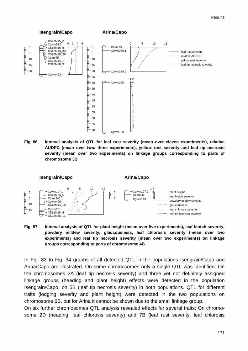
Results
171
Fig. 86 Interval analysis of QTL for leaf rust severity (mean over eleven experiments), relative
AUDPC (mean over two/ three experiments), yellow rust severity and leaf tip necrosis severity (mean over two experiments) on linkage groups corresponding to parts of chromosome 3B
Fig. 87 Interval analysis of QTL for plant height (mean over five experiments), leaf blotch severity,
powdery mildew severity, glaucousness, leaf chlorosis severity (mean over two experiments) and leaf tip necrosis severity (mean over two experiments) on linkage groups corresponding to parts of chromosome 4B
In Fig. 83 to Fig. 94 graphs of all detected QTL in the populations Isengrain/Capo and Arina/Capo are illustrated. On some chromosomes only a single QTL was identified: On the chromosomes 2A (leaf tip necrosis severity) and three yet not definitely assigned linkage groups (heading and plant height) effects were detected in the population Isengrain/Capo, on 5B (leaf tip necrosis severity) in both populations. QTL for different traits (lodging severity and plant height) were detected in the two populations on chromosome 6B, but for Arina it cannot be shown due to the small linkage group. On six further chromosomes QTL analysis revealed effects for several traits: On chromo-some 2D (heading, leaf chlorosis severity) and 7B (leaf rust severity, leaf chlorosis
XS23M15_3 Xgwm533 XS16M16_6 XS12M13_33 XS26M18_20 Xbarc75 XS26M14_1 XS13M20_9
Xgwm493
0 2 4 6
Isengrain/Capo
0 5 10 15 20
Xbarc75 Xgwm389.1
Xgwm389.2
0 5 10 15
Xgwm285
Xgwm108
1 2
Arina/Capo
0 5 10 15 20 25 30 35 40 45 50 55 60 65 70
Xgwm107.2 XS19M23_5 Xbarc340.1 Xgwm495 XS18M14_10 Xgwm251 XS11M18_6 XS23M15_11
0 5 10 15
Isengrain/Capo
0 5 10 15
Xgwm107.2 Xbarc25 Xgwm149
1 2
Arina/Capo
0 5
leaf rust severity relative AUDPC yellow rust severity leaf tip necrosis severity
plant height leaf blotch severity powdery mildew severity glaucousness leaf chlorosis severity leaf tip necrosis severity

Results
172
severity) only in the population Isengrain/Capo, on 3A (glaucousness, leaf chlorosis severity) and 5A (plant height, lodging severity and leaf tip necrosis severity) solely in Arina/Capo. The QTL detected on chromosome 3B were only partly consistent in both populations, the effects on 4B were different.
Fig. 88 Interval analysis of QTL for plant height, lodging severity and leaf tip necrosis severity
(each mean over two experiments) on a linkage group corresponding to a part of chromosome 5A
Fig. 89 Interval analysis of a QTL for leaf tip necrosis severity (mean over two experiments) on
linkage groups corresponding to parts of chromosome 5B
Fig. 90 Interval analysis of a QTL for lodging severity (mean over four scorings in three
experiments) on a linkage group corresponding to a part of chromosome 6B
Xgwm1057
Xbarc360
1 2 3
Arina/Capo
0 5 10 15 20 25
Xbarc319.1
Xgwm604
1 2 3 4 5
Arina/Capo
0 5
XS23M13_10 XS26M21_22
XS23M14_7
XS19M17_16 Xgwm604 Xwmc500.1
0 1 2 3 4
Isengrain/Capo
0 5 10 15 20 25
XS11M14_5
Xgwm518.1 Xgwm518.2
XS26M21_15 Xgwm133.3 Xwmc397 XS11M17_8
Xbarc24
0 1 2 3 4
Isengrain/Capo
0 5 10 15 20 25 30 35
leaf tip necrosis severity
plant height lodging severity leaf tip necrosis severity
lodging severity

Results
173
Fig. 91 Interval analysis of QTL for leaf rust severity (mean over eleven experiments), relative
AUDPC (mean over two experiments), the appearance of teliospores and leaf chlorosis severity (mean over two experiments) on a linkage group corresponding to a part of chromosome 7B
Fig. 92 Interval analysis of a QTL for heading (mean over eleven experiments) on a linkage group
not definitely assigned to chromosomes 2B, 2D, 6A, 6B or 7B
Xwmc25.1 Xgwm132.3 XS26M21_24 XS26M14_8 XS22M20_7 XS22M20_8
XS23M14_19
0 1 2 3 4 5
Isengrain/Capo
0 5 10 15 20 25 30
XS12M13_30
XS20M23_28 XS26M14_4 Xwmc273.2 Xwmc273.1 Xbarc32.2 XS22M17_24 XS11M26_2 Xwmc70 Xwmc10.2 Xbarc340.3 Xgwm146.1 Xgwm344.1 Xgwm132.1 XS19M23_13 XS18M20_10 Xwmc500.3 Xwmc232 Xbarc182 Xwmc557.1 XS23M13_22 XS20M23_39 XS20M11_6 XS14M12_14 XS23M15_15 XS26M18_24 XS23M13_35 XS12M18_4 XS23M17_20 XS22M13_7 XS18M14_11 XS11M14_23 XS12M13_26 XS12M13_12
0 10 20 30
Isengrain/Capo
0 5 10 15 20 25 30 35 40 45 50 55 60 65 70 75 80
leaf rust severity relative AUDPC appearance of teliospores leaf chlorosis severity
heading

Results
174
Fig. 93 Interval analysis of a QTL for plant height (mean over five experiments) on a linkage group
not definitely assigned to chromosomes 2B, 4B, 5A or 7B
Fig. 94 Interval analysis of a QTL for plant height (mean over five experiments) on a linkage group
not definitely assigned to chromosomes 6A or 6B
Xbarc10.1
XS26M21_23 XS22M17_5 XS22M17_6 XS20M11_14 XS20M23_31
1 2 3 4
Isengrain/Capo
0 5 10 15
XS23M13_14
XS23M15_18 XS14M12_24
Xbarc146.2
1 2 3 4 5
Isengrain/Capo
0 5 10 15 20 25
plant height
plant height

Results
175
5.5 Epistatic Interactions As has been shown in the previous results, the QTL of Capo and Isengrain were best seen in different experiments. Therefore epistatic interactions were calculated several times: for the mean of 3, 6 and 11 experiments as well as the 24 single assessments of leaf rust severity measured by the percentage of infected leaf area, leaf rust severity measured by the relative AUDPC (single experiments and the mean over them) and the appearance of teliospores. In total 1,647 significant (α = 0.0001) epistatic interactions were detected for these 31 different traits: 311 different markers from all linkage groups were involved in 1,230 pairs. On average one marker showed 21 significant epistatic interactions with 14 other markers, with a maximum of 95 interactions or 52 other markers. Epistatic interactions of a single marker combination were on average significant for just two traits. Because of the extremely high number of tested interactions – the framework map still comprised 318 markers, thus more than 1.6 million tests were performed in total – and despite the very low risk of the first kind (α = 0.0001) many of the epistatic interactions that were significant seemed to be detected just by chance. There was no obviously visible pattern: Only in a few cases markers located in two different QTL regions were involved in significant epistatic interactions. Two markers (XS16M16_6 and XS26M14_1) from the 3B QTL region and Xgwm148 from the 2B QTL region gave significant epistatic interactions, but only for one trait each. Similar epistatic interactions of XS26M14_1 and a third marker (XS23M15_3) with XS11M26_3 from the 7B QTL were only detected for one trait each. Also in the case of all other QTL markers, epistatic interactions were only significant for one or a few traits, which were not consistent over neighboring markers. When using the original map for the linkage groups comprising the Isengrain and Capo QTL and all that can possibly be assigned to chromosome 2B, where Lr13 previously described for Capo is located, only three markers located within the Isengrain QTL were identified that were involved in significant interactions with several other markers. Two of these markers were assigned to different parts of chromosome 2B the other was located in the linkage group 2BD6AB7B. Calculating ANOVA with and without the interaction term marker1*marker2 the improvement of the model when regarding the interaction term was less than 4 %. Due to these low values and no visible pattern, only additive, but no epistatic interactions between chromosomal regions are assumed in the population Isengrain/Capo.
5.6 SSR Marker Haplotype Comparison In order to get more information to which resistance genes the QTL for leaf rust resistance on chromosomes 3B and 7B might be related, a haplotype analysis with SSR markers either mapped in these regions or reported for the Lr genes of interest (Table 5) was performed. Primer Wmc221 revealed the same fragment size for Capo and Isengrain. Therefore it was possible to use only those markers already mapped in the population Isengrain/Capo.

Results
176
Capo and Isengrain alleles of the three SSR markers mapped near the QTL identified on the short arm of chromosome 3B were compared to nine different cultivars carrying Lr27. In addition fragment sizes of the Furore and Arina alleles were recorded. The results are presented in Table 91. Fragments of the same length as the Capo allele are highlighted in green (codominant markers) or light green if only Isengrain produced a fragment. Isengrain alleles are shown in red color. Fragments differing from both Capo and Isengrain are highlighted in yellow. All fragments that were repeatedly not scorable unambiguously are indicated by a question mark. At the position of the marker Xgwm493 Capo has the same allele as all lines except Shortim, Timgalen and possibly Gatcher. The size of the Capo fragment associated with Xbarc75 coincides at least with four cultivars, but at the position of the dominant marker Xgwm533 that was mapped next to the QTL, in contrast to Capo (and Furore) all lines except Gatcher showed a fragment. Table 91 Results of the haplotype comparison with lines carrying Lr27. For each cultivar the
previously described resistance genes (see Table 6 for references) are listed. The order of the markers is the same as in the genetic map (Fig. 45). C: same fragment size as Capo, I: Isengrain, -: no visible fragment, N: size different from C and I, ?: in doubt
Cap
o
Isen
grai
n
Cra
nbro
ok
Sho
rtim
Tim
gale
n
Hop
e
Gat
cher
Kar
l
Kal
kee
Res
cue
War
igo
Fur
ore
Arin
a
Lr
Marker
13+ 14a 27 i.a.
27 i.a.
27 i.a.
14a+27 i.a.
14a+27 i.a.
14a+27 i.a.
14a+27
14a+27
14a+27
13?
Xgwm533 - I N N N N - N N N N - N Xbarc75 C I C C C N I I C I ? Xgwm493 C I C I ? C ? C C C C C C
For the QTL region on the long arm of chromosome 7B fragment lengths of eleven lines carrying Lr14a and ten lines carrying Lr19 generated by 13 SSR markers were analyzed. In order to know from which parent the Isengrain allele originated, Apollo and Soissons were included in the analysis. In Fig. 95 haplotype comparison is shown on the example of marker Xgwm132.1. The primer produces two further fragments polymorphic between the parents, but assigned to other chromosomes. The fragment associated with the Isengrain allele conferring resistance is marked by a red line. In the left part cultivars with Lr14 are arranged, in the right with Lr19 and in the middle Isengrain’s parents, Isengrain, Capo, Furore and Arina. Fragments of the three lines at the very left are only interesting in the case of 3B markers as these carry Lr27. Transfer was confounded with Transfer-12 which carries Lr19 and included into the analysis although it has only Lr9. In addition to the markers previously mapped to the region associated with the QTL on chromosome 7B, Xgwm44 was used that was assigned to chromosome 7D, but described by Li et al. (2006) as a marker for Lr19. In Table 92 colors of the Capo and Isengrain alleles are interchanged compared to Table 91, as in this case the positive allele originated from Isengrain and not from Capo.

Results
177
Fig. 95 Haplotype comparison of SSR marker Xgwm132.1. The fragment of the Isengrain allele
associated with leaf rust resistance is marked with a red line.
Table 92 Results of the haplotype comparison with lines carrying Lr14a and Lr19. For each cultivar the previously described resistance genes (see Table 6 for references) are listed. The order of the markers is the same as in the genetic map (Fig. 57). C: same fragment size as Capo, I: Isengrain, -: no visible fragment, N: size different from C and I, ?: in doubt
Cap
o
Isen
grai
n
Apo
llo
Soi
sson
s
Hop
e
Gat
cher
Kar
l
Kal
kee
Res
cue
War
igo
Cou
rtot
Inia
-66
Réc
ital
For
no
Ren
an
F4
34/1
/1/9
8
F4
34-9
F4
34-1
0
F4/
8
F4
1/27
/2
Aga
tha
Agr
us
Han
d
Kaw
fars
Fun
dule
a-29
Lr
Marker
13+ 14a 13+26
14a 14a+27i.a.
14a+27i.a..
14a+27i.a..
14a+27
14a+27
14a+27
14a 14ai.a.
14a 14a 14a+37
19 19 19 19 19 19 19 19 19 19 i.a.
Xwmc273.2 C I ? I C N I N I C I I I C N ? I ? I I N N Xwmc273.1 C - - - C C - C - C ? - - C C C - - C - ? C - C Xbarc32.2 C I N I N N N N N N I I I N N N N N I N I C C N C Xwmc70 - I ? I I I ? - N I I I I I ? ? N N N - N ? ? - I Xwmc10.2 - I - I I I - - N I I I I I - I - I N - N I - - I Xbarc340.3 - I - I - - - N N - I I I - - - - I - I - - - ? Xgwm146.1 - I - I I ? - - N I I I I I - - - N - N - - N Xgwm344.1 - I - I I I - N - I I I I I - - - - - - - - - Xgwm132.1 - I I I I N ? N ? ? I I I I I I I I - I ? ? - ? ? Xwmc500.3 C - ? - N ? C C - - - C - ? N - - C - C C C C Xwmc232 C - - - - - C - - - - - - - C - - - - - - C - - C Xbarc182 C - N - N ? N ? N - - - N N N N N ? N ? C C N C Xwmc557.1 C - N - - N - N - - - - - - - C - - - - - C N - ?
Xgwm44 (7D) C I I C N N N N N N C N N N C C ? N N N N N N N
← Xgwm132.3
← Xgwm132.3
← Xgwm132.2
← Xgwm132.2
← Xgwm132.1

Results
178
Six out of the thirteen markers used for haplotype analysis of the 7B QTL were dominant for the Isengrain allele, four for the Capo allele. Whether the alleleles of two genotypes are the same can only be determined when they produce the same fragment length. Missing fragments can arise from the same or different allelic constitutions. Isengrain shares at least the alleles of all dominant markers with its parent Soissons and the cultivars Courtot, Inia-66 and Récital. At least five alleles of Isengrain, Forno and Hope coincide. With Warigo Isengrain has at least four alleles in common, with Gatcher three and with Karl and Renan one allele. All these lines carry Lr14a. The lines carrying Lr19 share only one or two alleles definitely with Isengrain. Agrus, Hand and Fundulea-29 are more similar to Capo than to Isengrain. In the case of marker Xgwm44 that was mapped to chromosome 7D the Isengrain allele was inherited from Apollo. Most of the lines showed a fragment different from Capo and Isengrain, only three lines with Lr14a and one or two with Lr19 had the same fragment size as Capo.

Discussion
179
6 Discussion
6.1 Leaf Rust Resistance No method of statistical analysis can make up for imprecise phenotypic assessment, but gives misleading results. To avoid biased data due to environmental influences as far as possible, altogether 42 field experiments were conducted: 18 for the population Isengrain/ Capo and 12 each for the two validation populations Arina/Capo and Furore/Capo. Artificial inoculation with leaf rust spores was performed to ensure an even disease pressure across the whole experimental site. In the years 2005, 2006, and in 2007 in one experiment infection with leaf rust in Tulln occurred very late in the growing season, however, and it was impossible to evaluate differences between lines before leaf senescence proceeded too far to assess a reasonable amount of lines. One reason was doubtlessly Capo’s medium susceptibility to Septoria leaf blotch (BAES 2013b). To delay Septoria nodorum infection without affecting leaf rust development, especially the antifungal agent Prochloraz® seemed to be suitable. Despite the same procedure for collection and storage of spores and the preparation of water based inoculum, control inoculations in the climate chamber revealed that at least in one case infection with leaf rust did not occur. Obviously these tests should not be omitted as leaf rust development is much faster under the favorable conditions of the climate chamber and the greenhouse. Thus, field inoculation can – if necessary – be repeated considerably earlier. Apart from the aggressiveness of the inoculum itself, inoculation method, plant developmental stage and the environmental conditions seemed to have a big influence on the success of leaf rust infection. Direct spraying of the plants (Micron® Sprayer and inoculation of spreader row plants) appeared to be more effective than planting of infected seedlings. A disadvantage of the Micron® Sprayer is the large amount of spores required. The assistance of many persons is the disadvantage of performing inoculation of individual spreader row plants with subsequent coverage in a reasonable time on a whole experimental site. As it was even impossible to influence humidity because a mist irrigation system was not available, repeated inoculations were necessary. Collection of spores was very laborious and thus availability of inocula limited. Therefore only spreader row plants of every second row were sprayed, but at two occasions within a few days. Another challenge was the disease assessment itself. Due to the large number of field trials in some years and experiments performed by project partners, scoring had to be done by different persons. Reproducibility of leaf rust assessment by means of the used scoring aid is discussed in a separate chapter. In 14 experiments of the population Isengrain/Capo leaf rust severity was assessed, as well as in twelve field trials of the population Arina/Capo and seven of Furore/Capo. Not all data were suitable for further statistical analysis, as in a few cases the infection level was too low for detecting clear differences between lines.

Discussion
180
6.1.1 Inter-rater and Intra-rater Reproducibility
Studies on reproducibility of disease assessment either focus on whole plots, the whole plant or on single plant parts, mainly leaves. Plants can be observed in greenhouse or field experiments. Different statistical tests can be applied to identify reproducibility of assessments as reviewed by Bock et al. (2010). The effect of field conditions has to be taken into account comparing the results of this work with greenhouse experiments. Field trials to study methods of determining disease severity were conducted e.g. by Large and Doling (1962) and Lipps and Madden (1989), working on powdery mildew of cereals, and Vereijssen et al. (2003) working on Cercospora leaf spot in sugar beet. As Large (1966 cited in Zadoks and Schein 1979) pointed out, plants to be scored for disease severity (% infected leaf area) frequently do not fit the scoring aid: pustules are larger or smaller than shown or they may not be equally distributed over the whole leaf area but more concentrated towards the leaf base. One possible reason for differences between assessments is how a rater assigns disease severity to the classes of the scoring aid in these cases. Sherwood et al. (1983) proved that estimates were different for varying size resp. number of lesions despite that the same leaf area was covered with pustules, and that larger symptoms were estimated more accurately. Additionally Forbes and Jeger (1987) showed that the plant structure influenced estimates. Hau et al. (1989) found influences of leaf shapes on estimates when comparing scores for oval apple and linear barley leaves. However, differences in leaf shapes between different wheat genotypes won’t be big enough for such an influence. But it is doubtful, whether disease severity of wheat plants with twisted leaves can be assessed correctly and reproducibly. This possible error can’t be tested in experiments with prepared plant parts (or photographs, drawings, sketches,…). In outdoor assessments additional influences may be the position of the sun and whether only the infection of the flag leaf or of all upper leaves is taken into account. In contrast to experiments of repeated disease assessments in the laboratory with constant light, solar radiation on the field is varying much. Differences between green to yellow leaves and reddish-brown pustules can be perceived better in the morning and afternoon or on cloudy days than about noon on sunny days. Wet leaves because of dew or on rainy days reduce the ability to distinguish colors. Vereijssen et al. (2003) detected influences in error susceptibility of the two compared disease assessment methods if plants were wet, varieties darker colored or the sunlight was bright. Hau et al. (1989) did not find any effect neither of leaf nor of lesion color on the estimates, but they were just comparing bright and dark lesions and bright and dark apple leaves under laboratory conditions. In the course of the study data of repeatedly scored plants by four different raters were gained. In 2004 rater one scored leaf rust severity of more than 3.500 plots. In 2006 and 2007 rater one and two did almost all scorings together, all in all more than 5.000 plots. In the same year or the past few years, rater three and four had scored over 1.000 plots. In every case the same scoring aid was used. Therefore all four raters had pretty much experience in the assessment of leaf rust severity using the same scoring aid before the scorings to be compared.

Discussion
181
Based on the available data, there seems to be no clear tendency that either for the classes for lower or higher leaf rust infection reproducibility of the assessment calculated as the percentage of identically scored plots is better. Even if the class with zero infection is not taken into account, it can’t be said whether there is a change in reproducibility with increasing severity level or decreasing class width. This is in contrast to the results of e.g. Sherwood et al. (1983), Forbes and Jeger (1987), Hau et al. (1989), and Smith et al. (2005) who studied the accuracy of disease assessment and unveiled a correlation between estimation error and disease severity level. Intra-rater reproducibility measured by the coefficient of determination for absolute differences (% infected leaf area) was between 0.86 and 0.92. Nutter et al. (1993) who studied dollar spot (Sclerotinia homoeocarpa) of bentgrass (Agrostis palustris) observed values between 0.83 and 0.93. Regarding the regression parameters, differences were larger: In the present study the values of the intercept varied between -5.64 and 1.13, the values found by Nutter et al. (1993) were lying between -2.66 and 0.74. Values of the slope varied between 0.98 and 1.11, in the study by Nutter et al. (1993) they were lower, lying between 0.80 and 0.93. The value of the correlation coefficient varied between 0.93 and 0.96, thus being higher than observed by Nita et al. (2003), who studied Phomopsis leaf blight (Phomopsis obscurans) of strawberry (Fragaria x ananassa). The value using the scale developed by Horsfall and Barratt (1945 cited in Horsfall and Cowling 1978) was 0.81. Inter-rater reproducibility measured by the coefficient of determination for absolute differences (% infected leaf area) was between 0.72 and 0.94. Nutter et al. (1993) observed slightly lower values (0.70 - 0.89). Godoy et al. (1997) studied different diseases and discovered a dependency on the disease with values of the coefficient of determination lying between 0.43 and 0.95. The values of the intercept were lying between -2.08 and 2.46. Nutter et al. (1993) got values between -0.42 and 6.95. The slope between estimates of different raters in the present study varied between 0.90 and 1.28, in the study by Nutter et al. (1993) between 0.74 and 0.88. The correlation coefficient was between 0.85 and 0.97, thus being higher than the values observed by Nita et al. (2003) that were all below 0.80. It seems that the intra-rater reproducibility remains constant over the three days of scoring in the year 2008 whereas the inter-rater reproducibility is best on the second day after joint scoring of 52 lines in the morning, and worst on the third day without any joint scoring and after separate rating of several hundred lines. Slightly lower values of the mean and maximum values of the absolute differences between the repeated assessments of rater one and two on the second day in 2008 could indicate that joint scoring of standard lines with different disease severity and different pustule size and distribution helped reducing discrepancies between these two persons despite joint scoring of numerous plots in the previous years. Joint scoring should be done regularly before the start of assessments.

Discussion
182
The larger deviations on the third day of assessment may be due to separate scoring of hundreds of plots, different perception of higher disease severity, other light conditions due to changed weather conditions or even other factors not considered yet. Scoring aids depicting different disease severity classes are helpful. Results can be improved using scoring aids not just for different lesion shapes but also for different pustule sizes. The percentage of identically scored lines is in the range of 30 % to 68 %, meaning that on average (over the whole range of infected leaf area) between one and two third of the plants do not get the same score in a second rating, neither by the same nor by another rater despite using the same scoring aid. It seems that joint scoring before the beginning at least slightly increases this value. All tests were done despite the problem that these data were not collected with preceding experimental design for these tests from a statistical point of view, but for QTL detection. For that reason all results can only be seen for these particular compared assessments and experiments, and no general statement can be deduced. The most important reasons for this limitation are:
• Not all lines were scored two times on the same day by all four raters as would be required for this kind of experiment. Not even the 136 standard lines repeatedly scored in 2008 were always the same in every comparison for different reasons. This is the cause for all further limitations listed:
• Sample size was unequal for the different comparisons and in most cases larger
than necessary for the given precision requirement (α – risk of the first kind, β – risk
of the second kind, δ – minimal distance) of the particular statistical test.
• In only one case rating was done by person three and four and once rater three repeated a preceding scoring together with person two. Intra-rater reproducibility can only be determined for rater one (three times) and rater two (two times). On three days rater one and rater two scored the same standard lines. No comparison between rater one and three or four and between rater two and four can be made. Only in two cases a joint rating by two raters was repeated afterwards.
• The range of leaf rust severity was not the same in all assessments. In the first assessment in 2008 the most heavily diseased plants were scored with 40 %, whereas on the third day leaf rust infection progressed up to 80 %.
These results of intra-rater and inter-rater reproducibility suggest that further research is worthy as it has not yet been extensively studied by others considering whole plant plots of cereals in field experiments. The following items have to be regarded:
• Sample size must be determined for the particular statistical test (regression parameters, correlation coefficient or absolute difference of the repeated
assessments) based on the difference (δ) that should be detected and the risk of the
first kind (α) and of the second kind (β).

Discussion
183
• All raters must score the same plants on the same day. They should have about the same experience in using the scoring aid, either having all scored together once before or none of them having experience in joint scoring.
• Before the first scoring there must be a short joint instruction. • The same plants are scored again a second time by all raters.
• After the second and before the third separate scoring there must be a joint scoring on separately planted lines in order that the raters can adjust their ratings.
If the experiment is designed in this way, it should be possible to answer the following three questions:
• Do scores by one rater fit together? • Is the scoring aid on its own enough to get comparable scores by different raters?
• Do scores by different raters fit better if there has been an intensive instruction before with joint scoring of lines?
The question, how many lines are necessary for the joint scoring before the beginning can not be answered with this experiment. Therefore a further experiment would be necessary with varying numbers of plants for joint scoring training of different raters. As the results of QTL analysis show, the number of lines and field experiments was large enough to compensate not just for environmentally caused experimental errors but also for possible deficiencies in reproducibility of disease assessment.
6.1.2 Field Experiments
Data of eleven experiments of the population Isengrain/Capo were used for QTL detection and further statistical analysis. In the other three experiments maximum leaf rust infection was too low for detecting clear differences between lines. Capo, which was used as the resistant parent for developing the RIL population, was on average less infected than Isengrain. In the experiments in Probstdorf the difference was small and in the two experiments Schmida 2007 and Rust 2008, Capo exhibited even more symptoms than Isengrain. If different populations were tested at the same experimental site, Capo did not always get the same score. Only in a few cases it can be explained by experimental conditions: In the trial Tulln 2004 the population Furore/Capo was assessed about two days later than Isengrain/Capo. In Probstdorf 2006 differences in the average leaf rust severity in different parts of the field were obvious with borders that did not coincide with those between populations, but perhaps with the prevailing wind direction or variable soil conditions. In the experiments Rust and Schmida 2008 the populations Isengrain/Capo and Arina/Capo were rated by different persons. Moreover, in Rust the microclimate at one end of the experimental site was more humid because of a rivulet and tall trees on the other side of the street shading in the morning. Thus there was a decline in humidity from the first replication of the population Isengrain/Capo to the second replication of Arina/Capo.
Discussion
184
Although these two populations were rated by the same person in Tulln, Capo’s scoring value was higher in the population Arina/Capo, though assessed two days earlier. In the year 2007 rainfall was infrequent over large parts of the growing season. The experiments in Tulln were planted alongside a street with a shelter belt at one end, a few trees along the street and houses opposite the street. It seemed that differences in leaf senescence – and presumably leaf rust development – were influenced by these factors in periods of water stress of the plants. The population Isengrain/Capo was planted next to the shelter belt and leaf senescence of all cultivars occurred very early, making leaf rust assessment impossible: In the first repetition it was possible to assess leaf rust infection of both parental lines in one plot each, as well as of five standard lines. In the second repetition two plots of Capo, one of Isengrain, 16 standard lines and 13 RILs were scorable. On the same day all plots in the second repetition of the population Furore/Capo and 230 out of 233 RILs of the population Arina/Capo were assessed. Unfortunately two days earlier it was impossible to assess more than the Arina/Capo experiment and the first repetition of Furore/Capo. Between these two days average leaf rust infection increased by about 30 %. The parental lines planted within Arina/Capo – the population located furthermost from the shelter belt – (and 230 out of 233 RILs) were scorable even three days later. This difference in senescence of the parental lines could only be caused by environmental conditions. The other experiment, Tulln (M) 2007, was planted at a greater distance to the shelter belt. In this experiment plants were cut once in the spring in order to prolong vegetation and thus the scoring period for leaf rust severity. Whereas almost all RILs and all parental lines of the populations Isengrain/Capo and Furore/Capo were scorable on the second day of assessment, three days later it was possible to evaluate just ten and two RILs but not a single parental line. In the two rows located next to the street senescence of the experimental plots coincided with those of the neighboring spreader rows, thus being obviously influenced by environmental conditions. In the experiment Tulln 2004 spreader rows were checked for leaf rust infection between the two scoring dates. Differences across the experimental site appeared to be marginal. In the subsequent years evaluation of the spreader rows was impossible as these plants died earlier than the RILs. Hence, in the year 2008 assessment of spreader row plants was done a few days before the populations. Plots were rated on a 1 (= no visible pustules on any plant) to 5 (= pustules on almost all plants) scale. These data were included as a covariate in an analysis of covariance in order to see whether results changed. The estimated coefficient of heritability calculated by the means of variance components improved by only 0.012 (Isengrain/Capo), 0.003 (Arina/Capo) and was reduced by 0.002 (standard and parental lines). Leaf rust severity of the population Furore/Capo was only assessed in one experiment. In 2008 differences on the experimental sites were not as obvious as in the experiments Probstdorf 2006, Tulln 2007 and Tulln (M) 2007. For a reliable statement whether inclusion of the spreader row infection into the model improves results, data of experiments with remarkable environmental influences would be necessary.

Discussion
185
For all three populations correlation coefficients between different experiments were rather low, only in two cases of the population Isengrain/Capo and in one of the Arina/Capo the values of Spearman’s rho were significantly beyond 0.71. For Furore/Capo values were generally lower, maybe because of the smaller range of the population due to the close relationship and hence similarity of the two parental lines.
6.1.3 Detection of Leaf Rust Resistance QTL
Five QTL for leaf rust resistance (measured by the percentage of infected leaf area) were identified in the population Isengrain/Capo, but not a single was consistent over all experiments: A minor effect located on chromosome 2B was only detected in the experiment Schmida 2007. The allele conferring reduced susceptibility was inherited from Isengrain. Effects transmitted by Capo alleles were identified on chromosome 1B in the experiment Piešťany 2006 and the unassigned linkage group 2BD6AB7B in the experiments Piešťany 2006 and Rust 2009. These two were also detected in the experiment Piešťany 2006 if leaf rust infection was measured by the relative AUDPC. The major QTL detected on chromosome 3B was consistent over six single assessments of leaf rust severity and the mean, and the relative AUDPC in the experiment Piešťany 2006 and the mean. Whereas the 3B allele associated with reduced leaf rust severity originated from Capo, in the case of the most effective QTL detected in the population Isengrain/Capo on chromosome 7B, the positive allele was inherited from the susceptible parent Isengrain. This QTL was consistent over twelve experiments. The experiments in which the 7B QTL explained much of the phenotypic variance did not coincide with those of the effect on 3B. Ranking the experiments according to the phenotypic variation explained by the QTL, the experiment Piešťany 2006 was first for 3B, but only eleventh (out of twelve) for 7B, Probstdorf 2006 second vs. sixth, Tulln 2004 third vs. fifth. Based on the present results, it seems impossible to make a reliable prediction about the effectiveness of these two major QTL: Neither can it be said that the 3B QTL was losing effectiveness, although Capo’s susceptibility to leaf rust has been slowly increasing since it was brought to market in the year 1989 from 2 to 4 on a 1 (= absent/ very low) to 9 (= very strong) scale (BAES 2013b). In the year 2004 the QTL was less effective than in 2006, although the experiment in Probstdorf was conducted in an area where the pressure on the pathogen is high for adapting to Capo’s resistance due to neighboring breeder’s fields with a large amount of Capo progeny. Nor is there any obvious common property of the frequency distribution characteristics (mean, range, variance) of the experiments in which the 3B or the 7B QTL was most effective. Regarding the disease progress curves in the experiments Piešťany 2006 and Tulln 2008, it seemed that the 3B QTL was more effective at the beginning of infection causing delayed infection, whereas the 7B QTL reduced speed of spreading or symptom development and was better to recognize the more severe the leaf rust infection was, meaning that genotypes carrying the allele associated with resistance were much less diseased until the end of the vegetation period. These assumptions are only based on the results of two experiments. Further experiments

Discussion
186
with repeated assessments starting at that time when the first lines exhibit symptoms of leaf rust infection would be necessary. Results of repeated leaf rust assessments and the resulting relative AUDPC were highly correlated with the exception of three experiments (Fundulea, Nyon and Piešťany, all 2008): The values of Spearman’s rho between two subsequent scorings ranged from 0.69 to 0.94, between first and third assessment correlation was lower (0.49 - 0.90). As not only correlation between data of a single scoring and relative AUDPC was high (0.67 - 0.99), but the same QTL were identified, from this point of view the calculation of AUDPC seemed unnecessary as was also previously stated by Lipps and Madden (1989). In this project it has also been shown, that the effectiveness of QTL varied over the scoring period, and thus repeated assessments seem inevitable for the identification of all effects. Despite the low number of SSR markers applied to the population Arina/Capo, the QTL located on chromosome 3B and in the linkage group 2BD6AB7B were consistently identified. In both cases the alleles conferring increased resistance were inherited from Capo. In the population Arina/Capo the QTL on chromosome 3B was detected in seven out of eleven experiments. Using the mean over these seven trials for further analysis, LOD value (5.45) and R2 (0.14) of the peak marker Xbarc75 increased compared to the mean over eleven experiments, but heritability dropped to 0.858.
6.1.3.1 Minor Effect on Chromosome 1B
The QTL for leaf rust resistance inherited from Capo detected in the experiment Piešťany 2006 for a single assessment and for the relative AUDPC was located on the short arm of chromosome 1B in the marker interval Xgwm413–XS26M14_10. In a similar region QTL inherited from the variety Forno were identified: in a population Forno/Oberkulmer for the amount of infected leaf area (Messmer et al. 2000), in the population Arina/Forno in the marker interval Xgwm604–OA93 for the AUDPC and for the response to infection (Schnurbusch et al. 2004). In durum wheat a QTL for seedling infection type was associated with SSR marker Xwmc500.1 (Maccaferri et al. 2010). The resistance gene Lr26 is located on chromosome 1RS of rye and the short arm of 1B of wheat lines with the 1RS translocation (Mettin et al. 1973, Zeller 1973 both cited in McIntosh et al. 1995, Singh et al. 1990, Hsam 2000, Mago et al. 2002). Mago et al. (2005) located Lr26 near the centromere of 1RS by high-resolution mapping and mutation analysis. Lr26 conferring seedling resistance was detected frequently in European wheat cultivars (detailed references in Table 95), but the infection level of Thatcher NILs was generally moderate to very high (detailed references in Table 94). In Hungary they were the most susceptible averaged over the period 2004-2008 with almost 90 % infected leaf area (Vida et al. 2009). In the experiment in Tulln 2007 leaf rust severity of these plants was 50 % infected leaf area. Throughout the world isolates virulent to Lr26 were found (detailed references in Table 93, Kosman et al. 2004).

Discussion
187
Table 93 Studies on the virulence distribution of Puccinia triticina in different regions
isolates collected in different years in several regions and identified pathotypes L
r2a
Lr2
b
Lr2
c L
r13
Lr1
4a
Lr1
4b
Lr1
5 L
r19
Lr2
2a
Lr2
3 L
r26
Lr2
7+L
r31
Lr1
0+27
+31
Lr3
3 L
r35
Lr4
1 L
r44
references
850 isolates (53 pathotypes) from Western Europe 1995
x x x x x x x x Park and Felsenstein (1998)
isolates from 4 regions of Nebraska (US) 1992-1996 x x x x
Watkins et al. (1998)
575 isolates from 4 regions of Nebraska (US) 1995-1998 x x x x
Watkins et al. (2001)
260 isolates from Israel 1993-1997 x x x x x Manisterski et al. (2000)
2608 isolates (105 pathotypes) from 12 European countries 1996-1999 x x x x x x x x x
Mesterházy et al. (2000)
259 isolates (12 pathotypes) from Slovakia 1997-2000 x x x x x x x
Huszár et al. (2002)
253 isolates (21 pathotypes) from 4 South Atlantic States 1999 x x x x Kolmer (2002)
56 isolates (35 pathotypes) from Andalusia (ES, hexaploid + durum wheat) 1998-2000 x x x x x x x
Martínez et al. (2005)
1300 isolates (> 17 pathotypes) from 3 locations of the Ukraine 2002-2003 x x x x x x x x x x x x x
Elyasi-Gomari and Panteleev (2006)
isolates from 4 German regions 2001-2003 x x x x x x x x x x x x x
Lind and Gultyaeva (2007)
isolates from 7 European regions of the Russian Federation 2001-2003 x x x x x x x x x x x x x
Lind and Gultyaeva (2007)
10 isolates from the United States (+ 78 on durum from 7 countries 2000-2003) x x x x x x x x x x x x
Ordoñez and Kolmer (2007)
148 isolates (91 pathotypes) from North America 1980s-2005 x x x x x
Ordoñez and Kolmer (2009)
178/ 138 isolates from 4 Pakistan regions (10-11 locations) 2002-2004 x x x x x x x x x x x x x Rattu et al. (2009)
233 isolates (71 pathotypes) from 27 locations of the Czech Rep. 2005-2008 x x x x x x x Hanzalová (2010)
122 isolates (91 pathotypes) from 11 locations of the Slovak Rep. 2009-2011 x x x x x x x x
Hanzalová et al. (2012)
124 isolates (44 pathotypes) from 4 regions of Turkey 2009 and 2010 x x x x x
Kolmer et al. (2013)
74 isolates from Eastern Canada 1987 and 251 from the prairie region 1988 x x x x Kolmer (1992b)
289 isolates (46 phenotypes) from 4 regions of Canada 1995 x x x x
Kolmer and Liu (1997)
275 isolates (50 phenotypes) from 4 regions of Canada 1996 x x x x Kolmer (1998)
362 isolates (75 pathotypes) from 4 regions of Canada 1997 x x x x Kolmer (1999)
268 isolates (34 pathotypes) from 4 regions of Canada 1998 x x x x Kolmer (2001)
748 isolates from 6 regions of the United States 1990-2006 x x x x x
Kolmer et al. (2007a)
1120 isolates (54 pathotypes) from 7 regions of the United States 2000 x x x x Long et al. (2002)
477 isolates (44 pathotypes) from 8 regions of the United States 2001 x x x x
Kolmer et al. (2003)
785 isolates (52 pathotypes) from 8 regions of the United States 2002 x x x x
Kolmer et al. (2004)
580 isolates (52 pathotypes) from 8 regions of the United States 2003 x x x x
Kolmer et al. (2005)
757 isolates (52 pathotypes) from 8 regions of the United States (2000-)2004 x x x x (x)
Kolmer et al. (2006)
797 isolates (72 pathotypes) from 8 regions of the United States 2005 x x x x x
Kolmer et al. (2007b)
718 isolates (56 pathotypes) from 8 regions of the United States 2006
x x x x x Kolmer et al. (2008)

Discussion
188
Table 94 Studies on the effectiveness of leaf rust resistance (Lr) genes in different regions
near isogenic lines (NILs) tested in different years in several regions or against collected isolates L
r2a
Lr2
b
Lr2
c L
r13
Lr1
4 L
r14a
L
r14b
L
r14a
b
Lr1
5 L
r19
Lr2
2 L
r22a
L
r22b
L
r23
Lr2
6 L
r27+
Lr3
1 L
r10+
27+3
1 L
r33
Lr4
4 L
r48
references
4 Indian locations, 1978-1981, NILs/ cultivars
x x x x x Sawhney et al. (1982)
8 European locations 1998 and/or 1999, Thatcher (Tc.) NILs x x x x x x x x x x x x x
Mesterházy et al. (2000)
Eastern Ukrainian forest-steppe isolates 2002-2003, NILs x x x x x x x x x x x x
Elyasi-Gomari and Panteleev (2006)
Omsk (Western Siberia) 2003-2005, Tc, NILs x x x x x x x x x x x x x
Morgounov et al. (2007)
Adapazari (Turkey) 2005-2006, Tc. NILs + other differentials x x x x x x x x x x x x x x Akin et al. (2008)
5 Pakistan locations 2004-2006, Tc. NILs x x x x x x x x x x x x x x
Fayyaz et al. (2008)
Inoculum from 2 Ukrainian locations 2005, NILs x x x x x x x x x x x x
Elyasi-Gomari and Lesovaya (2009)
Central + Eastern Ukrainian forest-steppe 2007, Tc. NILs x x x x x x x x x x x x x
Elyasi-Gomari and Mikhailovno (2009)
4 Pakistan provinces 2002-2004 (10-11 locations), Tc. NILs x x x x x x x x x x x x Rattu et al. (2009)
Martonvásár (Hungary) 2004-2008, Tc. NILs x x x x x x x x x x x x x Vida et al. (2009)
2002-2005 Aschersleben, 2006-2009 Quedlinburg (DE), Tc. NILs x x x x x x x x x x x x x x x
Serfling et al. (2011)
Ardabil (Iran) 2007, 2008, 2010, 2012, NILs/ cultivars
x x x x x x x x x x x x x x Safavi and Afshari (2013)
Another resistance gene, Lr33, was mapped on chromosome arm 1BL at a distance of just 3.1 cM from the centromere and 2.6 cM from Lr26 (Dyck et al. 1987). In durum wheat Lr33 was associated with SSR marker Xwmc419 (Maccaferri et al. 2010). High frequencies of virulence to this gene are common (detailed references in Table 93 to Table 95). Average infected leaf area of Thatcher NILs carrying Lr33 was in Tulln 2007 40 %. In Martonvásár average infection in the period 2004-2008 was 80 % (Vida et al. 2009). Lr44 is located on chromosome 1BL at a distance of 5.4 cM from Lr33 (Dyck and Sykes 1994). In most of the regions almost all isolates are virulent to Lr44 and effectiveness is generally low (detailed references in Table 93 to Table 95). Average infected leaf area of Thatcher NILs carrying Lr44 was in Tulln 2007 35 %. In the terminal region of 1BL Lr46 was identified (Singh et al. 1998, William et al. 2003, Rosewarne et al. 2006). Lr51 is a resistance gene from Triticum speltoides that was transferred by Dvořák and Knott (1980) to the long arm of chromosome 1B (Helguera et al. 2005), Lr55 is derived from Elymus trachycaulis (McIntosh et al. 2005). Singh D et al. (2013) mapped Lr71, which they proved to be different from Lr33, Lr44 and Lr46, on chromosome 1B close to the centromere between the markers Xgwm18 and Xbarc187. Compared to the wheat consensus map (Somers et al. 2004), marker order in this region was inverted. Regarding the marker region of the detected QTL on 1B, the effect might correspond to Lr26, Lr33, Lr71, the QTL identified in the population Forno/Oberkulmer (Messmer et al. 2000), in durum wheat (Maccaferri et al. 2010), on 1RS in a population Beaver/Soissons

Discussion
189
by Singh et al. (2009) or the temporarily designated LrZH84 identified by Zhao et al. (2008). As Capo does not possess the 1RS translocation, the effect can not be due to Lr26 or the 1RS QTL. Table 95 Studies on leaf rust resistance (Lr) genes of hexaploid wheat grown in different regions
number of wheat cultivars tested against several pathotypes L
r2a
Lr2
b
Lr2
c L
r13
Lr1
4a
Lr1
4b
Lr1
5 L
r19
Lr2
2a
Lr2
2b
Lr2
3 L
r26
Lr2
7 L
r27+
Lr3
1 L
r10+
27+3
1 L
r33
Lr4
1 L
r44
references
71 Indian and Pakistani cultivars, 14 Mexican pathotypes
x x x x x x x x Singh and Gupta (1991)
50 Mexican cultivars, 18 Mexican pathotypes x x x x x x x x x Singh and Rajaram (1991)
48 Indian + 63 exotic cultivars, 6 Indian pathotypes x x x x x x x x x x x x Kaur et al. (2000)
72 European cultivars, 10 Australian pathotypes x x x x x x x x x Winzeler et al. (2000)
91 Western European cultivars, 20 Australian pathotypes x x x x x x x x x Park et al. (2001)
70 cultivars from the UK, 10 Australian pathotypes x x x Singh D et al. (2001)
37 Japanese cultivars, 11 Mexican pathotypes x x x x x x x x x x x x x Singh RP et al. (2001b)
35 cult.+ 17 breeding lines from the US, 16 isolates from the US x x x x Kolmer (2003)
225 cult. from KZ, MN, RU, 10 Europ. and Mediterranean isolates x x x x x x x x x x Singrün et al. (2004)
84 cult. from DK, FI, NO, SE, 12 Mexican pathotypes x x x x x x x x x x x x x x x Hysing et al. (2006)
105 European cultivars, 5 Australian pathotypes x x x x x x x x x x Pathan and Park (2006)
28 Spanish + 41 durum wheat cult., 12 (durum: 7) pathotypes x x x x x Martínez et al. (2007)
76 Pakistani cultivars, 14 Mexican pathotypes x x x x x x x x x x x x x x Rattu et al. (2010)
36 Iranian cultivars, 13 Iranian isolates x x x x x x x x x x x Boroujeni et al. (2011)
66 Argentine cultivars, 17 Argentine pathotypes x x x x x x x x Vanzetti et al. (2011)
43 Turkish cultivars, 13 pathotypes from CA, US, TK
x x x x x Kolmer et al. (2013)
6.1.3.2 Minor Effect on Chromosome 2B
A minor effect on leaf rust severity inherited from Isengrain was detected in the experiment Schmida 2007 and located on chromosome 2B around the position of marker Xgwm148. Several resistance genes have been mapped to 2B: Lr13 (McIntosh et al. 1995, Seyfarth et al. 2000, Bansal et al. 2008b), Lr16 (Dyck and Kerber 1971, McCartney et al. 2005b) and Lr23 (McIntosh and Dyck 1975 cited in McIntosh et al. 1995, Nelson et al. 1997) on the short arm, as well as Lr50 (Brown-Guedira et al. 2003) and Lr58 (Kuraparthy et al. 2007) on the long arm. Also Lr35 derived from Aegilops speltoides (Kerber and Dyck 1990) and Lr48 (Bansal et al. 2008b, Singh A et al. 2011) are located on chromosome 2B. Lr48 first detected by Saini et al. (2002) was mapped by Bansal et al. (2008b) to the short arm between the markers Xgwm429b and Xbarc7, thus in the region of Xgwm148 if compared to the wheat consensus map (Somers et al. 2004). Proximal to Lr48 they

Discussion
190
mapped Lr13. Singh A et al. (2011) located Lr48 on the long arm between the markers Xwmc175 and Xwmc332, and thus did not confirm the mapping to the short arm. Seyfarth et al. (2000) located Lr13 distal to marker Xgwm630. Lr23 transferred from Triticum turgidum var. durum to hexaploid wheat was found to be closely linked to Lr13 (McIntosh et al. 1995). Nelson et al. (1997) detected a gene transferred from Triticum tauschii on the homoeologous chromosome arm 2DS suppressing Lr23. In durum wheat Lr48 was mapped distal to SSR marker Xgwm148, Lr13 distal and Lr23 proximal to Xbarc55.1 (Maccaferri et al. 2010). Lr13 is abundant in wheat cultivars, but effectiveness is low as virulence to Lr13 is common. Also isolates virulent to Lr23 have frequently been detected and effectiveness is similar, although it occurs in fewer varieties (detailed references in Table 93 to Table 95, Park and McIntosh 1994). Leaf rust infection of Thatcher NILs carrying Lr13 was 60 % infected leaf area in the experiment Tulln 2007 and about 50 % in Martonvásár averaged over the period 2004-2008 (Vida et al. 2009). For Lr23 leaf rust severity was much lower: about 2 % in Tulln and likewise not differing significantly from zero in Martonvásár (Vida et al. 2009). Lr48 was just included in a single study by Serfling et al. (2011) and belonged to the group of lines with medium infection level. Further effects on leaf rust development have been identified on chromosome 2B: Messmer et al. (2000) detected a QTL for infected leaf area on 2BS 15 cM proximal to the centromere and maybe allelic to Lr13, but maps are not comparable. Also Rosewarne et al. (2008) identified a QTL for slow rusting resistance on 2BS in the region of the Lr13 locus. Xu et al. (2005c) found significant effects on slow rusting resistance measured by the AUDPC, infection rate measured by the daily disease progress rate (AUDPC/day) and final severity (%) in the region proximal to SSR marker Xbarc167. It coincided with a QTL for prolonged latent period measured by the average number of days from inoculation to epidermis rupture of the first uredinium (Xu et al. 2005b). In a similar region Nelson et al. (1995) detected an effect on mean latent period. Leonova et al. (2007) detected a QTL for adult plant resistance on chromosome 2B in the marker interval Xgwm257-Xgwm120 coinciding with a QTL for seedling resistance. Compared to the wheat consensus map (Somers et al. 2004) and the Isengrain/Capo map the markers Xgwm148 and Xgwm257 mapped in reversed order and closer to each other. A QTL for leaf rust severity was identified by Rosewarne et al. (2008) in the region between marker Xgwm257 and Xgwm120. Unfortunately the SSR markers located closer to the detected effect on leaf rust infection were not mapped by Somers et al. (2004). In durum wheat Maccaferri et al. (2010) found association of Xwmc770 and the tightly linked loci Xgwm410.1/ Xgwm148/Xbarc183.1 with differences in seedling infection type. The QTL for relative disease severity of durum identified by Marone et al. (2009) in a single field experiment was located on the long arm in the marker region Xbarc101-Xwmc441, in the growth chamber in the Xcfd73-Xwmc441 interval. The other resistance genes were mapped clearly outside the region in which the minor effect was identified in the experiment Schmida 2007: Lr16 was the terminal locus of 2BS in three populations, distal to Xwmc764 (McCartney et al. 2005b). Lr50 was transferred

Discussion
191
from Triticum timopheevii ssp. armeniacum and located on the distal end of 2BL near marker Xgwm382 (Brown-Guedira et al. 2003). Also Lr58 occurred on the distal end of the long arm of chromosome 2B, but in a wheat-Aegilops triuncialis translocation (Kuraparthy et al. 2007). Lr35 was mapped by Seyfarth et al. (1999). Even by means of the Triticum aestivum maps Synthetic x Opatha (Nelson et al. 1995) and Synthetic x Opatha, BARC available from the GrainGenes database (USDA 2014) their map is hardly comparable with the wheat consensus map (Somers et al. 2004). It seems that Lr35 is located in the region around SSR marker Xgwm120. As the detected QTL originated from Isengrain and not from Capo, who carries Lr13 (Winzeler et al. 2000, Park et al. 2001, Mesterházy et al. 2002), and due to the marker position, it seems more likely to correspond to Lr48 or one of the other identified effects than to Lr13, Lr23 or any of the resistance genes mapped to the distal ends of chromosome 2B, although Triticum timopheevii occurs in the pedigree of Isengrain’s parent Apollo (Martynov et al. 2006).
6.1.3.3 Minor Effect on Chromosome 3A
On chromosome 3A the only minor leaf rust resistance QTL (% infected leaf area) inherited from Arina was detected in the experiment Reichersberg 2008. It was associated with SSR marker Xgwm720. In the population Arina/Forno no effect was identified on this chromosome (Schnurbusch et al. 2004), maybe because a QTL transmitted by Forno alleles was detected in the population Forno/Oberkulmer on the long arm near the centromere (Messmer et al. 2000). As far as the Forno/Oberkulmer map (Messmer et al. 1999) is comparable to the Arina/Capo map, it seems possible that the effects are located in a similar region. In durum wheat Maccaferri et al. (2008) detected a QTL for leaf rust severity measured by the percentage of infected leaf area effective at the early and medium stage and also for the AUDPC in the marker interval Xbarc45-Xwmc664 and distal (Mantovani et al. 2008). In a subsequent study the SSR markers Xwmc664 and Xwmc388.2 were associated with effects on seedling infection type and adult plant resistance (Maccaferri et al. 2010). Lr63 was introgressed from Triticum monococcum to common wheat and located on the short arm of chromosome 3AS, very closely linked to Xbarc321 and Xbarc75 (Kolmer et al. 2010). From Aegilops speltoides ssp. ligustica Lr66 was transferred to chromosome 3A of wheat (Marais et al. 2010b). As these introgressions happened just recently, it is unlikely that Arina, which was released in 1981 (Martynov et al. 2006), carries one of these genes.
6.1.3.4 Major Effect on Chromosome 3B
The only major leaf rust resistance QTL transmitted by Capo alleles was mapped to the short arm of chromosome 3B. It was consistent over single assessments of infected leaf area (six single experiments, mean over three and six experiments) and the relative AUDPC (experiment Piešťany 2006, mean over two experiments). The results of the

Discussion
192
population Isengrain/Capo were also verified in the population Arina/Capo, for which it was consistent over single assessments of seven experiments and the mean over eleven experiments as well as for the relative AUDPC of both experiments and the mean over them. As the marker order of the 3BS region of the Isengrain/Capo map differed from the wheat consensus map (Somers et al. 2004), the sequence of the few and partly not linked markers in the population Arina/Capo might differ from that shown in Fig. 45. Depending on the experiment, two different AFLP markers were closest in the population Isengrain/Capo with the SSR marker Xgwm533 lying in-between them. In single point ANOVA for means over eleven experiments and the mean relative AUDPC (two experiments) of the population Arina/Capo Xgwm533 was not significant. Xgwm389.1 which was throughout next to the QTL peak in this population revealed no polymorphism between the cultivars Isengrain and Capo and thus was not usable for genotyping. On the short arm of chromosome 3BS the resistance gene Lr27 is located (Singh and McIntosh 1984). It is only effective if the complementary gene Lr31 on 4BS (Singh and McIntosh 1984, McIntosh et al. 1995) or 4BL (Nelson et al. 1997) is present, too (Singh and McIntosh 1984). Just recently, Ingala et al. (2012) mapped a gene from the Argentinean durable leaf rust resistant cultivar Sinvalocho MA to this 3BS region. It was completely linked to marker Xgwm533 and designated LrSV2. As it confers adult plant resistance in contrast to the seedling resistance gene Lr27, further studies are required to find out, whether they are allelic. Faris et al. (1999) detected an effect on seedling leaf rust resistance in the Lr27 region in an Opata85/W-7984 (synthetic wheat) cross. In a population Frontana/Remus Steiner (2003) identified a major QTL for leaf rust resistance inherited from Frontana distal to Xgwm389. The most distal marker in the map was Xgwm493, thus marker order was inverted compared to the wheat consensus map (Somers et al. 2004) and the Isengrain/ Capo map. Distal to Xgwm493 Marza et al. (2006) identified a QTL for leaf rust reaction (% severity) consistent across environments in a population Ning7840/Clark (Chinese facultative wheat/US soft red winter wheat). In only one experiment Messmer et al. (2000) detected an effect in the population Forno/Oberkulmer transmitted by the Oberkulmer allele, which they assigned to the long arm of chromosome 3B near the centromere. In a similar region Maccaferri et al. (2010) found effects on adult plant resistance of durum measured by the AUDPC associated with the SSR markers Xgwm685 and Xbarc203 located in the centromeric and the proximal region of the long arm. Also the QTL for leaf rust resistance identified by Singh et al. (2009) on the short arm in a population Beaver/Soissons was effective in just one field experiment, another on the long arm in two experiments. Unfortunately no map with the linked AFLP and DArT markers is available. A further QTL for field infection type and infected area was detected on the long arm of chromosome 3B in a region distal to SSR marker Xbarc164 (Chu et al. 2009). WMS493 is a probe for Lr27 and Xgwm493-3B (USDA 2014). Marker Xgwm493 was mapped at a distance of about 20 cM from the peak marker, but in all experiments the LOD value has dropped below the threshold at this map position. Unfortunately markers mapped to 3BS in the population Isengrain/Capo clustered at the telomere and the

Discussion
193
nearest markers were located about 17 cM distal and 21 cM proximal to Xgwm493. Vast homology between Isengrain and Capo in this chromosomal region might be the reason for this low marker density: Out of eight SSR markers described for the terminal region of 3BS and tested for polymorphism between the parental lines Isengrain and Capo only five were applicable to the population, but two of them were mapped to other linkage groups. Nelson et al. (1997) mapped Lr27 in the marker interval Xbcd907-Xtam61, thus distal to Xgwm493 – as far as the maps are comparable in that detail. Therefore from this point of view it seems impossible to make any reliable statement whether Capo might carry Lr27 or not. As a consequence the haplotype comparison was performed (see 6.1.4 SSR Marker Haplotype Comparison). Australian pathotypes virulent to Lr27 and Lr31 occurred soon after the release of the decreasingly resistant cultivar Gatcher (McIntosh et al. 1995). The frequency of virulent isolates and the effectiveness differed considerably between studies (detailed references in Table 93 to Table 95).
6.1.3.5 Minor Effect on Chromosome 5A
In the population Arina/Capo a minor effect on leaf rust severity (% infected leaf area) located on chromosome 5A near SSR marker Xgwm1057 and transmitted by Arina alleles was detected in the experiment Tulln 2009. Tsomin et al. (1990) identified two complementary dominant genes for leaf rust resistance on the chromosomes 5A and 1D of the line Yantar. To the short arm of chromosome 5A (and to four further chromosomes) Lr38 from Agropyron intermedium was translocated (Friebe et al. 1993, 1996). In the population Forno/Oberkulmer a QTL for leaf rust resistance (leaf area covered with pustules) associated with the short arm of chromosome 5A and transmitted by Forno alleles was identified in a single experiment (Messmer et al. 2000), but it was not detected in the population Arina/Forno (Schnurbusch et al. 2004). On the same chromosome arm, proximal to SSR marker Xbarc10, Singh et al. (2009) detected a QTL for adult plant leaf rust resistance. Furthermore an APR gene and LrM (Tankimanova et al. 1993), LrM7 (Shulembaeva et al. 1997) and a resistance gene inherited from Triticum monococcum ssp. aegilopoides (Hussien et al. 1998) have been located on chromosome 5A of wheat. In durum wheat a QTL for seedling infection type on 5AS associated with SSR marker Xwmc489.1 was identified by Maccaferri et al. (2010). At the distal end of 5AL in the marker interval Xgwm595-Xgwm291 a QTL for relative latency period of adult plants was detected in the growth chamber (Marone et al. 2009). In the experiment Tulln 2007 Thatcher NILs with Lr38 were highly resistant with only 3 % infected leaf area, whereas in Martonvásár averaged infection over the period 2004-2008 was more than 80 %. Apart from that just in South America the effectiveness has been studied and Lr38 was reported to confer seedling resistance in Uruguay (Germán et al. 2007).

Discussion
194
6.1.3.6 Major Effect on Chromosome 7B
The most effective leaf rust resistance QTL detected in the population Isengrain/Capo was transmitted by Isengrain alleles and assigned to the long arm of chromosome 7B. It was consistent over single assessments of the percentage of infected leaf area of twelve experiments, the relative AUDPC and the appearance of teliospores. The QTL peak was located in the marker interval XS20M23_28-XS23M13_22 with Xgwm132.1 being closest in most of the experiments. As for the wheat consensus map (Somers et al. 2004) and the Arina/Forno map (Paillard et al. 2003), in the Isengrain/Capo map it is also a region of very high marker density: 28 AFLP and SSR markers were mapped within just 11 cM, thus about 2.5 markers/cM. In this chromosomal region the resistance gene Lr14a derived from Yaroslav emmer (Law and Johnson 1967, Kolmer 2007) and Lr14b from common wheat were identified (McIntosh et al. 1995). They were tightly linked with a recombination value of just 0.16 % and therefore considered as alleles, although it was possible to combine both in one single line (Dyck and Samborski 1970). Dyck and Samborski (1970) furthermore studied the inheritance of pathogenicity to the two alleles of Lr14 and found out that virulence to both was inherited by a single gene, which is recessive in the case of Lr14a, but dominant in the case of Lr14b. Lr14a showed high sensitivity to the environment (Browder 1980), and was more effective at temperatures below 20°C (Dyck and Johnson 1983 cited in McIntosh et al. 1995). Herrera-Foessel et al. (2008) mapped Lr14a 1 cM proximal to SSR marker Xgwm344 in durum wheat. Lr14a is a gene for seedling resistance present in many European wheat cultivars (Winzeler et al. 2000, Park et al. 2001, Pathan and Park 2006). In Northern Europe it is among the most common genes (Hysing et al. 2006). In the Canadian prairie region the release and large scale cultivation of the cultivar Renown and derivatives carrying Lr14a was followed by a rapid increase of virulence frequency to this gene (Kolmer 1991). This seems to be true for all wheat growing areas. All surveys revealed that virulence to Lr14a – and similar to Lr14b – is very common throughout the world (Table 93). Thus the level of protection in the field is very low (Table 94). Cultivars with Lr14ab were moderately resistant in India in the late 1970s/beginning 1980s (Sawhney et al. 1982), but susceptibility increased during the following decade (Sawhney et al. 1992). In durum wheat virulence to Lr14b is even more common than to Lr14a (Ordoñez and Kolmer 2007). In seedling tests Isengrain and its parental line Soissons showed a susceptible infection pattern to different isolates of Puccinia triticina similar to Thatcher NILs carrying Lr14a and were thus postulated to have Lr14a as a single resistance gene (Błaszczyk et al. 2004). Furthermore Yaroslav emmer, transmitting Lr14a, occurs in Apollo’s pedigree (Martynov et al. 2006). In the experiment in Tulln in 2007 about 60 % of the leaf area of Thatcher NILs with either of these two alleles exhibited leaf rust symptoms, in Martonvásár averaged infection over the period 2004-2009 of NILs carrying Lr14a was almost 90 % (Vida et al. 2009).

Discussion
195
Marone et al. (2009) identified a major QTL for reduced disease severity of adult durum wheat plants (measured by the percentage of leaf area covered with rust pustules) and for increased latency period (the time between inoculation and appearance of 50 % of the uredinia) on the long arm of chromosome 7B in a region very similar to Lr14a. As the used isolates of Puccinia triticina were virulent on Lr14a they concluded that the allele inherited from the cultivar Creso must be different and named it Lr14c. In the Creso derivative Colosseo Maccaferri et al. (2008) detected a major QTL effective across the entire cycle of disease development (QLr.ubo-7B.2) in the same chromosomal region. A much weaker but similar effect (QLr.ubo-7B.1) was identified in the proximal region of the short arm in the marker region Xwmc405.1-Xgwm573. But in this case Creso inherited the susceptible allele. Association mapping of elite durum lines revealed similar results: The main effect on seedling leaf rust infection type and adult plant response consistent across different field trials and isolates was associated with the marker interval Xgwm577-Xwmc10 in which Lr14 and QLr.ubo-7B.2 were located (Maccaferri et al. 2010). On the distal end of the short arm a further effect was associated with SSR marker Xwmc323 and another influence on seedling infection type with Xgwm1184 at the proximal end. In the population Arina/Forno Schnurbusch et al. (2004) identified a QTL for leaf rust resistance measured by the AUDPC using the Cobb scale (% infection) derived from Arina on the short arm of chromosome 7B in the marker interval sfr.BE427461-Xgwm573b. On the long arm in the region XksuD2-XgbxG218b they detected a QTL for leaf rust resistance measured by the AUDPC of response to infection inherited from Forno. As Park et al. (2001) found out that Forno carries Lr14a, Schnurbusch et al. (2004) assumed that the QTL detected on 7BL might correspond to Lr14a. In the population Forno/Oberkulmer several QTL for the leaf area covered with pustules were identified on chromosome 7B (Messmer et al. 2000): On the short arm in the marker interval Xpsr952-Xgwm46 the effect was transmitted by Oberkulmer alleles. It most likely corresponds to the QTL inherited from Arina in the population Arina/Forno, thus Forno seems to carry the adverse allele for this QTL. The other detected QTL were identified on the long arm. A major QTL which was effective in three out of four experiments was located in the Xpsr593c-Xpsr129c region. In the fourth experiment a major effect was detected in the proximal neighboring marker interval Xpsr350-Pwir232b. A further minor effect was identified in the distal Xglk750-Xmwg710a interval. In all three cases Forno transmitted the alleles associated with increased resistance. Unfortunately the Forno/Oberkulmer and the Arina/Forno map are hardly comparable in this chromosomal region. In a similar region as Schnurbusch et al. (2004) detected a QTL on 7BL in the population Arina/Forno an effect on field leaf rust severity in a population Synthetic/Opata was positioned (Nelson et al. 1997) and a QTL for adult plant reaction to leaf rust under conditions of natural infestation in another population Synthetic/Opata (Faris et al. 1999). In a single-seed-descent RIL population CI 13227/ Suwon 92 Xu et al. (2005b+c) revealed effects on latent period (average number of days from inoculation to epidermis rupture of the first uredinium), final leaf rust severity (%), AUDPC and infection rate (daily disease progress rate, AUDPC/day) associated with the marker interval Xbarc50-Xbarc182. Rosewarne et al. (2008) identified a QTL for leaf rust

Discussion
196
severity (%) in a RIL population Avocet-S/Attila in the marker interval Xgwm146-Xwmc273, Nyori (2010) a QTL for slow rusting resistance in a RIL population Avocet-S/Amadina proximal to Xwmc276. Davoyan and Tenovskaya (1996) introgressed two genes from Triticum miguschovea to common wheat, of which one seems to be located on chromosome 7B. William et al. (1997) detected a QTL for leaf rust resistance in the population Parula/Siete Cerros on 7BL which they speculated to be homoeoallelic to Lr34 on 7DS. As elaborated above, in several studies with different wheat and durum populations QTL were identified in or very tightly linked to the Lr14 region (Nelson et al. 1997, Faris et al. 1999, Messmer et al. 2000, Schnurbusch et al. 2004, Xu et al. 2005b+c, Maccaferri et al. 2008, Marone et al. 2009) and the region harboring the Isengrain QTL. As Lr14 is no longer very effective throughout the world (detailed references in Table 93 to Table 95), it seems that there might be alleles different from Lr14a and Lr14b as suggested by Marone et al. (2009), very closely located QTL or yet unknown factors influencing the effectiveness of this resistance gene. Sharma and Knott (1966) introgressed the resistance gene Lr19 from Agroypron elongatum (= Thinopyrum ponticum, Lophopyrum ponticum) to chromosome 7DL of wheat. By double crossover it was relocated to chromosome 7BL in the recombinant line Lr19-149 (Prins et al. 1997). In another case Lr19 was translocated to 7AL (Eizenga 1987). Also in durum Lr19 was located on 7AL (Zhang et al. 2005). Virulence to Lr19 occurs very rarely and thus the level of protection in the field is high. Leaf rust infection of lines carrying Lr19 has just been reported from India (Sawhney et al. 1982, Bhardwaj et al. 2005), Mexico (Huerta-Espino 1994), Ukraine (Elyasi-Gomari and Panteleev 2006, Elyasi-Gomari and Lesovaya 2009, Elyasi-Gomari and Mikhailovno 2009), Germany, the Russian Federation (Lind and Gultyaeva 2007), Western Siberia (Morgounov et al. 2007), Turkey (Akin et al. 2008), Pakistan (Rattu et al. 2009, 2010), Czech Republic (Hanzalová 2010), Argentina (Vanzetti et al. 2011) and Iran (Safavi and Afshari 2013), but the frequency of virulent isolates and the level of infection were very low. Neither in Tulln nor in Martonvásár Thatcher NILs with Lr19 were infected (Vida et al. 2009) and similar in all the other studies lines carrying Lr19 did not show any symptoms of leaf rust infection aside necrotic or chlorotic flecks (detailed references in Table 93 to Table 95). Several SSR markers located within the Isengrain QTL were described as nearby loci for Lr19 on 7BL in the GrainGenes database (USDA 2014). To gain more information of the Isengrain allele on 7BL conferring leaf rust resistance, haplotype comparison with lines carrying either Lr14a or Lr19 was performed (5.6 SSR Marker Haplotype Comparison). Just recently Herrera-Foessel et al. (2012) showed that the slow rusting adult plant resistance gene in the Lr14 region they designated Lr68, is close to Xgwm146, but different from the Lr14a and Lr14b loci. Lr68 or another tightly linked minor gene on 7B seems to be also the source of the French durum wheat Sachem’s resistance in addition to Lr14a and just as Lr14a located closely to Xgwm146 (Singh A et al. 2013).

Discussion
197
Zhang et al. (2011) identified a resistance gene closely linked to Xgwm344, but with a seedling reaction pattern different from Thatcher lines carrying Lr14a and Lr14b and temporarily designated it LrBi16.
6.1.3.7 Minor Effect Associated with Xwmc25.1 (Unassigned Linkage Group)
A second minor QTL originating from Capo was detected in the population Isengrain/Capo in the yet not definitely assigned linkage group 2BD6AB7B in the marker interval Xwmc25.1-XS22M20_8 in the experiments Piešťany 2006 and Rust 2009. By single point ANOVA it was also verified in the population Arina/Capo, in which it was consistent over single assessments (% infected leaf area) of five experiments and the relative AUDPC of the experiment Fundulea 2008. It was associated with SSR marker Xwmc25.1. As Xwmc25.2 was unambiguously mapped to chromosome 2BS, but not linked to Xwmc25.1, it is unlikely that this effect is related to chromosome 2B and thus to Lr13 that has already been described for Capo (Winzeler et al. 2000, Mesterházy et al. 2002, Park et al. 2001). A marker produced by the primer pair Wmc25 was also mapped to the short arm of chromosome 2D (Somers et al. 2004). Xgwm132.3 was a neighboring SSR marker in the linkage group 2BD6AB7B. Singh et al. (2010) mapped markers produced by the primer pair Gwm132 to chromosomes 2B, 6A, 6B and 7B. To the linkage group assigned to chromosome 6B marker Xgwm132.2 was assigned, to 7B Xgwm132.1. No linkage groups were assigned to the particular regions of chromosomes 2D and 6A. Therefore it is more likely that the effect is located there. Several effects on leaf rust resistance have already been identified on the short arm of chromosome 2D. For Lr2 (Luig and McIntosh 1968) three alleles (Lr2a, Lr2b and Lr2c) were detected (Soliman et al. 1964 cited in McIntosh et al. 1995, Dyck and Samborski 1968). In several surveys Lr2a appeared to be the most and Lr2c the least effective allele, but virulence to all three alleles has been detected frequently throughout the world (detailed references in Table 93 to Table 95). McIntosh and Baker (1968 cited in McIntosh et al. 1995) assumed that also Lr15 (Luig and McIntosh 1968) is allelic to Lr2. Whereas Manisterski et al. (2000) found low virulence frequency to Lr15 in Israel, others found widespread virulence in Europe and throughout the world. Effectiveness likewise varied between experiments (detailed references in Table 93 to Table 95). Furthermore Lr22 introgressed from Aegilops squarrosa is located on 2DS (Rowland and Kerber 1974). Another gene first described by Bartoš et al. (1969) was identified by Dyck (1979) to be an allele and was thus designated as Lr22b. Hiebert et al. (2007) mapped Lr22a 2.9 cM proximal to SSR marker Xgwm296. Virulence to Lr22b has been very common since at least the early 1960s and Lr22b was furthermore detected in the cultivar Thatcher (Dyck 1979). Moreover Lr22 confers adult plant resistance, thus virulence studies are rare. Two studies testing Lr22a revealed widespread virulence. The effectiveness of Lr22b seems to be generally lower compared to Lr22a. Whereas lines carrying Lr22a were highly susceptible to Ukrainian and Western Siberian inoculum, plants

Discussion
198
showed good protection against pathotypes from other European regions (detailed references in Table 93 to Table 95). Raupp et al. (2001) located Lr39 translocated from Aegilops tauschii distal and Lr2 as well as Lr22 proximal to SSR marker Xgwm210. Compared to the wheat consensus map (Somers et al. 2004) they mapped the markers Xgwm210 and Xgwm296 in reverse order and the distances both between them and to the next marker Xgwm455, were larger. By molecular mapping Singh S et al. (2004) also assigned Lr41 to chromosome 2DS, distal to SSR marker Xgwm210 and found strong evidence that it is allelic to Lr39, which was confirmed by Gill et al. (2006). Both, Singh S et al. (2004) and Sun et al. (2009), mapped Lr41 distal to Xgwm210 and Xbarc124, but with a much smaller distance (1.9 and 0.5 cM) compared to the wheat consensus map (Somers et al. 2004). Unfortunately no virulence data for Lr39 were available with the only exception of one German study testing isolates collected from certain Thatcher NILs (Serfling et al. 2011). Pathotypes virulent to Lr41 have been detected in South Africa (Pretorius 1997) and the United States, but the frequency was generally low and effectiveness high (detailed references in Table 93 and Table 95). Just recently Ingala et al. (2012) mapped LrSV1, a resistance gene of Sinvalocho MA, close to Xgwm296. Compared to the wheat consensus map (Somers et al. 2004) marker order was inverted. Whereas Lr22a can be excluded due to Sinvalocho MA’s available pedigree, it still has to be elucidated, whether LrSV1 is an allele different from Lr22b or a different locus. The percentage of infected leaf area of Thatcher NILs tested in Tulln 2007 and the averaged infection over the period 2004-2008 in Martonvásár (Vida et al. 2009) were (Tulln/ Martonvásár): 40/~55 % (Lr2a), 50/~63 % (Lr2b), 40/almost 80 % (Lr2c), 50/~65 % (Lr15) and 30/~15 % (Lr22/Lr22a). Additionally several studies detected effects on leaf rust infection that were assigned to the short arm of chromosome 2D. Schnurbusch et al. (2004) identified a QTL for leaf rust resistance transmitted by Forno alleles in a population Arina/Forno in the 2DS region around the SSR markers Xgwm296 and Xgwm261. They assumed that this effect might correspond to Lr2 or Lr22. Distal to Xgwm261 Xu et al. (2005c) identified a QTL for leaf rust infection duration (length of the sporulation period). Also the QTL associated with seedling and adult plant resistance transferred from Triticum tauschii and detected by Leonova et al. (2007) was located around Xgwm261. Proximal to Xgwm455 – the peak marker Xbarc124 is not contained in the wheat consensus map (Somers et al. 2004) – Xu et al. (2005b) detected an effect on latent period (mean number of days from inoculation to when a uredinium ruptured the epidermis). Lr54 transferred to wheat from Aegilops kotschyi was mapped by Marais et al. (2005) to the long arm of chromosome 2D. Regarding both the mapped region and the quite high infection level of these resistance genes, it is rather unlikely that the effect identified in the population Isengrain/Capo associated with Xwmc25.1 might correspond to one of them, most presumably to Lr39, Lr41 or one of the QTL identified on 2DS.

Discussion
199
Hussien et al. (1998) located a resistance gene inherited from Triticum monococcum ssp. monococcum on chromosome 6A. From Aegilops sharonensis Lr56 was introgressed into hexaploid wheat. This translocation involved the whole short and the proximal long arm of chromosome 6A (Marais et al. 2006). It is located near the telomere of the long arm (Marais et al. 2010a). A similar part of this chromosome was replaced by a spontaneous translocation from Aegilops neglecta carrying the resistance gene Lr62 (Marais et al. 2009). Lr64 was identified on the long arm of chromosome 6A in a wheat-Triticum turgidum ssp. dicoccoides cross (McIntosh et al. 2009). Due to lack of information on the pedigree of Purdue line PD-5517-1-8-2-1 (Martynov et al. 2006) and little knowledge on Martin, it is unclear, whether Capo can possess resistance genes from Triticum aestivum relatives.
6.1.4 SSR Marker Haplotype Comparison
Only two major QTL for leaf rust resistance that were consistent over several experiments and the mean were identified in the population Isengrain/Capo. The effect located on chromosome 3B in the marker interval XS23M15_3-XS13M20_9 was inherited from Capo and was verified in the population Arina/Capo. The second QTL originated from Isengrain and was assigned to chromosome 7BL. These two were further investigated by haplotype analysis of SSR markers in those regions.
6.1.4.1 Chromosome 3B
Near the region of the 3B QTL Lr27 was described (Singh and McIntosh 1984). In the GrainGenes database (USDA 2014) WMS493 is described as a probe for Lr27, WMS493 and WMC493 are quoted as probes for Xgwm493-3B, but marker Xgwm493 was in all experiments clearly outside the QTL region. For the haplotype comparison nine lines carrying Lr27 were analyzed with the two SSR markers located within the QTL as well as Xgwm493. Only for the latter most of the lines carrying Lr27 showed the same fragment as Capo. For Xgwm533, the marker closest to the QTL peak and dominant for the Isengrain allele, just a single line produced no fragment similar to Capo, the eight other lines showed a fragment different to the Isengrain allele. In the case of Xbarc75, the second SSR marker mapped within the QTL, the alleles of four lines corresponded to Capo, two to Isengrain, and the others produced either no fragment or fragments with a different length. Based on these results it seems very unlikely that Capo carries Lr27, but further investigation will be necessary.

Discussion
200
6.1.4.2 Chromosome 7B
In the region, where the QTL on the long arm of chromosome 7B was detected, Lr14a was identified (Law and Johnson 1967, McIntosh et al. 1995), which was also described for Isengrain (Błaszczyk et al. 2004). Lr14a was no longer effective in Tulln or in other studies (Table 93 and Table 94), and Isengrain was in most of the experiments clearly more susceptible than Capo. Five of the SSR markers located within the QTL (Xgwm344, Xbarc340, Xbarc182, Xgwm146, Xwmc232) and five further markers (Xgwm611, Xgwm577, Xbarc50, Xwmc276, Xwmc166) were described as nearby loci for Lr19 on 7BL in the GrainGenes database (USDA 2014). The latter were not usable for mapping because – if at all – they produced fragments that were too difficult to score or monomorphic. Numerous studies have been done on the genetics of Lr19, but in most of them endopeptidase, RFLP, STS, SCAR, RAPD or AFLP markers were used (e.g. Winzeler et al. 1995, Prins et al. 1996, 1997 and 2001, Prins and Marais 1998, Chełkowski 2003, Cherukuri et al. 2003, Groenewald et al. 2003 and 2005, Šliková et al. 2003 and 2004, Błaszczyk et al. 2004 and 2008, Prabhu et al. 2004, Singh R et al. 2004, Zhang et al. 2005, Gupta et al. 2006, Li et al. 2007, Uhrin et al. 2008). Only a few molecular genetic analyses were performed with SSR markers (e.g. Li et al. 2006, Dreisigacker 2009). WMC221 (Dreisigacker 2009) produced just a monomorphic fragment, Xgwm44 (Li et al. 2006) was already mapped to chromosome 7D in the population Isengrain/Capo. In total eleven lines carrying Lr14a and ten lines carrying Lr19 as well as Isengrain’s parents Apollo and Soissons, the latter transmitting Lr14a (Błaszczyk et al. 2004), were characterized with the 13 SSR markers mapped to the 7BL QTL and Xgwm44. The cultivar Hope occurs in Apollo’s pedigree, Courtot in Soissons’ (Martynov et al. 2006). These two were therefore included in the analysis. The results of the haplotype analysis indicate that Isengrain does not carry Lr19. There was good agreement of Isengrain with six lines carrying Lr14a and Isengrain’s parental line Soissons, but hardly any congruence between Isengrain and lines carrying Lr19. The effect is obviously inherited from Courtot via Soissons and not from Hope via Apollo. Regarding the level of infection of Thatcher NILs, and the parental lines Isengrain and Capo in field experiments, and the results of the haplotype analysis, it seems that the 7BL region in common wheat is as complex and yet not fully understood as in durum wheat. Maccaferri et al. (2010) performed haplotype analysis of different durum wheat elite accessions with main emphasis on the distal region of chromosome 7BL, where Lr14a (Law and Johnson 1967), Lr14c of Creso (Marone et al. 2009) and QLr.ubo-7B.2 inherited from the Creso derivative Colosseo (Maccaferri et al. 2008) were located. Though cultivated for over thirty years, Creso is still resistant in most of the durum growing areas (Maccaferri et al. 2010). They discovered that Creso, Creso derivatives and cultivars with Lr14a shared at least the alleles of the six most distal markers of 7BL and that just the most distal three of them, Xcfa2257.2, Xgwm344.2 and Xwmc10, were associated with the Creso phenotype of leaf rust infection type. Nevertheless they found analogously to Marone et al. (2009) that certain isolates of leaf rust were virulent on Thatcher NILs with

Discussion
201
Lr14a, but avirulent on Creso. Therefore Maccaferri et al. (2010) suggested that their relationship should be resolved by an allelism test plus cloning and sequencing of the genes and their upstream sequences as this 7B QTL region is currently one of the most important resistance sources in durum. Because of the strong effect also further research on the 7BL QTL inherited from Isengrain appears very attractive. It is worthwhile clarifying, whether Isengrain carries an Lr14 allele different from those already known or if there are any other not yet identified factors in the population Isengrain/Capo positively influencing the resistance of lines carrying the Lr14a allele.
6.1.5 Epistatic Interactions
No epistatic interactions, but only additive effects between QTL identified in the population Isengrain/Capo were detected. The maximum difference between best and worst allele combination is 13.9 %. This is smaller compared to e.g. the difference for the two alleles at the 7BL QTL (17.4 %). Therefore it can be said that the two major QTL act additively and are not biased by epistatic interactions. Not even between a QTL and another chromosomal region epistatic effects were detected that were consistent over tightly linked markers, although for several resistance genes that were described for regions of or close to QTL of the population Isengrain/Capo interactions with other genes have previously been reported. For the leaf rust resistance gene Lr14a Law and Johnson (1967) detected modifying genes in the cultivar Hope. They were located on the short arm of chromosome 7B and two possibly homoeologous genes on 7A and 7D. It was observed that cultivars carrying Lr13 identified in Capo (Winzeler et al. 2000) and Lr14a inherited by Isengrain (Błaszczyk et al. 2004) were highly resistant to Australian pathotypes that were virulent on Lr13 alone (McIntosh et al. 1995). Kolmer (1992a) reported several combinations of Lr13 with other resistance genes governing enhanced resistance compared to the parental lines with the individual Lr gene, with some further Lr genes no interactions were detected (Pretorius and Roelfs 1996, Bender et al. 2000). Some studies revealed that it depends on the virulence pattern of the rust pathotype, whether resistance is improved when Lr13 is combined with other genes or not (Kloppers and Pretorius 1997, Kolmer 1997, Park et al. 2002). Studying the resistance inherited from the cultivars Frontana and Manitou, both carrying Lr13, Dyck et al. (1966) found out that modifiers increased resistance and changed the gene from recessive to partially dominant, but that Lr13 as well as the modifiers showed high sensitivity to the environmental conditions. If Lr27 is responsible for the QTL on 3BS, then Lr31 located on chromosome 4B needs to be present for expression of resistance (Singh and McIntosh 1984). Singh et al. (1999) observed that cultivars with the gene combination Lr27 and Lr12 had a resistant phenotype similar to those with the complementary genes Lr27 and Lr31. They concluded that Lr12 and Lr31 are either the same genes or closely linked as has been previously suggested by Park and McIntosh (1994). Lr12 (Dyck and Kerber 1971, McIntosh et al.

Discussion
202
1995) as well as Lr31 (McIntosh et al. 1995) were located on chromosome 4B. Nelson et al. (1997) mapped Lr31 on the long arm next to RFLP marker XksuG10. Lr12 was identified in the marker interval Xgwm251-Xgwm149 about 1 cM proximal to the marker identified for Lr31 (Singh and Bowden 2011). Compared to the wheat consensus map (Somers et al. 2004) the two SSR markers were mapped in reverse order. Under high disease pressure the complementary genes Lr27 and Lr31 seemed to interact with Lr34 governing increased resistance (Sawhney 1992). Cappelle Desprez, which occurs three times in the pedigree of Isengrain’s parent Apollo (Martynov et al. 2006), was postulated to carry Lr34 (McIntosh 1992 cited in McIntosh et al. 1995). The leaf rust infection of Thatcher NILs with Lr34 in Tulln was between the level of Capo and Isengrain in 2007, and in Martonvásár average infection was more than 40 % (Vida et al. 2009). It appears very unlikely that both lines – Capo and Isengrain – carry this resistance gene and that Lr34 was therefore not detected in this population. It is tightly linked with leaf tip necrosis (Singh 1992), but both cultivars exhibited just few symptoms, and also the average level of the population was just about 2 on a 0-9 scale. Furthermore preliminary tests revealed that Capo does not carry Lr34 (Matiasch et al. 2007, 2010). Marker density of the Isengrain/Capo map is very variable, with an average marker distance of 3.5 cM. Thus it might be possible that a few epistatic interactions were not detected because of too large gaps. Nevertheless the absence of epistatic interactions might also be a further evidence that Capo does not carry Lr27 and Isengrain some resistance allele different from Lr14a.
6.2 Heading, Plant Height and Other Traits
6.2.1 Field Experiments
In all three populations Isengrain/Capo, Arina/Capo and Furore/Capo in addition to leaf rust severity heading was assessed in most of the experiments and plant height assessment performed in all trials in Tulln. If remarkable differences of the traits leaf blotch severity, Septoria leaf blotch severity, powdery mildew severity, yellow rust severity, frost heaving severity, lodging severity, leaf chlorosis severity and leaf tip necrosis severity between the genotypes occurred, they were evaluated in the particular population(s). In the population Arina/Capo furthermore the traits awnedness and glaucousness were assessed as Arina is an awned cultivar and clearly more waxy than Capo. For all these traits except awnedness all three populations showed continuous variation, suggesting that either genes are acting quantitatively, several genes are involved, or the traits are influenced by environmental factors. Generally there were not just significant (α = 0.05) effects of the genotypes, but differences between the experiments and interactions between genotype and experiment. In a few cases (Isengrain/Capo: leaf chlorosis severity and leaf tip necrosis severity; Arina/Capo: plant height and leaf tip necrosis severity) no significant interactions were detected. For both populations no difference between the experiments was detected for leaf chlorosis and leaf tip necrosis severity. This can be due

Discussion
203
to the fact that these two traits were assessed in only two experiments in the same year with a distance of about ten kilometers only between the fields. More remarkable was that in the population Furore/Capo no influence of the genotype on powdery mildew severity was detected, but significant differences between the two experiments and interactions between genotype and experiment. Differences between the parental lines were very low and thus obviously differences in powdery mildew severity between plots were primarily due to environmental influences.
6.2.2 QTL Detection
In the population Isengrain/Capo 17 QTL for seven different traits were identified in eleven linkage groups. In the population Arina/Capo eleven QTL were detected in linkage groups and five were associated with single markers, thus twelve different mapped or supposed linkage groups were associated with QTL for eight different traits. Table 96 gives an overview on the detected QTL and the relevant linkage groups in the two populations. “?” refers to markers with significant effects detected in single point ANOVA in the population Arina/Capo that were not identified in the population Isengrain/Capo. In these cases the linkage group to which the particular marker was mapped in the population Isengrain/Capo is given. With the exception of the leaf rust resistance QTL discussed in 6.1.3 no QTL identified in the population Isengrain/Capo was detected in the population Arina/Capo in the same chromosomal region. In the case of the leaf tip necrosis severity QTL associated with chromosome 5B different marker intervals seemed to be involved. The differences concerning chromosomes 2A_2 (leaf tip necrosis severity), 2B_2 (plant height), 2D (heading, leaf chlorosis severity), 4A (leaf tip necrosis severity), 4B (leaf tip necrosis severity), 6B (lodging severity), 7B_2 (leaf chlorosis severity) and the three yet not definitely assigned linkage groups 2BD6AB7B (heading), 2B4B5A7B (plant height), 6AB (plant height, lodging severity) can be explained by the lack of a corresponding group or chromosomal region mapped for the population Arina/Capo. The traits Septoria leaf blotch severity, glaucousness and yellow rust severity were only assessed in the population Arina/Capo, leaf blotch severity in the population Isengrain/Capo. A further reason for differences in QTL detection might be the significantly lower threshold in the population Arina/Capo. Thus several QTL with a maximum LOD value below three were detected that were not identified in the population Isengrain/Capo: on chromosomes 3A (leaf chlorosis severity), 3B_2 (leaf tip necrosis severity), 5A (plant height, lodging severity, and leaf tip necrosis severity), and 6B (plant height).

Discussion
204
Table 96 Comparative view on the QTL detected in the populations Isengrain/Capo and Arina/Capo
trait Isengrain/Capo Arina/Capo
leaf rust severity 1B_1C, 2B_1I, 2BD6AB7BC, 3BC, 7B_2I 2BD6AB7B?C,3AA, 3B_1C, 5AC relative AUDPC 1B_1C, 2BD6AB7BC, 3BC, 7B_2I 2BD6AB7B?C, 3B_1C teliospores 7B_2I not tested heading 2BD6AB7BI, 2DI plant height 2B_2I, 2B4B5A7BI, 4BI, 6ABI 5AC, 6BC awnedness not tested 4DC leaf blotch severity 4BC not tested Septoria leaf blotch severity not tested 7A_2?A powdery mildew severity 4BI yellow rust severity not tested 3B_1C glaucousness not tested 2B_1?C, 3AC, 4BA lodging severity 6ABI, 6BI 2B_1?A, 5AC leaf chlorosis severity 2DC, 4BC, 7B_2I 3AA leaf tip necrosis severity 2A_2I, 4AI, 4BC, 5B_2C 1A_2?C, 3B_2C, 5AA, 5BC, 7A_2?A
? The effect was detected in single point ANOVA. Given is the linkage group to which the marker was mapped in the population Isengrain/Capo A lower score associated with the Arina allele C lower score associated with the Capo allele I lower score associated with the Isengrain allele
6.2.2.1 Heading
In the population Isengrain/Capo two QTL for heading were identified. Both were consistent over those eleven experiments in which the date of heading (or flowering) was recorded and the mean over them as well as the experiment Piešťany 2006, in which heading was assessed on just three occasions, and Probstdorf 2006, in which it was rated on a 1-9 scale. The QTL on chromosome 2D in the marker interval XS18M14_9-Xgwm593 was classified as a major QTL as it explained 52-94 % of the phenotypic variability. The effect associated with the yet not definitely assigned linkage group 2BD6AB7B in the Xwmc25.1-XS22M20_8 marker region contributed to 8-14 % of the phenotypic variance. In both cases earliness was associated with the Isengrain allele. The Arina/Capo map lacks corresponding linkage groups. On the short arm of the homoeologous chromosomes 2B and 2D Ppd-B1 (formerly Ppd2) and Ppd-D1 (formerly Ppd1), genes for response to photoperiod, are located (Welsh et al. 1973 cited in Law et al. 1978). Suenaga et al. (2005) mapped Ppd-B1 between Xwmc257 and Xgwm429. Hanocq et al. (2004) identified a QTL for photoperiod sensitivity and vernalization requirement in the Ppd-B1 region on 2BS near Xgwm148. It is unlikely that the QTL identified in the linkage group 2BD6AB7B is allelic to Ppd-B1 or one of the QTL for photoperiod sensitivity, heading date, flowering time, narrow-sense earliness, and vernalization requirement detected on 2BS (Sourdille et al. 2000a, 2003, Börner et al. 2002, Gervais et al. 2003, Shindo et al. 2003, Hanocq et al. 2004, Kuchel et al. 2006, Wang et al. 2009, Zhang et al. 2009), as another group of the population Isengrain/Capo was definitely assigned to this or a tightly linked chromosomal region.

Discussion
205
Ppd-D1 was mapped to the marker interval Xgwm455-261 (Sourdille et al. 2000b), Xwmc112-Xbarc168 (Suenaga et al. 2005), but in both maps marker order was inverted compared to the wheat consensus map (Somers et al. 2004). Hanocq et al. (2004) located Ppd-D1 in the marker interval Xgwm261-Xgwm484, where they identified a QTL for photoperiod sensitivity and vernalization requirement. Huang et al. (2003) mapped Xgwm484 closest to the peak of a QTL for ear emergence time. This is the same marker as in the population Isengrain/Capo for the QTL on 2D. Huang et al. (2003) assumed a QTL for increased yield located more distal on 2DS to be a pleiotropic effect of Ppd-D1. In several other studies QTL related to heading time were detected in the Ppd-D1 region. Distal to Xgwm261 Xu et al. (2005a) identified a QTL for early heading. Proximal to Xgwm261 Liu et al. (2007) found a QTL for days to anthesis. A QTL for days to heading was detected by Kulwal et al. (2003) proximal to Xgwm261, by Narasimhamoorthy et al. (2006) around Xgwm261. Börner et al. (2002) found a QTL for ear emergence time and flowering time. Depending on the exact mapping of these genes and QTL, they might either correspond to the detected effect on 2D or the linkage group 2BD6AB7B. On the long arm of chromosome 2D distal to marker Xgwm539 Huang et al. (2004) mapped a QTL for ear emergence time. In the population Isengrain/Capo the linkage group assigned to 2D also spans this region, thus this QTL can not correspond to the effect detected in 2BD6AB7B. More likely the 2BD6AB7B QTL corresponds to the QTL for ear emergence time identified by Kuchel et al. (2007) on 2BS in the marker interval Xgwm614-Xbarc200. Marker distances of published 6A maps (Somers et al. 2004, Singh et al. 2010) vary considerably and it is impossible to say, whether the QTL located by Huang et al. (2003) near Xgwm494 might correspond to the effect on heading date detected in the linkage group 2BD6AB7B of the population Isengrain/Capo. On chromosome 6B Hoogendorn (1985) identified a factor with a major effect on earliness per se (expressed in days to ear emergence). Islam-Faridi et al. (1996) detected genes for sensitivity to day-length on the long arm of chromosome 6BL and furthermore genes for inhibition of ear emergence on the long arms of all group 6 chromosomes. If group 2BD6AB7B can be mapped to a group 6 chromosome at all, then most likely to the short arm of 6A. Thus it seems impossible that the detected QTL corresponds to one of these genes. On chromosome 6B Marza et al. (2006) detected a QTL for heading date, but unfortunately markers are not comparable. None of the QTL for flowering time identified by Lin et al. (2008) on chromosome 7B can be allelic to the effect associated with this unassigned linkage group as other linkage groups were mapped to these regions. More likely 2BD6AB7B corresponds to the 7BS chromosomal region, in which Sourdille et al. (2000a, 2003) detected a QTL for heading time or maybe earliness per se, and Vrn3 (formerly Vrn-B3, Vrn-B4, Vrn-5 or Vrn5), a gene for vernalization response, is located (McIntosh 1988 cited in Sourdille et al. 2000a, Chao et al. 1989, McIntosh et al. 2008 and 2010). Law (1966) identified an effect on ear emergence on 7BS.

Discussion
206
6.2.2.2 Plant Height
QTL for plant height were detected in the populations Isengrain/Capo and the Arina/Capo. The major QTL located on chromosomes 4B and 6AB were consistent over all five experiments and the mean over them. Two further effects were identified on chromosome 2B in the experiment Tulln 2007 and in the not yet definitely assigned linkage group 2B4B5A7B consistent over two experiments and the mean over five experiments. In the case of these four QTL the Isengrain allele was associated with reduced plant height and they were only detected in the population Isengrain/Capo. Whereas Arina had about the same height as Capo, Isengrain was almost 25 cm shorter. The effects on chromosome 5A and 6B were identified in the population Arina/Capo only. Maximum LOD values were clearly below the threshold of the population Isengrain/Capo and also the additive effect was less strong. This might be the reason, why these QTL were not be detected in the population Isengrain/Capo. The major QTL located in the marker interval Xgwm107.2-XS11M18_6 on the short arm of chromosome 4B explained 14-27 % of the phenotypic variance. The gibberellin insensitive dwarfing gene Rht1 originally by mistake located on 4A (Gale and Marshall 1976, Blanco and Simeone 1982) was mapped to the distal part of 4BS, a region including Xgwm107 (Börner et al. 1996a, Somers et al. 2004, Williams et al. 2006). Börner et al. (1996b) gave a good overview on the conventional and the newly proposed nomenclature of all previously described alleles of this gene, partly formerly regarded as distinct genes (Gale and Youssefian 1985 cited in Börner et al. 1996b, Worland 1986, Worland and Petrovic 1988, Börner et al. 1995 cited in Börner et al. 1996b). The semi-dwarfing allele Rht-B1b (formerly Rht1) has been described for Isengrain’s parent Soissons (Worland et al. 1998). Several further studies revealed QTL in the same or a nearby chromosomal region that might also be allelic (e.g. Cadalen et al. 1998, Rebetzke et al. 2001, Huang et al. 2003 and 2004, Sourdille et al. 2003, McCartney et al. 2005a, Liu et al. 2006, Marza et al. 2006, Rebetzke et al. 2008, Zhang et al. 2008, Wu et al. 2010). As allele specific PCR primers are already available (Ellis et al. 2002), it would be possible to verify whether the Rht-B1b allele was transmitted from Soissons to Isengrain or Isengrain carries another allele. The second major plant height QTL explaining 11-15 % of the genotypic variance of the population Isengrain/Capo is either located on chromosome 6A or 6B. It was associated with SSR marker Xbarc146.2. In the population Arina/Capo a minor QTL was detected on chromosome 6B in the experiment Tulln 2008 and the mean over two experiments. It was associated with SSR marker Xgwm518.1. Several QTL for plant height have been identified on chromosome 6A and 6B: On the short arm of 6A around Xpsr563a (Keller et al. 1999), and in the marker intervals Xwmc182-Xpsp3029 (Griffiths S et al. 2012) and Xgwm334-Xwmc297 (Wu et al. 2010); on the long arm of 6A around Xgwm786 (Huang et al. 2004), proximal to Xbarc3 (Spielmeyer et al. 2007), and in the marker intervals Xpsp3071-Xgwm570, P4232.4-Xcwm306 and Xgwm617-Xcwm487 (Wu et al. 2010); on the short arm of 6B in the marker intervals Xwmc486-Xwmc417 and Xgwm132-Xwmc104 (Wu et al. 2010); on the long arm of 6B in the intervals Xwmc269.3-P4232.1 and Xgwm644.1-Xwmc417.2 (Wu et al. 2010). Unfortunately maps and markers of the

Discussion
207
detected QTL on chromosome 6A by Marza et al. (2006), and the short arm of 6A by Börner et al. (2002) and Liu et al. (2005) are not comparable. As another linkage group was unambiguously mapped to the 6B region harboring Xbarc146, the detected plant height QTL is more likely to be located on 6AS and thus correspond to the QTL identified by Börner et al. (2002), Griffiths S et al. (2012) or Wu et al. (2010) in the distal part of this chromosome arm. The plant height QTL detected in the population Arina/Capo might also correspond to one of them. A minor plant height QTL was detected in the population Isengrain/Capo on the long arm of chromosome 2B. It was associated with AFLP marker XS14M18_20. In the Wheat, Synthetic x Opata, BARC map available from the GrainGenes database (USDA 2014), Xbarc114, the only SSR marker of this linkage group, was mapped near the centromere, in the Wheat, Physical, SSR map (USDA 2014) on the short arm of 2B. As another linkage group was unambiguously assigned to the chromosomal regions in question, it is unclear, where Xbarc114 is located exactly in the population Isengrain/Capo. The gibberellin sensitive dwarfing gene Rht4 (Hu et al. 1972 cited in McIntosh et al. 2003) was located on 2BL near marker Xwmc317 (Ellis et al. 2005). In this region several QTL have been detected: Around Xgwm47 by Schmolke et al. (2005), and in the interval Xcwm529-Xwmc317 by Wu et al. (2010). More proximal on 2BL Mathews et al. (2008) found a QTL associated with Xgwm388. On the short arm Gervais et al. (2003) identified a plant height QTL in the marker interval Xgwm429-Xgwm148. Regarding both linkage groups assigned to 2B in the population Isengrain/Capo, the identified QTL most likely corresponds to Rht4 or one of the two QTL located nearby. A further minor plant height QTL was detected in the population Arina/Capo in the experiment Tulln 2007 and the mean over experiments. It was associated with SSR marker Xgwm1057 on chromosome 5AS and thus possibly corresponds to an epistatic QTL identified by Wu et al. (2010) in the marker interval P2470-Xgwm154. Another plant height QTL found in the population Isengrain/Capo was not assigned to a certain chromosome. It was associated with AFLP marker XS22M17_5 and might be located on chromosome 2B, 4B, 5A or 7B. Xbarc10.1 was the only SSR marker included in this linkage group. As Xbarc10.3 was mapped to the distal region of 2BS and Xbarc10.2 of 5AS, and another linkage group was assigned to the region in question of 7BL, the linkage group most likely corresponds to the distal part of chromosome 4BL. In this region Verma et al. (2005) identified QTL for height of the first internode and plant height in the marker interval Xgwm538-Xgwm6. Marker order differs slightly from the wheat consensus map (Somers et al. 2004). Liu et al. (2005) detected a major QTL for plant height with a peak next to Xbarc125, the most distal marker in this 4BL map. With the exception of Xbarc10, mapped to the short arm of chromosome 4B, markers are not comparable with the wheat consensus map (Somers et al. 2004) or the Isengrain/Capo map.

Discussion
208
6.2.2.3 Other traits
Awnedness In the population Arina/Capo a QTL for awnedness was detected on chromosome 4D. It was only identified in the experiment Tulln 2008, but not in the three other experiments in which awnedness was rated. The effect was associated with SSR marker Xgwm624 and explained 4 % of the phenotypic variability. As awnedness is not subject to environmental influences, differences between experiments can just be explained by heterozygosity. Literature on awnedness attributable to chromosome 4D was not available. Leaf Blotch Severity and Septoria Leaf Blotch Severity In the population Isengrain/Capo leaf blotch severity was assessed in the experiment Aumühle 2004. A major QTL explaining 19 % of the phenotypic variability was identified on chromosome 4B. The LOD values of all markers of this linkage group were beyond the threshold, with a peak near Xgwm107.2. Reduced severity was transmitted by the Capo allele. More than 17 genes for resistance to Septoria tritici blotch (Stb) have been identified, but none on chromosome 4B (Goodwin and Thompson 2011, USDA 2014). Risser et al. (2011) detected a QTL for Septoria tritici blotch rating in a population Tuareg/Biscay on chromosome 4B in the marker interval Xwmc0471-Xwmc0238, thus in a similar region as in the population Isengrain/Capo. The QTL was inherited from Tuareg and consistent across experiments. In the population Forno/Oberkulmer Aguilar et al. (2005) detected a QTL for adult plant resistance to Stagnospora nodorum leaf blotch. It was located on chromosome 4B in the marker interval Xglk348-Xpsr921. Friesen et al. (2009) identified a QTL for flag leaf reaction type to Stagnospora nodorum on the short arm of chromosome 4BS. The effect was consistent across two experiments and located in the marker interval Xwmc47-Xfcp301. As far as these maps are comparable with the Isengrain/Capo map by the means of the wheat consensus map (Somers et al. 2004) and the Arina/Forno map (Paillard et al. 2003), these effects seem to be associated with chromosomal regions different from that harboring the leaf blotch severity QTL identified in the population Isengrain/Capo. In single point ANOVA for the population Arina/Capo an effect on Septoria tritici blotch resistance was identified in the experiment Nyon 2008. It was associated with the Arina allele of SSR marker Xgwm870 that was mapped to linkage group 7A_2 in the population Isengrain/Capo. Goodwin et al. (2007) located Stb3 on chromosome 7AS linked to Xwmc83. Previously it was erroneously assigned to chromosome 6DS as it was linked to microsatellite marker Xgdm132 (Adhikari et al. 2004). An Arina/Capo map in which Xgwm870 is assigned to a certain chromosome is necessary for locating the identified QTL exactly. Two Stb genes and a QTL have previously been identified in Arina: Stb6 on chromosome 3A (Chartrain et al. 2005) mapping close to Xgwm369 on the short arm (Brading et al. 2002), Stb15 on 6AS with Xpsr904 being closest, and a QTL on 7DS in the marker interval Xcdo475b-Xswm5 (Arraiano et al. 2007). None of them were detected in the population

Discussion
209
Arina/Capo. A linkage group was mapped to chromosome 3A, but there is no congruence with the wheat consensus map (Somers et al. 2004). To the two other chromosomes no linkage group was assigned. The very low number of markers that was not sufficient for a detailed genotyping of the population Arina/Capo is most probably the reason for not detecting these genes. Powdery Mildew Severity The major QTL for powdery mildew severity identified in the population Isengrain/Capo was another effect associated with SSR marker Xgwm107.2 on the short arm of chromosome 4B. It explained 12 % of the phenotypic variance in the experiment Probstdorf 2006. The powdery mildew gene Pm7 derived from rye (Secale cereale) was translocated to the distal end of the long arm of wheat chromosome 4B (Heun and Friebe 1990). Investigating the adult plant powdery mildew resistance of the cultivar Knox 62, Johnson et al. (2003) found out that amongst others chromosome 4B was responsible. In a population Fukuho-komugi/Oligoculm Liang et al. (2006) identified a QTL for maximum powdery mildew severity on the long arm of chromosome 4B. It was located in the marker interval Xgwm375-Xgwm251, thus distal to Xgwm495, but significant in one experiment only. In a similar region Lillemo et al. (2008) detected a major QTL in a population Saar/Avocet transmitted by the Avocet allele. It was consistent over all experiments and explained 21 % to 40 % of the phenotypic variance. The SSR markers Xgwm251 and Xgwm375 were closest to the QTL peak. In the population Isengrain/Capo SSR marker Xgwm495 was clearly distal to the QTL region. Furthermore several surveys showed that virulence to Pm7 is common (Niewoehner and Leath 1998, Imani et al. 2002, Parks et al. 2008) and lines carrying Pm7 are susceptible (Wang et al. 2005). Thus the effect identified in the population Isengrain/ Capo is most probably different from the previously detected QTL and Pm7. Yellow Rust Severity In the experiment Nyon 2009 a major QTL for yellow rust resistance was identified in the population Arina/Capo . It was located on the short arm of chromosome 3B close to SSR marker Xbarc75 and beyond the threshold across the whole linkage group spanning the 20 cM marker interval Xbarc75-Xgwm389.1-Xgwm389.2. Suenaga et al. (2003) detected a QTL for yellow rust severity and infection type in the distal region of 3BS close to marker Xgwm389 and effective across all five experiments. It was considered to be the same QTL as identified by Singh et al. (2000) and corresponding to Yr30 (Singh RP et al. 2001a cited in Suenaga et al. 2003). Several studies revealed QTL in a similar region: In a population Frontana/Remus Steiner (2003) detected a major QTL for yellow rust severity transmitted by Remus alleles near marker Xgwm493, the most distal marker of the map. By single marker analysis Badakhshan et al. (2008) identified a QTL for yellow rust AUDPC associated with Xgwm389. Dedryver et al. (2009) detected a QTL linked to Xgwm533 just for the last of three scoring times (grain filling stage of one

Discussion
210
parental line), but not for AUDPC. William et al. (2006) found a QTL for yellow rust severity and infection type with the maximum next to AFLP marker XPstAATMseCAC2, thus about 5 cM distal to Xgwm533. Bariana et al. (2010) identified the QTL in just one out of six experiments. It explained 5 % of the phenotypic variance, but was beyond the threshold in a region spanning more than 80 cM between the markers Xgwm533 and XwPt-5906 distal to Xgwm376 on 3BL. Lowe et al. (2011) detected a QTL for reaction type and disease severity close to Xgwm533.1 and most probably different from Yr30. Furthermore several yellow rust resistance genes were identified on chromosome 3B: Yr4 (Worland 1988 cited in McIntosh et al. 1995) was located distal to Xbarc75 (Bansal et al. 2010). In the cultivar Stephens the dominant race-specific resistance gene named YrS (Chen et al. 1994) or YrSte2 (Chen et al. 1996) was identified on chromosome 3B. In a breeding line with stable resistance since the 1970s Börner et al. (2000) detected Yrns-B1 about 20 cM proximal to Xgwm493. By mapping with additional SSR markers Khlestkina et al. (2007) located Yrns-B1 in a distance shorter than 2 cM to Xgwm493. Also Xgwm533 and three further markers were closely linked to the gene. SSR marker Xgwm533 was not linked to the group harboring the yellow rust resistance QTL in the population Arina/Capo. As the fragment size was different from the population Isengrain/Capo, it possibly maps to another chromosome. It seems likely that the yellow rust resistance QTL detected in the population Arina/Capo corresponds to one of the described QTL or resistance genes. For a clarification a marker enhanced map and possibly a haplotype and/or virulence analysis will be necessary. Glaucousness In the population Arina/Capo three QTL for glaucousness were detected. Capo inherited the alleles for reduced glaucousness of the effect associated with SSR marker Xgwm120 that was assigned to chromosome 2B in the population Isengrain/Capo and the major QTL located on chromosome 3A, whereas Arina transmitted the allele for reduced glaucous-ness identified on 4B. Allan and Vogel (1960) located a dominant factor for waxy culms of durum selection 396 on chromosome XIII. Tsunewaki (1964 cited in Tsunewaki and Ebona 1999) located W1, a gene for wax production in wheat, on chromosome 2B. Driscoll (1966) showed that the genes for glaucousness and a dominant inhibitor of wax on the nonstandard arm of chromosome XIII (i.e. the short arm of chromosome 2B) are not allelic. These results were confirmed by Tsunewaki and Ebona (1999). Rong et al. (2000) used RFLP-markers to map the glaucousness inhibitor W11 in the distal region of 2BS of the Israeli accession TTD140 of Triticum turgidum var. dicoccoides (wild emmer). The inhibitor of glaucousness on chromosome 2B inherited from the Aegilops speltoides accession k-389 showed to be allelic to W11 (Pshenichnikova et al. 2007). In a similar region Simmonds et al. (2008) mapped a gene for viridescense (Vir) derived from wild emmer in the wheat cultivar Shamrock. It was located on the distal end of 2BS 2 cM proximal to microsatellite marker Xgwm614. According to the wheat genes consensus map (Triticum-Genes-2B) available from the GrainGenes database (USDA 2014), W1 is positioned 4.3 cM distal to Lr16 and

Discussion
211
Sr23, which were mapped by Somers et al. (2004) 12 cM distal to Xgwm614. Thus it is not clear, whether W1 and the Vir gene are either closely linked or the same gene (Simmonds et al. 2008). As marker Xgwm120 was mapped on the long arm of chromosome 2B (Somers et al. 2004), it seems that all three effects on glaucousness identified in the population Arina/ Capo are different from those previously described. For verifying the results, glaucousness needs to be rated in further experiments and mapping repeated with a marker enriched Arina/Capo map. Lodging Severity In both populations two QTL for lodging severity were detected. In the population Isengrain/Capo the effect on chromosome 6B was identified in the experiment Probstdorf 2008 and the mean over the three experiments, the effect not definitely assigned to chromosome 6A or 6B in the experiment Probstdorf 2008 only. One QTL detected in the population Arina/Capo was detected on chromosome 5A, another by means of single point ANOVA. Both were consistent over the experiments Probstdorf and Rust 2008 and the mean over these two experiments. The maximum LOD values of the population Arina/ Capo were clearly beyond the threshold for the population Isengrain/Capo, but the additive effects were slightly larger. Regarding the scores of the parental lines (mean over experiments), Capo was the less susceptible in the Arina/Capo experiments (Capo: 0.6, Arina: 0.9), but clearly more prone to lodging in the Isengrain/Capo trials (Capo: 1.8, Isengrain: 0.4). Therefore the differences in the identified QTL might be explained by field data from different experiments used for QTL detection. In the first of two years of investigation, Verma et al. (2005) found a QTL for lodging severity in the marker interval Xgwm374-Xgwm344 on chromosome 2B. Whereas they located this region on the long arm, Somers et al. (2004) placed them into the centromeric region towards the short arm. Xgwm120, which was associated with lodging severity in the population Arina/Capo, was mapped by Somers et al. (2004) clearly more distal on 2BL. In the population Isengrain/Capo and by Verma et al. (2005) it was much closer to Xgwm374 and Xgwm344, thus the effect identified in the population Arina/Capo might correspond to the QTL detected by Verma et al. (2005). In the distal part of chromosome 5AL Keller et al. (1999) located a QTL for lodging severity in the population Forno/Oberkulmer. SSR marker Xgwm1057, which was associated with the effect in the population Arina/Capo, was mapped to the short arm in the population Isengrain/Capo. Regarding the chromosomal region, the QTL identified in the population Arina/Capo most likely corresponds to the QTL for lodging severity detected near Xbarc180 by Marza et al. (2006). On the long arm of chromosome 6B Keller et al. (1999) identified another QTL for lodging severity. As far as the maps are comparable, it might correspond to the QTL on chromosome 6B identified in the population Isengrain/Capo.

Discussion
212
No literature on lodging severity attributable to chromosome 6A was available. As another group was unambiguously assigned to chromosome 6B, the linkage group 6AB more likely corresponds to the 6A chromosome. Leaf Chlorosis Severity QTL for leaf chlorosis severity were detected in the population Isengrain/Capo on chromo-somes 2D, 4B and 7B, in the Arina/Capo on 3A. Leaf chlorosis can be caused by various influences such as nutrients and pathogens. Due to a lack of knowledge about the causal agent(s), these QTL are not discussed in detail. Leaf Tip Necrosis Severity For the trait leaf tip necrosis severity four QTL were identified in the population Isengrain/Capo. The effect on chromosome 2A was detected in the experiment Rust 2009 and the mean over both experiments, the effect on 4A only in the experiment Rust 2009, and the major QTL on 4B was detected in the experiment Tulln 2009 and the mean. Just the effect on 5B was consistent over both experiments and the mean. In the population Arina/Capo five QTL for leaf tip necrosis severity were detected: On chromosome 3B, 5A, 5B and by means of single point ANOVA two further associated with markers mapped to 1A and 7A in the population Isengrain/Capo. The only study investigating leaf tip necrosis severity on chromosomes different from 7D was done by Messmer et al. (2000) on the population Forno/Oberkulmer. Amongst others they identified QTL on chromosome 1A, 2A, 3B, 4B, 5A and 5B. Even by the means of the wheat consensus map (Somers et al. 2004) and the Arina/Forno map (Paillard et al. 2003), the map by Messmer et al. (2000) is hardly comparable with the Isengrain/Capo and Arina/Capo map. It seems that the QTL on chromosome 1A was mapped closer to the centromere than Xgwm135. On 2A the effect was located on the distal part of the short arm, whereas AFLP marker XS16M16_21 is close to the centromere on the long arm. Both QTL on 3B were identified on the short arm, but Xgwm108 assigned to the long arm. Similar for chromosome 4B two effects were detected on the short arm, but the QTL with a peak close to XS11M18_6 in the population Isengrain/Capo was located on the long arm. Messmer et al. (2000) identified one QTL in the distal region of the short and another in the proximal region of the long arm of 5A. The effect found in the population Arina/Capo might correspond to the proximal 5AL QTL. The QTL on the long arm of chromosome 5B seemed to be associated with different markers in the populations Isengrain/Capo and the Arina/Capo. It is possible that one of them corresponds to the QTL detected by Messmer et al. (2000). All in all it seems that at least six of the QTL for leaf tip necrosis severity identified in the two Capo derived populations are different from those previously published.

Discussion
213
6.3 Trait Associations In all three populations correlations between different traits were generally weak. With a value of about r = 0.40 to 0.50, Spearman’s rho as a measure of the monotone relation-ship was highest between leaf chlorosis severity and leaf tip necrosis severity in the populations Isengrain/Capo and Arina/Capo. In some experiments the correlation between plant height and heading in the population Isengrain/Capo reached similar levels, whereas in the two other populations it was almost zero. Leaf rust severity and leaf tip necrosis severity showed a negative correlation. Depending on the date of assessment, the absolute value of Spearman’s rho was slightly larger than 0.50 for both populations. Also leaf rust severity and leaf chlorosis severity were negatively correlated, but the absolute value of the population Arina/Capo was slightly, of Isengrain/Capo clearly, lower. With only a few exceptions the values of Spearman’s rho for all other trait associations in all experiments were below 0.40. Unfortunately plant height and lodging severity were never assessed in the same experiment. Between these two traits associations seem possible, even though Verma et al. (2005) estimated Pearson’s correlation coefficients of less than 0.30 in two experimental years. Keller et al. (1999) found correlation and coincident QTL not just for lodging severity and plant height, but also for days to ear emergence, culm stiffness, culm thickness, leaf width and leaf-growth habit. In the population Isengrain/Capo a major QTL for plant height and a minor QTL for lodging severity were identified on chromosome 6AB with the same marker being closest to the peak. The allele for reduced plant height was transmitted from Isengrain, the allele for reduced lodging severity from Capo. Also in the population Arina/Capo minor QTL for plant height and lodging severity were detected in the same region. Furthermore the QTL for leaf rust severity and leaf tip necrosis severity shared the same peak marker on chromosome 5A. Reduced plant height, lodging severity and leaf rust severity were associated with the Capo allele. Only reduced leaf tip necrosis severity was inherited from Arina. In both cases marker density in the particular QTL region was very low and results need to be verified with a more saturated map. Heading and lodging severity were assessed five times in the same experiments, at least once for each population. Correlation was low (-0.08 to 0.35), QTL were not detected in similar regions. In the population Arina/Capo another effect on lodging severity was coincident with an effect on glaucousness. Simón et al. (2004) observed that multiple regression models including plant height and heading date accounted for 44.3 to 99.1 % of the variation in necrosis percentage caused by Septoria tritici. In their study the positive correlation between heading date and necrosis severity seemed to be caused by environmental conditions. As leaf blotch or Septoria leaf blotch severity and plant height were not assessed in the same experiment for any of the three Capo derived populations, it was impossible to test this relationship. The correlation with heading was for the populations Arina/Capo and Furore/Capo almost zero. In the case of the population Isengrain/Capo, there was a negative, but low correlation (Aumühle 2004: -0.35).

Discussion
214
Van der Wal et al. (1970) and Zadoks and Schein (1979) described an interaction between leaf rust and Septoria nodorum on wheat: If Septoria inoculation occurred first, the urediniospores production of leaf rust was reduced. If leaf rust infection started earlier, the plants became even more susceptible to Septoria nodorum. Neither a relevant correlation between leaf blotch or Septoria leaf blotch and leaf rust severity nor a coincident QTL was detected in the populations Isengrain/Capo or the Arina/Capo. For both populations these traits were just once assessed in the same experiment. Furthermore, in the years 2005 to 2009 fungicides were applied against Septoria nodorum at the Austrian trial sites. Moreover, before the third year of field experiments, the number of tested lines of the population Isengrain/Capo was reduced: Lines difficult to score for leaf rust resistance in the first experimental years due to e.g. Septoria infection or other leaf diseases were excluded. All these facts may explain that no interaction between leaf rust and Septoria nodorum were detected. The only relevant trait correlations with r > 0.59 (α = 0.05) were between single assessments of leaf rust severity measured by the percentage of infected leaf area and the relative AUDPC. In some experiments correlation coefficients between all single assessments were significant; in a few not even those between subsequent scorings. The high correlation between a single assessment of the percentage of infected leaf area and the AUDPC at a certain growth stage is in congruence to Lipps and Madden (1989), who found a high correlation studying powdery mildew of wheat (r of 0.87-0.98). But still, for the detection of QTL repeated scoring seems inevitable, as data from the ideal date, when differences between genotypes are largest and the number of missing values due to leaf senescence as lowest as possible, are necessary. In the population Arina/Capo QTL for leaf rust severity and yellow rust severity were identified in a similar region on the short arm of chromosome 3B. In the case of both diseases, reduced susceptibility was inherited by the Capo allele. Whether the same locus is responsible for the resistance to both rust diseases is unclear yet. Further experiments to assess yellow rust resistance in all populations are in progress. Sr2, a stem rust resistance gene, has been found to be tightly linked to Lr27, to which the leaf rust QTL of Capo may correspond (Singh et al. 2000, Sharp et al. 2001). The marker Xgwm533 was described by Spielmeyer et al. (2003) to be diagnostic of Sr2. An effect on yellow rust resistance was identified by William et al. (2006) on 3BS distal to marker Xgwm533. This and other effects on yellow rust resistance are discussed in detail in chapter 6.2.2.3. Suenaga et al. (2003) suggested the same loci on 3BS close to Xgwm389 to effect leaf and yellow rust severity. Singh et al. (2000) identified not only effects on leaf, yellow and stem rust severity, but also on powdery mildew severity in the same chromosomal region and concluded that it is maybe not only race- but pathogen-non-specific. This is in contrast to the results of Steiner (2003), who identified effects on leaf and yellow rust severity in a similar region on 3BS, but not inherited from the same parental line. A high resolution map of all three populations together with the additional data of the yellow rust experiments can help to clarify the association of the effects on leaf and yellow rust severity on 3BS inherited from Capo.

Discussion
215
No leaf rust QTL identified in the populations Isengrain/Capo or the Arina/Capo was associated with leaf tip necrosis. This provides further evidence that Capo does not carry Lr34. Steiner (2003) found an association of leaf rust and leaf tip necrosis not just for the QTL on 7D, but also on 3B. A QTL for leaf tip necrosis severity was associated in the population Arina/Capo with a QTL for Septoria leaf blotch severity. In the population Isengrain/Capo the QTL for leaf blotch severity on 4B was coincident with the QTL for plant height, powdery mildew severity and leaf chlorosis severity. Shorter plants and reduced powdery mildew severity were associated with the Isengrain allele, whereas reduced leaf chlorosis and leaf tip necrosis severity were inherited from Capo. Thus, it can not be concluded that generally increased disease severity was associated with reduced plant height. Maybe the excess of the Capo alleles for all markers of this linkage group can be an explanation for the colocalization of these four effects. At any rate, further research would be necessary as powdery mildew severity has been assessed only in a single experiment, leaf chlorosis and leaf tip necrosis severity in two experiments.
6.4 Estimation Methods for the Coefficient of Heritability Two different calculation methods for estimating the coefficient of broad sense heritability (h2) were compared: The simplified formula after Nyquist (1991) that is only valid if all experiments have the same number of replications and no data are missing, and the exact calculation method by means of variance components. For all traits repeatedly assessed in one population the values after both calculation methods are summarized in Table 97. The number of experiments and the degrees of freedom of the error term are listed. If not all experiments had two replications or if there were no missing data, it is specified in the comment. The difference was in most of the cases less than 0.005. The only exception was ANOVA and analysis of covariance of the standard lines across four experiments including the data of spreader row infection. In these two cases the coefficient of heritability increased by 0.012 and 0.014. Independet of the number of experiments and the number of replications, if data of only a small part of lines, varying between the different experiments, are missing, the estimated coefficient of heritability after the simplified formula is at most solely incorrect at the second position after the decimal point.

Discussion
216
Table 97 Estimated coefficient of heritability calculated after the simplified formula by Nyquist (1991) (N) and by the means of variance components (vc) for different traits assessed in the three populations. df εεεε = degrees of freedom (error)
trait h2 (N) h2 (vc) population no. of exp. df εεεε comment
leaf rust severity (%) 0.90 0.91 Isengrain/Capo 11 1979 1 exp. only 1 rep. leaf rust severity (%) 0.89 0.90 Arina/Capo 11 2014 2 exp. only 1 rep. leaf rust severity (%) 0.79 0.80 Furore/Capo 6 914 1 exp. only 1 rep. LR severity (relative AUDPC) 0.55 0.55 Isengrain/Capo 2 477 LR severity (relative AUDPC) 0.61 0.62 Arina/Capo 3 688 LR severity with spreader (%) 0.85 0.85 Isengrain/Capo 4 766 LR sev. without spreader (%) 0.84 0.84 Isengrain/Capo 4 798 LR severity with spreader (%) 0.84 0.84 Arina/Capo 4 846 LR sev. without spreader (%) 0.83 0.83 Arina/Capo 4 864 LR severity with spreader (%) 0.94 0.96 standard lines 4 337 LR sev. without spreader (%) 0.95 0.96 standard lines 4 345 heading (day of the year) 0.98 0.98 Isengrain/Capo 11 2080 2 exp. only 1 rep. heading (day of the year) 0.96 0.96 Arina/Capo 9 1382 3 exp. only 1 rep. heading (day of the year) 0.86 0.87 Furore/Capo 9 1395 2 exp. only 1 rep. plant height (cm) 0.95 0.95 Isengrain/Capo 5 947 1 exp. only 1 rep. plant height (cm) 0.83 0.83 Arina/Capo 2 232 1 exp. only 1 rep. plant height (cm) 0.84 0.84 Furore/Capo 5 800 1 exp. only 1 rep. powdery mildew severity (1-9) 0.02 0.02 Furore/Capo 2 400 no missing data leaf chlorosis severity (0-9) 0.93 0.93 Isengrain/Capo 2 477 leaf chlorosis severity (0-9) 0.92 0.92 Arina/Capo 2 464 no missing data leaf tip necrosis severity (0-9) 0.92 0.92 Isengrain/Capo 2 476 leaf tip necrosis severity (0-9) 0.91 0.91 Arina/Capo 2 462
6.5 Genetic Map The genetic map of the population Isengrain/Capo is in good congruence with the wheat consensus map (Somers et al. 2004). In a few regions two loci were mapped in reversed
order, namely in linkage groups assigned to the chromosomes 2A (Xgwm558 ↔
Xgwm372), 2B (Xwmc500.2 ↔ Xgwm 120), 2D (Xgwm608 ↔ Xgwm539) or 3B
(Xgwm247 ↔ Xgwm 340). In the case of 2A and 3B these loci map very close to each other. Also in the region of the QTL for leaf rust resistance on chromosome 7B the marker density is very high and the order in the Isengrain/Capo map differs slightly from the consensus map. The largest deviations appear on chromosome 5A, where Xbarc197 maps to a rather distant region, as well as Xgwm295 on 7D. Primer Gwm295 and Gwm130 produced two fragments with only one being polymorphic. Using nulli-tetrasomic lines of hexaploid wheat, it was proven that the mapped loci are located on chromosome 7D (Matiasch 2005). In the Arina/Capo map the markers Xgwm1110 and Xgwm1121 mapped in reverse order compared to the Isengrain/Capo map. The polymorphic fragments produced by Gwm533 have a different length for the Isengrain and Arina allele. As Capo produced no fragment, the locus Xgwm533 in the population Arina/Capo at present can not be mapped definitely to chromosome 3B.

Discussion
217
The ratio of Isengrain : Capo allele in the RIL population is 1 : 1.06 if calculated across all mapped loci. Calculated for all codominant loci the ratio is 1 : 1.07, for those where only Capo produced a visible fragment 1 : 1.17 and for those with only the Isengrain allele yielding a visible fragment 1 : 0.93. The difference between the latter two may be due to difficulties to distinguish, whether a fragment was erroneously not produced or because of the allelic constitution, as in case of doubt the particular line was not rated and thus more of these lines were “missing”. In parts of several linkage groups segregation did not follow the Mendelian ratio. In most of the cases too many lines carried the Capo allele or were heterozygous. Also in the region of some QTL the assumption of a Mendelian segregation was violated: Whereas in the region of the QTL for leaf rust resistance on chromosome 3B clearly less than half of the lines carried the Capo allele in both populations, at the lower end of the 7B QTL less than fifty percent had the Isengrain allele. At the loci associated with QTL for plant height on the chromosomes 2B and 4B and in the linkage group 6AB more lines carried the Capo fragment than would be expected. Maybe taller plants had more chance to be selected at an early stage of RIL population development. Another reason for the general excess of the Capo allele might be Isengrain’s susceptibility to frost heaving, thus lines not enduring a cold winter. For all loci mapped to chromosome 4B, the ratio Isengrain : Capo allele was > 1 : 2. In the case of the QTL for leaf blotch severity, leaf chlorosis severity and leaf tip necrosis severity identified in this linkage group, the positive allele originated from Capo. Only for powdery mildew severity increased resistance was associated with the Isengrain allele. Maybe this fact explains the excess of the Capo allele as lines that were difficult to assess in the field experiments in the years 2004 and 2005 because of various leaf diseases were excluded from marker analysis and the subsequent field trials, although for leaf chlorosis severity and leaf tip necrosis severity also other QTL were detected, for which the Isengrain allele conferred resistance.
6.6 Conclusion The aim of the present study was to identify the leaf rust resistance source of the Austrian winter wheat cultivar Capo. The results suggest that Capo’s leaf rust resistance is based on the QTL on chromosome 3B and several further genes with minor effects. It is very unlikely that a major Capo derived QTL has been overseen as the Isengrain/Capo map is rather dense and should cover the whole genome. If it was not detected due to the strong effect of the QTL inherited from Isengrain, it should be possible to identify it in another Capo derived population. Molecular mapping of the populations Arina/Capo and the Furore/Capo is already in progress. The 3B QTL appears to be a promising resistance source as it is likely to be effective against leaf and yellow rust and working in a quantitative manner. Further field studies on yellow rust resistance of Capo derived populations are already underway to find out, whether the same QTL on 3B is effective against both rust fungi or the two effects are only tightly linked. If further, preferably codominant, markers for the 3B QTL region can be

Discussion
218
identified in these populations, they may help clarifying in another haplotype analysis, whether Capo carries Lr27 and Yr30. At any rate, markers for the Capo derived leaf rust QTL are valuable for rust resistance breeding as this cultivar and its relatives still play a decisive role in cultivar development for the Pannonian Region. As Isengrain was rather susceptible to leaf rust as well as Thatcher NILs carrying Lr14a, the QTL on chromosome 7B ought to be studied in more detail. Either must there be another locus influencing the effectiveness of this region not detected yet and/or there are more not yet known alleles at the Lr14 locus. Its power makes this effect interesting for resistance breeding. Due to difficulties in assessment of true leaf rust severity and troubles because of late infection or varying environmental influences, it is even more important than for other plant diseases to compare results of several experiments. Molecular markers tightly linked to major QTL facilitate breeding for leaf rust resistance as testing for this trait in field experiments becomes less important. The good leaf rust severity rating of Capo in recent field experiments suggests that its resistance is durable. After validation, breeding companies can use the identified markers for a more precise selection of durable leaf rust resistant offspring.

Literature
219
7 Literature Abeysekara NS, Friesen TL, Keller B, Faris JD (2009) Identification and characterization of a novel host-
toxin interaction in the wheat-Stagonospora nodorum pathosystem. Theoretical and Applied Genetics 120 (1): 117-126 DOI: 10.1007/s00122-009-1163-6
Adhikari TB, Wallwork H, Goodwin SB (2004) Microsatellite Markers Linked to the Stb2 and Stb3 Genes for Resistance to Septoria Tritici Blotch in Wheat. Crop Science 44 (4): 1403-1411
Agrios GN (2005) Plant pathology, 5th ed. Elsevier Academic Press, Burlington, MA, US.
Aguilar V, Stamp P, Winzeler M, Winzeler H, Schachermayr G, Keller B, Zanetti S, Messmer MM (2005) Inheritance of field resistance to Stagonospora nodorum leaf and glume blotch and correlations with other morphological traits in hexaploid wheat (Triticum aestivum L.). Theoretical and Applied Genetics 111 (2): 325-336 DOI: 10.1007/s00122-005-2025-5
Akin B, Zencirci N, Özseven I (2008) Field Resistance of Wheat (Triticum aestivum L.) Genotypes from Different Countries to Leaf Rust (Puccinia triticina). Turkish Journal of Agriculture and Forestry 32 (6): 479-486
Allan RE, Vogel OA (1960) F1 monosomic analysis involving a smooth-awn durum wheat. Wheat Information Service 11: 3-4
Amant P (1977) Modellversuche zur Ermittlung individueller und objektabhängiger Schätzfehler bei Pflanzenkrankheiten. Diss., Universität Gießen, DE.
Andenow Y, Hulluka M, Belay G, Tesemma T (1997) Resistance and tolerance to leaf rust in Ethiopian tetraploid wheat landraces. Plant Breeding 116 (6): 533-536
Arraiano LS, Chartrain L, Bossolini E, Slatter HN, Keller B, Brown JKM (2007) A gene in European wheat cultivars for resistance to an African isolate of Mycosphaerella graminicola. Plant Pathology 56 (1): 73-78 DOI: 10.1111/j.1365-3059.2006.01499.x
Asíns MJ (2002) Present and future of quantitative trait locus analysis in plant breeding. Plant Breeding 121 (4): 281-291 DOI: 10.1046/j.1439-0523.2002.730285.x
Azzimonti G, Lannou C, Sache I, Goyeau H (2013) Components of quantitative resistance to leaf rust in wheat cultivars: diversity, variability and specificity. Plant Pathology 62 (5): 970-981, DOI: 10.1111/ppa.12029
Badakhshan H, Mohammadi SA, Ahari Zad S, Moghaddam M, Jalal Kamali MR, Khodarahmi M (2008) Quantitative trait loci in bread wheat (Triticum aestivum L.) associated with resistance to stripe rust. Biotechnology and Biotechnological Equipment 22 (4): 901-906
BAES (2011) Österreichische Beschreibende Sortenliste 2011 - Winterweizen, Winterweichweizen http://www.baes.gv.at/uploads/media/03_Winterweizen.pdf accessed: 2012-02-11
BAES (2012a) Bio-Anerkennungsflächen von Saatgutvermehrungen der Saison 2011/2012 (Ernte 2012) in Österreich, gegliedert nach beantragten sowie zertifizierten Flächen (inkl. Flächen mit Auflage) in ha unter Berücksichtigung der Arten, Sorten und Kategorien. BAES-Institut für Saat- und Pflanzgut, Pflanzenschutzdienst und Bienen 2012 http://www.baes.gv.at/uploads/media/Winterungen_2012_Bio_Oesterreich.pdf accessed: 2013-09-10
BAES (2012b) Konventionelle und Bio-Anerkennungsflächen von Saatgutvermehrungen der Saison 2011/2012 (Ernte 2012) in Österreich, gegliedert nach beantragten sowie zertifizierten Flächen (inkl. Flächen mit Auflage) in ha unter Berücksichtigung der Arten, Sorten und Kategorien. BAES-Institut für Saat- und Pflanzgut, Pflanzenschutzdienst und Bienen 2012 http://www.baes.gv.at/uploads/media/Winterungen_2012_Österreich.pdf accessed: 2013-09-10

Literature
220
BAES (2012c) Konventionelle und Bio-Anerkennungsflächen von Saatgutvermehrungen der Saison 2011/2012 (Ernte 2012) in Österreich, gegliedert nach Bundesländern und beantragten sowie zertifizierten Flächen (inkl. Flächen mit Auflage) in ha unter Berücksichtigung der Arten, Sorten und Kategorien. BAES-Institut für Saat- und Pflanzgut, Pflanzenschutzdienst und Bienen 2012 http://www.baes.gv.at/uploads/media/Winterungen_2012_Bundeslaender_v1.pdf accessed: 2013-09-10
BAES (2013a) Die in Österreich erzeugten Saatgutmengen der Saison 2012/2013 unter Berücksichtigung der Art und Sorte, gegliedert nach beantragten und zertifizierten Mengen. AGES/BAES - Institut für Saatgut. Tabelle IV/2.3 http://www.baes.gv.at/saat-pflanzgut/statistiken/saatgutmengen/ accessed: 2013-09-10
BAES (2013b) Österreichische Beschreibende Sortenliste 2013 - Winterweizen, Winterweichweizen Stand: 10.1.2013 http://www.baes.gv.at/pflanzensorten/oesterreichische-beschreibende-sortenliste/pdf-version-der-bsl-2013/ accessed: 2013-09-10
BAES (2013c) Verzeichnis der in Österreich zugelassenen/genehmigten Pflanzenschutzmittel. http://pmg.ages.at/pls/psmlfrz/pmgweb2$.Startup Stand: 2013-09-05 accessed: 2013-09-10
Baird JC, Noma E (1978) Fundamentals of Scaling and Psychophysics. John Wiley & Sons, New York, NY, US.
Bansal UK, Bossolini E, Miah H, Keller B, Park RF, Bariana HS (2008a) Genetic mapping of seedling and adult plant stem rust resistance in two European winter wheat cultivars. Euphytica 164 (3): 821-828 DOI: 10.1007/s10681-008-9736-z
Bansal UK, Hayden MJ, Venkata BP, Khanna R, Saini RG, Bariana HS (2008b) Genetic mapping of adult plant leaf rust resistance genes Lr48 and Lr49 in common wheat. Theoretical and Applied Genetics 117 (3): 307-312 DOI: 10.1007/s00122-008-0775-6
Bansal UK, Hayden MJ, Keller B, Wellings CR, Park RF, Bariana HS (2009) Relationship between wheat rust resistance genes Yr1 and Sr48 and a microsatellite marker. Plant Pathology 58 (6): 1039-1043 DOI: 10.1111/j.1365-3059.2009.02144.x
Bansal UK, Hayden MJ, Gill MB, Bariana HS (2010) Chromosomal location of an uncharacterised stripe rust resistance gene in wheat. Euphytica 171 (1): 121-127 DOI: 10.1007/s10681-009-0007-4
Bariana HS, Bansal UK, Schmidt A, Lehmensiek A, Kaur J, Miah H, Howes N, McIntyre CL (2010) Molecular mapping of adult plant stripe rust resistance in wheat and identification of pyramided QTL genotypes. Euphytica 176 (2): 251-260 DOI: 10.1007/s10681-010-0240-x
Bartels G, Backhaus GF (2000) Die Prüfung von Pflanzen auf ihre Widerstandsfähigkeit gegen Schadorganismen in der Biologischen Bundesanstalt. Teil 2: Resistenzprüfung von Kulturpflanzen im Acker- und Gartenbau gegen Pilze, Bakterien und Viren. Mitteilungen aus der Biologischen Bundesanstalt für Land- und Forstwirtschaft Berlin-Dahlem, DE, Heft 373.
Bartoš P, Dyck PL, Samborski DJ (1969) Adult-plant Leaf Rust Resistance in Thatcher and Marquis Wheat: a genetic analysis of the host-parasite interaction. Canadian Journal of Botany 47 (2): 267-269
Basten CJ, Weir BS, Zeng Z-B (1994) Zmap–a QTL cartographer. In: Smith C, Gavora JS, Benkel B, Chesnais J, Fairfull W, Gibson JP, Kennedy BW, Burnside EB (eds.): Proceedings of the 5th World Congress on Genetics Applied to Livestock Production: Computing Strategies and Software. Guelph, ON, CA. Volume 22, pp. 65-66
Basten CJ, Weir BS, Zeng Z-B (2005) QTL Cartographer, Version 1.17. Department of Statistics, North Carolina State University, Raleigh, NC, US.
Becker H (2011) Pflanzenzüchung. 2. Aufl., Verlag Eugen Ulmer, Stuttgart, DE.

Literature
221
Bedo J, Wenzl P, Kowalczyk A, Kilian A (2008) Precision-mapping and statistical validation of quantitative trait loci by machine learning. BMC Genetics 9: 35 DOI: 10.1186/1471-2156-9-35
Bender CM, Pretorius ZA, Kloppers FJ, Spies JJ (2000) Histopathology of Leaf Rust Infection and Development in Wheat Genotypes containing Lr12 and Lr13. Journal of Phytopathology 148 (2): 65-76
BFL (2000) Richtlinien für die Pflanzenschutzarbeit (Integrierter Pflanzenschutz) 2000. Bundesamt und Forschungszentrum für Landwirtschaft, Institut für Phytomedizin, Bundesministerium für Land- und Forstwirtschaft, Wien, AT.
Bhardwaj SC, Prashar M, Kumar S, Jain SK, Datta D (2005) Lr19 Resistance in Wheat Becomes Susceptible to Puccinia triticina in India. Plant Disease 89 (12): 1360 DOI: 10.1094/PD-89-1360A
Birch RG (2001a) Disease Resistance. In: Maloy OC, Murray TD (eds.): Encyclopedia of Plant Pathology, John Wiley and Sons, Inc., New York, NY, US. pp. 356-364
Birch RG (2001b) Durable Resistance. In: Maloy OC, Murray TD (eds.): Encyclopedia of Plant Pathology. John Wiley and Sons, Inc., New York, NY, US. p. 384
Birch RG (2001c) Tolerance. In: Maloy OC, Murray TD (eds.): Encyclopedia of Plant Pathology. John Wiley and Sons, Inc., New York, NY, US. p. 1029
Bjørnstad Å, Westad F, Martens H (2004) Analysis of genetic marker-phenotype relationships by jack-knifed partial least squares regression (PLSR). Hereditas 141 (2): 149-165
Blanco A, Simeone R (1982) Genetic Control of Gibberellic Acid insensitivity in Semidwarf Durum wheat (Triticum durum Desf.). Zeitschrift für Pflanzenzüchtung 88: 185-190
Błaszczyk L, Goyeau H, Huang X-Q, Röder M, Stępień Ł, Chełkowski J (2004) Identifying leaf rust resistance genes and mapping gene Lr37 on the microsatellite map of wheat. Cellular and Molecular Biology Letters 9 (4B): 869-878
Błaszczyk L, Kramer I, Ordon F, Chełkowski J, Tyrka M, Vida G, Karsai I (2008) Validity of Selected DNA Markers for Breeding Leaf Rust Resistant Wheat. Cereal Research Communications 36 (2): 201-213
Bock CH, Poole GH, Parker PE, Gottwald TR (2010) Plant Disease Severity Estimated Visually, by Digital Photography and Image Analysis, and by Hyperspectral Imaging. Critical Reviews in Plant Sciences 29 (2): 59-107 DOI: 10.1080/07352681003617285
Bolton MD, Kolmer JA, Garvin DF (2008) Wheat leaf rust caused by Puccinia triticina. Molecular Plant Pathology 9 (5): 563-575
Börner A, Plaschke J, Korzun V, Ben Amer IM, Stracke S (1995) Wheat genetics research report. Annual Wheat Newsletter 41: in press
Börner A, Korzun V, Ben Amer IM, Stracke S, Fürste A (1996a) RFLP mapping of genes controlling dwarfness and crossability with rye. Annual Wheat Newsletter 42: 80-84
Börner A, Plaschke J, Korzun V, Worland AJ (1996b) The relationship between the dwarfing genes of wheat and rye. Euphytica 89: 69-75
Börner A, Röder MS, Unger O, Meinel A (2000) The detection and molecular mapping of a major gene for non-specific adult-plant disease resistance against stripe rust (Puccinia striiformis) in wheat. Theoretical and Applied Genetics 100 (7): 1095-1099
Börner A, Schumann E, Fürste A, Cöster H, Leithold B, Röder MS, Weber WE (2002) Mapping of quantitative trait loci determining agronomic important characters in hexaploid wheat (Triticum aestivum L.). Theoretical and Applied Genetics 105 (6-7): 921-936 DOI: 10.1007/s00122-002-0994-1
Börner H (2009) Pflanzenkrankheiten und Pflanzenschutz. 8. Aufl. Springer-Verlag, Berlin, DE.

Literature
222
Boroujeni FR, Arzani A, Afshari F, Torabi M (2011) Postulation of leaf rust resistance genes in Iranian wheat cultivars and breeding lines. Canadian Journal of Plant Pathology 33 (4): 550-558 DOI: 10.1080/07060661.2011.630023
Bossolini E, Krattinger SG, Keller B (2006) Development of simple sequence repeat markers specific for the Lr34 resistance region of wheat using sequence information from rice and Aegilops tauschii. Theoretical and Applied Genetics 113 (6): 1049-1062 DOI: 10.1007/s00122-006-0364-5
Brading PA, Verstappen ECP, Kema GHJ, Brown JKM (2002) A Gene-for-Gene Relationship Between Wheat and Mycosphaerella graminicola, the Septoria tritici Blotch Pathogen. Phytopathology 92 (4): 439-445
Brenchley R, Spannagl M, Pfeifer M, Barker GLA, D'Amore R, Allen AM, McKenzie N, Kramer M, Kerhornou A, Bolser D, Kay S, Waite D, Trick M, Bancroft I, Gu Y, Huo N, Luo M-C, Sehgal S, Gill B, Kianian S, Anderson O, Kersey P, Dvorak J, McCombie WR, Hall A, Mayer KFX, Edwards KJ, Bevan MW, Hall N (2012) Analysis of the bread wheat genome using whole-genome shotgun sequencing. Nature 491 (7426): 705-710 DOI: 10.1038/nature11650
Broman KW, Wu H, Sen Ś, Churchill GA (2003) R/qtl: QTL mapping in experimental crosses. Bioinformatics 19 (7): 889-890 DOI: 10.1093/bioinformatics/btg112
Browder LE (1971) Pathogenic Specialization in Cereal Rust Fungi, Especially Puccinia recondita f. sp. tritici: Concepts, Methods of Study and Application. Agric. Tech. Bull. 1432. United States Department of Agriculture, Washington, US.
Browder LE (1980) A Compendium of Information about Named Genes for Low Reaction to Puccinia recondita in Wheat. Crop Science 20: 775-779
Brown JKM, Kema GHJ, Forrer H-R, Verstappen ECP, Arraiano LS, Brading PA, Foster EM, Fried PM, Jenny E (2001) Resistance of wheat cultivars and breeding lines to Septoria tritici blotch caused by isolates of Mycosphaerella graminicola in field trials. Plant Pathology 50 (3): 325-338
Brown ME (2005) Windows QTL Cartographer 2.5.User Manual. Bioinformatics Research Center, North Carolina State University, Raleigh, NC, US.
Browne RA, Bequain C, Mascher F (2006) Components of partial disease resistance detected using a detached leaf assay in CIMMYT Fusarium head blight resistant wheat germplasm. European Journal of Plant Pathology 116 (3): 199-210
Brown-Guedira GL, Singh S, Fritz AK (2003) Performance and Mapping of Leaf Rust Resistance Transferred to Wheat from Triticum timopheevii subsp- armeniacum. Phytopathology 93 (7): 784-789
Buerstmayr H, Lemmens M, Patschka G, Grausgruber H, Ruckenbauer P (1996) Head blight (Fusarium spp.) resistance of wheat cultivars registered in Austria. Die Bodenkultur 47 (3): 183-190
Buerstmayr H, Lemmens M, Berlakovich S, Ruckenbauer P (1999) Combining ability of resistance to head blight caused by Fusarium culmorum (W.G. Smith) in the F1 of a seven parent diallel of winter wheat (Triticum aestivum L.). Euphytica 110 (3): 199-206
Buerstmayr H, Steiner B, Lemmens M, Ruckenbauer P (2000) Resistance to Fusarium Head Blight in Winter Wheat: Heritability and Trait Associations. Crop Science 40 (4): 1012-1018
Buerstmayr H, Lemmens M, Schmolke M, Zimmermann G, Hartl L, Mascher F, Trottet M, Gosman NE, Nicholson P (2008) Multi-environment evaluation of level and stability of FHB resistance among parental lines and selected offspring derived from several European winter wheat mapping populations. Plant Breeding 127 (4): 325-332 DOI: 10.1111/j.1439-0523.2008.01507.x

Literature
223
Buntjer J (2002) Carte Blanche: Software for high-density linkage mapping. Workshop: Keygene NV. Plant, Animal & Microbe Genomes X Converence, San Diego, CA, US. http://www.intl-pag.org/10/abstracts/PAGX_W317.html accessed: 2013-08-16
Cadalen T, Sourdille P, Charmet G, Tixier MH, Gay G, Boeuf C, Bernard S, Leroy P, Bernard M (1998) Molecular markers linked to genes affecting plant height in wheat using a doubled-haploid population. Theoretical and Applied Genetics 96 (6-7): 933-940
Cate P, Besenhofer G (2009) Krankheiten, Schädlinge und Nützlinge im Getreide- und Maisbau. Österreichischer Agrarverlag, Wien, AT.
Chao S, Sharp PJ, Worland AJ, Warham EJ, Koebner RMD, Gale MD (1989) RFLP-based genetic maps of wheat homoeologous group 7 chromosomes. Theoretical and Applied Genetics 78 (4): 495-504
Chartrain L, Brading PA, Makepeace JC, Brown JKM (2004a) Sources of resistance to Septoria tritici blotch and implications for wheat breeding. Plant Pathology 53 (4): 454-460 DOI: 10.1046/j.0032-0862.2004.01052.x
Chartrain L, Brading PA, Widdowson JP, Brown JKM (2004b) Partial Resistance to Septoria tritici Blotch (Mycosphaerella graminicola) in Wheat Cultivars Arina and Riband. Phytopathology 94 (5): 497-504
Chartrain L, Brading PA, Brown JKM (2005) Presence of the Stb6 gene for resistance to Septoria leaf blotch (Mycosphaerella graminicola) in cultivars used in wheat-breeding programmes worldwide. Plant Pathology 54 (2): 134-143 DOI: 10.1111/j.1365-3059.2005.01164.x
Chełkowski J, Golka L, Stępień Ł (2003) Application of STS markers for leaf rust resistance genes in near-isogenic lines of spring wheat cv. Thatcher. Journal of Applied Genetics 44 (3): 323-338
Chen XM, Line RF, Jones SS (1994) Chromosomal location of genes for resistance to Puccinia striiformis in wheat cultivars Druchamp, Stephens, and Yamhill. Phytopathology 84: 1116
Chen XM, Jones SS, Line RF (1996) Chromosomal Location of Genes for Resistance to Puccinia striiformis in Seven Wheat Cultivars with Resistance Genes at the Yr3 and Yr4 Loci. Phytopathology 86 (11): 1228-1233
Cherukuri DP, Gupta SK, Charpe A, Koul S, Prabhu KV, Singh RB, Haq QMR, Chauhan SVS (2003) Identification of a molecular marker linked to an Agropyron elongatum-derived gene Lr19 for leaf rust resistance in wheat. Plant Breeding 122 (3): 204-208
Cherukuri DP, Gupta SK, Charpe A, Koul S, Prabhu KV, Singh RB, Haq QMR (2005) Molecular mapping of Aegilops speltoides derived leaf rust resistance gene Lr28 in wheat. Euphytica 143 (1-2): 19-26 DOI: 10.1007/s10681-005-1680-6
Choulet F, Wicker T, Rustenholz C, Paux E, Salse J, Leroy P, Schlub S, Le Paslier M-C, Magdelenat G, Gonthier C, Couloux A, Budak H, Breen J, Pumphrey M, Liu S, Kong X, Jia J, Gut M, Brunel D, Anderson JA, Gill BS, Appels R, Keller B, Feuillet C (2010) Megabase Level Sequencing Reveals Contrasted Organization and Evolution Patterns of the Wheat Gene and Transposable Element Spaces. The Plant Cell 22 (6): 1686-1701 DOI: 10.1105/tpc.110.074187
Chrpová J, Šíp V, Matějová E, Sýkorová S (2007) Resistance of Winter Wheat Varieties Registered in the Czech Republic to Mycotoxin Accumulation in Grain Following Inoculation with Fusarium culmorum. Czech Journal of Genetics and Plant Breeding 43 (2): 44-52
Chu C-G, Friesen TL, Xu SS, Faris JD, Kolmer JA (2009) Identification of novel QTLs for seedling and adult plant leaf rust resistance in a wheat doubled haploid population. Theoretical and Applied Genetics 119 (2): 263-269 DOI: 10.1007/s00122-009-1035-0

Literature
224
Cobb NA (1892) Contributions to an economic knowledge of Australian rusts (Uredinae). Appendix B: Report on the resistiveness of wheat examined at Lambrigg. Agricultural Gazette of New South Wales 3(1): 60-68
Collard BCY, Mackill DJ (2008) Marker-assisted selection: an approach for precision plant breeding in the twenty-first century. Philosophical Transactions of the Royal Society B: Biological Sciences 363 (1491): 557-572 DOI: 10.1098/rstb.2007.2170
Crafts-Brandner SJ, Hölzer R, Feller U (1998) Influence of nitrogen deficiency on senescence and the amounts of RNA and proteins in wheat leaves. Physiologia Plantarum 102 (2): 192-200
Davoyan RO, Ternovskaya TK (1996) Use of a synthetic hexaploid Triticum miguschovae for transfer of leaf rust resistance to common wheat. Euphytica 89 (1): 99-102
de Givry S, Bouchez M, Chabrier P, Milan D, Schiex T (2005) CARTHAGENE: multipopulation integrated genetic and radiation hybrid mapping. Bioinformatics 21 (8): 1703-1704 DOI: 10.1093/bioinformatics/bti222
Dedryver F, Paillard S, Mallard S, Robert O, Trottet M, Nègre S, Verplancke G, Jahier J (2009) Characterization of Genetic Components Involved in Durable resistance to Stripe Rust in the Bread Wheat ‘Renan’. Phytopathology 99 (8): 968-973
Devos KM, Costa de Oliveira A, Xu X, Estill JC, Estep M, Jogi A, Morales M, Pinheiro J, San Miguel P, Bennetzen JL (2008) Structure and organization of the wheat genome – the number of genes in the hexaploid wheat genome. In: Appels R, Eastwood R, Lagudah E, Langridge P, Mackay M, McIntyre L, Sharp P (eds.): Proceedings of the 11th International Wheat Genetics Symposium. Sydney University Press, Sydney, AU. pp. 67-71 http://ses.library.usyd.edu.au/bitstream/2123/3389/1/O25.pdf accessed: 2013-06-11
Dingle J, McGee PA (2003) Some endophytic fungi reduce the density of pustules of Puccinia recondita f. sp. tritici in wheat. Mycological Research 107 (3): 310-316
Doohan FM, Mentewab A, Nicholson P (2000) Antifungal Activity Toward Fusarium culmorum in Soluble Wheat Extracts. Phytopathology 90 (6): 666-671
Doveri S, Lee D, Maheswaran M, Powell W (2008) Molecular Markers - History, Features and Applications. In: Kole C, Abbott AG (eds.): Principles and Practices of Plant Genomics, Vol. 1: Genome Mapping. Science Publishers, Enfield, NH, US. pp. 23-67
Draeger R, Gosman N, Steed A, Chandler E, Thomsett M, Srinivasachary, Schondelmaier J, Buerstmayr H, Lemmens M, Schmolke M, Mesterhazy A, Nicholson P (2007) Identification of QTLs for resistance to Fusarium head blight, DON accumulation and associated traits in the winter wheat variety Arina. Theoretical and Applied Genetics 115 (5): 617-625 DOI: 10.1007/s00122-007-0592-3
Dreisigacker S (2009) personal communication.
Driscoll CJ (1966) Gene-centromere distances in wheat by aneuploid F2 observations. Genetics 54 (1): 131-135
Dvořák J, Knott DR (1980) Chromosome Location of Two Leaf Rust Resistance Genes Transferred from Triticum speltoides to T. aestivum. Canadian Journal of Genetics and Cytology 22: 381-389
Dvorak J, Luo M-C, Akhunov ED (2011) N.I. Vavilov's Theory of Centres of Diversity in the Light of Current Understanding of Wheat Diversity, Domestication and Evolution. Czech Journal of Genetics and Plant Breeding 47 (Special Issue): S20-S27
Dyck PL, Samborski DJ, Anderson RG (1966) Inheritance of Adult-plant Leaf Rust Resistance Derived from the Common Wheat Varieties Exchange and Frontana. Canadian Journal of Genetics and Cytology 8: 665-671

Literature
225
Dyck PL, Samborski DJ (1968) Genetics of Resistance to Leaf Rust in the Common Wheat Varieties Webster, Loros, Brevit, Carina, Malakof and Centenario. Canadian Journal of Genetics and Cytology 10: 7-17
Dyck PL, Samborski DJ (1970) The Genetics of Two Alleles for Leaf Rust Resistance at the Lr14 Locus In Wheat. Canadian Journal of Genetics and Cytology 12: 689-694
Dyck PL, Kerber ER (1971) Chromosome Location of Three Genes for Leaf Rust Resistance in Common Wheat. Canadian Journal of Genetics and Cytology 13: 480-483
Dyck PL (1979) Identification of the gene for adult-plant leaf rust resistance in Thatcher. Canadian Journal of Plant Science 59 (2): 499-501
Dyck PL, Johnson R (1983) Temperature sensitivity of genes for resistance in wheat to Puccinia recondita. Canadian Journal of Plant Pathology 5 (4): 229-234 DOI: 10.1080/07060668309501601
Dyck PL, Kerber ER, Lukow OM (1987) Chromosome location and linkage of a new gene (Lr33) for reaction to Puccinia recondita in common wheat. Genome 29: 463-466
Dyck PL, Sykes EE (1994) Genetics of leaf-rust resistance in three spelt wheats. Canadian Journal of Plant Science 74 (2): 213-233
Eizenga GC (1987) Locating the Agropyron segment in wheat-Agropyron transfer no. 12. Genome 29 (2): 365-366 DOI: 10.1139/g87-061
Ellis MH, Spielmeyer W, Gale KR, Rebetzke GJ, Richards RA (2002) "Perfect" markers for the Rht-B1b and Rht-D1b dwarfing genes in wheat. Theoretical and Applied Genetics 105 (6-7): 1038-1042 DOI: 10.1007/s00122-002-1048-4
Ellis MH, Rebetzke GJ, Azanza F, Richards RA, Spielmeyer W (2005) Molecular mapping of gibberellin-responsive dwarfing genes in bread wheat. Theoretical and Applied Genetics 111 (3): 423-430 DOI: 10.1007/s00122-005-2008-6
Elsoms (2008) Isengrain. Elsoms Seeds Ltd, Spalding, Lincolnshire. http://www.elsoms.com/isengrai.htm last modified: 2008-09-15, accessed: 2009-04-17
Elsoms (2010) Soissons. Elsoms Seeds Ltd, Spalding, Lincolnshire. http://www.elsoms.com/agricultural-seed/wheat accessed: 2014-02-18
Elyasi-Gomari S, Panteleev VK (2006) Virulence Polymorphism of Puccinia recondita f. sp. tritici and Effectiveness of Lr Genes for Leaf Rust Resistance of Wheat in Ukraine. Plant Disease 90 (7): 853-857 DOI: 10.1094/ PD-90-0853
Elyasi-Gomari S, Lesovaya GM (2009) Harmfulness of wheat leaf rust in the eastern part of forest-steppe of Ukraine. Archives Of Phytopathology And Plant Protection 42 (7): 659-665 DOI: 10.1080/03235400701288394
Elyasi-Gomari S, Mikhailovno LG (2009) Virulence of Puccinia recondita f. sp. tritici on winter wheat in Ukraine in 2007. Journal of Plant Protection Research 49 (4): 382-389
Everitt BS (1998) The Cambridge Dictionary of Statistics. Cambridge University Press, Cambridge, UK.
FAO (2003) Molecular marker assisted selection as a potential tool for genetic improvement of crops, forest trees, livestock and fish in developing countries. Background document to Conference 10 of the FAO Biotechnology Forum. http://www.fao.org/biotech/C10doc.htm, last access: 2013-08-06
FAOSTAT (2013) Production Crops. Food and Agriculture Organization of the United Nations. http://faostat.fao.org/site/567/default.aspx#ancor updatet: 2013-01-16, accessed: 2013-02-08
Faris JD, Li WL, Liu DJ, Chen PD, Gill BS (1999) Candidate gene analysis of quantitative disease resistance in wheat. Theoretical and Applied Genetics 98 (2): 219-225

Literature
226
Fayyaz M, Rattu AR, Ahmad I, Akhtar MA, Hakro AA, Mujeeb-Kazi A (2008) Current status of the occurrence and distribution of (Puccinia triticina) wheat leaf rust virulence in Pakistan. Pakistan Journal of Botany 40 (2): 887-895
Feuillet C, Langridge P, Waugh R (2008) Cereal breeding takes a walk on the wild side. Trends in Genetics 24 (1): 24-32 DOI: 10.1016/j.tig.2007.11.001
Flaishman MA, Eyal Z, Zilberstein A, Voisard C, Haas D (1996) Suppression of Septoria tritici Blotch and Leaf Rust of Wheat by Recombinant Cyanide-Producing Strains of Pseudomonas putida. Molecular Plant-Microbe Interactions 9 (7): 642-645
Fleming RA (1980) The Potential for Control of Cereal Rust by Natural Enemies. Theoretical Population Biology 18 (3): 374-395
Forbes GA, Jeger MJ (1987) Factors affecting the estimation of disease intensity in simulated plant structures. Zeitschrift für Pflanzenkrankheiten und Pflanzenschutz 94 (2): 113-120
Friebe B, Jiang J, Gill BS, Dyck PL (1993) Radiation-induced nonhomoeologous wheat-Agropyron intermedium chromosomal translocations conferring resistance to leaf rust. Theoretical and Applied Genetics 86 (2-3): 141-149
Friebe B, Jiang J, Raupp WJ, McIntosh RA, Gill BS (1996) Characterization of wheat-alien translocations conferring resistance to diseases and pests: current status. Euphytica 91: 59-87
Fried PM, Winzeler H (1990) Variation of characters in near-isogenic lines of wheat with added genes for leaf rust resistance. Euphytica 45 (1): 87-92
Friesen TL, Chu C-G, Liu ZH, Xu SS, Halley S, Faris JD (2009) Host-selective toxins produced by Stagonospora nodorum confer disease susceptibility in adult wheat plants under field conditions. Theoretical and Applied Genetics 118 (8): 1489-1497 DOI: 10.1007/s00122-009-0997-2
Gale MD, Marshall GA (1976) The chromosomal location of Gai1 and Rht1, genes for gibberellin insensitivity and semi-dwarfism, in a derivative of Norin 10 wheat. Heredity 37 (2): 283-289
Gale MD, Youssefian S (1985) Dwarfing genes in wheat. In: Russell GE (ed.): Progress in plant breeding. Butterworth, London, UK. pp. 1-35
Germán S, Barcellos A, Chaves M, Kohli M, Campos P, de Viedma L (2007) The situation of common wheat rusts in the Southern Cone of America and perspectives for control. Australian Journal of Agricultural Research 58 (6): 620-630
Gervais L, Dedryver F, Morlais JY, Bodusseau V, Negre S, Bilous M, Groos C, Trottet M (2003) Mapping of quantitative trait loci for field resistance to Fusarium head blight in an European winter wheat. Theoretical and Applied Genetics 106 (6): 961-970 DOI: 10.1007/s00122-002-1160-5
Gill BS, Friebe B (2002) Cytogenetics, phylogeny and evolution of cultivated wheats. In: Curtis BC, Rajaram S, Macpherson HG (eds.): Bread Wheat - Improvement and Production. Plant Production and Protection Series No. 30, Food and Agriculture Organiziation of the United Nations, Rome, IT. pp. 71-88
Gill BS, Friebe B, Raupp WJ, Wilson DL, Cos TS, Sears RG, Brown-Guedira GL, Fritz AK (2006) Wheat Genetics Resource Center: The First 25 Years.
Godoy CV, Carneiro SMTPG, Iamauti MT, Dalla Pria M, Amorim L, Berger RD, Filho AB (1997) Diagrammatic scales for bean diseases: development and validation. Journal of Plant Diseases and Protection 104 (4): 336-345

Literature
227
Goodwin SB, Cavaletto JR, Lowe I, Thompson I, Xu SX, Adhikari TB, Dubcovsky J (2007) Validation of a New Map Location for the Stb3 Gene for Resistance to Septoria tritici Blotch in Wheat. The 7th International Mycosphaerella and Stagonospora Symposium, Monte Verita Conference Centre, Ascona, CH. Poster
Goodwin SB, Thompson I (2011) Development of Isogenic Lines for Resistance to Septoria Tritici Blotch in Wheat. Czech Journal of Genetics and Plant Breeding 47 (Special Issue): S98-S101
Grausgruber-Gröger S (2000) Weizenspeicherproteine: Ihre Bedeutung für die Backqualität und ihre Verwendung in der Qualitätsweizenselektion, Diss., Universität für Bodenkultur, Wien, AT.
Griffiths AJF, Wessler SR, Carroll SB, Doebley J (2012) Introduction to Genetic Analysis. International 10th ed. W. H. Freeman and Company, New York, NY, US.
Griffiths S, Simmonds J, Leverington M, Wang Y, Fish L, Sayers L, Alibert L, Orford S, Wingen L, Snape J (2012) Meta-QTL analysis of the genetic control of crop height in elite European winter wheat germplasm. Molecular Breeding 29 (1): 159-171, DOI 10.1007/s11032-010-9534-x
Groenewald JZ, Marais AS, Marais GF (2003) Amplified fragment length polymorphism-derived microsatellite sequence linked to the Pch1 and Ep-D1 loci in common wheat. Plant Breeding 122 (1): 83-85
Groenewald JZ, Fourie M, Marais AS, Marais GF (2005) Extension and use of a physical map of the Thinopyrum-derived Lr19 translocation. Theoretical and Applied Genetics 112 (1): 131-138 DOI: 10.1007/s00122-005-0113-1
Gupta PK, Balyan HS, Edwards KJ, Isaac P, Korzun V, Röder M, Gautier M-F, Joudrier P, Schlatter AR, Dubcovsky J, De la Pena RC, Khairallah M, Penner G, Hayden MJ, Sharp P, Keller B, Wang RCC, Hardouin JP, Jack P, Leroy P (2002) Genetic mapping of 66 new microsatellite (SSR) loci in bread wheat. Theoretical and Applied Genetics 105 (2-3): 413-422 DOI: 10.1007/s00122-002-0865-9
Gupta SK, Charpe A, Prabhu KV, Haque QMR (2006) Identification and validation of molecular markers linked to the leaf rust resistance gene Lr19 in wheat. Theoretical and Applied Genetics 113 (6): 1027-1036 DOI: 10.1007/s00122-006-0362-7
Guyomarc’h H, Sourdille P, Charmet G, Edwards KJ, Bernard M (2002) Characterisation of polymorphic microsatellite markers from Aegilops tauschii and transferability to the D-genome of bread wheat. Theoretical and Applied Genetics 104 (6-7): 1164-1172 DOI: 10.1007/s00122-001-0827-7
Haldane JBS (1919) The Combination of Linkage Values, and the Calculation of Distances between the Loci of Linked Factors. Journal of Genetics 8 (4): 299-309
Hallauer AR, Miranda Filho JB (1981) Quantitative genetics in maize breeding. Iowa State University Press, Ames, IA, US.
Hanocq E, Niarquin M, Heumez E, Rousset M, Le Gouis J (2004) Detection and mapping of QTL for earliness components in a bread wheat recombinant inbred lines population. Theoretical and Applied Genetics 110: 106-115 DOI: 10.1007/s00122-004-1799-1
Hanzalová A (2010) Physiologic Specialization of Wheat Leaf Rust (Puccinia triticina Eriks.) in the Czech Republic in 2005-2008. Cereal Research Communications 38 (3): pp. 366-374 DOI: 10.1556/CRC.38.2010.3.7
Hanzalová A, Sumíková T, Huszár J, Bartoš P (2012) Physiologic Specialization of Wheat Leaf Rust (Puccinia triticina Eriks.) in the Slovak Republic in 2009-2011. Czech Journal of Genetics and Plant Breeding 48 (3): 101-107

Literature
228
Hartl L, Mohler V, Zeller FJ, Hsam SLK, Schweizer G (1999) Identification of AFLP markers closely linked to the powdery mildew resistance genes Pm1c and Pm4a in common wheat (Triticum aestivum L.). Genome 42 (2): 322-329 DOI: 10.1139/g98-129
Hau B, Kranz J, König R (1989) Fehler beim Schätzen von Befallsstärken bei Pflanzenkrankheiten. Zeitschrift für Pflanzenkrankheiten und Pflanzenschutz 96 (6): 649-674
Hebert TT (1982) The Rationale for the Horsfall-Barratt Plant Disease Assessment Scale. Phytopathology 72 (10): 1269
Helguera M, Vanzetti L, Soria M, Khan IA, Kolmer J, Dubcovsky J (2005) PCR Markers for Triticum speltoides Leaf Rust Resistance Gene Lr51 and Their Use to Develop Isogenic hard Red Spring Wheat Lines. Crop Science 45 (3): 728-734
Henk DA, Farr DF, Aime MC (2011) Mycodiplosis (Diptera) infestation of rust fungi is frequent, wide spread and possibly host specific. Fungal Ecology 4 (4): 284-289
Herrera-Foessel SA, Singh RP, Huerta-Espino J, Crossa J, Yuen J, Djurle A (2006) Effect of Leaf Rust on Grain Yield and Yield Traits of Durum Wheats with Race-Specific and Slow-Rusting Resistance to Leaf Rust. Plant Disease 90 (8): 1065-1072 DOI: 10.1094/ PD-90-1065
Herrera-Foessel SA, Singh RP, Huerta-Espino J, William HM, Garcia V, Djurle A, Yuen J (2008) Identification and Molecular Characterization of Leaf Rust Resistance Gene Lr14a in Durum Wheat. Plant Disease 92 (3): 469-473 DOI: 10.1094/ PDIS-92-3-0469
Herrera-Foessel SA, Lagudah ES, Huerta-Espino J, Hayden MJ, Bariana HS, Singh D, Singh RP (2011) New slow-rusting leaf rust and stripe rust resistance genes Lr67 and Yr46 in wheat are pleiotropic or closely linked. Theoretical and Applied Genetics 122 (1): 239-249 DOI: 10.1007/s00122-010-1439-x
Herrera-Foessel SA, Singh RP, Huerta-Espino J, Rosewarne GM, Periyannan SK, Viccars L, Calvo-Salazar, V, Lan C, Lagudah ES (2012) Lr68: a new gene conferring slow rusting resistance to leaf rust in wheat. Theoretical and Applied Genetics 124 (8): 1475-1486 DOI: 10.1007/s00122-012-1802-1
Herrmann B, Feller U (1998) CO2, light and temperature influence senescence and protein degradation in wheat leaf segments. Physiologia Plantarum 103 (3): 320-326
Heun M, Friebe B (1990) Introgression of Powdery Mildew Resistance from Rye into Wheat. Phytopathology 80 (3): 242-245
HGCA (2009) HGCA Recommended List® Winter Wheat 2009/10. Home-Grown Cereals Authority, Kenilworth, Warwickshire
Hiebert CW, Thomas JB, Somers DJ, McCallum BD, Fox SL (2007) Microsatellite mapping of adult-plant leaf rust resistance gene Lr22a in wheat. Theoretical and Applied Genetics 115 (6): 877-886 DOI: 10.1007/s00122-007-0604-3
Hiebert CW, Thomas JB, McCallum BD, Humphreys DG, DePauw RM, Hayden MJ, Mago R, Schnippenkoetter W, Spielmeyer W (2010) An introgression on wheat chromosome 4DL in RL6077 (Thatcher*6/PI 250413) confers adult plant resistance to stripe rust and leaf rust (Lr67). Theoretical and Applied Genetics 121 (1): 1083-1091 DOI: 10.1007/s00122-010-1373-y
Hoffmann GM, Schmutterer H (1999) Parasitäre Krankheiten und Schädlinge an landwirtschaftlichen Nutzpflanzen. 2. Aufl., Verlag Eugen Ulmer, Stuttgart, DE.
Hoisington D, Khairallah M, Gonzalez-de-Leon D (1994) Laboratory protocols: CIMMYT applied molecular genetics laboratory. 2nd ed., CIMMYT, Mexico, ISBN 968-6923-30-6.

Literature
229
Holland J, Ingle H (2001) SAS example program to implement genome-wide search for epistasis using the trait days to heading measured in Aberdeen, ID on 84 recombinant inbred lines of oats.Version 2.0 Updated May 30, 2001
Holland JB (2004) Implementation of molecular markers for quantitative traits in breeding programs - challenges and opportunities. Proceedings of the 4th International Crop Science Congress, Session 3-4, Brisbane, AU. http://www.cropscience.org.au/icsc2004/ accesssed: 2013-08-02
Hollis JP (1984) The Horsfall-Barratt Grading System. Plant Pathology 33 (2): 145-146
Hoogendoorn J (1985) A reciprocal F1 monosomic analysis of the genetic control of time of ear emergence, number of leaves and number of spikelets in wheat (Triticum aestivum L.). Euphytica 34 (2): 545-558
Horsfall JG, Heuberger JW (1942) Measuring magnitude of a defoliation disease of tomatoes. Phytopathology 32: 226-232
Horsfall JG, Barratt RW (1945) An improved grading system for measuring plant diseases.
Horsfall JG, Cowling EB (1978) Pathometry: The Measurement of Plant Disease. In: Horsfall JG, Cowling EB (eds.): Plant Disease - An Advanced Treatise, Vol. II: How Disease Develops in Populations. Academic Press, New York, NY, US. pp. 119-136
Hsam SLK, Mohler V, Hartl L, Wenzel G, Zeller FJ (2000) Mapping of powdery mildew and leaf rust resistance genes on the wheat-rye translocated chromosome T1BL·1RS using molecular and biochemical markers. Plant Breeding 119 (1): 87-89
Hu ML, Favret G, Favret EA, Donaldson E, Allan RE (1972) Inheritance of insensitivity to gibberellic acid GA3 in derivatives of oriental semidwarf wheats. Agronomy Abstracts: 25
Huang XQ, Cöster H, Ganal MW, Röder MS (2003) Advanced backcross QTL analysis for the identification of quantitative trait loci alleles from wild relatives of wheat (Triticum aestivum L.). Theoretical and Applied Genetics 106 (8): 1379-1389 DOI: 10.1007/s00122-002-1179-7
Huang XQ, Kempf H, Ganal MW, Röder MS (2004) Advanced backcross QTL analysis in progenies derived from a cross between a German elite winter wheat variety and a synthetic wheat (Triticum aestivum L.). Theoretical and Applied Genetics 109 (5): 933-943 DOI: 10.1007/s00122-004-1708-7
Huerta-Espino J (1994) First Report of Virulence to Wheat with Leaf Rust Resistance Gene Lr19 in Mexico. Plant Disease 78 (6): 640 DOI: 10.1094/PD-78-0640C
Huerta-Espino J, Singh RP, Germán S, McCallum BD, Park RF, Chen WQ, Bhardwaj SC, Goyeau H (2011) Global status of wheat leaf rust caused by Puccinia triticina. Euphytica 179 (1): 143-160 DOI: 10.1007/s10681-011-0361-x
Hussien T, Bowden RL, Gill BS, Cox TS (1998) Chromosomal locations in common wheat of three new leaf rust resistance genes from Triticum monococcum. Euphytica 101 (1): 127-131
Huszár J, Bartoš P, Herzová E (2002) Effectiveness of leaf rust resistance genes and resistance of registered winter wheat cultivars to leaf rust and yellow rust in Slovakia. In: Bericht über die Arbeitstagung 2001 der Vereinigung der Pflanzenzüchter und Saatgutkaufleute Österreichs, Bundesanstalt für alpenländische Landwirtschaft Gumpenstein, Irdning, AT. pp. 21-24
Hysing S-C, Singh RP, Huerta-Espino J, Merker A, Liljeroth E, Diaz O (2006) Leaf rust (Puccinia triticina) resistance in wheat (Triticum aestivum) cultivars grown in Northern Europe 1992-2002. Hereditas 143 (2006): 1-14
Imani Y, Ouassou A, Griffey CA (2002) Virulence of Blumeria graminis f. sp. tritici Populations in Morocco. Plant Disease 86 (4): 383-388

Literature
230
Ingala L, López M, Darino M, Pergolesi MF, Diéguez MJ, Sacco F (2012) Genetic analysis of leaf rust resistance genes and associated markers in the durable resistant wheat cultivar Sinvalocho MA. Theoretical and Applied Genetics 124 (7): 1305-1314 DOI: 10.1007/s00122-012-1788-8
Islam-Faridi MN, Worland AJ, Law CN (1996) Inhibition of ear-emergence time and sensitivity to day-length determined by the group 6 chromosomes of wheat.
James WC (1971) An illustrated series of assessment keys for plant diseases, their preparation and usage. Canadian Plant Disease Survey 51 (2): 39-65
Jenny E, Hecker A, Kessler P, Külling C, Forrer HR (2000) Getreidefusariosen: Sortenresistenz und Toxingehalte. AGRARforschung 7 (6): 270-273
Joehanes R, Nelson JC (2008) QGene 4.0, an extensible Java QTL-analysis platform. Bioinformatics 24 (23): 2788-2789 DOI: 10.1093/bioinformatics/btn523
Johnson JW, Ge Y-F, Roberts JJ, Raymer P, Seo Y (2003) Adult-plant resistance to powdery mildew in Knox 62 wheat. Cereal Research Communications 31 (3-4): 281-288
Jones N, Ougham H, Thomas H (1997) Markers and mapping: we are all geneticists now. New Phytologist 137 (1): 165-177
Kang Z, Buchenauer H (2002) Immunocytochemical localization of β-1,3-glucanase and chitinase in Fusarium culmorum-infected wheat spikes. Physiological and Molecular Plant Pathology 60 (3): 141-153
Kang Z, Buchenauer H (2003) Immunocytochemical Localization of Cell Wall-Bound Thionins and Hydroxyproline-Rich Glycoproteins in Fusarium culmorum-Infected Wheat Spikes. Journal of Phytopathology 151 (3): 120-129
Kaur M, Saini RG, Preet K (2000) Adult plant leaf rust resistance from 111 wheat (Triticum aestivum L.) cultivars. Euphytica 113 (3): 235-243
Keller M, Karutz Ch, Schmid JE, Stamp P, Winzeler M, Keller B, Messmer MM (1999) Quantitative trait loci for lodging resistance in a segregating wheat x spelt population. Theoretical and Applied Genetics 98 (6-7): 1171-1182
Kempf HJ, Wolf G (1989) Erwinia herbicola as a Biocontrol Agent of Fusarium culmorum and Puccinia recondita f. sp. tritici on Wheat. Phytopathology 79: 990-994
Kerber ER, Dyck PL (1990) Transfer to hexaploid wheat of linked genes for adult-plant leaf rust and seedling stem rust resistance from an amphiploid of Aegilops speltoides x Triticum monococcum. Genome 33: 530-537
KeyGene (2010) Nomenclature AFLP primer enzyme combinations. http://www.keygene.com/keygene/pdf/KF%20Primer%20enzyme%20combinations accessed: 2010-02-22
Khlestkina EK, Röder MS, Unger O, Meinel A, Börner A (2007) More precise map position and origin of a durable non-specific adult plant disease resistance against stripe rust (Puccinia striiformis) in wheat. Euphytica 153 (1-2): 1-10 DOI: 10.1007/s10681-006-9182-8
Kimber G, Sears ER (1987) Evolution in the genus Triticum and the origin of cultivated wheat. In: Heyne EG (ed.) Wheat and Wheat Improvement. 2nd ed., American Society of Agronomy, Madison, WI, US. pp. 154-164
Klahr A, Zimmermann G, Wenzel G, Mohler V (2007) Effects of environment, disease progress, plant height and heading date on the detection of QTLs for resistance to Fusarium head blight in an European winter wheat cross. Euphytica 154 (1-2): 17-28 DOI: 10.1007/s10681-006-9264-7

Literature
231
Kloppers FJ, Pretorius ZA (1997) Effects of combinations amongst genes Lr13, Lr34 and Lr37 on components of resistance in wheat to leaf rust. Plant Pathology 46 (5): 737-750
Knott DR (1989) Monographs on Theoretical and Applied Genetics, Volume 12: The Wheat Rusts – Breeding for Resistance. Springer-Verlag, Berlin, DE.
Koch H, Hau B (1980) Ein psychologischer Aspekt beim Schätzen von Pflanzenkrankheiten. Zeitschrift für Pflanzenkrankheiten und Pflanzenschutz 87 (10/11): 587-593
Kolmer JA (1991) Evolution of Distinct Populations of Puccinia recondita f. sp. tritici in Canada. Phytopathology 81 (3): 316-322
Kolmer JA (1992a) Enhanced leaf rust resistance in wheat conditioned by resistance gene pairs with Lr13. Euphytica 61 (2):123-130
Kolmer JA (1992b) Virulence heterozygosity and gametic phase disequilibria in two populations of Puccinia recondita (wheat leaf rust fungus). Heredity 68 (6): 505-513
Kolmer JA (1996) Genetics of resistance to wheat leaf rust. Annual Review of Phytopathology 34: 435-455
Kolmer JA (1997) Virulence in Puccinia recondita f. sp. tritici Isolates from Canada to Genes for Adult-Plant Resistance to Wheat Leaf Rust. Plant Disease 81 (3): 267-271
Kolmer JA, Liu JQ (1997) Physiologic specialization of Puccinia recondita f. sp. tritici in Canada in 1995. Canadian Journal of Plant Pathology 19: 166-170
Kolmer JA (1998) Physiologic specialization of Puccinia recondita f. sp. tritici in Canada in 1996. Canadian Journal of Plant Pathology 20 (2): 176-181
Kolmer JA (1999) Physiologic Specialization of Puccinia triticina in Canada in 1997. Plant Disease 83 (2): 194-197
Kolmer JA (2001) Physiologic Specialization of Puccinia triticina in Canada in 1998. Plant Disease 85 (2): 155-158
Kolmer JA, Liu JQ (2001) Simple inheritance of partial resistance to leaf rust in two wheat cultivars. Plant Pathology 50 (5): 546-551
Kolmer JA (2002) Virulence Phenotypes of Puccinia triticina in the South Atlantic states in 1999. Plant Disease 86 (3): 288-291
Kolmer JA (2003) Postulation of Leaf Rust Resistance Genes in Selected Soft Red Winter Wheats. Crop Science 43 (4): 1266-1274
Kolmer JA, Long DL, Kosman E, Hughes ME (2003) Physiologic Specialization of Puccinia triticina on Wheat in the United States in 2001. Plant Disease 87 (7): 859-866
Kolmer JA, Long DL, Hughes ME (2004) Physiologic Specialization of Puccinia triticina on Wheat in the United States in 2002 . Plant Disease 88 (10): 1079-1084
Kolmer JA, Long DL, Hughes ME (2005) Physiologic Specialization of Puccinia triticina on Wheat in the United States in 2003. Plant Disease 89 (11): 1201-1206 DOI: 10.1094/ PD-89-1201
Kolmer JA, Long DL, Hughes ME (2006) Physiologic Specialization of Puccinia triticina on Wheat in the United States in 2004. Plant Disease 90 (9): 1219-1224 DOI: 10.1094/ PD-90-1219
Kolmer JA, Jin Y, Long DL (2007a) Wheat leaf and stem rust in the United States. Australian Journal of Agricultural Research 58 (6): 631-638
Kolmer JA, Long DL, Hughes ME (2007b) Physiologic Specialization of Puccinia triticina on Wheat in the United States in 2005. Plant Disease 91 (8): 979-984 DOI: 10.1094/ PDIS-91-8-0979

Literature
232
Kolmer JA, Long DL, Hughes ME (2008) Physiologic Specialization of Puccinia triticina on Wheat in the United States in 2006. Plant Disease 92 (8): 1241-1246 DOI: 10.1094/ PDIS-92-8-1241
Kolmer J (2009) Wheat leaf rust. Cereal Disease Laboratory, United States Department Of Agriculture. last modified 2013-07-11. http://www.ars.usda.gov/Main/docs.htm?docid=9915 accessed: 2014-02-18
Kolmer JA, Anderson JA, Flor JM (2010) Chromosome Location, Linkage with Simple Sequence Repeat Markers, and Leaf Rust Resistance Conditioned by Gene Lr63 in Wheat. Crop Science 50 (6): 2392-2395 DOI: 10.2135/cropsci2010.01.0005
Kolmer JA, Mert Z, Akan K, Demir L, Ünsal R, Şermet C, Keser M, Akin B, Morgounov A (2013) Virulence of Puccinia triticina in Turkey and leaf rust resistance in Turkish wheat cultivars. European Journal of Plant Pathology 135 (4): 703-716 DOI: 10.1007/s10658-012-0107-1
Korzun V, Börner A, Worland AJ, Law CN, Röder MS (1997) Application of microsatellite markers to distinguish inter-varietal chromosome substitution lines of wheat (Triticum aestivum L.). Euphytica 95 (2): 149-155
Korzun V, Röder MS, Wendehake K, Pasqualone A, Lotti C, Ganal MW, Blanco A (1999) Integration of dinucleotide microsatellites from hexaploid bread wheat into a genetic linkage map of durum wheat. Theoretical and Applied Genetics 98 (8): 1202-1207
Kosambi DD (1943) The estimation of map distances from recombination values. Annals of Eugenics 12 (1): 172-175 DOI: 10.1111/j.1469-1809.1943.tb02321.x
Kosman E, Pardes E, Anikster Y, Manisterski J, Ben Yehuda P, Szabo LJ, Sharon A (2004) Genetic Variation and Virulence on Lr26 in Puccinia triticina. Phytopathology 94 (6): 632-640
Kraic J (2006) personal communication.
Kranz J (1970) Schätzklassen für Krankheitsbefall. Journal of Phytopathology 69 (2): 131-139 DOI: 10.1111/j.1439-0434.1970.tb03912.x
Krattinger SG, Lagudah ES, Spielmeyer W, Singh RP, Huerta-Espino J, McFadden H, Bossolini E, Selter LL, Keller B (2009) A Putative ABC Transporter Confers Durable Resistance to Multiple Fungal Pathogens in Wheat. Science 323: 1360-1363 DOI: 10.1126/science.1166453
Kubinger KD (1990) Übersicht und Interpretation der verschiedenen Assoziationsmaße. Psychologische Beiträge 32: 290-346
Kubinger KD, Rasch D, Šimečkova M (2007) Testing a correlation coefficient’s significance: Using H0: 0 < ρ ≤ λ is preferable to H0: ρ = 0. Psychology Science 49 (2): 74-87
Kuchel H, Hollamby GJ, Langridge P, Williams K, Jefferies SP (2006) Identification of genetic loci associated with ear-emergence in bread wheat. Theoretical and Applied Genetics 113 (6): 1103-1112 DOI: 10.1007/s00122-006-0370-7
Kuchel H, Williams KJ, Langridge P, Eagles HA, Jefferies SP (2007) Genetic dissection of grain yield in bread wheat. I. QTL analysis. Theoretical and Applied Genetics 115 (8): 1029-1041 DOI: 10.1007/s00122-007-0629-7
Kulwal PL, Roy JK, Balyan HS, Gupta PK (2003) QTL mapping for growth and leaf characters in bread wheat. Plant Science 164 (2): 267-277
Kumar J, Choudhary AK, Solanki RK, Pratap A (2011) Towards marker-assisted selection in pulses: a review. Plant Breeding 130 (3): 297-313 DOI: 10.1111/j.1439-0523.2011.01851.x
Kuraparthy V, Sood S, Chhuneja P, Dhaliwal HS, Kaur S, Bowden RL, Gill BS (2007) A Cryptic Wheat-Aegilops triuncialis Translocation with Leaf Rust Resistance Gene Lr58. Crop Science 47 (5): 1995-2003 DOI: 10.2135/cropsci2007.01.0038

Literature
233
Lander ES, Green P, Abrahamson J, Barlow A, Daly MJ, Lincoln SE, Newburg L (1987) MAPMAKER: An Interactive Computer Package for Constructing Primary Genetic Linkage Maps of Experimental and Natural Populations. Genomics 1 (2): 174-181
Lander ES, Botstein D (1989) Mapping Mendelian Factors Underlying Quantitative Traits Using RFLP Linkage Maps. Genetics 121 (1): 185-199
Large EC, Doling DA (1962) The measurement of cereal mildew and its effect on yield. Plant Pathology 11 (2): 47-57
Large EC (1966) Measuring Plant Disease. Annual Review of Phytopathology 4: 9-26 DOI: 10.1146/annurev.py.04.090166.000301
Law CN (1966) The location of genetic factors affecting a quantitative character in wheat. Genetics 53 (3): 487-498
Law CN, Johnson R (1967) A Genetic Study of Leaf Rust Resistance In Wheat. Canadian Journal of Genetics and Cytology 9: 805-822
Law CN, Sutka J, Worland AJ (1978) A genetic study of day-length response in wheat. Heredity 41 (2): 185-191
Lehmensiek A, Eckermann PJ, Verbyla AP, Appels R, Sutherland MW, Daggard GE (2005) Curation of wheat maps to improve map accuracy and QTL detection. Australian Journal of Agricultural Research 56 (12): 1347-1354
Lehmensiek A, Bovill W, Wenzl P, Langridge P, Appels R (2009) Genetic Mapping in the Triticeae. In: Feuillet C, Muehlbauer GJ (eds.): Genetics and Genomics of the Triticeae - Plant Genetics and Genomics: Crops and Models, Vol. 7. Springer, New York, NY, US. pp. 201-235
Lemmens M, Buerstmayr H, Krska R, Schuhmacher R, Grausgruber H, Ruckenbauer P (2004) The effect of inoculation treatment and long-term application of moisture on Fusarium head blight symptoms and deoxynivalenol contamination in wheat grains. European Journal of Plant Pathology 110 (3): 299-308
Leonova IN, Laikova LI, Popova OM, Unger O, Börner A, Röder MS (2007) Detection of quantitative trait loci for leaf rust resistance in wheat-T. timopheevii/T. tauschii introgression lines. Euphytica 155 (1-2): 79-86 DOI: 10.1007/s10681-006-9303-4
Levy E, Eyal Z, Carmely S, Kashman Y, Chet I (1989) Suppression of Septoria tritici and Puccinia recondita of wheat by an antibiotic-producing fluorescent pseudomonad. Plant Pathology 38 (4): 564-570
Li X, Yang W-X, Li Y-N, Liu D-Q, Yan H-F, Meng Q-F, Zhang T (2006) A SSR Marker for Leaf Rust Resistance Gene Lr19 in Wheat. Agricultural Sciences in China 5 (2): 111-115
Li X, Yang W-X, Li Y-N, Liu D-Q, Yan H-F, Meng Q-F, Zhang T (2007) Identification of AFLP Markers Linked to Lr19 Resistance to Wheat Leaf Rust. Agricultural Sciences in China 6 (3): 311-315
Liang SS, Suenaga K, He ZH, Wang ZL, Liu HY, Wang DS, Singh RP, Sourdille P, Xia XC (2006) Quantitative Trait Loci Mapping for Adult-Plant Resistance to Powdery Mildew in Bread Wheat. Phytopathology 96 (7): 784-789
Lightfoot DA, Iqbal MJ (2008) Molecular Mapping and Breeding for Biotic Stress Resistance. In: Kole C, Abbott AG (eds.): Principles and Practices of Plant Genomics, Vol. 2: Molecular Breeding. Science Publishers, Enfield, NH, US. pp.143-163
Lillemo M, Asalf B, Singh RP, Huerta-Espino J, Chen XM, He ZH, Bjørnstad Å (2008) The adult plant rust resistance loci Lr34/Yr18 and Lr46/Yr29 are important determinants of partial resistance to powdery mildew in bread wheat line Saar. Theoretical and Applied Genetics 116 (8): 1155-1166 DOI: 10.1007/s00122-008-0743-1

Literature
234
Lin F, Xue SL, Tian DG, Li CJ, Cao Y, Zhang ZZ, Zhang CQ, Ma ZQ (2008) Mapping chromosomal regions affecting flowering time in a spring wheat RIL population. Euphytica 164 (3): 769-777 DOI: 10.1007/s10681-008-9724-3
Lin LI-K (1989) A Concordance Correlation Coefficient to Evaluate Reproducibility.
Lincoln SE, Daly MJ, Lander ES (1993a) Constructing Genetic Linkage Maps with MAPMAKER/EXP 3.0: A Tutorial and Reference Manual. Whitehead Institute for Biomedical Research Technical Report. 3rd ed. Cambridge, MA, US.
Lincoln SE, Daly MJ, Lander ES (1993b) Mapping Genes Controlling Quantitative Traits Using MAPMAKER/QTL Version 1.1: A Tutorial and Reference Manual. Whitehead Institute for Biomedical Research Technical Report. 2nd ed. Cambridge, MA, US.
Lind V, Gultyaeva E (2007) Virulence Frequences of Puccinia triticina in Germany and the European Regions of the Russian Federation. Journal of Phytopathology 155 (1): 13-21
Lindow SE (1983) Estimating Disease Severity of Single Plants. Phytopathology 73 (11): 1576-1581
Lindow SE, Webb RR (1983) Quantification of Foliar Plant Disease Symptoms by Microcomputer-Digitized Video Image Analysis. Phytopathology 73 (4): 520-524
Lipps PE, Madden LV (1989) Assessment of Methods of Determining Powdery Mildew Severity in Relation to Grain Yield of Winter Wheat Cultivars in Ohio. Phytopathology 79 (4): 462-470
Liu B-H (1998) Statistical Genomics - Linkage, Mapping, and QTL Analysis. CRC Press LLC, Boca Raton, FL, US.
Liu S, Zhou R, Dong Y, Li P, Jia J (2006) Development, utilization of introgression lines using a synthetic wheat as donor. Theoretical and Applied Genetics 112 (7): 1360-1373 DOI: 10.1007/s00122-006-0238-x
Liu S, Abate ZA, Lu H, Musket T, Davis GL, McKendry AL (2007) QTL associated with Fusarium head blight resistance in soft red winter wheat Ernie. Theoretical and Applied Genetics 115 (3): 417-427 DOI: 10.1007/s00122-007-0577-2
Liu ZH, Anderson JA, Hu J, Friesen TL, Rasmussen JB, Faris JD (2005) A wheat intervarietal genetic linkage map based on microsatellite and target region amplified polymorphism markers and its utility for detecting quantitative trait loci. Theoretical and Applied Genetics 111 (4): 782-794 DOI: 10.1007/s00122-005-2064-y
Löffler M, Schön C-C, Miedaner T (2009) Revealing the genetic architecture of FHB resistance in hexaploid wheat (Triticum aestivum L.) by QTL meta-analysis. Molecular Breeding 23 (3): 473-488 DOI: 10.1007/s11032-008-9250-y
Long DL, Kolmer JA, Leonard KJ, Hughes ME (2002) Physiologic Specialization of Puccinia triticina on Wheat in the United States in 2000 . Plant Disease 86 (9): 981-986
Lowe I, Jankuloski L, Chao S, Chen X, See D, Dubcovsky J (2011) Mapping and validation of QTL which confer partial resistance to broadly virulent post-2000 North American races of stripe rust in hexaploid wheat. Theoretical and Applied Genetics 123 (1): 143-157 DOI: 10.1007/s00122-011-1573-0
Lübberstedt T, Bhattacharyya MK (2008) Application of Genomics to Plant Breeding. In: Kole C, Abbott AG (eds.): Principles and Practices of Plant Genomics, Vol. 3: Advanced Genomics. Science Publishers, Enfield, NH, US. pp. 494-527
Luig NH, McIntosh RA (1968) Location and Linkage of Genes on Wheat Chromosome 2D. Canadian Journal of Genetics and Cytology 10: 99-105

Literature
235
Maccaferri M, Mantovani P, Tuberosa R, DeAmbrogio E, Giuliani S, Demontis A, Massi A, Sanguineti MC (2008) A major QTL for durable leaf rust resistance widely exploited in durum wheat breeding programs maps on the distal region of chromosome arm 7BL. Theoretical and Applied Genetics 117 (8) 1225-1240 DOI: 10.1007/s00122-008-0857-5
Maccaferri M, Sanguineti MC, Mantovani P, Demontis A, Massi A, Ammar K, Kolmer JA, Czembor JH, Ezrati S, Tuberosa R (2010) Association mapping of leaf rust response in durum wheat. Molecular Breeding 26 (2): 189-228 DOI: 10.1007/s11032-009-9353-0
Mago R, Spielmeyer W, Lawrence GJ, Lagudah ES, Ellis JG, Pryor A (2002) Identification and mapping of molecular markers linked to rust resistance genes located on chromosome 1RS of rye using wheat-rye translocation lines. Theoretical and Applied Genetics 104 (8): 1317-1324 DOI: 10.1007/s00122-002-0879-3
Mago R, Miah H, Lawrence GJ, Wellings CR, Spielmeyer W, Bariana HS, McIntosh RA, Pryor AJ, Ellis JG (2005) High-resolution mapping and mutation analysis separate the rust resistance genes Sr31, Lr26 and Yr9 on the short arm of rye chromosome 1. Theoretical and Applied Genetics 112 (1): 41-50 DOI: 10.1007/s00122-005-0098-9
Manisterski J, Eyal Z, Ben-Yehuda P, Kosman E (2000) Comparative Analysis of Indices in the Study of Virulence Diversity Between and Within Populations of Puccinia recondita f. sp. tritici in Israel. Phytopathology 90 (6): 601-607
Manly KF, Olson JM (1999) Overview of QTL mapping software and introduction to Map Manager QT. Mammalian Genome 10 (4): 327-334
Manly KF, Cudmore RH Jr., Meer JM (2001) Map Manager QTX, cross-platform software for genetic mapping. Mammalian Genome 12 (12): 930-932 DOI: 10.1007/s00335-001-1016-3
Mantovani P, Maccaferri M, Sanguineti MC, Tuberosa R, Catizone I, Wenzl P, Thomson B, Carling J, Huttner E, DeAmbrogio E, Kilian A (2008) An integrated DArT-SSR linkage map of durum wheat. Molecular Breeding 22 (4): 629-648 DOI: 10.1007/s11032-008-9205-3
Marais GF, McCallum B, Snyman JE, Pretorius ZA, Marais AS (2005) Leaf rust and stripe rust resistance genes Lr54 and Yr37 transferred to wheat from Aegilops kotschyi. Plant Breeding 124 (6): 538-541
Marais GF, McCallum B, Marais AS (2006) Leaf rust and stripe rust resistance genes derived from Aegilops sharonensis. Euphytica 149 (3): 373-380 DOI: 10.1007/s10681-006-9092-9
Marais F, Marais A, McCallum B, Pretorius Z (2009) Transfer of Leaf Rust and Stripe Rust Resistance genes Lr62 and Yr42 from Aegilops neglecta Req. ex Bertol. to Common Wheat. Crop Science 43 (4): 1266-1274 DOI: 10.2135/cropsci2008.06.0317
Marais GF, Badenhorst PE, Eksteen A, Pretorius ZA (2010a) Reduction of Aegilops sharonensis chromatin associated with resistance genes Lr56 and Yr38 in wheat. Euphytica 171 (1): 15-22 DOI: 10.1007/s10681-009-9973-9
Marais GF, Bekker TA, Eksteen A, McCallum B, Fetch T, Marais AS (2010b) Attempts to remove gametocidal genes co-transferred to common wheat with rust resistance from Aegilops speltoides. Euphytica 171 (1): 71-85 DOI: 10.1007/s10681-009-9996-2
Marasas CN, Smale M, Singh RP (2003) The economic impact of productivity maintenance research: breeding for leaf rust resistance in modern wheat. Agricultural Economics 29 (3): 253-263 DOI: 10.1016/S0169-5150(03)00052-5

Literature
236
Marone D, Del Olmo AI, Laidò G, Sillero JC, Emeran AA, Russo MA, Ferragonio P, Giovanniello V, Mazzucotelli E, De Leonardis AM, De Vita P, Blanco A, Cattivelli L, Rubiales D, Mastrangelo AM (2009) Genetic analysis of durable resistance against leaf rust in durum wheat. Molecular Breeding 24: 25-39 DOI: 10.1007/s11032-009-9268-9
Martínez F, Niks RE, Singh RP, Rubiales D (2001) Characterization of Lr46, a gene conferring partial resistance to wheat leaf rust. Hereditas 135 (2-3): 111-114
Martínez F, Sillero JC, Rubiales D (2005) Pathogenic Specialization of Puccinia triticina in Andalusia from 1998 to 2000. Journal of Phytopathology 153 (6): 344-349
Martínez F, Sillero JC, Rubiales D (2007) Resistance to leaf rust in cultivars of bread wheat and durum wheat grown in Spain. Plant Breeding 126 (1): 13-18
Martynov SP, Dobrotvorskaya TV, Hon I, Faberova I (2006) Wheat Pedigree and Identified Alleles of Genes - On Line. N.I. Vavilov Institute of Plant Industry, St. Petersburg & Crop Research Institute, Praha http://genbank.vurv.cz/wheat/pedigree/ default.htm last update: 2006-09-08
Marza F, Bai G-H, Carver BF, Zhou W-C (2006) Quantitative trait loci for yield and related traits in the wheat population Ning7840 x Clark. Theoretical and Applied Genetics 112 (4): 688-698 DOI: 10.1007/s00122-005-0172-3
Mathews KL, Malosetti M, Chapman S, McIntyre L, Reynolds M, Shorter R, van Eeuwijk F (2008) Multi-environment QTL mixed models for drought stress adaptation in wheat. Theoretical and Applied Genetics 117 (7): 1077-1091 DOI: 10.1007/s00122-008-0846-8
Matiasch L (2005) Feldprüfung von mehreren Winterweizen-Populationen auf Braunrostbefall der erwachsenen Pflanze. Dipl., Universität für Bodenkultur, Wien, AT.
Matiasch L, Herzog K, Kraic J, Šudyová V, Šliková S, Löschenberger F, Lafferty J, Bürstmayr H (2007) Molecular genetic analysis of durable adult plant leaf rust resistance in the Austrian winter wheat cultivar ‘Capo’. In: Bericht über die 57. Tagung 2006 der Vereinigung der Pflanzenzüchter und Saatgutkaufleute Österreichs, HBLFA Raumberg - Gumpenstein, AT. p. 111
Matiasch L, Herzog K, Kraic J, Šudyová V, Šliková S, Löschenberger F, Marn M, Lafferty J, Bürstmayr M, Bürstmayr H (2010) Mapping of leaf rust resistance in a Capo x Isengrain population. In: Bericht über die 60. Tagung 2009 der Vereinigung der Pflanzenzüchter und Saatgutkaufleute Österreichs, HBLFA Raumberg - Gumpenstein, AT. pp. 73-76
McCartney CA, Somers DJ, Humphreys DG, Lukow O, Ames N, Noll J, Cloutier S, McCallum BD (2005a) Mapping quantitative trait loci controlling agronomic traits in the spring wheat cross RL4452 x 'AC Domain'. Genome 48 (5): 870-883
McCartney CA, Somers DJ, McCallum BD, Thomas J, Humphreys DG, Menzies JG, Brown PD (2005b) Microsatellite tagging of the leaf rust resistance gene Lr16 on wheat chromosome 2BSc. Molecular Breeding 15 (4): 329-337 DOI: 10.1007/s11032-004-5948-7
McIntosh RA, Baker EP (1968) A linkage map for chromosome 2D. In: Findlay KW, Shepherd KW (eds.) Proceedings of the 3rd International Wheat Genetics Symposium, Canberra. Australian Academy of Science, Canberra, AU. pp. 305-309
McIntosh RA, Dyck PL (1975) Cytogenetical studies in wheat VII. Gene Lr23 for reaction to Puccinia recondita in Gabo and related cultivars.
McIntosh RA (1988) Catalogue of gene symbols for wheat. Proceedings of the 7th International Wheat Genetics Symposium, Vol. 2. (Eds TE Miller and RMD Koebner.) pp. 1225-1323. (Institute of Plant Science Research: Cambridge, UK.)

Literature
237
McIntosh RA (1992) Close genetic linkage of genes conferring adult-plant resistance to leaf rust and stripe rust in wheat. Plant Pathology 41 (3): 523-527.
McIntosh RA, Wellings CR, Park RF (1995) Wheat Rusts - An Atlas of Resistance Genes. CSIRO Publications, East Melbourne, Victoria, AU.
McIntosh RA, Hart GE, Devos KM, Rogers WJ (2001) Catalogue of Gene Symbols for Wheat: 2001 Supplement.Annual Wheat Newsletter 47: 333-354
McIntosh RA, Yamazaki Y, Devos KM, Dubcovsky J, Rogers WJ, Appels R (2003) Catalogue of Gene Symbols for Wheat. Proceedings of the 10th International Wheat Genetics Symposium. Paestum, IT: Gene Symbols http://wheat.pw.usda.gov/ggpages/wgc/2003/ accessed: 2010-09-10
McIntosh RA, Devos KM, Dubcovsky J, Rogers WJ, Morris CF, Appels R, Anderson OA (2005) Catalogue of Gene Symbols for Wheat: 2005 Supplement. Annual Wheat Newsletter 51: 272-285
McIntosh RA, Yamazaki Y, Dubcovsky J, Rogers J, Morris C, Somers DJ, Appels R, Devos KM (2008) Catalogue of Gene Symbols for Wheat. 11th International Wheat Genetics Symposium, Bisbane Qld, AU.
McIntosh RA, Dubcovsky J, Rogers WJ, Morris CF, Appels R, Xia XC (2009) Catalogue of Gene Symbols for Wheat: 2009 Supplement. Annual Wheat Newsletter 55: 256-278
McIntosh RA, Dubcovsky J, Rogers WJ, Morris CF, Appels R, Xia XC (2010) Catalogue of Gene Symbols for Wheat: 2010 Supplement. Annual Wheat Newsletter 56: 273-282
McIntosh RA, Dubcovsky J, Rogers WJ, Morris CF, Appels R, Xia XC (2012) Catalogue of Gene Symbols for Wheat: 2012 Supplement. Annual Wheat Newsletter 58: 259-279
McIntosh RA, Yamazaki Y, Dubcovsky J, Rogers J, Morris C, Appels R, Xia XC (2013) Catalogue of Gene Symbols for Wheat. http://www.shigen.nig.ac.jp/wheat/komugi/genes/macgene/2013/GeneSymbol.pdf accessed 2014-01-26
McNeal FH, Konzak CF, Smith EP, Tate WS, Russell TS (1971) A uniform system for recording and processing cereal research data.
Meier U (2001) Entwicklungsstadien mono- und dikotyler Pflanzen - BBCH Monografie. 2. Aufl., Biologische Bundesanstalt für Land und Forstwirtschaft, 165 S.
Meinert G, Mittnacht A (1992) Integrierter Pflanzenschutz – Unkräuter, Krankheiten und Schädlinge im Ackerbau. Verlag Eugen Ulmer, Stuttgart, DE.
Melchinger AE, Utz HF, Schön CC (2004) QTL analyses of complex traits with cross validation, bootstrapping and other biometric methods. Euphytica 137 (1): 1-11 DOI: 10.1023/B:EUPH.0000040498.48379.68
Messmer MM, Keller M, Zanetti S, Keller B (1999) Genetic linkage map of a wheat x spelt cross. Theoretical and Applied Genetics 98 (6-7): 1163-1170
Messmer MM, Seyfarth R, Keller M, Schachermayr G, Winzeler M, Zanetti S, Feuillet C, Keller B (2000) Genetic analysis of durable leaf rust resistance in winter wheat. Theoretical and Applied Genetics 100 (3-4): 419-431
Mesterházy Á, Bartoš B, Goyeau H, Niks RE, Csősz M, Andersen O, Casulli F, Ittu M, Jones E, Manisterski J, Manninger K, Pasquini M, Rubiales D, Schachermayr G, Strembicka A, Szunics L, Todorova M, Unger O, Vanco B, Vida G, Walther U (2000) European virulence survey for leaf rust in wheat. Agronomie 20 (7): 793-804

Literature
238
Mesterházy Á, Winzeler M, Park RF, Bartoš P, Goyeau H (2002) Europäische Virulenzverteilung in Braunrost des Weizens und Resistenzgene in Europa. In: Bericht über die Arbeitstagung 2001 der Vereinigung der Pflanzenzüchter und Saatgutkaufleute Österreichs, Bundesanstalt für alpenländische Landwirtschaft Gumpenstein, Irdning, AT. pp. 25-36
Mettin D, Blüthner WD, Schlegel G (1973) Additional evidence on spontaneous 1B/1R wheat-rye substitutions and translocations. In: Sears ER, Sears LMS (eds.): Proceedings of the 4th International Wheat Genetics Sympsium. Agricultural Experiment Station, University of Missouri: Columbia, MO, US. pp. 179-184
Mihovilovich E, Simon R, Bonierbale M (2008) Construction of Genetic Linkage Maps. In: Kole C, Abbott AG (eds.): Principles and Practices of Plant Genomics, Vol. 1: Genome Mapping. Science Publishers, Enfield, NH, US. pp. 93-138
Minder S, Feller U (2003) Dynamics of Sodium-22 and Cesium-134 in Young Wheat Plants. Journal of Plant Nutrition 26 (4): 731-744 DOI: 10.1081/PLN-120018561
Moll E, Walter U, Flath K, Prochnow J, Sachs E (1996) Methodische Anleitung zur Bewertung der partiellen Resistenz und die SAS-Anwendung RESI. Ber. Biol. Bundesanst. Land- Forstwirtsch. 12
Morgounov A, Rosseeva L, Koyshibayev M (2007) Leaf rust of spring wheat in Northern Kazakhstan and Siberia: incidence, virulence, and breeding for resistance. Australian Journal of Agricultural Research 58 (9): 847-853
Mujeeb-Kazi A, Rajaram S (2002) Transferring alien genes from related species and genera for wheat improvement. In: Curtis BC, Rajaram S, Macpherson HG (eds.): Bread Wheat - Improvement and Production. Plant Production and Protection Series No. 30, Food and Agriculture Organiziation of the United Nations, Rome, IT. pp. 199-215
Murray TD, Parry DW, Cattlin ND (1998) A colour handbook of diseases of small grain cereal crops. Manson Publishing Ltd., London, UK.
NABIM (2008) Wheat Guide 2008. National Association of British & Irish Millers, London 7.4.2010
Narasimhamoorthy B, Gill BS, Fritz AK, Nelson JC, Brown-Guerdira GL (2006) Advanced backcross QTL analysis of a hard winter wheat x synthetic wheat population. Theoretical and Applied Genetics 112 (5): 787-796 DOI: 10.1007/s00122-005-0159-0
Nelson JC, van Deynze AE, Autrique E, Sorrells ME, Lu YH, Merlino M, Atkinson M, Leroy P (1995) Molecular mapping of wheat. Homoeologous group 2. Genome 38 (3): 516-524
Nelson JC (1997) QGene: software for marker-based genomic analysis and breeding. Molecular Breeding 3 (3): 239-245
Nelson JC, Singh RP, Autrique JE , Sorrells ME (1997) Mapping Genes Conferring and Suppressing Leaf Rust Resistance in Wheat. Crop Science 37 (6): 1928-1935
Niewoehner AS, Leath S (1998) Virulence of Blumeria graminis f. sp. tritici on Winter Wheat in the Eastern United States. Plant Disease 82 (1): 64-68
Nita M, Ellis MA and Madden LV (2003) Reliability and Accuracy of Visual Estimation of Phomopsis Leaf Blight of Strawberry. Phytopathology 93 (8): 995-1005
Nutter FW Jr., Gleason ML, Jenco JH, Christians NC (1993) Assessing the Accuracy, Intra-rater Repeatability, and Inter-rater Reliability of Disease Assessment Systems. Phytopathology 83 (8): 806-812

Literature
239
Nutter FW Jr., Schultz PM (1995) Improving the accuracy and precision of disease assessments: selection of methods and use of computer-aided training programs. Canadian Journal of Plant Pathology 17 (2): 174-184
Nutter FW, Miller DL, Wegulo SN (1998) Do Standard Area Diagrams Improve the Accuracy and Precision of Disease Assessment? Proceedings of the 7th International Congress of Plant Pathology, Edinburgh, UK. ICPP98 Paper Number 2.1.16 http://www.bspp.org.uk/icpp98/2.1/16.html accessed: 2010-02-16
Nutter FW Jr. (2001) Disease Assessment. In: Maloy OC, Murray TD (eds.): Encyclopedia of Plant Pathology, John Wiley and Sons, New York, NY, US. pp. 312-323
Nutter FW Jr., Esker PD (2001) Disease Assessment Keys. In: Maloy OC, Murray TD (eds.): Encyclopedia of Plant Pathology. John Wiley & Sons, New York, NY, US. pp. 323-326
Nyori PMB (2010) Genetics of resistance to leaf and stripe rust diseases in the spring wheat ‘Amadina’. Diss., Kansas State Univ, Manhattan, KS, US.
Nyquist WE (1991) Estimation of Heritability and Prediction of Selection Response in Plant Populations. Critical Reviews in Plant Sciences 10 (3): 235-322
O'Brien RD, van Bruggen AHC (1992) Accuracy, Precision, and Correlation to Yield Loss of Disease Severity Scales for Corky Root of Lettuce. Phytopathology 82 (1): 91-96
Ordoñez ME, Kolmer JA (2007) Virulence Phenotypes of a Worldwide Collection of Puccinia triticina from Durum Wheat. Phytopathology 97 (3): 344-351
Ordoñez ME, Kolmer JA (2009) Differentiation of Molecular Genotypes and Virulence Phenotypes of Puccinia triticina from Common Wheat in North America. Phytopathology 99 (6): 750-758
Ortelli S, Giezendanner U, Nösberger J, Winzeler H, Keller B, Winzeler M (1996a) Effect of the Lr9 Resistance Gene on Pathogenesis of the Wheat Leaf Rust Fungus. Plant Disease 80 (1): 14-18
Ortelli S, Winzeler H, Winzeler M, Fried PM, Nösberger J (1996b) Leaf Rust Resistance Gene Lr9 and Winter Wheat Yield Reduction: I. Yield and Yield Components. Crop Science 36: 1590-1595
Ortelli S, Winzeler M, Winzeler H, Nösberger J (1996c) Leaf Rust Resistance Gene Lr9 and Winter Wheat Yield Reduction: II. Leaf Gas Exchange and Root Activity. Crop Science 36: 1595-1601
Page V, Feller U (2005) Selective Transport of Zinc, Manganese, Nickel, Cobalt and Cadmium in the Root System and Transfer to the Leaves in Young Wheat Plants. Annals of Botany 96 (3) 425-434 DOI: 10.1093/aob/mci189
Paillard S, Schnurbusch T, Winzeler M, Messmer M, Sourdille P, Abderhalden O, Keller B, Schachermayr G (2003) An integrative genetic linkage map of winter wheat (Triticum aestivum L.). Theoretical and Applied Genetics 107 (7): 1235-1242 DOI: 10.1007/s00122-003-1361-6
Paillard S, Schnurbusch T, Tiwari R, Messmer M, Winzeler M, Keller B, Schachermayr G (2004) QTL analysis of resistance to Fusarium head blight in Swiss winter wheat (Triticum aestivum L.). Theoretical and Applied Genetics 109 (2): 323-332 DOI: 10.1007/s00122-004-1628-6
Park J-H, Choi GJ, Jang KS, Lim HK, Kim HT, Cho KY, Kim J-C (2005) Antifungal activity against plant pathogenic fungi of chaetoviridins isolated from Chaetomium globosum. FEMS Microbiology Letters 252 (2): 309-313 DOI: 10.1016/j.femsle.2005.09.013
Park RF, McIntosh RA (1994) Adult plant resistances to Puccinia recondita f. sp. tritici in wheat. New Zealand Journal of Crop and Horticultural Science 22 (2): 151-158
Park RF, Felsenstein FG (1998) Physiological specialization and pathotype distribution of Puccinia recondita in western Europe, 1995. Plant Pathology 47 (2): 157-164

Literature
240
Park RF, Goyeau H, Felsenstein FG, Bartoš P, Zeller FJ (2001) Regional phenotypic diversity of Puccinia triticina and wheat host resistance in western Europe, 1995. Euphytica 122 (1): 113-127
Park RF, Bariana HS, Wellings CR, Wallwork H (2002) Detection and occurrence of a new pathotype of Puccinia triticina with virulence for Lr24 in Australia. Australian Journal of Agricultural Research 53 (9): 1069-1076
Parks R, Carbone I, Murphy JP, Marshall D, Cowger C (2008) Virulence Structure of the Eastern U.S. Wheat Powdery Mildew Population. Plant Disease 92 (7): 1074-1082 DOI: 0.1094/ PDIS-92-7-1074
Parry DW (1990) Plant pathology in agriculture. Cambridge University Press, Cambridge, GB.
Paterson AH, Lander ES, Hewitt JD, Peterson S, Lincoln SE, Tanksley SD (1988) Resolution of Quantitative Traits into Mendelian Factors by Using a Complete Linkage Map of Restriction Fragment Length Polymorphisms. Nature 335: 721-726 DOI: 10.1038/335721a0
Pathan AK, Park RF (2006) Evaluation of seedling and adult plant resistance to leaf rust in European wheat cultivars. Euphytica 149 (3): 327-342 DOI: 10.1007/s10681-005-9081-4
Paux E, Sourdille P (2009) A Toolbox for Triticeae Genomics. In: Feuillet C, Muehlbauer GJ (eds.): Genetics and Genomics of the Triticeae - Plant Genetics and Genomics: Crops and Models, Vol. 7. Springer, New York, NY, US. pp. 255-283
Peleg Z, Saranga Y, Suprunova T, Ronin Y, Röder MS, Kilian A, Korol AB, Fahima T (2008) High-density genetic map of durum wheat x wild emmer wheat based on SSR and DArT markers. Theoretical and Applied Genetics 117 (1): 103-115 DOI: 10.1007/s00122-008-0756-9
Pestsova E, Ganal MW, Röder MS (2000) Isolation and mapping of microsatellite markers specific for the D genome of bread wheat. Genome 43 (4): 689-697
Peterson RF, Campbell AB, Hannah AE (1948) A diagrammatic scale for estimating rust intensity on leaves and stems of cereals. Canadian Journal of Research 26c(5): 496-500 DOI: 10.1139/cjr48c-033
Piepho H-P (2000) Optimal marker density for interval mapping in a backcross population. Heredity 84 (3): 437-440 DOI: 10.1046/j.1365-2540.2000.00678.x
Poelt J (1985) Catalogus Florae Austriae - Ein systematisches Verzeichnis aller auf österreichischem Gebiet festgestellten Pflanzenarten. III. Teil: Thallophyten (Algen und Pilze). Heft 1: Uredinales. Verlag der Österreichischen Akademie der Wissenschaften, Wien, AT.
Poelt J, Zwetko P (1997) Die Rostpilze Österreichs - 2. Aufl. des Catalogus Florae Austriae, III. Teil, Heft 1, Uredinales. Edited by Wilfried Morawetz & Hans Winkler. Österreichische Akademie der Wissenschaften, Wien, AT.
Powell JM (1971) Additional records of Mycodiplosis larvae (Diptera: Cecidomyiidae) feeding on rust fungi. Canadian Plant Disease Survey 51 (2): 86-87
PPDB (2013) The Pesticide Properties DataBase (PPDB) developed by the Agriculture & Environment Research Unit (AERU), University of Hertfordshire, UK, funded by UK national sources and through EU-funded projects, 2006-2013. http://sitem.herts.ac.uk/aeru/iupac/ last updated: 2013-01-17
Prabhu KV, Gupta SK, Charpe A, Koul S (2004) SCAR marker tagged to the alien leaf rust resistance gene Lr19 uniquely marking the Agropyron elongatum-derived gene Lr24 in wheat: a revision. Plant Breeding 123 (5): 417-420
Pretorius ZA, Roelfs AP (1996) The Role of Lr10, Lr13, and Lr34 in the Expression of Adult-Plant Resistance to Leaf Rust in the Wheat Cultivar Era. Plant Disease 80 (2): 199-202
Pretorius ZA (1997) Detection of Virulence to Lr41 in a South African Pathotype of Puccinia recondita f. sp. tritici. DOI: 10.1094/PDIS.1997.81.4.423A

Literature
241
Prince JP, Ogundiwin EA (2004) Molecular Mapping and Marker-Assisted Selection of Quantitative Trait Loci in Plants. In: Christou P, Klee H (eds.): Handbook of Plant Biotechnology, Vol. 1. John Wiley & Sons Ltd, Chichester, West Sussex, England, GB. pp. 129-151
Prins R, Marais GF, Janse BJH, Pretorius ZA, Marais AS (1996) A physical map of the Thinopyrum-derived Lr19 translocation. Genome 39 (5): 1013-1019
Prins R, Marais GF, Pretorius ZA, Janse BJH, Marais AS (1997) A study of modified forms of the Lr19 translocation of common wheat. Theoretical and Applied Genetics 95 (3): 424-430
Prins R, Marais GF (1998) An extended deletion map of the Lr19 translocation and modified forms. Euphytica 103 (1): 95-102
Prins R, Groenewald JZ, Marais GF, Snape JW, Koebner RMD (2001) AFLP and STS tagging of Lr19, a gene conferring resistance to leaf rust in wheat. Theoretical and Applied Genetics 103 (4): 618-624
Priyamvada, Saharan MS, Tiwari R (2011) Durable resistance in wheat. International Journal of Genetics and Molecular Biology 3 (8): 108-114
Pshenichnikova TA, Lapochkina IF, Shchukina LV (2007) The inheritance of morphological and biochemical traits introgressed into common wheat (Triticum aestivum L.) from Aegilops speltoides Tausch. Genetic Resources and Crop Evolution 54 (2): 287-293 DOI: 10.1007/s10722-005-4499-z
Quarrie SA, Steed A, Calestani C, Semikhodskii A, Lebreton C, Chinoy C, Steele N, Pljevljakusić D, Waterman E, Weyen J, Schondelmaier J, Habash DZ, Farmer P, Saker L, Clarkson DT, Abugalieva A, Yessimbekova M, Turuspekov Y, Abugalieva S, Tuberosa R, Sanguineti M-C, Hollington PA, Aragués R, Royo A, Dodig D (2005) A high-density genetic map of hexaploid wheat (Triticum aestivum L.) from the cross Chinese Spring x SQ1 and its use to compare QTLs for grain yield across a range of environments. Theoretical and Applied Genetics 110 (5): 865-880 DOI: 10.1007/s00122-004-1902-7
Rasch D, Herrendörfer G, Bock J, Victor N, Guiard V (Hrsg.) (1996) Verfahrensbibliothek Versuchsplanung und -auswertung. Band I, R. Oldenbourg Verlag, München, DE.
Rasch D, Herrendörfer G, Bock J, Victor N, Guiard V (Hrsg.) (1998) Verfahrensbibliothek Versuchsplanung und -auswertung. Band II, R. Oldenbourg Verlag, München, DE.
Rasch D, Verdooren LR, Gowers JI (1999) Rasch D, Verdooren LR, Gowers JI (1999) Fundamentals in the Design and Analysis of Experiments and Surveys - Grundlagen der Planung und Auswertung von Versuchen und Erhebungen. R. Oldenbourg Verlag, München, DE.
Rattu AR, Ahmad I, Fayyaz M, Akhtar MA, Irfan-Ul-Haque, Zakria M, Afzal SN (2009) Virulence analysis of Puccinia triticina cause of leaf rust of wheat. Pakistan Journal of Botany 41 (4): 1957-1964
Rattu AR, Ahmad I, Singh RP, Fayyaz M, Mirza JI, Khanzada KA, Haque MI (2010) Resistance to Puccinia triticina in some Pakistani wheats. Pakistan Journal of Botany 42 (4): 2719-2735
Raupp WJ, Sukhwinder-Singh, Brown-Guedira GL, Gill BS (2001) Cytogenetic and molecular mapping of the leaf rust resistance gene Lr39 in wheat. Theoretical and Applied Genetics 102 (2-3): 347-352
Read CB (1982) Accuracy. In: Kotz S, Johnson NL (eds.): Encyclopedia of Statistical Sciences, Vol. 1. John Wiley & Sons, New York, NY, US. p. 15
Rebetzke GJ, Appels R, Morrison AD, Richards RA, McDonald G, Ellis MH, Spielmeyer W, Bonnett DG (2001) Quantitative trait loci on chromosome 4B for coleoptile length and early vigour in wheat (Triticum aestivum L.). Australian Journal of Agricultural Research 52 (11-12): 1221-1234
Rebetzke GJ, Condon AG, Farquhar GD, Appels R, Richards RA (2008) Quantitative trait loci for carbon isotope discrimination are repeatable across environments and wheat mapping populations. Theoretical and Applied Genetics 118 (1): 123-137 DOI: 10.1007/s00122-008-0882-4

Literature
242
Redman CE, Brown IF Jr. (1964) A statistical evaluation of the Barratt and Horsfall rating system. Phytopathology 54: 904
Reece JD, Haribabu E (2007) Genes to feed the world: The weakest link? Food Policy 32 (4): 459-479 DOI: 10.1016/j.foodpol.2006.10.003
Riesen O, Feller U (2005) Redistribution of Nickel, Cobalt, Manganese, Zinc, and Cadmium via the Phloem in Young and Maturing Wheat. Journal of Plant Nutrition 28 (3): 421-430 DOI: 10.1081/PLN-200049153
Rimé D, Robert C, Goyeau H, Lannou C (2005) Effect of host genotype on leaf rust (Puccinia triticina) lesion development and urediniospore production in wheat seedlings. Plant Pathology 54: 287-298 DOI: 10.1111/j.1365-3059.2005.01174.x
Risser P, Ebmeyer E, Korzun V, Hartl L, Miedaner T (2011) Quantitative Trait Loci for Adult-Plant Resistance to Mycosphaerella graminicola in Two Winter Wheat Populations. Phytopathology 101 (10): 1209-1216 DOI: 10.1094/ PHYTO-08-10-0203
Röder MS, Korzun V, Wendehake K, Plaschke J, Tixier M-H, Leroy P, Ganal MW (1998) A Microsatellite Map of Wheat. Genetics 149 (4): 2007-2023
Roelfs AP (1984) Race Specificity and Methods of Study. In: Bushnell WR, Roelfs AP (eds.): The Cereal Rusts. Vol. 1: Origins, Specificity, Structure, and Physiology. Academic Press, Orlando, FL, US. pp. 131-160
Roelfs AP (1988) Resistance to Leaf and Stem Rusts in Wheat. In: Simmonds NW, Rajaram S (eds.): Breeding Strategies for Resistance to the Rusts of Wheat. CIMMYT, Mexico D.F., MX. pp. 10-22
Roelfs AP, Sing RP, Saari EE (1992) Rust Diseases of Wheat – Concepts and Methods of Disease Management. CIMMYT, Mexico D.F., MX.
Roh JY, Liu Q, Choi JY, Wang Y, Shim HJ, Xu HG, Choi GJ, Kim J-C, Je YH (2009) Construction of a Recombinant Bacillus velezensis Strain as an Integrated Control Agent Against Plant Diseases and Insect Pests. Journal of Microbiology and Biotechnology 19 (10): 1223-1229 DOI: 10.4014/jmb.0902.065
Rong JK, Millet E, Manisterski J, Feldman M (2000) A new powdery mildew resistance gene: Introgression from wild emmer into common wheat and RFLP-based mapping. Euphytica 115 (2): 121-126
Rosewarne GM, Singh RP, Huerta-Espino J, William HM, Bouchet S, Cloutier S, McFadden H, Lagudah ES (2006) Leaf tip necrosis, molecular markers and β1-proteasome subunits associated with the slow rusting resistance genes Lr46/Yr29. Theoretical and Applied Genetics 112 (3): 500-508 DOI: 10.1007/s00122-005-0153-6
Rosewarne GM, Singh RP, Huerta-Espino J, Rebetzke GJ (2008) Quantitative trait loci for slow-rusting resistance in wheat to leaf rust and stripe rust identified with multi-environment analysis. Theoretical and Applied Genetics 116 (7): 1027-1034 DOI: 10.1007/s00122-008-0736-0
Rowland GG, Kerber ER (1974) Telocentric Mapping in Hexaploid Wheat of Genes for Leaf Rust Resistance and Other Characters Derived from Aegilops squarrosa. Canadian Journal of Genetics and Cytology 16: 137-144
Safavi SA, Afshari F (2013) Virulence factors of Puccinia triticina on wheat and effectiveness of Lr genes for leaf rust resistance in Ardabil. Archives Of Phytopathology And Plant Protection 46 (10): 1246-1254 DOI: 10.1080/03235408.2013.764055
Saini RG, Kaur M, Singh B, Sharma S, Nanda GS, Nayar SK, Gupta AK Nagarajan S (2002) Genes Lr48 and Lr49 for hypersensitive adult plant leaf rust resistance in wheat (Triticum aestivum L.). Euphytica 124 (3): 365-370

Literature
243
Sawhney RN, Goel LB, Mathur HC (1982) Adult Plant Responses of Specific Genes Resistant to Leaf Rust Against Indian Population of Leaf Rust Pathogen (Puccinia recondita Rob. ex Desm.). Zeitschrift für Pflanzenzüchtung 89: 222-228
Sawhney RN (1992) The role of Lr34 in imparting durable resistance to wheat leaf rust through gene interaction. Euphytica 61 (1): 9-12
Sawhney RN, Sharma JB, Sharma DN (1992) Genetic Diversity for Adult Plant Resistance to Leaf Rust (Puccinia recondita) in Near-Isogenic Lines and in Indian Wheats. Plant Breeding 109 (3): 248-254
Sax K (1923) The Association of Size Differences with Seed-coat Pattern and Pigmentation in Phaseolus vulgaris. Genetics 8 (6): 552-560
Schachermayr G, Siedler H, Gale MD, Winzeler H, Winzeler M, Keller B (1994) Identification and localization of molecular markers linked to the Lr9 leaf rust resistance gene of wheat. Theoretical and Applied Genetics 88: 110-115
Schachermayr GM, Messmer MM, Feuillet C, Winzeler H, Winzeler M, Keller B (1995) Identification of molecular markers linked to the Agropyron elongatum-derived leaf rust resistance gene Lr24 in wheat. Theoretical and Applied Genetics 90: 982-990
Schmolke M, Zimmermann G, Buerstmayr H, Schweizer G, Miedaner T, Korzun V, Ebmeyer E, Hartl L (2005) Molecular mapping of Fusarium head blight resistance in the winter wheat population Dream/Lynx. Theoretical and Applied Genetics 111 (4): 747-756 DOI: 10.1007/s00122-005-2060-2
Schnurbusch T, Paillard S, Fossati D, Messmer M, Schachermayr G, Winzeler M, Keller B (2003) Detection of QTLs for Stagonospora glume blotch resistance in Swiss winter wheat. Theoretical and Applied Genetics 107 (7): 1226-1234 DOI: 10.1007/s00122-003-1372-3
Schnurbusch T, Paillard S, Schori A, Messmer M, Schachermayr G, Winzeler M, Keller B (2004) Dissection of quantitative and durable leaf rust resistance in Swiss winter wheat reveals a major resistance QTL in the Lr34 chromosomal region. Theoretical and Applied Genetics 108 (3): 477-484 DOI: 10.1007/s00122-003-1444-4
Semagn K, Bjørnstad Å, Skinnes H, Marøy AG, Tarkegne Y, William M (2006) Distribution of DArT, AFLP, and SSR markers in a genetic linkage map of a doubled-haploid hexaploid wheat population. Genome 49 (5): 545-555
Semagn K, Skinnes H, Bjørnstad Å, Marøy AG, Tarkegne Y (2007) Quantitative Trait Loci Controlling Fusarium Head Blight Resistance and Low Deoxynivalenol Content in Hexaploid Wheat Population From 'Arina' and NK93604.Crop Science 47 (1): 294-303 DOI: 10.2135/cropsci2006.02.0095
Semagn K, Bjørnstad Å, Xu Y (2010) The genetic dissection of quantitative traits in crops. Electronic Journal of Biotechnology 13 (5) DOI: 10.2225/vol13-issue5-fulltext-14
Serfling A, Luthardt L, Ordon F (2011) Charakterisierung der Virulenz einer Braunrost- Feldpopulation (Puccinia triticina f. sp. tritici) und Nachweis effektiver Braunrostresistenzgene in Weizen (Triticum aestivum). Gesunde Pflanzen 63 (3): 135-146 DOI: 10.1007/s10343-011-0260-z
Seyfarth R, Feuillet C, Schachermayr G, Winzeler M, Keller B (1999) Development of a molecular marker for the adult plant leaf rust resistance gene Lr35 in wheat. Theoretical and Applied Genetics 99 (3-4): 554-560
Seyfarth R, Feuillet C, Schachermayr G, Messmer M, Winzeler H, Winzeler M, Keller B (2000) Molecular mapping of the adult-plant leaf rust resistance gene Lr13 in wheat (Triticum aestivum L.). Journal of Genetics & Breeding 54 (3): 193-198
Shaner G, Finney RE (1977) The Effect of Nitrogen Fertilization on the Expression of Slow-Mildewing Resistance in Knox Wheat. Phytopathology 67: 1051-1056

Literature
244
Sharma D, Knott DR (1966) The Transfer of Leaf-rust Resistance from Agropyron to Triticum by Irradiation. Canadian Journal of Genetics and Cytology 8: 137-143
Sharp PJ, Johnston S, Brown G, McIntosh RA, Pallotta M, Carter M, Bariana HS, Khatkar S, Lagudah ES, Singh RP, Khairallah M, Potter R, Jones MGK (2001) Validation of molecular markers for wheat breeding. Australian Journal of Agricultural Research 52 (11-12): 1357-1366
Sherwood RT, Berg CC, Hoover MR, Zeiders KE (1983) Illusions in Visual Assessment of Stagnospora Leaf Spot of Orchardgrass. Phytopathology 73 (2): 173-177
Shindo C, Tsujimoto H, Sasakuma T (2003) Segregation analysis of heading traits in hexaploid wheat utilizing recombinant inbred lines. Heredity 90 (1): 56-63
Shulembaeva KK, Nysanbaeva KN, Askarova NA, Bersimbaev RI (1997) Chromosome location of genes for leaf rust resistance in adult plants of common wheat accession I-398835 from the collection of the All-Russia Institute of Plant Industry
Silanpää MJ, Arjas E (1998) Bayesian Mapping of Multiple Quantitative Trait Loci From Incomplete Inbred Line Cross Data.Genetics 148 (3): 1373-1388
Silanpää MJ (2004) Multimapper Reference Manual - Bayesian QTL mapping software for inbred linecrosses (BC, F2). Rolf Nevanlinna Institute, Department of Mathematics and Statistics, University of Helsinki, FN. http://www.rni.helsinki.fi/~mjs/MMmanual.pdf accessed: 2013-08-22
Simmen U, Gisi U (1996) Uptake and distribution in germinating wheat of [14C]SAN 789 F and [14C]cyproconazole applied as seed treatment. Crop Protection 15 (3): 275-281
Simmonds JR, Fish LJ, Leverington-Waite MA, Wang Y, Howell P, Snape JW (2008) Mapping of a gene (Vir) for a non-glaucous, viridescent phenotype in bread wheat derived from Triticum dicoccoides, and its association with yield variation. Euphytica 159 (3): 333-341 DOI: 10.1007/s10681-007-9514-3
Simón MR, Worland AJ, Struik PC (2004) Influence of Plant Height and Heading Date on the Expression of the Resistance to Septoria Tritici Blotch in Near Isogenic Lines of Wheat. Crop Science 44(6): 2078-2085
Singh A, Pallavi JK, Gupta P, Prabhu KV (2011) Identification of microsatellite markers linked to leaf rust adult plant resistance (APR) gene Lr48 in wheat. Plant Breeding 130 (1): 31-34 DOI: 10.1111/j.1439-0523.2010.01820.x
Singh A, Pandey MP, Singh AK, Knox RE, Ammar K, Clarke JM, Clarke FR, Singh RP, Pozniak CJ, DePauw RM, McCallum BD, Cuthbert RD, Randhawa HS, Fetch TG Jr. (2013) Identification and mapping of leaf, stem and stripe rust resistance quantitative trait loci and their interactions in durum wheat. Molecular Breeding 31 (2): 405-418 DOI: 10.1007/s11032-012-9798-4
Singh D, Park RF, McIntosh RA (1999) Genetic relationship between the adult plant resistance gene Lr12 and the complementary gene Lr31 for seedling resistance to leaf rust in common wheat. Plant Pathology 48 (5): 567-573
Singh D, Park RF, McIntosh RA (2001) Postulation of leaf (brown) rust resistance genes in 70 wheat cultivars grown in the United Kingdom. Euphytica 120 (2): 205-218
Singh D, Simmonds J, Park RF, Bariana HS, Snape JW (2009) Inheritance and QTL mapping of leaf rust resistance in the European winter wheat cultivar ‘Beaver’. Euphytica 169 (2): 253-261 DOI: 10.1007/s10681-009-9959-7
Singh D, Mohler V, Park RF (2013) Discovery, characterisation and mapping of wheat leaf rust resistance gene Lr71. Euphytica 190 (1):131-136 DOI 10.1007/s10681-012-0786-x

Literature
245
Singh K, Ghai M, Garg M, Chhuneja P, Kaur P, Schnurbusch T, Keller B, Dhaliwal HS (2007) An integrated molecular linkage map of diploid wheat based on a Triticum boeoticum x T. monococcum RIL population. Theoretical and Applied Genetics 115 (3): 301-312 DOI: 10.1007/s00122-007-0543-z
Singh NK, Shepherd KW, McIntosh RA (1990) Linkage mapping of genes for resistance to leaf, stem and stripe rusts and ω-secalins on short arm of rye chromosome 1R. Theoretical and Applied Genetics 80: 609-616
Singh R, Datta D, Priyamvada, Singh S, Tiwari R (2004) Marker-assisted selection for leaf rust resistance genes Lr19 and Lr24 in wheat (Triticum aestivum L.). Journal of Applied Genetics 45 (4): 399-403
Singh R, Matus-Cádiz M, Båga M, Hucl P, Chibbar RN (2010) Identification of genomic regions associated with seed dormancy in white-grained wheat. Euphytica 174 (3): 391-408 DOI: 10.1007/s10681-010-0137-8
Singh RP, McIntosh RA (1984) Complementary genes for resistance to Puccinia recondita tritici in Triticum aestivum II. Cytogenetic studies. Canadian Journal of Genetics and Cytology 26: 736-742
Singh RP, Gupta AK (1991) Genes for leaf rust resistance in Indian and Pakistani wheats tested with Mexican pathotypes of Puccinia recondita f.sp. tritici. Euphytica 57 (1): 27-36
Singh RP, Rajaram S (1991) Resistance to Puccinia recondita f. sp. tritici in 50 Mexican bread wheat cultivars. Crop Science 31: 1472-1479
Singh RP (1992) Association between Gene Lr34 for Leaf Rust Resistance and Leaf Tip Necrosis in Wheat. Crop Science 32 (4): 874-878
Singh RP, Mujeeb-Kazi A, Huerta-Espino J (1998) Lr46: A Gene Conferring Slow-Rusting Resistance to Leaf Rust in Wheat. Phytopathology 88 (9): 890-894
Singh RP, Nelson JC, Sorrells ME (2000) Mapping Yr28 and Other Genes for Resistance to Stripe Rust in Wheat. Crop Science 40 (4): 1148-1155
Singh RP, Huerta-Espino J, William M (2001a) Slow rusting gene based resistance to leaf and yellow rusts in wheat: genetics and breeding at CIMMYT. Proc. 10th Assembly of the Wheat Breeding Soc. of Australia Inc., Mildura, Australia. Wheat Breeding Society of Australia Inc., AU., pp.103-108.
Singh RP, Nakamura K, Huerta-Espino J (2001b) Leaf Rust Resistance Genes in Japanese Wheat Cultivars. Breeding Science 51 (2): 83-87
Singh RP, Huerta-Espino J (2003) Effect of leaf rust resistance gene Lr34 on components of slow rusting at seven growth stages in wheat. Euphytica 129 (3): 371-376
Singh RP, Huerta-Espino J, Bhavani S, Herrera-Foessel SA, Singh D, Singh PK, Velu G, Mason RE, Jin Y, Njau P, Crossa J (2011) Race non-specific resistance to rust diseases in CIMMYT spring wheats. Euphytica 179 (1): 175-186 DOI: 10.1007/s10681-010-0322-9
Singh RP (2012) Pros and cons of utilizing major, race-specific resistance genes versus partial resistance in breeding rust resistant wheat. 2012 BGRI Technical Workshop. http://www.globalrust.org/db/attachments/bgriworkshop/14/1/singh_web.pdf acessed: 2013-07-30
Singh S, Bowden RL (2011) Molecular mapping of adult-plant race-specific leaf rust resistance gene Lr12 in bread wheat. Molecular Breeding 28 (2): 137-142 DOI 10.1007/s11032-010-9467-4
Singh S, Franks CD, Huang L, Brown-Guedira GL, Marshall DS, Gill BS, Fritz A (2004) Lr41, Lr39, and a leaf rust resistance gene from Aegilops cylindrica may be allelic and are located on wheat chromosome 2DS. Theoretical and Applied Genetics 108 (4): 586-591 DOI: 10.1007/s00122-003-1477-8

Literature
246
Singrün C, Rauch P, Morgounov A, Hsam S, Zeller F (2004) Identification of powdery mildew and leaf rust resistance genes in common wheat (Triticum aestivum L.). Wheat varieties from the Caucasus, Central and Inner Asia. Genetic Resources and Crop Evolution 51 (4): 355-370
Šíp V, Chrpová J, Leišová L, Sýkorová S, Kučera L, Ovesná J (2007) Effects of Genotype, Environment and Fungicide Treatment on Development of Fusarium Head Blight and Accumulation of DON in Winter Wheat Grain. Czech Journal of Genetics and Plant Breeding 43 (1): 16-31
Šíp V, Chrpová J, Sýkorová S (2008) Assessing Resistance to Head Blight in Wheat Cultivars Inoculated with Different Fusarium Isolates. Czech Journal of Genetics and Plant Breeding 44 (2): 43-59
Šliková S, Gregová E, Bartoš P, Kraic J (2003) Marker-Assisted Selection for Leaf Rust Resistance in Wheat by Transfer of Gene Lr19. Plant Protection Science 39 (1): 13-17
Šliková S, Gregová E, Bartoš P, Hanzalová A, Hudcovicová M, Kraic J (2004) Development of wheat genotypes possessing a combination of leaf rust resistance genes Lr19 and Lr24. Plant Soil and Environment 50 (10): 434-438
Smith AH, Pinkard EA, Stone C, Battaglia M, Mohammed CL (2005) Precision and Accuracy of Pest and Pathogen Damage Assessment in Young Eucalypt Plantations. Environmental Monitoring Assessment 111 (1-3): 243-256
Smith DB, Flavell RB (1975) Characterisation of the wheat genome by renaturation kinetics. Chromosoma 50 (3): 223-242
Soliman AS, Heyne EG, Johnston CO (1964) Genetic Analysis for Leaf Rust Resistance in the Eight Differential Varieties of Wheat. Crop Science 4 (3): 246-248 DOI: 10.2135/cropsci1964.0011183X000400030002x
Somers DJ (2004) Molecular marker systems and their evaluation for cereal genomics. In: Gupta PK, Varshney RK (eds.): Cereal Genomics. Kluwer Academic Publishers, Dordrecht, NL. pp.19-34
Somers DJ, Isaac P, Edwards K (2004) A high-density microsatellite consensus map for bread wheat (Triticum aestimvum L.). Theoretical and Applied Genetics 109 (6): 1105-1114 DOI: 10.1007/s00122-004-1740-7
Song QJ, Fickus EW, Cregan PB (2002) Characterization of trinucleotide SSR motifs in wheat. Theoretical and Applied Genetics 104 (2-3): 286-293
Song QJ, Shi JR, Singh S, Fickus EW, Costa JM, Lewis J, Gill BS, Ward R, Cregan PB (2005) Development and mapping of microsatellite (SSR) markers in wheat. Theoretical and Applied Genetics 110 (3): 550-560 DOI 10.1007/s00122-004-1871-x
Sourdille P, Snape JW, Cadalen T, Charmet G, Nakata N, Bernard S, Bernard M (2000a) Detection of QTLs for heading time and photoperiod response in wheat using a doubled-haploid population. Genome 43 (3) : 487-494
Sourdille P, Tixier MH, Charmet G, Gay G, Cadalen T, Bernard S, Bernard M (2000b) Location of genes involved in ear compactness in wheat (Triticum aestivum) by means of molecular markers. Molecular Breeding 6 (3): 247-255
Sourdille P, Guyomarc’h H, Baron C, Gandon B, Chiquet V et al (2001) Improvement of the genetic maps of wheat using new microsatellite markers. Plant & animal genome IX, final abstracts guide. Applied Biosystems Press, Foster City, California, US. P. 167
Sourdille P, Cadalen T, Guyomarc’h H, Snape JW, Perretant MR, Charmet G, Boeuf C, Bernard S, Bernard M (2003) An update of the Courtot × Chinese Spring intervarietal molecular marker linkage map for the QTL detection of agronomic traits in wheat. Theoretical and Applied Genetics 106 (3): 530-538 DOI: 10.1007/s00122-002-1044-8

Literature
247
Sourdille P, Singh S, Cadalen T, Brown-Guedira GL, Gay G, Qi L, Gill BS, Dufour P, Murigneux A, Bernard M (2004) Microsatellite-based deletion bin system for the establishment of genetic-physical map relationships in wheat (Triticum aestivum L.). Functional & Integrative Genomics 4 (1): 12-25 DOI: 10.1007/s10142-004-0106-1
Spencer DM, Atkey PT (1981) Parasitic effects of Verticillium lecanii on two rust fungi. Transactions of the British Mycological Society 77 (3): 535-542
Spielmeyer W, Sharp PJ, Lagudah ES (2003) Identification and Validation of Markers Linked to Broad-Spectrum Stem Rust Resistance Gene Sr2 in wheat (Triticum aestivum L.). Crop Science 43 (1): 333-336
Spielmeyer W, Hyles J, Joaquim P, Azanza F, Bonnett D, Ellis ME, Moore C, Richards RA (2007) A QTL on chromosome 6A in bread wheat (Triticum aestivum) is associated with longer coleoptiles, greater seedling vigour and final plant height. Theoretical and Applied Genetics 115 (1): 59-66 DOI: 10.1007/s00122-007-0540-2
Šrobárová A, Teixeira da Silva JA, Kogan G, Ritieni A, Santini A (2009) Beauvericin Decreases Cell Viability of Wheat. Chemistry and Biodiversity 6 (8) 1208-1215
Stam P (1993) Construction of integrated genetic linkage maps by means of a new computer package: JoinMap. The Plant Journal 3 (5): 739-744
Steiner B (2003) Molecular mapping of resistance to Fusarium head blight in the spring wheat cultivar Frontana. Diss., Universität für Bodenkultur, Wien, AT.
Steiner B, Lemmens M, Griesser M, Scholz U, Schondelmaier J, Buerstmayr H (2004) Molecular mapping of resistance to Fusarium head blight in the spring wheat cultivar Frontana. Theoretical and Applied Genetics 109 (1): 215-224 DOI: 10.1007/s00122-004-1620-1
Stephenson P, Bryan G, Kirby J, Collins A, Devos K, Busso C, Gale M (1998) Fifity new microsatellite loci for the wheat genetic map. Theoretical and Applied Genetics 97 (5-6): 946-949
Suenaga K, Singh RP, Huerta-Espino J, William HM (2003) Microsatellite Markers for Genes Lr34/Yr18 and Other Quantitative Trait Loci for Leaf Rust and Stripe Rust Resistance in Bread Wheat. Phytopathology 93 (7): 881-890
Suenaga K, Khairallah M, William HM, Hoisington DA (2005) A new intervarietal linkage map and its application for quantitative trait locus analysis of "gigas" features in bread wheat. Genome 48 (1): 65-75
Sun X, Bai G, Carver BF (2009) Molecular markers for wheat leaf rust resistance gene Lr41. Molecular Breeding 23 (2): 311-321 DOI:10.1007/s11032-008-9237-8
Tankimanova MK, Bersimbaev RI, Odintsova IG, Shulembaeva KK (1993) Chromosome location of new genes for leaf rust resistance in common wheat. Genetika 29 (7): 1116-1123
Tomerlin JR, Howell TA (1988) Distrain: A Computer Program for Training People to Estimate Disease Severity on Cereal Leaves. Plant Disease 72 (5): 455-459
Tsomin Y, Wenhua S, Kequan S (1990) Monosomic analyses of stripe rust and leaf rust resistance genes in winter wheat varieties Lüqiyu and Yantar. Euphytica 48 (1): 83-86
Tsunewaki K (1964) Genetic studies of a 6x-derivative from an 8x Triticale. Canadian Journal of Genetics and Cytology 6 (1): 1-11 DOI: 10.1139/g64-001
Tsunewaki K, Ebana K (1999) Production of near-isogenic lines of common wheat for glaucousness and genetic basis of this trait clarified by their use. Genes and Genetic Systems 74 (2): 33-41

Literature
248
Uhrin A, Láng L, Bedő Z (2008) Comparison of PCR-based DNA Markers for Using Different Lr19 and Lr24 Leaf Rust Resistance Wheat Sources. Cereal Research Communications 36 (4): 533-541
USDA (2014) GrainGenes: A Database for Triticeae and Avena. http://wheat.pw.usda.gov/GG2/index.shtml accessed: 2014-01-26
Utz HF, Melchinger AE (1996) PLABQTL: A program for composite interval mapping of QTL. Journal of Agricultural Genomics 2: 1-5
Utz HF, Melchinger AE, Schön CC (2000) Bias and Sampling Error of the Estimated Proportion of Genotypic Variance Explained by Quantitative Trait Loci Determined From Experimental Data in Maize Using Cross Validation and Validation With Independent Samples. Genetics 154 (4): 1839-1849
Utz HF, Melchinger AE (2006) PLABQTL – A computer program to map QTL Version 1.2. Institute of Plant Breeding, Seed Science, and Population Genetics, University of Hohenheim, DE. https://www.uni-hohenheim.de/plantbreeding/software/ accessed: 2014-03-09
van der Wal AF, Shearer BL, Zadoks JC (1970) Interaction between Puccinia recondita f. sp. triticina and Septoria nodorum on wheat, and its effect on yield. Netherlands Journal of Plant Pathology 76 (4): 261-263
van Ooijen JW (2006) JoinMap® 4 – Software for the calculation of genetic linkage maps in experimental populations. Plant Research International B.V. and Kyazma B.V., Wageningen, NL.
van Ooijen JW (2009) MapQTL® 6, software for the mapping of quantitative trait loci in experimental populations of diploid species. Kyazma B.V., Wageningen, NL.
Van Os H, Stam P, Visser RGF, Van Eck HJ (2005) RECORD: a novel method for ordering loci on a genetic linkage map. Theoretical and Applied Genetics 112 (1): 30-40 DOI: 10.1007/s00122-005-0097-x
van Slageren MW (1994) Wild wheat - a monograph of Aegilops L. and Amblyopyrum (Jaub. & Spach) Eig (Poaceae). Wageningen Agricultural University papers, Wageningen, NL.
Vanzetti LS, Campos P, Demichelis M, Lombardo LA, Aurelia PR, Vaschetto LM, Bainotti CT, Helguera M (2011) Identification of leaf rust resistance genes in selected Argentinean bread wheat cultivars by gene postulation and molecular markers. Electronic Journal of Biotechnology 14 (3) DOI: 10.2225/vol14-issue3-fulltext-14
Verbyla AP, Cullis BR, Thompson R (2007) The analysis of QTL by simultaneous use of the full linkage map. Theoretical and Applied Genetics 116 (1): 95-111 DOI: 10.1007/s00122-007-0650-x
Vereijssen J, Schneider JHM, Termorshuizen AJ, Jeger MJ (2003) Comparison of two disease assessment methods for assessing Cercospora leaf spot in sugar beet. Crop Protection 22 (1): 201-209
Verma V, Worland AJ, Sayers EJ, Fish L, Caligari PDS, Snape JW (2005) Identification and characterization of quantitative trait loci related to lodging resistance and associated traits in bread wheat. Plant Breeding 124 (3): 234-241
Vida G, Gál M, Uhrin A, Veisz O, Hasan Syed N, Flavell, AJ, Wang Z, Bedő Z (2009) Molecular markers for the identification of resistance genes and marker-assisted selection in breeding wheat for leaf rust resistance. Euphytica 170 (1_2): 67-76 DOI: 10.1007/s10681-009-9945-0
Voorrips RE (2002) MapChart: Software for the Graphical Presentation of Linkages Maps and QTLs. The Journal of Heredity 93 (1): 77-78
Walther U (1996) Künstliche Infektionen von Gerste und Weizen mit Getreiderosten im Feld und Gewächshaus. In: Epidemiologische und züchterische Aspekte von Viruserkrankungen bei landwirtschaftlichen Kulturpflanzen, Bericht über die 46. Arbeitstagung 1995 der Arbeitsgemeinschaft der Saatzuchtleiter im Rahmen der Vereinigung Österreichischer Pflanzenzüchter. pp. 233-234

Literature
249
Wang RX, Hai L, Zhang XY, You GX, Yan CS, Xiao SH (2009) QTL mapping for grain filling rate and yield-related traits in RILs of the Chinese winter wheat population Heshangmai x Yu8679. Theoretical and Applied Genetics 118 (2): 313-325 DOI: 10.1007/s00122-008-0901-5
Wang S, Basten CJ, Zeng Z-B (2007) Windows QTL Cartographer 2.5. Department of Statistics, North Carolina State University, Raleigh, NC, US. http://statgen.ncsu.edu/qtlcart/WQTLCart.htm
Wang ZL, Li LH, He ZH, Duan XY, Zhou YL, Chen XM, Lillemo M, Singh RP, Wang H, Xia XC (2005) Seedling and Adult Plant Resistance to Powdery Mildew in Chinese Bread Wheat Cultivars and Lines. Plant Disease 89 (5): 457-463 DOI: 10.1094/ PD-89-0457
Watkins JE, Rutledge SS, Baenziger PS, Youngquist W (1998) Physiologic Specialization of Puccinia recondita f. sp. tritici in Nebraska During 1995 and 1996. Plant Disease 82 (6): 679-682
Watkins JE, Schimelfenig J, Baenziger PS, Eskridge KM (2001) Virulence of Puccinia triticina on Wheat in Nebraska during 1997 and 1998. Plant Disease 85 (2): 159-164
Welsh JR, Keim DL, Pirasteh B, Richards RD (1973) Genetic control of photoperiod response in wheat. In: Sears ER, Sears LMS (eds.): Proceedings of the 4th International Wheat Genetics Symposium. Agricultural Experiment Station, University of Missouri: Columbia, MO US. pp. 879-884
Wilde K, Klocke B, Geiger HH, Weber WE, Flath K, Miedaner T (2002) Langfristige Nutzung rasssenspezifischer Braunrost-Resistenzen durch Erhöhung der Wirtskomplexität und Wirtsdiversität bei Hybridroggen? In: Bericht über die Arbeitstagung 2001 der Vereinigung der Pflanzenzüchter und Saatgutkaufleute Österreichs, Bundesanstalt für alpenländische Landwirtschaft Gumpenstein, Irdning, AT. pp. 41-48
William HM, Hoisington D, Singh RP, González-de-León D (1997) Detection of quantitative trati loci associated with leaf rust resistance in bread wheat. Genome 40 (2): 253-260
William HM, Singh RP, Huearta-Espino J, Palacios G, Suenaga K (2006) Characterization of genetic loci conferring adult plant resistance to leaf rust and stripe rust in spring wheat. Genome 49 (8): 977-990
William M, Singh RP, Huerta-Espino J, Ortiz Islas S, Hoisington D (2003) Molecular Marker Mapping of Leaf Rust Resistance Gene Lr46 and Its Association with Stripe Rust Resistance Gene Yr29 in Wheat. Phytopathology 93 (2): 153-159
Williams KJ, Willsmore KJ, Olson S, Matic M, Kuchel H (2006) Mapping of a novel QTL for resistance to cereal cyst nematode in wheat. Theoretical and Applied Genetics 112 (8): 1480-1486 DOI: 10.1007/s00122-006-0251-0
Winzeler M, Winzeler H, Keller B (1995) Endopeptidase polymorphism and linkage of the Ep-D1c null allele with the Lr19 leaf-rust-resistance gene in hexaploid wheat. Plant Breeding 114 (1): 24-28
Winzeler M, Mesterházy Á, Park RF, Bartoš P, Csősz M, Goyeau H, Ittu M, Jones E, Löschenberger F, Manninger K, Pasquini M, Richter K, Rubiales D, Schachermayr G, Strzembicka A, Trottet M, Unger O, Vida G, Walther U (2000) Resistance of European winter wheat germplasm to leaf rust. Agronomie 20 (7): 783-792
Worland AJ (1986) Gibberellic acid insensitive dwarfing genes in Southern European wheats. Euphytica 35: 857-866
Worland AJ (1988) Studies of the resistance of wheat to yellow rust. 1987 Annual Report, Institute of Plant Science Research, Cambridge, UK. pp. 8-9
Worland AJ, Petrovic S (1988) The gibberellic acid insensitive dwarfing gene from the wheat variety Saitama 27. Euphytica 38: 55-63

Literature
250
Worland AJ, Korzun V, Röder MS, Ganal MW, Law CN (1998) Genetic analysis of the dwarfing gene Rht8 in wheat. Part II. The distribution and adaptive significance of allelic variants at the Rht8 locus of wheat as revealed by microsatellite screening. Theoretical and Applied Genetics 96 (8): 1110-1120
Wu X, Wang Z, Chang X, Jing R (2010) Genetic dissection of the developmental behaviours of plant height in wheat under diverse water regimes. Journal of Experimental Botany 61 (11): 2923-2937
Xu X, Bai G, Carver BF, Shaner GE (2005a) A QTL for early heading in wheat cultivar Suwon 92. Euphytica 146 (3): 233-237 DOI: 10.1007/s10681-005-9017-z
Xu X-Y, Bai G-H, Carver BF, Shaner GE, Hunger RM (2005b) Mapping of QTLs prolonging the latent period of Puccinia triticina infection in wheat. Theoretical and Applied Genetics 110 (2): 244-251 DOI: 10.1007/s00122-004-1819-1
Xu X, Bai G, Carver BF, Shaner GE, Hunger RM (2005c) Molecular Characterization of Slow Leaf-Rusting Resistance in Wheat. Crop Science 45 (2): 758-765
Yandell BS, Mehta T, Banerjee S, Shriner D, Venkataraman R, Moon JY, Neely WW, Wu H, von Smith R, Yi N (2007) R/qtlbim: QTL with Bayesian Interval Mapping in experimental crosses. Bioinformatics 23 (5): 641-643 DOI: 10.1093/bioinformatics/btm011
Yoon M-Y, Choi GJ, Choi YH, Jang KS, Park MS, Cha B, Kim J-C (2010) Effect of polyacetylenic acids from Prunella vulgaris on various plant pathogens. Letters in Applied Microbiology 51 (5): 511-517 DOI:10.1111/j.1472-765X.2010.02922.x
Young ND (1999) A cautiously optimistic vision for marker-assisted breeding. Molecular Breeding 5 (6): 505-510
Zadoks JC, Schein RD (1979) Epidemiology and Plant Disease Management. Oxford University Press, New York, NY, US.
Zeller FJ (1973) 1B/1R wheat-rye chromosome substitutions and translocations. In: Sears ER, Sears LMS (eds.): Proceedings of the 4th International Wheat Genetics Sympsium. Agricultural Experiment Station, University of Missouri: Columbia, MO, US. pp. 209-221
Zeller S, Feller U (1999) Long-distance transport of cobalt and nickel in maturing wheat. European Journal of Agronomy 10 (2): 91-98
Zeller S, Feller U (2000) Long-distance transport of alkali metals in maturing wheat. Biologia Plantarum 43 (4): 523-528
Zeng Y, Li J, Wang C, Chang MM, Yang R, Wu R (2008) Genetic Mapping of Quantitative Trait Loci. In: Kole C, Abbott AG (eds.): Principles and Practices of Plant Genomics, Vol. 1: Genome Mapping. Science Publishers, Enfield, NH, US. pp. 175-204
Zeng Z-B (1993) Theoretical basis for separation of multiple linked gene effects in mapping quantitative trait loci. Proceedings of the National Academy of Sciences of the United States of America (PNAS) 90 (23): 10972-10976
Zeng Z-B (1994) Precision Mapping of Quantitative Trait Loci. Genetics 136 (4): 1457-1468
Zhang H, Xia X, He Z, Li X, Li Z, Liu D (2011) Molecular mapping of leaf rust resistance gene LrBi16 in Chinese wheat cultivar Bimai 16. Molecular Breeding 28 (4): 527-534 DOI: 10.1007/s11032-010-9501-6
Zhang K, Tian J, Zhao L, Wang S (2008) Mapping QTLs with epistatic effects and QTL × environment interactions for plant height using a doubled haploid population in cultivated wheat. Journal of Genetics and Genomics 35 (2): 119-127

Literature
251
Zhang K, Tian J, Zhao L, Liu B, Chen G (2009) Detection of quantitative trait loci for heading date based on the doubled haploid progeny of two elite Chinese wheat cultivars. Genetica 135 (3): 257-265 DOI: 10.1007/s10709-008-9274-6
Zhang W, Lukaszewski AJ, Kolmer J, Soria MA, Goyal S, Dubcovsky J (2005) Molecular characterization of durum and common wheat recombinant lines carrying leaf rust resistance (Lr19) and yellow pigment (Y) genes from Lophopyrum ponticum. Theoretical and Applied Genetics 111 (3): 573-582 DOI: 10.1007/s00122-005-2048-y
Zhao XL, Zheng TC, Xia XC, He ZH, Liu DQ, Yang WX, Yin GH, Li ZF (2008) Molecular mapping of leaf rust resistance gene LrZH84 in Chinese wheat line Zhou 8425B. Theoretical and Applied Genetics 117 (7): 1069-1075 DOI: 10.1007/s00122-008-0845-9
Zohary D, Hopf M, Weiss E (2012) Domestication of Plants in the Old World. 4th ed. Oxford University Press, New York, NY, US.
Zwart RS, Muylle H, van Huylenbroeck J, van Bockstaele E, Roldán-Ruiz I (2008) Combining ability analysis of Fusarium head blight resistance in western European wheat lines. Euphytica 162 (3): 449-456 DOI: 10.1007/s10681-007-9611-3

Appendix A
A-1
Appendix A: Lab Instructions and Protocols This part is mainly aimed at students or other future workers at the Institute of Biotechnology in Plant Production – IFA Tulln. Hopefully it is helpful when doing similar work. Some of these protocols are based on protocols already used at the institute, some lab instructions are –as far as I know– written down in detail for the first time. A few are based on various published protocols. Please have a look in the chapter “Materials and Methods” for the exact citations if you are interested in the published master protocols. Abbreviations used in this appendix:
APS ammoniumpersulfate ATP adenosin-5’-triphosphate BBCH coding system for plant growth stages (Maier 2001)
BME β-mercaptoethanol bp base pairs BSA bovine serum albumin CTAB cetyltrimethylammoniumbromide ddH2O double-distilled water DMSO dimethylsulfoxide DNA deoxyribonucleic acid dNTP deoxynucleotide-5’-triphosphate EDTA ethylendiaminetetraacetate EtOH ethanol mA milliampere MgCl2 magnesium chloride mL milliliter mM millimol Mse restriction enzyme from Micrococcus species NaCl sodiumchloride NaOH sodiumhydroxide NH4OAc ammoniumacetate OD optical density (absorption) PCR polymerase chain reaction rpm rounds per minute RXN reaction Sse restriction enzyme from Streptomyces species SM size marker SSR simple sequence repeat (or microsatellite) Taq DNA-polymerase from the bacterium Thermus aquaticus TBE Tris-borate-EDTA TE Tris-EDTA TEMED N,N,N’,N’-tetramethylethylendiamine Tris Tris(hydroxymethyl)amino-methane UV ultra violet radiation V Volt W Watt

Appendix A
A-2

Appendix A
A-3
Genomic DNA Isolation
Harvesting Plant Material
• Plant 8-10 grains of each line in 6x8 multi plates in the greenhouse.
• After about 2 weeks (BBCH 11 to 13) harvest leaves of all plants into parchment bags.
• Let them lyophilize for about 19 hours.
• If the leaves were afterwards stored at -80°C, let them dry for one more hour at maximum 40°C in the airing cupboard.
• Weigh about 300-400 mg of the lyophilized tissue into a 15 mL polypropylene centrifuge tube.
• Add 5-7 metal beads (∅ 3-4 mm) and put it into the shaking mill for about 15 minutes.
DNA Extraction
• Add 9.0 mL of warm (64°C) freshly made CTAB1 extraction buffer to the ground, lyophilized tissue. Distribute tissue along the sites of the tube before adding buffer to avoid clumping of dry tissue on the bottom. Mix well with a vortex mixer.
• Incubate for 90 min with continuous gentle rocking in a 65°C water bath. During this time mix again one time.
• Remove tubes from water bath, wait some minutes to cool down before adding 4 mL of chloroform/isoamylalcohol (3-methyl-1-butanol), 23+1. Rock gently to mix for 10 min.
• Spin in a laboratory centrifuge for 10 min at 4000 rpm and room temperature.
• Pour off aqueous layer into new 15 mL tubes. Add 3 mL chloroform2/isoamylalcohol3 (3-methyl-1-butanol), and rock gently for 10 min.
• Spin in a laboratory centrifuge for 10 min at 4000 rpm and room temperature.
• Pipette off top aqueous layer into new 15 mL tubes.
• Add 4.8 mL isopropanol (2-propanol4) (0.6 times the volume of the aqueous layer). Mix by gentle inversion.
1 CTAB buffer
• 100 mM Tris-pH 7.5 (tris(hydroxymethyl)amino-methane) Pufferan® Buffer Grade, Roth #AE15.3 • 700 mM NaCl (sodiumchloride) reinst • 50 mM EDTA-pH 8.0 (ethylendiamintetraacetate) p.a., Roth #8043.2 • 1% CTAB (hexadecyltrimethylammonium bromide), Sigma-Aldrich CHEMIE Gmbh, Steinheim,
DE #H-8882 • 140 mM BME (2-mercaptoethanol) p.a., Roth #4227.3 ⇒ heat buffer to 60-65°C before adding the CTAB and BME.
2 reinst, Merck, KGaA, Darmstadt, DE #6340.2 3 zur Synthese, Merck #8.18969.1000 4 zur Synthese, Carl Roth GmbH + Co. KG, Karlsruhe, DE #9866.5

Appendix A
A-4
• Remove precipitated DNA with glass hook. Place hook with DNA in 15 mL plastic tube containing 1 mL of TE; gently twirl hook until DNA slides off the hook. Cap tube and rock gently overnight at room temperature to dissolve DNA.
• Precipitate DNA by adding 50 µl of 5 M NaCl and then 2.5 mL absolute ethanol5 (2.5 times the original TE volume). Mix by gentle inversion.
• Remove precipitated DNA with glass hook. Place hook with DNA in 15 mL glass tube
containing 3.5 mL Wash 16. Leave DNA on hook in tube for about 20 min.
• Rinse DNA on hook briefly in 1.5 mL of Wash 27 and carefully dry it to get rid of the alcohol.
Transfer DNA to 2 mL plastic tube containing 1 mL TE8; gently twirl hook until DNA slides off the hook. Cap tube and rock gently overnight at room temperature to dissolve DNA. Store samples at –20°C.
Measuring and Adjusting DNA Concentration
• Small sample numbers can be measured on the lab photometer (e.g. Pharmacia GeneQuantTM), for larger amounts the use of a microplate reader (e.g. TECAN Multichannel Photometer, TECAN® Trading AG, CH) is advisable.
• Values of OD260 (absorption at a wavelength of 260 nm) should be in the range of 0.1 to 3.0. Therefore samples have to be diluted with TE-buffer and mixed well.
• At least one blind value (TE-buffer only) has to be included in the measurement.
• Using Pharmacia Gene Quant, DNA concentration can be calculated according to following formula:
1000]ml/g[50factordilutionOD
]l/g[ionconcentratDNA 260 µµµ ∗∗=
• Using TECAN photometer, measurement depth had to be calculated first:
])µl[wellpervolume.(max392])cm[depth.(max09.1]µl[wellpervolumemeasured
]cm[depthtmeasuremen∗=
Then DNA concentration can be calculated according to the formula
]cm[depthtmeasuremen50factordilution)ODOD(
]l/g[ionconcentratDNAvalueblind
260sample260 ∗∗−=µµ .
5 p.a., Merck #1.00988.2500 6 Wash 1
• 76% EtOH (ethanol) p.a. • 0.2 M NaOAc (sodiumacetate trihydrate) Sigma Ultra, Sigma #S-7670
7 Wash 2
• 76% EtOH (ethanol) p.a. • 10 mM NH4OAc (ammoniumacetate) p.a., Roth #7869.2
8 TE-buffer (pH 8.0) • 10 mM Tris: Pufferan® buffer grade • 1 mM EDTA p.a.

Appendix A
A-5
• The ratio valueblind260
sample260 OD/OD is a measure for DNA quality. The value should be between
1.8 and 2.0. If the ratio is above 2.0, samples may still be contaminated with chloroform. In this case, the steps ethanol precipitation and rinsing with Wash 1 and Wash 2 should be repeated. A lower ratio may result from proteins or other substances absorbing UV radiation. Then samples should be precipitated in ethanol (2.5 times the volume) again.
• Samples are adjusted with TE buffer to a uniform concentration of 200 ng/µl.
Checking DNA Quality by Neutral Agarose Gel Electrophoresis
Depending on the DNA size of the samples to be separated, different concentrations of agarose are used. To separate genomic DNA, 0.7% is common, for smaller fragments e.g. after digestion with restriction enzymes, agarose concentration can be increased to 2%. As ethidiumbromide is extremely mutagenic, always wear gloves and handle buffer, gel and equipment with care! Never throw used gels into the “normal” waste or pour used buffer into the sink! Liquids have to be preprocessed first!
• Prepare the gel casting unit.
• Weigh 0.7 g (resp. 2.0 g) of agarose9 on a weighing paper.
• Dissolve in 100 ml 1xTAE-buffer10 (the use of a graduated cylinder is exact enough).
• Melt agarose in a microwave oven. You have to heat it several times until boiling and shake inbetween to get a clear solution.
• For a small gel (2x12 samples) pour 50 ml into a 200 ml Erlenmeyer flask, for a big gel (2x6x8 samples), 100 ml.
• Cool down to <50°C. Rinsing the outside of the Erlenmeyer flask with tap water will fasten cooling.
• For a small gel, add 2.5 µl ethidium bromide11, for a big one 5 µl. Mix carefully.
• Pour gel and take care not to produce too many bubbles. If there are some bubbles near the future slots for the samples, try to remove them with some plastic pipette tip.
• Let the gel polymerize for at least 20 minutes.
• Cover the gel by at least 0.5 cm with 1xTAE-buffer.
• Load your samples:
The amount of DNA that can be loaded differs with the expected size range. The maximum volume is 20 µl. As larger amounts are easier to handle, dilute with dest. H2O. When loading a big gel you can use an 8-channel pipette.
9 Biozym LE Agarose for gel electrophoresis, Biozym Scientific GmbH, Hess. Oldendorf, DE #840004 10 10xTAE-buffer (pH 8.0)
• 400 mM Tris: Pufferan® buffer grade • 50 mM NaOAc, trihydrate Sigma Ultra • 7.7 mM EDTA ethylendiamintetraacetate p.a.
11 Sigma #E8751-1G

Appendix A
A-6
Digested DNA: 5°µl DNA + 1 µl 6x MassRuler™ Loading Dye (supplied with size marker) (e.g. after restriction or preselective amplification for AFLPs) Size marker: FastRuler™ DNA Ladder, Low Range, ready-to-use (Fermentas Life Sciences #SM1103) 1 µl SM + 6 µl H2O + 2 µl loading dye
Genomic DNA: 2 µl DNA (50 ng/µl) + 5 µl H2O + 2 µl 6x loading dye (e.g. Fermentas) Size marker: λ DNA/Hind III Fragments (Invitrogen #15612-013) 1 µl SM + 6 µl H2O + 2 µl loading dye
• Let the gel run for half an hour:
Digested DNA: 90 V Genomic DNA: 85 V 85 mA 60 mA 100 W 100 W
• Running buffer can be used several times. But if you want to discard it, don’t forget to pour it into the bottle for preprocessing.
• Put the gel without any plastic tray directly onto the cleaned glass plate of the Gel Doc™ XR 170-8170 (Biorad, Milan, IT).
• Start Programm “Quantity One” → Select Scanner → Gel Doc xr.
• Take care that the iris is not too much closed. Exposure time to UV radiation would be too long and the ethidium-DNA-complex destroyed before you could get a first glimpse on it.
• Select Auto “Exposure” to get a picture, then “Freeze” and “Save”.
• If your samples have not already been exposed for too long, you can try to get a nicer picture by changing iris, zoom or focus either direct with the lens control buttons on the Geldoc or in the scanning program and/or exposure time with “Manual Acquire”.
• Clean the glass plate of the scanning unit.

Appendix A
A-7
PCR Protocols
Microsatellites – SSRs
Reaction Mix for M13-tailed Primers
Table A 1 Concentrations and Volumes for 1 reaction (RXN) for M13-tailed SSR primers
stock final 1 RXN
ddH2O 5.464 µl
PCR-buffer 10 x 1 x 1 µl
dNTPs (ech) 2 mM 0.2 mM 1 µl
MgCl2 500 mM 1.8 mM 0.036 µl
R-primer 10 µM 0.2 µM 0.2 µl
F-primer 10 µM 0.02 µM 0.02 µl
M13-30 (labeled) 10 µM 0.18 µM 0.18 µl
Taq 5 U/µl 0.05 U/µl 0.1 µl
DNA 50 ng/µl 10 ng/µl 2 µl
Total 10 µl
Sequence M13-30 oligo: 5' IRD700/800 - CCC AGT CAC GAC GTT G 3'
Reaction Mix for Direct Labelled Primers
Table A 2 Concentrations and Volumes for 1 reaction (RXN) for direct labelled SSR primers
stock final 1 RXN
ddH2O 5.564 µl
PCR-buffer 10 x 1 x 1 µl
dNTPs (each) 2 mM 0.2 mM 1 µl
MgCl2 500 mM 1.8 mM 0.036 µl
F-primer (labeled) 10 µM 0.12 µM 0.12 µl
R-primer 10 µM 0.2 µM 0.2 µl
Taq 5 U/µl 0.04 U/µl 0.08 µl
DNA 50 ng/µl 10 ng/µl 2 µl
Total 10 µl
PCR-Program for M13-tailed Primers
• Denaturation 94°C 2 min
30 Cycles:
• Denaturation 94°C 1 min
• Cooling auf 51°C 0,5°C/sec
• Annealing 51°C 30 sec
• Heating auf 72°C 0,5°C/sec
• Extension 72°C 1 min
Final: 72°C 5 min
10°C ∞ min
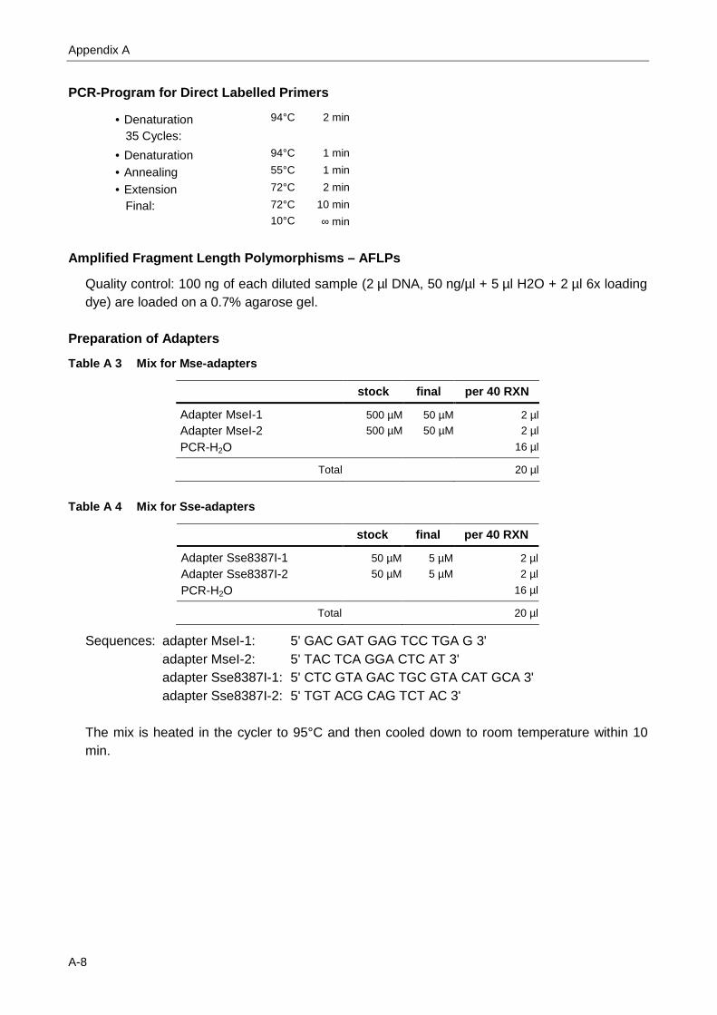
Appendix A
A-8
PCR-Program for Direct Labelled Primers
• Denaturation 94°C 2 min
35 Cycles:
• Denaturation 94°C 1 min
• Annealing 55°C 1 min
• Extension 72°C 2 min
Final: 72°C 10 min
10°C ∞ min
Amplified Fragment Length Polymorphisms – AFLPs
Quality control: 100 ng of each diluted sample (2 µl DNA, 50 ng/µl + 5 µl H2O + 2 µl 6x loading dye) are loaded on a 0.7% agarose gel.
Preparation of Adapters
Table A 3 Mix for Mse-adapters
stock final per 40 RXN
Adapter MseI-1 500 µM 50 µM 2 µl
Adapter MseI-2 500 µM 50 µM 2 µl
PCR-H2O 16 µl
Total 20 µl
Table A 4 Mix for Sse-adapters
stock final per 40 RXN
Adapter Sse8387I-1 50 µM 5 µM 2 µl
Adapter Sse8387I-2 50 µM 5 µM 2 µl
PCR-H2O 16 µl
Total 20 µl
Sequences: adapter MseI-1: 5' GAC GAT GAG TCC TGA G 3' adapter MseI-2: 5' TAC TCA GGA CTC AT 3' adapter Sse8387I-1: 5' CTC GTA GAC TGC GTA CAT GCA 3' adapter Sse8387I-2: 5' TGT ACG CAG TCT AC 3' The mix is heated in the cycler to 95°C and then cooled down to room temperature within 10 min.

Appendix A
A-9
Restriction/Ligation in 96-plates
Table A 5 Restriction/Ligation mix for 1 reaction (RXN)
stock final per 1 RXN
genomic DNA (200 ng/µl ) 50 ng/µl 250 ng 2.5 µl
Sse 8387 I (Takara) 10 U/µl 5 U 0.5 µl
MseI (New England Biolab) 10 U/µl 2.5 U 0.25 µl
T4-ligase 5 U/µl 1 U 0.2 µl
BSA (10x Takara) 10x=0.1% 0.01% 2 µl
10xrestricion buffer for Sse8387I (NEB2)
10x 1x 2 µl
Mse-adapter 50 µM 2 µM 0.5 µl
Sse-adapter 5 µM 0.2µM 0.5 µl
ATP 100 mM 1 mM 0.2 µl
PCR-H2O 11.35 µl
Total 20 µl 20 µl
• 17.5 µl of the ligation mix is added to each restriction mix and incubated at 37°C for 3 hours and then over night at room temp.
• After that 5 µl are loaded on a 2% agarose gel. A smear should appear at the range between 100 to 800 bp.
• Dilute with water four fold (e.g. add 60 µl H2O to 20 µl R/L mix).
Pre-selective PCR Amplification in 96 or 384-plates
Table A 6 Pre-amplification mix for 1 reaction (RXN)
stock final per 1 RXN
PreMseI-primer +0 10 µM 0.3 µM 0.6 µl
PreSse8387I-primer +0 10 µM 0.3 µM 0.6 µl dNTP 2 mM (each) 0.2 mM 1.5 µl
PCR buffer (incl. MgCl2) 10x 1x 2 µl
MgCl2 50 mM 1.5 mM 0 µl
Taq-polymerase 5 U/µl 0.05U 0.1 µl
ligated DNA 4.5 µl
PCR-H2O 10.7 µl
Total 20 µl 20 µl
Sequences: preselective primer PreMseI: 5' GAT GAG TCC TGA GTA A 3' preselective primer PreSse8387I: 5' GTA GAC TGC GTA CAT GCA G 3'
• 15.5 µl is added to each sample.
• Amplify using the following program:
2 min 72°C 20 cycles: 30 sec 94°C
60 sec 60°C 2 min 72°C
hold at: 4°C Note: All temperature ramps must be 1°C per second.

Appendix A
A-10
• After that 5 µl are loaded on a 2% agarose gel. A smear should appear at the range between 100 to 800 bp.
• Dilute with water twenty fold (add 95 µl H2O to 5 µl Pre-sel mix).
Selective PCR Amplification
Table A 7 Selective amplification mix for 1 reaction (RXN)
stock final per 1 RXN
PCR-H2O 4.24 µl
PCR buffer 10x 1x 1 µl
dNTP 2 mM (each) 0.2 mM 1 µl
MgCl2 50 mM 1.5 mM 0 µl
MseI-primer +2 10 µM 0.3 µM 0.3 µl
Sse83871I-primer +2* 10 µM 0.3/0.5 µM 0.3/0.5 µl
Taq-polymerase 5 U/µl 0.05U/µl 0.16 µl
preamplified DNA (5+95µl H2O) 3 µl
Total 10 µl 10 µl
* For the dyes Fam, IRD700 and IRD800 the concentration is 0.3 µM, for Cy3 and Cy5 0.5µM
Sequences: selective primer MseI: 5' GAT GAG TCC TGA GTA AAN N 3' selective primer PreSse8387I: 5' label - GAC TGC GTA CAT GCA GGN N 3' • 7 µl is added to each sample.
• Amplify using the following program:
2 min 94°C 10 cycles: 30 sec 94°C
30 sec 63°C 2 min 72°C
23 cycles: 30 sec 94°C 30 sec 54°C 2 min 72°C
hold at: 4°C Note: All Temperature ramps must be 1°C per second.

Appendix A
A-11
Separation of DNA-Fragments Using the LI-COR 12 – 4200 DNA Analyzer
Operating Instruction and Gimmicks
by L. Matiasch
modified: 2009-08-04
Gel preparation
Cleaning and assembling of the glass plates
• Carefully clean the glass plates. To get rid of dried gel-remainders, wash the plates with hot
water. If they are rather clean, it is sufficient to spray the inner sides13 of the plates that will
be in direct contact with the gel with aqua dest. and wipe off the water with “Roth”14 tissue. To improve later the filling with the liquid gel, clean the inner sides with ethanol (“70% Ethanol vergällt”) and wipe off with the tissue.
• Clean spacer with aqua dest. and put them on the very left and right sides of the glass.
• Put the other glass plate on top and fix the two plates. Leave the top screw open for pouring the gel. Always close one of the left and one of the right side at the same time and do not fix it too tightly to prevent both clamps and class plates from breaking.
Pouring the gel
• Move to the fume hood for pouring the gel15.
• Put the assembled glass plates in an angle of about 15° on a styrofoam plate (see Fig. A 1, left).
• In general we use a 7% acrylamide gel16. For gels with a length of 25 cm and a thickness of 0.25 mm you have to mix:
12 LI-COR Biosciences GmbH, Bad Hamburg, DE 13 Always take care to use the same side of the plates as inner respectively outer side and never touch the
plates without gloves. Fat on the inner side of the plates will result in bubbles and prevent you from getting a nice gel.
14 Carl Roth GmbH + Co. KG, Karlsruhe, DE 15 Acrylamide is carcinogenic – never work with acrylamide outside the fume hood until it has
polymerized to prevent inhalation and wear gloves! 16 If for some primer combinations bands do not separate well, you can increase the amount of acrylamide
up to 10%.

Appendix A
A-12
Urea+TBE17 19.5 ml
Acrylamide18 3.5 ml
DMSO19 250 µl
APS20 175 µl
TEMED21 25 µl
Fig. A 1 Preparing a gel for LI-COR – 4200 DNA Analyzer
• Mix urea+TBE and acrylamide in first thoroughly with a magnetic stirrer. Add DMSO, APS and TEMED and be ready for pouring the gel. It polymerizes soon!
• Pour the gel beginning at one side of the cavity. Whilst pouring, gently knock on the glass plates to prevent development of bubbles.
• If there are –despite following all the advises above– some bubbles in the gel, you can try to get them out with the very thin wire. But be quick. As soon as the gel starts polymerizing, you will cause even more harm!
• Where later the sharktooth comb for loading the samples will be inserted, place the opposite side of an old one comb to get a straight edge.
• Insert the plastic plate and fix the very top screws (see Fig. A 1, right)
• Let the gel polymerize for at least half an hour.
• Clean up fume hood.
17 8 M urea
• 210 g urea: Rotiphorese® NF-Harnstoff f automatische Sequencer, Roth #A120.1;
• 50 ml 10x TBE ⇒ Dissolve in 180 ml and fill then to 420 ml with osmotic H2O.
10x TBE • 162.0 g Tris base (tris(hydroxymethyl)amino-methane): Pufferan® buffer grade, Roth #AE15.3
• 27.5 g boric acid p.a., Roth #6943.1
• 9.3 g EDTA (ethylendiamintetraacetate) p.a., Roth #8043.2
⇒ Fill to 1000 ml with osmotic H2O.
18 Long Ranger ® Gel Solution, Cambrex Bio Science, Rockland Inc., Rockland, US, #50615 19 dimethylsulfoxide, p.a., Fluka Chemika, Chemia AG, Buchs, CH, #41640 20 10% ammoniumpersulfate: Dissolve 1 g (Roth #9592.2) in approx. 180 ml dest. H2O and freeze in
quantities of 190 µl. 21 N,N,N',N' tetramethylethylendiamin, Sigma-Aldrich #87687

Appendix A
A-13
• Remove the old sharktooth comb.
• Replace the plastic plate with a buffer tank.
• Remove gel particles on the outer parts by washing the glass plates. Clean with ethanol (“70% Ethanol vergällt”) and wipe off with the tissue.
Starting the LI-COR
• Switch on PC.
• Insert the glass plates into the LI-COR unit. Some plates have been used with both sides up and there are scratches from the gel loading syringe. Take care that this “band” is not at the same level where the laser is scanning.
• Fill both buffer reservoirs with running (1x TBE)-buffer up to the marks.
• Carefully clean the upper edge from all gel particles. These would later prevent loading of the samples. Washing with a 5 ml-syringe with running buffer, or using the teeth of an old comb or an old wire for getting out bubbles may be helpful.
• Insert the sharktooth comb. If it efforts much strength to insert it, wait until the temperature of the gel has increased.
• Cover the buffer tanks and connect the wires.
• Switch on LI-COR.
- Select “V4.10 Data Collection Model 4200 Dual Dye DEV1”
- Select File → New. In the “Project” window write a “Project name” and take care that for “Pixel size (bits)” 8 is selected. In the windows “700”' resp. “800” write an “Image name”.
- To adjust scanning intensity, select in the “Image” window Options → Auto gain →Auto After auto gain has finished, select Done. You have to do this for both images (wavelengths)!
• Before loading the first time let the gel run for about half an hour. At least the temperature should rise to the default 48°C. It seems the longer you wait until loading the first samples, the nicer the first picture. But if a gel is running for a too long time, it will become damaged.
• Settings:
Voltage (V) 1500 Current (ma) 50 Power (W) 40 Heater (degC) 48 Signal Filter 3 Scan Speed 3

Appendix A
A-14
Sample preparation
In general you get nice pictures when adding 1.2 µl of PCR samples to 5 µl loading buffer22. If the bands are too weak, you can raise the amount of samples of up to 5 µl. Larger amounts of
samples do not seem to improve the intensity of the bands.23
• Centrifuge mixture for some seconds at 3000 rpm.
• Denature at 95°C for 5 minutes.
• Immediately place on ice for fast cooling. After cooling down centrifuge again24.
Setting the Focus
• At first better do auto gain once more for both images (wavelengths): Options → Autogain → Auto.
• In the “Scanner Control” window select Options → Focus25. The “ideal focus” is shown in Fig. A 2. But despite a less “symmetric” bend or a smaller peak, gel pictures can be very nice.
Fig. A 2 Setting the Focus on LI-COR – 4200 DNA Analyzer
Loading the samples
• It is possible to load samples labeled with 700 and 800 nm at the same time.
• 1.2 – 1.5 µl can be loaded.
22 Loading buffer:
• 35.625 ml formamide Ultra for molecular biology, Fluka #47671
• 1.875 ml EDTA (0.5 mol/l, pH=8.0): Dissolve 186.12 g EDTA in approx. 750 ml of dest. H2O. Add conc. NaOH solution (dissolve NaOH pellets in a small volume of dest. H2O) slowly to bring pH to 7.95 Note: EDTA will dissolve only while adding NaOH . After EDTA is in solution, bring to 950 ml, check pH again and bring it to 8.0, fill up to 1000 ml. Autoclave
• 225 µl fuchsin, Merck für die Mikrobiologie und Mikroskopie #1358, dissolved in methanol
23 Bands will also be more intense, if you do not load a “fresh” PCR right from the cycler, but store it for one or more days at 4°C
24 But not for too long before loading! 25 The better results you get when selecting Channel 700.
Appendix A
A-15
• Always clean the gel-loading syringe (“Hamilton26”) carefully by pipetting running buffer several times.
• Always check, whether the needles are at the right places.
• After loading the first PCR, run the gel for about 3 minutes until the samples are in the gel. Then no dye of the loading buffer should be seen above the gel.
• Before loading the second PCR, wash the above edge of the gel again with running buffer.
• It is possible to load a gel several times. If the bands of the two samples are of very different length and you decide to load at different times, do not forget that the primer front is that intense that it is also detected by the laser of the other wavelength and can cover the fragments!
• You can adjust the number of frames either to let the gel run for a longer time or to stop it automatically without having to wait.
Cleaning up
• To get both glass plates apart, the black plastic device may be helpful.
• Generally the whole gel is sticking to one of the plates. The best way to remove it is to “curl” it off the plate by pressing first a tissue on the whole area.
• Clean glass plates, spacers and sharktooth comb by rinsing with hot water first.
• Afterwards rinse with osmotic water as the normal tap water will cause white spots when drying.
• Buffer in the lower reservoir can be used several times.
• Clean up the desk all around the LI-COR.
• Save your pictures.
- Select “PC Datenverbindung”
- In the upper part of the window you see the directories of the computer connected to your
LI-COR machine.
- In the lower part, the directory of the corresponding folder on the lab-PC should be shown, e.g. /ron. Select your own folder with the right mouse button.
- With the left mouse button select the *.tif-files you want to copy. Then drag them with the right mouse button to your folder. Take care to use the correct “Übertragungsmodus” (ASCII or Binär)!
- You will find your files on the lab-PC in C:\ftproot\Ron (resp. Maxime, Hagrid, Hermine).
• Close the Data Collection program by selecting
• Select “Systemabschluss”
• Switch off LI-COR and PC.
26 Hamilton Company, Reno, US

Appendix A
A-16

Appendix A
A-17
Separation of DNA-Fragments using the C.B.S. 27 System and Typhoon Trio TM28 scanner
Operating Instruction and Gimmicks
by L. Matiasch, G. Stift, A.I. Alimari and K. Herzog
modified: 2008-11-21
Gel preparation
Cleaning and assembling of the glass plates
• Carefully clean the glass plates. To get rid of dried gel-remainders, wash the plates with hot
water. If they are rather clean, it is sufficient to spray the inner sides29 of the plates that will
be in direct contact with the gel with aqua dest. and wipe off the water with “Roth”30 tissue. To improve later the filling with the liquid gel, clean the inner sides with some drops of
ethanol abs.31 Use a plastic Pasteur pipette and wipe off with the tissue.
• Clean spacer with aqua dest. and put them on the very left and right sides of the glass plate with the cavity for the sharktooth comb (as this is the broader of the two plates).
Put the other glass plate on top and fix the two plates with 5 black clamps on each side. Leave a space for a sixth clamp on the down end of the plates. It is best to fix the clamps on the very outer part of the spacers to prevent the liquid gel from spilling (see Fig. A 3, left).
Fig. A 3 Preparing a gel for C.B.S. chamber
27 Vertical Electrophoresis System (Sequencer), C.B.S. Scientific Company, Del Mar, US 28 Typhoon TRIO Variable Mode Imager, Amersham Biosciences, Buckinghamshire, GB 29 Always take care to use the same side of the plates as inner respectively outer side and never touch the
plates without gloves. Fat on the inner side of the plates will result in bubbles and prevent you from getting a nice gel.
30 Carl Roth GmbH + Co. KG, Karlsruhe, DE 31 Never use denatured ethanol (“70% ethanol vergällt”). It contains fluorescing substances that influence
the scanning.

Appendix A
A-18
Pouring the gel
• Move to the fume hood for pouring the gel32.
• Put the assembled glass plates in an angle of about 15° on a styrofoam plate.
• In general we use a 7% acrylamide gel33. For big gels (e.g. for AFLPs) you have to mix:
Urea+TBE34 60 ml
Acrylamide35 13 ml
APS36 400 µl
TEMED37 64 µl
• Mix Urea+TBE and acrylamide in first thoroughly with a magnetic stirrer. Add APS and TEMED and be ready for pouring the gel. It polymerizes soon!
• Pour the gel beginning at one side of the cavity. Whilst pouring, gently knock on the glass plates to prevent development of bubbles.
• If there are –despite following all the advises above– some bubbles in the gel, you can try to get them out with the very thin wire. But be quick. As soon as the gel starts polymerizing, you will cause even more harm!
• Insert a red spacer at the cavity to get a straight edge, where later the sharktooth comb for
loading the samples will be inserted. Fix the red spacer with two more black clamps38 and also add a sixth clamp on the left and right side of the very down part of the gel (see Fig. A 3, right).
• Let the gel polymerize for at least half an hour.
• Clean up fume hood.
• Remove gel particles on the outer parts by washing the glass plates. Dry the plates carefully.
32 Acrylamide is carcinogenic – never work with acrylamide outside the fume hood until it has
polymerized to prevent inhalation and wear gloves! 33 If for some primer combinations bands do not separate well, you can increase the amount of acrylamide
up to 10%. 34 8 M urea
• 240.24 g urea: Rotiphorese® NF-Harnstoff f automatische Sequencer, Roth #A120.1
• 59 ml 10x TBE ⇒ Fill to 500 ml with osmotic H2O (for the exact concentration 514.7 ml).
10x TBE • 162.0 g tris base (tris(hydroxymethyl)amino-methan): Pufferan® Buffer Grade, Roth #AE15.3;
• 27.5 g boric acid p.a., Roth #6943.1
• 9.3 g EDTA (ethylendiamintetraacetate) p.a., Roth #8043.2
⇒ Fill to 1000 ml with osmotic H2O.
35 Rotiphorese Gel 40 (19:1), Roth #3030.1 36 10% ammoniumpersulfate: Dissolve 1 g (Roth #9592.2) in approx. 180 ml dest. H2O and freeze in
quantities of 190 µl. 37 N,N,N',N' tetramethylethylendiamin, Sigma-Aldrich #87687 38 The clamps must not reach further from the boarder of the glass plates than the spacer!

Appendix A
A-19
Running-in the gel
• Insert the glass plates into the C.B.S. unit. The plate with the cavity has to be at the side of the buffer reservoir.
- Fix it at both sides with two white spring clamps.
- Tighten the gasket of the upper reservoir.
- Fill both buffer reservoirs with running (1x TBE)-buffer up to the marks.
Fig. A 4 C.B.S. chamber ready for running the gel
- Carefully clean the upper edge from all gel particles. These would later prevent loading of the samples. Washing with a 5ml-syringe with running buffer, or using the teeth of an old comb or an old wire for getting out bubbles may be helpful.
- Insert the sharktooth comb. If it efforts much strength to insert it, wait until the temperature of the gel has increased.
- Cover the buffer tanks and connect the other end of the cable to the power supply. Take care to use the correct adapters for the chosen power supply. If you are not sure, ask somebody to help you!!!
• Let the gel run for at least 40 minutes. The temperature of the gel should rise to about 45-50°C. It seems the longer you wait until loading the samples, the nicer the picture. But if a gel is running for a too long time, it will become damaged starting from the down side.
• Settings:
2500 V (never go beyond this!) 150 mA (or maximum of the power supply)
100 W39
39 If the temperature is rising too much, reduce to 65 W. High temperature can make the glass break and/or
the bands on the gel have the shape of a smile.

Appendix A
A-20
Sample preparation
In general you get nice pictures when adding 5 µl loading buffer40 to the original PCR41.
• Centrifuge mixture for some seconds at 3000 rpm.
• Denature at 95°C for 5 minutes.
• Immediately place on ice for fast cooling. After cooling down centrifuge again42.
Loading the samples
• It is possible to load up to 3 PCR labeled with different dyes.
Possible combinations:
- Fluorescein and HEX or
- Cy5, Fluorescein and TAMRA or
- Cy5 and FAM or
- Cy3 and FAM (But very intense FAM-band will be visible as very weak bands when scanning Cy3!) or
- Cy5, Cy3 and FAM (But only if you want to use your data for mapping ! When scanning Cy5, intense Cy3 bands will be visible too.)
If you are loading more than one PCR on the same gel, always take care, that the same sample will be at the same position !
• Depending on the used loading-comb you can load the following amounts:
- 126-comb: 1.4 – 1.5 µl43
- 94-comb44: 2.0 – 2.5 µl
- 62-comb: 2.0 – 3.0 µl
Even despite loading from behind, you can always check, whether the needles are at the right places.
40 Loading buffer:
• 35.625 ml formamide ultra for molecular biology, Fluka Chemica, Chemia AG, Buchs, CE, #47671
• 1.875 ml EDTA (0.5 mol/l, pH=8.0): Dissolve 186.12 g EDTA in approx. 750 ml of dest. H2O. Add conc. NaOH solution (dissolve NaOH pellets in a small volume of dest. H2O) slowly to bring pH to 7.95 Note: EDTA will dissolve only while adding NaOH . After EDTA is in solution, bring to 950 ml, check pH again and bring it to 8.0, fill up to 1000 ml. Autoclave
• 225 µl fuchsin, Merck für die Mikrobiologie und Mikroskopie #1358 or Bromphenol blue, United States Biochemical Corp, Cleveland, US, #12370
41 Bands will be more intense, if you do not load a “fresh” PCR right from the cycler, but store it for one or more days at 4°C.
42 But not for too long before loading! 43 Bands are not too nice, so use for testing parents only!

Appendix A
A-21
• Always clean the gel-loading syringe (“Hamilton45”) carefully by pipetting running buffer several times.
• After loading the first PCR, run46 the gel for several minutes until the samples are in the gel.
Then no dye of the loading buffer should be seen above the gel47.
• Before loading the second PCR, wash the above edge of the gel again with running buffer.
Running the gel
• Settings:
2500 V (never go beyond this!) 150 mA (or maximum of the power supply) 60 W (when running 1 gel) 80 W (when running 2 gels) Temperature should remain at about 45-50°C. If it is
becoming too hot, you have to reduce to 65 W or less to prevent the gel from a smile or even more damage and the glass from breaking.
In general an AFLP-gel is scanned after 2 and 4 hours. After 2 hours, small fragments can be scored. After 4 hours, also the big fragments are well separated, but small fragments have already reached the end of the gel and escaped. Depending on the pattern of the special case, other times may be better.
Scanning
• Switch on computer and Typhoon TrioTM scanner. It takes about 20 minutes until the scanner is ready (lamps stable).
• Take out some buffer of the upper reservoir with a big syringe or a 50ml-tube until the level is deep enough not to float out when taking off the gasket and the glass plates.
• Carefully clean the glass plates with aqua dest. Before scanning, the gel should cool down for 10 minutes or you should accelerate cooling by washing with cold water first.
• Control the glass plate of the scanner. If necessary, clean with aqua dest. You may use alcohol too, but never use “70% Ethanol vergällt” (denatured ethanol) !
• The thinner glass plate (the front one without the cavity) has to be the down one when scanning. Label your plates with a number and “left” or “right” that also on the scanned picture you can be sure that you did not change the gels or the side.
- To start the program, select the icon “Typhoon Scanner Control v 5.0” on the computer's
desktop. With “Template” → “Load” you can select the suitable template.
- If you want to change scanning intensity, choose “Setup” and “PMT”.
- Start with “Scan”.
44 Be aware that a PCR-Plate has 96 wells! 45 Hamilton Company, Reno, US 46 For settings see next section. 47 If you use the pink loading buffer, it won't enter into the gel. In this case you should load at least one lane
with blue loading buffer to recognize the entering of the bands into the gel.

Appendix A
A-22
Table A 8 Settings for Scanning AFLPs on Typhoon Trio TM Scanner
Fluorochrome Emission Filter
PMT Laser Sensitivity Beam Splitters
Fluorescein 526 SP 1000 Green (532) Normal HEX Normal
Cy5 670 BP 30 800 Red (633) Normal 580 Fluorescein 526 SP 1000 Green (532) Normal TAMRA 580 BP 30 800 Green (532) Normal
Cy5 670 BP 30 800 Red (633) Normal 630 Cy3 580 BP 30 800 Green (532) Normal FAM 520 BP 40 700 Blue (488) Normal
• The intensity of the bands is not the same for all possible AFLP-primer combinations. As a complete scan for 3 dyes takes about 20 minutes, it can save time, if you check the settings on a small part (about 4 rows) of the plate before scanning the entire one.
• If your bands are too weak or too dark, adjust scanning intensity by choosing “Setup” and
“PMT”48.
Cleaning up
• To get both glass plates apart, the red C.B.S. plastic device may be helpful.
• Generally the whole gel is sticking to one of the plates. The best way to remove it is to “curl” it off the plate.
• Clean glass plates, spacers and sharktooth comb by rinsing with hot water first.
• Afterwards rinse with osmotic water as the normal tap water will cause white spots when drying.
• Buffer in the lower reservoir can be used several times. So it is sufficient to empty the upper reservoir.
• Clean up the desk all around the C.B.S. units.
• Switch off power supply.
Have a look at the calendar: When does the next one want to use the scanner? To prevent dusting of the magnetic bands, Typhoon TrioTM should not be switched on for more than about 2 hours if not used.
48 If your picture is not too nice, check again if you diluted the primers correctly. Some of them should only
be diluted 1:5!

Appendix B
B-1
Appendix B: R © Functions and SAS ® Codes R© function for the generation of histograms for the traits heading, plant height and leaf rust resistance (mean over experiments)
function (file, cols=c(5:9))
{
## file ... character, filename
## cols ... vector, columnindexes, default: column 5 to 9
data <- read.Dummy(file) ## reading data from a .csv file, function: read.Dummmy
M <- as.matrix(data[, cols])
col.names <- dimnames(M)[[2]]
win.metafile(filename = paste("histogram_", col.names[1], ".wmf", sep=""),
width = 4, height = 4, pointsize = 7,
restoreConsole = TRUE)
hist(M[,1], breaks=c(130, 132, 134, 136, 138, 140, 142, 144, 146, 148, 150,
152, 154, 156, 158, 160, 162, 164),
labels=TRUE,
xlab="heading [day of the year]",
main=paste("histogram of", col.names[1]), ylim=c(0, 120))
dev.off()
win.metafile(filename = paste("histogram_", col.names[2], ".wmf", sep=""),
width = 3, height = 3, pointsize = 6,
restoreConsole = TRUE)
hist(M[,2], breaks=c(60, 70, 80, 90, 100, 110, 120, 130, 140),
labels=TRUE,
xlab="plant height [cm]",
main=paste("histogram of", col.names[2]), ylim=c(0, 120))
dev.off()
for (i in 3:5) {
win.metafile(filename = paste("histogramm_", col.names[i], ".wmf", sep=""),
width = 3, height = 3, pointsize = 6,
restoreConsole = TRUE)
hist(M[,i], breaks=c(0, 10, 20, 30, 40, 50, 60, 70, 80, 90, 100),
labels=TRUE,
xlab="diseased area [%]",
main=paste("histogram of", col.names[i]), ylim=c(0, 160))
dev.off()
}
}
Depending on the range of the data it might be necessary to adjust the height of the y-axis (ylim) or the graduation of the x-axis (breaks). If the columns different from 5 to 9 contain the traits of interest, the range has to be adjusted in the first line of this function. Histograms are stored as .wmf files and named "histogram_columnname".

Appendix B
B-2
R© function "read.Dummy"
function (file)
{
df1 <- read.csv(file)
df1 <- df1[-1,]
return(df1)
}
If this function is used for reading .csv files into R©, the first line must contain the variable names and the second line is a dummy that is deleted after reading. The decimal sign is the point.
SAS® code for single point ANOVA for the trait heading (mean over experiments)
data Data2;
set Work.Data;
data d;
set Work.Data;
array c(36) Xbarc25 -- Xwmc25_2; *name of the first marker -- name of the last marker
keep genotype marker response mheading;
do marker= 1 to 36; * number of markers
response=c(marker);
if response=0 then response=missing;
output;
end;
run;
proc sort;
by marker;
run;
proc glm data=d outstat=Work.Anova_out;
by marker;
class response;
model mheading = response;
means response;
run;
quit;
proc means noprint data=d;
class response ;
by marker;
var mheading ;
types response ;
output out=Work.Markermeans
n= nmheading
mean= mmheading
StdDev= smheading ;
run;
quit;

Appendix B
B-3
data F_Values;
set Work.Anova_out;
if _TYPE_ ='SS1' then delete;
keep marker df ss f prob;
run;
data t;
set Work.F_Values;
proc sort;
by prob;
run;

Appendix B
B-4

Appendix C
C-1
Appendix C: Trait Correlations Abbreviations used in the following tables:
P Pearson’s product moment correlation coefficient S Spearman’s rho Head heading (day of the year) PH plant height (cm) LR leaf rust severity (LR1, LR2,... if assessed several times) (% infected leaf area) AUDPC area under the disease progress curve for leaf rust resistance Seedling seedling resistance against leaf rust (0 = immune – 4 = susceptible) CD crop density (1 = no missing plants – 5 more than half of the plants missing) Leaf leaf blotch severity (1 = no visible symptoms – 9 = completely diseased) PM powdery mildew severity (1 = no visible symptoms – 9 = completely diseased) Sep Septoria leaf blotch severity (1 = no visible symptoms – 9 = completely diseased) YR yellow rust severity (1 = no visible symptoms – 9 = completely diseased) Glauc glaucousness (1 = no wax – 5) FH frost heaving severity (1 = no damage – 9 all plants frozen) Lodg lodging severity (Lodg1,... if assessed several times) (different scales) Chl leaf chlorosis severity (0 = no visible symptoms – 9 = extremely chlorotic) LTN leaf tip necrosis severity (0 = no visible symptoms – 9 = heavy symptoms)
Table A 9 Trait correlations population Isengrain/Capo: mean over experiments
P S P S P S S PH PH LR LR AUDPC AUDPC LTN
Head n 227 227 238 238 r 0.40 0.44 -0.17 -0.17 H0 acc. acc. acc. acc. PH n 226 226 r -0.01 -0.01 H0
acc. acc. LR n 240 240 r 0.94 0.96 H0
rej. rej. Chl n 240 r 0.48 H0
acc.
The means over the experiments were calculated as follows:
Head – PH: Tulln 2004, 2006, 2007 (M), 2007, 2008 Head – LR: Tulln 2004, Probstdorf 2007, Tulln (M) 2007, Rust 2008, Schmida 2008,
Tulln 2008 PH – LR: Tulln 2004, Tulln 2007 (M), Tulln 2008, LR – AUDPC: Piestany 2006, Tulln 2008 Chl – LTN: Rust 2009, Tulln 2009
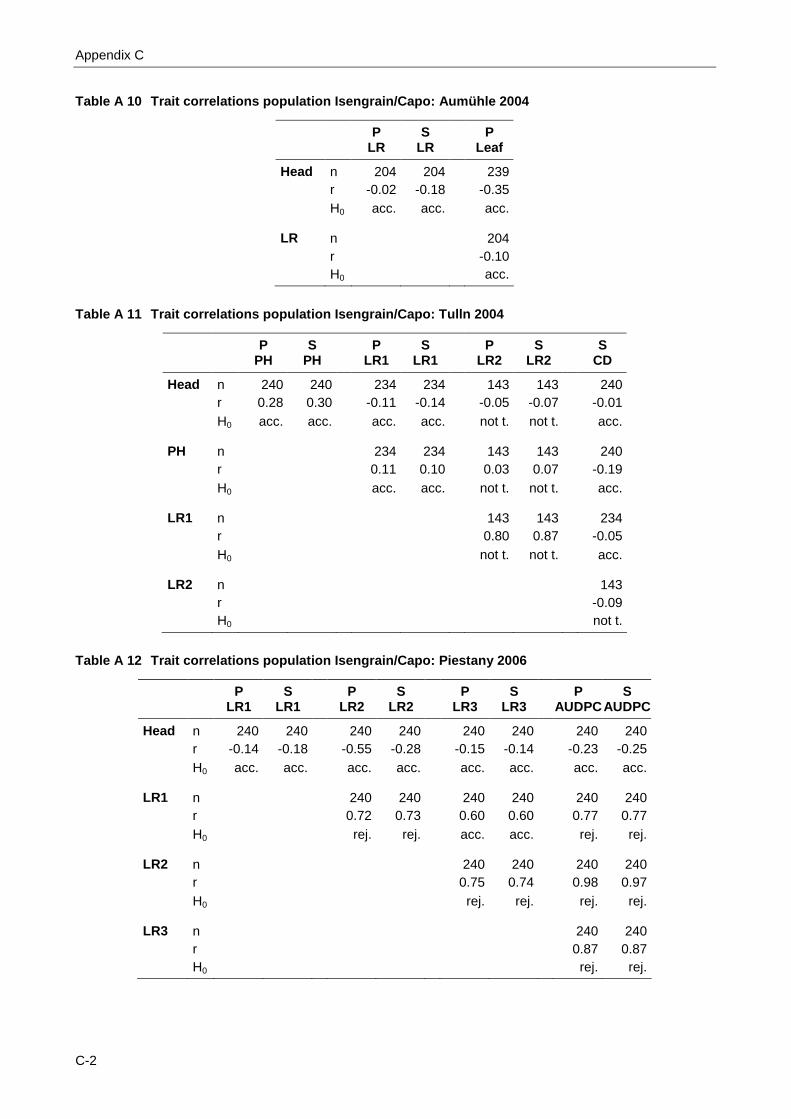
Appendix C
C-2
Table A 10 Trait correlations population Isengrain/Capo: Aumühle 2004
P S P LR LR Leaf
Head n 204 204 239 r -0.02 -0.18 -0.35 H0 acc. acc. acc. LR n 204 r -0.10 H0
acc.
Table A 11 Trait correlations population Isengrain/Capo: Tulln 2004
P S P S P S S PH PH LR1 LR1 LR2 LR2 CD
Head n 240 240 234 234 143 143 240 r 0.28 0.30 -0.11 -0.14 -0.05 -0.07 -0.01 H0 acc. acc. acc. acc. not t. not t. acc. PH n 234 234 143 143 240 r 0.11 0.10 0.03 0.07 -0.19 H0
acc. acc. not t. not t. acc. LR1 n 143 143 234 r 0.80 0.87 -0.05 H0
not t. not t. acc. LR2 n 143 r -0.09 H0
not t.
Table A 12 Trait correlations population Isengrain/Capo: Piestany 2006
P S P S P S P S LR1 LR1 LR2 LR2 LR3 LR3 AUDPC AUDPC
Head n 240 240 240 240 240 240 240 240 r -0.14 -0.18 -0.55 -0.28 -0.15 -0.14 -0.23 -0.25 H0 acc. acc. acc. acc. acc. acc. acc. acc. LR1 n 240 240 240 240 240 240 r 0.72 0.73 0.60 0.60 0.77 0.77 H0
rej. rej. acc. acc. rej. rej. LR2 n 240 240 240 240 r 0.75 0.74 0.98 0.97 H0
rej. rej. rej. rej. LR3 n 240 240 r 0.87 0.87 H0
rej. rej.

Appendix C
C-3
Table A 13 Trait correlations population Isengrain/Capo: Probstdorf 2006
S P S S S LR1 LR2 LR2 PM FH
Head1) n 239 130 240 240 r -0.15 0.05 0.02 0.22 H0 acc. not t. acc. acc. LR1 n 130 130 239 239 r 0.75 0.77 0.22 -0.13 H0
not t. not t. acc. acc. LR2 n 130 130 r 0.30 0.02 H0
not t. not t. PM n 240 r 0.08 H0
acc. 1) scored on a 1 (= early) to 9 (= late) scale
Table A 14 Trait correlations population Isengrain/Capo: Tulln 2006
P S PH PH
Head n 240 240 r 0.42 0.41 H0 acc. acc.
Table A 15 Trait correlations population Isengrain/Capo: Piestany 2007
P S P S P S P S LR1 LR1 LR2 LR2 LR3 LR3 AUDPC AUDPC
Head n 234 234 234 234 234 234 234 234 r 0.15 0.11 0.26 0.27 0.38 0.43 0.33 0.33 H0 acc. acc. acc. acc. acc. acc. acc. acc. LR1 n 234 234 234 234 234 234 r 0.66 0.71 0.44 0.49 0.64 0.67 H0
rej. rej. acc. acc. acc. rej. LR2 n 234 234 234 234 r 0.72 0.77 0.92 0.92 H0
rej. rej. rej. rej. LR3 n 234 234 r 0.89 0.89 H0
rej. rej.
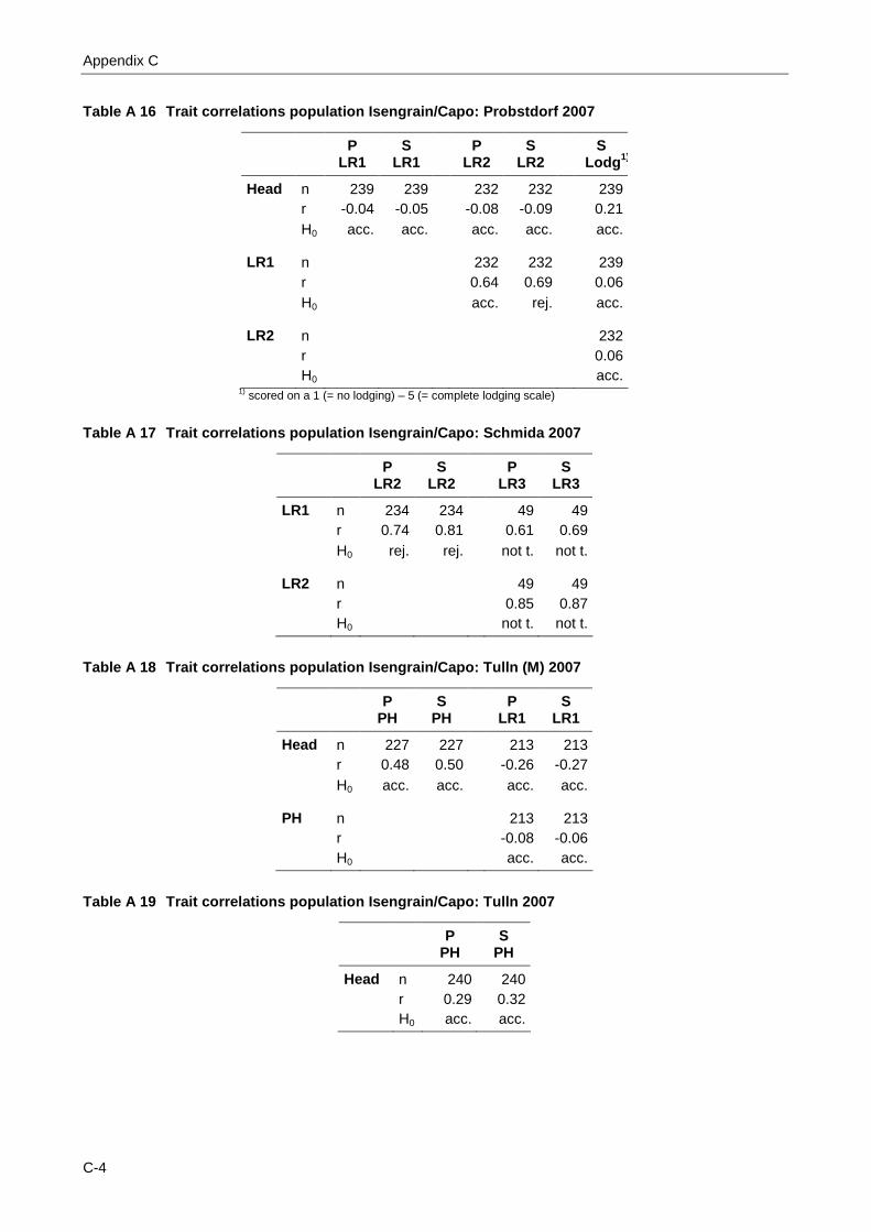
Appendix C
C-4
Table A 16 Trait correlations population Isengrain/Capo: Probstdorf 2007
P S P S S LR1 LR1 LR2 LR2 Lodg 1)
Head n 239 239 232 232 239 r -0.04 -0.05 -0.08 -0.09 0.21 H0 acc. acc. acc. acc. acc. LR1 n 232 232 239 r 0.64 0.69 0.06 H0
acc. rej. acc. LR2 n 232 r 0.06 H0
acc. 1) scored on a 1 (= no lodging) – 5 (= complete lodging scale)
Table A 17 Trait correlations population Isengrain/Capo: Schmida 2007
P S P S LR2 LR2 LR3 LR3
LR1 n 234 234 49 49 r 0.74 0.81 0.61 0.69 H0 rej. rej. not t. not t. LR2 n 49 49 r 0.85 0.87 H0
not t. not t.
Table A 18 Trait correlations population Isengrain/Capo: Tulln (M) 2007
P S P S PH PH LR1 LR1
Head n 227 227 213 213 r 0.48 0.50 -0.26 -0.27 H0 acc. acc. acc. acc. PH n 213 213 r -0.08 -0.06 H0
acc. acc.
Table A 19 Trait correlations population Isengrain/Capo: Tulln 2007
P S PH PH
Head n 240 240 r 0.29 0.32 H0 acc. acc.

Appendix C
C-5
Table A 20 Trait correlations population Isengrain/Capo: Probstdorf 2008
S Lodg 1)
LR n 213 r -0.14 H0 acc.
1) scored on a 0 (= no lodging) – 5 (= complete lodging scale)
Table A 21 Trait correlations population Isengrain/Capo: Rust 2008
P S S LR LR Lodg 1)
Head n 234 234 240 r -0.02 0.00 0.35 H0 acc. acc. acc. LR n 234 r 0.13 H0
acc. 1) scored on a 0 (= no lodging) – 5 (= complete lodging scale)
Table A 22 Trait correlations population Isengrain/Capo: Schmida 2008
P S LR LR
Head n 216 216 r -0.06 -0.04 H0 acc. acc.
Table A 23 Trait correlations population Isengrain/Capo: Tulln 2008
P S P S P S P S P S PH PH LR1 LR1 LR2 LR2 LR3 LR3 AUDPC AUDPC
Head n 240 240 240 240 240 240 240 240 240 240 r 0.15 0.11 -0.19 -0.17 -0.23 -0.24 -0.24 -0.23 -0.23 -0.24 H0 acc. acc. acc. acc. acc. acc. acc. acc. acc. acc. PH n 240 240 240 240 240 240 240 240 r 0.11 0.08 0.09 0.11 0.12 0.13 0.11 0.12 H0
acc. acc. acc. acc. acc. acc. acc. acc. LR1 n 240 240 240 240 240 240 r 0.87 0.92 0.76 0.90 0.90 0.94 H0
rej. rej. rej. rej. rej. rej. LR2 n 240 240 240 240 r 0.89 0.94 0.99 0.99 H0
rej. rej. rej. rej. LR3 n 240 240 r 0.93 0.97 H0
rej. rej.

Appendix C
C-6
Table A 24 Trait correlations population Isengrain/Capo: Rust 2009
P S S S LR2 LR2 Chl LTN
LR1 n 192 192 240 240 r 0.64 0.66 -0.33 -0.38 H0 not t. not t. acc. acc. LR2 n 192 192 r -0.32 -0.51 H0
not t. not t. Chl n 240 r 0.42 H0
acc.
Table A 25 Trait correlations population Isengrain/Capo: Tulln 2009
S S Chl LTN
Head n 240 240 r -0.02 -0.02 H0 acc. acc. Chl n 240 r 0.47 H0
acc.

Appendix C
C-7
Table A 26 Trait correlations population Arina/Capo: mean over experiments
P S P S S S P S S PH PH LR LR Chl LTN AUDPC AUDPC Lodg 1)
Head n 232 232 209 209 232 232 230 230 r 0.03 0.04 -0.30 -0.29 0.21 0.19 -0.33 -0.30 H0 acc. acc. acc. acc. acc. acc. acc. acc. PH n 230 230 r 0.12 0.11 H0
acc. acc. LR n 225 225 228 228 227 r -0.52 -0.58 0.95 0.95 -0.11 H0
acc. acc. rej. rej. acc. Chl n 233 r 0.56 H0
acc. 1) scored on a 0 (= no lodging) – 5 (= complete lodging scale)
The means were calculated over the experiments as follows:
Head – PH: Tulln 2007, 2008 Head – LR: Tulln 2007, Fundulea 2008, Nyon 2008, Rust 2008, Schmida 2008, Tulln
2008, Rust 2009, Tulln 2009 Head – Chl: Rust 2009, Tulln 2009 Head – LTN: Rust 2009, Tulln 2009 Head – AUDPC: Fundulea 2008, Tulln 2008 PH – LR: Tulln 2007, Tulln 2008 LR – Chl: Rust 2009, Tulln 2009 LR – LTN: Rust 2009, Tulln 2009 LR – AUDPC: Piestany 2008, Fundulea 2008, Tulln 2008 LR – Lodg: Probstdorf 2008, Rust 2008 Chl – LTN: Rust 2009, Tulln 2009

Appendix C
C-8
Table A 27 Trait correlations population Arina/Capo: Tulln 2007
P S P S P S P S PH PH LR1 LR1 LR2 LR2 LR3 LR3
Head n 232 232 232 232 229 229 183 183 r -0.05 -0.03 -0.14 -0.14 -0.15 -0.14 -0.14 -0.12 H0 acc. acc. acc. acc. acc. acc. not t. not t. PH n 233 233 230 230 184 184 r -0.01 -0.02 0.06 0.07 0.10 0.08 H0
acc. acc. acc. acc. not t. not t. LR1 n 230 230 184 184 r 0.77 0.79 0.76 0.77 H0
rej. rej. not t. not t. LR2 n 184 184 r 0.92 0.96 H0
not t. not t.
Table A 28 Trait correlations population Arina/Capo: Fundulea 2008
P S P S P S P S S LR1 LR1 LR2 LR2 LR3 LR3 AUDPC AUDPC Seedling
Head n 230 230 230 230 230 230 230 230 220 r -0.13 -0.13 -0.15 -0.17 -0.11 -0.11 -0.15 -0.17 -0.13 H0 acc. acc. acc. acc. acc. acc. acc. acc. acc. LR1 n 230 230 230 230 230 230 220 r 0.26 0.26 0.20 0.22 0.28 0.29 0.23 H0
acc. acc. acc. acc. acc. acc. acc. LR2 n 230 230 230 230 220 r 0.75 0.76 0.97 0.97 0.07 H0
rej. rej. rej. rej. acc. LR3 n 2320 230 220 r 0.88 0.89 0.07 H0
rej. rej. acc. AUDPC n 220 r 0.09 H0
acc.

Appendix C
C-9
Table A 29 Trait correlations population Arina/Capo: Nyon 2008
P S P S S S S LR1 LR1 LR2 LR2 PM Sep YR
Head n 228 228 225 225 228 228 228 r -0.03 -0.05 -0.15 -0.14 -0.06 0.02 -0.05 H0 acc. acc. acc. acc. acc. acc. acc. LR1 n 226 226 229 229 229 r 0.40 0.19 0.10 0.02 0.06 H0
acc. acc. acc. acc. acc. LR2 n 226 226 226 r 0.22 -0.14 0.16 H0
acc. acc. acc. PM n 229 229 r -0.03 0.23 H0
acc. acc. Sep n 229 r 0.23 H0
acc.
Table A 30 Trait correlations population Arina/Capo: Piestany 2008
P S P S P S P S LR1 LR1 LR2 LR2 LR3 LR3 AUDPC AUDPC
Head n 229 229 229 229 229 229 229 229 r -0.18 -0.19 -0.13 -0.19 -0.28 -0.27 -0.25 -0.25 H0 acc. acc. acc. acc. acc. acc. acc. acc. LR1 n 229 229 229 229 229 229 r 0.59 0.59 0.58 0.54 0.66 0.64 H0
acc. acc. acc. acc. rej. acc. LR2 n 229 229 229 229 r 0.63 0.67 0.85 0.87 H0
acc. rej. rej. rej. LR3 n 229 229 229 229 r 0.63 0.67 0.95 0.94 H0
acc. rej. rej. rej.
Table A 31 Trait correlations population Arina/Capo: Probstdorf 2008
S Lodg 1)
LR n 231 r -0.09 H0 acc.
1) scored on a 0 (= no lodging) – 5 (= complete lodging scale)

Appendix C
C-10
Table A 32 Trait correlations population Arina/Capo: Reichersberg 2008
P S LR LR
Head n 213 213 r -0.16 -0.14 H0 acc. acc.
Table A 33 Trait correlations population Arina/Capo: Rust 2008
P S S LR LR Lodg 1)
Head n 225 225 230 r -0.09 -0.08 0.11 H0 acc. acc. acc. LR n 226 r 0.00 H0
acc. 1) scored on a 0 (= no lodging) – 5 (= complete lodging scale)
Table A 34 Trait correlations population Arina/Capo: Schmida 2008
P S LR LR
Head n 232 232
r -0.22 -0.21 H0 acc. acc.
Table A 35 Trait correlations population Arina/Capo: Tulln 2008
P S P S P S P S P S PH PH LR1 LR1 LR2 LR2 LR3 LR3 AUDPC AUDPC
Head n 233 233 233 233 233 233 233 233 233 233 r 0.08 0.08 -0.37 -0.35 -0.40 -0.34 -0.35 -0.31 -0.40 -0.35 H0 acc. acc. acc. acc. acc. acc. acc. acc. acc. acc. PH n 233 233 233 233 233 233 233 233 r 0.10 0.12 0.17 0.19 0.14 0.16 0.15 0.17 H0
acc. acc. acc. acc. acc. acc. acc. acc. LR1 n 233 233 233 233 233 233 r 0.80 0.86 0.76 0.82 0.90 0.94 H0
rej. rej. rej. rej. rej. rej. LR2 n 233 233 233 233 r 0.88 0.87 0.98 0.97 H0
rej. rej. rej. rej. LR3 n 233 233 r 0.92 0.91 H0
rej. rej.

Appendix C
C-11
Table A 36 Trait correlations population Arina/Capo: Rust 2009
P S P S P S P S P S S S S LR1 LR1 LR2 LR2 LR3 LR3 LR4 LR4 LR5 LR5 Chl LTN Glauc
Head n 232 232 232 232 232 232 226 226 223 223 232 232 232 r -0.37 -0.41 -0.43 -0.44 -0.45 -0.48 -0.34 -0.35 -0.26 -0.28 0.18 0.17 -0.19 H0 acc. acc. acc. acc. acc. acc. acc. acc. acc. acc. acc. acc. acc. LR1 n 233 233 233 233 227 227 224 224 233 233 233 r 0.82 0.85 0.76 0.80 0.57 0.66 0.54 0.63 -0.39 -0.36 0.26 H0
rej. rej. rej. rej. acc. rej. acc. acc. acc. acc. acc. LR2 n 233 233 227 227 224 224 233 233 233 r 0.90 0.90 0.76 0.81 0.73 0.78 -0.45 -0.43 0.26 H0
rej. rej. rej. rej. rej. rej. acc. acc. acc. LR3 n 227 227 224 224 233 233 233 r 0.73 0.76 0.70 0.74 -0.40 -0.41 0.23 H0
rej. rej. rej. rej. acc. acc. acc. LR4 n 223 223 227 227 227
r 0.92 0.92 -0.52 -0.49 0.21
88 H0
rej. rej. acc. acc. acc. LR5 n 224 224 224 r -0.53 -0.52 0.20 H0
acc. acc. acc. Chl n 233 233 r 0.51 -0.40 H0
acc. acc. LTN n 233 r -0.26 H0
acc.

Appendix C
C-12
Table A 37 Trait correlations population Arina/Capo: Tulln 2009
P S P S P S P S S S LR1 LR1 LR2 LR2 LR3 LR3 LR4 LR4 Chl LTN
Head n 233 233 228 228 222 222 231 231 233 233 r -0.19 -0.21 -0.34 -0.37 -0.37 -0.37 -0.23 -0.22 0.21 0.17 H0 acc. acc. acc. acc. acc. acc. acc. acc. acc. acc. LR1 n 228 228 222 222 231 231 233 233 r 0.67 0.71 0.65 0.73 0.53 0.70 -0.26 -0.34 H0
rej. rej. acc. rej. acc. rej. acc. acc. LR2 n 222 222 227 227 228 228 r 0.91 0.91 0.75 0.78 -0.37 -0.50 H0
rej. rej. rej. rej. acc. acc. LR3 n 221 221 222 222 r 0.84 0.85 -0.40 -0.54 H0
rej. rej. acc. acc. LR4 n 231 231 r -0.44 -0.55 H0
acc. acc. Chl n 233 r 0.52 H0
acc.
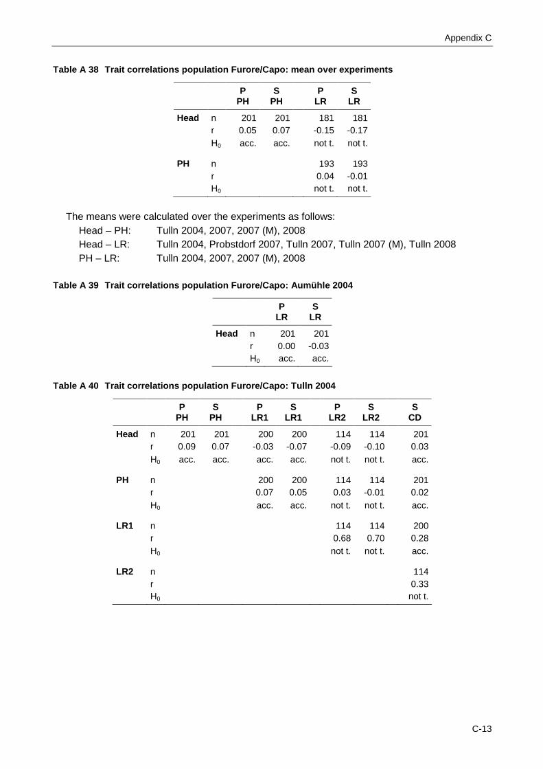
Appendix C
C-13
Table A 38 Trait correlations population Furore/Capo: mean over experiments
P S P S PH PH LR LR
Head n 201 201 181 181 r 0.05 0.07 -0.15 -0.17 H0 acc. acc. not t. not t. PH n 193 193 r 0.04 -0.01 H0
not t. not t.
The means were calculated over the experiments as follows:
Head – PH: Tulln 2004, 2007, 2007 (M), 2008 Head – LR: Tulln 2004, Probstdorf 2007, Tulln 2007, Tulln 2007 (M), Tulln 2008 PH – LR: Tulln 2004, 2007, 2007 (M), 2008
Table A 39 Trait correlations population Furore/Capo: Aumühle 2004
P S LR LR
Head n 201 201 r 0.00 -0.03 H0 acc. acc.
Table A 40 Trait correlations population Furore/Capo: Tulln 2004
P S P S P S S PH PH LR1 LR1 LR2 LR2 CD
Head n 201 201 200 200 114 114 201 r 0.09 0.07 -0.03 -0.07 -0.09 -0.10 0.03 H0 acc. acc. acc. acc. not t. not t. acc. PH n 200 200 114 114 201 r 0.07 0.05 0.03 -0.01 0.02 H0
acc. acc. not t. not t. acc. LR1 n 114 114 200 r 0.68 0.70 0.28 H0
not t. not t. acc. LR2 n 114 r 0.33 H0
not t.

Appendix C
C-14
Table A 41 Trait correlations population Furore/Capo: Probstdorf 2006
S P S S S LR1 LR2 LR2 PM FH
Head1) n 201 38 201 201 r -0.14 0.03 0.00 0.07 H0 acc. not t. acc. acc. LR1 n 38 38 201 201 r 0.82 0.81 0.42 0.13 H0
not t. not t. acc. acc. LR2 n 38 38 r 0.38 0.15 H0
not t. not t. PM n 201 r -0.05 H0
acc. 1) scored on a 1 (= early) to 9 (= late) scale
Table A 42 Trait correlations population Furore/Capo: Tulln 2006
P S PH PH
Head n 201 201 r 0.07 0.02 H0 acc. acc.
Table A 43 Trait correlations population Furore/Capo: Probstdorf 2007
P S P S S LR1 LR1 LR2 LR2 Lodg 1)
Head n 201 201 189 189 201 r -0.05 -0.04 0.03 -0.08 -0.08 H0 acc. acc. not t. not t. acc. LR1 n 189 189 201 r 0.60 0.74 -0.15 H0
not t. not t. acc. LR2 n 189 r 0.01 H0
not t. 1) scored on a 1 (= no lodging) – 5 (= complete lodging scale)

Appendix C
C-15
Table A 44 Trait correlations population Furore/Capo: Tulln 2007
P S P S PH PH LR LR
Head n 201 201 201 201 r -0.15 -0.15 -0.17 -0.18 H0 acc. acc. acc. acc. PH n 201 201 r 0.01 0.02 H0
acc. acc.
Table A 45 Trait correlations population Furore/Capo: Tulln (M) 2007
P S P S PH PH LR LR
Head n 201 201 194 194 r 0.10 0.12 -0.11 -0.11 H0 acc. acc. not t. not t. PH n 194 194 r -0.01 -0.03 H0
not t. not t.
Table A 46 Trait correlations population Furore/Capo: Probstdorf 2008
S S S S PM Sep Lodg1 1) Lodg2 2)
Head n 201 201 201 201 r 0.23 -0.04 0.11 0.14 H0 acc. acc. acc. acc. PM n 201 201 201 r -0.07 0.15 0.21 H0
acc. acc. acc. Sep n 201 201 r 0.00 -0.20 H0
acc. acc. Lodg1 n 201 r 0.04 H0
acc. 1) scored on a 0 (= no lodging) – 5 (= complete lodging scale) 2) scored on a 1 (= no lodging) – 9 (= complete lodging scale)

Appendix C
C-16
Table A 47 Trait correlations population Furore/Capo: Tulln 2008
P S P S P S P S P S PH PH LR1 LR1 LR2 LR2 LR3 LR3 AUDPC AUDPC
Head n 201 201 201 201 201 201 201 201 201 201 r -0.11 -0.09 -0.04 -0.06 -0.08 -0.08 -0.12 -0.14 -0.09 -0.09 H0 acc. acc. acc. acc. acc. acc. acc. acc. acc. acc. PH n 201 201 201 201 201 201 201 201 r 0.17 0.18 0.17 0.15 0.17 0.18 0.18 0.17 H0
acc. acc. acc. acc. acc. acc. acc. acc. LR1 n 201 201 201 201 201 201 r 0.74 0.75 0.56 0.68 0.79 0.81 H0
rej. rej. acc. rej. rej. rej. LR2 n 201 201 201 201 r 0.82 0.87 0.98 0.98 H0
rej. rej. rej. rej. LR3 n 201 201 r 0.90 0.93 H0
rej. rej.

Appendix D
D-1
Appendix D: Thatcher Near Isogenic Lines (NILs)
0
10
20
30
40
50
60
70
80Lr
9
Lr19
Lr
24
Lr23
Lr
29
Lr38
Lr
52
Lr25
Lr
35
Lr22
Lr
34
Lr3
bLr
18
Lr12
Lr
44
Lr30
Lr
17
Lr21
Lr
2c
Lr3
kLr
20
Lr28
Lr
2a
Lr33
Lr
32
Lr11
Lr
2b
Lr37
Lr
3a
Lr1
Lr
16
Lr26
T
c Lr
10
Lr15
L
r14
Lr13
L
r14
LrB
leaf
rust
sev
erity
(% in
fect
ed le
af a
rea)
1
2
Table A 48 Leaf rust infection (% infected leaf area) of Thatcher (Tc) and NILs with different Lr genes
in the experiment Tulln 2007 on two assessment days. 1: June 15 th, 2: June 18 th
Lr9
Lr
19
Lr24
Lr
23
Lr29
Lr
38
Lr52
Lr
25
Lr35
Lr
22
Lr34
Lr
3bg
Lr18
Lr
12
Lr44
Lr
30
Lr17
Lr
21
Lr2c
Lr
3ka
Lr
20
Lr28
Lr
2a
Lr33
Lr
32
Lr11
Lr
2b
Lr37
Lr
3a
Lr1
Lr
16
Lr26
T
c
Lr10
Lr
15
Lr14
b
Lr13
Lr
14a
Lr
B

University of Natural Resources and Applied Life Sciences, ViennaDepartment for Agrobiotechnology,
IFA-Tulln, Austria
Introduction
Leaf rust (see Fig. 1) caused by Puccinia recondita f. sp. tritici is a
worldwide occurring disease of wheat. In some areas the fungus can cause
yield losses of 40 to 90% (Hoffmann, 1999), in Austria losses of up to 20%
are possible (Zwatz 1998). An ecologically and economically sound option
for rust control is the use of resistant cultivars. Leaf rust resistance can be
governed by major genes (so called Lr-genes) and/or quantitative (minor)
resistance genes. There are already more than 50 known Lr-genes
(McIntosh 2003).
The Austrian winter wheat cultivar Capo, developed by Probstdorfer
Saatzucht, seems to possess durable adult plant leaf rust resistance (APR).
As APR is often difficult to evaluate, there is little information about the
genetic background. Besides Lr13, which is not effective in Europe
(Winzeler 2000), it seems that Capo does not carry any known effective Lr-
gene. This project aims at characterizing durable adult plant leaf rust
resistance in Capo and at developing tools for use in marker assisted
selection.
Materials and Methods
Recombinant inbred line populations from crosses between Capo
(Diplomat/Purdue5517//Extrem/HP3517) and two susceptible cultivars –
Isengrain (Apollo/Soissons) and Furore (Carolus//Pokal/Martin) – have been
developed. These are tested at several locations during three seasons in
replicated field experiments. To provoke an even disease pressure over the
whole experimental area, spreader rows (a mix of rust susceptible lines) are
sown between the tested lines (see Fig. 2).
Additionally susceptible plants that are artificially inoculated in the
greenhouse will be planted into the spreader rows.
Evaluation of leaf rust severity will be done using the scoring scheme (see
Fig. 3) by Walther (2000).
Molecular Genetic Analysis of Durable Adult Plant Leaf Rust Resistance in the Austrian Winter Wheat Cultivar ‘Capo’
Lydia Matiasch, Katharina Herzog, Ján Kraic1), Valéria Šudyová1), Svetlana Šliková1), Franziska Löschenberger2), Julia Lafferty2), Hermann Bürstmayr
E-Mail: [email protected]
In parallel 240 lines of the population Capo/Isengrain are characterized with
molecular markers, mainly SSR- (microsatellite-) and AFLP- (amplified
fragment length polymorphism) markers to construct a linkage map of this
cross. A biometrical analysis of the resistance and the marker data will allow
the detection of quantitative trait loci (QTLs) for leaf rust resistance and the
quantification of their effects and interactions. The second population
(Capo/Furore) will be used for QTL validation.
Preliminary Results and Future Work
In the first year of this project resistance data for leaf rust severity could be
collected on two locations. Although disease pressure was very high, there
were clear differences between the tested lines.
About 160 SSR-primers have been tested on the parental lines. Out of them
more than 50% proved to be polymorphic between Capo and Isengrain; half
of these markers have already been analyzed on the population. In the long
run the majority of the genome should be covered with SSRs (at least one to
three per chromosome arm) and AFLPs.
A potential candidate gene for Capo’s resistance could be Lr34. Therefore,
the SSR markers GWM130 and GWM295 mapping near Lr34 (Suenaga
2003) have been analyzed already. Analysis of variance revealed no
significant association of leaf rust severity with either GWM130 (see Fig. 4
and 5) or GWM295 alleles. Hence Lr34 does not seem to be involved in APR
of Capo.
ReferencesHoffmann et al. (1999): Parasitäre Krankheiten und Schädlinge an landwirtschaftlichen Kulturpflanzen.-Stuttgart, DE: Verlag Eugen Ulmer.
McIntosh et al. (2003) : Catalogue of Gene Symbols for Wheat. Proceedings of the 10th International Wheat Genetics Symposium (September 1st-6th 2003), Volume 4.-Paestum, IT: Istituto Sperimentale per la Cerealicoltura.
Suenaga et al. (2003): Microsatellite Markers for Genes Lr34/Yr18 and Other Quantitative Trait Loci for Leaf Rust and Stripe Rust Resistance in Bread Wheat, Phytopathology 93 (7): 881-890.
Walther et al. (2000): Methodische Anleitung zur Bewertung der partiellen Resistenz von Sorten bzw. Linien unter Berücksichtigung epidemiologischer Aspekte. Mitt BiolBundesanst Land-Forstwirtsch 374. http://barley.ipk-gatersleben.de/ methods/walther_ et_al_methods.pdf
Winzeler et al. (2000) : Resistance of European winter wheat germplasm to leaf rust. Agronomie 20 (7): 783-792.
Zwatz et al. (1998): Krankheiten, Schädlinge und Nützlinge im Getreide- und Maisbau, 4. Aufl.-Wien, AT: Verlag Jugend & Volk.
Acknowledgements
This work is supported by the Austrian Science Fund FWF, Translational Research Program (TRP), project number L182-B06, with additional support from INTERREG IIIA Austria – Slovakia and the government of Lower Austria. Project Partners
1) 2)
↑↑↑↑ Fig. 2: Layout of the field plots for evaluation of leaf rust resistance↑↑↑↑ Fig. 1: Symptoms of leaf rust
Fig. 3: Scoring scheme for evaluation ofleaf rust severity (Walther 2000) →→→→
Testing lines Spreader rows
17 cm 29 cm
1 m
↑↑↑↑ Fig. 4: PCR amplification pattern of SSR-marker GWM130 on
part of the population
Capo/Isengrain
Fig. 5: Boxplots for leaf rust severity
for the different groups of the
alleles for SSR-marker
GWM130 →→→→911194N =
Capo: 27,5%, Isengrain: 45%
heterozygousIsengrainCapo
% in
fecte
d le
af
are
a
100
80
60
40
20
0
-20
240234

1Bericht über die 57. Tagung 2006 der Vereinigung der Pflanzenzüchter und Saatgutkaufleute ÖsterreichsHBLFA Raumberg - Gumpenstein, 21. - 23. November 2006
Molecular genetic analysis of durable adult plant leaf rustresistance in the Austrian winter wheat cultivar ‘Capo’
L. MATIASCH, K. HERZOG, J. KRAIC, V. ŠUDYOVÁ, S. ŠLIKOVÁ,F. LÖSCHENBERGER, J. LAFFERTY and H. BÜRSTMAYR
Autoren: Dipl.-Ing. Lydia MATIASCH, [email protected], Dipl.-Ing. Katharina HERZOG, Dr. Hermann BÜRSTMAYR, BOKU-Uni-versity of Natural Resources and Applied Life Sciences, Vienna, Department IFA-Tulln, Institute for Biotechnology in Plant Produc-tion, Konrad Lorenz Straße 20, A-3430 TULLN; Ján KRAIC, Valéria ŠUDYOVÁ, Svetlana ŠLIKOVÁ, Výskumný ústav rastlinnejvýroby Pieštany, Research Institute of Plant Production, Slovakia; Dr. Franziska LÖSCHENBERGER, Dr. Julia LAFFERTY, Saat-zucht Donau GesmbH. & CoKG, A-2301 PROBSTDORF.
Pflanzenzüchtung und Genomanalyse
IntroductionLeaf rust (Puccinia recondita f. sp. triti-ci) is a worldwide occurring disease ofwheat. The ecological and economicalbest option for rust control is the use ofresistant cultivars. Leaf rust resistancecan be governed by major genes (Lr-ge-nes) and/or quantitative (minor) resis-tance genes. The Austrian winter wheatcultivar Capo seems to possess durableadult plant leaf rust resistance (APR). AsAPR is often difficult to evaluate, thereis little information about the geneticbackground. This project aims to gene-tically characterize durable adult plantleaf rust resistance in Capo and at de-veloping tools for use in marker assistedselection.
Materials and MethodsRecombinant inbred line populationsfrom crosses between Capo and two su-sceptible cultivars - Isengrain and Furo-re - have been developed. These are tes-ted at several locations during three
seasons in replicated field experiments.To provoke disease pressure over thewhole experimental area, spreader rows(a mix of rust susceptible lines) are sownbetween double rows of the tested lines.Additionally susceptible plants that areartificially inoculated in the greenhousewill be planted into the spreader rows.In parallel 240 lines of the populationCapo/Isengrain are characterized withmolecular markers, mainly SSR- andAFLP-markers to construct a linkagemap of this cross. A biometrical analy-sis of the resistance and the marker datawill allow the detection of quantitativetrait loci (QTLs) involved in leaf rustresistance. The second population (Capo/Furore) will be used for QTL validation.
Preliminary Resultsand Future WorkIn the first year of this project resistancedata for leaf rust severity could be coll-ected at two locations. Although diseasepressure was very high, there were cleardifferences between the tested lines.
Half of the tested SSR-primers provedto be polymorphic between Capo andIsengrain. Analysis of the population hasstarted.A potential candidate gene for Capo’sresistance could be Lr34. Therefore, theSSR markers Xgwm130 and Xgwm295mapping near Lr34 (SUENAGA, 2003)have been analyzed already. Analysis ofvariance revealed no significant associa-tion of leaf rust severity with eitherXgwm130 or Xgwm295 alleles. Hence,Lr34 does not seem to be involved inAPR of Capo.
ReferencesSUENAGA, A. et al., 2003: Phytopathology 93
(7): 881-890.
AcknowledgementsThis work is funded by the Austrian Sci-ence Fund - FWF, project number L182-B06. with additional support from theEuropean Union: INTERREG IIIA Aus-tria - Slovakia (EFRE co-financing) andthe government of Lower Austria.

60. Tagung der Vereinigung der Pfl anzenzüchter und Saatgutkaufl eute Österreichs 2009, 60. Tagung der Vereinigung der Pfl anzenzüchter und Saatgutkaufl eute Österreichs 2009, 1 – 4 ISBN: 978-3-902559-37-1ISBN: 978-3-902559-37-1
© 2010 2010
Kartierung der Braunrostresistenz in einer Kreuzungspopulation aus Capo x Isengrain
Mapping of leaf rust resistance in a Capo x Isengrain populationLydia Matiasch1*, Katharina Herzog1, Ján Kraic2, Valéria Šudyová2, Svetlana Šliková2,
Franziska Löschenberger3, Marion Marn3, Julia Lafferty3, Maria Bürstmayr1, Hermann Bürstmayr1
1 Universität für Bodenkultur Wien, Interuniversitäres Department für Agrarbiotechnologie IFA-Tulln, Konrad Lorenz Straße 20, A-3430 TULLN2 Research Institute of Plant Production, Bratislavská cesta 122, SK-921 68 PIEŠŤANY3 Saatzucht Donau GesmbH & CoKG, Saatzuchtstrasse 11, A-2301 PROBSTDORF* Ansprechpartner: Dipl.-Ing. Lydia MATIASCH, [email protected]
Lehr- und Forschungszentrum für LandwirtschaftLehr- und Forschungszentrum für LandwirtschaftRaumberg-Gumpenstein, Irdning, AustriaRaumberg-Gumpenstein, Irdning, Austria
AbstractThe fungal disease leaf rust, caused by Puccinia recon-dita f. sp. tritici, is occurring wherever wheat is grown. The best option to reduce yield losses due to earlier se-nescence of leafs is the cultivation of resistant varieties. Leaf rust resistance can be based upon one or more major genes (Lr-genes) and/or minor resistance genes acting quantitatively (quantitative trait loci, QTL). Capo is an Austrian winter wheat cultivar grown for 20 years with still low susceptibility to leaf rust. It seems to possess durable adult plant leaf rust resistance (APR). As this type of resistance can not be tested on seedling plants, molecular markers could facilitate early selection of new resistant varieties. 240 F6:7 recombinant inbred lines (RILs) of the cross Capo x Isengrain have been tested over a period of 6 years on different locations. A QTL for leaf rust severity inherited from Isengrain could be detec-ted at all experiments. Whether this is Lr14a, previously detected in seedling tests, needs further investigation, as Thatcher NILs with Lr14a were rather susceptible. One minor QTL inherited from Capo could only be detected in a few experiments. We could prove that Lr34, a gene conferring APR, is not present in Capo. Diversity array technology (DArT) marker will be added to the present microsatellite (SSR) and amplifi ed fragment length poly-morphism (AFLP) map. Two further Capo cross derived populations are also under investigation.
KeywordsPuccinia recondita, QTL mapping, Triticum aestivum
EinleitungBraunrost, hervorgerufen durch den Pilz Puccinia recondita f. sp. tritici, ist eine weltweit verbreitete Krankheit von Weizen. Ein starker Befall führt aufgrund der verfrühten Blattseneszenz zu Ertragseinbußen. In Österreich ist dieser Pilz besonders im Osten, im pannonischen Trockengebiet, verbreitet. Hier sind Reduktionen des Kornertrags von bis zu 20 % möglich (ZWATZ 1998). Vielfach ist der Einsatz von Fungiziden jedoch nicht wirtschaftlich bzw. im öko-
logischen Landbau überhaupt nicht zulässig. Daher ist der Anbau resistenter Sorten von großer Bedeutung.Braunrostresistenz kann zwei Ursachen haben: Die Resis-tenz beruht entweder auf einem oder wenigen Hauptgenen (Lr-Gene) oder auf sogenannten QTLs (quantitative trait loci). Bisher sind über 50 Lr-Gene beschrieben (MACIN-TOSH 1995, MCINTOSH et al. 1995, SCHNURBUSCH et al. 2004). Nur wenige davon gelten als dauerhaft, so zum Beispiel Lr46 (SINGH et al. 1998) und Lr34 insbesondere in Kombination mit Lr12 oder Lr13 (ROELFS 1988). Gegenüber den meisten anderen bekannten Lr-Genen sind früher oder später virulente Pilzrassen aufgetreten, sodass diese heute nicht mehr bzw. nur mehr regional wirksam sind. Als dauerhafter haben sich quantitative Resistenzen der erwachsenen Pfl anze erwiesen. Diese führen nie zu einer vollständigen Resistenz, sondern sie bewirken z.B. eine längere Latenzperiode, eine langsamere Ausbreitung auf der Pfl anze oder eine geringere Sporulationsfähigkeit. Dadurch sind die Pfl anzen nicht völlig befallsfrei, weshalb auch der Selektionsdruck auf den Pilz geringer ist.Braunrostresistenz kann nur in aufwändigen Inokulations-versuchen getestet werden. Sämlingstests sind nicht ausrei-chend, wenn die Resistenz erst in der erwachsenen Pfl anze wirksam ist (APR, adult plant resistance). Deshalb könnten molekulare Marker für Lr-Gene bzw. QTLs die praktische Pfl anzenzüchtung vereinfachen. Schon in einem sehr frühen Züchtungsstadium können große Pfl anzenzahlen in kurzer Zeit vorselektiert werden, da dazu nur DNS (Desoxyribo-nukleinsäure) von wenigen Blättern notwendig ist.
Material und MethodenUntersucht wurden 240 Inzuchtlinien (RILs, recombinant inbred lines), (F6:7) der Kreuzung Capo x Isengrain. Die von Hermann Hänsel gezüchtete und 1989 zugelassene Quali-tätswinterweizensorte Capo (Pokal/Martin) der Probstdorfer Saatzucht scheint dauerhaft braunrostresistent zu sein. Im Jahr der Zulassung wurde ihre Anfälligkeit gegenüber Braunrost auf einer Skala von 1 (fehlend/sehr gering) - 9 (sehr stark) mit 2 (sehr gering bis gering) beurteilt, bis vor wenigen Jahren mit 3 (gering) und erst seit kurzem wird sie

Kartierung der Braunrostresistenz in einer Kreuzungspopulation aus Capo x IsengrainKartierung der Braunrostresistenz in einer Kreuzungspopulation aus Capo x Isengrain2
Abbildung 1: Versuchsdesign. Links und rechts jeder Doppel-reihe einer Prüfl inie befi ndet sich ein Infektionsstreifen aus einem Gemisch braunrostanfälliger Sorten.Figure 1: Experimental design. Left and right of each double row of testing lines is a spreader row of leaf rust susceptible cultivars.
Abbildung 2: Boniturschema zur Schätzung des Prozentanteils mit Braunrost befallener Blattfl äche (MOLL et al. 1996; zitiert in BARTELS und BACKHAUS 2000)Figure 2: Scoring aid for estimating percentage of leaf rust infected leaf area
mit 4 (gering bis mittel) eingestuft (AGES 2009). Außerdem zeigt sie eine sehr geringe Anfälligkeit gegenüber Gelbrost (Puccinia striiformis) sowie mittlere Anfälligkeit gegenüber Mehltau (Erysiphe graminis) und Septoria (Septoria spp.). Aufgrund der Summe seiner agronomischen Eigenschaften ist Capo auch 20 Jahre nach seiner Zulassung immer noch die dominante Qualitätswinterweizensorte in Österreich. Sie macht fast ein Viertel der Vermehrungsfl äche für Z-Saatgut aus. Im pannonischen Trockengebiet bzw. für den ökologischen Landbau macht Capo sogar ca. ein Drittel der Fläche aus, das ist mehr als die Flächen der nächsten drei Sorten zusammen (BAES 2009). In Sämlingstests wurde in Capo Lr13 nachgewiesen (WINZELER et al. 2000). Dieses allein ist allerdings in weiten Teilen Europas nicht mehr wirksam und erklärt damit nicht die geringe Anfälligkeit dieser Sorte (MESTERHÁZY et al. 2000). In einem ersten Schritt sollte abgeklärt werden, ob Capo zusätzlich Lr34 hat, das in Sämlingstests nicht gut untersucht werden kann (MESTERHÁZY et al. 2002), da es erst in der erwachsenen Pfl anze wirksam ist. Capo zeigt allerdings nicht die typische Blattspitzendürre, die mit Lr34 eng gekoppelt ist (SINGH 1992). Isengrain (Apollo/Soissons) ist eine französische Weizensorte, gezüchtet von Florimond Desprez. Aufgrund ihrer Anfälligkeit gegenüber Braunrost wurde sie als Kreu-zungspartner gewählt.In den Jahren 2004 bis 2009 wurden die 240 RILs sowie die Eltern- und Standardlinien in insgesamt 18 Versuchen auf 6 Standorten (Aumühle, Tulln und Rust im Tullnerfeld; Schmida bei Hausleiten im Bezirk Korneuburg; Probstdorf im Marchfeld; Piešťany in der Slowakei) getestet. Das Versuchsdesign war eine vollständig randomisierte Blo-ckanlage mit 2 Wiederholungen. Um einen gleichmäßigen Krankheitsdruck auf der gesamten Versuchsfläche zu gewährleisten und auch um diesen überprüfen zu können,
wurde jeweils links und rechts der Doppelreihe jedes Prüf-glieds ein sogenannter Infektionsstreifen angebaut (Abbil-dung 1). Hierfür wurde ein Gemisch braunrostanfälliger Sorten verwendet.Verschiedene künstliche Inokulationsmethoden wurden ausprobiert: Auspfl anzen von infi zierten Sämlingspfl an-zen, die zuvor im Glashaus durch Ansprühen mit einer wässrigen Sporensuspension inokuliert wurden, in die Infektionsstreifen; Injektion der Sporensuspension direkt in die Blattscheide von Pfl anzen in den Infektionsstreifen; fl ächendeckendes Sprühen einer ölbasierten Sporensuspen-sion mit ULVA+ (Micron Sprayer Ltd., Bromyard, Here-fordshire, UK). Am effektivsten war das direkte Ansprühen einer Pfl anze je Infektionsstreifen während des Bestockens (BBCH 20-29) am späten Nachmittag mit ca. 2 ml einer wasserbasierten Sporensuspension (ca. 10 Mio. Sporen/ml) und anschließender Abdeckung über Nacht.Für die Bonitur wurde das Schema von Abbildung 2 verwen-det, wobei die Skala, sofern notwendig, in 10er Schritten bis 100 % Befall erweitert wurde.
Der Befall mit Braunrost war leider nicht in allen Jahren ausreichend stark bzw. früh genug, um bonitiert werden zu können bzw. ausreichend zu differenzieren. Deshalb konnten für die weiteren Berechnungen nur die Daten von 11 Versuchen verwendet werden.Parallel dazu wurde die Population mit molekularen Markern (SSR, simple sequence repeats; AFLP, amplifi ed fragment length polymorphism) charakterisiert. Die Be-rechnung der aktuellen genetischen Karte basiert auf 130 SSR- und 483 AFLP-Marken. Verwendet wurde JoinMap®
Vers. 4 mit Evaluation License (Haldane’s mapping func-tion, ansonsten Grundeinstellungen). Die resultierenden Kopplungsgruppen decken alle Chromosomen ab. Die anschließende QTL-Analyse erfolgte mit dem Programm Cartographer© Vers. 2.5. Für die Auswertung der Feldversu-che mittels Varianzanalyse (ANOVA, analysis of variances) bzw. die Einzelmarker-ANOVA wurde das Programm SAS® Vers. 9.2 TS Level 1M0 verwendet.

3Kartierung der Braunrostresistenz in einer Kreuzungspopulation aus Capo x IsengrainKartierung der Braunrostresistenz in einer Kreuzungspopulation aus Capo x Isengrain 33
Abbildung 3: Boxplotdarstellung des Braunrostbefalls (Mit-telwert über alle 11 Experimente) der 240 RILs der Kreu-zung Capo x Isengrain. Die Gruppen sind getrennt nach den Allelen C (Capo), H (Heterozygot) und I (Isengrain) für Mikrosatellitenmarker Xgwm130. Mittelwert für Capo 26,7 %, Isengrain 35,5 %Figure 3: Boxplots for leaf rust infection (mean over all 11 experiments) of the 240 Capo x Isengrain RILs. Groups are separated for the alleles C (Capo), H (heterozygous) and I (Isengrain) of microsatellite marker Xgwm130. Mean of Capo 26.7 %, Isengrain 35.5 %
Ergebnisse und DiskussionAufgrund der vorliegenden Ergebnisse lässt sich ausschlie-ßen, dass Capo Lr34 enthält. Die beiden bei SUENAGA et al. (2003) für dieses Resistenzgen beschriebenen Marker Xgwm130 und Xgwm295 wurden auch in dieser Populati-on auf Chromosom 7D in geringem Abstand kartiert. Die Allele unterscheiden sich nicht signifi kant hinsichtlich des Braunrostbefalls (MATIASCH et al. 2007). Boxplots der Population für die Allele der beiden Eltern Capo (C) und Isengrain (I) sowie Heterozygote (H) von Xgwm130 sind in Abbildung 3 gezeigt. Die Verteilung des Braunrostbefalls (Mittelwert über alle 11 Experimente) ist für alle 3 Allel-gruppen nahezu ident.Der bisher stärkste gefundene QTL konnte auf Chromosom 7BL lokalisiert werden. Diese Resistenz wird von Isengrain vererbt. In Sämlingstests konnte bereits von BŁASZCZYK et al. (2004) Lr14a in Isengrain nachgewiesen werden. Sowohl Isengrain selber als auch Thatcher NILs mit Lr14a und Lr14b waren im Versuch in Tulln 2007 mit bis zu 60 % befallener Blattfl äche wesentlich stärker infi ziert als die RILs mit dem entsprechenden Isengrain-Allel. Zu ähnlichen Ergebnissen kamen VIDA et al. (2009). Der Koeffi zient durchschnittlichen Befalls lag für Lr14a bei fast 90 %, für Lr14b bei 60 %. Hingegen zeigten Thatcher NILs mit Lr19 weder in Tulln noch in Martonvásár (VIDA et al. 2009) Be-fall mit Braunrost. Bei Durum wurde Lr19, das ursprünglich aus Agropyron elongatum (syn. Thynopyrum ponticum) (CHERUKURI et al. 2003) stammt, auf Chromosom 7B eingekreuzt. Ein Vergleich der Isengrain-Allele der in der Population signifi kanten Marker mit denen von verschiede-nen Sorten, für die Lr14a bzw. Lr19 nachgewiesen wurde, ist auf jeden Fall noch notwendig, um diesen QTL besser einordnen zu können.Für Capo konnte bisher nur ein QTL gefunden werden, der über dem Grenzwert liegt. Dieser ist jedoch nicht in allen Versuchen signifi kant. Dass kein stärkerer QTL gefunden wurde, könnte daran liegen, dass die Karte in einzelnen Bereichen noch nicht ausreichend dicht ist. Deshalb werden aktuell noch zusätzlich DArT (diversity array technology) Marker gemacht, um die Kopplungskarte zu verfeinern.Eine andere Ursache könnte sein, dass für die Resistenz von Capo sehr viele Gene verantwortlich sind, von denen jedes einzelne nur einen derart geringen Beitrag leistet, dass sie in der Kreuzungspopulation mit Isengrain nicht als QTL er-kennbar sind. Zwei weitere Kreuzungspopulationen - Arina x Capo und Furore x Capo - sollen noch mit genetischen Markern charakterisiert werden. Es ist zu erwarten, dass Capo QTLs aufgrund der stärkeren Braunrostanfälligkeit der Kreuzungspartner verglichen mit Isengrain besser zu sehen sind.
DanksagungDie dieser Arbeit zugrundeliegenden Projekte wurden unterstützt vom Österreichischen Fonds zur Förderung wissenschaftlicher Forschung (FWF) Projektnummer L182-B06, sowie im Rahmen von INTERREG IIIA Österreich-Slowakei (Kofi nanziert vom Europäischen Fonds für Re-gionale Entwicklung (EFRE) der Europäischen Union und der niederösterreichischen Landesregierung). Vielen Dank
an die zahlreichen Helferinnen und Helfer für die wichtige Unterstützung bei der künstlichen Inokulation, Matthias Fidesser für die Durchführung aller pfl anzenbaulichen Feldarbeiten sowie allen Projektpartnern für die Betreuung von Versuchen.
LiteraturAGES, 2009: Österreichische beschreibende Sortenliste 2009, Landwirt-
schaftliche Pfl anzenarten, Schriftenreihe 21/2009. Österreichische Agentur für Gesundheit und Ernährungssicherheit, Wien.
BAES, 2009: Feldanerkennungsfl ächen der Saison 2007/2008 (Ernte 2008). Bundesamt für Ernährungssicherheit, Wien [Available online: http://www.baes.gv.at/saat-pfl anzgut/statistiken/feldanerkennungs-fl aechen/; accessed 20 Nov 2009].
BARTELS G, BACKHAUS GF, 2000: Die Prüfung von Pfl anzen auf ihre Widerstandsfähigkeit gegen Schadorganismen in der Biologischen Bundesanstalt. Teil 2: Resistenzprüfungen von Kulturpfl anzen im Acker- und Gartenbau gegen Pilze, Bakterien und Viren. Mitt Biol Bundesanst Land- Forstwirtsch 373. Paul Parey, Berlin.
BŁASZCZYK L, GOYEAU H, HUANG XQ, RÖDER M, ŞTEPIEŃ Ł, CHEŁKOWSKI J, 2004: Identifying leaf rust resistance genes and mapping gene Lr37 on the microsatellite map of wheat. Cell Mol Biol Lett 9, 869-878.

Kartierung der Braunrostresistenz in einer Kreuzungspopulation aus Capo x IsengrainKartierung der Braunrostresistenz in einer Kreuzungspopulation aus Capo x Isengrain4
CHERUKURI DP, GUPTA SK, CHARPE A, KOUL S, PRABHU KV, SINGH RB, HAQ QMR, CHAUHAN SVS, 2003: Identifi cation of a molecular marker linked to an Agropyron elongatum-derived gene Lr19 for leaf rust resistance in wheat. Plant Breeding 122, 204-208.
MATIASCH L, HERZOG K, KRAIC J, ŠUDYOVÁ V, ŠLIKOVÁ S, LÖSCHENBERGER F, LAFFERTY J, BÜRSTMAYR H, 2007: Molecular genetic analysis of durable adult plant leaf rust resistance in the Austrian winter wheat cultivar ‘Capo’. In: Bericht der 57. Jahresta-gung 2006 der Vereinigung der Pfl anzenzüchter und Saatgutkaufl eute Österreichs, p 111. HBLFA Raumberg-Gumpenstein, Irdning.
MCINTOSH RA, WELLINGS CR, PARK RF, 1995: Wheat rusts - an atlas of resistance genes. Kluwer Acad Publ, Dordrecht.
MESTERHÁZY Á, BARTOŠ P, GOYEAU H, NIKS RE, CSÖSZ M, ANDERSEN O, CASULLI F, ITTU M, JONES E, MANISTERSKI J, MANNINGER K, PASQUINI M, RUBIALES D, SCHACHERMAYR G, STRZEMBICKA A, SZUNICS L, TODOROVA M, UNGER O, VANCO B, VIDA G, WALTHER U, 2000: European virulence survey for leaf rust in wheat. Agronomie 20, 793-804.
MESTERHÁZY Á, WINZELER M, PARK RF, BARTOŠ P, GOYEAU H, 2002: Europäische Virulenzverteilung in Braunrost des Weizens und Resistenzgene in Europa. In: Bericht der 52. Tagung 2001 der Vereinigung der Pfl anzenzüchter und Saatgutkaufl eute Österreichs, pp 25-36. BAL Gumpenstein, Irdning.
MOLL E, WALTHER U, FLATH K, PROCHNOW J, SACHS E, 1996: Methodische Anleitung zur Bewertung der partiellen Resistenz und die SAS-Anwendung RESI. Ber Biol Bundesanst Land- Forstwirtsch 12. Saphir, Ribbesbüttel.
ROELFS AP, 1988: Resistance to leaf rust and stem rust in wheat. In: Simmonds NW, Rajaram S (eds), Breeding strategies for resistance to the rusts of wheat, 10-22. CIMMYT, México.
SCHNURBUSCH T, PAILLARD S, SCHORI A, MESSMER M, SCHA-CHERMAYR G, WINZELER M, KELLER B, 2004: Dissection of quantitative and durable leaf rust resistance in Swiss winter wheat reveals a major resistance QTL in the Lr34 chromosomal region. Theor Appl Genet 108, 477-484.
SINGH RP, MUJEEB-KAZI A, HUERTA-ESPINO J, 1998: Lr46: a gene conferring slow-rusting resistance to leaf rust in wheat. Phytopathol 88, 890-894.
SINGH RP, 1992: Association between gene Lr34 for leaf rust resistance and leaf tip necrosis in wheat. Crop Sci 32, 874-878.
SUENAGA K, SINGH RP, HUERTA-ESPINO J, WILLIAM HM, 2003: Microsatellite markers for genes Lr34/Yr18 and other quantitative trait loci for leaf rust and stripe rust resistance in bread wheat. Phytopathol 93, 881-890.
VIDA G, GÁL M, UHRIN A, VEISZ O, SYED NH, FLAVELL AJ, WANG Z, BEDÖ Z, 2009: Molecular markers for the identifi cation of resistance genes and marker-assisted selection in breeding wheat for leaf rust resistance. Euphytica 170, 67-76.
WINZELER M, MESTERHÁZY Á, PARK RF, BARTOŠ P, CSÖSZ M, GOYEAU H, ITTU M, JONES E, LÖSCHENBERGER F, MANNIN-GER K, PASQUINI M, RICHTER K, RUBIALES D, SCHACHER-MAYR G, STRZEMBICKA A, TROTTET M, UNGER O, VIDA G, WALTHER U, 2000: Resistance of European winter wheat germplasm to leaf rust. Agronomie 20, 783-792.
ZWATZ B, CATE P, BERGER HK, 1998: Krankheiten, Schädlinge und Nützlinge im Getreide- und Maisbau, 4. Aufl . Jugend und Volk, Wien.

University of Natural Resources and Applied Life Sciences, ViennaDepartment for Agrobiotechnology
Mapping of adult plant leaf rust and stripe rust resistance in the Austrian winter wheat cultivar ‘Capo’
The Austrian cultivar Capo possesses quantitative and durable adult plant leaf rust resistance, but does not possess any effective major Lr gene to our knowledge. Aim of this work was to clarify the genetics of the durable rust resistance of the cultivar Capo.
RESULTS AND DISCUSSION
INTRODUCTION
MATERIALS AND METHODS Plant materialF6 derived RIL populations from the crosses: Capo/Isengrain (240 lines), Capo/Furore (201 lines), Capo/Arina (233 lines)
Resistance evaluationLeaf rust resistance testing was done at field trials in Austria, Slovakia, Switzerland, Romania and Hungary. Lr was provoked by spreading field collected rust spores from the previous seasons.Rust severity was scored once or twice in each experiment using a percent scale. In addition the Capo/Furore population was tested for adult plant stripe rust resistance in one field test and forseedling resistance in a greenhouse test.
Genotyping and QTL mappingThe populations were genotyped with SSR, AFLP and DArTmarkers. QTL analysis was done in QTL Cartographer and/or Qgene.
Table 1: QTL estimates for mean Lr severity (means over 6 informative experiments) in the population Capo/Isengrain
Table 2: QTL estimates for mean Lr severity (means over 11 informative experiments) in the population Capo/Arina
Table 3: QTL estimates for mean Lr severity (means over 6 informative experiments) and Yr severity (1 greenhouse and 1 field experiment) in the population Capo/Furore
SummaryThe obtained results indicate that CAPO possesses adult plant leaf rust resistance, with QTL mapping to chromosomes 2A, 2B and 3B and QTL for stripe rust resistance mapping to chromosomes 2B and 3B. Notably, the 3B QTL confers resistance to leaf rust and stripe rust and seems the most stable source of leaf rust resistance in Capo, significant over three populations. Whether some of the detected QTL are associated with already known Lr or Yr-genes needs further investigations. This QTL region therefore appears especially attractive for further genetic analysis. Markers for resistance breeding are available now.
AcknowledgementsThis work is supported by the Austrian Science Fund FWF, Translational Research Program (TRP), project number L182-B06, with additional support from INTERREG IIIA Austria – Slovakia and the government of Lower Austria.
1) BOKU- Department IFA-Tulln, AT. 2) Research Institute of Plant Production, Piešťany, SK,3) Saatzucht Donau, AT, 4) Research-Development Inst. Fundulea, RO, 5) Agroscope ChanginsWädenswil, CH , 6) Hungarian Academy of Sciences, Martonvásár, HU , 7) Bundesforschungsinstitutfür Kulturpflanzen, Institut für Pflanzenschutz in Ackerbau und Grünland, DE.
Lydia Matiasch 1 , K. Herzog 1, J. Kraic 2, V. Šudyová 2, S. Šliková 2, F. Löschenberger 3, M. Marn 3, J. Lafferty 3, A. Neumayer 3, M. Buerstmayr 1, M. Ittu 4, F. Mascher 5, G. Vida 6, K. Flath 7, H. Buerstmayr 1
BOKU-University of Natural Resources and Life Sciences, Vienna, Department IFA-Tulln Institute for Biotechnology in Plant ProductionKonrad Lorenz Straße 20, A-3430 Tulln Austria www.ifa-tulln.ac.at
For the QTL mapping of leaf rust resistance QTL data from 6 field experiments were informative for the Capo/Isengrain population, 11 experiments for the Capo/Arina population and 6 experiments for the Capo/Furore population. Quantitative variation for leaf rust severity was evident in all three populations. The broad sense heritability estimate for leaf rust severity across experiments was 0.8 (Capo/Furore) to 0.9 (Capo/Isengrain and Capo/Arina), indicating that this trait segregated in these populations.In the Capo/Isengrain population the largest effect QTL was derived from the susceptible parent Isengrain, mapping to chromosome 7BL, this QTL corresponds most likely to the gene Lr14a. Capo-derived reproducible QTL for Lr resistance mapped to chromosomes 2A, 2B and 3B. QTL for stripe rust resistance were detected at 2B and 3BS. The 3BS rust resistance QTL from Capo is close to the Lr27 and Yr30 resistance loci.
6
4
no of sign. exp.
Isengrain
Capo
Resistancesource
33.9
4.4
LOD
SIM
7BL
3BS
Chrom.
Xgwm132.1
XS12M13_33
Closest marker
48
8
R2
134.45CapowPt-85482B
4
10
no of sign. exp.
Capo
Capo
Resistancesource
3.3
7.2
LOD
SIM
3BS
2A
Chrom.
wPt-10192
wPt-665330
Closest marker
9.3
19
R2
(adult plant)
Yr(seedling)
YrLr
Trait
2712.41CapowPt-7433072B
2191CapowPt-7989703BS
4925.81CapowPt-7433072B
8.63.51CapowPt-7989703BS
6
no of sign. exp.
Capo
Resistancesource
13.5
LOD
SIM
3BS
Chrom.
wPt-7984
Closest marker
32
R2
Figure 1: symptoms of leaf rust (left) and stripe rust (right) on wheat leaves.

Puccinia triticina
Lr
P. striiformis
Lr14a
Keywords
Puccinia striiformis Puccinia triticinaTriticum aestivum
©