module 1 information theory - Notes4free

INFORMATION THEORY 15EC54

Dept. of ECE, ATMECE

MODULE 1 INFORMATION THEORY

STRUCTURE

1. Objectives

2. Introduction

3. Measure of information

4. Average information Content(entropy) in long independent sequences

5. Mark-off statistical model for information sources

6. Review questions.

7. Outcomes.

OBJECTIVES

After completion of this module the student will be able

1. To learn about the probability theory, linear algebra, random processes and

communication systems.

2. To learn the basic concept of information theory and coding.

3. To find the average information content.

notes

4free

.in



1.1 INTRODUCTION

The block diagram of an information system can be drawn as shown in figure. the

meaning of the word "information "in information theory is "message" or "intelligence". This

message may be an electrical message such as voltage, current or power or speech message •

picture message such as fascimile or television or music message. A source which produces

these messages is called "information source".

Noise

Figure: Block diagram of an Information source

Information sources can be classified into two categories: analog information sources id

discrete information sources. Analog information sources, such as a microphone actuated (

speech, or a TV camera scanning a scene, emit one or more continuous amplitude electrical finals

with respect to time. The output of discrete information sources such as a teletype or the

numerical output of a computer consists of a sequence of discrete symbols or letters. An

analog information source can be transformed into a discrete information source through the

ocess of sampling and quantizing.

Discrete information sources are characterized by (a) source alphabet (b) symbol rate )

source alphabet probabilities and (d) probabilistic dependance of symbols in a sequence.

Example of source alphabet (discrete information source) a teletype having 26 letters of

the English Alphabet plus several special characters such as full stop, comma etc. along

with numerals.

The Symbol rate refers to the rate at which the teletype produces characters. Ex: If the

teletype operates at the speed of 10 characters/sec, then the symbol rate is said to be

symbols/sec.

receiver decoder channel

Information source

encoder transmitter

notes

4free

.in



If the teletype is producing messages in English language, then some letters appear more

frequently than others. For example, the letter F appears more often than the letter Z and if a word

starts with Q, the next letter will be U and so on. These structural properties of symbol sequences

can be characterized by probability of occurrence of the individual symbols and by the conditional

properties of occurrence of symbols (i.e., probabilistic dependence).

SOURCE ENCODER: Let the input to the source encoder he a string Of source yymbti from

the source Alphabet S = {s1, s,, ...., sn }occurring at a rate of "r," symbols/sec.

The source encoder converts the symbol sequence into it binary sequence of U's and v by

assigning code-words to the symbols in the input sequence. Binary coding is preferit, because of its

high efficiency of transmission and also the case with which they can ii transmitted over the

channel [other types of coding such as ternary, quarternary coding etct discussed in unit 31. The

simplest way of coding is to assign a fixed length binary code-we, to each symbol in the input

sequence. But, fixed-length coding of individual symbols in, source output is efficient only if the

symbols occur with equal probabilities in a statistics independent sequence. In most practical

situations, the symbols occur with uricqt4 probabilities. The source encoder, then assigns variable

length code-words to these symb6 The important parameters of a source encoder namely block

size, length of code-words, average data rate and the encoder efficiency.

TRANSMITTER: The transmitter couples the input message signal to the channel. While it may

sometimes be possible to couple the input transducer directly to the channel. It is often necessary to

process and modify the input signal for efficient transmission over the channel. Signal processing

operations performed by the transmitter include arnplification, filtering and modulation. The most

important of these operations is modulation - a process designed to match the properties of the

transmitted signal to the channel through the use of carrier wave.

CHANNEL: A communication channel provides the electrical connection between the source

and the destination. The channel may be a pair of wires (2-line transmission system or a telephone

cable or free space over which the information bearing signal is radiated. Due to physical

limitations, communication channels have only finite bandwidth and the information bearing signal

suffers amplitude and phase distortion as it travels over the channel. In add° to the distortion, the

signal power also decreases due to attenuation of the channel.

DECODER AND RECEIVER: The source decoder converts the binary output of the

channel decoder into a symbol sequence. The decoder for fixed-length code-words is quite simple,

but the decoder for a system using variable-length code-words will be very complex. Therefore, the

function of the decoder is to convert the corrupted signals into a symbol sequence and the function

of the receiver is to identify the symbol sequence and match it with the correct sequence.

notes

4free

.in



In 1948, C.E. SHANNON, known as "Father of Information Theory", published a treatise on

the mathematical theory of communication in which he established basic theoretical bounds for the

performances of communication systems. Shannon's theory is based on probabilistic models for

information sources and communication channels. In the forthcoming sections, we present some of

the important aspects of Shannon's work.

1.2 MEASURE OF INFORMATION

In order to know and compare the "information content" of various messages produced by an

information source, a measure is necessary to quantitatively know that information content. For

this, let us consider an information source producing independent sequence of symbols from source

alphabet S = {s1, s2,… sq} with probabilities P = {p1, p2, …pq} respectively.

Let SK be a symbol chosen for transmission at any instant of time with a probability equal to

pK. Then the "Amount of Information" or "Self-Information" of message SK (provided it is

correctly identified by the receiver) is given by

1K = log(1/PK)

If the base of the logarithm is 2, then the units are called "BITS", which is the short form of

"Binary Units". If the base is ''10", the units are "HARTLEYS" or "DECITS". If the base is "e", the

units are "NATS" and if the base, in general, is "r", the units are called "r-ary units".

The most widely used unit of information is "BITS" where the base of the logarithm is 2.

Throughout this hook, log to the base 2 is simply written as log and the units can be assumed to the

bits, unless or otherwise specified.

Example 1.1 : The binary symbols '0' and '1' are transmitted with probabilities ¼ and ¾

respectively. Find the corresponding self-informations.

Solution

Self-information in a '0' = I0 = log(1/ P0) = log 4 = 2 bits.

Self-information in a '1' = I1 = log(1/ P1) = log 4/3

I1=0.415 bits.

Thus, it can be observed that more information is carried by a less likely message.

Logarithmic expression is chosen for measuring information because of the follow

reasons:

1. The information content or self-information of any message cannot be negative. Each

message must contain certain amount of information.

2. The lowest possible self-information is "zero" which occurs for a sure event since P

(sure event) = 1.

notes

4free

.in



1.2.1 Zero-Memory Source:- It represents a model of a discrete information source

emitting sequence of symbols from a fixed finite source alphabet S = {s1, s2,….sq}

Successive symbols are selected according to some fixed probability law and are

statistically independent of one another. This means that there is no connection between any

two symbols and that the urce has no memory. Such type of sources are called

"memoryless" or "zero-memory" sources.

1.3 AVERAGE INFORMATION CONTENT (ENTROPY) OF

SYMBOLS IN LONG INDEPENDENT SEQUENCES

Let us consider a zero-memory source producing independent sequences of symbols. while the

receiver of these sequences may interpret the entire message as a single unit, communication

systems often have to deal with individual symbols. Let us consider the source alphabet S = {s1,

s2, sq} with probabilities P = (p1, p2, pq} respectively.

Let us consider a long independent sequence of length L symbols. This long sequence en

contains

P1L number of messages of type s1

P2L number of messages of type s2,

and PqL number of messages of type sq.

Average self-information is also called entropy is given by

H(S)=∑

bits/message symbol

Note that the definition of MS) given in equation (1.4) is based on time-averaging-11: definition

is valid for ensemble averages provided the source is ergodic The source entropy given by

equation (1.4) is similar to the expression for entropy;.. statistical mechanics. The source entropy

can be interpreted as follows. On the average.., can expect to get H(S) bits of information per

symbol in long messages from the information source eventhough we cannot say in advance

what symbol sequences will occur in these messages. Thus H(S) represents the "average

uncertainty" or the 'average amount of the source.

Illustration: Let us consider a binary source with source alphabet S={s1,s2} with probabilities

P={1/256, 255/256}

Solution:

H(S)=∑

bits/message symbol

The entropy H(s)=0.037 bits/message symbol

INFORMATION RATE : Let us suppose that the symbols are emitted by the source at fixed

time rate "rs" symbols/sec. The "average source information rate R," in bits/sec is fined as the

product of the average information content per symbol and the message symbol rate rs

notes

4free

.in



R = rsH(S) bits/sec or BPS

1.4 PROPERTIES OF ENTROPY

The entropy function is given by equation (1.4) for a source alphabet S = {s1, s2,..sq} with P =

{p1, p2, pq} where q = number of source symbols, as

H(S)=∑

bits/message symbol

Many interesting properties can be observed as listed below:

The entropy function is continuous for every independent variable PK in the interval (0,1). i.e., if

Pi( varies continuously from 0 to 1, so does the entropy function.[Note: Entropy function

vanishes at both pK = 0 and pK = 1].

2. The entropy function is a symmetrical function of its arguments. i.e., H [pK, (1 — pK)] = H

[(1 — pK), pK] for all K = 1,2, …q i.e., the value of H(S) remains the same irrespective of

the locations of the probabilities. i.e., as long as the probabilities are same, it does not matter in

which order they are arranged. Thus the sources SA, SB and SC with probabilities.

PA ={P1,P2,P3}

PB ={P2,P3,P1}

PA ={P3,P1,P2}

Such that ∑ will all have the same entropy i.e.,H(SA)= H(SB)= H(SC)

1.4.1 Extremal Property

Let us consider the same source S with q symbols S={s1, s2,…….. sq} with probabilities

P={P1,P2,…..Pq}. the entropy of S is given by equation

H(S)=∑

The entropy has an upper bound is logq-H(S).

The lower bound for H(S) is zero.

1.4.2 Property of Additivity

Suppose that we split the symbol sq into ‗n‘ subsymbols such that sq= sq1, sq2,…… sqn .

occurring with probabilities Pq1, Pq2,……… Pqn such that

∑

Source Efficiency=H(S)/H(S)max

Redundancy= 1-source efficiency

notes

4free

.in



1.5MARK OFF MODEL FOR INFORMATION SOURCES ASSUMPTION

A source puts out symbols belonging to a finite alphabet according to certain

probabilities depending on preceding symbols as well as the particular symbol in

question.

1.5.1. Define a random process

A statistical model of a system that produces a sequence of symbols stated above is

and which is governed by a set of probs. is known as a random process.

Therefore, we may consider a discrete source as a random process

And the converse is also true.

i.e. A random process that produces a discrete sequence of symbols chosen from

a finite set may be considered as a discrete source.

1.5.2. Discrete stationary Mark off process

Provides a statistical model for the symbol sequences emitted by a discrete source.

General description of the model can be given as below:

1. At the beginning of each symbol interval, the source will be in the one of ―n‖

possible states 1, 2, ….. n

Where ―n‟ is defined as

n ≤ (M)m

M = no of symbol / letters in the alphabet of a discrete stationery source,

m = source is emitting a symbol sequence with a residual influence lasting

„m‟ symbols.

i.e. m: represents the order of the source.

m = 2 means a 2nd

order source

notes

4free

.in



m = 1 means a first order source.

The source changes state once during each symbol interval from say i to j. The

probabilityy of this transition is Pij. Pij depends only on the initial state i and the final state j

but does not depend on the states during any of the preceeding symbol intervals.

2. When the source changes state from I to j it emits a symbol. Symbol emitted depends

on the initial state i and the transition ij.

3. Let s1, s2, ….s M be the symbols of the alphabet, and let x1, x2, x3, …… x k,…… be a

sequence of random variables, where xk represents the kth

symbol in a sequence

emitted by the source. Then, the probability that the kth

symbol emitted is sq will

depend on the previous symbols x1, x2, x3, …………, x k–1 emitted by the source.

i.e., P (Xk = sq / x1, x2, ……, x k–1 )

4. The residual influence of x1, x2, ……, x k–1 on xk is represented by the state of the

system at the beginning of the kth

symbol interval.

i.e. P (xk = sq / x1, x2, ……, x k–1 ) = P (xk = sq / Sk)

When Sk in a discrete random variable representing the state of the system at the

beginning of the kth

interval.Term states‟ is used to remember past history or residual

influence in the same context as the use of state variables in system theory / states in

sequential logic circuits.

1.5.3 System Analysis with regard to Markoff sources

Representation of Discrete Stationary Markoff sources:

1. Are represented in a graph form with the nodes in the graph to represent states and

the transition between states by a directed line from the initial to the final state.

2. Transition probs. and the symbols emitted corresponding to the transition will be

shown marked along the lines of the graph.

A typical example for such a source is given below.

notes

4free

.in



It is an example of a source emitting one of three symbols X, Y, and Z

The probability of occurrence of a symbol depends on the particular symbol in

question and the symbol immediately proceeding it.

Residual or past influence lasts only for a duration of one symbol.

Last symbol emitted by this source

The last symbol emitted by the source can be A or B or C. Hence past history can be

represented by three states- one for each of the three symbols of the alphabet.

State transition and symbol

generation can also be illustrated using a

tree diagram.

1.6 Tree diagram

Tree diagram is a planar graph

where the nodes correspond to states

and branches correspond to

transitions. Transitions between states

occur once every Ts seconds. Along the

branches of the tree, the transition

probabilities and symbols

emitted will be indicated. Tree diagram

for the source considered

notes

4free

.in



Use of the tree diagram

Tree diagram can be used to obtain the probabilities of generating various symbol

sequences.

Generation a symbol sequence say AB

This can be generated by any one of the following transitions:

1 2 3

OR

2 1 3

OR

3 1 3

Therefore probabilities of the source emitting the two – symbol sequence AB is given by

P(AB) = P ( S1 = 1, S2 = 1, S3 = 3 )

Or

P ( S1 = 2, S2 = 1, S3 = 3 ) ----- (1)

Or

P ( S1 = 3, S2 = 1, S3 = 3 )

Note that the three transition paths are disjoint.

Therefore P (AB) = P ( S1 = 1, S2 = 1, S3 = 3 ) + P ( S1 = 2, S2 = 1, S3 = 3 )

+ P ( S1 = 2, S2 = 1, S3 = 3 ) ----- (2)

The first term on the RHS of the equation (2) can be written as

P ( S1 = 2, S2 = 1, S3 = 3 )

= P ( S1 = 1) P (S2 = 1 / S1 = 1) P (S3 = 3 / S1 = 1, S2 = 1)

= P ( S1 = 1) P (S2 = 1 / S1= 1) P (S3 = 3 / S2 = 1)

notes

4free

.in



Review questions:

1. Explain the terms (i) Self information (ii) Average information (iii) Mutual

Information (iv) Efficiency (v) Redundancy.

2. Discuss the reason for using logarithmic measure for measuring the amount of

information.

3. Explain the concept of amount of information associated with message. Also explain

what infinite information is and zero information.

4. A binary source emitting an independent sequence of 0‟s and 1‟s with pro

babilities p and (1-p) respectively. Plot the entropy of the source.

5. Explain the concept of information, average information, information rate and

redundancy as referred to information transmission.

6. Suppose that a large field is divided into 64 squares. In the dark night, a cow has

entered in this field and it is equally likely to be in any of the squares. This cow

is located by a member of searching party who sends back information giving

the location of the cow as 43 rd square. Calculate the amount of information

obtained in the reception of the message.

Outcome

Able to understand the concept of probability theory, linear algebra, random processes and

develop applications for communication systems.

Able to apply the knowledge to find the self-information, entropy and mutual information.

Able to apply the knowledge to analyze the Mark off statistical models.

Resources

• https://en.wikipedia.org/wiki

• www.inference.phy.cam.ac.uk/mackay/itprnn/1997/l1/node7.html

• web.ntpu.edu.tw/~yshan/intro_lin_code.pdf

• users.ece.cmu.edu/~koopman/des_s99/coding/

• elearning.vtu.ac.in/P4/EC63/S11.pdf

notes

4free

.in

MODULE 2

SOURCE CODING

Structure:

1. Introduction- Encoding of the source output 2. Shannon‟s encoding algorithm 3. Kraft McMillan Inequality property – KMI

4. Source coding theorem 5. Outcome

Objective:

1. To study the different encoding algorithms

2. To understand the concept of channels.

notes

4free

.in

2.1 Kraft McMillan Inequality Property

Encoding‟ or „Enciphering‟ is a procedure for asso ciating words constructed from a finite alphabet

of a language with given words of another language in a one-to- one manner. Let the source be characterized by the set of symbols

sequences of symbols of S into sequences of symbol of X. In other words “ coding means representing

each and every symbol of S by a sequence of symbols of X such that there shall be a one- to-one

relationship” Any finite sequence of symbols from an alphabet will be called a “ Word”. Thus any

sequence from the alphabet „ X‟ forms a “ code word”. The total number of symbols contained in the „

word‟ will be called “ word length”. For example the sequences { x1 ; x1x3x4 ; x3x5x7x9 ; x1x1x2x2x2} form code words. Their word lengths are respectively1; 3; 4; and 5.The sequences

{100001001100011000} and {1100111100001111000111000} are binary code words with word lengths

18 and 25 respectively.

Basic properties of codes:

The definition of codes given above is very broad and includes many undesirable properties.

In order that the definition is useful in code synthesis, we require the codes to satisfy certain properties. We shall intentionally take trivial examples in order to get a better understanding of the

desired properties.

S=

{s1,s2..sq}

We shall call „ S‟ as the “ Source alphabet”. Consider another set, X, comprising of „ r‟ symbols.

X={x1,x2…xr}

We shall call „ X‟ as the “ code alphabet”. We define “ coding” as the mapping of all possible

notes

4free

.in

1. Block codes:

A block code is one in which a particular message of the source is always encoded into the

same “fixed sequence” of the code symbol. Although, in general, block m eans „ a group having

identical property‟ we shall use the word here to mean a „ fixed sequence‟ only. Accordingly, the code can

be a „fixed length code‟ or a “ variable length code” and we shall be concentrating on the latter type in

this chapter. To be more specific as to what we mean by a block code, consider a communication system

with one transmitter and one receiver. Information is transmitted using certain set of code words. If the

transmitter wants to change the code set, first thing to be done is to inform the receiver. Otherwise the

receiver will never be able to understand what is being transmitted. Thus, until and unless the receiver is

informed about the changes made you are not permitted to change the code set. In this sense the code

words we are seeking shall be always finite sequences of the code alphabet-they are fixed sequence

codes.

Example 2.1: Source alphabet is S = {s1, s2, s3, s4}, Code alphabet is X = {0, 1} and The Code words

are: C = {0, 11, 10, 11}

2. Non – singular codes:

A block code is said to be nonsingular if all the words of the code set X1, are “distinct”. The

Codes given in Example 6.1 do not satisfy this property as the codes for s2 and s4 are not different. We cannot distinguish the code words. If the codes are not distinguishable on a simple inspection we say the code set is “ singular in the small”. We modify the code as below.

Example 2.2: S = {s1, s2, s3, s4}, X = {0, 1}; Codes, C = {0, 11, 10, 01}

However, the codes given in Example 6.2 although appear to be non-singular, upon transmission would pose problems in decoding. For, if the transmitted sequence is 0011, it might be interpreted as

s1 s1 s4 or s2 s4. Thus there is an ambiguity about the code. No doubt, the code is non-singular in the small, but becomes “Singular in the large”.

3. Uniquely decodable codes:

A non-singular code is uniquely decipherable, if every word immersed in a sequence of

words can be uniquely identified. The nth

extension of a code, that maps each message into the code words C, is defined as a code which maps the sequence of messages into a sequence of code words. This is also a block code, as illustrated in the following example.

Example 2.3: Second extension of the code set given in Example 6.2.

S2={s1s1,s1s2,s1s3,s1s4; s2s1,s2s2,s2s3,s2s4,s3s1,s3s2,s3s3,s3s4,s4s1,s4s2,s4s3,s4s4}

Source Codes Source Codes Source Codes Source Codes Symbols Symbols Symbols Symbols

s1s1 0 0 s2s1 1 1 0 s3s1 1 0 0 s4s1 0 1 0 s1s2 0 1 1 s2s2 1 1 1 1 s3s2 1 0 1 1 s4s2 0 1 1 1 s1s3 0 1 0 s2s3 1 1 1 0 s3s3 1 0 1 0 s4s3 0 1 1 0

s1s4 0 0 1 s2s4 1 1 0 1 s3s4 1 0 0 1 s4s4 0 1 0 1

Notice that, in the above example, the codes for the source sequences, s1s3 and s4s1 are not distinct and hence

the code is “Singular in the Large”. Since such singularity properties introduce ambiguity in the decoding

stage, we therefore require, in general, for unique decidability of our codes that “ The nth

extension of the code be non-singular for every finite n.”

notes

4free

.in

4. Instantaneous Codes:

A uniquely decodable code is said to be “ instantaneous” if the end of any code word is

recognizable with out the need of inspection of succeeding code symbols. That is there is no time lag

in the process of decoding. To understand the concept, consider the following codes:

Example 2.4:

Source symbols Code A Code B Code C s 1 0 0 0 0

s 2 0 1 1 0 0 1 s 3 1 0 1 1 0 0 1 1

s 4 1 1 1 1 1 0 0 1 1 1

Code A undoubtedly is the simplest possible uniquely decipherable code. It is non- singular and all

the code words have same length. The decoding can be done as soon as we receive two code symbols

without any need to receive succeeding code symbols.

Code B is also uniquely decodable with a special feature that the 0`s indicate the termination of a

code word. It is called the “comma code”. When scanning a sequence of code symbols, we may use

the comma to determine the end of a code word and the beginning of the other. Accordingly, notice

that the codes can be decoded as and when they are received and there is, once again, no time lag in

the decoding process.

Whereas, although Code C is a non- singular and uniquely decodable code it cannot be decoded word

by word as it is received. For example, if we receive „01‟, we cannot decode it as „ s2‟ until we

receive the next code symbol. If the next code symbol is „0‟, indeed the previous word corresponds to

s2, while if it is a „1‟ it may be the symbol s3; which can be concluded so if only if we receive a „0‟in

the fourth place. Thus, there is a definite „time lag‟ before a word can be decoded. Such a „time waste‟ is not there if we use either Code A or Code B. Further, what we are envisaging is the property by which a sequence of code words is uniquely and instantaneously decodable even if there is no spacing between successive words. The common English words do not posses this property. For example the words “ FOUND”, “ AT” and “ ION” when transmitted without spacing yield, at the receiver, an altogether new word” FOUNDATION”! A sufficient condition for such property is that

“No encoded word can be obtained from each other by the addition of more letters “This property

is called “ prefix property”.

Let Xk = xk1xk2….x km, be a code word of some source symbol sk. Then the sequences of

code symbols, (xk1xk2….x k j), j ≤ m, are called “prefixes” of the code word. Notice that a code

word of length „ m‟ will have „ m‟ prefixes. For example, the code word 0111 has four prefixes, viz; 0, 01, 011 and 0111.The complete code word is also regarded as a prefix.

Prefix property: “A necessary and sufficient condition for a code to be „instantaneous‟ is

that no complete code word be a prefix of some other code word”.

The sufficiency condition follows immediately from the definition of the word “Instantaneous”. If no word is a prefix of some other word, we can decode any received sequence of code symbols comprising of code words in a direct manner. We scan the received sequence until we come to subsequence which corresponds to a complete code word. Since by assumption it is not a prefix of any other code word, the decoding is unique and there will be no time wasted in the process of decoding. The “necessary” condition can be verified by assuming the contrary and deriving its

“contradiction”. That is, assume that there exists some word of our code, say xi, which is a prefix of

some other code word xj. If we scan a received sequence and arrive at a subsequence that corresponds

to xi, this subsequences may be a complete code word or it may just be the first part of code word xj. We cannot possibly tell which of these alternatives is true until we examine some more code symbols of the sequence. Accordingly, there is definite time wasted before a decision can be made and hence the code is not instantaneous.

notes

4free

.in

5. Optimal codes:

An instantaneous code is said to be optimal if it has “minimum average word length”, for a source

with a given probability assignment for the source symbols. In such codes, source symbols with higher probabilities of occurrence are made to correspond to shorter code words. Suppose that a

Source symbol si has a probability of occurrence Pi and has a code word of length li assigned to it,

while a source symbol sj with probability Pj has a code word of length lj. If Pi >Pj then let li<l j. For

the two code words considered, it then follows, that the average length L1 is given by

L1 = Pili + Pjlj

Now, suppose we interchange the code words so that the code word of length lj corresponds to si and

that of length li corresponds to sj. Then, the average length becomes

L2 = Pilj + Pjli It then follows,

L2 – L 1 =Pi(lj – l i) + Pj (li – l j)

= (Pi – P j) (lj – li)

Since by assumption Pi>Pj and li<lj, it is clear that (L2 –L 1) is positive. That is assignment of

source symbols and code word length corresponding to the average length L1 is shorter, which is the

requirement for optimal codes.

A code that satisfies all the five properties is called an “irreducible code”.

All the above properties can be arranged as shown in Fig 2.1 which serves as a quick reference of the

basic requirements of a code. Fig 2.2 gives the requirements in the form of a „Tree‟ diagram. Notice that both sketches illustrate one and the same concept.

2.1 Codes Sub grouping

2.2 Code Tree diagram

notes

4free

.in

2.2 Construction of Instantaneous Codes:

Consider encoding of a 5 symbol source into Binary instantaneous codes i.e.

S = {s1, s2, s3, s4, s5}; X = {0, 1}

We may start by assigning „0‟ to s1

i.e. s1 0

If this is the case, to have prefix property, all other source symbols must correspond to code words

beginning with 1. If we let s2 correspond to „ 1‟, we would be left with no code symbol for encoding the remaining three source symbols. We might have

s2 10

This in turn would require the remaining code words to start with 11. If

s3 110;

Then the only 3 bit prefix unused is 111 and we might set

s4 1110

s5 1111

In the above code, notice that the starting of the code by letting s1 correspond „0‟ has cut down the

number of possible code words. Once we have taken this step, we are restricted to code words starting

with „1‟. Hence, we might expect to have more freedom if we select a 2-binit code word for

s1. We now have four prefixes possible 00, 01, 10 and 11; the first three can be directly a s s i g n e d to s1, s2

and s3. With the last one we construct code words of length 3. Thus the possible instantaneous code is

s1 00

s2 01

s3 10

s4 110

s5 111

Thus, observe that shorter we make the first few code words, the longer we will have to make the later code words.

One may wish to construct an instantaneous code by pre-specifying the word lengths. The

necessary and sufficient conditions for the existence of such a code are provided by the „Kraft

Inequality‟.

Kraft Inequality:

Given a source S = {s1, s2…s q}.Let the word lengths of the codes corresponding to these symbols be l1, l2 …….l q and let the code alphabet be X = {x1, x2 …x r}. Then, an instantaneous code for the

source exists iffy is called Kraft Inequality.

q

∑ r lk 1

k 1

notes

4free

.in

Example 2.5:

A six symbol source is encoded into Binary codes shown below. Which of these codes are instantaneous?

Source Code A Code B Code C Code D Code E

symbol

s1 0 0 0 0 0 0

s2 0 1 1 0 0 0 1 0 1 0 0 0 1 0

s3 1 0 1 1 0 0 1 1 0 1 1 1 0 1 1 0 s4 1 1 0 1 1 1 0 1 1 1 0 1 1 1 1 1 1 0 s5 1 1 1 0 1 1 0 1 1 1 1 1 0 1 0 1 1 1 1 1 1 0

s6 1 1 1 1 1 1 1 1 1 1 1 1 1 1 1 0 0 1 1 1 1 6

13

7

1

∑2 l k 1 < 1 1 < 1 1 > 1 16

k 1 8 32

As a first test we apply the Kraft Inequality and the result is accordingly tabulated. Code E does not satisfy Kraft Inequality and it is not an instantaneous code.

2.3 Source coding theorem:

Compact code: Huffman‟s Minimum Redundancy code:

The Huffman code was created by American, D. A. Huffman, in 1952. Huffman`s procedure

is applicable for both Binary and Non- Binary encoding. It is clear that a code with minimum average

length, L, would be more efficient and hence would have minimum redundancy associated with it. A compact code is one which achieves this objective. Thus for an optimum coding we require:

(1) Longer code word should correspond to message lowest probability.

(2) lk lk 1 k 1,2 ,......qr 1

(3) lp-r = lq-r-1 = l q-r-2 = …..= lq

(4)The codes must satisfy the prefix property.

Huffman has suggested a simple method that guarantees an optimal code even is not satisfied.

The procedure consists of step- by- step reduction of the original source followed by a code

construction, starting with the final reduced source and working backwards to the original source.

The procedure requires steps, where

q = r + (r-1)

Notice that is an integer and if Eq.(6.24) is not satisfied one has to add few dummy

symbols with zero probability of occurrence and proceed with the procedure or the first step is

performed by setting r1 = q-(r-1) while the remaining steps involve clubbing of the last r messages of

the respective stages. The procedure is as follows:

List the source symbols in the decreasing order of probabilities

Check if q = r + (r-1) is satisfied and find the integer ‘ ’ . Otherwise add suitable number of dummy symbols of zero probability of occurrence to satisfy the equation. This step is not required if we are to determine binary codes.

notes

4free

.in

1. Repeat steps 1 and 3 respectively on the resulting set of symbols until in the final step exactly r- symbols are left.

2. Assign codes freely to the last r-composite symbols and work backwards to the original

source to arrive at the optimum code 3. Alternatively, following the steps carefully a tree diagram can be constructed starting

from the final step and codes read off directly.

4. Discard the codes of the dummy symbols.

Before we present an example, it is in order to discuss the steps involved. In the first step, after arranging the symbols in the decreasing order of probabilities; we club the last r-symbols into a

composite symbol, say 1 whose probability equals the sum of the last r-probabilities. Now we

are left with q-r+1 symbols .In the second step, we again club the last r-symbols and the second reduced source will now have (q-r+1)-r+1= q-2r+2 symbols .Continuing in this way we find the

k-th reduced source will have q- kr + k = q – k(r - 1) symbols. Accordingly, if -steps are

required and the final reduced source should have exactly r-symbols, then we must have r = q -

(r - 1) last r1=q-( r 1 ) symbols while the second and subsequent reductions involve last r-

symbols only. However, if the reader has any confusion, he can add the dummy messages as indicated and continue with the procedure and the final result is no different at all.

Let us understand the meaning of “ working backwards”. Suppose k is the composite symbol

obtained in the kth step by clubbing the last r-Symbols of the (k-1) th reduced source. Then

whatever code is assigned to k will form the starting code sequence for the code words of its

constituents in the (k-1) th reduction.

Example 2.5: (Binary Encoding)

S = {s1, s2, s3, s4,

s5, s6}, X = {0, 1};

1 1 1 1 1 1

P = , , , , ,

3 4 8 8 12 12

.Notice that the tree diagram can be easily constructed from the final step of the source reduction and decomposing the composite symbols towards the original symbols. Further, observe that the

codes are originating from the same source and diverge out into different tree branches thus ensuring prefix property to the resultant code. Finally, notice that there is no restriction in the

allocation of codes in each step and accordingly, the order of the assignment can be changed in

any or all steps. Thus for the problem illustrated there can be as many as 2. (2.2+2.2) = 16

possible instantaneous code patterns. For example we can take the compliments of First column,

Second column, or Third column and combinations there off as illustrated below.

Code I II III

s1 ……… 0 0

1 0 1 1

1 1 s2 …….. 1 0 0 0 0 1 0 1

s3 ……. 0 1 0 1 1 0 1 0 0 1 0 1

s4 ……. 0 1 1 1 1 1 1 0 1 1 0 0

s5 …… 1 1 0 0 1 0 0 0 0 0 0 1

s6 ……. 1 1 1 0 1 1 0 0 1 0 0 0

notes

4free

.in

Code I is obtained by taking complement of the first column of the original code. Code II is obtained by taking complements of second column of Code I. Code III is obtained by taking complements of third

column of Code II. However, notice that, lk, the word length of the code word for sk is a constant for all possible codes.

For the binary code generated, we have:

6

L ∑ pk lk 1 2 1 2 1 3 1 3 1 3 1 3 = 29 binits/sym=2.4167 binits/sym

k 1 3 4 8 8 12 12 12

H(S) = 1 log 3 1 log 4 2 1 log 8 2 1 log 12

3 4 8 12

= 1

( 6 log 3 19 ) bits/sym = 2.3758 bits/ sym

12

c = 6 log 3 19

98.31% ; Ec = 1.69%

29

Example 2.6(Trinary Coding)

We shall consider the source of Example 6.12. For Trinary codes r = 3, [X = (0, 1, 2)]

Since q = 6, we have from

q = r + α(r-1)

α = q r 6 3 3 1.5 r 1 2 2

Thus α is not an integer and hence we require one dummy message which makes α = 2.

notes

4free

.in

For this code, we have

L 1 1 1 1 2 1 2 1 3 1 3 1 19 Trinits / sym .

3 4 8 8 12 12 12

And 6 log 3 19 94.672% , Ec=5.328%

c 19

Example 2.7:

We conclude this section with an example illustrating Shannon‟s noiseless coding theorem.

Consider a source S = {s1, s, s3} with P = {1/2, 1/3, 1/6}

A compact code for this source is: s1 0, s2 10, s3 11

Hence we have

L 1 2 2 1.5

2 3 6

H (S ) 1 log 2 1 log 3 1 log 6 2 3 6

= 1.459147917 bits/sym

c = 97.28%

The second extension of this source will have 32

= 9 symbols and the corresponding probabilities are computed by multiplying the constituent probabilities as shown below

1 1 1

s1 s1 4 s2 s1 6 s3 s1 12

1 1 1

s1 s2 6 s2 s2 9 s3 s2 18

1 1 1

s1 s3 12 s2 s3 18 s3 s3 36

These messages are now labeled „ mk’ and are arranged in the decreasing order of probability.

M = {m1, m2, m3, m4, m5, m6, m7, m8, m9}

notes

4free

.in

c

1 1 1 1 1 1 1 1 1

P = , , , , , , , ,

4 6 6 9 12 12 18 18 36

The Reduction diagram and tree diagram for code construction of the second extended source is shown in Fig 5.9.

For the codes of second extension, we have the following:

H (S2) = 2 H(S)

L = 2 1 + 2 1 + 3 1 + 3 1 + 4 1 + 4 1 + 4 1 + 5 1 + 5 1

4 6 6 9 12 12 18 18 36

= 107 binits/symbol = 2.97222222 binits/sym 36

= H ( S 2

)

L log 2

2 x 1.459147917

2.97222222

= 98.186 % Ec = 1.814 %

An increase in efficiency of 0.909 % (absolute) is achieved.

This problem illustrates how encoding of extensions increase the efficiency of coding in

accordance with Shannon‟s noiseless coding theorem.

One non- uniqueness in Huffman coding arises in making decisions as to where to move a

composite symbol when you come across identical probabilities. In Shannon- Fano binary encoding

you came across a situation where you are required to make a logical reasoning in deciding the partitioning. To illustrate this point, consider the following example.

notes

4free

.in

Example 2.8: Consider a zero memory source with

S= {s1, s2, s3, s4, s5}; P= {0.55, 0.15, 0.15, 0.10, 0.05}; X= {0, 1}

Construct two different Huffman binary codes as directed below:

(a) Move the composite symbol as ‘high’ as possible. (b) Move the composite symbol as ‘low’ as possible

(c) In each case compute the variance of the word lengths and comment on the results.

(a)We shall place the composite symbol as „ high‟ as possible. The source reduction and the

corresponding tree diagram are shown in Fig 6.10

Symbols s1 s2 s3 s4 s5

Codes 0 100 101 110 111

lk 1 3 3 3 3

We compute the average word length and variance of the word lengths as below:

L=0.55+3(0.15+0.15+0.10+0.05) =1.90 binits/symbol

2 l = 0.55(1-1.90)2 + 0.45 (3-19)2 = 0.99 is the variance of the word length.

(a) We shall move the composite symbol as „ low‟ as possible. The source reduction and the

corresponding tree diagram are shown in Fig 5.11.We get yet another code, completely different in structure to the previous one.

Symbols s1 s2 s3 s4 s5

Codes 0 11 100 10

10

10

11

lk 1 2 3 4 4

notes

4free

.in

2

For this case we have: L = 0.55 + 0.30 + 0.45 + 0.20= 1.90 binits/symbol

Notice that the average length of the codes is same.

2 = 0.55 (1 -1.9)2 + 0.15 (2 -1.9)2 + 0.15(3 – 1.9) 2 + 0.10(4 -1.9)2 + 0.05(4 -1.9)2

= 1.29 is the variance of the word lengths.

Thus, if the composite symbol is moved as high as possible, the variance of the average code

word length over the ensemble of source symbols would become smaller, which, indeed, is desirable. Larger variance implies larger buffer requirement for storage purposes. Further, if the variance is

large, there is always a possibility of data overflow and the time required to transmit information would be larger. We must avoid such a situation. Hence we always look for codes that have minimum

possible variance of the word lengths. Intuitively “ avoid reducing a reduced symbol in the immediate next step as far as possible moving the composite symbol as high as possible”

Outcome:

Able to understand the concept of Kraft McMillan Inequality property.

Able to understand and apply Shannon‟s encoding algorithm steps and procedure.

Able to solve problem related to binary coding.

notes

4free

.in

notes

4free

.in

Information Channel 15EC54

Page 1

MODULE – 3 INFORMATION CHANNELS

STRUCTURE

1. Objectives

2. Introduction

3. Communication channel

4. Channel model and channel capacity

5. Mutual information

6. Review questions.

7. Outcomes.

OBJECTIVES

After completion of this module the student will be able

1. To learn about different Communication channel in communication systems.

2. To find channel capacity of different channels in communication system.

3. To develop channel matrix and to find out mutual information in channel.

notes

4free

.in


Page 2

3.1 COMMUNICATION CHANNELS:

Observe that the matrix is necessarily a square matrix. The principal diagonal entries are the self-impedances of the respective ports. The off diagonal entries correspond to the transfer or mutual impedances. For a passive network the

impedance matrix is always symmetric i.e. ZT

= Z, where the superscript indicates transposition.

Similarly, a communication network may be uniquely described by specifying the joint probabilities (JPM). Let us consider a simple communication

network comprising of a transmitter (source or input) and a receiver (sink or output) with the interlinking medium-the channel as shown in Fig 4.1.

Fig 4.1 A Simple Communication System

This simple system may be uniquely characterized by the „ Joint probability matrix‟ ( JPM),

P(X, Y) of the probabilities existent between the input and output ports.

P( X ,Y )

p( x1 , y1 )

P( x2 , y1 )

P( x3 , y1 )

M

M

P( xm , y1 )

p( x1 , y2 )

P( x2 , y2 )

P( x3 , y2 )

M

M P( xm , y2 )

P( x1 , y3 ) .....

P( x2 , y3 ) .....

P( x3 , y3 ) ..... M M

M M

P( xm , y3 ) .....

For jointly continuous random variables, the joint density function satisfies the following:

∫ ∫ f ( x, y)dxdy 1

∫ f ( x, y)dy f X (

x)

∫ f ( x, y)dx fY ( y)

…………. (4.3)

……… ………….. (4.4)

We shall make use of their discrete counterpart as below:

\ ∑∑ p( xk , y j ) 1 ,Sum of all entries of JPM

.........

(4.5)

k j

∑ p( xk , y j ) p( xk ) , Sum of all entries of JPM in the kth

r

…………..(4.6)

j

∑ p( xk , y j ) p( y j ) , Sum of all entries of JPM in the jth

column

............

(4.7)

k

And also

.......... (4.1)

.2)

notes

4free

.in


Page 3

Thus the joint probabilities, as also the conditional probabilities (as we shall see shortly) form

complete finite schemes. Therefore for this simple communication network there are five probability

schemes of interest viz: P(X), P(Y), P(X, Y), P (X|Y) and P (Y|X). Accordingly there are five

entropy functions that can be described on these probabilities:

H(X): Average information per character or symbol transmitted by the source or the entropy of the

source.

H(Y): Average information received per character at the receiver or the entropy of the receiver.

H(X, Y): Average information per pair of transmitted and received characters or the average

uncertainty of the communication system as a whole.

H (X|Y): A specific character yj being received. This may be the result of the transmission of one of the

xk with a given probability. The average value of the Entropy associated with this scheme when yj covers

all the received symbols i.e., E {H (X|yj)} is the entropy H (X|Y), called the „Equivocation‟, a measure of

information about the source when it is known that Y is received.

H (Y|X) : Similar to H (X|Y), this is a measure of information about the receiver.

The marginal Entropies H(X) and H(Y) give indications of the probabilistic nature of the

transmitter and receiver respectively. H (Y|X) indicates a measure of the „noise‟ or „error‟ in t he

channel and the equivocation H(X |Y) tells about the ability of recovery or reconstruction of the

transmitted symbols from the observed output symbols.

The above idea can be generalized to an n- port communication system, problem being similar

to the study of random vectors in a product space (n-dimensional random variables Theory). In each

product space there are finite numbers of probability assignments (joint, marginal and conditional) of

different orders, with which we may associate entropies and arrive at suitable physical interpretation.

However, concepts developed for a two-dimensional scheme will be sufficient to understand and

generalize the results for a higher order communication system.

3.2 JOINT AND CONDITIONAL ENTROPIES:

In view of Eq (4.2) to Eq (4.5), it is clear that all the probabilities encountered in a two

dimensional communication system could be derived from the JPM. While we can compare the JPM,

therefore, to the impedance or admittance matrices of an n-port electric network in giving a unique

description of the system under consideration, notice that the JPM in general, need not necessarily be a

square matrix and even if it is so, it need not be symmetric.

We define the following entropies, which can be directly computed from the JPM. 1 1 1

H(X, Y) = p(x1, y1)

log p(x1 , y1 )

+ p(x1, y2) log p(x1 , y2 ) +…+ p(x1, yn) log p(x1 , yn )

1 1 1 + p (x2, y1) log

+ p(x2,y2) log +…+ p(x2,yn) log

p(x2 , y1 ) p(x2 , y2 ) p(x1 , y1 )

notes

4free

.in


Page 4

1 1 1 +… p (xm, y1) log + p(xm,y2) log +… p(xm,yn) log or

p(xm , y1 ) p(xm , y2 ) p(xm , yn )

m n

H(X, Y) = ∑∑p(x k , y j )

log

k 1 j1 p(x k , y j )

………………(4.9)

m 1 H(X) = ∑ p(xk ) log

k 1 p( xk )

Using Eq (4.6) only for the multiplication term, this equation can be re-written as: m n 1

H(X) = ∑ ∑ p( xk , y j ) log ………………… (4.10)

k 1 j1 p( xk ) n m 1

Similarly, H(Y) = ∑ ∑ p( xk , y j ) log ………………. (4.11)

j1k 1 p( y j )

Next, from the definition of the conditional probability we have:

P{X = xk | Y = yj} = P{X xk ,Y y j }

P{Y y j }

i.e., p(xk | y j ) = p(xk , y j ) ) / p (yj)

m 1 m 1

Then ∑ p(xk | y j ) = ∑ p(xk , y j ) = . p(y j ) =1 ………. (4.12)

k 1 p( y j ) k 1 p( y j )

Thus, the set [X | yj] = {x1 | yj, x2 | yj… xm | yj}; P [X | yj] = {p(x1 | yj), p(x2 | yj)… p (xm | yj)}, forms a

complete finite scheme and an entropy function may therefore be defined for this scheme as below: m 1

H(X | yj) = ∑ p(xk | y j )log .

k 1 p(xk | y j )

Taking the average of the above entropy function for all admissible characters received, we have the

average “ conditional Entropy” or “Equivocation”:

H(X | Y) = E {H(X | yj)} j n

= ∑ p( y j ) H(X |

yj) j1

n m 1 = ∑ p( y j ) ∑ p( xk | y j ) log

p( xk | y j ) j1 k 1

nm 1

Or H(X | Y) = ∑∑ p(xk , y j ) log

(4.13) p(xk | y j )

………………

j 1 k 1

Eq (4.13) specifies the “ Equivocation “. It specifies the average amount of information n eeded to

specify an input character provided we are allowed to make an observation of the output produced by

that input. Similarly one can define the conditional entropy H(Y | X) by:

1

notes

4free

.in


Page 5

k j

m n 1

H(Y | X) = ∑ ∑ p( xk , y j ) log ……………… (4.14)

k 1 j1 p( y j | xk )

Observe that the manipulations, made in deriving Eq 4.10, Eq 4.11, Eq 4.13 and Eq 4.14, are intentional. „ The entropy you want is simply the double summation of joint probability multiplied by

logarithm of the reciprocal of the probability of interest‟ . For example, if you want joint entropy, then the probability of interest will be joint probability. If you want source entropy, probability of interest will

be the source probability. If you want the equivocation or conditional entropy, H (X|Y) then probability

of

interest will be the conditional probability p (xK |yj) and so on.

All the five entropies so defined are all inter-related. For example, consider Eq (4.14). We have:

∑∑ p(x k , y j ) 1

H(Y | X) = k j

log p(y j | x k )

1

Since, p( y j | x k ) =

We can straight away write:

p(xk )

p(xk , y j )

H (Y|X) = ∑∑p(x k , y j

1 ∑∑p(x

1

)log k j p(y j

k

| x k ) k j

, y j )log p(x k )

Or H(Y | X) = H(X, Y) – H(X)

That is: H(X, Y) = H(X) + H(Y | X) ……………………….. (4.15)

Similarly, you can show: H(X, Y) = H(Y) + H(X | Y) ………………. (4.16)

Consider H(X) - H(X |Y). We have:

H(X) - H(X |Y) = ∑∑p(x k , y j )

log

1 1

p(x ) log

p(x | y )

k j k k j

= ∑∑ p(xk , y j

)log k j

p(xk , y j )

p(xk ) . p(y j )

………

(4.17)

Using the logarithm inequality derived earlier, you can write the above equation as:

H(X) - H(X |Y) =log e ∑∑ p(xk , y p(xk , y j )

j )ln

k j p(xk ) . p(y j )

p(xk ) . p(y j

≥ log e ∑∑ p(xk , y j ) 1 - p(x , y )

≥log e ∑ ∑ p(xk , y j )

k j

- ∑∑ p(xk).p(yj)

k j k j

≥log e ∑ ∑ p(xk , y j ) - ∑ p(xk).∑ p(yj) ≥ 0

k j k j

Because ∑∑ p(xk , y j ) ∑ p(xk ) ∑ p(y j ) =1. Thus it follows that: k j k j

H(X) ≥ H (X|Y) ………. (4.18

notes

4free

.in


Page 6

0.26 log

Similarly, H(Y) H (Y|X) ………….. (4.19)

Equality in Eq (4.18) &Eq (4.19) holds iffy P (xk , yj) = p(xk) .p(yj); i.e., if and only if input symbols and output symbols are statistically independent of each other.

NOTE : Whenever you write the conditional probability matrices you should bear in mind the property described in

Eq.(4.12), i.e. For the CPM (conditional probability matrix ) P(X|Y), if you add all the elements in any

column the sum shall be equal to unity. Similarly, if you add all elements along any row of the CPM, P

(Y|X) the sum shall be unity

Example 4.1

Determine different entropies for the JPM given below and verify their relationships.

0.2 0 0.2 0

0.1 0.01 0.01

0.01

P(X, Y) = 0 0.02 0.02 0

0.04 0.04 0.01 0.06

0 0.06 0.02 0.2

n

Using p (xk) = ∑ p(xk , y j) , we have, by adding entries of P(X, Y) row-wise we get: j1

P(X) = [0.4, 0.1, 0.04, 0. 15, 0.28] Similarly adding the entries column-wise we get:

P(Y) = [0.34, 0.13, 0.26, 0.27]

Hence we have:

H(X,Y ) 3 0.2 log 1 0.1 log 1 4 0.01 log 1

0.2 0.1 0.01

3 0.02 log 1 2 0.04 log 1 2 0.06 log 1 0.02 0.04 0.06

= 3.188311023 bits /sym

H(X) = 0.4 log 1 0.13 log

1 0.04 log

1 0.15 log

1 0.28 log

1

0.4 0.13 0.04 0.15 0.28 = 2.021934821 bits / sym

H(Y) = 0.34 log 1

0.13 log 1

1 0.27 log

1

0.34 0.13 0.26 0.27 = 1.927127708 bits / sym

P(x k , y j ) Since p (xk | yj) = we have:

P( y j )

notes

4free

.in


Page 7

(Divide the entries in the jth

column of the JPM of p (yj)

0.2 0

0.2 0

P (X| Y) =

0.06 0.02 0.20

0 0.13 0.26 0.27

H(X | Y) 0.2log 0.34 0.2log 0.26 0.1log 0.34

0.2 0.2 0.1

+ 0.01log 0.13 0.01log 0.26 0.01log 0.27

0.01 0.01 0.01

+ 0.02log 0.13 0.02log 0.26 0.04log 0.34

0.02 0.02 0.04

+ 0.04log 0.13 0.01log 0.26 0.06 log 0.27

0.04 0.01 0.06

+ 0.06log 0.13 0.02log 0.26 0.2 log 0.27

0.06 0.02 0.2

=1.261183315 bits / symbol

Similarly, dividing the entries in the kth

row of JPM by p (xk,), we obtain the CPM P (Y|X).Then we

have:

0.2

0 0.2

0 0.4 0.4

0.1 0.01 0.01 0.01 0.13 0.13 0.13 0.13

P(Y | X) 0 0.02 0.02

0 0.04 0.04

0.04 0.04 0.01 0.06

0.15 0.15 0.15 0.15

0 0.06 0.02 0.20

0.28 0.28 0.28

Thus by actual computation we have

H(X, Y) = 3.188311023 bits/Sym H(X)= 2.02193482 bit/Sym H(Y)= 1.927127708 bits/Sym

H(X | Y) = 1.261183315 bits/Sym H(Y | X) = 1.166376202 bits/Sym

Clearly, H(X, Y) = H(X) + H(Y | X) = H(Y) + H(X | Y)

H(X) > H(X | Y) and H(Y) > H(Y | X)

And H(Y | X) 2 0.2log 0.4 0.1log 0.13 3 0.01 log 0.13 2 0.02 log 0.04

0.2 0.1 0.01 0.02

2 0.04 log 0.05 0.01 log 0.15 0.06 log 0.15 0.06 log 0.28

0.26

0.1 0.01 0.01

0.26 0.27

0 0.02

0

0.26

0.06

0.26 0.27

notes

4free

.in


Page 8

0.04 0.01 0.06 0.06

2 0.02 log 0.28 1.166376202 bits / sym . 0.02

3.3 Mutual information:

On an average we require H(X) bits of information to specify one input symbol. However, if

we are allowed to observe the output symbol produced by that input, we require, then, only H (X|Y) bits of information to specify the input symbol. Accordingly, we come to the conclusion, that on an

average, observation of a single output provides with [H(X) – H (X|Y)] bits of information. This

difference is called „ Mutual Information‟ or „ Transinformation‟ of the channel, denoted by I(X,

Y). Thus:

I(X, Y) H(X) - H (X|Y) ………………………….. (4.20)

Notice that in spite of the variations in the source probabilities, p (xk) (may be due to noise in the channel), certain probabilistic information regarding the state of the input is available, once the

conditional probability p (xk | yj) is computed at the receiver end. The difference between the initial

uncertainty of the source symbol xk, i.e. log 1/p(xk) and the final uncertainty about the same source

symbol xk, after receiving yj, i.e. log1/p(xk |yj) is the information gained through the channel. This

difference we call as the mutual information between the symbols xk and yj. Thus

I(x k , y j )

1

log p(x k )

1

log p(x k| y j )

log p(xk | y j )

p(xk )

……………………(4.21 a)

OrI (xk, yj) log p(x k .y j )

……………… (4.21 b)

p(x k ).p(y j )

Notice from Eq. (4.21a) that

I (xk) = I (xk, xk) = log p(x k | x k ) log 1

p(x k ) p(xk )

This is the definition with which we started our discussion on information theory! Accordingly I (xk)

is also referred to as „Self Informationnotes

4free

.in


Page 9

It is clear from Eq (3.21b) that, as p(xk , y j )

p(y j | xk ) , p(xk )

p(y j | x k ) 1 1 I (x k , y j ) log = log log

p(y j ) p(y j ) p(y j | x k )

Or I (xk, yj) = I (yj) – I (y j |xk) …………… (4.22)

Eq (4.22) simply means that “the Mutual information ‟ is symmetrical with respect to its

arguments.i.e.

I (xk, yj) = I (yj, xk) …………… (4.23)

Averaging Eq. (4.21b) over all admissible characters xk and yj, we obtain the average information gain of the receiver:

I(X, Y) = E {I (xk, yj)}

= ∑∑

I(xk

, y

j ). p(xk , y j ) k j

= ∑∑

p(xk

, y p(xk , y j )

j

k j

(4.24) we have:

).log p(xk )p(y j )

…………. (4.24) From Eq

1) I(X, Y) = ∑∑ p(xk , y j

) log

1 1

p(x ) . log

p(x | y )

= H(X) – H(X | Y)

k j k k j

…… (4.25)

I(X, Y) = ∑∑ p(xk , y 1 1

2) j ) [log . log

k j p(y j ) p(y j | xk )

= H(Y) – H(Y | X) ……………………. (4. 26)

I(X,Y) ∑∑ p(xk , 1 .∑∑ p(xk , y j 1

3)y j k j

∑∑ p(xk ,

)log ) p(xk ) k j

1

log p(y j )

y j ) log K J

p(xk y j )

Or I(X, Y) = H(X) + H(Y) – H(X, Y) ………………….. (4.27 )

Further, in view of Eq.(4.18) & Eq.(4.19) we conclude that, “ even though for a particular received

symbol, yj, H(X) – H(X | Yj) may be negative, when all the admissible ou tput symbols are covered, the

average mutual information is always nonnegative”. That is to say, we cannot loose information on an

average by observing the output of a channel. An easy method, of remembering the various relationships,

is given in Fig 4.2.Althogh the diagram resembles a Venn-diagram, it is not, and the diagram is only a

tool to remember the relationships. That is all. You cannot use this diagram for proving any result.

notes

4free

.in


Page 10

The entropy of X is represented by the circle on the left and that of Y by the circle on the right. The

overlap between the two circles (dark gray) is the mutual information so that the remaining (light

gray) portions of H(X) and H(Y) represent respective equivocations. Thus we have

H(X | Y) = H(X) – I(X, Y) and H (Y| X) = H(Y) – I(X, Y)

The joint entropy H(X,Y) is the sum of H(X) and H(Y) except for the fact that the overlap is added

twice so that

H(X, Y) = H(X) + H(Y) - I(X, Y)

Also observe H(X, Y) = H(X) + H (Y|X)

= H(Y) + H(X |Y)

For the JPM given in Example 4.1, I(X, Y) = 0.760751505 bits / sym

Shannon Theorem: Channel Capacity: Clearly, the mutual information I (X, Y) depends on the source probabilities apart from the

channel probabilities. For a general information channel we can always make I(X, Y) = 0 by choosing

any one of the input symbols with a probability one or by choosing a channel with independent input

and output. Since I(X, Y) is always nonnegative, we thus know the minimum value of the

Transinformation. However, the question of max I(X, Y) for a general channel is not easily answered.

Our intention is to introduce a suitable measure for the efficiency of the channel by making a

comparison between the actual rate and the upper bound on the rate of transmission of information. Shannon‟s contribution in this respect is most significant. Without botheration about the proof, let us

see what this contribution is.

Shannon’s theorem: on channel capacity(“coding Theo rem”)

It is possible, in principle, to device a means where by a communication system will transmit

information with an arbitrary small probability of error, provided that the information rate R(=r×I

(X,Y),where r is the symbol rate) is less than or equal to a rate „ C‟ called “channel capacity”.

The technique used to achieve this objective is called coding. To put the matter more

formally, the theorem is split into two parts and we have the following statements.

notes

4free

.in


Page 11

Positive statement:

“ Given a source of M equally likely messages, with M>>1, which is generating information at a

rate R, and a channel with a capacity C. If R ≤ C, then there exists a coding technique such that the

output of the source may be transmitted with a probability of error of receiving the message that can be

made arbitrarily small”.

This theorem indicates that for R< C transmission may be accomplished without error even in

the presence of noise. The situation is analogous to an electric circuit that comprises of only pure

capacitors and pure inductors. In such a circuit there is no loss of energy at all as the reactors have the

property of storing energy rather than dissipating.

Negative statement:

“ Given the source of M equally likely messages with M>>1, which is generating information at a

rate R and a channel with capacity C. Then, if R>C, then the probability of error of receiving the message

is close to unity for every set of M transmitted symbols”.

This theorem shows that if the information rate R exceeds a specified value C, the error probability

will increase towards unity as M increases. Also, in general, increase in the complexity of the coding

results in an increase in the probability of error. Notice that the situation is analogous to an electric

network that is made up of pure resistors. In such a circuit, whatever energy is supplied, it will be

dissipated in the form of heat and thus is a “lossy network”.

You can interpret in this way: Information is poured in to your communication channel. You should receive this without any loss. Situation is similar to pouring water into a tumbler. Once the

tumbler is full, further pouring results in an over flow. You cannot pour water more than your tumbler can hold. Over flow is the loss.

Shannon defines “ C” the channel capacity of a communication channel a s the maximum

value of Transinformation, I(X, Y):

C = ∆ Max I(X, Y) = Max [H(X) – H (Y|X)] …………. (4.28)

The maximization in Eq (4.28) is with respect to all possible sets of probabilities that could be

assigned to the input symbols. Recall the maximum power transfer theorem: „In any network, maximum power will be delivered to the load only when the load and the source are properly

matched‟. The device used for this matching purpose, we shall call a “transducer “. For example, in a

radio receiver, for optimum response, the impedance of the loud speaker will be matched to the impedance of the output power amplifier, through an output transformer.

This theorem is also known as “The Channel Coding Theorem” (Noisy Coding Theorem). It may

be stated in a different form as below:

R ≤ C or rs H(S) ≤ rc I(X,Y)Max or{ H(S)/Ts} ≤{ I(X,Y)Max/Tc}

“If a discrete memoryless source with an alphabet „S‟ has an entropy H(S) and produces

symbols every „T s‟ seconds; and a discrete memoryless channel has a capacity I(X,Y)Max and is

used once every Tc seconds; then if

notes

4free

.in


Page 12

There exists a coding scheme for which the source output can be transmitted over the channel and

be reconstructed with an arbitrarily small probability of error. The parameter C/Tc is called the

critical rate. When this condition is satisfied with the equality sign, the system is said to be signaling at the critical rate.

Conversely, if H ( S )

I ( X ,Y )Max

, it is not possible to transmit information over the Ts Tc

channel and reconstruct it with an arbitrarily small probability of error

A communication channel, is more frequently, described by specifying the source

probabilities P(X) & the conditional probabilities P (Y|X) rather than specifying the JPM. The CPM, P

(Y|X), is usually refereed to as the „ noise characteristic‟ of the channel. Therefore unless otherwise

specified, we shall understand that the description of the channel, by a matrix or by a „Channel diagram‟

always refers to CPM, P (Y|X). Thus, in a discrete communication channel with pre-specified noise

characteristics (i.e. with a given transition probability matrix, P (Y|X)) the rate of information

transmission depends on the source that drives the channel. Then, the maximum rate corresponds to a

proper matching of the source and the channel. This ideal characterization of the source depends in turn

on the transition probability characteristics of the given channel.

Redundancy and Efficiency:

A redundant source is one that produces „dependent‟ symbols. (Example: The Markov

source). Such a source generates symbols that are not absolutely essential to convey information. As

an illustration, let us consider the English language. It is really unnecessary to write “U” following the letter “Q”. The redundancy in English text is e stimated to be 50%(refer J Das etal, Sham

Shanmugam, Reza, Abramson, Hancock for detailed discussion.) This implies that, in the long run, half the symbols are unnecessary! For example, consider the following sentence.

“ Y.u sh..ld b. abl. t. re.d t.is ev.n tho… sev.r.l l.t..rs .r. m.s..ng ”

However, we want redundancy. Without this redundancy abbreviations would be impossible

and any two dimensional array of letters would form a crossword puzzle! We want redundancy even in communications to facilitate error detection and error correction. Then how to measure

redundancy? Recall that for a Markov source, H(S) < H(S), where S is an ad- joint, zero memory source. That is, when dependence creeps in, the entropy of the source will be reduced and this can be used as a measure indeed!

“ The redundancy of a sequence of symbols is measured by noting the amount by which the entropy

has been reduced”.

When there is no inter symbol influence the entropy at the receiver would be H(X) for any

given set of messages {X} and that when inter symbol influence occurs the entropy would be H (Y|X).

The difference [H(X) –H (Y|X) ] is the net reduction in entropy and is called “ Absolute Redundancy”.

Generally it is measured relative to the maximum entropy and thus we have for the “ Relative

Redundancy” or simply, „ redundancy‟ , E

E = (Absolute Redundancy) ÷ H(X)

notes

4free

.in


Page 13

Or E 1 H(Y | X)

………………………. ( 4.29) H(X)

Careful observation of the statements made above leads to the following alternative definition for redundancy,

E 1 R

………………………… (4.30) C

Where R is the actual rate of Transinformation (mutual information) and C is the channel

capacity. From the above discussions, a definition for the efficiency, η for the channel immediately

follows:

η Actual rate of mutual information maximum possible rate

That is. η R

C ……… ……………………. (4.31)

and η 1 E

……………………………… (4.32)

3.4 Capacity of Channels:

While commenting on the definition of „Channel capacity‟, Eq. (4.28), we have said that

maximization should be with respect to all possible sets of input symbol probabilities. Accordingly,

to arrive at the maximum value it is necessary to use some Calculus of Variation techniques and the problem, in general, is quite involved.

Example 3.2: Consider a Binary channel specified by the following noise characteristic (channel matrix):

1 1

P(Y | X ) 2 2

1 3

4 4

The source probabilities are: p(x1) = p, p(x2) = q =1-p

Clearly, H(X) = - p log p - (1 - p) log (1 - p)

We shall first find JPM and proceed as below:

p p p(x1 ). p(y1 | x1 ) p(x1 ). p(y2 | x1 ) 2 2

P(X,Y) p(x2). p(y1 | x 2 ) p(x2). p(y2 | x2 )

= 1 p 3(1 p)

)

4 4

Adding column-wise, we get:

notes

4free

.in

Information Theory and Coding 15EC54

Page 14

p (y1) = p 1 - p 1 p and p (y2) = p 3(1 - p) 3 p

2 4 4 2 4 4 1 p 4 3 - p 4

Hence H(Y) = log log

4 1 p 4 3 - p

And H (Y|X) = p log 2 p log 2 1 p log 4 3(1 p) log 4

2 2 4 4 3

I(X, Y) = H(Y) – H (Y|X) = 1 3 log 3

p 3log3

1 p

log(1 p) 3(1 - p)

log (3 p )

4 4 4 4

Writing log x = loge× ln x and setting dI

= 0 yields straight away: dp

p 3a 1 0.488372093 , Where a =2(4-3log3)

= 0.592592593

1 a

With this value of p, we find I(X, Y) Max = 0.048821 bits /sym

For other values of p it is seen that I(X, Y) is less than I(X, Y) max

Although, we have solved the problem in a straight forward way, it will not be the case

p . 0.2 . 0.4 .0.5 .0.6 .0.8 I(X,Y) .0.32268399 .0.04730118 .0.04879494 .0.046439344 .0.030518829 Bits / sym

When the dimension of the channel matrix is more than two. We have thus shown that the channel capacity of a given channel indeed depends on the source probabilities. The computation of the channel capacity would become simpler for certain class of channels called the „symmetric „or „uniform‟ channels.

Muroga‟s Theorem :

The channel capacity of a channel whose noise characteristic, P (Y|X), is square and non-

singular, the channel capacity is given by the equation: i n

C log ∑2 Qi

i 1

…………………. (4 .33)

Where Qi are the solutions of the matrix equation P (Y|X).Q = [h], where h= [h1, h2, h3, h4… h n] t

are the row entropies of P (Y|X).

p

p

p

p11

.....

22

.....

n1

n2

n3

.....

Q1 h1 1n

2n

M

nn Q n

n

notes

4free

.in


DEPT. OF ECE, ATMECE

From this we can solve for the source probabilities (i.e. Input symbol probabilities):

[p1, p2, p3 … p n] = [p1, p2, p3… p n ] P-1 [Y|X], provided the inverse exists.

However, although the method provides us with the correct answer for Channel capacity, this

value of C may not necessarily lead to physically realizable values of probabilities and if P-1

[Y|X]

does not exist ,we will not have a solution for Qi`s as well. One reason is that we are not able to

incorporate the inequality constraints 0≤ pi ≤ 1 .Still, within certain limits; the method is indeed very useful.

Example 3.2: Consider a Binary channel specified by the following noise characteristic (channel matrix):

1 1

P(Y | X ) 2 2 1 3

4 4

The row entropies are:

h 1 log 2 1 log 2 1 bit / symbol . 1 2 2

h 1 log 4 3 log 4 0.8112781 bits / symbol . 2 4 4 3

3 1

P 1 Y | X

Q 1 P 1

Q

2

1

Y | X

2 h 1.3774438

. 1 h

2 0.6225562

C log2Q1 2 Q 2 0.048821 bits / symbol , as before.

Further , p 2

Q1 C 0.372093 and p 2Q2 C 0.627907.

1 2

p p p p .P 1 Y | X 0.488372 0.511628

1 2 1 2 Giving us p = 0.488372

notes

4free

.in



Example 3.3:

Consider a 33 channel matrix as below:

PY | X 0.4 0.6 0

0.5 0 0.5

0 0.6 0.4

The row entropies are:

h1 = h3 = 0.4 log (1/0.4) + 0.6 log (1/0.6) = 0.9709505 bits / symbol.

h2 = 2 0.5 log (1/0.5) = 1 bit / symbol.

1.25 1 1.25

P 1

Y | X 5 6 2 3 5 6

1.25

Q1 1

1 1.25

Q 1.0193633 2

Q 3 1

C = log {2-1

+ 2-1.0193633

+ 2-1

} = 0.5785369 bits / symbol.

p1 =2-Q1 –C

=0.3348213 = p3, p2 = 2-Q2 –C

=0.3303574.

Therefore, p1 = p3 =0.2752978 and p2 = 0.4494043.

Suppose we change the channel matrix to:

PY | X 0.8 0.2 0

Y | X 0.625 1 0.625

0 0.5 P 1

2.5 4 2.5 0.5

0 0.2 0.8

0.625 1 0.625

We have:

h1 = h3 =0.721928 bits / symbol, and h2 = 1 bit / symbol.

This results in:

Q1 = Q3 = 1; Q2 = 0.39036.

C = log {2 21 + 2

+0.39036} = 1.2083427 bits / symbol.

p1 =2-Q1 –C =0.2163827 = p3, p2 = 2

-Q2 –C =0.5672345

Giving: p1 = p3 =1.4180863 and p2 = Negative!

notes

4free

.in



Thus we see that, although we get the answer for C the input symbol probabilities computed are not physically realizable. However, in the derivation of the equations, as already pointed out, had we included the conditions on both input and output probabilities we might have got an excellent result! But such a derivation becomes very formidable as you cannot arrive at a numerical solution! You will have to resolve your problem by graphical methods only which will also be a tough proposition! The formula can be used, however, with restrictions on the channel transition probabilities. For example,

in the previous problem, for a physically realizable p1, p11 should be less than or equal to 0.64.

(Problems 4.16 and 4.18 of Sam Shanmugam to be solved using this method)

Symmetric Channels:

The Muroga‟s approach is useful only when the noise characteristic P [X|Y] is a square and

invertible matrix. For channels with m ≠ n, we can determine the Channel capacity by simple inspection when the channel is “ Symmetric” or “Uniform”.

Consider a channel defined by the noise characteristic:

p

This channel is said to be Symmetric or Uniform if the second and subsequent rows of the channel matrix are certain permutations of the first row. That is the elements of the second and subsequent rows are exactly the same as those of the first row except for their locations. This is illustrated by the following matrix:

p1 p2 p3 ... pn p

n 1 p2 pn ... p4

P [Y | X ] p3 p2 p1 ... p5 …………… (4.35)

M

M

M

M M

pn P

n 1

p n 2

...

p1

Remembering the important property of the conditional probability matrix, P [Y|X], that the sum of all elements in any row should add to unity; we have:

n

∑ p j 1 ……………… (4.36) j 1

The conditional entropy H (Y|X) for this channel can be computed from:

m n 1

H ( Y | X ) ∑ ∑ p( xk , y j )log k 1 j 1 p( xk , y j )

m n 1 ∑ p( xk ).∑ p( y j | xk )log

k 1 j 1 p( y j | xk )

However, for the channel under consideration observe that:

p

p

p

p

…………… (4.34)

nn

notes

4free

.in



m n

1 n

1

∑ p( xk ).∑ p( y j | xk )log ∑ p j log h……… (4.37)

k 1 j 1 p( y j | xk ) j 1 p j

is a constant, as the entropy function is symmetric with respect to its arguments and depends only on the probabilities but not on their relative locations. Accordingly, the entropy becomes:

m

H (Y | X ) ∑ p( xk ).h h ……………..(4.38)

k 1

as the source probabilities all add up to unity.

Thus the conditional entropy for such type of channels can be computed from the elements of any row of the channel matrix. Accordingly, we have for the mutual information:

I(X, Y) = H(Y) – H (Y|X)

= H(Y) – h

Hence, C = Max I(X, Y) =Max

{H(Y) – h} = Max H(Y) – h

Since, H(Y) will be maximum if and only if all the received symbols are equally probable and as

there are n – symbols at the output, we have:

H(Y) Max = log n

Thus we have for the symmetric channel:

C = log n – h …………… (4.39)

The channel matrix of a channel may not have the form described in Eq (3.35) but still it can

be a symmetric channel. This will become clear if you interchange the roles of input and output. That is, investigate the conditional probability matrix P (X|Y).

We define the channel to be symmetric if the CPM, P (X|Y) has the form:

p1 pm p2 ..

.

pm

p m 1

p m 1

p2 p6 ...

P( X | Y ) p3 p4 pm ..

.

p m 2 ……………….(4.40)

M

M

M

M

M

pm

p1

p m 3

...

p1

That is, the second and subsequent columns of the CPM are certain permutations of the first column.

In other words entries in the second and subsequent columns are exactly the same as in the first column but for different locations. In this case we have:

n m

H ( X | Y ) ∑∑ p( xk , y j 1 n m 1

∑ p( y j )∑ p( xk | y j )log

)log j 1 k 1

p( xk | y j ) j 1 k 1 p( xk | y j )

n

Since ∑ p( y j ) 1 and m

p( x | y )log 1 m

p log 1 h is a constant, because j 1 k 1 p( xk | y j ) k 1 pk

all entries in any column are exactly the same except for their locations, it then follows that:

k

notes

4free

.in



m

p log k

*Remember that the sum of all entries in any column of Eq (3.40) should be unity.

As a consequence, for the symmetry described we have:

C = Max [H(X) – H ( X|Y)] = Max H(X) - h′

Or C = log m - h′ …………(4.42)

Thus the channel capacity for a symmetric channel may be computed in a very simple and

straightforward manner. Usually the channel will be specified by its noise characteristics and the

source probabilities [i.e. P (Y|X) and P(X)]. Hence it will be a matter of simple inspection to identify

the first form of symmetry described. To identify the second form of symmetry you have to first

compute P (X|Y) – tedious!

Example 3.4:

Consider the channel represented by the channel diagram shown in Fig 3.3:

The channel matrix can be read off from the channel diagram as:

Clearly, the second row is a permutation of the first row (written in the reverse order) and hence the channel given is a symmetric channel. Accordingly we have, for the noise entropy, h (from either of

the rows):

H (Y|X) = h =2× 1

log 3 + 2× 1

log 6 = 1.918295834 bits / symbol. 3 6

C = log n – h = log 4 – h =0.081704166 bits / symbol.

Example 4.5:

A binary channel has the following noise characteristic:

1

k 1

1 1 1 1

P( Y | X ) 3 3 6 6

6 6 3 3

notes

4free

.in



2

0 1

0 2 1

3 3 2

1

1

3 3

(a) If the input symbols are transmitted with probabilities 3 / 4 and 1 / 4 respectively, find H(X), H(Y), H(X, Y), H (Y|X) and I(X, Y).

(b) Find the channel capacity, efficiency and redundancy of the channel.

(c) What are the source probabilities that correspond to the channel capacity?

To avoid confusion, let us identify the input symbols as x1 and x2 and the output symbols by y1 and

y2. Then we have:

3 4 1 3 3 H ( X ) log log4 log4 log 3 2 log 3 0.811278125 bits / symbol . 4

3 4 4 4

Multiplying first row of P (Y|X) by p(x1) and second row by p(x2) we get:

2

3 1

3 1 1

3 4 3 4

2 4 P( X ,Y )

1 1 2 3 1 1 3 4 3 4 1 2 6

Adding the elements of this matrix columnwise, we get: p (y1) = 7/12, p (y2) = 5/12.

Dividing the first column entries of P (X, Y) by p (y1) and those of second column by

p (y2), we get: 6 3

P( X | Y ) 7 5

1

7 5 From these values we have:

H ( Y ) 7

log 12

5

log 12

0.979868756 bits / symbol .

12 7 12 5

H ( X ,Y ) log 2 log4 1 log12 log6 1.729573958 bits / symbol .

H ( X | Y ) log log 1 log7 log 0.74970520 bits / symbol

6 4 12 2

P(x1) = 3 /4 and p(x2) = 1 / 4

2

1

P( X | Y ) 3

2

3 3

H ( Y | X ) h log log 3 log 3 0.918295833 bits / symbol .

3 2 3 3

notes

4free

.in



H ( Y | X ) 1 log 3 1log 3 1 log 3 1 log 3 log 3 2 h ( asbefore ).

2 2 4 12 6 2 3

I ( X ,Y ) H ( X ) H ( X | Y ) 0.061572924 bits / symbol .

H ( Y ) h 0.061572923 bits / symbol .

C log n h log 2 h 1 h 0.081704167 bits / symbol .

Efficiency , I ( X ,Y ) 0.753608123 or 75.3608123%

C

Re dundancy , E 1 0.246391876 or 24.6391876%

To find the source probabilities, let p(x1) = p and p(x2) = q = 1 – p .Then the JPM becomes:

2

p, 1

p

P( X ,Y ) 3 3 1 ( 1 p ), 2

3 3

Adding columnwise we get: p( y1 ) 1 (1 p) and p( y2) 1 (2 p) 3 3

For H(Y) = H(Y) max, we want p (y1) = p (y2) and hence 1+p = 2-p or p 1 2

Therefore the source probabilities corresponding to the channel capacity are: p(x1) =1/2 = p(x2).

Binary Symmetric Channels (BSC): (Problem 2.6.2 – S imon Haykin)

The channel considered in Example 3.6 is called a „Binary Symmetric Channel‟ or ( BSC). It is one of the most common and widely used channels. The channel diagram of a BSC is shown in Fig

3.4. Here „ p‟ is called the error probability.

For this channel we have:

H (Y | X ) p log 1 q log 1 H ( p)

(4.43)

p q

1 1 H (Y ) [ p ( p

q)]log [q ( p q)]log …(4.44)

[ p ( p q)] [q ( p q)] I(X, Y) = H(Y) – H (Y|X) and the channel capacity is:

C=1 + p log p +q log q …………(4.45)

This occurs when α = 0.5 i.e. P(X=0) = P(X=1) = 0.5

In this case it is interesting to note that the equivocation, H (X|Y) =H (Y|X).

notes

4free

.in



An interesting interpretation of the equivocation may be given if consider an idealized communication system with the above symmetric channel as shown in Fig 4.5.

The observer is a noiseless channel that compares the transmitted and the received symbols.

Whenever there is an error a „ 1‟ is sent to the receiver as a correction signal and appropriate correction is effected. When there is no error the observer transmits a „ 0‟ indicating no change. Thus

the observer supplies additional information to the receiver, thus compensating for the noise in the

channel. Let us compute this additional information .With P (X=0) = P (X=1) = 0.5, we have:

Probability of sending a „1‟ = Probability of error in the channel .

Probability of error = P (Y=1|X=0).P(X=0) + P (Y=0|X=1).P(X=1)

= p × 0.5 + p × 0.5 = p

Probability of no error = 1 – p = q

Thus we have P (Z = 1) = p and P (Z = 0) =q

Accordingly, additional amount of information supplied is:

p log 1 q log

1 H ( X | Y ) H ( Y | X ) …….. (4.46)

p q

Thus the additional information supplied by the observer is exactly equal to the equivocation of the source. Observe that if „ p‟ and „ q‟ are interchanged in the channel matrix, the trans -information of

the channel remains unaltered. The variation of the mutual information with the probability of error is

notes

4free

.in



shown in Fig 3.6(a) for P (X=0) = P (X=1) = 0.5. In Fig 4.6(b) is shown the dependence of the mutual

information on the source probabilities.

Binary Erasure Channels (BEC):

The channel diagram and the channel matrix of a BEC are shown in Fig 3.7.

BEC is one of the important types of channels used in digital communications. Observe that

whenever an error occurs, the symbol will be received as „ y‟ and no decision will be made about the

information but an immediate request will be made for retransmission, rejecting what have been received

(ARQ techniques), thus ensuring 100% correct data recovery. Notice that this channel also is a symmetric

channel and we have with P(X = 0) =, P(X = 1) = 1 - .

H (Y | X )

plog

1 qlog

1 ……………… (4.47)

p q

H ( X ) log 1 ( 1 )log

1 ……………. (4.48)

( 1 )

The JPM is obtained by multiplying first row of P (Y|X) by and second row by (1– ).

We get:

qP( X ,Y ) p 0

…………….. (4.49)

0 p( 1 ) q( 1 )

Adding column wise we get: P (Y) = [q, p, q (1– )] ……………. (4.50) From which the CPM P (X|Y) is computed as:

notes

4free

.in



P( X | Y )

1 0 ……………… (4.51)

0 ( 1 ) 1

H ( X | Y ) q log1 p log 1 ( 1 ) p log 1 ( 1 )q log1

pH ( X )

( 1 )

I(X, Y) =H(X)– H (X|Y) = (1 – p) H(X) = q

H(X)

………… (4.52)

C = Max I (X, Y) = q bits / symbol.

…………… (4.53)

In this particular case, use of the equation I(X, Y) = H(Y) – H(Y | X) will not be correct, as H(Y)

involves „ y‟ and the information given by „ y‟ is rejected at the receiver.

Deterministic and Noiseless Channels: (Additional Information)

Suppose in the channel matrix of Eq (3.34) we make the following modifications.

a) Each row of the channel matrix contains one and only one nonzero entry, which necessarily should be a „ 1‟. That is, the channel matrix is symmetric and has the property, for a given k

and j, P (yj|xk) = 1 and all other entries are „ 0‟. Hence given xk, probability of receiving it as yj is one. For such a channel, clearly

H (Y|X) = 0 and I(X, Y) = H(Y) ……………. (4.54)

Notice that it is not necessary that H(X) = H(Y) in this case. The channel with such a property will

be called a „ Deterministic Channel‟.

Example 4.6:

Consider the channel depicted in Fig 3.8. Observe from the channel diagram shown that the

input symbol xk uniquely specifies the output symbol yj with a probability one. By observing the output, no decisions can be made regarding the transmitted symbol!!

b) Each column of the channel matrix contains one and only one nonzero entry. In this case,

since each column has only one entry, it immediately follows that the matrix P(X|Y) has also

one and only one non zero entry in each of its columns and this entry, necessarily be a „ 1‟

because:

If p (yj|xk) =, p (yj | xr) = 0, r k, r = 1, 2, 3… m.

Then p (xk, yj) = p (xk) × p (yj|xk) =α × p (xk),

notes

4free

.in



p (xr, yj) = 0, r k, r = 1, 2, 3… m. m

p (yj) = ∑ p( xr , y j ) = p (xk, yj) = α p (xk) r 1

p( xk | y j ) p( xk , y j ) 1, and p( xr | y j ) 0 , r k ,r 1,2 ,3,...m .

p( y j )

It then follows that H (X|Y) = 0 and I (X, Y) = H(X)

……... (4.55)

Notice again that it is not necessary to have H(Y) = H(X). However in this case, converse of (a)

holds. That is one output symbol uniquely specifies the transmitted symbol, whereas for a given

input symbol we cannot make any decisions about the received symbol. The situation is exactly

the complement or mirror image of (a) and we call this channel also a deterministic channel

(some people call the channel pertaining to case (b) as „Noiseless Channel‟, a classification can be

found in the next paragraph). Notice that for the case (b), the channel is symmetric with respect to

the matrix P (X|Y).

Example 3.7: Consider the channel diagram, the associated channel matrix, P (Y|X) and the conditional

probability matrix P (X|Y) shown in Fig 3.9. For this channel, let

p (x1)=0.5, p(x2) = p(x3) = 0.25.

Then p (y1) = p (y2) = p(y6) =0.25, p(y3) = p(y4) =0.0625 and p(y5) = 0.125.

It then follows I(X, Y) = H(X) =1.5 bits / symbol,

H(Y) = 2.375 bits / symbol, H (Y|X) = 0.875 bits / symbol and H (X|Y) = 0.

c) Now let us consider a special case: The channel matrix in Eq (3.34) is a square matrix and all entries except the one on the principal diagonal are zero. That is:

p (yk|xk) = 1 and p(yj|xk)=0kj

Or in general, p (yj|xk) =jk, where jk, is the „ Kronecker delta‟, i.e. jk =1 if j = k

=0 if j k.

That is, P (Y|X) is an Identity matrix of order „ n‟ and that P (X|Y) = P (Y|X) and

p(xk, yj) = p(xk) = p(yj) can be easily verified.

notes

4free

.in



m

For such a channel it follows:

H (X|Y) = H (Y|X) = 0 and I(X, Y) = H(X) = H(Y) = H(X, Y) ....…

(4.56)

We call such a channel as “ Noiseless Channel”. Notice that for the channel to be noiseless, it

is necessary that there shall be a one-one correspondence between input and output symbols. No

information will be lost in such channels and if all the symbols occur with equal probabilities, it

follows then:

C =I(X, Y) Max=H(X) Max=H(Y) Max=log n bits / symbol.

Thus a noiseless channel is symmetric and deterministic with respect to both descriptions

P (Y|X) and P (X|Y).

Finally, observe the major concept in our classification. In case (a) for a given transmitted

symbol, we can make a unique decision about the received symbol from the source end. In case

(b), for a given received symbol, we can make a decision about the transmitted symbol from the

receiver end. Whereas for case (c), a unique decision can be made with regard to the transmitted

as well as the received symbols from either ends. This uniqueness property is vital in calling the

channel as a „Noiseless Channel‟.

d) To conclude, we shall consider yet another channel described by the following JPM:

p1

P( X ,Y ) p2

M

p m

with ∑ pk 1

k 1 n

This means that there is no correlation between xk and yj and an input xk may be received as any

one of the yj‟s with equal probability. In other words, the input-output statistics are independent!!

This can be verified, as we have p (xk, yj) = pk

p(xk|yj) = npk and p(yj|xk) = 1/n

Thus we have:

m

=npk. ∑ pk = p (xk).p (yj) k 1

m 1 m

1 m 1 1

H ( X ,Y ) n. ∑ pk log, H ( X ) ∑ npk log n ∑ pk log log

k 1 pkk 1

n 1 H ( Y ) ∑ p( y j )log logn,

npk k 1 pk n

j 1 p( y j )

H ( X | Y ) H ( X ), H ( Y | X ) H ( Y ) and I ( X ,Y )

... p1

... p2

pm ...

m

i .e . p( yj ) 1

, j 1,2 ,3 ,...n.

notes

4free

.in



Such a channel conveys no information whatsoever. Thus a channel with independent input-

output structure is similar to a network with largest internal loss (purely resistive network), in

contrast to a noiseless channel which resembles a lossless network.

Some observations:

For a deterministic channel the noise characteristics contains only one nonzero entry,

which is a „ 1‟, in each row or only one nonzero entry in each of its columns. In either case there

exists a linear dependence of either the rows or the columns. For a noiseless channel the rows as

well as the columns of the noise characteristics are linearly independent and further there is only one nonzero entry in each row as well as each column, which is a „ 1‟ that appears only on the

principal diagonal (or it may be on the skew diagonal). For a channel with independent input- output structure, each row and column are made up of all nonzero entries, which are all equal and

equal to 1/n. Consequently both the rows and the columns are always linearly dependent!!

Franklin.M.Ingels makes the following observations:

1) If the channel matrix has only one nonzero entry in each column then the channel is termed

as “ loss-less channel”. True, because in this case H (X|Y) = 0 and I(X, Y) =H(X), i.e. the

mutual information equals the source entropy.

2) If the channel matrix has only one nonzero entry in each row (which necessarily should be a

„ 1‟ ), then the channel is called “ deterministic channel”. In this case there is no ambiguity

about how the transmitted symbol is going to be received although no decision can be made from the receiver end. In this case H (Y|X) =0, and I(X, Y) = H(Y).

3) An “ Ideal channel” is one whose channel matrix has only one nonzero element in each row

and each column, i.e. a diagonal matrix. An ideal channel is obviously both loss-less and

deterministic. Lay man‟s knowledge requires equal number of inputs and outputs-you

cannot transmit 25 symbols and receive either 30 symbols or 20 symbols, there shall be no

difference between the numbers of transmitted and received symbols. In this case

I(X,Y) = H(X) =H(Y); and H(X|Y) =H(Y|X) =0

4) A “ uniform channel” is one whose channel matrix has identical rows ex cept for

permutations OR identical columns except for permutations. If the channel matrix is square,

then every row and every column are simply permutations of the first row.

Observe that it is possible to use the concepts of “ sufficient reductions” and make the

channel described in (1) a deterministic one. For the case (4) observe that the rows and columns of the matrix (Irreducible) are linearly independent.

notes

4free

.in



Additional Illustrations:

Example 3.9

Consider two identical BSC„s cascaded as shown in Fig 4.10. Tracing along the transitions indicated

we find:

p (z1|x1) = p2

+ q2

= (p + q) 2

– 2pq =(1 – 2pq) = p(z 2|x2) and p(z1|x2) = 2pq = p(z2|x1)

Labeling ˆp 1 2 pq , qˆ 2 pq it then follows that:

I(X, Y) = 1 – H (q) =1 + p log p + q log q

I(X, Z) = 1 – H (2pq) = 1 + 2pq log 2pq + (1 – 2pq) log (1 – 2pq).

If one more identical BSC is cascaded giving the output (u1, u2) we have:

I(X, U) = 1 – H (3pq 2

+ p3)

The reader can easily verify that I(X, Y) I(X, Z) I(X, U)

Example 4.9:

Let us consider the cascade of two noisy channels with channel matrices:

1 1

0

1 1 2 2 2

P( Y | X ) 6 6 3 P( Z | Y ) 1 2 0 , with p(x1) = p(x2) =0.5

3 3 1 1 1

2 4 4 0 1 2

3 3

The above cascade can be seen to be equivalent to a single channel with channel matrix:

notes

4free

.in



5 5 4

P( Z | X ) 36 12 9 1 1 1

3 2 6

The reader can verify that: I(X, Y) = 0.139840072 bits / symbol.

I(X, Z) = 0.079744508 bits / symbol.

Clearly I(X, Y) > I(X, Z).

Example 3.10: Let us consider yet another cascade of noisy channels described by:

2 P( Z | Y ) 0

The channel diagram for this cascade is shown in Fig 4.12. The reader can easily verify in this case that the cascade is equivalent to a channel described by:

1 1 1

P( Z | X ) 3 3 3 P(Y | X ) ;

0 1 1 2 2

Inspite of the fact, that neither channel is noiseless, here we have I(X, Y) = I(X, Z).

notes

4free

.in


DEPT. ECE ATMECE

Review Questions:

1. What are important properties of the codes?

2. what are the disadvantages of variable length coding?

3. Explain with examples:

4. Uniquely decodable codes, Instantaneous codes

5. Explain the Shannon-Fano coding procedure for the construction of an optimum code

6. Explain clearly the procedure for the construction of compact Huffman code.

7. A discrete source transmits six messages symbols with probabilities of 0.3, 0.2, 0.2, 0.15, 0.1,

0.5. Device suitable Fano and Huffmann codes for the messages and determine the average length and efficiency of each code.

8. Consider the messages given by the probabilities 1/16, 1/16, 1/8, ¼, ½. Calculate H. Use the

Shannon-Fano algorithm to develop a efficient code and for that code, calculate the average

number of bits/message compared with H.

9. Consider a source with 8 alphabets and respective probabilities as shown:

A B C D E F G H

0.20 0.18 0.15 0.10 0.08 0.05 0.02 0.01

Construct the binary Huffman code for this. Construct the quaternary Huffman and code and show that the efficiency of this code is worse than that of binary code

10. Define Noiseless channel and deterministic channel.

11. A source produces symbols X, Y,Z with equal probabilities at a rate of 100/sec. Owing to

noise on the channel, the probabilities of correct reception of the various symbols are as

shown:

P (j/i) X Y z

X ¾ ¼ 0

y ¼ ½ ¼

z 0 ¼ ¾

Determine the rate at which information is being received.

12. Determine the rate of transmission l(x,y) through a channel whose noise characteristics is

shown in fig. P(A1)=0.6, P(A2)=0.3, P(A3)=0.1

A1 0.5 B1

T

R 0.5

A2 0.5 B2

0.5

notes

4free

.in


OUTCOME:

1. Able to understand different Communication channel in communication systems.

2. Capable of finding channel capacity of different channels in communication system.

3. Able to develop channel matrix and mutual information in channel.

notes

4free

.in

Error Control Coding And Binary Cyclic Code 15EC54

1

MODULE 4

CHAPTER 1: ERROR CONTROL CODING

STRUCTURE

Rationale for Coding

Discrete memory less channel

Shannon‟s theorem on channel capacity Revisited

Types of errors

Types of codes

Example of Error Control Coding

Block codes

Minimum Distance Considerations

Standard Array and Syndrome Decoding

Hamming Codes

OBJECTIVE

To analyze different types of erros

To develop procedures for designing efficient coding schemes for controlling various types of

errors in digital communication system.

To Study various methods of detecting and/or correcting error and compare different coding

schemes.

notes

4free

.in


2

INTRODUCTION

The earlier chapters have given you enough background of Information theory and Source

encoding. In this chapter you will be introduced to another important signal - processing

operation, namely, “Channel Encoding”, which is used to provide „reliable‟ transmission of

information over the channel. In particular, we present, in this and subsequent chapters, a survey

of „Error control coding‟ techniques that rely on the systematic addition of „Redundant‟ symbols

to the transmitted information so as to facilitate two basic objectives at the receiver: „Error-

detection‟ and „Error correction‟. We begin with some preliminary discussions highlighting the

role of error control coding.

4.1 RATIONALE FOR CODING:

The main task required in digital communication is to construct „cost effective systems‟ for

transmitting information from a sender (one end of the system) at a rate and a level of reliability that

are acceptable to a user (the other end of the system). The two key parameters available are

transmitted signal power and channel band width. These two parameters along with power spectral

density of noise determine the signal energy per bit to noise power density ratio, Eb/N0 and this ratio,

as seen in chapter 4, uniquely determines the bit error for a particular scheme and we would like to

transmit information at a rate RMax = 1.443 S/N. Practical considerations restrict the limit on Eb/N0

that we can assign. Accordingly, we often arrive at modulation schemes that cannot provide

acceptable data quality (i.e. low enough error performance). For a fixed Eb/N0, the only practical

alternative available for changing data quality from problematic to acceptable is to use “coding”.

Another practical motivation for the use of coding is to reduce the required Eb/N0 for a fixed

error rate. This reduction, in turn, may be exploited to reduce the required signal power or reduce the

hardware costs (example: by requiring a smaller antenna size).

The coding methods discussed in chapter 2 deals with minimizing the average word length of

the codes with an objective of achieving the lower bound viz. H(S) / log r, accordingly, coding is

termed “entropy coding”. However, such source codes cannot be adopted for direct transmission over

the channel. We shall consider the coding for a source having four symbols with probabilities

p (s1) =1/2, p (s2) = 1/4, p (s3) = p (s4) =1/8. The resultant binary code using Huffman‟s procedure is:

s1……… 0 s3…… 1 1 0

s2……… 10 s4…… 1 1 1

Clearly, the code efficiency is 100% and L = 1.75 bints/sym = H(S). The sequence s3s4s1 will

then correspond to 1101110. Suppose a one-bit error occurs so that the received sequence is 0101110.

This will be decoded as “s1s2s4s1”, which is altogether different than the transmitted sequence. Thus

although the coding provides 100% efficiency in the light of Shannon‟s theorem, it suffers a major

disadvantage. Another disadvantage of a „variable length‟ code lies in the fact that output data rates

notes

4free

.in


3

measured over short time periods will fluctuate widely. To avoid this problem, buffers of large length

will be needed both at the encoder and at the decoder to store the variable rate bit stream if a fixed

output rate is to be maintained.

Some of the above difficulties can be resolved by using codes with “fixed length”. For

example, if the codes for the example cited are modified as 000, 100, 110, and 111. Observe that even

if there is a one-bit error, it affects only one “block” and that the output data rate will not fluctuate.

The encoder/decoder structure using „fixed length‟ code words will be very simple compared to the

complexity of those for the variable length codes.

Here after, we shall mean by “Block codes”, the fixed length codes only. Since as discussed

above, single bit errors lead to „single block errors‟, we can devise means to detect and correct these

errors at the receiver. Notice that the price to be paid for the efficient handling and easy

manipulations of the codes is reduced efficiency and hence increased redundancy.

In general, whatever be the scheme adopted for transmission of digital/analog information, the

probability of error is a function of signal-to-noise power ratio at the input of a receiver and the data

rate. However, the constraints like maximum signal power and bandwidth of the channel (mainly the

Governmental regulations on public channels) etc, make it impossible to arrive at a signaling scheme

which will yield an acceptable probability of error for a given application. The answer to this problem

is then the use of „error control coding‟, also known as „channel coding‟. In brief, “error control

coding is the calculated addition of redundancy”. The block diagram of a typical data transmission

system is shown in Fig. 4.1

The information source can be either a person or a machine (a digital computer). The source

output, which is to be communicated to the destination, can be either a continuous wave form or a

sequence of discrete symbols. The „source encoder‟ transforms the source output into a sequence of

binary digits, the information sequence u. If the source output happens to be continuous, this involves

A-D conversion as well. The source encoder is ideally designed such that (i) the number of bints per

unit time (bit rate, rb) required to represent the source output is minimized (ii) the source output can

be uniquely reconstructed from the information sequence u.

notes

4free

.in


4

Fig 4.1: Block diagram of a typical data transmission

The „Channel encoder‟ transforms u to the encoded sequence v, in general, a binary

sequence, although non-binary codes can also be used for some applications. As discrete symbols are

not suited for transmission over a physical channel, the code sequences are transformed to waveforms

of specified durations. These waveforms, as they enter the channel get corrupted by noise. Typical

channels include telephone lines, High frequency radio links, Telemetry links, Microwave links, and

Satellite links and so on. Core and semiconductor memories, Tapes, Drums, disks, optical memory

and so on are typical storage mediums. The switching impulse noise, thermal noise, cross talk and

lightning are some examples of noise disturbance over a physical channel. A surface defect on a

magnetic tape is a source of disturbance. The demodulator processes each received waveform and

produces an output, which may be either continuous or discrete – the sequence r. The channel

decoder transforms r into a binary sequence, u which gives the estimate of u, and ideally should be

the replica of u. The source decoder then transforms u into an estimate of source output and delivers

this to the destination.

Error control for data integrity may be exercised by means of „forward error correction‟

(FEC) where in the decoder performs error correction operation on the received information

according to the schemes devised for the purpose. There is however another major approach known

as „Automatic Repeat Request‟ (ARQ), in which a re-transmission of the ambiguous information is

effected, is also used for solving error control problems. In ARQ, error correction is not done at all.

The redundancy introduced is used only for „error detection‟ and upon detection, the receiver

requests a repeat transmission which necessitates the use of a return path (feed back channel).

In summary, channel coding refers to a class of signal transformations designed to improve

performance of communication systems by enabling the transmitted signals to better withstand the

effect of various channel impairments such as noise, fading and jamming. Main objective of error

control coding is to reduce the probability of error or reduce the Eb/N0 at the cost of expending more

bandwidth than would otherwise be necessary. Channel coding is a very popular way of providing

performance improvement. Use of VLSI technology has made it possible to provide as much as

notes

4free

.in


5

8 – dB performance improvement through coding, at much lesser cost than through other methods

such as high power transmitters or larger Antennas.

We will briefly discuss in this chapter the channel encoder and decoder strategies, our major

interest being in the design and implementation of the channel „encoder/decoder‟ pair to achieve fast

transmission of information over a noisy channel, reliable communication of information and

reduction of the implementation cost of the equipment.

4.2 Discrete memory less channel:

Referring to the block diagram in Fig. 4.2 the channel is said to be memory less if the de-

modulator (Detector) output in a given interval depends only on the signal transmitted in the

interval, and not on any previous transmission. Under this condition, we may model (describe) the

combination of the modulator – channel – and the demodulator as a “Discrete memory less

channel”. Such a channel is completely described by the set of transition probabilities p (yj | xk)

where xk is the modulator input symbol.

The simplest channel results from the use of binary symbols (both as input and output). When

binary coding us used the modulator has only „0‟`s and „1‟`s as inputs. Similarly, the inputs to the

demodulator also consists of „0‟`s and „1‟`s provided binary quantization is used. If so we say a

„Hard decision‟ is made on the demodulator output so as to identify which symbol was actually

transmitted. In this case we have a „Binary symmetric channel‟ (BSC). The BSC when derived

from an additive white Gaussian noise (AWGN) channel is completely described by the transition

probability „p‟. The majority of coded digital communication systems employ binary coding with

hard-decision decoding due to simplicity of implementation offered by such an approach.

The use of hard-decisions prior to decoding causes an irreversible loss of information in the

receiver. To overcome this problem “soft-decision” coding is used. This can be done by including a

multilevel quantizer at the demodulator output as shown in Fig. 4.2(a) for the case of binary PSK

signals. The input-output characteristics and the channel transitions are shown in Fig. 4.2(b) and

Fig. 4.2(c) respectively. Here the input to the demodulator has only two symbols „0‟`s and „1‟`s.

However, the demodulator output has „Q‟ symbols. Such a channel is called a “Binary input-Q-ary

output DMC”. The form of channel transitions and hence the performance of the demodulator,

depends on the location of representation levels of the quantizer, which inturn depends on the signal

level and variance of noise. Therefore, the demodulator must incorporate automatic gain control, if an

effective multilevel quantizer is to be realized. Further the soft-decision decoding offers significant

improvement in performance over hard-decision decoding.

notes

4free

.in


6

Fig. 4.2 (a) - Reciever

Fig 4.2 (b) Transfer characteristics (c) Channel Diagram

4.3 Shannon‟s theorem on channel capacity Revisited:

The “Shannon‟s theorem on channel capacity” is re-stated here and call it the “Coding

Theorem”.

“It is possible in principle, to devise a means where by a communication system will transmit

information with an arbitrarily small probability of error, provided the information rate R (=r I(X,Y)

where r-is the symbol rate) is less than or equal to a rate „C‟ called the „channel capacity”. The

technique used to achieve this goal is called “Coding”. For the special case of a BSC, the theorem

tells us that if the code rate, Rc (defined later) is less than the channel capacity, then it is possible to

find a code that achieves error free transmission over the channel. Conversely, it is not possible to

find such a code if the code rate Rc is greater than C.

The channel coding theorem thus specifies the channel capacity as a “Fundamental limit” on

the rate at which reliable transmission (error-free transmission) can take place over a DMC. Clearly,

the issue that matters is not the signal to noise ratio (SNR), so long as it is large enough, but how the

input is encoded.

The most un-satisfactory feature of Shannon‟s theorem is that it stresses only about the

“existence of good codes”. But it does not tell us how to find them. So, we are still faced with the

notes

4free

.in


7

task of finding a good code that ensures error-free transmission. The error-control coding techniques

presented in this and subsequent chapters provide different methods of achieving this important

system requirement.

4.4 Types of errors:

The errors that arise in a communication system can be viewed as „independent errors‟ and

„burst errors‟. The first type of error is usually encountered by the „Gaussian noise‟, which is the

chief concern in the design and evaluation of modulators and demodulators for data transmission. The

possible sources are the thermal noise and shot noise of the transmitting and receiving equipment,

thermal noise in the channel and the radiations picked up by the receiving antenna. Further, in

majority situations, the power spectral density of the Gaussian noise at the receiver input is white.

The transmission errors introduced by this noise are such that the error during a particular signaling

interval does not affect the performance of the system during the subsequent intervals. The discrete

channel, in this case, can be modeled by a Binary symmetric channel. These transmission errors due

to Gaussian noise are referred to as „independent errors‟ (or random errors).

The second type of error is encountered due to the „impulse noise‟, which is characterized by

long quiet intervals followed by high amplitude noise bursts (As in switching and lightning). A noise

burst usually affects more than one symbol and there will be dependence of errors in successive

transmitted symbols. Thus errors occur in bursts

4.5 Types of codes:

There are mainly two types of error control coding schemes – Block codes and convolutional

codes, which can take care of either type of errors mentioned above.

In a block code, the information sequence is divided into message blocks of k bits each,

represented by a binary k-tuple, u = (u1, u2 ….uk) and each block is called a message. The symbol u,

here, is used to denote a k – bit message rather than the entire information sequence. The encoder

then transforms u into an n-tuple v = (v1, v2 ….vn). Here v represents an encoded block rather than

the entire encoded sequence. The blocks are independent of each other.

The encoder of a convolutional code also accepts k-bit blocks of the information sequence u

and produces an n-symbol block v. Here u and v are used to denote sequences of blocks rather than a

single block. Further each encoded block depends not only on the present k-bit message block but

also on m-pervious blocks. Hence the encoder has a memory of order „m‟. Since the encoder has

memory, implementation requires sequential logic circuits.

If the code word with n-bits is to be transmitted in no more time than is required for the

transmission of the k-information bits and if τb and τc are the bit durations in the encoded and coded

words, i.e. the input and output code words, then it is necessary that

n.τc = k.τb

We define the “rate of the code” by (also called rate efficiency)

notes

4free

.in


8

n

kRc

Accordingly, with b

bf

1 and c

cf

1 , we have c

b

c

c

b Rn

k

f

f

4.6 Example of Error Control Coding:

Better way to understand the important aspects of error control coding is by way of an

example. Suppose that we wish transmit data over a telephone link that has a useable bandwidth of 4

KHZ and a maximum SNR at the out put of 12 dB, at a rate of 1200 bits/sec with a probability of

error less than 10-3

. Further, we have DPSK modem that can operate at speeds of 1200, 1400 and

3600 bits/sec with error probabilities 2(10-3

), 4(10

-3) and 8(10

-3) respectively. We are asked to

design an error control coding scheme that would yield an overall probability of error < 10-3

.

We

have:

C = 16300 bits/sec, Rc = 1200, 2400 or 3600 bits/sec.

[C=Blog2 (1+N

S). 85.15ordB12

N

S , B=4KHZ], p = 2(10

-3), 4(10

-3) and 8(10

-3) respectively.

Since Rc < C, according to Shannon‟s theorem, we should be able to transmit data with arbitrarily

small probability of error. We shall consider two coding schemes for this problem.

(i) Error detection: Single parity check-coding. Consider the (4, 3) even parity check code.

Message 000 001 010 011 100 101 110 111

Parity 0 1 1 0 1 0 0 1

Codeword 0000 0011 0101 0110 1001 1010 1100 1111

Parity bit appears at the right most symbol of the codeword.

This code is capable of „detecting‟ all single and triple error patterns. Data comes out of the channel

encoder at a rate of 3600 bits/sec and at this rate the modem has an error probability of 8(10-3

). The

decoder indicates an error only when parity check fails. This happens for single and triple errors only.

pd = Probability of error detection.

= p(X =1) + p(X = 3), where X = Random variable of errors.

Using binomial probability law, we have with p = 8(10-3

):

notes

4free

.in


9

P(X = k) = knk)p1(p

k

n

4C43

4,4C4

1

4),p1(p

3

4)p1(p

1

4p 31

33d

Expanding we get 432d p8p16p12p4p

Substituting the value of p we get:

pd = 32 (10-3

) - 768 (10-6

) +8192 (10-9

) – 32768 (10-12

) = 0.031240326 > > (10-3

)

However, an error results if the decoder does not indicate any error when an error indeed has

occurred. This happens when two or 4 errors occur. Hence probability of a detection error = pnd

(probability of no detection) is given by:

4320422nd p7p12p6)p1(p

4

4)p1(p

2

4)4X(P)2X(Pp

Substituting the value of p we get pnd=0.410-3

10-3

Thus probability of error is less than 10-3

as required.

(ii) Error Correction: The triplets 000 and 111 are transmitted whenever 0 and 1 are

inputted. A majority logic decoding, as shown below, is employed assuming only single

errors.

Received

Triplet

000 001 010 100 011 101 110 111

Output

message

0 0 0 0 1 1 1 1

Probability of decoding error, pde= P (two or more bits in error)

=

2

3 p

2 (1-p) +

3

3 p

3 (1-p)

0 =3p

2-2p

3

notes

4free

.in


10

=190.464 x 10-6

=0.19x 10-3

< p= 10-3

Probability of no detection, pnd =P (All 3 bits in error) = p3

=512 x 10-9

< < pde!

In general observe that probability of no detection, pnd < < probability of decoding error, pde.

The preceding examples illustrate the following aspects of error control coding. Note that in

both examples with out error control coding the probability of error =8(10-3

) of the modem.

1. It is possible to detect and correct errors by adding extra bits-the check bits, to the message

sequence. Because of this, not all sequences will constitute bonafied messages.

2. It is not possible to detect and correct all errors.

3. Addition of check bits reduces the effective data rate through the channel.

4. Since probability of no detection is always very much smaller than the decoding error

probability, it appears that the error detection schemes, which do not reduce the rate efficiency

as the error correcting schemes do, are well suited for our application. Since error detection

schemes always go with ARQ techniques, and when the speed of communication becomes a

major concern, Forward error correction (FEC) using error correction schemes would be

desirable.

4.7 Block codes:

We shall assume that the output of an information source is a sequence of Binary digits. In

„Block coding‟ this information sequence is segmented into „message‟ blocks of fixed length, say k.

Each message block, denoted by u then consists of k information digits. The encoder transforms

these k-tuples into blocks of code words v, each an n- tuple „according to certain rules‟. Clearly,

corresponding to 2k information blocks possible, we would then have 2

k code words of length n > k.

This set of 2k

code words is called a “Block code”. For a block code to be useful these 2k code words

must be distinct, i.e. there should be a one-to-one correspondence between u and v. u and v are also

referred to as the „input vector‟ and „code vector‟ respectively. Notice that encoding equipment

must be capable of storing the 2k code words of length n > k. Accordingly, the complexity of the

equipment would become prohibitory if n and k become large unless the code words have a special

structural property conducive for storage and mechanization. This structural is the „linearity‟.

4.7.1 Linear Block Codes:

A block code is said to be linear (n ,k) code if and only if the 2k code words from a k-

dimensional sub space over a vector space of all n-Tuples over the field GF(2).

Fields with 2m

symbols are called „Galois Fields‟ (pronounced as Galva fields), GF (2m

).Their

arithmetic involves binary additions and subtractions. For two valued variables, (0, 1).The modulo –

2 addition and multiplication is defined in Fig 4.3.

notes

4free

.in


11

Fig 4.3

The binary alphabet (0, 1) is called a field of two elements (a binary field and is denoted by

GF (2). (Notice that represents the EX-OR operation and represents the AND operation).Further

in binary arithmetic, X=X and X – Y = X Y. similarly for 3-valued variables, modulo – 3

arithmetic can be specified as shown in Fig 6.4. However, for brevity while representing polynomials

involving binary addition we use + instead of and there shall be no confusion about such usage.

Polynomials f(X) with 1 or 0 as the co-efficients can be manipulated using the above

relations. The arithmetic of GF(2m

) can be derived using a polynomial of degree „m‟, with binary co-

efficients and using a new variable called the primitive element, such that p() = 0.When p(X) is

irreducible (i.e. it does not have a factor of degree m and >0, for example X3 + X

2 + 1, X

3 + X + 1,

X4 +X

3 +1, X

5 +X

2 +1 etc. are irreducible polynomials, whereas f(X)=X

4+X

3+X

2+1 is not as

f(1) = 0 and hence has a factor X+1) then p(X) is said to be a „primitive polynomial‟.

If vn represents a vector space of all n-tuples, then a subset S of vn is called a subspace if (i)

the all Zero vector is in S (ii) the sum of any two vectors in S is also a vector in S. To be more

specific, a block code is said to be linear if the following is satisfied. “If v1 and v2 are any two code

words of length n of the block code then v1 v2 is also a code word length n of the block code”.

Example 4.1: Linear Block code with k= 3, and n =6

Observe the linearity property: With v3 = (010 101) and v4 = (100 011), v3 v4 = (110 110) = v7.

notes

4free

.in


12

Remember that n represents the word length of the code words and k represents the number

of information digits and hence the block code is represented as (n, k) block code.

Thus by definition of a linear block code it follows that if g1, g2…gk are the k linearly

independent code words then every code vector, v, of our code is a combination of these code words,

i.e.

v = u1 g1u2 g2 … uk gk ……………… (4.1)

Where uj= 0 or 1, kj1

Eq (6.1) can be arranged in matrix form by nothing that each gj is an n-tuple, i.e.

gj= (gj1, gj2,….gjn) …………………… (4.2)

Thus we have v = u G …………………… (4.3)

Where: u = (u1, u2…uk) …………………… (4.4)

represents the data vector and

kn2k1k

n22221

n11211

3

2

1

ggg

ggg

ggg

g

g

g

G

…………………… (4.5)

is called the “generator matrix”.

Notice that any k linearly independent code words of an (n, k) linear code can be used to form

a Generator matrix for the code. Thus it follows that an (n, k) linear code is completely specified by

the k-rows of the generator matrix. Hence the encoder need only to store k rows of G and form linear

combination of these rows based on the input message u.

Example 4.2: The (6, 3) linear code of Example 6.1 has the following generator matrix:

011100

101010

110001

g

g

g

G

3

2

1

If u = m5 (say) is the message to be coded, i.e. u = (011)

We have v = u .G = 0.g1 + 1.g2 +1.g3

= (0,0,0,0,0,0) + (0,1,0,1,0,1) + (0,0,1,1,1,0) = (0, 1, 1, 0, 1, 1)

Thus v = (0 1 1 0 1 1)

notes

4free

.in


13

“v can be computed simply by adding those rows of G which correspond to the locations of

1`s of u.”

4.7.2 Systematic Block Codes (Group Property):

A desirable property of linear block codes is the “Systematic Structure”. Here a code word is

divided into two parts –Message part and the redundant part. If either the first k digits or the last k

digits of the code word correspond to the message part then we say that the code is a “Systematic

Block Code”. We shall consider systematic codes as depicted in Fig.4.5.

Fig 4.5 Systematic format of code word

In the format of Fig.4.5 notice that:

v1 = u1, v2 = u2, v3 = u3 … vk = uk …………… (4.6 a)

p u .. p u pu pu v

p u p u p u p u v

p u p u p u p u v

k-n k,kk-n3,3k-n2,2k-n1,1n

k2k323222121 2 k

k1k3132121111 k

……………… (4.6 b)

Or in matrix from we have

kn,k2k1k

kn,22221

kn,11211

k21

n2k1kk21

p...pp1...000

p...pp0...010

p...pp0...001

u...uu

v...vvv...vv

……. (4.7)

i.e., v = u.G

Where G = [Ik, P] ………………. (4.8)

Where P =

kn2,k1,k

kn22221

kn11211

,pkpp

,ppp

,ppp

………………. (4.9)

notes

4free

.in


14

Ik is the k k identity matrix (unit matrix), P is the k (n – k) „parity generator matrix‟, in

which pi, j are either 0 or 1 and G is a k n matrix. The (n k) equations given in Eq (4.6b) are

referred to as parity check equations. Observe that the G matrix of Example 4.2 is in the systematic

format.The n-vectors a = (a1, a2…an) and b = (b1, b2 …bn) are said to be orthogonal if their inner

product defined by:

a.b = (a1, a2…an) (b1, b2 …bn) T

= 0.

where, „T‟ represents transposition. Accordingly for any kn matrix, G, with k linearly independent

rows there exists a (n-k) n matrix H with (n-k) linearly independent rows such that any vector in

the row space of G is orthogonal to the rows of H and that any vector that is orthogonal to the rows

of H is in the row space of G. Therefore, we can describe an (n, k) linear code generated by G

alternatively as follows:

“An n – tuple, v is a code word generated by G, if and only if v.HT = O”. ……… (4.9a)

(O represents an all zero row vector.)

This matrix H is called a “parity check matrix” of the code. Its dimension is (n – k) n.

If the generator matrix has a systematic format, the parity check matrix takes the following form.

H = [PT.In-k] =

1...000p...pp

0...010p...pp

0...001p...pp

kn,kkn,2kn,1

2k2212

1k2111

……… (4.10)

The ith

row of G is:

gi = (0 0 …1 …0…0 pi,1 pi,2…pi,j…pi, n-k)

i th

element (k + j) th

element

The jth

row of H is:

i th

element (k + j) th

element

hj = ( p1,j p2,j …pi,j ...pk, j 0 0 … 0 1 0 …0)

Accordingly the inner product of the above n – vectors is:

gihj = (0 0 …1 …0…0 pi,1 pi,2…pi,j…pi, n-k) ( p1,j p2,j …pi,j ...pk, j 0 0 … 0 1 0 …0)T

notes

4free

.in


15

ith

element (k + j) th

element ith

element (k + j) th

element

= pij + pij. = 0 (as the pij are either 0 or 1 and in modulo – 2 arithmetic X + X = 0)

This implies simply that:

G. HT = Ok (n – k) …………………………. (4.11)

Where Ok (n – k) is an all zero matrix of dimension k (n – k).

Further, since the (n – k) rows of the matrix H are linearly independent, the H matrix of

Eq. (4.10) is a parity check matrix of the (n, k) linear systematic code generated by G. Notice that the

parity check equations of Eq. (4.6b) can also be obtained from the parity check matrix using the fact

v.HT = O.

Alternative Method of proving v.HT = O.:

We have v = u.G = u. [Ik: P]= [u1, u2… uk, p1, p2 …. Pn-k]

Where pi =( u1 p1,i + u2 p2,i + u3 p3,i …+ uk pk, i) are the parity bits found from Eq (4.6b).

Now

kn

T

I

PH

v.HT = [u1 p11 + u2 p21 +…. + …. + uk pk1 + p1, u1 p12 + u2 p22 + ….. + uk pk2 + p2, …

u1 p1, n-k + u2 p2, n-k + …. + uk pk, n-k + pn-k]

= [p1 + p1, p2 + p2… pn-k + pn-k]

notes

4free

.in


16

= [0, 0… 0]

Thus v. HT = O. This statement implies that an n- Tuple v is a code word generated by G if and only

if

v HT = O

Since v = u G, This means that: u G HT = O

If this is to be true for any arbitrary message vector v then this implies: G HT = Ok (n – k)

Example 4.3:

Consider the generator matrix of Example 4.2, the corresponding parity check matrix is

H =

100011

010101

001110

4.7.3 Circuit implementation of Block codes:

The implementation of Block codes is very simple. We need only combinational logic circuits.

Implementation of Eq (4.6) is shown in the encoding circuit of Fig.4.6. Notice that pij is either a „0‟

or a „1‟ and accordingly pij indicates a connection if pij = 1 only (otherwise no connection).

The encoding operation is very simple. The message u = (u1, u2 … uk) to be encoded is shifted into

the message register and simultaneously into the channel via the commutator. As soon as the entire

message has entered the message register, the parity check digits are formed using modulo -2 adders,

which may be serialized using, another shift register – the parity register, and shifted into the channel.

Notice that the complexity of the encoding circuit is directly proportional to the block length of the

code. The encoding circuit for the (6, 3) block code of Example 2 is shown in Fig 4.7

notes

4free

.in


17

Fig 4.6 Encoding circuit for systematic block code

Fig 4.7 Encoder for the (6,3) block code of example 4.2

4.7.4 Syndrome and Error Detection:

Suppose v = (v1, v2… vn) be a code word transmitted over a noisy channel and let:

r = (r1, r2 ….rn) be the received vector. Clearly, r may be different from v owing to the channel

noise. The vector sum

e = r – v = (e1, e2… en) …………………… (4.12)

is an n-tuple, where ej = 1 if rj vj and ej = 0 if rj = vj. This n – tuple is called the “error vector” or

“error pattern”. The 1‟s in e are the transmission errors caused by the channel noise. Hence from

Eq (4.12) it follows:

r = v e ………………………………. (4.12a)

Observer that the receiver noise does not know either v or e. Accordingly, on reception of r

the decoder must first identify if there are any transmission errors and, then take action to locate these

notes

4free

.in


18

errors and correct them (FEC – Forward Error Correction) or make a request for re–transmission

(ARQ). When r is received, the decoder computes the following (n-k) tuple:

s = r. HT ……………………..

(4.13)

= (s1, s2… sn-k)

It then follows from Eq (4.9a), that s = 0 if and only if r is a code word and s 0 iffy r is not

a code word. This vector s is called “The Syndrome” (a term used in medical science referring to

collection of all symptoms characterizing a disease). Thus if s = 0, the receiver accepts r as a valid

code word. Notice that there are possibilities of errors undetected, which happens when e is identical

to a nonzero code word. In this case r is the sum of two code words which according to our linearity

property is again a code word. This type of error pattern is referred to an “undetectable error

pattern”. Since there are 2k -1 nonzero code words, it follows that there are 2

k -1 error patterns as

well. Hence when an undetectable error pattern occurs the decoder makes a “decoding error”.

Eq. (4.13) can be expanded as below:

From which we have

nknkkknknkn

kkk

kkk

rprprprs

rprprprs

rprprprs

,,22,11

222221212

112121111

....

....

....

………… (4.14)

A careful examination of Eq. (4.14) reveals the following point. The syndrome is simply the vector

sum of the received parity digits (rk+1, rk+2 ...rn) and the parity check digits recomputed from the

received information digits (r1, r2 … rn). Thus, we can form the syndrome by a circuit exactly similar

to that of Fig.6.6 and a general syndrome circuit is as shown in Fig. 4.8.

Example 4.4:

We shall compute the syndrome for the (6, 3) systematic code of Example 4.2. We have

s = (s1, s2, s3) = (r1, r2, r3, r4, r5, r6)

100

010

001

011

101

110

notes

4free

.in


19

or s1 = r2 +r3 + r4

s2 = r1 +r3 + r5

s3 = r1 +r2 + r6

The syndrome circuit for this code is given in Fig.4.9.

Fig 4.8 Syndrome circuit for the (n,k) Linear systematic block code

Fig 4.8 Syndrome circuit for the (6,3) systematic block code

In view of Eq. (4.12a), and Eq. (4.9a) we have

s = r.HT = (v e) H

T

= v .HT e.H

T

notes

4free

.in


20

or s = e.HT …………… (4.15)

as v.HT= O. Eq. (4.15) indicates that the syndrome depends only on the error pattern and not on the

transmitted code word v. For a linear systematic code, then, we have the following relationship

between the syndrome digits and the error digits.

e + pe + ..…+ pe + pe= s

e + pe + … + pe + pe= s

e + pe + .… + pe + pe= s

nk-n k,kk-n 2,2k-n 1,1k-n

2+k 2k,k2221212

1+k1 k,k2121111

…………… (4.16)

Thus, the syndrome digits are linear combinations of error digits. Therefore they must provide

us information about the error digits and help us in error correction.

Notice that Eq. (4.16) represents (n-k) linear equations for n error digits – an under-determined

set of equations. Accordingly it is not possible to have a unique solution for the set. As the rank of the

H matrix is k, it follows that there are 2k non-trivial solutions. In other words there exist 2

k error

patterns that result in the same syndrome. Therefore to determine the true error pattern is not any easy

task

Example 4.5:

For the (6, 3) code considered in Example 4.2, the error patterns satisfy the following equations:

s1 = e2 +e3 +e4 , s2 = e1 +e3 +e5 , s3 = e1 +e2 +e6

Suppose, the transmitted and received code words are v = (0 1 0 1 0 1), r = (0 1 1 1 0 1)

Then s = r.HT = (1, 1, 0)

Then it follows that:

e2 + e3 +e4 = 1

e1 + e3 +e5 =1

e1 + e2 +e6 = 0

There are 23

= 8 error patterns that satisfy the above equations. They are:

{0 0 1 0 0 0, 1 0 0 0 0, 0 0 0 1 1 0, 0 1 0 0 1 1, 1 0 0 1 0 1, 0 1 1 1 0 1, 1 0 1 0 1 1, 1 1 1 1 1 0}

To minimize the decoding error, the “Most probable error pattern” that satisfies Eq (4.16) is

chosen as the true error vector. For a BSC, the most probable error pattern is the one that has the

smallest number of nonzero digits. For the Example 4.5, notice that the error vector (0 0 1 0 0 0) has

notes

4free

.in


21

the smallest number of nonzero components and hence can be regarded as the most probable error

vector. Then using Eq. (4.12) we have

v = r e

= (0 1 1 1 0 1) + (0 0 1 0 0 0) = (0 1 0 1 0 1)

Notice now that v indeed is the actual transmitted code word.

4.8 Minimum Distance Considerations:

The concept of distance between code words and single error correcting codes was first

developed by R .W. Hamming. Let the n-tuples,

= (1, 2 … n), = (1, 2 … n)

be two code words. The “Hamming distance” d (,) between such pair of code vectors is defined

as the number of positions in which they differ. Alternatively, using Modulo-2 arithmetic, we have

n

1jjj )(),(d ……………………. (4.17)

(Notice that represents the usual decimal summation and is the modulo-2 sum, the EX-OR

function).

The “Hamming Weight” () of a code vector is defined as the number of nonzero

elements in the code vector. Equivalently, the Hamming weight of a code vector is the distance

between the code vector and the „all zero code vector‟.

Example 4.6: Let = (0 1 1 1 0 1), = (1 0 1 0 1 1)

Notice that the two vectors differ in 4 positions and hence d (,) = 4. Using Eq (4.17) we find

d (,) = (0 1) + (1 0) + (1 1) + (1 0) + (0 1) + (1 1)

= 1 + 1 + 0 + 1 + 1 + 0

= 4 ….. (Here + is the algebraic plus not modulo – 2 sum)

Further, () = 4 and () = 4.

The “Minimum distance” of a linear block code is defined as the smallest Hamming

distance between any pair of code words in the code or the minimum distance is the same as the

notes

4free

.in


22

smallest Hamming weight of the difference between any pair of code words. Since in linear block

codes, the sum or difference of two code vectors is also a code vector, it follows then that “the

minimum distance of a linear block code is the smallest Hamming weight of the nonzero code

vectors in the code”.

The Hamming distance is a metric function that satisfies the triangle inequality. Let, and

be three code vectors of a linear block code. Then

d (,) + d (, ) d(,) ……………. (4.18)

From the discussions made above, we may write

d (,) = ( ) …………………. (4.19)

Example 4.7: For the vectors and of Example 4.6, we have:

= (01), (10), (11) (10), (01) (11)= (11 0 1 1 0)

( ) = 4 = d (,)

If = (1 0 1 01 0), we have d (,) = 4; d (,) = 1; d (,) = 5

Notice that the above three distances satisfy the triangle inequality:

d (,) + d (,) = 5 = d (,)

d (,) + d (,) = 6 > d (,)

d (,) + d (,) = 9 > d (,)

Similarly, the minimum distance of a linear block code, „C‟ may be mathematically

represented as below:

dmin =Min {d (,):, C, } …………. (4.20)

=Min {( ):, C, }

=Min {(v), v C, v 0} ………………. (4.21)

That is minmind . The parameter min is called the “minimum weight” of the linear

code C.The minimum distance of a code, dmin, is related to the parity check matrix, H, of the code in

a fundamental way. Suppose v is a code word. Then from Eq. (4.9a) we have:

notes

4free

.in


23

0 = v.HT

= v1h1 v2h2 …. vnhn

Here h1, h2 … hn represent the columns of the H matrix. Let vj1, vj2 …vjl be the „l‟ nonzero

components of v i.e. vj1 = vj2 = …. vjl = 1. Then it follows that:

hj1 hj2 … hjl = OT …………………. (4.22)

That is “if v is a code vector of Hamming weight „l‟, then there exist „l‟ columns of H such

that the vector sum of these columns is equal to the zero vector”. Suppose we form a binary n-

tuple of weight „l‟, viz. x = (x1, x2 … xn) whose nonzero components are xj1, xj2 … xjl. Consider the

product:

x.HT

= x1h1 x2h2 …. xnhn = xj1hj1 xj2hj2 …. xjlhjl = hj1 hj2 … hjl

If Eq. (4.22) holds, it follows x.HT

= O and hence x is a code vector. Therefore, we conclude

that “if there are „l‟ columns of H matrix whose vector sum is the zero vector then there exists a

code vector of Hamming weight „l‟ ”.

From the above discussions, it follows that:

i) If no (d-1) or fewer columns of H add to OT, the all zero column vector, the code has a

minimum weight of at least„d‟.

ii) The minimum weight (or the minimum distance) of a linear block code C, is the smallest

number of columns of H that sum to the all zero column vector.

For the H matrix of Example 6.3, i.e. H =

100011

010101

001110

, notice that all columns of H are non

zero and distinct. Hence no two or fewer columns sum to zero vector. Hence the minimum weight of

the code is at least 3.Further notice that the 1st, 2

nd and 3

rd columns sum to O

T. Thus the minimum

weight of the code is 3. We see that the minimum weight of the code is indeed 3 from the table of

Example 4.1.

4.8.1 Error Detecting and Error Correcting Capabilities:

The minimum distance, dmin, of a linear block code is an important parameter of the code. To

be more specific, it is the one that determines the error correcting capability of the code. To

understand this we shall consider a simple example. Suppose we consider 3-bit code words plotted at

the vertices of the cube as shown in Fig.4.10.

notes

4free

.in


24

Fig 4.10 The distance concept

Clearly, if the code words used are {000, 101, 110, 011}, the Hamming distance between the

words is 2. Notice that any error in the received words locates them on the vertices of the cube which

are not code words and may be recognized as single errors. The code word pairs with Hamming

distance = 3 are: (000, 111), (100, 011), (101, 010) and (001, 110). If a code word (000) is received

as (100, 010, 001), observe that these are nearer to (000) than to (111). Hence the decision is made

that the transmitted word is (000).

Suppose an (n, k) linear block code is required to detect and correct all error patterns (over a

BSC), whose Hamming weight, t. That is, if we transmit a code vector and the received vector

is = e, we want the decoder out put to be = subject to the condition (e) t.

Further, assume that 2k code vectors are transmitted with equal probability. The best decision

for the decoder then is to pick the code vector nearest to the received vector for which the

Hamming distance is the smallest. i.e., d (,) is minimum. With such a strategy the decoder will be

able to detect and correct all error patterns of Hamming weight (e) t provided that the minimum

distance of the code is such that:

dmin (2t + 1) …………………. (4.23)

dmin is either odd or even. Let „t‟ be a positive integer such that

2t + 1 dmin 2t + 2 ………………… (4.24)

Suppose be any other code word of the code. Then, the Hamming distances among

, and satisfy the triangular inequality:

d(,) + d(, ) d(,) ………………… (4.25)

notes

4free

.in


25

Suppose an error pattern of „t ‟ errors occurs during transmission of . Then the received vector

differs from in „t ‟ places and hence d(,) = t. Since and are code vectors, it follows from

Eq. (6.24).

d(,) dmin 2t + 1 ………………. (4.26)

Combining Eq. (4.25) and (4.26) and with the fact that d(,) = t, it follows that:

d (, ) 2t + 1- t ……………… (4.27)

Hence if t t, then: d (, ) > t ……………… (4.28)

Eq 4.28 says that if an error pattern of „t‟ or fewer errors occurs, the received vector is

closer (in Hamming distance) to the transmitted code vector than to any other code vector of the

code. For a BSC, this means P (|) > P (|) for . Thus based on the maximum likelihood

decoding scheme, is decoded as , which indeed is the actual transmitted code word and this

results in the correct decoding and thus the errors are corrected.

On the contrary, the code is not capable of correcting error patterns of weight l>t. To show

this we proceed as below:

Suppose d (,) = dmin, and let e1 and e2 be two error patterns such that:

i) e1 e2 =

ii) e1 and e2 do not have nonzero components in common places. Clearly,

(e1) + (e2) = ( ) = d( ,) = dmin ………………… (4.29)

Suppose, is the transmitted code vector and is corrupted by the error pattern e1. Then the received

vector is:

= e1 ……………………….. (4.30)

and d (,) = ( ) = (e1) ……………………… (4.31)

d (,) = ()

= ( e1) = (e2) ………………………. (4.32)

notes

4free

.in


26

If the error pattern e1 contains more than„t‟ errors, i.e. (e1) > t, and since 2t + 1 dmin 2t + 2,

it follows

(e2) t- 1 ………………………… (4.33)

d (,) d (,) …………………………. (4.34)

This inequality says that there exists an error pattern of l > t errors which results in a received

vector closer to an incorrect code vector i.e. based on the maximum likelihood decoding scheme

decoding error will be committed.

To make the point clear, we shall give yet another illustration. The code vectors and the

received vectors may be represented as points in an n- dimensional space. Suppose we construct two

spheres, each of equal radii,„t‟ around the points that represent the code vectors and . Further let

these two spheres be mutually exclusive or disjoint as shown in Fig.4.11 (a).

For this condition to be satisfied, we then require d (,) 2t + 1.In such a case if d (,) t,

it is clear that the decoder will pick as the transmitted vector.

Fig. 4.11(a)

On the other hand, if d (,) 2t, the two spheres around and intersect and if „‟ is located as in

Fig. 4.11(b), and is the transmitted code vector it follows that even if d (,) t, yet is as close to

as it is to. The decoder can now pick as the transmitted vector which is wrong. Thus it is

imminent that “an (n, k) linear block code has the power to correct all error patterns of weight„t‟ or

less if and only if d (,) 2t + 1 for all and”. However, since the smallest distance between any

pair of code words is the minimum distance of the code, dmin , „guarantees‟ correcting all the error

patterns of

t

)1d(2

1min …………………………. (4.35)

notes

4free

.in


27

where

)1d(2

1min denotes the largest integer no greater than the number

)1d(2

1min . The

parameter„t‟ =

)1d(2

1min is called the “random-error-correcting capability” of the code and

the code is referred to as a “t-error correcting code”. The (6, 3) code of Example 4.1 has a

minimum distance of 3 and from Eq. (6.35) it follows t = 1, which means it is a „Single Error

Correcting‟ (SEC) code. It is capable of correcting any error pattern of single errors over a block of

six digits.

For an (n, k) linear code, observe that, there are 2n-k

syndromes including the all zero

syndrome. Each syndrome corresponds to a specific error pattern. If „j‟ is the number of error

locations in the n-dimensional error pattern e, we find in general, there are jnCj

n

multiple error

patterns. It then follows that the total number of all possible error patterns =

t

j j

n

0

, where„t‟ is the

maximum number of error locations in e. Thus we arrive at an important conclusion. “If an (n, k)

linear block code is to be capable of correcting up to„t‟ errors, the total number of syndromes

shall not be less than the total number of all possible error patterns”, i.e.

2n-k

t

j j

n

0

………………………. (4.36)

Eq (6.36) is usually referred to as the “Hamming bound”. A binary code for which the Hamming

Bound turns out to be equality is called a “Perfect code”.

.9 Standard Array and Syndrome Decoding:

The decoding strategy we are going to discuss is based on an important property of the

syndrome.

Suppose vj , j = 1, 2… 2k, be the 2

k distinct code vectors of an (n, k) linear block code.

Correspondingly let, for any error pattern e, the 2k

distinct error vectors, ej, be defined by

ej = e vj , j = 1, 2… 2k

………………………. (4.37)

The set of vectors {ej, j = 1, 2 … 2k} so defined is called the “co- set” of the code. That is, a

„co-set‟ contains exactly 2k

elements that differ at most by a code vector. It then fallows that there are

2n-k

co- sets for an (n, k) linear block code. Post multiplying Eq (4.37) by HT, we find

ej HT

= eHT

vj HT

= e HT ………………………………………………. (4.38)

notes

4free

.in


28

Notice that the RHS of Eq (4.38) is independent of the index j, as for any code word the term

vj HT = 0. From Eq (4.38) it is clear that “all error patterns that differ at most by a code word

have the same syndrome”. That is, each co-set is characterized by a unique syndrome.

Since the received vector r may be any of the 2n

n-tuples, no matter what the transmitted code

word was, observe that we can use Eq (4.38) to partition the received code words into 2k

disjoint sets

and try to identify the received vector. This will be done by preparing what is called the “standard

array”. The steps involved are as below:

Step1: Place the 2k code vectors of the code in a row, with the all zero vector

v1 = (0, 0, 0… 0) = O as the first (left most) element.

Step 2: From among the remaining (2n – 2

k) - n – tuples, e2 is chosen and placed below the

all-zero vector, v1. The second row can now be formed by placing (e2 vj),

j = 2, 3… 2k

under vj

Step 3: Now take an un-used n-tuple e3 and complete the 3rd

row as in step 2.

Step 4: continue the process until all the n-tuples are used.

The resultant array is shown in Fig. 4.12.

Fig 4.12: Standard Array for an (n,k) linear block code

Since all the code vectors, vj, are all distinct, the vectors in any row of the array are also

distinct. For, if two n-tuples in the l-th row are identical, say el vj = el vm, j m; we should have

vj = vm which is impossible. Thus it follows that “no two n-tuples in the same row of a slandered

array are identical”.

Next, let us consider that an n-tuple appears in both l-th row and the m-th row. Then for some

j1 and j2 this implies el vj1 = em vj2, which then implies el = em (vj2 vj1); (remember that

X X = 0 in modulo-2 arithmetic) or el = em vj3 for some j3. Since by property of linear block

codes vj3 is also a code word, this implies, by the construction rules given, that el must appear in the

m-th row, which is a contradiction of our steps, as the first element of the m-th row is em and is an

unused vector in the previous rows. This clearly demonstrates another important property of the

array: “Every n-tuple appearance in one and only one row”.

notes

4free

.in


29

From the above discussions it is clear that there are 2n-k

disjoint rows or co-sets in the standard

array and each row or co-set consists of 2k distinct entries. The first n-tuple of each co-set, (i.e., the

entry in the first column) is called the “Co-set leader”. Notice that any element of the co-set can be

used as a co-set leader and this does not change the element of the co-set - it results simply in a

permutation.

Suppose DjT

is the jth

column of the standard array. Then it follows

Dj = {vj, e2 vj, e3 vj… e2n-k

vj} ………………….. (4.39)

where vj is a code vector and e2, e3, … e2n-k

are the co-set leaders.

The 2k disjoints columns D1

T, D2

T…

T

2kD can now be used for decoding of the code. If vj is

the transmitted code word over a noisy channel, it follows from Eq (5.39) that the received vector r is

in DjT if the error pattern caused by the channel is a co-set leader. If this is the case r will be decoded

correctly as vj. If not an erroneous decoding will result for, any error pattern e which is not a co-set

leader must be in some co-set and under some nonzero code vector is, say, in the i-th co-set and under

v 0. Then it follows

e = ei vl , and the received vector is r = vj e = vj (ei vl ) = ei vm

Thus the received vector is in DmT and it will be decoded as vm and a decoding error has been

committed. Hence it is explicitly clear that “Correct decoding is possible if and only if the error

pattern caused by the channel is a co-set leader”. Accordingly, the 2n-k

co-set leaders (including

the all zero vector) are called the “Correctable error patterns”, and it follows “Every (n, k) linear

block code is capable of correcting 2n-k

error patterns”.

So, from the above discussion, it follows that in order to minimize the probability of a

decoding error, “The most likely to occur” error patterns should be chosen as co-set leaders. For a

BSC an error pattern of smallest weight is more probable than that of a larger weight. Accordingly,

when forming a standard array, error patterns of smallest weight should be chosen as co-set leaders.

Then the decoding based on the standard array would be the „minimum distance decoding‟ (the

maximum likelihood decoding). This can be demonstrated as below.

Suppose a received vector r is found in the jth

column and lth

row of the array. Then r will be

decoded as vj. We have

d(r, vj) = (r vj ) = (el vj vj ) = (el )

where we have assumed vj indeed is the transmitted code word. Let vs be any other code word, other

than vj. Then

d(r, vs ) = (r vs ) = (el vj vs ) (el ) = (el vi )

notes

4free

.in


30

as vj and vs are code words, vi = vj vs is also a code word of the code. Since el and (el vi ) are in

the same co set and, that el has been chosen as the co-set leader and has the smallest weight it follows

(el ) (el vi ) and hence d(r, vj ) d(r, vs ). Thus the received vector is decoded into a closet

code vector. Hence, if each co-set leader is chosen to have minimum weight in its co-set, the standard

array decoding results in the minimum distance decoding or maximum likely hood decoding.

Suppose “a0, a1, a2 …, an” denote the number of co-set leaders with weights 0, 1, 2… n. This

set of numbers is called the “Weight distribution” of the co-set leaders. Since a decoding error will

occur if and only if the error pattern is not a co-set leader, the probability of a decoding error for a

BSC with error probability (transition probability) p is given by

n

0j

jnjj )p1(pa1)E(P …………………… (4.40)

Example 4.8:

For the (6, 3) linear block code of Example 4.1 the standard array, along with the syndrome

table, is as below:

The weight distribution of the co-set leaders in the array shown are a0 = 1, a1 = 6, a2 = 1, a3 = a4 = a5

= a6 = 0.From Eq (5.40) it then follows:

P (E) = 1- [(1-p) 6

+6p (1-p) 5 + p

2 (1-p)

4]

With p = 10-2

, we have P (E) = 1.3643879 10-3

A received vector (010 001) will be decoded as (010101) and a received vector (100 110) will be

decoded as (110 110).

Notice that an (n, k) linear code is capable of detecting (2n -2

k) error patterns while it is

capable of correcting only 2n-k

error patterns. Further, as n becomes large 2n-k

/ (2n-2

k) becomes

notes

4free

.in


31

smaller and hence the probability of a decoding error will be much higher than the probability of an

undetected error.

Let us turn our attention to Eq (5.35) and arrive at an interpretation. Let x1and x2 be two n-

tuples of weights„t‟ or less. Then it follows

(x1 x2) (x1) + (x2) 2t dm-n

Suppose x1 and x2 are in the same co-set then it follows that (x1 x2) must be a nonzero code

vector of the code. This is impossible because the weight of (x1 x2) is less than the minimum

weight of the code. Therefore, “No two n-tuples, whose weights are less than or equal to„t‟, can

be in the same co-set of the code and all such n-tuples can be used as co-set leaders”.

Further, if v is a minimum weight code vector, i.e. (v) = dmin and if the n-tuples, x1 and x2

satisfy the following two conditions:

i) x1 x2 = v

ii) x1 and x2 do not have nonzero components in common places

It follows from the definition, x1 and x2 must be in the same co-set and

(x1) + (x2) = (v) = dmin

Suppose we choose x2 such that (x2) = t + 1. Since 2t+1 dmin 2t+2, we have (x1) = t or (t+1).

If x1 is used as a co-set leader then x2 cannot be a co-set leader.

The above discussions may be summarized by saying “For an (n , k) linear block code with

minimum distance dmin, all n-tuples of weight

)1d(

2

1t min can be used as co-set leaders of

a standard array. Further, if all n-tuples of weight t are used as co-set leaders, there is at least

one n-tuple of weight (t + 1) that cannot be used as a co-set leader”.

These discussions once again re-confirm the fact that an (n, k) linear code is capable of

correcting error patterns of

)1d(

2

1min or fewer errors but is incapable of correcting all the

error patterns of weight (t + 1).

We have seen in Eq. (4.38) that each co-set is characterized by a unique syndrome or there is

a one- one correspondence between a co- set leader (a correctable error pattern) and a syndrome.

These relationships, then, can be used in preparing a decoding table that is made up of 2n-k

co-set

leaders and their corresponding syndromes. This table is either stored or wired in the receiver. The

following are the steps in decoding:

Step 1: Compute the syndrome s = r.HT

notes

4free

.in


32

Step 2: Locate the co-set leader ej whose syndrome is s. Then ej is assumed to be the error

pattern caused by the channel.

Step 3: Decode the received vector r into the code vector v = r ej

This decoding scheme is called the “Syndrome decoding” or the “Table look up decoding”.

Observe that this decoding scheme is applicable to any linear (n, k) code, i.e., it need not necessarily

be a systematic code. However, as (n-k) becomes large the implementation becomes difficult and

impractical as either a large storage or a complicated logic circuitry will be required.

For implementation of the decoding scheme, one may regard the decoding table as the truth

table of n-switching functions:

e1 = f1 (s1, s2... sn-k); e2 = f2 (s1, s2... sn-k); … en = fn (s1, s2... sn-k)

where s1, s2... sn-k are the syndrome digits and are regarded as the switching variables and e1, e2 … en

are the estimated error digits. The stages can be released by using suitable combinatorial logic

circuits as indicated in Fig 4.13.

Fig. 4.13 General Decoding scheme for an (n,k) linear block code

Example 4.9:

From the standard array for the (6, 3) linear block code of Example 4.8, the following truth table can

be constructed.

notes

4free

.in


33

The two shaded portions of the truth table are to be observed carefully. The top shaded

one corresponds to the all-zero error pattern and the bottom one corresponds to a double error patter

which cannot be corrected by this code. From the table we can now write expressions for the

correctable single error patterns as below:

321632153214

321332123211 .

sssesssessse

sssesssessse

The implementation of the decoder is shown in Fig.4.14.

Fig 4.14: Decoding circuit for (6,3) code

notes

4free

.in


34

Comments:

1) Notice that for all correctable single error patterns the syndrome will be identical to a

column of the H matrix and indicates that the received vector is in error corresponding to

that column position.

For Example, if the received vector is (010001), then the syndrome is (100). This is identical

withthe4th

column of the H- matrix and hence the 4th

– position of the received vector is in error.

Hence the corrected vector is 010101. Similarly, for a received vector (100110), the syndrome is 101

and this is identical with the second column of the H-matrix. Thus the second position of the

received vector is in error and the corrected vector is (110110).

2) A table can be prepared relating the error locations and the syndrome. By suitable

combinatorial circuits data recovery can be achieved. For the (6, 3) systematic linear code we have

the following table for r = (r1 r2 r3 r4 r5 r6.).

Notice that for the systematic encoding considered by us (r1 r2 r3) corresponds to the data digits and

(r4 r5 r6) are the parity digits.

Accordingly the correction for the data digits would be

1v = r1 + (s2. s3), 2v = r2 + (s1. s3), 3v = r3 + (s1. s2)

Hence the circuit of Fig 6.14 can be modified to have data recovery by removing only the

connections of the outputs .ˆˆ,ˆ654 vandvv

4.10 Hamming Codes:

Hamming code is the first class of linear block codes devised for error correction. The single error

correcting (SEC) Hamming codes are characterized by the following parameters.

Code length: n = (2m

-1)

Number of Information symbols: k = (2m

– m – 1)

Number of parity check symbols :( n – k) = m

notes

4free

.in


35

Error correcting capability: t = 1, (dmin= 3)

The parity check matrix H of this code consists of all the non-zero m-tuples as its columns. In

systematic form, the columns of H are arranged as follows

H = [Q Im]

Where Im is an identity (unit) matrix of order m m and Q matrix consists of

(2m

-m-1) columns which are the m-tuples of weight 2 or more. As an illustration for k=4 we have

from k = 2m

– m – 1.

m=1 k=0, m=2 k=1, m=3 k=4

Thus we require 3 parity check symbols and the length of the code 23 – 1 = 7. This results in the

(7, 4) Hamming code.

The parity check matrix for the (7, 4) linear systematic Hamming code is then

The generator matrix of the code can be written in the form

T

mQIG m

12

And for the (7, 4) systematic code it follows:

A non systematic Hamming code can be constructed by placing the parity check bits at 2l, l=0, 1,

2…locations. It was the conventional method of construction in switching and computer applications

(Refer, for example „Switching circuits and applications -Marcus).One simple procedure for

construction of such code is as follows:

Step 1: Write the BCD of length (n – k) for decimals from 1 to n.

Step 2: Arrange the sequences in the reverse order in a matrix form.

Step 3: Transpose of the matrix obtained in step 2 gives the parity check matrix H for the code.

notes

4free

.in


36

The code words are in the form

1 2 3 4 5 6 7 8 9 10 11 12 13 14 15 16 17

p1 p2 m1 p3 m2 m3 m4 p4 m5 m6 m7 m8 m9 m10 m11 p5 m12

Where p1, p2, p3…are the parity digits and m1, m2, m3…are the message digits. For example, let us

consider the non systematic (7, 4) Hamming code.

Step1:

Step2: HT=

111

110

101

100

011

010

001

Step3: H=

1111000

1100110

1010101

Notice that the parity check bits, from he above H matrix apply to positions.

p1 = 1, 3, 5, 7, 9, 11, 13, 15…

p2 = 2, 3, 6, 7, 10, 11, 14, 15 …

p3 = 4, 5, 6, 7, 12, 13, 14, 15…

p4 = 8, 9, 10, 11, 12, 13, 14, 15 and so on

Accordingly, the check bits can be represented as linear combinations of the message bits.

For the (7, 4) code under consideration we have

notes

4free

.in


37

p1 = m1 + m2 +m4

p2 = m1 + m3 +m4

p3 = m2 + m3 + m4

Accordingly, the generator matrix can written as

Notice that the message bits are located at the positions other than 2l, l = 0, 1, 2, 3….

locations. i.e., they are located in the positions of 3, 5, 7, 9, 11, 13, 15, 17, 18….. The k- columns of

the identity matrix Ik are distributed successively to these locations. The Q sub-matrix in the H

matrix can be identified to contain those columns which have weights more than one. The transpose

of this matrix then gives the columns to be filled, in succession, in the G- matrix. For the Example of

the (7, 4) linear code considered, the Q- sub-matrix is:

Q =

1110

1101

1011

, and hence QT

=

111

110

101

011

The first two columns of this matrix then are the first two columns of the G: matrix and the third

column is the Forth column of the G matrix. Table below gives the codes generated by this method. no

tes4f

ree.in


38

Observe that the procedure outlined for the code construction starts from selecting the H

matrix which is unique and hence the codes are also unique. We shall consider the correctable error

patterns and the corresponding syndromes listed in the table below.

Table: Error patterns and syndromes for the (7, 4) linear non-systematic code

Error Pattern

Syndrome

e1 e2 e3 e4 e5 e6

e7

s1 s2 s3

1 0 0 0 0 0

0

1 0 0

0 1 0 0 0 0

0

0 1 0

0 0 1 0 0 0

0

1 1 0

0 0 0 1 0 0

0

0 0 1

0 0 0 0 1 0

0

1 0 1

0 0 0 0 0 1

0

0 1 1

0 0 0 0 0 0

1

1 1 1

notes

4free

.in


39

If the syndrome is read from right to left i.e. if the sequence is arranged as „s3 s2 s1‟ it is interesting to

observe that the decimal equivalent of this binary sequence corresponds to the error location. Thus if

the code vector 1 0 1 1 0 1 0 is received as 1 0 1 0 0 1 0, the corresponding syndrome is „0 0 1‟,

which is exactly the same as the 4th

column of the H-matrix and also the sequence 100 corresponds to

decimal 4.

It can be verified that (7, 4), (15, 11), (31, 26), (63, 57) are all single error correcting

Hamming codes and are regarded quite useful.

An important property of the Hamming codes is that they satisfy the condition of Eq. (4.36)

with equality sign, assuming that t=1.This means that Hamming codes are “single error correcting

binary perfect codes”. This can also be verified from Eq. (4.35)

We may delete any „l‟columns from the parity check matrix H of the Hamming code resulting

in the reduction of the dimension of H matrix to m (2m

-l-1).Using this new matrix as the parity

check matrix we obtain a “shortened” Hamming code with the following parameters.

Code length: n = 2m

-l-1

Number of Information symbols: k=2m

-m-l-1

Number of parity check symbols: n – k = m

Minimum distance: dmin 3

Notice that if the deletion of the columns of the H matrix is proper, we may obtain a Hamming code

with dmin = 4.For example if we delete from the sub-matrix Q all the columns of even weight, we

obtain an m 2m-1

matrix

mIQH :

Where Q contains (2m-1

-m) columns of odd weight. Clearly no three columns add to zero as all

columns have odd weight .However, for a column in Q , there exist three columns in Im such that four

columns add to zero .Thus the shortened Hamming codes with H as the parity check matrix has

minimum distance exactly 4. The distance – 4 shortened Hamming codes can be used for correcting

all single error patterns while simultaneously detecting all double error patterns. Notice that when

single errors occur the syndromes contain odd number of one‟s and for double errors it contains even

number of ones. Accordingly the decoding can be accomplished in the following manner.

(1) If s = 0, no error occurred.

(2) If s contains odd number of ones, single error has occurred .The single error pattern pertaining

to this syndrome is added to the received code vector for error correction.

notes

4free

.in


40

(3) If s contains even number of one‟s an uncorrectable error pattern has been detected.

Alternatively the SEC Hamming codes may be made to detect double errors by adding an extra

parity check in its (n+1) Th

position. Thus (8, 4), (6, 11) etc. codes have dmin = 4 and correct single

errors with detection of double errors.

RECOMMENDATION QUESTIONS

1. Consider a (7, 4) linear code whose generator matrix is

G =

0111000

0110100

1110010

1010001

a) Find all code vectors of this code b) Find the parity check matrix for this code

c) Find the minimum weight of this code

2. For linear (n, k) block code, C, prove that CHT = O, where H is the parity check matrix.

3. The parity check bits of a ( 8,4) block code are generated by

c5 = d1 + d2 + d4

c6 = d1 + d2 + d3

c7 = d1 + d3 + d4

c8 = d2 + d3 + d4

Where d1, d2, d3, and d4 are the message bits

a) Find the generator matrix and parity check matrix for this code.

b) Find the minimum weight of this code

c) Find the error detecting and error correcting capabilities of this code

d) Show through an example that this code can detect 3 errors/code word.

4. Construct an encoder for the code given in problem 3.

5. Construct a syndrome circuit for the code given in problem 3.

6. Let H be the parity check matrix of an (n, k) linear code C that has both odd and even weight

code vectors. Construct new linear codes C1 and C2 with the following parity check matrices

respectively.

(Note that the last row of H1 (H2) consists of all 1‟s)

a) Show that C1 and C2, called extensions of C, are (n+1, k) linear block codes.

notes

4free

.in


41

b) Show that every code vector of C1 (C2) has an even weight.

c) Show that the minimum distance of C1 (C2) is (d+1),), where d is the minimum distance of C.

d) Show that C1 can be obtained from C by adding an extra parity check digit denoted by vo to

the left of each code vector v as follows (1) If v has odd weight then vo = 1 and (2) If v has even

weight vo = 0. The parity check digit vo is called an “overall parity check digit”.

7. Let C be a linear code with both even and odd-weight code words. Show that the number of

even weight code vectors is equal to the number of odd weight code vectors.

8. Since the (8, 4) linear code of problem 3 has a minimum distance 4, it is capable of correcting all

the single error patterns and simultaneously detecting any combination of double errors.

Construct a decoder for this code. The decoder must be capable of correcting any single error

and detecting any double error.

9. The (8, 4) linear code of problem 3 is capable of correcting 16 error patterns (The co-set leaders

of a standard array). Suppose that this code is used for a BSC. Device a decoder for this code

based on the table-look up decoding scheme. The decoder is designed to correct the 16 most

probable error patterns.

10. Verify whether the dual code of the (8, 4) linear code of problem 3 is identical to the code itself.

Is the code self dual?

11. Form a parity check matrix for a (15, 11) systematic Hamming code. Device a decoder for this

code.

12. Let C1 be an (n1, k) linear systematic code with dmin = d1 and generator matrix G1 = [P1, Ik]. Let

C2 be an (n2, k) linear systematic code with dmin = d2 and Generator matrix G2 = [P2, Ik].

Consider an (n1 + n2, k) linear code with the following parity check matrix.

Show that this code has minimum distance at least (d1 +d2).

13. The “design distance” of an (n, k) linear block code is defined as being equal to (n - k +1).

Show that the minimum distance of the code can never exceed its design distance.

14. “Repetition codes” represent the simplest type of linear block codes. The generator matrix

of a (5, 1) repetition code is given as G = [1 1 1 1| 1]

a) Write its parity check matrix.

b) Evaluate the syndrome for:

i) All five possible single error patterns. ii) All 10 possible double error patterns.

15. Show that the decoder for a Hamming code fails if there are two or more than two transmission

errors in the received sequence.

notes

4free

.in


42

OUTCOMES

• Detection of the errors.

• Correction of the errors using different techniques.

RESOURCES

• https://en.wikipedia.org/wiki/Block_code • www.inference.phy.cam.ac.uk/mackay/itprnn/1997/l1/node7.html • web.ntpu.edu.tw/~yshan/intro_lin_code.pdf • users.ece.cmu.edu/~koopman/des_s99/coding/ • elearning.vtu.ac.in/P4/EC63/S11.pdf

notes

4free

.in


43

CHAPTER 2 - BINARY CYCLIC CODES

STRUCTURE

Generator Polynomial for Cyclic Codes

Multiplication Circuits

Dividing Circuits

Systematic Cyclic Codes

Generator Matrix for Cyclic Codes

Syndrome Calculation - Error Detection and Error

Correction

OBJECTIVE

Discuss about cyclic codes and also study about implementation methods using feedback shift

registers.

Study about syndrome calculator for cyclic codes.

notes

4free

.in


44

INTRODUCTION

"Binary cyclic codes” form a sub class of linear block codes. Majority of important linear

block codes that are known to-date are either cyclic codes or closely related to cyclic codes. Cyclic

codes are attractive for two reasons: First, encoding and syndrome calculations can be easily

implemented using simple shift registers with feed back connections. Second, they posses well

defined mathematical structure that permits the design of higher-order error correcting codes.

A binary code is said to be "cyclic" if it satisfies:

1. Linearity property – sum of two code words is also a code word.

2. Cyclic property – Any lateral shift of a code word is also a code word.

The second property can be easily understood from Fig, 4.1. Instead of writing the code as a

row vector, we have represented it along a circle. The direction of traverse may be either clockwise or

counter clockwise (right shift or left shift).

For example, if we move in a counter clockwise direction then starting at „A‟ the code word is

110001100 while if we start at B it would be 011001100. Clearly, the two code words are related in

that one is obtained from the other by a cyclic shift.

Fig 4.1: Illustrating the cyclic property

If the n - tuple, read from „A‟ in the CW direction in Fig 4.1,

v = (vo, v1, v2, v3, vn-2, vn-1) …………………… (4.1)

is a code vector, then the code vector, read from B, in the CW direction, obtained by a one bit cyclic

right shift:

v(1)

= (vn-1 , vo, v1, v2, … vn-3,vn-2,) …………………… (4.2)

notes

4free

.in


45

is also a code vector. In this way, the n - tuples obtained by successive cyclic right shifts:

v(2)

= (vn-2, vn-1, vn, v0, v1…vn-3) ………………… (4.3a)

v(3)

= (vn-3 ,vn-2, vn-1, vn, ... vo, v1, vn-4) ………………… (4.3b)

v(i)

= (vn-i, vn-i+1,…vn-1, vo, v1,…. vn-i-1) …………… (4.3c)

are all code vectors. This property of cyclic codes enables us to treat the elements of each code vector

as the co-efficients of a polynomial of degree (n-1).

This is the property that is extremely useful in the analysis and implementation of these codes.

Thus we write the "code polynomial' V(X) for the code in Eq (6.1) as a vector polynomial as:

V(X) = vo + v1 X + v2 X2 + v3 X

3 +…+ vi-1 X

i-1 +... + vn-3 X

n-3 + vn-2 X

n-2 + vn-1 X

n-1 ….. (4.4)

Notice that the co-efficients of the polynomial are either '0' or '1' (binary codes), i.e. they belong to

GF (2) as discussed in sec 5.7.1.

. Each power of X in V(X) represents a one bit cyclic shift in time.

. Therefore multiplication of V(X) by X maybe viewed as a cyclic shift or rotation to the right subject

to the condition Xn = 1. This condition (i) restores XV(X) to the degree (n-1) (ii) Implies that right

most bit is fed-back at the left.

. This special form of multiplication is called "Multiplication modulo “Xn + 1”

. Thus for a single shift, we have

XV(X) = voX + v1 X2 + v2 X

3 + ...... + vn-2 X

n-l + vn-l X

n

(+ vn-1 + vn-1) … (Manipulate A + A =0 Binary Arithmetic)

= vn-1 + v0 X + v1 X2 + + vn-2 X

n-1 + vn-1(X

n + 1)

=V (1)

(X) = Remainder obtained by dividing XV(X) by Xn

+ 1

(Remember: X mod Y means remainder obtained after dividing X by Y)

Thus it turns out that

V (1)

(X) = vn-1 + vo X + v1 X2 + ... + vn-2 X

n-1 ……………… (4.5)

I is the code polynomial for v(1)

. We can continue in this way to arrive at a general format:

notes

4free

.in


46

X i V(X) = V

(i) (X) + q (X) (X

n + 1) …………………… (4.6)

Remainder Quotient

Where

V (i)

(X) = vn-i + vn-i+1X + vn-i+2X2 + …vn-1X

i+ …v0X

i +v1X

i+1+…vn-i-2X

n-2 +vn-i-1X

n- …… (4.7)

4.1 GENERATOR POLYNOMIAL FOR CYCLIC CODES:

An (n, k) cyclic code is specified by the complete set of code polynomials of degree (n-1)

and contains a polynomial g(X), of degree (n-k) as a factor, called the "generator polynomial" of

the code. This polynomial is equivalent to the generator matrix G, of block codes. Further, it is the

only polynomial of minimum degree and is unique. Thus we have an important theorem

Theorem 4.1 "If g(X) is a polynomial of degree (n-k) and is a factor of (Xn +1) then g(X) generates

an (n, k) cyclic code in which the code polynomial V(X) for a data vector u = (u0, u1… uk-1) is

generated by

V(X) = U(X) g(X) ………………… (4.8)

Where U(X) = u0 + u1 X + u2 X2 + ... + uk-1 X

k-I ……………….. (4.9)

is the data polynomial of degree (k-1).

The theorem can be justified by Contradiction: - If there is another polynomial of same degree, then

add the two polynomials to get a polynomial of degree < (n, k) (use linearity property and binary

arithmetic). Not possible because minimum degree is (n-k). Hence g(X) is unique

Clearly, there are 2k code polynomials corresponding to 2

k data vectors. The code vectors

corresponding to these code polynomials form a linear (n, k) code. We have then, from the theorem

1

1

1)(kn

i

knii XXgXg …………………… (4.10)

As g(X) = go + g1 X + g2 X2 +…….+ gn-k-1 X

n-k-1 + gn-k X

n-k ………… (4.11)

is a polynomial of minimum degree, it follows that g0 = gn-k = 1 always and the remaining co-

efficients may be either' 0' of '1'. Performing the multiplication said in Eq (4.8) we have:

U (X) g(X) = uo g(X) + u1 X g(X) +…+uk-1Xk-1

g(X) …………. (4.12)

notes

4free

.in


47

Suppose u0=1 and u1=u2= …=uk-1=0. Then from Eq (4.8) it follows g(X) is a code word polynomial

of degree (n-k). This is treated as a „basis code polynomial‟ (All rows of the G matrix of a block

code, being linearly independent, are also valid code vectors and form „Basis vectors‟ of the code).

Therefore from cyclic property Xi g(X) is also a code polynomial. Moreover, from the linearity

property - a linear combination of code polynomials is also a code polynomial. It follows therefore

that any multiple of g(X) as shown in Eq (4.12) is a code polynomial. Conversely, any binary

polynomial of degree (n-1) is a code polynomial if and only if it is a multiple of g(X). The code

words generated using Eq (4.8) are in non-systematic form. Non systematic cyclic codes can be

generated by simple binary multiplication circuits using shift registers. .

In this book we have described cyclic codes with right shift operation. Left shift version can

be obtained by simply re-writing the polynomials. Thus, for left shift operations, the various

polynomials take the following form

U(X) = uoXk-1

+ u1Xk-2

+…… + uk-2X + uk-1 ……………….. (4.13a)

V(X) = v0 Xn-1

+ v1Xn-2

+…. + vn-2X + vn-1 ……………… (4.13b)

g(X) = g0Xn-k

+ g1Xn-k-1

+…..+gn-k-1 X + gn-k …………… (4.13c)

=

kn

i

knikn

ikn gXgX1

………………… (4.13d)

Other manipulation and implementation procedures remain unaltered.

4.2 MULTIPLICATION CIRCUITS

Construction of encoders and decoders for linear block codes are usually constructed with

combinational logic circuits with mod-2 adders. Multiplication of two polynomials A(X) and B(X)

and the division of one by the other are realized by using sequential logic circuits, mod-2 adders and

shift registers. In this section we shall consider multiplication circuits.

As a convention, the higher-order co-efficients of a polynomial are transmitted first. This is

the reason for the format of polynomials used in this book.

For the polynomial: A(X) = a0 + a1 X + a2 X2 +...+ an-1X

n-1 ………… (4.14)

where ai‟s are either a ' 0' or a '1', the right most bit in the sequence (a0, a1, a2 ... an-1) is transmitted

first in any operation. The product of the two polynomials A(X) and B(X) yield:

C(X) = A(X) B(X)

notes

4free

.in


48

= (a0 + a1 X + a2 X2 +… .................. + an-1X

n-1) (b0 + b1 X + b2X

2 +…+ bm-1 X

m-1)

= a0b0+ (a1b0+a0b1) X + (a0b2 + b0a2+a1b1) X2 +…. + (an-2bm-1+ an-1bm-2) X

n+m -3 +an-1bm-1X

n+m -2

This product may be realized with the circuits of Fig 4.2 (a) or (b), where A(X) is the input and the

co-efficient of B(X) are given as weighting factor connections to the mod - 2 .adders. A '0' indicates

no connection while a '1' indicates a connection. Since higher order co-efficients are first sent, the

highest order co-efficient an-1 bm-1 of the product polynomial is obtained first at the output of

Fig 6.2(a). Then the co-efficient of Xn+m-3

is obtained as the sum of {an-2bm-1 + an-1 bm-2}, the first

term directly and the second term through the shift register SR1. Lower order co-efficients are then

generated through the successive SR's and mod-2 adders. After (n + m - 2) shifts, the SR's contain

{0, 0… 0, a0, a1} and the output is (a0 b1 + a1 b0) which is the co-efficient of X. After (n + m-1)

shifts, the SR's contain (0, 0, 0,0, a0) and the out put is a0b0. The product is now complete and the

contents of the SR's become (0, 0, 0 …0, 0). Fig 4.2(b) performs the multiplication in a similar way

but the arrangement of the SR's and ordering of the co-efficients are different (reverse order!). This

modification helps to combine two multiplication operations into one as shown in Fig 4.2(c).

From the above description, it is clear that a non-systematic cyclic code may be generated using

(n-k) shift registers. Following examples illustrate the concepts described so far.

Fig 4.2: Multiplication circuits

Example 4.1: Consider that a polynomial A(X) is to be multiplied by

B(X) = 1 + X + X3 + X

4 + X

6

The circuits of Fig 4.3 (a) and (b) give the product C(X) = A(X). B(X)

notes

4free

.in


49

Fig 4.3: Circuit to perform C(X)*(1+X

2+X

3+X

4+X

6)

Example 4.2: Consider the generation of a (7, 4) cyclic code. Here (n- k) = (7-4) = 3 and we have to

find a generator polynomial of degree 3 which is a factor of Xn + 1 = X

7 + 1.

To find the factors of‟ degree 3, divide X7+1 by X

3+aX

2+bX+1, where 'a' and 'b' are binary

numbers, to get the remainder as abX2+ (1 +a +b) X+ (a+b+ab+1). Only condition for the remainder

to be zero is a +b=1 which means either a = 1, b = 0 or a = 0, b = 1. Thus we have two possible

polynomials of degree 3, namely

gl (X) = X3+ X

2+ 1 and g2 (X) = X

3+X+1

In fact, X7 + 1 can be factored as:

(X7+1) = (X+1) (X

3+X

2+1) (X

3+X+1)

Thus selection of a 'good' generator polynomial seems to be a major problem in the design of cyclic

codes. No clear-cut procedures are available. Usually computer search procedures are followed.

Let us choose g (x) = X3+ X + 1 as the generator polynomial. The encoding circuits are shown

in Fig 4.4(a) and (b).

Fig 4.4 Generation of Non-systematic cyclic codes

notes

4free

.in


50

To understand the operation, Let us consider u = (10 1 1) i.e.

U (X) = 1 +X2+X

3.

We have V (X) = (1 +X2+X

3) (1 +X+X

3).

= 1 +X2+X

3+X+X

3+X

4+X

3+X

5+X

6

= 1 + X + X2+ X

3+ X

4+ X

5+ X

6 because (X

3+ X

3=0)

=> v = (1 1 1 1 1 1 1)

The multiplication operation, performed by the circuit of Fig 6.4(a), is listed in the Table below step

by step. In shift number 4, „000‟ is introduced to flush the registers. As seen from the tabulation the

product polynomial is:

V (X) = 1 +X+X2+X

3+X

4+X

5+X

6,

and hence out put code vector is v = (1 1 1 1 1 1 1), as obtained by direct multiplication. The reader

can verify the operation of the circuit in Fig 4.4(b) in the same manner. Thus the multiplication

circuits of Fig 6.4 can be used for generation of non-systematic cyclic codes.

Table showing sequence of computation

Shift

Number

Input

Queue

Bit

shifted

IN

Contents of shift

registers.

Ou

t

put

Remarks

SRI SR2 SR3

0 0001011 - 0 0 0 - Circuit In reset

mode

1 000101 1 1 0 0 1 Co-efficient of X6

2 00010 1 1 1 0 1 Co-efficient of X5

3 0001 0 0 1 1 1 X4

co-efficient

*4 000 1 1 0 1 1 X3 co-efficient

5 00 0 0 1 0 1 X2 co-efficient

6 0 0 0 0 1 1 X1

co-efficient

7 - 0 0 0 0 1 X0co-efficient

4.3 DIVIDING CIRCUITS:

As in the case of multipliers, the division of A (X) by B (X) can be accomplished by using

shift registers and Mod-2 adders, as shown in Fig 4.5. In a division circuit, the first co-efficient of the

quotient is (an-l (bm-1) = q1, and q1.B(X) is subtracted from A (X). This subtraction is carried out by

the feed back connections shown. This process will continue for the second and subsequent terms.

notes

4free

.in


51

However, remember that these coefficients are binary coefficients. After (n-1) shifts, the entire

quotient will appear at the output and the remainder is stored in the shift registers.

Fig 4.5: Dividing circuit

It is possible to combine a divider circuit with a multiplier circuit to build a “composite

multiplier-divider circuit” which is useful in various encoding circuits. An arrangement to accomplish

this is shown in Fig 4.6(a) and an illustration is shown in Fig 4.6(b).

We shall understand the operation of one divider circuit through an example. Operation of

other circuits can be understood in a similar manner.

Example 4.3:

Let A(X) = X3+X

5+X

6, A= (0001011), B(X) = 1 +X+X

3. We want to find the quotient and

remainder after dividing A(X) by B(X). The circuit to perform this division is shown in Fig 4.7,

drawn using the format of Fig 4.5(a). The operation of the divider circuit is listed in the table:

Fig 4.6 Circuits for Simultaneous Multiplication and division

notes

4free

.in


52

Fig 4.7 Circuits for dividing A(x) by (1 + X + X

3)

Table Showing the Sequence of Operations of the Dividing circuit

Shift

Numbe

r

Input

Queue

Bit

shifted

IN

Contents of shift

Registers.

Ou

t

put

Remarks

SRI SR

2

SR

3

0 0001011 - 0 0 0 - Circuit in reset

mode

1 000101 1 1 0 0 0 Co-efficient of X6

2 00010 1 1 1 0 0 Co-efficient of X5

3 0001 0 0 1 1 0 X4 co-efficient

4 *000 1 0 1 1 1 X3 co-efficient



7 - 0 1 0 0 1 Xo co-efficient

The quotient co-efficients will be available only after the fourth shift as the first three shifts

result in entering the first 3-bits to the shift registers and in each shift out put of the last register, SR3,

is zero.

The quotient co-efficient serially presented at the out put are seen to be (1111) and hence the

quotient polynomial is Q(X) =1 + X + X2 + X

3. The remainder co-efficients are (1 0 0) and the

remainder polynomial is R(X) = 1.

4.4 SYSTEMATIC CYCLIC CODES: Let us assume a systematic format for the cyclic code as below: v = (p0, p1, p2 … pn-k-1, u0, u1, u2… uk-1) …………… (4.15)

The code polynomial in the assumed systematic format becomes:

V(X) = p0 + p1X + p2X2 + … +pn-k-1X

n-k-1 +u0X

n-k + u1X

n-k+1 +… +uk-1X

n-1 ………... (4.16)

= P(X) + Xn-k

U(X) …………………… (4.17)

Since the code polynomial is a multiple of the generator polynomial we can write:

notes

4free

.in


53

V (X) = P (X) +X

n-k U (X) = Q (X) g (X) ....................... (4.18)

)(

)()(

)(

)(

Xg

XPXQ

Xg

XUXkn

………………. (4.19)

Thus division of Xn-k

U (X) by g (X) gives us the quotient polynomial Q (X) and the

remainder polynomial P (X). Therefore to obtain the cyclic codes in the systematic form, we

determine the remainder polynomial P (X) after dividing Xn-k

U (X) by g(X). This division process

can be easily achieved by noting that "multiplication by Xn-k

amounts to shifting the sequence by

(n-k) bits". Specifically in the circuit of Fig 4.5(a), if the input A(X) is applied to the Mod-2 adder

after the (n-k) th

shift register the result is the division of Xn-k

A (X) by B (X).

Accordingly, we have the following scheme to generate systematic cyclic codes. The generator polynomial is written as: g (X) = 1 +glX+g2X

2+g3X

3+…+gn-k-1 X

n-k-1 +X

n-k ………… (4.20)

The circuit of Fig 4.8 does the job of dividing X

n-kU (X) by g(X). The following steps describe the

encoding operation.

Fig 4.8 Syndrome encoding of cyclic codes using (n-k) shift register stages

1. The switch S is in position 1 to allow transmission of the message bits directly to an

out put shift register during the first k-shifts.

2. At the same time the 'GATE' is 'ON' to allow transmission of the message bits into the

(n-k) stage encoding shift register

3. After transmission of the kth

message bit the GATE is turned OFF and the switch S is

moved to position 2.

4. (n-k) zeroes introduced at "A" after step 3, clear the encoding register by moving the

parity bits to the output register

5. The total number of shifts is equal to n and the contents of the output register is the

code word polynomial V (X) =P (X) + Xn-k

U (X).

6. After step-4, the encoder is ready to take up encoding of the next message input

Clearly, the encoder is very much simpler than the encoder of an (n, k) linear block code and the

memory requirements are reduced. The following example illustrates the procedure.

notes

4free

.in


54

Example 4.4: Let u = (1 0 1 1) and we want a (7, 4) cyclic code in the systematic form. The generator polynomial

chosen is g (X) = 1 + X + X3

For the given message, U (X) = 1 + X2+X

3

Xn-k

U (X) = X3U (X) = X

3+ X

5+ X

6

We perform direct division Xn-k

U (X) by g (X) as shown below. From direct division observe that

p0=1, p1=p2=0. Hence the code word in systematic format is:

v = (p0, p1, p2; u0, u1, u2, u3) = (1, 0, 0, 1, 0, 1, 1)

Fig 4.9 Encoder for the (7,4) cyclic code

The encoder circuit for the problem on hand is shown in Fig 4.9. The operational steps are as follows:

Shift Number Input

Queue

Bit shifted IN Register

contents

Output

0 1011 - 000 -

1 101 1 110 1

2 10 1 101 1

3 1 0 100 0

4 - 1 100 1

After the Fourth shift GATE Turned OFF, switch S moved to position 2, and the parity bits

contained in the register are shifted to the output. The out put code vector is v = (100 1011) which

notes

4free

.in


55

agrees with the direct hand calculation.

4.5 GENERATOR MATRIX FOR CYCLIC CODES:

The generator polynomial g(X) and the parity check polynomial h(X) uniquely specify the

generator matrix G and the parity check matrix H respectively. We shall consider the construction of

a generator matrix for a (7, 4) code generated by the polynomial g(X) = 1 +X+X3.

We start with the generator polynomial and its three cyclic shifted versions as below:

g(X) = 1 + X + X3

X g(X) = X + X2 + X

4

X2g(X) = X

2 + X

3 + X

5

X3g(X) = X

3 + X

4 + X

6

The co-efficients of these polynomials are used as the elements of the rows of a (47) matrix to get

the following generator matrix:

1011000

0101100

0010110

0001011

G

Clearly, the generator matrix so constructed is not in a systematic format. We can transform this into

a systematic format using Row manipulations. The manipulations are:

First row = First row; Second row = Second row; Third row = First row + Third row; and Fourth row

= First row + second row + Fourth row.

These operations give the following result:

]IP[

1000101

0100111

0010110

0001011

G 4

Using this generator matrix, which is in systematic form the code word for u = (1 0 1 1) is

v = (1 0 0 1 0 1 1) (obtained as sum of 1st row + Third row + Fourth row of the G-matrix). The result

agrees with direct hand calculation.

To construct H-matrix directly, we start with the reciprocal of the parity check

polynomial defined by Xkh(X

-1). Observe that the polynomial X

kh(X

-1) is also a factor of the

polynomial Xn+ 1. For the polynomial (X

7+1) we have three primitive factors namely, (X + 1),

(X3+X+1) and (X

3+X

2+1). Since we have chosen (X

3+X+1) as the generator polynomial the

other two factors should give us the parity check polynomial.

h(X) = (X +1) (X3+X

2+1) = X

4+X

2+X+1

There fore with h(X) = 1 +X+X2+X

4, we have

notes

4free

.in


56

h(X-1

) = 1 +X-1

+X-2

+X-4

, and

Xk h(X

-1) = X

4h(X

-1) = X

4+X

3+X

2+1

The two cyclic shifted versions are:

X5h(X

-1) = X

5 + X

4 +X

3 + X

X6P(X

-1) = X

6 + X

5 + X

4 + X

2

Or X4h(X

-1) = X

4+X

3+X

2+1

X5h(X

-1) = X

5 + X

4 +X

3 + X

X6h(X

-1) = X

6 + X

5 + X

4 + X

2

Using the co-efficients of these polynomials, we have:

1110100

0111010

0011101

H

Clearly, this matrix is in non systematic form. It is interesting to check that for the non-

systematic matrixes obtained GHT = O. We can obtain the H matrix in the systematic format

H = ][ 3T

PI , by using Row manipulations. The manipulation in this case is simply.

'First row = First row + Third row'. The result is

1110100

0111010

1101001

H

Observe the systematic format adopted: ][][T

knk PIHandIPG

4.6 SYNDROME CALCULATION - ERROR DETECTION AND ERROR

CORRECTION :

Suppose the code vector v= (v0, v1, v2 …vn-1) is transmitted over a noisy channel. Hence the

received vector may be a corrupted version of the transmitted code vector. Let the received code

vector be r = (r0, r1, r2…rn-1). The received vector may not be anyone of the 2k valid code vectors.

The function of the decoder is to determine the transmitted code vector based on the received vector.

The decoder, as in the case of linear block codes, first computes the syndrome to check

whether or not the received code vector is a valid code vector. In the case of cyclic codes, if the

syndrome is zero, then the received code word polynomial must be divisible by the generator

polynomial. If the syndrome is non-zero, the received word contains transmission errors and needs

notes

4free

.in


57

error correction. Let the received code vector be represented by the polynomial

R(X) = r0+r1X+r2X2+…+rn-1X

n-l

Let A(X) be the quotient and S(X) be the remainder polynomials resulting from the division

of R(X) by g(X) i.e.

)(

)()(

)(

)(

Xg

XSXA

Xg

XR ……………….. (4.21)

The remainder S(X) is a polynomial of degree (n-k-1) or less. It is called the "Syndrome

polynomial". If E(X) is the polynomial representing the error pattern caused by the channel, then we

have:

R(X) =V(X) + E(X) ……………….. (4.22)

And it follows as V(X) = U(X) g(X), that:

E(X) = [A(X) + U(X)] g(X) +S(X) ………………. (4.23)

That is, the syndrome of R(X) is equal to the remainder resulting from dividing the error pattern by

the generator polynomial; and the syndrome contains information about the error pattern, which can

be used for error correction. Fig 4.5. A “Syndrome calculator” is shown in Fig 4.10.

Fig 4.10 Syndrome calculator using (n-k) shift register

The syndrome calculations are carried out as below:

1 The register is first initialized. With GATE 2 -ON and GATE1- OFF, the received vector is

entered into the register

2 After the entire received vector is shifted into the register, the contents of the register will be

the syndrome, which can be shifted out of the register by turning GATE-1 ON and GATE-2

OFF. The circuit is ready for processing next received vector.

Cyclic codes are extremely well suited for 'error detection' .They can be designed to

detect many combinations of likely errors and implementation of error-detecting and error correcting

circuits is practical and simple. Error detection can be achieved by employing (or adding) an

additional R-S flip-flop to the syndrome calculator. If the syndrome is nonzero, the flip-flop sets and

provides an indication of error. Because of the ease of implementation, virtually all error detecting

codes are invariably 'cyclic codes'. If we are interested in error correction, then the decoder must be

capable of determining the error pattern E(X) from the syndrome S(X) and add it to R(X) to

notes

4free

.in


58

determine the transmitted V(X). The following scheme shown in Fig 6.11 may be employed for the

purpose. The error correction procedure consists of the following steps:

Step1. Received data is shifted into the buffer register and syndrome registers with switches

SIN closed and SOUT open and error correction is performed with SIN open and SOUT

closed.

Step2. After the syndrome for the received code word is calculated and placed in the

syndrome register, the contents are read into the error detector. The detector is a

combinatorial circuit designed to output a „1‟ if and only if the syndrome corresponds

to a correctable error pattern with an error at the highest order position Xn-l

. That is, if

the detector output is a '1' then the received digit at the right most stage of the buffer

register is assumed to be in error and will be corrected. If the detector output is '0' then

the received digit at the right most stage of the buffer is assumed to be correct. Thus

the detector output is the estimate error value for the digit coming out of the buffer

register.

Fig 4.11 General decoder for cyclic code

Step3. In the third step, the first received digit in the syndrome register is shifted right once.

If the first received digit is in error, the detector output will be '1' which is used for

error correction. The output of the detector is also fed to the syndrome register to

modify the syndrome. This results in a new syndrome corresponding to the „altered

„received code word shifted to the right by one place.

Step4. The new syndrome is now used to check and correct the second received digit, which

is now at the right most position, is an erroneous digit. If so, it is corrected, a new

syndrome is calculated as in step-3 and the procedure is repeated.

Step5. The decoder operates on the received data digit by digit until the entire

notes

4free

.in


59

received code word is shifted out of the buffer.

At the end of the decoding operation, that is, after the received code word is shifted out of the

buffer, all those errors corresponding to correctable error patterns will have been corrected, and the

syndrome register will contain all zeros. If the syndrome register does not contain all zeros, this

means that an un-correctable error pattern has been detected. The decoding schemes described in Fig

6.10 and Fig6.11 can be used for any cyclic code. However, the practicality depends on the

complexity of the combinational logic circuits of the error detector. In fact, there are special classes

of cyclic codes for which the decoder can be realized by simpler circuits. However, the price paid for

such simplicity is in the reduction of code efficiency for a given block size.

A decoder of the form described above operates on the received data bit by bit; and each bit is

tested in turn for error and is corrected whenever an error is located. Such a decoder is called

a“Meggitt decoder”.

For illustration let us consider a decoder for a (7, 4) cyclic code generated by

g(X) = 1 + X + X 3

The circuit implementation of the Meggitt decoder is shown on Fig 6.12. The entire received

vector R(X) is entered in to the SR‟s bit by bit and at the same time it is stored in the buffer memory.

The division process will start after the third shift and after the seventh shift the syndrome will be

stored in the SR‟s. If S(X) = (000) then E(X) = 0 and R(X) is read out of the buffer. Since S(X) can

be found from E(X) with nonzero coefficients, suppose E(X) = (000 0001). Then the SR contents are

given as: (001, 110, 011, 111, 101) showing that S(X) = (101) after the seventh shift. At the eighth

shift, the SR content is (100) and this may be used through a coincidence circuit to correct the error

bit coming out of the buffer at the eighth shift. On the other hand if the error polynomial were

E(X) = (000 1000) then the SR content will be (100) at he eleventh shift and the error will be

corrected when the buffer delivers the error bit at the eleventh shift. The SR contents for different

shifts, for two other error patterns are as shown in the table below:

SR contents for the error patterns (1001010) and (1001111)

Shift

Number

Input SR-content for

(1001010)

Input SR- content for

(1001111)

1 0 000 1 100

2 1 100 1 110

3 0 010 1 111

4 1 101 1 001

5 0 100 0 110

6 0 010 0 011

7 1 101 1 011 *Indicates an error

8 0 100 0 111

9 - - 0 101

10 - - 0 100

notes

4free

.in


60

Fig 4.12 Meggitt decoder for (7,4) cyclic code

For R(X) = (1001010), the SR content is (100) at the 8-th shift and the bit in X6 position of

R(X) is corrected giving correct V(X) = (1001011). On the other hand , if R(X) = (1001111), then it

is seen from the table that at the 10-th shift the syndrome content will detect the error and correct the

X4

bit of R(X) giving V(X) = (1001011).

The decoder for the (15, 11) cyclic code, using g(X) = 1 + X + X 4, is shown in Fig 6.13. It is

easy to check that the SR content at the 16-th shift is (1000) for E(X) =X 14

. Hence a coincidence

circuit gives the correction signal to the buffer out put as explained earlier.

Although the Meggitt decoders are intended for Single error correcting cyclic codes, they may

be generalized for multiple error correcting codes as well, for example (15, 7) BCH code.

An error trapping decoder is a modification of a Meggitt decoder that is used for certain cyclic

codes.

Fig 4.13 Meggitt decoder for (15,11) cyclic code

The syndrome polynomial is computed as: S(X) = Remainder of [E(X) / g(X)]. If the error

E(X) is confined to the (n-k) parity check positions (1, X, X2… X

n-k-1) of R(X), then E(X) = S(X),

since the degree of E(X) is less than that of g(X). Thus error correction can be carried out by simply

adding S(X) to R(X). Even if E(X) is not confined to the (n-k) parity check positions of R(X) but has

nonzero values clustered together such that the length of the nonzero values is less than the syndrome

length, then also the syndrome will exhibit an exact replica of the error pattern after some cyclic

shifts of E(X). For each error pattern, the syndrome content S(X) (after the required shifts) is

subtracted from the appropriately shifted R(X), and the corrected V(X) recovered.

“If the syndrome of R(X) is taken to be the remainder after dividing Xn-k

R(X) by g(X),

and all errors lie in the highest-order (n-k) symbols of R(X), then the nonzero portion of the

error pattern appears in the corresponding positions of the syndrome”. Fig 4.14 shows an error

trapping decoder for a (15, 7) BCH code based on the principles described above. A total of 45 shifts

notes

4free

.in


61

are required to correct the double error, 15 shifts to generate the syndrome, 15 shifts to correct the

first error and 15 shifts to correct the second error.

Fig 4.14 Error trapping decoder for (15,7) BCH code

Illustration:

U(X) = X6 + 1; g(X) = X

8 + X

7 + X

6 + X

4 + 1

V(X) = X14

+ X13

+ X12

+ X10

+ X8 + X

7 + X

4 + 1

E(X) = X11

+ X

R(X) = X14

+ X13

+ X12

+ X11

+ X10

+ X8 + X

7 + X

4 + X + 1

r = (110010011011111)

Shift

Number

Syndrome

Generator

Register

Shift

Number

Middle

Register

Shift

Number

Bottom

Register

1 10001011 16 01100011 31 00000100

2 01000101 17 10111010 32 00000010

3 00100010 18 01011101 33 00000001

4 10011010 19 10100101 34 00000000

5 11000110 20 11011001 35 ;

6 01100011 21 11100111 36 :

7 00110001 22 11111000 37 :

8 00011000 23 01111100 38 All zeros

9 00001100 24 00111110 39 :

10 00000110 25 00011111 40 :

11 10001000 26 10000100 41 :

12 01000100 27 01000010 42 :

notes

4free

.in


62

13 00100010 28 00100001 43 :

14 10011010 29 00010000 44 :

15 11000110 30 00001000 45 :

Errors trapped at shift numbers 28 and 33.

Some times when error trapping cannot be used for a given code, the test patterns can be

modified to include the few troublesome error patterns along with the general test. Such a modified

error trapping decoder is possible for the (23, 12) Golay code in which the error pattern E(X) will be

of length 23 and weight of 3 or less (t 3). The length of the syndrome register is 11 and if E(X) has

a length greater than 11the error pattern is not trapped by cyclically shifting S(X). In this case, it is

shown that one of the three error bits must have at least five zeros on one side of it and at least six

zeros the other side. Hence all error patterns can be cyclically shifted into one of the following three

configurations (numbering the bit positions, e0, e1, e2 … e22):

(i) All errors (t 3 ) occur in the 11 high-order bits

(ii) One error occurs in position e5 and the other two errors occur in the 11

high-order bits.

(iii) One error occurs in position e6 and the remaining two errors occur in the

11 high-order bits.

In the decoder shown in Fig 4.15, the received code vector R(X) is fed at the rightmost stage

of the syndrome generator (as was done in Fig 6.14), equivalent to multiplying R(X) by X11

. Then the

syndrome corresponding to e5 and e6 are obtained (using g1(X) as the generator polynomial) as:

S (e5) = Remainder of [X 16

/g1(X)] = X + X2 + X

5 + X

6 + X

8 + X

9 and

S (e6) = Remainder of [X 17

/g1(X)] = X2 + X

3 + X

6 + X

7 + X

9 + X

10

Fig 4.15 Error trapping decoder for (23,12) Golay code

The syndrome vectors for the errors e5 and e6 will be (01100110110) or (00110011011)

respectively. Two more errors occurring in the 11 high-order bit positions will cause two 1‟s in the

notes

4free

.in


63

appropriate positions of the syndrome vectors, thereby complementing the vector for e5 or e6. Based

on the above relations, the decoder operates as follows:

(i).The entire received vector is shifted into the syndrome generator (with switch G1 closed)

and the syndrome S(X) corresponding to X 11

R(X) is formed.

(ii).If all the three or less errors are confined to X 12

, X 13

… X22

of R(X), then the syndrome

matches the errors in these positions. The weight of the syndrome is now 3 or less. This is

checked by a threshold gate and the gate output T0 switches G2 ON and G1 OFF. R(X) is now

received from the buffer and corrected by the syndrome bits (as they are clocked bit by bit)

through the modulo-2 adder circuit.

(iii).If the test in (ii) fails then it is assumed that one error is either at e5 or at e6, and the other

two errors are in the 11 high-order bits of R(X). Then if the weight of S(X) is more than 3 (in

test (ii)), then the weights of [S(X) + S (e5)] and [S(X) + S (e6)] are tested. The decisions

are:

1. If weight of [S(X) + S (e5)] 2 then the decision (T1 = 1) is that one error

is at position e5 and two errors are at positions where [S(X) + S (e5)] are nonzero.

2. If weight of [S(X) + S (e6)] 2 then the decision (T2 = 1) is that one error

is at position e6 and two errors are at positions where [S(X) + S (e6)] are nonzero.

The above tests are arranged through combinatorial switching circuits and the

appropriate corrections in R(X) are made as R(X) is read from the buffer.

(iv). If the above tests fail then with G1 and G3 ON and G2 OFF, the syndrome and buffer

contents are shifted by one bit. Tests (ii) and (iii) are now repeated. Bit by bit shifting of S(X)

and R(X) is continued till the errors are located, and then corrected. A maximum of 23 shifts

will be required to complete the process. After correction of R(X), the corrected V(X) is

further processed through a divider circuit to obtain the message U(X) = V(X) / g(X).

Assuming that upon shifting the block of 23 bits with t 3 cyclically, „at most one error will

lie outside the 11 high-order bits of R(X)‟ at some shift, an alternative decoding procedure can be

devised for a Golay coder – The systematic search decoder. Here the test (ii) is first carried out. If the

test fails, then first bit of R(X) is inverted and a check is made to find if the weight of S(X) 2. If

this test is successful, then the nonzero positions of S(X) give the two error locations (similar to test

(iii) above) and the other error is at first position. If this test fails, then the syndrome content is

cyclically shifted, each time testing for weight of S(X) 3; and if not, invert 2nd

, 3rd

……and 12th

bit

of R(X) successively and test for weight of S(X) 2. Since all errors are not in the parity check

section, an error must be detected in one of the shifts. Once one error is located and corrected, the

other two errors are easily located and corrected by test (ii). Some times the systematic search

decoder is simpler in hardware than the error trapping decoder, but the latter is faster in operation.

The systematic search decoder can be generalized for decoding other multiple-error-correcting cyclic

codes. It is to be observed that the Golay (23, 12) code cannot be decoded by majority-logic

decoders.

notes

4free

.in


64


1. Sketch the shift register circuit for multiplying A(X) by B(X) = 1 + X3 + X

4 + X

5 + X

6. Compute

the circuit output for A(X) = 1 + X + X4 by examining the shift register contents at each shift.

2. Draw a shift register circuit for simultaneous multiplication by B(X) and division by D(X), where

B(X) = 1 + X2 + X

5 + X

6 and D(X) = 1 + X

3 + X

4 + X

5 + X

8

If the input to the circuit is A(X) = 1 + X7, calculate the quotient and the remainder.

3. Determine which, if any, of the following polynomials can generate a cyclic code with code word

length n 7. Find the (n, k) values of any such codes that can be generated.

(a) 1 + X3 + X

4 (d) 1 + X + X

2 + X

4

(b) 1 + X2 + X

4 (e) 1 + X

3 + X

5

(c) 1 + X + X3 +X

4

4. A (15, 5) linear cyclic code has a generator polynomial: g(X) = 1+X+X2+X

4+X

5+X

8+X

10

a) Draw block diagrams of an encoder and syndrome calculator for this code.

b) Find the code polynomial for the message polynomial U(X) =1+X2+X

4 in systematic form.

c) Is V(X) =1+X4+X

6+X

8+X

14 a code polynomial? If not, find the syndrome of v (X).

d) Hard-decision detection gives the received code word as:

R(X) = 1 + X4 + X

7 + X

8 + X

9 + X

10 +X

14. Locate the errors.

5. Write the H Matrix for the (15, 11) cyclic code using g(X) = 1 + X + X2 + X

3 + X

4 determine the

code polynomial for U(X) = 1 + X3 + X

7 + X

10. Construct the decoder for the code.

6. Write the generator polynomial for (31, 26) SEC cyclic code. Write the G and H matrices for the

code. Find the code polynomial for the message:

U(X) =1 + X + X4 + X

20. Draw the Meggitt decoder circuit for the code.

7. Write the G matrix for the (15, 11) SEC code. Show that by successively removing some of the

rows of G, one obtains (14, 10), (13, 9), (12, 8), (11, 7), (10, 6) etc. SEC codes. Write H matrix

for the (10, 6) code. Construct the coder and decoder for the code.

8. Construct a Meggitt decoder for the (15, 7) BCH code. What are the error patterns which will

form the test syndromes for the decoder? Is it possible to reduce the test syndromes to only 8

error patterns as below:

0 0 0 0 0 0 0 1, 0 0 0 0 0 0 1 1

0 0 0 0 0 1 0 1, 0 0 0 0 1 0 0 1

0 0 0 1 0 0 0 1, 0 0 1 0 0 0 0 1

0 1 0 0 0 0 0 1, 1 0 0 0 0 0 0 1

What is the modification required in the new decoder? What is the total number of shifts required

to complete the decoding of a block?

notes

4free

.in


65

9. The generator polynomial for a cyclic code is g(X) =1+X4+X

6+X

7+X

8

a) Show that its length is 15.

b) Find the generator matrix and parity check matrix in systematic form.

c) Devise two shift register encoder circuits using k = 7 stages and (n – k) = 8 stages.

d) Find the code vector (In systematic form) for the message polynomial

U(X) =1+X2+X

3+X

4

e) Assume that the first and last bits of the code vector V(X) for U(X) given in (a)

Suffer transmission errors. Find the syndrome of V(X).

10. The decoder for a class of single error correcting cyclic codes (Hamming codes) is shown in Fig

P7.1 Show by way of an example, that single error in a (15, 11) Hamming code generated by

g(X) = 1+X+X4 can be decoded using the decoder shown in the figure.

11. A t-error correcting code is said to be a “perfect code” if it is possible to form a standard array,

with all patterns of„t‟ or fewer errors and no others as co-set leaders. Show that a (7, 4) linear

block code generated by g(X) =1+X+X3 is a perfect code.

12. The “Expurgated (n, k-1) Hamming code” is obtained from the original (n, k) Hamming code

by discarding some of the code words. Let g(X) Denote the generator polynomial of the original

code. The most common expurgated code is the one generated by g1(X) = (1+X) g(X), where

(1+X) is a factor of (1+Xn). Consider the (7, 4) Hamming code generated by g(X) =1+X

2+X

3.

a) Construct the eight code words in the expurgated (7, 3) Hamming code, assuming a

systematic format. Hence show that the minimum distance of the code is 4.

b) Determine the generator matrix G and the parity check matrix H of the expurgated

Hamming code.

c) Device the encoder and syndrome calculator for the expurgated Hamming code.

Hence determine the syndrome for the received sequence 0111110.

13. A systematic (7, 4) cyclic code is generated by g(X) = 1 + X2 + X

3. The message is

U(X) =1+X+X3, and after detection the effective error polynomial is E(X) = X

4. Find the first

syndrome word generated by a Meggitt decoder for decoding the first received symbol.

notes

4free

.in


66

14. For the (7, 4) cyclic code generated by g(X) of problem 9, write the generator matrix and the

parity check matrices. Delete the last three columns in the H matrix in order to generate a (4, 1)

shortened cyclic code. If the code word v = (1101) is received as r = (1111), show that the

decoder corrects the error on the fifth clock pulse.

15. Show that a binary cyclic code of length n generated by g(X) has minimum weight of at least 3 if

n is the smallest integer for which g(X) divides (Xn + 1).

16. Let G = [I: P] be the generator matrix of a cyclic code. If h(X)=1+h1X+h2X2+…+hk –1X

k–1+X

k

is the parity check polynomial of the code, show that the last column of the matrix P is:

(hk – 1, hk – 2 …..h2, h1, 1)

17. A (31, 21) binary double error correcting code has the generator polynomial:

g(X) = 1 + X3 + X

5 + X

6 + X

8 + X

9 + X

10

i. Show that an error-trapping decoder cannot decode this code to the designed distance.

ii. Show a simple modification of the error-trapping decoder that will decode to the

designed distance.

18. The triple-error-correcting Golay (23, 12) code may be constructed with the generator

polynomial: g(X) = 1 + X + X5 + X

6 + X

7 + X

9 + X

11. Find the parity check polynomial h(X).

Construct a decoder for the code. What are the test syndromes to be checked in the decoder?

OUTCOMES

How the cyclic codes can be implemented using feedback shift registers.

How the errors can be detected and corrected.

REFERENCE

www.mcs.csueastbay.edu/~malek/Class/Cyclic.pdf

www.fi.muni.cz/usr/.../CHAPTER%2003%20-%20Cyclic%20codes.ppt

elearning.vtu.ac.in/P4/EC63/S11.pdf

nptel.ac.in/courses/IIT...Of.../Lecture40-41_ErrorControlCoding.pdf

notes

4free

.in

Cyclic codes and Convolution codes 15EC54

Dept. of ECE, ATMECE Page 1

MODULE 5

CHAPTER 1: SOME IMPORTANT CYCLIC CODES

STRUCTURE

Golay codes

BCH codes

OBJECTIVE

Discuss about BCH codes and Golay codes.

notes

4free

.in



5.1 GOLAY CODES

Golay code is a (23, 12) perfect binary code that is capable of correcting any combination of

three or fewer random errors in a block of 23 bits. It is a perfect code because it satisfies the

Hamming bound with the equality sign for t = 3 as:

2312

223

23

2

23

1

23

0

23

The code has been used in many practical systems. The generator polynomial for the code is

obtained from the relation (X23

+1) = (X+ 1) g1(X) g2(X), where:

g1(X) = 1 + X2 + X

4 + X

5 + X

6 + X

10 + X

11 and g2 (X) = 1 + X + X

5 + X

6 + X

7 + X

9 + X

11

The encoder can be implemented using shift registers using either g1 (X) or g2 (X) as the divider

polynomial. The code has a minimum distance, dmin =7. The extended Golay code, a (924, 12) code

has dmin =8. Besides the binary Golay code, there is also a perfect ternary (11, 6) Golay code with

dmin = 5.

5.2 BCH CODES

BCH codes can also be used for burst error correction. If correction of single bursts is the only

requirement, implementation would be much simpler. The additional error correcting ability can be

used to error detection (any error pattern that the code would correct, if fully utilized, it could

certainly still detect) or it can be used to correct bursts beyond its guaranteed burst correcting

capability.

5.2.1 Decoding:

Burst error correcting cyclic codes can be decoded with an extremely simple version of the

error trapping decoder. Fig 5.1 illustrates a scheme for decoding an (n, k) cyclic code with burst error

correcting ability „b‟ (The following description assumes a Binary code. Defining suitable q-ary logic

gates it can be easily generalized for q – ary codes). To understand the operation of the circuit we

proceed as below.

Assume that a burst of length „b‟ or less has occurred.

The circuit computes a shifted version of the syndrome of the error pattern which is contained

in the received word.

If the burst is confined to the „b‟ high-order positions of the received word, then the „b‟ right

most stages of the syndrome generator contain the burst and the (n-k-b) left stages will

contain zeros.

notes

4free

.in



The logical OR gate detects this situation. Since its output is now 0, the feedback path in the

syndrome generator is opened and the path to the binary adder is closed.

Upon shifting the syndrome generator and buffer register, the syndrome, which is the error

burst, is added to the received word, thereby correcting it.

If the burst has occurred elsewhere in the word, it would be corrected in exactly the same

manner. For, after shifting, the burst will occupy the „b‟ high-order positions of the buffer. At

this time the „b‟ high-order bits of the syndrome will be identical to the burst as before.

This decoding procedure does not correct “bursts” that occupy only the „i‟ high-order

positions of the word and (b-i) low-order positions. Such bursts are correctable with a burst-b-

correcting cyclic code, however. It is possible, even simple; to do this if a syndrome generator

which does not pre multiply the received word by Xn-k

is used.

Fig 5.1 A decoder for burst error correcting cyclic codes

Example 5.1: Interleaver for a BCH code.

Consider a (15, 7) BCH code generated by g(X) = 1+X+X2+X

4+X

8. For this code dmin=5,

t = 22

1dmim

.With λ =5, we can construct a (75, 35) interleaved code with a burst error correcting

capability of b= λt=10. A 35-bit message block is divided into five 7-bit message blocks and five

code words of length 15 are generated using g(X).These code words are arranged as 5-rows of a 515

matrix. The columns of the matrix are transmitted in the sequence shown as a 75-bit long code vector.

wordcodebit15isrowsEach

1 6 11 …. 31 (36) ….. (66) 71

2 7 12 …. (32) (37) ….. 67 72

3 8 13 …. (33) (38) ….. 68 73

4 (9) 14 …. (34) 39 ….. 69 74

5 10 15 …. (35) 40 …… (70) 75

Fig 5.2 Block Interleaver for a (15, 7) BCH code.

notes

4free

.in



To illustrate the burst and random error correcting capabilities of this code, we have put the bit

positions 9, 32 to 38, 66 and 70 in parenthesis, indicating errors occurred in these positions .The de-

interleaver now feeds the rows of Fig 5.1 to the decoder. Clearly each row has a maximum of two

errors and since the (15, 7) BCH code, from which the rows were constructed, is capable of

correcting up to two errors per row. Hence the error pattern shown in parenthesis in the Figure can be

corrected. The isolated errors in bit positions 9, 66 and 70 may be thought of as random errors while

the cluster of errors in bit positions 32 to 38 as a burst error.

Example 5.2: The polynomial: G(X) = (1+X+ X4)(1+X

7) = 1+X+X

4+X

7+X

8+X

11 , generates a binary

fire code of length n=7(24-1)=105, which corrects any single burst of length 4 or less. It has 11 check

symbols and 105-11=94 information symbols. The encoder for the code is shown in Fig 5.3(a) and

the decoder in Fig 5.3(b).

Fig 5.3 Encoder/Decoder for a (105,94)

The decoder has a local encoder.

The entire received vector is read into the buffer and simultaneously in to the syndrome

generator with G1 closed and G2 open.

After the syndrome bits have been formed, the received bits are read out from the buffer

bit by bit and the syndrome bits are also shifted with flushing zero input.

When allzero bits appear in the first 7 syndrome positions, the test circuit indicates the

allzero pattern, at the same time the error pattern must be in the last 5 positions.

The erroneous symbols are now ready to leave the buffer and they are corrected by the last

4 syndrome bits by addition while they are shifted bit by bit with gates G2 closed and G1

open.

It may be desirable to shorten a burst error correcting code either because (i) bursts occur too

frequently or (ii) the total length or number of information bits is constrained by other system

requirements. If a code of suitable natural length is not available or it cannot be found, an available

notes

4free

.in



code can be shortened simply by making some high-order information bits completely „0‟ and

omitting them. By doing this, the encoding and parity check calculations are not affected, since the

leading 0’s do not affect them. However, such shortening of codes do affect the error correction

procedure. Suppose we want to form a shortened cyclic code of length (n-s) from an existing cyclic

code of natural length n. This requires omitting „s‟ information symbols from the original n. Then, to

have an unaltered correction procedure, we must first shift the „s‟ omitted information bits which are

assumed to be 0’s before reading the actual received code word out of the buffer. One possible

simplification could be achieved by an automated pre-multiplication by „Xs mod g(X)‟.

OUTCOMES

To know how the decoding can be done.

How the interleaving of coded data can be obtained for burst error correction.

REFERENCE

nptel.ac.in/Clarify_doubts.php?subjectId=117106031&lectureId=16

elearning.vtu.ac.in/EC63.html

www.inference.phy.cam.ac.uk/itprnn/book.pdf

notes

4free

.in



CHAPTER 2 CONVOLUTIONAL CODES

STRUCTURE

Connection Pictorial Representation

Convolutional Encoding – Time domain approach

Encoding of Convolutional Codes; Transform Domain Approach

Systematic Convolutional Codes

Structural Properties of Convolutional Codes

Maximum Likely-hood decoding of Convolutional Codes

Sequential Decoding

OBJECTIVE

Discuss about Convolution codes which is used to generate encoded sequences for input

sequence on bit by bit basis.

Discuss about the decoding of convolutional codes with the help of Viterbi algorithm.

notes

4free

.in



INTRODUCTION

In block codes, a block of n-digits generated by the encoder depends only on the block of k-

data digits in a particular time unit. These codes can be generated by combinatorial logic circuits. In a

convolutional code the block of n-digits generated by the encoder in a time unit depends on not only

on the block of k-data digits with in that time unit, but also on the preceding „m‟ input blocks. An (n,

k, m) convolutional code can be implemented with k-input, n-output sequential circuit with input

memory m. Generally, k and n are small integers with k < n but the memory order m must be made

large to achieve low error probabilities. In the important special case when k = 1, the information

sequence is not divided into blocks but can be processed continuously.

Similar to block codes, convolutional codes can be designed to either detect or correct errors.

However, since the data are usually re-transmitted in blocks, block codes are better suited for error

detection and convolutional codes are mainly used for error correction.

Convolutional codes were first introduced by Elias in 1955 as an alternative to block codes.

This was followed later by Wozen Craft, Massey, Fano, Viterbi, Omura and others. A detailed

discussion and survey of the application of convolutional codes to practical communication channels

can be found in Shu-Lin & Costello Jr., J. Das etal and other standard books on error control coding.

To facilitate easy understanding we follow the popular methods of representing convolutional

encoders starting with a connection pictorial - needed for all descriptions followed by connection

vectors.

5.1 CONNECTION PICTORIAL REPRESENTATION

The encoder for a (rate 1/2, K = 3) or (2, 1, 2) convolutional code is shown in Fig.5.1. Both

sketches shown are one and the same. While in Fig.5.1 (a) we have shown a 3-bit register, by noting

that the content of the third stage is simply the output of the second stage, the circuit is modified

using only two shift register stages. This modification, then, clearly tells us that" the memory

requirement m = 2. For every bit inputted the encoder produces two bits at its output. Thus the

encoder is labeled (n, k, m) (2, 1, 2) encoder.

Fig 5.1 A (2,1,2) Encoder (a) Representation using 3-bit shift register (b) Equivalent representation

requires only two shift register stages

notes

4free

.in



At each input bit time one bit is shifted into the left most stage and the bits that were present

in the registers shifted to the right by one position. Output switch (commutator /MUX) samples the

output of each X-OR gate and forms the code symbol pairs for the bits introduced. The final code is

obtained after flushing the encoder with "m" zero's where 'm'- is the memory order (In Fig.8.1, m =

2). The sequence of operations performed by the encoder of Fig.5.1 for an input sequence u = (101)

are illustrated diagrammatically in Fig 5.2.

Fig 5.2

From Fig 5.2, the encoding procedure can be understood clearly. Initially the registers are in

Re-set mode i.e. (0, 0). At the first time unit the input bit is 1. This bit enters the first register and

pushes out its previous content namely „0‟ as shown, which will now enter the second register and

pushes out its previous content. All these bits as indicated are passed on to the X-OR gates and the

output pair (1, 1) is obtained.The same steps are repeated until time unit 4, where zeros are

introduced to clear the register contents producing two more output pairs. At time unit 6, if an

additional „0‟ is introduced the encoder is re-set and the output pair (0, 0) obtained. However, this

step is not absolutely necessary as the next bit, whatever it is, will flush out the content of the second

register. The „0‟ and the „1‟ indicated at the output of second register at time unit 5 now vanishes.

Hence after (L+m) = 3 + 2 = 5 time units, the output sequence will read v = (11, 10, 00, 10, 11).

(Note: L = length of the input sequence). This then is the code word produced by the encoder. It is

very important to remember that “Left most symbols represent earliest transmission”.

As already mentioned the convolutional codes are intended for the purpose of error

correction. However, it suffers from the „problem of choosing connections‟ to yield good distance

properties. The selection of connections indeed is very complicated and has not been solved yet. Still,

good codes have been developed by computer search techniques for all constraint lengths less than

notes

4free

.in



20. Another point to be noted is that the convolutional codes do not have any particular block size.

They can be periodically truncated. Only thing is that they require m-zeros to be appended to the

end of the input sequence for the purpose of „clearing‟ or „flushing‟ or „re-setting‟ of the encoding

shift registers off the data bits. These added zeros carry no information but have the effect of

reducing the code rate below (k/n). To keep the code rate close to (k/n), the truncation period is

generally made as long as practical. The encoding procedure as depicted pictorially in Fig 5.2 is

rather tedious. We can approach the encoder in terms of “Impulse response” or “generator sequence”

which merely represents the response of the encoder to a single „1‟ bit that moves through it.

5.2 Convolutional Encoding – Time domain approach:

The encoder for a (2, 1, 3) code is shown in Fig. 8.3. Here the encoder consists of m=3 stage

shift register, n=2 module-2 adders (X-OR gates) and a multiplexer for serializing the encoder

outputs. Notice that module-2 addition is a linear operation and it follows that all convolution

encoders can be implemented using a “linear feed forward shift register circuit”.

The “information sequence‟ u = (u1, u2, u3 …….) enters the encoder one bit at a time starting from

u1. As the name implies, a convolutional encoder operates by performing convolutions on the

information sequence. Specifically, the encoder output sequences, in this case v(1)

= {v1(1)

, v2(1)

, v3(1)

… }and v(2)

= {v1(2)

,v2(2)

,v3(2)

… } are obtained by the discrete convolution of the information

sequence with the encoder "impulse responses'. The impulse responses are obtained by determining

the output sequences of the encoder produced by the input sequence u = (1, 0, 0, 0…).The impulse

responses so defined are called 'generator sequences' of the code. Since the encoder has a m-time

unit memory the impulse responses can last at most (m+ 1) time units (That is a total of (m+ 1) shifts

are necessary for a message bit to enter the shift register and finally come out) and are written as:

g (i)

= {g1(i)

, g2(i)

,g3(i)

…gm+l(i)

}.

Fig 5.3 (2,1,3) binary encoder

For the encoder of Fig.5.3, we require the two impulse responses,

g (1)

= {g1(1)

, g2(1)

, g3 (1)

, g4 (1)

} and

g (2)

= {g1(2)

, g2(2)

, g3 (2)

, g4 (2)

}

By inspection, these can be written as: g (1)

= {1, 0, 1, 1} and g (2)

= {1, 1, 1, 1}

Observe that the generator sequences represented here is simply the 'connection vectors' of the

notes

4free

.in



encoder. In the sequences a '1' indicates a connection and a '0' indicates no connection to the

corresponding X - OR gate. If we group the elements of the generator sequences so found in to pairs,

we get the overall impulse response of the encoder, Thus for the encoder of Fig 5.3, the over-all

impulse response‟ will be:

v = (11, 01, 11, 11)

The encoder outputs are defined by the convolution sums:

v (1)

= u * g (1)

………………. (5.1 a)

v (2)

= u * g (2)

……………. (5.1 b)

Where * denotes the „discrete convolution‟, which implies:

)(

10

)(.

j

i

m

iil

j

l guv

= ul g1 (j)

+ ul – 1 g2 (j)

+ ul – 2 g3 (j)

+ ….. +ul – m gm+1(j)

……………. (5.2)

for j = 1, 2 and where ul-i = 0 for all l < i and all operations are modulo - 2. Hence for the encoder of

Fig 5.3, we have:

vl(1)

= ul + ul – 2 + ul - 3

vl(2)

= ul + ul – 1+ ul – 2 + ul - 3

This can be easily verified by direct inspection of the encoding circuit. After encoding, the

two output sequences are multiplexed into a single sequence, called the "code word" for transmission

over the channel. The code word is given by:

v = {v1 (1)

v1 (2)

, v2 (1)

v2 (2)

, v3 (1)

v3 (2)

…}

Example 5.1:

Suppose the information sequence be u = (10111). Then the output sequences are:

v (1)

= (1 0 1 1 1) * (10 1 1)

= (1 0 0 0 0 0 0 1),

v (2)

= (1 0 1 1 1) * (1 1 1)

= (1 1 0 1 1 1 0 1),

and the code word is

v = (11, 01, 00, 01, 01, 01, 00, 11)

The discrete convolution operation described in Eq (8.2) is merely the addition of shifted

notes

4free

.in



impulses. Thus to obtain the encoder output we need only to shift the overall impulse response by

'one branch word', multiply by the corresponding input sequence and then add them. This is

illustrated in the table below:

INPUT OUT PUT

1 1 1 0 1 1 1 1 1

0 0 0 0 0 0 0 0 0 -----one branch word shifted

sequence

1 1 1 0 1 1 1 1 1 ---Two branch word

shifted

1 1 1 0 1 1 1 1 1

1 1 1 0 1 1 1 1 1 Modulo -2 sum 1 1 0 1 0 0 0 1 0 1 0 1 0 0 1 1

The Modulo-2 sum represents the same sequence as obtained before. There is no confusion at

all with respect to indices and suffices! Very easy approach - super position or linear addition of

shifted impulse response - demonstrates that the convolutional codes are linear codes just as the block

codes and cyclic codes. This approach then permits us to define a 'Generator matrix' for the

convolutional encoder. Remember, that interlacing of the generator sequences gives the overall

impulse response and hence they are used as the rows of the matrix. The number of rows equals the

number of information digits. Therefore the matrix that results would be “Semi-Infinite”. The second

and subsequent rows of the matrix are merely the shifted versions of the first row -They are each

shifted with respect to each other by "One branch word". If the information sequence u has a finite

length, say L, then G has L rows and n (m +L) columns (or (m +L) branch word columns) and v

has a length of n (m +L) or a length of (m +L) branch words. Each branch word is of length 'n'.

Thus the Generator matrix G, for the encoders of type shown in Fig 8.3 is written as:

)2(

4

)1(

4

)2(

3

)1(

3

)2(

2

)1(

2

)2(

1

)1(

1

)2(

4

)1(

4

)2(

3

)1(

3

)2(

2

)1(

2

)2(

1

)1(

1

)2(

4

)1(

4

)2(

3

)1(

3

)2(

2

)1(

2

)2(

1

)1(

1

gggggggg

gggggggg

gggggggg

G ….. (5.3)

(Blank places are zeros.)

The encoding equations in Matrix form is:

v = u .G …………………. (5.4)

Example 5.2:

For the information sequence of Example 5.1, the G matrix has 5 rows and 2(3 +5) =16 columns and

we have

notes

4free

.in



1111101100000000

0011111011000000

0000111110110000

0000001111101100

0000000011111011

G

Performing multiplication, v = u G as per Eq (5.4), we get: v = (11, 01, 00, 01, 01, 00, 11) same as

before.

As a second example of a convolutional encoder, consider the (3, 2, 1) encoder shown in

Fig.8.4. Here, as k =2, the encoder consists of two m = 1 stage shift registers together with n = 3

modulo -2 adders and two multiplexers. The information sequence enters the encoder k = 2 bits at a

time and can be written as u = {u1 (1)

u1 (2)

, u2 (1)

u2 (2)

, u3 (1)

u3 (2)

…} or as two separate input

sequences:

u (1)

= {u1 (1)

, u2 (1)

, u3 (1)

…} and u (2)

= {u1 (2)

, u2 (2)

, u3 (2)

…}.

Fig 5.4 (3,2,1) Convolution encoder

There are three generator sequences corresponding to each input sequence. Letting

gi ( j)

= {gi,1 ( j)

, gi,2 ( j)

, gi,3 ( j)

… gi,m+1 ( j)

} represent the generator sequence corresponding to

input i and output j. The generator sequences for the encoder are:

g1 (1)

= (1, 1), g1 (2)

= (1, 0), g1 (3)

= (1, 0)

g2 (1)

= (0, 1), g2 (2)

= (1, 1), g2 (3)

= (0, 0)

The encoding equations can be written as:

v (1)

= u (l)

* g1 (1)

+ u (2)

* g2 (1)

…………………. (5.5 a)

v (2)

= u (1)

* g1 (2)

+ u (2)

* g2 (2)

…………………. (5.5 b)

v (3)

= u (l)

* g1 (3)

+ u (2)

* g2 (3)

………………… (5.5 c)

The convolution operation implies that:

v l (1)

= u l (1)

+ u l-1 (1)

+ u l-1 (2)

notes

4free

.in



v l (2)

= u l (1)

+ u l (2)

+ u l-1 (2)

v l (3)

= u l (1)

as can be seen from the encoding circuit.

After multiplexing, the code word is given by:

v = { v 1 ( 1)

v 1 ( 2)

v 1 ( 3)

, v 2 ( 1)

v 2 ( 2)

v 2 ( 3)

, v 3 ( 1)

v 3 ( 2)

v 3 ( 3)

… }

Example 5.3:

Suppose u = (1 1 0 1 1 0). Hence u (1)

= (1 0 1) and u (2)

= (1 1 0). Then

v (1)

= (1 0 1) * (1,1) + (1 1 0) *(0,1) = (1 0 0 1)

v (2)

= (1 0 1) * (1,0) + (1 1 0) *(1,1) = (0 0 0 0)

v (3)

= (1 0 1) * (1,0) + (1 1 0) *(0,0) = (1 0 1 0)

v = (1 0 1, 0 0 0, 0 0 1, 1 0 0).

The generator matrix for a (3, 2, m) code can be written as:

)3(

22

)2(

22

)1(

22

)3(

21

)2(

21

)1(

21

)3(

12

)2(

12

)1(

12

)3(

11

)2(

11

)1(

11

)3(

1m,2

)2(

1m,2

)1(

1m,2

)3(

22

)2(

22

)1(

22

)3(

21

)2(

21

)1(

21

)3(

1m,1

)2(

1m,1

)1(

1m,1

)3(

13

)2(

12

)1(

12

)3(

11

)2(

11

)1(

11

gggggg

gggggg

ggggggggg

ggggggggg

G …… (5.6)

The encoding equations in matrix form are again given by v = u G. observe that each set of k = 2

rows of G is identical to the preceding set of rows but shifted by n = 3 places or one branch word to

the right.

Example 5.4:

For the Example 5.3, we have

u = {u1 (1)

u1 (2)

, u2 (1)

u2 (2)

, u3 (1)

u3 (2)

} = (1 1, 0 1, 1 0)

The generator matrix is:

notes

4free

.in



011,010

001,111

011,010

001,111

011,010

001,111

G

*Remember that the blank places in the matrix are all zeros.

Performing the matrix multiplication, v = u G, we get: v = (101,000,001,100), again agreeing

with our previous computation using discrete convolution.

This second example clearly demonstrates the complexities involved, when the number of

input sequences are increased beyond k > 1, in describing the code. In this case, although the encoder

contains k shift registers all of them need not have the same length. If ki is the length of the i-th shift

register, then we define the encoder "memory order, m" by

iki1

kMaxm

………………. (5.7)

(i.e. the maximum length of all k-shift registers)

An example of a (4, 3, 2) convolutional encoder in which the shift register lengths are 0, 1 and 2 is

shown in Fig 5.5.

Fig 5.5 (4,3,2) Binary convolution code encoder

Since each information bit remains in the encoder up to (m + 1) time units and during each

time unit it can affect any of the n-encoder outputs (which depends on the shift register connections)

it follows that "the maximum number of encoder outputs that can be affected by a single

information bit" is

)1( mnnA …………………… (5.8)

„nA‟ is called the 'constraint length" of the code. For example, the constraint lengths of the encoders

of Figures 5.3, 5.4 and 5.5 are 8, 6 and 12 respectively. Some authors have defined the constraint

length (For example: Simon Haykin) as the number of shifts over which a single message bit can

notes

4free

.in



influence the encoder output. In an encoder with an m-stage shift register, the “memory” of the

encoder equals m-message bits, and the constraint length nA = (m + 1). However, we shall adopt the

definition given in Eq (5.8).

The number of shifts over which a single message bit can influence the encoder output is

usually denoted as K. For the encoders of Fig 5.3, 5.4 and 5.5 have values of K = 4, 2 and 3

respectively. The encoder in Fig 8.3 will be accordingly labeled as a „rate 1/2, K = 4’ convolutional

encoder. The term K also signifies the number of branch words in the encoder‟s impulse response.

Turning back, in the general case of an (n, k, m) code, the generator matrix can be put in the

form:

1mm1m2m1

1mm1m21

1mm321

GGGGG

GGGGG

GGGGG

G …………… (5.9)

Where each Gi is a (k n) sub matrix with entries as below:

)n(

i,k

)2(

i,k

)1(

i,k

)n(

i,2

)2(

i,2

)1(

i,2

)n(

i,1

)2(

i,1

)1(

i,1

i

ggg

ggg

ggg

G

………………… (5.10)

Notice that each set of k-rows of G are identical to the previous set of rows but shifted n-places to

the right. For an information sequence u = (u1, u2…) where ui = {ui (1)

, ui (2)

…ui (k)

}, the code word is

v = (v1, v2…) where vj = (vj (1)

, vj (2)

….vj (n)

) and v = u G. Since the code word is a linear

combination of rows of the G matrix it follows that an (n, k, m) convolutional code is a linear code.

Since the convolutional encoder generates n-encoded bits for each k-message bits, we define

R = k/n as the "code rate". However, an information sequence of finite length L is encoded into a

code word of length n (L +m), where the final nm outputs are generated after the last non zero

information block has entered the encoder. That is, an information sequence is terminated with all

zero blocks in order to clear the encoder memory. The terminating sequence of m-zeros is called the

"Tail of the message". Viewing the convolutional-code as a linear block code, with generator matrix

G, then the block code rate is given by kL/n(L +m) - the ratio of the number of message bits to the

length of the code word. If L >> m, then, L/ (L +m) ≈ 1 and the block code rate of a convolutional

code and its rate when viewed as a block code would appear to be same. Infact, this is the normal

mode of operation for convolutional codes and accordingly we shall not distinguish between the rate

of a convolutional code and its rate when viewed as a block code. On the contrary, if „L’ were small,

the effective rate of transmission indeed is kL/n (L + m) and will be below the block code rate by a

fractional amount:

notes

4free

.in



mL

m

n/k

)mL(n/kLn/k

…………………….. (5.11)

and is called "fractional rate loss". Therefore, in order to keep the fractional rate loss at a minimum

(near zero), „L‟ is always assumed to be much larger than „m‟. For the information 'sequence of

Example 8.1, we have L = 5, m =3 and fractional rate loss = 3/8 = 37.5%. If L is made 1000, the

fractional rate loss is only 3/1003≈ 0.3%.

5.3 Encoding of Convolutional Codes; Transform Domain Approach:

In any linear system, we know that the time domain operation involving the convolution

integral can be replaced by the more convenient transform domain operation, involving polynomial

multiplication. Since a convolutional encoder can be viewed as a 'linear time invariant finite state

machine, we may simplify computation of the adder outputs by applying appropriate transformation.

As is done in cyclic codes, each 'sequence in the encoding equations can' be replaced by a

corresponding polynomial and the convolution operation replaced by polynomial multiplication. For

example, for a (2, 1, ni) code, the encoding equations become:

v (1)

(X) = u(X) g(l)

(X) …………….. (5.12a)

v(2)

(X) = u(X) g(2)

(X) ……………..... (5.12b)

Where u(X) = u1 + u2X + u3X2 + … is the information polynomial,

v(1)

(X) = v1(1)

+ v2(1)

X + v3(1)

X2 +....., and

v(2)

(X) = v1(2)

+ v2(2)

X + v3(2)

X2 +.....

are the encoded polynomials.

g(1)

(X) = g1(1)

+ g2(1)

X + g3(1)

X2 + ....., and

g(2)

(X) = g1(2)

+ g2(2)

X + g3(2)

X2 + .....

are the “generator polynomials” of' the code; and all operations are modulo-2. After multiplexing, the

code word becomes:

v(X) = v(1)

(X2) + X v

(2)(X

2) ………………… (5.13)

The indeterminate 'X' can be regarded as a “unit-delay operator”, the power of X defining

the number of time units by which the associated bit is delayed with respect to the initial bit in the

sequence.

notes

4free

.in



Example 5.5:

For the (2, 1, 3) encoder of Fig 8.3, the impulse responses were: g(1)

= (1,0, 1, 1), and g(2)

= (1,1, 1, 1)

The generator polynomials are: g(l)

(X) = 1 + X2 + X

3, and g

(2)(X) = 1 + X + X

2 + X

3

For the information sequence u = (1, 0, 1, 1, 1); the information polynomial is: u(X) = 1+X2+X

3+X

4

The two code polynomials are then:

v(1)

(X) = u(X) g(l)

(X) = (1 + X2 + X

3 + X

4) (1 + X

2 + X

3) = 1 + X

7

v(2)

(X) = u(X) g(2)

(X) = (1 + X2 + X

3 + X

4) (1 + X + X

2 + X

3) = 1 + X + X

3 + X

4 + X

5 + X

7

From the polynomials so obtained we can immediately write:

v(1)

= ( 1 0 0 0 0 0 0 1), and v(2)

= (1 1 0 1 1 1 0 1)

Pairing the components we then get the code word v = (11, 01, 00, 01, 01, 01, 00, 11).

We may use the multiplexing technique of Eq (5.13) and write:

v (l)

(X2) = 1 + X

14 and v

(2) (X

2) = 1+X

2+X

6+X

8+X

10+X

14; Xv

(2) (X

2) = X + X

3 + X

7 + X

9 + X

11 +

X15

;

and the code polynomial is: v(X) = v (1)

(X2) + X v

(2) (X

2) = 1 + X + X

3 + X

7 + X

9 + X

11 + X

14 + X

15

Hence the code word is: v = (1 1, 0 1, 0 0, 0 1, 0 1, 0 1, 0 0, 1 1); this is exactly the same as

obtained earlier.

The generator polynomials of an encoder can be determined directly from its circuit diagram.

Specifically, the co-efficient of Xl is a '1' if there is a "connection" from the l-th shift register stage to

the input of the adder of interest and a '0' otherwise. Since the last stage of the shift register in an

(n, l) code must be connected to at least one output it follows that at least one generator polynomial

should have a degree equal to the shift register length 'm', i.e.

)X(gdegnj1

Maxm

)j(

……………… (5.14)

In an (n, k) code, where k > 1, there are n-generator polynomials for each of the k-inputs,

each set representing the connections from one of the shift registers to the n-outputs. Hence, the

length Kl of the l-th shift register is given by:

kl1,)X(gdegnj1

MaxK

)j(

ll

………… (5.15)

Where gl (j)

(X) is the generator polynomial relating the l-th input to the j-th output and the encoder

memory order m is:

notes

4free

.in



)(

1

11

)(Xgdeg

kl

j

Max

Kkl

Maxm

j

ll

………… (5.16)

Since the encoder is a linear system and u (l)

(X) represents the l-th input sequence and v (j)

(X) represents the j-th output sequence the generator polynomial gl (j)

(X) can be regarded as the

'encoder transfer function' relating the input - l to the output – j. For the k-input, n- output linear

system there are a total of kn transfer functions which can be represented as a (k n) "transfer

function matrix".

)X(g),X(g),X(g

)X(g),X(g),X(g

)X(g),X(g),X(g

)X(G

)n(

k

)2(

k

)1(

k

)n(

2

)2(

2

)1(

2

)n(

1

)2(

1

)1(

1

…………… (5.17)

Using the transfer function matrix, the encoding equations for an (n, k, m) code can be expressed as

V(X) = U(X) G(X) ………… (5.18)

U(X) = [u (1)

(X), u (2)

(X)...u (k)

(X)] is the k-vector, representing the information polynomials, and.

V(X) = [v (1)

(X), v (2)

(X) … v (n)

(X)] is the n-vector representing the encoded sequences. After

multiplexing, the code word becomes:

v(X) = v(1)

(Xn) + X v

(2)(X

n) +X

2 v

(3)(X

n)+…+ X

n-l v

(n)(X

n) ………… (5.19)

Example 5.6:

For the encoder of Fig 5.4, we have:

g 1(1)

(X) = 1 + X, g 2(1)

(X) = X

g 1(2)

(X) = 1, g 2(2)

(X) =1+ X

g 1(3)

(X) = 1 , g 2(3)

(X) = 0

01

111)(

XX

XXG

For the information sequence u (1)

= (1 0 1), u (2)

= (1 1 0), the information polynomials are:

u (1)

(X) = 1 + X2, u

(2)(X) = 1 + X

Then V(X) = [v (1)

(X), v (2)

(X), v (3)

(X)]

= [1 + X2, 1 + X]

01

111

XX

X= [1 +X

3, 0, 1+X

2]

Hence the code word is:

notes

4free

.in



v(X) = v(1)

(X3) + Xv

(2)(X

3) + X

2v

(3)(X

3)

= (1 + X9) + X (0) + X

2(1 + X

6)

= 1 + X2 + X

8 + X

9

v = (1 0 1, 0 0 0, 0 0 1, 1 0 0).

This is exactly the same as that obtained in Example 5.3.From Eq (5.17) and (5.18) it follows that:

k

i

j

i

ijXgXuXv

1

)()()()()()(

And using Eq (8.19) we have:

n

1j

n)j(1j)x(vX)X(v

n

j

k

i

nj

i

nijXgXuX

1 1

)()(1)()(

v(X)

k

1ii

n)i()X(g)X(u …………………. (5.20)

Where

n

1j

n)j(

i1j

i )X(gX)X(g

)X(gX)X(gX)X(Xg)X(gn)n(

i1nn)3(

i2n)2(

in)1(

i ………….. (5.21)

is called the "composite generator polynomial" relating the i-th input sequence to v(X).

Example 5.7:

From Example 5.6, we have:

g1(X) = g1 (l)

(X3) + Xg1

(2) (X

3) + X

2gl

(3) (X

3) = 1 + X + X

2 + X

3

g2(X) = g2 (1)

(X3) + Xg2

(2) (X

3) + X

2g2

(3) (X

3)= X + X

3 + X

4

For the input sequence u (1)

(X) = 1 + X2, u

(2) (X) = 1 + X, we have

v (X) = u (1)

(X3) g1(X) + u

(2) (X

3) g 2 (X) = 1+ X

2 + X

8 + X

9. This is exactly the same as obtained

before.

5.4 Systematic Convolutional Codes:

In a systematic code, the first k-output sequences are exact replica of the k-input sequences

i.e.

v(i)

= u (i)

, i = 1,2, ...... k ………………………… (5.22)

and the generating sequences satisfy:

k....3,2,1ig j,i

)j(

i …………………. (5.23)

notes

4free

.in



where δi, j is the Kronecker delta, having values: δi, j = 1 … if j = i

= 0 … if j ≠ i The generator matrix for such codes is given by

OPOPOPI

POPOPOPI

POPOPOPI

Gmm

mm

m

11

121

1321

……………. (5.24)

Where I is a k k identity (unit) matrix, O is the k k all zero matrix and Pi is a k (n - k) matrix

given by:

)n(

i,k

)2k(

i,k

)1k(

i,k

)n(

i,2

)2k(

i,2

)1k(

i,2

)n(

i,1

)2k(

i,1

)1k(

i,1

i

ggg

ggg

ggg

P

………………… (5.25)

Further, the transfer function matrix of the code is given by:

)X(g)X(g1000

)X(g)X(g0100

)X(g)X(g0010

)X(g)X(g0001

)X(G

)n(

k

)1k(

k

)n(

3

)1k(

3

)n(

2

)1k(

2

)n(

1

)1k(

1

…………….. (5.26)

The first k-output sequences = Input sequences Information sequences

Last (n-k) sequences parity sequences.

Number of sequences required to specify a general (n, k, m) code = kn.

For a systematic code we require only k (n-k) sequences. Thus systematic codes form a sub class of

the set of all possible convolutional codes. Any code not satisfying Eq (5.22) to Eq (5.26) is said to

be "non systematic".

Example 5.8:

Consider a (2, 1, 3) systematic code whose encoder is shown in Fig 5.6.

notes

4free

.in



Fig 8.6 (2,1,3) systematic encoder

The generator sequences are: g (1)

= (1 0 0 0) and g (2)

= (1 1 0 1); and the generator matrix is:

10001011

10001011

10001011

G

The transfer function matrix is:

G(X) = [1, 1 + X + X3]

For an input sequence u(X) = 1+X+X3, the information sequence is:

v(1)

(X) = u(X) g(1)

(X) =( 1 + X + X3)

and the parity sequence is:

v(2)

(X) = u(X) g(2)

(X) = (1+ X + X3) (1 + X + X

3) = (1 + X

2 + X

6)

One advantage of systematic codes is that encoding is much simpler than for the non

systematic codes - because less hardware is required. For example, the (2, 1, 3) encoder of Fig 5.6

needs only one modulo-2 adder while that of Fig 5.5 requires three such adders. Notice also the total

number of inputs to the adders required. Further, for systematic (n, k, m) codes with K > n – k,

encoding schemes that normally require fewer than K-shift registers exist as illustrated in the

following simple example.

Example 5.9:

Consider a systematic (3, 2, 2) code with the transfer function matrix

2

2

110

101)(

X

XXXG

The straight forward realization requires a total of K=K1+K2=2+2=4 shift registers and is

shown in Fig 5.7(a). However, since the parity sequences are generated by:

v(3)

(X) = u(1)

(X). g1(3)

(X) + u(2)

(X) g2(3)

(X), an alternative realization as shown in Fig 5.7(b) can be

obtained.

notes

4free

.in



Fig 5.7 Realization of encoder for example 5.9

In majority of situations, the straight forward realization is the most efficient. However, in the

case of systematic codes simpler realizations usually exist as shown in Example 5.9.

Another advantage of' systematic codes is that no inverting circuit is needed for recovering

information from the code word. For information recovery from a non systematic code, inversion is

required in the form of an (n k) matrix G -1

(X) such that

G(X).G -1

(X) = Ik X l ……………… (5.27)

for some l 0 and Ik is the (k k) unit matrix. Then it follows that:

V(X).G -1

(X) = U(X) G(X) G -1

(X) = U(X).X l …………… (5.28)

and the information sequence can be recovered with an l-time unit delay from the code word by

letting V(X) to be the input to the n-input, k-output linear sequential circuit whose transfer function

matrix is G – 1

(X).

For an (n, l, m) code the transfer function matrix G(X) will have a "feed forward" inverse

G – 1

(X) of delay l units if and only if :

G.C.D [g (1)

(X), g (2)

(X) …g (n)

(X)] = X l ……………. (5.29)

for some l 0; where G.C.D denotes the 'greatest common divisor'. For an (n, k, m) code with k >

1, let i (X), i=1, 2 …

k

n be the determinants of the

k

n distinct k k sub-matrices of the transfer

function matrix G(X).Then a feed forward inverse of delay l-units exists if an only if:

GGD [i (X), i=1, 2 …

k

n ] = X

l ……………… (5.3

notes

4free

.in



Example 5.10:

For the (2, 1, 3) encoder of Fig 5.3, we have, from Example 8.5, the generator matrix as

G(X) = [1 + X2

+ X3, 1 +X + X

2 + X

3)

Its inverse can be computed as:

2

21 1

)(XX

XXXG

and the implementation of the inverse is shown in Fig 5.8.

Example 5.11:

For the (3, 2, 1) encoder of Fig 5.4, the generator matrix as found in Example 5.6 is:

01

111)(

XX

XXG

The determinants of the (2 2) sub matrices are 1+ X + X2, X and 1 + X. Their GCD is 1.

A feed forward inverse with no delay exists and can be computed as:

22

1

1

1

1

)(

XXX

XX

XX

XG I

Implementation of this inverse is shown in Fig 5.9.

Fig 5.8 Feed forward encoder of (2,1,3) code Fig 5.9 Feed forward encoder of (3,2,1) code

To understand what happens when a feed forward inverse does not exist consider an example

of a (2, 1, 2) encoder with generator matrix

G(X) = [1+X, 1 + X2]

Since the GCD of g (1)

(X) and g (2)

(X) is (1+ X) (not of the form X l), a feed forward inverse does

not exist. Suppose the input sequence is:

notes

4free

.in



...11

1)(

32

XXX

Xu Then the output sequences are: v(1)

(X) = 1, v(2)

(X) = 1 + X.

That is, the code word contains only three nonzero bits even though the information sequence has

infinite weight. If this code word is transmitted over a BSC and the three nonzero bits are changed to

zeros by the channel noise, the received sequence will be all zeros. A maximum likely hood decoder

(MLD) will then produce the all-zero code word as its estimate, since this a valid code word and it

agrees exactly with the received sequence. Thus, the estimated information sequence will be

0)(ˆ Xu , implying an infinite number of decoding errors caused by a finite number (only three in

this case) of channel errors. Clearly this is a very undesirable situation and the code is said to be

subject to "Catastrophic error propagation" and the code is called a "catastrophic code".

Equations (5.29) and (5.30) can be shown to be necessary and sufficient conditions for a code

to be 'non-catastrophic'. Hence any code for which a feed forward inverse exists is non-catastrophic.

Another advantage of systematic codes is that they are always non-catastrophic.

8.5 STATE DIAGRAMS:

The state of an encoder is defined as its shift register contents. For an (n, k, m) code with k > 1,

i-th shift register contains „Ki’ previous information bits. Defining

k

i

iKK1

as the total encoder -

memory (m - represents the memory order which we have defined as the maximum length of any

shift register), the encoder state at time unit T', when the encoder inputs are, {u l (1)

, u l (2)

…u l (k)

}, are

the binary k-tuple of inputs:

{u l-1 (1)

u l-2 (1)

, u l-3 (1)

… u l-k (1)

; u l-1 (2)

, u l-2(2

, u l-3 (2)

… u l-k (2)

; … ; u l-1 (k)

u l-2 (k)

, u l-3 (k)

… u l-k (k)

},

and there are a total of 2k different possible states. For a (n, 1, m) code, K = K1 = m and the encoder

state at time unit l is simply {ul-1, ul-2 … ul-m}.

Each new block of k-inputs causes a transition to a new state. Hence there are 2k branches

leaving each state, one each corresponding to the input block. For an (n, 1, m) code there are only

two branches leaving each state. On the state diagram, each branch is labeled with the k-inputs

causing the transition and the n-corresponding outputs. The state diagram for the convolutional

encoder of Fig 8.3 is shown in Fig 8.10. A state table would be, often, more helpful while drawing

the state diagram and is as shown.

State table for the (2, 1, 3) encoder of Fig 5.3

State S0 S1 S2 S3 S4 S5 S6 S7

Binary

Description 000 100 010 110 001 101 011 111

notes

4free

.in



Fig 5.10 State diagram of encoder of Fig 5.3

Recall (or observe from Fig 8.3) that the two out sequences are:

v (1)

= ul + ul – 2 + ul – 3 and

v (2)

= ul + ul – 1 + ul – 2 + ul – 3

Till the reader, gains some experience, it is advisable to first prepare a transition table using the

output equations and then translate the data on to the state diagram. Such a table is as shown below:

State transition table for the encoder of Fig 5.3

Previou

s

State

Binary

Descriptio

n

Input Next

State

Binary

Descriptio

n

ul ul – 1 ul – 2 ul - 3 Output

S0 0 0 0 0

1

S0

S1

0 0 0

1 0 0

0 0 0 0

1 0 0 0

0 0

1 1

S1 1 0 0 0

1

S2

S3

0 1 0

1 1 0

0 1 0 0

1 1 0 0

0 1

1 0

S2 0 1 0 0

1

S4

S5

0 0 1

1 0 1

0 0 1 0

1 0 1 0

1 1

0 0

S3 1 1 0 0

1

S6

S7

0 1 1

1 1 1

0 1 1 0

1 1 1 0

1 0

0 1

S4 0 0 1 0

1

S0

S1

0 0 0

1 0 0

0 0 0 1

1 0 0 1

1 1

0 0

S5 1 0 1 0

1

S2

S3

0 1 0

1 1 0

0 1 0 1

1 1 0 1

1 0

0 1

S6 0 1 1 0

1

S4

S5

0 0 1

1 0 1

0 0 1 1

1 0 1 1

0 0

1 1

S7 1 1 1 0

1

S6

S7

0 1 1

1 1 1

0 1 1 1

1 1 1 1

0 1

1 0

notes

4free

.in



For example, if the shift registers were in state S5, whose binary description is 101, an input

„1‟ causes this state to change over to the new state S3 whose binary description is 110 while

producing an output (0 1). Observe that the inputs causing the transition are shown first, followed by

the corresponding output sequences shown with in parenthesis.

Assuming that the shift registers are initially in the state S0 (the all zero state) the code word

corresponding to any information sequence can be obtained by following the path through the state

diagram determined by the information sequence and noting the corresponding outputs on the branch

labels. Following the last nonzero block, the encoder is returned to state S0 by a sequence of m-all-

zero block appended to the information sequence. For example, in Fig 5.10, if u = (11101), the code

word is v = (11, 10, 01, 01, 11, 10, 11, 10) the path followed is shown in thin gray lines with arrows

and the input bit written along in thin gray. The m = 3 zeros appended are indicated in gray which is

much lighter compared to the information bits.

Apart from obtaining the output sequence for a given input sequence, the state diagram can be

modified to provide a complete description of the Hamming weights of all nonzero code words. (That

is, the state diagram is useful in determining a weight- distribution for the code).

This is achieved as follows: The state S0 is split into an initial and a final state. The self loop

around S0 is discarded. Each branch is labeled with a 'branch gain', „X i‟, where 'i' is the weight

(number of ones) of the n-encoded bits on that branch. Each path that connects the initial state to the

final state which diverges from and remerges with state S0, exactly once, represents a nonzero code

word.

Those code words that diverge from and remerge with S0 more than once can be regarded as a

sequence of shorter code words. The "path gain" is the product of the branch gains along a path and

the weight of the associated code word is the power of X in the path gain. As an lustration, let us

consider the modified state diagram for the (2, 1, 3) code of Fig 5.3 as shown in Fig 5.11 and another

version of the same as shown in Fig 5.12.

Fig 5.11 Modified state diagram for the (2,1,3) code

Example 5.12: A (2, 1, 2) Convolutional Encoder:

Consider the encoder shown in Fig 5.15. We shall use this example for discussing further

graphical representations viz. Trees, and Trellis.

notes

4free

.in



Fig 5.15 (2,1,2) convolution encoder

For this encoder we have: v l (1)

= u l + u l – 1 + u l – 2 and v l (2)

= u l + u l – 2

The state transition table is as follows.

State transition table for the (2, 1, 2) convolutional encoder of Example 5.12

Previous

state

Binary

description

Input Next

State

Binary

description

u l u l – 1 u l - 2 Output

S0 0 0 0

1

S0

S1

0 0

1 0

0 0 0

1 0 0

0 0

1 1

S1 1 0 0

1

S2

S3

0 1

1 1

0 1 0

1 1 0

1 0

0 1

S2 0 1 0

1

S0

S1

0 0

1 0

0 0 1

1 0 1

1 1

0 0

S3 1 1 0

1

S2

S3

0 1

1 1

0 1 1

1 1 1

0 1

1 0

The state diagram and the augmented state diagram for computing the „complete path

enumerator function‟ for the encoder are shown in Fig 5.16.

Fig 5.16 State diagram for the (2,1,2) encoder

notes

4free

.in



There are three loops in the augmented state diagram:

S3 → S3: l1 = DLI, S1→ S2 → S1: l2 = DL2I, S1 → S3 → S2 → S1:l3 = D

2L

3I

2

The loops l1 and l2 are non-touching and their gain product is: l1l2 = D2L

3I

2

= 1 – (l1 + l2 + l3) – l1 l2

= 1 – DLI (1 + L)

There are two forward paths: F1 S0 → S1 → S2→ S0. Path gain = D5L

3I

F2 S0 → S1 → S3→ S2 → S0, Path gain = D6L

4I

2

The loop l1 does not touch the forward path F1. 1 = 1 – l1 = 1 – DLI.

All the three loops touch the forward path F2. 2 = 1

Now use Mason‟s gain formula to get:

...)L1(ILD)L1(ILDILD

)L1(DLI1

ILD

)L1(DLI1

ILD)DLI1(ILD)I,L,D(T

235724635

3524635

Thus there is one code word of weight 5 that has length 3 branches and an information

sequence of weight 1, Two code words of weight 6, of which one has length 4 branches and an

information sequence of weight 2, and the other has length 5 branches and an information sequence

of weight 2 and so on.

8.6 TREE AND TRELLIS DIAGRAMS:

Let us now consider other graphical means of portraying convolutional codes. The state

diagram can be re-drawn as a 'Tree graph'. The convention followed is: If the input is a '0', then the

upper path is followed and if the input is a '1', then the lower path is followed. A vertical line is called

a 'Node' and a horizontal line is called 'Branch'. The output code words for each input bit are shown

on the branches. The encoder output for any information sequence can be traced through the tree

paths. The tree graph for the (2, 1, 2) encoder of Fig 5.15 is shown in Fig 5.18. The state transition

table can be conveniently used in constructing the tree graph.

notes

4free

.in

29

Fig 5.18: The tree graph for the (2, 1, 2) encoder of Fig 5.15

Following the procedure just described we find that the encoded sequence for an information

sequence (10011) is (11, 10, 11, 11, 01) which agrees with the first 5 pairs of bits of the actual

encoded sequence. Since the encoder has a memory = 2 we require two more bits to clear and re-set

the encoder. Hence to obtain the complete code sequence corresponding to an information sequence

of length kL, the tree graph is to extended by n(m-l) time units and this extended part is called the

notes

4free

.in

30

"Tail of the tree", and the 2kL right most nodes are called the "Terminal nodes" of the tree. Thus

the extended tree diagram for the (2, 1, 2) encoder, for the information sequence (10011) is as in Fig

5.19 and the complete encoded sequence is (11, 10, 11, 11, 01, 01, 11).

Fig 5.19 Illustration of the “Tail of the tree”

At this juncture, a very important clue for the student in drawing tree diagrams neatly and

correctly, without wasting time appears pertinent. As the length of the input sequence L increases the

number of right most nodes increase as 2L. Hence for a specified sequence length, L, compute 2

L.

Mark 2L equally spaced points at the rightmost portion of your page, leaving space to complete the m

tail branches. Join two points at a time to obtain 2L-l

nodes. Repeat the procedure until you get only

one node at the left most portion of your page. The procedure is illustrated diagrammatically in

Fig 5.20 for L = 3. Once you get the tree structure, now you can fill in the needed information either

looking back to the state transition table or working out logically.

Fig 5.20 Procedure for drawing neat tree diagram

From Fig 5.18, observe that the tree becomes "repetitive' after the first three branches.

notes

4free

.in

31

Beyond the third branch, the nodes labeled S0 are identical and so are all the other pairs of nodes that

are identically labeled. Since the encoder has a memory m = 2, it follows that when the third

information bit enters the encoder, the first message bit is shifted out of the register. Consequently,

after the third branch the information sequences (000u3u4---) and (100u3u4---) generate the same code

symbols and the pair of nodes labeled S0 may be joined together. The same logic holds for the other

nodes.

Accordingly, we may collapse the tree graph of Fig 5.18 into a new form of Fig 5.21 called a

"Trellis". It is so called because Trellis is a tree like structure with re-merging branches (You will

have seen the trusses and trellis used in building construction).

Fig 5.21 Trellis diagram for encoder of fig 5.15

The Trellis diagram contain (L + m + 1) time units or levels (or depth) and these are labeled

from 0 to (L + m) (0 to 7 for the case with L = 5 for encoder of Fig 5.15 as shown in Fig 5.21.

The following observations can be made from the Trellis diagram

1. There are no fundamental paths at distance 1, 2 or 3 from the all zero path.

2. There is a single fundamental path at distance 5 from the all zero path. It diverges from the all-zero

path three branches back and it differs from the all-zero path in the single input bit.

3. There are two fundamental paths at a distance 6 from the all zero path. One path diverges from the

all zero path four branches back and the other five branches back. Both paths differ from the all zero

path in two input bits. The above observations are depicted in Fig 8.24(a).

4. There are four fundamental paths at a distance 7 from the all-zero path. One path diverges from the

all zero path five branches back, two other paths six branches back and the fourth path diverges seven

branches back as shown in Fig 8.24(b). They all differ from the all zero path in three input bits. This

information can be compared with those obtained from the complete path enumerator function found

earlier.

notes

4free

.in

32

8.7 THE VITERBI ALGORITHM:

The Viterbi algorithm, when applied to the received sequence r from a DMC finds the path

through the trellis with the largest metric. At each step, it compares the metrics of all paths entering

each state and stores the path with the largest metric called the "survivor" together with its metric.

The Algorithm:

Step: 1. Starting at level (i.e. time unit) j = m, compute the partial metric for the single path

entering each node (state). Store the path (the survivor) and its metric for each state.

Step: 2. Increment the level j by 1. Compute the partial metric for all the paths entering a

state by adding the branch metric entering that state to the metric of the connecting

survivor at the preceding time unit. For each state, store the path with the largest

metric (the survivor), together with its metric and eliminate all other paths.

Step: 3. If j < (L + m), repeat Step 2. Otherwise stop.

Notice that although we can use the Tree graph for the above decoding, the number of

nodes at any level of the Trellis does not continue to grow as the number of incoming message bits

increases, instead it remains a constant at 2m

.

There are 2k survivors from time unit „m‟ up to time unit L, one for each of the 2

kstates. After

L time units there are fewer survivors, since there are fewer states while the encoder is returning to

the all-zero state. Finally, at time unit (L + m) there is only one state, the all-zero state and hence

only one survivor and the algorithm terminates.

Fig 5.22 Survivor after time unit „j‟

Suppose that the maximum likely hood path is eliminated by the algorithm at time unit j as

shown in Fig 8.22. This implies that the partial path metric of the survivor exceeds that of the

maximum likely hood path at this point. Now, if the remaining portion of the maximum likely hood

path is appended onto the survivor at time unit j, then the total metric of this path will exceed the total

metric of the maximum likely hood path. But this contradicts the definition of the 'maximum likely

hood path' as the 'path with largest metric'. Hence the maximum likely hood path cannot be

eliminated by the algorithm and it must be the final survivor and it follows

notes

4free

.in

33

vvvrMvrM ˆ),|()ˆ|( .Thus it is clear that the Viterbi algorithm is optimum in the sense that it

always finds the maximum likely hood path through the Trellis. From an implementation point of

view, however, it would be very inconvenient to deal with fractional numbers. Accordingly, the bit

metric M (ri|vi) = ln P (ri|vi) can be replaced by “C2 [ln P (ri|vi) + C1]”, C1 is any real number and C2

is any positive real number so that the metric can be expressed as an integer. Notice that a path v

which maximizes

N

iii

N

iii vrPlnvrMvrM

11

)|()|()|( also maximizes

N

iii CvrPlnC

112 )|( .

Therefore, it is clear that the modified metrics can be used without affecting the performance of the

Viterbi algorithm. Observe that we can always choose C1 to make the smallest metric as zero and

then C2 can be chosen so that all other metrics can be approximated by nearest integers. Accordingly,

there can be many sets of integer metrics possible for a given DMC depending on the choice of C2.

The performance of the Viterbi algorithm now becomes slightly sub-optimal due to the use of

modified metrics, approximated by nearest integers. However the degradation in performance is

typically very low.

Example 5.13:

As an illustration let us consider a binary input-quaternary output DMC shown in Fig 5.23(a).

The bit metrics ln P (ri| vi) are shown in Fig 5.23(b). Choosing C1= − 2.3 and C2 = 7.195 yields the

"integer metric table" shown in Fig 5.23(c).

Fig 5.23 Diagran for example 5.13

Now suppose that a code word from the (2,1,2) encoder of Fig 5.15, whose Trellis diagram is

shown in Fig 5.21, is transmitted over the DMC of Fig 8.26 and the quaternary received sequence is:

r = {y3 y4, y3 y1, y3 y2, y3 y4, y3 y4, y2 y4, y1 y3}

Let us apply Viterbi algorithm to determine the transmitted sequence.

In the first time unit (j = 1) there are two branches originating from the state S0 with output

vectors (00) terminating at S0 and (11) terminating at S1. The received sequence in this time unit is

(y3 y4) and using the integer metric table of Fig 8.23(c) we have:

notes

4free

.in

34

M [r1|v1 (1)

] = M (y3 y4|00) = M (y3|0) + M (Y4|0) = 5 + 0 = 5, and

M [r1|v1 (2)

] = M (y3 y4|11) = M (y3|1) + M (Y4|1) = 8 + 10 = 18

These computations are indicated in Fig 8.24(a). The path discarded is shown by a cross. Note that

the branch metrics are also indicated along the branches with in brackets and the state metrics are

indicated at the nodes.

For j = 2 there are single branches entering each state and the received sequence in this time

unit is (y3 y1). The four branch metrics are computed as below.

M1 = M (y3 y1|00) = M (y3|0) + M (y1|0) =5 + 10 =15

M2 = M (y3 y1|11) = M (y3|1) + M (y1|1) =8 + 0 =8

M3= M (y3 y1|10) = M (y3|1) + M (y1|0) =8 + 10 =18

M4 = M (y3 y1|01) = M (y3|0) + M (y1|1) =5 + 0 =5

The metrics at the four states are obtained by adding the branch metrics to the metrics of the previous

states (survivors) and are shown in Fig 8.24(b).

Fig 5.24 Computation for time units j=1, j=2 and j=3

Next for j = 3, notice that there are two branches entering each state as shown in Fig 8.24(c).

The received sequence in this time unit is (y3, y2) and the branch metrics are computed as below:

M1 = M (y3 y2|00) = M (y3|0) + M (y2|0) =5 + 8 =13

M2 = M (y3 y2|11) = M (y3|1) + M (y2|1) =8 + 5 =13

M3 = M (y3 y2|10) = M (y3|1) + M (y2|0) =8 + 8 =16

M4 = M (y3 y2|01) = M (y3|0) + M (y2|1) =5 + 5 =10

Following the above steps, we arrive at the following diagram.

notes

4free

.in

35

Fig 5.25 Application of Viterbi algorithm

Notice that, in the last step we have ignored the highest metric computed! Indeed, if the

sequence had continued we should take this into account. However, in the last m-time units

remember that the path must remerge with S0.

From the path that has survived, we observe that the transmitted sequence is:

v = (11, 10, 11, 11, 01, 01, 11)

and the information sequence at the encoder input is: u = (1 0 0 1 1)

Notice that “the final m-branches in any trellis path always corresponds to „0‟ inputs and

hence not considered part of the information sequence”.

As already mentioned, the MLD reduces to a 'minimum distance decoder' for a BSC (see

Eq 8.40). Hence the distances can be reckoned as metrics and the algorithm must now find the path

through the trellis with the smallest metric (i.e. the path closest to r in Hamming distance). The

details of the algorithm are exactly the same, except that the Hamming distance replaces the log

likely hood function as the metric and the survivor at each state is the path with the smallest metric.

The following example illustrates the concept.

Example 5.14:

Suppose the rode word r = (01, 10, 10, 11, 01, 01, 11), from the encoder of Fig 5.15 is received

through a BSC. The path traced is shown in Fig 5.25 as dark lines.

notes

4free

.in

36

Fig 5.26 Viterbi algorithm for a BSC

The estimate of the transmitted code word is

v = (11, 10, 11, 11, 01, 01, 11)

and the corresponding information sequence is: u = (1 0 0 1 1)

Notice that the distances of the code words of each branch with respect to the corresponding

received words are indicated in brackets. Note also that at some states neither path is crossed out

indicating a tie in the metric values of the two paths entering that state. If the final survivor goes

through any of these states there is more than one maximum likely hood path (i.e. there may be more

than one path whose distance from r is a minimum). From an implementation point of view whenever

a tie in metric values occur, one path is arbitrarily selected as survivor, because of the non-

practicability of storing a variable number of paths. However, this arbitrary resolution of ties has no

effect on the decoding error probability. Finally, the Viterbi algorithm cannot give fruitful results

when more errors in the transmitted code word than permissible by the dfree of the code occur. For the

example illustrated, the reader can verify that the algorithm fails if there are three errors. Discussion

and details about the performance bounds, convolutional code construction, implementation of the

Viterbi algorithm etc are beyond the scope of this book.


1. Fig P 8.1 shows a convolutional encoder. i) What is the constraint length and rate efficiency?

ii) Find the encoder output produced by the sequence 101101…….. iii) Is the code systematic?

notes

4free

.in

37

2. Consider the convolutional encoder shown in Fig P 8.2. The message bits are shifted into the

encoder two bits at a time. Repeat the questions asked in problem P 8.1.

3. A convolution encoder has a single shift register with two stages (i.e. m=2), three Modulo-2

adders and Output multiplexer. The generator sequences of the encoder are as follows:

g(1)

=(1,0,1); g(2)

=(1,1,0) ; g(3)

=(1,1,1)

Draw the block diagram of the encoder.

4. Fig P8.4 shows the encoder of a rate 1/2, constraint length =4 convolutional encoder.

Determine the encoder out-put produced by the information sequence (10111…) using the following

two approaches: i) Time domain approach, based on convolution. ii) Transform domain approach.

5. For the encoder of problem 3,

a) Find the generator matrix G

b) Find the code word corresponding to the information sequence (11101…)

6. For the encoder of problem 3,

a) Find the transfer function matrix G(X)

b) Find the set of output sequences V(X) and the code word v(X) corresponding to the

information sequence u(X)=1=X2+X

3+X

4.

7. Determine which of the following rate 1/2 convolutional codes are „catastrophic‟:

(a) g (1)

(X) = X2, g

(2) (X) = 1 + X + X

3

(b) g (1)

(X) =1 + X2 + X

4, g

(2) (X) = 1 + X + X

3+X

4

(c) g

(1) (X) =1 + X + X

2 + X

4, g

(2) (X) = 1 + X

3+X

4

(d) g (1)

(X) =1 + X4 + X

5 + X

6, g

(2) (X) = 1 + X + X

3+X

5

notes

4free

.in

38

8. Consider the encoder of problem 3,

a) Draw the state diagram of the encoder

b) Draw the modified state diagram

c) Find the generating function T(X)

d) Draw the augmented state diagram

e) Find the Complete Path Enumerator function T (D, L, I)

8. Consider the (3, 1, 5) systematic code with g (2)

= (101101), g (3)

= (110011)

a) Find the generator matrix

b) Find the parity sequences corresponding to the information sequence

u= (1101…)

9. Consider the (3, 2, 3) systematic code with

g1 (3)

(X) = 1+X2+X

3 and g2

(3) (X) = 1+X+X

3

a) Draw the straight forward realization of the encoder

b) Draw a simple encoder realization which requires only three shift register stages.

10. Consider the (2, 1, 2) code with G(X) = [1+X2, 1+X+X

2]

a) Find the GCD of its generator polynomials

b) Find the transfer function matrix G-1

(X) of its minimum delay feed forward

inverse.

11. Consider a (2, 1, 3) code with G(X) = [1+X2, 1+X+X

2 +X

3]

a) Find the GCD of its generator polynomials

b) Draw the encoder state diagram.

c) Find the infinite-weight information sequence that generates a code word of finite

weight

d) Is this code catastrophic?

12. Construct the code tree for the convolutional encoder of Fig P 8.1. Trace the path through the tree

that corresponds to the information sequence (101101…) and compare the output with that

determined in problem 21.

2. The code tree for the encoder of Fig 8.15, assuming that the incoming message sequence has L =

2 is shown in Fig P 8.13.Validate this tree.

notes

4free

.in

39

14. Construct the code tree for the encoder of Fig P 8.4. Trace the path through the tree that

corresponds to the information sequence (10111…). Compare the resulting encoder output with

that found in problem 4.

15. Draw the state diagram and augmented state diagram for the encoder of Fig P.8.4.

i) Show that generating function is

T(X) = 8

876

21 XX

XXX

ii) What is the free distance of this code? How many errors it can correct?

iii) Find the path enumerator function T (D, L, I)

16. Construct the Trellis diagram for the encoder of Fig P.8.4, assuming a message sequence of

length 5. Trace the path through the Trellis diagram corresponding to the message sequence

(10111…). Compare the resulting encoder output with that found in problem 4.

17. Consider the encoder of Fig P 8.17.

i) What is its rate efficiency and constraint length?

ii) Using the transform domain approach, determine the code sequence produced by the

information sequence (10111…).

iii) Construct the state diagram.

iv) Starting from the all zero state, trace the path that corresponds to the information sequence

(10111…). Compare your answer with that in part (ii).

18. For a (3, 1, 2) code the transfer function matrix is: G(X) = [1+X, 1+X2, 1+X+X

2]

a) Draw the Trellis diagram for an information sequence of length L = 5.

b) Trace the path and write the code word corresponding to information sequence

(11101).

19. Find the integer metric table for the DMC of Fig 8.26(a) with C1 = -2.3 and C2 = 3.0.

Decode the receiver sequence for the encoder of problem 18:

r = (y3y4y1, y4y4y2, y4y4y1, y4y4y4, y1y3y1, y3y2y4, y3y1y4) using the Viterbi algorithm

Also decode the same sequence using the integer metric table of Fig 8.26(c). Compare the results.

20. Consider a binary input 8-ary output DMC with transition probabilities P (ri|vi) given by the

following table.

notes

4free

.in

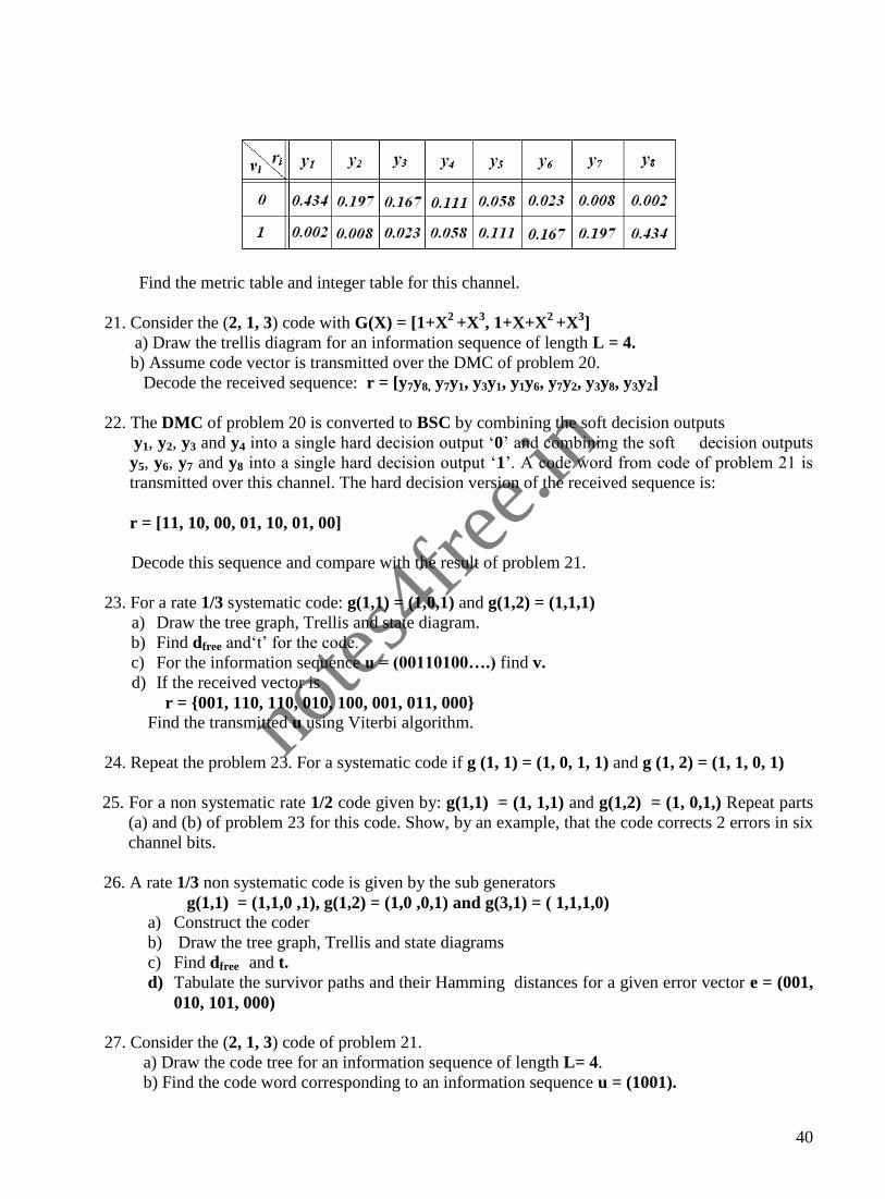
40

Find the metric table and integer table for this channel.

21. Consider the (2, 1, 3) code with G(X) = [1+X2

+X3, 1+X+X

2 +X

3]

a) Draw the trellis diagram for an information sequence of length L = 4.

b) Assume code vector is transmitted over the DMC of problem 20.

Decode the received sequence: r = [y7y8, y7y1, y3y1, y1y6, y7y2, y3y8, y3y2]

22. The DMC of problem 20 is converted to BSC by combining the soft decision outputs

y1, y2, y3 and y4 into a single hard decision output „0‟ and combining the soft decision outputs

y5, y6, y7 and y8 into a single hard decision output „1‟. A code word from code of problem 21 is

transmitted over this channel. The hard decision version of the received sequence is:

r = [11, 10, 00, 01, 10, 01, 00]

Decode this sequence and compare with the result of problem 21.

23. For a rate 1/3 systematic code: g(1,1) = (1,0,1) and g(1,2) = (1,1,1)

a) Draw the tree graph, Trellis and state diagram.

b) Find dfree and„t‟ for the code.

c) For the information sequence u = (00110100….) find v.

d) If the received vector is

r = {001, 110, 110, 010, 100, 001, 011, 000}

Find the transmitted u using Viterbi algorithm.

24. Repeat the problem 23. For a systematic code if g (1, 1) = (1, 0, 1, 1) and g (1, 2) = (1, 1, 0, 1)

25. For a non systematic rate 1/2 code given by: g(1,1) = (1, 1,1) and g(1,2) = (1, 0,1,) Repeat parts

(a) and (b) of problem 23 for this code. Show, by an example, that the code corrects 2 errors in six

channel bits.

26. A rate 1/3 non systematic code is given by the sub generators

g(1,1) = (1,1,0 ,1), g(1,2) = (1,0 ,0,1) and g(3,1) = ( 1,1,1,0)

a) Construct the coder

b) Draw the tree graph, Trellis and state diagrams

c) Find dfree and t.

d) Tabulate the survivor paths and their Hamming distances for a given error vector e = (001,

010, 101, 000)

27. Consider the (2, 1, 3) code of problem 21.

a) Draw the code tree for an information sequence of length L= 4.

b) Find the code word corresponding to an information sequence u = (1001).

notes

4free

.in

41

28. Consider the (2, 1, 3) code of problem 21.

a) For a BSC with p =0.045, find an integer metric table for the Fano metric.

b) Decode the received sequence: r = (11, 00, 11, 00, 01, 10, 11) using the stack algorithm.

Compare the number of decoding steps with the number required by the Viterbi algorithm.

c) Repeat part (b) for the received sequence r = (11, 10, 00,01,10,01,00)

29. Consider again the (2, 1, 3) code of problem 21.

a) For the binary input-8-ary-output DMC of problem 20, find an integer metric table for the

Fano metric.(Hint: Use appropriate scale factor for each metric and round to the nearest

integer).

b) Decode the received sequence: r = [y7y8, y7y1, y3y1, y1y6, y6y2, y3y8, y3y2] using the Stack

algorithm. Compare the final decoded path with the result of problem 21(b) where the same

received sequence is decoded using Viterbi algorithm.

30. Repeat problem 29 using Fano algorithm with threshold increments of = 5 and

= 9.Compare the final decoded path and the number of computations with the

Stack algorithm.

31. Refer to the code tree of Fig P 8.13. The branch metrics are specified as below.

iijj

iijjiijj

iijj

ijij

vrandvrif9

vrandvrorvrandvrif4

vrandvrif1

)vv|rr(M

Calculate the path metrics at the nodes of the tree for an all zero transmitted sequence, and the

received sequence (10, 00, 01, 01) with three transmissions errors. Then apply Fano algorithm to

decode the received sequence under the assumptions:

a) The decoder chooses the lower branch in the case of a tie in path metrics.

b) The decoder chooses the upper branch in the case of a tie in path metrics.

OUTCOMES

To know the encoding of convolutional codes.

How to decode the convolutional codes using algorithm.

REFERENCE

www.youtube.com/watch?v=AnyVu5eDhAQ

nptel.ac.in/courses/117106031/

elearning.vtu.ac.in/P4/EC63/S11.pdf

notes

4free

.in

module 1 information theory - Notes4free

Documents

Transcript of module 1 information theory - Notes4free