1

Modern and Ancient Cultural Capital. A Worldwide Cross-Sectional Analysis.

Guido Travaglini Università di Roma “La Sapienza”, Italy Email: jay_of_may@yahoo.com December 2005

Take a rest sometimes in your life and listen to the immense music of your past”. Benhabib.

2

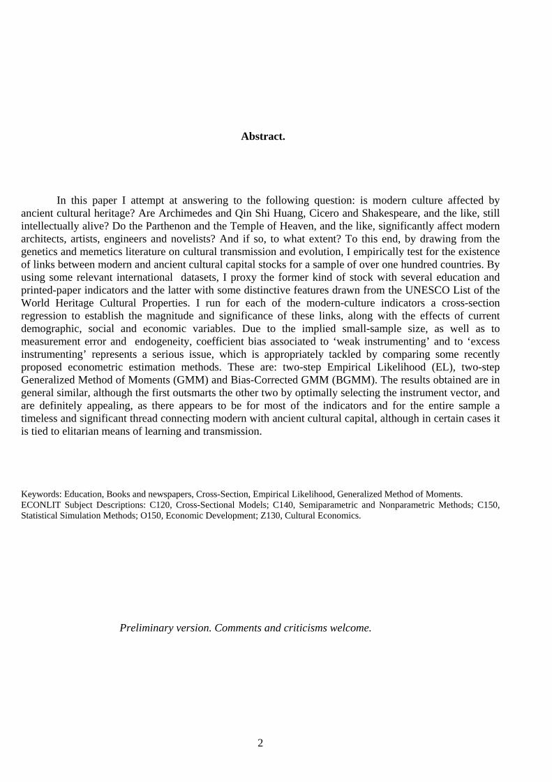
Abstract.

In this paper I attempt at answering to the following question: is modern culture affected by ancient cultural heritage? Are Archimedes and Qin Shi Huang, Cicero and Shakespeare, and the like, still intellectually alive? Do the Parthenon and the Temple of Heaven, and the like, significantly affect modern architects, artists, engineers and novelists? And if so, to what extent? To this end, by drawing from the genetics and memetics literature on cultural transmission and evolution, I empirically test for the existence of links between modern and ancient cultural capital stocks for a sample of over one hundred countries. By using some relevant international datasets, I proxy the former kind of stock with several education and printed-paper indicators and the latter with some distinctive features drawn from the UNESCO List of the World Heritage Cultural Properties. I run for each of the modern-culture indicators a cross-section regression to establish the magnitude and significance of these links, along with the effects of current demographic, social and economic variables. Due to the implied small-sample size, as well as to measurement error and endogeneity, coefficient bias associated to ‘weak instrumenting’ and to ‘excess instrumenting’ represents a serious issue, which is appropriately tackled by comparing some recently proposed econometric estimation methods. These are: two-step Empirical Likelihood (EL), two-step Generalized Method of Moments (GMM) and Bias-Corrected GMM (BGMM). The results obtained are in general similar, although the first outsmarts the other two by optimally selecting the instrument vector, and are definitely appealing, as there appears to be for most of the indicators and for the entire sample a timeless and significant thread connecting modern with ancient cultural capital, although in certain cases it is tied to elitarian means of learning and transmission. Keywords: Education, Books and newspapers, Cross-Section, Empirical Likelihood, Generalized Method of Moments. ECONLIT Subject Descriptions: C120, Cross-Sectional Models; C140, Semiparametric and Nonparametric Methods; C150, Statistical Simulation Methods; O150, Economic Development; Z130, Cultural Economics.

Preliminary version. Comments and criticisms welcome.

3

1. Introduction.

The issue of cultural transmission and evolution has received growing attention in the last decades, especially thanks to the introduction of mathematical models in the field of memetics [Dawkins, 1976, 1982; Kendal and Laland, 2000] and of population genetics and epidemiology [Cavalli-Sforza and Feldman,1981; Lumsden and Wilson, 1981; Boyd and Richerson, 1985; Hofbauer and Sigmund, 1988]. In spite of different definitions of culture across specialists and of different methodologies used, the issue preserves high intellectual appeal in attempting to establish the extent to which, whether by memes or by genes, ancient and modern cultural capital stock are linked. At the same time, a large body of literature has developed by analyzing the relationship between modern cultural capital and economic growth [Becker, 1964; Lucas, 1988; Sala-i-Martin, 1997; Barro, 1999, 2000; Barro and Sala-i-Martin, 1999] or wage rates [Mincer,1974; Mincer and Polachek, 1974; Card, 1999; Card and Krueger, 1992; Heckman et al., 2003], or for its own determinants [Becker, 1964; Acemoglu, 1997; Brunello et al., 2000; Brunello and Checchi, 2003]. However, to date, only few economists have tackled the topic of growth in a long-term historical perspective or by making use of ancient cultural capital [Kremer, 1993; De Long and Shleifer, 1993; Casson, 1993; Gray, 1996; Cozzi, 1998; Faria and León-Ledesma, 2003].

In the present paper, I attempt to link together the experiences of these two bodies of literature in order to find, by means of econometric testing, the size and significance of cultural transmission and evolution across centuries and even millennia,. The goal can be achieved, however, only once a generally acceptable and measurable definition of culture is provided.

Although largely intuitive, in fact, the definition of culture in the present context is by no means given for granted. Cavalli-Sforza and Feldman [1981] define culture as: “Those aspects of thought, speech, action, and artifacts which can be learned and transmitted”. Because general and encompassing, this definition may be split into two mutually-exclusive categories: ‘High culture’ and ‘Low culture’ [Allott, 1999]. The former is: “The intellectual and artistic activity and the works produced by it - usually of high expertise and aesthetic value - that are passed on to future generations by means of education and training, and the resulting enlightenment and excellence of taste”1. High culture is identifiable with invisible accumulated capital, of recent or ancient quality and vintage which takes the visible form of scientific, technological or artistic capital, viz. the national cultural heritage. Low culture is instead defined as the totality of customs, tastes, behavior patterns, vocational arts and crafts, social arrangements and institutions of a given nation or ethnicity, and in part corresponds to the concept of ‘social capital’ [Putnam, 1993], but definitely does not enter cultural capital.

Because of their different natures, these two forms of culture also bear different time characteristics. In fact, within a (very) long-run perspective, low culture is subject to frequent and fundamental changes, whereas high culture is usually destined to remain unabated overtime, while both affect one another sometimes significantly and other times mildly. Cultural heritage is in fact a capital stock and thus a low-frequency phenomenon which provides the foundations of national identity in spite of multiethnical diversity, which usually positively affects it by fostering competition and improvement in mentifacts and artifacts. Low culture, instead, is a high-frequency phenomenon which may be affected by cultural heritage depending on the extent to which its intrinsic values (expertise and aesthetics) are embedded in the society, usually as a function of education. In a typical peaceful society they cohabit, but low culture in several cases may swamp high culture, especially when forcefully imposed or in the presence of a decadent society.2. Only high culture by definition has the capability of fully embedding the quality values of national cultural heritages and to pass them on the future generations, even in the not unfrequent case of dramatic socio-political and economic changes. By consequence, the word culture used in this paper is referred to as ‘High culture’, and may be defined as either ‘modern’ or ‘ancient cultural capital stock’ [Bourdieu, 1986].

While there is general agreement on the definition and measurement of modern cultural capital stock, nothing similarly accepted exists for its ancient counterpart. The former is proxied by standard education indicators, known as ‘human capital’ [Becker, 1964; Lucas, 1988; Barro, 1999, 2000; Barro and Sala-i-Martin, 1999], that are available from different data sets [Barro and Lee, 1996, 2001; Kiriacou,

4

1991; Cohen and Soto, 2001; UIS, 2004;] although quite often marred by measurement error3. To complete on the classic definition of culture mentioned above [Cavalli-Sforza and Feldman, 1981; Bourdieu, 1986] I add to these learning indicators a complementary set of cultural-transmission vehicles, represented by the different classes of books and newspapers titles (henceforth defined as ‘printed-paper culture’)4. Proxies for ancient cultural capital, instead, are to date unavailable and most likely very difficult to concoct because of poor data and no received uniformity in selection criteria5. However, a proxy that best defines it can be retrieved from the UNESCO List of the World Heritage Cultural Properties (WHCP) [Faria and León-Ledesma, 2003], whereby a number of quantitative indicators may be extracted, ranging from the number of sites to their mean age down to more specific characteristics of religious and political nature.

Given thus the availability of homogenous data striding the two cultural capital stocks, it is quite straightforward to carry econometric testing for the causality effects, and their significance, running from ancient cultural capital over modern cultural capital. The testing is conducted by means of three different Instrumental-Variables Estimation (IVE) techniques of a cross-section regression of each indicator of modern capital against a vector of exogenous variables represented by the indicators of ancient capital plus dummies, with the instruments being a vector of several current demographic, social and economic variables retrieved from official sources (UNDP, WHO, UIS, and others). The IVEs respectively are: Empirical Likelihood (EL), two-step Generalized Method of Moments (GMM) and Bias-Corrected GMM (BGMM).

The paper is subdivided as follows. Section 2 introduces the data and provides some preliminary descriptive statistics on the data set used. Section 3 describes the estimation methods adopted and may be comfortably skipped by the non-technical reader, while Section 4 provides and discusses the empirical results. Section 5 concludes.

2. Data and descriptive statistics.

2.1. The data. The available data encompassing ancient and modern cultural capital stocks are divided into four

categories: 1) modern-culture indicators, 2) ancient-culture indicators, 3) binary dummies, 4) demographic, social and economic indicators. The first set of indicators constitutes the endogenous variables undergoing the cross-section regression, the second and third sets of indicators sum up to the vector of the exogenous variables, while the last set includes the instruments. Sect. 3 describes formally the implied econometric setting, and the Appendix provides details on the complete list of the data and their sources.

1) As far as modern cultural capital is concerned, many indicators are available as proxy candidates, all stemming from updated world databases. I have identified a total of eighteen, subdivided into two main categories: educational and printed-paper indicators, by and large respectively associated to learning and transmission culture. The Appendix provides details and data sources.

Out of the educational indicators, I have selected seven: the population shares of post-secondary school enrolment and completion, the average years of school, the combined education index, gross enrolment ratios in tertiary education, years of school life expectancy and the literacy rate. Most of the indicators, however, are flawed by country data non-availabity, so that missing data is quite frequent and the workable number of observations hovers on average around 90. Moreover, if available, some data are not recent (several of them cover the period 1994-97), although many are updated to the years 2000 and beyond. In order to maximize the number of observations per indicator and preserve series continuity, the older date is adopted if the newer is unavailable.

Of the educational indicators, the first three pertain to the educational-attainment Barro-Lee dataset (henceforth BL) [1996, 2001] and the others to the UNDP [UNDP, 2004] and UNESCO Institute of Statistics (UIS) datasets [UIS, 2004]. The BL indicators are the country population shares of post-secondary schooling enrolment and completion as well as the average years of school, all referred to populations aged 25 and over. The UNDP indicator used is the combined education index, while the UIS

5

indicators include gross enrolment ratios in tertiary education, school life expectancy and the adult literacy rate. While conflicting or overlapping, the selected indicators may supply – upon careful interpretation – the necessary information embedding the cultural heritage of a country. This is the reason why a more detailed explanation of their features is necessary at this juncture.

In fact, worth of notice for definitional purposes are some of these indicators. The adult literacy rate is defined as “The percentage of population aged 15 and over who can both read and write with understanding a short simple statement in his/her everyday life” [UIS, 2004], and is a very general proxy for modern cultural capital, yet viable because of the assumption that also lower-educated people may have (some) perception of their own cultural heritage. School life expectancy is less general as it encompasses the average length of years of schooling with no maximal age bound, while the tertiary-school gross enrolment ratio is expected to represent, in the absence of larger data availability on academic attendance, the workhorse of modern cultural capital. Finally, the UNDP combined educational index, by encompassing all school levels and including the adult literacy rate, attempts at supplying the broadest concept of human capital available to date.

The printed-paper indicators pertain all to the UIS dataset which includes total newspapers (number of titles of dailies and nondailies) and total book production (number of titles, therein including school textbooks) subdivided into nine Universal Decimal Classification (UDC) classes: generalities, philosophy and psychology, religion and theology, social sciences, philology, pure and applied sciences, arts and recreation, literature, geography and history. These book classes include also school textbooks and, from the intuitive viewpoint, they are all expected to embody ancient cultural heritage in one way or the other. In particular, those with a longstanding tradition, like philosophy, religion, arts and recreation, and literature, are expected to embody it in a significant way. On the other hand, other book classes and newspapers, being of very recent diffusion within and among countries, are expected to be weakly related to ancient cultural heritage6.

2) As for ancient cultural capital, the WHCP list supplies precious qualitative and quantitative information usable to construct appropriate proxies that may retain its major features of intellectual and artistic dynamics. Even if incomplete and subject to continuous updating, and in spite of some subjectively unexplainable exclusions (e.g. Bhubaneswar in India and Rangoon in Myanmar) and inclusions (e.g. the Varberg Radio Station in Sweden), the WHCP list consists, as of July 2005, of 628 sites distributed across 116 countries of which I exclude three (Afghanistan, Iraq and the Democratic People’s Republic of Korea) because of missing data or data unreliability of most if not all of the modern-culture indicators. We are thus left with a data base of 608 sites distributed across 113 countries of the five continents. Incidentally, the city of Jerusalem is included in Israel and the Holy See in Italy. In addition, the site of Auschwitz is removed from Poland7.

From the WHCP list, which supplies for each country the number and a cursory description of the sites, I have contructed a total of five quantity indicators addressed at proxying ancient cultural capital stock: the total number of sites, their average age, the ratio (percent share) of sites older than 250 years, a historical dummy ratio and the ratio of ‘Temples and Castles’. The number of sites offers a clue on the amount of cultural wealth accumulated by each country in the past, and also – at least form the probabilistic viewpoint – on its degree of technical expertise and aesthetics, according to the competitive principle whereby the larger the size of its input human capital stock (e.g. the number of artists, engineers and technicians employed) in an open society the higher the mean value of the output. By this reasoning, the number of sites is taken to represent the quality level of high culture expressed by the country.

The average site age8 provides information on the time span covered to materialize the site construction process, thereby helping identify ‘ancient’ as opposed to ‘young’ cultures, without bearing any specific relationship with expertise and aesthetic values. Time is in fact a necessary yet not sufficient condition for cultural improvement in the long run, especially if the country has undergone destructive events like systematic warfare or frequent social and political turmoils, thereby negatively affecting its human capital stock. In quite a few cases, however, the amount and quality of cultural heritage may at least partially outweigh such consequences9.

6

The ratio of sites exceeding 250 years is a subtle yet arbitrary concept that sets on a quarter millennium ago the commencement of the ‘Modern Era’ marked by the expansion of trade, colonization and conquest by the Western nations of the four corners of the world and initiation of the industrialization process still underway nowadays. Because of such dramatic changes on the features of cultural capital accumulation on both sides, the ratio is expected to expresses, albeit loosely, the returns to site production which may be considered decreasing (increasing) when the average age is high (low) and the ratio equals or is very close to (well below) unity. In essence, the ratio measures the overtime continuity of the quality level of sites by relating distant-past cultural capital stock with more recent additions, thereby revealing an improvement or deterioration in technical expertise and aesthetics10.

Subsequently, I add a ratio denominated ‘Pre-post overhaul’, which may seem unpalatable for some scholars but appealing from the qualitative viewpoint. A cultural ‘overhaul’ is defined as a permanent shock, or series of shocks, that the religious and/or the socio-political setting of a country may have historically undergone by means of peaceful change(s) or violent upheaval(s). For each country, I establish the approximate date of the overhaul(s), if applicable (e.g. fall of the Roman Empire, Islamic conquest, colonization) and then check the amount of its sites that have been erected or manufactured prior to and after that date. The former amount divided by the latter yields the ratio, which is equal to zero for countries that have never experienced overhauls 11.

Finally, I consider the share of ‘Temples and Castles’, which reflects the amount of cultural wealth accumulated in the country by the traditional income-rich ruling classes (aristocrats and clerics) as opposed to the works and artifacts belonging to middle- and low-income classes (bourgeoisie and populace) [De Long and Shleifer, 1993]12. Essentially, this variable intends to test for whether the impact on high modern culture more significantly stems from the former than from the latter.

3) I add to the regressor list a set of binary dummies, based on the official or largely prevailing religion practiced in each country. The dummy is unity for either of the four most diffused religions in the world (Islam, Christian, Catholic, Buddhist and Confucian) and zero elsewise. Christian includes Protestantism and Orthodoxy, while all other religions (Animist, Hindu, Other and Mixed) constitute the complementary dummy and must thus be excluded13.

The rationale for using these dummies is based on cross-country historical evidence of the strong relationship between cultural heritage and religion via the very frequent agreements that have tied together the ruling classes (aristocrats and clerics). Moreover, by extending the intuition of Barro and McCleary [2003], the fact that both modern education and printed paper production are frequently tied to religion, either directly or indirectly, cannot be dismissed. In other words, it may be reasonably assumed that religions in general, due to their traditionally populistic stance, avail themselves with powerful means of seduction represented by ‘Temples and Castles’ and of coercion - especially with modern Islam and Catholicism - by influencing and often by directing modern culture, both in the educational and in the printed-paper forms. Econometric testing of these assumptions is conducted in Sect. 4 by checking for the sign and statistical significance of religious dummies in explaining the endogenous variables14.

4) The world data base for demographic, social and economic indicators is to date very large and supplied by many authors and international institutions of which, in particular, the Penn World Tables, the United Nations, the World Bank and other specialized agencies. For the present purpose a limited amount of variables is required, specifically those mostly correlated to modern-culture indicators, in the spirit of the cited studies that deal with the relationship between education and growth and/or wages. All of the data reported are the most recent available as possible depending on the source (see Appendix).

The variables used (20 in total) are the following: real GDP percapita level and annual growth rate, total country population and annual growth rate, trade openness, fertility and urbanization rates, human development index, three indexes of freedom, civil liberties and political rights, average life expectancy, and the following percent ratios: Public Expenditure on Tertiary Education/Total Public Expenditure on Education, Public Expenditure on Total Education/GDP (or GNP), Total Public Expenditure/GDP (or GNP), average primary, secondary and tertiary school pupils/teacher, females/males gross tertiary school enrolment ratios (known as the ‘gender ratio’), internet users/total population, population aged 0-19/total population. I have added also the percent of endangered sites from the WHCP list.

7

The rationale for using these variables, as mentioned above, is justified on the following grounds, largely adopted by the recent literature on growth and education [Barro, 1999, 2000; Comi and Lucifora, 2000; Brunello and Checchi, 2003; Baldacci et al., 2004; Chen and Dahlam, 2004]. The ratio of educational government spending represents the effort of institutions to foster and disseminate education addressed at human capital formation [Schultz, 1961; Barro and Sala-i-Martin, 1999 ], while real GDP percapita is a proxy of the family income input in the education function, reflecting the ‘parental role’ of investment in youth education, especially in countries where education is not totally cost-free (e.g. textbooks, tuition fees and accomodation expenses) and/or private schooling is supplied in abundance [Mincer, 1974; Mincer and Polachek, 1974; Becker, 1981; Cremer et al., 1992; Brauninger and Vidal, 1999; Brunello et al., 2000]. Fertility measures the impact of incoming generations on extant schooling infrastructures [Barro, 1999, 2000], while the pupil-teacher ratio represents a school-quality indicator, and is interpreted as a substitute to parental education [Card and Krueger, 1992; Brunello and Checchi, 2003].

Moreover, introduction of the indexes of freedom, civil liberties and political rights involves the hypothesis that poor governance [Putnam, 1993] has an adverse effect on cultural dissemination and, more specifically, on public spending [Gupta et al., 2002; Baldacci et al., 2003], while urbanization and gender ratio are important factors of cultural dissemination as they widen the share of population potentially involved in learning and transmitting culture [Galor and Weil, 1996; Treiman, 2002], so much as trade openness and internet [Chen and Dahlam, 2004], either directly or via economic growth [Barro, 2000]. Also a comparatively good health and long life expectancy should positively affect human capital [Dahlin, 2003; Baldacci et al, 2004]. The share of endangered sites, finally, is regarded as an index of cure and maintenance of the local cultural heritage.

2.2. Descriptive statistics. Precious as it may be due to its illustrative features, descriptive statistics offers only a general and

generic overview for the understanding of cross-country or time-series phenomena. Hypothesis testing and statistical inferencing can be pursued only by the econometrics science. It is in this spirit that Tables 1 to 4 are subsequently exhibited and interpreted, letting Sect. 4 supply and explain the chore problem of the present paper.

Table 1 displays some relevant descriptive statistics regarding the variables used in the present context. There I report the number of sites for each country, the average age, the share of sites exceeding 250 years of age and some select modern-culture indicators, namely, three educational indicators plus total books and newspapers.

Figure 1 displays on a logarithmic scale the scatterplots of the relationship between the number of sites and the select modern-culture indicators reported in Table 1. While the squares depicted indicate the countries, the diamonds line illustrates the ‘best fit’ among each couple of variables for the entire country sample15. Simple eyeballig reveals a positive relationship across all indicators, which is particularly marked for two educational indicators (average years of schooling and combined education index) and for both total printed-paper indicators. The results are indeed appealing, as they evidence prima facie a connection between ancient and modern cultural capital stocks, and thus lend support to the hypothesis of overtime cultural transmission and evolution advanced by the genetics and the memetics literature. In fact most of the indicators are significantly correlated with the number of sites16

Table 2 goes a bit further by exhibiting the nine UDC classes that compose total book titles. Some countries of Table 1 are absent because of no data reporting. Several Islamic countries (most notably Iran, Oman, Algeria and Egypt) and quite a few Catholic countries (especially Brazil, Croatia, Italy and Poland) exhibit high reading rates of religious books, while social sciences, pure and applied sciences and literature constitute almost everywhere the majority of the books read. Social sciences share similar reading rates for most part of the sample with many Islamic countries in the trailing positions, while pure and applied sciences are particularly appreciated in the ex-communist countries and in Scandinavia as well as in some energy-exporting Islamic countries, but shunned in several Catholic countries like Italy, Brazil, the Philippines and Chile. Literature exhibits a very mixed pattern, yet quite a few Islamic countries occupy

8

the lowest ranks. Apart from that, there appears to be no strict relationship between this reading class and the country amount of cultural heritage, a feature shared also – in general - by the the disciplines which are more directly related to antiquity: philosophy and psychology, arts and recreation, and geography plus history17. Notable exceptions, amongst others, are Mexico, Brazil and Argentina on the first discipline; Oman, Andorra and the Republic of Korea on the second; Bahrain, France, Tunisia and Italy on the third.

Table 3 to a certain extent summarizes Tables 1 and 2 by providing, together with real GDP percapita, some select educational and printed-paper indicators classified on the basis of the official or largely prevailing religion where, for explanatory purposes, I have split Christianity into its components: Protestantism and Orthodoxy. Interestingly, Islamic countries on average appear to fare worse than the others (excluding ‘Other religions’ which is represented mainly by Sub-Sahelian countries and Southern Asia) in terms of incomes and educational standards, while are much in line with world averages for the printed-paper indicators, except for religion and theology, social sciences and literature.

Tables 4 to 5 exhibit the country rankings of the ratios of select educational and printed-paper indicators with respect to the number of cultural sites. The purpose of this reported evidence stands in the need of search for the countries which are most ‘virtuous’ at teaching and transmitting the quality values of their own cultural heritage, whichever its size. As to the educational indicators, the following countries stand out in Table 4 in at least two of them: Australia, Azerbaijan, Estonia, Iceland, Latvia, Luxembourg, Kenya, Mongolia and Uruguay. All of them share one single site only, and may be viewed as virtuous. At the lowest ranks stand instead many cultural-heritage rich countries, like China, France, Germany, Greece, India, Italy, Mexico, Spain and the United Kingdom. As to books and newspapers, to which I add ‘humanities’ (the sum of all book classes from philosophy and psychology downwards), from Table 5 the following countries occupy the top ranks in at least two of them: Canada, Denmark, Japan, the Republic of Korea, Switzerland, the United Kingdom and the United States.

An interesting picture emerges from careful reading of these two tables: while the schooling ratios exhibit a negative relationship with size, the books ratios exhibit a positive one. As proven by the Spearman rank correlation coefficients18, I conclude that schooling, which is usually governmental and/or religious, despises size and thus quality such that an abundant (scarce) ancient cultural wealth conduces to lower (higher) education. Probably this evidence is due to the widely received, yet so far unproven, dictum that public education masters disregard the amount and quality of their own high-culture traditions. The opposite occurs with book reading, which significantly appreciates them.

Tables 6 to 7 exhibit the country rankings of select educational and printed-paper indicators with respect to the average age of sites. The purpose here is to find evidence on the relationship existing between modern cultural indicators and the vintage of their ancient counterpart. The value judgement implied is obviously crude and gross as compared to the finesse required to value the sites quality, namely, the expertise and aesthetics therein embedded. While educational ratios exhibit a mixed pattern, books and newspapers ratios indicate that reading is significantly correlated to age, as evidenced by Table 7, where many top ranks are occupied by many cultural-heritage rich countries, most notably Germany, Italy, Japan, the Russian Federation and the United Kingdom.

3. Estimation methods.

3.1. Two-Stage Least Squares and Generalized Method of Moments.

With all the data selected at hand, I now describe the estimation methods adopted for running, one at a time, the linear cross-section regressions of the eighteen modern cultural-capital indicators against the regressors and with the instruments described in Sect. 2. The implied small-sample size, coupled with measurement error and regressor endogeneity may cause severe coefficient inconsistency associated to ‘weak instrumenting’ and to ‘excess instrumenting’ [Staiger and Stock, 1997; Andrews, 1991, 1999; Donald and Newey, 2001; Hahn and Hausman, 2002, 2003; Hahn et al., 2001, 2002; Stock and Wright, 2000; Stock et al., 2002; Chao and Swanson, 2004] so that biased estimates may result from using the

9

traditional Two-Stage-Least-Squares (2SLS) and the two-step Generalized Method of Moments (GMM) [Hansen, 1982; Hansen and Singleton, 1982; Hansen and West, 2002]. For this reason, along with GMM, I introduce two well-known alternative methods: the two-step Empirical Likelihood (EL) [Owen, 1988, 2001; Qin and Lawless, 1994; Imbens, 1997; Donald et al., 2003; Guggenberger and Hahn, 2005] and the two-step Bias-Corrected GMM estimator (BGMM) [Donald et al., 2002], which is based upon the Bias-Corrected Two-Stages Least Squares (B2SLS) estimator [Donald and Newey, 2001]. In Sect. 4, EL, GMM and BGMM cross-section estimates will be analyzed and compared in terms of coefficient consistency and efficiency.

Let N be the number of countries for which data are available, and 1 2( , ,... )Ny y y y= the Nx1 vector of any of the modern-culture indicators, 1 2( , ,... )NX x x x= the NxK matrix of ancient-culture indicators plus the religious dummies, and 1 2( , ,... )NZ z z z= the NxL (L >K) matrix of the demographic and socio-economic variables.

A typical linear structural cross-section model of each of the modern-culture indicators may be represented as follows: (3.1) 'i i iy X eβ= + ; i=1,…N where β is a Kx1 vector of coefficients, ie is a Nx1 vector of I.I.D. disturbances, and ( ' ) 0i iE X e = , ( ) 0iE e = , 2 2( )

ii eE e σ= , 2 2( )ie eE σ σ= , which respectively imply no endogeneity bias, zero mean and

given variance of the disturbance, and no heteroskedasticity. In addition, for iη and iν being Nx1 vectors of I.I.D. disturbances such that *

i i iy y η= + and *i i iX X ν= + , where *

iy and *iX are the respective

‘true’ observations, ( ' ) 0i iE y η = and/or ( ' ) 0i iE X η = , namely, no expected measurement error on both the left and the right hand side of the equation is assumed [Portela et al., 2004]. If all of the stated ‘well-behavedness’ conditions apply, Ordinary Least-Squares (OLS) estimation is consistent and efficient. However, if any of the following occurs, namely ' 0i iX e ≠ , ' 0i iy η ≠ or ' 0i iX ν ≠ , IVE is required to correct for estimation bias, while heteroskedasticity calls for specific correction methods, e.g. the White [1980] or the Aitken [1935] estimators.

In turn, IVE requires instruments ‘validity’, that is, the orthogonality conditions ( ' ) 0i iE Z e = . In applied work, however, orthogonality may not hold for several or many of the instruments chosen. Moreover, while meeting this requirement, instruments may be ‘weak’ by exhibiting low correlation with the regressors. Two well-known IVEs, the Two-Stages Least Squares (2SLS) and the two-step Generalized Method of Moments (GMM) are addressed at performing this task, by minimizing a criterion function based on sample counterparts of the population orthogonality conditions and on a specific weight matrix. To describe both IVEs, some notation is necessary at the onset.

For some compact coefficient space Β of real numbers, let the ‘true’ population estimator be 0β ∈ Β , and denote 0 0( ) ( , )ig g Xβ β≡ 'i iZ e= a LxN matrix of the ‘long-run’ unconditional moments

with the assumed orthogonality property ( )0( ) 0iE g β = , (i=1,…N). A LxL weight matrix, known as the long-run covariance or second-moments matrix [Hansen and West, 2002] may thus be constructed as follows

10 0

1

( ) ( )'N

N i ii

W N g gβ β−

=

= ∑

with typical element , ,' 'i m i i i nz e e z ; 1,... ; 1,...m L n L= = , m n= for the diagonals and m n≠ for the

off-diagonals. For N → ∞ , the ‘regularity conditions’ are: ( )10 0 0

1

( ) ( ) ( )N

i ii

N g g E gβ β β−

=

≡ =∑ , which

10

constitute the L-sized vector of population moment averages, and 1/2 10

1

( ) . . .(0, )N

i Ni

N g N I D Wβ− −

=

→∑ ,

which represents their asymptotics. Linearity in the coefficients, to preserve the simplicity involved in the present context, is assumed throughout.

The first partial derivatives of the ‘true’ long-run moments, denoted as ( )0( )/ ( )iE g β β∂ ∂ , form

an LxK matrix 'G Z X= − of rank K, with typical element 1

'N

ii iz x

=∑ . By making use of 0( )g β and NW , a

quadratic scalar criterion function can be constructed such that: (3.2) ( ) ( )'N NJ g W gβ β= from which, after letting 'Z e be the stacked version of 'i iZ e , the K first-order conditions (FOCs) may be derived: (3.3 ) ' ' 0NG W Z e = to solve by minimization for the coefficient of interest 1

0 ( ' ) ' 'N NG W G G W Z yβ −= . The same setup may be adopted to solve for the IVEs in an empirically applied context, where the

actual sample moments replace the long-run moments and consistency of the estimated coefficient with 0β is expected as N → ∞ . By letting ( ) ( , )ig g Xβ β≡ be the moment functions based on actual data and

1

1

( ) ( )N

ii

g N gβ β−

=

≡ ∑ be their sample means evaluated at β ∈ Β , the 2SLS estimator is expressed as

(3.4) ( )2 argmin ( ) ( )'SLS B

g Wgβ

β β β∈

=

where ( ) ( )'g Wgβ β is the sample counterpart of eq. 3.2 and the LxL nonsingular weight matrix W is

1( ' )Z Z − . Similarly, given 1

1

ˆ ˆ( ) ( )N

ii

g N gβ β−

=

≡ ∑ the sample moment means evaluated at β , the GMM

estimator is expressed as

(3.5) ( )ˆ

ˆ ˆ ˆargmin ( ) ( ) ( )'GMMBg W g

ββ β β β

∈=

so that, for β a preliminary estimator (usually 2SLSβ ), ˆ ˆ( ) ( )'g Wgβ β is the sample counterpart of eq. 3.2, where

1

1

1

ˆ ˆ ˆ( ) ( ) ( )'N

i ii

W N g gβ β β−

−

=

⎛ ⎞⎟⎜= ⎟⎜ ⎟⎟⎜⎝ ⎠∑

defined as the optimal GMM weight matrix if β is a consistent estimate of 0β and, furthermore, if the orthogonality conditions ( )ˆ( ) 0iE g β = are satisfied. The 2SLS estimation procedure and the GMM use sample moments derived from the first-stage estimated disturbance vector of the structural model (eq. 3.1), and the two models coincide when this vector is characterized by homoskedasticity and serially independent disturbances. In such case, the two weight matrices W and ˆ( )W β coincide and, for N sufficiently large, both 2SLSβ and GMMβ are the unique solutions to the minimand thereby being consistent estimates of 0β . In a cross-sectional context, heteroskedasticity is expected to prevail because both the

11

mean and the variance of the dependent variable tend to be large the larger the independent variable(s). Therefore, a cross-sectional IVE model must account for this occurrence and GMM fares better than 2SLS in terms of efficiency if the preliminary estimator is a consistent estimate of 0β .

In general, however, this consistency is not granted in standard 2SLS, because of several reasons related to the choice of the instrument vector and to the available number of observations N. Hence, a biased estimator of β may be a quite frequent and undesirable occurrence. To describe it, let

(3.6) ' ' 'i i iX Z v= Π + be the reduced-form auxiliary model tying all of the regressors of eq. (3.1) to the predetermined instruments iZ , where Π is a KxL matrix of coefficients and ( ' ) 0i iE Z e = , that is, the instruments are ‘valid’. In addition, the disturbance is I.I.D. with ( ) 0iE v = , 2 2( )

ii vE v σ= , 2 2( )iv vE σ σ= . Finally,

( )rank KΠ ≤ depending on the arbitrarily selected minimum correlation coefficient below which the regressors are considered weakly correlated to the instruments, whereby some of them may be excluded in each of the K reduced-form equations19. Substituting eqs. (3.2) into (3.1) yields:

'i i iy Z δ ε= + where the KxL-sized vector klδ π β= , with klπ a typical element of Π (l=1,..L; k=1,…K ), is a linear combination of the coefficients of eqs (3.1) and (3.2), and similarly for 'i i ie vε δ= + .

The sample analog of the moments partial first derivatives is denoted as ˆ( )/ ( )ig β β∂ ∂ , which form

the LxK Jacobian matrix 1 1

1

' 'N

ii

i iG N Z X N z x− −

=

= − = ∑ . For ˆˆ 'i i ie y X β= − and ˆ ˆ' 'i iX Z= Π , where

Π is the estimated reduced-form coefficient matrix of eq. 3.6, and for ˆ'Z e the stacked version of ˆ'i iZ e , the sample counterpart of eq. 3.3 constitutes the sample K-sized vector of FOCs, namely (3.7) ˆ' ' 0iG WZ e = which, solved for β , yields the 2SLS estimator

12 ( ' ) ' 'SLS i iG WG G WZ yβ −=

whose asymptotic bias is (3.8) 1 1 1/2

0ˆ ˆ( ) ( ' ) ( ' ' )i i iN N G WG N G WZ eβ β − − −− = .

Let ˆ WGΠ = and 1 1ˆ ˆ'H N W− −= Π Π be the covariance of the estimated endogenous regerssors of eq. 3.1. A stochastic higher-order expansion of eq. 3.8, after a few arrangements [Bekker, 1994; Bound et al., 1995; Hahn et al., 2001, 2002; Hahn and Hausman, 2003; Donald and Newey, 2001], produces the following normality properties of the asymptotic bias, in case of heteroskedasticity correction [White, 1980] in terms of mean and variance: (3.9) ( )1/2 1 1

2 0ˆ( ) . . . ,( ' ' )

d

SLS ve iN N I D N H L G WG X Xβ β σ κ− − −− → − where veσ is the square-rooted covariance of the disturbances of the structural and of the reduced form. In other words, the 2SLS bias never approaches zero as either or all of the following circumstances occur: a too large number of instruments L relative to the number of observations N (‘excess instrumenting’) , a

12

large covariance of the disturbances (‘model inefficiency’ due to bad choice of regressors and/or of instruments) and ˆ 0Π → (‘weak instrumenting’) [Hahn et al., 2001, 2002; Stock et al., 2002; Chao and Swanson, 2005]. The bias vanishes if its causes are removed, and in general if N grows at a faster rate than L, such that 2 / 0L N → as N → ∞ , under the proviso that the instruments used be valid. If not, the bias persists [Hahn and Hausman, 2003].

The Bias-Corrected Two-Stage least Squares (B2SLS) estimator [Donald and Newey, 2001; Chao and Swanson, 2005], assuming validity, is: (3.10) [ ] [ ]1

2ˆ ' ' ) ' ' 'B SLS i iG WG X X G WZ y X yβ κ κ−= − −

for 1( 2)N Lκ −= − . If 0κ = , eq. 3.10 reduces to 2SLSβ .

The heteroskedasticity-corrected asymptotics of 2B SLSβ , which may be compared with those of eq. 3.9 , are (3.11) ( )1/2 1 1/2 1

2 0ˆ( ) . . . ( ),( ' )

d

B SLS ve e v iN N I D N H L G WGβ β σ σ σ− − −− → + such that the B2SLS asymptotic bias vanishes at the rate / 0L N → as N → ∞ , In such case, the B2SLS estimator is expected to converge to the true coefficient at a faster rate than its 2SLS counterpart20, and therefore to provide a more consistent preliminary estimator β for the two-step GMM procedure.

The two-step GMM estimation of the coefficient vector β of eq. 3.1 essentially follows the same path as above, as it uses sample moments to determine both the Jacobian and the weight matrix. The latter is optimal if the orthogonality conditions are satisfied and if the preliminary estimator is consistent so that, for what shown above, 2B SLSβ is the best bias-minimizing candidate. The GMM criterion function is (3.12) ˆ ˆ ˆ ˆ( ) ( ) ( ) ( )'J Ng W gβ β β β= and ist first derivative with respect to the estimator is ˆ ˆ( )/ 0J β β∂ ∂ =

from which the following FOCs are derived (3.13) ˆ ˆ' ( ) ( ) 0iG W gβ β = and solved for β to yield the optimal estimator (3.14) 1ˆ ˆ ˆ( ' ( ) ) ' ( ) 'GMM i iG W G G W Z yβ β β−= whose variance is denoted as (3.15) 1ˆ ˆ( ' ( ) )iG W Gβ −Σ = which is the minimum possible variance compared to any other estimator (e.g. 2SLS) that does not use ˆ( )W β as the weight matrix. Hence the estimator of eq. 3.14 is efficient, namely 0

ˆ p

GMMβ β→ , and

0ˆ. . .( , )N I D β Σ [Chamberlain, 1987].

13

Given that the orthogonality conditions for the instrument vector iZ exhibit the property of

( )ˆ( ) 0iE g β = , a statistical check for this requirement in applied work is conducted by means of the ‘J -statistic’ [Hansen, 1982; Hansen and Singleton, 1982]. The criterion function of eq. 3.12 is a scalar whose expected value is zero. Therefore, for 1L L< a subset of the L-sized instrument vector, under the null hypothesis of 1L K= (perfect identification of the subset) ˆ( )J β is asymptotically distributed as a

1

2L Kχ − statistic. The statistic provides a test for the ‘overidentifying restrictions’, because nonrejection of

the null, within a given significance level, implies that the preselected subset of 1L instruments satisfy the orthogonality conditions as they are truly predetermined. Contrarywise, additional information would be necessary in favor of an alternative or even of the entire set.

The GMM estimator in the presence of autocorrelation and heteroskedasticity is thus shown to be, for N sufficiently large, asymptotically consistent and more efficient than 2SLS. Moreover, it disposes of the consistency problems associated to instrument selection since minimization of eq. 3.12, with the weight matrix appropriately treated [Newey and West, 1987, 1994], bypasses weak instrumenting [Hayashi and Sims, 1983; Bound et al, 1995; Hayashi, 2000], excess intrumenting [Koenker and Machado, 1999; West et al., 2001; Hansen and West, 2002] and invalid instrumenting [Hahn and Hausman, 2003]. Hence, virtually, any L-sized vector of the instruments is considered optimal insofar as the orthogonality conditions are significantly proven to hold by means of the J-statistic test, and the larger is L for N → ∞ the greater the gains in asymptotic efficiency of the estimator [West et al., 2001].

However, even if the preliminary estimator is consistent, in a small-sample setting with heteroskedasticity (as is the usual case of cross sections), estimation bias may be a very serious issue in the presence of weak instrumenting [Staiger and Stock, 1997; Stock and Wright, 2000; Donald and Newey, 2001] and/or of excess instrumenting relative to the number of observations [Hansen et al., 1988; Nelson and Starz, 1990; Hall et al., 1996; Gallant and Tauchen, 1996; Andrews, 1991, 1999; West et al., 2001; Donald et al., 2002]. In such setting, the sample moment averages are in fact shown by Montecarlo evidence to be negatively signed and asymmetric [Altonji and Segal, 1996]. Moreover, in cross-section models, the bias is proven to be proportional to the number of instruments [Newey and Smith, 2004; Okui, 2004]. It follows that, for 0

p

GMMβ β→ to hold as N → ∞ , the sample moments and their first derivatives must share the same distributional properties as their population counterparts. Figure 2 illustrates, by Montecarlo simulations based on 1,000 replications of artificial series of different length (50, 75,100 and 200 observations), the magnitude of the bias-variance tradeoff emerging from an increasing number of instruments21. As these are made to linearly grow for each selected sample size, the squared bias decreases and the variance rises, and their ratio rises the larger is the instrument set, albeit less intensely the larger is the sample size.

3.2. Asymptotic bias in the Generalized Method of Moments and Empirical Likelihood.

To theoretically explain the nature of the asymptotic bias in the GMM estimator, the following notation is required. Eq. 3.12 may be rewitten as ˆ ' 0iGλ− = , with the auxiliary coefficient ˆ ˆ ˆ( ) ( )GMM GMMW gλ β β= , where GMMβ replaces β to indicate explicit reference to the estimator. After some

manipulation: ˆ ˆ ˆ( ) ( ) 0GMM GMMS gλ β β− − = . First-order Taylor expansion of ˆ ' 0iGλ− = and of the last equation around the long-run values, 0β and 0, provides the asymptotics of GMMβ and λ . In fact, given that the long-run counterparts of ˆ( )GMMg β , ˆ( )GMMW β and iG respectively are 0( )g β , NW and ( )iG E G≡ , the two-equation system describing the dynamics of GMMβ and λ is the following:

14

0

0

ˆ00

ˆ( )

GMM

g

β β

β λ

⎡ ⎤−⎡ ⎤ ⎢ ⎥⎢ ⎥ + Μ =⎢ ⎥⎢ ⎥− ⎢ ⎥⎢ ⎥⎣ ⎦ ⎣ ⎦;

0 '

N

G

G W

⎡ ⎤⎢ ⎥Μ = −⎢ ⎥⎢ ⎥⎣ ⎦

which, upon inversion to solve for 0GMMβ β− and λ , yields:

01

0

ˆ 0

ˆ ( )

GMMM

g

β β

βλ−

⎡ ⎤− ⎡ ⎤⎢ ⎥ ⎢ ⎥= −⎢ ⎥ ⎢ ⎥−⎢ ⎥ ⎢ ⎥⎣ ⎦⎣ ⎦; 1

'−

−Σ Θ⎡ ⎤⎢ ⎥Μ = −⎢ ⎥Θ Ρ⎢ ⎥⎣ ⎦

where for M nonsingular, 1 1( ' )NG W G− −Σ = , 1 1 1'N N NW W G G W− − −Ρ = − Σ and 1' NG W −Θ = Σ . The first two are variance terms, the last is a covariance. In addition, 1

NW−Ρ = if there is perfect collinearity

among endogenous regressors and instruments, and LIΡ = with exact identification (L=K) when 1

N LW I− = . Since ˆ( )GMMg β and λ are both 1/2( )Op N − , by virtue of the Central Limit Theorem and of the Weak Law of Large Numbers, the asymptotics of GMMβ and λ are the following: (3.16) ( )0

ˆ( ) . . . 0, ( )d

GMMN N I D diagβ β− → Σ , ( )ˆ . . . 0, ( )d

N N I D diagλ→ Ρ namely, both GMMβ and λ are asymptotically normal.

The higher order bias of GMMβ , in the presence of heteroskedasticity and conditional moments, follows from the stochastic expansion up to 1/2( )Op N − [Rothemberg,1984; Newey and Smith, 2004] of the expression:

10 0

ˆ ( )GMM M gβ β β−− = − which, after letting ˆ ( )/GMM GMMM g β β= ∂ ∂ and 1

0ˆ ( )U M g β−= − , yields the following approximation

formula:

10 0

ˆ ˆ ˆ ˆ( )( )GMM GMMU M M Mβ β β β−− = − − − where 1/2ˆ ( )U Op N −= and the second term is 1( )Op N − . Therefore:

10

ˆ ˆ ˆ ˆ( ) ( )GMMN U M M M Uβ β −− = − − where:

[ ]1 1ˆ ˆ( ) ( ' ) ( ) ( ' )i i i i i i iM E MU N E G Pg E G g E g g Pg− −− = −Σ +Θ Θ +Θ .

The approximate asymptotic bias of GMMβ may thus be expressed as the sum of three components, two of which heavily depend on the number of instruments used. The first bias component depends on the sample estimate of the Jacobian iG , the second on the sample estimate of the weight matrix ˆ( )W β , and the third on the moment vector, which is the product of iG and ˆ( )W β , as well as on the conditional moments.

Out of these components, the major source of asymptotic bias is represented by the first, denoted as 1 ( )G i iB N E G Pg−= −Σ . This expression may be developed as:

15

1 1ˆ ˆ( ' ' ) ( ' ' )N E X ZPZ e N E e XZ PZ− −Σ = − Σ

where the latter equation equals [ ]1 ˆ' ( ' )N e X tr Z Z P−− Σ ⋅ so that, finally: (3.17) 1 1ˆ ˆ ˆ( ' ) ' ( 2)GB N e e e X L− −= Σ − which implies that this form of bias, defined as the long-run covariance of moments with their first derivatives or as the bias in the Jacobian [Newey and Smith, 2004], is proportional to the ratio between the number of instruments L (minus two) and the number of observations. Moreover, it is affected by the covariance of the endogenous regressors with the first-step residuals, the component ˆ'e X in eq. (3.17). This bias will be partly reduced if, for given N, the disturbance vector e is associated to 2B SLSβ .

The second form of asymptotic bias is denoted as 1 ( ' )W i i iB N E g g Pg−= Θ . It arises from sample estimation of the weight matrix, that is, from the second-moment moment matrix 'i ig g , and can be very severe if the moments ig are far from normality [Altonji and Segal, 1996]. The bias vanishes if the residuals used to construct ig are all normal (conditionally symmetric), which in turn requires a consistent estimate of NW , namely ˆ( )

p

NW Wβ → in the first-step estimation, hence absence of excess or weak instrumenting in the 2SLS procedure. This expression, as with GB , may be developed as follows:

13' ( ' )WB N Z E Z PZμ−= Θ = 1

3' ( ' )N Z tr Z Z Pμ− Θ where the latter equation equals (3.18) 1

3' ( 2)WB N Z Lμ−= Θ − for 2 2

3 /i ieμ σ= . This bias, in essence, grows with the number of instruments and zeroes out for perfect symmetry

( 3 0μ = ). Reduction of this bias may be achieved either by suitably intervening on the latter by appropriately choosing the conditional disturbance ie or a subset of conditional moments characterized by or at least approaching normality, as suggested by some authors [Donald et al., 2002].

The third form of asymptotic bias is denoted as (3.19) 1 ( )I i iB N E G g−= Θ Θ which does not grow with number of moments but is affected, as the above, by endogeneity. This bias is the asymptotic bias for a GMM estimator where 1'i N iG W g− is the optimal (asymptotic variance minimizing) linear combination which uses the ‘true’ optimal instruments [Hansen, 1982; Newey and Smith, 2004].

A fourth form of bias should be added if the first-step estimator β is reputed inefficient. The

assumption to depart from is that 1

'k

K

N i ik

W g g Wβ=

= +∑ , where ( / )k N kW E Wβ β= ∂ ∂ . Derivation of NW

with respect to kβ yields a K-sized sequence of LxL matrices whose typical diagonal element is 2( ' ' ' )

k k k l l k k lW x z z x x z yβ β= − , 1,... ; 1,...k K l L= = . Summation over K of each such matrix yields

1k

K

k

Wβ=∑ . Let the covariance matrix associated to β be denoted as WΘ ≠ Θ . Then, after several

arrangements [Newey and Smith, 2004], the bias is defined as

16

(3.20) 1

1

( / )( )K

B k Wk

B N E W β−

=

= −Θ ∂ ∂ Θ −Θ∑ .

Needless to say, the bias vanishes if WΘ = Θ , i.e. if β is asymptotically efficient. However, this may not be the usual case as efficiency implies a large L at the expense of bias in β , so that reduction of this form of bias implies careful instrumenting although, in principle, the B2SLS estimator approximates the efficient β .

The mean squared error (MSE) of the GMM estimator includes the squared biases described above and a variance 1 1ˆ ˆ( ) ' 'N NV L Z W Z G W G− −= − , where 2' vZ σ . This term shrinks as L grows giving rise to the well-known ‘bias-variance tradeoff’, on which the Montecarlo experiments shown in Figure 2.

With the bias forms so far described, a bias-corrected GMM estimator is obviously preferable to GMMβ . To obtain it, Newey and Smith [2004] suggest simply subtracting the four biases from GMMβ , and

at the same time, exhibit the reduced-bias advantages of alternative IVEs, such as the Continuous Updating Estimator (CUE) [Hansen et al., 1996], the Empirical Likelihood (EL) and the Generalized Empirical Likelihood (GEL) [Smith, 1997, 2001] of which, under specific circumstances, the first two are a special case [Newey and Smith, 2004]. An alternative and perhaps equally efficient way to obtain it is to compute the following (3.21) 1

2 2ˆ ˆ ˆ( ' ( ) ) ' ( ) 'BGMM i B SLS i B SLSG W G G W Z yβ β β−=

where 2B SLSβ is defined in eq. (3.10) 22. Of the other bias-reducing methods, EL - different from two-step GMM and CUE - is a

nonparametric Maximum-Likelihood estimation method which uses weighted sample moment conditions, not just their sample averages. The weights are derived from the probability ip (i=1,…N) that each of the L moment conditions ( )ig β be close enough to zero. The EL estimator is the unique solution to a saddlepoint problem represented by an empirical log-likelihood function subject to given constraints. The function is expressed as [Qin and Lawless, 1994]:

(3.22) 1

log( )N

ii

p=∑

while the constraints are the following:

(3.23) 0ip ≥ , 1

1N

ii

p=

=∑ , 1

( ) 0N

i ii

p g β=

=∑ .

such that, for each probability ip , ( ) 1/iE p N= , i=1,…N. Combining eqs. (3.22) and (3.23) yields the following Lagrangean to be maximized [Qin and Lawless, 1994]

L1 1 1

log( ) (1 ) ' ( )N N N

i i i ii i i

p p N p gγ λ β= = =

= + − −∑ ∑ ∑

where γ and 'λ respectively are a scalar and an L-sized vector of Lagrangean multipliers pertaining to the compact coefficient space Λ of real numbers. Derivation of L with respect to ip yields, after some manipulation, the optimal EL probabilities

17

* 1 1log[1 ' ( )]i ip N gλ β− −= + which substituted back into eq. 3.21 produce the following empirical log-likelihood function

- 1

1

log[1 ' ( )]N

ii

N gλ β−

=

+∑

whose FOCs, comparable with eqs. 3.7 and 3.13, are:

3.24.1) 1 1

1

ˆ ˆ ˆ[1 ' ( )] ( ) 0N

EL i EL i ELi

N g gλ β β− −

=

+ =∑

with respect to λ , and

3.24.2) ( ){ }1 1

1

ˆ ˆ ˆ ˆ[1 ' ( )] ( )/ ' 0N

EL i EL i EL ELi

N g gλ β β β λ− −

=

+ ∂ ∂ =∑

with respect to β , where ELλ and ELβ are the numerical solutions to the FOCs23. In particular, as far as the present context is concerned, the EL estimator of β is:

(3.25) 1

1

argminmax log[1 ' ( )]N

EL iBi

N gβ λ

β λ β−

∈ ∈Λ=

⎛ ⎞⎟⎜= + ⎟⎜ ⎟⎟⎜⎝ ⎠∑

definitely the unique solution to a saddlepoint problem.

A formula for the EL estimator that compares with eqs. (3.10) and (3.14) is given by the following: (3.26) * * * 1 * * *ˆ ˆ ˆ( ' ( ) ) ' ( )EL i i i iG W G G W Z yβ β β−= where, for the optimal instrument set * ˆ ˆ/[1 ' ( )]i i EL i ELZ Z gλ β= + , the optimal Jacobian and the optimal weight matrices respectively are: * *'i iG X Z= −

( ) ( ){ } 1* ˆ ˆ ˆ ˆ ˆ ˆ ˆ( ) ( )/[1 ' ( )] ' ( )/[1 ' ( )]i EL EL i EL i EL EL i ELW g g g gβ β λ β β λ β−

= + + .

The asymptotic variance matrix and the J-statistic may be easily obtained along the same lines as those of the GMM estimator. In particular, the former mey be written as (3.27) ( )* * * 1

0ˆ ˆ( ) . . . 0, ' ( ) )

d

EL i iN N I D G W Gβ β β −− → which compares with eq. (3.16).

A typical test of the conditional moment restrictions of eq. (3.23) is supplied by the Empirical Log-likelihood Ratio Test (ELRT) [Owen, 1988, 2001; Qin and Lawless, 1994], which is the difference of the log-likelihood for the empirical distribution, with ( ) 1/iE p N= for each i.th observation and the restricted distribution of eq. (3.22). Formally:

18

(3.28) ELRT ( )1

1 1

ˆ ˆ2 log( ) log( ) 2 log 1 ' ( )N N

i EL i ELi i

N N p N gλ β−

= =

⎛ ⎞⎟⎜= − = +⎟⎜ ⎟⎟⎜⎝ ⎠∑ ∑

such that, for given K, ELRT 2d

L Kχ −→ . As a consequence of optimality, the solution to the saddlepoint problem via the FOCs, the EL

estimation method – in comparison with GMM and BGMM - straightforwardly elimates three sources of bias: GB , because it uses the optimal Jacobian matrix, a characteristic shared also by CUE [Donald and Newey, 2001]; BB , because it involves single-step estimation in the one-step case [Newey and Smith, 2004] and a consistent initial estimator in the two-step case [Guggenberger and Hahn, 2005]; WB , because it uses the optimal weight matrix. The sole and inescapable form of bias that EL cannot eliminate is IB , which is the same as that emerging for any other estimator which uses 1

NW− as the optimal weight matrix.

Finally, EL estimation is shown to be more efficient than GMM when the moment conditions are thin-tailed [Newey and Smith, 2004], although two-step EL may be characterized by fat tails [Guggenberger and Hahn, 2005]24.

A final word is due on the pseudo-logarithm (henceforth pseudolog) function [Owen, 2001] which, for the variable iy and for given N, is the following: (3.29 ) 1 2

*log ( ) log( ) 1.5 2 .5( )i i iy N Ny Ny−= − + − where *log ( )iy is a special transformation of log( )iy adopted to accommodate for values of iy lying in the neighborhood of zero, i.e. when 1

iy N −≤ . If instead 1iy N −≥ , log( )iy is retained.

4. The empirical results.

4.1. Equation setup: regressors and instruments. Because of the need to log transform all series, some of these must undergo the above-shown

pseudolog transformation [Owen, 2001] whenever some of their original values are unity, as with the number of sites, or zero as with the pre-post overhaul ratio, the ratio of sites exceeding 250 years, and the ‘Temples and Castles’ ratio. Preserving the classical log transformation would produce a zero in the first case and a non available (NA) datum in the second case, thereby heavily distorting coefficient estimation and reducing the sample size, respectively25.

All of the percent rates and ratios (r) are treated as the log-ratio transformation (LRT) specified as log(1+r/100). Of all of the selected modern-capital indicators, the average years of schooling and the combined education index are originally expressed in levels, as well as total books and newspapers of the regressor list, plus real GDP per capita, total country population, trade openness, human development index, the indexes of freedom, civil liberties and political rights, and average life expectancy of the instrument list. All of these variables undergo log-level transformation, while all of the remaining variables undergo LRT, including the nine UDC book-title classes which I have transformed into ratio terms with respect to the total book titles, as they are exhibited in Table 2. This transformation is necessary for two reasons: avoiding the stock-flow criticism advanced by some authors on the nature of human capital (see fn. 6) and supplying interesting information on the the structural composition of book reading by classes, as already shown in Tables 2,3,5 and 7.

To avoid collinearity among regressors, the ‘Temples and Castles’ ratio is moved to the instrument list, which thus reaches a total of 21 variables and reduces the number of regressors to eight, excluding the constant term for both26. This is quite an unfortunate occurrence with regard to the assumed relevant role that this variable may exercise on modern culture (see Sect. 2) but technically unavoidable. A quick check on the orthogonality degree of the regressors (‘exogeneity’) has proven that some are endogenous or are,

19

together with the endogenous variable, affected by measurement error27, whereby the IVE approach is fully justified in all of the cross-section equations.

All of the cross-section regressions run for the eighteen selected modern-capital indicators exhibit a fixed format in terms of number of regressors. No potential regressor drawn from the instrument list described in Sect. 2 is added or substitutes for the fixed regressors, as used by selection methods like the extreme-bounds and the general-to-simple reduction techniques [Levine and Renelt, 1992; Sala-i-Martin, 1997; Temple, 2000, 2001; Hoover and Perez, 2004; Hendry and Krolzig, 2004]. A search procedure for such plausible candidates within the entire instrument list has been performed by sensitivity analysis of the fixed regressor coefficients and has proven that the fixed regressors are robust to any augmentation. This analysis has been performed via the following steps: i) GMM estimation of each cross-section equation with the fixed-regressor list; ii) selection of the potential regressors out of the instrument list via two alternative (yet similar) methods: the rankings of their signal-to-noise ratio with respect to the endogenous variable and the rankings of their partial correlation coefficient with the endogenous variable28; iii) GMM estimation of each cross-section equation with the fixed regressors augmented by the the top-ranking potential regressors found by either method; iv) elimination of the additional potential regressors with low t-statistic significance (p-value higher than 5%) and sequential re-estimation until only the significant ones are left; v) sensitivity analysis of the coefficients of the fixed-regressor list obtained from step (i) with respect to those obtained from step (iv) by checking the distribution of the former within the confidence bands (plus or minus two standard errors) of the latter [Sala-i-Martin, 1997; Hoover and Perez, 2004].

The results of the sensitivity analysis are not reported here, but suffice here to state that in most cross-sections either method used (signal-to-noise and correlation rankings) conduces to robustness of the fixed regressors with respect to augmentation of other potential regressors, whose role in explaining the dependent variable of each cross-section is by consequence reputed as statistically irrelevant.

No particular small-sample instrument selection criterion of those most reknown in the recent literature for 2SLS [Donald et al., 2003] and GMM [Andrews, 1999] has been adopted in the runs exhibited in Table 5. Admittedly, I have attempted two alternative instrument-selection criterion based on the ranking of the moment conditions that satisfy the orthogonality requirement (‘valid’ intrumenting) [Okui, 2004] and on small-sample normality requirements [D’Agostino and Stephens, 1986]29. However, the method – which is still void of theoretical underpinnings - was subsequently dismissed because, by removing a substantial source of bias derived from excess and weak instrumenting in both the Jacobian and the weight matrix ( GB and WB respectively), many coefficients exhibited excess inefficiency as compared to the three other estimators and could not be safely relied upon for inferencing.

4.2. Results and their interpretation. Table 8 exhibits the cross-section results of the eighteen modern-capital indicators by means of the

three alternative estimation methods proposed and introduced in Sect. 3. These are: EL, GMM and BGMM, which are being compared to test for coefficient consistency and efficiency and are respectively expected, as from the discussion in Sect. 3, to be unbiased and efficient, highly biased and efficient, and mildly biased and inefficient. The instrument set used is the same for all equations and totals 22, including the constant term. The number of available observations attached to each endogenous-variable estimation refers to number of available observations minus the 22 degrees of fredom of the instrument set. Apart from the estimated coefficients and their absolute t-statistic values, the table sequentially reports the J-statistic and its p-value (for a total of L-K=13 restrictions), the Root Mean Squared Error (RMSE), the Durbin-Watson coefficient for residual first-order autocorrelation, and also the Empirical Log-likelihood Ratio Test (ELRT) described in eq. (3.28) with its corresponding p-value (13 restrictions).

In one third of the cross sections, EL is more efficient than the other methods when measured by the size of RMSE, and much more efficient when measured by single-coefficient t-statistic values. In fact, for more than 20 of the reported coefficients in the entire table, as may be easily viewed, the EL t-statistic passes at least the 5% p-value test while the GMM and BGMM counterparts fail. These results, which are

20

in line with the Montecarlo evidence exhibited above (Sect. 3, fn. 24), are at odds with what maintained by Newey and Smith [2004], because in all cross-section equations the EL moment conditions exhibit fatter tails [Guggenberger and Hahn, 2005] than those of the other two estimators.

All in all, the EL method may be viewed as the most robust interpretive tool of the hypothesis being tested in the present paper, unless the size of its RMSE were sizably lower (80% or below) than that of the other two methods, a rare occurrence which regards only the literacy rate, literature and newspapers. In such cases, although respectively highly biased and highly inefficient, the GMM and BGMM results should be taken seriously especially if their coefficient t-statistics are markedly different from those estimated by the EL method. As revealed by its p-values, the ELRT statistic indicates that in the vast majority of the cross-section regressions the moment conditions satisfy the orthogonality requirement stated in Sect. 3, that is, the selected instruments are optimal and valid. Only the complete educational attainment and the newspapers equations fail the test within a 5% significance level.

As for the educational indexes, coeteris paribus the number of cultural sites - which is taken as a proxy for the quality of cultural heritage (Sect. 2) – exhibits a positive and at least 5% significant t-statistic of the coefficient for the following four: average years of school, combined education index, gross tertiary enrolment ratio and school life expectancy. Educational attainments for populations of 25 years of age and over, and the literacy rate are instead apparently unaffected. Whether because of reported measurement error on the first two [Portela et al., 2004] or because of the very nature of the latter (as previously advanced in Sect. 2), these results may be loosely interpreted as implying that older generations, by being on average less educated than the young, place less emphasis on the technical expertise and aesthetics embedded in their own cultural heritage. This conclusion is reinforced by the fact that the share of sites exceeding 250 years carries a significantly negative coefficient, and their average age appears mostly irrelevant, which attaches to these educational classes the despicable opinion that ‘ancient equals decrepit’. The precise opposite occurs with gross tertairy school enrolment and school life expectancy, which are indicators that definitionally imply younger and more educated people, more prone to cultural assimilation and more able to express value judgements related to the quality of their sites. The combined education index, by encompassing all of the mentioned educational indexes, stands in between these two extrema. The dummy ‘Pre-post overhaul’ is significantly positive in all but one case indicating that people, irrespective of their age or educational level, are fully conscious of their current institutional and/or religious setting as opposed to the previously dominant one (if any).

Religious dummies play a relevant role at explaining, along with ancient cultural capital, the current educational standards. Because of their historical intermesh, as shown in Sect. 2, the following results come as no surprise. Islam plays no significant role whatsoever in the indicators, exclusion made for gross tertiary school enrolment and school life expectancy, maybe because of the recent diffusion of the ‘madrassa effect’ on the younger generations. The dummy of Buddhism and Confucianism is somewhat more pervasive, as it significantly affects these two indicators and also average years of school, most likely because the countries involved have recently carried out extensive public education programs (e.g. Korea and China). The other two religions considered, Christianity and Catholicism, are robust determinants of modern culture at any age and educational level, obviously due to their longstanding traditions in those fields.

As for printed-paper modern cultural indicators, the ancient cultural capital stock and the dummies bear different effects depending on the book classes considered, while seemingly affecting in a positive way total books titles and, partly, also newspaper titles. This evidence substantiates the finding of Sect.2 whereby Spearman rank correlation coefficients significantly point to a positive relationship between the book ratios of Table 5 and the number of sites (see fn. 19).

Total book reading is very diffused interculturally and is positively affected by both the number and the average age of sites, indicating that quality and antiquity are similarly embedded in this form of modern culture. This effect is however outweighed by the negative coefficient exhibited by the share of sites exceeding 250 years, possibly because more recent rather than more ancient authorships are on average preferred worldwide. The dummies included are all significant and positively signed, also the one regarding the ‘pre-post overhaul’. Quite the same occurs with newspaper reading for which the share of

21

sites effect is unexpectedly absent (maybe because swamped by other effects) and only the Islam and Christianity dummies are significant. However, because the GMM reports a sizably lower RMSE, its results although biased as compared to EL are more efficient, and thus may be taken seriously insofar as they essentially skim off the dummy ‘pre-post overhaul’ and restore the role of Buddhism and Confucianism while downplaying that of Islam.

A cursory glance at the single UDC book classes reveals an interesting pattern: coeteris paribus, the number of sites positively affects in a significant way the reading of philosophy and psichology, arts and recreation, and geography and history. These disciplines appear thus to significantly incorporate the expertise and aesthetic values of their national cultural heritage, but only the first is deeply rooted in the past while the other two are definitely ‘younger’. In fact, the average age of sites positively affects philosophy and psychology reading (a paltry mean value of 3% out of all book titles read, as from Table 3), whereby one may conclude that Aristotle and Plato are well and alive so much as their thinking and scholarly stature. This is not so for the other two disciplines, for which Pollock and Picasso are prefered to Phidias and Titian, the British explorers Stanley and Livingstone are more reknown than Hanno and Ibn Battutah, and Lyndon B. Johnson is more famous than Qin Shi Huang. In addition and quite unfortunately, both these disciplines (which tally together an average of 13% of all book titles read) appear to exhibit a vanishing relevance in countries with a longstanding artistic and historic tradition, since the coefficient of the share of sites older than 250 years is significantly negative. Finally, while the ‘pre-post overhaul’ dummy bears no significance in all three, the religious dummies play an interesting role by evidencing the intercultural relevance of philosophy and psychology, and a similar irrelevance for geography and history, while arts and recreation stand somewhere in between with Islam and Catholicism distinctively caring less about their development and dissemination.

A quite unexpected evidence (by common intuitive standards) is the insignificant role played by the number of sites on books of religion and theology and of literature. Religious books (read on average by than 7% of total book titles) appear to be, across all religious beliefs, absolutely unlinked with the national cultural heritage in any way. Therefore, neither its aesthetics nor its vintage nor even past overhaul(s), very often mastered by these same religions in the past centuries, happen to affect current religious printed-paper propaganda. Moreover, such books fare very poorly in the Christian and Catholic countries whose dummies are significantly negative, revealing a marked overproduction with respect to the reading capacity of the public. This is no wonder, however, because in these countries recent statistical evidence puts religious attendance to unprecedented historical lows due to higher education and percapita incomes. In a nutshell, religious book production worldover is historically ungrounded and void of ancient cultural values, which are being assimilated by the younger generations into alternative and richer forms of modern human capital accumulation in the Christian and Catholic countries and barely accepted in the other.

Also literature books (whose world reading share over total books averages 20%) shun expertise and aesthetics of their ancient cultural capital and are negatively related to the length of their historical time span. In essence, Stephen King is prefered to William Shakespeare, Quasimodo to Dante, and Tagore to Omar Khayyam, although a large ancient cultural capital sizably spurs current production, as evidenced by the positive coefficient of the share of sites exceeding 250 years. Therefore, modern literary production is abundant in countries with a longstanding and established tradition, but does not stick to quality output and generally dislikes themes related to or drawn from the ancient past. The religious dummies do not affect such readings in a significant way, except perhaps for the downweighting effect of Buddhism and Confucianism, not confirmed however by the GMM estimate whose RMSE is low as compared to that of the EL and would in this case provide a more reliable figure.

A final word on the last four book classes: generalities, social sciences, philology, and pure and applied sciences. Because of its very nature, a mix of low and high culture where the former on average prevails, generalities is quite obviously unaffected by the number of sites but places significant relevance on their average age, meaning that some recognition of the distant past is perceived by the readers of this discipline. This may be a partial proof of the scarce relevance experienced by ancient cultural capital in low culture, as advanced in Sect. 2 (see fn. 2). As a substitute for high culture in poorly-educated countries, generalities is shown to be mostly appreciated in the Islamic world as evidenced by its coefficient and by

22

its reading audience as shown in Table 3. In a similar vein, it is highly likely that also the coefficient of generalities would exhibit the same pattern for Orthodox countries.

Social sciences as well as pure and applied sciences (which total together a mean value of 45% of total book titles read) are quite obviously unlinked to any ancient cultural heritage indicator, except for the average age of sites for the former because of its political and sociological contents. Barring this exception, the evidence provided is not unexpected, as both disciplines are comparatively very young with respect to all the others listed, especially the latter. In practice, while past institutional arrangements still bear some clout with today’s study of political affairs and codifications, past scientific achievements and discoveries do not matter in modern pure and applied sciences. In essence, Cicero is still alive and Archimedes is dead, although the latter is reknowingly incorporated into modern interpretations of his distinguished scientific experience. Interesting as it may be, none of the religious dummies significantly affects either of the two as an upshot of what may be defined as ‘scientific democracy’ or perhaps as ‘religious opportunism’.

Philology is a rather restricted field of reading that accounts for an average of no more than 5% of total books read, and to a larger extent than its parent discipline, literature, shuns expertise and aesthetics of ancient cultures while still delving into their past, perhaps because of the still relevant role played by language and linguistic traditions that constitute an important part of national cultural identities. The Christianity dummy bears a significantly negative coefficient, which may be interpreted as a proof of anedoctal evidence that the related countries, while open to the influx of foreign languages in spoken terms, possibly regard this discipline as characterized by excess book production.

5. Conclusions.

By making use in this paper of several indicators drawn from the UNESCO List of the World Heritage Cultural Properties (WHCP), from education and printed-paper datasets, and from other demographic and socio-economic sources I have demonstrated that cultural learning and transmission over centuries and even millennia is an empirical reality that strides most of the countries worldover. Their ancient cultural capital, whether by virtue of technical expertise and aesthetics developed overtime or simply because of its antiquity, significantly affects most forms of modern cultural capital. In fact only books of religion and theology, and of pure and applied sciences are - for different reasons - absolutely unaffected.

In particular, when ancient cultural capital is measured as the number of sites of the WHCP list to proxy technical expertise and aesthetics, i.e. its quality level, cultural learning and transmission is shown to be an elitarian phenomenon confined to specific educational and book-reading classes as may have been, mutatis mutandis, also in the distant past. Hence the tedophores of qualitatively valuable high culture are nowadays - and most likely since immemorial - the more educated people and especially the young, who appear to be more prone to cultural assimilation and, complementarily, the people engaged in reading philosophy and psychology, arts and recreation, and literature. In other words, the value judgement on technical expertise and aesthetics of the cultural heritage is monopolized by a rather restricted elite of students and readers.

There is additional evidence that cultural learning is a peculiar phenomenon, as in many countries a little amount of ancient heritage fosters high interest in education, and the reverse with a large amount. This is not true, however, with cultural transmission since book reading heavily relies on abundant quality heritage. Antiquity, as measured by the time span covered by the culture, still preserves its appeal at all latitudes independent of the size of the cultural capital accumulated, but requires a crude and gross value judgement of the cultural heritage solely based on its average age. All in all, however, the immense music of the past is well alive and in tune, and keeps on touching the intellectual chords of people worldover.

23

Appendix. Sources of complete list of cultural, demographic and economic indicators. Heston et al. [2002] (PWT6.1). Barro-Lee (BL) [1996, 2001]. International Telecommunication Union (ITU, 2002-2003). Heritage Foundation (HF, 2005). Freedom House (FH, 2005). United Nations Development Program (UNDP), Human Development Report 2004. Sala-i-Martin (SM) [1997]. CIA Factbook (CIA, 2005). United Nations (UN), Population Statistics, 2003. World Health Organization (WHO, 2003). UNESCO List of World Heritage Cultural Properties (WHCP, 2005). UNESCO Institute for Statistics (UIS, Global-Statistics electronic tables, 2005*): AP (Access and Participation), RE (Resources), LA (Literacy and Attainment), BP (Book and newspapers production). A. Ancient-culture indicators: 1) Total number of sites (WHCP). 2) Average age of sites (WHCP). 3) Ratio of sites with age equal to or exceeding 250 years (WHCP). 4) Ratio of sites denominated ‘Temples and castles’ to total sites (WHCP). 5) Ratio of pre-post overhaul sites. 6) Religious dummies, (SM, CIA). B. Modern-culture indicators: 1) Post-secondary total educational attainment of the share of population aged 25 and over (BL). 2) Post-secondary complete educational attainment of the share of population aged 25 and over (BL). 3) Average years of school (BL). 4) Combined education index (UNDP). 5) Gross tertiary school enrolment ratio, both sexes (AP). 6) School life expectancy (expected number of years of formal schooling, approximation method) (AP). 7) Adult (population aged 15 and over) literacy rate (LA, 2000-2004, Aug. 2005 Assessment). 8) Book production: total number of book titles by Universal Decimal Classification Consortium (UDCC) classes (BP, Table IV.5, 1995-1999). 9) Daily and nondaily newspapers: total number of titles (BP, Table IV.8, 1995-1999). C. Demographic and economic indicators: 1) Real GDP percapita level, chain index (PWT6.1). 2) Annual growth rate of real GDP percapita, chain index (PWT6.1). 3) Total country population (PWT6.1). 4) Annual growth rate of total country population (PWT6.1). 5) Trade openness (PWT6.1). 6) Fertility rate (WHO). 7) Urbanization rate (UN). 8) Human development index (UNDP). 9) Index of freedom, 2005 score (HF).

24

10) Indexes of civil liberties and political rights (FH). 101 Average life expectancy (WHO). 12) Public Expenditure on Tertiary Education/Total Public Expenditure on Education (RE). 13) Public Expenditure on Total Education/GDP (or GNP) (RE). 14) Total Public Expenditure/GDP (or GNP) (PWT6.1). 15) Primary, secondary and tertiary school pupil-teacher ratio (AP). 16) Gender ratio (Females/Males gross tertiary school enrolment ratios) (AP). 17) Internet users/total population (ITU). 18) Population aged 0-19/total population (UNDP). * Unless otherwise indicated, the years of data availability – depending on the reporting country – are 2002-2003, 2003-2004. Data sources and links: UNESCO (http://unesco.org, http://whc.unesco.org, http://uis.unesco.org). PWT6.1 (http://pwt.econ.upenn.edu). WHO (http://www.who.int). BL (http://www.nber.org/pub/barro.lee) HF (http://www.heritage.org/research) FH (http://www.freedomhouse.org) UNDP (http://hdr.undp.org/statistics) UDCC (http://www.udcc.org) CIA (http://www.odci.gov/cia/publications/factbook/geos) The UDC classes adopted by UNESCO are ten. Two of them, applied and pure sciences, are stacked into one for simplicity purposes. The resulting nine classes broadly include each of the following: 1) Generalities: fundamentals of knowledge and culture, computer science, information and general reference; 2) Religion and Theology: history of religions, religious activities and practice, theology; 3) Philosophy and Psychology: philosophy (logics, ethics and aesthetics), psychology, psychophysiology; 4) Social Sciences: demography, statistics, sociology, politics, social welfare, law, economics, education; 5) Philology: history of literature and literacy criticism; 6) Pure and Applied Sciences: mathematics, physics, astrophysics, chemistry, engineering and technology, geology, medical sciences, zoology, botany, biology; 7) Arts and Recreation: architecture, painting, photography, music, graphics, recreation, entertainment, sports; 8) Literature: linguistics and languages, literature(poetry, fiction, literary criticism); 9) Geography and History: geography, exploration, history of individual places and of the world (ancient and modern), science of history.

25

Table 1.

Main characteristics of cultural sites and select modern-capital indicators. (1) Number of sites; (2) Average age; (3) Ratio of sites aged 250 years or more; (4) Literacy ratio; (5) School life expectancy; (6) Tertiary gross enrolment ratio; (7) Combined education index; (8) Total book titles; (9) Total daily and nondaily newspaper titles.

(1) (2) (3) (4) (5) (6) (7) (8) (9)

1 Albania 2 1650 1.00 0.99 11 15.1 0.8 381 NA 2 Algeria 6 1483 1.00 0.69 11 15.11 0.69 670 106 3 Andorra 1 1000 1.00 1.00 16 NA NA 173 4 4 Argentina 4 5450 1.00 0.97 11 56.31 0.92 11991 NA 5 Armenia 3 1000 1.00 0.99 20 26.66 0.92 516 91 6 Australia 1 120 0.00 1.00 15 74.35 0.99 NA 145 7 Austria 8 1918 0.88 1.00 10 48.27 0.96 8056 136 8 Azerbaijan 1 2600 1.00 0.99 8 24.05 0.88 444 344 9 Bahrain 1 4300 1.00 0.81 11 44.18 NA 92 NA

10 Bangladesh 2 900 1.00 0.41 14 6.26 0.39 NA NA 11 Belarus 2 500 1.00 1.00 19 60.27 0.92 6073 620 12 Belgium 9 1630 0.78 1.00 7 59.82 0.99 13913 NA 13 Benin 1 375 1.00 0.40 7 3.63 0.41 9 15 14 Bolivia 5 690 1.00 0.87 14 39.07 0.80 NA 39 15 Botswana 1 10000 1.00 0.79 12 4.38 0.74 158 NA 16 Brazil 10 2787 0.60 0.85 15 18.22 0.83 21689 2245 17 Bulgaria 7 1500 1.00 0.88 12 37.68 0.90 4971 579 18 Cambodia 1 1200 1.00 0.69 9 2.40 0.66 NA NA 19 Canada 5 1630 0.80 0.99 16 57.70 0.98 22941 NA 20 Chile 4 575 0.76 0.96 14 42.41 0.90 1443 62 21 China 23 2272 0.95 0.91 10 12.72 0.80 100951 2007 22 Colombia 4 1112 1.00 0.92 11 24.18 0.85 5302 29 23 Croatia 5 1546 1.00 0.98 13 36.42 0.88 2309 243 24 Cuba 6 340 0.67 0.97 13 27.36 NA 952 33 25 Cyprus 3 4833 1.00 0.97 13 25.56 0.87 931 46 26 Czech Republic 12 560 0.92 1.00 15 33.66 0.89 12551 815 27 Denmark 3 791 1.00 1.00 17 62.57 0.98 14455 43 28 Dominican Rep. 1 500 1.00 0.84 NA NA 0.79 NA 17 29 Ecuador 2 475 1.00 0.92 NA NA 0.86 996 76 30 Egypt 6 2583 1.00 0.56 12 38.29 0.62 1410 61 31 El Salvador 1 2000 1.00 0.80 11 16.66 0.73 NA NA 32 Estonia 1 800 1.00 1.00 16 63.93 0.94 3265 109 33 Ethiopia 6 834633 1.00 0.42 5 1.72 0.34 444 80 34 Finland 5 852 0.40 1.00 18 85.66 0.99 13173 204 35 France 27 1330 0.95 1.00 15 53.58 0.97 39083 329 36 Gambia 1 1500 1.00 0.37 NA NA 0.39 NA 5 37 Georgia 3 1433 1.00 1.00 11 36.49 0.89 697 157 38 Germany 29 722 0.79 1.00 16 26.51 0.97 71515 431 39 Ghana 2 462 1.00 0.54 7 3.35 0.61 7 NA 40 Greece 14 2357 1.00 0.97 15 68.32 0.92 4067 221 41 Guatemala 2 1185 1.00 0.69 NA NA 0.62 NA NA 42 Haiti 1 180 0.00 0.49 NA NA 0.50 NA NA

26

43 Honduras 1 1500 1.00 0.80 NA 14.26 0.70 NA NA 44 Hungary 7 2178 1.00 0.99 15 44.09 0.93 10352 200 45 Iceland 1 1100 1.00 1.00 18 54.56 0.96 1796 25 46 India 21 1404 0.90 0.61 9 11.44 0.56 14085 43828 47 Indonesia 3 334133 1.00 0.88 11 15.24 0.79 4018 1142 48 Iran 6 1890 1.00 0.80 11 20.31 0.75 14783 955 49 Ireland 2 8200 1.00 1.00 17 49.89 0.96 NA 67 50 Israel 7 1790 0.78 0.95 16 57.65 0.91 1969 NA 51 Italy 40 1640 0.98 0.99 15 53.14 0.94 32365 NA 52 Japan 10 766 0.90 1.00 15 49.17 0.93 56221 116 53 Jordan 3 1966 1.00 0.91 13 31.03 0.78 511 25 54 Kazakhstan 2 2552 1.00 1.00 13 38.36 0.92 1223 NA 55 Kenya 1 200 0.00 0.84 9 2.90 0.71 300 14 56 Laos Peo. Dem. Rep. 2 600 0.50 0.69 9 5.53 0.51 88 NA 57 Latvia 1 800 1.00 1.00 15 68.54 0.93 2178 227 58 Lebanon 5 2500 1.00 0.86 13 44.67 0.83 289 17 59 Libya 5 4440 1.00 0.80 16 58.07 0.83 NA NA 60 Lithuania 3 6933 1.00 1.00 15 64.45 0.93 4097 361 61 Luxembourg 1 600 1.00 1.00 14 11.51 0.90 681 15 62 Madagascar 1 500 1.00 0.71 6 2.17 0.59 108 NA 63 Mali 3 1120 1.00 0.19 4 2.46 0.36 33 NA 64 Malta 3 4066 1.00 0.93 14 24.44 0.88 237 15 65 Mauritania 1 2000 1.00 0.41 7 3.2 0.41 NA NA 66 Mexico 22 851 0.91 0.91 12 21.48 0.84 6952 337 67 Mongolia 1 1500 1.00 0.98 10 34.65 0.61 285 32 68 Morocco 8 995 0.88 0.51 9 10.3 0.49 918 530 69 Mozambique 1 450 1.00 0.47 5 0.57 0.36 NA 52 70 Nepal 2 1875 1.00 0.49 10 5.37 0.47 NA NA 71 Netherlands 7 347 0.57 1.00 16 56.97 0.99 34067 84 72 Nicaragua 1 475 1.00 0.64 NA NA 0.66 NA NA 73 Nigeria 2 625 0.50 0.65 NA NA 0.57 1314 NA 74 Norway 5 3624 1.00 1.00 17 74.07 0.98 4985 151 75 Oman 3 3300 1.00 0.74 10 7.48 0.66 12 NA 76 Pakistan 6 3085 1.00 0.43 NA NA 0.43 NA 912 77 Panama 2 417 1.00 0.92 12 33.56 0.86 NA NA 78 Paraguay 1 350 1.00 0.97 12 18.55 0.83 152 NA 79 Peru 6 1415 1.00 0.85 14 31.79 0.86 1942 NA 80 Philippines 3 895 0.67 0.93 12 31.06 0.91 1380 89 81 Poland 10 608 0.90 1.00 15 59.51 0.94 19192 66 82 Portugal 12 2830 1.00 0.92 16 53.06 0.93 8331 585 83 Rep. of Korea 7 1115 0.86 0.98 16 84.73 0.95 30487 4824 84 Romania 6 819 1.00 0.98 12 30.42 0.88 7874 465 85 Russian Fed. 14 1488 0.95 1.00 13 69.79 0.92 36237 10521 86 Senegal 2 450 1.00 0.37 6 3.75 0.36 NA 144 87 Serbia & Montenegro 4 728 1.00 0.93 13 36.03 NA NA NA 88 Slovakia 4 736 1.00 1.00 14 32.11 0.91 3153 451 89 South Africa 3 1166916 1.00 0.82 13 14.99 0.87 5418 277 90 Spain 34 31455 0.94 0.98 16 58.9 0.97 59174 98 91 Sri Lanka 6 1668 1.00 0.96 NA NA 0.84 4655 48 92 St. Kitts & Nevis 1 400 1.00 0.9 16 NA NA NA NA 93 Sudan 1 2900 1.00 0.59 5 NA 0.49 NA 16 94 Suriname 1 390 1.00 0.95 12 12.24 0.89 47 11

27

95 Sweden 11 1791 0.82 1.00 19 76.15 0.99 12547 161 96 Switzerland 4 1162 1.00 1.00 16 44.37 0.94 18273 201 97 Syrian Ar. Rep. 4 4250 1.00 0.83 9 5.71 0.70 598 65 98 Thailand 3 3816 1.00 0.93 12 36.67 0.84 8142 354 99 Togo 1 250 0.00 0.57 10 3.73 0.58 5 53 100 Tunisia 7 1890 1.00 0.73 13 23.22 0.71 720 36 101 Turkey 7 2625 1.00 0.85 11 24.76 0.77 9313 1230 102 Turkmenistan 2 3000 1.00 NA NA NA 0.92 450 24 103 Uganda 1 200 0.00 0.69 11 3.24 0.59 288 12 104 Ukraine 2 850 1.00 1.00 13 57.98 0.92 6282 2667 105 United Kingdom 21 1050 0.76 1.00 22 63.57 0.99 110965 575 106 Un. Rep. of Tanzania 2 650 1.00 0.77 5 0.7 0.61 172 NA 107 United States 8 843 0.62 1.00 16 81.35 0.98 68175 NA 108 Uruguay 1 325 1.00 0.98 15 37.13 0.92 674 NA 109 Uzbekistan 4 1475 1.00 0.89 11 9.38 0.84 1003 354 110 Venezuela 2 270 0.50 0.93 11 27.07 0.83 3851 NA 111 Viet Nam 3 900 1.00 0.93 11 10.02 0.84 5581 NA 112 Yemen 3 1766 1.00 0.46 8 11.15 0.47 NA NA 113 Zimbabwe 3 3816 1.00 0.93 9 4.32 0.80 232 NA

Table 2*.

Shares of total book titles by UDC classes**. (1) Generalities; (2) Religion and Theology; (3) Philosophy and Psychology; (4) Social Sciences; (5) Philology; (6) Pure and Applied Sciences; (7) Arts and Recreation; (8) Literature; (9) Geography and History.

(1) (2) (3) (4) (5) (6) (7) (8) (9) 1 Albania 0.03 0.01 0.00 0.07 0.09 0.53 0.05 0.17 0.05 2 Algeria 0.06 0.17 0.03 0.14 0.05 0.34 0.04 0.11 0.05 3 Andorra 0.03 0.01 NA 0.26 0.02 NA 0.27 0.16 0.16 4 Argentina 0.03 0.05 0.08 0.29 0.01 0.14 0.07 0.27 0.06 5 Armenia 0.04 0.05 0.04 0.25 0.02 0.10 0.05 0.36 0.07 7 Austria 0.03 0.04 0.04 0.35 0.03 0.17 0.12 0.15 0.09 8 Azerbaijan 0.02 0.02 0.01 0.24 0.02 0.10 0.03 0.44 0.11 9 Bahrain 0.03 0.11 NA 0.16 0.01 NA 0.04 0.13 0.42

11 Belarus 0.03 0.02 0.03 0.32 0.04 0.28 0.03 0.20 0.03 12 Belgium 0.02 0.05 0.02 0.20 0.03 0.22 0.10 0.27 0.09 13 Benin 0.00 0.22 0.00 0.00 0.00 0.11 0.00 0.56 0.11 15 Botswana 0.05 NA 0.00 0.79 0.01 0.13 0.00 0.00 0.02 16 Brazil 0.05 0.18 0.10 0.26 0.03 0.13 0.03 0.16 0.05 17 Bulgaria 0.03 0.04 0.05 0.21 0.03 0.19 0.04 0.36 0.05 19 Canada 0.03 0.03 0.02 0.36 0.03 0.21 0.06 0.19 0.08 20 Chile 0.00 0.08 0.03 0.27 0.02 0.11 0.03 0.37 0.09 21 China 0.03 0.00 0.01 0.55 0.03 0.19 0.05 0.10 0.04 22 Colombia 0.12 0.04 0.05 0.35 0.02 0.18 0.04 0.17 0.03 23 Croatia 0.03 0.09 0.04 0.28 0.00 0.22 0.05 0.24 0.05 24 Cuba 0.08 0.01 0.01 0.27 0.02 0.12 0.04 0.40 0.07 25 Cyprus 0.02 0.03 0.01 0.41 0.09 0.19 0.10 0.09 0.06 26 Czech Republic 0.03 0.03 0.03 0.19 0.03 0.24 0.06 0.30 0.09 27 Denmark 0.02 0.03 0.04 0.20 0.02 0.30 0.06 0.23 0.09

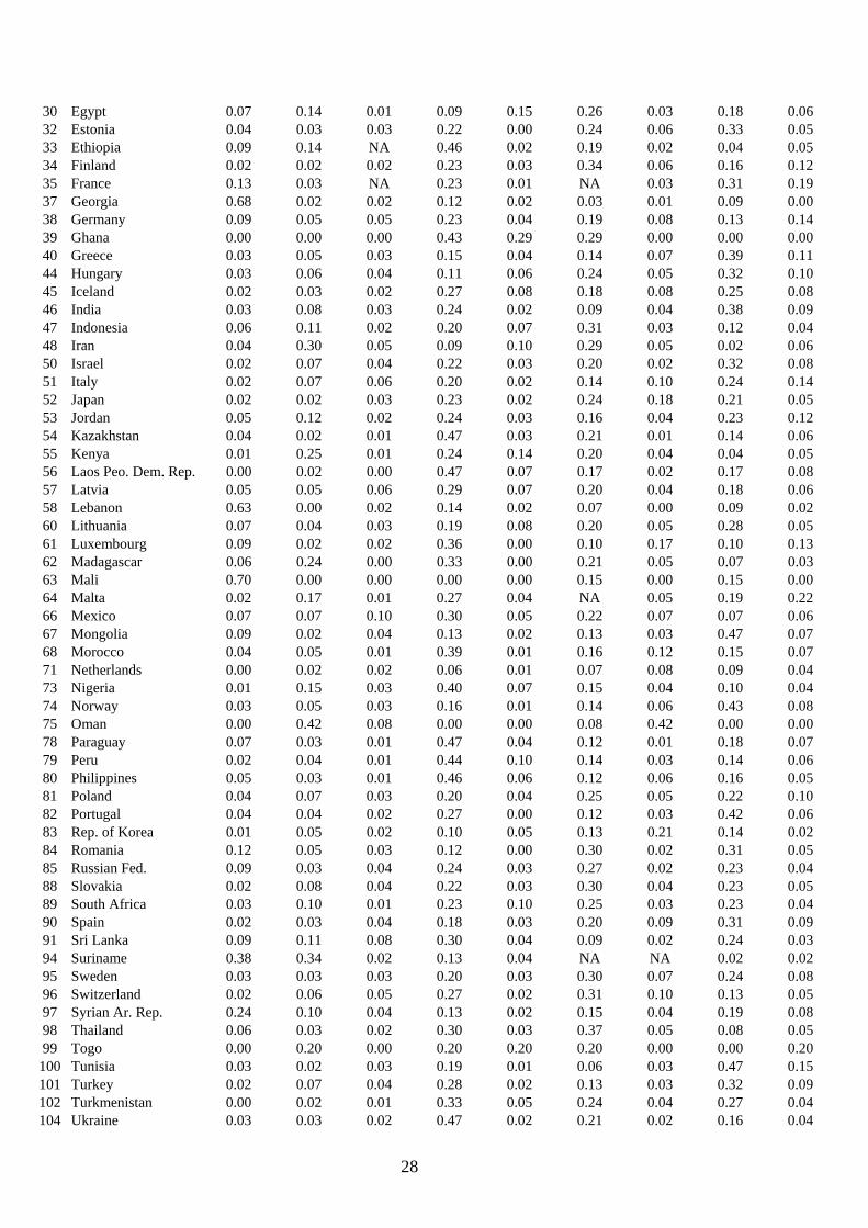
28

30 Egypt 0.07 0.14 0.01 0.09 0.15 0.26 0.03 0.18 0.06 32 Estonia 0.04 0.03 0.03 0.22 0.00 0.24 0.06 0.33 0.05 33 Ethiopia 0.09 0.14 NA 0.46 0.02 0.19 0.02 0.04 0.05 34 Finland 0.02 0.02 0.02 0.23 0.03 0.34 0.06 0.16 0.12 35 France 0.13 0.03 NA 0.23 0.01 NA 0.03 0.31 0.19 37 Georgia 0.68 0.02 0.02 0.12 0.02 0.03 0.01 0.09 0.00 38 Germany 0.09 0.05 0.05 0.23 0.04 0.19 0.08 0.13 0.14 39 Ghana 0.00 0.00 0.00 0.43 0.29 0.29 0.00 0.00 0.00 40 Greece 0.03 0.05 0.03 0.15 0.04 0.14 0.07 0.39 0.11 44 Hungary 0.03 0.06 0.04 0.11 0.06 0.24 0.05 0.32 0.10 45 Iceland 0.02 0.03 0.02 0.27 0.08 0.18 0.08 0.25 0.08 46 India 0.03 0.08 0.03 0.24 0.02 0.09 0.04 0.38 0.09 47 Indonesia 0.06 0.11 0.02 0.20 0.07 0.31 0.03 0.12 0.04 48 Iran 0.04 0.30 0.05 0.09 0.10 0.29 0.05 0.02 0.06 50 Israel 0.02 0.07 0.04 0.22 0.03 0.20 0.02 0.32 0.08 51 Italy 0.02 0.07 0.06 0.20 0.02 0.14 0.10 0.24 0.14 52 Japan 0.02 0.02 0.03 0.23 0.02 0.24 0.18 0.21 0.05 53 Jordan 0.05 0.12 0.02 0.24 0.03 0.16 0.04 0.23 0.12 54 Kazakhstan 0.04 0.02 0.01 0.47 0.03 0.21 0.01 0.14 0.06 55 Kenya 0.01 0.25 0.01 0.24 0.14 0.20 0.04 0.04 0.05 56 Laos Peo. Dem. Rep. 0.00 0.02 0.00 0.47 0.07 0.17 0.02 0.17 0.08 57 Latvia 0.05 0.05 0.06 0.29 0.07 0.20 0.04 0.18 0.06 58 Lebanon 0.63 0.00 0.02 0.14 0.02 0.07 0.00 0.09 0.02 60 Lithuania 0.07 0.04 0.03 0.19 0.08 0.20 0.05 0.28 0.05 61 Luxembourg 0.09 0.02 0.02 0.36 0.00 0.10 0.17 0.10 0.13 62 Madagascar 0.06 0.24 0.00 0.33 0.00 0.21 0.05 0.07 0.03 63 Mali 0.70 0.00 0.00 0.00 0.00 0.15 0.00 0.15 0.00 64 Malta 0.02 0.17 0.01 0.27 0.04 NA 0.05 0.19 0.22 66 Mexico 0.07 0.07 0.10 0.30 0.05 0.22 0.07 0.07 0.06 67 Mongolia 0.09 0.02 0.04 0.13 0.02 0.13 0.03 0.47 0.07 68 Morocco 0.04 0.05 0.01 0.39 0.01 0.16 0.12 0.15 0.07 71 Netherlands 0.00 0.02 0.02 0.06 0.01 0.07 0.08 0.09 0.04 73 Nigeria 0.01 0.15 0.03 0.40 0.07 0.15 0.04 0.10 0.04 74 Norway 0.03 0.05 0.03 0.16 0.01 0.14 0.06 0.43 0.08 75 Oman 0.00 0.42 0.08 0.00 0.00 0.08 0.42 0.00 0.00 78 Paraguay 0.07 0.03 0.01 0.47 0.04 0.12 0.01 0.18 0.07 79 Peru 0.02 0.04 0.01 0.44 0.10 0.14 0.03 0.14 0.06 80 Philippines 0.05 0.03 0.01 0.46 0.06 0.12 0.06 0.16 0.05 81 Poland 0.04 0.07 0.03 0.20 0.04 0.25 0.05 0.22 0.10 82 Portugal 0.04 0.04 0.02 0.27 0.00 0.12 0.03 0.42 0.06 83 Rep. of Korea 0.01 0.05 0.02 0.10 0.05 0.13 0.21 0.14 0.02 84 Romania 0.12 0.05 0.03 0.12 0.00 0.30 0.02 0.31 0.05 85 Russian Fed. 0.09 0.03 0.04 0.24 0.03 0.27 0.02 0.23 0.04 88 Slovakia 0.02 0.08 0.04 0.22 0.03 0.30 0.04 0.23 0.05 89 South Africa 0.03 0.10 0.01 0.23 0.10 0.25 0.03 0.23 0.04 90 Spain 0.02 0.03 0.04 0.18 0.03 0.20 0.09 0.31 0.09 91 Sri Lanka 0.09 0.11 0.08 0.30 0.04 0.09 0.02 0.24 0.03 94 Suriname 0.38 0.34 0.02 0.13 0.04 NA NA 0.02 0.02 95 Sweden 0.03 0.03 0.03 0.20 0.03 0.30 0.07 0.24 0.08 96 Switzerland 0.02 0.06 0.05 0.27 0.02 0.31 0.10 0.13 0.05 97 Syrian Ar. Rep. 0.24 0.10 0.04 0.13 0.02 0.15 0.04 0.19 0.08 98 Thailand 0.06 0.03 0.02 0.30 0.03 0.37 0.05 0.08 0.05 99 Togo 0.00 0.20 0.00 0.20 0.20 0.20 0.00 0.00 0.20

100 Tunisia 0.03 0.02 0.03 0.19 0.01 0.06 0.03 0.47 0.15 101 Turkey 0.02 0.07 0.04 0.28 0.02 0.13 0.03 0.32 0.09 102 Turkmenistan 0.00 0.02 0.01 0.33 0.05 0.24 0.04 0.27 0.04 104 Ukraine 0.03 0.03 0.02 0.47 0.02 0.21 0.02 0.16 0.04

29

105 United Kingdom 0.02 0.05 0.03 0.22 0.04 0.23 0.09 0.20 0.11 106 Un. Rep. of Tanzania 0.00 0.10 0.01 0.26 0.01 0.27 0.02 0.27 0.05 107 United States 0.04 0.06 0.03 0.21 0.01 0.21 0.06 0.19 0.10 108 Uruguay 0.02 0.01 0.03 0.29 0.01 0.23 0.04 0.27 0.10 109 Uzbekistan 0.01 0.02 0.01 0.37 0.04 0.20 0.01 0.28 0.07 110 Venezuela 0.04 0.05 0.04 0.28 0.01 0.25 0.08 0.18 0.06 113 Zimbabwe 0.03 0.06 0.00 0.46 0.06 0.22 0.03 0.10 0.03

*87 fully or partly reporting countries. Countries absent from the list reported NA data for all columns. **The country numbers are those of Table 1.

Table 3.

Select percapita income, educational and printed-paper indicators by religious groups*

Islam Protestant Orthodox Catholic Buddist & Confucian Other

World average

1 Real GDP percapita in $** 3687 14000 5235 7093 3261 4295 6397 2 Average years > 25 4.55 9.99 8.30 6.84 6.27 5.06 6.71 3 Gross tertiary enrolment 20.55 56.79 46.16 35.36 26.81 13.10 32.53 4 School life expectancy 10.30 15.69 13.67 13.63 11.33 10.07 12.48 5 Combined educ. index 0.64 0.93 0.86 0.86 0.75 0.69 0.79 6 Literacy rate 0.68 0.97 0.93 0.92 0.86 0.72 0.84 7 Generalities 0.12 0.05 0.12 0.04 0.04 0.02 0.07 8 Religion & Theology 0.10 0.07 0.05 0.06 0.04 0.10 0.07 9 Philosophy & Psychology 0.02 0.03 0.03 0.04 0.03 0.01 0.03

10 Social Sciences 0.19 0.25 0.26 0.28 0.27 0.29 0.26 11 Philology 0.04 0.04 0.03 0.03 0.04 0.07 0.04 12 Pure & applied sciences 0.20 0.22 0.20 0.18 0.19 0.19 0.20 13 Arts & recreation 0.06 0.08 0.03 0.06 0.08 0.03 0.06 14 Literature 0.19 0.20 0.23 0.24 0.21 0.16 0.21 15 Geography & History 0.09 0.08 0.05 0.09 0.05 0.06 0.07 16 Daily & Nondaily news.† 245 337 429 186 109 143 234

* Christianity is subdivided into Protestantism and Orthodoxy. ** Heston et al. [2002]. † Daily and nondaily newspapers in circulation, per 1,000 inhabitants.

Table 4*.

Ratios of select educational indicators with number of sites by country rank.

(1) Tertiary gross enrolment ratio/number of sites; (2) Combined education index/number of sites; (3) Literacy ratio/number of sites.

(1) (2) (3)

1 Australia 74.4 1 Australia 0.99 1 Australia 1.00 2 Latvia 68.5 2 Iceland 0.96 2 Iceland 1.00 3 Estonia 63.9 3 Estonia 0.94 3 Luxembourg 1.00 4 Iceland 54.6 4 Latvia 0.93 4 Estonia 1.00 5 Bahrain 44.2 5 Uruguay 0.92 5 Latvia 1.00 6 Uruguay 37.1 6 Luxembourg 0.90 6 Andorra 1.00 7 Mongolia 34.7 7 Suriname 0.89 7 Azerbaijan 0.99 8 Belarus 30.1 8 Azerbaijan 0.88 8 Mongolia 0.98

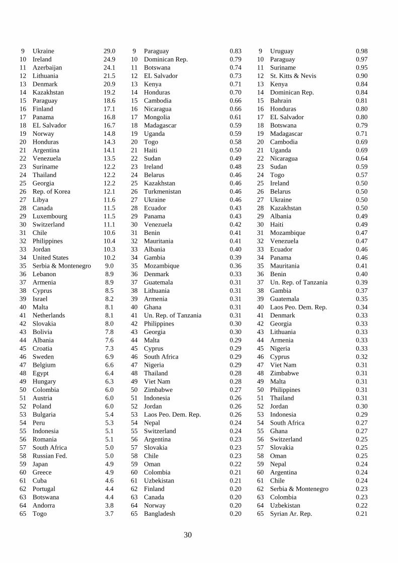
30

9 Ukraine 29.0 9 Paraguay 0.83 9 Uruguay 0.98 10 Ireland 24.9 10 Dominican Rep. 0.79 10 Paraguay 0.97 11 Azerbaijan 24.1 11 Botswana 0.74 11 Suriname 0.95 12 Lithuania 21.5 12 EL Salvador 0.73 12 St. Kitts & Nevis 0.90 13 Denmark 20.9 13 Kenya 0.71 13 Kenya 0.84 14 Kazakhstan 19.2 14 Honduras 0.70 14 Dominican Rep. 0.84 15 Paraguay 18.6 15 Cambodia 0.66 15 Bahrain 0.81 16 Finland 17.1 16 Nicaragua 0.66 16 Honduras 0.80 17 Panama 16.8 17 Mongolia 0.61 17 EL Salvador 0.80 18 EL Salvador 16.7 18 Madagascar 0.59 18 Botswana 0.79 19 Norway 14.8 19 Uganda 0.59 19 Madagascar 0.71 20 Honduras 14.3 20 Togo 0.58 20 Cambodia 0.69 21 Argentina 14.1 21 Haiti 0.50 21 Uganda 0.69 22 Venezuela 13.5 22 Sudan 0.49 22 Nicaragua 0.64 23 Suriname 12.2 23 Ireland 0.48 23 Sudan 0.59 24 Thailand 12.2 24 Belarus 0.46 24 Togo 0.57 25 Georgia 12.2 25 Kazakhstan 0.46 25 Ireland 0.50 26 Rep. of Korea 12.1 26 Turkmenistan 0.46 26 Belarus 0.50 27 Libya 11.6 27 Ukraine 0.46 27 Ukraine 0.50 28 Canada 11.5 28 Ecuador 0.43 28 Kazakhstan 0.50 29 Luxembourg 11.5 29 Panama 0.43 29 Albania 0.49 30 Switzerland 11.1 30 Venezuela 0.42 30 Haiti 0.49 31 Chile 10.6 31 Benin 0.41 31 Mozambique 0.47 32 Philippines 10.4 32 Mauritania 0.41 32 Venezuela 0.47 33 Jordan 10.3 33 Albania 0.40 33 Ecuador 0.46 34 United States 10.2 34 Gambia 0.39 34 Panama 0.46 35 Serbia & Montenegro 9.0 35 Mozambique 0.36 35 Mauritania 0.41 36 Lebanon 8.9 36 Denmark 0.33 36 Benin 0.40 37 Armenia 8.9 37 Guatemala 0.31 37 Un. Rep. of Tanzania 0.39 38 Cyprus 8.5 38 Lithuania 0.31 38 Gambia 0.37 39 Israel 8.2 39 Armenia 0.31 39 Guatemala 0.35 40 Malta 8.1 40 Ghana 0.31 40 Laos Peo. Dem. Rep. 0.34 41 Netherlands 8.1 41 Un. Rep. of Tanzania 0.31 41 Denmark 0.33 42 Slovakia 8.0 42 Philippines 0.30 42 Georgia 0.33 43 Bolivia 7.8 43 Georgia 0.30 43 Lithuania 0.33 44 Albania 7.6 44 Malta 0.29 44 Armenia 0.33 45 Croatia 7.3 45 Cyprus 0.29 45 Nigeria 0.33 46 Sweden 6.9 46 South Africa 0.29 46 Cyprus 0.32 47 Belgium 6.6 47 Nigeria 0.29 47 Viet Nam 0.31 48 Egypt 6.4 48 Thailand 0.28 48 Zimbabwe 0.31 49 Hungary 6.3 49 Viet Nam 0.28 49 Malta 0.31 50 Colombia 6.0 50 Zimbabwe 0.27 50 Philippines 0.31 51 Austria 6.0 51 Indonesia 0.26 51 Thailand 0.31 52 Poland 6.0 52 Jordan 0.26 52 Jordan 0.30 53 Bulgaria 5.4 53 Laos Peo. Dem. Rep. 0.26 53 Indonesia 0.29 54 Peru 5.3 54 Nepal 0.24 54 South Africa 0.27 55 Indonesia 5.1 55 Switzerland 0.24 55 Ghana 0.27 56 Romania 5.1 56 Argentina 0.23 56 Switzerland 0.25 57 South Africa 5.0 57 Slovakia 0.23 57 Slovakia 0.25 58 Russian Fed. 5.0 58 Chile 0.23 58 Oman 0.25 59 Japan 4.9 59 Oman 0.22 59 Nepal 0.24 60 Greece 4.9 60 Colombia 0.21 60 Argentina 0.24 61 Cuba 4.6 61 Uzbekistan 0.21 61 Chile 0.24 62 Portugal 4.4 62 Finland 0.20 62 Serbia & Montenegro 0.23 63 Botswana 4.4 63 Canada 0.20 63 Colombia 0.23 64 Andorra 3.8 64 Norway 0.20 64 Uzbekistan 0.22 65 Togo 3.7 65 Bangladesh 0.20 65 Syrian Ar. Rep. 0.21

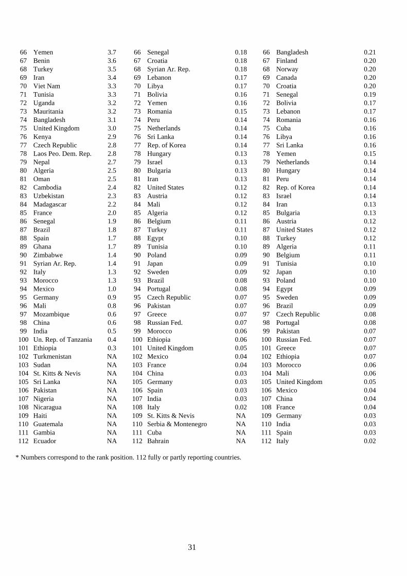
31

66 Yemen 3.7 66 Senegal 0.18 66 Bangladesh 0.21 67 Benin 3.6 67 Croatia 0.18 67 Finland 0.20 68 Turkey 3.5 68 Syrian Ar. Rep. 0.18 68 Norway 0.20 69 Iran 3.4 69 Lebanon 0.17 69 Canada 0.20 70 Viet Nam 3.3 70 Libya 0.17 70 Croatia 0.20 71 Tunisia 3.3 71 Bolivia 0.16 71 Senegal 0.19 72 Uganda 3.2 72 Yemen 0.16 72 Bolivia 0.17 73 Mauritania 3.2 73 Romania 0.15 73 Lebanon 0.17 74 Bangladesh 3.1 74 Peru 0.14 74 Romania 0.16 75 United Kingdom 3.0 75 Netherlands 0.14 75 Cuba 0.16 76 Kenya 2.9 76 Sri Lanka 0.14 76 Libya 0.16 77 Czech Republic 2.8 77 Rep. of Korea 0.14 77 Sri Lanka 0.16 78 Laos Peo. Dem. Rep. 2.8 78 Hungary 0.13 78 Yemen 0.15 79 Nepal 2.7 79 Israel 0.13 79 Netherlands 0.14 80 Algeria 2.5 80 Bulgaria 0.13 80 Hungary 0.14 81 Oman 2.5 81 Iran 0.13 81 Peru 0.14 82 Cambodia 2.4 82 United States 0.12 82 Rep. of Korea 0.14 83 Uzbekistan 2.3 83 Austria 0.12 83 Israel 0.14 84 Madagascar 2.2 84 Mali 0.12 84 Iran 0.13 85 France 2.0 85 Algeria 0.12 85 Bulgaria 0.13 86 Senegal 1.9 86 Belgium 0.11 86 Austria 0.12 87 Brazil 1.8 87 Turkey 0.11 87 United States 0.12 88 Spain 1.7 88 Egypt 0.10 88 Turkey 0.12 89 Ghana 1.7 89 Tunisia 0.10 89 Algeria 0.11 90 Zimbabwe 1.4 90 Poland 0.09 90 Belgium 0.11 91 Syrian Ar. Rep. 1.4 91 Japan 0.09 91 Tunisia 0.10 92 Italy 1.3 92 Sweden 0.09 92 Japan 0.10 93 Morocco 1.3 93 Brazil 0.08 93 Poland 0.10 94 Mexico 1.0 94 Portugal 0.08 94 Egypt 0.09 95 Germany 0.9 95 Czech Republic 0.07 95 Sweden 0.09 96 Mali 0.8 96 Pakistan 0.07 96 Brazil 0.09 97 Mozambique 0.6 97 Greece 0.07 97 Czech Republic 0.08 98 China 0.6 98 Russian Fed. 0.07 98 Portugal 0.08 99 India 0.5 99 Morocco 0.06 99 Pakistan 0.07

100 Un. Rep. of Tanzania 0.4 100 Ethiopia 0.06 100 Russian Fed. 0.07 101 Ethiopia 0.3 101 United Kingdom 0.05 101 Greece 0.07 102 Turkmenistan NA 102 Mexico 0.04 102 Ethiopia 0.07 103 Sudan NA 103 France 0.04 103 Morocco 0.06 104 St. Kitts & Nevis NA 104 China 0.03 104 Mali 0.06 105 Sri Lanka NA 105 Germany 0.03 105 United Kingdom 0.05 106 Pakistan NA 106 Spain 0.03 106 Mexico 0.04 107 Nigeria NA 107 India 0.03 107 China 0.04 108 Nicaragua NA 108 Italy 0.02 108 France 0.04 109 Haiti NA 109 St. Kitts & Nevis NA 109 Germany 0.03 110 Guatemala NA 110 Serbia & Montenegro NA 110 India 0.03 111 Gambia NA 111 Cuba NA 111 Spain 0.03 112 Ecuador NA 112 Bahrain NA 112 Italy 0.02

* Numbers correspond to the rank position. 112 fully or partly reporting countries.

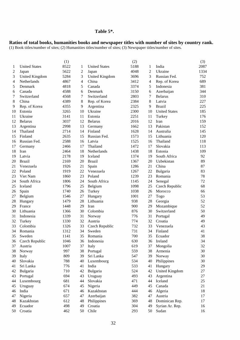
32

Table 5*. Ratios of total books, humanities books and newspaper titles with number of sites by country rank. (1) Book titles/number of sites; (2) Humanities titles/number of sites; (3) Newspaper titles/number of sites. (1) (2) (3)

1 United States 8522 1 United States 5188 1 India 2087 2 Japan 5622 2 Japan 4048 2 Ukraine 1334 3 United Kingdom 5284 3 United Kingdom 3696 3 Russian Fed. 752 4 Netherlands 4867 4 China 3412 4 Rep. of Korea 689 5 Denmark 4818 5 Canada 3374 5 Indonesia 381 6 Canada 4588 6 Denmark 3150 6 Azerbaijan 344 7 Switzerland 4568 7 Switzerland 2803 7 Belarus 310 8 China 4389 8 Rep. of Korea 2384 8 Latvia 227 9 Rep. of Korea 4355 9 Argentina 2325 9 Brazil 225

10 Estonia 3265 10 Ukraine 2300 10 United States 185 11 Ukraine 3141 11 Estonia 2251 11 Turkey 176 12 Belarus 3037 12 Belarus 2016 12 Iran 159 13 Argentina 2998 13 Germany 1662 13 Pakistan 152 14 Thailand 2714 14 Finland 1628 14 Australia 145 15 Finland 2635 15 Russian Fed. 1573 15 Lithuania 120 16 Russian Fed. 2588 16 Latvia 1525 16 Thailand 118 17 Germany 2466 17 Thailand 1472 17 Slovakia 113 18 Iran 2464 18 Netherlands 1438 18 Estonia 109 19 Latvia 2178 19 Iceland 1374 19 South Africa 92 20 Brazil 2169 20 Brazil 1367 20 Uzbekistan 89 21 Venezuela 1926 21 Spain 1286 21 China 87 22 Poland 1919 22 Venezuela 1267 22 Bulgaria 83 23 Viet Nam 1860 23 Poland 1239 23 Romania 78 24 South Africa 1806 24 South Africa 1145 24 Senegal 72 25 Iceland 1796 25 Belgium 1098 25 Czech Republic 68 26 Spain 1740 26 Turkey 1038 26 Morocco 66 27 Belgium 1546 27 Hungary 1001 27 Togo 53 28 Hungary 1479 28 Lithuania 938 28 Georgia 52 29 France 1448 29 Iran 900 29 Mozambique 52 30 Lithuania 1366 30 Colombia 876 30 Switzerland 50 31 Indonesia 1339 31 Norway 776 31 Portugal 49 32 Turkey 1330 32 Austria 774 32 Croatia 49 33 Colombia 1326 33 Czech Republic 732 33 Venezuela 43 34 Romania 1312 34 Sweden 731 34 Finland 41 35 Sweden 1141 35 Romania 700 35 Ecuador 38 36 Czech Republic 1046 36 Indonesia 630 36 Ireland 34 37 Austria 1007 37 Italy 619 37 Mongolia 32 38 Norway 997 38 Portugal 559 38 Armenia 30 39 Italy 809 39 Sri Lanka 547 39 Norway 30 40 Slovakia 788 40 Luxembourg 534 40 Philippines 30 41 Sri Lanka 776 41 India 533 41 Hungary 29 42 Bulgaria 710 42 Bulgaria 524 42 United Kingdom 27 43 Portugal 694 43 Uruguay 493 43 Argentina 27 44 Luxembourg 681 44 Slovakia 471 44 Iceland 25 45 Uruguay 674 45 Nigeria 449 45 Canada 21 46 India 671 46 Kazakhstan 444 46 Algeria 18 47 Nigeria 657 47 Azerbaijan 382 47 Austria 17 48 Kazakhstan 612 48 Philippines 369 48 Dominican Rep. 17 49 Ecuador 498 49 Croatia 304 49 Syrian Ar. Rep. 16 50 Croatia 462 50 Chile 293 50 Sudan 16

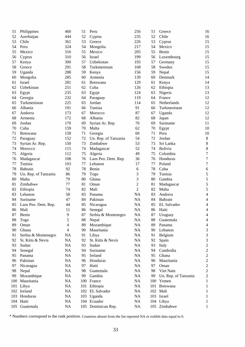
33

51 Philippines 460 51 Peru 256 51 Greece 16 52 Azerbaijan 444 52 Cyprus 235 52 Chile 16 53 Chile 361 53 Greece 226 53 Cyprus 15 54 Peru 324 54 Mongolia 217 54 Mexico 15 55 Mexico 316 55 Mexico 205 55 Benin 15 56 Cyprus 310 56 Israel 199 56 Luxembourg 15 57 Kenya 300 57 Uzbekistan 193 57 Germany 15 58 Greece 291 58 Turkmenistan 168 58 Sweden 15 59 Uganda 288 59 Kenya 156 59 Nepal 15 60 Mongolia 285 60 Armenia 139 60 Denmark 14 61 Israel 281 61 Botswana 129 61 Kenya 14 62 Uzbekistan 251 62 Cuba 126 62 Ethiopia 13 63 Egypt 235 63 Egypt 124 63 Nigeria 13 64 Georgia 232 64 Paraguay 119 64 France 12 65 Turkmenistan 225 65 Jordan 114 65 Netherlands 12 66 Albania 191 66 Tunisia 91 66 Turkmenistan 12 67 Andorra 173 67 Morocco 87 67 Uganda 12 68 Armenia 172 68 Albania 82 68 Japan 12 69 Jordan 170 69 Syrian Ar. Rep. 76 69 Suriname 11 70 Cuba 159 70 Malta 62 70 Egypt 10 71 Botswana 158 71 Georgia 60 71 Peru 10 72 Paraguay 152 72 Un. Rep. of Tanzania 54 72 Jordan 8 73 Syrian Ar. Rep. 150 73 Zimbabwe 53 73 Sri Lanka 8 74 Morocco 115 74 Madagascar 52 74 Bolivia 8 75 Algeria 112 75 Algeria 49 75 Colombia 7 76 Madagascar 108 76 Laos Peo. Dem. Rep. 36 76 Honduras 7 77 Tunisia 103 77 Lebanon 17 77 Poland 7 78 Bahrain 92 78 Benin 6 78 Cuba 6 79 Un. Rep. of Tanzania 86 79 Togo 3 79 Tunisia 5 80 Malta 79 80 Ghana 3 80 Gambia 5 81 Zimbabwe 77 81 Oman 2 81 Madagascar 5 82 Ethiopia 74 82 Mali 2 82 Malta 5 83 Lebanon 58 83 Panama NA 83 Andorra 4 84 Suriname 47 84 Pakistan NA 84 Bahrain 4 85 Laos Peo. Dem. Rep. 44 85 Nicaragua NA 85 EL Salvador 4 86 Mali 11 86 Senegal NA 86 Haiti 4 87 Benin 9 87 Serbia & Montenegro NA 87 Uruguay 4 88 Togo 5 88 Nepal NA 88 Guatemala 4 89 Oman 4 89 Mozambique NA 89 Panama 4 90 Ghana 4 90 Mauritania NA 90 Lebanon 3 91 Serbia & Montenegro NA 91 Libya NA 91 Belgium 3 92 St. Kitts & Nevis NA 92 St. Kitts & Nevis NA 92 Spain 3 93 Sudan NA 93 Sudan NA 93 Italy 2 94 Senegal NA 94 Suriname NA 94 Cambodia 2 95 Panama NA 95 Ireland NA 95 Ghana 2 96 Pakistan NA 96 Honduras NA 96 Mauritania 2 97 Nicaragua NA 97 Haiti NA 97 Oman 2 98 Nepal NA 98 Guatemala NA 98 Viet Nam 2 99 Mozambique NA 99 Gambia NA 99 Un. Rep. of Tanzania 2

100 Mauritania NA 100 France NA 100 Yemen 1 101 Libya NA 101 Ethiopia NA 101 Botswana 1 102 Ireland NA 102 EL Salvador NA 102 Mali 1 103 Honduras NA 103 Uganda NA 103 Israel 1 104 Haiti NA 104 Ecuador NA 104 Libya 1 105 Guatemala NA 105 Dominican Rep. NA 105 Zimbabwe 1

* Numbers correspond to the rank position. Countries absent from the list reported NA or exhibit data equal to 0.

34

Table 6*.

Ratios of select educational indicators with average age of sites by country rank. (1) Tertiary gross enrolment ratio/average age of sites; (2) Combined education index/average age; (3) Literacy ratio/average age.

(1) (2) (3)

1 Australia 0.62 1 Australia 0.83 1 Australia 0.83 2 Netherlands 0.16 2 Kenya 0.36 2 Kenya 0.42 3 Belarus 0.12 3 Venezuela 0.31 3 Uganda 0.34 4 Uruguay 0.11 4 Uganda 0.30 4 Venezuela 0.34 5 Finland 0.10 5 Netherlands 0.29 5 Uruguay 0.30 6 Venezuela 0.10 6 Uruguay 0.28 6 Netherlands 0.29 7 Poland 0.10 7 Haiti 0.28 7 Cuba 0.29 8 United States 0.10 8 Paraguay 0.24 8 Paraguay 0.28 9 Latvia 0.09 9 Togo 0.23 9 Haiti 0.27

10 Panama 0.08 10 Suriname 0.23 10 Suriname 0.24 11 Cuba 0.08 11 Panama 0.21 11 Togo 0.23 12 Estonia 0.08 12 Belarus 0.18 12 St. Kitts & Nevis 0.23 13 Denmark 0.08 13 Ecuador 0.18 13 Panama 0.22 14 Rep. of Korea 0.08 14 Czech Republic 0.16 14 Belarus 0.20 15 Chile 0.07 15 Dominican Rep. 0.16 15 Ecuador 0.19 16 Ukraine 0.07 16 Chile 0.16 16 Czech Republic 0.18 17 Japan 0.06 17 Poland 0.15 17 Dominican Rep. 0.17 18 United Kingdom 0.06 18 Luxembourg 0.15 18 Luxembourg 0.17 19 Czech Republic 0.06 19 Nicaragua 0.14 19 Chile 0.17 20 Bolivia 0.06 20 Germany 0.13 20 Poland 0.16 21 Paraguay 0.05 21 Ghana 0.13 21 Madagascar 0.14 22 Iceland 0.05 22 Denmark 0.12 22 Germany 0.14 23 Serbia & Montenegro 0.05 23 Slovakia 0.12 23 Slovakia 0.14 24 Russian Fed. 0.05 24 Japan 0.12 24 Nicaragua 0.13 25 Slovakia 0.04 25 Madagascar 0.12 25 Japan 0.13 26 Sweden 0.04 26 Estonia 0.12 26 Serbia & Montenegro 0.13 27 France 0.04 27 United States 0.12 27 Denmark 0.13 28 Switzerland 0.04 28 Latvia 0.12 28 Bolivia 0.13 29 Romania 0.04 29 Finland 0.12 29 Estonia 0.12 30 Germany 0.04 30 Bolivia 0.12 30 Latvia 0.12 31 Belgium 0.04 31 Benin 0.11 31 Romania 0.12 32 Canada 0.04 32 Ukraine 0.11 32 Un. Rep. of Tanzania 0.12 33 Philippines 0.03 33 Romania 0.11 33 United States 0.12 34 Italy 0.03 34 Philippines 0.10 34 Finland 0.12 35 Israel 0.03 35 Mexico 0.10 35 Ukraine 0.12 36 Suriname 0.03 36 United Kingdom 0.09 36 Ghana 0.12 37 Greece 0.03 37 Un. Rep. of Tanzania 0.09 37 Laos Peo. Dem. Rep. 0.11 38 Armenia 0.03 38 Viet Nam 0.09 38 Mexico 0.11 39 Georgia 0.03 39 Armenia 0.09 39 Benin 0.11 40 Mexico 0.03 40 Nigeria 0.09 40 Nigeria 0.10 41 Austria 0.03 41 Iceland 0.09 41 Viet Nam 0.10 42 Bulgaria 0.03 42 Rep. of Korea 0.09 42 Philippines 0.10 43 Croatia 0.02 43 Laos Peo. Dem. Rep. 0.09 43 Mozambique 0.10 44 Mongolia 0.02 44 Switzerland 0.08 44 Andorra 0.10 45 Peru 0.02 45 Mozambique 0.08 45 Armenia 0.10 46 Colombia 0.02 46 Senegal 0.08 46 United Kingdom 0.10 47 Norway 0.02 47 Colombia 0.08 47 Iceland 0.09 48 Hungary 0.02 48 France 0.07 48 Rep. of Korea 0.09 49 Luxembourg 0.02 49 Georgia 0.06 49 Switzerland 0.09

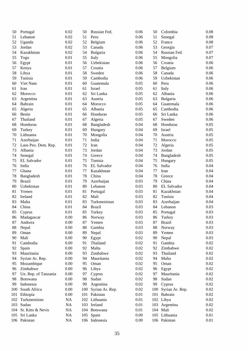
35

50 Portugal 0.02 50 Russian Fed. 0.06 50 Colombia 0.08 51 Lebanon 0.02 51 Peru 0.06 51 Senegal 0.08 52 Uganda 0.02 52 Belgium 0.06 52 France 0.08 53 Jordan 0.02 53 Canada 0.06 53 Georgia 0.07 54 Kazakhstan 0.02 54 Bulgaria 0.06 54 Russian Fed. 0.07 55 Togo 0.01 55 Italy 0.06 55 Mongolia 0.07 56 Egypt 0.01 56 Uzbekistan 0.06 56 Croatia 0.06 57 Kenya 0.01 57 Croatia 0.06 57 Belgium 0.06 58 Libya 0.01 58 Sweden 0.06 58 Canada 0.06 59 Tunisia 0.01 59 Cambodia 0.06 59 Uzbekistan 0.06 60 Viet Nam 0.01 60 Guatemala 0.05 60 Peru 0.06 61 Iran 0.01 61 Israel 0.05 61 Italy 0.06 62 Morocco 0.01 62 Sri Lanka 0.05 62 Albania 0.06 63 Argentina 0.01 63 Austria 0.05 63 Bulgaria 0.06 64 Bahrain 0.01 64 Morocco 0.05 64 Guatemala 0.06 65 Algeria 0.01 65 Albania 0.05 65 Cambodia 0.06 66 Benin 0.01 66 Honduras 0.05 66 Sri Lanka 0.06 67 Thailand 0.01 67 Algeria 0.05 67 Sweden 0.06 68 Honduras 0.01 68 Bangladesh 0.04 68 Honduras 0.05 69 Turkey 0.01 69 Hungary 0.04 69 Israel 0.05 70 Lithuania 0.01 70 Mongolia 0.04 70 Austria 0.05 71 Azerbaijan 0.01 71 India 0.04 71 Morocco 0.05 72 Laos Peo. Dem. Rep. 0.01 72 Iran 0.04 72 Algeria 0.05 73 Albania 0.01 73 Jordan 0.04 73 Jordan 0.05 74 Senegal 0.01 74 Greece 0.04 74 Bangladesh 0.05 75 EL Salvador 0.01 75 Tunisia 0.04 75 Hungary 0.05 76 India 0.01 76 EL Salvador 0.04 76 India 0.04 77 Ghana 0.01 77 Kazakhstan 0.04 77 Iran 0.04 78 Bangladesh 0.01 78 China 0.04 78 Greece 0.04 79 Brazil 0.01 79 Azerbaijan 0.03 79 China 0.04 80 Uzbekistan 0.01 80 Lebanon 0.03 80 EL Salvador 0.04 81 Yemen 0.01 81 Portugal 0.03 81 Kazakhstan 0.04 82 Ireland 0.01 82 Mali 0.03 82 Tunisia 0.04 83 Malta 0.01 83 Turkmenistan 0.03 83 Azerbaijan 0.04 84 China 0.01 84 Brazil 0.03 84 Lebanon 0.03 85 Cyprus 0.01 85 Turkey 0.03 85 Portugal 0.03 86 Madagascar 0.00 86 Norway 0.03 86 Turkey 0.03 87 Andorra 0.00 87 Yemen 0.03 87 Brazil 0.03 88 Nepal 0.00 88 Gambia 0.03 88 Norway 0.03 89 Oman 0.00 89 Nepal 0.03 89 Yemen 0.03 90 Mali 0.00 90 Egypt 0.02 90 Nepal 0.03 91 Cambodia 0.00 91 Thailand 0.02 91 Gambia 0.02 92 Spain 0.00 92 Malta 0.02 92 Zimbabwe 0.02 93 Mauritania 0.00 93 Zimbabwe 0.02 93 Thailand 0.02 94 Syrian Ar. Rep. 0.00 94 Mauritania 0.02 94 Malta 0.02 95 Mozambique 0.00 95 Oman 0.02 95 Oman 0.02 96 Zimbabwe 0.00 96 Libya 0.02 96 Egypt 0.02 97 Un. Rep. of Tanzania 0.00 97 Cyprus 0.02 97 Mauritania 0.02 98 Botswana 0.00 98 Sudan 0.02 98 Sudan 0.02 99 Indonesia 0.00 99 Argentina 0.02 99 Cyprus 0.02

100 South Africa 0.00 100 Syrian Ar. Rep. 0.02 100 Syrian Ar. Rep. 0.02 101 Ethiopia 0.00 101 Pakistan 0.01 101 Bahrain 0.02 102 Turkmenistan NA 102 Lithuania 0.01 102 Libya 0.02 103 Sudan NA 103 Ireland 0.01 103 Argentina 0.02 104 St. Kitts & Nevis NA 104 Botswana 0.01 104 Mali 0.02 105 Sri Lanka NA 105 Spain 0.00 105 Lithuania 0.01 106 Pakistan NA 106 Indonesia 0.00 106 Pakistan 0.01

36

107 Nigeria NA 107 South Africa 0.00 107 Ireland 0.01 108 Nicaragua NA 108 Ethiopia 0.00 108 Botswana 0.01 109 Haiti NA 109 St. Kitts & Nevis NA 109 Spain 0.00 110 Guatemala NA 110 Serbia & Montenegro NA 110 Indonesia 0.00 111 Gambia NA 111 Cuba NA 111 South Africa 0.00 112 Ecuador NA 112 Bahrain NA 112 Ethiopia 0.00

*Numbers correspond to the rank position. 112 fully or partly reporting countries.

Table 7*.

Ratios of total books, humanities and newspapers with average age of sites by country rank. (1) Book Titles/average age; (2) Humanities/average age; (3) Newspapers/average age.

(1) (2) (3)

1 United Kingdom 105.68 1 United Kingdom 73.92 1 India 31.22 2 Germany 99.05 2 Germany 66.76 2 Russian Fed. 7.07 3 Netherlands 98.18 3 Japan 52.84 3 Rep. of Korea 4.33 4 United States 80.87 4 United States 49.23 4 Ukraine 3.14 5 Japan 73.40 5 China 34.54 5 United States 1.75 6 China 44.43 6 Netherlands 29.01 6 Czech Republic 1.46 7 Poland 31.57 7 Poland 20.38 7 Belarus 1.24 8 France 29.39 8 Czech Republic 15.68 8 Australia 1.21 9 Rep. of Korea 27.34 9 Italy 15.11 9 China 0.88

10 Russian Fed. 24.35 10 Rep. of Korea 14.97 10 Brazil 0.81 11 Czech Republic 22.41 11 Russian Fed. 14.80 11 Slovakia 0.61 12 Italy 19.73 12 Denmark 11.95 12 Germany 0.60 13 Denmark 18.27 13 Canada 10.35 13 Romania 0.57 14 Switzerland 15.73 14 Switzerland 9.65 14 United Kingdom 0.55 15 Finland 15.46 15 Finland 9.55 15 Morocco 0.53 16 Venezuela 14.26 16 Venezuela 9.38 16 Iran 0.51 17 Canada 14.07 17 Belarus 8.06 17 Turkey 0.47 18 Belarus 12.15 18 India 7.98 18 Mexico 0.40 19 India 10.03 19 Belgium 6.06 19 Bulgaria 0.39 20 Romania 9.61 20 Ukraine 5.41 20 Senegal 0.32 21 Belgium 8.54 21 Mexico 5.30 21 Venezuela 0.32 22 Mexico 8.17 22 Romania 5.13 22 Pakistan 0.30 23 Iran 7.82 23 Brazil 4.90 23 Latvia 0.28 24 Brazil 7.78 24 Sweden 4.49 24 France 0.25 25 Ukraine 7.39 25 Austria 3.23 25 Netherlands 0.24 26 Sweden 7.01 26 Hungary 3.22 26 Uzbekistan 0.24 27 Viet Nam 6.20 27 Colombia 3.15 27 Finland 0.24 28 Colombia 4.77 28 Iran 2.86 28 Togo 0.21 29 Hungary 4.75 29 Estonia 2.81 29 Portugal 0.21 30 Slovakia 4.28 30 Turkey 2.77 30 Switzerland 0.17 31 Austria 4.20 31 Slovakia 2.56 31 Ecuador 0.16 32 Estonia 4.08 32 Bulgaria 2.45 32 Croatia 0.16 33 Turkey 3.55 33 Portugal 2.37 33 Japan 0.15 34 Bulgaria 3.31 34 Cuba 2.22 34 Estonia 0.14 35 Portugal 2.94 35 Chile 2.04 35 Azerbaijan 0.13 36 Cuba 2.80 36 Sri Lanka 1.97 36 Mozambique 0.12 37 Sri Lanka 2.79 37 Latvia 1.91 37 Georgia 0.11 38 Latvia 2.72 38 Argentina 1.71 38 Poland 0.11 39 Chile 2.51 39 Uruguay 1.52 39 Chile 0.11 40 Argentina 2.20 40 Nigeria 1.44 40 Philippines 0.10

37

41 Thailand 2.13 41 Spain 1.39 41 Cuba 0.10 42 Nigeria 2.10 42 Greece 1.34 42 Greece 0.09 43 Ecuador 2.10 43 Iceland 1.25 43 Thailand 0.09 44 Uruguay 2.07 44 Philippines 1.24 44 Hungary 0.09 45 Spain 1.88 45 Thailand 1.16 45 Armenia 0.09 46 Greece 1.73 46 Peru 1.08 46 Sweden 0.09 47 Iceland 1.63 47 Norway 1.07 47 Algeria 0.07 48 Philippines 1.54 48 Croatia 0.98 48 Austria 0.07 49 Kenya 1.50 49 Luxembourg 0.89 49 Kenya 0.07 50 Croatia 1.49 50 Kenya 0.78 50 Canada 0.06 51 Uganda 1.44 51 Israel 0.78 51 Uganda 0.06 52 Norway 1.38 52 Morocco 0.70 52 Bolivia 0.06 53 Peru 1.37 53 Uzbekistan 0.52 53 Denmark 0.05 54 Luxembourg 1.14 54 Armenia 0.42 54 Italy 0.05 55 Israel 1.10 55 Lithuania 0.41 55 Lithuania 0.05 56 Morocco 0.92 56 Kazakhstan 0.35 56 Norway 0.04 57 Uzbekistan 0.68 57 Paraguay 0.34 57 Peru 0.04 58 Lithuania 0.59 58 Tunisia 0.34 58 Benin 0.04 59 Egypt 0.55 59 Egypt 0.29 59 Nigeria 0.04 60 Armenia 0.52 60 Algeria 0.20 60 Dominican Rep. 0.03 61 Georgia 0.49 61 Jordan 0.17 61 Sri Lanka 0.03 62 Kazakhstan 0.48 62 Un. Rep. of Tanzania 0.16 62 Suriname 0.03 63 Algeria 0.45 63 Azerbaijan 0.15 63 Colombia 0.03 64 Paraguay 0.43 64 Cyprus 0.15 64 Luxembourg 0.03 65 Tunisia 0.38 65 Mongolia 0.14 65 Egypt 0.02 66 Un. Rep. of Tanzania 0.26 66 Georgia 0.13 66 Iceland 0.02 67 Jordan 0.26 67 Laos Peo. Dem. Rep. 0.12 67 Haiti 0.02 68 Albania 0.23 68 Turkmenistan 0.11 68 Mongolia 0.02 69 Madagascar 0.22 69 Madagascar 0.10 69 Argentina 0.02 70 Cyprus 0.19 70 Albania 0.10 70 Tunisia 0.02 71 Mongolia 0.19 71 Syrian Ar. Rep. 0.07 71 Belgium 0.02 72 Andorra 0.17 72 Malta 0.05 72 Panama 0.02 73 Azerbaijan 0.17 73 Zimbabwe 0.04 73 Nepal 0.02 74 Turkmenistan 0.15 74 Lebanon 0.03 74 Syrian Ar. Rep. 0.02 75 Laos Peo. Dem. Rep. 0.15 75 Benin 0.02 75 Jordan 0.01 76 Syrian Ar. Rep. 0.14 76 Botswana 0.01 76 Uruguay 0.01 77 Suriname 0.12 77 Togo 0.01 77 Madagascar 0.01 78 Lebanon 0.12 78 Ghana 0.01 78 Cyprus 0.01 79 Zimbabwe 0.06 79 Indonesia 0.01 79 Ghana 0.01 80 Malta 0.06 80 Mali 0.00 80 Ireland 0.01 81 Mali 0.03 81 South Africa 0.00 81 Turkmenistan 0.01 82 Benin 0.02 82 Oman 0.00 82 Lebanon 0.01 83 Bahrain 0.02 83 Panama NA 83 Guatemala 0.01 84 Togo 0.02 84 Pakistan NA 84 Viet Nam 0.01 85 Botswana 0.02 85 Nicaragua NA 85 Sudan 0.01 86 Ghana 0.02 86 Senegal NA 86 Honduras 0.00 87 Indonesia 0.01 87 Serbia & Montenegro NA 87 Un. Rep. of Tanzania 0.00 88 South Africa 0.00 88 Nepal NA 88 Andorra 0.00

*Numbers correspond to the rank position. The countries not shown exhibit either NA or 0.00.

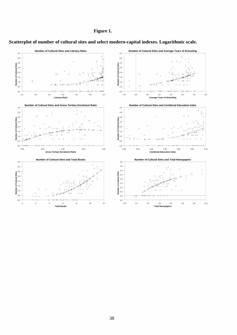
38

Figure 1. Scatterplot of number of cultural sites and select modern-capital indexes. Logarithmic scale.

Number of Cultural Sites and Literacy Ratio

Literacy Ratio

Nu

mb

er o

f C

ult

ura

l Sit

es

0.1 0.2 0.3 0.4 0.5 0.6 0.7

0.0

0.5

1.0

1.5

2.0

2.5

3.0

3.5

4.0

Number of Cultural Sites and Gross Tertiary Enrolment Ratio

Gross Tertiary Enrolment Ratio

Nu

mb

er o

f C

ult

ura

l Sit

es

0.00 0.16 0.32 0.48 0.64

0.0

0.5

1.0

1.5

2.0

2.5

3.0

3.5

4.0

Number of Cultural Sites and Total Books

Total Books

Nu

mb

er o

f C

ult

ura

l Sit

es

0 2 4 6 8 10 12

0.0

0.5

1.0

1.5

2.0

2.5

3.0

3.5

4.0

Number of Cultural Sites and Average Years of Schooling

Average Years of Schooling

Nu

mb

er o

f C

ult

ura

l Sit

es

-0.5 0.0 0.5 1.0 1.5 2.0 2.5 3.0

0.0

0.5

1.0

1.5

2.0

2.5

3.0

3.5

4.0

Number of Cultural Sites and Combined Education Index

Combined Education Index

Nu

mb

er o

f C

ult

ura

l Sit

es

0.28 0.35 0.42 0.49 0.56 0.63 0.70

0.0

0.5

1.0

1.5

2.0

2.5

3.0

3.5

4.0

Number of Cultural Sites and Total Newspapers

Total Newspapers

Nu

mb

er o

f C

ult

ura

l Sit

es

0.0 1.6 3.2 4.8 6.4 8.0 9.6 11.2

-0.5

0.0

0.5

1.0

1.5

2.0

2.5

3.0

3.5

4.0

39

Figure 2. Montecarlo simulation of squared bias, variance and their ratio. 1,000 replications of a stationary AR(1) ‘true’ model .

Squared bias Variance Ratio

Monte Carlo simulation of 50 Observations

Number of instruments2 4 6 8 10 12 14 16 18 20 22 24

0.000

0.005

0.010

0.015

0.020

0.025

0.030

0.035

0.040

0.045

0.1

0.2

0.3

0.4

0.5

0.6

0.7

0.8

0.9

Squared bias Variance Ratio

Monte Carlo simulation of 75 Observations

Number of instruments5 10 15 20 25 30 35

0.000

0.005

0.010

0.015

0.020

0.025

0.030

0.0

0.1

0.2

0.3

0.4

0.5

0.6

Squared bias Variance Ratio

Monte Carlo simulation of 100 Observations

Number of instruments5 10 15 20 25 30 35 40 45 50

0.0000

0.0025

0.0050

0.0075

0.0100

0.0125

0.0150

0.0175

0.0200

0.0225

0.00

0.25

0.50

0.75

Squared bias Variance Ratio

Monte Carlo simulation of 250 Observations

Number of instruments25 50 75 100 125

0.000

0.001

0.002

0.003

0.004

0.005

0.006

0.007

0.008

0.009

0.00

0.08

0.16

0.24

0.32

0.40

0.48

0.56

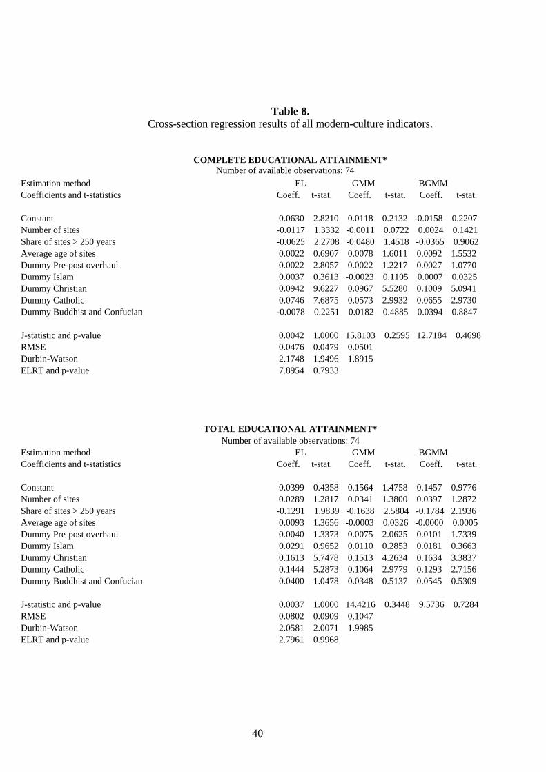
40

Table 8. Cross-section regression results of all modern-culture indicators.

COMPLETE EDUCATIONAL ATTAINMENT* Number of available observations: 74

Estimation method EL GMM BGMM Coefficients and t-statistics Coeff. t-stat. Coeff. t-stat. Coeff. t-stat. Constant 0.0630 2.8210 0.0118 0.2132 -0.0158 0.2207 Number of sites -0.0117 1.3332 -0.0011 0.0722 0.0024 0.1421 Share of sites > 250 years -0.0625 2.2708 -0.0480 1.4518 -0.0365 0.9062 Average age of sites 0.0022 0.6907 0.0078 1.6011 0.0092 1.5532 Dummy Pre-post overhaul 0.0022 2.8057 0.0022 1.2217 0.0027 1.0770 Dummy Islam 0.0037 0.3613 -0.0023 0.1105 0.0007 0.0325 Dummy Christian 0.0942 9.6227 0.0967 5.5280 0.1009 5.0941 Dummy Catholic 0.0746 7.6875 0.0573 2.9932 0.0655 2.9730 Dummy Buddhist and Confucian -0.0078 0.2251 0.0182 0.4885 0.0394 0.8847 J-statistic and p-value 0.0042 1.0000 15.8103 0.2595 12.7184 0.4698 RMSE 0.0476 0.0479 0.0501 Durbin-Watson 2.1748 1.9496 1.8915 ELRT and p-value 7.8954 0.7933

TOTAL EDUCATIONAL ATTAINMENT* Number of available observations: 74

Estimation method EL GMM BGMM Coefficients and t-statistics Coeff. t-stat. Coeff. t-stat. Coeff. t-stat. Constant 0.0399 0.4358 0.1564 1.4758 0.1457 0.9776 Number of sites 0.0289 1.2817 0.0341 1.3800 0.0397 1.2872 Share of sites > 250 years -0.1291 1.9839 -0.1638 2.5804 -0.1784 2.1936 Average age of sites 0.0093 1.3656 -0.0003 0.0326 -0.0000 0.0005 Dummy Pre-post overhaul 0.0040 1.3373 0.0075 2.0625 0.0101 1.7339 Dummy Islam 0.0291 0.9652 0.0110 0.2853 0.0181 0.3663 Dummy Christian 0.1613 5.7478 0.1513 4.2634 0.1634 3.3837 Dummy Catholic 0.1444 5.2873 0.1064 2.9779 0.1293 2.7156 Dummy Buddhist and Confucian 0.0400 1.0478 0.0348 0.5137 0.0545 0.5309 J-statistic and p-value 0.0037 1.0000 14.4216 0.3448 9.5736 0.7284 RMSE 0.0802 0.0909 0.1047 Durbin-Watson 2.0581 2.0071 1.9985 ELRT and p-value 2.7961 0.9968

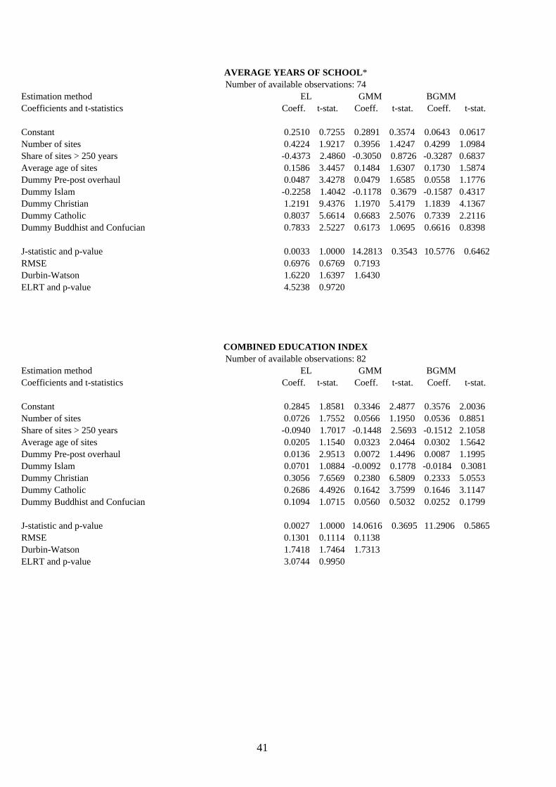
41

AVERAGE YEARS OF SCHOOL* Number of available observations: 74

Estimation method EL GMM BGMM Coefficients and t-statistics Coeff. t-stat. Coeff. t-stat. Coeff. t-stat. Constant 0.2510 0.7255 0.2891 0.3574 0.0643 0.0617 Number of sites 0.4224 1.9217 0.3956 1.4247 0.4299 1.0984 Share of sites > 250 years -0.4373 2.4860 -0.3050 0.8726 -0.3287 0.6837 Average age of sites 0.1586 3.4457 0.1484 1.6307 0.1730 1.5874 Dummy Pre-post overhaul 0.0487 3.4278 0.0479 1.6585 0.0558 1.1776 Dummy Islam -0.2258 1.4042 -0.1178 0.3679 -0.1587 0.4317 Dummy Christian 1.2191 9.4376 1.1970 5.4179 1.1839 4.1367 Dummy Catholic 0.8037 5.6614 0.6683 2.5076 0.7339 2.2116 Dummy Buddhist and Confucian 0.7833 2.5227 0.6173 1.0695 0.6616 0.8398 J-statistic and p-value 0.0033 1.0000 14.2813 0.3543 10.5776 0.6462 RMSE 0.6976 0.6769 0.7193 Durbin-Watson 1.6220 1.6397 1.6430 ELRT and p-value 4.5238 0.9720

COMBINED EDUCATION INDEX Number of available observations: 82

Estimation method EL GMM BGMM Coefficients and t-statistics Coeff. t-stat. Coeff. t-stat. Coeff. t-stat. Constant 0.2845 1.8581 0.3346 2.4877 0.3576 2.0036 Number of sites 0.0726 1.7552 0.0566 1.1950 0.0536 0.8851 Share of sites > 250 years -0.0940 1.7017 -0.1448 2.5693 -0.1512 2.1058 Average age of sites 0.0205 1.1540 0.0323 2.0464 0.0302 1.5642 Dummy Pre-post overhaul 0.0136 2.9513 0.0072 1.4496 0.0087 1.1995 Dummy Islam 0.0701 1.0884 -0.0092 0.1778 -0.0184 0.3081 Dummy Christian 0.3056 7.6569 0.2380 6.5809 0.2333 5.0553 Dummy Catholic 0.2686 4.4926 0.1642 3.7599 0.1646 3.1147 Dummy Buddhist and Confucian 0.1094 1.0715 0.0560 0.5032 0.0252 0.1799 J-statistic and p-value 0.0027 1.0000 14.0616 0.3695 11.2906 0.5865 RMSE 0.1301 0.1114 0.1138 Durbin-Watson 1.7418 1.7464 1.7313 ELRT and p-value 3.0744 0.9950

42

GROSS TERTIARY SCHOOL ENROLMENT RATIO

Number of available observations: 75 Estimation method EL GMM BGMM Coefficients and t-statistics Coeff. t-stat. Coeff. t-stat. Coeff. t-stat. Constant 0.0633 0.6530 -0.0634 0.4454 0.3093 0.6009 Number of sites 0.1611 4.0122 0.1660 3.2459 0.1215 0.8208 Share of sites > 250 years -0.0300 0.5472 0.0049 0.0588 -0.1642 0.5662 Average age of sites -0.0139 1.0582 0.0076 0.4729 -0.0121 0.2260 Dummy Pre-post overhaul 0.0161 3.1019 0.0127 1.5237 -0.0121 0.2819 Dummy Islam 0.1036 2.0194 0.0618 0.8991 0.1333 0.5671 Dummy Christian 0.5415 15.0823 0.5458 12.7564 0.4335 2.1207 Dummy Catholic 0.3583 7.5162 0.2412 3.6165 0.2189 1.1483 Dummy Buddhist and Confucian 0.4128 1.8360 0.4127 2.7287 0.0696 0.1489 J-statistic and p-value 0.0031 1.0000 12.5212 0.4854 6.6705 0.9183 RMSE 0.1685 0.1686 0.1790 Durbin-Watson 1.9635 1.8484 1.9407 ELRT and p-value 3.5315 0.9905

SCHOOL LIFE EXPECTANCY Number of available observations: 74

Estimation method EL GMM BGMM Coefficients and t-statistics Coeff. t-stat. Coeff. t-stat. Coeff. t-stat. Constant 1.4262 3.9515 1.6118 3.6855 2.1105 1.9429 Number of sites 0.2548 1.7358 0.3824 2.0582 0.3267 1.1786 Share of sites > 250 years 0.0279 0.1712 -0.0024 0.0133 -0.2966 0.4715 Average age of sites 0.0270 0.6163 0.0323 0.6064 -0.0074 0.0639 Dummy Pre-post overhaul 0.0366 3.1671 0.0235 1.3548 -0.0115 0.1028 Dummy Islam 0.5366 3.2200 0.4436 2.3584 0.5653 1.0471 Dummy Christian 1.0494 8.7059 0.9550 6.4767 0.9668 2.0782 Dummy Catholic 0.9197 5.1272 0.5961 3.3483 0.7622 1.7847 Dummy Buddhist and Confucian 1.0837 4.6345 0.8706 2.5415 0.7517 0.8754 J-statistic and p-value 0.0028 1.0000 11.6523 0.5563 5.7759 0.9539 RMSE 0.4262 0.3796 0.3931 Durbin-Watson 2.1547 1.9931 1.9509 ELRT and p-value 2.6773 0.9974

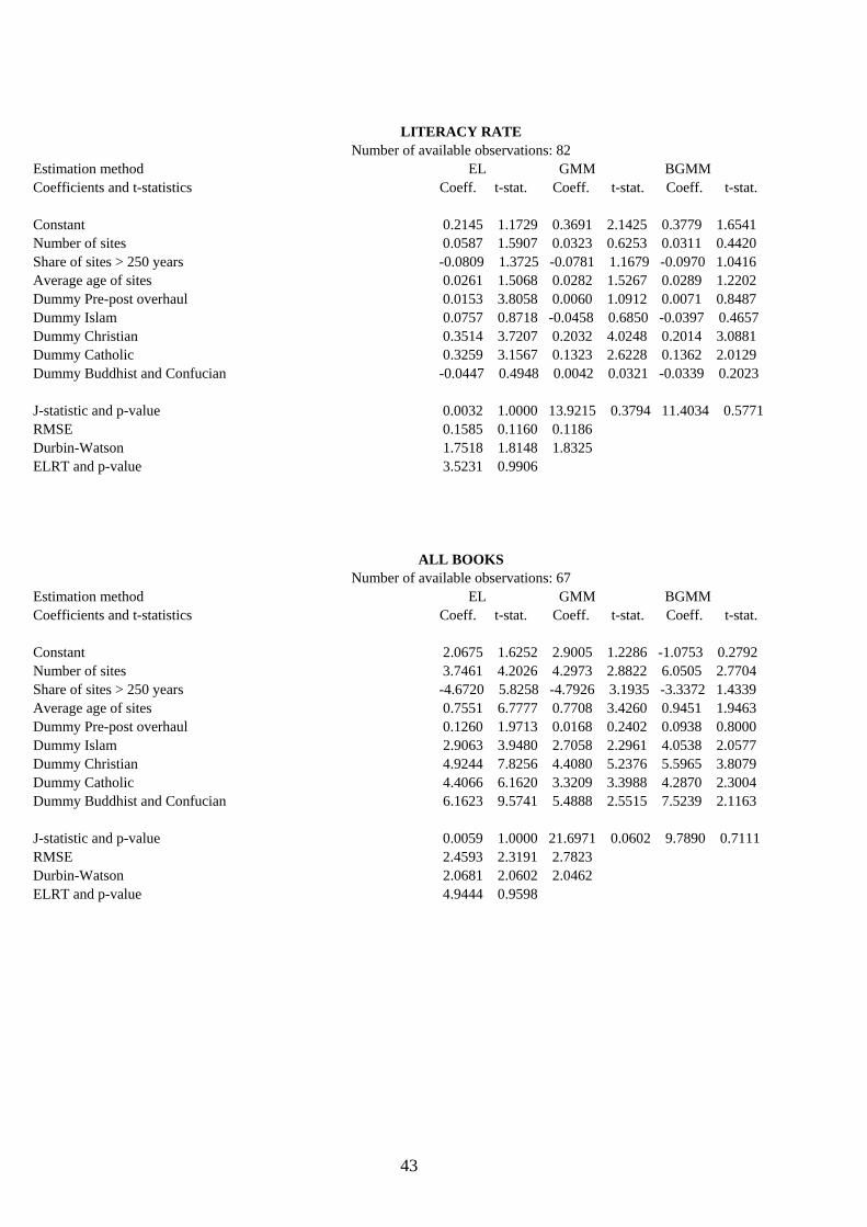
43

LITERACY RATE Number of available observations: 82

Estimation method EL GMM BGMM Coefficients and t-statistics Coeff. t-stat. Coeff. t-stat. Coeff. t-stat. Constant 0.2145 1.1729 0.3691 2.1425 0.3779 1.6541 Number of sites 0.0587 1.5907 0.0323 0.6253 0.0311 0.4420 Share of sites > 250 years -0.0809 1.3725 -0.0781 1.1679 -0.0970 1.0416 Average age of sites 0.0261 1.5068 0.0282 1.5267 0.0289 1.2202 Dummy Pre-post overhaul 0.0153 3.8058 0.0060 1.0912 0.0071 0.8487 Dummy Islam 0.0757 0.8718 -0.0458 0.6850 -0.0397 0.4657 Dummy Christian 0.3514 3.7207 0.2032 4.0248 0.2014 3.0881 Dummy Catholic 0.3259 3.1567 0.1323 2.6228 0.1362 2.0129 Dummy Buddhist and Confucian -0.0447 0.4948 0.0042 0.0321 -0.0339 0.2023 J-statistic and p-value 0.0032 1.0000 13.9215 0.3794 11.4034 0.5771 RMSE 0.1585 0.1160 0.1186 Durbin-Watson 1.7518 1.8148 1.8325 ELRT and p-value 3.5231 0.9906

ALL BOOKS Number of available observations: 67

Estimation method EL GMM BGMM Coefficients and t-statistics Coeff. t-stat. Coeff. t-stat. Coeff. t-stat. Constant 2.0675 1.6252 2.9005 1.2286 -1.0753 0.2792 Number of sites 3.7461 4.2026 4.2973 2.8822 6.0505 2.7704 Share of sites > 250 years -4.6720 5.8258 -4.7926 3.1935 -3.3372 1.4339 Average age of sites 0.7551 6.7777 0.7708 3.4260 0.9451 1.9463 Dummy Pre-post overhaul 0.1260 1.9713 0.0168 0.2402 0.0938 0.8000 Dummy Islam 2.9063 3.9480 2.7058 2.2961 4.0538 2.0577 Dummy Christian 4.9244 7.8256 4.4080 5.2376 5.5965 3.8079 Dummy Catholic 4.4066 6.1620 3.3209 3.3988 4.2870 2.3004 Dummy Buddhist and Confucian 6.1623 9.5741 5.4888 2.5515 7.5239 2.1163 J-statistic and p-value 0.0059 1.0000 21.6971 0.0602 9.7890 0.7111 RMSE 2.4593 2.3191 2.7823 Durbin-Watson 2.0681 2.0602 2.0462 ELRT and p-value 4.9444 0.9598

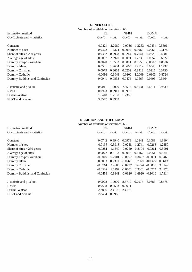
44

GENERALITIES Number of available observations: 66

Estimation method EL GMM BGMM Coefficients and t-statistics Coeff. t-stat. Coeff. t-stat. Coeff. t-stat. Constant -0.0824 2.2989 -0.0786 1.3263 -0.0434 0.5896 Number of sites 0.0372 1.2374 0.0094 0.5965 0.0063 0.3178 Share of sites > 250 years 0.0362 0.9968 0.0244 0.7644 0.0229 0.4881 Average age of sites 0.0097 2.9970 0.0091 1.2730 0.0052 0.6322 Dummy Pre-post overhaul 0.0020 1.3533 0.0001 0.0556 -0.0002 0.0836 Dummy Islam 0.0531 1.9654 0.0665 1.9512 0.0548 1.1937 Dummy Christian 0.0079 0.6665 0.0202 0.9419 0.0115 0.3750 Dummy Catholic -0.0093 0.6043 0.0300 1.2009 0.0303 0.8724 Dummy Buddhist and Confucian 0.0041 0.0853 0.0476 1.0567 0.0406 0.5864 J-statistic and p-value 0.0041 1.0000 7.8515 0.8531 5.4511 0.9639 RMSE 0.0923 0.0911 0.0915 Durbin-Watson 1.6448 1.7190 1.7385 ELRT and p-value 3.5547 0.9902

RELIGION AND THEOLOGY Number of available observations: 66

Estimation method EL GMM BGMM Coefficients and t-statistics Coeff. t-stat. Coeff. t-stat. Coeff. t-stat. Constant 0.0742 0.9940 0.0976 1.2841 0.1089 1.3604 Number of sites -0.0136 0.5913 -0.0258 1.2741 -0.0268 1.2550 Share of sites > 250 years -0.0281 1.1849 -0.0250 0.8104 -0.0261 0.8091 Average age of sites 0.0072 0.8138 0.0057 0.6167 0.0051 0.5343 Dummy Pre-post overhaul -0.0007 0.2901 -0.0007 0.3697 -0.0011 0.5465 Dummy Islam 0.0083 0.2301 -0.0263 0.7369 -0.0325 0.8613 Dummy Christian -0.0761 3.2606 -0.0797 3.6774 -0.0855 3.8149 Dummy Catholic -0.0532 1.7197 -0.0701 2.3301 -0.0774 2.4870 Dummy Buddhist and Confucian -0.0453 0.9141 -0.0926 1.6920 -0.1010 1.7314 J-statistic and p-value 0.0028 1.0000 8.6710 0.7973 8.0883 0.8378 RMSE 0.0598 0.0598 0.0611 Durbin-Watson 2.3836 2.4106 2.4192 ELRT and p-value 2.8404 0.9966

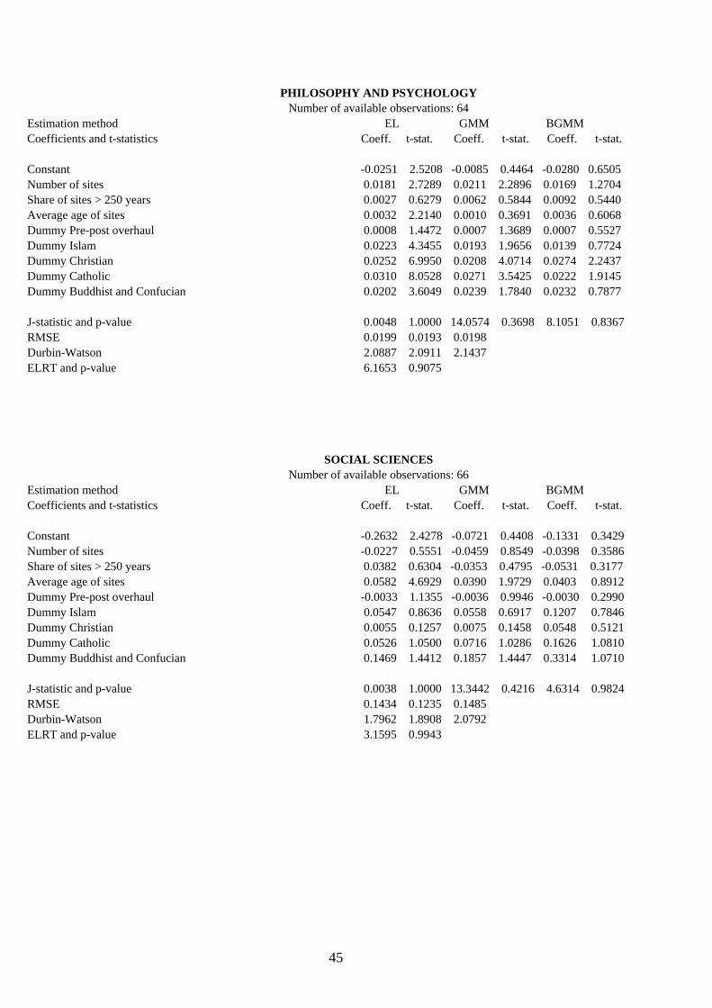
45

PHILOSOPHY AND PSYCHOLOGY Number of available observations: 64

Estimation method EL GMM BGMM Coefficients and t-statistics Coeff. t-stat. Coeff. t-stat. Coeff. t-stat. Constant -0.0251 2.5208 -0.0085 0.4464 -0.0280 0.6505 Number of sites 0.0181 2.7289 0.0211 2.2896 0.0169 1.2704 Share of sites > 250 years 0.0027 0.6279 0.0062 0.5844 0.0092 0.5440 Average age of sites 0.0032 2.2140 0.0010 0.3691 0.0036 0.6068 Dummy Pre-post overhaul 0.0008 1.4472 0.0007 1.3689 0.0007 0.5527 Dummy Islam 0.0223 4.3455 0.0193 1.9656 0.0139 0.7724 Dummy Christian 0.0252 6.9950 0.0208 4.0714 0.0274 2.2437 Dummy Catholic 0.0310 8.0528 0.0271 3.5425 0.0222 1.9145 Dummy Buddhist and Confucian 0.0202 3.6049 0.0239 1.7840 0.0232 0.7877 J-statistic and p-value 0.0048 1.0000 14.0574 0.3698 8.1051 0.8367 RMSE 0.0199 0.0193 0.0198 Durbin-Watson 2.0887 2.0911 2.1437 ELRT and p-value 6.1653 0.9075

SOCIAL SCIENCES Number of available observations: 66

Estimation method EL GMM BGMM Coefficients and t-statistics Coeff. t-stat. Coeff. t-stat. Coeff. t-stat. Constant -0.2632 2.4278 -0.0721 0.4408 -0.1331 0.3429 Number of sites -0.0227 0.5551 -0.0459 0.8549 -0.0398 0.3586 Share of sites > 250 years 0.0382 0.6304 -0.0353 0.4795 -0.0531 0.3177 Average age of sites 0.0582 4.6929 0.0390 1.9729 0.0403 0.8912 Dummy Pre-post overhaul -0.0033 1.1355 -0.0036 0.9946 -0.0030 0.2990 Dummy Islam 0.0547 0.8636 0.0558 0.6917 0.1207 0.7846 Dummy Christian 0.0055 0.1257 0.0075 0.1458 0.0548 0.5121 Dummy Catholic 0.0526 1.0500 0.0716 1.0286 0.1626 1.0810 Dummy Buddhist and Confucian 0.1469 1.4412 0.1857 1.4447 0.3314 1.0710 J-statistic and p-value 0.0038 1.0000 13.3442 0.4216 4.6314 0.9824 RMSE 0.1434 0.1235 0.1485 Durbin-Watson 1.7962 1.8908 2.0792 ELRT and p-value 3.1595 0.9943

46

PHILOLOGY Number of available observations: 66

Estimation method EL GMM BGMM Coefficients and t-statistics Coeff. t-stat. Coeff. t-stat. Coeff. t-stat. Constant -0.0141 0.4493 -0.0213 0.4043 -0.0292 0.2708 Number of sites -0.0353 2.8528 -0.0163 1.4476 -0.0212 0.9435 Share of sites > 250 years -0.0407 1.8746 -0.0094 0.4081 -0.0166 0.3657 Average age of sites 0.0142 3.6948 0.0120 2.1917 0.0137 1.1595 Dummy Pre-post overhaul -0.0008 1.0645 -0.0011 0.9212 -0.0013 0.4927 Dummy Islam 0.0052 0.2783 -0.0193 0.7781 -0.0063 0.1427 Dummy Christian -0.0406 3.0028 -0.0340 1.8817 -0.0236 0.8279 Dummy Catholic -0.0081 0.5723 -0.0249 1.0632 -0.0285 0.6923 Dummy Buddhist and Confucian 0.0119 0.6121 -0.0114 0.3136 -0.0104 0.1297 J-statistic and p-value 0.0038 1.0000 10.7561 0.6312 4.2799 0.9878 RMSE 0.0498 0.0475 0.0495 Durbin-Watson 2.0569 2.0972 2.1260 ELRT and p-value 2.6513 0.9975

PURE AND APPLIED SCIENCES Number of available observations: 65

Estimation method EL GMM BGMM Coefficients and t-statistics Coeff. t-stat. Coeff. t-stat. Coeff. t-stat. Constant 0.1224 1.8745 0.0636 0.8092 0.0319 0.3584 Number of sites -0.0198 1.3376 -0.0187 1.2735 -0.0198 1.1079 Share of sites > 250 years -0.0197 0.4878 0.0105 0.2388 0.0065 0.1247 Average age of sites 0.0105 1.2878 0.0138 1.5602 0.0174 1.8406 Dummy Pre-post overhaul 0.0005 0.2109 0.0019 0.7894 0.0024 0.7238 Dummy Islam -0.0333 0.9959 -0.0589 1.6863 -0.0471 1.2947 Dummy Christian 0.0233 0.8232 0.0235 1.1021 0.0265 1.0407 Dummy Catholic -0.0125 0.3909 0.0053 0.1732 0.0153 0.4712 Dummy Buddhist and Confucian -0.0274 0.5212 -0.0267 0.4779 -0.0070 0.1213 J-statistic and p-value 0.0038 1.0000 10.2280 0.6752 10.3487 0.6652 RMSE 0.0631 0.0693 0.0728 Durbin-Watson 1.8896 1.7804 1.8106 ELRT and p-value 2.4210 0.9984

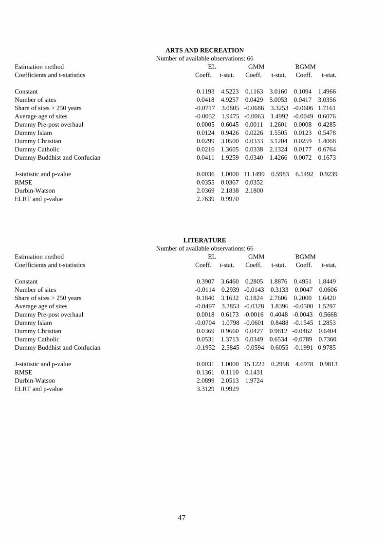
47

ARTS AND RECREATION Number of available observations: 66

Estimation method EL GMM BGMM Coefficients and t-statistics Coeff. t-stat. Coeff. t-stat. Coeff. t-stat. Constant 0.1193 4.5223 0.1163 3.0160 0.1094 1.4966 Number of sites 0.0418 4.9257 0.0429 5.0053 0.0417 3.0356 Share of sites > 250 years -0.0717 3.0805 -0.0686 3.3253 -0.0606 1.7161 Average age of sites -0.0052 1.9475 -0.0063 1.4992 -0.0049 0.6076 Dummy Pre-post overhaul 0.0005 0.6045 0.0011 1.2601 0.0008 0.4285 Dummy Islam 0.0124 0.9426 0.0226 1.5505 0.0123 0.5478 Dummy Christian 0.0299 3.0500 0.0333 3.1204 0.0259 1.4068 Dummy Catholic 0.0216 1.3605 0.0338 2.1324 0.0177 0.6764 Dummy Buddhist and Confucian 0.0411 1.9259 0.0340 1.4266 0.0072 0.1673 J-statistic and p-value 0.0036 1.0000 11.1499 0.5983 6.5492 0.9239 RMSE 0.0355 0.0367 0.0352 Durbin-Watson 2.0369 2.1838 2.1800 ELRT and p-value 2.7639 0.9970

LITERATURE Number of available observations: 66

Estimation method EL GMM BGMM Coefficients and t-statistics Coeff. t-stat. Coeff. t-stat. Coeff. t-stat. Constant 0.3907 3.6460 0.2805 1.8876 0.4951 1.8449 Number of sites -0.0114 0.2939 -0.0143 0.3133 0.0047 0.0606 Share of sites > 250 years 0.1840 3.1632 0.1824 2.7606 0.2000 1.6420 Average age of sites -0.0497 3.2853 -0.0328 1.8396 -0.0500 1.5297 Dummy Pre-post overhaul 0.0018 0.6173 -0.0016 0.4048 -0.0043 0.5668 Dummy Islam -0.0704 1.0798 -0.0601 0.8488 -0.1545 1.2853 Dummy Christian 0.0369 0.9660 0.0427 0.9812 -0.0462 0.6404 Dummy Catholic 0.0531 1.3713 0.0349 0.6534 -0.0789 0.7360 Dummy Buddhist and Confucian -0.1952 2.5845 -0.0594 0.6055 -0.1991 0.9785 J-statistic and p-value 0.0031 1.0000 15.1222 0.2998 4.6978 0.9813 RMSE 0.1361 0.1110 0.1431 Durbin-Watson 2.0899 2.0513 1.9724 ELRT and p-value 3.3129 0.9929

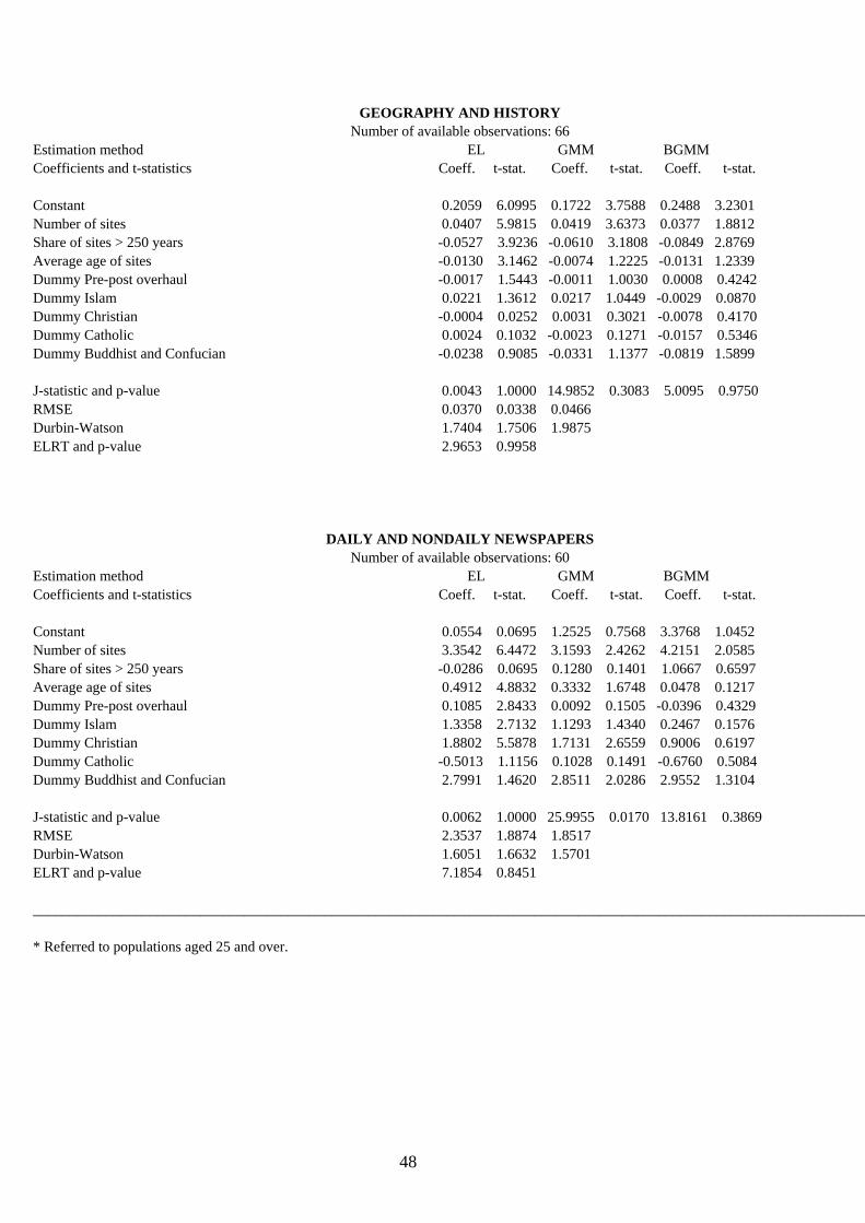
48

GEOGRAPHY AND HISTORY Number of available observations: 66

Estimation method EL GMM BGMM Coefficients and t-statistics Coeff. t-stat. Coeff. t-stat. Coeff. t-stat. Constant 0.2059 6.0995 0.1722 3.7588 0.2488 3.2301 Number of sites 0.0407 5.9815 0.0419 3.6373 0.0377 1.8812 Share of sites > 250 years -0.0527 3.9236 -0.0610 3.1808 -0.0849 2.8769 Average age of sites -0.0130 3.1462 -0.0074 1.2225 -0.0131 1.2339 Dummy Pre-post overhaul -0.0017 1.5443 -0.0011 1.0030 0.0008 0.4242 Dummy Islam 0.0221 1.3612 0.0217 1.0449 -0.0029 0.0870 Dummy Christian -0.0004 0.0252 0.0031 0.3021 -0.0078 0.4170 Dummy Catholic 0.0024 0.1032 -0.0023 0.1271 -0.0157 0.5346 Dummy Buddhist and Confucian -0.0238 0.9085 -0.0331 1.1377 -0.0819 1.5899 J-statistic and p-value 0.0043 1.0000 14.9852 0.3083 5.0095 0.9750 RMSE 0.0370 0.0338 0.0466 Durbin-Watson 1.7404 1.7506 1.9875 ELRT and p-value 2.9653 0.9958

DAILY AND NONDAILY NEWSPAPERS Number of available observations: 60

Estimation method EL GMM BGMM Coefficients and t-statistics Coeff. t-stat. Coeff. t-stat. Coeff. t-stat. Constant 0.0554 0.0695 1.2525 0.7568 3.3768 1.0452 Number of sites 3.3542 6.4472 3.1593 2.4262 4.2151 2.0585 Share of sites > 250 years -0.0286 0.0695 0.1280 0.1401 1.0667 0.6597 Average age of sites 0.4912 4.8832 0.3332 1.6748 0.0478 0.1217 Dummy Pre-post overhaul 0.1085 2.8433 0.0092 0.1505 -0.0396 0.4329 Dummy Islam 1.3358 2.7132 1.1293 1.4340 0.2467 0.1576 Dummy Christian 1.8802 5.5878 1.7131 2.6559 0.9006 0.6197 Dummy Catholic -0.5013 1.1156 0.1028 0.1491 -0.6760 0.5084 Dummy Buddhist and Confucian 2.7991 1.4620 2.8511 2.0286 2.9552 1.3104 J-statistic and p-value 0.0062 1.0000 25.9955 0.0170 13.8161 0.3869 RMSE 2.3537 1.8874 1.8517 Durbin-Watson 1.6051 1.6632 1.5701 ELRT and p-value 7.1854 0.8451 ___________________________________________________________________________________________________________________ * Referred to populations aged 25 and over.

49

References.

Acemoglu D., 1997; Training and Innovation in an Imperfect Labor Market, Review of Economic Studies, 64, 445-464. Aitken A. C., 1935; On Least Squares and Linear Combination of Observations, Proceedings of the Royal Society of Edinburgh, 55, 42-48. Allott, R., 1999; Evolution and Culture: The Missing Link. Van der Dennen, Smillie D.R. eds., The Darwinian Heritage and Sociobiology, Ch.5, p. 67-81, Praeger, Westport, CT. Altonji J. G. and Segal L.M., 1996; Small-Sample Bias in GMM Estimation of Covariance Structures, Journal of Business and Economic Statistics, 4, 353-366. Andrews D.W.K., 1991; Heteroskedasticity and Autocorrelation Consistent Covariance Matrix Estimation, Econometrica, 59, 817-858. Andrews D.W.K., 1999; Consistent Moment Selection Procedures for Generalized Method of Moments Estimation, Econometrica, 67, 543-564. Baldacci E., Guin-Sui M. T. and de Mello L., 2003; More on the Effectiveness of Public Spending on Health Care and Education; A Covariance Structure Model, Journal of International Development, 15, 709-25. Baldacci E., Clements B., Gupta S. and Cui Q., 2004; Social Spending, Human Capital, and Growth in Developing Countries: Implications for Achieving the MDGs, IMF Working Paper No. 04/217. Barro R., 1991; Economic Growth in a Cross-Section of Countries, Quarterly Journal of Economics, 106, 407-502.

Barro R., 1999; Human Capital and Growth in Cross-Country Regressions, Swedish Economic Policy Review, 6, 237-277. Barro R., 2000; Education and Economic Growth, Manuscript, Harvard University. Barro, R. and Lee J.W., 1996; International Measures of Schooling Years and Schooling Quality, American Economic Review, Papers and Proceedings, 2, 218-223 . Barro, R. and Lee J.W., 2001; International Data on Educational Attainment: Updates and Implications, Oxford Economic Papers, 53, 541-563 . Barro R. and McCleary, 2003, International Determinants of Religiosity, NBER Working Paper, W10147. Barro R. and Sala-i-Martin, 1999; Economic Growth, MIT Press, Cambridge, Mass. Becker G., 1964; Human Capital, Chicago IL., University of Chicago Press. Becker G, 1981; A Treatise on the Family, Cambridge MA., Harvard University Press.

50

Bekker P. A., 1994; Alternative Approximations to the Distributions of Instrumental Variable Estimators, Econometrica, 62, 657-681. Bound J., Jaeger D. A. and Baker R. M., 1995, Problems with Instrumental Variables Estimation when the Correlation Between the Instruments and the Endogenous Variable is Weak, Journal of the American Statistical Association, 90, 443-450. Bourdieu P., 1986; The Forms of Capital, Handbook of Theory and Research for the Sociology of Education. Trans. R. Nice, Richardson J. G. ed., Greenwood Press, 241-258. Boyd R. and P.J. Richerson, 1985; Culture and the Evolutionary Process, University of Chicago Press. Brauninger M. and Vidal J. P. , 1999; Private versus Public Financing of Education and Endogenous Growth, Journal of Population Economics, 13, 387-401. Brunello G, Comi S. and Lucifora C., 2000; The Returns to Education in Italy: A New Look at the Evidence, IZA Discussion Papers No. 130. Brunello G. and Checchi D., 2003; School Quality and Family Background in Italy, IZA Discussion Papers No. 705. Card D., 1999; The Causal effect of Education on Earnings, in Ashenfelter O. and Card D. eds., Handbook of Labor Economics, Vol. 3, Amsterdam, Elsevier-North-Holland. Card D. and Krueger A., 1992; Does School Quality Matter? Returns to Education and the Characteristics of Public Schools in the United States, Journal of Political Economy, p. 1-39. Casson M. C., 1993; Cultural Determinants of Economic Performance, Journal of ComparativeEconomics, 17, 418-442. Cavalli-Sforza L.L. and Feldman M.W., 1981; Cultural Transmission and Evolution: A Quantitative Approach. Princeton University Press. Chamberlain G., 1987; Asymptotic Efficiency in Estimation with Conditional Moment Restrictions, Journal of Econometrics, 34, 395-434. Chao J. C. and Swanson N. R., 2005; Consistent Estimation with a Large Number of Weak Instruments, Econometrica, 73, 1673-1692. Chen D. H. C. and Dahlam C. J., 2004, Knowledge and Development. A Cross-Section Approach, World Bank Policy Research Working Paper No. 3366. Cohen D. and Soto M., 2001; Growth and Human Capital: Good Data, Good Results, OECD Development Center Technical Paper No. 179. Cozzi G., 1998; Culture as a Bubble, Journal of Political Economy, Journal of Poliitical Economy, 106, 376-394. Cremer H., Kessler D. and Pestieau P., 1992; Intergenerational Transfers Within the Family, European Economic Review, 36, p. 1-16.

51

D'Agostino, R. B. and Stephens, M. A., eds. 1986; Goodness-of-fit Techniques. New York: Dekker.

Dahlin B., 2003; The Impact of Education on Economic Growth. Theory, Findings and Policy Implications, Manuscript, Duke University

Dawkins R. ,1976; The Selfish Gene, Oxford University Press.

Dawkins R., 1982; The Extended Phenotype, W. H. Freeman and Company.

De Long B. and Shleifer A., 1993, Princes and Merchants: European City Growth Before the Industrial Revolution, NBER Working Paper No. 4274.

Donald S. G. and Newey W.K., 2001, Choosing the number of instruments, Econometrica, 69, 1161-1191.

Donald S. G., Imbens G. and Newey W.K., 2002, Choosing the Number of Instruments for GMM and GEL Estimators, Working Paper, Department of Economics,M.I.T.

Donald S. G., Imbens G. and Newey W.K., 2003, Empirical Likelihood Estimation and Consistent Tests with Conditional Moment Restrictions, Journal of Econometrics, 117, 55-93.

Faria J. R. and León-Ledesma M., 2003; Cultural Heritage and Growth, Department of Economics, University of Kent, Discussion Paper 0303

Gallant A. R. and Tauchen G., 1996, Which Moments to Match?, Econometric Theory, 12, 657-681.

Galor O. and Weil D. N., 1996; The Gender Gap, Fertility and Growth, American Economic Review, 86, 374-387.

Gray H. P., 1996; Culture and Economic Performance: Policy as an Intervening Variable, Journal of Comparative Economics, 23, 278-291.

Guggenberger P. and Hahn J., 2005; Finite Sample Properties of the Two-step Empirical Likelihood Estimator, Econometric Reviews, 24, 247-263.

Gupta S., Verhoeven M. and Tjongson E., 2002; The Effectiveness of Government Spending on Education and Health Care in Developing and Transition Economies, European Journal of Political Economy, 18, 717-737.

Hahn J. and Hausman J., 2002; A New Specification Test for the Validity of Instrumental Variables, Econometrica, 70, 163-189.

Hahn J. and Hausman J., 2003; IV Estimation with Valid and Invalid Instruments, manuscript, MIT, Department of Economics.

Hahn J., Hausman J. and Kuersteiner G., 2001; Bias Corrected Instrumental Variables Estimation for Dynamic Panel Models with Fixed Effects, manuscript, MIT, Department of Economics.

Hahn J., Hausman J. and Kuersteiner G., 2002; Estimation with Weak Instruments: Accuracy of Higher Order Bias and MSE Approximations, manuscript, MIT, Department of Economics.

52

Hall A. R., Rudebusch G. D. and Wilcox D. W., 1996, Judging Instrument Relevance in Instrumental Variables Estimation, International Economic Review, 39, 283-298.

Hansen L. P., 1982; Large Sample Properties of Generalized Method of Moments Estimators, Econometrica, 50, 1029-1054.

Hansen L. P. and Singleton K. J., 1982, Generalized Instrumental Variables Estimation of Nonlinear Rational Expectations Models, Econometrica, 50, 1269-86.

Hansen, L. P., Heaton J. C. and Ogaki M., 1988, Efficiency Bounds Implied by Multiperiod Conditional Moment Restrictions, Journal of the American Statistical Association, 83, 863-871.

Hansen, L. P., Heaton J. C. and Yaron A., 1996; Finite-Sample Properties of Some Alternative GMM Estimators, Journal of Business and Economic Statistics, 14, 262-280.

Hansen B. E. and West K. D., 2002; Generalized Method of Moments and Macroeconomics, Journal of Business and Economic Statistics, p. 1-9.

Hayashi F., 2000; Econometrics, Princeton, NJ, Princeton University Press.

Hayashi F. and Sims C. A., 1983; Nearly Efficient Estimation of Time Series Models With Predetermined but not Exogenous Instruments, Econometrica, 51, p. 783-798.

Heckman J.J., Lochner L.J. and Todd P.E., 2003; Fifty Years of Mincer Earnings Regressions, IZA Discussion Papers No. 775.

Hendry D. and Krolzig H.M., 2004; We Ran One Regression, Oxford Bulletin of Economics and Statistics, 2004, 1-9.

Heston A., Summers R. and Aten B., 2002, Penn World Table Version 6.1 (PWT6.1), Center for International Comparisons at the University of Pennsylvania (CICUP).

Hofbauer, J. and Sigmund, K., 1988; The theory of evolution and dynamical systems, Cambridge University Press.

Hoover K.D. and Perez S.J., 2004; Truth and Robustness in Cross-country Growth Regressions, Oxford Bulletin of Economics and Statistics, 66, 765-798.

Imbens, G. W., 1997; One-Step Estimators for Over-Identified Generalized Method of Moments Models, Review of Economic Studies, 64, 359-383.

Kendal J. R. and Laland K. N., 2000; Mathematical Models for Memetics, Journal of Memetics, vol.4.

Kiriacou G., 1991; Level and Growth Effects of Human Capital: A Cross-Country study of the Convergence Hypothesis, New York University Economic Research Report, 91-126.

Kremer M., 1993; Population Growth and Technological Change: One Million B.C. to 1990, Quarterly Journal of Economics, 108, 681-716.

Levine R. and Renelt D., 1992; A Sensitivity Analysis of Cross-country Growth Regressions, American Economic Review, 82, 942-963.

53

Lucas R. E. Jr,, 1988; On the Mechanics of Economic Development, Journal of Monetary Economics, 22, 3-42.

Lumsden, C. and Wilson, E. O., 1981; Genes, mind, and culture, Harvard University Press.

Mincer J., 1974; Schooling, Experience and Earnings, New York, NY., NBER Press.

Mincer J. and Polachek S., 1974; Family Investment in Human Capital: Earnings of Women, Journal of Political Economy, 82/2, p. 76-108.

Nelson C. R. and Starz R., 1990, Further Results on the Exact Small Sample Properties of the Instrumental Variable Estimator, Econometrica, 58, 967-976.

Newey W.K. and Smith R. J., 2004; Higher Order Properties of GMM and Generalized Empirical Likelihood Estimators, Econometrica, 72, 219-255.

Newey W. K. and West K. D., 1987; A Simple Positive Semi-Definite Heteroskedasticity and Autocorrelation Consistent Covariance Matrix, Econometrica, 55, p.703-708.

Newey W. K. and West K. D., 1994; Automatic Lag Selection in Covariance Matrix Estimation, Review of Economic Studies, 61, p. 631-653.

Okui R., 2004; The Optimal Choice of Moments in Dynamic Panel Data Models, University of Pennsylvania, unpublished manuscript.

Owen A. B., 1988; Empirical Likelihood Ratio Confidence Intervals for a Single Functional, Biometrika, 75, 237-249.

Owen A. B., 2001; Empirical Likelihood, Chapman and Hall, New York.

Portela M., Alessie R. and Tuelings C., 2004; Measurement Error in Education and Growth Regressions, IZA Discussion Paper No. 1165.

Putnam R., 1993; Making Democracy Work, Princeton University Press, Princeton.

Qin J. and Lawless J., 1994; Empirical Likelihood and General Estimating Equations, Annals of Statistics, 22, 300-325.

Rothemberg T. J., 1984, Approximating the Distributions of Econometric Estimators and Test Statistics, in Griliches Z. and Intriligator M.D. eds., Handbook of Econometrics, North Holland, 881-935.

Sala-i-Martin X.X., 1997; I Have Just run Two Million Regressions, American Economic Review, 87, 178-183.

Schultz T., 1961; Investment in Human Capital, American Economic Review, 51, 1-17.

Smith R. J., 1997; Alternative Semi-Parametric Likelihood Approaches to Generalized Methods of Moments Estimation, Economic Journal, 107, 503-519.

Smith R. J., 2001; GEL Methods for Moment Condition Models, Working Paper, University of Bristol.

54

Staiger D. and Stock J.H., 1997; Instrumental Variables Regression with Weak Instruments, Econometrica, 65, 557-586.

Stock J. H. and Wright J. , 2000; GMM with Weak Identification, Econometrica, 68, 1055-1096.

Stock J. H., Yogo M. and Wright J., 2002; A Survey of Weak Instruments and Weak Identification in Generalized Method of Moments, Journal of Business and Economic Statistics, 20, 518-529.

Temple J., 2000; Growth Regressions and What the Textbooks Don’t Tell You, Bulletin of Economic Research, 52, 181-205.

Temple J., 2001, Growth Effects of Education and Social Capital in the OECD Countries, OECD Economic Studies, 33, 2001/11.

Treiman D.J., 2002; The Growth and Determinants of Literacy in China, California Center for Population Research, University of California, Los Angeles.

West K. D., Wong Ka-fu and Anatolyev S., 2001, Instrumental Variables Estimation of Heteroskedastic Linear Models Using all Lags of Instruments, University of Wisconsin, unpublished manuscript.

UNESCO Institute for Statistics (UIS), 2004; Education indicators. Technical guidelines.

UNDP, 2004; Human Development Report.

White H., 1980; A Heteroskedasticity-Consistent Covariance Matrix Estimator and a Direct Test for Heteroskedasticity, Econometrica, 48, 817-838.

Endnotes.

1 The definition supplied is a combination of the Yahoo and of the Merriam-Webster online dictionaries currently available on the Web. For the sake of completeness, I would add, at the end of the quotation, the words: “and knowledge”. 2 Examples are the Christian Revolution in Western Europe, the Islamic Involution following the ‘Granada Syndrome’ occurred in many Arabic countries, and the colonization episodes of the Americas and Africa. Also the reverse happens: notable examples are the acquisition of the Greek culture by the Romans and by ancient Islam, and of the Indian and Chinese cultures by the Moghuls and the Mongols of the Khan dynasty, respectively. On average, high culture tends to absorb and even to feed in from low culture to a larger extent than the reverse. Typical examples are the evolutionary phenomena of arts and sciences in many societies, where low culture frequently provides a substantial part of the supply of human capital. 3 Measurement error due to misreporting by national statistical agencies or to data construction methodologies [Portela et al., 2004] as well as differences in data collection criteria and lack of data are frequent phenomena facing the applied researcher. An example among the countless: cross-section differences in graduation rates or in school life expectancy, or in the percentage of repeaters, by no means imply that comparatively higher country rankings are associated to smarter or more-cultured students because of the high worldwide variance in educational selectivity criteria. However, see Brunello et al. [2000] and Brunello and Checchi [2003]. 4 From now onwards, for simplicity purposes, I define as ‘learning’ all forms of schooling and educational standards, and as ‘transmission’ all of the printed-paper means, even if books – as is the case in the present context – include school textbooks. 5Apart from the lack of some time-series and cross-section statistics, no uniform criterion may be used to compare ancient cultures among them and with modern cultures as well. For instance, even within similar or identical fields of artistic production, many ancient cultures have specialized in fine arts (e.g. painting and architecture), others in humanities (e.g. poetry and romance), others in performing arts (e.g. dance and theater), and so on. In addition, even in the case of countries sharing the identical class of artistic production, a quantity output indicator may severely run counter the universally-received coefficients of quality, i.e. of expertise and aesthetics contained in the definition of high culture. In practice: is culturally wealthier a country that has produced hundreds of Cubist paintings or one that has produced only a dozen of reputed Old Masters ? And similarly: is

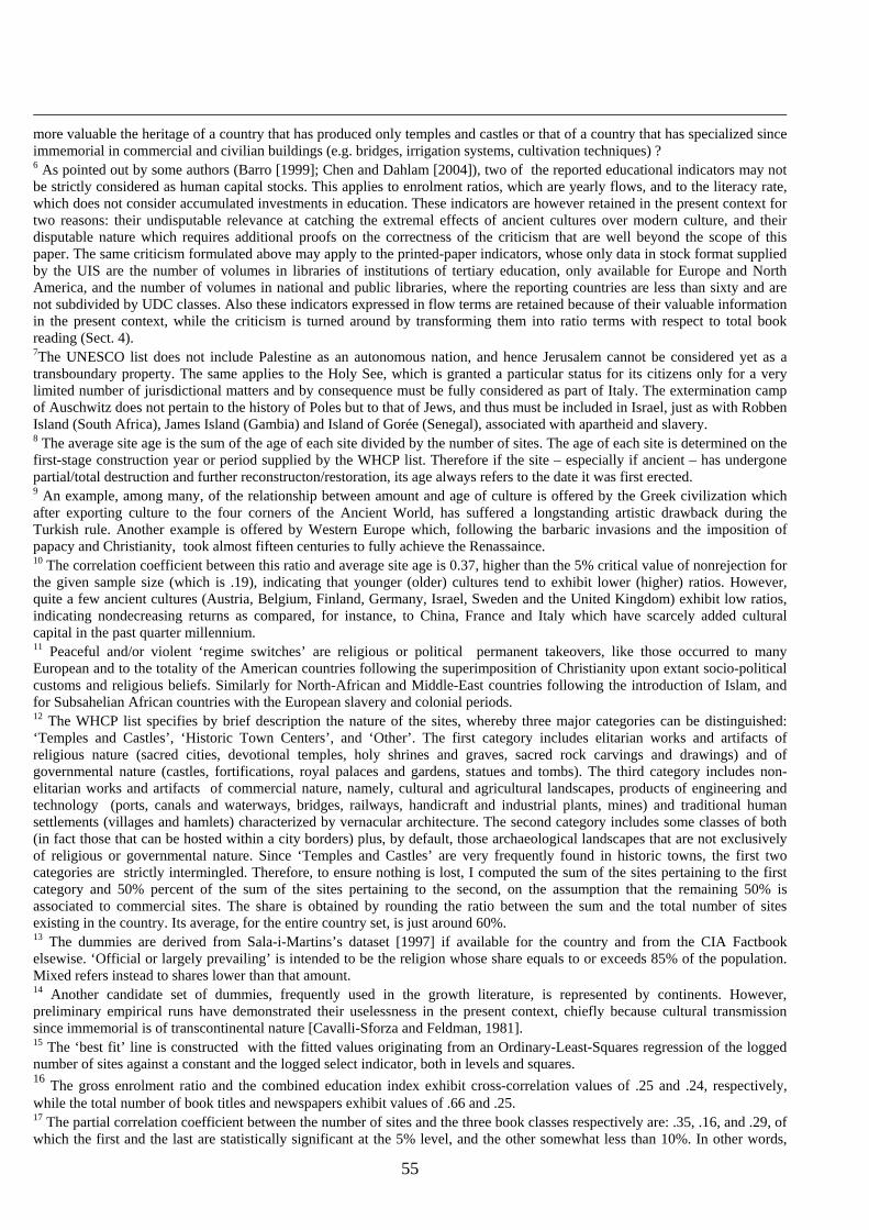
55

more valuable the heritage of a country that has produced only temples and castles or that of a country that has specialized since immemorial in commercial and civilian buildings (e.g. bridges, irrigation systems, cultivation techniques) ? 6 As pointed out by some authors (Barro [1999]; Chen and Dahlam [2004]), two of the reported educational indicators may not be strictly considered as human capital stocks. This applies to enrolment ratios, which are yearly flows, and to the literacy rate, which does not consider accumulated investments in education. These indicators are however retained in the present context for two reasons: their undisputable relevance at catching the extremal effects of ancient cultures over modern culture, and their disputable nature which requires additional proofs on the correctness of the criticism that are well beyond the scope of this paper. The same criticism formulated above may apply to the printed-paper indicators, whose only data in stock format supplied by the UIS are the number of volumes in libraries of institutions of tertiary education, only available for Europe and North America, and the number of volumes in national and public libraries, where the reporting countries are less than sixty and are not subdivided by UDC classes. Also these indicators expressed in flow terms are retained because of their valuable information in the present context, while the criticism is turned around by transforming them into ratio terms with respect to total book reading (Sect. 4). 7The UNESCO list does not include Palestine as an autonomous nation, and hence Jerusalem cannot be considered yet as a transboundary property. The same applies to the Holy See, which is granted a particular status for its citizens only for a very limited number of jurisdictional matters and by consequence must be fully considered as part of Italy. The extermination camp of Auschwitz does not pertain to the history of Poles but to that of Jews, and thus must be included in Israel, just as with Robben Island (South Africa), James Island (Gambia) and Island of Gorée (Senegal), associated with apartheid and slavery. 8 The average site age is the sum of the age of each site divided by the number of sites. The age of each site is determined on the first-stage construction year or period supplied by the WHCP list. Therefore if the site – especially if ancient – has undergone partial/total destruction and further reconstructon/restoration, its age always refers to the date it was first erected. 9 An example, among many, of the relationship between amount and age of culture is offered by the Greek civilization which after exporting culture to the four corners of the Ancient World, has suffered a longstanding artistic drawback during the Turkish rule. Another example is offered by Western Europe which, following the barbaric invasions and the imposition of papacy and Christianity, took almost fifteen centuries to fully achieve the Renassaince. 10 The correlation coefficient between this ratio and average site age is 0.37, higher than the 5% critical value of nonrejection for the given sample size (which is .19), indicating that younger (older) cultures tend to exhibit lower (higher) ratios. However, quite a few ancient cultures (Austria, Belgium, Finland, Germany, Israel, Sweden and the United Kingdom) exhibit low ratios, indicating nondecreasing returns as compared, for instance, to China, France and Italy which have scarcely added cultural capital in the past quarter millennium. 11 Peaceful and/or violent ‘regime switches’ are religious or political permanent takeovers, like those occurred to many European and to the totality of the American countries following the superimposition of Christianity upon extant socio-political customs and religious beliefs. Similarly for North-African and Middle-East countries following the introduction of Islam, and for Subsahelian African countries with the European slavery and colonial periods. 12 The WHCP list specifies by brief description the nature of the sites, whereby three major categories can be distinguished: ‘Temples and Castles’, ‘Historic Town Centers’, and ‘Other’. The first category includes elitarian works and artifacts of religious nature (sacred cities, devotional temples, holy shrines and graves, sacred rock carvings and drawings) and of governmental nature (castles, fortifications, royal palaces and gardens, statues and tombs). The third category includes non-elitarian works and artifacts of commercial nature, namely, cultural and agricultural landscapes, products of engineering and technology (ports, canals and waterways, bridges, railways, handicraft and industrial plants, mines) and traditional human settlements (villages and hamlets) characterized by vernacular architecture. The second category includes some classes of both (in fact those that can be hosted within a city borders) plus, by default, those archaeological landscapes that are not exclusively of religious or governmental nature. Since ‘Temples and Castles’ are very frequently found in historic towns, the first two categories are strictly intermingled. Therefore, to ensure nothing is lost, I computed the sum of the sites pertaining to the first category and 50% percent of the sum of the sites pertaining to the second, on the assumption that the remaining 50% is associated to commercial sites. The share is obtained by rounding the ratio between the sum and the total number of sites existing in the country. Its average, for the entire country set, is just around 60%. 13 The dummies are derived from Sala-i-Martins’s dataset [1997] if available for the country and from the CIA Factbook elsewise. ‘Official or largely prevailing’ is intended to be the religion whose share equals to or exceeds 85% of the population. Mixed refers instead to shares lower than that amount. 14 Another candidate set of dummies, frequently used in the growth literature, is represented by continents. However, preliminary empirical runs have demonstrated their uselessness in the present context, chiefly because cultural transmission since immemorial is of transcontinental nature [Cavalli-Sforza and Feldman, 1981]. 15 The ‘best fit’ line is constructed with the fitted values originating from an Ordinary-Least-Squares regression of the logged number of sites against a constant and the logged select indicator, both in levels and squares. 16 The gross enrolment ratio and the combined education index exhibit cross-correlation values of .25 and .24, respectively, while the total number of book titles and newspapers exhibit values of .66 and .25. 17 The partial correlation coefficient between the number of sites and the three book classes respectively are: .35, .16, and .29, of which the first and the last are statistically significant at the 5% level, and the other somewhat less than 10%. In other words,

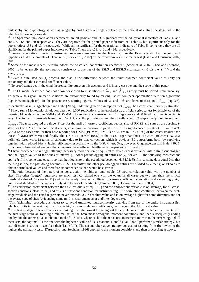
56

philosophy and psychology as well as geography and history are highly related to the amount of cultural heritage, while the other book class only weakly. 18 The Spearman rank correlation coefficients are all positive and 5% significant for the educational indicators of Table 4, and are .27, .64 and .70 respectively. They are negative for the printed-paper indicators of Table 5, but significant only for the books ratios: -.38 and -.34 respectively. While all insignificant for the educational indicators of Table 5, conversely they are all significant for the printed-paper indicators of Table 7, and are -.52, -.46 and -.34, respectively. 19 Several alternative criteria of instrument relevance are used in the literature, like the F-test statistic for the joint null hypothesis that all elements of Π are zero [Stock et al., 2002] or the forward/reverse estimator test [Hahn and Hausman, 2002, 2003]. 20 Some of the most recent literature adopts the so-called ‘concentration coefficient’ [Stock et al, 2002; Chao and Swanson, 2005] to better specify the asymptotic consistency properties of the 2SLS and B2SLS estimators vis-á-vis the 2 /L N and the L/N criteria. 21 Given a simulated AR(1) process, the bias is the difference between the ‘true’ assumed coefficient value of unity for stationarity and the estimated coefficient value. 22 No proof stands yet in the cited theoretical literature on this account, and is in any case beyond the scope of this paper. 23 The EL model described does not allow for closed-form solutions to ELλ and ELβ , as they must be solved simultaneously. To achieve this goal, numeric solutions are customarily found by making use of nonlinear optimization iteration algorithms (e.g. Newton-Raphson). In the present case, starting ‘guess’ values of λ and β are fixed to zero and GMMβ (eq. 3.5), respectively, as in Guggenberger and Hahn [2005], under the generic assumption that GMMβ be a consistent first-step estimator. 24 I have run a Montecarlo simulation based on 1,000 replications of heteroskedastic artificial series to test for efficiency of the two-step EL with respect to GMM and BGMM. The model is a regression with 10 regressors and 30 fixed instruments, which is very close to the experiments being run in Sect. 4, and the procedure is initialized with λ and β respectively fixed to zero and

GMMβ . The tests adopted are three: F-test for the null of nonzero coefficient vector, size of RMSE and sum of the absolute t-statistics (T-SUM) of the coefficient vector, an alternative measure to jointly test for its significance. F-tests of EL are in 40% (70%) of the cases smaller than hose reported for GMM (BGMM), RMSEs of EL are in 50% (70%) of the cases smaller than those of GMM (BGMM) and, finally, the T-SUM is in 90% (98%) of the cases larger than those of GMM (BGMM). BGMM definitely fares worst in terms of efficiency due to its bias correction, which is obvious. EL outperforms both, by supplying together with reduced bias a higher efficiency, especially with the T-SUM test. See, however, Guggenberger and Hahn [2005] for a more substantiated analysis that compares the small-sample efficiency properties of EL and 2SLS. 25 I have proceeded to a slight although necessary modification of eq. 3.29 to avoid excess variance within the pseudologged and the logged values of the series of interest iy . After pseudologging all entries of iy , for N=113 the following constructions apply: i) if in iy some data equal 1 so that their log is zero, the pseudolog becomes -6164.72; ii) if in iy some data equal 0 so that their log is NA, the pseudolog becomes -6.22. Thereafter, the other pseudologged entries are divided by either i) or ii) so as to obtain normalized values and therefore smoother series than would be elsewise. 26 The ratio, because of the nature of its construction, exhibits an untolerable .98 cross-correlation value with the number of sites. The other (logged) regressors are much less correlated one with the other, in all cases but two less than the critical threshold value of .19 (see fn. 11) and can be safely retained. Collinearity causes coefficient attenuation and exceedingly high coefficient standard errors, and is closely akin to model uncertainty [Temple, 2000; Hoover and Perez, 2004]. 27 The correlation coefficient between the OLS residuals of eq. (3.1) and the endogenous variable is on average, for all cross-section equations, close to .80, and this is a sufficient condition for instrumenting. The correlation coefficient between the first-stage residuals and the fixed regressors never exceeds .35 in absolute value and is on average higher for some dummies and for the average age of sites (evidencing some mild measurement error and/or endogeneity). 28This ‘skimming’ procedure is necessary to avoid unwanted multicollinearity deriving from use of the entire instrument list; which exhibits in the vast majority of cases high cross-correlation coefficients, well beyond the .19 critical value. 29 The first strategy followed consists of ranking from the lowest to the highest the correlations of all available instruments with the first-stage residual, forming a minimal set of the L=K most orthogonal moment conditions, and then subsequently adding one by one the others so as to obtain a total of L-K sets, where each of them has one instrument more than the preceding. Of all these sets, the ‘optimal’ is the one with the highest p-value of its J-statistic. Donald et al. [2003] perform a similar strategy, but use ‘discrete’ instrument sets (see their Table VII). The second alternative strategy consists of ranking from the lowest to the highest the normality tests [D'Agostino and Stephens, 1986] applied to the moment conditions and then proceeding as above.

57