Models used in NER
23
UNIVERSITY OF CAMBRIDGE Models used in NER Computer Laboratory Sriwantha Sri Aravinda 4/29/2011 Due to the scope explosion the essay will not compare every possible model combinations in NER (e.g HMM vs CRF, MEMM vs HMM etc) into detail. We will mainly compare MIIM model with CRF, HMM and MEMM with very few cases where we compare CRF, HMM, MEMM with each other in nutshell. Only the missing links in the literature will be presented
Transcript of Models used in NER

UNIVERSITY OF CAMBRIDGE
Models used in NER Computer Laboratory
Sriwantha Sri Aravinda
4/29/2011
Due to the scope explosion the essay will not compare every possible model combinations in NER (e.g HMM vs CRF, MEMM vs HMM etc) into detail. We will mainly compare MIIM model with CRF, HMM and MEMM with very few cases where we compare CRF, HMM, MEMM with each other in nutshell. Only the missing links in the literature will be presented

Table of Contents Structure ........................................................................................................................................... 3
Notation ............................................................................................................................................ 3
1. Introduction .............................................................................................................................. 4
2. Mutual Information Independent Model (MIIM) ........................................................................ 5
3. Discriminative and Generative Model Analysis ........................................................................... 9
4. State Dependency in NER......................................................................................................... 10
5. Feature Dependency in NER..................................................................................................... 12
6. CRF Vs MIIM Comparison on Label Bias Issue ........................................................................... 14
7. Named Alias Algorithm and Skip Chain CRF .............................................................................. 15
8. Conclusion & Discussion .......................................................................................................... 16
Appendix ......................................................................................................................................... 18
Reference ........................................................................................................................................ 22

Structure The essay will explore NER task and specific language processing techniques applied on it. During inception, it will structure around the paper “Named Entity Recognition using an HMM-based Chunk Tagger” by Zhou. As the NER task is a vast field, boundaries of the essay will be as follows.
First I will do an analysis on what Mutual Information Independence Model (MIIM) assumption means in terms of structure of HMM and how it differs from conventional generative approach. Next MIIM will be represented in a factor graphs and analyzed against two HMM. The MIIM does not make independent assumption among features, which is desirable especially when you have large number of over lapping features. This is somewhat similar to what CRF and MEMM models promise. The similarities between CRF and MIIM (Mutual Information Independence Model) will be explored. After careful investigation, I thought the best way to theoretically and experimentally compare models is to break up the investigation into how a) state dependencies b) feature dependencies c) feature-state dependencies are represented in various models.
Due to the scope explosion the essay will not compare every possible model combinations in NER (e.g HMM vs CRF, MEMM vs HMM etc) into detail. We will mainly compare MIIM model with CRF, HMM and MEMM with very few cases where we compare CRF, HMM, MEMM with each other in nutshell. Only the missing links in the literature will be presented.
Content in the appendix, reference or in this section are not considered for word counts and is provided as background reading. Each equation is taken as 1 word regardless of its content. Video lectures given in the reference give some background into the models discussed here.
Notation Throughout the essay following notation will be used.
Let 푋 = 푥 푥 푥 … 푥 be a token sequence.
In NER task, X forms the input and has the form 푥 =< 푤 , 푓 > where 푤 is the ith word in the input sequence and 푓 is the feature vector associated with word 푤 .
Let 푌 = 푦 푦 푦 … 푦 be the output sequence
In NER task, Y forms the set of name entities like LOCATION and PERSON. It’s worth mentioning that unlike푥 , 푦 is drawn from a set which can be fixed for the task.
Our goal is to find the stochastic optimal tag sequence 푌 that maximize 푃(푌|푋)

1. Introduction Task definition
Named Entity Recognition (NER) is the task of finding boundaries of entity segments in an input text and naming each such segment with a label taken from a finite set. It is nothing more than a classification task with added requirement of having to find entity boundaries. This general definition came from Message Understanding Conference (MUC) 6-7 task definition [1]. Most NER systems were built around MUC task definition which we could consider as the standard to compare NER models. However, variations exist, especially in bio NER task, where hierarchy of labels have to be assigned [2] [23].
The challenge of NER is that many entities are rare to appear even in a large training set. Hence, the system should have intuition to find the category from the context. The task is challenging as the same piece of text can refer to two different entities when appear at two different places in the same document.
Historical Survey
I was fascinated and sometimes surprised towards the variation of names different communities use for their models although the underlying first principals remain the same. For example, Logistic regression in ML community is known as maximum entropy classifier in NLP community which is a week version of a CRF classifier. Most researches related to NER involve using one of these fundamental models (HMM, MEMM, CRF, MIIM etc) where feature set and smoothing techniques are altered to get better results. Some hybrid approaches were tried in nested NER task.
Early works of NER involved manually building rule engines [3]. Such methods suffered from domain adaptation, nevertheless promised fast operation. Propelled by Message Understanding Conference, several supervised and semi supervised [4] systems were developed which used ML fundamentals. Examples include, Maximum Entropy [5], CRF [20], MIIM [7], Decision Trees [6].
Interesting parties can refer to the survey on David Nadeau PhD dissertation [4] which captures the essence of NER research from 1991 to 2006. Latest trends are mainly on Bio NER, search query NER task and in nested NER task where direct application of common methods are not possible.

2. Mutual Information Independent Model (MIIM) In this section I will represent the mutual information independent assumption in a graphical model. In doing so we will identify parameter interaction and which variables are considered to be independent. Finally I will argue why MIIM is a better choice for NER task than a conventional generative HMM. However, we can’t give a theoretically intuitive statement that states “MIIM is better than CRF or MEMM for NER”.
In the papers [7] [23] mutual information independence is assumed between X and Y yielding
MI(Y, X) = ∑ MI(y , X)
This assumes that the reduction in uncertainty for the state sequence in knowing the observation sequence is equal to the summation of the reduction in uncertainty for each individual state of the state sequence in knowing the observation sequence.
Alternatively it can be stated as
A given tag/state 풚풊 only depends on X/entire input but not other tags/states
To best of my knowledge this alternative statement is not given in the literature. Hence, the proof is given in the appendix.
Model Structures
We can map earlier form of assumption into MIIM as E 2.1 [Figure 1]. Note that this assumption is used only in the 3rd term ∑ log푃(푦 |푋) [7].
log푃(푌|푋) = log푃(푌)−∑ log 푃(푦 ) +∑ log푃(푦 |푋)
It’s worth investigating why this model is far relaxed version than the conventional HMM for NER. In conventional HMM for NER, the joint distribution P(X,Y) is modelled with two independence assumption. First, the model assumes that each state (entity) 푦 , is independent from its ancestors 푦 ,푦 …푦 given 푦 . Second, it assumes each observation 푥 depends only on 푦 .
The optimization equation of conventional HMM model (let’s say HMM1) is
Input sequence
Output sequence or conversely states Y1 ...
X1 X2 Xn ...
Y2 Yn
1 2 3
Figure 1
E 2.1
푃(푋,푌) = 푃(푦 ) × 푃(푦 |푦 ) × 푃(푥 |푦 )
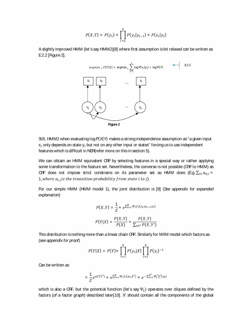
A slightly improved HMM (let’s say HMM2)[8] where first assumption is bit relaxed can be written as E 2.2 [Figure 2].
푎푟푔푚푎푥 푃(푌|푋) = argmax log P(x |y ) + log P(Y)
Still, HMM2 when evaluating log P(X|Y) makes a strong independence assumption as “a given input x only depends on state y but not on any other input or states” forcing us to use independent features which is difficult in NER(refer more on this in section 5).
We can obtain an HMM equivalent CRF by selecting features in a special way or rather applying some transformation to the feature set. Nevertheless, the converse is not possible (CRF to HMM) as CRF does not impose strict constrains on its parameter set as HMM does (E.g. ∑ 푎 , =∀
1,푤ℎ푒푟푒 푎 , 푖푠 푡ℎ푒 푡푟푎푛푠푖푡푖표푛 푝푟표푏푎푏푖푙푖푡푦 푓푟표푚 푠푡푎푡푒 푖 푡표 푗).
For our simple HMM (HMM model 1), the joint distribution is [9] (See appendix for expanded explanation)
푃(푋,푌) =1푍
× 푒∑ ( , , )
푃(푌|푋) =푃(푋,푌)푃(푋)
=푃(푋,푌)
∑ 푃(푋,푌 )∀
This distribution is nothing more than a linear chain CRF. Similarly for MIIM model which factors as (see appendix for proof)
푃(푌|푋) = 푃(푌)× 푃(푦 |푋) 푃(푦 )
Can be written as
=1푍푒 ( ) × 푒∑ ( , ) × 푒 ∑ ( )
which is also a CRF, but the potential function (let’s say Ψ ) operates over cliques defined by the factors (of a factor graph) described later[10]. X’ should contain all the components of the global
Y1 ...
X1 X2 Xn ...
Y2 Yn
Figure 2
E 2.2
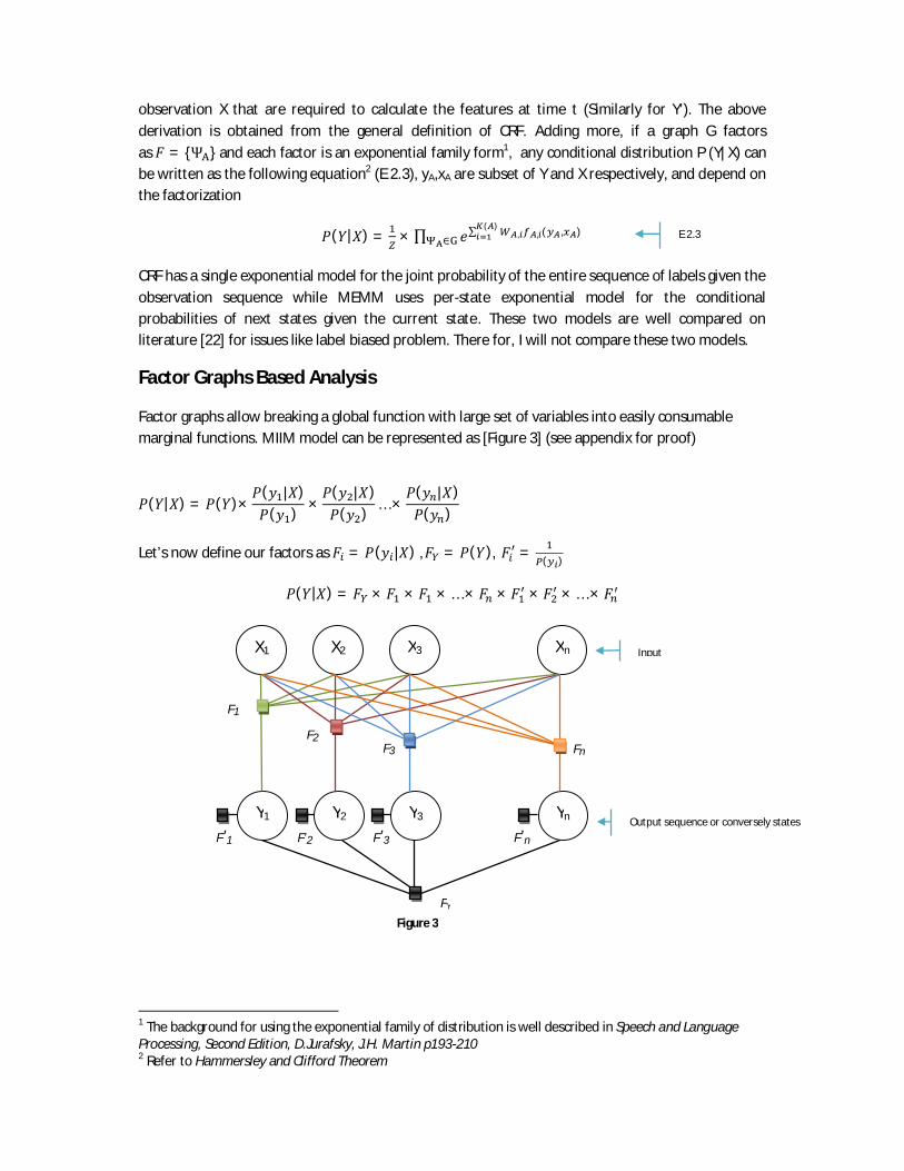
observation X that are required to calculate the features at time t (Similarly for Y’). The above derivation is obtained from the general definition of CRF. Adding more, if a graph G factors as 퐹 = {Ψ } and each factor is an exponential family form1, any conditional distribution P (Y|X) can be written as the following equation2 (E 2.3), yA,xA are subset of Y and X respectively, and depend on the factorization
푃(푌|푋) = × ∏ 푒∑ , , ( , )( )
∈
CRF has a single exponential model for the joint probability of the entire sequence of labels given the observation sequence while MEMM uses per-state exponential model for the conditional probabilities of next states given the current state. These two models are well compared on literature [22] for issues like label biased problem. There for, I will not compare these two models.
Factor Graphs Based Analysis
Factor graphs allow breaking a global function with large set of variables into easily consumable marginal functions. MIIM model can be represented as [Figure 3] (see appendix for proof)
푃(푌|푋) = 푃(푌)×푃(푦 |푋)푃(푦 ) ×
푃(푦 |푋)푃(푦 ) … ×
푃(푦 |푋)푃(푦 )
Let’s now define our factors as 퐹 = 푃(푦 |푋) ,퐹 = 푃(푌), 퐹 = ( )
푃(푌|푋) = 퐹 × 퐹 × 퐹 × … × 퐹 × 퐹 × 퐹 × … × 퐹
1 The background for using the exponential family of distribution is well described in Speech and Language Processing, Second Edition, D.Jurafsky, J.H. Martin p193-210 2 Refer to Hammersley and Clifford Theorem
Figure 3
Output sequence or conversely states
Input
FY
F1
..X1 X2 X3
Xn
..Y1
Y2
Y3
Yn
F2 F3 Fn
F’1 F’2 F’3 F’n
E 2.3

Similarly the conventional HMM (HMM model 1) can be represented as [Figure 4]
푃(푥,푦) = 푃(푦 ) × 푃(푦 |푦 ) × 푃(푥 |푦 )
Slightly improved HMM (HMM model 2) can be represented as [Figure 5]
P(X|Y) = argmax log P(Y) + log P(x |y )
It’s clear that neither traditional HMM (model 1) nor slightly improved HMM (model 2) creates factors based on global feature set, yet MIIM does. In terms of modelling relationships among
F1
..X1 X2 X3
Xn
..Y1
Y2
Y3
Yn
F2 F3 Fn
FY
FY2 FYn-1 FY1
F1
F2 F3 Fn
..X1 X2 X3
Xn
..Y1
Y2
Y3
Yn
FY0
Figure 4
Figure 5

named entities there is no difference between MIIM and slightly improved HMM (HMM model 2). MIIM is better than HMM 2 as MIIM captures global input features. More detail analysis on state dependency and feature dependency will be done later. Forward Backward algorithm used in these models is same as sum-product algorithm in factor graphs. As we now have the factors of MIIM, analysis of sum product algorithm and message parsing is same as in [11].For a detail analysis of how messages get parsed during forward backward algorithm refer to section IV (A) in [11].
3. Discriminative and Generative Model Analysis We can compare discriminative nature of MIIM and CRF vs. generative approach of traditional HMM. Such an approach was first proposed by Minka[12].
Imagine we have a generative model with parameter α.
푃 (푋,푌;α) = P (Y;α) × P(X|Y;α)
Let’s try to create a joint distribution from a generative model, such that we derive conditional distribution and prior from our generative model with different parameter settings. To do this, assume the prior is generated from a generative model under some special set of parameters (let’s say under α1)
푃 (푋;α ) = P (Y, X|α )∀
Also let the conditional distribution arises from another set of parameters of the generative model (let’s say α2)
푃 (푌|푋; α ) =P (Y, X;α )
P (X;α )=
P (Y, X;α )∑ P (Y, X;α )∀
Form above equations we get
푃 (푋,푌) = 푃 (푋; α ) × 푃 (푌|푋;α )
Also form (E 3.1)
푃 (푋,푌;α) = P (Y;α) × P(X|Y;α) = P (X;α) × P(Y|X;α)
Comparing (E3.2) and (E3.3) it’s clear that conditional approach does not demand α = α while generative approach does. Alternatively we can say that the generative model, when trying to fit model parameters, is trading off the accuracy of more important distribution P(Y|X) in sake of modelling a trivial distribution P(X). Note that in NER we don’t care what P(X) is. After all, X is already given for NER. Our concern is getting a set of labels/name entities given the input. In machine learning theory there is a famous saying that states “Don’t learn something that you don’t want to learn” where generative NER models are not following.
E 3.1
E 3.2
E 3.3

4. State Dependency in NER In MIIM, only the 3rd term (E 2.1) assumes independence among states (푦 ) given the input. The first term (shown in red) does not need to assume independence among states (unless a back off model is used). There for I argue that the amount of information being lost due to the independence assumption in 3rd term is in fact partially captured by the 1st term. Hence, theoretically MIIM captures more contextual information among states (alternately among tags, entity names like LOC, PER) than HMM1. However, HMM2 is indifferent to MIIM in terms of capturing contextual information among entities. Consequently we could expect HMM2 and MIIM to better encode sentences such as <ORG>IBM</ORG><DESIG>Chairman</DESIG>Mr.<PER>Palmisano</PER> than HMM1 or even linear chain CRF. Nevertheless, such a statement can’t be made for MIIM vs. MEMM, since they both do the encoding well. Although theoretically it’s plausible to have wider state dependencies, the question is does it matter in NER task? In the next argument I discuss more on this topic. Note that it is semantically justifiable to encode more probable patterns like <ORG><DESIG><PER> inside the model. However, I argue that creating far long distance “sequence” dependencies among entities is over ambitious as there is no semantic explanation for such patterns in NER.I have specifically used the term “sequence” sate dependencies to emphasis the fact that what we don’t want is arbitrary sequence patterns like “yi-3yi-2yi-1yi” which may not have a true dependency but only introduce noise. It’s perfectly acceptable to have long distance dependencies (like skip chain CRF described later) as long as those dependencies are semantically motivated. Unlike PoS tagging task where you have to encapsulate extra long distance dependencies to encode natural language grammar pattern, NER task involves local entity patterns which you could well do with weak dependency assumption among states. Thus, I believe large part of performance gain in HMM2 and MIIM in NER task can’t be attributed to long distance sequence state dependency present in MIIM and HMM2. Further, our simple HMM1 is “good enough” to model entity/tag dependencies in NER. Theoretically “semantically motivated” tying states should give better results as it allows capturing rich context that does not add noise (More on this at Skip Chain CRF). One way to test whether my standing hold is to compare performance among Baseline Model (BM), MIIM, HMM2, HMM1, 2nd and 3rd order HMM. A baseline model will have a probability model as follows.
푃(푌|푋) = 푃(푦 |푥 )
Such a comparison should be carried out with a simple non overlapping feature set (probably 1 or 2), to isolate and focus only on state dependency. By doing so we will not favour ME and MIIM models for their ability to integrate overlapping features without breaking model assumptions. The closet research I found where we can get some intuition to my experiment is by R. Malouf[13] where he compared baseline model with HMM and ME models with simple feature set [Table 1]. However, this experiment is not an exact replica of what I have described as it contains overlapping features.

Precision Recall F
Baseline model (BM)
overall 44.59 43.52 44.05 LOCATION 52.67 72.18 60.9 MISC 22.27 22.52 22.4 ORGANIZATION 51.59 45.29 48.23 PERSON 32.81 25.61 28.77
HMM1 overall 44.03 42.97 43.5 LOCATION 31.35 69.04 43.12 MISC 44.09 25.23 32.09 ORGANIZATION 65.3 46.18 54.1 PERSON 47.49 23.98 31.87
MEMM overall 71.5 50.95 59.5 LOCATION 66.36 72.49 69.29 MISC 58.04 33.33 42.35 ORGANIZATION 73.67 49.26 59.04 PERSON 81.8 42.31 55.77
Table 1
Compared to BM, HMM1’s overall F score has degraded which gives promise to my argument. However, major part of this is imputed by LOCATION tag in HMM1. Nevertheless, F score gain in other tags in HMM1 is minor compared to that of ME model (mainly propelled by ME model’s ability to capture overlapping features). Presumable, we should do this test for higher order HMM and decide how much performance gain we can get by making wider sequence state dependencies. To intuitively say that adding dependencies which are not semantically motivated creates noise in NER task, I will use some results obtain in skip chain CRF experiment [25].
Precision Recall F Score
Linear chain CRF 74.09 69.49 71.73
Similar word skip edges 76.26 71.53 73.82
GR type dependency skip edges 75.99 70.49 73.14
Random skip edges 73.66 69.13 71.32 Table 2
Adding random skip edges (to a linear chain CRF) has decreased the F score compared to a pure linear chain CRF. Also semantically motivated skip edges has increased the score. In summary the significance of the first term in (E 2.1) which captures wider state dependency in MIIM model is questionable for NER task. In retrospect, I think we don’t need to model strong wide state dependency [7] for NER task as PoS tagging demands. Further, what Zhou[7][23] claims as important by incorporating wide state transition model is not so important, at least for NER task. But I agree his claim on importance of model’s ability to add dependent features without breaking model assumptions (discuss in next section).

5. Feature Dependency in NER Both HMM1 and HMM2 differ to MIIM as they assume independence among features. Also MEMM and CRF are similar to MIIM in terms of their ability to model overlapping features. Mathematical reasoning can be found in [5][23][9]. So what is the implication of this for NER task? As we don’t assume independence among 푥 terms in MIIM, we don’t assume independence among features. This is a desirable property as we can have several thousand features, semi automatically or manually selected (or even randomly chosen) without worrying whether they are inter dependent. Consider following example.
F1: First word is capitalized
F2: Semantic feature: Mr. (implies a name of a person)
Clearly F1 and F2 are interdependent. CRF, MEMM and MIIM can use both features at the same time without breaking the model assumptions. To allow a generative model to capture such dependencies we have two options. First is to improve the model. However, this approach is intractable as there is no easy way to model, for instance, the relationship between capitalization and prefixes. The second is adding independence assumption among inputs (some n-gram model) which can hurts performance.
The model selected should have a good impedance match with the features that have been selected. Consider a second order HMM where we can theoretically assume to capture non local features well. But do the practical results prove that in NER task? As we don’t have literature explaining this aspect, we can do an “indirect” analysis based on the performance of the search techniques being used. Consider greedy, beam search and Viterbi algorithms. The assumption I make here is that greedy algorithm favours and captures local features while Viterbi and Beam search captures both local and non local features. Although Viterbi can’t operate over some non local features, we could expect it to perform better than greedy as it can assign the best tag sequence for second order models. We could expect beam search also to perform better than greedy since it based decision on wider context. But amazingly test result won’t prove that in NER. Consider results [14] for second order HMM [Table 3].
Algorithm Baseline model F1 score
Greedy 83.29
Beam size=10 83.38
Beam size=100 83.38
Viterbi 83.71 Table 3
The system uses a minimalistic feature set as in [15], yet those features incorporate non local features. The difference in F score is subtle which shows that second order HMM did not actual capture the non local features in NER. If it is, we would have got significant higher scores for Viterbi and bream search. One theoretical explanation for this observation is that named entities form short segments with several outside the entity tokens, where Viterbi carries independent maximization process over short chunks, which greedy too can do well. The key concept behind non local features is to make sure that identical tokens get identical tag assignment. The name alias algorithm based feature in MIIM [7] and skip edges in CRF[25] are used for this purpose. However, even in the same document similar tokens can have different labels. (E.g. <ORG>Royal Bank of Scotland</ORG> Vs.

<LOC>Scotland</LOC>). Assuming that similar entities occur in close proximity we can forget document boundaries and break text into chucks of let’s say 500 tokens (this may depends on the writing style being used and has to be selected experimentally, probably after testing a small sample from the domain) forcing same names to get same assignments. Also it’s worth mention here that the search method to adopt also depends on the model. For instance if there is no long distance contextual features we can use greedy (which run significantly faster than Viterbi) and still get a good F score.
One can argue that, it’s possible to manually select independent features. To refute that, I present following argument. Consider a situation where you have to employ a method to select the best distinguishing features out of several million features. This is not uncommon in bio-NER task [16] or email NER task. The common method employed (yet complex) is to partition the feature set into set of homogeneous clusters and then selecting a representative feature for each such cluster. Partitioning is done using K-nearest neighbour method based on some feature similarity [17]. Consider following simple method used to automatically order features based on their ability to represent an entity.
푆푐표푟푒(푓푒푎푡푢푟푒 ) =푁푢푚푏푒푟 표푓 푡푖푚푒푠 푠푒푒푛 푤푖푡ℎ푖푛 푒푛푡푖푡푦 퐸 − 푛푢푚푏푒푟 표푓 푡푖푚푒푠 푠푒푒푛 표푢푡푠푖푑푒 푒푛푡푖푡푦 퐸푁푢푚푏푒푟 표푓 푡푖푚푒푠 푠푒푒푛 푤푖푡ℎ푖푛 푒푛푡푖푡푦 퐸 + 푛푢푚푏푒푟 표푓 푡푖푚푒푠 푠푒푒푛 표푢푡푠푖푑푒 푒푛푡푖푡푦 퐸
The highest scored features can be used to represent that entity. This method does not guarantee that the features being selected are independent. Careful investigation of several such methods [17][18] showed none of them assured feature independence. So employing automatic feature selection is troublesome unless we assume features are dependent. Adding more, results of the MEMM given earlier in [Table 1] also shows importance of overlapping features.
Most NER systems use gazetteers where some dictionary lookup is done to improve the performance. The gazetteer used in [7] has given about 5.5% increase3 in F score than having minimalistic feature f1 and f2. As we could include large number of features in CRF, MEMM and MIMM without breaking model assumption I believe the importance of gazetteer becomes less important when the contextual features get “rich enough” to capture what is captured by the gazetteer. For instance after including f3 the gazetteer was able to increase3 f score only by 4.8%. In some cases inclusion of a gazetteer has slightly decreased the performance [13].
In summary I agree the importance of the model assumption that “we cannot assume independence among features” present in MIIM, CRF, MEMM models for NER task. Adding more, MIIM, CRF and MEMM are all similar in their ability to model feature dependency.
3 See paper[7] table 8

6. CRF Vs MIIM Comparison on Label Bias Issue CRFs are undirected statistical graphical models. There are several issues in comparing these models. First the research already carried out for MIIM in NER either use MUC 6-7[Error! Bookmark not defined.] data set or GENIA V1.1/V3.0 data set[16]. On the other hand the models that use CRF for NER task are tested on either bio NLP data sets[19] ( BioNLP/NLPBA 2004 shared task) or some other non overlapping data set[20][21] with MIIM tested data. Second, these models use different feature sets which prevent meaningful comparison of goodness of the “model”. Especially those made to MUC6-MUC7 and GENIA tasks have tailor-made feature set to increase task accuracy. Ideally we should keep single feature set to compare models so that effect of different features can be eliminated.
To alleviate the problem of comparison I propose following experiment inspired by the experiment carried out in CRF main paper [22Error! Bookmark not defined.].
Proposed Experiment for Model Comparison The optimization equation given in papers[7] [23] for MIIM does not discuss the normalization carried out for the probabilities of each atomic part of the equation. Unlike MEMM [24] [5] where per state/tag normalization is obvious, the breakup of the conditional probability 푃(푌|푋) in MIIM is confusing and we can’t intuitively find how the author performs the normalization for the probabilities (globally or per state). I feel MIIM is mildly label biased. The proposed method allows finding whether MIIM has label bias problem. The best method is to compare the MIIM with a CRF where we isolate only label bias problem. For a meaningful comparison with the values given in CRF main paper [22] we generate data from a simple HMM [
Figure 6] that encodes finite state network given in the paper[22]. We create a single feature containing only the observation symbols. This is obviously not an overlapping feature. It’s important that we eliminate the effect of richness of features so that we can isolate label bias issue. As we have 4 symbols (r,i,b,o) we let each state emits it’s corresponding symbol at 29/32 and reaming 3 each at 1/32 probability4. We then create CRF and MIIM with the same topologies and train them with the synthesised data obtained from handmade HMM. For better comparison we can keep same number of training and testing samples 2000 and 500 respectively as in the paper. We can then compare each model’s error rate. If MIIM’s error rate is significantly similar to that of CRF we can conclude MIIM does not suffer from label bias problem as it can discriminated between two branches 1 and 4. This allows us to test whether MIIM model actual contains the label biased issue.
Figure 6
4 These values are selected for one to one comparison with the paper[22]
1 2
4 5
3 0
r:_
r:_
i:_
o:_
b:rib
r:rob

Due to CRFs ability to capture global overlapping features, we don’t theoretically expect MIIM to perform better than CRF. The high accuracy obtained by MIIM in MUC-7 task should there for mainly driven by feature set [7].
7. Named Alias Algorithm and Skip Chain CRF Arbitrary tying of states in a CRF makes it impractical to use in practice due to tractability issues. However it’s possible to tie few states allowing better dependencies and is called skip chain CRF [22][25]. This involves deciding which skip edge to include based on the input. Such input dependent edge addition is tough for generative models because of complications introduced during generation. However, ability to incorporate overlapping features allows CRF to exploit input dependent model structure.
One aspect that captured my attention was that, naive methods have been used to find similarity between two words during skip edge creation (E.g. similar capitalization [9]). However there exist better ways to find similarity between words. Name alias resolution described in some HMM NER models [2], MIIM NER models [7][23] can be used to create skip edges in CRF. For example; parenthesis based abbreviation resolution used in [2] can be easily used in bio medical name entity task to find similar words which can be easily incorporated to create skip edges. For best of my knowledge these methods have never being used for skip edge creation
There are wide variety of parsers like Stanford Parser and RASP[26] which output grammar relations of the form |grammar-relation, head, dependent|; e.g. non clausal modifier (ncmod), subject (subj), direct object (dobj) etc. Doing a first parse from one of these and then creating skip edges allow better semantically motivated edge creation. However, only Stanford Parser is evaluated in such an attempt [25]. RASP and Stanford parsers are not good in capturing long distance relations as that of C&C parser. Since C&C parser uses a complete different parsing model based on categorical grammar [27] [28], it is famous for its ability to capture long distance semantically motivated categorical grammar relations. Nevertheless, to best of my knowledge it has never been used for skip chain CRF. As it was proven that semantic representation like lambda expressions and relations similar to Stanford and RASP can be generated from combinatory categorical grammar (CCG) (by application of a transformation)[27] I think there is no reason why it can’t be used for skip edge creation in CRF.
Skip chain CRF is promising as it is theoretically sounder than MIIM as it prevents arbitrary relation creation among states. To find this, the only close comparison we can make is between the researches [25] and [23] since they used the same data set. With better way to address data sparseness (SVM model) MIIM is similar in performance (77.8 F score) for skip chain CRF (77.82 F Score) in GENIA dataset.
8. Conclusion & Discussion In this essay we have explored MIIM and its relation to other widely used NER models. Although theoretically it is possible to show that MIIM is a better version than HMM1 and HMM2 described earlier, there is no theoretically sound method to say that MIIM is better than MEMM or CRF models for NER. However, practically implementation would prefer MIIM and MEMM due to their simplicity, fast operation and better results.
There is a fundamental issue in NER error analysis method occupied by evaluation systems (E.g. MUC 6-7, GENIA). For entities involving descriptive terms like “normal’, “classical” there is no hard and fast rule to tell even by experts how to form an entity boundary. Also there are inconsistent annotations even in popular evaluation schemes [23]. Consider following example obtained from GENIA data set; where both are acceptable.
In Corpus: classical <PROTEIN>1,25 (OH) 2D3 receptor</PROTEIN> Possible: <PROTEIN> classical 1,25 (OH) 2D3 receptor </PROTEIN> As F-Score won’t capture such issues, I believe it’s better to run through the results (complete or sampled) and do a post-mortem on the types of errors being made (e.g. as in [23]). A gauge like “acceptable errors” should be developed to report such results concisely.
Data sparseness is an issue in calculating the term ∑ log푃(푦 |푋) in MIIM. Usually a back off model is used, which at best case captures features in a window of size 5 [7]. A later research explored SVM based method to address this issue in MIIM [23]. However MEMM does not impose such restriction which is desirable. This essay does not discuss data sparseness issue in NER models. Nevertheless this is important as most theoretically “nice” models may not be implementable. For instance, arbitrary factored CRF are simply intractable due to explosion of parameters although it is possible in theory. Even in MIIM case although the factor graph shows the inclusion of entire global features, it won’t do so in practice.
Further investigation is required by research communities to isolate different aspects of models (like state dependency, feature dependency, label biased) and compare them for their strength and weakness. Currently there is no framework to compare theoretical aspect of models. A good start would be to define a minimalist feature set as in [15]. I believe there should be a standard set of features which each model should be tested along so that we can distinguish which systems perform better due to richness of features from those performed due to solidity of theory. This would drive NER research towards building more solid theories and models rather than forming good feature set to fit the dataset on hand. This is by no mean discouraging developing good features but encouraging developing good theories and models.
Due to flat structure used in MUC, research community focused on sequence models. Most advancement in NER is on flat structure NER. Nested name entities on the other hand can encode arbitrary number of hierarchical ordering. For instance, 16.57% of GENIA entities are nested [23]. E.g.
< RNA >< DNA > CIITA < /DNA > mRNA < /RNA >

Incorporating nested name entities into MIIM, CRF and MEMM requires a whole new approach of generating features because none on them allow direct incorporation of nested NE. Adapting the research already done on flat structure data set like MUC 6-7 into hierarchical NER data set is tough. For instance, almost all promising NER systems in flat structure use BIO feature where you create a feature based on whether the token is at the Begining, Inside, Ouside of an entity. However, when a token belongs to more than one entity (in nested NE case) this feature can’t be directly applied. Some transformation based methods [29] have being used with encouraging results.
There is a contradiction between practicality and what mathematics tells us. For instance, MEMM are more expressive than CRF in the sense that any distribution expressible with CRF can also be expressed with an MEMM. However, CRF has being more effective in practical application as we can easily encode expert knowledge in CRF than MEMM as MEMM demands per state normalization.
One question that arises is, how applicable these models away from the domains they are designed on. Consider an extreme case where the models are to be used in different languages. In a language like “Sinhalese” there is no concept called capitalization and no honorific prefixes like “Mr.” or “Mrs.”. So capitalization based features present in almost all the NER systems are not applicable for “Sinhalese”. This is evident from large variation in F score observed when the same recognizer is used in different languages [13][30]. So the easiness of feature engineering/induction/learning should be a factor that defines model’s ability. For instance, in the case of CRF there are easy methods for feature induction [31] while MIIM does not.
Appendix 1. Mutual information independence assumption
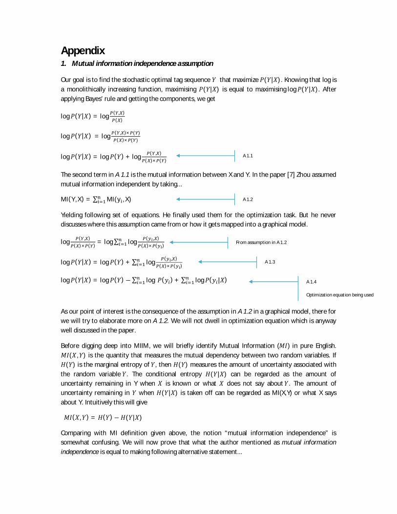
Our goal is to find the stochastic optimal tag sequence 푌 that maximize 푃(푌|푋). Knowing that log is a monolithically increasing function, maximising 푃(푌|푋) is equal to maximising log푃(푌|푋). After applying Bayes’ rule and getting the components, we get
log푃(푌|푋) = log ( , )( )
log푃(푌|푋) = log ( , )× ( )( )× ( )
log푃(푌|푋) = log푃(푌) + log ( , )( )× ( )
The second term in A 1.1 is the mutual information between X and Y. In the paper [7] Zhou assumed mutual information independent by taking...
MI(Y, X) = ∑ MI(y , X)
Yielding following set of equations. He finally used them for the optimization task. But he never discusses where this assumption came from or how it gets mapped into a graphical model.
log ( , )( )× ( ) = log∑ log ( , )
( )× ( )
log푃(푌|푋) = log푃(푌) +∑ log ( , )( )× ( )
log푃(푌|푋) = log푃(푌) −∑ log 푃(푦 ) + ∑ log푃(푦 |푋)
As our point of interest is the consequence of the assumption in A 1.2 in a graphical model, there for we will try to elaborate more on A 1.2. We will not dwell in optimization equation which is anyway well discussed in the paper.
Before digging deep into MIIM, we will briefly identify Mutual Information (푀퐼) in pure English. 푀퐼(푋,푌) is the quantity that measures the mutual dependency between two random variables. If 퐻(푌) is the marginal entropy of 푌, then 퐻(푌) measures the amount of uncertainty associated with the random variable 푌. The conditional entropy 퐻(푌|푋) can be regarded as the amount of uncertainty remaining in Y when 푋 is known or what 푋 does not say about 푌. The amount of uncertainty remaining in 푌 when 퐻(푌|푋) is taken off can be regarded as MI(X,Y) or what X says about Y. Intuitively this will give
푀퐼(푋,푌) = 퐻(푌)− 퐻(푌|푋)
Comparing with MI definition given above, the notion “mutual information independence” is somewhat confusing. We will now prove that what the author mentioned as mutual information independence is equal to making following alternative statement...
A 1.1
A 1.2
From assumption in A 1.2
A 1.4
Optimization equation being used
A 1.3

“a given tag/state 풚풊 only depends on X/whole input but not other tags/state”
Taking the second term of A 1.1 we have
log푃(푌,푋)
푃(푋) × 푃(푌) = log푃(푦 ,푦 ,푦 , … ,푦 ,푋)
푃(푋) × 푃(푦 ,푦 ,푦 , … ,푦 )
= log푃(푦 |푦 ,푦 , … ,푦 ,푋) × 푃(푦 ,푦 , … ,푦 ,푋)
푃(푋) × 푃(푦 ,푦 ,푦 , … ,푦 )
= log푃(푦 |푦 ,푦 , … ,푦 ,푋) × 푃(푦 |푦 , … ,푦 ,푋) × 푃(푦 , … ,푦 ,푋)
푃(푋) × 푃(푦 ,푦 ,푦 , … ,푦 )
...repeatedly expanding = log ( | , ,…, , )× ( | ,…, , )… ( | , )× ( | )× ( )
( )× ( , , ,…, )
From our alternative assumption “a given tag 풚풊 only depends on X but not other tags”, we get
푃(푦 |푦 ,푦 , … ,푦 ,푋) = 푃(푦 |푋)
푃(푦 |푦 ,푦 … ,푦 ,푋) = 푃(푦 |푋)
...
푃(푦 |푦 ,푋) = 푃(푦 |푋)
Substituting on A 1.1 we get
log푃(푌,푋)
푃(푋) × 푃(푌) = log푃(푦 |푋) × 푃(푦 |,푋) … 푃(푦 |푋) × 푃(푦 |푋) × 푃(푋)
푃(푋) × 푃(푦 ,푦 ,푦 , … ,푦 )
= log푃(푦 |푋) × 푃(푦 |,푋) … 푃(푦 |푋) × 푃(푦 |푋)
푃(푦 ,푦 ,푦 , … ,푦 )
As 푦 are independent 푃(푦 ,푦 ,푦 , … ,푦 ) = 푃(푦 ) × 푃(푦 ) × 푃(푦 ) × … × 푃(푦 )
= log푃(푦 |푋) × 푃(푦 |,푋) … 푃(푦 |푋) × 푃(푦 |푋)
푃(푦 ) × 푃(푦 ) × 푃(푦 ) × … × 푃(푦 )
= log ( | )( )
+ log ( | )( )
+ log ( | )( )
+ ⋯+ log ( | )( )
= log ( , )( ) × ( )
+ log ( , )( ) × ( )
+ log ( , )( ) × ( )
+⋯+ + log ( , )( ) × ( )
= ∑ log ( , )( ) × ( )
= log푃(푦 |푋)푃(푦 )
A 1.5

log푃(푌,푋)
푃(푋) × 푃(푌) = log푃(푦 |푋)− log푃(푦 )
This is same as the mutual information independence we have assumed earlier. Hence, mutual information independence in MIIM model can be alternatively stated as...
“a given tag/state, 풚풊 only depends on X/entire input but not other tags/states”
2. Factorization of MIIM We will first define factor graphs as follows.
Let 푉 = 푣 , 푣 ,푣 , … 푣 where 푣 ∈ 퐷
Let domain 퐷 = 퐷 × 퐷 × 퐷 × … × 퐷
Let g be a function such that 푔:퐷 → 푅 {note that this is important as we are going to define, addition and multiplication of
factors which is well defined for real numbers 푅}
Assume5 that g factors into t factors of F local functions, as follows, where 푉 ⊆ D
g(푣 , 푣 , 푣 , … , 푣 ) = F (V )
A factor graph is an undirected, bipartite, graph with set of vertexes and edges. Each vertex represent either a variable 푣 or a factor F , such that there is an edge between the vertex 퐹 and vertex 푣 if and only if, 푣 is an argument to factor function F (V ). (i.e. 푣 ∈ V ).
The general form given above can be specialized for MIIM model. As no literature gives MIIM factorization I have presented it bellow. Factorization of optimization function is as follows
E4: log푃(푌|푋) = log푃(푌)− log 푃(푦 ) + log푃(푦 |푋)
= log푃(푌) + log푃(푦 |푋)푃(푦 )
= log푃(푌) + log푃(푦 |푋)푃(푦 )
= log 푃(푌) ×푃(푦 |푋)푃(푦 )
5 Note that there may be functions defined over D that are not factorable as given. But our interest is on those than “can be” factored.

= log 푃(푌) ×푃(푦 |푋)푃(푦 ) ×
푃(푦 |푋)푃(푦 ) … ×
푃(푦 |푋)푃(푦 )
3. CRF Representation of HMM
For a given input X and an output Y CRF models the conditional probability p(Y|X) rather than the joint distribution. Similar to MIIM model the discriminative approach makes this model more suitable for NER task as we can use rich set of global features without assuming crude independence among them. Further CRF has a convex objective function with a guaranteed global optimal with only issue of being slow. We can get an HMM equivalent CRF by selecting features in a special way or rather applying some transformation to our feature set. However the converse is not possible (CRF to HMM) as CRF does not impose strict constrains on its parameter set as HMM does (E.g.∑ 푎 , = 1,푤ℎ푒푟푒 푎 , 푖푠 푡푟푎푛푠푖푡푖표푛 푝푟표푏푎푏푖푙푖푡푦∀ ). For our simple HMM (HMM model 1), the joint distribution is
푃(푋,푌) = 푃(푦 |푦 ) × 푃(푥 |푦 )
By taking each above conditional probability values to be proportional to exponentials defined bellow, the same HMM can be written as
푃(푋,푌) =1푍
× 푒∑ ∑ , ( ) ( ), ∈ ∑ ∑ ∑ , ( ) ( )∈∈
Where S is our state set, O is observation set, Z is a normalization term (globally normalized, rather than per state) to create probability values and I is an indicator function of the form
퐼(푥 = 푥 ) = 1 푤ℎ푒푛 푥 = 푥′0 표푡ℎ푒푟푤푖푠푒
By introducing one feature for each state transition ( 퐼(푦 = 푖)퐼(푦 = 푗)) and another for state observation 퐼(푦 = 푖)퐼(푥 = 표) we can write the above equation in a more compact way as bellow
푃(푋,푌) =1푍
× 푒∑ ( , , )

Reference [1] N. Chinchor, MUC-7 Named Entity Task Definition, Version 3.5 [2] D. Shen, J. Zhang, G.D Zhou,J. Su,C.L. Tan, Effective Adaptation of a Hidden Markov Model-based Named Entity Recognizer for Biomedical Domain [3] K. Humphreys, R. Gaizauskas, S. Azzam, C. Huyck, B. Mitchell, H. Cunningham,Y. Wilks, Description of the LaSIE-II System as Used for MUC-7, University of Sheffield [4] D. Nadeau, Semi-Supervised Named Entity Recognition, Learning to Recognize 100 Entity Types with Little Supervision, PhD dissertation [5] A. Borthwick, A Maximum Entropy Approach to Named Entity Recognition, PhD dissertation [6] Introduction to the CoNLL-2002 Shared Task: Language-Independent Named Entity Recognition, E.F.T.K. Sang , University of Antwerp [7] G.D. Zhou, J. Su, Named Entity Recognition using an HMM-based Chunk Tagger, Laboratories for Information Technology, Singapore [8] S. Miller, M. Crystal, H. Fox, L. Ramshaw, R. Schwartz,R. Stone, R. Weischedel, BBN: Description of the Sift System as Used For MUC 7 [9] A. McCallum, C. Sutton, An Introduction to Conditional Random Fields for Relational Learning [10] K.P. Murphy, An introduction to graphical models [11 ] F.R. Kschischang, Factor Graphs and the Sum-Product Algorithm, IEEE Transactions on Information Theory, vol. 47, no. 2, February 2001 (p498-p519)
[12] T. Minka, Discriminative models, not discriminative training, Microsoft Research Cambridge, Oct 17, 2005 (TR-2005-144) [13] R. Malouf, Markov models for language-independent named entity recognition [14] L. Ratinov, D. Roth, Design Challenges and Misconceptions in Named Entity Recognition, University of Illinois [15] T. Zhang, D. Johnson, A Robust Risk Minimization based Named Entity Recognition System, IBM T.J. Watson Research Centre [16] G.D. Zhou , J. Zhang , J. Su , D. Shen and C.L Tan, Recognizing Names in Biomedical Texts: a Machine Learning Approach, Institute for Infocomm Research Singapore, School of Computing, National University of Singapore [17] P. Mitra, C.A. Murthy, S.K. Pal, Unsupervised feature selection using feature similarity, Machine Intelligence Unit, Indian Statistical Institute, Calcutta [18] N. Wiratunga, R. Lothian, S. Massie, Unsupervised Feature Selection for Text data, School of Computing, Robert Gordon University

[19] B. Settles, Biomedical Named Entity Recognition Using Conditional Random Fields and Rich Feature Sets, Department of Computer Sciences, Department of Biostatistics and Medical Informatics, University of Wisconsin Madison [20] W. Li, A. McCallum, Rapid Development of Hindi Named Entity Recognition using Conditional Random Fields and Feature Induction, University of Massachusetts Amherst [21] W. Li, A. McCallum, Early Results for Named Entity Recognition with Conditional Random Fields, Feature Induction and Web-Enhanced Lexicons, University of Massachusetts Amherst [22] J. Laffertyy, A. McCallum, F. Pereira, Conditional Random Fields: Probabilistic Models for Segmenting and Labeling Sequence Data [23] G.D. Zhou, Recognizing names in biomedical texts using mutual information independence model and SVM plus sigmoid, Institute for Infocomm Research, Singapore [24] D.Jurafsky, J.H. Martin, Speech and Language Processing, 2nd Edition [25] J. Liu, M. Huan, X. Zhu, Recognizing Biomedical Named Entities using Skip-chain Conditional Random Fields [26] T. Briscoe, An introduction to tag sequence grammars and the RASP system parser: Technical Report [27] J. Bos, S. Clark, M. Steedman, Wide-Coverage Semantic Representations from a CCG Parser, School of Informatics, University of Edinburgh [28] S. Clark, J.R. Curran, Parsing the WSJ using CCG and Log-Linear Models [29] B. Alex, B. Haddow, C. Grover, Recognising Nested Named Entities in Biomedical Text, University of Edinburgh [30]S. Cucerzan, D. Yarowsky, Language Independent Named Entity Recognition Combining Morphological and Contextual Evidence, Department of Computer Science, Center for Language and Speech Processing, Johns Hopkins University [31]A. McCallum, Efficiently Inducing Features of Conditional Random Fields, Computer Science Department, University of Massachusetts Amhers [32] Z. Ghahramani, Graphical models, University of Cambridge,[Video Lecture] Available:http://videolectures.net/mlss07_ghahramani_grafm/ [33] C. Elkan, Log-linear Models and Conditional Random Fields, , Department of Electrical Engineering and Computer Sciences, UC Berkeley,[Video Lecture] Available:http://videolectures.net/cikm08_elkan_llmacrf/