Models of crustal flow in the India–Asia collision zone
16
Geophys. J. Int. (2007) 169, 683–698 doi: 10.1111/j.1365-246X.2007.03343.x GJI Tectonics and geodynamics Models of crustal flow in the India–Asia collision zone Alex Copley 1 and Dan McKenzie 2 1 COMET, Department of Earth Sciences, University of Cambridge, Cambridge, UK. E-mail: [email protected] 2 Department of Earth Sciences, University of Cambridge, Cambridge, UK Accepted 2007 January 2. Received 2006 December 21; in original form 2006 June 6 SUMMARY Surface velocities in parts of the India–Asia collision zone are compared to velocities calculated from equations describing fluid flow driven by topographically produced pressure gradients. A good agreement is found if the viscosity of the crust is ∼10 20 Pa s in southern Tibet and ∼10 22 Pa s in the area between the Eastern Syntaxis and the Szechwan Basin. The lower boundary condition of the flow changes between these two areas, with a stress-free lower boundary in the area between the Szechwan basin and the Eastern Syntaxis, and a horizontally rigid but vertically deformable boundary where strong Indian lithospheric material underlies southern Tibet. Deformation maps for olivine, diopside and anorthite show our findings to be consistent with laboratory measurements of the rheology of minerals. Gravitationally driven flow is also suggested to be taking place in the Indo–Burman Ranges, with a viscosity of ∼10 19 – 10 20 Pa s. Flow in both southern Tibet and the Indo–Burman Ranges provides an explanation for the formation of the geometry of the Eastern Himalayan Syntaxis. The majority of the normal faulting earthquakes in the Tibetan Plateau occur in the area of southern Tibet which we model as gravitationally spreading over the Indian shield. Key words: continental deformation, gravity, rheology, topography. 1 INTRODUCTION At temperatures greater than around two thirds of the melting tem- perature, minerals can deform by thermally activated creep at ge- ologically significant strain-rates. In areas where the lower crust is hot either because the crust is thick or the heat flux is high, it can de- form by creep at high enough rates to behave as a fluid on geological timescales. Lower crustal flow has been suggested as an explana- tion for the absence of Moho topography in regions where the upper crust is highly strained, such as the Basin and Range province of the western United States (e.g. Block & Royden 1990; Kruse et al. 1991; M c Kenzie et al. 2000). Shapiro et al. (2004) used the disper- sion of surface waves to suggest that significant anisotropy exists in the Tibetan crust, which they interpret as the result of lower crustal flow. Crustal flow has also been suggested as a cause of the low re- lief in the interior of the Tibetan Plateau (e.g. Fielding et al. 1994). Motivated by the indications that flow is occurring in the Tibetan crust, in this paper we calculate surface velocities for southern Tibet and the area between the Eastern Syntaxis and the Szechwan Basin (Fig. 1) using equations for fluid flow. The results of these calcula- tions are in agreement with published GPS measurements. Under the assumption that deformation is occurring by diffusion creep in the thick sequence of sediments, we also model the deformation of the Indo–Burman Ranges as that of a viscous fluid. Deformation maps have been created to test if the viscosities which we calculate for the crust in Tibet are consistent with the rheology of minerals. These deformation maps have also been used to deduce the domi- nant mechanism of creep likely to be operating in the ductile part of the crust, and so determine the rheology used in our models. 2 MODEL AND RELATION TO PREVIOUS WORK The study of continental deformation and crustal flow using the equations for fluid flow has been undertaken using a number of different methods and boundary conditions. Throughout this paper we take ‘stress-free’ to mean that the shear stress on the boundary of a layer is zero, and there is no restriction on the horizontal velocity. By ‘rigid’ we mean that the horizontal velocity is zero. A boundary is described as undeformable if the vertical velocity is zero, and as deformable if the normal stress is continuous. A boundary may be both rigid and deformable if the horizontal velocity is zero, but the vertical velocity is not. England & M c Kenzie (1982) modelled the continental lithosphere as a thin sheet of power-law fluid overlying an inviscid half-space. England & Houseman (1986) compared the predications of this model to topography and strain within the India–Asia collision zone. This model assumes that vertical gradients of horizontal ve- locity are negligible, and uses stress-free upper and lower boundary conditions. Royden (1996) studied the basally driven flow of a Newtonian fluid with depth-dependent viscosity and described two end-member situations, where the deformation of the crust is coupled to, or decou- pled from, the motion in an upper mantle with a specified horizontal C 2007 The Authors 683 Journal compilation C 2007 RAS
-
Upload
khangminh22 -
Category
Documents
-
view
1 -
download
0
Transcript of Models of crustal flow in the India–Asia collision zone

Geophys. J. Int. (2007) 169, 683–698 doi: 10.1111/j.1365-246X.2007.03343.x
GJI
Tec
tonic
sand
geo
dyn
am
ics
Models of crustal flow in the India–Asia collision zone
Alex Copley1 and Dan McKenzie2
1COMET, Department of Earth Sciences, University of Cambridge, Cambridge, UK. E-mail: [email protected] of Earth Sciences, University of Cambridge, Cambridge, UK
Accepted 2007 January 2. Received 2006 December 21; in original form 2006 June 6
S U M M A R Y
Surface velocities in parts of the India–Asia collision zone are compared to velocities calculated
from equations describing fluid flow driven by topographically produced pressure gradients.
A good agreement is found if the viscosity of the crust is ∼1020 Pa s in southern Tibet and
∼1022 Pa s in the area between the Eastern Syntaxis and the Szechwan Basin. The lower
boundary condition of the flow changes between these two areas, with a stress-free lower
boundary in the area between the Szechwan basin and the Eastern Syntaxis, and a horizontally
rigid but vertically deformable boundary where strong Indian lithospheric material underlies
southern Tibet. Deformation maps for olivine, diopside and anorthite show our findings to be
consistent with laboratory measurements of the rheology of minerals. Gravitationally driven
flow is also suggested to be taking place in the Indo–Burman Ranges, with a viscosity of ∼1019–
1020 Pa s. Flow in both southern Tibet and the Indo–Burman Ranges provides an explanation
for the formation of the geometry of the Eastern Himalayan Syntaxis. The majority of the
normal faulting earthquakes in the Tibetan Plateau occur in the area of southern Tibet which
we model as gravitationally spreading over the Indian shield.
Key words: continental deformation, gravity, rheology, topography.
1 I N T RO D U C T I O N
At temperatures greater than around two thirds of the melting tem-
perature, minerals can deform by thermally activated creep at ge-
ologically significant strain-rates. In areas where the lower crust is
hot either because the crust is thick or the heat flux is high, it can de-
form by creep at high enough rates to behave as a fluid on geological
timescales. Lower crustal flow has been suggested as an explana-
tion for the absence of Moho topography in regions where the upper
crust is highly strained, such as the Basin and Range province of
the western United States (e.g. Block & Royden 1990; Kruse et al.
1991; McKenzie et al. 2000). Shapiro et al. (2004) used the disper-
sion of surface waves to suggest that significant anisotropy exists in
the Tibetan crust, which they interpret as the result of lower crustal
flow. Crustal flow has also been suggested as a cause of the low re-
lief in the interior of the Tibetan Plateau (e.g. Fielding et al. 1994).
Motivated by the indications that flow is occurring in the Tibetan
crust, in this paper we calculate surface velocities for southern Tibet
and the area between the Eastern Syntaxis and the Szechwan Basin
(Fig. 1) using equations for fluid flow. The results of these calcula-
tions are in agreement with published GPS measurements. Under
the assumption that deformation is occurring by diffusion creep in
the thick sequence of sediments, we also model the deformation of
the Indo–Burman Ranges as that of a viscous fluid. Deformation
maps have been created to test if the viscosities which we calculate
for the crust in Tibet are consistent with the rheology of minerals.
These deformation maps have also been used to deduce the domi-
nant mechanism of creep likely to be operating in the ductile part
of the crust, and so determine the rheology used in our models.
2 M O D E L A N D R E L AT I O N T O
P R E V I O U S W O R K
The study of continental deformation and crustal flow using the
equations for fluid flow has been undertaken using a number of
different methods and boundary conditions. Throughout this paper
we take ‘stress-free’ to mean that the shear stress on the boundary of
a layer is zero, and there is no restriction on the horizontal velocity.
By ‘rigid’ we mean that the horizontal velocity is zero. A boundary
is described as undeformable if the vertical velocity is zero, and as
deformable if the normal stress is continuous. A boundary may be
both rigid and deformable if the horizontal velocity is zero, but the
vertical velocity is not.
England & McKenzie (1982) modelled the continental lithosphere
as a thin sheet of power-law fluid overlying an inviscid half-space.
England & Houseman (1986) compared the predications of this
model to topography and strain within the India–Asia collision
zone. This model assumes that vertical gradients of horizontal ve-
locity are negligible, and uses stress-free upper and lower boundary
conditions.
Royden (1996) studied the basally driven flow of a Newtonian
fluid with depth-dependent viscosity and described two end-member
situations, where the deformation of the crust is coupled to, or decou-
pled from, the motion in an upper mantle with a specified horizontal
C© 2007 The Authors 683Journal compilation C© 2007 RAS
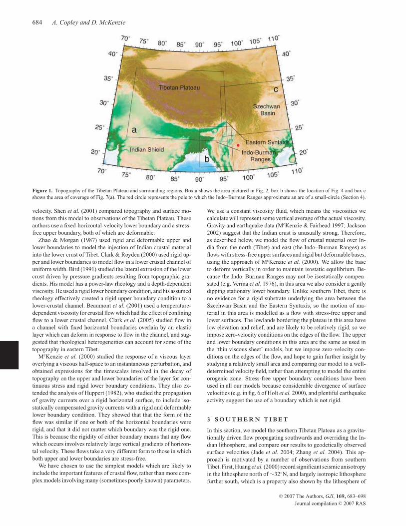
684 A. Copley and D. McKenzie
Figure 1. Topography of the Tibetan Plateau and surrounding regions. Box a shows the area pictured in Fig. 2, box b shows the location of Fig. 4 and box c
shows the area of coverage of Fig. 7(a). The red circle represents the pole to which the Indo–Burman Ranges approximate an arc of a small-circle (Section 4).
velocity. Shen et al. (2001) compared topography and surface mo-
tions from this model to observations of the Tibetan Plateau. These
authors use a fixed-horizontal-velocity lower boundary and a stress-
free upper boundary, both of which are deformable.
Zhao & Morgan (1987) used rigid and deformable upper and
lower boundaries to model the injection of Indian crustal material
into the lower crust of Tibet. Clark & Royden (2000) used rigid up-
per and lower boundaries to model flow in a lower crustal channel of
uniform width. Bird (1991) studied the lateral extrusion of the lower
crust driven by pressure gradients resulting from topographic gra-
dients. His model has a power-law rheology and a depth-dependent
viscosity. He used a rigid lower boundary condition, and his assumed
rheology effectively created a rigid upper boundary condition to a
lower-crustal channel. Beaumont et al. (2001) used a temperature-
dependent viscosity for crustal flow which had the effect of confining
flow to a lower crustal channel. Clark et al. (2005) studied flow in
a channel with fixed horizontal boundaries overlain by an elastic
layer which can deform in response to flow in the channel, and sug-
gested that rheological heterogeneities can account for some of the
topography in eastern Tibet.
McKenzie et al. (2000) studied the response of a viscous layer
overlying a viscous half-space to an instantaneous perturbation, and
obtained expressions for the timescales involved in the decay of
topography on the upper and lower boundaries of the layer for con-
tinuous stress and rigid lower boundary conditions. They also ex-
tended the analysis of Huppert (1982), who studied the propagation
of gravity currents over a rigid horizontal surface, to include iso-
statically compensated gravity currents with a rigid and deformable
lower boundary condition. They showed that that the form of the
flow was similar if one or both of the horizontal boundaries were
rigid, and that it did not matter which boundary was the rigid one.
This is because the rigidity of either boundary means that any flow
which occurs involves relatively large vertical gradients of horizon-
tal velocity. These flows take a very different form to those in which
both upper and lower boundaries are stress-free.
We have chosen to use the simplest models which are likely to
include the important features of crustal flow, rather than more com-
plex models involving many (sometimes poorly known) parameters.
We use a constant viscosity fluid, which means the viscosities we
calculate will represent some vertical average of the actual viscosity.
Gravity and earthquake data (McKenzie & Fairhead 1997; Jackson
2002) suggest that the Indian crust is unusually strong. Therefore,
as described below, we model the flow of crustal material over In-
dia from the north (Tibet) and east (the Indo–Burman Ranges) as
flows with stress-free upper surfaces and rigid but deformable bases,
using the approach of McKenzie et al. (2000). We allow the base
to deform vertically in order to maintain isostatic equilibrium. Be-
cause the Indo–Burman Ranges may not be isostatically compen-
sated (e.g. Verma et al. 1976), in this area we also consider a gently
dipping stationary lower boundary. Unlike southern Tibet, there is
no evidence for a rigid substrate underlying the area between the
Szechwan Basin and the Eastern Syntaxis, so the motion of ma-
terial in this area is modelled as a flow with stress-free upper and
lower surfaces. The lowlands bordering the plateau in this area have
low elevation and relief, and are likely to be relatively rigid, so we
impose zero-velocity conditions on the edges of the flow. The upper
and lower boundary conditions in this area are the same as used in
the ‘thin viscous sheet’ models, but we impose zero-velocity con-
ditions on the edges of the flow, and hope to gain further insight by
studying a relatively small area and comparing our model to a well-
determined velocity field, rather than attempting to model the entire
orogenic zone. Stress-free upper boundary conditions have been
used in all our models because considerable divergence of surface
velocities (e.g. in fig. 6 of Holt et al. 2000), and plentiful earthquake
activity suggest the use of a boundary which is not rigid.
3 S O U T H E R N T I B E T
In this section, we model the southern Tibetan Plateau as a gravita-
tionally driven flow propagating southwards and overriding the In-
dian lithosphere, and compare our results to geodetically observed
surface velocities (Jade et al. 2004; Zhang et al. 2004). This ap-
proach is motivated by a number of observations from southern
Tibet. First, Huang et al. (2000) record significant seismic anisotropy
in the lithosphere north of ∼32◦N, and largely isotropic lithosphere
further south, which is a property also shown by the lithosphere of
C© 2007 The Authors, GJI, 169, 683–698
Journal compilation C© 2007 RAS
Models of crustal flow in Tibet 685
74˚
74˚
76˚
76˚
78˚
78˚
80˚
80˚
82˚
82˚
84˚
84˚
86˚
86˚
88˚
88˚
90˚
90˚
92˚
92˚
94˚
94˚
96˚
96˚
24˚ 24˚
26˚ 26˚
28˚ 28˚
30˚ 30˚
32˚ 32˚
34˚ 34˚
36˚ 36˚
38˚ 38˚
1000
2000
3000
4000
4000
5000
scale:
15 mm/yr
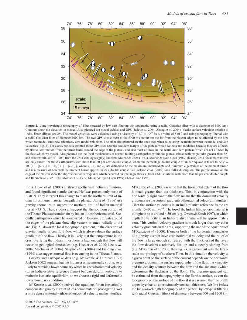
Figure 2. Long-wavelength topography of Tibet (created by low-pass filtering the topography using a radial Gaussian filter with a diameter of 1000 km).
Contours show the elevation in metres. Also pictured are model (white) and GPS (Jade et al. 2004; Zhang et al. 2004) (black) surface velocities relative to
India. Error ellipses are 2σ . The model velocities were calculated using a viscosity of 1.7 × 10²⁰ Pa s, a value of f of 7 and using topography filtered with
a radial Gaussian filter of diameter 1000 km. The two GPS sites closest to the 5000 m contour are too far from the plateau edges to be affected by the flow
which we model, and show effectively zero model velocities. The other sites pictured are the ones used when calculating the misfit between the model and GPS
velocities (Fig. 3). For clarity we have omitted those GPS sites near the southern margin of the plateau which we have not modelled because they are affected
by elastic deformation from the thrust faults around the edge of the plateau, and also most of those in the central/northern plateau which are not affected by
the flow which we model. Also pictured are the focal mechanisms of normal faulting earthquakes within the plateau (those with magnitudes greater than 5.5,
and rakes within 30◦ of −90◦) from the CMT catalogue (grey) and from Molnar & Chen (1983), Molnar & Lyon-Caen (1989) (black). CMT focal mechanisms
are only shown for those earthquakes with more than 80 per cent double couple, where the percentage double couple of an earthquake is taken to be γ =100{1 − [(2|λ2| × 1.5)/(|λ1| + |λ3|)]}, where λ1, λ2 and λ3 are defined to be the maximum, intermediate and minimum eigenvalues of the moment tensor,
and is a measure of how well the moment tensor approximates a double couple. See Jackson et al. (2002) for a fuller description. The purple arrows on the
edge of the plateau show the slip vectors for earthquakes which occurred on low-angle thrusts (from CMT solutions with more than 80 per cent double couple
and Baranowski et al. 1984; Molnar et al. 1977; Molnar & Lyon-Caen 1989; Chen & Kao 1996).
India. Hoke et al. (2000) analysed geothermal helium emissions,
and found significant mantle-derived He3 was present only north of
∼30◦N. They interpret this change to mark the northern limit of In-
dian lithospheric material beneath the plateau. Jin et al. (1996) use
gravity anomalies to suggest the northern limit of Indian material
lies at ∼33◦N. These studies all suggest that the southern portion of
the Tibetan Plateau is underlain by Indian lithospheric material. Sec-
ondly, earthquakes which have occurred on low-angle thrusts around
the edges of the plateau show slip vectors oriented radially to the
arc (Fig. 2), down the local topographic gradient, in the direction of
gravitationally driven fluid flow, which is always down the surface
gradient of the flow. Thirdly, it is likely that the temperature in the
crust overlying the Indian lithosphere is high enough that flow will
occur on geological timescales (e.g. Hacker et al. 2000; Lee et al.
2004; Mechie et al. 2004). Shapiro et al. (2004) and Fielding et al.
(1994) also suggest crustal flow is occurring in the Tibetan Plateau.
Gravity and earthquake data (e.g. McKenzie & Fairhead 1997;
Jackson 2002) suggest that the Indian crust is unusually strong, so is
likely to provide a lower boundary which has zero horizontal velocity
(in an India-relative reference frame) but can deform vertically to
maintain isostatic equilibrium, so we choose a rigid and deformable
lower boundary condition.
McKenzie et al. (2000) derived the equations for an isostatically
compensated gravity current of less dense material propagating over
a more dense material with zero horizontal velocity on the interface.
McKenzie et al. (2000) assume that the horizontal extent of the flow
is much greater than the thickness. This, in conjunction with the
horizontally rigid base to the flow, means that the dominant velocity
gradients are the vertical gradients of horizontal velocity. In southern
Tibet the surface velocities in an India-relative reference frame are
mostly 15–20 mm yr−1. The top of the Indian lithospheric material is
thought to be at around ∼50 km (e.g. Owens & Zandt 1997), at which
depth the velocity in an India-relative frame will be approximately
zero. This vertical velocity gradient is much larger than any other
velocity gradients in the area, supporting the use of the equations of
McKenzie et al. (2000). If one or both of the horizontal boundaries
of a gravity current have zero horizontal velocity and the relief of
the flow is large enough compared with the thickness of the layer,
the flow develops a relatively flat top and a steeply sloping front
(e.g. McKenzie et al. 2000, their fig. 7), in agreement with the large-
scale morphology of southern Tibet. In this situation the velocity at
a given point on the surface of the current depends on the horizontal
pressure gradient, the surface topography of the flow, the viscosity,
and the density contrast between the flow and the substrate (which
determines the thickness of the flow). The pressure gradient can
be estimated from the topography at the Earth’s surface, as can the
topography on the surface of the flow if it is assumed that the brittle
upper layer has an approximately constant thickness. We first isolate
the long-wavelength topography of the plateau by low-pass filtering
with radial Gaussian filters of diameters between 600 and 1200 km.
C© 2007 The Authors, GJI, 169, 683–698
Journal compilation C© 2007 RAS
686 A. Copley and D. McKenzie
4
5
6
7
8
9
10
ρ1/(
ρ2 -
ρ1)
1e+19 1e+201e+20 1e+21
η, Pa s
600
4
5
6
7
8
9
10
ρ1/(
ρ2 -
ρ1)
1e+19 1e+201e+20 1e+21
η, Pa s
800
4
5
6
7
8
9
10
ρ1/(
ρ2 -
ρ1)
1e+19 1e+201e+20 1e+21
η, Pa s
1000
4
5
6
7
8
9
10
ρ1/(
ρ2 -
ρ1)
1e+19 1e+201e+20 1e+21
η, Pa s
1200
0.0 2.5 5.0 7.5 10.0 12.5 15.0 17.5 20.0
RMS misfit, mm/yr
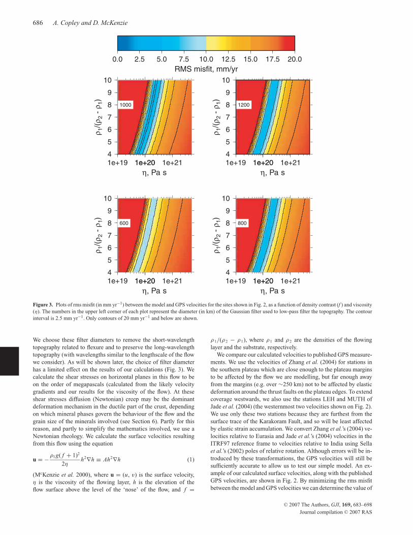
Figure 3. Plots of rms misfit (in mm yr−1) between the model and GPS velocities for the sites shown in Fig. 2, as a function of density contrast (f ) and viscosity
(η). The numbers in the upper left corner of each plot represent the diameter (in km) of the Gaussian filter used to low-pass filter the topography. The contour
interval is 2.5 mm yr−1. Only contours of 20 mm yr−1 and below are shown.
We choose these filter diameters to remove the short-wavelength
topography related to flexure and to preserve the long-wavelength
topography (with wavelengths similar to the lengthscale of the flow
we consider). As will be shown later, the choice of filter diameter
has a limited effect on the results of our calculations (Fig. 3). We
calculate the shear stresses on horizontal planes in this flow to be
on the order of megapascals (calculated from the likely velocity
gradients and our results for the viscosity of the flow). At these
shear stresses diffusion (Newtonian) creep may be the dominant
deformation mechanism in the ductile part of the crust, depending
on which mineral phases govern the behaviour of the flow and the
grain size of the minerals involved (see Section 6). Partly for this
reason, and partly to simplify the mathematics involved, we use a
Newtonian rheology. We calculate the surface velocities resulting
from this flow using the equation
u = −ρ1g( f + 1)2
2ηh2∇h ≡ Ah2∇h (1)
(McKenzie et al. 2000), where u = (u, v) is the surface velocity,
η is the viscosity of the flowing layer, h is the elevation of the
flow surface above the level of the ‘nose’ of the flow, and f =
ρ 1/(ρ 2 − ρ 1), where ρ 1 and ρ 2 are the densities of the flowing
layer and the substrate, respectively.
We compare our calculated velocities to published GPS measure-
ments. We use the velocities of Zhang et al. (2004) for stations in
the southern plateau which are close enough to the plateau margins
to be affected by the flow we are modelling, but far enough away
from the margins (e.g. over ∼250 km) not to be affected by elastic
deformation around the thrust faults on the plateau edges. To extend
coverage westwards, we also use the stations LEH and MUTH of
Jade et al. (2004) (the westernmost two velocities shown on Fig. 2).
We use only these two stations because they are furthest from the
surface trace of the Karakoram Fault, and so will be least affected
by elastic strain accumulation. We convert Zhang et al.’s (2004) ve-
locities relative to Eurasia and Jade et al.’s (2004) velocities in the
ITRF97 reference frame to velocities relative to India using Sella
et al.’s (2002) poles of relative rotation. Although errors will be in-
troduced by these transformations, the GPS velocities will still be
sufficiently accurate to allow us to test our simple model. An ex-
ample of our calculated surface velocities, along with the published
GPS velocities, are shown in Fig. 2. By minimizing the rms misfit
between the model and GPS velocities we can determine the value of
C© 2007 The Authors, GJI, 169, 683–698
Journal compilation C© 2007 RAS
Models of crustal flow in Tibet 687
the parameter A in eq. (1) to be ∼10−15 m−1 s−1. We cannot uniquely
determine the viscosity, but the rms misfit between the model and
GPS velocities, as a function of viscosity and the density contrast
between the flowing layer and the substrate (and so the thickness of
the flow), is shown in Fig. 3. It is not clear what densities should be
used when deciding on the value of f . However, f can be estimated
from the size of the surface relief and the depth of the top of the
underthrust Indian lithosphere (∼50 km in the northern part of the
area we study (e.g. Owens & Zandt 1997)). The value of f is the
factor which, if multiplied by the relief on the surface of the flow,
gives the thickness of the corresponding ‘root’. In the northern part
of the area we have studied, towards the centre of the plateau, if the
brittle upper crust is taken to be ∼10 km thick, the flowing layer
is ∼40 km thick, of which ∼5 km represents the relief on the up-
per surface. This means the thickness of the corresponding root is
∼35 km, which gives a value of f of ∼7. For this value of f and
90˚
90˚
92˚
92˚
94˚
94˚
96˚
96˚
20˚ 20˚
22˚ 22˚
24˚ 24˚
26˚ 26˚
(a)
52
52 38
41
29 36
31
29
61
46
6156
43
57
90
"shallow"
14 mm/yr
50
41
365
90˚
90˚
92˚
92˚
94˚
94˚
96˚
96˚
20˚ 20˚
22˚ 22˚
24˚ 24˚
26˚ 26˚
(b)
A
A’
020406080
100120140
De
pth
, km
-150
-100
-50
0
ele
vatio
n/d
ep
th,
km
0 100 200 300 400 500
distance, km
0
1
20 100 200 300 400 500
(c)
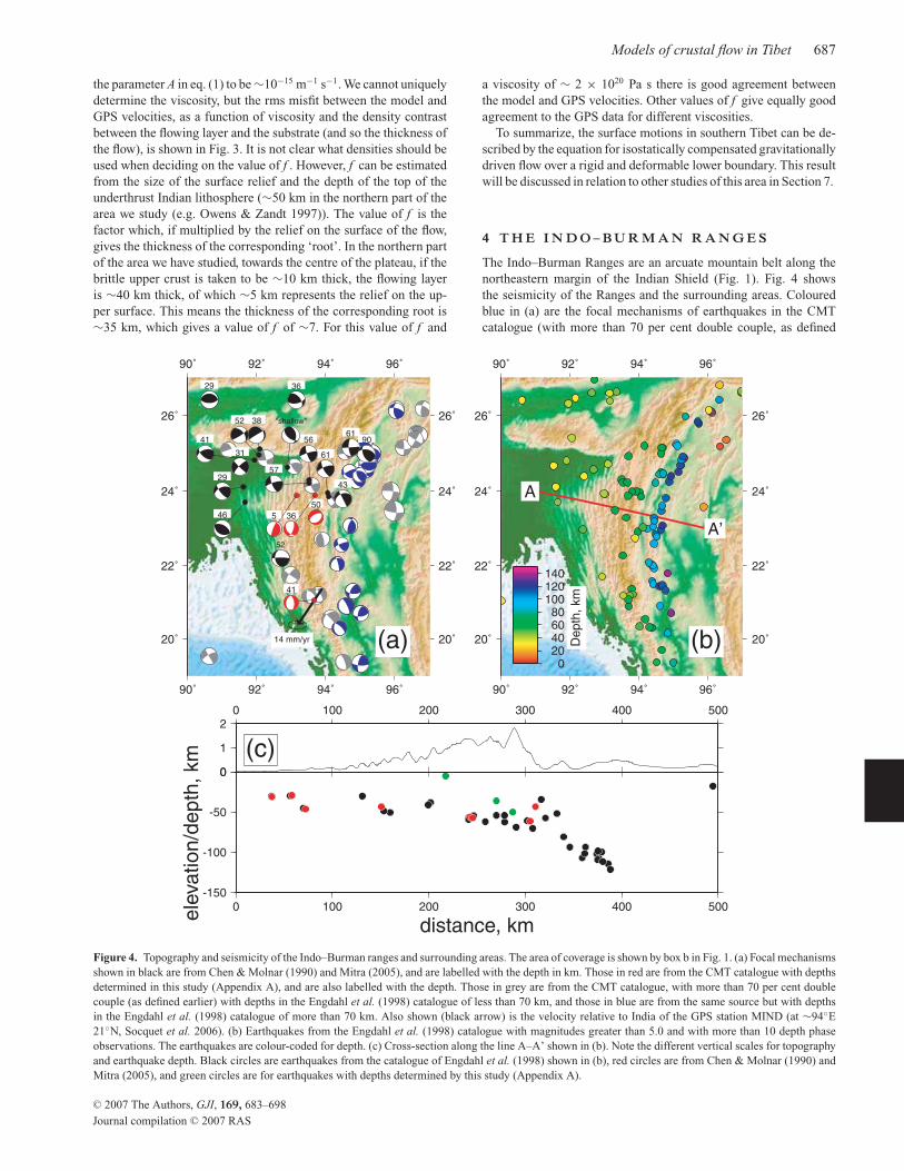
Figure 4. Topography and seismicity of the Indo–Burman ranges and surrounding areas. The area of coverage is shown by box b in Fig. 1. (a) Focal mechanisms
shown in black are from Chen & Molnar (1990) and Mitra (2005), and are labelled with the depth in km. Those in red are from the CMT catalogue with depths
determined in this study (Appendix A), and are also labelled with the depth. Those in grey are from the CMT catalogue, with more than 70 per cent double
couple (as defined earlier) with depths in the Engdahl et al. (1998) catalogue of less than 70 km, and those in blue are from the same source but with depths
in the Engdahl et al. (1998) catalogue of more than 70 km. Also shown (black arrow) is the velocity relative to India of the GPS station MIND (at ∼94◦E
21◦N, Socquet et al. 2006). (b) Earthquakes from the Engdahl et al. (1998) catalogue with magnitudes greater than 5.0 and with more than 10 depth phase
observations. The earthquakes are colour-coded for depth. (c) Cross-section along the line A–A’ shown in (b). Note the different vertical scales for topography
and earthquake depth. Black circles are earthquakes from the catalogue of Engdahl et al. (1998) shown in (b), red circles are from Chen & Molnar (1990) and
Mitra (2005), and green circles are for earthquakes with depths determined by this study (Appendix A).
a viscosity of ∼ 2 × 10²⁰ Pa s there is good agreement between
the model and GPS velocities. Other values of f give equally good
agreement to the GPS data for different viscosities.
To summarize, the surface motions in southern Tibet can be de-
scribed by the equation for isostatically compensated gravitationally
driven flow over a rigid and deformable lower boundary. This result
will be discussed in relation to other studies of this area in Section 7.
4 T H E I N D O – B U R M A N R A N G E S
The Indo–Burman Ranges are an arcuate mountain belt along the
northeastern margin of the Indian Shield (Fig. 1). Fig. 4 shows
the seismicity of the Ranges and the surrounding areas. Coloured
blue in (a) are the focal mechanisms of earthquakes in the CMT
catalogue (with more than 70 per cent double couple, as defined
C© 2007 The Authors, GJI, 169, 683–698
Journal compilation C© 2007 RAS

688 A. Copley and D. McKenzie
in the caption to Fig. 2) which have depths in the Engdahl et al.
(1998) catalogue of more than 70 km. As can be seen in (c), these
events all occur beneath the lowlands to the east of the Ranges,
and occur at depths of up to ∼150 km, showing subduction to
be occurring beneath the lowlands. To the west of the Ranges,
earthquakes occur at depths of up to ∼50 km (which is unusually
deep for the continents, e.g. Jackson 2002), and commonly have
strike-slip mechanisms with N–NE oriented P-axes (Chen & Molnar
1990). Below the ranges themselves, the majority of the earthquakes
which have well-determined depths (Chen & Molnar 1990; Mitra
2005, this paper Appendix A) occur at similar depths to those fur-
ther west. This is a feature also shown by the earthquakes in the
Engdahl et al. (1998) catalogue, shown in (b). Most of the earth-
quakes below the ranges are one of the following two types. First,
numerous earthquakes have strike-slip mechanisms with N–NE ori-
ented P-axes. The similarity between the depths and focal mecha-
nisms of these earthquakes and those in Indian lithospheric material
further west suggests that the Indian lithosphere underlies the Indo–
Burman ranges at depth. The second commonly occurring type of
earthquake below the ranges are normal-faulting earthquakes with
N–NE oriented nodal planes. It is likely that these earthquakes oc-
curred in response to tension in the Indian lithosphere caused by
bending due to the downward pull of the subducting slab to the
east, much like the normal faulting earthquakes often seen beneath
the outer rises near subduction zones (Chapple & Forsyth 1979).
Gowd et al. (1992) showed that the orientation of the maximum
compressive stress in the Indo–Burman ranges (∼E–W) is differ-
ent from that in the central to northern Indian shield (∼NE–SW),
and from that in the underthrust Indian lithosphere (as suggested
by N–NE oriented earthquake P-axes, Chen & Molnar 1990). The
range-parallel trend of fold axes (e.g. Le Dain et al. 1984, and visible
in the elevation data shown in Fig. 4) suggests that shortening occurs
normal to the range throughout the mountain belt, regardless of local
strike. This pattern is consistent with the observed velocity of the
GPS station MIND (Socquet et al. 2006) which is approximately
radial to the strike of the belt (see Fig. 4a), and with the mecha-
nism of the earthquake which occurred at a depth of 5 km and is
shown in red at ∼93◦E 24◦N in Fig. 4, which presumably occurred
on the low-angle nodal plane, and if so would have a slip vector
approximately radial to the local strike of the range. The earthquake
just to the north of this described as ‘shallow’ by Chen & Molnar
(1990) (Fig. 4) may also have had a slip vector approximately ra-
dial to the range, depending on which nodal plane was the fault
plane.
Deformed quaternary sediments (e.g. Le Dain et al. 1984), and
the shallow thrusting earthquake just discussed show the deforma-
tion in the ranges to be currently active. Without significant ∼N/S
shortening of the Indian lithosphere, or ∼N/S extension in the Indo–
Burman Ranges themselves, for which there is no evidence, it is hard
to see how the shortening can remain belt-perpendicular through-
out the Indo–Burman Ranges if the deformation is the result of
the relative motion of two rigid blocks. We suggest that the belt-
perpendicular shortening throughout the length of the Indo–Burman
Ranges is the result of gravitationally driven deformation in the
ranges causing range-perpendicular flow over the underlying Indian
lithosphere, in exactly the same way as we suggest southern Tibet
overrides India (Section 3). We model this as the flow of a gravity
current with a zero-horizontal-velocity base and a stress-free sur-
face. We suggest that this deformation represents diffusion creep in
the thick sequence of turbiditic shales and sandstones which form
the ranges (Brunnschweiler 1966; Mitchell 1981). Diffusion creep
(often referred to in the literature as pressure solution creep when
water-assisted diffusive mass transfer is occurring over the scale of
grains in sedimentary rocks) is known to occur in sediments at rel-
atively low temperatures, and will result in a Newtonian rheology
(e.g. Rutter 1983), so we model the deformation in this area as that
of a Newtonian fluid. Shear-enhanced compaction and granular flow
may also play a role in the deformation (e.g. Ngwenya et al. 2001),
as might brittle failure. The lack of earthquakes within the Ranges
(the seismicity being confined to the underlying Indian lithosphere
and, in the case of the shallow thrust event mentioned above, the in-
terface between the ranges and the underthrusting Indian material),
supports the choice of a ductile rheology.
The Indo–Burman Ranges describe a small-circle on the Earth’s
surface with a radius of approximately 500 km. Unlike the Tibetan
Plateau, the surface velocities in the Indo–Burman Ranges are not
well known. Therefore, rather than calculating a detailed velocity
field, we make use of the axisymmetric nature of the ranges and
calculate velocities from a profile produced by projecting the to-
pography of the ranges onto a single plane. We then suggest what
viscosities would produce the likely surface velocities.
The pole to the small-circle which approximates the Indo–
Burman Ranges was calculated by finding the best-fitting small-
circles to contours of elevation on the westward flank of the range
(Fig. 1). The poles we have calculated using different contours
vary in position by up ∼60 km from the mean, but undertaking
the following calculations using the extremes in the range of val-
ues does not appreciably change our results. The topography of
the ranges was projected onto a single plane using the position
of the pole and Fig. 5(a) shows how the topography varies with
distance from the pole, along with the value of the topographic
gradient.
We calculate the velocities which result from this combination
of elevation and surface slope using two different geometries for
the lower boundary. The first is an isostatically compensated lower
boundary, in which case the velocity is given by eq. (1). The second
geometry is that of a gently dipping lower boundary (dipping in the
direction perpendicular to the flow front at all times), which will
approximate the geometry expected for a gently flexed elastic layer.
In this case the instantaneous velocity is given by
ur = −ρg
η
{
h2
2+
[(rn − r ) m]2
2+ hm (rn − r )
}
∂h
∂r, (2)
where ur is the radial velocity, r is the radial coordinate (with zero at
the pole to which the ranges describe a small circle), m is the gradient
of the lower boundary, rn is the radial position of the ‘nose’ of the
flow, and all other symbols have the same meanings as earlier. This
equation is derived by following the method of Huppert (1982), but
applying the lower boundary condition at a depth of z =− (rn − r ) m.
We show the results of our calculations for lower boundaries with
gradients of 0.05, 0.1 and 0.15, a range which covers the gradients
compatible with the variation in depth of the earthquakes below the
Ranges.
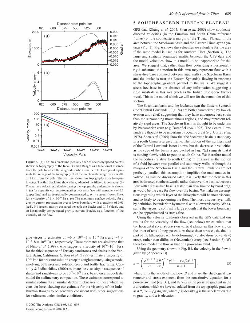
Fig. 5(c) shows how the maximum surface velocities for the two
geometries of flow we have considered vary with the viscosity of
the flow. The precise velocity of the flow is unknown. However, it
probably lies in the range 1–20 mm yr−1 (the GPS station MIND
moves at ∼14 mm yr−1, Socquet et al. (2006), see Fig. 4) , which
would suggest a viscosity of ∼ 2 × 10¹⁹–3 × 10²⁰ Pa s for an iso-
statically compensated flow, or one with a lower boundary with a
gradient of 0.1. Lower boundaries with gradients of 0.05 and 0.15
C© 2007 The Authors, GJI, 169, 683–698
Journal compilation C© 2007 RAS
Models of crustal flow in Tibet 689
0
1000
2000E
leva
tio
n,
m500525550575600625
Distance from pole, km
(a)
-0.020
-0.015
-0.010
-0.005
0.000
0.005
0.010
0.015
0.020
Gra
die
nt
0
2
4
6
Velo
city,
mm
/yr
500525550575600625
Distance from pole, km
(b)
0.001
0.010.01
0.1
1
10
100
1000
Velo
city,
mm
/yr
1e+18 1e+191e+19 1e+20 1e+21 1e+22 1e+23
Viscosity, Pa s
(c)
Figure 5. (a) The thick black line (actually a series of closely spaced points)
shows the topography of the Indo–Burman Ranges as a function of distance
from the pole to which the ranges describe a small circle. Each point repre-
sents the average of the topography of all the points in the range over a width
of 1 km from the pole. The red line shows this topography after low-pass
filtering. The thin black line shows the gradient of the filtered topography. (b)
The surface velocities calculated using the topography and gradients shown
in (a) for a gravity current propagating over a surface with a gradient of 0.1
(upper line) and an isostatically compensated gravity current (lower line),
for a viscosity of 1 × 10²⁰ Pa s. (c) The maximum surface velocity for a
gravity current propagating over a lower boundary with a gradient of 0.05
(red), 0.1 (green, mostly obscured beneath the black) and 0.15 (blue), and
an isostatically compensated gravity current (black), as a function of the
viscosity of the flow.
give viscosity estimates of ∼6 × 10¹⁹–1 × 10²⁰ Pa s and ∼4 ×10¹⁹–8 × 10²⁰ Pa s, respectively. These estimates are similar to that
of Nino et al. (1998), who suggest a viscosity of 1020–1021 Pa s
for the thick sequence of Tertiary sandstones and shales in the Ven-
tura Basin, California. Gratier et al. (1999) estimate a viscosity of
1021 Pa s for pressure solution creep in conglomerates, using a model
involving both pressure solution creep and brittle fracturing. Con-
nolly & Podladchikov (2000) estimate the viscosity in a sequence of
shales and sandstones to be 1020–1021 Pa s, based on a viscoelastic
model for sedimentary compaction. These estimates correspond to
similar sediments at similar depths/thicknesses to those which we
consider here, showing our estimate for the viscosity of the Indo–
Burman Ranges to be generally consistent with other suggestions
for sediments under similar conditions.
5 S O U T H E A S T E R N T I B E TA N P L AT E AU
GPS data (Zhang et al. 2004; Shen et al. 2005) show southeast-
directed velocities (in the Eurasian and South China reference
frames) on the southeastern margin of the Tibetan Plateau, in the
area between the Szechwan basin and the Eastern Himalayan Syn-
taxis (Fig. 1). Fig. 6 shows the velocities we calculate for the area
if the same model is used as for southern Tibet (Section 3). The
large and spatially organized misfits between the GPS data and
the model velocities show this model to be inappropriate for this
area. We suggest that, rather than flow overriding a horizontally
rigid substrate, the motion in this area may represent flow with a
stress-free base confined between rigid walls (the Szechwan Basin
and the lowlands near the Eastern Syntaxis), flowing in response
to the topographic gradient parallel to the walls. We suggest a
stress-free base in the absence of any information suggesting a
rigid substrate in this area (such as the Indian lithosphere further
west). This is the model which we will use for the remainder of this
section.
The Szechwan basin and the lowlands near the Eastern Syntaxis
(the ‘Central Lowlands’, Fig. 7a) are both characterized by low el-
evation and relief, suggesting that they have undergone less strain
than the surrounding mountainous regions, and may represent rel-
atively rigid areas. The Szechwan Basin is thought to be underlain
by Precambrian crust (e.g. Burchfiel et al. 1995). The Central Low-
lands are thought to be underlain by oceanic crust (e.g. Curray et al.
1978). Shen et al. (2005) show that the Szechwan basin is stationary
in a south China reference frame. The motion of the northern part
of the Central Lowlands is not known, but the decrease in velocities
as the edge of the basin is approached in Fig. 7(a) suggests that it
is moving slowly with respect to south China. We therefore model
the velocities (relative to south China) in this area as the motion
of a fluid between two parallel and stationary walls. Although the
margins of the Szechwan Basin and the Central Lowlands are not
perfectly parallel, this assumption simplifies the mathematics in-
volved. As will be discussed later, it is likely that the flow in this
area is directed southeastwards, rather than over the basins, because
flow with a stress-free base is faster than flow limited by basal drag,
as would be the case for flow over the basins. We make no assump-
tions regarding which layer of the lithosphere will be most viscous,
and so likely to be governing the flow. The most viscous layer will,
by definition, be underlain by material with a lower viscosity. We as-
sume the viscosity contrast is large enough that the lower boundary
can be approximated as stress-free.
Using the velocity gradients observed in the GPS data and our
results for the viscosity of the flow (see below) we calculate that
the horizontal shear stresses on vertical planes in this flow are on
the order of tens of megapascals. At these shear stresses, the ductile
part of the lithosphere will be deforming by dislocation (power-law)
creep, rather than diffusion (Newtonian) creep (see Section 6). We
therefore model the flow as that of a power-law fluid.
Using the geometry shown in Fig. B1, the velocity in the flow is
given by (Appendix B)
u =
(√2
1/n−1
B
∂ P
∂x
)n[
yn+1 − (w/2)n+1
n + 1
]
, (3)
where w is the width of the flow, B and n are the rheological pa-
rameter and stress exponent from the constitutive equation for a
power-law fluid (eq. B1), and ∂ P/∂x is the pressure gradient in the
x direction, which we have calculated from the topographic gradient
as ∂ P/∂x = ρg ∂h/∂x , where ρ is density, g is the acceleration due
to gravity, and h is elevation.
C© 2007 The Authors, GJI, 169, 683–698
Journal compilation C© 2007 RAS

690 A. Copley and D. McKenzie
96˚
96˚
98˚
98˚
100˚
100˚
102˚
102˚
104˚
104˚
106˚
106˚
26˚ 26˚
28˚ 28˚
30˚ 30˚
32˚ 32˚10
00
2000
2000
3000
4000
scale:
15 mm/yr
Szechwan
Basin
Central
Lowlands
Figure 6. Long-wavelength topography of southeastern Tibet (created by low-pass filtering the topography using a radial Gaussian filter with a diameter of
500 km). Contours show the elevation in metres. Also pictured are GPS velocities (Shen et al. 2005) relative to south China (black). Error ellipses are omitted
for clarity, but are small compared with the velocities (typically 1–2 mm yr−1 at the 1σ level). Shown in white are the velocities calculated using the model we
used for southern Tibet (Section 3). The model velocities were calculated using a viscosity of 2 × 10²⁰ Pa s, a value of f of 7, and using topography filtered
with a Gaussian filter of diameter 500 km. Note the large and spatially organized misfits between the model and GPS velocities.
We find the values of B, n, and w which best fit a profile through
the GPS measurements of Shen et al. (2005) (Fig. 7b). We find
that a flow width of ∼500 km gives the lowest rms misfits, a value
which agrees well with the width of the area of elevated topography
between the Szechwan basin and the Central Lowlands (Fig. 7b).
B and n are related through the constitutive equation for a power-
law fluid (eq. B1). We find that the rms misfit between the model
and the GPS velocities is not significantly changed between values
for n of 1 (Newtonian) and 5 (the maximum experimentally ob-
served value of the stress-exponent in the dislocation creep of crustal
and mantle minerals). The best-fitting value of B varies according
to the value of n, but the effective viscosity of the lowest-misfit
cases remains approximately constant at ∼ 1 × 10²² Pa s. The rms
misfit of these best-fitting combinations of parameters is less than
2 mm yr−1 (Fig. 7c), which is approaching the accuracy of the GPS
data.
To summarize, the surface motions in the area between the Szech-
wan Basin and the Eastern Syntaxis can be accurately described by
an equation describing fluid flow between stationary walls in re-
sponse to a horizontal pressure gradient.
6 D E F O R M AT I O N M A P S
In this section, we use experimental results (Boland & Tullis
1986; Bystricky & Mackwell 2001; Dimanov et al. 2003; Hirth &
Kohlstedt 2003; Rybacki & Dresen 2004; Hier-Majumder et al.
2005, and references therein) to create deformation maps for the
mineral phases likely to play an important role in crustal and mantle
flow. We calculate strain-rates which can be used to plot contours
of effective viscosity for a range of temperatures and differential
stresses, and compare this rheological information for thermally
activated creep to the results of the calculations described above.
Experimental results and theoretical considerations suggest flow
laws (for a given mineral deforming by a given creep mechanism)
of the form
ǫ̇ = Aσ nd−pCrO H exp
(
−E∗ + PV ∗
RT
)
, (4)
(e.g. Hirth & Kohlstedt 2003) where ǫ̇ is strain rate, A, p, and r are
constants, σ is differential stress, n is a constant known as the stress
exponent, d is grain size, COH is a measure of water content (some-
times replaced by a water fugacity term), E∗ is the activation energy,
V ∗ is the activation volume, P is pressure, T is temperature, and R
is the gas constant. For diffusion creep, n equals 1, and the rheology
is Newtonian. For dislocation creep, n is 3 or more, and the defor-
mation is described as power-law creep. Using the values for the pa-
rameters in eq. (4) which have been experimentally determined, it is
possible to extrapolate from the relatively small grain sizes and high
strain-rates used in laboratory experiments to geological conditions.
Effective viscosities can then be calculated using the values of stress
and strain-rate. We calculated strain-rates for ‘wet’ and ‘dry’ condi-
tions for olivine, diopside, and anorthite deforming in the diffusion
creep and dislocation creep regimes at a range of differential stresses
and temperatures, and grain sizes of 1 and 10 mm. For olivine we
have used the values of parameters from Hirth & Kohlstedt (2003)
and references therein. The experimental results for diopside and
anorthite are from Boland & Tullis (1986); Bystricky & Mackwell
(2001); Dimanov et al. (2003); Rybacki & Dresen (2004); Hier-
Majumder et al. (2005), although these papers do not contain infor-
mation regarding the activation volume and in some cases the wa-
ter content/fugacity exponent. In these cases the ‘wet’ deformation
maps represent extrapolations made using the water contents used
in the experimental studies. The activation volume is likely to have a
value of ∼10−5 m3 mol−1 (e.g. Hirth & Kohlstedt 2003) and has little
effect on the creep behaviour at the shallow depths with which we are
concerned.
The calculations described above (Section 5) suggest that the ef-
fective viscosity of the flow in the area between the Szechwan Basin
C© 2007 The Authors, GJI, 169, 683–698
Journal compilation C© 2007 RAS
Models of crustal flow in Tibet 691
0
2
4
6
8
10
12
14
RM
S m
isfit,
mm
/yr
1e+221e+22 1e+23
Effective viscosity, Pa s
(c)
-2
0
2
4
6
8
10
12
14
16
Ve
locity a
lon
g 1
45
o,
mm
/yr
0 100 200 300 400 500 600 700 800 900
Distance, km
(b)
SW NE
0
1000
2000
3000
4000
5000
Ele
vatio
n,
m
95˚
95˚
100˚
100˚
105˚
105˚
110˚
110˚
25˚ 25˚
30˚ 30˚
35˚ 35˚
scale:
10 mm/yr
(a)
Szechwan Basin
Central Lowlands
Figure 7. (a) Topography of the southeastern Tibetan Plateau. The area of
coverage is shown by box c in Fig. 1. The red circles denote the locations
of the GPS sites of Shen et al. (2005) which were used in modelling the
flow. Error ellipses omitted for clarity. Velocities are in the South China
reference frame. Also shown are normal faulting earthquakes which have
occurred in the area (those shown in grey are from the CMT catalogue, with
rakes within 30◦ of −90◦ and with more than 80 per cent double couple, and
those shown in black are from Zhou et al. 1983). (b) The black line shows
the topography along the line of the profile through the GPS data shown
as the dashed line in (a). The black circles show the component of velocity
in the direction 145◦ (down the topographic slope and parallel to the ‘walls’
of the flow). The error bars represent 1σ error estimates. The red line shows
the best-fitting velocity profile from the model if the stress-exponent is set to
3. (c) rms misfit between the GPS velocities shown in (b) and the model, for
a stress-exponent of 3, as a function of effective viscosity (calculated from
the value of B in eq. (3) and a strain-rate of 10−15 s−1). Only those GPS
sites at locations which correspond to a distance of less than 700 km from
the Central Lowlands in (b) were used to calculate the misfit.
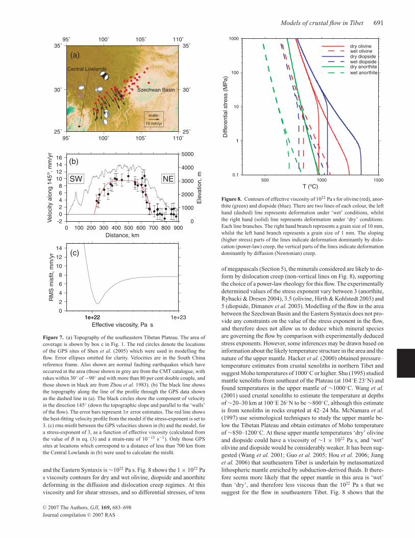
and the Eastern Syntaxis is ∼1022 Pa s. Fig. 8 shows the 1 × 10²² Pa
s viscosity contours for dry and wet olivine, diopside and anorthite
deforming in the diffusion and dislocation creep regimes. At this
viscosity and for shear stresses, and so differential stresses, of tens
0.1
11
10
100
1000
Diffe
rential str
ess (
MP
a)
500 1000 1500
T (oC)
dry olivinewet olivinedry diopsidewet diopsidedry anorthite
wet anorthite
Figure 8. Contours of effective viscosity of 1022 Pa s for olivine (red), anor-
thite (green) and diopside (blue). There are two lines of each colour, the left
hand (dashed) line represents deformation under ‘wet’ conditions, whilst
the right hand (solid) line represents deformation under ‘dry’ conditions.
Each line branches. The right hand branch represents a grain size of 10 mm,
whilst the left hand branch represents a grain size of 1 mm. The sloping
(higher stress) parts of the lines indicate deformation dominantly by dislo-
cation (power-law) creep, the vertical parts of the lines indicate deformation
dominantly by diffusion (Newtonian) creep.
of megapascals (Section 5), the minerals considered are likely to de-
form by dislocation creep (non-vertical lines on Fig. 8), supporting
the choice of a power-law rheology for this flow. The experimentally
determined values of the stress exponent vary between 3 (anorthite,
Rybacki & Dresen 2004), 3.5 (olivine, Hirth & Kohlstedt 2003) and
5 (diopside, Dimanov et al. 2003). Modelling of the flow in the area
between the Szechwan Basin and the Eastern Syntaxis does not pro-
vide any constraints on the value of the stress exponent in the flow,
and therefore does not allow us to deduce which mineral species
are governing the flow by comparison with experimentally deduced
stress exponents. However, some inferences may be drawn based on
information about the likely temperature structure in the area and the
nature of the upper mantle. Hacker et al. (2000) obtained pressure–
temperature estimates from crustal xenoliths in northern Tibet and
suggest Moho temperatures of 1000◦C or higher. Shu (1995) studied
mantle xenoliths from southeast of the Plateau (at 104◦E 23◦N) and
found temperatures in the upper mantle of ∼1000◦C. Wang et al.
(2001) used crustal xenoliths to estimate the temperature at depths
of ∼20–30 km at 100◦E 26◦N to be ∼800◦C, although this estimate
is from xenoliths in rocks erupted at 42–24 Ma. McNamara et al.
(1997) use seismological techniques to study the upper mantle be-
low the Tibetan Plateau and obtain estimates of Moho temperature
of ∼850–1200◦C. At these upper mantle temperatures ‘dry’ olivine
and diopside could have a viscosity of ∼1 × 10²² Pa s, and ‘wet’
olivine and diopside would be considerably weaker. It has been sug-
gested (Wang et al. 2001; Guo et al. 2005; Hou et al. 2006; Jiang
et al. 2006) that southeastern Tibet is underlain by metasomatized
lithospheric mantle enriched by subduction-derived fluids. It there-
fore seems more likely that the upper mantle in this area is ‘wet’
than ‘dry’, and therefore less viscous than the 1022 Pa s that we
suggest for the flow in southeastern Tibet. Fig. 8 shows that the
C© 2007 The Authors, GJI, 169, 683–698
Journal compilation C© 2007 RAS
692 A. Copley and D. McKenzie
0.1
11
10
100
1000D
iffe
rential str
ess (
MP
a)
500 1000 1500
T (oC)
dry olivinewet olivinedry diopsidewet diopsidedry anorthite
wet anorthite
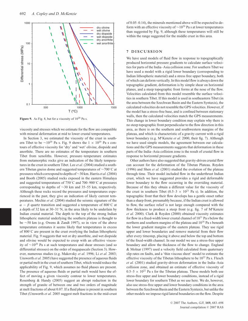
Figure 9. As Fig. 8, but for a viscosity of 1020 Pa s.
viscosity and stresses which we estimate for the flow are compatible
with mineral deformation at mid to lower crustal temperatures.
In Section 3, we estimated the viscosity of the crust in south-
ern Tibet to be ∼1020 Pa s. Fig. 9 shows the 1 × 10²⁰ Pa s con-
tours of effective viscosity for ‘dry’ and ‘wet’ olivine, diopside and
anorthite. There are no estimates of the temperature in southern
Tibet from xenoliths. However, pressure–temperature estimates
from metamorphic rocks give an indication of the likely tempera-
tures in the crust in southern Tibet. Lee et al. (2004) studied a south-
ern Tibetan gneiss dome and suggested temperatures of ∼700◦C at
pressures which correspond to depths of∼30 km. Harris et al. (2004)
and Booth (2005) studied rocks exposed in the eastern Himalaya
and suggested temperatures of 750◦C and 700–900◦C at pressures
corresponding to depths of ∼30 km and 35–55 km, respectively.
Although these rocks record the pressures and temperatures expe-
rienced in the past, they give an indication of likely current tem-
peratures. Mechie et al. (2004) studied the seismic signature of the
α − β quartz transition and suggested a temperature of 800◦C at
a depth of 32 km at 30–31◦N, in the area likely to be underlain by
Indian crustal material. The depth to the top of the strong Indian
lithospheric material underlying the southern plateau is thought to
be ∼50 km (e.g. Owens & Zandt 1997), so in view of the above
temperature estimates it seems likely that temperatures in excess
of 800◦C are present in the crust overlying the Indian lithospheric
material. Fig. 9 suggests that wet or dry anorthite, and wet diopside
and olivine would be expected to creep with an effective viscos-
ity of ∼1020 Pa s at such temperatures and shear stresses (and so
differential stresses) on the order of megapascals (Section 3). How-
ever, numerous studies (e.g. Makovsky et al. 1996; Li et al. 2003;
Unsworth et al. 2005) have suggested the presence of aqueous fluids
or partial melt in the crust of southern Tibet, which would reduce the
applicability of Fig. 9, which assumes no fluid phases are present.
The presence of aqueous fluids or partial melt would have the ef-
fect of moving a given viscosity contour to lower temperatures.
Rosenberg & Handy (2005) suggest an abrupt reduction in the
strength of granite of between one and two orders of magnitude
at melt fractions of about 0.07. If a fluid phase is present in southern
Tibet (Unsworth et al. 2005 suggest melt fractions in the mid-crust
of 0.05–0.14), the minerals mentioned above will be expected to de-
form with an effective viscosity of ∼1020 Pa s at lower temperatures
than suggested by Fig. 9, although these temperatures will still be
within the range suggested for the middle crust in this area.
7 D I S C U S S I O N
We have used models of fluid flow in response to topographically
produced horizontal pressure gradients to calculate surface veloci-
ties for parts of the India–Asia collision zone. For southern Tibet we
have used a model with a rigid lower boundary (corresponding to
Indian lithospheric material) and a stress free upper boundary, both
of which can deform vertically. In this model flow is always down the
topographic gradient, deformation is by simple shear on horizontal
planes, and a steep topographic front forms at the nose of the flow.
Velocities calculated from this model resemble the surface veloci-
ties in southern Tibet. If this model is used in southeastern Tibet (in
the area between the Szechwan Basin and the Eastern Syntaxis), the
calculated velocities do not resemble the GPS velocities. However, if
the model has a stress-free base, and is confined between stationary
walls, then the calculated velocities match the GPS measurements.
This change in lower boundary condition may explain why there is
no steep topographic front perpendicular to the flow direction in this
area, as there is on the southern and southwestern margins of the
plateau, and which is characteristic of a gravity current with a rigid
lower boundary (e.g. McKenzie et al. 2000, their fig. 7). Although
we have used simple models, the agreement between our calcula-
tions and the GPS measurements suggests that deformation in these
parts of the India–Asia collision zone is the result of crustal flow in
response to horizontal pressure gradients.
Other authors have also suggested that gravity-driven crustal flow
can account for the deformation of the Tibetan Plateau. Royden
(1996) and Shen et al. (2001) studied the evolution of the plateau
through time. Their model included flow in the underthrust Indian
crust, which we have suggested provides a rigid and deformable
lower boundary to the flow occurring in the overriding material.
Because of this they obtain a different value for the viscosity of
the crust in southern Tibet (0.5–3 × 10²¹ Pa s). In addition, the
topographic front that their flow develops has a gentle onset rather
than a sharp front, presumably because, if the Indian crust is allowed
to flow, the surface relief is not large enough compared with the
flow thickness to produce a steep front (e.g. fig. 7 of McKenzie
et al. 2000). Clark & Royden (2000) obtained viscosity estimates
for flow in a fixed-width lower crustal channel of 1021 Pa s below the
northern and southern margins of the plateau and 1018 Pa s beneath
the lower gradient margins of the eastern plateau. They use rigid
upper and lower boundaries and remove material from their flow
after every timestep, placing it above and below the top and bottom
of the fixed-width channel. In our model we use a stress-free upper
boundary and allow the thickness of the flow to change. England
& Molnar (1997) used a velocity field calculated from quaternary
slip rates on faults, and a ‘thin viscous sheet’ model to estimate the
effective viscosity of the Tibetan lithosphere to be 1022 Pa s. Flesch
et al. (2001) studied gravity-driven deformation in the India–Asia
collision zone, and obtained an estimate of effective viscosity of
0.5–5 × 10²² Pa s for the Tibetan plateau. These models both use
stress-free upper and lower boundary conditions, instead of a rigid
lower boundary for southern Tibet as we use here. We do, however,
also use stress-free upper and lower boundary conditions in the area
between the Szechwan Basin and the Eastern Syntaxis, but unlike the
other models we impose rigid lateral boundaries on the flow. Despite
C© 2007 The Authors, GJI, 169, 683–698
Journal compilation C© 2007 RAS
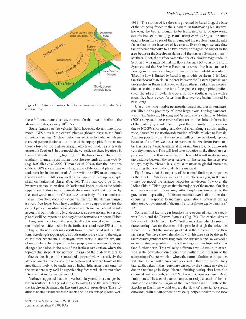
Models of crustal flow in Tibet 693
Figure 10. Cartoon to illustrate the deformation we model in the India–Asia
collision zone.
these differences our viscosity estimate for this area is similar to the
above estimates, namely 1022 Pa s.
Some features of the velocity field, however, do not match our
model. GPS sites in the central plateau (those closest to the 5000
m contour in Fig. 2) show velocities relative to India which are
directed perpendicular to the strike of the topographic front, as are
those closer to the plateau margin which we model as a gravity
current in Section 3. In our model the velocities at these locations in
the central plateau are negligible (due to the low values of the surface
gradient). If underthrust Indian lithosphere extends as far as ∼33◦N
(e.g. DeCelles et al. 2002; Tilmann et al. 2003), then the locations
of these GPS sites, along with large areas of the central plateau, are
underlain by Indian material. Along with the GPS measurements,
this means the middle crust in the area may be deforming by simple
shear on horizontal planes (Fig. 10). This shear could be driven
by stress transmission through horizontal layers, such as the brittle
upper crust. In this situation, simple shear in central Tibet is driven by
the southwards motion of Eurasia. Alternatively, if the underthrust
Indian lithosphere does not extend this far from the plateau margin,
a stress-free lower boundary condition may be appropriate for the
central plateau, in which case stresses which we have not taken into
account in our modelling (e.g. deviatoric stresses normal to vertical
planes) will be important, and may drive the motions in central Tibet.
Large misfits between the geodetically determined velocities and
our model velocities occur for the furthest east and west GPS stations
in Fig. 2. These misfits may result from our method of isolating the
long wavelength topography, as both stations are close to the edges
of the area where the Himalayan front forms a smooth arc, and
close to where the shape of the topography undergoes more abrupt
changes (and also, in the case of the furthest east station, where the
topographic slope at the northern margin of the plateau begins to
influence the shape of the smoothed topography). Alternatively, the
stations are also the closest to the eastern and western limits of the
area that is likely to be underlain by Indian lithospheric material, so
the crust here may well be experiencing forces which are not taken
into account in our simple model.
We have suggested that the lower boundary condition changes be-
tween southern Tibet (rigid and deformable) and the area between
the Szechwan Basin and the Eastern Syntaxis (stress-free). This situ-
ation is analagous to that of ice sheets and ice streams (e.g. MacAyeal
1989). The motion of ice sheets is governed by basal drag, the base
of the ice being frozen to the substrate. In fast-moving ice-streams,
however, the bed is thought to be lubricated, or to overlie easily
deformable sediments (e.g. Blankenship et al. 1987), so the main
drag is from the edges of the stream, and the ice flows significantly
faster than in the interiors of ice sheets. Even though we calculate
the effective viscosity to be two orders of magnitude higher in the
area between the Szechwan Basin and the Eastern Syntaxis than in
southern Tibet, the surface velocities are of a similar magnitude. In
Section 5, we suggested that the flow in the area between the Eastern
Syntaxis and the Szechwan Basin has a stress-free base, and so is
flowing in a manner analagous to an ice stream, whilst in southern
Tibet the flow is limited by basal drag, as with ice sheets. It is likely
that the flow of material in the area between the Eastern Syntaxis and
the Szechwan Basin is directed to the southeast, rather than perpen-
dicular to this in the direction of the greatest topographic gradient
(over the adjacent lowlands), because flow southeastwards with a
stress-free base occurs faster than flow over the basins limited by
basal drag.
One of the more notable geomorphological features in southeast-
ern Tibet is the proximity of three large rivers flowing southeast-
wards (the Salween, Mekong and Yangtze rivers). Hallet & Molnar
(2001) suggested these river valleys record the finite deformation
of the underlying crust. They suggest the proximity of the rivers is
due to NE-SW shortening, and dextral shear along a north trending
zone, caused by the northwards motion of India relative to Eurasia.
Another possibility is that the river valleys may be closely spaced
because of the flow we describe between the Szechwan Basin and
the Eastern Syntaxis. As material flows into this area, the SSE-wards
velocity increases. This will lead to contraction in the direction per-
pendicular to the flow direction, which would result in decreasing
the distance between the river valleys. In this sense, the large river
valleys may be viewed in a similar manner to glacial moraines,
recording the flow of the underlying material.
Fig. 2 shows that the majority of the normal faulting earthquakes
in the Tibetan Plateau occur near the southern margin, in the area
where we model the surface velocities as viscous flow over the
Indian Shield. This suggests that the majority of the normal faulting
earthquakes currently occurring within the plateau are caused by the
gravitational spreading of Tibetan material over India, rather than
occurring in response to increased gravitational potential energy
after convective removal of the mantle lithosphere (e.g. Molnar et al.
1993).
Some normal faulting earthquakes have occurred near the Szech-
wan Basin and the Eastern Syntaxis (Fig. 7a). The earthquakes at
latitudes of ∼30◦N have ∼E–W fault planes. Immediately south of
these earthquakes (in the area of the profile through the velocities
shown in Fig. 7b) the surface gradient in the direction of the flow
increases. We have shown that the flow in this area can be driven by
the pressure gradient resulting from the surface slope, so we would
expect a steeper gradient to result in larger downslope velocities
than further north. This velocity difference would result in exten-
sion in the downslope direction at the northernmost margin of the
steepening of slope, which is where the normal faulting earthquakes
with the ∼E–W fault planes have occurred. It therefore seems likely
that earthquakes in this region are caused by the change in velocity
due to the change in slope. Normal faulting earthquakes have also
occurred further south, at ∼27◦N. These earthquakes have ∼N–S
fault planes. These earthquakes have occurred just south of the lat-
itude of the southern margin of the Szechwan Basin. South of the
Szechwan Basin we would expect the flow of material to spread
outwards, with a component of velocity perpendicular to the flow
C© 2007 The Authors, GJI, 169, 683–698
Journal compilation C© 2007 RAS
694 A. Copley and D. McKenzie
direction further north, and down the topographic slope to the east.
We would also expect increased westwards motion on the western
margin of the flow, because the margin of the lowlands bounding the
flow curves to the southwest in this area. These two effects would re-
sult in extension perpendicular to the bulk flow direction, and in the
brittle upper crust would result in normal faulting with ∼N–S fault
planes, as with the earthquakes. Further work, with more detailed
modelling, is needed to confirm these suggestions.
The lowlands near the Eastern Syntaxis have a distinctive shape.
An elongate area with low relief and low elevation lies between the
eastern Himalaya and the Indo–Burman Ranges, and is seemingly
being overthrust on three sides. This geometry is not compatible with
the motions of rigid blocks, given what we know about the tectonics
of this area. The work presented in Sections 3 and 4 gives an alterna-
tive explanation for the formation of such syntaxes. Both southern
Tibet and the Indo–Burman ranges are gravity currents propagat-
ing over the Indian shield, with motion down the topographic gra-
dients, so normal to the strike of the fronts of the two mountain
ranges. These two gravity currents are flowing towards each other
in the area of the Eastern Syntaxis, both overriding the lowlands
mentioned above, creating the distinctive geometry (Fig. 10). Syn-
taxes elsewhere (e.g. the western Himalayan Syntaxis) may also
have formed in this manner.
8 C O N C L U S I O N S
We have modelled the measured surface velocities in parts of the
India–Asia collision zone using equations describing fluid flow, and
suggest that the motions in these areas are governed by gravitation-
ally driven crustal flow. The viscosity of the material in southern
Tibet is ∼1020 Pa s, and in the area between the Szechwan Basin
and the Eastern Syntaxis it is ∼1022 Pa s. We suggest that the lower
boundary condition changes between these two areas, from hori-
zontally rigid and vertically deformable where strong Indian litho-
spheric material underlies southern Tibet, to stress-free in the area
between the Szechwan Basin and the Eastern Syntaxis. We have used
deformation maps, created using results from experimental studies,
to show that the shear stresses, temperatures, and viscosities present
in the flows we suggest are consistent with the available informa-
tion on the rheology of minerals. Gravitationally driven flow also
occurs in the Indo–Burman Ranges, with an effective viscosity of
∼1019–1020 Pa s. We suggest that the normal faulting earthquakes in
southern Tibet (which account for most of the normal faulting earth-
quakes on the plateau) are caused by the gravity-driven spreading
of Tibet southwards over the Indian shield.
A C K N O W L E D G M E N T S
We thank L. Royden and an anonymous reviewer for helpful com-
ments. The authors wish to thank James Jackson for many useful
discussions and comments on the manuscript. Some figures were
created using the Generic Mapping Tools (GMT) software (Wessel
& Smith 1995).
R E F E R E N C E S
Baranowski, J., Armbruster, J., Seeber, L. & Molnar, P., 1984. Focal depths
and fault plane solutions of earthquakes and active tectonics of the Hi-
malayas, J. geophys. Res., 89, 6918–6928.
Beaumont, C., Jamieson, R.A., Nguyen, M.H. & Lee, B., 2001. Himalayan
tectonics explained by extrusion of a low-viscosity crustal channel coupled
to focused surface denudation, Nature, 141, 738–742.
Bird, P., 1991. Lateral extrusion of lower crust from under high topography,
in the isostatic limit, J. geophys. Res., 96, 10 275–10 286.
Blankenship, D.D., Bentley, C.R., Rooney, S.T. & Alley, R.B., 1987. Till
beneath ice stream B, 1, Properties derived from seismic travel times, J.
geophys. Res., 92, 8903–8911.
Block, L. & Royden, L.H., 1990. Core complex geometries and regional
scale flow in the lower crust, Tectonics, 9, 557–567.
Boland, J.N. & Tullis, T.E., 1986. Deformation behavoir of wet and dry
clinopyroxenit in the brittle to ductile transition region, in Mineral and
Rock Deformation: Laboratory Studies, Geophysical Monograph, Vol. 36,
pp. 35–49, eds Hobbs, B.E. & Heard, H.C., AGU, Washington.
Booth, A.L., 2005. Pressure-temperature conditions and timing of metamor-
phism at Namche Barwa, Eastern Himalayan Syntaxis, SE Tibet, Geolog-
ical Scoiety of America Abstracts with Programs, 37, 89.
Brunnschweiler, R.O., 1966. On the geology of the Indoburman Ranges, J.
Geol. Soc. Aust., 13, 137–194.
Burchfiel, B.C., Chen, Z., Liu, Y. & Royden, L.H., 1995. Tectonics of the
Longmen Shan and adjacent regions, central China, Int. Geol. Rev., 37,
661–735.
Bystricky, M. & Mackwell, S., 2001. Creep of dry clinopyroxene aggregates,
J. geophys. Res., 106, 13 443–13 454.
Chapman, C.H., 1978. A new method for computing synthetic seismograms,
Geophys. J. R. astr. Soc., 54, 481–518.
Chapple, W.M. & Forsyth, D.W., 1979. Earthquakes and the bending of plates
at trenches, J. geophys. Res., 84, 6729–6749.
Chen, W.-P. & Kao, H., 1996. Seismotectonics of Asia: some recent progress,
in The Tectonic Evolution of Asia, pp. 37–62, eds Yin, A. & Harrison, M.,
Cambridge University Press, Cambridge.
Chen, W.-P. & Molnar, P., 1990. Source parameters of earthquakes and in-
traplate deformation beneath the Shillong Plateau and the northern In-
doburman ranges, J. geophys. Res., 95, 12 527–12 552.
Clark, M.K. & Royden, L.H., 2000. Topographic ooze: building the eastern
margin of Tibet by lower crustal flow, Geology, 28, 703–706.
Clark, M.K., Bush, J.M.W. & Royden, L.H., 2005. Dynamic topography
produced by lower crustal flow against rheological strength heterogeneities
bordering the Tibetan Plateau, Geophys. J. Int., 162, 575–590.
Connolly, J.A.D. & Podladchikov, Yu. Yu., 2000. Temperature-dependent
viscoelastic compaction and compartmentalization in sedimentary basins,
Tectonophysics, 324, 137–168.
Curray, J.R., Moore, D.G., Lawver, L.A., Emmel, F.J., Raitt, R.W., Henry,
M. & Kieckhefer, R., 1978. Tectonics of the Andaman Sea and Burma. in
Geological and Geophysical Investigations of Continental Margins, Mem.
Am. Assoc. Pet. Geol., Vol. 29, pp. 189–198, eds Watkins, J.S., Montadert,
L. & Dickerson, P., AAPG, Tulsa.
DeCelles, P., Robinson, D. & Zandt, G., 2002. Implications of shortening in
the Himalayan fold-thrust belt for uplift of the Tibetan plateau, Tectonics,
21, doi:10.1029/2001TC001322.
Dimanov, A., Lavie, M.P., Dresen, G., Ingrin, J. & Jaoul, O., 2003.
Creep of polycrystalline anorthite and diopside, J. geophys. Res., 108,
doi:10.1029/2002JB001815.
Engdahl, E.R., van der Hilst, R. & Buland, R., 1998. Global teleseismic
earthquake relocation with improved travel times and procedures for depth
determination, Bull. seism. Soc. Am., 88, 722–743.
England, P. & Houseman, G., 1986. Finite strain calculations of continental
deformation 2. Comparison with the India–Asia collision zone, J. geophys.
Res., 91, 3664–3676.
England, P. & McKenzie, D., 1982. A thin viscous sheet model for continental
deformation, Geophys. J. R. astr. Soc., 70, 295–321.
England, P. & Molnar, P., 1997. Active deformation of Asia: from kinematics
to dynamics, Science, 278, 647–650.
Fielding, E.J., Isacks, B., Barazangi, M. & Duncan, C., 1994. How flat is
Tibet?, Geology, 22, 163–167.
Flesch, L.M., Haines, A.J. & Holt, W.E., 2001. Dynamics of the India-Eurasia
collision zone, J. geophys. Res., 106, 16 435–16 460.
C© 2007 The Authors, GJI, 169, 683–698
Journal compilation C© 2007 RAS
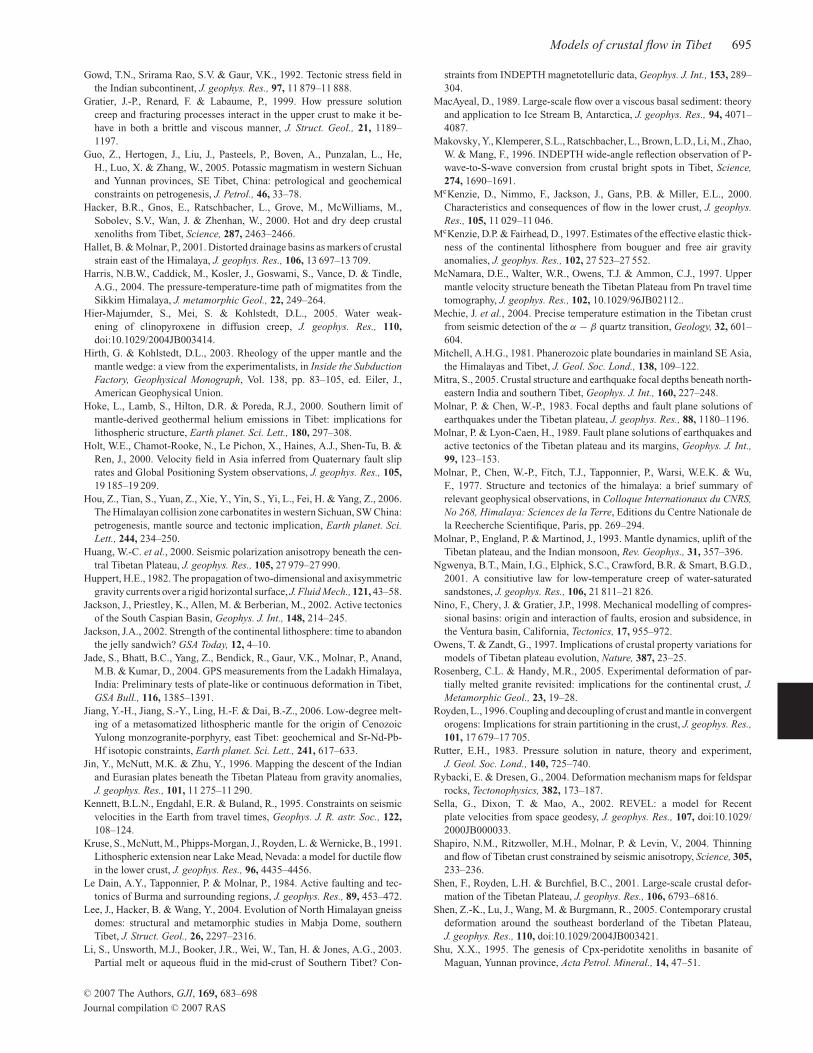
Models of crustal flow in Tibet 695
Gowd, T.N., Srirama Rao, S.V. & Gaur, V.K., 1992. Tectonic stress field in
the Indian subcontinent, J. geophys. Res., 97, 11 879–11 888.
Gratier, J.-P., Renard, F. & Labaume, P., 1999. How pressure solution
creep and fracturing processes interact in the upper crust to make it be-
have in both a brittle and viscous manner, J. Struct. Geol., 21, 1189–
1197.
Guo, Z., Hertogen, J., Liu, J., Pasteels, P., Boven, A., Punzalan, L., He,
H., Luo, X. & Zhang, W., 2005. Potassic magmatism in western Sichuan
and Yunnan provinces, SE Tibet, China: petrological and geochemical
constraints on petrogenesis, J. Petrol., 46, 33–78.
Hacker, B.R., Gnos, E., Ratschbacher, L., Grove, M., McWilliams, M.,
Sobolev, S.V., Wan, J. & Zhenhan, W., 2000. Hot and dry deep crustal
xenoliths from Tibet, Science, 287, 2463–2466.
Hallet, B. & Molnar, P., 2001. Distorted drainage basins as markers of crustal
strain east of the Himalaya, J. geophys. Res., 106, 13 697–13 709.
Harris, N.B.W., Caddick, M., Kosler, J., Goswami, S., Vance, D. & Tindle,
A.G., 2004. The pressure-temperature-time path of migmatites from the
Sikkim Himalaya, J. metamorphic Geol., 22, 249–264.
Hier-Majumder, S., Mei, S. & Kohlstedt, D.L., 2005. Water weak-
ening of clinopyroxene in diffusion creep, J. geophys. Res., 110,
doi:10.1029/2004JB003414.
Hirth, G. & Kohlstedt, D.L., 2003. Rheology of the upper mantle and the
mantle wedge: a view from the experimentalists, in Inside the Subduction
Factory, Geophysical Monograph, Vol. 138, pp. 83–105, ed. Eiler, J.,
American Geophysical Union.
Hoke, L., Lamb, S., Hilton, D.R. & Poreda, R.J., 2000. Southern limit of
mantle-derived geothermal helium emissions in Tibet: implications for
lithospheric structure, Earth planet. Sci. Lett., 180, 297–308.
Holt, W.E., Chamot-Rooke, N., Le Pichon, X., Haines, A.J., Shen-Tu, B. &
Ren, J., 2000. Velocity field in Asia inferred from Quaternary fault slip
rates and Global Positioning System observations, J. geophys. Res., 105,
19 185–19 209.
Hou, Z., Tian, S., Yuan, Z., Xie, Y., Yin, S., Yi, L., Fei, H. & Yang, Z., 2006.
The Himalayan collision zone carbonatites in western Sichuan, SW China:
petrogenesis, mantle source and tectonic implication, Earth planet. Sci.
Lett., 244, 234–250.
Huang, W.-C. et al., 2000. Seismic polarization anisotropy beneath the cen-
tral Tibetan Plateau, J. geophys. Res., 105, 27 979–27 990.
Huppert, H.E., 1982. The propagation of two-dimensional and axisymmetric
gravity currents over a rigid horizontal surface, J. Fluid Mech., 121, 43–58.
Jackson, J., Priestley, K., Allen, M. & Berberian, M., 2002. Active tectonics
of the South Caspian Basin, Geophys. J. Int., 148, 214–245.
Jackson, J.A., 2002. Strength of the continental lithosphere: time to abandon
the jelly sandwich? GSA Today, 12, 4–10.
Jade, S., Bhatt, B.C., Yang, Z., Bendick, R., Gaur, V.K., Molnar, P., Anand,
M.B. & Kumar, D., 2004. GPS measurements from the Ladakh Himalaya,
India: Preliminary tests of plate-like or continuous deformation in Tibet,
GSA Bull., 116, 1385–1391.
Jiang, Y.-H., Jiang, S.-Y., Ling, H.-F. & Dai, B.-Z., 2006. Low-degree melt-
ing of a metasomatized lithospheric mantle for the origin of Cenozoic
Yulong monzogranite-porphyry, east Tibet: geochemical and Sr-Nd-Pb-
Hf isotopic constraints, Earth planet. Sci. Lett., 241, 617–633.
Jin, Y., McNutt, M.K. & Zhu, Y., 1996. Mapping the descent of the Indian
and Eurasian plates beneath the Tibetan Plateau from gravity anomalies,
J. geophys. Res., 101, 11 275–11 290.
Kennett, B.L.N., Engdahl, E.R. & Buland, R., 1995. Constraints on seismic
velocities in the Earth from travel times, Geophys. J. R. astr. Soc., 122,
108–124.
Kruse, S., McNutt, M., Phipps-Morgan, J., Royden, L. & Wernicke, B., 1991.
Lithospheric extension near Lake Mead, Nevada: a model for ductile flow
in the lower crust, J. geophys. Res., 96, 4435–4456.
Le Dain, A.Y., Tapponnier, P. & Molnar, P., 1984. Active faulting and tec-
tonics of Burma and surrounding regions, J. geophys. Res., 89, 453–472.
Lee, J., Hacker, B. & Wang, Y., 2004. Evolution of North Himalayan gneiss
domes: structural and metamorphic studies in Mabja Dome, southern
Tibet, J. Struct. Geol., 26, 2297–2316.
Li, S., Unsworth, M.J., Booker, J.R., Wei, W., Tan, H. & Jones, A.G., 2003.
Partial melt or aqueous fluid in the mid-crust of Southern Tibet? Con-
straints from INDEPTH magnetotelluric data, Geophys. J. Int., 153, 289–
304.
MacAyeal, D., 1989. Large-scale flow over a viscous basal sediment: theory
and application to Ice Stream B, Antarctica, J. geophys. Res., 94, 4071–
4087.
Makovsky, Y., Klemperer, S.L., Ratschbacher, L., Brown, L.D., Li, M., Zhao,
W. & Mang, F., 1996. INDEPTH wide-angle reflection observation of P-
wave-to-S-wave conversion from crustal bright spots in Tibet, Science,
274, 1690–1691.
McKenzie, D., Nimmo, F., Jackson, J., Gans, P.B. & Miller, E.L., 2000.
Characteristics and consequences of flow in the lower crust, J. geophys.
Res., 105, 11 029–11 046.
McKenzie, D.P. & Fairhead, D., 1997. Estimates of the effective elastic thick-
ness of the continental lithosphere from bouguer and free air gravity
anomalies, J. geophys. Res., 102, 27 523–27 552.
McNamara, D.E., Walter, W.R., Owens, T.J. & Ammon, C.J., 1997. Upper
mantle velocity structure beneath the Tibetan Plateau from Pn travel time
tomography, J. geophys. Res., 102, 10.1029/96JB02112..
Mechie, J. et al., 2004. Precise temperature estimation in the Tibetan crust
from seismic detection of the α − β quartz transition, Geology, 32, 601–
604.
Mitchell, A.H.G., 1981. Phanerozoic plate boundaries in mainland SE Asia,
the Himalayas and Tibet, J. Geol. Soc. Lond., 138, 109–122.
Mitra, S., 2005. Crustal structure and earthquake focal depths beneath north-
eastern India and southern Tibet, Geophys. J. Int., 160, 227–248.
Molnar, P. & Chen, W.-P., 1983. Focal depths and fault plane solutions of
earthquakes under the Tibetan plateau, J. geophys. Res., 88, 1180–1196.
Molnar, P. & Lyon-Caen, H., 1989. Fault plane solutions of earthquakes and
active tectonics of the Tibetan plateau and its margins, Geophys. J. Int.,
99, 123–153.
Molnar, P., Chen, W.-P., Fitch, T.J., Tapponnier, P., Warsi, W.E.K. & Wu,
F., 1977. Structure and tectonics of the himalaya: a brief summary of
relevant geophysical observations, in Colloque Internationaux du CNRS,
No 268, Himalaya: Sciences de la Terre, Editions du Centre Nationale de
la Reecherche Scientifique, Paris, pp. 269–294.
Molnar, P., England, P. & Martinod, J., 1993. Mantle dynamics, uplift of the
Tibetan plateau, and the Indian monsoon, Rev. Geophys., 31, 357–396.
Ngwenya, B.T., Main, I.G., Elphick, S.C., Crawford, B.R. & Smart, B.G.D.,
2001. A consitiutive law for low-temperature creep of water-saturated
sandstones, J. geophys. Res., 106, 21 811–21 826.
Nino, F., Chery, J. & Gratier, J.P., 1998. Mechanical modelling of compres-
sional basins: origin and interaction of faults, erosion and subsidence, in
the Ventura basin, California, Tectonics, 17, 955–972.
Owens, T. & Zandt, G., 1997. Implications of crustal property variations for
models of Tibetan plateau evolution, Nature, 387, 23–25.
Rosenberg, C.L. & Handy, M.R., 2005. Experimental deformation of par-
tially melted granite revisited: implications for the continental crust, J.
Metamorphic Geol., 23, 19–28.
Royden, L., 1996. Coupling and decoupling of crust and mantle in convergent
orogens: Implications for strain partitioning in the crust, J. geophys. Res.,
101, 17 679–17 705.
Rutter, E.H., 1983. Pressure solution in nature, theory and experiment,
J. Geol. Soc. Lond., 140, 725–740.
Rybacki, E. & Dresen, G., 2004. Deformation mechanism maps for feldspar
rocks, Tectonophysics, 382, 173–187.
Sella, G., Dixon, T. & Mao, A., 2002. REVEL: a model for Recent
plate velocities from space geodesy, J. geophys. Res., 107, doi:10.1029/
2000JB000033.
Shapiro, N.M., Ritzwoller, M.H., Molnar, P. & Levin, V., 2004. Thinning
and flow of Tibetan crust constrained by seismic anisotropy, Science, 305,
233–236.
Shen, F., Royden, L.H. & Burchfiel, B.C., 2001. Large-scale crustal defor-
mation of the Tibetan Plateau, J. geophys. Res., 106, 6793–6816.
Shen, Z.-K., Lu, J., Wang, M. & Burgmann, R., 2005. Contemporary crustal
deformation around the southeast borderland of the Tibetan Plateau,
J. geophys. Res., 110, doi:10.1029/2004JB003421.
Shu, X.X., 1995. The genesis of Cpx-peridotite xenoliths in basanite of
Maguan, Yunnan province, Acta Petrol. Mineral., 14, 47–51.
C© 2007 The Authors, GJI, 169, 683–698
Journal compilation C© 2007 RAS
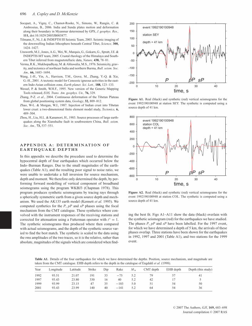
696 A. Copley and D. McKenzie
Socquet, A., Vigny, C., Chamot-Rooke, N., Simons, W., Rangin, C. &
Ambrosius, B., 2006. India and Sunda plates motion and deformation
along their boundary in Myanmar determined by GPS, J. geophys. Res.,
111, doi:10.1029/2005JB003877.
Tilmann, F., Ni, J. & INDEPTH III Seismic Team, 2003. Seismic imaging of
the downwelling Indian lithosphere beneath Central Tibet, Science, 300,
1424–1427.
Unsworth, M.J., Jones, A.G., Wei, W., Marquis, G., Gokarn, G., Spratt, J.E. &
INDEPTH-MT team, 2005. Crustal rheology of the Himalaya and South-
ern Tibet inferred from magnetotelluric data, Nature, 438, 78–81.
Verma, R.K., Mukhopadhyay, M. & Ahluwalia, M.S., 1976. Seismicity, grav-
ity, and tectonics of northeast India and northern Burma, Bull. seism. Soc.
Am., 66, 1683–1694.
Wang, J.-H., Yin, A., Harrison, T.M., Grove, M., Zhang, Y.-Q. & Xie,
G.-H., 2001. A tectonic model for Cenozoic igneous activities in the east-
ern Indo-Asian collision zone, Earth planet. Sci. Lett., 188, 123–133.
Wessel, P. & Smith, W.H.F., 1995. New version of the Generic Mapping
Tools released, EOS, Trans. Am. geophys. Un., 76, 329.
Zhang, P-Z. et al., 2004. Continuous deformation of the Tibetan Plateau
from global positioning system data, Geology, 32, 809–812.
Zhao, W-L. & Morgan, W.J., 1987. Injection of Indian crust into Tibetan
lower crust: a two-dimensional finite element model study, Tectonics, 6,
489–504.
Zhou, H., Liu, H.L. & Kanamori, H., 1983. Source processes of large earth-
quakes along the Xianshuihe fault in southwestern China, Bull. seism.
Soc. Am., 73, 537–551.
A P P E N D I X A : D E T E R M I N AT I O N O F
E A RT H Q UA K E D E P T H S
In this appendix we describe the procedure used to determine the
hypocentral depth of four earthquakes which occurred below the
Indo–Burman Ranges. Due to the small magnitudes of the earth-
quakes (Table A1), and the resulting poor signal to noise ratio, we
were unable to undertake a full inversion for source mechanism,
depth and moment. We therefore only determined the depth, by per-
forming forward modelling of vertical component of broadband
seismograms using the program WKBJ3 (Chapman 1978). This
program produces synthetic seismograms by tracing rays through
a spherically symmetric earth from a given source depth and mech-
anism. We used the AK135 earth model (Kennett et al. 1995). We
computed synthetics for the P, pP and sP phases using the focal
mechanism from the CMT catalogue. These synthetics where con-
volved with the instrument responses of the receiving stations and
corrected for attenuation using a Futterman operator with t∗ = 1.
The synthetic seismograms thus produced where then compared
with actual seismograms, and the depth of the synthetic source var-
ied to find the best match. The synthetic is scaled to the data using
the rms amplitudes of the two traces, so it is the relative, rather than
absolute, magnitudes of the signals which are considered when find-
Table A1. Details of the four earthquakes for which we have determined the depths. Position, source mechanism, and magnitude are
taken from the CMT catalogue. EHB depth refers to the depth in the catalogue of Engdahl et al. (1998).
Year Longitude Latitude Strike Dip Rake M w CMT depth EHB depth Depth (this study)
1992 93.51 21.07 191 33 −75 5.2 79 57 41
1997 93.43 23.80 330 16 40 5.2 42 17 5
1999 93.99 23.15 47 35 −103 5.0 51 54 50
2001 93.43 23.99 140 40 −141 5.2 64 54 36
-200
-150
-100
-50
0
50
100
150
200
0 10 20 30 40
time, s
P pP sP
Figure A1. Real (black) and synthetic (red) vertical seismograms for the
event 1992190100948 at station SEY. The synthetic is computed using a
source depth of 41 km.
-800
-600
-400
-200
0
200
400
600
800
0 10 20 30 40
time, s
P pP sP
Figure A2. Real (black) and synthetic (red) vertical seismograms for the
event 1992190100948 at station COL. The synthetic is computed using a
source depth of 41 km.
ing the best fit. Figs A1–A11 show the data (black) overlain with
the synthetic seismogram (red) for the earthquakes we have studied.
The phases P, pP and sP have been labelled. For the 1997 event,
for which we have determined a depth of 5 km, the arrivals of thesephases overlap. Three stations have been shown for the earthquakes
in 1992, 1997 and 2001 (Table A1), and two stations for the 1999
event.
C© 2007 The Authors, GJI, 169, 683–698
Journal compilation C© 2007 RAS
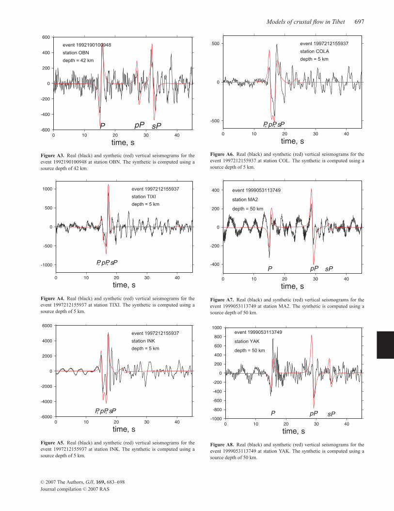
Models of crustal flow in Tibet 697
-600
-400
-200
0
200
400
600
0 10 20 30 40
time, s
P pP sP
Figure A3. Real (black) and synthetic (red) vertical seismograms for the
event 1992190100948 at station OBN. The synthetic is computed using a
source depth of 42 km.
-1000
-500
0
500
1000
0 10 20 30 40
time, s
P, pP, sP
Figure A4. Real (black) and synthetic (red) vertical seismograms for the
event 1997212155937 at station TIXI. The synthetic is computed using a
source depth of 5 km.
-6000
-4000
-2000
0
2000
4000
6000
0 10 20 30 40
time, s
P, pP, sP
Figure A5. Real (black) and synthetic (red) vertical seismograms for the
event 1997212155937 at station INK. The synthetic is computed using a
source depth of 5 km.
-500
0
500
0 10 20 30 40
time, s
P, pP, sP
Figure A6. Real (black) and synthetic (red) vertical seismograms for the
event 1997212155937 at station COL. The synthetic is computed using a
source depth of 5 km.
-400
-200
0
200
400
0 10 20 30 40
time, s
P pP sP
Figure A7. Real (black) and synthetic (red) vertical seismograms for the
event 1999053113749 at station MA2. The synthetic is computed using a
source depth of 50 km.
-1000
-800
-600
-400
-200
0
200
400
600
800
1000
0 10 20 30 40
time, s
P pP sP
Figure A8. Real (black) and synthetic (red) vertical seismograms for the
event 1999053113749 at station YAK. The synthetic is computed using a
source depth of 50 km.
C© 2007 The Authors, GJI, 169, 683–698
Journal compilation C© 2007 RAS
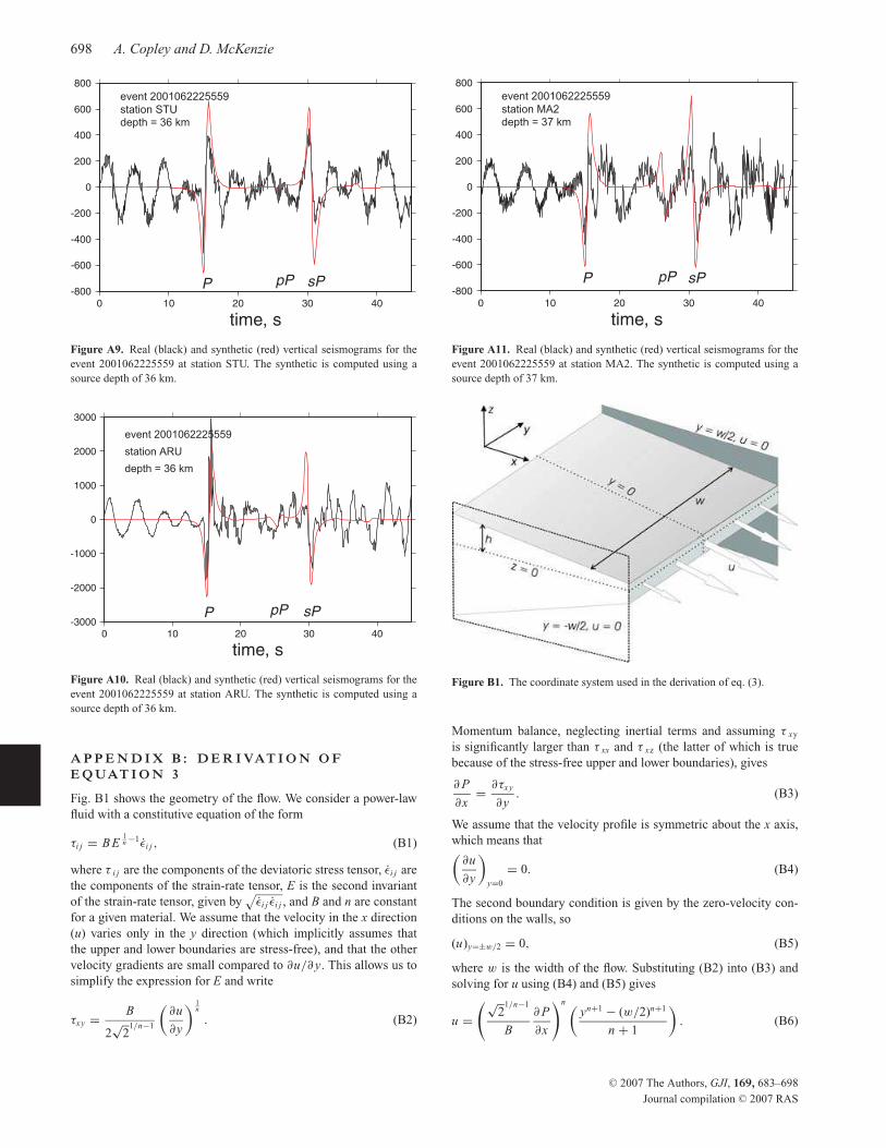
698 A. Copley and D. McKenzie
-800
-600
-400
-200
0
200
400
600
800
0 10 20 30 40
time, s
P pP sP
Figure A9. Real (black) and synthetic (red) vertical seismograms for the
event 2001062225559 at station STU. The synthetic is computed using a
source depth of 36 km.
-3000
-2000
-1000
0
1000
2000
3000
0 10 20 30 40
time, s
P pP sP
Figure A10. Real (black) and synthetic (red) vertical seismograms for the
event 2001062225559 at station ARU. The synthetic is computed using a
source depth of 36 km.
A P P E N D I X B : D E R I VAT I O N O F
E Q UAT I O N 3
Fig. B1 shows the geometry of the flow. We consider a power-law
fluid with a constitutive equation of the form
τi j = B E1n −1ǫ̇i j , (B1)
where τ i j are the components of the deviatoric stress tensor, ǫ̇i j are
the components of the strain-rate tensor, E is the second invariant
of the strain-rate tensor, given by√
ǫ̇i j ǫ̇i j , and B and n are constant
for a given material. We assume that the velocity in the x direction
(u) varies only in the y direction (which implicitly assumes that
the upper and lower boundaries are stress-free), and that the other
velocity gradients are small compared to ∂u/∂ y. This allows us to
simplify the expression for E and write
τxy =B
2√
21/n−1
(
∂u
∂y
)1n
. (B2)
-800
-600
-400
-200
0
200
400
600
800
0 10 20 30 40
time, s
P pP sP
Figure A11. Real (black) and synthetic (red) vertical seismograms for the
event 2001062225559 at station MA2. The synthetic is computed using a
source depth of 37 km.
Figure B1. The coordinate system used in the derivation of eq. (3).
Momentum balance, neglecting inertial terms and assuming τ xy
is significantly larger than τ xx and τ xz (the latter of which is true
because of the stress-free upper and lower boundaries), gives
∂ P
∂x=
∂τxy
∂y. (B3)
We assume that the velocity profile is symmetric about the x axis,
which means that(
∂u
∂y
)
y=0
= 0. (B4)
The second boundary condition is given by the zero-velocity con-
ditions on the walls, so
(u)y=±w/2 = 0, (B5)
where w is the width of the flow. Substituting (B2) into (B3) and
solving for u using (B4) and (B5) gives
u =
(√2
1/n−1
B
∂ P
∂x
)n(
yn+1 − (w/2)n+1
n + 1
)
. (B6)
C© 2007 The Authors, GJI, 169, 683–698
Journal compilation C© 2007 RAS