Models for Logics and Conditional Constraintsin Automated Proofs of Termination

Salvador Lucas1,2 and Jose Meseguer2

1 DSIC, Universitat Politecnica de Valencia, Spain2 CS Dept. University of Illinois at Urbana-Champaign, IL, USA

Abstract. Reasoning about termination of declarative programs, whichare described by means of a computational logic, requires the definition ofappropriate abstractions as semantic models of the logic, and also han-dling the conditional constraints which are often obtained. The formaltreatment of such constraints in automated proofs, often using numericinterpretations and (arithmetic) constraint solving, can greatly benefitfrom appropriate techniques to deal with the conditional (in)equations atstake. Existing results from linear algebra or real algebraic geometry areuseful to deal with them but have received only scant attention to date.We investigate the definition and use of numeric models for logics andthe resolution of linear and algebraic conditional constraints as unifyingtechniques for proving termination of declarative programs.

Keywords: Conditional constraints, program analysis, termination.

1 Introduction

The operational semantics of sophisticated rule-based programming languagessuch as CafeOBJ [7], Maude [3], or Haskell [8] is often formalized in a proof-theoretic style by means of a computational logic, and the corresponding lan-guage interpreters better understood as inference machines [15]. The notion ofoperational termination [11] was introduced to give an account of the termina-tion behavior of programs of such languages [12]. An interpreter for a logic L(for instance the logic for Conditional Term Rewriting Systems (CTRSs) withinference system in Figure 1) is an inference machine that, given a theory S(e.g., the CTRS R in Example 1) and a goal formula ϕ (e.g., a one-step rewrit-ing s → t for terms s and t) tries to incrementally build a proof tree for ϕ byusing (instances of) the inference rules B1,...,Bn

A ∈ I(L) of the inference systemI(L) of L. Then, S is operationally terminating if for any ϕ the interpreter ei-ther finds a proof, or fails in all possible attempts (always in finite time). In thissetting, practical methods for proving operational termination involve two mainissues (see [13] and also [17] for CTRSs): (1) the simulation of the (one-step)rewrite relations→ and→∗ associated to a CTRSR and defined by means of theinference system in Figure 1; and (2) the use of (automatically generated) well-founded relations A to abstract rewrite computations and guarantee the absence

(Refl) t→∗ t (Cong)

si → tif(s1, . . . , si, . . . , sk)→ f(s1, . . . , ti, . . . , sk)

for all k-ary symbols f and 1 ≤ i ≤ k

(Tran)

s→ u u→∗ t

s→∗ t (Repl)

s1 →∗ t1 . . . sn →∗ tn`→ r

for each rule `→ r ⇐ s1 → t1 · · · sn → tn

Fig. 1. Inference rules for the CTRS logic (all variables are universally quantified)

of infinite ones. Here, (1) amounts at dealing with abstractions for sentences like∀x(B1 ∧ · · · ∧Bn ⇒ A) which simulate the use of the aforementioned inferencerules; and (2) often involves the comparison of expressions s and t using A, pro-vided that a number of semantic conditions (e.g., rewriting steps si →∗R ti forsome terms si and ti) hold. Abstractions can be formalized as semantic modelsM = (D,FD, ΠD) of L (see Section 2), where D is a domain and FD and ΠD areinterpretations of the function symbols F and predicates Π of L, respectively.For instance, relations → and →∗ (which are predicates in the correspondinglogic) are typically interpreted as orderings on D, often a numeric domain like Nor [0,+∞). In this paper we introduce the idea of using conditional expressionsto restrict such domains in logical models (Section 3). This is often useful.

Example 1. Consider the following CTRS R:

or(0, x) → x (1)

or(x, 0) → x (2)

or(1, x) → 1 (3)

or(x, 1) → 1 (4)

or(x, not(x)) → 1 (5)

or(not(x), x) → 1 (6)

and(0, x) → 0 (7)

and(x, 0) → 0 (8)

and(1, x) → x (9)

and(x, 1) → x (10)

and(x, not(x)) → 0 (11)

and(not(x), x) → 0 (12)

not(1) → 0 (13)

not(0) → 1 (14)

implies(x, y) → 1⇐ not(x)→ 1 (15)

implies(x, y) → 1⇐ y → 1 (16)

implies(x, y) → 0⇐ x→ 1, y → 0 (17)

f(x) → f(0)⇐ implies(implies(x, implies(x, 0)), 0)→ 1 (18)

We failed to prove operational termination of R by using the ordering-basedtechniques introduced in [13] and also with the more advanced techniques in[14]. However, below we provide a very simple proof of operational terminationbased on the use (within [13]!) of a bounded domain [0, 1] which can be easilyimplemented by using conditional constraints.

As an interesting specialization of this general idea, Section 4 introduces convexmatrix interpretations as a new, twofold extension of the framework introducedby Endrullis et al. [5] for TRSs, where rather than using vectors x of naturalnumbers (or non-negative numbers, as in [2]), we use convex sets satisfying amatrix inequality Ax ≥ b. Section 5 discusses existing approaches to deal withthe obtained numeric conditional constraints: Farkas’ Lemma and results fromAlgebraic Geometry. Section 6 compares with related work. Section 7 concludes.

2

2 Models of Logics for Proofs of Termination

In this paper, X denotes a set of variables and F denotes a signature: a set offunction symbols {f, g, . . .}, each with a fixed arity given by a mapping ar : F →N. The set of terms built from F and X is T (F ,X ). A CTRS R = (F , R) consistof a signature F and a set R of rules ` → r ⇐ s1 → t1, · · · , sn → tn, wherel, r, s1, t1, · · · , sn, tn ∈ T (F ,X ). For s, t ∈ T (F ,X ), we write s →R t (s →∗R t)if there is a proof for s→ t (s→∗ t) with the inference system in Figure 1.

Given a (first order) logic signature Σ = (F , Π) where F is a signature offunction symbols and Π is a signature of predicate symbols, the formulas ϕ of a(first order) logic L over Σ are built up from atoms P (t1, . . . , tk) with P ∈ Πand t1, . . . , tk ∈ T (F ,X ), logic connectives (e.g., ∧, ¬, ⇒) and quantifiers (∀,∃)in the usual way; FormΣ is the set of such formulas. A theory S of L is a setof formulas, S ⊆ FormΣ , and its theorems are the formulas ϕ ∈ FormΣ forwhich we can derive a proof using the inference system I(L) of L in the usualway (written S ` ϕ). Given a logic L describing computations in a (declarative)programming language, programs are viewed as theories S of L.

Example 2. In the logic of CTRSs, with binary predicates → and→∗, the theoryfor a CTRS R = (F , R) is obtained from the inference rules in Figure 1 afterspecializing them as (Cong)f,i for each f ∈ F and i, 1 ≤ i ≤ ar(f) and (Repl)ρfor all ρ : ` → r ⇐ c ∈ R. Then, inference rules B1,...,Bn

A become implicationsB1∧· · ·∧Bn ⇒ A. For instance, for (Tran), (Cong)not, (Repl)(1), and (Repl)(15):

∀s, t, u (s→ u ∧ u→∗ t⇒ s→∗ t) (19)

∀s, t (s→ t⇒ not(s) → not(t)) (20)

∀x (or(0, x) → x) (21)

∀x, y (not(x)→∗ 1⇒ implies(x, y) → 1) (22)

For analysis and verification purposes we often need to abstract L into a numericsetting (e.g., arithmetics, linear algebra, or algebraic geometry) where appropri-ate techniques are available to prove properties of interest. This amounts atgiving a (numeric) model of L that satisfies S.

An F-algebra is a pair A = (D,FD), where D is a set and FD is a set ofmappings fA : Dk → D for each f ∈ F where k = ar(f). A Σ-model is a tripleM = (D,FD, ΠD) where (D,FD) is an F-algebra, and for each k-ary P ∈ Π,PM ∈ ΠD is a k-ary relation PM ⊆ Dk. Given a valuation mapping α : X → D,the evaluation mapping [ ]Aα : T (F ,X )→ D (also [ ]Mα if A is part of M) is theunique homomorphism extending α. Finally, [ ]Mα : FormΣ → Bool is given by:

1. [P (t1, . . . , tk)]Mα = true if and only if ([t1]Mα , . . . , [tk]Mα ) ∈ PA;2. [ϕ ∧ ψ]Mα = true if and only if [ϕ]Mα = true and [ψ]Mα = true;3. [ϕ⇒ ψ]Mα = true if and only if [ϕ]Mα = false or [ψ]Mα = true;4. [¬ϕ]Mα = true if and only if [ϕ]Mα = false;5. [∃x ϕ]Mα = true if and only if there is a ∈ D such that [ϕ]Mα[x 7→a] = true;

6. [∀x ϕ]Mα = true if and only if for all a ∈ D, [ϕ]Mα[x 7→a] = true;

3

We say thatM satisfies ϕ ∈ FormΣ if there is α ∈ X → D such that [ϕ]Mα = true.If [ϕ]Mα = true for all valuations α, we write M |= ϕ. A closed formula, i.e., aformula whose variables are all universally or existentially quantified, is called asentence. We say that M is a model of a set of sentences S ⊆ FormΣ (writtenM |= S) if for all ϕ ∈ S, M |= ϕ. And, given a sentence ϕ, we write S |= ϕ ifand only if for all models M of S, M |= ϕ. Sound logics guarantee that everyprovable sentence ϕ is true in every model of S, i.e., S ` ϕ implies S |= ϕ.

In practice, F-algebras A can be obtained if we first consider a new set ofterms T (G,X ) where the new symbols g ∈ G have ‘intended’ (often arithmetic)interpretations over an (arithmetic) domain D as mappings g from D into D. Theuse of the same name for the syntactic and semantic objects stresses that theyhave an intended meaning. We associate an expression ef ∈ T (G, {x1, . . . , xk}) toeach k-ary symbol f ∈ F , where x1, . . . , xk ∈ X are different variables: we write[f ](x1, . . . , xk) = ef ; and homomorphically extend it to [ ] : T (F ,X )→ T (G,X ).Then, for all a1, . . . , ak ∈ D, we let fA(a1, . . . , ak) = [ef ]αa , for αa given byαa(xi) = ai for all 1 ≤ i ≤ k.

Example 3. For R in Example 1, F = {0, 1, or, and, not, implies, f}, wherear(0) = ar(1) = 0, ar(f) = 1, and ar(or) = ar(and) = ar(implies) = 2. LetG = {0, 1,max,min, − } with ar(0) = ar(1) = 0 and ar(max) = ar(min) =ar( − ) = 2. We define an F-algebra over the reals R as follows:

[0] = 0 [and](x, y) = min(x, y) [or](x, y) = max(x, y) [f](x) = 0[1] = 1 [not](x) = 1− x [implies](x, y) = max(1− x, y)

We define a modelM = (D,FD, ΠD) if each P ∈ Π is interpreted as a predicatePM ∈ ΠD, and each ϕ ∈ FormΣ as a formula ϕM, where ϕM = PM([t1], . . . , [tk])if ϕ = P (t1, . . . , tk); ϕM = ϕM ⊕ ψA if ϕ = χ ⊕ ψ for ⊕ ∈ {∧,⇒} and ϕM =�χM if ϕ = �χ for � ∈ {¬,∀,∃}. The goal is proving that M |= S holds.

Example 4. We can interpret both→ and→∗ as ‘=’ (intended to be the equalityamong real numbers). Then, the sentences in Example 2 become

∀s, t, u ∈ R (s = u ∧ u = t⇒ s = t) (23)

∀s, t ∈ R (s = t⇒ 1− s = 1− t) (24)

∀x ∈ R (max(0, x) = x) (25)

∀x, y ∈ R (1− x = 1⇒ max(1− x, y) = 1) (26)

Unfortunately, (25) and (26) do not hold in the intended model due to the (big)algebraic domain R. For instance, max(0,−1) = 0 6= −1, i.e., (25) is not true.

Example 4 shows that the appropriate definition of the domain of a model iscrucial to satisfy a set of formulas. The next section investigates this problem.

3 Domains for algebras and models revisited

In proofs of termination, domains D for numeric F-algebras A usually are infinite(subsets of) n-dimensional open intervals which are bounded from below: Nn or

4

[0,+∞)n for some n ≥ 1. Furthermore, considered orderings often make thecorresponding ordered sets total (like [0,+∞) ordered by ≥R), or nontotal butwith subsets B ⊆ D bounded by some value xB ∈ D (like [0,+∞)n orderedby the pointwise extension of the usual ordering ≥R over the reals, which is acomplete lattice). More general domains can be often useful, though.

Example 5. (Continuing Example 4) Although (23) and (24) always hold(under the intended interpretation of ‘=’ as the equality), satisfiability of othersentences may depend on the considered domain of values: if D = [0, 1], then(25) and (26) hold; if D = N, then only (25) holds. The use of D = [0, 1] can bemade explicit in (25) and (26) by adding further constraints:

∀x ∈ R ( x ≥ 0 ∧ 1 ≥ x⇒ max(0, x) = x) (27)

∀x, y ∈ R ( x ≥ 0 ∧ 1 ≥ x ∧ y ≥ 0 ∧ 1 ≥ y ∧ 1− x = 1⇒ max(1− x, y) = 1) (28)

Thus, we need to deal with conditional constraints for using such more generaldomains. Also to handle max expressions [6, 16].

Example 6. We can expand the definition of max in (27) and (28) into:

∀x ∈ R ( x ≥ 0 ∧ 1 ≥ x ∧ 0 ≥ x⇒ 0 = x) (29)

∀x ∈ R ( x ≥ 0 ∧ 1 ≥ x ∧ x ≥ 0⇒ x = x) (30)

∀x, y ∈ R ( x ≥ 0 ∧ 1 ≥ x ∧ y ≥ 0 ∧ 1 ≥ y ∧ 1− x = 1 ∧ 1− x ≥ y ⇒ 1− x = 1) (31)

∀x, y ∈ R ( x ≥ 0 ∧ 1 ≥ x ∧ y ≥ 0 ∧ 1 ≥ y ∧ 1− x = 1 ∧ y > 1− x⇒ y = 1) (32)

where (30) clearly holds true and we do not longer care about it.

3.1 Conditional domains for term algebras and models

Given a set D and a predicate χ over D, we let Dχ = {x ∈ D | χ(x)} be therestriction of D by χ. An F-algebra A = (D,FD) yields a restricted F-algebraAχ = (Dχ,FDχ), where for each f ∈ F , fAχ is the restriction of fA to Dkχ, if forall k-ary symbols f ∈ F , this algebraicity or closedness condition holds:

∀x1, . . . , xk

∧i≤i≤k

χ(xi)

⇒ χ(fA(x1, . . . , xk))

(33)

guaranteeing that if fA is given inputs in Dχ, the outcome belongs to Dχ as well.

Remark 1. Algebraicity is a standard requirement for algebraic interpretations.Most times, however, the imposition of simple requirements on the shape of thenumeric expressions ef used to define fA (see Section 2) makes this task easyand often avoids any checking. A well-known example is taking D = [0,+∞)and requiring ef to be a polynomial whose coefficients are all non-negative.

The relations PM ⊆ Dk interpreting k-ary predicates P ∈ Π can be restrictedto PMχ

= PM∩Dkχ to yield a new interpretation of P inMχ = (Dχ,FDχ , ΠDχ).For practical purposes, in this paper we only consider simple restrictions of F-algebras and models, where D is obtained as the solution of linear constraints.

5

Definition 1 (Convex polytopic domain). Given a matrix A ∈ Rm×n, andb ∈ Rm, the set of solutions of the inequality Ax ≥ b is a convex polytopeD(A, b) = {x ∈ Rn | Ax ≥ b}. We call D(A, b) a convex polytopic domain.

Example 7. For A = (−1, 1)T and b = (−1, 0), we have D(A, b) = [0, 1]. IfA = (1) and b = (0), then D(A, b) = [0,+∞).

Example 8. Continuing Example 3, we obtain an F-algebra A[0,1] =([0, 1],F[0,1]) as the restriction to [0, 1] of the F-algebra over R defined there.The constraints (25) and (26) are written in the restricted model as follows

∀x ∈ [0, 1] (max(0, x) = x) (34)

∀x, y ∈ [0, 1] (1− x = 1⇒ max(1− x, y) = 1) (35)

After encoding memberships like x ∈ [0, 1] as inequalities x ≥ 0 ∧ 1 ≥ x andexpanding the definition of max, we obtain (29)− (32).

In sharp contrast with Example 4, restricting the model at hand to [0, 1] leads toa model for R in Example 1 which is useful to prove its operational termination.

Example 9. According to [13], R in Example 1 is operationally terminat-ing if there is a relation & on terms such that →∗ ⊆ &, and a well-founded ordering A satisfying & ◦ A ⊆ A such that, for all substitutions σ, ifσ(implies(implies(x, implies(x, 0)), 0))→∗R σ(1) holds, then σ(F(x)) A σ(F(0)) forthe rule (dependency pair3) F(x)→ F(0)⇐ implies(implies(x, implies(x, 0)), 0)→1 (where F is a fresh symbol). LetM = ([0, 1],F ′[0,1], Π[0,1]) where F ′ = F∪{F},F ′[0,1] is F[0,1] as in Example 8 extended with [F](x) = x, and Π[0,1] given by

→[0,1]=→∗[0,1]= (=[0,1]) (i.e., the equality on [0, 1]).M is a model ofR; by sound-

ness, if s→∗ t holds for s, t ∈ T (F ,X ), we have [s] =[0,1] [t]. Let & be as follows:for all s, t ∈ T (F ,X ), s & t holds if and only if [s] =[0,1] [t]. Then, →∗ ⊆ &, asdesired.

Now, consider the ordering >1 over R given by x >1 y if and only if x−y ≥ 1;it is a well-founded relation on [0, 1] (see [10]). We let A be the (well-founded)relation on T (F ,X ) induced by >1 as before. Again, for all substitutions σ, ifσ(implies(implies(x, implies(x, 0)), 0))→∗R σ(1) holds, then, by soundness,

[σ(implies(implies(x, implies(x, 0)), 0))] =[0,1] [σ(1)] (36)

holds as well. We also have

∀x ∈ [0, 1]([implies(implies(x, implies(x, 0)), 0)] =[0,1] [1]⇒ [F(x)] >1 [F(0)]) (37)

because, for all x ≥ 0,

[implies(implies(x, implies(x, 0)), 0)] = max(1−max(1− x,max(1− x, 0)), 0)= max(1−max(1− x, 1− x), 0)= max(1− (1− x), 0)= max(x, 0)= x

3 For the purpose of this paper, the procedure to obtain this new rule is not relevant.The interested reader can find the details in [13].

6

and hence [implies(implies(x, implies(x, 0)), 0)] =[0,1] [1] holds only if x = 1 =[1]. Combining (36) and (37), we conclude that, for all substitutions σ, ifσ(implies(implies(x, implies(x, 0)), 0)) →∗R σ(1) holds, then [F(x)]M = 1 >1 0 =[F(0)]M, as desired. This proves operational termination of R in Example 1.

In the following section we discuss an interesting application of convex polytopicdomains to improve the well-known matrix interpretations [5, 2].

4 Convex matrix interpretations

A convex matrix intepretation for a k-ary symbol f is a linear expression F1x1 +· · · + Fkxk + F0, where F1, . . . , Fk ∈ Rn×n are (square) matrices, F0 ∈ Rn andx1, . . . ,xk ∈ Rn, which is closed on D(A, b), i.e., that satisfies

∀x1, . . .xk ∈ Rn(

k∧i=1

Axi ≥ b⇒ A(F1x1 + · · ·+ Fkxk + F0) ≥ b

)(38)

An F-algebra A = (D,FD) is obtained if D = D(A, b), and each k-ary symbolf ∈ F is given fA(x1, . . . , xk) = F1x1 + · · · + Fkxk + F0 that satisfies (38).The following ordering ≥ is considered: x = (x1, . . . , xn) ≥ (y1, . . . , yn) = y ifxi ≥ yi for all 1 ≤ i ≤ n. Given δ > 0, the (strict) ordering >δ is also used: x =(x1, . . . , xn) >δ (y1, . . . , yn) = y if x1 − y1 ≥ δ and (x2, . . . , xn) ≥ (y2, . . . , yn).

Remark 2. Convex matrix interpretations include the usual matrix interpreta-tions in [5, 2] if A = In×n and b = 0 ∈ Rn.

In contrast to (N,≥) and ([0,+∞),≥), that are total orders, and also to (Nn,≥)and ([0,+∞)n,≥), that are not total, but are complete lattices, (D(A, b),≥) doesnot need to be total or a complete lattice. This has some interesting advantages.

Example 10. Consider the CTRS R [17, Example 7.2.45]:

a→ a⇐ b→ x, c→ x (39)

b→ d⇐ d→ x, e→ x (40)

c→ d⇐ d→ x, e→ x (41)

According to [13], R is operationally terminating if there is a relation & suchthat →∗ ⊆ &, and A is a well-founded ordering such that & ◦ A ⊆ A and forthe dependency pair a] → a] ⇐ b → x, c → x (for a] a new symbol), we havethat, for all substitutions σ, if b →∗ σ(x) and c →∗ σ(x), then a] A a]. With

A =

1 11 00 1

and b = (1, 0, 0)T , together with:

[a] = [a]] =

[10

][b] = [d] =

[10

][c] = [e] =

[01

]

we have [a], [a]], [b], [c], [d], [e] ∈ D(A, b), as required by (38). It can be provedthat (D(A, b),FD(A,b), ΠD(A,b)), where →,→∗ ∈ Π are both interpreted (in

7

ΠD(A,b)) as ≥ is a model of R. For s, t ∈ T (F ,X ), we let s & t if and onlyif [s] ≥ [t]. Thus, →∗ ⊆ & holds. The ordering >1 on D(A, b) is well-foundedbecause [0,+∞) is bounded from below (see [10]). Thus, for s, t ∈ T (F ,X ), wedefine s A t if and only if [s] >1 [t]. Now, since →∗ ⊆ &, we only have to provethat [b] ≥ [x] ∧ [c] ≥ [x]⇒ [a]] >1 [a]], i.e.,

∀x1, x2 ∈ R

1 11 00 1

[x1

x2

]≥

100

∧ [ 10

]≥[x1

x2

]∧[

01

]≥[x1

x2

]⇒[

10

]>1

[10

](42)

which can be written as a universally quantified conjunction of two formulas:

x1 + x2 ≥ 1 ∧ x1 ≥ 0 ∧ x2 ≥ 0 ∧ 1 ≥ x1 ∧ 0 ≥ x2 ∧ 0 ≥ x1 ∧ 1 ≥ x2 ⇒ 1 >1 1 (43)

x1 + x2 ≥ 1 ∧ x1 ≥ 0 ∧ x2 ≥ 0 ∧ 1 ≥ x1 ∧ 0 ≥ x2 ∧ 0 ≥ x1 ∧ 1 ≥ x2 ⇒ 0 ≥ 0 (44)

The crucial point is that the conditional part of the implications does not holdbecause no x ∈ D(A, b) satisfies (1, 0)T ≥ x and (0, 1)T ≥ x (see Example 11).

The following sections discuss existing mathematical techniques that can be usedto automatically deal with the conditional constraints obtained so far.

5 Conditional polynomial constraints

In this section, we explore well-known results from linear algebra [20] and alge-braic geometry [18] to deal with conditional polynomial constraints.

5.1 Conditional constraints with linear polynomials

Farkas’ Lemma provides a (universal) quantifier elimination result for linear(conditional) sentences (cf. [20]).

Theorem 1 (Affine form of Farkas’ Lemma). Let Ax ≥ b be a linear systemof k inequalities and n unknowns over the real numbers with non-empty solutionset S and let c ∈ Rn and β ∈ R. Then, the following statements are equivalent:

1. cTx ≥ β for all x ∈ S,2. ∃λ ∈ Rk0 such that c = ATλ and λT b ≥ β.

By condition (1) in Theorem 1 proving ∀x (Ax ≥ b ⇒ cTx ≥ β) can be recastas the constraint solving problem of finding a nonnegative vector λ such that cis a linear nonnegative combination of the rows of A and β is smaller than thecorresponding linear combination of the components of b. Note that if Ax ≥ bhas no solution, i.e., S in Theorem 1 is empty, the conditional sentence triviallyholds. Thus, we do not need to check S for emptiness when using Farkas’ result.

Example 11. Sentences (43) and (44) can be proved using Theorem 1. Thisproves operational termination of R in Example 10.

8

Example 12. After encoding the equality as the conjunction of ≥ and ≤, wetransform sentences (29), (31) and (32) into:

∀x ∈ R ( x ≥ 0 ∧ 1 ≥ x ∧ 0 ≥ x ⇒ 0 ≥ x) (45)

∀x ∈ R ( x ≥ 0 ∧ 1 ≥ x ∧ 0 ≥ x ⇒ x ≥ 0) (46)

∀x, y ∈ R ( x ≥ 0 ∧ 1 ≥ x ∧ y ≥ 0 ∧ 1 ≥ y ∧ 1− x = 1 ∧ 1− x ≥ y ⇒ 1− x ≥ 1) (47)

∀x, y ∈ R ( x ≥ 0 ∧ 1 ≥ x ∧ y ≥ 0 ∧ 1 ≥ y ∧ 1− x = 1 ∧ 1− x ≥ y ⇒ 1 ≥ 1− x) (48)

∀x, y ∈ R ( x ≥ 0 ∧ 1 ≥ x ∧ y ≥ 0 ∧ 1 ≥ y ∧ 1− x = 1 ∧ y > 1− x ⇒ y ≥ 1) (49)

∀x, y ∈ R ( x ≥ 0 ∧ 1 ≥ x ∧ y ≥ 0 ∧ 1 ≥ y ∧ 1− x = 1 ∧ y > 1− x ⇒ 1 ≥ y) (50)

which are conditional linear sentences provable using Farkas’ Lemma.

5.2 Conditional constraints with arbitrary polynomials

Given polynomials h1, . . . , hm ∈ R[X1, . . . , Xn], the semialgebraic set defined byh1, . . . , hm is WR(h) = WR(h1, . . . , hm) = {x ∈ Rn | h1(x) ≥ 0∧· · ·∧hm(x) ≥ 0}.A well-known representation theorem establishes that a polynomial which ispositive for all tuples (x1, . . . , xn) ∈ WR(h) can be written as a linear combina-tion of h1, . . . , hm with ‘coefficients’ s that are sums of squares of polynomials(s ∈

∑R[X]2) [18, Theorem 5.3.8]. If we can write a polynomial f as a linear

combination of h1, . . . , hm with ‘coefficients’ that are sums of squares, this pro-vides a certificate of non-negativeness of f on WR(h1, . . . , hm): sums of squaresare non-negative, all hi are non-negative on values in WR(h1, . . . , hm) and theproduct and addition of non-negative numbers is non-negative. Explicitly:

Theorem 2. Let R[X] := R[X1, . . . , Xn], h1, . . . , hm ∈ R[X], WR(h) =WR(h1, . . . , hm) and S ⊆ R such that WR(h1, . . . , hm) ⊆ Sn. Let si ∈

∑R[X]2

for all i, 0 ≤ i ≤ m. If for all x1, . . . , xn ∈ S, f ≥ s0 +∑mi=1 si · hi, then, for all

(x1, . . . , xn) ∈WR(h1, . . . , hm), f(x1, . . . , xn) ≥ 0.

Example 13. Consider the constraint X1 ≥ X22 ∧ X2 ≥ X2

3 ⇒ X1 ≥ X43 from

[16, page 51]. With s0 = (X23 −X2)2, s1 = 1 and s2 = 2X2

3 , we have:

X1 −X43 = (X2

3 −X2)2 + (X1 −X22 ) + 2X2

3 · (X2 −X23 )

witnessing that the constraint holds.

6 Related work

The material in Section 2 can be thought of as a generalization and extensionof the intepretation method for proving termination of Term Rewriting Systems(see, e.g., [17, Section 5]). The interpretation method uses ordered algebras whichare algebras A with domain D including one or more ordering relations �D, �D,etc., satisfying a number of properties (stability, monotonicity, etc.). Such rela-tions are used to induce relations �, � on terms which are then used to comparethe left- and right-hand sides ` and r of rewrite rules `→ r. The targeted rules

9

in such comparisons and the conclusions we may reach depend on the consideredapproach for proving termination (see [17, Sections 5.2 and 5.4], for instance).In our setting, orderings are introduced as interpretations of computational re-lations (e.g., → and →∗), and we do not require anything special about thembeyond their ability to provide a model of the theory at hand. For instance, wherethe interpretation method requires monotonicity, we just expect the relation toprovide a model of rules (Cong), which encode the monotonicity of the rewriterelation. The advantage is that we do not need reformulations of the frameworkwhen other logics are considered; in contrast, the interpretation method requiresexplicit adaptations. For instance, in Context-Sensitive Rewriting [9] rewritingsare propagated to selected arguments of function symbols only. Thus, (Cong)may have no specialization for some arguments i of some symbols f . Whereasthis requires specific adaptations of the interpretation method (see, e.g., [21]),we can apply our methods without any change. Furthermore, although our prac-tical examples involve CTRSs, our development does not really depend on thatand applies to arbitrary declarative languages.

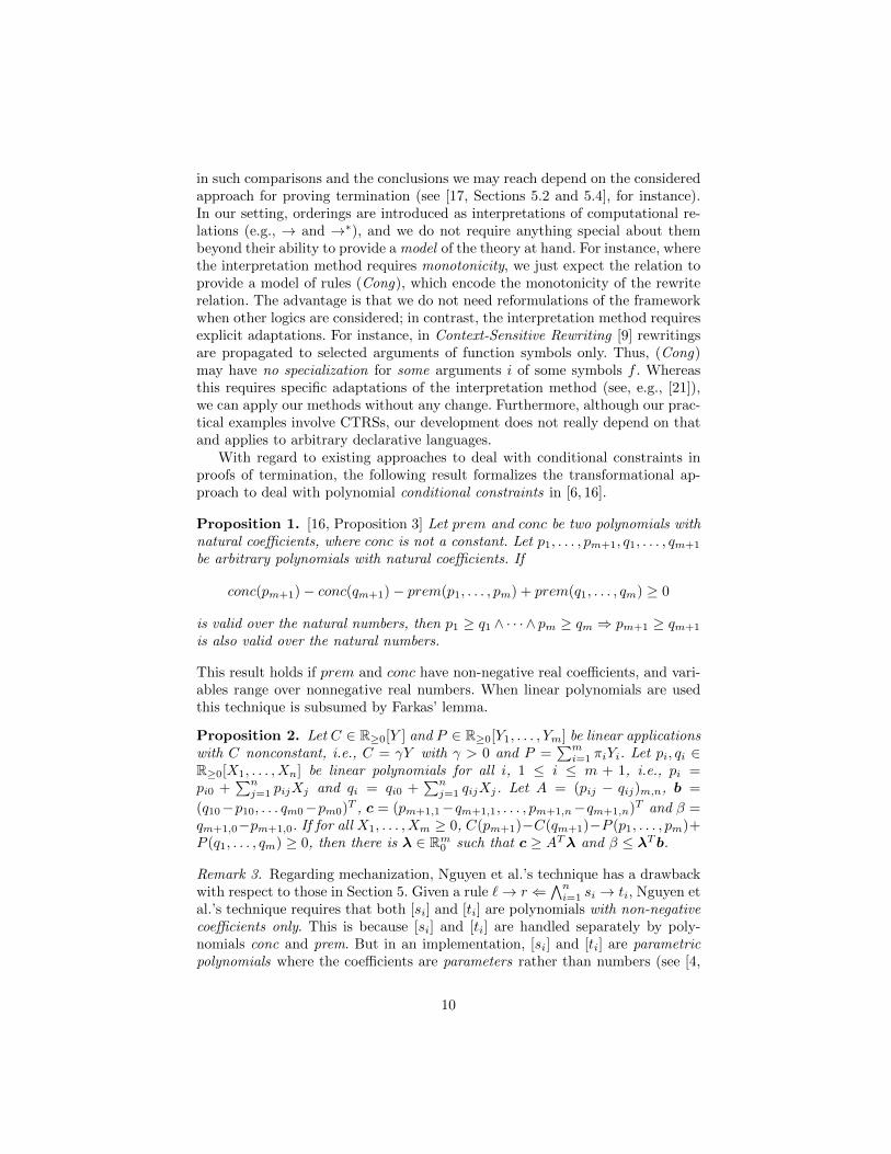
With regard to existing approaches to deal with conditional constraints inproofs of termination, the following result formalizes the transformational ap-proach to deal with polynomial conditional constraints in [6, 16].

Proposition 1. [16, Proposition 3] Let prem and conc be two polynomials withnatural coefficients, where conc is not a constant. Let p1, . . . , pm+1, q1, . . . , qm+1

be arbitrary polynomials with natural coefficients. If

conc(pm+1)− conc(qm+1)− prem(p1, . . . , pm) + prem(q1, . . . , qm) ≥ 0

is valid over the natural numbers, then p1 ≥ q1 ∧ · · · ∧ pm ≥ qm ⇒ pm+1 ≥ qm+1

is also valid over the natural numbers.

This result holds if prem and conc have non-negative real coefficients, and vari-ables range over nonnegative real numbers. When linear polynomials are usedthis technique is subsumed by Farkas’ lemma.

Proposition 2. Let C ∈ R≥0[Y ] and P ∈ R≥0[Y1, . . . , Ym] be linear applicationswith C nonconstant, i.e., C = γY with γ > 0 and P =

∑mi=1 πiYi. Let pi, qi ∈

R≥0[X1, . . . , Xn] be linear polynomials for all i, 1 ≤ i ≤ m + 1, i.e., pi =pi0 +

∑nj=1 pijXj and qi = qi0 +

∑nj=1 qijXj. Let A = (pij − qij)m,n, b =

(q10−p10, . . . qm0−pm0)T , c = (pm+1,1−qm+1,1, . . . , pm+1,n−qm+1,n)T and β =qm+1,0−pm+1,0. If for all X1, . . . , Xm ≥ 0, C(pm+1)−C(qm+1)−P (p1, . . . , pm)+P (q1, . . . , qm) ≥ 0, then there is λ ∈ Rm0 such that c ≥ ATλ and β ≤ λT b.

Remark 3. Regarding mechanization, Nguyen et al.’s technique has a drawbackwith respect to those in Section 5. Given a rule `→ r ⇐

∧ni=1 si → ti, Nguyen et

al.’s technique requires that both [si] and [ti] are polynomials with non-negativecoefficients only. This is because [si] and [ti] are handled separately by poly-nomials conc and prem. But in an implementation, [si] and [ti] are parametricpolynomials where the coefficients are parameters rather than numbers (see [4,

10

10] for instance). Thus, we need to constrain them to be non-negative in order touse the technique. In contrast, we do not restrict the coefficients of polynomialsin any way. Hence, the coefficients of the parametric polynomials could be neg-ative numbers without any problem. For instance, this is crucial to synthesizeD(A, b) = [0, 1] used in the examples above, where A and b require negativenumbers.

Farkas’ Lemma is used in proofs of termination of imperative programs in [19].

7 Conclusion

We have provided a generic, logic-oriented approach to abstraction in proofs oftermination of programs in declarative languages, which is based on defining ap-propriate models for logics. We have used numeric domains defined as restrictionsof ‘big’ numeric sets by means of predicates that can be handled as conditionalconstraints. We have introduced convex domains and used them to extend thepowerful matrix interpretation method for proving termination of TRSs in twodirections: the use of convex domains and the application to other logics (e.g.,CTRSs). We have shown the usefulness of these general purpose ideas by ap-plying them to prove operational termination of CTRSs: R in Example 1 couldnot be handled within the recently introduced 2D DP framework for provingoperational termination of CTRSs [13] or its extensions [14]; but the weaknesswas not in the framework itself, but in the available algebraic interpretations: wecan prove R operationally terminating now due to the use of a convex domainlike [0, 1]. And powerful tools like AProVE do not find a proof of operationaltermination of R in Example 10 by using transformations. In contrast, we founda simple proof with convex matrix interpretations and the techniques in [13].

We have shown that existing, powerful techniques to deal with numericconstraints provide an appropriate framework for implementing the previoustechniques. We have implemented most of these techniques as part of our toolmu-term [1]. In particular, the use of Farkas’ Lemma for dealing with linear con-ditional constraints obtained from linear polynomial interpretations and matrixinterpretations plays a central role in the implementation of the 2D DP frame-work for operational termination of CTRSs [13] which is presented in [14]. In [10,Example 13], we advocate the use of negative coefficients in proofs of termina-tion of CSR using polynomial interpretations. The implementation, though, wastricky (see [10, Sections 6.1.3 and 7]). This paper is a step forward because: (1)our treatment is valid for arbitrary polynomials. We do not need to provide spe-cial results as [10, Observation 1] to deal with polynomials of some specific form(quadratic, cubic, ...); (2) we avoid the introduction of disjunctive constraintswhich lead to an exponential blowup and to an expensive constraint solving pro-cess; and (3) we admit negative numbers everywhere. They are treated as anyother number and there is no need to ‘assert’ which of the coefficients could benegative in order to handle them apart (see [10, Section 7] and [10, Example 20]).However, much work is necessary to make fully general use of these techniquesin practical applications. We plan to address these issues in the near future.

11

References

1. B. Alarcon, R. Gutierrez, S. Lucas, R. Navarro-Marset. Proving Termination Prop-erties with MU-TERM. In Proc. of AMAST’10, LNCS 6486:201-208, 2011.

2. B. Alarcon, S. Lucas, R. Navarro-Marset. Using Matrix Interpretations over theReals in Proofs of Termination. In Proc. of PROLE’09. pages 255-264, 2009.

3. M. Clavel, F. Duran, S. Eker, P. Lincoln, N. Martı-Oliet, J. Meseguer, and C. Tal-cott. All About Maude – A High-Performance Logical Framework. Lecture Notesin Computer Science 4350, 2007.

4. E. Contejean, C. Marche, A.-P. Tomas, and X. Urbain. Mechanically provingtermination using polynomial interpretations. J. of Aut. Reas., 34(4):325-363, 2006.

5. J. Endrullis, J. Waldmann, and H. Zantema. Matrix Interpretations for ProvingTermination of Term Rewriting. J. of Aut. Reas. 40(2-3):195-220, 2008.

6. C. Fuhs, J. Giesl, A. Middeldorp, P. Schneider-Kamp, R. Thiemann, and H. Zankl.Maximal Termination. In Proc. of RTA’08, LNCS 5117:110-125, 2008.

7. K. Futatsugi and R. Diaconescu. CafeOBJ Report. World Scientific, AMASTSeries, 1998.

8. P. Hudak, S.J. Peyton-Jones, and P. Wadler. Report on the Functional Program-ming Language Haskell: a non–strict, purely functional language. Sigplan Notices,27(5):1-164, 1992.

9. S. Lucas. Context-sensitive computations in functional and functional logic pro-grams. Journal of Functional and Logic Programming, 1998(1):1-61, January 1998.

10. S. Lucas. Polynomials over the reals in proofs of termination: from theory topractice. RAIRO Theoretical Informatics and Applications, 39(3):547-586, 2005.

11. S. Lucas, C. Marche, and J. Meseguer. Operational termination of conditionalterm rewriting systems. Information Processing Letters, 95:446–453, 2005.

12. S. Lucas and J. Meseguer. Proving Operational Termination Of Declarative Pro-grams In General Logics. In Proc. of PPDP’14, pages 111-122, ACM Digital Li-brary, 2014.

13. S. Lucas and J. Meseguer. 2D Dependency Pairs for Proving Operational Termi-nation of CTRSs. In Proc. of WRLA’14, LNCS vol. 8663, to appear, 2014.

14. S. Lucas, J. Meseguer, and R. Gutierrez. Extending the 2D DP Framework forCTRSs. In Selected papers of LOPSTR’14, LNCS to appear, 2015.

15. J. Meseguer. General Logics. In H.-D. Ebbinghaus et al., editors, Logic Collo-quium’87, pages 275-329, North-Holland, 1989.

16. M.T. Nguyen, D. de Schreye, J. Giesl, and P. Schneider-Kamp. Polytool: Poly-nomial interpretations as a basis for termination of logic programs. Theory andPractice of Logic Programming 11(1):33-63, 2011.

17. E. Ohlebusch. Advanced Topics in Term Rewriting. Springer-Verlag, Apr. 2002.18. A. Prestel and C.N. Delzell. Positive Polynomials. From Hilbert’s 17th Problem

to Real Algebra. Springer-Verlag, Berlin, 2001.19. A. Podelski and A. Rybalchenko. A Complete Method for the Synthesis of Linear

Ranking Functions, In Proc. of VMCAI’04, LNCS 2937:239 - 251, 2004.20. A. Schrijver. Theory of linear and integer programming. John Wiley & sons, 1986.21. H. Zantema. Termination of Context-Sensitive Rewriting. In Proc. of RTA’97,

LNCS 1232:172-186, Springer-Verlag, Berlin, 1997.

12