1 The Foundations: Logic and Proofs

IntroductionThis chapter describes how Mathematica can be used to further your understanding of logic andproofs. In particular, we describe how to construct truth tables, check the validity of logical arguments,and verify logical equivalence. In the final two sections, we provide examples of how Mathematica canbe used as part of proofs, specifically to find counterexamples, carry out proofs by exhaustion, and tosearch for witnesses for existence proofs.

1.1 Propositional LogicIn this section, we will discuss how to use Mathematica to explore propositional logic. Specifically, wewill see how to use logical connectives, describe the connection between logical implication and condi-tional statements in a program, show how Mathematica can be used to create truth tables for compoundpropositions, and demonstrate how Mathematica can be used to carry out bit operations.In Mathematica, the truth values true and false are represented by the symbols True and False.Propositions can be represented by symbols (variables) such as p, q, or prop1. Note that if you havenot yet made an assignment to a symbol, entering it will return the name.

In[1]:= prop1

Out[1]= prop1

Once you have assigned a value, Mathematica will evaluate the symbol to the assigned value wheneverit appears.

In[2]:= prop1 = True

Out[2]= True

In[3]:= prop1

Out[3]= True

You can cause Mathematica to “forget” the assigned value using either the function Clear or theUnset (=.) operator. Both of the expressions below have the effect of removing the assigned valuefrom the symbol prop1. Neither expression returns an output.

In[4]:= Clear@prop1D

In[5]:= prop1 =.

Logical ConnectivesMathematica supports all of the basic logical operators discussed in the textbook. We illustrate thelogical operators of negation (Not, !), conjunction (And, &&), disjunction (Or, ||), exclusive or(Xor), implication (Implies), and the biconditional (Equivalent). Note that these are referred toas Boolean operators, and expressions formed from them are Boolean expressions. For all of the operators, you can enter expressions in standard form, that is, by putting the names of theoperators at the head of an expression with truth values or other expressions as operands. For example,the computations T fi F, T fl HF fl TL, and T Å⊕ T are shown below.

In[6]:= Or@True, FalseD

Out[6]= True

In[7]:= Implies@True, And@False, TrueDD

Out[7]= False

In[8]:= Xor@True, TrueD

Out[8]= False

For negation, conjunction, and disjunction, you can use the infix operators !, &&, and || instead.These are common symbols used in place of ¬, fl, and fi that can be easily typed on a standard key-board. The computations below show Ÿ T and HT fiFL flT using the operators !, &&, and ||.

In[9]:= ! True

Out[9]= False

In[10]:= HTrue »» FalseL && True

Out[10]= True

Mathematica also allows you to enter and compute with expressions using the traditional symbols. Youenter the symbol by pressing the escape key, followed by a sequence identifying the symbol, and thenthe escape key once again. Mathematica refers to this as an alias. For example, entering ÂandÂproduces the traditional symbol for conjunction.

In[11]:= True Ï False

Out[11]= False

An alias is the only way to produce an infix implication operator, via Â=>Â (escape followed byequals and the greater than sign and terminating with escape).

In[12]:= False fl False

Out[12]= True

In this manual, we will typically not use aliases as part of commands, since it is more difficult for areader to imitate such commands. However, for convenience, we include a table of the operatorsdefined in the textbook along with their names in Mathematica and their infix representations with andwithout aliases.

name function without alias alias symbolnegation Not ! Ânot Ÿ

conjunction And && Âand Ï

exclusive or Xor Âxor „disjunction Or »» Âor Í

biconditional Equivalent Âequiv Íimplication Implies Â=> fl

2 Chapter01.nb

name function without alias alias symbolnegation Not ! Ânot Ÿ

conjunction And && Âand Ï

exclusive or Xor Âxor „disjunction Or »» Âor Í

biconditional Equivalent Âequiv Íimplication Implies Â=> fl

Note that the symbol for exclusive or used by Mathematica differs from that in the textbook. Also, theorder in which the operators appear in the table above is the order of precedence that the operatorshave in Mathematica. Observe that the order of the biconditional and implication are the reverse of theorder specified in the textbook. It is always a good idea to use parentheses liberally whenever prece-dence is in doubt.

Conditional StatementsWe saw above that Mathematica includes the operator Implies for evaluating logical implication. Inmathematical logic, “if p, then q” has a very specific meaning, as described in detail in the text. Incomputer programming, and Mathematica in particular, conditional statements also appear very fre-quently, but have a slightly different meaning.From the perspective of logic, a conditional statement is, like any other proposition, a sentence that iseither true or false. In most computer programming languages, when we talk about a conditional state-ment, we are not referring to a kind of proposition. Rather, conditional statements are used to selec-tively execute portions of code. Consider the following example of a function, which adds 1 to theinput value if the input is less than or equal to 5 and not otherwise.

In[13]:= ifExample@x_D := If@x § 5, x + 1, xD

(To type the inequality into Mathematica, you type “x<=5”. The graphical front end will automaticallyturn the key combination “<=” into §, unless you have set options to prevent it from doing so.) Wenow see that this function works as promised.

In[14]:= ifExample@3D

Out[14]= 4

In[15]:= ifExample@7D

Out[15]= 7

Because this is our first Mathematica function, let’s spend a moment breaking down the general struc-ture before detailing the workings of the conditional statement. First we have the name of the function,ifExample. Note that symbols for built-in Mathematica functions typically begin with capital letters,so making a habit of naming functions you define with initial letters lower case helps ensure that youwon’t accidentally try to assign to a built-in function. Following the name of the function, we specify the arguments that will be accepted by the functionenclosed in brackets. The underscore (_), referred to as Blank, tells Mathematica that this is a parame-ter and that the symbol preceding the underscore is the name that will be used to refer to the parameter. Then comes the operator :=, the delayed assignment operator. The difference between using Set (=)and SetDelayed (:=) is that the delayed assignment ensures that Mathematica does not attempt toevaluate the function definition until the function is actually invoked. SetDelayed (:=) should beused when you define a function, while Set (=) is appropriate for assigning values to variables.

Chapter01.nb 3

Then comes the operator :=, the delayed assignment operator. The difference between using Set (=)and SetDelayed (:=) is that the delayed assignment ensures that Mathematica does not attempt toevaluate the function definition until the function is actually invoked. SetDelayed (:=) should beused when you define a function, while Set (=) is appropriate for assigning values to variables.On the right hand side of the delayed assignment operator is the expression that tells Mathematicawhat to do with the argument. In this case, the body of the function makes use of the If function tochoose between two possible results. Note that we provided three arguments, separated by commas, toIf. The first argument, x<=5, specifies the condition. Mathematica evaluates this expression to deter-mine which of the branches, that is which of the other two arguments, to execute. If the condition istrue, then Mathematica evaluates the second argument, x+1, and this is the value of the function. Thisis traditionally called the “then” clause. If the condition specified in the first argument is false, then thethird argument, called the “else” clause, is evaluated.It is important to be aware of two additional variations on the If function. First, you are allowed toomit the “else” and provide only two arguments. As you can see in the example below, when thecondition is false, Mathematica appears to return nothing. In fact, the expression returns the specialsymbol Null, which does not produce output.

In[16]:= If@3 < 1, 5D

The second variation on If has four arguments. Mathematica is very strict with regards to conditionalstatements. Specifically, it only evaluates the second argument if the result of evaluating the conditionis the symbol True. And it only evaluates the third argument when the result of the condition isFalse. But many expressions do not evaluate to either of these symbols. In these cases, Mathematicareturns the If function unevaluated. For example, in the expression below, the symbol z has not beenassigned a value and thus z>5 cannot be resolved to a truth value.

In[17]:= If@z > 5, 4, 11D

Out[17]= If@z > 5, 4, 11D

By specifying a fourth argument, you can give Mathematica explicit instructions on how to handle thissituation.

In[18]:= If@z > 5, 4, 11, 0D

Out[18]= 0

This fourth argument is useful if there is some question of whether or not Mathematica will be able toresolve the condition into a truth value. We will typically not use the fourth argument, however, sincein nearly all cases, a failure to properly evaluate the condition indicates an error in either our functiondefinition or the input to it and providing the fourth argument will only hide such errors from us.

Evaluating ExpressionsIn the textbook, you saw how to construct truth tables by hand. Here we’ll see how to have Mathemat-ica create them for us. We’ll begin by considering the simplest case of a compound proposition: thenegation of a single propositional variable.

In[19]:= prop2 := ! p

Note that we’ve defined the proposition prop2 as an expression in terms of the symbol p, which hasnot been assigned. We can determine the truth value of prop2 in one of two ways. The obvious way isto assign a truth value to p and then ask Mathematica for the value of prop2 as follows.

4 Chapter01.nb

Note that we’ve defined the proposition prop2 as an expression in terms of the symbol p, which hasnot been assigned. We can determine the truth value of prop2 in one of two ways. The obvious way isto assign a truth value to p and then ask Mathematica for the value of prop2 as follows.

In[20]:= p = False

Out[20]= False

In[21]:= prop2

Out[21]= True

The drawback of this approach, however, is that our variable p is now identified with false and if wewant to use it as a name again, we need to manually unassign it.

In[22]:= p =.

The better approach is to use the ReplaceAll operator (/.). This function has a variety of uses, oneof which is to allow you to evaluate an expression for particular values of variables without the need toassign (and then Clear) values to the variables. We first demonstrate its use and then we’ll explainthe syntax.

In[23]:= prop2 ê. p Ø True

Out[23]= False

On the left hand side of the /. operator is the expression to be evaluated. In this case, we have thesymbol prop2 on the left, which was assigned to be !p. On the right hand side of the operator, weindicate the substitution to be made using the notation aØb, called a rule, to indicate that a is replacedby b. (Note that you obtain the arrow by typing a hyphen followed by the greater than symbol (->).The Mathematica front end will automatically turn that into the arrow character.)In order to substitute for more than one variable, list the substitutions as rules separated by commasand enclosed in braces. The following evaluates the proposition pÏ HŸ qL for p true and q false.

In[24]:= p && H! qL ê. 8p Ø True, q Ø False<

Out[24]= True

Truth Tables and LoopsMathematica has a built-in function for producing a truth table, BooleanTable, which will bedescribed in Section 1.2. While the built-in function is useful, it is worthwhile to consider how suchtables can be created using more primitive programming tools. In this subsection, we will see how tocreate truth tables using only basic loop constructs.To make a truth table for a proposition, we need to evaluate the proposition at all possible truth valuesof all of the different variables. To do this, we make use of loops (refer to the Introduction for a generaldiscussion of loops in Mathematica). Specifically, we want to loop over the two possible truth values,true and false, so we will construct a loop over the list {True, False}.In Mathematica, the Do function is used to create a loop that executes commands for each member of alist. The Do function requires two arguments. The first argument is the expression that you want evalu-ated, typically involving one or more variables that change during the execution of the loop. The sec-ond argument specifies the iterative behavior and can take several forms. The form we will be usinghere is 8i, 8i1, i2, …<<. The character i represents the loop variable and the list 8i1, i2, …< represents anexplicit list of particular values that will be assigned to the loop variable.The first example will be to produce a truth table for the proposition Ÿ p. Each iteration in the loop,therefore, should print out one line of the truth table. Since a Do loop does not produce any outputunless explicitly told to do so (it normally returns Null), we will use the Print function to tell theloop what should be displayed. The Print function takes any number of arguments and displays themconcatenated together. In this example, we want to display the value of the propositional variable p andthe truth value of the proposition Ÿ p. We will also explicitly insert some space between the two truthvalues by putting “ “ as an argument as well. So the first argument to Do will be Print[p,”“,!p].

Chapter01.nb 5

The first example will be to produce a truth table for the proposition Ÿ p. Each iteration in the loop,therefore, should print out one line of the truth table. Since a Do loop does not produce any outputunless explicitly told to do so (it normally returns Null), we will use the Print function to tell theloop what should be displayed. The Print function takes any number of arguments and displays themconcatenated together. In this example, we want to display the value of the propositional variable p andthe truth value of the proposition Ÿ p. We will also explicitly insert some space between the two truthvalues by putting “ “ as an argument as well. So the first argument to Do will be Print[p,”“,!p].For the second argument, the specification of the iteration, we must give Mathematica the name of theloop variable, in this case p, and the list of values that we want assigned to that variable in each itera-tion, namely true and false. So the second argument will be {p,{True,False}}.

In[25]:= Do@Print@p, " ", ! pD, 8p, 8True, False<<D

True False

False True

As a second example, we will construct the truth table for HpÏ qL fl p. Notice that here there are twovariables instead of one. This indicates that two loops should be used, one for each variable. In mostprogramming languages, this is approach that you would need to take, called “nesting” loops. In effect,you would use a Do function as the first argument to another Do function. Indeed, this approach wouldwork in Mathematica as well, but there is another way. The Do syntax allows you to provide more thanone iteration specification. For this example, we want both variables p and q to take on both truthvalues, so we provide the iteration specifications for both of them. Mathematica ensures that it exe-cutes the expression in the first argument with every possible pair of values for p and q.

In[26]:= Do@Print@p, " ", q, " ", Implies@p && q, pDD,8p, 8True, False<<, 8q, 8True, False<<D

True True True

True False True

False True True

False False True

Note that the output indicates that the proposition, HpÏ qL fl p, is a tautology. In fact, this is a rule ofinference called simplification, discussed in Section 1.6 of the textbook.

Logic and Bit OperationsWe can also use Mathematica to explore the bit operations OR, AND, and XOR. Recall that bit opera-tions correspond to logical operators by equating 1 with true and 0 with false. Mathematica provides alot of support for working with bits and bit strings. Here, we will briefly introduce the relevant Mathe-matica functions. Our main goal of this section, however, will be to develop a function essentially fromscratch for computing with bit strings, in order to further illustrate programming in Mathematica.The Built-in FunctionsMathematica provides several functions corresponding to the basic logical operations for operation onbits: BitAnd, BitOr, BitXor, BitNot. With the exception of BitNot, these operations operateas you would expect. For example, you can compute 1fl 0 as follows.

6 Chapter01.nb

Mathematica provides several functions corresponding to the basic logical operations for operation onbits: BitAnd, BitOr, BitXor, BitNot. With the exception of BitNot, these operations operateas you would expect. For example, you can compute 1fl 0 as follows.

In[27]:= BitAnd@1, 0D

Out[27]= 0

Also, you are not limited to two arguments. For example, computing 0fi 0fi 1fi 0 requires only oneapplication of BitOr.

In[28]:= BitOr@0, 0, 1, 0D

Out[28]= 1

Conveniently, the bitwise functions are Listable. This means that the function is automaticallythreaded over lists that are given as arguments. This can be made clearer by demonstrating withanother listable function: addition.

In[29]:= 81, 2, 3< + 8a, b, c<

Out[29]= 81 + a, 2 + b, 3 + c<

Because addition is listable, when it is applied to two lists of equal length, it returns the list formed byacting on corresponding elements of the lists. In the current context, this means we can apply thebitwise operations to bit strings by representing the bit strings a lists. For example, 10 010fl 01 011 canbe computed as follows.

In[30]:= BitAnd@81, 0, 0, 1, 0<, 80, 1, 0, 1, 1<D

Out[30]= 80, 0, 0, 1, 0<

The bitwise functions actually operate on integers, not just the bits 0 and 1. For example, we can applyBitOr to 18 and 5.

In[31]:= BitOr@18, 5D

Out[31]= 23

The reason for this result is that Mathematica applied the bitwise OR to the binary representations ofthe integers 18 and 5. You can use the function IntegerDigits with an integer as the first coordi-nate and 2 as the second coordinate to see the binary representation of an integer.

In[32]:= IntegerDigits@18, 2D

Out[32]= 81, 0, 0, 1, 0<

In[33]:= IntegerDigits@5, 2D

Out[33]= 81, 0, 1<

We need to pad the result for 5 with 0s in order to have lists of equal size and then we can applyBitOr on the lists of bits as we did above.

In[34]:= BitOr@81, 0, 0, 1, 0<, 80, 0, 1, 0, 1<D

Out[34]= 81, 0, 1, 1, 1<

The FromDigits function reverses IntegerDigits. Given a list of bits and second argument 2, itwill return the integer with that binary representation.

Chapter01.nb 7

In[35]:= FromDigits@81, 0, 1, 1, 1<, 2D

Out[35]= 23

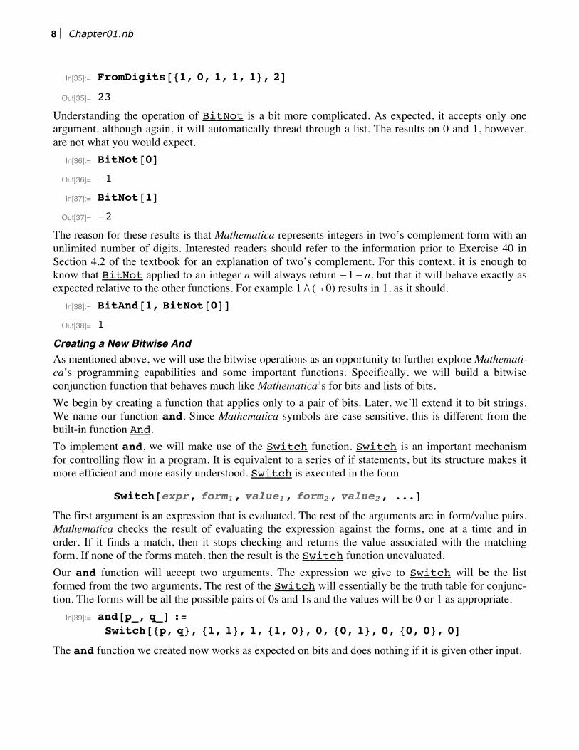
Understanding the operation of BitNot is a bit more complicated. As expected, it accepts only oneargument, although again, it will automatically thread through a list. The results on 0 and 1, however,are not what you would expect.

In[36]:= BitNot@0D

Out[36]= -1

In[37]:= BitNot@1D

Out[37]= -2

The reason for these results is that Mathematica represents integers in two’s complement form with anunlimited number of digits. Interested readers should refer to the information prior to Exercise 40 inSection 4.2 of the textbook for an explanation of two’s complement. For this context, it is enough toknow that BitNot applied to an integer n will always return -1- n, but that it will behave exactly asexpected relative to the other functions. For example 1fl HŸ 0L results in 1, as it should.

In[38]:= BitAnd@1, BitNot@0DD

Out[38]= 1

Creating a New Bitwise AndAs mentioned above, we will use the bitwise operations as an opportunity to further explore Mathemati-ca’s programming capabilities and some important functions. Specifically, we will build a bitwiseconjunction function that behaves much like Mathematica’s for bits and lists of bits. We begin by creating a function that applies only to a pair of bits. Later, we’ll extend it to bit strings.We name our function and. Since Mathematica symbols are case-sensitive, this is different from thebuilt-in function And. To implement and, we will make use of the Switch function. Switch is an important mechanismfor controlling flow in a program. It is equivalent to a series of if statements, but its structure makes itmore efficient and more easily understood. Switch is executed in the form

Switch@expr, form1, value1, form2, value2, ...D

The first argument is an expression that is evaluated. The rest of the arguments are in form/value pairs.Mathematica checks the result of evaluating the expression against the forms, one at a time and inorder. If it finds a match, then it stops checking and returns the value associated with the matchingform. If none of the forms match, then the result is the Switch function unevaluated. Our and function will accept two arguments. The expression we give to Switch will be the listformed from the two arguments. The rest of the Switch will essentially be the truth table for conjunc-tion. The forms will be all the possible pairs of 0s and 1s and the values will be 0 or 1 as appropriate.

In[39]:= and@p_, q_D :=Switch@8p, q<, 81, 1<, 1, 81, 0<, 0, 80, 1<, 0, 80, 0<, 0D

The and function we created now works as expected on bits and does nothing if it is given other input.

8 Chapter01.nb

In[40]:= and@1, 1D

Out[40]= 1

In[41]:= and@1, 0D

Out[41]= 0

In[42]:= and@18, 5D

Out[42]= Switch@818, 5<,81, 1<, 1,81, 0<, 0,80, 1<, 0,80, 0<, 0D

We can handle non-bit input a bit more elegantly by adding one more form/value pair. Using a blank(_) for the form will create a default value. By creating a message associated to the and function, wecan display a useful error message, as shown below. The message is defined by setting the symbolf ::tag equal to the message in quotation marks, where f is the name of the function and tag is the“name” of the message. When this symbol is given as the argument to the Message function, themessage is shown.

In[43]:= and::arg = "and called with non-bit arguments.";

In[44]:= and@p_, q_D := Switch@8p, q<, 81, 1<, 1, 81, 0<,0, 80, 1<, 0, 80, 0<, 0, _, Message@and::argDD

Now, applying and to 18 and 5 has a more useful result.In[45]:= and@18, 5D

and::arg : and called with non-bit arguments.

Threading and ListableWe saw above that Mathematica’s built-in function would extend to lists of integers without any addi-tional effort on our part. Here we’ll see that it’s easy to make our function do that as well.Mathematica provides a general way to cause a function to be applied to lists in the functions Map andMapThread. We describe Map first.

Given a function of one argument, such as f HxL = x2, Map allows you to have Mathematica apply thefunction to all the elements of a list. First, define the function.

In[46]:= f@x_D := x^2

Now, call Map with the name of the function as the first argument and the list of input values as thesecond.

In[47]:= Map@f, 81, 2, 3, 4, 5, 6<D

Out[47]= 81, 4, 9, 16, 25, 36<

The result, as you see above, is the list of the results of applying the function to each element of thelist. The same result can be obtained with the /@ operator, as shown below.

Chapter01.nb 9

In[48]:= f êü 81, 2, 3, 4, 5, 6<

Out[48]= 81, 4, 9, 16, 25, 36<

When the function has more than one argument, as and does, MapThread can be used. Like Map,MapThread takes two arguments and the first is a function. The second argument is a list of lists.Provided that each of the inner lists is of the same length, the result of MapThread is the list formedby evaluating the function with arguments from corresponding positions in the lists. For example, wecan apply gHx, yL = x2 + y3 to 81, 2, 3< and 8a, b, c<.

In[49]:= g@x_, y_D := x^2 + y^3

In[50]:= MapThread@g, 881, 2, 3<, 8a, b, c<<D

Out[50]= 91 + a3, 4 + b3, 9 + c3=

Using MapThread, we can compute 10 010fl 01 011 as follows.In[51]:= MapThread@and, 881, 0, 0, 1, 0<, 80, 1, 0, 1, 1<<D

Out[51]= 80, 0, 0, 1, 0<

This shows how to thread a function in a particular case. But what we really want is for our and func-tion to behave like this automatically. Fortunately, this is such a common requirement for functions,that Mathematica provides a very easy way to do this automatically. The attribute Listable, whenapplied to a function, tells Mathematica that the function should be automatically threaded over listswhenever the function is given a list as its argument. The SetAttributes function causes Mathemat-ica to associate the attribute specified in the second argument with the object in the first argument.

In[52]:= SetAttributes@and, ListableD

Now applying and to lists works just as the built-in BitAnd does.In[53]:= and@81, 0, 0, 1, 0<, 80, 1, 0, 1, 1<D

Out[53]= 80, 0, 0, 1, 0<

1.2 Applications of Propositional LogicIn this section we will describe how Mathematica’s computational abilities can be used to solveapplied problems in propositional logic. In particular, we will consider consistency for system specifica-tions and Smullyan logic puzzles.

System SpecificationsThe textbook describes how system specifications can be translated into propositional logic and how itis important that the specifications be consistent. As suggested by the textbook, one way to determinewhether a set of specifications is consistent is with truth tables.Recall that a collection of propositions is consistent when there is an assignment of truth values to thepropositional variables that makes all of the propositions in the collection true simultaneously. Forexample, consider the following collection of compound propositions: p Ø HqÏ rL, pÍ q, and pÍŸ r.We can see that these propositions are consistent because we can satisfy all three with the assignment p= false, q = true, r = false. In Mathematica, we can confirm this by evaluating the list of propositionswith that assignment of truth values.

10 Chapter01.nb

Recall that a collection of propositions is consistent when there is an assignment of truth values to thepropositional variables that makes all of the propositions in the collection true simultaneously. Forexample, consider the following collection of compound propositions: p Ø HqÏ rL, pÍ q, and pÍŸ r.We can see that these propositions are consistent because we can satisfy all three with the assignment p= false, q = true, r = false. In Mathematica, we can confirm this by evaluating the list of propositionswith that assignment of truth values. Above we saw that you can evaluate an expression using the replacement operator /.. On the left sideof the replacement operator, put the expression we want evaluated, in this case a list of the three logicalpropositions. On the right side of the /., enter the assignments as a list of rules of the form s->v forsymbol s and value v.

In[54]:= 8Implies@p, q && rD, p »» q, p »» H! rL< ê.8p Ø False, q Ø True, r Ø False<

Out[54]= 8True, True, True<

To determine if a collection of propositions is consistent, we can create a truth table. In the previoussection, we created truth tables from scratch using the Do function to loop through all possible assign-ments of truth values to the variables. In this section, we’ll instead use Mathematica’s built-in functionBooleanTable.The BooleanTable function produces the truth values obtained by replacing the variables by allpossible combinations of true and false. Its first argument is the expression to be evaluated and thesecond argument is a list of the propositional variables.

In[55]:= BooleanTable@p && H! qL, 8p, q<D

Out[55]= 8False, True, False, False<

Note that, unlike a truth table you construct by hand, BooleanTable does not show the assignmentsto the propositional variables. We can see the values of the propositional variables by making the firstargument a list that includes them.

In[56]:= BooleanTable@8p, q, p && H! qL<, 8p, q<D

Out[56]= 88True, True, False<, 8True, False, True<,8False, True, False<, 8False, False, False<<

The TableForm function will make the output easier to read. We will apply TableForm with thepostfix operator (//). The postfix operator allows you to put the name of a function after an expres-sion. It is commonly used for functions that affect the display of a result and has the benefit of makingthe main part of the command being evaluated easier to read.

In[57]:= BooleanTable@8p, q, p && H! qL<, 8p, q<D êê TableFormOut[57]//TableForm=

True True FalseTrue False TrueFalse True FalseFalse False False

Returning to the question of consistency, consider Example 4 from Section 1.2 of the text. We translatethe three specifications as the following list of propositions.

In[58]:= specEx4 = 8p »» q, ! p, Implies@p, qD<

Out[58]= 8p »» q, ! p, p fl q<

Chapter01.nb 11

Then we can construct the truth table using BooleanTable.In[59]:= BooleanTable@8p, q, specEx4<, 8p, q<D êê TableForm

Out[59]//TableForm=

True TrueTrueFalseTrue

True FalseTrueFalseFalse

False TrueTrueTrueTrue

False FalseFalseTrueTrue

Notice that because specEx4 is itself a list, TableForm displays the results from the three compo-nent propositions as a column within the row corresponding to the values for p and q. We see that theonly assignment of truth values that results in all three statements being satisfied is with p = false andq = true.We can make the output a bit easier to read if, instead of considering the truth table for the list of thepropositions, we consider the proposition formed by the conjunction of the individual propositions:HpÍ qL Ï HŸ pL Ï Hp Ø qL.

In[60]:= specEx4b = And@Hp »» qL, ! p, Implies@p, qDD

Out[60]= Hp »» qL && ! p && Hp fl qL

In[61]:= BooleanTable@8p, q, specEx4b<, 8p, q<D êê TableFormOut[61]//TableForm=

True True FalseTrue False FalseFalse True TrueFalse False False

In this case, the fact that the final truth value in the third row is true tells us that this assignment oftruth values satisfies all of the propositions in the system specification.Mathematica also has useful built-in functions for checking for consistency. The SatisfiableQfunction accepts the same arguments as BooleanTable (a Boolean expression and the list of proposi-tional variables). Note that you may not give a list of expressions as the first argument toSatisfiableQ.

In[62]:= SatisfiableQ@specEx4b, 8p, q<D

Out[62]= True

The SatisfiabilityInstances command will generate an assignment of truth values to thevariables that do in fact satisfy the proposition, assuming it is satisfiable.

12 Chapter01.nb

In[63]:= SatisfiabilityInstances@specEx4b, 8p, q<D

Out[63]= 88False, True<<

By providing a positive integer as an optional third argument, you can ask for more choices that makethe proposition true. Below, we find all 3 ways that p Ø q can be satisfied.

In[64]:= SatisfiabilityInstances@Implies@p, qD, 8p, q<, 3D

Out[64]= 88True, True<, 8False, True<, 8False, False<<

If we add, as in Example 5, the proposition Ÿ q, we see that all of the assignments yield false for theconjunction of all four propositions.

In[65]:= specEx5 = specEx4b && ! q

Out[65]= Hp »» qL && ! p && Hp fl qL && ! q

In[66]:= BooleanTable@8p, q, specEx5<, 8p, q<D êê TableForm

Out[66]//TableForm=True True FalseTrue False FalseFalse True FalseFalse False False

Also, note that SatisfiableQ returns false and SatisfiabilityInstances returns an emptylist.

In[67]:= SatisfiableQ@specEx5, 8p, q<D

Out[67]= False

In[68]:= SatisfiabilityInstances@specEx5, 8p, q<D

Out[68]= 8<

Logic PuzzlesRecall the knights and knaves puzzle presented in Example 7 of Section 1.2 of the text. In this puzzle,you are asked to imagine an island on which each inhabitant is either a knight and always tells the truthor is a knave and always lies. You meet two people named A and B. Person A says “B is a knight” andperson B says “The two of us are opposite types.” The puzzle is to determine which kind of inhabitantsA and B are.We can solve this problem with Mathematica using truth tables. First we must write A and B’s state-ments as propositions. Let a represent the statement that A is a knight and b the statement that B is aknight. Then A’s statement is “b”, and B’s statement is “HaÏŸ bL Í HŸ aÏ bL”, as discussed in the text.While these propositions precisely express the content of A and B’s assertions, it does not capture theadditional information that A and B are making the statements. We know, for instance, that A eitheralways tells the truth (knight) or always lies (knave). If A is a knight, then we know the statement “b”is true. If A is not a knight, then we know the statement is false. In other words, the truth value of theproposition a, that A is a knight, is the same as the truth value of A’s statement, and likewise for B.Therefore, we can capture the meaning of “A says proposition p” by the proposition a ¨ p. Using thefunction Equivalent, we can express the two statements in the puzzle in Mathematica as follows.

Chapter01.nb 13

While these propositions precisely express the content of A and B’s assertions, it does not capture theadditional information that A and B are making the statements. We know, for instance, that A eitheralways tells the truth (knight) or always lies (knave). If A is a knight, then we know the statement “b”is true. If A is not a knight, then we know the statement is false. In other words, the truth value of theproposition a, that A is a knight, is the same as the truth value of A’s statement, and likewise for B.Therefore, we can capture the meaning of “A says proposition p” by the proposition a ¨ p. Using thefunction Equivalent, we can express the two statements in the puzzle in Mathematica as follows.

In[69]:= ex7a = Equivalent@a, bD

Out[69]= a Í b

In[70]:= ex7b = Equivalent@b, Ha && ! bL »» H! a && bLD

Out[70]= b Í Ha && ! bL »» H! a && bL

Like the system specifications above, a solution to this puzzle will consist of an assignment of truthvalues to the propositions a and b that make both people’s statements true.

In[71]:= SatisfiabilityInstances@ex7a && ex7b, 8a, b<, 4D

Out[71]= 88False, False<<

We see that both statements are satisfied when both propositions a and b are false, that is, when A andB are both knaves. Note also that since we asked, in the final argument, for as many as 4 differentinstances but only one was returned, we know that this is the only solution to the puzzle.

1.3 Propositional EquivalenceIn this section we consider logical equivalence of propositions. We will first look at Mathematica’sbuilt-in functions for testing equivalence, and then we will create a function from scratch to accom-plish the same goal.

Built-in FunctionsTwo propositions p and q are logically equivalent if the proposition p ¨ q is a tautology. Mathematicaincludes a function for checking whether a proposition is a tautology, TautologyQ. This functionuses the same arguments as BooleanTable, SatisfiableQ, and SatisfiabilityIn-stances do, as described above. Specifically, the first argument should be the proposition and thesecond argument should be a list of the propositional variables. For example, we can confirm that the DeMorgan’s Law Ÿ HpÏ qL ª Ÿ pÍŸ q is a propositional equiva-lence as shown below.

In[72]:= TautologyQ@Equivalent@! Hp && qL, ! p »» ! qD, 8p, q<D

Out[72]= True

Remember that the Equivalent function, used above, is Mathematica’s function for forming thebiconditional proposition, and should not be confused with the notion of equivalence as used in Section1.3 of the textbook. Note that the second argument to TautologyQ is not generally necessary. Mathematica’s Boolean-Variables function, which determines the variables in a logical expression, will invisibly supply themissing argument. This is, in fact, true about most of the functions that require the variable list as thesecond argument. We demonstrate with the other DeMorgan’s Law.

In[73]:= TautologyQ@Equivalent@! Hp »» qL, ! p && ! qDD

Out[73]= True

You might find it convenient to have a single function that, given two propositions, will determinewhether they are logically equivalent. In Mathematica, this is easy to achieve. We just need to create afunction that takes two propositions, uses the Equivalent function to create the biconditional, andthen applies TautologyQ.

14 Chapter01.nb

You might find it convenient to have a single function that, given two propositions, will determinewhether they are logically equivalent. In Mathematica, this is easy to achieve. We just need to create afunction that takes two propositions, uses the Equivalent function to create the biconditional, andthen applies TautologyQ.

In[74]:= equivalentQ@p_, q_D := TautologyQ@Equivalent@p, qDD

We apply this function to see if we can generalize DeMorgan’s Laws to three variables.In[75]:= equivalentQ@! Hp »» q »» rL, ! p && ! q && ! rD

Out[75]= True

In[76]:= equivalentQ@! Hp && q && rL, ! p »» ! q »» ! rD

Out[76]= True

Built from Scratch FunctionMathematica provides very complete built-in support for working with logical propositions and, inparticular, checking propositional equivalence. Here, however, we are going to build a new functionfor checking whether or not two propositions are logically equivalent using a minimum of existinghigh-level functions. In fact, other than asking Mathematica to evaluate propositional expressions forparticular truth values assigned to propositional variables, we will make use only of Mathematica’sessential programming functionality.There are two goals here. First, to illustrate more of Mathematica’s programming abilities. Second, toreveal some of the more fundamental concepts and methods used in Mathematica. We will create a function myEquivalentQ, that has the same effect as the equivalentQ that webuilt above using Mathematica’s built-in functions. Specifically, it should take two propositions anddetermine whether or not they are equivalent. This will require quite a bit of work. The main hurdlesfor such a function are: (1) having Mathematica determine what propositional variables are used in theinput propositions, and (2) without a priori knowledge of the number of propositional variables, hav-ing Mathematica test every possible assignment of truth values. Note that we could avoid both of thesehurdles by insisting that the propositional variables be limited to a certain small set of symbols, per-haps p, q, r, and s. Then we could implement the function using a static nested Do loop.However, the two hurdles mentioned are not insurmountable, will provide a much more elegant andflexible procedure, and will also give us the opportunity to see examples of some important program-ming constructs.Extracting VariablesThe first hurdle is to get Mathematica to determine the variables used in a logical expression. Considerthe following example.

In[77]:= variableEx = HHp && qL »» Hp && ! rLL && Implies@s, rD

Out[77]= HHp && qL »» Hp && ! rLL && Hs fl rL

Our task is to write a function that will, given the above expression, tell us that the variables in use arep, q, r, and s.

Chapter01.nb 15

Replacing the HeadFundamentally, everything in Mathematica is an expression. And every expression is of the formheadAarg1, arg2, ...E, that is, a head followed by arguments in brackets and separated bycommas. You can see this structure at the heart of any expression by using the FullForm function.Below, we show the full form of three examples. Recall that the postfix operator (//) allows us to putthe name of the function at the end of the input.

In[78]:= x + y êê FullFormOut[78]//FullForm=

Plus@x, yD

In[79]:= variableEx êê FullFormOut[79]//FullForm=

And@Or@And@p, qD, And@p, Not@rDDD, Implies@s, rDD

In[80]:= 8p, q, r, s< êê FullFormOut[80]//FullForm=

List@p, q, r, sD

Mathematica provides a function, Head, that takes an expression and returns the type of head of thatexpression.

In[81]:= Head@x + yD

Out[81]= Plus

In[82]:= Head@variableExD

Out[82]= And

In[83]:= Head@8p, q, r, s<D

Out[83]= List

You can also access the head of an expression using the Part ([[…]]) operator with index 0.In[84]:= Hx + yL@@0DD

Out[84]= Plus

In[85]:= variableEx@@0DD

Out[85]= And

In[86]:= 8p, q, r, s<@@0DD

Out[86]= List

Remember that our goal here is to transform a logical expression, such asHHpÏ qL Í HpÏŸ rLL Ï Hs Ø rL into a list 8p, q, r, s<. Since the main difference, in terms of the internalrepresentation of the two objects, is their heads, it is natural to ask if we can change the head. In particu-lar, in our example variableEx, the head is And. If we can replace the And head with a List head,we would have a list comprised of the two parts of the expression, as illustrated below.

16 Chapter01.nb

In[87]:= List@Or@And@p, qD, And@p, Not@rDDD, Implies@s, rDD

Out[87]= 8Hp && qL »» Hp && ! rL, s fl r<

Our strategy, broadly, will be to replace all of the heads in the logical expression with List heads.There are two approaches to replacing the head of an expression. One is to use the fact that the headlies at index 0 to replace the heads by assigning the 0 indexed element to List using the syntaxx@@0DD = List, as illustrated below.

In[88]:= sumExample = x + y

Out[88]= x + y

In[89]:= sumExample@@0DD = List

Out[89]= List

In[90]:= sumExample

Out[90]= 8x, y<

The second approach is to use the Apply (@@) function or operator. An expression formed from thedesired head, followed by two at symbols and the original expression will output the expression withthe new head. Unlike the previous approach, if the expression is stored as a symbol, the stored expres-sion is not changed, unless you explicitly reassign the output to the symbol. We illustrate by transform-ing sumExample from a list into a product.

In[91]:= sumExample = Times üü sumExample

Out[91]= x y

Note that the Head command gives us a way to test what kind of expression we have. In particular, wecan differentiate between variables, which have head Symbol, and other expressions. Note that tocompare heads, you must use the SameQ relation (===) rather than Equal (==), which only appliesto raw data (such as numerical values and strings).

In[92]:= If@Head@x + yD === Head@x - yD,Print@"+ equals -"D,Print@"different"DD

+ equals -

The above shows that the heads of x+ y and x- y are in fact the same. Both expressions have headPlus. (We could also do this with the [[0]] syntax, but the Head function makes it clearer whatwe’re doing.)Illustrating with an ExampleWe can now remove operators to obtain simpler expressions, and we have a way to test whether anexpression is a variable or not. The general idea is that we keep replacing the heads of the subexpres-sions until we’re down to nothing but names. The strategy we will use is a fairly typical one. We illus-trate the approach step by step with the variableEx example first, and then we’ll build a function.First we define a new symbol, variableExList, to be the result of applying (Apply, @@) theList head to the variableEx expression. Remember that this does not change the expressionstored in variableEx, We wish to preserve variableEx, which is why we take this approachhere. Moving forward, we will use the Part ([[…]]) approach.

Chapter01.nb 17

First we define a new symbol, variableExList, to be the result of applying (Apply, @@) theList head to the variableEx expression. Remember that this does not change the expressionstored in variableEx, We wish to preserve variableEx, which is why we take this approachhere. Moving forward, we will use the Part ([[…]]) approach.

In[93]:= variableExList = List üü variableEx

Out[93]= 8Hp && qL »» Hp && ! rL, s fl r<

Observe that the top-most conjunction has been removed and we now have a list of the twosubexpressions.Now we need to do the same thing to the elements of this list. Remember that the Part function([[…]]) is used to obtain and to modify elements of a list. So we can obtain the first element in thelist as follows.

In[94]:= variableExList@@1DD

Out[94]= Hp && qL »» Hp && ! rL

We can turn this into a list by assigning the 0-indexed element of variableExList[[1]] to List.In[95]:= variableExList@@1DD@@0DD = List

Out[95]= List

Inspecting variableExList, we see that this has replaced what was the first element with the newresult.

In[96]:= variableExList

Out[96]= 88p && q, p && ! r<, s fl r<

You can see that we’ve already made quite a bit of progress. But now we have lists nested together.We can eliminate this nesting with the Flatten function. We assign the result of applying the func-tion to variableExList back to variableExList, so the result is kept.

In[97]:= variableExList = Flatten@variableExListD

Out[97]= 8p && q, p && ! r, s fl r<

The first element of variableExList is still a logical expression, so we repeat. This time, we’lluse [[1,0]], which is shorthand for [[1]][[0]]. We also combine the asisgnment and the inspec-tion of variableExList into one input.

In[98]:= variableExList@@1, 0DD = List;variableExList

Out[99]= 88p, q<, p && ! r, s fl r<

Again we use Flatten since this has created a nested list structure.In[100]:= variableExList = Flatten@variableExListD

Out[100]= 8p, q, p && ! r, s fl r<

The first two elements of variableExList are now symbols. So we skip to the third element.Again, we change the head of the third element to the List head.In[101]:= variableExList@@3, 0DD = List;

variableExList

Out[102]= 8p, q, 8p, ! r<, s fl r<

18 Chapter01.nb

And again flatten the resulting list.In[103]:= variableExList = Flatten@variableExListD

Out[103]= 8p, q, p, ! r, s fl r<

Now that the third element is a symbol, we do the same thing with the fourth element ofvariableExList. We also include the Flatten step in the same input.In[104]:= variableExList@@4, 0DD = List;

variableExList = Flatten@variableExListD

Out[105]= 8p, q, p, r, s fl r<

And once more.In[106]:= variableExList@@5, 0DD = List;

variableExList = Flatten@variableExListD

Out[107]= 8p, q, p, r, s, r<

Now that every element in the list is a variable, we remove the duplicate elements with DeleteDupli-cates.In[108]:= variableExList = DeleteDuplicates@variableExListD

Out[108]= 8p, q, r, s<

The FunctionThe explicit example above gives us the outline of our procedure:1. Initialize a list, varList, to the list with the given proposition as the sole element. We did not do

this in the example, but doing so means that we will always be working with a list, rather than having the first step be different.

2.We also initialize an index variable, i, to 1. This will keep track of where we are in the list, taking the place of the explicit value 5, for example, in the third to last line above.

3. Use Head to test whether the element in position i in the list is a Symbol. † If it is, then it is the name of a variable, and we move on to the next position in the list by

increasing i by 1. † If varList[[i]] is not a symbol, then it must be an expression. So replace its head with List and flatten varList, using the same syntax as above.

4. Repeat step 3 until the end of the list. This repetition is controlled by a While loop which continues as long as i is not greater than the number of elements in the list, determined by Length. Once the loop is complete, remove duplicate entries.

Here is the implementation.

Chapter01.nb 19

In[109]:= getVars@p_D := Module@8L = 8p<, i = 1<,While@i <= Length@LD,If@Head@L@@iDDD === Symbol,i++,L@@i, 0DD = List;L = Flatten@LD

DD;DeleteDuplicates@LD

D

The use of Module requires explanation. The purpose of Module is to encapsulate the variables usedwithin a function so that they do not change the values of variables used outside of the function. Forexample, if you set L equal to some value before executing getVars, it will still have that valueafterwards. Likewise, Module prevents values set outside the function from affecting the behavior ofthe function. That is, Module ensures that the specified variables are treated as local to the module, orthat they have a local scope, as distinguished from global.The Module function takes two arguments. The first is the list of variables to be held local. Within thelist of variables, you can either provide just the name of the variable, or, if you wish, you can assignthe initial value of the variable, as was done in getVars. The expression 8L = 8p<, i = 1< as thefirst argument to Module means that the symbols L and i are local and that they are initially assignedvalues {p} and 1, respectively. The second argument to Module is the body of the function definition. Note that semicolons are usedto separate commands when there is more than one within the body. For example, in the third to lastline of getVars, the semicolon separates the conclusion of the While loop from the application ofDeleteDuplicates.Finally, observe that the function getVars works as expected.In[110]:= getVars@variableExD

Out[110]= 8p, q, r, s<

In[111]:= getVars@Implies@! w, Equivalent@Q »» q, P && pDDD

Out[111]= 8w, P, p, Q, q<

Truth Value AssignmentsThe second hurdle that we mentioned at the beginning of this section is that we don't know the numberof propositional variables in advance. If we knew there would always be two variables, we would usetwo nested for loops. But since we want our procedure to work with any number of variables, we needa different approach.Since our getVars function produces a list of variables, it is natural to model an assignment of truthvalues to variables as a list of truth values. For example,In[112]:= variableExVars = getVars@variableExD

Out[112]= 8p, q, r, s<

20 Chapter01.nb

In[113]:= truthValEx = 8True, True, False, True<

Out[113]= 8True, True, False, True<

We consider the truthValEx (for truth values example) to indicate that we assign the first variableof variableExVars to the value true, the second variable to true, the third to false, and the fourthto true.Evaluating an expression Recall the use of the ReplaceAll operator (/.) to evaluate an expression. In particular, this operatorrequires that the second operand is a list of rules of the form s Ø v with s a symbol and v a value. So,for example, the following evaluates variableEx at the values p = true, q = true, r = false, ands = true.In[114]:= variableEx ê. 8p Ø True, q Ø True, r Ø False, s Ø True<

Out[114]= False

In order to perform that evaluation programmatically, using the result of getVars and a list represent-ing an assignment of truth values, we need to turn the pair of lists into a list of rules. We will demon-strate how to do this with the variableExVars and truthValEx lists defined above.We introduced the MapThread function at the end of Section 1.1 of this manual. Recall that the basicpurpose of MapThread is to take a function of n variables together with a list of n lists (with thesublists having the same size) and apply the function to corresponding elements of the lists. For exam-ple, we can use MapThread to add corresponding elements of two lists using the Plus function.(Note that this is generally unnecessary since addition automatically threads in Mathematica, but itserves as an example.)In[115]:= MapThread@Plus, 881, 2, 3<, 8a, b, c<<D

Out[115]= 81 + a, 2 + b, 3 + c<

In our context, the two lists are the lists of variables, variableExVars, and the truth value assign-ment, truthValEx. The function that forms a rule is Rule.In[116]:= MapThread@Rule, 8variableExVars, truthValEx<D

Out[116]= 8p Ø True, q Ø True, r Ø False, s Ø True<

So we can evaluate the expression with the following.In[117]:= variableEx ê. MapThread@Rule, 8variableExVars, truthValEx<D

Out[117]= False

Finding All Possible Truth AssignmentsNow that we know that we can effectively use lists of truth values to represent truth value assignments,we need a way to produce all such lists. We’ll use a strategy similar to binary counting. Start with thelist of all falses. Get the next list by changing the first element to true. For the next assignment, changethe first element back to false and the second element to true. Then change the first element to true.Then change the first true to false, the second true to false, and the third element becomes true. Con-tinue in this pattern: given a list of truth values, obtain the next list by changing the left-most false totrue and changing all trues up until that first false into false. (It is left to the reader to verify that thisproduces all possible truth value assignments.)We implement this idea in the nextTA function (for next truth assignment). The nextTA functionwill accept a list of truth values as input and return the “next” list. The main work of this procedure isdone inside of a For loop. The loop considers each position in the list of truth values in turn. If thevalue in the current position is true, then it is changed to false. On the other hand, if the value is false,then it is changed to true and the function is terminated by returning the list of truth values. If the Forloop ends without having returned a new list, then the input to the procedure was all trues, which is thelast possible truth assignment, and the function returns Null to indicate that there is no next truthassignment.

Chapter01.nb 21

We implement this idea in the nextTA function (for next truth assignment). The nextTA functionwill accept a list of truth values as input and return the “next” list. The main work of this procedure isdone inside of a For loop. The loop considers each position in the list of truth values in turn. If thevalue in the current position is true, then it is changed to false. On the other hand, if the value is false,then it is changed to true and the function is terminated by returning the list of truth values. If the Forloop ends without having returned a new list, then the input to the procedure was all trues, which is thelast possible truth assignment, and the function returns Null to indicate that there is no next truthassignment.In[118]:= nextTA@A_D := Module@8i, newTA = A<,

Catch@For@i = 1, i <= Length@AD, i++,If@newTA@@iDD,newTA@@iDD = False,newTA@@iDD = True; Throw@newTAD

DD;Throw@NullD

DD

Once again we use a Module structure. This ensures that i, the loop variable, and newTA, the truthassignment that is being constructed, are private to the function. Note that newTA is initialized to be acopy of A, the input list. We will describe Catch momentarily.The For function is Mathematica’s implementation of a for loop. The first argument contains theinitialization command, in this case setting the loop variable i equal to 1. The second argument definesthe test that specifies the termination conditions of the loop. In nextTA, the loop is to run through allof the entries in the list representing the truth assignment, so the test is that the value of the index i hasnot exceeded the number of entries in the list, determined by the Length function. The third argumentto For is the increment specification. In this case, we’ve used the Increment (++) operator, whichincreases the value of i by 1. It has the same effect as i = i + 1. The final argument to For is the body of the loop. The basic strategy is to work our way through the“old” truth value assignment turning trues into falses until we hit a false. That first false is changed totrue and we stop. The body of our for loop is dominated by an If statement. The first argument of theIf statement accesses the value in the current position of newTA. In case that value is true, accordingto our strategy, we change it to false and move on to the next element in the list. If the current value isfalse, we change it to true. Once a false has been changed to true, we want to stop the evaluation of the function and have thecurrent value of newTA returned as the output of the function. This is the purpose of Catch andThrow. The Throw function is a way for you to tell Mathematica, “This (the argument) is the resultof this section of code.” Catch defines the scope of the Throw, that is, the argument of the Catch isthe block of code to which Throw refers. In other words, when Mathematica encounters a Throw, itevaluates its argument and considers that result to be the result of the entire Catch block. In this case,when the loop encounters a false entry in newTA, it changes that entry to true and then executes theThrow, which has the effect of ending any further evaluation and declaring the result to be the currentvalue of newTA. Should all of the entries be true initially, then the Throw@newTAD will never beencountered and the loop will be allowed to complete. Once the loop is complete, the Throw@NullDstatement will be encountered, causing the Catch, and thus the module, to return Null.

22 Chapter01.nb

Once a false has been changed to true, we want to stop the evaluation of the function and have thecurrent value of newTA returned as the output of the function. This is the purpose of Catch andThrow. The Throw function is a way for you to tell Mathematica, “This (the argument) is the resultof this section of code.” Catch defines the scope of the Throw, that is, the argument of the Catch isthe block of code to which Throw refers. In other words, when Mathematica encounters a Throw, itevaluates its argument and considers that result to be the result of the entire Catch block. In this case,when the loop encounters a false entry in newTA, it changes that entry to true and then executes theThrow, which has the effect of ending any further evaluation and declaring the result to be the currentvalue of newTA. Should all of the entries be true initially, then the Throw@newTAD will never beencountered and the loop will be allowed to complete. Once the loop is complete, the Throw@NullDstatement will be encountered, causing the Catch, and thus the module, to return Null.You may be wondering why we did not use a Return statement in the above. While Mathematicadoes have a Return function, Mathematica’s programming language has functional style, as opposedto procedural. Because of this, the behavior of Return can be unexpected. In fact, it is impossible forReturn to have the same behaviour in a functional language such as Mathematica as it would in aprocedural language like C. More than this, Return in Mathematica is a bit of a square peg in a roundhole situation – it does not fit with the conceptual framework of a functional language.We can confirm, in the case of three variables, that nextTA does in fact produce all of the possibletruth value assignments using the following simple While loop. Note that While executes the secondargument so long as the first argument is true. Also note the use of =!= in the test. This is theUnsameQ (=!=) relation, which is the negation of SameQ (===), which we discussed earlier.In[119]:= nextTAdemo = 8False, False, False<;

While@nextTAdemo =!= Null,Print@nextTAdemoD;nextTAdemo = nextTA@nextTAdemoD

D

8False, False, False<

8True, False, False<

8False, True, False<

8True, True, False<

8False, False, True<

8True, False, True<

8False, True, True<

8True, True, True<

Logical Equivalence ImplementationWe now have the necessary pieces in place to write the promised myEquivalentQ function. Thisfunction accepts two propositions as arguments and returns true if they are equivalent and falseotherwise.The function proceeds as follows:1. First we create the biconditional, which we name bicond, that asserts the equivalence of the

two propositions. We use the getVars function to determine the list of variables used in the propositions and we initialize the truth assignment variable TA to the appropriately sized list of all false values using the ConstantArray function applied to the value False and the desired length of the list.

2. Then we begin a While loop. As long as TA is not Null, we evaluate the biconditional bicond on the truth assignment. If this truth value is false, we know that the biconditional is not a tautology and thus the propositions are not equivalent and we immediately throw false. Otherwise, we use nextTA to update TA to the next truth assignment.

Chapter01.nb 23

3. If the While loop terminates, that indicates that all possible truth assignments have been applied to the biconditional and that each one evaluated true, otherwise the procedure would have returned false and terminated. Thus the biconditional is a tautology and true is returned.

In[121]:= myEquivalentQ@p_, q_D :=Module@8bicond, vars, numVars, i, TA, val<,bicond = Equivalent@p, qD;vars = getVars@bicondD;numVars = Length@varsD;TA = ConstantArray@False, numVarsD;Catch@While@TA =!= Null,val = bicond ê. MapThread@Rule, 8vars, TA<D;If@! val, Throw@FalseDD;TA = nextTA@TAD

D;Throw@TrueD

DD

We can use our function to computationally verify that Ÿ HpÍ HŸ pÏ qLL ª Ÿ pÏŸ q. This was shownin Example 7 of Section 1.3 of the text via equivalences.In[122]:= myEquivalentQ@! Hp »» H! p && qLL, ! p && ! qD

Out[122]= True

1.4 Predicates and QuantifiersIn this section we will see how Mathematica can be used to explore propositional functions and theirquantification. We can think about a propositional function P as a function that takes as input a mem-ber of the domain and that outputs a truth value.For example, let PHxL denote the statement “x > 0”. We can create a Mathematica function, say gt0(for greater than 0), that takes x as input and returns true or false as appropriate. All we have to do isassign the inequality as the body of the function.In[123]:= gt0@x_D := x > 0

Evaluating the propositional function at different values demonstrates that the result is a truth value.In[124]:= gt0@5D

Out[124]= True

In[125]:= gt0@-3D

Out[125]= False

24 Chapter01.nb

Representation of QuantifiersMathematica represents quantification using the functions ForAll and Exists. These functionshave the same syntax. In their most basic form, they take two arguments. The first argument is thevariable being bound by the quantifier, and the second is the expression being quantified. For example,to represent the statement "x PHxL, you would enter the following.In[126]:= ForAll@x, P@xDD

Out[126]= "x P@xD

Likewise, we can represent the assertion that there exists an x for which the opposite is negative asfollows.In[127]:= Exists@x, -x < 0D

Out[127]= $x -x < 0

The ForAll and Exists commands also allow you to express conditions on the bound variable byuse of an optional second argument. For example, to symbolically express the assertion “For all x > 0,-x < 0” you include the condition x > 0 as the second argument and the expression -x < 0 as the thirdargument.In[128]:= ForAll@x, x > 0, -x < 0D

Out[128]= "x,x>0 -x < 0

You can, in particular, use the condition to specify the domain, or universe of discourse, by assertingthat the variable belongs to one of Mathematica’s recognized domains using the Element function.To assert, for example, that x is a real number, use the Element function with first argument x andsecond argument Reals, Mathematica’s symbol for the domain of real numbers.In[129]:= Exists@x, Element@x, RealsD, x^2 < 0D

Out[129]= $x,xœReals x2 < 0

Mathematica has seven defined domains that you can use: Reals, Integers, Complexes, Alge-braics, Primes, Rationals, Booleans.

Truth Value of Quantified StatementsIn addition to symbolically representing quantified statements, Mathematica can determine whetherthey are true or false. The Resolve function, applied to an expression involving quantifiers, willeliminate the quantifiers. For expressions like the ones given above, this result will be the truth valueof the statement.In[130]:= Resolve@Exists@x, -x < 0DD

Out[130]= True

In[131]:= Resolve@ForAll@x, x > 0, -x < 0DD

Out[131]= True

In[132]:= Resolve@Exists@x, Element@x, RealsD, x^2 < 0DD

Out[132]= False

The syntax of the last example can be simplified by using a second argument to Resolve. Rather thanusing the Element function within the existential statement, we can obtain the same effect by puttingthe domain Reals as a second argument to Resolve.

Chapter01.nb 25

The syntax of the last example can be simplified by using a second argument to Resolve. Rather thanusing the Element function within the existential statement, we can obtain the same effect by puttingthe domain Reals as a second argument to Resolve.In[133]:= Resolve@Exists@x, x^2 < 0D, RealsD

Out[133]= False

Note that we obtain a different result by changing the domain.In[134]:= Resolve@Exists@x, x^2 < 0D, ComplexesD

Out[134]= True

For existential quantification, Mathematica can go beyond just finding the truth value and actually giveyou witnesses for the existence of objects with the desired property. This is done using the FindIn-stance function. For example, the statement $x x3 = 8 is true. (Note that to enter an equation, wemust use the Equal (==) relation so as to avoid confusion with assignment.)In[135]:= Resolve@Exists@x, x^3 ã 8DD

Out[135]= True

We can find a witness for this by applying FindInstance with the expression x3 = 8 as the firstargument and the variable as the second variable. In[136]:= FindInstance@x^3 ã 8, xD

Out[136]= 88x Ø 2<<

FindInstance accepts two optional arguments. You can ask for more than one witness just bygiving the number of instances you would like to find as an argument.In[137]:= FindInstance@x^3 ã 8, x, 3D

Out[137]= 98x Ø 2<, 9x Ø -1 - Â 3 =, 9x Ø -1 + Â 3 ==

You can also restrict the results to a particular domain by giving the domain as an argument. Note thatwhen giving both a domain and a specific number of results, the domain should be the third argumentand the number the fourth. Below, we have asked for more instances than exist, so Mathematica justreturns the one witness.In[138]:= FindInstance@x^3 ã 8, x, Integers, 3D

Out[138]= 88x Ø 2<<

If a statement has one or more free variables, Mathematica can be used to find conditions on thosevariables in order to make a statement true. For example, consider the statement "x x ÿ y = 0. In thisstatement, x is bound and y is free. The Reduce function can be used to solve for free variables.Apply it with the statement as the first argument and the free variable (or list of variables) as thesecond.In[139]:= Reduce@ForAll@x, x*y ã 0D, yD

Out[139]= y ã 0

The result, y = 0, means that if the free variable y is replaced by the value 0, then the statement will betrue.

26 Chapter01.nb

The result, y = 0, means that if the free variable y is replaced by the value 0, then the statement will betrue.Reduce accepts a domain as an optional third argument.In[140]:= Reduce@Exists@x, x^2 ã yD, y, RealsD

Out[140]= y ¥ 0

This result means that, restricting all variables to the real numbers, if y is replaced by any non-negativereal number, the existential statement $x x2 = y will be true. Note that if the domain restriction isremoved, Mathematica defaults to complex numbers and so there would be no restriction on y.In[141]:= Reduce@Exists@x, x^2 ã yD, yD

Out[141]= True

1.5 Nested QuantifiersIn this section we will see how Mathematica can be used to represent statements with nestedquantifiers.For statements in which all the quantifiers are of the same kind, you only need to use a single Existsor ForAll with the list of variables surrounded by braces as the first argument. For example, to repre-sent the statement "x "y Hx ÿ y = 0L Ø Hx = 0Í y = 0L, we only need one ForAll function with {x,y}as the first argument.In[142]:= ForAll@8x, y<, Implies@x*y ã 0, x ã 0 »» y ã 0DD

Out[142]= "8x,y< Hx y ã 0 fl x ã 0 »» y ã 0L

Using the Resolve command, we see that Mathematica recognizes this as true.In[143]:= Resolve@ForAll@8x, y<, Implies@x*y ã 0, x ã 0 »» y ã 0DDD

Out[143]= True

Note that since we did not specify a domain, Mathematica uses the default domain based on the con-text. In this case, it uses the complex numbers as its domain, since the content of the statement is aboutequations. In general, the default domain is the largest domain that makes sense in the context.For statements that involve more than one type of quantifier, we must nest the Exists and ForAllfunctions. For example, to represent "x¹≠0 $y x ÿ y = 1, we enter the following.

In[144]:= ForAll@x, x ¹≠ 0, Exists@y, x*y ã 1DD

Out[144]= "x,x¹≠0 $y x y ã 1

Again, Resolve recognizes the truth of this statement.In[145]:= Resolve@ForAll@x, x ¹≠ 0, Exists@y, x*y ã 1DDD

Out[145]= True

But limiting the domain to the integers makes the statement false.

Chapter01.nb 27

In[146]:= Resolve@ForAll@x, x ¹≠ 0, Exists@y, x*y ã 1DD, IntegersD

Out[146]= False

Also observe that reversing the order of the quantifiers changes the meaning of the statement.In[147]:= Exists@y, ForAll@x, x ¹≠ 0, x*y ã 1DD

Out[147]= $y "x,x¹≠0 y x ã 1

In[148]:= Resolve@Exists@y, ForAll@x, x ¹≠ 0, x*y ã 1DDD

Out[148]= False

Finally, Mathematica will automatically apply DeMorgan’s laws for quantifiers to a statement that youenter.In[149]:= ! ForAll@x, Exists@y, ForAll@z, P@x, y, zDDDD

Out[149]= $x "y $z ! P@x, y, zD

1.6 Rules of InferenceIn this section, we’ll see how Mathematica can be used to verify the validity of arguments in proposi-tional logic. In particular, we’ll write a function that, given a list of premises and a possible conclusion,will determine whether or not the conclusion necessarily follows from the premises. Recall from Defini-tion 1 in the text that an argument is defined to be a sequence of propositions, the last of which iscalled the conclusion and all others are premises. Also recall that an argument p1, p2, …, pn, q is saidto be valid when Hp1Ï p2Ϻ⋯Ï pnL Ø q is a tautology.We can use the TautologyQ function described in Section 1.3 of this manual to test whether a propo-sition is a tautology. For example, we can confirm modus tollens. (See Table 1 in Section 1.6 of thetext for the tautologies associated to the rules of inference.)In[150]:= TautologyQ@Implies@H! q && Implies@p, qDL, ! pDD

Out[150]= True

To determine if an argument is valid, we need to: (1) form the conjunction of the premises, (2) formthe conditional statement that the premises imply the conclusion, and (3) test the resulting propositionwith TautologyQ. The validQ function below will accept as input an argument, i.e., a list of propo-sitions, and return true if the argument is valid.In[151]:= validQ@A_D := Module@8premiseList, premises, i<,

premiseList = A@@1 ;; -2DD;premises = Apply@And, premiseListD;TautologyQ@Implies@premises, A@@-1DDDD

D

Two comments on the code above are needed. First, the double-semicolons used in the definition ofpremiseList is the Span (;;) operator. When used to refer to a Part ([[…]]) of a list, i ;; jindicates the range from index i to index j. In this case, the -2 indicates the next to last entry of the list.So A@@ 1 ;; -2 DD refers to all of A except the last entry and is thus the premises of the argument A.Second, the Apply operator is used to apply the function And to the arguments contained in the listpremiseList. This is necessary because, while And can accept any number of arguments and formthe logical conjunction, it won’t do anything with a single list like premiseList. When Apply isgiven a function and a list, the result is the same as if the elements of the list were given as the argu-ments to the function. Fundamentally, Mathematica is replacing the head of the list, List, by thename of the function.

28 Chapter01.nb

Two comments on the code above are needed. First, the double-semicolons used in the definition ofpremiseList is the Span (;;) operator. When used to refer to a Part ([[…]]) of a list, i ;; jindicates the range from index i to index j. In this case, the -2 indicates the next to last entry of the list.So A@@ 1 ;; -2 DD refers to all of A except the last entry and is thus the premises of the argument A.Second, the Apply operator is used to apply the function And to the arguments contained in the listpremiseList. This is necessary because, while And can accept any number of arguments and formthe logical conjunction, it won’t do anything with a single list like premiseList. When Apply isgiven a function and a list, the result is the same as if the elements of the list were given as the argu-ments to the function. Fundamentally, Mathematica is replacing the head of the list, List, by thename of the function.We can use this function to verify that the argument described in Exercise 12 of Section 1.6 of the textis in fact valid.In[152]:= validQ@8Implies@p && t, r »» sD,

Implies@q, u && tD, Implies@u, pD, ! s, Implies@q, rD<D

Out[152]= True

Note that Exercise 12, which this example was based on, asks you to verify the validity of the argu-ment using rules of inference. It is important to note that our function did not do that. It essentiallyused truth tables to check validity. It would be considerably more difficult to program Mathematica tocheck validity with rules of inference than it was to do so with truth tables. On the other hand, for ahuman it is typically much easier to use rules of inference than a truth table. Especially with practice,you will develop an intuition about logical arguments that cannot be easily created in a computer.

Finding Conclusions (optional)In the remainder of this section we’ll consider a slightly different question: given a list of premises,what conclusions can you draw using valid arguments? We’ll approach this problem in Mathematica ina straightforward (and naïve) way: generate possible conclusions and use validQ to determine whichare valid conclusions.Making Compound PropositionsTo generate possible conclusions, we’ll use the following function, allCompound. This functiontakes a list of propositions and produces all possible propositions formed from one logical connective(from and, or, and implies) and two of the given propositions, along with the negations of the proposi-tions. To avoid including some trivialities, we’ll exclude those propositions that are tautologies orcontradictions.The function is provided below. Note the use of AppendTo, which accepts a list and an element to beadded to the list as arguments. It has the result of adding the given element to the list and updating thelist without the need of an explicit assignment. Also note that at the end of the function we applyDeleteDuplicates so as to remove repeated elements from the list. Also pay attention to the usesof Do, which allow us to loop over all the elements (or combinations of elements) of lists.The bulk of the function is taken up by adding the conjunction, disjunction, and implication of thechosen pair to the result list, provided that they do not form tautologies or contradictions.

Chapter01.nb 29

In[153]:= allCompound@vars_D := Module@8p, q, tempList = vars, propList<,Do@AppendTo@tempList, ! pD, 8p, vars<D;propList = tempList;Do@If@! TautologyQ@p && qD && ! TautologyQ@! Hp && qLD,

AppendTo@propList, p && qDD;If@! TautologyQ@p »» qD && ! TautologyQ@! Hp »» qLD,AppendTo@propList, p »» qDD;

If@! TautologyQ@Implies@p, qDD &&! TautologyQ@! Implies@p, qDD,

AppendTo@propList, Implies@p, qDDD, 8p, tempList<, 8q, tempList<D;

DeleteDuplicates@propListDD

Finding Valid ConclusionsNow we write a function to explore possible conclusions given a set of premises. This function willtake two arguments. The first will be a list of premises. The second a positive integer indicating thenumber of times that allCompound should, recursively, be used to generate possibilities. You willgenerally not want to use any number other than 1 for this second value as the time requirement can bequite substantial.The operation of this function is fairly straightforward. First, it determines the variables used in theprovided premises by applying the getVars function we wrote above. Second, it recursively appliesallCompound, beginning with the list of variables, a number of times equal to the level, which is thesecond argument to the function. Finally, for each of the possible conclusions generated by theallCompound function, it uses validQ to see if it is a valid conclusion from the premises, and addsthose that are to the output.In[154]:= findConsequences@premises_, level_D :=

Module@8vars, P, possibleC, conclusions = 8<, c, i<,vars = getVars@premisesD;possibleC = vars;For@i = 1, i § level, i++,possibleC = allCompound@possibleCDD;

Do@If@validQ@Append@premises, cDD,AppendTo@conclusions, cDD, 8c, possibleC<

D;conclusions

D

Here is the result of applying findConsequences to the premises of Exercise 12 with only oneiteration of allCompound. (With two iterations, the function takes quite some time to complete andproduces thousands of valid conclusions.)

30 Chapter01.nb

In[155]:= findConsequences@8Implies@p && t, r »» sD,Implies@q, u && tD, Implies@u, pD, ! s<, 1D

Out[155]= 8! s, p »» ! s, p fl ! s, p »» ! q, p »» ! u, t »» ! s, t fl ! s, t »» ! q,r »» ! s, r fl ! s, r »» ! q, s fl p, s fl t, s fl r, s fl q, s fl u,s fl ! p, s fl ! t, s fl ! r, s fl ! s, s fl ! q, s fl ! u, q fl p, q fl t,q fl r, q fl u, q »» ! s, q fl ! s, u fl p, u »» ! s, u fl ! s, u »» ! q,! p »» ! s, ! p fl ! s, ! p fl ! q, ! p fl ! u, ! t »» ! s, ! t fl ! s,! t fl ! q, ! r »» ! s, ! r fl ! s, ! r fl ! q, ! s »» p, ! s »» t, ! s »» r,! s »» q, ! s »» u, ! s »» ! p, ! s »» ! t, ! s »» ! r, ! s && ! s,! s »» ! s, ! s »» ! q, ! s »» ! u, ! q »» p, ! q »» t, ! q »» r, ! q »» u,! q »» ! s, ! q fl ! s, ! u »» p, ! u »» ! s, ! u fl ! s, ! u fl ! q<

In[156]:= Length@%D

Out[156]= 64

Observe that some of the conclusions are just merely restating premises. But even after eliminatingthose, there are still 60 valid conclusions involving at most two of the propositional variables. Most ofthose conclusions are going to be fairly uninteresting in any particular context. This illustrates a funda-mental difficulty with computer assisted proof. Neither checking the validity of conclusions nor generat-ing valid conclusions from a list of premises are particularly difficult. The difficulty is in creatingheuristics and other mechanisms to help direct the computer to useful results.

1.7 Introduction to ProofsIn this section we will see how Mathematica can be used to find counterexamples. This is the prooftechnique most suitable to Mathematica’s computational abilities.Example 14 of Section 1.7 of the textbook considers the statement “Every positive integer is the sumof the squares of two integers.” This is demonstrated to be false with 3 as a counterexample. Here,we’ll consider the related statement that “Every positive integer is the sum of the squares of threeintegers.” This statement is also false.

Finding a CounterexampleTo find a counterexample, we’ll create a function that, given an integer, looks for three integers suchthat the sum of their squares are equal to the given integer. If the function finds three such integers, itwill return a list containing them. On the other hand, if it cannot find three such integers, it will returnfalse. Here is the function:

Chapter01.nb 31

In[157]:= find3squares@n_D := Module@8a, b, c, max = Floor@Sqrt@nDD<,Catch@For@a = 0, a § max, a++,For@b = 0, b § max, b++,For@c = 0, c § max, c++,If@n ã a^2 + b^2 + c^2, Throw@8a, b, c<DD

DD

D;Throw@FalseD

DD

The find3squares function is straightforward. We use three For loops to check all possible valuesof a, b, and c. Each loop can range from 0 to the floor of n (the floor of a number is the largestinteger that is less than or equal to the number). Note that these bounds are sufficient to guarantee thatif n can be written as the sum of the squares of three integers, then this procedure will find them. Weobserve that 3, the counterexample from Example 14, can be written as the sum of three squares.In[158]:= find3squares@3D

Out[158]= 81, 1, 1<

To find a counterexample to the claim that “Every positive integer is the sum of the squares of threeintegers,” we write a function that, starting with 1, tests numbers using find3squares until a valueis found that causes it to return false.In[159]:= find3counter := Module@8n = 1<,

While@find3squares@nD =!= False, n++D;n

D

First note that this “function” does not take an argument, so we will not use brackets when we executeit.Also note that the While loop is controlled by the return value of find3squares. This is a fairlycommon approach when you are looking for an input value that will cause another function to return adesired result. As before, when comparing non-numerical objects, we use UnsameQ (=!=).To find the counterexample, all we need to do is call the function.In[160]:= find3counter

Out[160]= 7

This indicates that 7 is an integer that is not the sum of the squares of three integers.Let’s take a step back and review what we did. Our goal was to disprove the statement "n PHnL wherePHnL is the statement that “n can be written as the sum of the squares of three integers.” We first wrotefind3squares, which is a function whose goal is to find three integers whose squares add to itsargument. Observe that if find3squares returns three values for a given n, then we know PHnL istrue for that n. Only after we wrote the find3squares function did we write find3counter,whose task was to find a counterexample to the universal statement. This is a common strategy whenusing a computer to find a counterexample — write a program that seeks to verify the PHnL statementfor input n and then look to find a value of n that causes the program to fail.

32 Chapter01.nb

Let’s take a step back and review what we did. Our goal was to disprove the statement "n PHnL wherePHnL is the statement that “n can be written as the sum of the squares of three integers.” We first wrotefind3squares, which is a function whose goal is to find three integers whose squares add to itsargument. Observe that if find3squares returns three values for a given n, then we know PHnL istrue for that n. Only after we wrote the find3squares function did we write find3counter,whose task was to find a counterexample to the universal statement. This is a common strategy whenusing a computer to find a counterexample — write a program that seeks to verify the PHnL statementfor input n and then look to find a value of n that causes the program to fail.

ProofWe have not yet actually disproved the statement that “Every positive integer is the sum of the squaresof three integers.” The functions we wrote found a candidate for a counterexample, but we don’t yetknow for sure that it is in fact a counterexample (after all, our program could be flawed). To prove thestatement is false, we must prove that 7 is in fact a counterexample. We can approach this in one oftwo ways. The first approach is to follow the Solution to Example 17 in Section 1.8 of the text.The alternative is to prove the correctness of our algorithm. Specifically, we need to prove the state-ment: “The positive integer n can be written as the sum of the squares of three integers if and only iffind3squares[n] returns a list of three integers.” Let’s prove this biconditional.First we’ll prove the statement: if the positive integer n can be written as the sum of the squares ofthree integers, then find3squares[n] returns a list of three integers. We’ll use a direct proof. Weassume that n can be written as the sum of three squares. Say n = a2 + b2 + c2 for integers a, b, c. Notethat we may take a, b, and c to be non-negative integers, since an integer and its negative have thesame square. Also, n = a2 + b2 + c2 ¥ a2. So n ¥ a2 and a ¥ 0, which means that a § n . Since a is aninteger and is less than or equal to the square root of n, a must be less than or equal to the floor of nsince the floor of a real number is the greatest integer less than or equal to the real number. The sameargument applies to b and c. We started with n = a2 + b2 + c2 and have now shown that a, b, and c canbe assumed to be non-negative integers and must be less than or equal to the floor of the square root ofn. The nested for loops in find3squares set a, b, and c equal to every possible combination ofintegers between 0 and max, which is the floor of the square root of n. Hence, a, b, and c must, atsome point during the execution of find3squares, be set to a, b, and c, and thus the condition thatn ã a^2 + b^2 + c^2 will be satisfied and 8a, b, c< will be returned by the function. We’veassumed that n can be written as the sum of three squares and concluded that find3squares[n]must return a list of the integers.The converse is: if find3squares[n] returns a list of three integers, then n can be written as thesum of the squares of three integers. This is nearly obvious, since if find3squares[n] returns8a, b, c<, it must have been because n ã a^2 + b^2 + c^2 was found to be true.Therefore, the find3squares procedure is correct and since find3squares[n] returns false,we can conclude that 7 is, in fact, a counterexample to the assertion that every positive integer is thesum of the squares of three integers.We will typically not be proving the correctness of procedures in this manual — that is a topic foranother course. The above merely serves to illustrate how you can approach such a proof and to rein-force the principle that just because a program produces output does not guarantee that the program orthe output is correct.

1.8 Proof Methods and StrategyIn this section, we will consider two additional proof techniques that Mathematica can assist with:exhaustive proofs and existence proofs.

Chapter01.nb 33

In this section, we will consider two additional proof techniques that Mathematica can assist with:exhaustive proofs and existence proofs.

Exhaustive ProofIn an exhaustive proof we must check all possibilities. For an exhaustive proof to be feasible by hand,there must be a fairly small number of possibilities. With computer software such as Mathematica,though, the number of possibilities can be greatly expanded. Consider Example 2 from Section 1.8 ofthe text. There it was determined by hand that the only consecutive positive integers not exceeding 100that are perfect powers are 8 and 9.We will consider a variation of this problem: prove that the only consecutive positive integers notexceeding 100,000,000 that are perfect powers are 8 and 9.Our approach will be the same as was used in the text. We will generate all the perfect powers notexceeding the maximum value and then we will check to see which of the perfect powers occur as aconsecutive pair. We will implement this strategy with two procedures. The first function,findPowers, will accept as an argument the maximum value to consider (e.g., 100) and will returnall of the perfect powers no greater than that maximum. The second function,findConsecutivePowers, will also accept the maximum value as its input. It will usefindPowers to generate the powers and then check them for consecutive pairs.For the first function, findPowers, we need to generate all perfect powers up to the given limit. Todo this, we’ll use a nested pair of loops for the exponent (p) and the base (b). Both of the loops will beWhile loops controlled by a Boolean variable, continuep and continueb. In the inner loop, wecheck to see if b^p is greater than the limit, n, given as the input to the function. If it is, then we setcontinueb to false, which terminates the inner loop, and if not, we add b^p to the list of perfectpowers, L, and increment b. Once the inner b loop has terminated, we increment the power p. If 2^pexceeds the limit, then we know that no more exponents need to be checked and we terminate the outerloop by setting continuep to false.In[161]:= findPowers@n_D :=

Module@8L = 8<, b, p = 2, continuep = True, continueb<,While@continuep,b = 1;continueb = True;While@continueb,If@b^p > n, continueb = False, AppendTo@L, b^pD; b++D

D;p++;If@2^p > n, continuep = FalseD

D;Union@LD

D

Note that the Union function, applied to a single list, returns the list sorted and with duplicatesremoved. We confirm that the list of powers produced by this algorithm is the same as the powersconsidered in Example 2 from the text.

34 Chapter01.nb

In[162]:= findPowers@100D

Out[162]= 81, 4, 8, 9, 16, 25, 27, 32, 36, 49, 64, 81, 100<

The second function, findConsecutivePowers, begins by calling findPowers and storing thelist of perfect powers as powers. Then we use a Do loop with second argument {x,powers}. Thissets the variable x equal to each element of the list powers. In our procedure, this means that x is setto each of the perfect powers in turn. In the body of the loop, we check to see if the next consecutiveinteger, x+1, is also a perfect power using the MemberQ function. The MemberQ function requirestwo arguments. The first is a list to search and the second specifies what is being sought. When we findconsecutive perfect powers, we Print them. In[163]:= findConsecutivePowers@n_D := Module@8powers, x<,

powers = findPowers@nD;Do@If@MemberQ@powers, x + 1D, Print@x, " ", x + 1DD, 8x, powers<D

D

Subject to the correctness of our procedures, we can demonstrate that the only consecutive perfectpowers less than 100, 000, 000 are 8 and 9 by running the function.In[164]:= findConsecutivePowers@100 000 000D

8 9

It is worth pointing out that in fact, 8 and 9 are the only consecutive perfect powers. That assertion wasconjectured by Eugéne Charles Catalan in 1844 and was finally proven in 2002 by Preda Mihăilescu.

Existence ProofsProofs of existence can also benefit from Mathematica. Consider Example 10 in Section 1.8 of the text.This example asks, “Show that there is a positive integer that can be written as the sum of cubes ofpositive integers in two different ways.” The solution reports that 1729 is such an integer and indicatesthat a computer search was used to find that value. Let’s see how this can be done.The basic idea will be to generate numbers that can be written as the sum of cubes. If we generate anumber twice, that will tell us that the number can be written as the sum of cubes in two differentways. We’ll create a list L and every time we generate a new sum of two cubes, we’ll check to see ifthat number is already in L using the MemberQ function. If the new value is already in L, then that’sthe number we’re looking for. Otherwise, we add the new number to L and generate a new sum of twocubes.We generate the sums of cubes with two nested loops that control integers a and b. The inner loop willbe a For loop that causes b to range from 1 to the value of a. Using a as the maximum value meansthat b will always be less than or equal to a and so the procedure will not falsely report results comingfrom commutativity of addition (e.g., 9 = 23 + 13 = 13 + 23). The outer loop will be a While loop withcondition (first argument) True. The value of a will be initialized to 1 and incremented by 1 after theinner b loop completes. The While loop in this case is called an infinite loop because it will neverstop on its own. When the function finds an integer which can be written as the sum of cubes in twodifferent ways, the function will Throw that value. That ends the loop and is sent to the Catch, whichencompasses the entire body. The infinite loop means that the value of a will continue getting largerand larger with no upper bound. This is useful because we don’t know how large the numbers willneed to be in order to find the example. However, infinite loops should be used with caution, especiallyif you’re not certain that the procedure will terminate in a reasonable amount of time.

Chapter01.nb 35

We generate the sums of cubes with two nested loops that control integers a and b. The inner loop willbe a For loop that causes b to range from 1 to the value of a. Using a as the maximum value meansthat b will always be less than or equal to a and so the procedure will not falsely report results comingfrom commutativity of addition (e.g., 9 = 23 + 13 = 13 + 23). The outer loop will be a While loop withcondition (first argument) True. The value of a will be initialized to 1 and incremented by 1 after theinner b loop completes. The While loop in this case is called an infinite loop because it will neverstop on its own. When the function finds an integer which can be written as the sum of cubes in twodifferent ways, the function will Throw that value. That ends the loop and is sent to the Catch, whichencompasses the entire body. The infinite loop means that the value of a will continue getting largerand larger with no upper bound. This is useful because we don’t know how large the numbers willneed to be in order to find the example. However, infinite loops should be used with caution, especiallyif you’re not certain that the procedure will terminate in a reasonable amount of time.Here is the function and its result.In[165]:= twoCubes := Module@8L = 8<, a = 1, b, n<,

Catch@While@True,For@b = 1, b § a, b++,n = a^3 + b^3;If@MemberQ@L, nD, Throw@nD, AppendTo@L, nDD

D;a++

DDD

In[166]:= twoCubes

Out[166]= 1729

Solutions to Computer Projects and Computations and Explorations

Computer Projects 3

Given a compound proposition, determine whether it is satisfiable by checking its truth value for all positive assignments of truth values to its propositional variables.

Solution: Recall that a proposition is satisfiable if there is at least one assignment of truth values tovariables that results in a true proposition. Our approach will be similar to the way we checked forlogical equivalence in the myEquivalentQ function in Section 1.3. Note, of course, that Mathemat-ica provides a built-in function, SatisfiableQ, that performs this function. The goal of this exer-cise is to see how such a function might be implemented.We create a function, mySatisfiableQ, that checks all possible assignments of truth values to thepropositional variables. The mySatisfiableQ function accepts one argument, a logical expression.It will print out all, if any, truth value assignments that satisfy the proposition. We will initialize aresult variable to False. When an assignment that satisfies the proposition is found, this variableis set to True and the assignment is printed. After all possible assignments are considered, the func-tion returns the result variable.Since this function is otherwise very similar to myEquivalentQ, we offer no further explanation.

36 Chapter01.nb

In[167]:= mySatisfiableQ@p_D :=Module@8result = False, vars, numVars, i, TA, val<,vars = getVars@pD;numVars = Length@varsD;TA = ConstantArray@False, numVarsD;While@TA =!= Null,val = p ê. MapThread@Rule, 8vars, TA<D;If@val, result = True; Print@TADD;TA = nextTA@TAD;

D;result

D

We apply this function to the propositions in Example 9 of Section 1.3 of the text.In[168]:= mySatisfiableQ@Hp »» ! qL && Hq »» ! rL && Hr »» ! pLD

8False, False, False<

8True, True, True<

Out[168]= True

In[169]:= mySatisfiableQ@Hp »» q »» rL && H! p »» ! q »» ! rLD

8True, False, False<

8False, True, False<

8True, True, False<

8False, False, True<

8True, False, True<

8False, True, True<

Out[169]= True

In[170]:= mySatisfiableQ@Hp »» ! qL && Hq »» ! rL &&Hr »» ! pL && Hp »» q »» rL && H! p »» ! q »» ! rLD

Out[170]= False

Computations and Explorations 1

Look for positive integers that are not the sum of the cubes of eight positive integers.

Solution: We will find integers n such that n ¹≠ a13 + a23 +º⋯+ a83 for any integers a1, a2, …, a8. We canrestate the problem as finding a counterexample to the assertion that every integer can be written as thesum of eight cubes.Our approach will be to generate all of the integers that are equal to the sum of eight cubes and thencheck to see what integers are missing. For this, we need to set a limit n, i.e., the maximum integer thatwe’re considering as a possible answer to the question. For instance, we might restrict our search tointegers less than 100. Then we know that each ai is at most the cube root of this limit, since ai3 § n.

Chapter01.nb 37

Our approach will be to generate all of the integers that are equal to the sum of eight cubes and thencheck to see what integers are missing. For this, we need to set a limit n, i.e., the maximum integer thatwe’re considering as a possible answer to the question. For instance, we might restrict our search tointegers less than 100. Then we know that each ai is at most the cube root of this limit, since ai3 § n.We’ll also want to make our approach as efficient as possible in order to find as many such integers aswe can. So we make the following observations.Every number that can be expressed as the sum of eight cubes can be expressed as the sum of twointegers each of which is the sum of four cubes. Those, in turn, can be expresses as the sum of twointegers which are the sum of two cubes each. That is,

n = AIa13 + a23M+ Ia33 + a43ME+ AIa53 + a63M+ Ia73 + a83ME

This means that we don’t need to write a function to find all possible sums of eight cubes. Instead,we’ll write a function that, given a list of numbers, will find all possible sums of two numbers that are

both in that list. If we apply this function to the cubes of the numbers from 0 through n3 , that willproduce all numbers that are the sums of two cubes. Applying the function again to that result will giveall numbers that are the sum of four cubes. And applying it once again to that result will produce thenumbers (up to n) that are the sum of eight cubes.Additionally, when we find all the possible sums of two integers, we will exclude any sum that exceedsour maximum. Recall that we’ve determined that if an integer less than or equal to n can be written as

the sum of cubes, then it can be written as the sum of cubes with each ai between 0 and n3 . There

will be numbers greater than n that are generated as the sum of cubes of integers less than n3 , how-ever, these do not provide us with any information about numbers that cannot be generated as the sumof eight cubes. And excluding them at each step of the process decreases the number of sums that needto be computed.

Finally, we may assume that the second number is at least as large as the first. Since if we add 23 + 53

to our list of sums, there is no need to also include 53 + 23.Here is the function that finds all possible sums of pairs of integers from the given list L up to thespecified maximum value max. Note that we use the Union function to remove redundancies and alsoput the list in increasing order.In[171]:= allPairSums@L_, max_D :=

Module@8a = 1, b, s, sumList = 8<, num = Length@LD<,While@a § num,b = a;While@b § num,s = L@@aDD + L@@bDD;If@s § max, AppendTo@sumList, sD, b = numD;b++;

D;a++;

D;Union@sumListD

D

With this function in place, we need to apply it (three times) to a list of cubes. We’ll consider cubes upto 73, and including 0. The Table function used below forms the list of all values obtained by evaluat-ing the first argument after replacing the variable i by every integer between (inclusive) the two givenin the second argument.

38 Chapter01.nb

With this function in place, we need to apply it (three times) to a list of cubes. We’ll consider cubes upto 73, and including 0. The Table function used below forms the list of all values obtained by evaluat-ing the first argument after replacing the variable i by every integer between (inclusive) the two givenin the second argument.In[172]:= someCubes = Table@i^3, 8i, 0, 7<D

Out[172]= 80, 1, 8, 27, 64, 125, 216, 343<

Applying the allPairSums function once gives us all the sums of pairs of cubes (up to 73 = 343).In[173]:= twoCubes = allPairSums@someCubes, 343D

Out[173]= 80, 1, 2, 8, 9, 16, 27, 28, 35, 54, 64, 65, 72, 91, 125, 126,128, 133, 152, 189, 216, 217, 224, 243, 250, 280, 341, 343<

Applying it to that result gives all possible sums of four cubes.In[174]:= fourCubes = allPairSums@twoCubes, 343D

Out[174]= 80, 1, 2, 3, 4, 8, 9, 10, 11, 16, 17, 18, 24, 25, 27, 28, 29, 30, 32,35, 36, 37, 43, 44, 51, 54, 55, 56, 62, 63, 64, 65, 66, 67, 70,72, 73, 74, 80, 81, 82, 88, 89, 91, 92, 93, 99, 100, 107, 108,118, 119, 125, 126, 127, 128, 129, 130, 133, 134, 135, 136, 137,141, 142, 144, 145, 149, 152, 153, 154, 155, 156, 160, 161, 163,168, 179, 180, 182, 187, 189, 190, 191, 192, 193, 197, 198, 200,205, 206, 216, 217, 218, 219, 224, 225, 226, 232, 233, 240,243, 244, 245, 250, 251, 252, 253, 254, 256, 258, 259, 261,266, 270, 271, 277, 278, 280, 281, 282, 285, 288, 289, 296,297, 304, 307, 308, 314, 315, 317, 322, 334, 341, 342, 343<

And once again we obtain all integers up to 343 which can be obtained as the sum of eight cubes.In[175]:= eightCubes = allPairSums@fourCubes, 343D

Out[175]= 80, 1, 2, 3, 4, 5, 6, 7, 8, 9, 10, 11, 12, 13, 14, 15, 16, 17, 18, 19,20, 21, 22, 24, 25, 26, 27, 28, 29, 30, 31, 32, 33, 34, 35, 36,37, 38, 39, 40, 41, 42, 43, 44, 45, 46, 47, 48, 49, 50, 51, 52,53, 54, 55, 56, 57, 58, 59, 60, 61, 62, 63, 64, 65, 66, 67, 68,69, 70, 71, 72, 73, 74, 75, 76, 77, 78, 79, 80, 81, 82, 83, 84,85, 86, 87, 88, 89, 90, 91, 92, 93, 94, 95, 96, 97, 98, 99, 100,101, 102, 103, 104, 105, 106, 107, 108, 109, 110, 111, 112, 113,114, 115, 116, 117, 118, 119, 120, 121, 122, 123, 124, 125,126, 127, 128, 129, 130, 131, 132, 133, 134, 135, 136, 137,138, 139, 140, 141, 142, 143, 144, 145, 146, 147, 148, 149,150, 151, 152, 153, 154, 155, 156, 157, 158, 159, 160, 161,162, 163, 164, 165, 166, 167, 168, 169, 170, 171, 172, 173,174, 175, 176, 177, 178, 179, 180, 181, 182, 183, 184, 185, 186,187, 188, 189, 190, 191, 192, 193, 194, 195, 196, 197, 198,199, 200, 201, 202, 203, 204, 205, 206, 207, 208, 209, 210,211, 212, 213, 214, 215, 216, 217, 218, 219, 220, 221, 222,

Chapter01.nb 39

Out[175]=

211, 212, 213, 214, 215, 216, 217, 218, 219, 220, 221, 222,223, 224, 225, 226, 227, 228, 229, 230, 231, 232, 233, 234,235, 236, 237, 238, 240, 241, 242, 243, 244, 245, 246, 247,248, 249, 250, 251, 252, 253, 254, 255, 256, 257, 258, 259,260, 261, 262, 263, 264, 265, 266, 267, 268, 269, 270, 271,272, 273, 274, 275, 276, 277, 278, 279, 280, 281, 282, 283,284, 285, 286, 287, 288, 289, 290, 291, 292, 293, 294, 295,296, 297, 298, 299, 300, 301, 302, 303, 304, 305, 306, 307,308, 309, 310, 311, 312, 313, 314, 315, 316, 317, 318, 319,320, 321, 322, 323, 324, 325, 326, 327, 328, 329, 330, 331,332, 333, 334, 335, 336, 337, 338, 339, 340, 341, 342, 343<

And finally, we print out the integers that are missing from the list.In[176]:= For@i = 1, i § 343, i++, If@! MemberQ@eightCubes, iD, Print@iDDD

23

239

Exercises1. Write functions or, xor, and not to implement those bit string operators.2. Use Mathematica to solve exercises 19 through 23 in Section 1.2, using the knights and

knaves puzzle that was solved earlier in this chapter as a guide.3. Write a Mathematica function to find the dual of a proposition. Dual is defined in the

Exercises of Section 1.3. (Hint: you may find it useful to know that And and Or are heads in logical expressions.)

4. Write a function uniqueness, based on the built-in Exists and ForAll functions, to implement the uniqueness quantifier, described in Section 1.4 of the text.

5. Write a Mathematica function that plays the obligato game in the role of the student, as described in the Supplementary Exercises of Chapter 1. Specifically, the function should accept two arguments. The first argument is the new statement that you, as the teacher, provide. The second argument should be the list of Mathematica’s responses to all the previous statements. For example, suppose the teacher’s first statement is p Ø HqÍ rL, the second statement is Ÿ pÍ q, and the third statement is r. If the function/student accepts the first statement and denies the second statement, then you would obtain the response to the third statement by executing

obligato@r, 8Implies@p, q »» rD, ! H! p »» qL<D

The function must accept the statement r and thus returns the list with that response included, as shown below:

8p fl q »» r, ! H! p »» qL, r<

40 Chapter01.nb