Modelling the size distribution of aggregated volcanic ash and ...

Atmos. Chem. Phys., 21, 1–23, 2021https://doi.org/10.5194/acp-21-1-2021© Author(s) 2021. This work is distributed underthe Creative Commons Attribution 4.0 License.

Modelling the size distribution of aggregated volcanic ash andimplications for operational atmospheric dispersion modellingFrances Beckett1, Eduardo Rossi2, Benjamin Devenish1, Claire Witham1, and Costanza Bonadonna2

1Met Office, Exeter, UKTS12University of Geneva, SwitzerlandCE1

Correspondence: Frances Beckett ([email protected])

Received: 25 March 2021 – Discussion started: 31 May 2021Revised: 3 September 2021 – Accepted: 2 October 2021 – Published:

Abstract. TS2We have developed an aggregation schemefor use with the Lagrangian atmospheric transport and dis-persion model NAME (Numerical Atmospheric Dispersionmodelling Environment), which is used by the London Vol-canic Ash Advisory Centre (VAAC) to provide advice and5

guidance on the location of volcanic ash clouds to the avi-ation industry. The aggregation scheme uses the fixed pivottechnique to solve the Smoluchowski coagulation equationsto simulate aggregation processes in an eruption column.This represents the first attempt at modelling explicitly the10

change in the grain size distribution (GSD) of the ash dueto aggregation in a model which is used for operational re-sponse. To understand the sensitivity of the output aggre-gated GSD to the model parameters, we conducted a simpleparametric study and scaling analysis. We find that the mod-15

elled aggregated GSD is sensitive to the density distributionand grain size distribution assigned to the non-aggregatedparticles at the source. Our ability to accurately forecast thelong-range transport of volcanic ash clouds is, therefore, stilllimited by real-time information on the physical characteris-20

tics of the ash. We assess the impact of using the aggregatedGSD on model simulations of the 2010 Eyjafjallajökull ashcloud and consider the implications for operational forecast-ing. Using the time-evolving aggregated GSD at the top ofthe eruption column to initialize dispersion model simula-25

tions had little impact on the modelled extent and mass load-ings in the distal ash cloud. Our aggregation scheme doesnot account for the density of the aggregates; however, if weassume that the aggregates have the same density of singlegrains of equivalent size, the modelled area of the Eyjafjalla-30

jökull ash cloud with high concentrations of ash, significantfor aviation, is reduced by∼ 2 %, 24 h after the start of the re-

lease. If we assume that the aggregates have a lower density(500 kg m−3) than the single grains of which they are com-posed and make up 75 % of the mass in the ash cloud, the 35

extent is 1.1 times larger.

1 Introduction

In volcanic plumes ash can aggregate, bound by hydro-bondsand electrostatic forces. Aggregates typically have diameters> 63 µm (Brown et al., 2012), and their fall velocity differs 40

from that of the single grains of which they are composed(Lane et al., 1993; James et al., 2003; Taddeucci et al., 2011;Bagheri et al., 2016). Neglecting aggregation in atmosphericdispersion models could, therefore, lead to errors when mod-elling the rate of the removal of ash from the atmosphere and, 45

consequently, inaccurate forecasts of the concentration andextent of volcanic ash clouds used by civil aviation for hazardassessment (e.g. Folch et al., 2010; Mastin et al., 2013, 2016;Beckett et al., 2015).

The theoretical description of aggregation is still far from 50

fully understood, mostly due to the complexity of particle–particle interactions within a highly turbulent fluid. Therehave been several attempts to provide an empirical descrip-tion of the aggregated grain size distribution (GSD) by as-signing a specific cluster settling velocity to fine ash (Carey 55

and Sigurdsson, 1983) or fitting the distribution used in dis-persion models to observations of tephra deposits retrospec-tively (e.g. Cornell et al., 1983; Bonadonna et al., 2002;Mastin et al., 2013, 2016). Cornell et al. (1983) found that,by replacing a fraction of the fine ash with aggregates which 60

had a diameter of 200 µm, they were able to reproduce the ob-

Plea

seno

teth

ere

mar

ksat

the

end

ofth

em

anus

crip

t.

Published by Copernicus Publications on behalf of the European Geosciences Union.

2 F. Beckett et al.: Modelling ash aggregation

served dispersal of the Campanian Y-5 ash. Bonadonna et al.(2002) found that the ash deposition from co-pyroclastic den-sity currents and the plume associated with both dome col-lapses and Vulcanian explosions of the 1995–1999 eruptionof the Soufrière Hills volcano (Montserrat) were better de-5

scribed by considering the variation in the aggregate sizeand in the grain size distribution within individual aggre-gates. Mastin et al. (2016) determined optimal values forthe mean and standard deviation of input aggregated GSDsfor ash from the eruptions of Mount St Helens, Crater Peak10

(Mount Spurr), Mount Ruapehu, and Mount Redoubt, usingthe Ash3d model. They assumed that the aggregates had aGaussian size distribution and found that, for all the erup-tions, the optimal mean aggregate size was 150–200 µm.

There have been only a few attempts to model the process15

of aggregation explicitly. Veitch and Woods (2001) were thefirst to represent aggregation in the presence of liquid waterin an eruption column using the Smoluchowski coagulationequations (Smoluchowski, 1916). Textor et al. (2006a, b) in-troduced a more sophisticated aggregation scheme to the Ac-20

tive Tracer High-resolution Atmospheric Model (ATHAM),also designed to model eruption columns, which included amore robust representation of the microphysical processesand simulated the interaction of hydrometeors with volcanicash. They suggest that wet rather than icy ash has the great-25

est sticking efficiency, and that aggregation is fastest withinthe eruption column where ash concentrations are high andregions of liquid water exist. More recently, microphysical-based aggregation schemes which represent multiple colli-sion mechanisms have been introduced to atmospheric dis-30

persion models FALL3D (Costa et al., 2010; Folch et al.,2010), WRF-Chem (Egan et al., 2020), and an eruption col-umn model, FPLUME (Folch et al., 2016). They all usean approximate solution of the Smoluchowski coagulationequations, which assumes that aggregates can be described35

by a fractal geometry and particles aggregating onto a singleeffective aggregate class defined by a prescribed diameter.

Here we introduce an aggregation scheme coupled to aone-dimensional steady-state buoyant plume model, whichuses a discrete solution of the Smoluchowski coagulation40

equations based on the fixed pivot technique (Kumar andRamkrishna, 1996). As such, we are able to model explicitlythe evolution of the aggregated GSD with time in the erup-tion column. We have integrated our aggregation scheme intothe Lagrangian atmospheric dispersion model NAME (Nu-45

merical Atmospheric Dispersion modelling Environment).NAME is used operationally by the London Volcanic AshAdvisory Centre (VAAC) to provide real-time forecasts ofthe expected location and mass loading of ash in the atmo-sphere (Beckett et al., 2020). In our approach, the aggregated50

GSD at the top of the plume is supplied to NAME to providea time-varying estimate of the source conditions. This meansthat aggregation is considered as being a key process insidethe buoyant plume above the vent but neglected in the atmo-spheric transport. This choice ensures aggregation is repre-55

sented where ash concentrations are highest (and aggrega-tion most likely), while also respecting the need for reason-able computation times for an operational system. The paperis organized as follows. In Sect. 2, we present the aggrega-tion scheme. In Sect. 3, we perform a parametric study to 60

investigate the sensitivity of the modelled aggregated GSDto the internal model parameters. We show that the modelledsize distribution of the aggregates is sensitive to the stick-ing parameters and the initial erupted GSD and density ofthe non-aggregated particles. In Sect. 3.1 we present a scale 65

analysis to understand the dependency of the collision ker-nel on these parameters. In Sect. 4, we assess the impact ofusing the modelled aggregated GSD on the simulated extentand mass loading of ash in the distal volcanic ash cloud fromthe eruption of Eyjafjallajökull volcano in 2010 and consider 70

the implications of using an aggregated GSD for operationalforecasting. We discuss the results in Sect. 5, before the con-clusions are presented in Sect. 6.

2 The aggregation scheme

We use a one-dimensional steady-state buoyancy model, 75

where mass, momentum, and total energy are derived for acontrol volume, and time variations are assumed to be neg-ligible (Devenish, 2013, 2016). It combines the effects ofmoisture (liquid water and water vapour) and the ambientwind and includes the effects of humidity and phase changes 80

of water on the growth of the plume. The governing equa-tions are given by the following:CE2

dMz

ds=(ρa− ρp

)gπb2 (1)

dMx,y

ds=−Qm

dUi

ds(2)

dHds=((

1− qav)cpd+ q

avcpv

)Ta

dQm

ds− gQm

ρa

ρp

wp

vp

+ [Lvo− 273(cpv− cpl

)]dQl

ds(3) 85

dQt

ds= Eqa

v (4)

dQm

ds= E, (5)

where s is the distance along the plume axis, Mz =Qmwpis the vertical momentum flux, Mi =

(upi−Ui

)Qm is the

horizontal momentum flux relative to the environment, H = 90

cppTQm is the enthalpy flux,Qt =Qmnt is the total moistureflux within the plume, and Qm = ρpπb

2vp is the mass flux.The bulk specific heat capacity is given by the following:

cpp = ndcpd+ nvcpv+ nlcpl+ (1− ng− nl)cps. (6)

The meaning of the symbols used throughout are given in 95

Tables 1 and 2. The entrainment rate depends on the ambient

Plea

seno

teth

ere

mar

ksat

the

end

ofth

em

anus

crip

t.

Atmos. Chem. Phys., 21, 1–23, 2021 https://doi.org/10.5194/acp-21-1-2021

F. Beckett et al.: Modelling ash aggregation 3

and plume densities and when the plume is rising buoyantly,as follows:

E = 2πb√ρaρpue, (7)

where ρp is the plume density, as follows:

1ρp=ng

ρg+

1− ng− nl

ρs+nl

ρl, (8)5

and ue is the entrainment velocity, as follows:

ue =((ks|1us|)

f+ (kn|1un|)

f)1/f

. (9)

Here two entrainment mechanisms are considered – one dueto velocity differences parallel to the plume axis (us) andone due to the velocity differences perpendicular (un) to the10

plume axis. ks and kn are the entrainment coefficients as-sociated with each respective entrainment mechanism (notethat ks is given the symbol α and kn the symbol β in De-venish, 2013). The radial and cross-flow entrainment termsare raised to an exponent, f , which controls the relative im-15

portance of these two terms. Devenish et al. (2010) found thatf = 1.5 gave the best agreement with large eddy simulationsof buoyant plumes in a crosswind and field observations, andwe adopt this here.

As aggregation is controlled by the amount of available20

water, it is essential that we adequately consider the entrain-ment of water vapour, its condensation threshold, and phasechanges from water vapour to ice and liquid water and viceversa. As such, we have modified the scheme presented byDevenish (2013) to introduce an ice phase. Ice is produced25

whenever T < 255 K, the critical temperature in the pres-ence of volcanic ash, following Durant et al. (2008); Costaet al. (2010); Folch et al. (2016). It is assumed that there is nosource liquid water or ice flux, given the high temperatures,and that there is no entrainment of ambient liquid water (only30

water vapour). Liquid water condensate and ice are formedwhenever the water vapour mixing ratio (rv) is larger thanthe saturation mixing ratio (rs), which is determined usingthe Clausius–Clapeyron equation as follows:

rs =εes

pd, (10)35

where ε = 0.62 is the ratio of the molecular mass of watervapour to dry air, pd is the dry ambient pressure, and es isthe saturation vapour pressure, which, for liquid, is givenby a modification of Tetens’ empirical formula as follows(Emanuel, 1994, p. 117):40

es,l = 6.112 exp(

17.65(T − 273.5)T − 29.65

), (11)

and, for ice, is given by the following (Murphy and Koop,2005, p. 1558):

log es,ice =−9.09718(

273.16T− 1

)− 3.56654

log(

273.16T

)+ 0.876793

(1−

T

273.16

)+ log(610.71). (12)

The mass fractions of water (nl) and ice (nice) can then be 45

expressed as follows:

nl =Max(0,nt,T >255 K− ndrs,l) (13)nice =Max(0,nt,T <255 K− ndrs,ice), (14)

where nt is the total moisture fraction (nt = nv+nl, ice), nl, iceis the mass fraction of either liquid water or ice, and nd is the 50

dry gas fraction. It is assumed that any liquid condensate andice that forms remains in the plume, and thus, the total watercontent is conserved.

The Smoluchowski coagulation equations are solved us-ing the fixed pivot technique, which transforms a continuous 55

domain of masses (while conserving mass) into a discretespace of sections, each identified by the central mass of thebin, i.e. the pivot. The growth of the aggregates is describedby the sticking efficiency between the particles and their col-lision frequencies. The approach is computationally efficient 60

but can be affected by numerical diffusion if the number ofbins is too coarse compared to the population under analy-sis. The coupling of the fixed pivot technique with the one-dimensional buoyant plume model is applied at the level ofthe mass flux conservation equations. The mass flux is mod- 65

ified such that the mass fractions of the dry gas (nd), totalmoisture (nt, which is the mass fraction of vapour (nv) only,as neither liquid water or ice are entrained), and solid phases(ns) are treated separately, as follows:

Qm =d

ds

[(ρpπb

2vp

)nd

]+d

ds

[(ρpπb

2vp

)nt

]+d

ds

[(ρpπb

2vp

)ns

]= E, (15) 70

where nd+nt+nv = 1. As there is no entrainment or falloutof solids, Eq. (15) can be expressed as follows:

d

ds

[(ρpπb

2vp

)nd

]+d

ds

[(ρpπb

2vp

)nt

]= E (16)

d

ds

[(ρpπb

2vp

)ns

]= 0. (17)

We assume a discretized GSD composed of Nbins, where 75

the mass fractions of a given size (xi) are divided across a setof bins, such that

∑Nbinsi=1 xi = 1. Assuming each size shares

an amount of mass flux that is proportional to xi, Eq. (17)

https://doi.org/10.5194/acp-21-1-2021 Atmos. Chem. Phys., 21, 1–23, 2021


becomes the following:

d

ds

[(ρpπb

2vp

)ns

]Nbins∑n=1

xi = 0→Nbins∑i=1

d

ds

[(ρpπb

2vp

)nsxi

]= 0, (18)

where we used the linearity of the sum with respect to thederivative operator. This is the continuity equation for solidmass flux in the case of a steady-state process. The continuity5

equation can be seen as being a set ofNbins equations, one foreach ith section, where aggregation is then taken into accountby introducing source (Bi) and sink (Di) terms in the right-hand side of Eq. (18). The continuity equation for the ith binthen becomes the following:10

d

ds

[(ρpπb

2vp

)nsxi

]= b2mi [Bi−Di] . (19)

In the fixed pivot technique, the source term Bi states that agiven particle of the ith section can be created when the sumof the massesmsum of two interacting particles k and j is be-tween the pivots [i− 1, i] and [i, i+ 1]. A fraction of msum15

is then proportionally attributed to the ith pivot, accordingto how close the mass msum is to mi. The redistribution ofmsum among the bins is done in such a way that the mass isconserved by definition. The sink termDi, on the other hand,is just related to the number of collisions and the sticking20

processes of the ith particles with all the other pivots avail-able, and there is no need to redistribute mass. The fixed pivottechnique applied to Eq. (19) then becomes the following:

Bi =∑

mi≤(mk+mj)<mi+1

(1−

12δkj

)(mi+1−msum

mi+1−mi

)Kk,jNkNj

+

∑mi−1≤(mk+mj)<mi

(1−

12δkj

)(msum−mi−1

mi−mi−1

)Kk,jNkNj

Di =

Nbins∑j=1

Ki,jNiNj , (20)

where Ni is the number of particles of a given mass per unit25

volume, as follows:

Ni =ρpnsxi

mi. (21)

Kk,j is the aggregation kernel between particles belonging tobins k and j , respectively, and δkj is the Kronecker delta func-tion. As such, the Smoluchowski coagulation equations have30

been transformed into a set of ordinary differential equationswhich are solved for each bin representing the ith mass. Theprocess of aggregation between two particles of massmk andmj , at a given location s along the central axis of the plume,depends on the aggregation kernel (Kk,j ), which can be ex-35

pressed in terms of the sticking efficiency (αk,j ) and the col-lision rate (βk,j ) of the particles, as follows:

Kk,j = αk,jβk,j , (22)

where αk,j is a dimensionless number between 0 and 1,which quantifies the probability of the particles successfully 40

sticking together after a collision. βk,j describes the averagevolumetric flow of particles (cubic metres per secondCE3 ;hereafter m3 s−1) involved in the collision between particlesk and j . We consider the following five different mecha-nisms (after Pruppacher and Klett, 1996, Costa et al., 2010, 45

and Folch et al., 2016): Brownian motion (βBk,j ), interactions

due to the differential settling velocities between the parti-cles (βDS

k,j ), and the interaction of particles due to turbulenceof the inertial turbulent kernel (βTI

k,j ) and the fluid shear andboth laminar βLS

k,j and turbulent βTSk,j , as follows: 50

βBk,j =

2kBT

3µa

(dk + dj

)2dkdj

(23)

βDSk,j =

π

4

(dk + dj

)2|Vk −Vj | (24)

βTIk,j =

14πε3/4

gν1/4a

(dk + dj

)2|Vk −Vj | (25)

βLSk,j =

0

6

(dk + dj

)3 (26)

βTSk,j =

(1.7ενa

)1/2 18

(dk + dj

)3, (27) 55

where dk and dj are the diameters, and Vk and Vj are thesedimentation velocities of the colliding particles, as follows:

Vk,j =

√(43dk,j

Cdgρs− ρa

ρa

), (28)

whereCd is the drag coefficient, andRe is the Reynolds num-ber. 60

Cd =24Re

(1+ 0.15Re0.687

). (29)

Re =Vk,jdk,j

νa, (30)

and the sedimentation velocity is evaluated using an itera-tive scheme following Arastoopour et al. (1982). The laminar 65

fluid shear is taken to be 0 = |dwp/dz|. The dissipation rateof turbulent kinetic energy per unit mass (ε) is constrainedby the parameters controlling the large-scale flow, the mag-nitude of velocity fluctuations (about 10 % of the axial plumevelocity), and the size of the largest eddies, which we take to 70

be the plume radius, as follows (Textor and Ernst, 2004):

ε =(0.1vp)

3

b. (31)

The total contribution from collisions due to each of the dif-ferent mechanisms is represented by a linear superposition of

Plea

seno

teth

ere

mar

ksat

the

end

ofth

em

anus

crip

t.



each of the kernels (taking the maximum of the shear laminarand shear turbulent kernels):

βk,j = βBk,j +Max(βLS

k,j ,βTSk,j )+β

TIk,j +β

DSk,j . (32)

The different collision mechanisms are evaluated at each po-sition s along the central axis of the plume.5

We assume that ash can stick together due to the pres-ence of a layer of liquid water on the ash, following Costaet al. (2010). In this framework, the energy involved in thecollision of particles k and j , identified from the relative ki-netic energy of the bodies (i.e. rotations are not taken into ac-10

count), can be parameterized in terms of the collision Stokesnumber (Stv) as follows:

Stv =8ρ̂Ur9µl

dkdj

dk + dj, (33)

which is a function of the average density of the two collidingparticles (ρ̂), the liquid viscosity (µl), and the relative veloc-15

ities between the colliding particles (Ur), here approximatedas follows:

Ur =8kBT

3πµadkdj+ |Vk −Vj | +

4π0max(dk + dj ) (34)

0max =max

(0

6,

18

(1.7ενa

)1/2). (35)

Following a collision, particles stick together if the relative20

kinetic energy of the colliding particles is completely de-pleted by viscous dissipation in the surface liquid layer onthe particles (Liu et al., 2000). The condition for this to oc-cur is given by the following:

Stv < Stcr = ln(h

ha

), (36)25

where h is the thickness of the liquid layer, and ha is the sur-face asperity or surface roughness (Liu et al., 2000; Liu andLister, 2002). Unfortunately, this information is poorly con-strained for volcanic ash. Instead, Costa et al. (2010) proposethe following parameterization for the sticking efficiency:30

αk,j =1

1+(StvStcr

)q , (37)

using the experimental data of Gilbert and Lane (1994),which considered particles with diameters between 10 and100 µm and set Stcr = 1.3 and q = 0.8 (see Fig. 12 in Gilbertand Lane, 1994, and Fig. 1 in Costa et al., 2010).35

The influence of the ambient conditions, such as the rel-ative humidity, on liquid bonding of ash aggregates still re-mains poorly constrained. Moreover, when trying to deriveenvironmental conditions from one-dimensional plume mod-els, it should be remembered that this description of a three-40

dimensional turbulent flow simply represents an average of

the flow conditions and lacks details on local pockets of liq-uid water due to clustering of the gas mixture (Cerminaraet al., 2016b). In these local regions, the concentration of wa-ter vapour can be high enough to reach the saturation condi- 45

tion and trigger the formation of liquid water. Furthermore,aggregation can occur even when the bulk value of the rel-ative humidity is relatively low (Telling and Dufek, 2012;Telling et al., 2013; Mueller et al., 2016). As such, we al-low sticking to occur in regions where the relative humidity 50

is< 100 %, and liquid water is not yet present in the one-dimensional description of the plume, and we scale the stick-ing efficiency (αk,j ) by the relative humidity as follows:

αk,j = αk,j ·RH. (38)

In the presence of ice, we assume that the sticking efficiency 55

is constant, and αk,j = 0.09, following Costa et al. (2010)and Field et al. (2006).

3 Aggregation model sensitivities

To consider the influence of uncertainty on the source and in-ternal model parameters on the simulated aggregated GSD, 60

we have conducted a simple sensitivity study whereby theinput parameters are varied one at a time. As such, we as-sess the difference between the simulated output using theset of default parameters (the control case) from a perturbedcase. This approach assumes model variables are indepen- 65

dent when considering the effects of each on model predic-tions.

For our case study, we consider the 2010 eruption ofthe Eyjafjallajökull volcano, Iceland (location 63.63◦ lat,−19.62◦ long; summit height 1666 m a.s.l. – above sea level), 70

between 4 and 8 May 2010. We use the time profile of plumeheights given in Webster et al. (2012), which are based onradar data, pilot reports, and Icelandic coastguard observa-tions. Meteorological data, used by the aggregation schemeand NAME simulations, are from the global configuration of 75

the unified model (UM) which, for this period, had a horizon-tal resolution of ∼ 25 km (at mid-latitudes) and a temporalresolution of 3 h. Figure 1 shows the relative humidity (RH),temperature (T ), and mixing ratios of liquid water (nl/nd),water vapour (nv/nd), and ice (ni/nd) with height along the 80

plume axis at different times during the eruption. Note thatthe maximum height of the modelled plume axis, when theplume is bent over as in this case, is the maximum observedplume height minus the plume radius (Mastin, 2014; De-venish, 2016). At 19:00 UTC on 04 May 2010, the maximum 85

observed plume height is 7000 m a.s.l., liquid water startsto form at 4056 m a.s.l., but no ice forms in the plume. At12:00 UTC on 5 May 2010, the observed maximum plumeheight is lower, reaching just 5500 m a.s.l., liquid water ispresent from 3629 m a.s.l., and again no ice is formed. How- 90

ever, at 13:00 UTC on 6 May 2010, no liquid water formsin the plume, only ice, which is present from 5867 m a.s.l.,



Table 1. List of Latin symbols. Quantities with a superscript of 0 indicate values at the source.

Symbol Definition Units Comments

b Plume radius m –B Birth of mass m−3 s−1 –Cd Drag coefficient –cpd Specific heat capacity of dry air J K−1 kg−1 Value of 1005cps Specific heat capacity of the solid phase J K−1 kg−1 Value 1100cpv Specific heat capacity of water vapour J K−1 kg−1 Value of 1859cpl Specific heat capacity of liquid water J K−1 kg−1 Value of 4183cpp Bulk specific heat capacity of plume J K−1 kg−1 –D Death of mass m−3 s−1 –d Particle diameter m -E Entrainment rate k m−1 s−1 –eo Restitution coefficient of dry particles – Value of 0.7es Saturation vapour pressure Pa –f Tunable parameter in model of entrainment velocity – Value of 1.5g Acceleration due to gravity m s−2 Value of 9.81H Enthalpy flux J s−1 -h Thickness of liquid layer m –ha Height of surface asperity m –K Collision kernel m3 s−1 –kB Boltzmann constant J K−1 Value of 1.38× 10−23

ks Entrainment coefficient normal to plume axis – Default 0.1kn Entrainment coefficient perpendicular to plume axis – Default 0.5Lvo Latent heat of vaporization at 0 ◦C MJ kg−1 Value of 2.5m Mass kg -m32 Mass fraction on d ≤ 32 µm – -N Number of particles – –nl Mass fraction of liquid water – -nice Mass fraction of ice – -nd Mass fraction of dry air – Default n0

d = 0.03nv Mass fraction of water vapour – Default n0

v = 0.00ng Mass fraction of gas – ng = nd+ nvns Mass fraction of solids – –nt Mass fraction of total moisture content – nt = nv+ nl, icepd Dry ambient pressure Pa –Ql Flux of liquid water in plume kg s−1 Ql = nlQmQm Mass flux kg s−1 -Qt Total moisture flux kg s−1 -q Sticking parameter – Default 0.8qa

v Ambient specific humidity kg kg−1

Re Reynolds number – –rs Saturation mixing ratio – -Stcr Critical Stokes number – Default 1.3Stv Collision Stokes number – –s Distance along the plume axis m -T Temperature K Default 1273t Time s –U Ambient wind velocity m s−1 U = U(z)

Ur Relative velocity of colliding particles m s−1 -ue Entrainment velocity m s−1 -up Horizontal plume velocity m s−1 –un Velocity perpendicular to the plume radius m s−1 –us Velocity parallel to the plume radius m s−1 -V Particle sedimentation velocity m s−1 –

vp Magnitude of velocity along plume axis – vp =√u2

px + u2py +w

2p

wp Vertical component of plume velocity m s−1 -x Mass fraction on a given particle class – –

Subscripts

i Sections (bins)j,k Particle size classes (from 1 to Nbins)ice Icel Liquidv Vapourd Dry airt Total moisture contents Solid phasep Plumex,y Horizontal coordinatesz Vertical coordinate



Table 2. List of Greek symbols.

Symbol Definition Units Comments

α Sticking efficiency – –β Collision rate m3 s−1 –βB Collision rate due to Brownian motion m3 s−1 –βDS Collision rate due to differential settling m3 s−1 –βTI Collision rate due to inertia m3 s−1 –βLS Collision rate due to laminar fluid shear m3 s−1 -βTS Collision rate due to turbulent fluid shear m3 s−1 –δkj Kronecker delta function – –ε Dissipation rate of turbulent kinetic energy m2 s−3 –ε Ratio of the molecular mass of water vapour to dry air – Value 0.620 Fluid shear s−1 –µl Dynamic viscosity of water Pa s Value 5.43× 10−4

µa Dynamic viscosity of air Pa s Value 1.83× 10−5

νa Kinematic viscosity of air m2 s−1 –ρa Ambient density kg m−3 –ρp Plume density kg m−3 –ρl Liquid density kg m−3 –ρs Particle density kg m−3 Default 2000ρagg Aggregate density kg m−3 –ρ̂ Average density of two colliding particles kg m−3 –

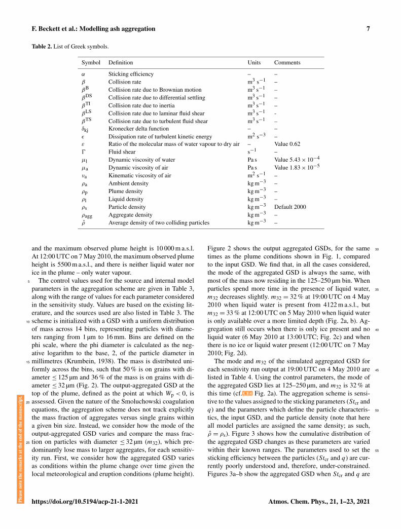
and the maximum observed plume height is 10 000 m a.s.l.At 12:00 UTC on 7 May 2010, the maximum observed plumeheight is 5500 m a.s.l., and there is neither liquid water norice in the plume – only water vapour.

The control values used for the source and internal model5

parameters in the aggregation scheme are given in Table 3,along with the range of values for each parameter consideredin the sensitivity study. Values are based on the existing lit-erature, and the sources used are also listed in Table 3. Thescheme is initialized with a GSD with a uniform distribution10

of mass across 14 bins, representing particles with diame-ters ranging from 1 µm to 16 mm. Bins are defined on thephi scale, where the phi diameter is calculated as the neg-ative logarithm to the base, 2, of the particle diameter inmillimetres (Krumbein, 1938). The mass is distributed uni-15

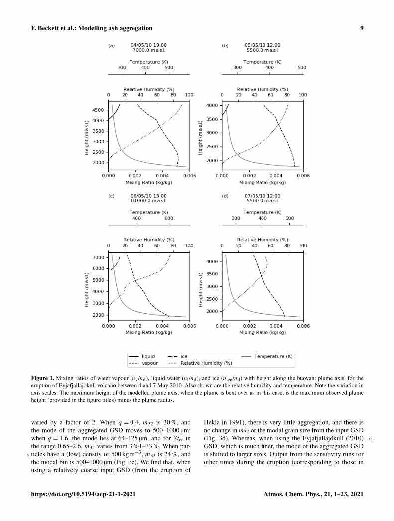
formly across the bins, such that 50 % is on grains with di-ameter ≤ 125 µm and 36 % of the mass is on grains with di-ameter ≤ 32 µm (Fig. 2). The output-aggregated GSD at thetop of the plume, defined as the point at which Wp < 0, isassessed. Given the nature of the Smoluchowski coagulation20

equations, the aggregation scheme does not track explicitlythe mass fraction of aggregates versus single grains withina given bin size. Instead, we consider how the mode of theoutput-aggregated GSD varies and compare the mass frac-tion on particles with diameter ≤ 32 µm (m32), which pre-25

dominantly lose mass to larger aggregates, for each sensitiv-ity run. First, we consider how the aggregated GSD variesas conditions within the plume change over time given thelocal meteorological and eruption conditions (plume height).

Figure 2 shows the output aggregated GSDs, for the same 30

times as the plume conditions shown in Fig. 1, comparedto the input GSD. We find that, in all the cases considered,the mode of the aggregated GSD is always the same, withmost of the mass now residing in the 125–250 µm bin. Whenparticles spend more time in the presence of liquid water, 35

m32 decreases slightly. m32 = 32 % at 19:00 UTC on 4 May2010 when liquid water is present from 4122 m a.s.l., butm32 = 33 % at 12:00 UTC on 5 May 2010 when liquid wateris only available over a more limited depth (Fig. 2a, b). Ag-gregation still occurs when there is only ice present and no 40

liquid water (6 May 2010 at 13:00 UTC; Fig. 2c) and whenthere is no ice or liquid water present (12:00 UTC on 7 May2010; Fig. 2d).

The mode and m32 of the simulated aggregated GSD foreach sensitivity run output at 19:00 UTC on 4 May 2010 are 45

listed in Table 4. Using the control parameters, the mode ofthe aggregated GSD lies at 125–250 µm, and m32 is 32 % atthis time (cf.CE4 Fig. 2a). The aggregation scheme is sensi-tive to the values assigned to the sticking parameters (Stcr andq) and the parameters which define the particle characteris- 50

tics, the input GSD, and the particle density (note that hereall model particles are assigned the same density; as such,ρ̂ = ρs). Figure 3 shows how the cumulative distribution ofthe aggregated GSD changes as these parameters are variedwithin their known ranges. The parameters used to set the 55

sticking efficiency between the particles (Stcr and q) are cur-rently poorly understood and, therefore, under-constrained.Figures 3a–b show the aggregated GSD when Stcr and q are

Plea

seno

teth

ere

mar

ksat

the

end

ofth

em

anus

crip

t.



Table 3. Model variables used in the aggregation scheme to represent the eruption conditions. The control values listed for each parameterare based on the defaults used in the existing literature. The range of parameter values considered in the sensitivity study are also given.

Model variable Control value Range considered References

Plume Entrainment coefficientproperties – normal (ks) 0.1 0.05–0.15 Woodhouse et al. (2016)

perpendicular (kn) 0.5 0.4–0.9 Aubry et al. (2017); Costa et al. (2016)Source plume temperature (T0) 1273 K 953–1373 K Woodhouse et al. (2016)Source mass fraction of– dry air (n0

d) 0.03 0.01–0.03 Devenish (2013); Woods (1988)– water vapour (n0

v) 0.0 0.0–0.05 Devenish (2013); Costa et al. (2016)Mass flux (Qm) Plume scheme Qm× 0.1−×10 Costa et al. (2016)

Aggregation Critical Stokes number (Stcr) 1.3 0.65–2.6 Costa et al. (2010); Gilbert and Lane (1994)properties Sticking parameter (q) 0.8 0.4–1.6 Costa et al. (2010); Gilbert and Lane (1994)

Particle Particle density (ρs) 2000 kg m−3 500–3000 kg m−3 Bonadonna and Phillips (2003)properties GSD Uniform Eyjafjallajökull (2010; fine); Bonadonna et al. (2011)(non-aggregated) m32 36 % mode 500–1000 µm, m32 26 %

Hekla (1991; coarse); Gudnason et al. (2017);mode 8000–16 000 µm, m32 2 %

Table 4. Properties of the simulated aggregated GSD from the model sensitivity runs. The output is for 19:00 UTC on 4 May 2010. Usingcontrol values (Table 3), the mode is at 125–250 µm and m32 32 %.

Model Value Mode m32variable

Plume ks 0.05 125–250 µm 32 %properties 0.15 125–250 µm 32 %

kn 0.4 125–250 µm 32 %0.9 125–250 µm 33 %

T0 953 K 125–250 µm 30 %1373 K 125–250 µm 32 %

n0d 0.01 125–250 µm 32 %

0.02 125–250 µm 32 %

n0v 0.03 125–250 µm 32 %

0.05 125–250 µm 32 %

Qm 0.1Qm 125–250 µm 33 %10Qm 125–250 µm 31 %

Aggregation Stcr 0.65 125–250 µm 33 %properties 2.6 125–250 µm 31 %

q 0.4 500–1000 µm 30 %1.6 64–125 µm 33 %

Particle ρs 500 kg m−3 500–1000 µm 24 %properties 3000 kg m−3 125–250 µm 33 %

GSD Eyjafjallajökull (2010) 500–1000 µm 23 %Hekla (1991) 8000–16 000 µm 2 %



Figure 1. Mixing ratios of water vapour (nv/nd), liquid water (nl/nd), and ice (nice/nd) with height along the buoyant plume axis, for theeruption of Eyjafjallajökull volcano between 4 and 7 May 2010. Also shown are the relative humidity and temperature. Note the variation inaxis scales. The maximum height of the modelled plume axis, when the plume is bent over as in this case, is the maximum observed plumeheight (provided in the figure titles) minus the plume radius.

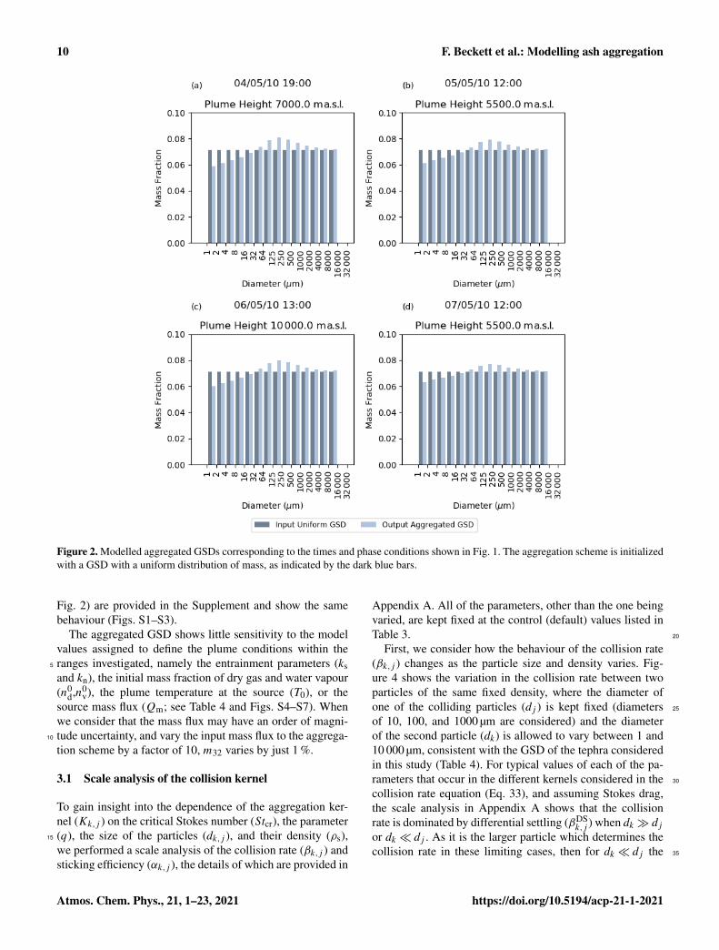
varied by a factor of 2. When q = 0.4, m32 is 30 %, andthe mode of the aggregated GSD moves to 500–1000 µm;when q = 1.6, the mode lies at 64–125 µm, and for Stcr inthe range 0.65–2.6, m32 varies from 3 %1–33 %. When par-ticles have a (low) density of 500 kg m−3, m32 is 24 %, and5

the modal bin is 500–1000 µm (Fig. 3c). We find that, whenusing a relatively coarse input GSD (from the eruption of

Hekla in 1991), there is very little aggregation, and there isno change inm32 or the modal grain size from the input GSD(Fig. 3d). Whereas, when using the Eyjafjallajökull (2010) 10

GSD, which is much finer, the mode of the aggregated GSDis shifted to larger sizes. Output from the sensitivity runs forother times during the eruption (corresponding to those in



Figure 2. Modelled aggregated GSDs corresponding to the times and phase conditions shown in Fig. 1. The aggregation scheme is initializedwith a GSD with a uniform distribution of mass, as indicated by the dark blue bars.

Fig. 2) are provided in the Supplement and show the samebehaviour (Figs. S1–S3).

The aggregated GSD shows little sensitivity to the modelvalues assigned to define the plume conditions within theranges investigated, namely the entrainment parameters (ks5

and kn), the initial mass fraction of dry gas and water vapour(n0

d,n0v), the plume temperature at the source (T0), or the

source mass flux (Qm; see Table 4 and Figs. S4–S7). Whenwe consider that the mass flux may have an order of magni-tude uncertainty, and vary the input mass flux to the aggrega-10

tion scheme by a factor of 10, m32 varies by just 1 %.

3.1 Scale analysis of the collision kernel

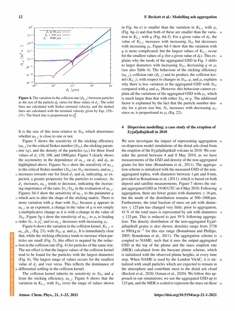
To gain insight into the dependence of the aggregation ker-nel (Kk,j ) on the critical Stokes number (Stcr), the parameter(q), the size of the particles (dk,j ), and their density (ρs),15

we performed a scale analysis of the collision rate (βk,j ) andsticking efficiency (αk,j ), the details of which are provided in

Appendix A. All of the parameters, other than the one beingvaried, are kept fixed at the control (default) values listed inTable 3. 20

First, we consider how the behaviour of the collision rate(βk,j ) changes as the particle size and density varies. Fig-ure 4 shows the variation in the collision rate between twoparticles of the same fixed density, where the diameter ofone of the colliding particles (dj ) is kept fixed (diameters 25

of 10, 100, and 1000 µm are considered) and the diameterof the second particle (dk) is allowed to vary between 1 and10 000 µm, consistent with the GSD of the tephra consideredin this study (Table 4). For typical values of each of the pa-rameters that occur in the different kernels considered in the 30

collision rate equation (Eq. 33), and assuming Stokes drag,the scale analysis in Appendix A shows that the collisionrate is dominated by differential settling (βDS

k,j ) when dk � djor dk � dj . As it is the larger particle which determines thecollision rate in these limiting cases, then for dk � dj the 35



Figure 3. Sensitivity of the output aggregated GSD to the sticking efficiency parameters, (a) Stcr and (b) q, and the physical characteristicsassigned to the particles, (c) particle density ρs, and (d) input GSD. Output is for 19:00 UTC on 4 May 2010, and the plume height is7000 m a.s.l. (cf. Fig. 2a). Note that the blue lines represent simulations using the control values.

collision rate is effectively constant; the scale analysis givesthe correct order of magnitude for βk,j in these cases. Whendk � dj , then, to leading order, the collision rate increasesto the fourth power of the diameter of the colliding parti-cle (βk,j ∝ d4

k ) and is independent of dj . However, Fig. 45

shows that when dk&102 µm, βk,j departs from this powerlaw when the Reynolds-number-dependent terminal veloc-ity is used (Eqs. 29–31). When dk = dj , then the collisionrate is dominated by shear, except for the very smallest parti-cles (of the order of 1 µm) when it is dominated by Brownian10

motion. The scale analysis gives the correct order of mag-nitude for these cases and explains the kinks seen in Fig. 4,when dk = dj , and why they become sharper as dj increases.When the assumption of constant ρs is relaxed, it is easilyseen that βk,j depends linearly on ρs (through βTI

k,j and βDSk,j )15

for dk 6= dj ; when dk = dj , the collision rate is independentof ρs.

We now turn to the sensitivity of the sticking efficiency(αk,j ) to the critical Stokes number (Stcr), the sticking param-eter (q), and the density of the particles (ρs). It follows imme-20

diately from Eq. (37) that increasing Stcr increases the rangeof values of the collision Stokes number (Stv) for which co-alescence can occur. When Stv� Stcr, αk,j ≈ 1, and coa-lescence is almost certain, q has the effect of enhancing orreducing the effect of Stv/Stcr, with q > 1 reducing the ef- 25

fect in this limit and so increasing the sticking efficiency fur-ther and vice versa for q < 1. When Stv� Stcr, αk,j � 1,and there is effectively no coalescence; q > 1 has the ef-fect of increasing the value of Stv/Stcr relative to its valuewith q = 1 and, hence, reducing the sticking efficiency still 30

further, whereas the converse applies when q < 1. How thesticking efficiency depends on diameter is determined by thedependence of Stv on dj and dk , and this is given by thescale analysis in Appendix A. When dk = dj , Stv (via Ur, asgiven by Eq. 35) is dominated by shear (Stv ∝ d2

j ), except for 35

the smallest particles (of the order of 1 µm) when it is domi-nated by Brownian motion (Stv ∝ 1/dj ). When dk 6= dj , Stvis dominated by differential settling; for dk � dj , we findthat Stv ∝ d2

j dk , whereas, for dk � dj , we have Stv ∝ d2k dj .



Figure 4. The variation in the collision rate (βk,j ) between particlesas the size of the particle dk varies for three values of dj . The solidlines are calculated with Stokes terminal velocity, and the dashedlines are calculated with the terminal velocity given by Eqs. (29)–(31). The black line is proportional to d4

k.

It is the size of this term relative to Stcr which determineswhether αk,j is close to one or not.

Figure 5 shows the sensitivity of the sticking efficiency(αk,j ) to the critical Stokes number (Stcr), the sticking param-eter (q), and the density of the particles (ρs) for three fixed5

values of dj (10, 100, and 1000 µm). Figure 5 clearly showsthe asymmetry in the dependence of αk,j on dj and dk , ashighlighted above. Figures 5a–c show the sensitivity of αk,jto the critical Stokes number (Stcr) as Stcr increases, and αk,jincreases towards one for fixed dj and dk indicating, as ex-10

pected, a greater propensity for the particles to coalesce. Asdj increases, αk,j tends to decrease, indicating the increas-ing importance of the ratio Stv/Stcr in the evaluation of αk,j .Figures 5d–f show the sensitivity of αk,j to the parameter qwhich acts to alter the shape of the sticking matrix. There is15

more variation with q than with Stcr; because q appears inαk,j as an exponent, a change in the value of q is not simplya multiplicative change as it is with a change in the value ofStcr. Figure 5g–i show the sensitivity of αk,j to ρs to leadingorder Stv ∝ ρ2

s , and so αk,j decreases with increasing ρs.20

Figure 6 shows the variation in the collision kernel,Kk,j =αk,jβk,j (Eq. 23), with Stcr, q, and ρs. It is immediately clearthat, while the sticking efficiency tends to increase when par-ticles are small (Fig. 5), this effect is negated by the reduc-tion in the collision rate (Fig. 4) for particles of the same size.25

The net effect is that the largest values of the collision kerneltend to be found for the particles with the largest diameters(Fig. 6). The largest range of values occurs for the smallestvalue of dj and vice versa. This reflects the dominance ofdifferential settling in the collision kernel.30

The collision kernel inherits its sensitivity to Stcr and qfrom the sticking efficiency, αk,j . Figure 6 shows that thevariation in Kk,j with Stcr (over the range of values shown

in Fig. 6a–c) is smaller than the variation in Kk,j with ρs(Fig. 6g–i) and that both of these are smaller than the varia- 35

tion in Kk,j with q (Fig. 6d–f). For a given value of dk , thevalue of Kk,j increases with increasing Stcr but decreaseswith increasing ρs. Figure 6d–f show that the variation withq is more complicated, but the largest values of Kk,j occurfor the smallest values of q (for a given value of dk). This ex- 40

plains why the mode of the aggregated GSD in Fig. 3 shiftsto larger diameters with increasing Stcr, decreasing q or ρs(see also Table 4). The behaviour of the sticking efficiency(αk,j ), collision rate (βk,j ) and its product, the collision ker-nel (Kk,j ), with respect to changes in Stcr, q, and ρs explains 45

why there is less variation in the aggregated GSD with Stcrcompared with q and ρs. However, this behaviour cannot ex-plain all the variations of the aggregated GSD with ρs, whichis much larger than that with either Stcr or q. The additionalfactor is explained by the fact that the particle number den- 50

sity for a given size bin, Ni, increases with decreasing ρs,since mi is proportional to ρs (Eq. 22).

4 Dispersion modelling: a case study of the eruption ofEyjafjallajökull in 2010

We now investigate the impact of representing aggregation 55

on dispersion model simulations of the distal ash cloud fromthe eruption of the Eyjafjallajökull volcano in 2010. We con-sider the period between 4 and 8 May 2010, as we havemeasurements of the GSD and density of the non-aggregatedgrains for this time (Bonadonna et al., 2011). The aggrega- 60

tion scheme is initialized with the measured GSD of the non-aggregated tephra, with diameters between 1 µm and 8 mm,provided in Bonadonna et al. (2011), which is based on bothdeposit and satellite measurements. Figure 7 shows the out-put aggregated GSD at 19:00 UTC on 4 May 2010. Following 65

aggregation, there are fewer grains with diameters ≤ 16 µm,but the mode of the distribution remains at 500–1000 µm.Furthermore, the total fraction of mass on ash with diame-ters ≤ 125 µm has changed very little; prior to aggregation,41 % of the total mass is represented by ash with diameters 70

≤ 125 µm. This is reduced to just 39 % following aggrega-tion. The density distribution of the non-aggregated Eyjaf-jallajökull grains is also shown; densities range from 2738to 990 kg m−3 for this size range (Bonadonna and Phillips,2003; Bonadonna et al., 2011). The aggregation scheme is 75

coupled to NAME, such that it uses the output-aggregatedGSD at the top of the plume and the mass eruption rate(MER) calculated from the buoyant plume scheme, whichis initialized with the observed plume heights, at every timestep. When NAME is used by the London VAAC, it is ini- 80

tialized with small particles which are expected to remain inthe atmosphere and contribute most to the distal ash cloud(Beckett et al., 2020; Osman et al., 2020). We follow this ap-proach in our simulations; we use the aggregated GSD up to125 µm, and the MER is scaled to represent the mass on these 85

Plea

seno

teth

ere

mar

ksat

the

end

ofth

em

anus

crip

t.



Figure 5. The variation in sticking efficiency (αk,j ), with Stcr (a–c), q (d–f), and ρs (g–i) for three fixed values of dj , i.e. dj = 10 µm(a, d, g) TS3 , dj = 100 µm (b, e, h) TS4 , and dj = 1000 µm (c, f, i) TS5 . The terminal velocity is calculated using Eqs. (29)–(31). The diameterdk0 = 1 µm.

grains only. For example, at 19:00 UTC on 4 May 2010, 39 %of the total mass erupted is released over the seven bins rep-resenting ash with diameters ≤ 125 µm (Fig. 7). The exactdiameter of each model particle is allocated such that the logof the diameter is uniformly distributed within each size bin.5

These model particles are then released with a uniform distri-bution over the depth of the modelled (bent-over) plume. SeeDevenish (2013, 2016) for details of how the plume radius(depth) is constrained. The set-up of the NAME runs is givenin Table 5, and we use the control internal model parameters10

in the aggregation scheme (Table 3).Figure 8a shows the modelled 1 h averaged total column

mass loadings in the ash cloud at 00:00 UTC on 5 May 2010,24 h after the release start, using the measured GSD and den-sity distribution of the non-aggregated Eyjafjallajökull par-15

ticles. In comparison, Fig. 8b shows the modelled plumeusing the time-varying aggregated GSD. As the density ofthe Eyjafjallajökull aggregates is not known, the measureddensity distribution of the single grains is applied. Current

regulations in Europe state that airlines must have a safety 20

case accepted to operate in ash concentrations greater than2× 10−3 g m−3. We assume a cloud depth of 1 km and con-sider the area of the ash cloud with mass loadings > 2 g m−2

to compare the differences in the modelled areas, whichare significant for aircraft operations. Using the aggregated 25

GSD, the extent of the ash cloud is only slightly smaller, andit is reduced by just∼ 2 %, reflecting the slight increase in thefraction of larger (aggregated) grains in the ash cloud, whichhave a greater fall velocity and, hence, shorter residence timein the atmosphere. 30

However, it is expected that porous aggregates, specif-ically cored clusters which consist of a large core parti-cle (> 90 µm) covered by a thick shell of smaller particles(Brown et al., 2012; Bagheri et al., 2016) may have lowerdensities than single grains of ash of equivalent size (Bagheri 35

et al., 2016; Gabellini et al., 2020; Rossi et al., 2021). Fig-ure 9 shows the modelled ash cloud when we assume thatthe aggregates have densities of 1000 and 500 kg m−3 (Tad-



Figure 6. The variation in the collision kernel (Kk,j ) with Stcr (a–c), q (d–f), and ρs (g–i) for three fixed values of dj , i.e. dj = 10 µm(a, d, g) TS6 , dj = 100 µm (b, e, h) TS7 , and dj = 1000 µm (c, f, i) TS8 . The terminal velocity is calculated using Eqs. (29)–(31). The diameterdk0 = 1 µm.

deucci et al., 2011; Gabellini et al., 2020; Rossi et al., 2021).As the aggregation scheme does not track explicitly the massfraction represented by aggregates versus single grains for agiven size bin, we must also make an assumption about howmuch of the mass released is represented by aggregates with5

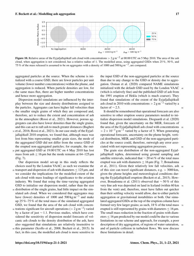
lower density. Here we consider the case where 25 %, 50 %,and 75 % of the mass on each size bin, for ash with diameters≤ 125 µm, is represented by aggregates. Assigning a lowerdensity to the aggregates reduces their fall velocity, and theextent of the simulated ash cloud increases. If we assume that10

75 % of the mass of ash ≤ 125 µm is represented by aggre-gates, then, when they are assigned a density of 1000 kg m−3,the simulated ash cloud with mass loadings > 2 g m−2 is152 687 km2. This increases to 160 584 km2 when they areassigned a density of 500 kg m−3. Figure 10 shows the rela-15

tive increase in the area of the ash cloud with concentrations> 2 g m−2 as a function of the mass fraction of aggregates inthe ash cloud and their density. The circle, with a diameterof 1, represents the extent of the modelled cloud when ag-

gregation is not considered (area 142 462 km2). The largest 20

modelled ash cloud is ∼ 1.1 times bigger. This is achievedwhen we use the aggregated GSD, assign the aggregates adensity of 500 kg m−3, and assume that aggregates constitute75 % of the total mass released in NAME (ash ≤ 125 µm).

5 Discussion 25

We have integrated an aggregation scheme into the atmo-spheric dispersion model NAME. The scheme is coupled toa one-dimensional buoyant plume model and uses the fixedpivot technique to solve the Smoluchowski coagulation equa-tions to simulate aggregation processes in an eruption col- 30

umn. The time-evolving aggregated GSD at the top of theplume is provided to NAME as part of the source conditions.This represents the first attempt at modelling explicitly thechange in the GSD of the ash due to aggregation in a modelwhich is used for operational response, as opposed to assum- 35

ing a single aggregate class (Cornell et al., 1983; Bonadonna



Figure 7. The GSD of the Eyjafjallajökull (2010) non-aggregated tephra (dark grey bars; from Bonadonna et al., 2011), used to initialize theaggregation scheme, and the modelled aggregated GSD at the top of the plume (light grey bars), at 19:00 UTC on 4 May 2010. The densitydistribution of the non-aggregated particles, taken from Bonadonna et al. (2011), is also shown.

Table 5. Input parameters for the NAME runs.

Model parameter Value

Source location Eyjafjallajökull, 63.63◦ lat, −19.62◦ longSummit height 1666 m a.s.l.Source start and end times 00:00 on 4 May 2010–23:00 on 8 May 2010Source shape Line source, using depth of the modelled plume and uniform distributionSource strength From buoyant plume scheme, given the observed plume heightModel particle release rate 15 000 h−1

Particle shape SphericalGSD Set by the aggregation schemeMeteorological data Unified model (global configuration): ∼ 25 km horizontal resolution (mid-latitudes);

3 h temporal resolutionTime step 10 min

et al., 2002; Costa et al., 2010). Our scheme predicts thatmass is preferentially removed from bins representing thesmallest ash (≤ 64 µm). This agrees well with field and labo-ratory experiments which have also observed that aggregatesmainly consist of particles < 63 µm in diameter (Bonadonna5

et al., 2011; James et al., 2002, 2003). This suggests that ag-gregation will be more prevalent when large quantities of fineash are generated by the eruption.

Previous sensitivity studies of dispersion model simula-tions of volcanic ash clouds have highlighted the importance 10

of constraining the GSD of ash for operational forecasts, asthis parameter strongly influences its residence time in theatmosphere (Scollo et al., 2008; Beckett et al., 2015; Durant,2015; Poret et al., 2017; Osman et al., 2020; Poulidis andIguchi, 2020). Here we show that the modelled aggregated 15

GSD is also sensitive to the GSD, and the density, of the non-



Figure 8. Modelled 1 h averaged total column mass loadings of the Eyjafjallajökull ash cloud at 00:00 UTC on 5 May 2010, using (a) themeasured GSD of the non-aggregated ash and (b) the time-varying aggregated GSD. The measured density distribution of the non-aggregatedash grains is applied in both cases. The area of the ash cloud with mass loadings > 2 g m−2, which is significant for aircraft operations, isshown.

Figure 9. Modelled 1 h averaged total column mass loadings of the Eyjafjallajökull ash cloud at 00:00 UTC on 5 May 2010 when 25 %, 50 %,and 75 % of the mass is on aggregates with densities of 1000 and 500 kg m−3. The area of the ash cloud with mass loadings> 2 g m−2, whichis significant for aircraft operations, is shown.



Figure 10. Relative areas of the Eyjafjallajökull ash cloud with concentrations > 2 g m−2 at 00:00 UTC on 5 May 2010. The area of the ashcloud, when aggregation is not considered, has a relative radius of 1. The modelled areas, using aggregated GSDs when 25 %, 50 %, and75 % of the mass released is assumed to be on aggregates with a density of 1000 and 500 kg m−3, are compared.

aggregated particles at the source. When the scheme is ini-tialized with a coarse GSD, there are fewer particles per unitvolume (lower number concentrations) within the plume, andaggregation is reduced. When particle densities are low, forthe same mass flux, there are higher number concentrations5

and hence more aggregation.Dispersion model simulations are influenced by the inter-

play between the size and density distributions assigned tothe particles. Aggregates can have higher fall velocities thanthe smaller single grains of which they are composed and,10

therefore, act to reduce the extent and concentration of ashin the atmosphere (Rossi et al., 2021). However, porous ag-gregates can also have lower densities than the single grains,and this can act to raft ash to much greater distances (Bagheriet al., 2016; Rossi et al., 2021). In our case study of the Eyjaf-15

jallajökull 2010 eruption, we found that, although mass waslost from bins representing smaller grain sizes, the mode ofthe aggregated GSD did not differ from the source GSD ofthe erupted non-aggregated particles; for example, the out-put aggregated GSD at 19:00 UTC on 4 May 2010 has lost20

mass from ash ≤ 16 µm but the mode remains at 64–125 µm(Fig. 7).

Our dispersion model set-up in this study reflects thechoices used by the London VAAC; as such we examine thetransport and dispersion of ash with diameters≤ 125 µm, and25

we consider the implications for the modelled extent of theash cloud with mass loadings of significance to the aviationindustry. We found that using the time-varying aggregatedGSD to initialize our dispersion model, rather than the sizedistribution of the single grains, had little impact on the sim-30

ulated ash cloud. When we considered that aggregates mayhave (lower) densities of 1000 and 500 kg m−3 and makeup 25 %–75 % of the total mass of the simulated aggregatedGSD, we found that the area of the ash cloud with concen-trations significant for aircraft operations (> 2 g m−2) varied35

by a factor of just ∼ 1.1. Previous studies, which have con-sidered the sensitivity of dispersion model forecasts of vol-canic ash clouds to the density distribution of the ash, havealso suggested that simulations are relatively insensitive tothis parameter (Scollo et al., 2008; Beckett et al., 2015). In40

fact, in this case, the modelled ash cloud is more sensitive to

the input GSD of the non-aggregated particles at the sourcethan due to any change to the GSD or density due to aggre-gation. Osman et al. (2020) compared NAME simulationsinitialized with the default GSD used by the London VAAC 45

(which is relatively fine) and the published GSD of ash fromthe 1991 eruption of Hekla (which is much coarser). Theyfound that simulations of the extent of the Eyjafjallajökullash cloud in 2010 with concentrations > 2 g m−2 varied by afactor of ∼ 2.5. 50

It should be remembered that operational forecasts are alsosensitive to other eruption source parameters needed to ini-tialize dispersion model simulations. Dioguardi et al. (2020)found that, given the uncertainty on the MER, forecasts ofthe area of the Eyjafjallajökull ash cloud with concentrations 55

> 2× 10−3 g m−3 varied by a factor of 5. When generatingoperational forecasts, uncertainty on the plume height, verti-cal distribution, MER, and GSD of the non-aggregated parti-cles at the source could, therefore, outweigh any error asso-ciated with not representing aggregation processes. 60

The grain size distribution of the non-aggregated Eyjaf-jallajökull tephra, determined using ground sampling andsatellite retrievals, indicated that ∼ 20 wt % of the total masserupted was ash with diameters ≤ 16 µm (Fig. 7; Bonadonnaet al., 2011). Given their relatively low fall velocities, ash 65

of this size can travel significant distances, e.g. > 3000 km,given the plume heights and meteorological conditions dur-ing the Eyjafjallajökull eruption (Beckett et al., 2015). How-ever, Bonadonna et al. (2011) observed that ∼ 50 % of thisvery fine ash was deposited on land in Iceland (within 60 km 70

from the vent) and, therefore, must have fallen out quickerthan their settling velocity would allow, due to either particleaggregation or gravitational instabilities or both. Our simu-lated aggregated GSDs at the top of the eruption column haveformed very few larger grains; as such, 18 % of the total mass 75

erupted is still represented by grains with diameters≤ 16 µm.The small mass reduction in the fraction of grains with diam-eters≤ 16 µm predicted by our model could be due to variouslimitations in our scheme and approach, for example, a poordescription of dry aggregation, of regions of water saturation, 80

and of particle collision in turbulent flows. We now discussthese limitations in detail.



5.1 Limitations

To be considerate of the computational costs for operationalsystems, we have limited aggregation processes to the erup-tion column only. However, it is likely that, while ash con-centrations remain high, aggregation will continue in the dis-5

persing ash cloud. As we do not represent electric fields inour scheme, we are also unable to explicitly simulate aggre-gation through electrostatic attraction (Pollastri et al., 2021).Further work is needed to consider this contribution and theimplications for the long-range transport of the ash cloud.10

Our approach may, therefore, underestimate the amount ofaggregation, which could further shift the mode of the ag-gregated GSD to larger grain sizes. We also disregard dis-aggregation due to collisions with other aggregates and ashgrains (Del Bello et al., 2015; Mueller et al., 2017). This pro-15

cess has received little attention and remains relatively under-constrained and, as such, has also been neglected here.

Volcanic plumes are highly turbulent flows characterizedby a wide range of interacting length and timescales. Thelength scale of the largest eddies (the integral scale) is the20

plume radius (e.g. Cerminara et al., 2016a), whereas thesmallest eddies are at the Kolmogorov scale, i.e. the pointat which viscosity dominates, and the turbulent kinetic en-ergy is dissipated into heat. In the treatment of the collisionkernels in our scheme, we have assumed that the Saffman–25

Turner limit is satisfied and that the particles are smaller thanthe smallest turbulent scale and, as such, are completely cou-pled with the flow. However, larger particles lie outside thislimit and, if sufficiently large, will be uncorrelated with theflow. Further work is needed to consider the treatment of30

large uncorrelated particles, for example the application ofthe Abrahamson limit in the treatment of the collision ker-nels could be explored (Textor and Ernst, 2004).

We consider that particle sticking can occur due to viscousdissipation in the surface liquid layer on the ash (Liu et al.,35

2000; Liu and Lister, 2002). This is based on the assump-tion that large amounts of water (magmatic, ground water,and atmospheric) will be available, and the assumption thatthis mechanism will play a dominant role over other possiblesticking mechanisms, e.g. electrostatic forces (Costa et al.,40

2010). Furthermore, this approach could neglect the presenceof particle clusters (Brown et al., 2012), which usually re-quire less water to form, and so our approach might also beunderestimating the formation of these aggregates.

Using scaling analysis (Sect. 3.1), we show that the mod-45

elled aggregated GSDs are particularly sensitive to the pa-rameters used in the aggregation scheme to control the stick-ing efficiency of two colliding particles, i.e. the criticalStokes number (Stcr) and parameter q (an exponent). Vary-ing these parameters is, in some sense, equivalent to chang-50

ing the amount of viscous dissipation acting on the surfaceof the particles, which is, in turn, related to the thickness ofthe surface water layers. Both of these parameters are poorlyconstrained, and our aggregation scheme would benefit from

further calibration with field and laboratory studies. In partic- 55

ular, the depth of the liquid layers on ash grains needs to bebetter understood and applied here. The sticking efficiencyalso depends on the relative velocities between the collidingparticles. In Eq. (35), we have neglected any effect of the par-ticle inertia induced by the background turbulent flow which 60

represents a further source of uncertainty.For the eruption considered in this study, liquid water is

only present in top ∼ 1 km of the plume, and in some in-stances, no liquid water was formed (e.g. 13:00 UTC on6 May 2010 and 12:00 UTC on 7 May 2010; Fig. 1). 65

Folch et al. (2010) found, using their one-dimensional plumemodel, that there was only a 30 s window for ash to aggre-gate in the presence of liquid water in the initial phase ofthe eruption at Mount St Helens in 1980, which generateda plume which rose 32 km, and only a ∼ 45 s window dur- 70

ing the less vigorous eruption of Crater Peak in 1992. At-mospheric conditions in the tropics can generate taller erup-tion plumes, which entrain more water, than these eruptionsin drier environments and, as such, may promote conditionsmore ideal for aggregation (Tupper et al., 2009). 75

Our one-dimensional treatment of the plume does not fullyrepresent the three-dimensional turbulent flow and may bemissing local pockets of liquid water. Initial experimentalstudies also suggest that aggregation can occur at relativelylow humidity (Telling and Dufek, 2012; Telling et al., 2013; 80

Mueller et al., 2016). As such, in our approach, we allowsticking to occur in regions where the relative humidity is< 100 % and liquid water is not yet present. Experimentaldata which better constrain the influence of the ambient con-ditions, such as the relative humidity, on liquid bonding of 85

ash aggregates could improve our simulations of aggregateformation in volcanic ash clouds.

When liquid water and ice did form, mass mixing ratiossuggest that our modelled plumes are liquid water/ice rich;the maximum mass mixing ratio of liquid water (at the top 90

of the plume) was 8.3× 10−4 kg kg−1 at 19:00 UTC on 4May 2010, and the maximum mass mixing ratio of ice was8.6× 10−4 kg kg−1 at 13:00 UTC on 6 May 2010. In com-parison, mid-level mixed-phase clouds typically have liquidwater mixing ratios of 1.5× 10−4–4× 10−4 kg kg−1 and ice 95

mixing ratios of 5× 10−6–4× 10−5 kg kg−1 (Smith et al.,2009). Atmospheric conditions in the tropics would likelyensure even higher quantities of ice in volcanic plumes (Tup-per et al., 2009). Our scheme does not account for interac-tions between the hydrometeors formed and the ash parti- 100

cles; as such, we can neither represent the role of ash as aneffective ice-nucleating particle (Durant et al., 2008; Gibbset al., 2015), nor can we account for the process of ash-ladenhailstones acting to preferentially remove fine ash from theatmosphere (Van Eaton et al., 2015). 105

Fine ash could also be preferentially removed from boththe plume and dispersing ash cloud due to other size-selectiveprocesses currently not described in NAME, such as gravita-tional instabilities, which represent a dominant process for



this eruption (Durant, 2015; Manzella et al., 2015). Ash ag-gregation might be also enhanced by the formation of fingersas a result of gravitational instabilities due to an increasein both ash concentration and turbulence (e.g. Carazzo andJellinek, 2012; Scollo et al., 2017).5

Finally, our one-dimensional treatment of the Smolu-chowski coagulation equations does not allow us to representthe change in density of the simulated aggregates or track ex-plicitly the mass fraction of aggregates versus single grainswithin a given bin size. Our scheme could be significantly10

improved by using a multi-dimensional description whichrepresents the fluctuation in the density of the growing aggre-gates and retains information on the mass fraction of aggre-gated particles. To implement this change effectively wouldalso require a better understanding of the structure (porosity)15

of aggregates.

6 Conclusions

We have integrated an aggregation scheme into the atmo-spheric dispersion model NAME. The scheme uses an iter-ative buoyant plume model to simulate the eruption column20

dynamics, and the Smoluchowski coagulation equations aresolved with a sectional technique which allows us to simu-late the aggregated GSD in discrete bins. The modelled ag-gregated GSD at the top of the eruption column is then usedto represent the time-varying source conditions in the disper-25

sion model simulations. Our scheme is based on the assump-tion that particle sticking is due to the viscous dissipationof surface liquid layers on the ash, and scale analysis indi-cates that our output-aggregated GSD is strongly controlledby under-constrained parameters which attempt to represent30

these liquid layers. The modelled aggregated GSD is alsosensitive to the physical characteristics assigned to the par-ticles in the scheme, namely the initial GSD and density dis-tribution. Our ability to accurately forecast the long-rangetransport of volcanic ash clouds is, therefore, still limited35

by real-time information on the physical characteristics ofthe ash. We found that using the time-evolving aggregatedGSD in dispersion model simulations of the Eyjafjallajökull(2010) eruption had very little impact on the modelled extentof the distal ash cloud with mass loadings significant for avia-40

tion. However, our scheme neither represents all the possiblemechanisms by which ash may aggregate (i.e. electrostaticforces), nor does it distinguish the density of the aggregatedgrains. Our results indicate the need for more field and lab-oratory experiments to further constrain the binding mecha-45

nisms and composition of aggregates, their size distribution,and density.

Appendix A: Scaling analysis

In order to gain more insight into the dependence of the col-lision kernel Kj,k on q, Stcr, and ρs, we carry out a scale50

analysis of αk,j and βk,j in turn. Starting with the collisionrate, we can write Eq. (33) as follows:

βk,j = B(dk + dj )

2

dkdj

+S(dk + dj )3+ I(dk + dj )2|d2k − d

2j |

+D(dk + dj )2|d2k − d

2j |, (A1)

where, in the following:

B =2kBT

3µaS =

18

(1.7ενa

)1/2

I =172πε3/4

ν1/4a

ρs

µa

D =π

4gρs

18µa(A2) 55

are taken to be constant (including ρs). Here we have as-sumed that the particles settle with Stokes’ terminal veloc-ity (i.e. we neglect the second term on the right-hand sideof Eq. (30); this will lead to quantitative discrepancies withthe collision kernel calculated in Sect. 3 for larger diameters, 60

but the qualitative behaviour will be correct). We have alsoassumed that βTS

i,j > βLSi,j ; this assumption does not affect our

conclusions below. Since aggregation is associated with thepresence of liquid water or ice, and αk,j only depends onq and Stcr in the presence of liquid water, we choose val- 65

ues of the constituent parameters in Eq. (A2) that are appro-priate for this case. Thus, with T = 300 K, ε = 0.01 m2 s−3,ρa = 1.297 kg m−3, and ρs = 2000 kg m−3, the constants inEq. (A2) have the following orders of magnitude:

B ∼ 10−16m3s−1

S ∼ 1m3s−1I ∼ 106m3s−1

D ∼ 107m3s−1. (A3) 70

As in Sect. 3, we restrict attention to diameters in the range[1,104

] µm. Figure 4 shows the variation in βk,j , given byEq. (A1), with dk for three fixed values of dj . The differencebetween assuming Stokes’ terminal velocity and using theterminal velocity as given by Eqs. (29)–(31) becomes clear 75

for large diameters. Note that βk,j is symmetric in the indicesj and k.

In the special case that dk = dj , Eq. (A1) becomes the fol-lowing:

βj,j = 4B+ 8Sd3j . (A4) 80

For dj ∼ 1 µm, the first term dominates. The second termdominates for all values of dj&10 µm. For dj ∼ 10 µmwe obtain βj,j ∼ 10−14 m3 s−1, for dj ∼ 100 µm we obtainβj,j ∼ 10−11 m3 s−1, and for dj ∼ 1000 µm we obtain βj,j ∼10−8 m3 s−1. 85



In the case that dk � dj , Eq. (A1) becomes the following:

βk,j ≈ Bdj

dk+Sd3

j + Id4j +Dd4

j . (A5)

Scale analysis (using the values above) shows that the thirdterm can be neglected, and the second term is only com-parable with the last term when dj ∼ 0.1 µm, which is out-5

side the range of interest. Noting that the smallest val-ues of dj ,dk ∈ [1,104

] µm that satisfy dk � dj are dj ∼

10 µm and dk ∼ 1 µm, we see that, for all dj&10 µm, thefourth term will dominate, and so βk,j is effectively constant(since we are considering fixed dj ). Thus, for dj ∼ 10 µm10

we obtain βk,j ∼ 10−13 m3 s−1, for dj ∼ 100 µm we obtainβk,j ∼ 10−9 m3 s−1, and for dj ∼ 1000 µm we obtain βk,j ∼10−5 m3 s−1. These are consistent with what is observed inFig. 4 for dk � dj . Furthermore, we note that these values areall larger than the values of βk,j in the special case dk = dj ,15

and that this difference increases as dj increases in magni-tude. This explains the kink in Fig. 4, when dk = dj , and whyit becomes sharper as dj increases.

For dk � dj , the scale analysis shows that, in the follow-ing:20

βk,j ≈ Bdk

dj+Sd4

k . (A6)

For dj ∈ [1,104] µm and dk � dj , the second term domi-

nates. Thus, this leads to the order of βk,j ∝ d4k for dk � dj ,

which is consistent with what is observed in Fig. 4 when βk,jis computed with Stokes’ terminal velocity, or for dk not be-25

ing too large when βk,j is computed with the terminal veloc-ity given by Eqs. (29)–(31).

We now turn to the sticking efficiency. On making use ofEqs. (34) and (35), we can write Stv as follows:

Stv = V |dj − dk|djdk +B

dj + dk+ Sdjdk, (A7)30

where, in the following:

V =4gρ2

s81µlµa

B =64ρskBT

27πµlµa

S =4ρs

9πµl

(1.7ενa

)1/2

(A8)

are assumed to be constant, and we have also assumed thatthe two colliding particles have the same density (as inSect. 3). Using the same values of the parameters as above35

(with constant ρs), the constants have the following orders ofmagnitude:

V ∼ 1014m−3

B ∼ 10−10m−1

S ∼ 107m−2. (A9)

Note that Stv and, hence, αk,j are symmetric in the indices kand j . The ranges of q and Stcr we consider are the same as 40

those in Sect. 3, i.e. q ∈ [0.4,1.6] and Stcr ∈ [0.65,2.6].Consider first the special case dk = dj . Then, Eq. (A7) be-

comes the following:

Stv =B

2dj+ Sd2

j . (A10)

The first term dominates for dj.1 µm; the second term dom- 45

inates for dj&10 µm. For dj6100 µm, Stv� Stcr and so, inthe following:

αk,j ≈ 1−(Stv

Stcr

)q≈ 1, (A11)

for qnot� 1, whereas for dj>1000 µm, Stv� Stcr and so,in the following: 50

αk,j ≈

(Stcr

Stv

)q (1−

(Stcr

Stv

)q)� 1, (A12)

for qnot� 1.In the case dk � dj , Eq. (A7) becomes the following:

Stv = V d2j dk +

B

dj+ Sdjdk. (A13)

Again, we fix dj and allow dk to vary. The smallest admis- 55

sible values of dj and dk that are in the range [1,10 000] µmare dj ∼ 10 µm and dk ∼ 1 µm; for these values, a scale anal-ysis shows that the first term on the right-hand side is dom-inant. For dj ∼ 104 µm, the largest admissible value, anddk ∈ [1,1000] µm, a scale analysis also shows that the first 60

term on the right-hand side is dominant. Thus, Eq. (38) be-comes the following.

αk,j ≈

(Stcr

V d2j dk

)q (1−

(Stcr

V d2j dk

)q), (A14)

if V d2j dk/Stcr > 1, whereas, in the following:

αk,j ≈ 1−

(V d2

j dk

Stcr

)q, (A15) 65

if V d2j dk/Stcr < 1. Since Stcr is always of the order of unity,

if V d2j dk � 1, then α ≈ 1. As dj increases, the range of dk

values for which V d2j dk � 1 decreases. For dj&100 µm, we

see that V d2j dk&1 for all admissible values of dk .

In the case dk � dj , a similar scale analysis to that above 70

shows that the first term on the right-hand side of Eq. (A7)is again the dominant term; it now takes the form V d2

k dj .For dj ∼ 1 µm, V d2

k dj&1, if dk&100 µm. For dj ∼ 1000 µm,it follows from the condition dk � dj that dk ∼ 104 µm, andso V d2

k dj&1 is always satisfied. For these values we would 75



expect α < 1. As dj increases, the range of dk values forwhich V d2

k dj&1 and α < 1 increases (e.g. if dj ∼ 100 µm,then dk&10 µm for V d2

k dj&1 to hold).Consider first the variation in αk,j with Stcr (Fig. 5a–

c); when dj = 10 µm, (Fig. 5a) then, for both dk < dj and5

dknot� dj , it can be seen that α ≈ 1, as expected, sincehere V d2

j dk � 1 and V d2k dj � 1, for dknot� 10 µm. For in-

creasing dk � dj , we see αk,j decreasing for all values ofStcr, since here V d2

k dj � 1. For a given value of dk � dj ,Fig. 5a shows that αk,j increases by approximately 4q over10

the range of Stcr shown. A similar pattern can be seen fordk � dj in Fig. 5b and c. Compared with Fig. 5a, b, and c, thepatterns show more variation with Stcr for dk � dj and de-creasing values of αk,j ; this occurs because V d2

j dk increaseswith increasing dj , and of course, the range of dk values sat-15

isfying dk � dj also increases with increasing dj .Turning now to the variation in αk,j , with q shown in

Fig. 5d–f. Raising V d2k dj > 1 to the power q > 1 will en-

hance its value, whereas raising it to the power q < 1 willdiminish its value (similarly for V d2

j dk). Thus, for exam-20

ple, as shown in Fig. 5d when dj = 10 µm and dk � dj ,V d2

k dj > 1 for dk&10−4 m, and so, for q > 1, αk,j is smallerthan it would be for q = 1, whereas, for q < 1, it is larger.These patterns hold true in Fig. 5e and f for dk � dj , thoughwith diminishing values of αk,j for increasing values of dj .25

Similarly, we see in Fig. 5f, for example, that, for dk � dj ,V d2

j dk > 1 for all values of dk ∈ [1,100] µm, and so αk,j iscloser to unity for q < 1 and vice versa for q > 1.

It should be noted that αk,j , computed with Stokes’ ter-minal velocity, shows a larger variation than that shown in30

Fig. 5. Since Stokes’ terminal velocity is larger than that cal-culated from Eqs. (29)–(31) for large diameters, and αk,j isdominated by differential settling, then, for large diameters,αk,j becomes smaller than the values shown in Fig. 5. Con-versely, Fig. 4 shows that βk,j is larger when using Stokes’35

terminal velocity. The net effect is that the collision kernelcomputed with Stokes’ terminal velocity is similar in magni-tude to that shown in Fig. 6.

Code and data availability. Data used in this paper may be re-quested from the corresponding author and can be downloaded from40

https://doi.org/10.5281/zenodo.4607421TS9 . The NAME code isavailable under license from the Met Office.

Supplement. The supplement related to this article is available on-line at: https://doi.org/10.5194/acp-21-1-2021-supplement.

Author contributions. FB performed the sensitivity study, the ag-45

gregation NAME modelling, and wrote the first draft. ER designedthe aggregation scheme as part of his doctoral project, as supervisedby CB. FB, ER, and BD integrated the scheme into NAME. BD per-formed the scaling analysis. CW supervised the project. CB over-

saw the analysis and instigated the project. All authors contributed 50

to the project design and the finalization of the paper.

Competing interests. The authors declare that they have no conflictof interest.

Disclaimer. Publisher’s note: Copernicus Publications remainsneutral with regard to jurisdictional claims in published maps and 55

institutional affiliations.

Acknowledgements. This project has received funding from the Eu-ropean Union’s Horizon 2020 research and innovation programme(grant no. 731070; EUROVOLC). Frances Beckett would like tothank Matthew Hort, for his enthusiastic support and for reviewing 60

a draft of this paper. The authors would like to thank Larry Mastinand an anonymous reviewer, for their thoughtful and thorough re-views, which helped to greatly improve this paper.

Financial support. This research has been supported by the Hori-zon 2020 (grant no. 731070; EUROVOLC).TS10 65

Review statement. This paper was edited by Qiang Zhang and re-viewed by Larry Mastin and two anonymous referees.

References

Arastoopour, H., Wang, C. H., and Weil, S.: Particle-particle inter-action force in a diluite gas-solid system., Chem. Eng. Sci., 37, 70

1379–1386, 1982. TS11

Aubry, T., Carazzo, G., and Jellinek, A. M.: Turbulent entrainmentinto volcanic plumes: New constraints from laboratory experi-ments on buoyant jets rising in a stratified crossflow., Geophys.Res. Lett., 44, https://doi.org/10.1002/2017GL075069, 2017. 75

Bagheri, G., Rossi, E., Biass, S., and Bonadonna, C.: Timing andnature of volcanic particle clusters based on field and numericalinvestigations, J. Volc. Geotherm. Res., 327, 520–530, 2016.

Beckett, F., Witham, C., Hort, M., Stevenson, J., Bonadonna,C., and Millington, S.: Sensitivity of dispersion model 80

forecasts of volcanic ash clouds to the physical charac-teristics of the particles, J. Geophys. Res.-Atmos., 120,https://doi.org/10.1002/2015JD023609, 2015.TS12

Beckett, F., Witham, C., Leadbetter, S., Crocker, R., Web-ster, H., Hort, M.C. Jones, A., Devenish, B., and Thom- 85

son, D.: Atmospheric Dispersion Modelling at the Lon-don VAAC: A Review of Developments since the 2010Eyjafjallajökull Volcano Ash Cloud, Atmosphere, 11, 352,https://doi.org/10.3390/atmos11040352, 2020.

Bonadonna, C. and Phillips, J.: Sedimentation from strong volcanic 90

plumes, J. Geophys. Res., 108, B00203, 2003. TS13

Bonadonna, C., Macedonio, G., and Sparks, R.: Numerical mod-elling of tephra fallout associated with dome collapses and Vul-canian explosions: application to hazard assessment on Montser-

Plea

seno

teth

ere

mar

ksat

the

end

ofth

em

anus

crip

t.


https://doi.org/10.5281/zenodo.4607421

https://doi.org/10.5194/acp-21-1-2021-supplement

https://doi.org/10.1002/2017GL075069

https://doi.org/10.1002/2015JD023609

https://doi.org/10.3390/atmos11040352


rat, in: The Eruption of Soufriere Hills Volcano, Montserrat, from1995 to 1999, edited by: Druitt, T. and Kokelaar, B., GeologicalSociety of London, 517–537, 2002.

Bonadonna, C., Genco, R., Gouhier, M., Pistolesi, M., Cioni, R., Al-fano, F., Hoskuldsson, A., and Ripepe, M.: Tephra sedimentation5

during the 2010 Eyjafjallajökull eruption (Iceland) from deposit,radar, and satellite observations, J. Geophys. Res., 116, B12202,2011. TS14

Brown, R., Bonadonna, C., and Durant, A.: A review of volcanicash aggregation, Phys. Chem. Earth, 45, 65–78, 2012.10

Carazzo, G. and Jellinek, A.: A new view of the dynamics, stabilityand longevity of volcanic clouds, Earth Planet. Sc. Lett., 325,39–51, 2012.

Carey, S. and Sigurdsson, H.: Influence of particle aggregation ofdeposition of distal tephra from the May 18, 1980, eruption of15

Mount St. Helens Volcano, J. Geophys. Res., 87, 7061–7072,1983.

Cerminara, M., Esposti Ongaro, T., and Berselli, L. C.:ASHEE-1.0: a compressible, equilibrium–Eulerian model forvolcanic ash plumes, Geosci. Model Dev., 9, 697–730,20

https://doi.org/10.5194/gmd-9-697-2016, 2016a.Cerminara, M., Ongaro, T., and Neri, A.: Large Eddy Simulation

of gas-particle kinematic decoupling and turbulent entrainmentin volcanic plumes, J. Volcanol. Geotherm. Res., 326, 143–171,2016b.25

Cornell, W., Carey, S., and Sigurdsson, H.: Computer-simulation oftransport and deposition of the Campanian Y-5 ash, J. Volcanol.Geotherm. Res., 17, 89–109, 1983.

Costa, A., Folch, A., and Macedonio, G.: A model for wet aggrega-tion of ash particles in volcanic plumes and clouds: 1. Theoretical30

formulation, J. Geophys. Res., 115, B09201, 2010.TS15

Costa, A., Suzuki, Y. J., Cerminara, M., Devenish, B. J., Esposti On-garo, T., and et al. TS16 : Results of the eruptive column modelinter-comparison study, J. Volc. Geotherm. Res., 326, 2–25,2016.35

Del Bello, E., Taddeucci, J., Scarlato, P., Giacalone, E., and Cesa-roni, C.: Experimental investigation of the aggregation-disaggre-gation of colliding volcanic ash particles in turbulent, low-hu-midity suspensions, Geophys. Res. Lett., 42, 1068–1075, 2015.

Devenish, B.: Using simple plume models to refine the source mass40

flux of volcanic eruptions according to atmospheric conditions,J. Volc. Geotherm. Res., 326, 114–119, 2013.

Devenish, B.: Estimating the total mass emitted by the eruptionof Eyjafjallajökull in 2010 using plume-rise models, J. Volc.Geotherm. Res., 256, 118–127, 2016.45

Devenish, B., Rooney, G., Webster, H., and Thomson, D.: The en-trainment rate for buoyant plumes in a crosswind, Bound.-Lay.Meteorol., 134, 411–439, 2010.

Dioguardi, F., Beckett, F., Dürig, T., and Stevenson, J.: The im-pact of eruption source parameter uncertainties on ash dispersion50

forecasts during explosive volcanic eruptions, J. Geophys. Res.-Atmos., TS17 https://doi.org/10.1029/2020JD032717, 2020.TS18

Durant, A.: Toward a realistic formulation of fine-ash lifetime involcanic clouds, Geology, 43, 271–272, 2015.

Durant, A., Shaw, R., Rose, W., Mi, Y., and Ernst, G.: Ice nucleation55

and overseeding of ice in volcanic clouds, J. Geophys. Res., 113,D09206, 2008. TS19

Egan, S. D., Stuefer, M., Webley, P. W., Lopez, T., Cahill, C.F., and Hirtl, M.: Modeling volcanic ash aggregation pro-

cesses and related impacts on the April–May 2010 eruptions 60

of Eyjafjallajökull volcano with WRF-Chem, Nat. HazardsEarth Syst. Sci., 20, 2721–2737, https://doi.org/10.5194/nhess-20-2721-2020, 2020. TS20

Emanuel, K.: Atmospheric Convection, Oxford University Press,Oxford, 1994. 65

Field, P., Heymsfield, A., and Bansemer, A.: A test of ice self-collection kernels using aircraft data, J. Atmos. Sci., 9, 651–666,2006.

Folch, A., Costa, A., Durant, A., and Macedonio, G.: A modelfor wet aggregation of ash particles in volcanic plumes and 70

clouds: 2. Model application, J. Geophys. Res.., 115, B09202,https://doi.org/10.1029/2009JB007176, 2010.

Folch, A., Costa, A., and Macedonio, G.: FPLUME-1.0: An in-tegral volcanic plume model accounting for ash aggregation,Geosci. Model Dev., 9, 431–450, https://doi.org/10.5194/gmd-9- 75

431-2016, 2016.Gabellini, P., Rossi, E., Bonadonna, C., Pistolesi, M., Bagheri,

G., and Cioni, R.: Physical and Aerodynamic Characteriza-tion of Particle Clusters at Sakurajima Volcano (Japan), Front.Earth Sci., 8, 575874, https://doi.org/10.3389/feart.2020.575874, 80

2020.Gibbs, A., Charman, M., Schwarzacher, W., and A.C., R.: Immer-

sion freezing of supercooled water drops containing glassy vol-canic ash particles, Geo. Res. J., 7, 66–69, 2015.

Gilbert, J. and Lane, S.: The origin of accretionary lapilli, Bull. 85

Volc, 56, 398–411, 1994.Gudnason, J., Thordarson, T., Houghton, B., and Larsen, G.: The

opening subplinian phase of the Hekla 1991 eruption: Propertiesof the tephra fall deposit, Bull. Volc., 79, 34, 2017. TS21

James, M., Gilbert, J., and Lane, S.: Experimental investigation of 90

volcanic particle aggregation in the absence of a liquid phase, J.Geophys. Res., 107, 2191, 2002. TS22

James, M., Lane, S., and Gilbert, J.: Density, construction, and dragcoeffcient of electrostatic volcanic ash aggregates, J. Geophys.Res., 108, 2435, 2003. TS23 95

Krumbein, W.: Size frequency distributions of sediments and thenormal phi curve., J. Sediment. Petrol., 8, 84–90, 1938.

Kumar, S. and Ramkrishna, TS24 : On the solution of populationbalance equations by discretization, 1. A fixed pivot technique,Chem. Eng. Sci., 51, 1311–1332, 1996. 100

Lane, S., Gilbert, J., and Hilton, M.: The aerodynamic behaviour ofvolcanic aggregates., Bull. Volcanol., 55, 481–488, 1993.

Liu, L. and Lister, J.: Population balance modelling of granulationwith a physically based coalescence kernel., Chem. Eng. Sci., 57,2183–2191, 2002. 105

Liu, L., Litster, J., Iveson, S., and Ennis, B.: Coalescence of De-formable Granules in Wet Granulation Processes., AIChE, 46,529–539, 2000.

Manzella, I., Bonadonna, C., Phillips, J., and Monnard, H.: The roleof gravitational instabilities in deposition of volcanic ash, Geol- 110

ogy, 43, 211–214, 2015.Mastin, L.: Testing the accuracy of a 1-D volcanic plume model

in estimating mass eruption rate, J. Geophys. Res.-Atmos., 119,474–2495, 2014.

Mastin, L., Schwaiger, H., Schneider, D., Wallace, K., Schaefer, J., 115

and Denlinger, R.: Injection, transport, and deposition of tephraduring event 5 at Redoubt Volcano, 23 March, 2009, J. Volc.Geotherm. Res., 259, 201–213, 2013.

Plea

seno

teth

ere

mar

ksat

the

end

ofth

em

anus

crip

t.


https://doi.org/10.5194/gmd-9-697-2016

https://doi.org/10.1029/2020JD032717

https://doi.org/10.5194/nhess-20-2721-2020



https://doi.org/10.1029/2009JB007176

https://doi.org/10.5194/gmd-9-431-2016

https://doi.org/10.5194/gmd-9-431-2016

https://doi.org/10.5194/gmd-9-431-2016

https://doi.org/10.3389/feart.2020.575874


Mastin, L. G., Van Eaton, A. R., and Durant, A. J.: Adjustingparticle-size distributions to account for aggregation in tephra-deposit model forecasts, Atmos. Chem. Phys., 16, 9399–9420,https://doi.org/10.5194/acp-16-9399-2016, 2016.

Mueller, S., Kueppers, U., Ayrisa, P., Jacob, M., and Dingwell, D.:5

Experimental volcanic ash aggregation: Internal structuring ofaccretionary lapilli and the role of liquid bonding, Earth Planet.Sc. Lett., 433, 232–240, 2016.

Mueller, S., Kueppers, U., Ametsbilcher, J. Cimarelli, C., Merrison,J., Poret, M., Wadsworth, F., and Dingwell, D.: Stability of vol-10

canic ash aggregates and break-up processes, Sci. Rep., 7, 7440,2017. TS25

Murphy, D. and Koop, T.: Review of the vapour pressures of ice andsupercooled water for atmospheric applications, Q. J. R. Meteo-rol. Soc., 131, 1539–1565, 2005.15

Osman, S., Beckett, F., Rust, A., and Snee, E.: Understanding grainsize distributions and their impact on ash dispersal modelling,Atmosphere, 11, 567, 2020.TS26

Pollastri, S., Rossi, E., Bonadonna, C., and J.P., M.: Effect of Elec-trification on Volcanic Ash Aggregation, Front. Earth Sci., 8,20

574106, 2021. TS27

Poret, M., Costa, A., Folch, A., and Martí, A.: Modelling tephradispersal and ash aggregation: The 26th April 1979 eruption, LaSoufrière St. Vincent, J. Volc. Geotherm. Res., 347, 207–220,2017.25

Poulidis, A. and Iguchi, M.: Model sensitivities in the case of high-resolution Eulerian simulations of local tephra transport and de-position, Atmos. Res., 247, 105136, 2020. TS28

Pruppacher, H. and Klett, J.: Microphysics of Clouds and Precipita-tion, Springer, 1st edn, 976, 1996.30

Rossi, E., Bagheri, G., Beckett, F., and Bonadonna, C.: The fate ofvolcanic ash aggregates: premature or delayed sedimentation?,Nat. Commun., 12, 1303, 2021. TS29

Scollo, S., Folch, A., and Costa, A.: A parametric and comparativestudy of different tephra fall out models, J. Volc. Geotherm. Res.,35

176, 199–211, 2008.Scollo, S., Bonadonna, C., and Manzella, I.: Settling-driven gravita-

tional instabilities associated with volcanic clouds: new insightsfrom experimental investigations, Bull. Volc.., 79, 39, 2017. TS30

Smith, A., Larsen, V., Niu, J., Kankiewicz, J., and Carey, L.: Pro-40

cesses that generate and deplete liquid water and snow in thinmidlevel mixed-phase clouds., J. Geophys. Res., 114, D12203,2009. TS31

Smoluchowski, M.: Drei Vorträge über Diffusion, BrownscheMolekularbewegung und Koagulation von Kolloidteilchen.,45

Physik. Z., 17, 557–585, 1916.Taddeucci, J., Scarlato, P., Montanaro, C., Cimarelli, C., Del Bello,

E., Freda, C., Andronicao, D., Gudmundsson, M., and Dingwell,D.: Aggregation-dominated ash settling from the Eyjafjallajökullvolcanic cloud illuminated by field and laboratory high-speed50

imaging, Geology, 39, 891–894, 2011.Telling, J. and Dufek, J.: An experimental evaluation of ash aggre-

gation in explosive volcanic eruptions, J. Volc. Geotherm. Res.,209, 1–8, 2012.

Telling, J., Dufek, J., and Shaikh, A.: Ash aggregation in explosive55

volcanic eruptions, Geophys. Res. Lett., 40, 1–6, 2013.Textor, C. and Ernst, G.: Comment on “Particle aggregation in

volcanic eruption columns” by Graham Veitch and Andrew W.Woods, J. Geophys. Res., 109, B05202, 2004. TS32

Textor, C., Graf, H., Herzog, M., Oberhuber, J., Rose, W., and Ernst, 60

G.: Volcanic particle aggregation in explosive eruption columns.Part I: Parameterization of the microphysics of hydrometeors andash, J. Volc. Geotherm. Res., 150, 359–377, 2006a.

Textor, C., Graf, H., Herzog, M., Oberhuber, J., Rose, W., and Ernst,G.: Volcanic particle aggregation in explosive eruption columns, 65

Part II: Numerical experiments, J. Volc. Geotherm. Res., 150,378–394, 2006b.

Tupper, A., Textor, C., Herzog, M., Graf, H., and Richards, M.: Tallclouds from small eruptions: the sensitivity of eruption heightand fine ash content to tropospheric instability, Natural Hazards, 70

51, 375–401, 2009.Van Eaton, A., Mastin, L., Herzog, M., Schwaiger, H., Schneider,

D., Wallace, K., and Clarke, A.: Hail formation triggers rapid ashaggregation in volcanic plumes, Nat. Commun., 6, 7860, 2015.TS33 75

Veitch, G. and Woods, A.: Particle Aggregation in volcanic eruptioncolumns, J. Geophys. Res., 106, 26425–26441, 2001.

Webster, H., Thomson, D., Johnson, B., Heard, I., Turnbull, K.,Marenco, F., Kristiansen, N., Dorsey, J., Minikin, A., Weinzierl,B., Schumann, U., Sparks, R., Loughlin, S., Hort, M., Leadbet- 80

ter, S., Devenish, B., Manning, A., Witham, C., Haywood, J., andGolding, B.: Operational prediction of ash concentrations in thedistal volcanic cloud from the 2010 Eyjafjallajökull eruption, J.Geophys. Res., 117, D00U08, 2012. TS34

Woodhouse, M., Hogg, A., and Phillips, J.: A global sensitivity 85

analysis of the PlumeRise model of volcanic plumes, J. Volc.Geotherm. Res., 326, 54–76, 2016.

Woods, A.: The fluid dynamics and thermodynamics of eruptioncolumns, Bull. Volcan., 50, 169–193, 1988.

Plea

seno

teth

ere

mar

ksat

the

end

ofth

em

anus

crip

t.


https://doi.org/10.5194/acp-16-9399-2016

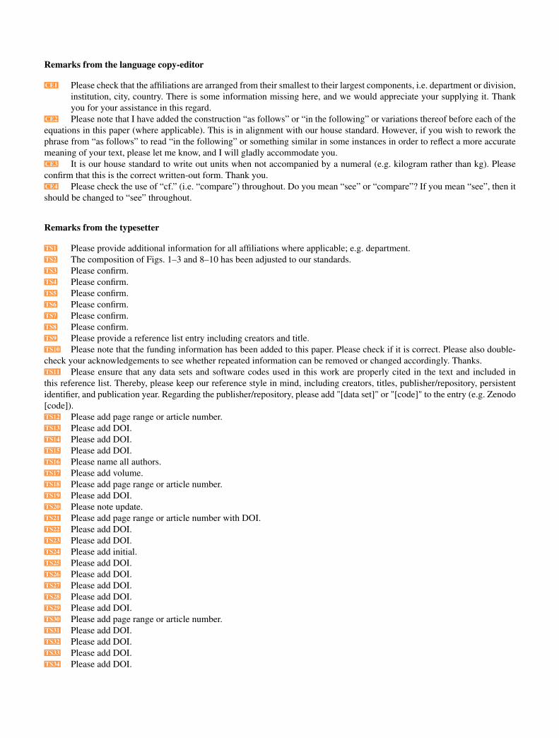
Remarks from the language copy-editor

CE1 Please check that the affiliations are arranged from their smallest to their largest components, i.e. department or division,institution, city, country. There is some information missing here, and we would appreciate your supplying it. Thankyou for your assistance in this regard.

CE2 Please note that I have added the construction “as follows” or “in the following” or variations thereof before each of theequations in this paper (where applicable). This is in alignment with our house standard. However, if you wish to rework thephrase from “as follows” to read “in the following” or something similar in some instances in order to reflect a more accuratemeaning of your text, please let me know, and I will gladly accommodate you.CE3 It is our house standard to write out units when not accompanied by a numeral (e.g. kilogram rather than kg). Pleaseconfirm that this is the correct written-out form. Thank you.CE4 Please check the use of “cf.” (i.e. “compare”) throughout. Do you mean “see” or “compare”? If you mean “see”, then itshould be changed to “see” throughout.

Remarks from the typesetter

TS1 Please provide additional information for all affiliations where applicable; e.g. department.TS2 The composition of Figs. 1–3 and 8–10 has been adjusted to our standards.TS3 Please confirm.TS4 Please confirm.TS5 Please confirm.TS6 Please confirm.TS7 Please confirm.TS8 Please confirm.TS9 Please provide a reference list entry including creators and title.TS10 Please note that the funding information has been added to this paper. Please check if it is correct. Please also double-check your acknowledgements to see whether repeated information can be removed or changed accordingly. Thanks.TS11 Please ensure that any data sets and software codes used in this work are properly cited in the text and included inthis reference list. Thereby, please keep our reference style in mind, including creators, titles, publisher/repository, persistentidentifier, and publication year. Regarding the publisher/repository, please add "[data set]" or "[code]" to the entry (e.g. Zenodo[code]).TS12 Please add page range or article number.TS13 Please add DOI.TS14 Please add DOI.TS15 Please add DOI.TS16 Please name all authors.TS17 Please add volume.TS18 Please add page range or article number.TS19 Please add DOI.TS20 Please note update.TS21 Please add page range or article number with DOI.TS22 Please add DOI.TS23 Please add DOI.TS24 Please add initial.TS25 Please add DOI.TS26 Please add DOI.TS27 Please add DOI.TS28 Please add DOI.TS29 Please add DOI.TS30 Please add page range or article number.TS31 Please add DOI.TS32 Please add DOI.TS33 Please add DOI.TS34 Please add DOI.

Modelling the size distribution of aggregated volcanic ash and ...

Documents

Transcript of Modelling the size distribution of aggregated volcanic ash and ...