Ple

ase

note

that

this

is a

n au

thor

-pro

duce

d P

DF

of a

n ar

ticle

acc

epte

d fo

r pub

licat

ion

follo

win

g pe

er re

view

. The

def

initi

ve p

ublis

her-a

uthe

ntic

ated

ver

sion

is a

vaila

ble

on th

e pu

blis

her W

eb s

ite

1

Ecological Modelling February 2008, Volume 210, Issue 4, Pages 351-376 http://dx.doi.org/10.1016/j.ecolmodel.2007.08.025 © 2008 Published by Elsevier B.V.

Archimer Archive Institutionnelle de l’Ifremer

http://www.ifremer.fr/docelec/

Modelling the Karenia mikimotoi bloom that occurred in the western

English Channel during summer 2003

Alice Vanhoutte-Bruniera, b, Liam Fernandc, Alain Ménesguena, *, Sandra Lyonsd, Francis Gohina and Philippe Cugiera

aIFREMER Centre de Brest, BP 70, 29280 Plouzané, France bIFREMER Centre de Boulogne-sur-mer, BP 699, 62200 Boulogne-sur-Mer, France cCEFAS Lowestoft Laboratory, Pakefield Road, Lowestoft, Suffolk NR33 OHT, UK dMartin Ryan Institute, National University of Ireland, Ireland *: Corresponding author : Alain Ménesguen, email address : Alain.Menesguen@ifremer.fr

Abstract: Observations from space and in situ from the R.V. Corystes 8/03 Cruise show that a massive Karenia mikimotoi bloom occured during summer 2003 in the western English Channel. Due to exceptional climatoligical conditions that occured in June 2003, the installation of a very strong thermocline enhanced the development of a massive bloom over 1 million cells l−1 in the Central English Channel. This paper presents the application of a mathematical model of this species, previously developed in for the Bay of Biscay, into a general 3D model of the primary production of the English Channel and southern Bight of the North Sea. Allelopathic interactions exerted by K. mikimotoi on other phytoplankton species and the role of agitation in the mortality of this species are taken into account. The model includes the dynamics of the bloom and consequently reproduces with good agreement the geographical distribution of the K. mikimotoi bloom both surface and subsurface. The model suggests that the apparent transport of the bloom towards the French coasts as inferred from the satellite observation was not due to advection but was only caused by the establishment of suitable conditions. The sensivity of the K. mikimotoi distribution to boundary conditions, initialization and the role of turbulence is discussed. Keywords: Coupled physical-biogeochemical 3D modelling; Karenia mikimotoi; Primary production; SeaWiFS; Western English Channel

1 Introduction

Harmful algal blooms have occured for many centuries in many pelagic ecosystems, before the1

possible influence of significant human activity, however, during the last decades these events2

have increased in number, areal distribution and biomass (Anderson, 1997; Chretiennot-Dinet,3

1998; Riegman, 1998; Graneli, 2004). They have many forms and effects (Anderson, 1997),4

impressive primary production by non-toxic algae can provoke a temporary oxygen deficiency5

when decaying and strongly disturb the ecosystem. This primary production can often occur6

during a short period. A number of other species, for example Dinophysis, are poisonous at7

low concentrations. Estimates of the number of phytoplanktonic species that contain toxins8

varies from 60-78 (Sournia, 1995) to 100 (Graneli, 2004). The majority of these species belong9

to the Dinophyceae class (Sournia, 1995). Among them, the dinoflagellate Karenia mikimotoi10

is observed in all of the oceans and particularly in the coastal waters of northern Europe.11

This species was previously described as Gyrodinium aureolum, Gymnodinium cf. nagasakiense12

and Gymnodinium mikimotoi. Karenia G. Hansen and Moestrup is a new genus defined by13

Daugbjerg et al. (2000). It is responsible for the red to dark-brown discolouring waters when14

the density reaches over one million cells l−1. Effects on marine fauna are measurable above a15

few million cells per litre (Gentien, 1998). The production of high rates of viscous extracellular16

polysaccharides can cause asphyxiation in fish, a property called “rheotoxicity” (Jenkinson and17

Arzul, 1998, 2001). Widespread mortality events of wild fishes and benthic invertebrates were18

observed along the English south coast in 1978 and off the southwest Ireland in 1976 and 197819

(review of Jones et al. 1982). The economic consequences of fish kills due to red tides can be20

significant, e.g. fish farms in Scottish lochs in September 1980 (review of Jones et al. 1982),21

3,546 tons of caged fish were killed in Hong-Kong Bay in 1998 (Hodgkiss and Yang, 2001; Yang22

and Hodgkiss, 2001). In 1985, the occurence of a bloom at 800,000 cells l−1 of K. mikimotoi23

in the Bay of Brest caused a loss of 4,000,000 individuals in scalop nurseries and culture trays24

(Erard-Le Denn et al., 2001). Along the French Atlantic coast, a mortality of 800-900 tons of25

the mussel Mytilus edulis (Gentien, 1998) and many fish in 1995 coincided with an exceptional26

bloom of 48 million cells l−1 (Arzul et al., 1995). Exotoxin production can also affect the growth27

of other algae, this allelopathic effect has been demonstrated in many phytoplankton groups,28

for example on the diatom Chaetoceros gracile in the Ushant Front (Arzul et al., 1993) and on29

a natural population of dinoflagellates (Fistarol et al., 2004).30

In the western English Channel, blooms of this species have often been observed in the Ushant31

Front (Pingree, 1975; Holligan, 1979; Holligan et al., 1984; Garcia and Purdie, 1994) and in32

the seasonally stratified region which extends from the central western English Channel to the33

coast of Cornwall (Le Corre et al., 1993; Rodrıguez et al., 2000). These monospecific blooms34

can reach many millions of cells per litre and represent up to 100 mg m−3 of chl-a (Holligan,35

1979).36

During summer 2003, spectacular sea surface chlorophyll a (SS-Chla) concentrations were ob-37

served from space by ocean colour images. Observations from the R.V. Corystes Cruise 8/0338

from 26 th June to 9 th July 2003 in the western English Channel highlighted that these high39

chlorophyll concentrations were due to a monospecific bloom of K. mikimotoi. The exceptional40

characteristic of this event is visible in Figure 1 (SS-Chla derived from SeaWiFS), while blooms41

are common in this area, the 2003 bloom started much earlier and reached a much greater cell42

2

density (up to 1,000,000 cells l−1).43

A modelling study of K. mikimotoi blooms in the context of the Bay of Biscay was first devel-44

oped by Loyer (2001) and Loyer et al. (2001). The goal of this work is to introduce the Loyer’s45

K. mikimotoi submodel in a regional ecosystem model of the Channel and southern North Sea,46

in order to test the robustness of this model in another ecosystem which is hydrodynamically47

and hydrologically different from the Bay of Biscay. The model is also used to evaluate the48

importance of each process in the Karenias ’s dynamics and the sensitivity of the model to49

some parameters.50

2 Description of the study site51

The English Channel is part of the Northwest European continental shelf, it connects the52

Atlantic Ocean to the North Sea (Fig. 2). Its boundaries are normally defined as the Dover53

Strait in the east, with the western end marked by the Isles of Scilly (UK) to Ushant (France).54

This system receives significant freshwater and nutrient inputs, in the east, from the river Seine55

(mean flow about 600 m3 s−1). However, the rivers that discharge into the western English56

Channel contribute very little to the overall input of nutrients compared to loadings of water57

masses coming from the Atlantic.58

The strong tidal regime leads to a range of hydrographic features, such as the high tidal range in59

the region of the Normand-Breton Gulf (Fig. 2), a complicated gyre system around the Channel60

islands of Jersey and Guernsey (Salomon et al., 1988), strong tides in the Dover straits with61

the residual circulation generally directed to the North Sea (Prandle et al., 1993). North of the62

Bay of Seine, along the French coast of the eastern English Channel, a front limits a narrow63

strip of fresher and chl-a richer waters called the “coastal flow” (Quisthoudt, 1987; Brylinski64

et al., 1991). In the Bay of Seine, high river flows induce a plume with strong horizontal and65

vertical gradients.66

Further west with weaker tides the waters stratify, where the Ushant Tidal Front (drawn in67

Fig. 2) separates well mixed waters along the north-western coast of Brittany, from summer68

stratified shelf waters of the central English Channel (Pingree, 1975).69

3 The model70

During the last decades, the enhanced computer capacities allowed to build sophisticated models71

in terms of spatial refinement and biochemical complexity. 3D models are useful for the study72

of harmful algae events which are associated to local imbalance of nutrients or/and to local73

specific hydrodynamical structure. Ecological models are developped to study the dynamics74

of macroalgae (eg. Zostera marina in Mediterranean lagoons, Zharova et al., 2001; Plus et al.,75

2003; Pastres et al., 2004; Ulva lactuca in the Bay of Brest, Menesguen et al., 2006) or microalgae76

species (eg. Phaeocystis globosa in the Channel and southern North Sea, Lacroix et al., 2007).77

Some of them are coupled to models of the catchment area of the rivers that discharge in the78

area of interest, like lagoons (eg. the Thau lagoon, Plus et al., 2006) or bays (eg. the Bay of79

Seine, Cugier et al., 2005a). In such enclosed environments, the oxygen dynamics is investigated80

3

because of the mortality of various aerobic organisms wich results from the oxygen deficiency81

and its total disappearence in the bottom layer (Plus et al., 2003; Tuchkovenko and Lonin,82

2003). The accumulation of detrital organic matter, as a consequence of massive algal blooms,83

increases the oxygen demand for biochemical oxidation.84

Good reviews of regional ecosystem models of the European Shelf can be found in the papers of85

Moll (1998) and Allen et al. (2001). Real coupling studies between general circulation models86

and ecosystem models appeared in late 1990’s with generally quite large meshes of 20 km87

(Skogen et al., 1995; Moll, 1998). As far as the biogeochemical modelling strategy is concerned,88

models differ from the number of cycles taken into account (among N, P, Si, C), the number89

of prognostic variables and the growth’s scheme chosen (Flynn, 2003). First models were of90

Nutrient-Phytoplankton-Zooplankton type. Trophic pathways have been expansed to microbial91

processes and to the benthic fauna. Actually, one of the more complex ecological model is92

ERSEM (Baretta et al., 1995; Ebenhoh et al., 1997; Baretta-Bekker et al., 1998). It describes93

the N, P, Si and C cycles in both pelagic and benthic foodwebs. Allen et al. (2001)’s model of the94

North West European Continental Shelf ecosystem is the first that combines both high spatial95

refinement and high biogeochemical complexity at a so large scale. It couples the biogeochemical96

module of ERSEM to the POL-3DB baroclinic model (Proctor and James, 1996; Holt and97

James, 2001) on a 12 km grid. Recently, Lacroix et al. (2007) coupled the mechanistic model98

MIRO (Lancelot et al., 2005), which in particular describes the dynamics of the mucilage99

forming algal species Phaeocystis globosa, with the high resolution 3D hydrodynamical model100

COHERENS applied to the Channel and Southern Bight of the North Sea (Lacroix et al.,101

2004).102

In this study, the hydrodynamical model MARS3D is directly coupled to a biogeochemical103

model that describes locally the evolution of the non-conservative variables in water and sed-104

iment. At the same time, the hydrosedimental model SiAM-3D (Cugier and Le Hir, 2000)105

computes exchanges of particulate matters at the water/sediment interface from erosion and106

deposition processes. The sedimental velocity of diatoms and detrital matters are assessed, at107

each time step, in the biogeochemical module. The diffusion of dissolved substance between the108

multilayered sedimental bed and the bottom layer of the water column follows the concentration109

gradient.110

3.1 The hydrodynamical model111

In the Channel, due to the strong tidal gradient and the presence of small scale features a112

high resolution model is required. In this work, the MARS3D provides high resolution phys-113

ical 3D characteristics. It was developed by Ifremer (Lazure and Jegou, 1998; Lazure and114

Dumas, 2006) and is commonly used in many oceanographic regions some with coupling to115

higher trophic levels. It uses a finite difference scheme to solve the primitive Navier-Stokes116

equations under both hydrostatic and Boussinesq assumptions. The domain simulated in this117

study extends from the south of Brittany (47.5˚N, 5.6˚W) to north of the Rhine river plume118

(52.5˚N, 5.0˚W). The model is in spherical coordinates; the mean size of meshes is about 4119

km by 4 km. The water column is divided into 12 layers all over the domain and the thickness120

of the layers follows the bathymetry (σ-coordinates). The layers in the first third of the water121

column are thinner in order to have a good representation of the thermo-haline stratifications.122

4

The bathymetry is provided by the SHOM (Service Hydrographique et Oceanographique de la123

Marine, France).124

3.2 The biogeochemical model125

The aim of this ecosystem model is to reproduce the dynamics of the free-living plankton with a126

simple biogeochemical model, similar to that previously developed for the Bay of Biscay (Loyer127

et al., 2001; Huret et al., 2007), the Bay of Seine (Menesguen et al., 1995; Guillaud et al., 2000;128

Cugier et al., 2005b) and the Channel (Hoch and Menesguen, 1997; Menesguen and Hoch, 1997;129

Hoch, 1998; Hoch and Garreau, 1998). The originality of our approach lies in the adding of a130

specific submodel Karenia mikimotoi, as previously applied in the Bay of Biscay (Loyer et al.,131

2001).132

3.2.1 State variables and common processes133

The biochemical model is an extension of the NPZD model type (Nutrient-Phytoplankton-134

Zooplankton-Detritus). The model of the planktonic network (Figure 3) aims to simulate the135

fluxes between each level with only limiting elements such as nitrogen, silicon and phosphorus136

modelled, while carbon, the main constituent of the algal biomass, is not explicitly simulated137

because it is provided in non-limiting concentrations in marine systems by respiration and air-138

sea exchanges (Menesguen et al., 2001). Oxygen in the sediment is also modelled due to its role139

in the fate of phosphorus and nitrogen in the sediment.140

In the model, the phytoplankton feeds on two dissolved inorganic nitrogen forms, nitrate (NO−

3 ),141

ammonia (NH+4 ) and the dissolved orthophosphate (PO2−

4 ). For (PO2−4 ) due to its high affinity142

with sediment particles and suspended matter in the water column, exchanges through ad-143

sorption and desorption with the particulate exchangeable phosphate pool (Pads) are handled144

using kinetics already described in Guillaud et al. (2000) and Cugier et al. (2005b). The last145

nutrient required for siliceous algae (diatoms) is silicate (Si(OH)4) and the two functional phy-146

toplankton groups are simulated according to their dependence (diatoms Dia) or independence147

(dinoflagellates Din and nanoflagellates Nan) on silicon for growth. Karenia mikimotoi (Kar)148

can be distinguished from the general class of dinoflagellates by consideration of its own dy-149

namics and the special processes linked to it. The food-chain is closed by zooplankton divided150

into two classes by size, the microzooplankton (Miz) and the mesozooplankton (Mez), and by151

benthic suspension feeders (Bent). The detrital matter (Ndet, Pdet and Sidet) is composed of152

faecal pellets and dead organisms.153

Equations for the local evolution of the non-conservative variables are listed in table 1 with154

the equations that govern the processes listed in appendices A and B. Parameter values are155

reported in tables 2, 3 and 4. The parameters for the suspended particulate matters (SPM)156

which are primarily fine particles are given in table 5.157

3.2.2 Factors controlling phytoplankton growth158

5

The phytoplankton growth rate (µ in d−1) depends of the availability of nutrients, the irradi-159

ance and the ambient temperature. The multi-nutrient interactions in phytoplankton growth160

is of Monod type, which is of low complexity. Temperature acts independently from the other161

factors on the mortality and on the growth according to an Arrhenius law with Q10=2. Among162

the limiting factors (light, nutrients), the growth of each species is limited by the strongest163

limiting factor. However, high irradiance (above Iopt) inhibits growth of diatoms and dinoflag-164

ellates according to Steele’s formula (Steele, 1962) but does not apply to all algal groups of the165

model. The light limiting function for pico-nanophytoplankton conforms to a Michaelis-Menten166

function. From the irradiance at the sea surface level (I0), the availability of light for primary167

producers is a function of the depth (z) and the extinction coefficient (k). The equation for k168

has been verified in the bay of Biscay with SeaWiFS images (Gohin et al., 2005) and is derived169

from a combination of chl-a (to account for self-shading) and SPM concentrations (appendix170

B). Chl-a is deduced from diatom, dinoflagellate, nanophytoplankton and K. mikimotoi con-171

centrations assuming a group dependant N:chl-a. It is well known that some dinoflagellates, by172

the release of exotoxins, can affect the growth of their potential competitors. This allelopathic173

effect is exerted by Karenia on many sympatric species (Gentien, 1998; Hansen et al., 2003;174

Kubanek and Hicks, 2005). Growth inhibition has been reported for diatoms (Arzul et al., 1993)175

and for dinoflagellates (Fistarol et al., 2004). Exotoxin production also induces autoinhibition176

(Gentien, 1998; Kubanek and Hicks, 2005) and is thus important in the termination of the177

bloom (see Karenia mikimotoi submodel, §3.2.3). Thus, adding to the Loyer (2001)’s model,178

this property is taken into account. A positive correlation between the density of K. mikimotoi179

and its repression of the growth of the diatom Chaetoceros gracile was observed in the Ushant180

front system (Arzul et al., 1993) above a threshold K. mikimotoi concentration of between181

7,000 and 10,000 cells l−1. The growth attenuation rate (rall in %) fitted by Arzul et al. (1993)182

is :183

rall = 11.05 × log(Kar) − 33.06 (1)

where Kar is the concentration of Karenia mikimotoi in cells l−1. Although Kubanek and Hicks184

(2005) showed that K. brevis uses species-specific allelopathic strategies, for simplicity the above185

equation has been applied to all phytplanktonic functional groups.186

187

The omnivorous mesozooplankton feeds on the diatoms, dinoflagellates and microzooplankton,188

with the microzooplankton eating detrital matter and nanoflagellates with each class of zoo-189

plankton having its own preferential consumption behaviour (see table 3). The ingestion of the190

microzooplankton obeys a Michaelis-Menten equation (Hoch, 1998), whereas the capture rate191

of mesozooplankton follows the Ivlev’s equation (Hoch, 1998). The mortality of the mesozoo-192

plankton (mMez) is a second order process linked to the concentration of Mez.193

Phytoplankton and detritus can be ingested by benthic suspension feeders (Bent) located in194

the surface sediment. The description of the benthos dynamics is a compromise between (1) a195

complex system of suspension feeders as used in the benthic submodel of the Bay of Brest196

(Le Pape and Menesguen, 1997; Le Pape et al., 1999) and (2) a rough grazing pressure used197

by Savina (2004) to control the primary production in an ecosystem box model of the Chan-198

nel (appendix A). The ingestion rate is higher during summer due to the use of a sinusoidal199

function to describe the seasonal time-course of maximum filtration. The grazing pressure and200

the release of matter by the benthos are only exerted on the bottom layer of the water column201

(layer number 1, of thickness equal to z(l=1)).202

Nutrients are regenerated by the remineralization of the detrital matters. The rate at which203

6

diatoms sink (wDia) is linked to the nutritive limitation (fNlim) described in appendix B while204

the sedimentation velocity of detrital matter (wDet) takes into account its origin, either phyto-205

planktonic or zooplanktonic. Each type of detrital matters has it’s own sinking rate (wDetPhy and206

wDetZoo).207

All the variables involved in the nitrogen cycle are expressed in µmol l−1 N , except zooplankton208

groups (µg l−1 dry wt) and benthic fauna (g m−2 C).209

3.2.3 Karenia mikimotoi submodel210

The processes involved in the local evolution of K. mikimotoi (Kar, in cells l−1) are given by211

(Loyer, 2001; Loyer et al., 2001).212

213

dKar

dt= µKar × Kar − mKar × Kar2 (2)

Karenia mikimotoi is extremely sensitive to agitation, Gentien (1998) observed that in cultures,214

the growth is optimal when the turbulence is very limited. Moreover, Gentien (1998) showed that215

turbulence increases the sensivity of K. mikimotoi to its own exotoxins. Turbulence increases the216

encounter rate and thus, the mortality rate. The term Kar2 of the above equation is proportional217

to the encounter rate. However, K. mikimotoi cells secrete some mucus which leads to the218

aggregation of cells. The probability for cells to stay “attached” after collision and to increase219

the autotoxicity is expressed by the parameter α (non-dimensional) which is thermo-dependant220

(Jenkinson and Arzul, 1999). Thus, α evolves following an exponential function between 15˚C221

and 20˚C; below 15˚C, α=0.05 and above 20˚C, α=1 (Loyer et al., 2001).222

The mortality rate formulation integrates the shear stress (γ, in s−1) resulting from the energy223

dissipation. According to Moum and Lueck (1985) :224

γ =

√

ǫ

7.5 ν(3)

where ν is the kinematic viscosity. ǫ is the energy dissipation rate, which is fully computed from225

the turbulent kinetic energy by the MARS3D model.226

Following these considerations, the mortality rate (in d−1) equation is :227

mKar = γ × α × mcKar (4)

with mcKar, the nominal mortality rate ((cells l−1)−1).228

The growth is dependent on the temperature (µKarT ), the available light (fKar

lum ) and nutrients229

(fKarN and fKar

P ) :230

µKar = min(fKarlum , fKar

N , fKarP ) × µKar

T (5)

The light limiting function is of Michaelis-Menten type, with a half-saturation constant (KKarI )231

determined in laboratory by Loyer (2001) : fKarlum = Iz/(Iz + KKar

I ). The value of KKarI corre-232

sponds to an adaptation of cells to low irradiances as shown by Garcia and Purdie (1992). The233

nutrient limitations are assessed as for other phytoplanktonic species by a Michaelis-Menten234

equation. The half-saturation constant for ammonia was calibrated by Loyer et al. (2001) high-235

lighting the ability of K. mikimotoi to grow at low mineral nitrogen concentrations (KKarNH4=0.01236

µmol l−1) and to thrive mainly on ammonia (KKarNH4 << KKar

NO3).237

Unlike the other phytoplanktonic classes, the growth of K. mikimotoi is directly linked to the238

7

temperature by a polynomial function (µKarT ). The rewiew by Loyer et al. (2001), gives the239

optimal temperature range for growth to be 14˚C-20˚C with maximum value of the growth240

rate to be 1.2 d−1 (Yamaguchi and Honjo, 1989). In this model, the growth is optimal (0.75241

d−1) at 15˚C and equal to 0.05 d−1 below 13˚C and above 23˚C. Grazing is generally an242

important factor on the control of the planktonic primary producers, however this not nesse-243

carily true for Karenia. Rodrıguez et al. (2000) report consumation by Noctiluca scintillans,244

while Bjoernsen and Nielsen (1991) observed the avoidance by microzooplankton of subsurface245

waters dominated by K. mikimotoi. Birrien et al. (1991) noted the absence of zooplankton246

during a K. mikimotoi bloom in the Iroise Sea. It is not well established if the K. mikimotoi247

bloom area is avoided by the zooplankton or if K. mikimotoi is lethal for its potential predators248

(Gentien, 1998). As the grazing by copepods is probably low (Gentien, 1998), and perhaps nill,249

no top-down control is exerted on the K. mikimotoi population.250

The conversion of the cell density of Karenia mikimotoi into chl-a concentration is done with a251

ratio (rKarcell:chl) calculated with data from the Corystes cruise. Only samples with Kar > 100,000252

cells l−1 are kept as being nearly monospecific. rKarcell:chl=53,000 ± 31,000 cells (µg chl)−1 (n=45).253

Parameter values are displayed in table 3.254

3.3 Initialization, forcings and boundary conditions255

The transit time through the Western English Channel is typically a few months. Thus, after256

one year of spin-up, the initial conditions do not significantly influence the simulation. The257

1 st of January concentration of diatoms is imposed following SeaWiFS-derived chl-a and K.258

mikimotoi is initialized as 500 cells l−1 over the domain.259

A mean flow threshold of 5 m3s−1 has been fixed for the selection of rivers shown on figure260

2. Data was provided by the Cellule Anti-Pollution de la Seine, the Regional Agencies of the261

Environnement (DIREN) of Bretagne, Basse-Normandie, Nord-Pas de Calais and the Water262

Agencies of Loire-Bretagne, Seine-Normandie and Artois-Picardie. Data for English rivers cames263

from UK Environment Agency (South, South West and Thames Regions) and flow data from264

the National River Flow Archive of UK (NRFA). The inputs of the Rhine, Meuse and Sheldt265

came from the Institute for Inland Water Management and Waste Water treatment and the266

Rhine and Scheldt International Commissions.267

The meteorological model ARPEGE (Meteo-France) provided fields of air temperature, air268

moisture, atmospheric pressure and wind with a 0.5˚ spatial and 6 hours temporal resolution269

respectively. The hourly sea solar irradiance (SSI) data came from a treatment of the satellite270

METEOSAT-7 sensor data (Brisson et al., 1994, 1996). Daily averages of the cloud cover at the271

Cap de La Heve meteorological station were provided by Meteo-France and were considered272

spatially homogeneous over the model’s domain.273

The free-surface elevation and currents at the open boundaries of the 3D model are off-line274

provided by a 2D barotropic model of greater geographic extent which covers the north-western275

European Shelf (from 40˚N to 65˚N and from 20˚W to 15˚W). Monthly climatologies of276

nutrient concentrations, salinity and temperature at the northern boundary are deduced from277

ICES data (http://www.ices.dk/datacentre/data intro.asp). This boundary is divided278

into four sections to replicate the coastal-offshore gradient. Strong vertical gradients occur at279

8

the western limit due to seasonal stratification, thus different bottom and surface values are280

imposed on both sides of the thermocline level computed by the model, in a similar manner to281

Menesguen and Hoch (1997). The salinity is provided by a 3D model of the Bay of Biscay shelf282

(Huret et al., 2007) and temperature is relaxed to the climatology of Reynaud et al. (1998)283

with a time lag of 13 days.284

At the end of winter light availabity is the limiting factor in the growth of phytoplankton.285

At that period of the year, the light in the water column is governed primarily by mineral286

SPM whose modelling is difficult as its concentration results from the effect of sucessive strong287

winter storms. For that reason, we have forced the offshore SPM of our model by using monthly288

mineral SPM maps derived from SeaWiFS (Gohin et al., 2005). This algorithm calibrated with289

in situ data deduces the non-living SPM concentration from the total SPM. From the sea290

surface SeaWiFS SPM data (SPMsat), the computed SPM concentration (SPMc) in the water291

column (depth z) is corrected by an exponential law as in Huret et al. (2007). This relationship292

is adapted in order to take into account a linear gradient effect of salinity :293

SPM(z) = SPMc(z) + (SPMsat − SPMc(z)) × exp−α×z × max(

0;S − Sth

Smax − Sth

)

(6)

with α = 0.03, Sth = 30.0 p.s.u. and Smax = 35.6 p.s.u.. In regions of fresh water influence (de-294

fined by a salinity threshold value Sth=30.0 p.s.u.), the turbidity is fully described by SiAM-3D.295

Due to the high presence of cloud cover in the Channel, daily satellites scenes were not available,296

so monthly composites of the sea surface mineral SPM were constructed from SeaWiFS-derived297

“Ocean color” data and were interpolated to daily values to force the model.298

4 Validation data299

A large data set was available for the validation of the model. The stations used are displayed300

in Figure 2. The CEFAS research vessel Corystes (Cruise 8/03) provides an extensive source301

of validation with numerous CTD profiles, surface samplings and scanfish sections collected302

during fromthe 26 th June - 9 th July. Samples for phytoplankton analysis were taken from dis-303

crete depths at each CTD station by preserving 55 ml sub-samples withdrawn from the CTD304

rosette sampling bottles, in acidified Lugol’s Iodine. Samples were kept cool and in the dark305

until analysis. Cell densities were estimated after sedimentation using the technique outlined in306

Raine et al. (1990). Cells that conformed to the description outlined in Ottoway et al. (1979)307

were scored as Karenia mikimotoi.308

309

The “ocean colour” sea surface information was processed from SeaWiFS (Sea-viewing Wide310

Field-of-view Sensor) satellite data by an empirical specific algorithm (Gohin et al., 2002, 2005).311

SS-Chla concentrations estimates within the bloom were above 20 µg l−1 in the central English312

Channel and up to 70 µg l−1 locally during the Corystes 08/03 Cruise. The bloom had dimen-313

sions of the order 60×30 nautical miles. According to the SeaWiFS images, the K. mikimotoi314

bloom appeared in the central western English Channel at the end of June and reached the315

French coast of Brittany by the beginning of August. The French Phytoplankton and Phyco-316

toxin Monitoring Network (REPHY) counted 405,000 K. mikimotoi cells l−1 in the Saint-Brieuc317

9

Bay on the 15 th of August 2003 and the mortality of many wild fish species was observed.318

319

The validation data set is completed with field data from regular survey networks. The Station320

ROS (48˚46’40”N 3˚56’15”W, 60 m depth) is situated off Roscoff and is part of the SOM-321

LIT network (French national network of Marine Stations). The Station CHA (Chausey Island,322

48˚52.71’N 1˚46.08’W, 11.5 m depth) is managed by the “Reseau Hydrologique Littoral Nor-323

mand” network. E1 is a long-term time series observatory of the JGOFS program is located 20324

miles off Plymouth (50˚02’N 4˚22’W, 55 m depth).325

5 Results326

The performance of the model was statistically evaluated by linear regressions between observed327

versus computed data. For each parameter, the slope (a) and the ordinate at origin (b) of the328

regression are indicated. The outputs are saved every 4 days at midday.329

5.1 Seasonal stratification330

Figure 5 gives the SST provided by the AVHRR at mid-July 2003 (Fig. 5a) and the difference331

of the monthly average of SST given by the AVHRR and the circulation model for July 2003.332

A mass of warmer surface water appears isolated in the central western English Channel and333

is limited to the south by the Ushant Front. Here, the SST reached 20.1˚C on the 13 th July334

2003, whereas during the same period the SST along the north-western coast of Brittany was335

approximately 15.5˚C. The model accurately reproduces these satelite - observed patterns.336

For two stations located in the contrasting water masses (E1 for the warmer and ROS for337

the cooler), computed and measured water temperature at the sea surface and bottom are338

displayed in Figure 4. The seasonal course of the surface-bottom temperature difference (∆Θs−b)339

is also very different for these two stations. At Station E1, waters were mixed until April340

2003. A smooth stratification appeared during spring, reaching a maximum measurement of341

approximatively ∆Θs−b of 5.7˚C on the 3 rd August. This sharp two-layer structure, previously342

observed in the western English Channel during summer (e.g. Sharples et al., 2001), is also343

accurately reproduced by the model (Fig. 6). The model output shows a strong thermocline at344

15-20 meter, which is consitent with observations from a section perpendicular to the cornish345

coast. (Fig. 6b). In contrast vertically mixed waters with a maximal ∆Θs−b of only 0.95˚C346

(31 st August (Fig. 4) exist in the coastal strip off Roscoff. The figures 4b and 5b show that the347

model overestimates the temperature in the coastal mixed strip by about 2˚C during summer.348

5.2 Spatial and temporal distribution of chlorophyll a and nutrients in 2003349

In order to have an overview of the accuracy of the computed chl-a distribution, the simulated350

SS-Chla is compared to SeaWiFS-derived SS-Chla by using monthly averages and compos-351

ites respectively (Fig. 7). These comparisons show a satisfactory agreement from March to352

10

May 2003, especially for the onset of the spring bloom in the eastern English Channel and353

the southern Bight of the North Sea. High chl-a concentrations (>10 µg l−1), exist along the354

coastal strip which extends from the Seine river mouth to the Dover Strait (Brylinski et al.,355

1991) and northwards to the Rhine river mouth whereas the southern English coast and the356

western English Channel experianced a lower spring bloom. The SS-Chla computed north off357

the Bay of Somme is lower than in the corresponding SeaWiFS composit for the three spring358

months presented, while in the western English Channel, the computed SS-Chla is higher than359

the mean SeaWiFS-derived SS-Chla during May (2.5-3.0 µg l−1 and <1.0 µg l−1 respectively).360

361

The ability of the model to replicate the seasonal cycle of nutrients and chl-a for the 3 sta-362

tions where extensive temporal data exists is shown in Figure 8. Historical data of nitrate and363

phosphate (Jordan and Joint, 1998) are used as a climatology for Station E1, the other field364

data were collected in 2003. The chlorophyll maximum is relatively well reproduced for these365

three stations both temporally and in magnitude. At Station E1, the simulated chl-a maximum366

(4.5 µg l−1) occurs in May, while at Station CHA in the mixed region the maximum occurs367

in April. Dissolved nutrients are sharply depleted after the spring bloom all over the Channel,368

except in the Bay of Seine, where the nutrient inputs are still supplied in summer. Thus, phy-369

toplankton groups which have high nutrient half-saturation constants become nutrient limited370

(e.g. diatoms).371

The seasonal cycle of the principal nutrients is well simulated except in the summer months in372

the coastal station where riverine sources from northern Brittany, not taken into account due373

to their low mean flow, have a strong local influence. The increase in ammonnia concentration374

at station ROS post spring bloom is due to the regeneration of detrital nitrogen and excretion375

from primary consumers. Subsequent to the spring bloom, the nutrient concentration for all376

three sites increases similarly in both the model outputs and the data. As a results of this, a377

smaller diatom bloom is induced during Autumn, which is consistent with previous observa-378

tions (Rodrıguez et al., 2000) and modelling results (Menesguen and Hoch, 1997; Anderson and379

Williams, 1998; Hoch, 1998).380

381

5.3 The 2003 Karenia mikimotoi’s bloom382

The figure 9 shows the computed time-depth sequence of temperature, diatoms and Karenia383

mikimotoi at Station 275. Phytoplankton counts at the sea surface revealed that the bloom384

was monospecific during the Corystes Cruise 8/03. Figure 10 displays the depth-maximum385

concentration of K. mikimotoi sampled during the Corystes Cruise 8/03 superimposed on the386

depth-maximum computed on the 12 th July 2003. The model quite strongly underestimates the387

maximum concentration. While the in situ data indicates that the K. mikimotoi bloom reached388

in excess of 1,000,000 cells l−1 (1,370,800 cells l−1, sea surface level at Station 275), the model389

only provides a maximum concentration of 300’000 cells l−1. The computed K. mikimotoi cell390

density at Station 275 during 2003 is shown in Figure 9 with the diatom concentration and the391

temperature time-depth variation.392

Massive concentrations were frequently encountered at the sea surface in the central Channel393

11

(e.g. Station 275), while the cells seemed more abundant at the subsurface in the western394

region (e.g. Station 90, 1,171,100 cells l−1 at 19 m depth). If we refer to a W-E cross-section395

of the western English Channel (Fig. 2), the model simulates a spatially homogeneous K.396

mikimotoi maximum at 15-20 m depth (Fig. 11a) and cell densities of 75,000 cells l−1 at the397

sea surface. This inability of the model to reproduce high concentrations above the pycnocline is398

also displayed along the vertical profiles of three Corystes stations (Fig. 12). Nevertheless for 2399

out of 3 stations, the subsurface concentrations provided by the model are close to observations.400

6 Discussion401

6.1 Global characteristics of the model402

Compared to other recents ecosystem models developped in this area, ECO-MARS3D appears403

as a compromise between biogeochemical and hydrodynamical complexity. The phytoplanktonic404

compartment is described by three functionnal groups and one dinoflagellate species. Some405

marine ecosystem models still simulate one aggregated state variable for phytoplankton (e.g.406

Tuchkovenko and Lonin, 2003). The top-down control is also quite finely represented with two407

class of size of zooplankton. According to the meta-analysis of the 153 aquatic biogeochemical408

models of Arhonditsis and Brett (2004), this 16 state variables model has an intermediate level409

of complexity.410

The model underestimates the spring phytoplankton bloom in the eastern English Channel,411

particularly between the mouth of the Seine river and the Dover Strait. Even if it is not412

our principal area of interest, many assumptions can be discussed. This area is dominated413

every spring by the Prymnesiophyte Phaeocystis globosa (Lancelot, 1995; Lefebvre and Libert,414

2003), thus our model cannot reproduce these observed high chl-a concentrations. Another415

ecological model including a Phaeocystis glogosa module shows similar under-estimations of416

the chlorophyll-a computation (Lacroix et al., 2007) in this coastal area, without one being417

able to say if it implies that the causes are identical into our two models. The comparison of418

the SS-Chla situations show that the computed coastal productive area is probably too large.419

The offshore dispersion of phytoplankton cells could be explained by a too diffusive advection420

scheme which leads to a drop of the spring peaks of phytoplankton.421

In the mixed coastal strip bordering the North Brittany coast (station ROS), the computed422

bloom starts too early at station ROS. This is perhaps due to an insufficient grazing pressure423

exerted by the benthic fauna. The actual empiric feeding formula concentrates the benthos424

grazing pressure in summer and does not take into account any influence of the bottom current425

velocity. This may have a significant effect in mixed area where the suspension feeders can delay426

the beginning of the bloom.427

Such other regional ecosystem models reproduce more or less accurately the spatial and tempo-428

ral variability of chl-a concentrations. Arhonditsis and Brett (2004) assess that the simulation of429

the biological planktonic components is less satisfying than physical/chemical variables. Com-430

plex ecosystem models, like NEMURO model applied to the North-West Pacific Ocean (Hash-431

ioka and Yamanaka, 2007), ERSEM or MIRO use fixed sets of parameters tuned in some limits432

12

indicated by the literature, it is often the weakest point in modelling (Jørgensen, 1999). One way433

to improve the parameterization of model values is data assimilisation. Applications to 3D bio-434

geochemical models are quite limited (Arhonditsis and Brett, 2004). For the model of the Gulf435

of Biscay, Huret et al. (2007) used optimization routines that assimilate the SSChl-a deduced436

from ocean color data during a three weeks spring period. Even if the simulation of the spring437

bloom is significantly improved, it would be probably necessary to perform the optimization of438

the whole set of parameters at different periods. A new generation of aquatic models carries out439

simulations using time-varying parameters or goal functions that determine the self-organizing440

response of ecosystems to perturbation (Jørgensen, 1999; Arhonditsis and Brett, 2004). Such441

structural models are able to account for the change in the species composition as well as for442

the ability of species to adapt to the prevailing conditions (Jørgensen, 1999). Adaptation pro-443

cesses are parsimoniously used in regional ecosystem models. The ERSEM model considers an444

adaptation mechanism for phytoplankton to light conditions with an adaptation time of 4 days445

(Kholmeier and Ebenhoh, 2007). But the research on photoacclimatation processes in adimen-446

sionnal systems is much more advanced. It requires the modelling of varying intracellular ratios447

(N:C and Chl:C, Smith and Yamanaka, 1996). Our model does not include such complex pro-448

cesses than structural models do. But the focus on the parameters and equations which govers449

the dynamics of Karenia mikimotoi, one species among the dinoflagellate functionnal groups,450

follows a common aim, i.e. the assessment of physical and chemical conditions which control451

the development of one temporarly dominating microalgal species.452

6.2 Controlling factors in the dynamics of Karenia mikimotoi453

This study benefits of the the occurence of an exceptionnal bloom of Karenia mikimotoi dur-454

ing the Corystes 8/03 cruise. The off-shore validation of the K. mikimotoi submodel is more455

advanced than for it’s first application in the Bay of Biscay Loyer (2001).456

It is remarkable that from a spatial homogeneous initialization of 500 cells l−1 K. mikimotoi457

only survives in the western English Channel. Mathematical models allow to quantify the rela-458

tive importance of physico-chemical factors into the phytoplankton’s dynamics. The following459

discussion centres on why the western English Channel is the only favourable place for K.460

mikimotoi ’s development.461

6.2.1 Growth and mortality462

The development of the bloom at the subsurface is due to favourable conditions of light, tem-463

perature, turbulence and nutrients. Modelling offers the possibility to quantify the importance464

of each physico-chemical factors in the development of the Karenia bloom (analyzed in Figure465

13 for station 70). The growth limiting factors were calculated for light and each nutrient (Fig.466

13a), they range from 0 (total limitation) to 1 (no limitation). Under 15 m depth, the nutritive467

conditions are non-limitig (fN and fP effects above 0.8). As previously observed by Holligan468

(1979), the upward mixing of nutrient-rich bottom water provides unlimited nutrient condi-469

tions for K. mikimotoi development at the floor of the seasonal thermocline. The subsurface470

bloom uses the diapycnal source of nitrogen and appears at the nitracline level (Morin et al.,471

1989; Birrien et al., 1991). As K. mikimotoi does not suffer from photo inhibition, favourable472

13

light is encountered from the sea surface to 20 m depth. The maximal growth rate of 0.4 d−1473

occurred at 20 m, where the balance of light penetration with depth against the depletion of474

nutrients to the surface was at an optimum for growth. These observations contribute to the475

idea (e.g. Smayda, 2002) that stratification primarily controls the population dynamics through476

interactions with the vertical irradiance and nutrient gradients. Dinoflagellates are generally the477

dominant photosynthetic organisms after the spring diatom outburst (eg. Holligan et al., 1979).478

K. mikimotoi represents more that 50 % of the computed sea surface phytoplanktonic nitrogen479

biomass in mid-July at station E1, and reached a maximum of 80 % by mid-August. Karenia480

never dominates the phytoplanktonic community at the two mixed stations.481

As suggested by Le Corre et al. (1993), the phenomenon of the K. mikimotoi bloom in the482

fronts and offshore stratified areas differs from that in coastal waters and estuaries. In the483

regions of freshwater influence, the nitrogen provided for the K. mikimotoi bloom is generally484

allochthonous, derived either as dissolved inorganic (Jones et al., 1982; Blasco et al., 1996) or485

remineralized biodegradable organic nitrogen (Prakash, 1987) brought into the system in spring486

by the less saline waters.487

Vertical profiles of the stickiness factor α and the shear stress γ are presented in Figure 13b.488

The shear stress γ is higher in the upper and bottom layers due to wind stress and bottom489

current friction respectively. The stickiness coefficient is only modulated by temperature and490

thus, its mean spatial distribution at the sea surface during July (Fig. 14a) quite accurately491

follows the SST distribution displayed in Figure 5. In a vertical profile, the mortality sharply492

increases above the thermocline due to the stickiness factor increasing with temperature. The493

role of the stickiness factor α was investigated by a sensitivity simulation using a fixed low value494

of α. Results are shown (Fig. 14b, left) with a corresponding depth-maximum K. mikimotoi495

reached on the 12 th July with a slightly greater than the concentration reached in the reference496

run. The time series at station 275 (Fig. 14b, right) shows higher concentrations in July (days497

180-210) at both thermocline and surface levels, when compared to the corresponding nominal498

situation (Fig. 9c). Therefore, without any temperature effect on mortality, the K. mikimotoi499

computed bloom is more impressive in July compared to observations. Evidence to support the500

relevance of this parameters comes from a second R.V. Corystes cruise from the 14 th to the501

27 th August 2003 (results not shown) in the same area where no K. mikimotoi were observed.502

As α enhances K. mikimotoi ’s autotoxicity property, it plays a key-role in the termination of503

the bloom.504

Figure 15a displays the mean γ value at the sea surface.the shear stress γ is higher in the505

eastern English Channel Concentrations are lower (<70,000 cells l−1) in the western English506

Channel when compared to the standard output (Fig. 10). Even with quite a low fixed γ value,507

it denotes the impact of turbulence on the start of the bloom. Interestingly in contrast with508

the standard run, concentrations above 25,000 cells l−1 are predicted in the eastern English509

Channel. The term γ in the mortality rate is of primary importance for the simulation of the510

spatial distribution of K. mikimotoi.it is the turbulent conditions that control the survival of511

cells transported eastwards by the residual circulation.512

The accurate replication of temperature is important because it effects both the growth of513

Karenia dynamics (µKarT ), and the mortality rate (through α). The model overestimates the514

SST by about 2-2.5˚C in the mixed coastal strip delimited by the Ushant front (Figs. 5b and515

4b), leading to overestimation in of growth in this area, due to the higher temperature and516

14

reduced mixing. There is a balancing effect of increased stickiness values, increasing mortality,517

but α still remains quite low (< 0.4) in comparison with offshore sea surface values. This518

results in a slight overestimation of the K. mikimotoi cell concentration along the coasts of519

North Brittany. Similarly the model predicts Karenia inshore along the Cornish coast, where520

the model underestimates the local turbulence, possibly in the due to wave mixing in the near521

coastal region.522

The absolute magnitude of the bloom is underestimated, as has been noted before in the523

Bay of Biscay (Loyer, 2001). Several behavioural mechanisms are not described in the model,524

in particular, the ability of K. mikimotoi cells to migrate vertically in relation to a nutrient525

tropism. This strategy of vertical depth-keeping (Smayda, 2002) is made possible by means526

of a swimming behaviour. K. mikimotoi cells can migrate vertically at approximatively 230527

µm s−1 (Throndsen, 1979). Many other assumptions can also be noted; this model considers528

that Karenia mikimotoi is autotrophic, but many studies report an assimilation of organic529

substances by this species (Yamaguchi and Itakura, 1999; Purina et al., 2004). The ecosystem530

model parameterizes the microbial loop action, thus the dissolved organic pool is not described531

and the hypothetized mixotrophic behaviour cannot be studied. In addition, K. mikimotoi is532

able to store a large quantity of phosphorus during nutrient-replete conditions (Yamaguchi,533

1994), and appears to make dark uptake of nitrate under N-limiting conditions (Dixon and534

Holligan, 1989). These processes all contribute to sustain K. mikimotoi growth.535

6.2.2 Allelopathy536

In our model, Karenia mikimotoi inhibits the growth of other phytoplankters (eq. 1). The effect537

begins once a sufficiently high cell concentration has been reached. It is diffucult to transpose538

studies reported among other HAB species, however Sole et al. (2005) demonstrated a such539

threshold effect with a simple Lotka-Volterra model calibrated with laboratory experiments540

and with the simulation of the Chrysocromulina polypepsis bloom of 1998 with the ERSEM541

ecosystem model.542

In order to assess the importance of allelopathy in the inter-specific competition, a simulation543

was carried out without any inhibitory effect (rall = 1).The depth-maximum K. mikimotoi544

concentration and the relative abundance of phytoplankton groups are displayed in Figure 16.545

Without an inhibitory effect, the maximum K. mikimotoi concentration computed at Station546

275 drops from 200,000 cells l−1 to 100,000 cells l−1. In the standard run, K. mikimotoi547

represents 60% of the total phytoplanctonic nitrogen at the end of July (Fig. 8), whereas,548

without the inhibitory effect, it only reaches 40 % of the N biomass (Fig. 16b).549

In addition, the autumnal bloom is stronger when the inhibitory effect is removed (3.5 v.s.550

1.5 µg l−1). It demonstrates that, although the diatoms are no longer nutrient-limited, the K.551

mikimotoi exotoxins still inhibit diatom growth. However, observational evidence suggests that552

K. mikimotoi does not usually dominate the planktonic system in autumn (Rodrıguez et al.,553

2000). It is therefore likely that the modelled termination of the bloom is certainly not abrupt554

enough. As the collapse of the bloom is essentially due to nutrient exhaustion (Partensky and555

Sournia, 1986; Morin et al., 1989; Birrien et al., 1991), in this instance as the magnitude of556

the bloom is underestimated nutrient depletion takes longer to occur. A secondary effect of the557

underestimation of K. mikimotoi ’s density by the model is that the importance of self-shading558

15

on the blooms disappearance is thus also underestimated. Additionally, other factors can affect559

weakened cells and thus accelerate the bloom termination, viruses are able to repress Karenia560

mikimotoi growth (Onji et al., 2003) and bacteria can have an algicidal action (Yoshinaga et al.,561

1995; Lovejoy et al., 1998).562

According to our assumptions (c.f. §3.2.3), K. mikimotoı is not grazed by zooplankton. Mukhopad-563

hyay and Bhattacharyya (2006) investigated the role of zooplankton grazing in a theoretical564

NPZ system. The single phytoplanktonic compartment produces inhibitoring substances for565

the zooplankton. The toxication process is modelized through the grazing function of type IV566

due to prey toxicity. The repulsive effect exerted by the phytoplankton is incorporated through567

a term of zooplankton positive cross-diffusion. According to the authors, the grazing pressure568

could play a significant role in controlling the bloom episode for specific values of parameters.569

But the grazing would be a sink term in the K. mikimotoı equation. Since the model actually570

under-estimates Karenia cells densites, this potential lacking process is probably not a major571

key for the understand of the model performances.572

6.2.3 Role of advection573

According to SeaWiFS images, the K. mikimotoi bloom originally located in the central western574

English Channel, seemed to have a trajectory directed towards the French coast. Similar events575

have been persistently observed elsewhere. Raine et al. (1993) suggested that the red tide576

observed off the south-west Irish coast during the summer 1991 had been advected towards577

the coast from the shelf. A special run was undertaken to test the role of advection in the578

propagation of the bloom. A passive tracer patch of concentration 100 was initialized on the579

23 rd July in the central western Channel, the spill moved northwards and never reached the580

coasts the French coast Figure 17. The visible displacement observed from satellite is most581

likely due not to mass transport but to the presence of favorable conditions in successive spots582

closer to the coast.583

6.3 Inoculum and overwintering of Karenia’s cells584

In contrast to other dinoflagellate species (Persson, 2000; Morquecho and Lechuga-Deveze,585

2003), vegetative cells of K. mikimotoi are capable of overwintering (Yamaguchi, 1994; Gen-586

tien, 1998) and may not form cysts. Indeed, blooms of this eurytherm species have been reported587

to occur at temperatures as low as 4˚C (Blasco et al., 1996). A number of low winter concen-588

trations (5-10 cells l−1) have been observed in the Bay of Brest and it is hypothetized that589

the population originates from southern Brittany (Gentien, 1998). These low winter concen-590

trations would act as the seed population for later blooms when environmental conditions are591

favourable.592

Hydrological conditions at the entrance of the English Channel were investigated thanks to593

a ship of opportunity operating year-round between Plymouth (UK) and Bilbao (Spain) by594

Kelly-Gerreyn et al. (2004, 2005). Field data from 2002 to 2004 highlighted the fact that the595

discharge from major rivers of the Bay of Biscay (Loire, Gironde) was higher in 2003 than596

in 2002 and that favourable winds enhanced an unusual intrusion of lower salinity waters in597

16

2003 (mean=34.93 p.s.u., equal in 2002 to 35.02 p.s.u.) off the North French Atlantic coast598

in late winter. It was hypothesized that this favoured the spectacular bloom of K. mikimotoi599

through increased buoyancy in the upper water column. If true then it demonstrates importance600

of good boundary conditions. In this model the salinity boundary condition is provided by a601

model of the Bay of Biscay (Huret et al., 2007). This model is itself strongly influenced at its602

northern limit by the Reynaud’s climatology (Reynaud et al., 1998) and thus does not provide603

an acute enough interannual variability of hydrological conditions. It is doubtful if this model604

has sufficient information on salinity to adequately investigate the role of buoyancy on the605

success of K. mikimotoi blooms.606

7 Conclusion607

A species specific model for Karenia mikimotoi has been developped and inserted in a 3D model608

of primary production. Such refined ecosystem models focused on a species of interest are few609

and mainly focused on microalgae (eg. Phaeocystis, Lacroix et al., 2007) or macroalgae (eg.610

Ulva, Menesguen et al., 2006) responsible for eutrophication disturbance.611

The sensitivity of Karenia mikimotoi to agitation was taken into account through the shear612

rate (γ) in the mortality calculation as first suggested by Gentien (1998) and adapted by Loyer613

et al. (2001) in the 3D ecosystem model of the Bay of Biscay. In adding to the original processes614

described by Loyer et al. (2001), our model describes the detrimental effect of the production615

of exotoxins on the growth of co-occurring phytoplankton species (rall).616

This model reproduces blooms at the subsurface level and highlights the importance of the617

two major factors in K. mikimotoi dynamics : lower turbulence and stratification. The excep-618

tional warm conditions in June 2003 produced a massive bloom. The results show that the619

model is very sensitive to its paramerization. Growth (through fT ) and mortality (through α)620

are strongly modulated by the water temperature. Sensitivity simulations highlight the key-621

role played by agitation for the spatial distribution of the bloom. Moreover, the K. mikimotoi622

biomass is doubled due to allelopathy exerted on competitors for resources. Although the spatial623

distribution of the computed Karenia mikimotoi shows a satisfactory accordance with Corystes624

data, the computed cell densities are lower. The simulated bloom does not exceed the hivernal625

nitrogen pool, whereas field population did. This may be due to swimming behaviour as has626

been investigated for Karenia brevis by (Liu et al., 2002) in the Florida shelf region. Modelling627

dark-uptake of nitrogen (done by Yanagi et al., 1995) or temporarily intracellular storage of628

nutrients may increase the biomass. However, this requires the use of quota model. In con-629

trast to derived-Monod models, quota models consider that growth not only depends on the630

extracellular nutrient concentration, but also on the internal pool of nutrients (Menesguen and631

Hoch, 1997; Flynn, 2003). The disadvantage being that quota models increase considerably the632

number of prognostic variables and consequently the computing time. Thus, in spite the limits633

of application of Monod models for the modelling of multi-nutrient interactions in phytoplank-634

ton (Droop, 1975; Flynn, 2003), it is these models that are still being coupled to circulation635

models. Thus, processes that would increase the Karenia mikimotoi biomass at the subsurface636

level can’t actually be replicated with 3D refined ecosystem models as the computing time is637

still a strong constraint.638

17

As well as the limitations in the models dynamics, it could be that interannual variability of fresh639

water intrusions from the Atlantic shelf could directly effect the bloom intensity (Kelly-Gerreyn640

et al., 2005). This interesting hypothesis could be tested by further extending the model do-641

main in addition to possesing increased knowledge of the location of over wintering populations.642

643

Acknowledgements644

This study was part of a project managed by Alain Lefevre (IFREMER/LER, Boulogne-sur-645

mer) and funded by IFREMER, the Region Nord-Pas de Calais and the national program646

’PNEC-Chantier Manche orientale’. We thank Franck Dumas for the improvement of the circu-647

lation model MARS3D for this study. We are indebted also to Sophie Loyer for her advice con-648

cerning the Karenia mikimotoi submodel and her comments on the paper. The authors would649

like to thank Dr Matthew Frost from the Marine Environmental Change Network (MECN)650

to have communicated bottom and surface temperature at Station E1 for 2003. Herve Roquet651

(METEO-FRANCE/CMS) facilitated the access to METEOSAT/AJONC products. The Sea-652

WiFS images are available through a GMES service browser at : http://www.ifremer.fr/653

cersat/facilities/browse/del/roses/browse.htm. In addition we would like to thank Ro-654

main de Joux for his help in plotting the majority of the figures. L.Fernand and the Corsystes655

cruises were funded by UK Department DEFRA under project AE1225.656

18

Appendix A - Processes linked to the plankton in the657

biogeochemical model.658

The effect of the temperature fT is an exponential function with a doubling of the

effect for each 10˚C variation (Q10=2): fT = expa T , with T the water temperature.

Growth of the phytoplankton µi (d−1), with i=Dia, Din, Nan : µi = µi0 fT flimi

The limiting effect f ilim is a Liebig low extended to the effect of light :

Dia : f ilim = min(f i

lum, f iN , f i

Si, fiP ) Din and Nan : f i

lim = min(f ilum, f i

N , f iSi, f

iP )

The effet of light at the depth z, flumi(z), is approched by Steele (1962)’s formula :

f ilum(z) = 1

∆z

∫ z+ 1

2∆z

z− 1

2∆z

(

Iz/PAR

Iiopt

)

exp

(

1−Iz/PAR

Iiopt

)

dz , with Iopti the optimal irradiance of i.

From the sea surface irradiance I0, the irradiance decreases exponentially : Iz = I0 exp−k z

The extinction coefficient k is a combination of chlorophyll and SPM concentration

(Gohin et al., 2005) : k = kw + kp Chl0.8 + kspm SPM

with kw, kp and kspm are respectively the k of water, phytoplankton and mineral SPM.

The limiting effect exerted by each nutrient is described by a Michaelis-Menten relationship :

for a nutrient n of concentration Cn : f in = Ci

n

Cn+Kin

; for nitrogen, it takes into account

the both DIN forms : f iN = f i

NO3 + f iNH4 = NO3

NO3+KiNO3

+NH4

KiNO3

KiNH4

+ NH4

NHi4+K

NHi4

+NO3

KiNH4

KiNO3

Death of the phytoplankton mi (d−1), with i=Dia, Din, Nan : mi = m0i fT

Growth of the zooplankton µj (d−1), with j=Mez, Miz :

For Mez, it is described by an Ivlev function :

µMez = µ0Mez fT

(

1 − exp(−γ max(0,P Mez−δ))

)

with µ0Mez : the growth rate at 0˚, δ : the escape threshold, PMez the available preys

and γ : the slope of the Ivlev function.

For Miz it is described by a Michaelis-Menten function : µMiz = µ0Miz fTP Miz

P Miz+kprey

The available quantity of preys for each zooplankton class j is assessed with preferency factors :

Pj =∑

pij j , with for Mez, i=Dia, Din, Miz and for Miz, i=Nano,Det

The assimilation rate of zooplankton is approached by : τj = 0.3(

3 − 0.67 P j

µ0j fT

)

.

Excretion of the zooplankton ej (d−1), with j = Mez, Miz : ej = e0j fT

Death of the zooplankton mj (d−1), with j = Mez, Miz :

For Miz, it’s only linked to the temperature : mMiz = m0Miz fT

For Mez, it’s also dependant of its biomass : mMez = fT max(m0Mez, mb0Mez Mez)

19

Appendix B - Processes linked to the suspended feeders, detrital659

matters and sinking processes in the biogeochemical model.660

Uptake of phytoplankton and detritus by suspension feeders uBent (µmol N l−1 d−1) :

It is dependant of a seasonal filtration intensity (fsin(t)) and of the prey availability (PBent) :

uqBent(t) = filmax fsin(t) fP P q

Bent , with q = (Phy, Det).

PPhyBent =

∑

i , with i=Dia, Din, Nan and PDetBent = min(Ndet, Pdet rDet

N :P ).

With t the julian day : fsin(t) =(

1 + sin (2 π365 (t − 125))

)

/2

Preys escape to the grazing pressure following a Michaelis-Menten function : fP = PBentPBent+KBent

Mortality mBent and excretion eBent of suspension feeders (d−1) :

The mortality is dependant of the benthos biomass : mBent = fT max(m0Bent, mb0Bent Bent)

The dissolved excretion kinetics is only moduled by temperature : eBent = fT e0Bent

The sedimentation velocity of diatoms wDia (m d−1) depends of the nutrient limitation fNlim :wDia = wDia

min fNlim0.2 + wDia

max

(

1 − fNlim0.2

)

, with fNlim = min(fN , fP , fSi).

Sedimentation velocity of detrital matters wDet (m d−1) :

wDet = wDetZoo

(

1r+1

)

+ wDetPhy

(

1 − 1r+1

)

, with r = Qphyto/QZoo

Qphyto =∑4

i=1 mi i , with i=Dia, Din, Nan, Kar.

QZoo =∑2

j=1

(

(1 − τi) µj + mj

)

j , with j=Mez, Miz.

wDetZoo is a constant, but wDet

Phyto is driven by the Stockes law (Yamamoto, 1983) :

wDetPhyto = 1

18 g rDetρDet−ρw

ν ρw

with g the gravitational acceleration, ρDet the density of detrital particles of phytoplanktonic

origin, rDet the radius of these particles, ρw the water density and ν the molecular viscosity.

Adsorption and desorption of phosphate (d−1) :

kadsorp = Cadsorp max(0 , Cmaxadsorp SPM − Pads) kdesorp = Cdesorp min(1 , Pads

Cmaxadsorp

SPM)

Remineralization of detrital matters in water and sediment (c: water w or sediment s) :

Remineralization of N and P in water : minNw = minN0w fT minPw = minP0w fT

Nitrification in water : nitw = nit0w fT

In sediment, remineralization of nitrogen and phosphorus are drived by the oxic condition :

minNs = minN0s fT fminO2

, minPs = minP0s fT fminO2

, nits = nit0s fT fnitO2

with fminO2

= O2/(O2 + KminO2

) and fnitO2

= O2/(O2 + KnitO2

)

Dissolution of biogenic silicon : disSic = disSi0c fT

20

References661

Aksnes D., Ulvestad K., Balino B., Berntsen J., Egge J., Svendsen E., 1995. Ecological mod-662

elling in coastal waters : towards predictive physical-chemical-biological simulation models.663

Ophelia, 41: 5–36.664

Allen J. I., Blackford J., Holt J., Proctor R., Ashworth M., Siddorn J., 2001. A highly spatially665

resolved ecosystem model for the North West European Continental Shelf. Sarsia, 86: 423–666

440.667

Andersen V., Nival P., 1989. Modelling of phytoplankton population dynamics in an enclosed668

water column. J. Mar. Biol. Assoc. UK, 69: 625–646.669

Anderson D., 1997. Turning back the harmful red tide. Nature, 388: 513–514.670

Anderson T., Williams P., 1998. Modelling the seasonal cycle of dissolved organic carbon at671

station E1 in the English Channel. Est. Coast. Shelf Sci., 46: 93–109.672

Arhonditsis George B., Brett Michael T., 2004. Evaluation of the current state of mechanistic673

aquatic biogeochemical modeling. Mar. Ecol. Prog. Ser., 271: 13–26.674

Arzul G., Erard-Le Denn E., Videau C., Jegou A. M., Gentien P., 1993. Diatom growth re-675

pressing factors during an offshore bloom of Gyrodinium cf. aureolum, vol. 283, pp. 365–367.676

Arzul G., Erard-Le Denn E., Belin C., Nezan E., 1995. Ichtyotoxic events associated with677

Gymonodinium cf. nagasakiense on the Atlantic coast of France. Harmful Algal News, 2–3:678

8–9.679

Azam F., Fenchel T., Field J., Gray J., Meyer-Reil L., Thingstad F., 1983. The ecological role680

of water-column microbes in the sea. Mar. Ecol. Prog. Ser., 10: 257–263.681

Baretta J., Ebenhoh W., Ruardij P., 1995. The European Regional Seas Ecosystem Model, a682

complex marine ecosystem model. Neth. J. Sea Res., 33: 233–246.683

Baretta-Becker J., Riemann B., Baretta J., Koch-Ramsmussen E., 1994. Testing the microbial684

loop concept by comparing mesocosm data with results from a dynamical simulation model.685

Mar. Ecol. Prog. Ser., 106: 187–198.686

Baretta-Bekker J. G., Baretta J. W., Hansen A. S., Riemann B., 1998. An improved model687

of carbon and nutrient dynamics in the microbial food web in marine enclosures. Aquatic688

Microbial Ecology, 14: 91–108.689

Birrien J.-L., Wafar M. V., Le Corre P., Riso R., 1991. Nutrients and primary production in a690

shallow stratified ecosystem in the Iroise Sea. J. Plank. Res., 13 (4): 1251–1265.691

Bjoernsen P. K., Nielsen T. G., 1991. Decimeter scale heterogeneity in the plankton during a692

pycnocline bloom of Gyrodinium aureolum. Mar. Ecol. Prog. Ser., 73: 262–267.693

Blasco D., Berard-Therriault L., Levasseur M., Vrieling E., 1996. Temporal and spatial distri-694

bution of the ichthyotoxic dinoflagellate Gyrodinium aureolum Hulburt in the St Lawrence,695

Canada. Journal of Plankton Research, 18 (10): 1917–1930.696

Brisson A., Le Borgne P., Marsouin A., Moreau T., 1994. Surface irradiance calculated from697

Meteosat sensor during SOFIA-ASTEX. Int. J. Remote Sens., 15: 197–204.698

Brisson A., Le Borgne P., Marsouin A., 1996. Operational surface solar irradiance using Me-699

teosat data : Routine calibration and validation results. In : 1996 Meteorological satellite700

data users’ conference EUMETSAT, pp. 229–238. 16-20 September 1996, Wien, Austria.701

Brylinski J.-M., Lagadeuc Y., Gentilhomme V., Dupont J.-P., Lafite R., Dupeuble P.-A., Huault702

M.-F., Auger Y., Puskaric E., Wartel M., Cabioch L., 1991. Le ”Fleuve cotier” : un phenomene703

hydrologique important en Manche orientale. Exemple du Pas-de-Calais. In : Chamley704

H., (Ed.), Actes du Colloque International sur l’Environnement des mers epicontinentales.705

Oceanologica Acta, vol. sp. (11): 197–203.706

21

Chretiennot-Dinet M.-J., 1998. Global increase of algal blooms, toxic events, casual species707

introductions and biodiversity. Oceanis, 24 (4): 223–238.708

Cugier P., Le Hir P., 2000. Modelisation 3D des matieres en suspension en baie de Seine orientale709

(Manche, France). C.R. Acad. Sci. Paris, Sciences de la Terre et des Planetes, 331: 287–294.710

Cugier P., Billen G., Guillaud J. F., Garnier J., Menesguen A., 2005a. Modelling the eutrophica-711

tion of the Seine Bight (France) under historical, present and future riverine nutrient loading.712

Journal of Hydrology, 304: 381–396.713

Cugier P., Menesguen A., Guillaud J.-F., 2005b. Three dimensional (3D) ecological modelling714

of the Bay of Seine (English Channel, France). J. Sea Res., 54: 104–124.715

Daugbjerg N., Hansen G., Larsen J., Moestrup O., 2000. Phylogeny of some of the major genera716

of dinoflagellates based on ultrastructure and partial LSU rDNA sequence data, including717

the erection of three new genera of unarmoured dinoflagellates. Phycologia, 39 (4): 302–317.718

Dixon G. K., Holligan P. M., 1989. Studies on the growth and nitrogen assimilation of the719

bloom dinoflagellate Gyrodinium aureolum Hulburt. Journal of Plankton Research, 11 (1):720

105–118.721

Droop M., 1975. The nutrient status of algal cells in batch culture. Journal of Marine Biological722

Association U.K., 55: 541–555.723

Ebenhoh W., Baretta-Bekker J., Baretta J., 1997. The primary production module in the marine724

ecosystem model ERSEM II, with emphasis on the light forcing. J. Sea Res., 38: 173–193.725

Erard-Le Denn E., Belin C., Billard C., 2001. Various cases of ichtyotoxic blooms in France.726

In : Arzul G., (Ed.), Aquaculture environement and marine phytoplankton. 21-23 May 1992,727

Brest (France).728

Fistarol G. O., Legrand C., Rengefors K., Graneli E., 2004. Temporary cysts formation in729

phytoplankton : a response to allelopathic competitors ? Environmental Microbiology, 6 (8):730

791–798.731

Flynn K. J., 2003. Modelling multi-nutrient interactions in phytoplankton; balancing simplicity732

and realism. Progress in Oceanography, 56: 249–279.733

Garcia V. M., Purdie D. A., 1992. The influence of irradiance on growth, photosynthesis and734

respiration of Gyrodinium cf. aureolum. J. Plank. Res., 14 (9): 1251–1265.735

Garcia V. M., Purdie D. A., 1994. Primary production studies during a Gyrodinium cf. aureolum736

(Dinophyceae) bloom in the western English Channel. Marine Biology, 119 (2): 297–305.737

Gentien P., 1998. Bloom dynamics and ecophysiology of the Gymnodinium mikimotoi species738

complex. In : Anderson D. M., Cembella A. D., Hallegraef G. M., (Ed.), Physiological Ecology739

of Harmful Algal Blooms, vol. G 41, pp. 155–173. NATO ASI Series. Springer-Verlag.740

Gohin F., Druon J.-N., Lampert L., 2002. A five channel chlorophyll concentration algorithm741

applied to SeaWiFS data processed by Sea DAS in coastal waters. Int. J. Remote Sensing,742

23 (8): 1639–1661.743

Gohin F., Loyer S., Lunven M., Labry C., Froidefond J.-M., Delmas D., Huret M., Herbland744

A., 2005. Satellite-derived parameters for biological modelling in coastal waters : illustration745

over the eastern continental shelf of the Bay of Biscay. Remote Sens. Environ., 95 (1): 29–46.746

Graneli E., 2004. Eutrophication and Harmful Algal Blooms. In : Wassman P., Olli K., (Ed.),747

Drainage basin nutrient inputs and eutrophication : an integrated approach, incollection 7,748

pp. 99–112.749

Guillaud J.-F., Andrieux F., Menesguen A., 2000. Biochemical modelling in the Bay of Seine750

(France): an improvement by the introducing phosphorus in nutrient cycles. J. Mar. Sys.,751

25: 369–386.752

Hansen P. J., Graneli E., Legrand C., Salomon G., Skovgaard A., 2003. Allelopathy and mixotro-753

22

phy among bloom forming algae : Kill or eat your competitor. In : Hallegraeff G., Blackburn754

S. I., Bolch C., Lewis R., (Ed.), EUROHAB workshop 2003, pp. 40–42. 17-18 March 2003,755

Amsterdam.756

Hashioka Y., Yamanaka Y., 2007. Seasonal and regional variations of phytoplankton groups by757

top-down and bottom-up controls obtained by a 3D ecosystem model. Ecological Modelling,758

202: 68–80.759

Hoch T., 1998. Modelisation du reseau trophique pelagique et de la production primaire en760

Manche. Oceanol. Acta, 21 (6): 871–885.761

Hoch T., Garreau P., 1998. Phytoplankton dynamics in the English Channel: a simplified three-762

dimensional approach. J. Mar. Syst., 16: 133–150.763

Hoch T., Menesguen A., 1997. Modelling the biogeochemical cycles of elements limiting the764

primary production in the Channel. II. Sensivity analysis. Mar. Ecol. Prog. Ser., 146: 189–765

205.766

Hodgkiss I., Yang Z., 2001. New and dominant species from Sam Xing Wan, Sai Kung during767

the 1998 massive killing red tide in Hong Kong. In : Hallegraeff G. M., Blackburn S. I., Bolch768

C. J., Lewis R. J., (Ed.), Harmful Algal Blooms 2000, pp. 62–65.769

Holligan P. M., 1979. Dinoflagellate blooms associated with tidal fronts around the Brittish Iles.770

In : Taylor D. L., Seliger Howard H., (Ed.), International conference on Toxic Dinoflagellate771

blooms, 31 Oct. - 5 Nov. 1978, Key Biscayne (Florida), pp. 249–256. Elsevier, New York.772

Holligan P. M., Harris R. P., Newell R. C., Harbour D. S., Head R. N., Linley E. A., Lucas M.773

I., Tranter P. R., Weekley C. M., 1984. The vertical distribution and partitioning of organic774

carbon in mixed, frontal and stratified waters of the English Channel. Mar. Ecol. Prog. Ser.,775

14: 111–127.776

Holt J., James I., 2001. An s coordinate density evolving model of the northwest European777

continental shelf. 1. Model description and density structure. J. Geophys. Res., 106 (C7):778

14,015–14,034.779

Huret M., 2005. Apports des donnees ”couleur de l’eau” a la modelisation couplee physique-780

biogeochimie en milieu dynamique cotier. Ph.D. thesis, Universite de Toulouse III, p. 269.781

Huret M., Gohin F., Delmas D., Lunven M., Garcon V., 2007. Use of the SeaWiFS data for782

improving the simulation of winter to spring phytoplankton production in the Bay of Biscay.783

J. Mar. Syst., 65 (1-4): 509–531.784

Jenkinson I., Arzul G., 1998. Effect of the flagellates, Gymnodinium mikimotoi, Heterosigma785

akashiwo and Pavlova lutheri, on flow through fish gills. In : Reguera G., Blanco J., Fernandez786

M., Wyatt T., (Ed.), Harmful Microalgae, pp. 425–428.787

Jenkinson I., Arzul G., 1999. Roles de la rheologie et des effets lies a l’activite cytolytique dans788

la dynamique et l’action toxique de Gymnodinium mikimotoi et d’autres algues nuisibles.789

Rapport final du PNEAT 1998-1999. Tech. report, ACRO-IFREMER.790

Jenkinson I., Arzul G., 2001. Mitigation by cysteine compounds of rheotoxicity, ctytotoxyc-791

ity and fish mortalities caused by the dinoflagellates, Gymonidinium mikimotoi and G. cf.792

maguelonnense. In : Hallegraeff G. M., Blackburn S. I., Bolch C. J., Lewis R. J., (Ed.),793

Harmful Algal Blooms 2000, pp. 461–464.794

Jitts H. R., Morel A., Saijo Y., 1976. The relation of oceanic primary production to available795

photosynthetic irradiance. Austral. J. Mar. Fresh. Res., 27: 441–454.796

Jones K. J., Ayres P., Bullock A. M., Roberts R. J., Tett P., 1982. A red tide of Gyrodinium797

aureolum in sea lochs of the Firth of Clyde and associated mortality of pond-reared salmon.798

J. Mar. Biol. Assoc. U.K., 62: 771–782.799

Jordan M. B., Joint I., 1998. Seasonal variations in nitrate:phosphate ratios in the English800

23

Channel 1923-1987. Estuarine, Coastal and Shelf Science, 46: 157–164.801

Jørgensen S. E., 1999. State-of-the-art of ecological modelling with emphasis on development802

of structural dynamic models. Ecological Modelling, 120: 75–96.803

Kelly-Gerreyn B. A., Qurban M. A., Hydes D. J., Miller P., Fernand L., 2004. Coupled ”Fer-804

ryBox” Ship of Opportunity and satellite data observations of plankton succession across805

the European shelf sea and Atlantic Ocean. In : Annual ICES Science Conference, 22-25806

September 2004, Vigo, vol. CM 2004/P:28.807

Kelly-Gerreyn B. A., Hydes D. J., Fernand L. J., Jegou A.-M., Lazure P., Puillat I., 2005. Low808

salinity intrusions in the western English Channel and possible consequences for biological809

production. Continental Shelf Research, in press.810

Kholmeier C., Ebenhoh W., 2007. Modelling the ecosystem dynamics and nutrient cycling of the811

Spiekeroog back barrier system with a coupled EulerLagrange model on the base of ERSEM.812

Ecological Modelling, 202: 297–310.813

Kubanek J., Hicks M. K., 2005. Does the red tide dinoflagellate Karenia brevis use allelopathy814

to outcompete other phytoplankton ? Limonol. Oceanogr., 50 (3): 883–895.815

Lacroix G., Ruddick K., Ozer J., Lancelot C., 2004. Modelling the impact of the Scheldt and816

Rhine/Meuse plumes on the salinity distribution in Belgian waters (southern North Sea). J.817

Mar. Res., 52 (3): 149–153.818

Lacroix G., Ruddick K., Gypens N., Spitz Y., Lancelot C., 2007. Validation of the 3D ecosys-819

tem model MIRO&CO with in situ measurements and MERIS-derived surface chlorophyll a820

images. 64 (1–4): 66–88.821

Lancelot C., 1995. The mucilage phenomenon in the continental coastal waters in the North822

Sea. The Science of Total Environement, 165: 83–102.823

Lancelot C., Spitz Y., Gypens N., Ruddick K., Becquevort S., Rousseau V., Lacroix G., Billen824

G., 2005. Modelling diatom-Phaeocystis blooms and nutrient cycles in the Southern Bight of825

the North Sea: the MIRO model. Mar. Ecol. Prog. Ser., 289: 63–78.826

Lazure P., Dumas F., 2006. A 3D hydrodynamical model for applications at regional scale827

(MARS3D). Application to the Bay of Biscay. Advance in water ressources, submitted.828

Lazure P., Jegou A.-M., 1998. 3D modelling of seasonal evolution of Loire and Gironde plumes829

on Biscay Bay continental shelf. Oceanologica Acta, 21: 165–177.830

Le Corre P., L’Helguen S., Wafar M., 1993. Nitrogen source for uptake by Gyrodinium cf.831

aureolum in a tidal front. Limnol. Oceanogr., 38 (2): 446–451.832

Le Fevre-Lehoerff G., Erard-Le Denn E., Arzul G., 1993. Planktonic ecosystems in the Channel.833

Trophic relations. vol. 16, pp. 661–670.834

Le Pape O., Menesguen A., 1997. Hydrodynamic prevention of eutrophication in the Bay of835

Brest (France), a modelling approch. Journal of Marine Systems, 12: 171–186.836

Le Pape O., Jean F., Menesguen A., 1999. Pelagic and benthic trophic chain coupling in a837

semi-enclosed coastal system, the Bay of Brest (France) : a modelling approach. Marine838

Ecology Progress Series, 189: 135–147.839

Lefebvre A., Libert A., 2003. Suivi regional des nutriments sur le littoral Nord / Pas de Calais840

/ Picardie. Bilan de l’annee 2003. techreport, IFREMER DEL/BL/TMR/02/05.841

Liu G., Janowitz G., Kamykowski D., 2002. Influence of current shear on Gymnodinium breve842

(Dinophyceae) population dynamics: a numerical study. Marine Ecology Progress Series, 231:843

47–66.844

Lovejoy C., Bowman J., Hallegraeff G. M., 1998. Algicidal effects of a novel marine Pseudoal-845

teromonas Isolate (Class Proteobacteria, Gamma Subdivision) on harmful algal bloom species846

of the genera Chattonella, Gymnodinium, and Heterosigma. Applied and Environmental Mi-847

24

crobiology, Tome 13: 2806–2813.848

Loyer S., 2001. Modelisation de la production phytoplanctonique dans la zone cotiere atlantique849

enrichie par les apports fluviaux. Ph.D. thesis, Universite de Paris VI, p. 256.850

Loyer S., Lazure P., Gentien P., Menesguen A., 2001. Modelling of Gymnodinium mikimotoi851

blooms along the French Atlantic coast : geographical and vertical distributions. Hydroecol.852

Appl., Tome 13 (volume 1): 57–76.853

Menesguen A., Hoch T., 1997. Modelling the biogeochemical cycles of elements limiting the854

primary production in the Channel. I. The role of thermohaline stratification. Mar. Ecol.855

Prog. Ser., 146: 173–188.856

Menesguen A., Guillaud J.-F., Hoch T., 1995. Modelling the eutrophication process in a river857

plume : the Seine case study (France). Ophelia, 42: 205–225.858

Menesguen A., Cugier P., Leblond I., 2006. A new numerical technique for tracking chemical859

species in a multi-source, coastal ecosystem, applied to nitrogen causing Ulva blooms in the860

Bay of Brest (France). Limnol. Oceanogr., 51 (1): 591–601.861

Moll A., 1998. Regional distribution in the North Sea by a three-dimensional model. J. Mar.862

Sys., 16: 151–170.863

Morin P., Birrien J.-L., Le Corre P., 1989. The frontal systems in the Iroise Sea : Development864

of Gyrodinium aureolum Hulburt on the inner front. Scient. Mar., 53 (02/03): 215–221.865

Morquecho L., Lechuga-Deveze C. H., 2003. Dinoflagellate cysts in recent sediments from Bahıa866

Concepcion, Gulf of California. Botanica Marina, 46: 132–141.867

Mortain-Bertand A., Descolas-Gros C., Jupin H., 1988. Growth, synthesis and carbon868

metabolism in the temperate marine diatom Skeletonema costatum adapted to low tem-869

perature and low photo-flux density. Marine Biology, 100: 135–141.870

Moum J. N., Lueck R. G., 1985. Causes and implications of noise in oceanic dissipation mea-871

surements. Deep-Sea Res., 32: 379–392.872

Mukhopadhyay B., Bhattacharyya R., 2006. Modelling phytoplankton allelopathy in a nutrient-873

plankton model with spatial heterogeneity. Ecological Modelling, 198: 163–173.874

Menesguen A., Aminot A., Belin C., Chapelle A., Guillaud J.-F., Joanny M., Lefebvre A., Mer-875

ceron M., Piriou J.-Y., Souchu P., 2001. Tech. report. Rapport IFREMER DEL/EC/01.02876

pour la Commission Europeenne-DG.ENV.B1.877

Onji M., Nakano S.-I., Suzuki S., 2003. Virus-like Particles Suppress Growth of the Red-Tide-878

Forming Marine Dinoflagellate Gymnodinium mikimotoi. Marine Biotechnology, 5 (5): 435–879

442.880

Ottoway B., Parker M., D. M., Crowley M., 1979. Observations on a bloom of Gyrodinium881

aureolum Hulbert on the south coast of Ireland, summer 1976, associated with mortalities of882

littoral and sub-littoral organisms. Irish Fisheries Investigations, (18).883

Paasche E., 1973. Silicon and the ecology of marine plankton diatoms. II Silicate-uptake kinetics884

in five diatom species. Mar. Biol., 19: 262–269.885

Partensky F., Sournia A., 1986. Le dinoflagelle Gyrodinium cf. aureolum dans le plancton de886

l’Atlantique Nord : Identification, ecologie, toxicite. Cryptogam. Algol., 7: 251–275.887

Pastres R., Brigolin D., Petrizzo A., Zucchetta M., 2004. Testing the robustness of primary888

production models in shallow coastal areas : a case study. Ecological Modelling, 179: 221–889

233.890

Persson A., 2000. Possible predation of cysts - a gap in the knowledge of dinoflagellate ecology.891

Journal of Plankton Research, 22 (4): 803–809.892

Pingree R., 1975. The advance and retreat of the thermocline on the continental shelf. J. Mar.893

Biol. Ass. U.K., 55: 965–974.894

25

Plus M., Deslous-Paoli J.-M., Auby I., Dagault F., 2003. Factors influencing primary production895

of seagrass beds (Zostera noltii hornem.) in the Thau lagoon (French Mediterranean coast).896

Journal of Experimental Marine Biology and Ecology, 259 (1): 63–84.897

Plus M., La Jeunesse I., Bouraoui F., Zaldıvar J.-M., Chapelle A., Lazure P., 2006. Modelling898

water discharges and nitrogen inputs into a Mediterranean lagoon. Impact on the primary899

production. Ecological Modelling, 193: 69–89.900

Prakash A., 1987. Coastal organic pollution as a contributing factor to red-tide develop-901

ment. techreport 187, Rapport et Proces-verbaux des Reunions, Conseil International pour902

l’Exploration de la Mer.903

Prandle D., Loch S., Player R., 1993. Tidal flow through the Straits of Dover. J. of Physical904

Oceanography, 23 (1): 23–37.905

Proctor R., James I. D., 1996. A fine-resolution 3D model of the southern North Sea. Journal906

of Marine Systems, 8: 285–295.907

Purina I., Balode M., Bechemin C., Poder T., Verite C., Maestrini S., 2004. Influence of dissolved908

organic matter from terrestrial origin on the changes of dinoflagellates species composition909

in the Gulf of Riga, Baltic Sea. Hydrobiologia, 514: 127–137.910

Quisthoudt C., 1987. Production primaire phytoplanctonique dans le detroit du Pas de Calais911

(France): variations spatiales et annuelles au large du Cap Gris-Nez. C. R. Acad. Sci., Paris,912

304 (3): 245–250.913

Raine R., O’Mahony J., McMahon T., Roden C., 1990. Hydrography and phytoplankton of914

waters off south-west Ireland. Estuarine, Coastal and Shelf Science, 30 (6): 579–592.915

Raine R., Joyce B. R. J., Pazos Y., Moloney M., Jones K., Patching J., 1993. The development916

of a bloom of the dinoflagellate Gyrodinium aureolum (Hulbert) on the south-west Irish coast.917

ICES J. Mar. Sci., 50: 461–469.918

Redfield A., Ketchum B., Ridchards F., 1963. The influence of organisms on the composition of919

sea water. In : Hill M. N., (Ed.), The Sea, vol. 2, pp. 26–77. Wiley Interscience, New-York.920

Reynaud T., Legrand P., Mercier H., Barnier B., 1998. A new analysis of hydrographic data in921

the Atlantic and its application to an inverse modelling study. Int. WOCE Newsletter, 32:922

29–31.923

Riegman R., 1998. Species composition of harmful algal blooms in relation to macronutrient924

dynamics. In : Anderson D. M., Cembella A. D., Hallegraef G. M., (Ed.), Physiological925

Ecology of Harmful Algal Blooms, vol. G 41, pp. 475–488. NATO ASI Series Springer-Verlag.926

Rodrıguez F., Fernandez E., Head R., Harbour D., Bratak G., Heldal M., Harris R., 2000.927

Temporal variability of viruses, bacteria, phytoplankton and zooplankton in the western928

English Channel off Plymouth. J. Mar. Biol. Ass. U. K., 80: 575–586.929

Salomon J.-C., Guegueniat P., Orbi A., Baron Y., 1988. A lagrangian model for long term930

tidally induced transport and mixing. Verification by artificial radionucleide concentrations,931

pp. 384–394. Elsevier Applied Science Publishers.932

Savina M., 2004. Modelisation ecologique des populations de palourdes roses (Paphia933

rhomboıdes) et d’amandes de mer (Glycymeris glycymeris) en Manche. Ph.D. thesis, Uni-934

versite d’Aix-Marseille II, p. 200.935

Sharples J., Moore C., Rippeth T., Holligan P., Hydes D., Fisher N., Simpson J., 2001. Phyto-936

plankton distribution and survival in the thermocline. Limnol. Oceanogr., 46 (3): 486–496.937

Skogen M., Svendsen E., Berntsen J., Aksnes D., Ulvestad K., 1995. Modelling the primary938

production in the North Sea using a coupled 3 dimensional Physical Chemical Biological939

Ocean model. Est. Coast. Shelf Sci., 41: 545–565.940

Smayda T. J., 2002. Turbulence, watermass stratification and harmful algal blooms : an alter-941

26

native view and frontal zones as ”pelagic seed banks”. Harmful Algae, 1: 95–112.942

Smith S. L., Yamanaka Y., 1996. Quantitative comparison of photoacclimation models for943

marine phytoplankton. Ecological Modelling, 201: 547–552.944

Sole J., Garcıa-Ladona E., Ruardij P., Estrada M., 2005. Modelling allelopathy among marine945

algae. Ecological Modelling, 183: 373–384.946

Sournia A., 1995. Red tide and toxic marine phytoplankton of the world’s oceans : an inquiry947

into biodiversity. In : Lassus P., Arzul G., Erard E., Gentien P., Marcaillou C., (Ed.), Harmful948

Marine Algal Blooms, pp. 103–112. Lavoisier.949

Steele J., 1962. Environmental control of photosynthesis in the sea. Limnol. Oceanogr., 7 (2):950

137–150.951

Tuchkovenko Y. S., Lonin S. A., 2003. Mathematical model of the oxygen regime of Cartagena952

Bay. Ecol. Model., 165: 91–106.953

Yamaguchi M., 1994. Physiological ecology of the red tide flagellate Gymnodinium nagasakiense954

(Dinophyceae). Mechanism of the red tide occurrence and its prediction. Bulletin of the955

Nansei National Fisheries Research Institute, 27: 251–394.956

Yamaguchi M., Honjo T., 1989. Effects of temperature, salinity and irradiance on the growth957

of the noxious red tide flagellate Gymnodinium nagasakiense (Dinophyceae). Nippon Suisan958

Gakkaishi, 55 (11): 2029–2036.959

Yamaguchi M., Itakura S., 1999. Nutrition and growth kinetics in nitrogen- or phophorus-960

limited cultures of the noxious red tide dinoflagellate Gymnodinium mikimotoi. Fisheries961

Science, 65 (3): 367–373.962

Yamamoto S., 1983. Settling velocity and accumulation of silt-sized quartz grain in the water963

column of the deep sea: a conceptual approach. Bull. Coll. Sci. Univ., 36: 117–128.964

Yanagi T., Yamamoto T., Koizumi Y., Ikeda T., Kamizono M., Tamori H., Yamaguchi M.,965

1995. A numerical simulation of red tide formation. Bulletin of the Nansei National Fisheries966

Research Institute, 6 (3): 269–285.967

Yang Z. B., Hodgkiss I. J., 2001. Early 1998 massive fish kills and associated phytoplankton in968

Port Shelter waters, Hong Kong. In : Hallegraeff G. M., Blackburn S. I., Bolch C. J., Lewis969

R. J., (Ed.), Harmful Algal Blooms 2000, pp. 70–73.970

Yoshinaga I., Kawai T., Ishida Y., 1995. Lysis of Gymnodinium nagasakiense by marine bac-971

teria. In : Lassus P., Arzul G., Erard E., Gentien P., Marcaillou C., (Ed.), Harmful Marine972

Algal Blooms, pp. 687–692. Lavoisier.973

Zharova N., Sfriso A., Voinov A., Pavoni B., 2001. A simulation model for the annual Auctuation974

of Zostera marina in the Venice lagoon. Aquat. Bot., 70: 135–150.975

27

List of Tables

1 Differential equations for local sources and sinks of the non-conservativevariables in water. 31

2 Parameters used for the general planktonic system (1/2). 32

3 Parameters used for the general planktonic system (2/2). LL93 : Le Fevre-Lehoerff et al., 1993 33

4 Parameters in relation to the benthic suspension feeders. 34

5 Parameters used in mineralization processes and in exchanges of particlesbetween water and sediment. 40

28

List of Figures

1 Monthly composites of the sea surface chlorophyll a concentration derived from

SeaWiFS/OC5. 35

2 Catchment of the model and rivers taken into account. Validation data used : •

Cruise 08/03 (bigger and numbered particularly when used in the present paper), →

: Scanfish leg 120 (same cruise), 99K : Scanfish leg 240 (same cruise), ◦ : additional

stations from survey networks. The position of the Ushant Front is drawn after

Pingree (1975). 36

3 Conceptual scheme of the ecological model and forcings. 37

4 Surface and bottom water temperature at Station E1 (a) and Station ROS (b)

computed by the model (continuous and dashed lines respectively), from field data

(surface : •, bottom : ◦ ) and from AVHRR captor (×). E1 field data supplied by

Marine Environmental Change Network and Marine Biological Association of the UK. 38

5 SST from AVHRR captor on the 13 th of July 2003 (a) and difference between the

model and the AVHRR captor in the assessment of the mean SST of July 2003 (b),

red colorscale indicates areas of overestimation by the model, blue colorscale indicates

areas of underestimation by the model. 38

6 Vertical pattern of temperature along leg 120 of the Corystes campaign computed by

the model (a) and measured by the scanfish (b). 39

7 Monthly mean of sea surface chlorophyll a situations calculated from SeaWiFS

images (left) and outputs of the model (right). 41

8 2003 annual cycle of nutrients, chlorophyll and phytoplanktonic successions for 3

stations. Results of the model (−), data from SeaWiFS (×) and in situ data (•).

Nutrient data at Station E1 are monthly means from 1980-1987 data (Jordan and

Joint, 1998). 42

9 Computed depth-time course of temperature (a), diatoms (b) and Karenia mikimotoi

concentration (c) at Station 275 during 2003. 43

10 Superimposition of depth maximum concentration of Karenia mikimotoi sampled

during the Corystes Cruise (circles) and computed on the 14 th July 2003. 44

11 Vertical pattern of the computed Karenia mikimotoi cell concentration (a) and

mesured chlorophylle a concentration along scanfish section 241 (b). 45

12 Profiles of Karenia mikimotoi and nutrients from the Corystes Cruise (•) and model

(−) at many stations located in Figure 2. 46

29

13 Computed vertical distributions of growth limiting effects (a) and processes involved

in the mortality of Karenia mikimotoi (b) at Station 70 (see Figure 2) the 12/th July

2003, at midday. 47

14 Sensitivity analysis on the stickiness factor α. (a) Mean surface values of α in July

2003 during the nominal run. (b) Depth-maximum of Karenia the 12 th of July 2003

(left) and computed depth-time course of Karenia at Station 275 (right) during the

special run when α is fixed (α = αmin). 48

15 Sensitivity analysis on the turbulent factor γ. (a) Mean surface values of the γ in

April 2003 during the nominal run. (b) Depth-maximum of Karenia the 12 th of July

2003 of the special run when γ is fixed (γ = 0.2 s−1). 49

16 The importance of the allelopathy. (a) Depth-maximum of Karenia the 12 th of July

2003 of the special run when rall = 0., (b) relative importance of phytoplanktonik

groups at Station E1 when rall = 1. 49

17 Fate of a passive tracer spill during the Karenia mikimotoi bloom. Isolines of surface

concentration > 10 indicated every week time lag. 50

30

31

dNH4

dt= minNw Ndet − nit NH4 − rKar

NH4 µKar Kar rKarN :cell + rZoo

N :dw

∑

j=Mez, Miz

[

ej j]

−∑

i=Dia, Din, Nan

[

riNH4 µi i

]

+[

eBent Bent MC 10−3 /(

rBentC:N z(l)

)]l=1

dNO3

dt= nitN NH4 −

∑

i=Dia, Din, Nan

[

riNO3 µi i

]

− rKarNO3 µKar Kar rKar

N :cell

dSiOH

dt= disSiw Sidet − rPhy

Si:N µDia Dia

dPO4

dt= minPw Pdet + rP :N

[

rZooN :dw

∑

j=Mez, Miz

[

ej j]

−∑

i=Dia, Din, Nan

[

µi i]

+ µKar Kar rKarN :cell

+[

eBent Bent MC 10−3 /(

rBentC:N z(l)

)]l=1]

− kadsorp PO4 + kdesorp Pads

dPads

dt= kadsorp PO4 − kdesorp Pads

dDia

dt= (µDia − mDia) Dia − µMez (pDia

Mez Dia/PMez) Mez rZooN :dw − uPhy

Bent

(

Dia / PPhyBent

)

dDin

dt= (µDin − mDin) Din − µMez (pDin

Mez Din/PMez) Mez rZooN :dw − uPhy

Bent

(

Din / PPhyBent

)

dNan

dt= (µNan − mNan) Nan − µMiz (pNan

Miz Nan/PMiz) Miz rZooN :dw − uPhy

Bent

(

Nan / PPhyBent

)

dKar

dt= µKar Kar − mKar Kar2

dNdet

dt=

∑

i=Dia, Din, Nan

[

mi i]

+ mKar Kar rKarN :cell +

∑

j=Mez, Miz

[

mj + (1 − τj) µj j]

rZooN :dw

−minNw Ndet − µMiz (pDetMiz Det/PMiz) Miz rZoo

N :dw

−uDetBent τDet + uPhy

Bent (1 − τPhy) +[

mBent Bent MC 10−3 / (rBentC:N z(l))

]l=1

dSidet

dt=−disSiw Sidet + rSi:N

[

(mDia Dia + µDiaMez (1 − τMez) Mez rZoo

N :dw)

+[

uPhyBent

(

Dia / PBentPhy

)

(1 − τPhy)]l=1]

dPdet

dt=−minPw Pdet + rP :N

[

∑

i=Dia, Din, Nan

[

mi i]

+ mKar Kar rKarN :cell

+(

∑

j=Mez, Miz

[

(mj + µj (1 − τj)) j]

− µMiz (pDetMiz Det/PMiz) Miz

)

rZooN :dw

+[

mBent Bent MC 10−3 / (rBentC:N z(l)) − uDet

Bent τDet + uPhyBent (1 − τPhy)

]l=1]

dMez

dt= (µMez τMez) − eMez − mMez) Mez

dMiz

dt= (µMiz τMiz) − eMiz − mMiz) Miz − µMez (pMiz

Mez Miz/PMez) Mez

dBent

dt= (uPhy

Bent τPhy + uDetBent τDet) 103 1/MC rBent

C:N z(l=1) − (eBent + mBent) Bent

Table 1Differential equations for local sources and sinks of the non-conservative variables in water.

32

symbol parameter value unit source

General

a coefficient in thermal effect 0.07 (˚C)−1 Baretta-Becker et al., 1994

rP :N P:N ratio 0.0625 mol mol−1 Redfield et al., 1963

MC molar mass of carbon 12 g mol−1

Phytoplankton

rN :Chl N:chl-a ratio 0.6285 mol µg l−1 Huret et al., 2007

rPhyC:N C:N ratio (K. mikimotoi execpted) 6.625 mol mol−1 Redfield et al., 1963

Diatoms

µ0Dia growth rate at 0˚C 0.7 d−1 Paasche, 1973

m0Dia mortality rate at 0˚C 0.03 d−1 Cugier et al., 2005b

KDiaNO3 half-saturation constant for NO3 2 µmol l−1 Andersen and Nival, 1989

KDiaNH4 half-saturation constant for NH4 1.5 µmol l−1 Loyer, 2001

KDiaP half-saturation constant for P 0.15 µmol l−1 Aksnes et al., 1995

KDiaSi half-saturation constant for Si 1 µmol l−1 Paasche, 1973

IDiaopt optimal irradiance 70 W m−2 Mortain-Bertand et al., 1988

rDiaSi:N Si:N ratio 0.65 mol mol−1 adjusted

Dinoflagellates

µ0Din growth rate at 0˚C 0.35 d−1 Cugier et al., 2005b

m0Din mortality rate at 0˚C 0.02 d−1 Cugier et al., 2005b

KDinNO3 half-saturation constant for NO3 4 µmol l−1 Loyer, 2001

KDinNH4 half-saturation constant for NH4 0.9 µmol l−1 Loyer, 2001

KDinP half-saturation constant for P 0.1 µmol l−1 Aksnes et al., 1995

IDinopt optimal irradiance 170 W m−2 Cugier et al., 2005b

Nanophytoplankton

µ0Nan growth rate at 0˚C 1 d−1 Hoch, 1998

mNan mortality rate 0.115 d−1 adjusted

KNanN03 half-saturation constant for NO3 0.1 µmol l−1 adjusted

KNanNH4 half-saturation constant for NH4 0.05 µmol l−1 Loyer, 2001

KNanP half-saturation constant for P 0.1 µmol l−1 Hoch, 1998

INanopt half-sat. constant for irradiance 20 W m−2 Loyer, 2001

Table 2Parameters used for the general planktonic system (1/2).

33

symbol parameter value unit source

Coefficients for ligth attenuation

PAR photosynthetic active radiation coeff. 42.5 % Jitts et al., 1976

kw attenuation coefficient due to water 0.1 m−1 Gohin et al., 2005

kp attenuation coefficient due to chl-a 0.05 m−1(mg m−3)−1 Gohin et al., 2005

kspm attenuation coefficient due to SPM 0.0625 m−1(mg l−1)−1 Gohin et al., 2005

Karenia mikimotoi

mcKar mortality rate 3.2 10−9 cell l−1 Loyer, 2001

KKarN03 half-saturation constant for NO3 5 µmol N l−1 Loyer et al., 2001

KKarNH4 half-saturation constant for NH4 0.01 µmol P l−1 Loyer et al., 2001

KKarP half-saturation constant for P 0.05 µmol Si l−1 Loyer et al., 2001

IKaropt half-saturation constant for irradiance 1.15 W m−2 Loyer, 2001

rKarcell:chl number of cells per unit of chl-a biomass 53,000 cells µg−1 Corystes 8/03

rKarN :cell internal quota in N 4 10−6 pmol cell−1 adjusted

Common parameters of the Zooplankton

rZooC:dw C:dry weight ratio 0.25 g g−1 LL93

rZooC:N C:N ratio 5 mol mol−1 LL93

Mesozooplankton

µ0Mez growth rate at 0˚C 0.3 d−1 Hoch, 1998

m0Mez mortality rate at 0˚C 0.06 d−1 Cugier et al., 2005b

mb0Mez biomass-dependant mortality rate at 0˚C 0.0006 d−1 (µg−1 l) Cugier et al., 2005b

δ predation escape threshold 0.75 µmol N l−1 adjusted

τMiz assimilation rate 0.6 adim. Azam et al., 1983

e0Mez excretion rate at 0˚C 0.03 d−1 Hoch, 1998

γ slope of the Ivlev function 0.15 l (µmol N)−1 adjusted

pDia preferency coeficient for Dia 1.0 dimens. less Loyer, 2001

pDin preferency coeficient for Din 0.1 dimens. less Loyer, 2001

pMiz preferency coeficient for Miz 0.7 dimens. less Loyer, 2001

Microzooplankton

µ0Miz growth rate at 0˚C 0.3 d−1 Hoch, 1998

m0Miz mortality rate at 0˚C 0.1 d−1 Hoch, 1998

kprey half-saturation coefficient of preys 0.5 µmol N l−1 adjusted

pDet preferency coeficient for detrital matters 0.8 dimens. less adjusted

e0Miz excretion rate at 0˚C 0.1 d−1 Hoch, 1998

Table 3Parameters used for the general planktonic system (2/2). LL93 : Le Fevre-Lehoerff et al., 199334

symbol parameter value unit source

filmax maximum filtration rate 15 dm3 j−1 m−2 calibrated

m0Bent mortality rate at 0˚C 0.001 d−1 Le Pape et al., 1999

mb0Bent biomass-dependant mortality at 0˚C 0.0002 d−1 (g m−2C)−1 calibrated

e0Bent excretion rate at 0˚C 0.0025 d−1 calibrated

KBent half-saturation constant for preys 0.5 µmol l−1 N calibrated

τPhy assimilation rate of phytoplankton 0.6 adim. Le Pape et al., 1999

τDet assimilation rate of detrital matters 0.2 adim. Le Pape et al., 1999

rBentC:N C:N ratio of benthos 5 mol mol−1 Le Pape et al., 1999

Table 4Parameters in relation to the benthic suspension feeders.

35

Fig. 1. Monthly composites of the sea surface chlorophyll a concentration derived from SeaWiFS/OC5.

36

-5° -4° -3° -2° -1° 0° 1° 2° 3° 4° 5° 6°

48°

49°

50°

51°

52°

CELTIC SEA

Bay of

Seine

Wight isl.

Thames

Seine

Somm

e

Scheldt

Rhine

Meuse

Meuse

Tamar

Exe

TestAvon

Authie

Canche

OrneVire

DouveDouve

FRANCE

BELGIUM

NETHERLANDS

UNITED-KINGDOM

Brest

PlymouthPlymouth

SouthamptonBrussels

Paris

London

Stour

Itchen

CouesnonTrieux

Aulne

Elorn

Stra

it of Do

ver

Guernsey

Jersey

Lyme bay

N

0 50 100 km

Lille

Le Havre

Liane

Lizard point

52°

10° E

NORTH SEA

ATLANTICOCEAN

Normand-BretonGulf

60° N

45° N

12° W 0°

France

Belg.

Neth.UKIr.

No.

Da.

ENGLISH CHANNEL

ROS

CHA

Ushant front

7090

275

E178

Fig. 2. Catchment of the model and rivers taken into account. Validation data used : • Cruise 08/03(bigger and numbered particularly when used in the present paper), → : Scanfish leg 120 (same cruise),99K : Scanfish leg 240 (same cruise), ◦ : additional stations from survey networks. The position of theUshant Front is drawn after Pingree (1975).

37

Dinoflagellates

ZOOPLANKTON

WATER

SEDIMENTS

Diatoms

NO3

NH4

NO3

NH4

O2

Diatoms

Si det. P det.

Si det. P det.

PHYTOPLANKTON

DETRITAL MATTERS

DETRITAL MATTERS

NUTRIENTS

PO4

NUTRIENTS

PO4Pexch.

Pexch.

Si(OH)4

Si(OH)4

Mesozooplankton

K. mikimotoi

Microzooplankton

N det.

N det.

O2

G

Mi

respiration

Mi

U

G

Mi

F

R

Ni

M

feces

grazing

mortality

mineralisation

nitrification

uptake

photosynthesisP

Ad E

De

Di

EDD

adsorption

diffusion

desorption

dissolution

excretion

erosion-deposition

sinkingS

SUSPENSION FEEDERS

Nanoflagellates G

FORCINGS

meteorological model ARPEGE : winds, air temperature, ...

riverine inputs

open boundary conditions :sea surface elevation, currents, nutrients

solar irradiance : METEOSAT/AJONC

mineral SPM : SeaWiFS

ED

G

Ad

De

ED

M

FE

U

U

Ni

Ni

Di

S

G

M

Di

Ad

De

DD

R

P

M

processes :

MF U

U

E

Fig. 3. Conceptual scheme of the ecological model and forcings.

38

J a n F e b M a r A p r M a y J u n J u l A u g S e p O c t N o v D e c2 0 0 381 01 21 41 61 82 0)Co (

erutare

pmet

a)

J a n F e b M a r A p r M a y J u n J u l A u g S e p O c t N o v D e c2 0 0 381 01 21 41 61 82 0

)Co (

erutare

pmet

b)

Fig. 4. Surface and bottom water temperature at Station E1 (a) and Station ROS (b) computed by themodel (continuous and dashed lines respectively), from field data (surface : •, bottom : ◦ ) and fromAVHRR captor (×). E1 field data supplied by Marine Environmental Change Network and MarineBiological Association of the UK.

-3 -2 -1 0 1 2 3

celcius degrees-4˚

-4˚

-2˚

-2˚

0˚

0˚

2˚

2˚

4˚

4˚

48˚ 48˚

50˚ 50˚

52˚ 52˚

July 2003

13 14 15 16 17 18 19 20 21 22

celcius degrees−4˚

−4˚

−2˚

−2˚

0˚

0˚

2˚

2˚

4˚

4˚

48˚ 48˚

50˚ 50˚

52˚ 52˚

SST AVHRR 13/07/2003

a) b)

Fig. 5. SST from AVHRR captor on the 13 th of July 2003 (a) and difference between the model andthe AVHRR captor in the assessment of the mean SST of July 2003 (b), red colorscale indicates areasof overestimation by the model, blue colorscale indicates areas of underestimation by the model.

39

11 12 13 14 15 16 17 18

celcius degrees

12131415161718

−80

−70

−60

−50

−40

−30

−20

−10

0

0 25 50 75Model 12/07/2003

11 12 13 14 15 16 17 18

celcius degrees

12

12

13

13

14

14

1515

16

1617

−80

−70

−60

−50

−40

−30

−20

−10

0

0 25 50 75Leg 120 Corystes

a) b)

degrees celsius degrees celsius

Fig. 6. Vertical pattern of temperature along leg 120 of the Corystes campaign computed by the model(a) and measured by the scanfish (b).

40

symbol parameter value unit source

Detrital matters

minN0w N nimeralization rate at 0˚C in water 0.025 d−1 adjusted

nit0w nitrification rate at 0˚C in water 0.023 d−1 adjusted

minP0w P nimeralization rate at 0˚C in water 0.02 d−1 adjusted

disSi0w Si dissolution rate at 0˚C in water 0.005 d−1 Huret, 2005

minN0s N nimeralization rate at 0˚C in sedi-ment

0.01 d−1 adjusted

nit0s nitrification rate at 0˚C in sediment 0.02 d−1 adjusted

minP0s P nimeralization rate at 0˚C in sedi-ment

0.01 d−1 adjusted

disSi0s Si dissolution rate at 0˚C in sediment 0.0035 d−1 Cugier et al., 2005b

KminO2

half-saturation constant of O2 in remin. 0.6 adim. Cugier et al., 2005b

KnitO2

half-saturation constant of O2 in nitrif. 1.2 adim. Cugier et al., 2005b

Particulate adsorbed phosphorus

Cadsop P adsorption rate 2.4 d−1 Cugier et al., 2005b

Cdesorp P desorption rate 0.12 d−1 dm3 µmol−1Cugier et al., 2005b

Qmaxadsop maximum P adsorption capacity 40 µmol g−1 Cugier et al., 2005b

Sedimentation processes and characteristics of the sediment

wDiamin diatom minimum sedimentation velocity 0.5 m d−1 Loyer, 2001

wDiamax diatom maximum sedimentation veloc-

ity1.8 m d−1 Loyer, 2001

wdetZoo sedimentation velocity of zooplankton

detritus120 m d−1 Huret, 2005

rDet radius of phytoplankton detritus 1.5 10−5 m Loyer, 2001

ρDet density of phytoplankton detritus 2000 kg m−3 Loyer, 2001

ν molecular viscosity 10−6 m2 s−1 Loyer, 2001

wSPMmin SPM’s minimum sedimentation velocity 5 10−6 m s−1 Cugier and Le Hir, 2000

wSPMmax SPM’s maximum sedimentation velocity 10−5 m s−1 Cugier and Le Hir, 2000

τcd threshold constraint for deposition 1.0 N m−2 Cugier and Le Hir, 2000

τce threshold constraint for erosion 0.89 N m−2 Cugier and Le Hir, 2000

csed concentration of the sediment 500 kg m−3 adjusted

ersed erosion rate 0.05 kg m−2 s−1 Cugier and Le Hir, 2000

Table 5Parameters used in mineralization processes and in exchanges of particles between water and sediment.

41

0.0 2.5 5.0 7.5 10.0 12.5 15.0 17.5 20.0 22.5 25.0

microg chl.l-1356˚

356˚

358˚

358˚

0˚

0˚

2˚

2˚

4˚

4˚

48˚ 48˚

50˚ 50˚

52˚ 52˚

SeaWiFS/OC5 Chl-a March 2003

0.0 2.5 5.0 7.5 10.0 12.5 15.0 17.5 20.0 22.5 25.0

microg chl.l−1−4˚

−4˚

−2˚

−2˚

0˚

0˚

2˚

2˚

4˚

4˚

48˚ 48˚

50˚ 50˚

52˚ 52˚

Model Chl−a March 2003

0.0 2.5 5.0 7.5 10.0 12.5 15.0 17.5 20.0 22.5 25.0

microg chl.l-1356˚

356˚

358˚

358˚

0˚

0˚

2˚

2˚

4˚

4˚

48˚ 48˚

50˚ 50˚

52˚ 52˚

SeaWiFS/OC5 Chl-a April 2003

0.0 2.5 5.0 7.5 10.0 12.5 15.0 17.5 20.0 22.5 25.0

microg chl.l−1−4˚

−4˚

−2˚

−2˚

0˚

0˚

2˚

2˚

4˚

4˚

48˚ 48˚

50˚ 50˚

52˚ 52˚

Model Chl−a April 2003

0.0 2.5 5.0 7.5 10.0 12.5 15.0 17.5 20.0 22.5 25.0

microg chl.l-1356˚

356˚

358˚

358˚

0˚

0˚

2˚

2˚

4˚

4˚

48˚ 48˚

50˚ 50˚

52˚ 52˚

SeaWiFS/OC5 Chl-a May 2003

0.0 2.5 5.0 7.5 10.0 12.5 15.0 17.5 20.0 22.5 25.0

microg chl.l−1−4˚

−4˚

−2˚

−2˚

0˚

0˚

2˚

2˚

4˚

4˚

48˚ 48˚

50˚ 50˚

52˚ 52˚

Model Chl−a May 2003

SeaWiFS/OC5 MODEL

Fig. 7. Monthly mean of sea surface chlorophyll a situations calculated from SeaWiFS images (left)and outputs of the model (right).

42

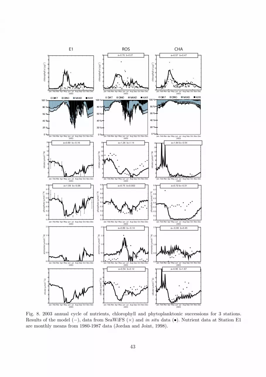
E1

nit

rate

(mm

ol l

N

)-1

a=0.89 b=-0.16

ph

osp

ha

te (mm

ol l

P

)-1

a=1.09 b=-0.06

silic

ate

(mm

ol l

S

i)-1

am

mo

nia

(mm

ol l

N

)-1

ROS CHA

chlo

rop

hyl

l a (mg

l )

-1n

itra

te (mm

ol l

N

)-1

ph

osp

ha

te (mm

ol l

P

)-1

silic

ate

(mm

ol l

S

i)-1

am

mo

nia

(mm

ol l

N

)-1

nit

rate

(mm

ol l

N

)-1

ph

osp

ha

te (mm

ol l

P

)-1

silic

ate

(mm

ol l

S

i)-1

a=1.26 b=1.14

a=0.76 b=0.27

a=0.75 b=0.002

a=0.89 b=-0.14

a=0.54 b=2.12

chlo

rop

hyl

l a (mg

l )

-1

a=0.57 b=0.47

a=1.84 b=-0.54

a=0.72 b=-0.31

a=-0.08 b=0.45

a=0.90 b=1.67

am

mo

nia

(mm

ol l

N

)-1

chlo

rop

hyl

l a (mg

l )

-1

Fig. 8. 2003 annual cycle of nutrients, chlorophyll and phytoplanktonic successions for 3 stations.Results of the model (−), data from SeaWiFS (×) and in situ data (•). Nutrient data at Station E1are monthly means from 1980-1987 data (Jordan and Joint, 1998).

43

8 9 10 11 12 13 14 15 16 17 18 19 20

celsius degrees

−60

−50

−40

−30

−20

−10

0

25 50 75 100 125 150 175 200 225 250 275 300 325 350temperature Julian day

0.0 0.5 1.0 1.5 2.0 2.5 3.0 3.5 4.0

µmol l−1 N

−60

−50

−40

−30

−20

−10

0

25 50 75 100 125 150 175 200 225 250 275 300 325 350diatoms Julian day

0 25 50 75 100 125 150 175 200

cell ml−1

−60

−50

−40

−30

−20

−10

0

25 50 75 100 125 150 175 200 225 250 275 300 325 350Karenia mikimotoi Julian day

a)

b)

c)

Fig. 9. Computed depth-time course of temperature (a), diatoms (b) and Karenia mikimotoi concen-tration (c) at Station 275 during 2003.

44

10 25 50 75 100 150 200 250 500 1000 2000

cell ml−1

10

10

10

10

25

25

25

25 50

50

50

50

50

50

75

75

75

75

75

100

100

100

100

100100

150

150

150

150

150

200

200200

200

250

250

250

250

−4˚

−4˚

−2˚

−2˚

48˚ 48˚

50˚ 50˚

Fig. 10. Superimposition of depth maximum concentration of Karenia mikimotoi sampled during theCorystes Cruise (circles) and computed on the 14 th July 2003.

45

0 5 10 15 20

microg chl-a/l

-90

-80

-70

-60

-50

-40

-30

-20

-10

0

0 25 50 75 100 125 150 175Z Cut Leg241

0 25000 50000 75000 100000 125000 150000 175000

cell l-1

-90

-80

-70

-60

-50

-40

-30

-20

-10

0

0 25 50 75 100 125 150 175Karenia mikimotoi 14/07/2003 13:26

b)a)km

Fig. 11. Vertical pattern of the computed Karenia mikimotoi cell concentration (a) and mesuredchlorophylle a concentration along scanfish section 241 (b).

46

10 10 10 10 104 5 6 7 8

Karenia mikimotoi (cells l ) -1

78 90 275

10 10 10 10 104 5 6 7 8

10 10 10 10 104 5 6 7 8

nitrate (mmol l N)-1 nitrate (mmol l N)-1 nitrate (mmol l N)-1

ammonia (mmol l N)-1

ammonia (mmol l N)-1

ammonia (mmol l N)-1

phosphate (mmol l P)-1 phosphate (mmol l P)-1 phosphate (mmol l P)-1

silicate (mmol l Si)-1

silicate (mmol l Si)-1

silicate (mmol l Si)-1

Karenia mikimotoi (cells l ) -1

Karenia mikimotoi (cells l ) -1

Fig. 12. Profiles of Karenia mikimotoi and nutrients from the Corystes Cruise (•) and model (−) atmany stations located in Figure 2.

47

a) b)0.0 0.2 0.4 0.6 0.8 1.0

-80

-70

-60

-50

-40

-30

-20

-10

0

dept

h (m

)

µ (d )

f (s.u.)

f (s.u.)

f (s.u.)

f (s.u)

T

lum

N

P

-1

0.0 0.2 0.4 0.6 0.8 1.0

-80

-70

-60

-50

-40

-30

-20

-10

0

dept

h (m

)

m (d )

a (s.u.)

g (d )

-1

-1

Fig. 13. Computed vertical distributions of growth limiting effects (a) and processes involved in themortality of Karenia mikimotoi (b) at Station 70 (see Figure 2) the 12/th July 2003, at midday.

48

10 25 50 75 100 150 200 250 500 1000 2000

cell ml−1

10

10

10

10

10

10

25

2525

25

25

50

50

50

75

75

75

100

100

150

150

150

150

200

200

200

200

250

250250

250

250

−4˚

−4˚

−2˚

−2˚

0˚

0˚

48˚ 48˚

50˚ 50˚

0 25 50 75 100 125 150 175 200

cell ml−1

−60

−50

−40

−30

−20

−10

0

25 50 75 100 125 150 175 200 225 250 275 300 325 350

0.0 0.1 0.2 0.3 0.4 0.5 0.6 0.7 0.8 0.9 1.0

adimensional−4˚

−4˚

−2˚

−2˚

0˚

0˚

2˚

2˚

4˚

4˚

48˚ 48˚

50˚ 50˚

52˚ 52˚

a) mean sea surface value during July 1999

z−maximum K.mikimotoi12/07/2003

b) sensitivity analysis

α

depth−time course of Karenia mikimotoi Julian day

Fig. 14. Sensitivity analysis on the stickiness factor α. (a) Mean surface values of α in July 2003during the nominal run. (b) Depth-maximum of Karenia the 12 th of July 2003 (left) and computeddepth-time course of Karenia at Station 275 (right) during the special run when α is fixed (α = αmin).

49

0.0 0.1 0.2 0.3 0.4 0.5

s−1−4˚

−4˚

−2˚

−2˚

0˚

0˚

2˚

2˚

4˚

4˚

48˚ 48˚

50˚ 50˚

52˚ 52˚

10 25 50 75 100 150 200 250 500 1000 2000

cell ml−1

10

10

10

10

10

25 25

25

2525

50

50

50

50

75

−4˚

−4˚

−2˚

−2˚

0˚

0˚

48˚ 48˚

50˚ 50˚

a) mean sea surface value during July 1999 b) sensitivity analysis

z maximum of Karenia mikimotoi12/07/2003

γ

Fig. 15. Sensitivity analysis on the turbulent factor γ. (a) Mean surface values of the γ in April 2003during the nominal run. (b) Depth-maximum of Karenia the 12 th of July 2003 of the special run whenγ is fixed (γ = 0.2 s−1).

10 25 50 75 100 150 200 250 500 1000 2000

cell ml−1

10

10

10

1025

25

25

50

50

50

50

75

75

75

100

150

150

200

−4˚

−4˚

−2˚

−2˚

0˚

0˚

48˚ 48˚

50˚ 50˚

DIAT DINO NANO KAR100 %

80 %

60 %

40 %

20 %

0 %γ

z maximum of Karenia mikimotoi12/07/2003

a) b)

Fig. 16. The importance of the allelopathy. (a) Depth-maximum of Karenia the 12 th of July 2003 ofthe special run when rall = 0., (b) relative importance of phytoplanktonik groups at Station E1 whenrall = 1.

50

Guernsey

island

23/06 07/07 21/07 04/08

γ

Fig. 17. Fate of a passive tracer spill during the Karenia mikimotoi bloom. Isolines of surface concen-tration > 10 indicated every week time lag.

51