Available online at www.sciencedirect.com

Measurement 41 (2008) 222–229

www.elsevier.com/locate/measurement

Modelling study for assessment and forecasting variationof urban air pollution

Gregorio Andria a, Giuseppe Cavone b, Anna M.L. Lanzolla a,*

a Department of Environmental Engineering and Sustainable Development (DIASS), Politecnico di Bari, Italyb Department of Electrics and Electronics (DEE), Politecnico di Bari, Italy

Received 16 January 2006; received in revised form 5 June 2007; accepted 20 June 2007Available online 30 June 2007

Abstract

This work proposes the development of an air pollution model based on a joint application of Kalman filter and Kri-ging technique. The use of modelling techniques in data environmental analysis allows engineers to characterize in a betterway the behaviour of air pollutants, in order: (i) to validate the measured data; and (ii) to predict the values of contaminantsubstances emissions. These techniques are, therefore, a very useful analysis tool, especially when the analyzed time seriesare characterized by numerous missing or erroneous data.

The joint application of both Kalman filter and Kriging algorithms allows users to benefit from the main advantages oftwo independent methods, in order both to improve the performance of the developed model and to reduce its uncertainty.The agreement of estimated and measured values highlights how well the developed model reproduces the reality and soconfirms its efficiency.� 2007 Elsevier Ltd. All rights reserved.

Keywords: Urban air quality; Modelling system; Kalman filter; Kriging technique; Air-pollutant measurement-system

1. Introduction

The alarming growth of atmospheric pollutionhas led many countries in the world to establishsevere laws and regulations defining air qualityand the required standard emission levels [1]. Partic-ular attention is devoted to urban areas where theproblem of atmospheric air pollution is especially

0263-2241/$ - see front matter � 2007 Elsevier Ltd. All rights reserved

doi:10.1016/j.measurement.2007.06.004

* Corresponding author. Tel.: +39 099 4733268/+39 0805963318; fax: +39 099 4733269/+39 080 5963436.

E-mail addresses: andria@misure.poliba.it (G. Andria), cavo-ne@misure.poliba.it (G. Cavone), lanzolla@misure.poliba.it(A.M.L. Lanzolla).

worrying, because the output of pollutants is highand the number of people exposed to health hazardsgrowing constantly.

In this context, many public administrationshave installed several monitoring networks able tocarry out, in real time, qualitative and quantitativeinformation about the characteristics of the envi-ronment of urban centres. Particular importance isgiven to both atmospheric pollution and air qualityevaluation and forecasting.

It is well known that air quality depends on differ-ent factors, including the population density, thevolume of traffic, the energy demand and the physi-cal characteristics of the territory (i.e. geographical

.

G. Andria et al. / Measurement 41 (2008) 222–229 223

conformation, orography). The development of acoherent picture of national environmental trendsand conditions requires the collection of sufficientdata, the statistical analysis and integration of theinformation and the provision of complete, accurateand understandable presentations.

The availability of measured environmental datauseful in determining the air pollution level, is oftennot enough to describe the temporal and spatialbehaviour of all pollutant emissions (in most casesmuch of the data do not exist or are not available).Moreover, there are constant variations in pollutionand meteorological conditions, so the overall pictureof the environment is frequently not clear. For thisreason, it is very important to integrate the availablemeasurements with the evaluation of pollutant con-centrations, estimated by suitable mathematicalmodels allowing to represent the atmospheric processand to investigate on eventual missing and/or incor-rect data.

In this context, the use of forecast algorithmsassumes a remarkable importance. They must assurehigh accuracy, considerable versatility and facility inemployment. These characteristics are easily verifi-able in Kalman filter and in Kriging, which becomeimportant tools to deal with the diversity of data andinformation concerning the environment, to checkthe reliability of measured values and to forecastthe future behaviour of analyzed pollutants. In addi-tion, modelling systems is an important regulatoryassessment support for environmental impact assess-ment by national authorities [2,3].

2. Proposed method

In our study, we propose the analysis of environ-mental data measured in a monitoring networklocated in the Taranto area (South Italy) in orderto test and validate the proposed models: Kalmanfilter, Kriging technique, and a hybrid based onthe joint application of both. The analyzed city ischaracterized by various emission sources that canbe classified in two main classes:

• Sources producing daily averaged values of pol-lutants that are practically constant in the time,such as the large industrial centre (with a contin-uous production cycle) for the manufacture ofsteel, for the refinement of the oil and the produc-tion of cement.

• Sources producing emissions whose concentra-tion values vary in the space of a day as small

industries, road traffic, heating and cooling sys-tems and so on. All these sources contribute toreducing the air quality, by introducing smogand gas in the urban centre and compromisingthe quality of life of the people who live there.

The examined environmental network consists ofseven automatic acquisition and recording stationsthat continuously measure both chemical substancesand meteorological quantities. Each station has acomplex instrumentation including chemical sub-stances analyzers (based on photo-ionization, gaschromatography, and IR and UR absorption) andseveral sensors to acquire meteorological quantities,able to automatically perform operations such asdaily calibration and pre-treating data.

The stations are placed in different typologies ofurban areas (parks, residential areas, sub-urbanareas, roads with high traffic level), according tothe prescriptions of the international directive(Council Directive 96/62/EC of 27 September 1996on ambient air quality assessment and management,Annex IV) and national laws (Ministerial decree of20 May 1991 on standards for air quality data col-lection). Our main attention is addressed to stationslocated near busy traffic junctions and so character-ized by high road-traffic levels.

The most important pollutants analyzed in ourstudy are CO, benzene and toluene, since they rep-resent the main contributors to air pollution causedby road traffic [2]. Besides they are primary pollu-tants (i.e. those directly emitted from sources) [4]and are, therefore, reliable indicators of the presenceand typology of emission sources.

In urban areas, the main causes of pollution are: (i)the consumption of fuel for domestic heating thatproduces emissions concentrated in the wintermonths; and (ii) the vehicular traffic producing emis-sions that are distributed all year round [5]. So, inorder to analyze correctly the behaviour of substancesinvolved, it would be necessary to study separately thecontributions of domestic heating and the vehiculartraffic. Really contribution of the former is negligible,because the relative pollution sources are located at alevel higher than the ground (where the motor trafficpollution is emitted) allowing easy pollution disper-sion. Moreover, the buildings in the urban area ana-lyzed have few floors (five or six) and this favoursfurther the dispersion of noxious substances and soreduces their accumulation on the ground.

This assertion is confirmed by the analysis ofacquired values that not highlights considerable

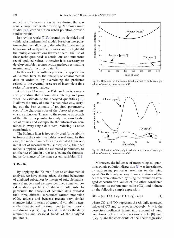
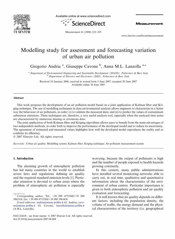
Fig. 1a. Behaviour of the annual trend relevant to daily averagedvalues of toluene, benzene and CO.

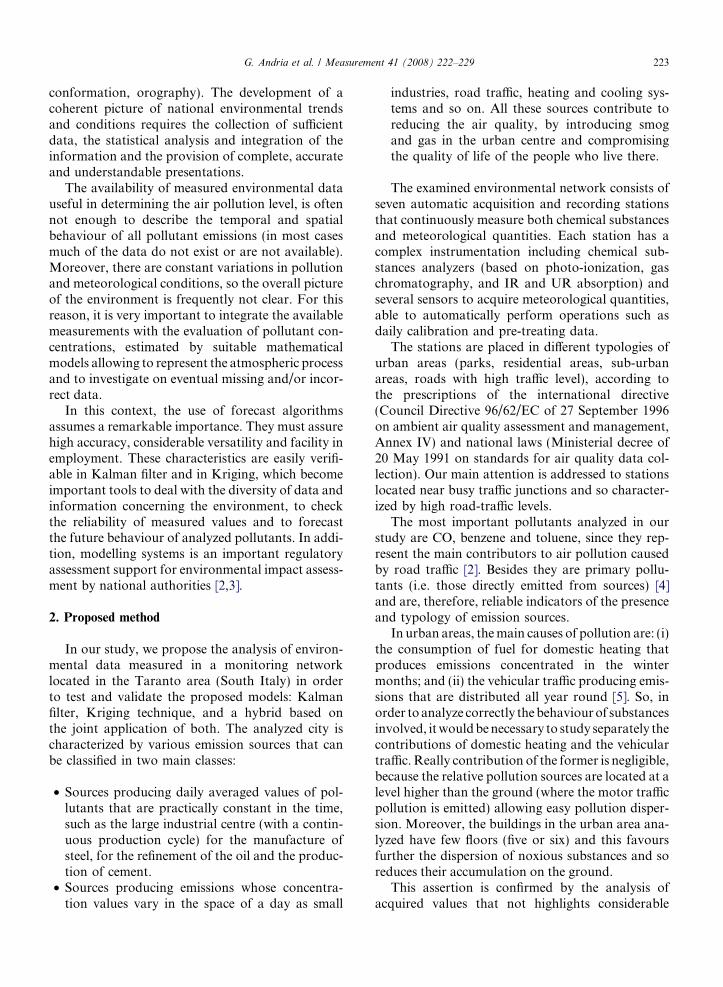
Fig. 1b. Behaviour of the daily trend relevant to annual averagedvalues of toluene, benzene and CO.

224 G. Andria et al. / Measurement 41 (2008) 222–229

reduction of concentration values during the sea-sonal change from winter to spring. Moreover somestudies [5,6] carried out on urban pollution providesimilar results.

In previous works [7,8], the authors identified andvalidated a mathematical model, based on interpola-tion techniques allowing to describe the time-varyingbehaviour of analyzed substances and to highlightthe multiple correlations between them. The use ofthese techniques needs a continuous and numerousset of updated values, otherwise it is necessary todevelop suitable reconstruction methods estimatingmissing and/or incorrect data [9].

In this work, the authors propose the applicationof Kalman filter to the analysis of environmentaldata in order to try overcoming the problemsrelated to the eventual presence of incomplete timeseries of measured values.

As it is well known, the Kalman filter is a recur-sive procedure that allows data filtering and pro-vides the estimate of the analyzed quantities [10].It allows the study of data in a recursive way, carry-ing out the best estimate of required parameters,even if the characteristics of the observed phenom-ena are unknown. Thanks to the recursive approachof the filter, it is possible to analyze a considerableset of values and extrapolate the information con-tained in every single data item, reducing its noisecontribution.

The Kalman filter is frequently used for its abilityto forecast the system variables in real time. In thiscase, the model parameters are estimated from oneinitial set of measurements; subsequently, the filtermodel is applied, with the estimated parameters, toanother set of data in order to calculate the forecast-ing performance of the same system variables [11].

3. Results

By applying the Kalman filter to environmentalanalysis, we have characterized the time-behaviourof analyzed substances by means of suitable mathe-matical models and we have identified some tempo-ral relationships between different pollutants. Inparticular, the analysis of acquired data revealedthat three different substances carbon monoxide(CO), toluene and benzene present very similarcharacteristics in terms of temporal variability gen-erally characterized by time trend (annual, weeklyand diurnal cycles). Fig. 1a and 1b shows the dailyrecurrences and seasonal trends of the analyzedpollutants.

Moreover, the influence of meteorological quan-tities on air pollution dispersion [6] was investigatedby addressing particular attention to the windspeed. So the daily averaged concentrations of thebenzene were estimated by using the evaluated aver-aged concentration values of the other consideredpollutants as carbon monoxide (CO) and tolueneby the following simple expression:

BEi ¼ ðc3 � COi þ c2 � TOi þ c1Þ � kðviÞ ð1Þ

where COi and TOi represent the ith daily averagedvalues of CO and toluene, respectively, k(vi) is thecorrective coefficient taking into account of windconditions defined in a previous article [8], andc3,c2, c1 are the coefficients of the linear regression

G. Andria et al. / Measurement 41 (2008) 222–229 225

obtained by applying Kalman filter to the measureddata. As already stated, Kalman filter needs an ini-tial estimate to get started. In our case, we have im-posed null initial conditions, so the coefficients havebeen calculated in iterative way, by means of the fol-lowing expression:

c3s

c2s

c1s

264

375

¼c3ðs�1Þ

c2ðs�1Þ

c1ðs�1Þ

264

375þ Ks � BEi � COi TOi 1½ � �

c3ðs�1Þ

c2ðs�1Þ

c�1ðs�1Þ

264

375

8><>:

9>=>; ð2Þ

where c3s, c2s, c1s and c3(s�1), c2(s�1), c1(s�1) are theestimates of coefficients at sth and (s�1)th step,respectively, Ks is the Kalman gain at sth step, andfinally, BEi, COi and TOi represent the ith dailyaveraged values of benzene, CO and toluene,respectively.

Thanks to the iterative structure of Kalman filterit is possible to improve the estimate of the vectorrelevant to the analyzed quantities until the dataare available or the difference between two subse-quent estimated values is negligible enough.Fig. 2a shows the behaviour of daily averaged val-ues of benzene and its estimate obtained by applyingKalman filter.

By comparing the coefficient values obtainedwith the application of Kalman filter (c1 = �0.024,c2 = 0.121, c3 = 0.797), and with the use of multiplecorrelations (c1 = �0.068, c2 = 0.121, c3 = 0.831), itcan be observed that the results are very similar forboth the methods.

Fig. 2a. Daily averaged benzene concentrations relevant year2001 (dark line) and estimate values obtained by applyingKalman filter (grey line). The sketch highlights the differencebetween the measured values of benzene and their estimate.

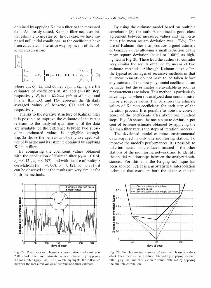
By using the estimate model based on multiplecorrelation [8], the authors obtained a good closeagreement between measured values and their esti-mate (the mean square deviation was 1.73%). Theuse of Kalman filter also produces a good estimateof benzene values allowing a small reduction of themean square deviation (equal to 1.60%) as high-lighted in Fig. 2b. These lead the authors to considervery similar the results obtained by means of twoestimate methods. Although Kalman filter offersthe typical advantages of recursive methods in thatall measurements do not have to be taken beforeany estimate of the best polynomial coefficients canbe made, but the estimates are available as soon asmeasurements are taken. This method is particularlyadvantageous when the analyzed data contain miss-ing or erroneous values. Fig. 3a shows the estimatevalues of Kalman coefficients for each step of theiteration process. It is possible to note the conver-gence of the coefficients after about one hundredsteps. Fig. 3b shows the mean square deviation percent of benzene estimate obtained by applying theKalman filter versus the steps of iteration process.

The developed model examines environmentaldata acquired in only one monitoring station. Toimprove the model’s performances, it is possible totake into account the values measured in the otherstations of the monitoring network and to identifythe spatial relationships between the analyzed sub-stances. For this aim, the Kriging technique hasbeen applied [12]. It is a geostatistical interpolationtechnique that considers both the distance and the

Fig. 2b. Sketch showing a zoom of measured benzene values(dark line), their estimate values obtained by applying Kalmanfilter (grey line) and their estimate values obtained by applyingthe multiple correlation.

Fig. 3a. Estimate values of Kalman coefficients for each step ofiteration process.

Fig. 3b. Mean square deviation per cent of benzene estimateobtained by applying the Kalman filter versus the steps ofiteration process.

226 G. Andria et al. / Measurement 41 (2008) 222–229

degree of variation between the quantity values inknown data points in order to estimate quantity val-ues in an unknown area. This method uses a func-tion called variogram expressing the spatialvariation; it minimizes the error of predicted valuesthat are estimated by spatial distribution. So, weconsider a stochastic spatial process:

ZðxÞ : x 2 D � R2� �

ð3Þ

The goal of spatial forecasting using Kriging is topredict Z(x0) from data Z(x1),Z(x2),. . .,Z(xn).

The estimate is obtained by means of a weightedlinear combination of the known sample valuesaround the point to be estimated. Kriging algorithmpossesses three major advantages with respect toother interpolation methods:

• its interpolations are made by weights that do notdepend upon data values;

• it provides an estimate of the interpolation error;• it is an exact interpolation since the interpolation

at any observation point is the observation itself.

The effectiveness of Kriging depends on both thecorrect specification of several parameters thatdescribe the variogram and the stationary character-istics of analyzed variables.

In order to characterize properly the analyzedterritory, a classification relevant to pollutantspreading characteristics, was carried out. In partic-ular, the monitored stations were separated in twodifferent classes: isotropy (the pollution dispersionvaries in the same way in all directions) and anisot-

ropy (the pollution dispersion varies differently indifferent directions) [13]. In addition, the stationswere classified on the basis of different typologiesof area and emission sources near there. So, we indi-cated as A, the stations placed in park or residentialareas; B, the stations placed in very high road-trafficareas; and C, the stations placed near industrialcentres.

By analyzing the data acquired in monitoring sta-tions placed in Taranto area, it is possible to observethat the concentrations of pollutants vary againstseveral factors such as the territorial characteristics,the typology of emission sources and the meteoro-logical conditions.

In our analysis, only three stations have beenexamined (two of them are of typology C and theother one is of typology A), that have a reciprocal dis-tance less than 2 km. In this way, it is possible toassume that the local conditions are very similar inall analyzed areas. Fig. 4 shows a map of Tarantowhere the three selected stations (indicated as 2, 3and 4) are contained in the circled area. In particular,stations 2 and 4 have similar characteristics becausethey are both located on roads with very high-vehic-ular traffic. Station 3 although placed in a park, isaffected by the pollution emissions caused by heavytraffic on the nearby road. These remarks led us tochoose the three specified stations that bound ahomogeneous area. None of the three stations ischaracterized by a preferential direction for pollutiondispersion (caused by a different territorial confor-mation or by a strong prevailing wind in a particulardirection), so they have been considered as isotropy.

When the area of interest has been defined, thefunction describing in the best way the behaviourof pollutant concentrations in the spatial domain

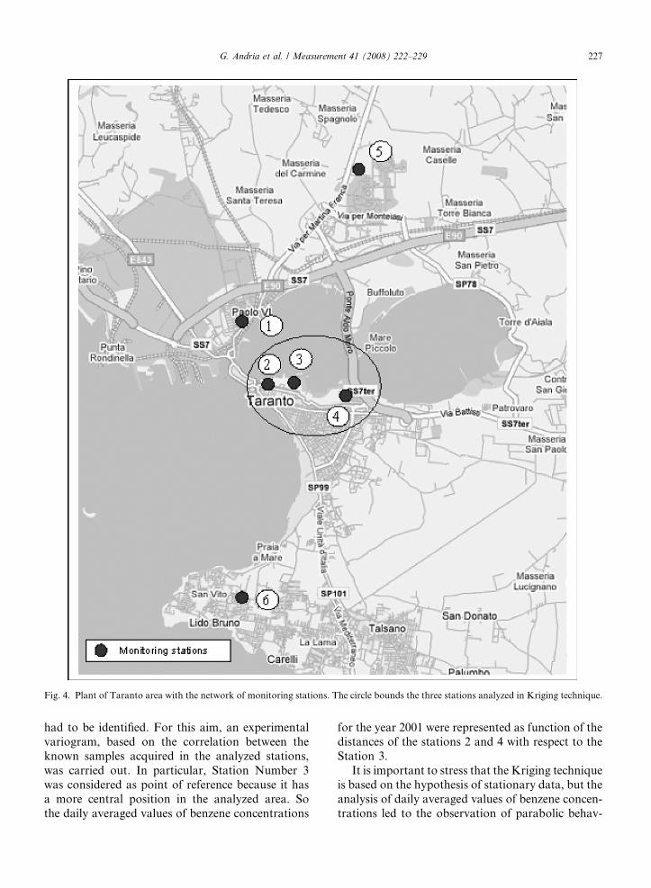
Fig. 4. Plant of Taranto area with the network of monitoring stations. The circle bounds the three stations analyzed in Kriging technique.

G. Andria et al. / Measurement 41 (2008) 222–229 227

had to be identified. For this aim, an experimentalvariogram, based on the correlation between theknown samples acquired in the analyzed stations,was carried out. In particular, Station Number 3was considered as point of reference because it hasa more central position in the analyzed area. Sothe daily averaged values of benzene concentrations

for the year 2001 were represented as function of thedistances of the stations 2 and 4 with respect to theStation 3.

It is important to stress that the Kriging techniqueis based on the hypothesis of stationary data, but theanalysis of daily averaged values of benzene concen-trations led to the observation of parabolic behav-

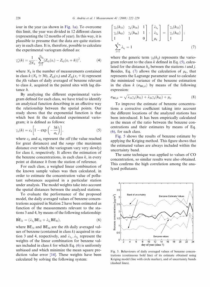
Fig. 5. Behaviours of daily averaged values of benzene concen-trations (continuous bold line) of its estimate obtained usingKriging model (line with circle marker), and of uncertainty bands(dashed lines).

228 G. Andria et al. / Measurement 41 (2008) 222–229

iour in the year (as shown in Fig. 1a). To overcomethis limit, the year was divided in 12 different classes(representing the 12 months of year). In this way, it isplausible to presume that the data are quite station-ary in each class. It is, therefore, possible to calculatethe experimental variogram defined as:

c�kðhÞ ¼1

2Nk�XNk

j¼1

ðZkjðxiÞ � Zkjðxi þ hÞÞ2; ð4Þ

where Nk is the number of measurements containedin class k (Nk ffi 30), Zkj(xi) and Zkj(xi + h) representthe jth values of daily averaged of benzene relevantto class k, acquired in the paired sites with lag dis-tance h.

By analyzing the different experimental vario-gram defined for each class, we have tried to identifyan analytical function describing in an effective waythe relationship between the spatial points. Ourstudy shows that the exponential function is thatwhich best fit the calculated experimental vario-gram; it is defined as follows:

ckðhÞ ¼ ck 1� exp � 3hak

� �� �; ð5Þ

where ck and ak represent the sill (the value reachedfor great distances) and the range (the maximumdistance over which the variogram vary very slowly)for class k, respectively. It allows the estimation ofthe benzene concentrations, in each class k, in everypoint at distance h from the station of reference.

For each class, a weighed linear combination ofthe known sample values was then calculated, inorder to estimate the concentration value of pollu-tant substances acquired in a particular stationunder analysis. The model weights take into accountthe spatial distances between the analyzed stations.

To evaluate the performance of the proposedmodel, the daily averaged values of benzene concen-trations acquired in Station 2 have been estimated asfunction of the measurements relevant to the sta-tions 3 and 4, by means of the following relationship:

BE2i ¼ ðk1k BE3i þ k2k BE4iÞ; ð6Þ

where BE3i and BE4i are the ith daily averaged val-ues of benzene (contained in class k) acquired in sta-tion 3 and 4, respectively, and k1k ; k2k represent theweights of the linear combination for benzene val-ues included in class k for which Eq. (6) is uniformlyunbiased and which minimize the mean square pre-diction value error [14]. These weights have beencalculated by solving the following system:

ckðh33Þ ckðh34Þ 1

ckðh43Þ ckðh44Þ 1

1 1 0

264

375 �

k1k

k2k

lk

264

375 ¼

ckðh32Þckðh42Þ1

264

375;

Xn

i¼1

kik ¼ 1 ð7Þ

where the generic term ck(hij) represents the vario-gram relevant to the class k defined in Eq. (5), calcu-lated for the distance hij between the stations i and j.Besides, Eq. (7) allows the calculation of lk, thatrepresents the Lagrange parameter used to calculatethe minimized variance of the benzene estimationin the class k (rBE2kÞ by means of the followingexpression:

rBE2k ¼ffiffiffiffiffiffiffiffiffiffiffiffiffiffiffiffiffiffiffiffiffiffiffiffiffiffiffiffiffiffiffiffiffiffiffiffiffiffiffiffiffiffiffiffiffiffiffiffiffiffiffiffiffiffiffik1kckðh32Þ þ k2kckðh42Þ þ lk

p: ð8Þ

To improve the estimate of benzene concentra-tions a corrective coefficient taking into accountthe different locations of the analyzed stations hasbeen introduced. It has been empirically calculatedas the mean of the ratio between the benzene con-centrations and their estimates by means of Eq.(6), for each class.

Fig. 5 shows the results of benzene estimate byapplying the Kriging method. This figure shows thatthe estimated values are always included within theuncertainty band.

The same technique was applied to values of COconcentration, so similar results were also obtained.This confirms the high correlation among the ana-lyzed pollutants.

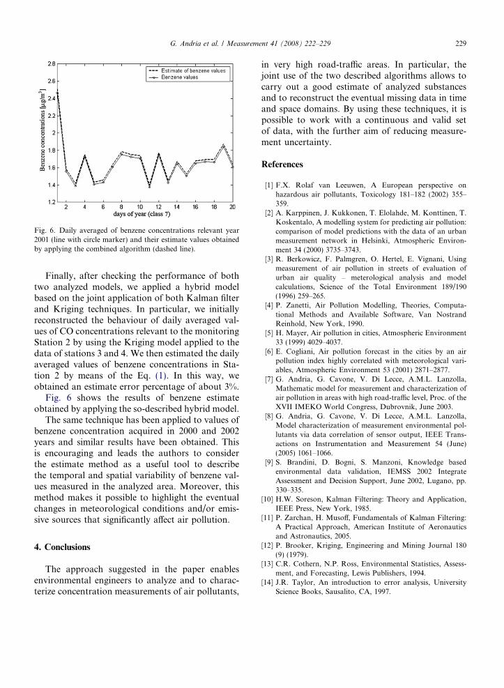
Fig. 6. Daily averaged of benzene concentrations relevant year2001 (line with circle marker) and their estimate values obtainedby applying the combined algorithm (dashed line).

G. Andria et al. / Measurement 41 (2008) 222–229 229

Finally, after checking the performance of bothtwo analyzed models, we applied a hybrid modelbased on the joint application of both Kalman filterand Kriging techniques. In particular, we initiallyreconstructed the behaviour of daily averaged val-ues of CO concentrations relevant to the monitoringStation 2 by using the Kriging model applied to thedata of stations 3 and 4. We then estimated the dailyaveraged values of benzene concentrations in Sta-tion 2 by means of the Eq. (1). In this way, weobtained an estimate error percentage of about 3%.

Fig. 6 shows the results of benzene estimateobtained by applying the so-described hybrid model.

The same technique has been applied to values ofbenzene concentration acquired in 2000 and 2002years and similar results have been obtained. Thisis encouraging and leads the authors to considerthe estimate method as a useful tool to describethe temporal and spatial variability of benzene val-ues measured in the analyzed area. Moreover, thismethod makes it possible to highlight the eventualchanges in meteorological conditions and/or emis-sive sources that significantly affect air pollution.

4. Conclusions

The approach suggested in the paper enablesenvironmental engineers to analyze and to charac-terize concentration measurements of air pollutants,

in very high road-traffic areas. In particular, thejoint use of the two described algorithms allows tocarry out a good estimate of analyzed substancesand to reconstruct the eventual missing data in timeand space domains. By using these techniques, it ispossible to work with a continuous and valid setof data, with the further aim of reducing measure-ment uncertainty.

References

[1] F.X. Rolaf van Leeuwen, A European perspective onhazardous air pollutants, Toxicology 181–182 (2002) 355–359.

[2] A. Karppinen, J. Kukkonen, T. Elolahde, M. Konttinen, T.Koskentalo, A modelling system for predicting air pollution:comparison of model predictions with the data of an urbanmeasurement network in Helsinki, Atmospheric Environ-ment 34 (2000) 3735–3743.

[3] R. Berkowicz, F. Palmgren, O. Hertel, E. Vignani, Usingmeasurement of air pollution in streets of evaluation ofurban air quality – meterological analysis and modelcalculations, Science of the Total Environment 189/190(1996) 259–265.

[4] P. Zanetti, Air Pollution Modelling, Theories, Computa-tional Methods and Available Software, Van NostrandReinhold, New York, 1990.

[5] H. Mayer, Air pollution in cities, Atmospheric Environment33 (1999) 4029–4037.

[6] E. Cogliani, Air pollution forecast in the cities by an airpollution index highly correlated with meteorological vari-ables, Atmospheric Environment 53 (2001) 2871–2877.

[7] G. Andria, G. Cavone, V. Di Lecce, A.M.L. Lanzolla,Mathematic model for measurement and characterization ofair pollution in areas with high road-traffic level, Proc. of theXVII IMEKO World Congress, Dubrovnik, June 2003.

[8] G. Andria, G. Cavone, V. Di Lecce, A.M.L. Lanzolla,Model characterization of measurement environmental pol-lutants via data correlation of sensor output, IEEE Trans-actions on Instrumentation and Measurement 54 (June)(2005) 1061–1066.

[9] S. Brandini, D. Bogni, S. Manzoni, Knowledge basedenvironmental data validation, IEMSS 2002 IntegrateAssessment and Decision Support, June 2002, Lugano, pp.330–335.

[10] H.W. Soreson, Kalman Filtering: Theory and Application,IEEE Press, New York, 1985.

[11] P. Zarchan, H. Musoff, Fundamentals of Kalman Filtering:A Practical Approach, American Institute of Aeronauticsand Astronautics, 2005.

[12] P. Brooker, Kriging, Engineering and Mining Journal 180(9) (1979).

[13] C.R. Cothern, N.P. Ross, Environmental Statistics, Assess-ment, and Forecasting, Lewis Publishers, 1994.

[14] J.R. Taylor, An introduction to error analysis, UniversityScience Books, Sausalito, CA, 1997.