Physics Letters A 367 (2007) 114–119

www.elsevier.com/locate/pla

Modelling of non-uniform DC driven glow discharge in argon gas

I.R. Rafatov ∗,1, D. Akbar, S. Bilikmen

Physics Department, Middle East Technical University, TR-06531 Ankara, Turkey

Received 18 November 2006; received in revised form 18 January 2007; accepted 19 February 2007

Available online 23 February 2007

Communicated by F. Porcelli

Abstract

Physical properties of non-uniform DC-driven glow discharge in argon at pressure 1 torr are analyzed numerically. Spatially two-dimensionalaxial-symmetric model is based on the diffusion-drift theory of gas discharge. Results presented compare favorably with the classic theory of glowdischarges and exhibit good agreement with the experimental result. Comparison with the result of spatially one-dimensional model is performed.© 2007 Elsevier B.V. All rights reserved.

PACS: 52.80.-s; 02.60.Cb; 52.25.-b

Keywords: Glow discharge; Plasma; Modelling; Positive column

1. Introduction

Low-pressure glow discharges are of topical interest forlots of technological applications like plasma light sources,plasma processing for surface modification, and plasma chem-istry. Therefore, a detailed understanding of the fundamentalprocesses of glow discharges is required for the design, charac-terization, and optimization the discharge parameters in theseplasma applications. Such understanding can be gained frommodelling the processes occurring in the plasma.

The modelling approaches can be classified as fluid meth-ods, kinetic (particle) methods and their combinations, calledas hybrid methods, which represent a compromise between thecomputationally very efficient fluid models and fully kineticparticle models that require very extensive computations.

The glow discharge models are usually developed in uni-form geometry. The aim of this work is to study the effect ofnon-uniformity of the discharge tube on the discharge proper-ties. We used a simple fluid model based on the diffusion-drifttheory of gas discharge [1–3] and consisted of continuity equa-tions for electrons and ions, as well as Poisson equation for the

* Corresponding author.E-mail address: rafatov@metu.edu.tr (I.R. Rafatov).

1 Also at American University—Central Asia, 205 Abdumomunov Street,Bishkek 720000, Kyrgyzstan.

0375-9601/$ – see front matter © 2007 Elsevier B.V. All rights reserved.doi:10.1016/j.physleta.2007.02.073

self-consistent electric field. We adopted a local field approx-imation: the ionization source term and the particle transportcoefficients (drift and diffusion) are defined as functions of thelocal value of the reduced electric field E/p (where E is themagnitude of the field and p is the gas pressure). The modelis spatially two-dimensional (axial-symmetric). Though such a‘diffusion-drift theory’ approach has serious limitations, e.g. inthe prediction of absolute values of charge densities (see, e.g.[4]), and in adequate describing of the sheath regions of a spacecharge at the immediate vicinity to electrodes [1,5,6], it is stillable to predict some general characteristics of the glow dis-charge [1–3,7–9].

For the testing of the model, we apply conditions and use ex-perimental results for the non-uniform DC-driven argon glowdischarge described in [10]. Schematic diagram of this dis-charge system is shown in Fig. 1. The system was made oftwo Pyrex glasses, one of them is uniform (external) and theother is non-uniform (internal). The inner tube consists of twoquasi-sphere parts with diameters 4.1 cm, and each side of thespheres is connected with cylindrical parts with diameters 3 cm.The distance between the cylindrical electrodes was adjusted tobe 30 cm. A floating double probe characteristic has been em-ployed for this measurements. For the details we refer to [10].

This Letter is organized as follows. In Section 2, we definethe model, perform dimensional analysis, describe physical pa-rameters and solution approach. In Section 3, we present and

I.R. Rafatov et al. / Physics Letters A 367 (2007) 114–119 115

Fig. 1. Experimental setup [10].

discus calculation results. Finally, concluding remarks are givenin Section 4.

2. Two-component plasma model

2.1. Gas-discharge model

The gas-discharge is modelled by continuity equations fortwo charged species, namely, electrons and positive ions withparticle densities ne and n+,

(1)∂tne + ∇Γ e = source,

(2)∂tn+ + ∇Γ + = source,

which are coupled to Poisson’s equation for the electric field inelectrostatic approximation,

(3)∇E = e

ε0(n+ − ne), E = −∇Φ.

Here, Φ is the electric potential, E is the electric field, e is theelectron unite charge, ε0 is the dielectric constant, Γ e and Γ +are the particle current densities, which are described by driftand diffusion, where drift velocities are assumed to be linearlydependent on the local electric field with mobilities μ+ � μe,

(4)Γ e = −De∇ne − neμeE,

(5)Γ + = −D+∇n+ + n+μ+E.

Two types of ionization processes are taken into account: the α

process of electron impact ionization in the bulk of the gas, andthe γ process of electron emission by ion impact onto the cath-ode. In a local field approximation, the α process of ionizationand process of recombination determine the source terms in thecontinuity Eqs. (1) and (2),

source = |Γ e|α(|E|) − βn+ne,

(6)α(|E|) = α0α

(|E|/E0),

which, due to charge conservation, is identical for both equa-tions [1]. Constant β denotes the recombination coefficient.

2.2. Boundary conditions

The system is axially symmetric. In dimensional units, cylin-drical coordinates R and Z parametrize the directions paralleland orthogonal to the electrodes. The anode is located at Z = 0,and the cathode is at Z = H (Fig. 2). (Below, in dimensionlessunits, this corresponds to coordinates (r, z), z = 0 and z = h).

Boundary conditions at the anode (Z = 0) describe the ab-sence of ion emission. When diffusion at the anode is neglected,then the ion density vanishes,

(7)Γ +(R,0, t) = 0 ⇒ n+(R,0, t) = 0.

The boundary condition at the cathode, Z = H , describes γ -process of secondary electron emission,∣∣Γ e(R,H, t)

∣∣ = γ∣∣Γ +(R,H, t)

∣∣(8)⇒ μene(R,H, t) = γμ+n+(R,H, t).

Denoting applied DC voltage as U , due to gauge freedom, weset

(9)Φ(R,0, t) = 0, Φ(R,H, t) = −U.

2.3. Dimensional analysis

We introduce the following dimensionless time, coordinatesand fields,

τ = t

t0, r = R

R0,

σ (r, τ ) = ne(R, t)

n0, ρ(r, t) = n+(R, t)

n0,

(10)E(r, t) = E(R, t)

E0, φ(r, t) = Φ(R, t)

R0E0,

measuring quantities in terms of the intrinsic parameters of thesystem,

(11)R0 = 1

α0, t0 = R0

μeE0, n0 = ε0α0E0

e.

Here the dimensional R is expressed by coordinates (R,Z)

and the dimensionless r by coordinates (r, z). The total ap-plied voltage, discharge tube length, and diffusion coefficients

116 I.R. Rafatov et al. / Physics Letters A 367 (2007) 114–119

Fig. 2. Computational domain.

are rescaled as

U = U

R0E0, h = H

R0,

(12)De = De

μeE0R0, D+ = D+

μeE0R0.

The mobility ratio μ of electrons and ions is

(13)μ = μ+μe

.

Finally, the recombination coefficient is rescaled as β =βε0/(eμe).

2.4. Physical parameters

Our choice of parameters was guided by the experiments[10]. We used shape and dimensions for the discharge tube as inFig. 1, with tube hight H = 30 cm and tube diameter changingbetween 3 and 4.2 cm. Pressure is p = 1 torr. Applied voltageis U = 400 V.

We tested a number of estimations for the ionization coef-ficient (6) with classical Townsend approximation of the formα(E) = Ap exp[−(B/pE)s] with different choices for parame-ters A, B , and s from [1,11], and more accurate approximationsfor α from [12,13] and [14]. The better agreement with the ex-periment [10] is provided by the estimation proposed in [12,13],

α(E/n)/n = 1.1 × 10−18 exp[−72/(E/n)

]

+ 5.5 × 10−17 exp[−187/(E/n)

]

+ 3.2 × 10−16 exp[−700/(E/n)

]

(14)− 1.5 × 10−16 exp[−10 000/(E/n)

],

where E/n is given in Td with 1 Td = 10−17 V cm2, andα(E/n)/n is in cm2. The range of E/n, where this formulais valid, is 15–6000 Td [13]. (Actual range of E/n from thenumerical example below is 14–4000 Td.) The gas density istaken as n = 3.54 × 1016 cm−3, which corresponds to a pres-sure p = 1 torr at 273 K. For comparison, we presented resultsof calculation with coefficient α [14]

α(E/n)/n

(15)=⎧⎨⎩

−2.748 × 10−18√E/n + 4.04 × 10−19E/n

− 7.40 × 10−23(E/n)2 for E/n > 67.8 Td,

1.416 × 10−23(E/n)3 for E/n � 67.8 Td.

The ion mobility is calculated also as a function of the re-duced electric field. We tested estimations for μ+ from [15],

(16)μ+ =⎧⎨⎩

103×(1−2.22×10−3E/p)p

, E/p � 60 Vcm torr ,

8.25×103

p√

E/p

(1 − 86.52

(E/p)3/2

), E/p > 60 V

cm torr ,

where μ+ is in cm2/(s V) and p is in torr, and from [14] (whichis closed to estimations from [12,16]),

(17)μ+ = 4.411 × 1019

(1 + (7.721 × 10−3E/n)1.5)0.33)n

cm2

s V

where reduced electric field is given in Td.Estimations for the ion diffusion, according to Einstein’s re-

lations, can be approximated by

(18)D+ = 0.025μ+(assuming ion temperature T+ = 0.025 eV) [14], and as in [15],

(19)D+ = 2 × 102

p

cm2

s.

The recombination coefficient is taken as β = 2 ×10−7 cm3 s−1 [1,15].

The electron yields of cathode materials are the least knowndata of gas discharge physics. At the same time the modellingresults may sensitively depend on the electron yield data [4,17–19]. Therefore, it is more appropriate in discharge models tocalculate γ dependent on the discharge conditions rather than touse any constant value. There is an alternative approach [18,19],where γ is treated as a fitting parameter to match the calculatedelectrical characteristics with their experimental counterparts.

For the secondary emission coefficient, we tested a constantapproximation γ = 0.07 [1,15], as well as estimations in theform of functions of the reduced electric field [12,16,20], where

(20)γ = 0.01 + 0.64[(E/n)c/30 000]1.3

1 + (E/n)c/30 000

in [16], and

(21)γ = 0.01(E/n)0.6c

in [20], with E/n given in Td and evaluated at the cathode.Calculations showed (and it is also stated in [8,21]) that dis-

charge structure changes slightly at electronic temperature upto 5 eV, and Te = 1 eV can be used as a reasonable approxima-tion. The electron mobility and diffusion coefficients, assumingTe = 1 eV, are taken in the same way as in [15],

μe = 3 × 105

p

cm2

s V, De = 3 × 105

p

cm2

s.

I.R. Rafatov et al. / Physics Letters A 367 (2007) 114–119 117

2.5. Resulting dimensionless system and solution approach

The dimensionless system of equations has the form of

∂τ σ − ∇(De∇σ + Eσ)

(22)= |De∇σ + σE|α − βρσ,

∂τ ρ − ∇(D+∇ρ − μEρ)

(23)= |De∇σ + σE|α − βρσ,

(24)∇E = ρ − σ, E = −∇φ.

This system is solved using the finite element computa-tional package COMSOL Multiphysics™, by stationary nonlin-ear solver ‘Direct (UMFPACK)’ [22]. Computational domain isshown in Fig. 2.

Boundary conditions described in Section 2.2 take the fol-lowing form. At the anode, z = 0 (segment AB in Fig. 2),vanishing of the ion density (7) and homogeneous Neumanncondition for the electrons,

(25)ρ(r,0, τ ) = 0, ∂zσ (r,0, τ ) = 0.

At the cathode, z = h (segment CD in Fig. 2), condition ofsecondary electron emission (8) and homogeneous Neumanncondition for the ion density,

(26)σ(r,h, τ ) = γμρ(r,h, τ ), ∂zρ(r, h, τ ) = 0.

At the outer boundaries z = 0 and z = h, the electrodes are onthe electric potential φ(r,0, τ ) = 0 and φ(r,h, τ ) = −U , re-spectively. Finally, we used homogeneous Neumann conditionsfor the particle densities and potential on the symmetry axis (z-axis, segment AD in Fig. 2) and on the wall of the dischargetube (segment BC).

Calculations showed that solving of this system with station-ary solver is very sensitive to initial estimate for the unknownvariables. To provide a convergence, we started from some ap-propriate initial conditions, using first a time-dependent solver,and then started the stationary ‘Direct (UMFPACK)’, when thesolution was about its steady state. To resolve steep layers nearthe electrodes, we used mesh adaptation. The numerical con-vergence was checked by performing the successive refinementof the space grid. Iteration process was stopped when the rela-tive error was smaller than 10−6 in one-dimensional and 10−4

in two-dimensional case.

3. Results

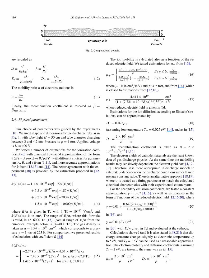
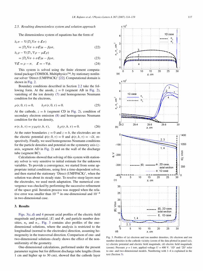
Figs. 3(c, d) and 4 present axial profiles of the electric fieldmagnitude and potential, |E| and Φ , and particle number den-sities, ne and n+. Fig. 3 contains also profiles of the one-dimensional solutions, where the analysis is restricted to thelongitudinal (normal to the electrodes) direction, assuming ho-mogeneity in the transversal direction. Comparison of one- andtwo-dimensional solutions clearly shows the effect of the non-uniformity of the geometry.

One-dimensional calculations, performed under the presentparameter regime but for different discharge tube lengths (from1 cm and higher up to 30 cm), showed that the cathode layer

Fig. 3. Profiles of (a) electron and ion number densities, (b) electron and ionnumber densities in the cathode vicinity (zoom of the data plotted in panel (a)),(c) electric potential and electric field magnitude, (d) electric field magnitude(zoom). Pressure p = 1 torr, applied voltage U = 400 V. ‘1D’ and ‘2D’ referto one- and two-dimensional models. Numbering with 1–4 is explained in thetext (Section 3).

118 I.R. Rafatov et al. / Physics Letters A 367 (2007) 114–119

Fig. 4. Axial values of electron and ion number densities. Asterisks indicateexperimental data [10]. Conditions are the same as in Fig. 3.

is about several millimeters in width and does not practicallydepend on the tube length. Hence, at tube length H = 30 cm,cathode layer occupies extremely small region in relation tothe entire discharge dimensions, and solutions have extremelyabrupt profiles near the cathode. This complicates strongly thenumerical solution. Fig. 3(b) illustrates extracted from the panelabove Fig. 3(a) particle densities profiles in the cathode vicinity.

In order to show the effect of different transport and ion-ization coefficients on the discharge properties, we performedone-dimensional calculations, using

– expressions (14), (16), and (19) for the ionization coef-ficient, α, ion mobility, μ+, and ion diffusion, D+, andsecondary electron emission coefficient, γ = 0.07 (corre-sponding solution is numbered with ‘1’ in Fig. 3);

– the same set of parameters but with ionization coefficient(15) (solution numbered by ‘2’);

– the same set (14), (16), and (19), but not taking recombina-tion (6) into account (solution ‘3’, notice that the particlenumber densities in Fig. 3(a) are noticeably higher in thiscase);

– secondary emission coefficient dependent on the reducedelectric field (20) (solution ‘4’).

Solutions with ion mobility coefficient (17), diffusion coeffi-cient (18), secondary yield estimation from [12] differ from thesolution ‘1’ very slightly, and they are not presented in Fig. 3.Eq. (21) for γ , in comparison with other estimations, led tothe essentially smaller emission coefficient (about 0.023, e.g.,value of γ followed from (20) is about 0.05), and seemed tobe not appropriate for the present conditions: calculated parti-cle number densities differed from the experimental [10] ones.Concerning the two-dimensional calculations, they have beenperformed using the same estimations for α, μ+, D+, and γ asfor solution ‘1’.

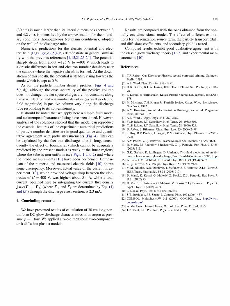
Fig. 5 presents shapes of the electric field magnitude (a) andpotential (b), the electron (c) and ion number densities (d). No-tice that the radial profiles of the discharge characteristics arepractically constants (as it is in the case of glow discharge inabnormal mode [15]). This tendency, especially in the presentcase when length of the discharge tube in forward direction

Fig. 5. Shapes of the electric field magnitude (a), electric potential (b), electronnumber density (c), and ion number density (d). Conditions are the same as inFig. 3.

I.R. Rafatov et al. / Physics Letters A 367 (2007) 114–119 119

(30 cm) is much larger than its lateral dimensions (between 3and 4.2 cm), is intensified by the approximation for the bound-ary conditions (homogeneous Neumann conditions), adoptedon the wall of the discharge tube.

Numerical predictions for the electric potential and elec-tric field (Figs. 3(c, d), 5(a, b)) demonstrate in general similar-ity with the previous references [1,15,21,23,24]. The potentialsharply drops from about −125 V to −400 V which leads toa drastic difference in ion and electron number densities nearthe cathode where the negative sheath is formed. At the down-stream of this sheath, the potential is steadily rising towards theanode which is kept at 0 V.

As for the particle number density profiles (Figs. 4 and5(c, d)), although the quasi-neutrality of the positive columndoes not change, the net space-charges are not constants alongthe axis. Electron and ion number densities (as well as electricfield magnitude) in positive column vary along the dischargetube responding to its non-uniformity.

It should be noted that we apply here a simple fluid modeland no attempts of parameter fitting have been aimed. However,analysis of the solutions showed that the model can reproducethe essential features of the experiment: numerical predictionsof particle number densities are in good qualitative and quanti-tative agreement with probe measurements (Fig. 4). This canbe explained by the fact that discharge tube is long, conse-quently the effect of boundaries (which cannot be adequatelypredicted by the present model) is weak at the inner regions,where the tube is non-uniform (see Figs. 1 and 2) and wherethe probe measurements [10] have been performed. Compar-ison of the numeric and measured electric fields [10] showssome discrepancy. Moreover, actual value of the current in ex-periment [10], which provided voltage drop between the elec-trodes of U = 400 V, was higher, about 5 mA, while a totalcurrent, obtained here by integrating the current flux densityj = e(Γ + − Γ e) (where Γ + and Γ e are determined by Eqs. (4)and (5)) through the discharge cross section, is 2.3 mA.

4. Concluding remarks

We have presented results of calculation of 30 cm long non-uniform DC glow discharge characteristics in an argon at pres-sure p = 1 torr. We applied a two-dimensional two-componentdrift-diffusion plasma model.

Results are compared with the ones obtained from the spa-tially one-dimensional model. The effect of different estima-tions for the ionization source term, the particle transport (driftand diffusion) coefficients, and secondary yield is tested.

Computed results exhibit good qualitative agreement withthe classic glow discharge theory [1,23] and experimental mea-surements [10].

References

[1] Y.P. Raizer, Gas Discharge Physics, second corrected printing, Springer,Berlin, 1997.

[2] A.L. Ward, Phys. Rev. 6 (1958) 1852.[3] D.B. Graves, K.E.A. Jensen, IEEE Trans. Plasma Sci. PS-14 (2) (1986)

78.[4] Z. Donkó, P. Hartmann, K. Kutasi, Plasma Sources Sci. Technol. 15 (2006)

178.[5] M. Mitchner, C.H. Kruger Jr., Partially Ionized Gases, Wiley–Inerscience,

New York, 1992.[6] A.M. Howatson, An Introduction to Gas Discharge, second ed., Pergamon

Press, Oxford, 1975.[7] A.L. Ward, J. Appl. Phys. 33 (1962) 2789.[8] Yu.P. Raizer, S.T. Surzhikov, High Temp. 26 (1988) 304.[9] Yu.P. Raizer, S.T. Surzhikov, High Temp. 28 (1990) 324.

[10] D. Akbar, S. Bilikmen, Chin. Phys. Lett. 23 (2006) 2498.[11] S. Roy, B.P. Pandey, J. Poggie, D.V. Gaitonde, Phys. Plasmas 10 (2003)

2578.[12] A.V. Phelps, Z.Lj. Petrovic, Plasma Sources Sci. Technol. 8 (1999) R21.[13] D. Maric, M. Radmilovic-Radenovic, Z.Lj. Petrovic, Eur. Phys. J. D 35

(2005) 313.[14] G.K. Grubert, D. Loffhagen, D. Uhrlandt, Two-fluid modelling of an ab-

normal low-pressure glow discharge, Proc. Femlab Conference 2005, 6 pp.[15] A. Fiala, L.C. Pitchford, J.P. Boeuf, Phys. Rev. E 49 (1994) 5607.[16] Z.Lj. Petrovic, A.V. Phelps, Phys. Rev. E 56 (1997) 5920.[17] M.M. Nikolic, A.R. Dordevic, I. Stefanovic, S. Vrhovac, Z.Lj. Petrovic,

IEEE Trans. Plasma Sci. PS 31 (2003) 717.[18] D. Maric, K. Kutasi, G. Malovic, Z. Donkó, Z.Lj. Petrovic, Eur. Phys. J.

D 21 (2002) 73.[19] D. Maric, P. Hartmann, G. Malovic, Z. Donkó, Z.Lj. Petrovic, J. Phys. D:

Appl. Phys. 36 (2003) 2639.[20] Z. Donkó, Phys. Rev. E 64 (2001) 026401.[21] S.T. Surzhikov, J.S. Shang, J. Comput. Phys. 199 (2004) 437.[22] COMSOL Multiphysics™ 3.2 (2006), COMSOL Inc., http://www.

comsol.com/.[23] A. Von Engel, Ionized Gases, Oxford Univ. Press, Oxford, 1965.[24] J.P. Boeuf, L.C. Pitchford, Phys. Rev. E 51 (1995) 1376.