Autonomous adaptive sensorless controller of inverter-based islanded-distributed generation system
Upload
khangminh22Category
view
0download
0
727
MODELLING OF INVERTER-BASED GENERATION FOR POWER SYSTEM
DYNAMIC STUDIES
JOINT WORKING GROUP
C4/C6.35/CIRED
MAY 2018

Members
K. YAMASHITA, Convenor CIGRE JP H. RENNER, Convenor CIRED AT
S. MARTINEZ VILLANUEVA, Secretary ES P. ARISTIDOU UK
T. VAN CUTSEM BE I. GREEN US
G. IRWIN CA G. LAMMERT DE
J. CARVALHO MARTINS PT L.D. PABON OSPINA DE
Z. SONG UK K. VENNEMANN DE
L. ZHU CN
Corresponding Authors
R. ADAMS AU I. ARONOVICH IS J. MA AU
B. BADRZADEH AU A.H. BAKAR MY T.E. MCDERMOTT US
M. BARBIERI IT E.T. DE BERARDINIS IT P. POURBEIK US
J.C. BOEMER US M. BRAUN DE R. TURRI IT
H. BRONZEADO BR N. CAMMALLERI IT E. VITTAL US
A. CERRETTI IT K. CHAN CH C. ZHAN DE
F.E. CIAUSIU RO V. DEBUSSCHERE FR P. MATTAVELLI IT
L. GE CN D. GEIBEL DE J. MILANOVIC UK
A. HALLEY AU S. JANKOVIC DE M. STEURER US
K. KAROUI BE L.M. KORUNOVIC RS S. UTTS RU
X. WU US
JWG C4/C6.35/CIRED
Copyright © 2018
“All rights to this Technical Brochure are retained by CIGRE. It is strictly prohibited to reproduce or provide this publication in any form or by any means to any third party. Only CIGRE Collective Members companies are allowed to store their copy on their internal intranet or other company network provided access is restricted to their own employees. No part of this publication may be reproduced or utilized without permission from CIGRE”.
Disclaimer notice
“CIGRE gives no warranty or assurance about the contents of this publication, nor does it accept any responsibility, as to the accuracy or exhaustiveness of the information. All implied warranties and conditions are excluded to the maximum extent permitted by law”.
WG XX.XXpany network provided access is restricted to their own employees. No part of this publication may be reproduced or utilized without permission from CIGRE”.
Disclaimer notice
“CIGRE gives no warranty or assurance about the contents of this publication, nor does it accept any responsibility, as to the accuracy or exhaustiveness of the information. All implied warranties and conditions are excluded to the maximum extent
MODELLING OF INVERTER-
BASED GENERATION FOR
POWER SYSTEM DYNAMIC
STUDIES
ISBN : 978-2-85873-429-0
MODELLING OF INVERTER-BASED GENERATION FOR POWER SYSTEM DYNAMIC STUDIES
3
EXECUTIVE SUMMARY
Over the past decades, inverter-based generators (IBGs) such as modern wind turbine generators
(WTGs) and photovoltaics (PVs), have spread around the world in response to the commitment by numerous governments to increase renewable energy production to deal with the global warming and
other environmental concerns. In the past, the dynamics and resulting security of power systems were largely determined by the characteristics of (large) synchronous generators connected at the
transmission system level, whereas nowadays, the impact of IBGs and their specific characteristics can no longer be neglected and they are beginning to dominate the dynamic performance of the power
system.
In the past when the percentage penetration of IBGs was low, their impact on power system security and performance was minimal or even negligible. In contrast, Transmission System Operators (TSOs)
are today facing operational situations where the penetration of IBGs is reaching over 50%. A number of power systems are now operating at times with over 60% of the instantaneous load demand being
supplied from IBGs1. The increasing penetration of IBGs affects the resilience of networks to withstand
a wide range of contingency events if they are not integrated appropriately. This is in part due to the displacement of conventional large synchronous generators with their stabilising controls (such as AVR
and PSS). The dynamic response of synchronous generators is defined by their physics (flux linkage etc.) and controllers, whereas the dynamic response of IBGs is defined by their controllers or control
algorithms only i.e. without the physics of synchronous generators, which in turn, is specified to meet
the requirements of the relevant grid code. Such difference is likely to be a trigger to evolve some grid codes to require new IBGs to contribute to grid stability and operation by mandating certain ancillary
service capabilities such as voltage and frequency controls. In other words, grid codes have driven the development of IBGs.
Dynamic simulations have played an important role for many years in assessing the stability and security of power systems. Such studies are usually performed by power system planners and operators by
means of mathematical simulation models within commercially available software tools. With this
purpose, tailored dynamic models representing all critical elements in the power system are developed, with model complexity adjusted to account for the physical phenomena being investigated. Models for
synchronous generators and their associated controls have been developed over many years, especially by IEEE, and are well understood and standardised. In comparison, the development and availability of
public and generic models for representing the various types of IBGs has only recently been achieved
for large utility scale IBG power plants [1], [2], and is still in its infancy for mini and micro installations that represent a growing percentage of embedded (distributed) generation connections. In fact, for
representing IBGs for the distributed generation, industry research indicates that around one third of utilities and system operators still model IBGs through negative loads in bulk power system dynamic
studies, effectively neglecting their dynamic behaviour [3]. According to the results of the questionnaire survey performed as part of this Joint Working Group (JWG), the rationale behind this approach is
described as follows:
Lack of defined modelling requirements for IBGs specific to particular power system phenomena. Limited access to well-validated, detailed IBG models.
Lack of widely accepted generic IBG models for distributed generation and associated parameters. Varying grid code requirements.
A lack of information about the power system at the lower voltage levels associated with distribution
and sub-transmission networks. A lack of an accepted (agreed) methodology for the aggregation of distributed IBGs.
Insufficient knowledge and experience about the practical operation of IBGs in the power system.
Significant efforts have been made in the past by modelling experts to establish generic Root Mean
Square (RMS) type models through organisations like the International Electrotechnical Commission
(IEC), CIGRE and the Western Electricity Coordinating Council (WECC) in the United States [2],[4],[5]. The recent activities of the IEC working group have focused on the development of generic wind turbine
generator and wind power plant models, while the WECC have focused on large-scale IBGs connected to the transmission system level. However, these generic models are not yet widely applied to power
1 Which may in some power systems include HVDC import from neighbouring regions or countries.
MODELLING OF INVERTER-BASED GENERATION FOR POWER SYSTEM DYNAMIC STUDIES
4
system dynamic studies which are regularly performed by TSOs and DSOs, especially in Europe. In
regards to IBGs connected to distribution networks (e.g. residential PVs), there are still no generally
accepted aggregated dynamic models available for use that adequately capture the dynamic performance of such equipment and the impact it may have on the bulk power system.
The objective of this CIGRE and CIRED Joint Working Group is to review and report on the latest developments relating to IBG modelling for power system dynamic studies. The scope has included both
large-scale IBGs connected to a single point of common coupling at the transmission level as well as
distributed IBGs on the medium and low voltage level. Given previous work on the modelling of WTGs, special focus has been given to PV and battery system modelling. The Technical Brochure (TB) provides
guidance on the selection of appropriate IBG models and the required characteristics/functions that should be represented. Model structure and functionality are described in terms of the type of dynamic
study to be undertaken and the general characteristics of the associated power system.
This TB identifies and categorises the main differences of characteristics between IBGs with minimum functionalities and with no advanced capability and the conventional large capacity synchronous
generators which will be displaced by IBGs where there is a high level of penetration of renewables. The major differences are summarised as follows:
The short-term dynamic response of synchronous generators is mainly defined by physics (flux linkage etc.)
The short-term dynamic response of IBGs is defined by their control algorithms, which in turn
follows the requirements established in technical specifications.
It may be concluded that system inertia, short-circuit current/strength, synchronising capabilities
(existence of a synchronous torque component) and a constant internal voltage source (grid forming capability) are inherent to synchronous generators but cannot always be easily emulated (if at all) by
IBGs from either technical or commercial perspectives. Based on these differences, the main features
that the Joint Working Group concluded that needs to be integrated into future IBG designs are identified and detailed in the TB. Moreover, a comprehensive list of functions already offered by IBGs has been
reported, as well as the corresponding model components required to emulate the resulting performance characteristics. The components have been categorised into three: a) Inverter control, b)
Inverter protection, c) Grid support capability.
This TB investigates two types of models: Electromagnetic Transient (EMT) and Root Mean Square
(RMS), the latter also being referred to as positive sequence modelling of the fundamental frequency
dynamic response. The benefits and limitations of each model type are presented, along with the functionalities that need to be implemented depending on the dynamic study being undertaken. EMT
models are capable of incorporating significant levels of detail. They are typically more complex than RMS models and generally require advanced knowledge of the equipment componentry and control
system design. They are generally unsuitable for large scale studies (incorporating hundreds or even
thousands of IBGs) due largely to the computational burden that comes with running complex models at time steps typically in the order of ‘tens of microseconds’, as well as the difficulty of the post-
processing more complex output data from detailed 3-phase EMT models. On the contrary, RMS models are computationally efficient and allow large scale simulations to be performed in minutes rather than
hours. Furthermore, the data inputs and post-processing of output data for RMS models is far less
burdensome. Nevertheless, RMS models have their limitations and have been identified in this TB as being inadequate to accurately model IBGs in the following circumstances:
Weak system conditions (typically characterised as having very low short-circuit ratio (SCR)). For undertaking detailed inverter and collector system design.
For performing certain system interaction studies such as those involving sub-synchronous resonance (SSR) and sub-synchronous control interactions (SSCI).
For analysing the response of IBGs to unbalanced faults and resulting voltage phase angle shifts.
It remains the responsibility of the power system engineer setting out to perform dynamic simulations, to understand the benefits and limitations of each modelling method and tool. Judicious selection of
model type is required if the power system dynamics of interest are to be properly identified and analysed. It is emphasized that the above remarks related to the selection of the model type are more
critical especially when the penetration of IBGs becomes high.
This TB has catalogued the components and functions that need to be included in the IBG model, depending on the power system phenomena being studied. Twenty-five functions are classified into the

MODELLING OF INVERTER-BASED GENERATION FOR POWER SYSTEM DYNAMIC STUDIES
5
three categories as outlined above. While the classifications are not without any ambiguity, they do
provide a reasonable indication of the relevance of each function for different types of power system
dynamic studies. The necessity of each function is examined for the following five power system phenomena that are of common interest to system operators:
Frequency deviations. Large signal voltage deviations (large voltage deviations associated with transient network faults
and temporary over voltages).
Small signal voltage deviations (smaller magnitude but longer duration changes in network voltage).
Small signal analysis (oscillatory stability & damping studies). Examining network performance during unintentional islanding events.
The TB discusses how certain functions may be critical for performing one type of study, but can be
reasonably neglected when performing another. A selection of representative power system dynamic simulation studies is also illustrated to demonstrate how certain power system phenomena interact. For
example, large voltage deviations are relevant when considering short-term voltage stability, transient stability and LVRT/HVRT studies and there may be overlap between these issues depending on the
characteristics of the power system being considered. The necessity of each model component is discussed, with focus on the impact that omitting certain functionalities may have when performing
specific types of analysis. Secondary modelling components, i.e. unnecessary model components to be
modelled are also identified in the TB. It is noted that so long as the IBG dynamic behaviour is sufficiently accurate for the type of phenomenon being studied, applying appropriate simplifications which exclude
secondary components can help to reduce the computational burden and resulting time to perform simulations.
In this TB, the model components used to represent key functionalities are further classified into two
sub-categories: a) Local, b) Plant level. This categorisation recognises the fact that single IBG installations (such as rooftop PVs) will typically rely only on local controls within a single inverter,
whereas utility scale IBGs that potentially combine tens of hundreds of individual inverters to form an aggregated generating system, will apply over-arching plant level controls to enable a coordinated
response to be delivered at the point of connection. When considering the structure of each model component, there is also a need to differentiate between the RMS and EMT model types. While the
high-level controls are usually the same both for RMS and EMT models, the representation of low-level
control equipment could be significantly different depending on what the EMT model is to be used for. Various EMT models and the corresponding positive sequence (RMS) representations are presented in
each chapter. This TB provides block diagrams for both existing functionalities already known to be in-service, as well as future (planned) functionalities that are likely to become more common going
forward. Two complete examples of generic RMS models with representative model parameters are
provided as an appendix.
Aggregation methodologies for IBGs, specifically distributed PV installations, are not adequately defined
at the present time. This TB reviews one of the most advanced and recent aggregation methodologies proposed by the WECC. The methodology is categorised into the following two sub-groups:
Aggregation principles suitable for steady-state power flow and simplified short-circuit studies.
Aggregation principles for dynamic simulations.
Prior to aggregating multiple individual IBGs, consideration needs to be given as to what functionalities
are provided by the units and whether there is an adequate level of commonality. For instance, as there may be different grid code requirements for MV and LV connected IBGs, it may not be appropriate to
aggregate all units across multiple voltage levels to create a single model. Depending on the analysis being undertaken, this TB asserts that it may be more appropriate to capture the individual
characteristics of MV and LV IBGs as two separate aggregated models. The same principle applies when
the rated capacity of a single IBG exceeds a certain threshold, irrespective of its connection voltage. As a dominant source in a particular area of a network, consideration needs to be given to representing
such plant separately, using specific models.
This TB summarises the main IBG model validation methodologies that are currently used by industry.
Given that relevant work is still ongoing within the IEC [6] and has already completed in Germany [7]
to define the process of validating IBG models, this TB focuses more on available mechanisms that can be used for validation purposes. These include the use of dedicated testing facilities, as well as the use

MODELLING OF INVERTER-BASED GENERATION FOR POWER SYSTEM DYNAMIC STUDIES
6
of real time monitoring systems to capture the performance of in-service equipment during actual power
system disturbances to validate the IBG model output provided by simulation tools. A “general model
validation iterative procedure” is provided in this TB.
This TB reviews state-of-the-art and current industry practices relating to the modelling of IBGs. It adds
to the existing narrative by providing recommendations for the ongoing development and use of IBG models in power system dynamic studies. It has been identified that the functionality that needs to be
incorporated into IBG models is different depending on the type of dynamic study being undertaken, as
well as the characteristics of the connection point and/or power system being analysed, e.g. ‘system strength’ as one consideration. The control block diagrams introduced in this TB are provided as
examples and are not the only way of modelling various IBG functionalities. As such, the TB does not recommend the application of any specific dynamic model for a given power system dynamic study, but
rather identifies models which can be applied and provides some fundamental information and guidance
on their use. Based on the key findings and observations coming from the Joint Working Group activities, this TB emphasises the necessity and importance of the proper use of the various IBG models that are
available. The objective is to encourage utilities, system operators, research institutes and academia to focus on selecting what functionalities need to be properly represented in IBG models as well as the
type of model that is most appropriate. The need to appropriately capture the response characteristics of embedded IBG units is also highlighted noting that, in aggregate, they may represent a substantial
contribution to the overall generation of a grid.
References
[1] P. Pourbeik, J. Sanchez-Gasca, J. Senthil, J. Weber, P. Zadehkhost, Y. Kazachkov, S. Tacke and
J. Wen, “Generic Dynamic Models for Modeling Wind Power Plants and other Renewable Technologies in Large Scale Power System Studies”, IEEE Trans. on Energy Conversion,
September 2017, Vol. 32, No. 3, Page(s): 1108 – 1116.
[2] Ö. Göksu, P. Sørensen, J. Fortmann, A. Morales, S. Weigel and P. Pourbeik, “Compatibility of IEC 61400-27-1 Ed 1 and WECC 2nd Generation Wind Turbine Models,” Conference: 15th
International Workshop on Large-Scale Integration of Wind Power into Power Systems as well as on Transmission Networks for Offshore Wind Power Plants, November 2016.
[3] G. Lammert, K. Yamashita, L. D. Pabón. Ospina, et. al., “International Industry Practice on Modelling and Dynamic Performance of Inverter Based Generation in Power System Studies,”
CIGRE Science & Engineering Vol. 8, June 2017.
[4] CIGRE C4.601 WG, "Wind turbines - Electrical simulation models for wind power generation," TB328, Aug. 2007.
[5] International Electrotechnical Commission (IEC) TC88 WG27, "Wind turbines - Electrical simulation models for wind power generation," [Online]. Available:
http://www.iec.ch/dyn/www/f?p=103:14:0::::FSP_ORG_ID,FSP_LANG_ID:5613,25
[6] IEC 61400-27-2 Ed. 1: “Wind energy generation systems – Part 27-2: Electrical simulation models – Model validation,” CD as of Feb. 2017.
[7] FGW, “Technical guidelines for power generating Units and Systems Part 4, -Demands on Modelling and Validating Simulation Models of the Electrical Characteristics of Power Generating
Units and Systems,” FGW -TR4, Rev-08, Jan. 2016.
MODELLING OF INVERTER-BASED GENERATION FOR POWER SYSTEM DYNAMIC STUDIES
7
CONTENTS
EXECUTIVE SUMMARY ............................................................................................................................... 3
CONTENTS ................................................................................................................................................... 7
1. INTRODUCTION ............................................................................................................................. 17
1.1 BACKGROUND ................................................................................................................................................................. 17
1.2 SCOPE ................................................................................................................................................................................. 18
1.3 STRUCTURE ........................................................................................................................................................................ 19
2. CHARACTERISTICS OF INVERTER BASED GENERATION ........................................................ 21
2.1 MAIN DIFFERENCES OF CHARACTERISTICS BETWEEN AN INVERTER BASED GENERATOR AND A SYNCHRONOUS GENERATOR ................................................................................................................................................... 21
2.2 INVERTER CHARACTERISTICS ......................................................................................................................................... 30
2.3 PRIMARY ENERGY SOURCES OF INVERTER BASED GENERATORS ...................................................................... 34
2.4 CONCLUSION ................................................................................................................................................................... 36
3. NECESSARY FUNCTIONALITIES OF INVERTER BASED GENERATORS FOR KEY PHENOMENA ............................................................................................................................................. 39
3.1 INTRODUCTION ................................................................................................................................................................ 39
3.2 BEHAVIOUR IN RESPONSE TO FREQUENCY DEVIATIONS ..................................................................................... 41
3.3 BEHAVIOUR IN RESPONSE TO LARGE VOLTAGE DEVIATIONS............................................................................ 53
3.4 BEHAVIOUR IN RESPONSE TO SMALL AND LONG-TERM VOLTAGE DEVIATIONS ......................................... 73
3.5 SMALL DISTURBANCE ANALYSIS .................................................................................................................................. 79
3.6 UNINTENTIONAL ISLANDING OPERATION ................................................................................................................ 82
3.7 OTHER PHENOMENA AND STUDIES ............................................................................................................................ 86
3.8 SELECTION OF TYPE OF MODELS [4].......................................................................................................................... 89
3.9 CONCLUSION ................................................................................................................................................................... 91
4. EMT MODELS FOR INVERTER BASED GENERATION ............................................................... 93
4.1 INTRODUCTION ................................................................................................................................................................ 93
4.2 POWER SYSTEM PHENOMENA REQUIRING EMT SIMULATION ........................................................................... 98
4.3 SELECTION OF ELECTRICAL INTERFACING MODELS AND CONTROL MODELS................................................ 98
4.4 DETAILED DESCRIPTION OF INVERTER MODELS FOR EMT STUDIES ................................................................. 101
4.5 INVERTER CONTROLS AND INTERNAL PROTECTION ........................................................................................... 105
4.6 SYSTEM MODELS FOR EMT STUDIES ........................................................................................................................ 109
4.7 CONCLUSIONS .............................................................................................................................................................. 110
5. RMS MODELS FOR INVERTER BASED GENERATION ........................................................... 111
5.1 INTRODUCTION ............................................................................................................................................................. 111
5.2 POWER SYSTEM PHENOMENA REQUIRING RMS SIMULATION ........................................................................ 112
5.3 MODELLING OVERVIEW ............................................................................................................................................. 113
MODELLING OF INVERTER-BASED GENERATION FOR POWER SYSTEM DYNAMIC STUDIES
8
5.4 INVERTER MODEL, CONTROL AND PROTECTION ................................................................................................. 114
5.5 FREQUENCY AND VOLTAGE CONTROL AT COMPONENT/LOCAL LEVEL ..................................................... 127
5.6 FREQUENCY AND VOLTAGE CONTROL AT PLANT LEVEL .................................................................................. 131
5.7 FUTURE TECHNICAL CHALLENGES OF IBG MODELLING ..................................................................................... 137
5.8 REMAINING TASKS ....................................................................................................................................................... 137
5.9 CONCLUSIONS .............................................................................................................................................................. 138
6. MODELLING OF AGGREGATED DISTRIBUTED INVERTER-BASED GENERATION ........... 139
6.1 BACKGROUND AND MOTIVATION ......................................................................................................................... 139
6.2 POWER FLOW REPRESENTATION ............................................................................................................................ 141
6.3 SIMPLIFIED DYNAMIC MODEL .................................................................................................................................... 152
6.4 CONCLUSION ................................................................................................................................................................ 155
7. VALIDATION OF INVERTER-BASED GENERATOR MODEL .................................................. 157
7.1 INTRODUCTION ............................................................................................................................................................. 157
7.2 SOURCE DATA FOR MODEL VALIDATION .............................................................................................................. 157
7.3 RECOMMENDED SPECIFICATION OF MEASUREMENT DEVICES ........................................................................ 164
7.4 VALIDATION PROCEDURES ......................................................................................................................................... 164
7.5 STUDIES AND TESTS TO BE CARRIED OUT FOR MODEL VALIDATION ............................................................. 165
7.6 MODEL VALIDATION EXAMPLE .................................................................................................................................. 168
7.7 CONCLUSION ................................................................................................................................................................ 175
8. CONCLUSIONS AND FUTURE WORK .................................................................................... 177
APPENDIX A. DEFINITIONS, ABBREVIATIONS AND SYMBOLS .................................................... 181
A.1. GENERAL TERMS ............................................................................................................................................................ 181
A.2. SPECIFIC TERMS ............................................................................................................................................................. 185
APPENDIX B. LINKS AND REFERENCES ............................................................................................. 187
APPENDIX C. EXAMPLE STUDIES ........................................................................................................ 195
APPENDIX 1-A INTERNATIONAL INDUSTRY PRACTICE ON MODELLING AND DYNAMIC PERFORMANCE OF INVERTER BASED GENERATION IN POWER SYSTEM STUDIES ......................................................................................... 195
APPENDIX 1-B MODELLING AND DYNAMIC PERFORMANCE OF INVERTER-BASED GENERATION IN POWER SYSTEM STUDIES: AN INTERNATIONAL QUESTIONNAIRE SURVEY ................................................................................ 207
APPENDIX 2-A DYNAMIC VOLTAGE BEHAVIOUR BEFORE AND AFTER ISLANDING IN RESPONSE TO REACTIVE POWER VARIATION ................................................................................................................................................................... 213
APPENDIX 3-A EXAMPLE PROTECTION FOR INVERTER-BASED GENERATOR CONNECTING IN MV AND LV NETWORK 215
APPENDIX 3-B CALIFORNIA ISO EXPERIENCE: OVER-GENERATION ASSESSMENT ............................................... 222
APPENDIX 3-C LVRT STUDY FOR FREQUENCY STABILITY IN TASMANIAN GRID .................................................... 234
APPENDIX 3-D IMPACT OF CCGT TRIPPING WITH PV ON FREQUENCY STABILITY IN ISRAELI GRID .............. 235
APPENDIX 3-E CALIFORNIA ISO EXPERIENCE: IMPACT OF PV ON SHORT-TERM VOLTAGE STABILITY ........... 239
APPENDIX 3-F EXAMPLE MODEL COMPONENTS FOR FREQUENCY STABILITY STUDY ........................................ 249

MODELLING OF INVERTER-BASED GENERATION FOR POWER SYSTEM DYNAMIC STUDIES
9
APPENDIX 3-G HIGHLIGHT OF GRID-CODE REQUIREMENTS IN STEADY STATE .................................................... 250
APPENDIX 3-K PROBABILISTIC APPAROCH FOR DYNAMIC STABILITY STUDY ........................................................ 252
APPENDIX 5-A REPRESENTATION OF UNBALANCED FAULT USING RMS MODEL [44], [45] ............................... 266
APPENDIX 5-B PV ARRAY MODEL ...................................................................................................................................... 270
APPENDIX 5-C EXAMPLES OF RMS-TYPE INTEGRATED PV MODELS ......................................................................... 272
APPENDIX 5-D BATTERY ENERGY STORAGE MODELS .................................................................................................. 284
APPENDIX 6-A EXAMPLE OF TYPICAL DATA FOR OVERHEAD AND UNDERGROUND CABLES IN PORTUGAL 288
APPENDIX 7-A AN OPEN-SOURCE DISTRIBUTED CONTROL PLATFORM FOR HIL-BASED TESTING AND DEMONSTRATION OF ADVANCED POWER SYSTEMS ...................................................................................................... 289
APPENDIX 7-B TYPE OF STUDIES AND TESTS FOR MODEL VALIDATION ................................................................. 292
LINKS AND REFERENCES OF APPENDIX C ............................................................................................................................. 294

MODELLING OF INVERTER-BASED GENERATION FOR POWER SYSTEM DYNAMIC STUDIES
13
FIGURES AND ILLUSTRATIONS Figure 2.1 Image of generator output and frequency reponses in case of generator tripping. ........... 22 Figure 2.2 Example transition of synchronizing torque coefficient in case of a generator tripping. ..... 24 Figure 2.3 General control circuit structure of PV. .......................................................................... 31 Figure 2.4 Main components of generic inverter-based generator. .................................................. 35 Figure 2.5 PV systems, battery systems or fuel cells (a) micro-turbine or full converter WTG (b) and
DFIG (c). .................................................................................................................................... 35 Figure 3.1 Transient stability scenario due to loss of generation. .................................................... 42 Figure 3.2 WAMS recording (50 Hz sampling). ............................................................................... 43 Figure 3.3 System response after the normative contingency in interconnected operation [42]. ....... 44 Figure 3.4 Example of measured PV output (12 kW three phase inverter). ...................................... 45 Figure 3.5 July 2002 peak week wind and load in NYISO [44]. ....................................................... 46 Figure 3.6 Solar energy production during the solar eclipse and on the adjacent days in CAISO [45]. 47 Figure 3.7 Solar energy production during the solar eclipse and the system frequency [45]. ............. 47 Figure 3.8 Frequency on a 500 kV bus in central California with an outage of two nuclear units in the
cases with high and low headroom and inertia. ............................................................................. 48 Figure 3.9 Simulation of 50.2 Hz effect, tripping and automatic reconnection of PV in Europe [46]. .. 49 Figure 3.10 Voltage phrase jump mechanism by means of active power [47]. ................................. 51 Figure 3.11 One example mechanism how frequency is forced to be oscillated via Q variation type active anti-islanding control signal. ............................................................................................... 52 Figure 3.12 Voltage phase jump mechanism by means of reactive power [47]. ............................... 52 Figure 3.13 Image of dynamic behaviour of voltage and current in case of OOS. ............................. 54 Figure 3.14 Example short-circuit current (schematic diagram) [50]. .............................................. 55 Figure 3.15 Type of studies and phenomena with large voltage deviation. ...................................... 56 Figure 3.16 Measured response obtained in power system simulator [53]. ...................................... 59 Figure 3.17 WECC test system with large-scale PV plants [54]. ...................................................... 60 Figure 3.18 Voltage at PCC (230 kV) [54]. .................................................................................... 62 Figure 3.19 Voltage at load bus [54]. ............................................................................................ 62 Figure 3.20 Example of short-circuit current provision measured in PV plant. .................................. 64 Figure 3.21 Two equivalent machine system and example power swing oscillation. ......................... 65 Figure 3.22 Change in power flow over transmission lines before and after disconnection of PVs at different locations [16]. ............................................................................................................... 65 Figure 3.23 Rotor angle of G1 with relative to centre of inertia with various level of LVRT requirements
[16]. ........................................................................................................................................... 66 Figure 3.24 Western interconnection frequency during fault [58].................................................... 66 Figure 3.25 SCE solar resonance output SCADA graph [58]. ........................................................... 67 Figure 3.26 System voltage with PLL (a) tracks (b) loses voltage [57]. ........................................... 70 Figure 3.27 Expanded Nordic system [65]. .................................................................................... 75 Figure 3.28 Detailed distribution network model [63]. .................................................................... 75 Figure 3.29 LVRT capability curve of RES [65]. .............................................................................. 76 Figure 3.30 Voltage on TN bus 4044 [65]. .................................................................................... 76 Figure 3.31 Terminal voltages of two RES units in two different DNs (The one in DN1 violates the
LVFRT curve while the other not) [63]. ......................................................................................... 77 Figure 3.32 Total active power generation by RES in all the DNs [65]. ............................................ 77 Figure 3.33 Schematic representation of unintentional islanding. .................................................... 82 Figure 3.34 Classification of Sub-synchronous interaction [31]. ...................................................... 87 Figure 3.35 Cumulative distribution function of transient stability index .......................................... 88 Figure 3.36 Frequency nadir with response to the instant penetration of RES (40% loading) [86]. ... 89 Figure 3.37 Grid frequency on bus 60 [86]. ................................................................................... 89 Figure 4.1 EMT formulation of inductor differential equation as a difference equation via Trapezoidal
integration. ................................................................................................................................. 94 Figure 4.2. EMT formulation of a capacitor differential equation as a difference equation via
Trapezoidal integration. ............................................................................................................... 94 Figure 4.3. Linear equivalent circuit - conversion of differential equations to finite difference
equations. ................................................................................................................................... 95 Figure 4.4. Structure of discrete switch model. ............................................................................. 101
MODELLING OF INVERTER-BASED GENERATION FOR POWER SYSTEM DYNAMIC STUDIES
14
Figure 4.5. Stages of forward collapsing and back substitution for derivation of an averaged switch
model. ....................................................................................................................................... 102 Figure 4.6. Comparison of currents (a,b,c) from averaged switch model and exact discrete switch model for a transient event [103]. ............................................................................................... 104 Figure 4.7. Simple current source model interfaced to the EMT electrical circuit. ............................ 104 Figure 4.8. Typical cascaded PI control structure for VSC inverters. ............................................... 105 Figure 4.9. Typical phase locked loop (PLL) .................................................................................. 106 Figure 4.10. Example of PWM firing for 2 level VSC converters. ..................................................... 107 Figure 4.11. Example of multi-level converter output (400 MW with 200 power modules per converter
arm). ......................................................................................................................................... 108 Figure 5.1 Overview of IBG model. .............................................................................................. 114 Figure 5.2 Inverter generator model. ........................................................................................... 114 Figure 5.3 Reference frame for phasors and active/reactive currents. ............................................ 115 Figure 5.4 Example of converter with LVPL block diagram with peripheral blocks [114]. ................. 116 Figure 5.5 Example of current limiter block diagram of PVs [113]. ................................................. 116 Figure 5.6 Example of HVRT block diagram of PVs [113], [114]. ................................................... 117 Figure 5.7 Example of frequency ride-through block diagram. ....................................................... 118 Figure 5.8 Example of LVRT characteristics [17]. .......................................................................... 118 Figure 5.9 Example pseudo code of LVRT characteristics [116]. .................................................... 119 Figure 5.10. Generic PLL structure and operation [117]. ............................................................... 120 Figure 5.11 Example of simplified PLL behaviour [114]. ................................................................ 120 Figure 5.12 Example of DC source model [118]. ........................................................................... 121 Figure 5.13 Example of restarting sequences for PVs in LV network [120]...................................... 122 Figure 5.14 Example of grid protection system control block diagram [113]. .................................. 123 Figure 5.15 Example of over- and under- voltage relay models for single-phase PV inverter. ........... 123 Figure 5.16 Example of over- and under-frequency relay models for single-phase PV inverter. ........ 124 Figure 5.17 Example of instantaneous overvoltage relay models for single phase PV inverter. ......... 125 Figure 5.18 Example of voltage phase jump type passive anti-islanding protection block diagram
[124]. ........................................................................................................................................ 125 Figure 5.19 Example of rate of change of frequency type passive anti-islanding protection block
diagram [124]. ........................................................................................................................... 126 Figure 5.20 Example of reactive power variation type active anti-islanding protection block diagram [124]. ........................................................................................................................................ 126 Figure 5.21 Example of frequency-shift type active anti-islanding protection block diagram [124].... 127 Figure 5.22 Local frequency-and voltage controller [111]. ............................................................. 127 Figure 5.23 Example of reactive power control block diagram [114]. ............................................. 128 Figure 5.24 Example of reactive power control block diagram [114]. ............................................. 129 Figure 5.25 Example of active power control block diagram [113]. ................................................ 130 Figure 5.26 Representative flowchart of voltage rise mitigation functions [125]. ............................. 131 Figure 5.27 Representative PV power plant topology [111]. .......................................................... 132 Figure 5.28 Plant level Q control block diagram for PV plants and wind farms [111]. ...................... 133 Figure 5.29 Plant level Q control block diagram for PV plants [113]. .............................................. 133 Figure 5.30 Dynamic voltage control characteristics [126]. ............................................................ 133 Figure 5.31 Example of frequency control categories [127]. .......................................................... 134 Figure 5.32 Plant level primary frequency control block diagram for PV plants and wind farms [109].
................................................................................................................................................. 134 Figure 5.33 Plant level active power control block diagram for PV plants [113]. .............................. 135 Figure 5.34 Inertial response profile [48]. .................................................................................... 136 Figure 5.35 Functional representation of a closed-loop inertia-based FFR control [9]. ..................... 136 Figure 5.36 Example of LFSM-O block diagram. ............................................................................ 137 Figure 6.1 Response to a three-phase fault with varying control parameters for PV in LV networks [134]. ........................................................................................................................................ 140 Figure 6.2 Example of utility-scale PV power plant topology [7]. .................................................... 142 Figure 6.3 Single-machine equivalent representation of an example solar PV plant [7]. .................. 142 Figure 6.4 Sample utility-scale PV plant topology [137]. ................................................................ 144 Figure 6.5 Composite load model with distributed behind the meter generation [111]. ................... 147 Figure 6.6 Recommended power flow representation for study of medium-penetration PV scenarios
with single equivalent distribution impedance [7]. ........................................................................ 148

MODELLING OF INVERTER-BASED GENERATION FOR POWER SYSTEM DYNAMIC STUDIES
15
Figure 6.7 Recommended power flow representation for study of medium-penetration PV scenarios
with multiple equivalent distribution impedance and changing interconnection requirements [130],
[131]. ........................................................................................................................................ 150 Figure 6.8 Block diagram of WECC small PV plant model [111]. ..................................................... 153 Figure 7.1 Model validation test systems for PV inverter in CEPRI. ................................................. 159 Figure 7.2 Model validation test systems for PV inverter in CRIEPI. ............................................... 160 Figure 7.3 Example interactions between synchronous generator and 24 single-phase PV inverters. 161 Figure 7.4 The 5 MW PHIL facility at Florida state university-CAPS. ............................................... 163 Figure 7.5 CAPS open-source distributed control system layout. .................................................... 163 Figure 7.6 Flowchart of general model validation procedure. ......................................................... 165 Figure 7.7 Model validation of large voltage disturbance. .............................................................. 169 Figure 7.8 Model validation of active power command disturbance. ............................................... 169 Figure 7.9 Schematic diagram of Ningxia network. ....................................................................... 170 Figure 7.10 Structure of PV power plant A. .................................................................................. 171 Figure 7.11 Representative structure of PV plant A [157]. ............................................................. 172 Figure 7.12 Example of measured and simulated responses following faults at 750 kV [157]. .......... 173 Figure 7.13 Chinese standard local controller module model [113]. ............................................... 174
TABLES Table 2.1 Major existing and/or potential differences between IBGs and synchronous generators .... 28 Table 2.2 Requirement for IBG in grid code and standard .............................................................. 32 Table 2.3 Classification of inverter-based generator technologies ................................................... 35 Table 2.4 List of functionalities of IBGs ......................................................................................... 37 Table 3.1 Type of phenomena and type of studies ........................................................................ 39 Table 3.2 Size of grid and key frequency control ........................................................................... 45 Table 3.3 Necessary functionalities for frequency deviations .......................................................... 50 Table 3.4 Difference between normal short-circuit and out-of-step phenomenon ............................. 54 Table 3.5 Condition of voltage and reactive power control [54] ...................................................... 61 Table 3.6 Summary of short-term dynamic voltage response [54] .................................................. 61 Table 3.7 Necessary functionalities for large voltage deviations ...................................................... 69 Table 3.8 Necessary functionalities for small and long-term voltage deviations ................................ 78 Table 3.9 Necessary IBG’s functionalities for small signal stability analysis ...................................... 82 Table 3.10 Necessary functionalities for unintentional islanding operation ....................................... 86 Table 3.11 Necessary functionalities for controller interaction studies (simplified table).................... 88 Table 3.12 Selection of type of models for typical power system dynamic studies ............................ 90 Table 4.1 Type of phenomena and studies typically performed using EMT-type models ................... 98 Table 4.2 Control model for type of study .................................................................................... 101 Table 5.1 Type of phenomena and studies typically performed using RMS-type models .................. 112 Table 5.2 Overview of components and selection in RMS-type models ........................................... 113 Table 5.3 Recommended performance guidelines for inertial response profile in Hydro-Quebec [48]136 Table 6.1 Computation of collector system’s equivalent parameters for sample system in Figure 6.4. ................................................................................................................................................. 145 Table 6.2 Sample equivalent collector system parameters [139] .................................................... 145 Table 6.3 Suggested data for single distribution network equivalent [139] ..................................... 149 Table 6.4 Example of modelling equivalent solar PV on distribution network .................................. 149 Table 6.5 Suggested data for multiple distribution system equivalents for typical German active distribution systems (Data provided here is simply an example, more detail discussion required for
specific systems) [6], [131], [137] .............................................................................................. 150 Table 6.6 Input parameters and sample settings of PVD1 [111] .................................................... 154 Table 6.7 Internal variables of PVD1 [111] ................................................................................... 154 Table 7.1 Pros and cons of play-back method and full grid simulation method [155] ...................... 165 Table 7.2 Type of studies and tests for model validation ............................................................... 166 Table 7.3 Major specification of PV inverter .................................................................................. 171 Table 7.4 Derived model parameters ........................................................................................... 174

MODELLING OF INVERTER-BASED GENERATION FOR POWER SYSTEM DYNAMIC STUDIES
16
EQUATIONS Equation 2.1 ............................................................................................................................... 23 Equation 3.1 ............................................................................................................................... 51 Equation 3.2 ............................................................................................................................... 52 Equation 3.3 ............................................................................................................................... 72 Equation 3.4 ............................................................................................................................... 79 Equation 3.5 ............................................................................................................................... 79 Equation 4.1 .............................................................................................................................. 109 Equation 5.1 .............................................................................................................................. 115 Equation 5.2 .............................................................................................................................. 117 Equation 5.3 .............................................................................................................................. 119 Equation 5.4 .............................................................................................................................. 119 Equation 5.5 .............................................................................................................................. 122 Equation 5.6 .............................................................................................................................. 129 Equation 5.7 .............................................................................................................................. 136 Equation 6.1 .............................................................................................................................. 143 Equation 6.2 .............................................................................................................................. 144 Equation 6.3 .............................................................................................................................. 145 Equation 6.4 .............................................................................................................................. 146 Equation 6.5 .............................................................................................................................. 146 Equation 6.6 .............................................................................................................................. 146
MODELLING OF INVERTER-BASED GENERATION FOR POWER SYSTEM DYNAMIC STUDIES
17
1. INTRODUCTION
1.1 BACKGROUND
With the sudden uptake of renewable energy sources (RES) in many power systems around the world, the demand for high quality, validated dynamic models to capture their performance characteristics has dramatically increased. While significant efforts have been made recently to document and validate wind turbine models [1], [2], [3], other types of RES are just starting to gain attention. These include photovoltaics (PVs), micro-turbines of various configurations, as well as battery storage systems, either forming part of a renewable energy generating system or standing alone. A common characteristic of RES is that they are typically interfaced to the grid through power electronic inverters. As a result, they have a different dynamic response characteristic when compared to that of classical synchronous generators. None-the-less, there are a few recent examples of both wind and PV model validation using recently developed generic models for large scale winds and PVs at the transmission system level [1], [2].
A notable observation is the variety of RES, both in terms of scale as well as diversity of network connection points. Transmission connected wind and solar plants are now relatively common place, with single network connection points facilitating many hundreds of megawatts (MW) or more of installed capacity. However, rooftop PV has also found favour in many countries but is comprised of a multitude of small installations ranging from a few kilowatts (kW) to tens or hundreds of kW at a single location. This type of RES is normally connected to the local distribution network. While individual unit sizes may be small, the aggregate capacity can be very significant and can represent a major generation source for the broader power systems. For example, the total installed capacity of rooftop PV in the Australian National Electricity Market (NEM) has reached approximately 5 gigawatts (GW) in 2017 and continues to grow. This compares with a typical NEM wide system load demand of approximately 25-30 GW.
The existing and forecast prevalence of RES has provoked serious concerns in the industry as to how these new technologies can and should be represented in dynamic simulations. In practice, there is a lack of validated dynamic models available for many individual RES technologies such as photovoltaics, fuel cells, micro turbines and other inverter-based sources. In addition, there is no agreed methodology as to how to aggregate and represent the enormous number of distributed RES so that their response characteristics can be accounted for as part of system-wide dynamic simulations.
As the penetration of such RES technologies continues to increase, the stability and dynamic performance characteristics of the power system will change as will the impacts on network protection systems and various aspects of power quality. Higher penetrations of RES will also make real time system operation more challenging than in the past, for both transmission system operators (TSOs) and distribution system operators (DSOs).
TSOs routinely perform dynamic time-domain simulations to assess the stability of their power systems. The requirements to do so are often embedded within grid codes, systems standards or rules that govern e.g. the connection to their networks and the operation of the electricity system. While technical information (including modelling data) is generally available for the transmission system and the large centralised generating systems that connect to it, the models that are currently used to represent distribution networks (and any RES embedded within) are typically based on a very limited amount of information. In many cases, TSOs simplify the sub-transmission and/or distribution network down to a ‘net load’ representing the power exchange at the HV-MV boundary. The ‘net load’ is assigned a model which attempts to capture all of the downstream dynamic response characteristics including embedded RES and all load devices.
DSOs may or may not have a detailed representation of their network for use in simulation software packages and often rely on load flow analysis rather than dynamic studies. They typically have steady state data available for electricity consumers and (to some extent) embedded generators which may include load profiles, equipment ratings, installed capacities etc, however these data are generally not suitable for developing dynamic models. Larger DSOs may have access to significantly more technical information depending on the complexity of the networks they are responsible for.
In order to better understand what information is available to various parties and explore what IBG models are currently being used for dynamic time-domain simulations by TSOs and DSOs, a comprehensive questionnaire was developed by the JWG and distributed in 2015 [4],[5]. The

MODELLING OF INVERTER-BASED GENERATION FOR POWER SYSTEM DYNAMIC STUDIES
18
questionnaire was sent to 63 utilities and system operators covering some 21 countries on all continents. The results of the survey, based on 45 responses (71% response rate) are summarised in this TB.
The survey revealed that the ‘negative load model2’ is still the most widely used IBG representation within dynamic simulations intended to investigate frequency stability and rotor angle stability. It also showed that Root Mean Square (RMS) IBG models are more likely to be used for frequency stability studies and rotor angle stability studies, while the Electro-Magnetic Transient (EMT) type IBG models are more likely to be used for short-term voltage stability studies, fault ride through (FRT) studies, and various EMT studies. A full analysis of the survey results is given in Appendices 1-A and 1-B.
It should be emphasised that it is necessary to use simplified models for most bulk power system dynamic studies so that the simulation run times can be maintained in a reasonable range (See also Sub-Chapter 6.1). This TB discusses the importance of understanding the impact that various functions and characteristics embedded in IBGs can have on different types of power system studies and ensuring that they are suitably represented in any model that is then applied when performing those studies. An acceptable model should capture what is important and apply simplifications where appropriate in the interests of being efficient.
It can be seen that there are a number of important issues facing the power industry:
Increasing penetration of IBG technologies.
Lack of validated dynamic models available for many IBGs including PV, the installed capacity of which is already significant and growing in a number of countries3.
Lack of understanding as to what functionalities are important for different types of power system studies, i.e. what should be modelled explicitly and what can be reasonably ignored or represented in a simplified way. This issue inherently includes a consideration of when RMS or EMT models are most applicable for use.
No agreed or well documented methodology to perform aggregation of embedded IBGs.
Given that detailed design information may simply not be available to develop explicit models of some types of IBGs, there is a need for more generic modelling information with appropriate guidance provided on its use.
On the other hand, no particular guidance for the model selection is also seen as an important issue facing the academia. Inappropriate model selection with inappropriate model parameter(s) can be observed even in journal papers, which can cause further inappropriate model selection in other research studies.
It is in this context that this TB has been developed.
1.2 SCOPE
The CIGRE and CIRED JWG, “Modelling and dynamic performance of inverter based generation in power system transmission and distribution studies” was established in 2014. The aims of this JWG, as described in its terms of reference, were to address the following issues:
Provide a critical overview of existing RES dynamic simulation models and modelling methodologies, focusing primarily on photovoltaics and some other inverter-based sources. The review should include relevant model parameters for both distribution and transmission system studies.
Generation technologies for which adequate dynamic simulation models do not presently exist or are not appropriate for the expected purposes will be identified. The activities of existing working groups within the IEC and WECC will be considered. Suggestions will be offered on potential improvements to existing models and modelling methods as appropriate.
Develop a set of recommendations and step-by-step procedures for developing dynamic models for RES and consider how such models may be validated.
Provide recommendations for developing equivalent aggregated models for simulating clusters of similar types of RES technologies.
2 Load voltage characteristics and load frequency characteristics are not specified in the survey. 3 There are now validated models of relevant manufacturers of WTGs and PVs which are available. For example, the list of
validated models currently includes over 1000 models of different manufacturers in Germany.

MODELLING OF INVERTER-BASED GENERATION FOR POWER SYSTEM DYNAMIC STUDIES
19
Provide an overview of new system performance issues that may arise as a result of very large penetration of IBG (and load) technologies.
It should be noted that models for distributed generation will be aggregated models as seen at the MV-LV and/or HV-MV interface and should therefore try to account for:
Extension, configuration and composition (bare conductors, cables, etc.) of the LV and MV networks.
Characteristics of any embedded generation (types of IBG, installed capacity, built-in protective functions, control capabilities and associated settings, etc.).
Automated operation and/or protection systems such as load-shedding functions, self-healing characteristics, etc.
Issues associated with islanded operation of MV networks.
The appropriate characterisation of loads is also important in these activities. Much of this work has already been completed by CIGRE WG C4.605 “Modelling and aggregation of loads in flexible power networks” [6]. The intent of this JWG has not been to significantly expand upon the work of C4.605 but rather focus on the modelling of embedded generation that may form part of the overall aggregate response at the point of common coupling (PCC).
1.3 STRUCTURE
In addition to the introductory chapter, this TB contains further seven chapters and a number of appendices. The appendices include further detailed analyses, case studies and descriptions of different IBG models (with sample parameters).
1.3.1 Characteristics of IBG (Chapter 2)
Originally, IBGs were designed with a minimum set of functions, driven by the limited technical requirements necessary for their connection to the network at the time. As a result, key capabilities which contribute to system reliability and security were not implemented. Because synchronous generators (which inherently offer many of these capabilities) are now being displaced with IBGs, the increasing levels of RES integration is beginning to have negative impacts on power system security and dynamic performance.
In recent years, grid code requirements have evolved such that new connected IBGs need to provide more functionalities and capabilities, similar to that offered by synchronous generators. Nevertheless, a significant percentage of existing IBGs in many countries still remain connected without necessarily complying with the technical requirements unless a retrofitting campaign is enforced.
Chapter 2 examines the important technical characteristics of IBGs that need to be accounted for when developing dynamic models for use in power system simulation studies.
1.3.2 Necessary functionalities of IBG for key phenomena (Chapter 3)
To decrease the computational burden involved in large-scale stability studies, Chapter 3 lists which functions should be represented in a dynamic model for each type of power system phenomenon typically studied. It also notes which functions can be reasonably neglected. Trying to include all functionalities in every type of study could be inefficient and is unnecessary. Once the engineer selects the type of study to be performed, the TB helps to define the necessary IBG functions that should be included in the dynamic model.
1.3.3 EMT models for IBG (Chapter 4)
When the phenomena to be studied is significantly outside the bandwidth of RMS models, i.e. fundamental frequency models (for example analysis of switching transients or sub-synchronous torsional interactions, etc.), then EMT simulations should be conducted using detailed, equipment specific models. EMT analysis tools solve the differential-algebraic equations of a three-phase electrical network (as compared to transient stability analysis which generally uses RMS positive sequence phasor equations to represent the fundamental frequency response of the electrical network).
This distinction means that EMT analyses using appropriately detailed models are capable of representing the non-linear response of electrical devices (e.g. transformer saturation or surge
MODELLING OF INVERTER-BASED GENERATION FOR POWER SYSTEM DYNAMIC STUDIES
20
arresters) and are suitable for investigating issues such as harmonic instability phenomena, sub-synchronous resonances, AC transient overvoltages, lightning surges, and the control interactions of power electronic devices. Chapter four investigates some of these issues in the context of IBG impacts on AC power systems.
1.3.4 RMS models for IBG (Chapter 5)
RMS models are mainly used to study the stability of large interconnected power systems, including phenomena such as electromechanical oscillations (small-signal stability), rotor-angle stability of synchronous generators and voltage and frequency stability. Phasor simulation methods, using RMS models, are used when the fundamental frequency behaviour is of interest.
The network is simulated with fixed complex impedances for modelling its fundamental frequency behaviour. Converters are included in RMS programs using their positive sequence equivalent models. They capture the fundamental frequency behaviour of the converter while ignoring fast switching transients and simplifying control and protection functions that would otherwise require a more detailed representation to capture the behaviour and their operation fully. Chapter 5 explores the benefits and limitations of RMS modelling techniques in the context of representing IBGs in power system simulation studies.
1.3.5 Modelling of aggregated distributed IBG (Chapter 6)
It is well known that wind and solar plants (parks) may contain many individual wind turbine generators (WTG) and individual PV inverter units, respectively. As different IBG could have different dynamic behaviours following faults, the individual modelling of each IBG type is an ideal solution for accurately representing such dynamic behaviours. However, as the number of RES increases, it is becoming more challenging to model the huge number of individual generators as part of large-scale dynamic stability studies (mainly due to the high computational burden and the limited assigned time for completing analysis activities).
Therefore, aggregation techniques need to be applied to achieve a reasonable balance between the accuracy and the computational burden of the time-domain simulation. The key observations for the modelling of aggregated IBGs are summarised in Chapter 6 including that provided by the WECC [7].
1.3.6 Validation of IBG models (Chapter 7)
Model validation is an important aspect of any model development process. It is important for the model vendor to ensure the validity of its products as well as the end-users who rely on the models for a host of reasons, including maintaining power system security and reliability. It should be noted that there are often many differences between the models used by manufacturers and the ones made available to utilities. The former can be built on the individual cell-inverter level with very detailed and complicated control and protection logical circuits for equipment design. The model used by utilities and system operators is often simplified with many devices being represented by a lumped element in the model.
The guidance provided in this chapter on model validation approaches applies only for lumped models representing an aggregated PV power plant connected to the grid. It may be partially applied to wind farms, too.
MODELLING OF INVERTER-BASED GENERATION FOR POWER SYSTEM DYNAMIC STUDIES
21
2. CHARACTERISTICS OF INVERTER BASED GENERATION
2.1 MAIN DIFFERENCES OF CHARACTERISTICS BETWEEN AN INVERTER BASED GENERATOR AND A SYNCHRONOUS GENERATOR
As interconnection requirements (grid codes) evolve, inverter-based generator (IBG) functionalities and their behaviours will approach that of large capacity synchronous generators but at the present time, i.e. as of 2017, their behaviours are quite different as detailed in the following paragraphs. The term, “IBG” which is used in Sub-Chapter 2.1 only denotes IBGs with minimum functionalities and with no advanced capability4. The term, “synchronous generator” which is used in Sub-Chapter 2.1 only denotes large capacity synchronous generators and which it is assumed will be replaced with the IBGs where there is a high level of penetration of renewables. The main difference of characteristics and behaviours between the IBG and the conventional synchronous generator are summarized as follows:
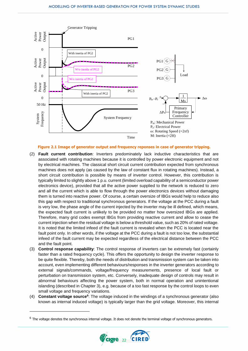
(1) Rotating mass/inertia: Inverters do not have a rotating mass component; i.e. there is no inherent
inertia. The prime mover behind the inverter might have the inertia, but its “usage” has to be
achieved via the inverter controls and the inverter size because all IBGs are limited in terms of
maximum current through the power electronics devices, as well as maximum voltage. To use the
real available inertia, if any, of the “prime mover”, a significant oversize of the inverter generator5
or room to increase output may be necessary because the available energy reserve in IBGs is very
limited and thus the inertial response of IBGs is eventually withdrawn. Moreover, synthetic inertia
cannot be considered completely equivalent to the inertia provided by conventional synchronous
generators which are directly connected to the grid as measuring devices and controls introduce
delays to the synthetic inertia reaction to events in the grid. Although the fast frequency response
has been commercially available, the synthetic inertia is still carefully evaluated and not in practical
use.
One of the promising schemes for representing the synthetic inertia captures the Rate of Change
of Frequency (ROCOF) and increases or decreases the IBG output so that the frequency change
is mitigated. This concept enables the reduction of the mismatch between the mechanical output
and the electrical output when ROCOF is not zero. When a generator tripping is considered as an
example, the power output of remaining synchronous generators shows the stepwise increase right
when the generator tripping occurs (See Figure 2-1).
It should be noted that the ROCOF is zero at the moment the generator trip occurs because the
system frequency is the pre-disturbance/initial frequency at the moment. Even if the primary
frequency response can be ideally emulated in IBGs, the immediate increase in the IBG output
cannot be observed without the inertia effect (See pink dotted line of PG2 in Figure 2.1). Such
stepwise increase in the synchronous generator output will definitely alleviate the frequency drop.
Synthetic inertia cannot achieve this behaviour mainly due to delay in ROCOF measurement,
filtering and control. Therefore, the synthetic inertia concept of modifying the controls dependent
on the measured ROCOF cannot be currently considered completely equivalent to the inertia
provided by conventional synchronous generators. It should be noted that other concepts for
inverter controls are also under discussion [8], [9], which may offer other means of control in the
future, e.g. concepts such as using a battery system for providing the fast frequency response
and/or the synthetic inertia. (See bullet point 4).
4 In other words, IBGs which were in their infancy and the size of which was unlikely to be categorized as large utility scale. 5 Air-cooled IGBT converters have substantial short-term overload capability (for around up to 1 s).
MODELLING OF INVERTER-BASED GENERATION FOR POWER SYSTEM DYNAMIC STUDIES
22
Time
50 Hz
0
0
Generator Tripping
PG2
PG1
System Frequency
Act
ive
Po
wer
Outp
ut
Act
ive
Po
wer
Outp
ut
Sy
stem
Fre
quen
cy
G
GPG2
PG1
Load
Dw+ 1
Ms
DPm
-
Pm -Pe
PrimaryFrequencyController
Pm: Mechanical Power
Pe: Electrical Power
w: Rotating Speed (=2pf)
M: Inertia (=2H)
0
PG3Act
ive
Po
wer
Outp
ut
GPG3
With inertia of PG2
W/o inertia of PG2
With inertia of PG2
W/o inertia of PG2
Figure 2.1 Image of generator output and frequency reponses in case of generator tripping.
(2) Fault current contribution: Inverters predominately lack inductive characteristics that are
associated with rotating machines because it is controlled by power electronic equipment and not
by electrical machines. The classical short circuit current contribution expected from synchronous
machines does not apply (as caused by the law of constant flux in rotating machines). Instead, a
short circuit contribution is possible by means of inverter control. However, this contribution is
typically limited to slightly above 1 p.u. current (limited overload capability of a semiconductor power
electronics device), provided that all the active power supplied to the network is reduced to zero
and all the current which is able to flow through the power electronics devices without damaging
them is turned into reactive power. Of course, a certain oversize of IBGs would help to reduce also
this gap with respect to traditional synchronous generators. If the voltage at the PCC during a fault
is very low, the phase angle of the current injected by the inverter may be ill defined, which means,
the expected fault current is unlikely to be provided no matter how oversized IBGs are applied.
Therefore, many grid codes exempt IBGs from providing reactive current and allow to cease the
current injection when the residual voltage is below a threshold value, such as 20% of rated voltage.
It is noted that the limited infeed of the fault current is revealed when the PCC is located near the
fault point only. In other words, if the voltage at the PCC during a fault is not too low, the substantial
infeed of the fault current may be expected regardless of the electrical distance between the PCC
and the fault point.
(3) Control response capability: The control response of inverters can be extremely fast (certainly
faster than a rated frequency cycle). This offers the opportunity to design the inverter response to
be quite flexible. Thereby, both the needs of distribution and transmission system can be taken into
account, even implementing different behaviours/responses in the inverter generators according to
external signals/commands, voltage/frequency measurements, presence of local fault or
perturbation on transmission system, etc. Conversely, inadequate design of controls may result in
abnormal behaviours affecting the power system, both in normal operation and unintentional
islanding (described in Chapter 3), e.g. because of a too fast response by the control loops to even
small voltage and frequency variations.
(4) Constant voltage source6: The voltage induced in the windings of a synchronous generator (also
known as internal induced voltage) is typically larger than the grid voltage. Moreover, this internal
6 The voltage denotes the synchronous internal voltage. It does not denote the terminal voltage of synchronous generators.
MODELLING OF INVERTER-BASED GENERATION FOR POWER SYSTEM DYNAMIC STUDIES
23
induced voltage is independently regulated from the grid voltage. It will cause increased current
injection as the grid voltage sags and hence typically contributes positively to network stability.
IBGs do not have such an inherent internal voltage source. The current that can be provided to the
grid during a voltage sag is dominated by the IBG control behaviour and typically limited to 1 p.u. It
should be noted that the operation mode of IBGs typically cannot change without stopping the
inverter, although the IBGs also have the ability to create voltage through U-F mode (also called
isolated operation mode [10]7) instead of P-Q mode.
(5) Transmission-level voltage support: Large capacity synchronous generators generally operate
in AVR mode. That means such generators have an ability to regulate the terminal voltage and the
system voltage in HV network (e.g. typically equal to or higher than 200 kV) near the generator bus.
Small capacity synchronous generators generally operate with Automatic Q Regulator (AQR) or
Automatic Power Factor Regulator (APFR) mode (this means they do not regulate the terminal
voltage but the reactive power or the power factor coming from the terminals). That is because the
reactive power injection of these units is limited, thus they do not have a capability for changing the
terminal voltage and regulating the system voltage (See Appendix 2-A). The IBGs are generally
assumed to operate with a unity power factor. That means most of the IBGs operate with AQR
mode, the power factor of which is one8. Thus, actual voltage control for transmission-level voltage
support cannot be expected or achieved. However large-scale IBGs can support the transmission-
level voltage with the aid of other external voltage controls such as reactive power compensator
and/or Static Var Compensator (SVC). The IBGs themselves can change the reactive power output
through the oversized inverter and/or through the reduction of active power output. Modern grid
codes such as VDE4120 in Germany have required the voltage control9 at the IBG’s PCC.
(6) Synchronization (torque) capability: The synchronous generators have the synchronizing torque
capability which is a very important factor for angle stability [11]. The synchronizing torque index,
Kij is proportional to the internal voltage of the synchronous generator and the equivalent
synchronous generators and/or the angle difference between the synchronous generators and the
equivalent synchronous generator (See Equation 2.1). Such generators can automatically change
their active power output so as to mitigate the change in the angle difference. It is noted that this
capability does not denote the ability which tells how the IBGs in general capture the voltage angle
through a Phase Locked Loop (PLL) algorithm in order to output the active power and reactive
power in a correct phasor form. This capability reacts not to the voltage angle itself but the angle
difference between two different points in order to contain such angle difference within 180 degrees.
This ability is one of the important contributions especially for rotor angle stability.
It should be emphasized that this capability is not literally required for IBGs because they have no
rotor-angle stability issue. On the other hand, the IBGs might be required to have the synchronizing
torque capability in the future although IBGs do not need to be synchronized. In such a case, this
is not easy to be achieved because the communication infrastructure for measuring the
aforementioned angle difference is basically required. Even such angle difference is assumed to
be measured nearly in real time, tremendous number of measurements are required in wide area,
because the equivalent synchronous generator to be measured for calculating the angle difference
is not always the same and significantly changes especially when a synchronous generator in a
network of equivalent synchronous generators is disconnected (See Figure 2.2).
sin cosi j i j
ij ij ij
V V V VdP dK
d d X X
Equation 2.1
Where, Kij denotes synchronizing torque coefficient induced between generator i and j,
P denotes active power output of a generator
Vi denotes internal induced voltage of generator i,
7 Recent developments in power electronics allow for the inverters to operate in U-F mode (also called voltage-frequency mode
and grid-forming), giving them the ability to start and maintain the system frequency and voltage using the appropriate controls. It should be noted that this mode of operation is not widely used and it requires inverters with increase capabilities. Moreover, in general, the operation mode of IBGs typically cannot promptly change without stopping the inverter.
8 In some countries, the power factor has been set as a value less than 1 even for IBGs which are connected to LV networks. 9 For example, this voltage control is known as fast voltage control in German grid code, VDE4120.
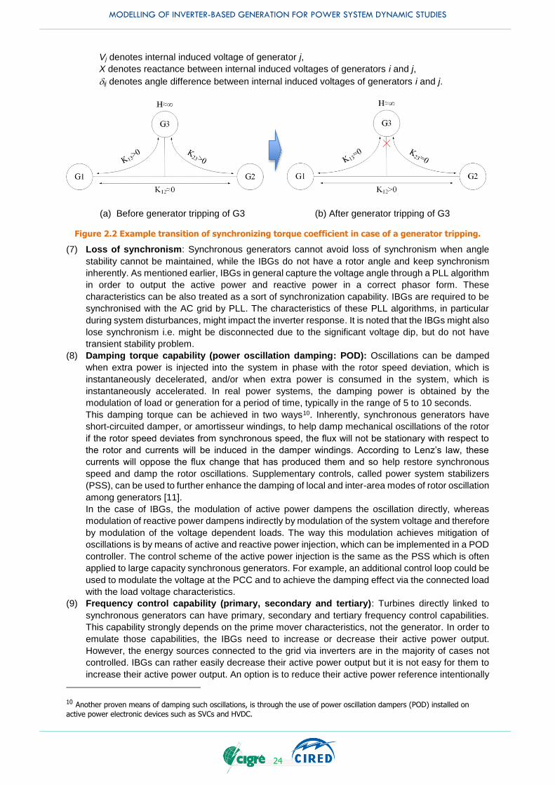
MODELLING OF INVERTER-BASED GENERATION FOR POWER SYSTEM DYNAMIC STUDIES
24
Vj denotes internal induced voltage of generator j,
X denotes reactance between internal induced voltages of generators i and j,
ij denotes angle difference between internal induced voltages of generators i and j.
(a) Before generator tripping of G3 (b) After generator tripping of G3
Figure 2.2 Example transition of synchronizing torque coefficient in case of a generator tripping.
(7) Loss of synchronism: Synchronous generators cannot avoid loss of synchronism when angle
stability cannot be maintained, while the IBGs do not have a rotor angle and keep synchronism
inherently. As mentioned earlier, IBGs in general capture the voltage angle through a PLL algorithm
in order to output the active power and reactive power in a correct phasor form. These
characteristics can be also treated as a sort of synchronization capability. IBGs are required to be
synchronised with the AC grid by PLL. The characteristics of these PLL algorithms, in particular
during system disturbances, might impact the inverter response. It is noted that the IBGs might also
lose synchronism i.e. might be disconnected due to the significant voltage dip, but do not have
transient stability problem.
(8) Damping torque capability (power oscillation damping: POD): Oscillations can be damped
when extra power is injected into the system in phase with the rotor speed deviation, which is
instantaneously decelerated, and/or when extra power is consumed in the system, which is
instantaneously accelerated. In real power systems, the damping power is obtained by the
modulation of load or generation for a period of time, typically in the range of 5 to 10 seconds.
This damping torque can be achieved in two ways10. Inherently, synchronous generators have
short-circuited damper, or amortisseur windings, to help damp mechanical oscillations of the rotor
if the rotor speed deviates from synchronous speed, the flux will not be stationary with respect to
the rotor and currents will be induced in the damper windings. According to Lenz’s law, these
currents will oppose the flux change that has produced them and so help restore synchronous
speed and damp the rotor oscillations. Supplementary controls, called power system stabilizers
(PSS), can be used to further enhance the damping of local and inter-area modes of rotor oscillation
among generators [11].
In the case of IBGs, the modulation of active power dampens the oscillation directly, whereas
modulation of reactive power dampens indirectly by modulation of the system voltage and therefore
by modulation of the voltage dependent loads. The way this modulation achieves mitigation of
oscillations is by means of active and reactive power injection, which can be implemented in a POD
controller. The control scheme of the active power injection is the same as the PSS which is often
applied to large capacity synchronous generators. For example, an additional control loop could be
used to modulate the voltage at the PCC and to achieve the damping effect via the connected load
with the load voltage characteristics.
(9) Frequency control capability (primary, secondary and tertiary): Turbines directly linked to
synchronous generators can have primary, secondary and tertiary frequency control capabilities.
This capability strongly depends on the prime mover characteristics, not the generator. In order to
emulate those capabilities, the IBGs need to increase or decrease their active power output.
However, the energy sources connected to the grid via inverters are in the majority of cases not
controlled. IBGs can rather easily decrease their active power output but it is not easy for them to
increase their active power output. An option is to reduce their active power reference intentionally
10 Another proven means of damping such oscillations, is through the use of power oscillation dampers (POD) installed on
active power electronic devices such as SVCs and HVDC.

MODELLING OF INVERTER-BASED GENERATION FOR POWER SYSTEM DYNAMIC STUDIES
25
at steady state in order to ensure an adequate upper margin or headroom. This has obvious
economic implications, particularly for RESs where curtailing the IBG means essentially lost
opportunity costs that cannot be recovered since the energy source is variable. Another option is
to marry an energy storage option with the IBGs. It should be noted that this could cause additional
burden to the IBG owners. Also, it has to be considered that even for traditional power plants with
synchronous generators keeping additional generation margins available for regulation represents
an additional cost.
(10) Limited frequency sensitive mode: In the case of significant frequency rise, power plants need
to decrease their outputs. This emergency corrective action is called "Limited Frequency Sensitive
Mode – over frequency" It is important to note that any kind of generator can operate in the limited
frequency sensitivity mode, but their prime movers may not be able to provide this operating mode.
(For example, in the case of gas turbine power plants, the sudden decrease of fuel input will
increase the air-fuel rate and could cause the undesired/unintentional flame-out of the combustion
system.11). This capability strongly depends on the prime mover characteristics, not the generator.
For many IBGs, this is not a limitation. For example, PV can easily reduce its output if the inverter
is controlled according to this mode.
(11) Maintenance: The periodical maintenance for synchronous generators is more onerous as longer
down time and more expensive intervention is required than compared to IBGs
(12) FRT capability: Synchronous generators are required to withstand without failure a short circuit of
any kind at its terminals by IEC Standards (IEC 60034-3 Clause 4.16). On the other hand, the prime
movers do not always have the fault ride-through capability. While most of the representative prime
movers of large-scale hydro power plants, coal-fired power plants and nuclear power plants have
such capability, some prime movers of medium-scale thermal power plants have a shear pin
embedded in the rotating shaft and designed to break during severe voltage dip (when the shear
pin breaks during severe voltage dip, the power plant is tripped). To date, distributed IBG typically
do not ride through severe three phase faults because the voltage phase angle could not be
detected when the line voltage is very low, e.g. less than 30% because the magnetic contactor
which is placed between the inverter and the grid will open due to the loss of its excitation of the
magnetic coil. It is noted that this is the issue of the contactor and not of the inverter. New
techniques such as higher resolution frequency calculation, and the use of the off-delay release
type magnetic contactor or the UPS can now achieve the fault ride-through capability12.
(13) Reactive power support:
(a) V-Q control during steady-state: The rated power factor of the synchronous generators is
generally in the range of 0.80 - 0.95, with the higher value being typical of modern units. The rated
power factor for distributed IBGs is not often provided, which means the rated power factor is
assumed to be unity13. Distribution-connected PVs are still operated at unity power factor over their
entire active power output range in many countries. Most of these inverters are not sized to provide
any reactive current at full output. In order to provide reactive power support at full output, larger
inverters will be required. On the other hand, system operators usually require that IBGs include
reactive power control at the PCC. In addition, this reactive power control to be independently
activated by such multiple alternatives as voltage regulation, reactive power regulation or power
factor regulation14.
(b) Reactive current control during network incidents: A synchronous generator can
dynamically support the reactive power output from the moment when the system fault occurs thus
providing an immediate/instant increase of reactive power output. In contrast, it cannot be
guaranteed that the IBG can increase the reactive power output from the moment when the fault
occurs to mitigate the voltage drop mainly because the detection time of the voltage magnitude of
11 As the countermeasure, there is typically a rate limit on how quickly a gas turbine can reduce its output. 12 Due to the advanced technologies, most large scale (many tens of MWs) utility scale wind power plants connected to the
transmission system do have FRT capability and some WTGs are able to ride through solid faults up to 3 s, which is most unlikely to be achieved by synchronous generators from mechanical point of view and from transient stability point of view. 13 Nowadays, the power factor in some countries has been set as a value less than 1 even for IBGs which are connected to LV
networks. 14 Large scale IBGs do provide these same capabilities, i.e. voltage regulation, however, this requires more work and research
to identify the proper and suitable means of providing such capabilities at the distribution level. One such effort is the current revision of the IEEE Standard 1547 in North America.
MODELLING OF INVERTER-BASED GENERATION FOR POWER SYSTEM DYNAMIC STUDIES
26
the IBG cannot physically be instantaneous. The IBG enables an increase in the reactive power
output with some delay during the fault by decreasing the active power output within the rated
current. Therefore, no matter how quickly the IBG is able to control voltage and current, the IBG
cannot show the same immediate/instant increase of the reactive power support provided by the
synchronous generator. In addition, a synchronous generator allows a negative sequence current
to flow, whereas the IBG is often designed to block negative sequence currents. In the future a
TSO may require that the IBG provides a negative sequence current in case of unsymmetrical faults
mainly to ensure sufficient voltage recovery for all three phases15.
(14) Harmonic emission: Inverters may produce non-sinusoidal currents that can be described and
quantified as harmonic emission in frequency domain. The harmonic emissions need to be
assessed and controlled before the connection is permitted. The IEC has standards of harmonic
emissions and some countries impose their own limits for connection of nonlinear appliances to the
grid. Harmonic currents emitted by synchronous generators (airgap flux harmonics, slot harmonics,
etc.) are usually negligible. The harmonic current emission of IBGs depends on the following; type
of technology used, control strategy of the DC/AC-inverter, existence of high- or low-frequency
coupling transformer and the harmonic voltages prevailing in the AC-power system.
(15) Harmonic voltage reduction: Since the effective impedance of synchronous generators for low
order harmonics is based on the small sub-transient reactance, synchronous generators provide a
rather low impedance path for harmonic currents and thus tend to reduce harmonic voltages. All
voltage source converters absorb harmonics because inverters can act as an impedance using the
voltage source converter technologies.
(16) Black start: is the ability of the power system to restart itself after a full or partial system black out.
Most conventional generators are designed to require an electrical supply from the power system
to start up. Normally this is provided from the transmission or distribution system, however under
black start this supply is not available. Therefore, to restart the system it is required to some power
stations have their own auxiliary supplies to they can restart themselves. These power stations can
then be used to restart other power stations and thus the whole system can be restarted.
Traditionally black start capability relies on large transmission-connected synchronous generators.
Over the coming years the trend of reduction in the number of these plants is expected to continue
leading to fewer traditional black start providers being available. For an IBG the ability of the
technology to achieve black start is more limited under extreme network conditions due to factors
such less inertia, less overload capacity to provide inrush current for energization and the use of
PLL technology [12].
Most of the power systems around the world are undergoing fundamental changes. This includes strong moves away from heavy reliance on fossil fuels as the primary energy source mainly provided by large synchronous generators connected to the transmission systems, towards a decarbonised future supply relying increasingly on variable renewable energy sources (RES) using non-synchronous generation predominantly connected to the network via power electronics and extensively connected deeply embedded in the distribution networks. Some countries in Europe have already experienced times in which in some periods the national demand for electricity has been exceeded by the RES production alone [13] That means the functionalities which the conventional generators have and which the IBGs do not have, will be lost and the system stability could be affected. In order to cope with this, such functionalities have been required by the IBGs through updating of grid codes. It should be noted that the aforementioned advanced functionalities and capabilities could usually be require to newly installed IBGs.
In general, if equipped with proper control logics, the IBGs could offer to the grid many flexible features,
like:
Frequency regulation
Reactive power/voltage regulation
Insensitivity/immunity to large electrical torque variation (i.e. due to automatic reclosing near the
plant)
Low Voltage Ride-Through (LVRT)
15 This is now regulated in Germany (See VDE-AR-4120).

MODELLING OF INVERTER-BASED GENERATION FOR POWER SYSTEM DYNAMIC STUDIES
27
Table 2-1 summarizes the main existing and/or potential differences between IBGs and conventional synchronous generators.
In terms of simulation models for IBGs the following challenges and requirements can be highlighted:
Recently a lot of new capabilities (with reference to IBGs, because many of these were common
for traditional synchronous generators) have been required for IBGs in grid codes, some of them
are still at the definition stage, to comply with both DSOs and TSOs needs. Those capabilities have
to be represented in each model (at least according to the specific simulation to be performed).
Specific capabilities are already available on the market (e.g. simulation of inertia), even if obtained
by additional devices (storage). However, they are not described in detail in any standard approach
in terms of algorithms, performance, implementation, compliance assessments, etc., making it
difficult to develop appropriate and generic models.
From a “model definition” perspective, it is very important to be aware that IBGs have no “natural”
features (because the feature can depend on how the IBG controller is designed), while the
synchronous generators have these.
The scope of application (area of validity) of any given model has to be defined. For example, a
specific capability (frequency support, voltage support etc.) might be represented in a Root Mean
Square (RMS) model for stability analysis, but the model is only valid under certain conditions (e.g.
no smaller than the minimum short circuit ratio).

MODELLING OF INVERTER-BASED GENERATION FOR POWER SYSTEM DYNAMIC STUDIES
28
Table 2.1 Major existing and/or potential differences between IBGs and synchronous generators
Relevant phenomena
Conventional synchronous
generator with standard AVR and turbine governor
IBG with minimum functionalities
(before interconnection
requirements are evolved)
Advanced capability / Advanced feasibility of IBG (after interconnection requirements are evolved)
Rotating mass/inertia
Frequency Stability
Yes No Yes (prime mover dependent), but enough headroom (or unloaded synchronized capacity) is required (The use of battery energy storage could be needed depending on the type of devices). The capability might also depend on the direction of frequency deviation (over- or under-frequency). In addition, exact emulation cannot be performed16. See (1) above.
Frequency response capability (primary, secondary and tertiary)
Frequency Stability
Yes* No Yes (prime mover dependent), but enough headroom and/or upper margin need to be ensured. See (9) above.
Limited frequency sensitive mode
Frequency Stability (over-frequency)
Yes** No
Yes (prime mover dependent). See (10) above.
Constant voltage source17
Voltage stability
Yes, internal induced voltage
No, if connected to the grid (inverter is synchronized to external grid frequency/phase)
Yes, but isolated system is required. Stiff voltage and stiff frequency (U-F mode) are required for inverter). Oversized IBG may be required. See (4) above.
Transmission-level voltage support (steady state)
Voltage Stability
Yes, but large capacity machines with AVR only
No Yes (large-scale IBGs only) often with large capacity reactive power compensators such as shunt capacitor/reactor, SVC. See (5) above.
Reactive power support (V-Q control during steady state)
Voltage Stability /support
Yes, according to PQ-capability
No Yes, but larger IBG is required or active power needs to be reduced according to PQ capability characteristics. See (13) above.
16 None-the-less, studies have been shown that so-called “synthetic inertia” for wind turbine generators can be an effective
means of helping to reduce system ROCOF during frequency events. See https://www.nerl.gov/grid/wwsis.html 17 The voltage denotes the synchronous internal voltage. It does not denote the terminal voltage of synchronous generators.

MODELLING OF INVERTER-BASED GENERATION FOR POWER SYSTEM DYNAMIC STUDIES
29
Relevant phenomena
Conventional synchronous
generator with standard AVR and turbine governor
IBG with minimum functionalities
(before interconnection
requirements are evolved)
Advanced capability / Advanced feasibility of IBG (after interconnection requirements are evolved)
Reactive power support (reactive current control during network incidents)
Rotor angle stability Voltage Stability
Yes No Yes, usually during faults IBGs may be able to provide a reactive current injection with some delay which helps keeping them grid connected, as per TSO/DSO requirements. See (13) above.
Synchronization (torque) capability18
Rotor angle stability
Yes No Yes (but almost infeasible), angle difference needs to be observed without time delay. See (6) above.
Damping torque capability (power oscillation damping capability)
Rotor angle stability
Yes, damper windings and addition of PSS
No Yes, POD functionality. See (8) above.
Loss of synchronism
Rotor angle (transient) stability Protection
Yes Not applicable to IBGs
See (7) above.
FRT capability
Rotor angle (transient) stability Frequency stability
Yes*** No. Yes (prime mover dependent). See (12) above.
Harmonic emission
Power quality Low Yes, including the frequency band dedicated to utilities for PLC based communications
See (14) above.
Harmonic voltage reduction
Power quality Yes, for low order harmonics
Yes Yes. See (15) above.
Short-circuit contribution in case of symmetrical and unsymmetrical faults
Protection, limit voltage decline
Yes No Yes, but contribution is limited to around 1 p.u., unless inverter has short-term rating to exceed 1 p.u.). See (2) above.
18 Note that this capability is NOT literally required for IBGs because they have no rotor-angle stability issue.

MODELLING OF INVERTER-BASED GENERATION FOR POWER SYSTEM DYNAMIC STUDIES
30
Relevant phenomena
Conventional synchronous
generator with standard AVR and turbine governor
IBG with minimum functionalities
(before interconnection
requirements are evolved)
Advanced capability / Advanced feasibility of IBG (after interconnection requirements are evolved)
Control response capability
Voltage and frequency stability
Fast, depending on the time constants involved or other external dependencies****
Inverter itself very fast (faster than generator controllers of synchronous generators), limitations possible due to measurement delay, prime mover or other external dependencies****
See (3) above.
Overload capability (up to few seconds)
misc. Yes Limited (nearly negligible), depending on semiconductor devices*****
Yes, but significant oversized IBGs are required. See (2) above.
Maintenance
misc. regularly Low for inverter itself, prime mover depending on the type
See (11) above.
* Generator with enough headroom and/or upper margin. ** Depending on rotating prime mover characteristics. *** Generators with damper windings are for local modes of oscillations, while generators with the PSS are
for inter-area modes of oscillations.
**** E.g. industrial process supplying primary energy to be converted in electricity ***** Air-cooled IGBT converters have pretty good short-term overload capability (E.g. up to 1s), while water
cooled MV-connected converters have almost no short-term overload capability.
2.2 INVERTER CHARACTERISTICS
2.2.1 Topology and controller structure
There is a variety of inverter topologies available on the market, developed by different manufacturers and optimised for specific applications. Optimisation targets generally consider reliability, maintenance, losses, overall costs etc. For example, 3-phase connected wind-turbines may be equipped with 2 level voltage sourced back-to-back inverters or multilevel voltage sourced back-to-back inverters, depending on the wind-turbine rated power.
Using different primary energy sources, the inverter topology remains substantially the same even using different energy sources. The following is an example of the topology for a PV plant. As regards PV inverters, among different possible topologies [14], two typical inverter families are:
H-bridge topology
Neutral point clamped topology
Most of the inverter topologies for PV available today have been derived from these basic design structures. It is not the aim of this TB to describe all inverter topologies and their specifics for the different energy resource. The principal scheme of a photovoltaic power plant with H-bridge as a representative example is described in Figure 2-3 (a)
The PV plant consists of the following elements [14]:
Photovoltaic array: The array of photovoltaic modules forms the solar generator. Several modules
can be connected in series, forming a so-called string. Strings in turn can be connected in parallel.
It is possible to connect either a common inverter to the entire array, with an inverter per string or
to connect a single inverter for each module.
Chopper: Boost DC voltage, among others, to ensure Maximum Power Point Tracking (MPPT),
measuring the PV voltage (VPV) and PV current (IPV)

MODELLING OF INVERTER-BASED GENERATION FOR POWER SYSTEM DYNAMIC STUDIES
31
DC link: Filter/Energy storage
Inverter: Conversion of DC power to AC power with the output filter (denoted as LCL filter in Figure
2-3 (a)).
(a) Simplified PV block scheme with different control layers [14]
Chopper Inverter
Filter
Grid PV Array
Valve device control
DC-AVR
DC-ACR
MPPT
PLL
vg
iac
iin
vdc
vin
Comparator
vg vdc
VDC-ref
iin vin
Reference voltage
waveform
iac
Control
Circuit
IDC-ref
IDC-cmd
IAC-cmd
Sm
oot
hing
cap
acit
or
Amplify
(b) Example of control circuit of PV [16]
Figure 2.3 General control circuit structure of PV.
The inverter control enables the AC (active) current waveform to match with the voltage at the PCC in
terms of the frequency and the phase at unity power factor. The inner current control monitors the
voltage at the PCC and creates the current waveform with the same frequency and the same phase of
the voltage at the PCC with the aid of the PLL. At the DC side, the Maximum Power Point Tracking
(MPPT) control maximizes the active power output. As shown in Figure. 2-3 (b), DC-ACR monitors input
active power and changes the input DC current periodically in order to control the input DC current via
Vdc PWMPWM
Ig
VgVPV
IPV

MODELLING OF INVERTER-BASED GENERATION FOR POWER SYSTEM DYNAMIC STUDIES
32
controlling the switching action of the chopper. The DC-AVR monitors the internal DC voltage and
amplifies the reference voltage waveform (created via PLL) which results in the AC (Active) current
control signal. The power electronic device switching action is controlled by comparing the
aforementioned AC current control signal with the measured AC current.
For most of the phenomena described in this technical brochure, the modelling of the switching action
is generally not necessary. An average model, i.e. a model where all the variables are averaged over
the switching period, is able to precisely reproduce most of the phenomena reported in this chapter.
Only a few of them, such as the prediction of harmonic distortion and electromagnetic interference (EMI)
compliance, require a more precise switching model.
2.2.2 Ancillary functions
Because of the flexibility of the inverter control design, IBGs may be required from either the technical standards and/or from grid codes, to provide some additional capabilities for grid support, among them:
Negative sequence current injection; (ref 4.7.4.1.2) [15]
Reactive current control calculated by mean of power factor input;
Maximum reactive current injection;
Reactive current level depending on voltage depth (ref 4.7.4.1.1) [15]
Table 2-2 shows the most relevant required IBGs capabilities from the EU Regulation 2016/631 “establishing a network code on requirements for grid connection of generators” [17] and the IEEE 1547
“Standard for Interconnecting Distributed Resources with Electric Power Systems” [18]. As IEEE
1547 and UL1741, “Standard for Inverters, Converters, Controllers and Interconnection System Equipment for use with Distributed Energy Resources” [19] have been evolved, the latest requirements coming from IEEE 1547-2018 are also introduced in this table.
Table 2.2 Requirement for IBG in grid code and standard
Requirement EU 2016/631 IEEE 1547-2014 IEEE 1547-2018
P(f) (over/under) x x
Voltage control by means of reactive power (Q(V)) x (x) x
Voltage control by means of active power (P(V)) x
Synthetic Inertia (x)
ROCOF immunity x x
FRT (LV/HV) x (LVRT only) (x) x
Inverter internal protections
Anti-islanding active detection methods x (ROCOF) x x
Dynamic voltage support during faults and voltage steps
(x) (x)
Power Oscillation Damping (x)
Black start Capability (x)
Capability of Islanding Operation x
Automatic Disconnection with Abnormal Voltage x x
Automatic Connection with active power recovery speed
x x
Constant Power at Low Voltage x
Constant Power at Low Frequency x Note: The sign “x” means one or more classes/categories of the IBGs are required to meet with the designated requirement. ( ) denotes a non-mandatory requirement.
2.2.3 Inverter protection
An Inverter’s protection may be separated into two main classes, internal and external. This classification has nothing to do with the physical location of the protections. Internal protections are primarily to assure the safety of the inverter itself and may be not in accordance with relevant standards of protection relays (IEC TC 95 “Measuring relays and protection equipment” [20]) and are applied by the manufacturers. External protection is required to serve a different purpose and considers the network. Physically, in some cases, the external protection may be the same as the internal inverter protection, but, despite this, they are not “monitoring” the inverter (internal), but the network (external). Although protection functions based on pure electric measurements (passive protection methods) shall comply

MODELLING OF INVERTER-BASED GENERATION FOR POWER SYSTEM DYNAMIC STUDIES
33
with requirements of IEC TC 95, other protections (not mentioned and/or based on active methods) are not defined at all by IEC TC 95 at the present moment.
Internal protections are generally inserted in inverter models and do not affect IBG capabilities and requirements. External protections, despite that they are physically inside the inverter control, may be modelled separately, to allow for changes in the protection models or different regulation combinations without any change in inverter model.
2.2.3.1 Internal Protection
Each IBG type has its own type of internal protections focused on avoiding damage to the inverter itself.
These internal protections are also known as generator protections (i.e. nothing to do with Interface Protection).
Some examples of inverter internal protections are:
Reduction of maximum inverter current when the DC voltage exceeds a certain limit;
Limitation of inverter current’s variation rate after a fault;
Limitation of total reactive current;
Manual PV field shutdown with emergency stop;
PV field insulation detection;
DC overcurrent protection;
Over/under voltage protection;
Over/under frequency protection.
It should be noted that “Limitation of inverter current’s variation rate after a fault” and “Limitation of total reactive current” are generally categorized as control instead of protection. Because their control functions can operate for protection purposes as well as for control purposes, they are treated as the internal protection in this technical brochure.
2.2.3.2 External Protection
IBGs may have external protections to:
Detect uncontrolled local islanding situations and disconnect generators to shut down this island.
This functionally is also known as “Loss of Mains Protection”;
Reduce the power production from the generating plant to prevent an over-voltage or over-
frequency situation in the network it is connected to;
Assist the power system to reach a controlled state in case of voltage or frequency deviations
beyond corresponding regulation values.
These protections (or combination of different elementary protection functions) are usually referred to as interface protection or interface protection system.
The interface protection system is generally based on combinations of over/under voltage and over/under frequency protections.
It is not the purpose of the interface protection system to:
Disconnect the generating plant from the network in case of faults internal to the power generating
plant. Protection against internal plant faults or abnormal operation conditions (short-circuits, earth
faults, overloads, etc.) is in charge of other external protection relays coordinated with network
protection, according to electric system operator protection criteria. Protection against electric
shock and against fire hazards are out of the scope of this TB;
Prevent damages to the generating unit due to incidents (e.g. short circuits, asynchronous reclosing
operations) on the network. To avoid these possible damages, the generating unit shall have an
appropriate immunity level.
The interface protection system has to be coordinated with power system protections and power system needs. Generator disconnection shall happen as fast as possible and with high reliability in case of local faults or outside of normal operation conditions, and shall not happen in case of global perturbations unless voltage and frequency values are far from normal operation conditions for a relatively long time.
The type of protection and the sensitivity and operating times of the interface protection system depend on the electric system protections and on the characteristics of the network.
MODELLING OF INVERTER-BASED GENERATION FOR POWER SYSTEM DYNAMIC STUDIES
34
The interface protection system is meant as a dedicated external device. Protection functions and other features (e.g. EMC, mechanical, climatic requirements, etc.) shall be according to IEC TC 95 and other relevant standards.
A good overview on external protection can be found in CIGRE TB 613 “Protection of Distribution Systems with Distributed Energy Resources”[21] and CIGRE TB 421 “The impact of renewable energy sources and distributed generation on substation protection automation” [22].
2.3 PRIMARY ENERGY SOURCES OF INVERTER BASED GENERATORS
Renewable Energy Sources (RES) are mainly connected to the grid via inverters. A power inverter, or
inverter, is an electric energy converter that converts direct current (DC) to single-phase or polyphase
alternating current (AC) [23]. These IBGs represent 100% of the total for the Photovoltaic (PV) plants and an appreciable and continuously increasing percentage of wind plants (full inverter generators and
Doubly Fed Induction Generators (DFIG) reach sizes much higher than 4 MW). In addition, inverters are also used in Organic Rankine Cycle (ORC) plants [24] and in micro turbines equipped with high
frequency permanent magnet synchronous generators. It is noted that the doubly fed technology has
originally been developed for hydro plants, e.g. variable speed pumped storage units [25]. The inverter provides the interface between the grid and primary energy source to be transformed into electricity.
Although the inverter technologies may be similar to all devices, an appreciable difference may exist related to the prime mover features, therefore influencing at least the inverter control. The response
and achievable performance of the combined system depends both on the capability of the inverter and the capability of the primary energy source.
Examples:
PV plants (PV array) neither have physical inertia nor mechanical/thermal processes involved.
Therefore nearly “real time” regulation is possible, limited only by inverter capabilities and inverter
control reaction time (for the whole chain, including measurement time of relevant quantities, such
as voltage, frequency, etc.; the theoretical reaction times may be some milliseconds or shorter).
There is no inherent energy storage (due to missing inertia) and thus, no possibility to support the
system in case of under-frequency due to incentive systems (unless additional storage devices are
foreseen or unless the generation is curtailed by several percent of the available active power [26]).
The prime mover of wind turbines (rotor blades) exhibits mechanical effects, including for instance
inertia. The inverter control has to take into account the dynamics of the prime mover. For example,
in case that such power cannot be delivered to the grid (e.g. during a fault), even though pitch
control may be very fast, some energy may be injected in the DC stage of the inverter causing an
increase of the DC voltage (possibly limited by the activation of a chopper or of electronic operated
short time duty resistors)
In case of ORC generators (not widely used at present), the capability and the reaction time
depends on the thermal cycle of the “prime mover” from the ORC itself, which is usually an industrial
process, thus it is not easily controlled in a rapid manner without serious consequences to the main
process itself.
As stated before, some of the RES capabilities might not be used due to existing economic
incentives (or the lack thereof): RES is mostly allowed to operate at maximum momentary available
power supplied from the primary energy source (there are some exceptions at present, for instance
Eirgrid, Hydro Quebec, ERCOT (for those IBGs participating in the primary frequency response
market), etc. have already introduced the requirement to operate RES at a power some % below
the available maximum power, to allow for primary frequency regulation). Moreover, the power
factor is often equal to one, the reactive power exchange with the network for voltage control on
distribution networks and power flows on transmission system, not being generally requested, (the
main reason for this is to avoid any oversize of the inverter or any momentary active power
reduction to allow the Q exchange)
The generation units that use different technologies can be characterized according to their primary energy source and the existence, or not, of a prime mover and a rotating electrical machine as a generator [27], [28], as shown in Table 2-3 and Figure 2-4. It is noted that the generator protection somehow depends on the type of primary source (See Appendix 3-A.2.3).
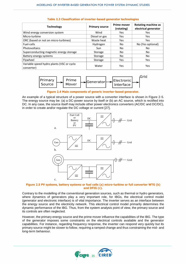
MODELLING OF INVERTER-BASED GENERATION FOR POWER SYSTEM DYNAMIC STUDIES
35
Table 2.3 Classification of inverter-based generator technologies
Technology Primary source Prime mover
(rotating) Rotating machine as electrical generator
Wind energy conversion system Wind Yes Yes Micro-turbine Diesel or gas Yes Yes
ORC (based or not on micro-turbines) Waste heat Yes Yes
Fuel-cells Hydrogen No No (Yes optional)
Photovoltaics Sun No No
Superconducting magnetic energy storage Storage No No Battery energy systems Storage No No
Flywheel Storage Yes Yes
Variable speed hydro plants (VSC or cyclo converter)
Water Yes Yes
Figure 2.4 Main components of generic inverter-based generator.
An example of a typical structure of a power source with a converter interface is shown in Figure 2-5. The energy source may be: (a) a DC-power source by itself or (b) an AC source, which is rectified into DC. In any case, the source itself may include other power electronics converters (AC/DC and DC/DC), in order to create and/or regulate the DC voltage or current [27].
Fuel Cellor
BatteryorPV
=DCGrid
=DCGrid
=Gen
a.
b.
=
Grid
=
Gen
c.
Figure 2.5 PV systems, battery systems or fuel cells (a) micro-turbine or full converter WTG (b) and DFIG (c).
Contrary to the modelling of the conventional generation sources, such as thermal or hydro generators, where dynamics of generators play a very important role, for IBGs, the electrical control model (generator and electronic interface) is of vital importance. The inverter serves as an interface between the energy source and the electricity network. This electrical control model primarily determines the dynamic performance of the IBG. Thus, from the system analysis point of view, the primary source and its controls are often neglected.
However, the primary energy source and the prime mover influence the capabilities of the IBG. The type of the generator imposes some constraints on the electrical controls available and the generator capabilities. For instance, regarding frequency response, the inverter can respond very quickly but its primary source might be slower to follow, requiring a ramped change and thus constraining the mid- and long-term behaviour.
MODELLING OF INVERTER-BASED GENERATION FOR POWER SYSTEM DYNAMIC STUDIES
36
When studying the short-term, transient and dynamic performance of the inverters at the grid terminals or when the generator is interfaced to the grid with the auxiliary help of a storage system to supply the transient need of power, the details on the primary source behaviour tend to lose importance. We can regard the system as an inverter connected to a stiff DC source which simplifies the design and analysis of the power electronic interface. However, the controls, features and capabilities of the generator’s inverter following disturbances strongly rely on the type of its primary source.
PV plants that are fully interfaced by power electronic converters and have the ability to provide fast response during frequency rise/drop have no rotating masses that introduce increased time responses. The loss of stabilization effect due to the lack of inertia could be compensated from a much faster reaction time. The fast reaction time may also have some adverse effects, which must be properly taken into consideration in the dynamic studies, because these effects may affect different parts or levels of the electric system from the one under consideration (for instance may increase uncontrolled islanding on distribution systems).
Simple micro-turbines consist of a compressor, a combustor, a turbine, and a generator. The compressors and turbines are typically radial flow designs that resemble automotive engine turbochargers. Most designs are single-shaft and use a high-speed, permanent magnet generator to produce variable-voltage, variable-frequency AC power.
Battery energy storages may heavily affect dynamic system behaviour according to the way they are used [29].
For further detail, it is necessary to consider primary energy sources using inverters/converters to interface with the network, but it is noted that providing the primary source model is out of the scope of this TB. IBGs shall be considered as two components: inverter and generator which both have independent requirements for frequency control and different frequency response characteristics.
2.4 CONCLUSION
Chapter 2 addressed the characteristics of IBGs focusing on the differences between IBGs with minimum functionalities and large capacity synchronous generators. The representative natural feature of synchronous generators is the inertia; fault current provision, synchronization capability and the constant/fixed internal voltage19 source. They cannot easily be emulated (if at all or if needed) by IBGs from technical or commercial perspectives20. On the other hand, many of the characteristics such as limited frequency control capability and the reactive power control capability can be provided by IBGs. Because of the increasing functionalities of IBGs, the IBG models have been further developed. Although the synthetic inertia concept has emerged over the last few years, it is not completely equivalent to inertia provided by synchronous machines mainly because the immediate/instant change in active power is feasible by only synchronous generators. However, the control response of IBGs is much faster than that of synchronous generators and such fast frequency response might be able to compensate such lack of immediate/instant change in active power.
Chapter 2 also addressed the difference from a protection point of view, of the characteristics of IBGs compared to synchronous generators. In general, IBGs are more likely to be disconnected due to the high sensitivity of inverter protections. Therefore, modern grid codes are asking for IBGs to have FRT capabilities. Because the operation of the inverter protection could result in the disconnection of the IBG, the inverter protection models play an important role for most of the dynamic stability analyses. On the other hand, the primary source and its controls may often be neglected for power system dynamic studies.
Chapter 2 introduces in a basic fashion the type of models which is used for dynamic power system analysis. The selection of the model type (EMT or RMS) is not discussed in Chapter 2 because it is very dependent on the specific phenomena to be investigated. The selection of the model type with the necessary model element for each type of phenomenon is discussed in Sub-Chapter 3.8. The addressed characteristics in Chapter 2 are then used to extract the necessary functionalities of the IBG model components which can be classified into three categories: 1) Control, 2) Protection and 3) Capability (See Table 2.4). The definition of those categories will be provided in Chapter 3 (See also Appendix A.2).
19 The voltage denotes the synchronous internal voltage. It does not denote the terminal voltage of synchronous generators. 20 Note that this capability is NOT literally required for IBGs because they have no rotor-angle stability issue.
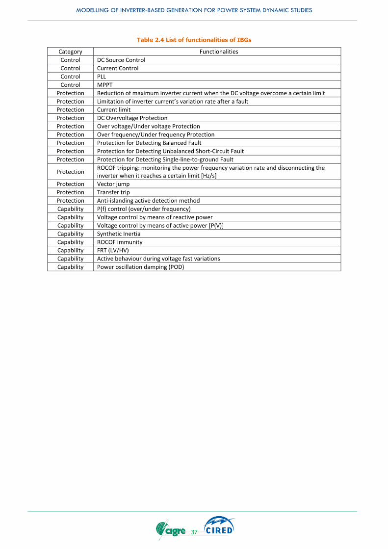
MODELLING OF INVERTER-BASED GENERATION FOR POWER SYSTEM DYNAMIC STUDIES
37
Table 2.4 List of functionalities of IBGs
Category Functionalities
Control DC Source Control
Control Current Control
Control PLL
Control MPPT
Protection Reduction of maximum inverter current when the DC voltage overcome a certain limit
Protection Limitation of inverter current’s variation rate after a fault
Protection Current limit
Protection DC Overvoltage Protection
Protection Over voltage/Under voltage Protection
Protection Over frequency/Under frequency Protection
Protection Protection for Detecting Balanced Fault
Protection Protection for Detecting Unbalanced Short-Circuit Fault
Protection Protection for Detecting Single-line-to-ground Fault
Protection ROCOF tripping: monitoring the power frequency variation rate and disconnecting the inverter when it reaches a certain limit [Hz/s]
Protection Vector jump
Protection Transfer trip
Protection Anti-islanding active detection method
Capability P(f) control (over/under frequency)
Capability Voltage control by means of reactive power
Capability Voltage control by means of active power [P(V)]
Capability Synthetic Inertia
Capability ROCOF immunity
Capability FRT (LV/HV)
Capability Active behaviour during voltage fast variations
Capability Power oscillation damping (POD)

MODELLING OF INVERTER-BASED GENERATION FOR POWER SYSTEM DYNAMIC STUDIES
38
MODELLING OF INVERTER-BASED GENERATION FOR POWER SYSTEM DYNAMIC STUDIES
39
3. NECESSARY FUNCTIONALITIES OF INVERTER BASED GENERATORS FOR KEY PHENOMENA
3.1 INTRODUCTION
The list of functionalities of inverter-based generators (IBGs) has been described in Chapter 2. It should be noted that those functionalities were developed in terms of the capability of the inverter and the control and protections of the IBGs. That means, those functionalities were neither developed from system phenomena perspectives nor modelling perspectives (RMS or EMT). Illustrating and ranking the necessary functions for each type of phenomenon becomes important for many power system studies/analysis because considering all functions in any study requires an extremely heavy computation burden. Therefore, Chapter 3 lists the relevant phenomena simulated in power system dynamic studies and provides the functions which should be considered for each type of phenomenon. The list of the phenomena and the mapping to the type of studies are illustrated in Table 3.1. It is noted that the type of studies shown in Table 3.1 are based on [30].
Table 3.1 Type of phenomena and type of studies
Sub-Chapter Type of Phenomena Relevant Key Words Type of Studies
3.2 Behaviour in response to frequency deviations
●Device protection ●System support ●Plant level control ●Synthetic inertia ●Frequency Response
●Frequency regulation ●Frequency stability ●Transient stability
3.3 Behaviour in response to large voltage deviations
●Device protection against damage ●FRT capability ●Grid support ● (Synthetic inertia)
●Short-term voltage stability ●Transient stability ●Provision of fault current ●Low/High voltage ride through
3.4 Behaviour in response to long-term voltage deviations
●V/Q control ●<permanent> limits ●Plant level control
Long-term voltage stability
3.5 Modelling simplifications for small-disturbance stability analysis
Small-disturbance stability
3.6 Unintentional islanding operation
Unintentional islanding detection
3.7 Other phenomena and studies Low- and high-frequency interaction of controller, switching transients
Many impact analysis studies of IBGs have been performed around the world [31]-[35] and TB 450 [36], “Grid integration of wind generation” which introduces how WTGs could influence the system performance for each type of power system studies. However, according to the questionnaire survey (which was performed during this CIGRE/CIRED JWG activities), still over 30% of the utilities and the system operators do not use any IBG models and just rely on the negative load model for their regular power system dynamic stability studies. The reasons for this may be summarized as follows [4]:
Lack of model requirements of IBG for specific power system phenomena: As the penetration level of such IBG technologies increases, various aspects of power system stability and dynamic performance in the grid may change. Therefore, requirements that address the necessary functions that need to be modelled of IBG for specific power system phenomena need to be developed. These functions include various aspects, such as control, protection and the capability of IBG. Considering these requirements, utilities and system operators can select specific models for each power system phenomenon.
Lack of well-validated detailed IBG models:
MODELLING OF INVERTER-BASED GENERATION FOR POWER SYSTEM DYNAMIC STUDIES
40
In recent years, there has been much effort in the development of validated models for IBG. This work has been primarily related to wind generation but has extended to other types of IBGs in North America. Now, further attention is starting to be devoted to PV systems and other technologies world-wide. In North America, there is one set of approved generic models for large utility scale IBGs that is starting to gain traction [37], however, in general, there is still a lack of well-validated and generally accepted dynamic simulation models, particularly for distributed PV systems, for the use in power system dynamic studies. Even in the case of large utility scale generic IBG models, there is a continued effort to add more features and to refine them.
Lack of widely accepted generic IBG models: Usually utilities and system operators do not create their own (user-written) models. They request validated models from manufacturers, either proprietary or adjusted generic models. This request poses two main disadvantages: 1) the manufacturer wants to keep the confidentiality of their proprietary user-written model; and 2) the extra effort for the manufacturer to tune the parameters of the generic model which includes the validation of the simulations against the field measurements. Thus, the importance of developing reliable and flexible generic models for different technologies and manufacturers of IBG should not be underestimated. The advantages of generic models include: vendor and manufacturer independent, grid code compatible, public model structure (control block diagram), software simulation tool independent, etc. For some technologies, like wind generation, these models are already being widely used, however, the latest generic models had only recently been developed at the time the questionnaire survey was conducted.
Lack of widely accepted range of IBG model parameters: Even if widely accepted generic models are provided, the control model parameters are crucial for power system dynamic studies. Because many grid codes do not yet define the detailed specification/characteristics of the inverter control, the control model parameters could be different depending on the manufacturer of the inverter. Even if the control model parameters of one inverter can be identified through validation, it is almost impossible to identify the parameters of all inverters connected to the power system. Therefore, a set of realistic control model parameters need to be provided.
Lack of specific grid code requirements: Due to the lack of grid code requirements in the past which specified detailed control functionalities for the IBG, the approach of using negative load models for power system dynamic studies was justified. However, with the development of new grid codes, and high penetration of IBG, certain functions of IBG are required (e.g. voltage control, frequency response etc.) and therefore, the negative load model is no longer adequate.
Lack of information about dynamic performance of power system with IBGs: The aforementioned increased penetration level of IBGs also makes system operation, both for TSOs and DSOs, more challenging than in the past. Already, in some areas the consumers’ demand is mostly covered by generation which is connected directly to the distribution system. TSOs routinely run time-domain simulations to assess the stability of the power system. Models, which are currently used to represent distribution systems, are only based on a limited amount of information, generally related to the high voltage network.
Lack of agreed or well documented methodology for the aggregation of IBG: Present trends towards the integration of an increasing range of IBG technologies, widely differing in size and number, poses serious concerns in the industry on how to represent these new technologies in power system dynamic studies. There is not only a lack of validated dynamic computer models of individual distributed generating technologies, such as distributed PV systems, fuel cells, micro turbines etc., but also there is no agreed methodology on how to represent or aggregate the enormous number of embedded LV distributed generation for power system dynamic studies, focusing on both, local (distribution level) and widespread (transmission level) studies.
The high penetration level of IBGs has resulted in the displacement of conventional synchronous generators. Therefore, the impact of IBGs on the dynamic performance of the system increases. The dynamic characteristic of an IBG is different compared to synchronous generators, and with proper control system design and functionalities of modern IBG technologies, they can provide many of the same or even better services (e.g. voltage control, frequency response etc.) than a synchronous generator. However, they do need to be modelled differently and correctly. Therefore, the development
MODELLING OF INVERTER-BASED GENERATION FOR POWER SYSTEM DYNAMIC STUDIES
41
of the appropriate computer simulation models for IBGs with such additional functions is vital for power system analyses.
DSOs have, to some extent, a representation of their networks and details about connected consumers and producers. The limited system and network data is generally not suitable for dynamic simulations for either the distribution or the transmission system or, at least, has not been used for that purpose in the past, due to the high level of detail required. From the point of view of the DSOs, time-domain simulations may also now be necessary to assess protection system behaviour, distribution network automated operation, unintentional islanding of part of distribution systems including IBG, voltage issues, etc. For these types of power system dynamic studies detailed IBG models are needed.
Therefore, the necessity of IBG models should be clarified for each type of power system dynamic study. Although many key descriptions shown in TB 450 are cited, Chapter 3 focuses more on providing the dynamic response of IBGs to each phenomenon (instead of each type of study) and the fundamental impact on the system performance, which is the distinctive contribution of this JWG.
3.2 BEHAVIOUR IN RESPONSE TO FREQUENCY DEVIATIONS
3.2.1 Description of phenomena
Frequency stability refers to the power system’s ability to cope with the imbalance between generation and load. Short-term phenomena in the range of a few seconds and below is related especially to the ROCOF, inertia (including synthetic inertia) and fast frequency regulation response. Long-term phenomena with a time frame up to several minutes includes frequency recovery.
Frequency control is the capability of a power generating module – direct or inverter connected - to control the active power output in order to maintain the system frequency.
Frequency deviation in large, interconnected systems and in islanded systems could be significantly different. The latter might arise as a frequency containment issue or a frequency stability issue even in normal operating condition in autonomous micro grids or during conditions outside of normal operation (i.e. grid restoration after black out).
The frequency stability phenomenon is gaining importance with large penetration of dispersed potentially RES, including IBGs. With high penetration of IBGs, the system inertia tends to reduce, resulting in larger frequency excursions and higher ROCOF [31], if the low inertia is not compensated by fast response times. The increase in ROCOF causes a lower frequency nadir, which could result in the operation of the under-frequency relay and a lower settled frequency which would result in the lower frequency containment. Thus, this leads to the new requirements to frequency response of IBGs.
3.2.2 Relationship between behaviour in response to frequency deviation to relevant study
3.2.2.1 Frequency stability
The frequency stability within a power system represents the capability of that particular power system to maintain the frequency within the predefined limits by assuring the equilibrium between power generation and power consumption. The frequency stability issue can be split into two main categories: medium-term frequency stability and long-term frequency stability. The medium-term frequency stability is often characterized by disturbances causing large power imbalance like the unplanned loss of large generating units resulting in large frequency variations and usually the studied time interval is up to several minutes. System separation is more likely to occur during severe system fault. The long-term frequency stability is characterized by small perturbations within the system such as power variation of a generating unit/units or an equipment disconnection without the occurrence of a large disturbance. In this case the system frequency does not deviate significantly in all the system (no networks separation occurs) and its behaviour follows the slow dynamic process within the power plants and usually the studied time interval is up to tens of minutes.
A frequency stability study is therefore classified into two types. The first type of frequency instability is provoked by a large disturbance within the analysed system such as system faults and/or unplanned power plant tripping which leads of the power plant or by system faults near the power plant. The system separation is more likely to be formed when the system fault occurs. The second type of frequency instability may be provoked by a small system disturbance (no system separation involved) which may lead to a long-term frequency stability problem due to the slow dynamic phenomena within power plants operation.
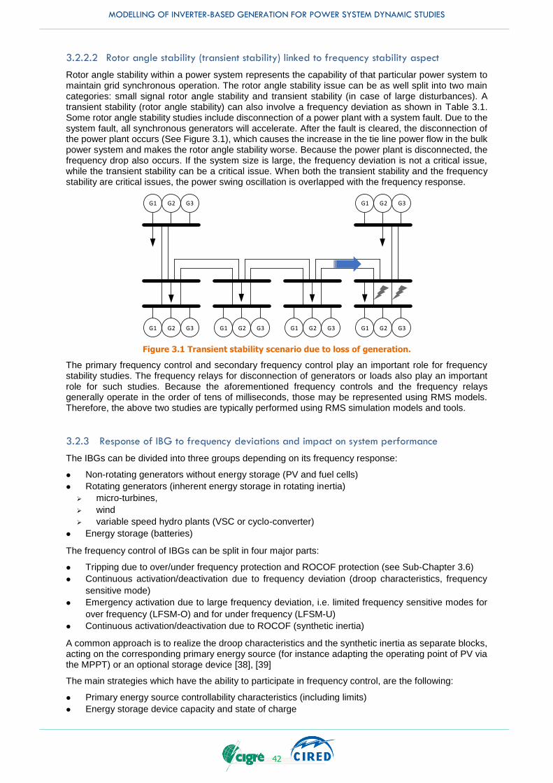
MODELLING OF INVERTER-BASED GENERATION FOR POWER SYSTEM DYNAMIC STUDIES
42
3.2.2.2 Rotor angle stability (transient stability) linked to frequency stability aspect
Rotor angle stability within a power system represents the capability of that particular power system to maintain grid synchronous operation. The rotor angle stability issue can be as well split into two main categories: small signal rotor angle stability and transient stability (in case of large disturbances). A transient stability (rotor angle stability) can also involve a frequency deviation as shown in Table 3.1. Some rotor angle stability studies include disconnection of a power plant with a system fault. Due to the system fault, all synchronous generators will accelerate. After the fault is cleared, the disconnection of the power plant occurs (See Figure 3.1), which causes the increase in the tie line power flow in the bulk power system and makes the rotor angle stability worse. Because the power plant is disconnected, the frequency drop also occurs. If the system size is large, the frequency deviation is not a critical issue, while the transient stability can be a critical issue. When both the transient stability and the frequency stability are critical issues, the power swing oscillation is overlapped with the frequency response.
G1 G2 G3G1 G2 G3G1 G2 G3 G1 G2 G3
G1 G2 G3 G1 G2 G3
Figure 3.1 Transient stability scenario due to loss of generation.
The primary frequency control and secondary frequency control play an important role for frequency stability studies. The frequency relays for disconnection of generators or loads also play an important role for such studies. Because the aforementioned frequency controls and the frequency relays generally operate in the order of tens of milliseconds, those may be represented using RMS models. Therefore, the above two studies are typically performed using RMS simulation models and tools.
3.2.3 Response of IBG to frequency deviations and impact on system performance
The IBGs can be divided into three groups depending on its frequency response:
Non-rotating generators without energy storage (PV and fuel cells)
Rotating generators (inherent energy storage in rotating inertia)
micro-turbines,
wind
variable speed hydro plants (VSC or cyclo-converter)
Energy storage (batteries)
The frequency control of IBGs can be split in four major parts:
Tripping due to over/under frequency protection and ROCOF protection (see Sub-Chapter 3.6)
Continuous activation/deactivation due to frequency deviation (droop characteristics, frequency
sensitive mode)
Emergency activation due to large frequency deviation, i.e. limited frequency sensitive modes for
over frequency (LFSM-O) and for under frequency (LFSM-U)
Continuous activation/deactivation due to ROCOF (synthetic inertia)
A common approach is to realize the droop characteristics and the synthetic inertia as separate blocks, acting on the corresponding primary energy source (for instance adapting the operating point of PV via the MPPT) or an optional storage device [38], [39]
The main strategies which have the ability to participate in frequency control, are the following:
Primary energy source controllability characteristics (including limits)
Energy storage device capacity and state of charge

MODELLING OF INVERTER-BASED GENERATION FOR POWER SYSTEM DYNAMIC STUDIES
43
Controller structure and parameter settings (droop, dead-band, synthetic inertia)
Protection settings, over/under frequency, ROCOF
3.2.3.1 Increase in ROCOF [31]
The initial ROCOF that occurs is purely related to the system inertia at the time. IBG technologies behave differently from conventional synchronous generators hence the system inertia in small networks or islanding areas of a power system can significantly be reduced in case of a large penetration of IBGs. This will have an influence on the ROCOF in case of generation-demand imbalance.
The presence of synthetic inertia in IBGs could contribute to limit ROCOF, but currently is very limited and not as fast as the initial and inertial response from a synchronous generator (See Sub-Chapter 2.1, point 1 Rotating mass/inertia). As shown in some recent studies, so-called inertia-based fast-frequency response, or “synthetic inertia” may offer a means of limiting ROCOF as the penetration of IBGs increases, This, however, needs to be studied on a case by case basis to identify if the particular design will meet the needs of the particular system. Consequently, the frequency might drop significantly in the first seconds before primary control will start to operate. This can lead to high frequency variations after disturbances and hence increasing amount of load shedding. Similar results are shown in Figure. 3-2 and can be derived from the studies performed in [40], [41]. Many small power systems rely upon ROCOF to detect power islanding. With increased ROCOF for the trip of a unit, such systems are likely to falsely detect islanding. In such a case, the protection relays settings will have to be adjusted.
Figure 3.2 WAMS recording (50 Hz sampling).
3.2.3.2 Increasing over frequency transient and steady state frequency excursion
3.2.3.2.1 Over frequency transients
Generally, over frequency transients are a consequence of generation exceeding load demand; some possible causes are:
Complete trip of a line/lines connecting an electrical area that previous was exporting energy
Formation of a small/large island / system splitting
Loss of a large load or trip/temporary interruption (i.e. commutation failure) of a HVDC link which
was exporting energy in interconnected or islanded systems
The area with excess generation suffers a fast over frequency transient, that must be controlled by conventional power plants and IBGs by means of an over frequency control droop (i.e. LFSM-O) as an

MODELLING OF INVERTER-BASED GENERATION FOR POWER SYSTEM DYNAMIC STUDIES
44
emergency solution. Depending on the system configuration, staged disconnection is also a valid solution, instead of the LFSM-O capability referred to. The system operator may choose to allow within its control area automatic disconnection and reconnection of generators at randomized times, ideally uniformly distributed, to keep frequency within the threshold. In case of staged disconnection applications, it must be verified that shedding blocks of generation is sustainable for the system.
3.2.3.2.2 Under frequency transients
Fast primary frequency response (delivered in the first few seconds of an event) may be required if the nadir is likely to be reached inside the time frame required for governor action to be effective.
The main causes are likely to be:
Complete trip of line/lines connecting an electrical area that previously was importing energy
Formation of an electrical island
Loss of a large generation units or trip/temporary interruption (i.e. commutation failure) of a HVDC
link which was importing energy in interconnected or islanded systems.
Figure 3.2 is a reported real recording showing the effect of a trip of dispersed generation during an under frequency transient; the frequency decrease caused by loss of conventional generation reaching the typical trip value of dispersed generation (49.7 Hz). The system was managed in agreement with N-1 criteria but the loss of dispersed generation drove the frequency behaviour to the intervention of load shedding relays. This practical case demonstrates the importance of proper settings of IBGs and stability of the protection devices.
Figure 3.3 System response after the normative contingency in interconnected operation [42].
When the fraction of dispersed generators (including IBGs) was small, the frequency response was limited by the fault detection relays, which disconnected the generator from power system after each fault. Due to large penetration of dispersed generators including IBGs the disconnection approach can lead to large frequency oscillations (See Figure 3.3). It means if the frequency exceeds a certain threshold value (e.g. 50.2Hz in Germany [43]) the RES including IBGs were required to disconnect from the grid. In the case of a small grid with some PV installations (an island system), a large power plant disconnecting from the grid maybe disconnect some PV installations from the grid which can have a large influence on any load shedding activation.

MODELLING OF INVERTER-BASED GENERATION FOR POWER SYSTEM DYNAMIC STUDIES
45
Table 3.2 Size of grid and key frequency control
Small Isolated Grid Large Network
Main generator ●Diesel engine ●Gas turbine ●Small hydro
●Thermal power (oil and coal, natural gas, etc.) ●Hydro power ●Nuclear power
Potential penetration rate of IBGs Highly Likely Over 50% Not likely over 50%
System inertia
Rather small with inverter in case of high share of IBGs (H < 3s)
Inertia constant: in range of 3s and 6s
Critical load/generation change which causes maximum frequency deviation
Load/generation change in several seconds to a dozen seconds
Load/generation change in several minutes to a dozen minutes.
Relevant frequency control for maximum frequency deviation
Governor response/primary frequency control
AGC/secondary frequency control
3.2.3.3 Critical dynamic behaviour with respect to system size
It should be noted that the impact of dispersed generators including IBGs in small isolated islands can be different from the impact of dispersed generators including IBGs in large island or in interconnected grid. This difference could come from 1) Type of source, 2) Potential penetration rate, 3) Critical deviation in terms of frequency regulation, as shown in Table 3.2.
In the case of small isolated grids, such as a few MW scale grids, new integration of one utility scale IBG into the grid could result in over 50% of penetration rate of renewables. As shown in Figure 3.4, a steep change in IBG output such as a 70 - 80% (equal to 8 kW / 12 kW) change, relative to rated power output of RES, within 10 seconds can impact in an entire small island grid because the smoothing effect of IBG output cannot always be expected. In addition, not all generators in the small isolated islands are equipped with the Automatic Generation Control (AGC), i.e. the secondary frequency control. Such a steep change in IBG output with high penetration of IBGs can cause a significant system frequency change. Therefore, the primary frequency control which is expected to reduce the frequency deviation caused by the steep change in IBG output is the key for the impact analysis of the IBGs in the small island grid from frequency stability point of view.
Figure 3.4 Example of measured PV output (12 kW three phase inverter).

MODELLING OF INVERTER-BASED GENERATION FOR POWER SYSTEM DYNAMIC STUDIES
46
Conversely, in the case of large (interconnected) grids, in which the penetration rate is unlikely to be over 50%, a steep change in IBG output as in Figure 3.4 is not generally observed in the large-scale network because a smoothing effect of the IBG output can be expected even for the high frequency component of IBG output (corresponding to the primary frequency control range) due to the widespread location of the IBGs. Thus, a relatively long trend of increase/decrease in IBG output (with the ramping speed of a few % per hour), such as a small % change relative to the total demand in an hour, becomes the dominant dynamic behaviour (See Figure 3.5). Because the large capacity thermal power plant such as coal fired units and AGCC units has relatively low ramp rate limit (normally 1-5 percentage per min) for the change in active power output, the secondary frequency control which is expected to reduce the frequency deviation caused by the slow and long change in IBG output is the key for the impact analysis of the IBGs in large-scale network from frequency stability point of view.
Figure 3.5 July 2002 peak week wind and load in NYISO [44].
In large systems, a steep change in IBG output may still present a challenge when penetration of IBG is high. The solar eclipse that occurred on August 21, 2017 in the USA, particularly in California, may serve as an example. The eclipse had obscuration ranging from 58% in Southern California to 76% in Northern California and lasted for about two hours from 9:11 am to 11:17 am. In the California ISO, the solar eclipse resulted in a loss of approximately 6 GW of utility based solar generation and 1.460 GW of behind the meter solar generation. In addition, there was reduction of load due to cooler temperatures. Half of the reduction in solar generation during the solar eclipse was replaced with an increase in electricity imports. During the solar eclipse, the system absorbed a downward ramp of 48 MW a minute; after the sun emerged from the solar eclipse, solar production ramped upward rapidly as much as 150 MW per minute.
Since the solar eclipse was expected, the California ISO developed a readiness plan and procured additional reserves for regulation to help control frequency swings and meet required control performance metrics. In addition to preparing for the loss of significant solar production, the California ISO also prepared for the near-immediate reversal and rapid increase in solar production coming out of the eclipse, which could also create operational challenges. It was also anticipated that the rapid increases in large amounts of generation following maximum obscuration could cause oversupply conditions and system frequency management issues. Having Energy Imbalanced Market (EIM) that gives western states utilities access to a real-time trading market and sophisticated optimization technology, facilitated system operation during and after the solar eclipse.
Figure 3.6 shows solar energy production on the day of the solar eclipse and on the adjacent days. Figure 3.7 shows solar production during the solar eclipse compared to the system frequency. More detailed description of the eclipse and the system operation during that time can be found at [45].

MODELLING OF INVERTER-BASED GENERATION FOR POWER SYSTEM DYNAMIC STUDIES
47
Figure 3.6 Solar energy production during the solar eclipse and on the adjacent days in CAISO [45].
Figure 3.7 Solar energy production during the solar eclipse and the system frequency [45].
3.2.4 Real life examples
The California ISO (CAISO) is concerned that during periods of light load and high renewable production, the system may require reserving headroom on governor responsive resources or primary frequency control capability to meet frequency response obligations. Initial study results indicated acceptable frequency performance within WECC.
A dynamic stability data file was created to match the power flow case. The latest WECC Master Dynamic File was used as a starting dataset. Missing dynamic stability models for the new renewable projects were added to the dynamic file by using typical models according to the type and capacity of the projects. The latest models for IBGs recently approved by WECC were utilized. For the new wind projects, the models for double-fed induction generators or full converters were used depending on the type and size of the project. For the solar PV projects, three types of models were used: large PV plant, small PV plant and distributed PV generation. It was assumed that the large plants (20 MW and higher) have centralized plant control. The most severe credible contingency impacting frequency was studied: an outage of two units of a large nuclear power plant with a loss of approximately 2.6 GW of generation.
As shown in Figure 3.8, the CAISO’s frequency response was lower than the CAISO frequency response obligation. Compared to the CAISO’s actual system performance during disturbances, the study results

MODELLING OF INVERTER-BASED GENERATION FOR POWER SYSTEM DYNAMIC STUDIES
48
seem optimistic because actual frequency responses for some contingencies were lower than the dynamic model indicated. Optimistic results were partly due to large headroom of responsive generation modelled in the study case. Amount of headroom on responsive governors is a good indicator of the frequency response metric, but it is not the only indicator. Higher available headroom on a smaller number of governor responsive resources can result in less frequency control capability as well as the lower available headroom on a larger number of governor responsive resources for the same contingency.
Requirement to provide frequency response from IBGs may be a good solution to the problem of
insufficient frequency response. Simulations of a grid restoration study in continental Europe after a
blackout revealed possible problems with distributed generation. Starting grid restoration with a
frequency above nominal frequency with 51.5 Hz leaves a sufficient margin to avoid load shedding at 49 Hz due to unintentional frequency fluctuations. However, a system will have to reduce frequency
close to nominal frequency in order to synchronise with neighbouring systems. According to older standards, distributed generation was intended to reconnect at 50.2 Hz automatically. This leads to an
increase of system frequency, decrease of generation from conventional units participating in primary
frequency control and possible tripping of distributed generation in case 50.2 Hz is exceeded. Depending on the time constant of primary frequency control and switching hysteresis as well as accuracy of
frequency measurement of distributed generation, the system might get unstable. The example shown in Figure 3.9 emphasizes the need of taking over/under frequency protection and automated
reconnection of distributed generation into account for frequency stability studies.
Figure 3.8 Frequency on a 500 kV bus in central California with an outage of two nuclear units in the cases with high and low headroom and inertia.
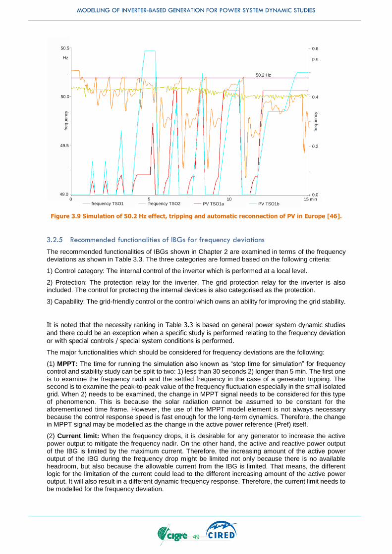
MODELLING OF INVERTER-BASED GENERATION FOR POWER SYSTEM DYNAMIC STUDIES
49
Figure 3.9 Simulation of 50.2 Hz effect, tripping and automatic reconnection of PV in Europe [46].
3.2.5 Recommended functionalities of IBGs for frequency deviations
The recommended functionalities of IBGs shown in Chapter 2 are examined in terms of the frequency deviations as shown in Table 3.3. The three categories are formed based on the following criteria:
1) Control category: The internal control of the inverter which is performed at a local level.
2) Protection: The protection relay for the inverter. The grid protection relay for the inverter is also included. The control for protecting the internal devices is also categorised as the protection.
3) Capability: The grid-friendly control or the control which owns an ability for improving the grid stability.
It is noted that the necessity ranking in Table 3.3 is based on general power system dynamic studies
and there could be an exception when a specific study is performed relating to the frequency deviation or with special controls / special system conditions is performed.
The major functionalities which should be considered for frequency deviations are the following:
(1) MPPT: The time for running the simulation also known as “stop time for simulation” for frequency control and stability study can be split to two: 1) less than 30 seconds 2) longer than 5 min. The first one is to examine the frequency nadir and the settled frequency in the case of a generator tripping. The second is to examine the peak-to-peak value of the frequency fluctuation especially in the small isolated grid. When 2) needs to be examined, the change in MPPT signal needs to be considered for this type of phenomenon. This is because the solar radiation cannot be assumed to be constant for the aforementioned time frame. However, the use of the MPPT model element is not always necessary because the control response speed is fast enough for the long-term dynamics. Therefore, the change in MPPT signal may be modelled as the change in the active power reference (Pref) itself.
(2) Current limit: When the frequency drops, it is desirable for any generator to increase the active power output to mitigate the frequency nadir. On the other hand, the active and reactive power output of the IBG is limited by the maximum current. Therefore, the increasing amount of the active power output of the IBG during the frequency drop might be limited not only because there is no available headroom, but also because the allowable current from the IBG is limited. That means, the different logic for the limitation of the current could lead to the different increasing amount of the active power output. It will also result in a different dynamic frequency response. Therefore, the current limit needs to be modelled for the frequency deviation.
50.5
50.0
49.5
49.0
Hz
0 5 10 15 minfrequency TSO1 frequency TSO2 PV TSO1a PV TSO1b
50.2 Hz
fre
que
ncy
freq
ue
ncy
0.2
0.0
0.4
0.6
p.u.
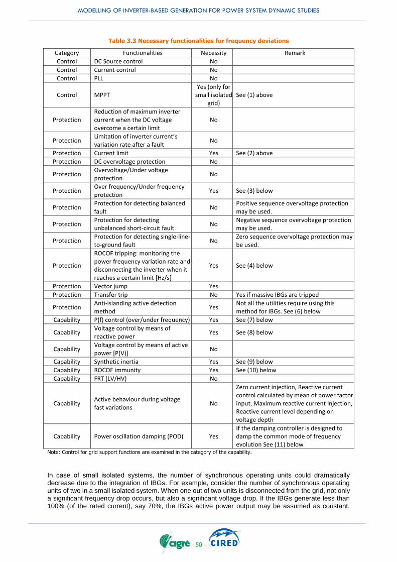
MODELLING OF INVERTER-BASED GENERATION FOR POWER SYSTEM DYNAMIC STUDIES
50
Table 3.3 Necessary functionalities for frequency deviations
Category Functionalities Necessity Remark
Control DC Source control No
Control Current control No
Control PLL No
Control MPPT Yes (only for
small isolated grid)
See (1) above
Protection Reduction of maximum inverter current when the DC voltage overcome a certain limit
No
Protection Limitation of inverter current’s variation rate after a fault
No
Protection Current limit Yes See (2) above
Protection DC overvoltage protection No
Protection Overvoltage/Under voltage protection
No
Protection Over frequency/Under frequency protection
Yes See (3) below
Protection Protection for detecting balanced fault
No Positive sequence overvoltage protection may be used.
Protection Protection for detecting unbalanced short-circuit fault
No Negative sequence overvoltage protection may be used.
Protection Protection for detecting single-line-to-ground fault
No Zero sequence overvoltage protection may be used.
Protection
ROCOF tripping: monitoring the power frequency variation rate and disconnecting the inverter when it reaches a certain limit [Hz/s]
Yes See (4) below
Protection Vector jump Yes
Protection Transfer trip No Yes if massive IBGs are tripped
Protection Anti-islanding active detection method
Yes Not all the utilities require using this method for IBGs. See (6) below
Capability P(f) control (over/under frequency) Yes See (7) below
Capability Voltage control by means of reactive power
Yes See (8) below
Capability Voltage control by means of active power [P(V)]
No
Capability Synthetic inertia Yes See (9) below
Capability ROCOF immunity Yes See (10) below
Capability FRT (LV/HV) No
Capability Active behaviour during voltage fast variations
No
Zero current injection, Reactive current control calculated by mean of power factor input, Maximum reactive current injection, Reactive current level depending on voltage depth
Capability Power oscillation damping (POD) Yes If the damping controller is designed to damp the common mode of frequency evolution See (11) below
Note: Control for grid support functions are examined in the category of the capability.
In case of small isolated systems, the number of synchronous operating units could dramatically decrease due to the integration of IBGs. For example, consider the number of synchronous operating units of two in a small isolated system. When one out of two units is disconnected from the grid, not only a significant frequency drop occurs, but also a significant voltage drop. If the IBGs generate less than 100% (of the rated current), say 70%, the IBGs active power output may be assumed as constant.
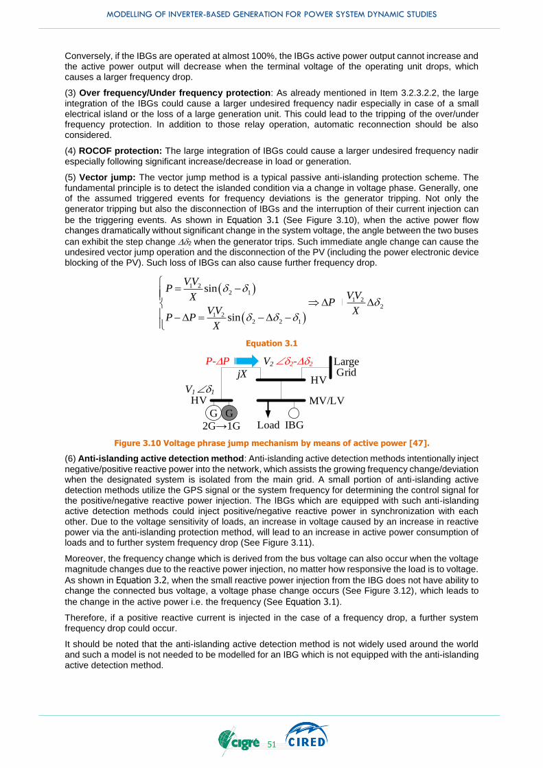
MODELLING OF INVERTER-BASED GENERATION FOR POWER SYSTEM DYNAMIC STUDIES
51
Conversely, if the IBGs are operated at almost 100%, the IBGs active power output cannot increase and the active power output will decrease when the terminal voltage of the operating unit drops, which causes a larger frequency drop.
(3) Over frequency/Under frequency protection: As already mentioned in Item 3.2.3.2.2, the large integration of the IBGs could cause a larger undesired frequency nadir especially in case of a small electrical island or the loss of a large generation unit. This could lead to the tripping of the over/under frequency protection. In addition to those relay operation, automatic reconnection should be also considered.
(4) ROCOF protection: The large integration of IBGs could cause a larger undesired frequency nadir especially following significant increase/decrease in load or generation.
(5) Vector jump: The vector jump method is a typical passive anti-islanding protection scheme. The fundamental principle is to detect the islanded condition via a change in voltage phase. Generally, one of the assumed triggered events for frequency deviations is the generator tripping. Not only the generator tripping but also the disconnection of IBGs and the interruption of their current injection can
be the triggering events. As shown in Equation 3.1 (See Figure 3.10), when the active power flow changes dramatically without significant change in the system voltage, the angle between the two buses
can exhibit the step change D2 when the generator trips. Such immediate angle change can cause the undesired vector jump operation and the disconnection of the PV (including the power electronic device blocking of the PV). Such loss of IBGs can also cause further frequency drop.
1 22 1
1 22
1 22 2 1
sin
sin
VVP
VVXP
VV XP P
X
-
D D - D - D -
Equation 3.1
V1
V2
jX
P-DP
1
2-D2
IBG
MV/LV
HV
LargeGrid
LoadG G
2G 1G
HV
Figure 3.10 Voltage phrase jump mechanism by means of active power [47].
(6) Anti-islanding active detection method: Anti-islanding active detection methods intentionally inject negative/positive reactive power into the network, which assists the growing frequency change/deviation when the designated system is isolated from the main grid. A small portion of anti-islanding active detection methods utilize the GPS signal or the system frequency for determining the control signal for the positive/negative reactive power injection. The IBGs which are equipped with such anti-islanding active detection methods could inject positive/negative reactive power in synchronization with each other. Due to the voltage sensitivity of loads, an increase in voltage caused by an increase in reactive power via the anti-islanding protection method, will lead to an increase in active power consumption of loads and to further system frequency drop (See Figure 3.11).
Moreover, the frequency change which is derived from the bus voltage can also occur when the voltage magnitude changes due to the reactive power injection, no matter how responsive the load is to voltage.
As shown in Equation 3.2, when the small reactive power injection from the IBG does not have ability to change the connected bus voltage, a voltage phase change occurs (See Figure 3.12), which leads to
the change in the active power i.e. the frequency (See Equation 3.1).
Therefore, if a positive reactive current is injected in the case of a frequency drop, a further system frequency drop could occur.
It should be noted that the anti-islanding active detection method is not widely used around the world and such a model is not needed to be modelled for an IBG which is not equipped with the anti-islanding active detection method.

MODELLING OF INVERTER-BASED GENERATION FOR POWER SYSTEM DYNAMIC STUDIES
52
PV Inverter
PV Array
Controller
Active Power
Variation
Frequency
Variation
Load Voltage
Characteristics
PV Capacity
Electric Distance
Inertia
Protection
0.0kW
Voltage
Variation
Reactive Power
VariationActive
Anti-islanding
Control Signal
Figure 3.11 One example mechanism how frequency is forced to be oscillated via Q variation type active anti-islanding control signal.
2
1 2 22 1
1 22 1 22
1 2 22 2 1
cos
cos
VV VQ
VVX XQ
XVV VQ Q
X X
- -
D - D - D + D - -
Equation 3.2
Figure 3.12 Voltage phase jump mechanism by means of reactive power [47].
(7) P(f) control [35]: The increased utilization of tie-lines is encouraged in terms of increased integration of RES. The increased tie-line power flow could lead to more significant frequency increases/decreases after a power system is split into two sub-systems due to tie-line tripping. A frequency rise in the system could lead to a disconnection of a large amounts IBGs due to the over frequency protection. On the other hand, the tripping of this large amount of generation can lead to a frequency drop and therefore a disconnection of load due to the under frequency load shedding scheme. To overcome this problem, IBGs can control frequency by means of active power, i.e., reduce their active power feed-in during over frequency, or increase their active power feed-in during under frequency. Hence, this function can play an important role when the power system experiences a significant frequency change. In this context, the following topics are addressed:
Modelling the primary power source control (if existing) including maximum range and gradients
(for frequency rise/drop)
Modelling the optional storage devices including charging management controls (for frequency
rise/drop)
Modelling the power reserve in the case, where the IBG is operated at a point below the maximum
power point in order to allow primary frequency control (for frequency drop only).
(8) Voltage control by means of reactive power: Although the dynamic behaviour is not directly related to this capability, the pre-fault active and reactive power feed-in of the IBG can affect the fault-on and post-fault dynamic behaviour of the IBG output. This could indirectly change the dynamic frequency response of the system.
(9) Synthetic Inertia: The displacement of synchronous generators by IBGs could cause a reduction of the system inertia. According to the power swing equation, the lower inertia will increase the change in
MODELLING OF INVERTER-BASED GENERATION FOR POWER SYSTEM DYNAMIC STUDIES
53
rotor angle speed (df/dt) for the same mismatch between the mechanical power and the electrical power. The increase in the ROCOF could endanger frequency stability.
IBGs will not exhibit an inertia-like behaviour per se. While some of the prime movers could deliver the inertia, it is not certain that the IBG is able to provide it, because it requires a modification of the control (See Sub-Chapter 2.1 (1)). However, assuming an appropriate control scheme of the inverter and a (limited) energy storage capability, a “synthetic inertia” can be provided to the grid.
Potential solutions that can be used are
Installation of energy storage devices, e.g., large flywheel generators or flywheel coupled synchronous compensators.
Adopt alternative approaches to detect electrical islands and ensure that the main equipment is robust against ROCOF.
Operate PV systems below the maximum power point.
Modify control of IBGs to provide synthetic inertia21, which can be done by a change of active power output during frequency deviations. This is the approach which has been followed by Hydro Quebec [48], [49]. It is noted that this technology is recognized as the fast frequency response (FFR) and the closed-loop inertia-based FFR has been commercially available for many years. However, the practical use of FFR has still being discussed and needs to be carefully examined and implemented.
(10) ROCOF immunity: ROCOF immunity is equivalent to frequency ride-through, i.e., low and high frequency ride-through. If the ROCOF setting for the ROCOF immunity is the same as the relay setting for the ROCOF protection, the ROCOF immunity model is not necessary. On the other hand, it is more likely that the relay setting of ROCOF protections could change depending on the location. In such a case, the ROCOF immunity needs to be modelled independently.
(11) POD: If the loss of generation causes poorly damped power swing oscillations, POD plays an important role to ensure transient stability. Therefore, in the aforementioned case and if the POD is assumed to be implemented into IBGs, IBGs with POD should be modelled, otherwise, there is no need to model POD.
3.3 BEHAVIOUR IN RESPONSE TO LARGE VOLTAGE DEVIATIONS
A brief introduction of stability studies, with the key responses relevant to system faults are examined in this sub-chapter. The real-life examples with and without the IBGs are illustrated. In addition, the important functionalities of IBGs for their behaviour in response to large voltage deviations are discussed.
3.3.1 Description of phenomena
Large voltage deviations may be triggered by system faults such as three-phase faults, single-line to ground faults and short-circuit faults. Unless a great fraction of generation or loads compared to total rated power output change, frequency stability can be omitted. Severe system faults could cause the out-of-step phenomenon and possibly lead to large-scale blackouts. This issue has generated great interest in knowing the system response behaviour to large voltage deviation for the power system planners and operators.
Several phenomena can be linked to the system faults, such as:
Out-of-step phenomenon: This phenomenon refers to losing synchronism of a synchronous generator connected to the system following large voltage deviations. When a synchronous generator falls into the Out-Of-Step (OOS) condition, at least one voltage angle difference between two buses including the machine internal (fictional) bus behind its transient reactance becomes equal to 180 degrees. When the angle difference is 180 degrees, there is a point where voltage is zero between the two generators showing this difference. The point is known as the “electrical centre (See point Ec in Figure 3.13)”. The impact of the OOS condition at the electrical centre is the same as a short-circuit at this point. However, the difference between a short-circuit and the OOS phenomenon at the electrical centre is the duration and the repetition of the zero voltage, as shown in Table 3.4. In practice, OOS is generally caused by more than two synchronous generators and it seems that OOS is more important when the network size is larger and the voltage level is higher.
21 The model of the wind turbine aerodynamics is also needed when simulating the synthetic inertia.
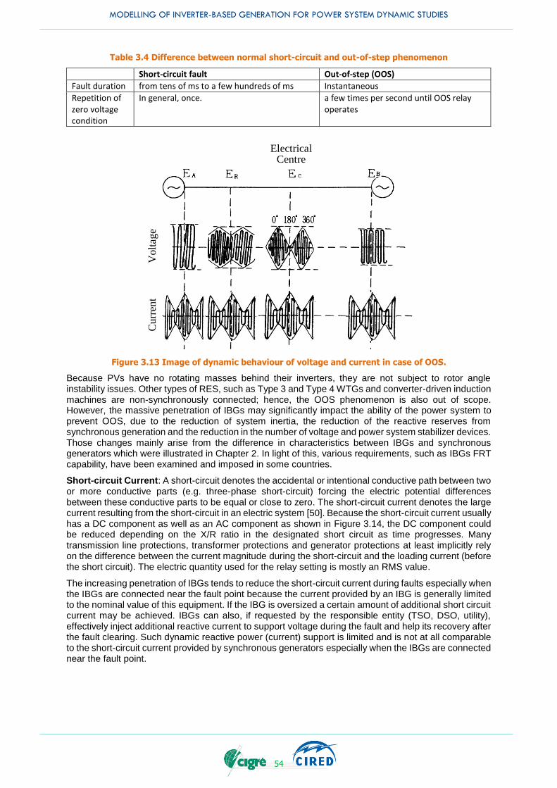
MODELLING OF INVERTER-BASED GENERATION FOR POWER SYSTEM DYNAMIC STUDIES
54
Table 3.4 Difference between normal short-circuit and out-of-step phenomenon
Short-circuit fault Out-of-step (OOS)
Fault duration from tens of ms to a few hundreds of ms Instantaneous
Repetition of zero voltage condition
In general, once. a few times per second until OOS relay operates
Volt
age
Curr
ent
Electrical Centre
Figure 3.13 Image of dynamic behaviour of voltage and current in case of OOS.
Because PVs have no rotating masses behind their inverters, they are not subject to rotor angle instability issues. Other types of RES, such as Type 3 and Type 4 WTGs and converter-driven induction machines are non-synchronously connected; hence, the OOS phenomenon is also out of scope. However, the massive penetration of IBGs may significantly impact the ability of the power system to prevent OOS, due to the reduction of system inertia, the reduction of the reactive reserves from synchronous generation and the reduction in the number of voltage and power system stabilizer devices. Those changes mainly arise from the difference in characteristics between IBGs and synchronous generators which were illustrated in Chapter 2. In light of this, various requirements, such as IBGs FRT capability, have been examined and imposed in some countries.
Short-circuit Current: A short-circuit denotes the accidental or intentional conductive path between two or more conductive parts (e.g. three-phase short-circuit) forcing the electric potential differences between these conductive parts to be equal or close to zero. The short-circuit current denotes the large current resulting from the short-circuit in an electric system [50]. Because the short-circuit current usually has a DC component as well as an AC component as shown in Figure 3.14, the DC component could be reduced depending on the X/R ratio in the designated short circuit as time progresses. Many transmission line protections, transformer protections and generator protections at least implicitly rely on the difference between the current magnitude during the short-circuit and the loading current (before the short circuit). The electric quantity used for the relay setting is mostly an RMS value.
The increasing penetration of IBGs tends to reduce the short-circuit current during faults especially when the IBGs are connected near the fault point because the current provided by an IBG is generally limited to the nominal value of this equipment. If the IBG is oversized a certain amount of additional short circuit current may be achieved. IBGs can also, if requested by the responsible entity (TSO, DSO, utility), effectively inject additional reactive current to support voltage during the fault and help its recovery after the fault clearing. Such dynamic reactive power (current) support is limited and is not at all comparable to the short-circuit current provided by synchronous generators especially when the IBGs are connected near the fault point.

MODELLING OF INVERTER-BASED GENERATION FOR POWER SYSTEM DYNAMIC STUDIES
55
Ik”: initial symmetrical short-circuit current Ip: peak short-circuit current Ik: steady-state short-circuit current iDC: DC component of short-circuit current A: initial value of DC component, iDC
Figure 3.14 Example short-circuit current (schematic diagram) [50].
A unique property of IBGs is the power electronics interface and the ability of the electronics to control fault current contributions. This adjustability can thereby optimise the system protection coordination issues by controlling fault current levels. Typically, IBGs are designed to act as ideal current sources. They provide minimal fault current contributions and have little effect on overcurrent protection and coordination strategies for fuse and circuit breakers. Even though the fault contribution from a single, small IBG unit is not significant, the total contribution of many small units may alter the fault current level enough to cause lack of coordination for overcurrent protection and wrong fuse operation or hamper fault detection [51]. For instance, in case of islanding situations for small IBGs, the fault current contribution can be relevant from the protection coordination point of view in low voltage and/or medium voltage network although such contribution depends on the system size of the isolated grid.
Short-term dynamic voltage response: This term generally refers to the voltage recovery after a fault is cleared. The time frame is at most a few seconds after fault is cleared 22. If a large number of conventional (i.e. not interfaced to the grid through power electronics) induction motor (IM) loads are connected to the power system, the voltage recovery may be delayed by the IMs taking time to re-accelerate, which requires a large amount of reactive power. If the situation becomes severe, the IMs cannot re-accelerate and stall; then, if the IMs are not disconnected by the under-voltage protection, the load bus voltage is locked at a very low value before slower (thermal) protections disconnect the motors. This situation may occur due to the presence of massive IM-based air conditioning load in summer peak load conditions; those IMs usually have low inertia. Conversely, the motors controlled by drives or inverter-interfaced IMs, widely used around the world mainly in domestic appliances, such as in air conditioners and in refrigerators, seem to be less prone to depressing the voltages.
The inverters react in the same time frame and hence it is relevant to consider their impact on short-term voltage stability/recovery. The reduction of active power output of IBGs can cause an increase in the net load which is derived from “pure loads minus IBG active power output”. The increase in the net load can cause a lowering of the voltage level at the load bus. Therefore, IBGs without the dynamic reactive power support will worsen the voltage recovery, and can eventually deteriorate short-term voltage stability. It is noted that such dynamic reactive power support provided by IBGs can lead to excessive voltage recovery (The real event revealed that IBGs were tripped due to the overvoltage), which is very much likely to require HVRT (See also Figure 5.6 in Chapter 5).
Although both short-term voltage instability and rotor angle instability result in low voltage at certain buses in the grid, it is appropriate to differentiate those instabilities based on the final behaviour of the grid such as OOS or voltage collapse as well as the effective remedial actions such as generator tripping or load shedding. In light of this, various requirements, such as dynamic reactive current (power) support, have been examined and imposed by grid codes in some countries. It should be noted that different
22 Very similar time frame for transient stability
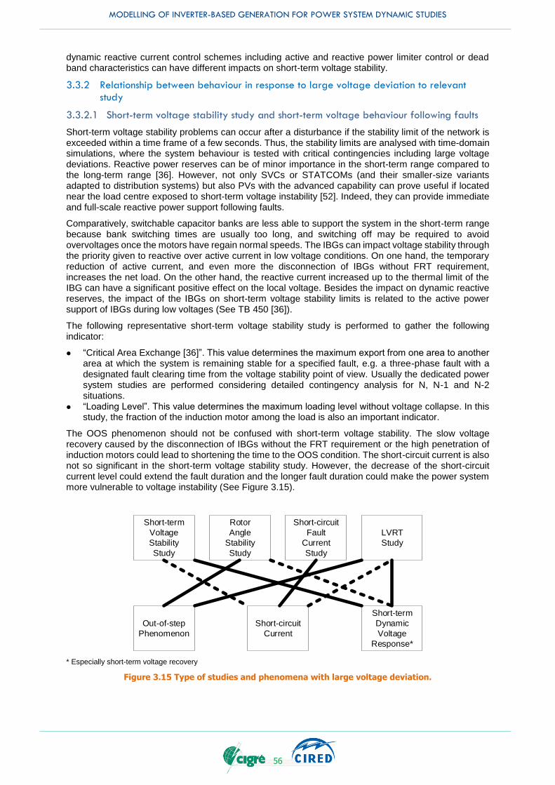
MODELLING OF INVERTER-BASED GENERATION FOR POWER SYSTEM DYNAMIC STUDIES
56
dynamic reactive current control schemes including active and reactive power limiter control or dead band characteristics can have different impacts on short-term voltage stability.
3.3.2 Relationship between behaviour in response to large voltage deviation to relevant study
3.3.2.1 Short-term voltage stability study and short-term voltage behaviour following faults
Short-term voltage stability problems can occur after a disturbance if the stability limit of the network is exceeded within a time frame of a few seconds. Thus, the stability limits are analysed with time-domain simulations, where the system behaviour is tested with critical contingencies including large voltage deviations. Reactive power reserves can be of minor importance in the short-term range compared to the long-term range [36]. However, not only SVCs or STATCOMs (and their smaller-size variants adapted to distribution systems) but also PVs with the advanced capability can prove useful if located near the load centre exposed to short-term voltage instability [52]. Indeed, they can provide immediate and full-scale reactive power support following faults.
Comparatively, switchable capacitor banks are less able to support the system in the short-term range because bank switching times are usually too long, and switching off may be required to avoid overvoltages once the motors have regain normal speeds. The IBGs can impact voltage stability through the priority given to reactive over active current in low voltage conditions. On one hand, the temporary reduction of active current, and even more the disconnection of IBGs without FRT requirement, increases the net load. On the other hand, the reactive current increased up to the thermal limit of the IBG can have a significant positive effect on the local voltage. Besides the impact on dynamic reactive reserves, the impact of the IBGs on short-term voltage stability limits is related to the active power support of IBGs during low voltages (See TB 450 [36]).
The following representative short-term voltage stability study is performed to gather the following indicator:
“Critical Area Exchange [36]”. This value determines the maximum export from one area to another area at which the system is remaining stable for a specified fault, e.g. a three-phase fault with a designated fault clearing time from the voltage stability point of view. Usually the dedicated power system studies are performed considering detailed contingency analysis for N, N-1 and N-2 situations.
“Loading Level”. This value determines the maximum loading level without voltage collapse. In this study, the fraction of the induction motor among the load is also an important indicator.
The OOS phenomenon should not be confused with short-term voltage stability. The slow voltage recovery caused by the disconnection of IBGs without the FRT requirement or the high penetration of induction motors could lead to shortening the time to the OOS condition. The short-circuit current is also not so significant in the short-term voltage stability study. However, the decrease of the short-circuit current level could extend the fault duration and the longer fault duration could make the power system more vulnerable to voltage instability (See Figure 3.15).
Short-term
Voltage
Stability
Study
Rotor
Angle
Stability
Study
Short-circuit
Fault
Current
Study
LVRT
Study
Out-of-step
Phenomenon
Short-circuit
Current
Short-term
Dynamic
Voltage
Response*
* Especially short-term voltage recovery
Figure 3.15 Type of studies and phenomena with large voltage deviation.

MODELLING OF INVERTER-BASED GENERATION FOR POWER SYSTEM DYNAMIC STUDIES
57
3.3.2.2 Rotor angle stability in case of large disturbances (transient stability)
Transient stability is defined as the ability of the power system to maintain synchronism after severe disturbances such as short-circuits cleared by lines opening or generator trips [30]. It is also referred to by the term large-disturbance rotor angle stability. Hence this aspect of power system stability is related to the behaviour of the synchronous generators located near the fault trying to maintain synchronism with other synchronous generators during and after the disturbance. The system behaviour is highly dependent on the type and duration of the disturbance. Hence, to ensure rotor angle stability, a number of critical contingencies have to be simulated at different locations. For evaluating rotor angle stability, the following three indices are used [36], [40] alone or combined:
CCT: The fault Critical Clearing Time (CCT) is calculated for various critical contingencies, i.e.
different fault conditions. The CCT represents a useful measure for characterizing the security
margin with respect to rotor angle instability in a given dispatch scenario.
Critical area exchange: determines the maximum export from one area to another at which the
system still remains stable after a specified fault with a designated fault clearing sequence.
Maximum power transfer: This value determines the maximum export from one power station to
another area without loads at which the system is remaining stable for a specified fault, e.g. a three-
phase fault with a designated fault clearing time from the rotor angle stability point of view.
Although the CCT is a very common indicator for showing the degree of rotor angle stability, it is not frequently used in large system rotor angle stability studies performed by the system operators in many countries. The major reason is that the primary and back-up relay operation times are always fixed / constant for the designated fault points (usually these times are derived from previous CCT studies). It is likely that in the EHV and HV networks the shortest fault clearing time is around 3 cycles and the longest in MV network is in the range of a few cycles and less than several hundreds of milliseconds. Therefore, the derivation of the critical area exchange or the maximum power transfer are usually the studies preferred by system operators as regards rotor angle stability point of view.
If the power system cannot maintain synchronism, OOS occurs, which could trigger a cascaded failure and a large blackout. If a first-swing OOS occurs, a resulting short-term swing of voltage magnitude can be observed near the electrical centre of the system. On the other hand, if a multi-swing OOS occurs, such a short-term voltage response is not likely to be observed since its short-circuit current is not directly linked to rotor angle stability. However, if the protection cannot detect the fault properly due to insufficient short-circuit current from the grid, the longer fault clearing time could endanger rotor angle stability. In this respect, the decrease in short-circuit current level caused by the replacement of synchronous generators by IBGs can be of interest in a rotor angle stability study.
3.3.2.3 Provision of short-circuit fault current (short-circuit fault current)
Provision of fault current by IBGs is often examined in the case of the grid interconnection study. In some countries, the fault current level is assumed to be 150%of the rated current of the inverter23. Then, the short-circuit current which flows through the circuit breaker (CB) is calculated based on a simple electric circuit calculation and is checked to see if it is less than the maximum current for which the CB can properly operate to clear the fault. However, due to the dynamic behaviour of the inverter, the short-circuit current could vary depending on controller action such as dynamic reactive power support. In addition, the current that is to be examined is not only the peak fault current [50] but also the breaking current [50] which is interrupted when the CB operates. This means that the fault current 70 - 100 milliseconds after the fault occurrence is determined and examined. It is noted that [50] provides the way how to calculate the fault current provided by IBGs focusing on DFIGs. On the other hand, the infeed of the fault current very much changes on the design of the inverter control including the FRT function. Therefore, the importance of the simulation-based approach would be getting higher and higher as the penetration rate of IBGs increases.
Another typical study related to the provision of short-circuit current is aimed at confirming the proper operation of protection systems such as the line protection. The additional current could cause an error in some line protection schemes, which could result in an unwanted operation or a failure to operate. Usually under this scenario study detailed short-circuit computations are performed both for peak short-circuit conditions (i.e. the power system operating condition which gives the largest transient short-circuit
23 For example, the fault current provision of IBGs is assumed to be in the range of 1.1 to 1.5 times of the rated current of
IBGs according to the results of the laboratory test using the actual IBGs in Japan. Those quantities have been used for countermeasure of electric facilities (e.g. examination of thermal limits) and for the analysis of the relay operation.
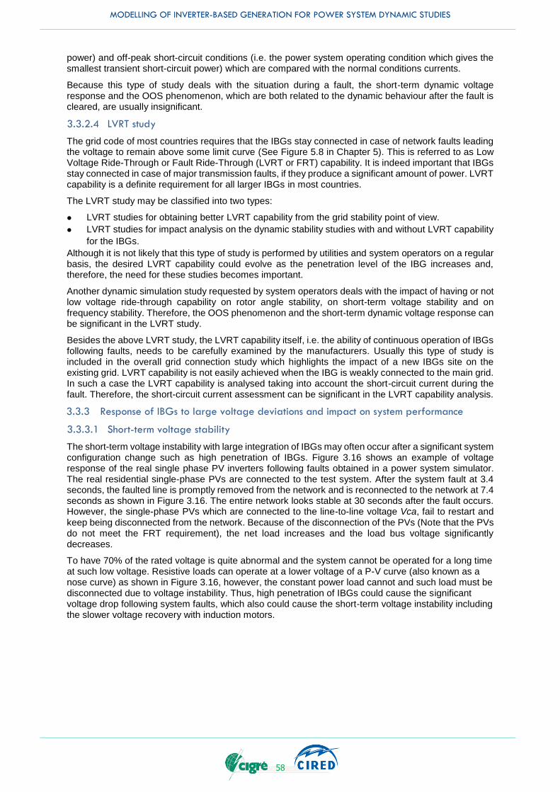
MODELLING OF INVERTER-BASED GENERATION FOR POWER SYSTEM DYNAMIC STUDIES
58
power) and off-peak short-circuit conditions (i.e. the power system operating condition which gives the smallest transient short-circuit power) which are compared with the normal conditions currents.
Because this type of study deals with the situation during a fault, the short-term dynamic voltage response and the OOS phenomenon, which are both related to the dynamic behaviour after the fault is cleared, are usually insignificant.
3.3.2.4 LVRT study
The grid code of most countries requires that the IBGs stay connected in case of network faults leading the voltage to remain above some limit curve (See Figure 5.8 in Chapter 5). This is referred to as Low Voltage Ride-Through or Fault Ride-Through (LVRT or FRT) capability. It is indeed important that IBGs stay connected in case of major transmission faults, if they produce a significant amount of power. LVRT capability is a definite requirement for all larger IBGs in most countries.
The LVRT study may be classified into two types:
LVRT studies for obtaining better LVRT capability from the grid stability point of view.
LVRT studies for impact analysis on the dynamic stability studies with and without LVRT capability
for the IBGs.
Although it is not likely that this type of study is performed by utilities and system operators on a regular basis, the desired LVRT capability could evolve as the penetration level of the IBG increases and, therefore, the need for these studies becomes important.
Another dynamic simulation study requested by system operators deals with the impact of having or not low voltage ride-through capability on rotor angle stability, on short-term voltage stability and on frequency stability. Therefore, the OOS phenomenon and the short-term dynamic voltage response can be significant in the LVRT study.
Besides the above LVRT study, the LVRT capability itself, i.e. the ability of continuous operation of IBGs following faults, needs to be carefully examined by the manufacturers. Usually this type of study is included in the overall grid connection study which highlights the impact of a new IBGs site on the existing grid. LVRT capability is not easily achieved when the IBG is weakly connected to the main grid. In such a case the LVRT capability is analysed taking into account the short-circuit current during the fault. Therefore, the short-circuit current assessment can be significant in the LVRT capability analysis.
3.3.3 Response of IBGs to large voltage deviations and impact on system performance
3.3.3.1 Short-term voltage stability
The short-term voltage instability with large integration of IBGs may often occur after a significant system configuration change such as high penetration of IBGs. Figure 3.16 shows an example of voltage response of the real single phase PV inverters following faults obtained in a power system simulator. The real residential single-phase PVs are connected to the test system. After the system fault at 3.4 seconds, the faulted line is promptly removed from the network and is reconnected to the network at 7.4 seconds as shown in Figure 3.16. The entire network looks stable at 30 seconds after the fault occurs. However, the single-phase PVs which are connected to the line-to-line voltage Vca, fail to restart and keep being disconnected from the network. Because of the disconnection of the PVs (Note that the PVs do not meet the FRT requirement), the net load increases and the load bus voltage significantly decreases.
To have 70% of the rated voltage is quite abnormal and the system cannot be operated for a long time at such low voltage. Resistive loads can operate at a lower voltage of a P-V curve (also known as a nose curve) as shown in Figure 3.16, however, the constant power load cannot and such load must be disconnected due to voltage instability. Thus, high penetration of IBGs could cause the significant voltage drop following system faults, which also could cause the short-term voltage instability including the slower voltage recovery with induction motors.

MODELLING OF INVERTER-BASED GENERATION FOR POWER SYSTEM DYNAMIC STUDIES
59
(a) Measured response of synchronous generator (Rated Voltage of PV is 200 V)
(b) Measured response of PVs (Rated Voltage of PV is 200 V) Figure 3.16 Measured response obtained in power system simulator [53].

MODELLING OF INVERTER-BASED GENERATION FOR POWER SYSTEM DYNAMIC STUDIES
60
3.3.3.2 Short-term dynamic voltage response [54]
The short-term voltage instability is indirectly linked to the slow voltage recovery after the system fault is cleared. Therefore, the study of the dynamic voltage response following faults is important in terms of the short-term voltage stability. WECC performed a study to investigate the need of the reactive power control function in IBGs. The example test system included 800 MW PV plants and a three-phase fault was applied to the Point Of Interconnection (POI) at the 230 kV Switching Station as shown in Figure 3.17. The conditions for the study, are listed in Table 3.5.
The example of the simulation results are summarised as Table 3.6 and Figures 3.18 and 3.19. The detailed simulation results including the provided models are described in Appendix 3-E. The major findings are the following:
Slightly lower voltage without voltage control from the solar PV plant (at 230kV)
Better damping and faster voltage recovery with the solar PV plant (at 230 kV)
Overshoot in voltage control scenario (at 230 kV)
No impact from motor load stalling (at 230 kV)
Delayed voltage recovery with stalling of single-phase induction motor loads (at the load bus)
Voltage control of the solar PV plant has no impact (at the load bus)
Other than those above findings, the following bullet points also need to be considered for the study that includes short-term dynamic response. It is noted that
Positive impact on transient voltage performance from IBGs – better damping and faster voltage
recovery due to low inertia and faster controls (if a PV plant regulates voltage).
For large system studies, very detailed models of the generators are not necessary.
Without LVRT Capability (for example, with large amount of distributed solar PV), loss of large
amount of generation with a fault may be a concern
High voltages under normal system conditions may be a concern with large penetration of
distributed solar PV generation
Figure 3.17 WECC test system with large-scale PV plants [54].
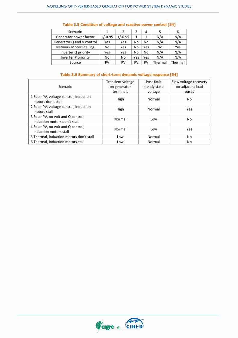
MODELLING OF INVERTER-BASED GENERATION FOR POWER SYSTEM DYNAMIC STUDIES
61
Table 3.5 Condition of voltage and reactive power control [54]
Scenario 1 2 3 4 5 6
Generator power factor +/-0.95 +/-0.95 1 1 N/A N/A
Generator Q and V control Yes Yes No No N/A N/A
Network Motor Stalling No Yes No Yes No Yes
Inverter Q priority Yes Yes No No N/A N/A
Inverter P priority No No Yes Yes N/A N/A
Source PV PV PV PV Thermal Thermal
Table 3.6 Summary of short-term dynamic voltage response [54]
Scenario Transient voltage
on generator terminals
Post-fault steady state
voltage
Slow voltage recovery on adjacent load
buses
1 Solar PV, voltage control, induction motors don’t stall
High Normal No
2 Solar PV, voltage control, induction motors stall
High Normal Yes
3 Solar PV, no volt and Q control, induction motors don’t stall
Normal Low No
4 Solar PV, no volt and Q control, induction motors stall
Normal Low Yes
5 Thermal, induction motors don’t stall Low Normal No
6 Thermal, induction motors stall Low Normal No
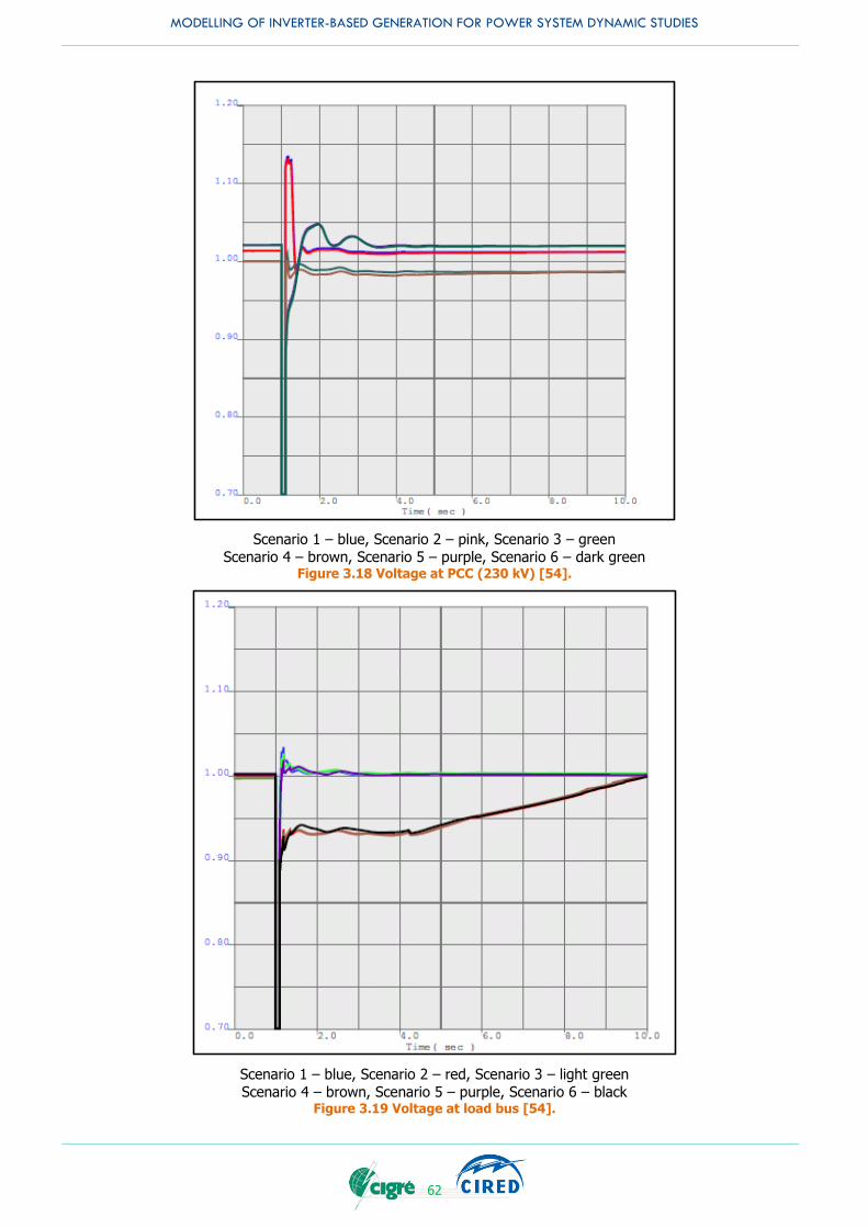
MODELLING OF INVERTER-BASED GENERATION FOR POWER SYSTEM DYNAMIC STUDIES
62
Scenario 1 – blue, Scenario 2 – pink, Scenario 3 – green
Scenario 4 – brown, Scenario 5 – purple, Scenario 6 – dark green Figure 3.18 Voltage at PCC (230 kV) [54].
Scenario 1 – blue, Scenario 2 – red, Scenario 3 – light green
Scenario 4 – brown, Scenario 5 – purple, Scenario 6 – black Figure 3.19 Voltage at load bus [54].
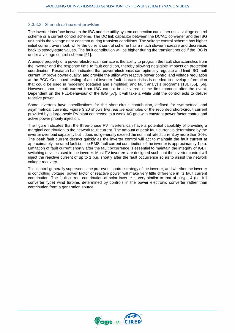
MODELLING OF INVERTER-BASED GENERATION FOR POWER SYSTEM DYNAMIC STUDIES
63
3.3.3.3 Short-circuit current provision
The inverter interface between the IBG and the utility system connection can either use a voltage control scheme or a current control scheme. The DC link capacitor between the DC/AC converter and the IBG unit holds the voltage near constant during transient conditions. The voltage control scheme has higher initial current overshoot, while the current control scheme has a much slower increase and decreases back to steady-state values. The fault contribution will be higher during the transient period if the IBG is under a voltage control scheme [51].
A unique property of a power electronics interface is the ability to program the fault characteristics from the inverter and the response time to fault condition, thereby allowing negligible impacts on protection coordination. Research has indicated that power electronics can optimally regulate and limit IBG fault current, improve power quality, and provide the utility with reactive power control and voltage regulation at the PCC. Continued testing of actual inverter fault characteristics is needed to develop information that could be used in modelling (detailed and simplified) and fault analysis programs [18], [55], [56]. However, short circuit current from IBG cannot be delivered in the first moment after the event. Dependent on the PLL-behaviour of the IBG [57], it will take a while until the control acts to deliver reactive power.
Some inverters have specifications for the short-circuit contribution, defined for symmetrical and asymmetrical currents. Figure 3.20 shows two real life examples of the recorded short-circuit current provided by a large-scale PV plant connected to a weak AC grid with constant power factor control and active power priority injection.
The figure indicates that the three-phase PV inverters can have a potential capability of providing a marginal contribution to the network fault current. The amount of peak fault current is determined by the inverter overload capability but it does not generally exceed the nominal rated current by more than 30%. The peak fault current decays quickly as the inverter control will act to maintain the fault current at approximately the rated fault i.e. the RMS fault current contribution of the inverter is approximately 1 p.u. Limitation of fault current shortly after the fault occurrence is essential to maintain the integrity of IGBT switching devices used in the inverter. Most PV inverters are designed such that the inverter control will inject the reactive current of up to 1 p.u. shortly after the fault occurrence so as to assist the network voltage recovery.
This control generally supersedes the pre-event control strategy of the inverter, and whether the inverter is controlling voltage, power factor or reactive power will make very little difference in its fault current contribution. The fault current contribution of solar inverter is very similar to that of a type 4 (i.e. full converter type) wind turbine, determined by controls in the power electronic converter rather than contribution from a generation source.

MODELLING OF INVERTER-BASED GENERATION FOR POWER SYSTEM DYNAMIC STUDIES
64
Figure 3.20 Example of short-circuit current provision measured in PV plant.

MODELLING OF INVERTER-BASED GENERATION FOR POWER SYSTEM DYNAMIC STUDIES
65
3.3.3.4 Transient stability with and without LVRT [16]
The angle stability is strongly related to angle difference between two or more synchronous generators (See Figure 3.21). Especially as the synchronizing torque component, which is one of the two important aspects of stability, is directly linked to the angle difference between them. From a qualitative point of view, the effect of increasing or decreasing amplitude of power swing (active power oscillation) following faults can be the cause of angle stability or instability.
G
V1 ∠ V2 ∠ 0
X
P
G
Figure 3.21 Two equivalent machine system and example power swing oscillation.
It is well known that the amplitude of the power swing depends on the dynamic behaviour of loads following faults and their location in the network. For example, if loads are connected near the power station generators which are accelerated following faults, the constant power load gives better damping effect compared to the constant impedance load, because the dynamically larger loads can play a role of a dynamic braking system and because the constant power load, during voltage sag, consumes more active power compared to the constant impedance load case. There also may be IBGs in the vicinity, residential PV in particular. The most critical case is the disconnection of PVs right after the fault occurs. Although LVRT capability has been regulated in many countries, a large number of installed PVs, do not meet LVRT requirement. The disconnection of PVs is equivalent to increase in net loads. The momentary cessation of power output for the duration of the voltage sag also results in increase in the net loads. If PVs are connected near a huge power station, the power transfer over the transmission line from G1 to G2 (See pink arrow and dotted red line in Figure 3.22 (a)) after the disconnection of PVs could decrease because the increased net loads near the power station consume more active power coming from the power station as shown in Figure 3.22 (a). Conversely, if PVs are connected near a load centre, the power transfer over the transmission line from G1 to G2 (See pink arrow and dotted red line in Figure 3.22 (b)) could increase after the disconnection of PVs because the increased net loads near the power station require more active power coming from the power station as shown in Figure 3.22 (b). The increase in power transfer over the transmission line from G1 to G2 could lead to a growing or poorly damped power swing oscillation. Therefore, the dynamic behaviour of active power output of IBGs is a key factor in the case of transient stability studies and their network location is another key factor in these studies.
G1
Load
PL[MW]
PG[MW] PG-PL[MW]
G1
PG[MW] PG-0.5PL
After stoppage
of PV
Before
stoppage of PV
Load
0.5PL
G2
G2 G
Load
PL[MW]
PG[MW] PT[MW]
G
Load
0.5PL
PG-0.5PL PT
After stoppage
of PV
Before
stoppage of PV
PL=PG+PT
G
G
(a) PV is located near power source (b) PV is located near power sink
Figure 3.22 Change in power flow over transmission lines before and after disconnection of PVs at different locations [16].
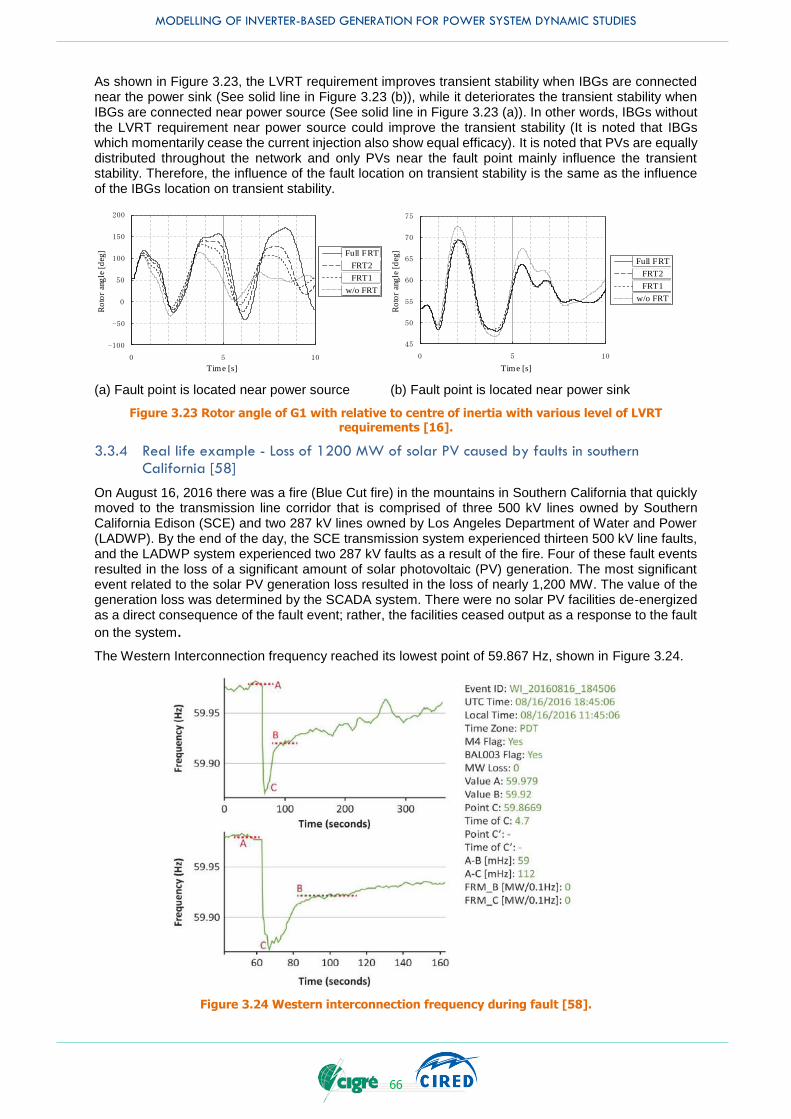
MODELLING OF INVERTER-BASED GENERATION FOR POWER SYSTEM DYNAMIC STUDIES
66
As shown in Figure 3.23, the LVRT requirement improves transient stability when IBGs are connected near the power sink (See solid line in Figure 3.23 (b)), while it deteriorates the transient stability when IBGs are connected near power source (See solid line in Figure 3.23 (a)). In other words, IBGs without the LVRT requirement near power source could improve the transient stability (It is noted that IBGs which momentarily cease the current injection also show equal efficacy). It is noted that PVs are equally distributed throughout the network and only PVs near the fault point mainly influence the transient stability. Therefore, the influence of the fault location on transient stability is the same as the influence of the IBGs location on transient stability.
-100
-50
0
50
100
150
200
0 5 10
内部相差
角(deg)
時間(秒)
脱落なし
2016年
2012年
現在モデル
Ro
tor
ang
le [
deg
]
Time [s]
w/o FRT
FRT1
FRT2
Full FRT
45
50
55
60
65
70
75
0 5 10
内部相差
角(deg)
時間(秒)
脱落なし
2016年
2012年
現在モデル
Ro
tor
ang
le [
deg
]
Time [s]
w/o FRT
FRT1
FRT2
Full FRT
(a) Fault point is located near power source (b) Fault point is located near power sink
Figure 3.23 Rotor angle of G1 with relative to centre of inertia with various level of LVRT requirements [16].
3.3.4 Real life example - Loss of 1200 MW of solar PV caused by faults in southern California [58]
On August 16, 2016 there was a fire (Blue Cut fire) in the mountains in Southern California that quickly moved to the transmission line corridor that is comprised of three 500 kV lines owned by Southern California Edison (SCE) and two 287 kV lines owned by Los Angeles Department of Water and Power (LADWP). By the end of the day, the SCE transmission system experienced thirteen 500 kV line faults, and the LADWP system experienced two 287 kV faults as a result of the fire. Four of these fault events resulted in the loss of a significant amount of solar photovoltaic (PV) generation. The most significant event related to the solar PV generation loss resulted in the loss of nearly 1,200 MW. The value of the generation loss was determined by the SCADA system. There were no solar PV facilities de-energized as a direct consequence of the fault event; rather, the facilities ceased output as a response to the fault
on the system.
The Western Interconnection frequency reached its lowest point of 59.867 Hz, shown in Figure 3.24.
Figure 3.24 Western interconnection frequency during fault [58].
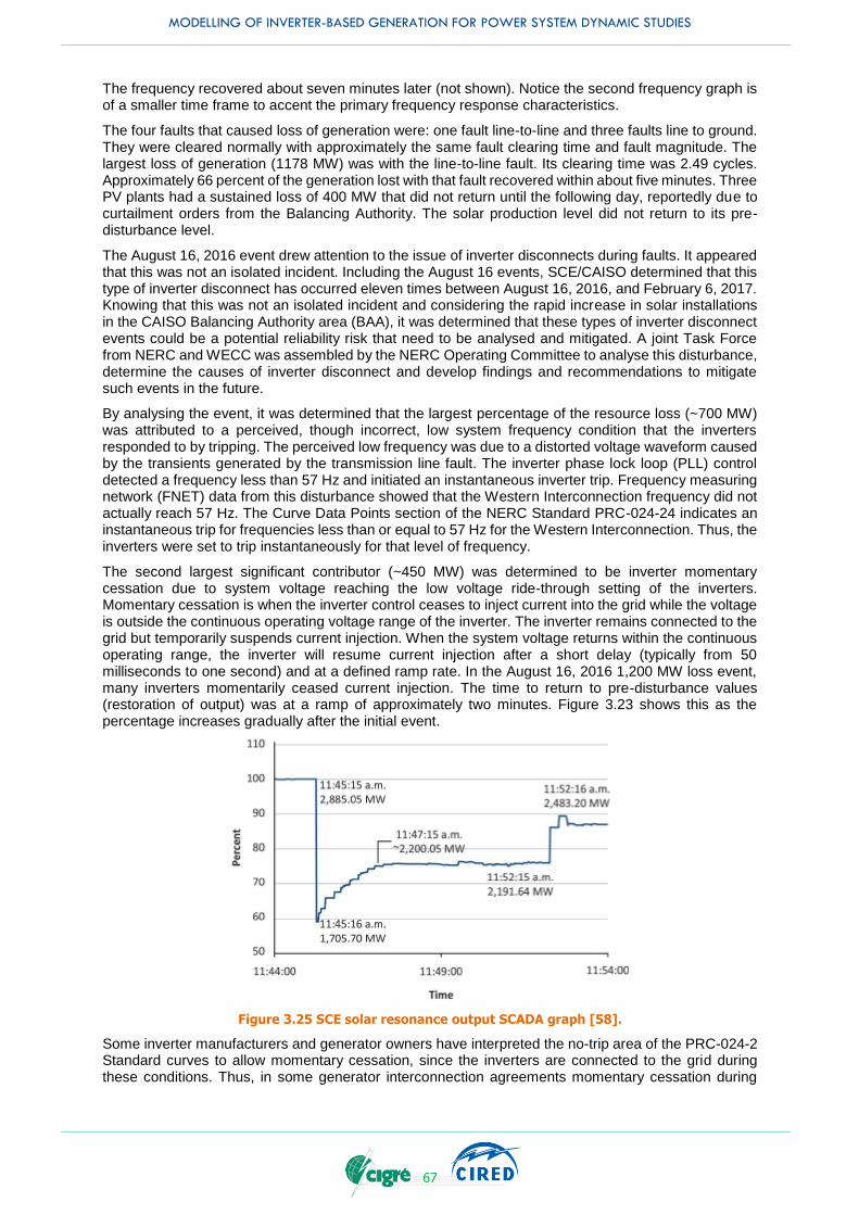
MODELLING OF INVERTER-BASED GENERATION FOR POWER SYSTEM DYNAMIC STUDIES
67
The frequency recovered about seven minutes later (not shown). Notice the second frequency graph is of a smaller time frame to accent the primary frequency response characteristics.
The four faults that caused loss of generation were: one fault line-to-line and three faults line to ground. They were cleared normally with approximately the same fault clearing time and fault magnitude. The largest loss of generation (1178 MW) was with the line-to-line fault. Its clearing time was 2.49 cycles. Approximately 66 percent of the generation lost with that fault recovered within about five minutes. Three PV plants had a sustained loss of 400 MW that did not return until the following day, reportedly due to curtailment orders from the Balancing Authority. The solar production level did not return to its pre-disturbance level.
The August 16, 2016 event drew attention to the issue of inverter disconnects during faults. It appeared that this was not an isolated incident. Including the August 16 events, SCE/CAISO determined that this type of inverter disconnect has occurred eleven times between August 16, 2016, and February 6, 2017. Knowing that this was not an isolated incident and considering the rapid increase in solar installations in the CAISO Balancing Authority area (BAA), it was determined that these types of inverter disconnect events could be a potential reliability risk that need to be analysed and mitigated. A joint Task Force from NERC and WECC was assembled by the NERC Operating Committee to analyse this disturbance, determine the causes of inverter disconnect and develop findings and recommendations to mitigate such events in the future.
By analysing the event, it was determined that the largest percentage of the resource loss (~700 MW) was attributed to a perceived, though incorrect, low system frequency condition that the inverters responded to by tripping. The perceived low frequency was due to a distorted voltage waveform caused by the transients generated by the transmission line fault. The inverter phase lock loop (PLL) control detected a frequency less than 57 Hz and initiated an instantaneous inverter trip. Frequency measuring network (FNET) data from this disturbance showed that the Western Interconnection frequency did not actually reach 57 Hz. The Curve Data Points section of the NERC Standard PRC-024-24 indicates an instantaneous trip for frequencies less than or equal to 57 Hz for the Western Interconnection. Thus, the inverters were set to trip instantaneously for that level of frequency.
The second largest significant contributor (~450 MW) was determined to be inverter momentary cessation due to system voltage reaching the low voltage ride-through setting of the inverters. Momentary cessation is when the inverter control ceases to inject current into the grid while the voltage is outside the continuous operating voltage range of the inverter. The inverter remains connected to the grid but temporarily suspends current injection. When the system voltage returns within the continuous operating range, the inverter will resume current injection after a short delay (typically from 50 milliseconds to one second) and at a defined ramp rate. In the August 16, 2016 1,200 MW loss event, many inverters momentarily ceased current injection. The time to return to pre-disturbance values (restoration of output) was at a ramp of approximately two minutes. Figure 3.23 shows this as the percentage increases gradually after the initial event.
Figure 3.25 SCE solar resonance output SCADA graph [58].
Some inverter manufacturers and generator owners have interpreted the no-trip area of the PRC-024-2 Standard curves to allow momentary cessation, since the inverters are connected to the grid during these conditions. Thus, in some generator interconnection agreements momentary cessation during

MODELLING OF INVERTER-BASED GENERATION FOR POWER SYSTEM DYNAMIC STUDIES
68
voltages below than 0.9 per unit or above 1.1 per unit was allowed, which is according to the NERC Standard PRC-024-2 is a no trip area.
The third largest amount of loss was approximately 100 MW that tripped by inverter DC overcurrent protection after starting the momentary cessation operation. The exact cause of these inverters tripping has not been determined and is still under investigation by the manufacturers.
Of the two types of interruption, tripping and momentary cessation, tripping is the most impactful as it removes the resource from the interconnection for approximately five minutes. If momentary cessation is restored quickly, the frequency decline is less severe than an equivalent MW amount of tripping.
The California ISO (CAISO) balancing area has experienced a rapid growth of solar photovoltaic (PV) resources in the recent past. CAISO has recorded a peak of 9,800 MW of utility scale solar PV generation. During light load days, they have experienced 47 percent of the area load served by utility scale solar. This widespread disconnection of inverter-connected resources is a significant concern for CAISO. Additionally, with the proliferation of solar in many balancing areas across the North America, this issue needs to be resolved to ensure interconnection reliability.
As the result of the investigation of the solar PV generation loss on August 16, 2016, the following recommendations were made.
Inverter manufacturers that experienced tripping during the Blue Cut fire event have recommended changes to their inverter settings to avoid the erroneous tripping due to the distorted measurement of the frequency; this change will add a time delay to inverter frequency tripping that will allow the inverter to “ride through” the transient/distorted waveform period without tripping. Solar development owners and operators involved in this event are working with their inverter manufacturers, CAISO and SCE to develop a corrective action plan for implementation of changes to inverter parameters.
Inverters that momentarily cease output for voltages outside their continuous operating range should be configured to restore output with a delay no greater than five seconds. NERC should review PRC-024-2 to determine if it needs to be revised to indicate that momentary cessation of inverter connected resources is not allowed within the no-trip area of the voltage curves.
Additional recommendations include that a NERC alert should be issued to the NERC registered Generator Owners (GOs) and Generator Operators (GOPs) to ensure they are aware of the recommended changes to inverter settings and alert them of the risk of unintended loss of resources. This alert should include a recommendation for Balancing Authorities (BAs) and Reliability Coordinators (RCs) to assess the reliability risk of solar PV momentary cessation and take appropriate measures. NERC should review PRC-024-2 to determine if it needs to be revised to add clarity that outside the frequency curves is a “may-trip” area (if needed to protect equipment) and not a must-trip area and to determine if there should be a required delay for the lowest levels of frequency to ensure transient/distorted waveform ride through.
Additional analysis is needed to assess the risk and consequences of the momentary cessation with higher penetration of the IBGs. These studies are currently underway in NERC.
3.3.5 Recommended functionalities of IBGs for large voltage deviations
The necessary functionalities of IBGs shown in Chapter 2 are examined in terms of the large voltage deviations as shown in Table 3.7. It is noted that the “necessity” in Table 3.7 is based on general power system dynamic studies and there could be exceptions especially when a specific study related to the large voltage deviation or the study with special controls or special system conditions is performed. The necessary major functionalities for large voltage deviation are the following:
(1) (4) and (7) DC source control, DC overvoltage protection, reduction of maximum inverter current when the DC voltage exceeds a certain limit: If a system fault occurs and if the voltage level is extremely low, the power electronic device in the inverter could be blocked, which is known as the momentary cessation of the interruption of the current injection [58]. In such a case, the DC voltage will rise because the DC source continues to provide DC current, while the AC current is controlled to zero. That could cause an over voltage in the DC link and would trigger the DC over voltage protection. Without this DC overvoltage protection model, the simulated response of the active and reactive power can be different from the actual measured response.
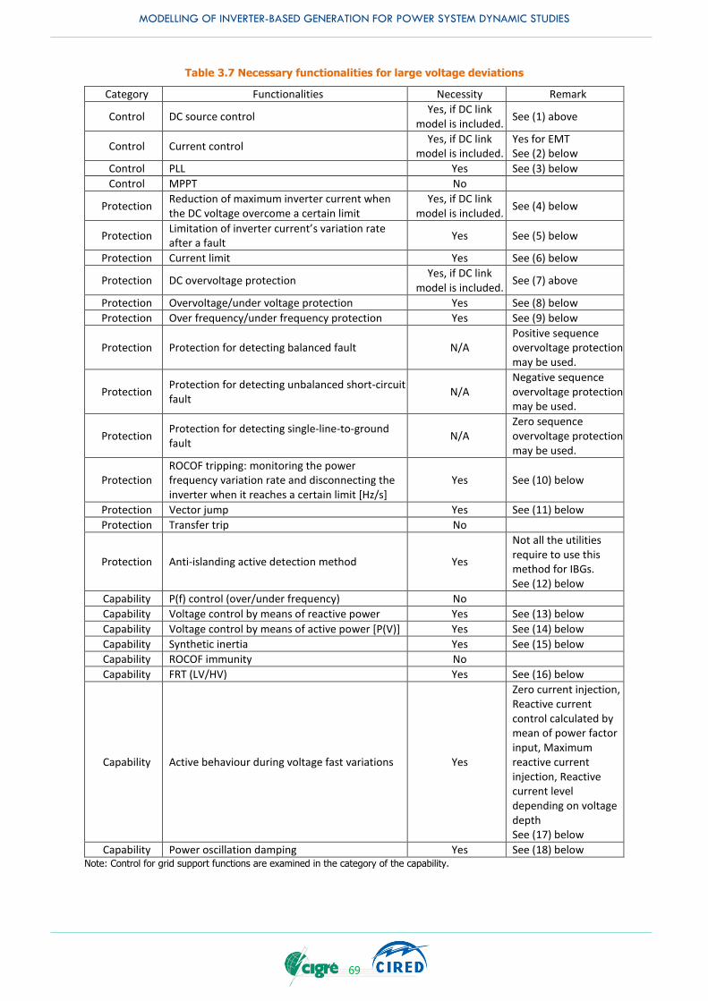
MODELLING OF INVERTER-BASED GENERATION FOR POWER SYSTEM DYNAMIC STUDIES
69
Table 3.7 Necessary functionalities for large voltage deviations
Category Functionalities Necessity Remark
Control DC source control Yes, if DC link
model is included. See (1) above
Control Current control Yes, if DC link
model is included. Yes for EMT See (2) below
Control PLL Yes See (3) below
Control MPPT No
Protection Reduction of maximum inverter current when the DC voltage overcome a certain limit
Yes, if DC link model is included.
See (4) below
Protection Limitation of inverter current’s variation rate after a fault
Yes See (5) below
Protection Current limit Yes See (6) below
Protection DC overvoltage protection Yes, if DC link
model is included. See (7) above
Protection Overvoltage/under voltage protection Yes See (8) below
Protection Over frequency/under frequency protection Yes See (9) below
Protection Protection for detecting balanced fault N/A Positive sequence overvoltage protection may be used.
Protection Protection for detecting unbalanced short-circuit fault
N/A Negative sequence overvoltage protection may be used.
Protection Protection for detecting single-line-to-ground fault
N/A Zero sequence overvoltage protection may be used.
Protection ROCOF tripping: monitoring the power frequency variation rate and disconnecting the inverter when it reaches a certain limit [Hz/s]
Yes See (10) below
Protection Vector jump Yes See (11) below
Protection Transfer trip No
Protection Anti-islanding active detection method Yes
Not all the utilities require to use this method for IBGs. See (12) below
Capability P(f) control (over/under frequency) No
Capability Voltage control by means of reactive power Yes See (13) below
Capability Voltage control by means of active power [P(V)] Yes See (14) below
Capability Synthetic inertia Yes See (15) below
Capability ROCOF immunity No
Capability FRT (LV/HV) Yes See (16) below
Capability Active behaviour during voltage fast variations Yes
Zero current injection, Reactive current control calculated by mean of power factor input, Maximum reactive current injection, Reactive current level depending on voltage depth See (17) below
Capability Power oscillation damping Yes See (18) below Note: Control for grid support functions are examined in the category of the capability.

MODELLING OF INVERTER-BASED GENERATION FOR POWER SYSTEM DYNAMIC STUDIES
70
(2) Current Control (Inner current control loop): The current control is necessary for large voltage deviations at the DC link. The converter model is simplified to a current controller model that generates the desired currents. The electrical controller of this type of model only extracts the essential component of a more detailed electrical controller, i.e. a decoupled active and reactive power controller via current control. The controller has a double-loop structure. The outer loop uses the active power and reactive power references to generate the respective d-axis and q-axis current references for the inner loop. The inner loop regulates its current output to the respective current reference. In both control loops, PI controllers are usually used. It is often the case that the inner current control loop is also omitted in the RMS model mainly because the current control is most likely to be completed in the time step of the RMS simulation. Such a model is less complex when compared to the detailed generator/converter and electrical control model, however, it focuses on the fundamental characteristics of the converter outputs and has been widely applied in many engineering projects for bulk power system dynamic studies.
(3) PLL: When a large voltage deviation occurs, the bus voltage angle could quickly and significantly change. Such an immediate jump of the voltage angle could delay in tracking the voltage angle change at the PCC. Such time delay, coming from the response speed of the PLL could result in undesirable transient positive or negative current (active or reactive power) variations. To maintain stable operation of a converter, the PLL needs to track the voltage during a network fault, as shown in Figure 3.26 (a). If the PLL loses track of the voltage, the converter instability could be induced as shown in Figure 3.26
(b). This can cause damage to network equipment and loss of the generator.[57]
Figure 3.26 System voltage with PLL (a) tracks (b) loses voltage [57].
It is noted that most state-of-the-art IBGs may have very short time delays. The change in active and reactive power of the IBGs following system faults can affect the critical area exchange or the maximum power transfer with respect to transient stability or short-term voltage stability. It is also noted that the detailed PLL control block is usually modelled in the EMT model and the simplified control block which approximates the PLL behaviour is normally modelled in the RMS model because the assumption that the IBG model can be represented only by a current source can be justified by the fact that the converter control is much faster than the dynamics/transients of interest.
(5) Limitation of inverter current’s variation rate after a fault: The rate of current variation (di/dt) needs to be designed to be below the maximum permissible value of the inverter switching devices. It is often set by selecting appropriate values for the inductance in the main circuitry and therefore it is by design a constant. In some systems, an adjustable current variation rate exists, which can be implemented within the current control loop, in order to protect the switching devices from excessive current stresses. When a short circuit in the power system occurs, the excessive current will flow through the switching devices which results in extra stresses on the devices. If the temperature at the junctions of the switching devices rises higher than a fixed internal threshold with a hysteresis, the current variation rate will be reduced for a certain period of time to protect the switching devices.
Because the operation of this type of protection will lead to the disconnection of the IBGs, the massive disconnection of the IBG could affect the critical area exchange or the maximum power transfer with respect to transient stability or short-term voltage stability.
(6) Current limit: When voltage drop is significant, active or reactive power output of the IBGs can increase quickly. That means, the current of the IBGs is more likely to hit its limit and the active or reactive power of the IBGs will be restricted so as to control the current of the IBG within a permissible range. It should be noted that the dynamic behaviour of the active and reactive power of the IBGs could be different because the control scheme including the active or reactive current prioritisation can vary
MODELLING OF INVERTER-BASED GENERATION FOR POWER SYSTEM DYNAMIC STUDIES
71
depending on the designer/manufacturer of IBGs and on the grid code. The possibility of hitting the current limiter also depends on the initial current of the IBGs, i.e. the pre-fault current of the IBGs. If the initial current of the IBG is high, the recovery of the active power or the increase in reactive power is more likely to be limited, which results in a different critical area exchange or a different maximum power transfer and therefore could affect transient stability and the short-term voltage stability.
(8) Over voltage/under voltage protection: If a system fault occurs and if the fault duration is long, the under voltage protection for both loads and IBGs is likely to operate. After the fault is cleared the slow voltage recovery may be of a long duration (e.g. due to the massive induction motor loads) the under voltage protection is likely to operate. The dynamic reactive power (current) support of the IBGs could cause a significant voltage rise after the fault is cleared. The self-disconnection of loads with the active power recovery of the IBGs could also cause a significant voltage rise after the fault is cleared. Such significant voltage rise is most likely to operate the overvoltage protection, which leads to different critical area exchange or different maximum power transfer and hence could impact transient or short-term voltage stability.
(9) Over frequency/under frequency protection: If a large power plant is connected to the main grid via a transmission line and if a short-circuit occurs on that transmission line, not only a large voltage deviation but also a significant frequency deviation could occur. When massive amounts of residential and utility-scale IBGs, with improperly designed LVRT/HVRT capability and/or PLL [31] disconnect following system faults, significantly frequency drop can be observed. If loads are disconnected due to the underfrequency load shedding scheme, an over frequency could also occur. Therefore, the over or under frequency protection might operate in case of the large voltage deviation with high penetration of IBGs.
(10) ROCOF tripping: The frequency is normally measured using the bus voltage. When a system fault occurs, the bus voltage angle could immediately shift to a different voltage bus angle [31]. Such jump of the voltage angle could also cause a significantly large ROCOF value. In order to avoid the undesirable ROCOF relay operation, a filter may be used. However, this can result in a slower operation of the ROCOF relay in the case of a real frequency drop. The ROCOF tripping is closely related to frequency deviations. However, frequency instability could occur together with transient instability through high penetration of IBGs [58]. Therefore, the ROCOF relay might operate due to the large voltage deviation with high penetration of IBGs.
(11) Vector jump: Jump method is a typical passive anti-islanding protection scheme (See also Clause 3.2.5 (5)). It is highly possible that the voltage phase jumps to another voltage phase when the network is split into multiple networks. On the other hand, the voltage phase could jump due to a change in the network configuration although the network is not separated. A typical change in the system configuration is during a system fault which has a large voltage excursion, i.e. when the system fault occurs and when the system fault is cleared. As mentioned earlier, the voltage phase jump can lead to significant change in frequency seen by the IBG, which could lead to a disconnection of the IBG [58]. Hence, such disconnection of IBGs may be represented by the vector jump protection as well as the over/under frequency protection.
(12) Anti-islanding active detection method: As mentioned earlier, when the magnitude of bus voltages changes, i.e., if the small reactive power injection from the IBG does not have ability to change the connected bus voltage, a voltage phase change occurs. However, if the penetration of IBGs is very high and if the cumulative reactive current injection from the distributed IBGs has ability to change the voltage magnitude, a negative reactive current injection during the voltage dip could lead to a further voltage drop (in short-term and long-term).
(13) Voltage control by means of reactive power: This capability is generally required for the steady-state condition. Therefore, the dynamic reactive power (current) support is not included in this capability. As mentioned earlier, although the dynamic behaviour is not directly related to this capability, the pre-fault active and reactive power feed-in of the IBG can affect the fault-on and post-fault dynamic behaviour of the IBG output. This could also result in a different critical area exchange or a different maximum power transfer and therefore affect rotor angle and short-term voltage stability.
(14) Voltage control by means of active power: The voltage control by means of active power is commonly used for residential PV systems in a few countries. The IBG mainly in LV network reduces its active power when the voltage exceeds a threshold value, e.g., 1.09 p.u. If a significant voltage dip occurs in the grid, induction motors might stall and loads could be disconnected from the power system. A large amount of self-disconnected loads can cause a voltage rise. The control speed of this type of voltage control is slow and the reduction of active power output from PV systems is in the order of tens

MODELLING OF INVERTER-BASED GENERATION FOR POWER SYSTEM DYNAMIC STUDIES
72
of seconds to a minute. Therefore, transient stability could be affected by voltage control by means of active power if the simulation time considers the before mentioned study period.
(15) Synthetic inertia: Rotor angle stability consists of two elements: i) synchronizing torque in phase with rotor angle deviations, and ii) damping torque inphase with speed deviations. The damping torque
can be expressed as Equation 3.3.
2
0
2
2
0 0
2
2 4
d
m
MD
T
D K Ds j
M M M
M Ds s K T
w
w w
- -
D + D + D D
Equation 3.3
where: M denotes system inertia, D denotes damping torque, K denotes synchronizing torque, S denotes Laplace operator, Td denotes decay time constant, Tm denotes mechanical torque.
Equation 3.3, includes the variable of the system inertia, M, which means the system inertia can affect the damping torque and therefore rotor angle stability. Because the power swing oscillations caused by large voltage deviations can change with and without synthetic inertia, it could also influence the critical area exchange or the maximum power transfer with respect to rotor angle and short-term voltage stability.
(16) FRT (LV/HV): The Low Voltage Ride-Through (LVRT) characteristic clarifies a zone where IBGs have to stay connected to the grid during grid disturbances depending on the duration and depth of the voltage sag. IBGs may trip if the voltage is outside the zone. The most conservative way from the stability point of view is, to trip the IBGs when the voltage is outside the zone. Thus, the LVRT characteristic is most likely to be represented as an undervoltage protection with different settings for time delays and voltage thresholds. These protection settings ensure the LVRT and HVRT capability. Although, different manufacturers have different control strategies for active and reactive power during the fault-on period, there are common principles. In general, when the voltage drops, the IBGs will reduce its active power output. In some countries, the active power output is not allowed to be zero during the fault unless the residual voltage is below a threshold value, e.g., 0.2 p.u. Hence, the IBG is allowed to temporarily stop the current injection when the residual voltage is extremely low. In other countries, the active power output is allowed to be zero, while the reactive power output is required to increase. When modelling the FRT characteristics, it is important to set the up-to-date under voltage limits according to the information provided by the manufacturer or the grid code requirements.
Because the dynamic behaviour of the IBG output following faults can significantly change with and without the LVRT/HVRT characteristics, it could also affect the critical area exchange or the maximum power transfer and therefore transient and short-term voltage stability.
(17) Active behaviour during voltage fast variations: This capability is typically known as dynamic reactive power (current) support or dynamic voltage support. As already mentioned in the previous clause, this capability supports the voltage during and following faults by injecting reactive current and reducing active current. Such dynamic voltage support can change the critical area exchange or the maximum power transfer and therefore influence transient and short-term voltage stability. It is noted that the current limit function is extremely related to this function during large voltage variations because the active and/or reactive currents are more likely to hit their limitation during large voltage deviations. In such a case, the inverter control modes such as active power priority and reactive power priority play an important role how the active and/or reactive current hit the current limit, through which the different dynamic behaviour of active power and reactive power of IBGs can affect power system dynamic stability.
(18) Power oscillation damping: Although it is not currently implemented into IBGs except HVDC, this capability can contribute to the mitigation of undamped power swing oscillations or acts to shorten the decay time of damped power swing oscillations. Such mitigation of power swing oscillations following
MODELLING OF INVERTER-BASED GENERATION FOR POWER SYSTEM DYNAMIC STUDIES
73
faults can change the critical area exchange or the maximum power transfer and therefore influence transient and short-term voltage stability.
(19) Misc.: To make a compromise between simulation accuracy and computational efficiency for the bulk power system studies, while at the same time considering the requirement for electromechanical transient analysis, a current-source based model has been proposed and is widely applied to the RMS model. The current source model neglects the dynamics in the prime mover/converter model block. So, there are no explicit prime mover models in these types of IBG models. Consequently, not only all the inductances connecting the converter to the power grid but also the detailed PLL block are unlikely to be modelled. The assumption that a generator/converter model can be represented only by a current source can be justified by the fact that the converter control is much faster than the transients of interest and in its steady state (i.e. the end of the control transients) it injects the specified active and reactive currents. It should be noted that the current source model causes a numerical problem when the voltage magnitude is very low and the active/reactive current cannot be injected independently. If the injection of the active current, i.e. active power net load exceeds the voltage stability limit of the system for a low voltage condition, the model fails to converge.
3.4 BEHAVIOUR IN RESPONSE TO SMALL AND LONG-TERM VOLTAGE DEVIATIONS
A brief introduction of stability studies with the key response relevant to the system faults are overviewed. Real-life examples with and without the IBGs are illustrated. In addition, the necessary functionalities of IBGs for the behaviour in response to small and long-term voltage deviation are discussed here.
3.4.1 Description of phenomena
Long-term voltage instability is mainly driven by automatic load tap changers and over-excitation limiters and develops from a few seconds to tens of minutes after a disturbance. Most long-term voltage instability incidents are as a result of transmission and/or generation equipment outages, regardless of the severity of the initial fault. The disturbance could also be a sustained load build up, like morning load increase, and to avoid islanding, one of the possible defensive actions is to introduce a delay on the Q(V) regulation rules of IBGs; to avoid interferences and, as a consequence, further long-term voltage stability problems, this delay must be limited to a maximum value, so it does not interfere with on load tap-changers operation times.
In many cases, static analysis can be used to estimate stability margins, to identify factors influencing stability, and to screen a wide range of system conditions and a large number of other scenarios. Where timing of control actions is important, this analysis should be complemented by quasi-steady-state time-domain resolved simulations [30]. It does not mean the problem is of static nature; it is a dynamic problem but it can be assessed in some systems using static power flow calculations. This condition is no longer valid when automatic controls are activated in response to the system evolution or when these controls may be beneficial for voltage stability (e.g. automatic shunt compensation switching).
With more and more systems relying on post-disturbance controls (or system integrity protection schemes), the need for dynamic simulations will increase, particularly for real-time dynamic security assessments.
The computational power and tools available today allow the simulation of long-term dynamics (in the range of 5 to 10 minutes simulation time) performed efficiently.
Voltage stability refers to the ability of a power system to maintain steady-state voltages at all buses in the system after being subjected to a disturbance from a given initial operating condition or in the case of gradual increase in loads (a typical scenario to cause voltage instability). It depends on the ability to maintain/restore equilibrium between load demand and generation supply from the power system. Instability that may result occurs in the form of a progressive fall or rise of voltages of some buses. A possible outcome of voltage instability is loss of load in an area, or tripping of transmission lines and other elements by their protective systems leading to cascading outages. Loss of synchronism of some generators may result from these outages or from violation of field current limit to out-of- step conditions [30], [59].

MODELLING OF INVERTER-BASED GENERATION FOR POWER SYSTEM DYNAMIC STUDIES
74
The term voltage collapse is also often used 24 as the process by which the sequence of events accompanying voltage instability leads to a blackout or abnormal low voltages in a significant part of the power system [11], [60], [61].
Voltage stability problems normally occur in heavily stressed systems. While the disturbance leading to voltage collapse may be initiated by a variety of causes, the underlying problem is deficit(or excess) of reactive power in the power system. In addition to the strength of transmission network and power transfer levels, the principal factors contributing to voltage collapse are the generator reactive power/voltage control limits, load characteristics, characteristics of reactive compensation devices, and undesired action of voltage control devices such as transformer on-load tap changers (OLTCs) [11].
For a load demand, higher than the maximum generating power, control of power by varying the load would be unstable, i.e., an increase on load admittance would reduce power consumed. In this region, the load voltage may or may not progressively decrease depending on the load-voltage characteristic. With a constant-admittance load characteristic, the system condition stabilises at a voltage level that is lower than normal. On the other hand, if the load is supplied by a transformer with OLTC, the tap-changer action will try to raise the load voltage, which has effect of reducing effective impedance of the load. This lowers the voltage regulator still further and leads to a progressive reduction of voltage. This process leads to the phenomenon of voltage instability.
The analysis of voltage stability for a given system state involves the examination of two aspects [11], [62]:
(a) Proximity to voltage instability: How close is the system to voltage instability?
Distance to instability may be measured in terms of physical quantities, and reactive power reserve. The most appropriate measure for any given situation depends on the specific system and the intended use of the margin; for example, planning versus operating decisions. Consideration must be given to possible contingencies (line outages, loss of a generating unit or a reactive power source, etc.).
(b) Mechanism of voltage instability: How and why does instability occur? What are the key factors contributing to instability? What are the voltage-weak areas? What measures are most effective in improving voltage stability?
Time domain, in which appropriate modelling is included, can capture the events and their chronology leading to instability. However, such simulations are time-consuming and do not readily provide sensitivity information and the degree of stability.
System dynamics influencing long-term voltage stability are usually slow. Therefore, many aspects of the problem can be effectively analysed by using static methods, which examine the viability of the equilibrium point represented by a specified operating condition of the power system. The static analysis techniques allow examination of a wide range of system conditions and, if appropriately used, can provide much insight into the nature of the problem and identify the key contributing factor. Dynamic analysis, on the other hand, is useful for detailed studies of specific voltage collapse situations, coordination of protection and controls, and testing of remedial measures. Dynamic simulations also examine whether and how the steady-state equilibrium point will be reached.
3.4.2 Response of IBGs to long-term voltage stability triggered by large voltage deviation and impact on system performance
3.4.2.1 Long-term voltage response with and without LVRT [63]
An example of long-term voltage stability dynamic analysis is shown in a large-scale combined transmission and distribution network model based on the Nordic system [62]. It is noted that the phenomena being studied in this example is the combination of “large voltage deviation” and “small and long-term voltage deviation” rather than “small and long-term voltage deviation”. The transmission network (TN) model (presented in Figure 3.27) is expanded with 146 distribution networks (DNs) (shown in Figure 3.28) that replace the aggregated distribution loads.
24 Voltage instability can arise: on fault event or started by a “normal” event like opening a line or spontaneously by very slow phenomenon such as load increase or decrease

MODELLING OF INVERTER-BASED GENERATION FOR POWER SYSTEM DYNAMIC STUDIES
75
Figure 3.27 Expanded Nordic system [65].
Figure 3.28 Detailed distribution network model [63].

MODELLING OF INVERTER-BASED GENERATION FOR POWER SYSTEM DYNAMIC STUDIES
76
Each one of the 146 DNs is connected to the TN through two parallel transformers equipped with On Load Tap Changing (OLTC) devices. Each DN includes 100 buses, one distribution voltage regulator equipped with OLTC, three PV units, three type-3 WTs, and 133 dynamically modelled loads (such as combination of small induction machines and exponential loads). In addition, each DGs complies with the LVRT requirements sketched in Figure 3.29. More information on the models and data used, can be found in [63].
To test the long-term voltage stability of the system, a 5-cycle 3-phase fault near the TN bus 4032 cleared by the opening the faulted line 4032-4042 was considered. The system was simulated for 180 seconds with a time-step size of half cycle (10 milliseconds in a 50 Hz system). The simulation was performed twice. Firstly, when the LVRT curve of an IBG was violated, automatically disconnecting the IBGs; and secondly, with all the IBGs remaining connected throughout the entire simulation.
Figure 3.29 LVRT capability curve of RES [65].
Figure 3.30 shows the voltage at the TN bus 4044 for both simulations.
Figure 3.30 Voltage on TN bus 4044 [65].
Both cases are short-term stable. After the electromechanical oscillations have died out, the system evolves in the longer-term under the effect of OLTCs acting to restore distribution voltages, and the over excitation limiters on the generators. It can be seen that, while second case is long-term stable, the first one is unstable with the system collapsing at t ≈ 150 s.
Figure 3.31 shows the voltage evolution of the terminal voltage of two IBGs in DN1 and DN2, where in the first case the LVRT is violated and in the second not. In the first case, the successive disconnection of IBGs in accordance with the LVRT is reflected on the voltages and leads to the voltage collapse shown in Figure 3.30.
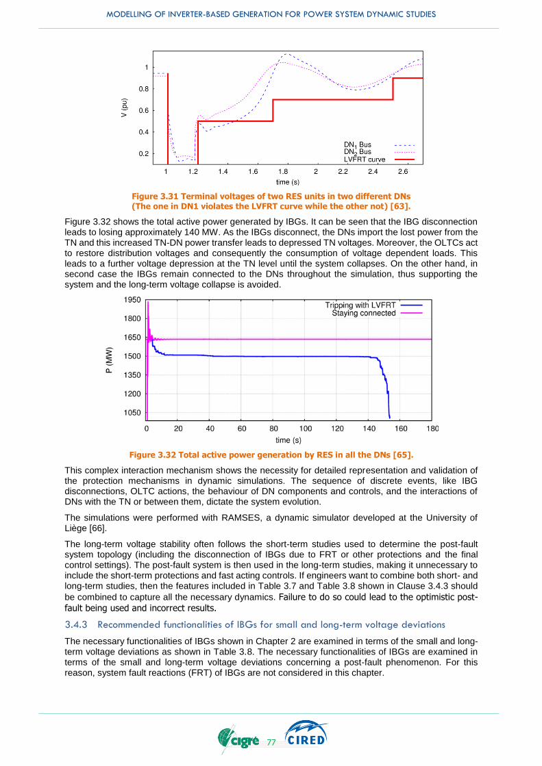
MODELLING OF INVERTER-BASED GENERATION FOR POWER SYSTEM DYNAMIC STUDIES
77
Figure 3.31 Terminal voltages of two RES units in two different DNs (The one in DN1 violates the LVFRT curve while the other not) [63].
Figure 3.32 shows the total active power generated by IBGs. It can be seen that the IBG disconnection leads to losing approximately 140 MW. As the IBGs disconnect, the DNs import the lost power from the TN and this increased TN-DN power transfer leads to depressed TN voltages. Moreover, the OLTCs act to restore distribution voltages and consequently the consumption of voltage dependent loads. This leads to a further voltage depression at the TN level until the system collapses. On the other hand, in second case the IBGs remain connected to the DNs throughout the simulation, thus supporting the system and the long-term voltage collapse is avoided.
Figure 3.32 Total active power generation by RES in all the DNs [65].
This complex interaction mechanism shows the necessity for detailed representation and validation of the protection mechanisms in dynamic simulations. The sequence of discrete events, like IBG disconnections, OLTC actions, the behaviour of DN components and controls, and the interactions of DNs with the TN or between them, dictate the system evolution.
The simulations were performed with RAMSES, a dynamic simulator developed at the University of Liège [66].
The long-term voltage stability often follows the short-term studies used to determine the post-fault system topology (including the disconnection of IBGs due to FRT or other protections and the final control settings). The post-fault system is then used in the long-term studies, making it unnecessary to include the short-term protections and fast acting controls. If engineers want to combine both short- and long-term studies, then the features included in Table 3.7 and Table 3.8 shown in Clause 3.4.3 should
be combined to capture all the necessary dynamics. Failure to do so could lead to the optimistic post-
fault being used and incorrect results.
3.4.3 Recommended functionalities of IBGs for small and long-term voltage deviations
The necessary functionalities of IBGs shown in Chapter 2 are examined in terms of the small and long-term voltage deviations as shown in Table 3.8. The necessary functionalities of IBGs are examined in terms of the small and long-term voltage deviations concerning a post-fault phenomenon. For this reason, system fault reactions (FRT) of IBGs are not considered in this chapter.

MODELLING OF INVERTER-BASED GENERATION FOR POWER SYSTEM DYNAMIC STUDIES
78
Table 3.8 Necessary functionalities for small and long-term voltage deviations
Category Functionalities Necessity Remark
Control DC source control No
Control Current control No
Control PLL No
Control MPPT Yes See (1) below
Protection Reduction of maximum inverter current when the DC voltage overcome a certain limit
No
Protection Limitation of inverter current’s variation rate after a fault
No
Protection Current limit Yes See (2) below
Protection DC overvoltage protection No
Protection Overvoltage/under voltage protection Yes See (3) below
Protection Over frequency/under frequency protection No
Protection Protection for detecting balanced fault No Positive sequence overvoltage protection may be used.
Protection Protection for detecting unbalanced short-circuit fault
No Negative sequence overvoltage protection may be used.
Protection Protection for detecting single-line-to-ground fault
No Zero sequence overvoltage protection may be used.
Protection ROCOF tripping: monitoring the power frequency variation rate and disconnecting the inverter when it reaches a certain limit [Hz/s]
No
Protection Vector jump No
Protection Transfer trip No
Protection Anti-islanding active detection method Yes
Not all the utilities require to use this method for IBGs. See (4) below
Capability P(f) control (over/under frequency) No
Capability Voltage control by means of reactive power Yes See (5) below
Capability Voltage control by means of active power [P(V)]
Yes See (6) below
Capability Synthetic inertia No
Capability ROCOF immunity No
Capability FRT (LV/HV) No Not used for long-term post fault analysis.
Capability Active behaviour during voltage fast variations No
Zero current injection and Reactive current control calculated by mean of power factor input. Maximum reactive current injection and Reactive current level depending on voltage depth.
Capability Power oscillation damping No Note: Control for grid support functions are examined in the category of the capability.
The major necessary functionalities for small and long-term voltage deviation are the following:
1) MPPT: “stop time for simulation” could be set as over 10 min when the small and long-term voltage deviation is examined. As mentioned earlier, because the solar radiation cannot be assumed to be constant for the aforementioned time frame, the change in MPPT signal needs to be considered for this

MODELLING OF INVERTER-BASED GENERATION FOR POWER SYSTEM DYNAMIC STUDIES
79
type of phenomenon. The change in MPPT signal may be modelled as the change in the active power reference (Pref) itself.
2) Current limit: When the power system is about to experience long-term voltage instability, any significant low voltage at a system bus must be observed. Extremely low voltages could lead to a current limitation of the IBG due to a high current injection.
3) Over voltage and under voltage protection: When the power system is about to experience long-term voltage instability, any significant low voltage at a system bus must be observed. Extremely low voltages could trip the under voltage protection.
4) Anti-islanding active detection method: Same as Clause 3.3.5-(12).
5) Voltage control by means of reactive power: This voltage control is in general intentionally set as slow as possible in order to coordinate with the other voltage controllers, such as tap changers and reactive power compensators. Therefore, the operation of the voltage control by means of reactive power of IBGs can play an important role when the power system experiences long-term voltage instability. It should be highlighted that the voltage control by means of reactive power is required not only for the inverter control but for the plant control (See Chapter 5).
6) Voltage control by means of active power: Without the large voltage deviation, the voltage control by means of active power can be activated when the load decreases and/or when the PV output increases in steady-state. Once voltage control by means of active power is activated, the post-fault steady-state operating point keeps moving for a long time. Therefore, the voltage control by means of active power can play an important role when the power system experiences long-term voltage instability.
3.5 SMALL DISTURBANCE ANALYSIS
3.5.1 Description of phenomena
Small signal stability is defined as the ability of the system to maintain synchronism when it is subjected to small disturbances. The definition of small disturbance is limited to the case when the response of the system to such a disturbance can be analysed with linearized equations. The dynamics is generally analysed in the frequency domain. Small-signal analysis uses linear techniques, based on eigenvalues/eigenvectors calculations, and provides valuable information about the inherent dynamic characteristics of power systems and assists in their design [30],[67]. This analysis can be performed by the linearization of the non-linear power system model at a certain operating state. A linearized power
system model at a given operating point can be represented by Equation 3.4.
D D + D
D D + D
x A x B u
y C x D u
Equation 3.4
where, x is the vector of state variables, y is the vector of output variables, u is the vector of input variables, A is the state matrix, B is the input matrix, C is the output matrix, and D is the matrix which defines the proportion of input that appears directly in the output variables.
Stability of a non-singular linear system is determined by the eigenvalues of the matrix A. A real eigenvalue corresponds to a non-oscillatory mode. A pair of complex eigenvalues λ=σ ± jω with a positive real part corresponds to an undamped oscillatory mode but with a negative real part, the original system is asymptotically stable. The frequency of the oscillatory mode is given by f= ω/2π.
The damping ratio of the oscillatory mode is given by Equation 3.5.
𝜁 =𝜎
√𝜎2 + 𝜔2
Equation 3.5
In addition, the right and left eigenvectors corresponding to the eigenvalues of interest, are the basis of sensitivity tools to identify the relationships between variables and eigenvalues.
The relationship between the i-th mode and the j-th mode is given by their right eigenvectors. The magnitude of the right eigenvector element indicates how much the mode excites the specific frequency component of the power swing oscillation from the viewpoint of the amplitude of the frequency component. The angle of the right eigenvector element indicates how much the i-th mode and the j-th
MODELLING OF INVERTER-BASED GENERATION FOR POWER SYSTEM DYNAMIC STUDIES
80
mode are synchronised during the power swing oscillation from the viewpoint of the phase of the frequency component, which can be used to group the generators to two or more subgroups.
In a power system with high IBG penetration, some of the synchronous generators are replaced with IBGs, e.g. PV units. The addition of the PV and other inverter-based resources are certain to occur in the future, hence the exact effect of these systems, particularly on the transmission systems, must be adequately studied from the small signal stability perspective [68].
When a system is no longer small signal stable, a power swing oscillation is initiated even by the natural change in loads and the growing power swing oscillation cannot be damped without the power system oscillation damping devices, such as PSS. The small signal stability is theoretically violated when the angle difference between the two buses exceeds 90 degrees. The power-angle curve is often used for understanding the relationship between the synchronizing torque coefficient and the operating point on the power-angle curve. The synchronizing torque coefficient is defined as the slope of the power-angle curve. Because the slope of the power-angle curve becomes zero when the angle difference becomes 90 degrees, a positive synchronizing torque coefficient is the condition for which the small signal stability is not violated.
The system faults are not normally considered as small disturbances. However, even the single-line-to ground fault in the bulk power system could be treated as an equivalent small disturbance. Therefore, the definition of a small disturbance very much depends on how little an impact the disturbance provides to the power system.
Once the growing power swing oscillation occurs, it is difficult to initially detect such oscillation, because the power swing oscillation could be almost imperceptible due to the existence of steady-state oscillations caused by natural load changes. When the growing power swing oscillation is detected, it may be too late for any corrective actions. In light of this, the small-signal stability study is of growing interest to power system operators.
3.5.2 Relationship between behaviour in response to small signal stability and relevant study [36]
It is paramount to analyse the impact of massive addition of PVs both on distribution and transmission systems. The effects of the high penetration of PVs on distribution systems are well described in [69]–[72], where it is suggested that the high PV penetration can affect the voltage profile depending on the loading conditions and the amount of the PV penetration.
However, the effect of PVs on the transmission systems can no longer be neglected. The objective of the small signal stability analysis is to examine stability of the system under various PV penetration levels. In order to locate the critical modes of the system, an eigenvalue analysis is conducted to explore poorly damped modes within the frequency range of 0.1–2 Hz. According to [73] a damping ratio below 3-5% is critical. The objective of such analysis is to investigate whether the increase in PV penetration affects the critical modes of the system. The following steps are proposed to undertake this type of investigation:
1) Identify the most critical, i.e., poorly damped, modes of the system by performing eigenvalue analysis on the base case with no PV generation.
2) Perform eigenvalue analysis for the cases after introducing various levels of residential rooftop and utility scale PVs.
3) Compare the results of the eigenvalue analysis under different PV penetration levels to investigate the impact of high PV penetration on small signal stability of the system under study.
4) Perform eigenvalue sensitivity analysis with respect to the displaced generators’ inertia to validate the results achieved from the eigenvalue analysis.
5) To confirm the aforementioned critical eigenvalue, analyse the transient stability performance of the system applying less severe disturbance and examine whether the identified critical modes can be excited and substantiate the results obtained by eigenvalue analysis.
6) Check if the concentration of a large IBG within a critical area within a power system is affecting the steady-state stability limits of that particular network area. Therefore, usually when performing the steady-state stability limits the grid operators are requesting to include the involved IBGs within the grid model developed for studies analysing the power exchanges between critical areas.
MODELLING OF INVERTER-BASED GENERATION FOR POWER SYSTEM DYNAMIC STUDIES
81
3.5.3 Response of IBG to small disturbance analysis and impact on system performance
Unlike synchronous generators, IBGs do not interact with the power network through an internal power angle. Therefore, there are no state variables such as angle, associated with the IBG model in the right eigenvector (mode shape).
IBGs that are asynchronously connected to the grid will not cause electromechanical modes of oscillation in their own right. However, introduction of large amounts of IBGs does have the potential to indirectly change the electromechanical damping performance of the system by:
Significantly altering the dispatch of synchronous generation in order to accommodate the IBG. If
the small signal stability is adversely affected by e.g. PV integration, critical synchronous generators
may need to be kept on-line or other countermeasures are required to maintain sufficient damping
for low frequency oscillations
Significantly altering power flows in the transmission network
Interacting with synchronous machines to change the damping torques induced on their shafts.
This factor depends on the dynamic performance characteristics of the inverter and on other
relatively fast-acting controls (e.g. STATCOMs which may be installed for voltage control
purposes.)
The presence of the IBG may change the mode shape of the inter-area mode for the synchronous
generators that are not displaced by the IBG.
The replacement of the synchronous generators by the IBGs might cause reduction in the system
inertia especially with a high penetration of IBGs.
The small signal stability as well as transient stability needs to be evaluated from two metrics; damping torque coefficient and synchronizing torque coefficient ([11],[74]). The displacement of the synchronous generators with a low penetration of IBGs could lead to positive effect in terms of synchronizing torque coefficient perspective, because the net load of the system becomes lighter and therefore, the largest angle difference between the generators will be decreased. The case study introduced in [68] shows that the eigenvalue frequency increases and damping ratio also increases when the PV penetration rate changes from 10% to 20%.
Both the first generation WECCIBG models and the IEC 61400-27 wind turbine generator models [77] have not been developed explicitly with eigenvalue calculation (for small signal stability) in mind. These IBGs include highly non-linear components and simplifications in the development of the models. Thus, linearisation for eigenvalue analysis is not trivial nor necessarily appropriate based on these simplified models. Some publications [75] refer to special cases where there is a problem in linearizing the system matrix for the eigenvalue analysis when the first generation WECC generic models is used. To avoid the problem, an extra term in the models may be introduced, but there is no guarantee that similar problems may not occur in the future. Further information to [75] can be found in [76]
The authors in [68] proposed another approach for integration of variable energy resources in terms of small signal stability. The approach suggested that for every 3-MW addition of renewable generation to the system, there would be a 2-MW reduction in conventional generator commitment and 1-MW reduction in their dispatch. While the choice of the cited “1/3–2/3 rule” could be quite arbitrary, which can lead to potential small signal stability problems (note that the overall system inertia is decreased). Consequently, with displacing/rescheduling of conventional units as a result of the addition of PV generation, it is advantageous to determine if a particular generator’s inertia has a significant impact on a particular inertial oscillation mode. This could be determined by performing sensitivity analysis with respect to generator inertia and performing de-commitment/rescheduling using the sensitivity to inertia as a constraint [68].
3.5.4 Recommended functionalities of IBGs for small disturbance analysis
The necessary functionalities of IBGs shown in Chapter 2 are examined in terms of the small signal stability as shown in Table 3.9. Protections and limiters are ignored in this table due to the way this analysis is performed, i.e. using small increments around the operating point. The rest of the controls and capabilities need to be implemented to the IBG models as shown in Table 3.9. The main point here is that the same system and control data for transient stability analysis and small signal stability analysis are generally used. Unless a functionality is required for transient stability, it should be also required for small signal stability.

MODELLING OF INVERTER-BASED GENERATION FOR POWER SYSTEM DYNAMIC STUDIES
82
Table 3.9 Necessary IBG’s functionalities for small signal stability analysis
Category Functionalities Necessity Remark
Control DC source Control Yes, if DC link
model is included.
Control Current control No
Control PLL Yes
Control MPPT No
Protection ALL functionalities related to protection No
Capability P(f) control (over/under frequency) No
Capability Voltage control by means of reactive power Yes
Capability Voltage control by means of active power [P(V)] Yes
Capability Synthetic inertia Yes
Capability ROCOF immunity No
Capability FRT (LV/HV) No
Capability Active behaviour during voltage fast variations Yes
It may be non-required functionality especially when the voltage level is not much decreased. Even this functionality is implemented in the model, it is highly likely that this functionality is not even activated for tiny voltage dip.
Capability Power oscillation damping Yes Note: Control for grid support functions are examined in the category of the capability.
3.6 UNINTENTIONAL ISLANDING OPERATION
3.6.1 Description of phenomena and mechanism of island formation
Islanding is when a portion of a power network is disconnected from the main supply, where the local loads are entirely supplied by the local embedded generation and where the voltage and frequency levels are maintained within permissible limits around nominal values.
Islanding itself is not necessarily undesirable, if intentional, but unintentional islanding can have undesirable impacts on customer and utility equipment integrity. Some countries strictly prohibit the unintentional islanding in terms of safety and it is regulated to prevent the unintentional islanding in a few seconds after islanding.
To understand how an unintentional island may form, consider the schematic representation shown in Figure 3.33, representing a local IBG and load which are normally connected to the main power system through a circuit interrupted by the switch.
Figure 3.33 Schematic representation of unintentional islanding.
In order for this system to enter a sustained unintentional island when the switch is opened, the fundamental-frequency active and reactive power (Pgrid, Qgrid) must be nearly zero at the moment when the switch is opened. This means that the IBG output and the local load demand must match closely in terms of both real and reactive power. If this is not the case, either the voltage or the frequency
MODELLING OF INVERTER-BASED GENERATION FOR POWER SYSTEM DYNAMIC STUDIES
83
will quickly drift outside of normal operating range when the switch opens, and the Loss of Mains (LOM) condition can be easily detected. If such a balance does exist, then the island may “self-excite,” in the sense that the IBG output current flowing into the load gives rise to a voltage that appears sufficiently similar to the grid voltage that the IBG cannot detect the difference. The loading balance conditions that could result in unintentional islanding is referred to as a non-detection zone (NDZ).
Theoretically, any subsection of the local electric power system that contains both IBG and loads, and can be fully isolated from the utility voltage source by automatic protection/control or operator action, can be considered a potential island. If a particular feeder contains downstream reclosers, sectionalizing switches, or other circuit interrupters, the network section that is isolated by these devices would be a “potential island”. If an IBG system is within the customer premises, the customer premises themselves could be a potential island. This mechanism for the formation of an "intentional" island is in fact quite complicated, using appropriate load reductions and / or adjustments on the generation in the cases of connection as shown in Appendix 3-A.
If unintentional islanding conditions continue for a significant period of time (sustained islanding), personnel safety could become a concern. Even if the unintentional islanding period is short (temporary islanding), the potential degraded power quality could still be a concern.
3.6.2 Relationship of behaviour in response to islanding to relevant study
3.6.2.1 Role of power balancing
In order for an island to be sustained, both the active and reactive power demand of the load and power system components must be satisfied. Since most loads and power system components consume or absorb reactive power, there must be a source of vars in the potential island in order for islanding to be sustained. The most obvious var source is capacitance, which may be deliberately added for power factor correction or may arise as a parasitic form from underground cabling. Many of today’s residential PV inverters are designed to operate at unity power factor, but, increasingly, larger inverters are being equipped with the ability to operate at a fixed power factor according to a schedule or command. In this case, the inverters may produce or absorb reactive power. If the demand of reactive power is larger than the supply of reactive power in the island, the system voltage in the isolated island decreases in case of the unintentional islanding condition due to insufficient var supply in the island. That leads to decrease in active power load consumption in the isolated island due to the load voltage characteristics. Such decrease in active power load in the island leads to prompt frequency rise beyond the mandated limit and over frequency protection will operate. Thus, the reactive power balance in the island can indirectly affect the active power balance in the island. Therefore, the risk of a sustained islanding is very negligible if the demand of reactive power is larger than the supply of reactive power in the isolated island.
3.6.2.2 Presence of rotating generators
If a potential island includes both rotating and inverter-based DGs, the case should be analysed carefully. The increase of the inertia associated with the rotating generation leads to a significant slowdown of the voltage and frequency variations, increasing the risk of possible counter-phase reclosing events (i.e. the condition that the voltage angle difference between the two separated systems becomes 180 degrees). This also applies in the case where there is a rotating load connected to the islanded network, because its inertia is to be added to the inertia of the system. In such particular cases dedicated power system studies are requested by grid operators in order to highlight the special conditions for which the island operation will be avoided.
3.6.2.3 Automatic reclosers of network protections
The main purpose of the procedure for automatic selection of faulted line sections in MV feeder is the fast fault detection and the isolation of the faulted section, and the automatic supply of the healthy sections. As an example, in Italy MV distribution feeders are equipped with circuit breakers from the establishment of the system, operated from maximum current relays (50/51) and directional earth-fault relays located in HV/MV Primary Substation. These protection relays perform automatic three pole reclosing cycles both involving the whole feeder, and sections of it, in case of MV network automation (switch disconnectors along the feeders may open and close in coordination or not with the automatic reclosing cycle of the CB, depending on the way the network is operated (isolated/compensated) and from the nature of the fault (overcurrent/earth fault) in order to reduce interruption number and duration.
This type (three-pole) of automatic reclosure procedure may introduce further risks associated with the possibility of out-of-synchronism reconnection of two separate grids, also in case of temporary islanded operations (some seconds or hundreds of ms).

MODELLING OF INVERTER-BASED GENERATION FOR POWER SYSTEM DYNAMIC STUDIES
84
The voltage phase angle within an island is not synchronized with the voltage phase angle of the interconnected grid. This is not a problem in itself but if an undetected islanded network is reconnected to the main supply system, this will lead to high transient currents. The jump of the voltage vector directly affects connected electrical machines, which may then damage mechanical drives or prime movers such as gas or steam turbines or combustion engines. Usually, no central control for frequency and voltage is available within a local island and no synchro-check is installed at breakers at HV/MV substations, so a shock-free resynchronization is not possible.
Anti-islanding detection studies are performed through field tests and/or computer simulation studies. It is often the case that a field test is first performed, the mathematical simulation model is created second and then verified through the field test. The examination of the anti-islanding detection is then performed using the validated mathematical simulation model through the time-domain simulation. In Japan for example, the certification test for the anti-islanding detection performance is performed in an authorised laboratory, not in the time-domain simulation. The type of the certification test is provided by the certification test standard. Conversely, the replacement of the overvoltage ground relay with the anti-islanding protection especially in LV network may be accepted in exceptional circumstances by the utility. Once the application is submitted by the IBG owner, the corresponding utility initiates the examination study and the time-domain simulation is sometimes utilised under the various power balance at the PCC in order to ensure that the anti-islanding can be resolved in a specified time duration following islanding no matter how much the power balance at the PCC occurs.
Both the RMS model and EMT model are used for anti-islanding detection studies. In general, the test system model is not as large as the model for the bulk power system stability studies. Therefore, the constant voltage source may be assumed and the EMT model can be used for the anti-islanding detection study. Some anti-islanding detection methods use the harmonic current injection. Because the RMS model cannot represent harmonics, the use of EMT model is the only option for this type of study. Alternatively, an induction motor model and an intricate generator control model sometimes need to be used. The interference between one anti-islanding protection and another anti-islanding protection also needs to be examined in the study. If the number of anti-islanding protection systems becomes too large, it takes an extremely long time to complete the study. In addition, the number of the simulation cases can be almost infinite when the anti-islanding active detection method is examined and when the reactive power injection is not synchronized between one IBG and another IBG25. It should be noted that the anti-islanding detection performance could change depending on the reactive power injection from IBGs. The RMS model is sometimes used for the anti-islanding detection study especially in the case of the high penetration of IBGs.
Using RMS model for anti-islanding detection studies implies developing a time simulation dynamic model of the network including the following key elements:
a load flow simulation file including the details of the analysed area in terms of load and generation
profile;
a dynamic simulation file including the details of all generating units and induction motor loads (if
any) within analysed area (IBGs and synchronous generators if both types are present);
an incident simulation file for representing the loss of network element/elements which may lead to
the formation of an islanded area.
Usually the aforementioned files are specific for each of the following three different scenarios:
un-intentional islanding when the analysed area has a power deficit of about 5%-10% from the total
load;
unintentional islanding when the analysed area has a power excess of about 5%-10% from the total
load;
unintentional islanding when within analysed area the generation profile is matching the load profile.
The results of the dynamic simulation are analysed using the following profiles: frequency, active power (generated and consumed), voltage and reactive power (generated and consumed). The interpretation of the results is focused on:
25 For example, in the case of reactive power variation method, the reactive power injection forms a sinusoidal wave, the
frequency component of which is about 5 Hz. The reactive power variation starts when the IBG is launched. Therefore, if there are more than 2 IBGs, the phase difference of the reactive power variation injection can be in the range of 0 degree and 360 degrees. When the phase differences are assumed to be 360 types, 360 cases need to be examined. It is most likely that the necessary number of cases could be nearly infinity if the number of IBGs becomes 10.

MODELLING OF INVERTER-BASED GENERATION FOR POWER SYSTEM DYNAMIC STUDIES
85
verifying if the frequency or/and voltage protection thresholds associated to the IBGs within
analysed area are reached or not and
computing the ROCOF [Hz/s] – usually this should be identified for both situations: P(f) control
capability ON and OFF associated to the analysed IBGs.
3.6.3 Response of IBG to islanding and impact on system performance
In order to prevent islanding, various types of anti-islanding protection have been introduced. Those protections are implemented in the inverter as an additional function and the IBGs execute an internal algorithm producing a small perturbation on the network and checking the response of the grid. If the response exceeds a certain limit, the inverter is automatically disconnected.
Anti-islanding (loss of main) passive protections/detection methods may include:
ROCOF tripping: monitoring the power frequency variation rate and disconnecting the inverter when
it reaches a certain limit [Hz/s];
Vector jump;
Switch to narrow frequency band (on external command/signal or following the action of protection
listed in Clause 2.2.3, and/or ROCOF, vector jump, etc.);
Transfer trip.
The following protection functions and their combinations may also assure anti-islanding (loss of main) functionalities.
Under/over voltage protection:
Over-voltage 10 min mean protection;
Positive sequence under-voltage protection;
Negative sequence over-voltage protection;
Zero sequence over-voltage protection;
Under/over frequency protection.
TBN: only some of the detection methods are thoroughly described by protection relays relevant standards (e.g. ROCOF and vector jump relays).
Besides what described above, further active means to detect an island may be present in the IBGs and accepted from system operators and utilities.
3.6.4 Recommended functionalities of IBGS for unintentional islanding
The necessary functionalities of IBGs shown in Chapter 2 are examined in terms of the unintentional islanding operation as shown in Table 3.10.
Because most of the functionalities are necessary for the study related to the unintentional islanding operation, the only unnecessary functionalities for unintentional islanding are the following:
1) MPPT: Anti-islanding is most likely to be detected in less than 2 or 3 seconds after forming islanding. The MPPT reference varies depending on the change in solar radiation. In general, the change in the radiation is not assumed for examining anti-islanding detection.
2) Voltage control by means of active power: Anti-islanding is most likely to be detected in less than 2 or 3 seconds after forming islanding. The voltage control by means of active power is generally provoked a few seconds after the voltage limit is violated, say over 1.09 p.u. Therefore, before such control action, the islanding detection needs to be completed. In general, the voltage control by means of active power is not assumed for examining anti-islanding detection.
3) Power oscillation damping: The functionality of the power oscillation damping is more likely to be associated with HVDC mainly for improving damping of the power swing oscillation. The power swing oscillation is generally manifested between one large generator group against another generator group. When islanding is established, at least one generator group will be in the islanded system and the power swing oscillation would no longer exists in the islanded network.

MODELLING OF INVERTER-BASED GENERATION FOR POWER SYSTEM DYNAMIC STUDIES
86
Table 3.10 Necessary functionalities for unintentional islanding operation
Category Functionalities Necessity Remark
Control DC source control Yes
Control Current control Yes
Control PLL Yes
Control MPPT No See (1) above
Protection Reduction of maximum inverter current when the DC voltage overcome a certain limit
Yes
Protection Limitation of inverter current’s variation rate after a fault
Yes
Protection Current limit Yes
Protection DC overvoltage protection Yes
Protection Overvoltage/under voltage protection Yes
Protection Over frequency/under frequency protection
Yes
Protection Protection for detecting balanced fault Yes
Protection Protection for detecting unbalanced short-circuit fault
Yes
Protection Protection for detecting single-line-to-ground fault
Yes
Protection
ROCOF tripping: monitoring the power frequency variation rate and disconnecting the inverter when it reaches a certain limit [Hz/s]
Yes
Protection Vector jump Yes
Protection Transfer trip Yes
Protection Anti-islanding active detection method Yes Not all the utilities require to use this method for IBGs.
Capability P(f) control (over/under frequency) Yes Unnecessary for LV network islanding
Capability Voltage control by means of reactive power
Yes
Capability Voltage control by means of active power [P(V)]
No See (2) above
Capability Synthetic inertia Yes
Capability ROCOF immunity Yes
Capability FRT (LV/HV) Yes
Capability Active behaviour during voltage fast variations
Yes
Zero current injection and Reactive current control calculated by mean of power factor input. Maximum reactive current injection and Reactive current level depending on voltage depth.
Capability Power oscillation damping No See (3) above Note: Control for grid support functions are examined in the category of the capability.
3.7 OTHER PHENOMENA AND STUDIES
3.7.1 High frequency and low frequency control interaction [31], [76]
The possibility of the interaction between two or more devices is very broad. IBGs may interact with each other, or they may interact with other power electronic devices such as HVDC ties, FACTS devices (SVCs or STATCOMs). IBGs may also interact with the non-power electronic based devices such as series capacitors, switched shunt devices and conventional generators.
The interactions could cause control instability phenomena. The fast, high gain controllers of IBGs interaction with the power system, with other nearby plants such as HVDC converters, SVCs or STATCOMs, or with the other nearby Wind Power Plants (WPPs) could be the possible reasons of the
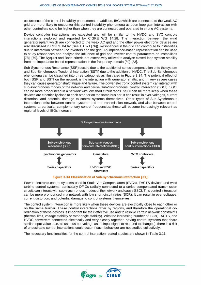
MODELLING OF INVERTER-BASED GENERATION FOR POWER SYSTEM DYNAMIC STUDIES
87
occurrence of the control instability phenomena. In addition, IBGs which are connected to the weak AC grid are more likely to encounter this control instability phenomena as open loop gain interaction with other controllers could be higher than when they are connected and operated in strong AC systems.
Device controller interactions are expected and will be similar to the HVDC and SVC controls interactions explored and reported by CIGRE WG 14.28. The interaction between the wind generators/plant which are connected to the weak AC grid and the other power electronic devices are also discussed in CIGRE B4.62 (See TB 671 [76]). Resonances in the grid can contribute to instabilities due to interaction between PV inverters and the grid. An impedance-based representation can be used to study resonances and analyse the influence of grid and inverter control parameters on instabilities [78], [79]. The Nyquist and Bode criteria are extensively utilized to analyse closed-loop system stability from the impedance-based representation in the frequency domain [80]-[83].
Sub-Synchronous Resonance (SSR) occurs due to the addition of series compensation onto the system and Sub-Synchronous Torsional Interaction (SSTI) due to the addition of HVDC. The Sub-Synchronous phenomena can be classified into three categories as illustrated in Figure 3.34. The potential effect of both SSR and SSTI on the network is the interaction with generator shafts, and in very severe cases they can cause generator shaft fatigue and failure. The power electronic control system can interact with sub-synchronous modes of the network and cause Sub-Synchronous Control Interaction (SSCI). SSCI can be more pronounced in a network with low short circuit ratios. SSCI can be more likely when these devices are electrically close to each other or on the same bus bar. It can result in over-voltages, current distortion, and potential damage to control systems themselves. Other types of Sub-Synchronous Interactions exist between control systems and the transmission network, and also between control systems at particular complementary control frequencies; these will become increasingly relevant as regional levels of IBGs increase.
Figure 3.34 Classification of Sub-synchronous interaction [31].
Power electronic control systems used in Static Var Compensators (SVCs), FACTS devices and wind turbine control systems, particularly DFIGs radially connected to a series compensated transmission circuit, can interact with sub-synchronous modes of the network and cause SSCI. This control interaction can be more pronounced in a network with low short circuit ratios (SCR). It can result in over-voltages, current distortion, and potential damage to control systems themselves.
The control system interaction is more likely when these devices are electrically close to each other or on the same busbar. These control interactions differ by regions, and therefore the operational co-ordination of these devices is important for their effective use and to resolve certain network constraints (thermal limit, voltage stability or rotor angle stability). With the increasing number of IBGs, FACTS, and HVDC converters connected electrically and very closely together, having control systems that share similar input values (i.e. all use bus bar voltage as an input signal to respond to changes), there is a risk of undesirable control interactions could occur if such behaviour are not studied collectively.
The necessary functionalities for the control interaction related studies are shown in Table 3.11.

MODELLING OF INVERTER-BASED GENERATION FOR POWER SYSTEM DYNAMIC STUDIES
88
Table 3.11 Necessary functionalities for controller interaction studies (simplified table)
Category Functionalities Necessity Remark
Control All Yes
Protection All No no protection due to small signal analysis
Capability All Yes
3.7.2 Maximum Penetration of IBGs
The increasing penetration of IBG has changed the dynamic behaviour of power systems. In the future, even more IBG units are planned to be integrated, eventually displacing conventional synchronous generators. Therefore, the investigation of the maximum penetration rate of IBGs as well as the necessary amount of conventional synchronous generators than need to stay connected on system stability could become one of the critical studies in power system control, operation and planning. In general, IBGs affect dynamic system stability by changing the pre-disturbance operating conditions as well as by exhibiting different dynamic response during and right after disturbances. The intermittent nature of most of the IBG units such as WTG and PV units could introduce higher uncertainty in determining pre-fault operating conditions raising also the need for evaluation of worst case operating conditions. The probabilistic stability assessment has proven to be one of the promising ways to do this type of study due to the appropriate accounting of uncertain parameters affecting their behaviour, e.g., system loading, fault location, fault duration, etc. The probabilistic stability assessment is typically performed using Monte Carlo (MC) dynamic simulations. The maximum penetration rate of IBGs considering the displacement of the synchronous generators (either disconnection or unloading of generators) is investigated in [84]-[86]. According to the transient stability study, as shown in Figure 3.35, a turning point in terms of power swing oscillation behaviour can be observed when the penetration rate is around 50%, which is likely to be relevant to the maximum penetration rate of IBGs, i.e., the minimum necessary amount of the synchronous generators.
Figure 3.35 Cumulative distribution function of transient stability index
for different spare capacity [84].
According to a frequency instability study, shown in Figure 3.36, a turning point in terms of the dynamic behaviour/aspect of the frequency drop can be also observed when the penetration rate is around 50%. In both cases the maximum penetration rate is around 50%. Although the results illustrated in the figure
-100 -80 -60 -40 -20 0 20 40 60 800
0.1
0.2
0.3
0.4
0.5
0.6
0.7
0.8
0.9
1
Transient Stability Index
Cu
mu
lati
ve P
ro
ba
bil
ity
no IBG
20% IBG
30% IBG
40% IBG
50% IBG
60% IBG
-80 -60 -40 -20 0 200.05
0.1
0.15
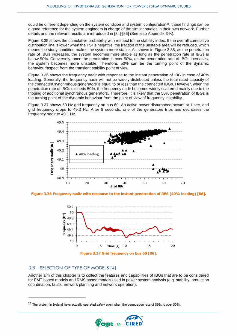
MODELLING OF INVERTER-BASED GENERATION FOR POWER SYSTEM DYNAMIC STUDIES
89
could be different depending on the system condition and system configuration26, those findings can be a good reference for the system engineers in charge of the similar studies in their own network. Further details and the relevant results are introduced in [84]-[86] (See also Appendix 3-K).
Figure 3.35 shows the cumulative probability with respect to the stability index. If the overall cumulative distribution line is lower when the TSI is negative, the fraction of the unstable area will be reduced, which means the study condition makes the system more stable. As shown in Figure 3.35, as the penetration rate of IBGs increases, the system becomes more stable as long as the penetration rate of IBGs is below 50%. Conversely, once the penetration is over 50%, as the penetration rate of IBGs increases, the system becomes more unstable. Therefore, 50% can be the turning point of the dynamic behaviour/aspect from the transient stability point of view.
Figure 3.36 shows the frequency nadir with response to the instant penetration of IBG in case of 40% loading. Generally, the frequency nadir will not be widely distributed unless the total rated capacity of the connected synchronous generators is equal to or less than the connected IBGs. However, when the penetration rate of IBGs exceeds 50%, the frequency nadir becomes widely scattered mainly due to the tripping of additional synchronous generators. Therefore, it is likely that the 50% penetration of IBGs is the turning point of the dynamic behaviour from the point of view of frequency instability.
Figure 3.37 shows 50 Hz grid frequency on bus 60. An active power disturbance occurs at 1 sec, and grid frequency drops to 49.3 Hz. After 8 seconds, one of the generators trips and decreases the frequency nadir to 49.1 Hz.
Figure 3.36 Frequency nadir with response to the instant penetration of RES (40% loading) [86].
Figure 3.37 Grid frequency on bus 60 [86].
3.8 SELECTION OF TYPE OF MODELS [4]
Another aim of this chapter is to collect the features and capabilities of IBGs that are to be considered for EMT based models and RMS based models used in power system analysis (e.g. stability, protection coordination, faults, network planning and network operation).
26 The system in Ireland have actually operated safely even when the penetration rate of IBGs is over 50%.
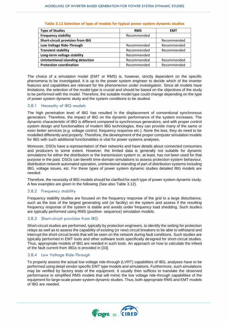
MODELLING OF INVERTER-BASED GENERATION FOR POWER SYSTEM DYNAMIC STUDIES
90
Table 3.12 Selection of type of models for typical power system dynamic studies
Type of Studies RMS EMT
Frequency stability Recommended
Short-circuit provision from IBG Recommended
Low Voltage Ride-Through Recommended Recommended
Transient stability Recommended Recommended
Long-term voltage stability Recommended
Unintentional islanding detection Recommended Recommended
Protection coordination Recommended Recommended
The choice of a simulation model (EMT or RMS) is, however, strictly dependent on the specific phenomena to be investigated. It is up to the power system engineer to decide which of the inverter features and capabilities are relevant for the phenomenon under investigation. Since all models have limitations, the selection of the model type is crucial and should be based on the objectives of the study to be performed with the model. Therefore, the suitable model type could change depending on the type of power system dynamic study and the system conditions to be studied.
3.8.1 Necessity of IBG models
The high penetration level of IBG has resulted in the displacement of conventional synchronous generators. Therefore, the impact of IBG on the dynamic performance of the system increases. The dynamic characteristic of IBG is different compared to synchronous generators, and with proper control system design and functionalities of modern IBG technologies, they can provide many of the same or even better services (e.g. voltage control, frequency response etc.). None the less, they do need to be modelled differently and properly. Therefore, the development of the proper computer simulation models for IBG with such additional functionalities is vital for power systems analyses.
Moreover, DSOs have a representation of their networks and have details about connected consumers and producers to some extent. However, the limited data is generally not suitable for dynamic simulations for either the distribution or the transmission system or, at least, has not been used for that purpose in the past. DSOs can benefit time-domain simulations to assess protection system behaviour, distribution network automated operation, unintentional islanding of part of distribution systems including IBG, voltage issues, etc. For these types of power system dynamic studies detailed IBG models are needed.
Therefore, the necessity of IBG models should be clarified for each type of power system dynamic study. A few examples are given in the following (See also Table 3.12).
3.8.2 Frequency stability
Frequency stability studies are focused on the frequency response of the grid to a large disturbance, such as the loss of the largest generating unit (or facility) on the system and assess if the resulting frequency response of the system is stable and avoids under frequency load shedding. Such studies are typically performed using RMS (positive- sequence) simulation models.
3.8.3 Short-circuit provision from IBG
Short-circuit studies are performed, typically by protection engineers, to identify the setting for protection relays as well as to assess the capability of existing (or new) circuit breakers to be able to withstand and interrupt the short-circuit levels that will be seen on the network during fault conditions. Such studies are typically performed in EMT tools and other software tools specifically designed for short-circuit studies. Thus, appropriate models of IBG are needed in such tools. An approach on how to calculate the infeed of the fault current from IBGs is provided in [33].
3.8.4 Low Voltage Ride-Through
To properly assess the actual low voltage ride-through (LVRT) capabilities of IBG, analyses have to be performed using detail vendor specific EMT type models and simulations. Furthermore, such simulations may be verified by factory tests of the equipment. It usually then suffices to translate the observed performance to simplified RMS models that will mimic the low voltage ride-through capabilities of the equipment for large-scale power system dynamic studies. Thus, both appropriate RMS and EMT models of IBG are needed.
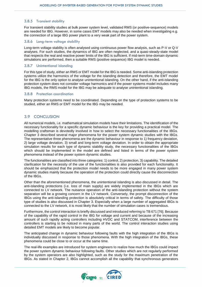
MODELLING OF INVERTER-BASED GENERATION FOR POWER SYSTEM DYNAMIC STUDIES
91
3.8.5 Transient stability
For transient stability studies at bulk power system level, validated RMS (or positive-sequence) models are needed for IBG. However, in some cases EMT models may also be needed when investigating e.g. the connection of a large IBG power plant to a very weak part of the power system.
3.8.6 Long-term voltage stability
Long-term voltage stability is often analysed using continuous power flow analysis, such as P-V or Q-V analyses. For such studies, the dynamics of IBG are often neglected, and a quasi-steady-state model that respects the real and reactive power limits of the IBG is sufficient. If mid-term time-domain dynamic simulations are performed, then a suitable RMS (positive-sequence) IBG model is needed.
3.8.7 Unintentional islanding
For this type of study, either an RMS or EMT model for the IBG is needed. Some anti-islanding protection systems utilize the harmonics of the voltage for the islanding detection and therefore, the EMT model for the IBG is the only option to analyse unintentional islanding. On the other hand, if the anti-islanding protection system does not consider voltage harmonics and if the power systems model includes many IBG models, the RMS model for the IBG may be adequate to analyse unintentional islanding.
3.8.8 Protection coordination
Many protection systems need to be coordinated. Depending on the type of protection systems to be studied, either an RMS or EMT model for the IBG may be needed.
3.9 CONCLUSION
All numerical models, i.e. mathematical simulation models have their limitations. The identification of the necessary functionality for a specific dynamic behaviour is the key for providing a practical model. The modelling craftsman is devotedly involved in how to select the necessary functionalities of the IBGs. Chapter 3 described several major phenomena for the power system dynamic studies with the IBGs. The representative three phenomena are the dynamic behaviour in response to 1) frequency deviation, 2) large voltage deviation, 3) small and long-term voltage deviation. In order to obtain the appropriate simulation results for each type of dynamic stability study, the necessary functionalities of the IBGs which should be implemented in the model are defined and listed in terms of the power system phenomena instead of the power system dynamic studies.
The functionalities are classified into three categories: 1) control, 2) protection, 3) capability. The detailed clarification for the necessity of the use of the functionalities is also provided for each functionality. It should be emphasized that the protection model needs to be more engaged in many power system dynamic studies mainly because the operation of the protection could directly cause the disconnection of the IBGs.
Other than the aforementioned phenomena, the unintentional islanding is also discussed in detail. The anti-islanding protections (i.e. loss of main supply) are widely implemented in the IBGs which are connected to LV network. The nuisance operation of the anti-islanding protection without the system separation will be a growing concern in the LV network. Conversely, the prompt disconnection of the IBGs using the anti-islanding protection is absolutely critical in terms of safety. The difficulty of those type of studies is also discussed in Chapter 3. Especially when a large number of aggregated IBGs is connected to the LV network, it is most likely that the number of simulation cases is tremendous.
Furthermore, the control interaction is briefly discussed and introduced referring to TB 671 [76]. Because of the capability of the rapid control in the IBG for voltage and current and because of the increasing amount of such rapidly acting controllers including HVDC and STATCOM, interference between the controllers is starting to be noticed in many parts of the world. The control interaction studies using detailed EMT models are likely to become popular.
The anticipated change in dynamic behaviour following faults with the high integration of the IBGs is individually discussed in response to those phenomena. With the high integration of the IBGs, these phenomena could be close to or occur at the same time.
The real-life examples are introduced for system engineers to realize how much the IBGs could impact the power system dynamic behaviour following faults. Other studies which are not regularly performed by the system operators are also highlighted, such as the study for the maximum penetration of the IBGs. As stated in Chapter 2, IBGs cannot accomplish all the capability that synchronous generators

MODELLING OF INVERTER-BASED GENERATION FOR POWER SYSTEM DYNAMIC STUDIES
92
have. Therefore, the required amount of percentage of the synchronous generators in the system should be more the focus from the power system operator's point of view. The new methodology using the probabilistic approach is also described in Chapter 3.
MODELLING OF INVERTER-BASED GENERATION FOR POWER SYSTEM DYNAMIC STUDIES
93
4. EMT MODELS FOR INVERTER BASED GENERATION
4.1 INTRODUCTION
There are two commonly used power system simulation models:
Electromagnetic transient (EMT) models and
Phasor models or RMS-type models
The electromagnetic transients tools/program has been the most well-known and widely used simulation tool as a circuit theory-based approach assuming a transverse electromagnetic mode (TEM) since its original development in the Bonneville Power Administration of the US Department of Energy from 1966 to 1984 [87], [88], [91]. In EMT tools, power system components are adequately modelled to simulate high-frequency transients in power systems. This makes EMT programs valuable when studying the effects of power-electronic devices on system behaviour. In order to cover the necessary bandwidth, these programs use small integration time steps of the order of 50 µs or less, making EMT simulation much slower than RMS simulation. The common practice in dealing with large systems in EMT programs is to divide the system into a study zone where the transient phenomena occur and an external system encompassing the rest of the system, in order to reduce computational burden [92].
EMT and real-time time domain analysis programs solve the differential equations of the electrical network as compared to transient stability analysis which uses RMS positive sequence phasor equations to represent the electrical network. This distinction means that EMT analysis is capable of representing:
The non-linear response of electrical devices (e.g. transformer saturation or surge arresters)
Frequency dependent effects (generally over a wide range of frequencies, including DC, sub-
synchronous frequencies, harmonics, interharmonics, resonances and higher frequency transients)
Unbalanced networks (suitable for single line to ground faults, negative and zero sequence
components of transients, etc.)
Detailed power electronic devices (including switching transients and associated harmonics, as well
as the detailed controls and protection systems)
For IBGs, EMT analysis can be used to model the detailed switching devices (IGBTs, GTOs, thyristors, diodes etc.) in a converter, as well as the control systems. EMT models are subsequently used to investigate transient phenomena of power systems such as:
Switching transients and over-voltages.
Short-term analysis of the disturbances.
Transient over-currents.
Internal and external IBG protection performance.
Power quality degradation and harmonics.
Dynamic controls of electric generators and drives.
Operation of FACTS, HVDC, SVC, STATCOMs, etc.
Dynamic operation of wind plants, PV inverters, etc.
Sub-synchronous phenomena (SSR, SSTI, SSCI) and torque amplification.
Control interactions between complex devices.
Generally, EMT analysis is not required in the initial or feasibility stages of a project and is often only introduced later in the overall design and study process. EMT models may also be required under special system conditions where RMS transient stability programs may not be sufficiently accurate or even suitable:
Weak system conditions.
Phenomena to be studied at other frequencies than fundamental frequency, e.g. SSR or
harmonics.
Systems with multiple power electronic inverters or devices in close proximity.
Applications where detailed control algorithms or the use of the actual controller code, compiled and
linked into the EMT program are required.

MODELLING OF INVERTER-BASED GENERATION FOR POWER SYSTEM DYNAMIC STUDIES
94
4.1.1 EMT algorithms and variations
The EMT algorithm which uses trapezoidal integration and nodal analysis was originally developed by Dr. Herman Dommel in his 1969 paper [87] – this was the original EMT tools/programs. An independent development effort of the EMT tool/program that covers DC network was undertaken by Dennis Woodford [89], following the basic Dommel algorithm [87]-[90]. Other common programs using the EMT algorithm or derivatives have also been developed. Commercial programs for translation from an RMS program to EMT programs are available, as well as parallel processing add-ons and hybrid simulation (running EMT and transient stability programs interfaced together in the same simulation). Other common real time digital simulators have also been developed. Some ad-hoc tools can be also used for hardware in loop real-time simulations.
The key concept of the aforementioned original EMT tools/programs is the use of a linear finite difference equation to solve a differential equation – each passive electrical element of the power system (i.e. inductors, capacitors, etc.) is represented individually as a resistor and parallel current injection (which depends only on quantities from the previous time step (i.e. known as a history term).
The formulation for a simple inductor is shown in Figure 4.1, and for a capacitor in Figure 4.2. The example of the aforementioned key concept is also shown in Figure 4.3.
Figure 4.1 EMT formulation of inductor differential equation as a difference equation via Trapezoidal integration.
Figure 4.2. EMT formulation of a capacitor differential equation as a difference equation via Trapezoidal integration.
The above EMT formulation allows each individual circuit element in a complex system of non-linear differential equations to be represented by a resistor and current injection. The problem is reduced to a linear matrix solution for each time step (i.e. solving N linear equations with N unknowns). Other circuit elements (like transformers, transmission lines, machines, etc.) can also be derived in similar fashion. Standard sparse matrix solution techniques can be used to solve such equations with minimal memory and maximum speed [93].
The use of trapezoidal integration is deliberate and key in this formulation. An integration is the area under the waveform with respect to time, and trapezoidal integration essentially approximates the waveform (over 1 time step) as a trapezoid – the area therefore is the time step dt times the average of the quantities at time T and T-dt, which is in the case of voltage, waveform [v(t) + v(t-dt)]/2. Higher order approximations are possible, but can lead to numerical instabilities whereas trapezoidal integration is guaranteed to be stable for linear circuits.
Note that the application of trapezoidal integration is a first order linear approximation applied between successive simulation time steps. The smaller the time step, the more accurate the approximation will be. This places an inherent error in any EMT simulation, as well as an effective limitation on the frequency bandwidth over which the solution is valid. A good "rule of thumb" is that there should be at least 20 time steps per cycle at the highest frequency of interest – for typical transient over-voltage

MODELLING OF INVERTER-BASED GENERATION FOR POWER SYSTEM DYNAMIC STUDIES
95
simulations with a frequency range of interest from DC to approximately 2 kHz this requires a time step of 25 µs. The same simulation method can be used for transients over a wider range of frequencies (e.g. for lightning transients) if a small enough time step is used.
Thevenin to Norton Transformation
Figure 4.3. Linear equivalent circuit - conversion of differential equations to finite difference equations.
Some simulation programs use the concept of subsystems, which identifies sub-networks whose network is coupled to other sub-networks only by traveling wave transmission line models. Bergeron or frequency dependent models have no impedance element connecting the sending end to the receiving end of the line or cable and the responses on either end to a change on the other end is delayed by the traveling time of the electromagnetic (EM) wave. For an overhead transmission lines (in open air) the EM wave travels with almost the speed of light. Therefore, a 30-km long line exhibits a natural delay of approximately 50 µs. This technique of using Bergeron line models to couple sub-networks allows those sub-networks to be solved on parallel processors without introducing artificial delays during the exchange of state variables, provided the natural delay in the coupling lines are at least one simulation time step long. As such it is often used in digital real-time (RT) simulators (DRTSs) which require parallel processing for simulation speed and large networks are broken up onto numerous CPUs with communication delays mapped to traveling wave line model delays. This technique can also be used to interconnect sub-networks solved at smaller time steps e.g. a network of power electronic switches represented as a transition between a large resistance in the off state and a small resistance in the on state.
Many modern non-RT EMT programs also make use of interpolation, which allows switching instants to occur at precise points between the regular time step grids. This has accuracy benefits such as precise turn-on and turn-off instants for power electronic devices as well as stability benefits such as the prevention of on/off/on/off and interactions due to trying to switch two or more devices in the same time step. It can also be demonstrated that trapezoidal integration can result in time-step to time-step high frequency numerical problems when a circuit with only inductors to ground or with capacitors in a loop are represented. This is also solved with interpolation (i.e. half steps) or with the critical damping adjustment procedure (CDA) [94].
Some non-RT programs are also able to change the simulation time step, either dynamically during the run (perhaps to use a smaller time step around a switching instant) or allowing a reduction in the time step near a transient. A reduction in the time step brings the time for a switching closer to the exact point. However numerous devices may still need to switch in one time step which can lead to on/off/on/off instabilities, or more importantly, the switching of one device may initiate the need to switch another device, immediately. This illustrates the fundamental problem associated with modelling power electronic switches in EMT programs: while in reality, parasitic capacitances, inductances, and a finite
MODELLING OF INVERTER-BASED GENERATION FOR POWER SYSTEM DYNAMIC STUDIES
96
switching time (during which the semiconductor layers lose conductivity) all play a role in the actual transition between the “on” and “off” state of, say, an IGBT, these transitions are typically not properly modelled in EMT type simulations. The transitions are approximated by “ideal switching” which in turn can lead to numerical problems. For example, if the current through an inductor is forced from any value i(t) to zero in one time step dt, it will result in a voltage across that inductor proportional to L*i/dt. The smaller the time step the larger the artificial voltage spike. Interpolation and variable time step techniques can minimize these numerical problems and so can proper applications of artificial damping and snubber circuits (often used with fixed time step solvers) within the representation of the power electronic switches in the model.
EMT algorithms are inherently solved in the time domain (like RMS transient stability programs) – i.e. the solution produces time series of voltages, currents, control signals which can also be graphed as such. Some programs also include a native frequency domain solution – this is useful for filter design, or for computation/plotting of the frequency response of the system. Techniques for deriving the equivalent impedance vs. frequency of a non-linear device can also be applied (known as perturbation analysis) and can supplement the linear frequency domain solution of a network.
It is also worth noting there are variations in the main circuit nodal admittance (NA) matrix solutions – the classic EMT algorithm uses a sparse matrix solver where G is the N x N conductance matrix, V is the vector of node voltages to be solved, and I is the vector of known current sources. Ideal voltage sources and zero impedance branches can be added to this formulation – this avoids ill-conditioned matrix problems from the use of extremely small switch resistances (i.e. large conductance). A modified version of these techniques is called Modified Nodal Admittance (MNA), which directly solves both nodal voltages and current flows in the ideal branches [95].
Most modern programs are driven by a graphical user interface (GUI) – this allows the user to construct both the electrical circuit and the controllers using building blocks that can be connected together. These programs usually also allow interfacing to custom user-written code, often supplied by the manufacturer of the device. In order to hide the confidential source code, the end user will often receive only binary code (i.e. .lib, .obj or .dll files).
4.1.2 Real-time simulation
Digital real-time (RT) digital simulators (DRTSs) may require special processing in order to maintain real-time speed. For example, interpolation of the electrical network may not be possible due to a non-determinable number of switching events that may be required over a given small time period.
One solution used in DRTSs is to take advantage of the Dommel algorithm conductance for a switching device, so it does not change when the state of the switching device changes. When a switch is in the closed state, it is represented in the Dommel algorithm as an inductor (L) branch. Conversely, when it is in the open state, it is represented as a series resistor-capacitor (RC) branch. The R in the RC branch can be selected as a user-specifiable damping factor, so that if the closed branch was connected in series with a branch with the open state, there would be a series RLC branch. This method avoids switching of the conductance matrix altogether, with natural savings in processing time [96].
When a device model switches from an open state to a closed state, the energy in the capacitor C is lost and should eventually be replaced. Assume that i is the rated switched current and v is the rated switched voltage. The expenditure of energy in this case is equal to Cv2. When a device model switches from a closed state to an open state, energy in the inductor L is lost, which is equal to Li
2/2. In order to minimize the losses, the suggestion on constraint is applied for selecting R, L and C: Cv2 should be equal to Li
2/2. Examination of L and C indicates that the ratio of the open state impedance to the closed state impedance at any frequency (f) is above 1/(2 π f ΔT f)2 [97]. Consequently, the smaller time-step leads to greater ratio of the impedances. Hence, it is desirable to keep the time step as small as possible or ensure the switching frequency of the converter is not too high. For time steps around 2.5 µs the converter switching frequency should not exceed 3 kHz. The smaller the simulation time step the larger the allowable switching frequency.
Modern RT simulators also can directly implement “Discrete Switch Models” [98], [99], due to improvements in sparsity/subsystem/partitioning matrix algorithms, as well as faster processors. If the limit on the number of switch/conductance states is avoided by on-line computation of changes in switches, this may alleviate the restrictions on topology and the number of switching elements in a given case.
4.1.3 Advanced EMT modelling
Recent advances in EMT modelling include [91], [100], [101]:
MODELLING OF INVERTER-BASED GENERATION FOR POWER SYSTEM DYNAMIC STUDIES
97
Large system modelling and EMT dynamic performance studies. Parallel processing of EMT cases. Hybrid simulation with EMT and RMS programs. Databases to translate/initialize EMT models from RMS load flow/models.
Large systems can be modelled in today’s EMT programs. Such models have numerous SVCs, HVDC links, wind plants, PV inverters, complex load models, large AC system models, comprehensive setup for faults/contingencies, etc. This is really only warranted in complex networks with numerous complex devices, or in weak system conditions, for most studies large system analysis is limited to RMS/transient stability analysis. The lure of three phase analysis, proper representation of unbalanced/single phase faults, use of exact controls/protection models, customizable models of power electronic devices, etc. is attractive however the line between RMS tools and EMT tools is certainly blurring.
When large system studies are required, the CPU time for the analysis is a significant factor EMT tools
use small time steps (often 50 s, or less for some device models), three phases (instead of positive sequence circuits) and include non-linear devices – all of which make models slower compared to RMS transient stability analysis.
Parallel processing is now possible in some programs – systems can be broken up into subsystems, using similar methods as developed for RT simulators. The power system can be separated at any transmission or cable line location (specifically lines/cables whose travel time is larger than the simulation time step) or at any transformer (by using a transformer scaling component). Each subsystem can be operated at a different time step using interpolation of traveling waves in the line models – this
is a significant factor, as otherwise a single demanding device say a VSC inverter which requires a 5 s time step to operate would dominate the time step for the entire simulation.
Hybrid simulation techniques have also been developed and can be used to run EMT and RMS transient stability programs in the same combined simulation. The RMS program results (i.e. magnitude and phase angle of fundamental voltage/currents at the interface) are used to update network equivalents in the EMT programs. EMT results are processed via FFT/DFT (Fast Fourier Transform/Discrete Fourier Transform) algorithms to extract the positive sequence behaviour, which is communicated to the RMS program where it updates a dynamic load/generator model. Operation of the two programs can be made transparent so a single start command initiates both programs.
Hybrid simulation can be viewed as the imbedding of complex/exact EMT models into RMS transient stability programs. Alternatively, the hybrid interface can be seen to provide a dynamic network equivalent to EMT programs. These techniques allow fast development and implementation of accurate EMT models (which would otherwise be complex/time consuming to develop custom models in RMS transient stability programs – say a detailed PV inverter model) into traditional and widely used RMS algorithms.
The development of hybrid interfaces and parallel processing will allow for more detailed modelling of power electronic inverters on a large scale – this will be important for the future as the power systems become more complex.
4.1.4 Confidentiality aspects of EMT models
EMT models are often developed by the manufacturer using real code (i.e. the source code which are used for the actual hardware) and are usually considered to be highly confidential. Users who require access to these models are often required to sign strict non-disclosure agreements (NDAs) – this is often troublesome in many interconnection agreements, where the developer must provide models to the system operator, consultants, or other utilities.
One possible method to avoid some NDA issues if any part is deemed confidential is by “black-boxing” – this takes either a complete control circuit model or electrical circuit model or in some cases both (i.e. a complete model) and encloses the model into a single object or component thus removing the ability to dig deeper into the model and see its sub-contents.
Some programs can automate the process of black-boxing or provide user-access passwords before sub-pages can be opened. In other cases, the process to blackbox models can be time consuming and expenses, particularly for the electrical system.
However, there are some clear disadvantages:
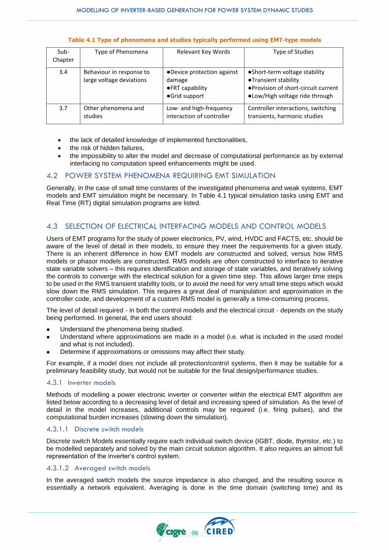
MODELLING OF INVERTER-BASED GENERATION FOR POWER SYSTEM DYNAMIC STUDIES
98
Table 4.1 Type of phenomena and studies typically performed using EMT-type models
Sub-Chapter
Type of Phenomena Relevant Key Words Type of Studies
3.4 Behaviour in response to large voltage deviations
●Device protection against damage ●FRT capability ●Grid support
●Short-term voltage stability ●Transient stability ●Provision of short-circuit current ●Low/High voltage ride through
3.7 Other phenomena and studies
Low- and high-frequency interaction of controller
Controller interactions, switching transients, harmonic studies
the lack of detailed knowledge of implemented functionalities,
the risk of hidden failures,
the impossibility to alter the model and decrease of computational performance as by external interfacing no computation speed enhancements might be used.
4.2 POWER SYSTEM PHENOMENA REQUIRING EMT SIMULATION
Generally, in the case of small time constants of the investigated phenomena and weak systems, EMT models and EMT simulation might be necessary. In Table 4.1 typical simulation tasks using EMT and Real Time (RT) digital simulation programs are listed.
4.3 SELECTION OF ELECTRICAL INTERFACING MODELS AND CONTROL MODELS
Users of EMT programs for the study of power electronics, PV, wind, HVDC and FACTS, etc. should be aware of the level of detail in their models, to ensure they meet the requirements for a given study. There is an inherent difference in how EMT models are constructed and solved, versus how RMS models or phasor models are constructed. RMS models are often constructed to interface to iterative state variable solvers – this requires identification and storage of state variables, and iteratively solving the controls to converge with the electrical solution for a given time step. This allows larger time steps to be used in the RMS transient stability tools, or to avoid the need for very small time steps which would slow down the RMS simulation. This requires a great deal of manipulation and approximation in the controller code, and development of a custom RMS model is generally a time-consuming process.
The level of detail required - in both the control models and the electrical circuit - depends on the study being performed. In general, the end users should:
Understand the phenomena being studied. Understand where approximations are made in a model (i.e. what is included in the used model
and what is not included). Determine if approximations or omissions may affect their study.
For example, if a model does not include all protection/control systems, then it may be suitable for a preliminary feasibility study, but would not be suitable for the final design/performance studies.
4.3.1 Inverter models
Methods of modelling a power electronic inverter or converter within the electrical EMT algorithm are listed below according to a decreasing level of detail and increasing speed of simulation. As the level of detail in the model increases, additional controls may be required (i.e. firing pulses), and the computational burden increases (slowing down the simulation).
4.3.1.1 Discrete switch models
Discrete switch Models essentially require each individual switch device (IGBT, diode, thyristor, etc.) to be modelled separately and solved by the main circuit solution algorithm. It also requires an almost full representation of the inverter’s control system.
4.3.1.2 Averaged switch models
In the averaged switch models the source impedance is also changed, and the resulting source is essentially a network equivalent. Averaging is done in the time domain (switching time) and its

MODELLING OF INVERTER-BASED GENERATION FOR POWER SYSTEM DYNAMIC STUDIES
99
components. One application for an Averaged Switch Model is for a modular multilevel converter (MMC) or similar type of converter.
4.3.1.3 Simple source models
In this simplified model, the inverter output current reference signal (from an outer PI controller for example) is converted to a three phase ABC reference system using the PLL angle which in turn is injected into the electrical grid via current sources.
4.3.2 Controller models
EMT models are solved with fixed or sometimes variable time step techniques. The controller receives the voltages and currents from the last time step, then the controls are called (possibly in the exact order in which the real controls are called, and possibly with the same controller sampling time as the real controls) to generate output signals such as firing pulses. Then the output signals are connected back into the electrical simulation to turn on/off IGBTs, etc. The EMT method of modelling often uses much smaller time steps than the real controller sampling time which means that less manipulation and fewer approximations are required. However, the oversampling of the control system can sometimes lead to inaccurate results if controller interrupts are not modelled appropriately. Programming of detailed power electronic models is often much easier accomplished in the EMT world. The level of detail in the controls is also related to the level of detail in the electrical portion of the models – for example a Simple Source Interfaced converter model may inject only high level currents into the system (similar to RMS models) and hence will not require inner PI loops, nor IGBT firing pulse logic, capacitor balancing logic, etc.
Controls for power electronic inverters can be implemented in many ways in EMT programs as described in the following clauses:
4.3.2.1 Generic control models
Generic (EMT) models are probably quite similar to the models used in RMS programs. Standard controller building blocks are used (say for an integrator, or a first order real pole, lead lag, etc.) without attention to how each model is implemented (integration method used, Z transform methods, etc.) or the time step used in the controls. The controls are usually sampled at the same time step as is used in the electrical solution. Often these models are included in the programs as a library model (say for a PLL function, or for VSC firing logic), or may be available as a collection of standard building blocks.
4.3.2.2 Detailed models with standard library building block functions
Detailed models can also be constructed using standard library building block functions. However, they are constructed to a much greater level of detail. Since they are not an exact representation of the real code, many parts of the code are omitted, and the details of how a given function is implemented are ignored due to the inherent use of standard functions. These control models are often solved with the same time step as the main electrical circuit.
4.3.2.3 Custom detailed models
Custom detailed models can be a near-exact representation of the real code. Most real controllers are developed with a GUI (graphical user interface) – sometimes proprietary, but which can also be part of a simulation package. The tool which is used to develop the real controls, inherently has controller building blocks, which can be duplicated in a given simulation program on an individual building block basis. Once an equivalent library of building blocks is complete, the overall controller functions can be duplicated, either by manually manipulating control blocks or possibly automated, if such features are provided. The overall level of detail in “Custom Detailed Models” varies, depending on the manufacturer and developer of the model – factors to consider are:
How much of the controller is represented and which portions are omitted? Are protection functions included? Is the model maintained and kept up-to-date with site changes or project changes? Are all gains
and settings the same as the “as-built” in service converter? Is the order of execution of the individual building blocks guaranteed to be the same as in the real
code? Is the time step used in the controls the same as the real hardware (which is likely different than
the time step used in the EMT electrical network solver)? Have the model been validated and compared to the site traces/real code?
MODELLING OF INVERTER-BASED GENERATION FOR POWER SYSTEM DYNAMIC STUDIES
100
4.3.2.4 Exact models
Exact models are constructed by taking the actual source code from the real controller, and compiling/linking/interfacing it directly into the EMT simulation. Since the real code is used, the concerns regarding the level of detail and approximations used above are avoided. Some of the special aspects which must be considered when developing or using “Exact Models” are:
Is the sample time of the real code reproduced? A sample/hold mechanism should be implemented to ensure the real code is called only at the desired sampling instants.
Is the model capable of being called more than once in the same simulation (i.e. is it re-entrant)? This requires the identification and storage of all controller state variables, such that the state variables from one call to the model are kept separate from other subsequent calls in the same time step.
Is the model capable of being initialized? This is particularly important if the model has long time constants to avoid long run-up times and compatible with a program’s feature to stop and re-start a simulation at any point in time (i.e. snapshots or multiple runs)?
Possible code language and linking issues – when models from many suppliers are required to be executed in the same simulation, this can create linking problems due to incompatibilities between compiler languages or versions, or with overlapping subroutine names in models from each supplier. This is largely resolved if the binary models are released in source code format (if allowed under non-disclosure agreement (NDA) requirements – see above) or if the binaries are released in standard .DLL format (which alleviates most compile/linking issues).
Have all aspects of the controller been included? For example, protection functions imbedded in the controller code are likely included in the “Exact Model” but are all such processor code and external protection functions included?
Validation of “Exact Models” is inherently provided for or may not be required as the complete model generally works “out of the box” without much tweaking or customization required.
An essential disadvantage of detailed (or exact) control models is confidentiality and NDA issues. Since the models may include actual code, either in source code format or in binary form, the model capability could potentially be studied and reverse-engineered/probed to determine its capabilities. Licensing of such models is possible ensuring only validated customers can run the model to avoid such difficulties, but often NDAs are required which prevent general distribution of the models.
The biggest advantage of “Exact Models” is the inherent accuracy and confidence level in the model. It is the “real code” from the actual hardware, simply compiled, validated and linked into a simulation program on a PC. This technique also provides a black-boxed model, somewhat resolving NDA concerns, but also means the end user cannot see the block-by-block control functions and implementation.
There is an effort underway to create a standard suitable for interfacing to both EMT and RMS models – this effort is referenced as IEC-61400-27-1 [77] and is primarily aimed at models of wind turbine controllers. Programs have been developed to directly import the DLL-files and to create the interface to an EMT program (with support for state variable storage, control of the sampling time, re-entrance) including the creation of the graphical appearance and inputs/outputs.
4.3.3 Selection guidelines
The level of detail required, in both the control models and the electrical circuit, depends on the study being performed. The following table illustrates some of these requirements.
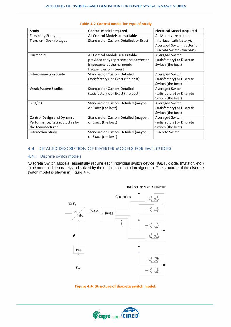
MODELLING OF INVERTER-BASED GENERATION FOR POWER SYSTEM DYNAMIC STUDIES
101
Table 4.2 Control model for type of study
Study Control Model Required Electrical Model Required
Feasibility Study All Control Models are suitable All Models are suitable
Transient Over voltages Standard or Custom Detailed, or Exact Interface (satisfactory), Averaged Switch (better) or Discrete Switch (the best)
Harmonics All Control Models are suitable provided they represent the converter impedance at the harmonic frequencies of interest
Averaged Switch (satisfactory) or Discrete Switch (the best)
Interconnection Study Standard or Custom Detailed (satisfactory), or Exact (the best)
Averaged Switch (satisfactory) or Discrete Switch (the best)
Weak System Studies Standard or Custom Detailed (satisfactory), or Exact (the best)
Averaged Switch (satisfactory) or Discrete Switch (the best)
SSTI/SSCI Standard or Custom Detailed (maybe), or Exact (the best)
Averaged Switch (satisfactory) or Discrete Switch (the best)
Control Design and Dynamic Performance/Rating Studies by the Manufacturer
Standard or Custom Detailed (maybe), or Exact (the best)
Averaged Switch (satisfactory) or Discrete Switch (the best)
Interaction Study Standard or Custom Detailed (maybe), or Exact (the best)
Discrete Switch
4.4 DETAILED DESCRIPTION OF INVERTER MODELS FOR EMT STUDIES
4.4.1 Discrete switch models
“Discrete Switch Models” essentially require each individual switch device (IGBT, diode, thyristor, etc.) to be modelled separately and solved by the main circuit solution algorithm. The structure of the discrete switch model is shown in Figure 4.4.
PLL
D
D
Half Bride MMC Converter
D
D
D
D
...
Half Bridge MMC Converter
Vabc
q
Gate pulses
PWMVref, abc dq
abc
Vd, Vq
Figure 4.4. Structure of discrete switch model.
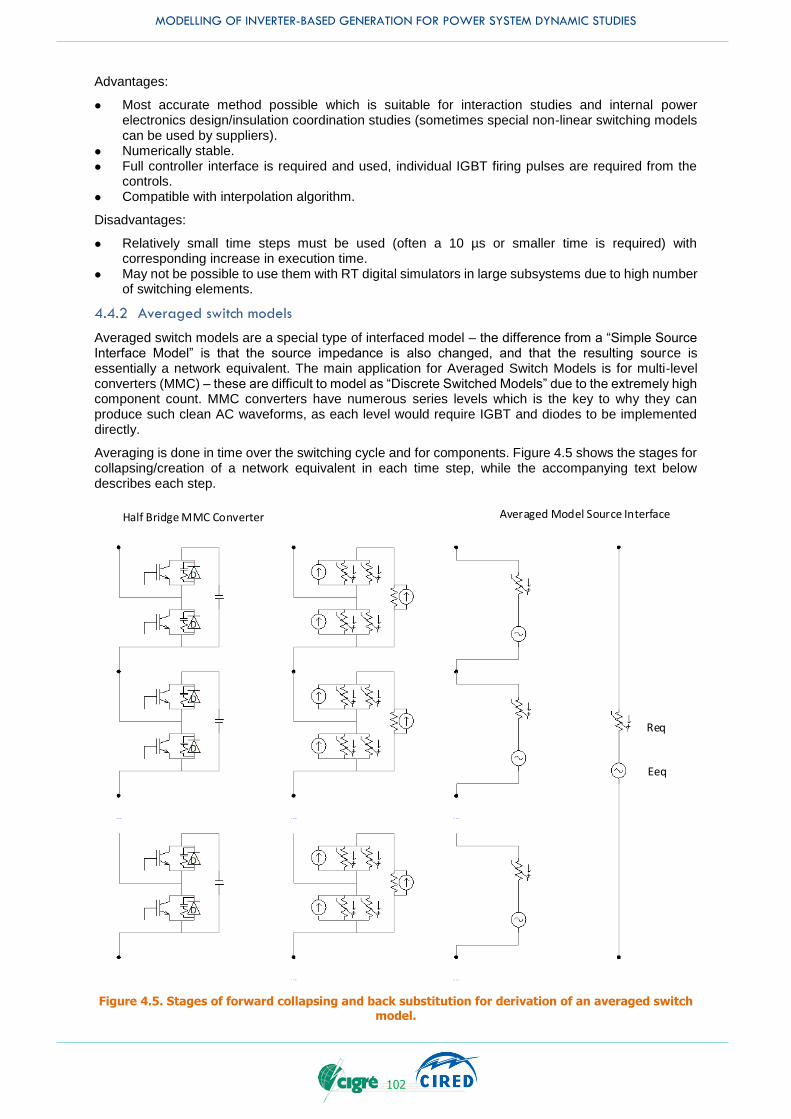
MODELLING OF INVERTER-BASED GENERATION FOR POWER SYSTEM DYNAMIC STUDIES
102
Advantages:
Most accurate method possible which is suitable for interaction studies and internal power electronics design/insulation coordination studies (sometimes special non-linear switching models can be used by suppliers).
Numerically stable. Full controller interface is required and used, individual IGBT firing pulses are required from the
controls. Compatible with interpolation algorithm.
Disadvantages:
Relatively small time steps must be used (often a 10 µs or smaller time is required) with corresponding increase in execution time.
May not be possible to use them with RT digital simulators in large subsystems due to high number of switching elements.
4.4.2 Averaged switch models
Averaged switch models are a special type of interfaced model – the difference from a “Simple Source Interface Model” is that the source impedance is also changed, and that the resulting source is essentially a network equivalent. The main application for Averaged Switch Models is for multi-level converters (MMC) – these are difficult to model as “Discrete Switched Models” due to the extremely high component count. MMC converters have numerous series levels which is the key to why they can produce such clean AC waveforms, as each level would require IGBT and diodes to be implemented directly.
Averaging is done in time over the switching cycle and for components. Figure 4.5 shows the stages for collapsing/creation of a network equivalent in each time step, while the accompanying text below describes each step.
Half Bridge MMC Converter Averaged Model Source Interface
Req
Eeq
Figure 4.5. Stages of forward collapsing and back substitution for derivation of an averaged switch model.
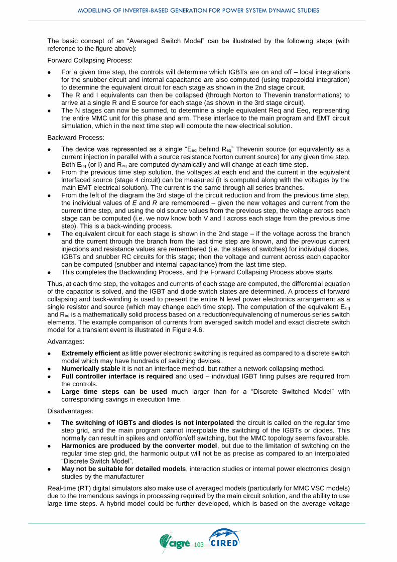
MODELLING OF INVERTER-BASED GENERATION FOR POWER SYSTEM DYNAMIC STUDIES
103
The basic concept of an “Averaged Switch Model” can be illustrated by the following steps (with reference to the figure above):
Forward Collapsing Process:
For a given time step, the controls will determine which IGBTs are on and off – local integrations for the snubber circuit and internal capacitance are also computed (using trapezoidal integration) to determine the equivalent circuit for each stage as shown in the 2nd stage circuit.
The R and I equivalents can then be collapsed (through Norton to Thevenin transformations) to arrive at a single R and E source for each stage (as shown in the 3rd stage circuit).
The N stages can now be summed, to determine a single equivalent Req and Eeq, representing the entire MMC unit for this phase and arm. These interface to the main program and EMT circuit simulation, which in the next time step will compute the new electrical solution.
Backward Process:
The device was represented as a single “Eeq behind Req” Thevenin source (or equivalently as a current injection in parallel with a source resistance Norton current source) for any given time step. Both Eeq (or I) and Req are computed dynamically and will change at each time step.
From the previous time step solution, the voltages at each end and the current in the equivalent interfaced source (stage 4 circuit) can be measured (it is computed along with the voltages by the main EMT electrical solution). The current is the same through all series branches.
From the left of the diagram the 3rd stage of the circuit reduction and from the previous time step, the individual values of E and R are remembered – given the new voltages and current from the current time step, and using the old source values from the previous step, the voltage across each stage can be computed (i.e. we now know both V and I across each stage from the previous time step). This is a back-winding process.
The equivalent circuit for each stage is shown in the 2nd stage – if the voltage across the branch and the current through the branch from the last time step are known, and the previous current injections and resistance values are remembered (i.e. the states of switches) for individual diodes, IGBTs and snubber RC circuits for this stage; then the voltage and current across each capacitor can be computed (snubber and internal capacitance) from the last time step.
This completes the Backwinding Process, and the Forward Collapsing Process above starts.
Thus, at each time step, the voltages and currents of each stage are computed, the differential equation of the capacitor is solved, and the IGBT and diode switch states are determined. A process of forward collapsing and back-winding is used to present the entire N level power electronics arrangement as a single resistor and source (which may change each time step). The computation of the equivalent Eeq and Req is a mathematically solid process based on a reduction/equivalencing of numerous series switch elements. The example comparison of currents from averaged switch model and exact discrete switch model for a transient event is illustrated in Figure 4.6.
Advantages:
Extremely efficient as little power electronic switching is required as compared to a discrete switch model which may have hundreds of switching devices.
Numerically stable it is not an interface method, but rather a network collapsing method. Full controller interface is required and used – individual IGBT firing pulses are required from
the controls. Large time steps can be used much larger than for a “Discrete Switched Model” with
corresponding savings in execution time.
Disadvantages:
The switching of IGBTs and diodes is not interpolated the circuit is called on the regular time step grid, and the main program cannot interpolate the switching of the IGBTs or diodes. This normally can result in spikes and on/off/on/off switching, but the MMC topology seems favourable.
Harmonics are produced by the converter model, but due to the limitation of switching on the regular time step grid, the harmonic output will not be as precise as compared to an interpolated “Discrete Switch Model”.
May not be suitable for detailed models, interaction studies or internal power electronics design studies by the manufacturer
Real-time (RT) digital simulators also make use of averaged models (particularly for MMC VSC models) due to the tremendous savings in processing required by the main circuit solution, and the ability to use large time steps. A hybrid model could be further developed, which is based on the average voltage
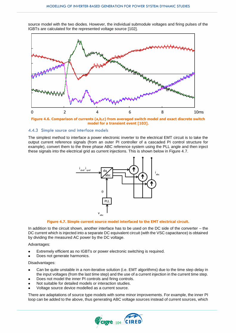
MODELLING OF INVERTER-BASED GENERATION FOR POWER SYSTEM DYNAMIC STUDIES
104
source model with the two diodes. However, the individual submodule voltages and firing pulses of the IGBTs are calculated for the represented voltage source [102].
Figure 4.6. Comparison of currents (a,b,c) from averaged switch model and exact discrete switch model for a transient event [103].
4.4.3 Simple source and interface models
The simplest method to interface a power electronic inverter to the electrical EMT circuit is to take the output current reference signals (from an outer PI controller of a cascaded PI control structure for example), convert them to the three phase ABC reference system using the PLL angle and then inject these signals into the electrical grid as current injections. This is shown below in Figure 4.7.
Figure 4.7. Simple current source model interfaced to the EMT electrical circuit.
In addition to the circuit shown, another interface has to be used on the DC side of the converter – the DC current which is injected into a separate DC equivalent circuit (with the VSC capacitance) is obtained by dividing the measured AC power by the DC voltage.
Advantages:
Extremely efficient as no IGBTs or power electronic switching is required. Does not generate harmonics.
Disadvantages:
Can be quite unstable in a non-iterative solution (i.e. EMT algorithms) due to the time step delay in the input voltages (from the last time step) and the use of a current injection in the current time step.
Does not model the inner PI controls and firing controls. Not suitable for detailed models or interaction studies. Voltage source device modelled as a current source.
There are adaptations of source type models with some minor improvements. For example, the inner PI loop can be added to the above, thus generating ABC voltage sources instead of current sources, which
0 2 4 6 8 10ms
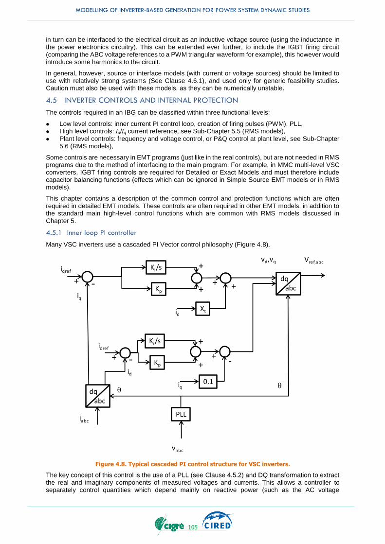
MODELLING OF INVERTER-BASED GENERATION FOR POWER SYSTEM DYNAMIC STUDIES
105
in turn can be interfaced to the electrical circuit as an inductive voltage source (using the inductance in the power electronics circuitry). This can be extended ever further, to include the IGBT firing circuit (comparing the ABC voltage references to a PWM triangular waveform for example), this however would introduce some harmonics to the circuit.
In general, however, source or interface models (with current or voltage sources) should be limited to use with relatively strong systems (See Clause 4.6.1), and used only for generic feasibility studies. Caution must also be used with these models, as they can be numerically unstable.
4.5 INVERTER CONTROLS AND INTERNAL PROTECTION
The controls required in an IBG can be classified within three functional levels:
Low level controls: inner current PI control loop, creation of firing pulses (PWM), PLL, High level controls: Id/Iq current reference, see Sub-Chapter 5.5 (RMS models), Plant level controls: frequency and voltage control, or P&Q control at plant level, see Sub-Chapter
5.6 (RMS models),
Some controls are necessary in EMT programs (just like in the real controls), but are not needed in RMS programs due to the method of interfacing to the main program. For example, in MMC multi-level VSC converters, IGBT firing controls are required for Detailed or Exact Models and must therefore include capacitor balancing functions (effects which can be ignored in Simple Source EMT models or in RMS models).
This chapter contains a description of the common control and protection functions which are often required in detailed EMT models. These controls are often required in other EMT models, in addition to the standard main high-level control functions which are common with RMS models discussed in Chapter 5.
4.5.1 Inner loop PI controller
Many VSC inverters use a cascaded PI Vector control philosophy (Figure 4.8).
Figure 4.8. Typical cascaded PI control structure for VSC inverters.
The key concept of this control is the use of a PLL (see Clause 4.5.2) and DQ transformation to extract the real and imaginary components of measured voltages and currents. This allows a controller to separately control quantities which depend mainly on reactive power (such as the AC voltage
iq
iqref
+
Ki/s
PLL
qdqabc
iabc
vabc
dqabc
vd,vq
q
Vref,abc
Kp
+
++ +
Ki/s
Kp
+
++
-+idref
id
Xtid
0.1iq
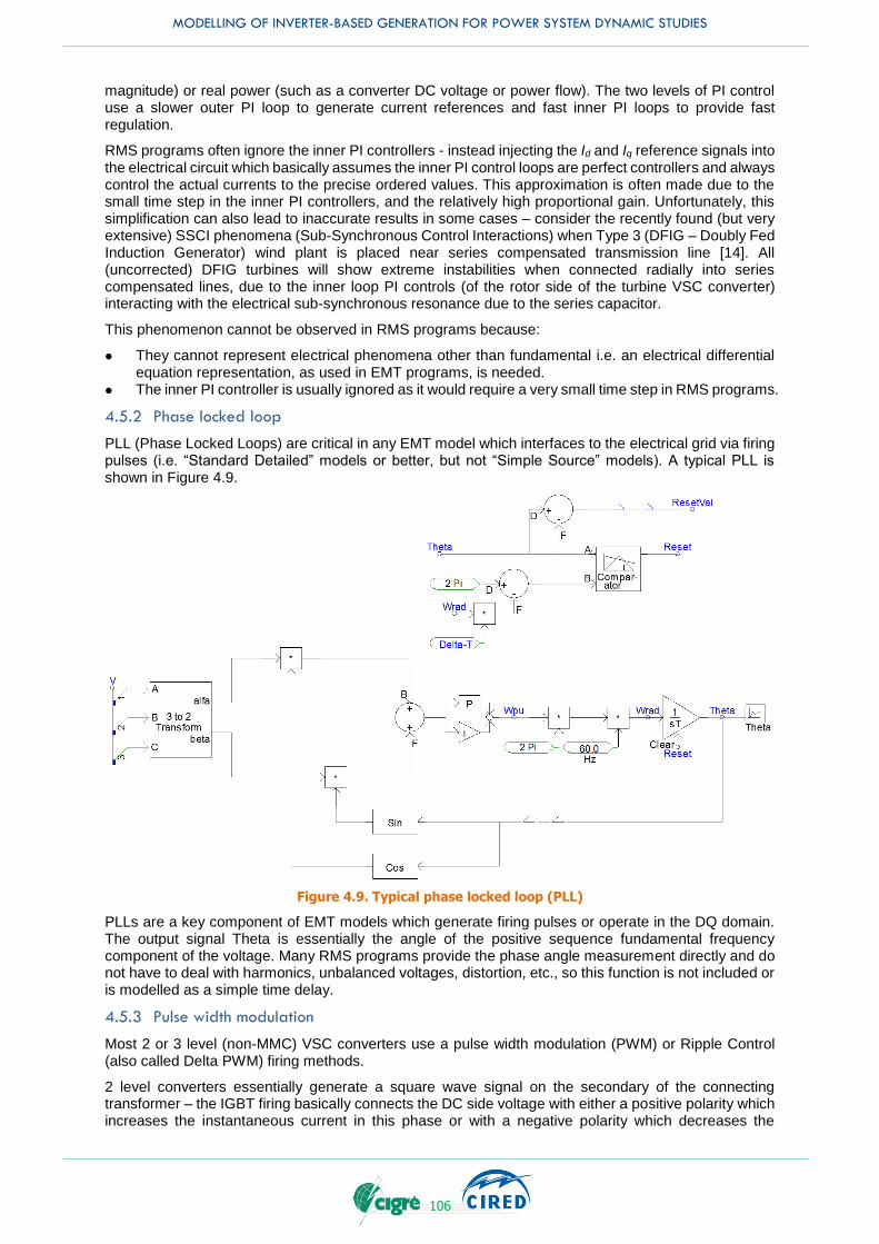
MODELLING OF INVERTER-BASED GENERATION FOR POWER SYSTEM DYNAMIC STUDIES
106
magnitude) or real power (such as a converter DC voltage or power flow). The two levels of PI control use a slower outer PI loop to generate current references and fast inner PI loops to provide fast regulation.
RMS programs often ignore the inner PI controllers - instead injecting the Id and Iq reference signals into the electrical circuit which basically assumes the inner PI control loops are perfect controllers and always control the actual currents to the precise ordered values. This approximation is often made due to the small time step in the inner PI controllers, and the relatively high proportional gain. Unfortunately, this simplification can also lead to inaccurate results in some cases – consider the recently found (but very extensive) SSCI phenomena (Sub-Synchronous Control Interactions) when Type 3 (DFIG – Doubly Fed Induction Generator) wind plant is placed near series compensated transmission line [14]. All (uncorrected) DFIG turbines will show extreme instabilities when connected radially into series compensated lines, due to the inner loop PI controls (of the rotor side of the turbine VSC converter) interacting with the electrical sub-synchronous resonance due to the series capacitor.
This phenomenon cannot be observed in RMS programs because:
They cannot represent electrical phenomena other than fundamental i.e. an electrical differential equation representation, as used in EMT programs, is needed.
The inner PI controller is usually ignored as it would require a very small time step in RMS programs.
4.5.2 Phase locked loop
PLL (Phase Locked Loops) are critical in any EMT model which interfaces to the electrical grid via firing pulses (i.e. “Standard Detailed” models or better, but not “Simple Source” models). A typical PLL is shown in Figure 4.9.
Figure 4.9. Typical phase locked loop (PLL)
PLLs are a key component of EMT models which generate firing pulses or operate in the DQ domain. The output signal Theta is essentially the angle of the positive sequence fundamental frequency component of the voltage. Many RMS programs provide the phase angle measurement directly and do not have to deal with harmonics, unbalanced voltages, distortion, etc., so this function is not included or is modelled as a simple time delay.
4.5.3 Pulse width modulation
Most 2 or 3 level (non-MMC) VSC converters use a pulse width modulation (PWM) or Ripple Control (also called Delta PWM) firing methods.
2 level converters essentially generate a square wave signal on the secondary of the connecting transformer – the IGBT firing basically connects the DC side voltage with either a positive polarity which increases the instantaneous current in this phase or with a negative polarity which decreases the
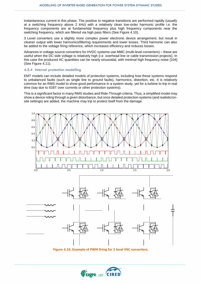
MODELLING OF INVERTER-BASED GENERATION FOR POWER SYSTEM DYNAMIC STUDIES
107
instantaneous current in this phase. The positive to negative transitions are performed rapidly (usually at a switching frequency above 2 kHz) with a relatively clean low-order harmonic profile i.e. the frequency components are at fundamental frequency plus high frequency components near the switching frequency, which are filtered via high pass filters (See Figure 4.10).
3 Level converters use a slightly more complex power electronic device arrangement, but result in cleaner output with lower harmonics/filtering requirements and lower losses. Third harmonic can also be added to the voltage firing reference, which increases efficiency and reduces losses.
Advances in voltage source converters for HVDC systems use MMC (multi-level converters) – these are useful when the DC side voltage is relatively high (i.e. overhead line or cable transmission projects). In this case the produced AC quantities can be nearly sinusoidal, with minimal high frequency noise [104] (See Figure 4.11).
4.5.4 Internal protection modelling
EMT models can include detailed models of protection systems, including how these systems respond to unbalanced faults (such as single line to ground faults), harmonics, distortion, etc. It is relatively common for an RMS model to show good performance in a system study, yet for a turbine to trip in real time (say due to IGBT over currents or other protection systems).
This is a significant factor in many RMS studies and Ride-Through criteria. Thus, a simplified model may show a device riding through a given disturbance, but once detailed protection systems (and realistic/on-site settings) are added, the machine may trip to protect itself from the damage.
Figure 4.10. Example of PWM firing for 2 level VSC converters.
D
D
D
D
D
D

MODELLING OF INVERTER-BASED GENERATION FOR POWER SYSTEM DYNAMIC STUDIES
108
Figure 4.11. Example of multi-level converter output (400 MW with 200 power modules per converter arm).
It is recommended to include the detailed internal protection systems in final studies where controller gains/settings are finalized, including RT simulator tests. Earlier/generic studies do not necessarily need this – the hope is that protection operations can be relatively easily fixed by algorithm adjustment, settings, delays, etc.
Some examples of inverter internal protections used in EMT models, in addition to the higher-level protection listed in Clause 2.3.3 are:
Reduction of maximum inverter current when the DC voltage exceeds a certain limit; Limitation of inverter current’s variation rate after a fault; Limitation of total reactive current; Differential AC overcurrent protection; DC overcurrent protection; Over/under voltage protection; Over/under frequency protection.
4.5.5 Measurements techniques
Other aspects to consider include voltage measurement time constants (RMS programs can generate a pure step in a measured RMS voltage, whereas EMT programs inherently must include a delay effect due to a true RMS or FFT/DFT measurement delay). This additional delay can generate instabilities in the overall controller response, but it is masked in simple models or RMS models.
The input signals to converter controls often include:
Instantaneous voltages and current. RMS quantities. Frequency measurements. Status of nearby breakers, disconnects, etc. Input from operators (reference signals).
There are numerous methods of measurements possible – for example: a simple RMS signal can be derived with an analogue rectifier/smoothing method, true RMS, DFT/FFT methods, etc. The accuracy of the method may have influence on the real control performance. Similarly, the type of transducer used in the real system (CT, CVT, PTs, etc.) can also have an impact (due to saturation or non-linearity, frequency attenuation, etc.).
Common measurements in EMT programs may show effects not seen in RMS programs – for example: DC offsets, or fundamental frequency oscillations during periods of DC offsets, second harmonic

MODELLING OF INVERTER-BASED GENERATION FOR POWER SYSTEM DYNAMIC STUDIES
109
oscillations during periods of large negative sequence unbalances, single line to ground faults, etc. The behaviour of EMT models during unbalanced faults can also be interesting (and realistic) – often a DC offset or second harmonic can appear in a measurement and be amplified by a controller response due to the measurement algorithm for the RMS signal. This is a common problem dealt with in real controls, but often is not necessary in simpler models. In inverters used near synchronous machines, a second harmonic oscillation of the rotor side quantities will also appear in detailed EMT models, due to negative sequence content on the machine stator side.
For these reasons, it is important to understand the methods and types of measurements used in the real controls when performing EMT modelling. If “Exact Models” are available from the manufacturer, these issues will be largely resolved as the actual code is used for measurements.
4.6 SYSTEM MODELS FOR EMT STUDIES
The previous sub-chpaters discuss specific inverter modelling aspects for simulation studies. In addition to the converter, filters, controls and the protection, a successful simulation also will require modelling of the surrounding AC system.
4.6.1 System strength - short circuit MVA ratio
When connecting a power electronic converter to an AC system, the “system strength” is a key indicator that is the size of the converter relative to the system 𝑆𝐶𝑀𝑉𝐴 (short circuit MVA), this is called the system SCR (short circuit ratio). A commonly used adaptation of the SCR is the ESCR (Effective Short Circuit Ratio) which subtracts the MVARs of nearby shunt capacitors or AC filters from the 𝑆𝐶𝑀𝑉𝐴 (as the capacitors have a weakening effect on the fundamental frequency impedance, yet do not impact the short circuit MVA).
These are defined as:
𝑆𝐶𝑅 =𝑆𝐶𝑀𝑉𝐴
𝑃𝑛 and 𝐸𝑆𝐶𝑅 =
𝑆𝐶𝑀𝑉𝐴−𝑄𝐶
𝑃𝑛
Equation 4.1
where: 𝑆𝐶𝑀𝑉𝐴 is the short-circuit power of the AC grid at the PCC (MVA)
𝑃𝑛 is nominal power of the IBG (MW) 𝑄𝑐 includes the effect of AC side equipment associated with the IBG (filters, shunt capacitors, synchronous condensers, etc.) (Mvar)
As a general rule of thumb, projects in weak systems (i.e. SCR less than 5) will face significantly more challenges in the controls and protection of the device (see Sub-Chapter 4.1). The exact safe ESCR level depends on the manufacturer and project – even higher SCR conditions can still pose the same problems. More information is provided in TB671 [76].
For the projects which use “off the shelf” control designs (i.e. designs which do not undergo significant tuning, special control design or custom modelling efforts) caution should be used, plan on significant study efforts, delays, working with the manufacturer to design/tune controls, etc. in weak power systems.
4.6.2 Size of system model required and system equivalents
EMT simulations are often used to study power electronic devices and the interactions with the nearby electrical system. Some factors to consider when determining how large the system model is required are:
Try to reproduce the frequency response of the electrical system in addition to the fundamental frequency response. The use of system equivalents relatively far away from the study area (or FDNE – frequency dependent network equivalents) should be considered for some studies.
Are there other nearby complex devices which should also be modelled (i.e. other nearby FACTS devices, power electronic devices, large industrial loads, series capacitors, etc.).
The level of detailed required in your device. If detailed models are available from the manufacturer, these should be preferred.
A common method to determine how much of the AC system should be modelled, is to first develop a very large system model (this can be automated using translation tools) and to compare it to successively smaller system models (which run faster). The goal is to achieve a reasonably accurate frequency response (and sometimes the inclusion of nearby machines to get accuracy of the electro-
MODELLING OF INVERTER-BASED GENERATION FOR POWER SYSTEM DYNAMIC STUDIES
110
magnetic response) with the smallest model possible to keep the simulation speed reasonable. The counterpart process is to develop a small system model that included all the models under study and to compare it with its successively larger system until no significant resolution is achieved.
4.6.3 Further modelling aspects for EMT studies
Other factors in AC system modelling can be important, including [91]:
Frequency dependent line and cable models to get the wanted accuracy for high frequency responses and higher damping at higher frequencies.
Transformers and saturation for transient overvoltage, grounding, and inrush phenomena. Load modelling to accurately reproduce induction motor loads (which dominate the ratings of
reactive power support needed in response to faults) and to model possible interactions between nearby power electronic devices with complex/significant or industrial loads.
Generator modelling and electro-mechanical models for other rotating machines – some system studies (such are: SSR, SSCI, SSTI, dynamic performance studies, etc.) require modelling of nearby generators.
Power electronic converters generate harmonics and usually require filters. Load flow and RMS tools are not concerned with harmonics or power quality, and only represent the fundamental frequency MVARs of filters (i.e. an RLC filter is often modelled as a simple fixed shunt capacitor bank). A comprehensive set of guidelines for harmonics is outside of the scope of this JWG, however the end user should be aware of potential harmonic conditions and their effort on the power system, and should expect models to include resistor, inductor and capacitor filter models with appropriate tuned resonance conditions and damping.
4.7 CONCLUSIONS
In Chapter 4, guidelines for the application of EMT models for IBG are given. Advantages of EMT simulation and typical cases where EMT modelling is inevitable are listed. Different levels of detail in the models is discussed in the descriptive part on the electrical interface and control models. However, only components exclusively used in EMT models are covered. These are especially the inverter models at the switching level and low-level control functions like the inner loop current controller. The high-level controls are included in Chapter 5 (RMS model) since they are the identical for RMS and EMT simulation.
The level of detail required in both the control models and the electrical circuit, depends on the study being performed. In general, the end users should:
Understand the phenomena being studied. Understand where approximations are made in a model (i.e. what is included in the used model and
what is not included). Determine if approximations or omissions may affect their study. Discuss the modelling of the external system.
MODELLING OF INVERTER-BASED GENERATION FOR POWER SYSTEM DYNAMIC STUDIES
111
5. RMS MODELS FOR INVERTER BASED GENERATION
5.1 INTRODUCTION
Power system dynamic simulation tools using RMS-type models were mainly developed to study electromechanical oscillations of power systems consisting of large generators and motors. Phasor simulation methods are used when the fundamental frequency behaviour is of interest, i.e. it is not necessary to solve all the differential equations of the network resulting from its R, L, and C elements. Instead, a much simpler set of differential-algebraic equations involving the voltage and current phasors is solved. Time-varying complex numbers are used to represent sinusoidal voltages and currents at system frequency, expressing their value either in Cartesian (real and imaginary) or polar coordinates (amplitude and phase).
Although there is diverse range of opinions, but RMS-type simulation tools are more likely to consider phenomena mainly in a bandwidth of at most 10 Hz (i.e., periods higher than 0.1 s are of interest)27. The numerical integration time-step is therefore chosen in the range of 1–10 milliseconds, while software employing variable step-size techniques can use larger time-steps during the periods of low dynamic activity. For frequencies outside the operational range of a nominal network frequency (e.g. several Hz smaller/larger than the rated frequency) or the analysis of harmonics is required, the use of Electro-Magnetic Transient (EMT) simulation software is recommended, as they contain more detailed and higher-order equipment models [105]. Even so, RMS-type simulations are much faster to execute than EMT and are thus the dominant simulation method used in stability studies.
Simplified converter models are included in RMS programs (also known as averaged models). RMS-type models provide the behaviour of the converter ignoring fast switching transients and any control with very small time constants compared to the simulation time steps and the phenomena considered. That is, in stability analysis there is usually no need to model the inverter in detail when its transients are likely to decay within the time step of the time-domain simulation. Only the fundamental frequency outputs of the converter are modelled, mainly reflected in the electrical control model. Due to this averaged representation, the modelling of different technologies of inverter-based generators can be unified using generic sub-models for the basic components.
The performance of these models should be valid, within a reasonable tolerance, for a wide range of operating conditions of quantities such as voltage, active and reactive power at their terminal connections. While it is desirable for the models to be valid for the entire operating range of the converter (normal and abnormal), this is sometimes not possible due to the modelling limitations of RMS models.
RMS-type models are not recommended for use in power system dynamic studies in a weak grid. The definition of a weak system is often defined using the Short-Circuit Ratio (SCR) and it is sometimes said that RMS-type models might not be reliable in the case of the SCR of below 3. However, such criteria can be different between the conventional technologies such as Line Commutated Converter (LCC) and the recent technologies such as Voltage Source Converter (VSC). If conventional technologies are used, the models should perform accurately for systems with a SCR of three and higher at the Point Of Interconnection (POI). For the parts of the system with low SCR levels, detailed vendor specific models may be needed. For very weak connections, a vendor-specific EMT-type model may be necessary even for transient stability-type studies. In the case of LCC technologies, the following classification is proposed when dealing with power electronic interfaced technologies connected to weak points in the network:
Connection is considered to be weak if SCR at the POI is less than 5 or if SCR at the MV collection grid is less than 4 (whichever of these criteria is met).
Connection is considered to be very weak if SCR at the POI is less than 3 or if the SCR at the MV collection grid is less than 2 (whichever of these criteria is met).
The following approaches are recommended when undertaking power system studies for planning and connection assessment:
For weak connection applications: Comparison of RMS-type dynamic models against the detailed EMT-type models and field
measurements (at the time of commissioning) is advantageous.
27 This does not mean that the fault current cannot be modelled. The periods of few milliseconds may be of interest.
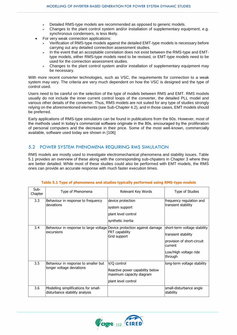
MODELLING OF INVERTER-BASED GENERATION FOR POWER SYSTEM DYNAMIC STUDIES
112
Detailed RMS-type models are recommended as opposed to generic models. Changes to the plant control system and/or installation of supplementary equipment, e.g.
synchronous condensers, is less likely.
For very weak connection applications: Verification of RMS-type models against the detailed EMT-type models is necessary before
carrying out any detailed connection assessment studies. In the event that an acceptable correlation does not exist between the RMS-type and EMT-
type models, either RMS-type models need to be revised, or EMT-type models need to be used for the connection assessment studies.
Changes to the plant control system and/or installation of supplementary equipment may be necessary.
With more recent converter technologies, such as VSC, the requirements for connection to a weak system may vary. The criteria are very much dependent on how the VSC is designed and the type of control used.
Users need to be careful on the selection of the type of models between RMS and EMT. RMS models usually do not include the inner current control loops of the converter, the detailed PLL model and various other details of the converter. Thus, RMS models are not suited for any type of studies strongly relying on the aforementioned elements (see Sub-Chapter 4.2), and in those cases, EMT models should be preferred.
Early applications of RMS-type simulators can be found in publications from the 60s. However, most of the methods used in today’s commercial software originate in the 80s, encouraged by the proliferation of personal computers and the decrease in their price. Some of the most well-known, commercially available, software used today are shown in [106]
5.2 POWER SYSTEM PHENOMENA REQUIRING RMS SIMULATION
RMS models are mostly used to investigate electromechanical phenomena and stability issues. Table 5.1 provides an overview of these along with the corresponding sub-chpaters in Chapter 3 where they are better detailed. While most of these studies could also be performed with EMT models, the RMS ones can provide an accurate response with much faster execution times.
Table 5.1 Type of phenomena and studies typically performed using RMS-type models
Sub-Chapter
Type of Phenomena Relevant Key Words Type of Studies
3.3 Behaviour in response to frequency deviations
device protection
system support
plant level control
synthetic inertia
frequency regulation and transient stability
3.4 Behaviour in response to large voltage excursions
Device protection against damage FRT capability Grid support
short-term voltage stability
transient stability
provision of short-circuit current
Low/High voltage ride through
3.5 Behaviour in response to smaller but longer voltage deviations
V/Q control
Reactive power capability below maximum capacity diagram
plant level control
long-term voltage stability
3.6 Modelling simplifications for small-disturbance stability analysis
small-disturbance angle stability
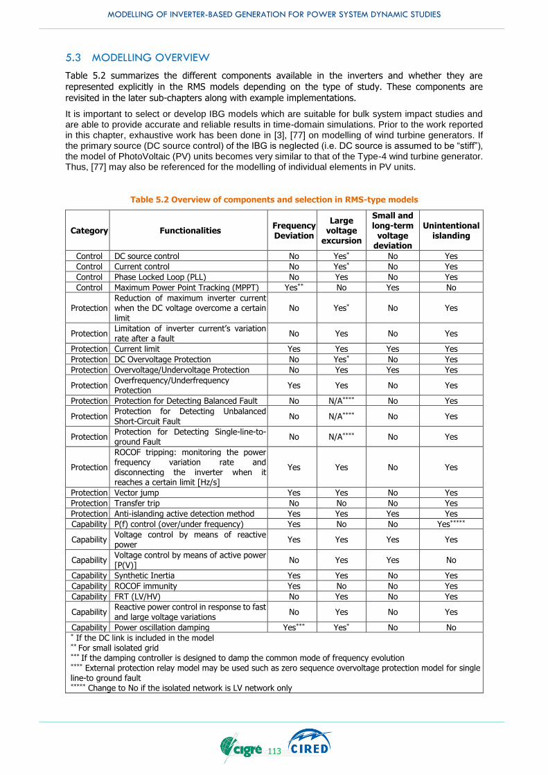
MODELLING OF INVERTER-BASED GENERATION FOR POWER SYSTEM DYNAMIC STUDIES
113
5.3 MODELLING OVERVIEW
Table 5.2 summarizes the different components available in the inverters and whether they are
represented explicitly in the RMS models depending on the type of study. These components are
revisited in the later sub-chapters along with example implementations.
It is important to select or develop IBG models which are suitable for bulk system impact studies and are able to provide accurate and reliable results in time-domain simulations. Prior to the work reported in this chapter, exhaustive work has been done in [3], [77] on modelling of wind turbine generators. If the primary source (DC source control) of the IBG is neglected (i.e. DC source is assumed to be “stiff”), the model of PhotoVoltaic (PV) units becomes very similar to that of the Type-4 wind turbine generator. Thus, [77] may also be referenced for the modelling of individual elements in PV units.
Table 5.2 Overview of components and selection in RMS-type models
Category Functionalities Frequency Deviation
Large voltage
excursion
Small and
long-term voltage
deviation
Unintentional islanding
Control DC source control No Yes* No Yes
Control Current control No Yes* No Yes
Control Phase Locked Loop (PLL) No Yes No Yes
Control Maximum Power Point Tracking (MPPT) Yes** No Yes No
Protection Reduction of maximum inverter current when the DC voltage overcome a certain limit
No Yes* No Yes
Protection Limitation of inverter current’s variation rate after a fault
No Yes No Yes
Protection Current limit Yes Yes Yes Yes
Protection DC Overvoltage Protection No Yes* No Yes
Protection Overvoltage/Undervoltage Protection No Yes Yes Yes
Protection Overfrequency/Underfrequency Protection
Yes Yes No Yes
Protection Protection for Detecting Balanced Fault No N/A**** No Yes
Protection Protection for Detecting Unbalanced Short-Circuit Fault
No N/A**** No Yes
Protection Protection for Detecting Single-line-to-ground Fault
No N/A**** No Yes
Protection
ROCOF tripping: monitoring the power frequency variation rate and disconnecting the inverter when it reaches a certain limit [Hz/s]
Yes Yes No Yes
Protection Vector jump Yes Yes No Yes
Protection Transfer trip No No No Yes
Protection Anti-islanding active detection method Yes Yes Yes Yes
Capability P(f) control (over/under frequency) Yes No No Yes*****
Capability Voltage control by means of reactive power
Yes Yes Yes Yes
Capability Voltage control by means of active power [P(V)]
No Yes Yes No
Capability Synthetic Inertia Yes Yes No Yes
Capability ROCOF immunity Yes No No Yes
Capability FRT (LV/HV) No Yes No Yes
Capability Reactive power control in response to fast and large voltage variations
No Yes No Yes
Capability Power oscillation damping Yes*** Yes* No No * If the DC link is included in the model ** For small isolated grid *** If the damping controller is designed to damp the common mode of frequency evolution **** External protection relay model may be used such as zero sequence overvoltage protection model for single
line-to ground fault ***** Change to No if the isolated network is LV network only
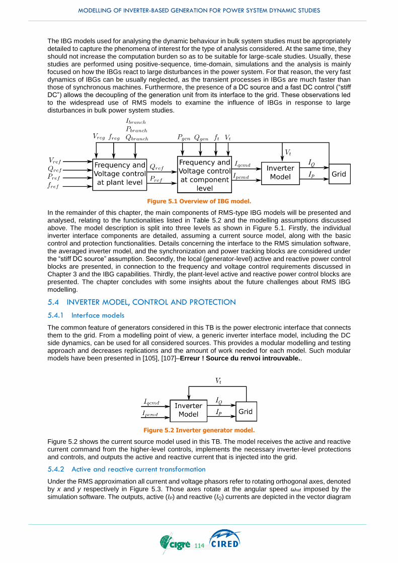
MODELLING OF INVERTER-BASED GENERATION FOR POWER SYSTEM DYNAMIC STUDIES
114
The IBG models used for analysing the dynamic behaviour in bulk system studies must be appropriately detailed to capture the phenomena of interest for the type of analysis considered. At the same time, they should not increase the computation burden so as to be suitable for large-scale studies. Usually, these studies are performed using positive-sequence, time-domain, simulations and the analysis is mainly focused on how the IBGs react to large disturbances in the power system. For that reason, the very fast dynamics of IBGs can be usually neglected, as the transient processes in IBGs are much faster than those of synchronous machines. Furthermore, the presence of a DC source and a fast DC control (“stiff DC”) allows the decoupling of the generation unit from its interface to the grid. These observations led to the widespread use of RMS models to examine the influence of IBGs in response to large disturbances in bulk power system studies.
Figure 5.1 Overview of IBG model.
In the remainder of this chapter, the main components of RMS-type IBG models will be presented and analysed, relating to the functionalities listed in Table 5.2 and the modelling assumptions discussed above. The model description is split into three levels as shown in Figure 5.1. Firstly, the individual inverter interface components are detailed, assuming a current source model, along with the basic control and protection functionalities. Details concerning the interface to the RMS simulation software, the averaged inverter model, and the synchronization and power tracking blocks are considered under the “stiff DC source” assumption. Secondly, the local (generator-level) active and reactive power control blocks are presented, in connection to the frequency and voltage control requirements discussed in Chapter 3 and the IBG capabilities. Thirdly, the plant-level active and reactive power control blocks are presented. The chapter concludes with some insights about the future challenges about RMS IBG modelling.
5.4 INVERTER MODEL, CONTROL AND PROTECTION
5.4.1 Interface models
The common feature of generators considered in this TB is the power electronic interface that connects them to the grid. From a modelling point of view, a generic inverter interface model, including the DC side dynamics, can be used for all considered sources. This provides a modular modelling and testing approach and decreases replications and the amount of work needed for each model. Such modular models have been presented in [105], [107]–Erreur ! Source du renvoi introuvable..
Figure 5.2 Inverter generator model.
Figure 5.2 shows the current source model used in this TB. The model receives the active and reactive current command from the higher-level controls, implements the necessary inverter-level protections and controls, and outputs the active and reactive current that is injected into the grid.
5.4.2 Active and reactive current transformation
Under the RMS approximation all current and voltage phasors refer to rotating orthogonal axes, denoted by x and y respectively in Figure 5.3. Those axes rotate at the angular speed ωref imposed by the simulation software. The outputs, active (IP) and reactive (IQ) currents are depicted in the vector diagram
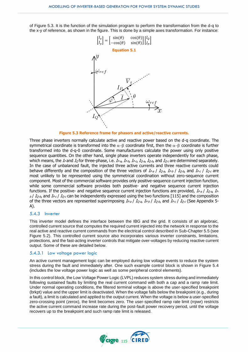
MODELLING OF INVERTER-BASED GENERATION FOR POWER SYSTEM DYNAMIC STUDIES
115
of Figure 5.3. It is the function of the simulation program to perform the transformation from the d-q to the x-y of reference, as shown in the figure. This is done by a simple axes transformation. For instance:
[𝐼𝑥
𝐼𝑦] = [
sin (𝜃) cos (𝜃)−cos (𝜃) sin (𝜃)
] [𝐼𝑄
𝐼𝑃]
Equation 5.1
Figure 5.3 Reference frame for phasors and active/reactive currents.
Three phase inverters normally calculate active and reactive power based on the d-q coordinate. The
symmetrical coordinate is transformed into the - coordinate first, then the - coordinate is further
transformed into the d-q-0 coordinate. Some manufacturers calculate the power using only positive
sequence quantities. On the other hand, single phase inverters operate independently for each phase,
which means, the IP and IQ for three-phase, i.e. IP-a, IP-b, IP-c, IQ-a, IQ-b, and IQ-c are determined separately. In the case of unbalanced fault, the injected three active currents and three reactive currents could
behave differently and the composition of the three vectors of IP-a / IQ-a, IP-b / IQ-b, and IP-c / IQ-c are most unlikely to be represented using the symmetrical coordination without zero-sequence current
component. Most of the commercial software provides only positive-sequence current injection function,
while some commercial software provides both positive- and negative sequence current injection functions. If the positive- and negative sequence current injection functions are provided, IP-a / IQ-a, IP-
b / IQ-b, and IP-c / IQ-c can be independently expressed using the two functions [115] and the composition of the three vectors are represented superimposing IP-a / IQ-a, IP-b / IQ-b, and IP-c / IQ-c (See Appendix 5-
A).
5.4.3 Inverter
This inverter model defines the interface between the IBG and the grid. It consists of an algebraic, controlled current source that computes the required current injected into the network in response to the real active and reactive current commands from the electrical control described in Sub-Chapter 5.5 (see Figure 5.2). This controlled current source also incorporates various inverter constraints, limitations, protections, and the fast-acting inverter controls that mitigate over-voltages by reducing reactive current output. Some of these are detailed below.
5.4.3.1 Low voltage power logic
An active current management logic can be employed during low voltage events to reduce the system stress during the fault and immediately after. One such example control block is shown in Figure 5.4 (includes the low voltage power logic as well as some peripheral control elements).
In this control block, the Low Voltage Power Logic (LVPL) reduces system stress during and immediately following sustained faults by limiting the real current command with both a cap and a ramp rate limit. Under normal operating conditions, the filtered terminal voltage is above the user-specified breakpoint (brkpt) value and the upper limit is deactivated. When the voltage falls below the breakpoint (e.g., during a fault), a limit is calculated and applied to the output current. When the voltage is below a user-specified zero-crossing point (zerox), the limit becomes zero. The user-specified ramp rate limit (rrpwr) restricts the active current command increase rate during the post-fault power recovery period, until the voltage recovers up to the breakpoint and such ramp rate limit is released.
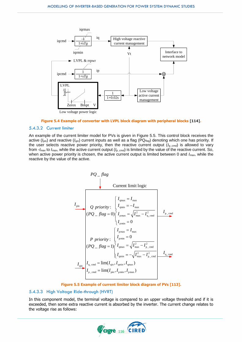
MODELLING OF INVERTER-BASED GENERATION FOR POWER SYSTEM DYNAMIC STUDIES
116
Interface to
network model
ipcmd1
1+sTg ×
Low voltage power logic
LVPL & rrpwr
ip
iqcmd
iqrmax
-1
1+sTg
iqrmin
iq High voltage reactive
current management
Vt
lvp
l1
V
LVPL
Low voltage
active current
management
Zerox Brkpt
1
1+0.02s
Figure 5.4 Example of converter with LVPL block diagram with peripheral blocks [114].
5.4.3.2 Current limiter
An example of the current limiter model for PVs is given in Figure 5.5. This control block receives the active (Ipin) and reactive (Iqin) current inputs as well as a flag (PQflag) denoting which one has priority. If the user selects reactive power priority, then the reactive current output (Iq_cmd) is allowed to vary from -Imax to Imax, while the active current output (Ip_cmd) is limited by the value of the reactive current. So, when active power priority is chosen, the active current output is limited between 0 and Imax, while the reactive by the value of the active.
p _ cmdI
q_ cmdI
qmax max
qmin max
2 2
pmax max q_ cmd
pmin
pmax max
pmin
2 2
qmax max p _ cmd
2 2
qmin max p _ cmd
q_ cmd qin qmin qmax
p _ cmd
:
( _ 0)
0
0:
( _ 1)
lim( , , )
lim(
I I
I IQ priority
I I IPQ flag
I
I I
IP priority
I I IPQ flag
I I I
I I I I
I
-
-
-
- -
pin pmin pmax, , )I I I
_PQ flag
Current limit logic
pinI
qinI
Figure 5.5 Example of current limiter block diagram of PVs [113].
5.4.3.3 High Voltage Ride-through (HVRT)
In this component model, the terminal voltage is compared to an upper voltage threshold and if it is
exceeded, then some extra reactive current is absorbed by the inverter. The current change relates to the voltage rise as follows:
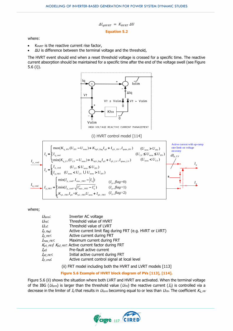
MODELLING OF INVERTER-BASED GENERATION FOR POWER SYSTEM DYNAMIC STUDIES
117
𝛥𝐼𝑞𝐻𝑉𝑅𝑇 = 𝐾𝐻𝑉𝑅𝑇 𝛥𝑈
Equation 5.2
where:
KHVRT is the reactive current rise factor,
ΔU is difference between the terminal voltage and the threshold,
The HVRT event should end when a reset threshold voltage is crossed for a specific time. The reactive current absorption should be maintained for a specific time after the end of the voltage swell (see Figure
5.6 (i)).
(i) HVRT control model [114]
0
qI
pIp _ cmdI
q_ cmdI
q_ HV HV term Iq0_flag q0 q0_ HV qmin_HV term HV
q q_cmd LV term HV
term LVq_LV LV term Iq0_flag q0 q0_LV qmax_LV
p _cmd LV term HV
p
term LV tep_FRT
max( ( ) , ) ( )
( )
( )min( ( ) , )
( )
(
K U U K I I I U U
I I U U U
U UK U U K I I I
I U U UI
U U UI
- + +
- + +
rm HV
p _cmd max _ FRT qp
2 2
p_FRT p _cmd max _ FRT q p
pp1_ FRT p0 p2_ FRT term p0_ FRT
)
min( , )( _ =0)
min( , ) ( _ =1)
( _ =2)+
U
I I II flag
I I I I I flag
I flagK I K U I
-
-
+
dIp_LV
Active current with up-ramp
rate limit on voltage
recovery
where;
Uterm: Inverter AC voltage
UHV: Threshold value of HVRT ULV: Threshold value of LVRT
Ip_flag: Active current limit flag during FRT (e.g. HVRT or LVRT) Ip_FRT: Active current during FRT
Imax_FRT: Maximum current during FRT Kp1_FRT/ Kp2_FRT: Active current factor during FRT
Ip0: Pre-fault active current
Ip0_FRT: Initial active current during FRT Ip_cmd: Active current control signal at local level
(ii) FRT model including both the HVRT and LVRT models [113]
Figure 5.6 Example of HVRT block diagram of PVs [113], [114].
Figure 5.6 (ii) shows the situation where both LVRT and HVRT are activated. When the terminal voltage
of the IBG (Uterm) is larger than the threshold value (UHV) the reactive current (Iq) is controlled via a
decrease in the limiter of Iq that results in Uterm becoming equal to or less than UHV. The coefficient Kq_HV
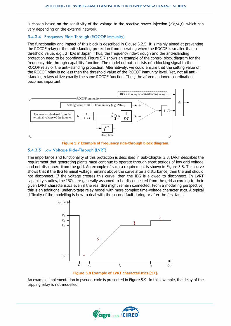
MODELLING OF INVERTER-BASED GENERATION FOR POWER SYSTEM DYNAMIC STUDIES
118
is chosen based on the sensitivity of the voltage to the reactive power injection (𝑑𝑉/𝑑𝑄), which can
vary depending on the external network.
5.4.3.4 Frequency Ride-Through (ROCOF Immunity)
The functionality and impact of this block is described in Clause 3.2.5. It is mainly aimed at preventing
the ROCOF relay or the anti-islanding protection from operating when the ROCOF is smaller than a threshold value, e.g., 2 Hz/s in Japan. Thus, the frequency ride-through and the anti-islanding
protection need to be coordinated. Figure 5.7 shows an example of the control block diagram for the frequency ride-through capability function. The model output consists of a blocking signal to the
ROCOF relay or the anti-islanding protection. Alternatively, we could ensure that the setting value of the ROCOF relay is no less than the threshold value of the ROCOF immunity level. Yet, not all anti-
islanding relays utilize exactly the same ROCOF function. Thus, the aforementioned coordination
becomes important.
ROCOF relay or anti-islanding relay
&
1
Frequency calculated from the terminal voltage of the inverter
1
1+Ts
+
- DT
1
Dead time
DT
+
-
Setting value of ROCOF immunity (e.g. 2Hz/s)
ROCOF immunity
Figure 5.7 Example of frequency ride-through block diagram.
5.4.3.5 Low Voltage Ride-Through (LVRT)
The importance and functionality of this protection is described in Sub-Chapter 3.3. LVRT describes the requirement that generating plants must continue to operate through short periods of low grid voltage
and not disconnect from the grid. An example of such a requirement is shown in Figure 5.8. This curve
shows that if the IBG terminal voltage remains above the curve after a disturbance, then the unit should not disconnect. If the voltage crosses this curve, then the IBG is allowed to disconnect. In LVRT
capability studies, the IBGs are generally assumed to be disconnected from the grid according to their given LVRT characteristics even if the real IBG might remain connected. From a modelling perspective,
this is an additional undervoltage relay model with more complex time-voltage characteristics. A typical difficulty of the modelling is how to deal with the second fault during or after the first fault.
Figure 5.8 Example of LVRT characteristics [17].
An example implementation in pseudo-code is presented in Figure 5.9. In this example, the delay of the
tripping relay is not modelled.
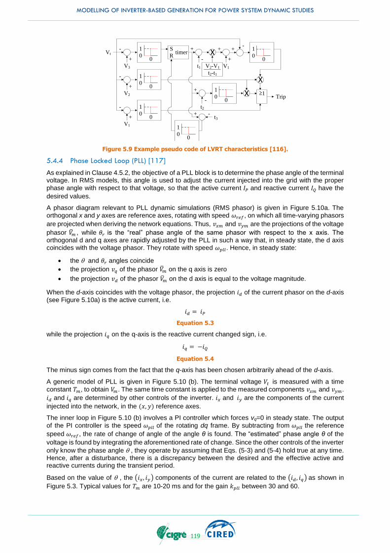
MODELLING OF INVERTER-BASED GENERATION FOR POWER SYSTEM DYNAMIC STUDIES
119
V3
Vt
+
-
0
1
0
V2
+
-
0
1
0
V1
+
-
0
1
0
X
0
1
0
X
timerS
R
t1
-
+
V2-V1
t2-t1
+
V1
-+
0
1
0
+
1
t2
-
+
0
1
0 X
t3-+
Trip
Figure 5.9 Example pseudo code of LVRT characteristics [116].
5.4.4 Phase Locked Loop (PLL) [117]
As explained in Clause 4.5.2, the objective of a PLL block is to determine the phase angle of the terminal voltage. In RMS models, this angle is used to adjust the current injected into the grid with the proper phase angle with respect to that voltage, so that the active current 𝐼𝑃 and reactive current 𝐼𝑄 have the
desired values.
A phasor diagram relevant to PLL dynamic simulations (RMS phasor) is given in Figure 5.10a. The orthogonal x and y axes are reference axes, rotating with speed 𝜔𝑟𝑒𝑓, on which all time-varying phasors
are projected when deriving the network equations. Thus, 𝑣𝑥𝑚 and 𝑣𝑦𝑚 are the projections of the voltage
phasor ��𝑚 , while 𝜃𝑟 is the “real” phase angle of the same phasor with respect to the x axis. The orthogonal d and q axes are rapidly adjusted by the PLL in such a way that, in steady state, the d axis coincides with the voltage phasor. They rotate with speed 𝜔𝑝𝑙𝑙. Hence, in steady state:
the q and 𝜃𝑟 angles coincide
the projection 𝑣𝑞 of the phasor ��𝑚 on the q axis is zero
the projection 𝑣𝑑 of the phasor ��𝑚 on the d axis is equal to the voltage magnitude.
When the d-axis coincides with the voltage phasor, the projection 𝑖𝑑 of the current phasor on the d-axis (see Figure 5.10a) is the active current, i.e.
𝑖𝑑 = 𝑖𝑃
Equation 5.3
while the projection 𝑖𝑞 on the q-axis is the reactive current changed sign, i.e.
𝑖𝑞 = −𝑖𝑄
Equation 5.4
The minus sign comes from the fact that the q-axis has been chosen arbitrarily ahead of the d-axis.
A generic model of PLL is given in Figure 5.10 (b). The terminal voltage 𝑉𝑡 is measured with a time
constant 𝑇𝑚, to obtain 𝑉𝑚. The same time constant is applied to the measured components 𝑣𝑥𝑚 and 𝑣𝑦𝑚.
𝑖𝑑 and 𝑖𝑞 are determined by other controls of the inverter. 𝑖𝑥 and 𝑖𝑦 are the components of the current
injected into the network, in the (𝑥, 𝑦) reference axes.
The inner loop in Figure 5.10 (b) involves a PI controller which forces vq=0 in steady state. The output
of the PI controller is the speed 𝜔𝑝𝑙𝑙 of the rotating dq frame. By subtracting from 𝜔𝑝𝑙𝑙 the reference
speed 𝜔𝑟𝑒𝑓, the rate of change of angle of the angle θ is found. The “estimated” phase angle θ of the
voltage is found by integrating the aforementioned rate of change. Since the other controls of the inverter
only know the phase angle q , they operate by assuming that Eqs. (5-3) and (5-4) hold true at any time. Hence, after a disturbance, there is a discrepancy between the desired and the effective active and reactive currents during the transient period.
Based on the value of q , the (𝑖𝑥 , 𝑖𝑦) components of the current are related to the (𝑖𝑑 , 𝑖𝑞) as shown in
Figure 5.3. Typical values for 𝑇𝑚 are 10-20 ms and for the gain 𝑘𝑝𝑙𝑙 between 30 and 60.
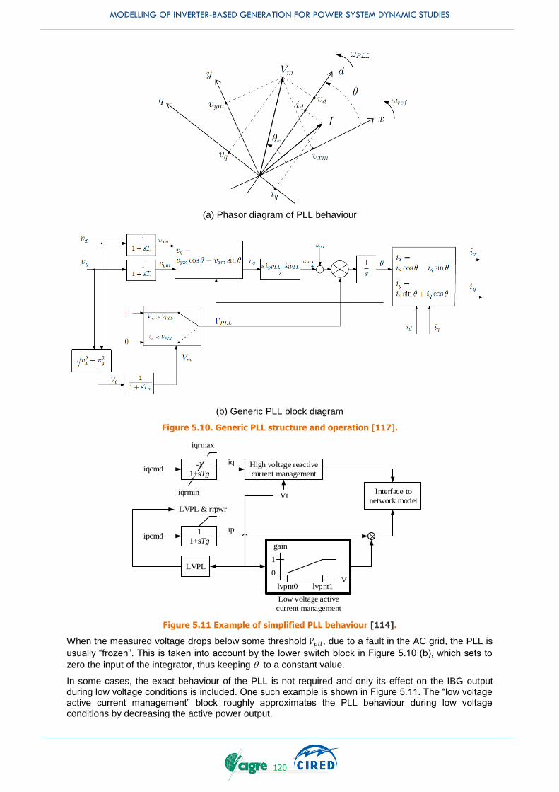
MODELLING OF INVERTER-BASED GENERATION FOR POWER SYSTEM DYNAMIC STUDIES
120
(a) Phasor diagram of PLL behaviour
(b) Generic PLL block diagram
Figure 5.10. Generic PLL structure and operation [117].
Interface to
network model
ipcmd1
1+sTg ×
Low voltage active
current management
LVPL & rrpwr
ip
LVPL
iqcmd
iqrmax
-1
1+sTg
iqrmin
iq High voltage reactive
current management
Vt
lvpnt0 lvpnt1V
gain
0
1
Figure 5.11 Example of simplified PLL behaviour [114].
When the measured voltage drops below some threshold 𝑉𝑝𝑙𝑙, due to a fault in the AC grid, the PLL is
usually “frozen”. This is taken into account by the lower switch block in Figure 5.10 (b), which sets to
zero the input of the integrator, thus keeping q to a constant value.
In some cases, the exact behaviour of the PLL is not required and only its effect on the IBG output during low voltage conditions is included. One such example is shown in Figure 5.11. The “low voltage active current management” block roughly approximates the PLL behaviour during low voltage conditions by decreasing the active power output.
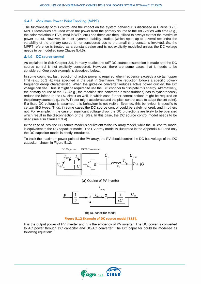
MODELLING OF INVERTER-BASED GENERATION FOR POWER SYSTEM DYNAMIC STUDIES
121
5.4.5 Maximum Power Point Tracking (MPPT)
The functionality of this control and the impact on the system behaviour is discussed in Clause 3.2.5. MPPT techniques are used when the power from the primary source to the IBG varies with time (e.g., the solar radiation in PVs, wind in WTs, etc.) and these are then utilized to always extract the maximum power output. However, in most dynamic stability studies (which span up to several seconds) the variability of the primary source is not considered due to the small time-constants involved. So, the MPPT reference is treated as a constant value and is not explicitly modelled unless the DC voltage needs to be modelled (see Clause 5.4.6).
5.4.6 DC source control
As explained in Sub-Chapter 2.4, in many studies the stiff DC source assumption is made and the DC source control is not explicitly considered. However, there are some cases that it needs to be considered. One such example is described below.
In some countries, fast reduction of active power is required when frequency exceeds a certain upper limit (e.g., 50.2 Hz was specified in the past in Germany). The reduction follows a specific power-frequency droop characteristic. When the grid-side converter reduces active power quickly, the DC voltage can rise. Thus, it might be required to use the IBG chopper to dissipate this energy. Alternatively, the primary source of the IBG (e.g., the machine side converter in wind turbines) has to synchronously reduce the infeed to the DC circuit as well, in which case further control actions might be required on the primary source (e.g., the WT rotor might accelerate and the pitch control used to adapt the set point). If a fixed DC voltage is assumed, this behaviour is not visible. Even so, this behaviour is specific to certain IBG types. Thus, in some cases the DC source control could be safely ignored, and in others not. For example, in the case of significant voltage drop, the DC protections are likely to be operated which result in the disconnection of the IBGs. In this case, the DC source control model needs to be used (see also Clause 3.3.4).
In the case of PVs, the DC source model is equivalent to the PV array model, while the DC control model is equivalent to the DC capacitor model. The PV array model is illustrated in the Appendix 5-B and only the DC capacitor model is briefly introduced.
To track the maximum power point of the PV array, the PV should control the DC bus voltage of the DC capacitor, shown in Figure 5.12.
dcU
dcI tUtermU
acIP jQ+
TxC
DC Capacitor DC/AC converter
arrayI
(a) Outline of PV inverter
÷1
sCdcI
arrayI
- dcU1
P
(b) DC capacitor model
Figure 5.12 Example of DC source model [118].
P is the output power of PV inverter and η is the efficiency of PV inverter. The DC power is converted to AC power through DC capacitor and DC/AC converter. The DC capacitor could be modelled as following equation:
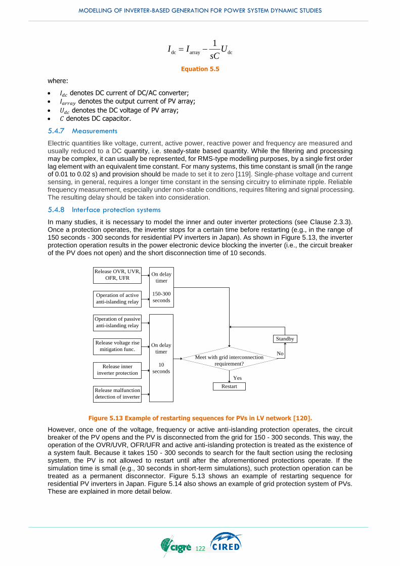
MODELLING OF INVERTER-BASED GENERATION FOR POWER SYSTEM DYNAMIC STUDIES
122
dc array dc
1I I U
sC -
Equation 5.5
where:
𝐼𝑑𝑐 denotes DC current of DC/AC converter;
𝐼𝑎𝑟𝑟𝑎𝑦 denotes the output current of PV array;
𝑈𝑑𝑐 denotes the DC voltage of PV array;
𝐶 denotes DC capacitor.
5.4.7 Measurements
Electric quantities like voltage, current, active power, reactive power and frequency are measured and usually reduced to a DC quantity, i.e. steady-state based quantity. While the filtering and processing may be complex, it can usually be represented, for RMS-type modelling purposes, by a single first order lag element with an equivalent time constant. For many systems, this time constant is small (in the range of 0.01 to 0.02 s) and provision should be made to set it to zero [119]. Single-phase voltage and current sensing, in general, requires a longer time constant in the sensing circuitry to eliminate ripple. Reliable frequency measurement, especially under non-stable conditions, requires filtering and signal processing. The resulting delay should be taken into consideration.
5.4.8 Interface protection systems
In many studies, it is necessary to model the inner and outer inverter protections (see Clause 2.3.3). Once a protection operates, the inverter stops for a certain time before restarting (e.g., in the range of 150 seconds - 300 seconds for residential PV inverters in Japan). As shown in Figure 5.13, the inverter protection operation results in the power electronic device blocking the inverter (i.e., the circuit breaker of the PV does not open) and the short disconnection time of 10 seconds.
Release OVR, UVR,
OFR, UFR
Operation of active
anti-islanding relay
Operation of passive
anti-islanding relay
Release voltage rise
mitigation func.
Release inner
inverter protection
Release malfunction
detection of inverter
On delay
timer
150-300
seconds
Meet with grid interconnection
requirement?
Restart
Standby
Yes
No
On delay
timer
10
seconds
Figure 5.13 Example of restarting sequences for PVs in LV network [120].
However, once one of the voltage, frequency or active anti-islanding protection operates, the circuit breaker of the PV opens and the PV is disconnected from the grid for 150 - 300 seconds. This way, the operation of the OVR/UVR, OFR/UFR and active anti-islanding protection is treated as the existence of a system fault. Because it takes 150 - 300 seconds to search for the fault section using the reclosing system, the PV is not allowed to restart until after the aforementioned protections operate. If the simulation time is small (e.g., 30 seconds in short-term simulations), such protection operation can be treated as a permanent disconnector. Figure 5.13 shows an example of restarting sequence for residential PV inverters in Japan. Figure 5.14 also shows an example of grid protection system of PVs. These are explained in more detail below.
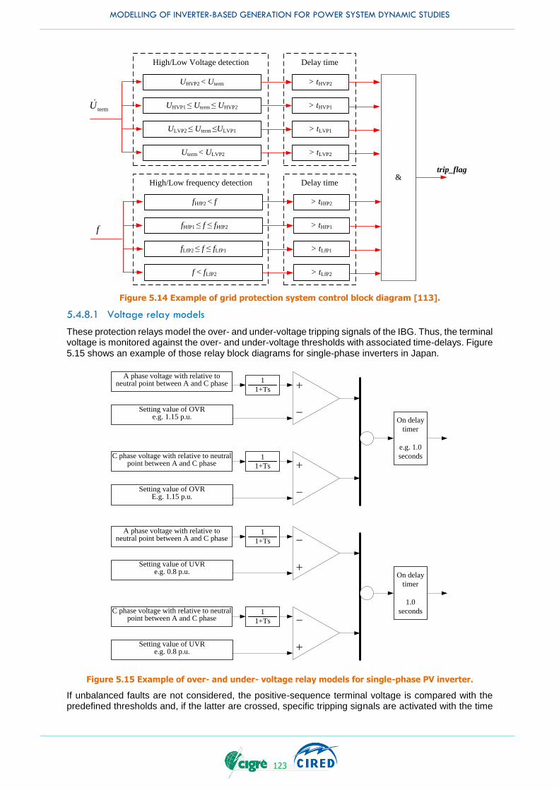
MODELLING OF INVERTER-BASED GENERATION FOR POWER SYSTEM DYNAMIC STUDIES
123
trip_flag
f
UHVP2 < Uterm
termU UHVP1 ≤ Uterm ≤ UHVP2
ULVP2 ≤ Uterm ≤ULVP1
Uterm < ULVP2
> tHVP2
> tHVP1
> tLVP1
> tLVP2
&
fHfP2 < f
fHfP1 ≤ f ≤ fHfP2
fLfP2 ≤ f ≤ fLfP1
f < fLfP2
> tHfP2
> tHfP1
> tLfP1
> tLfP2
High/Low Voltage detection Delay time
High/Low frequency detection Delay time
Figure 5.14 Example of grid protection system control block diagram [113].
5.4.8.1 Voltage relay models
These protection relays model the over- and under-voltage tripping signals of the IBG. Thus, the terminal voltage is monitored against the over- and under-voltage thresholds with associated time-delays. Figure 5.15 shows an example of those relay block diagrams for single-phase inverters in Japan.
A phase voltage with relative to neutral point between A and C phase
On delay
timer
e.g. 1.0
seconds
Setting value of OVRe.g. 1.15 p.u.
+
-
+
-
C phase voltage with relative to neutral point between A and C phase
Setting value of OVRE.g. 1.15 p.u.
1
1+Ts
1
1+Ts
A phase voltage with relative to neutral point between A and C phase
On delay
timer
1.0
seconds
Setting value of UVRe.g. 0.8 p.u.
-
+
-
+
C phase voltage with relative to neutral point between A and C phase
Setting value of UVRe.g. 0.8 p.u.
1
1+Ts
1
1+Ts
Figure 5.15 Example of over- and under- voltage relay models for single-phase PV inverter.
If unbalanced faults are not considered, the positive-sequence terminal voltage is compared with the predefined thresholds and, if the latter are crossed, specific tripping signals are activated with the time

MODELLING OF INVERTER-BASED GENERATION FOR POWER SYSTEM DYNAMIC STUDIES
124
delay specified by the on-delay timer. The voltage at the terminal of the inverter is normally used with a certain time delay, often set to 0.01 to 0.02 second as the response time of a transducer.
5.4.8.2 Frequency relay models
Similarly, to the previous protections, this relay model represents the over- and under-frequency tripping signals. In this model, the measured frequency is monitored and compared against predefined thresholds and if these are crossed, specific tripping signals are activated with a time delay specified by the on-delay timer. Figure 5.16 shows the example over- and under-frequency relay block diagrams for single-phase inverters in Japan. The frequency measurement at the terminal of the inverter is normally obtained with a certain time delay. The time delay which is not actively revealed but included in Figure 5.16 (See pink heavy line) is often set to 0.01 to 0.3 second as the time constant of the first-order lag element of a transducer.
Frequency calculated from the terminal voltage of the inverter On delay
timer
e.g. 1.0
secondsSetting value of OFR
e.g. 51.0/61.2 Hz
+
-
-
+
Frequency calculated from the terminal voltage of the inverter
Setting value of UFRe.g. 49.0/58.8 Hz
On delay
timer
e.g. 1.0
seconds
Figure 5.16 Example of over- and under-frequency relay models for single-phase PV inverter.
A brief overview of recommended protection settings based on European regulation is presented in [17], while an example of selecting values for the voltage and frequency protections thresholds is shown in [23].
Similar protections are described in [121]–[123] in the case of fuel-cells. According to those references, for secure operation, the fuel-cell units are assumed to be disconnected from the network if they are operating far from their rated values. This is important to protect the power electronics converter of these units. A time delay of five cycles is assumed for measurements and disconnection of any fuel cell after reaching the critical limit.
5.4.8.3 Instantaneous overvoltage relay model
Contrary to the over-voltage relays, the instantaneous over-voltage relays are sometimes present in the inverters as inner protections. Figure 5.17 shows an example of such a relay block for single-phase inverters in Japan. If unbalanced faults are out of scope, the positive-sequence terminal voltage is compared with the predefined thresholds and, if the latter are crossed, specific tripping signals are activated with the time delay specified by the on-delay timer. The voltage at the terminal of the inverter is normally used with a certain first-order lag. The time constant of the first-order lag element is often set to 0.01 to 0.02 second as the response time of a transducer.
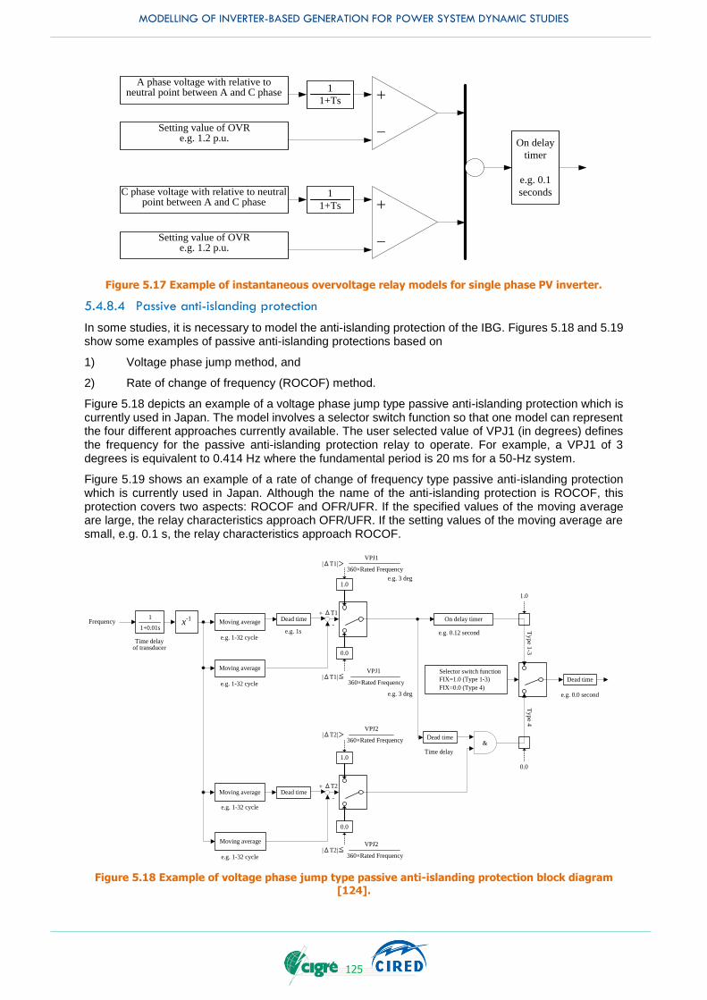
MODELLING OF INVERTER-BASED GENERATION FOR POWER SYSTEM DYNAMIC STUDIES
125
A phase voltage with relative to neutral point between A and C phase
On delay
timer
e.g. 0.1
seconds
Setting value of OVRe.g. 1.2 p.u.
+
-
+
-
C phase voltage with relative to neutral point between A and C phase
Setting value of OVRe.g. 1.2 p.u.
1
1+Ts
1
1+Ts
Figure 5.17 Example of instantaneous overvoltage relay models for single phase PV inverter.
5.4.8.4 Passive anti-islanding protection
In some studies, it is necessary to model the anti-islanding protection of the IBG. Figures 5.18 and 5.19 show some examples of passive anti-islanding protections based on
1) Voltage phase jump method, and
2) Rate of change of frequency (ROCOF) method.
Figure 5.18 depicts an example of a voltage phase jump type passive anti-islanding protection which is currently used in Japan. The model involves a selector switch function so that one model can represent the four different approaches currently available. The user selected value of VPJ1 (in degrees) defines the frequency for the passive anti-islanding protection relay to operate. For example, a VPJ1 of 3 degrees is equivalent to 0.414 Hz where the fundamental period is 20 ms for a 50-Hz system.
Figure 5.19 shows an example of a rate of change of frequency type passive anti-islanding protection which is currently used in Japan. Although the name of the anti-islanding protection is ROCOF, this protection covers two aspects: ROCOF and OFR/UFR. If the specified values of the moving average are large, the relay characteristics approach OFR/UFR. If the setting values of the moving average are small, e.g. 0.1 s, the relay characteristics approach ROCOF.
1+0.01s
1Frequency
Time delay of transducer
x-1 Dead time+
-
1.0
0.0
|ΔT1|>
On delay timer
|ΔT1|≦
VPJ1
360×Rated Frequency
VPJ1
360×Rated Frequency
Moving average
Moving average
Moving average
Moving average
Dead time+
-
1.0
0.0
|ΔT2|>
|ΔT2|≦
VPJ2
360×Rated Frequency
VPJ2
360×Rated Frequency
Dead time
Selector switch function
FIX=1.0 (Type 1-3)
FIX=0.0 (Type 4)
1.0
0.0
Time delay
Dead time
Ty
pe 1
-3T
yp
e 4
&
ΔT1
ΔT2
e.g. 1-32 cycle
e.g. 1-32 cycle
e.g. 1-32 cycle
e.g. 1-32 cycle
e.g. 0.12 second
e.g. 3 deg
e.g. 3 deg
e.g. 1s
e.g. 0.0 second
Figure 5.18 Example of voltage phase jump type passive anti-islanding protection block diagram [124].
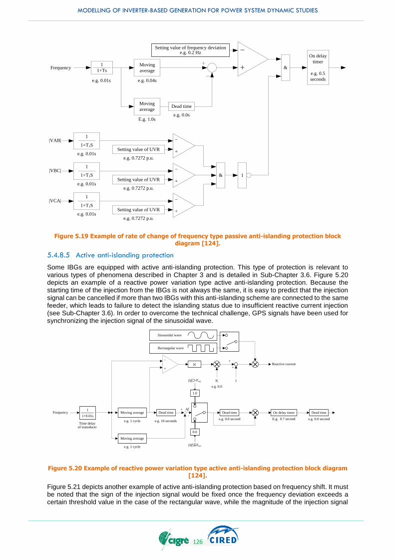
MODELLING OF INVERTER-BASED GENERATION FOR POWER SYSTEM DYNAMIC STUDIES
126
Moving
average
+
-
Moving
averageDead time
On delay
timer
e.g. 0.5
seconds
+
-
1
1+Ts
Setting value of frequency deviatione.g. 0.2 Hz
Frequency
e.g. 0.04se.g. 0.01s
e.g. 0.0sE.g. 1.0s
|VAB|1+T1S
1
|VCA|1
|VBC|1
1+T1S
1+T1S
&
e.g. 0.01s
e.g. 0.01s
e.g. 0.01s
Setting value of UVR +
-
+
-
Setting value of UVR
Setting value of UVR +
-
&
1
e.g. 0.7272 p.u.
e.g. 0.7272 p.u.
e.g. 0.7272 p.u.
Figure 5.19 Example of rate of change of frequency type passive anti-islanding protection block diagram [124].
5.4.8.5 Active anti-islanding protection
Some IBGs are equipped with active anti-islanding protection. This type of protection is relevant to various types of phenomena described in Chapter 3 and is detailed in Sub-Chapter 3.6. Figure 5.20 depicts an example of a reactive power variation type active anti-islanding protection. Because the starting time of the injection from the IBGs is not always the same, it is easy to predict that the injection signal can be cancelled if more than two IBGs with this anti-islanding scheme are connected to the same feeder, which leads to failure to detect the islanding status due to insufficient reactive current injection (see Sub-Chapter 3.6). In order to overcome the technical challenge, GPS signals have been used for synchronizing the injection signal of the sinusoidal wave.
1+0.01s
1Frequency
Time delay of transducer
Rectangular wave
Moving average
Moving average
Dead time+
-
1.0
0.0
|Df|>Fact
|Df|≦Fact
Dead timeDf
e.g. 1 cycle
e.g. 1 cyclee.g. 0.0 second
Dead time On delay timer
E.g. 0.7 second
+
-
|x|
×
×
K
+
+
1
× Reactive current
Sinusoidal wave
e.g. 10 secondse.g. 0.0 second
e.g. 0.0
Figure 5.20 Example of reactive power variation type active anti-islanding protection block diagram [124].
Figure 5.21 depicts another example of active anti-islanding protection based on frequency shift. It must be noted that the sign of the injection signal would be fixed once the frequency deviation exceeds a certain threshold value in the case of the rectangular wave, while the magnitude of the injection signal
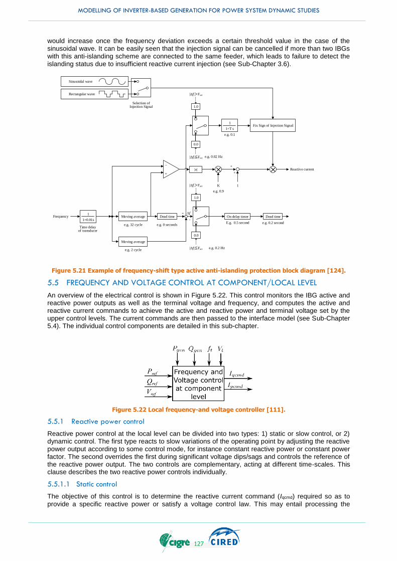
MODELLING OF INVERTER-BASED GENERATION FOR POWER SYSTEM DYNAMIC STUDIES
127
would increase once the frequency deviation exceeds a certain threshold value in the case of the sinusoidal wave. It can be easily seen that the injection signal can be cancelled if more than two IBGs with this anti-islanding scheme are connected to the same feeder, which leads to failure to detect the islanding status due to insufficient reactive current injection (see Sub-Chapter 3.6).
1+0.01s
1Frequency
Time delay of transducer
Rectangular wave
Moving average
Moving average
Dead time+
-
1.0
0.0
|Df|>Fact
|Df|≦Fact
Dead timeDf
e.g. 2 cycle
e.g. 32 cyclee.g. 0.2 second
On delay timer
E.g. 0.5 second
+
-
|x| ×
K
+
+
1
× Reactive current
Sinusoidal wave
e.g. 0 seconds
e.g. 0.2 Hz
e.g. 0.9
1.0
0.0
|Df|≦Fset
|Df|>Fset
Fix Sign of Injection Signal
Selection of Injection Signal
e.g. 0.02 Hz
1+T s
1
e.g. 0.1
Figure 5.21 Example of frequency-shift type active anti-islanding protection block diagram [124].
5.5 FREQUENCY AND VOLTAGE CONTROL AT COMPONENT/LOCAL LEVEL
An overview of the electrical control is shown in Figure 5.22. This control monitors the IBG active and reactive power outputs as well as the terminal voltage and frequency, and computes the active and reactive current commands to achieve the active and reactive power and terminal voltage set by the upper control levels. The current commands are then passed to the interface model (see Sub-Chapter 5.4). The individual control components are detailed in this sub-chapter.
Figure 5.22 Local frequency-and voltage controller [111].
5.5.1 Reactive power control
Reactive power control at the local level can be divided into two types: 1) static or slow control, or 2) dynamic control. The first type reacts to slow variations of the operating point by adjusting the reactive power output according to some control mode, for instance constant reactive power or constant power factor. The second overrides the first during significant voltage dips/sags and controls the reference of the reactive power output. The two controls are complementary, acting at different time-scales. This clause describes the two reactive power controls individually.
5.5.1.1 Static control
The objective of this control is to determine the reactive current command (Iqcmd) required so as to provide a specific reactive power or satisfy a voltage control law. This may entail processing the
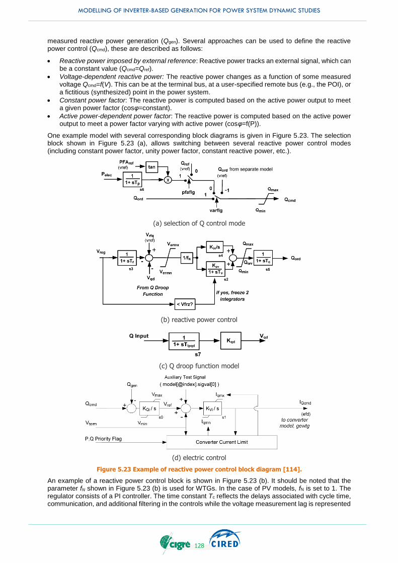
MODELLING OF INVERTER-BASED GENERATION FOR POWER SYSTEM DYNAMIC STUDIES
128
measured reactive power generation (Qgen). Several approaches can be used to define the reactive power control (Qcmd), these are described as follows:
Reactive power imposed by external reference: Reactive power tracks an external signal, which can be a constant value (Qcmd=Qref).
Voltage-dependent reactive power: The reactive power changes as a function of some measured voltage Qcmd=f(V). This can be at the terminal bus, at a user-specified remote bus (e.g., the POI), or a fictitious (synthesized) point in the power system.
Constant power factor: The reactive power is computed based on the active power output to meet a given power factor (cosφ=constant).
Active power-dependent power factor: The reactive power is computed based on the active power output to meet a power factor varying with active power (cosφ=f(P)).
One example model with several corresponding block diagrams is given in Figure 5.23. The selection block shown in Figure 5.23 (a), allows switching between several reactive power control modes (including constant power factor, unity power factor, constant reactive power, etc.).
(a) selection of Q control mode
(b) reactive power control
(c) Q droop function model
(d) electric control
Figure 5.23 Example of reactive power control block diagram [114].
An example of a reactive power control block is shown in Figure 5.23 (b). It should be noted that the parameter fN shown in Figure 5.23 (b) is used for WTGs. In the case of PV models, fN is set to 1. The regulator consists of a PI controller. The time constant Tc reflects the delays associated with cycle time, communication, and additional filtering in the controls while the voltage measurement lag is represented
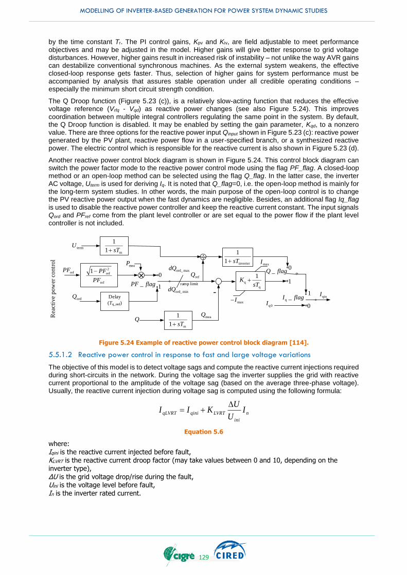
MODELLING OF INVERTER-BASED GENERATION FOR POWER SYSTEM DYNAMIC STUDIES
129
by the time constant Tr. The PI control gains, Kpv and Kiv, are field adjustable to meet performance objectives and may be adjusted in the model. Higher gains will give better response to grid voltage disturbances. However, higher gains result in increased risk of instability – not unlike the way AVR gains can destabilize conventional synchronous machines. As the external system weakens, the effective closed-loop response gets faster. Thus, selection of higher gains for system performance must be accompanied by analysis that assures stable operation under all credible operating conditions – especially the minimum short circuit strength condition.
The Q Droop function (Figure 5.23 (c)), is a relatively slow-acting function that reduces the effective voltage reference (Vrfq - Vqd) as reactive power changes (see also Figure 5.24). This improves coordination between multiple integral controllers regulating the same point in the system. By default, the Q Droop function is disabled. It may be enabled by setting the gain parameter, Kqd, to a nonzero value. There are three options for the reactive power input Qinput shown in Figure 5.23 (c): reactive power generated by the PV plant, reactive power flow in a user-specified branch, or a synthesized reactive power. The electric control which is responsible for the reactive current is also shown in Figure 5.23 (d).
Another reactive power control block diagram is shown in Figure 5.24. This control block diagram can switch the power factor mode to the reactive power control mode using the flag PF_flag. A closed-loop method or an open-loop method can be selected using the flag Q_flag. In the latter case, the inverter AC voltage, Uterm is used for deriving Iq. It is noted that Q_flag=0, i.e. the open-loop method is mainly for the long-term system studies. In other words, the main purpose of the open-loop control is to change the PV reactive power output when the fast dynamics are negligible. Besides, an additional flag Iq_flag is used to disable the reactive power controller and keep the reactive current constant. The input signals Qord and PFref come from the plant level controller or are set equal to the power flow if the plant level controller is not included.
Q
×refPF
refQ
ordQ Delay
(Tq_ord)
_PF flag
m
1
1 sT+
-
÷
q
q
1K
sT+
_Q flag
maxI
maxI-
inverter
1
1 sT+
2
ref
ref
1 PF
PF
-0
10
1
Rea
ctiv
e po
wer
con
tro
l
meaP
qinI
ord_ maxdQ
ord_ mindQramp limit
q _I flag
0
1
q0I
meaQ
termUm
1
1 sT+
Figure 5.24 Example of reactive power control block diagram [114].
5.5.1.2 Reactive power control in response to fast and large voltage variations
The objective of this model is to detect voltage sags and compute the reactive current injections required during short-circuits in the network. During the voltage sag the inverter supplies the grid with reactive current proportional to the amplitude of the voltage sag (based on the average three-phase voltage). Usually, the reactive current injection during voltage sag is computed using the following formula:
n
ini
LVRTqiniqLVRT IU
UKII
D+
Equation 5.6
where:
Iqini is the reactive current injected before fault,
KLVRT is the reactive current droop factor (may take values between 0 and 10, depending on the inverter type),
ΔU is the grid voltage drop/rise during the fault, Uini is the voltage level before fault,
In is the inverter rated current.

MODELLING OF INVERTER-BASED GENERATION FOR POWER SYSTEM DYNAMIC STUDIES
130
5.5.2 Active power control
Similarly, to the control of reactive power considered in Clause 5.5.1, the objective of this control is to determine the active current command (𝐼𝑝𝑖𝑛). Several approaches exist for defining this value, and two
examples are explained below and shown in Figure 5.25:
mP
P
ordP Delay
(Tp_ord)
min
mpp
1
1 sT+
refP-
m
1
1 sT+
maxI
maxI-
p
p
1K
sT+
termU ÷inverter
1
1 sT+
_P flag
m
1
1 sT+
0
1
Act
ive
po
wer
co
ntr
ol
meaP
Reset if active
power recovers
after fault clear
pinI
ord_ maxdP
ord_ mindP
m _ maxdP
ramp limit
ramp limit
Figure 5.25 Example of active power control block diagram [113].
5.5.2.1 Active power imposed by external reference (P_flg=0):
In this mode of operation, active power tracks an external signal (Pord) with some delay. This signal is limited by the maximum available power (Pm) and compared to the measured active power of the IBG (Pmea). Finally, a PI controller drives the current setpoint. The active power is likely to be controlled for the additional requirement/capability, such as the LFSM-O and FSM. The ramp rate limits shown in Figure 5.25 are employed to represent such capabilities.
5.5.2.2 Voltage-dependent active power (P_flg=1):
In this mode of operation, the active power current changes as a function of some measured voltage (Uterm) and the reference power (Pref). This can be the terminal bus, a user-specified remote bus (e.g., the POI), or a fictitious (synthesized) point in the power system. The main purpose of this type of control is to change the PV output when the fast dynamics are negligible. This type of model is used mainly when studying long-term dynamics.
Alternatively, voltage control can be performed by decreasing the active power with a fixed ramping rate. In such a case, Pord in Figure 5.25 may be used for the reduction of the active power of the PVs instead of the voltage-dependent active power control. Residential PVs which are connected to LV network may be equipped with voltage control by means of active power. The representative flowchart of the voltage rise mitigation function with characteristics of PV inverter is illustrated in Figure 5.26. Multiple strategies for the voltage control by means of active power are implemented in the flowchart and some strategies control not only the active power but also the reactive power. It is also noted that Figure 5.26 illustrates the procedure of how to determine Pord in Figure 5.25.
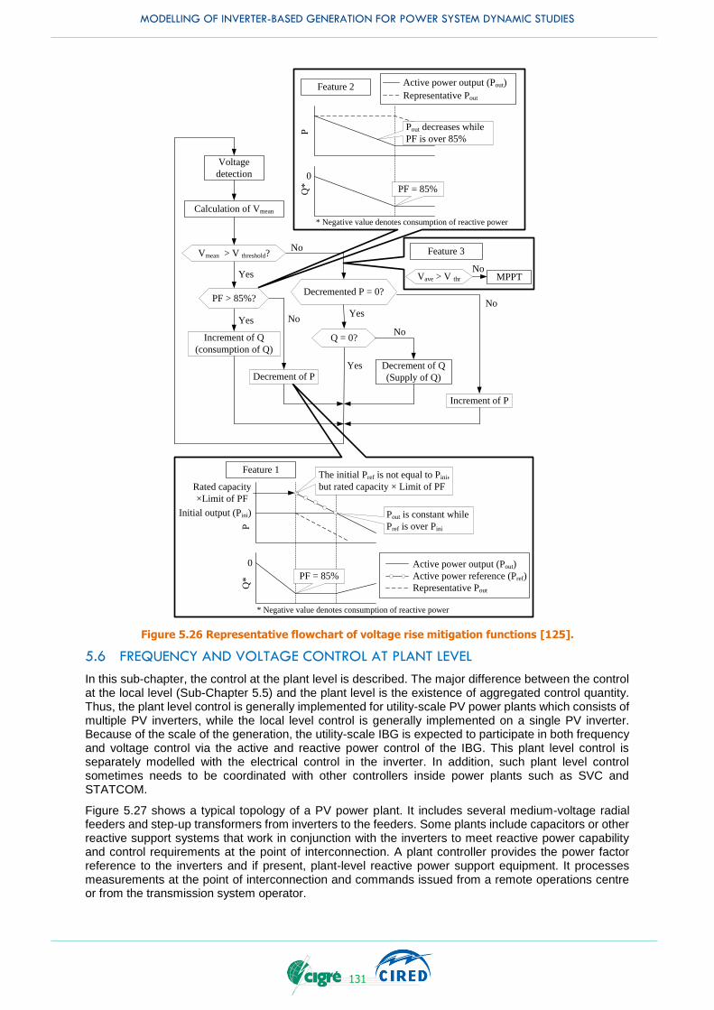
MODELLING OF INVERTER-BASED GENERATION FOR POWER SYSTEM DYNAMIC STUDIES
131
Voltage
detection
Calculation of Vmean
Decrement of Q
(Supply of Q)
Increment of Q
(consumption of Q)
Decrement of P
Increment of P
No
Yes
YesYes
Yes
No
No
PF > 85%?
Vmean > V threshold?
Decremented P = 0?
Q = 0?
Q*
0
P
Feature 2 Active power output (Pout)
Representative Pout
Pout decreases while
PF is over 85%
Initial output (Pini)
Rated capacity
×Limit of PF
PQ
*
0
PF = 85%
Feature 1
Active power output (Pout)
Active power reference (Pref)
Representative Pout
Pout is constant while
Pref is over Pini
MPPTVave > V thr
Feature 3
No
* Negative value denotes consumption of reactive power
No
No
PF = 85%
* Negative value denotes consumption of reactive power
The initial Pref is not equal to Pini,
but rated capacity × Limit of PF
Figure 5.26 Representative flowchart of voltage rise mitigation functions [125].
5.6 FREQUENCY AND VOLTAGE CONTROL AT PLANT LEVEL
In this sub-chapter, the control at the plant level is described. The major difference between the control at the local level (Sub-Chapter 5.5) and the plant level is the existence of aggregated control quantity. Thus, the plant level control is generally implemented for utility-scale PV power plants which consists of multiple PV inverters, while the local level control is generally implemented on a single PV inverter. Because of the scale of the generation, the utility-scale IBG is expected to participate in both frequency and voltage control via the active and reactive power control of the IBG. This plant level control is separately modelled with the electrical control in the inverter. In addition, such plant level control sometimes needs to be coordinated with other controllers inside power plants such as SVC and STATCOM.
Figure 5.27 shows a typical topology of a PV power plant. It includes several medium-voltage radial feeders and step-up transformers from inverters to the feeders. Some plants include capacitors or other reactive support systems that work in conjunction with the inverters to meet reactive power capability and control requirements at the point of interconnection. A plant controller provides the power factor reference to the inverters and if present, plant-level reactive power support equipment. It processes measurements at the point of interconnection and commands issued from a remote operations centre or from the transmission system operator.
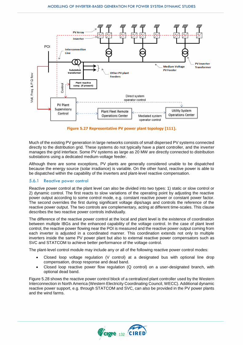
MODELLING OF INVERTER-BASED GENERATION FOR POWER SYSTEM DYNAMIC STUDIES
132
Figure 5.27 Representative PV power plant topology [111].
Much of the existing PV generation in large networks consists of small dispersed PV systems connected directly to the distribution grid. These systems do not typically have a plant controller, and the inverter manages the grid interface. Some PV systems as large as 20 MW are directly connected to distribution substations using a dedicated medium-voltage feeder.
Although there are some exceptions, PV plants are generally considered unable to be dispatched because the energy source (solar irradiance) is variable. On the other hand, reactive power is able to be dispatched within the capability of the inverters and plant-level reactive compensation.
5.6.1 Reactive power control
Reactive power control at the plant level can also be divided into two types: 1) static or slow control or 2) dynamic control. The first reacts to slow variations of the operating point by adjusting the reactive power output according to some control mode, e.g. constant reactive power or constant power factor. The second overrides the first during significant voltage dips/sags and controls the reference of the reactive power output. The two controls are complementary, acting at different time-scales. This clause describes the two reactive power controls individually.
The difference of the reactive power control at the local and plant level is the existence of coordination between multiple IBGs and the enhanced capability of the voltage control. In the case of plant level control, the reactive power flowing near the POI is measured and the reactive power output coming from each inverter is adjusted in a coordinated manner. This coordination extends not only to multiple inverters inside the same PV power plant but also to external reactive power compensators such as SVC and STATCOM to achieve better performance of the voltage control.
The plant-level control module may include any or all of the following reactive power control modes:
Closed loop voltage regulation (V control) at a designated bus with optional line drop compensation, droop response and dead band.
Closed loop reactive power flow regulation (Q control) on a user-designated branch, with optional dead band.
Figure 5.28 shows the reactive power control block of a centralized plant controller used by the Western Interconnection in North America (Western Electricity Coordinating Council, WECC). Additional dynamic reactive power support, e.g. through STATCOM and SVC, can also be provided in the PV power plants and the wind farms.
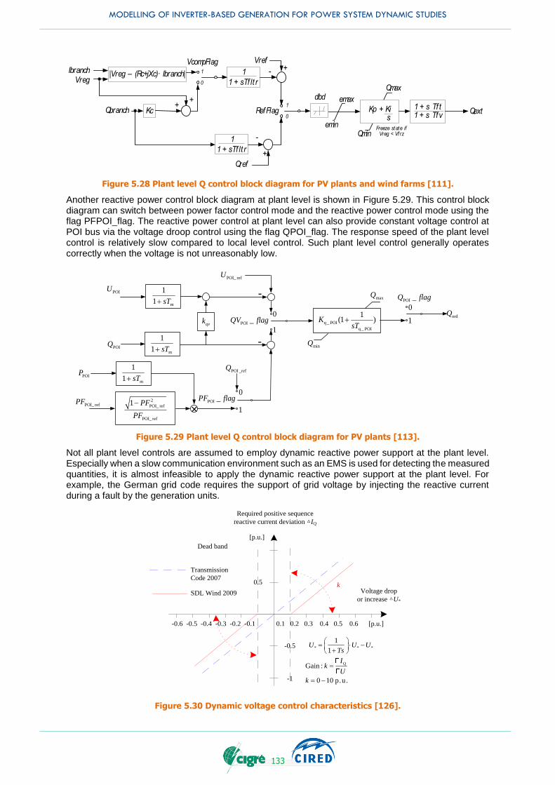
MODELLING OF INVERTER-BASED GENERATION FOR POWER SYSTEM DYNAMIC STUDIES
133
1
0
Vreg
Vref
Freeze state if Vreg < Vf rz
Ibranch
Kc
-
Qbranch
emax
emin
Kp + Ki s
Qmax
Qmin
1 + s Tf t1 + s Tfv
QextRefFlag
dbd
1
1 + sTf lt r
VcompFlag
|Vreg – (Rc+jXc)· Ibranch|
1
1 + sTf lt r
1
0
Qref
-
++
+
+
Figure 5.28 Plant level Q control block diagram for PV plants and wind farms [111].
Another reactive power control block diagram at plant level is shown in Figure 5.29. This control block diagram can switch between power factor control mode and the reactive power control mode using the flag PFPOI_flag. The reactive power control at plant level can also provide constant voltage control at POI bus via the voltage droop control using the flag QPOI_flag. The response speed of the plant level control is relatively slow compared to local level control. Such plant level control generally operates correctly when the voltage is not unreasonably low.
m
1
1 sT+-
-
POI _QV flag
maxQ
minQ
q _ POI
q _ POI
1(1 )K
sT+
ordQ
POI _Q flagPOIU
POIQ
POI_ refU
m
1
1 sT+POIP
POI_ refPF 2
POI_ ref
POI_ ref
1 PF
PF
-×
POI _PF flag
POI _refQ
0
1
0
1
0
1qvk
m
1
1 sT+
Figure 5.29 Plant level Q control block diagram for PV plants [113].
Not all plant level controls are assumed to employ dynamic reactive power support at the plant level. Especially when a slow communication environment such as an EMS is used for detecting the measured quantities, it is almost infeasible to apply the dynamic reactive power support at the plant level. For example, the German grid code requires the support of grid voltage by injecting the reactive current during a fault by the generation units.
Required positive sequence
reactive current deviation △IQ
0.5
Dead band
[p.u.]
-0.5
-1
-0.6 -0.5 -0.4 -0.3 -0.2 -0.1 0.1 0.2 0.3 0.4 0.5 0.6 [p.u.]
k
Transmission
Code 2007
SDL Wind 2009 Voltage drop
or increase △U*
* * *
Q
1
1
Gain :
0 10 p.u.
U U UTs
Ik
U
k
-
+
-
Figure 5.30 Dynamic voltage control characteristics [126].
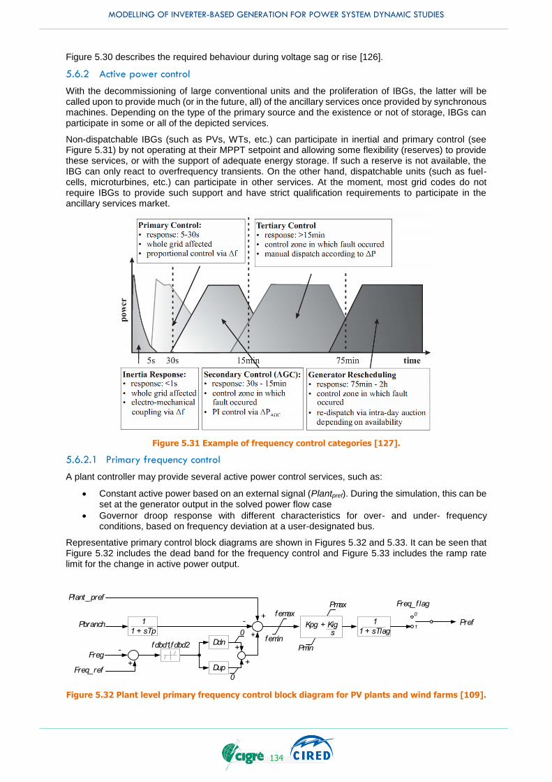
MODELLING OF INVERTER-BASED GENERATION FOR POWER SYSTEM DYNAMIC STUDIES
134
Figure 5.30 describes the required behaviour during voltage sag or rise [126].
5.6.2 Active power control
With the decommissioning of large conventional units and the proliferation of IBGs, the latter will be called upon to provide much (or in the future, all) of the ancillary services once provided by synchronous machines. Depending on the type of the primary source and the existence or not of storage, IBGs can participate in some or all of the depicted services.
Non-dispatchable IBGs (such as PVs, WTs, etc.) can participate in inertial and primary control (see Figure 5.31) by not operating at their MPPT setpoint and allowing some flexibility (reserves) to provide these services, or with the support of adequate energy storage. If such a reserve is not available, the IBG can only react to overfrequency transients. On the other hand, dispatchable units (such as fuel-cells, microturbines, etc.) can participate in other services. At the moment, most grid codes do not require IBGs to provide such support and have strict qualification requirements to participate in the ancillary services market.
Figure 5.31 Example of frequency control categories [127].
5.6.2.1 Primary frequency control
A plant controller may provide several active power control services, such as:
Constant active power based on an external signal (Plantpref). During the simulation, this can be set at the generator output in the solved power flow case
Governor droop response with different characteristics for over- and under- frequency conditions, based on frequency deviation at a user-designated bus.
Representative primary control block diagrams are shown in Figures 5.32 and 5.33. It can be seen that Figure 5.32 includes the dead band for the frequency control and Figure 5.33 includes the ramp rate limit for the change in active power output.
femin
femax
Pbranch
Plant_pref
Ddn
Dup
0
0Freq_ref
-fdbd1,fdbd2
- Kpg + Kig s
Pmax
PminFreg
1
1 + sTp
1
1 + sTlagPref
+
+
+
+
+ 0
1
Freq_f lag
Figure 5.32 Plant level primary frequency control block diagram for PV plants and wind farms [109].
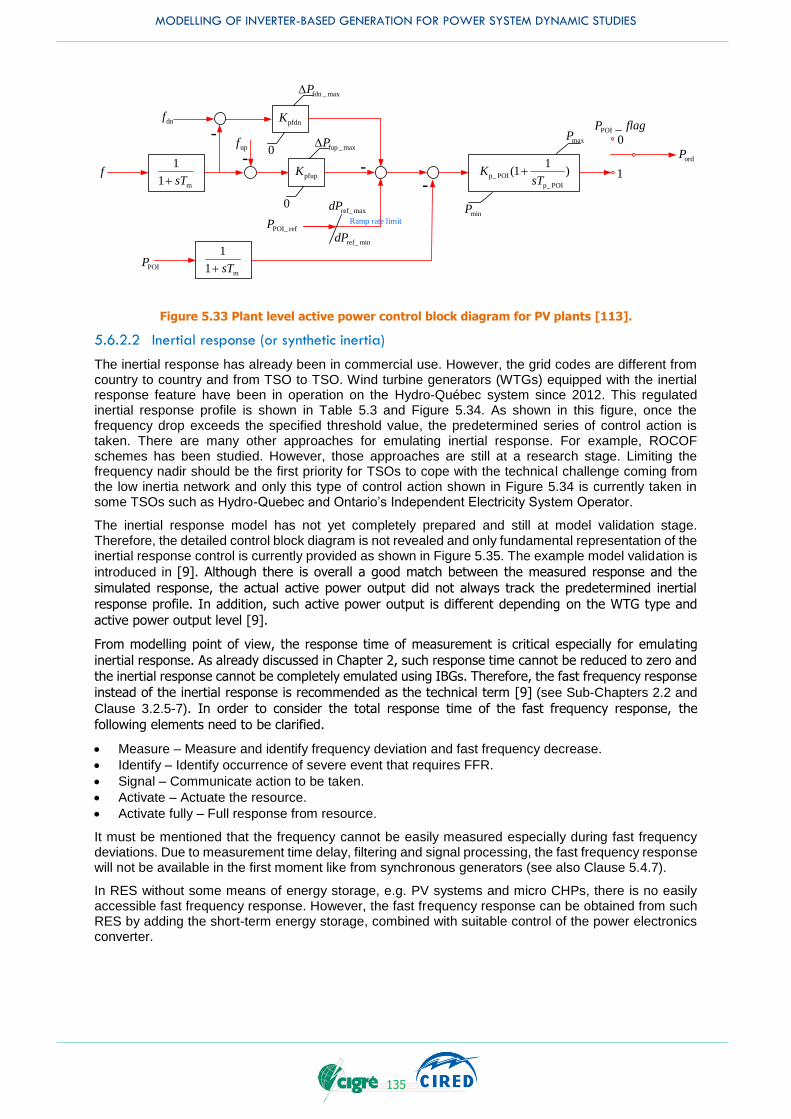
MODELLING OF INVERTER-BASED GENERATION FOR POWER SYSTEM DYNAMIC STUDIES
135
upf
m
1
1 sT+
-f pfupK
m
1
1 sT+
-
POI_ refP
maxP
minP
p_ POI
p_ POI
1(1 )K
sT+
ordP
POI _P flag
0
-1
0fup max_P
pfdnK
0
fdn max_P
dnf
-
ref_ maxdP
ref_ mindP
Ramp rate limit
POIP
D
D
Figure 5.33 Plant level active power control block diagram for PV plants [113].
5.6.2.2 Inertial response (or synthetic inertia)
The inertial response has already been in commercial use. However, the grid codes are different from country to country and from TSO to TSO. Wind turbine generators (WTGs) equipped with the inertial response feature have been in operation on the Hydro-Québec system since 2012. This regulated inertial response profile is shown in Table 5.3 and Figure 5.34. As shown in this figure, once the frequency drop exceeds the specified threshold value, the predetermined series of control action is taken. There are many other approaches for emulating inertial response. For example, ROCOF schemes has been studied. However, those approaches are still at a research stage. Limiting the frequency nadir should be the first priority for TSOs to cope with the technical challenge coming from the low inertia network and only this type of control action shown in Figure 5.34 is currently taken in some TSOs such as Hydro-Quebec and Ontario’s Independent Electricity System Operator.
The inertial response model has not yet completely prepared and still at model validation stage. Therefore, the detailed control block diagram is not revealed and only fundamental representation of the inertial response control is currently provided as shown in Figure 5.35. The example model validation is
introduced in [9]. Although there is overall a good match between the measured response and the
simulated response, the actual active power output did not always track the predetermined inertial
response profile. In addition, such active power output is different depending on the WTG type and
active power output level [9].
From modelling point of view, the response time of measurement is critical especially for emulating
inertial response. As already discussed in Chapter 2, such response time cannot be reduced to zero and the inertial response cannot be completely emulated using IBGs. Therefore, the fast frequency response
instead of the inertial response is recommended as the technical term [9] (see Sub-Chapters 2.2 and
Clause 3.2.5-7). In order to consider the total response time of the fast frequency response, the
following elements need to be clarified.
Measure – Measure and identify frequency deviation and fast frequency decrease.
Identify – Identify occurrence of severe event that requires FFR.
Signal – Communicate action to be taken.
Activate – Actuate the resource.
Activate fully – Full response from resource.
It must be mentioned that the frequency cannot be easily measured especially during fast frequency deviations. Due to measurement time delay, filtering and signal processing, the fast frequency response will not be available in the first moment like from synchronous generators (see also Clause 5.4.7).
In RES without some means of energy storage, e.g. PV systems and micro CHPs, there is no easily accessible fast frequency response. However, the fast frequency response can be obtained from such RES by adding the short-term energy storage, combined with suitable control of the power electronics converter.
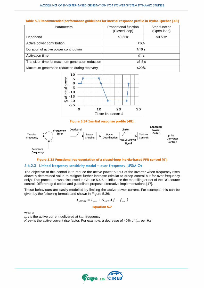
MODELLING OF INVERTER-BASED GENERATION FOR POWER SYSTEM DYNAMIC STUDIES
136
Table 5.3 Recommended performance guidelines for inertial response profile in Hydro-Quebec [48]
Parameters Proportional function (Closed loop)
Step function (Open-loop)
Deadband ≤0.3Hz ≤0.5Hz
Active power contribution ≥6%
Duration of active power contribution ≥10 s
Activation time ≤1 s
Transition time for maximum generation reduction ≥3.5 s
Maximum generation reduction during recovery ≤20%
Figure 5.34 Inertial response profile [48].
Figure 5.35 Functional representation of a closed-loop inertia-based FFR control [9].
5.6.2.3 Limited frequency sensitivity model – over-frequency (LFSM-O)
The objective of this control is to reduce the active power output of the inverter when frequency rises above a determined value to mitigate further increase (similar to droop control but for over-frequency only). This procedure was discussed in Clause 5.4.6 to influence the modelling or not of the DC source control. Different grid codes and guidelines propose alternative implementations [17].
These behaviours are easily modelled by limiting the active power current. For example, this can be given by the following formula and shown in Figure 5.36:
startHFRTpinipHFRT ffKII -+
Equation 5.7
where: Ipini is the active current delivered at fstart frequency KHFRT is the active current rise factor. For example, a decrease of 40% of Ipini per Hz
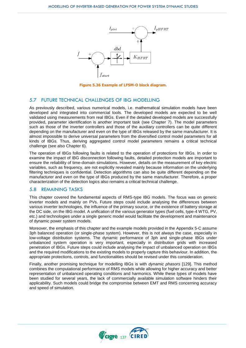
MODELLING OF INVERTER-BASED GENERATION FOR POWER SYSTEM DYNAMIC STUDIES
137
Figure 5.36 Example of LFSM-O block diagram.
5.7 FUTURE TECHNICAL CHALLENGES OF IBG MODELLING
As previously described, various numerical models, i.e. mathematical simulation models have been developed and integrated into commercial tools. The developed models are expected to be well validated using measurements from real IBGs. Even if the detailed developed models are successfully provided, parameter identification is another important task (see Chapter 7). The model parameters such as those of the inverter controllers and those of the auxiliary controllers can be quite different depending on the manufacturer and even on the type of IBGs released by the same manufacturer. It is almost impossible to derive universal parameters from the diversified control model parameters for all kinds of IBGs. Thus, deriving aggregated control model parameters remains a critical technical challenge (see also Chapter 6).
The operation of IBGs following faults is related to the operation of protections for IBGs. In order to examine the impact of IBG disconnection following faults, detailed protection models are important to ensure the reliability of time-domain simulations. However, details on the measurement of key electric variables, such as frequency, are not explicitly revealed mainly because information on the underlying filtering techniques is confidential. Detection algorithms can also be quite different depending on the manufacturer and even on the type of IBGs produced by the same manufacturer. Therefore, a proper characterization of the detection logics also remains a critical technical challenge.
5.8 REMAINING TASKS
This chapter covered the fundamental aspects of RMS-type IBG models. The focus was on generic inverter models and mainly on PVs. Future steps could include analysing the differences between various inverter technologies, the influence of the primary source, or the existence of battery storage at the DC side, on the IBG model. A unification of the various generator types (fuel cells, type-4 WTG, PV, etc.) and technologies under a single generic model would facilitate the development and maintenance of dynamic power system models.
Moreover, the emphasis of this chapter and the example models provided in the Appendix 5-C assume 3ph balanced operation (or single-phase system). However, this is not always the case, especially in low-voltage distribution systems. The dynamic performance of 3ph and single-phase IBGs under unbalanced system operation is very important, especially in distribution grids with increased penetration of IBGs. Future steps could include analysing the impact of unbalanced operation on IBGs and the required modifications to the existing models to properly capture this behaviour. In addition, the appropriate protections, controls, and functionalities should be revised under this consideration.
Finally, another promising technique for modelling IBGs is with dynamic phasors [129]. This method combines the computational performance of RMS models while allowing for higher accuracy and better representation of unbalanced operating conditions and harmonics. While these types of models have been studied for several years, the lack of commercially available simulation software hinders their applicability. Such models could bridge the compromise between EMT and RMS concerning accuracy and speed of simulation.

MODELLING OF INVERTER-BASED GENERATION FOR POWER SYSTEM DYNAMIC STUDIES
138
5.9 CONCLUSIONS
Chapter 5 investigates the methods for modelling IBGs under the RMS modelling assumption and provides a number of example block diagrams and characteristic functions to achieve this. In addition to the individual IBG model elements provided and described, some all-in-one models have also been provided in the Appendix 5-C. The model elements consist of control and protection components, respectively. Most of the IBG model elements presented in this chapter are currently implemented in commercial time-domain simulation tools around the world. However, it should be noted that only some capabilities/controls may be implemented in real IBGs. In addition, the specific capabilities and controls implemented in the IBGs vary from country to country. Therefore, the numerical models, i.e. mathematical simulation models can play an important role to figure out the recommended specification of the capabilities from TSO/DSO’s point of view.
In this chapter, each IBG model element was classified into two categories: 1) Component level, and 2) Plant level. The plant level elements were extracted from the controls which are generally required for the utility-scale IBGs. It should be emphasized that the representative parameters or the representative ranges of parameters of the all-in-one models, as well as the individual elements, were revealed as much as possible.
Finally, this chapter has also discussed the limitations of RMS models depending on the phenomena analysed and the required sampling frequency. If the RMS models are not suited to a specific type of study, the EMT model can be one of the options. Chapter 4 details the way to model IBGs from EMT modelling perspectives. Finally, the future technical challenge of IBG modelling has been briefly discussed focusing on the establishment of the aggregation approach for distributed IBGs with diversified control parameters.
MODELLING OF INVERTER-BASED GENERATION FOR POWER SYSTEM DYNAMIC STUDIES
139
6. MODELLING OF AGGREGATED DISTRIBUTED INVERTER-BASED GENERATION
6.1 BACKGROUND AND MOTIVATION
It is well known that there are many individual wind turbine generators (WTG) in wind plants and many individual solar PV units in solar PV plants. Because different renewables could show different dynamic behaviour following faults, the individual modelling is an ideal solution for representing such dynamic behaviour precisely. However, as the number of renewables increases, it is almost infeasible to model huge number of renewables individually, mainly due to the very high computation burden. Therefore, the aggregation techniques presented in this chapter to lump together all individual WTGs or PVs could be one of the solutions to achieve a reasonable balance between the accuracy of the individual behaviour and the permissible computation burden. The level of modelling detail that will ultimately be required depends not only on the type of studies performed but also on the expected maximum instantaneous wind/PVs penetration to be modelled.
Apart from reducing computational demands, another strong reason for using aggregated models is that they are adequate for most of the studies required by utilities, i.e., grid planning and performance of the system at the point of interconnection (POI) where the events to be considered are in the timescale from tens of milliseconds to seconds. Also, in large power system dynamic studies, it may not be reasonable to model each individual unit and individual low voltage feeder.
Overall, modelling of aggregated Inverter-Based Generators (IBG) is an ongoing field of research and its importance is likely to increase with IBG deployment all over the world. The modelling of aggregated IBG for large-scale power system dynamic studies is required for:
1) Steady-state power flow studies 2) Power system dynamic studies
The variance of the terminal voltage of IBGs connected in different locations of a feeder or the variance between the medium voltage (MV) network and the low voltage (LV) network may cause a very different dynamic response of these IBGs. The current practice of the modelling of the aggregated IBG is classified into three categories in the order of complexity (from less detailed to more detailed modelling) [7], [130], [131]:
Joint aggregation of IBGs in MV and LV networks without considering the variation of the dynamic behaviour of P and Q during and following faults (e.g., simple netting of IBGs with load),
Joint aggregation of IBGs in MV and LV network (with) considering the variation of the dynamic behaviour of P and Q during and following faults (WECC approach using PVD1 model, see below)
Separate aggregation of IBGs in MV and in LV networks (with) considering the variation of the dynamic behaviour of P and Q during and following faults (German academic approach, see below).
While the modelling of the aggregated IBG for the steady-state power flow analysis, the power flow studies have already been performed and applied in some countries such as the U.S. and some European countries. The industrial practice for the aggregated IBG modelling for 2), the power system dynamic studies are very limited [6]. Proposals come mainly from academic research and are summarized in [6] with recent contributions in [131], [132], [133].
Practical applications for aggregation include the generic wind generation model defined by IEC TC 61400-27-1 Ed.1 that is used for wind parks of significant size in power system dynamic studies in some European countries. However, no generally accepted approaches for the modelling of the aggregated IBG, such as medium-scale, distributed wind parks, and aggregation of small-scale PVs in low voltage networks are currently available in some countries (contributions in [131], [132] are still of academic nature). Conversely, validated user-defined models including IBGs at distribution level are used in power system dynamic studies in other countries. The modelling of the aggregated IBG for the power flow studies and the power system dynamic studies have been developed by WECC. The aggregation approach of the collector system of large PV plants and the aggregation approach of residential PVs in LV networks have been separately established. Because WECC has used the composite load model including motor loads, a simplified, yet reasonable, aggregated model of distributed IBGs can be added into the composite load model. On the other hand, the current modelling of this aggregated IBG used in WECC still lacks certain stability study modelling details. Ongoing research is addressing the technical challenges related to aggregation of the IBG’s control input parameters for power system dynamic studies.
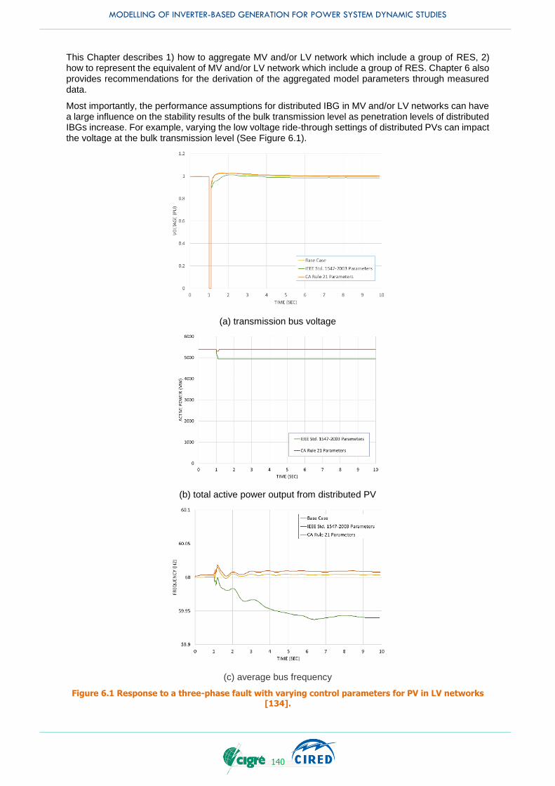
MODELLING OF INVERTER-BASED GENERATION FOR POWER SYSTEM DYNAMIC STUDIES
140
This Chapter describes 1) how to aggregate MV and/or LV network which include a group of RES, 2) how to represent the equivalent of MV and/or LV network which include a group of RES. Chapter 6 also provides recommendations for the derivation of the aggregated model parameters through measured data.
Most importantly, the performance assumptions for distributed IBG in MV and/or LV networks can have a large influence on the stability results of the bulk transmission level as penetration levels of distributed IBGs increase. For example, varying the low voltage ride-through settings of distributed PVs can impact the voltage at the bulk transmission level (See Figure 6.1).
(a) transmission bus voltage
(b) total active power output from distributed PV
(c) average bus frequency
Figure 6.1 Response to a three-phase fault with varying control parameters for PV in LV networks [134].
MODELLING OF INVERTER-BASED GENERATION FOR POWER SYSTEM DYNAMIC STUDIES
141
It is noted that CA Rule 21 in the legend denotes a tariff (or set of regulations) that describes the interconnection, operation and metering requirements for distributed generators that will be connected to a utility’s electric system.
The methodologies described in Sub-Chapter 6.2 were developed by the Western Electricity Coordinating Council (WECC) to represent wind and solar PV power plants in large-scale power flow and power system dynamic studies for the use in the North America Western Interconnection [7], [135] and have recently been adopted by the North American Electric Reliability Corporation (NERC) [134]. These WECC methods are currently one of the most elaborate standardised industry guidelines to study the aggregated impact of distributed IBGs in large-scale power systems. These methods are continuously evolving; in their current state, they are believed to create accurate modelling results for winds/PVs penetration levels of up to approximately 50% of instantaneous interconnection-wide load.
A refined aggregation method, representing aggregated IBGs in further detail compared to the WECC methodology, was used in a case study for assessing the dynamic stability in an example power system resembling the German situation in the year 2022 [130]. Modelling recommendations based on this refined aggregation method are added in the following sub-chapters where appropriate.
6.2 POWER FLOW REPRESENTATION
The aim of power flow modelling of wind/PV generation is to accurately represent distributed IBGs in grid planning studies in order to determine network expansion and reactive power/voltage control schemes coming from the reactive power range of inverters (See Appendix 3-G). A power flow case can also be used to initialize the state variables of dynamic models for large-scale power system dynamic studies.
Solar PV systems can be designed for a wide range of applications from small residential systems to utility-scale, (sub-) transmission-connected power plants as described in the following clauses
(1) Distribution-connected residential and commercial PV systems
Distribution-connected residential (small-scale) and commercial (medium-scale) PV systems typically connect to the customer side of the meter at single phase (e.g. 120/230V) or three-phase (e.g. 208/400V). Typical residential solar PV systems have a nameplate rating of less than 10 kW per phase and have a single inverter, while commercial systems can reach a capacity of several MW and typically have multiple inverters. Plants as large as 14 MW may be connected directly to an existing medium-voltage primary distribution feeder, or to the unit station through a dedicated feeder.
(2) Large, utility-scale wind and solar PV plants
Modern large, utility-scale inverters used in wind and solar PV plants have nameplate rating ranging from 1 MW to 4 MW. They connect at a terminal voltage of about 600 V or lower. Utility-scale PV and wind plants may have hundreds of these units and the plant capacity of more than 100 MW. Furthermore, they would be connected to the (sub-) transmission network.
6.2.1 Equivalent representation of utility-scale wind and solar PV plants
Utility scale generators are usually electrically separated from the transmission system by two transformer stages and equivalent line impedance. In large and medium size wind and solar PV plants, individual generating units are tied to a medium voltage (typically 12.5 kV to 34.5kV in the North America and 10 kV to 36 kV in Europe [135]) collector system through step-up transformers and connected to the transmission system at a single location, referred to as the POI. Several inverters may be connected to a single pad-mounted transformer. The collector system consists of one or several feeders connected together at a collector system station. One or more station transformers at the collector system station are used to step-up to transmission system voltage. Unless the collector system station is adjacent to the POI, an interconnection transmission line will be needed.
Reactive power support at the POI, to the extent that it is demanded by interconnection requirements, can be provided by the inverters, dedicated plant-level reactive power support equipment such as fixed or mechanically-switched capacitors, or a combination of both. STATCOM devices may also be installed to provide dynamic reactive power support. The amount and nature (static or dynamic) of reactive power compensation is driven by interconnection requirements and collector system design considerations, including voltage profile and losses. Figure 6.2 shows a typical topology for a large, utility-scale solar PV plant.
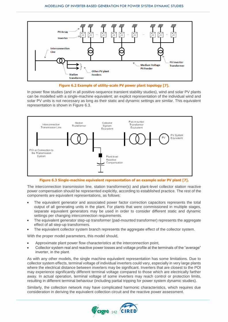
MODELLING OF INVERTER-BASED GENERATION FOR POWER SYSTEM DYNAMIC STUDIES
142
Figure 6.2 Example of utility-scale PV power plant topology [7].
In power flow studies (and in all positive-sequence transient stability studies), wind and solar PV plants can be modelled with a single-machine equivalent; an explicit representation of the individual wind and solar PV units is not necessary as long as their static and dynamic settings are similar. This equivalent representation is shown in Figure 6.3.
Figure 6.3 Single-machine equivalent representation of an example solar PV plant [7].
The interconnection transmission line, station transformer(s) and plant-level collector station reactive power compensation should be represented explicitly, according to established practice. The rest of the components are equivalent representations, as follows:
The equivalent generator and associated power factor correction capacitors represents the total output of all generating units in the plant. For plants that were commissioned in multiple stages, separate equivalent generators may be used in order to consider different static and dynamic settings per changing interconnection requirements.
The equivalent generator step-up transformer (pad-mounted transformer) represents the aggregate effect of all step-up transformers.
The equivalent collector system branch represents the aggregate effect of the collector system.
With the proper model parameters, this model should,
Approximate plant power flow characteristics at the interconnection point,
Collector system real and reactive power losses and voltage profile at the terminals of the “average” inverter, in the plant.
As with any other models, the single machine equivalent representation has some limitations. Due to collector system effects, terminal voltage of individual inverters could vary, especially in very large plants where the electrical distance between inverters may be significant. Inverters that are closest to the POI may experience significantly different terminal voltage compared to those which are electrically farther away. In actual operation, terminal voltage of some inverters may reach control or protection limits, resulting in different terminal behaviour (including partial tripping for power system dynamic studies).
Similarly, the collection network may have complicated harmonic characteristics, which requires due consideration in deriving the equivalent collection circuit and the reactive power assessment.
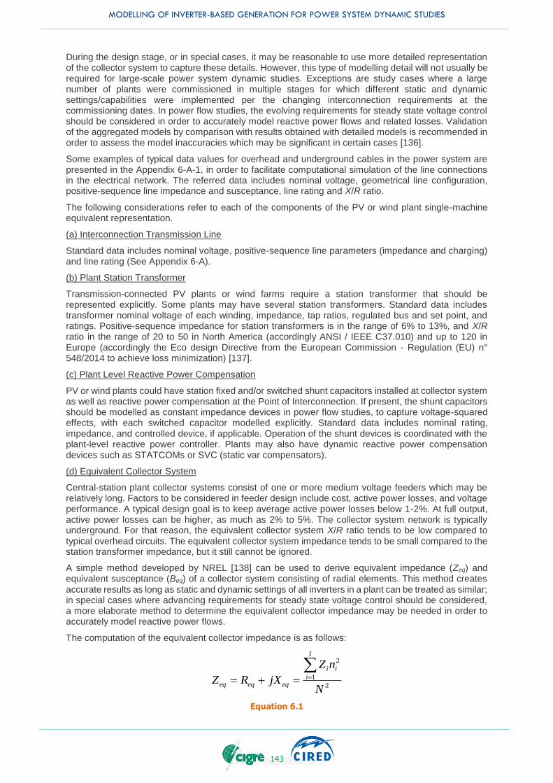
MODELLING OF INVERTER-BASED GENERATION FOR POWER SYSTEM DYNAMIC STUDIES
143
During the design stage, or in special cases, it may be reasonable to use more detailed representation of the collector system to capture these details. However, this type of modelling detail will not usually be required for large-scale power system dynamic studies. Exceptions are study cases where a large number of plants were commissioned in multiple stages for which different static and dynamic settings/capabilities were implemented per the changing interconnection requirements at the commissioning dates. In power flow studies, the evolving requirements for steady state voltage control should be considered in order to accurately model reactive power flows and related losses. Validation of the aggregated models by comparison with results obtained with detailed models is recommended in order to assess the model inaccuracies which may be significant in certain cases [136].
Some examples of typical data values for overhead and underground cables in the power system are presented in the Appendix 6-A-1, in order to facilitate computational simulation of the line connections in the electrical network. The referred data includes nominal voltage, geometrical line configuration, positive-sequence line impedance and susceptance, line rating and X/R ratio.
The following considerations refer to each of the components of the PV or wind plant single-machine equivalent representation.
(a) Interconnection Transmission Line
Standard data includes nominal voltage, positive-sequence line parameters (impedance and charging) and line rating (See Appendix 6-A).
(b) Plant Station Transformer
Transmission-connected PV plants or wind farms require a station transformer that should be represented explicitly. Some plants may have several station transformers. Standard data includes transformer nominal voltage of each winding, impedance, tap ratios, regulated bus and set point, and ratings. Positive-sequence impedance for station transformers is in the range of 6% to 13%, and X/R ratio in the range of 20 to 50 in North America (accordingly ANSI / IEEE C37.010) and up to 120 in Europe (accordingly the Eco design Directive from the European Commission - Regulation (EU) n° 548/2014 to achieve loss minimization) [137].
(c) Plant Level Reactive Power Compensation
PV or wind plants could have station fixed and/or switched shunt capacitors installed at collector system as well as reactive power compensation at the Point of Interconnection. If present, the shunt capacitors should be modelled as constant impedance devices in power flow studies, to capture voltage-squared effects, with each switched capacitor modelled explicitly. Standard data includes nominal rating, impedance, and controlled device, if applicable. Operation of the shunt devices is coordinated with the plant-level reactive power controller. Plants may also have dynamic reactive power compensation devices such as STATCOMs or SVC (static var compensators).
(d) Equivalent Collector System
Central-station plant collector systems consist of one or more medium voltage feeders which may be relatively long. Factors to be considered in feeder design include cost, active power losses, and voltage performance. A typical design goal is to keep average active power losses below 1-2%. At full output, active power losses can be higher, as much as 2% to 5%. The collector system network is typically underground. For that reason, the equivalent collector system X/R ratio tends to be low compared to typical overhead circuits. The equivalent collector system impedance tends to be small compared to the station transformer impedance, but it still cannot be ignored.
A simple method developed by NREL [138] can be used to derive equivalent impedance (Zeq) and equivalent susceptance (Beq) of a collector system consisting of radial elements. This method creates accurate results as long as static and dynamic settings of all inverters in a plant can be treated as similar; in special cases where advancing requirements for steady state voltage control should be considered, a more elaborate method to determine the equivalent collector impedance may be needed in order to accurately model reactive power flows.
The computation of the equivalent collector impedance is as follows:
2
1
2
N
nZ
jXRZ
I
i
ii
eqeqeq
+
Equation 6.1
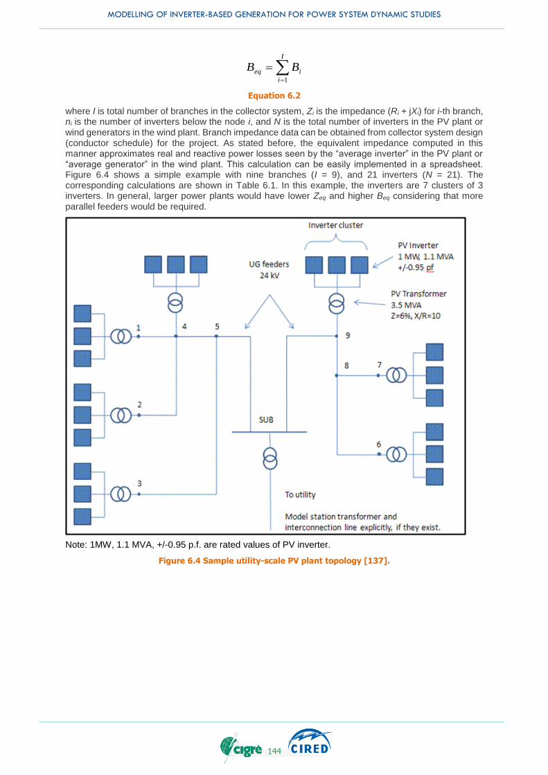
MODELLING OF INVERTER-BASED GENERATION FOR POWER SYSTEM DYNAMIC STUDIES
144
I
i
ieq BB1
Equation 6.2
where I is total number of branches in the collector system, Zi is the impedance (Ri + jXi) for i-th branch, ni is the number of inverters below the node i, and N is the total number of inverters in the PV plant or wind generators in the wind plant. Branch impedance data can be obtained from collector system design (conductor schedule) for the project. As stated before, the equivalent impedance computed in this manner approximates real and reactive power losses seen by the “average inverter” in the PV plant or “average generator” in the wind plant. This calculation can be easily implemented in a spreadsheet. Figure 6.4 shows a simple example with nine branches (I = 9), and 21 inverters (N = 21). The corresponding calculations are shown in Table 6.1. In this example, the inverters are 7 clusters of 3 inverters. In general, larger power plants would have lower Zeq and higher Beq considering that more parallel feeders would be required.
Note: 1MW, 1.1 MVA, +/-0.95 p.f. are rated values of PV inverter.
Figure 6.4 Sample utility-scale PV plant topology [137].
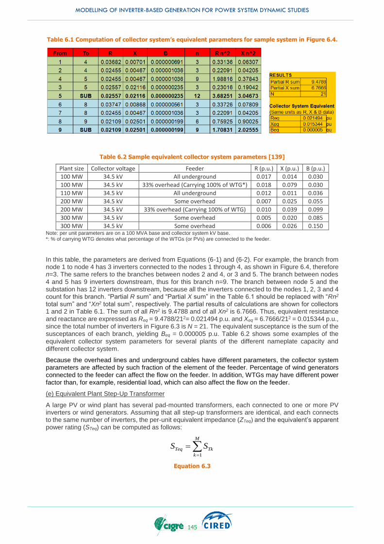
MODELLING OF INVERTER-BASED GENERATION FOR POWER SYSTEM DYNAMIC STUDIES
145
Table 6.1 Computation of collector system’s equivalent parameters for sample system in Figure 6.4.
Table 6.2 Sample equivalent collector system parameters [139]
Plant size Collector voltage Feeder R (p.u.) X (p.u.) B (p.u.)
100 MW 34.5 kV All underground 0.017 0.014 0.030
100 MW 34.5 kV 33% overhead (Carrying 100% of WTG*) 0.018 0.079 0.030
110 MW 34.5 kV All underground 0.012 0.011 0.036
200 MW 34.5 kV Some overhead 0.007 0.025 0.055
200 MW 34.5 kV 33% overhead (Carrying 100% of WTG) 0.010 0.039 0.099
300 MW 34.5 kV Some overhead 0.005 0.020 0.085
300 MW 34.5 kV Some overhead 0.006 0.026 0.150 Note: per unit parameters are on a 100 MVA base and collector system kV base. *: % of carrying WTG denotes what percentage of the WTGs (or PVs) are connected to the feeder.
In this table, the parameters are derived from Equations (6-1) and (6-2). For example, the branch from node 1 to node 4 has 3 inverters connected to the nodes 1 through 4, as shown in Figure 6.4, therefore n=3. The same refers to the branches between nodes 2 and 4, or 3 and 5. The branch between nodes 4 and 5 has 9 inverters downstream, thus for this branch n=9. The branch between node 5 and the substation has 12 inverters downstream, because all the inverters connected to the nodes 1, 2, 3 and 4 count for this branch. “Partial R sum” and “Partial X sum” in the Table 6.1 should be replaced with “Rn2 total sum” and “Xn2 total sum”, respectively. The partial results of calculations are shown for collectors 1 and 2 in Table 6.1. The sum of all Rn2 is 9.4788 and of all Xn2 is 6.7666. Thus, equivalent resistance and reactance are expressed as Req = 9.4788/212= 0.021494 p.u. and Xeq = 6.7666/212 = 0.015344 p.u., since the total number of inverters in Figure 6.3 is N = 21. The equivalent susceptance is the sum of the susceptances of each branch, yielding Beq = 0.000005 p.u. Table 6.2 shows some examples of the equivalent collector system parameters for several plants of the different nameplate capacity and different collector system.
Because the overhead lines and underground cables have different parameters, the collector system parameters are affected by such fraction of the element of the feeder. Percentage of wind generators connected to the feeder can affect the flow on the feeder. In addition, WTGs may have different power factor than, for example, residential load, which can also affect the flow on the feeder.
(e) Equivalent Plant Step-Up Transformer
A large PV or wind plant has several pad-mounted transformers, each connected to one or more PV inverters or wind generators. Assuming that all step-up transformers are identical, and each connects to the same number of inverters, the per-unit equivalent impedance (ZTeq) and the equivalent’s apparent power rating (STeq) can be computed as follows:
M
k
TkTeq SS1
Equation 6.3
MODELLING OF INVERTER-BASED GENERATION FOR POWER SYSTEM DYNAMIC STUDIES
146
M
k Tk
Tk
Teq
Teq
Z
S
SZ
1
Equation 6.4
where M is the total number of step-up transformers in the collector system, STk is the apparent power rating of k-th step-up transformer in MVA, and ZTk is the per-unit impedance of k-th step-up transformer on its own MVA base.
In the particular case where all step-up transformers are identical, and as such STk=ST and ZTk=ZT, the
assumed equations, Equation 6.3 and Equation 6.4 can be simplified to the following equations Equation
6.5 and Equation 6.6.
TTeq SMS
Equation 6.5
TTeq ZZ
Equation 6.6
For the example system discussed above where all step-up transformers are identical, the equivalent transformer impedance would be 6% on a 24.5 MVA base (7×3.5 MVA), with an X/R ratio of 10.
Step-up transformers associated with utility-scale PV plants are in the range of 500 kVA to 2 MVA, and have impedance of approximately 6% on the transformer MVA base, with X/R ratio of about 8.
(f) Equivalent Generator Representation
For power flow simulations, the aggregated PV or wind generator should be represented as a standard static generator, as opposed to a negative load, so that various IBG controls can be implemented for dynamic simulations. Active power level and reactive power capability must be specified as described in Appendix 3-G.
Representation of reactive power capability of the equivalent inverter depends on the reactive power range of the inverters, and how that range is utilised in operations. For example, the equivalent generator for the sample system shown in Figure 6.4 would have a nameplate rating of 21 MW (21 × 1 MW) and 23.1 MVA (21 × 1.1 MVA). If the inverters participate in steady-state voltage control, then the equivalent generator should be modelled with a reactive range of +/- 0.95 power factor, which corresponds to setting Qmin = -6.9 Mvar and Qmax = +6.9 Mvar, respectively. If the inverters operate at a fixed power factor, then the equivalent generator should have Qmin = Qmax at the corresponding power factor level (considering the correct sign in terms of leading or lagging operation). At an output level below rated, the reactive power limits should be adjusted according to the inverter reactive power output that is programmed into the controls and adjusted by a power factor correction that considers the effect of the terminal voltage of the inverters.
6.2.2 Equivalent representation of distribution-connected PV
In large-scale power system dynamic studies for systems with low wind/PVs penetration, the distribution system does not have to be modelled in detail and the load can be aggregated at the transmission buses with embedded distributed generation netted as negative load. However, in large-scale power system dynamic studies for which the aggregate distributed generation has the potential to affect grid reliability and compliance with system planning and performance standards (e.g., [140]), distribution-connected PV systems should be represented explicitly and not netted with load.
Modelling distributed generation explicitly, yet in an aggregated way, allows for proper load scaling and gives planners the ability to account for existing and emerging (changing) interconnection requirements and performance standards applicable to distributed generation. These may include requirements for voltage and frequency tolerance/ride-through capability, static and dynamic reactive power support, anti-islanding, etc.
A modular approach to represent IBGs in bulk system studies as illustrated in Figure 6.5 is recommended [141] to ensure accurate representation of the resources for the specific bulk system
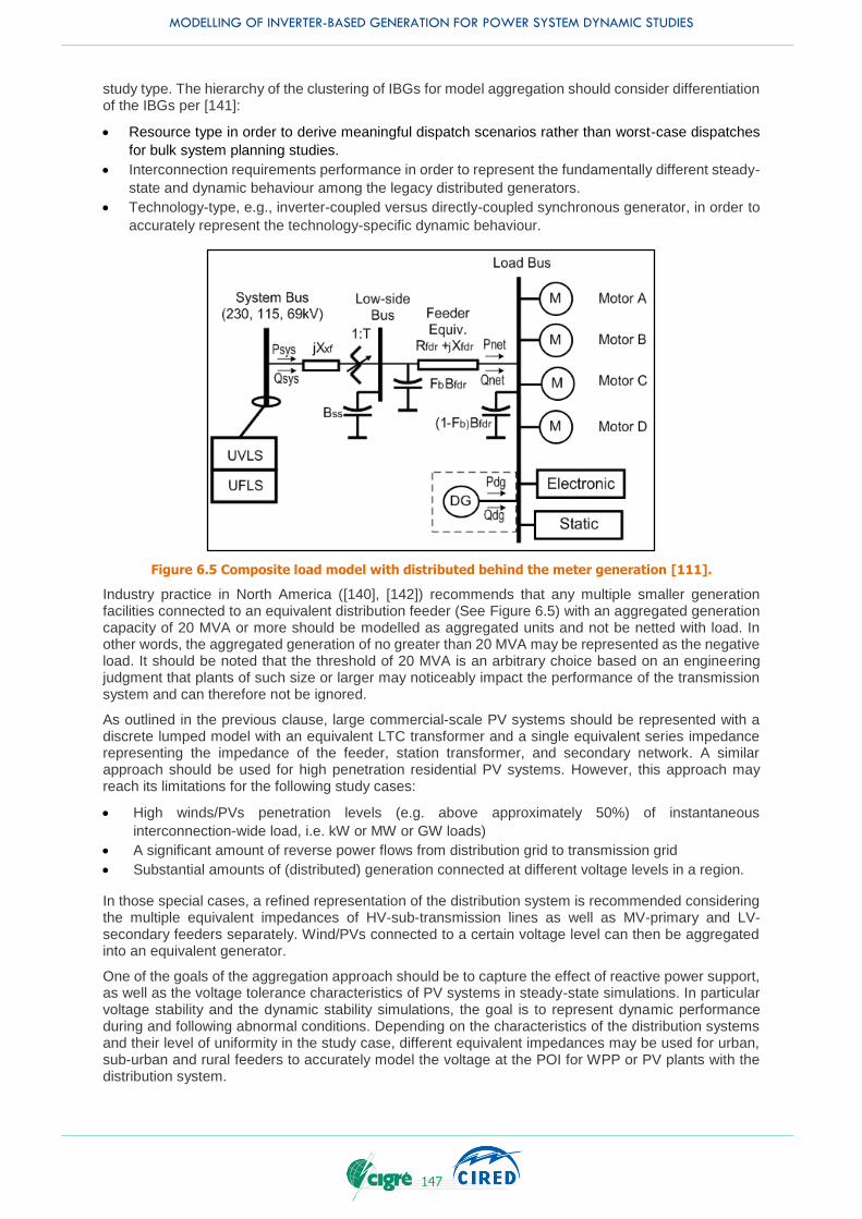
MODELLING OF INVERTER-BASED GENERATION FOR POWER SYSTEM DYNAMIC STUDIES
147
study type. The hierarchy of the clustering of IBGs for model aggregation should consider differentiation of the IBGs per [141]:
Resource type in order to derive meaningful dispatch scenarios rather than worst-case dispatches
for bulk system planning studies.
Interconnection requirements performance in order to represent the fundamentally different steady-
state and dynamic behaviour among the legacy distributed generators.
Technology-type, e.g., inverter-coupled versus directly-coupled synchronous generator, in order to
accurately represent the technology-specific dynamic behaviour.
Figure 6.5 Composite load model with distributed behind the meter generation [111].
Industry practice in North America ([140], [142]) recommends that any multiple smaller generation facilities connected to an equivalent distribution feeder (See Figure 6.5) with an aggregated generation capacity of 20 MVA or more should be modelled as aggregated units and not be netted with load. In other words, the aggregated generation of no greater than 20 MVA may be represented as the negative load. It should be noted that the threshold of 20 MVA is an arbitrary choice based on an engineering judgment that plants of such size or larger may noticeably impact the performance of the transmission system and can therefore not be ignored.
As outlined in the previous clause, large commercial-scale PV systems should be represented with a discrete lumped model with an equivalent LTC transformer and a single equivalent series impedance representing the impedance of the feeder, station transformer, and secondary network. A similar approach should be used for high penetration residential PV systems. However, this approach may reach its limitations for the following study cases:
High winds/PVs penetration levels (e.g. above approximately 50%) of instantaneous
interconnection-wide load, i.e. kW or MW or GW loads)
A significant amount of reverse power flows from distribution grid to transmission grid
Substantial amounts of (distributed) generation connected at different voltage levels in a region.
In those special cases, a refined representation of the distribution system is recommended considering the multiple equivalent impedances of HV-sub-transmission lines as well as MV-primary and LV-secondary feeders separately. Wind/PVs connected to a certain voltage level can then be aggregated into an equivalent generator.
One of the goals of the aggregation approach should be to capture the effect of reactive power support, as well as the voltage tolerance characteristics of PV systems in steady-state simulations. In particular voltage stability and the dynamic stability simulations, the goal is to represent dynamic performance during and following abnormal conditions. Depending on the characteristics of the distribution systems and their level of uniformity in the study case, different equivalent impedances may be used for urban, sub-urban and rural feeders to accurately model the voltage at the POI for WPP or PV plants with the distribution system.

MODELLING OF INVERTER-BASED GENERATION FOR POWER SYSTEM DYNAMIC STUDIES
148
In regions where interconnection requirements for distributed generation have been changed or are expected to change substantially in the future, separate equivalent generators may be used for each WT or PV technology generation in order to comply with their modelling parameters. This is important when considering different static and dynamic settings/capabilities for voltage/frequency tolerance/ride-through and reactive power standards. Existing wind/PV plants are typically not upgraded to meet the latest interconnection requirements and may need to be considered separately (especially in power system dynamic studies).
Finally, the proper representation of load, especially its voltage dependency, is very important [6]. Suitable load models should be used while considering that it is often difficult to obtain the required data and to validate the load model.
Behind the meter distributed solar PV generation may be modelled as part of load. For dynamic stability simulations, composite load model with distributed generation can be used. This model is used in WECC for dynamic stability studies of the systems with high penetration of renewable resources, including distributed solar PV (roof-top solar panels). It is represented in Figure 6.5.
This model includes substation transformer, distribution feeder, shunt capacitors, several types of induction motor load (three-phase and single phase), electronic and static load and distributed generation. Utility scale generation is modelled as aggregated generators on low voltage side of transmission transformers, and retail scale generation (roof-top PV) is modelled as part of composite load model. It is also aggregated by distribution feeders. The composite load model for dynamic stability studies that includes distributed generators has the generation part substantially simplified. Currently, only solar PV can be modelled as a part of the composite load.
6.2.2.1 Single equivalent distribution impedance approach with non-changing interconnection requirements
The recommended power flow representation for medium penetration distribution-connected PV plants with a single equivalent impedance and non-changing interconnection requirements is shown in Figure 6.6. Note that the load was moved to the low voltage bus as well. The term medium penetration level denotes “a level of penetration of renewables where changes are required to either control strategies or capabilities, or both, to manage the system, but where renewables are still seen as a relatively small part of the overall energy portfolio on the electricity system.” (See CIGRE TB 527 [143])
Medium-penetration PV on distribution systemTypical load flow model Recommended load flow model
Transmissionsystem
Transmissionsystem
Transmissionsystem
Unit stationtransformer
Unit stationtransformer
EquivalentImpedance
Distributionsystem
Utility-scale PV
Commertial
Residential
Pad/Poletransformer
PV Load
Load
Figure 6.6 Recommended power flow representation for study of medium-penetration PV scenarios with single equivalent distribution impedance [7].
Typical power flow data for the single equivalent distribution feeder is shown for North America in Table 6.3 below.
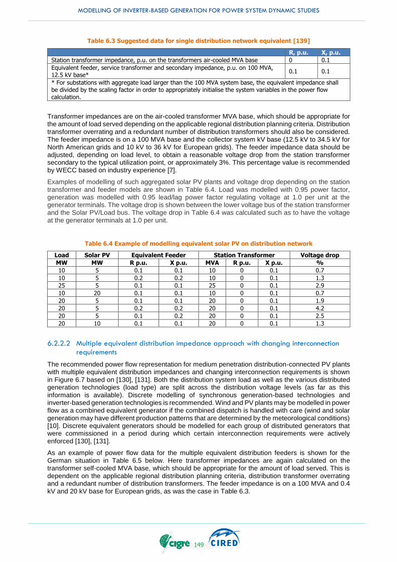
MODELLING OF INVERTER-BASED GENERATION FOR POWER SYSTEM DYNAMIC STUDIES
149
Table 6.3 Suggested data for single distribution network equivalent [139]
R, p.u. X, p.u.
Station transformer impedance, p.u. on the transformers air-cooled MVA base 0 0.1
Equivalent feeder, service transformer and secondary impedance, p.u. on 100 MVA, 12.5 kV base*
0.1 0.1
* For substations with aggregate load larger than the 100 MVA system base, the equivalent impedance shall be divided by the scaling factor in order to appropriately initialise the system variables in the power flow calculation.
Transformer impedances are on the air-cooled transformer MVA base, which should be appropriate for the amount of load served depending on the applicable regional distribution planning criteria. Distribution transformer overrating and a redundant number of distribution transformers should also be considered. The feeder impedance is on a 100 MVA base and the collector system kV base (12.5 kV to 34.5 kV for North American grids and 10 kV to 36 kV for European grids). The feeder impedance data should be adjusted, depending on load level, to obtain a reasonable voltage drop from the station transformer secondary to the typical utilization point, or approximately 3%. This percentage value is recommended by WECC based on industry experience [7].
Examples of modelling of such aggregated solar PV plants and voltage drop depending on the station transformer and feeder models are shown in Table 6.4. Load was modelled with 0.95 power factor, generation was modelled with 0.95 lead/lag power factor regulating voltage at 1.0 per unit at the generator terminals. The voltage drop is shown between the lower voltage bus of the station transformer and the Solar PV/Load bus. The voltage drop in Table 6.4 was calculated such as to have the voltage at the generator terminals at 1.0 per unit.
Table 6.4 Example of modelling equivalent solar PV on distribution network
Load Solar PV Equivalent Feeder Station Transformer Voltage drop
MW MW R p.u. X p.u. MVA R p.u. X p.u. %
10 5 0.1 0.1 10 0 0.1 0.7
10 5 0.2 0.2 10 0 0.1 1.3
25 5 0.1 0.1 25 0 0.1 2.9
10 20 0.1 0.1 10 0 0.1 0.7
20 5 0.1 0.1 20 0 0.1 1.9
20 5 0.2 0.2 20 0 0.1 4.2
20 5 0.1 0.2 20 0 0.1 2.5
20 10 0.1 0.1 20 0 0.1 1.3
6.2.2.2 Multiple equivalent distribution impedance approach with changing interconnection requirements
The recommended power flow representation for medium penetration distribution-connected PV plants with multiple equivalent distribution impedances and changing interconnection requirements is shown in Figure 6.7 based on [130], [131]. Both the distribution system load as well as the various distributed generation technologies (load type) are split across the distribution voltage levels (as far as this information is available). Discrete modelling of synchronous generation-based technologies and inverter-based generation technologies is recommended. Wind and PV plants may be modelled in power flow as a combined equivalent generator if the combined dispatch is handled with care (wind and solar generation may have different production patterns that are determined by the meteorological conditions) [10]. Discrete equivalent generators should be modelled for each group of distributed generators that were commissioned in a period during which certain interconnection requirements were actively enforced [130], [131].
As an example of power flow data for the multiple equivalent distribution feeders is shown for the German situation in Table 6.5 below. Here transformer impedances are again calculated on the transformer self-cooled MVA base, which should be appropriate for the amount of load served. This is dependent on the applicable regional distribution planning criteria, distribution transformer overrating and a redundant number of distribution transformers. The feeder impedance is on a 100 MVA and 0.4 kV and 20 kV base for European grids, as was the case in Table 6.3.
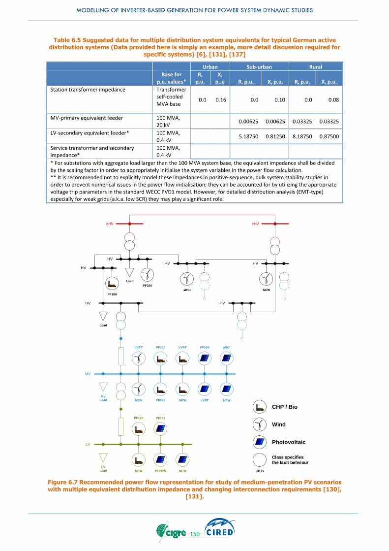
MODELLING OF INVERTER-BASED GENERATION FOR POWER SYSTEM DYNAMIC STUDIES
150
Table 6.5 Suggested data for multiple distribution system equivalents for typical German active distribution systems (Data provided here is simply an example, more detail discussion required for
specific systems) [6], [131], [137]
Urban Sub-urban Rural
Base for
p.u. values* R,
p.u. X,
p..u R, p.u. X, p.u. R, p.u. X, p.u.
Station transformer impedance Transformer self-cooled MVA base
0.0 0.16 0.0 0.10 0.0 0.08
MV-primary equivalent feeder 100 MVA, 20 kV
0.00625 0.00625 0.03325 0.03325
LV-secondary equivalent feeder* 100 MVA, 0.4 kV
5.18750 0.81250 8.18750 0.87500
Service transformer and secondary impedance*
100 MVA, 0.4 kV
* For substations with aggregate load larger than the 100 MVA system base, the equivalent impedance shall be divided by the scaling factor in order to appropriately initialise the system variables in the power flow calculation. ** It is recommended not to explicitly model these impedances in positive-sequence, bulk system stability studies in order to prevent numerical issues in the power flow initialisation; they can be accounted for by utilizing the appropriate voltage trip parameters in the standard WECC PVD1 model. However, for detailed distribution analysis (EMT-type) especially for weak grids (a.k.a. low SCR) they may play a significant role.
Figure 6.7 Recommended power flow representation for study of medium-penetration PV scenarios with multiple equivalent distribution impedance and changing interconnection requirements [130],
[131].
HV
MV
eHV
Load
MV
Load LVRT
PF100
LV
LV
Load
PF100
aRCI NEW
NEW
LVRT
NEW
PF100 LVRT
PF095 NEW
PF100 aRCI
NEW
PF100
PFPOW
PF100
NEW
HV
HV
HV HV
eHV
Load
HV
CHP / Bio
Wind
Photovoltaic
Class
Class specifies
the fault behviour

MODELLING OF INVERTER-BASED GENERATION FOR POWER SYSTEM DYNAMIC STUDIES
151
The feeder impedance data should be adjusted depending on the load level for normal power flow cases and distributed generation feeder penetration for reverse power flow cases so as to obtain a reasonable voltage drop between the station transformer secondary to the typical utilization point, or approximately 2–3%.
6.2.3 Essential assumptions and control to be modelled
6.2.3.1 Active power output level
PV plant output varies as a function of solar input and, to a lesser extent, temperature. Wind power plant output varies depending on the season and time of the day. Typically, PV plants achieve full output for several hours of the day under clear sky conditions. The active power level assumed for the PV or wind plant depends on the purpose of the study with the plants modelled at full output for the generation interconnection studies and at partial or zero output for regional transmission planning studies depending on the season and the time of the day.
For wind or PV plants that use an active power-dependent reactive power control mode, at least those two active power levels that correspond to the extreme reactive power exchange cases, e.g., zero and maximum reactive power exchange should be modelled. Otherwise, the full impact of wind and solar PV plants on power flows and dynamic behaviour will not be adequately examined.
6.2.3.2 Reactive power capability
Interconnection requirements and performance standards addressing reactive power capability from inverter-based generating systems are still evolving. Inverters used in utility-scale PV systems are currently required and designed to provide a certain minimum reactive power support at full active power to the grid (typically with a power factor of 0.95 leading and 0.95 lagging). The amount of reactive power at partial output is generally even higher and depends on the inverter current limits and on grid voltage conditions. The reactive power capability curves for inverters differ from those of synchronous machines because they are normally limited by internal voltage and current constraints (See Appendix 5-C). Inverters are typically designed for continuous operation between 90% and 110% of nominal terminal voltage. Depending on the interconnection requirements and the inverter design, the full reactive power capability can only be achieved within a smaller voltage band around nominal voltage. In special cases, PV inverters are designed to provide reactive power support even if solar irradiation is zero; such STATCOM functionality should then be considered in the study.
Distribution-connected PV systems have traditionally been operated at unity power factor over their entire active power output range, i.e., with zero reactive power exchange to the grid. Hence, many existing inverters used in residential and commercial areas were not designed to inject any reactive current. However, new interconnection requirements for distribution-connected PV systems are increasingly requiring reactive power capability from small-scale plants because this reduces distribution grid upgrades through the mitigation of overvoltage in LV-secondary feeders when many solar PV systems are connected to the same feeder. For studies with a mid-term and long-term planning horizon, the reactive power capability and controls of distribution-connected PV systems should be modelled.
At the plant level of utility-scale PV plants, a portion of the inverters in the plant may be turned off at low plant power output (via the valve device blocking), resulting in a reduction of reactive power capability. Therefore, reactive power output for an equivalent aggregated generator modelled in power flow studies should be modified accordingly.
To meet operating requirements at the point of interconnection, the settings of individual inverters can be adjusted via a plant-level reactive power controller. The plant level controller also coordinates operation of the switched capacitors, if present.
Several control modes are required (refer to [23] and [144] for further details):
Closed-loop voltage control - Maintain voltage reference at the scheduled value over a certain range of active power output while considering the reactive power capability of the PV plant.
Open-loop voltage (droop) control – Increase or decrease reactive power output linearly as a function of voltage. This type of control allows the PV plant to provide voltage support while avoiding large reactive power swings that a small PV plant would see when connected to a relatively stiff grid.
Fixed power factor control - Maintain a fixed power factor at the interconnection point close to a specified value.
Active power-dependent power factor control [144] – Set the power factor value at the interconnection point according to an active power-dependent characteristic curve. Typically, unity

MODELLING OF INVERTER-BASED GENERATION FOR POWER SYSTEM DYNAMIC STUDIES
152
power factor is used for low to medium active power output. For medium to high active power output, the power factor is often linearly increased to the plant’s maximum inductive capability.
Reactive power control - Maintain reactive power flow at the interconnection point within some specified limits.
6.3 SIMPLIFIED DYNAMIC MODEL
Even if the aggregated model is perfect for power flow studies, it will probably not be sufficient to represent the dynamic behaviour of IBGs following faults. One critical point that needs to be considered is the self-disconnection of IBGs. The self-disconnection of IBGs is most likely to occur when IBGs do not meet the LVRT requirement of mainly LV networks. The total generation disconnected on secondary side of one HV-MV (or MV-HV) transformer will depend on how much the voltage decreases. The self-disconnection of IBGs is more likely to increase as the system voltage decreases. Sub-Chapter 6.3 introduces the model which can represent the dynamic behaviour following faults in an aggregated way considering the self-disconnection of IBGs.
6.3.1 Model for distributed and small PV
Unlike utility-scale PV plants, i.e. the central station PV plants in Clause 6.3.1, distributed PV systems are connected at the distribution level. Reliability and interconnection requirements vary from country to country.
For example, in North America, the requirements outlined in IEEE Standard 1547-2003 [18] are reflected. In contrast with bulk system utility-scale PV plants reliability requirements, distributed PV systems in North America do not participate in steady state voltage regulation, and tighter bounds on operation for off-nominal voltage and frequency conditions result in significantly different fault ride-through capability [111]. IEEE Standard. 1547 has been amended in 2014 and now allows for both steady state voltage regulation and extended frequency and voltage ride-through. However, binding and standardised requirements are not expected to enter into force until sometime in the future years. Hence, it can be assumed in near-term studies that the PV inverters connected in distribution systems will continue to comply with IEEE Standard 1547-2003 [18], and will operate under constant power factor or constant reactive power modes of operation. This allows for the (temporary) elimination of the closed-loop voltage regulator dynamics, along with the elimination of the DC dynamics (for the same reasons described for the Central Station model), making for a substantial simplification of the model with respect to that of the Central Station. However, unlike a utility-scale PV plants, the terminal voltages seen by the individual inverters within the composite load in the large-scale power system dynamic model are likely to vary substantially. A different control model should be used to capture the effect of the diverse terminal conditions on the aggregate generation [111].
In Europe, and particularly in Germany, distributed PV systems are required to provide steady state voltage regulation since the year 2011 [144]. This should be adequately modelled and may increase the model complexity. However, voltage and frequency ride-through is currently mandated only for wind/PVs connected to medium voltage (primary) distribution feeders but not for those connected to low voltage (secondary) distribution feeders. Ride-through requirements are likely to be introduced for LV-secondary connected distributed generation in the near future [130] as penetration is reaching a level where the aggregated impact of these small-scale, residential plants cannot be ignored in large-scale power system dynamic studies any longer.
In some countries, such as Japan, voltage and frequency ride-through has been mandated for almost all types of IBGs regardless of the voltage level. On the other hand, the anti-islanding protections have been required for IBGs which are connected to LV network only [145]. Therefore, the IBGs in MV network and LV network need to be separately aggregated for the modelling.
Generally, the minimum level of modelling detail should allow for basic reactive power control modes, such as:
Constant reactive power, initialized at the generator output in the solved power flow case,
Volt/var control at the generator terminals, with user-defined Q versus V characteristic and optional line drop compensation, if any.
The model should also allow for basic active power control modes, such as:
Constant active power, initialized at the generator output in the solved power flow case,
Over-frequency response, with user-defined dead band and droop.
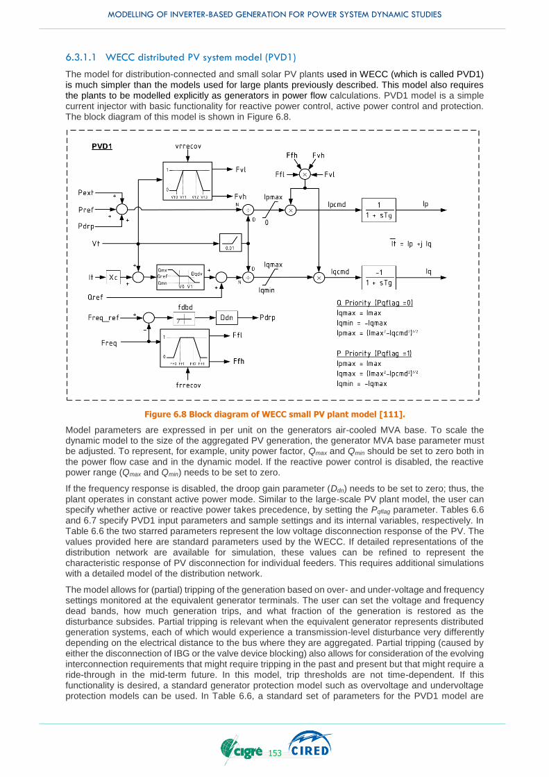
MODELLING OF INVERTER-BASED GENERATION FOR POWER SYSTEM DYNAMIC STUDIES
153
6.3.1.1 WECC distributed PV system model (PVD1)
The model for distribution-connected and small solar PV plants used in WECC (which is called PVD1) is much simpler than the models used for large plants previously described. This model also requires the plants to be modelled explicitly as generators in power flow calculations. PVD1 model is a simple current injector with basic functionality for reactive power control, active power control and protection. The block diagram of this model is shown in Figure 6.8.
Figure 6.8 Block diagram of WECC small PV plant model [111].
Model parameters are expressed in per unit on the generators air-cooled MVA base. To scale the dynamic model to the size of the aggregated PV generation, the generator MVA base parameter must be adjusted. To represent, for example, unity power factor, Qmax and Qmin should be set to zero both in the power flow case and in the dynamic model. If the reactive power control is disabled, the reactive power range (Qmax and Qmin) needs to be set to zero.
If the frequency response is disabled, the droop gain parameter (Ddn) needs to be set to zero; thus, the plant operates in constant active power mode. Similar to the large-scale PV plant model, the user can specify whether active or reactive power takes precedence, by setting the Pqflag parameter. Tables 6.6 and 6.7 specify PVD1 input parameters and sample settings and its internal variables, respectively. In Table 6.6 the two starred parameters represent the low voltage disconnection response of the PV. The values provided here are standard parameters used by the WECC. If detailed representations of the distribution network are available for simulation, these values can be refined to represent the characteristic response of PV disconnection for individual feeders. This requires additional simulations with a detailed model of the distribution network.
The model allows for (partial) tripping of the generation based on over- and under-voltage and frequency settings monitored at the equivalent generator terminals. The user can set the voltage and frequency dead bands, how much generation trips, and what fraction of the generation is restored as the disturbance subsides. Partial tripping is relevant when the equivalent generator represents distributed generation systems, each of which would experience a transmission-level disturbance very differently depending on the electrical distance to the bus where they are aggregated. Partial tripping (caused by either the disconnection of IBG or the valve device blocking) also allows for consideration of the evolving interconnection requirements that might require tripping in the past and present but that might require a ride-through in the mid-term future. In this model, trip thresholds are not time-dependent. If this functionality is desired, a standard generator protection model such as overvoltage and undervoltage protection models can be used. In Table 6.6, a standard set of parameters for the PVD1 model are
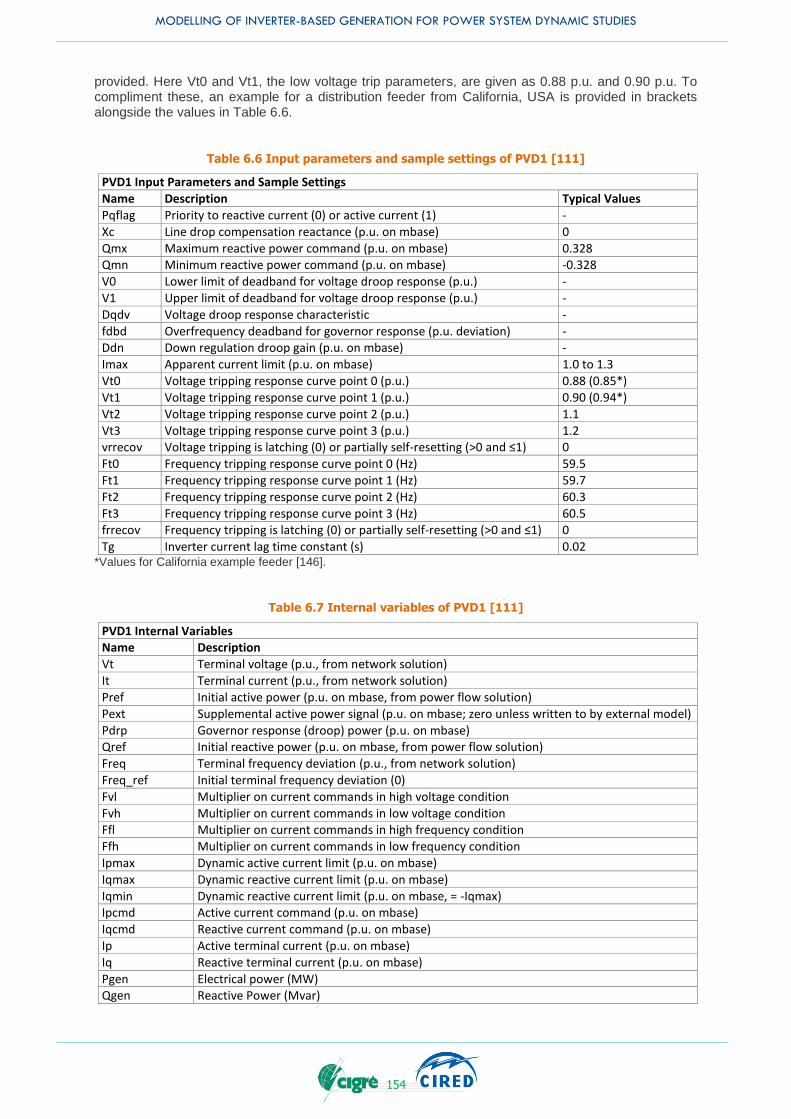
MODELLING OF INVERTER-BASED GENERATION FOR POWER SYSTEM DYNAMIC STUDIES
154
provided. Here Vt0 and Vt1, the low voltage trip parameters, are given as 0.88 p.u. and 0.90 p.u. To compliment these, an example for a distribution feeder from California, USA is provided in brackets alongside the values in Table 6.6.
Table 6.6 Input parameters and sample settings of PVD1 [111]
PVD1 Input Parameters and Sample Settings
Name Description Typical Values
Pqflag Priority to reactive current (0) or active current (1) -
Xc Line drop compensation reactance (p.u. on mbase) 0
Qmx Maximum reactive power command (p.u. on mbase) 0.328 Qmn Minimum reactive power command (p.u. on mbase) -0.328
V0 Lower limit of deadband for voltage droop response (p.u.) -
V1 Upper limit of deadband for voltage droop response (p.u.) -
Dqdv Voltage droop response characteristic -
fdbd Overfrequency deadband for governor response (p.u. deviation) - Ddn Down regulation droop gain (p.u. on mbase) -
Imax Apparent current limit (p.u. on mbase) 1.0 to 1.3
Vt0 Voltage tripping response curve point 0 (p.u.) 0.88 (0.85*)
Vt1 Voltage tripping response curve point 1 (p.u.) 0.90 (0.94*)
Vt2 Voltage tripping response curve point 2 (p.u.) 1.1
Vt3 Voltage tripping response curve point 3 (p.u.) 1.2 vrrecov Voltage tripping is latching (0) or partially self-resetting (>0 and ≤1) 0
Ft0 Frequency tripping response curve point 0 (Hz) 59.5
Ft1 Frequency tripping response curve point 1 (Hz) 59.7
Ft2 Frequency tripping response curve point 2 (Hz) 60.3
Ft3 Frequency tripping response curve point 3 (Hz) 60.5 frrecov Frequency tripping is latching (0) or partially self-resetting (>0 and ≤1) 0
Tg Inverter current lag time constant (s) 0.02 *Values for California example feeder [146].
Table 6.7 Internal variables of PVD1 [111]
PVD1 Internal Variables Name Description
Vt Terminal voltage (p.u., from network solution)
It Terminal current (p.u., from network solution)
Pref Initial active power (p.u. on mbase, from power flow solution)
Pext Supplemental active power signal (p.u. on mbase; zero unless written to by external model)
Pdrp Governor response (droop) power (p.u. on mbase) Qref Initial reactive power (p.u. on mbase, from power flow solution)
Freq Terminal frequency deviation (p.u., from network solution)
Freq_ref Initial terminal frequency deviation (0)
Fvl Multiplier on current commands in high voltage condition
Fvh Multiplier on current commands in low voltage condition Ffl Multiplier on current commands in high frequency condition
Ffh Multiplier on current commands in low frequency condition
Ipmax Dynamic active current limit (p.u. on mbase)
Iqmax Dynamic reactive current limit (p.u. on mbase)
Iqmin Dynamic reactive current limit (p.u. on mbase, = -Iqmax) Ipcmd Active current command (p.u. on mbase)
Iqcmd Reactive current command (p.u. on mbase)
Ip Active terminal current (p.u. on mbase)
Iq Reactive terminal current (p.u. on mbase)
Pgen Electrical power (MW) Qgen Reactive Power (Mvar)
MODELLING OF INVERTER-BASED GENERATION FOR POWER SYSTEM DYNAMIC STUDIES
155
6.4 CONCLUSION
Correct modelling the aggregated response of distributed IBG will influence the stability results at the bulk transmission system level and become more critical as penetration levels of distributed PVs increase. A modular approach to represent IBGs in bulk system studies as illustrated in Figure 6.7 is recommended to ensure accurate representation of the resources for the specific bulk system study type. The hierarchy of the clustering of IBGs for model aggregation should consider differentiation of IBGs per:
Resource type, to derive meaningful dispatch scenarios rather than worst-case dispatches.
Interconnection requirements performance, to represent the different steady-state and dynamic behaviour among the legacy distributed generators.
Technology-type, e.g., inverter-coupled versus directly-coupled synchronous generator, to accurately represent the technology-specific dynamic behaviour.
Dynamic models for distributed IBGs are available to model the evolving interconnection requirements related performance requirements. WECC’s simplified distributed PV model (PVD1) currently seems to be the most promising concept to reach a reasonable balance between modelling accuracy, computational requirements, and handling of the system model, but some further improvement may be needed. In addition, there is other remaining work. For example, the way how to aggregate tremendous number of residential PVs in LV network from HV network perspectives is still under research (See also Sub-Chapter 5.7). Also, there is the work to introduce modular approach (also known as bottom-up approach) to the modelling of IBG, especially the units connected to distribution systems and to develop more accurate aggregated models [147].
A refined representation of the distribution system is recommended by considering the multiple equivalent impedances of HV-sub-transmission lines as well as MV-primary and LV-secondary feeders separately if any of the following conditions apply:
High WTs/PVs penetration levels (e.g. above approximately 50%) of instantaneous interconnection-wide load, i.e. kW or MW or GW loads)
A significant amount of reverse power flows from distribution to bulk system level
Substantial amounts of (distributed) generation connected at different voltage levels in a region.
In those special cases, WT/PVs connected to a certain voltage level would then be aggregated into an equivalent generator.

MODELLING OF INVERTER-BASED GENERATION FOR POWER SYSTEM DYNAMIC STUDIES
156
MODELLING OF INVERTER-BASED GENERATION FOR POWER SYSTEM DYNAMIC STUDIES
157
7. VALIDATION OF INVERTER-BASED GENERATOR MODEL
7.1 INTRODUCTION
As a final step in the process of model development the model validation is to
confirm the assumptions made in the model creation
proof that the model performs in the way it is designed to
confirm the conditions where the model should be used, and
identify any limitations that the model may have.
Model validation is a very important part in the model development. The users of any model need to understand the model’s characteristics, its limitations and have confidence in it. The developers need to ensure its fidelity before finally issuing it for use. A model can be developed by the engineer who will use it later in his/her simulation studies. In this case, the details of the model validation can be understood and followed. In most cases though, a model is developed by third parties or exists in a commercial software suite. In this case, validation by the user is even more important.
Usually the models used by the PV manufacturers are very different from those used by the power companies. The manufacturers’ models are usually built at the individual cell level with detailed control and protection logic circuits. This type of model is complicated and contains intellectual property from manufacturer, and is usually for a specific project. Models of this type are used in EMT studies for inverter design to assess the transient stresses on the devices or for designing control and protection function at a microsecond scale. As the model has very small time constants the model is not suitable for power system dynamic studies in a large power grid.
Because the power grid under study is in general very large, the models of IBGs used for studies in a large power grid can be simplified. Individual inverters will be lumped together to model the entire power plant. By doing so, the model has a large time constant and can be executed efficiently with the power grid model in terms of numerical stability and computation time in simulation.
The focus of this simplified model is on the voltage and current at the connection terminals to the grid and its P and Q regulation behaviour in response to the control commands or a change in the grid. It is a RMS model, representing the inverter outputs and control behaviour to the positive sequence components in the AC system, for studying balanced events from either normal variation or transient faults. These models are designed for power system dynamic studies like system stability, voltage regulations or frequency control as described in previous chapters.
There is no difference between the RMS model validation approach and the EMT model validation approach. However, the type of disturbance or the type of phenomenon (which should be observed) can be quite different depending on type of model (RMS or EMT). This chapter focuses only on the RMS model validation.
IEC 61400-27-2 (though mainly for wind plants) presents some useful methods for the model validation.
The validation is a process of comparing the simulation results produced on the model with the data obtained independently by other means. In practice, obtaining a set of good data for model validation can be difficult and expensive especially in high power applications. However, the quality of the data is critical in the model validation process.
7.2 SOURCE DATA FOR MODEL VALIDATION
7.2.1 Field measurements
Field measurements are considered to be best for model validation and the in-the-field type-testing of IBGs is getting common in many countries and has already been mandatory in some countries, particularly in Germany. Providing the data quality is guaranteed it is reasonable to use this measurement data and the model validation is easily accepted on this basis. The field measurements can be either obtained from specific tests during the system commissioning tests or via a set of recorded data from system operations. In practice, however, data from field measurements may not be readily available due to the following reasons
field measurements and data from them may be expensive

MODELLING OF INVERTER-BASED GENERATION FOR POWER SYSTEM DYNAMIC STUDIES
158
insufficient data available; only limited tests may be allowed and conducting a test on a real system requires permission from the authority and detailed coordination of many parties involved
the commissioning tests will not be available until after the design work is completed
the accuracy and performance of measurement instruments could not provide the quality of the data required
The power systems from which the field measurements were taken are different from the conditions of the model development. It is important to check under what conditions the measurements were obtained and an engineering judgement may be required on the validity of the field measurements.
7.2.2 Physical laboratory test systems
Generating the data from a physical test system in a laboratory can be a good alternative for model validation. The test system is a representation of the AC grid but at a laboratory scale in which, the engineer has freedom to set the system for its need. It can offer the flexibility of changing the system strength, simulating the variations in voltage, frequency and fault events in the AC grid. With a test the system engineer can set up some extreme cases for model validation.
When building a physical test system, it is important to take into consideration the inverter characteristics and its operation with the primary energy source – solar generation. An analogue system is a good way to simulate the electrical-mechanic interactions in the AC grid, but it has limitations and it is not easy to adopt changes. Using a digital system, especially a real time digital simulator, is a popular choice nowadays. There are several commercial products available for testing the power system including converter systems. With the development of the IGBT, voltage source converter technology, there have appeared hybrid simulators where the inverter is a real physical element. Below are two examples.
7.2.2.1 Test facility in China
China EPRI (also known as CEPRI) established a commercial test platform for grid compliance test of photovoltaic inverters as shown in Figure 7.1. It mainly consists of controllable DC source, grid emulator, fault generator, anti-islanding test facility and other necessary components such as transformers, switches and data acquisition equipment. This platform can be also used for model validation studies of PV inverters. This is the “test-container” according to IEC 61400-27 [148] for WTGs, which can be applied to PV.
The controllable DC source can emulate the output of PV panels. Different I-V and solar radiation characteristics of PV panels can be achieved by programming. The grid emulator can generate voltage and frequency changes of AC system. Harmonics of different orders and amplitude can be injected through the grid-emulator. The fault generator consists of reactors which can be flexible and combined in serial and parallel connection. In addition, different grid fault and voltage dip can be emulated by this fault generator through switch operation. The anti-islanding test facility consists of adjustable R-L-C load which is used to create the condition where islanding may occur. Using this platform, a set of tests which are necessary in model validation studies can be performed:
1. Small voltage disturbance test at AC side. 2. Large voltage disturbance (short circuit fault) test at AC side. 3. Frequency disturbance test at AC side. 4. Disturbance test at DC side. 5. Active power dispatch command control test. 6. Reactive power dispatch command control test.
The test system is configurable. It is easy to change its configuration to conduct different tests with different conditions. It is noted that type-tests of IBGs have already been mandatory in some countries, such as China and Germany.
Analogue test systems can have limits in representing a high voltage power system. For example, the R/X ratio of a piece of copper wire at a low voltage is higher than that in the overhead lines of the high voltage transmission systems. As a result, the wires in the test system can introduce more damping and the system is less oscillating than the system it is trying to represent. This problem becomes more severe with generators and transformers. With a generator, it was found that it is easy to reduce the leakage inductance X but difficult to reduce the winding resistance R without significant enlarging the size of the generator. A way to cope with it was to increase the leakage reactance X of the model generator intentionally in order to make its R/X ratio equal to the real generator. In the case of transformer, the losses of the model transformer are proportionally higher than the high-power transformers due to higher copper loss. These discrepancies should not be ignored when building a test system or when analysing the simulation results for model validation.

MODELLING OF INVERTER-BASED GENERATION FOR POWER SYSTEM DYNAMIC STUDIES
159
Controllable DC Power Source
PV Inverter
SZ
SU
External Grid10kV Bus
Grid disturbance generator
Measuring
point
(a) Single line diagram of test circuit
(b) Controllable DC Power Source (c) Grid disturbance generator
(d) Overview of test facilities
Figure 7.1 Model validation test systems for PV inverter in CEPRI.

MODELLING OF INVERTER-BASED GENERATION FOR POWER SYSTEM DYNAMIC STUDIES
160
7.2.2.2 Test facility in Japan
The traditional dynamic electric-mechanic laboratory facility can be retrofitted to a test system for electronic inverter systems. The synchronous generators are useful devices in the test system for the studies like rotor angle stability. The power swing oscillation is mainly provoked by the physical presence of the synchronous generators connected through the transmission lines/cables to the rotating machines. The power swings between the power grid and the dynamic response of the IBGs can be studied on this test system.
Figure 7-2 shows an old test facility but still in use in Central Research Institute of Electric Power Industry (CRIEPI), Japan. Figure 7-2 (a) shows a synchronous generator unit rated at 100 kVA. It has a massive core rotor instead of a laminated core to represent the eddy current on the surface of the rotor. This design gives a large leakage reactance X so as to make its ratio of X/R a representation of generators up to 1000 MW class. This model generator can produce the dynamic behaviours close to those that are 10,000 times greater during fault conditions. The length of the emulated transmission line can be as much as 600km. This facility has been satisfactorily used in study of low frequency power swing oscillations.
(a) Synchronous generator units (100 kVA) (b) 275 kV emulated transmission line (LL voltage: 3.3 kV)
(c) Single phase PV inverters (d) DC source emulator
Figure 7.2 Model validation test systems for PV inverter in CRIEPI.
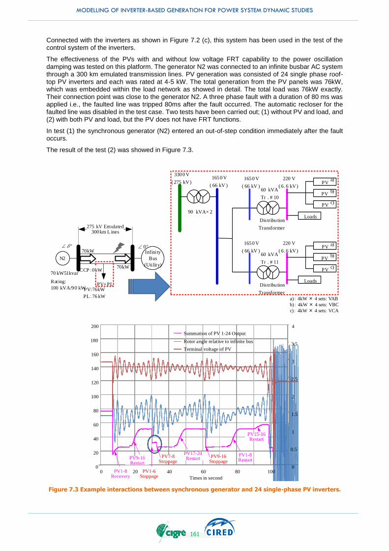
MODELLING OF INVERTER-BASED GENERATION FOR POWER SYSTEM DYNAMIC STUDIES
161
Connected with the inverters as shown in Figure 7.2 (c), this system has been used in the test of the control system of the inverters.
The effectiveness of the PVs with and without low voltage FRT capability to the power oscillation damping was tested on this platform. The generator N2 was connected to an infinite busbar AC system through a 300 km emulated transmission lines. PV generation was consisted of 24 single phase roof-top PV inverters and each was rated at 4-5 kW. The total generation from the PV panels was 76kW, which was embedded within the load network as showed in detail. The total load was 76kW exactly. Their connection point was close to the generator N2. A three phase fault with a duration of 80 ms was applied i.e., the faulted line was tripped 80ms after the fault occurred. The automatic recloser for the faulted line was disabled in the test case. Two tests have been carried out; (1) without PV and load, and (2) with both PV and load, but the PV does not have FRT functions.
In test (1) the synchronous generator (N2) entered an out-of-step condition immediately after the fault occurs.
The result of the test (2) was showed in Figure 7.3.
N2
70 kW 5 kvar1
Infini ty
Bus
(Uti lity)
PV+PL
CCP:0kW
PV:76kW
PL:76 kW
0
275 kV Emulated 300km L ines
3300 V
( 275 kV)220 V
( 6.6 kV)
Dis tribu tion
Transformer
PVb)
90 kVA× 2
60 kVA
Tr . # 10
1650 V
( 66 kV )
Loads
1650 V
( 66 kV )
PVc)
PVa)
220 V
( 6.6 kV)
Dis tribu tion
Transformer
PVb)60 kVA
Tr . # 11
Loads
1650 V
( 66 kV )
PVc)
PVa)
a): 4kW × 4 sets: VAB
b): 4kW × 4 sets: VBC
c): 4kW × 4 sets: VCA
Rating:
100 kVA/90 kW
70kW
70kW
Figure 7.3 Example interactions between synchronous generator and 24 single-phase PV inverters.
0
0.5
1
1.5
2
2.5
3
3.5
4
0
20
40
60
80
100
120
140
160
180
200
0 20 40 60 80 100
Summation of PV 1-24 Output
PV1-8 Restart
PV15-16 Restart
PV17-24 Restart
PV1-8 Recovery
PV1-6 Stoppage
PV7-8 Stoppage
Rotor angle relative to infinite bus
Times in second
PV9-16 Stoppage
PV9-16 Restart
Terminal voltage of PV
MODELLING OF INVERTER-BASED GENERATION FOR POWER SYSTEM DYNAMIC STUDIES
162
As the PV inverters did not have the FRT control function, the PV inverters were disconnected when the terminal voltage of the PV dropped below the 70% of the nominal voltage. There were a number of stoppages and restarts by different suites of PVs. It took over 90 seconds for the generator to result in the out-of-step operation/condition.
These tests showed one fact. i.e. the PVs installed near a power source and do not have the low voltage FRT function can actually improve transient stability in comparison with the PVs which have the low voltage FRT function (see also Clause 3.3.3 with Figure 3.20). When the PVs are located close to the synchronous generator (i.e. near power source) and without low voltage FRT capability, they can produce an effect equivalently as dynamic braking. As shown in Figure 7.3, the disconnection of PVs near the power source resulted an increase in the net load. This reduces the active power transfer over the transmission lines and makes the system more stable.
As already mentioned in Chapter 3, the influence of the PVs on transient stability depends on the location of the PVs i.e. near the power source or the power sink. If the location of the PVs is closer to the load centre, i.e. the power sink, the opposite and adverse effect can be observed.
Because the FRT requirement will prevent the PVs from disconnecting from the grid, the equivalent dynamic braking effect will be diminished, which means transient stability decreases as the FRT requirement is applied to the PVs which are connected to the bus near the accelerating generators.
The dynamic braking effect coming from the disconnection of PVs depends not only on the location of the PVs in the network but also on the penetration level of PVs. If the penetration rate is low, the equivalent dynamic braking effect may be negligible and the lighter power flow over the transmission lines contributes to the increase of the transient stability
7.2.3 Real-time digital simulator in North America
Nowadays, digital real time simulators (DRTS) are often used to help in the development of converter systems. In order to test such a converter, the DRTS which represents the surrounding rest of system (ROS, e.g. the DC and AC grids to which a DC/AC converter may be connected in real life) is connected to appropriately sized amplifiers such that the simulated AC and DC quantities can be imposed upon the converter as necessary. By feeding the electrical responses of the converter back to the DRTS a power hardware in the loop (PHIL) simulation can be established. In such a PHIL simulation, all the control functions of the converter are fully represented.
If a PHIL setup is unavailable, the physical control and protection unit can be connected to the DRTS to form a controller hardware in the loop (CHIL) simulation. Such a setup can be used very effectively to test the control and protection system within a realistic system environment. There can be many measurement points where the parameters of the primary system, variables within the inverter and the control signals and variation are accessible.
The Centre for Advanced Power Systems (CAPS) at Florida State University in Tallahassee, FL, USA, can serve as an example for a state-of-the-art PHIL and CHIL facility. This laboratory was designed to test electrical and mechanical hardware under test (HUT) with power ratings up to 5 MW. As depicted in Figure 7.4, the facility offers many different flavours of power connections all fully interfaced with the DRTS.
Controller hardware in the loop (CHIL) experiments are achieved through either dedicated wiring using analogue and digital signals or standard communication network protocols such as distributed network protocol (DNP3), and IEC 61850 (communication networks and systems in substations). In both cases—PHIL and CHIL—the HUT is part of a closed-loop simulation which allows evaluation of dynamic responses, while the remaining part is modelled and simulated using the real-time environments.
CAPS has utilized real-time simulation capabilities successfully in numerous projects, such as dynamic testing of a prototype 5 MW high-temperature superconducting motor [149], a high-speed generator [150], superconducting fault current limiters [151], PV converters, and numerous power converters for the US Navy. CAPS also successfully conducted co-simulations of electro-mechanical and electro-thermal systems [152], [153].
Most recently, integration of all the PHIL and CHIL resources begun to allow experimenting with up to approximately 100 distributed control nodes simultaneously. This will provide researchers with the ability to test and evaluate control algorithms for emerging next generation terrestrial and shipboard power systems in a realistic system environment to meet technology readiness level 6 (TRL6) requirements at reasonable system scale. Figure 7.5 is a systems level overview of the open-source distributed control concept that is envisioned after full implementation of this DURIP award. The two major DRTS engines at CAPS are made by two different manufacturers. They provide the ability to simulate large-scale

MODELLING OF INVERTER-BASED GENERATION FOR POWER SYSTEM DYNAMIC STUDIES
163
systems and provide emulation characteristics and commands to physical equipment. The physical systems near the top of the diagram are connected via fibre optics to the DRTS. At each of the physical devices is an array of distributed control nodes corresponding to physical controller devices. In addition to the physical systems, virtual loads and sources are present in the simulation. In the same way as the physical devices, the virtual devices are connected to physical controller devices. Each of the distributed control platforms are connected via Ethernet to create a true networked distributed control layer. An emulated network layer is also added, which via emulation software can more accurately represent the complexity of a physical distributed network.
Figure 7.4 The 5 MW PHIL facility at Florida state university-CAPS.
Figure 7.5 CAPS open-source distributed control system layout.
7.2.4 Other model responses
Comparison between the different models running on different simulation programs is also widely used in model validation. For example, a simplified RMS model can be checked against a well- proven EMT simulation. It should be pointed out that it is often not that easy to reach a full agreement between RMS and EMT simulations. One should not expect so either, even when running the same event with the same conditions. This can be due to many reasons. The EMT model is built with details of converter components and its control system for simulating the fast transients and capturing the variations in very
Real-time ControlsNetwork Simulator
OPNET
Embedded Controls
0…1.1 kV
0…2.5 kA
0…4.16 kV
0…0.4/0.8 kA
1.5 kA
VVS
Dynos
DRTS
Network Emulation(Opnet, Omnet)
5 MW VVS5 MW
DynamometerMMC-based5MW MVDC
Low Voltage 10kVADistributed Control
Test Bed
Real-Time ComputationalSystems (RTDS, OPAL-RT)
SimulatedSources
SimulatedLoads
Controller(s) Controller(s)
Controller Controller Controller(s) Controller(s)
Network
OtherHardware
Controller(s)

MODELLING OF INVERTER-BASED GENERATION FOR POWER SYSTEM DYNAMIC STUDIES
164
small time scale. The RMS model is often built with some approximations for representing the characteristics of the converter to the external system at the point of interest. The RMS is used to study relatively slow variation processes by ignoring or simplifying the fast variations. The different algorithms used in the RMS and EMT simulations can also introduce some discrepancies to a certain extent.
Also, the IBG models used in different software platforms are compared and the models are adjusted to show identical performance in all the software used. In WECC, three different software platforms are used for power flow and dynamic stability studies with RMS models. In development of the new models, the models are developed simultaneously in these three simulation programs. The model performance is compared and the models are validated using these three software platforms to ensure that the models and simulations are identical.
7.3 RECOMMENDED SPECIFICATION OF MEASUREMENT DEVICES
The precision of the measurement transducers like CT and VT needs to be carefully considered. Their precision can affect the readings of the parameters like active power flows. IEC 61400-21-1 [154] provides some guidelines to follow. The bandwidth of the transducers should adequately cover the range of frequencies of the measured parameters. The response speed of the transducer is critical for obtaining the quality measurement data for validating the model dynamics. It is desirable that the response speed of the transducer is equal to or less than 20ms for the RMS model validation.
The transient (or so called dynamic) fault recorder is an instrument designed to capture slow variation and fast transient events. It is capable of logging several analogue and digital measurements simultaneously. It is recommended to install a transient fault recorder at the grid connection point of the PV generation site and log the voltage and current of the connection circuit as well as major parameters from the inverter. These measurements can be useful for checking the plant performance as well as for the model validation.
Based on the industry experience for model validation, a sampling rate of 10 kHz has been used for data recording. This rate was found to be adequate to capture most of transient events in terms of P and Q and V and I for RMS model validation.
7.4 VALIDATION PROCEDURES
The process of the model validation can be described by the following steps:
1. Preparation for model validation
Set up the model for simulation studies in the computer program
Ensure the input parameters (like P, Q command order, solar irradiation energy input (W/m2) and output parameters (like P, Q and V, I at the PCC) are accessible and can be measured
Ensure the AC network model is accurate in terms of strength, loading level etc. for the type of studies
Run the simulation with different conditions and scenarios to ensure the model is robust and the results are reliable
2. Selection of the type of tests/studies to be performed
Define the events (or studies) that the model is intended for
Define the tests to be carried out with the details of operation points, the variation range, time interval and test duration and measurements etc. (as will hereinafter be described in detail).
3. Performing the validation test
(this can be an independent study if the simulation method is used for model validation)
Performing the tests and logging in the measurement data in the tests
4. Performing the computer simulation studies
Run the computer simulation study for each case defined in Step 2.
5. Comparing the test results
If the simulation results match the test measurement data within the defined tolerance, the validation is completed and the model is accepted.
Otherwise, change should be made to the model and then repeat the tests in step 4 till the satisfaction results are obtained.
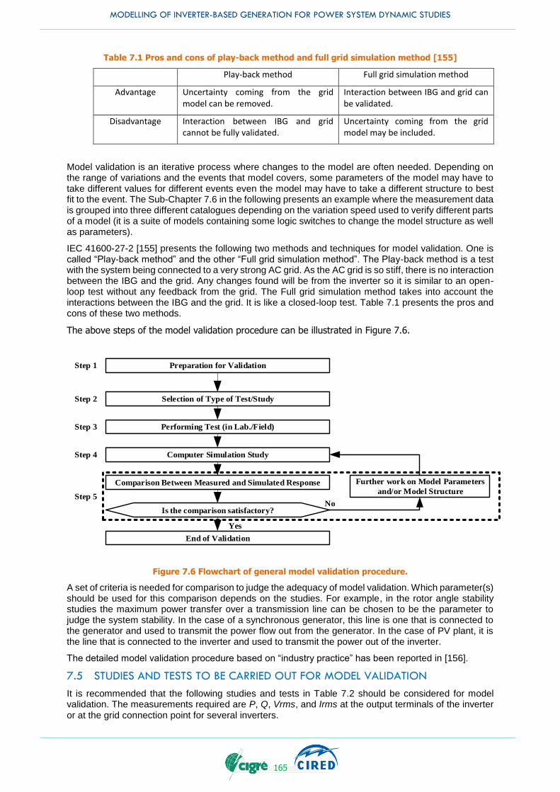
MODELLING OF INVERTER-BASED GENERATION FOR POWER SYSTEM DYNAMIC STUDIES
165
Table 7.1 Pros and cons of play-back method and full grid simulation method [155]
Play-back method Full grid simulation method
Advantage Uncertainty coming from the grid model can be removed.
Interaction between IBG and grid can be validated.
Disadvantage Interaction between IBG and grid cannot be fully validated.
Uncertainty coming from the grid model may be included.
Model validation is an iterative process where changes to the model are often needed. Depending on the range of variations and the events that model covers, some parameters of the model may have to take different values for different events even the model may have to take a different structure to best fit to the event. The Sub-Chapter 7.6 in the following presents an example where the measurement data is grouped into three different catalogues depending on the variation speed used to verify different parts of a model (it is a suite of models containing some logic switches to change the model structure as well as parameters).
IEC 41600-27-2 [155] presents the following two methods and techniques for model validation. One is called “Play-back method” and the other “Full grid simulation method”. The Play-back method is a test with the system being connected to a very strong AC grid. As the AC grid is so stiff, there is no interaction between the IBG and the grid. Any changes found will be from the inverter so it is similar to an open-loop test without any feedback from the grid. The Full grid simulation method takes into account the interactions between the IBG and the grid. It is like a closed-loop test. Table 7.1 presents the pros and cons of these two methods.
The above steps of the model validation procedure can be illustrated in Figure 7.6.
Preparation for Validation
Computer Simulation Study
Selection of Type of Test/Study
Comparison Between Measured and Simulated Response
End of Validation
Step 1
Step 4
Step 5
Step 2
Is the comparison satisfactory?
Yes
No
Performing Test (in Lab./Field)
Further work on Model Parameters
and/or Model Structure
Step 3
Figure 7.6 Flowchart of general model validation procedure.
A set of criteria is needed for comparison to judge the adequacy of model validation. Which parameter(s) should be used for this comparison depends on the studies. For example, in the rotor angle stability studies the maximum power transfer over a transmission line can be chosen to be the parameter to judge the system stability. In the case of a synchronous generator, this line is one that is connected to the generator and used to transmit the power flow out from the generator. In the case of PV plant, it is the line that is connected to the inverter and used to transmit the power out of the inverter.
The detailed model validation procedure based on “industry practice” has been reported in [156].
7.5 STUDIES AND TESTS TO BE CARRIED OUT FOR MODEL VALIDATION
It is recommended that the following studies and tests in Table 7.2 should be considered for model validation. The measurements required are P, Q, Vrms, and Irms at the output terminals of the inverter or at the grid connection point for several inverters.
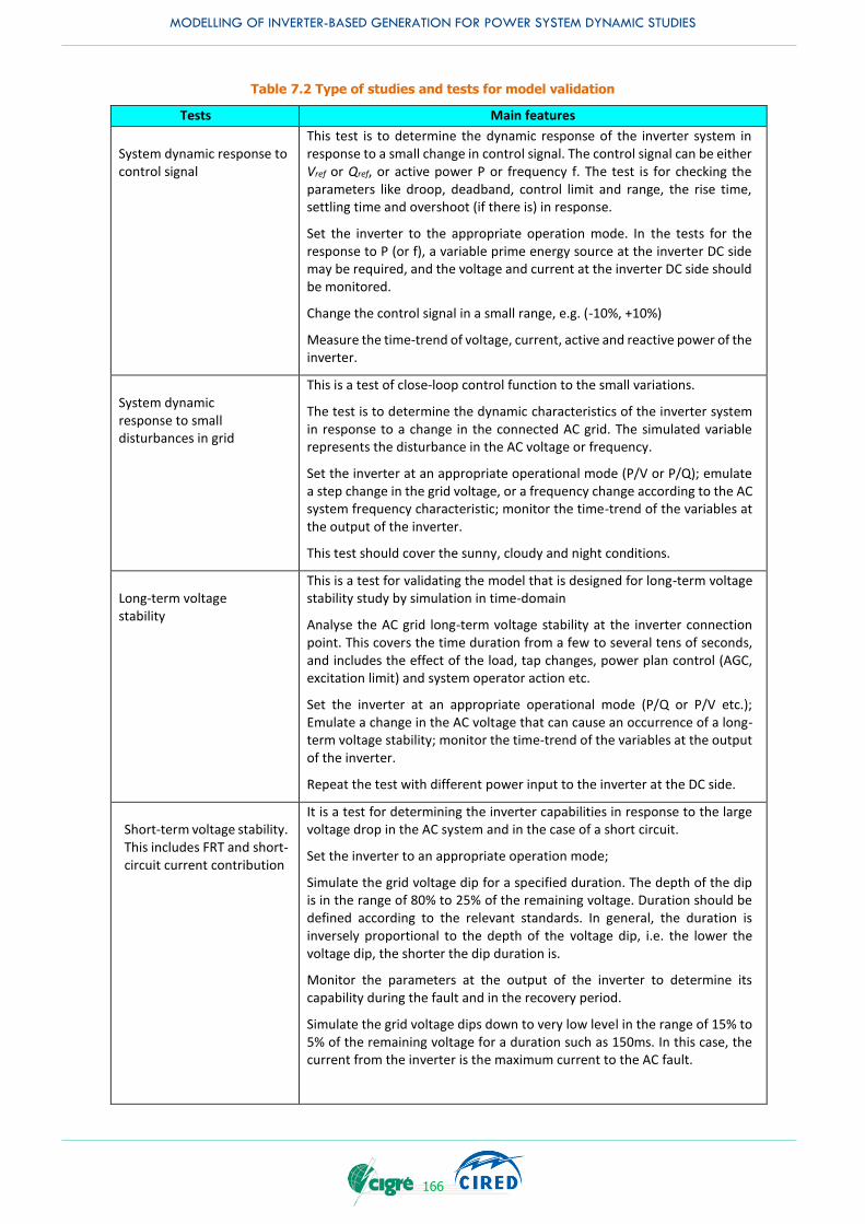
MODELLING OF INVERTER-BASED GENERATION FOR POWER SYSTEM DYNAMIC STUDIES
166
Table 7.2 Type of studies and tests for model validation
Tests Main features
System dynamic response to control signal
This test is to determine the dynamic response of the inverter system in response to a small change in control signal. The control signal can be either Vref or Qref, or active power P or frequency f. The test is for checking the parameters like droop, deadband, control limit and range, the rise time, settling time and overshoot (if there is) in response.
Set the inverter to the appropriate operation mode. In the tests for the response to P (or f), a variable prime energy source at the inverter DC side may be required, and the voltage and current at the inverter DC side should be monitored.
Change the control signal in a small range, e.g. (-10%, +10%)
Measure the time-trend of voltage, current, active and reactive power of the inverter.
System dynamic response to small disturbances in grid
This is a test of close-loop control function to the small variations.
The test is to determine the dynamic characteristics of the inverter system in response to a change in the connected AC grid. The simulated variable represents the disturbance in the AC voltage or frequency.
Set the inverter at an appropriate operational mode (P/V or P/Q); emulate a step change in the grid voltage, or a frequency change according to the AC system frequency characteristic; monitor the time-trend of the variables at the output of the inverter.
This test should cover the sunny, cloudy and night conditions.
Long-term voltage stability
This is a test for validating the model that is designed for long-term voltage stability study by simulation in time-domain
Analyse the AC grid long-term voltage stability at the inverter connection point. This covers the time duration from a few to several tens of seconds, and includes the effect of the load, tap changes, power plan control (AGC, excitation limit) and system operator action etc.
Set the inverter at an appropriate operational mode (P/Q or P/V etc.); Emulate a change in the AC voltage that can cause an occurrence of a long-term voltage stability; monitor the time-trend of the variables at the output of the inverter.
Repeat the test with different power input to the inverter at the DC side.
Short-term voltage stability. This includes FRT and short-circuit current contribution
It is a test for determining the inverter capabilities in response to the large voltage drop in the AC system and in the case of a short circuit.
Set the inverter to an appropriate operation mode;
Simulate the grid voltage dip for a specified duration. The depth of the dip is in the range of 80% to 25% of the remaining voltage. Duration should be defined according to the relevant standards. In general, the duration is inversely proportional to the depth of the voltage dip, i.e. the lower the voltage dip, the shorter the dip duration is.
Monitor the parameters at the output of the inverter to determine its capability during the fault and in the recovery period.
Simulate the grid voltage dips down to very low level in the range of 15% to 5% of the remaining voltage for a duration such as 150ms. In this case, the current from the inverter is the maximum current to the AC fault.
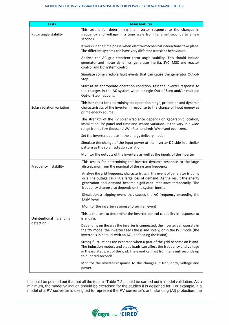
MODELLING OF INVERTER-BASED GENERATION FOR POWER SYSTEM DYNAMIC STUDIES
167
Tests Main features
Rotor angle stability
This test is for determining the inverter response to the changes in frequency and voltage in a time scale from tens milliseconds to a few seconds.
It works in the time phase when electro-mechanical interactions take place. The different systems can have very different transient behaviours.
Analyse the AC grid transient rotor angle stability. This should include generator and motor dynamics, generator inertia, SVC, MSC and reactor control and DC system control.
Simulate some credible fault events that can cause the generator Out-of-Step.
Start at an appropriate operation condition, test the inverter response to the changes in the AC system when a single Out-of-Step and/or multiple Out-of-Step happens.
Solar radiation variation
This is the test for determining the operation range, protection and dynamic characteristics of the inverter in response to the change of input energy as prime energy source.
The strength of the PV solar irradiance depends on geographic location, installation, PV panel and time and season variation. It can vary in a wide range from a few thousand W/m2 to hundreds W/m2 and even zero.
Set the inverter operate in the energy delivery mode;
Simulate the change of the input power at the inverter DC side in a similar pattern as the solar radiation variation
Monitor the outputs of the inverters as well as the inputs of the inverter
Frequency instability
This test is for determining the inverter dynamic response to the large discrepancy from the nominal of the system frequency
Analyse the grid frequency characteristics in the event of generator tripping or a line outage causing a large loss of demand. As the result the energy generation and demand become significant imbalance temporarily. The frequency change also depends on the system inertia.
Simulation a tripping event that causes the AC frequency exceeding the LFSM level
Monitor the inverter response to such an event
Unintentional islanding detection
This is the test to determine the inverter control capability in response to islanding.
Depending on the way the inverter is connected, the inverter can operate in the f/V mode (the inverter feeds the island solely) or in the P/V mode (the inverter is in parallel with an AC line feeding the island).
Strong fluctuations are expected when a part of the grid become an island. The induction motors and static loads can affect the frequency and voltage in the isolated part of the grid. The event can last from tens milliseconds up to hundred seconds
Monitor the inverter response to the changes in frequency, voltage and power.
It should be pointed out that not all the tests in Table 7.2 should be carried out in model validation. As a minimum, the model validation should be exercised for the studies it is designed for. For example, if a model of a PV converter is designed to represent the PV converter’s anti islanding (AI) protection, the
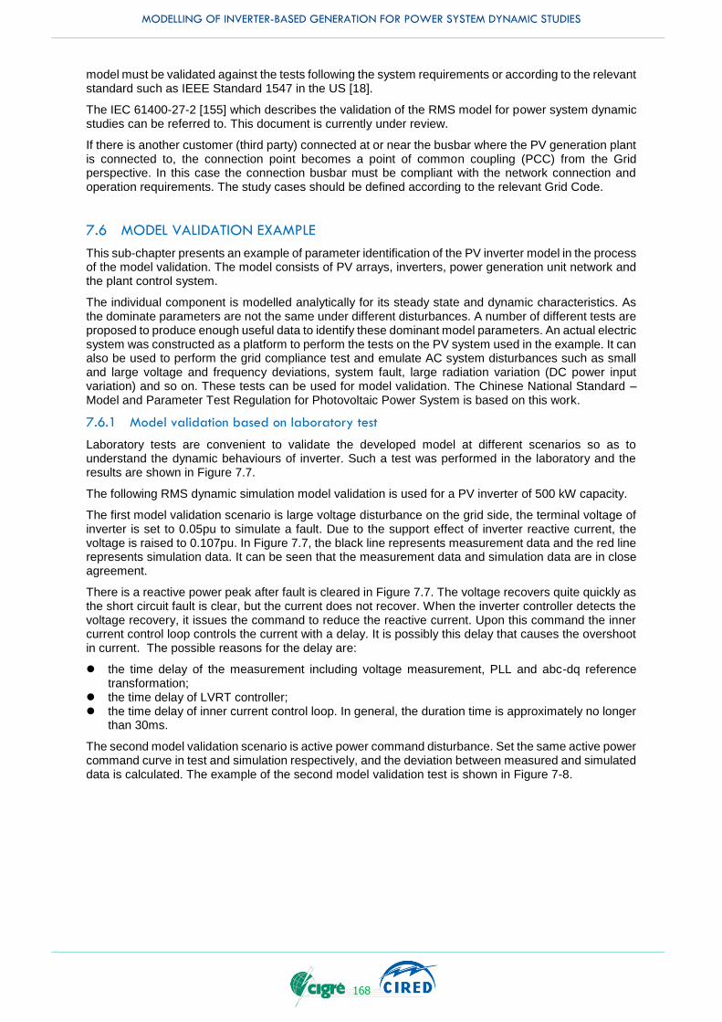
MODELLING OF INVERTER-BASED GENERATION FOR POWER SYSTEM DYNAMIC STUDIES
168
model must be validated against the tests following the system requirements or according to the relevant standard such as IEEE Standard 1547 in the US [18].
The IEC 61400-27-2 [155] which describes the validation of the RMS model for power system dynamic studies can be referred to. This document is currently under review.
If there is another customer (third party) connected at or near the busbar where the PV generation plant is connected to, the connection point becomes a point of common coupling (PCC) from the Grid perspective. In this case the connection busbar must be compliant with the network connection and operation requirements. The study cases should be defined according to the relevant Grid Code.
7.6 MODEL VALIDATION EXAMPLE
This sub-chapter presents an example of parameter identification of the PV inverter model in the process of the model validation. The model consists of PV arrays, inverters, power generation unit network and the plant control system.
The individual component is modelled analytically for its steady state and dynamic characteristics. As the dominate parameters are not the same under different disturbances. A number of different tests are proposed to produce enough useful data to identify these dominant model parameters. An actual electric system was constructed as a platform to perform the tests on the PV system used in the example. It can also be used to perform the grid compliance test and emulate AC system disturbances such as small and large voltage and frequency deviations, system fault, large radiation variation (DC power input variation) and so on. These tests can be used for model validation. The Chinese National Standard – Model and Parameter Test Regulation for Photovoltaic Power System is based on this work.
7.6.1 Model validation based on laboratory test
Laboratory tests are convenient to validate the developed model at different scenarios so as to understand the dynamic behaviours of inverter. Such a test was performed in the laboratory and the results are shown in Figure 7.7.
The following RMS dynamic simulation model validation is used for a PV inverter of 500 kW capacity.
The first model validation scenario is large voltage disturbance on the grid side, the terminal voltage of inverter is set to 0.05pu to simulate a fault. Due to the support effect of inverter reactive current, the voltage is raised to 0.107pu. In Figure 7.7, the black line represents measurement data and the red line represents simulation data. It can be seen that the measurement data and simulation data are in close agreement.
There is a reactive power peak after fault is cleared in Figure 7.7. The voltage recovers quite quickly as the short circuit fault is clear, but the current does not recover. When the inverter controller detects the voltage recovery, it issues the command to reduce the reactive current. Upon this command the inner current control loop controls the current with a delay. It is possibly this delay that causes the overshoot in current. The possible reasons for the delay are:
the time delay of the measurement including voltage measurement, PLL and abc-dq reference transformation;
the time delay of LVRT controller; the time delay of inner current control loop. In general, the duration time is approximately no longer
than 30ms.
The second model validation scenario is active power command disturbance. Set the same active power command curve in test and simulation respectively, and the deviation between measured and simulated data is calculated. The example of the second model validation test is shown in Figure 7-8.
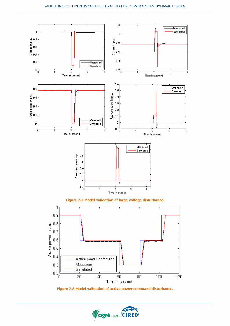
MODELLING OF INVERTER-BASED GENERATION FOR POWER SYSTEM DYNAMIC STUDIES
169
Figure 7.7 Model validation of large voltage disturbance.
Figure 7.8 Model validation of active power command disturbance.

MODELLING OF INVERTER-BASED GENERATION FOR POWER SYSTEM DYNAMIC STUDIES
170
7.6.2 Model validation based on field test
Short-circuit or ground faults in the real network are useful in the validation of the developed model to demonstrate the dynamic behaviour following such faults. The measurements following faults can be utilized to then validate RMS dynamic simulation model.
~
~
~
750 kV substation
AC/DC convertor station
330 kV substation
110 kV substation
Heat power plant
Hydro power plant
Wind power plant
PV power plant
Load
PV power
plant A
Figure 7.9 Schematic diagram of Ningxia network.
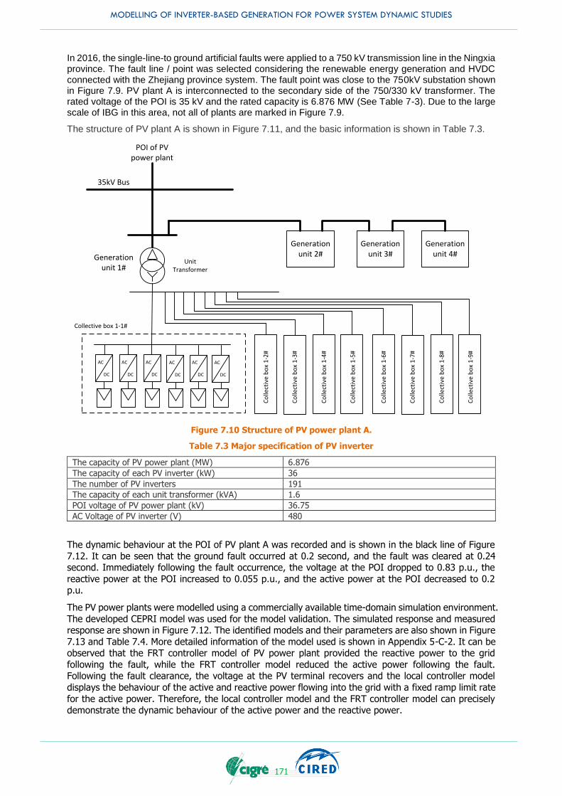
MODELLING OF INVERTER-BASED GENERATION FOR POWER SYSTEM DYNAMIC STUDIES
171
In 2016, the single-line-to ground artificial faults were applied to a 750 kV transmission line in the Ningxia province. The fault line / point was selected considering the renewable energy generation and HVDC connected with the Zhejiang province system. The fault point was close to the 750kV substation shown in Figure 7.9. PV plant A is interconnected to the secondary side of the 750/330 kV transformer. The rated voltage of the POI is 35 kV and the rated capacity is 6.876 MW (See Table 7-3). Due to the large scale of IBG in this area, not all of plants are marked in Figure 7.9.
The structure of PV plant A is shown in Figure 7.11, and the basic information is shown in Table 7.3.
AC DC
AC DC
Unit Transformer
Generation unit 1#
Generation unit 4#
Generation unit 3#
Generation unit 2#
POI of PV power plant
35kV Bus
AC DC
AC DC
AC DC
AC DC
Collective box 1-1#
Co
llect
ive
bo
x 1
-2#
Co
llect
ive
bo
x 1
-3#
Co
llect
ive
bo
x 1
-4#
Co
llect
ive
bo
x 1
-5#
Co
llect
ive
bo
x 1
-6#
Co
llect
ive
bo
x 1
-7#
Co
llect
ive
bo
x 1
-8#
Co
llect
ive
bo
x 1
-9#
Figure 7.10 Structure of PV power plant A.
Table 7.3 Major specification of PV inverter
The capacity of PV power plant (MW) 6.876
The capacity of each PV inverter (kW) 36
The number of PV inverters 191
The capacity of each unit transformer (kVA) 1.6
POI voltage of PV power plant (kV) 36.75
AC Voltage of PV inverter (V) 480
The dynamic behaviour at the POI of PV plant A was recorded and is shown in the black line of Figure
7.12. It can be seen that the ground fault occurred at 0.2 second, and the fault was cleared at 0.24 second. Immediately following the fault occurrence, the voltage at the POI dropped to 0.83 p.u., the
reactive power at the POI increased to 0.055 p.u., and the active power at the POI decreased to 0.2 p.u.
The PV power plants were modelled using a commercially available time-domain simulation environment.
The developed CEPRI model was used for the model validation. The simulated response and measured response are shown in Figure 7.12. The identified models and their parameters are also shown in Figure
7.13 and Table 7.4. More detailed information of the model used is shown in Appendix 5-C-2. It can be observed that the FRT controller model of PV power plant provided the reactive power to the grid
following the fault, while the FRT controller model reduced the active power following the fault. Following the fault clearance, the voltage at the PV terminal recovers and the local controller model
displays the behaviour of the active and reactive power flowing into the grid with a fixed ramp limit rate
for the active power. Therefore, the local controller model and the FRT controller model can precisely demonstrate the dynamic behaviour of the active power and the reactive power.
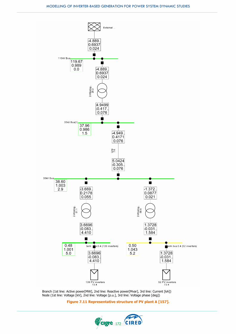
MODELLING OF INVERTER-BASED GENERATION FOR POWER SYSTEM DYNAMIC STUDIES
172
Branch (1st line: Active power[MW], 2nd line: Reactive power[Mvar], 3rd line: Current [kA]) Node (1st line: Voltage [kV], 2nd line: Voltage [p.u.], 3rd line: Voltage phase [deg])
Figure 7.11 Representative structure of PV plant A [157].
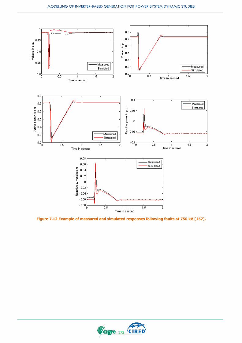
MODELLING OF INVERTER-BASED GENERATION FOR POWER SYSTEM DYNAMIC STUDIES
173
Figure 7.12 Example of measured and simulated responses following faults at 750 kV [157].
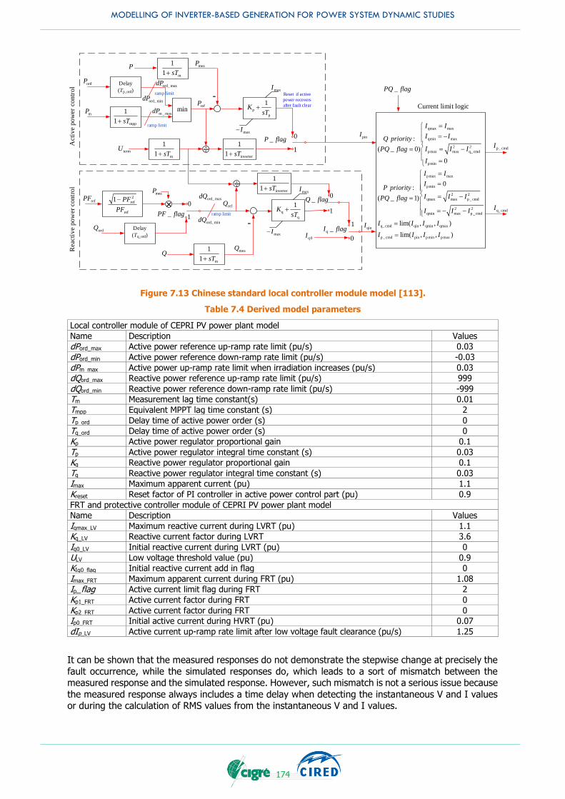
MODELLING OF INVERTER-BASED GENERATION FOR POWER SYSTEM DYNAMIC STUDIES
174
Q
mP
P
p _ cmdI
q_ cmdI
ordP Delay
(Tp_ord)
min
mpp
1
1 sT+
refP-
m
1
1 sT+
maxI
maxI-
p
p
1K
sT+
termU ÷inverter
1
1 sT+
_P flag
×refPF
refQ
ordQ Delay
(Tq_ord)
_PF flag
m
1
1 sT+
m
1
1 sT+
-
÷
q
q
1K
sT+
_Q flag
qmax max
qmin max
2 2
pmax max q_ cmd
pmin
pmax max
pmin
2 2
qmax max p _ cmd
2 2
qmin max p _ cmd
q_ cmd qin qmin qmax
p _ cmd
:
( _ 0)
0
0:
( _ 1)
lim( , , )
lim(
I I
I IQ priority
I I IPQ flag
I
I I
IP priority
I I IPQ flag
I I I
I I I I
I
-
-
-
- -
pin pmin pmax, , )I I I
maxI
maxI-
_PQ flag
inverter
1
1 sT+
2
ref
ref
1 PF
PF
-
0
1
0
10
1
Act
ive
po
wer
co
ntr
ol
Current limit logic
Rea
ctiv
e p
ow
er c
on
tro
lmeaP
meaP
Reset if active
power recovers
after fault clear
pinI
qinI
ord_ maxdP
ord_ mindP
m _ maxdP
ord_ maxdQ
ord_ mindQ
ramp limit
ramp limit
ramp limit
q _I flag
0
1
q0I
meaQ
Figure 7.13 Chinese standard local controller module model [113].
Table 7.4 Derived model parameters
Local controller module of CEPRI PV power plant model
Name Description Values
dPord_max Active power reference up-ramp rate limit (pu/s) 0.03
dPord_min Active power reference down-ramp rate limit (pu/s) -0.03
dPm_max Active power up-ramp rate limit when irradiation increases (pu/s) 0.03
dQord_max Reactive power reference up-ramp rate limit (pu/s) 999
dQord_min Reactive power reference down-ramp rate limit (pu/s) -999
Tm Measurement lag time constant(s) 0.01
Tmpp Equivalent MPPT lag time constant (s) 2
Tp_ord Delay time of active power order (s) 0
Tq_ord Delay time of active power order (s) 0
Kp Active power regulator proportional gain 0.1
Tp Active power regulator integral time constant (s) 0.03
Kq Reactive power regulator proportional gain 0.1
Tq Reactive power regulator integral time constant (s) 0.03
Imax Maximum apparent current (pu) 1.1
Kreset Reset factor of PI controller in active power control part (pu) 0.9
FRT and protective controller module of CEPRI PV power plant model
Name Description Values
Iqmax_LV Maximum reactive current during LVRT (pu) 1.1
Kq_LV Reactive current factor during LVRT 3.6
Iq0_LV Initial reactive current during LVRT (pu) 0
ULV Low voltage threshold value (pu) 0.9
KIq0_flag Initial reactive current add in flag 0
Imax_FRT Maximum apparent current during FRT (pu) 1.08
Ip_flag Active current limit flag during FRT 2
Kp1_FRT Active current factor during FRT 0
Kp2_FRT Active current factor during FRT 0
Ip0_FRT Initial active current during HVRT (pu) 0.07
dIp_LV Active current up-ramp rate limit after low voltage fault clearance (pu/s) 1.25
It can be shown that the measured responses do not demonstrate the stepwise change at precisely the
fault occurrence, while the simulated responses do, which leads to a sort of mismatch between the measured response and the simulated response. However, such mismatch is not a serious issue because
the measured response always includes a time delay when detecting the instantaneous V and I values or during the calculation of RMS values from the instantaneous V and I values.

MODELLING OF INVERTER-BASED GENERATION FOR POWER SYSTEM DYNAMIC STUDIES
175
7.7 CONCLUSION
The model validation is an important and final step in the model development. It confirms the assumptions made, the conditions and limitations of the model and gives confidence to the model developers and users. The quality of the model validation can be only as good as the data used for the model validation. Several data sources with their pros and cons were presented in this chapter including the measurements taken from the field in real systems, the data produced on the laboratory test systems, from real time digital simulators and from other simulation models and programs.
The chapter is limited to the validation work for RMS models. A procedure with a list of studies and test events is proposed for the IBGs. They present most of the events that the RMS models are required to perform and should be considered as a guideline in validation. They are by no means inclusive, and equally, there is no intention to recommend all of them are performed in a model validation. A different study may require not only a different model (that matches the purpose of the study) but different model parameters, such as sampling rates, length of data etc.
The results of a model validation based on a laboratory test platform in response to large voltage disturbance and the system response to power command, and the results of the FRT tests on PV plant in a transmission grid system were provided in order to demonstrate the actions and how good the model validation can be.

MODELLING OF INVERTER-BASED GENERATION FOR POWER SYSTEM DYNAMIC STUDIES
176
MODELLING OF INVERTER-BASED GENERATION FOR POWER SYSTEM DYNAMIC STUDIES
177
8. CONCLUSIONS AND FUTURE WORK
Any numerical models, i.e. mathematical simulation models have limitations. A mathematical simulation model will provide correct simulation results to the type of phenomena to be observed or examined by including appropriate individual model component (such as protections, controls and capabilities). Thus, the proper selection of the mathematical simulation model needs to be performed by power system engineers in academia as well as in industry. However, the proper selection of the mathematical simulation model is not an easy task. The selection of the inverter-based generator (IBG) model is much more difficult compared to the conventional mathematical simulation models such as the power plant models and conventional power electronics models such as static var compensator models. Considerable industry experience concerning power system dynamic studies and the dynamics of the power electronics is required for the proper selection of the IBG model. The established CIGRE C4-C6.35/CIRED JWG has successfully gathered a wide variety of experts which fully cover the required industry experience. Thanks to this JWG, this TB provides the guidance and recommendation for the IBG models to be used for the power system dynamic studies.
At the beginning of the CIGRE C4-C6.35/CIRED JWG activities, a questionnaire survey was performed to clarify the currently used IBG models by utilities and system operators for the power system dynamic studies. Through the analysis of the questionnaire survey, it is remarkable finding that around one third of the utilities and system operators still use negative load models for the representation of IBG in power system dynamic studies. According to the results of the questionnaire survey, the following reasons may explain this approach, by the lack of:
model requirements of IBG for specific power system phenomena
well-validated detailed IBG models
widely accepted generic IBG models
widely accepted range of IBG model parameters
specific grid code requirements
information about dynamic performance of power system with IBGs
agreed or well documented methodology to perform aggregation of embedded IBGs
knowledge and experience of IBG impact on daily operation of power system
The dynamic characteristics of IBGs are different when compared to synchronous generators, but with good control system design and increased functionalities of modern IBG technologies, they can provide many of the same or even better services (e.g. voltage control, frequency response etc.). None the less, they do need to be modelled differently and appropriately. Therefore, the development of the proper computer simulation models for IBGs with such additional functionalities is vital for power systems analyses.
DSOs have to some extent a representation of their networks and details about connected consumers and producers. However, the limited data is generally not suitable for dynamic simulations for either the distribution or the transmission system or, at least, has not been used for that purpose in the past, due to the high level of detail required. From the point of view of the DSOs, time-domain simulations may also now be necessary to assess protection system behaviour, distribution network automated operation, unintentional islanding of part of distribution systems including IBG, voltage issues, etc. For these types of power system dynamic studies detailed IBG models are needed.
The extraction of the model component, i.e., the necessary functionality for a specific dynamic behaviour/phenomenon is a key to provide the proper selection of the model. Several major phenomena such as 1) frequency deviation, 2) large voltage deviation, 3) small and long-term voltage deviation for the power system dynamic studies with the IBGs are required to be obtained. In order to obtain the appropriate simulation results for each type of dynamic stability study, more than sixty modelling experts who were nominated as the members of CIGRE C4-C6.35/CIRED JWG around the world, organised the necessary functionalities of the IBGs which should be implemented in the model in terms of the power system phenomena instead of the power system dynamic studies. However, even unnecessary functionalities may be essential under a special circumstance, even if the table says no need for the functionality. That means, there can be exceptions. Therefore, it is suggested to carefully read the descriptions on why the functionality is or was not necessary.
The functionalities are classified into three areas: 1) control, 2) protection, 3) capability. The detailed clarification for the necessity of the use of the functionalities is also provided for each necessary functionality. It should be highlighted that the protection model needs to be paid more attention to in

MODELLING OF INVERTER-BASED GENERATION FOR POWER SYSTEM DYNAMIC STUDIES
178
many power system dynamic studies, because the IBGs are disconnected by their protection systems and because such disconnection can affect the power system stability.
It is noted that the complete functionality list provides clarification of the characteristics of IBGs focusing on the difference between IBGs with minimum requirements and those of synchronous generators. The four main characteristics
System inertia
Short-circuit current provision (which is large enough for protections to operate)
Synchronization capability (existence of a synchronous torque component)28
Constant internal voltage29 source
are inherently possessed by synchronous generators. However, they cannot easily be emulated (if at all or if needed) by IBGs from technical or commercial perspectives although many of the characteristics such as the frequency control capability and the reactive power control capability can be provided by large-scale IBGs. It should be noted that the IBGs can be much better controlled with much shorter delays than synchronous generators. In addition to that the IBGs have no critical clearing time, i.e. no transient stability issue.
The example control block diagrams for representing each functionality are provided for the type of model, RMS or EMT and depending on the level of the controller, either local level controller or plant level controller. It should be emphasized that most of the functionalities are existing functionalities which are currently implemented by commercial software tools for power system dynamic studies. On the other hand, some functionalities such as the synthetic inertia are not required as a mandatory functionality and the modelling of such functionalities are not presently offered.
Although the computer technology has been developed, it is becoming more challenging to model the increasing number of individual generators as part of large-scale dynamic stability studies (mainly due to the high computational burden and the limited assigned time for completing analysis activities). On the other hand, correctly representing the aggregated response of the distributed IBGs will influence the power system dynamic stability results at the bulk transmission system level and become more critical as the penetration level of distributed IBGs increases. However, there is no generally agreed or accepted methodology for aggregating IBGs and there are ongoing studies for developing such a methodology. One of the latest aggregation methodologies which is proposed by WECC is discussed individually in both power flow representation and dynamic simulation representation.
Other than the establishment of the generally accepted methodology of the aggregated IBGs, there are several future technical challenges:
The control and protection model parameter derivation for aggregated models.
The aggregated active power recovery after the fault is cleared.
Clarification of the aggregated dynamic behaviour of all IBGs during faults in the case of medium or high penetration level.
The balance of the levels of details of the load model and the IBG model needs to be considered. The loads and the IBGs can be connected to the same bus and they can interact with each other. For example, the level of details of the load model is assumed to be low and the level of details of the IBG model is assumed to be high. In this example, the sufficient levels of details of the whole system data cannot be expected and an important behaviour could be missing.
The selection of the IBG model validation test condition and type of IBG model and IBG model elements are vital for representing dynamic behaviour with IBGs in power system dynamic studies performed by utilities and system operators. For the model validation, measurement is the key. The required levels of the measurement data are not always the same for the phenomenon to be observed. The desirable model validation test condition can vary depending on the type of power system dynamic studies. The possible different levels of the validation test, such as the laboratory level and the field level are illustrated. The suitable dynamic behaviour for each level of the tests is also clarified. Then, the recommended model validation test conditions including the necessary electric quantities which are generally captured by measurement devices are discussed. The general procedure for the model validation is illustrated and the permissible model error which can be different depending on the type of
28 Note that this capability is NOT literally required for IBGs because they have no rotor-angle stability issue. 29 The voltage denotes the synchronous internal voltage. It does not denote the terminal voltage of synchronous generators.

MODELLING OF INVERTER-BASED GENERATION FOR POWER SYSTEM DYNAMIC STUDIES
179
power system dynamic studies is briefly discussed. Because the model error can be caused by three possible reasons:
Appropriate model with inappropriate model parameters,
Inappropriate model with appropriate model parameters,
Inappropriate model with inappropriate model parameters,
exploring the proper model parameters is usually performed as the first step. If any parameters cannot obtain a good agreement between the simulated response and the model response, the model itself needs to be changed. This procedure is generic and is for the model validation not only for IBGs but also loads and other generator controllers.
It is ideal that the same IBG model parameters may be used for different/various power system conditions. Identifying one set of model parameters for one incident is relatively easy. However, identifying the same set of model parameters for more than two incidents is not at all easy. There are two approaches
Collect data for all incidents and identify the most reasonable set of model parameters.
Identify one set of model parameters for all incidents one by one and collect all sets of model parameters.
Then, the statistical process is applied to all the collected sets of model parameters. However, both approaches have pros and cons. The derivation of a sort of the universal set of IBG model parameters for various power system conditions can also be a technical challenge.
Both synchronous generators and IBGs have pros and cons. For example, thanks to the natural feature or inherent characteristics which come from physics (flux linkage etc.), synchronous generators can increase/decrease instantaneously at the moment when the fault occurs. In other words, IBGs cannot attain such immediate/instant response. On the other hand, the ramping speed of voltage and current provided by IBGs is much higher than that provided by synchronous generators. Therefore, such prominent ramping speed of controllers of IBGs is expected to be utilised to provide more control quantity for compensating the deficiency of control quantity at the moment when the fault occurs.
More advanced coordination between IBGs and synchronous generators can be a key to integrate more IBGs into the grid without deteriorating power system security. In order to obtain the advanced coordination, the modelling of IBGs become vital and the time-domain simulation using the aforementioned models is required in order to figure out how those generations can be coordinated.
The time-domain simulation becomes more important especially when
The interaction between one device/system and another device/system is not negligible.
The (complicated) operation of protection devices is not negligible.
With the higher penetration of the IBGs, the above two points will be no longer negligible. Therefore, more effort for better modelling of the IBGs will be required in the future. In other words, the continuous improvement of simulation accuracy is never too old an issue to address.

MODELLING OF INVERTER-BASED GENERATION FOR POWER SYSTEM DYNAMIC STUDIES
180
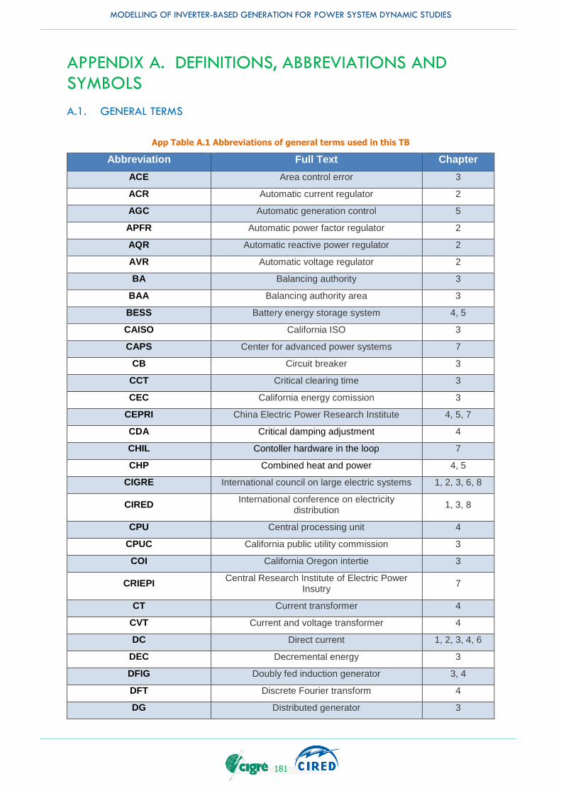
MODELLING OF INVERTER-BASED GENERATION FOR POWER SYSTEM DYNAMIC STUDIES
181
APPENDIX A. DEFINITIONS, ABBREVIATIONS AND SYMBOLS
A.1. GENERAL TERMS
App Table A.1 Abbreviations of general terms used in this TB
Abbreviation Full Text Chapter
ACE Area control error 3
ACR Automatic current regulator 2
AGC Automatic generation control 5
APFR Automatic power factor regulator 2
AQR Automatic reactive power regulator 2
AVR Automatic voltage regulator 2
BA Balancing authority 3
BAA Balancing authority area 3
BESS Battery energy storage system 4, 5
CAISO California ISO 3
CAPS Center for advanced power systems 7
CB Circuit breaker 3
CCT Critical clearing time 3
CEC California energy comission 3
CEPRI China Electric Power Research Institute 4, 5, 7
CDA Critical damping adjustment 4
CHIL Contoller hardware in the loop 7
CHP Combined heat and power 4, 5
CIGRE International council on large electric systems 1, 2, 3, 6, 8
CIRED International conference on electricity
distribution 1, 3, 8
CPU Central processing unit 4
CPUC California public utility commission 3
COI California Oregon intertie 3
CRIEPI Central Research Institute of Electric Power
Insutry 7
CT Current transformer 4
CVT Current and voltage transformer 4
DC Direct current 1, 2, 3, 4, 6
DEC Decremental energy 3
DFIG Doubly fed induction generator 3, 4
DFT Discrete Fourier transform 4
DG Distributed generator 3

MODELLING OF INVERTER-BASED GENERATION FOR POWER SYSTEM DYNAMIC STUDIES
182
DLL Dynamic link library 4
DN Distribution network 3
DSO Distribution system operator 1, 2, 3
DTRS Digital real time simulator 7
DURIP Defence university research instrumentation
program 7
EMS Energy management system 3
EMT Electromagnetic transient 1, 2, 3, 4, 6
ENTSO-E European network of transmission system
operators 2
EPRI Electric power research institute 3
ERCOT Electric reliability council of tewas 2
ESCR Effective short circuit ratio 4
EU European union 2
FACTS Flexible alternating current transmission system 3, 6
FDNE Flexible dependent network equivalent 4
FFT Fast Fourier transfor 4
FRO Frequency response obligation 3
(F)FRT (Frequency) Fault ride through 1, 2
FSM Frequency sensisitive mode 4
GPS Global positionning system 3
GTO Gate turn off 4
GUI Graphic user interface 4, 6
HUT Hardware under test 7
HV High voltage 1, 2, 3, 5
HVDC High voltage direct current 2, 3, 5, 6
HVRT High voltage ride through 2, 3, 4
IBG Inverter based generators 1, 2, 3, 4, 5
IEC International electrotechnical commission 1, 2, 6
IEEE Institute of electrical and electronics engineers 1, 2
IGBT Insulated gate bipolar transistors 4
IM Induction motor 3
IPS Internal protection system 2
JWG Joint working group 3
LCC Line commuted converter 4
LFSM-O Limited frequency sensitive mode-
overfrequency 3
LFSM-U Limited frequency sensitive mode-
underfrequency 3
LOM(D) Loss of main (detection) 3
LRS Load and resources subcommittee 3

MODELLING OF INVERTER-BASED GENERATION FOR POWER SYSTEM DYNAMIC STUDIES
183
LTC Load tap changer 3
LV Low voltage 1, 2, 3, 4, 5
LV(F)RT Low voltage (fault) ride through 1, 2, 3, 5
LVPL Low voltage power logic 5
MMC Multi-level converter 4
MPPT Maximum power point tracking 1, 2, 3, 4
MC Monte Carlo 3
MV Medium voltage 1, 2, 3, 4, 5
NA Nodal admittance 4
NDA Non disclosure agreement 4
NDZ Non detection zone 3
NERC North american electric reliability corporation 3
NYISO New York ISO 3
OFR Over frequency relay 4
OLTC On load tap changer 3
OOS Out of step 3
ORC ORankine cycle 2
OVR Over voltage relay 4
PCC Point of common coupling 1, 2, 3, 4, 7
PCU Power conditioning unit 4
PDCI Pacific DC intertie 3
PF Power factor 4
PHIL Power hardware in the loop 7
PI control Proportional and integral control 4, 6
PLL Phase locked loop 1, 2, 4
POD controller Power oscillation damping controller 2
POI Point of interconnection 3, 6, 7
PS Power system 2
PSS Power system stabilizer 2, 3
p.u. Per unit 3
PV Photovoltaics 1, 2, 3, 4, 5, 6
PWM Pulse width modulation 4, 6
RER Renewable energy resources 3
RES Renewable energy source 1, 2, 3, 4, 5
RMS Root means square 1, 2, 3, 4, 6
ROS Rest of system 7
RPS Renewable portfolio standard 3
ROCOF Rate of change of frequency 1, 2
RT Real time 4

MODELLING OF INVERTER-BASED GENERATION FOR POWER SYSTEM DYNAMIC STUDIES
184
RTDS Real time digital simulator 4, 6
SCUC Security-constrained unit commitment 3
SCUD Security-constrained unit dispatch 3
SCR Short circuit ratio 3, 4, 6
SOC State of charge 4, 5
SOFC Solid oxide fuel cell 4
STATCOM Static var compensator 3, 4, 5
SSCI Sub-synchronous control interaction 3, 4
SSR Sub-synchronous resonance 3, 4
SSTI Sub-synchronous torsional interaction 3, 4
SVC Static var compensator 2, 4, 5
SVS Static var system 3
TB Technical brochure 2
TEPPC Transmission expansion planning policy
committee 3
TN Transmission network 3
TSO Transmission system operator 1, 2, 3, 4
UFR Under frequency relay 4
ULTC Under load tap changer 3
UVR Under voltage relay 4
VSC Voltage source converter 2, 4, 5
VT Voltage transformer 4
WECC Western electricity coordinating council 3, 4, 5
WPP Wind power plant 3, 5
WT(G) Wind turbine (generators) 1, 3, 4, 5
ZVRT Zero voltage ride through 5
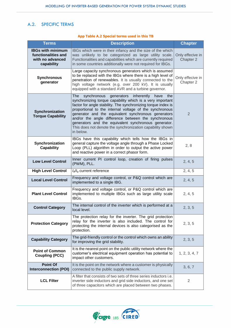
MODELLING OF INVERTER-BASED GENERATION FOR POWER SYSTEM DYNAMIC STUDIES
185
A.2. SPECIFIC TERMS
App Table A.2 Special terms used in this TB
Terms Description Chapter
IBGs with minimum functionalities and with no advanced
capability
IBGs which were in their infancy and the size of the which was unlikely to be categorized as large utility scale. Functionalities and capabilities which are currently required in some countries additionally were not required for IBGs.
Only effecive in Chapter 2
Synchronous generator
Large capacity synchronous generators which is assumed to be replaced with the IBGs where there is a high level of penetration of renewables. It is usually connected to the high voltage network (e.g. over 200 kV). It is usually equipped with a standard AVR and a turbine governor.
Only effecive in Chapter 2
Synchronization Torque Capability
The synchronous generators inherently have the synchronizing torque capability which is a very important factor for angle stability. The synchronizing torque index is proportional to the internal voltage of the synchronous generator and the equivalent synchronous generators and/or the angle difference between the synchronous generators and the equivalent synchronous generator. This does not denote the synchronization capability shown in below.
2
Synchronization Capability
IBGs have this capability which tells how the IBGs in general capture the voltage angle through a Phase Locked Loop (PLL) algorithm in order to output the active power and reactive power in a correct phasor form.
2, 8
Low Level Control Inner current PI control loop, creation of firing pulses (PWM), PLL.
2, 4, 5
High Level Control Id/Iq current reference 2, 4, 5
Local Level Control Frequency and voltage control, or P&Q control which are implemented to a single IBG.
2, 4, 5
Plant Level Control Frequency and voltage control, or P&Q control which are implemented to multiple IBGs such as large utility scale IBGs.
2, 4, 5
Control Category The internal control of the inverter which is performed at a local level.
2, 3, 5
Protection Category
The protection relay for the inverter. The grid protection relay for the inverter is also included. The control for protecting the internal devices is also categorised as the protection.
2, 3, 5
Capability Category The grid-friendly control or the control which owns an ability for improving the grid stability.
2, 3, 5
Point of Common Coupling (PCC)
It is the nearest point on the public utility network where the customer’s electrical equipment operation has potential to impact other customers.
1, 2, 3, 4, 7
Point Of Interconnection (POI)
It is the point on the network where a customer is physically connected to the public supply network.
3, 6, 7
LCL Filter A filter that consists of two sets of three series inductors i.e. inverter side inductors and grid side inductors, and one set of three capacitors which are placed between two phases.
2

MODELLING OF INVERTER-BASED GENERATION FOR POWER SYSTEM DYNAMIC STUDIES
186
MODELLING OF INVERTER-BASED GENERATION FOR POWER SYSTEM DYNAMIC STUDIES
187
APPENDIX B. LINKS AND REFERENCES
[1] P. Pourbeik, J. Sanchez-Gasca, J. Senthil, J. Weber, P. Zadehkhost, Y. Kazachkov, S. Tacke
and J. Wen, “Generic Dynamic Models for Modeling Wind Power Plants and other Renewable Technologies in Large Scale Power System Studies”, IEEE Trans. on Energy Conversion, Sep. 2017, Vol. 32, No. 3, pp 1108 – 1116.
[2] Ö. Göksu, P. Sørensen, J. Fortmann, A. Morales, S. Weigel and P. Pourbeik, “Compatibility of IEC 61400-27-1 Ed 1 and WECC 2nd Generation Wind Turbine Models,” Conference: 15th International Workshop on Large-Scale Integration of Wind Power into Power Systems as well as on Transmission Networks for Offshore Wind Power Plants, Nov. 2016.
[3] CIGRE TB 328, “Wind turbines - Electrical simulation models for wind power generation,” WG C4.601, Aug. 2007.
[4] G. Lammert, K. Yamashita, L. D. Pab´on Ospina, H. Renner, S. Martinez Villanueva, P. Pourbeik, F.-E. Ciausiu, and M. Braun, “International Industry Practice on Modelling and Dynamic Performance of Inverter Based Generation in Power System Studies,” CIGRE Science & Engineering Vol. 8, June 2017.
[5] G. Lammert, K. Yamashita, L. D. Pab´on Ospina, H. Renner, S. Martinez Villanueva, P. Pourbeik, F.-E. Ciausiu, and M. Braun, “Modelling and Dynamic Performance of Inverter Based Generation in Power System Studies: An International Questionnaire Survey,” CIRED -Open Access Proceedings Journal, Vol. 1, 2017
[6] CIGRE TB 566, “Modelling and Aggregation of Loads in Flexible Power Networks”, WG C4.605, 2014.
[7] WECC, “WECC Guide for Representation of Photovoltaic Systems In Large-Scale Power flow Simulations. WECC Modelling and Validation Work Group. Jan. 2011, URL: https://www.wecc.biz/_layouts/15/WopiFrame.aspx?sourcedoc=/Reliability/WECC/PV/Plant/Power/Flow/Modeling/Guidelines/-/August/2010.pdf&action=default&DefaultItemOpen=1
[8] DGA Consulting. “International review of frequency control adaptation,” Oct. 2016, URL: https://www.aemo.com.au/-/media/Files/Electricity/NEM/Security and Reliability/Reports/FPSS---International-Review-of-Frequency-Control.pdf.
[9] N. Miller. “Technology Capabilities for Fast Frequency Response,” GE Final Report, March 2017, URL: https://www.aemo.com.au/-/media/Files/Electricity/NEM/Security and Reliability/Reports/2017-03-10-GE-FFR-Advisory-Report-Final---2017-3-9.pdf.
[10] IEC “Solar photovoltaic energy systems -Terms, definitions and symbols,” IEC Technical Specification, IEC/TS 61386, Ed. 2, Dec. 2007.
[11] P. Kundur, “Power System Stability and Control,” New York: McGraw-Hill, 1994. [12] National grid, “Black Start from Distributed Sources,” Dec. 2017, URL:
https://www.nationalgrid.com/sites/default/files/documents/SOF/Report/Black/Start/2017.pdf [13] H. Udal, S. M. Villanueva, J. Kilter and A. Baranaukas, “Future System Challenges in Europe.
Contributions to Solutions from Connection Network Codes,” 2016 CIGRÉ USNC International Colloquium Evolution of Power System Planning to Support Connection of Generation, Distributed Resources and Alternative Technologies, 2016.
[14] R. Teodorescu, M. Liserre and P. Rodriguez, “Grid Converters for Photovoltaic and Wind Power Systems,” Wiley, 2011, ISBN: 978-0-470-05751-3.
[15] CENELEC, “Requirements for generating plants to be connected in parallel with distribution networks - Part 2: Connection to a MV distribution network,” CLC/TS 50549-2:2015, 2015.
[16] ETRA, “Countermeasure for instantaneous voltage dips in power systems,” Electric Technology Research Association Report No. 67, Vol. 2, 2011 (in Japanese).
[17] ENTSO-E, “Commission regulation (EU) 2016/631 of 14 April 2016 establishing a network code on requirements for grid connection of generators,” URL: http://eur-lex.europa.eu/legal-content/EN/TXT/?uri=OJ:JOL_2016_112_R_0001.
[18] IEEE standards coordinating comittee 21, “IEEE 1547-2003 - IEEE Standard for Interconnecting Distributed Resources with Electric Power Systems,” July 2013.
[19] UL1741, “Standard for Inverters, Converters, Controllers and Interconnection System Equipment for Use With Distributed Energy Resources,” Ed. 2, 2010.
[20] IEC TC95, “Measuring relays and protection equipment - Part 181: Functional requirements for frequency protection,” IEC 60255-181 Ed.1, CDV status as of 2018.1.
[21] CIGRE/CIRED TB 613 “Protection of Distribution Systems with Distributed Energy Resources”,
JWG B5/C6.26/CIRED, March, 2015.
MODELLING OF INVERTER-BASED GENERATION FOR POWER SYSTEM DYNAMIC STUDIES
188
[22] CIGRE TB 421, “The impact of renewable energy sources and distributed generation on
substation protection automation,” WG B5.34, Aug. 2010. [23] BDEW German Association of Energy and Water Industries,“Generating Plants Connected to
the Medium-Voltage Network,” BDEW medium-voltage guideline, Ed. 3, June, 2008. [24] V. Lemort, “Sustainable energy conversion through the use of Organic Rankine Cycles for waste
heat recovery and solar applications,” Disseminations and Thesis of University of Liege, Belgium, Oct. 2011.
[25] Energy Storage Association, “Variable Speed Pumped Hydroelectric Storage,” URL: http://energystorage.org/energy-storage/technologies/variable-speed-pumped-hydroelectric-storage
[26] B. Seal, “Common Functions for Smart Inverters, Version 3,” EPRI Report, 3002002233, Feb. 2014.
[27] CEI, Italian National Standards, “Standard-CEI 0-16: Reference technical rules for the connection of active and passive consumers to the HV and MV electrical networks of distribution Company,”.(in Italian), Dec. 2012.
[28] DIN, German National Standards, “Automatic disconnection device between a generator and the public low-voltage grid,” VDE V 0126-1-1, Aug. 2013.
[29] CIGRE TB 458, “Electric Energy Storage Systems,” WG C6.15, 2011. [30] P. Kundur, J. Paserba, V. Ajjarapu, G. Andersson, A. Bose, C. Canizares, N. Hatziargyriou, D.
Hill, A. Stankovic, C. Taylor, T. Van Cutsem, and V. Vittal, “Definition and Classification of power system stability,” IEEE Trans. on power systems, Vol. 19, No. 2, May 2004.
[31] National Grid, “System Operability Framework 2016,” Nov., 2016. URL: https://www.nationalgrid.com/sites/default/files/documents/8589937803-SOF/2016/-/Full/Interactive/Document.pdf
[32] D. Lew et. al., “Western wind and solar integration study,” NERL Subcontract Report NERL-SR-550-47434, May 2010.
[33] D. Lew et. al., “Western wind and solar integration study Phase 2,” NERL Technical Report NREL/TP-5500-55599, Sep. 2013.
[34] N. W. Miller, “Western wind and solar integration study Phase 3,” NERL Subcontract Report NERL/SR-5D00-62906, Dec. 2014.
[35] RG-CE System Protection & Dynamics Sub Group, “Frequency Stability Evaluation Criteria for the Synchronous Zone of Continental Europe – Requirements and impacting factors –,” ENTSO-E Report, March 2016.
[36] CIGRE TB 450, “Grid Integration of Wind Generation,” WG C6.08, Feb., 2011. [37] P. Pourbeik, J. Sanchez-Gasca, J. Senthil, J. Weber, P. Zadehkhost, Y. Kazachkov, S. Tacke
and J. Wen, “Generic Dynamic Models for Modeling Wind Power Plants and other Renewable Technologies in Large Scale Power System Studies”, IEEE Trans. on Energy Conversion, September 2017, Vol. 32, No. 3, Page(s): 1108 – 1116.
[38] P. Tielens and D. V. Hertem, “Grid Inertia and Frequency Control in Power Systems with High Penetration of Renewables,” Proceedings of the 6th IEEE Young Researchers Symposium in Electrical Power Engineering, Delft, The Netherlands, April 2012.
[39] P. P Zarina, S. Mishra and P. C. Sekhar, “Deriving inertial response from a non-inertial PV system for frequency regulation,” in Proceedings of the IEEE International Conference on Power Electronics, Drives and Energy Systems, Karnataka, India, Dec. 2012.
[40] NEMMCO, “Assessment of Potential Security Risks due to High Levels of Wind Generation in South Australia - Summary of DIgSILENT Studies (Stage1),” ABN 94 072 010 327, Dec. 2005.
[41] M. Pöller, H. Müller, K. Theron, P. Ravalli and A. Robertson. “Assessment of Potential Security Risks due to High Levels of Wind Generation in South Australia,”. 4th World Wind Energy Conference & Renewable Energy Exhibition 2005, Melbourne, Australia, Nov. 2005.
[42] ENTSO-E, “Continental Europe Operation Handbook Policy 1: Load-frequency control and performance,” URL: https://www.entsoe.eu/fileadmin/user_upload/_library/publications/entsoe/Operation_Handbook/Policy_1_Appendix/_final.pdf
[43] ECOFYS, “Impact of Large-scale Distributed Generation on Network Stability During Over-Frequency Events and Development of Mitigation Measures,” Sep. 2011, URL: http://www. ecofys.com/files/files/ecofys_ifk_2011_50_2_hz_summary.pdf
[44] GE Energy Consulting, “The effects of integrating wind power on transmission system planning, reliability and operations,” March 4, 2005.
[45] California ISO, “Performance of ISO’s system during August 21, 2017 Eclipse,” Oct. 2017, URL: http://www.caiso.com/Documents/Performance-ISOSystemsDuringSolarEclipse.pdf

MODELLING OF INVERTER-BASED GENERATION FOR POWER SYSTEM DYNAMIC STUDIES
189
[46] K. Misak, Blackout im Übertragungsnetz – den Ernstfall beherrschen, 2. Fachtagung Blackout - Auswirkungen, Maßnahmen und Konsequenzen auf allen Spannungsebenen, 6.- 7.5. 2014, Hannover (in German)
[47] K. Yamashita, H. Renner, S. M. Villanueva, G. Lammert, P. Aristidou, J. C. Martins, L. Zhu, L. D. P. Ospina, and T. V. Cutsem, “Industrial Recommendation of Modeling of Inverter Based Generators for Power System Dynamic Studies with Focus on Photovoltaic,” IEEE Power and Energy Technology Systems Journal, Vol. 5, No. 1, pp. 1-10, March 2018.
[48] M Asmine and C-E Langlois, “Field measurements for the assessment of inertia response for wind power plants based on Hydro-Québec TransÉnergie requirements,” IET Renewable Power Generation, Vol.10, No. 1, pp. 25-32, 2016.
[49] J. Brisebois and N Aubut, “Wind Farm Inertia Emulation to Fulfill Hydro-Québec's Specific Need,” in Proc. of IEEE PES GM 2011, Detroit USA, 2011.
[50] IEC “Short-circuit currents in three-phase a.c. systems - Part 0: Calculation of currents,” IEC Standard 60909-0 Ed. 2, Jan. 2016.
[51] J. Keller and B. Kroposki, “Understanding Fault Characteristics of Inverter-Based Distributed Energy Resources,” JTechnical Report NREL/TP-550-46698 Jan. 2010, URL: http://www.nrel.gov/docs/fy10osti/46698.pdf.
[52] G. Lammert, J. C. Boemer, D. Premm, O. Glitza, L. D. Pabón Ospina, D. Fetzer, M. Braun, “Impact of Fault Ride-Through and Dynamic Reactive Power Support of Photovoltaic Systems on Short-Term Voltage Stability,” IEEE PowerTech 2017, Manchester, Great Britain, June, 2017.
[53] K Yamashita, et. al, “Experimental Verification of the Fundamental Influence of High Penetration of PVs on Power Systems Following System Disturbance,” in Proc. of CIGRE AORC 2014 Tokyo, May 2014.
[54] I. Green, “CAISO Experience with Impact of High Penetration of Renewable Resources on Short-term Voltage Stability,” IEEE PES GM 2015, Panel - Challenges of Voltage and Reactive Power Control from Renewable Resources, July 2015.
[55] NERC, “NERC Reliability Standards for the Bulk Electric Systems of North America,” URL: http://www.nerc.com/pa/Stand/Reliability/Standards/Complete/Set/RSCompleteSet.pdf.
[56] NERC, “Standard Models for Variable Generation,” NERC Special Report, May 2010. [57] National Grid, “Performance of Phase-Locked Loop Based Converters,” URL:
https://www.nationalgrid.com/sites/default/files/documents/Phase/locked/loop/FINAL.pdf [58] NERC, “1,200 MW Fault Induced Solar photovoltaic Resource Interuuption Disturbance Report
-Southern California Aug. 2016,” June 2017. [59] T. Van Cutsem and C. Vournas, “Voltage Stability of Electric Power Systems,” Norwell, MA:
Kluwer, 1998. [60] C. W. Taylor, “Power System Voltage Stability,” New York: McGraw-Hill, 1994. [61] IEEE PSDP Committee, “Voltage Stability of Power Systems: Concepts, Analytical Tools, and
Industry Experience,” Aug. 1990. [62] G.K. Morison, B. Gao, and P. Kundur, “Voltage Stability Analysis Using Static and Dynamic
Approaches,” IEEE Trans. on power systems, Vol. 8, No. 3, pp. 1159-1171, 1993. [63] P. Aristidou. “Time-domain simulation of large electric power systems using
domaindecomposition and parallel processing methods,” Dissertation, Université de Liège, June 2015.
[64] T. Van Cutsem and L. Papangelis, “Description, modeling and simulation results of a test system for voltage stability analysis,” Internal Report, University of Liège (Nov. 2013). URL http://hdl.handle.net/2268/141234
[65] P. Aristidou and T. Van Cutsem, “A Parallel Processing Approach to Dynamic Simulations of Combined Transmission and Distribution Systems,” In International Journal of Electrical Power & Energy Systems, Vol. 72, pp. 58–65, 2015.
[66] P. Aristidou, S. Lebeau, T. Van Cutsem, “Power System Dynamic Simulations using a Parallel Two-level Schur-complement Decomposition,” IEEE Trans on Power Systems, Dec. 2015.
[67] M.J. Gibbard, P. Pourbeik and D.J. Vowles, “Small-signal stability, control and dynamic performance of power systems,” 2015, URL: https://www.adelaide.edu.au/press/titles/small-signal/
[68] S. Eftekharnejad, V. Vittal, G. T. Heydt, B. Keel, and J. Loehr, “Small Signal Stability Assessment of Power Systems With Increased Penetration of Photovoltaic Generation: A Case Study,” IEEE Trans on Sustainable Energy Vol. 4, No. 4, Oct. 2013.
[69] J. Machowski, J.W. Bialek and J.R. Bumby. “Power System Dynamics Stability and Control,” 2nd Edition, John Wiley & Sons, 2008.
[70] M. Stubbe, A. Bihain, J. Deuse and J.C. Baader. “STAG – A New Unified Software Program for the Study of the Dynamic Behavior of Electrical Power Systems,” IEEE Trans. on Power Systems, Vol. 4, No. 1, pp. 129-138, 1989.
MODELLING OF INVERTER-BASED GENERATION FOR POWER SYSTEM DYNAMIC STUDIES
190
[71] N. Fatabo, R. Rgnedal, and T. Carlsen. “Voltage Stability Condition in a Power Transmission System Calculated by Sensitivity Methods,” IEEE Trans. on Power Systems, Vol. 5, No. 4., pp. 1286-1293, November 1990.
[72] C. Leaitre, J. P. Paul, J. M. Tesseron, Y. Harmand and Y.S. Zaho, “An Indicator of the Risk of Voltage Profile Instability for Real-Time Control Applications,” IEEE Trans on Power Systems, Vol. 5, No. 1, pp. 154-161, 1990.
[73] CIGRE TB 111, “Analysis and Control of Power System Oscillations”, TF 07 of Advisory Group 01 of SC 38, Dec. 1996.
[74] P.M. Anderson and A.A. Fouad, “Power System Control and Stability,” Second edition, Wiley-IEEE Press, 2003.
[75] Ian A. Hiskens, “Dynamics of Type-3 Wind Turbine Generator Models, IEEE Trans. on power systems,” Vol. 27, No. 1, Feb. 2012.
[76] CIGRE TB 671, “Connection of wind farms to weak AC networks,” WG B4.62, Dec. 2016. [77] IEC, “IEC-61400-27-1:2015, Wind turbines - Part 27-1: Electrical simulation models - Wind
turbines,” Ed. 1, Feb. 2015 [78] J. Sun, “Modeling and Analysis of Harmonic Resonance Involving Renewable Energy Sources,”
International Conference on Power Systems Transients (IPST2013) in Vancouver, Canada July 18-20, 2013.
[79] H. Hu, Q. Shi, Z. He, J. He, S. Gao, “Potential Harmonic Resonance Impacts of PV Inverter Filters on Distribution Systems,” IEEE Trans. on sustainable energy, Vol. 6, No. 1, Jan. 2015.
[80] F. D. Freijedo, S. K. Chaudhary, R. Teodorescu, J. M. Guerrero, C. L. Bak, L. H. Kocewiak, and C. F. Jensen, “Harmonic resonances in wind power plants: modeling, analysis and active mitigation methods,” Proc. of the IEEE PowerTech Eindhoven, pp. 1–6, June–July 2015.
[81] L. Harnefors, M. Bongiorno, and S. Lundberg, “Input-admittance calculation and shaping for controlled voltage-source converters,” IEEE Trans. on Industrial Electronics, Vol. 54, No. 6, pp. 3323–3334, Dec. 2007.
[82] J. Sun, “Impedance-based stability criterion for grid-connected inverters,” IEEE Trans.on Power Electronics, Vol. 26, No. 11, pp. 3075–3078, Nov. 2011.
[83] L. Sainz, J. J. Mesas, L. Monjo, J. Pedra and M. Cheah-Mané, “Electrical Resonance Instability Study in Wind Power Plants”, in Proc. of Electric Power Quality and Supply Reliability (PQ), Tallinn, 2016.
[84] P N. Papadopoulos and J. V. Milanovic, “Problematic Framework for Transient Stability Assessment of Power Systems with High Penetration of Renewable Generation,” IEEE Trans. on Power Systems, Vol. 32, No. 4, pp. 3078-3088, July 2017.
[85] P. N. Papadopoulous, A. Adrees and J. V. Milanović, “Probabilistic Assessment of Transient Stability in Reduced Inertia Systems,” in Proc. of IEEE PES GM, Boston, USA, July, 2016.
[86] A. Adees, P. N. Paoadopoulos and J. V. Milanovic, “A Framework to Assess the Effect of Reduction in Inertia on System Frequency Response,” in Proc. of IEEE PES GM, Boston, USA, July, 2016.
[87] H.W. Dommel, “Digital Computer Solution of Electromagnetic Transients in Single- and Multiphase Networks”, IEEE Trans. On Power Apparatus and Systems, Vol. PAS-88, No. 4, pp. 388-399, April 1969.
[88] Dommel H. W., Scott-Meyer W. S. ‘‘Computation of electromagnetic transients,’’ Proc. IEEE.; 62, pp. 983–93 Jul. 1974.
[89] Woodford D. A., ‘‘Electromagnetic design considerations for fast acting controllers,’’ IEEE Transaction on Power Delivery. Vol. 11, No. 3, pp. 1515–21, 1996.
[90] Gole A. M., Woodford S. A., Nordstrom J. E., Irwin G. D., ‘‘A fully interpolated controls library for electromagnetic transients simulation of power electronic systems,’’ Proc. of International Conference on Power System Transients; Rio de Janiero, Brazil, June 24–28, 1995.
[91] A. Ametani, “Numerical Analysis of Power System Transients and Dynamics,” The Institution of Engineering and Technology 2015.
[92] U. D. Annakkage et.al., “Dynamic System Equivalents: A Survey of Available Techniques,” IEEE Trans. on Power Delivery, Vol. 27, No. 1, Jan. 2012.
[93] W. Tinney and W. Meyer, ‘‘Solution of large sparse systems by ordered triangular factorization,’’ IEEE Trans. on Auto. Control. Vol. 18, No. 4, pp. 333-346, Aug 1973.
[94] J Lin; J. R. Marti “Implementation of the CDA procedure in the EMTP,” IEEE Trans. on Power Systems, Vol. 5, No. 2, pp 394 - 402, DOI: 10.1109/59.54545, 1990.
[95] C. W. Ho, A. E. Ruehli and P. A. Brennan, “The modified nodal approach to network analysis,” IEEE Trans. on circuits and systems, Vol. 22, No. 6, pp. 504-509, June 1975.
[96] T. Maguire, B. Warkentin, Y. Chen and J. Hasler “Efficient Techniques for Real Time Simulation of MMC Systems,” International Conference on Power Systems Transients (IPST2013), 2013.
MODELLING OF INVERTER-BASED GENERATION FOR POWER SYSTEM DYNAMIC STUDIES
191
[97] T. Maguire, P. Forsyth and R. Kuffel, “Small Time-step (<2uSec) VSC Machine Drives for the Real Time Digital Simulator,” presented at the 8th International Conference on Modeling and Simulation of Electric Machines, Converters and System (Electromacs 2005), in Hammamet, Tunisia, April 2005.
[98] S. Hui and C. Christopoulos, “A Discrete Approach to the Modeling of Power Electronic Switching Networks”, IEEE Trans. on Power Electronics, Vol. 5, No. 4, pp. 398-403, Oct. 1990.
[99] P. Pejovic and D. Maksimovic, “A Method of Fast Time-Domain Simulation of Networks with Switches”, IEEE Trans. on Power Electronics, Vol. 9, No. 4, pp. 449-456, July 1994.
[100] F. Plumier, P. Aristidou, C. Geuzaine and T. Van Cutsem, “Co-Simulation of Electromagnetic Transients and Phasor Models: A Relaxation Approach,” IEEE Trans. on Power Delivery, Vol. 31, No. 5, pp. 2360 – 2369, 2016.
[101] V. Jalili-Marandi, V. Dinavahi, K. Strunz, J. A. Martinez and A. Ramirez, “Interfacing Techniques for Transient Stability and Electromagnetic Transient Programs IEEE Task Force on Interfacing Techniques for Simulation Tools,” IEEE Trans. on Power Delivery, Vol.24, No. 4, pp.2385 - 2395, 2009.
[102] O. Venjakob, S. Kubera, R. Hibberts-Caswell, P.A. Forsyth and T.L. Maguire, “Setup and Performance of the Real-Time Simulator used for Hardware-in-Loop-Tests of a VSC-Based HVDC scheme for Offshore Applications,” International Conference on Power Systems Transients (IPST2013), 2013.
[103] M. Davies, M. Dommaschk, J. Dorn, J. Lang, D. Retzmann and D. Soerangr, “HVDC PLUS – Basics and Principle of Operation,” Siemens Energy Sector, E T PS SL/DSoe/Re – 2008-08-10 – HVDC PLUS V3.
[104] O. Mo, “Average model of PWM converter,” Project memo AN 03.12.103, Sintef energy research, 2003.
[105] J. G. Slootweg, S. W. H. de Haan, H. Polinder and W. L. Kling, “Modeling new generation and storage technologies in power system dynamics simulations,” in IEEE PES Summer Meeting, Vol. 2, pp. 868–873, 2002.
[106] URL: https://wiki.openelectrical.org/index.php?title=Power_Systems_Analysis_Software. [107] CIGRE Task Force 38.01.10, “Modeling New Forms of Generation and Storage,” 2001. [108] X. Mao and R. Ayyanar, “Average and Phasor Models of Single Phase PV Generators for
Analysis and Simulation of Large Power Distribution Systems,” 2009 Twenty-Fourth Annu. IEEE Appl. Power Electron. Conf. Expo., pp. 1964–1970, Feb. 2009.
[109] A. Nagarajan and R. Ayyanar, “Dynamic phasor model of single-phase inverters for analysis and simulation of large power distribution systems,” in 2013 4th IEEE International Symposium on Power Electronics for Distributed Generation Systems, pp. 1–6, 2013.
[110] N. Pogaku, M. Prodanović and T. C. Green, “Modeling, analysis and testing of autonomous operation of an inverter-based microgrid,” IEEE Trans. on Power Electron., Vol. 22, No. 2, pp. 613–625, 2007.
[111] A. Ellis, M. Behnke, and R. Elliott, “Generic Solar Photovoltaic System Dynamic Simulation Model Specification,” Sandia National Laboratories, 2013.
[112] S. Winjnbergen, S. W. H. de Haan and J. G. Slootweg, “A System for Dispersed Generator Participation in Voltage Control and Primary Frequency Control of the grid,” in IEEE 36th Conference on Power Electronics Specialists, pp. 2918–2924, 2005.
[113] L. Ge, L. Zhu, L. Qu, L. Zhang, L. Zhao and N. Chen, “Model study of photovoltaic inverter for bulk power system studies based on comprehensive tests,” proceedings of IET renewable power generation 2015.
[114] K. Clark, R. A. Walling, and N. W. Miller, “Solar photovoltaic (PV) plant models in PSLF,” in Proc. of IEEE PES GM 2011, Detroit, USA, 2011.
[115] K. Yamashita, K. Shirasaki and T. Ohno, “Dynamic Behavior of Photovoltaic Single-phase Inverter Following Faults in Medium-voltage Networks Using CRIEPI's Power System Simulator,” in Proc. of IEEE PES APPEEC 2013, Hong Kong, China. Dec. 2013.
[116] P. Aristidou and T. Van Cutsem, “A parallel processing approach to dynamic simulations of combined transmission and distribution systems,” Int. J. Electr. Power & Energy Syst., Vol. 72, pp. 58–65, 2015.
[117] G. Chaspierre, P. Panciatici, and T. Van Cutsem, “Dynamic Equivalent of a Distribution Grid Hosting Dispersed Photovoltaic Units,” IREP’2017 Symposium: X Bulk Power Systems Dynamics and Control Symposium, Espinho, 2017.
[118] Chinese National Standard Committee, “Guide for modeling PV power system,” GB/T 32826, 2016 (in Chinese).
[119] IEEE PES Energy Development and Power Generation Committee, “IEEE Std. 421.5-2005, IEEE Recommended Practice for Excitation System Models for Power System Stability Studies,” April 2006.
MODELLING OF INVERTER-BASED GENERATION FOR POWER SYSTEM DYNAMIC STUDIES
192
[120] JEA “Grid Interconnection Code,” JEAC 9701-2016, 2016 (in Japanese). [121] J. Schlabbach, “Low voltage fault ride through criteria for grid connection of wind turbine
generators,” in Proc. of 5th International Conference on the European Electricity Market, 2008. [122] Á. Ortega and F. Milano, “Generalized Model of VSC-based Energy Storage Systems for
Transient Stability Analysis,” IEEE Trans. on Power Systems, Vol. 31, No. 5, pp. 3369-3380, 2016.
[123] L. Schwartfeger and D. Santos-Martin, “Review of Distributed Generation Interconnection Standards,” in EEA Conference & Exhibition 2014, 2014.
[124] K. Yamashita and H. Sato, “Small-scale Three-Phase Photovoltaic Inverter Model for Grid Interconnection Studies,” in Proc. of CIGRE AORC Auckland New Zealand, Sep. 2017.
[125] K Tokumitsu, K Shirasaki and K. Yamashita, “Development of Photovoltaic Model for CPAT - Modeling and Experimental Verification of Suppressive Function of Voltage Rise -,” in Proc. of IEEJ Annual Conference of Power and Energy Society, Sep. 2012 (in Japanese).
[126] T. Neumann and I. Erlich, “Short Circuit Current Contribution of a Photovoltaic Power Plant,” Institute of Electrical Power Systems, University Duisburg Essen, 2012, URL: https://www.uni-due.de/ean/downloads/papers/neumann2012.pdf
[127] A. Ulbig, T. Rinke, S. Chatzivasileiadis and G. Andersson, "Predictive control for real-time frequency regulation and rotational inertia provision in power systems," in 2013 IEEE 52nd Annual Conference on Decision and Control (CDC), pp. 2946-2953, Dec. 2013.
[128] N. Miller, “Final Report: Technology Capabilities for Fast Frequency Response,” GE Report, March 2017, URL: https://www.aemo.com.au/-/media/Files/Electricity/NEM/Security_and_Reliability/Reports/2017-03-10-GE-FFR-Advisory-Report-Final---2017-3-9.pdf
[129] D. Maksimovic, A. M. Stankovic, V. J. Thottuvelil and G. C. Verghese, “Modeling and simulation of power electronic converters,” Proc. IEEE, Vol. 89, No. 6, pp. 898-912 Jun. 2001.
[130] E. van Ruitenbeek, J. C. Boemer, J. L. Rueda, M. Gibescu and M. A. van der Meijden, “A Proposal for New Requirements for the Fault Behaviour of Distributed Generation Connected to Low Voltage Networks,” in 4th International Workshop on Integration of Solar Power into Power Systems, Berlin, Germany, 2014.
[131] J. C. Boemer, “On Stability of Sustainable Power Systems. Network Fault Response of Transmission Systems with Very High Penetration of Distributed Generation,” Dissertation, Delft University of Technology, June 2016, ISBN 978-94-6186-646-2.
[132] S. Altschäffl and R. Witzmann, “A modelling approach for dynamic short-circuit analysis of the German power system considering all voltage levels,” in Die Energiewende - Blueprint for the new energy age International ETG Congress 2015, Bonn, 2015.
[133] I. Maqbool, G. Lammert, A. Ishchenko and M. Braun, “Power System Model Reduction with Grid-Connected Photovoltaic Systems Based on Hankel Norm Approximation,” 6th Solar Integration Workshop, Vienna, Austria, Nov. 2016.
[134] NERC, “Reliability Guideline on Modeling Distributed Energy Resources in Dynamic Load Models: NERC DER Modeling Guideline,” Dec. 2016, URL: http://www.nerc.com/pa/RAPA/rg/Pages/Reliability-Guidelines.aspx
[135] WECC, “WECC Wind Power Plant Power Flow Modelling Guide,” May 2008, URL: https://www.wecc.biz/_layouts/15/WopiFrame.aspx?sourcedoc=/Reliability/WECC/Wind/Plant/Power/Flow/Modeling/Guide.pdf&action=default&DefaultItemOpen=1
[136] J. Langstadtler, A. Schnettler, A. Roehder and M. Mittelstaedt, “Investigation and Application of Aggregated Wind Farm Models for Large Scale Power System Stability Analyses,” presented at the 1. Conference for Wind Power Drives, Aachen, March, 2013.
[137] CIGRE TB 575, “Benchmark Systems for Network Integration of Renewable and Distributed Energy Resources,” TF C6.04.02, Paris (21 rue d'Artois, 75008): CIGRÉ, 2014.
[138] E. Muljadi, C. P. Butterfield, A. Ellis, J. Mechenbier, J. Hochheimer, R. Young, N. Miller, R. Delmerico, R. Zavadil and J. C. Smith, “Equivalencing the Collector System of a Large Wind Power Plant,” in Proc. of IEEE PES GM 2006, Montreal, Quebec, June, 2006.
[139] E. Muljadi and A. Ellis. “WEEC Wind Generator Development. Final Project Report Appendix III – Wind Power Plant Equivalencing (Appendix II - Typical Values of Collector System Impedance),” NREL. March, 2010. URL: https://uc-ciee.org/downloads/WGM_Final_Report.pdf
[140] WECC, “WECC Steady State and Dynamic Data Requirements MOD-(11 and 13)-WECC-CRT-1 Regional Criterion”, June 2013. URL http://www.wecc.biz/library/Documentation/Categorization/Files/Regional/Criteria/MOD-11/and/13-WECC-CRT-1.pdf
[141] NERC, “Distributed Energy Resources: Connection, Modeling and Reliability Considerations,” NERC, Feb. 2017, URL,

MODELLING OF INVERTER-BASED GENERATION FOR POWER SYSTEM DYNAMIC STUDIES
193
http://www.nerc.com/comm/Other/essntlrlbltysrvcstskfrcDL/Distributed_Energy_Resources_Report.pdf
[142] WECC “WECC Data Preparation Manual for Steady State and Dynamic Base Case Data”, System Review Work Group, Technical Studies Subcommittee, November 2012. URL: http://www.wecc.biz/committees/StandingCommittees/PCC/TSS/SRWG/Shared/Documents/WECC/Data/Preparation/Manual.pdf.
[143] CIGRE TB 527, “Performance Coping with Limits for Very High Penetrations of Renewable Energy,” JWG C1/C2/C6.18 2013.
[144] VDE, “Power generation systems connected to low voltage distribution network -Technical minimum requirements for the connection to and parallel operation with low-voltage distribution networks,” VDE-AR-N 4105, Aug. 2011.
[145] O. Tsukamoto, “Grid Code Development in Japan,” Session 2 of IRED 2014, URL: http://www.nedo.go.jp/english/ired2014/program/pdf/s2/s2_2_osami_tsukamoto.pdf.
[146] J. C. Boemer, E. Vittal, M. Rylander, B. Mather, “Determination of WECC Distributed PV System Model Parameters for Partial Loss of Generation Due to Bulk System Voltage Sags” in Proc. of IEEE PES GM 2017, Chicago July 2017.
[147] “The DER_A Model Proposal,” WECC memo, URL: https://www.wecc.biz/Administrative/DER_A_Final_021518.pdf.
[148] IEC-61400-27-1:2015, Wind turbines - Part 27-1: Electrical simulation models - Wind turbines. [149] M. Steurer, S. Woodruff, T. Baldwin, H. Boenig, F. Bogdan, T. Fikse, M. Sloderbeck, and G.
Snitchler, “Hardware-in-the-Loop Investigation of Rotor Heating in a 5 MW HTS Propulsion Motor,” IEEE Trans. on Applied Superconductivity, Vol. 17, No. 2, Part 2, pp. 1595-1598, 2007.
[150] J. Langston, M. Steurer, K. Schoder, J. Hauer, F. Bogdan, I. Leonard, T. Chiocchio, M. Sloderbeck, A. Farrell, J. Vaidya, and K. Yost, “Megawatt Scale Hardware-in-the-Loop Testing of a High Speed Generator,” in Proc. ASNE Day, May 9-10, 2012, Arlington, VA.
[151] C. Schacherer, J. Langston, M. Steurer, and M. Noe, “Power Hardware-in-the-Loop Testing of a YBCO Coated Conductor Fault Current Limiting Module,” IEEE Trans. on Applied Superconductivity, Volume 19, No. 3, Part 2, June 2009 Page(s):1801 – 1805.
[152] T. Chiocchio, R. Leonard, Y. Work, R. Fang, M. Steurer, A. Monti, J. Khan, J. Ordonez, M. Sloderbeck, and S. L. Woodruff, “A Co-Simulation Approach for Real-Time Transient Analysis of Electro-Thermal System Interactions on Board of Future All-Electric Ships,” in Proc. of Summer Computer Simulation Conference, July 15-18, 2007.
[153] M. O. Faruque, M. Sloderbeck, M. Steurer, and V. Dinavahi, “Thermo-electric co-simulation on geographically distributed real-time simulators,” in Proc. of IEEE PES GM, Calgary, AB, Canada, July, 2009.
[154] IEC 61400-21-1 Ed. 1: “Measurement and assessment of electrical characteristics -Part 1 -Wind Turbines,” CDV as of July 2017.
[155] IEC 61400-27-2 Ed. 1: “Wind energy generation systems – Part 27-2: Electrical simulation models – Model validation,” CDV as of Feb. 2017.
[156] FGW, “Technical guidelines for power generating Units and Systems Part 4, -Demands on Modelling and Validating Simulation Models of the Electrical Characteristics of Power Generating Units and Systems,” FGW -TR4, Rev-08, Jan. 2016.
[157] L. Qu, L. Zhu, L. Ge, and M. Sun, “Research on multi-time scale modelling of photovoltaic power plant,” in proc. of IET renewable power generation 2015, Beijing, 2015.

MODELLING OF INVERTER-BASED GENERATION FOR POWER SYSTEM DYNAMIC STUDIES
194
MODELLING OF INVERTER-BASED GENERATION FOR POWER SYSTEM DYNAMIC STUDIES
195
APPENDIX C. EXAMPLE STUDIES
APPENDIX 1-A INTERNATIONAL INDUSTRY PRACTICE ON MODELLING AND DYNAMIC PERFORMANCE OF INVERTER BASED GENERATION IN POWER SYSTEM STUDIES
Chapter 1-A.1 Introduction
Presently, many regions around the world are seeing ever increasing penetration of Inverter Based Generation (IBG), such as type 3 and 4 wind generation systems and PhotoVoltaic (PV) generation. The dynamic characteristic of IBG is different from conventional synchro-nous generators, and so this ever-increasing penetration of IBG means that the dynamic performance of the power system following disturbances may change. Therefore, analyses of the high penetration levels of IBG require much focus on the type of the IBG models being used in power system dynamic studies.
There are many levels of models used for all types of power equipment. At one end of the spectrum are stability models, sometimes also referred to as positive sequence or Root Mean Square (RMS) models. At the other end of the spectrum are very detailed equipment level Electro-Magnetic Transient (EMT) based models. However, since all models have limitations, the selection of the model type is crucial based on the objectives of the study to be performed with the model. Therefore, the adequate model type could change depending on the type of power system dynamic study and the system conditions to be studied.
Static load models are still widely used around the world, except in North America [1], where reliability standards now mandate that dynamic load models be used at least when studying heavy summer loading conditions [2]. Thus, because most of the PV generation in many regions around the world is connected to the distribution level, such as medium and low voltage networks, it is more likely that negative static load models are being used in many countries for the representation of IBG.
RMS models for IBG have been developed over the last years for generation connected at the bulk electric system level that is, at the transmission level. Two industry working groups were established, one within the Western Electricity Coordinating Council (WECC) [3] in North America, and another within the International Electrotechnical Commission (IEC) [4], in order to develop generic models of different types of IBG for power system dynamic studies. Some of those models have been already implemented in widely used commercial power system analysis software tools [5], [6]. However, these generic models are still not widely used yet by the industry, especially in Europe, as they are still relatively new. With respect to IBG, connected at the medium and low voltage distribution level (e.g. residential PV), there are still no widely accepted aggregated dynamic models. In this context, the most recent work has been done by WECC [7], but it is presently under review and discussion for further changes. Some of this is driven by new grid code requirements that need to be considered in the development of generic models for IBG, e.g., the changing IEEE 1547 standard in North America or the newly proposed German grid code for the high voltage network VDE-AR-N 4120. This might be another reason that generic models for IBG are not widely used yet.
In October 2013, CIGRE and CIRED established the new Joint Working Group (JWG) CI-GRE C4/C6.35/CIRED: “Modelling and dynamic performance of inverter-based generation in power system transmission and distribution studies”, to look at some of these evolving issues. One of the tasks of the JWG is to identify the present industry practice on modelling of IBG, with the focus on PV systems, for power system dynamic studies. For that purpose, a comprehensive questionnaire was developed and distributed during the spring of 2015 to 63 utilities and system operators in 21 countries on five continents. This Sub-Chapter summarizes some of the key findings from 45 responses to the survey, which have been received by the summer of 2016.
The aim of this Sub-Chapter is not necessarily to recommend the application of any specific dynamic model for a specific power system dynamic study, but, rather, to identify what dynamic models are presently applied and to provide some fundamental information on their use. Based on the key findings and observations, this Sub-Chapter states a clear message for the necessity and importance of the use of IBG models.
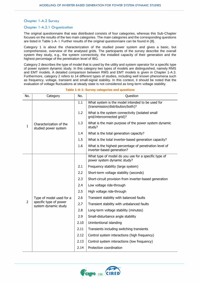
MODELLING OF INVERTER-BASED GENERATION FOR POWER SYSTEM DYNAMIC STUDIES
196
Chapter 1-A.2 Survey
Chapter 1-A.2.1 Organization
The original questionnaire that was distributed consists of four categories, whereas this Sub-Chapter focuses on the results of the two main categories. The main categories and the corresponding questions are listed in Table 1-A- I. Further results of the original questionnaire can be found in [8].
Category 1 is about the characterization of the studied power system and gives a basic, but comprehensive, overview of the analysed grids. The participants of the survey describe the overall system they study, e.g., the system connectivity, the installed capacity of their generation and the highest percentage of the penetration level of IBG.
Category 2 describes the type of model that is used by the utility and system operator for a specific type of power system dynamic study. In this category two types of models are distinguished, namely RMS and EMT models. A detailed comparison between RMS and EMT models is given in Chapter 1-A.3. Furthermore, category 2 refers to 14 different types of studies, including well known phenomena such as frequency, voltage, transient and small-signal stability. In this context, it should be noted that the evaluation of voltage fluctuations at steady state is not considered as long-term voltage stability.
Table 1-A-1: Survey categories and questions
No. Category No. Question
1 Characterization of the
studied power system
1.1 What system is the model intended to be used for
(transmission/distribution/both)?
1.2 What is the system connectivity (isolated small grid/interconnected grid)?
1.3 What is the main purpose of the power system dynamic study?
1.4 What is the total generation capacity?
1.5 What is the total inverter-based generation capacity?
1.6 What is the highest percentage of penetration level of inverter-based generation?
2
Type of model used for a
specific type of power system dynamic study
What type of model do you use for a specific type of
power system dynamic study?
2.1 Frequency stability (large system)
2.2 Short-term voltage stability (seconds)
2.3 Short-circuit provision from inverter-based generation
2.4 Low voltage ride-through
2.5 High voltage ride-through
2.6 Transient stability with balanced faults
2.7 Transient stability with unbalanced faults
2.8 Long-term voltage stability (minutes)
2.9 Small-disturbance angle stability
2.10 Unintentional islanding
2.11 Transients including switching transients
2.12 Control system interactions (high frequency)
2.13 Control system interactions (low frequency)
2.14 Protection coordination

MODELLING OF INVERTER-BASED GENERATION FOR POWER SYSTEM DYNAMIC STUDIES
197
Chapter 1-A-2.2 Participants
Potential survey participants were identified by the JWG members and contacted via e-mail. The considered utilities and system operators were either Transmission System Operators (TSOs), or utilities and system operators that operate both, transmission and distribution systems. However, Distribution System Operators (DSOs) were not considered for this Sub-Chapter, because most of them replied that they do not perform power system dynamic studies.
As depicted in Table 1-A- II, the questionnaire was sent to 63 utilities and system operators around the world between spring 2015 and summer 2016. Out of these 63 contacted utilities and system operators, 45 replied to the JWG. Hence, the response rate of 71% was reached. The 45 received questionnaires from utilities and system operators came from 21 countries on five continents.
Table 1-A-2: Survey participants and response rate
Participants Total
Sent questionnaires to utilities and system operators 63
Received questionnaires from utilities and system
operators 45
Response rate from utilities and system operators [%] 71
Received questionnaires from continents 5
Received questionnaires from countries 21
It should be noted that software vendors, consultancies, research organizations and academia are out of scope and only responses from utilities and system operators were considered for the survey. Out of the 45 received questionnaires, 35 came from TSOs, and 10 came from utilities and system operators that operate both, transmission and distribution systems.
Chapter 1-A.3 Type of models
Chapter 1-A-3.1 RMS models
RMS models are mainly used to study power system stability for large interconnected systems, this includes electromechanical oscillations (small-signal stability), as well as rotor-angle stability of synchronous generators and voltage and frequency stability [9]. Phasor simulation methods are used when only the magnitude and phase of the voltages and currents are of interest. It is not necessary to solve all the differential equations resulting from the interaction of R, L, and C elements. Hence, the network is simulated with fixed complex impedances in-stead of differential equations [10]. RMS simulation tools consider phenomena with a band-width of typically 0.1 to 3 Hz, since the network model’s fidelity diminishes rapidly for phenomena with frequencies significantly outside of this range. However, the control loops modelled on individual power plants may cover phenomena up to 10 Hz. Another commonly used terminology for RMS type models is to call them “positive-sequence stability” models. In essence, such models assume a perfectly balanced network and consider only the positive sequence components of all phenomena.
Converters are included in RMS programs using their averaged models. They provide the behaviour of the converter ignoring fast switching transients and any control with very small-time constants compared to the time steps and the phenomena considered. For instance, in stability analysis there is usually no need to model the inverter in detail since its transients are much faster than the dynamics being studied. Therefore, only the fundamental frequency outputs of the converter are modelled, which are mainly reflected in the electrical control model. Due to this averaged representation, the modelling of different technologies of IBG can be unified using sub-models for each basic component according to their characteristics.
Chapter 1-A-3.2 EMT models
When the phenomena to be studied are significantly outside of the range of fidelity of RMS models (for example studying electro-magnetic transients, or sub-synchronous torsional interactions, etc.), then EMT simulation software should be used, together with detailed equipment specific models. EMT analysis programs solve the differential-algebraic equations of a three-phase electrical network [11]. This distinction means that EMT analysis is capable of representing electro-magnetic transients (hence the name EMT), the frequency dependence of network components (e.g. change in transmission line

MODELLING OF INVERTER-BASED GENERATION FOR POWER SYSTEM DYNAMIC STUDIES
198
resistance/reactance with frequency), harmonics, unbalanced networks, power electronic devices, including the switching transients as well as the detailed controls and protection systems.
Users need to be careful on the selection of the type of models between RMS and EMT. RMS models usually do not include the inner current control loops of the converter, the detailed phase-locked loop model and various other details of the converter. Nevertheless, RMS simulations are much faster to execute than EMT and are thus dominant for specific types of power system dynamic studies.
EMT models may also be required under the following special system conditions (where RMS time-domain simulation programs may not be accurate or suitable anymore):
Weak system conditions (with a very low short-circuit ratio)
Detailed inverter and collector system design
Detailed equipment and system interaction studies
Unbalanced faults (note that many RMS models are positive sequence models)
Chapter 1-A.4 results
The survey results are introduced for each question in this Sub-Chapter. Most of the survey results include the mean value inserted at the bottom of each table. It is noted that such mean value is an invented index that makes no real sense since each type of study weights the same but allows us to discover which model is more likely to be selected.
Chapter 1-A-4.1 Category 1: Characterization of the studied power system
Question 1.1 (What system is the model intended to be used for (transmission/distribution/both)?) in this category is about the type of power system that is studied. For this Sub-Chapter only utilities and system operators that perform studies with either the transmission system only, or with both, the transmission and the distribution system, were considered. Out of the considered participants, 78% perform transmission system studies only, whereas 22% per-form studies for both, the transmission and the distribution system.
Question 1.2 (What is the system connectivity (isolated small grid/interconnected grid)?) analyses the system connectivity. Out of the considered participants, 87% of the utilities and system operators operate an interconnected grid. Furthermore, there are 9% of the utilities and system operators, which operate both, an interconnected and an isolated small grid. This is the case for countries that also consist of islands. Just 4% of the survey participants perform studies with an isolated small grid only.
Question 1.3 (What is the main purpose of the power system dynamic study?) in this category is about the predominant studies that utilities and system operators usually perform and the results are shown in Figure 1-A-1. The participants could select between different types of studies given in category 2 in Table 1-A- I. The results indicate that the utilities and system operators mainly perform stability studies, such as frequency stability (study 2.1) with 89%, short-term volt-age stability (study 2.2) with 89% and transient stability with balanced faults (study 2.6) with 89%. It should be noted that recently announced grid code requirements for IBG, like low voltage ride-through (study 2.4), are also very common with 82%. Other power system dynamic studies, such as transients including switching transients (study 2.11) with 40%, control system interactions (studies 2.12 and 2.13) for high frequencies with 44% and low frequencies with 47% as well as unintentional islanding (study 2.10) with 53% are less commonly performed by the utilities and system operators. However, even for the less commonly performed studies it should be noted that almost every second utility and system operator performs these types of studies. The main observation of the results is that 69% of the participants perform the listed power system dynamic studies (studies 2.1 to 2.14), as seen in the last row of Figure 1-A-1.
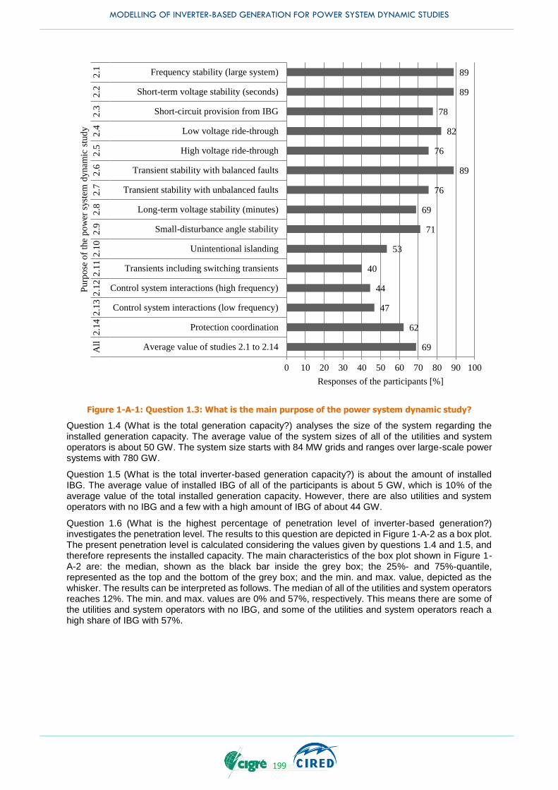
MODELLING OF INVERTER-BASED GENERATION FOR POWER SYSTEM DYNAMIC STUDIES
199
Figure 1-A-1: Question 1.3: What is the main purpose of the power system dynamic study?
Question 1.4 (What is the total generation capacity?) analyses the size of the system regarding the installed generation capacity. The average value of the system sizes of all of the utilities and system operators is about 50 GW. The system size starts with 84 MW grids and ranges over large-scale power systems with 780 GW.
Question 1.5 (What is the total inverter-based generation capacity?) is about the amount of installed IBG. The average value of installed IBG of all of the participants is about 5 GW, which is 10% of the average value of the total installed generation capacity. However, there are also utilities and system operators with no IBG and a few with a high amount of IBG of about 44 GW.
Question 1.6 (What is the highest percentage of penetration level of inverter-based generation?) investigates the penetration level. The results to this question are depicted in Figure 1-A-2 as a box plot. The present penetration level is calculated considering the values given by questions 1.4 and 1.5, and therefore represents the installed capacity. The main characteristics of the box plot shown in Figure 1-A-2 are: the median, shown as the black bar inside the grey box; the 25%- and 75%-quantile, represented as the top and the bottom of the grey box; and the min. and max. value, depicted as the whisker. The results can be interpreted as follows. The median of all of the utilities and system operators reaches 12%. The min. and max. values are 0% and 57%, respectively. This means there are some of the utilities and system operators with no IBG, and some of the utilities and system operators reach a high share of IBG with 57%.
89
89
78
82
76
89
76
69
71
53
40
44
47
62
69
0 10 20 30 40 50 60 70 80 90 100
Frequency stability (large system)
Short-term voltage stability (seconds)
Short-circuit provision from IBG
Low voltage ride-through
High voltage ride-through
Transient stability with balanced faults
Transient stability with unbalanced faults
Long-term voltage stability (minutes)
Small-disturbance angle stability
Unintentional islanding
Transients including switching transients
Control system interactions (high frequency)
Control system interactions (low frequency)
Protection coordination
Average value of studies 2.1 to 2.14
2.1
2.2
2.3
2.4
2.5
2.6
2.7
2.8
2.9
2.1
02
.11
2.1
22
.13
2.1
4A
ll
Responses of the participants [%]
Purp
ose
of
the
po
wer
syst
em d
ynam
ic s
tud
y
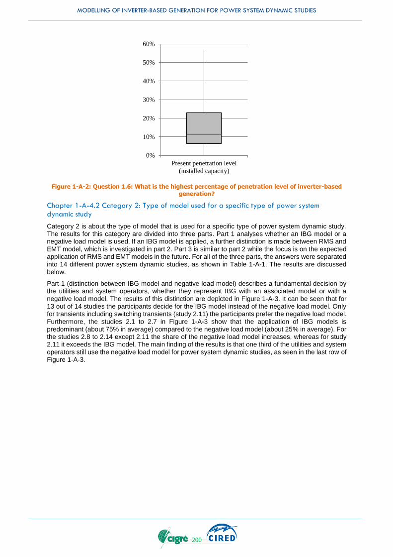
MODELLING OF INVERTER-BASED GENERATION FOR POWER SYSTEM DYNAMIC STUDIES
200
Figure 1-A-2: Question 1.6: What is the highest percentage of penetration level of inverter-based generation?
Chapter 1-A-4.2 Category 2: Type of model used for a specific type of power system dynamic study
Category 2 is about the type of model that is used for a specific type of power system dynamic study. The results for this category are divided into three parts. Part 1 analyses whether an IBG model or a negative load model is used. If an IBG model is applied, a further distinction is made between RMS and EMT model, which is investigated in part 2. Part 3 is similar to part 2 while the focus is on the expected application of RMS and EMT models in the future. For all of the three parts, the answers were separated into 14 different power system dynamic studies, as shown in Table 1-A-1. The results are discussed below.
Part 1 (distinction between IBG model and negative load model) describes a fundamental decision by the utilities and system operators, whether they represent IBG with an associated model or with a negative load model. The results of this distinction are depicted in Figure 1-A-3. It can be seen that for 13 out of 14 studies the participants decide for the IBG model instead of the negative load model. Only for transients including switching transients (study 2.11) the participants prefer the negative load model. Furthermore, the studies 2.1 to 2.7 in Figure 1-A-3 show that the application of IBG models is predominant (about 75% in average) compared to the negative load model (about 25% in average). For the studies 2.8 to 2.14 except 2.11 the share of the negative load model increases, whereas for study 2.11 it exceeds the IBG model. The main finding of the results is that one third of the utilities and system operators still use the negative load model for power system dynamic studies, as seen in the last row of Figure 1-A-3.
0%
10%
20%
30%
40%
50%
60%
Present penetration level
(installed capacity)
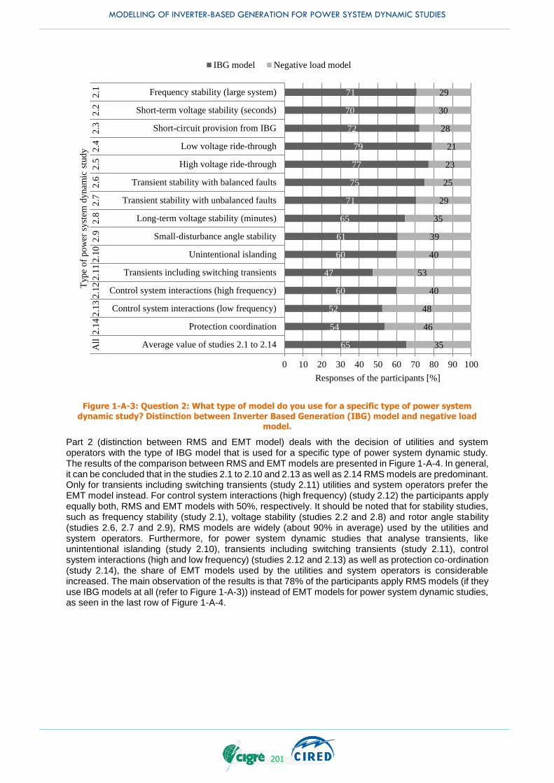
MODELLING OF INVERTER-BASED GENERATION FOR POWER SYSTEM DYNAMIC STUDIES
201
Figure 1-A-3: Question 2: What type of model do you use for a specific type of power system dynamic study? Distinction between Inverter Based Generation (IBG) model and negative load
model.
Part 2 (distinction between RMS and EMT model) deals with the decision of utilities and system operators with the type of IBG model that is used for a specific type of power system dynamic study. The results of the comparison between RMS and EMT models are presented in Figure 1-A-4. In general, it can be concluded that in the studies 2.1 to 2.10 and 2.13 as well as 2.14 RMS models are predominant. Only for transients including switching transients (study 2.11) utilities and system operators prefer the EMT model instead. For control system interactions (high frequency) (study 2.12) the participants apply equally both, RMS and EMT models with 50%, respectively. It should be noted that for stability studies, such as frequency stability (study 2.1), voltage stability (studies 2.2 and 2.8) and rotor angle stability (studies 2.6, 2.7 and 2.9), RMS models are widely (about 90% in average) used by the utilities and system operators. Furthermore, for power system dynamic studies that analyse transients, like unintentional islanding (study 2.10), transients including switching transients (study 2.11), control system interactions (high and low frequency) (studies 2.12 and 2.13) as well as protection co-ordination (study 2.14), the share of EMT models used by the utilities and system operators is considerable increased. The main observation of the results is that 78% of the participants apply RMS models (if they use IBG models at all (refer to Figure 1-A-3)) instead of EMT models for power system dynamic studies, as seen in the last row of Figure 1-A-4.
71
70
72
79
77
75
71
65
61
60
47
60
52
54
65
29
30
28
21
23
25
29
35
39
40
53
40
48
46
35
0 10 20 30 40 50 60 70 80 90 100
Frequency stability (large system)
Short-term voltage stability (seconds)
Short-circuit provision from IBG
Low voltage ride-through
High voltage ride-through
Transient stability with balanced faults
Transient stability with unbalanced faults
Long-term voltage stability (minutes)
Small-disturbance angle stability
Unintentional islanding
Transients including switching transients
Control system interactions (high frequency)
Control system interactions (low frequency)
Protection coordination
Average value of studies 2.1 to 2.14
2.1
2.2
2.3
2.4
2.5
2.6
2.7
2.8
2.9
2.1
02
.11
2.1
22
.13
2.1
4A
ll
Responses of the participants [%]
Typ
e o
f p
ow
er s
yst
em d
ynam
ic s
tud
y
IBG model Negative load model

MODELLING OF INVERTER-BASED GENERATION FOR POWER SYSTEM DYNAMIC STUDIES
202
Figure 1-A-4: Question 2: What type of model do you use for a specific type of power system dynamic study? Distinction between Root Mean Square (RMS) and Electro-Magnetic Transient
(EMT) model.
Part 3 (distinction between RMS and EMT model in the future) analyses in the same way as part 2 (distinction between RMS and EMT model) the type of IBG model that is used by the utility and system operator, with the difference that part 3 is focused on the expected application of RMS and EMT models in the future. The results are shown in Figure 1-A-5. At the first sight, it can be seen that RMS models are still prevailing compared to EMT models. The majority of the participants use RMS models for 11 out of 14 power system dynamic studies. Only for transients including switching transients (study 2.11) as well as control system inter-actions (high and low frequency) (studies 2.12 and 2.13) EMT models are predominant. It should be noted that for stability studies, such as frequency stability (study 2.1), voltage stability (studies 2.2 and 2.8) and rotor angle stability (studies 2.6, 2.7 and 2.9), RMS models are still widely used (about 75% in average) by the utilities and system operators. Furthermore, similar to Figure 1-A-4, for power system dynamic studies that analyse transients, like unintentional-al islanding (study 2.10), transients including switching transients (study 2.11), control system interactions (high and low frequency) (studies 2.12 and 2.13) as well as protection coordination (study 2.14), the share of expected EMT models in the future used by the participants is considerable increased. The main finding by analysing the results is that 63% of the participants apply RMS models instead of EMT models for power system dynamic studies in the future, as seen in the last row of Figure 1-A-5. By comparing the results, the last row of Figure 1-A-5 with the last row Figure 1-A-4, it is important to mention that the share of EMT models used for power system dynamic studies will increase in the future from 22% to 37%.
91
88
81
83
84
91
85
95
95
74
38
50
62
70
78
9
13
19
17
16
9
15
5
5
26
62
50
38
30
22
0 10 20 30 40 50 60 70 80 90 100
Frequency stability (large system)
Short-term voltage stability (seconds)
Short-circuit provision from IBG
Low voltage ride-through
High voltage ride-through
Transient stability with balanced faults
Transient stability with unbalanced faults
Long-term voltage stability (minutes)
Small-disturbance angle stability
Unintentional islanding
Transients including switching transients
Control system interactions (high frequency)
Control system interactions (low frequency)
Protection coordination
Average value of studies 2.1 to 2.14
2.1
2.2
2.3
2.4
2.5
2.6
2.7
2.8
2.9
2.1
02
.11
2.1
22
.13
2.1
4A
ll
Responses of the participants [%]
Typ
e o
f p
ow
er s
yst
em d
ynam
ic s
tud
y
RMS model EMT model

MODELLING OF INVERTER-BASED GENERATION FOR POWER SYSTEM DYNAMIC STUDIES
203
Figure 1-A-5: Question 2: What type of model do you use for a specific type of power system dynamic study? Distinction between Root Mean Square (RMS) and Electro-Magnetic Transient
(EMT) model in the future.
Chapter 1-A.5 discussion
Chapter 1-A-5.1 negative load model
From the results it is remarkable that still around one third of the utilities and system operators use negative load models for the representation of IBG in power system dynamic studies. According to the results of the questionnaire survey, the following reasons may explain this approach:
Lack of model requirements of IBG for specific power system phenomena:
As the penetration level of such IBG technologies increases, various aspects of power system stability and dynamic performance in the grid may change. Therefore, requirements that address the necessary functionalities that need to be modelled of IBG for specific power system phenomena need to be developed. These functionalities include various aspects, such as control, protection and the capability of IBG. Considering these requirements, utilities and system operators can select specific models for each power system phenomenon.
Lack of well-validated IBG models:
In recent years there has been much effort on the development of validated models for IBG. This work has been primarily related to wind generation. Now, further attention is starting to be devoted to PV systems and other technologies. In general, there is still a lack of well-validated and generally accepted dynamic simulation models, particularly for distributed PV systems, for the use in power system dynamic studies.
Lack of widely accepted generic models for IBG:
78
72
65
65
68
74
73
81
76
57
32
46
38
58
63
22
28
35
35
33
26
27
19
24
43
68
54
62
42
37
0 10 20 30 40 50 60 70 80 90 100
Frequency stability (large system)
Short-term voltage stability (seconds)
Short-circuit provision from IBG
Low voltage ride-through
High voltage ride-through
Transient stability with balanced faults
Transient stability with unbalanced faults
Long-term voltage stability (minutes)
Small-disturbance angle stability
Unintentional islanding
Transients including switching transients
Control system interactions (high frequency)
Control system interactions (low frequency)
Protection coordination
Average value of studies 2.1 to 2.14
2.1
2.2
2.3
2.4
2.5
2.6
2.7
2.8
2.9
2.1
02
.11
2.1
22
.13
2.1
4A
ll
Responses of the participants [%]
Typ
e o
f p
ow
er s
yst
em d
ynam
ic s
tud
y
RMS model in future EMT model in future
MODELLING OF INVERTER-BASED GENERATION FOR POWER SYSTEM DYNAMIC STUDIES
204
Usually utilities and system operators do not create their own (user-written) models. They request validated models from manufacturers, either proprietary or adjusted generic models. This request poses two main disadvantages: 1) the manufacturer wants to keep the confidentiality of their proprietary user-written model; and 2) the extra effort for the manufacturer for tuning the parameters of the generic model including the validation of the simulations against the field measurements. Thus, the importance of developing reliable and flexible generic models for different technologies and manufacturers of IBG should be noted. Advantages of generic models are: vendor and manufacturer independent, grid code compatible, public model structure (control block diagram), software simulation tool independent, etc. For some technologies, like wind generation, these models are already being widely used, however, the latest generic models had only recently been developed at the time the questionnaire survey was conducted.
Lack of widely accepted range of model parameters for IBG:
Although widely accepted generic models are provided, the control model parameters are crucial for power system dynamic studies. Because many grid codes do not define the detailed specification/characteristics of the inverter control, the control model parameters could be different depending on the manufacturer of the inverter. Even if the control model parameters of one inverter can be identified through validation, it is al-most infeasible to identify the parameters of all inverters connected to the power system. Therefore, a set of realistic control model parameters need to be provided.
Lack of grid code requirements:
Due to the lack of grid code requirements in the past, specifying detailed control functionalities of IBG, the approach of using negative load models for power system dynamic studies was justified. However, with the development of new grid codes, certain functionalities of IBG are required (e.g. voltage control, frequency response etc.) and therefore, the negative load model is not adequate anymore.
Lack of information about the power system:
The aforementioned increased penetration level of IBG also makes system operation, both for TSOs and DSOs, more challenging than in the past. Already, in some areas the consumers’ demand is mostly covered by generation which is connected directly to the distribution system. TSOs routinely run time-domain simulations to assess the stability of the power system. Models, which are currently used to represent distribution systems, are only based on a limited amount of information, generally related to the high voltage network.
Lack of agreed methodology for the aggregation of IBG:
Present trends towards the integration of an increasing range of IBG technologies, widely differing in size and number, poses serious concerns in the industry on how to represent these new technologies in power system dynamic studies. There is not only a lack of validated dynamic computer models of individual distributed generating technologies, such as distributed PV systems, fuel cells, micro turbines etc., but also there is no agreed methodology on how to represent or aggregate the enormous number of distributed generation, embedded in very low voltage grids, for power system dynamic studies, focusing on both, local (distribution level) and widespread (transmission level) studies.
Chapter 1-A-5.1 Necessity of IBG models
The high penetration level of IBG has resulted in the displacement of conventional synchro-nous generators. Therefore, the impact of IBG on the dynamic performance of the system in-creases. The dynamic characteristic of IBG is different compared to synchronous generators, and with proper control system design and functionalities of modern IBG technologies, they can provide many of the same or even better services (e.g. voltage control, frequency response etc.). None the less, they do need to be modelled differently and properly. Therefore, the development of the proper computer simulation models for IBG with such additional functionalities is vital for power systems analyses.
Moreover, DSOs have a representation of their networks and have details about connected consumers and producers to some extent. However, the limited data is generally not suitable for dynamic simulations for either the distribution or the transmission system or, at least, has not been used for that purpose in the past, due to the high level of detail. From the point of view of the DSOs, time-domain simulations may also now be necessary to assess, e.g., protection system behaviour, distribution network automated operation, unintentional islanding of part of distribution systems including IBG, voltage issues, etc. For these types of power system dynamic studies detailed IBG models are needed.
MODELLING OF INVERTER-BASED GENERATION FOR POWER SYSTEM DYNAMIC STUDIES
205
Therefore, the necessity of IBG models should be clarified for each type of power system dynamic study. A few examples are given as follows:
Frequency stability (refer to study 2.1 in Table 1-A- I):
Frequency stability studies often involve looking at the frequency response of the grid to a large disturbance, such as the loss of the largest generating unit (or facility) on the system and assessing if the resulting frequency response of the system is stable and avoids under frequency load shedding. Such studies are typically performed using RMS (positive-sequence) simulation models and tools.
Short-circuit provision from IBG (refer to study 2.3 in Table 1-A- I):
Short-circuit studies are performed, typically by protection engineers, to identify the setting for protection relays as well as to assess the capability of existing (or new) circuit breakers to be able to withstand and interrupt the short-circuit levels that will be seen on the network during fault conditions. Such studies are typically performed in EMT tools and other software tools specifically designed for short-circuit studies. Thus, appropriate models of IBG are needed in such tools.
Low voltage ride-through (refer to study 2.4 in Table 1-A- I):
To properly assess the actual low voltage ride-through capabilities of IBG, analyses have to be performed using detail vendor specific EMT type models and simulations. Furthermore, such simulations may be verified by factory tests of the equipment. It usually then suffices to translate the observed performance to simplified RMS models that will mimic the low voltage ride-through capabilities of the equipment for large-scale power system dynamic studies. Thus, both appropriate RMS and EMT models of IBG are needed.
Transient stability (refer to study 2.6 in Table 1-A- I):
For bulk power system transient stability studies validated RMS (or positive-sequence) models are needed for IBG. However, in some cases EMT models may also be needed when investigating, e.g., the connection of a large IBG power plant to a very weak part of the power system.
Long-term voltage stability (refer to study 2.8 in Table 1-A- I):
Long-term voltage stability is often analysed using continuous power flow analysis, such as P-V or Q-V analyses. For such studies, the dynamics of IBG are often neglected, and a quasi-steady-state model that respects the real and reactive power limits of the IBG is sufficient. If mid-term time-domain dynamic simulations are performed, then a suitable RMS (positive-sequence) IBG model is needed.
Unintentional islanding (refer to study 2.10 in Table 1-A- I):
For this type of study, either an RMS or EMT model for IBG is needed. Some anti-islanding protection systems utilize the harmonics of the voltage for the islanding detection and therefore, the EMT model for IBG is the only option to analyse unintentional islanding. On the other hand, if the used anti-islanding protection system does not consider voltage harmonics and if the power systems model includes many IBG models, the RMS model for IBG may be adequate to analyse unintentional islanding.
Protection coordination (refer to study 2.14 in Table 1-A- I):
Many protection systems need to be coordinated. Depending on the type of protection systems to be studied, either an RMS or EMT model for IBG is needed.
Chapter 1-A.6 conclusion
The aim of this Sub-Chapter is not necessarily to recommend the application of any dynamic model for a specific power system dynamic study, but, rather, to identify what dynamic models are presently applied and to provide some fundamental information on their use.
The main contributions and key findings of this Sub-Chapter are:
Prevalent type of power system dynamic studies:
The most dominant type of studies performed by TSOs are stability studies, such as frequency stability, short-term voltage stability and transient stability with balanced faults. This is done by 89% of those who responded to the survey.
Prevalent type of model (IBG/negative load) for power system dynamic studies:
MODELLING OF INVERTER-BASED GENERATION FOR POWER SYSTEM DYNAMIC STUDIES
206
around one third of the utilities and system operators still use a negative load model for power system dynamic studies.
Prevalent type of model (RMS/EMT) for power system dynamic studies:
78% of the utilities and system operators apply RMS models instead of EMT models for power system dynamic studies. EMT models are more likely to be used for various high-frequency transient studies (e.g. switching transients).
Prevalent type of model (RMS/EMT) in the future for power system dynamic studies:
63% of the utilities and system operators expect to continue to apply RMS models in-stead of EMT models in the future for power system dynamic studies. It is important to mention that the share of EMT models used for power system dynamic studies will increase in the future from 22% to 37%.
Based on the results of the questionnaire, the following reasons for the approach of the negative load model are identified:
Lack of model requirements of IBG for specific power system phenomena
Lack of well-validated IBG models
Lack of widely accepted generic models for IBG
Lack of widely accepted range of model parameters for IBG
Lack of grid code requirements
Lack of information about the power system
Lack of agreed methodology for the aggregation of distributed IBG
Some reasons have been resolved mainly for models of wind generation. The IEC 61400-27-1 and 61400-27-2 standards under development are presently in the process of providing more refined generic wind turbine and generic wind power plant models and the procedures for validating those models. A standard range of parameters, similar to WECC [12], is also expected to be illustrated in the future IEC documents. The methodology for the aggregation of distributed IBG has been discussed in the WECC and is presently under review [7]. The second-generation generic renewable energy system models, developed in the WECC, as well as the generic wind turbine models, developed in the IEC, are now implemented by several commercial software vendors and utilities and system operators start using these models for power system dynamic studies with IBG. None the less, much learning as well as technical challenges still remain, such as the methodology of the aggregation of distributed IBG considering the diversified control parameters, and therefore, further effort is needed.
In light of the observations of the survey, the necessity of the IBG model for the several representative power system dynamic studies is discussed highlighting the need of IBG models. Furthermore, the recommended type of model is also emphasized providing the approach of RMS or EMT model for IBG. It can be concluded that every type of model has advantages and disadvantages and the proper model type needs to be selected depending on the type of power system dynamic study and the system condition.
The results of the questionnaire emphasize the clear message for the necessity and importance of the use of IBG models. Furthermore, the final technical brochure of the CIGRE JWG C4/C6.35/CIRED will give guidance in selecting adequate models for IBG for specific power system dynamic studies.
With these contributions the Sub-Chapter supports utilities and system operators as well as research institutes and academia to benchmark their approach against the prevailing international industry practice.

MODELLING OF INVERTER-BASED GENERATION FOR POWER SYSTEM DYNAMIC STUDIES
207
APPENDIX 1-B MODELLING AND DYNAMIC PERFORMANCE OF INVERTER-BASED GENERATION IN POWER SYSTEM STUDIES: AN INTERNATIONAL QUESTIONNAIRE SURVEY
Chapter 1-B.1 Introduction
Nowadays, the electrical power system is undergoing fundamental changes due to the ever-increasing penetration of IBG. The dynamic characteristic of IBG, such as wind or PV generation, is fundamentally different from conventional synchronous generators, and thus the dynamic performance of the system following disturbances might change due to the increasing impact of IBG. Therefore, studies are required that analyse the impact of high penetration levels of IBG on the dynamic performance of the system. In this context, the selection of the IBG model type is crucial for the analysis.
There are many levels of models used for all types of power system components. On the one hand, there are detailed models of IBG, also referred to as individual models. On the other hand, there are simplified models that represent an aggregation of IBG, also referred to as aggregated models. However, since all models have limitations, the selection of the model type is crucial based on the objectives of the study.
Different types of models for IBG have been developed over the last years. Two industry working groups were established, one within the Western Electricity Coordinating Council (WECC) [3], and another within the International Electrotechnical Commission (IEC) [4], in order to develop generic models of different types of IBG. Some of those models have been already implemented in widely used commercial power system analysis software tools [5], [6]. However, these generic models are still not widely used yet by the industry.
In 2013, the new Joint Working Group (JWG) CIGRE C4/C6.35/CIRED: “Modelling and dynamic performance of inverter-based generation in power system transmission and distribution studies” was established, to look at some of these evolving issues. One of the tasks of the JWG is to identify the present industry practice on modelling of IBG, with the focus on PV generation. For that purpose, a comprehensive questionnaire was distributed to utilities and system operators around the world. This report summarizes some of the key findings.
The aim of this report is not necessarily to recommend the application of any specific dynamic model for a specific power system dynamic study, but, rather, to identify what dynamic models are presently applied and to provide some real pictures on their application.
Chapter 1-B.2 Survey
Chapter 1-B-2.1 Organization
The original questionnaire that was distributed to the utilities and system operators consists of four categories, whereas this report focuses on the results of two of them. The two categories and the corresponding questions to each of them are listed in Table I. Further findings and observations of the original questionnaire can be found in [13].
Category 1 sorts the IBG technology and its modelling by type. The participants of the survey could select between different technologies, such as wind or PV generation, micro turbines, fuel cells or battery energy systems. This category reveals which type of IBG technology is modelled by utilities and system operators for power system dynamic studies.
Category 2 describes the type of model that is presently used by the utility and system operator for a specific type of power system dynamic study. In this category two types of models are classified, namely individual models and aggregated models. A detailed comparison between individual and aggregated models is provided in Chapter 1-B.3, titled: “Type of models”. Furthermore, category 2 refers to 14 different types of power system dynamic studies, including well known phenomena such as frequency stability, short-term and long-term voltage stability as well as transient and small-disturbance angle stability.
Chapter 1-B-2.2 Participants
Potential survey participants were selected by the JWG members and contacted via e-mail. The considered utilities and system operators were either Transmission System Operators (TSOs), or utilities and system operators that operate both, transmission and distribution systems. However, Distribution System Operators (DSOs) were not included in the results of this report, because the responses show that power system dynamic studies are barely conducted by DSOs.
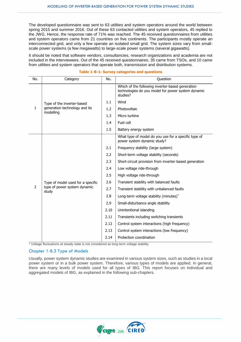
MODELLING OF INVERTER-BASED GENERATION FOR POWER SYSTEM DYNAMIC STUDIES
208
The developed questionnaire was sent to 63 utilities and system operators around the world between spring 2015 and summer 2016. Out of these 63 contacted utilities and system operators, 45 replied to the JWG. Hence, the response rate of 71% was reached. The 45 received questionnaires from utilities and system operators came from 21 countries on five continents. The participants mostly operate an interconnected grid, and only a few operate an isolated small grid. The system sizes vary from small-scale power systems (a few megawatts) to large-scale power systems (several gigawatts).
It should be noted that software vendors, consultancies, research organizations and academia are not included in the interviewees. Out of the 45 received questionnaires, 35 came from TSOs, and 10 came from utilities and system operators that operate both, transmission and distribution systems.
Table 1-B-1: Survey categories and questions
No. Category No. Question
1 Type of the inverter-based generation technology and its modelling
Which of the following inverter-based generation technologies do you model for power system dynamic studies?
1.1 Wind
1.2 Photovoltaic
1.3 Micro turbine
1.4 Fuel cell
1.5 Battery energy system
2 Type of model used for a specific type of power system dynamic study
What type of model do you use for a specific type of power system dynamic study?
2.1 Frequency stability (large system)
2.2 Short-term voltage stability (seconds)
2.3 Short-circuit provision from inverter-based generation
2.4 Low voltage ride-through
2.5 High voltage ride-through
2.6 Transient stability with balanced faults
2.7 Transient stability with unbalanced faults
2.8 Long-term voltage stability (minutes)*
2.9 Small-disturbance angle stability
2.10 Unintentional islanding
2.11 Transients including switching transients
2.12 Control system interactions (high frequency)
2.13 Control system interactions (low frequency)
2.14 Protection coordination
* Voltage fluctuations at steady state is not considered as long-term voltage stability
Chapter 1-B.3 Type of Models
Usually, power system dynamic studies are examined in various system sizes, such as studies in a local power system or in a bulk power system. Therefore, various types of models are applied. In general, there are many levels of models used for all types of IBG. This report focuses on individual and aggregated models of IBG, as explained in the following sub-chapters.
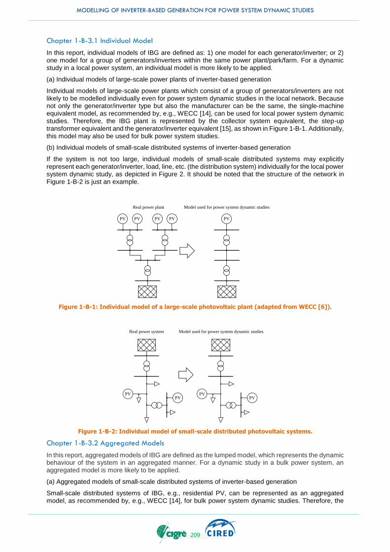
MODELLING OF INVERTER-BASED GENERATION FOR POWER SYSTEM DYNAMIC STUDIES
209
Chapter 1-B-3.1 Individual Model
In this report, individual models of IBG are defined as: 1) one model for each generator/inverter; or 2) one model for a group of generators/inverters within the same power plant/park/farm. For a dynamic study in a local power system, an individual model is more likely to be applied.
(a) Individual models of large-scale power plants of inverter-based generation
Individual models of large-scale power plants which consist of a group of generators/inverters are not likely to be modelled individually even for power system dynamic studies in the local network. Because not only the generator/inverter type but also the manufacturer can be the same, the single-machine equivalent model, as recommended by, e.g., WECC [14], can be used for local power system dynamic studies. Therefore, the IBG plant is represented by the collector system equivalent, the step-up transformer equivalent and the generator/inverter equivalent [15], as shown in Figure 1-B-1. Additionally, this model may also be used for bulk power system studies.
(b) Individual models of small-scale distributed systems of inverter-based generation
If the system is not too large, individual models of small-scale distributed systems may explicitly represent each generator/inverter, load, line, etc. (the distribution system) individually for the local power system dynamic study, as depicted in Figure 2. It should be noted that the structure of the network in Figure 1-B-2 is just an example.
Real power plant
PVPV PVPV
Model used for power system dynamic studies
PV
Figure 1-B-1: Individual model of a large-scale photovoltaic plant (adapted from WECC [6]).
Real power system Model used for power system dynamic studies
PVPV
PVPV
Figure 1-B-2: Individual model of small-scale distributed photovoltaic systems.
Chapter 1-B-3.2 Aggregated Models
In this report, aggregated models of IBG are defined as the lumped model, which represents the dynamic behaviour of the system in an aggregated manner. For a dynamic study in a bulk power system, an aggregated model is more likely to be applied.
(a) Aggregated models of small-scale distributed systems of inverter-based generation
Small-scale distributed systems of IBG, e.g., residential PV, can be represented as an aggregated model, as recommended by, e.g., WECC [14], for bulk power system dynamic studies. Therefore, the
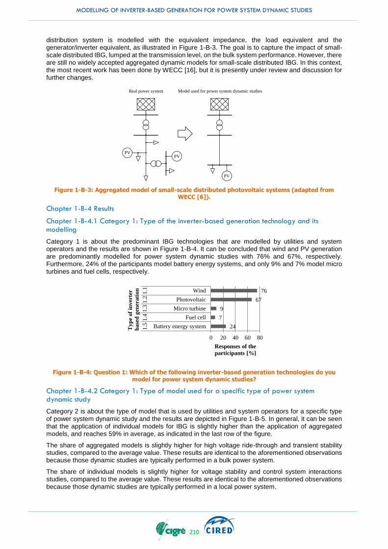
MODELLING OF INVERTER-BASED GENERATION FOR POWER SYSTEM DYNAMIC STUDIES
210
distribution system is modelled with the equivalent impedance, the load equivalent and the generator/inverter equivalent, as illustrated in Figure 1-B-3. The goal is to capture the impact of small-scale distributed IBG, lumped at the transmission level, on the bulk system performance. However, there are still no widely accepted aggregated dynamic models for small-scale distributed IBG. In this context, the most recent work has been done by WECC [16], but it is presently under review and discussion for further changes.
Real power system Model used for power system dynamic studies
PV
PVPV
Figure 1-B-3: Aggregated model of small-scale distributed photovoltaic systems (adapted from WECC [6]).
Chapter 1-B-4 Results
Chapter 1-B-4.1 Category 1: Type of the inverter-based generation technology and its modelling
Category 1 is about the predominant IBG technologies that are modelled by utilities and system operators and the results are shown in Figure 1-B-4. It can be concluded that wind and PV generation are predominantly modelled for power system dynamic studies with 76% and 67%, respectively. Furthermore, 24% of the participants model battery energy systems, and only 9% and 7% model micro turbines and fuel cells, respectively.
Figure 1-B-4: Question 1: Which of the following inverter-based generation technologies do you model for power system dynamic studies?
Chapter 1-B-4.2 Category 1: Type of model used for a specific type of power system dynamic study
Category 2 is about the type of model that is used by utilities and system operators for a specific type of power system dynamic study and the results are depicted in Figure 1-B-5. In general, it can be seen that the application of individual models for IBG is slightly higher than the application of aggregated models, and reaches 59% in average, as indicated in the last row of the figure.
The share of aggregated models is slightly higher for high voltage ride-through and transient stability studies, compared to the average value. These results are identical to the aforementioned observations because those dynamic studies are typically performed in a bulk power system.
The share of individual models is slightly higher for voltage stability and control system interactions studies, compared to the average value. These results are identical to the aforementioned observations because those dynamic studies are typically performed in a local power system.
76
67
9
7
24
0 20 40 60 80
Wind
Photovoltaic
Micro turbine
Fuel cell
Battery energy system
1.1
1.2
1.3
1.4
1.5
Responses of the
participants [%]
Ty
pe
of
inver
ter
base
d g
ener
ati
on
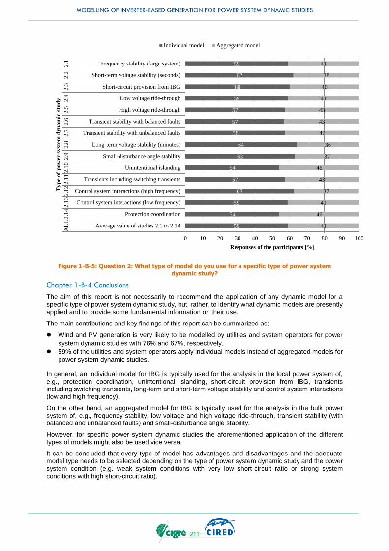
MODELLING OF INVERTER-BASED GENERATION FOR POWER SYSTEM DYNAMIC STUDIES
211
Figure 1-B-5: Question 2: What type of model do you use for a specific type of power system dynamic study?
Chapter 1-B-4 Conclusions
The aim of this report is not necessarily to recommend the application of any dynamic model for a specific type of power system dynamic study, but, rather, to identify what dynamic models are presently applied and to provide some fundamental information on their use.
The main contributions and key findings of this report can be summarized as:
Wind and PV generation is very likely to be modelled by utilities and system operators for power
system dynamic studies with 76% and 67%, respectively.
59% of the utilities and system operators apply individual models instead of aggregated models for
power system dynamic studies.
In general, an individual model for IBG is typically used for the analysis in the local power system of, e.g., protection coordination, unintentional islanding, short-circuit provision from IBG, transients including switching transients, long-term and short-term voltage stability and control system interactions (low and high frequency).
On the other hand, an aggregated model for IBG is typically used for the analysis in the bulk power system of, e.g., frequency stability, low voltage and high voltage ride-through, transient stability (with balanced and unbalanced faults) and small-disturbance angle stability.
However, for specific power system dynamic studies the aforementioned application of the different types of models might also be used vice versa.
It can be concluded that every type of model has advantages and disadvantages and the adequate model type needs to be selected depending on the type of power system dynamic study and the power system condition (e.g. weak system conditions with very low short-circuit ratio or strong system conditions with high short-circuit ratio).
59
62
60
59
57
57
58
64
63
54
57
63
59
54
59
41
38
40
41
43
43
42
36
37
46
43
37
41
46
41
0 10 20 30 40 50 60 70 80 90 100
Frequency stability (large system)
Short-term voltage stability (seconds)
Short-circuit provision from IBG
Low voltage ride-through
High voltage ride-through
Transient stability with balanced faults
Transient stability with unbalanced faults
Long-term voltage stability (minutes)
Small-disturbance angle stability
Unintentional islanding
Transients including switching transients
Control system interactions (high frequency)
Control system interactions (low frequency)
Protection coordination
Average value of studies 2.1 to 2.14
2.1
2.2
2.3
2.4
2.5
2.6
2.7
2.8
2.9
2.1
02
.11
2.1
22
.13
2.1
4A
LL
Responses of the participants [%]
Ty
pe
of
pow
er s
yst
em d
yn
am
ic s
tud
y
Individual model Aggregated model

MODELLING OF INVERTER-BASED GENERATION FOR POWER SYSTEM DYNAMIC STUDIES
212
The results of the questionnaire emphasize the clear message for the necessity and importance of the use of IBG models. Furthermore, the final technical brochure of the CIGRE JWG C4/C6.35/CIRED will give guidance in selecting adequate models for IBG for specific power system dynamic studies.
With these contributions the report supports utilities and system operators as well as research institutes and academia to benchmark their approach against the prevailing international industry practice.
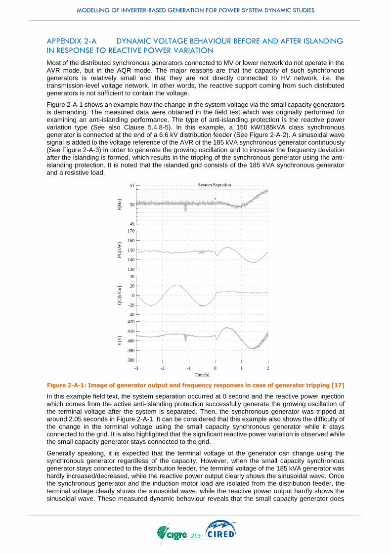
MODELLING OF INVERTER-BASED GENERATION FOR POWER SYSTEM DYNAMIC STUDIES
213
APPENDIX 2-A DYNAMIC VOLTAGE BEHAVIOUR BEFORE AND AFTER ISLANDING IN RESPONSE TO REACTIVE POWER VARIATION
Most of the distributed synchronous generators connected to MV or lower network do not operate in the AVR mode, but in the AQR mode. The major reasons are that the capacity of such synchronous generators is relatively small and that they are not directly connected to HV network, i.e. the transmission-level voltage network. In other words, the reactive support coming from such distributed generators is not sufficient to contain the voltage.
Figure 2-A-1 shows an example how the change in the system voltage via the small capacity generators is demanding. The measured data were obtained in the field test which was originally performed for examining an anti-islanding performance. The type of anti-islanding protection is the reactive power variation type (See also Clause 5.4.8-5). In this example, a 150 kW/185kVA class synchronous generator is connected at the end of a 6.6 kV distribution feeder (See Figure 2-A-2). A sinusoidal wave signal is added to the voltage reference of the AVR of the 185 kVA synchronous generator continuously (See Figure 2-A-3) in order to generate the growing oscillation and to increase the frequency deviation after the islanding is formed, which results in the tripping of the synchronous generator using the anti-islanding protection. It is noted that the islanded grid consists of the 185 kVA synchronous generator and a resistive load.
Figure 2-A-1: Image of generator output and frequency responses in case of generator tripping [17]
In this example field text, the system separation occurred at 0 second and the reactive power injection which comes from the active anti-islanding protection successfully generate the growing oscillation of the terminal voltage after the system is separated. Then, the synchronous generator was tripped at around 2.05 seconds in Figure 2-A-1. It can be considered that this example also shows the difficulty of the change in the terminal voltage using the small capacity synchronous generator while it stays connected to the grid. It is also highlighted that the significant reactive power variation is observed while the small capacity generator stays connected to the grid.
Generally speaking, it is expected that the terminal voltage of the generator can change using the synchronous generator regardless of the capacity. However, when the small capacity synchronous generator stays connected to the distribution feeder, the terminal voltage of the 185 kVA generator was hardly increased/decreased, while the reactive power output clearly shows the sinusoidal wave. Once the synchronous generator and the induction motor load are isolated from the distribution feeder, the terminal voltage clearly shows the sinusoidal wave, while the reactive power output hardly shows the sinusoidal wave. These measured dynamic behaviour reveals that the small capacity generator does
-40
-20
0
20
40
QG
[kV
ar]
-3 -2 -1 0 1 2
Time[s]
420
410
400
390
380
V[V
]
51
50
49
F[H
z]
170
160
150
140
130
PG
[kW
]
System Sepration
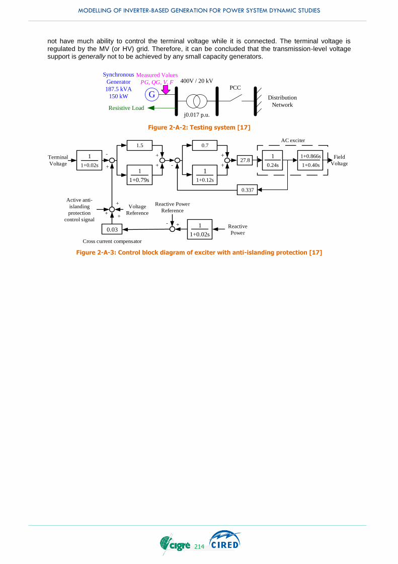
MODELLING OF INVERTER-BASED GENERATION FOR POWER SYSTEM DYNAMIC STUDIES
214
not have much ability to control the terminal voltage while it is connected. The terminal voltage is regulated by the MV (or HV) grid. Therefore, it can be concluded that the transmission-level voltage support is generally not to be achieved by any small capacity generators.
G
Synchronous
Generator
187.5 kVA
150 kW
400V / 20 kV
Resistive Loadj0.017 p.u.
PCC
Distribution
Network
Measured Values
PG, QG, V, F
Figure 2-A-2: Testing system [17]
+
+1+0.02s
1Terminal
Voltage
1.5
1+0.40s
1+0.866s
1+0.79s
1
+
+
0.7
1+0.12s
10.24s
1
0.337
Active anti-
islanding
protection
control signal
0.03
Reactive Power
Reference
1+0.02s
1 Reactive
Power
+
Voltage
Reference
+
+
+
+-
-
27.8Field
Voltage
AC exciter
-
Cross current compensator
Figure 2-A-3: Control block diagram of exciter with anti-islanding protection [17]
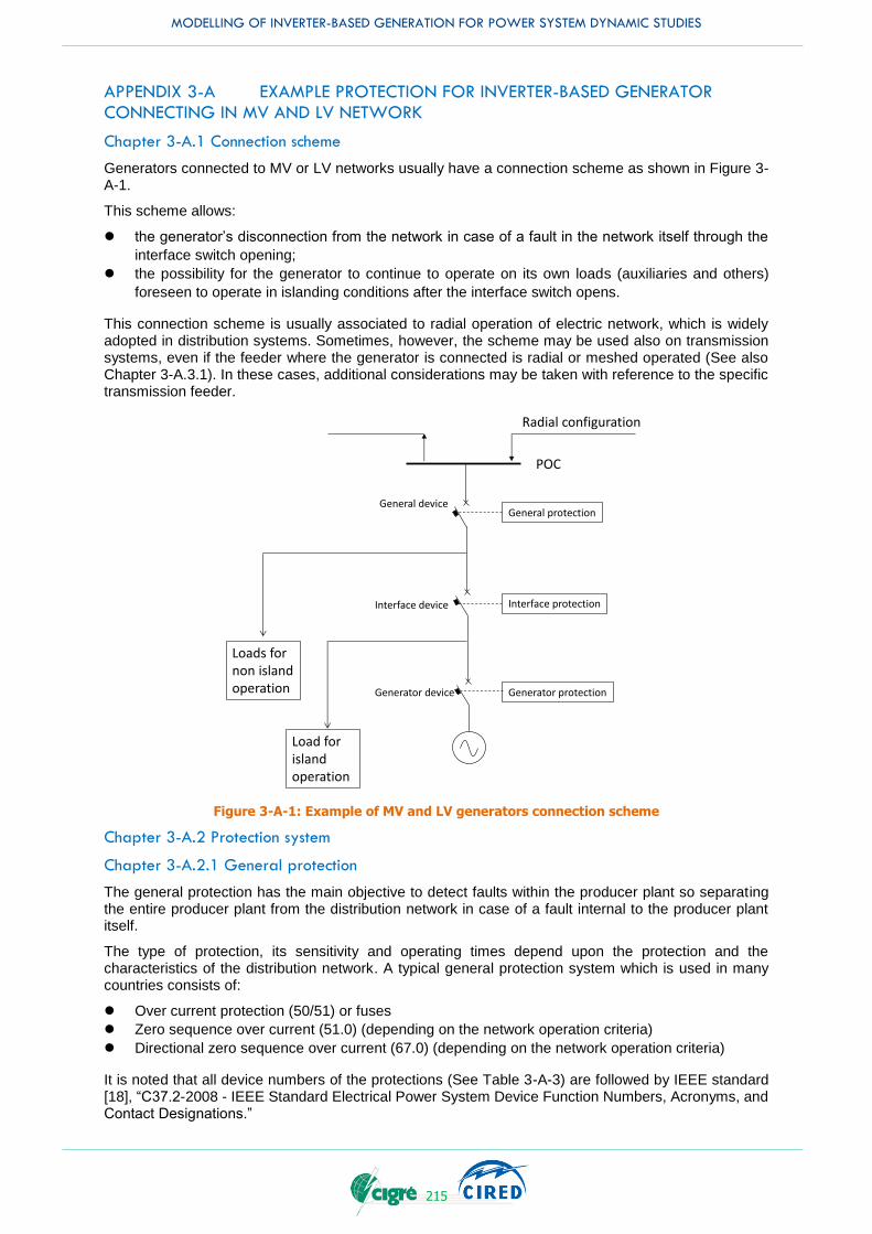
MODELLING OF INVERTER-BASED GENERATION FOR POWER SYSTEM DYNAMIC STUDIES
215
APPENDIX 3-A EXAMPLE PROTECTION FOR INVERTER-BASED GENERATOR CONNECTING IN MV AND LV NETWORK
Chapter 3-A.1 Connection scheme
Generators connected to MV or LV networks usually have a connection scheme as shown in Figure 3-A-1.
This scheme allows:
the generator’s disconnection from the network in case of a fault in the network itself through the
interface switch opening;
the possibility for the generator to continue to operate on its own loads (auxiliaries and others)
foreseen to operate in islanding conditions after the interface switch opens.
This connection scheme is usually associated to radial operation of electric network, which is widely adopted in distribution systems. Sometimes, however, the scheme may be used also on transmission systems, even if the feeder where the generator is connected is radial or meshed operated (See also Chapter 3-A.3.1). In these cases, additional considerations may be taken with reference to the specific transmission feeder.
Figure 3-A-1: Example of MV and LV generators connection scheme
Chapter 3-A.2 Protection system
Chapter 3-A.2.1 General protection
The general protection has the main objective to detect faults within the producer plant so separating the entire producer plant from the distribution network in case of a fault internal to the producer plant itself.
The type of protection, its sensitivity and operating times depend upon the protection and the characteristics of the distribution network. A typical general protection system which is used in many countries consists of:
Over current protection (50/51) or fuses
Zero sequence over current (51.0) (depending on the network operation criteria)
Directional zero sequence over current (67.0) (depending on the network operation criteria)
It is noted that all device numbers of the protections (See Table 3-A-3) are followed by IEEE standard [18], “C37.2-2008 - IEEE Standard Electrical Power System Device Function Numbers, Acronyms, and Contact Designations.”
Load for islandoperation
Loads for non islandoperation
POC
General device
Interface device
Generator device
General protection
Interface protection
Generator protection
Radial configuration

MODELLING OF INVERTER-BASED GENERATION FOR POWER SYSTEM DYNAMIC STUDIES
216
Chapter 3-A.2.2 Interface protection system (IPS)
A typical IPS consists of:
Under Frequency protection (81U)
Over Frequency protection (81O)
Under Voltage protection stage 1 (27.1)
Under Voltage protection stage 2 (27.2) (optional)
Over Voltage protection stage 1 (59.1)
Over Voltage protection stage 1 (59.2) (optional)
Zero sequence over voltage (59.0) (depending on the network operation criteria)
Additional loss of mains passive function (optional).
IPS functions may be also supported by anti-islanding active detection methods (which are not to be considered as IPS functions). It’s up to the electric system operator to accept or not these additional methods and to define their interactions with IPS.
Chapter 3-A.2.3 Generator protection
In general, the generator protection has the main objective to detect faults into the generator in order to protect the generator or within the producer plant in order to eliminate the fault.
The type of protection, its sensitivity and operating times depend upon the generator technology, the characteristics of the plant and the distribution network they are connected to. A typical, non-exhaustive, generator protection system is illustrated in Table 3-A-1. In case of inverter-based generators, generators protections are, of course, different (See Clause 2.2.3-1).
Table 3-A-1: Comparison of typical generator protections
Protection Synchronous Asynchronous Static converter
Out-of-Step / Pole Slip (78) X - -
Overexcitation (Volts per Hertz) (24) X - -
Loss of Field (40) X - -
Field Ground (64F) X - -
Overcurrent (50/51) X X -
Over/under frequency (81) X X X
Negative Sequence Overcurrent (46N) X X -
Differential (87G) X - -
Over/under voltage (59/27) - X X
Others X X X
Chapter 3-A.2.4 Protection coordination
The generating plant and the electric system protection systems should be coordinated in order to detect and eliminate faults isolating the minimum network section. The connection scheme and the protection system adopted should be coordinated in such a way that:
1. start up, operation and stop of the generator under normal network operating conditions, i.e. in the
absence of faults or malfunctions, should be assured;
2. faults and malfunctions within the generating plant should not impair the integrity of the distribution
network;
3. co-ordinated operation of the interface switch with the generator switch, the general switch, and the
distribution network switch, for faults or malfunctions during operation in parallel with the distribution
network itself should be assured;
4. reliable disconnection (with reference to the specific operation rules and distribution network) of the
generating plant from the distribution network by tripping the interface device should take place in
the following cases:
intentional opening of the distribution network switch,
faults at the distribution network level (local event),
abnormal voltage or frequency (i.e. excursions outside of set limits);
5. no disconnection of the generating plant due to IPS/loss of main functions should take place in
case of perturbations at transmission system level (system event), unless these perturbations
exceed voltage and frequency thresholds defined from TSOs, even if these thresholds are much
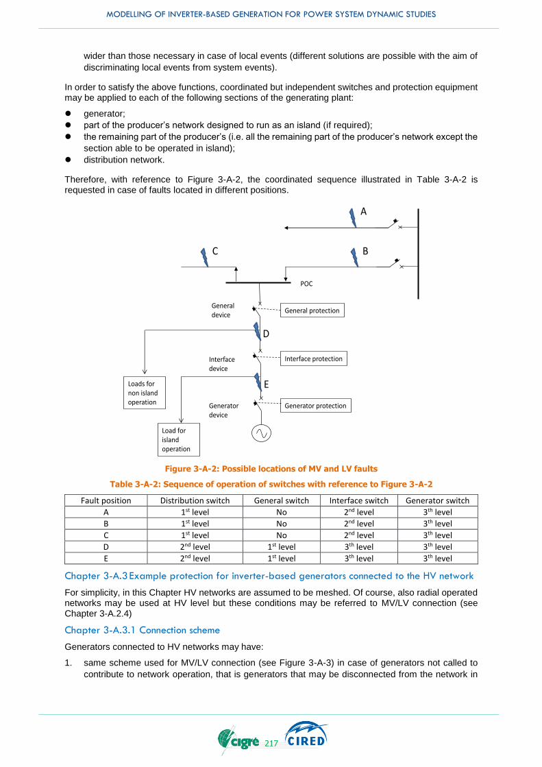
MODELLING OF INVERTER-BASED GENERATION FOR POWER SYSTEM DYNAMIC STUDIES
217
wider than those necessary in case of local events (different solutions are possible with the aim of
discriminating local events from system events).
In order to satisfy the above functions, coordinated but independent switches and protection equipment may be applied to each of the following sections of the generating plant:
generator;
part of the producer’s network designed to run as an island (if required);
the remaining part of the producer’s (i.e. all the remaining part of the producer’s network except the
section able to be operated in island);
distribution network.
Therefore, with reference to Figure 3-A-2, the coordinated sequence illustrated in Table 3-A-2 is requested in case of faults located in different positions.
Figure 3-A-2: Possible locations of MV and LV faults
Table 3-A-2: Sequence of operation of switches with reference to Figure 3-A-2
Fault position Distribution switch General switch Interface switch Generator switch
A 1st level No 2nd level 3th level
B 1st level No 2nd level 3th level
C 1st level No 2nd level 3th level
D 2nd level 1st level 3th level 3th level
E 2nd level 1st level 3th level 3th level
Chapter 3-A.3 Example protection for inverter-based generators connected to the HV network
For simplicity, in this Chapter HV networks are assumed to be meshed. Of course, also radial operated networks may be used at HV level but these conditions may be referred to MV/LV connection (see Chapter 3-A.2.4)
Chapter 3-A.3.1 Connection scheme
Generators connected to HV networks may have:
1. same scheme used for MV/LV connection (see Figure 3-A-3) in case of generators not called to
contribute to network operation, that is generators that may be disconnected from the network in
Load for islandoperation
Loads for non islandoperation
POC
General device
Interface device
Generator device
General protection
Interface protection
Generator protection
A
BC
D
E
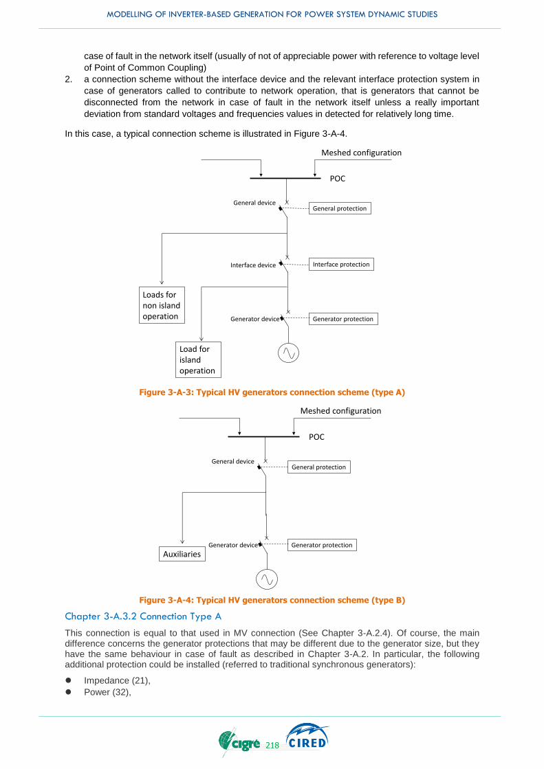
MODELLING OF INVERTER-BASED GENERATION FOR POWER SYSTEM DYNAMIC STUDIES
218
case of fault in the network itself (usually of not of appreciable power with reference to voltage level
of Point of Common Coupling)
2. a connection scheme without the interface device and the relevant interface protection system in
case of generators called to contribute to network operation, that is generators that cannot be
disconnected from the network in case of fault in the network itself unless a really important
deviation from standard voltages and frequencies values in detected for relatively long time.
In this case, a typical connection scheme is illustrated in Figure 3-A-4.
Figure 3-A-3: Typical HV generators connection scheme (type A)
Figure 3-A-4: Typical HV generators connection scheme (type B)
Chapter 3-A.3.2 Connection Type A
This connection is equal to that used in MV connection (See Chapter 3-A.2.4). Of course, the main difference concerns the generator protections that may be different due to the generator size, but they have the same behaviour in case of fault as described in Chapter 3-A.2. In particular, the following additional protection could be installed (referred to traditional synchronous generators):
Impedance (21),
Power (32),
Load for islandoperation
Loads for non islandoperation
POC
General device
Interface device
Generator device
General protection
Interface protection
Generator protection
Meshed configuration
Auxiliaries
POC
General device
Generator device
General protection
Generator protection
Meshed configuration

MODELLING OF INVERTER-BASED GENERATION FOR POWER SYSTEM DYNAMIC STUDIES
219
Power swing blocking (68).
Chapter 3-A.3.3 Protection coordination
It is worth remembering that the generator protection should both detect faults into the generator in order to protect the generator and within the producer plant in order to eliminate the fault. But, at the same time, it should allow the generator to continue to operate during faults in the HV network (within certain limits in voltage, frequency and duration).
Therefore, with this connection scheme the protection coordination is quite similar to that described in app. 3-A.2.4. The difference is present only in case of faults on the line where the generator is connected (fault position B or C in Figure 3-A-5) because MV (LV) network is usually radial operated, whereas HV is usually meshed operated.
With reference to Figure 3-A-5 and Figure 3-A-6, the coordinated operation sequence driven from protection system in case of faults located in different positions of the line is:
Fault position B (see Figure 3-A-5): B is intended to be not very close to the busbar where the
generating plant is connected.
In this case CB1 and CB2 switches will open and the fault will be cleared. No protection inside the producer plant shall trip due to the coordination of the regulations (in terms of values of input quantities and of intentional operating delay): in the example the undervoltage interface protection is properly delayed.
CB1 and CB2 switches will re-close if automatic reclosing is foreseen and, again, no protection of the producer plant shall trip.
Fault position B’ (see Figure 3-A-6): B’ is intended to be very close to the busbar where the
generating plant is connected.
In this case three switches, CB1, CB2 and CB3, will open because no pilot scheme is used, and the fault will be cleared. No protection of the producer plant shall trip during the fault because the undervoltage interface protection is delayed. After the three switches open, the plant is disconnected from the HV network and the interface protection will trip.
It’s worth noting that in case of pilot protection scheme (POTT, PUTT), only two switches will open and the co-ordinated sequence is equal to fault position B.
Chapter 3-A.3.4 Connection Type B
This connection is completely different from that used in distribution systems, because the goal is to maintain the generator connected as long as possible.
Chapter 3-A.3.5 Protection system
Since the goal is to maintain the generator connected as long as possible, there is no interface protection included. In addition, the generator protections may be extremely different depending on the importance of the generator in terms of rated power.
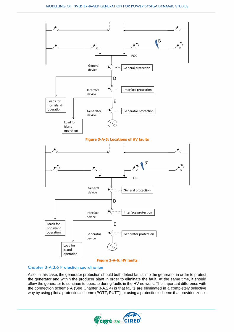
MODELLING OF INVERTER-BASED GENERATION FOR POWER SYSTEM DYNAMIC STUDIES
220
Figure 3-A-5: Locations of HV faults
Figure 3-A-6: HV faults
Chapter 3-A.3.6 Protection coordination
Also, in this case, the generator protection should both detect faults into the generator in order to protect the generator and within the producer plant in order to eliminate the fault. At the same time, it should allow the generator to continue to operate during faults in the HV network. The important difference with the connection scheme A (See Chapter 3-A.2.4) is that faults are eliminated in a completely selective way by using pilot a protection scheme (POTT, PUTT); or using a protection scheme that provides zone-
Load for islandoperation
Loads for non islandoperation
POC
General device
Interface device
Generator device
General protection
Interface protection
Generator protection
D
E
B
Load for islandoperation
Loads for non islandoperation
POC
General device
Interface device
Generator device
General protection
Interface protection
Generator protection
D
E
B’

MODELLING OF INVERTER-BASED GENERATION FOR POWER SYSTEM DYNAMIC STUDIES
221
extension in combination with single-pole reclosing procedure. Therefore, the generator remains always connected to the network and in case of fault:
continues to supply the fault before completely selective fault elimination,
continues to operate after the fault elimination.
Table 3-A-3: Device number of protections shown in Appendix 3-A
Device number Name of protection (IEEE Std C37.2) Sign used in some countries
21 Distance relay DZ
24 Voltage per Hertz relay V/F
27 Undervoltage relay UVR
32 Directional power relay
40 Field (over/under excitation) relay
46 Reverse phase or phase balance current relay
50 Instantaneous overcurrent relay
51 AC time overcurrent relay OCR
59 Overvoltage relay OVR
64 Ground detector relay
67 AC directional overcurrent relay
68 Blocking relay or out-of-step relay
78 phase-angle measuring relay
81 Frequency relay
81O Overfrequency relay OFR
81U Underfrequency relay UFR
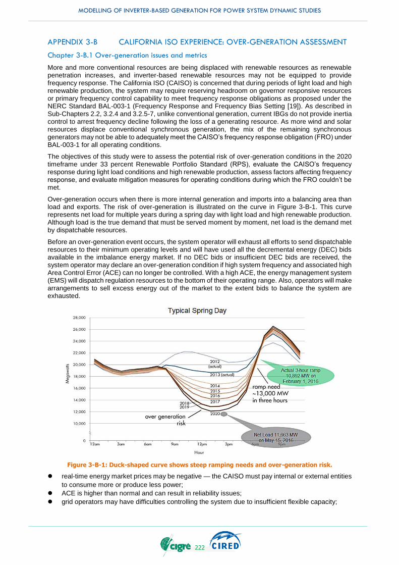
MODELLING OF INVERTER-BASED GENERATION FOR POWER SYSTEM DYNAMIC STUDIES
222
APPENDIX 3-B CALIFORNIA ISO EXPERIENCE: OVER-GENERATION ASSESSMENT
Chapter 3-B.1 Over-generation issues and metrics
More and more conventional resources are being displaced with renewable resources as renewable penetration increases, and inverter-based renewable resources may not be equipped to provide frequency response. The California ISO (CAISO) is concerned that during periods of light load and high renewable production, the system may require reserving headroom on governor responsive resources or primary frequency control capability to meet frequency response obligations as proposed under the NERC Standard BAL-003-1 (Frequency Response and Frequency Bias Setting [19]). As described in Sub-Chapters 2.2, 3.2.4 and 3.2.5-7, unlike conventional generation, current IBGs do not provide inertia control to arrest frequency decline following the loss of a generating resource. As more wind and solar resources displace conventional synchronous generation, the mix of the remaining synchronous generators may not be able to adequately meet the CAISO’s frequency response obligation (FRO) under BAL-003-1 for all operating conditions.
The objectives of this study were to assess the potential risk of over-generation conditions in the 2020 timeframe under 33 percent Renewable Portfolio Standard (RPS), evaluate the CAISO’s frequency response during light load conditions and high renewable production, assess factors affecting frequency response, and evaluate mitigation measures for operating conditions during which the FRO couldn’t be met.
Over-generation occurs when there is more internal generation and imports into a balancing area than load and exports. The risk of over-generation is illustrated on the curve in Figure 3-B-1. This curve represents net load for multiple years during a spring day with light load and high renewable production. Although load is the true demand that must be served moment by moment, net load is the demand met by dispatchable resources.
Before an over-generation event occurs, the system operator will exhaust all efforts to send dispatchable resources to their minimum operating levels and will have used all the decremental energy (DEC) bids available in the imbalance energy market. If no DEC bids or insufficient DEC bids are received, the system operator may declare an over-generation condition if high system frequency and associated high Area Control Error (ACE) can no longer be controlled. With a high ACE, the energy management system (EMS) will dispatch regulation resources to the bottom of their operating range. Also, operators will make arrangements to sell excess energy out of the market to the extent bids to balance the system are exhausted.
Figure 3-B-1: Duck-shaped curve shows steep ramping needs and over-generation risk.
real-time energy market prices may be negative — the CAISO must pay internal or external entities
to consume more or produce less power;
ACE is higher than normal and can result in reliability issues;
grid operators may have difficulties controlling the system due to insufficient flexible capacity;

MODELLING OF INVERTER-BASED GENERATION FOR POWER SYSTEM DYNAMIC STUDIES
223
insufficient frequency responsive generation on-line may reduce the system ability to quickly arrest
frequency decline following a disturbance;
inability to shut down a resource because it would not have the ability to restart in time to meet
system peak;
need to commit more resources on governor control; and
possible curtailment of resources that cannot provide frequency response.
Frequency response is the overall response of the power system to large, sudden mismatches
between generation and load. The study focused on light spring conditions, because the relatively
low level of conventional generation may present a challenge in meeting the FRO. NERC
developed the frequency response obligation of the Western Interconnection based on the loss of
two fully loaded Palo Verde nuclear power station units (2,750 MW). This is a credible outage that
results in the most severe frequency excursion post-contingency.
The following frequency performance metrics that were proposed by the CAISO and General
Electric Energy were used in the study and are illustrated in Figure 3-B-2.
Figure 3-B-2: Frequency performance metrics.
where, Cf — Frequency Nadir (Hz) Ct — Frequency Nadir Time (sec) Bf — Settling Frequency (Hz) Δ MW/Δfc *0.1 — Nadir-Based Frequency Response (MW/0.1HZ) Δ MW/Δfb*0.1 — Settling-Based Frequency Response Cp — Nadir-based governor response (MW) Bp — Settling frequency-based governor response (MW)
The system frequency performance is acceptable when the frequency nadir post-contingency is above the set point for the first block of the under-frequency load shedding relays, which for most loads are set at 59.5 Hz. Another metric is the actual CAISO’s frequency response following a contingency. The Western Interconnection Frequency Response Obligation is updated annually, according to the NERC BAL-003-1 standard. The NERC-established annual interconnection frequency response obligation for the Western Interconnection is currently set at 949 MW/0.1Hz, which was the value used for this study. Frequency response of the Interconnection is calculated as:
𝐹𝑅 =Δ𝑃
Δ𝐵𝑓[𝑀𝑊 0.1𝐻𝑧⁄ ]
Equation 3-B-1
MODELLING OF INVERTER-BASED GENERATION FOR POWER SYSTEM DYNAMIC STUDIES
224
where 𝛥𝑃 is the difference in the generation output before and after the contingency, and 𝛥𝐵𝑓 is the difference between the system frequency just prior to the contingency and the settling frequency. For each balancing authority within an Interconnection to meet the NERC Standard BAL-003-1, the actual frequency response should exceed the FRO of the balancing authority. FRO is allocated to each balancing authority and is calculated using the formula below.
intint
intPloadPgen
PloadPgenFROFRO BABA
BA+
+
Equation 3-B-2
where BA stands for Balancing Authority, Int for interconnection, Pgen for annual generation output (MWH) and Pload for annual demand (MWH). For the CAISO, annual FRO obligation is approximately 30 percent of WECC FRO, which is 285 MW/0.1 Hz.
The ratio of generation that provides governor response or primary frequency control capability to all generation running on the system is used to quantify overall system readiness to provide frequency response. This ratio is introduced as the metric Kt; the lower the Kt, the smaller the fraction of generation that will respond. The exact definition of Kt is not standardized. For this study, it is defined as ratio of power generation capability of units with responsive governors to the MW capability of all generation units. For units that don’t respond to frequency changes, power capability is defined as equal to the MW dispatch rather than the nameplate rating because these units will not contribute beyond their initial dispatch.
The other metric that was evaluated was the headroom of the units with responsive governors. The headroom is defined as a difference between the maximum capacity of the unit and the unit’s output. For a system to react most effectively to changes in frequency, enough total headroom must be available. Block loaded units have no headroom.
Chapter 3-B.2 Study assumptions
The power-flow base case selected for the study was based on the results of production simulations for the year 2024. Production simulations represent the system performance considering security-constrained unit commitment (SCUC) and security-constrained unit dispatch (SCUD) for each hour of the year. The model for production simulation was obtained from the WECC Transmission Expansion Planning Policy Committee (TEPPC) Study Program. The latest 2024 Common Case was used. The Common Case is the first base case for the 10-year timeframe from which additional portfolio cases can be developed. The production simulation case selected for the study modelled 33 percent of renewable resources in California and had the latest updates on the new transmission and generation projects. The model used the California Energy Commission (CEC) load forecast for California for the year 2024 developed in 2013 and the load forecasts for other areas from the latest WECC Load and Resources Subcommittee (LRS) data developed in 2012. New renewable generation projects were modelled according to the California Public Utility Commission (CPUC) renewable resources portfolios. All other assumptions were consistent with the CAISO 2014 Unified Study Assumptions and the latest TEPPC database.
The production simulation was run for the year 2024 using ABB Grid View software. The hour of the year selected for the detailed transient stability studies modelled low load and high renewable generation that usually occurs in spring. Based on the production simulation results, the hour of 11 am April 7, 2024 was selected because it represents a low load and high renewable production scenario. Power flow case was created for the 11 am, April 7, 2024 with the generation dispatch and load distribution from the results of the production simulation study. The power flow case was created by exporting the results of the Grid View production simulation for the selected hour and solving the case in a commercially available time-domain simulation tool. Due to high voltages because of low load in the selected hour, reactive support was adjusted by turning off shunt capacitors and turning on all available shunt reactors.
Dynamic stability data file was created to match the power flow case. The latest WECC Master Dynamic File was used as a starting dataset. Missing dynamic stability models for the new renewable projects were added to the dynamic file by using typical models according to the type and capacity of the projects. The latest models for IBG recently approved by WECC were utilized. For the new wind projects, the models for type 3 (double-fed induction generator) or type 4 (full converter) were used depending on the type and size of the project. For the solar PV projects, three types of models were used: large PV plant, small PV plant and distributed PV generation. It was assumed that the large plants (20 MW and higher) have centralized plant control. More detailed description of the RMS dynamic stability models for renewable generation used in WECC is provided in the Appendix 5-C.
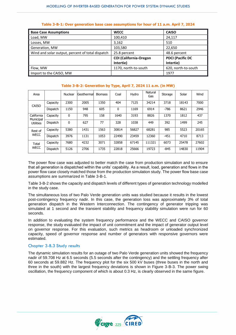
MODELLING OF INVERTER-BASED GENERATION FOR POWER SYSTEM DYNAMIC STUDIES
225
Table 3-B-1: Over generation base case assumptions for hour of 11 a.m. April 7, 2024
Base Case Assumptions WECC CAISO
Load, MW 100,410 24,117
Losses, MW 3,162 510
Generation, MW 103,580 22,650
Wind and solar output, percent of total dispatch 25.8 percent 48.6 percent
COI (California-Oregon Intertie)
PDCI (Pacific DC Intertie)
Flow, MW 1170, north-to-south 620, north-to-south
Import to the CAISO, MW 1977
Table 3-B-2: Generation by Type, April 7, 2024 11 a.m. (in MW)
Area Nuclear Geothermal Biomass Coal Hydro Natural
Gas Storage Solar Wind
CAISO Capacity 2300 2005 1350 404 7125 34214 3718 18143 7000
Dispatch 1150 948 605 0 1169 6914 -786 8621 2946
California Municipal Utilities
Capacity 0 795 158 1640 3193 8826 1370 1812 437
Dispatch 0 627 77 328 1038 449 392 1499 245
Rest of WECC
Capacity 5380 1431 1563 30814 56827 68281 985 5523 20165
Dispatch 3976 1131 1053 22490 23459 12360 -451 4710 8713
Total WECC
Capacity 7680 4232 3071 32858 67145 111321 6073 25478 27602
Dispatch 5126 2706 1735 22818 25666 19723 -845 14830 11904
The power flow case was adjusted to better match the case from production simulation and to ensure that all generation is dispatched within the units’ capability. As a result, load, generation and flows in the power flow case closely matched those from the production simulation study. The power flow base case assumptions are summarized in Table 3-B-1.
Table 3-B-2 shows the capacity and dispatch levels of different types of generation technology modelled in the study case.
The simultaneous loss of two Palo Verde generation units was studied because it results in the lowest post-contingency frequency nadir. In this case, the generation loss was approximately 3% of total generation dispatch in the Western Interconnection. The contingency of generator tripping was simulated at 1 second and the transient stability and frequency stability simulation were run for 60 seconds.
In addition to evaluating the system frequency performance and the WECC and CAISO governor response, the study evaluated the impact of unit commitment and the impact of generator output level on governor response. For this evaluation, such metrics as headroom or unloaded synchronized capacity, speed of governor response and number of generators with responsive governors were estimated.
Chapter 3-B.3 Study results
The dynamic simulation results for an outage of two Palo Verde generation units showed the frequency nadir of 59.708 Hz at 6.5 seconds (5.5 seconds after the contingency) and the settling frequency after 60 seconds at 59.882 Hz. The frequency plot for the six 500 kV buses (three buses in the north and three in the south) with the largest frequency deviations is shown in Figure 3-B-3. The power swing oscillation, the frequency component of which is about 0.3 Hz, is clearly observed in the same figure.
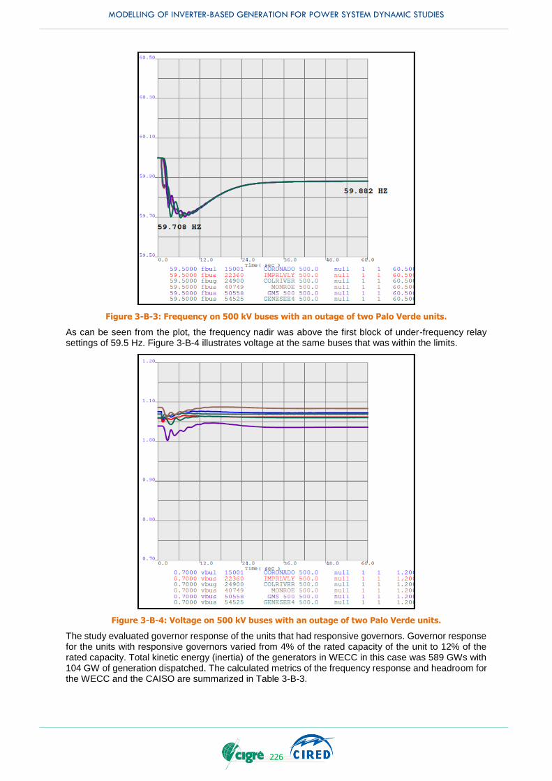
MODELLING OF INVERTER-BASED GENERATION FOR POWER SYSTEM DYNAMIC STUDIES
226
Figure 3-B-3: Frequency on 500 kV buses with an outage of two Palo Verde units.
As can be seen from the plot, the frequency nadir was above the first block of under-frequency relay settings of 59.5 Hz. Figure 3-B-4 illustrates voltage at the same buses that was within the limits.
Figure 3-B-4: Voltage on 500 kV buses with an outage of two Palo Verde units.
The study evaluated governor response of the units that had responsive governors. Governor response for the units with responsive governors varied from 4% of the rated capacity of the unit to 12% of the rated capacity. Total kinetic energy (inertia) of the generators in WECC in this case was 589 GWs with 104 GW of generation dispatched. The calculated metrics of the frequency response and headroom for the WECC and the CAISO are summarized in Table 3-B-3.

MODELLING OF INVERTER-BASED GENERATION FOR POWER SYSTEM DYNAMIC STUDIES
227
Table 3-B-3: Frequency response and headroom, April 7, 2024 11 a.m.
As can be seen from the table, the total WECC frequency response was within the BAL-003-1 standard and well above the FRO: 2292 MW/0.1 Hz compared with the WECC FRO of 949 MW/0.1 Hz. However, the CAISO frequency response was below its FRO: 269 MW/0.1 Hz when the ISO FRO is 285 MW/0.1 Hz. Thus, this study showed that although the total system performance was stable with no criteria violations and the WECC frequency response was within the standard, the CAISO may not meet the BAL-003-1 standard because its frequency response was below the frequency response obligation.
The metric Kt for this case was 56 percent for WECC and 31 percent for the ISO. Due to the large amount of IBG within the ISO Balancing Authority Area (BAA), which is not responsive to changes in frequency, the Kt metrics for the ISO was significantly lower than for the WECC as a whole. The headroom of the frequency responsive generation at the ISO was relatively large (4420 MW), but it still wasn’t sufficient to meet the frequency response obligation.
Sensitivity studies were performed to evaluate the system performance in case of reduced headroom in the CAISO and in WECC. The original April 7, 2024 11 a.m. case had high headroom at the frequency-responsive generation due to low dispatch of the generators that were modelled on-line. The sensitivity case was created by turning off some units that had low dispatch and re-dispatching their output to other on-line units in the same geographical zone, or at the same river for hydro power plants. The CAISO generation headroom was reduced in this case from 4420 MW to 1925 MW and the total WECC headroom was reduced to 12,000 MW. This case had 486 GWs of inertia with the same 104GW of generation dispatched as in the initial case, which is 17.5% reduction in inertia.
The same contingency of an outage of two Palo Verde units was studied. Frequency on 500 kV buses in the sensitivity case is shown in Figure 3-B-5.

MODELLING OF INVERTER-BASED GENERATION FOR POWER SYSTEM DYNAMIC STUDIES
228
Figure 3-B-5: Frequency on 500 kV buses with an outage of two Palo Verde units in case of reduced headroom.
The study results showed the frequency performance that still was acceptable (nadir at 59.557 Hz and settling frequency at 59.754 Hz), but it was close to the margin. 27 MW of load in British Columbia that had under-frequency relay settings at 59.7 Hz was tripped. These loads did not include distributed PV models. Also, 579 MW of distributed solar PV generation in WECC and CAISO was tripped due to the under-frequency relays built in the distributed PV models, which had additional negative impact on frequency.
For distributed solar PV generation, the WECC model PVD1 described in the Sub-Chapter 4.1 on the RMS models was used, which is a simplified model of aggregated distributed PV units. This model provides for tripping of some distributed units for low or high voltage or frequency. The range of frequencies and voltages for which certain amount of distributed units may be tripped is specified by the user. It was assumed that distributed generation will start tripping when the system frequency falls below 59.7 Hz and all distributed generation will be tripped at 59.5 Hz. The fraction of generation tripped by the PVD1 model when the system frequency is between these set points is proportional to the frequency deviation in the transient stability simulation. In this sensitivity study, it was assumed that the tripped distributed solar PV will not reconnect during the timeframe of the simulation (60 seconds). These assumptions are consistent with the IEEE 1547 standard. Since the PVD1 is a simplified model, it doesn’t include the timer circuit element, so the reduction in the distributed generation output starts as soon as the frequency reaches the first set point (in this case, 59.7 Hz).
The case had the total of 826 MW of distributed solar PV generation. The transient stability simulation with frequency excursion of the case with the 12,000 MW headroom showed that 70 percent of distributed generation was tripped. WECC frequency response was 1219 MW/0.1 Hz, which is within the BAL-003-1 standard. However, the ISO frequency response was only 154 MW/0.1 Hz, which is significantly below its frequency response obligation. Amount of responsive governors in this sensitivity case was 46 percent for WECC and 26 percent for the ISO.
More sensitivity studies were performed to determine at which unit commitment and dispatch the system performance may become unacceptable. Therefore, the headroom was reduced even more; however, generation dispatch was changed only outside the CAISO since the CAISO already had insufficient governor response.
The study with the headroom in WECC reduced to 10,100 MW identified frequency nadir at 59.5 Hz and significant under-frequency load shedding: 537 MW of load, including pumping loads was lost, as well
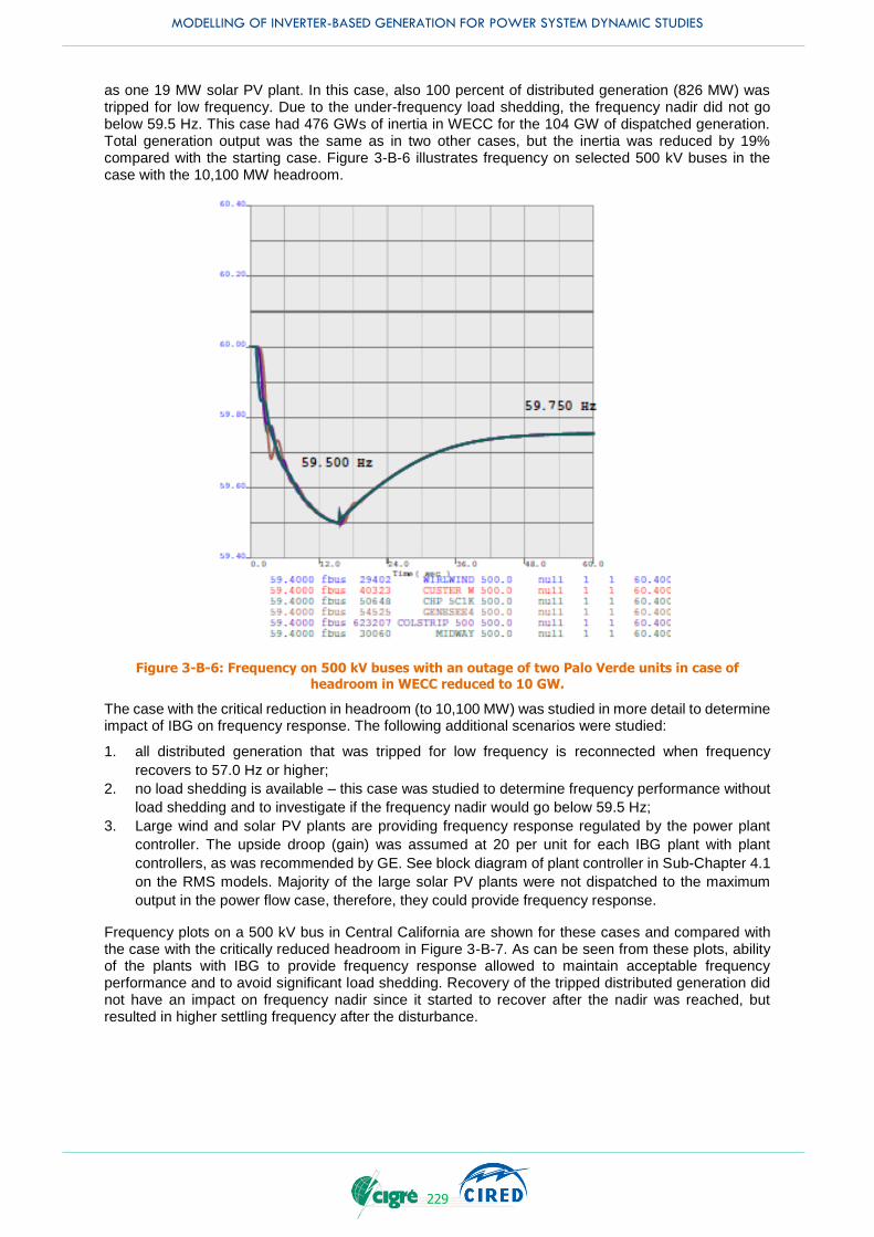
MODELLING OF INVERTER-BASED GENERATION FOR POWER SYSTEM DYNAMIC STUDIES
229
as one 19 MW solar PV plant. In this case, also 100 percent of distributed generation (826 MW) was tripped for low frequency. Due to the under-frequency load shedding, the frequency nadir did not go below 59.5 Hz. This case had 476 GWs of inertia in WECC for the 104 GW of dispatched generation. Total generation output was the same as in two other cases, but the inertia was reduced by 19% compared with the starting case. Figure 3-B-6 illustrates frequency on selected 500 kV buses in the case with the 10,100 MW headroom.
Figure 3-B-6: Frequency on 500 kV buses with an outage of two Palo Verde units in case of headroom in WECC reduced to 10 GW.
The case with the critical reduction in headroom (to 10,100 MW) was studied in more detail to determine impact of IBG on frequency response. The following additional scenarios were studied:
1. all distributed generation that was tripped for low frequency is reconnected when frequency
recovers to 57.0 Hz or higher;
2. no load shedding is available – this case was studied to determine frequency performance without
load shedding and to investigate if the frequency nadir would go below 59.5 Hz;
3. Large wind and solar PV plants are providing frequency response regulated by the power plant
controller. The upside droop (gain) was assumed at 20 per unit for each IBG plant with plant
controllers, as was recommended by GE. See block diagram of plant controller in Sub-Chapter 4.1
on the RMS models. Majority of the large solar PV plants were not dispatched to the maximum
output in the power flow case, therefore, they could provide frequency response.
Frequency plots on a 500 kV bus in Central California are shown for these cases and compared with the case with the critically reduced headroom in Figure 3-B-7. As can be seen from these plots, ability of the plants with IBG to provide frequency response allowed to maintain acceptable frequency performance and to avoid significant load shedding. Recovery of the tripped distributed generation did not have an impact on frequency nadir since it started to recover after the nadir was reached, but resulted in higher settling frequency after the disturbance.

MODELLING OF INVERTER-BASED GENERATION FOR POWER SYSTEM DYNAMIC STUDIES
230
Figure 3-B-7: Frequency on Midway 500 kV buses with an outage of two Palo Verde units in case of 10 GW headroom and different scenarios.
In the case with the large wind and solar PV plants providing frequency response, there still was some distributed solar PV generators that were tripped, since the frequency nadir was at 59.626 Hz which is below the first set point for distributed generation tripping (59.7 Hz). Tripped distributed generation in all of WECC amounted to 314 MW, or 38% of the dispatched distributed generation. The response from large inverter-based plants was 919 MW, which is 8.4% of their installed capacity. Thanks to frequency response from the IBG, the settling frequency after the contingency increased from 59.75 Hz to 59.83 Hz and the frequency nadir increased from 59.50 Hz to 59.63 Hz. Frequency response from total WECC increased from 1063 MW/0.1 Hz to 1603 MW/0.1Hz and frequency response from the CAISO increased
Legend:
- Case with the
WECC headroom reduced to
10,100 MW (case 1)
- Case 1 with the
tripped distributed generation
reconnected
- Case 1 with under-
frequency load shedding
disabled
- Case 1 with large
inverter-based generation plants
providing frequency response
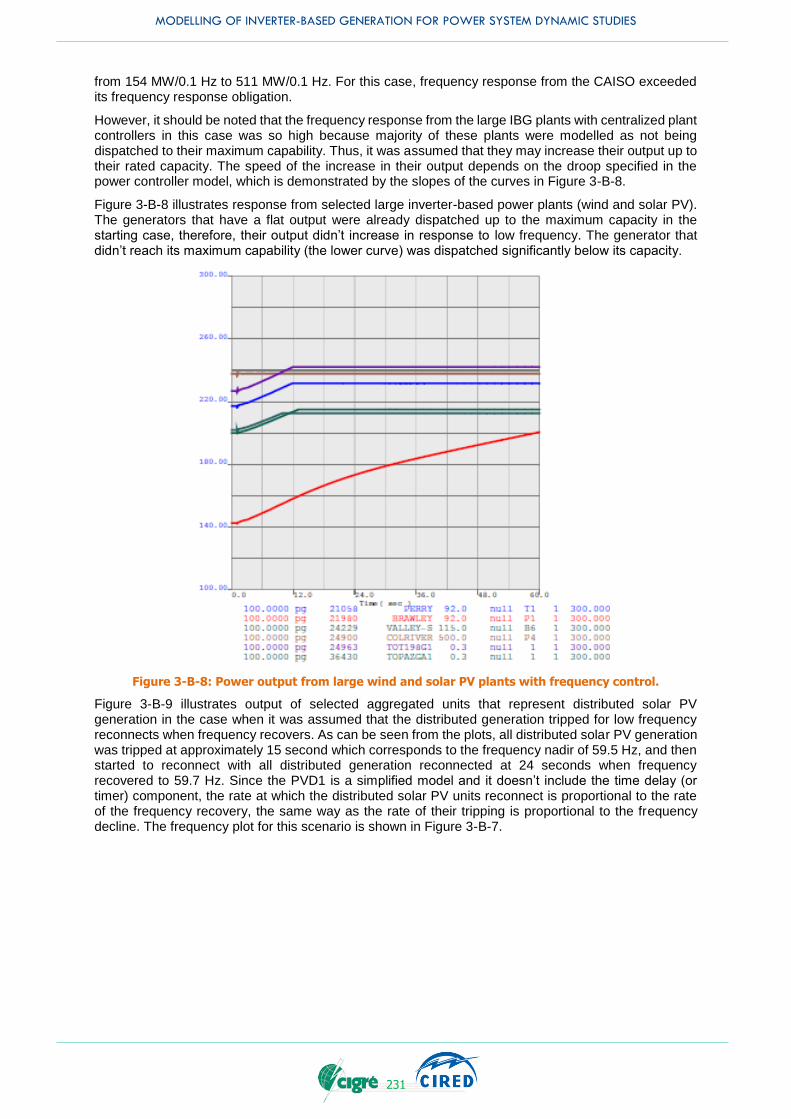
MODELLING OF INVERTER-BASED GENERATION FOR POWER SYSTEM DYNAMIC STUDIES
231
from 154 MW/0.1 Hz to 511 MW/0.1 Hz. For this case, frequency response from the CAISO exceeded its frequency response obligation.
However, it should be noted that the frequency response from the large IBG plants with centralized plant controllers in this case was so high because majority of these plants were modelled as not being dispatched to their maximum capability. Thus, it was assumed that they may increase their output up to their rated capacity. The speed of the increase in their output depends on the droop specified in the power controller model, which is demonstrated by the slopes of the curves in Figure 3-B-8.
Figure 3-B-8 illustrates response from selected large inverter-based power plants (wind and solar PV). The generators that have a flat output were already dispatched up to the maximum capacity in the starting case, therefore, their output didn’t increase in response to low frequency. The generator that didn’t reach its maximum capability (the lower curve) was dispatched significantly below its capacity.
Figure 3-B-8: Power output from large wind and solar PV plants with frequency control.
Figure 3-B-9 illustrates output of selected aggregated units that represent distributed solar PV generation in the case when it was assumed that the distributed generation tripped for low frequency reconnects when frequency recovers. As can be seen from the plots, all distributed solar PV generation was tripped at approximately 15 second which corresponds to the frequency nadir of 59.5 Hz, and then started to reconnect with all distributed generation reconnected at 24 seconds when frequency recovered to 59.7 Hz. Since the PVD1 is a simplified model and it doesn’t include the time delay (or timer) component, the rate at which the distributed solar PV units reconnect is proportional to the rate of the frequency recovery, the same way as the rate of their tripping is proportional to the frequency decline. The frequency plot for this scenario is shown in Figure 3-B-7.
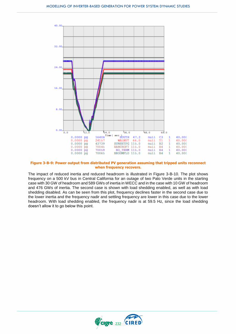
MODELLING OF INVERTER-BASED GENERATION FOR POWER SYSTEM DYNAMIC STUDIES
232
Figure 3-B-9: Power output from distributed PV generation assuming that tripped units reconnect when frequency recovers.
The impact of reduced inertia and reduced headroom is illustrated in Figure 3-B-10. The plot shows frequency on a 500 kV bus in Central California for an outage of two Palo Verde units in the starting case with 30 GW of headroom and 589 GWs of inertia in WECC and in the case with 10 GW of headroom and 476 GWs of inertia. The second case is shown with load shedding enabled, as well as with load shedding disabled. As can be seen from this plot, frequency declines faster in the second case due to the lower inertia and the frequency nadir and settling frequency are lower in this case due to the lower headroom. With load shedding enabled, the frequency nadir is at 59.5 Hz, since the load shedding doesn’t allow it to go below this point.
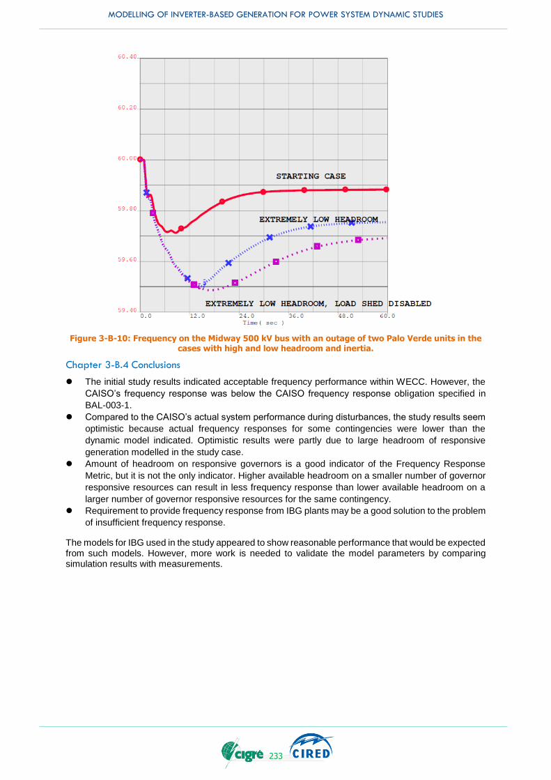
MODELLING OF INVERTER-BASED GENERATION FOR POWER SYSTEM DYNAMIC STUDIES
233
Figure 3-B-10: Frequency on the Midway 500 kV bus with an outage of two Palo Verde units in the cases with high and low headroom and inertia.
Chapter 3-B.4 Conclusions
The initial study results indicated acceptable frequency performance within WECC. However, the
CAISO’s frequency response was below the CAISO frequency response obligation specified in
BAL-003-1.
Compared to the CAISO’s actual system performance during disturbances, the study results seem
optimistic because actual frequency responses for some contingencies were lower than the
dynamic model indicated. Optimistic results were partly due to large headroom of responsive
generation modelled in the study case.
Amount of headroom on responsive governors is a good indicator of the Frequency Response
Metric, but it is not the only indicator. Higher available headroom on a smaller number of governor
responsive resources can result in less frequency response than lower available headroom on a
larger number of governor responsive resources for the same contingency.
Requirement to provide frequency response from IBG plants may be a good solution to the problem
of insufficient frequency response.
The models for IBG used in the study appeared to show reasonable performance that would be expected from such models. However, more work is needed to validate the model parameters by comparing simulation results with measurements.

MODELLING OF INVERTER-BASED GENERATION FOR POWER SYSTEM DYNAMIC STUDIES
234
APPENDIX 3-C LVRT STUDY FOR FREQUENCY STABILITY IN TASMANIAN GRID
The blue trace is a simulation of network frequency that follows a simple trip of the largest single generating system (a radially connected CCGT unit). The red trace shows the exact same contingency, i.e. the largest generator tripping, only this time as a result of a transmission line fault. The FRT (FRT) response of the Tasmanian HVDC link and wind farms causes a very large transient energy deficit which results in a more rapid decline in frequency than if a fault did not occur. The concern is that PV inverters will add to this issue, especially under low short circuit conditions when voltage disturbances (due to network fault events) will propagate more widely and therefore have an effect on more individual PV installations. The protection characteristics of embedded inverters (pickup setting and time delays), along with the modelling assumptions applied for the distribution network, will affect how significant this issue becomes with more PV connected to the network.
Figure 3-C-1: Impact of low-voltage FRT response on network frequency control.
Understanding the potential range of under/over voltage settings (that might cause an FRT type response), and being confident about how transmission voltage disturbances propagate downward into the distribution network, are some of the challenges going forward. Note that the response of load devices to the same voltage disturbance means that there is probably a growing need to understand the appropriateness of existing load models because of the feedback effect this has on voltages which the inverter is then exposed to.
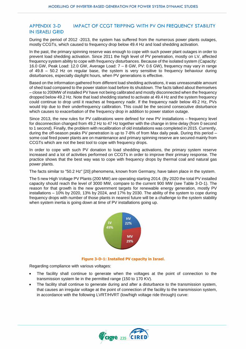
MODELLING OF INVERTER-BASED GENERATION FOR POWER SYSTEM DYNAMIC STUDIES
235
APPENDIX 3-D IMPACT OF CCGT TRIPPING WITH PV ON FREQUENCY STABILITY IN ISRAELI GRID
During the period of 2012 -2013, the system has suffered from the numerous power plants outages, mostly CCGTs, which caused to frequency drop below 49.4 Hz and load shedding activation.
In the past, the primary spinning reserve was enough to cope with such power plant outages in order to prevent load shedding activation. Since 2011 the high level of PV penetration, mostly on LV, affected frequency system ability to cope with frequency disturbances. Because of the isolated system (Capacity: 16.0 GW, Peak Load: 12.0 GW, Average Load: 7 – 8 GW, PV: 0.6 GW), frequency may vary in range of 49.8 – 50.2 Hz on regular base, the system is very sensitive to frequency behaviour during disturbances, especially daylight hours, when PV generations is effective.
Based on the information gathered from different load shedding activations, it was unreasonable amount of shed load compared to the power station load before its shutdown. The facts talked about themselves – close to 200MW of installed PV have not being calibrated and mostly disconnected when the frequency dropped below 49.2 Hz. Note that load shedding started to activate at 49.4 Hz and the system frequency could continue to drop until it reaches at frequency nadir. If the frequency nadir below 49.2 Hz, PVs would trip due to their underfrequency calibration. This could be the second consecutive disturbance which causes to exacerbation of the frequency drop in addition to power station outage.
Since 2013, the new rules for PV calibrations were defined for new PV installations – frequency level for disconnection changed from 49.2 Hz to 47 Hz together with the change in time delay (from 0 second to 1 second). Finally, the problem with recalibration of old installations was completed in 2015. Currently, during the off-season peaks PV penetration is up to 7-8% of from Max daily peak. During this period – some coal fired power plants are on maintenance and primary spinning reserve are secured mainly from CCGTs which are not the best tool to cope with frequency drops.
In order to cope with such PV donation to load shedding activations, the primary system reserve increased and a lot of activities performed on CCGTs in order to improve their primary response. The practice shows that the best way was to cope with frequency drops by thermal coal and natural gas power plants.
The facts similar to "50.2 Hz" [20] phenomena, known from Germany, have taken place in the system.
The 5 new High Voltage PV Plants (200 MW) are operating starting 2014. (By 2020 the total PV installed capacity should reach the level of 3000 MW, compare to the current 900 MW (see Table 3-D-1). The reason for that growth is the new government targets for renewable energy generation, mostly PV installations – 10% by 2020, 13% by 2024, and 17% by 2030. The ability of the system to cope during frequency drops with number of those plants in nearest future will be a challenge to the system stability when system inertia is going down at time of PV installations going up.
Figure 3-D-1: Installed PV capacity in Israel.
Regarding compliance with various voltages:
The facility shall continue to generate when the voltages at the point of connection to the
transmission system lie in the permitted range (150 to 170 KV).
The facility shall continue to generate during and after a disturbance to the transmission system,
that causes an irregular voltage at the point of connection of the facility to the transmission system,
in accordance with the following LVRT/HVRT (low/high voltage ride through) curve:

MODELLING OF INVERTER-BASED GENERATION FOR POWER SYSTEM DYNAMIC STUDIES
236
Figure 3-D-2: LVRT AND HVRT functionality.
where
Region 1: The facility shall not disconnect from the grid and shall continue to generate. Region 2: The facility shall be entitled to disconnect for a short time until removal of the disturbance.
If the facility did not disconnect from the grid, after removal of the disturbance, the active power shall be increased at a rate that shall be not less than 20% of the available power per second.
Regarding compliance with frequency regulation:
Continuous operation in range 47 Hz to 51.5 Hz
The plant should be disconnected from the grid in case of grid frequency will be:
Table 3-D-1: Amended grid requirement for PV from voltage point of view in Israel
Frequency level at the point of grid connection Max time before disconnection
F< 47 Hz 1 sec
51.5 Hz < F 0.2 sec
47<F<51.2 Hz Continuous Operation
Other than the above, the frequency response requirement is also regulated:
50.2available
base
P f HzP
R f
-D - (50.2 Hz 51.5 Hzf )
where, f denotes system frequency, fbase denotes nominal system frequency, Pavailable denotes available capacity, R denotes droop (3%), Pgenerated denotes power generated in the range of 50.2 Hz and 51.5 Hz,
DP denotes power deviation in case of the aforementioned frequency deviation.
The new challenge of the last year is coping with single and multiple phase short circuits in the system. The LVRT and HVRT functionality of the HV PV plants is still under the cloud of uncertainty. The different Grid Codes define those requirements in general and leave the place to inverter's and control system manufacturers to implementations based on hardware and equipment limitations. The system Operator challenge is to define those features from the best proximity to system stability.
Presented underneath couple diagrams from LVRT activations triggered by SC close to HV PV plant – 40 MW installed capacity.
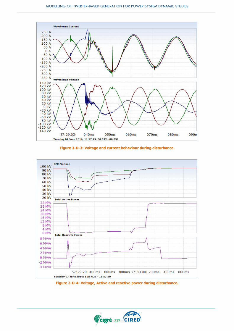
MODELLING OF INVERTER-BASED GENERATION FOR POWER SYSTEM DYNAMIC STUDIES
237
Figure 3-D-3: Voltage and current behaviour during disturbance.
Figure 3-D-4: Voltage, Active and reactive power during disturbance.
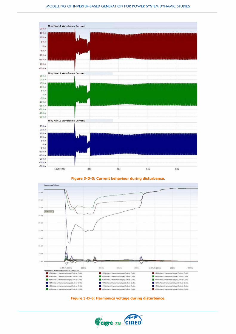
MODELLING OF INVERTER-BASED GENERATION FOR POWER SYSTEM DYNAMIC STUDIES
238
Figure 3-D-5: Current behaviour during disturbance.
Figure 3-D-6: Harmonics voltage during disturbance.
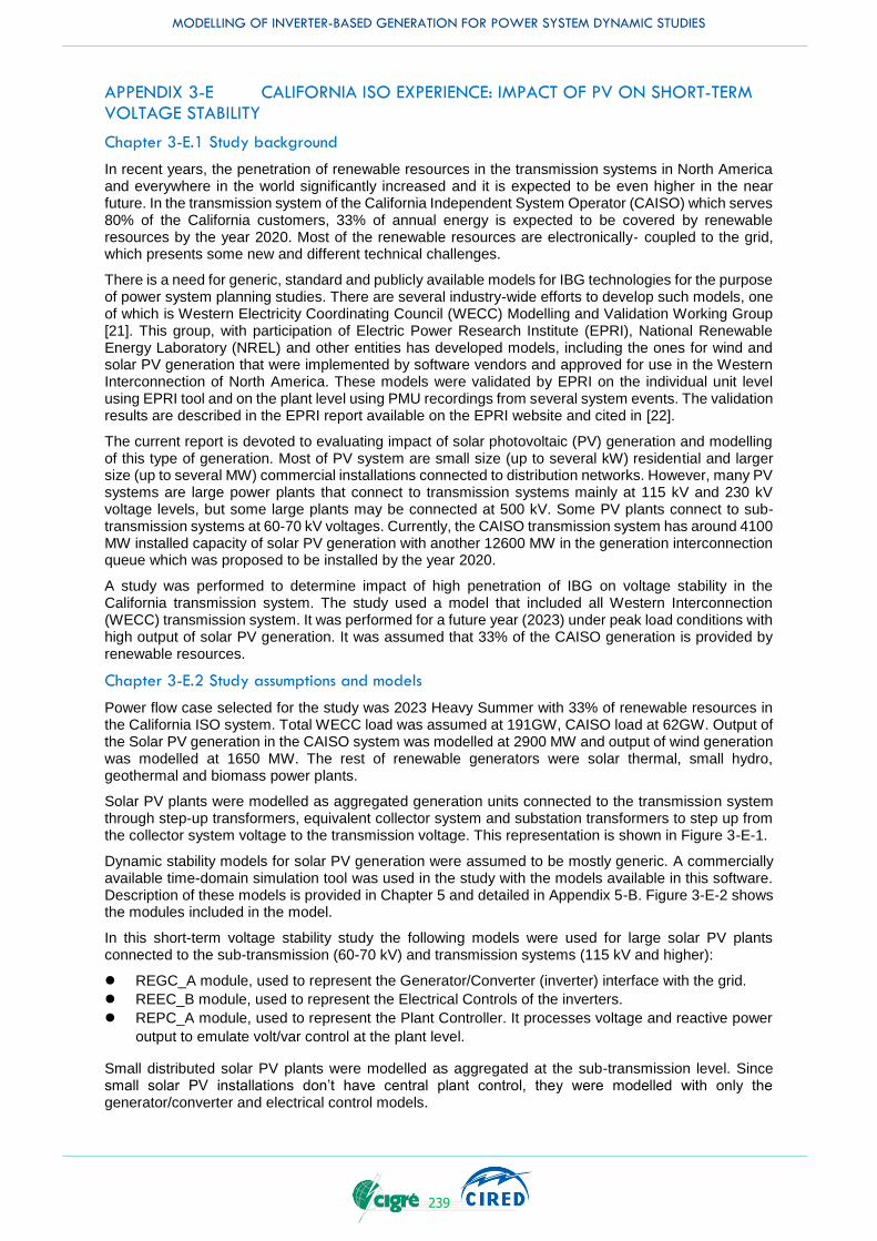
MODELLING OF INVERTER-BASED GENERATION FOR POWER SYSTEM DYNAMIC STUDIES
239
APPENDIX 3-E CALIFORNIA ISO EXPERIENCE: IMPACT OF PV ON SHORT-TERM VOLTAGE STABILITY
Chapter 3-E.1 Study background
In recent years, the penetration of renewable resources in the transmission systems in North America and everywhere in the world significantly increased and it is expected to be even higher in the near future. In the transmission system of the California Independent System Operator (CAISO) which serves 80% of the California customers, 33% of annual energy is expected to be covered by renewable resources by the year 2020. Most of the renewable resources are electronically‐ coupled to the grid, which presents some new and different technical challenges.
There is a need for generic, standard and publicly available models for IBG technologies for the purpose of power system planning studies. There are several industry-wide efforts to develop such models, one of which is Western Electricity Coordinating Council (WECC) Modelling and Validation Working Group [21]. This group, with participation of Electric Power Research Institute (EPRI), National Renewable Energy Laboratory (NREL) and other entities has developed models, including the ones for wind and solar PV generation that were implemented by software vendors and approved for use in the Western Interconnection of North America. These models were validated by EPRI on the individual unit level using EPRI tool and on the plant level using PMU recordings from several system events. The validation results are described in the EPRI report available on the EPRI website and cited in [22].
The current report is devoted to evaluating impact of solar photovoltaic (PV) generation and modelling of this type of generation. Most of PV system are small size (up to several kW) residential and larger size (up to several MW) commercial installations connected to distribution networks. However, many PV systems are large power plants that connect to transmission systems mainly at 115 kV and 230 kV voltage levels, but some large plants may be connected at 500 kV. Some PV plants connect to sub-transmission systems at 60-70 kV voltages. Currently, the CAISO transmission system has around 4100 MW installed capacity of solar PV generation with another 12600 MW in the generation interconnection queue which was proposed to be installed by the year 2020.
A study was performed to determine impact of high penetration of IBG on voltage stability in the California transmission system. The study used a model that included all Western Interconnection (WECC) transmission system. It was performed for a future year (2023) under peak load conditions with high output of solar PV generation. It was assumed that 33% of the CAISO generation is provided by renewable resources.
Chapter 3-E.2 Study assumptions and models
Power flow case selected for the study was 2023 Heavy Summer with 33% of renewable resources in the California ISO system. Total WECC load was assumed at 191GW, CAISO load at 62GW. Output of the Solar PV generation in the CAISO system was modelled at 2900 MW and output of wind generation was modelled at 1650 MW. The rest of renewable generators were solar thermal, small hydro, geothermal and biomass power plants.
Solar PV plants were modelled as aggregated generation units connected to the transmission system through step-up transformers, equivalent collector system and substation transformers to step up from the collector system voltage to the transmission voltage. This representation is shown in Figure 3-E-1.
Dynamic stability models for solar PV generation were assumed to be mostly generic. A commercially available time-domain simulation tool was used in the study with the models available in this software. Description of these models is provided in Chapter 5 and detailed in Appendix 5-B. Figure 3-E-2 shows the modules included in the model.
In this short-term voltage stability study the following models were used for large solar PV plants connected to the sub-transmission (60-70 kV) and transmission systems (115 kV and higher):
REGC_A module, used to represent the Generator/Converter (inverter) interface with the grid.
REEC_B module, used to represent the Electrical Controls of the inverters.
REPC_A module, used to represent the Plant Controller. It processes voltage and reactive power
output to emulate volt/var control at the plant level.
Small distributed solar PV plants were modelled as aggregated at the sub-transmission level. Since small solar PV installations don’t have central plant control, they were modelled with only the generator/converter and electrical control models.
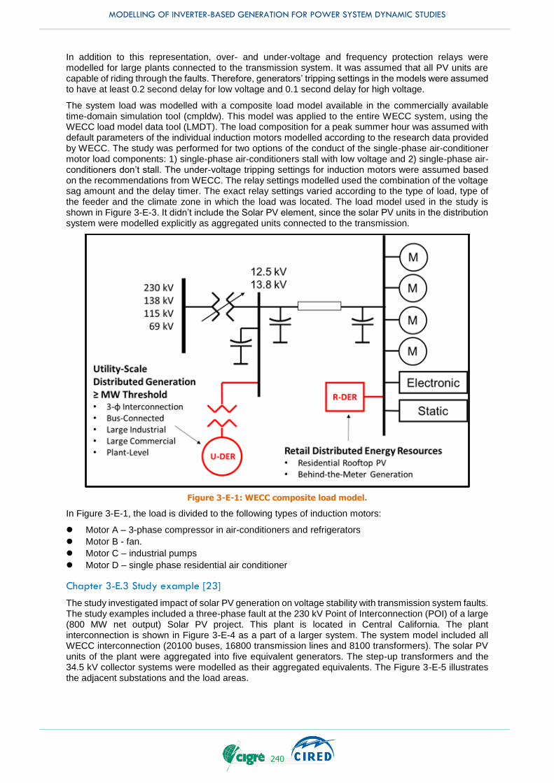
MODELLING OF INVERTER-BASED GENERATION FOR POWER SYSTEM DYNAMIC STUDIES
240
In addition to this representation, over- and under-voltage and frequency protection relays were modelled for large plants connected to the transmission system. It was assumed that all PV units are capable of riding through the faults. Therefore, generators’ tripping settings in the models were assumed to have at least 0.2 second delay for low voltage and 0.1 second delay for high voltage.
The system load was modelled with a composite load model available in the commercially available time-domain simulation tool (cmpldw). This model was applied to the entire WECC system, using the WECC load model data tool (LMDT). The load composition for a peak summer hour was assumed with default parameters of the individual induction motors modelled according to the research data provided by WECC. The study was performed for two options of the conduct of the single-phase air-conditioner motor load components: 1) single-phase air-conditioners stall with low voltage and 2) single-phase air-conditioners don’t stall. The under-voltage tripping settings for induction motors were assumed based on the recommendations from WECC. The relay settings modelled used the combination of the voltage sag amount and the delay timer. The exact relay settings varied according to the type of load, type of the feeder and the climate zone in which the load was located. The load model used in the study is shown in Figure 3-E-3. It didn’t include the Solar PV element, since the solar PV units in the distribution system were modelled explicitly as aggregated units connected to the transmission.
Figure 3-E-1: WECC composite load model.
In Figure 3-E-1, the load is divided to the following types of induction motors:
Motor A – 3-phase compressor in air-conditioners and refrigerators
Motor B - fan.
Motor C – industrial pumps
Motor D – single phase residential air conditioner
Chapter 3-E.3 Study example [23]
The study investigated impact of solar PV generation on voltage stability with transmission system faults. The study examples included a three-phase fault at the 230 kV Point of Interconnection (POI) of a large (800 MW net output) Solar PV project. This plant is located in Central California. The plant interconnection is shown in Figure 3-E-4 as a part of a larger system. The system model included all WECC interconnection (20100 buses, 16800 transmission lines and 8100 transformers). The solar PV units of the plant were aggregated into five equivalent generators. The step-up transformers and the 34.5 kV collector systems were modelled as their aggregated equivalents. The Figure 3-E-5 illustrates the adjacent substations and the load areas.
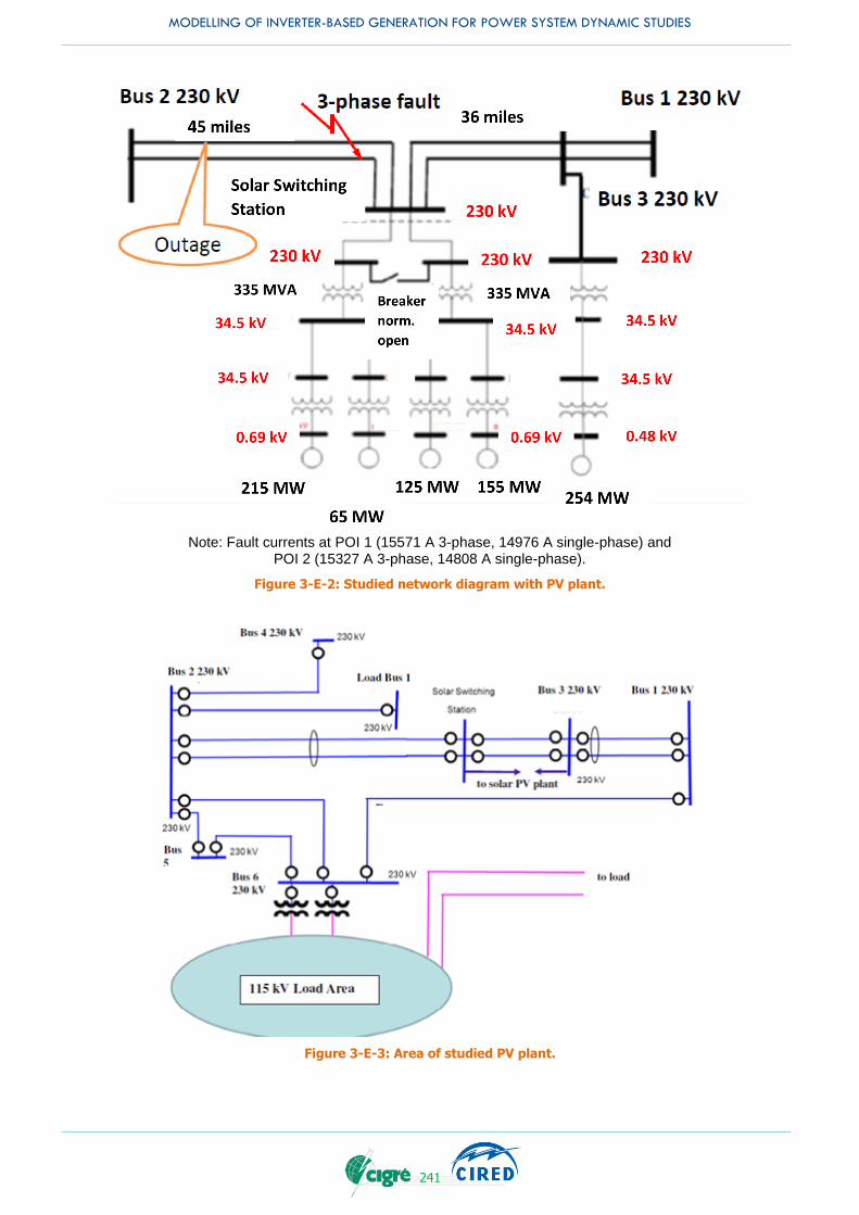
MODELLING OF INVERTER-BASED GENERATION FOR POWER SYSTEM DYNAMIC STUDIES
241
Note: Fault currents at POI 1 (15571 A 3-phase, 14976 A single-phase) and POI 2 (15327 A 3-phase, 14808 A single-phase).
Figure 3-E-2: Studied network diagram with PV plant.
Figure 3-E-3: Area of studied PV plant.

MODELLING OF INVERTER-BASED GENERATION FOR POWER SYSTEM DYNAMIC STUDIES
242
Table 3-E-1: Test Scenarios
Scenario 1 2 3 4 5 6
Generator power factor +/-0.95 +/-0.95 1 1 N/A N/A
Generator Q and V control Yes Yes No No N/A N/A
Network Motor Stalling No Yes No Yes No Yes
Inverter Q priority Yes Yes No No N/A N/A
Inverter P priority No No Yes Yes N/A N/A
Source PV PV PV PV AGCC AGCC
A three-phase 6-cycle fault was modelled at the 230 kV double-circuit transmission line between the Solar Switching Station and the Bus 2 next to the bus of the Solar Switching Station cleared by opening both circuits between the Solar Switching Station and Bus 2. The study monitored dynamic stability performance of the solar PV units and the surrounding system, as well as performance of all Western Interconnection. Several scenarios were studied. They are summarized in the following table and also described below.
1. The Solar PV plant is capable of maintaining power factor between 0.95 lead and 0.95 lag and
controls reactive power and voltage. The inverters have reactive power priority selection in the
current limit logic because in this scenario generator regulates voltage. Plant controller controls
voltage. Stalling of the single-phase air conditioner motor load components is disabled.
2. Same as 1, but stalling of the single-phase air conditioner motor load components is enabled.
3. The Solar PV plant holds unity power factor and provides neither reactive support nor voltage
regulation. The inverters have real power priority in the current limit logic, which means that real
power output of the units is maintained as much as possible at the initial output level. Stalling of the
single-phase air conditioner motor load components is disabled.
4. Same as 3, but stalling of the single-phase air conditioner motor load components is enabled.
5. The Solar PV plant is replaced by a fictitious combined-cycle plant of the same size to compare the
response and to evaluate impact of IBG plant. Stalling of the single-phase air conditioner motor
load components is disabled.
6. Same as bullet point No. 5, but stalling of the single-phase air conditioner motor load components
is enabled.
Chapter 3-E.4 Study results
The following plots illustrate the study results. Figure 3-E-6 shows voltage at the 230 kV bus of the Solar Switching station where the three phase fault was applied. Voltage is shown per unit; only first 5 seconds of the simulation are shown. As can be seen from the plots, voltage recovered to the pre-fault values in all scenarios, except for the solar PV plant with unity power factor. In this case, voltage recovered to a slightly lower value. The inverter-based plant showed even faster recovery than the combined-cycle plant. Whether single-phase air conditioning load stalled or not did not have almost any impact on the voltage on this bus.
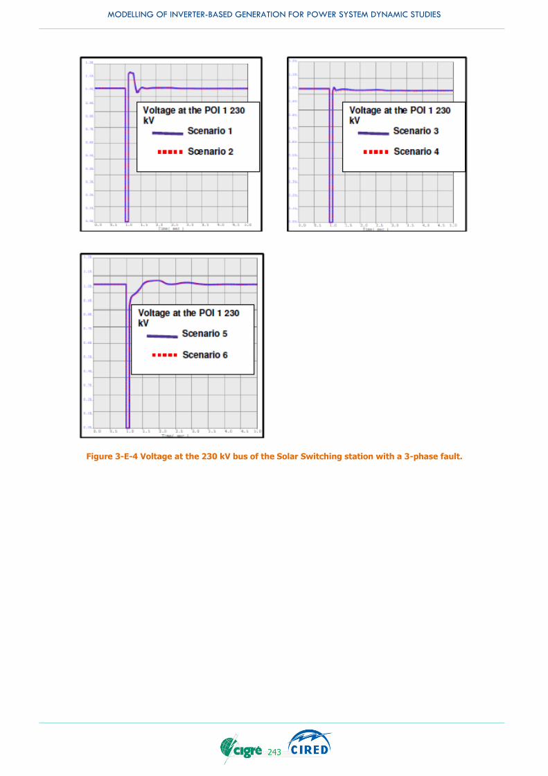
MODELLING OF INVERTER-BASED GENERATION FOR POWER SYSTEM DYNAMIC STUDIES
243
Figure 3-E-4 Voltage at the 230 kV bus of the Solar Switching station with a 3-phase fault.
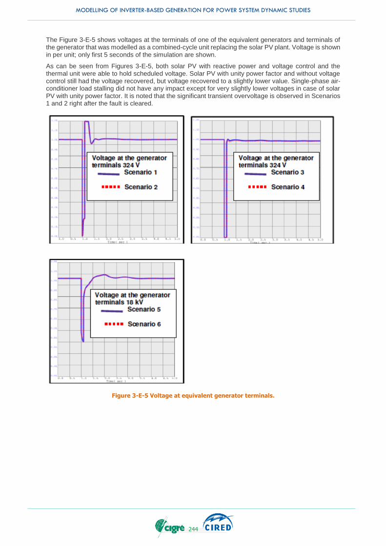
MODELLING OF INVERTER-BASED GENERATION FOR POWER SYSTEM DYNAMIC STUDIES
244
The Figure 3-E-5 shows voltages at the terminals of one of the equivalent generators and terminals of the generator that was modelled as a combined-cycle unit replacing the solar PV plant. Voltage is shown in per unit; only first 5 seconds of the simulation are shown.
As can be seen from Figures 3-E-5, both solar PV with reactive power and voltage control and the thermal unit were able to hold scheduled voltage. Solar PV with unity power factor and without voltage control still had the voltage recovered, but voltage recovered to a slightly lower value. Single-phase air-conditioner load stalling did not have any impact except for very slightly lower voltages in case of solar PV with unity power factor. It is noted that the significant transient overvoltage is observed in Scenarios 1 and 2 right after the fault is cleared.
Figure 3-E-5 Voltage at equivalent generator terminals.

MODELLING OF INVERTER-BASED GENERATION FOR POWER SYSTEM DYNAMIC STUDIES
245
The Figures 3-E-6 and 3-E-7 show real and reactive power response from the solar PV equivalent generator and the replacement combined cycle plant unit. As can be seen from these plots, inverter-based generators had better damping; however, they had slightly slower real power recovery after a fault. Generator in scenarios 3 and 4 (unity power factor) didn’t provide any reactive power output, thus, didn’t provide voltage support. This can be seen in Figure 3-E-7. The studies didn’t show any impact from the single-phase air-conditioners stalling, except for a very slight increase in reactive power output from the generators in scenarios 2 and 6 to compensate for the induction motor stalling
Figure 3-E-6 Active power output from PV equivalent or thermal generator.
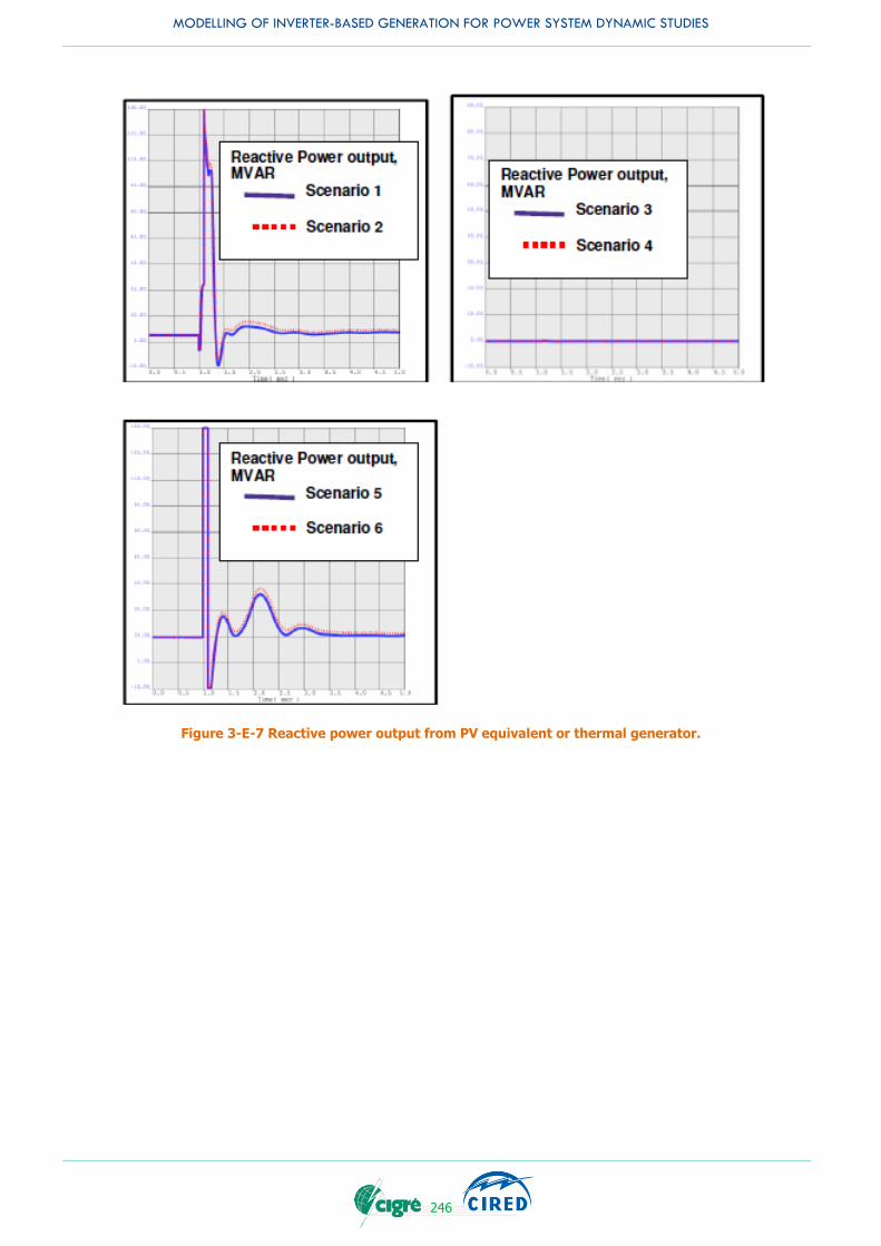
MODELLING OF INVERTER-BASED GENERATION FOR POWER SYSTEM DYNAMIC STUDIES
246
Figure 3-E-7 Reactive power output from PV equivalent or thermal generator.

MODELLING OF INVERTER-BASED GENERATION FOR POWER SYSTEM DYNAMIC STUDIES
247
The Figure 3-E-8 illustrates the voltages in per unit at a load bus close to the fault (Load Bus 1 in Figure 3-E-3). As can be seen from these plots, voltage recovery on the load bus was not impacted by whether the plant was solar PV or combined-cycle. In the cases when stalling of air-conditioners was modelled, the plots showed delayed voltage recovery in all three scenarios.
Figure 3-E-8 Voltage at load bus closed to fault (Load Bus 1, 230 kV).
All six scenarios showed some loss of load due to tripping of induction motor load and sensitivity of some loads to voltage and frequency. The loss of load was rather insignificant and was not much different between the scenarios. In an assumption that single phase air-conditioners don’t stall, loss of load was 66 MW in the case with solar PV plant with 0.95 power factor and voltage control, 67 MW in the case of a solar PV with unity power factor without voltage control and 69 MW in the case of the combined-cycle plant. With stalling of the air-conditioners, the loss of load was respectively 91MW, 96 MW and 97MW. This loss of load was only local, in the area close to the fault.
Chapter 3-E.5 Conclusions
Studies of transient voltage stability performance of a large interconnected transmission system with high penetration of IBG during faults showed that the IBG did not have adverse impact on the system performance. On the contrary, system voltages recovered faster with IBG than with conventional generation and scenarios with IBG showed better damping after a fault. The reasons for better damping and faster voltage recovery are low inertia of the inverter-based generators and fast control of the inverters.
The study was performed in an assumption that the IBG units have FRT capability and are not tripped with transmission system faults such as three phase ground fault on HV network. The IBG models used
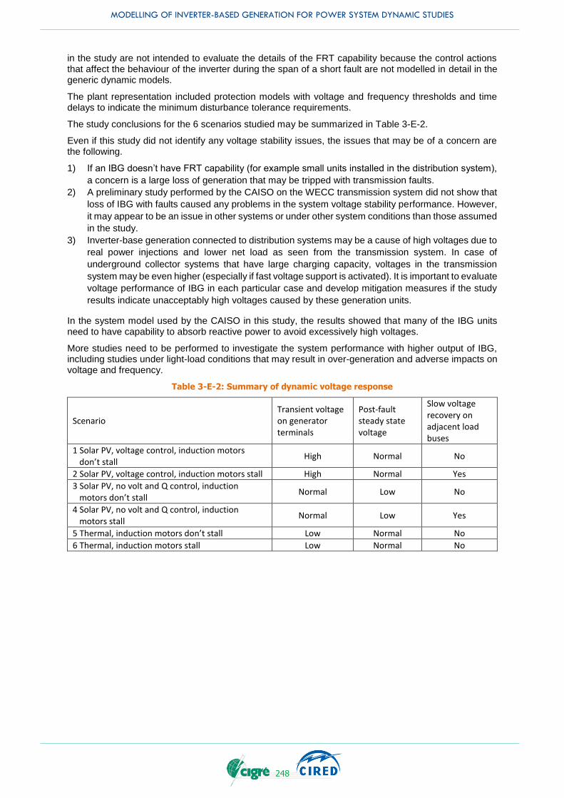
MODELLING OF INVERTER-BASED GENERATION FOR POWER SYSTEM DYNAMIC STUDIES
248
in the study are not intended to evaluate the details of the FRT capability because the control actions that affect the behaviour of the inverter during the span of a short fault are not modelled in detail in the generic dynamic models.
The plant representation included protection models with voltage and frequency thresholds and time delays to indicate the minimum disturbance tolerance requirements.
The study conclusions for the 6 scenarios studied may be summarized in Table 3-E-2.
Even if this study did not identify any voltage stability issues, the issues that may be of a concern are the following.
1) If an IBG doesn’t have FRT capability (for example small units installed in the distribution system),
a concern is a large loss of generation that may be tripped with transmission faults.
2) A preliminary study performed by the CAISO on the WECC transmission system did not show that
loss of IBG with faults caused any problems in the system voltage stability performance. However,
it may appear to be an issue in other systems or under other system conditions than those assumed
in the study.
3) Inverter-base generation connected to distribution systems may be a cause of high voltages due to
real power injections and lower net load as seen from the transmission system. In case of
underground collector systems that have large charging capacity, voltages in the transmission
system may be even higher (especially if fast voltage support is activated). It is important to evaluate
voltage performance of IBG in each particular case and develop mitigation measures if the study
results indicate unacceptably high voltages caused by these generation units.
In the system model used by the CAISO in this study, the results showed that many of the IBG units need to have capability to absorb reactive power to avoid excessively high voltages.
More studies need to be performed to investigate the system performance with higher output of IBG, including studies under light-load conditions that may result in over-generation and adverse impacts on voltage and frequency.
Table 3-E-2: Summary of dynamic voltage response
Scenario Transient voltage on generator terminals
Post-fault steady state voltage
Slow voltage recovery on adjacent load buses
1 Solar PV, voltage control, induction motors don’t stall
High Normal No
2 Solar PV, voltage control, induction motors stall High Normal Yes
3 Solar PV, no volt and Q control, induction motors don’t stall
Normal Low No
4 Solar PV, no volt and Q control, induction motors stall
Normal Low Yes
5 Thermal, induction motors don’t stall Low Normal No
6 Thermal, induction motors stall Low Normal No
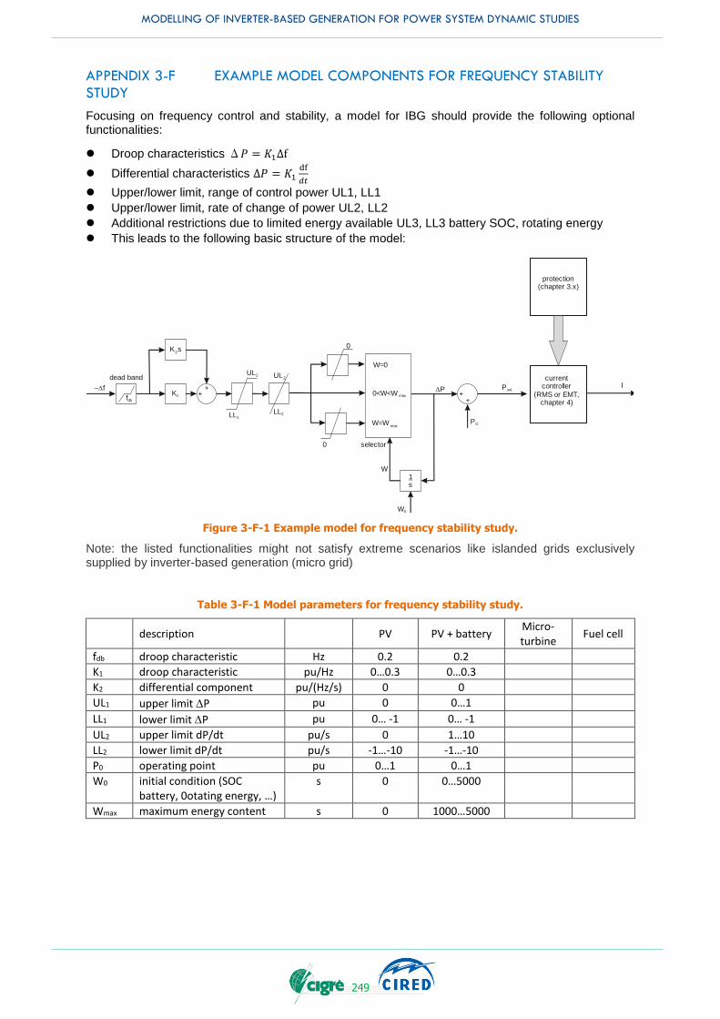
MODELLING OF INVERTER-BASED GENERATION FOR POWER SYSTEM DYNAMIC STUDIES
249
APPENDIX 3-F EXAMPLE MODEL COMPONENTS FOR FREQUENCY STABILITY STUDY
Focusing on frequency control and stability, a model for IBG should provide the following optional functionalities:
Droop characteristics Δ𝑃 = 𝐾1Δf
Differential characteristics Δ𝑃 = 𝐾1df
𝑑𝑡
Upper/lower limit, range of control power UL1, LL1
Upper/lower limit, rate of change of power UL2, LL2
Additional restrictions due to limited energy available UL3, LL3 battery SOC, rotating energy
This leads to the following basic structure of the model:
Figure 3-F-1 Example model for frequency stability study.
Note: the listed functionalities might not satisfy extreme scenarios like islanded grids exclusively supplied by inverter-based generation (micro grid)
Table 3-F-1 Model parameters for frequency stability study.
description
PV PV + battery Micro-turbine
Fuel cell
fdb droop characteristic Hz 0.2 0.2
K1 droop characteristic pu/Hz 0…0.3 0…0.3
K2 differential component pu/(Hz/s) 0 0
UL1 upper limit DP pu 0 0…1
LL1 lower limit DP pu 0… -1 0… -1
UL2 upper limit dP/dt pu/s 0 1…10
LL2 lower limit dP/dt pu/s -1…-10 -1…-10
P0 operating point pu 0…1 0…1
W0 initial condition (SOC battery, 0otating energy, …)
s 0 0…5000
Wmax maximum energy content s 0 1000…5000
current controller
(RMS or EMT,chapter 4)
protection(chapter 3.x)
IPset
++
P0
++
K1
K s2
DP-Df
UL2
LL2
UL1
LL1
1s
0
0
W=0
W=Wmax
0<W<W max
selector
W
W0
dead band
fdb

MODELLING OF INVERTER-BASED GENERATION FOR POWER SYSTEM DYNAMIC STUDIES
250
APPENDIX 3-G HIGHLIGHT OF GRID-CODE REQUIREMENTS IN STEADY STATE
For steady-state analysis, such as power flow analysis, the operating point of IBGs needs to be considered. Recently the reactive power capability has changed mainly due to the evolvement of the grid interconnection code. Figures 3-G-1, 3-G-2, and 3-G-3 shows an example of two commercially available 2500 kW and 3000 kW PV inverters.
(a) 2.5 MW PV inverter (b) 3.0 MW PV inverter
Figure 3-G-1 Example reactive power capability of commercially available inverters (for nominal voltage)[24] .
(a) 2.5 MW PV inverter (b) 3.0 MW PV inverter
Figure 3-G-2 Example reactive power capability of commercially available inverters (for 90% of nominal voltage) [24].
Figure 3-G-3 Example reactive power capability of commercially available inverters (for 110% of nominal voltage) [24].

MODELLING OF INVERTER-BASED GENERATION FOR POWER SYSTEM DYNAMIC STUDIES
251
Chapter 3-G.1.2 Reactive power capability at maximum capacity
Reactive power provision capability requirements in the context of varying voltage. It shall be defined a U-Q/Pmax-profile within the boundaries of which the generator shall be capable of providing reactive power at its maximum capacity. The defined U-Q/Pmax profile may take any shape, having regard to the potential costs of delivering the capability to provide reactive power production at high voltages and reactive power consumption at low voltages.
Chapter 3-G.1.3 Reactive power capability below maximum capacity
Reactive power provision capability requirements. It shall be defined a P-Q/Pmax-profile that may take any shape within the boundaries of which the generator is capable of providing reactive power below maximum capacity.

MODELLING OF INVERTER-BASED GENERATION FOR POWER SYSTEM DYNAMIC STUDIES
252
APPENDIX 3-K PROBABILISTIC APPAROCH FOR DYNAMIC STABILITY STUDY
Probabilistic studies can be used as an additional tool to provide information considering the impact of IBGs on the dynamic behaviour of power systems. The inherent uncertainties of Renewable Energy Sources (RES) operation coupled with electricity market and load (including conventional and new types of load, e.g., electric vehicles) driven uncertainties lead to an overall increase in operating condition-based uncertainties that are becoming one of the key attributes of modern power systems.
It has been acknowledged that the increasing participation of RES in the power generation mix of the system can significantly affect its dynamic behaviour following a disturbance due to multiple reasons: i) RES exhibiting different dynamic behaviour than conventional synchronous generators; ii) the increasing amount of connected RES results in synchronous generators displacement either by de-loading or disconnection; iii) changing power flows in the network depending on RES availability, both temporal and spatial. It has not yet been clarified, let alone quantified, though to what extent each of these influences affects overall system dynamic behaviour [25]. Due to spatial and temporal uncertainties associated with RES operation, in particular, it is neither practical nor feasible to identify easily “worst case scenarios” that are representative enough to capture the overall impact of RES on power system dynamics. Probabilistic methods can be used as a tool to assess various aspects of the dynamic behaviour of power systems with RES [26]-[29].
Chapter 3-K.1 Probabilistic methodology
A number of Ns Monte Carlo (MC) simulations are performed following the procedure explained below. A power system dynamic model suitable for the respective stability studies is required, taking into consideration the connected RES with the associated controllers. Since system stability can be also significantly affected by pre-fault operating conditions, the uncertainties concerning system loading and wind/PV generation for a 24-hour period are considered. Moreover, the uncertainties related to the disturbance (i.e. fault location and duration) are also accounted for. All random variables are sampled according to appropriate probability distributions describing the uncertain parameter behaviour. The sampling of the respective distributions is performed separately for each load and each RES unit in the system to consider independent behaviour of loads and RES units. After the uncertainties in loading and RES contribution to power generation have been accounted for, an Optimal Power Flow (OPF) problem is solved to determine the output of conventional generators. The dispatch obtained from OPF also determines the amount of disconnection of conventional generation and consequently system inertia reduction due to increased RES penetration.
The proposed framework offers full flexibility when accounting for relevant uncertain parameters. The sampling of uncertain factors can be done according to any probability distribution based on historical data, prior knowledge or forecast and solving the OPF problem can include any number of additional security constraints associated with RES, as for example proposed in [30].
Statistical analysis of the obtained results can be useful in drawing conclusions and identifying tendencies considering the dynamic behaviour of the system, from the abundance of available simulated data. For example, plotting Cumulative Distribution Functions (CDFs) of the random variables (i.e. relevant stability indices) can reveal the associated probabilities for the whole range of values each index takes.
Chapter 3-K.2 Uncertainty modelling
The effect of the intermittent behaviour of wind generators and Photo-Voltaic (PV) units is modelled using appropriate Probability Distribution Functions (PDFs) [28],[29]. The uncertainties related to the conventional part of the system such as system loading as well as the investigated disturbances are also included in this study. For system loading and PV generation, typical daily curves are initially used, obtained from national grid data and the literature [29], respectively. The system load is considered to vary from 0.6 to 1 p.u. The hour of the day is sampled randomly and for each hour, an appropriate PDF is used to model the uncertainty within the hour. For system loading a normal distribution with mean value 1 p.u and standard deviation 3.33% is used, while for PV generation, a beta distribution with a and b parameters 13.7 and 1.3. For wind generation, a Weibull distribution is used with φ =11.1 and k=2.2, assuming constant mean wind speed for every hour within the day. For each load within the system and each DER unit, the PDFs are sampled separately, to consider independent behaviour of each unit. For example, assuming the total load is 0.8 p.u. for a given hour of the day, one load might have a value of 0.75pu and another 0.85pu.
Frequency stability studies are performed for three operating conditions of the network, nominal loading, 60% and 40% loading of the network.
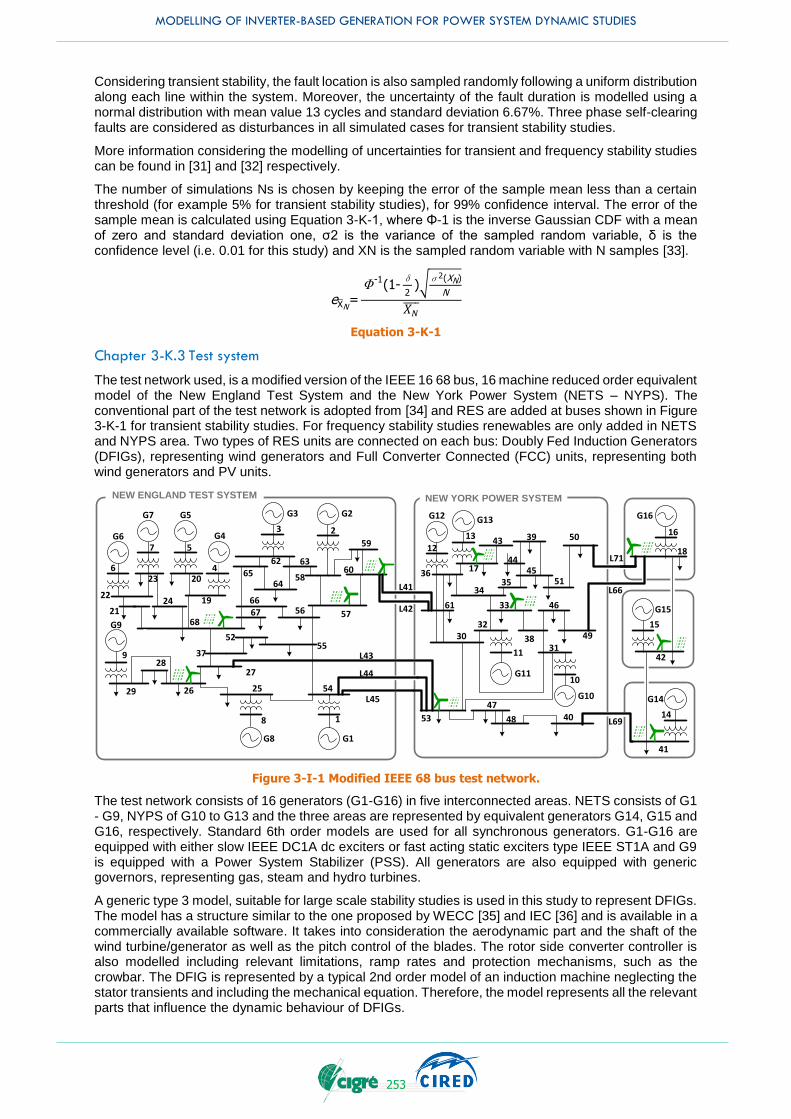
MODELLING OF INVERTER-BASED GENERATION FOR POWER SYSTEM DYNAMIC STUDIES
253
Considering transient stability, the fault location is also sampled randomly following a uniform distribution along each line within the system. Moreover, the uncertainty of the fault duration is modelled using a normal distribution with mean value 13 cycles and standard deviation 6.67%. Three phase self-clearing faults are considered as disturbances in all simulated cases for transient stability studies.
More information considering the modelling of uncertainties for transient and frequency stability studies can be found in [31] and [32] respectively.
The number of simulations Ns is chosen by keeping the error of the sample mean less than a certain threshold (for example 5% for transient stability studies), for 99% confidence interval. The error of the sample mean is calculated using Equation 3-K-1, where Φ-1 is the inverse Gaussian CDF with a mean of zero and standard deviation one, σ2 is the variance of the sampled random variable, δ is the confidence level (i.e. 0.01 for this study) and XN is the sampled random variable with N samples [33].
eXN=Φ-1
(1-δ
2)√σ2(XN)
N
𝑋𝑁
Equation 3-K-1
Chapter 3-K.3 Test system
The test network used, is a modified version of the IEEE 16 68 bus, 16 machine reduced order equivalent model of the New England Test System and the New York Power System (NETS – NYPS). The conventional part of the test network is adopted from [34] and RES are added at buses shown in Figure 3-K-1 for transient stability studies. For frequency stability studies renewables are only added in NETS and NYPS area. Two types of RES units are connected on each bus: Doubly Fed Induction Generators (DFIGs), representing wind generators and Full Converter Connected (FCC) units, representing both wind generators and PV units.
Figure 3-I-1 Modified IEEE 68 bus test network.
The test network consists of 16 generators (G1-G16) in five interconnected areas. NETS consists of G1 - G9, NYPS of G10 to G13 and the three areas are represented by equivalent generators G14, G15 and G16, respectively. Standard 6th order models are used for all synchronous generators. G1-G16 are equipped with either slow IEEE DC1A dc exciters or fast acting static exciters type IEEE ST1A and G9 is equipped with a Power System Stabilizer (PSS). All generators are also equipped with generic governors, representing gas, steam and hydro turbines.
A generic type 3 model, suitable for large scale stability studies is used in this study to represent DFIGs. The model has a structure similar to the one proposed by WECC [35] and IEC [36] and is available in a commercially available software. It takes into consideration the aerodynamic part and the shaft of the wind turbine/generator as well as the pitch control of the blades. The rotor side converter controller is also modelled including relevant limitations, ramp rates and protection mechanisms, such as the crowbar. The DFIG is represented by a typical 2nd order model of an induction machine neglecting the stator transients and including the mechanical equation. Therefore, the model represents all the relevant parts that influence the dynamic behaviour of DFIGs.
G7
G6 G4
G5 G3 G2
G8 G1
G9
G16
G15
G14
G12 G13
G11
G10
NEW ENGLAND TEST SYSTEM NEW YORK POWER SYSTEM
9
29
28
26 25
8
54
1 53
47
48 40
10
31
46
49
11
3032
33
34
61
36
12
17
1343
44
39
4535 51
50
60
59
57
5552
27
37
3 2
4
57
6
22
21
23
68
24
20
19
62
6563
5864
6667 56
16
18
15
42
14
41
L44
L43
L71
L66
L69
L41
L42
L45
38
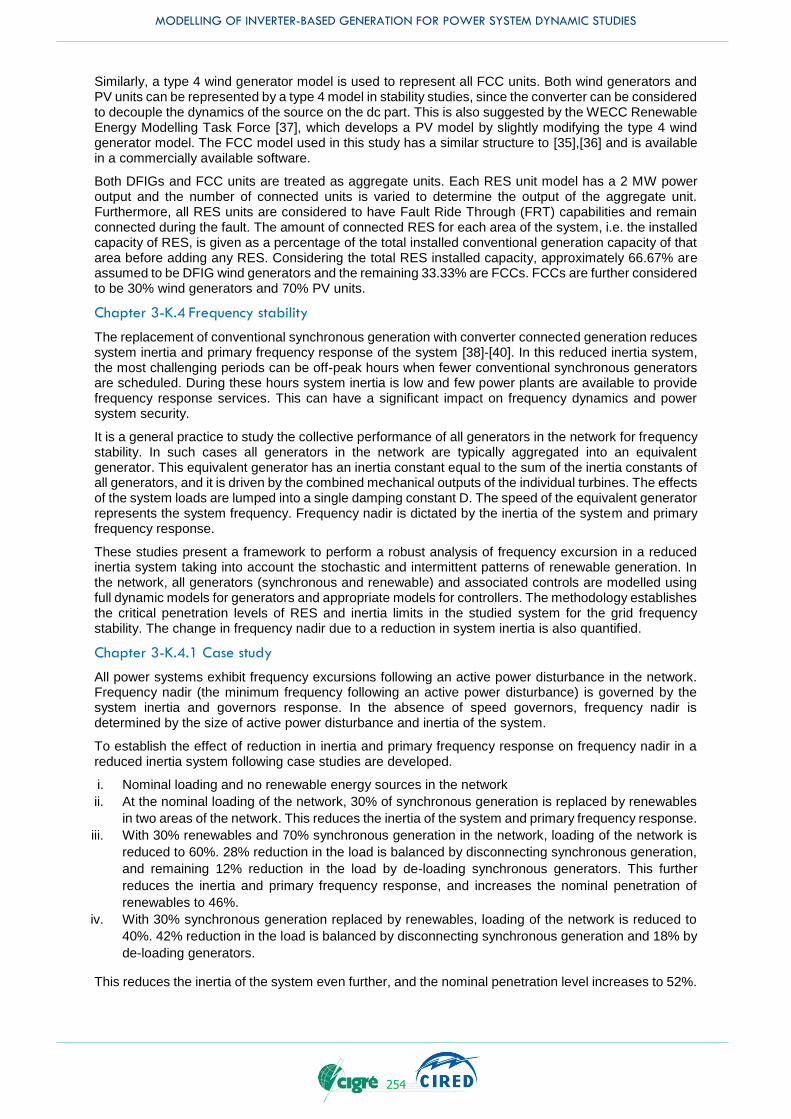
MODELLING OF INVERTER-BASED GENERATION FOR POWER SYSTEM DYNAMIC STUDIES
254
Similarly, a type 4 wind generator model is used to represent all FCC units. Both wind generators and PV units can be represented by a type 4 model in stability studies, since the converter can be considered to decouple the dynamics of the source on the dc part. This is also suggested by the WECC Renewable Energy Modelling Task Force [37], which develops a PV model by slightly modifying the type 4 wind generator model. The FCC model used in this study has a similar structure to [35],[36] and is available in a commercially available software.
Both DFIGs and FCC units are treated as aggregate units. Each RES unit model has a 2 MW power output and the number of connected units is varied to determine the output of the aggregate unit. Furthermore, all RES units are considered to have Fault Ride Through (FRT) capabilities and remain connected during the fault. The amount of connected RES for each area of the system, i.e. the installed capacity of RES, is given as a percentage of the total installed conventional generation capacity of that area before adding any RES. Considering the total RES installed capacity, approximately 66.67% are assumed to be DFIG wind generators and the remaining 33.33% are FCCs. FCCs are further considered to be 30% wind generators and 70% PV units.
Chapter 3-K.4 Frequency stability
The replacement of conventional synchronous generation with converter connected generation reduces system inertia and primary frequency response of the system [38]-[40]. In this reduced inertia system, the most challenging periods can be off-peak hours when fewer conventional synchronous generators are scheduled. During these hours system inertia is low and few power plants are available to provide frequency response services. This can have a significant impact on frequency dynamics and power system security.
It is a general practice to study the collective performance of all generators in the network for frequency stability. In such cases all generators in the network are typically aggregated into an equivalent generator. This equivalent generator has an inertia constant equal to the sum of the inertia constants of all generators, and it is driven by the combined mechanical outputs of the individual turbines. The effects of the system loads are lumped into a single damping constant D. The speed of the equivalent generator represents the system frequency. Frequency nadir is dictated by the inertia of the system and primary frequency response.
These studies present a framework to perform a robust analysis of frequency excursion in a reduced inertia system taking into account the stochastic and intermittent patterns of renewable generation. In the network, all generators (synchronous and renewable) and associated controls are modelled using full dynamic models for generators and appropriate models for controllers. The methodology establishes the critical penetration levels of RES and inertia limits in the studied system for the grid frequency stability. The change in frequency nadir due to a reduction in system inertia is also quantified.
Chapter 3-K.4.1 Case study
All power systems exhibit frequency excursions following an active power disturbance in the network. Frequency nadir (the minimum frequency following an active power disturbance) is governed by the system inertia and governors response. In the absence of speed governors, frequency nadir is determined by the size of active power disturbance and inertia of the system.
To establish the effect of reduction in inertia and primary frequency response on frequency nadir in a reduced inertia system following case studies are developed.
i. Nominal loading and no renewable energy sources in the network
ii. At the nominal loading of the network, 30% of synchronous generation is replaced by renewables
in two areas of the network. This reduces the inertia of the system and primary frequency response.
iii. With 30% renewables and 70% synchronous generation in the network, loading of the network is
reduced to 60%. 28% reduction in the load is balanced by disconnecting synchronous generation,
and remaining 12% reduction in the load by de-loading synchronous generators. This further
reduces the inertia and primary frequency response, and increases the nominal penetration of
renewables to 46%.
iv. With 30% synchronous generation replaced by renewables, loading of the network is reduced to
40%. 42% reduction in the load is balanced by disconnecting synchronous generation and 18% by
de-loading generators.
This reduces the inertia of the system even further, and the nominal penetration level increases to 52%.
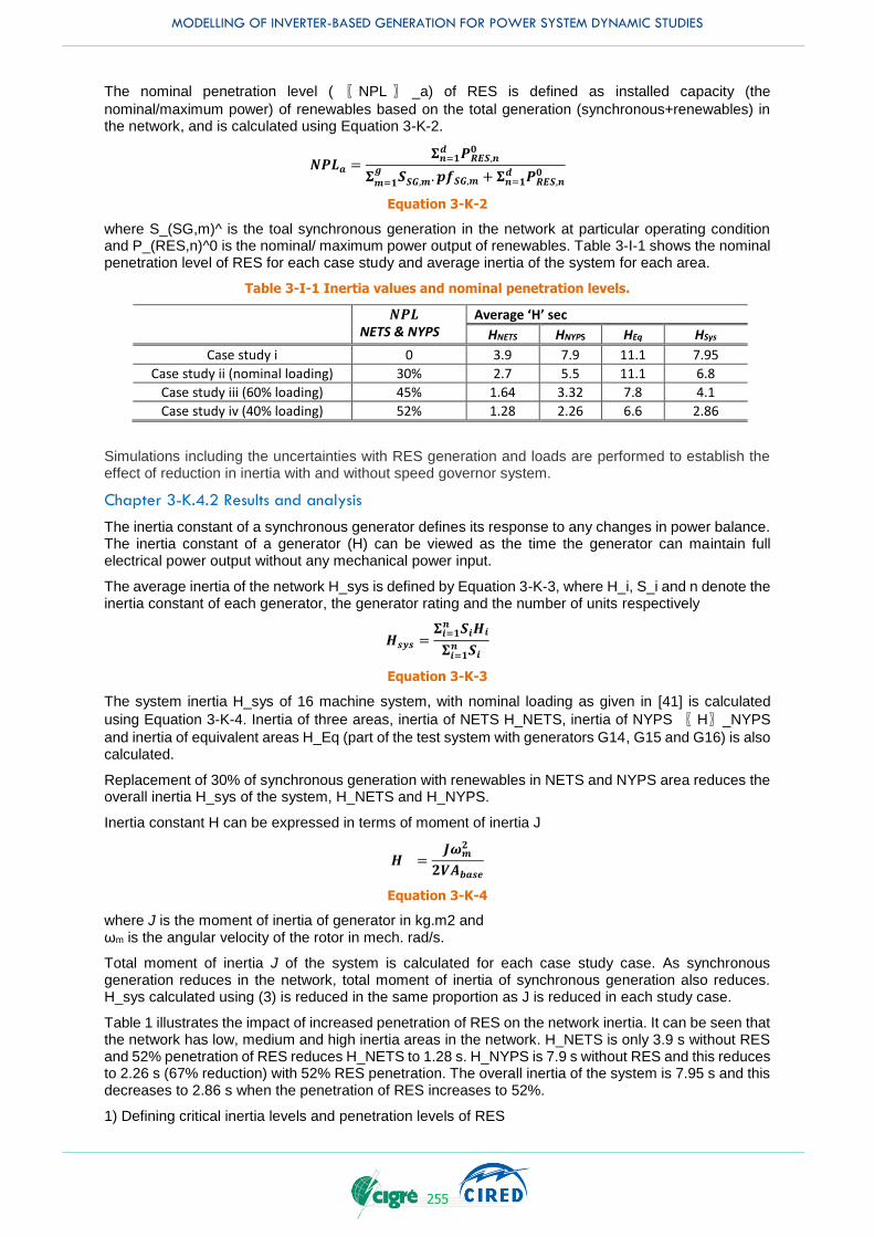
MODELLING OF INVERTER-BASED GENERATION FOR POWER SYSTEM DYNAMIC STUDIES
255
The nominal penetration level ( 〖 NPL 〗 _a) of RES is defined as installed capacity (the
nominal/maximum power) of renewables based on the total generation (synchronous+renewables) in the network, and is calculated using Equation 3-K-2.
𝑵𝑷𝑳𝒂 =𝚺𝒏=𝟏
𝒅 𝑷𝑹𝑬𝑺,𝒏𝟎
𝚺𝒎=𝟏𝒈
𝑺𝑺𝑮,𝒎. 𝒑𝒇𝑺𝑮,𝒎 + 𝚺𝒏=𝟏𝒅 𝑷𝑹𝑬𝑺,𝒏
𝟎
Equation 3-K-2
where S_(SG,m)^ is the toal synchronous generation in the network at particular operating condition and P_(RES,n)^0 is the nominal/ maximum power output of renewables. Table 3-I-1 shows the nominal penetration level of RES for each case study and average inertia of the system for each area.
Table 3-I-1 Inertia values and nominal penetration levels.
𝑵𝑷𝑳 NETS & NYPS
Average ‘H’ sec
HNETS HNYPS HEq HSys
Case study i 0 3.9 7.9 11.1 7.95
Case study ii (nominal loading) 30% 2.7 5.5 11.1 6.8
Case study iii (60% loading) 45% 1.64 3.32 7.8 4.1
Case study iv (40% loading) 52% 1.28 2.26 6.6 2.86
Simulations including the uncertainties with RES generation and loads are performed to establish the effect of reduction in inertia with and without speed governor system.
Chapter 3-K.4.2 Results and analysis
The inertia constant of a synchronous generator defines its response to any changes in power balance. The inertia constant of a generator (H) can be viewed as the time the generator can maintain full electrical power output without any mechanical power input.
The average inertia of the network H_sys is defined by Equation 3-K-3, where H_i, S_i and n denote the inertia constant of each generator, the generator rating and the number of units respectively
𝑯𝒔𝒚𝒔 =𝚺𝒊=𝟏
𝒏 𝑺𝒊𝑯𝒊
𝚺𝒊=𝟏𝒏 𝑺𝒊
Equation 3-K-3
The system inertia H_sys of 16 machine system, with nominal loading as given in [41] is calculated
using Equation 3-K-4. Inertia of three areas, inertia of NETS H_NETS, inertia of NYPS 〖 H〗_NYPS
and inertia of equivalent areas H_Eq (part of the test system with generators G14, G15 and G16) is also calculated.
Replacement of 30% of synchronous generation with renewables in NETS and NYPS area reduces the overall inertia H_sys of the system, H_NETS and H_NYPS.
Inertia constant H can be expressed in terms of moment of inertia J
𝑯 =𝑱𝝎𝒎
𝟐
𝟐𝑽𝑨𝒃𝒂𝒔𝒆
Equation 3-K-4
where J is the moment of inertia of generator in kg.m2 and ωm is the angular velocity of the rotor in mech. rad/s.
Total moment of inertia J of the system is calculated for each case study case. As synchronous generation reduces in the network, total moment of inertia of synchronous generation also reduces. H_sys calculated using (3) is reduced in the same proportion as J is reduced in each study case.
Table 1 illustrates the impact of increased penetration of RES on the network inertia. It can be seen that the network has low, medium and high inertia areas in the network. H_NETS is only 3.9 s without RES and 52% penetration of RES reduces H_NETS to 1.28 s. H_NYPS is 7.9 s without RES and this reduces to 2.26 s (67% reduction) with 52% RES penetration. The overall inertia of the system is 7.95 s and this decreases to 2.86 s when the penetration of RES increases to 52%.
1) Defining critical inertia levels and penetration levels of RES

MODELLING OF INVERTER-BASED GENERATION FOR POWER SYSTEM DYNAMIC STUDIES
256
As the inertia of the system reduces due to disconnection of synchronous generation and increased nominal penetration of renewables, small variations in the active power cause bigger variation in frequency nadir. In these studies, a threshold of 500mHz for frequency nadir variation is considered. When ±10% variation in active power disturbance leads to a variation in frequency nadir greater than 500 mHz; the inertia of the system and the nominal penetration level of RES in the network is considered to be critical. Variation in active power disturbance and threshold for frequency nadir can be customized.
2) Impact of increased penetration of RES on system inertia for each studied operating condition
Modelling the stochastic and intermittent behaviour of the wind and solar generation, and uncertainties in the loading forecast changes the instantaneous penetration level of RES in NETS and NYPS at each operating condition in continuous manner as shown in Figure 3-K-2. Instantaneous penetration of renewables PLia of the area is calculated as
𝑷𝑳𝒊𝒂 =𝚺𝒏=𝟏
𝒅 𝑷𝑹𝑬𝑺,𝒊𝒏
𝚺𝒎=𝟏𝒈
𝑷𝑺𝑮,𝒊𝒎 + 𝚺𝒏=𝟏𝒅 𝑷𝑹𝑬𝑺,𝒊𝒏
Equation 3-K-5
The subscript i=1…1000 denotes the dynamic simulations number, a =1…5 the system area, g the generator number and d the wind and solar farm number. Where P_(RES,in) is the active power produced by the wind and solar farm in the area, P_(SG,im) is the power generated by each synchronous generator in the area.
Simulations are performed by introducing an active power disturbance of 1340MW (a simultaneous outage of G2, G7 and G10) for each operating point. Due to uncertainties in loads and renewables, the power output of generators varies by ±10%. Therefore, active power disturbance varies within ±10% of 1350MW. Frequency nadir following this active power disturbance is recorded on each tie-line between NETS and NYPS area. Power transfer through line L41 is the highest; therefore, frequency nadir at L41 is discussed throughout this work It can be seen from Figure 3-K-2, penetration levels of RES vary between 10%-30%, 18-46% and 28%-64% at the nominal, 60% and 40% loading respectively.
Figure 3-K-2 Inertia of system plotted against instantaneous penetration of renewables.
For the same installed capacity of RES, the instant percentage penetration of RES and the range of its variation increases with the increase in disconnection of synchronous generation. It can also be observed from Figure 3-K-2 that penetration levels of RES at 60% loading overlap penetration levels at nominal loading and 40% loading. However, the band of variation of frequency nadir for each operating condition is distinct.
In this analysis, the inertia of the system is constant for one operating conditions and only varies with the operating condition of the network. The small variations in the active power disturbance result in small variations in frequency nadir within one operating condition. The variation range in frequency nadir within one operating condition increases as the inertia of the system reduces.
Figure 3-K-3 Inertia of system plotted against instantaneous penetration of renewables.
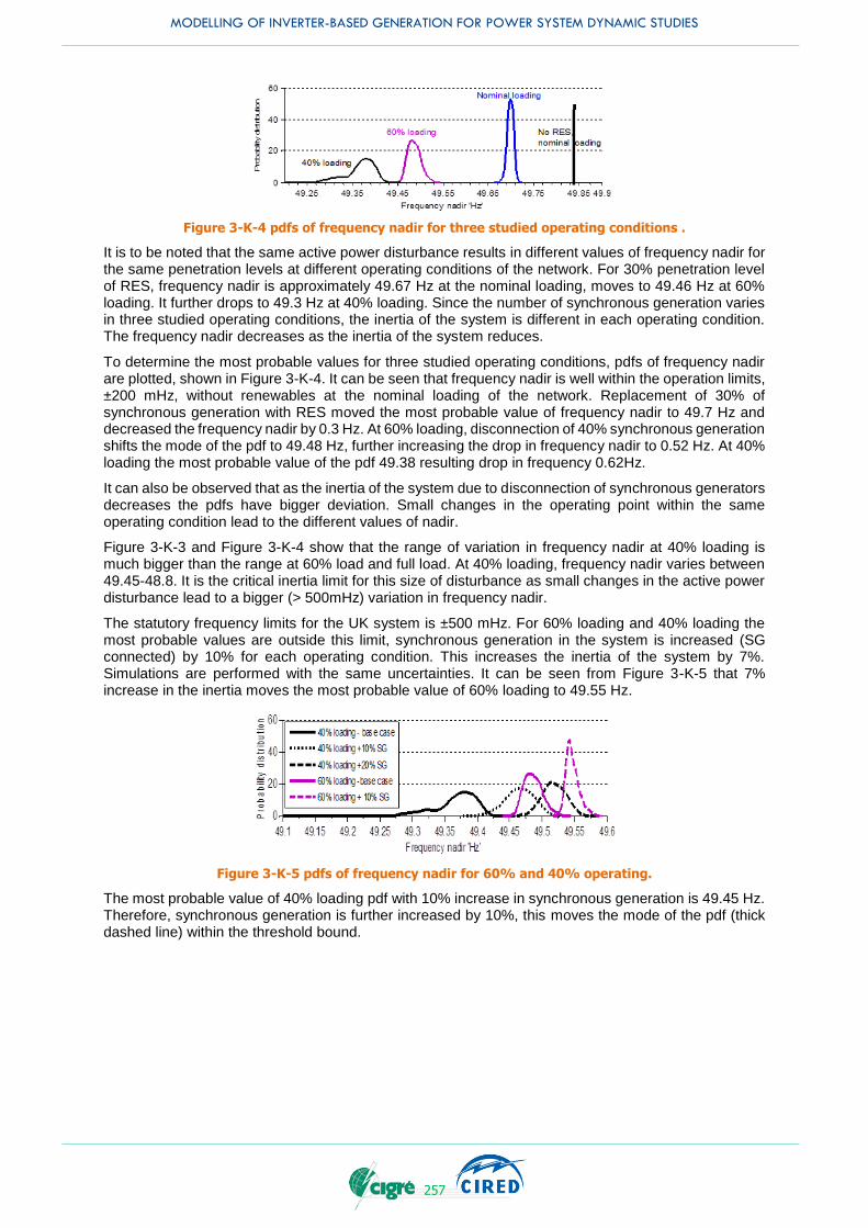
MODELLING OF INVERTER-BASED GENERATION FOR POWER SYSTEM DYNAMIC STUDIES
257
Figure 3-K-4 pdfs of frequency nadir for three studied operating conditions .
It is to be noted that the same active power disturbance results in different values of frequency nadir for the same penetration levels at different operating conditions of the network. For 30% penetration level of RES, frequency nadir is approximately 49.67 Hz at the nominal loading, moves to 49.46 Hz at 60% loading. It further drops to 49.3 Hz at 40% loading. Since the number of synchronous generation varies in three studied operating conditions, the inertia of the system is different in each operating condition. The frequency nadir decreases as the inertia of the system reduces.
To determine the most probable values for three studied operating conditions, pdfs of frequency nadir are plotted, shown in Figure 3-K-4. It can be seen that frequency nadir is well within the operation limits, ±200 mHz, without renewables at the nominal loading of the network. Replacement of 30% of synchronous generation with RES moved the most probable value of frequency nadir to 49.7 Hz and decreased the frequency nadir by 0.3 Hz. At 60% loading, disconnection of 40% synchronous generation shifts the mode of the pdf to 49.48 Hz, further increasing the drop in frequency nadir to 0.52 Hz. At 40% loading the most probable value of the pdf 49.38 resulting drop in frequency 0.62Hz.
It can also be observed that as the inertia of the system due to disconnection of synchronous generators decreases the pdfs have bigger deviation. Small changes in the operating point within the same operating condition lead to the different values of nadir.
Figure 3-K-3 and Figure 3-K-4 show that the range of variation in frequency nadir at 40% loading is much bigger than the range at 60% load and full load. At 40% loading, frequency nadir varies between 49.45-48.8. It is the critical inertia limit for this size of disturbance as small changes in the active power disturbance lead to a bigger (> 500mHz) variation in frequency nadir.
The statutory frequency limits for the UK system is ±500 mHz. For 60% loading and 40% loading the most probable values are outside this limit, synchronous generation in the system is increased (SG connected) by 10% for each operating condition. This increases the inertia of the system by 7%. Simulations are performed with the same uncertainties. It can be seen from Figure 3-K-5 that 7% increase in the inertia moves the most probable value of 60% loading to 49.55 Hz.
Figure 3-K-5 pdfs of frequency nadir for 60% and 40% operating.
The most probable value of 40% loading pdf with 10% increase in synchronous generation is 49.45 Hz. Therefore, synchronous generation is further increased by 10%, this moves the mode of the pdf (thick dashed line) within the threshold bound.
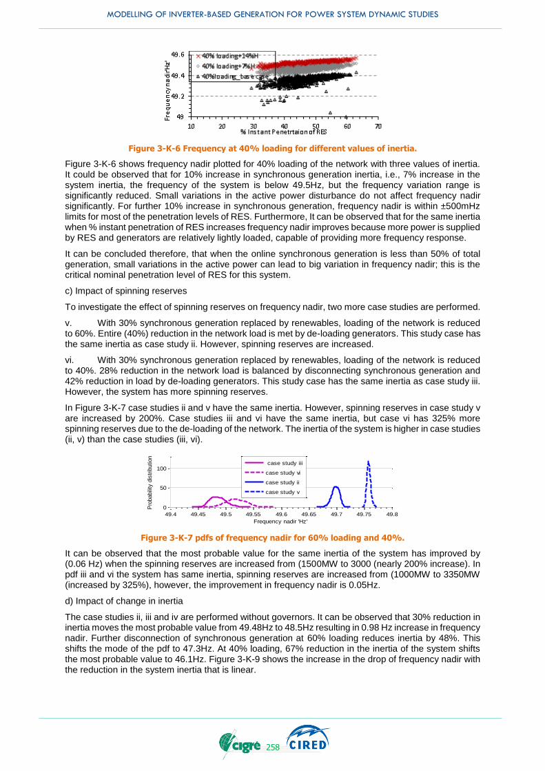
MODELLING OF INVERTER-BASED GENERATION FOR POWER SYSTEM DYNAMIC STUDIES
258
Figure 3-K-6 Frequency at 40% loading for different values of inertia.
Figure 3-K-6 shows frequency nadir plotted for 40% loading of the network with three values of inertia. It could be observed that for 10% increase in synchronous generation inertia, i.e., 7% increase in the system inertia, the frequency of the system is below 49.5Hz, but the frequency variation range is significantly reduced. Small variations in the active power disturbance do not affect frequency nadir significantly. For further 10% increase in synchronous generation, frequency nadir is within ±500mHz limits for most of the penetration levels of RES. Furthermore, It can be observed that for the same inertia when % instant penetration of RES increases frequency nadir improves because more power is supplied by RES and generators are relatively lightly loaded, capable of providing more frequency response.
It can be concluded therefore, that when the online synchronous generation is less than 50% of total generation, small variations in the active power can lead to big variation in frequency nadir; this is the critical nominal penetration level of RES for this system.
c) Impact of spinning reserves
To investigate the effect of spinning reserves on frequency nadir, two more case studies are performed.
v. With 30% synchronous generation replaced by renewables, loading of the network is reduced to 60%. Entire (40%) reduction in the network load is met by de-loading generators. This study case has the same inertia as case study ii. However, spinning reserves are increased.
vi. With 30% synchronous generation replaced by renewables, loading of the network is reduced to 40%. 28% reduction in the network load is balanced by disconnecting synchronous generation and 42% reduction in load by de-loading generators. This study case has the same inertia as case study iii. However, the system has more spinning reserves.
In Figure 3-K-7 case studies ii and v have the same inertia. However, spinning reserves in case study v are increased by 200%. Case studies iii and vi have the same inertia, but case vi has 325% more spinning reserves due to the de-loading of the network. The inertia of the system is higher in case studies (ii, v) than the case studies (iii, vi).
Figure 3-K-7 pdfs of frequency nadir for 60% loading and 40%.
It can be observed that the most probable value for the same inertia of the system has improved by (0.06 Hz) when the spinning reserves are increased from (1500MW to 3000 (nearly 200% increase). In pdf iii and vi the system has same inertia, spinning reserves are increased from (1000MW to 3350MW (increased by 325%), however, the improvement in frequency nadir is 0.05Hz.
d) Impact of change in inertia
The case studies ii, iii and iv are performed without governors. It can be observed that 30% reduction in inertia moves the most probable value from 49.48Hz to 48.5Hz resulting in 0.98 Hz increase in frequency nadir. Further disconnection of synchronous generation at 60% loading reduces inertia by 48%. This shifts the mode of the pdf to 47.3Hz. At 40% loading, 67% reduction in the inertia of the system shifts the most probable value to 46.1Hz. Figure 3-K-9 shows the increase in the drop of frequency nadir with the reduction in the system inertia that is linear.
49.4 49.45 49.5 49.55 49.6 49.65 49.7 49.75 49.8
0
50
100
Frequency nadir 'Hz'
Pro
babili
ty d
istr
ibution
case study iii
case study vi
case study ii
case study v

MODELLING OF INVERTER-BASED GENERATION FOR POWER SYSTEM DYNAMIC STUDIES
259
Figure 3-K-8 pdfs of frequency nadir for three operating conditions without governors.
Figure 3-K-9 Variation in frequency nadir corresponding to variation in inertia.
This work presented an approach to perform a robust analysis of the effect of reduction in inertia and primary response of frequency excursions in a large system. The analysis successfully established the reduction in inertia limits and the critical nominal penetration level of RES for the grid frequency in the test system. The results established when nominal penetration level of RES generation is higher than the online synchronous generation; small changes in the active power disturbance can lead to much bigger variation in frequency nadir.
The performed analysis also shows that amount of spinning reserves required to mitigate the frequency nadir as the inertia of the system decreases.
Chapter 3-K.5 Transient stability
Chapter 3-K.5.1 Transient stability indices
The percentage of cases that each generator is exhibiting instability (i.e. the probability of instability of each generator) is a measure of how stable each generator is. Critical generators and generator groups can be identified in this way. The overall impact of RES on transient stability can be investigated by observing changes in the probability of instability of the generators. The effect of added uncertainties and of the different dynamic behaviour of RES units on system stability is identified in this way.
Transient Stability Index (TSI) is an index considering the stability of the whole system for a specific contingency [42]. Negative value of the TSI means that the case is unstable since the difference between rotor angles of at least two generators for the same time instance is more than 360 degrees.
max,
max,
360100
360
i
i
i
TSI
-
+
Equation 3-K-6
where δmax,i is the maximum rotor angle deviation between any two generators in the system for the same time instance.
An additional measure is used to identify the impact of conventional generation disconnection on transient stability of the system. When RES is connected, this will eventually lead to conventional generation disconnection. The generator spare capacity SCig, defined in Equation 3-K-7, is a measure of the conventional generator loading which is an important parameter considering transient stability. Moreover, when spare capacity is kept low this means that in general more conventional generation will be disconnected leading also to lower system inertia. The effect of conventional generation spare capacity on transient stability is also investigated in this study.
,
, ,
1SG ig
ig
SG ig SG ig
PSC
S pf -
Equation 3-K-7
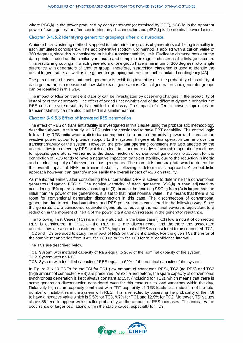
MODELLING OF INVERTER-BASED GENERATION FOR POWER SYSTEM DYNAMIC STUDIES
260
where PSG,ig is the power produced by each generator (determined by OPF), SSG,ig is the apparent power of each generator after considering any disconnection and pfSG,ig is the nominal power factor.
Chapter 3-K.5.2 Identifying generator groupings after a disturbance
A hierarchical clustering method is applied to determine the groups of generators exhibiting instability in each simulated contingency. The agglomerative (bottom up) method is applied with a cut-off value of 360 degrees, since this is considered to be the transient stability limit. Euclidean distance between the data points is used as the similarity measure and complete linkage is chosen as the linkage criterion. This results in groupings in which generators of one group have a minimum of 360 degrees rotor angle difference with generators of another group. Therefore, hierarchical clustering is used to identify the unstable generators as well as the generator grouping patterns for each simulated contingency [43].
The percentage of cases that each generator is exhibiting instability (i.e. the probability of instability of each generator) is a measure of how stable each generator is. Critical generators and generator groups can be identified in this way.
The impact of RES on transient stability can be investigated by observing changes in the probability of instability of the generators. The effect of added uncertainties and of the different dynamic behaviour of RES units on system stability is identified in this way. The impact of different network topologies on transient stability can be also identified in a similar manner.
Chapter 3-K.5.3 Effect of increased RES penetration
The effect of RES on transient stability is investigated in this clause using the probabilistic methodology described above. In this study, all RES units are considered to have FRT capability. The control logic followed by RES units when a disturbance happens is to reduce the active power and increase the reactive power output to provide support to the system. In general, this operation can improve the transient stability of the system. However, the pre-fault operating conditions are also affected by the uncertainties introduced by RES, which can lead to either more or less favourable operating conditions for specific generators. Furthermore, the disconnection of conventional generation to account for the connection of RES tends to have a negative impact on transient stability, due to the reduction in inertia and nominal capacity of the synchronous generators. Therefore, it is not straightforward to determine the overall impact of RES on transient stability following a deterministic approach. A probabilistic approach however, can quantify more easily the overall impact of RES on stability.
As mentioned earlier, after considering the uncertainties OPF is solved to determine the conventional generators dispatch PSG,ig. The nominal capacity of each generator SSG,ig is then adjusted by considering 15% spare capacity according to (3). In case the resulting SSG,ig from (3) is larger than the initial nominal power of the generators, it is set to that initial nominal value. This means that there is no room for conventional generation disconnection in this case. The disconnection of conventional generation due to both load variations and RES penetration is considered in the following way: Since the generators are considered equivalent generators, reducing the nominal power, is equivalent to a reduction in the moment of inertia of the power plant and an increase in the generator reactance.
The following Test Cases (TCs) are initially studied: In the base case (TC1) low amount of connected RES is considered. In TC2, all the RES units are disconnected and therefore the associated uncertainties are also not considered. In TC3, high amount of RES is considered to be connected. TC1, TC2 and TC3 are used to study the impact of RES on transient stability. For the given TCs the error of the sample mean varies from 3.4% for TC3 up to 5% for TC3 for 99% confidence interval.
The TCs are described below;
TC1: System with installed capacity of RES equal to 20% of the nominal capacity of the system TC2: System with no RES TC3: System with installed capacity of RES equal to 60% of the nominal capacity of the system.
In Figure 3-K-10 CDFs for the TSI for TC1 (low amount of connected RES), TC2 (no RES) and TC3 (high amount of connected RES) are presented. As explained before, the spare capacity of conventional synchronous generation is kept always constant at 15% (including for TC2), which means that there is some generation disconnection considered even for this case due to load variations within the day. Relatively high spare capacity combined with FRT capability of RES leads to a reduction of the total number of instabilities in the system with RES. This is reflected by observing the probability of the TSI to have a negative value which is 9.5% for TC3, 9.7% for TC1 and 12.9% for TC2. Moreover, TSI values above 55 tend to appear with smaller probability as the amount of RES increases. This indicates the occurrence of larger oscillations within the stable cases, especially for TC3.
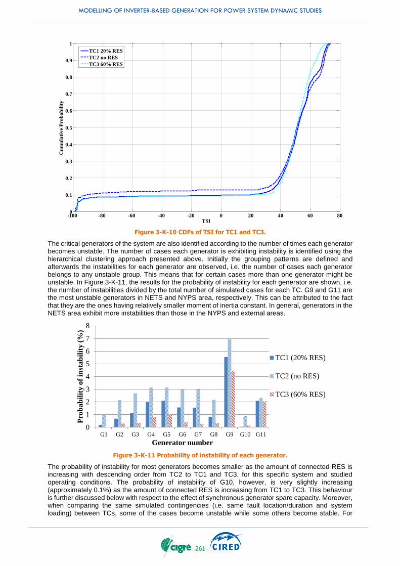
MODELLING OF INVERTER-BASED GENERATION FOR POWER SYSTEM DYNAMIC STUDIES
261
Figure 3-K-10 CDFs of TSI for TC1 and TC3.
The critical generators of the system are also identified according to the number of times each generator becomes unstable. The number of cases each generator is exhibiting instability is identified using the hierarchical clustering approach presented above. Initially the grouping patterns are defined and afterwards the instabilities for each generator are observed, i.e. the number of cases each generator belongs to any unstable group. This means that for certain cases more than one generator might be unstable. In Figure 3-K-11, the results for the probability of instability for each generator are shown, i.e. the number of instabilities divided by the total number of simulated cases for each TC. G9 and G11 are the most unstable generators in NETS and NYPS area, respectively. This can be attributed to the fact that they are the ones having relatively smaller moment of inertia constant. In general, generators in the NETS area exhibit more instabilities than those in the NYPS and external areas.
Figure 3-K-11 Probability of instability of each generator.
The probability of instability for most generators becomes smaller as the amount of connected RES is increasing with descending order from TC2 to TC1 and TC3, for this specific system and studied operating conditions. The probability of instability of G10, however, is very slightly increasing (approximately 0.1%) as the amount of connected RES is increasing from TC1 to TC3. This behaviour is further discussed below with respect to the effect of synchronous generator spare capacity. Moreover, when comparing the same simulated contingencies (i.e. same fault location/duration and system loading) between TCs, some of the cases become unstable while some others become stable. For
-100 -80 -60 -40 -20 0 20 40 60 800
0.1
0.2
0.3
0.4
0.5
0.6
0.7
0.8
0.9
1
TSI
Cu
mu
lati
ve
Pro
ba
bil
ity
TC1 20% RES
TC2 no RES
TC3 60% RES
0
1
2
3
4
5
6
7
8
G1 G2 G3 G4 G5 G6 G7 G8 G9 G10 G11
Pro
ba
bil
ity
of
inst
ab
ilit
y (
%)
Generator number
TC1 (20% RES)
TC2 (no RES)
TC3 (60% RES)

MODELLING OF INVERTER-BASED GENERATION FOR POWER SYSTEM DYNAMIC STUDIES
262
example, when comparing TC2 to TC3 there are 106 cases (out of the 6000) that change from unstable to stable and 92 that change from stable to unstable, i.e., net increase (14 cases) in stable cases.
An additional study is performed in [31] where the amount of connected RES is increased gradually from 20% to 30%, 40%, 50% and finally 60% of the nominal capacity of the system. While the differences in the probability of instability as the amount of connected RES are not very significant, a turning point at around 50% can be observed after which the positive effect of RES FRT control starts to reduce due to the high amount of conventional generation disconnection. Furthermore, the probability of the TSI to observe relatively large positive values tends to decrease for 60% RES, indicating the existence of larger oscillations for the stable cases (as also observed in Figure 3-K-10).
It should be mentioned that this turning point is most probably network specific. It might be affected by network specific characteristics such as the network topology and special operating conditions and limitations that might be present in different networks. This is even more prominent considering transient stability where certain local conditions might cause the instability of specific generators. However, using the probabilistic methodology described in a given network, can identify the point where deterioration of the overall system stability starts to be observed.
To visualize the amount of conventional generation disconnection, Figure 3-K-12a is presented where, the amount of conventional generation disconnection is plotted against the RES instantaneous penetration level (as defined in Equation 3-K-5) for NETS area for TC1 and TC3. There is a linear trend between the two variables, i.e. as the penetration level increases the amount of conventional generation disconnection is also increasing. However, the values are dispersed for specific instantaneous penetration levels within a range of approximately 15% due to different system loading level, which varies from approximately 0.6 to 1 p.u. in this study. In Figure 3-K-12b, the CDFs of the amount of conventional generation disconnection for different amount of connected RES (0%-60%) are presented. As the amount of connected RES increases, the amount of conventional generation disconnection generally increases. The amount of disconnection varies from 15% to 54% for 20% RES, from 21% to 71% for 50% RES and from 23% to 77% for 60% RES.
Figure 3-K-12 a) Variation of amount of synchronous generation disconnection with instantaneous penetration level and b) CDF of amount of synchronous generation disconnection.
Moreover, from the CDFs it is shown that there is a 40% probability that the amount of conventional generation disconnection is larger than 20% for the case without RES and it becomes 50% for 60% RES. The shape of the CDFs is also changing as the amount of connected RES increases. In the case without RES the only variable affecting generation disconnection is the system loading. From 20% to 60% connected RES, the curve is slowly changing shape, indicating the increasing impact of RES intermittency on conventional generation disconnection.
0 10 20 30 40 50 60 700
20
40
60
80a)
Instantaneous Penetration Level NETS (%)
Sy
n. G
en
. D
isc. N
ET
S (
%)
20% RES
60% RES
0 10 20 30 40 50 60 70 800
0.2
0.4
0.6
0.8
1
Synchronous generation disconnection NETS area (%)
Cu
mu
l. P
ro
b.
b)
20% RES
no RES
30% RES
40% RES
50% RES
60% RES
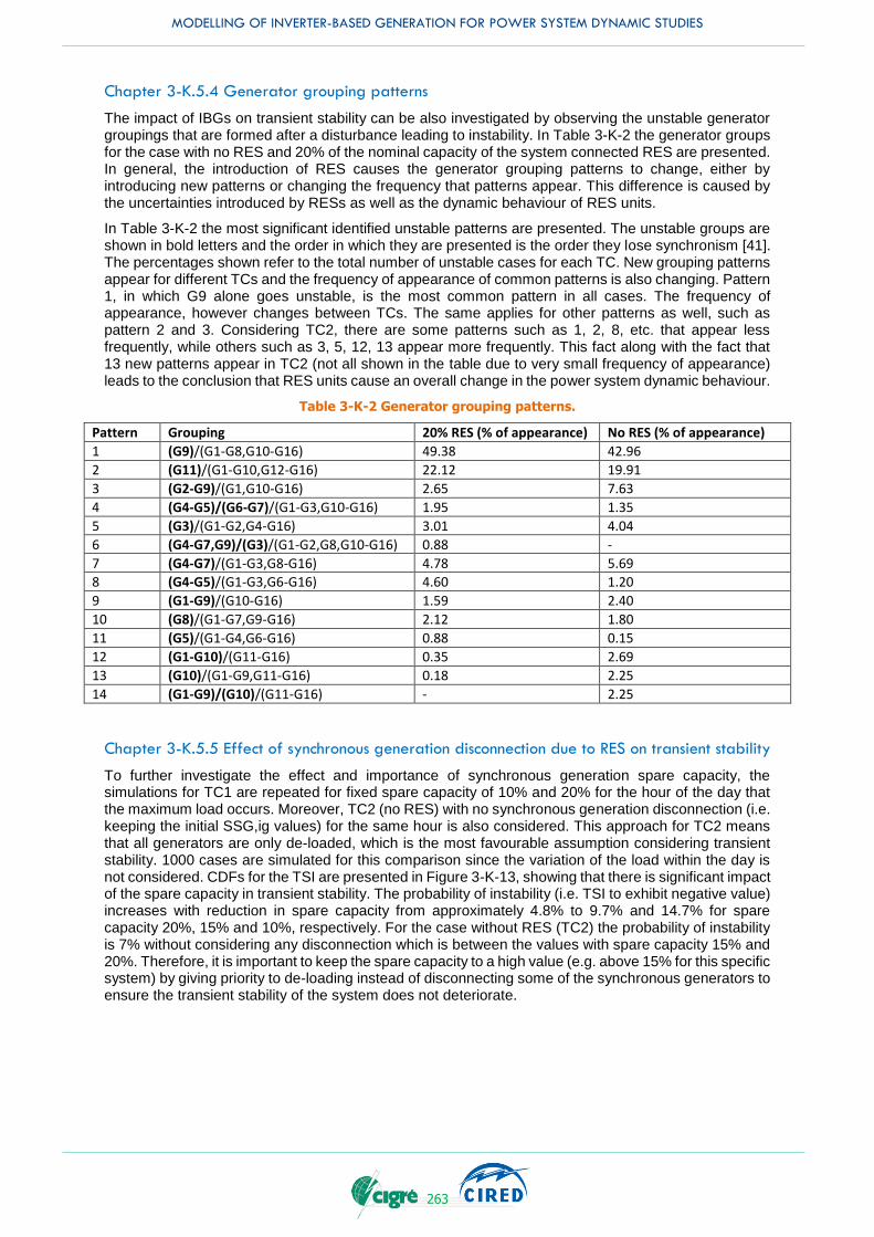
MODELLING OF INVERTER-BASED GENERATION FOR POWER SYSTEM DYNAMIC STUDIES
263
Chapter 3-K.5.4 Generator grouping patterns
The impact of IBGs on transient stability can be also investigated by observing the unstable generator groupings that are formed after a disturbance leading to instability. In Table 3-K-2 the generator groups for the case with no RES and 20% of the nominal capacity of the system connected RES are presented. In general, the introduction of RES causes the generator grouping patterns to change, either by introducing new patterns or changing the frequency that patterns appear. This difference is caused by the uncertainties introduced by RESs as well as the dynamic behaviour of RES units.
In Table 3-K-2 the most significant identified unstable patterns are presented. The unstable groups are shown in bold letters and the order in which they are presented is the order they lose synchronism [41]. The percentages shown refer to the total number of unstable cases for each TC. New grouping patterns appear for different TCs and the frequency of appearance of common patterns is also changing. Pattern 1, in which G9 alone goes unstable, is the most common pattern in all cases. The frequency of appearance, however changes between TCs. The same applies for other patterns as well, such as pattern 2 and 3. Considering TC2, there are some patterns such as 1, 2, 8, etc. that appear less frequently, while others such as 3, 5, 12, 13 appear more frequently. This fact along with the fact that 13 new patterns appear in TC2 (not all shown in the table due to very small frequency of appearance) leads to the conclusion that RES units cause an overall change in the power system dynamic behaviour.
Table 3-K-2 Generator grouping patterns.
Pattern Grouping 20% RES (% of appearance) No RES (% of appearance)
1 (G9)/(G1-G8,G10-G16) 49.38 42.96
2 (G11)/(G1-G10,G12-G16) 22.12 19.91
3 (G2-G9)/(G1,G10-G16) 2.65 7.63
4 (G4-G5)/(G6-G7)/(G1-G3,G10-G16) 1.95 1.35
5 (G3)/(G1-G2,G4-G16) 3.01 4.04
6 (G4-G7,G9)/(G3)/(G1-G2,G8,G10-G16) 0.88 -
7 (G4-G7)/(G1-G3,G8-G16) 4.78 5.69
8 (G4-G5)/(G1-G3,G6-G16) 4.60 1.20
9 (G1-G9)/(G10-G16) 1.59 2.40
10 (G8)/(G1-G7,G9-G16) 2.12 1.80
11 (G5)/(G1-G4,G6-G16) 0.88 0.15
12 (G1-G10)/(G11-G16) 0.35 2.69
13 (G10)/(G1-G9,G11-G16) 0.18 2.25
14 (G1-G9)/(G10)/(G11-G16) - 2.25
Chapter 3-K.5.5 Effect of synchronous generation disconnection due to RES on transient stability
To further investigate the effect and importance of synchronous generation spare capacity, the simulations for TC1 are repeated for fixed spare capacity of 10% and 20% for the hour of the day that the maximum load occurs. Moreover, TC2 (no RES) with no synchronous generation disconnection (i.e. keeping the initial SSG,ig values) for the same hour is also considered. This approach for TC2 means that all generators are only de-loaded, which is the most favourable assumption considering transient stability. 1000 cases are simulated for this comparison since the variation of the load within the day is not considered. CDFs for the TSI are presented in Figure 3-K-13, showing that there is significant impact of the spare capacity in transient stability. The probability of instability (i.e. TSI to exhibit negative value) increases with reduction in spare capacity from approximately 4.8% to 9.7% and 14.7% for spare capacity 20%, 15% and 10%, respectively. For the case without RES (TC2) the probability of instability is 7% without considering any disconnection which is between the values with spare capacity 15% and 20%. Therefore, it is important to keep the spare capacity to a high value (e.g. above 15% for this specific system) by giving priority to de-loading instead of disconnecting some of the synchronous generators to ensure the transient stability of the system does not deteriorate.
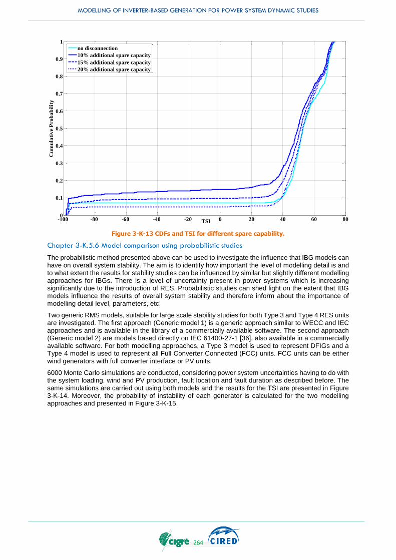
MODELLING OF INVERTER-BASED GENERATION FOR POWER SYSTEM DYNAMIC STUDIES
264
Figure 3-K-13 CDFs and TSI for different spare capability.
Chapter 3-K.5.6 Model comparison using probabilistic studies
The probabilistic method presented above can be used to investigate the influence that IBG models can have on overall system stability. The aim is to identify how important the level of modelling detail is and to what extent the results for stability studies can be influenced by similar but slightly different modelling approaches for IBGs. There is a level of uncertainty present in power systems which is increasing significantly due to the introduction of RES. Probabilistic studies can shed light on the extent that IBG models influence the results of overall system stability and therefore inform about the importance of modelling detail level, parameters, etc.
Two generic RMS models, suitable for large scale stability studies for both Type 3 and Type 4 RES units are investigated. The first approach (Generic model 1) is a generic approach similar to WECC and IEC approaches and is available in the library of a commercially available software. The second approach (Generic model 2) are models based directly on IEC 61400-27-1 [36], also available in a commercially available software. For both modelling approaches, a Type 3 model is used to represent DFIGs and a Type 4 model is used to represent all Full Converter Connected (FCC) units. FCC units can be either wind generators with full converter interface or PV units.
6000 Monte Carlo simulations are conducted, considering power system uncertainties having to do with the system loading, wind and PV production, fault location and fault duration as described before. The same simulations are carried out using both models and the results for the TSI are presented in Figure 3-K-14. Moreover, the probability of instability of each generator is calculated for the two modelling approaches and presented in Figure 3-K-15.
-100 -80 -60 -40 -20 0 20 40 60 800
0.1
0.2
0.3
0.4
0.5
0.6
0.7
0.8
0.9
1
TSI
Cu
mu
lati
ve
Pro
ba
bil
ity
no disconnection
10% additional spare capacity
15% additional spare capacity
20% additional spare capacity
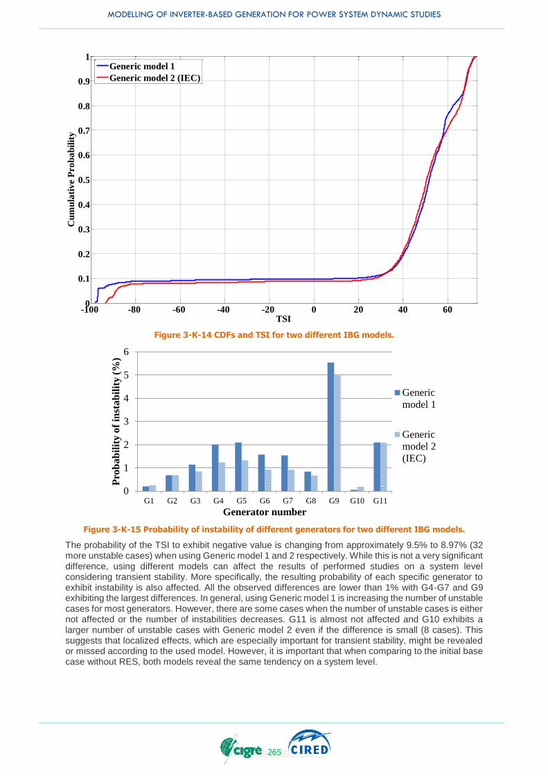
MODELLING OF INVERTER-BASED GENERATION FOR POWER SYSTEM DYNAMIC STUDIES
265
Figure 3-K-14 CDFs and TSI for two different IBG models.
Figure 3-K-15 Probability of instability of different generators for two different IBG models.
The probability of the TSI to exhibit negative value is changing from approximately 9.5% to 8.97% (32 more unstable cases) when using Generic model 1 and 2 respectively. While this is not a very significant difference, using different models can affect the results of performed studies on a system level considering transient stability. More specifically, the resulting probability of each specific generator to exhibit instability is also affected. All the observed differences are lower than 1% with G4-G7 and G9 exhibiting the largest differences. In general, using Generic model 1 is increasing the number of unstable cases for most generators. However, there are some cases when the number of unstable cases is either not affected or the number of instabilities decreases. G11 is almost not affected and G10 exhibits a larger number of unstable cases with Generic model 2 even if the difference is small (8 cases). This suggests that localized effects, which are especially important for transient stability, might be revealed or missed according to the used model. However, it is important that when comparing to the initial base case without RES, both models reveal the same tendency on a system level.
-100 -80 -60 -40 -20 0 20 40 600
0.1
0.2
0.3
0.4
0.5
0.6
0.7
0.8
0.9
1
TSI
Cu
mu
lati
ve P
ro
ba
bil
ity
Generic model 1
Generic model 2 (IEC)
0
1
2
3
4
5
6
G1 G2 G3 G4 G5 G6 G7 G8 G9 G10 G11
Pro
ba
bil
ity
of
inst
ab
ilit
y (
%)
Generator number
Generic
model 1
Generic
model 2
(IEC)
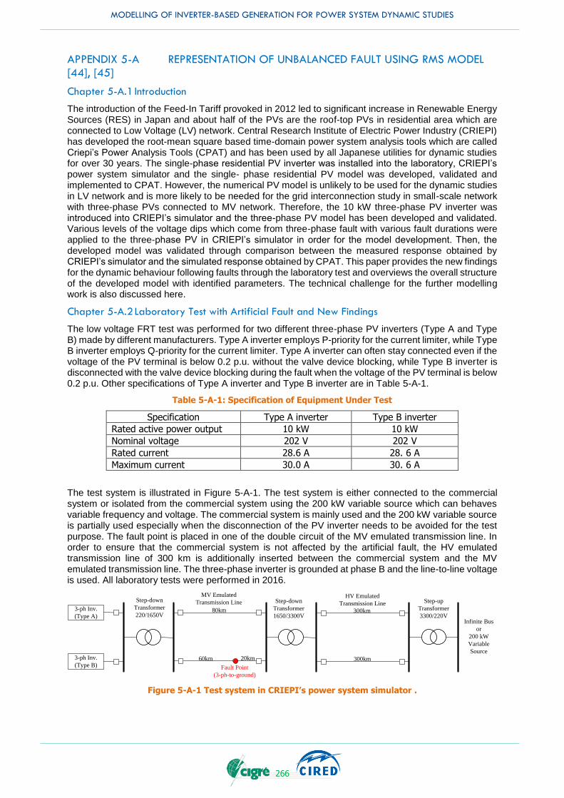
MODELLING OF INVERTER-BASED GENERATION FOR POWER SYSTEM DYNAMIC STUDIES
266
APPENDIX 5-A REPRESENTATION OF UNBALANCED FAULT USING RMS MODEL [44], [45]
Chapter 5-A.1 Introduction
The introduction of the Feed-In Tariff provoked in 2012 led to significant increase in Renewable Energy Sources (RES) in Japan and about half of the PVs are the roof-top PVs in residential area which are connected to Low Voltage (LV) network. Central Research Institute of Electric Power Industry (CRIEPI) has developed the root-mean square based time-domain power system analysis tools which are called Criepi’s Power Analysis Tools (CPAT) and has been used by all Japanese utilities for dynamic studies for over 30 years. The single-phase residential PV inverter was installed into the laboratory, CRIEPI’s power system simulator and the single- phase residential PV model was developed, validated and implemented to CPAT. However, the numerical PV model is unlikely to be used for the dynamic studies in LV network and is more likely to be needed for the grid interconnection study in small-scale network with three-phase PVs connected to MV network. Therefore, the 10 kW three-phase PV inverter was introduced into CRIEPI’s simulator and the three-phase PV model has been developed and validated. Various levels of the voltage dips which come from three-phase fault with various fault durations were applied to the three-phase PV in CRIEPI’s simulator in order for the model development. Then, the developed model was validated through comparison between the measured response obtained by CRIEPI’s simulator and the simulated response obtained by CPAT. This paper provides the new findings for the dynamic behaviour following faults through the laboratory test and overviews the overall structure of the developed model with identified parameters. The technical challenge for the further modelling work is also discussed here.
Chapter 5-A.2 Laboratory Test with Artificial Fault and New Findings
The low voltage FRT test was performed for two different three-phase PV inverters (Type A and Type B) made by different manufacturers. Type A inverter employs P-priority for the current limiter, while Type B inverter employs Q-priority for the current limiter. Type A inverter can often stay connected even if the voltage of the PV terminal is below 0.2 p.u. without the valve device blocking, while Type B inverter is disconnected with the valve device blocking during the fault when the voltage of the PV terminal is below 0.2 p.u. Other specifications of Type A inverter and Type B inverter are in Table 5-A-1.
Table 5-A-1: Specification of Equipment Under Test
Specification Type A inverter Type B inverter
Rated active power output 10 kW 10 kW
Nominal voltage 202 V 202 V
Rated current 28.6 A 28. 6 A
Maximum current 30.0 A 30. 6 A
The test system is illustrated in Figure 5-A-1. The test system is either connected to the commercial system or isolated from the commercial system using the 200 kW variable source which can behaves variable frequency and voltage. The commercial system is mainly used and the 200 kW variable source is partially used especially when the disconnection of the PV inverter needs to be avoided for the test purpose. The fault point is placed in one of the double circuit of the MV emulated transmission line. In order to ensure that the commercial system is not affected by the artificial fault, the HV emulated transmission line of 300 km is additionally inserted between the commercial system and the MV emulated transmission line. The three-phase inverter is grounded at phase B and the line-to-line voltage is used. All laboratory tests were performed in 2016.
3-ph Inv.
(Type A)
3-ph Inv.
(Type B)
Infinite Bus
or
200 kW
Variable
Source
HV Emulated
Transmission Line
MV Emulated
Transmission Line Step-up
Transformer
3300/220V
Step-down
Transformer
1650/3300V
Step-down
Transformer
220/1650V300km
300km
80km
60km 20km
Fault Point
(3-ph-to-ground)
Figure 5-A-1 Test system in CRIEPI’s power system simulator .
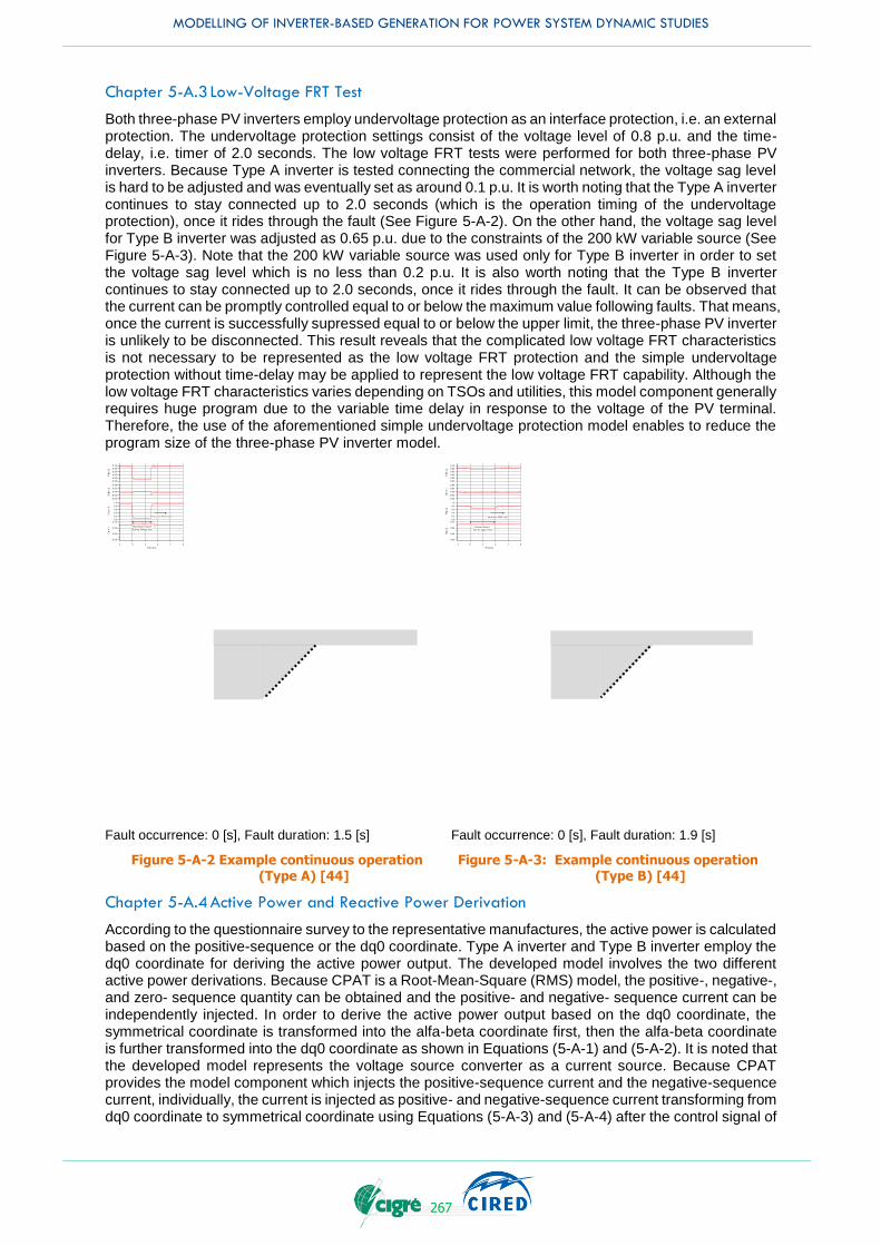
MODELLING OF INVERTER-BASED GENERATION FOR POWER SYSTEM DYNAMIC STUDIES
267
Chapter 5-A.3 Low-Voltage FRT Test
Both three-phase PV inverters employ undervoltage protection as an interface protection, i.e. an external protection. The undervoltage protection settings consist of the voltage level of 0.8 p.u. and the time-delay, i.e. timer of 2.0 seconds. The low voltage FRT tests were performed for both three-phase PV inverters. Because Type A inverter is tested connecting the commercial network, the voltage sag level is hard to be adjusted and was eventually set as around 0.1 p.u. It is worth noting that the Type A inverter continues to stay connected up to 2.0 seconds (which is the operation timing of the undervoltage protection), once it rides through the fault (See Figure 5-A-2). On the other hand, the voltage sag level for Type B inverter was adjusted as 0.65 p.u. due to the constraints of the 200 kW variable source (See Figure 5-A-3). Note that the 200 kW variable source was used only for Type B inverter in order to set the voltage sag level which is no less than 0.2 p.u. It is also worth noting that the Type B inverter continues to stay connected up to 2.0 seconds, once it rides through the fault. It can be observed that the current can be promptly controlled equal to or below the maximum value following faults. That means, once the current is successfully supressed equal to or below the upper limit, the three-phase PV inverter is unlikely to be disconnected. This result reveals that the complicated low voltage FRT characteristics is not necessary to be represented as the low voltage FRT protection and the simple undervoltage protection without time-delay may be applied to represent the low voltage FRT capability. Although the low voltage FRT characteristics varies depending on TSOs and utilities, this model component generally requires huge program due to the variable time delay in response to the voltage of the PV terminal. Therefore, the use of the aforementioned simple undervoltage protection model enables to reduce the program size of the three-phase PV inverter model.
Fault occurrence: 0 [s], Fault duration: 1.5 [s] Fault occurrence: 0 [s], Fault duration: 1.9 [s]
Figure 5-A-2 Example continuous operation Figure 5-A-3: Example continuous operation (Type A) [44] (Type B) [44]
Chapter 5-A.4 Active Power and Reactive Power Derivation
According to the questionnaire survey to the representative manufactures, the active power is calculated based on the positive-sequence or the dq0 coordinate. Type A inverter and Type B inverter employ the dq0 coordinate for deriving the active power output. The developed model involves the two different active power derivations. Because CPAT is a Root-Mean-Square (RMS) model, the positive-, negative-, and zero- sequence quantity can be obtained and the positive- and negative- sequence current can be independently injected. In order to derive the active power output based on the dq0 coordinate, the symmetrical coordinate is transformed into the alfa-beta coordinate first, then the alfa-beta coordinate is further transformed into the dq0 coordinate as shown in Equations (5-A-1) and (5-A-2). It is noted that the developed model represents the voltage source converter as a current source. Because CPAT provides the model component which injects the positive-sequence current and the negative-sequence current, individually, the current is injected as positive- and negative-sequence current transforming from dq0 coordinate to symmetrical coordinate using Equations (5-A-3) and (5-A-4) after the control signal of

MODELLING OF INVERTER-BASED GENERATION FOR POWER SYSTEM DYNAMIC STUDIES
268
active power and reactive power are determined/decided. It should be emphasized that the positive and negative voltages have to be obtained from the line-to-line voltage the phase voltage must not be used because this results in the large discrepancy between the simulated response and measured response in case of unbalanced fault.
[V1
V2
] =1
3[1 a (a2)
1 (a2) a] [
Vab
Vbc
Vca
] [
Vα
Vβ
V0
] = [1 1 0
−j j 00 0 1
] [
V1
V2
V0
] [
Iα
Iβ
I0
] = [1 1 0
−j j 00 0 1
] [
I1
I2
I0
]
Equation 5-A-1
[
Vd
Vq
V0
] = [cosθ sinθ 0
−sinθ cosθ 00 0 1
] [
Vα
Vβ
V0
] [
Id
Iq
I0
] = [cosθ sinθ 0
−sinθ cosθ 00 0 1
] [
Iα
Iβ
I0
]
Equation 5-A-2
[
Iα
Iβ
I0
] = [cosθ −sinθ 0sinθ cosθ 0
0 0 1] [
Id
Iq
I0
]
Equation 5-A-3
[
I1
I2
I0
] =1
2[1 j 01 −j 00 0 2
] [
Iα
Iβ
I0
]
Equation 5-A-4
Chapter 5-A.5 Outline of Developed Model
The developed model consists of the active and reactive power control model component with the current limiter, AC protection model components including two different types of the anti-islanding protections, the simplified DC source control model component. The electric control block diagrams with the simplified DC source model are shown in Figures 5-A-4.
I
Capacitor
Ini=VDC0
P
I
Limiter
P-Priority: Idmax = Imax
Q-Priority: Idmax = (Imax2-Iqref
2)
limiterP
I
DCVref
(1.0p.u.)
Idini
(Initial
Value)
Idref
(3-ph mean)
P-Priority: Iqmax = (Imax2-Idref
2)Q-Priority: Iqmax = Imax
0
Idmax
Iqmax
-Iqmax
0: Disconnection
1: Stay connected
I-V Panel Characteristics
P [
p.u
.]
P=a×DCV2 + b×DCV + c
DCV [p.u.]
1
1.2
×
Active Power
(3-ph mean)
Pin_chopper
(MPPT)
Qref
(Reference)Iqini
(Initial Value)
1) dq0 coordinate based calculation
2) positive-sequence based calculation
Simplified DC Source Controller0: Disconnection
1: Stay connected
Iqref
(3-ph mean)
Reactive Power
(3-ph mean)
1) dq0 coordinate based calculation
2) positive-sequence based calculation
1) convert to positive-sequence current
2) use positive-sequence current as it is
1) convert to positive-sequence current
2) use positive-sequence current as it is
Figure 5-A-4 Electric control model with DC source [44].
Chapter 5-A.6 Model Validation
The developed model was validated comparing the measured response obtained in CRIEPI’s simulator and the model response calculated using CPAT. It is noted that only commercial system is used for the model validation test. In addition, all anti-islanding protections are deactivated in order to differentiate of the dynamic behaviour between the inner inverter control and the reactive power control coming from

MODELLING OF INVERTER-BASED GENERATION FOR POWER SYSTEM DYNAMIC STUDIES
269
the anti-islanding protection. Figure 5-A-5 shows an example result of Type A inverter when the fault duration is 100 ms and the power factor of the PV output is unity. As shown in Figure 5-A-5, there is a good match for active power, reactive power especially between the occurrence of the fault and the clearance of the fault.
The derived electric control model parameters for unbalanced faults are shown in Table 5-A-2. Because 5 ms is used for I element of PI controller of the reactive current control, the time step of 1 ms is usually required for the time-domain simulation. It is noted that the same parameters derived for balanced faults are not the same as those that are shown in Table 5-A-2.
(a) AB phase line-to-line fault (b) BC phase line-to-line fault
(c) CA phase line-to-line fault
Figure 5-A-5 Dynamic behaviour following faults (Type A) [45].
Table 5-A-2: Derived electric control parameters
P I
Active current control 5.0 0.03s
Reactive current control 5.0 0.005s
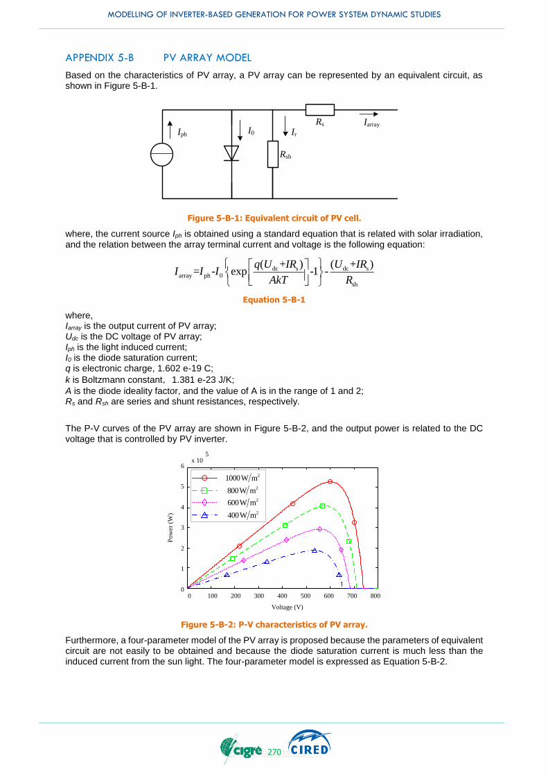
MODELLING OF INVERTER-BASED GENERATION FOR POWER SYSTEM DYNAMIC STUDIES
270
APPENDIX 5-B PV ARRAY MODEL
Based on the characteristics of PV array, a PV array can be represented by an equivalent circuit, as shown in Figure 5-B-1.
Rs
Rsh
Iph I0 Ir
Iarray
Figure 5-B-1: Equivalent circuit of PV cell.
where, the current source Iph is obtained using a standard equation that is related with solar irradiation, and the relation between the array terminal current and voltage is the following equation:
dc s dc sarray ph 0
sh
( + ) ( + )= - exp -1 -
q U IR U IRI I I
AkT R
Equation 5-B-1
where, Iarray is the output current of PV array; Udc is the DC voltage of PV array; Iph is the light induced current; I0 is the diode saturation current; q is electronic charge, 1.602 e-19 C;
k is Boltzmann constant,1.381 e-23 J/K;
A is the diode ideality factor, and the value of A is in the range of 1 and 2; Rs and Rsh are series and shunt resistances, respectively.
The P-V curves of the PV array are shown in Figure 5-B-2, and the output power is related to the DC voltage that is controlled by PV inverter.
0 100 200 300 400 500 600 700 8000
1
2
3
4
5
6x 10
5
Voltage (V)
Pow
er (
W)
21000W m
2800W m2600W m2400W m
Figure 5-B-2: P-V characteristics of PV array.
Furthermore, a four-parameter model of the PV array is proposed because the parameters of equivalent circuit are not easily to be obtained and because the diode saturation current is much less than the induced current from the sun light. The four-parameter model is expressed as Equation 5-B-2.
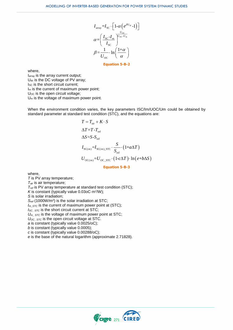
MODELLING OF INVERTER-BASED GENERATION FOR POWER SYSTEM DYNAMIC STUDIES
271
dc
OC
OC m
array SC
-SC m
SC
OC
= 1- -1
-=
1 1+= ln
U
U
U U
I I e
I I
I
U
Equation 5-B-2
where, Iarray is the array current output; Udc is the DC voltage of PV array; ISC is the short circuit current; Im is the current of maximum power point; UOC is the open circuit voltage; Um is the voltage of maximum power point.
When the environment condition varies, the key parameters ISC/Im/UOC/Um could be obtained by standard parameter at standard test condition (STC), and the equations are:
air
ref
ref
SC( m) SC( m)_STC
ref
OC( m) OC _STC
= -
= -
= 1+
= 1- ln +
T T K S
T T T
S S S
SI I a T
S
U U c T e b S
+
D
D
D
D D
Equation 5-B-3
where, T is PV array temperature; Tair is air temperature; Tref is PV array temperature at standard test condition (STC); K is constant (typically value 0.03oC·m2/W); S is solar irradiation; Sref (1000W/m2) is the solar irradiation at STC; Im_STC is the current of maximum power point at (STC); ISC_ STC is the short circuit current at STC; Um_ STC is the voltage of maximum power point at STC; UOC_ STC is the open circuit voltage at STC. a is constant (typically value 0.0025/oC); b is constant (typically value 0.0005); c is constant (typically value 0.00288/oC); e is the base of the natural logarithm (approximate 2.71828).

MODELLING OF INVERTER-BASED GENERATION FOR POWER SYSTEM DYNAMIC STUDIES
272
APPENDIX 5-C EXAMPLES OF RMS-TYPE INTEGRATED PV MODELS
Two generic PV models, namely the WECC PV power plant model and the CEPRI PV power plant model are introduced in this Sub-Chapter together with example parameters. It should be noted that these parameter values are given for illustration purposes. They are not generic and, hence, they should be re-used with caution.
Chapter 5-C.1 WECC PV Power Plant Model [45]
a) WECC Renewable Energy Generator/Converter Model (REGC_A – see Figure 5-C-1)
This clause describes the model used in WECC (Western Electricity Coordinating Council) for studies of the Western Interconnection of North America. The system model used in the studies is a positive-sequence three-phase symmetrical model of the high-voltage transmission system, therefore models of IBG are RMS models aggregated and adjusted to a three-phase balanced system.
The model incorporates a high bandwidth current regulator that injects real and reactive components of inverter current into the external network in response to real and reactive current commands. Current injection includes the following capabilities:
Reactive current management during high voltage events at the generator terminal bus
Active current management during low voltage events to approximate the response of the inverter
controls during voltage dips. This is intended to approximate the behaviour of PLL devices at very
low voltages when the PLL cannot operate correctly.
Power logic during low voltage events to allow for a controlled response of active current during and immediately following voltage dips. This functionality is particular to some vendors and is included for generality.
In this model, the voltage and frequency protections are handled separately by external modules. This model is similar to the Type-3 and Type-4 generic wind generator models documented in [47].
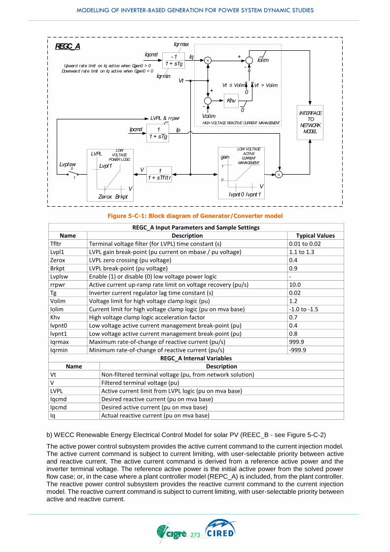
MODELLING OF INVERTER-BASED GENERATION FOR POWER SYSTEM DYNAMIC STUDIES
273
REGC_A
Ipcmd 1
1 + sTg
LVPL & rrpwr
lvpnt0 lvpnt1
gain
V
1
0×
Ip
INTERFACE
TO
NETWORK
MODEL
LOW VOLTAGE
ACTIVE
CURRENT
MANAGEMENT
Iqcmd -1
1 + sTg
Iq×
Volim
-Khv
0
0
Vt ≤ Volim Vt > Volim
HIGH VOLTAGE REACTIVE CURRENT MANAGEMENT
Iolim
Vt
-
V
Zerox Brkpt
Lvpl1
LVPL
V
LOW
VOLTAGE
POWER LOGIC
0
1
Lvplsw1
1 + sTf lt r
Iqrmin
Iqrmax
+
+
Upward rate limit on Iq act ive when Qgen0 > 0
Downward rate limit on Iq act ive when Qgen0 < 0
Figure 5-C-1: Block diagram of Generator/Converter model
REGC_A Input Parameters and Sample Settings Name Description Typical Values
Tfltr Terminal voltage filter (for LVPL) time constant (s) 0.01 to 0.02
Lvpl1 LVPL gain break-point (pu current on mbase / pu voltage) 1.1 to 1.3
Zerox LVPL zero crossing (pu voltage) 0.4
Brkpt LVPL break-point (pu voltage) 0.9 Lvplsw Enable (1) or disable (0) low voltage power logic -
rrpwr Active current up-ramp rate limit on voltage recovery (pu/s) 10.0
Tg Inverter current regulator lag time constant (s) 0.02
Volim Voltage limit for high voltage clamp logic (pu) 1.2
Iolim Current limit for high voltage clamp logic (pu on mva base) -1.0 to -1.5 Khv High voltage clamp logic acceleration factor 0.7
lvpnt0 Low voltage active current management break-point (pu) 0.4
lvpnt1 Low voltage active current management break-point (pu) 0.8
Iqrmax Maximum rate-of-change of reactive current (pu/s) 999.9
Iqrmin Minimum rate-of-change of reactive current (pu/s) -999.9
REGC_A Internal Variables Name Description
Vt Non-filtered terminal voltage (pu, from network solution)
V Filtered terminal voltage (pu)
LVPL Active current limit from LVPL logic (pu on mva base)
Iqcmd Desired reactive current (pu on mva base) Ipcmd Desired active current (pu on mva base)
Iq Actual reactive current (pu on mva base)
b) WECC Renewable Energy Electrical Control Model for solar PV (REEC_B - see Figure 5-C-2)
The active power control subsystem provides the active current command to the current injection model. The active current command is subject to current limiting, with user-selectable priority between active and reactive current. The active current command is derived from a reference active power and the inverter terminal voltage. The reference active power is the initial active power from the solved power flow case; or, in the case where a plant controller model (REPC_A) is included, from the plant controller. The reactive power control subsystem provides the reactive current command to the current injection model. The reactive current command is subject to current limiting, with user-selectable priority between active and reactive current.
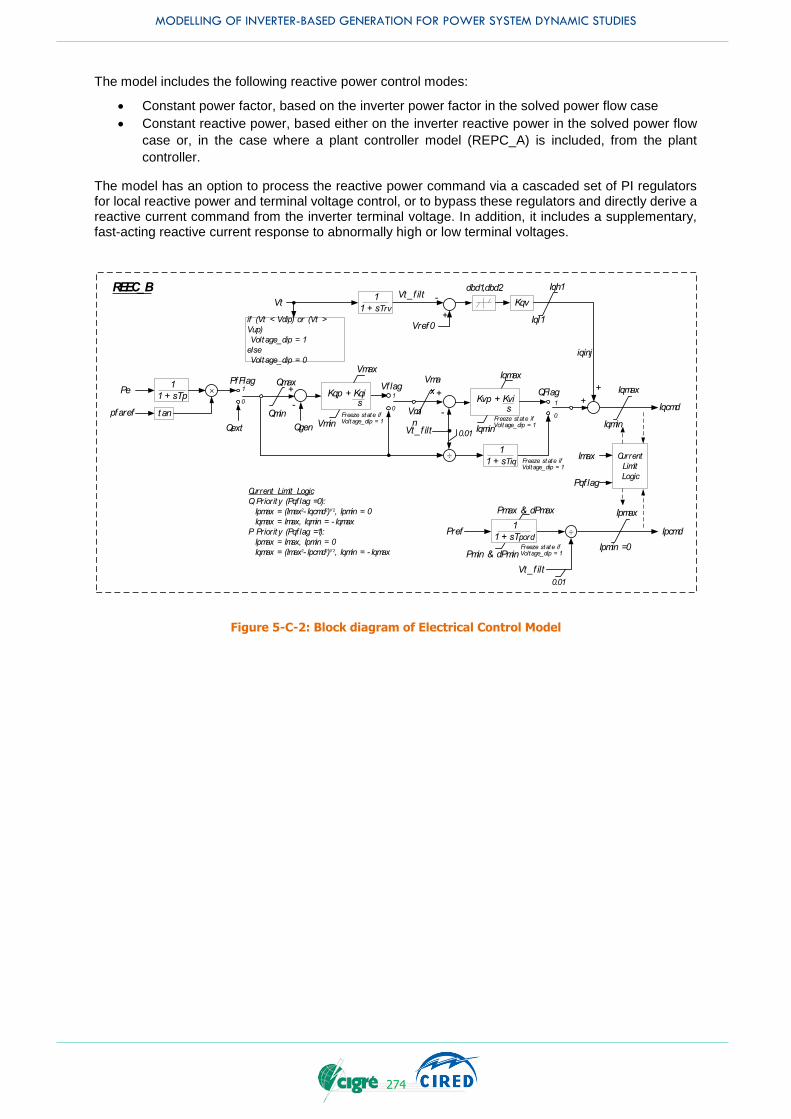
MODELLING OF INVERTER-BASED GENERATION FOR POWER SYSTEM DYNAMIC STUDIES
274
The model includes the following reactive power control modes:
Constant power factor, based on the inverter power factor in the solved power flow case
Constant reactive power, based either on the inverter reactive power in the solved power flow
case or, in the case where a plant controller model (REPC_A) is included, from the plant
controller.
The model has an option to process the reactive power command via a cascaded set of PI regulators for local reactive power and terminal voltage control, or to bypass these regulators and directly derive a reactive current command from the inverter terminal voltage. In addition, it includes a supplementary, fast-acting reactive current response to abnormally high or low terminal voltages.
Current Limit Logic
Q Priorit y (Pqf lag =0):
Ipmax = (Imax2- Iqcmd2)1/ 2, Ipmin = 0
Iqmax = Imax, Iqmin = - Iqmax
P Priorit y (Pqf lag =1):
Ipmax = Imax, Ipmin = 0
Iqmax = (Imax2- Ipcmd2)1/ 2, Iqmin = - Iqmax
÷ Ipcmd1
1 + sTpord
Pmax & dPmax
Pmin & dPmin
Iqcmd
÷
Iqmax
Iqmin
Iqh1
Iql1
Kqv
dbd1,dbd2
Vref0
Vt-
iqinj
REEC_B
pfaref
×
tan Qmin
Qmax1
1 + sTpPe 1
0
PfFlag
Qext Qgen
-
Kqp + Kqi s
Vmax
Freeze state if Voltage_dip = 1Vmin
1
0 Vmi
n
Vf lagVma
x
Iqmax
Kvp + Kvi s
Freeze state if Voltage_dip = 1
Iqmin
1
1 + sTrv
Vt_f ilt
if (Vt < Vdip) or (Vt >
Vup)
Voltage_dip = 1
else
Voltage_dip = 0
Current
Limit
Logic
1
0
QFlag
-
Vt_f ilt 0.01
1
1 + sTiq Freeze state if Voltage_dip = 1
Vt_f ilt
0.01
Ipmax
Ipmin =0
Imax
Pqf lag
Freeze state if Voltage_dip = 1
Pref
+
+
++
+
Figure 5-C-2: Block diagram of Electrical Control Model
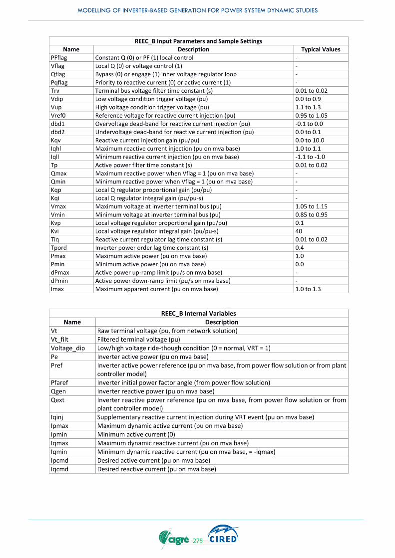
MODELLING OF INVERTER-BASED GENERATION FOR POWER SYSTEM DYNAMIC STUDIES
275
REEC_B Input Parameters and Sample Settings Name Description Typical Values
PFflag Constant Q (0) or PF (1) local control -
Vflag Local Q (0) or voltage control (1) -
Qflag Bypass (0) or engage (1) inner voltage regulator loop -
Pqflag Priority to reactive current (0) or active current (1) - Trv Terminal bus voltage filter time constant (s) 0.01 to 0.02
Vdip Low voltage condition trigger voltage (pu) 0.0 to 0.9
Vup High voltage condition trigger voltage (pu) 1.1 to 1.3
Vref0 Reference voltage for reactive current injection (pu) 0.95 to 1.05
dbd1 Overvoltage dead-band for reactive current injection (pu) -0.1 to 0.0 dbd2 Undervoltage dead-band for reactive current injection (pu) 0.0 to 0.1
Kqv Reactive current injection gain (pu/pu) 0.0 to 10.0
Iqhl Maximum reactive current injection (pu on mva base) 1.0 to 1.1
Iqll Minimum reactive current injection (pu on mva base) -1.1 to -1.0
Tp Active power filter time constant (s) 0.01 to 0.02
Qmax Maximum reactive power when Vflag = 1 (pu on mva base) - Qmin Minimum reactive power when Vflag = 1 (pu on mva base) -
Kqp Local Q regulator proportional gain (pu/pu) -
Kqi Local Q regulator integral gain (pu/pu-s) -
Vmax Maximum voltage at inverter terminal bus (pu) 1.05 to 1.15
Vmin Minimum voltage at inverter terminal bus (pu) 0.85 to 0.95 Kvp Local voltage regulator proportional gain (pu/pu) 0.1
Kvi Local voltage regulator integral gain (pu/pu-s) 40
Tiq Reactive current regulator lag time constant (s) 0.01 to 0.02
Tpord Inverter power order lag time constant (s) 0.4
Pmax Maximum active power (pu on mva base) 1.0 Pmin Minimum active power (pu on mva base) 0.0
dPmax Active power up-ramp limit (pu/s on mva base) -
dPmin Active power down-ramp limit (pu/s on mva base) -
Imax Maximum apparent current (pu on mva base) 1.0 to 1.3
REEC_B Internal Variables Name Description
Vt Raw terminal voltage (pu, from network solution) Vt_filt Filtered terminal voltage (pu) Voltage_dip Low/high voltage ride-though condition (0 = normal, VRT = 1) Pe Inverter active power (pu on mva base) Pref Inverter active power reference (pu on mva base, from power flow solution or from plant
controller model) Pfaref Inverter initial power factor angle (from power flow solution) Qgen Inverter reactive power (pu on mva base) Qext Inverter reactive power reference (pu on mva base, from power flow solution or from
plant controller model) Iqinj Supplementary reactive current injection during VRT event (pu on mva base) Ipmax Maximum dynamic active current (pu on mva base) Ipmin Minimum active current (0) Iqmax Maximum dynamic reactive current (pu on mva base) Iqmin Minimum dynamic reactive current (pu on mva base, = -iqmax) Ipcmd Desired active current (pu on mva base) Iqcmd Desired reactive current (pu on mva base)

MODELLING OF INVERTER-BASED GENERATION FOR POWER SYSTEM DYNAMIC STUDIES
276
c) Renewable Energy Plant Controller Model (REPC_A – see Figure 5-C-3)
This model is used when plant-level control of active and/or reactive power is implemented. The model incorporates the following:
REPC_A
1
0
Vreg
Vref
Freeze state if Vreg < Vfrz
Ibranch
Kc
-
Qbranch
emax
emin
Kp + Ki s
Qmax
Qmin
1 + s Tft1 + s Tfv QextRefFlag
dbd
11 + sTfltr
VcompFlag|Vreg – (Rc+jXc)·
Ibranch|
11 + sTfltr
1
0
Qref
-
femin
fema
xPbranch
Plant_pref
Ddn
Dup
0
0Freq_ref
-fdbd1,fdbd2
- Kpg + Kig s
Pmax
PminFreg
11 + sTp
11 + sTlag
Pref
++
+
+
+
+
+
+
+ 0
1
Freq_flag
Figure 5-C-3: Block diagram of Plant Controller Model
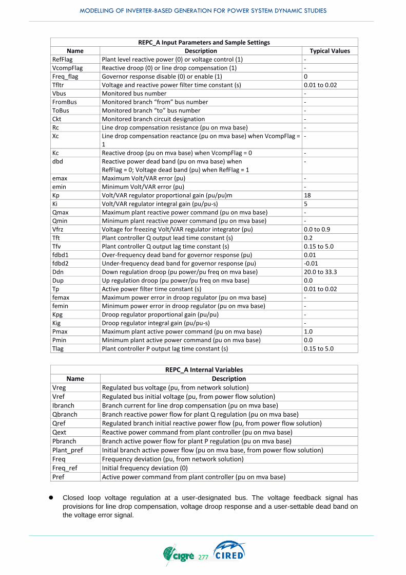
MODELLING OF INVERTER-BASED GENERATION FOR POWER SYSTEM DYNAMIC STUDIES
277
REPC_A Input Parameters and Sample Settings Name Description Typical Values
RefFlag Plant level reactive power (0) or voltage control (1) -
VcompFlag Reactive droop (0) or line drop compensation (1) -
Freq_flag Governor response disable (0) or enable (1) 0
Tfltr Voltage and reactive power filter time constant (s) 0.01 to 0.02 Vbus Monitored bus number -
FromBus Monitored branch “from” bus number -
ToBus Monitored branch “to” bus number -
Ckt Monitored branch circuit designation -
Rc Line drop compensation resistance (pu on mva base) - Xc Line drop compensation reactance (pu on mva base) when VcompFlag =
1 -
Kc Reactive droop (pu on mva base) when VcompFlag = 0 -
dbd Reactive power dead band (pu on mva base) when RefFlag = 0; Voltage dead band (pu) when RefFlag = 1
-
emax Maximum Volt/VAR error (pu) -
emin Minimum Volt/VAR error (pu) -
Kp Volt/VAR regulator proportional gain (pu/pu)m 18
Ki Volt/VAR regulator integral gain (pu/pu-s) 5
Qmax Maximum plant reactive power command (pu on mva base) - Qmin Minimum plant reactive power command (pu on mva base) -
Vfrz Voltage for freezing Volt/VAR regulator integrator (pu) 0.0 to 0.9
Tft Plant controller Q output lead time constant (s) 0.2
Tfv Plant controller Q output lag time constant (s) 0.15 to 5.0
fdbd1 Over-frequency dead band for governor response (pu) 0.01 fdbd2 Under-frequency dead band for governor response (pu) -0.01
Ddn Down regulation droop (pu power/pu freq on mva base) 20.0 to 33.3
Dup Up regulation droop (pu power/pu freq on mva base) 0.0
Tp Active power filter time constant (s) 0.01 to 0.02
femax Maximum power error in droop regulator (pu on mva base) - femin Minimum power error in droop regulator (pu on mva base) -
Kpg Droop regulator proportional gain (pu/pu) -
Kig Droop regulator integral gain (pu/pu-s) -
Pmax Maximum plant active power command (pu on mva base) 1.0
Pmin Minimum plant active power command (pu on mva base) 0.0
Tlag Plant controller P output lag time constant (s) 0.15 to 5.0
REPC_A Internal Variables Name Description
Vreg Regulated bus voltage (pu, from network solution) Vref Regulated bus initial voltage (pu, from power flow solution) Ibranch Branch current for line drop compensation (pu on mva base) Qbranch Branch reactive power flow for plant Q regulation (pu on mva base) Qref Regulated branch initial reactive power flow (pu, from power flow solution) Qext Reactive power command from plant controller (pu on mva base) Pbranch Branch active power flow for plant P regulation (pu on mva base) Plant_pref Initial branch active power flow (pu on mva base, from power flow solution) Freq Frequency deviation (pu, from network solution) Freq_ref Initial frequency deviation (0) Pref Active power command from plant controller (pu on mva base)
Closed loop voltage regulation at a user-designated bus. The voltage feedback signal has
provisions for line drop compensation, voltage droop response and a user-settable dead band on
the voltage error signal.
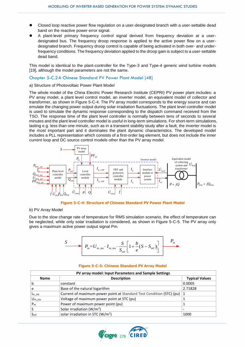
MODELLING OF INVERTER-BASED GENERATION FOR POWER SYSTEM DYNAMIC STUDIES
278
Closed loop reactive power flow regulation on a user-designated branch with a user-settable dead
band on the reactive power error signal.
A plant-level primary frequency control signal derived from frequency deviation at a user-
designated bus. The frequency droop response is applied to the active power flow on a user-
designated branch. Frequency droop control is capable of being activated in both over- and under-
frequency conditions. The frequency deviation applied to the droop gain is subject to a user-settable
dead band.
This model is identical to the plant-controller for the Type-3 and Type-4 generic wind turbine models [19], although the model parameters are not the same.
Chapter 5-C.2 A Chinese Standard PV Power Plant Model [48]
a) Structure of Photovoltaic Power Plant Model
The whole model of the China Electric Power Research Institute (CEPRI) PV power plant includes: a PV array model, a plant level control model, an inverter model, an equivalent model of collector and transformer, as shown in Figure 5-C-4. The PV array model corresponds to the energy source and can emulate the changing power output during solar irradiation fluctuations. The plant level controller model is used to simulate the dynamic response corresponding to the dispatch command received from the TSO. The response time of the plant level controller is normally between tens of seconds to several minutes and the plant level controller model is useful in long-term simulations. For short-term simulations, lasting e.g. less than one minute, such as in a transient stability study after a fault, the inverter model is the most important part and it dominates the plant dynamic characteristics. The developed model includes a PLL representation which consists of a first-order lag element, but does not include the inner current loop and DC source control models other than the PV array model.
p _ cmdI
q_ cmdI
Local
controller
module
FRT and
protective
controller
module
Interface
module to
power
system
termU
acI
POI _ refP
P jQ+
POI_ refU
qI
pIPlant level
controller
model
mP
PV array
model
ordP
ordQ
POIU
0f
POI_ refQ
POI POIP jQ+
POIQPOIP termU
termU
refPF
QPPOIU
Inverter model
ff
POI_ refPF
S
Equivalent model
of collecting
system and
transformer
Figure 5-C-4: Structure of Chinese Standard PV Power Plant Model
b) PV Array Model
Due to the slow change rate of temperature for RMS simulation scenario, the effect of temperature can be neglected, while only solar irradiation is considered, as shown in Figure 5-C-5. The PV array only gives a maximum active power output signal Pm.
m m_sta m_sta ref
ref
1 ( )S b
P =U I S SS e
+ -
S mP
Figure 5-C-5: Chinese Standard PV Array Model
PV array model: Input Parameters and Sample Settings
Name Description Typical Values
b constant 0.0005 e Base of the natural logarithm 2.71828
Im_sta Current of maximum power point at Standard Test Condition (STC) (pu) 1
Um_sta Voltage of maximum power point at STC (pu) 1
Pm Power of maximum power point (pu) 1
S Solar irradiation (W/m2) - Sref solar irradiation in STC (W/m2) 1000
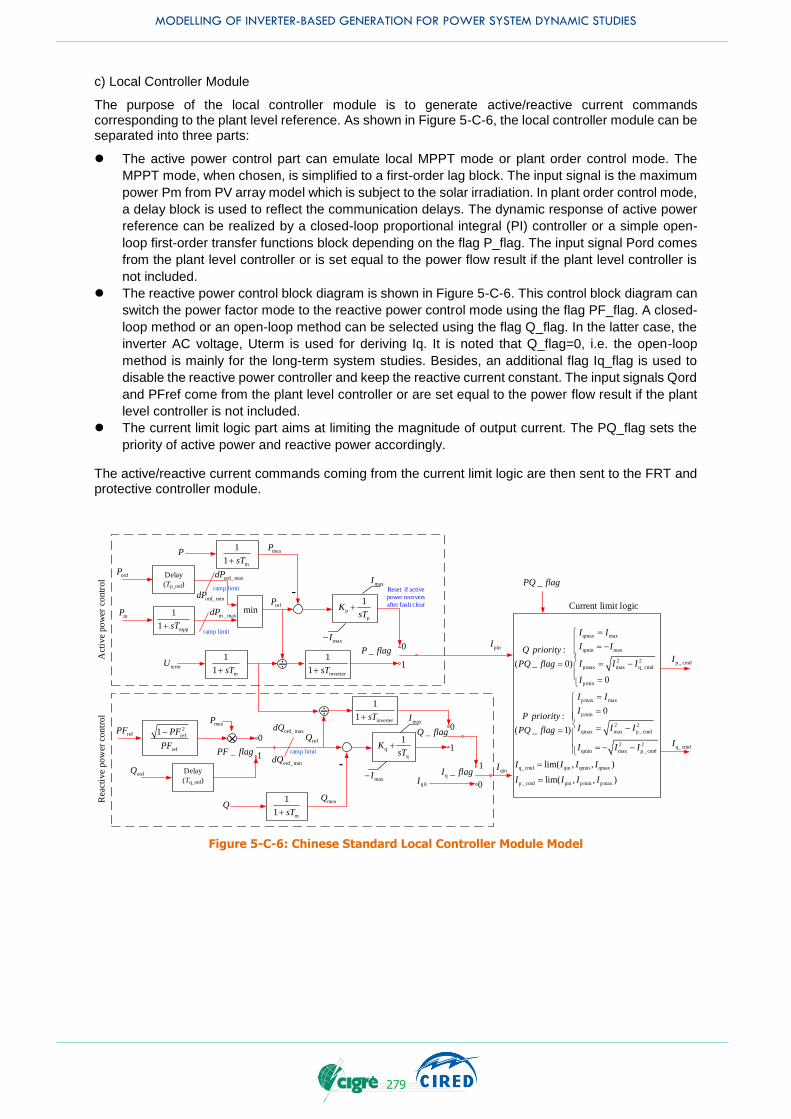
MODELLING OF INVERTER-BASED GENERATION FOR POWER SYSTEM DYNAMIC STUDIES
279
c) Local Controller Module
The purpose of the local controller module is to generate active/reactive current commands corresponding to the plant level reference. As shown in Figure 5-C-6, the local controller module can be separated into three parts:
The active power control part can emulate local MPPT mode or plant order control mode. The
MPPT mode, when chosen, is simplified to a first-order lag block. The input signal is the maximum
power Pm from PV array model which is subject to the solar irradiation. In plant order control mode,
a delay block is used to reflect the communication delays. The dynamic response of active power
reference can be realized by a closed-loop proportional integral (PI) controller or a simple open-
loop first-order transfer functions block depending on the flag P_flag. The input signal Pord comes
from the plant level controller or is set equal to the power flow result if the plant level controller is
not included.
The reactive power control block diagram is shown in Figure 5-C-6. This control block diagram can
switch the power factor mode to the reactive power control mode using the flag PF_flag. A closed-
loop method or an open-loop method can be selected using the flag Q_flag. In the latter case, the
inverter AC voltage, Uterm is used for deriving Iq. It is noted that Q_flag=0, i.e. the open-loop
method is mainly for the long-term system studies. Besides, an additional flag Iq_flag is used to
disable the reactive power controller and keep the reactive current constant. The input signals Qord
and PFref come from the plant level controller or are set equal to the power flow result if the plant
level controller is not included.
The current limit logic part aims at limiting the magnitude of output current. The PQ_flag sets the
priority of active power and reactive power accordingly.
The active/reactive current commands coming from the current limit logic are then sent to the FRT and protective controller module.
Q
mP
P
p _ cmdI
q_ cmdI
ordP Delay
(Tp_ord)
min
mpp
1
1 sT+
refP-
m
1
1 sT+
maxI
maxI-
p
p
1K
sT+
termU ÷inverter
1
1 sT+
_P flag
×refPF
refQ
ordQ Delay
(Tq_ord)
_PF flag
m
1
1 sT+
m
1
1 sT+
-
÷
q
q
1K
sT+
_Q flag
qmax max
qmin max
2 2
pmax max q_ cmd
pmin
pmax max
pmin
2 2
qmax max p _ cmd
2 2
qmin max p _ cmd
q_ cmd qin qmin qmax
p _ cmd
:
( _ 0)
0
0:
( _ 1)
lim( , , )
lim(
I I
I IQ priority
I I IPQ flag
I
I I
IP priority
I I IPQ flag
I I I
I I I I
I
-
-
-
- -
pin pmin pmax, , )I I I
maxI
maxI-
_PQ flag
inverter
1
1 sT+
2
ref
ref
1 PF
PF
-
0
1
0
10
1
Act
ive
po
wer
co
ntr
ol
Current limit logic
Rea
ctiv
e p
ow
er c
on
tro
l
meaP
meaP
Reset if active
power recovers
after fault clear
pinI
qinI
ord_ maxdP
ord_ mindP
m _ maxdP
ord_ maxdQ
ord_ mindQ
ramp limit
ramp limit
ramp limit
q _I flag
0
1
q0I
meaQ
Figure 5-C-6: Chinese Standard Local Controller Module Model
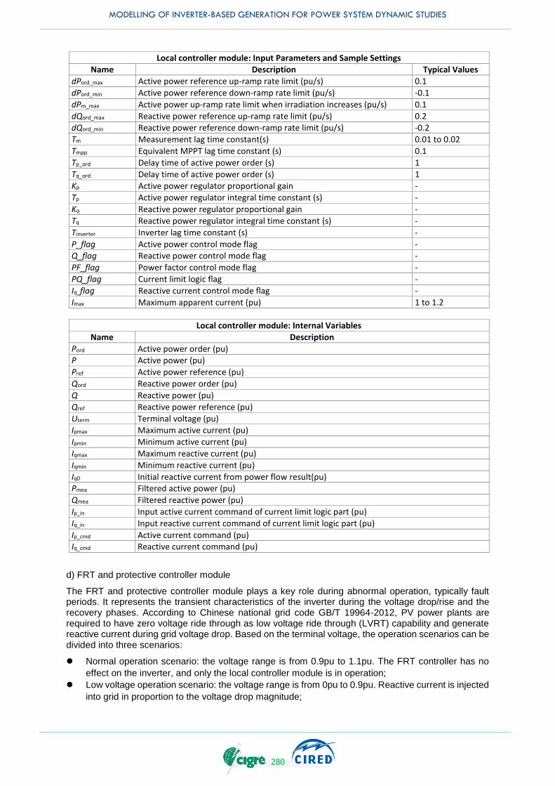
MODELLING OF INVERTER-BASED GENERATION FOR POWER SYSTEM DYNAMIC STUDIES
280
Local controller module: Input Parameters and Sample Settings Name Description Typical Values
dPord_max Active power reference up-ramp rate limit (pu/s) 0.1
dPord_min Active power reference down-ramp rate limit (pu/s) -0.1
dPm_max Active power up-ramp rate limit when irradiation increases (pu/s) 0.1
dQord_max Reactive power reference up-ramp rate limit (pu/s) 0.2 dQord_min Reactive power reference down-ramp rate limit (pu/s) -0.2
Tm Measurement lag time constant(s) 0.01 to 0.02
Tmpp Equivalent MPPT lag time constant (s) 0.1
Tp_ord Delay time of active power order (s) 1
Tq_ord Delay time of active power order (s) 1 Kp Active power regulator proportional gain -
Tp Active power regulator integral time constant (s) -
Kq Reactive power regulator proportional gain -
Tq Reactive power regulator integral time constant (s) -
Tinverter Inverter lag time constant (s) -
P_flag Active power control mode flag - Q_flag Reactive power control mode flag -
PF_flag Power factor control mode flag -
PQ_flag Current limit logic flag -
Iq_flag Reactive current control mode flag -
Imax Maximum apparent current (pu) 1 to 1.2
Local controller module: Internal Variables
Name Description
Pord Active power order (pu) P Active power (pu)
Pref Active power reference (pu)
Qord Reactive power order (pu)
Q Reactive power (pu)
Qref Reactive power reference (pu)
Uterm Terminal voltage (pu) Ipmax Maximum active current (pu)
Ipmin Minimum active current (pu)
Iqmax Maximum reactive current (pu)
Iqmin Minimum reactive current (pu)
Iq0 Initial reactive current from power flow result(pu) Pmea Filtered active power (pu)
Qmea Filtered reactive power (pu)
Ip_in Input active current command of current limit logic part (pu)
Iq_in Input reactive current command of current limit logic part (pu)
Ip_cmd Active current command (pu) Iq_cmd Reactive current command (pu)
d) FRT and protective controller module
The FRT and protective controller module plays a key role during abnormal operation, typically fault periods. It represents the transient characteristics of the inverter during the voltage drop/rise and the recovery phases. According to Chinese national grid code GB/T 19964-2012, PV power plants are required to have zero voltage ride through as low voltage ride through (LVRT) capability and generate reactive current during grid voltage drop. Based on the terminal voltage, the operation scenarios can be divided into three scenarios:
Normal operation scenario: the voltage range is from 0.9pu to 1.1pu. The FRT controller has no
effect on the inverter, and only the local controller module is in operation;
Low voltage operation scenario: the voltage range is from 0pu to 0.9pu. Reactive current is injected
into grid in proportion to the voltage drop magnitude;
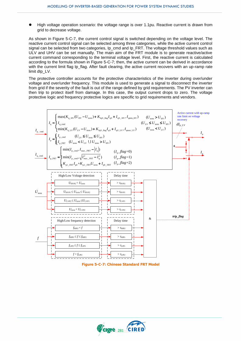
MODELLING OF INVERTER-BASED GENERATION FOR POWER SYSTEM DYNAMIC STUDIES
281
High voltage operation scenario: the voltage range is over 1.1pu. Reactive current is drawn from
grid to decrease voltage.
As shown in Figure 5-C-7, the current control signal is switched depending on the voltage level. The reactive current control signal can be selected among three categories, while the active current control signal can be selected from two categories, Ip_cmd and Ip_FRT. The voltage threshold values such as ULV and UHV can be set manually. The main aim of the FRT module is to generate reactive/active current command corresponding to the terminal voltage level. First, the reactive current is calculated according to the formula shown in Figure 5-C-7; then, the active current can be derived in accordance with the current limit flag Ip_flag. After fault clearing, the active current recovers with an up-ramp rate limit dIp_LV.
The protective controller accounts for the protective characteristics of the inverter during over/under voltage and over/under frequency. This module is used to generate a signal to disconnect the inverter from grid if the severity of the fault is out of the range defined by grid requirements. The PV inverter can then trip to protect itself from damage. In this case, the output current drops to zero. The voltage protective logic and frequency protective logics are specific to grid requirements and vendors.
0
trip_flag
qI
pIp _ cmdI
q_ cmdI
q_ HV HV term Iq0_flag q0 q0_ HV qmin_HV term HV
q q_cmd LV term HV
term LVq_LV LV term Iq0_flag q0 q0_LV qmax_LV
p _cmd LV term HV
p
term LV tep_FRT
max( ( ) , ) ( )
( )
( )min( ( ) , )
( )
(
K U U K I I I U U
I I U U U
U UK U U K I I I
I U U UI
U U UI
- + +
- + +
rm HV
p _cmd max _ FRT qp
2 2
p_FRT p _cmd max _ FRT q p
pp1_ FRT p0 p2_ FRT term p0 _ FRT
)
min( , )( _ =0)
min( , ) ( _ =1)
( _ =2)+
U
I I II flag
I I I I I flag
I flagK I K U I
-
-
+
dIp_LV
Active current with up-ramp
rate limit on voltage
recovery
f
UHVP2 < Uterm
termU UHVP1 ≤ Uterm ≤ UHVP2
ULVP2 ≤ Uterm ≤ULVP1
Uterm < ULVP2
> tHVP2
> tHVP1
> tLVP1
> tLVP2
&
fHfP2 < f
fHfP1 ≤ f ≤ fHfP2
fLfP2 ≤ f ≤ fLfP1
f < fLfP2
> tHfP2
> tHfP1
> tLfP1
> tLfP2
High/Low Voltage detection Delay time
High/Low frequency detection Delay time
Figure 5-C-7: Chinese Standard FRT Model
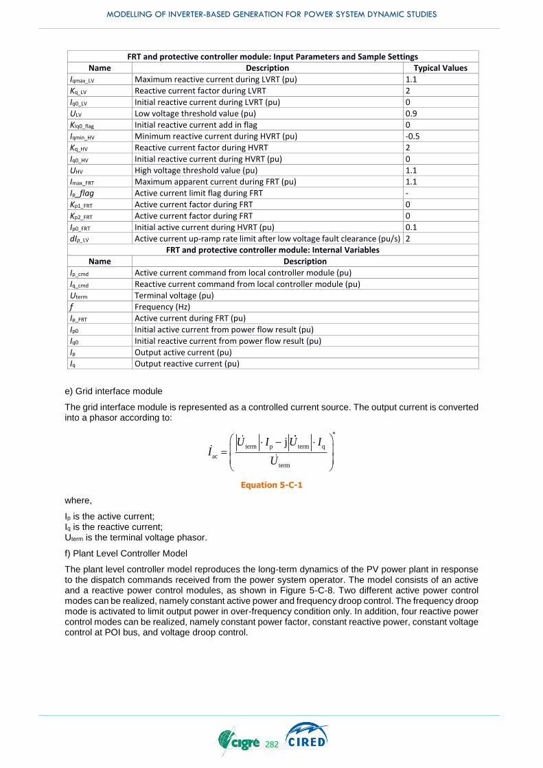
MODELLING OF INVERTER-BASED GENERATION FOR POWER SYSTEM DYNAMIC STUDIES
282
FRT and protective controller module: Input Parameters and Sample Settings Name Description Typical Values
Iqmax_LV Maximum reactive current during LVRT (pu) 1.1
Kq_LV Reactive current factor during LVRT 2
Iq0_LV Initial reactive current during LVRT (pu) 0
ULV Low voltage threshold value (pu) 0.9 KIq0_flag Initial reactive current add in flag 0
Iqmin_HV Minimum reactive current during HVRT (pu) -0.5
Kq_HV Reactive current factor during HVRT 2
Iq0_HV Initial reactive current during HVRT (pu) 0
UHV High voltage threshold value (pu) 1.1 Imax_FRT Maximum apparent current during FRT (pu) 1.1
Ip_flag Active current limit flag during FRT -
Kp1_FRT Active current factor during FRT 0
Kp2_FRT Active current factor during FRT 0
Ip0_FRT Initial active current during HVRT (pu) 0.1
dIp_LV Active current up-ramp rate limit after low voltage fault clearance (pu/s) 2 FRT and protective controller module: Internal Variables
Name Description
Ip_cmd Active current command from local controller module (pu)
Iq_cmd Reactive current command from local controller module (pu)
Uterm Terminal voltage (pu) f Frequency (Hz)
Ip_FRT Active current during FRT (pu)
Ip0 Initial active current from power flow result (pu)
Iq0 Initial reactive current from power flow result (pu)
Ip Output active current (pu) Iq Output reactive current (pu)
e) Grid interface module
The grid interface module is represented as a controlled current source. The output current is converted into a phasor according to:
term p term q
ac
term
j*
U I U II
U
-
Equation 5-C-1
where,
Ip is the active current; Iq is the reactive current; Uterm is the terminal voltage phasor.
f) Plant Level Controller Model
The plant level controller model reproduces the long-term dynamics of the PV power plant in response to the dispatch commands received from the power system operator. The model consists of an active and a reactive power control modules, as shown in Figure 5-C-8. Two different active power control modes can be realized, namely constant active power and frequency droop control. The frequency droop mode is activated to limit output power in over-frequency condition only. In addition, four reactive power control modes can be realized, namely constant power factor, constant reactive power, constant voltage control at POI bus, and voltage droop control.
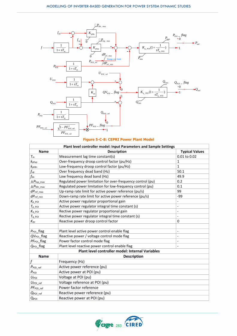
MODELLING OF INVERTER-BASED GENERATION FOR POWER SYSTEM DYNAMIC STUDIES
283
m
1
1 sT+-
-
POI _QV flag
maxQ
minQ
q _ POI
q _ POI
1(1 )K
sT+
ordQ
POI _Q flagPOIU
POIQ
POI_ refU
upf
m
1
1 sT+
-f pfupK
m
1
1 sT+POIP
-
POI_ refP
maxP
minP
p_ POI
p_ POI
1(1 )K
sT+
ordP
POI _P flag
m
1
1 sT+POIP
POI_ refPF 2
POI_ ref
POI_ ref
1 PF
PF
-×
POI _PF flag
0
-
POI _refQ
0
1
0
1
0
1
1
0
qvK
m
1
1 sT+
fup max_P
pfdnK
0
fdn max_P
dnf
-
ref_ maxdP
ref_ mindP
Ramp rate limit
Figure 5-C-8: CEPRI Power Plant Model
Plant level controller model: Input Parameters and Sample Settings
Name Description Typical Values
Tm Measurement lag time constant(s) 0.01 to 0.02 kpfup Over-frequency droop control factor (pu/Hz) 1
kpfdn Low-frequency droop control factor (pu/Hz) 1
fup Over frequency dead band (Hz) 50.1
fdn Low frequency dead band (Hz) 49.9
△Pfup_max Regulated power limitation for over-frequency control (pu) 0.2 △Pfdn_max Regulated power limitation for low-frequency control (pu) 0.1
dPref_max Up-ramp rate limit for active power reference (pu/s) 99
dPref_min Down-ramp rate limit for active power reference (pu/s) -99
Kp_POI Active power regulator proportional gain -
Tp_POI Active power regulator integral time constant (s) - Kq_POI Rective power regulator proportional gain -
Tq_POI Rective power regulator integral time constant (s) -
Kqv Reactive power droop control factor 0
PPOI_flag Plant level active power control enable flag - QVPOI_flag Reactive power / voltage control mode flag -
PFPOI_flag Power factor control mode flag -
QPOI_flag Plant level reactive power control enable flag -
Plant level controller model: Internal Variables Name Description
f Frequency (Hz) PPOI_ref Active power reference (pu) PPOI Active power at POI (pu) UPOI Voltage at POI (pu) UPOI_ref Voltage reference at POI (pu) PFPOI_ref Power factor reference QPOI_ref Reactive power reference (pu) QPOI Reactive power at POI (pu)

MODELLING OF INVERTER-BASED GENERATION FOR POWER SYSTEM DYNAMIC STUDIES
284
APPENDIX 5-D BATTERY ENERGY STORAGE MODELS
There are various battery energy storage models for different purposes. For power system dynamic stability studies, a simplified model is generally acceptable. Such a model assumes that the battery has the same characteristics during charging and discharging, internal resistance is constant, temperature does not affect the battery. The model also neglects self-discharge due to losses, and other phenomena such as memory, and Peukert effects [49]. In general, more detailed equivalent circuit dynamic battery models [49] are able to represent the battery charge/discharge behaviour and predict the batteries operating temperature [49]. However, such details are not pertinent in large-scale power system simulations and are thus neglected. On the other hand, functionalities such as active and reactive power controls are extremely important and certainly modelled for power system studies. One such energy storage model, useful for power system studies, is the WECC battery energy storage system model [50],[51], which is described below.
Battery Energy Storage Systems (BESS) can perform active and reactive power control, voltage support and frequency regulation, renewable energy smoothing, peak shaving, demand reduction, support for islanding operations, and other functions for transmission systems [52].
As all other WECC renewable energy models, the BESS model is positive sequence model, presently implemented in several commercially used power system simulation tools. This model does not consider the battery chemical process because it is mostly intended for solid state batteries. As in the WECC solar PV model, details of DC dynamics are also ignored. The WECC Renewable Energy Model for Energy Storage consists of the same modules as other models: generator/converter, electrical controls and possibly centralized plant controller. The generator/converter model and plant control, if present, are the same as for solar PV plants (models recg_a and repc_a) described earlier. However, due to its charging capabilities the model for electrical controls is different from the electrical control models for the Solar PV plants. This model was developed and validated by EPRI [51].
For a BESS, the model structure is shown in Figure 5-D-1. Here, regc_a is the renewable energy generator/converter model; its inputs are the real (Ipcmd) and reactive (Iqcmd) current commands and its outputs the active (Ip) and reactive (Iq) currents injected into the grid. This represents the inverter interface for the BESS unit. The reec_c model is the renewable energy electrical controls model c; its inputs are the real power reference (Pref), and the reactive power reference (Qref). Both of them can be externally controlled, and feedback of the reactive power generated (Qgen). The outputs of this model are the active (Ipcmd) and reactive (Iqcmd) current command. This represents the BESS inverter controls and includes a basic representation of the charging/discharging dynamics.
In addition to the above models, a repc_a (renewable energy plant controller model a) model may also be used together with this configuration to allow for voltage and frequency control at a point of common coupling. Furthermore, the more complex plant controller currently being developed may be used to control a BESS unit together with other devices in a complex plant.
A detailed description of the reec_c model is given in [51], and is shown in Figure 5-D-2.
Figure 5-D-1: Structure of BESS Model [49].
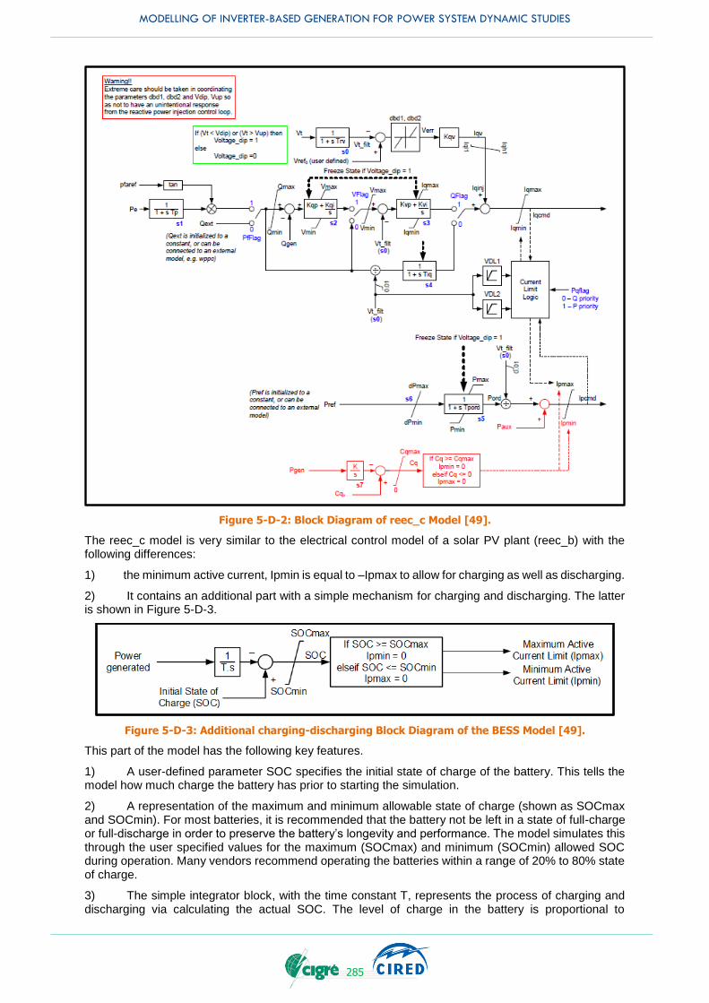
MODELLING OF INVERTER-BASED GENERATION FOR POWER SYSTEM DYNAMIC STUDIES
285
Figure 5-D-2: Block Diagram of reec_c Model [49].
The reec_c model is very similar to the electrical control model of a solar PV plant (reec_b) with the following differences:
1) the minimum active current, Ipmin is equal to –Ipmax to allow for charging as well as discharging.
2) It contains an additional part with a simple mechanism for charging and discharging. The latter is shown in Figure 5-D-3.
Figure 5-D-3: Additional charging-discharging Block Diagram of the BESS Model [49].
This part of the model has the following key features.
1) A user-defined parameter SOC specifies the initial state of charge of the battery. This tells the model how much charge the battery has prior to starting the simulation.
2) A representation of the maximum and minimum allowable state of charge (shown as SOCmax and SOCmin). For most batteries, it is recommended that the battery not be left in a state of full-charge or full-discharge in order to preserve the battery’s longevity and performance. The model simulates this through the user specified values for the maximum (SOCmax) and minimum (SOCmin) allowed SOC during operation. Many vendors recommend operating the batteries within a range of 20% to 80% state of charge.
3) The simple integrator block, with the time constant T, represents the process of charging and discharging via calculating the actual SOC. The level of charge in the battery is proportional to
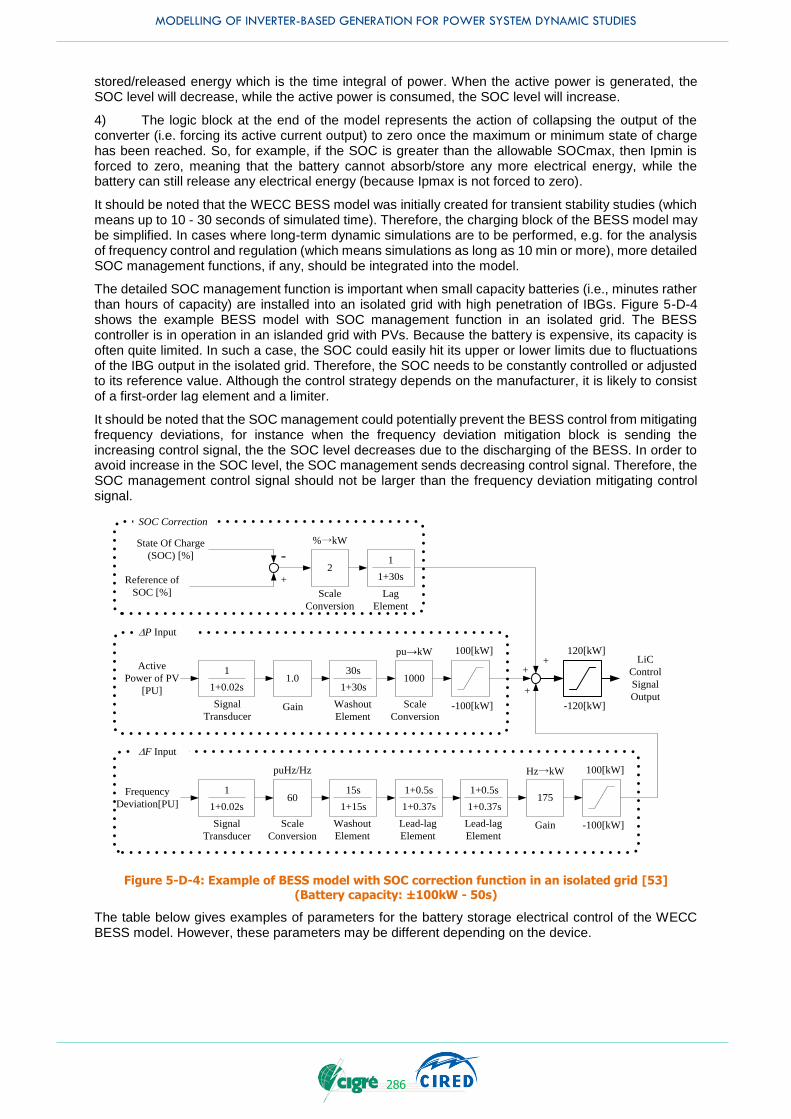
MODELLING OF INVERTER-BASED GENERATION FOR POWER SYSTEM DYNAMIC STUDIES
286
stored/released energy which is the time integral of power. When the active power is generated, the SOC level will decrease, while the active power is consumed, the SOC level will increase.
4) The logic block at the end of the model represents the action of collapsing the output of the converter (i.e. forcing its active current output) to zero once the maximum or minimum state of charge has been reached. So, for example, if the SOC is greater than the allowable SOCmax, then Ipmin is forced to zero, meaning that the battery cannot absorb/store any more electrical energy, while the battery can still release any electrical energy (because Ipmax is not forced to zero).
It should be noted that the WECC BESS model was initially created for transient stability studies (which means up to 10 - 30 seconds of simulated time). Therefore, the charging block of the BESS model may be simplified. In cases where long-term dynamic simulations are to be performed, e.g. for the analysis of frequency control and regulation (which means simulations as long as 10 min or more), more detailed SOC management functions, if any, should be integrated into the model.
The detailed SOC management function is important when small capacity batteries (i.e., minutes rather than hours of capacity) are installed into an isolated grid with high penetration of IBGs. Figure 5-D-4 shows the example BESS model with SOC management function in an isolated grid. The BESS controller is in operation in an islanded grid with PVs. Because the battery is expensive, its capacity is often quite limited. In such a case, the SOC could easily hit its upper or lower limits due to fluctuations of the IBG output in the isolated grid. Therefore, the SOC needs to be constantly controlled or adjusted to its reference value. Although the control strategy depends on the manufacturer, it is likely to consist of a first-order lag element and a limiter.
It should be noted that the SOC management could potentially prevent the BESS control from mitigating frequency deviations, for instance when the frequency deviation mitigation block is sending the increasing control signal, the the SOC level decreases due to the discharging of the BESS. In order to avoid increase in the SOC level, the SOC management sends decreasing control signal. Therefore, the SOC management control signal should not be larger than the frequency deviation mitigating control signal.
LiC
Control
Signal
Output
+
+
60 1751+15s
15s
100[kW]
-100[kW]
1+0.02s
1
Signal
Transducer
Hz→kWpuHz/Hz
GainScale
Conversion
Frequency
Deviation[PU]
Washout
Element
1+0.02s
1
Signal
Transducer
Active
Power of PV
[PU]
1.01+30s
30s
Gain Washout
Element
1000
100[kW]
-100[kW]
pu→kW
Scale
Conversion
1+0.37s
1+0.5s
Lead-lag
Element
DF Input
DP Input
1+0.37s
1+0.5s
Lead-lag
Element
SOC Correction
Reference of
SOC [%]
2
Scale
Conversion
%→kW
1+30s
1-State Of Charge
(SOC) [%]
+
+
Lag
Element
120[kW]
-120[kW]
Figure 5-D-4: Example of BESS model with SOC correction function in an isolated grid [53] (Battery capacity: ±100kW - 50s)
The table below gives examples of parameters for the battery storage electrical control of the WECC BESS model. However, these parameters may be different depending on the device.
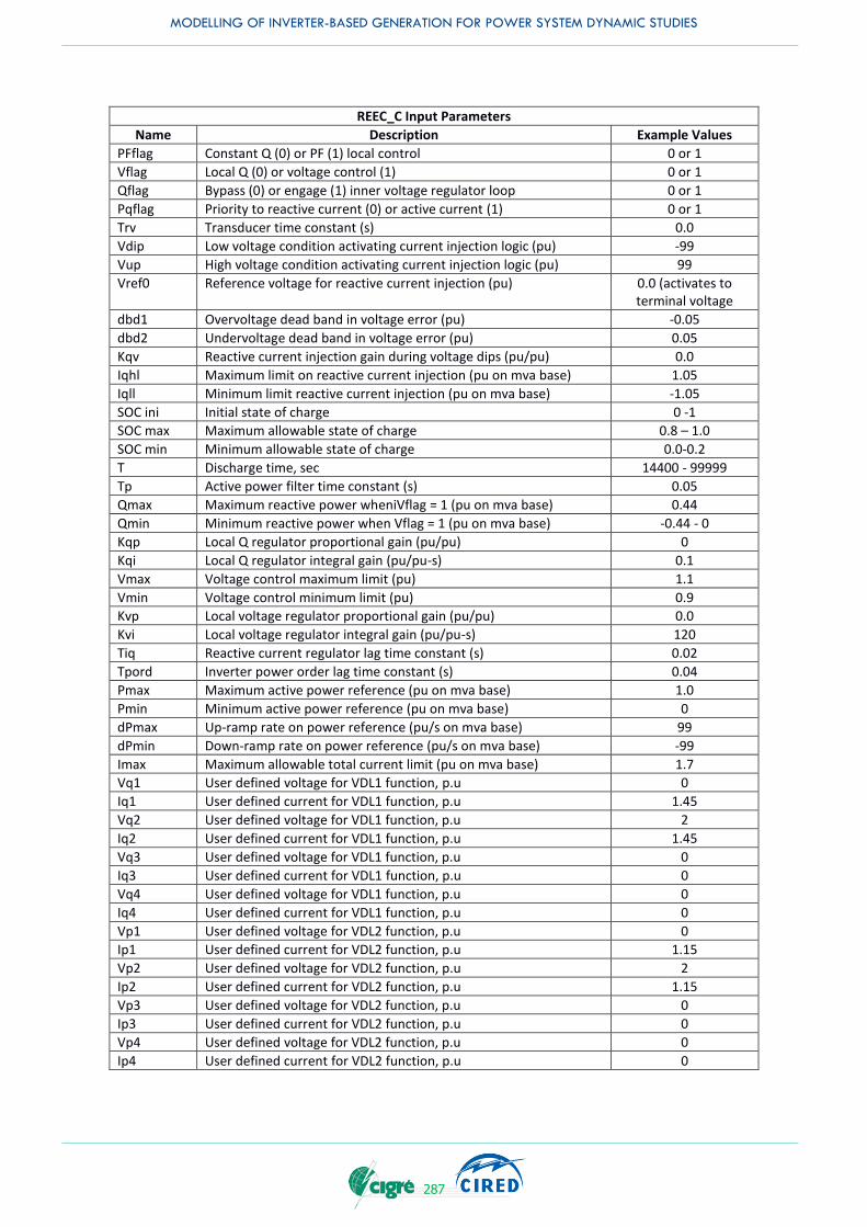
MODELLING OF INVERTER-BASED GENERATION FOR POWER SYSTEM DYNAMIC STUDIES
287
REEC_C Input Parameters
Name Description Example Values
PFflag Constant Q (0) or PF (1) local control 0 or 1
Vflag Local Q (0) or voltage control (1) 0 or 1
Qflag Bypass (0) or engage (1) inner voltage regulator loop 0 or 1
Pqflag Priority to reactive current (0) or active current (1) 0 or 1
Trv Transducer time constant (s) 0.0
Vdip Low voltage condition activating current injection logic (pu) -99
Vup High voltage condition activating current injection logic (pu) 99
Vref0 Reference voltage for reactive current injection (pu) 0.0 (activates to terminal voltage
dbd1 Overvoltage dead band in voltage error (pu) -0.05
dbd2 Undervoltage dead band in voltage error (pu) 0.05
Kqv Reactive current injection gain during voltage dips (pu/pu) 0.0
Iqhl Maximum limit on reactive current injection (pu on mva base) 1.05
Iqll Minimum limit reactive current injection (pu on mva base) -1.05
SOC ini Initial state of charge 0 -1
SOC max Maximum allowable state of charge 0.8 – 1.0
SOC min Minimum allowable state of charge 0.0-0.2
T Discharge time, sec 14400 - 99999
Tp Active power filter time constant (s) 0.05
Qmax Maximum reactive power wheniVflag = 1 (pu on mva base) 0.44
Qmin Minimum reactive power when Vflag = 1 (pu on mva base) -0.44 - 0
Kqp Local Q regulator proportional gain (pu/pu) 0
Kqi Local Q regulator integral gain (pu/pu-s) 0.1
Vmax Voltage control maximum limit (pu) 1.1
Vmin Voltage control minimum limit (pu) 0.9
Kvp Local voltage regulator proportional gain (pu/pu) 0.0
Kvi Local voltage regulator integral gain (pu/pu-s) 120
Tiq Reactive current regulator lag time constant (s) 0.02
Tpord Inverter power order lag time constant (s) 0.04
Pmax Maximum active power reference (pu on mva base) 1.0
Pmin Minimum active power reference (pu on mva base) 0
dPmax Up-ramp rate on power reference (pu/s on mva base) 99
dPmin Down-ramp rate on power reference (pu/s on mva base) -99
Imax Maximum allowable total current limit (pu on mva base) 1.7
Vq1 User defined voltage for VDL1 function, p.u 0
Iq1 User defined current for VDL1 function, p.u 1.45
Vq2 User defined voltage for VDL1 function, p.u 2
Iq2 User defined current for VDL1 function, p.u 1.45
Vq3 User defined voltage for VDL1 function, p.u 0
Iq3 User defined current for VDL1 function, p.u 0
Vq4 User defined voltage for VDL1 function, p.u 0
Iq4 User defined current for VDL1 function, p.u 0
Vp1 User defined voltage for VDL2 function, p.u 0
Ip1 User defined current for VDL2 function, p.u 1.15
Vp2 User defined voltage for VDL2 function, p.u 2
Ip2 User defined current for VDL2 function, p.u 1.15
Vp3 User defined voltage for VDL2 function, p.u 0
Ip3 User defined current for VDL2 function, p.u 0
Vp4 User defined voltage for VDL2 function, p.u 0
Ip4 User defined current for VDL2 function, p.u 0

MODELLING OF INVERTER-BASED GENERATION FOR POWER SYSTEM DYNAMIC STUDIES
288
APPENDIX 6-A EXAMPLE OF TYPICAL DATA FOR OVERHEAD AND UNDERGROUND CABLES IN PORTUGAL
Example of representative data for overhead lines and underground cables for nominal voltage, positive-sequence line parameters (impedance and charging) and line rating are shown in Table 6-A-1 [54].
Table 6-A-1: Generator protection [54]
pu
1 pu
400 400_ACSR_B595_O_H10DG150
400 kV ACSR 595 mm2 | Overhead simple line with twin Bundle conductors |
Suspended chains of insulators | Horizontal configuration (d=10 m) | Double
Ground wires ACSR 150 mm2
0.0294 0.3239 3.528E-06 11.23 564.45 2 306 2 532 2 680 136.1 1 754 11.0
400 400_ACSR_DB595_O_VDG150
400 kV ACSR 595 mm2 | Overhead Double line with twin Bundle conductors |
Suspended chains of insulators | Vertical configuration | Double Ground wires
ACSR 150 mm2
0.0290 0.3280 3.535E-06 11.25 565.66 9 224 10 127 10 720 272.3 7 016 11.3
220 220_ACSR_485_O_FDG150220 kV ACSR 485 mm2 | Overhead simple line | Suspended chains of insulators |
Flag configuration | Double Ground wires ACSR 150 mm2
0.0770 0.4230 2.702E-06 8.60 130.80 1 002 1 086 1 141 51.0 413.8 5.49
220 220_ACSR_D485_O_VDG150220 kV ACSR 485 mm2 | Overhead Double line | Suspended chains of insulators |
Vertical configuration | Double Ground wires ACSR 150 mm20.0765 0.3933 2.891E-06 9.20 139.93 2 004 2 173 2 284 102.0 828.0 5.14
60 60_ACSR_160_O_SFG13060 kV ACSR 160 mm2 | Overhead simple line | Suspended chains of insulators |
Flag configuration | Ground wire ACSR 130 mm20.2295 0.3781 2.934E-06 9.34 10.56 225 360 450 16.1 37.4 1.65
60 60_ACSR_325_O_SFG13060 kV ACSR 325 mm2 | Overhead simple line | Suspended chains of insulators |
Flag configuration | Ground wire ACSR 130 mm20.1181 0.3716 3.082E-06 9.81 11.09 330 545 685 31.3 56.6 3.15
60 60_ACSR_D160_O_SVG13060 kV ACSR D160 mm2 | Overhead Double line | Suspended chains of insulators |
Vertical configuration | Ground wire ACSR 130 mm20.1151 0.1981 5.689E-06 18.11 20.48 450 720 900 32.1 74.8 1.72
60 60_ACSR_D325_O_SVG13060 kV ACSR D325mm2 | Overhead Double line | Suspended chains of insulators |
Vertical configuration | Ground wire ACSR 130 mm20.0594 0.1920 6.050E-06 19.26 21.78 660 1 090 1 370 62.5 113.3 3.23
60 60_LXHIOLE_185_U60 kV AL-Core 185 mm2 | Underground simple line (3 single core cables in
touching trefoil laid on the bottom of a trench)0.2103 0.1382 43.982E-06 140.00 158.34 328 365 365 24.7 37.9 0.66 *
60 60_LXHIOLE_400_U60 kV AL-Core 400 mm2 | Underground simple line (3 single core cables in
touching trefoil laid on the bottom of a trench)0.0997 0.1194 59.690E-06 190.00 214.88 486 540 540 53.5 56.1 1.20
60 60_LXHIOLE_630_U60 kV AL-Core 630 mm2 | Underground simple line (3 single core cables in
touching trefoil laid on the bottom of a trench)0.0601 0.1100 78.540E-06 250.00 282.74 630 700 710 65.9 72.7 1.83
60 60_LXHIOLE_1000_U60 kV AL-Core 1000 mm2 | Underground simple line (3 single core cables in
touching trefoil laid on the bottom of a trench)0.0373 0.1005 106.814E-06 340.00 384.53 788 875 875 133.6 90.9 2.69
30 30_ACSR_050_O_SF30 kV ACSR 50 mm2 | Overhead simple line | Suspended chains of insulators |
Flag configuration0.7309 0.3940 2.897E-06 9.22 2.61 115 180 220 5.0 9.4 0.54 *
30 30_ACSR_070_O_SF30 kV ACSR 70 mm2 | Overhead simple line | Suspended chains of insulators |
Flag configuration0.5208 0.3834 2.981E-06 9.49 2.68 130 205 255 7.0 10.7 0.74 *
30 30_ACSR_090_O_SF30 kV ACSR 90 mm2 | Overhead simple line | Suspended chains of insulators |
Flag configuration0.4112 0.3759 3.043E-06 9.69 2.74 160 255 315 8.9 13.3 0.91 *
30 30_ACSR_160_O_SF30 kV ACSR 160 mm2 | Overhead simple line | Suspended chains of insulators |
Flag configuration0.2294 0.3566 3.215E-06 10.23 2.89 225 360 450 16.1 18.7 1.55
30 30_ACSR_325_O_SF30 kV ACSR 325 mm2 | Overhead simple line | Suspended chains of insulators |
Flag configuration0.1089 0.3357 3.311E-06 10.54 2.98 325 540 685 31.3 28.1 3.08
30 30_ACSR_D160_O_SV30 kV ACSR D160 mm2 | Overhead Double line | Suspended chains of insulators |
Vertical configuration0.1147 0.1980 4.778E-06 15.21 4.30 450 720 900 40.0 37.4 1.73
30 30_ACSR_D325_O_SV30 kV ACSR D325 mm2 | Overhead Double line | Suspended chains of insulators |
Vertical configuration0.0720 0.1746 4.778E-06 15.21 4.30 560 920 1 150 47.6 47.8 2.43
30 30_AAAC_055_O_SF30 kV AAAC 55 mm2 | Overhead simple line | Suspended chains of insulators |
Flag configuration0.6507 0.3909 2.921E-06 9.30 2.63 125 190 235 6.1 9.9 0.60 *
30 30_AAAC_117_O_SF30 kV AAAC 117 mm2 | Overhead simple line | Suspended chains of insulators |
Flag configuration0.3038 0.3713 3.098E-06 9.86 2.79 190 300 380 16.0 15.6 1.22
30 30_AAAC_148_O_SF30 kV AAAC 148 mm2 | Overhead simple line | Suspended chains of insulators |
Flag configuration0.2415 0.3639 3.167E-06 10.08 2.85 220 350 435 20.3 18.2 1.51
30 30_LXHIOV_120_U30 kV AL-Core 120 mm2 | Underground simple line (3 single core cables in
touching trefoil laid on the bottom of a trench)0.3244 0.1172 53.460E-06 170.17 48.11 240 285 325 15.9 14.8 0.36 *
30 30_LXHIOV_240_U30 kV AL-Core 240 mm2 | Underground simple line (3 single core cables in
touching trefoil laid on the bottom of a trench)0.1603 0.1049 69.069E-06 219.85 62.16 355 420 480 32.2 21.8 0.65 *
30 30_LXHIOV_D120_U30 kV AL-Core D120 mm2 | Underground Double line (two sets of 3 single core
cables in touching trefoil laid on the bottom of a trench)0.1622 0.0586 106.920E-06 340.34 96.23 480 570 650 31.8 29.6 0.36 *
30 30_LXHIOV_D240_U30 kV AL-Core D240 mm2 | Underground Double line (two sets of 3 single core
cables in touching trefoil laid on the bottom of a trench)0.0801 0.0458 277.887E-06 884.54 250.10 714 840 960 64.5 43.6 0.57 *
30 30_PHCAV_095_U30 kV CU-Core 95 mm2 | Underground simple line (a three core cable with one
lead sheath laid on the bottom of a trench)0.2271 0.1130 78.540E-06 250.00 70.69 210 245 245 14.8 12.7 0.50 *
30 30_PHCAV_120_U30 kV CU-Core 120 mm2 | Underground simple line (a three core cable with one
lead sheath laid on the bottom of a trench)0.1801 0.1068 87.965E-06 280.00 79.17 240 280 280 18.8 14.5 0.59 *
30 30_PHCAV_185_U30 kV CU-Core 185 mm2 | Underground simple line (a three core cable with one
lead sheath laid on the bottom of a trench)0.1161 0.1107 94.248E-06 300.00 84.82 350 415 470 28.7 21.6 0.95 *
30 30_PHCAV_240_U30 kV CU-Core 240 mm2 | Underground simple line (a three core cable with one
lead sheath laid on the bottom of a trench)0.0902 0.0929 157.079E-06 500.00 141.37 415 485 485 39.8 25.2 1.03
0.4 0.4_LXS_4x16_O0,4 kV AL-Core 16 mm
2 |Aerial bundled cables (4 single core cables in twisted
assembly with ph1+ph2+ph3+neutral)2.15 0.10 --- --- --- 68 75 83 1.9 0.052 0.05 *
0.4 0.4_LXS_4x25+16_O0,4 kV AL-Core 25+16 mm2 | Aerial bundled cables [5 single core cables in twisted
assembly with ph1+ph2+ph3+neutral (25 mm2)+public street lighting (16 mm2)]1.34 0.10 --- --- --- 90 100 110 3.0 0.069 0.07 *
0.4 0.4_LXS_4x50+16_O0,4 kV AL-Core 50+16 mm2 | Aerial bundled cables [5 single core cables in twisted
assembly with ph1+ph2+ph3+neutral (50 mm2)+public street lighting (16 mm2)]0.72 0.10 --- --- --- 135 150 165 6.0 0.104 0.14 *
0.4 0.4_LXS_4x70+16_O0,4 kV AL-Core 70+16 mm
2 | Aerial bundled cables [5 single core cables in twisted
assembly with ph1+ph2+ph3+neutral (70 mm2)+public street lighting (16 mm2)]0.50 0.10 --- --- --- 171 190 209 8.4 0.132 0.20 *
0.4 0.4_LXS_4x95+16_O0,4 kV AL-Core 95+16 mm2 | Aerial bundled cables [5 single core cables in twisted
assembly with ph1+ph2+ph3+neutral (95 mm2)+public street lighting (16 mm2)]0.36 0.10 --- --- --- 207 230 253 11.4 0.159 0.28 *
0.4 0.4_LSVAV_4x16_U0,4 kV AL-Core 16 mm2 | Underground simple line (4 core cable with
ph1+ph2+ph3+neutral laid on the bottom of a trench)2.29 0.10 --- --- --- 81 90 99 1.9 0.062 0.04 *
0.4 0.4_LSVAV_4x35_U0,4 kV AL-Core 35 mm2 | Underground simple line (4core cable with
ph1+ph2+ph3+neutral laid on the bottom of a trench)1.04 0.10 --- --- --- 117 130 143 4.2 0.090 0.10 *
0.4 0.4_LSVAV_4x50_U0,4 kV AL-Core 50 mm2 | Underground simple line (4 core cable with
ph1+ph2+ph3+neutral laid on the bottom of a trench)0.769 0.10 --- --- --- 135 150 165 6.0 0.104 0.13 *
0.4 0.4_LSVAV_4x95_U0,4 kV AL-Core 95 mm2 | Underground simple line (4 core cable with
ph1+ph2+ph3+neutral laid on the bottom of a trench)0.384 0.10 --- --- --- 212 235 259 11.4 0.163 0.26 *
0.4 0.4_LVAV_3x185+95_U
0,4 kV AL-Core 185 mm2 | Underground simple line [4 core cable with
ph1+ph2+ph3 (185 mm2)+neutral (95 mm2) laid on the bottom of a trench]
Note: For phase-neutral fault (Rd neutral = 0.384 W / km ; Xd neutral = 0.10 W / km)
0.197 0.10 --- --- --- 320 355 391 22.3 0.246 0.51 *
0.23 0.23_LXS_2x16_O0.23 kV AL-Core 16 mm2 | Aerial bundled cables (2 single core cables in twisted
assembly with phase+neutral)2.15 0.10 --- --- --- 77 85 94 1.9 0.020 0.05 *
0.23 0.23_LSVAV_2x16_U0.23 kV AL-Core 16 mm2 | Underground simple line (2 core cable with
phase+neutral laid on the bottom of a trench)2.29 0.10 --- --- --- 86 95 105 1.9 0.022 0.04 *
Note - An asterisk * is shown in the table when the ratio Xd / Rd ≤ 1 p.u. is reached.
UN
kVLine Code Line Structure and Physical Constitution
(Cross section per phase)
I F/S
Fall / Spring
A
Rd
W / Km
Xd
W / Km
Bd
W-1 / Km
Cd
nF / Km
-QC d
kvar / km
I S
Summer
A
I W
Winter
A
Iccrms
(0.5 s)
kA
S F/S
Fall / Spring
MVA
Xd / Rd

MODELLING OF INVERTER-BASED GENERATION FOR POWER SYSTEM DYNAMIC STUDIES
289
APPENDIX 7-A AN OPEN-SOURCE DISTRIBUTED CONTROL PLATFORM FOR HIL-BASED TESTING AND DEMONSTRATION OF ADVANCED POWER SYSTEMS
Chapter 7-A.1 Motivation
The management of emerging, high agile power and energy systems in the context of achieving the overall mission operations must be facilitated by a distributed control environment [55]. Applied and basic research in distributed control is a subject actively being addressed by the naval community. The aim of such work is to provide autonomy, intelligence, and resilience under the extreme conditions that exist in potential mission operations, enabling a high Quality of Service (QoS) to mission loads (weapons, sensor arrays, etc.) while maintaining other critical infrastructure needs. The difficulty of the transition from theoretical control research, especially in a distributed context, to a physical demonstration should not be underestimated. Simply put, the theory must be validated in a large, multi-faceted test bed platform. Our expertise in modelling and simulation at the Florida State University (FSU) Centre for Advanced Power Systems (CAPS) has led us to the conclusion that the unconstrained or over-simplified models that are typically used for the purpose of advanced control research and development will often result in what might be considered as an over-optimistic assessment of the control reachability and functionality. This may be especially problematic during physical controller instantiation. This text describes the existing controller hardware in the loop (CHIL) and power hardware in the loop (PHIL) capabilities at FSU-CAPS along with recently funded infrastructure upgrades necessary to meet the United States Department of Defence (DoD) power and energy community needs in assessing the validity and efficacy of any particular distributed control methodology in a highly flexible and realistic environment that is appropriate for the specific applications.
Chapter 7-A.2 Existing Facilities
The CAPS PHIL laboratory has been designed to test electrical and mechanical hardware under test (HUT) with power capability up to 5 MW, as depicted in Figure 7-A-1, while coupled with a rest-of-system, real-time simulation. CAPS’ real-time modelling and simulation capabilities are currently based on the two most prevalent commercially available real-time simulators (RTDS from RTDS Technologies, Inc. and eMEGAsim/RT-LAB from Opal-RT Technologies, Inc.). CHIL experiments are achieved through either dedicated wiring using analogue and digital signals or standard communication network protocols such as Distributed Network Protocol (DNP3), and IEC 61850 (communication networks and systems in substations). In both cases—PHIL and CHIL—the HUT is part of a closed-loop simulation and it allows evaluation of dynamic responses, while the remaining part is modelled and simulated using the real-time environments.
CAPS has utilized real-time simulation capabilities successfully in numerous projects, such as dynamic testing of a prototype 5 MW high-temperature superconducting motor [56], a high-speed generator [57], superconducting fault current limiters [58], and also successfully conducted co-simulation of electro-mechanical and thermal systems [59], [60]. CAPS’ founding role in the Electric Ship Research and Development Consortium (ESRDC), its research and development contributions in this community, and its success with PHIL and CHIL testing, have established a credible foundation with the Navy and the Navy ship systems supplier community [61]. Based on this established competency, developmental testing and characterization of candidate future ship technologies is an on-going process at CAPS.
In addition to the aforementioned facilities, two key test beds have been developed that are focused on distributed controls. The low-power Distributed Controls test bed is shown in Figure 7-A-2. The 400 V/10 kVA system in Figure 7-A-2a consists of 1) controllable power electronics-based source/sinks (Rk1 or Rk2) that are fully integrated into the test bed for emulation of a variety of devices allowing for AC/DC or hybrid systems to be developed, 2) AC inverter-fed (INV+AC) loads to emulate ship propulsion, 3) controllable storage (Bat) to emulate batteries, ultra-capacitors, or flywheels, and 4) a pulse power load (DC) structure to emulate EMRG or radar. The test bed has distributed control platform composed of 18 national instruments devices (15 myRIO and 3 sbRIO) operating with LabVIEW environment (Figure 7-A-2c). The control units are connected via dedicated Ethernet and to test bed equipment via CAN, RS232, Ethernet, and serial communication. This test bed can cooperate with RTDS (Figure 7-A-2d) via analogue and digital I/O (Figure 7-A-2e) to do the CHIL or PHIL experiments.

MODELLING OF INVERTER-BASED GENERATION FOR POWER SYSTEM DYNAMIC STUDIES
290
Figure 7-A-1: 5 MW PHIL facility at FSU-CAPS.
Figure 7-A-2: Low-power Distributed Controls Test Bed: a) architectural layout, b) control room, c) distributed control devices, d) simulator room, e) analogue and digital IO interface to RTDS.
Additionally, CAPS has developed a CHIL test bed composed of 6 Mamba computational platforms. The platforms are networked together via Ethernet and connected via fibre to the RTDS system. This test bed has been mainly used with simulated power sources and sinks, with up to 4 control nodes per board. The maximum number of control nodes is based on the complexity of the devices and the required control cycle-time. Most importantly, controller-controller communication is networked through an OPNET real-time platform which simulates the salient features of the controls network infrastructure between the Mamba nodes. This unique laboratory setup, referred to as the Cyber-Physical Hardware-in-the-Loop Test Bed (CP-HIL-TB) allows the researcher to conduct a realistic CHIL experiment utilizing distributed controls. Given high fidelity sources, loads and systems in the RTDS, a distributed control
RTDS Simulator Lab
Rest of System Simulation
Feedback and
Control Signals
12.47 kVUtility
MVDC Lab
Each Module: +/- 0...6 kV DC,
+/- 0...210 A DC
Parallel: 6 kV, 0.8 kA
Series: 24 kV, 0.21 kA
MMC 3
(PU3)
MMC 4
(PU 4)
CU4
MMC 2(PU 2)
4.16 kV
5 MW High Bay
AC
VVS
Controller
DC
VVS
Controller
0...4.16 kV
0...0.4/0.8 kA
Variable Voltage Source Converter
225
450
1800
3600
12000
24000
Gear
Box DYNO
VSD
45...120 Hz
0...1.1 kV
0...2.5 kA
Gear
Box
MMC 1(PU1)
+ - + -
CU2
CU3
+ -
CU1
+ -
MVDC
T2MVDC
T1
T1
T9.2 T9.1
0...480 V
1.5 kA
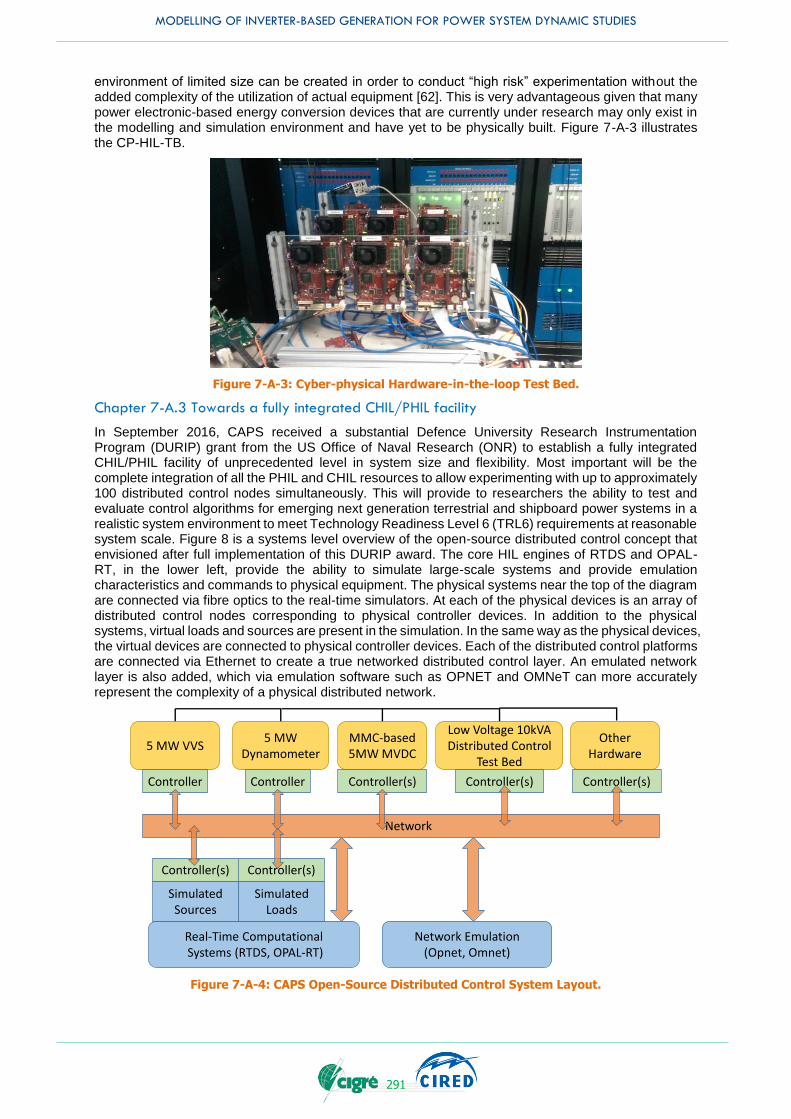
MODELLING OF INVERTER-BASED GENERATION FOR POWER SYSTEM DYNAMIC STUDIES
291
environment of limited size can be created in order to conduct “high risk” experimentation without the added complexity of the utilization of actual equipment [62]. This is very advantageous given that many power electronic-based energy conversion devices that are currently under research may only exist in the modelling and simulation environment and have yet to be physically built. Figure 7-A-3 illustrates the CP-HIL-TB.
Figure 7-A-3: Cyber-physical Hardware-in-the-loop Test Bed.
Chapter 7-A.3 Towards a fully integrated CHIL/PHIL facility
In September 2016, CAPS received a substantial Defence University Research Instrumentation Program (DURIP) grant from the US Office of Naval Research (ONR) to establish a fully integrated CHIL/PHIL facility of unprecedented level in system size and flexibility. Most important will be the complete integration of all the PHIL and CHIL resources to allow experimenting with up to approximately 100 distributed control nodes simultaneously. This will provide to researchers the ability to test and evaluate control algorithms for emerging next generation terrestrial and shipboard power systems in a realistic system environment to meet Technology Readiness Level 6 (TRL6) requirements at reasonable system scale. Figure 8 is a systems level overview of the open-source distributed control concept that envisioned after full implementation of this DURIP award. The core HIL engines of RTDS and OPAL-RT, in the lower left, provide the ability to simulate large-scale systems and provide emulation characteristics and commands to physical equipment. The physical systems near the top of the diagram are connected via fibre optics to the real-time simulators. At each of the physical devices is an array of distributed control nodes corresponding to physical controller devices. In addition to the physical systems, virtual loads and sources are present in the simulation. In the same way as the physical devices, the virtual devices are connected to physical controller devices. Each of the distributed control platforms are connected via Ethernet to create a true networked distributed control layer. An emulated network layer is also added, which via emulation software such as OPNET and OMNeT can more accurately represent the complexity of a physical distributed network.
Figure 7-A-4: CAPS Open-Source Distributed Control System Layout.
Network Emulation(Opnet, Omnet)
5 MW VVS5 MW
DynamometerMMC-based5MW MVDC
Low Voltage 10kVADistributed Control
Test Bed
Real-Time ComputationalSystems (RTDS, OPAL-RT)
SimulatedSources
SimulatedLoads
Controller(s) Controller(s)
Controller Controller Controller(s) Controller(s)
Network
OtherHardware
Controller(s)
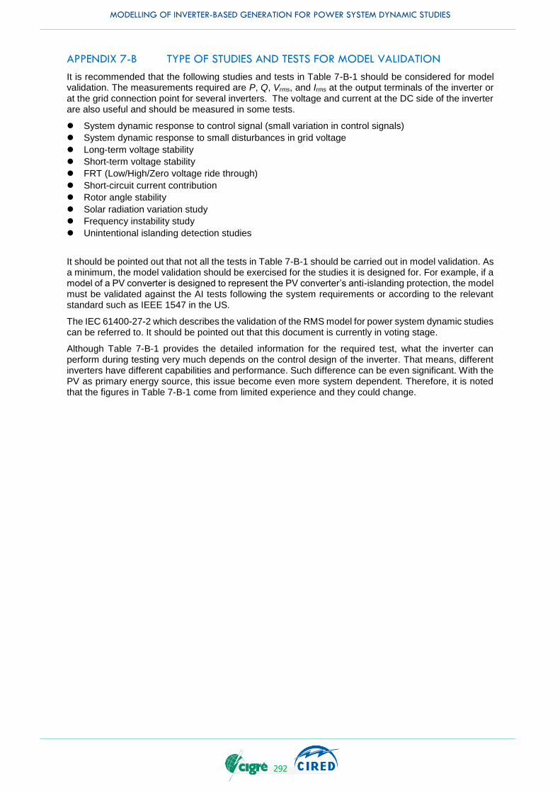
MODELLING OF INVERTER-BASED GENERATION FOR POWER SYSTEM DYNAMIC STUDIES
292
APPENDIX 7-B TYPE OF STUDIES AND TESTS FOR MODEL VALIDATION
It is recommended that the following studies and tests in Table 7-B-1 should be considered for model validation. The measurements required are P, Q, Vrms, and Irms at the output terminals of the inverter or at the grid connection point for several inverters. The voltage and current at the DC side of the inverter are also useful and should be measured in some tests.
System dynamic response to control signal (small variation in control signals)
System dynamic response to small disturbances in grid voltage
Long-term voltage stability
Short-term voltage stability
FRT (Low/High/Zero voltage ride through)
Short-circuit current contribution
Rotor angle stability
Solar radiation variation study
Frequency instability study
Unintentional islanding detection studies
It should be pointed out that not all the tests in Table 7-B-1 should be carried out in model validation. As a minimum, the model validation should be exercised for the studies it is designed for. For example, if a model of a PV converter is designed to represent the PV converter’s anti-islanding protection, the model must be validated against the AI tests following the system requirements or according to the relevant standard such as IEEE 1547 in the US.
The IEC 61400-27-2 which describes the validation of the RMS model for power system dynamic studies can be referred to. It should be pointed out that this document is currently in voting stage.
Although Table 7-B-1 provides the detailed information for the required test, what the inverter can perform during testing very much depends on the control design of the inverter. That means, different inverters have different capabilities and performance. Such difference can be even significant. With the PV as primary energy source, this issue become even more system dependent. Therefore, it is noted that the figures in Table 7-B-1 come from limited experience and they could change.
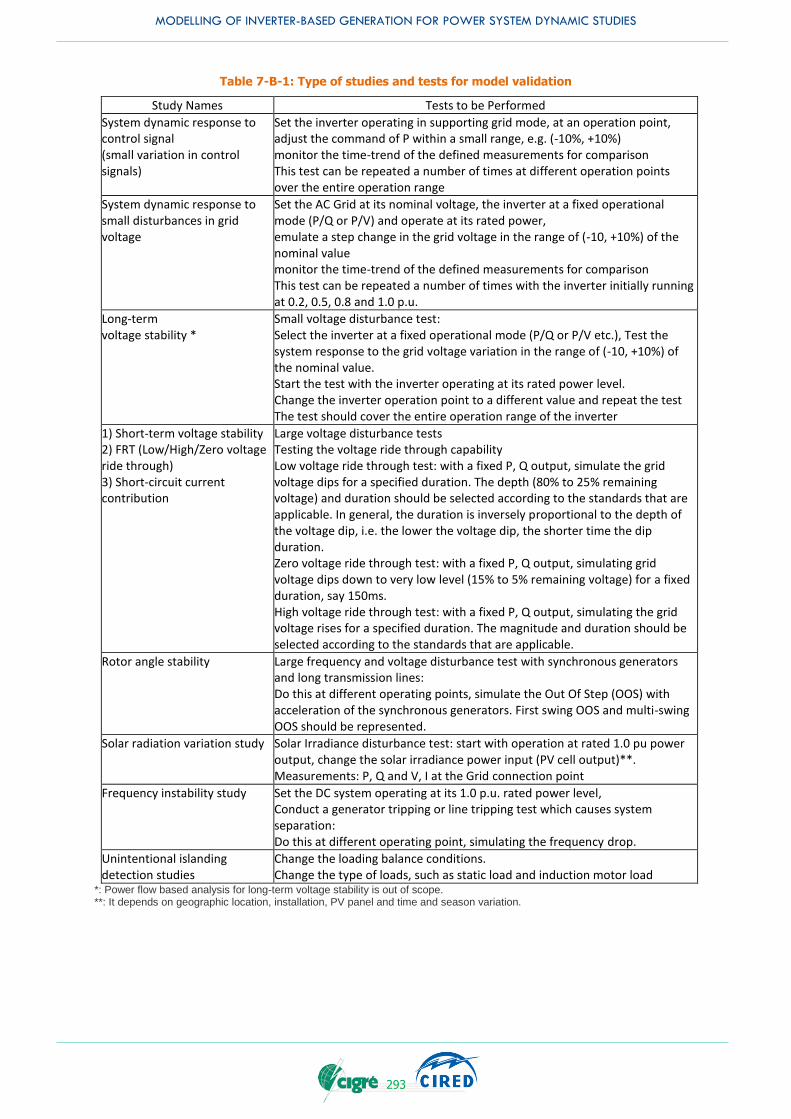
MODELLING OF INVERTER-BASED GENERATION FOR POWER SYSTEM DYNAMIC STUDIES
293
Table 7-B-1: Type of studies and tests for model validation
Study Names Tests to be Performed
System dynamic response to control signal (small variation in control signals)
Set the inverter operating in supporting grid mode, at an operation point, adjust the command of P within a small range, e.g. (-10%, +10%) monitor the time-trend of the defined measurements for comparison This test can be repeated a number of times at different operation points over the entire operation range
System dynamic response to small disturbances in grid voltage
Set the AC Grid at its nominal voltage, the inverter at a fixed operational mode (P/Q or P/V) and operate at its rated power, emulate a step change in the grid voltage in the range of (-10, +10%) of the nominal value monitor the time-trend of the defined measurements for comparison This test can be repeated a number of times with the inverter initially running at 0.2, 0.5, 0.8 and 1.0 p.u.
Long-term voltage stability *
Small voltage disturbance test: Select the inverter at a fixed operational mode (P/Q or P/V etc.), Test the system response to the grid voltage variation in the range of (-10, +10%) of the nominal value. Start the test with the inverter operating at its rated power level. Change the inverter operation point to a different value and repeat the test The test should cover the entire operation range of the inverter
1) Short-term voltage stability 2) FRT (Low/High/Zero voltage ride through) 3) Short-circuit current contribution
Large voltage disturbance tests Testing the voltage ride through capability Low voltage ride through test: with a fixed P, Q output, simulate the grid voltage dips for a specified duration. The depth (80% to 25% remaining voltage) and duration should be selected according to the standards that are applicable. In general, the duration is inversely proportional to the depth of the voltage dip, i.e. the lower the voltage dip, the shorter time the dip duration. Zero voltage ride through test: with a fixed P, Q output, simulating grid voltage dips down to very low level (15% to 5% remaining voltage) for a fixed duration, say 150ms. High voltage ride through test: with a fixed P, Q output, simulating the grid voltage rises for a specified duration. The magnitude and duration should be selected according to the standards that are applicable.
Rotor angle stability Large frequency and voltage disturbance test with synchronous generators and long transmission lines: Do this at different operating points, simulate the Out Of Step (OOS) with acceleration of the synchronous generators. First swing OOS and multi-swing OOS should be represented.
Solar radiation variation study Solar Irradiance disturbance test: start with operation at rated 1.0 pu power output, change the solar irradiance power input (PV cell output)**. Measurements: P, Q and V, I at the Grid connection point
Frequency instability study Set the DC system operating at its 1.0 p.u. rated power level, Conduct a generator tripping or line tripping test which causes system separation: Do this at different operating point, simulating the frequency drop.
Unintentional islanding detection studies
Change the loading balance conditions. Change the type of loads, such as static load and induction motor load
*: Power flow based analysis for long-term voltage stability is out of scope. **: It depends on geographic location, installation, PV panel and time and season variation.
MODELLING OF INVERTER-BASED GENERATION FOR POWER SYSTEM DYNAMIC STUDIES
294
LINKS AND REFERENCES OF APPENDIX C
[1] J. V. Milanović, K. Yamashita, S. Martínez Villanueva, S. Ž. Djokic and L. M. Korunović,
"International Industry Practice on Power System Load Modeling," IEEE Trans. on Power
Systems, pp. 3038-3046, August 2013.
[2] NERC Standard TPL-001-4, "Transmission System Planning Performance Requirements,"
January 2016, URL:
http://www.nerc.com/_layouts/PrintStandard.aspx?standardnumber=TPL-001-
4&title=TransmissionSystem/Planning/Performance/Requirements&jurisdiction=United/States.
[3] Western Electricity Coordinating Council (WECC) Renewable Energy Modeling Task Force,
URL: https://www.wecc.biz/PCC/Pages/MVWG.aspx.
[4] International Electrotechnical Commission (IEC) TC88 WG27, "Wind turbines - Electrical
simulation models for wind power generation," URL:
http://www.iec.ch/dyn/www/f?p=103:14:0::::FSP_ORG_ID,FSP_LANG_ID:5613,25.
[5] R. Elliott, A. Ellis, P. Pourbeik, J. J. Sanchez-Gasca, J. Senthil and J. Weber, "Generic
Photovoltaic System Models for WECC – A Status Report," in 2015 IEEE Power & Energy
Society General Meeting, Denver, July 2015. pp. 1-5.
[6] G. Lammert, L. D. Pabón Ospina, P. Pourbeik, D. Fetzer and M. Braun, "Implementation and
Validation of WECC Generic Photovoltaic System Models in DIgSILENT PowerFactory," in 2016
IEEE Power & Energy Society General Meeting, Boston, July 2016. pp. 1-5.
[7] P. Pourbeik, „Proposal for the DER_A model, “Presentation at WECC meeting, November 2016.
[8] G. Lammert, K. Yamashita, L. D. Pabón Ospina, H. Renner, S. Martínez Villanueva, P. Pourbeik,
F.-E. Ciausiu and M. Braun, "Modelling and Dynamic Performance of Inverter Based Generation
in Power System Studies: An International Questionnaire Survey," in CIRED conference,
Glasgow, 2017. (to be published)
[9] P. Kundur, Power System Stability and Control, Mc-Graw Hill, 1994.
[10] O. Ruhle and F. Balasin, "Simulations of Power System Dynamic Phenomena," in 2009 IEEE
PowerTech, Bucharest, June-July 2009. pp. 1-6.
[11] H. W. Dommel, "Digital Computer Solution of Electromagnetic Transients in Single- and
Multiphase Networks," IEEE Trans. on Power Apparatus and Systems, pp. 388-399, April 1969.
[12] Western Electricity Coordinating Council (WECC) Renewable Energy Modeling Task Force,
"WECC solar PV dynamic model specification," September 2012, URL:
https://www.wecc.biz/Reliability/WECC/Solar/PV/Dynamic/Model/Specification/-
/September/2012.pdf.
[13] G. Lammert, K. Yamashita, L. D. Pab´on Ospina, H. Renner, S. Martinez Villanueva, P.
Pourbeik, F.-E. Ciausiu, and M. Braun, “International Industry Practice on Modelling and
Dynamic Performance of Inverter Based Generation in Power System Studies,” CIGRE Science
& Engineering Vol. 8, June 2017.
[14] Western Electricity Coordinating Council (WECC) Renewable Energy Modeling Task Force,
August 2010, “WECC PV plant power flow modeling guidelines,” pp. 1-15.
[15] S. Soni, G. G. Karady, M. Morjaria and V. Chadliev, April 2014, “Comparison of full and reduced
scale solar PV plant models in multi-machine power systems,” 2014 IEEE PES T&D Conference
and Exposition, Chicago, pp. 1–5.
[16] P. Pourbeik, November 2016, “Proposal for the DER_A model,” Presentation at WECC meeting.
[17] K. Yamashita, S. Uemura, H. Kameda, K. Yokoi, S. Fubo and A. Takeuchi, “Verification of model
accuracy of islanding protection relay for synchronous generator,” in proc. of IEEJ annual
meeting, Vol. 6, No. 191, Japan, 2005 (in Japanese).
[18] IEEE C.37.2-2008, "Electrical Power System Device Function Numbers, Acronyms, and
Contact Designations," Oct. 2008.
[19] NERC Standard BAL-003-1 “Frequency Response & Frequency Bias Setting,” April 2015, URL:
http://www.nerc.com/_layouts/PrintStandard.aspx?standardnumber=BAL-003-
0.1b&title=Frequency Response and Bias&jurisdiction=United States
[20] K. Misak, Blackout im Übertragungsnetz – den Ernstfall beherrschen, 2. Fachtagung Blackout -
Auswirkungen, Maßnahmen und Konsequenzen auf allen Spannungsebenen, 6.- 7.5. 2014,
Hannover (in German).
MODELLING OF INVERTER-BASED GENERATION FOR POWER SYSTEM DYNAMIC STUDIES
295
[21] WECC, “WECC Guide for Representation of Photovoltaic Systems In Large-Scale Power flow
Simulations. WECC Modelling and Validation Work Group. Jan. 2011, URL:
https://www.wecc.biz/_layouts/15/WopiFrame.aspx?sourcedoc=/Reliability/WECC/PV/Plant/P
ower/Flow/Modeling/Guidelines/-/August/2010.pdf&action=default&DefaultItemOpen=1
[22] EPRI Technical Update – Generic Models and Model Validation for Wind Turbine Generators
and Photovoltaic Generation, URL:
http://www.epri.com/abstracts/Pages/ProductAbstract.aspx?ProductId=000000003002001002
[23] I. Green, “CAISO Experience with Impact of High Penetration of Renewable Resources on
Short-term Voltage Stability,” IEEE PES GM 2015, Panel - Challenges of Voltage and Reactive
Power Control from Renewable Resources, July 2015.
[24] Chen Wei, “Reactive power capability of SG2500HV_SG3000HV Inverter,” Aug. 2016.
[25] N.W. Miller, "Keeping It Together: Transient Stability in a World of Wind and Solar
Generation," in IEEE Power and Energy Magazine, vol.13, no.6, pp.31-39, Nov.-Dec. 2015.
[26] R. Preece and J. V Milanović, “Assessing the Applicability of Uncertainty Importance
Measures for Power System Studies,” IEEE Trans. Power Syst., 2015, available online.
[27] P. Lund, C. L. Bak, P. Thogersen, Z. Chen, C. Liu, K. Sun, and Z. H. Rather, “A Systematic
Approach for Dynamic Security Assessment and the Corresponding Preventive Control
Scheme Based on Decision Trees,” IEEE Trans. Power Syst., vol. 29, no. 2, pp. 717–730,
2014.
[28] L. Shi, S. Sun, L. Yao, Y. Ni, and M. Bazargan, “Effects of wind generation intermittency and
volatility on power system transient stability,” IET Renew. Power Gener., vol. 8, no. 5, pp.
509–521, 2014.
[29] M. Fan, V. Vittal, G. T. Heydt, R. Ayyanar, “Probabilistic power flow analysis with generation
dispatch including photovoltaic resources,” IEEE Trans. Power Syst., vol. 28, no. 2, pp. 1797–
1805, 2013.
[30] S. Eftekharnejad, G. T. Heydt, L. Fellow, V. Vittal, “Optimal Generation Dispatch With High
Penetration of Photovoltaic Generation,” in IEEE Power & Energy Society General Meeting,
26-30 July 2015.
[31] P. N. Papadopoulos, A. Adrees, J. V. Milanovic, “Probabilistic Assessment of Transient
Stability in Reduced Inertia Systems,” PES General Meeting 2016, Boston, July 2016.
[32] A. Adrees, P. N. Papadopoulos, J. V. Milanovic, “Framework to Assess the Effect of Reduction
in Inertia on System Frequency Response,” PES General Meeting 2016, Boston, July 2016.
[33] R. Preece, J. V. Milanovic, “Efficient Estimation of the Probability of Small-Disturbance
Instability of Large Uncertain Power Systems,” IEEE Trans. Power Syst., vol. 31, no. 2, pp.
1063–1072, 2015.
[34] G. Rogers, Power System Oscillations. Kluwer Academic, 2000.
[35] WECC Wind Power Plant Dynamic Modeling Guide, WECC Renewable Energy Modeling
Task Force, January 2014.
[36] Wind turbines - Part 27-1: Electrical simulation models - Wind turbines, IEC 61400-27-1, 2015.
[37] WECC PV Power Plant Dynamic Modeling Guide, WECC Renewable Energy Modeling Task
Force, May 2014.
[38] T. Weissbach and E. Welfonder, "High-frequency deviations within the European Power
System: Origins and proposals for improvement," in IEEE Power Systems Conference and
Exposition, 2009.
[39] J. W. Ingleson and D. M. Ellis, "Tracking the Eastern interconnection frequency governing
characteristic," in IEEE PES General Meeting, 2005.
[40] I. Erlich, K. Rensch, and F. Shewarega, "Impact of large wind power generation on frequency
stability," in IEEE PES General Meeting, 2006.
[41] P. Pal and B. Chauduri, Robust Control in Power Systems. New York: Springer Science &
Business Media, 2005.
[42] “DSA Tools TSAT User Manual,” Powertech Labs Inc, 2011.
[43] T. Guo and J. V Milanović, “Online Identification of Power System Dynamic Signature Using
PMU Measurements and Data Mining,” IEEE Trans. Power Syst., 2015, available online.
[44] K. Yamashita and H. Satoh, “Small-scale Three-Phase Photovoltaic Inverter Model for Grid
Interconnection Studies,” in Proc. of CIGRE AORC 2017, Auckland, New Zealand. Sep. 2017.

MODELLING OF INVERTER-BASED GENERATION FOR POWER SYSTEM DYNAMIC STUDIES
296
[45] H. Sato and K. Yamashita, “Three-Phase Photovoltaic Inverter Model for Unbalanced Fault,” in
Proc. of IEEJ Annual Conference of Power and Energy Society, Sep. 2018 (in Japanese).
[46] A. Ellis, M. Behnke, and R. Elliott, “Generic Solar Photovoltaic System Dynamic Simulation
Model Specification,” Sandia National Laboratories, 2013.
[47] A. Ellis, Y. Kazachkov, E. Muljadi, P. Pourbeik, and J. J. Sanchez-Gasca, “Description and
technical specifications for generic WTG models - A status report,” in Proceedings of 2011 IEEE
PES Power Systems Conference and Exposition (PSCE 2011), 2011.
[48] L. Ge, L. Zhu, L. Qu, L. Zhang, L. Zhao and N. Chen, “Model study of photovoltaic inverter for
bulk power system studies based on comprehensive tests,” proceedings of IET renewable
power generation 2015.
[49] EPRI, “Model User Guide for Generic Renewable Energy System Models,” NB 3002006525,
2015.
[50] P. Pourbeik, S. E. Williams, J. Weber, J. Sanchez-Gasca, J. Senthil, S. Huang, and K. Bolton,
“Modeling and Dynamic Behavior of Battery Energy Storage: A Simple Model for Large-Scale
Time-Domain Stability Studies,” IEEE Electrif. Mag., vol. 3, no. 3, pp. 47–51, Sep. 2015.
[51] P. Pourbeik, “Simple Model Specification for Battery Energy Storage System,” WECC REMTF,
MVWG and EPRI, NB 173.003, 2015.
[52] E. Sasano, K. Shinya, M. Matsumoto, and S. Horiuchi, “Demonstration projects for providing
ancillary services using different three types of large-scale battery systems,” CIGRE Paris
Session 2018 (to be published).
[53] K. Yamashita, O. Sakamoto, Y. Kitauchi, T. Nanahara, T. Inoue, T. Arakaki, and H. Fukuda, “A
frequency-stabilizing scheme for integrating photovoltaics into a small island grid,” in 2011 2nd
IEEE PES International Conference and Exhibition on Innovative Smart Grid Technologies,
2011, pp. 1–7.
[54] José Carvalho Martins. “Electrical Characteristics of Overhead and Underground Lines VHV,
HV, MV and LV”. Work Report to Support the Planning of Electrical Networks. EDP Distribuição.
Lisbon. Feb. 2017.
[55] A. Seman, “Autonomy Is a Must for Ship Systems,” in Future Force, Spring Edition, pp 17-19,
2014.
[56] M. Steurer, S. Woodruff, T. Baldwin, H. Boenig, F. Bogdan, T. Fikse, M. Sloderbeck, and G.
Snitchler, “Hardware-in-the-Loop Investigation of Rotor Heating in a 5 MW HTS Propulsion
Motor,” IEEE Trans. on Applied Superconductivity, Vol. 17, No. 2, Part 2, pp. 1595-1598, 2007.
[57] James Langston, Michael Steurer, Karl Schoder, John Hauer, Ferenc Bogdan, Isaac Leonard,
Tim Chiocchio, Michael Sloderbeck, Andrew Farrell, Jay Vaidya, and Kevin Yost, “Megawatt
Scale Hardware-in-the-Loop Testing of a High Speed Generator,” in Proc. ASNE Day, May 9-
10, 2012, Arlington, VA.
[58] C. Schacherer, J. Langston, M. Steurer, M. Noe, “Power Hardware-in-the-Loop Testing of a
YBCO Coated Conductor Fault Current Limiting Module,” IEEE Trans. on Applied
Superconductivity, Vol. 19, No. 3, Part 2, June 2009 pp. 1801 – 1805.
[59] T. Chiocchio, R. Leonard, Y. Work, R. Fang, M. Steurer, A. Monti, J. Khan, J. Ordonez, M.
Sloderbeck, and S. L. Woodruff, “A Co-Simulation Approach for Real-Time Transient Analysis
of Electro-Thermal System Interactions on Board of Future All-Electric Ships,” in Proc. of
Summer Computer Simulation Conference, July, 2007.
[60] M. O. Faruque, M. Sloderbeck, M. Steurer, and V. Dinavahi, “Thermo-electric co-simulation on
geographically distributed real-time simulators,” in Proc. of the IEEE Power & Energy Society
General Meeting, Calgary, AB, Canada, July, 2009.
[61] James Langston, Mike Sloderbeck, Mischa Steurer, Don Dalessandro, Tom Fikse, “Role of
Hardware-in-the-Loop Simulation Testing in Transitioning New Technology to the Ship,” in Proc.
of IEEE Electric Ship Technologies Symposium (ESTS), April 2013.
[62] K. Schoder, Z. Cai, S. Sundararajan, M. Yu, M. Sloderbeck, I. Leonard, M. Steurer, “Real-Time
Simulation of Communications and Power Systems for Testing Distributed Embedded
Controls,” Engineering & Technology Reference, 10.1049/etr.2015.0022, ISSN 2056-4007,
www.ietdl.org
Copyright © 2022 FDOKUMEN