MODELLING OF A COLLAGE PROBLEM

2005-Oujda International Conference on Nonlinear Analysis.

Electronic Journal of Differential Equations, Conference 14, 2006, pp. 35–51.

ISSN: 1072-6691. URL: http://ejde.math.txstate.edu or http://ejde.math.unt.edu

ftp ejde.math.txstate.edu (login: ftp)

MODELLING OF A COLLAGE PROBLEM

ABDELAZIZ AIT MOUSSA, LOUBNA ZLAIJI

Abstract. In this paper we study the behavior of elastic adherents connected

with an adhesive. We use the Γ-convergence method to approximate the prob-

lem modelling the assemblage with density energies assumed to be quasiconvex.In particular for the adhesive problem, we assume periodic density energy and

some growth conditions with respect to the spherical and deviational compo-

nents of the gradient. We obtain a problem depending on small parameterslinked to the thickness and the stiffness of the adhesive.

1. Introduction

The problem under investigation arises in the study of adhesive bonding of elas-tic bodies, and the question is how to model the behavior of the adhesive materialinterposed between the adherents. Such problems find their applications for exam-ple in aeronautics, in the study of composites, and in other fields of engineering. Ingeneral, the computation of the solution using numerical methods is very difficult.In one hand, this is because the thickness of the adhesive requires a fine mesh,which in turn implies an increase of the degrees of freedom of the system, and inthe other, the adhesive is usually more flexible than the adherents, and this pro-duces numerical instabilities in the stiffness matrix. To overcome this difficulties,thanks to Goland and Reissner [12], it is usual to find a limit problem in which theadhesive is treated as a material surface; it disappears from a geometrical point ofview, but it is represented by the energy of adhesion. In this framework, we findmany works investigated on this theoretical approach; see for example Moussa [19],Suquet [20], Ganghoffer, Brillard and Schultz [10], Geymonat, Krasucki and Lenci[11], Licht and MiChaille [15], Brezis, Caffarelli and Friedman [4], Acerbi, Buttazoand Percivale [1], Klarbring [14], Caillerie [5].

This work is specially interested in approximating a minimization problem (Pr),where r is a small parameter linked to the thickness and the stiffness of the ad-hesive. In particular, we associate to each component of gradient (spherical ordeviational) an independent stiffness parameter. We use the method described in[15] to find a certain limit problem denoted (P). Precisely, by the Γ-convergencemethod (introduced in a paper by De Giorgi and Franzoni in 1975 [9]), we look for

2000 Mathematics Subject Classification. 35K22, 58D25, 73D30.Key words and phrases. Adhesive; spherical; deviational; Γ-convergence; homogenization;

quasiconvexity; subadditivity.c©2006 Texas State University - San Marcos.

Published September 20, 2006.

35

36 A. A. MOUSSA, L. ZLAIJI EJDE/CONF/14

a weak limit of a (Pr)-minimizing sequence which is a solution of (P). The outlineof the paper is the following.

Section 2 contains some notation and a brief summary of results related to no-tions of Γ-convergence, quasiconvexity and subadditivity . Section 3 is devoted toProblem statement, hypothesis which we assume on his different components andexistence of solutions. In section 4, we discuss topology that we shall consider forlimit problem study, we compute Γ-limit of the stored strain energies representedby the functionals (Fr)r and we deduce the limit problem.

2. Notation and preliminaries

We begin by introducing some notation which is used throughout the paper.First, let O1 and O2 be two open subsets of RN with interface S. For a functionv defined on O1 ∪ O2, we call the jump of v across S the function defined on S by[v]S = v/O1 −v/O2 . Let MN be the space of N ×N real matrices endowed with theHilbert-Schmidt scalar product A : A′ = trace(AtA′). For a given A ∈MN , we callspherical part of A the matrix As = trace A

N IN , where IN is the unit matrix of RN .The deviational part will be Ad = A− As. In mechanics, the spherical part of thedeformation tensor changes the volume without changing the shape whereas thedeviational tensor changes the shape preserving the same volume (the trace is void,therefore there is no relative variation of volume). On the space MN , operatorsA 7→ As and A 7→ Ad are linear continuous for matrix norm |A| = Σ1≤i,j≤N |Ai j |,where A = (Ai j)1≤i,j≤N .Definition. A a Caratheodory function f : RN ×MN → R satisfies condition (Cp)if there exists αp, βp, c ∈ RN , such that for x ∈ RN and all (A,A′) ∈ (MN )2, wehave

αp|A|p ≤ f(x,A) ≤ βp(1 + |A|p)|f(x,A)− f(x,A′)| ≤ c|A−A′|(1 + |A|p−1 + |A′|p−1).

(2.1)

As we have already mentioned, our method will be based on the notion of Γ-convergence. Let (X, τ) be a metrisable topological space, and for every n ∈ N letFn, F : X → R be functions defined on X. For every x ∈ X, the Γ(τ)-liminf Fn

(respectively, Γ(τ)-limsup Fn ) are defined as:

Γ(τ)− lim inf Fn(x) = inflim inf Fn(xn) : xnτ→ x

Γ(τ)− lim inf Fn(x) = inflim supFn(xn) : xnτ→ x

If the two expressions are equal to F (x), then we say that the sequence (Fn) Γ(τ)-converges to F on X and we write F = Γ(τ)-limFn. An other way to defineF=Γ-limFn is the following:(∀x ∈ X)(∃x0,n ∈ X) such that x0,n

τ→ x and lim supn→+∞ Fn(x0,n) ≤ F (x)(∀x ∈ X)(∀xn ∈ X) such that xn

τ→ x, lim infn→+∞ Fn(xn) ≥ F (x)The Γ-convergence method is made precise in item (1) below.

Proposition 2.1. Suppose that (Fn)n Γ-converges to F .(1) [2, Theorem 2.11]. Let xn ∈ X be such that Fn(xn) ≤ infFn(x) : x ∈ X+ εn,where εn > 0, εn → 0. We assume furthermore that xn, n ∈ N is τ -relativelycompact, then any cluster point x of xn, n ∈ N is a minimizer of F and

lim infn→+∞

Fn(x) : x ∈ X = F (x).

EJDE/CONF/14 MODELLING OF A COLLAGE PROBLEM 37

(2) [2, Theorem 2.15]. If L : X → R is continuous, then (Fn + L)n Γ-converges toF+L.

For details about Γ-convergence, we refer the reader to [2, 7]. To establishexistence of solutions for our initial problem, it will be useful to consider quasiconvexenergy densities. So if f is a Borel measurable and locally integrable functiondefined on MN , we say that f is quasiconvex if

f(A) ≤ 1measD

∫D

f(A+∇ϕ)dx

where D is a bounded domain of RN , A ∈ MN and ϕ ∈ W 1,∞0 (D,RN ). If f is not

quasiconvex, his quasiconvex envelope is given as

Qf = supg ≤ f : g is quasiconvex If f is locally bounded, then the definition of Qf can be expressed as [6, Page 201]

Qf(A) = inf 1measD

∫D

f(A+∇ϕ)dx : ϕ ∈W 1,∞0 (D,RN )

The following proposition establish sufficiency of quasiconvexity to obtain weaklower semicontinuity in W 1,p

Proposition 2.2. Let O be an open bounded subset of RN and f : O ×MN → Ra continuous quasiconvex function satisfying condition (2.1), for p ≥ 1. Then,the functional F : u →

∫O f(x,∇u(x))) dx is weakly lower semicontinuous on

W 1,p(O,RN ).

For the proof of the above proposition, see [6, Theorem 2.4 and Remark iv].To describe a global subadditive theorem, we consider Bb(Rd) the family of

Borel bounded subsets of Rd and δ Euclidean distance in Rd. for every A ∈ Bb(Rd),ρ(A) = supr ≥ 0 : ∃Br(x) ⊂ A, where Br(x) = y ∈ Rd : δ(x, y) ≤ r. Asequence (Bn)n∈N ⊂ Bb(Rd) is called regular if there exist an increasing sequenceof intervals (In)n ⊂ Zd and a constant C independent of n such that Bn ⊂ In andmeas(In) ≤ Cmeas(Bn), ∀n. The global subadditive theorem is essentially basedon subadditive Zd-periodic functions . A function S : A ∈ Bb(Rd) → SA ∈ R iscalled subadditive Zd-periodic if it satisfy the following conditions:

(i) For all A,B ∈ Bb(Rd) such that A ∩B = ∅, SA∪B ≤ SA + SB .(ii) For all A ∈ Bb(Rd), all z ∈ Zd, SA+z = SA.

Now, we shall see the global subadditive theorem, firstly used in the setting of thecalculus of variation by Dal Maso and Modica [8], and generalized to sequencesindexed by convex sets by Licht and Michaille [15]

Theorem 2.3. Let S be a subadditive Zd-periodic function such that

γ(S) = inf SI

meas I: I = [a, b[, a, b ∈ Zd and ai < bi ∀1 ≤ i ≤ d > −∞

In addition, we suppose that S satisfies the dominant property: There exists C(S),for every Borel convex subset A ⊂ [0, 1[d, |SA| ≤ C(S). Let (An)n be a regularsequence of Borel convex subsets of Bb(Rd) with limn→+∞ ρ(An) = +∞. Thenlimn→+∞

SAn

meas Anexists and is equal to

limn→+∞

SAn

measAn= inf

m∈N∗S[0,m[d

md = γ(S)

For the proof of the above theorem see [16, page 24].


3. Statement of the problem

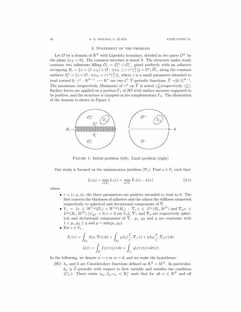
Let O be a domain of RN with Lipschitz boundary, divided in two parts O± bythe plane xN = 0. The common interface is noted S. The structure under studycontains two adherents filling Oε = O+

ε ∪ O−ε , glued perfectly with an adhesiveoccupying Bε = x = (x, xN ) ∈ O : ±xN ≤ ε γ±( ex

ε ) = O \ Oε, along the commonsurfaces S±ε = x ∈ O : ±xN = εγ±( ex

ε ), where ε is a small parameter intended totend toward 0, γ± : RN−1 −→ R+ are two C1 Y -periodic functions, Y =]0, 1[N−1.The maximum (respectively Minimum) of γ± on Y is noted γ±M (respectively γ±m).Surface forces are applied on a portion Γ1 of ∂O with surface measure supposed tobe positive, and the structure is clamped on his complementary Γ0. The illustrationof the domain is shown in Figure 1.

Bε→

O+ε

O−ε

S+ε

S−ε

Γ1

←S

O+

O−

Γ1

Figure 1. Initial problem (left). Limit problem (right)

Our study is focused on the minimization problem (Pr): Find u ∈ Vε such that:

Ir(u) = minv∈Vε

Ir(v) = minv∈Vε

Fr(v)− L(v) (3.1)

where

• r = (ε, µ, η), the three parameters are positive intended to tend to 0. Thefirst concern the thickness of adhesive and the others the stiffness connectedrespectively to spherical and deviational components of ∇.• Vε = v ∈ W 1,q(Oε) × W 1,p(Bε) : ∇s v ∈ Lps(Bε,M

N ) and ∇d v ∈Lpd(Bε,M

N ), [v]S±ε = 0, v = 0 sur Γ0, ∇s and ∇d are respectively spher-ical and deviational components of ∇. ps, pd and q are constants with1 < ps, pd ≤ q and p = min(ps, pd).

• For v ∈ Vε,

Fr(v) =∫Oε

h(x,∇v) dx+∫

Bε

µ bs(x

ε,∇s v) + η bd(

x

ε,∇d v) dx

L(v) =∫Of(x) v(x) dx+

∫Γ1

g(x) v(x) dσ(x)

In the following, we denote w = s or w = d, and we make the hypotheses:

(H1) bw and h are Caratheodory functions defined on RN ×MN . In particular,bw is Y -periodic with respect to first variable and satisfies the condition(Cw): There exists αw, βw, cw ∈ R+

∗ such that for all x ∈ RN and all


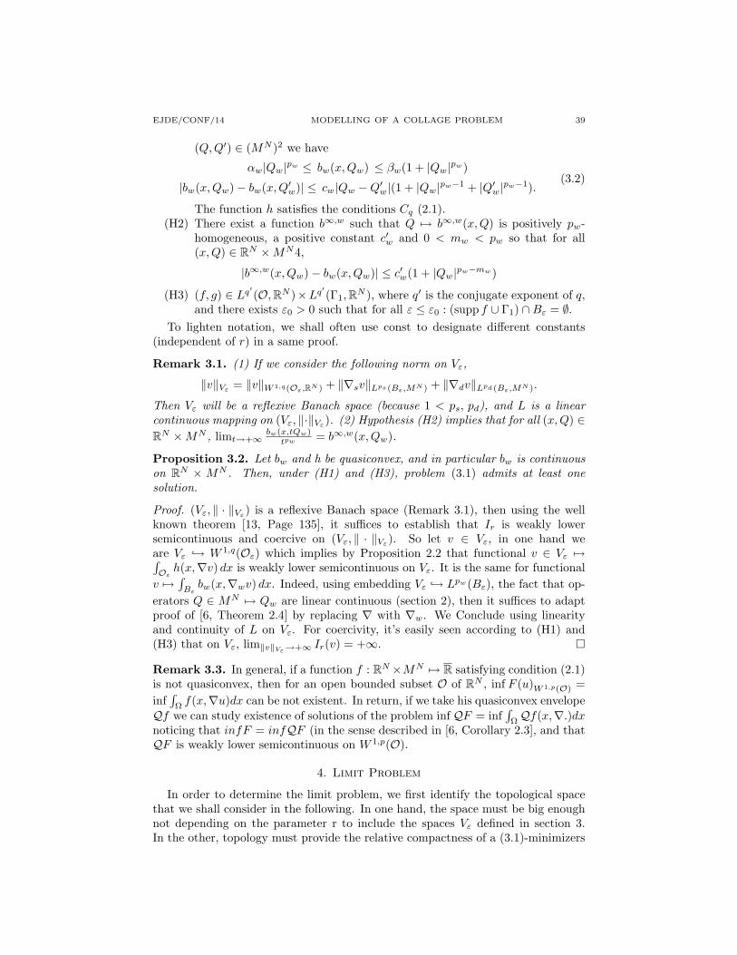
(Q,Q′) ∈ (MN )2 we have

αw|Qw|pw ≤ bw(x,Qw) ≤ βw(1 + |Qw|pw)

|bw(x,Qw)− bw(x,Q′w)| ≤ cw|Qw −Q′w|(1 + |Qw|pw−1 + |Q′w|pw−1).(3.2)

The function h satisfies the conditions Cq (2.1).(H2) There exist a function b∞,w such that Q 7→ b∞,w(x,Q) is positively pw-

homogeneous, a positive constant c′w and 0 < mw < pw so that for all(x,Q) ∈ RN ×MN4,

|b∞,w(x,Qw)− bw(x,Qw)| ≤ c′w(1 + |Qw|pw−mw)

(H3) (f, g) ∈ Lq′(O,RN )×Lq′(Γ1,RN ), where q′ is the conjugate exponent of q,and there exists ε0 > 0 such that for all ε ≤ ε0 : (supp f ∪ Γ1) ∩Bε = ∅.

To lighten notation, we shall often use const to designate different constants(independent of r) in a same proof.

Remark 3.1. (1) If we consider the following norm on Vε,

‖v‖Vε= ‖v‖W 1,q(Oε,RN ) + ‖∇sv‖Lps (Bε,MN ) + ‖∇dv‖Lpd (Bε,MN ).

Then Vε will be a reflexive Banach space (because 1 < ps, pd), and L is a linearcontinuous mapping on (Vε, ‖·‖Vε

). (2) Hypothesis (H2) implies that for all (x,Q) ∈RN ×MN , limt→+∞

bw(x,tQw)tpw = b∞,w(x,Qw).

Proposition 3.2. Let bw and h be quasiconvex, and in particular bw is continuouson RN × MN . Then, under (H1) and (H3), problem (3.1) admits at least onesolution.

Proof. (Vε, ‖ · ‖Vε) is a reflexive Banach space (Remark 3.1), then using the well

known theorem [13, Page 135], it suffices to establish that Ir is weakly lowersemicontinuous and coercive on (Vε, ‖ · ‖Vε). So let v ∈ Vε, in one hand weare Vε → W 1,q(Oε) which implies by Proposition 2.2 that functional v ∈ Vε 7→∫Oεh(x,∇v) dx is weakly lower semicontinuous on Vε. It is the same for functional

v 7→∫

Bεbw(x,∇wv) dx. Indeed, using embedding Vε → Lpw(Bε), the fact that op-

erators Q ∈ MN 7→ Qw are linear continuous (section 2), then it suffices to adaptproof of [6, Theorem 2.4] by replacing ∇ with ∇w. We Conclude using linearityand continuity of L on Vε. For coercivity, it’s easily seen according to (H1) and(H3) that on Vε, lim‖v‖Vε→+∞ Ir(v) = +∞.

Remark 3.3. In general, if a function f : RN ×MN 7→ R satisfying condition (2.1)is not quasiconvex, then for an open bounded subset O of RN , inf F (u)W 1,p(O) =inf

∫Ωf(x,∇u)dx can be not existent. In return, if we take his quasiconvex envelope

Qf we can study existence of solutions of the problem infQF = inf∫ΩQf(x,∇.)dx

noticing that infF = infQF (in the sense described in [6, Corollary 2.3], and thatQF is weakly lower semicontinuous on W 1,p(O).

4. Limit Problem

In order to determine the limit problem, we first identify the topological spacethat we shall consider in the following. In one hand, the space must be big enoughnot depending on the parameter r to include the spaces Vε defined in section 3.In the other, topology must provide the relative compactness of a (3.1)-minimizers


sequence. Let X = W 1,qloc (O \ S) and τ his weak topology. Let us consider the

subsetV = v ∈ X : v ∈W 1,q(O \ S), v = 0 on Γ0

Proposition 4.1. If (vr)r is a sequence in X verifying Fr(vr) ≤ C, then thereexist v ∈ V and a subsequence such that vr

τ→ v in X. Moreover,(1) XOε∇vr ∇v in Lq(O).(2)

∫RN−1 |vr(x,±εγ( ex

ε ))− v±(x)|qdx r→ 0.For the proof of the above proposition see [15, page 9].

Remark 4.2. (1) Let (ur)r be a (3.1)-minimizer sequence, i.e.

limr→0

Ir(ur)− infIr(v) : v ∈ Vε = 0,

then (ur)r is relatively compact in (X, τ). It suffices to show lim infr→0 Ir(ur) <+∞, which implies according to conditions (3.2) and (3.2) with w replaced by qthat lim infr→0 Fr(ur) < +∞, and we apply Proposition 4.1.

(2) Let p = min(ps, pd). In accordance with results of [15], we obtain (X, τ) sothat:• If lim sup(ε,µ)

εµ1/ps

and lim sup(ε,η)ε

η1/pd< +∞, then X = Lα(O) and τ is his

strong topology for any α ∈ [1, p[.• If lim sup(ε,µ)

εµ1/ps

= lim sup(ε,η)ε

η1/pd= 0, then X = Lp(O) and τ is his strong

topology.

Now, we look for the Γ-limit of functionals Ir. First we have to remark thatThe functional L is linear continuous on (X, τ) (for the proof, is a straightforwardconsequence of (H3) and the compact embedding W 1,q

loc (O \ S,RN ) → Lq(S)), thenaccording to Proposition 2.1, it suffices to study Γ-limit for functionals Fr. To thisend, we extend Fr on the space (X, τ) as

Fr(v) =

∫Oεh(x,∇v) dx+

∫Bεµbs(x

ε ,∇s v) + η bd(xε ,∇d v) dx if v ∈ Vε

+∞ if v 6∈ Vε

we recall that Vε = v ∈ W 1,q(Oε) ×W 1,p(Bε) : ∇s v ∈ Lps(Bε,MN ) and ∇d v ∈

Lpd(Bε,MN ), [v]S±ε = 0, v = 0 on Γ0. Let

ls = lim(ε,µ)

µ

2(2ε)ps−1and ld = lim

(ε,η)

η

2(2ε)pd−1.

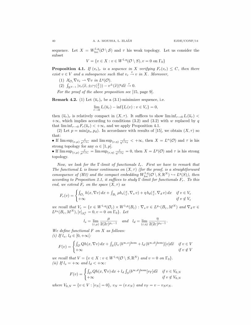
We define functional F on X as follows:(i) If ls, ld ∈ [0,+∞[:

F (v) =

∫O Qh(x,∇v) dx+

∫Sls (b∞,s)hom + ld (b∞,d)hom[v]dx if v ∈ V

+∞ if v 6∈ V

we recall that V = v ∈ X : v ∈W 1,q(O \ S,RN ) and v = 0 on Γ0.(ii) If ls = +∞ and ld < +∞:

F (v) =

∫O Qh(x,∇v) dx+ ld

∫S(b∞,d)hom[vT ]dx if v ∈ V0,N

+∞ if v 6∈ V0,N

where V0,N = v ∈ V : [vN ] = 0, vN = (v.eN ) and vT = v − vNeN .


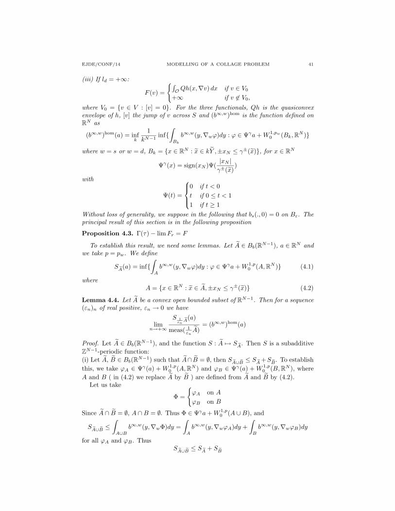
(iii) If ld = +∞:

F (v) =

∫O Qh(x,∇v) dx if v ∈ V0

+∞ if v 6∈ V0,

where V0 = v ∈ V : [v] = 0. For the three functionals, Qh is the quasiconvexenvelope of h, [v] the jump of v across S and (b∞,w)hom is the function defined onRN as

(b∞,w)hom(a) = infk

1kN−1

inf∫

Bk

b∞,w(y,∇wϕ)dy : ϕ ∈ Ψγa+W 1,pw

0 (Bk,RN )

where w = s or w = d, Bk = x ∈ RN : x ∈ kY ,±xN ≤ γ±(x), for x ∈ RN

Ψγ(x) = sign(xN )Ψ(|xN |γ±(x)

)

with

Ψ(t) =

0 if t < 0t if 0 ≤ t < 11 if t ≥ 1

Without loss of generality, we suppose in the following that bs(., 0) = 0 on Bε. Theprincipal result of this section is in the following proposition

Proposition 4.3. Γ(τ)− limFr = F

To establish this result, we need some lemmas. Let A ∈ Bb(RN−1), a ∈ RN andwe take p = pw. We define

S eA(a) = inf∫

A

b∞,w(y,∇wϕ)dy : ϕ ∈ Ψγa+W 1,p0 (A,RN ) (4.1)

whereA = x ∈ RN : x ∈ A,±xN ≤ γ±(x) (4.2)

Lemma 4.4. Let A be a convex open bounded subset of RN−1. Then for a sequence(εn)n of real positive, εn → 0 we have

limn→+∞

S 1εn

eA(a)

meas( 1εnA)

= (b∞,w)hom(a)

Proof. Let A ∈ Bb(RN−1), and the function S : A 7→ S eA. Then S is a subadditiveZN−1-periodic function:(i) Let A, B ∈ Bb(RN−1) such that A∩ B = ∅, then S eA∪ eB ≤ S eA +S eB . To establishthis, we take ϕA ∈ Ψγ(a) + W 1,p

0 (A,RN ) and ϕB ∈ Ψγ(a) + W 1,p0 (B,RN ), where

A and B ( in (4.2) we replace A by B ) are defined from A and B by (4.2).Let us take

Φ =

ϕA on AϕB on B

Since A ∩ B = ∅, A ∩B = ∅. Thus Φ ∈ Ψγa+W 1,p0 (A ∪B), and

S eA∪ eB ≤∫

A∪B

b∞,w(y,∇wΦ)dy =∫

A

b∞,w(y,∇wϕA)dy +∫

B

b∞,w(y,∇wϕB)dy

for all ϕA and ϕB . ThusS eA∪ eB ≤ S eA + S eB


(ii) Let A ∈ Bb(RN−1) and z ∈ ZN−1. Let A and Az subsets associated respec-tively to A and A+ z by relation (4.2), and ϕ ∈W 1,p

0 (Az). Since bw is Y -periodic,it’s the same for b∞, w. Thus∫

Az

b∞, w(x,∇wϕ)dx =∫

eA+z

∫xN :±xN≤γ±(ex)

b∞, w(x,∇wϕ)dxN dx

=∫

eA∫xN :±xN≤γ±(ex+z)

b∞, w(x+ z, xN ,∇wϕ)dxN dx

=∫

A

b∞, w(x,∇wϕ)dxN dx

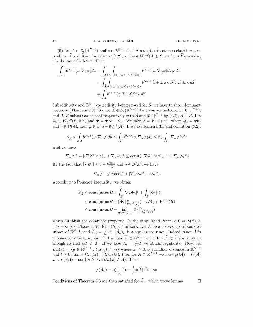
Subadditivity and ZN−1-periodicity being proved for S, we have to show dominantproperty (Theorem 2.3). So, let A ∈ Bb(RN−1) be a convex included in [0, 1[N−1,and A, B subsets associated respectively with A and [0, 1[N−1 by (4.2), A ⊂ B. LetΦ0 ∈ W 1,p

0 (B,RN ) and Φ = Ψγa + Φ0. We take ϕ = Ψγa + ϕ0, where ϕ0 = ηΦ0

and η ∈ D(A), then ϕ ∈ Ψγa+W 1,p0 (A). If we use Remark 3.1 and condition (3.2),

S eA ≤∫

A

b∞,w(y,∇wϕ)dy ≤∫

B

b∞,w(y,∇wϕ)dy ≤ βw

∫B

|∇wϕ|pdy

And we have

|∇wϕ|p = |(∇Ψγ ⊗ a)w +∇wϕ0|p ≤ const(|(∇Ψγ ⊗ a)w|p + |∇wϕ0|p)

By the fact that |∇Ψγ | ≤ 1 + constγ±m

and η ∈ D(A), we have

|∇wϕ|p ≤ const(1 + |∇wΦ0|p + |Φ0|p).

According to Poincare inequality, we obtain

S eA ≤ const(measB +∫

B

|∇wΦ0|p +∫

B

|Φ0|p)

≤ const(measB + ‖Φ0‖pW 1,p0 (B)

) ,∀Φ0 ∈W 1,p0 (B)

≤ const(measB + infW 1,p

0 (B)‖Φ0‖pW 1,p

0 (B))

which establish the dominant property. In the other hand, b∞,w ≥ 0 ⇒ γ(S) ≥0 > −∞ (see Theorem 2.3 for γ(S) definition). Let A be a convex open boundedsubset of RN−1, and An = 1

εnA. (An)n is a regular sequence. Indeed, since A is

a bounded subset, we can find a cube I ⊂ ZN−1 such that A ⊂ I and α smallenough so that αI ⊂ A. If we take In = 1

εnI we obtain regularity. Now, let

Bm(x) = y ∈ RN−1 : δ(x, y) ≤ m where m ≥ 0, δ euclidian distance in RN−1

and t ≥ 0. Since tBm(x) = Btm(tx), then for A ⊂ RN−1 we have ρ(tA) = tρ(A)where ρ(A) = supm ≥ 0 : ∃Bm(x) ⊂ A. Thus

ρ(An) = ρ(1εnA) =

1ερ(A) n→ +∞

Conditions of Theorem 2.3 are then satisfied for An, which prove lemma.


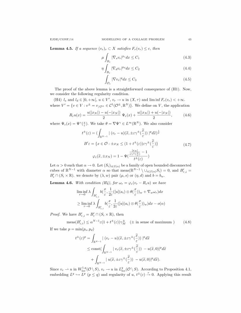
Lemma 4.5. If a sequence (vr)r ⊂ X satisfies Fr(vr) ≤ c, then

µ

∫Bε

|∇svr|psdx ≤ C1 (4.3)

η

∫Bε

|∇dvr|pddx ≤ C2 (4.4)∫Oε

|∇vr|qdx ≤ C3 (4.5)

The proof of the above lemma is a straightforward consequence of (H1). Now,we consider the following regularity condition.

(H4) ls and ld ∈ [0,+∞[, u ∈ V ′, vr → u in (X, τ) and lim inf Fr(vr) < +∞.where V ′ = v ∈ V : v± = v/O± ∈ C1(O±,RN ). We define on V , the application

Rεu(x) =u(|xN |)− u(−|xN |)

2Ψε(x) +

u(|xN |) + u(−|xN |)2

, (4.6)

where Ψε(x) = Ψγ(xε ). We take θ = ∇Ψγ ∈ L∞(RN ). We also consider

t±(ε) = (∫

RN−1| (vr − u)(x,±εγ±(

x

ε)) |pdx)

1p

B′ε = x ∈ O : ±xN ≤ (1 + t±(ε))εγ±(x

ε)

ϕε(x,±xN ) = 1−Ψ(

|xN |εγ±( ex

ε )− 1

t±(ε))

(4.7)

Let α > 0 such that α→ 0. Let (Si)i∈I(α) be a family of open bounded disconnectedcubes of RN−1 with diameter α so that meas(RN−1 \ ∪i∈I(α)Si) = 0, and B′ε,i =B′ε ∩ (Si × R). we denote by (λ,w) pair (µ, s) or (η, d) and b = bw.

Lemma 4.6. With condition (H4), for ωr = ϕε(vr −Rεu) we have

lim infr→0

λ

∫B′

ε,i

b(x

ε,

12ε

([u](ai)⊗ θ(x

ε))w +∇wωr)dx

≥ lim infr→0

λ

∫B′

ε,i

b(x

ε,

12ε

([u](ai)⊗ θ(x

ε))w)dx− o(α)

Proof. We have B′ε,i = B′ε ∩ (Si × R), then

meas(B′ε,i) ≤ αN−1ε(1 + t±(ε))γ±M (± in sense of maximum ) (4.8)

If we take p = min(ps, pd)

t±(ε)p =∫

RN−1| (vr − u)(x,±εγ±(

x

ε)) |pdx

≤ const(∫

RN−1| vr(x,±εγ±(

x

ε)) − u(x, 0)|pdx

+∫

RN−1| u(x,±εγ±(

x

ε)) − u(x, 0)|pdx).

Since vr u in W 1,qloc (O \ S), vr → u in Lq

loc(O \ S). According to Proposition 4.1,embedding Lq → Lp (p ≤ q) and regularity of u, t±(ε) r→ 0. Applying this result


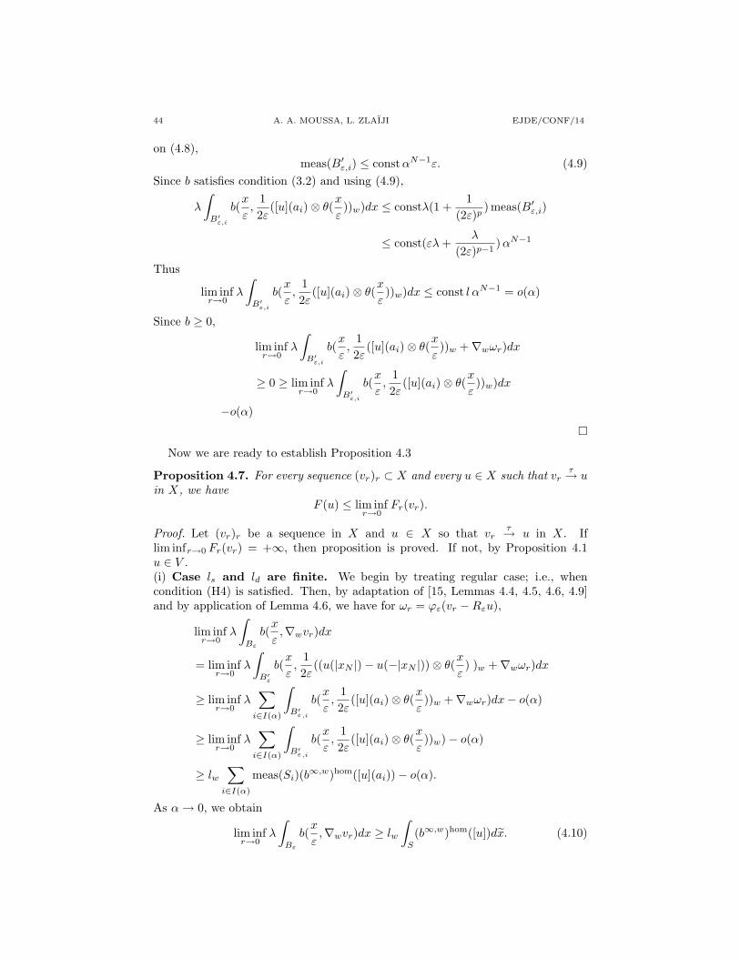
on (4.8),meas(B′ε,i) ≤ constαN−1ε. (4.9)

Since b satisfies condition (3.2) and using (4.9),

λ

∫B′

ε,i

b(x

ε,

12ε

([u](ai)⊗ θ(x

ε))w)dx ≤ constλ(1 +

1(2ε)p

) meas(B′ε,i)

≤ const(ελ+λ

(2ε)p−1)αN−1

Thus

lim infr→0

λ

∫B′

ε,i

b(x

ε,

12ε

([u](ai)⊗ θ(x

ε))w)dx ≤ const l αN−1 = o(α)

Since b ≥ 0,

lim infr→0

λ

∫B′

ε,i

b(x

ε,

12ε

([u](ai)⊗ θ(x

ε))w +∇wωr)dx

≥ 0 ≥ lim infr→0

λ

∫B′

ε,i

b(x

ε,

12ε

([u](ai)⊗ θ(x

ε))w)dx

−o(α)

Now we are ready to establish Proposition 4.3

Proposition 4.7. For every sequence (vr)r ⊂ X and every u ∈ X such that vrτ→ u

in X, we haveF (u) ≤ lim inf

r→0Fr(vr).

Proof. Let (vr)r be a sequence in X and u ∈ X so that vrτ→ u in X. If

lim infr→0 Fr(vr) = +∞, then proposition is proved. If not, by Proposition 4.1u ∈ V .(i) Case ls and ld are finite. We begin by treating regular case; i.e., whencondition (H4) is satisfied. Then, by adaptation of [15, Lemmas 4.4, 4.5, 4.6, 4.9]and by application of Lemma 4.6, we have for ωr = ϕε(vr −Rεu),

lim infr→0

λ

∫Bε

b(x

ε,∇wvr)dx

= lim infr→0

λ

∫B′

ε

b(x

ε,

12ε

((u(|xN |)− u(−|xN |))⊗ θ(x

ε) )w +∇wωr)dx

≥ lim infr→0

λ∑

i∈I(α)

∫B′

ε,i

b(x

ε,

12ε

([u](ai)⊗ θ(x

ε))w +∇wωr)dx− o(α)

≥ lim infr→0

λ∑

i∈I(α)

∫B′

ε,i

b(x

ε,

12ε

([u](ai)⊗ θ(x

ε))w)− o(α)

≥ lw∑

i∈I(α)

meas(Si)(b∞,w)hom([u](ai))− o(α).

As α→ 0, we obtain

lim infr→0

λ

∫Bε

b(x

ε,∇wvr)dx ≥ lw

∫S

(b∞,w)hom([u])dx. (4.10)


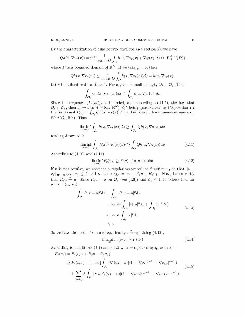
By the characterization of quasiconvex envelope (see section 2), we have

Qh(x,∇vr(x)) = inf 1meas D

∫D

h(x,∇vr(x) +∇ϕ(y)) : ϕ ∈W 1,∞0 (D)

where D is a bounded domain of RN . If we take ϕ = 0, then

Qh(x,∇vr(x)) ≤1

meas D

∫D

h(x,∇vr(x))dy = h(x,∇vr(x))

Let δ be a fixed real less than 1. For a given ε small enough, Oδ ⊂ Oε. Thus∫Oδ

Qh(x,∇vr(x))dx ≤∫Oε

h(x,∇vr(x))dx

Since the sequence (Fr(vr))r is bounded, and according to (4.5), the fact thatOδ ⊂ Oε, then vr u in W 1,q(Oδ,RN ). Qh being quasiconvex, by Proposition 2.2the functional I(v) =

∫OδQh(x,∇v(x))dx is then weakly lower semicontinuous on

W 1,q(Oδ,RN ). Thus

lim infr→0

∫Oε

h(x,∇vr(x))dx ≥∫Oδ

Qh(x,∇u(x))dx

tending δ toward 0

lim infr→0

∫Oε

h(x,∇vr(x))dx ≥∫OQh(x,∇u(x))dx (4.11)

According to (4.10) and (4.11)

lim infr→0

Fr(vr) ≥ F (u), for u regular (4.12)

If u is not regular, we consider a regular vector valued function uδ so that ‖u −uδ‖W 1,q(O\S,RN ) ≤ δ and we take vδ,r = vr − Rεu + Rεuδ. Now, let us verifythat Rεu

τ→ u. Since Rεu = u on Oε (see (4.6)) and ψε ≤ 1, it follows that forp = min(ps, pd),∫

O|Rεu− u|pdx =

∫Bε

|Rεu− u|pdx

≤ const∫

Bε

|Rεu|pdx+∫

Bε

|u|pdx

≤ const∫

Bε

|u|pdx

ε→ 0

(4.13)

So we have the result for u and uδ, thus vδ,rτ→ uδ. Using (4.12),

lim infr→0

Fr(vδ,r) ≥ F (uδ) (4.14)

According to conditions (3.2) and (3.2) with w replaced by q, we have

Fr(vr) = Fr(vδ,r +Rεu−Rεuδ)

≥ Fr(vδ,r)− const ∫Oε

|∇ (uδ − u)|(1 + |∇vr|q−1 + |∇vδ,r|q−1 )

+∑(λ,w)

λ

∫Bε

|∇w Rε(uδ − u)|(1 + |∇wvr|pw−1 + |∇wvδ,r|pw−1 )

(4.15)


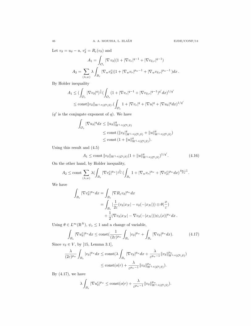
Let vδ = uδ − u, vεδ = Rε(vδ) and

A1 =∫Oε

|∇ vδ|(1 + |∇vr|q−1 + |∇vδ,r|q−1)

A2 =∑(λ,w)

λ

∫Bε

|∇wvεδ |(1 + |∇wvr|pw−1 + |∇wvδ,r|pw−1 )dx .

By Holder inequality

A1 ≤ (∫Oε

|∇vδ|q)1q (

∫Oε

(1 + |∇vr|q−1 + |∇vδ,r|q−1)q′dx)1/q′

≤ const‖vδ‖W 1,q(O\S).(∫Oε

1 + |∇vr|q + |∇u|q + |∇uδ|qdx)1/q′

(q′ is the conjugate exponent of q). We have∫Oε

|∇uδ|qdx ≤ ‖uδ‖qW 1,q(O\S)

≤ const (‖vδ|q|W 1,q(O\S) + ‖u‖qW 1,q(O\S))

≤ const (1 + ‖u‖qW 1,q(O\S)).

Using this result and (4.5)

A1 ≤ const ‖vδ‖W 1,q(O\S)(1 + ‖u‖qW 1,q(O\S))1/q′ . (4.16)

On the other hand, by Holder inequality,

A2 ≤ const∑(λ,w)

λ(∫

Bε

|∇vεδ |pw)

1pw (

∫Bε

1 + |∇wvr|pw + |∇vεδ |pwdx)

pw−1pw .

We have ∫Bε

|∇vεδ |pwdx =

∫Bε

|∇Rεvδ|pwdx

=∫

Bε

| 12ε

(vδ|xN | − vδ(−|xN |))⊗ θ(x

ε)

+12(∇vδ|xN | − ∇vδ(−|xN |))ψε(x)|pwdx .

Using θ ∈ L∞(RN ), ψε ≤ 1 and a change of variable,∫Bε

|∇uεδ|pwdx ≤ const(

1(2ε)pw

∫Bε

|vδ|pw +∫

Bε

|∇vδ|pwdx). (4.17)

Since vδ ∈ V , by [15, Lemma 3.1],

λ

(2ε)pw

∫Bε

|vδ|pwdx ≤ const(λ∫

Bε

|∇vδ|pwdx+λ

εpw−1‖vδ‖pw

W 1,q(O\S))

≤ const(o(r) +λ

εpw−1‖vδ‖pw

W 1,q(O\S)).

By (4.17), we have

λ

∫Bε

|∇uεδ|pw ≤ const(o(r) +

λ

εpw−1‖vδ‖pw

W 1,q(O\S)).


Using this result, (4.3) and (4.4),

A2

≤ const∑(λ,w)

(o(r) +λ

εpw−1‖vδ‖pw

W 1,q(O\S))1

pw (1 + o(r) +λ

εpw−1‖vδ‖pw

W 1,q(O\S))pw−1

pw

(4.18)Applying (4.14), (4.15), (4.16) and (4.18), we obtain

lim infr→0

Fr(vr) ≥ F (uδ)− C(u)‖vδ‖W 1,q(O\S) (4.19)

where C(u) is a constant depending on u. On the other hand, since b∞,w and hsatisfies respectively conditions (3.2) and (3.2) with w replaced by q, (b∞,w)hom andQh are lipshitz functions (the proof is an adaptation of the proof of [18, Proposition2.1]). Then

F (uδ) ≥ F (u)− const∫O|∇vδ|(1 + |∇u|q−1 + |∇uδ|q−1)

+∫

S

|[vδ]|(1 + |[u]|pw−1 + |[uδ]|pw−1)dx.

Using the fact that pw ≤ q, Holder inequality, continuity of the jump, the compactembeding W 1,q(O \ S) → Lq(S) and that ‖uδ‖W 1,q(O\S) ≤ ‖u‖W 1,q(O\S) + 1, wehave

F (uδ) ≥ F (u)− C(u)‖vδ‖W 1,q(O\S).

We then use this result and (4.19), and we let δ approach 0. Thus

lim infr→0

Fr(vr) ≥ F (u)

(ii) Case ls = +∞ and ld < +∞: We have [uN ] = 0. Indeed, let σ ∈ D(O,MN ).By Green formula and Proposition 4.1∫

Bε

σ : ∇vr dx =∫Oσ : ∇vr dx−

∫Oσ : (XOε∇vr) dx

= −∫Odivσ : vr dx−

∫Oσ : (XOε∇vr) dx

r→∫

S

σn.[u] dx,

where n is the unit vector normal exterior to O+ . If we take σ = φ.IN , where INis the unit matrix of RN and φ ∈ D(O), we have

limr

∫Bε

φdivvr dx =∫

S

φ.[uN ] dx (4.20)

According to (4.5) and that ls = +∞∣∣ ∫Bε

φdivvr dx∣∣ ≤ ‖φ‖

Lp′s (Bε)‖divvr‖Lps (Bε)

≤ const(εps−1

µ)

1ps

r→ 0

where p′s is the conjugate exponent of ps. By (4.20), we obtain [uN ] = 0. Thus,u ∈ V0,N . And we have (b∞,s)hom[u] = 0. Indeed let us take (b∞,s)hom(a) =


(b∞,s)hom(a, γ). According to [15, Proposition 3.8], we have

(b∞,s)hom([u]) ≤ (b∞,s)hom([u], γm).

Let k ∈ N and ϕ = Ψγm .[u], where for a given y ∈ Bk, Ψγm(y) = sign(yN )Ψ( |yN |γ±m

) =

± yN

γ±m. Definition of (b∞,s)hom implies

(b∞,s)hom([u]) ≤ 1kN−1

∫Bk

b∞,s(y, ∇sϕ)dy.

Since [uN ] = 0, ∇sϕ(y) = (∇Ψγm(y) ⊗ [u])s = ± 1γ±m

(eN ⊗ [u])s = 0. By the factthat bs(x, 0) = 0, we deduce that (b∞,s)hom([u]) = 0 and we conclude using resultof case (i).(iii) case ld = +∞: In this case, [u] = 0. Indeed, let σ ∈ D(O,MN ). We have

limr

∫Bε

σ : ∇dvrdx =∫

S

σdn.[u]dx

for all σ ∈ D(O,MN ). Thus u ∈ V0, and ϕ = Ψγm .[u] = 0. Consequently

(b∞,w)hom([u]) ≤ 1kN−1

∫Bk

b∞,w(y,∇wϕ)dy = 0

for w = s and w = d. The result is then proved.

Proposition 4.8. If u ∈ X, then there exist a sequence (vr)r ⊂ X such that vrτ→ u

andlim sup

r→0Fr(vr) ≤ F (u)

Proof. (i) Case ls and ld are finite: Let u ∈ X. If u 6∈ V , F (u) = +∞, and theresult is established taking for example vr = u. If not, we first take u regular. Let(Si) be the family of open bounded disconnected cubes of RN−1 with diameter αso that meas(RN−1 \ ∪i∈I(α)Si) = 0, and vr = Rεu (4.6). By (4.13), vr

τ→ u. Leta ∈ RN , for (λ,w) = (µ, s) or (η, d) we have∑

i∈I(α)

lw meas(Si)(b∞,w)hom([u](a)) ≥ limr→0

λ

∫Bε

b(x

ε,∇wvr)dx− o(α). (4.21)

Indeed, let uε,i be an ε-minimizer of S 1ε Si

(a) defined by

S 1ε Si

(a) = inf∫

1ε Bε,i

b∞,w(y,∇wϕ)dy : ϕ ∈ Ψγa+W 1,pw

0 (1εBε,i),

where Bε,i = Bε ∩ (Si × R). Let θ = ∇Ψγ ∈ L∞(RN ). Using lemma 4.4 and thechange of variable x = εy, we have

lw meas(Si)(b∞,w)hom([u](a))

= limr→0

εN−1 λ

2(2ε)pw−1

∫1ε Bε,i

b∞,w(y, ([u](a)⊗ θ(x))w +∇wuε,i)dy

= limr→0

λ

(2ε)pw

∫Bε,i

b∞,w(x

ε, ([u](a)⊗ θ(x

ε))w + (∇wuε,i)(

x

ε))dx

(4.22)

According to (H2) and the inequalities meas(Bε,i) ≤ γ±MαN−1ε and∫Bε,i

|(∇wuε,i)(x

ε)|pwdx ≤ const ε(αN−1 + εN )


(this last result is obtained using the uε,i definition and condition (3.2) satisfied byb∞,w), (4.22) becomes


= limr→0

λ

∫Bε,i

b(x

ε,

12ε

([u](a)⊗ θ(xε))w +

12ε

(∇wuε,i)(x

ε))dx .

(4.23)

By Holder inequality, condition (3.2) and the result |∇Rεu| ≤ const(1 + 1ε ), we

deduce


≥ limr→0

λ

∫Bε,i

b(x

ε,∇wRεu+

12ε

(∇wuε,i)(x

ε))dx− o(α)

≥ limr→0

λ

∫Bε,i

b(x

ε,∇wRεu)dx− o(α)

Summing over I(α) and tending α towards 0, we deduce that

lw

∫S

(b∞,w)hom([u])dx ≥ limr→0

λ

∫Bε

b(x

ε,∇wvr)dx .

Since vr = u on Oε,

limr→0∫Oε

h(x,∇vr)dx+∑λ,w

λ

∫Bε

b(x

ε,∇wvr)dx

≤∫Oh(x,∇u)dx+

∑w

lw

∫S

(b∞,w)hom([u])dx

Thus

G(u) = inflim supr

Fr(vr) : vrτ→ u

≤∫Oh(x,∇u)dx+

∑w

lw

∫S

(b∞,w)hom([u])dx

If we take the weak lower semicontinuous envelope on W 1,q(O \ S) denoted Γτ forthe two members, we obtain

ΓτG(u) ≤∫OQh(x,∇u)dx+

∑w

lw

∫S

(b∞,w)hom([u])dx

(we use the integral representation of quasiconvex envelope for the first integralterm and compact embeeding W 1,q(O \ S) → Lpw(S) for the second, noticing thatfunction (b∞,w)hom is convex [17, Proposition 2.6]. Since G is the Γ-limsup of Fr,it will be τ -lower semicontinuous [2, Theorem 2.1]; thus

G(u) = ΓτG(u) ≤∫OQh(x,∇u)dx+

∑w

lw

∫S

(b∞,w)hom([u])dx ≤ F (u).

We conclude noticing the infimum in the definition of G is attained. If u is notregular, we use a density argument like in Proposition 4.7.(ii) Case ls = +∞ and ld < +∞: If u 6∈ V0,N , F (u) = +∞ and we take forexample vr = u. If not, u ∈ V0,N ⊂ V and it suffice to apply results of case (i)noticing that (b∞,s)hom([u]) = 0.


(iii) Case ld = +∞: It is deduced from the fact that (b∞,w)hom([u]) = 0 for w = sand w = d.

The proof of Proposition 4.3 is a direct consequence of Propositions 4.7 and 4.8.Recall the functional Ir = Fr − L is defined on the space (X, τ) and take I =

F − L. Let

W =

V if ls and ld are finiteV0,N if ls = +∞ and ld is finiteV0 if ld = +∞

Corollary 4.9. Let (ur)r be a (3.1)-minimizing sequence. Thus (ur)r is relativelycompact in (X, τ). Moreover, for every cluster point u and a subsequence, we have

limr→0

Ir(ur) = I(u) = infI(v) : v ∈W.

The proof of this corollary is a straightforward application of Remark 4.2, propo-sitions 2.1 and 4.3.

References

[1] E. Acerbi, G. Buttazzo and D. Percivale, Thin inclusions in linear elasticity: a variationalapproach, J. Reine Angew. Math., 386, P. 99-115 (1988).

[2] H. Attouch, Variational Convergence for Functions and Operators. Pitman Advance Pub-

lishing Program, (1984).[3] E. Acerbi, G. Buttazzo and D. Percivale, Thin inclusions in linear elasticity: a variational

approach, J. Reine Angew. Math., 386, P. 99-115 (1988).[4] H. Brezis, L. A. Caffarelli and A. Friedman; Reinforcement problems for elliptic equations

and variational inequalities. Ann. Math. Pur. Appl., 4(123), 219-246 (1980).

[5] F. Caillerie, The effect of a thin inclusion of high rigidity in an elastic body, Math. Meth.Appl. Sci., 2, p.251-270 (1980).

[6] B. Dacorognat, Direct Methods in Calculus of Variations, Applied Mathematical sciences,

n078,Springer-Verlag, Berlin, (1989).[7] G. Dal Maso, An introduction to Γ-convergence. Birkauser, Boston (1993).

[8] G. Dal Maso and L. Modica,; Non linear stochastic homogenization and ergodic theory, J.

Reine angew. Math., 363:27-43 (1986).[9] E. De Giorgi and T.Franzoni, Su un tipo di convergenza variazionale, Atti Accad. Naz. Lincei

Rend. Cl. Sci. Mat. (8) 58 (1975), 842-850.

[10] J. F. Ganghoffer, A. Brillard and J. Schultz; Modelling of the mechanical Behaviour of JointsBonded by a nonlinear incompressible elastic adhesive. Eur. J. Mech., A/Solids, 16, 255-276(1997).

[11] G. Geymonat, F. krasucki, and S. Lenci, Mathematical Analysis of a bonded joint with a softthin adhesive, Mathematics and Mechanics of Solids, 201-225 (1999).

[12] M. Goland and E. Reissner, The stresses in cemented joints, J.Appl. Mesh., ASME, 11,A17-A27 (1944).

[13] O. Kavian, Introduction a La Theorie de Points Critiques et Applications aux ProblemesElliptiques, Springer-Verlag, Paris (1993).

[14] A. klarbring, Derivation of model of adhesively bonded joints by the asymptotic expansionmethod, Int. J. Engng. Sci. 29, p. 493-512 (1991).

[15] C. Licht and G. Michaille, A Modelling of Elastic Adhesive Bonded Joints ,Preprint 1995/12,departement des sciences mathematiques, Universite Montpellier II, (1995).

[16] C. Licht and G. Michaille, Global-local subadditive ergodic theorems and application to ho-mogenization in elasticity, Annales Mathematiques, Blaise Pascal 9, 21-62 (2002).

[17] C. Licht, G. Michaille and Y. Abddaimi, Stochastic homogenization for an integral of aquasiconvex function with linear growth, asymptotic Analysis 15, IOS press 183-202 (1997).

[18] K. Messaoudi et G.Michaille, Stochastic Homogenization of Nonconvex Integral Functionals,Mathematical Modelling and Numerical Analysis, Vol 28, no3, p. 329-356 (1994).


[19] A. Ait Moussa, Comportement Asymptotique des Solutions d’un Probleme de Bandes Minces,

These de Doctorat (1995).

[20] P. Suquet, discontinuities and Plasticity, Nonsmooth Mechanics and Applications, MoreauPanagiotopoulos Ed., Springer. p. 279-330( 1988).

Abdelaziz Aıt Moussa

Universite Mohamed Premier, Faculte des sciences, Departement de Mathematiques et

Informatique, Oujda, MarocE-mail address: [email protected]

Loubna ZlaıjiUniversite Mohamed Premier, Faculte des sciences, Departement de Mathematiques et

Informatique, Oujda, Maroc

E-mail address: [email protected]

MODELLING OF A COLLAGE PROBLEM

Documents

Transcript of MODELLING OF A COLLAGE PROBLEM