Modelling intercrops functioning to advance thedesign of innovative agroecological systemsRémi Vezy  ( remi.vezy@cirad.fr )

CIRAD https://orcid.org/0000-0002-0808-1461Sebastian Munz 

cInstitute of Crop Science, Cropping Systems and Modelling, University of HohenheimNoémie Gaudio 

INRAE, AGIR, University of ToulouseMarie Launay 

INRAEPatrice Lecharpentier 

INRAE, US1116 AgroClimDominique Ripoche 

INRAE, US1116 AgroClimEric Justes 

CIRAD, Persyst Department

Article

Keywords: species mixture, spatial design, wheat, pea, faba bean, sun�ower, barley, soybean

Posted Date: August 18th, 2022

DOI: https://doi.org/10.21203/rs.3.rs-1930394/v1

License: This work is licensed under a Creative Commons Attribution 4.0 International License.  Read Full License

1

Modelling intercrops functioning to advance the design of innovative 1

agroecological systems 2

Rémi Vezya,b,*, Sebastian Munzc, Noémie Gaudiod, Marie Launaye, Patrice Lecharpentiere, Dominique 3 Ripochee, Eric Justesf 4 aCIRAD, UMR AMAP, F-34398 Montpellier, France. 5 bAMAP, Univ Montpellier, CIRAD, CNRS, INRAE, IRD, Montpellier, France. 6 cInstitute of Crop Science, Cropping Systems and Modelling, University of Hohenheim, 70599 Stuttgart, 7 Germany 8 dAGIR, University of Toulouse, INRAE Castanet-Tolosan, France 9 eINRAE, US1116 AgroClim, Avignon Cedex 9 France 10 fCIRAD, Persyst Department, F-34398 Montpellier, France 11

*Corresponding author. Email address: remi.vezy@cirad.fr (Rémi Vezy). 12

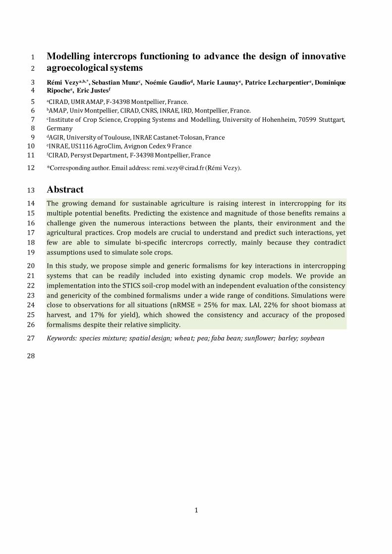
Abstract 13

The growing demand for sustainable agriculture is raising interest in intercropping for its 14

multiple potential benefits. Predicting the existence and magnitude of those benefits remains a 15

challenge given the numerous interactions between the plants, their environment and the 16 agricultural practices. Crop models are crucial to understand and predict such interactions, yet 17

few are able to simulate bi-specific intercrops correctly, mainly because they contradict 18

assumptions used to simulate sole crops. 19

In this study, we propose simple and generic formalisms for key interactions in intercropping 20

systems that can be readily included into existing dynamic crop models. We provide an 21

implementation into the STICS soil-crop model with an independent evaluation of the consistency 22

and genericity of the combined formalisms under a wide range of conditions. Simulations were 23 close to observations for all situations (nRMSE = 25% for max. LAI, 22% for shoot biomass at 24

harvest, and 17% for yield), which showed the consistency and accuracy of the proposed 25

formalisms despite their relative simplicity. 26

Keywords: species mixture; spatial design; wheat; pea; faba bean; sunflower; barley; soybean 27

28

2

Main 29

Modern agriculture needs to develop transition pathways towards sustainable, resilient, agro-30

ecological cropping systems. Cropping system diversification using multispecies crops or 31 intercropping and notably cereal-grain legume mixtures (intercrops) is a key pathway to such 32

agroecological intensification (Malézieux et al., 2009). Transitioning from classical sole cropping 33

to intercropping can bring many benefits such as a reduction in fertilizer use, greater drought and 34 disease resistance, higher productivity and increased carbon sequestration (Bedoussac et al., 35

2015; Beillouin et al., 2021; Jensen et al., 2020; Li et al., 2021; Martin-Guay et al., 2018; 36

Raseduzzaman and Jensen, 2017; Tilman, 2020; Yin et al., 2020; Yu et al., 2015). However, these 37

benefits require plant complementarity and facilitation processes to outperform competitive 38 interactions (Justes et al., 2021). Consequently, there is a need for models that can examine large 39

combinations of species, agricultural practices, climate and soil through virtual experiments to 40

evaluate the potential of intercrop productivity, resilience and sustainability (Gaudio et al., 2022). 41

Soil-crop models are particularly well suited for such objectives, as they usually simulate the most 42

important processes such as phenology, light interception, plant growth, yield formation, nutrient 43

cycles, and water balance (Stomph et al., 2020). 44

Very few soil-crop models are able to simulate interspecific interactions, even for the simplest 45 case of bi-specific intercrops. This is mainly due to the difficulty of defining new formalisms that 46

consider the dynamic interactions between plants for all processes while maintaining a few, easily 47

measurable parameters and a fast computation time. Some attempts have been made to adapt 48 existing classical sole crop models to bi-specific intercrops, for instance STICS (Brisson et al., 49

2004), APSIM (Keating et al., 2003) and CROPSYST (see Chimonyo, Modi, et Mabhaudhi (2015) 50

and Gaudio et al. (2019) for more details). The first results were encouraging, but some 51

discrepancies were identified between simulations and observations, mainly due to the lack of an 52 integrative representation of the processes accounting for the interactions in the soil-crop system. 53

Singh et al. (2013), for instance, identified high levels of simulated nitrogen (N) uptake for rice 54

using CROPSYST in a wheat-rice intercropping system as the cause of underestimating crop 55 performance. Berghuijs et al. (2021) found that APSIM overestimates faba bean performance 56

compared to the associated wheat crop, probably due to a poor simulation of plant height that 57

affected the simulation of faba bean-wheat competition for light. 58

More extensive literature is available for the intercrop algorithms in STICS, called STICS-IC (for 59 InterCropping) in this manuscript. STICS-IC generally performs correctly compared to 60

observations, thus providing the first relevant basis for simulating bi-specific intercrops (Brisson 61

et al., 2004; Kherif et al., 2022; Launay et al., 2009), but several inconsistencies were identified in 62

some cases. Shili-Touzi et al. (2010) applied the model on a winter wheat-red fescue intercrop and 63 found a tendency to overestimate N uptake for the fescue. Corre-Hellou et al. (2007, 2009) had 64

difficulties in computing light competition related to poor simulation of plant height, an issue also 65

found in APSIM. We also identified some discrepancies between observations and simulations for 66 STICS-IC using a database from works published by Bedoussac (2009) and Bedoussac and Justes 67

(2010), indicating that the model needs further improvements. Those discrepancies were found 68

in the computation of Leaf Area Index (LAI), aerial and belowground biomass, N acquisition and 69

light interception using the radiative transfer option (Brisson et al., 2004). The latter is based on 70 a 3D projection of the crop with homogeneous structure within the row (Figure 1), a formalism 71

found relevant to simulate the light capture and sharing dynamics between the two components 72

of the bi-specific intercrop. 73

3

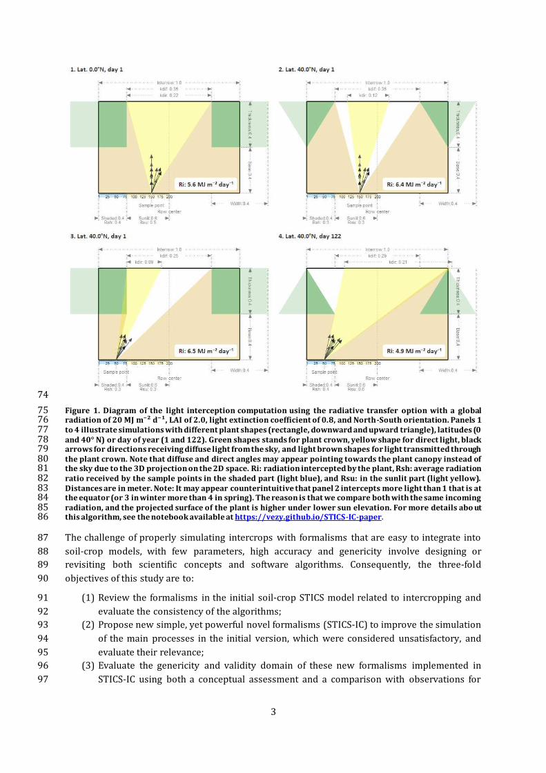
74

Figure 1. Diagram of the light interception computation using the radiative transfer option with a global 75 radiation of 20 MJ m⁻² d⁻¹, LAI of 2.0, light extinction coefficient of 0.8, and North-South orientation. Panels 1 76 to 4 illustrate simulations with different plant shapes (rectangle, downward and upward triangle), latitudes (0 77 and 40° N) or day of year (1 and 122). Green shapes stands for plant crown, yellow shape for direct light, black 78 arrows for directions receiving diffuse light from the sky, and light brown shapes for light transmitted through 79 the plant crown. Note that diffuse and direct angles may appear pointing towards the plant canopy instead of 80 the sky due to the 3D projection on the 2D space. Ri: radiation intercepted by the plant, Rsh: average radiation 81 ratio received by the sample points in the shaded part (light blue), and Rsu: in the sunlit part (light yellow). 82 Distances are in meter. Note: It may appear counterintuitive that panel 2 intercepts more light than 1 that is at 83 the equator (or 3 in winter more than 4 in spring). The reason is that we compare both with the same incoming 84 radiation, and the projected surface of the plant is higher under lower sun elevation. For more details abo ut 85 this algorithm, see the notebook available at https://vezy.github.io/STICS-IC-paper. 86

The challenge of properly simulating intercrops with formalisms that are easy to integrate into 87

soil-crop models, with few parameters, high accuracy and genericity involve designing or 88 revisiting both scientific concepts and software algorithms. Consequently, the three-fold 89

objectives of this study are to: 90

(1) Review the formalisms in the initial soil-crop STICS model related to intercropping and 91

evaluate the consistency of the algorithms; 92 (2) Propose new simple, yet powerful novel formalisms (STICS-IC) to improve the simulation 93

of the main processes in the initial version, which were considered unsatisfactory, and 94

evaluate their relevance; 95 (3) Evaluate the genericity and validity domain of these new formalisms implemented in 96

STICS-IC using both a conceptual assessment and a comparison with observations for 97

4

various types of arable bi-specific intercrops: winter and spring legume-based intercrops 98

associated with cereal or sunflower with a wide range of measured plant traits. 99

These goals were investigated keeping in mind several constraints. First, the formalisms had to be 100 generic, simple and robust. Second, the number of parameters had to be minimal with parameters 101

derived from sole-crop data without the need for any re-calibration to simulate intercrops. Last, 102

the formalisms implemented in STICS-IC had to generate a similar or lower range of error for bi-103 specific intercrops compared to sole crops to ensure they could be used for in silico comparisons 104

of species mixtures or management, for example by calculating their land equivalent ratio as 105

shown by Launay et al. (2009). 106

Intraspecific interactions 107

The same sole crops were simulated using STICS-IC as regular sole crops, or as a “self-intercrop”, 108

i.e. considering twice half of the same species. The purpose of this simulation was to test whether 109

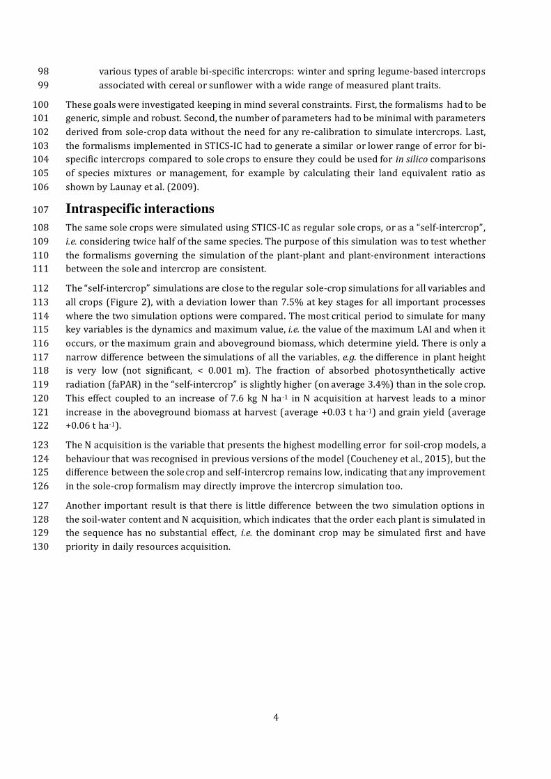
the formalisms governing the simulation of the plant-plant and plant-environment interactions 110 between the sole and intercrop are consistent. 111 The “self-intercrop” simulations are close to the regular sole-crop simulations for all variables and 112

all crops (Figure 2), with a deviation lower than 7.5% at key stages for all important processes 113

where the two simulation options were compared. The most critical period to simulate for many 114 key variables is the dynamics and maximum value, i.e. the value of the maximum LAI and when it 115

occurs, or the maximum grain and aboveground biomass, which determine yield. There is only a 116

narrow difference between the simulations of all the variables, e.g. the difference in plant height 117 is very low (not significant, < 0.001 m). The fraction of absorbed photosynthetically active 118

radiation (faPAR) in the “self-intercrop” is slightly higher (on average 3.4%) than in the sole crop. 119

This effect coupled to an increase of 7.6 kg N ha-1 in N acquisition at harvest leads to a minor 120

increase in the aboveground biomass at harvest (average +0.03 t ha-1) and grain yield (average 121 +0.06 t ha-1). 122

The N acquisition is the variable that presents the highest modelling error for soil-crop models, a 123

behaviour that was recognised in previous versions of the model (Coucheney et al., 2015), but the 124 difference between the sole crop and self-intercrop remains low, indicating that any improvement 125

in the sole-crop formalism may directly improve the intercrop simulation too. 126

Another important result is that there is little difference between the two simulation options in 127

the soil-water content and N acquisition, which indicates that the order each plant is simulated in 128 the sequence has no substantial effect, i.e. the dominant crop may be simulated first and have 129

priority in daily resources acquisition. 130

5

131

Figure 2. Sole crops either simulated as a regular sole crop or a self-intercrop (half-density intercropped with 132 itself). Simulated variables include from top to bottom: 1. Aboveground biomass (Biomass), 2. Fraction of 133 absorbed photosynthetically active radiation (faPAR), 3. Grain yield (Grain), 4. Plant height (Height), 5. Leaf 134 area index (LAI), and 6. Nitrogen acquisition in the aboveground biomass (N acq.). Symbols represent field 135 measurements. The parameters of the model were optimized on sole crop systems, and then used without any 136 recalibration to simulate the self-intercrop. 137

Interspecific interactions 138

The approach with STICS-IC is to calibrate the model on sole-crop data, and let the model simulate 139 the intercrop interactions without any re-calibration of the parameters, thus facilitating the 140 evaluation of the model’s ability to simulate interspecific interactions and possible plant plasticity 141

resulting from intercropping. Sole-crop and intercrop simulation results were compared to 142

observations for each individual species to investigate whether STICS-IC simulates species 143

6

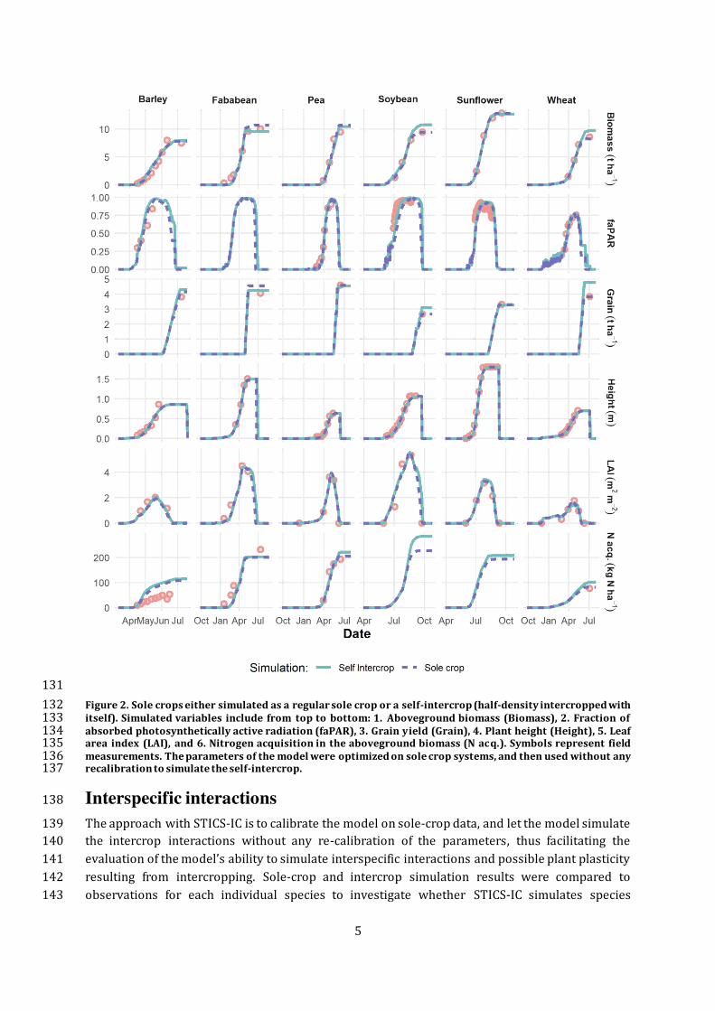
behaviour from sole crop to intercrop. In sole crops, the simulations are close to the observations 144

for all variables (Figure 3). The plant height is particularly close between cropping systems in 145

observations and simulations. The model underestimates the N derived from the atmosphere 146 (NDFA) from the beginning of the crop growth and until the last measurement, at which point it 147

becomes more accurate. 148

149

Figure 3. Observed (points) and simulated (lines) 1. Aboveground biomass (Biomass), 2. Grain yield (Grain), 3. 150 Plant height (Height), 4. Leaf area index (LAI), 5. Nitrogen acquisition in the aboveground biomass (N acq.), and 151 6. Ratio of nitrogen derived from atmosphere (NDFA), for each plant species (a: Pea, b: Wheat) both grown and 152 simulated either in sole crop or intercrop at Auzeville during the 2005-2006 growing season. Values for the 153 intercrop are adjusted (x2) for comparison relative to the equivalent total surface area of the two sole crops. 154 The parameters of the model were optimized on sole crop systems, and then used without any recalibration to 155 simulate the intercrop systems. 156

7

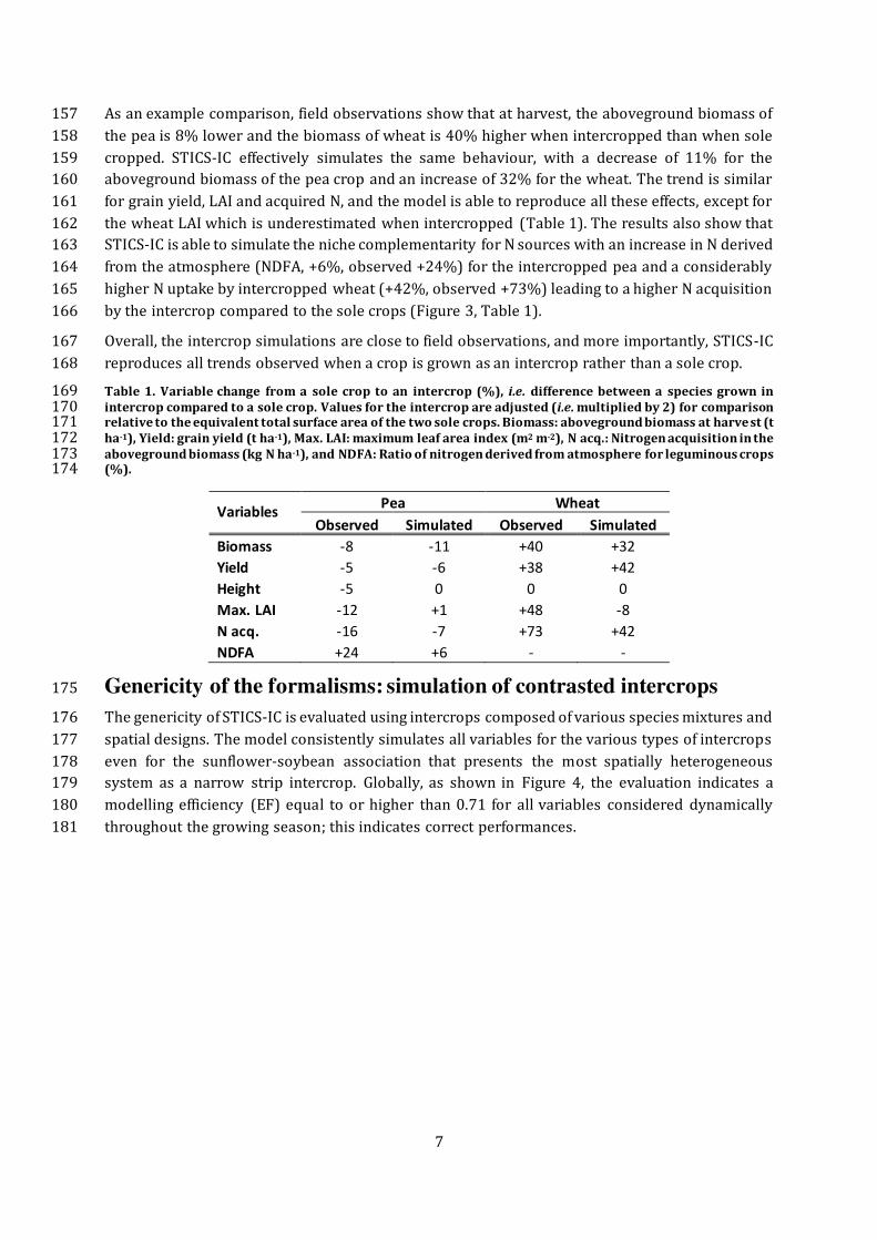
As an example comparison, field observations show that at harvest, the aboveground biomass of 157

the pea is 8% lower and the biomass of wheat is 40% higher when intercropped than when sole 158

cropped. STICS-IC effectively simulates the same behaviour, with a decrease of 11% for the 159 aboveground biomass of the pea crop and an increase of 32% for the wheat. The trend is similar 160

for grain yield, LAI and acquired N, and the model is able to reproduce all these effects, except for 161

the wheat LAI which is underestimated when intercropped (Table 1). The results also show that 162 STICS-IC is able to simulate the niche complementarity for N sources with an increase in N derived 163

from the atmosphere (NDFA, +6%, observed +24%) for the intercropped pea and a considerably 164

higher N uptake by intercropped wheat (+42%, observed +73%) leading to a higher N acquisition 165

by the intercrop compared to the sole crops (Figure 3, Table 1). 166

Overall, the intercrop simulations are close to field observations, and more importantly, STICS-IC 167

reproduces all trends observed when a crop is grown as an intercrop rather than a sole crop. 168

Table 1. Variable change from a sole crop to an intercrop (%), i.e. difference between a species grown in 169 intercrop compared to a sole crop. Values for the intercrop are adjusted (i.e. multiplied by 2) for comparison 170 relative to the equivalent total surface area of the two sole crops. Biomass: aboveground biomass at harve st (t 171 ha-1), Yield: grain yield (t ha-1), Max. LAI: maximum leaf area index (m2 m-2), N acq.: Nitrogen acquisition in the 172 aboveground biomass (kg N ha-1), and NDFA: Ratio of nitrogen derived from atmosphere for leguminous crops 173 (%). 174

Variables Pea Wheat

Observed Simulated Observed Simulated

Biomass -8 -11 +40 +32

Yield -5 -6 +38 +42

Height -5 0 0 0

Max. LAI -12 +1 +48 -8

N acq. -16 -7 +73 +42

NDFA +24 +6 - -

Genericity of the formalisms: simulation of contrasted intercrops 175

The genericity of STICS-IC is evaluated using intercrops composed of various species mixtures and 176

spatial designs. The model consistently simulates all variables for the various types of intercrops 177

even for the sunflower-soybean association that presents the most spatially heterogeneous 178 system as a narrow strip intercrop. Globally, as shown in Figure 4, the evaluation indicates a 179

modelling efficiency (EF) equal to or higher than 0.71 for all variables considered dynamically 180

throughout the growing season; this indicates correct performances. 181

8

182

Figure 4. Observed (x) and simulated (y) values of contrasting intercrops for 1. Aboveground biomass 183 (Biomass), 2. Plant height (Height), 3. Leaf area index (LAI), 4. N acquisition in the aboveground biomass (N 184 acq.), 5. Accumulated nitrogen from symbiotic fixation (N Fix.), and 6. Ratio of nitrogen derived from the 185 atmosphere (NDFA) for legumes. Symbols are colored by plant species and shaped by cropping system. The 186 parameters of the model were optimized on sole crop systems, and then used without any recalibration to 187 simulate the intercrop systems. 188

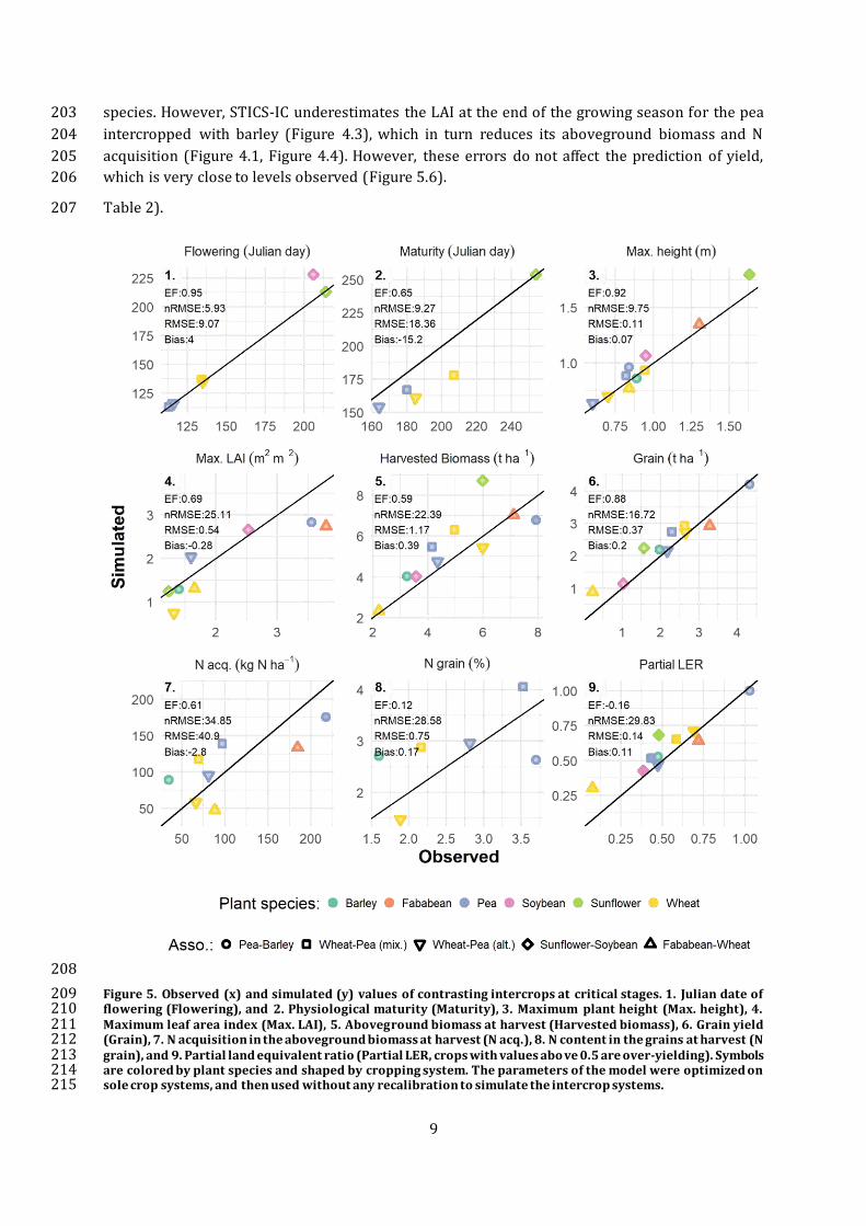
STICS-IC was also evaluated at critical stages, which requires a more demanding value assessment 189

for the model, but produces a better evaluation of its capability to reproduce the system behaviour 190

at crucial stages and over time. STICS-IC can also satisfactorily reproduce crop functioning for all 191 variables, with an EF above 0.6, except for the N content of the grains at harvest and the partial 192

LER that showed lower efficiency (Figure 5). Those two variables are by far the most complex to 193

simulate because they depend on many processes that interact throughout the crop development 194 cycle in intercrop systems. Partial and total LER are particularly difficult to simulate because they 195

both require accurate simulations of the sole crop and the intercrop. It is also worth noting that 196

both present a low bias of 0.17% for the N content in the grain and 0.11 unit for partial LER, and 197

a relatively low nRMSE (<30%). Furthermore, the total LER of intercrops presents a relatively low 198 error of 13% in average over all systems, with a minimum at 2% for both the pea–barley and 199

wheat–pea (alternate rows) intercrops, and a maximum error of 29% for sunflower-soybean 200

(Plant height simulations are very close to observations, with little bias (0.01 m) and a high EF, 201 which is crucial for the simulation of light capture and interspecific competition for the two 202

9

species. However, STICS-IC underestimates the LAI at the end of the growing season for the pea 203

intercropped with barley (Figure 4.3), which in turn reduces its aboveground biomass and N 204

acquisition (Figure 4.1, Figure 4.4). However, these errors do not affect the prediction of yield, 205 which is very close to levels observed (Figure 5.6). 206

Table 2). 207

208

Figure 5. Observed (x) and simulated (y) values of contrasting intercrops at critical stages. 1. Julian date of 209 flowering (Flowering), and 2. Physiological maturity (Maturity), 3. Maximum plant height (Max. height), 4. 210 Maximum leaf area index (Max. LAI), 5. Aboveground biomass at harvest (Harvested biomass), 6. Grain yield 211 (Grain), 7. N acquisition in the aboveground biomass at harvest (N acq.), 8. N content in the grains at harvest (N 212 grain), and 9. Partial land equivalent ratio (Partial LER, crops with values abo ve 0.5 are over-yielding). Symbols 213 are colored by plant species and shaped by cropping system. The parameters of the model were optimized on 214 sole crop systems, and then used without any recalibration to simulate the intercrop systems. 215

10

Plant height simulations are very close to observations, with little bias (0.01 m) and a high EF, 216

which is crucial for the simulation of light capture and interspecific competition for the two 217

species. However, STICS-IC underestimates the LAI at the end of the growing season for the pea 218 intercropped with barley (Figure 4.3), which in turn reduces its aboveground biomass and N 219

acquisition (Figure 4.1, Figure 4.4). However, these errors do not affect the prediction of yield, 220

which is very close to levels observed (Figure 5.6). 221

Table 2. Observed and simulated land equivalent ratio (LER) for different species mixtures and intercropping 222 designs. 223

Association Intercropping design Observed

LER

Simulated

LER

Normalized error

(%)

Faba bean-Wheat Alternate rows 0.8 0.94 18

Pea-Barley Alternate rows 1.5 1.53 2

Sunflower-

Soybean

Alternate narrow

strips

0.86 1.11 29

Wheat-Pea Alternate rows 1.16 1.18 2

Wheat-Pea Mixed 1.02 1.17 15

Sunflower biomass is slightly overestimated which in turn leads to a higher yield and partial LER 224

compared to the observations (Figure 4.1, Figure 5.6 and Figure 5.9). STICS-IC is able to reproduce 225 the low yield for the wheat intercropped with faba bean, but still overestimates its value (Figure 226

5.6). This observation was particularly low for 2007 intercrops (0.23 t ha -1) compared to 227

subsequent years (1.51 t ha-1 in 2010; 2.11 t ha-1 in 2011) which suggests that the model’s 228 overestimation may have resulted from factors that are not considered by the model. As expected, 229

the error is then reflected in the simulated partial LER (Figure 5.9), but has relatively little effect 230

on the overall predicted LER of the intercrop, with a normalized error of 18% (Plant height 231

simulations are very close to observations, with little bias (0.01 m) and a high EF, which is crucial 232 for the simulation of light capture and interspecific competition for the two species. However, 233

STICS-IC underestimates the LAI at the end of the growing season for the pea intercropped with 234

barley (Figure 4.3), which in turn reduces its aboveground biomass and N acquisition (Figure 4.1, 235

Figure 4.4). However, these errors do not affect the prediction of yield, which is very close to levels 236 observed (Figure 5.6). 237

Table 2). 238

Overall, STICS-IC was able to simulate all key measured variables as evidenced by the consistency 239 between simulations and observations in all intercrops tested, where the prediction of grain yield, 240

for instance, had an nRMSE of 17%, an EF of 0.9 and a low bias towards overestimation (0.2 t ha-241 1, Figure 5.6). 242

Discussion 243

Intercropping can contribute to ecological intensification by reducing or eliminating chemical 244

inputs and has great potential for increasing the sustainability of cropping systems. There is a 245

growing need to investigate which intercropped species provide the highest performance, and 246 which management practices are optimal considering the local pedoclimatic conditions. 247

Modelling virtual pre-experiments can help answer these questions by pre-identifying promising 248

11

combinations. Unfortunately, few models can simulate such intercrops accurately, mainly because 249

of the numerous direct or indirect plant-plant interactions and processes involved. 250

In this study, we showed that STICS-IC had a consistent behaviour in the simulation of both regular 251 sole crops and self-intercrops, which is needed when analysing system performances based on 252

sole crops vs. intercrop comparisons with high certainty. These results are a great improvement 253

over previous results using the initial version of STICS developed by Brisson et al. (2008, 2004) 254 and allow to go further in the optimization of intercropping. 255

Legume species usually have relatively low competitiveness for soil mineral N uptake compared 256

to cereal crops, thus allowing the latter to develop a better N nutrition status, which initiates a 257

positive feedback loop with increased crop biomass leading to more N uptake thanks to greater 258 root exploration in the soil. During their first development phases, legume crops may experience 259

an increase in the number of nodules due to the soil nitrate concentration that drops off as a result 260

of the greater competition for N uptake by the cereal crop, which stimulates N2 fixation 261 (Bedoussac and Justes, 2010). This niche complementarity between cereal and legume crops is an 262

important property of this type of intercropping and is precisely what we seek when designing 263

intercrops (Malézieux et al., 2009; Stomph et al., 2020; Tilman, 2020). The simulations showed 264

that the improved version of STICS-IC could simulate niche complementarity for N (Figure 3) with 265 a significant increase in N acquisition per plant in wheat crops and in the NDFA in pea crops. This 266

increase leads to a higher overall N content in the intercrop compared to cereal sole crop, and to 267

an over-yielding illustrated by a land equivalent ratio (LER) significantly above one (Stomph et 268 al., 2020). 269

These results reflect a particularly interesting emergent property of STICS-IC that is able to 270

simulate niche complementarity without any explicit simulation of the facilitation processes 271

stricto sensu, and with formalisms that require no recalibration or new specific implementation 272 procedure. This is precisely what we seek in soil-crop models, i.e. implementing simple and 273

generic formalisms that once coupled make the model able to simulate the functioning of more 274

complex systems by simulating dynamic interactions of processes and emerging properties of the 275 systems. This approach has also proven useful in studies on nutrient stress (Bouain et al., 2019), 276

periodic patterns in plant development (Mathieu et al., 2008; Vezy et al., 2020), environmental 277

impact on plant architecture (Eschenbach, 2005) and even population and community dynamics 278

predicted from individual-based algorithms (Hammond and Niklas, 2009). 279

Numerous studies have found that plant architecture is influenced by the type of species mixture 280

(Liu et al., 2017). In STICS-IC, we do not implement such behaviour explicitly except for the shoot 281

elongation, which was not found significant in the observations. Accordingly, simulations for 282 durum wheat were consistent for situations where the plant was dominant (associated with pea) 283

and dominated (associated with faba bean). Such results may indicate another possible emergent 284

property of STICS-IC, showing that plant plasticity in the field may also act as a buffer to 285

behavioural changes when considering plants at the community scale, which could alleviate the 286 need for changes in parameter values (Louarn et al., 2020). 287

Another interesting result is that most of the errors found in the simulation of intercrops were 288

also found in the sole crops (Figure 2 and Figure 3), indicating that the errors either came from 289 the calibration of the model or from the formalisms shared with the sole crops, an issue not within 290

the scope of this paper. In STICS-IC, new formalisms for intercrops were developed to share the 291

12

sole crop code-base, thus enabling free transfer of future improvements of the model to intercrop 292

simulations. 293

The improved version of STICS-IC is promising. For example, the APSIM model was recently used 294 to simulate maize and soybean with different row arrangements of strip or mixed intercropping 295

(Wu et al., 2021). This model was applied using parameters derived from intercropping 296

experiments, and found to predict key variables with an nRMSE of 7.6-11.6% for biomass and 4.8-297 11.4% for grain yield. It was also applied on a pearl millet-cowpea intercrop with a resulting RMSE 298

of 1.1 m2 m-2 for LAI, 1.02 t ha-1 for biomass and 0.4 t ha-1 for grain yield (Nelson et al., 2021). 299

The M3 crop model was applied on a wheat-faba bean intercrop and presented an average RMSE 300

over the two crops of 0.78 m2 m-2 for LAI, 0.64 t ha-1 for aboveground biomass and 0.43 t ha-1 301 for yield (Berghuijs et al., 2020). The previous standard version of STICS-IC was also recently 302

calibrated for chickpea and wheat, and reached modelling efficiency of 0.23 for the chickpea yield 303

and 0.48 for the wheat (Kherif et al., 2022). Considering the high modelling efficiency value (0.9) 304 obtained with STICS-IC with an independent evaluation using the improved formalisms, we can 305

expect significantly more accurate predictions for given situations, by either directly using STICS-306

IC, or by implementing the new formalisms in other models. 307

It should be noted that the novel formalisms implemented, and more generally STICS-IC, were 308 only calibrated on sole crops and applied with sole crop parameter values on intercrops, the 309

hypothesis being that STICS-IC should simulate all interactions directly rather than adding or 310

tuning parameters. STICS-IC successfully simulated different cropping systems regardless of soil, 311 weather conditions, fertilization, irrigation regimes and spatial complexity: from the well mixed 312

wheat-pea and barley-pea canopy to the wheat-faba bean and sunflower-soybean system known 313

for its large vertical and horizontal heterogeneity. Our results show that the combination of the 314

new simple formalisms implemented proved sufficient to reproduce the main processes at play in 315 arable intercrops such as competition and complementarity in the processes governing light 316

interception, N demand and water fluxes of the intercropping systems. 317

Of all the new formalisms implemented in STICS-IC, one stands out particularly for its relevance 318 and accuracy although it is relatively simple (see Methods section below): the computation of 319

plant height using the phasic development of the plant based on the thermal time corrected by i) 320

vernalisation and photoperiodic effects, ii) abiotic stresses on stem elongation rate, and iii) 321

shading on etiolation of plants in intercropping. To the contrary of the initial formalisms that used 322 the crop LAI, the new algorithm was generic enough to provide accurate simulations for both sole 323

crops and intercrops using the parameter values optimized on sole crops. This is particularly 324

interesting because plant height was repeatedly identified as one of the most important factors 325 for intercrop simulation because of its role in determining competition for light (Berghuijs et al., 326

2021; Corre-Hellou et al., 2009; Launay et al., 2009). The new formalism can be introduced into 327

other crop models, the only requirement being the correct simulation of the species 328

developmental stages. 329

More generally, STICS-IC can be applied to any intercrop system where the planting design allows 330

direct interspecific interactions for resources between the two crops. Although the threshold 331

value for the acceptable width of the strip has not yet been determined, we recommend not 332 simulating strip intercrops with a strip width superior to the plant height or to the horizontal root 333

distribution, in agreement with the concepts used. Our results showed that STICS-IC can simulate 334

strip intercrops with narrow width and few rows (i.e. 2 to 3 rows per strip), which were found to 335

exhibit the most benefits from intercropping (van Oort et al., 2020). Intercrop systems that are 336

13

more spatially complex are excluded from the validity domain unless proven otherwise. They may 337

include low-density agroforestry systems or intercrops that do not present a periodic row-338

manner of mixing (e.g. one row of one crop, then two of the other, and two of the first one). 339 Although not considered in this study, on a conceptual basis, STICS-IC can also simulate varietal 340

mixtures, relay intercropping and all intercrop mixtures within the row and in strict alternate 341

rows. 342

Overall, our results show that our new formalisms appear generic enough to simulate properly 343

different types of interspecific plant-plant interactions regardless of the species intercropped. 344

These formalisms are simple enough to parameterize and fast to compute, which is required for 345

long-term simulations and mathematical optimization of parameters that need repeated 346 execution of the model until convergence of the statistical criteria. STICS-IC, and any other model 347

that integrates the new formalisms, will be particularly well suited to address current challenges 348

such as generalizing results of intercropping from one site to another, or virtually pre-screening 349 innovative intercrop systems that are more sustainable, easier to manage, and well adapted to 350

local conditions, as a tool for the agro-ecological transition, and to assess the impact of climate 351

change scenarios on sole versus intercrop production and GHG emissions. 352

Methods 353

New formalisms 354

General description of the STICS soil-crop model 355

The STICS model is a dynamic 1D soil-crop model that combines crop development, growth and 356

yield formation with the carbon, nitrogen, energy and water cycles of the soil-crop system 357 (Beaudoin et al., in press; Brisson et al., 2008, 2003, 1998). The model runs at a daily time-step 358

using input data related to climate, crop species, soil, agricultural management, and the state of 359

the system at initialization, such as the water and nitrogen content of each soil layer. The crop is 360 represented as a set of organs with a given development stage, biomass and nitrogen content. The 361

biomass growth is mainly driven by light interception as a function of leaf area index with a big 362

leaf approach, i.e. using the Beer-Lambert law of light extinction coupled with a radiation use 363

efficiency, while crop development is driven by thermal time corrected by vernalisation and 364 photoperiodic effects. Stress effects from frost, insufficient supply of nitrogen or water, and root 365

anoxia can all potentially affect development, leaf area, growth and yield. 366

The STICS model was adapted to simulate bi-specific crop mixtures in alternate rows by Brisson 367

et al. (2004) and further by Launay et al. (2009). Both crop species are simulated sequentially 368

starting from the dominant one (i.e. the taller one) and the model simulates several interactions 369

between the two crops, allowing inversion of dominancy during the crop cycle. These interspecific 370

interactions were reviewed and are described below including new formalisms proposed for the 371 improvement of some processes that were found incorrect or not sufficient to simulate daily 372

plant-plant interactions. 373

In this paper, we only describe the equations that were modified in or added to the improved 374 version of STICS-IC. The other equations are available from the first version published by Brisson 375

et al. (2004), in other previous papers (Brisson et al., 2003, 1998) and in the STICS book detailing all 376

equations and associated information (Beaudoin et al., in press; Brisson et al., 2008). 377

In addition, various bugs were fixed in the algorithms, mainly in the computation of leaf 378 senescence, effect of frost and energy balance. 379

14

Light interception 380

Radiative transfer 381

In order to encompass light interception by heterogeneous canopies, STICS-IC implements a 382 geometrical formalism called “radiative transfer” where each plant is described by a geometric 383 shape: upward triangle, downward triangle, or rectangle (Figure 1). The dimensions of the plants 384

are computed using the total plant height, crown base height, and a ratio between the height and 385

width. The spatial design is then determined using the plant shape and the inter-row spacing. The 386

light intercepted by the plants is computed as the total incoming radiation from the sky minus the 387 radiation transmitted to the soil (Brisson et al., 2008, 2004). The transmitted light is computed 388

over 200 sample points evenly spaced on the ground surface from the plant on the left-hand side 389

until the centre of the inter-row, i.e. one half of the inter-row. Direct and diffuse light from the sky 390

are then computed separately. Direct light uses the average position of the sun in the sky 391 throughout the day, and diffuse light is computed by discretizing the hemisphere centred on the 392

point into 46 evenly distributed angles. The dimension along the row is considered infinite. For 393

each angle between the origin of direct or diffuse light and each sample point on the ground, it is 394 tested whether its direction is pointing above or below the crown height in the 3D space. The 395

angles pointing above the crown receive direct and diffuse light directly from the sky. The 396

resulting sky view angle is then used to compute the proportion of direct light effectively 397

intercepted by a point p (𝐾𝑑𝑖𝑟), or the cumulative proportion of diffuse light (𝐾𝑑𝑖𝑓) received on a 398

given direction using the standard overcast sky (Brisson et al., 2004). 399 Rdir,p = R𝑑𝑖𝑟 ∗ 𝐾𝑑𝑖𝑟 (1) Rdif,p = R𝑑𝑖𝑓 ∗ 𝐾𝑑𝑖𝑓

(2)

where 𝑅𝑑𝑖𝑟 and 𝑅𝑑𝑖𝑓 (MJ m-2 d-1) are the incoming radiation from the sky for direct and diffuse light, 400

respectively, and 𝐾𝑑𝑖𝑟 and 𝐾𝑑𝑖𝑓 are the proportions of direct and diffuse light effectively 401

intercepted by a point p. 402

The light transmitted to the point (𝑅𝑡𝑝 ) from the plant canopy is then: 403 Rtp = (1 − Rdir,p − Rdif ,p) ∙ e−k∙LAI (3)

where 𝑘 is the canopy light extinction coefficient and 𝐿𝐴𝐼 the leaf area index (m2 m-2). 404

The total light intercepted by each point (𝑅𝑡𝑝 + 𝑅𝑑𝑖𝑟,𝑝 + 𝑅𝑑𝑖𝑓,𝑝) is then averaged over all points 405

from two distinct surfaces: the ground surface directly below the plant, called the shaded surface, 406 and the ground surface in-between the plant and the centre of the inter-row, called the sunlit 407

surface. Finally, the light intercepted by the plants can be computed as the incoming radiation 408

coming from the atmosphere minus the light intercepted in average by the shaded and sunlit 409 surfaces of the ground. 410

In the case of intercrops, the same computation for light interception is applied iteratively and 411

relatively independently for each crop using only the transmitted light as a medium, without any 412

explicit knowledge of the shape of the other crop. The sample points are positioned on top of the 413 dominated plant (i.e. the shorter plant) instead of the ground for computing the light interception 414

of the dominant plant, and on the ground surface for the dominated plant. The dominated plant is 415

divided into a shaded and a sunlit compartment that are simulated independently, with the only 416

15

difference being the incoming global radiation, either coming from the shaded or sunlit surface 417

receiving transmitted light from the dominant plant. The dominated plant is then the result of the 418

average or sum of the two compartments, depending on the variable of interest. The light 419 transmitted to the soil is the radiation coming from the atmosphere minus the interception of the 420

dominant plant and the interception of both compartments weighted by their relative surface for 421

the dominated plant. 422

Several discrepancies were found in the initial algorithm following a careful review of the 423

formalism, the most notable were: 424

- The light available for the dominated crop was set to the global radiation coming from the 425

sky instead of the light computed using the sample points above its canopy; 426 - The shape of the right-hand side plant was not considered properly for the direct light 427

computation; 428

- Plant shapes (i.e. right and left-hand sides) were always considered as a rectangle for the 429

diffuse light, other chosen shapes were disregarded; 430 - The complete occultation of the sky by the plants for some points was not properly 431

considered. 432

All these discrepancies were corrected in the new version presented in this work (STICS-IC). 433

Beer-Lambert law of light extinction 434

The radiative transfer formalism is generic and allows simulating a wide range of intercropping 435

designs with heterogeneous canopies due to the relative independence between the shapes of 436 both crops. However, some intercrops present well mixed canopies, where the assumption of 437

spatially divided crop canopies or dominance in terms of height is not verified. Therefore, a 438

simpler approach to account for intercrops with well-mixed canopies was also implemented. This 439 new formalism uses the Beer-Lambert law of light extinction in plant canopies adapted for 440

intercropping (Keating and Carberry, 1993) by considering the leaf area index and extinction 441

coefficients of both crops. For example, the fraction of Photosynthetically Active Radiation 442

intercepted by the first crop (𝐹𝑎𝑃𝐴𝑅1) is calculated as: 443

FaPAR1 = LAI1 ∙ k1(LAI1 ∙ k1 + LAI2 ∙ k2) ∙ (1 − e−LAI1 ∙k1−LAI2 ∙k2) (4)

where LAI is the leaf area index, k is the light extinction coefficient, and 1 and 2 denote crop index. 444 The crop index is relative to the other plant, plant 1 is the currently simulated plant and plant 2 is 445

the other plant. 446

This formalism is available as a new option, which can be selected by the user, and as a fallback 447

for the radiative transfer approach when there is no clear dominance between both crops and 448 both canopies are considered well mixed during a part of the crop cycle. In this case, the pure 449

radiative transfer approach would result in an overestimation of light competition between the 450

plants, because it is always considered that one plant dominates the other. This fallback can be 451 triggered by parameterizing a height threshold parameter to a value greater than zero, i.e. the 452

height difference between both crop species above which we consider a significant dominance of 453

one crop. In other words, if the difference in height between the two crops is below the threshold 454

of few centimetres, light interception is simulated using the Beer-Lambert law of light extinction 455

16

instead of the radiative transfer formalism. If the difference becomes larger than the threshold, 456

the model shifts again to the radiative transfer computation. 457

Plant density effect 458

When simulating a sole crop, the interspecific competition for light interception and growth is 459

computed using a density effect (𝑆𝐷 ) that results from the current plant density and two model 460 parameters: adens and bdens (see equation (5)). This effect is used to downregulate the 461

development of the plant with higher plant density (Brisson et al., 2008, 2003). 462

SD = Dbdensadens (5)

where 𝐷 is the plant density (plant m-2), 𝑎𝑑𝑒𝑛𝑠 is a genotypic scaling factor for the plant density 463 effect, and 𝑏𝑑𝑒𝑛𝑠 is the minimal density above which interplant competition starts. 464

An equivalent plant density was then introduced by Brisson et al. (2004) to use the same equation 465

for intercrops, but applied to both intra- and interspecific competition. In the previous version of 466

STICS, the equivalent density (𝐷𝑒) was set to the actual plant density for the dominant plant, i.e. 467 the taller plant, and computed as follows for the dominated plant: 468 De1 = D1 (6)

De2 = D2 + D1bdens1 ∙ bdens2 (7)

Where 𝐷𝑒1 and 𝐷𝑒2 are the equivalent density of the dominant (i.e. taller) and dominated (i.e. 469 shorter) plants respectively, 𝐷1 is the actual density of the dominant plant, 𝐷2 is the actual density 470

of the dominated plant, and 𝑏𝑑𝑒𝑛𝑠1 and 𝑏𝑑𝑒𝑛𝑠2 are the bdens parameters for the dominant and 471

dominated plant, respectively. 472

This equivalent plant density was originally implemented to represent the increased competition 473 for light experienced by the dominated plant compared to a sole crop (Brisson et al., 2004). 474

However, we argue that part of this computation is redundant with the computations of light 475

interception, nitrogen and water uptake that already consider the competition between crop 476 species. We propose to only use equation (5) for both crops to represent the intra-row (i.e. intra-477

specific) competition as intended in a sole crop simulation. Hence, the new definition of the 478

equivalent density for each plant is now considered as the ratio of sole crop plant density divided 479

by intercrop plant density, i.e. twice the actual density in intercrop for a replacement intercrop 480 designs (i.e. half density in intercrop vs. sole crop). The intraspecific competition is now 481

guaranteed to be the same for the equivalent sole crop, because the adens and bdens parameters 482

are determined for sole crops. 483

Plant traits and dimensions 484

The plant height was computed using the LAI for sole crops, and is often ignored by users because 485

it has no impact on other output variables in STICS, except when using the radiative transfer 486 option, which was previously mandatory for intercrops (Brisson et al., 2008, 2003). In 487

intercropping, the plant height is a crucial variable because it allows computing plant dominance, 488

which in turn affects light competition between plants (Brisson et al., 2004). Because the calculation 489

of plant height was found inconsistent over the course of the plant development, and in particular 490

17

after the flowering stage (Corre-Hellou et al., 2009), we developed a new formalism that computes 491

plant height using plant phasic development instead, with an implementation close to the one 492

proposed by Gou et al. (2017) and Berghuijs et al. (2020). The de-coupling of the plant height from 493

LAI also allows for a common parameterization for sole crops and intercrops. 494

The new computation of plant height is then defined by a logistic function as follows: 495

Hi = H0 + a1 + e−c∙(devi−b) (8)

where 𝐻𝑖 is the plant height (m) on day i without any other stresses (see next paragraph for 496

stresses), 𝐻0 is the plant base height (m), 𝑑𝑒𝑣𝑖 (degree days) is the sum of development units from 497

sowing, corresponding to thermal-time corrected by the effects of vernalisation and photoperiod, 498

a the maximum plant height under optimal conditions (m), b the value of dev at which the plant is 499 at half the maximum height (i.e. value at inflection point, in degree days), and c the logistic growth 500

rate, or steepness of the curve at the inflection point. 501

The height of a plant can also be up- or down-regulated in response to stresses, such as light 502 competition with another species, drought, root anoxia, low nitrogen availability and frost. The 503

resulting integrated effect arising from those individual stresses is computed as the minimum of 504

all down-regulating effects (𝑆), and the up-regulating effect (𝐸, the shoot elongation) separately, 505

which are both applied to the daily height increment. This increment is given by the difference 506 between the potential height from the day before and the current potential height modulated by 507

up- and down-regulating effects according to equation (9). 508 ∆Hi = (Hi − Hi−1) ∙ S ∙ E (9)

where ∆𝐻𝑖 is the actual daily increment in plant height, 𝐻𝑖 is the current potential height 509

determined by the simulated developmental stage, 𝐻𝑖 −1 is the potential height of the previous day, 510 𝑆 is the stress effect due to nitrogen availability, drought, root anoxia, or frost (see equation (10)), 511

and 𝐸 is the shoot elongation effect (see equation (11)) that act as an up-regulating effect. 512

The stress effect 𝑆 is calculated as follows: 513 S = 1 − (1 − min(SN , SW , SF , SA) ∙ sp) (10)

where 𝑆𝑁 ,𝑆𝑊, 𝑆𝐹 and 𝑆𝐴 are the stress effects from nitrogen (N) and water (W) limitations, frost 514 (F) and root anoxia (A), and sp is the scaling parameter that helps defining the importance of the 515

total effect on plant height. S is equal to one (no stress) when 𝑠𝑝 is close to zero, and close to the 516

minimum value (i.e. higher stress) of all down-regulating stresses when 𝑠𝑝 is close to one. All 517

stresses are defined between zero (maximum effect) and one (no effect). 518

The magnitude of the elongation of the plant can theoretically change with the associated species 519

depending on light quantity and quality, e.g. a proxy of the photomorphogenetic effect. However, 520

the type of response, i.e. shade avoidant or shade tolerant, remains stable based on the plant 521 species. The shoot elongation effect due to light competition with another species (E) is 522

considered directly correlated with shading, and is computed as: 523 E = Ashaded ∙ (ep − 1.0) + 1.0 (11)

18

where 𝐴𝑠ℎ𝑎𝑑𝑒𝑑 is the relative surface of the plant that is shaded (0: full sun; 1: fully shaded), and 524

ep is a parameter that represents the maximum elongation effect when the plant is fully shaded. 525

The plant width is then computed using a ratio between plant height and width. This ratio can be 526 affected by pruning or manual leaf removal, otherwise it is considered constant throughout the 527

plant life cycle (Brisson et al., 2008, 2003). 528

Intercrops sown in a narrow strip design, i.e. more than one alternating row per species, can also 529 be simulated using the same principle, but simulating the whole strip as a single big average plant 530 instead. In this case the user must activate the “strip intercrop” option in the model, and input the 531

number of rows of each strip, and the inter-row distance as the total width of both strips. Users 532

should only simulate narrow strips relative to crop dimensions, because the model has a 533 1D/pseudo 2D representation based on the assumption that there are interactions between crops 534

for light, temperature, nitrogen and water. This assumption might fail for wider strips, where 535

species interactions are mostly limited to the border rows of the strips leading to a clear spatial 536 heterogeneity in the plant-plant interactions. 537

Nitrogen demand 538

The nitrogen (N) uptake of the plant depends on its N demand, N availability in the soil layers and 539 root exploration. The latter is computed using the rooting depth and the root length density along 540

the soil profile. The N requirements are computed using a dilution curve that relates the crop 541

aboveground biomass to its N concentration (Corre-Hellou et al., 2009). The underlying hypothesis 542

is that leaves have a higher N content compared to other organs, and as the plant grows, the 543 proportion of leaves compared to structural organs (e.g. straw) decreases, thereby diluting the N 544

content in the aboveground biomass (Justes et al., 1994). 545

In the previous version of STICS, the dilution curve was computed using the aboveground biomass 546 of the plant per ground surface area (Brisson et al., 2004). This computation is fine for sole crops 547

because the N requirement of a plant depends on its biomass and is relatively independent from 548

its plant density due to tillering in cereals or ramification in other species, i.e. plants can 549

compensate for low densities by increasing the biomass per plant. However, plants cannot always 550 offset the effect of lower density in intercropping, because they are in competition with another 551

plant species. Therefore, the expected biomass per ground surface area for a plant grown in 552

mixture at a given development stage is often lower than its counterpart in sole crop, hereby 553 artificially increasing its N demand in STICS because the dilution curve uses parameters fitted on 554

sole crops. The approach in STICS-IC is to fit species parameters on sole crops and then use the 555

same values for intercropping (i.e. no re-calibration) assuming that potential interactions between 556

crops are considered by the model formalisms. Given these constraints, we compute the total 557 biomass of the intercrop (i.e. both crops together) as a proxy for the equivalent biomass in sole 558

crop instead of the biomass of the crop itself grown as intercrop, as proposed by Louarn et al. 559

(2021), to represent in a first acceptable approximation the dynamic N nutrition status of bi-560

specific intercrops. This modification helps avoiding an underestimation of the N status of plants 561 simulated in intercrops, as shown by Corre-Hellou et al. (2009). This assumption should be valid 562

for a wide range of applications, unless both development and biomass of the crops are largely 563

different (Louarn et al., 2021). The following equation is used to simulate the plant N demand of 564 each crop in the bi-specific intercrop: 565

19

demandi,p = ∆Nmaxi,p∆max(Wi,tot, biometa) ∙ Gi,p (12)

with 𝑑𝑒𝑚𝑎𝑛𝑑𝑖 ,𝑝 the N demand of the crop (kg N ha-1 day-1), 𝑁𝑚𝑎𝑥𝑖 ,𝑝 the maximum N 566

concentration of the crop (gN kg-1) , 𝐺𝑖 ,𝑝 the daily crop growth rate (t ha-1 day-1), 𝑊𝑖 ,𝑡𝑜𝑡 the total 567

aerial biomass of both associated crops (t ha-1), and 𝑏𝑖𝑜𝑚𝑒𝑡𝑎 the threshold of 𝑊𝑖 ,𝑡𝑜𝑡 above which 568

N dilution becomes significant (t ha-1), 𝑖 denotes the current day, ∆ the change in the variable 569

value between the previous and the current day, and 𝑝 the current computed crop. 𝑁𝑚𝑎𝑥𝑖,𝑝 is 570

computed as follows: 571 Nmaxi,p = adilmax ∙ Wi,tot−bdilmax (13)

with 𝑎𝑑𝑖𝑙𝑚𝑎𝑥 the maximum plant N concentration (%) at a crop biomass of 1 t ha -1 and 𝑏𝑑𝑖𝑙𝑚𝑎𝑥 a 572

coefficient defining the steepness of the curve relating the decrease of N concentration as crop 573 biomass increases. Both 𝑎𝑑𝑖𝑙𝑚𝑎𝑥 and 𝑏𝑑𝑖𝑙𝑚𝑎𝑥 are species-specific, allowing a different response 574

between species for a similar 𝑊𝑖,𝑡𝑜𝑡. 575

The N nutrition index (𝑁𝑁𝐼𝑖 ,𝑝, 0-1) is computed as the ratio between the actual N concentration 576

([𝑁]𝑖,𝑝 in %) and the critical N concentration ([𝑁𝑐]𝑖,𝑝 in %), which defines the minimum value of N 577

for non-limiting growth rate (Justes et al., 1994). The computation of 𝑁𝑁𝐼𝑖 ,𝑝 is done for each crop 578

of the intercrop as follows: 579

NNIi,p = [N]i,p[𝑁𝑐]i,p (14)

and [𝑁𝑐]𝑖,𝑝 is computed similarly to equation (13), but using the current parameters instead of 580

the maximum: 581 [Nc]i,p = adil ∙ Wi−bdil (15)

Water and nitrogen competition and complementarity 582

In addition to light interception, competition and complementarity for water and N are mainly 583 determined by the presence and density of roots in the soil layers in depth. The resource-use is 584

species-specific, and considered by specific values of parameters in STICS-IC (Brisson et al., 2004; 585

2008). 586

The availability of water and N in the soil depends on initial conditions, climate, management, and 587 dynamic plant N and water uptake. The latter depends on the resource acquisition efficiency and 588

the presence and density of roots of each species, which is also influenced by the availability of 589

those resources in the soil. This means that root systems of the intercrop do not directly interact, 590 but affect each other via their influence on the status of water and N availability in the soil. This 591

feedback is already considered in STICS-IC. Hence, it is important to consider the competition and 592

complementarity effects for these resources between plants with a sufficient description of the 593

aforementioned processes. 594

As for a sole crop, the root development of each species in the intercrop depends on species–595

specific parameters, thermal time, several potential stresses, such as anoxia, drought, soil 596

20

properties (high bulk density), frost, or low N content, and potentially a trophic linked production 597

depending on the simulation option (Brisson et al., 2008, 2004). 598

The computation of the density effect is already considered in the shoot biomass production when 599 using the trophic-linked root length expansion option. However, it is not when choosing the self-600

governing root length expansion option, which is the default. Consequently, we introduced an 601

effect of the equivalent plant density (𝐷𝑒) for the computation of the root length growth rate (𝑅𝐿𝐺 , 602 mroot d-1) when using this option: 603

RLG = 𝑅𝐿𝐺𝑑𝑑𝑚𝑎𝑥1 + e5.5∙𝑠𝐿𝐴𝐼𝑚𝑎𝑥 −𝑈𝑟𝑜𝑜𝑡 ∙ SD ∙ D ∙ dtj ∙ SA + RLGf (16)

with 𝑅𝐿𝐺𝑑𝑑𝑚𝑎𝑥 the maximum rate of root length production (m plant-1 degree day-1), 𝑠𝐿𝐴𝐼𝑚𝑎𝑥 a 604

growth rate-linked parameter common with the LAI calculation, 𝑈𝑟𝑜𝑜𝑡 the daily relative 605

development unit for root growth, ranging between 1 and 3, 𝑆𝐷 the density stress effect, 𝐷 the 606

actual plant density (plants m-2), 𝑑𝑡𝑗 the daily efficient temperature for root growth (C° day-1), 𝑆𝐴 607 the root anoxia stress effect and 𝑅𝐿𝐺𝑓 the root growth rate at the root front (m day-1), which is 608

calculated as: 609

RLGf = 𝑅𝐷𝑓𝑟𝑜𝑛𝑡 ∙ DDe ∙ deltaz ∙ 104 (17)

with 𝑅𝐷𝑓𝑟𝑜𝑛𝑡 the root density at the root front (cmroot cm-3) which is supposed to remain 610

constant, and 𝑑𝑒𝑙𝑡𝑎𝑧 the root front growth rate (cmroot d-1). 611

Starting with the dominant crop, each crop sequentially uptakes water and N from the soil layers 612 based on the presence and density of their roots. The order in this formalism seems adequate 613

considering the daily time-step, only affecting the potential water or N stresses by a lag of one day. 614

Furthermore, STICS is also able to simulate different affinity for N for each species and the effect 615 of soil nitrate concentration on nodulation and N2 fixation by leguminous crops (Brisson et al., 616

2008, 2004). Consequently, niche complementarity for N can be simulated in STICS-IC for cereal-617

legume intercrops since the computation of the N2 fixation rate depends on both growth rate and 618

nitrate uptake by the leguminous crop. Then the competition between the two species for soil 619 mineral N uptake could induce a higher rate of N2 fixation of the legume due to the simulation of 620

a reduced inhibition of nitrate reductase activity under a lower soil nitrate concentration by the 621

stronger cereal N uptake. 622

Microclimate 623

Microclimate can be impacted by crops, especially when the canopy is heterogeneous. In 624

intercropping, the taller plants can decrease the wind experienced by the smaller one by 625 increasing the size of the boundary layer above its canopy. It can also increase air humidity and 626

regulate the local temperature. All these effects can greatly influence the development of a plant 627

by modifying the daily and cumulative thermal-time. These effects are taken into account in STICS-628

IC by using a resistive approach first presented in Brisson et al. (2004) and adapted from 629 Shuttleworth et Wallace (1985). This approach is quite simple and coherent to simulate canopy 630

temperature in intercropping, and was kept in its original form. 631

21

Spatial designs that theoretically determine the validity domain of the model 632

Before simulating intercrops with the improved version of STICS-IC, the user should address how 633 plants interact in the soil-intercrop system, and whether these interactions are correctly 634

considered in the model. Based on the main processes described above, STICS-IC is able to 635

simulate intercropping in alternate rows (each species in a different row, inter-row set to distance 636 between rows of the same species) and mixed within-row (inter-row set to distance between each 637

rows). These two intercropping designs can be simulated for any plant density as long as their 638

root distribution can be assumed horizontally homogeneous. For the light interception, the 639

geometrical approach should be used for heterogeneous canopies, but only for crops with 640 homogeneous canopies along the row, and as long as there is a dominant plant. If not, the option 641

of Beer-Lambert approach for intercrop canopies should be used. The type of design to avoid using 642

our formalisms is a horizontally heterogeneous canopy with no clear dominance between species, 643 e.g. plants grown further apart with the same height, or crops grown in wide strips with 644

interaction only at the interface of both crops. However, strip designs that present a clear 645

dominant crop sown in one or several rows should conceptually be in the domain of validity of the 646

model as each strip is represented as a single plant. Such systems and whether they are part of the 647 validity domain of STICS-IC are tested in this paper. 648

Finally, theoretically and technically, STICS-IC is able to simulate relay intercropping in alternate 649

rows (or with the second crop sown in the inter-row of the first crop) where the two species are 650 not sown, neither harvested, at the same time; however, we did not test this type of intercropping 651

in this paper. 652

As a rule of thumb, the improved version of STICS-IC can simulate any bi-specific intercrop system 653

that presents these three characteristics: 654 - root systems that interact horizontally, for soil layers where both root systems are 655

present; 656

- shoots forming a canopy that is at least homogeneously distributed in the row; 657

- shoots interacting for light capture, either mixed or with a significant or large dominance. 658

Methodology for the calibration and evaluation of STICS-IC 659

Parameter calibration 660

The parameters and options of the model were first calibrated manually using data from literature 661

and expert knowledge. Then an automatic calibration was performed based on the 662 recommendations of Guillaume et al. (2011) and Buis et al. (2011) on the most influential 663

parameters following the same procedure consisting of 15 steps of calibration for 25 parameters 664

optimized over 13 variables. The parameters were first optimized using the Beer-Lambert law of 665 extinction for the light interception, and then using the radiative transfer option, because the 666

latter can fall back to the Beer-Lambert law whenever the plant height of the two species are close, 667

and by doing so, the light extinction parameter of the Beer-Lambert law is used. 668 The parameters were optimized using the “CroptimizeR” R package (Buis et al., 2021) with the 669

Nelder–Mead simplex algorithm (Nelder and Mead, 1965) and seven repetitions with different 670

initial parameter values to better sample the range of values while minimizing the risk of 671

converging to a local minimum. Analyses of the estimated values were performed to investigate 672 whether the initial values had any impact on the optimized value. 673

22

Parameters calibrated for intercrops 674

The new formalisms of STICS-IC were designed to be calibrated on sole crops and then applied to 675 intercrops with no further parameterization. This method assumes that there is either no 676

significant influence of the other crop on a given process, or the model explicitly simulates those 677

interspecific interactions, including trait plasticity such as enhanced shoot elongation or root 678 exploration. 679

The formalisms implemented only need two parameters to be calibrated when necessary for the 680

simulation of bi-specific intercrops: a threshold for the difference in crop height activating the 681

dominance effect, and an elongation effect due to shading (i.e. ep from equation (11)). The former 682 defines the threshold of difference in plant height under which both canopies are considered well-683

mixed and no clear dominance is occurring between the two species, indicating that light is shared 684

depending on the LAI of each plant and their respective light extinction coefficient. It is associated 685 to the intercrop system under consideration, but its value should be consistent between 686

intercropping systems because it defines the limit of the validity domain of the 1D and 3D 687

representations. The parameter for the elongation effect cannot be parameterized on sole cro ps 688

as it is the result of plant-plant interactions and should be measured in the field when the given 689 crop is dominated by the other, or in growth chambers with light control. The value of this 690

parameter can change depending on the type of species associated. Surprisingly, we did not 691

observe a significant elongation effect in our data set, so this parameter was set to 1.0 for all 692 species in a first approximation, i.e. no elongation due to shading. 693

Combination of strategies to evaluate the relevance and the genericity of the model 694

Three complementary strategies were adopted to evaluate the new version of STICS-IC presented 695 in this paper. 696

First, the model formalisms were evaluated in detail using a purely conceptual approach with the 697

hypothesis that it should provide the same results when simulating a sole crop as usual or 698

simulating the same sole crop using the intercrop formalisms. This means simulating a sole crop 699 as an intercrop with itself, which also allows analysing if intraspecific interactions are correctly 700

taken into consideration and implemented in the algorithm. We refer to these simulations as “self-701 intercrop”, where sole crops are simulated by considering half a sole crop combined with another 702 half sole crop. Another objective of this analysis was to investigate whether there is an effect of 703

the order each plant is computed in the sequence, i.e. whether the dominant crop grows more 704

because it has priority in resource acquisition each day as it is simulated first. Our hypothesis is 705

that the maximum delay of one-day between the plants has a very low impact on the simulation, 706 i.e. the dominated plant can also be considered having priority over the dominant plant because it 707

acquired resources last on day i-1. Nevertheless, this assumption needed to be evaluated. 708

Second, we used data from two crops either grown as sole crops or intercropped, and simulated 709 both cases to evaluate the ability of STICS-IC to reproduce the interspecific interactions as well as 710

the intraspecific interactions. 711

Third, we evaluated the model using experimental data of intercrops with contrasting species 712

mixtures and spatial heterogeneity, at contrasting sites, to investigate its genericity and the 713 domain of validity of STICS-IC. 714

Note that all intercrop simulations are independent evaluations of the model as it is only 715

calibrated on sole crop situations. 716

23

Dataset 717 The first experimental site is located on the INRAE research station in Auzeville (43°31′N, 1°30′E) 718

in South of France (from published and unpublished data). The climate is temperate oceanic under 719

Mediterranean influence and characterized by summer droughts and cool, wet winters (Cfa in 720 Köpper-Geiger climate classification, Beck et al., 2018). The 25-year mean annual rainfall in 721

Auzeville is 650 mm and the mean annual air temperature is 13.7°C. The site has a deep loamy soil 722

with little or no stoniness. Phosphorus and potassium are assumed non-limiting at this site. The 723 experiment included four cropping systems, plants either grown as sole crops or intercrops in a 724

replacement design (half density of sole crops for each species): 1) durum wheat and winter pea 725

in alternate rows, 2) durum wheat and winter pea mixed on the row, 3) durum wheat and faba 726

bean in alternate rows, and 4) sunflower and soybean in alternating narrow strips. 727

The second site corresponds to data published by Corre-Hellou, Fustec, and Crozat (2006) from an 728

experiment located at the FNAMS near Angers, France (47°27’ N, 0°24'W). The location benefits 729

from a temperate climate with oceanic influence with no dry season and warm summer (Cfb in 730 Köpper-Geiger climate classification). Angers has a mean temperature of 12.4 °C and mean annual 731

rainfall of 703 mm averaged over 20 years (1999 and 2019). The soil is a clay-loam. We used one 732

treatment of this published paper with spring barley and pea intercrops in alternate rows and the 733

two sole crops with no N fertilizer application. 734

Alternate row intercrop of durum wheat and winter pea 735

This experiment was carried out during the 2005-2006 growing season in Auzeville (Table 3). 736

Durum wheat (Triticum turgidum L., cv. Nefer) and winter pea (Pisum sativum L., cv. Lucy) were 737 grown as sole crops and intercrops. The durum wheat and winter pea were sown at the 738

recommended density (336 and 72 seeds m−2, respectively) in sole crops and at half density in an 739

alternate rows design in the intercrop, both with an inter-row distance of 0.145 m. 740

Initial mineral N was 39 kg N ha-1 on the whole soil profile to 1.2 m depth. Fungicide-treated seeds 741

were sown on 8 November 2005. Weeds, diseases and green aphids were controlled with 742

appropriate pesticides. 743

An incorporation of 7 t ha−1 (C:N = 63) of sorghum (Sorghum bicolor (L.) Moench) residues, the 744 previous crop, was performed on 26 September 2005 by tillage at 20–25 cm depth. 745

More information on the experimental setup can be found in Bedoussac and Justes (2010). 746

Durum wheat and winter pea mixed on the row 747

Similarly, the same species and varieties than presented above were grown as sole or intercrops 748

in Auzeville during the 2012-2013 growing season, but in this experiment, the intercrops were 749

mixed on the row instead of sown in alternate rows. The durum wheat (cv. Nefer) and winter pea 750 (cv. Lucy) were sown at a density of 280 and 70 seeds m−2 respectively in sole crops and at half 751

density in the bi-specific intercrop, both with an inter-row distance of 0.16 m. 752

Initial mineral N content was 41 kg N ha-1 over the 0-1.2 m soil profile. Seeds were sown on 20 753

November 2012. Mineral fertilizers were applied on 25 March with 80 kg N ha-1 and on 14 May 754 with 60 kg N ha-1. Weeds, diseases and green aphids were controlled with appropriate pesticides. 755

The previous crop was a sunflower (Helianthus annuus L.). 756

More experimental details can be found in Kammoun (2014) and Kammoun et al. (2021). 757

24

Alternate row intercrop of durum wheat and winter faba bean 758

Durum wheat (cv. Nefer) and faba bean (Vicia Faba L., cv. Castel) were grown in sole and intercrop 759 during the 2006-2007 growing season in Auzeville. The experimental design included four 760

replicates for wheat in sole crop and the intercrop, and seven for faba bean in sole crop. The 761

intercrop consisted of alternate rows of each crop species. 762

Crops were sown 0.05 m deep in the soil at 336 seeds m-2 for wheat in sole crop, 30 seeds m-2 for 763

faba bean in sole crop, and at half density in alternate rows for the intercrop. The inter-row 764

distance was 0.145 m. Management included ploughing prior to sowing, 20 mm irrigation after 765

sowing for crop establishment and an incorporation of 5 t ha−1 (C:N = 49) sunflower residues, the 766 previous crop, on 25 September 2006 by tillage at 20–25 cm depth. Initial mineral N content was 767

30 kg N ha-1 on the whole soil profile down to 1.2 m depth. Appropriate herbicide and pesticides 768

were applied to control weeds, pests and diseases and no mineral N fertilizer was applied. 769

More information on the experimental setup is available from Bedoussac (2009) and Falconnier et 770

al. (2019). 771

Narrow strip intercrop of sunflower and soybean 772

This experiment consisted in growing sunflower (cv. Ethic) and soybean (Glycine max (L.) Merr., 773

cv. Ecudor) either in sole crop or strip-intercrop. 774

Crops were sown in Auzeville on 25 May 2012 with 0.5 m inter-row distance at a density of 5.4 775

seeds m-2 for sunflower in sole crop and 29 seeds m-2 for soybean in sole crop. For the intercrop, 776

the design was composed of 1 row of sunflower and 2 rows of soybean, corresponding to a sowing 777

density of 1.8 seeds m-2 and 19.3 seeds m-2 respectively, i.e. 1/3 density sunflower, 2/3 density 778

soybean considering the surface unit of the strip with the same plant density within the row as in 779 sole crops. Three replicates were performed for each treatment. Initial mineral N content was 181 780

kg N ha-1 within the whole soil profile down to 1.2 m depth. The crop was rain-fed and no N 781

fertilizers were applied. Weed control consisted of a single application of a pre-emergence 782

herbicide. 783

Alternate row intercrop of spring barley and spring pea 784

Field experiments were carried out in Angers in 2003 with field pea (Pisum sativum L., cv. Baccara) 785

and spring barley (Hordeum vulgare L., cv. Scarlett) grown as sole crops and alternate row 786 intercrops. Crops were sown on 12 March 2003 with plant densities of 80 plants m -2 for the sole 787

crop pea, 250 plants m-2 for the sole crop barley and at half-density of each crop in the intercrop. 788

The soil contained 71 kg ha-1 inorganic N at sowing from 0 to 0.7 m depth. 789

Irrigation was performed based on tensiometer readings, and no N fertilizer was applied. The 790

previous crop was a winter durum wheat. Weeds, pests and diseases were controlled with 791

appropriate pesticides. 792

More experimental details can be found in Corre-Hellou, Fustec, and Crozat (2006). 793

794

25

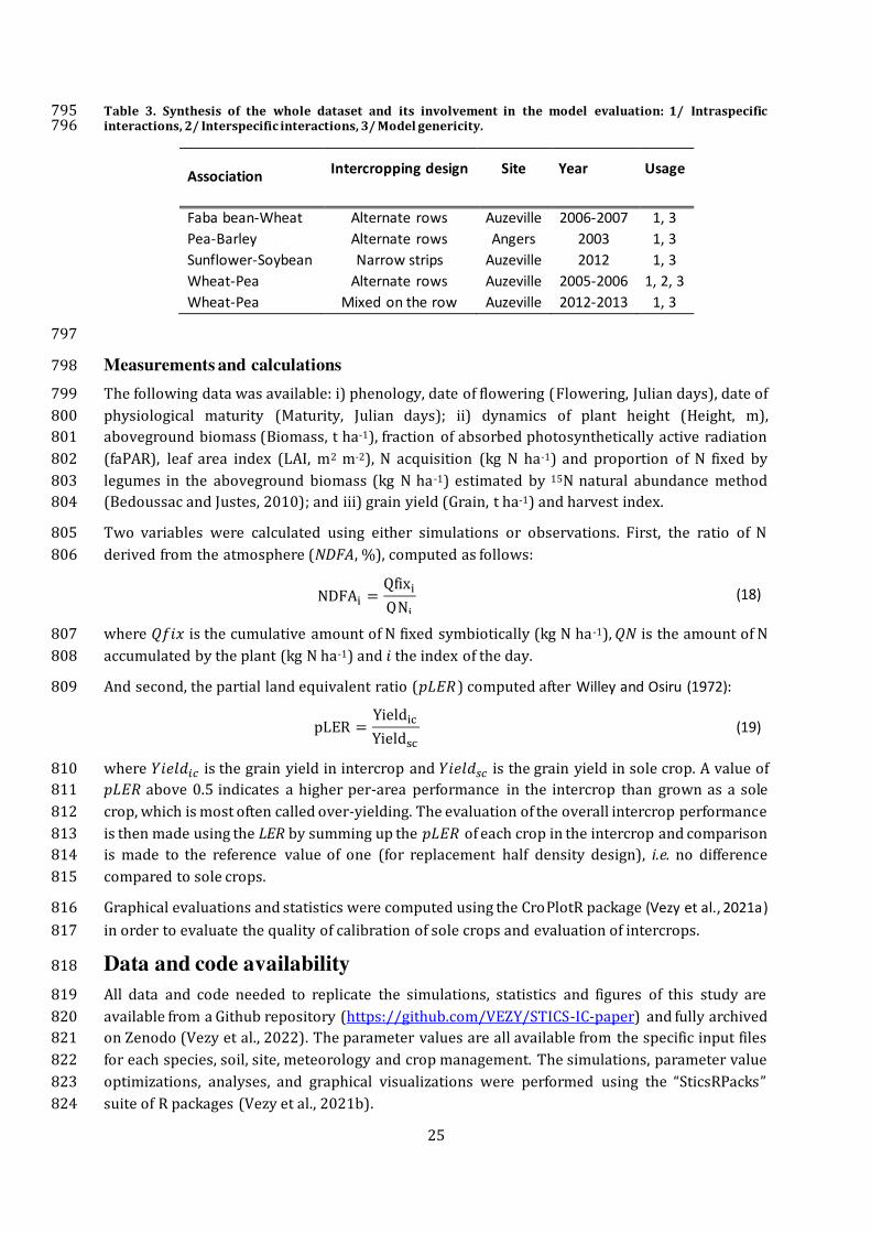
Table 3. Synthesis of the whole dataset and its involvement in the model evaluation: 1/ Intraspecific 795 interactions, 2/ Interspecific interactions, 3/ Model genericity. 796

Association Intercropping design Site Year Usage

Faba bean-Wheat Alternate rows Auzeville 2006-2007 1, 3

Pea-Barley Alternate rows Angers 2003 1, 3

Sunflower-Soybean Narrow strips Auzeville 2012 1, 3

Wheat-Pea Alternate rows Auzeville 2005-2006 1, 2, 3

Wheat-Pea Mixed on the row Auzeville 2012-2013 1, 3

797

Measurements and calculations 798

The following data was available: i) phenology, date of flowering (Flowering, Julian days), date of 799

physiological maturity (Maturity, Julian days); ii) dynamics of plant height (Height, m), 800 aboveground biomass (Biomass, t ha-1), fraction of absorbed photosynthetically active radiation 801

(faPAR), leaf area index (LAI, m2 m-2), N acquisition (kg N ha-1) and proportion of N fixed by 802

legumes in the aboveground biomass (kg N ha-1) estimated by 15N natural abundance method 803 (Bedoussac and Justes, 2010); and iii) grain yield (Grain, t ha-1) and harvest index. 804

Two variables were calculated using either simulations or observations. First, the ratio of N 805

derived from the atmosphere (NDFA, %), computed as follows: 806 NDFAi = QfixiQNi (18)

where 𝑄𝑓𝑖𝑥 is the cumulative amount of N fixed symbiotically (kg N ha-1), 𝑄𝑁 is the amount of N 807

accumulated by the plant (kg N ha-1) and 𝑖 the index of the day. 808

And second, the partial land equivalent ratio (𝑝𝐿𝐸𝑅) computed after Willey and Osiru (1972): 809 pLER = YieldicYieldsc (19)

where 𝑌𝑖𝑒𝑙𝑑𝑖𝑐 is the grain yield in intercrop and 𝑌𝑖𝑒𝑙𝑑𝑠𝑐 is the grain yield in sole crop. A value of 810 𝑝𝐿𝐸𝑅 above 0.5 indicates a higher per-area performance in the intercrop than grown as a sole 811

crop, which is most often called over-yielding. The evaluation of the overall intercrop performance 812

is then made using the LER by summing up the 𝑝𝐿𝐸𝑅 of each crop in the intercrop and comparison 813 is made to the reference value of one (for replacement half density design), i.e. no difference 814

compared to sole crops. 815

Graphical evaluations and statistics were computed using the CroPlotR package (Vezy et al., 2021a) 816

in order to evaluate the quality of calibration of sole crops and evaluation of intercrops. 817

Data and code availability 818

All data and code needed to replicate the simulations, statistics and figures of this study are 819

available from a Github repository (https://github.com/VEZY/STICS-IC-paper) and fully archived 820 on Zenodo (Vezy et al., 2022). The parameter values are all available from the specific input files 821

for each species, soil, site, meteorology and crop management. The simulations, parameter value 822 optimizations, analyses, and graphical visualizations were performed using the “SticsRPacks” 823

suite of R packages (Vezy et al., 2021b). 824

26

The new version of STICS-IC included 177 commits with a total of 220978 additions and 108471 825

deletions. The changes were applied to the source-code of the STICS version 8.5 and STICS-IC is 826

planned to be included in the upcoming version of STICS in the coming months, in order to provide 827 a version 11 of the standard STICS model. 828

Conflicts of interest 829

None. 830

Acknowledgements 831

We thank Mme Tilly Gaillard for her professional English reviewing of the manuscript. This 832

research was supported by the European Research Council under the European Union’s Horizon 833 2020 research and innovation program in the framework of the ReMIX (Redesigning European 834

cropping systems based on species mixtures, https://www.remix-intercrops.eu/) project from 835

2017 to 2021 [grant number 727217]. 836

Authors' Contributions 837

RV wrote the manuscript, made the simulations and the visualizations, modified the code of STICS-838

IC, and developed the code to run the evaluation. SM prepared the simulations for Angers and 839

revised the manuscript, NG provided data for Auzeville and the idea for self-intercropping 840 evaluation. EJ, RV, SM, ML and DR conceptualized the new formalisms. RV, EJ and SM evaluated 841

the formalisms. PL and DR helped on the software infrastructure and for implementing new 842

algorithms. EJ supervised the project. RV, EJ, SM, ML and NG reviewed and edited the manuscript. 843

References 844

Beaudoin, N., Lecharpentier, P., Ripoche, D., Justes, E., Launay, M., Leonard, J., Mary, B., Strullu, L., 845 in press. Conceptual framework, equations and uses of the STICS soil-crop model. Quae. 846

Beck, H.E., Zimmermann, N.E., McVicar, T.R., Vergopolan, N., Berg, A., Wood, E.F., 2018. Present 847 and future Köppen-Geiger climate classification maps at 1-km resolution. Scientific data 5, 848 1–12. 849

Bedoussac, L., 2009. Analyse du fonctionnement des performances des associations blé dur-pois 850 d’hiver et blé dur-féverole d’hiver pour la conception d’itinéraires techniques adaptés à 851 différents objectifs de production en systèmes bas-intrants (Theses). Institut National 852 Polytechnique (Toulouse). 853

Bedoussac, L., Journet, E.-P., Hauggaard-Nielsen, H., Naudin, C., Corre-Hellou, G., Jensen, E.S., 854 Prieur, L., Justes, E., 2015. Ecological principles underlying the increase of productivity 855 achieved by cereal-grain legume intercrops in organic farming. A review. Agron. Sustain. 856 Dev. 35, 911–935. https://doi.org/10.1007/s13593-014-0277-7 857

Bedoussac, L., Justes, E., 2010. Dynamic analysis of competition and complementarity for light and 858 N use to understand the yield and the protein content of a durum wheat–winter pea 859 intercrop. Plant Soil 330, 37–54. https://doi.org/10.1007/s11104-010-0303-8 860

Beillouin, D., Ben-Ari, T., Malézieux, E., Seufert, V., Makowski, D., 2021. Positive but variable effects 861 of crop diversification on biodiversity and ecosystem services. Global Change Biology. 862

Berghuijs, H.N.C., Wang, Z., Stomph, T.J., Weih, M., Van der Werf, W., Vico, G., 2020. Identification 863 of species traits enhancing yield in wheat-faba bean intercropping: development and 864 sensitivity analysis of a minimalist mixture model. Plant Soil 455, 203–226. 865 https://doi.org/10.1007/s11104-020-04668-0 866

27

Berghuijs, H.N.C., Weih, M., van der Werf, W., Karley, A.J., Adam, E., Villegas-Fernández, Á.M., Kiær, 867 L.P., Newton, A.C., Scherber, C., Tavoletti, S., Vico, G., 2021. Calibrating and testing APSIM 868 for wheat-faba bean pure cultures and intercrops across Europe. Field Crops Research 869 264, 108088. https://doi.org/10.1016/j.fcr.2021.108088 870

Bouain, N., Krouk, G., Lacombe, B., Rouached, H., 2019. Getting to the Root of Plant Mineral 871 Nutrition: Combinatorial Nutrient Stresses Reveal Emergent Properties. Trends in Plant 872 Science 24, 542–552. https://doi.org/10.1016/j.tplants.2019.03.008 873

Brisson, N., Bussière, F., Ozier-Lafontaine, H., Tournebize, R., Sinoquet, H., 2004. Adaptation of the 874 crop model STICS to intercropping. Theoretical basis and parameterisation. Agronomie 875 24, 409–421. https://doi.org/10.1051/agro:2004031 876

Brisson, N., Gary, C., Justes, E., Roche, R., Mary, B., Ripoche, D., Zimmer, D., Sierra, J., Bertuzzi, P., 877 Burger, P., Bussière, F., Cabidoche, Y.M., Cellier, P., Debaeke, P., Gaudillère, J.P., Hénault, C., 878 Maraux, F., Seguin, B., Sinoquet, H., 2003. An overview of the crop model stics. European 879 Journal of Agronomy, Modelling Cropping Systems: Science, Software and Applications 18, 880 309–332. https://doi.org/10.1016/S1161-0301(02)00110-7 881

Brisson, N., Launay, M., Mary, B., Beaudoin, N., 2008. Conceptual Basis, Formalisations and 882 Parameterization of the Stics Crop Model. Editions Quae, Paris. 883

Brisson, N., Mary, B., Ripoche, D., Jeuffroy, M.-H., Ruget, F., Nicoullaud, B.B., Gate, P., Devienne-884 Barret, F., Antonioletti, R., Dürr, C., Richard, G., Beaudoin, N., Recous, S., Tayot, X., Plenet, 885 D., Cellier, P., Machet, J.M., Meynard, J.M.J.M., Delecolle, R., 1998. STICS: a generic model for 886 the simulation of crops and their water and nitrogen balances. I. Theory and 887 parameterization applied to wheat and corn. Agronomie 18, 311–346. 888

Buis, S., Lecharpentier, P., Vezy, R., Giner, M., 2021. CroptimizR: A package to estimate parameters 889 of crop models. 890

Buis, S., Wallach, D., Guillaume, S., Varella, H., Lecharpentier, P., Launay, M., Guerif, M., Bergez, J.-891 E., Justes, E., 2011. The STICS crop model and associated software for analysis, 892 parameterization, and evaluation. Methods of introducing system models into agricultural 893 research 2, 395–426. 894

Chimonyo, V.G.P., Modi, A.T., Mabhaudhi, T., 2015. Perspective on crop modelling in the 895 management of intercropping systems. Archives of Agronomy and Soil Science 61, 1511–896 1529. https://doi.org/10.1080/03650340.2015.1017816 897

Corre-Hellou, G., Brisson, N., Launay, M., Fustec, J., Crozat, Y., 2007. Effect of root depth penetration 898 on soil nitrogen competitive interactions and dry matter production in pea–barley 899 intercrops given different soil nitrogen supplies. Field Crops Research 103, 76–85. 900 https://doi.org/10.1016/j.fcr.2007.04.008 901

Corre-Hellou, G., Faure, M., Launay, M., Brisson, N., Crozat, Y., 2009. Adaptation of the STICS 902 intercrop model to simulate crop growth and N accumulation in pea–barley intercrops. 903 Field Crops Research 113, 72–81. https://doi.org/10.1016/j.fcr.2009.04.007 904

Corre-Hellou, G., Fustec, J., Crozat, Y., 2006. Interspecific Competition for Soil N and its Interaction 905 with N2 Fixation, Leaf Expansion and Crop Growth in Pea–Barley Intercrops. Plant Soil 906 282, 195–208. https://doi.org/10.1007/s11104-005-5777-4 907

Coucheney, E., Buis, S., Launay, M., Constantin, J., Mary, B., García de Cortázar-Atauri, I., Ripoche, 908 D., Beaudoin, N., Ruget, F., Andrianarisoa, K.S., Le Bas, C., Justes, E., Léonard, J., 2015. 909 Accuracy, robustness and behavior of the STICS soil–crop model for plant, water and 910 nitrogen outputs: Evaluation over a wide range of agro-environmental conditions in 911 France. Environmental Modelling & Software 64, 177–190. 912 https://doi.org/10.1016/j.envsoft.2014.11.024 913

28

Eschenbach, C., 2005. Emergent properties modelled with the functional structural tree growth 914 model ALMIS: Computer experiments on resource gain and use. Ecological Modelling, 915 Emergent Properties in Individual-based Models Case Studies from the Bornhöved Project 916 (Northern Germany) 186, 470–488. https://doi.org/10.1016/j.ecolmodel.2005.02.013 917

Falconnier, G.N., Journet, E.-P., Bedoussac, L., Vermue, A., Chlébowski, F., Beaudoin, N., Justes, E., 918 2019. Calibration and evaluation of the STICS soil-crop model for faba bean to explain 919 variability in yield and N2 fixation. European Journal of Agronomy 104, 63–77. 920 https://doi.org/10.1016/j.eja.2019.01.001 921

Gaudio, N., Escobar-Gutiérrez, A.J., Casadebaig, P., Evers, J.B., Gérard, F., Louarn, G., Colbach, N., 922 Munz, S., Launay, M., Marrou, H., Barillot, R., Hinsinger, P., Bergez, J.-E., Combes, D., Durand, 923 J.-L., Frak, E., Pagès, L., Pradal, C., Saint-Jean, S., Van Der Werf, W., Justes, E., 2019. Current 924 knowledge and future research opportunities for modeling annual crop mixtures. A 925 review. Agron. Sustain. Dev. 39, 20. https://doi.org/10.1007/s13593-019-0562-6 926

Gaudio, N., Louarn, G., Barillot, R., Meunier, C., Vezy, R., Launay, M., 2022. Exploring 927 complementarities between modelling approaches that enable upscaling from plant 928 community functioning to ecosystem services as a way to support agroecological 929 transition. in silico Plants 4, diab037. https://doi.org/10.1093/insilicoplants/diab037 930

Gou, F., van Ittersum, M.K., van der Werf, W., 2017. Simulating potential growth in a relay-strip 931 intercropping system: Model description, calibration and testing. Field Crops Research 932 200, 122–142. https://doi.org/10.1016/j.fcr.2016.09.015 933

Guillaume, S., Bergez, J.E., Wallach, D., Justes, E., 2011. Methodological comparison of calibration 934 procedures for durum wheat parameters in the STICS model. European Journal of 935 Agronomy 35, 115–126. https://doi.org/10.1016/J.EJA.2011.05.003 936

Hammond, S.T., Niklas, K.J., 2009. Emergent properties of plants competing in silico for space and 937 light: Seeing the tree from the forest. American Journal of Botany 96, 1430–1444. 938 https://doi.org/10.3732/ajb.0900063 939

Jensen, E.S., Carlsson, G., Hauggaard-Nielsen, H., 2020. Intercropping of grain legumes and cereals 940 improves the use of soil N resources and reduces the requirement for synthetic fertilizer 941 N: A global-scale analysis. Agron. Sustain. Dev. 40, 5. https://doi.org/10.1007/s13593 -942 020-0607-x 943

Justes, E., Bedoussac, L., Dordas, C., Frak, E., Louarn, G., Boudsocq, S., Journet, E. -P., Lithourgidis, 944 A., Pankou, C., Zhang, C., others, 2021. The 4C approach as a way to understand species 945 interactions determining intercropping productivity. Frontiers of Agricultural Science and 946 Engineering. 947

Justes, E., Mary, B., Meynard, J.-M., Machet, J.-M., Thelier-Huché, L., 1994. Determination of a critical 948 nitrogen dilution curve for winter wheat crops. Annals of botany 74, 397–407. 949

Kammoun, B., 2014. Analyse des interactions génotype x environnement x conduite culturale de 950 peuplement bi-spécifique de cultures associées de blé dur et de légumineuses à graines, à 951 des fins de choix variétal et d’optimisation de leurs itinéraires techniques. 952

Kammoun, B., Journet, E.-P., Justes, E., Bedoussac, L., 2021. Cultivar Grain Yield in Durum Wheat-953 Grain Legume Intercrops Could Be Estimated From Sole Crop Yields and Interspecific 954 Interaction Index. Front. Plant Sci. 12, 733705. 955 https://doi.org/10.3389/fpls.2021.733705 956

Keating, B.A., Carberry, P.S., 1993. Resource capture and use in intercropping: solar radiation. 957 Field Crops Research, Intercropping-Bases of Productivity 34, 273–301. 958 https://doi.org/10.1016/0378-4290(93)90118-7 959

29

Keating, B.A., Carberry, P.S., Hammer, G.L., Probert, M.E., Robertson, M.J., Holzworth, D., Huth, N.I., 960 Hargreaves, J.N.G., Meinke, H., Hochman, Z., McLean, G., Verburg, K., Snow, V., Dimes, J.P., 961 Silburn, M., Wang, E., Brown, S., Bristow, K.L., Asseng, S., Chapman, S., McCown, R.L., 962 Freebairn, D.M., Smith, C.J., 2003. An overview of APSIM, a model designed for farming 963 systems simulation. European Journal of Agronomy, Modelling Cropping Systems: Science, 964 Software and Applications 18, 267–288. https://doi.org/10.1016/S1161-965 0301(02)00108-9 966

Kherif, O., Seghouani, M., Justes, E., Plaza-Bonilla, D., Bouhenache, A., Zemmouri, B., Dokukin, P., 967 Latati, M., 2022. The first calibration and evaluation of the STICS soil-crop model on 968 chickpea-based intercropping system under Mediterranean conditions. European Journal 969 of Agronomy 133, 126449. https://doi.org/10.1016/j.eja.2021.126449 970

Launay, M., Brisson, N., Satger, S., Hauggaard-Nielsen, H., Corre-Hellou, G., Kasynova, E., Ruske, R., 971 Jensen, E.S., Gooding, M.J., 2009. Exploring options for managing strategies for pea–barley 972 intercropping using a modeling approach. European Journal of Agronomy 31, 85–98. 973 https://doi.org/10.1016/j.eja.2009.04.002 974

Li, X.-F., Wang, Z.-G., Bao, X.-G., Sun, J.-H., Yang, S.-C., Wang, P., Wang, C.-B., Wu, J.-P., Liu, X.-R., Tian, 975 X.-L., Wang, Yu, Li, J.-P., Wang, Yan, Xia, H.-Y., Mei, P.-P., Wang, X.-F., Zhao, J.-H., Yu, R.-P., 976 Zhang, W.-P., Che, Z.-X., Gui, L.-G., Callaway, R.M., Tilman, D., Li, L., 2021. Long-term 977 increased grain yield and soil fertility from intercropping. Nat Sustain 4, 943–950. 978 https://doi.org/10.1038/s41893-021-00767-7 979

Liu, X., Rahman, T., Song, C., Su, B., Yang, F., Yong, T., Wu, Y., Zhang, C., Yang, W., 2017. Changes in 980 light environment, morphology, growth and yield of soybean in maize-soybean 981 intercropping systems. Field Crops Research 200, 38–46. 982 https://doi.org/10.1016/j.fcr.2016.10.003 983

Louarn, G., Barillot, R., Combes, D., Escobar-Gutiérrez, A., 2020. Towards intercrop ideotypes: non-984 random trait assembly can promote overyielding and stability of species proportion in 985 simulated legume-based mixtures. Annals of Botany 126, 671–685. 986 https://doi.org/10.1093/aob/mcaa014 987

Louarn, G., Bedoussac, L., Gaudio, N., Journet, E.-P., Moreau, D., Steen Jensen, E., Justes, E., 2021. 988 Plant nitrogen nutrition status in intercrops– a review of concepts and methods. European 989 Journal of Agronomy 124, 126229. https://doi.org/10.1016/j.eja.2021.126229 990

Malézieux, E., Crozat, Y., Dupraz, C., Laurans, M., Makowski, D., Ozier-Lafontaine, H., Rapidel, B., de 991 Tourdonnet, S., Valantin-Morison, M., 2009. Mixing plant species in cropping systems: 992 concepts, tools and models. A review. Agron. Sustain. Dev. 29, 43–62. 993 https://doi.org/10.1051/agro:2007057 994

Martin-Guay, M.-O., Paquette, A., Dupras, J., Rivest, D., 2018. The new Green Revolution: 995 Sustainable intensification of agriculture by intercropping. Science of The Total 996 Environment 615, 767–772. https://doi.org/10.1016/j.scitotenv.2017.10.024 997

Mathieu, A., Cournède, P.-H., Barthélémy, D., de Reffye, P., 2008. Rhythms and Alternating Patterns 998 in Plants as Emergent Properties of a Model of Interaction between Development and 999 Functioning. Annals of Botany 101, 1233–1242. https://doi.org/10.1093/aob/mcm171 1000

Nelder, J.A., Mead, R., 1965. A simplex method for function minimization. The Computer Journal 7, 1001 308–313. https://doi.org/10.1093/comjnl/7.4.308 1002

Nelson, W.C.D., Hoffmann, M.P., Vadez, V., Rötter, R.P., Koch, M., Whitbread, A.M., 2021. Can 1003 intercropping be an adaptation to drought? A model-based analysis for pearl millet–1004 cowpea. Journal of Agronomy and Crop Science n/a. https://doi.org/10.1111/jac.12552 1005

30

Raseduzzaman, Md., Jensen, E.S., 2017. Does intercropping enhance yield stability in arable crop 1006 production? A meta-analysis. European Journal of Agronomy 91, 25–33. 1007 https://doi.org/10.1016/j.eja.2017.09.009 1008

Shili-Touzi, I., De Tourdonnet, S., Launay, M., Dore, T., 2010. Does intercropping winter wheat 1009 (Triticum aestivum) with red fescue (Festuca rubra) as a cover crop improve agronomic 1010 and environmental performance? A modeling approach. Field Crops Research 116, 218–1011 229. https://doi.org/10.1016/j.fcr.2009.11.007 1012

Shuttleworth, W.J., Wallace, J.S., 1985. Evaporation from sparse crops‐an energy combination 1013 theory. Quarterly Journal of the Royal Meteorological Society 111, 839–855. 1014

Singh, A.K., Goyal, V., Mishra, A.K., Parihar, S.S., 2013. Validation of CropSyst simulation model for 1015 direct seeded rice–wheat cropping system. Current Science 104, 1324–1331. 1016

Stomph, T., Dordas, C., Baranger, A., de Rijk, J., Dong, B., Evers, J., Gu, C., Li, L., Simon, J., Jensen, E.S., 1017 Wang, Q., Wang, Y., Wang, Z., Xu, H., Zhang, C., Zhang, L., Zhang, W.-P., Bedoussac, L., van 1018 der Werf, W., 2020. Chapter One - Designing intercrops for high yield, yield stability and 1019 efficient use of resources: Are there principles?, in: Sparks, D.L. (Ed.), Advances in 1020 Agronomy. Academic Press, pp. 1–50. https://doi.org/10.1016/bs.agron.2019.10.002 1021

Tilman, D., 2020. Benefits of intensive agricultural intercropping. Nat. Plants 6, 604–605. 1022 https://doi.org/10.1038/s41477-020-0677-4 1023

van Oort, P.A.J., Gou, F., Stomph, T.J., van der Werf, W., 2020. Effects of strip width on yields in 1024 relay-strip intercropping: A simulation study. European Journal of Agronomy 112, 1025 125936. https://doi.org/10.1016/j.eja.2019.125936 1026

Vezy, R., Buis, S., Lecharpentier, P., Giner, M., 2021a. CroPlotR: A package to analyse crop model 1027 simulations outputs with plots and statistics. 1028

Vezy, R., Buis, S., Lecharpentier, P., Giner, M., 2021b. SticsRPacks: Easily install and load 1029 `SticsRPacks` packages. 1030

Vezy, R., le Maire, G., Christina, M., Georgiou, S., Imbach, P., Hidalgo, H.G., Alfaro, E.J., Blitz-Frayret, 1031 C., Charbonnier, F., Lehner, P., Loustau, D., Roupsard, O., 2020. DynACof: A process-based 1032 model to study growth, yield and ecosystem services of coffee agroforestry systems. 1033 Environmental Modelling & Software 124, 104609. 1034 https://doi.org/10.1016/j.envsoft.2019.104609 1035

Vezy, R., Munz, S., Gaudio, N., Launay, M., Lecharpentier, P., Ripoche, D., Justes, E., 2022. Data, code 1036 and software to reproduce the article entitled “Modelling intercrops functioning to 1037 advance the design of innovative agroecological systems.” 1038 https://doi.org/10.5281/zenodo.6803363 1039

Willey, R.W., Osiru, D.S.O., 1972. Studies on mixtures of maize and beans (Phaseolus vulgaris) with 1040 particular reference to plant population. The Journal of Agricultural Science 79, 517–529. 1041 https://doi.org/10.1017/S0021859600025909 1042

Wu, Y., He, D., Wang, E., Liu, X., Huth, N.I., Zhao, Z., Gong, W., Yang, F., Wang, X., Yong, T., Liu, J., Liu, 1043 W., Du, J., Pu, T., Liu, C., Yu, L., van der Werf, W., Yang, W., 2021. Modelling soybean and 1044 maize growth and grain yield in strip intercropping systems with different row 1045 configurations. Field Crops Research 265, 108122. 1046 https://doi.org/10.1016/j.fcr.2021.108122 1047

Yin, W., Chai, Q., Zhao, C., Yu, A., Fan, Z., Hu, F., Fan, H., Guo, Y., Coulter, J.A., 2020. Water utilization 1048 in intercropping: A review. Agricultural Water Management 241, 106335. 1049 https://doi.org/10.1016/j.agwat.2020.106335 1050

31

Yu, Y., Stomph, T.-J., Makowski, D., van der Werf, W., 2015. Temporal niche differentiation 1051 increases the land equivalent ratio of annual intercrops: A meta-analysis. Field Crops 1052 Research 184, 133–144. https://doi.org/10.1016/j.fcr.2015.09.010 1053

1054

1055