Modelling interactions and feedback mechanisms between land use change and landscape processes

This article appeared in a journal published by Elsevier. The attachedcopy is furnished to the author for internal non-commercial researchand education use, including for instruction at the authors institution

and sharing with colleagues.

Other uses, including reproduction and distribution, or selling orlicensing copies, or posting to personal, institutional or third party

websites are prohibited.

In most cases authors are permitted to post their version of thearticle (e.g. in Word or Tex form) to their personal website orinstitutional repository. Authors requiring further information

regarding Elsevier’s archiving and manuscript policies areencouraged to visit:

http://www.elsevier.com/copyright

http://www.elsevier.com/copyright

Author's personal copy

Modelling interactions and feedback mechanisms between land use changeand landscape processes

L. Claessens a,b,*, J.M. Schoorl a, P.H. Verburg a, L. Geraedts a, A. Veldkamp a

a Land Dynamics Group, Landscape Center, Wageningen University, P.O. Box 47, 6700 AA Wageningen, Netherlandsb International Potato Center, P.O. Box 25171, 00603 Nairobi, Kenya

1. Introduction

Land use change is influenced by a large series of interactingprocesses involving both the bio-physical environment and humandecision-making. Land use changes may affect the environmental

properties of a landscape and/or the living conditions of peopleleading to either an amplification or attenuation of the change.These interactions between the driving factors and impacts of landuse change are often referred to as feedback mechanisms. Anexplicit inclusion of feedback mechanisms in the analysis is stillone of the major challenges in studying land use systems (Verburg,2006; Turner et al., 2007).

The feedback of changes made within the land use system onconditions influencing human livelihood may result in a change indecision-making affecting future land use changes. Rather than a

Agriculture, Ecosystems and Environment 129 (2009) 157–170

A R T I C L E I N F O

Article history:

Received 11 June 2008

Received in revised form 12 August 2008

Accepted 15 August 2008

Available online 10 October 2008

Keywords:

LAPSUS

CLUE

Land use change

Soil erosion

Coupled models

A B S T R A C T

Land use changes and landscape processes are interrelated and influenced by multiple bio-physical and

socio-economic driving factors, resulting in a complex, multi-scale system. Consequently in landscapes

with active landscape processes such as erosion, land use changes should not be analysed in isolation

without accounting for both on-site and off-site effects on landscape processes. To investigate the

interactions between land use, land use change and landscape processes, a case study for the Alora region

in southern Spain is carried out, coupling a land use change model (CLUE) and a landscape process model

simulating water and tillage erosion and sedimentation (LAPSUS). First, both models are run

independently for a baseline scenario of land use change. Secondly, different feedbacks are added to

the coupled model framework as ‘interaction scenarios’. Firstly effects of land use change on landscape

processes are introduced by means of a ‘changed erodibility feedback’. Secondly effects of landscape

processes on land use are introduced stepwise: (i) an ‘observed erosion feedback’ where reallocation of

land use results from farmers’ perception of erosion features, and (ii) a ‘reduced productivity feedback’

whereby changes in soil depth result in a land use relocation. Quantities and spatial patterns of both land

use change and soil redistribution are compared with the baseline scenario to assess the cumulative

effect of including each of the interaction mechanisms in the modelling framework.

Overall, total quantities of land use change (areas) and soil redistribution do not differ much for the

different interaction scenarios. However, there are important differences in the spatial patterns of both

land use and soil redistribution. In addition, by incorporating the perception and bio-physical feedback

mechanisms, land use types with stable or increasing acreages are increasingly relocated from their

original positions, suggesting a current location on landscape positions prone to soil erosion and

sedimentation. Implementing the ‘reduced productivity feedback’ causes most of these effects. Another

important outcome is that on-site land use changes trigger major off-site soil redistribution dynamics.

These off-site effects are attributed to down slope or downstream changes in sediment transport rates

and/or discharge caused by changes in land surface characteristics.

The results of this study provide insight into the interactions between different processes occurring

within landscapes and the influence of feedbacks on the development of the landscape. The interaction

between processes goes across various spatial and temporal scales, leading to difficulties in linked model

representation and calibration and validation of the coupled modelling system.

� 2008 Elsevier B.V. All rights reserved.

* Corresponding author at: International Potato Center, P.O. Box 25171, 00603

Nairobi, Kenya. Tel.: +254 20 422 3612; fax: +254 20 422 3001.

E-mail addresses: [email protected], [email protected] (L. Claessens).

Contents lists available at ScienceDirect

Agriculture, Ecosystems and Environment

journal homepage: www.e lsev ier .com/ locate /agee

0167-8809/$ – see front matter � 2008 Elsevier B.V. All rights reserved.

doi:10.1016/j.agee.2008.08.008


straightforward, linear development the land use system willexperience an increasing number of complex interactions whichcan either lead to an acceleration of the system dynamics or adecrease in change of the system. Feedbacks within the systemmay play an important role in determining the vulnerability of thehuman-environment system and are therefore an important topicof research (Clark and Dickson, 2003; Young et al., 2006; Polskyet al., 2007).

Feedback mechanisms operate over different spatial andtemporal scales (Veldkamp et al., 2001). An example of a globalscale feedback is the interaction between land use and the climatesystem. The cumulative effect of many small scale changes in landuse have a global impact on climate conditions due to changes incarbon emissions and land surface characteristics. Such changes inclimate conditions may again feed back on land use by changes innatural vegetation, crop productivity and vulnerability for landdegradation (Foley et al., 1998; Pielke et al., 2002). Also at the localscale level feedback mechanisms are important, e.g. the perceptionof farmers to erosion features in a field can guide the decisions oncrop allocation or cause abandonment (Veihe, 2000).

For unravelling the complex dynamics of land use systems thereis a tendency for model-based quantitative analysis, rather thanusing descriptive more qualitative approaches (Verburg, 2006).Both the development of the model itself and the interpretation ofsimulation results may lead to improved understanding of thefunctioning of the land use system in relation to its environmentaland socio-economic context. Despite the recognition of theimportance of interactions between landscape processes andsocial systems (Geoghegan et al., 1998; Overmars and Verburg,2005) and the emergence of agent-based studies at the local scale(Matthews et al., 2007), most current, regional approaches to landuse change modelling do not explicitly link human decision-making with the analysis of the spatial and temporal variability oflandscapes. Several researchers have studied the unidirectionalinfluence of land use/cover (changes) on mostly human-inducedlandscape processes (Bathurst et al., 1996, 2005; Kosmas et al.,

1997; Schoorl and Veldkamp, 2001; Vanacker et al., 2003; VanRompaey et al., 2002, 2007; Huisman et al., 2004; Van Beek andVan Asch, 2004; Breuer et al., 2006; Lesschen et al., 2007). Otherstudies focus on longer timescales and link geomorphic responseto regional landscape characteristics lumping climate and humanimpact (Seguis et al., 2004; Edwards and Whittington, 2001). Asmaller number of studies deal with the opposite unidirectionaleffect, i.e., the influence of landscape processes on land use change(Marathianou et al., 2000; Bakker et al., 2005; Claessens et al.,2008). However, little attention has been given to integratedapproaches assessing the interactions and feedback mechanisms ofthe coupled land use- and landscape processes system.

In this paper a methodology for modelling interactions andfeedbacks between land use change and geomorphic processes isexplored for a case study area in southern Spain. The effects ofdifferent types of feedbacks are investigated by dynamicallylinking a land use change model (CLUE; Verburg et al., 2002) with alandscape evolution model (LAPSUS; Schoorl et al., 2002).

2. Materials and methods

2.1. Concepts of interactions between landscape processes and land

use change

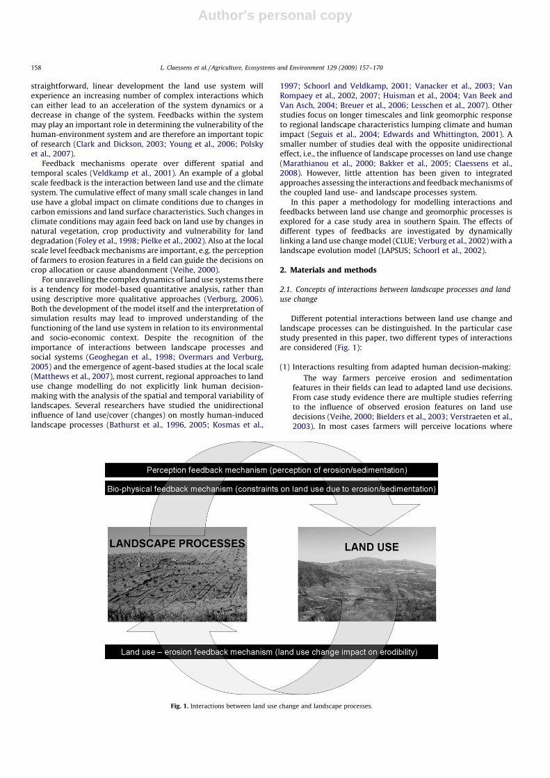
Different potential interactions between land use change andlandscape processes can be distinguished. In the particular casestudy presented in this paper, two different types of interactionsare considered (Fig. 1):

(1) Interactions resulting from adapted human decision-making:

The way farmers perceive erosion and sedimentationfeatures in their fields can lead to adapted land use decisions.From case study evidence there are multiple studies referringto the influence of observed erosion features on land usedecisions (Veihe, 2000; Bielders et al., 2003; Verstraeten et al.,2003). In most cases farmers will perceive locations where

Fig. 1. Interactions between land use change and landscape processes.

L. Claessens et al. / Agriculture, Ecosystems and Environment 129 (2009) 157–170158


large quantities of erosion or sedimentation are observed, asless suitable compared to locations with exactly the sameconditions without these features. As a consequence this maylead to the relocation of intensive agricultural land use typesthat are suffering from erosion or re-sedimentation, after theobservation of certain amounts or features of erosion and/orsedimentation. The strength of this interaction mechanism isdependent on the perception farmers have about landdegradation, the possibilities and costs to relocate farmingactivities and may also be influenced by extension, socialnetworks and the overall societal attitude towards sustain-ability. We refer to this feedback as ‘observed erosion’ feedback.

(2) Interactions resulting from bio-physical processes and con-straints:(a) Erosion and sedimentation can cause constraints on crop

production. Specific types of cultivation require a minimumsoil depth for rooting and water retention. Therefore,erosion may lead to soils becoming too shallow to allowfurther cultivation. In the opposite, locations frequentlyaffected by sedimentation may lead to damaged or buriedcrops making risks for cultivation too high. We refer to thisfeedback as the ‘reduced productivity’ feedback.

(b) Land use changes result in a change of surface character-istics of the landscape influencing erodibility and tillagepractices associated with the land use at the location. Werefer to this feedback as ‘changed erodibility’ feedback. Thisfeedback can cause either an increase or decrease of theerosion rates.

2.2. Study area

The study area is located in the Betic Cordilleras of southernSpain in the province of Malaga, along the lower reach of theGuadalhorce river. The village of Alora is situated in the centre ofthe 312 km2 study area and has about 24,000 inhabitants (Fig. 2).

2.2.1. Geology, soils and climate

The Betic Cordilleras can be divided into an external zone,mainly consisting of Mesozoic and Tertiary age sedimentary rocks(limestone, marl and sandstone) and an internal zone, composed ofPalaeozoic and Triassic metamorphic (phyllite, schist and gneiss)and igneous (serpentinite) rocks (Schoorl and Veldkamp, 2003).The study area is located in the transition zone, with the externalzone in the north (Sierra Huma), while the rest of the study area is

Fig. 2. Location of the study area (DEM with topographical localities).

L. Claessens et al. / Agriculture, Ecosystems and Environment 129 (2009) 157–170 159


part of the internal zone (Montes de Malaga, Sierra Gibralgalia,Sierra Robla and Sierra de Aguas). Furthermore, remnants ofimportant stages in the landscape development (both erosionaland sedimentary) can be found from the Late Tortonian (tabularmarine cemented conglomerates: Hachos de Chorro, Alora andPizarra), the Pliocene (marine unconsolidated marls, conglomer-ates and sands) and from the Pleistocene (river terraces, alluvialfans) (Schoorl and Veldkamp, 2003 and references within). Theconsequent dominant soil types comprise typical catenas for semi-arid to sub-humid areas, ranging from Skeletic Leptosols andCalcaric Cambisols to Chromic Luvisols and Calcaric Phaeozems(Ruiz et al., 1993; FAO, 1988; Wielemaker et al., 2001). The Aloraarea has a Mediterranean climate with a mean annual temperatureof 17.5 8C. The mean annual rainfall is 534 mm but the spatial andtemporal distribution is highly variable (Pardo Iguzquiza, 1998;Renschler et al., 1999).

2.2.2. Land use history

For at least 2000 years, people have been living in and aroundthe study area using the land for agricultural purposes introducingolives, almonds, grapes, citrus and cereals. Large deforestationoccurred and almost all natural vegetation has been removedsince. Land use became rather intensive with the introduction ofirrigation schemes, manure applications and later on large-scaleland use systems (‘latifundio’). Furthermore, in the last fewcenturies a network of railways and roads was constructed and thearea became increasingly important for the development of thecity of Malaga. During the last decades, the countryside of southernSpain has been facing rural out-migration, due to flourishing of theindustry and tourist sectors. However, improved infrastructureand high housing prices near the coast have reversed this trend. Amajor problem is the general water deficit in southern Spain:agriculture, industry and tourism are competing for water. Becausedrinking water always comes first there is less water left forirrigation purposes and as a consequence, large areas ofagricultural land become abandoned. Most land is cultivatedwithout soil conservation practices inducing land degradation.

2.2.3. Current land use and location factors of land use (change) and

soil redistribution

Using two different sets of geo-referenced digitized aerialphotographs (Junta de Andalucia, 2003, 2004), with a resolution of0.5 and 1.0 m respectively, different land use types weredistinguished within a GIS and an initial land use map wascomposed, with minimal mapping units of 500 m2. Additional fieldsurveys were done in 2005 in order to verify the initial land usemap. Field surveys showed that a differentiation of 15 initial landuse classes was adequate to cover all land use types. For the modelsimulations the original land use map was converted to a grid with50 � 50 meter resolution. Land use types with low prevalence andmore or less similar characteristics, management practices anderosion vulnerabilities were merged to facilitate the analysis (seeTable 1 for the 10 final land use classes).

Additional data were collected and processed in order to serveas potential location factors that can explain the spatial variation ofland use and/or as determinant of the erosion/sedimentationprocesses in the study area (Table 2). Information concerningparent material was gathered from the geological maps of the area(IGME, 1978; ITGE, 1990). Soil properties were taken from fieldsurveys (Wielemaker et al., 2001; Schoorl et al., 2002). Altitude andslope were derived from the Digital Elevation Model (DEM) with aresolution of 50 m (SGE, 1997). Accessibility to villages and roadswere hypothesized to be important determinants of land usedecisions (Verburg et al., 2004), therefore a cost weighted distancemap to the villages was constructed accounting for the road

network derived from the regional infrastructure map (ICA, 2000).In addition the straight line distance to all individual roads wascalculated. Access to irrigation is important for the agriculturalland use types, especially the citrus orchards, and therefore thedistance to the nearest river was taken into account and calculatedfrom the river map as a proxy for irrigation possibilities (ICA, 2000).

2.3. Land use change model: CLUE

CLUE (‘Conversions of Land Use and its Effects’, version Dyna-CLUE) is a descriptive model that simulates spatial changes in landuse pattern based on present land use pattern, location factors andcompetition between land uses in space and time under changingconditions of (external) land requirements for different uses(Verburg et al., 2002, 2006). The model has been used in differentcontexts and the predictive accuracy has been measured in severalvalidation exercises (e.g. Pontius et al., 2008).

2.3.1. Modelling approach

The CLUE model is a simulation model to spatially allocate landuse changes. The regional quantities of change of the ‘demand-driven’ land uses are to be determined exogenous of the model.

Table 1Land use in the Alora study area

Land use Total area (ha) Land cover (%)

Olive orchards 3,863 12.3

Almond orchards 2,365 7.6

Abandoned agricultural land 3,342 10.7

Citrus orchards 3,684 11.8

Arable land 6,459 20.7

Semi-natural vegetation 5,657 18.1

Forest 4,449 14.2

Bare rock 1,059 3.4

Built-up/residential area 239 0.8

Water (mainly reservoirs) 163 0.5

Total 31,280 100

Table 2Location factors of land use (change) and soil redistribution

Location factor Description and data source

Altitude Altitude in meters above sea level

(from DEM, 50 m resolution)

Slope Slope in degrees (from DEM, ArcGIS, mean

slope between all neighbours)

Soil depth Depth of soil in cm (field surveys)

Conglomerate Conglomerate (geology map)

Marls Marls and brown clay (geology map)

Sandstone Sandstone (geology map)

Limestone Limestone (geology map)

Phyllites Phyllites (geology map)

Gneiss Banded gneiss (geology map)

Serpentinite Harzburg pyroxene, olivine (Periodite)

(geology map)

Terraces Pebbles, sand and clays (geology map)

Piedmonts Pebbles, sand and clays (recent colluvium)

(geology map)

Gravel Surface gravel content in % (field surveys)

Stones Surface stones content in % (field surveys)

Mulch Mulch features present yes/no (field surveys)

Drainage Soil drainage class from well to poorly drained

(field surveys)

Distance to river Distance to the nearest river in meters

(from river map)

Distance to road Distance to the nearest main road in meters

(from infrastructure map)

Cost weighted distance Composite measure of transport cost and

travel time to the main villages



Natural and semi-natural land use types either respond to changesin agricultural and residential land uses or develop through naturalsuccession, e.g., on abandoned land. The spatial allocation of landuse is simulated by combining the relative suitability of a locationfor different uses, the regional competitiveness of the differentland use types, the land use history and specific land use policies orconstraints. The location preference for the different land use typesis based on the spatial variation of the location factors that werehypothesized to be important determinants of the land use pattern(Table 2). Since quantitative information about the relativeimportance of the different location factors is lacking, the relationsare estimated by logistic regression analysis using the land usemap of 2005 as dependent variable. The occurrence of most landuse types can be explained by the location factors as indicated byan area under the ROC curve between 0.69 and 0.94, whereas arandom model has a value of 0.5 and a perfect model has a value of1.0 (Swets, 1988). The estimated probabilities based on the logisticregression model are used as a proxy for the location preference forthe considered land use.

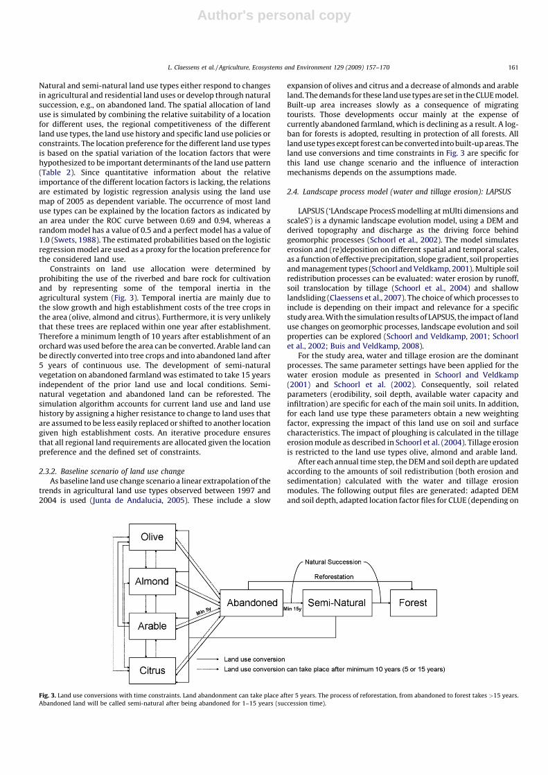
Constraints on land use allocation were determined byprohibiting the use of the riverbed and bare rock for cultivationand by representing some of the temporal inertia in theagricultural system (Fig. 3). Temporal inertia are mainly due tothe slow growth and high establishment costs of the tree crops inthe area (olive, almond and citrus). Furthermore, it is very unlikelythat these trees are replaced within one year after establishment.Therefore a minimum length of 10 years after establishment of anorchard was used before the area can be converted. Arable land canbe directly converted into tree crops and into abandoned land after5 years of continuous use. The development of semi-naturalvegetation on abandoned farmland was estimated to take 15 yearsindependent of the prior land use and local conditions. Semi-natural vegetation and abandoned land can be reforested. Thesimulation algorithm accounts for current land use and land usehistory by assigning a higher resistance to change to land uses thatare assumed to be less easily replaced or shifted to another locationgiven high establishment costs. An iterative procedure ensuresthat all regional land requirements are allocated given the locationpreference and the defined set of constraints.

2.3.2. Baseline scenario of land use change

As baseline land use change scenario a linear extrapolation of thetrends in agricultural land use types observed between 1997 and2004 is used (Junta de Andalucia, 2005). These include a slow

expansion of olives and citrus and a decrease of almonds and arableland. The demands for these land use types are set in the CLUE model.Built-up area increases slowly as a consequence of migratingtourists. Those developments occur mainly at the expense ofcurrently abandoned farmland, which is declining as a result. A log-ban for forests is adopted, resulting in protection of all forests. Allland use types except forest can be converted into built-up areas. Theland use conversions and time constraints in Fig. 3 are specific forthis land use change scenario and the influence of interactionmechanisms depends on the assumptions made.

2.4. Landscape process model (water and tillage erosion): LAPSUS

LAPSUS (‘LAndscape ProcesS modelling at mUlti dimensions andscaleS’) is a dynamic landscape evolution model, using a DEM andderived topography and discharge as the driving force behindgeomorphic processes (Schoorl et al., 2002). The model simulateserosion and (re)deposition on different spatial and temporal scales,as a function of effective precipitation, slope gradient, soil propertiesand management types (Schoorl and Veldkamp, 2001). Multiple soilredistribution processes can be evaluated: water erosion by runoff,soil translocation by tillage (Schoorl et al., 2004) and shallowlandsliding (Claessens et al., 2007). The choice of which processes toinclude is depending on their impact and relevance for a specificstudy area. With the simulation results of LAPSUS, the impact of landuse changes on geomorphic processes, landscape evolution and soilproperties can be explored (Schoorl and Veldkamp, 2001; Schoorlet al., 2002; Buis and Veldkamp, 2008).

For the study area, water and tillage erosion are the dominantprocesses. The same parameter settings have been applied for thewater erosion module as presented in Schoorl and Veldkamp(2001) and Schoorl et al. (2002). Consequently, soil relatedparameters (erodibility, soil depth, available water capacity andinfiltration) are specific for each of the main soil units. In addition,for each land use type these parameters obtain a new weightingfactor, expressing the impact of this land use on soil and surfacecharacteristics. The impact of ploughing is calculated in the tillageerosion module as described in Schoorl et al. (2004). Tillage erosionis restricted to the land use types olive, almond and arable land.

After each annual time step, the DEM and soil depth are updatedaccording to the amounts of soil redistribution (both erosion andsedimentation) calculated with the water and tillage erosionmodules. The following output files are generated: adapted DEMand soil depth, adapted location factor files for CLUE (depending on

Fig. 3. Land use conversions with time constraints. Land abandonment can take place after 5 years. The process of reforestation, from abandoned to forest takes >15 years.

Abandoned land will be called semi-natural after being abandoned for 1–15 years (succession time).



the different feedbacks, Fig. 1). For the land use – erosion feedbackmechanism, the updated land use map from CLUE is used as inputfor LAPSUS.

2.5. Model interactions

In Fig. 4 the different interaction processes described in Section2.1 and Fig. 1 are given schematically showing inputs and outputsfor the models and the information that must be exchanged toimplement the interactions. Both CLUE and LAPSUS run indepen-dently, for one time step (in this case one year) at a time, and for atotal of 25 years. The exchange of inputs and outputs between thetwo models in order to address the interaction mechanisms ismanaged through a script that copies the yearly data files betweenthe models.

2.5.1. Baseline scenario (BS)

Before including feedback mechanisms in the coupled models,each is run independently for the baseline scenario of land usechange (Section 2.3.2) in order to allow evaluation of the relativeperformance.

2.5.2. Changed erodibility feedback (FB1)

As a first step the land use – erosion feedback mechanism isimplemented (land use change impact on erodibility, Section 2.1,Figs. 1 and 5) for which no particular changes in model structureare required (only copying inputs and outputs between models).After each time step the output land use map from CLUE is copiedto the input land use map for LAPSUS. LAPSUS is running with landsurface characteristics based on the adapted land use map. Inaddition, the DEM and soil depth maps used as input by LAPSUS areupdated between time steps based on the simulated soilredistribution. CLUE also uses an updated land use map aftereach time step (Fig. 4), but there are no interactions with LAPSUSresults yet. As a consequence, the simulation results for CLUE withthe ‘changed erodibility feedback’ implemented are the same as forthe base scenario without interactions.

2.5.3. Observed erosion feedback (FB2)

This feedback mechanism is included by modifying the locationpreferences for the different land use types in CLUE (Section 2.3.1).

In this case we assume the way farmers perceive erosion orsedimentation features in the field can lower the suitability of alocation for intensive agricultural land uses (olives, cereals andcitrus). In other words, farmers tend to relocate these land usetypes from places with high erosion/sedimentation rates to moresuitable locations. The LAPSUS model is set up to calculate for eachtime step a ‘weighted’ erosion and sedimentation index. Erosionand sedimentation are weighted against the mean of the maximumerosion and sedimentation values over 25 years. Each location getsan index between 0 and 1 for each year, for which 1 indicates thehighest erosion or sedimentation. A map with these indexes isexchanged with CLUE and used to adapt the location preference forland use allocation accordingly.

2.5.4. Reduced productivity feedback (FB3)

The last feedback mechanism implemented is the bio-physicalfeedback (constraint on land use due to erosion/sedimentation,Section 2.1, Figs. 1 and 5); the land use change model takes intoaccount bio-physical limitations on crop growth. In this case weidentify locations where the soil becomes too shallow to continueagricultural use. In the model it is assumed that these locationsmay no longer be used for agricultural purposes and will beabandoned. This is implemented in the CLUE model by a forcedconversion into abandoned land for locations where the soil depthis below the defined threshold. The LAPSUS model is set up tocalculate for each time step a true/false map indicating where soilsbecome less then 10 cm deep, which is assumed to be the limitingsoil depth for agricultural land use.

3. Results

In this section the simulation results of the coupled CLUE andLAPSUS modelling framework are shown while gradually imple-menting the different interaction mechanisms (Tables 3 and 4,Figs. 6 and 7). Note that we are referring to ‘interaction scenarios’,while these are not scenarios in the usual sense but rather differentimplementations of the interaction mechanisms through modelcoupling. The initial land use map and configuration (Table 3 andFig. 5) are compared with the simulations with and without modelinteractions (BS to FB3 as described above, simulations show thecumulative result of implementing the different feedbacks).

Fig. 4. Flowchart of interactions between LAPSUS and CLUE. Solid lines indicate inputs and outputs of the models. Dashed lines represent the three feedback mechanisms

(Section 2.1) and exchange of information between the models. Annual time steps are indexed by t.



3.1. Land use change

In general the most extensive land use changes can beobserved when comparing the initial land use map with thesimulations for all interaction scenarios (FB1 to FB3) but alsobetween the interaction scenarios land use changes for semi-natural and abandoned land use types can be distinguished(Table 3). Implementing the ‘reduced productivity feedback’(FB3) has the largest quantitative effect: there is a relativeincrease in area for abandoned land and a slight decrease forsemi-natural compared to the other interaction scenarios. Moreimportantly, the different simulations represent large differ-ences in spatial patterns of land use (Fig. 5). For agricultural landuse types the demands set in the CLUE model are allocated. Thedistinction between abandoned land and semi-natural land is

Fig. 5. Initial land use map for 2005 (a) and final land use after 25 years simulation for interaction mechanisms: base scenario and ‘changed erodibility feedback’ (b), ‘observed

erosion feedback’ (c) and ‘reduced productivity feedback’ (d). (For interpretation of the references to colour in this artwork, the reader is referred to the web version of the

article.)

Table 3Percentages of land use change for the different interaction scenarios, with

comparison to the previous interaction scenario(s)

BS/FB1 FB2 FB3

Initial Initial BS/FB1 initial BS/FB1 FB2

Olive 43.0 42.9 0.0 42.9 0.0 0.0

Almond �64.4 �64.3 0.2 �64.3 0.2 0.0

Abandoned �95.9 �95.3 14.6 �75.7 488.6 413.4

Citrus 24.8 24.7 �0.1 24.7 0.0 0.0

Arable �22.2 �22.3 0.0 �22.3 0.0 0.0

Semi-natural 61.1 60.8 �0.2 49.2 �7.4 �7.2

Forest 0.2 0.2 0.0 0.2 0.0 0.0

Bare rock 0.0 0.0 0.0 0.0 0.0 0.0

Built-up 51.6 51.6 0.0 51.6 0.0 0.0

Water 0.0 0.0 0.0 0.0 0.0 0.0



dependent on the duration of abandonment (time needed fornatural succession of vegetation, Fig. 3). The spatial andtemporal dynamics are hereby important; if land use isrelocated frequently, abandoned agricultural land represents a

fallow period while a long constant fallow will lead to re-growthof natural vegetation. More details about the effects of includingeach of the interaction mechanisms will be given in the nextsections.

Table 4Mean annual soil loss rates and Sediment Delivery Ratio for the total study area, after 25 years of simulation for the baseline (BS) and three interaction scenarios

BS (ton/ha) FB1 (ton/ha) FB2 (ton/ha) FB3 (ton/ha) FB1/BS (%) FB2/BS (%) FB3/BS (%)

Erosion �103.85 �101.74 �100.42 �102.31 �2.0 �3.3 �1.5

Sedimentation 59.08 58.48 59.57 59.32 �1.0 0.8 0.4

Net soil loss �44.77 �43.26 �40.85 �42.99 �3.4 �8.8 �4.0

SDRa 0.431 0.425 0.407 0.420 �1.4 �5.6 �2.5

Changes (in %) between the interaction scenarios and BS are also given.a Sediment Delivery Ratio (dimensionless) = the relative amount of eroded material that leaves the study area (0 = none, 1 = all).

Fig. 6. LAPSUS simulated mean soil redistribution for 25 years in ton/(ha year�1) for baseline scenario (a) and including the ‘changed erodibility feedback’ (b), ‘observed

erosion feedback’ (c) and ‘reduced productivity feedback’ (d) interaction mechanisms. Negative values (red colours) are erosion, positive values (green colours) re-

sedimentation. (For interpretation of the references to colour in this figure legend, the reader is referred to the web version of the article.)



3.2. Soil redistribution

In Fig. 6, erosion and sedimentation patterns have beenanalysed by comparing the DEM after 25 years with the initialDEM. At first sight the soil redistribution patterns for the differentinteraction scenarios do not show many evident differences. Thetotal amounts of soil redistribution in Table 4 vary between 1% upto almost 9%. These relative small differences may be explained bythe size of the area (a large total number of grids) andcompensating effects (for example less erosion in one area andmore erosion in the other). However, looking in more detail, thereare certainly important effects of the implementation of thedifferent interaction mechanisms. These will also be discussed inthe following sections in more detail.

3.2.1. Baseline scenario (BS) and changed erodibility feedback (FB1):

land use change

The CLUE land use simulation for the baseline scenario BS(which is equal to ‘changed erodibility feedback’ because of the oneway exchange of information between CLUE and LAPSUS) is shownin Tables 3 and 5 and Fig. 5b. In general, semi-natural land useshows the largest relative expansion followed by built-up, oliveand citrus respectively. Abandoned land shows the highest declinefollowed by almond and arable land use. The increase of semi-natural land use at the expense of abandoned land can be

attributed to the succession of vegetation of the extensive areas ofabandoned farmland present in the study area at the start of theanalysis. The land use classes forest, bare and water do not showany change as can be expected from the model setup and thesimulated land use change scenario (as described in Section 2.3.2).Except for abandoned land, differences in land use change betweenthe interaction mechanisms are almost negligible. However, thereare important effects on the spatial patterns and distribution ofland use within the landscape.

The locations with changed land use between the initial 2005and the simulated 2030 baseline scenario and ‘changed erodibilityfeedback’ land use map are indicated in Fig. 7a. The spatial patternsshow the land use changes from the baseline CLUE simulationwithout interactions with landscape processes (also compareFig. 6a and b). In general, the conversion of abandoned into semi-natural is the most obvious change pattern. This is the result of theautomatic conversion of abandoned land into semi-natural after acertain amount of time has passed without any change (Fig. 3). Inaddition, both citrus and olive have expanded and are spatiallyconcentrated in certain areas: the projected increasing demand forolives and citrus results in expansion of these crops at the cost ofalmonds, arable and abandoned areas in between or adjacent toareas where the crop is already grown (mainly the river valley forcitrus, slopes of the mountains (Hachos) and in the north-east forolives).

Fig. 7. Location of changes in land use between 2005 and 2030 with No Change (light gray), 1 (dark gray) indicating changes with the initial land use and 2 (white) indicating

changes compared both with BS/FB1 and FB2 for (a) comparing BS/FB1 with initial condition, (b) comparing FB2 with BS/FB1 and initial and (c) comparing FB3 with FB2 and

initial condition.

Table 5Matrix showing the main areal land use conversions (in ha) for the baseline CLUE simulation (baseline scenario (BS) and ‘changed erodibility feedback’ (FB1))

BS/FB1 2030 Total 2030 Net gain/loss

Olive Almond Abandoned Citrus Arable Semi-natural Built-up

2005

Olive (3.3)a 0.0 0.0 0.0 0.0 3.3 0.0 5522.5 1659.5

Almond 680.8 129.8 56.3 2.0 587.3 66.5 842.8 �1522.5

Abandoned 285.5 0.0 (135.5) 234.3 58.0 2749.3 1.3 138.3 �3203.7

Citrus 1.5 0.0 4.8 (108.8) 0.0 101.8 0.8 4596.0 912.2

Arable 689.8 0.0 0.0 627.0 (60.0) 124.3 54.5 5023.8 �1435.5

Semi-natural 5.3 0.0 0.0 103.5 0.0 (109.0) 0.3 9113.8 3456.8

Built-up 0.0 0.0 0.0 0.0 0.0 0.0 362.3 123.3

a Values between brackets indicate the total area of relocated land use.



Looking in more detail, the conversion matrix in Table 5 showssome remarkable trends of land use change. Each land use type hasits specific preferences for gaining or loosing to a particular othertype as a consequence of typical location conditions and theimposed land use change sequences (Fig. 3). For example, olivegains most from almond and arable, while citrus gains most fromarable and to a lesser extent from abandoned land. Almond loosesmost to olive and semi-natural, while arable looses most to oliveand citrus. The data also show the relocation of some of theexpanding land uses (values between brackets). For example, inspite of a general total area increase of almost 25%, citrus isrelocated from more than 100 ha of its original location.

3.2.2. Baseline scenario (BS): soil redistribution

Fig. 6a shows the results of the LAPSUS model independentlysimulating water and tillage erosion for 25 years, withoutincluding any interaction with land use change. Land use is thusconsidered a static input and all the land use related parametersare applied at the same location and with the same extent for thewhole 25-year simulation period.

Analysing the study area, four different patterns are recogni-sable (for locations refer to Fig. 2). Firstly, mainly in the north(Sierra Huma) large areas with no erosion are visible, due to thenumerous bare rock surfaces in this limestone-dominatedmountain range. However, directly down slope of these areassevere erosion has taken place because of the run-off generated atthese bare rock surfaces. Secondly, upland mountainous areas (forexample the different Hachos and the Sierra de Aguas) showintermediate to strong erosion on steep slopes, low erosion rateson the crests and water divides and hardly any re-sedimentation inthe channels and valleys. Thirdly, we can recognize areas with astrong pattern of severe erosion and local re-sedimentation, forexample, large areas south of the Sierra Aguas and Sierra Huma.These patterns are clearly the result of 25 years of tillage erosion ofthe convex shoulders and sloping areas and re-sedimentation ofconcave slopes and local valley areas. Finally, the central river areaof the Guadalhorce exhibits low to no erosion and numerous areaswith deposition of sediments coming from the upslope andmountainous areas.

3.2.3. Changed erodibility feedback (FB1): soil redistribution

Fig. 6b shows the results of the LAPSUS model includinginteractions with land use change as simulated by the CLUE model.Visual comparison of Fig. 7b and a does not show many evidentdifferences. Furthermore, the mean total rates (Table 4) show onlya small decrease of 2.0%, 1.0% and 3.4% for erosion, sedimentationand soil loss respectively. However, the important changes in landuse type and location discussed in the previous section suggestmuch more local changes. This becomes apparent from Fig. 8 andTable 6.

Fig. 8a shows the spatial distribution of areas with changes insoil redistribution rates comparing the baseline scenario with‘changed erodibility feedback’. Since a change in land use directlyinfluences on-site parameter settings for LAPSUS, the land usechanges described in the previous sections are responsible for thechanges in erosion and sedimentation dynamics. Quite remarkableis the contrast between Fig. 8a and b/c: the on-site effects of landuse change trigger almost the same amount of off-site effects,therefore almost doubling the total area with changes (see alsoTable 6). These off-site effects are attributed to down slope ordownstream changes in sediment transport rates and or dischargecaused by changes in surface characteristics (erodibility, infiltra-tion).

3.2.4. Observed erosion feedback (FB2): land use change

The results of the land use change simulation including the‘observed erosion feedback’ are shown in Tables 3 and 7 and Fig. 5c.The land use areas show a higher amount of abandoned land andless semi-natural land as compared to the earlier simulations. Ifabandoned land remains at the same location it will be convertedto a semi-natural land use as result of the succession of naturalvegetation (Fig. 3). In the case of this simulation the feedbackmechanism leads to some re-location of agricultural activities inresponse to observed erosion and sedimentation features. Aban-doned land at the start of the simulation may be taken inproduction again, leading to an end of the succession into semi-natural vegetation. New, recently abandoned farmland appears aterosion/sedimentation sensitive locations. The effects of interac-tion mechanism ‘observed erosion feedback’ can also be seen in the

Fig. 8. Location of changes in erosion and/or sedimentation dynamics with No Change (light gray), 1 (dark gray) indicating changes with BS and 2 (white) indicating changes

compared with FB1 and FB2 for (a) comparing FB1 and BS, (b) comparing FB2 with FB1 and BS and (c) comparing FB3 with FB2 and BS.



differences in spatial patterns of land use change. Fig. 6b and c andthe white colours in Fig. 7b indicate the subtle changes caused byadding interaction mechanism FB2 to the simulation. Intensiveagricultural land use types are relocated from positions withsevere erosion or sedimentation features (mostly gullies).

Further details about land use conversions can be found inTable 7. The same trends of certain land use types being convertedto specific others hold as in Table 5. However, land use types thatexpand in area are increasingly relocated from their originalpositions, and this is particularly true for olives (174 ha, comparedwith only 3.3 ha for BS/FB1, Table 5). This suggests olives arecurrently growing on positions in the landscape that are prone toerosion and sedimentation (showing features influencing farmers’land use decisions) and are predicted to be relocated to lesserprone areas when taking FB2 into account.

3.2.5. Observed erosion feedback (FB2): soil redistribution

Detailed changes in erosion and sedimentation dynamicscaused by implementing interaction mechanism FB2 can beobserved in Fig. 8b. The amount and spatial extent of changescomparing FB2 with FB1 (white colours) appears substantialcompared with the land use changes in Fig. 7b. This is again causedby the off-site effects of erosion and sedimentation (abandonmentof heavily gullied areas) as affected by the interaction withincreased local land use change (Table 6).

3.2.6. Reduced productivity feedback (FB3): land use change

The final simulation implements all interaction mechanismsbetween CLUE and LAPSUS including the bio-physical feedbackmechanism (bio-physical constraints on land use). All proposedhuman and bio-physical feedback mechanisms are now appliedand all exchanges of files between the models are now activated(Fig. 4).

The percentages and total surface area of the land use changesimulations as shown in Tables 3 and 8 and Fig. 5d indicate a majorincrease in abandoned land and a small decrease in semi-naturalvegetation for FB3 compared to the previous simulations. This canbe attributed to the use of abandoned land and semi-natural landfor the cultivation of agricultural products and the abandonment oferosion/sedimentation sensitive areas due to the lower preferencefor such locations (observed erosion feedback) or the impossibilityto longer use these locations due to the decrease in soil depth

(reduced productivity feedback). Taking a closer look at Fig. 5d,again the spatial pattern markedly changes compared to the initialand BS/FB1 scenarios. This becomes clear from Fig. 7c, where thespatial distribution and total area of changed land use is given toshow the effect of including the bio-physical feedback mechanism.The white colours point to the relocation of intensive agriculturalland use types from areas where soil redistribution forms a bio-physical constraint, in this case from locations where the soilbecomes too shallow.

Further details about land use conversions can be found inTable 8. Generally the same trends of certain land use types beingconverted to specific others hold as in Tables 5 and 7 but olive gainsmore from abandoned, citrus more from semi-natural and arablelooses more to semi-natural. In addition, there is now a dramaticincrease in relocation of land use types that expand in area fromtheir original positions: for olive, citrus and semi-natural the arearelocated from their initial location increases with 340%, 230% and615% respectively compared to the FB1 interaction scenario. Thissuggests these land use types are currently on positions in thelandscape that are prone to getting affected by erosion (shallowsoils) and are relocated to less prone areas when taking the bio-physical feedback mechanism FB3 into account. Both in quanti-tative terms and regarding changes in spatial patterns, adding thebio-physical constraint interaction mechanism to the analysis hasthe largest effect.

3.2.7. Reduced productivity feedback (FB3): soil redistribution

Again, major differences in soil redistribution might not beapparent from comparing Fig. 7c and d, but detailed changes inerosion and sedimentation dynamics caused by implementinginteraction mechanism FB3 can be observed in Fig. 8c. The spatialextent of changes comparing FB3 with FB1 (white colours) appearssubstantial compared with the land use changes in Fig. 7c. This isagain caused by the off-site effects of erosion and sedimentation asaffected by the interaction with increased local land use change(Table 6).

4. Discussion

The methodology and results presented in this paper indicatethat it is possible to analyze the potential role of feedbackmechanisms between landscape processes and land use change by

Table 6Total surface area (in ha) with a different land use type and erosion/sedimentation comparing the initial land use configuration with the baseline scenario and all interaction

scenarios

FB1–BSa (ton/ha) FB2–BSa (ton/ha) FB3–BSa (ton/ha) FB2–FB1 (ton/ha) FB3–FB2 (ton/ha)

Land use change 6577.3 6813.5 8033.5 1162.3 4465.3

Erosedb rates 10468.3 11406.5 13050.8 7360.8 12033.5

a For land use compared with the initial 2005 land use.b Erosion and/or sedimentation.

Table 7Matrix showing the main areal land use conversions (in ha) for the ‘observed erosion feedback’ interaction scenario (FB2)

FB2 2030 Total 2030 Net gain/loss


2005

Olive (174.0)a 0.0 13.8 20.0 2.8 126.0 11.5 5521.3 1658.3

Almond 674.5 136.0 59.5 2.8 604.0 44.3 844.3 �1521.0

Abandoned 407.0 0.0 (158.5) 205.3 95.3 2617.5 3.3 158.5 �3183.5

Citrus 7.8 0.0 5.0 (121.0) 2.3 93.3 12.8 4593.0 909.2

Arable 735.8 0.0 0.0 634.0 (103.0) 119.3 51.5 5021.8 �1437.5

Semi-natural 7.3 0.0 0.0 111.5 0.0 (118.8) 0.0 9098.3 3423.3

Built-up 0.0 0.0 0.0 0.0 0.0 0.0 362.3 123.3




embedding two models in an integrated modelling framework. Themain purpose of this study is to assess the (cumulative) effects ofincluding different interaction mechanisms on simulation results,not to make detailed quantitative predictions of land use change orsoil redistribution. Because of assumptions and boundary condi-tions used in this paper, there are limitations on the generalapplicability of the described methodology and validity of theresults.

In the first place, there is a lack of calibration and/or validationof the modelling system and results, especially regarding thequantity and direction of the interactions. Usually a lot of effort isdone on calibration and validation of sub-systems or models. Theaccuracy of the two models used in this study was assessed inseparate validation exercises (Pontius et al., 2008; Schoorl et al.,2004). Calibration and validation of a coupled modelling system ismuch more complicated since cause/effect relations throughcomplexity are not always well defined (Manson, 2007). Forexample, methods to quantify decision-making under perceivedrisk are not well equipped to provide information to quantitativemethods (Turner et al., 2003; Polsky et al., 2007).

Because of data availability and computational requirements,we use grid cells as units of simulation. Both for land use anderosion and sedimentation dynamics, decision-making units (e.g.parcels) could be considered more consistent with reality(Rindfuss et al., 2004). However, parcel subdivisions, ownershipand management data are difficult to obtain and were not availablefor the study area. In contrast with LAPSUS, another soilredistribution model called WATDEM/SEDEM (Van Rompaeyet al., 2007) works with artificial parcels to cope with thisproblem. However, it can be questioned if the bias due to theartificial generation of parcels is smaller than the bias due to therepresentation in grid cells.

The coupled modelling system works with annual time steps sosimulation results reflect total (net) land use changes and amountsof soil redistribution for a whole year. Interaction processes mighthowever work in a timeframe different than one year. For example,land use decisions or crop failure due to bio-physical constraintstypically occur as ‘thresholds’, i.e. at one specific moment in theyear and usually only after several years of crop failure. There arediscrepancies between process and model time steps, although thethresholds are supposed to be captured in the overall yearlysimulation result. It is therefore important to emphasise that thepresented interaction scenarios are not predictions but rathermodelling experiments to understand potential system behaviour.

The baseline land use scenario we used projects a continuationof the present (1997–2004) trends in agricultural land use changesfor the next 25 years. In this way we have not taken into accountthe possible impacts of changing policies (e.g. EU subsidies) ormarket prices of agricultural products on directions and quantitiesof land use change. We used this scenario of land use change tofocus the analysis on the effects of interactions between the

models. Alternative scenarios of land use change could account forchanges in national and international trade and competition,policies etc. It is likely that the feedback mechanisms would lead todifferent interactions in the coupled simulation system given thedifferent competition between land uses and the differences inpressure of the land, probably leading to less pressure on erosion-sensitive locations in the landscape.

Interpreting simulation results for total areas or amounts ofchange is sometimes difficult because those numbers maskimportant local changes and altered spatial patterns of both landuse and soil redistribution. For example, increased erosion rates forone sub-area can be compensated by abandonment of fields inanother sub-area, sometimes referred to as landscape scalefarming (Veldkamp et al., 2001).

5. Conclusion

To investigate interactions between land use, land use changeand landscape processes, a case study for the Alora region insouthern Spain was carried out, coupling a land use change model(CLUE) and a landscape process model (LAPSUS). Both models werefirst run independently for a baseline scenario of land use changeand different interaction scenarios were then gradually imple-mented. We assessed important changes in spatial patterns of landuse change by performing map overlays comparing the simulationresults for the different interaction scenarios. In addition, we foundthat each land use type seems to have its specific preference forgaining or loosing to a particular other type. By incorporating theperception and bio-physical feedback mechanisms, expandingland use types are increasingly relocated from their originalpositions, suggesting they are currently located in landscapepositions prone to productivity loss and soil erosion or deposition.Implementing a bio-physical constraint (reduced productivity)interaction mechanism had the largest effect, both in quantitativeterms as in changes in spatial patterns. Another important result isthat on-site land use changes trigger major off-site soil redis-tribution. These off-site effects are attributed to down slope ordownstream changes in sediment or water transport rates bychanges in surface characteristics.

This study has indicated that interactions between sub-systemsof the land change system can potentially lead to complex spatialdynamics linking bio-physical processes and human decision-making. We argue that integrated modelling of complex systemsmay help to identify which interactions are critical in determiningthe system behaviour as a whole and focus research agendas tothese issues rather than focusing on less important details ofindividual sub-systems. Studying interactions can also assist inunderstanding the role of decision-making in land change andhuman vulnerability towards landscape change processes. Theissue of on- and off-site effects of decision-making is referred to asa ‘scaling and governance’ challenge (Veldkamp, in press). Similar

Table 8Matrix showing the main areal land use conversions (in ha) for the ‘reduced productivity feedback’ interaction scenario (FB3)

FB3 2030 Total 2030 Net gain/loss


2005

Olive (596.0)a 0.0 201.8 9.5 2.3 353.8 29.0 5520.8 1657.8

Almond 931.0 158.0 54.8 10.5 356.3 10.3 844.5 �1520.8

Abandoned 579.3 0.0 (758.3) 314.3 171.3 2206.5 5.3 813.8 �2528.2

Citrus 1.3 0.0 46.5 (282.0) 1.0 207.5 25.8 4593.8 910.0

Arable 525.5 0.0 350.0 307.8 (185.0) 387.0 52.3 5021.8 �1437.5

Semi-natural 217.0 0.0 2.0 505.8 0.0 (725.5) 0.8 8442.5 2785.5

Built-up 0.0 0.0 0.0 0.0 0.0 0.0 362.3 123.3




to the interactions between land use change and erosion/sedimentation processes as analyzed in this case study, otherinteractions within the land system need further investigation.Rather than focussing our attention to better understand theindividual sub-systems in isolation, as agent-based models tend todo, an increased focus on such interactions may enhance ourcapacity to understand and simulate land change dynamics.

Acknowledgments

This research made use of the database of the field practical‘Field Training Land Science in Spain’ organized by the LandDynamics Group at Wageningen University. All participants whocollected data over the years are greatly acknowledged. We alsothank two anonymous reviewers whose constructive commentsgreatly improved an earlier version of this manuscript.

References

Bakker, M.M., Govers, G., Kosmas, C., Vanacker, V., van Oost, K., Rounsevell, M., 2005.Soil erosion as a driver of land-use change. Agriculture Ecosystems & Environ-ment 105 (3), 467–481.

Bathurst, J.C., Kilsby, C., White, S., 1996. Modelling the impact of climate change andland use change on basin hydrology and soil erosion in Mediterranean Europe.In: Brandt, C.J., Thornes, J.B. (Eds.), Mediterranean Desertification and Land Use.Wiley, Chichester, UK.

Bathurst, J.C., Moretti, G., El-Hames, A., Moaven-Hashemi, A., Burton, A., 2005.Scenario modelling of basin-scale, shallow landslide sediment yield, Valsassina,Italian Southern Alps. Natural Hazards and Earth System Sciences 5 (2), 189–202.

Bielders, C.L., Ramelot, C., Persoons, E., 2003. Famer perception of runoff and erosionand extent of flooding in the silt-loam belt of the Belgian Walloon Region.Environmental Science and Policy 6, 85–93.

Breuer, L., Huisman, J.A., Frede, H.G., 2006. Monte Carlo assessment of uncertainty inthe simulated hydrological response to land use change. Environmental Mod-eling & Assessment 11 (3), 209–218.

Buis, E., Veldkamp, A., 2008. Modelling dynamic water redistribution patterns inarid catchments in the Negev Desert of Israel. Earth Surface Processes andLandforms 33 (1), 107–122.

Claessens, L., Schoorl, J.M., Veldkamp, A., 2007. Modelling the location of shallowlandslides and their effects on landscape dynamics in large watersheds: anapplication for Northern New Zealand. Geomorphology 87 (1–2), 16–27.

Claessens, L., Stoorvogel, J.J., Antle, J., 2008. Impacts of hydrological field interac-tions in an integrated assessment model for terraced crop systems in thePeruvian Andes. Working Paper, International Potato Center, Lima, Peru; Sub-mitted to Environmental Modelling and Software.

Clark, W.C., Dickson, N.M., 2003. Sustainability science: the emerging researchprogram. Proceedings of the National Academy of Sciences of the United Statesof America 100 (14), 8059–8061.

Edwards, K.J., Whittington, G., 2001. Lake sediments, erosion and landscape changeduring the Holocene in Britain and Ireland. Catena 42 (2–4), 143–173.

FAO, 1988. FAO/Unesco soil map of the world, revised legend. World resourcesreport 60, FAO, Rome, 119 pp. Reprinted as technical paper 20, ISRIC, Wagenin-gen, the Netherlands, 138 pp.

Foley, J.A., Levis, S., Prentice, I.C., Pollard, D., Thompson, S.L., 1998. Coupling dynamicmodels of climate and vegetation. Global Change Biology 4 (5), 561–579.

Geoghegan, J.L.P.J., Ogneva-Himmelberger, Y., Chowdhury, R., Sanderson, S.,Turner II, B.L., 1998. Socializing the pixel and pixelizing the social in land-use and land-cover change. In: Liverman, D., Moran, E.F., Rindfuss, R.R.,Stern, P.C. (Eds.), People and Pixels: Linking Remote Sensing and SocialScience. National Academy Press, Washington, DC, pp. 51–69.

Huisman, J.A., Breuer, L., Frede, H.G., 2004. Sensitivity of simulated hydrologicalfluxes towards changes in soil properties in response to land use change.Physics and Chemistry of the Earth 29 (11–12), 749–758.

IGME, 1978. Mapa geologico de Espana, Escala 1: 50000, Hoja Alora 1052 (16–44).IGME, Madrid.

ITGE, 1990. Mapa geologico de Espana, Escala 1: 50000, Hoja Ardales 1038 (16–43).ITGE Madrid.

ICA, 2000. Mapa topografico de Andalucia 1:10000, provincia de Malaga. CDromICA: Instituto de Cartografia de Andalucia, Consejeria de Obras Publicas yTransportes, Junta de Andalucia.

Junta de Andalucia, 2003. Ortofotografia digital en colour, Provincia de Malaga(Vuelo 1:60000, 1998–1999). DVD Junta de Andalucia.

Junta de Andalucia, 2004. Ortofotografia digital de Andalucia, Provincia de Malaga(Vuelo 1:20000, 2001–2002). DVD, Consejeria de Obras Publicas y Transportes,Consejeria de Agricultura y Pesca, Consejeria de Medio Ambiente, Junta deAndalucia.

Junta de Andalucia, 2005. <http://www.juntadeandalucia.es/agriculturaypesca>(visited 15.11.05).

Kosmas, C., Danalatos, N.G., Cammeraat, L.H., Chabart, M., Diamantopoulos, J.,Farand, R., Gutierrez, L., Jacob, A., Marques, H., Martinez-Fernandez, J., 1997.The effect of land use on runoff and soil erosion rates under Mediterraneanconditions. Catena 29, 45–59.

Lesschen, J.P., Kok, K., Verburg, P.H., Cammeraat, L.H., 2007. Identification ofvulnerable areas for gully erosion under different scenarios of land abandon-ment in Southeast Spain. Catena 71, 110–121.

Manson, S.M., 2007. Challenges in evaluating models of geographic complexity.Environment and Planning B: Planning and Design 34 (2), 245–260.

Marathianou, M., Vanderschaeghe, Kosmas, C., Geronditis, S., Detsis, V., 2000. Land-use evolution and degradation in Lesvos (Greece): a historical approach. LandDegradation & Development 11, 63–73.

Matthews, R.B., Gilbert, N.G., Roach, A., Polhill, J.G., Gotts, N.M., 2007. Agent-basedland-use models: a review of applications. Landscape Ecology 22, 1447–1459.

Overmars, K.P., Verburg, P.H., 2005. Analysis of land use drivers at the watershedand household level: linking two paradigms at the Philippine forest fringe.International Journal of Geographical Information Science 19 (2), 125–152.

Pardo Iguzquiza, E., 1998. Comparison of geostatistical methods for estimating theareal average climatological rainfall mean using data on precipitation andtopography. International Journal of Climatology 18, 1031–1047.

Pielke Sr., R.A., Marland, G., Betts, R.A., Chase, T.N., Eastman, J.L., Niles, J.O., Niyogi,D.D.S., Running, S.W., 2002. The influence of land-use change and landscapedynamics on the climate system: relevance to climate-change policy beyondthe radiative effect of Greenhouse gases. Philosophical Transactions: Mathe-matical, Physical and Engineering Sciences 360 (1797), 1705–1719.

Polsky, C., Neff, R., Yarnal, B., 2007. Building comparable global change vulnerabilityassessments: the vulnerability scoping diagram. Global Environmental Change17, 472–485.

Pontius Jr., R.G., Boersma, W., Castella, J., Clarke, K., de Nijs, T., Dietzel, C., Zengqiang,D., Fotsing, E., Goldstein, N., Kok, K., Koomen, E., Lippitt, C.D., McConnell, W.,Pijanowski, B., Pithadia, S., Sood, A.M., Sweeney, S., Trung, T.N., Veldkamp, A.,Verburg, P.H., 2008. Comparing the input, output, and validation maps forseveral models of land change. Annals of Regional Science 24 (1), 11–37.

Renschler, C.S., Mannaerts, C., Diekkruger, B., 1999. Evaluating spatial and temporalvariability in soil erosion risk, rainfall erosivity and soil loss ratios in Andalusia,Spain. Catena 34, 209–225.

Rindfuss, R.R., Walsh, S.J., Turner, B.L., Fox, J., Mishra, V., 2004. Developing a scienceof land change: challenges and methodological issues. Proceedings of theNational Academy of Sciences of the United States of America 101 (39),13976–13981.

Ruiz, J.A., Ortega, E., Sierra, C., Saura, I., Asensio, C., Roca, A., Iriarte, A., 1993. ProyectoLUCDEME: mapa de suelos escala 1: 100.000, Alora-1052. ICONA, Granada.

SGE, 1997. Cartografia Digital, MDT 25, uf23, uf24, uf33, uf34. Servicio Geograficodel Ejercito, Madrid.

Schoorl, J.M., Veldkamp, A., 2001. Linking land use and landscape process model-ling: a case study for the Alora region (south Spain). Agriculture Ecosystems &Environment 85 (1–3), 281–292.

Schoorl, J.M., Veldkamp, A., Bouma, J., 2002. Modeling water and soil redistributionin a dynamic landscape context. Soil Science Society of America Journal 66 (5),1610–1619.

Schoorl, J.M., Veldkamp, A., 2003. Late Cenozoic landscape development and itstectonic implications for the Guadalhorce valley near Alora (south Spain).Geomorphology 50, 43–57.

Schoorl, J.M., Boix Fayos, C., de Meijer, R.J., van der Graaf, E.R., Veldkamp, A., 2004.The Cs-137 technique applied to steep Mediterranean slopes. Part II. Landscapeevolution and model calibration. Catena 57 (1), 35–54.

Seguis, L., Cappelaere, B., Milesi, G., Peugeot, C., Massuel, S., Favreau, G., 2004.Simulated impacts of climate change and land-clearing on runoff from a smallSahelian catchment. Hydrological Processes 18 (17), 3401–3413.

Swets, J.A., 1988. Measuring the accuracy of diagnostic systems. Science 240, 1285–1293.

Turner, B.L., Kasperson, R.E., Matson, P.A., McCarthy, J.J., Corell, R.W., Christensen, L.,Eckley, N., Kasperson, J.X., Luers, A., Martello, M.L., Polsky, C., Pulsipher, A.,Schiller, A., 2003. A framework for vulnerability analysis in sustainabilityscience. Proceedings of the National Academy of Sciences of the United Statesof America 100 (14), 8074–8079.

Turner, B.L., Lambin, E.F., Reenberg, A., 2007. The emergence of land change sciencefor global environmental change and sustainability. Proceedings of the NationalAcademy of Sciences of the United States of America 104 (52), 20666–20671.

Van Beek, L.P.H., Van Asch, T.W.J., 2004. Regional assessment of the effects of land-use change on landslide hazard by means of physically based modelling.Natural Hazards 31 (1), 289–304.

Van Rompaey, A.J.J., Govers, G., Puttemans, C., 2002. Modelling land use changes andtheir impact on soil erosion and sediment supply to rivers. Earth SurfaceProcesses and Landforms 27 (5), 481–494.

Van Rompaey, A., Krasa, J., Dostal, T., 2007. Modelling the impact of land coverchanges in the Czech Republic on sediment delivery. Land Use Policy 24, 576–583.

Vanacker, V., Govers, G., Poesen, J., Deckers, J., Dercon, G., Loaiza, G., 2003. Theimpact of environmental change on the intensity and spatial pattern of watererosion in a semi-arid mountainous Andean environment. Catena 51 (3–4),329–347.

Veihe, A., 2000. Sustainable farming practices: Ghanaian farmers’ perception oferosion and their use of conservation measures. Environmental Management25, 393–402.



Veldkamp, A., Kok, K., De Koning, G.H.J., Schoorl, J.M., Sonneveld, M.P.W., Verburg,P.H., 2001. Multi-scale system approaches in agronomic research at the land-scape level. Soil and Tillage Research 58, 129–140.

Veldkamp, A., in press. Investigating land dynamics: future research perspectives.Journal of Land Use Science.

Verburg, P.H., 2006. Simulating feedbacks in land use and land cover changemodels. Landscape Ecology 21 (8), 1171–1183.

Verburg, P.H., Soepboer, W., Veldkamp, A., Limpiada, R., Espaldon, V., 2002. Model-ing the spatial dynamics of regional land use: the CLUE-S model. EnvironmentalManagement 30 (3), 391–405.

Verburg, P.H., Overmars, K.P., Witte, N., 2004. Accessibility and land use patterns atthe forest fringe in the northeastern part of the Philippines. The GeographicalJournal 170 (3), 238–255.

Verburg, P.H., Schulp, C.J.E., Witte, N., Veldkamp, A., 2006. Downscaling of land usechange scenarios to assess the dynamics of European landscapes. AgricultureEcosystems & Environment 114 (1), 39–56.

Verstraeten, G., Poesen, J., Govers, G., Gillijns, K., Van Rompaey, A., Van Oost, K.,2003. Integrating science, policy and farmers to reduce soil loss and sedimentdelivery in Flanders, Belgium. Environmental Science and Policy 6, 95–103.

Wielemaker, W.G., de Bruin, S., Epema, G.F., Veldkamp, A., 2001. Significance andapplication of the multi-hierarchical landsystem in soil mapping. Catena 43,15–34.

Young, O.R., Lambin, E.F., Alcock, F., Haberl, H., Karlsson, S.I., McConnell, W.J., Myint,T., Pahl-Wostl, C., Polsky, C., Ramakrishnan, P., Schroeder, H., Scouvart, M.,Verburg, P.H., 2006. A portfolio approach to analyzing complex human-environ-ment interactions: institutions and land change. Ecology and Society 11 (2), 31.


Modelling interactions and feedback mechanisms between land use change and landscape processes

Documents

Transcript of Modelling interactions and feedback mechanisms between land use change and landscape processes