Modelling and Control of a Twin Rotor MIMO System - White ...
161
Modelling and Control of a Twin Rotor MIMO System by Sarvat Mushtaq Ahmad B A thesis sublnitted to the University of Sheffield for the degree of Doctor of Philosophy Departlnent of Autolnatic Control and Systems Engineering The University of Sheffield Mappin Street Sheffield, S 1 3JD UK Febnlary 2001 Department of AUIDMATIC CONTROL and SYSTEMS ENGINEERING UNIVERSITY of SHEFFIELD
-
Upload
khangminh22 -
Category
Documents
-
view
1 -
download
0
Transcript of Modelling and Control of a Twin Rotor MIMO System - White ...
Modelling and Control of a Twin Rotor MIMO System
by
Sarvat Mushtaq Ahmad B
A thesis sublnitted to the University of Sheffield for the degree of
Doctor of Philosophy
Departlnent of Autolnatic Control and Systems Engineering The University of Sheffield
Mappin Street Sheffield, S 1 3JD
UK
F ebnlary 2001
Department of
AUIDMATIC CONTROL
and SYSTEMS ENGINEERING
UNIVERSITY of SHEFFIELD
ABSTRACT
In this research, a laboratory platform wh~ch has 2 degrees of freedom (DOF), the Twin Rotor MIMO System (TRMS), is investigated. Although, the TRMS does not fly, it has a striking similarity with a helicopter, such as system nonlinearities and cross-coupled modes. Therefore, the TRMS can be perceived as an unconventional and complex "air vehicle" that poses formidable challenges in modelling, control design and analysis and implementation. These issues are the subject of this work.
The linear models for 1 and 2 DOFs are obtained via system identification techniques. Such a black-box modelling approach yields input-output models with neither a priori defined model structure nor specific parameter settings reflecting any physical attributes. Further, a nonlinear model using Radial Basis Function networks is obtained. Such a high fidelity nonlinear model is often required for nonlinear system simulation studies and is commonly employed in the aerospace industry. Modelling exercises were conducted that included rigid as well as flexible modes of the system. The approach presented here is shown to be suitable for modelling complex new generation air vehicles.
Modelling of the TRMS revealed the presence of resonant system modes which are responsible for inducing unwanted vibrations. In this research, open-loop, closed-loop and combined open and closed-loop control strategies are investigated to address this problem. Initially, open-loop control techniques based on "input shaping control" are employed. Digital filters are then developed to shape the command signals such that the resonance modes are not overly excited. The effectiveness of this concept is then demonstrated on the TRMS rig for both 1 and 2 DOF motion, with a significant reduction in vibration.
The linear model for the 1 DOF (SISO) TRMS was found to have the non-minimum phase characteristics and have 4 states with only pitch angle output. This behaviour imposes certain limitations on the type of control topologies one can ado·pt. The LQG approach, which has an elegant structure with an embedded Kalman filter to estimate the unmeasured states, is adopted in this study.
The identified linear model is employed in the design of a feedback LQG compensator for the TRMS with 1 DOF. This is shown to have good tracking capability but requires. high control effort and has inadequate authority over residual vibration of the system. These problems are resolved by further augmenting the system with a command path prefilter. The combined feedforward and feedback compensator satisfies the performance objectives and obeys the constraint on the actuator. Finally, 1 DOF controller is implemented on the laboratory platform.
Acknowledgements
I gratefully acknowledges the financial support of the University of Sheffield and the Department of Automatic Control and Systems Engineering, which made this study feasible.
This thesis was made possible because of few people who command acknowledgement foremost, they are, my family, Prof P. Fleming, Andy (my supervisor) and Dr. O. Tokhi. I thank all of them for their support, advice, supervision and patience. Special thanks goes to Prof Fleming for his timely support, encouragement and continual expert advises on research matters, from which I benefited immensely. I appreciate and thank Andy for his excellent supervision and friendly approach. His guidance and help at every stage of my work, kept me motivated and focused on my research objectives. I was fortunate to indulge in lengthy technical discussions with Dr. Tokhi, which ultimately culminated into realisation of research ideas. I am obliged to him for his patience, compassion and help in publishing research papers.
I would also like to thank Dr. H. A. Thompson, Manager, Rolls-Royce (UTC, the University of Sheffield), for many valuable comments on helicopter dynamics. Thanks are also due to Prof S. Billings and Dr. Zi-Qiang Lang for useful discussions on linear and nonlinear system identification.
Craig Bacon provided technical support for the rig along with Stan and Roger. The departmental staff - Mr. Alex Price, Ms. A. Kisby, Mrs. C. A. Spurr and Mrs. A. N. Meah helped much in planning my visits to various conferences, again with the generous support of the Department, Andy and Dr. Tokhi. Not to be missed are Mike Bluet, Tony and Ian Durkaz for their help with the MATLAB. A big thanks to all of them.
I also benefited from many academic discussions, presentation and lively time with my friends and colleagues in A14, B20 and C13: Val, Katya, Wael, Steve, Daniela (all PhD holders now), Edin, Hasan, Othman, Yudi, Dong, Beatrice, Hi sham, Sadaat, Dr. M. Abbod, Zahruddin, Ibrahim, Afljan and Siddique. Thanks to all of them for creating a serious yet relaxed research environment.
Now, the ones who kept me ticking, my nephew and niece. The memories of their sweet talk and innocent charm would often boost my sagging energy supplies.
Finally, a very-very deep thanks to my brothers, sisters and brother-in-law for their unflinching and unswerving support during my stay in the UK, while they braved countless upheavals back home. They were equal partners in my father's prolonged b,attle against cancer, to which he succumbed ultimately. This work, therefore, truly belongs to them and my parents.
11

to myfamily
111
Contents
Chapter 1 Introduction
1.1 Background
1.2 Problems and challenges of modern systems
1.3 Motivation
1.4 Aims of this research
1.4.1 Contributions
1.5 Thesis outline
1.6 Publications
Chapter 2 The twin rotor MIMO system description
2.1 Introduction
2.2 The TRMS hardware and software description
2.2.1 Real-time kernel
2.2.2 The TRMS toolbox
2.3 TRMS experimentation
2.4 Concluding remarks
Chapter 3 Dynamic modelling of the twin rotor MIMO system
3.1 Introduction
3.2 One DOF modelling
3.2.1 Experimentation
3.2.2 Flight test data base
3.2.3 Data reliability analysis
3.2.4 Sampling Rate
3.2.5 Coherence test for linearity
3.3 Results: 1 DOF
3.3.1 Mode or structure determination
3.3.2 Parametric modelling
3.3.3 Identification
IV
1
5
7
9
9
10
12
14
17
17
19
20
21
22
25
25
26
27
28
29
31
32
33
35
3.3.4 Time-domain validation
3.3.5 Frequency domain validation
3.4 Two DOF modelling
3.4.1 Experimentation
3.4.2 Flight test data base
3.4.3 Data reliability
3.4.4 Sampling rate
3.4.5 Coherence test for linearity
3.5 Results: 2 DOF
3.5. 1 Mode or structure determination
3.5.2 Parametric modelling
3.5.3 Identification
3.5.4 Time-domain validation
3.5.5 Frequency domain validation
3.6 Interpreting the 1 DOF black-box model
3.7 Concluding remarks
Chapter 4 Open-loop control design for vibration suppression
4. 1 Introduction .
4.2 The TRMS vibration mode analysis
4.3 Digital filters for command shaping
4.3.1 Butterworth filter
4.3.2 Elliptic filter
4.4 Filter implementation and results: 1 DOF TRMS
4.4.1 Low-pass shaped input
4.4.2 Band-stop shaped input
4.5 Coupling analysis for a 2-DOF TRMS
4.6 Filter implementation and results: 2 DOF TRMS
4.6.1 Low-pass shaped input
4.7 Band-stop shaped input
4.8 Concluding remarks
v
39
39
40
40
41
42
42
42
44
44
46
46
49
51
52
54
55
58
59
60
61
62
63
64
66
66
67
69
72
Chapter 5 Nonlinear modelling of a 1 DOF TRMS using radial basis function networks
5.1 Introduction
5.2. Nonlinear modelling
5.3 Radial basis function
5.3.1 RBF-NN learning algorithms
5.4 Excitation signal and data pre-processing
5.4.1 Excitation signal
5.4.2. Data pre-processing
5.5 Implementation and results
5.5.1. Mode determination
5.5.2. Correlation tests
5.5.3. Verification
5.6 Comparison between linear and nonlinear modelling
5.7. Concluding remarks
Chapter 6 Control law development for a 1 DOF TRMS
74
76
77
80
80
80
82
82
83
84
87
90
92
6.1 Introduction 93
6.1.1 Laboratory platforms 96
6.1.2 Evaluation of different control methods 97
6.1.3 Control paradigm selection 98
6.2 Concept of optimal control 99
6.2.1 Formulation of optimisation problems 100
6.3 Linear quadratic regulator (LQR) - optimal state feedback 102
6.4 Optimallinear-quadratic-quassian (LQG) regulator 104
6.4.1 Observer formulation 106 .
6.4.2 Error dynamics 106
6.4.3 The optimum observer estimator 107
6.4.4 Kalman gain 108
6.5 LQG compensator: Combined control law and estimator 109
6.5.1 Closed-loop system stability: The separation principle 110
6.6 Problem definition III
6.6.1 The 1 DOF TRMS model III
VI
6.6.2 Performance requirements
6.7 LQG regulator
6.7.1 Selection of weighting matrices and .
6.7.2 Selection of covariance matrices and .
6.8 LQG simulation results
6.9 Command path prefilter
6.9. 1 Prefilter results
6.9.2 Low-pass shaped input
6.9.3 Band-stop shaped input
6.10 Observations
6. 11 Concluding remarks
112
112
113
114
114
116
117
118
120
121
122
Chapter 7 Experimental investigation of optimal control paradigm
7. 1 Introduction 124
7.2 The general control problem revisited
7.3 Controller implementation results
7.3.1 SAS implementation results
7.3.2 CSAS implementation results
7.3.2.1 Low-pass shaped input
7.3.2.2 Band-stop shapped input
7.4 Robustness to disturbance
7.5 Concluding remark
Chapter 8 Conclusions and future work
8.1 Conclusion
8.2 Suggestions for future work
Appendix!
References
Vll
124
126
127
129
130
134
136
137
139
142 .
144
146
Chapter 1 Introduction
Chapter 1
Introduction
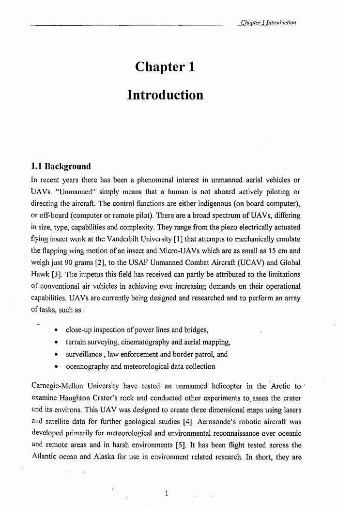
1.1 Bacl{ground
In recent years there has been a phenomenal interest in unmanned aerial vehicles or
DAVs. "Unmanned" simply means that a human is not aboard actively piloting or
directing the aircraft. The control functions are either indigenous (on board computer),
or off-board (computer or remote pilot). There are a broad spectrum ofUAVs, differing
in size, type, capabilities and complexity. They range from the piezo electrically actuated
flying insect work at the Vanderbilt University [1] that attempts to mechanically emulate
the flapping wing motion of an insect and Micro-U A V s which are as small as 15 cm and
weigh just 90 grams [2], to the USAF Unmanned Combat Aircraft (UCA V) and Global
Hawk [3]. The impetus this field has received can partly be attributed to the limitations
of conventional air vehicles in achieving ever increasing demands on their operational
capabilities. UAVs are currently being designed and researched and to perform an array
of tasks, such as :
• close-up inspection of power lines and bridges,
• terrain surveying, cinematography and aerial mapping,
• surveillance, law enforcement and border patrol, and
• oceanography and meteorological data collection
Carnegie-Mellon University have tested an unmanned helicopter In the Arctic to'
examine Haughton Crater's rock and conducted other experiments to. asses the crater
and its environs. This UAV was designed to create three dimensional maps using lasers
and satellite data for further geological studies [4]. Aerosonde's robotic aircraft was
developed primarily for meteorological and environmental reconnaissance over oceanic
and remote areas and in harsh environments [5]. It has been flight tested across the
Atlantic ocean and Alaska for use in environment related research. In short, they are
1
Chapter 1 Introduction
expected to carry out difficult and dangerous tasks. The advantages outlined above have
led to a burst of activity in this arena. It is important to note that there are few
operational UAVs and fewer still available for academic research-most current UAVs
have been developed for military applications.
The vast majority of modern systems incorporate the latest light-weight material, smart
sensors and complex control paradigms, in order to facilitate characteristics such as
greater payload capability for a given structure, high manoeuvrability and a fast speed of
response. Therefore, design, control and analysis of such systems are non trivial and
entail multi-disciplinary expertise from domains such as aerodynamics (modelling),
control, structures, sensors and e1ctronic hardware. Thus, challenges associated with
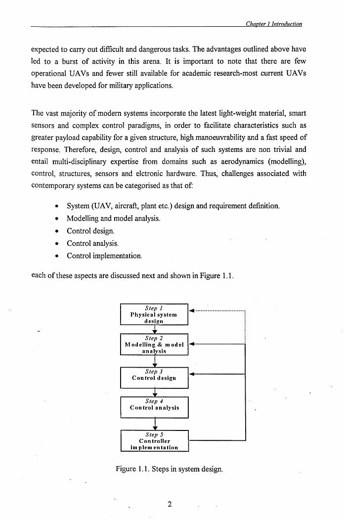
contemporary systems can be categorised as that of:
• System (U A V, aircraft, plant etc.) design and requirement definition.
• Modelling and model analysis.
• Control design.
• Control analysis.
• Control implementation.
each of these aspects are discussed next and shown in Figure 1.1.
Step J ................................... Physical system
design
~ Step 2
Modelling & model ....
an alysis
~ Step 3 ..
Control design -
+ Step 4
Control analysis
~ Step 5
Controller im p lem en ta tion
Figure 1.1. Steps in system design.
2

Chapter 1 Introduction
System design and requirement: Traditionally, application-specific engineers design
the system or plant. After completing the design, control engineers inherit two products
from the designer: i) the system itself and ii) physical requirements that the system must
achieve after control design. Requirements define the problem, that is what is expected
from the system. A good example is the ultra-agile military aircraft, in order to induce
agility, canards or fore wings were appended to the aircraft. Another one is the need of
light weight flexible space observatories so that they can carry a greater payload or on
board equipments. Such high performance systems are no longer crafted in isolation but
with increasing participation of control experts from an early stage. A cohesive
mechanism requires control engineers to be involved early in the design phase of these
systems, to provide input into how a particular plant design may affect controller design
and vice-versa. Agile aircraft and flexible structures are prime examples where the role
of control specialist is evident from the embryonic system design stage. It is only in the
design stage that significant changes can be made. Thus, requirements feed the control
design steps for modelling, design, analyses and implementation.
Modelling: Suitable plant models are required for the ensuing control design and
analyses steps. After the design process, the most daunting task is to develop a working
model. In fact an old saying in the control field is that Hmost of the work in a control
design is in developing the model" [6]. Modem control techniques can achieve
extraordinary. results using state-space models. However, not even the most robust
controller can compensate for a poor model. The model obtained either via
mathematical modelling or the system identification route must be checked, analysed
(i.e. determine its properties), and refined throughout the course of the control law
dev~lopment. Simplified rigid body models may be employed initially and if necessary
more complex flexible or elastic modes may be included. This two stage procedure is
commonly practised for flexible space craft appendages, helicopter rotor or agile air
vehicle modelling and subsequent control. The control design model forms the basis for
all designs and analyses. Generally, models for flight control imply a high-fidelity linear
model for controller design and a nonlinear model for the closed system evaluation in a simulation environment.
Control design: Control design step begins with the selection of operating conditions at
which the control design is to be accomplished. Then, a particular design methodology
is selected. The designer has an impressive list of control paradigms from which to
3

Chapter 1 Introduction
choose, using either classical or modern state-space approaches. Much would depend
upon the type of plant i.e. single input single output (SISO) or multi-input multi-ouptut
(MIMO). Classical frequency domain methods have been very successful in handling
SISO systems. On the other hand, modern control techniques are more amenable for
MIMO systems. Also, factors like past history of successful application of certain
control mechanism for a specific type of plant play an important role. For instance, to
date PID controller is the most successful control paradigm in the process industry.
Although alternative and more advanced paradigms exist for the process industry, such
as Model Predictive Control, the industry is wary of changing practice that already
works well. It could be said that there are many factors which decides a fate of a
particular control option.
Control Analysis: Closely related to the control design step is the control analysis in
the design process. For a requirement to be valid, it must be verifiable. Thus, as a
requirement is included into a design, the control analysis test provides an immediate
check on whether the requirement is met. If the resulting controlled system analysis is
unsatisfactory then the specification/requirements could be modified or the type of
controller or system design itself could be altered. As such, the analysis test forms the
basis for the design iteration decision.
Control implementation: Once the design has passed all of its analysis assessments,
considerable effort is still required to take the algorithm to a plant operational state. A
simulated operational environment will never be a perfect representation of the real
thing. Real systems are built from real imperfect (not mathematical) components and
~ust operate under real (non ideal) conditions. Therefore, factors such as noise,
quantization, nonlinearities, saturation (rate or amplitude), delays,· model errors,
sensors/actuator dynamics and . disturbances can adversely affect control system
operation.
Therefore, the controller implementation stage is regarded as the ultimate test for the
validity of the whole design process i.e. step 1 to 5 of Figure 1.1. Generally, design
steps 2 to 5 are carried out in an iterative manner until the design and operational
requirements are satisfied. If this is unachievable then the plant itself may be modified
and the design process repeated. This is indicated by the dotted line in Figure 1.1.
4

Chapter 1 Introduction
1.2 Problems and challenges of modern systems
Research interest in unconventional aircraft, such as tilt rotor, tilt wmg, delta-wing,
canard or talieron control surfaces, X-wing, tilt body, different types of light, micro,
hand held unmanned aerial vehicles etc. , have assumed increased importance in recent
years. Two examples are shown in Figure 1.2. Figure 1.2 (a) shows the traffic
surveillance drone being developed at Georgia Tech [7], and Figure 1.2 (b), is the
Freewing Inc.[8] tilt-body UAV, to be employed for remote sensing applications.
The rrof'fic SurveilJa.nee Drone p'roject h~ r eceJved ;.n;ciol (,undingfr'o ,rn "the Ge'orgia > Department 0'( Tran:sporto:tion and the F~ldA'r'l'2'l H'igh'\!VoyAd,nin,;s't:r'a"tilon"S"Priorit:y Techno(ogy' P, \rb,f,II'inr!lln
The drone j.sc:ur.'~nuy ,under CO"~.ruc~~o.nctC'", 'the Georgia' Te.ch Re.search Ins;ci tut;e"s ' , Advanced Vehicle Development a :nd In't:egra'don Ldboratory.
(a)
UAV ReRlote Se sling roject
R(';:.'l11ot;.e:.- ~).(,::''T¥';;' l,.f'~ Ins -i:;rume nt6 .a nd JY/(A l...caLuxlS
e'tJdc.J IJ~-3 .,a ~JLk)'., .. " ~j.cGile Mode.-A
(b)
Figure 1.2. Illustrations of small UAVs.
5
Chapter 1 Introduction
The latter's hinged mid-body feature allows it to take-off and land like a bird. The
importance of U A V s can be attributed to the increasing emphasis on the aircraft to be
stealthy, agile, multi-purpose, autonomous etc., for varied civilian and military
operations. However, modelling details of these vehicles are not reported due to
classified nature of such projects. Moreover, the flight mechanics equations are not
always easy to establish from first principles for a non-standard aircraft configuration. A
case in point is the UAV Pegasus XL, which crashed due to the poor modelling
procedure adopted [9]. However, these equations are imperative for subsequent control
law development. A high fidelity nonlinear model is also often required to study
controlled system performance in a simulation environment. Modelling of such vehicles
is non-trivial and therefore, presents considerable challenges The modelling task is
further complicated if coupling exists between different axis (plane) of motion, as for
example in the case of a helicopter.
The last decade has witnessed a phenomenal growth in numerous fields, including
robotics, space structures/space telerobotics, and unconventional air vehicles. The
significant features of these endeavours have included the introduction of innovative
design, fascinating structural materials and sophisticated control paradigms. This is a
striking departure from the classical systems engineering philosophy. The assimilation of
the above in systems development has led to systems which are sophisticated, accurate
and robust. For instance, Artificial Intelligence (AI) techniques, such as neural
networks, fuzzy-logic, and genetic algorithms, have been employed to address a range
of engineering issues, such as modelling, optimisation, control, guidance, and fault
diagnosis. Flexible structures, an area of intense interest in robotics [10-12] and
spacecraft with flexible appendages [13 -15] research, are attractive mainly because of
tbeir lightweight and strength. In aerospace vehicles [16,17] too, a flexible airframe is
adopted due to its light weight, thereby improving the thrust to weight ratio for a given
propulsion system.
However, these advances have come at a cost, and the penalties imposed are comple~
systems with little historical data, no exhaustive literature or proven track record. An
unconventional system configuration means considerable efforts are required to develop
new mathematical models, especially in case of air vehicles. AI based control paradigms
are complex and have not yet gained the confidence of the industry. In flexible or elastic
structures the added complexity of the control problem is due to the inherently lightly
6

Chapter 1 Introduction
damped nature of the structure which causes vibration in the system. Control of modern
system with flexible modes is a rather daunting and necessitates knowledge of a braod
range of control methodologies.
In spite of the increased difficulties most of the control problems can be addressed using
open loop, closed loop or a combined open and closed loop strategy. The open loop
control technique of shaped command methods [10-12] have been particularly
attractive. This method involves development of a suitable forcing function so that the
vibrations at the resonance modes are reduced. Open-loop control topologies are
particularly suitable for systems with slow dynamics, for instance flexible manipulators
or similar plants.
On the other hand, fast manoeuvring systems, such as high speed robots [18], large
flexible space structures [19], flexible aircraft [16,17] as well as the flexible missile [20]
invariably incorporate feedback control mechanisms. With a variety of feedback control
methods available, such as LQRJLQG, LQG-LTR, H-oo, eigenstructure assignments,
dynamic inversion, classical method and including AI based control methods mentioned
above, it is unclear which control scheme provides the best' all round solution for a
complex systems. Highly agile system such as combat aircraft are generally non
minimum phase in nature. As some of the modem control techniques have limitations '
dealing with non minimum phase plants, control method selection becomes problamatic.
Perhaps, the optimum approach is to evaluate different paradigms or rely on past
experiences of researchers who have addressed analogous problems.
Thus, it is apparent from the above discussion that there are various issue connected
with these sophisticated contemporary systems. These issues invariably "fall under the
broad guidelines described earlier in Section 1.1.
1.3 Motivation
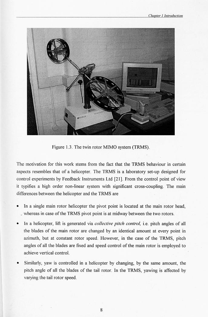
Although, the twin rotor MIMO system (TRMS) shown in Figure 1.3 does not fly, it
has a striking similarity with a helicopter, such as system nonlineafityies and cross
coupled modes. The TRMS, therefore, can be perceived as an unconventional and
complex "air vehicle" with a flexible main body. These system characteristics present
formidable challenges in modelling, control design, control analysis and implementation.
7
Chapter 1 Introduction
Figure 1.3 . The twin rotor MIMO system (TRMS).
The lTIotivation for this work stems from the fact that the TRMS behaviour in certain
aspects resembles that of a helicopter. The TRMS is a laboratory set-up designed for
control experiments by Feedback Instruments Ltd [21]. From the control point of view
it typifies a high order non-linear system with significant cross-coupling. The main
differences between the helicopter and the TRMS are
• In a single main rotor helicopter the pivot point is located at the main rotor head,
_ whereas in case of the TRMS pivot point is at midway between the two rotors.
• In a helicopter, lift is generated via collective pitch control, i.e. pitch angles of all
the blades of the main rotor are changed by an identical amount at every point in
azimuth, but at constant rotor speed. However, in the case of the TRMS, pitch
angles of all the blades are fixed and speed control of the main rotor is employed to
achieve vertical control.
• Similarly, yaw is controlled in a helicopter by changing, by the same amount, the
pitch angle of all the blades of the tail rotor. In the TRMS, yawing is affected by
varying the tail rotor speed.
8
Chapter 1 Introduction
• There are no cyclical controls in the TRMS, cyclic is used for directional control in
a helicopter.
However, like a helicopter there is strong cross-coupling between the collective (main
rotor) and the tail rotor.
The hovering property of helicopter/TRMS is the main area of interest in this work.
Station keeping, or hovering, is vital for variety of flight missions such as load delivery,
air-sea rescue etc. Yet maintaining a station is one of the most difficult problems in
helicopter flight because in this mode the dynamically unstable helicopter is flying at
near zero forward speed. Although the TRMS rig reference point is fixed, it still
resembles a helicopter by being highly non-linear with strongly coupled modes. Such a
plant is thus a good benchmark problem to test and explo~e modem identification and
control methodologies. The experimental set-up simulates similar problems and
challenges encountered in real systems. These include complex dynamics leading to both
parametric and dynamic uncertainty, unmeasurable states, sensor and actuator noise,
saturation and quantization, bandwidth limitations and delays.
The presence of flexible dynamics in the TRMS is an additional motivating factor for
this research. There is an immense interest in design, development, modelling and
control of flexible systems, due to its utility in a multitude of applications, as discussed
briefly in Section 1.2.
1.4 Aims of this research
From the foregoing discussion it is evident that the fundamental issues .regarding the
TRMS are: modelling, control design, analysis and implementation. These problems are
systematically investigated in this work.
1.4.1 Contributions
The main contributions of this thesis are:
• Dynamic modelling of a 1 degree of freedom (DOF) TRMS using linear black box
system identification techniques. The concept is extended to model a 2 DOF TRMS,
. which has cross-coupled dynamic modes. Cross-coupling renders MIMO modelling
rather daunting. Helicopters too exhibit coupling between different axes and this is
9
· Chapter 1 Introduction
an area of active research [22]. The extracted model is to be employed to detect
system resonance modes for subsequent control design. It has been demonstrated
that the black-box modelling approach presented is suitable to model a class of
unconventional air platforms, whose flight dynamics are not well understood or
difficult to model from first principles:·
• Nonlinear modelling of a 1 DOF TRMS utilising radial basis function networks
(RBF). The modelling concept provides an attractive alternative to model new
generation VA V s with significant nonlinearities. Such a high fidelity nonlinear model
is often required for gauging the performance of control design and analyses. The
linear and nonlinear modelling exercise is carried out to include rigid as well as
flexible modes of the system. The presence of high frequency modes in flexible
systems have profound impact on the ensuing control design.
• Development and real-time realisation of open-loop vibration control for the 1 and 2
nOF TRMS. This concept is particularly useful in addressing vibration problems in
MIMO systems, if modal coupling exists.
• Control law development and evaluation In the MA TLAB/Simulink simulation
environment for the 1 nOF TRMS to achieve vibration attenuation as well robust
tracking performance. Investigation of feedback and combined feedforward and
feedback techniques. Demonstration of the suitability of integrated feedforward and
feedback method to tackle the dual problem of vibration reduction and command
tracking in the system.
• Real-time realisation of the developed control strategies for the TRMS application.
1.5 Thesis outline
The organisation of the thesis reflects the sequence of steps involved in the development
of a complete systems solution for the TRMS. A brief outline of the thesis contents is as
follows:
Chapter 2 describes the experimental test bed, the Twin Rotor MIMO System,'
developed by Feedback Instruments Ltd. [21], designed for control
experiments. A brief description of the rig, necessary instrumentation,
hardware and software is presented. The TRMS is used as a test bed
throughout this work.
10
Chapter 1 Introduction
Chapter 3 presents the development of linear models of both 1 and 2 DOF TRMS
using the linear system identification techniques. Rigid and flexible modes
are accounted for in the modelling procedure. Identification of 1 and 2 DOF
discrete time linear models are presented in detail. The identification process
for a MIMO system is non-trivial and a systematic approached is explained.
Rigorous time and frequency domain test are employed to validate the
identified models.
Chapter 4 explains the development of open-loop control strategies on the basis of the
system's identified resonance modes. Command signals are preshaped using
low-pass and a band-stop filter. For the 2 nOF case, due to coupling
between horizontal and vertical planes as well as presence of vibrational
modes in different channels poses significant difficulties in filter design. The
filtered inputs are thus employed for both 1 and 2 DOF TRMS in the open
loop configuration. Their performance in suppressing structural vibrations
of the TRMS is evaluated in comparison to a doublet signal. A comparative
study of the low-pass and band-stop shaped inputs in suppressIng the
system's vibrations is also presented.
Chapter 5 describes the nonlinear system identification technique for modelling the 1
DOF TRMS using the radial basis function networks (RBF). The extracted
models are verified using several time and frequency domain tests including
model predicted output, correlation tests and time domain cross validation
tests. The rationale for obtaining a high fidelity nonlinear model is that such
a model is often required for assessing the performance of control design
and system analysis.
Chapter 6 utilises the 1 DOF linear model obtained in Chapter 3 to design a feedback
control mechanism. The LQG method is initially investigated within the
simulation environment. The controller is shown to exhibit good tracking
capabilities, but requires high control effort and has inadequate authority
over residual vibration of the system. These problems are resolyed by'
further augmenting the system with a command pat~ prefilter. The
combined feedforward and feedback compensator satisfies the performance
objectives and obeys the actuator constraint.
11
Chapter 1 Introduction
Chapter 7 presents the implementation and realisation of the proposed control
strategies of Chapter 6 on the TRMS test bed. Several additional designs
are tested to improve the systems performance. The system's performance
for various LQG weighting matrices are assessed and discussed from
practical perspective.
Chapter 8 concludes the thesis with notable remarks. Future probable research
directions are also outlined in this chapter.
1.6 Publications
Technical papers arising from this research, which are either published or under review,
are listed below.
a) Journal Papers:
[1] S. M. Ahmad, A. 1. Chipperfield and M. o. Tokhi. "Parametric Modelling and Dynamic Characterisation of a 2-DOF Twin Rotor MIMO System", IMechE, Part G, Journal of Aerospace Engineering (to appear).
[2] S. M. Ahmad, A. 1. Chipperfield and M. O. Tokhi. "Dynamic modelling" and open loop control of a twin rotor mimo system", (submitted to IF A C Journal of Control Engineering Practice).
b) Conference Papers:
[1] S. M. Ahmad, A. 1. Chipperfield and M. O. Tokhi (2000). "Modelling and Control of a Twin Rotor Multi-Input Multi-output System", Proc. American Control Conference (ACC' 2000), Chicago, IL, USA, 28-30 June, pp 1720-1724.
[2] S. M. Ahmad, A. 1. Chipperfield and M. O. Tokhi (2000). "Dynamic Modelling of a Two Degree-of-Freedom Twin Rotor Multi-Input Multi-output System", Proc. lEE United Kingdo111 Auto111atic Control Conference (UKACC' 2000), 4-7 Sept., Cambridge, UK.
[3] S. M. Ahmad, A. 1. Chipperfield and M. o. Tokhi (2000). "Dynamic Modelling and Control of a 2 DOF Twin Rotor Multi-Input Multi-Output System", Proc. IEEE Industrial Electronics, Control and Instru111entation Conference (IECON' 2000), . Nagoya, Japan, 22-28 Oct., pp 1451-1456.
[4] S. M. Ahmad, A. 1. Chipperfield and M. O. Tokhi (2000). "Dynamic modelling and Optimal Control of a Twin Rotor MIMO System", Proc. IEEE National Aerospace and Electronics Conference (NAECON' 2000), Dayton, Ohio, USA, 10-12 Oct., pp 391-398.
12

Chapter 1 Introduction
[5] S. M. Ahmad, M. H. Shaheed, A. 1. Chipperfield and M. O. Tokhi (2000). "Nonlinear Modelling of a Twin Rotor MIMO System using Radial Basis Function Networks", Proc. IEEE National Aerospace and Electronics Conference (NAECON' 2000), Dayton, Ohio, USA, 10-12 Oct., pp 313-320. .
[6] S. M. Ahmad, A. 1. Chipperfield, and M. O. Tokhi. (1999). "System Identification of a One Degree-of-Freedom Twin Rotor Multi-Input Multi-Output System", In International Conference on Computer and Infornlation Technology (ICCIT' 99). SUST, Sylhet, Bangladesh, 3-5 Dec., pp 94-98.
13
Chapter 2 The twin rotor M[}vfO system descn'ption
Chapter 2
The twin rotor MIMO system description
This Chapter presents the general description oj the TRMS. The physical as well as the
hardware and sojnvare aspects oj the TRMS are explained Inlportant considerations
essential for conducting the experiments have been highlighted
2.1 Introduction
The Twin Rotor MIMO System (TRMS) is a laboratory platform designed for control
experiments by Feedback Instruments Ltd [21]. In certain aspects, its behaviour
resembles that of a helicopter. For example, like a helicopter there is a strong cross
Coupling between the collective (main rotor) and the tail rotor. The main differences
between a helicopter and the TRMS are described in Section 1.3. As such it can
considered a static test rig for an air vehicle. There is a small, but growing, literature on
laboratory platforms simulating complex aircraft manoeuvre and problems. These
platforms are often employed to test the suitability of different control m~thods for these
systems. Some specific laboratory rigs used by researchers are described' in Section
6. ~: 1. The remainder of this Chapter will describe the TRMS, a schematic diagram of
which is shown in Figure 2.1.
14
Chapter 2 The twin rotor MIMO system description
Yaw
~ ..................... fIj Pitch
Main Rotor \ Beam
Tail Rotor F2 Counterbalance
PC
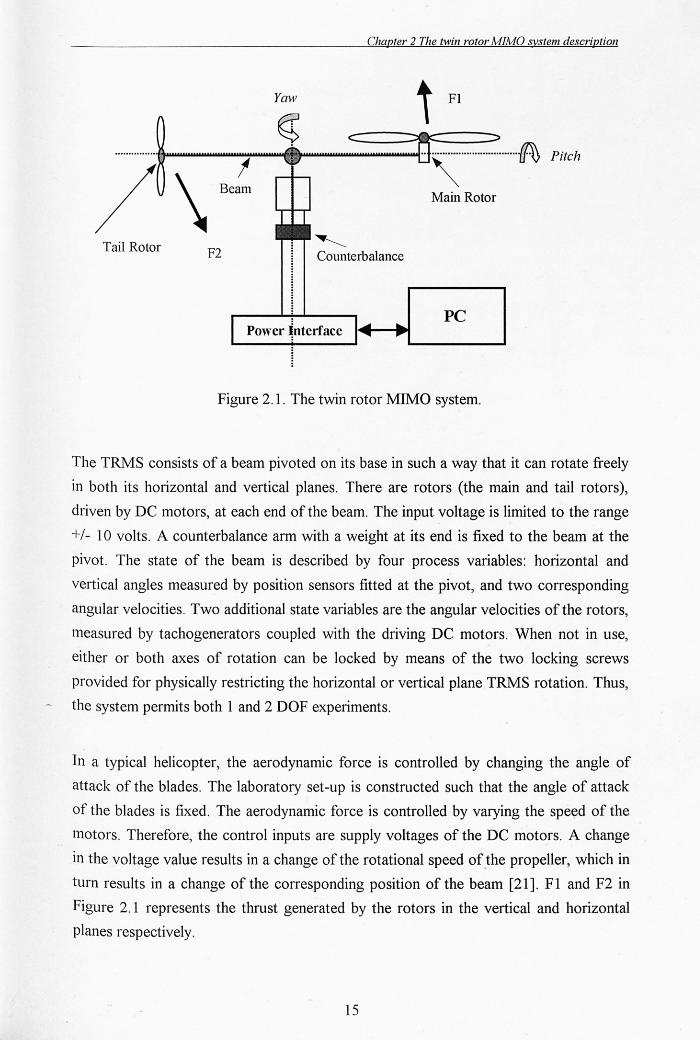
Figure 2.1. The twin rotor MIMO system.
The TRMS consists of a beam pivoted on its base in such a way that it can rotate freely
in both its horizontal and vertical planes. There are rotors (the main and tail rotors),
driven by DC lTIotors, at each end of the beam. The input voltage is limited to the range
+/- 10 volts. A counterbalance arm with a weight at its end is fixed to the beam at the
pivot. The state of the beam is described by four process variables: horizontal and
vertical angles measured by position sensors fitted at the pivot, and two corresponding
angular velocities. Two additional state variables are the angular velocities of the rotors,
measured by tachogenerators coupled with the driving DC motors. When not in use,
either or both axes of rotation can be locked by means of the two locking screws
provided for physically restricting the horizontal or vertical plane TRMS rotation. Thus,
the system permits both 1 and 2 DOF experiments.
In a typical helicopter, the aerodynamic force is controlled by changing the angle of
attack of the blades. The laboratory set-up is constructed such that the angle of attack
of the blades is fixed. The aerodynamic force is controlled by varying the speed of the
Inotors. Therefore, the control inputs are supply voltages of the DC motors. A change
in the voltage value results in a change of the rotational speed of . the propeller, which in
turn results in a change of the corresponding position of the beam [21]. F 1 and F2 in
Figure 2.1 represents the thrust generated by the rotors in the vertical and horizontal
planes respectively.
15
Chapter 2 The twin rotor MllvlO system description
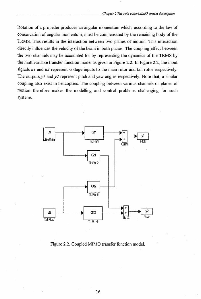
Rotation of a propeller produces an angular momentum which, according to the law of
conservation of angular momentum, must be compensated by the remaining body of the
TRMS. This results in the interaction between two planes of motion. This interaction
directly influences the velocity of the beam in both planes. The coupling effect between
the two channels may be accounted for by representing the dynamics of the TRMS by
the multivariable transfer-function model as given in Figure 2.2. In Figure 2.2, the input
signals u1 and u2 represent voltage inputs to the main rotor and tail rotor respectively.
The outputs y1 and y2 represent pitch and yaw angles respectively. Note that, a similar
coupling also exist in helicopters. The coupling between various channels or planes of
motion therefore makes the modelling and control problems challenging for such
systems.
G11
Tr.Fh1
G12
Tr.Fh3
Tr.Fh4
Figure 2.2. Coupled MIMO transfer function model.
16
Chapter 2 The twin rotor "'{JMO system description
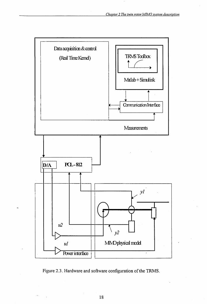
2.2 The TRMS hardware and software description
A PC can be used for real-time control of the TRMS. The computer is supplied with an
interface board-PCL-812. The PCL-812PG is a high performance, high speed, multi
function data acquisition card for IBM PC/XT / AT and compatible computers from
Advantech Co. Ltd. Figure 2.3 shows details of the hardware and software
configuration of the control system for the TRMS.
The control software for the TRMS consists of:
• Real-time kernel (RTK).
• The TRMS toolbox.
2.2.1 Real-time l{ernel
The real-time kernel (RTK) provides a mechanism of real-time measurements and
control of the TRMS in the WINDOWS environment. It is implemented by dynamic
linked library (DLL) and contains measurement procedures, digital filters, a data
acquisition buffer, built-in control algorithms, software to ~ontrol system actuators and
a MATLAB-to-RTK interface. The RTK controls flow of all signals to and from the
TRMS. It contains functions for performing analogue-to-digital and digital-to-analogue
conversions. The RTK DLL library is excited by time interrupts. The main part of the
R TK is executed during interrupt time. In summary, the RTK contains all the functions
that are required for feedback control and data acquisition in real ti~e. A typical TRMS
Simulink block diagram is shown in Figure 2.4.
- Example control algorithms are embedded in the real-time-kernel, including open-loop,
PID and state-space controller. It is possible to tune the parameters of the controller
without emphasis on analytical model. Such an approach to the control problem seems
to be reasonable, if a well defined model of the TRMS is not available. These controller
parameters are functions of error signals, that is the difference between the desired and
actual TRMS beam positions and angular velocities. Selection of control algorithms and
tuning of their parameters is done by means of the communication software (Figure 2.3)
from the MATLAB environment. Since the focus of this research is on model-based
Control law development therefore, these controllers were of no use to this work. The
interested reader can refer to the TRMS manual [21] for further details of these
Controllers.
17
ilia aap.risitiOl &mltrd
(Rffil Ture Kfrncl)
ID/A ~ KL- 812 -
Chapter 2 The twin rotor MIA10 system description
1Rl\IE TailxK
t C . Mltlab + Similink
~- Canrunicatim~ .. ,..
11asllrannts
Figure 2.3. Hardware and software configuration of the TRMS.
18
Chapter 2 The twin rotor MIMO system description
Rotor Velocity
Tail rotor input Mux
Control Control Value
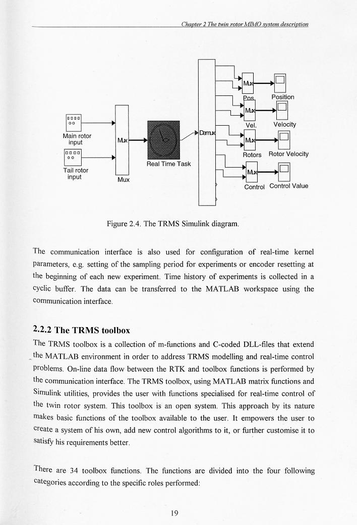
Figure 2.4. The TRMS Simulink diagram.
The communication interface is also used for configuration of real-time kernel
parameters, e.g. setting of the sampling period for experiments or encoder resetting at
the beginning of each new experiment. Time history of experiments is collected in a
cyclic buffer. The data can be transferred to the MATLAB workspace using the
communication interface.
2.2.2 The TRMS toolbox
The TRMS toolbox is a collection of m-functions and C-coded DLL-files that extend
_ the MATLAB environment in order to address TRMS modelling and real-time control
problems. On-line data flow between the R TK and toolbox functions is performed by
the communication interface. The TRMS toolbox, using MATLAB matrix functions and
Simulink utilities, provides the user with functions specialised for real-time control of
the twin rotor system. This toolbox is an open system. This approach by its nature
makes basic functions of the toolbox available to the user. It empowers the user to
create a system of his own, add new control algorithms to it, or further customise it to
satisfy his requirements better.
There are 34 toolbox functions. The functions are divided into the four following
categories according to the specific roles performed:
19
Chapter 2 The twin rotor MIAfO system description
hardware: the functions in this category is used to obtain and set the base address of
PCL-812 interface board. A function is also available to reset the encoders at the
beginning of each experiment.
data acquisition: the functions in this category is employed to set the sampling time,
acquire the sampling interval and retrieves the time histories of various measurements.
software: the loading and the unloading of the RTK to and from the memory is carried
out by functions in this category.
control: the job of assigning different control parameters for various in-built control
algorithms are mainly achieved by invoking functions in this category.
The important ones used during this research are described in Appendix 1.
2.3 TRMS experimentation
Important consideration for carrying out the experiments with the TRMS are level of
input signals, sampling time and environmental conditions. Each of these are explained
next.
The level of input signals have been selected in this research so that these signals no not
drive the TRMS out of its linear operating range. The range of operation is the slight
deviation from the steady-state "hover" mode. Throughout this research the
experimentation was carried out with the TRMS beam in a flat horizontal position
representing the "hover" mode. The TRMS in this position is shown in Figure 2.5. The
hovering property of the TRMS is the main area of interest in this work. Station keeping
_ or hovering is vital for a variety of flight missions such as load delivery and air-sea
rescue.
F or the identification of the discrete time models, the sampling time has to be selected
before starting the experiments. The sampling time depends on the final application and
the intended accuracy of the resulting model. The model can easily exhibit high order
behaviour if the sampling period is chosen too short. On the other h~nd, if the sampling
period is too large, the model looks like a constant or multiple integrators and its
dynamics representation would be inaccurate. Some useful guidelines for sampling
period selection are given in Section 3.2.4.
20
Chapter 2 The twin rotor MIMO system description
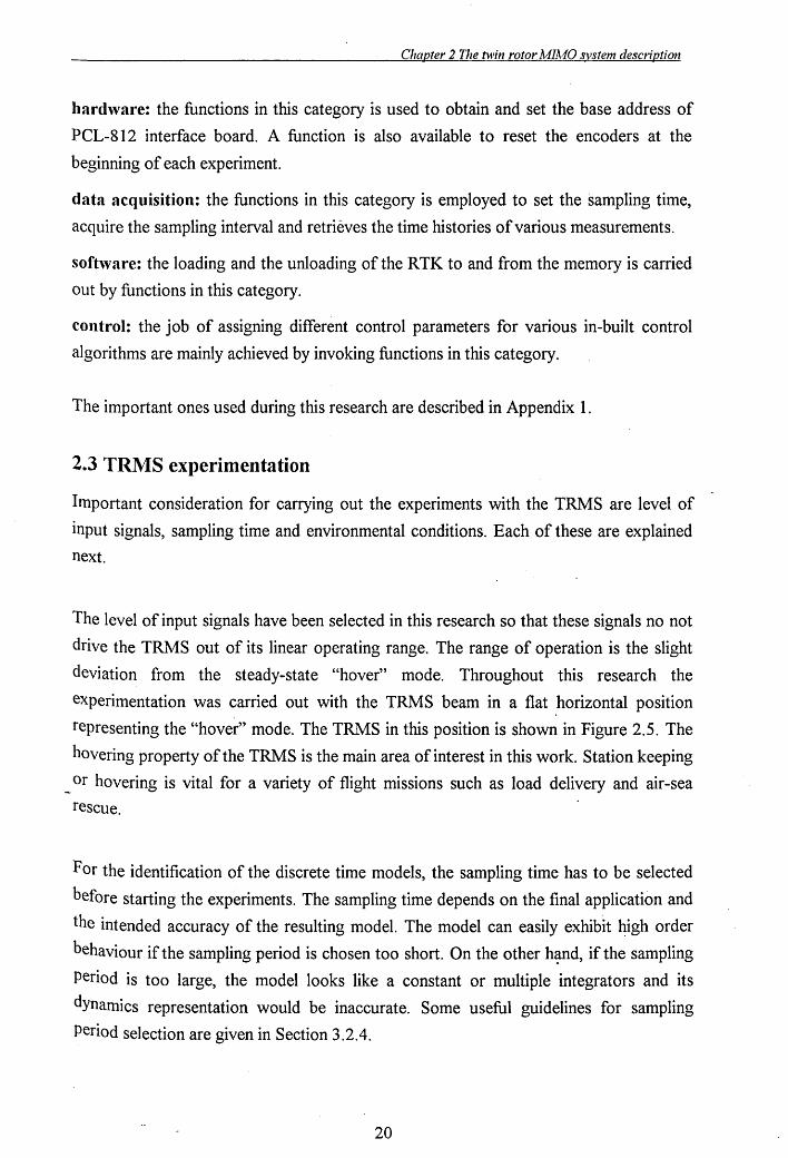
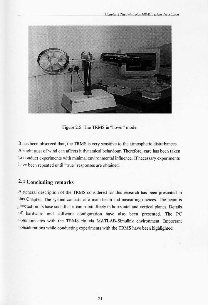
Figure 2.5. The TRMS in "hover" mode.
It has been observed that, the TRMS is very sensitive to the atmospheric disturbances.
A slight gust of wind can affects it dynamical behaviour. Therefore, care has been taken
to conduct experiments with minimal environmental influence. If necessary experiments
have been repeated until "true" responses are obtained.
2.4 Concluding remarks
A general description of the TRMS considered for this research has been presented in
this Chapter. The system consists of a main beam and measuring devices. The beam is
_ pivoted on its base such that it can rotate freely in horizontal and vertical planes. Details
of hardware and software configuration have also been presented. The PC
communicates with the TRMS rig via MATLAB-Simulink environment. Important
considerations while conducting experiments with the TRMS have been highlighted.
21
Chapter3 Dynamic modelling oOhe twin rotor MllvfO system
Chapter 3
Dynamic modelling of the twin rotor MIMO system
Mathe111atical 111 ode Is for the dyna111ic characterisation of one and two-degree-offreedo111 twin rotor 111ulti-input 111ulti-oufput syste111 (TRMS) in hover, are detennined using a black-box syste111 identification technique. Identification for 1 and 2-DOF rigid-body, discrete-time linear 1110dels are presented in detail. The extracted 1110del is shown to have a good degree of prediction capability. The 1110delling approach presented is suitable for c0111plex new generation air vehicles.
3.1 Introduction
Mathenlatical 1110delling is perhaps the best known analytical method of describing the
dynamics of a physical system. The parameters associated with such a model have a
direct link and influence on the physical and dynamical properties of the system. An
important feature of such characterisation of a system is that it helps in observing the
"cause" and "effect" phenomena clearly, that is, which parameter has what effect on the
system behaviour. The approach is generally best suited to simple systems. However,
with the increasingly complex nature of systems, which may constitute many
-SUbsystems, modelling of such a system is often a formidable task. Furthermore,
mechanical systems in general have electro-mechanical components and mathematical
modelling would entail specialist knowledge of these areas. Mathematical models are
derived from first principles and, in the process, employ many simplifications and
assumptions. Such methods will thereby ignore less important dynamics and
disturbances acting on the system. These factors, if not accounted for, ~ould yield· a
POor system model. Thus, the utility of mathematical modelling to f~irly complex plants
is limited. Syste111 identification, on the other hand, is an experimental technique, and
has proven to be an excellent tool to model complex processes where it is not possible
to obtain reasonable models using only physical insight. Important applications of
system identification are visible in areas that require higher accuracy of the mathematical
22
Chapter3 Dynamic modelling o(the twin rotor MIMO ~stem
model for simulation, validation, control system design and handling qualities, in
aerospace applications for example. It provides an accurate, rapid and reliable approach
for defining design specifications and for validating control systems.
In aircraft applications, the typical tole of system identification is to estimate the
parameters of the linearized 6 degree-of-freedom equation of motion from flight or wind
tunnel data. Here, the model structure is known and the parameters of the model have
Some physical meaning, and are often called stability and control derivatives. These
derivatives are functions of altitude and Mach number of the aircraft and therefore
would change at different operating conditions. This holds true for most classical fixed
and rotary wing aircraft. There are a vast number of papers addressing parameter
estimation techniques for conventional aircraft for example, [23,24]. However, with
many new innovative experimental aircraft designs or those which are inherently more
complex such as the tilt rotor, tilt wing, delta-wing, canard or talieron control surfaces,
X-wing and tilt body, flight mechanics equations are not always easy to establish from
first-principles. Yet, these equations are essential for designing and studying flight
control systems. System identification is a viable alternative for modelling
unconventional aircraft, where both model structure and model parameters are unknown
and need to be identified. Modelling of such vehicles is the subject matter of this
Chapter.
A number of unmanned aerial vehicles (UAVs) such as Bluebird [25], Frog [26], Solus
[27]. Raven-2 [28], have been reported recently. These are based on conventional
aircraft aerodynamic design philosophy and are often scaled versions of contemporary
aircraft. The dynamic models of these aircraft have been derived from first-principles
--through determination of the aerodynamic stability and control derivatives, with usual
decoupling of longitudinal and lateral dynamics. Many other unconventional but
faSCinating experimental air vehicles have also been reported in the literature, some of
these are briefly discussed below. These innovative platforms or "next generation air
vehicles" are designed for specific applications, and differ significantly from . the!r
classical counterparts. Recently, a considerable amount of research effort has been
devoted to different modelling and control aspects of these unconventional vehicles. A
free wing [8] UAV is modelled using conventional mathematical modelling techniques.
The Caltech ducted fan laboratory aircraft [29] has been developed to demonstrate
Control techniques for hover to forward flight transition for thrust-vectored aircraft.
23
Chapter3 Dynamic modelling of the twin rotor MIMO system
Modelling and control of a radio controlled (RC) laboratory helicopter has been
reported by Morris et al [30] where modern identification and robust control techniques
have been investigated for the hover mode. Identification of an auto gyro (gyroplane), a
popular sport and recreational flying machine, has been documented by I:I0uston [31].
Werner and Meister [32] have developed a mathematical model, from first-principles,
for a 2 DOF laboratory aircraft. This plant was developed primarily to model the
behaviour of a vertical-take-off plane. Nonlinear system identification techniques such
as neural networks have been applied in modelling of an Ariel UAV [33]. Neural
networks were also employed for characterising the wind-tunnel wing model at NASA
[34]. It is evident from the above cases that the plant is modelled using mathenlatical
modelling based on the analysis of plant aerodynamics i.e. using laws of physics.
Furthermore, the parameters of the model are either known or obtained using linear or
nonlinear system identification techniques.
However, the modelling technique presented in this Chapter is suitable for a wide range
of new generation air vehicles whose flight dynamics are either difficult to obtain via
mathematical modelling or not easily understood. The modelling is done assuming no
prior knowledge of the model structure or parameters relating to physical phenomena,
i.e. black-box modelling. Such an approach yields input-output transfer function models
with neither prior defined model structure nor specific parameter settings reflecting any
physical aspects. It is then the responsibility of the systems engineer to examine the
resultant black-box model and interpret the extracted model parameters in relation to
the plant dynamics. This is discussed in more detail in Section 3.6 of this Chapter.
System identification is a powerful interim solution for such systems. The designer can
use these models to build an initial understanding of the whole system and develop
-. general solutions. If more rigorous analytical models become available, they can then be
used to fine-tune the general solutions, if they prove to be more accurate.
The work in this Chapter addresses modelling of an experimental test rig, representing a
complex TRMS using system identification techniques. In this Chapter, attention is first
focused on the identification and verification of longitudinal dynamics of a 1 DOF
TRMs with its main beam (body) in a flat horizontal position representing the hover
mode. Although the system permits multi-input multi-output (MIMO) experiments,
initially single-input single-output (SISO) set-up will be discussed. The concept is then
extended for modelling a 2 DOF MIMO twin rotor. plant. The objective is to get
24
Chapter3 Dynamic modelling ofthe twin rotor AlIMO system
satisfactory models of the pitch and the yaw plane dynamics, including the cross
coupled dynamics that may exist between different channels. The primary interest lies in
the identification of low frequency (0-3 Hz) dynamic modes corresponding to the rigid
body dynamics of the TRMS. This range is assumed to be good enough for high fidelity
modelling of the TRMS. The extracted model can be used for many purpose such as
dynamic simulation of the system, model validation, vibration suppression and control
design. These areas are investigated in Chapters 4, 6 and 7 respectively. Hence, the
issue of sampling rate and accurate identification of resonance modes is also addressed.
The remainder of the Chapter is split into two main parts. The first part deals with the 1
DOF TRMS modelling. The experimentation and data analysis is given in Section 3.2
and the results of the system identification are presented in Section 3.3. The second part
investigates the 2 DOF modelling. Similar to 1 DOF, the MIMO experimentation
procedure is described in Section 3.4, while the results are delineated in Section 3.5. A
physical interpretation of the 1 DOF black-box model is given in Section 3.6 and the
Chapter is concluded in Section 3.7.
3.2 One DOF modelling
In this Section a 1 DOF modelling procedure is described in detail and the following
Section will present the results.
3.2.1 Experimentation
The objective of the identification experiments is to estimate a linear time-invariant
(LTI) model of the 1 DOF TRMS in hover without any prior system knowledge
-pertaining to the exact mathematical model structure. No model structure is assumed a
priori unlike aircraft system identification wherein the identification procedure is
reduced to estimating the coefficients of a set of differential equations describing the
aircraft dynamics. The differential equations describe the external forces and moments in
terms of accelerations, state and control variables, where the coefficients are the stability
and control derivatives. The extracted model is to be utilised for low frequency
Vibration control (Chapter 4) and design of a suitable feedback control law for
disturbance rejection and reference tracking (Chapter 6 and 7 respectively). Hence,
aCCurate identification of the rigid body dynamics is imperative. This would also
faCilitate understanding of the dominant modes of the TRMS. Since no mathematical
25
Chapter3 Dynamic modelling ofthe twin rotor MIMO system
model is available, a level of confidence has to be established in the identified model
through rigorous frequency and time domain analyses and cross-validation tests.
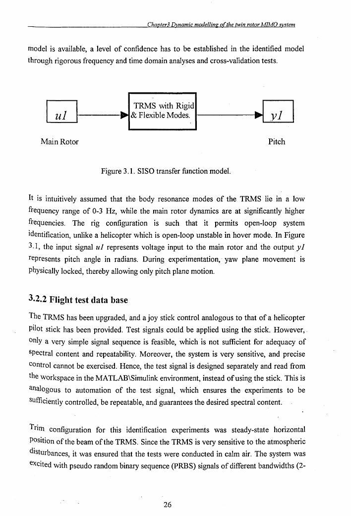
TRMS with Rigid
ui ...... & Flexible Modes. ... .yi ~ ......
Main Rotor Pitch
Figure 3.1. SISO transfer function model.
It is intuitively assumed that the body resonance modes of the TRMS lie in a low
frequency range of 0-3 Hz, while the main rotor dynamics are at significantly higher
frequencies. The rig configuration is such that it permits open-loop system
identification, unlike a helicopter which is open-loop unstable in hover mode. In Figure
3.1, the input signal ul represents voltage input to the main rotor and the outputyl
represents pitch angle in radians. During experimentation,· yaw plane movement is
physically locked, thereby allowing only pitch plane motion.
3.2.2 Flight test data base
The TRMS has been upgraded, and a joy stick control analogous to that of a helicopter
pilot stick has been provided. Test signals could he applied using the stick. However"
only a very simple signal sequence is feasible, which is not sufficient for adequacy of
spectral content and repeatability. Moreover, the system is very sensitive, and precise
Control cannot be exercised. Hence, the test signal is designed separately and read from
the workspace in the MATLAB\Simulink environment, instead of using the stick. This is
analogous to automation of the test signal, which ensures the experiments to be
SUfficiently controlled, be repeatable, and guarantees the desired spectral content.
Trim configuration for this identification experiments was steady-state horizontal
Position of the beam of the TRMS. Since the TRMS is very sensitive to the atmospheric
disturbances, it was ensured that the tests were conducted in calm air. The system was
eXcited with pseudo random binary sequence (PRBS) signals of different bandwidths (2-
26
Chapter3 Dynamic modelling of the twin rotor MIMO system
20 Hz), so as to ensure that all resonance modes are captured both in the range of
interest, i.e. 0-3 Hz, and out of curiosity to find out if any modes exist beyond this
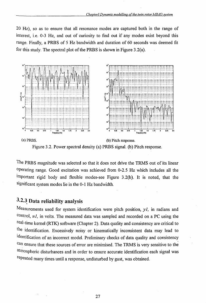
range. Finally, a PRBS of 5 Hz bandwidth and duration of 60 seconds was deemed fit
for this study. The spectral plot of the PRBS is shown in Figure 3.2(a).
10'·~--I.---'------'-_-'-----'------'----"_..I----1----' o 0.25 0.5 0.75 1 125 1.5 1.75 2 225 2.5
10.·'----'-----'-----L_-'----J..---1----"_..I----1-----' o 0.25 0.5 0.75 1 125 1.5 1.75 2 225 2.5
Frequency (Hz) Frequency (Hz)
(a) PRBS. (b) Pitch response.
Figure 3.2. Power spectral density (a) PRBS signal. (b) Pitch response.
The PRB S magnitude was selected so that it does not drive the TRMS out of its linear
operating range. Good excitation was achieved from 0-2.5 Hz which includes all the
Important rigid body and flexible modes-see Figure 3 .2(b). It is noted, that the
significant system modes lie in the 0-1 Hz bandwidth.
3.2.~ Data reliability analysis
Measurements used for system identification were pitch position, yJ, in radians and
Control, uJ, in volts. The measured data was sampled and recorded on a PC using the
real-time kernel (RTK) software (Chapter 2). Data quality and consistency are critical to
the identification. Excessively noisy or kinematically inconsistent data may lead to
identification of an incorrect model. Preliminary checks of data quality and consistency
can ensure that these sources of error are minimised. The TRMS is very sensitive to th~ atmospheric disturbances and in order to ensure accurate identification each signal was
repeated many times until a response, undisturbed by gust, was obtained.
27
Chapter3 Dvnamic modelling o(the twin rotor MIMO system
3.2.4 Sampling Rate
One of the important considerations in discrete-time systems is the sampling rate. A low
sampling rate would yield data with little information about the process dynamics. A
high sampling rate, on the other hand, will lead to poor signal to noise ratio (SNR).
Low SNR means less informative data and the estimation would be biased. A good
choice of sampling rate thus is a trade-off between noise reduction and relevance for the
process dynamics.
Since the intended use of the system model is for control purposes, certain other aspects
need to be considered. It is recommended that the sampling interval for which the model
is built should be the same for the control application [35]. There are, however, some
useful guidelines, which relate the sample interval to the response of the system to be
identified. Certain symptoms will appear in the estimated model if a wrong sample
interval is selected. This can be done by observing the position of all poles of the
obtained model in the z-plane. If the poles and zeros are found clustered tightly around
I z I ==1, this indicates that the system has been sampled too rapidly. If the poles and
zeros are found clustered tightly around the origin of the z-plane, this indicates that the
system has been sampled too slowly. The ideal aim is for a set of estimated model
parameters, which correspond to a reasonable spread of pole-zero positions in the z
plane [36].
There are some useful rules of thumb for setting the initial sampling rate, based on the
dominant time constant (i.e. from the step response), process settling 'time and guessed
bandwidth of the system. For instance, one could choose i) sampling rate of 1/5 of time
~onstant or 10 times the guessed system bandwidth [35], ii) four times the guessed
system bandwidth [36], and iii) 10 % of settling time [37], with optimal choice lying
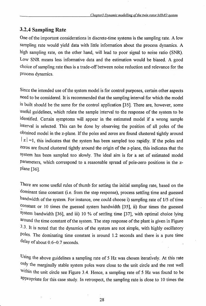
around the time constant of the system. The step response of the plant is given in Figure
3.3. It is noted that the dynamics of the system are not simple, with highly oscillatory
Poles. The dominating time constant is around 1.2 seconds and there is a pure time
delay of about O. 6~0. 7 seconds.
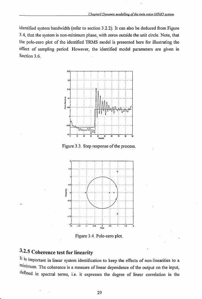
Dsing the above guidelines a sampling rate of 5 Hz was chosen iteratively. At this rate
on~y the marginally stable system poles were close to the unit circle and the rest well
Within the unit circle see Figure 3.4. Hence, a sampling rate of 5 Hz was found to be
appropriate for this case study. In retrospect, the sampling rate is close to 10 times the
28
Chapter3 Dynamic modelling ofthe twin rotor A1MO system
identified system bandwidth (refer to section 3.2.2). It can also be deduced from Figure
3.4, that the system is non-minimum phase, with zeros outside the unit circle. Note, that
the pole-zero plot of the identified TRMS model is presented here for illustrating the
effect of sampling period. However, the identified model parameters are given in
Section 3.6.
Figure 3.3. Step response of the process.
Figure 3.4. Pole-zero plot.
3.2.5 Coherence test for linearity
It is important in linear system identification to keep the effects of non-linearities to a
lllinimum. The coherence is a measure of linear dependence of the output on the input,
defined in spectral terms, i. e. it expresses the degree of linear correlation in the
29
Chapter3 Dvnamic modelling ofthe twin rotor MIMO system
frequency domain between the input and the output signal. An important use of the
coherence spectrum is its application as a test of signal-to-noise ratio and linearity
between one or more input variables and an output variable. The coherence function
Y\y(f) is given by:
S xx (f)Syy (f) (3.1)
where S.'I:."( and Syy are the auto-spectral densities of the input and output signals
respectively and S xy is the cross-spectral density between the input and output signals.
By definition, the coherence function lies between 0 and 1 for all frequencies f,
o ~y2>.y(f) ~ 1
If x(t) and y(t) are completely unrelated, the coherence function will be zero. While a
totally noise-free linear system would yield y\y{ f) = 1. The coherence function may
thus be viewed as a type of correlation function in the frequency domain where a
coherence function not equal to 1 indicates the presence of one or more of the following [38].
• Extraneous noise is present in the input and the output measurements.
• The system relating x(t) and y(t) is not linear.
• The output y(t) is due to an input x(t) as well as other inputs such as external
disturbances.
• Resolution bias errors are present in the spectral estimates.
When a system is noisy or nonlinear, the coherence function indicates the accuracy of a
--linear identification as a function of frequency. The closer it is to unity at a given
frequency, the more reliance can be placed on an accompanying frequency response
estimate, at that frequency. For a real-world application, which will be nonlinear and
affected, to some extent by noise, a plot of the coherence function against frequency
wiII indicate the way in which the disturbances change across the frequency band.
Coherence testing is employed on the input-output data channel and is discussed next.·
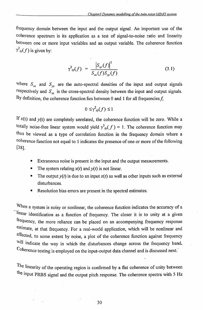
The linearity of the operating region is confirmed by a flat coherence of unity between
the input PRB S signal and the output pitch response. The coherence spectra with 5 Hz
30
Clwpter3 Dvnamic modelling o(the twin rotor MIMO system
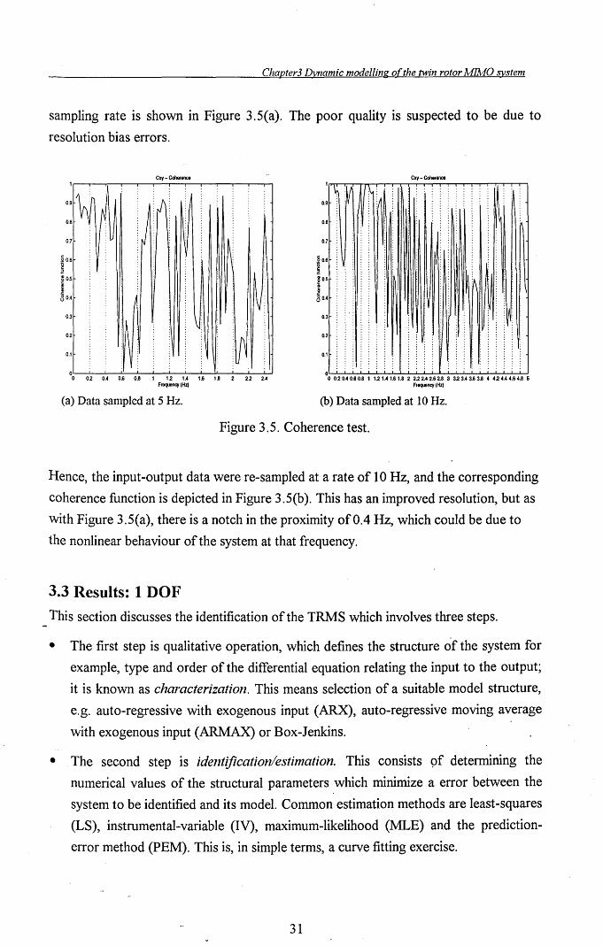
sampling rate is shown in Figure 3.5(a). The poor quality is suspected to be due to
resolution bias errors.
Cxy - Coherence
0.7
0.3
0.2
0.1
o~~~~~~~~~~~~~~
o 02 0.4 0.6 0.8 1 12 1.4 1.6 1.8 2 22 2.4 Fmquency(Hz)
(a) Data sampled at 5 Hz.
Cxy - Coharence
1.~ •.• 11" T~ 0.9 IV
:
0.8
0.7
0.3
0.2
0.1
o~~~~~~~~~~~~~ o 0.20.40.60.8 1 1.2 1.4 1.6 1.8 2 2.2 2.4 2.6 2.8 3 3.23.4 3.6 3.8 4 4.24.44.64.8 5
Frequency (Hz)
(b) Data sampled at 10Hz.
Figure 3.5. Coherence test.
Hence, the input-output data were re-sampled at a rate of 10Hz, and the corresponding
coherence function is depicted in Figure 3.5(b). This has an improved resolution, but as
with Figure 3.5(a), there is a notch in the proximity of 0.4 Hz, which could be due to
the nonlinear behaviour of the system at that frequency.
3.3 Results: 1 DOF
This section discusses the identification of the TRMS which involves three steps.
• The first step is qualitative operation, which defines the structure of the system for
example, type and order of the differential equation relating the input to the output;
it is known as characterization. This means selection of a suitable model structure,
e.g. auto-regressive with exogenous input (ARX), auto-regressive moving average
with exogenous input (ARMAX) or Box-Jenkins.
• The second step is identijication/estinlation. This consists pf determining the
numerical values of the structural parameters which minimize a error between the
system to be identified and its model. Common estimation methods are least-squares
(LS), instrumental-variable (IV), maximum-likelihood (MLE) and the prediction
error method (PEM). This is, in simple terms, a curve fitting exercise.
31
ChapterJ Dynamic modelling ofthe twin rotor MIlvlO system
• The third step, vertfication, consists of relating the system to the identified model
responses in time or frequency domain to instil confidence in the obtained model.
Residual test, bode plots and cross-validation tests are generally employed for model
validation.
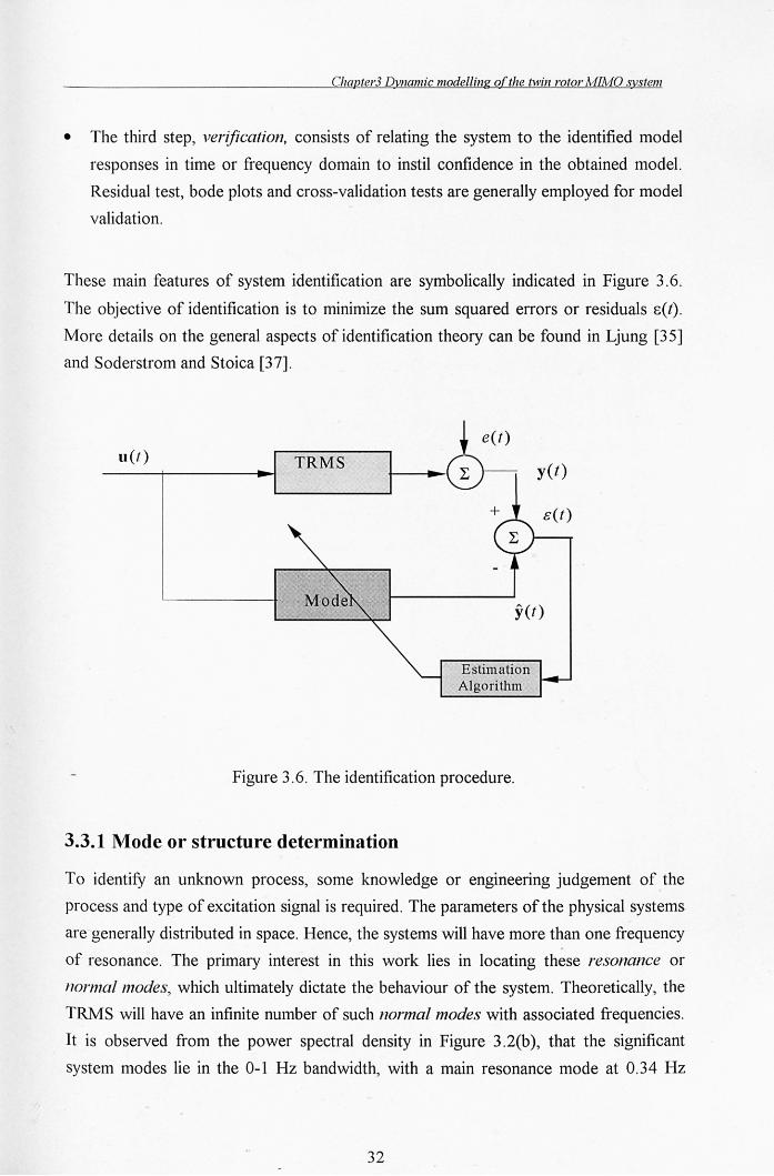
These main features of system identification are symbolically indicated in Figure 3.6.
The objective of identification is to minimize the sum squared errors or residuals e(t).
More details on the general aspects of identification theory can be found in Ljung [35]
and Soderstrom and Stoica [37].
u(t) TRMS yet)
y(t)
Estimation , Algorithm
Figure 3.6. The identification procedure.
3.3.1 Mode or structure determination
To identify an unknown process, some knowledge or engineering judgement of the
process and type of excitation signal is required. The parameters of the physical systems
are generally distributed in space. Hence, the systems will have more than one frequency
of resonance. The primary interest in this work lies in locating these resonance or
normal modes, which ultimately dictate the behaviour of the system. Theoretically, the
TRMS will have an infinite number of such normal modes with associated frequencies.
It is observed from the power spectral density in Figure 3 .2(b), that the significant
system modes lie in the 0-1 Hz bandwidth, with a main resonance mode at 0.34 Hz
32
ChapterJ Dynamic modelling ofthe twin rotor AIIMO B'stem
which can be attributed to the main body dynamics. A model order of 2, 4 or 6
corresponding to prominent normal modes at 0.25, 0.34 and 0.46 Hz and a rigid body
pitch mode is thus anticipated.
3.3.2 Parametric modelling
Equipped with the insight mentioned above, attention IS focused on selecting
paranleters in the model to obtain a satisfactory system description. A parametric
method can be characterised as a mapping from the experimental data to the estimated
parameter vector. Such models are often required for control application purposes. With
no prior knowledge of sensor or instrument noise, a preliminary second order ARX
model was assumed for the ul ~ yl channel. The auto-correlation of residuals revealed
negative correlation at lag 1, indicating the presence of non-white, sensor or external
noise. This necessitates estimating the noise statistics. Therefore, the ARMAX model
structure:
(3.2)
was selected for further analysis, where, ai' hi' ci , are the parameters to be identified,
and, e(t) is a zero mean white noise. This structure takes into account both the true
system and noise models.
The predictor for equation (3.2) is given by
y(tI8) = B(q) u(t) + [1- A(q)]y(t) C(q) C(q)
(3.3)
where
y(t18) = is the predicted output according to model parameter 8.
A(q) - 1 + -1 + + -na - a1q ......... an q a
33

CIlapter3 Dynamic modelling oftlle twin rotor MIA-fO system
C( ) - 1 + -1 -nc q - c1q + ........ ,+Cn q c
This means that the prediction is obtained by filtering u and y through a filter with
denominator dynamics determined by C( q) [35].
The predictor (3.3) can-be rewritten as follows. Adding [1- C(q)lY(tI8) to both sides of
equation (3.3) gives
y(tI8) = B(q)u(t) + [1- A(q)]y(t) + [C(q) -1][ y(t) - y(tI8)] (3.4)
Introducing the prediction error
E ( t , 8) = y ( t ) - y ( t 18 ) (3.5)
and the vector
<p(t,8) = [-y(t-1) ... - y(t-na ) u(t-1) ... - U(t-nb) £(t -1,8) ... £(t -nc ,8)]T
(3.6)
Then equation (3.4) can be expressed as
y(t18) = <p(t, 8) 8 (3.7)
The equation (3.7) is referred as a pseudolinear regression due to the nonlinear effect
of 8 in the vector <p(t,8) .
In the time-domain identification, prediction errors or residuals E(t) (this form is used
for notational simplicity instead of E ( t , 8) ) are analysed for determining an
appropriate model structure. Residuals are the errors observed between the model
response and the actual response of the plant to the same excitation. A model structure.
can be found, iteratively, that minimises the absolute sum of the residuals. Ideally, the
residuals E(t) should be reduced to an uncorrelat~d sequence denoted by e(t) with zero
mean and finite variance. Correlation based model validity tests are employed to verify if
e(t) ~ E(t) (3.8)
34
Chapter3l)ynamic modelling of the twin rotor MIMO system
This can be achieved by verifying if all the correlation functions are within the
confidence intervals. When equation (3.8) is true then,
<\> EE ('t) = E [ E (t - 'C) E ( t )] = () ( 'C ) (3.9a)
<\>UE ('C) = E[u(t - 'C)E(t)] = 0 (3.9b)
where <l>n: (t) and <l>ue (t) are the estimated auto-correlation function of the residuals
and the cross-correlation function between u(t) and £(t), respectively. o( -r) is an
impulse function. These two tests can be used to check the deficiencies of both the plant
and the noise model. The expression (3. 9b) implies that the plant model is correct and
the residuals are uncorrelated with the input. But if <l>ee ('t) 1= o(t), then it is an
indication that although the plant model is correct, the noise model is incorrect and
therefore, the residuals are autocorreleted. On the other hand, if the noise model is
correct and the plant model is biased, then the residuals are both autocorrelated such
that <l>ee ('t) 1= o(t) and correlated with the input <l>ue(-r) 1= O.
3.3.3 Identification
Having selected a model structure, it is next desired to estimate the parameter vector
e . The search for the best model within the set then becomes a problem of determining
or estimating e. Once the model and the predictor are given, the prediction errors are
computed as in (3.5). The parameter estimate eN is then chosen to make the prediction
error E ( 1 , e), ..... E (N , e) small. One of the common method to obtain eN is to
minimise a quadratic cost-function VN (e) defined as,
(3.10)
Where N denotes the number of data points.
This problem is known as "the nonlinear least-squares problem" in numerical analysis.
However, since y(tle) in equation (3.7) is a nonlinear function of e, and therefore, the
function V N (e) cannot be minimised analytically. Instead, some numerical minimisation
routines such as the gradient or steepest-descent and Gauss-Newton can be used to
35
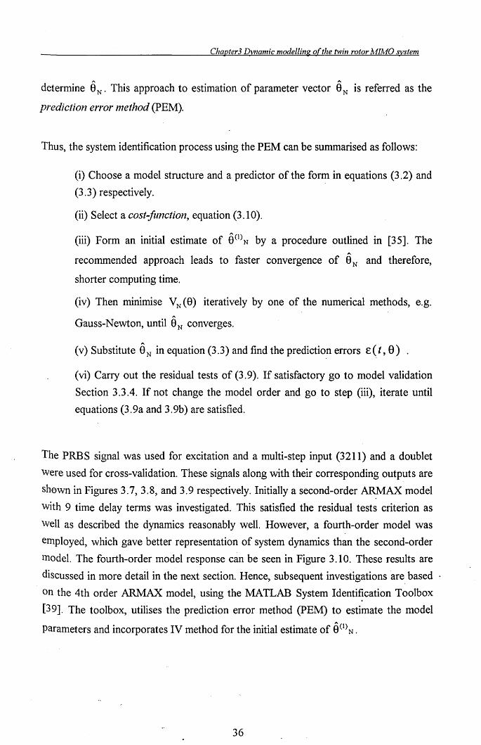
Chapter3 Dynamic modelling o(the twin rotor MIMO system
determine eN' This approach to estimation of parameter vector eN is referred as the
prediction error nlethod (PEM).
Thus, the system identification process using the PEM can be summarised as follows:
(i) Choose a model structure and a predictor of the form in equations (3.2) and
(3.3) respectively.
(ii) Select a cost-function, equation (3.10).
(iii) Form an initial estimate of e(l)N by a procedure outlined in [35]. The
recommended approach leads to faster convergence of eN and therefore,
shorter computing time.
(iv) Then minimise VN (8) iteratively by one of the numerical methods, e.g.
Gauss-Newton, until eN converges.
(v) Substitute eN in equation (3.3) and find the prediction errors E( t, e)
(vi) Carry out the residual tests of (3.9). If satisfactory go to model validation
Section 3.3.4. If not change the model order and go to step (iii), iterate until
equations (3. 9a and 3. 9b) are satisfied.
The PRBS signal was used for excitation and a multi-step input (3211) and a doublet
Were used for cross-validation. These signals along with their corresponding outputs are
shewn in Figures 3.7, 3.8, and 3.9 respectively. Initially a second-order ARMAX model
with 9 time delay terms was investigated. This satisfied the residual tests criterion as
well as described the dynamics reasonably well. However, a fourth-order model was
employed, which gave better representation of system dynamics than the second-order
model. The fourth-order model response can be seen in Figure 3.10. These results are
discussed in more detail in the next section. Hence, subsequent investigations are based
on the 4th order ARMAX model, using the MATLAB System Identi~cation Toolbox
[39]. The toolbox, utilises the prediction error method (PEM) to estimate the model
parameters and incorporates IV method for the initial estimate of e(l)N.
36
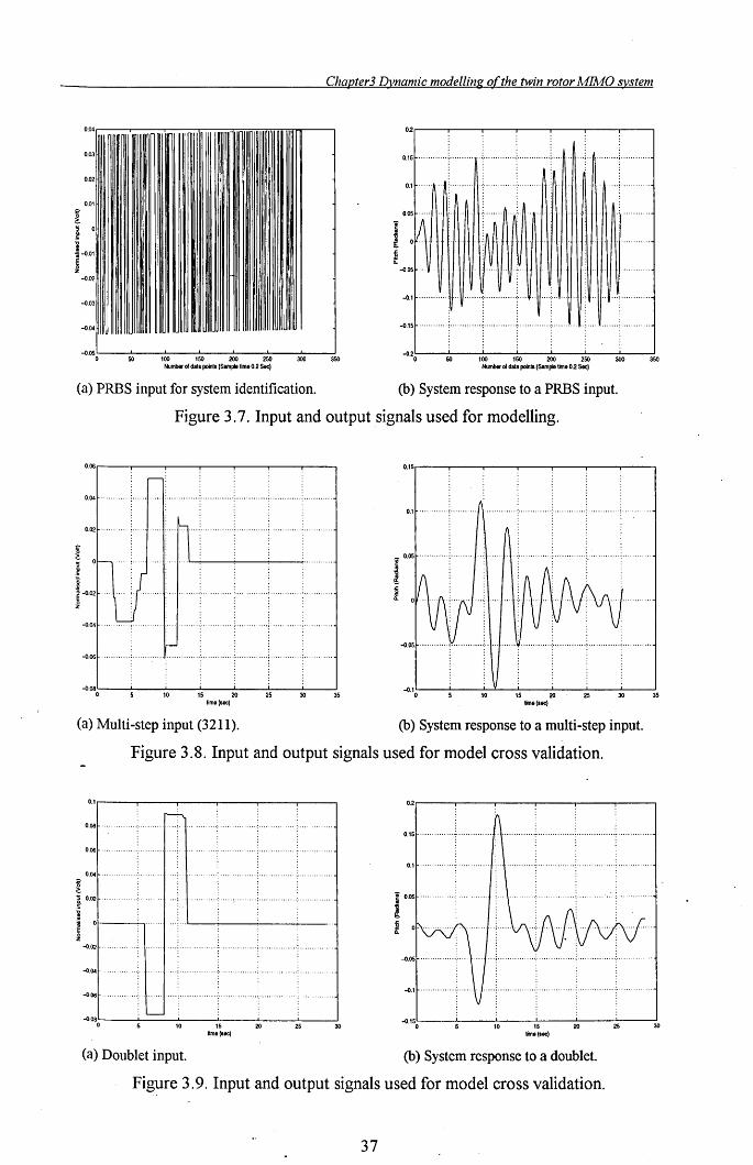
Chapter3 Dynamic modelling of the twin rotor MIA10 system
0.04 02,--,---,----,----,--......---,.----,
.m I O.'sl-······· .. ···;··········\···;.······ .... ···: ...... ·· .. ····:·····fl If· .. , ., ........ ; ............ -1
0.02 il 0.' .....
0.Q1
! '3 0 .e- III1III1I
0.05 .....
I I~ 'I 1-0.Q1
I,
l o·
~ .• N j I -0.02 I
I
-0.03
-0.04
-0.05 0 50 '00 ,SO 200 250 300 350
Num"'" of data points (Sampte tlma 0.2 Sec)
Q. -0.05 ... ~ ..
-0.' .......... ..
-o.'S!- .... , ...... ·~ .... · ...... ··< .. · .. ·· .... ·· .. : .......... ·· .. ,· .... ·' .. ·1 .. , ............. , ............ ,
-0.201--~50--'-'00---1.'50----:-I200-:-----:-250~----:3OO~~350 Number at claiR points (Sampte lima 02 Sac)
(a) PRBS input for system identification. (b) System response to a PRBS input.
Figure 3.7. Input and output signals used for modelling.
0.06,..---.----.----,------r----r-----r----,
0.04 ...... · ...... ·; ...... 1
0.02
! ! on'" I~~tj
-0.04 ............ · ...... ·· .. ·+·· .. 1 ........ : .............. : ............. ; ............. ; ............ -1
Ii---0.06 ........... : ............. ~ .............. : .............. : ............. ; ............. ; ........... -i
-o·080'---"----'-'0---"'S---'2O--2':-S --30"-----'35
tlmo(sac)
0.' ............ , ........... /1 ............. : .............. : .............. , ............. , .......... ,
_ 0.051- .......... :: .... · .. ·,
; l ~
-0.051- ............ ,~ ........... ··: .. 1
-o·'0'---~-..J...,0....!...-----1:'S-~2O:------:2:-S --30~----!3S' tima(aac)
(a) Multi-step input (3211). (b) System response to a multi-step input.
Figure 3.8. Input and output signals used for model cross validation.
O.,r-----r----.---.-----..--.-----. 0.2,----......----.---.-----..--,------,
0.08 ............ · ... : ...... · .. ·1 .... ;·+ ...... · .... : .. · ...... · ....... , .......... · .... -: .... . O.'sl- .. · ........ · .. :- .. · .. · .... ·· .. 1 , ............... : ............... ,; ................ : ............... -1
0.06 ...... ·· ...... ·: ...... · .. ·/··:11 .. · ... : ............... : ................ : ............ -1
0.'1- .. , ........ ·;··· .... · .... +·+· ...... ·· .. :·· ........ · .... ·: ...... · .... · .. ·, .. · ......... -1 0.04!- ........ · ... :.... ·I .... ; .. I .... · ...... ·: .. · ............. ; .......... · .... ·:· ...... ·· .... -i
0.02 I 0.051-· .. · ...... ·· ... : ............. j .. :: .... \ ........... :- .............. , ................ , ............. ,
-0.02 ...... I ..
-0.04
-0.06," ............... :
-0.0810:--_L.-'---,L.o --"'-5 ---'2O---'-2S-----I
30 timo(lec)
(a) Doublet input.
l
-0.051-· .......... ·· .. : ....
-o.,!- ............. : ... \ / ... ; ................ :- .............. : ............ : ......... '''-1
-o.'S'OI---'----"0'-----',S---'-2O---=2S-----!30
timo( ... )
(b) System response to a doublet.
Figure 3.9. Input and output signals used for model cross validation.
37
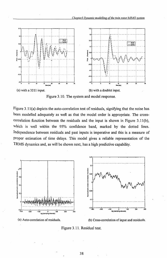
Chapter3 Dvnamic modelling ofthe twin rotor MIMO ~stem
0.15.-----..---..---..---.,..--.,..--.,..---,
~.05 '''''. \/
~.1
~.15
....... i .... j ...... ,.
,.-. Mtll -51em ....................................
~.2'---.L-.._-'--_-'--_-'--_-'--_...L...-------'
o w ~ ~ ~ ~ ~ lime (sec)
0.25.-------.-----,---,----,----,-------,
: : : 0.2 ............... : ................ ,:, .............. : ................ , ............... -: .............. .
. :,', . : : 0.15 ............ ...: ............... ,. \ ............. : ................ ; ................ ~ ............ ..
: i i : 1-' ~odeIl: : i: i .-5Iem : 0.1 ......... ... ;: .. , .......
i 0.05 .................... .
[
~.05 .....
~.2:0L------I~-..J..l0---I:-15 ----:~1:-----!25::-----:'~
time (sec)
(a) with a 3211 input. (b) with a doublet input.
Figure 3.10. The system and model response.
Figure 3. 11 (a) depicts the auto-correlation test of residuals, signifying that the noise has
been modelled adequately as well as that the model order is appropriate. The cross
correlation function between the residuals and the input is shown in Figure 3 .11 (b),
which is well within the 95% confidence band, marked by the dotted lines.
Independence between residuals and past inputs is imperative and this is a measure of
proper estimation of time delays. This model gives a reliable representation of the
TRMS dynamics and, as will be shown next, has a high predictive capability.
0.6
0.4
0.2
-~~0::-0----'200--_....Ll00---'-0 ----'100'----'-200-----'300
lag (sampling intelVals)
(a) Auto-correlation of residuals.
0.15.------r----,-----,.------r-----.----,
0.1 c .~
~ ~ 0.05
til G ~ Y 0
~ 'i ~ -0.05
§ z
-0.1
-0'%-0 --_2...L.00--_l00'---...... 0--,..L..00--200'----l300
lag (sampling Intervals)
(b) Cross-correlation of input and residuals.
Figure 3. 11. Residual test.
38
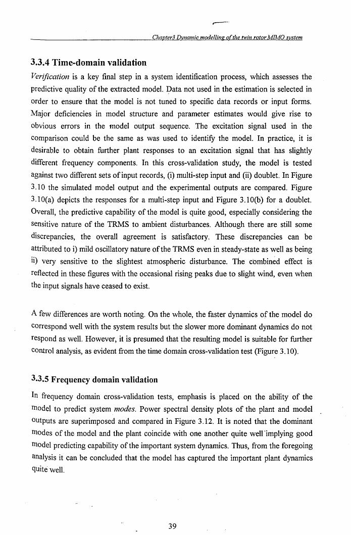
Chapter3 Dynamic modelling o(the twin rotor MlJvfO system
3.3.4 Time-domain validation
Verification is a key final step in a system identification process, which assesses the
predictive quality of the extracted model. J?ata not used in the estimation is selected in
order to ensure that the model is not tuned to specific data records or input forms.
Major deficiencies in model structure and parameter estimates would give rise to
obvious errors in the model output sequence. The excitation signal used in the
comparison could be the same as was used to identify the model. In practice, it is
desirable to obtain further plant responses to an excitation signal that has slightly
different frequency components. In this cross-validation study, the model is tested
against two different sets of input records, (i) multi-step input and (ii) doublet. In Figure
3. 10 the simulated model output and the experimental outputs are compared. Figure
3.10(a) depicts the responses for a multi-step input and Figure 3.10(b) for a doublet.
Overall, the predictive capability of the model is quite good, especially considering the
sensitive nature of the TRMS to ambient disturbances. Although there are still some
discrepancies, the overall agreement is satisfactory. These discrepancies can be
attributed to i) mild oscillatory nature of the TRMS even in steady-state as well as being
ii) very sensitive to the slightest atmospheric disturbance. The cbmbined effect is
reflected in these figures with the occasional rising peaks due to slight wind, even when
the input signals have ceased to exist.
A few differences are worth noting. On the whole, the faster dynamics of the model do
correspond well with the system results but the slower more dominant dynamics do not
respond as well. However, it is presumed that the resulting model is suitable for further
corurol analysis, as evident from the time domain cross-validation test (Figure 3.10).
3.3.5 Frequency domain validation
In frequency domain cross-validation tests, emphasis is placed on the ability of the
Inodel to predict system nlodes. Power spectral density plots of the plant and model
outputs are superimposed and compared in Figure 3.12. It is noted that the dominant
modes of the model and the plant coincide with one another quite wen·implying good
model predicting capability of the important system dynamics. Thus, from the foregoing
analysis it can be concluded that the model has captured the important plant dynamics
quite well.
39
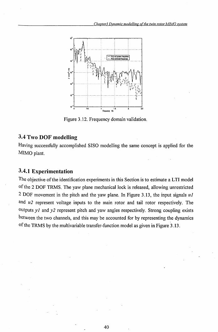
Chapter3 Dynamic modelling ofthe twin rotor A1lAI0 ~stem
1~~--~----~--~----~--~
10-" ................ ..
10-.,L-----J.-----.l------'-----.l.-------' o 0.5 1 1.5 2.5
Frequency Hz
Figure 3.12. Frequency domain validation.
3.4 T,vo DOF modelling
Having successfully accomplished SISO modelling the same concept is applied for the
MIMO plant.
3.4.1 Experimentation
The objective of the identification experiments in this Section is to estimate a LTI model
of the 2 DOF.TRMS. The yaw plane mechanical lock is released, allowing unrestricted
2 DOF movement in the pitch and the yaw plane. In Figure 3.13, the input signals u1
and u2 represent voltage inputs to the main rotor and tail rotor respectively. The
outputs y1 and y2 represent pitch and yaw angles respectively. Strong coupling exists
between the two channels, and this may be accounted for by representing the dynamics
of the TRMS by the multivariable transfer-function model as given in Figure 3.13.
40
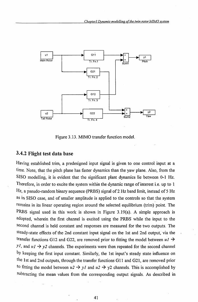
Chapter3 I)ynamic modelling of the twin rotor MIMO &stem
Figure 3.13. MIMO transfer function model.
3.4.2 Flight test data base
Having established trim, a predesigned input signal is given to one control input at a
time. Note, that the pitch plane has faster dynamics than the yaw plane. Also, from the
SISO modelling, it is evident that the significant plant dynamics lie bet~een 0-1 Hz.
Therefore, in order to excite the system within the dynamic range of interest i.e.·up to 1
Hz, a p'seudo-random binary sequence (PRBS) signal of2 Hz band limit, instead of 5 Hz
as in SISO case, and of smaller amplitude is applied to the controls so that the system
remains in its linear operating region around the selected equilibrium (trim) point. The
PRBS signal used in this work is shown in Figure 3.19(a). A simple approach is
adopted, wherein the first channel is excited using the PRBS while the input to the
second channel is held constant and responses are measured for the two outputs. The
steady-state effects of the 2nd constant input signal on the 1 st and 2nd output, via the
transfer functions G 12 and G22, are removed prior to fitting the model between u1 ~
Yi, and u1 ~ y2 channels. The experiments were then repeated for the second channel
by keeping the first input constant. Similarly, the 1st input's steady state influence on
the 1 st and 2nd outputs, through the transfer functions GIl and G21, are removed prior
to fitting the model between u2 ~ y 1 and u2 ~ y2 channels. This is accomplished by
SUbtracting the mean values from the corresponding output signals. As described in
41
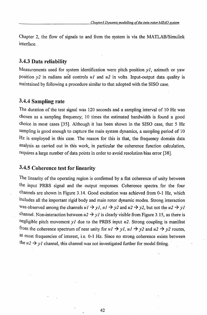
Chapter3 Dynamic modelling o(the twin rotor MMO system
Chapter 2, the flow of signals to and from the system is via the MA TLAB/Simulink
interface.
3.4.3 Data reliability
Measurements used for system identification were pitch position y J, azimuth or yaw
position y2 in radians and controls uJ and u2 in volts. Input-output data quality is
maintained by following a procedure similar to that adopted with the SISO case.
3.4.4 Sampling rate
The duration of the test signal was 120 seconds and a sampling interval of 10Hz was
chosen as a sampling frequency; 10 times the estimated bandwidth is found a good
choice in most cases [35]. Although it has been shown in the SISO case, that 5 Hz
sampling is good enough to capture the main system dynamics, a sampling period of 10
Hz is employed in this case. The reason for this is that, the frequency domain data
analysis as carried out in this work, in particular the coherence function calculation,
requires a large number of data points in order to avoid resolution bias error [38].
3.4.5 Coherence test for linearity
The linearity of the operating region is confirmed by a flat coherence of unity between
the input PRBS signal and the output responses. Coherence spectra, for the four
channels are shown in Figure 3.14. Good excitation was achieved from 0-1 Hz, which
includes all the important rigid body and main rotor dynamic modes. Strong interaction
Was {)bserved among the channels uJ ~ yJ, uJ ~ y2 and u2 ~ y2, but not t~e u2 ~ yJ
channel. Non-interaction between u2 ~ yJ is clearly visible from Figure 3.15, as there is
negligible pitch movement y J due to the PRB S input u2. Strong coupling is manifest
from the coherence spectrum of near unity for uJ ~ yJ, uJ ~ y2 and u2 ~ y2 routes,
at most frequencies of interest, i.e. 0-1 Hz. Since no strong coherence exists between
the u2 ~ y J channel, this channel was not investigated further for model fitting.
42
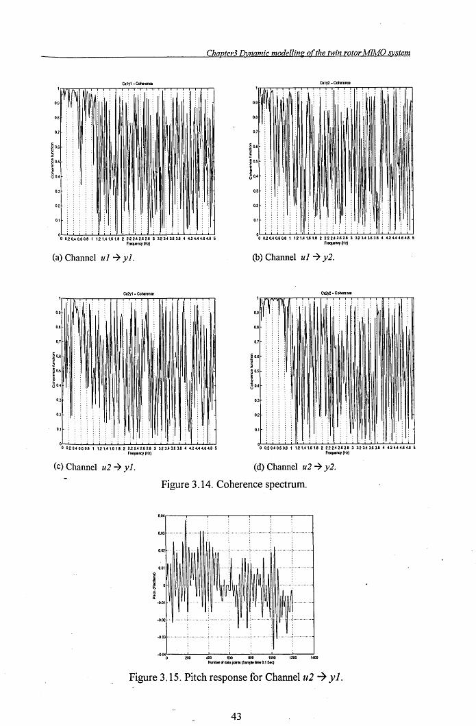
Chapter3 Dynamic modelling ofthe twin rotor MIMO system
Cxlyl - Coherence
0.7
0.6
0.5
0.4
0.3
0.2
0.1
O~~~-L~~~~~~~~-L~~~~
o 0.20.40.60.8 1 1.2 1.4 1.6 1.8 2 2.22.42.62.8 3 3.23.43.63.8 4 4.24.44.64.8 5 Frequency (Hz)
(a) Channel ul -7 yl.
Cx2yl - Coherence
0.9 I~: 0.8
I
0.7
c jO.6
g 0.5
j 80.4
0.3
0.2
0.1
O~~~~~-L~~~~~LJ-L~~~~ o 0.20.40.60.8 1 1.21.41.61.8 2 2.22.42.62.8 3 3.23.43.63.8 4 4.24.44.64.8 5
Frequency (Hz)
(c) Channel u2 -7 yl.
0.9
0.8
0.1
OLi~~-L~LL~~~~~~-L~~~~
o 0.20.40.60.6 1 1.2 1.4 1.6 1.8 2 2.22.42.62.8 3 3.2 3.U.6 3.8 4 4.24.44.64.8 5 Frequency (Hz)
(b) Channel ul -7 y2.
Cx2y2 - Coherence
0.8
0.7
0.3
0.2
0.1
o~~~~~-L~~~~~~-U~~~~ o 0.20.40.60.6 1 1.21.41.61.8 2 2.22.42.62.8 3 3.23.43.63.8 4 4.24.44.64.8 5
Frequency (Hz)
(d) Channel u2 -7 y2.
Figure 3.14. Coherence spectrum.
I ~
0.04
0.03
0.02
0.0 1
0
-0.0 1
-0.02
-0.0 3
-0.04 o
.........
,- .....
','"
...
w~ N
~~. .......... ..... . ...
:
200 400 600 800 1000 1200 1400 Number 01 data poilt. (Sample 1ino 0.1 Sec)
Figure 3.15. Pitch response for Channel u2 ~ y 1.
43
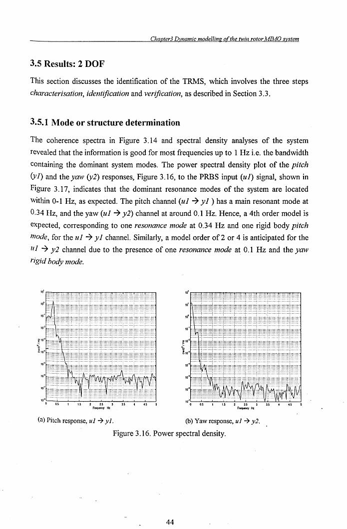
Chapter3 Dvnamic modelling o(the twin rotor MIA10 system
3.5 Results: 2 DOF
This section discusses the identification of the TRMS, which involves the three steps
characterisation, identification and verification, as described in Section 3.3.
3.5.1 Mode or structure determination
The coherence spectra in Figure 3.14 and spectral density analyses of the system
revealed that the information is good for most frequencies up to 1 Hz i.e. the bandwidth
containing the dominant system modes. The power spectral density plot of the pitch
(yi) and the yaw (y2) responses, Figure 3.16, to the PRBS input (ui) signal, shown in
Figure 3. 17, indicates that the dominant resonance modes of the system are located
within 0-1 Hz, as expected. The pitch channel (ui ~ yJ ) has a main resonant mode at
0.34 Hz, and the yaw (ui ~ y2) channel at around 0.1 Hz. Hence, a 4th order model is
expected, corresponding to one resonance mode at 0.34 Hz and one rigid body pitch
mode, for the ui ~ yi channel. Similarly, a model order of 2 or 4 is anticipated for the
u i ~ Y 2 channel due to the presence of one resonance nlode at 0.1 Hz and the yaw
rigid body nl0de.
(a) Pitch response, ul 7 yl. (b) Yaw response, ul 7 y2.
Figure 3.16. Power spectral density.
44
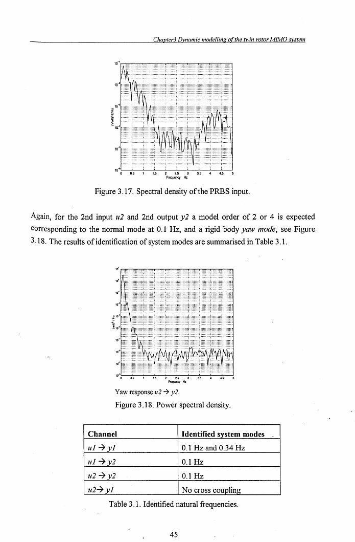
Chapter3 Dynamic modelling o(the twin rotor A1IlvfO system
1O-1mp~DITTT2T2§illS+TITIITl U\/ :~\ .. ; ......... ; .......... ; ......... ; ......... : .... ······:·········~··········;·········;·, ........ l
10-2 \II~ ::::::: :I:
:::.
10-6'----'----1..-----L._.L...--'----'-----L_..L---'----' o 0.5 1 1.5 2 2.5 3 3.5 4 4.5 5
Frequency Hz
Figure 3.17. Spectral density of the PRBS input.
Again, for the 2nd input u2 and 2nd output y2 a model order of 2 or 4 is expected
corresponding to the normal mode at 0.1 Hz, and a rigid body yaw mode, see Figure
3.18. The results of identification of system modes are summarised in Table 3.1.
1.5 2 2.5 3 3.5 4 4.5 Frequency Hz
Yaw response u2 -7 y2.
Figure 3.18. Power spectral density.
Channel Identified system modes
ul ~ yl 0.1 Hz and 0.34 Hz
ul ~ y2 0.1 Hz
u2~y2 0.1 Hz
u2~ yl No cross coupling
Table 3.1. Identified natural frequencies.
45
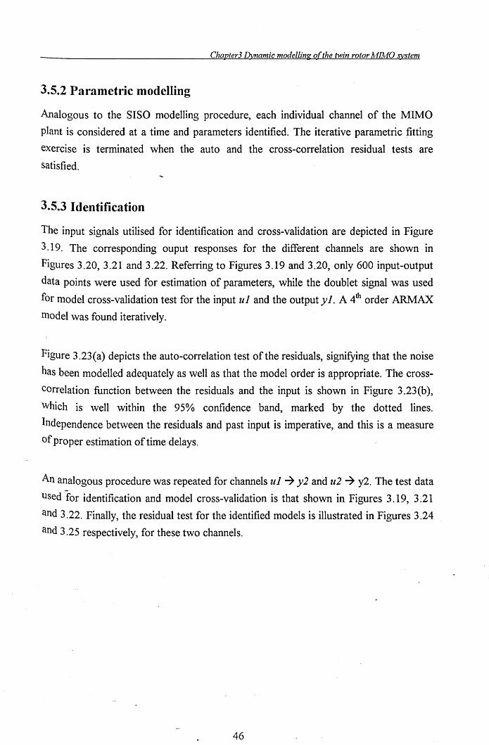
Chapter3 Dynamic modelling of the twin rotor A4lJvfO system
3.5.2 Parametric modelling
Analogous to the SISO modelling procedure, each individual channel of the MIMO
plant is considered at a time and parameters identified. The iterative parametric fitting
exercise is terminated when the auto and the cross-correlation residual tests are
satisfied.
3.5.3 Identification
The input signals utilised for identification and cross-validation are depicted in Figure
3.19. The corresponding ouput responses for the different channels are shown in
Figures 3.20, 3.21 and 3.22. Referring to Figures 3.19 and 3.20, only 600 input-output
data points were used for estimation of parameters, while the doublet signal was used
for model cross-validation test for the input ul and the output yl. A 4th order ARMAX
model was found iteratively.
Figure 3.23 ( a) depicts the auto-correlation test of the residuals, signifying that the noise
has been modelled adequately as well as that the model order is appropriate. The cross
correlation function between the residuals and the input is shown in Figure 3.23 (b ),
Which is well within the 95% confidence band, marked by the dotted lines.
Independence between the residuals and past input is imperative, and this is a measure
of proper estimation of time delays.
An analogous procedure was repeated for channels ul ~ y2 and u2 ~ y2. The test data
used for identification and model cross-validation is that shown in Figures 3.19, 3.21
and 3.22. Finally, the residual test for the identified models is illustrated in Figures 3.24
and 3.25 respectively, for these two channels.
46
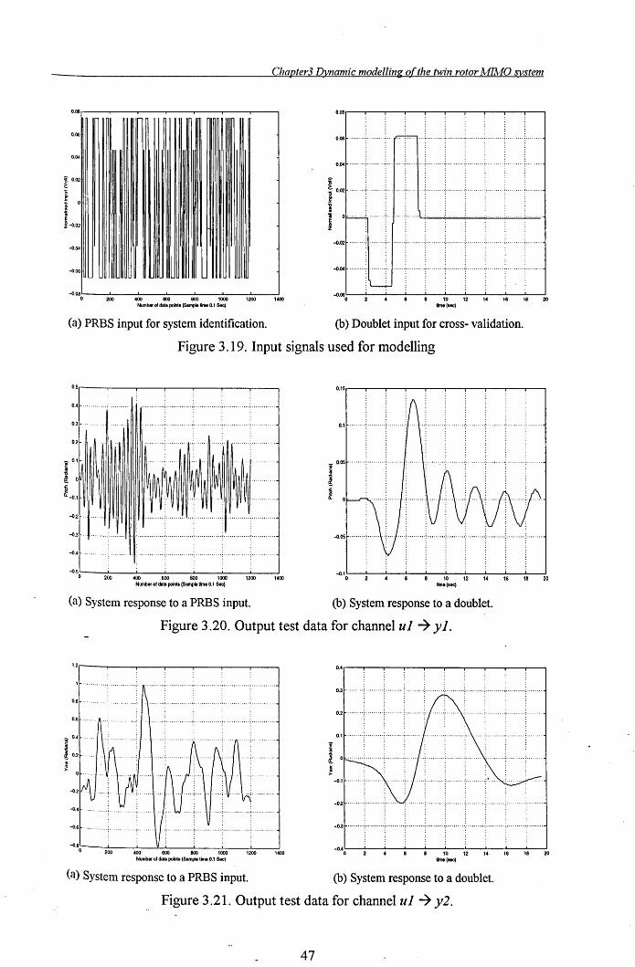
Chapter3 Dynamic modelling o(the twin rotor MIA10 ~stem
0.08r---.----r----r--~-___,.-___,-____.
0.06
0.04
-0.04
-0.06
-o·080'---200-'--...... 400--600'----800"'---1..L000
---'I200-----J,400
Number 01 data point. (Sample tl ... 0.1 Sec)
(a) PRBS input for system identification.
0.08..--..--,..--..--,..---.--,.---,--...----.-0
0.061- ........ ; ........ ·; .. (~=·-"'l .. ·: .... · .... :· ...... ·.:. ........ : ........ ·: .... · .... : ....... oj
0.04~ ........ : ........ ·: .. I· .... ~ .. ·+· , ........ , ........ , ........ ; ......... ; ........ , ...... -1
i s O.02~ .. · .... ; ........ ·;·+· .. ·! .... I .. ·: .. · ...... :·· .. · .... ·: .... ··· .. ·,·· ....... , ........ , ........ -1 .e-: I 0~; ........ : .. I .... ·:· .... ·L~~~~~=1 z
'-O.02r .. · .. · .. q ....... ; .+ .... ; ......... ; .......... ; ........... ; .......... : ........ , ......... , ....... -1
.-0.041- .. · .... ·;1 ...... ·:·1· .... : ........ ··" ......... , ......... ·: ..... · .. ·" ......... , ......... : ....... oj
'-O.06L--'---'---'---'----1...-"'---..L..--'---..L.----l own « ffl ffl ~
time (IOC)
(b) Doublet input for cross- validation.
Figure 3. 19. Input signals used for modelling
O. 5
O. 4
O. 3
O. 2
" O. 1
.~
l ~ II. -0
-0
-0
-0
.-0
0
.1
.2·
.3·
.4
.5 o
#l~ ~
.. ~ ~ ~ II
~\ .........
.....
200 400 600 800 1000 1200 1400 Number.' data points (Sample tin. 0.1 Soc)
(a) System response to a PRBS input.
0.15.---..--,..---,--,----.--,.---,--...----.----.
0.1~ .... · .. ·!· .... • .. ·! ...... · .. :·1
_ O.05r ...... ·' .... · .... , .... · .. + ...... I~ .... ··: .. , .. ··· .... ·; .. · .. ·;· .... · .. i· .. · .... , .. · .. ·-I .i l j Q. O~~· ...... ;·· .. ··,·' ........ :I .... f·; .. ··I .... ·;f
.-o.OSr .. · .... ·! .. ·· .. \ .. ! .... } .... ; ........ ··: .......... , .. · .. · .... ·, ...... ·· .. ·, .... · .... i ......... ~ ........ -I
'-O·IO'---'---'----1...-"'---,J....O -'-'-2 --'-'4 -.J...16-...l..,8----'~
ttm.(soc)
(b) System response to a doublet.
Figure 3.20. Output test data for channel ul ~ yl.
1.2r----.--_-r-_-..-_---.-_--. __ ,..-----.
0.8 ................. ..
0.6 .
! 0.4
! 0.2 t )!
.-0.6, ........ ·:· .. · .. · .. ·,· .... 1 I.: .............. , ............. , ............. , ......... -1
-o.80::--2...l..00---'400---l!-600-'---800....l..---'1000--12J....00----I,400
Numbor.' data point. (Sample time 0.1 Soc)
(a) System response to a PRBS input.
o. 4
o. 3
2 f ~ /
\ 1 J
\ 0 ____
~ I \ .1
'\V ~
.2
O.
o.
.-0
.-0 .3 ,
.-0 .4 w n « ffl ffl ~
limo ( .. c)
(b) System response to a doublet.
Figure 3.21. Output test data for channel ul ~ y2.
47
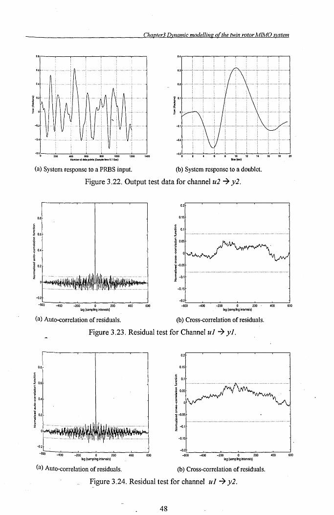
ChapterJ Dynamic modelling ofthe twin rotor MIMO system
0.8
o. 6
!\ 4
2 . 'A ... \ A ~.~ n
0\
~ .~ ~
If " J ... 2 ~
.. v ... II 4
v lJ .....
o.
-0.
-0.
-0. 6 200 400 600 800 1000 1200 1400
Numbe, 01 dal. point, (Samplo 11m. 0.1 Soc)
(a) System response to a PRES input.
0.4
o. 3
02
1
07 I \ I 1
\ I ~!
-0.
-02
-0. 3 o
~
I \ I \
\1 :\ .. ,~
ro n M ~ ~ ~ limo ( ... )
(b) System response to a doublet.
Figure 3.22. Output test data for channel u2 ~ y2.
0.8
c 2 ~ 0.6
g g ~ 0.4
~ ~ 0.2
I
-0.2
-600 -400 -200 0 200 lag (sampling intervals)
(a) Auto-correlation of residuals.
400 600
0.2
0.15
.g 01 g .
.2 ........................................................................ . c .g 0.05 ..!!!
~ Y 0
! 1-0·05 1-0.1 ............................................................................................... .
z
-0.15
-o.2~_--'--_--'-__ ,..I...-_--'-______ ~_ .....
-600 -400 -200 0 200' 400 600 lag (sampling intervals)
(b) Cross-correlation of residuals.
Figure 3.23. Residual test for Channel u1 ~ y 1.
0.8
~ .a 0.6
I~ ~ ~ 0.2
I
-0.2
-6oo~--4....J.00--_....I.200---'-0--2.l-00--4J-OO-----l600 lag (sampling intervals)
(a) Auto-correlation of residuals.
0.2
0.15
.g 01 g .
.2
.g 0.05
..!!!
~ Y 0
~ i -0.05 ., ............................................................................................... . ~ -0.1 z
-0.15
-o.2l...-_....I...-_--L.._----''---_-'--_--'-_--' -600 -400 -200 0 200 400 600
lag (sampling Intervals)
(b) Cross-correlation of residuals.
Figure 3.24. Residual test for channel u1 ~ y2.
48
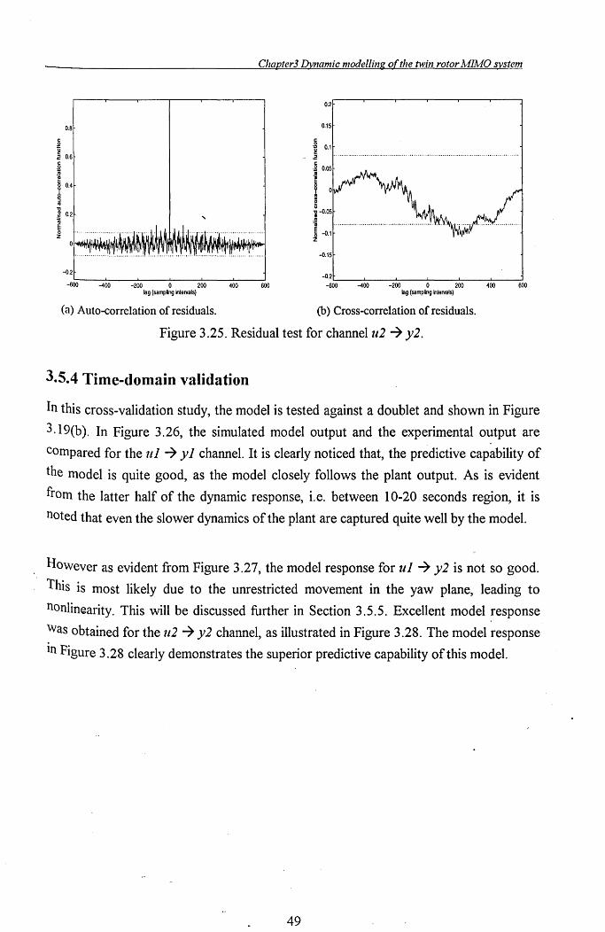
ChapterJ Dynamic modelling of the twin rotor MIMO ~stem
0.2
O.B O.tS
0.6
0.4
0.2 "
-{l.tS
-0.2 -600'----4..J....
00--_-'-200---'-0-----'200--
40L-0 -.--J
600 -{l.2L-_-'---_""--_~_-'--_--'--_ __I
-600 -400 -200 0 200 400 600 lag (sampling iltervals) lag (sampling Intervals)
(a) Auto-correlation of residuals. (b) Cross-correlation of residuals.
Figure 3.25. Residual test for channel u2 ~ y2.
3.5.4 Time-domain validation
In this cross-validation study, the model is tested against a doublet and shown in Figure
3.19(b). In Figure 3.26, the simulated model output and the experimental output are
compared for the ul ~ yl channel. It is clearly noticed that, the predictive capability of
the model is quite good, as the model closely follows the plant output. As is evident
from the latter half of the dynamic response, i.e. between 10-20 seconds region, it is
noted that even the slower dynamics of the plant are captured quite well by the model.
lIowever as evident from Figure 3.27, the model response for ul ~ y2 is not so good.
This is most likely due to the unrestricted movement in the yaw plane, leading to
nonlinearity. This will be discussed further in Section 3.5.5. Excellent model response
Was obtained for the u2 ~ y2 channel, as illustrated in Figure 3.28. The model response
in Figure 3.28 clearly demonstrates the superior predictive capability of this model.
49
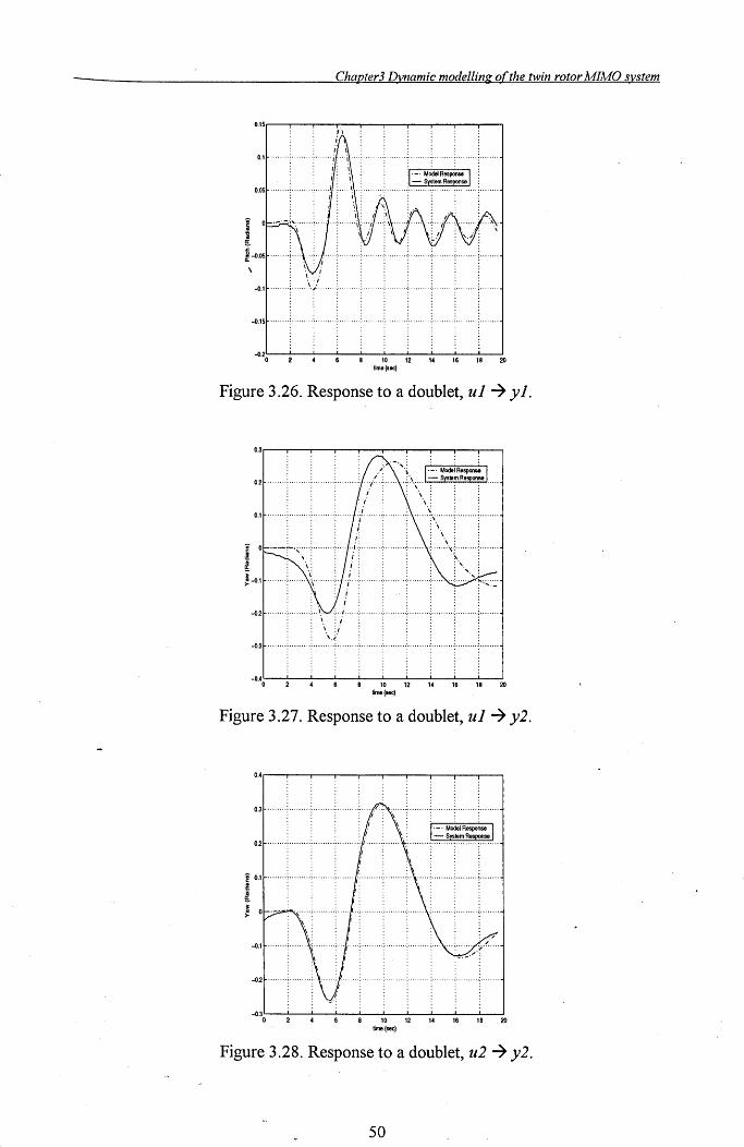
Chapter3 Dynamic modelling of the twin rotor MIMO system
0.15r----,---,---,--..,.--,...----,---,---,--..,---,
0.1 .... . ...
'1' -. Model Resp0n88 1 : - System Response :
0.05
I ... \.
~ .c f -0.05
-0.1 ......•.
-0.15
-O.20'------L----'--....I--.l.--, ..... 0
- ..... 12--,..L..--','-6 -"""8--'20
time (soc)
Figure 3.26. Response to a doublet, ul ~ yl.
0.3r----,---,---,--..,.--,--r-----r---,---,---,
0.21- ................... ; ......... ; ......... ;/ ... / .... : ...... \ ... :.\\ .. 1 ~ =~~=se I.. " : \.
O.t 1- ........ ~ .......... ~ ......... , ...... 'J~ . c': ......... , .......... \ ..... \: ....... ; ......... ; ...... ..
: " . " : " : '[ Ot-·_···_!-.,· .... , ......... , .... I .. ,f·' .. · ....... : .......... : ....... " ........ ,,~. ~ ~ (1
~-O.,I- ........ ; ....... \; ......... ;.,/ .. ' ... -: .......... -: .......... : .......... :- .. .. "
-021- .. ·· .... ; .... ·· .... ;··~~~·; .. I ..... ~ ......... : .......... : ......... ; ......... . ; .......... ; ........ ~
-0.31- .. · .... : .... ·· .... :· .. · .... ·: ...... · .. :· .. · .... ··: .. · ...... : .... · .... ·:·· ........ , ......... : ........ ~
-0.40'--~--L-....JL...-....L--..L.,0-....JL...-....L--..L...--'----'2O
time ( ... c)
Figure 3.27. Response to a doublet, ul ~ y2.
0.4r-----r---,---,--..,--,--r------r---,---,---,
0.31- ........ • .... ·· .... ;· .... · .. ·; ...... · .. ;· ... f< .... ~ .. ~ .......................... .
021- ........ , ........ ·: ...... · .. : .. · ...... ·11 ....... , ...... ··~· ...... ..J.=.;~5~.I..
! 0.11- ........ ·, .... · .... ,· .... · .. ·, ...... ·/.': .......... ·: .......... : .. \ !!
l :
-0.11- .. · .... ·; .... · .. ·ti ......... : ... -£'- .... ~ ......... : .......... : .......... : .... '"
-021-", .... : ......... :. , ..... :I': ....... : ......... : ......... : ......... ; ......... : ......... : ........ ~
_0.3'----'---'-_-'-_-'-_.1.-_'----'_--'-_-'-_-' o 10 12 14 16 18 20
time (sec)
Figure 3.28. Response to a doublet, u2 ~ y2.
50
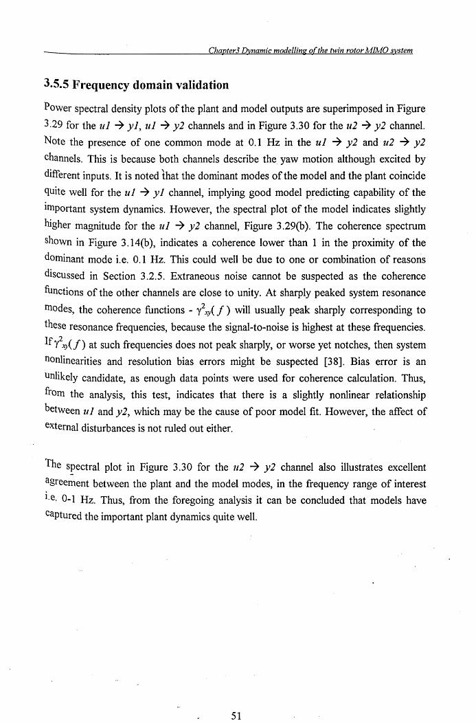
Chapter3 Dynamic modelling ofthe twin rotor MIMO -D'stem
3.5.5 Frequency domain validation
Power spectral density plots of the plant and model outputs are superimposed in Figure
3.29 for the ul ~ yl, ul ~ y2 channels and in Figure 3.30 for the u2 ~ y2 channel.
Note the presence of one common mode at 0.1 Hz in the ul ~ y2 and u2 ~ y2
channels. This is because both channels describe the yaw motion although excited by
different inputs. It is noted that the dominant modes of the model and the plant coincide
quite well for the u 1 ~ Y 1 channel, implying good model predicting capability of the
Important system dynamics. However, the spectral plot of the model indicates slightly
higher magnitude for the ul ~ y2 channel, Figure 3.29(b). The coherence spectrum
shown in Figure 3 .14(b), indicates a coherence lower than 1 in the proximity of the
dominant mode i.e. 0.1 Hz. This could well be due to one or combination of reasons
discussed in Section 3.2.5. Extraneous noise cannot be suspected as the coherence
functions of the other channels are close to unity. At sharply peaked system resonance
modes, the coherence functions - y2xy( f) will usually peak sharply corresponding to
these resonance frequencies, because the signal-to-noise is highest at these frequencies.
If"?xy(f) at such frequencies does not peak sharply, or worse yet notches, then system
nonlinearities and resolution bias errors might be suspected [38]. Bias error is an
unlikely candidate, as enough data points were used for coherence calculation. Thus,
from the analysis, this test, indicates that there is a slightly nonlinear relationship
between ul and y2, which may be the cause of poor model fit. However, the affect of
external disturbances is not ruled out either.
The spectral plot in Figure 3.30 for the u2 .~ y2 channel also illustrates excellent
agreement between the plant and the model modes, in the frequency range of interest
I.e. 0-1 Hz. Thus, from the foregoing analysis it can be concluded that models have
captured the important plant dynamics quite well.
51
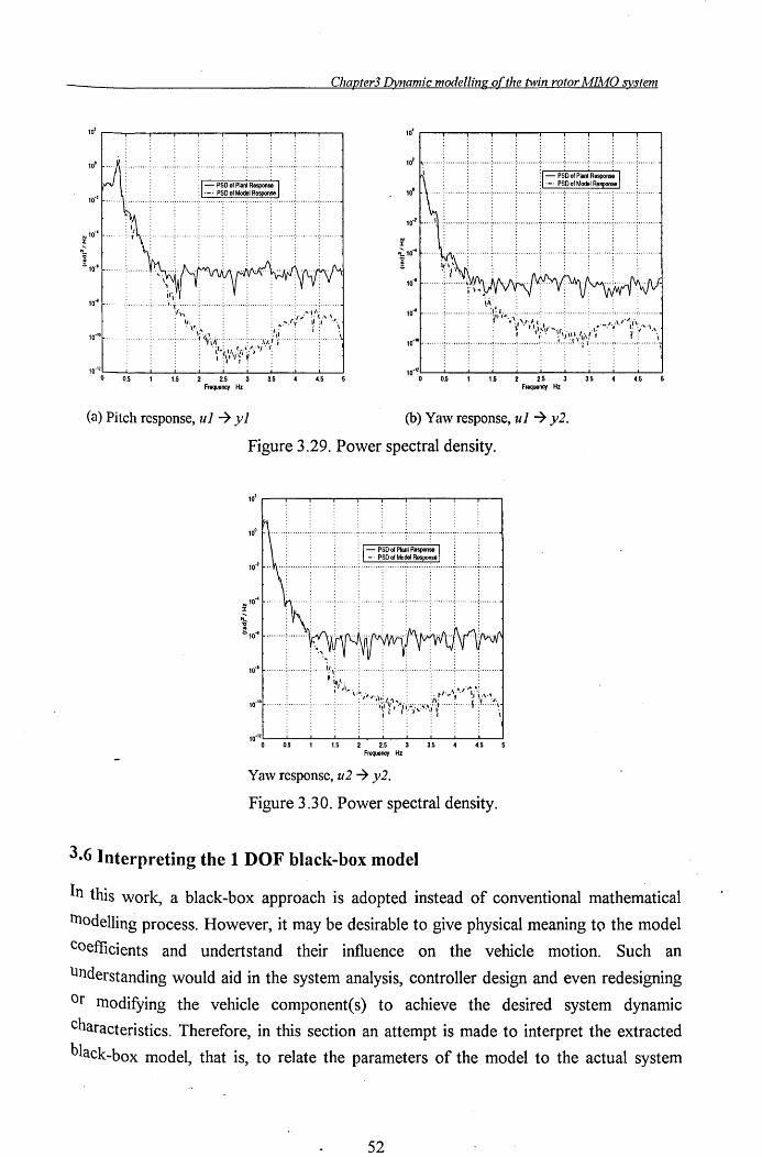
Chapter3 Dynamic modelling oOhe twin rotor MIMO system
10' 10' h· .. · .. ·; .. ·· .... ··;· .... · .. ··: .. · .. · .... :· ........ ·:: ...... · .. ·: .......... :.·· ........ : ......... ; ....... ,
10'
10" 1- .. ······,· ....... 1
10" ....... ; ........ ~. .. : ~ \''''... :
10" .
:::. • ••••••• ' ••••••••• : ••••• '1",··t;. .. ,;,~":;.;~:;~J,;.:t'YE.,'., 10'''0'----Jo.'--s --L_..J...1.s-...L..
2 -2.1-.
5 ---'3--'-3.s-...I...--
4.1-.
s---J
Frequency Hz
10'''OL -OL-.S ---I-....I.1.s-...J..2-~2.s-~3 ---:3:1:-.5 -L---:-4.I:-S ~ Frequency Hz
(a) Pitch response, ul ~ yl (b) Yaw response, ul ~ y2.
Figure 3.29. Power spectral density.
10."L----L..---L_....L.---1..._.L---L-_L---I---L---I o 0.5 1.5 2 2.5 3 3.5 4.5
Frequency Hz
Yaw response, u2 ~ y2.
Figure 3.30. Power spectral density.
3.6 Interpreting the 1 DOF black-box model
In this work, a black-box approach is adopted instead of conventional mathematical
l110delling process. However, it may be desirable to give physical meaning to the model
coefficients and undertstand their influence on the vehicle motion. Such an
understanding would aid in the system analysis, controller design and even redesigning
Or modifying the vehicle component( s) to achieve the desired system dynamic
characteristics. Therefore, in this section an attempt is made to interpret the extracted
blaCk-box model, that is, to relate the parameters of the model to the actual system
52

Chapter3 Dynamic modelling ofthe twin rotor MIMO system
dynamic behaviour. If one is only interested in an input-output representation of the
pitch axis of the TRMS, a discrete-time transfer function can be obtained from the
identified 1 DOF parametric model as:
l!.. == 0.0097 Z3 - 0.0086z 2 + 0.006z + 0.0284
ul Z4 - 3.0077z3 + 3.500lz2 -1.8096z + 0.3407
where, y 1 = pitch angle, radians; and
ul == main rotor input, volts.
(3.11)
The coefficients of the transfer function in equation (3.11) have no physical meaning,
but the dynamic characteristics of the system depend directly upon them, and it would
be interesting to make it evident in the structure. Factoring the numerator and the
denominator polynomials of equation (3.11) yields
~ _ (z - 9805 + I.328Ii)(z - 9805 -I.328li)(z + 1.0743)
ul (z - 0.8926 - 0.4095i)(z - 0.8926 + 0.4095i)(z - 0.7541 )(z - 0.4685) (3.12)
implying that the system has complex poles, refer Figure 3.4. Thus, bringing into
evidence the (almost) unstable oscillatory mode, which is a significant dynamic
characteristic of the TRMS and also of a helicopter in hover. The oscillatory or
Vibrational motion is imparted to the system due to flexible structural component(s).
The complex poles in the characteristic equation are therefore, directly related to the
phYsical properties of the structural material.
1.5
0.5
-0.5
-1
-1.5
-~2L---'------'---'-----'-0 --'-----L-1.L-.
6 ------I
Real
Figure 3.4. Pole-zero plot.
53
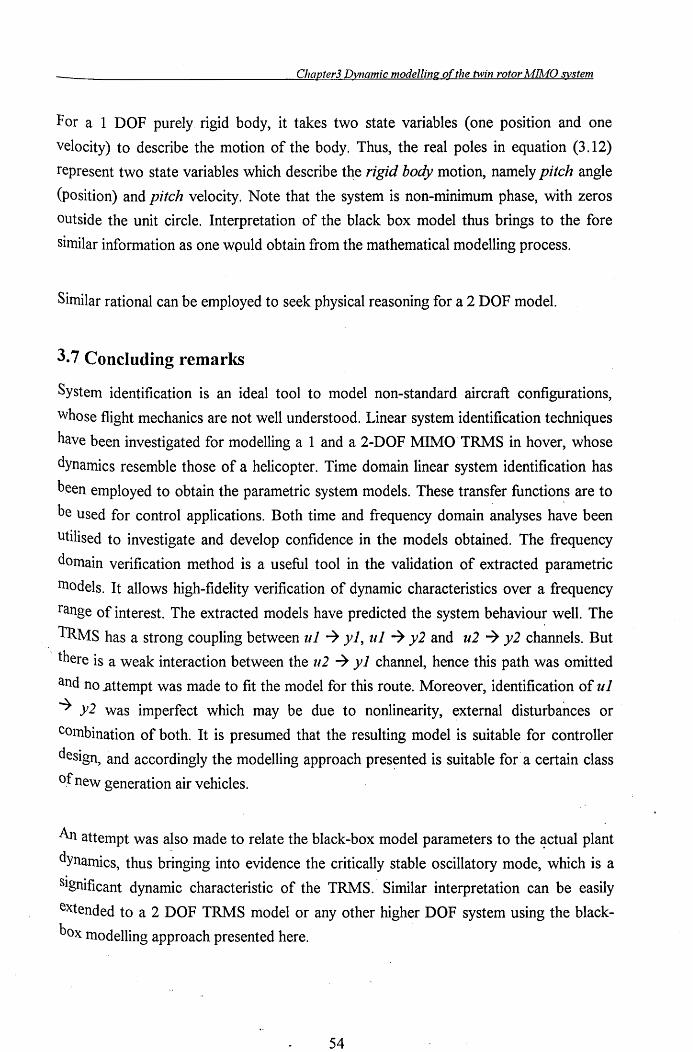
Chapter3 Dynamic modelling ofthe twin rotor MIMO ~stem
For a 1 DOF purely rigid body, it takes two state variables (one position and one
velocity) to describe the motion of the body. Thus, the real poles in equation (3.12)
represent two state variables which describe the rigid body motion, namely pitch angle
(position) and pitch velocity. Note that the system is non-minimum phase, with zeros
outside the unit circle. Interpretation of the black box model thus brings to the fore
similar information as one wpuld obtain from the mathematical modelling process.
Similar rational can be employed to seek physical reasoning for a 2 DOF model.
3.7 Concluding remarks
System identification is an ideal tool to model non-standard aircraft configurations,
Whose flight mechanics are not well understood. Linear system identification techniques
have been investigated for modelling a 1 and a 2-DOF MIMO TRMS in hover, whose
dynamics resemble those of a helicopter. Time domain linear system identification has
been employed to obtain the parametric system models. These transfer functions are to
be used for control applications. Both time and frequency domain ~nalyses have been
utilised to investigate and develop confidence in the models obtained. The frequency
domain verification method is a useful tool in the validation of extracted parametric
mOdels. It allows high-fidelity verification of dynamic characteristics over a frequency
range of interest. The extracted models have predicted the system behaviour well. The
TRMs has a strong coupling between u1 ~ y 1, u1 ~ y2 and u2 ~ y2 ch~nnels. But
there is a weak interaction between the 11 2 ~ Y 1 channel, hence this path was omitted
and no Jlttempt was made to fit the model for this route. Moreover, identification of u1
~ y2 was imperfect which may be due to nonlinearity, external disturbances or
Combination of both. It is presumed that the resulting model is suitable for controller
deSign, and accordingly the modelling approach pres~nted is suitable for a certain class
of new generation air vehicles.
An attempt was also made to relate the black-box model parameters to the ~ctual plant
dynamics, thus bringing into evidence the critically stable oscillatory mode, which is a
Significant dynamic characteristic of the TRMS.· Similar interpretation can be easily
extended to a 2 DOF TRMS model or any other higher DOF system using the black
box modelling approach presented here.
54
Chapter 4 Open-loop control design for vibration suppression
Chapter 4
Open-loop ~ontrol design for vibration • suppression
In Chapter 3, linear 1110dels of the TRMS were developed andfound to have vibrational modes. The presence of resonance frequencies are undesirable in 111any engineering applications. An active vibration control paradignl is employed in this Chapter for attenuating the unwanted structural elastic 1110des. The TRMS residual oscillations are substantially reduced using the open-loop control technique, which utilises digital fi lters for shaping the c0111mand inputs. Open-loop study is often necessary for designing more c0111plex feedback control laws.
4.1 Introduction
The successful completion of the modelling exercise leads to Step 2 of Figure 1.1 in the
overall control system design process. The model analysis reveals the p'resence of
flexible structural modes in both 1 and 2 DOF models as seen from the spectral plots of
the TRl\1S output (pitch and yaw) responses of Figures 3.2(b), 3.16 and 3.18. The
lightly damped natural frequency of oscillation of the TRMS arising from the structural
(main beam) elasticity, induces undesirable residual vibration. In general, the residual
motion (vibration) is induced in flexible structures primarily as a result of faster motion
commands. The occurrence of any vibration after the commanded position has reached
will necessitate additional settling time before a new manoeuvres may be initiated.
Therefore, in order to achieve fast system response to command input signals, it is
Imperative to reduce this vibration. Although, vibrations are undesirable, light weight
yet strong flexible structures along with other associated advantages like low energy
consumption and smaller actuator requirements, are highly desirable in a number of
modern systems such as spacecraft with flexible appendages [13-15], robotics [10-12],
fleXible aircraft [16,17] and flexible missile and launch vehicle [20].
55
Chapter 4 Open-loop control design for vibration suppression
Fast speed of response is another important characteristics imparted to the system due
to flexible material. Essentially, the choice of the physical parameters, for example mass,
stiffness and damping factor of the material, determine the response of the system. The
choice of these parameters can be thought of as passive control. For example, adding
mass to the TRMS main beam would lower its natural frequency. If adding the mass is
not practical, such as in the ,case of most aerospace structures, a common and and very
effective way to reduce transient and steady-state vibration is to increase the amount of
damping in the structure so that there is greater energy dissipation. A damping
treatment consists of adding a layer of visco-elastic material, such as rubber, to an
existing structure. The combined system often has a higher damping level and thus
reduces unwanted vibration. Thus, passive control in essence involves changing the
physical parameters of the material to attenuate structural vibrations. Hybrid approaches
involving passive and active ( discussed next) control techniques have been found to be
ideal for damping the vibration modes of civil structures such as high rise buildings [40,41].
If the materials are fixed for a given system, such as the TRMS, it is difficult to change
the mass and stiffness of the system by more than a few percent. Despite this constraint,
it is often possible that the desired system response can be achieved with active control.
Active control employes external adjustable or active devices, actuator (for e.g, electric
motors, hydrulic pistons, piezo-electric devices etc.,) to provide a force to the structure,
machine or the device whose vibration properties are to be altered. In this work, active
Control option is considered without resorting to changing the physical properties of the
!RMs:-- Active control can be broadly categorise as open-loop (feedforward), c1osed
loop (feedback) or combination of feedforward and feedback methods. O~en-Ioop Control is the subject matter of this Chapter, feedback and combined feedforward and
feedback topologies are presented in Chapter 6. The feedback and combined
feedforward and feedback controllers are implemented on the TRMS rig and results
described in Chapter 7.
Vibration control by open-loop or feedforward methods, essentially consists of
manipulating the input signal to the plant by investigating the physical and vibrational
prOperties of the flexible system. The goal of this input shaping control is to avoid
eXcitation of the residual vibration at the end of the manoeuvre. Early papers on input
shaping considers feedforward control defined by a finite expansion, e.g. trignometric
56
Chapter 4 Open-loop control design for vibration suppression
[42], that mlmmlses the frequency content over a wide range of frequencies, but
requires longer time to complete the motion. More recently, Suk et al [43] designed and
implemented an optimal shaped input torque based on a trignometric series expansion
for simultaneous slewing and vibration suppression of flexible structures. They also
incorporated a feedback loop to achieve the desired set-point tracking. Another
approach based on trignometric series expansion is the work of Meck et al [44]. Later,
a version of the same approach using a pulse sequence expansion was proposed by
Singer and Seering [45]. It is well known that when two signals are convolved the
resulting signal will have a spectra which will produce a zero excitation at frequencies
where one or the other of the original signal spectra is zero. Singer and Seering[ 45],
Watkins and Yurkovich [46] and Tzes and Yurkovich [47], made use of this fact in their
work by convolving the command signal with a pulse sequence. The result of the
convolution is used to drive the system. Therefore, the computation of the appropriate
pulse sequence can be considered as the design of a notch filter to remove the resonance
excitation from the command signal. In a relatively recent paper, Banerjee and Singhose
[48] applied the same technique for end point tracking of a two link flexible robot with a
feedback control. They showed that the input shaping of closed-loop control modes
gave a robust performance and improved tracking.
Tzse and Yurkovich [47] investigated an adaptive input shaping strategy for vibration
attenuation in a slewing flexible structure. In the case of a change in payload or
modelling errors, the proposed scheme integrates a frequency domain identification
technique along with the input shaping, in order to adjust parameters of the input
shapers. The problem of active noise control of multi-degree-of-freedom high rise
buildings is considered by [41], who employed direct model reference adaptive control
(bMRAC) on a spring-mass-damper system representing a building .. The adaptive
scheme was shown to yield good disturbance rejection to earthquake and wind effects.
Note, that the above frequency-based input shaping methods are only applicable to
linear systems. For nonlinear flexible systems, Gorinvesky and Vukovich [49], trained a
neural network to obtain the desired system's output trajectory. More recently, Tokhi et
al [50] employed Multi Layer Perceptron (MLP) to model the inverse plant dyanmics,
Which in turn is used to cancel out the dominant plant vibrational f~equency from the
input signal. An adaptive feedback mechanism is also incorporated to address changing
plant parameters at different payloads. However, the simplest method to achieve the
resonance suppression is via classical digital filters, such as the Butterworth, elliptic and
Chebyshev. This concept was demonstrated by [10,11] on a single-link flexible
57
Chapter 4 Open-loop control design for vibration suppression
manipulator.
The remainder of this Chapter develops and applies a feedforward control technique
which is related to a number of approaches known as "input shaping control", discussed
above. The goal of the open-loop control is to shape the input signal so as to avoid
excitation of residual vibrations during and at the end of the plant manoeuvre. The
fundamental concept for this type of control is based on the well established theory of
digital filters. In these method, a feedforward input signal is shaped so that it does not
contain spectral components at the system's resonant eigen-frequencies. The approach
requires that the natural resonant frequencies, such as those used in Chapter 3, of the
system be determined through suitable identification and modelling techniques.
Investigation of SISO and MIMO open-loop control is a prelude to subsequent
development of more complex multivariable feedback control laws.
The Chapter is organised as follows: Section 4.2 analyses the TRMS vibrational modes.
Section 4.3 discusses digital filters used for command shaping. Section 4.4 and 4.6
discusses filter design, implementation and results. A 2 DOF coupling anaysis is
presented in Section 4.5 prior to 2 DOF experiments. Finally, Section 4.8 concludes the
work.
4.2 The TRMS vibration mode analysis
In general, for flexible structures/aircraft the parameters which have an influence on the
flexible modes are the mass distribution, which may change the frequencies of the
modes, the accuracy of the model. For an aircraft, altitude and Mach number also have
arr influence on the system modes. This is relevant to the TRMS which can be
interpreted as a centrally supported cantilever beam with loads (rotors) at both ends.
The non-uniform mass distribution due to the rotors and the rotor torque at normal
operating conditions are the main causes of beam deflection, which in turn causes
vibration. A schematic of a flexible system is illustrated in Figure 4.1. In this Figure u is
the rotor input and y is the combined output due to rigid-body as well as elastic motion.
In conventional resonance, a dynamic system is excited by a fluctuating input, the
frequency of which is equal to the natural frequency of the dynamic system. The TRMS
could oscillate and become unstable if its natural frequency of oscillation is close or
58
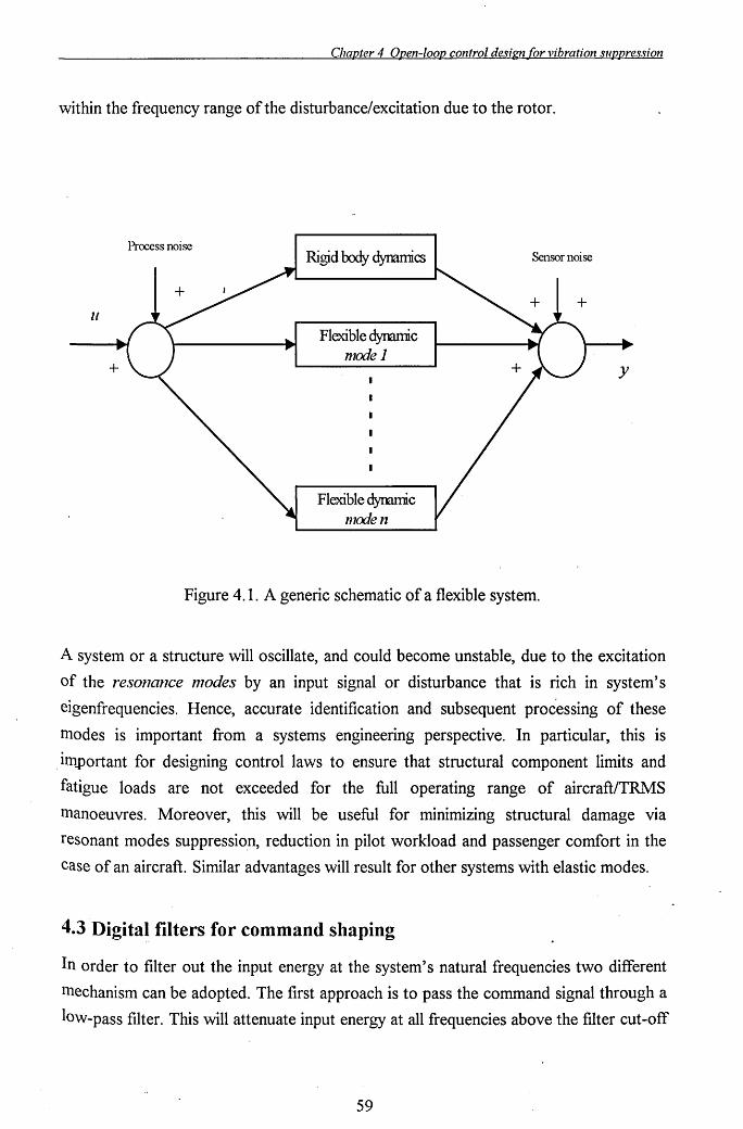
Chapter 4 Open-loop control design for vibration suppression
within the frequency range of the disturbance/excitation due to the rotor.
Process noise
u
Rigid body dynamics
Flexible dynamic model
Flexible dynamic moden
Sensor noise
Figure 4.1. A generic schematic of a flexible system.
A system or a structure will oscillate, and could become unstable, due to the excitation
of the resonance nlodes by an input signal or disturbance that is rich in system's
eigenfrequencies. Hence, accurate identification and subsequent processing of these
modes is important from a systems engineering perspective. In particular, this is
important for designing control laws to ensure that structural component limits and
fatigue loads are not exceeded for the full operating range of aircraft/TRMS
manoeuvres. Moreover, this will be useful for minimizing structural damage via
resonant modes suppression, reduction in pilot workload and passenger comfort in the
case of an aircraft. Similar advantages will result for other systems with elastic modes.
4.3 Digita~ filters for command shaping
In order to filter out the input energy at the system's natural frequencies two different
mechanism can be adopted. The first approach is to pass the command signal through a
lOw-pass filter. This will attenuate input energy at all frequencies above the filter cut-off
59
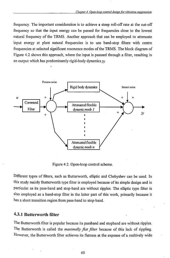
Chapter 4 Open-loop control design for vibration sUl2,pression
frequency. The important consideration is to achieve a steep roll-off rate at the cut-off
frequency so that the input energy can be passed for frequencies close to the lowest
natural frequency of the TRMS. Another approach that can be employed to attenuate
input energy at plant natural frequencies is to use band-stop filters with centre
frequencies at selected significant resonance modes of the TRMS. The block diagram of
Figure 4.2 shows this approach, where the input is passsed through a filter, resulting in
an output which has predominantly rigid-body dynamics Yl-
u Corrmmd
Filter
Process noise
Rigid body dynamics
Attenuated flexible dynamic mode 1
Attenuated flexible dynamic mode n
Figure 4.2. Open-loop control scheme.
Sensor noise
Yt
Different types of filters, such as Butterworth, elliptic and Chebyshev can be used. In
this study mainly Butterworth type filter is employed because of its simple design and in
particular as its pass-band and stop-band are without ripples. The elliptic type filter is
also employed as a band-stop filter in the latter part of this work, primarily because it
has a short transition region from pass-band to stop-band.
4.3.1 Buttenvorth filter
The Butterworth filter is popular because its passband and stopband are without ripples.
The Butterworth is called the maximally flat filter because of this lack of rippling.
Bowever, the Butterworth filter achieves its flatness at the expense of a realtively wide
60
Chapter 4 Open-loop control design for vibration suppression
transition region. This filter has only two design parameters: the order of the filter and
the filter's cut-off frequency, Ole. The order of the filter is also the number of poles for
the filter and it determines its complexity. The Butterworth filter is defined by the
following squared transfer function, where, n is the order of the filter and Ole, is the
filter cut-off frequency.
(4.1)
1 =-----
1+(-!-J2n jffic
The magnitude-squared of the Butterworth's frequency response is its squared transfer
function, equation 4.1 with s replaced by jm.
(4.2)
4.3.2 Elliptic filter
The elliptic filter has the shortest transition region from pass-band to stop-band of any
filter with the same order and ripple heights. The elliptic design is optimum in this sense.
Therefore, the elliptic filter is ideal for those applications where ripples can be tolerated
and short transition regions are demanded.
The magnitude squared transfer function of the elliptic filter is as follows:
(4.3)
Where, the parameter E controls the height of ripples and Ole controls the frequency
breakpoint. R n is a rational function, the parameter L controls the width of the
61
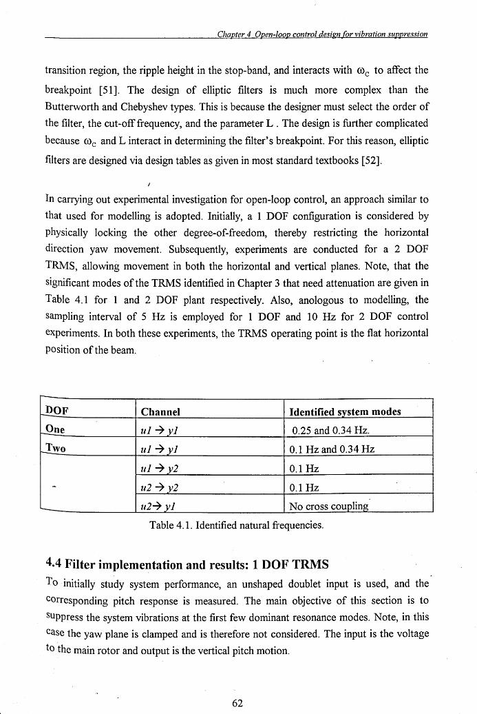
Chapter 4 Open-loop control design for vibration suppression
transition region, the ripple height in the stop-band, and interacts with roc to affect the
breakpoint [51]. The design of elliptic filters is much more complex than the
Butterworth and Chebyshev types. This is because the designer must select the order of
the filter, the cut-off frequency, and the parameter L . The design is further complicated
because roc and L interact in determining the filter's breakpoint. For this reason, elliptic
filters are designed via design tables as given in most standard textbooks [52].
In carrying out experimental investigation for open-loop control, an approach similar to
that used for modelling is adopted. Initially, a 1 DOF configuration is considered by
physically locking the other degree-of-freedom, thereby restricting the horizontal
direction yaw movement. Subsequently, experiments are conducted for a 2 DOF
TRMS, allowing movement in both the horizontal and vertical planes. Note, that the
significant modes of the TRMS identified in Chapter 3 that need attenuation are given in
Table 4.1 for 1 and 2 DOF plant respectively. Also, anologous to modelling, the
sampling interval of 5 Hz is employed for 1 DOF and 10Hz for 2 DOF control
experiments. In both these experiments, the TRMS operating point is the flat horizontal
position of the beam.
roo--
r-DOF Channel Identified system modes
rilne ul ~ yl 0.25 and 0.34 Hz.
r-Iwo ul ~ yl 0.1 Hz and 0.34 Hz
ul ~ y2 0.1 Hz
- u2~y2 0.1 Hz
'---- u2~ yl No cross coupling
Table 4.1. Identified natural frequencies.
4.4 Filter implementation and results: 1 DOF TRMS
To . initially study system performance, an unshaped doublet input is used, and the
corresponding pitch response is measured. The main objective of this section is to
suppress the system vibrations at the first few dominant resonance modes. Note, in this
case the yaw plane is clamped and is therefore not considered. The input is the voltage
to the main rotor and output is the vertical pitch motion.
62
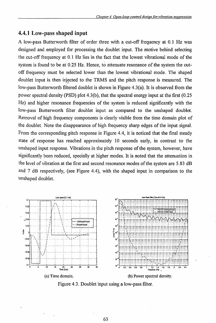
Chapter 4 Open-loop control design for vibration sUT2,pression
4.4.1 Low-pass shaped input
A low-pass Butterworth filter of order three with a cut-off frequency at 0.1 Hz was
designed and employed for processing the doublet input. The motive behind selecting
the cut-off frequency at 0.1 Hz lies in the fact that the lowest vibrational mode of the
system is found to be at 0.25 Hz. Hence, to attenuate resonance of the system the cut
off frequency must be selected lower than the lowest vibrational mode. The shaped
doublet input is then injected to the TRMS and the pitch response is measured. The I
low-pass Butterworth filtered doublet is shown in Figure 4.3(a). It is observed from the
power spectral density (PSD) plot 4.3(b), that the spectral energy input at the first (0.25
Hz) and higher resonance frequencies of the system is reduced significantly with the
low-pass Butterworth filter doublet input as compared to the unshaped doublet.
Removal of high frequency components is clearly visible from the time domain plot of
the doublet. Note the disappearance of high frequency sharp edges of the input signal.
From the corresponding pitch response in Figure 4.4, it is noticed that the final steady
state of response has reached approximately 10 seconds early, in contrast to the
unshaped input response. Vibrations in the pitch response of the system, however, have
significantly been reduced, specially at higher modes. It is noted that the attenuation in
the level of vibration at the first and second resonance modes of the system are 5.83 dB
and 7 dB respectively, (see Figure 4.4), with the shaped input in comparison to the
unshaped doublet.
Low-pass [0.1 Hz) O.l.------r-==,---,---,------r---,------,----.
0.08t-· .. ··· .... ·: .. , .. · .. ····.: .... · .. , ., 0.061- .... ·· .... : .. ,· .. · .... ·,·· ... -: .. \ .......... ! ...... ;
0.02t- .. · ...... · .. ,· ...... ··, ...... ,
~ g Ot- ...... ;.' ......... ;r.'~_~~_~~
-0.02t-'·· ....... ; .. , ......... " .......... ; ............ ; ......... ~,,,.': ......... ; ............ ; ......... -1
-0.04t-' .. ·· .. ·.:·, .... · .. ·:;· .. · .. · .. · .. ; ............ ; ...... · .... ·;· ........ · .. ; ............ , .......... -1
-O.06t-l .. · .... ; .. r· ..... :·!.·; ...... · .... , .... · .. · .... ;. .... · .. · .. ·!· .......... ·; ............ ; .......... -i
-0.081-1 .... · .... , .. ,· ...... ··, .......... ·: .... · .... · .. , .... · .. · .. ·:· .......... , .... · ....... , .......... -1
10 15 20 25 30 35 40 Time (Sec)
(a) Time domain. (b) Power spectral density.
Figure 4.3. Doublet input using a low-pass filter.
63
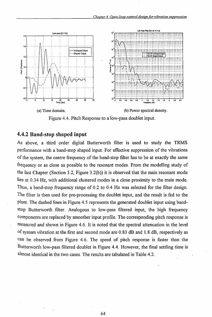
Chapter 4 Open-loop control design for vibration suppression
Low-pass [0.1 Hz)
0.3 ............ ;· .... ·1 \ .. ~ .... · ...... ~ .... · .... ' .. ~ .... · ...... :~:.:.:.:..:.:..:==:.:..:.:.:..:.:~·i
0.2 .... · ...... : .... ·j
0.1 ..
-0.1
- Unshaped Ouiput . - . - Shaped OutpiJt
_0.21.----1.-_...1...----'-_-'-----"_--'--_'------' o 10 15 20 25 30 35 40
Time (Sec)
(a) Time domain.
••••••• : •••••• ': ••••••• : ••••••• : •••••• ': ••• 0 ••• : ••••••• : ••••••• :' •••••• ~ ••••••• ~ ••••••• ~ ••••••• :' ••
10-lL-.L-.L-.L-...I...-...I...-....L.-....L.--.....L.--'---'----'----'--' o 0.2 0.4 0.6 0.8 1 1.2 1.4 1.6 1.8 2 22 2.4
Frequency (Hz)
(b) Power spectral density.
Figure 4.4. Pitch Response to a low-pass doublet input.
4.4.2 Band-stop shaped input
As above, a third order digital Butterworth filter is used to study the TRMS
performance with a band-stop shaped input. For effective suppression of the vibrations
of the system, the centre frequency of the band-stop filter has to be at exactly the same
frequency or as close as possible to the resonant modes. From the modelling study of
the last Chapter (Section 3.2, Figure 3.2(b» it is observed that the main resonant mode
lies at 0.34 Hz, with additional clustered modes in a close proximity to the main mode.
Thus, a band-stop frequency range of 0.2 to 0.4 Hz was selected for the filter design.
The filter is then used for pre-processing the doublet input, and the resu.lt is fed to the
plant. The dashed lines in Figure 4.5 represents the generated doublet input using band
stop Butterworth filter. Analogous to low-pass filtered input, the high frequency
components are replaced by smoother input profile. The corresponding pitch response is
measured and shown in Figure 4.6. It is noted that the spectral attenuation in the level
of system vibration at the first and second mode are 0.83 dB and 1.8 dB, respectively as
can be observed from Figure 4.6. The speed of pitch response is faster than the
Butterworth low-pass filtered doublet in Figure 4.4. However, the final settling time is
almost identical in the two cases. The results are tabulated in Table 4.2.
64
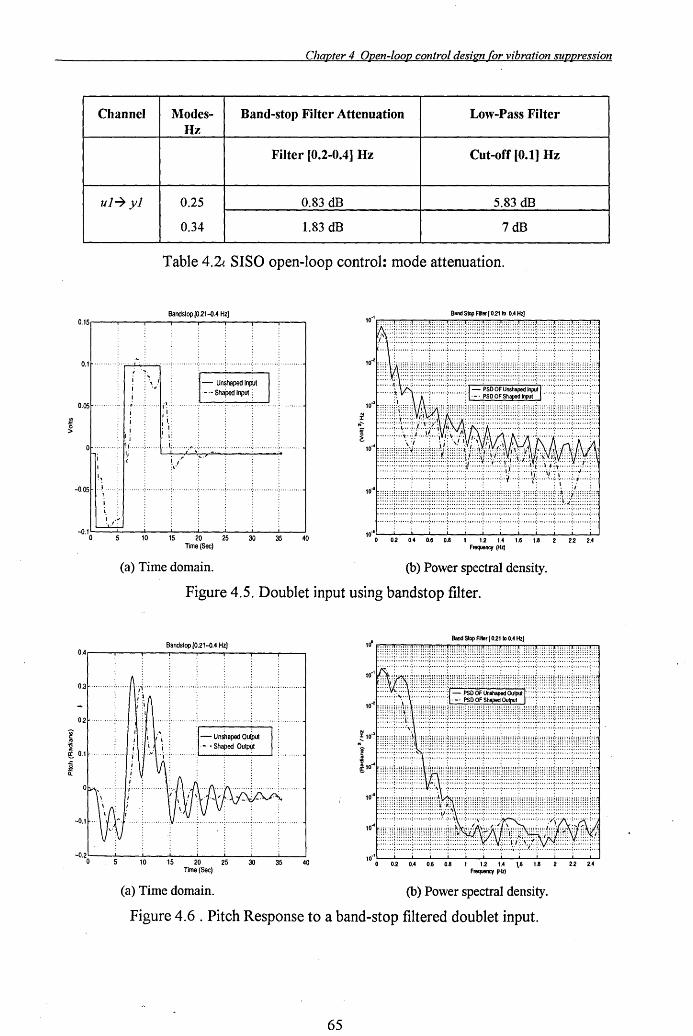
Chapter 4 Open-loop control design for vibration suppression
Channel Modes- Band-stop Filter Attenuation Low-Pass Filter Hz
Filter [0.2-0.4] Hz Cut-off [0.1] Hz
1.11-7 y1 0.25 0.83 dB 5.83 dB
0.34 1.83 dB 7dB
Table 4.21. SISO open-loop control: mode attenuation.
Bandstop [0.21-0.4 Hz) Band stop Rller (0.21 10 0.4 Hz)
, ..... ; ....... ; ....... ~ ....... ~ ....... ~ ....... ~ ....... : ........ : ....... ~ ...... \ ....... ~ ........ '" : :
:::::::::::::::::::::::::.
10 15 20 25 30 35 10"L-~-"'\'_..I-..--'----I_..L---J.._.L--~-"'\'_...L--l-.J
o 0.2 0.4 0.6 0.8 1 12 1.4 1.6 1.8 40 2.2 2.4 Time (Sec) FllIquency (Hz)
(a) Time domain. (b) Power spectral density.
Figure 4.5. Doublet input using bandstop filter.
Bandstop [0.21-0.4 Hz) Band Slop Filter (02110 0.4 Hz)
df"\:.,
...... 2 j 1'-'
\
... 10
10 .. ',\ "~'. rJ 'T, " '1\ <(.:\ /,
., 10
o 0.2 0.4 0.6 0.8 1 12 1.4 1,.6 1.8 22 2.4 40 FllIquency (Hz)
(a) Time domain. (b) Power spectral density.
Figure 4.6 . Pitch Response to a band-stop filtered doublet input.
65
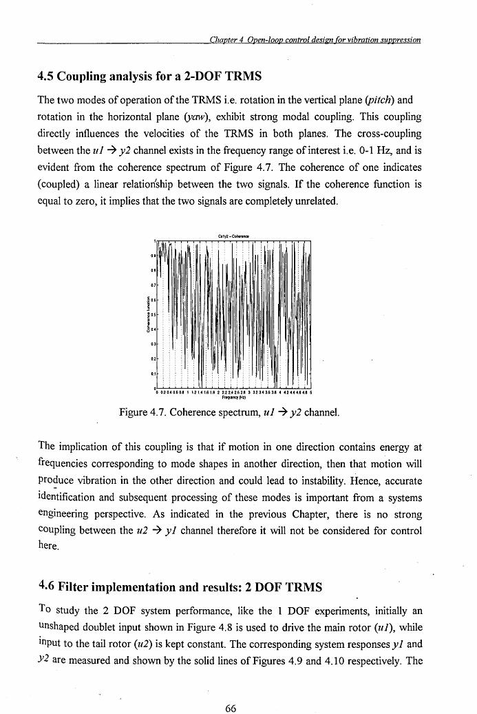
Chapter 4 Open-loop control design for vibration suppression
4.5 Coupling analysis for a 2-DOF TRMS
The two modes of operation of the TRMS i.e. rotation in the vertical plane (pitch) and
rotation in the horizontal plane (ymv) , exhibit strong modal coupling. This coupling
directly influences the velocities of the TRMS in both planes. The cross-coupling
between the ul ~ y2 channel exists in the frequency range of interest i.e. 0-1 Hz, and is
evident from the coherence spectrum of Figure 4.7. The coherence of one indicates
(coupled) a linear relationship between the two signals. If the coherence function is
equal to zero, it implies that the two signals are completely unrelated.
Cxly2 - Coherence
.: ~ :
0.8
0.7
.~ 0.6
i jO.5 j
.~I~III <3 0.4
0.3
0.2
0.1
O~~~~~~~~~~~~~
o 0.20.40.60.8 1 1.21.41.6 1.8 2 2.22.42.62.8 3 3.23.43.63.8 4 4.24.44.64.8 5 Froquoncy(Hz)
Figure 4.7. Coherence spectrum, ul ~ y2 channel.
The implication of this coupling is that if motion in one direction contains energy at
frequencies corresponding to mode shapes in another direction, then that motion will
produce vibration in the other direction and could lead to instability. Hence, accurate
identification and subsequent processing of these modes is important from a systems
engineering perspective. As indicated in the previous Chapter, there is no strong
coupling between the u2 ~ y 1 channel therefore it will not be considered for control
here.
4.6 Filter implementation and results: 2 DOF TRMS
To study the 2 DOF system performance, like the 1 DOF experiments, initially an
unshaped doublet input shown in Figure 4.8 is used to drive the main rotor (ul), while
Input to the tail rotor (u2) is kept constant. The corresponding system responses yl and
Y2 are measured and shown by the solid lines of Figures 4.9 and 4.10 respectively. The
66
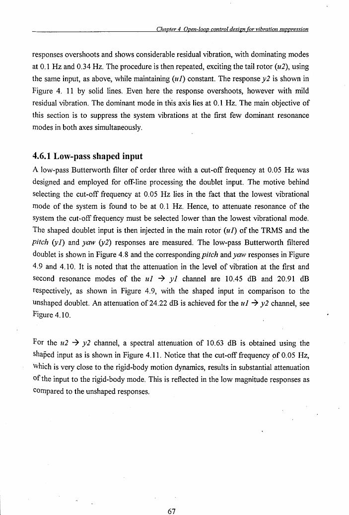
Chapter 4 Open-loop control design for vibration suppression
responses overshoots and shows considerable residual vibration, with dominating modes
at 0.1 Hz and 0.34 Hz. The procedure is then repeated, exciting the tail rotor (u2), using
the same input, as above, while maintaining (u1) constant. The response y2 is shown in
Figure 4. 11 by solid lines. Even here the response overshoots, however with mild
residual vibration. The dominant mode in this axis lies at 0.1 Hz. The main objective of
this section is to suppress the system vibrations at the first few dominant resonance
modes in both axes simultaneously.
4.6.1 Low-pass shaped input
A low-pass Butterworth filter of order three with a cut-off frequency at 0.05 Hz was
designed and employed for off-line processing the doublet input. The motive behind
selecting the cut-off frequency at 0.05 Hz lies in the fact that the lowest vibrational
mode of the system is found to be at 0.1 Hz. Hence, to attenuate resonance of the
system the cut-off frequency must be selected lower than the lowest vibrational mode.
The shaped doublet input is then injected in the main rotor (u1) of the TRMS and the
pitch (y1) and yaw (y2) responses are measured. The low-pass Butterworth filtered
doublet is shown in Figure 4.8 and the corresponding pitch and yaw respons~s in Figure
4.9 and 4.10. It is noted that the attenuation in the level of vibration at the first and
second resonance modes of the 111 ~ y1 channel are 10.45 dB and 20.91 dB
respectively, as shown in Figure 4.9, with the shaped input in comparison to the
unshaped doublet. An attenuation of24.22 dB is achieved for the u1 ~ y2 channel, see
Figure 4.10.
For the 112 ~ y2 channel, a spectral attenuation of 10.63 dB is obtained using the
shaped input as is shown in Figure 4.11. Notice that the cut-off frequency 9f 0.05 Hz,
which is very close to the rigid-body motion dynamics, results in substantial attenuation
of the input to the rigid-body mode. This is reflected in the low magnitude responses as
compared to the unshaped responses.
67
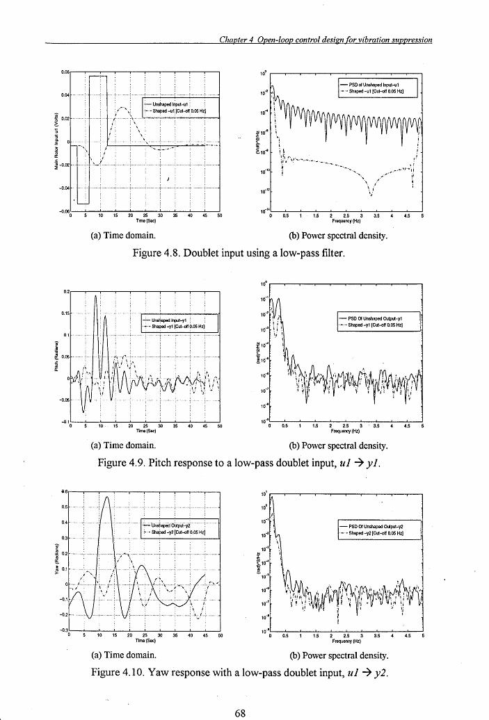
'; :; ~
~ "
Chapter 4 Open-loop control design for vibration suppression
: I· .... ·'\~
.,: .. \ ..... 4 .. .,.,.,.".,.".",..."....,.,.,.,.",.,....,.,....,.,.,.".."...,.,...,....",.,.,...,.,'"" i:
i .'
:\
" \: ',: ....... ~ .... ",:" ..................... ~:.::.:.. - _._.-,,-:.-.-
. . .
10-2
Ii I
10" \
N 10~
~ ~10~
j j j "
j
iI
- PSD of Unshaped Input-ul ._.- Shaped -ul [Cut-off O.OS Hz)
~ -0.02 : : : .....................................
·i:i,,\,. ........ ... jl
............ ................
~ ~
1
-0.04
10 IS 20 2S 30 35 40 4S SO 10-"·L----'---'---'---'---'---'--~---'---'---l
o 0.5 1.5 2 2.5 3 3.5 4.5 Time (Sec) Frequency (Hz)
(a) Time domain. (b) Power spectral density.
Figure 4.8. Doublet input using a low-pass filter.
0.2.----.---.---.--'"T"'""-..----.---.---.--...-----,
O.IS
0.1
-'- Unshaped IniM-yl ~ , .... - Shaped -yl [Cut-off 9.05 Hz]
/. 10-2 '1 I,
\ j 10'" ~ i
~i
- PSD Of Unshaped Output-Yl . _. - Shaped -yl [Cut-off O.OS Hz)
g, 0.05
~10"
I 10"' ~ II.
-O.OS .
-0.1 '--~ _ __'_ _ _'_ _ _'___'__~_--L.. _ _'_ _ _'__--I
o 10 15 20 25 30 35 40 45 50 Time (Sec)
10'"
10-·0L-~0.S---'---I'-.S-...J.2--2..L..S--3'--~3.S---'---4'-.5~ Frequency (Hz)
(a) Time domain. (b) Power spectral density.
Figure 4.9. Pitch response to a low-pass doublet input, ul ~ yl.
ur---.---.---,----.--~-.--__r-......... --.-___. 101 ....---.---.---,----.--...---.----.---.---,----.
0.4~ ........ : ....... :/ ..... \, ......... ~.... \
0.3~ .. · .... :·· .... ·
0.2~ .. · .... ·, ........ f
0.1
-0.2
-o.30:----'---'-10--I'-S -...J.20--2.J..S--3'-0 -...J.35--4J....0-....J4'-S ---lso Time (Sec)
(a) Time domain.
10-3
~10" ,,-~
10-5
10'"
10-7
10'"
10-· 0 0.5
- PSD Of Unshaped Output-y2 . - . - Shaped -y2 [Cut-off O.OS Hz)
1.5 2 2.5 3 3.5 Frequency (Hz)
(b) Power spectral density.
Figure 4.10. Yaw response with a low-pass doublet input, ul ~ y2.
68
4.5
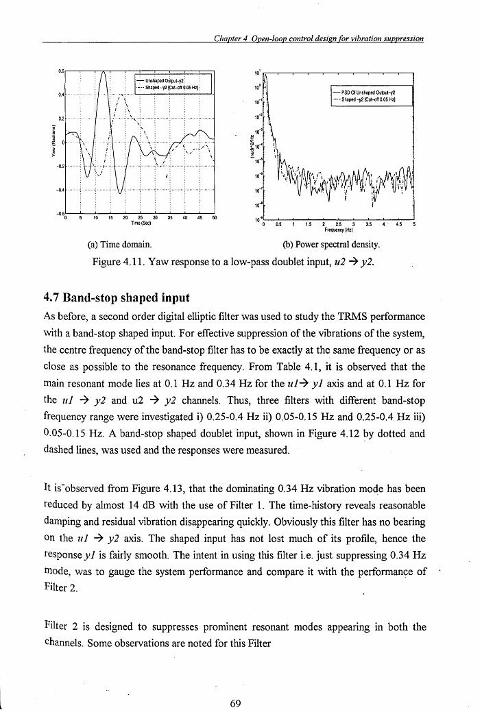
Chapter 4 Open-loop control design for vibration suppression
10 15 20 25 30 35 40 45 50 Time (Sec)
(a) Time domain.
10~
10"
- PSD 01 Unshaped Output-y2 . - . - Shaped -y2 (Cut-off 0.05 Hz)
10-0<---....1....---'----'-_.1....---'----'----'-_...1....---'-----' o 0.5 1 1.5 2 2.5 3 3.5 4' 4.5 5
Frequency (Hz)
(b) Power spectral density.
Figure 4.11. Yaw response to a low-pass doublet input, u2 ~ y2.
4.7 Band-stop shaped input
As before, a second order digital elliptic filter was used to study the TRMS performance
with a band-stop shaped input. For effective suppression of the vibrations of the system,
the centre frequency of the band-stop filter has to be exactly at the same freq~ency or as
close as possible to the resonance frequency. From Table 4.1, it is observed that the
main resonant mode lies at 0.1 Hz and 0.34 Hz for the u1~ y1 axis and at 0.1 Hz for
the u1 ~ y2 and u2 ~ y2 channels. Thus, three filters with different band-stop
frequency range were investigated i) 0.25-0.4 Hz ii) 0.05-0.15 Hz and 0.25-0.4 Hz iii)
0.05-0.15 Hz. A band-stop shaped doublet input, shown in Figure 4.12 ~y dotted and
dashed lines, was used and the responses were measured.
It is-observed from Figure 4.13, that the dominating 0.34 Hz vibration mode has been
reduced by almost 14 dB with the use of Filter 1. The time-history reveals reasonable
damping and residual vibration disappearing quickly. Obviously this filter has no bearing
on the u1 ~ y2 axis. The shaped input has not lost much of its profile, hence the
response y1 is fairly smooth. The intent in using this filter i.e. just suppressing 0.34 Hz
mode, was to gauge the system performance and compare it with the performance of
Filter 2.
Filter 2 is designed to suppresses prominent resonant modes appearing in both the
channels. Some observations are noted for this Filter
69
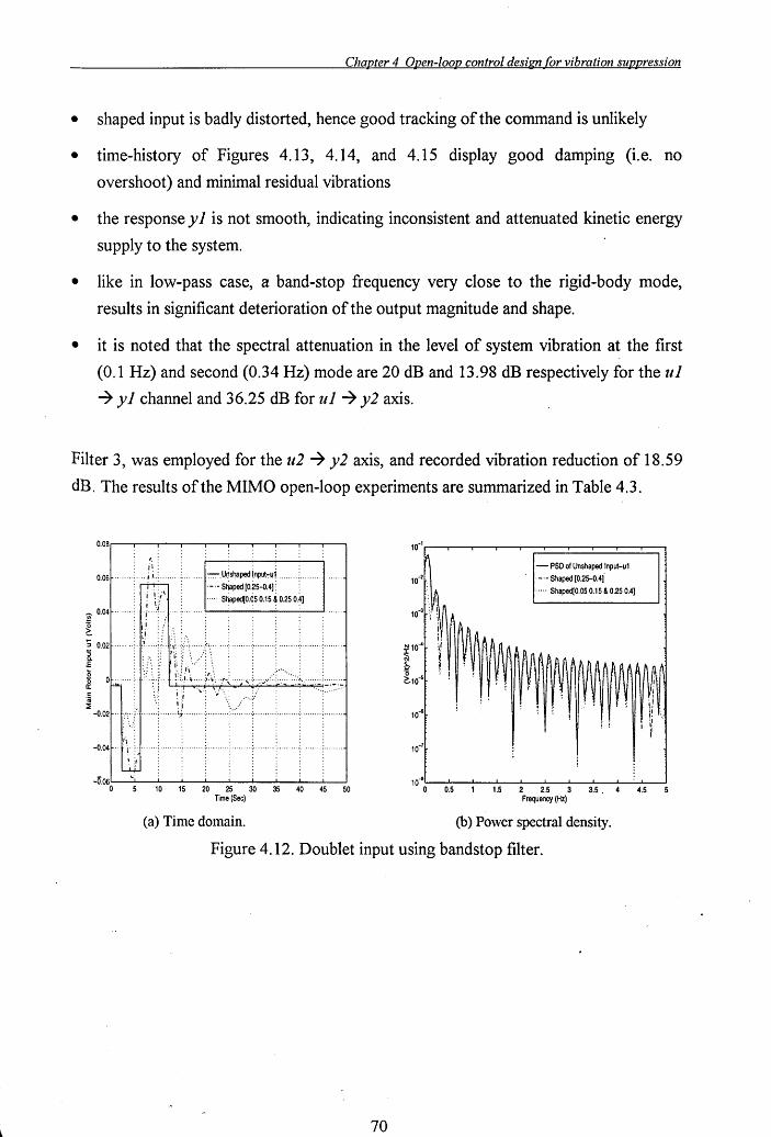
Chapter 4 Open-loop control design for vibration suppression
• shaped input is badly distorted, hence good tracking of the command is unlikely
• time-history of Figures 4.13, 4.14, and 4.15 display good damping (i.e. no
overshoot) and minimal residual vibrations
• the response y 1 is not smooth, indicating inconsistent and attenuated kinetic energy
supply to the system.
• like in low-pass case, a band-stop frequency very close to the rigid-body mode,
results in significant deterioration of the output magnitude and shape.
• it is noted that the spectral attenuation in the level of system vibration at the first
(0.1 Hz) and second (0.34 Hz) mode are 20 dB and 13.98 dB respectively for the ul
~ yl channel and 36.25 dB for ul ~ y2 axis.
Filter 3, was employed for the u2 ~ y2 axis, and recorded vibration reduction of 18.59
dB. The results of the MIMO open-loop experiments are summarized in Table 4.3.
10-6
10 15 20 25 30 35 40 45 50 Time (Sec)
- PSD of Unshaped Input-u1 . _. - Shaped [o.25-0.4f
..... ShapedlO.05 0.15 & 0.25 0.4]
! !
1.5 2 2.5 3 3.5. 4 4.5 Frequency (Hz)
(a) Time domain. (b) Power spectral density.
Figure 4.12. Doublet input using bandstop filter.
70
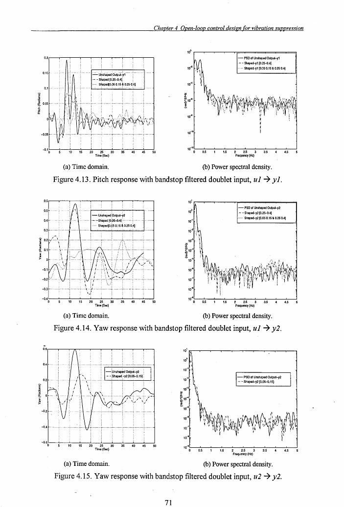
Chapter 4 Open-loop control design for vibration sU12pression
100
10-1
10"
~10" 'S !
10-1
10·'0
10·'2 10 15 20 25 30 35 40 45 50 0
Time (Sec)
(a) Time domain.
- PSD of Unshaped Output-yl
. - .• Shaped-yl [0.25-0.4)
..... Shaped-yl[O.05 0.15 & 0.25 0.4)
0.5 1.5 2 2.5 3 3.5 Frequency (Hz)
(b) Power spectral density.
4.5
Figure 4.13. Pitch response with bandstop filtered doublet input, U 1 ~ Y 1.
O.Gr----r--,--,.--.---.---r--,---,--,----,
0.5
0.4
0.31- .... · .. ·;·· .... · .. 1
10' r--r--r--.,..--r_,__ ...... ----_-...... _. - PSD of Unshaped Oulpul-y2
. - .• Shaped-y2 [0.25-0.4)
..... Shaped-y2 [0.050.15 & 0.25 0.4)
00.2~/' .. ··~'· .... ··" .. · .. · .. \ .. · ...... :·· ...... ·~ ........ ,· .. · .... :~·, .... .... , .......... : ........ ~ ~
10'"
~ !E. 0.1 ~ ..... :;, ..... 1' ......... '.1 .,; .. "'···;~ ..... ·I' ... \ ........ : ...... .: ... : ... ,: ..... : ......... : ....... ~ ~10·4 'S !
-0.1
-0.3f- ........ ;· .. · .. · .. , .. ·· .... ·, .... ··\· .. ·:,1 ........ : ........... : .......... : ......... , .......... : ........ ~
10 15 20 25 30 35 40 45 50 Time (Sec)
(a) Time domain.
1O.S
10.6
10.1
10-1
10.1
0 0.5 1.5 2 2.5 3 3.5 Frequency (Hz)
(b) Power spectral density.
4.5
Figure 4.14. Yaw response with bandstop filtered doublet input, u1 ~ y2.
-0.6r---..--,--.,..-,.--.----..--,--,.--.---r--.
0.4~ .. ·····:·······:·1
0.2 t-... ... :...... .j- .... ; .... :, ... : .......... : ... 1_'----'-_-'-_-'---1
-0.41- .... ·· .. :··· .... · .. : ........ ·: ... ·, h·, .... , .. ; .. · ...... ; .... , .... :, ...... , .. ; ........ ·; ........ ~
10 15 20 25 30 35 40 45 50 Time (Sec)
(a) Time domain.
10' r.--r--,--,.--.----..--,---.--.,..---,--,
- PSD of Unshaped Output-y2 - .• Shaped-y2 [0.05-0.15)
10"
10··0:------="0.5:---L---'1.S:---'-2 --:'2.5:--~3 --:'3.:""5 --'--J4.'::-5---.J
Frequency (Hz)
(b) Power spectral density.
Figure 4.15. Yaw response with bandstop filtered doublet input, u2 ~ y2.
71
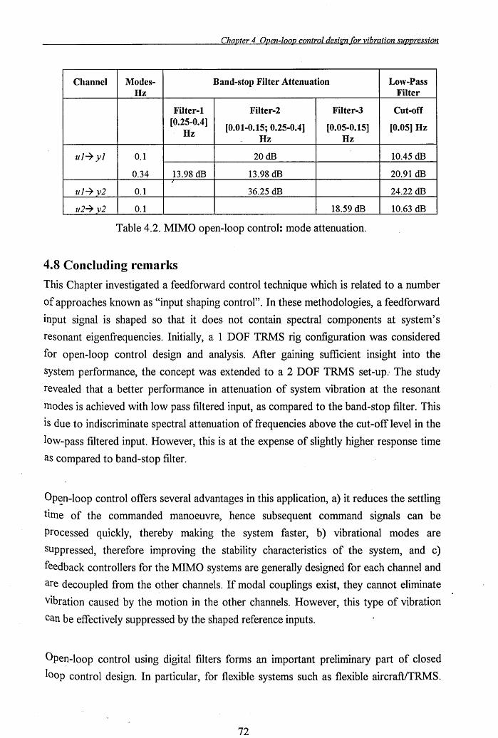
Chapter 4 Open-loop control design for vibration sU12,pression
Channel Modes- Band-stoll Filter Attenuation Low-Pass Hz Filter
Filter-1 Filter-2 Filter-3 Cut-off [0.25-0.4]
[0.01-0.15; 0.25-0.4] [0.05-0.15] [0.05] Hz Hz
Hz Hz
ul-7 yl 0.1 20 dB 10.45 dB
0.34 13.98 dB 13.98 dB 20.91 dB I
ul-7 y2 0.1 36.25 dB 24.22 dB
u2-7 y2 0.1 18.59 dB 10.63 dB
Table 4.2. MIMO open-loop control: mode attenuation.
4.8 Concluding remarks
This Chapter investigated a feedforward control technique which is related to a number
of approaches known as "input shaping control". In these methodologies, a feedforward
input signal is shaped so that it does not contain spectral components at system's
resonant eigenfrequencies. Initially, a 1 DOF TRMS rig configuration was considered
for open-loop control design and analysis. After gaining sufficient insight into the
system performance, the concept was extended to a 2 DOF TRMS set-up: The study
revealed that a better performance in attenuation of system vibration at the resonant
modes is achieved with low pass filtered input, as compared to the band-stop filter. This
is due to indiscriminate spectral attenuation of frequencies above the cut-off level in the
low-pass filtered input. However, this is at the expense of slightly higher response time
as compared to band-stop filter.
Op~n-Ioop control offers several advantages in this application, a) it reduces the settling
time of the commanded manoeuvre, hence subsequent command signals can be
processed quickly, thereby making the system faster, b) vibrational modes are
sUppressed, therefore improving the stability characteristics of the system, and c)
feedback controllers for the MIMO systems are generally designed for each channel and
are decoupled from the other channels. If modal couplings exist, they cannot eliminate
Vibration caused by the motion in the other channels. However, this type of vibration
can be effectively suppressed by the shaped reference inputs.
Open-loop control using digital filters forms an important preliminary part of closed
loop control design. In particular, for flexible systems such as flexible aircrafi/TRMS.
72

Chapter 4 Open-loop control design for vibration suppression
To acheive good tracking and disturbance rejection characteristics open-loop is not
sufficient. Hence, for overcoming the limitations of this approach, feedback control
techniques are investigated in Chapter 6.
73
Chapter 5 Nonlinear modelling ora 1 DOF TRMS using radial basis (unction networks
Chapter 5
Nonlinear modelling of a 1 DOF TRMS using radial basis function networks
I
Highfidelity nonlinear systenl models are often employed/or accurate representation of the plant in the simulation environment. This Chapter utilises a nonlinear systenl identification nlethod to nlodel the 1 DOF TRMS.. Extensive time and frequencydonlain nlodel-validation tests are employed to instil confidence in the estinlated model. The estinlated model has a good predictive capability and can be utilised for nonlinear sinlulation studies.
5.1 Introduction
Recent advances in aircraft technology has led to the development of many new
concepts in aircraft design, which are strikingly different from their predecessors. The
differences are in both aircraft configuration and control paradigms. This trend can be
attributed to the increasing emphasis on the aircraft to be agile (i. e. high Angle Of
Attack), low-observable (stealth), multi-purpose etc. for varied civilian and military
operations. These new generation air vehicles have presented a variety of unprecedented
cha~lenges and opportunities to aerodynamicists and control engineers. The expectations
of the new generation air vehicles to be highly agile and multi-functional demands that
they perform over a large flight envelope. Enhanced agility in control terms implies a
large excursion from the trim condition. In such a situation the linearized models can no
longer describe the aircraft dynamics well ,enough. Hence, there is a need for high
fidelity nonlinear dynamic models. Such models are essential for the design of control
systems, validation and for piloted simulation.
This Chapter presents a suitable modelling technique for such air vehicles. In this work,
a nonlinear system identification technique based on Radial basis function (RBF) is
utilised to model the TRMS. While the Newtonian mechanics or the Lagrange equations
74
Chapter 5 Nonlinear modelling ora 1 DOF TRMS using radial basis function networks
of motion can be used to find the nonlinear differential equations in a generic form, the
unknown parameters must still be identified. Such model based identification is
commonly employed with practical systems. There are numerous examples that
demonstrate the applicability, feasibility and versatility of the model based concepts. For
instance, neural networks have been employed for estimating the aerodynamic
coefficients of unmanned air vehicles (UAV's) [33]. More recently, RBF networks were
used by Kim and Calise [531 to capture variations in aircraft mach number. Here the
neural network (NN) is used to perform the dual roles of i) identifying the input-output
model parameters (off-line learning) using the mathematical model of an aircraft and, ii)
an adaptive network that compensates for imperfect inversion and in-flight changes in
the actual aircraft dynamics. An innovative time-domain nonlinear mapping-based
identification method is presented by Lyshevski [54] for identification of unsteady flight
dynamics. Lately, B-splines have been investigated in modelling and identification of
aircraft's nonlinear aerodynamic functions [55]. In all these cases the model structure is
known. However, in the present study, no model structure was assumed a priori i.e.
black-box modelling. Such an approach yields input-output models with neither a priori
defined model structure nor specific parameter settings reflecting any physical aspects.
In this study RBF networks are used to demonstrate these concepts by successfully
modelling the dynamical behaviour of the TRMS. Such a high fidelity nonlinear model is
often required for the nonlinear flight simulation studies. Since, there is no reliance on
the mathematical model, the estimated RBF model has to be thoroughly verified using
rigorous time and frequency domain tests. If the model structure and' the estimated
parameters are correct then the residuals (difference between model and system output)
sho~lld be unpredictable from all linear and nonlinear combinations of past inputs and
outputs. This is ensured by carrying out higher order cross-correlation tests, proposed
by Billings and Voon [56].
This Chapter first describes the nonlinear modelling approach adopted in Section 5.2,
which is followed by a discussion of RBF networks in Section 5.3. The type of
excitation signal and data pre-processing needed to identify the nonlinear model is
Outlined in Section 5.4. Implementation and results are presented in Section 5.5. In
Section 5.6 the nonlinear model and the linear model from Chapter 3 are compared.
Finally, the main findings of this Chapter are summarised in Section 5.7. ~ .
75
Chapter 5 Nonlinear modelling ofa 1 DOF TRlvfS using radial basis function networks
5.2. Nonlinear modelling
There are a number of different types of nonlinear models that are potentially suited to
this problem. Some examples are the output-affine model, the polynomial model and the
rational model. In this investigation, a nonlinear gutoregressive model with e~ogenous
inputs (NARX) [57], which provides a concise representation for a wide class of
nonlinear systems, is employed. The model is of the form:
y(t) = f(y(t -J), ... y (t - ny),u(t -J), ... u (t - nu))+ e(t) (5.1)
where, y(t), is the output, u(t) is the input and e(t) accounts for uncertainties, possible
noise, unmodelled dynamics, etc. lly , llu are the maximum lags in the output and the
input; { e( t)} is assumed to be a zero mean white noise sequence; and j{ • ) is some
vector valued nonlinear function ofy(t) and u(t) respectively. The NARX model is also
referred in the literature by various other names such as one-step ahead predictor or as
series-parallel model. Because the system noise e(t) is generally unobserved, it can only
be replaced by the prediction error or residual 8 (t), and equation (5.1), can be re
written as:
y(t) = f«(y(t -J), ... y (t - ny),u(t -J), ... u (t - nu)) + E(t) (5.2)
Where the residual is defined as:
E( t) = y ( t ) - y (t) (5.3)
where y (I) is the model predicted output.
Two considerations are of practical importance for the application of the NARX
approach. The nonlinear functional form j{ • ) should be capable of describing nonlinear
input-output space. Secondly, an efficient identification procedure for selecting a
parsimonious model structure is required. The present study employs an RBF network
to model the input-output relationship. This is depicted in Figure 5.1. The nonlinearity
within the RBF can be selected from a small set of typical nonlinear fu~ctions, such as
the thin-plate-spline function, the Guassian function, the multiquadratic and the inverse
multi quadratic functions. A generally held opinion is that the choice of the nonlinearity
IS not crucial for performance [58].The nonlinear functional form, f( . ) in the RBF
expansion, used in this study is the Guassian function. Orthogonal least square (OLS)
76
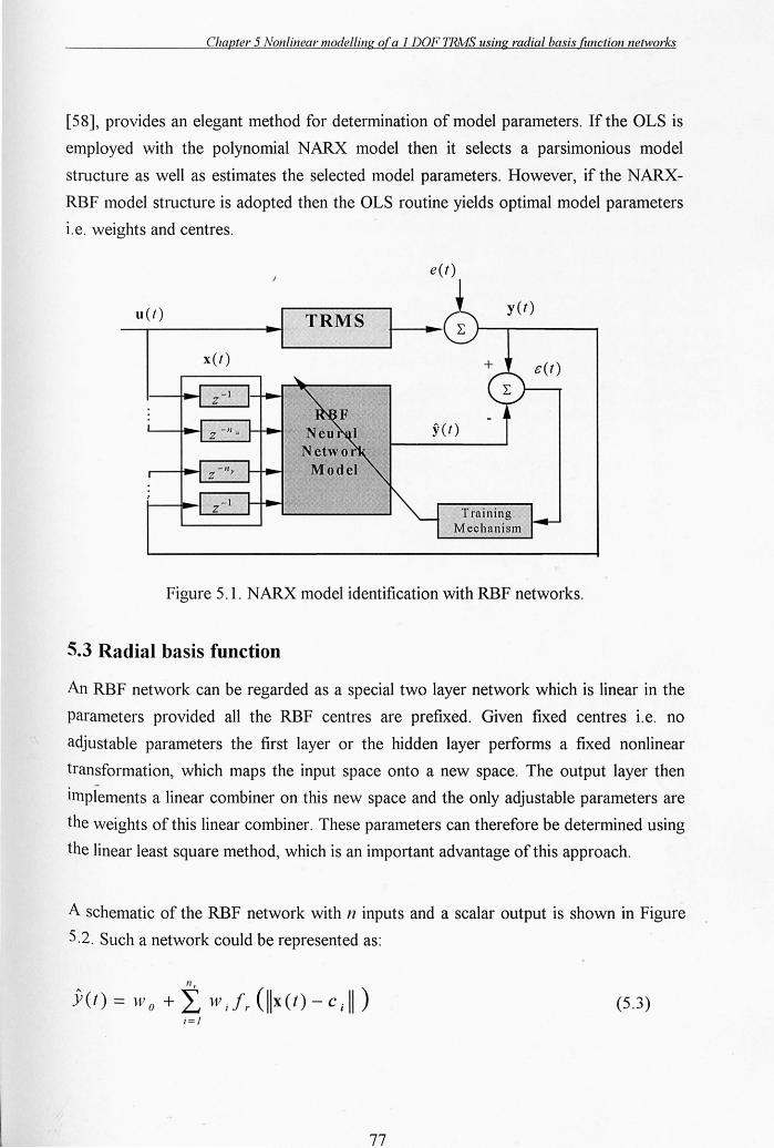
Chapter 5 Nonlinear modelling ora 1 DOF TRMS using radial basis fimctionnetworks
[58], provides an elegant method for determination of model parameters. If the OLS is
employed with the polynomial NARX model then it selects a parsimonious model
structure as well as estimates the selected model parameters. However, if the NARX
RBF model structure is adopted then the OLS routine yields optimal model parameters
i.e. weights and centres.
u(t) TRMS y(t)
x(t)
Figure 5.1. NARX model identification with RBF networks.
5.3 Radial basis function
An RBF network can be regarded as a special two layer network which is linear in the
parameters provided all the RBF centres are prefixed. Given fixed centres i. e. no
adjustable parameters the first layer or the hidden layer performs a fixed nonlinear
transformation, which maps the input space onto a new space. The output layer then
implements a linear combiner on this new space and the only adjustable parameters are
the weights of this linear combiner. These parameters can therefore be determined using
the linear least square method, which is an important advantage of this approach.
A schematic of the RBF network with n inputs and a scalar output is shown in Figure
5.2. Such a network could be represented as:
nr
y (1) = W 0 + L W i I,. (11x ( t) - C i II ) (5.3) i=1
77

Chapter 5 Nonlinear modelling ofa 1 DOF TRMS using radial basis function networks
where y(t) is the network predicted output, x(t) IS the network's input vector
containing all regressors of equation (5.1), that is,
x(t) = [(yet -l), ... y (t - ny), u(t -l), ... u (t - nu )]T (5.4)
Wi, are the weights or parameters, Wo is the bias or the d.c level term at the output, Ci
are known as RBF centres apd nr is the number of centres or the hidden neurons. Once
the functional form.f{.) and the centres Ci are fixed, and the set of input x(t) and the
corresponding desired output vector (y(t) in this study) provided, the weights Wi can be
determined using the linear least squares method. Clearly, y (I) is the nonlinear model
predicted output determined by the past values of the system output vector y( t), and the
input vector u(t), with maximum lags ny, and nu respectively.
1
+-~ yet)
Linear Combinator
Nonlinear Transformation
Figure 5.2. Radial basis function network.
The Guassian form for the RBF Ii ( x) is
-{( x (t) - C .) 2 + (x (t) - C .)
2 + .... + (x (t) - C .) 2
] / 1 1,.. 2 21 n m
f;(x1(t), X 2 (t), .... xn(t)) = e (j.2 I .
(5.5)
Where c. = (C Ii ' C2
. ••••• , C .) is a vector which defines the centre of'the RBF Ii in 1 I m
neuron i, and (j.2 is the "shape" of the function or the spread constant. Input patterns x I
activate the nodes according to their distance Ilx - c j II from the node centres C.' Thus, I
78
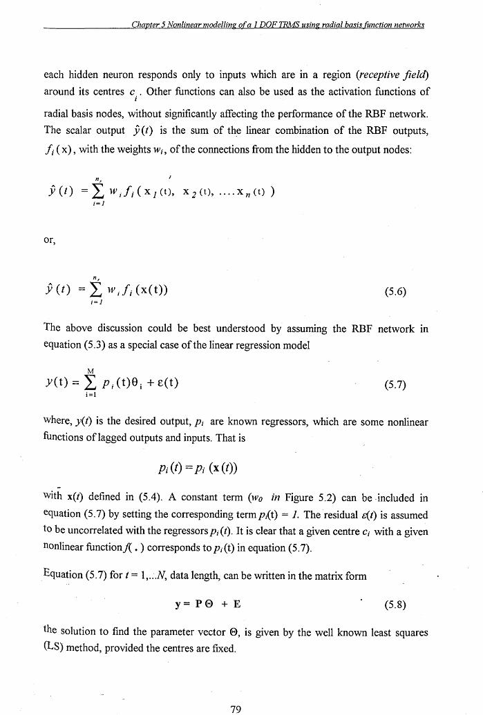
Chapter 5 Nonlinear modelling ora 1 DOF TRMS using radial basis function networks
each hidden neuron responds only to inputs which are in a region (receptive field)
around its centres c . Other functions can also be used as the activation functions of i
radial basis nodes, without significantly affecting the performance of the RBF network.
The scalar output y(t) is the sum of the linear combination of the RBF outputs,
Ii (x), with the weights Wi, of the connections from the hidden to the output nodes:
nr
yet) = L W;li(xj(t), X2(t), .... Xn(t)) ;=1
or,
nr
y (t) = L W; Ii (X ( t ) ) (5.6) ;=1
The above discussion could be best understood by assuming the RBF network in
equation (5.3) as a special case of the linear regression model
M
yet) = L P; (t)8 i + E(t) (5.7) i=l
Where, y(t) is the desired output, Pi are known regressors, which are some nonlinear
functions of lagged outputs and inputs. That is
Pi (t) = Pi (x (t))
-with x(t) defined in (5.4). A constant term (wo in Figure 5.2) can be .included in
equation (5.7) by setting the corresponding term Pi( t) = 1. The residual 8{t) is assumed
to be uncorrelated with the regressors Pi (t). It is clear that a given centre Ci with a given
nonlinear function./{. ) corresponds to Pi(t) in equation (5.7).
Equation (5.7) for t = 1, .. . N, data length, can be written in the matrix form
y=P0 +E (5.8)
the solution to find the parameter vector 0, is given by the well known least squares
(LS) method, provided the centres are fixed.
79
Chapter 5 Nonlinear modelling ora 1 DOF TRMS using radial basis fimction networks
5.3.1 RBF -NN learning algorithms
The task of a learning algorithm, or an optimisation routine, in an RBF network is to
select the centres and to find a set of weights that makes the network perform the
desired mapping. In essence, the objective is to minimise the variance or the sum
squared of the residual.
N
&'£2 = L £2(1) (5.9) 1=1
A number of algorithms are frequently utilised for this purpose [59], for instance,
• random centre selection and a least square algorithm.
• clustering and a least square algorithm.
• nonlinear optimisation of all the parameters i.e. centres, output weights and
other free parameters.
• the orthogonal least square algorithm (OLS).
Among these the OLS is widely used. The orthogonal least squares (OLS) method
proposed by Chen et at [58], yields both number of centres Cj, i.e: significant" regressors,
as well as the corresponding parameter vector e in equation (5.6). The underlying idea
of the algorithm is to transfer the regression equation into an equivalent orthogonal
form. Then the RBF centres can be selected and weights optimised in a simple
procedure according to a criterion referred as the "error-reduction-ratio" (ERR) due to
the orthogonality property. Details of the OLS can be found in Chen et at [58].
5.4_ Excitation signal and data pre-processing
In this Section the characteristic of the excitation signal for nonlinear ide~tification is
delineated followed by some guidelines for input-output data pre-processing before
applying it to the neural networks.
5.4.1 Excitation signal
In nonlinear system identification, the type of input signal to be used plays a crucial role
and has a direct bearing on the fidelity of the resulting identified model. The excitation
signal should have two important characteristics:
80
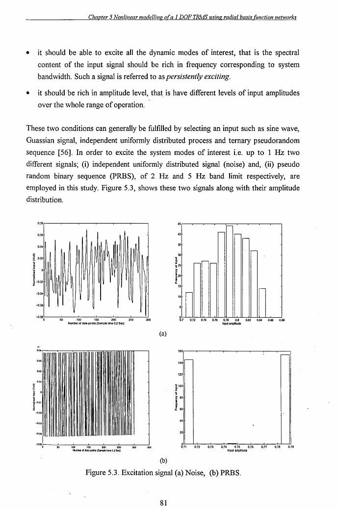
Chapter 5 Nonlinear modelling ora 1 DOF TRA1S using radial basis (unction networks
• it should be able to excite all the dynamic modes of interest, that is the spectral
content of the input signal should be rich in frequency corresponding to system
bandwidth. Such a signal is referred to as persistently exciting.
• it should be rich in amplitude level, that is have different levels of input amplitudes
over the whole range of operation.
These two conditions can generally be fulfilled by selecting an input such as sine wave,
Guassian signal, independent uniformly distributed process and ternary pseudorandom
sequence [56]. In order to excite the system modes of interest i.e. up to 1 Hz two
different signals; (i) independent uniformly distributed signal (noise) and, (ii) pseudo
random binary sequence (PRBS), of 2 Hz and 5 Hz band limit respectively, are
employed in this study. Figure 5.3, shows these two signals along with their amplitude
distribution.
0.08
0.06
0.04
~ 0.02 :; Q, .J;
] 0
i -0.02 Z
~~ ~ :l ~ IU
I~
-0.04 ~
-0.06
-0.08 0 50 100 150 200 250
Number of data points (Sample time 0.2 Sec)
0.04r---'-~----",...,..,.,..,-:==
lillll!11
0.03
0.02
0.01
! 1 0
1 l-o.ot
~ -0.02
-0,03
-0.04
300
-0.05 O::------:!:50:---~IOO---:,~50 --:-'200~~250--300-'------'350 Number 01 data points (Sample limo 0.2 Sec)
(a)
(b)
45 -40
r-- -r--
35
-30
'5 ~ 'S 25
--r--
~ c ~20 ~ IL
15 r--
r--10
o V ~ ~ ~ ~ M ~ ~ ~ ~
Inputal'fllUlUde
O~~--~~--~---'--~--~~ 0.71 0.72 0.73 0.74 0.75 0.76 0.77 0.78 0.79
Input amplhude
Figure 5.3. Excitation signal (a) Noise, (b) PRBS.
81
Chapter 5 Nonlinear modelling ora 1 DOF TRMS using radial basis function networks
5.4.2. Data pre-processing
Processing of the raw input-output data obtained from the experiments is recommended
for system identification. Pre-processing could involve removal of outliers, stray data
points and normalisation. In the case of identifying a system model using NN, it is
advantageous to apply pre-processing transformations to the input data before
presenting it to the network. Reducing the difference of magnitude of input variables
used to train network leads to faster convergence. One of the common method of pre
processing is the linear rescaling of the input variables. The normalised data is obtained
by carrying out the following data manipulation:
(5.10)
where X; is the mean and cr; is the variance of each variable of the training set and
defined as:
X. =_1 fx~ I NL..J I
n=1
(5.11)
(5.12)
Where 11 = 1,···,N are the number of data points or the data length. The re-scaled
variables defined by xt have zero mean and unit standard deviation. The target values
are also subjected to similar linear rescaling.
5.5 Implementation and results
In this Section results of modelling the TRMS with neural networks is described. The
modelling with NN was carried out with the TRMS pitch response to a uniformly
distributed noise signal as described in the previous section. The rationale of using the
noise signal is that the two level PRBS signal may not be good enough to capture
nonlinearities, if present, in the system. For the sake of comparison the t~o-level PRBS
tnput shown in Figure 5.3 is also utilised for modelling the 1 DOF TRMS. Results
obtained with the main rotor input and the pitch output are described below.
82
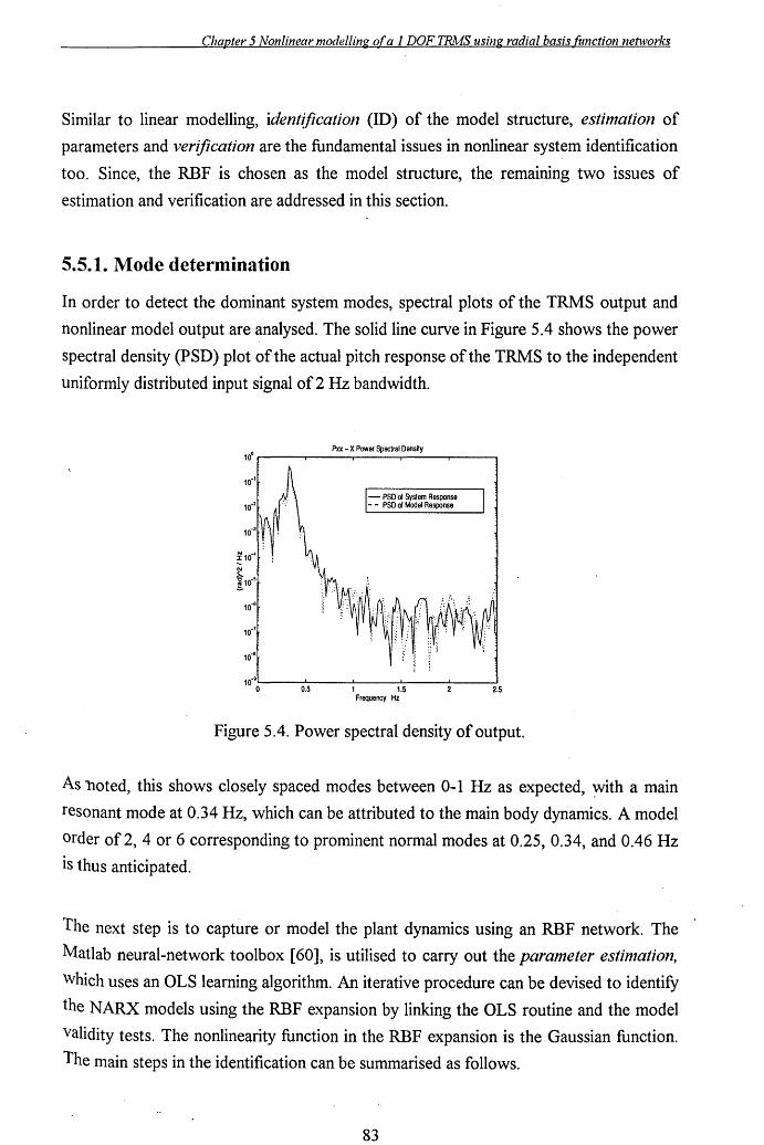
Chapter 5 Nonlinear modelling ora 1 DOF TRJvfS using radial basis function networks
Similar to linear modelling, identification (ID) of the model structure, estimation of
parameters and verification are the fundamental issues in nonlinear system identification
too. Since, the RBF is chosen as the model structure, the remaining two issues of
estimation and verification are addressed in this section.
5.5.1. Mode determination
In order to detect the dominant system modes, spectral plots of the TRMS output and
nonlinear model output are analysed. The solid line curve in Figure 5.4 shows the power
spectral density (PSD) plot of the actual pitch response of the TRMS to the independent
uniformly distributed input signal of 2 Hz bandwidth.
Pxx - X Power Spectral Dens~y
- PSD of System Response - - PSD of Model Response
10-9'-----'-__ 1---_-'-__ "--_--' o 0.5 1 1.5 2.5
Frequency Hz
Figure 5.4. Power spectral density of output.
As noted, this shows closely spaced modes between 0-1 Hz as expected, ~ith a main
resonant mode at 0.34 Hz, which can be attributed to the main body dynamics. A model
order of2, 4 or 6 corresponding to prominent normal modes at 0.25, 0.34, and 0.46 Hz
is thus anticipated.
The next step is to capture or model the plant dynamics using an RBF network. The
Matlab neural-network toolbox [60], is utilised to carry out the parameter estinlation,
Which uses an OLS learning algorithm. An iterative procedure can be devised to identify
the NARX models using the RBF expansion by linking the OLS routine and the model
validity tests. The nonlinearity function in the RBF expansion is the Gaussian function.
The main steps in the identification can be summarised as follows.
83
Chapter 5 Nonlinear modelling ora 1 DOF TRlvfS using radial basis (unction networks
(i) Choose ny, and nu' Initially the set of candidates centres are all the
x(t) = [(y(t -l), ... y (t - ny),u(t -l), ... u (t - nu)]T
(ii) Select the Guassian spread constant cr i and define the error goal.
(iii) An iterative loop is then entered to update the model based on the "error
reduction-ratio" (ERR) criteria [58].
(iv) Different time and frequency domain validity tests are performed to assess
the model. If the model is good enough the procedure is terminated. Otherwise
go to step (i).
The OLS learning method selects a suitable set of centres Ci (regressors) from a large
set of candidates as well as estimates the linear parameters Wi, or the weights. The
iterative procedure described above is used to identify the RBF model. The RBF model
was trained with 300 data points and different combinations of input-output lags were
tried. Using a generate-and-test method, an 8th order NARX model was found to give a
better representation of the system dynamics in the frequency domain (see Figure 5.4)
than the 6th order model as envisaged. This model reached a sum-squared error level of
0.002 after 13 training passes. The identified model included a constant term and 13
centres or neurons. The PSD obtained from the RBF model and the experimental data
are superimposed in Figure 5.4. It is observed that the dominant modes of the model
and the plant coincide quite well, implying good model predicting capability of the
important system dynamics. Thus, it is assumed that the identified model is fairly
accurate and suitable for system analyses.
5.5.2. Correlation tests
In the previous section frequency domain test was employed to detect the system
modes. In order to ensure further confidence in the identified model time domain
correlation tests are employed next.
A more convincing method of model validation is to use correlation tests. If a model of
a system is adequate then the residuals or prediction errors e(t) should be unpredictable
from (uncorrelated with) all linear and nonlinear combinations of past inputs and
Outputs. This can be tested by means of the following correlation functions [56]:
84
Chapter 5 Nonlinear modelling ora 1 DOF TRMS using radial basis (unction networks
<I> EE ( t) = E [ E (t - t) E ( t )] = 8 ( t )
<l>uE (t) = E[u(t - t)E(t)] = 0 "It
(5.13)
<l>E(EU) (t) = E[ E(t)E(t -1- t)u(t -1-t)] = 0 t ~ 0
where <PUE ('t) indicates the cross-correlation function between u(t) and E(t),
EU(t) = E(t + l)u(t + 1), and 8('t) is an impulse function.
In the case of linear modelling, discussed in Chapter 3, the first two tests alone were
adequate to test the model validity. The first two linear correlation tests in equation
(5.13) alone are not sufficient to validate nonlinear models. Hence, higher-order
correlation tests are also included in this study. All five tests defined by equation (5.13)
should be satisfied if the u(.)' sand y(.) 's are used as network i~put nodes .. In practice
normalised, correlation's are computed. In general, if the correlation functions in
equation (5.13) are within the 95% confidence intervals, ±1.96 /.IN, where, N is the
total number of data points, the model is regarded as satisfactory.
Figure 5.5, shows the correlation tests described by equation (5.13). It is important to
note that only the first few lags are significant. The lags in the x-axis of Figure 5.5 are
eq~valent to sampling period, that is, each lag ('t) is equivalent to 0.2 seconds. The y-
axis of each plot in Figure 5.5 is given by the corresponding correlation· function of
equation (5.13).
85
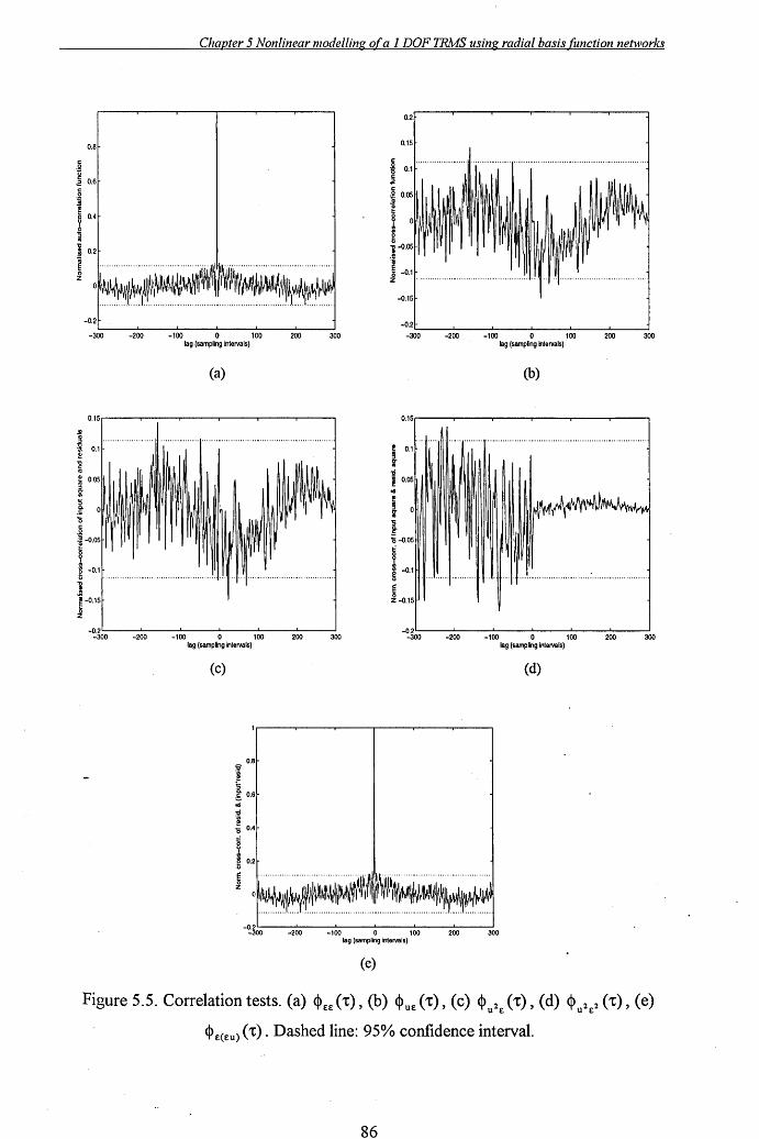
Chapter 5 Nonlinear modelling ora 1 DOF TRMS using radial basis function networks
0.8
0.6
0.4
0.2
-0.2 ~--~----~--~----~--~--~
-300 -200 -100 0 100 200 300 lag (sampling intervals)
(a)
0.15.------.------,..------r------,-----r-----,
.!! ~ ...................... . ............................ , ......................................... . ~ 0.1 e ~ ~ 0.05
i 5 .~ 0 '0 .g ~ -0.05 t:
i -0.1 ............................................... _ ........................................ ..
'i .!II ~ -0.15
~
_0.2~----'-----L------'-----''-----"'"'''--------J -300 -200 -100 0 100
lag (sampling intervals)
(c)
0.8 :2 .~ 5 .§: 0.6
oil
:2
~ 0.4
t:
I 0.2
200 300
0.2
0.15
c ....•.•.....•.•.•........•....••....•....•.... _ .........•.....•.•.............•...............
. ~ 0.1
.2 c ..g 0.05 .!'l
I ' -i -0.05 .!II
1-0.1 z .............................................. ..
-0.15
-O.2L--__ --'-__ --' ____ "'""'---__ ----' ____ ....I..-__ ---J -300 -200 -100 0 100 200 300
lag (sampling Intervals)
(b)
0.15.------r------,------,-------.-----r-----,
i 0.1
'd .~ 0.05
oil
i 0
5 .~ '0 -0.05 to
i -0.1
~ z -0.15
-0.2~----'-----''-------'-----'----"'"'''--------l -300 -200 -100 0 100 200 300
lag (sampling intervals)
(d)
S '1\~~_~~~/~~1II. .. MJI\·· .. 1IL "vlI\"W'I"I
.. ~ ............. -............................................... .. -':~00'-----2oo'----..... looL----..... 0L-----Jl0L-0 ----'200'------'300
lag (sampling intervals)
(e)
Figure 5.5. Correlation tests. (a) <l>EE ('t), (b) <l>uE ('t), (c) <l>u2E ('t), (d) <l>u 2E2 ('t), (e)
<l>E(EU) ('t). Dashed line: 95% confidence interval.
86
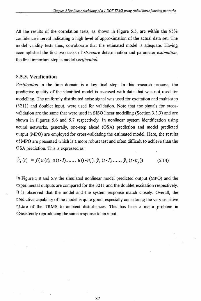
Chapter 5 Nonlinear modelling ora 1 DOF TRlvfS using radial basis (unction networks
All the results of the correlation tests, as shown in Figure 5.5, are within the 95%
confidence interval indicating a high-level of approximation of the actual data set. The
model validity tests thus, corroborate that the estimated model is adequate. Having
accomplished the first two tasks of structure determination and parameter estimation,
the final important step is model verification.
5.5.3. Verification
Verification in the time domain is a key final step. In this research process, the
predictive quality of the identified model is assessed with data that was not used for
modelling. The uniformly distributed noise signal was used for excitation and multi-step
(3211) and doublet input, were used for validation. Note that the signals for cross
validation are the same that were used in SISO linear modelling (Section 3.3.3) and are
shown in Figures 5.6 and 5.7 respectively. In nonlinear system identification using
neural networks, generally, one-step ahead (OSA) prediction and model predicted
output (MPO) are employed for cross-validating the estimated model. Here, the results
of MPO are presented which is a more robust test and often difficult to achieve than the
OSA prediction. This is expressed as:
Yd (t) = f(u(t), u(t-i), ..... , u(t-nu)' Yd (t-i), ..... , Yd (t-ny)) (5.14)
In Figure 5.8 and 5.9 the simulated nonlinear model predicted output (MPO) and the
experimental outputs are compared for the 3211 and the doublet excitation respectively.
It is observed that the model and the system response match closely. Overall, the
predictive capability of the model is quite good, especially considering the very sensitive
nature of the TRMS to ambient disturbances. This has been a major problem In
consistently reproducing the same response to an input.
87
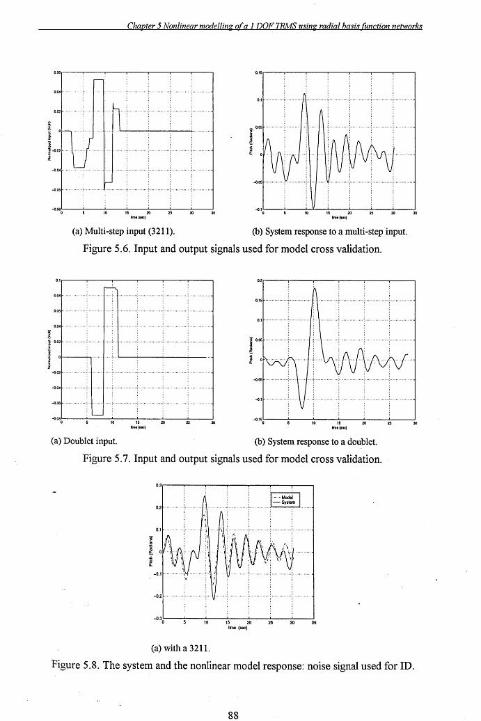
Chapter 5 Nonlinear modelling ora 1 DOF TRMS using radial basis fimction networks
0.06
.--
0.04 :
0.02
°h .....
r··· 2
1--0.0
-0.04
-0.06
-0.08 o
] ...
r--
10 15 20 limo (I .. )
25 30 35
0.15r---~-"--..---'---'-----.-----'
O.I~············i············I\·············:········· ..... -: .............. , ............. , ............ -1
-O.05I-············!"·············:-·1
-O.10~-~--7::10...!.--!:15:----:2O::------:2~5 --30~----:l35· IImO(IIC)
(a) Multi-step input (3211). (b) System response to a multi-step input.
Figure 5.6. Input and output signals used for model cross validation.
O.I,...-----,-----,r---,-----r--..-----,
0.08
0.06 ··························1 ... + ......... -: ............. : ............... ; ............. -l
0.04 ............... : ...... ··+···:···1···········:················:·············· .. c ...•...•.... -l
0.02 ···············:········+···;···'1············:······· ......... ; ................ : ............... -1
-0.021-·········· ... : 1
-0.041- .... ········;.·1
-0.061-··············:··1
L
-O·080'----'------'10'----'15---'-2O---'-25--.J30
tImO(IOC)
(a) Doublet input.
0.2·,...-----,-----,r---,-----r--..-----,
0.15~··········.····-:-·· ... · ........ /'+ ........... -:- ............... : ................ , .... , .......... -1
0.11-········,···~··············,:·+·,·········:······· ......... :, .............. , ............... -l
-O.05~"'" ......... : .... ,.\ ... , ... ; ............. , .. : ................ ; ........ , ........ : ............... -1
-0.11-···············:······\ , ..... : ................ : ..•............. : ................ : ...... , ........ -l
-O.15'-----1...-----'---L------1.--....l-----.J o 10 15 20 25 30
limo (I .. )
(b) System response to a doublet.
Figure 5.7. Input and output signals used for model cross validation.
0.3,...---.,---~-....----,.---,----r--___.
0.21-············,;···········, .......... mJ--~ L
-0.1
-0.21-···········:··········· : ... \/ .... , ........... ; ............. : ............. : ............ -l
-O.30~-~--7::,O---:'::,S---:'-20---:2':-S --=3i::-O ----:las time (sec)
(a) with a 3211.
Figure 5.8. The system and the nonlinear model response: noise signal used for ID.
88
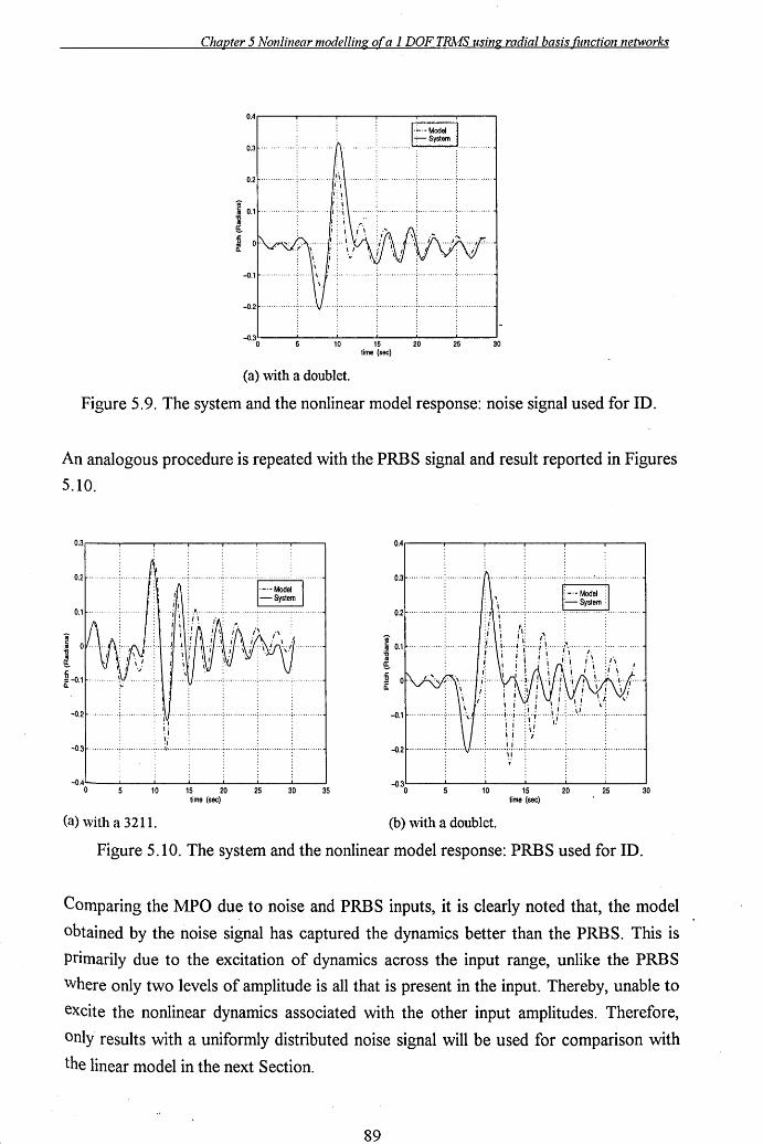
Chapter 5 Nonlinear modelling ora 1 DOF TRMS using radial basis (unction networks
0.4.------.-------r-----,.--...,-----.------,
0.3~··············:···············{\··············:···· .......... ''"''"'==~ ............. .j
0.21-··· .. ········· :.... ... ·I::I .. \ ........... : ............... : ................ ~ ............... -i
Ui" ~ 0.11-··············:-··········" :.j.\ .......... : ................ ! ..............•. -: ............. -i '2 ~
-O.II-· .. · .......... :· .... hl; .. ·: .............. ··:· .... · .. · ...... ·: ...... · .. · ...... ·~ ............. -i
-0.21- .... · ........ ··:·· .. ··V .. ··: .............. : ............... : ................ ~ .............. -i
-O.3"---'----'--~---'---_'_--' o 10 15 20 25 30
time (sec)
(a) with a doublet.
Figure 5.9. The system and the nonlinear model response: noise signal used for ID.
An analogous procedure is repeated with the PRBS signal and result reported in Figures
5.10.
0.4.------.-------r-----,.--...,----,---.,
0.31- .. · .. · ........ ·:· .............. H
0.21- .......... · .. ··: .... · ........ ·l
IO.ll- ............... : .... · ..... · .. l
~ ~
-0.11- ........ · .... ··:· .... ·\
-O.21- ........ · .. · .. ··: .. · .. · .. V
. . . . . . . . . . . . . . . . . . . . r.---"",
II ~. :
10 15 20 25 30 35 10 15 20 25 time (sec) time (sec)
(a) with a 3211. (b) with a doublet.
Figure 5.10. The system and the nonlinear model response: PRBS used for ID.
30
Comparing the MPO due to noise and PRBS inputs, it is clearly noted that, the model
obtained by the noise signal has captured the dynamics better than the PRBS. This is
primarily due to the excitation of dynamics across the input range, unlike the PRBS
where only two levels of amplitude is all that is present in the input. Thereby, unable to
excite the nonlinear dynamics associated with the other input amplitudes. Therefore,
only' results with a uniformly distributed noise signal will be used for comparison with
the linear model in the next Section.
89
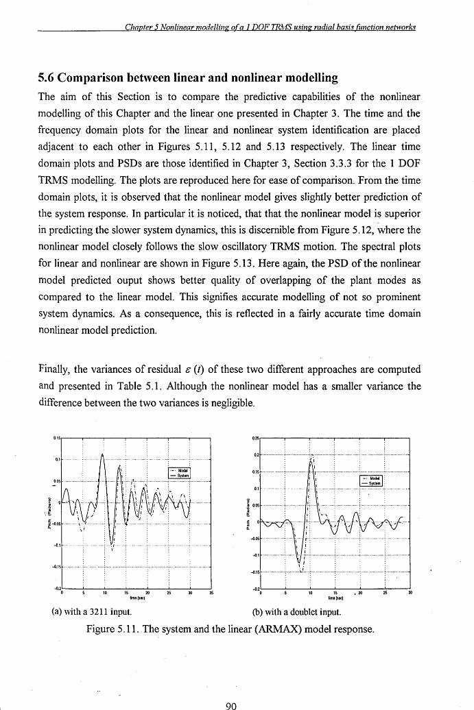
Chapter 5 Nonlinear modelling ora 1 DOF TRMS using radial basis (unction networks
5.6 Comparison between linear and nonlinear modelling
The aim of this Section is to compare the predictive capabilities of the nonlinear
modelling of this Chapter and the linear one presented in Chapter 3. The time and the
frequency domain plots for the linear and nonlinear system identification are placed
adjacent to each other in Figures 5.11, 5.12 and 5.13 respectively. The linear time
domain plots and PSDs are those identified in Chapter 3, Section 3.3.3 for the 1 DOF
TRMS modelling. The plots are reproduced here for ease of comparison. From the time
domain plots, it is observed that the nonlinear model gives slightly better prediction of
the system response. In particular it is noticed, that that the nonlinear model is superior
in predicting the slower system dynamics, this is discernible from Figure 5.12, where the
nonlinear model closely follows the slow oscillatory TRMS motion. The spectral plots
for linear and nonlinear are shown in Figure 5.13. Here again, the PSD of the nonlinear
model predicted ouput shows better quality of overlapping of the plant modes as
compared to the linear model. This signifies accurate modelling of not so prominent
system dynamics. As a consequence, this is reflected in a fairly accurate time domain
nonlinear model prediction.
Finally, the variances of residual 8 (t) of these two different approaches are computed
and presented in Table 5.1. Although the nonlinear model has a smaller variance the
difference between the two variances is negligible.
0,25r--,---..,----r---,.----r----,
0,2 ····,,·····, .. ·;··········.· .. ··i,,··.·.····· .... :··.·.···········i················;··············· : ;/', : . :
: " ; : ; 0.15 ............... ; ............... !' ·i·············;············'···~···············';···· ......... .
: Ii: 1-' ~oda I: : f i . .-5 'em: 0.1 ............. .: ............ !: ... , ........... ; ............... : .............. p ••••••••• , ••••
1 ~ 0.05··············.··········· g . ~ ; '_'_ ., ..... , I.: ..... ,
: \ !: ; i ~ : . : -0.05 .... ....... : ... ','" ~ .. : ............... : ............. : ....... ' ..... ' ........ " .. .
: i !: : : . -0.1 .•.....•...... .:. ..... , i. ·f··:················:·········.······;·.···· .. ·.··.·· .: .............. .
; ,!: . -0.15 ..............• : ......... ~! .... ~ ................ : .............. .. i ..... , .......... ~ .............. . . . . . .
, 10 15 20 lime (sec)
25 30 35 -O.2l----'----'---....I..----l---..I:--~,
o w ~ .20 ~ 30 time (sec)
(a) with a 3211 input. (b) with a doublet input.
Figure 5.11. The system and the linear (ARMAX) model response.
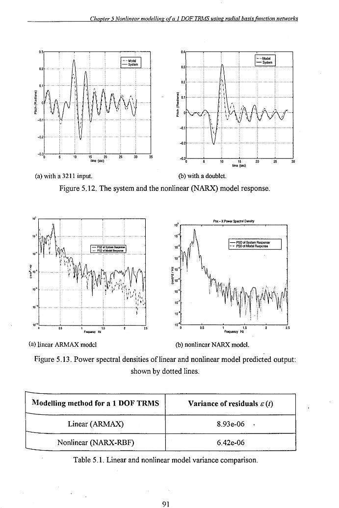
Chapter 5 Nonlinear modelling ora 1 DOF TRlvfS using radial basis (unction networks
0.41--:--:--"--~==::!;-1
1--'. Model I ... :=Syst~ ....
10 15 20 25 30 35 time (sec)
0.2
., ~ 0.1 '6 C1I
~
...................................................... , ............. . : : :
10 15 20 25 lime (sec)
(a) with a 3211 input. (b) with a doublet.
Figure 5.12. The system and the nonlinear (NARX) model response.
10' r---..,.----,------,---,----.,
10'10 ................. .
10·"0'-----'---'-0.5---1'----'-1.5---'------'2.5
Frequency Hz
100 .-__ -.--__ Pxx_-_xl'"""p_ow_er_Sp_8C_tra...,...1 D_en_sn_y _-,-__ --,
- PSD of System Response - - PSD of Model Response
~10"
~ 110'
S
10.8
10.7
10.8
10·D
0 0.5 1 1.5 2.5 Frequency Hz
30
(a) linear ARMAX model (b) nonlinear NARX model.
-
Figure 5.13. Power spectral densities of linear and nonlinear model predicted output:
shown by dotted lines.
Modelling method for a 1 DOF TRMS Variance of residuals 8 (I) r---
Linear(~) 8.93e-06 -Nonlinear (NARX-RBF) 6.42e-06 -
Table 5.1. Linear and nonlinear model variance comparison.
91
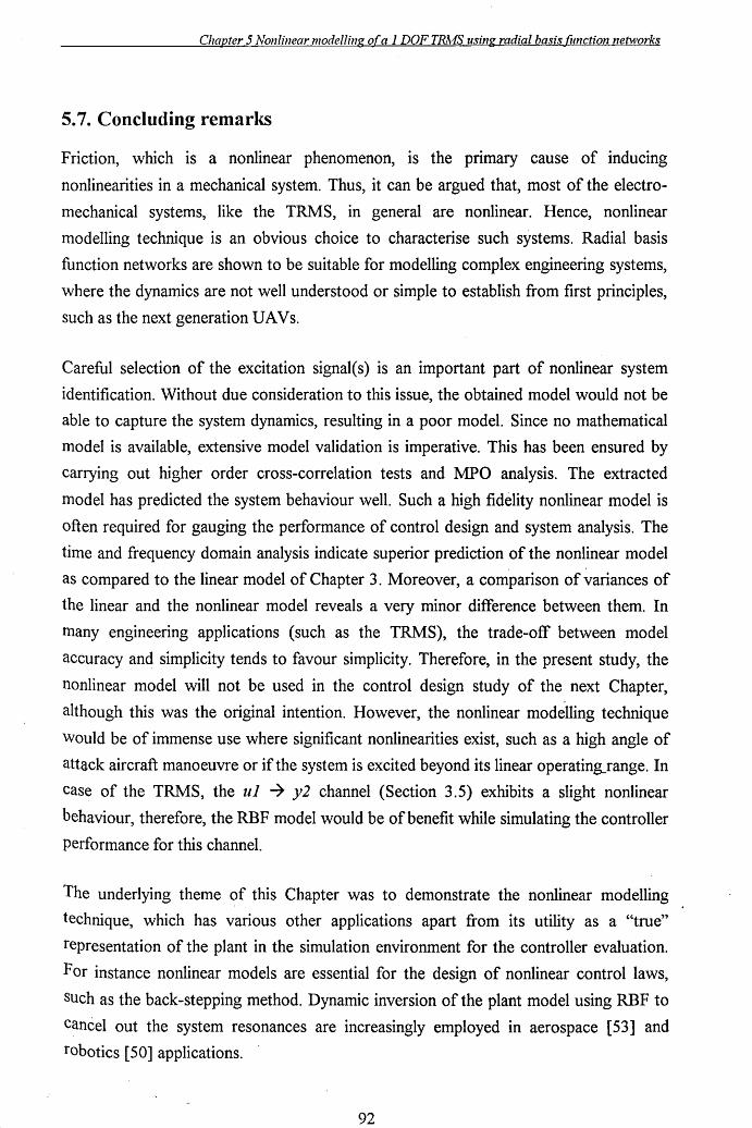
Chapter 5 Nonlinear modelling ora 1 DOF TRJvfS using radial basis (unction networks
5.7. Concluding remarks
Friction, which is a nonlinear phenomenon, is the pnmary cause of inducing
nonlinearities in a mechanical system. Thus, it can be argued that, most of the electro
mechanical systems, like the TRMS, in general are nonlinear. Hence, nonlinear
modelling technique is an obvious choice to characterise such systems. Radial basis
function networks are shown to be suitable for modelling complex engineering systems,
where the dynamics are not well understood or simple to establish from first principles,
such as the next generation DAVs.
Careful selection of the excitation signal( s) is an important part of nonlinear system
identification. Without due consideration to this issue, the obtained model would not be
able to capture the system dynamics, resulting in a poor model. Since no mathematical
model is available, extensive model validation is imperative. This has been ensured by
carrying out higher order cross-correlation tests and MPO analysis. The extracted
model has predicted the system behaviour well. Such a high fidelity nonlinear model is
often required for gauging the performance of control design and system analysis. The
time and frequency domain analysis indicate superior prediction of the nonlinear model . .
as compared to the linear model of Chapter 3. Moreover, a comparison of variances of
the linear and the nonlinear model reveals a very minor difference between them. In
many engineering applications (such as the TRMS), the trade-off between model
accuracy and simplicity tends to favour simplicity. Therefore, in the present study, the
nonlinear model will not be used in the control design study of the next Chapter,
although this was the original intention. However, the nonlinear modelling technique
Would be of immense use where significant nonlinearities exist, such as. a high angle of
attack aircraft manoeuvre or if the system is excited beyond its linear operatin8-range. In
case of the TRMS, the ul ~ y2 channel (Section 3.5) exhibits a slight nonlinear
behaviour, therefore, the RBF model would be of benefit while simulating the controller
performance for this channel.
The underlying theme of this Chapter was to demonstrate the nonlinear modelling
technique, which has various other applications apart from its utility as a "true"
representation of the plant in the simulation environment for the controller evaluation.
F or instance nonlinear models are essential for the design of nonlinear control laws,
Such as the back-stepping method. Dynamic inversion of the plant model using RBF to
cancel out the system resonances are increasingly employed in aerospace [53] and
robotics [50] applications.
92
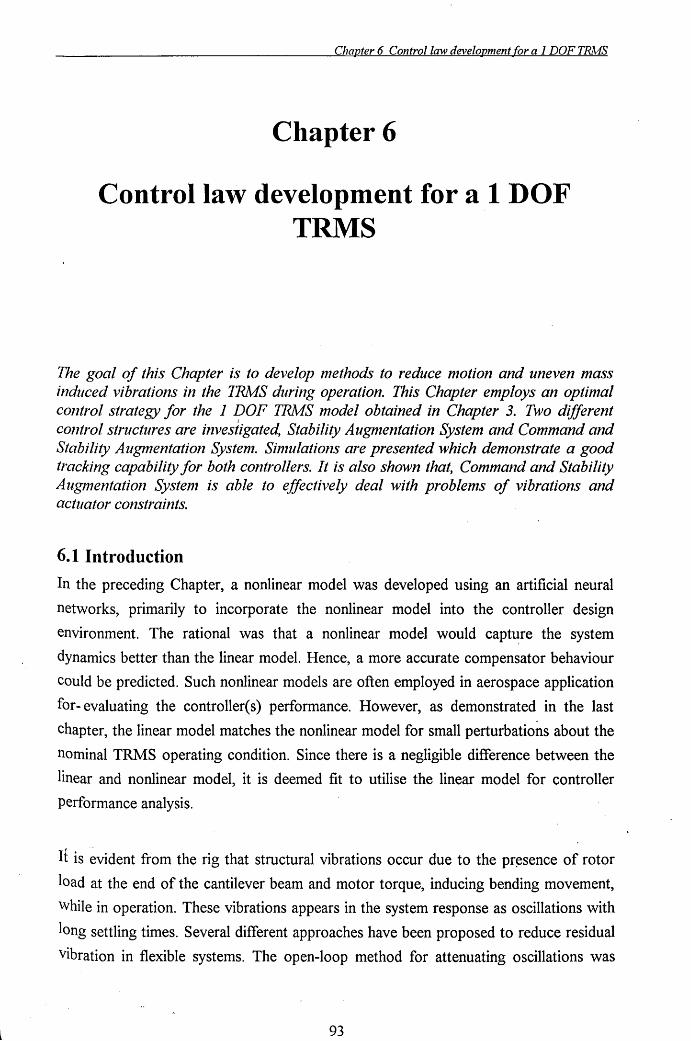
Chapter 6 Control law development for a 1 DOF TRMS
Chapter 6
Control law development for a 1 DOF TRMS
The goal of this Chapter is to develop methods to reduce motion and uneven mass induced vibrations in the TRMS during operation. This Chapter employs an optimal control strategy for the 1 DOF TRMS nl0del obtained in Chapter 3. Two different
I
control structures are investigated, Stability Augmentation System and Command and Stability Augnlentation Systenl. Simulations are presented which denlonstrate a good tracking capability for both controllers. It is also shown that, Command and Stability Augmentation Systenl is able to effectively deal with problems of vibrations and actuator constraints.
6.1 Introduction
In the preceding Chapter, a nonlinear model was developed using an artificial neural
networks, primarily to incorporate the nonlinear model into the controller design
environment. The rational was that a nonlinear model would capt~re the system
dynamics better than the linear model. Hence, a more accurate compensator behaviour
could be predicted. Such nonlinear models are often employed in aerospace application
for- evaluating the controller(s) performance. However, as demonstrated in the last
chapter, the linear model matches the nonlinear model for small perturbations about the
nominal TRMS operating condition. Since there is a negligible difference between the
linear and nonlinear model, it is deemed fit to utilise the linear model for controller
performance analysis.
Ii is evident from the rig that structural vibrations occur due to the pr~sence of rotor
load at the end of the cantilever beam and motor torque, inducing bending movement,
while in operation. These vibrations appears in the system response as oscillations with
long settling times. Several different approaches have been proposed to reduce residual
vibration in flexible systems. The open-loop method for attenuating oscillations was
93
Chapter 6 Control law development for a 1 DOF TRMS
examined in Chapter 4. However, in order to achieve a good tracking capability of
command inputs and disturbance rejection properties, this method on its own is
inadequate. Therefore, closed-loop strategies employing constant feedback gains have
also been designed for robust tracking and attenuation of residual vibration of elastic
systems. Both classical and modern feedback methods have been proposed to
manoeuvre flexible systems.
Doughtery et al [61] and Franklin et al [62] applied classical controllers to space
structures, to control the vibration and attitude (orientation). The control design
adopted basically treats the flexible modes as separable subsystems. Therefore, the gains
originally chosen for the rigid body alone need to be decreased for lower bandwidth to
assure stability when flexible modes are present. Azad [63] demonstrated control of a
single link flexible manipulator utilising a collocated PD feedback incorporating hub
angle and hub velocity feedback variables. This is then extended, additionally, to
incorporate non-collocated end-point acceleration feedback through a PID controller,
achieving a hybrid collocated and non-collocated feedback control mechanism. The
Naval Research Laboratory's (NRL) foldable remotely piloted UAV, adopted classical
techniques for controlling different flight phases, such as boost,transition to the cruise
phase and the cruise phase. [64]. Take off to a particular height, land and cruise mode
control of Georgia Tech [65] robot helicopter is accomplished using the classical PID
controller structure.
Modern control paradigms have been studied for a variety of complex systems, some of
which are discussed here. Recently, Teague et al [66] developed, a novel method for
active control of the attitude and vibration of a flexible space structure using the Global
Positioning System (GPS) as a sensor. Linear Quadratic Regulator (LQR) feedback was
employed in this study. Franklin et al [62], in addition to PD control, used modern
optimal control methods to achieve command tracking and vibration suppression of a
Space satellite. LQR based control design for commercial aircraft control applications
Was investigated by Blight et al [67] to redesign an autopilot control law in· order to
improve stability and reduce sensitivity to plant parameter variations. An improved
Control law wasdesigned compared to classical approaches, flight tested and
ilnplemented in the autopilot of the Boeing 767 commercial transport airplane. Their
experience in implementing the LQR paradigm is documented in [67].
94
Chapter 6 Control law development for a 1 DOF TR/yfS
In the autonomous flight control study of an UAV Aerial, LQR is used as a baseline line
inner loop controller [68]. It is expected to track commands generated by the 6 DOF
manoeuvre algorithm. The controller is employed to gauge the adverse effects of
uncertainty in the UAV aerodynamic and control derivatives (i.e. parameters) on the
stability and performance of the closed-loop system. LQR has also been adopted for an
autopilot design for a high-altitude, supersonic air-to-air bank-to-tum (BTT) missile
[69]. One of the design requirements for such systems is a high level of robustness to
parameter variations, which is difficult to meet with classical method.
LQR well-known counterpart LQG with an in-built observer design has also been
successfully employed for plants with elastic modes. Henrichfriese et al [70] developed
a controller with an observer to estimate the vibrating states based on a detailed system
model. Kosut et al [71] studied the robustness properties of several linear LQG based
designs. Design of control algorithms for a supersonic air-to-air missile presents a very a
challenging problem for the control engineer. Severe coupling between the guidance law
and autopilot is the main cause of design complexity. Added complexity occurs when
steering the missile in the terminal phase. The digital LQG compensator for such
systems is considered by Langehough and Simons [72] and found to be better than the
classical and eigenstructure methods. Control law development for a HAVE DASH II
missile autopilot is investigated by Lin [73] who employed LQR and LQG topologies.
Pitch, roll-yaw and combined pitch and roll-yaw designs are developed and shown to be
robust against plant parameter and operating range variations.
The LQG-Loop Transfer Recovery (LTR) approach has been investigated in areas such
as control of large space structures [73], weapon control [74], missile autopilot design
[73,75] and Integrated Flight Propulsion and Control [73]. More recently~ LQG-LTR
and H -00 based attitude control system have been designed for a large flexible space
structure with subassemblies [19]. Such large structures with flexible appendages are
the subject of considerable interest at present. Here, vibrations are not controlled
directly, the effect of flexibility is incorporated as modelling error. The controller design
is thus made robust against unmodelled flexible dynamics ensuring that instability in the
closed-loop system will not arise.
Modelling and H-oo control of a single link manipulator is reported in [76]. The H-oo
Controller is compared experimentally with a PI controller and shown to give improved
95
Chapter 6 Control law development for a 1 DOF TRMS
vibration control in the vertical plane. One of the seminal works on H-oo flight control,
is that of Hyde [77]. Here, H-oo is applied to a Generic Vertical Short Take-Off and
Landing (VSTOL) Aircraft Model (GV AM) developed by the Royal Aerospace
Establishment. A systematic procedure for the H-oo loop-shaping and the results of
flight tests are given in [77]. The H-oo control theory was used to design the controller
for a VTOL UAV and described in [78]. The control strategy was tested using real-time
hardware-in-the-Ioop simulation.
Robust control design can also be achieved via the eigenstructure assignment method.
This method has found to be particularly suitable for the aerospace applications. Livet et
al [16,17] has extensively studied the utility of this approach for a highly flexible
aircraft.
A dynamic inversion method has been investigated for flexible manipulators [50], BTT
air-to-air missile [79] and high angle of attack combat aircarft [80]. This approach has a
low design complexity and has several practical advantages.
6.1.1 Laboratory platforms
There is a small but growing body of literature on laboratory platforms to simulate
complex aircraft manoeuvres and problems, and to investigate different control
paradigms. A multimodel approach to robust controller design is illustrated for a 2 DOF
laboratory aircraft model, developed to model the behaviour of a vertical-take-off
aircraft by Werner and Meister [32]. In this work, the Linear Matrix Inequality (LMI)
formulation in conjunction with convex programming for robust command tracking and
disturbance rejection in normal operation as well as in failure mode is employed. This
platform is quite similar to the TRMS. It has roll and yaw movement where as the
TRMS has pitch and yaw motion.
A radio controlled (RC) model helicopter is adopted as a platform by Morris et a.l [30]
to study various modern identification and robust control synthesis t.echniques. The
helicopter is mounted on a 3 DOF wrist which in turn is connected to a 3 DOF stand.
This experimental set up is perceived as the hover mC?de. Stabilising LQG and H-oo,
Controllers with setpoint tracking are designed and compared for the RC helicopter. The
Caltech ducted fan flight control experiment is designed to represent the dynamics of
96
Chapter 6 Control law development for a 1 DOF TRMS
either a Harrier in hover mode or a thrust vectored aircraft such as the USAF F 18-
HARV or X-31 in forward flight [29]. A comparison of several different linear and
nonlinear controllers was performed by Kantner et al [81] on the same same rig. The
Georgia Tech model helicopter and NRL's foldable UAV, mentioned early in this
section, and VTOL UA V referred earlier [78], fall under the small experimental
platform category. These platforms are thus, ideal test-bench for modelling, design and
control research.
6.1.2 Evaluation of different control methods
From the earlier discussion it is clear that, there are many theoretical techniques that are
available for complex modern control system design. The classical single input single
output (SISO) control design methods utilising design criteria such as the phase and
gain margin, bandwidth, maximum overshoot and damping ratio, lead to systems that
would satisfy the desired performance criteria but are not optimised. Modern optimal
control theory relies on design techniques that maximise or minimise a performance
index, yielding a designed system that is optimal in some prescribed sense. For an LQR
controlled system, i.e. assuming all the states are available and no stochastic inputs, it is
well known that the open-loop regulator transfer function has a phase margin greater
than sixty degrees and an infinite gain margin. Therefore, this control method not only
ensures stability, but also provides the system with a good robustness properties.
However, LQR necessitates measurement of all states, which may not be possible or
could be expensive or unreliable to measure. On the other hand, for an LQG controlled
system with a combined Kalman filter and LQR control law, unmeasured states can be
estimated. This approach however, lacks the robustness characteristics of the LQR full
stafe feedback design.
Doyle and Stein [82] proposed LQG-LTR method, to address the issue of deterioration
of the robustness caused by the introduction of the estimator. The LQG-LTR
formulation requires the plant to be minimum phase, which is a fundamental drawback
of this paradigm. A further disadvantage is that, the design process introduces high gain
Which may cause problems with unmodelled dynamics [83]. Robustness characteristic
for a SISO controller design are accomplish by ensuring satisfactory gain and phase
margins. For multivariable systems, gain and phase margin are unreliable because they
cannot cater for simultaneous perturbation in different loops. The H-oo method
addresses this issue by explicitly addressing the issue of robustness in its design
97

Chapter 6 Control law development for a 1 DOF TRJvfS
formulation. Because of this property, it has attracted lot of attention in academia, but
has not yet been fully accepted in industry. The intuitive reasons are that, H-oo is
mathematically involved and complex, and that, the weights selection procedure is
tedious. For aerospace applications, other factors are also critical such as flight
certification. Although the computations involved in eigenstructure design are straight
forward, there are concerns about its ability to deal with robust stability and robust
performance. Dynamic inversion methods have a low design complexity and have
several practical advantages. A practical limitation of dynamic inversion is that it
implicitly assumes full state feedback. Also as the plant zeros becomes controller poles,
this would render system unstable, hence dynamic inversion method is not directly
applicable to non-minimum phase systems.
6.1.3 Control paradigm selection
In this Section, a number of potential design methodologies are examined to asses their
suitability for the TRMS application. The TRMS has the following important features:
• multi input multi output system,
• non-minimum phase system model (Chapter 3),
• full state feedback is not available,
• flexible dynamics,
• cross-coupling between pitch and yaw plane, and
• is dynamically similar to a helicopter,
While designing controllers for multivariable systems, such as the TRMS, the designer is
motivated to look for techniques that are inherently multivariable and also addresses the
optimality issue in some sense. Classical robustness pointers such as gain and phase
margins are unreliable when applied to multivariable systems because they cannot cater
for simultaneous perturbation in different loops [83]. Further, modern controller design
techniques exploit the full multi-variable nature of the plant. This aspect is particularly
useful in dealing with cross-coupling terms since all the feedback loops are available to
the controller which can then utilise any combination of inputs.
The TRMS' s MIMO structure, with cross-coupling between different channels, renders
it unsuitable for classical design methods and hence, a modern MIMO control approach
is an obvious choice. From the previous discussion on the TRMS, LQG appears to be
an attractive starting point. Primarily because the LQG has:
98
Chapter 6 Control law development for a 1 DOF TRJv1S
• an in-built estimator for constructing the unavailable states,
• no non-minimum phase restrictions, and
• its suitability for aerospace systems.
Thus, use of modern optimal LQG design technique is a prudent and pragmatic choice.
The goal of this Chapter is to develop methods to reduce motion and uneven mass
induced vibrations in the TRMS during operation. The assumption is that the motion
and the rotor load are the main source of system vibration as highlighted in Chapter 3. A
practical way of controlling a system with resonant modes is to use a combination of
feedback and feedforward. The feedforward option was demonstrated in Chapter 4. In
this Chapter, a Linear Quadratic Guassian (LQG) compensator is used as a state
feedback inner loop controller and digital filters as a feedforward compensator. The
inner feedback controller is referred as the Stability Augnlentation Systenl (SAS). The
background theory on optimal control is given in Section 6.2 to Section 6.5. The TRMS
control problem is defined in Section 6.6, and the integral LQG design is formulated in
Section 6.7. The SAS results with LQG as the feedback mechanism are given in Section
6.8. The combined feedforward and feedback control technique~ referred as Comnland
and Stability Augnlentation System (CSAS) is presented in Section 6.9. This combined
approach has been widely employed in aircraft control design [67]. The approach
requires that the natural resonant frequencies of the system be determined through
suitable identification and modelling techniques. Some important observations are given
in Section 6.10.
6.2 Concept of optimal control
Optimal control is based on state variable models of the system. The pole-placenlent
design approach using state feedback is appropriate for SISO systems. In this approach,
if the system is completely state controllable, then poles of the closed-loop system may
be placed at any desired locations by means of state feedback via a suitable state
feedback gain matrix [84]. Optimal control methods provide an alternate way of placing
the closed loop poles of a system in order to achieve some desired behaviour. In this
case, the designer does not know the exact closed-loop pole locations. Instead, the
eigenvalues are placed by the controller, in locations which seek to make the resulting
closed loop performance the best possible hence, optinlal, in some sense that the
designer can specify in advance. Thus, optimal control methods are one more way of
99
Chapter 6 Control law development for a 1 DOF TRMS
selecting the contents of the feedback gain matrix. However, unlike pole-placenlent,
which is not amenable for MIMO systems, an optinlal approach is quite appropriate. In
the design of SISO schemes by pole-placenlent, there is a unique feedback gain matrix
which would place the closed-loop poles in the desired position. In order to see the
limitations of the pole-placement approach, consider a multivariable case, having n
states and nl inputs, the dimensions of the feedback gain matrix are m x n, so that it
contains nl x n feedback gains. However, only n of these are needed to position the
closed-loop poles which are n in number. Optimal control is one way of constructively
using up the extra degrees offreedom in satisfying complicated design objectives.
To refine the meamng of "optimal control" it is necessary to define a rule for
determining the control action, subject to certain constraints, so as to minimise some
measure of the deviation from ideal behaviour. That measure is usually provided by the
chosen Performance Index (PI), which is a function whose value is considered to be an
indication of how well the actual performance of the system matches the desired
performance. In most cases, the behaviour of the system is optimised by choosing the
control vector u(k) in such a way that the PI is minimised [84]. A good introduction on
optimal control can be found in [84,85].
6.2.1 Formulation of optimisation problems
The problem of optimisation of a control system may be formulated if the following
information is given:
• system equations
• class of allowable control vectors
• constraints on the problems
• performance index
• system parameters
The solution of an optimal control problem is to determine the optimal control yector
lI(k) within the class of allowable control vectors. This vector u(k) depe~ds on:
• the nature of the performance index
• the nature of the constraints
• the initial state or initial output
100
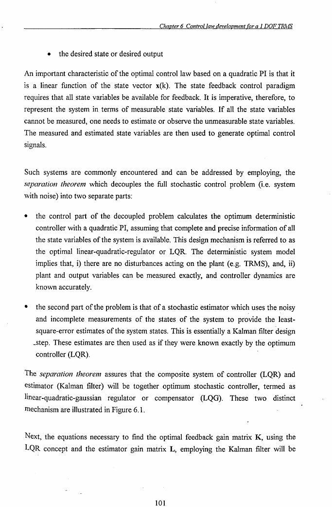
Chapter 6 Control law development for a 1 DOF TRAfS
• the desired state or desired output
An important characteristic of the optimal control law based on a quadratic PI is that it
is a linear function of the state vector x(k). The state feedback control paradigm
requires that all state variables be available for feedback. It is imperative, therefore, to
represent the system in terms of measurable state variables. If all the state variables
cannot be measured, one needs to estimate or observe the unmeasurable state variables.
The measured and estimated state variables are then used to generate optimal control
signals.
Such systems are commonly encountered and can be addressed by employing, the
separation theorenl which decouples the full stochastic control problem (i.e. system
with noise) into two separate parts:
• the control part of the decoupled problem calculates the optimum deterministic
controller with a quadratic PI, assuming that complete and precise information of all
the state variables of the system is available. This design mechanism is referred to as
the optimal linear-quadratic-regulator or LQR. The deterministic system model
implies that, i) there are no disturbances acting on the plant (e.g. TRMS), and, ii)
plant and output variables can be measured exactly, and controller dynamics are
known accurately.
• the second part of the problem is that of a stochastic estimator which uses the noisy
and incomplete measurements of the states of the system to provide the least
square-error estimates of the system states. This is essentially a Kalman filter design
_step. These estimates are then used as if they were known exactly by the optimum
controller (LQR).
The separation theorenl assures that the composite system of controller (LQR) and
estimator (Kalman filter) will be together optimum stochastic controller, termed as
linear-quadratic-gaussian regulator or compensator (LQG). These two. distinct
mechanism are illustrated in Figure 6.1.
Next, the equations necessary to find the optimal feedback gain matrix K, using the
LQR concept and the estimator gain matrix L, employing the Kalman filter will be
101
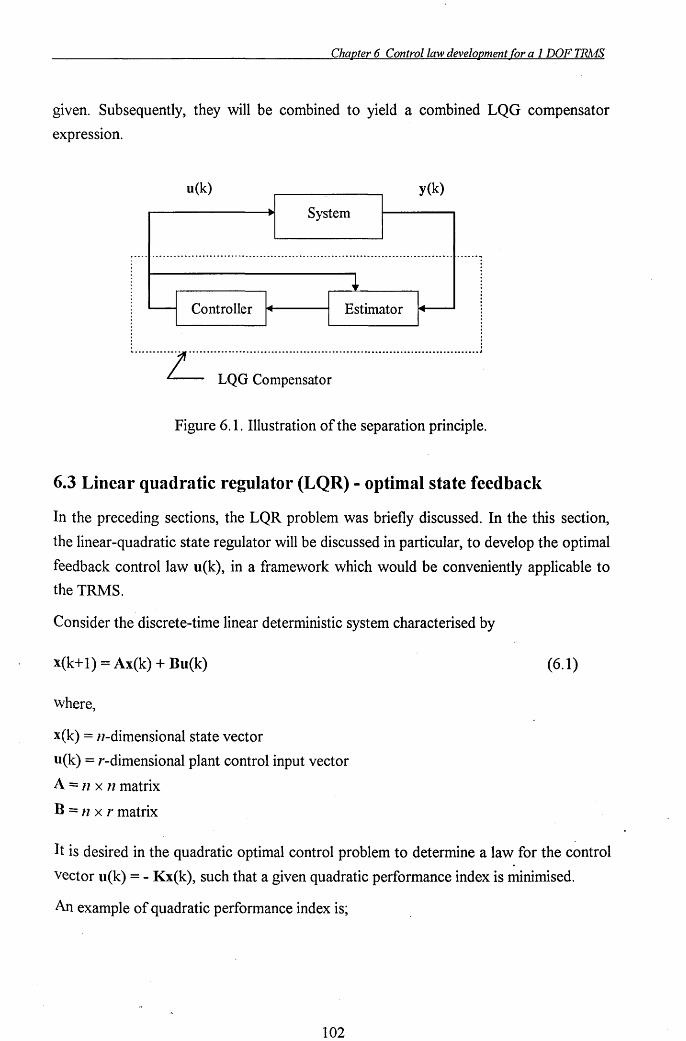
Chapter 6 Control law development for a 1 DOF TRMS
gIven. Subsequently, they will be combined to yield a combined LQG compensator
expression.
u(k) y(k)
System
Controller
· .. ···· .. ·L· .. · .. · .. · .... ·· .. · .. · .... · .. · .. · .. · .. · .. · .. · .......... · .. · .. · .. · .... · ....... LQG Compensator
Figure 6.1. Illustration of the separation principle.
6.3 Linear quadratic regulator (LQR) - optimal state feedback
In the preceding sections, the LQR problem was briefly discussed. In the this section,
the linear-quadratic state regulator will be discussed in particular, to develop the optimal
feedback control law u(k), in a framework which would be conveniently applicable to
the TRMS.
Consider the discrete-time linear deterministic system characterised by
x(k+ 1) = Ax(k) + Bu(k)
where,
x(k) = n-dimensional state vector
lICk) = r-dimensional plant control input vector
A = n x 11 matrix
B == n x r matrix
(6.1)
It is desired in the quadratic optimal control problem to determine a law for the control
vector u(k) = - Kx(k), such that a given quadratic performance index is minimised.
An example of quadratic performance index is;
102

Chapter 6 Control law development for a 1 DOF TRAiS
J 1 N -I, [xT(k)Qx(k)+ uT(k)Ru(k)] 2 k=O
(6.2)
subject to the constraint equation:
x(k+ 1) = Ax(k) + Bu(k)
where, the superscript denotes matrix transposition;
Q = is a 11 x 11 positive definite or semi-definite matrix.
R = is a symmetric 11 x 11 positive definite-definite matrix.
The weighting matrices Q and R are selected by the control-system designer to place
bounds on the trajectory and control respectively. From a design point of view, the
control system designer may design the system so that the term x T (k)Qx(k) is chosen
to penalise deviations of the regulated state x(k).
The control law that minimises J can be given by
n(k) = - Kx(k) (6.3)
with
(6.4)
Where p = P T ~ 0, is the unique positive definite solution, found by solving the
discrete matrix Riccati equation:
(6.5)
Limitations
Generally, assumptions necessary for a unique positive definite solution P = pT ~ 0 ,.to
the discrete LQR problem to exist are [85],
• Matrix Q must be symmetric and positive semi-definite.
• Matrix R must be symmetric and positive definite.
• . The pair [A,B] must be controllable.
• The matrix A must be non-singular.
103
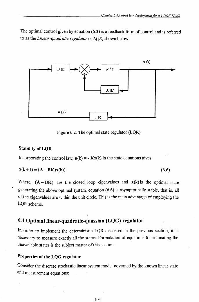
Chapter 6 Control law development for a 1 DOF TRAfS
The optimal control given by equation (6.3) is a feedback form of control and is referred
to as the Linear-quadratic regulator or LQR, shown below.
x (k)
u (k)
Figure 6.2. The optimal state regulator (LQR).
Stability of LQR
Incorporating the control law, u(k) = - Kx(k) in the state equations gives
x(k + 1) = (A - BK)x(k» (6.6)
Where, (A - BK) are the closed loop eigenvalues and x(k) is the optimal state
generating the above optimal system. equation (6.6) is asymptotically stable, that is, all
of the eigenvalues are within the unit circle. This is the main advantage of employing the
LQR scheme.
6.4 Optimallinear-quadratic-quassian (LQG) regulator
. In order to implement the deterministic LQR discussed in the previous section, it is
necessary to measure exactly all the states. Formulation of equations for estimating the
unavailable states is the subject matter of this section.
Properties of the LQG regulator
Consider the discrete stochastic linear system model governed by the known linear state
and measurement equations:
104
Chapter 6 Control law development for a 1 DOF TRAIS
x(k+ 1) = Ax(k) + Bu(k) + BIW(k)
y(k) = Cx(k) + Du(k) + v(k)
where,
y(k) = is the nl -dimensional output vector.
C = is nl x 11 matrix.
D = is a 11 x r direct feedthrough matrix.
w(k) = process noise.
v(k) = measurement noise.
and process and measurement noise covariances:
E[wwT] = Q e
E[vvT] = Re
E[wvT] = 0
E[w] = E[v] = 0
Where,
E is the expectation operator and,
Qe is a symmetric and positive semi-definite i.e., Qe = Qe T ~ o.
Re is a symmetric positive definite i.e., Re = Re T)O.
(6.7)
(6.8)
_ Now, it is desired to produce an estimate i(k) , of the state x(k) , using only the noisy
input and output measurement data. This can be achieved by forming the state error
vector, given by,
e(k) = x(k) - i(k) (6.9)
. and minimising the mean square error, i.e. the covariance of the estimate error, .. Pe ,
defined to be
Pe = E [//x(k) - X(k)//2 ] (6.10)
= E [ eT(k)e(k) ] (6.11 )
this is further elaborated in Section 6.4.2.
105
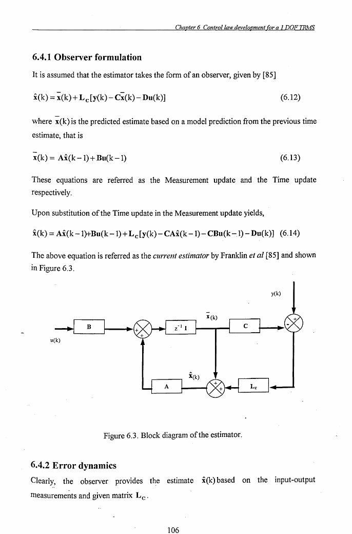
Chapter 6 Control law development for a 1 DOF TRMS
6.4.1 Observer formulation
It is assumed that the estimator takes the form of an observer, given by [85]
i(k) = ~(k) + L c [y(k) - C~(k) - Du(k)] (6.12)
where x(k) is the predicted estimate based on a model prediction from the previous time
estimate, that is
-x(k) = Ai(k -1) + Bu(k -1) (6.13)
These equations are referred as the Measurement update and the Time update
respectively.
Upon substitution of the Time update in the Measurement update yields,
i(k) = Ai(k -l}+Bu(k -1) + Lc[y(k) - CAi(k -1) - CBu(k -1) - Du(k)] (6.14)
The above equation is referred as the current estinlator by Franklin et al [85] and shown
in Figure 6.3.
y(k)
~B u(k)
Figure 6.3. Block diagram of the estimator.
6.4.2 Error dynamics
Clearly, the observer provides the estimate i(k) based on the input-output
measurements and given matrix L c .
106
Chapter 6 Control law development for a 1 DOF TRJvfS
The estimation error as defined earlier
e(k) = x(k) - i(k) (6.15)
is a measure that determines the performance of the estimator. Utilising the foregoing
formulations, it can be shown that for the stochastic system describe by equation (6.7)
and (6.8).
e(k + 1) = x(k + 1) - i(k + 1)
which can be written as
e(k + 1) = x(k + 1)-i(k + 1) - Le[y(k + 1) - Ci(k+ 1)- Du(k + 1)] (6.16)
after some algebraic manipulation results in:
e(k + 1) = [LeC- I] [i(k + 1) - x(k + 1)] - Le v(k + 1) (6.17)
employing the error term e(k), thus, gives:
e(k + 1) = [A - ALeC]e(k)+[I- LeC]Bl w(k) - Lev(k + 1) (6.18)
Equation 6.18 represents the dynamics of the estimation error e, where wand v are the
forcing functions and the eigenvalues of [A - ALeC] determine the nature of the
convergence process of the state estimate given the initial condition e(O) = eo.
6.4.3 The optimum observer estimator
~he main issue in the preceding section is the estimator gain matrix L e' which
minimises the expectation of e2, that is, equation 6.10, namely, the covariance of e,
. which is denoted by Pe
• As per the assumptions (not necessarily realistic) that v and w
are white noise processes. Therefore, the weighted sum of the v .and w is also a white
noise process:
11 = [I - LeC]Bl w(k) - Le v(k + 1) (6.19)
Thus ,
e(k+ 1) = [A-ALeC]e(k)+l1 (6.20)
107
Chapter 6 Control law development for a 1 DOF TRMS
is a linear system excited by white noise, therefore, the poles of [A - AL c C] are the
poles of the estimator. Naturally, these poles should be stable, or the estimator will fail
to estimate the states, i. e. the error must become small and not large. In the absence of
noise, i.e. 11 = 0, e will converge from some initial value eo to zero.
6.4.4 I(aIman gain Lc
The optimal choice of L c , i.e. the Kalman gain matrix, which minimises equation 6.10
is given by [85]
L = (R +CP CT]-lp CT . C e e e (6.20)
Here, Pe= Pe T ~ 0 is the covariance of the estimate error (which under assumptions is
constant, since e(k) is also stationary) and is found by solving the discrete filter Riccati
equation [84],
P =(BQB +APAT-APCT(R +CPCT)-lCPAT e 1 el e e e e (6.22)
The solution Pe= Pe T ~ 0, is the unique positive definite, and a sufficient condition for
Pe to exist is that the pair [A, C] is completely observable. This condition may be
relaxed to detectability, in which case it is necessary and sufficient, and Pe may be
_ positive semidefinite. The constraints required for a unique positive definite solution to
the discrete LQE problem to exist can be summarised as [85]:
• Matrix Qe must be symmetric and positive semi-definite i.e., Qe = Qe T ~ O.
• Matrix Re must be symmetric positive definite i.e., Re = Re T)O.
• .. The pair [A,C] must be observable .
The matrix A must be non-singUlar .
Since, the Kalman gain matrix Lc can be determined a priori and remains constant, this
kind of filter is referred as the stationalY or constant-gain Kalman filter. It is important
to note that it is an estimator whose gain matrix has been optimised on the basis of
statistical models of the process and measurement noises. Obviously, if the actual noise
statist~,cs vary with time, the optimality of the filter is not retained.
108
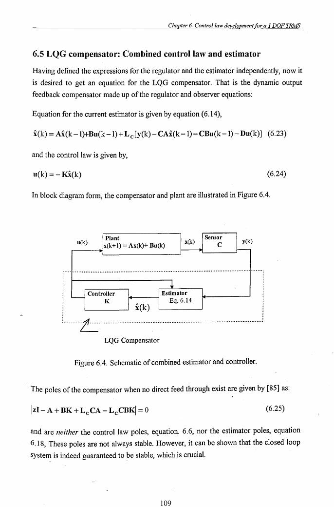
Chapter 6 Control law development for a 1 DOF TRAfS
6.5 LQG compensator: Combined control law and estimator
Having defined the expressions for the regulator and the estimator independently, now it
is desired to get an equation for the LQG compensator. That is the dynamic output
feedback compensator made up of the regulator and observer equations:
Equation for the current estimator is given by equation (6.14),
i(k) = Ai(k-1}tBu(k-1)+ Lc[y(k)- CAi(k-1)-CBu(k-1) -Du(k)] (6.23)
and the control law is given by,
u(k) = - Ki(k) (6.24)
In block diagram form, the compensator and plant are illustrated in Figure 6.4.
Plant x(k)
Sensor y(k) u(k) x(k+ 1) = Ax(k)+ Bu(k) C
~ I-
- .......................................................................................................
~ Controller .... Estimator
~
I......-
K ~ Eq.6.14
i(k) . . : .. ~..... : : ......... 'C .............................................................................................. !
LQG Compensator
Figure 6.4. Schematic of combined estimator and controller.
The poles of the compensator when no direct feed through exist are given by [85] as:
(6.25)
and are neither the control law poles, equation. 6.6, nor the estimator poles, equation
6.18, These poles are not always stable. However, it can be shown that the closed loop
system is indeed guaranteed to be sta~le, which is crucial.
109
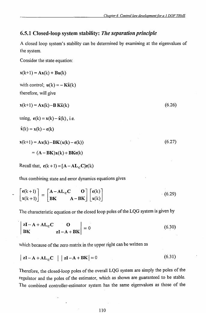
Chapter 6 Control law development for a 1 DOF TRAlS
6.5.1 Closed-loop system stability: Tile separation principle
A closed loop system's stability can be determined by examining at the eigenvalues of
the system.
Consider the state equation:
x(k+ 1) = Ax(k) + Bu(k)
with control; u(k) = - Ki(k)
therefore, will give
x(k+l) = Ax(k)-BKX(k)
using, e(k) = x(k) - i(k) , i.e.
i(k) = x(k) - e(k)
x(k+ 1) = Ax(k) - BK(x(k) - e(k))
= (A - BK)x(k) + BKe(k)
Recall that, e(k+l) =[A-ALeC]e(k)
thus combining state and error dynamics equations gives
[e(k + 1)] = [A - ALeC 0] [e(k)] x(k+l) BK A-BK x(k)
(6.26)
(6.27)
. (6.29)
The characteristic equation or the closed loop poles of the LQG system is given by
zI-A+ALeC 0 =0
BK zI-A+BK (6}0)
which because of the zero matrix in the upper right can be written as
I zI-A+ALeC I I zI-A+BKI =0 (6.31)
Therefore, the closed-loop poles of the overall LQG system are simply the poles of the
regulator and the poles of the estimator, which as shown are guaranteed to be stable.
The combined controller-estimator system has the same eigenvalues as those of the
110
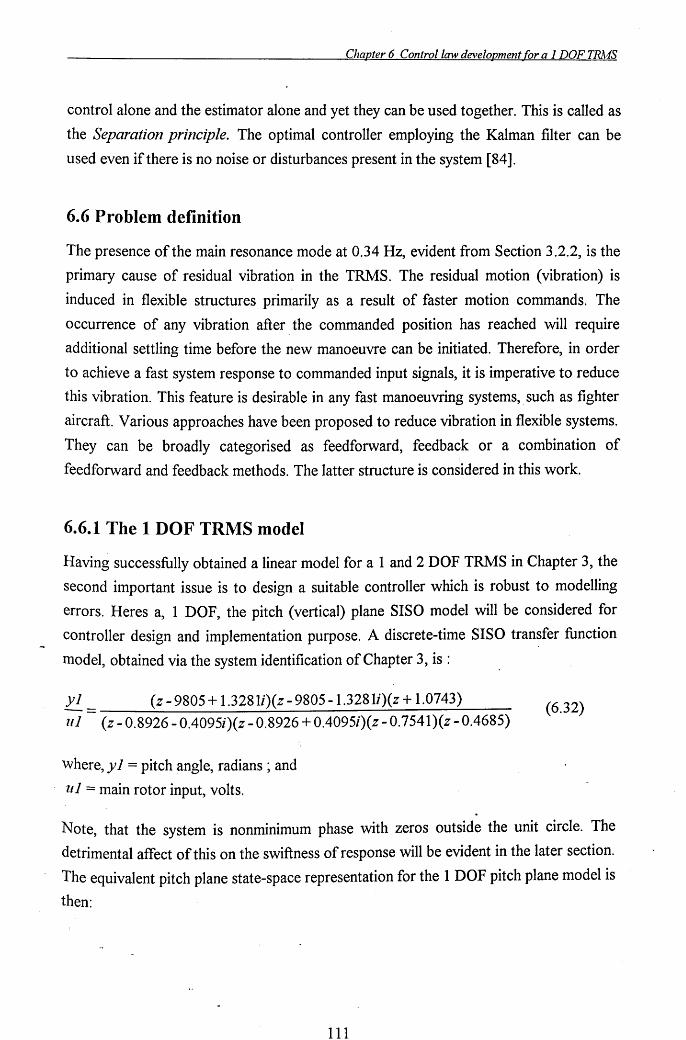
Chapter 6 Control law development for a 1 DOF TRAlS
control alone and the estimator alone and yet they can be used together. This is called as
the Separation principle. The optimal controller employing the Kalman filter can be
used even if there is no noise or disturbances present in the system [84].
6.6 Problem definition
The presence of the main resonance mode at 0.34 Hz, evident from Section 3.2.2, is the
primary cause of residual vibration in the TRMS. The residual motion (vibration) is
induced in flexible structures primarily as a result of faster motion commands. The
occurrence of any vibration after the commanded position has reached will require
additional settling time before the new manoeuvre can be initiated. Therefore, in order
to achieve a fast system response to commanded input signals, it is imperative to reduce
this vibration. This feature is desirable in any fast manoeuvring systems, such as fighter
aircraft. Various approaches have been proposed to reduce vibration in flexible systems.
They can be broadly categorised as feedforward, feedback or a combination of
feedforward and feedback methods. The latter structure is considered in this work.
6.6.1 The 1 DOF TRMS model
Having successfully obtained a linear model for a 1 and 2 DOF TRMS in Chapter 3, the
second important issue is to design a suitable controller which is robust to modelling
errors. Heres a, 1 DOF, the pitch (vertical) plane SISO model will be considered for
controller design and implementation purpose. A discrete-time SISO transfer function
model, obtained via the system identification of Chapter 3, is :
y 1 = (z - 9805 + 1.328li)(z - 9805 -1.328li)(z + 1.0743)
ul (z - 0.8926 - 0.4095i)(z - 0.8926 + 0.4095i)(z - 0.7541)(z -0.4685)
where, y 1 = pitch angle, radians ; and
ul = main rotor input, volts.
(6.32)
Note, that the system is nonminimum phase with zeros outside the unit circle. The
detrimental affect of this on the swiftness of response will be evident in the later section.
The equivalent pitch plane state-space representation for the 1 DOF pitch plane model is
then:
111
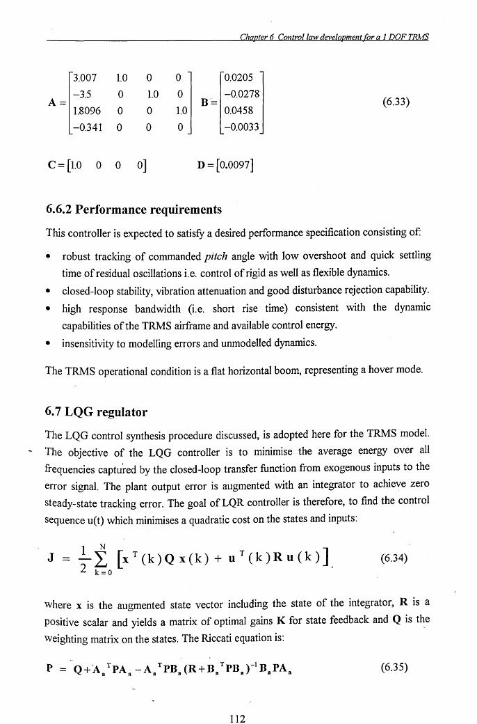
Chapter 6 Control law development for a 1 DOF TRA1S
3.007 1.0 0 0 0.0205
-3.5 0 1.0 0 -0.0278 A= B'= (6.33)
1.8096 0 0 1.0 0.0458
-0.341 0 0 0 -0.0033
C = [1.0 0 0 0] D = [0.0097]
6.6.2 Performance requirements
This controller is expected to satisfy a desired performance specification consisting of:
• robust tracking of commanded pitch angle with low overshoot and quick settling
time of residual oscillations i. e. control of rigid as well as flexible dynamics.
• closed-loop stability, vibration attenuation and good disturbance rejection capability .
• high response bandwidth (Le. short rise time) consistent with the dynamic
capabilities of the TRMS airframe and available control energy.
• insensitivity to modelling errors and unmodelled dynamics.
The TRMS operational condition is a flat horizontal boom, representing a hover mode.
6.7 LQG regulator
The LQG control synthesis procedure discussed, is adopted here for the TRMS model.
The objective of the LQG controller is to minimise the average energy over all
frequencies captured by the closed-loop transfer function from exogenous inputs to the
error signal. The plant output error is augmented with an integrator to achieve zero
steady-state tracking error. The goal of LQR controller is therefore, to find the control
sequence u(t) which minimises a quadratic cost on the states and inputs:
(6.34)
where x is the augmented state vector including the state of the integrator, R is a
positive scalar and yields a matrix of optimal gains K for state feedback and Q is the
weighting matrix on the states. The Riccati equation is:
(6.35)
112
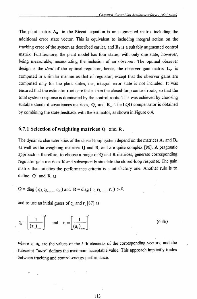
Chapter 6 Control law development for a 1 DOF TRA4S
The plant matrix Aa in the Riccati equation is an augmented matrix including the
additional error state vector. This is equivalent to including integral action on the
tracking error of the system as described earlier, and Ba is a suitably augmented control
matrix. Furthermore, the plant model has four states, with only one state, however,
being measurable, necessitating the inclusion of an observer. The optimal observer
design is the dual of the optimal regulator, hence, the observer gain matrix Leis
computed in a similar manner as that of regulator, except that the observer gains are
computed only for the plant states, i.e., integral error state is not included. It was
ensured that the estimator roots are faster than the closed-loop control roots, so that the
total system response is dominated by the control roots. This was achieved by choosing
suitable standard covariances matrices, Q e and Re' The LQG compensator is obtained
by combining the state feedback with the estimator, as shown in Figure 6.4.
6.7.1 Selection of weighting matrices Q and R.
The dynamic characteristics of the closed-loop system depend on the matrices Aa and Ba
as well as the weighting matrices Q and R, and are quite complex [86]. A pragmatic
approach is therefore, to choose a range of Q and R matrices, generate corresponding
regulator gain matrices K and subsequently simulate the closed-loop response. The gain
matrix that satisfies the performance criteria is a satisfactory one. Another rule is to
define Q and R as
Q == diag ( ql, q2, .......... qo,) and R == diag ( rl, r2, .......... ro,) > O.
and to use an initial guess of q~ and r~ [87] as
(6.36)
where Zj, Uj, are the values of the i th elements of the corresponding vectors, and the
subscript "nlax" defines the maximum acceptable value. This approach implicitly trades
between tracking and control-energy performance.
113
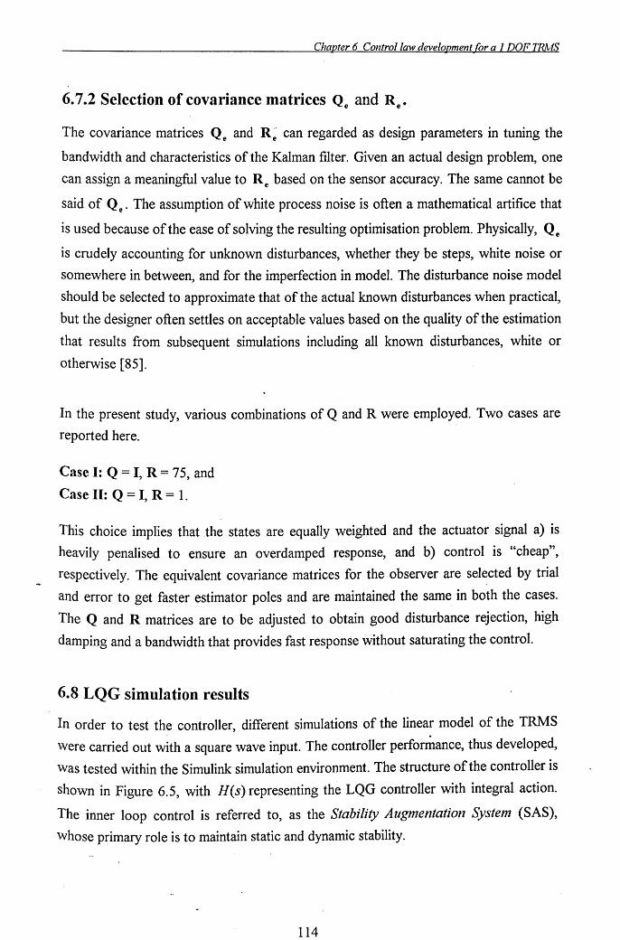
Chapter 6 Control law development for a 1 DOF TRMS
6.7.2 Selection of covariance matrices Qe and Re.
The covariance matrices Q e and R ~ can regarded as design parameters in tuning the
bandwidth and characteristics of the Kalman filter. Given an actual design problem, one
can assign a meaningful value to Re based on the sensor accuracy. The same cannot be
said of Q e' The assumption of white process noise is often a mathematical artifice that
is used because of the ease of solving the resulting optimisation problem. Physically, Q e
is crudely accounting for unknown disturbances, whether they be steps, white noise or
somewhere in between, and for the imperfection in model. The disturbance noise model
should be selected to approximate that of the actual known disturbances when practical,
but the designer often settles on acceptable values based on the quality of the estimation
that results from subsequent simulations including all known disturbances, white or
otherwise [85].
In the present study, various combinations of Q and R were employed. Two cases are
reported here.
Case I: Q = I, R = 75, and
Case II: Q = I, R = 1.
This choice implies that the states are equally weighted and the actuator signal a) is
heavily penalised to ensure an overdamped response, and b) control is "cheap",
respectively. The equivalent covariance matrices for the observer are selected by trial
and error to get faster estimator poles and are maintained the same in both the cases.
The Q and R matrices are to be adjusted to obtain good disturbance rejection, high
damping and a bandwidth that provides fast response without saturating the control.
6.8 LQG simulation results
In order to test the controller different simulations of the linear model of the TRMS , were carried out with a square wave input. The controller performance, thus developed,
Was tested within the Simulink simulation environment. The structure of the controller is
shown in Figure 6.5, with H(s) representing the LQG controller with integral action.
The inner loop control is referred to, as the Stability Augnlentation Systenl (SAS),
whose primary role is to maintain static and dynamic stability.
114
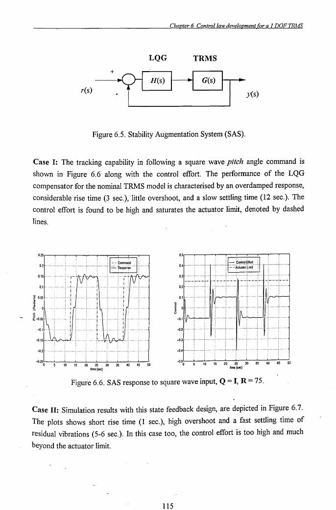
Chapter 6 Control law development for a 1 DOF TRMS
LQG TRMS
+-Li H(s) I ~I G(S)
'I ~
res) yes)
Figure 6.5. Stability Augmentation System (SAS).
Case I: The tracking capability in following a square wave pitch angle command is
shown in Figure 6.6 along with the control effort. The performance of the LQG
compensator for the nominal TRMS model is characterised by an overdamped response,
considerable rise time (3 sec.), little overshoot, and a slow settling time (12 sec.). The
control effort is found to be high and saturates the actuator limit, denoted by dashed
lines.
0.21-··· .. ···;·,·,·· .. ,; .. ,· .. ·· .. ; .... · .... :, ..... · .. ·:· ........ ,;,1
0,15 ..
0.1 ~ ................. , .... I ... :'/ ........ ~ ......... : \·· .. · .. , ........ ·,·"j .. ·:l ...... · ~, .... -l
~ 0.05~ .. · .... " .. · .. · .. ·;· .. · ... · ,· .. · .... · .......... ;1 ...... :· ........ ,; .. · .. 1 .,
.!l! '0 III ~ 0 .. · .... :: .... · .... :· .. I.f'~:· .. · .... ·:·· .... · .. 1 ~c .... : .... · .. ··;· .... ;·f". ...... : ...... ·-l
-0,2~ .. · .... : .... ·· .. ·: .. · ...... ~· .. · .. · .. : .. , ':" " ....... : ........... : ........ ~ ...... ,-l
-0,250~-1--11-0 ----'-15-21-0
----'-25-31-0
----'-35-41..-0 ----L-45---l50
time (sec)
0,5..---r---r----r--.-----r--r----r--r----r---,
0.' ······:······,····,H=Lt:t:li, 0.3 ....... ,! ..... ,+ .... ,.: .......... :' ........ : ....... ": ......... : ....... : ....... ~ .......
_._. -;_. -.-':._. .-:._.- .-~ _. _.-: . _.- t-· _.-: _. . -;- ._.- ';-' _._. 0.2 ....... ! ........ ; .... ,: ......... ~................................' ....... " .......
, OJ ..•...•.•...•..... , .. ~ •. § o .. · .... i· .... · .. ,i .. HI·: .. · ...... : ........ HI
o -0.1 If\:: I~~: -..;..-lll·;: ........ ·; ...... ·-l -O,2~ ........ ; ......... ; .... H.; ......... .: ......... I .... · .. :· ........ ·: .. ·" u .. ·: .... · .... ;· .. · .. ,
-0,3~ ........ ! ........ ,!· .. · .... .; .... · .. · .. -: .... ·" .. 1 " ...... :: ... , ...... : .......... :" .... ,,', ..... "'-\
-0.4~'" , .. :." .... ,.: ......... ; ......... ; ..... + ... , .. ; ......... : .......... ; ..... '''~''''''-I
-0.50 5 10 15 20 25 30 35 40 45 50 time (sec)
Figure 6.6. SAS response to square wave input, Q = I, R = 75.
Case II: Simulation results with this state feedback design, are depicted in Figure 6.7.
The plots shows short rise time (1 sec.), high overshoot and a fast settling time of
residual vibrations (5-6 sec.). In this case too, the control effort is too high and much
beyond the actuator limit.
115
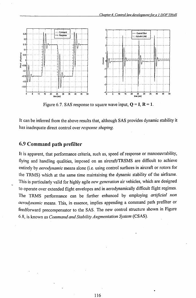
0.2 5
. 2
0.1 5 ..
.1 .
5 .. ~ 0.0
~ !:S 0
.c ~ -0.0 5 ..
-0. 1·
-0.1 5
-0.2
-0.25
f\
V
Chapter 6 Control law development for a 1 DOF TRMS
I Command I I' RespOnse I····· - C6ntrol Effort
3 .... .. ..... , .... .............. '-:-:.: .A.ci.uat~r .Li.hn . ....
1\
~ V I
. . . . . . . 2 ...... ..: ......... ~ ........ ~ ......... ; ......... :... ..... \ .......... \ ..... 1· .. ·:- .. · .. · .. ~ .. " ..... -l
I 1 ........ : ......... :..... . . ... -:- ........ ~ ...
I
I
I I il
j 0 f:<:::>: . fI---,--- ~;;::-:,: 'v.::-:-. ~ ~ -1~: .. · .... : .... · .... : .. ··1I· .. :· ........ :: ........ ·U 11 ...... ; ...... · .... ; .... ·11·; .. · ...... ;·· ...... -1
, Ai I v -21- ........ ; .... · .... ; .... + .. ;· ........ ·; ...... ·· .. 1· .. · .... ·;· .. " ...... ;· .. · .. 1· .. ; ......... , ........ -1
10 15 20 25 30 35 40 45 50 10 15 20 25 30 35 40 45 50 time (sec) time (sec)
Figure 6.7. SAS response to square wave input, Q = I, R = 1.
It can be inferred from the above results that, although SAS provides dynamic stability it
has inadequate direct control over response shaping.
6.9 Command path prefilter
It is apparent, that performance criteria, such as, speed of response or manoeuvrability,
flying and handling qualities, imposed on an aircraft/TRSMS are difficult to achieve
entirely by aerodynanlic means alone (i.e. using control surfaces in aircraft or rotors for
the TRMS) which at the same time maintaining the dynamic stability of the airframe.
This is particularly valid for highly agile new generation air vehicles, which are designed
to operate over extended flight envelopes and in aerodynamically difficult flight regimes.
The TRMS performance can be further enhanced by employing artificial non
aerodynanlic means. This, in essence, implies appending a command path prefilter or
feedforward precompensator to the SAS. The new control structure shown in Figure
6.8, is known as Conmland and Stability Augnlentation Systenl (CSAS).
116
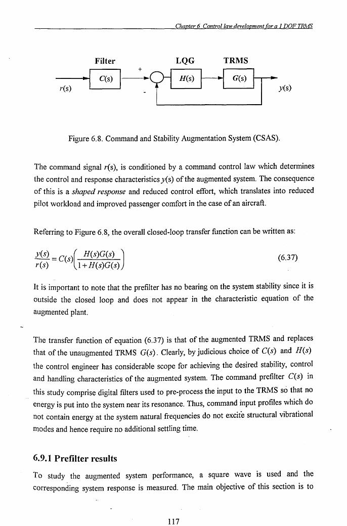
Chapter 6 Control law development for a 1 DOF TRMS
Filter LQG TRMS
~I +
~?l I ~I II C(s) H(s) G(s) ..
res) yes)
Figure 6.8. Command and Stability Augmentation System (CSAS).
The command signal r( s), is conditioned by a command control law which determines
the control and response characteristics y( s) of the augmented system. The consequence
of this is a shaped response and reduced control effort, which translates into reduced
pilot workload and improved passenger comfort in the case of an aircraft.
Referring to Figure 6.8, the overall closed-loop transfer function can be written as:
yes) = C(s)( H(s)G(s) ) res) 1 + H(s)G(s)
(6.37)
It is important to note that the prefilter has no bearing on the system stability since it is
outside the closed loop and does not appear in the characteristic equation of the
augmented plant.
The transfer function of equation (6.37) is that of the augmented TRMS and replaces
that of the unaugmented TRMS G(s). Clearly, by judicious choice of C(s) and H(s)
the control engineer has considerable scope for achieving the desired stability, control
and handling characteristics of the augmented system. The command prefilter C(s) in
this study comprise digital filters used to pre-process the input to the TRMS so that no
energy is put into the system near its resonance. Thus, command input profiles which do
not contain energy at the system natural frequencies do not excite structural vibrational
modes and hence require no additional settling time.
6.9.1 Prefilter results
To study the augmented system performance, a square wave is used and the
corresponding system response is measured. The main objective of this section is to
117
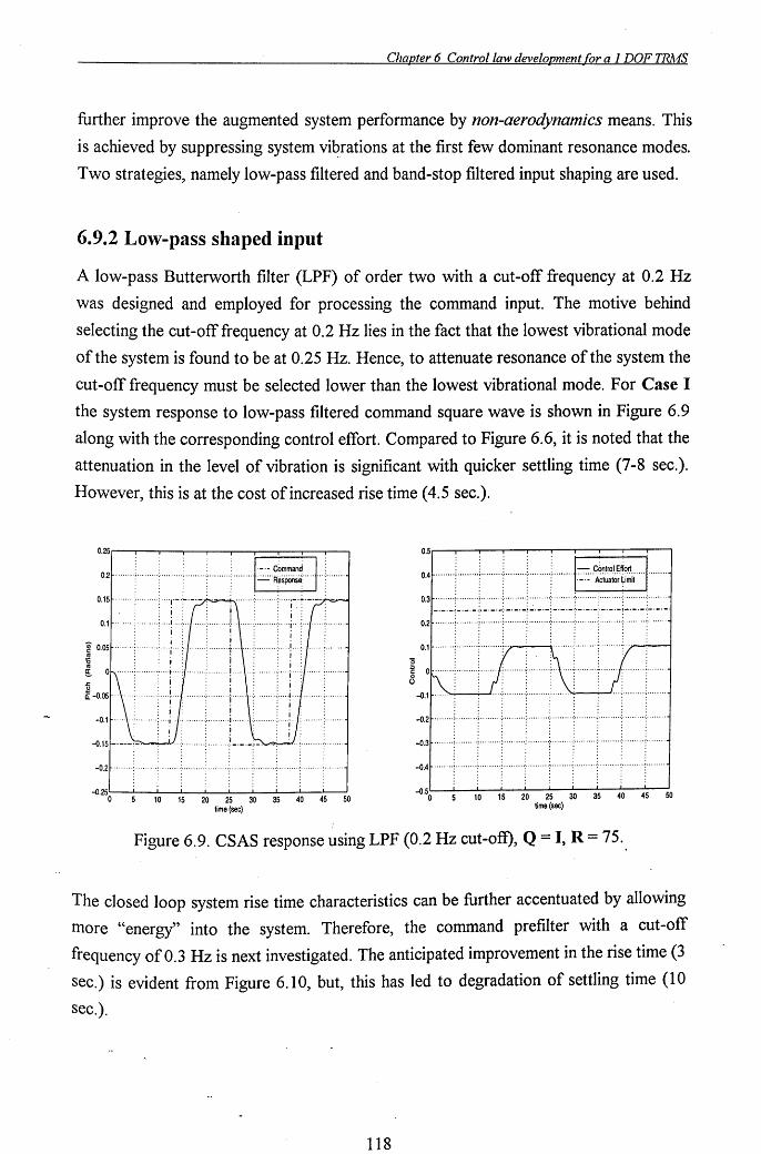
Chapter 6 Control law development for a 1 DOF TRMS
further improve the augmented system performance by non-aerodynanlics means. This
is achieved by suppressing system vibrations at the first few dominant resonance modes.
Two strategies, namely low-pass filtered and band-stop filtered input shaping are used.
6.9.2 Low-pass shaped input
A low-pass Butterworth filter (LPF) of order two with a cut-off frequency at 0.2 Hz
was designed and employed for processing the command input. The motive behind
selecting the cut-off frequency at 0.2 Hz lies in the fact that the lowest vibrational mode
of the system is found to be at 0.25 Hz. Hence, to attenuate resonance of the system the
cut-off frequency must be selected lower than the lowest vibrational mode. For Case I
the system response to low-pass filtered command square wave is shown in Figure 6.9
along with the corresponding control effort. Compared to Figure 6.6, it is noted that the
attenuation in the level of vibration is significant with quicker settling time (7-8 sec.).
However, this is at the cost of increased rise time (4.5 sec.).
0.2~ .... · .. ; .... · .... ; .. · ...... ;· .. · .... ·: .. · .. · .. · .. : ........ 1
0.15~ .... · .. : .... · .... : .. ·,·-·:-·-·-~~ ......
0.1 ~ ....... , ......... , .... f ... ·, .. I .... ·: ........ ·~·\
'W 0.05~··"··,,,·,,,,,,,,,·,·":/· .. ·~ ...... ··t·\ .!!! '0 os ~ O~""""'''':'''f'';I'''''''':'''''''!'''\
-O.151-·-·,,-~~...., .. -:·· .... · .. ·:· .. · .,-.-.. -,-~~~ .. , ......... , ....... -i
-0.2~"" ..................... , ...... : ............... : ........ : ....... ~''''''':'''''-i
-0.250'-....L.--
1L-0
-I...15
-2L-0
-I...25
-3L-0
--L35
-4L-0
-L-45 ---J50
time (sec)
0.5.---.----.----r--....---.----.----r--....--...,....----, ., .
0.4 ........ : ......... [ ......... : ......... L ........ l .... · .. · ·= .. ~;~:i~~1f;ii .......... .. 0.3 ·· .. ····~· ...... ··f .. ·· .. ···:·· ........ :··:· .. · .. ·:··· .... · .. :···· .. · .. : ......... : ......... : ....... .
_._. -~_._.- ';- - ._.-:--._. -~-.-.-! -._.-;'-' _._! _. - '-;-'-'-';-' _._. 0.2 ........ ! .. · .. · .. ·( .... · .. i ........ ·: ........ '( .... · .. '( .. · .... ( ...... : ...... · .. j ........ 0.1 ........ i ......... i ........ y- .~ \ .... j ........ ( ...... y-r-
! ">:[/. \J'} -O.2~ ........ ;· ........ : .. · ...... :· ........ : ........ · .. : .......... ·: .. · ...... ,· .... · .. ··: ......... , ........ -1
-0.3 ~ ............................ , ......... : .......... : .......... : ........... : ............ , ......... , .. · .... ·1
-O.4~ ....... ; ......... ; ........ ; ......... , ....... : .......... : .......... : .......... : ......... : ....... -1
10 15 20 25 30 35 40 45 50 time (sec)
Figure 6.9. CSAS response using LPF (0.2 Hz cut-oft), Q = I, R = 75.
The closed loop system rise time characteristics can be further accentuated by allowing
more "energy" into the system. Therefore, the command prefilter with a cut-off
frequency of 0.3 Hz is next investigated. The anticipated improvement in the rise time (3
sec.) is evident from Figure 6.10, but, this has led to degradation of settling time (10
sec.).
118
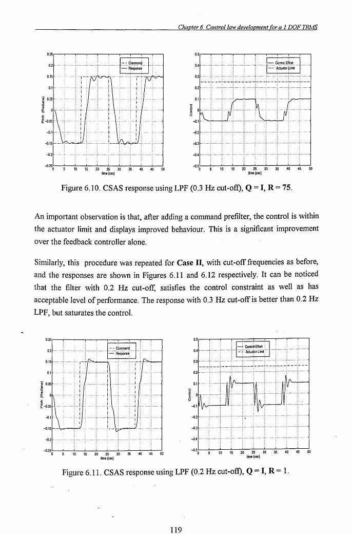
Chapter 6 Control law development for a 1 DOF TRMS
0.25 0.5
0.2 0.4 1- ........ ; ......... ; ......... ; .....•... : ........•. : .....•.... j = .. ~n~roL~il.0~ ............ . . _. - Actuator ~im~
0.15 0.3
0.1 0.2
F 0.05 0.1 os '6 "2 os ~ 0 g 0
0 \ -0.1
-0.1 -0.2
-0.15 -0.3
-0.2 -0.4
-0.25 -0.5 0 0 10 15 20 25 30 35 40 45 50
time (sec)
Figure 6.10. CSAS response using LPF (0.3 Hz cut-oft), Q = I, R = 75.
An important observation is that, after adding a command prefilter, the control is within
the actuator limit and displays improved behaviour. This is a significant improvement
over the feedback controller alone.
Similarly, this procedure was repeated for Case II, with cut-off frequencies as before,
and the responses are shown in Figures 6.11 and 6.12 respectively. It can be noticed
that the filter with 0.2 Hz cut-off, satisfies the control constraint as well as has
acceptable level of performance. The response with 0.3 Hz cut-off is better than 0.2 Hz
LPF, but saturates the control.
10 15 20 25 30 35 40 45 50 time (sec)
"2
0.5r--:-:-:-;:::::r::=::::!:==:~-:-:-'~
I ~ Contr~1 Effort ~ I 0.4 ~ ........ ; .... , ..... ; ......... ; ... tl: :':':f" iiCiuiiior 'Lirii~'r' Jf ..... : ......... ;: ......... , ........ ;
0.3~ ........ i ........ ·i ...... · ... : .......... : .... · .... ·: .. ·"""·:""""":""· .... :·· .... ·' ...... ·1
0.2~ ........ : ......... ; ......... : .............................. : .......... : ......... ·: .. · ...... ~ ...... ·1
0.11- .. ··, .. :., .... "'~'''''I ~--~I ..... ~ ......... : ... II\~I
~ Om,. VI\,,~.~.~~~,.; ......... ; .......... ,I\jA\~~~, .. : ........ ·, .... ·' .. 1
-0.1 V v V V
-0.2
-O.3~"··";" ...... i .................... : .......... : .......... : .......... -: .......... : ........ : .... ··1
-0.4~ ........ : ...... , .. : ........ ·: ...... · .. : ................... : ........ : .. · .. · .. :· ...... · .. ~· .... i
10 15 20 25 30 35 40 45 50 time (sec)
Figure 6.11. CSAS response using LPF (0.2 Hz cut-oft), Q = I, R = 1.
119
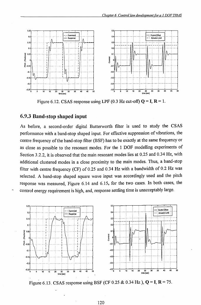
0.2 5
o. 2
0.1 5
o. 1
I 0.05
~ !!. o ...
~ -0.0 J -0. ,. ~~ -0.15
-0.2
-0.25 o
Chapter 6 Control law development for a 1 DOF TRMS
• -. 0 Command
A -Respon~
AT ~ r i-,;..-
:
IV
:
IA V \
I
V
0.4 · .. ·· .. ·l··· .. ·+ ·· .. ··,· .. · .. · .. I·· .. ····i=·j~i~~:~~~~it·· .. f .. · .. · .. , .. ······ 0.3 ~:~.j.'~:~:~..: ... _.: .... : ......... ; ......... .; ........ : .......... : ........ ; ........ i ....... .
:, _. -. -; -. _. -i _._. -~. _. _. -; -.-0.2 ........ ; ......... ; ..... ; ......... ; ....... ) ..... ) ....... ) ......
0.1': ... '" ._- . lr--j -0: i~·"·'V ......... ; ......... III~ .. 0-.. (-. ....;.-.I.\1.' ......... ; ...... .j
-O.2r· L · .. ' .... · .... , .. ··+·: .......... : .......... :VIl· .... : .......... ·: ...... ·,·: ......... , ....... .j
V: -0.41- ........ : ......... ; ......... ; ......... , ......... , ......... , .......... : .......... , ......... ; ........ .j
10 15 20 25 30 35 40 45 50 10 15 20 25 30 35 40 45 50 time (sec) time (sec)
Figure 6.12. CSAS response using LPF (0.3 Hz cut-oft) Q = I, R = 1.
6.9.3 Band-stop shaped input
As before, a second-order digital Butterworth filter is used to study the CSAS
performance with a band-stop shaped input. For effective suppression of vibrations, the
centre frequency of the band-stop filter (BSF) has to be ex'actly at the same frequency or
as close as possible to the resonant modes. For the 1 DOF modelling experiments of
Section 3.2.2, it is observed that the main resonant modes lies at 0.25 and 0.34 Hz, with
additional clustered modes in a close proximity to the main modes. Thus, a band-stop
filter with centre frequency (CF) of 0.25 and 0.34 Hz with a bandwidth of 0.2 Hz was
selected. A band-stop shaped square wave input was accordingly used and the pitch
response was measured, Figure 6.14 and 6.15, for the two cases. In both cases, the
control energy requirement is high, and, response settling time is unacceptably large.
-0.2
-O.250~ -1--1.1-0 -1-
15-
2.1-0 -1-
25-
3.1-0
--'-35-41.....0
--'-45
----J50
time (sec)
0.5r-:--:---:-:-:-:-;:::::::::!:==:!::=~1
041- ........ ; ......... ; ......... , .......... ; ...... " ... ; .... " ..... ; .. j[ =: ':'~nt~~I~~~rt ... !. .1 .... . . '._.0; Actuat~rLim~ ~ I 0.3~ ........ i· ........ ; .. · ...... , ........ :· .... · .... : ........ : .... · .. · .. :· .... · .... ;· .. · .... ·, .... · .. ·1
0.2~"" ... ; ....... ";;" .. I .. ·; ......... , ... · ...... 111 ....... : .......... ; .... 11· .. ~ ......... ~ ........ i
0.1~"·"··:""""·'''''1 k/=- r'-~ OI\~ ..... : ......... : ... RlIf.· .... · .. ·: ........ ·IIII .... ~··· .... ·:· .. ·HHI· ...... ;·· .. · .. 1
8 -0.1 I/h .~~r. .. --.lIIII ........ ' ....... .j
-0.21- ........ ; ......... ; .... 1, ... , ......... ; ........ + ...... ·; .. · ...... ; .... ·11· .. ; .. · ...... ·,· ...... ·-1
-0.4~'" .... : ......... , ......... : ......... , ........ ; ........... ; .......... ; ......... ~ ......... ~ ....... 1
10 15 20 25 30 35 40 45 50 time (sec)
Figure 6.13. CSAS response using BSF (CF 0.25 & 0.34 Hz), Q = I, R = 75.
120
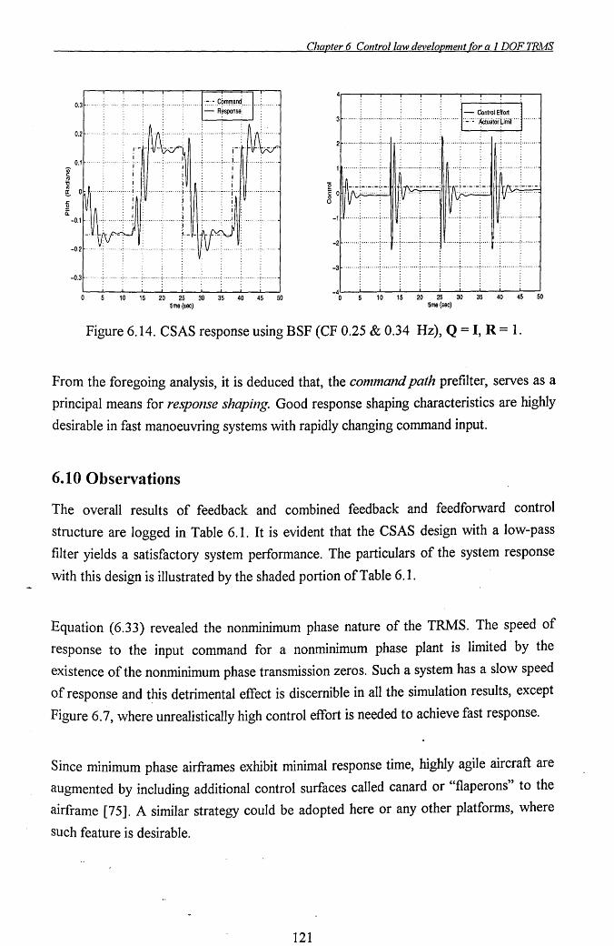
Chapter 6 Control law development for a 1 DOF TRMS
0.3
3 ...... , ....... ; ......... : ........ ~ ......... :
0.21""''';''''''''';''''''''':'''11 ·(\-: .......... : .. · ...... ·: .. · .. · .... : ........ ..: .. ·11· ·"i .. """~
2 ........ ! ......... ~ ....... ~ .......... ~ .......... : ....... ........... ...... . ..................... ..
0.11- ...; ......... ; .... ! .. Ill ...... ·:: .......... ~"I· .... : ......... ·:· .. ·1..11 .. ~ ........ ': ........ " ..... '............... . .. ........ , ......... .
~ 0:
-0.1 . -ll-f .... · .. ; .... · .... ;· .. ·IIY;· ........ ; .... · .. ·111 ...... :· ........ ~ .... II ~.: ......... ; ....... -1
-2'1- .. · .. · .. ;··· .. · .. ·;· .. + .. : ...... ·· .. : .... ·· .... 11.. .. ····:·· ........ : .... ·~ ... ( ........... :- ....... ~ -0.2
-31- .... · .. ! .... ·· .. ·:· .. · .. · .. :· ........ : ........ -: ......... ~ .......... : .......... : ......... ~"''' .. -I -0.3r ....i .. ..... .. i ........ < .......... : .......... : .......... : .......... : ............ : ......... , ....... ~
_4l-..L.---L..--.l..._L---....L---1-.--.I...---JI--....L---l o 10 15 20 25 30 35 40 45 50
lime (sec)
Figure 6.14. CSAS response using BSF (CF 0.25 & 0.34 Hz), Q = I, R = 1.
From the foregoing analysis, it is deduced that, the conlmand path prefilter, serves as a
principal means for response shaping. Good response shaping characteristics are highly
desirable in fast manoeuvring systems with rapidly changing command input.
6.10 Observations
The overall results of feedback and combined feedback and feedforward control
structure are logged in Table 6.1. It is evident that the CSAS design with a low-pass
filter yields a satisfactory system performance. The particulars of the system response
with this design is illustrated by the shaded portion of Table 6.1.
Equation (6.33) revealed the nonminimum phase nature of the TRMS. The speed of
response to the input command for a nonminimum phase plant is limited by the
existence of the nonminimum phase transmission zeros. Such a system has a slow speed
of response and this detrimental effect is discernible in all the simulation results, except
Figure 6.7, where unrealistically high control effort is needed to achieve fast response.
Since minimum phase airframes exhibit minimal response time, highly agile aircraft are
augmented by including additional control surfaces called canard or "flaperons" to the
airframe [75]. A similar strategy could be adopted here or any other platforms, where
such feature is desirable.
121
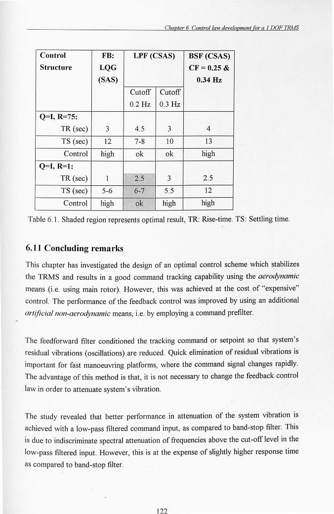
Chapter 6 Control law development for a 1 DOF TRMS
Control FB: LPF (CSAS) BSF (CSAS)
Structure LQG CF= 0.25 &
(SAS) 0.34 Hz
Cutoff Cutoff
0.2 Hz 0.3 Hz
Q=I, R=75:
TR (sec) 3 4.5 3 4
TS (sec) 12 7-8 10 13
Control high ok ok high
Q=I, R=l:
TR (sec) 1 2.5 3 2.5
TS (sec) 5-6 ,"" 6-7- ':. 5.5 12
Control high ok high high
Table 6.1. Shaded region represents optimal result, TR: Rise-time. TS: Settling time.
6.11 Concluding remarks
This chapter has investigated the design of an optimal control scheme which stabilizes
the TRMS and results in a good command tracking capability using the aerodynamic
means (i .e. using main rotor). However, this was achieved at the cost of "expensive"
control. The performance of the feedback control was improved by using an additional
art?ficial non-aerodynamic means, i.e. by employing a command prefilter.
The feedforward filter conditioned the tracking command or setpoint so that system's
residual vibrations ( oscillations) are reduced. Quick elimination of residual vibrations is
important for fast manoeuvring platforms, where the command signal changes rapidly.
The advantage of this method is that, it is not necessary to change the feedback control
law in order to attenuate system's vibration.
The study revealed that better performance in attenuation of the system vibration is
achieved with a low-pass filtered command input, as compared to band-stop filter. This
is due to indiscriminate spectral attenuation of frequencies above the cut-off level in the
low-pass filtered input. However, this is at the expense of slightly higher response time
as compared to band-stop filter.
122

Chapter 6 Control law development for a 1 DOF TRMS
With a command pre-filter, the control effort is found to be within the actuator limits.
Several different combinations of ,weighting matrices and command prefilter are
essential to achieve optimal performance. Thus, an appropriately designed feedforward
and feedback controller is a practical approach to satisfy the design specification.
123
Chapter 7 Experimental investigation of optimal control paradigm
Chapter 7
Experimental investigation of optimal control paradigm
The Stability Augnlentation Systenl (SAS) and the Conlnland and Stability Augnlentation Systenl (CSAS) developed in the last Chapter will be executed in this Chapter. The control law is implenlented in real-time, on the TRMS platforln.
7.1 Introduction
In the last Chapter various control schemes for controlling the TRMS were developed
and tested within a simulation environment. The crucial test for any control paradigm is
when implemented on the real system in presence of real world uncertainties and
disturbances. The aim of this Chapter is to apply these schemes to the TRMS. The
TRMS hardware and software configuration was described in Chapter 2 and the control
strategies are those developed in the previous Chapter. It will be shown however, in
Section 7.3, that the two cases investigated in the simulation environment are
inadequate to get the desired closed-loop system performance. Hence, more cases are
investigated. The experimental results of SAS are first presented in Section 7.3.1,
f9110wed by those of CSAS in Section 7.3.2. Finally, optimal control scheme robustness
to disturbances is demonstrated in Section.7.4. The findings of experiments are
encapsulated in Section 7.5.
7.2 The general control problem revisited
The various stages involved in establishing a control system for a physical plant were
described in Chapter 1. So far, the first four stages have been addressed, this Chapter
will cover the crucial final step of control law implementation. The five steps can be re
cast in a general control problem (GCP) framework. A schematic of the general control
problem is illustrated in Figure 7.1 .. [88]. This figure shows two worlds, a real world
124

Chapter 7 Experimental investigation of optimal control paradigm
and a mathematical world. In the real world, plants are ill-defined and often difficult to
describe, hence the rugged boundari~s. In contrast, the mathematical world is generally
well defined, hence the smooth circular boundary. The five steps are re-visited in the
light of Figure 7. 1.
Real World
Real plant
) j Real controller
I Controller evaluation
Plant analysis
Obtain mathematical model
~
Implement controller
Mathematical World
Controller design & simulation
Figure 7.1. The general control problem.
System design and requirement: It is expected from the application specific designer
to design a sophisticated system but not too complex to achieve the desired control
system requirements. Therefore, interaction and involvement of control specialist at an
early stage is essential.
Modelling of the given system: This step entails migration from the real world to the
mathematical world in the GCP framework. Both modelling arid system identification
can be used depending upon whether the system exists or is still being designed and
whether the plant dynamics are well understood. The modelling step is the most
demanding and crucial stage in the whole control design process.
125
Chapter 7 Experimental investigation o(optimal control paradigm
Control design and control system analysis: These tasks occur in the mathematical
world. A controller is designed usi~g the plant model in order to satisfy the system
specifications determined in the system design phase. While designing the controller it is
vital to understand the relationship between a model and the real plant. Other concepts
like the equilibrium point, different operating regimes, actuator saturation limits, and so
on, need to be well understood and translated in the control design exercise. The control
system analysis examines the controlled system behaviour and determines if the
controller is good enough to be transferred to the plant.
Control implementation: There is a strong focus on simplicity at the controller
implementation stage. Simplicity means reduced hardware, which in turn means a
cheaper control system which weighs less and takes up less space. Simplicity also results
in greater integrity of the control system which is vital for safety critical systems such as
for aerospace applications. For instance the A320 Airbus triplicates all hardware for the
control law, plus there is a fourth independently designed back-up control law [89].
Once the designer is convinced that the controller performs well in the mathematical
world, and that it has a good chance of meeting the required specifications in the real
world, the controller can be implemented. The implemented controller then need to be
evaluated functionally. This is rarely a one step procedure and, as will be shown later in
this Chapter, requires several set of control laws are needed to meet or achieve
acceptable functional requirements. It is tedious trial and error procedure from the
silTIulation (mathematical world) steps 3 and 4, to implementation (real world) step 5.
The remainder of this Chapter will focus on the last step.
7.3 Controller implementation results
The controllers designed in the last Chapter are linked to the TRMS in real-time
through the MATLAB-Simulink interface described in Chapter 2. Both control
schemes, the Stability Augmentation System (SAS) and the Command and Stability
Augmentation System (CSAS) will be executed. Essentially, the task of the LQG
controller is to achieve robust tracking of commanded pitch angle by manipulating the
input to the main rotor. The controlled output (pitch angle) is expected to have low
overshoot, quick settling time of residual oscillation and reasonably fast speed of
126
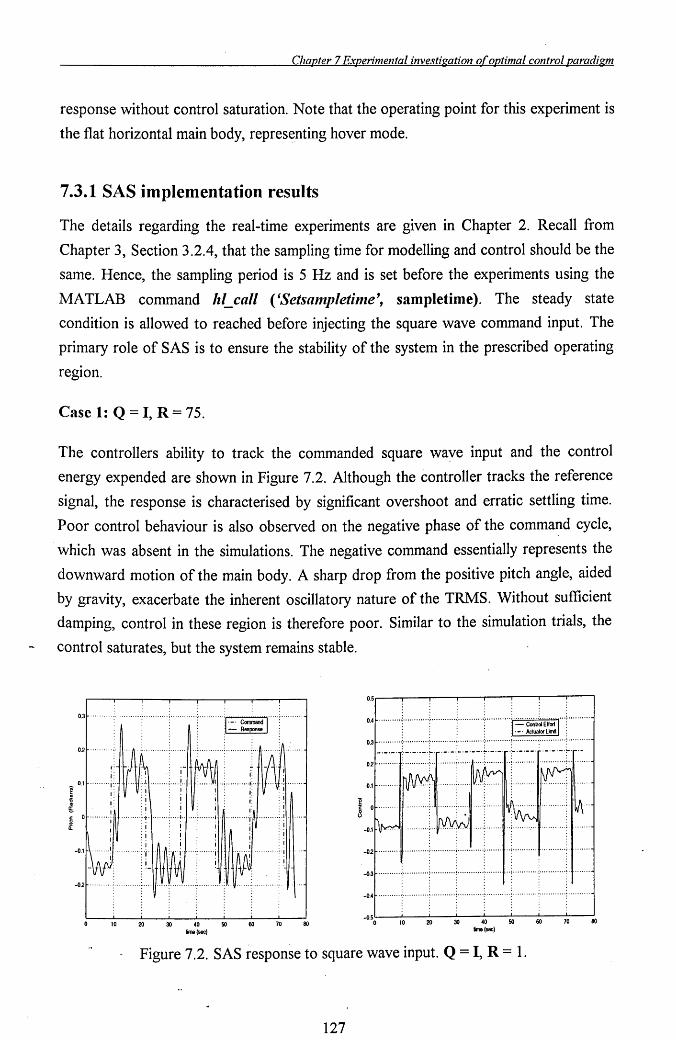
Chapter 7 Experimental investigation o(optimal control paradigm
response without control saturation. Note that the operating point for this experiment is
the flat horizontal main body, representing hover mode.
7.3.1 SAS implementation results
The details regarding the real-time experiments are given in Chapter 2. Recall from
Chapter 3, Section 3.2.4, that the sampling time for modelling and control should be the
same. Hence, the sampling period is 5 Hz and is set before the experiments using the
MATLAB command hi_call ('Setsanlpletinle', sampletime). The steady state
condition is allowed to reached before injecting the square wave command input. The
primary role of SAS is to ensure the stability of the system in the prescribed operating
region.
Case 1: Q = I, R = 75.
The controllers ability to track the commanded square wave input and the control
energy expended are shown in Figure 7.2. Although the controller tracks the reference
signal, the response is characterised by significant overshoot and erratic settling time.
Poor control behaviour is also observed on the negative phase of the command cycle,
which was absent in the simulations. The negative command essentially represents the
downward motion of the main body. A sharp drop from the positive pitch angle, aided
by gravity, exacerbate the inherent oscillatory nature of the TRMS. Without sufficient
damping, control in these region is therefore poor. Similar to the simulation trials, the
control saturates, but the system remains stable.
0.3
0.2
i: 0.1 ...... · .. i:·
I: i : I·. . . :j
o ......... ! ........... U ........ : .... i ...... ~ ....... i . . I ......... :.1. 1 :! '!' ........... j. '1
1
-0.1 ....... 1
-02
'1 :1 : j :j
:1 :i
......... :.j
: 1
10 20 30 40 50 60 70 80 lime (sec)
. . 0.3 ···········~············~···········~···········t···········i············~············~··········
:. _. -.. -.~. .-. -.:-._.- -.~ ._. _. ';' _.- _. . _._. -.~. .-02 ..................... , ........................................................ , ....... ..
0.1
-02 ........ ··u············;············;·····:·····.;········If··;·········· .. ,···········;·,
-0.31-··········;··········· ... ~ ........... i··········· -: ....... ·1 .. ·::··········· .: ............ ~.!-
-0.41- ......... ~ ............ ~ ........•.. ! ............. ~ ........... : ........... ~ ............. ~ .......... i
-0.50 10 20 30 40 50 60 70 80 lime (soc)
Figure 7.2. SAS response to square wave input. Q = I, R = 1.
127

Chapter 7 Experimental investigation of optimal control paradigm
Case II : Q = I, R = 1.
This is the second of the two cases studied in the simulation environment. This
controller failed to perform in real-time, which was marked by unstable behaviour. The
likely causes appear to be slow observer poles in comparison to the regulator poles. In
spite of functioning well in the mathematical domain, it fails in the real world, clearly
indicating a gap that exist between theory and practice.
Since Case 1 SAS results are unsatisfactory and the failure of Case II, the trial and
error procedure becomes apparent. Hence, it was necessary to go back to the
mathematical world i.e., steps 2 and 3 carry out few more controller designs and return
once again to the real world. The following additional cases are investigated:
Case III: Q = I, R = 100; and
Case IV: Q = I, R = 125.
The rational for choosing these weights is to achieve further damped response, which is
possible by penalising the input.
Case III : Q = I, R = 100.
Figure 7.3 represents SAS performance. Here, the response is better than Case I, with
relatively less overshoot and reasonable output settling time. However, analogous to
Case I, the closed-loop plant is unable to maintain a tight control on the negative pitch
command, indicating a need for further damping. On the control' effort side,
performance is acceptable with slight saturation. The overall system remains stable.
0.5...-----.---.----.--.,.----,--,--,----,
0.3 ..........•............•... ·········1·_· Conm&ndl ... _ ......... . : - R.sp~,""
0.2
02 ·· .. · .... ·~···· .... ·· .. f· ........ j ........... + .......... : ......... < ............ ~ .... , .. .. 0.1
......... :.i.··· i 0 ........ .
8 :j
-O.3~···· ....... : ............ ; ·1···· ..... , ............. : .......................... :- ............ ~ .......... i -O.2~ ········:············:···· .. yIJ : ............ : ............... y
-0.4 b···· ..... ·i .. .......... ~ ........... , ............ ~ ........... ! ........... ~ ............ ! .......... i
10 20 30 40 50 60 70 60 70 60
Ime(sec)
Figure 7.3. SAS response to square wave input. Q = I, R = 100.
128
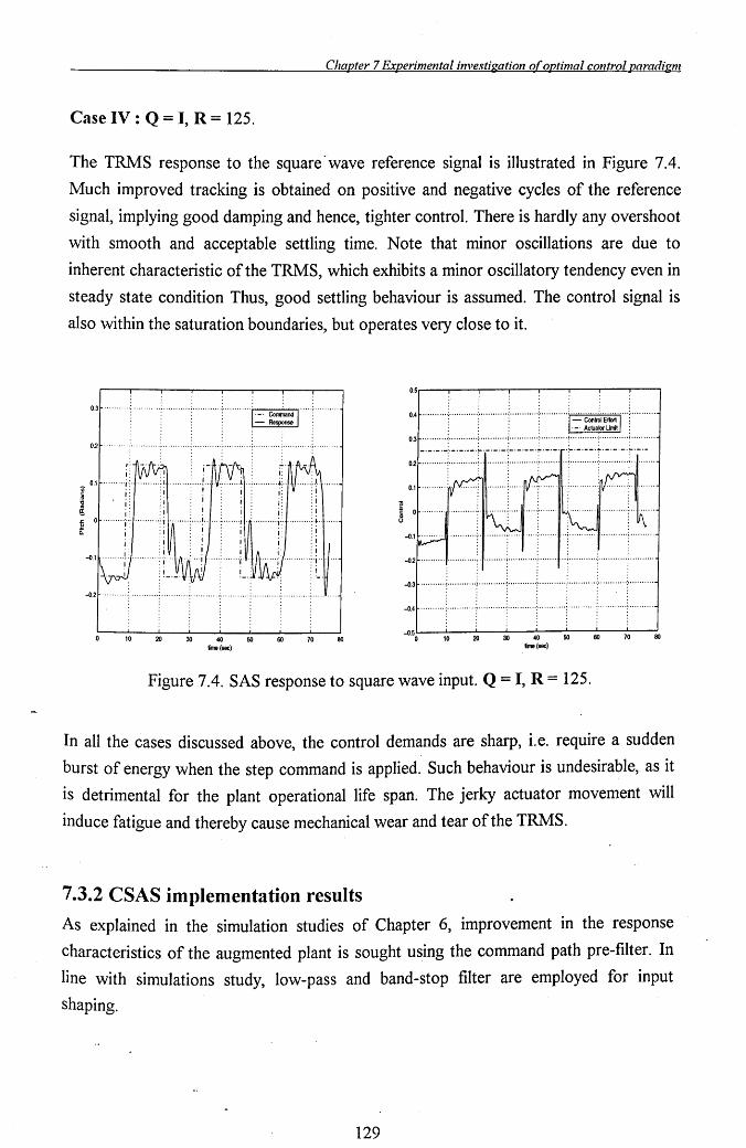
Chapter 7 Experimental investigation o(optimal control paradigm
Case IV: Q = I, R= 125.
The TRMS response to the square . wave reference signal is illustrated in Figure 7.4.
Much improved tracking is obtained on positive and negative cycles of the reference
signal, implying good damping and hence, tighter control. There is hardly any overshoot
with smooth and acceptable settling time. Note that minor oscillations are due to
inherent characteristic of the TRMS, which exhibits a minor oscillatory tendency even in
steady state condition Thus, good settling behaviour is assumed. The control signal is
also within the saturation boundaries, but operates very close to it.
0.3 ..
0.2 .......... , ....... ,., .......... : ........... : ........... ~ ............ : ... . -._. -._;. _. _ .. -.~. _._. -';-'-'- _.:-. _. _. ';' _. --':' _. -, -':'-'-02 .......... j ............ ~ .......... ! ............ ~ .......... : ............ : ............ ~ ..
~ 0 .........
8
-02 .......... 1 ...... · .... ·,·11 ...... · .. , .... · ...... ·: ........ 1 .. ·; .. ··· ........ : ............ : ........... ,
-0.31- .......... ; ............ ) ........... ( ............. : ............ ! ............ : ............. ~ .......... -1
-02 .......... . ................ . ......... . .........•.....
-0.41- ......... ; ............ ; ........... : ............ ; ........... : ............ : ............ : .......... ,
10 20 30 40 50 60 70 80 -0.50 10 20 30 40 50 60 80
ima(sec) lme(sac)
Figure 7.4. SAS response to square wave input. Q = I, R = 125.
In all the cases discussed above, the control demands are sharp, i.e. require a sudden
burst of energy when the step command is applied. Such behaviour is undesirable, as it
is detrimental for the plant operational life span. The jerky actuator movement will
induce fatigue and thereby cause mechanical wear and tear of the TRMS.
7.3.2 CSAS implementation results
As explained in the simulation studies of Chapter 6, improvement in the response
characteristics of the augmented plant is sought using the command path pre-filter. In
line with simulations study, low-pass and band-stop filter are employed for input
shaping.
129
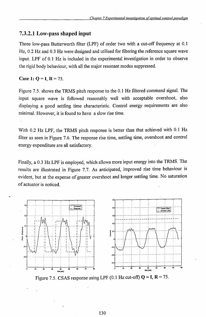
Chapter 7 Experimental investigation of optimal control paradigm
7.3.2.1 Low-pass shaped input
Three low-pass Butterworth filter (LPF) of order two with a cut-off frequency at 0.1
Hz, 0.2 Hz and 0.3 Hz were designed and utilised for filtering the reference square wave
input. LPF of 0.1 Hz is included in the experimental investigation in order to observe
the rigid body behaviour, with all the major resonant modes suppressed.
Case 1: Q = I, R= 75.
Figure 7.5. shows the TRMS pitch response to tpe 0.1 Hz filtered command signal. The
input square wave is followed reasonably well with acceptable overshoot, also
displaying a good settling time characteristic. Control energy requirements are also
minimal. However, it is found to have a slow rise time.
With 0.2 Hz LPF, the TRMS pitch response is better than that achieved with 0.1 Hz
filter as seen in Figure 7.6. The response rise time, settling time, overshoot and control
energy expenditure are all satisfactory.
Finally, a 0.3 Hz LPF is employed, which allows more input energy into the TRMS. The
results are illustrated in Figure 7.7. As anticipated, improved rise time behaviour is
evident, but at the expense of greater overshoot and longer settling time. No saturation
of actuator is noticed.
0,3 "
0,2 """"""
10 20 30 40 50 60 70 80 tima(sec)
0'5r----r---.------r---r--,----,---r----,
0,4 "",.
0,3 ....... , •• ~ ............ ; •• " .••••.• ~ ............ ~ ••••••••• '·:····'···· .. ~··'····· .. ·'i······'··· _. _._.-:. _. _ .. -.~. -.-. -':- ._.- -.~.-. -. -.~._.- _. ~. _. -.-.~. _.-
02 "····"···~·,·"···,,··f,,·····,···,·····"'····:····"""";""""""~"""""":"""""
Figure 7.5. CSAS response using LPF (0.1 Hz cut-off) Q = I, R = 75.
130
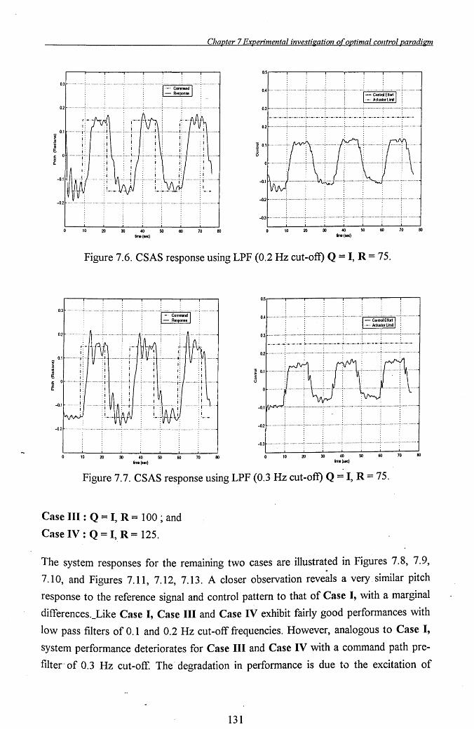
Chapter 7 Experimental investigation of optimal control paradigm
0.3
0.2 . 0.3 ....•..... : ...•....•... : ........... : ............ ~ ........... ; ....•...... : ............ : ....•...•. . . . -._.- .-;' _. -.. -.~.-. _. -:-. _.- -.~.-. _. -,;-. _. --. ~. -. -. _.~._.-
02 ........... : ............ ~ ........... ~ ............ : ............ ! ............ : ............ ~ ......... .
I 0.1 ." ........ ~ ...
() .
-0.2
-0.31- .......... ,.· .......... ·;· ...... ·· .. ; .. ··· .... ·· .. ; ........ · .. ·! .... ·· ....... ;- ........... ; .......... -1
10 20 30 40 50 60 70 80 W 20 30 ~ 50 60 70 80
time (sec) lime (sec)
Figure 7.6. CSAS response using LPF (0.2 Hz cut-off) Q = I, R = 75.
0.5r----r---r---,----.---r--,-----,---,
0.3 ......... "
0.3 ~:~·.·~·j~:~::·~·t:~:~·.·~'L:~:~~:L~· .. ~:~:L·~· .. ~·~:l:~·.·~·.·~·t:~:~··· 02 ·· .. ···· .. ·:· ...... ·· .. ·i· .... ·· .... : .. ·· .. ·· .. ·.;·· .. ··· .. ···,·
e 0.1 .......... i. ~ .
-0.2 -0.21- .......... : ............. : ........... ; ............. ~ ........... : ............ ~ ............ ~ .......... -I
-0.3~" ......... ; ............ ~ ........... i .. ·· ...... · .. ; ............ ! ............ ; ............ ; ........... ,
10 20 30 40 50 60 70 80 10 20 30 40 50 60 80
time (sec) Irne(sec)
Figure 7.7. CSAS response using LPF (0.3 Hz cut-off) Q = I, R = 75.
Case III : Q = I, R = 100 ; and
Case IV: Q = I, R= 125.
The system responses for the remaining two cases are illustrated in Figures 7.8, 7.9,
7.10, and Figures 7.11, 7.12, 7.13. A closer observation reveals a very similar pitch
response to the reference signal and control pattern to that of Case I, with a marginal
differences._Like Case I, Case III and Case IV exhibit fairly good performances with
low pass filters of 0.1 and 0.2 Hz cut-off frequencies. However, analogous to Case I,
system performance deteriorates for Case III and Case IV with a command path pre
filter" of 0.3 Hz cut-off. The' degradation in performance is due to the excitation of
131
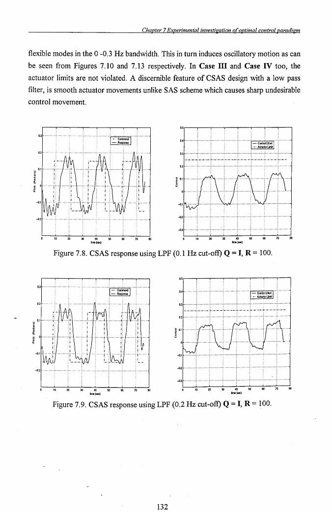
Chapter 7 Experimental investigation o(optimal control paradigm
flexible modes in the 0 -0.3 Hz bandwidth. This in turn induces oscillatory motion as can
be seen from Figures 7.10 and 7.13 respectively. In Case III and Case IV too, the
actuator limits are not violated. A discernible feature of CSAS design with a low pass
filter, is smooth actuator movements unlike SAS scheme which causes sharp undesirable
control movement.
0.5,---,,-----,,------,----,----,----r----r---,
···t:·~=~·I·····[·"·· 0.3 ......
0.4 .......
0.3 ~:~·.·~·.·J:~:~:·.·~t:~:·~·.·~t:~:~~·.L·~·:~:~L·~·:~·~:i:~·.·~·.·~t:~:·~··· 0.2 ........•. j ............ ! ........... j ............ ; ..... ·······1············;············;··········
-0.2 .. -0.2 .......... j ............ ~ ........... j ........... -; ........... : ........... ~ ............ ~ ......... .
-0.3 ......... ; ............ ~ ......... : .. ; ............ ; ............ : ........... ; ............ , ......... .
10 20 30 40 50 60 70 80 10 20 30 40 50 60 70 80 time (soc) Ime(soc)
Figure 7.8. CSAS response using LPF (0.1 Hz cut-oft) Q = I, R = 100.
0.5,..-----,.-----.r-----.----,---.----r----r---,
0.3 """""" """"""" ""I="~=T .... " ....... 0.3 ··········j············i········· .. j······· .. ···~······· .... ; ........... : ............ ; ......... .
_.- .-.-:.-. -.. -.~. _. -.- ';-. -.-- '?_. _. -.:-.-.--.~. _. _. -.~. _.-0.2 .... · .... ·t""·""·["·"""·T"""""·:""""""!""""'''''j''''·''''''·~''''''''''
g 0.1 .......... ~ ..
8 :
-0.2 ......... " ... -O.2~ .......... :; ............ :· .......... ·i ............ ~ .. · .. · .... ·:· .......... ;· .......... ·:"""""1
-O.3~ .......... ; ............. ; ............ , ............ : ............ ! ............ ;- ......... ":"''''''''1
10 20 30 40 50 60 70 80 10 70 80
lime (soc)
Figure 7.9. CSAS response using LPF (0.2 Hz cut-oft) Q = I, R = 100.
132
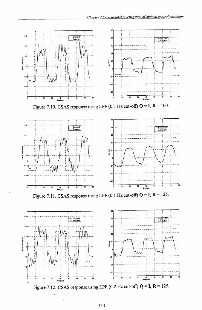
Chapter 7 Experimental investigation o(optimal control paradigm
0.5r----.---,....----.---,....---..---.----..-----.
.. _. Co~nd j""' - Response
0.3 ........ ': ........... :, ........... ~ ... . 0.4
02 0.3 ··········j············i···········:············~····· ...... : ........... ~ ............ ~ ......... . - .-. - .-:. _. _ .. -.~.-. -. - .:-. _. - _.;... _. _. -.;..... _. --.~. _._. _.;... _.-. . . . . . .
02 ...... ~ ........... : ........ .
0.1 ......... ,
~ I
~ '!. I ~ o· ....... , f
-0.1 .......... ; ............ : ........... : ............ : ........... : ........... : ............ : ......... .
-0.2 -0.2 ..........•.............
-0.3 ........... : ............ ~ .......... : ........... -: ......... .
10 30 40 50 Ime(sec)
60 20 70 60 10 20 30 40 50 Ime(sec)
60 70 60
Figure 7.10. CSAS response using LPF (0.3 Hz cut-off) Q = I, R = 100.
0.5r----.---,....---.---r---;----;r---;----;
0.3 ;........-...:.....---.., ........... . 0.4
0.3 ....•..... ~ ............ : ........... : ............ ~ ........... : ....•..•... ~ .......•..•. : ......... .
-.-.-.-:.-.-.. -.~.-.-.-~-.-.--.~.-.-.-.:-.-.--.~.-.-'-.~.-.-0.2 ........ ~ ........... : ........ ..
-02 ., ........... . .....
10 20 30 40 50 60 70 80 10 20
ime(sec)
Figure 7.11. CSAS response using LPF (0.1 Hz cut-off) Q = I, R ~ 125.
0.3
10 60 20 30 40 50 ime(sec)
70 80 10 20 30 40 50 time (sec)
60 70 80
Figure 7.12. CSAS response using LPF (0.2 Hz cut-off) Q = I, R = 125.
133
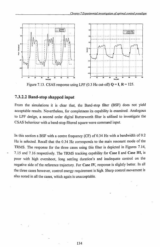
Chapter 7 Experimental investigation o(optimal control paradigm
0.3
02
': 0.1 ··· .. ····i~··· ,.
,: :, o ........ y .......... i·
,: :1 .,
:j
10 20 30 40 50 60 70 80 lime (sec)
0.4 .......... ~ ............ ~ ........... ~ ...
· . .. . 0.3 ··········;············~ .. ·········i············:···········f·· .. ·······;············:··········
-._. -.-;' _. _. --. ~. -. _. -.~- . .:..- _. ~. -. -. -.~.-. --.~. _._. - .~. _.-02 ........... : ............ ; ........... ; ............ : ............ ; ............................... .
: . :. :. -0.1 ..•....... ~ .......•.... ~ ...•••.•... ~ ............ : ........... ~ ........... ~ ......•..... : ......... .
· . · . : :.
-02 .......... ; ............ ~ ........... ! ............ ~ ........... ! ....................... , ......... . · . . . .
-0.3 ........... : ......... .) ............ ; ............ : ............ j ...
W 20 30 ~ 50 60 ro 80 time (sec)
Figure 7.13. CSAS response using LPF (0.3 Hz cut-oft) Q = I, R = 125.
7.3.2.2 Band-stop shapped input
From the simulations it is clear that, the Band-stop filter (BSF) does not yield
acceptable results. Nevertheless, for completness its capability is examined. Analogous
to LPF design, a second order digital Butterworth filter is utilised to investigate the
CSAS behaviour with a band-stop filtered square wave command input.
In this section a BSF with a centre frequency (CF) of 0.34 Hz with a bandwidth of 0.2
Hz is selected. Recall that the 0.34 Hz corresponds to the main resonant mode of the
TRMS. The response for the three cases using this filter is depicted in Figures 7.14,
7.15 and 7.16 respectively. The TRMS tracking capability for Case I and Case III, is
poor with high overshoot, long settling duration's and inadequate control on the
negative side of the reference trajectory. For Case IV, response is slightly better. In all
the three cases however, control energy requirement is high. Sharp control movement is
also noted in all the cases, which again is unacceptable.
134
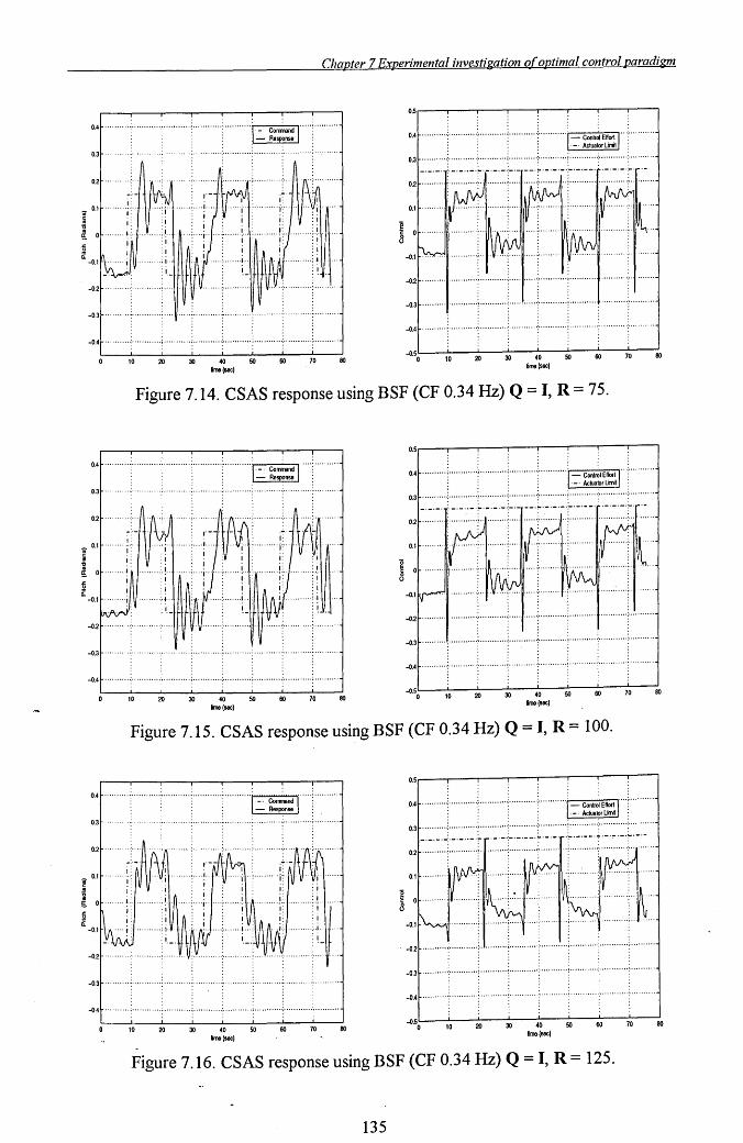
Chapter 7 Experimental investigation o(optimal control paradigm
0.4 ...................................................... ~ ~;:~ 1""
0.3
02 .....
_ 0.1
~ ~ !& 0
-0.2
-0.3
-0.4
......... !.:. ,: "
10
....... :' .......... ,:' ........... : ........... ~ ........... , ......... .
20 30 40 50 60 70 time (sec)
I
80
0.5,-----r--.----.---..---....---.---.---.,
0.4
. . . . . 0.3 .....•..... :- ...•..... , . ~ .•.......... : ...•••...... ! ............ : .•....... "';' ......... .
. . -.-.. -.~ ._._._.:-.- --.~.-.-.-.:-.-.--.
02
0.1
0 ........
-02
-0.3
-0.4
-0.5 0 10 20 30 40 50 60 70 80
time (sac)
Figure 7.14. CSAS response using BSF (CF 0.34 Hz) Q = I, R = 75.
0.4 .... · .. · .. •· .... · .. · .. ·• ............ · .. · .. · .. · .. • .... · .... ··I~ ~~~ r .............. · 0.3 ....................... .
0.2
~ 0.1
~ !& 0
~ Q.
-0.1
-0.2
-0.3 ................... .
-0.4 .......... ; ............ : ........... i ............ ; ..... ...... : ........... :. ........... : ......... .
10 20 30 40 50 60 70 lime (sec)
80
0.5,.----r--.----r--.... --,-----r--,----;
0.4 ;.--~-,="....,.., .. " ..........
0.3 ........... ; ............ ; ........... i •••• · •• ·····;····· .•.•••. ; ....••.•...• ; ••••••..••.• ; .....••.••
:. _.- .. -.~.-.-.-.~-.- --.;..-.-.- .:-.-.--..
-02 ........... ; ........... , .......... : ............ ; ...................... ; ......... .
-0.3 ....................... ; .....••.... ; ...•........ ; .....•...... ; ............ : ............ ; ......... .
-0.4
-0.5 0 10 20 30 40 50 60 70 80
time (sac)
Figure 7.15. CSAS response using BSF (CF 0.34 Hz) Q = I, R = 100.
0.4 .. · ........ · ...... · .. · .......................... : .. · ........ 1 ~ ~=~ I ...... · .. · .... ..
0.3
0.2
W 0.1
~ g 0
J: 2 Ii:
-0.1
-0.3 ........... ..
-0.4 .......... ; ............ : ........... ; ............ : ............ ; ........... ': ............ ; ......... .
10 20 30 40 50 60 70 time (sac)
80
0.5.-----r--.----.---r---,----.--.--,
0.4 ······ .. ··1·· .. ···· .. ··~ .. ···· .. ···j··········· r----'--.......... , ........ ..
0.3 .......... , ............ ; ............ , ......... ..
-.-.-.-:.-.- .. -.~ ._.-.:-._. __ . ........... ; ............ ; ............ ~ ......... .
.;-.-.-- . .;..-.~ .-.~.-.-. . . 02 .. · ...... ·t .. · .... · .. ~ .. ........ , .......... . .. ; ............ ; ............ ~ ..
0.1
-02~ .......... ; ........... ,.;.I ......... , ............ -: ........ : ... ; .... ' .... ' .... :. .... · .. · .. .; .. · .. · .. · .. 1
-0.31- .. ·, .... · .. , ............ ~ ............ ~ ............ : .. , .......... ~ ............. : ............ , ........... ;
-O.41- .. ·· ...... ·;·· ........ ··; .. ·· .. · .... :· ........ · .. ~· .... · .... ·: ............ : ............ , ........... .
-O.5L-_-..L.--.J.----'---'---J....---..L.--.J.----' o 10 20 30 40 50 60 70 80
fime(sac)
Figure 7.16. CSAS response using BSF (CF 0.34 Hz) Q = I, R = 125.
135
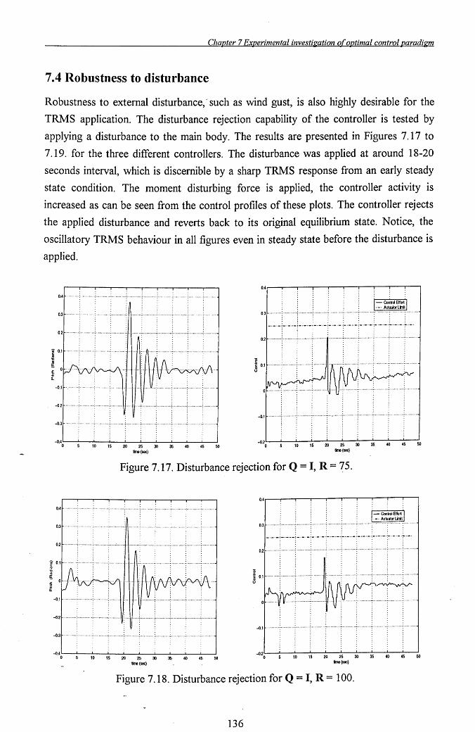
Chapter 7 Experimental investigation of optimal control paradigm
7.4 Robustness to disturbance
Robustness to external disturbance,'· such as wind gust, is also highly desirable for the
TRMS application. The disturbance rejection capability of the controller is tested by
applying a disturbance to the main body. The results are presented in Figures 7.17 to
7.19. for the three different controllers. The disturbance was applied at around 18-20
seconds interval, which is discernible by a sharp TRMS response from an early steady
state condition. The moment disturbing force is applied, the controller activity is
increased as can be seen from the control profiles of these plots. The controller rejects
the applied disturbance and reverts back to its original equilibrium state. Notice, the
oscillatory TRMS behaviour in all figures even in steady state before the disturbance is
applied.
OAI-· .. ·,··;·········;··········;·········.;···· .. · .. .; ...... .... : .......... : ..... , ..... : .......... : ...... ..j
0.31- .... ···;·····, .. ··;····· .... ; .... · .. ·.:// ...... : .......... : .......... : .......... :. ........ ; ........ ~
0.21- .. · .. · .. ;· .. · .. · .. ; .. · .. · .. ·:; .. · ...... ;11 .. · .. ·; ........ ·: .......... : ...... · .. : ......... : ........ -1
I 0.11-·· .. ····:· ...... ··;··· ...... :·· .... · .. +1 IF·/I .. ··;·· .... · .. :· ........ :· .. ··· .. ·,; .... ····-I '6 ~ i 0 .
II.
-0.11-····,· .. ······;········.;··· .. ·11
-0.21- ...... ··; .. · .. · .. ·; .. · .. · .. ·;· ...... 1/
-0.31- .. ·,··;···· .... ·;··, .... ···; .. · .... , .. ; ......... ; ........ : ......... : ......... : ......... :., ....... ..j
-O.40'-~--'-10 ---J15'-----'-20-2..L..5
---'30-....L..35
-4'--0 ---L45----1SO
limo (sec)
0.3 ........ : ....... : ......... : ......... ; ...... " .................... .
-.-. +._ .. -: -. -._!_._. _.:-._. -L. _ .. -.:-. -._.:- .-. _.;.. _. -.;.. _. 0.2 ........ ~ ......... ; ......... ~ ........ : ......... ~ ......... ~ ......... ; ......................... .
g 8 0.1 ... ~ ......... ~ ......... : ....... .
-0.1 ~ ........ : ......... : ......... :: ......... : ....... , .... : ......... : ........ '.~ ......... ~ ......... : ........ i
-0'20L--L--..L..10
---'15-....L..2O
-2'--5 ---L
30-
35.1.-.-L----'::'-:so·
time (sec)
Figure 7.17. Disturbance rejection for Q = I, R = 75.
0.41-·······,······ .. ·;··· ...... :···· ..... -; .......... ; .......... :: ......... -: .......... ; ......... -: ........ .j
0.31- .. ····;·········;··, .. ·····;·.· ..... .:./1 ...... .: .......... : .......... ; .......... ; .......... :. ...... -1
02~··· .. ·' .. ; ........ ·; ......... : .... · ..... ~+ ..... ; ......... : ......... , ..... , .... : ......... :., ....... -1
-O.It-· .... ···;· .... · .. ·; .. ··· .. ··;· .. ···H
-0.2t- ........ ; .... ·· .. ·; .. ·· .... ·,· .... ··1I
-0.3~·······:···· .. · .. :··' ....... : ......... : .......... : ......... : ......... : ......... : ......... : ..... -1
-O.40~~-:L----J1L-5 ---'-20-2..L..5
---'30-....L..35-4QL---1.45----1SO
time (sec)
10 15 20 25 30 time (sec)
Figure 7.18. Disturbance rejection for Q = I, R = 100.
136
so
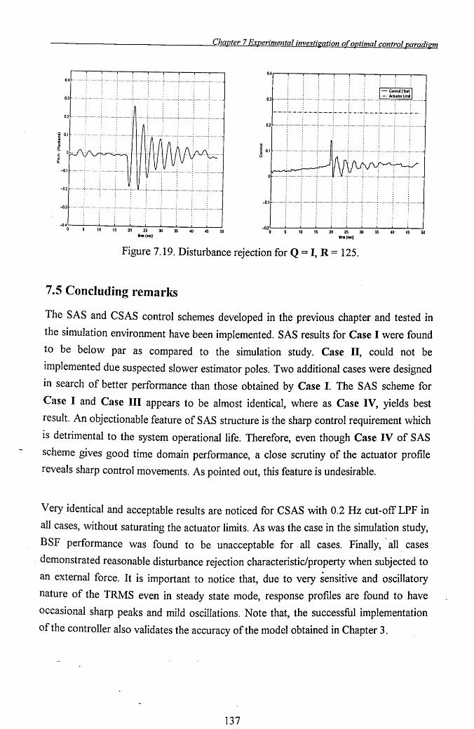
Chapter 7 Experimental investigation of optimal control paradigm
-0.11"""""''''''''''''''''''";",, .... 11
-0.3~""··";"" .... : ........ : .......... ; ......... ; ........ ; .......... : .......... ; ......... : ....... ~
0.3 ·· ...... :· .. · .. "·i .. ,, .... ·i .. ,,· .... i· .. ,,· .. ·;·· ... · ... ! ......... : _.- '-j-'---; _. _. -i-·_·_·;_·_· -L. -" -j_. _.- .:-. _.-L. _. _.~._.
02 ········!·········:·········~·········f·········:····· ... ; ......... j ......... j ......... ! ....... . . .
J 0.1 ........ 1 ...... · .. 1 ........ ·; .... '" · ........ ·; ........ ·1 ...... · .. ; ........ ·: ...... "'; . .. .... .
: :: -0.1 ········:·········i·········i·········:·········~····· ... ; ......... ; ......... : ......... : ....... .
-02~0L---1.-1:1:-0 ----:l:1S:---:l:-2O ----!.2S:---~30 --:35:--~40 ----:4:-S --:50 lime (sec)
Figure 7.19. Disturbance rejection for Q = I, R = 125.
7.5 Concluding remarl<s
The SAS and CSAS control schemes developed in the previous chapter and tested in
the simulation environment have been implemented. SAS results for Case I were found
to be below par as compared to the simulation study. Case II, could not be
implemented due suspected slower estimator poles. Two additional cases were designed
in search of better performance than those obtained by Case I. The SAS scheme for
Case I and Case III appears to be almost identical, where as Case IV, yields best
result. An objectionable feature of SAS structure is the sharp control requirement which
is detrimental to the system operational life. Therefore, even though Case IV of SAS
scheme gives good time domain performance, a close scrutiny of the actuator profile
reveals sharp control movements. As pointed out, this feature is undesirable.
Very identical and acceptable results are noticed for CSAS with 0.2 Hz cut-off LPF in
all cases, without saturating the actuator limits. As was the case in the simulation study,
BSF performance was found to be unacceptable for all cases. Finally,' all. cases
demonstrated reasonable disturbance rejection characteristic/property when subjected to
an external force. It is important to notice that, due to very sensitive and oscillatory
nature of the TRMS even in steady state mode, response profiles are found to have
occasional sharp peaks and mild oscillations. Note that, the successful implementation
of the controller also validates the accuracy of the model obtained in Chapter 3.
137

Chapter 7 Experimental investigation of optimal control paradigm
Sampling period selection is an important design criteria for modelling as well as for
control application. Therefore, succ~ssful execution of controller further corroborates
the rationale of sampling period choice.
138
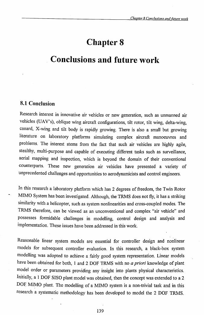
Chapter 8 Conclusions and future work
Chapter 8
Conclusions and future work
8.1 Conclusion
Research interest in innovative air vehicles or new generation, such as unmanned air
vehicles (UAV's), oblique wing aircraft configurations, tilt rotor, tilt wing, delta-wing,
canard, X-wing and tilt body is rapidly growing. There is also a small but growing
literature on laboratory platforms simulating complex .aircraft manoeuvres and
problems. The interest stems from the fact that such air vehicles are highly agile,
stealthy, multi-purpose and capable of executing different tasks such as surveillance,
aerial mapping and inspection, which is beyond the domain of their conventional
counterparts. These new generation air vehicles have presented a variety of
unprecedented challenges and opportunities to aerodynamicists and control engineers.
In this research a laboratory platform which has 2 degrees of freedom, the Twin Rotor
MIMO System has been investigated. Although, the TRMS does not fly, it has a striking
similarity with a helicopter, such as system nonlinearities and cross-coupled modes. The
TRMS therefore, can be viewed as an unconventional and complex "air vehicle" and
possesses formidable challenges in modelling, control design and analysis and
implementation. These issues have been addressed in this work.
Reasonable linear system models are essential for controller design and nonlinear
models for subsequent controller evaluation. In this research, a black-box system
modelling was adopted to achieve a fairly good system representation. Linear models
have been obtained for both, 1 and 2 DOF TRMS with no a priori knowledge of plant
model order or parameters providing any insight into plants physical characteristics.
Initially, a 1 DOF SISO plant model was obtained, then the concept was extended to a 2
DOE MI~O plant. The modelling of a MIMO system is a non-trivial task and in this
research a systematic methodology has been developed to model the 2 DOF TRMS.
139
Chapter 8 Conclusions and future work
The difficulty in the modelling procedure for the two input two output system is
compounded due to the presence of. cross-coupling between the planes of motion. The
coupled nature is also a typical characteristic of helicopters. The identified models have
been exhaustively validated using time and frequency domain tests in order to instil
confidence in the models for their subsequent use in the controller design. For the
MIMO plant, coherence analysis has also been used to detect system nonlinearities and
the degree of coupling between the various channels. The coherence metric is often
employed in helicopter modelling procedure [22]. The modelling procedure adopted is
suitable for a class of new generation air vehicles whose dynamics are not well
understood or difficult to model from first principles. The approach presented here is an
important contribution of this thesis. The identified models include the rigid as well as
the flexible plant dynamics.
Vibrations due to random excitation of structures are common phenomena experienced
by large space structures with flexible appendages, ships, fl~xible aircraft and missiles.
Although flexible structures are desirable, the vibrations are not. These vibrations may
cause discomfort to passengers and degrade system performance. Vibration suppression
can be accomplished via active, passive or hybrid active and passive means. Passive
treatment is essential but is limited in rendering the desired accuracy. Hence, active
control is needed. The modelling exercise for the TRMS revealed the presence of
resonant system modes which are responsible for inducing unwanted vibrations during,
and at the end of, system manoeuvres. In this research, open-loop, closed-loop and
combined open and closed-loop strategies have been investigated to address this
problem. Open-loop control methods have been developed based on the identification of
the resonant modes of the TRMS. These have been detected through the analysis of the
plant spectral responses and the modelling process. Low pass and band-stop filters have
been developed to shape the command signals. This method ensures that the system
does not experience the undesirable resonant eigen-frequencies, thereby preventing the
excitation of vibrational modes. The effectiveness of this concept has been demonstrated
on the TRMS rig for 1 and 2 DOF motion, with significant reduction in vibration. This
is evident from smooth time domain responses as well as from the attenuated resonant
modes in the frequency domain. The band-stop filter is found to be effective in the
selective removal of energy from the input signal corresponding to significant dynamic
modes, thereby retaining the maximum amount of energy in the input signal. On the
cont~ary, if the number of closely _ spaced vibration modes contribute to the system
vibration; low pass filtered inputs are recommended.
140
Chapter 8 Conclusions and filture work
Once the controller has been designed using the linear system model, its performance is
often gauged in a simulation envi~onment using a nonlinear plant model. This is a
common practise in the aerospace industry. To study the performance of next
generation air vehicles researchers are increasingly relying on nonlinear modelling and
control techniques. Therefore, a nonlinear plant model is essential for predicting the
system behaviour accurately in order to evaluate the controlled system performance, as
well as for controlling a highly nonlinear plant by the dynamic inversion control method.
In this research, neural networks were utilised to obtain the nonlinear system model.
Unlike linear system identification, nonlinear techniques for modelling require special
excitation signals, rich both in frequency and amplitude as well as higher order
correlation tests for model validation. An RBF based NN model was identified for the 1
nOF plant. The nonlinear modelling method adopted in this work is appropriate for
modelling complex new generation highly agile air platforms with significant
nonlinearities. The main aim of NN based modelling has been to achieve a highly
accurate model. It has been noted, however, that the nonlinear model is only slightly
better than the linear 1 nOF model. For this reason, the nonlinear model is not
incorporated in the controller evaluation, rather the linear model is used for simplicity.
However, the utility of the nonlinear model cannot be precluded in 2 nOF controller
analysis, in particular for the ul ~ y2 channel that exhibits nonlinear behaviour. Hence,
the RBF model will be of benefit while analysing the controller performance for this
channel.
In addition to vibration attenuation, it is also desirable to achieve other performance
criteria such as command tracking, disturbance rejection, fast rise time and robustness
to modelling errors. These objectives cannot be achieved by open-loop mechanisms
alone, thus closed-loop strategies have also been investigated. An inner feedback LQG
compensator was initially designed and analysed in the simulation environment for the 1
nOF TRMS, using the identified system model. This feedback mechanism referred to as
Stability Augnlentation System (SAS) demonstrates good tracking capabilities but
requires high control effort and has inadequate authority over residual system vibrations.
These problems were resolved by further augmenting the system with a command path
prefilter. The combined feedforward and feedback compensator is known as the
C0l11111and and Stability Augmentation Syste111 (CSAS) and satisfies the performance
objectives and obeys the actuator constraint.
141
Chapter 8 Conclusions and future work
Finally, the crucial test for any control design is the implementation. The SAS and CSAS
control schemes developed in this ~ork here, have been evaluated on the TRMS test
rig. One of the controllers faired poorly as compared to the simulation runs for the SAS
scheme. While the other failed due to the slow estimator poles, hence could not be
evaluated. Therefore, two additional controller were designed with a larger penalty on
the control in search of better performance. Implementation of the new controllers
showed much improved results. An important drawback of the SAS scheme is the sharp
or abrubt control requirement which eventually could lead to mechanical wear and tear
of the plant. On the other hand quite similar and acceptable results are observed for the
CSAS scheme with 0.1 and 0.2 Hz cut-off low-pass filter in all cases, without saturating
the actuator limits. A desirable feature of this scheme being the smooth control
movement. With the CSAS, performance objectives are realised in a fewer control
design iterations as opposed to SAS scheme. This is another advantage of the CSAS
strategy. Analogous to the simulation study, band stop filter performance was
unacceptable, however, this was investigated for completeness. Robustness to external
disturbance such as wind gust has also been demonstrated with an acceptable
disturbance rejection capability.
This research has presented a black-box approach to model the TRMS. The method is
generic and provides a novel alternative to model a class of unconventional air vehicles
[90-92]. A similar scheme is proposed to derive nonlinear models for highly
manoeuvrable air platforms [93]. Further, this work also presented approaches to
effectively deal with undesirable flexible dynamics in modern systems [94,95]. The
presence or inclusion of flexible dynamics leads to higher order system models, which
renders the control design difficult. Since, it is not practical to measure all the states of
high order systems, therefore, estimator based optimal control has been shown to be an
effective choice for the TRMS and similar system [96].
8.2 Suggestions for future work
In this research the SISO control design has been investigated, an obvious extension is
therefore, the MIMO LQG controller design. A 2 DOF autopilot to control pitch and
the yaw plane would involve the decoupling objective of the ul ~ yl channel. It should
be fairly straight forward to accomplish this design.
142
Chapter 8 Conclusions and future work
Further work on the nonlinear modelling of a 2 DOF TRMS would be useful. In
p,articular for the ul ~ y2 channel"which exhibits nonlinear behaviour. As pointed out
earlier, this would aid in contoller performance evaluation for this channel.
An interesting development of this work would be to study the roll control of the
TRMS. This will necessitate modification of the TRMS rig to provide an additional
degree of freedom for the roll movement. The modified TRMS would then mimic the
hover mode for a vertical take off and landing (VTOL) type aircraft. This is a non trivial
problem and has attracted considerable attention [32,78,81]. The design objectives
would then be roll as well as pitch and yaw control.
In order to control a physical system, a plant model is often required and the modelling
invariably involves approximation of the real system. Also, the real system undergoes
degradation leading to parameter variations and the system is also acted upon by
environmental disturbances. Recent robust control design methods, such as H-oo and Jl
synthesis, are capable of tolerating such levels of uncert'ainty. Robust control methods
address the issue of robustness explicitly in the design formulation. Since, the TRMS is
very sensitive to external disturbances, robust control could be an attractive alternate
proposition.
Reconfiguration is highly desirable in many advanced systems such as advanced tactical
fighters, adaptive structures and autonomous robots. The main motivation of
reconfiguration is greater survivability and controllability, attained through the ability of
the feedback system to reorganise itself in the presence of actuator/sensor failures and
surface damage. Two main approaches can be distinguished for plant control
reconfiguration. The first is based on the concept of failure detection and identification.
This approach works well in restricted cases, but suffers from significant drawbacks. As
the number of failures grows, it becomes increasingly difficult and time consuming to
carry out the detection and classification. The second consists of identifying the dynamic
behaviour of the system in real-time and designing a controller' automatically. Because
such an approach does not rely on failure classification, it is expected that the resulting
system would tolerate a larger class of failures. Adaptive control such as Model
Reference Adaptive Control (MRAC), both indirect and direct methods, can be used for
reconfiguring control. The TRMS rig is an ideal platform upon which the reconfigurable
control strategies can be tested.
143
Appendix 1
Appendix 1
A.I Description of the toolbox functions
All functions desired for communication between the RTK and Matlab environment
have the following general form:
ReturnValue = hl_call(FunctionNanle, [Argunlentj)
where:
ReturnValue- value returned by the function,
hl_ call- name of the DLL library responsible for the communication,
FunctionNanle- name of the desired operation, string format.
Argunlent- argument passed to the hi_call function (optional).
GetBaseAddress
Purpose: Get the base address of the PCL-8I2 board.
Synopsis: BaseAddr = hl_ call{'GetBaseAddress ').
Description: The function is called to obtain the base address of PCL-8I2 interface
board. If the based address ofPCL-8I2 board is set to zero the RTK generates dummy
data. This mode is useful to test communication between the RTK and Matlab without
using external hardware.
GetSampleTime
Purpose: Get the basic sampling time.
Synopsis: SanlplT = hl_call{'GetSampleTime ').
Description: The function returns the period of the basic RTK clock. The period is
given in s~conds.
144
Al2.Pendix 1
SetSampleTime
Purpose: Set the basic clock.
Synopsis: hl_call{'SetSanlpleTinle', Period).
Description: The function sets the basic clock of RTK. The sampling period of AID
converter is set by this function. The controller output rate (DI A) can be equal to or
greater than the basic clock frequency. The Period parameter must be in the range from
O.OOls to 32.767s. The lower bound depends on the hardware configurations. The
resolution is O.OOls.
GetHistory
Purpose:Get content of the internal RTK buffer.
Synopsis: hl_ call{'GetHistory ').
Description: The function returns the Hist matrix containing the history of an
experiment and set the buffer to zero. Hist matrix contains various input-ouput
measurements.
145
References
[1] http://fourier.vuse.vanderbilt.edu/cimlprojects/flying.htm.
[2] Harvey B (1997). Micro unmanned aerial vehicles. Intelligent Automation Inc. USA.
[3] Warwick G (2000). Agents for change. Flight International, UK, July, pp. 151-153.
[4] Long M E (1999). Mars on earth. National geographic, USA, July, pp. 36-51.
[5] http://www.aerosonde.com.
[6] Ting T (1999). Bridging the gap between the theory and practice of control:
Aerospace perspective. IEEE Control Systems, Vol. 19, No.6, pp.45-48.
[7] http://avdil.gtri.gatech.edu/RCM/RCMlDroneProject.html.
[8] Freewing aerial robotics corp. (1997). Company R&D history. College station,
Texas, USA. www.freewing.com.
[9] Howard R M and Kaminer I (1995). Survey of unmanned air vehicles. In Proc.
Anlerican Control Conference, Seattle, Washington, USA, pp. 2950-2953.
[10] Tokhi M 0 and Azad A K M (1995). Active vibration suppression of flexible
manipulator system open-loop control methods. International Journal of Active
Control, 1, (1), pp. 15-43.
[11] Poerwanto H (1998). Dynamic simulation and control of flexible nlanipulators
systenls, Ph.D thesis, Department of Automatic Control and Systems Engineering, The
University of Sheffield, UK.
[12] Singer N C and Seering W P (1990). Preshaping command inputs to reduce system
vibration. ASME Journal of Dynanlics SystenlS, Measurenlent, and Control, vol 112,
pp.76-81.
[13] Dimitry G and Vukovich G (1998). Nonlinear input shaping control of flexible
spacecraft reorientation maneuver. Journal of Guidance, Control, and Dynanlics, Vol.
21, No.2, pp.264-269. .
[14] Suk J, Kim Y and Bang H (1998). Experimental evaluation of the torque-shaping
method for slew maneuver of flexible space structures. Journal of Guidance, Control,
and Dynanlics, Vol. 21, No.6, pp.817-822.
146
[15] Teague E H, How J P, and Parkinson B W (1998). Control of flexible structures
using GPS : methods and experimental results. Journal of Guidance, Control, and
Dyna111ics, Vol. 21, No.5, pp.673-683.
[16] Livet T, Kubica F and Magni J F (1995). Robust flight control design with respect
to delays, control efficiencies and flexible modes. Control Engineering Practice, Vol. 3,
No.10, pp.1373-1384.
[17] Livet T, Fath D and Kubica F (1996). Robust autopilot design for a highly flexible
aircraft. IFAC'96, San Francisco, CA, USA. Preprints, Vol. P, pp 279-284.
[18] Karkoub M, Balas G, Tamma K and Donath M (2000). Robust control of flexible
manipulators via J.l-synthesis . Control Engineering Practice, Vol. 8, pp. 725-734.
[19] Grewal A and Modi V J (2000). Multibody dynamics and robust control of flexible
spacecraft. IEEE Trans. on Aerospace and Electronics Systems, Vol. 36, No.2, pp.
491-500.
[20] George K K and Bhat M S (1998). Two-degree-of-freedom H-oo robust controller
for a flexible missile. Journal of Guidance, Control, and Dynanlics, Vol. 21, No.3,
pp.518-520.
[21] Feedback Instruments Ltd (1996). Twin rotor MIMO system. Manual 33-007-0.
Sussex, UK.
[22] Patton R, Miles M and Taylor P (1993). Design and application of test signals for
helicopter model validation in the frequency domain. In Godfrey, K. (Ed.), Perturbation
Signals For System Identification. Prentice Hall, UK, pp 298-320.
[23] AGARD (1974). Methods for aircraft state and paranleter identification
AGARD, NASA Research centre, Hampton, Virginia, U.S.A.
[24] Bruce P D, Silva J E and Kellet F M G (1998). Maximum likelihood identification
of linear aircraft dynamics using a hybrid genetic algorithm. In Proceedings of AIAA
36th Aerospaec Sciences Conference, Reno, Nevada, USA.
[25] Kaminer I Pascoal, A Hallberg E and Silvestre C (1998): Trajectory tracking for
autonomous vehicles: an integrated approach to guidance and control. AIAA, Journal of
Guidance, Control, and Dynamics, 1998, vol 21, 29-38.
[26] Hallberg E, Kaminer I and Pascoal A (1999). Development of a flight test system
for unmanned air vehicles. IEEE Control Systems, vol. 19, No.1, pp. 55-65.
147
[27] Atkins E M, Miller R H, Pelt T V, Shaw K D, Ribbens W B, Washabaugh P D and
Bernstein D S (1998). SOLUS: An ~utonomous aircraft for flight control and trajectory
planning research. In proceedings of the American Control Conference, Philadelphia,
USA, pp. 689-693.
[28] Linehan R D, Burnham K J and James D J G (1996). 4-Dimensional control of a
remotely piloted vehicle. In Proceedings of United Kingdonl Autonlatic Control
Conferenece, Exeter, UK, pp. 770-775.
[29] Van Nieuwstadt M J and Murray R M (1998). Rapid hover-to-forward-flight
transitions for a thrust-vectored aircraft. AIAA, Journal of Guidance, Control, and
Dynanlics, vol. 21,93-100.
[30] Morris J C, Van Nieuwstadt M J and Pascale B (1994). Identification and control
of a model helicopter in hover. In proceedings of the American Control Conference,
Baltimore, vol. 2, pp.1238-1242.
[31] Houston S S (1998). Identification of autogyro longitudinal stability and control
characteristics. AIAA, Journal of Guidance, Control, and Dynanlics, vol. 21, 391-399.
[32] Werner H and Meister T (1999). Robust control ofa laboratory aircraft model via
fast output sampling. Control Engineering Practice, vol. 7, 305-313.
[33] Blythe P Wand Chamitoff G (1995). Estimation of aircrafts aerodynamic
coefficients using recurrent neural networks. In Proc. Second Pacific International
Conference on Aerospace Science and Technology, Australia.
[34] Haley P and Soloway D (1997). Generalized predictive control for active flutter
suppression. IEEE Control Systenls, pp. 64-70.
[35] Ljung L (1987). System identification theory for the user. Prentice Hall
International.
[36] Well stead P E and Zarrop M B (1991). Self-tuning systems: control and signal
processing. John Wiley & Sons.UK. pp.126-128.
[37] Soderstrom T and Stoica P (1989). System identification. Prentice Hall.
[38] Bendat J S and Piersol, A. G. (1980). Engineering application of correlation and
spectral analysis. John-Wiley & Sons, 83-84.
[39] Ljung L (1991). System Identification Toolbox. The Math Works Inc, NJ, USA.
[40]. Nis~imura H and Kojima A (1999). Seismic isolation control for a building like
structure.
148
IEEE Control Systenls, vol. 19, No.6, pp. 38-44.
[ 41] Agarwala R, Selahattin ° and Mohammed F (2000). Active vibration control of a
multi-degree -of-freedom· structure by the use of direct model reference adaptive
control. In Proceedings of the Anlerican Control Conference, Chicago, Illinois, USA.
[42] Aspinwall D M (1980). Acceleration profiles for minimising residual response.
ASME Journal of Dynamic Systenls, Measurement and Control, 102, (1), pp. 3-6.
[43] Suk J Y, Kim, and Bang H (1998). Experimental evaluation of the torque-shaping
method for slew maneuver of flexible space structures. Journal of Guidance, Control,
and Dynanlics, Vol. 21, No.6, pp.817-822.
[44] Meckl P Hand Seering W P (1990). Experimental evaluation of shaped inputs to
reduce vibration of a cartesian robot. Trans. of the ASME Journal of Dynanlic SystenlS,
Measllrenlent and Control, Vol. 112, No.6, pp. 159-165.
[45] Singer N C and Seering W P (1990). Preshaping command inputs to reduce system
vibration ASME Journal of Dynanlics Systems, Measurement, and Control, vol 112,
pp 76-81.
[46] Watkins J and Yurkovich S (1992). Input shaping controllers for slewing flexible
structures. In Proceedings of the first conference on Control Applications, Dayton,
Ohio, USA, pp. 188-193.
[47] Tzes A. and Yurkovich S (1993). An adaptive input shaping control scheme for
vibration suppression in slewing flexible structures. The IEEE Transactions on Control
Systenls Technology, 1, (2), pp. 114-121.
[48] Banerjee A K and Singhose W E (1998). Command shaping in tracking control of
a two-link flexible robot. Journal of Guidance, Control, and Dynanlics, Vol. 21, No.6,
pp.1 012-1 015.
[49] Gorinevvsky D and Vukovich G (1996). Control of flexible spacecraft nonlinear
approximation of input shape dependence on reorientation maneuver parameters. In
IFAC'96, San Francisco, CA, USA, Preprints, Vol. P, pp. 285-290.
[50] Tokhi M 0, Shaheed M Hand Poerwanto H (2000). Adaptive neuro-inverse
dynamic active vibration control of a flexible manipulator. In Proceedings of the
Mechatronics-2000, Atlanta, USA.
[51] Williams C S (1986). Designing digital filters. Prentice Hall, NJ, USA.
149
[52] Dwight H B (1957). Tables and integrals and other mathematical data, 3rd Ed.,
Macmillan, New York.
[53] Kim B S and Calise A J (1998). Nonlinear flight control using neural networks.
Journal oj Guidance, Control, and Dynanlics, Vol. 20, No.1, pp.26-33.
[54] Lyshevski S E (2000). Identification of nonlinear flight dynamics: theory and
practice. IEEE Trans. on Aerospace and Electronics Systems, Vol. 36, No.2, pp.383-
392.
[55] Bruce P D and Kellet M G (2000). Modelling and identification of non-linear
aerodynamic functions using b-splines. In Proc. Instn. oj Mech. Engrs. Vol 214, Part G,
pp.27-40.
[56] Billings S A and Voon W S F (1986). Correlation based validity tests for nonlinear
models. Int. Journal oj Control, Vol. 44, No.1, pp. 235-244.
[57] Leontaritis I J and Billings S A (1985). Input-output parametric models for
nonlinear systems part 1: deterministic nonlinear systems. Int. Journal oj Control 41(2),
pp. 303-328.
[58] Chen S, Cowan C F N and Grant P M (1991). Orthogonal least squares learning
algorithm for radial basis function networks. IEEE Trans. on Neural Networks, Vol. 2,
No.2, pp. 302-309.
[59] Bishop C M (1995). Neural networks for pattern recognition. Clarendon press,
Oxford.
[60] M. T Hagan, Demuth H B and Beale M (1993). The Neural Networks Toolbox,
Mathworks Inc. USA.
[61] Dougherty H, Tompetrini K, Levinthal J and Nurre G (1982). Space telescope
pointing control system. Journal oj Guidance, Control, and Dynamics, Vol. 5, No.4,
pp. 403-409, 1982.
[62] Franklin G F, Powell J D and Emami-Naeini A (1988). Feedback control of
dynamic systems. Addison-Wesley, USA, pp. 447-473.
[63] Azad, A K M (1994). Analysis and design oj control mechanisnls jor flexible
nlanipulator systenls, PhD thesis, Department of Automatic Control and Systems
Engineering, The University of Sheffield, UK.
150
[64] Ozimina C D, Tayman S K and Chaplin H E (1995). Flight control system design
for a small unmanned aircraft. In Proc. Anlerican Control Conference, Seattle,
Washington, USA, pp 2964-2969.
[65] Hansen T, Kahn A, Kannan S, Peon R and Tapia F (1997). Georgia Tech entry for
the 1997 international aerial robotics competition. In Proc. AUVSI 97.
[66] Teague E H, How J P, and Parkinson B W (1998). Control of flexible structures
using gps: methods and experimental results. Journal of Guidance, Control, and
Dynal11ics, Vol. 21, No.5, pp.673-683.
[67] Blight J D, Dailey R Land Gangsaas D (1996). Practical control law design for
aircraft using multivariable techniques. In Tischler M.B (Ed.), Advances in Aircraft
Flight Control, pp 231-267.
[68] Boyle D P and Chamitoff G E (1999). Automous maneuver tracking for self
piloted vehicles. Journal of Guidance, Control, and Dynamics, Vol. 22, No.1, pp. 58-
67.
[69] Bossi J A and Langehough M A (1988). Multivariable autopilot designs for a bank
to-turn missile. In Proc. American Control Conference, Atlanta, Georgia, USA, pp
567-572.
[70] Henrichfreise H, Moritz Wand Siemensmeyer H (1987). Control of a light, elastic
manipulation device. In Proc. of the Conference on Applied Motion Control,
Minneapolis, USA.
[71] I(osut R L, Salzwedel Hand Emami-Naeini A (1983). Robust control of flexible
spacecraft. Journal of Guidance, Control, and Dynamics, Vol. 6, No.2, pp. 104-111.
[72] Langehough M A and Simons F E (1988). 6 DOF simulation analysis for a digital
bank-to-turn autopilot. In Proc. A111erican Control Conference, Atlanta, Georgia, USA,
pp.573-578
[73] Lin C F (1994). Advanced control systems design. Prentice Hall Inc. USA.
[74] Rubio F Rand Aracil J (1997). Designed of a combined tracking control systems.
Control Engineering Practice, Vol. 5, No.1 pp.23-31.
[75] Sheperd C Land Valavani L (1988).Autopilot design for bank-to-tum missiles
using LQGIL TR methodology. In Proc. A111erican Control Conference, Atlanta,
Georgia, USA Vol. 1.
151
[76] Sutton R P, Halikias G D, Plummer A R and Wilson D A (1999). Modelling and
H-oo control of a single-link flexible !llanipulator. In Proc. Instn. Mech Engrs, Vol 213
Part I, pp. 85-102.
[77] Hyde R and Glover K (1993). The application of scheduled H-oo controllers to a
VSTOL aircraft. IEEE Transactions on Aut0111atic Control, Vol 38, pp. 1021-1039.
[78] Sivashankar N, Kaminer I and Kuechenmeister D (1994). Design, analysis and
hardware-in-the-Ioop simulation of MIMO controller for a VTOL unmanned aerial
vehicle using synthesis. In Proc. A111erican Control Conference, Baltimoore, Maryland,
USA, pp 2506-2510.
[79] Schumacher C and Khargonekar P (1998). Stability analysis of a missile control
system with a dynamic inversion controller. Journal of Guidance, Control, and
Dyna111ics, Vol. 21, No.3, pp. 508-515.
[80] Littleboy D M and Smith P R (1998). Using bifurcation methods to aid nonlinear
dynamic inversion control law design. Journal of Guidance, Control, and Dyna111ics,
Vol. 21, No.4, pp. 632-638.
[81] Kantner M, Bodenheimer B, Bendotti P and Murray R M (1995). An experimental
comparison of controllers for a vecored thrust, ducted fan engine. In Proc. American
Control Conference, Seattle, Washington, USA.
[82] Doyle J C and Stein G (1981). Multivariable feedback design: concepts for a
classical Imodern synthesis. IEEE Transactions on Automatic Control, Vol 26, No.1,
pp.4-16.
[83] Skogestad S and Postlethwaite I (1996). Multivariable feedback control, analysis
and design. Wiley, UK.
[84] Ogata K (1995). Discrete-time ~ontrol systems. Prentice Hall, NJ, USA.
[85] Franklin G, Powell JD and Workman M (1998). Digital control of. dynamic
systems. Addison-Wesley, USA.
[86] Friedland B (1987). Control system design, McGraw-Hill. N.Y., USA.
[87] Bryson A E and Ho Y C (1975). Applied optimal control. Halsted Press, USA.
[88] Craig I K and Henning R G D (2000). Evaluation of advanced industrial control
projects: a framework for determining economic benefits. Control Engineering
Practice, Vol. 5, pp.769-780.
152
[89] Pelegrin M J (1987). A new complement for air and spacecraft: a mania computer.
In Proc. of IFAC Congress on Autol~latic Control, Munich, Germany.
[90] Ahmad S M, Chipperfield A J and Tokhi M 0 (1999). System identification of a
one degree-of-freedom twin rotor Multi-Input Multi-Output system. In International
Conference on Conlputer and Infornlation Technology (ICCIT' 99). SUST, Sylhet,
Bangladesh, 3-5 Dec., pp 94-98.
[91] Ahmad S M, Chipperfield A J and Tokhi M 0 (2000). Parametric modelling and
dynamic characterisation of a 2-dof twin rotor MIMO system. IMechE, Journal of
Aerospace Eng. (to appear).
[92] Ahmad S M, Chipperfield A J and Tokhi M 0 (2000). Dynamic modelling ofa two
degree-of-freedom twin rotor Multi-Input Multi-output system. In Proc. lEE United
Kingdonl Autonlatic Control Conference (UKACC '2000), Cambridge, UK.
[93] Ahmad S M, Chipperfield A J and Tokhi M 0 (2000). Nonlinear modelling of a
twin rotor MIMO system using Radial Basis Function N"etworks. In Proc. IEEE
National Aerospace and Electronics Conference (NAECON'2000), Dayton, Ohio,
USA, 10-12 Oct., pp 313-320.
[94] Ahmad S M, Chipperfield A J and Tokhi M 0 (2000). Modelling and control of a
twin rotor Multi-Input Multi-output system. In Proc. Anlerican Control Conference,
Chicago, IL, USA, pp 1720-1724.
[95] Ahmad S M, Chipperfield A J and Tokhi M 0 (2000). Dynamic modelling and
control of a 2 dof twin rotor Multi-Input Multi-Output system. In Proc. IEEE
Industrial Electronics, Control and Instrumentation Conference (IECON'2000),
Nagoya, Japan, 22-28 Oct. pp 1451-1456.
[96] Ahmad S M, Chipperfield A J and Tokhi M 0 (2000). Dynamic modelling and
optimal control of a twin rotor MIMO system. In Proc. IEEE National Aerospace and
Electronics Conference (NAECON'2000), Dayton, Ohio, USA, 10-12 Oct. pp 391-398.
153