Modélisation des systèmes synchrones en BIP

HAL Id: tel-00688253https://tel.archives-ouvertes.fr/tel-00688253

Submitted on 17 Apr 2012

HAL is a multi-disciplinary open accessarchive for the deposit and dissemination of sci-entific research documents, whether they are pub-lished or not. The documents may come fromteaching and research institutions in France orabroad, or from public or private research centers.

L’archive ouverte pluridisciplinaire HAL, estdestinée au dépôt et à la diffusion de documentsscientifiques de niveau recherche, publiés ou non,émanant des établissements d’enseignement et derecherche français ou étrangers, des laboratoirespublics ou privés.

Modélisation des systèmes synchrones en BIPVasiliki Sfyrla

To cite this version:Vasiliki Sfyrla. Modélisation des systèmes synchrones en BIP. Autre [cs.OH]. Université de Grenoble,2011. Français. �NNT : 2011GRENM022�. �tel-00688253�

https://tel.archives-ouvertes.fr/tel-00688253

https://hal.archives-ouvertes.fr

THESEPour obtenir le grade de

DOCTEUR DE L’UNIVERSITE DE GRENOBLESpecialite : Informatique

Arrete ministerial : 7 aout 2006

Presentee par

Vasiliki S FYRLA

These dirigee par Joseph S IFAKISet codirigee par Marius B OZGA

preparee au sein du Laboratoire VERIMAGet de l’Ecole Doctorale Math ematiques, Sciences et Technologies del’Information, Informatique

Modelisation des Syst emes Syn-chrones sur BIP

These soutenue publiquement le 21 Juin 2011 ,devant le jury compose de :

Mr. Nicolas H ALBWACHSDirecteur de Recherche au CNRS, VERIMAG/CNRS, PresidentMr. Albert B ENVENISTEDirecteur de Recherche a l’INRIA, IRISA/INRIA, RapporteurMr. Jordi C ORTADELLAProfessor, Universite Polytechnique de Catalogne (UPC), RapporteurMr. Daniel K ROENINGFellow, Magdalen College, ExaminateurMr. Roberto P ASSERONEAssistant Professor, Universite de Trente, ExaminateurMr. Joseph S IFAKISDirecteur de Recherche au CNRS, VERIMAG/CNRS, Directeur de theseMr. Marius B OZGAIngenieur de Recherhce au CNRS, VERIMAG/CNRS, Co-Directeur de these

Table des matieres

Abstract 5

1 Introduction 9

2 The BIP Framework 15

2.1 Abstract Model of BIP . . . . . . . . . . . . . . . . . . . . . . . . . . . . . . . . . 16

2.1.1 Behavior . . . . . . . . . . . . . . . . . . . . . . . . . . . . . . . . . . . . . 16

2.1.2 Abstract Model of Interactions . . . . . . . . . . . . . . . . . . . . . . . . 16

2.1.3 Abstract Model of Priorities . . . . . . . . . . . . . . . . . . . . . . . . . . 17

2.1.4 Composition of Atomic Components . . . . . . . . . . . . . . . . . . . . . 17

2.2 Concrete Model of BIP . . . . . . . . . . . . . . . . . . . . . . . . . . . . . . . . . 18

2.2.1 Modeling BIP Atomic Components . . . . . . . . . . . . . . . . . . . . . . 18

2.2.2 Semantics of Atomic Components . . . . . . . . . . . . . . . . . . . . . . 20

2.2.3 Concrete Model of Interactions . . . . . . . . . . . . . . . . . . . . . . . . 23

2.2.4 Concrete Model of Priorities . . . . . . . . . . . . . . . . . . . . . . . . . 24

2.2.5 Composition of Atomic Components . . . . . . . . . . . . . . . . . . . . . 24

2.3 The BIP Language . . . . . . . . . . . . . . . . . . . . . . . . . . . . . . . . . . . 27

2.4 The BIP Toolset . . . . . . . . . . . . . . . . . . . . . . . . . . . . . . . . . . . . 30

2.4.1 Code Generation for BIP Models . . . . . . . . . . . . . . . . . . . . . . . 32

2.5 Discussion . . . . . . . . . . . . . . . . . . . . . . . . . . . . . . . . . . . . . . . . 33

3 Synchronous Formalisms 37

3.1 The LUSTRE Language . . . . . . . . . . . . . . . . . . . . . . . . . . . . . . . . 37

3.1.1 Single-clock Operators . . . . . . . . . . . . . . . . . . . . . . . . . . . . . 38

3.1.2 Multi-clock Operators . . . . . . . . . . . . . . . . . . . . . . . . . . . . . 39

3.1.3 LUSTRE Compiler and Code Generation . . . . . . . . . . . . . . . . . . 41

3.2 SIGNAL . . . . . . . . . . . . . . . . . . . . . . . . . . . . . . . . . . . . . . . . . 42

3.2.1 Clock Relations . . . . . . . . . . . . . . . . . . . . . . . . . . . . . . . . . 43

3.2.2 Single-clocked operators . . . . . . . . . . . . . . . . . . . . . . . . . . . . 43

3.2.3 Multi-clocked operators . . . . . . . . . . . . . . . . . . . . . . . . . . . . 44

3.2.4 Parallel Composition . . . . . . . . . . . . . . . . . . . . . . . . . . . . . . 44

3.2.5 An example . . . . . . . . . . . . . . . . . . . . . . . . . . . . . . . . . . . 44

3.3 MATLAB/Simulink . . . . . . . . . . . . . . . . . . . . . . . . . . . . . . . . . . 45

3.3.1 Signals . . . . . . . . . . . . . . . . . . . . . . . . . . . . . . . . . . . . . . 45

3.3.2 Ports and Atomic Blocks . . . . . . . . . . . . . . . . . . . . . . . . . . . 46

3.3.3 Subsystems . . . . . . . . . . . . . . . . . . . . . . . . . . . . . . . . . . . 47

3.4 Discussion . . . . . . . . . . . . . . . . . . . . . . . . . . . . . . . . . . . . . . . . 49

3

4 TABLE DES MATIERES

4 Modeling synchronous data-flow systems in BIP 534.1 Cyclic BIP Components . . . . . . . . . . . . . . . . . . . . . . . . . . . . . . . . 54

4.1.1 Modeling Cyclic BIP Atomic Components . . . . . . . . . . . . . . . . . . 544.1.2 Composition of Cyclic BIP Atomic Components . . . . . . . . . . . . . . 56

4.2 Synchronous BIP Components . . . . . . . . . . . . . . . . . . . . . . . . . . . . 594.2.1 Modeling Synchronous BIP Atomic Components . . . . . . . . . . . . . . 594.2.2 Well-triggered Modal Flow Graphs . . . . . . . . . . . . . . . . . . . . . . 604.2.3 Composition of Synchronous BIP Atomic Components . . . . . . . . . . . 64

4.3 Structural Properties of Synchronous BIP Components . . . . . . . . . . . . . . . 674.4 The Synchronous BIP Language . . . . . . . . . . . . . . . . . . . . . . . . . . . 694.5 Related Work . . . . . . . . . . . . . . . . . . . . . . . . . . . . . . . . . . . . . . 714.6 Conclusion . . . . . . . . . . . . . . . . . . . . . . . . . . . . . . . . . . . . . . . 73

5 Language Factory for Synchronous BIP 755.1 From LUSTRE to Synchronous BIP . . . . . . . . . . . . . . . . . . . . . . . . . 75

5.1.1 Principles of the Translation for Single-clock LUSTRE Nodes . . . . . . . 755.1.2 Translation of Single-clock LUSTRE Operators . . . . . . . . . . . . . . . 765.1.3 Principles of the Translation for Multi-clock LUSTRE Nodes . . . . . . . 785.1.4 Translation of Multi-clock LUSTRE Operators . . . . . . . . . . . . . . . 835.1.5 Implementation of the Translation . . . . . . . . . . . . . . . . . . . . . . 89

5.2 From MATLAB/Simulink into Synchronous BIP . . . . . . . . . . . . . . . . . . 895.2.1 Principles of the Translation . . . . . . . . . . . . . . . . . . . . . . . . . 895.2.2 Translation of Simulink Ports and Simulink Atomic Blocks . . . . . . . . 905.2.3 Translation of Triggered Subsystems . . . . . . . . . . . . . . . . . . . . . 925.2.4 Translation of Enabled Subsystems . . . . . . . . . . . . . . . . . . . . . . 955.2.5 Clock Generator . . . . . . . . . . . . . . . . . . . . . . . . . . . . . . . . 975.2.6 Translation of a Simulink Model . . . . . . . . . . . . . . . . . . . . . . . 1005.2.7 Implementation of the Translation . . . . . . . . . . . . . . . . . . . . . . 1005.2.8 Similar Translations . . . . . . . . . . . . . . . . . . . . . . . . . . . . . . 100

5.3 Conclusion . . . . . . . . . . . . . . . . . . . . . . . . . . . . . . . . . . . . . . . 101

6 Code Generation for Synchronous BIP 1036.1 Sequential Implementation . . . . . . . . . . . . . . . . . . . . . . . . . . . . . . . 103

6.1.1 Experimental Results . . . . . . . . . . . . . . . . . . . . . . . . . . . . . 1046.2 Distributed Implementation . . . . . . . . . . . . . . . . . . . . . . . . . . . . . . 106

6.2.1 Direct Method for Distributed Code Generation . . . . . . . . . . . . . . 1076.2.2 Cluster-oriented Method for Distributed Code Generation . . . . . . . . . 112

6.3 Related Work . . . . . . . . . . . . . . . . . . . . . . . . . . . . . . . . . . . . . . 1156.4 Discussion . . . . . . . . . . . . . . . . . . . . . . . . . . . . . . . . . . . . . . . . 116

7 Representation of Latency-Insensitive Designs in Synchronous BIP 1177.1 The Methodology . . . . . . . . . . . . . . . . . . . . . . . . . . . . . . . . . . . . 1177.2 The Single-clock Synchronous Design . . . . . . . . . . . . . . . . . . . . . . . . . 1197.3 Transformation of Synchronous BIP Systems to LID . . . . . . . . . . . . . . . . 1217.4 Discussion . . . . . . . . . . . . . . . . . . . . . . . . . . . . . . . . . . . . . . . . 126

8 Conclusion 127

Abstract

A central idea in systems engineering is that complex systems are built by assembling com-ponents. Components have different characteristics, from a large variety of viewpoints, eachhighlighting different dimensions of a system. A central problem is the meaningful compositionof heterogeneous components to ensure their correct interoperation. A fundamental source ofheterogeneity is the composition of subsystems with different execution and interaction seman-tics. At one extreme of the semantic spectrum are fully synchronized components which proceedin a lockstep with a global clock and interact in atomic transactions. At the other extremeare completely asynchronous components, which proceed at independent speeds and interactnon-atomically. Between the two extremes a variety of intermediate models can be defined (e.g.globally-asynchronous locally-synchronous models).

In this work, we study the combination of synchronous and asynchronous systems. To achievethis, we rely on BIP (Behavior-Interaction-Priority), a general component-based framework en-compassing rigorous design. We define an extension of BIP, called Synchronous BIP, dedicatedto model synchronous data-flow systems. Steps are described by acyclic Petri nets equippedwith data and priorities. Petri nets are used to model concurrent flow of computation. Prioritiesare instrumental for enforcing run-to-completion in the execution of a step. We study a class ofwell-triggered synchronous systems which are by construction deadlock-free and their computa-tion within a step is confluent. For this class, the behavior of components is modeled by modalflow graphs. These are acyclic graphs representing three different types of dependency betweentwo events p and q : strong dependency (p must follow q), weak dependency (p may follow q),conditional dependency (if both p and q occur then p must follow q).

We propose translation of LUSTRE and discrete-time MATLAB/Simulink into well-triggeredsynchronous systems. The translations are modular and exhibit data-flow connections betweencomponents and their synchronization by using clocks. This allows for integration of synchronousmodels within heterogeneous BIP designs. Moreover, they enable the application of validationand automatic implementation techniques already available for BIP. Both translations are cur-rently implemented and experimental results are provided.

For Synchronous BIP models we achieve efficient code generation. We provide two methods,sequential implementation and distributed implementation. The sequential implementation pro-duces endless single loop code. The distributed implementation transforms modal flow graphsto a particular class of Petri nets, that can be mapped to Kahn Process Networks.

Finally, we study the theory of latency-insensitive design (LID) which deals with the problemof interconnection latencies within synchronous systems. Based on the LID design, synchronoussystems can be “desynchronized” as networks of synchronous processes that might run withincreased frequency. We propose a model for LID design in Synchronous BIP by representingspecific LID interconnect mechanisms as synchronous BIP components.

5

Resume

Une idee centrale en ingenierie des systemes est de construire les systemes complexes parassemblage de composants. Chaque composant a ses propres caracteristiques, suivant differentspoints de vue, chacun mettant en evidence differentes dimensions d’un systeme. Un problemecentral est de definir le sens la composition de composants heterogenes afin d’assurer leur in-teroperabilite correcte. Une source fondamentale d’heterogeneite est la composition de sous-systemes qui ont des differentes semantiques d’execution et d’ interaction. A un extreme duspectre semantique on trouve des composants parfaitement synchronises par une horloge glo-bale, qui interagissent par transactions atomiques. A l’autre extreme, on a des composantscompletement asynchrones, qui s’executent a des vitesses independantes et interagissent no-natomiquement. Entre ces deux extremes, il existe une variete de modeles intermediaires (parexemple, les modeles globalement asynchrones et localement synchrones).

Dans ce travail, on etudie la combinaison des systemes synchrones et asynchrones. A ce fin, onutilise BIP (Behavior-Interaction-Priority), un cadre general a base de composants permettantla conception rigoureuse de systemes. On definit une extension de BIP, appelee BIP synchrone,destine a modeliser les systemes flot de donnees synchrones. Les pas d’execution sont decrites pardes reseaux de Petri acycliquemunis de donnees et des priorites. Ces reseaux de Petri sont utilisespour modeliser des flux concurrents de calcul. Les priorites permettent d’assurer la terminaisonde chaque pas d’execution. Nous etudions une classe des systemes synchrones “well-triggered”qui sont sans blocage par construction et le calcul de chaque pas est confluent. Dans cette classe,le comportement des composants est modelise par des ‘graphes de flux modaux”. Ce sont desgraphes acycliques representant trois differents types de dependances entre deux evenements pet q : forte dependance (p doit suivre q), dependance faible (p peut suivre q) et dependanceconditionnelle (si p et q se produisent alors p doit suivre q).

On propose une transformation de modeles LUSTRE et MATLAB/Simulink discret a tempsdiscret vers des systemes synchrones “well-triggered”. Ces transformations sont modulaires etexplicitent les connexions entre composants sous forme de flux de donnees ainsi que leur syn-chronisation en utilisant des horloges. Cela permet d’integrer des modeles synchrones dans lesmodeles BIP heterogenes. On peut ensuite utiliser la validation et l’implantation automatiquedeja disponible pour BIP. Ces deux traductions sont actuellement implementees et des resultatsexperimentaux sont fournis.

Pour les modeles BIP synchrones nous parvenons a generer du code efficace. Nous pro-posons deux methodes : une implementation sequentielle et une implementation distribues.L’implementation sequentielle consiste en une boucle infinie. L’implementation distribuee trans-forme les graphes de flux modaux vers une classe particulieere de reseaux de Petri, que l’on peuttransformer en reseaux de processus de Kahn.

Enfin, on etudie la theorie de la conception de modeeles insensibles a la latence (latency-insensitive design, LID) qui traite le probleme de latence des interconnexionsdans les systemessynchrones. En utilisant la conception LID, les systemes synchrones peuvent etre «desynchronises»en des reseaux de processus synchrones qui peuvent fonctionner a plus haute frequence. Nous

7


proposons un modele permettant de construire des modeles insensibles a la latence en BIP syn-chrone, en representant les mecanismes specifiques d’interconnexion par des composants BIPsynchrone.

Chapter 1

Introduction

Motivation of this thesis

The last decades computer technology has become ubiquitous. Computer systems are used for awide range of tasks, embedded in many forms. Examples can be found in consumer electronicssuch as mobile phones, house electrical appliances and in industries like avionics, aerospaceand nuclear plants. We call these systems embedded systems. Embedded systems constitute adomain where there is a special need for rigorous design methods. Such methods require formalframeworks to model the system at different design stages, from specification to implementation,and formal techniques to assess its correctness and performance.

In this context, the component-based design has been established as an important paradigmfor the development of embedded systems. The main principle is that complex systems can beobtained by assembling components (building blocks) [67]. Components are systems character-ized by their interface, an abstraction that is adequate for composition and reuse. Compositionis used to build complex components by “gluing” together simpler ones. “Gluing” can be seen asan operation that takes in components and their integration constraints. From these, it providesthe description of a new, more complex component.

Embedded systems are often built from heterogeneous components [9]. A common sourceof heterogeneity concerns on different execution paradigms. On one hand, the synchronousexecution paradigm, widely accepted for the design of hardware components. It considers systemsthat are designed as the composition of parallel components which are strongly synchronized.These components proceed in lock-step with a global clock and interact in atomic transactions.In each execution step, all the system components contribute by executing some quantum ofcomputation. The synchronous execution paradigm, therefore, has a built in strong assumptionof fairness: in each step all components can move forward. On the other hand, the asynchronousexecution paradigm, used for the design of software components. It considers systems, designedfrom sequential components which are completely asynchronous. These components proceedat independent speeds and interact nonatomically. This execution model is adopted in mostdistributed systems description languages such as UML, and in multi threaded programminglanguages such as ADA and Java. The lack of built in mechanisms for sharing computationbetween components can be compensated through scheduling mechanisms, e.g., priorities.

However, for general applications, an adequate mix of synchronous and asynchronous compu-tation is demanded e.g. GALS models. Many recent microprocessor designs address the GALSdesign challenge. Modern system-on-a-chip (SoC) products migrate from fully synchronousdesign to GALS designs. In GALS designs, each core is a synchronous block of logic while com-munication between cores is asynchronous [47]. The core interface logic is usually considered tobe a wrapper around the synchronous functional logic. Cores which are critical to system per-formance run at higher frequencies, while less critical cores run at lower frequencies to conserve

9

10 CHAPTER 1. INTRODUCTION

power. The paradigm shift to GALS is being driven by the impracticality of fully synchronousdesign for large SoCs.

Presently, there is a lack of formalisms encompassing both synchronous and asynchronousexecution. Encompassing heterogeneity of execution semantics is the vision that motivates thisthesis. This requires in principle, the use of common semantic model encompassing both thesynchronous and the asynchronous formalisms.

Context of this thesis

Two are the main domains that constitute the context of this thesis, the rigorous component-based design of embedded systems and the synchronous execution paradigm.

To encompass heterogeneity of execution we need to rely on a component-based frameworkwhich provides rigorous semantics. BIP (Behavior, Interaction, Priority) is such a formalismfor modeling heterogeneous component-based systems [12], developed in Verimag. It allows thedescription of systems as the composition of generic atomic components characterized by theirbehavior and their interfaces. It supports a system construction methodology based on the useof two families of composition operators: interactions and priorities. Interactions are used tospecify multiparty synchronization between components as the combination of two protocols:rendezvous (strong symmetric synchronization) and broadcast (weak asymmetric synchroniza-tions). Priorities between interactions are used to restrict non determinism inherent to parallelsystems. They are particularly useful to model scheduling polices.

In contrast to existing formal frameworks, BIP is expressive enough to directly model anycoordination mechanism between components [23]. It has been successfully used to model com-plex systems including mixed hardware/software systems and complex software applications.BIP can be used as a unifying semantic model for structural representation of different, domainspecific languages and programming models, as illustrated in figure 1.1.

Lustre NesC

DOL

AADL

Heterogeneous

Simulink

Components and Models

BIPBIPBIP

BIP BIP BIP

BIP

BIP System Integration

BIP BIP BIP

Figure 1.1: The Language Factory of BIP

A general method has been established for generating BIP models from languages withwell-defined operational semantics. This method involves the following three steps. First, thesource language is translated/transformed into BIP components. The translation focuses on thedefinition of adequate interfaces. It encapsulates and reuses data structures and behavior ofthe original components. Second, it translates coordination mechanisms between components of

11

the source language into connectors and priorities in the BIP model. Third, it generates a BIPcomponent, modeling the operational semantics of the source language. This components playsthe role of an engine that coordinates the overall execution. It is actually needed only if specificexecution constraints, (that are not directly captured by coordination through connectors andpriorities) need to be enforced. There have been developed BIP model generators for severalprogramming models used by embedded system developers including the Architecture Analysisand Design Language AADL[32], NesC/TinyOS[14], the Distributed Operation Layer DOL [60],the programming model GeNoM [13], etc. The generated models preserve the structure andtheir size is linear with respect to the size of the initial programs. Furthermore, they are easyto understand by developers in source languages.

Synchronous programming is a design method for modeling, specifying, validating and im-plementing safety critical applications [18]. The synchronous paradigm provides ideal primitiveswhich allow a program to be considered as instantaneously reacting to external events [42].

Figure 1.2: A Synchronous System

Synchronous systems, as shown in Figure 1.2, consist of a network of parallel blocks/operators(A,B,C,...) the execution of which is triggered by a global clock. This clock produces successive“clock ticks” which divide the computation of a synchronous program in execution instants(synchronous steps). Inside each instant (step), input signals occur, internal computations takeplace and data is propagated to the outputs. Computations are performed instantaneously andtake place as a reaction to external events. A program reacts fast enough to receive and toproceed with all external events in suitable order. In addition, the communications betweendifferent processes are performed via instantaneous broadcasting which are considered to “takeno time”.

Synchronous processes are composed in parallel. Parallel composition helps in structuringthe model, without introducing non-determinism. The determinism of the model is an invalu-able advantage for its understanding, validation and the verification. Concurrency is anotherimportant property for synchronous programming. Programs can be decomposed into subunitsand be executed in parallel. During each step, each subunit reacts instantaneously to triggeringevents and communicates with other subunits instantaneously. This decompositions leads toreadable, maintainable and reusable components.

Synchronous programming is based on mathematical principles that makes possible handlingthe compilation, verifying the programs in a formal way and proving logical correctness [16]defined with respect to input/output specification.


Contributions of this thesis

This work aims to extend the BIP component-based framework by building a framework dedi-cated to modeling synchronous data-flow systems. The benefits of this extension are two-folded.First, it presents a general approach for modeling synchronous component-based systems. Syn-chronous formalisms such as the LUSTRE language and the Simulink framework can be trans-lated to the extension of BIP and be represented as Synchronous components. The definitionof synchronous components as an extension of the BIP framework allows their combinationwith other asynchronous languages that can be translated into BIP (see Figure 1.1). Second,it opens the way for studying combination of synchronous and asynchronous systems. It allowsintegration of synchronous systems theory in all encompassing component framework [23] with-out loosing advantages such as correctness-by-construction and efficient code generation. Thisallows modeling mixed synchronous/asynchronous systems without artefacts.

The contributions that this thesis brings are the following:

• We present the Synchronous BIP framework , an extension of BIP for modeling syn-chronous data-flow systems. We define a notion of synchronous BIP component whichdiffers from general components in that its behavior is described by a step. The behaviorof a component in a step is described by a safe extended priority Petri net. We definecomposition of synchronous components as a partial internal operation parametrized bya set of interactions. We define the class of modal flow components where priority Petrinets are replaced by modal flow graphs. These graphs correspond to a subclass of priorityPetri nets for which deadlock-freedom and confluence can be decided at low cost. Modalflow graphs are structures expressing dependency relations between events.

• We translate the LUSTRE language and the MATLAB/Simulink framework into Syn-chronous BIP. Both translations are modular and make explicit all the interactions neededto perform a synchronous computation in an inherently parallel (component-based) system.Moreover, they exhibit data-flow connections between components and their synchroniza-tion by using clocks. This allows for integration of synchronous models within hetero-geneous BIP designs. In addition, they enable the application of validation,verificationand automatic implementation techniques already available for BIP. Both translations arecurrently implemented and experimental results are provided.

• We provide a method for generating sequential code. This method produces endless singleloop C code. We provide tool that implement this method and we report results forseveral examples. We compare performances with C code generated from the LUSTREand MATLAB native code generators.

• We provide two methods for generating distributed code, the “direct” method and the“cluster-oriented” method. Generation of code is done in two steps. First, they transformmodal flow graphs to Petri nets. Second, they map the produced Petri nets to Kahnprocess networks.

• We propose a desynchronization of Synchronous BIP components based on the theory ofLatency-Insensitive Design (LID). This theory deals with the problem of interconnectionlatencies within synchronous systems. Based on the LID design, synchronous systems canbe “desynchronized” as networks of synchronous processes that might run with increasedfrequency. We propose a model for LID design in Synchronous BIP by representing specificLID interconnection mechanisms as synchronous BIP components.

13

Organization of this document

The rest of this document is structured as follows. Chapter 2 describes the BIP component-basedframework which is the foundation of this work. Chapter 3 gives an introduction to synchronouslanguages and provides the basics of LUSTRE language and MATLAB/Simulink. Chapter 4describes the Synchronous BIP framework. The translations of LUSTRE and Simulink to Syn-chronous BIP are provided in Chapter 5. Chapter 6 describes the sequential and distributedmethods for code generation from Synchronous BIP models. Chapter 7 proposes a method forLatency-Insensitive Design in Synchronous BIP. Chapter 8 draws the conclusions of this workand possible future directions.

Chapter 2

The BIP Framework

Component-based design is a paradigm that wants complex systems to be obtained by assemblingcomponents. Components are characterized by abstractions that ignore implementation detailsand describe properties relevant to their composition. Composition is used to build complexcomponents from simpler ones.

In this chapter, we present the BIP [12, 40] (Behavior, Interaction, Priority) component-based design framework encompassing heterogeneous composition. A BIP component consistsof the superposition of three layers: behavior, interaction and priority, as shown in Figure 2.1.

BIP allows the description of systems as the composition of generic atomic components char-acterized by their behavior and their interfaces. It supports a system construction methodologybased on the use of two families of composition operators: interactions and priorities. Interac-tions are used to specify multiparty synchronization between components. Priorities betweeninteractions are used to restrict non determinism between interactions simultaneously enabled.They are particularly useful to model scheduling policies.

Figure 2.1: Structure of a BIP model

Complex components are obtained by “gluing” together simpler components [67]. Compo-sition of components provides the description of a new component based on the integrationcharacteristics and constraints of a set of atomic components, by composing their correspondinglayers separately.

This chapter is structured as follows. The abstract model of BIP is described in section 2.1.In this model, the behavior of atomic components is described as a labeled transition system.Section 2.2 describes the concrete model of BIP. In this model, atomic components are describedas Petri nets extended with data. Interactions provide data transfer between components. Wedefine the operational semantics for all three layers (behavior, interaction, priorities) givingadditional information on the functionality of atomic components and on valuation of data inatomic components and interactions. We illustrate the concrete model of BIP using the PrecisionTime Protocol example [37].

The basic constructs of the BIP language are described in section 2.3. Section 2.4 describesthe BIP toolset and and the code generation for BIP models. Finally, section 2.5 draws some

15

16 CHAPTER 2. THE BIP FRAMEWORK

conclusions.

2.1 Abstract Model of BIP

2.1.1 Behavior

An atomic component is the most basic BIP component which represents behavior and hasempty interaction and priority layers. A formal definition for the behavior of an atomic BIPcomponent is given below:

Definition 1 (Behavior) A behavior B of an atomic component is a labeled transition system(LTS) represented by a triple (Q,P,→) where:

• Q is a set of control states,

• P is a set of ports,

• →⊆ Q × P × Q is a set of transitions.

For a pair of states q, q′ ∈ Q and a port p ∈ P , we write qp−→ q′, iff (q, p, q′) ∈→ and we say

that p is enabled at q. If such q′ does not exist, we write qp

9 and we say that p is disabled at q.

A set of atomic components can be combined together by using a special “glue”. A glue GLis a separate layer, composing the underlying layer of behaviors. It is a set of operators mappingtuples of behavior into behavior. The BIP component framework uses two models of glue forcomposition of behavior, the interaction model and the priority model.

2.1.2 Abstract Model of Interactions

Let {Bi = (Qi, Pi,→i)}ni=1 be a set of atomic components and P =

⋃ni=1 Pi be the set of all

ports.

We consider that for components, the respective sets of ports and the sets of states arepairwise disjoint i.e., for all i 6= j, we have Pi ∩ Pj = ∅ and Qi ∩ Qj = ∅ respectively.

The following definition describes an interaction and a connector.

Definition 2 (Interaction, Connector) An interaction a is a non-empty subset of ports i.e.a ⊆ P such that ∀i ∈ 1, n, |a ∩ Pi| ≤ 1. A connector γ is defined as a set of interactions that isγ ⊆ 2P .

Interactions a of γ can be enabled or disabled. An interaction a is enabled iff (∀p ∈ P ,with p ∈ a, p is enabled). That is, an interaction is enabled if each port that is involved inthis interaction, is enabled. An interaction a is disabled iff (∃p ∈ P , with p ∈ P such that pis disabled). That is, an interaction is disabled if there exists at least a port, involved in thisinteraction, that is disabled.

Connectors are described using algebraic formalisms as shown in [23]. They are modelledas terms of the algebra of connectors AC(P ), generated from a set of ports P by using specialoperators. The semantics of AC(P ) associates with a connector the set of its interactions.

2.1. ABSTRACT MODEL OF BIP 17

2.1.3 Abstract Model of Priorities

In a behavior, more than one interactions can be enabled at the same time, introducing a degreeof non-determinism. This can be restricted with priorities by filtering the possible interactionsbased on the current global state of the system. The formal definition for a priority is givenbelow.

Definition 3 (Priority) A priority is a relation ≺⊆ γ×Q×γ, where γ is the set of interactions,and Q is the global set of states.

For a ∈ γ, q ∈ Q and a′ ∈ γ, the priority (a, q, a′) ∈≺ is denoted as a ≺q a′. This relationsays that interaction a has less priority than interaction a′ at state q. Furthermore, we requirethat for all q ∈ Q,≺q is a strict partial order on γ.

2.1.4 Composition of Atomic Components

The interaction model γ is a set of interactions. The priority model is a set of priorities π.The glue GL is composed of the two previous models γ and π and defined as GL = πγ. Fora set of components {Bi = (Qi, Pi,→i)}

ni=1, an interaction model γ and a priority model π,

the compound component is obtained by application of the glue πγ , i.e. πγ({Bi}ni=1). An

interaction is enabled in πγ({Bi}ni=1) only if it is enabled in γ and maximal according to π

among the enabled interactions in {Bi}ni=1.

The following definitions provide the operational semantics for the composition of a system ofbehavior with respect to an interaction model and restricted from the priority model respectively.

Definition 4 (Composition for Interaction Model) The composition of a set of compo-nents {Bi = (Qi, Pi,→i)}

ni=1 is a transition system represented by the triple (Q, γ,−→γ), where:

• Q = ⊗ni=1Qi,

• γ is the set of interactions γ ⊆ 2P where P = ∪ni=1Pi and

• −→γ is the least set of transitions defined by the rule:

a = {pi}i∈I ∈ γ, I ⊆ 1, n

(∀i ∈ I : {qipi−→i q′i}), (∀i 6∈ I : q′i = qi),

(q1, ...qn)a−→γ (q′1, ..., q

′n)

The rule says that the obtained behavior, that we will note as γ(B1, ..., Bn), can execute atransition a ∈ γ, iff for each i ∈ I, port pi is enabled in Bi.

Definition 5 (Composition restricted from the Priority Model) Given a behavior B =(Q, γ,−→γ), its restriction by the priority model π is the behavior B′ = (Q, γ,−→π) defined by therule

a ∈ γ

qa−→γ q′, (∀a′ ∈ γ : a ≺q a′) ⇒ q

a′

9γ

qa−→π q′

The rule says that the obtained behavior γ can execute a transition a ∈ γ iff each transitiona′ ∈ γ, with higher priority than a in state q, is disabled.


2.2 Concrete Model of BIP

In this section we give formal definitions for the concrete model of BIP. We illustrate the useof BIP by modeling a concrete example, the Precision Time Protocol (PTP) [37].

Running Example: The Precision Time Protocol

PTP is a high precision time protocol for synchronizing multiple clocks. The protocol definessynchronization messages used between a Master and one or many Slave clocks. The Masterclock is the provider of time and a Slave clock synchronizes to the Master. The communicationfrom the Master to a Slave and from a Slave to the Master is done through specific messages.Precise timestamps are captured at the Master and Slave clock and are used to determine thelatency of the Slave clock. As shown in Figure 2.2 these timestamps are referred to as t1, t2, t3, t4.There is a sync message transmitted periodically from the Master clock which contains the timet1 of the Master clock. The sync message is received by the Slave clock at time t2. The timestampt1 is transmitted from the Master clock to the Slave clock via the message followUp. A requestmessage is transmitted from the Slave clock at timestamp t3. The timestamp t4 represents thetime that the request message was received at the Master clock. The timestamp t4 is transmittedfrom the Master clock to the Slave clock via the message reply. The offset o is calculated as((t2 − t1)− (t4 − t3))/2 and it is utilized by the Slave clock to adjust to the time to agree with theMaster clock. The protocol assures the communication delays between the Master and the Slaveto be equal.

Master clock(θm)

(θs)

Slave clock

followUpsync

t3

request reply

time

o := ((t2 − t1) − (t4 − t3))/2θs := θs − o

t1 t4

t2

Figure 2.2: PTP behavior

2.2.1 Modeling BIP Atomic Components

An atomic BIP component represents behavior and has empty interactions and priority layers.The formal definition of a BIP atomic component is given below.

Definition 6 (Atomic BIP component:syntax) An atomic component B is a tuple (X,P,N)where:

• X is a set of data variables

• P is a set of ports p, each one labelled with a subset of variables Xp ⊆ X, the ones exportedon interactions through p.

• N = (L, T, F,L0) is an 1-safe Petri net:

2.2. CONCRETE MODEL OF BIP 19

– L is a finite set of places

– T is a finite set of transitions τ labelled by (pτ , guτ , fτ ) where:

∗ pτ is the port triggered by the transition τ ,

∗ guτ is the guard of τ and it is a predicate on X.

∗ fτ is the update function associated with the transition τ . fτ = (f(x)τ )x∈X , that is,

for every x ∈ X, it provides an arbitrary expression on X defining the next (up-dated) value for x. We concretely represent fτ as sequential programs operatingon data X.

– F ⊆ L × T ∪ T × L is the token flow relation,

– L0 ⊆ L is the set of initial places.

Let us remark that, within an atomic component, variables attached to ports can overlap.That is, for ports pi, pj of an atomic component with i 6= j and for their associated variablesXpi

and Xpjrespectively, it holds Xpi

∩ Xpj6= ∅.

Graphically, an atomic component is represented as a box. The behavior of an atomiccomponent is represented as a Petri net. Each transition is labelled with a port, a guard andan update function. Ports and variables associated to ports are represented as boxes and shownon the border of the atomic component.

Example 1 Figure 2.3(left) shows the Master clock BIP atomic component that corresponds tothe Master clock for the PTP model. It has five ports tick, sync, followUp, reply and requestand variables x, t1, t4 and θm where t1 and t4 are associated with the ports followUp and replyrespectively. The set of places is {q1, q2, q3, q4}.

Initially, the tick transition can be executed. This transition is associated with the updatefunction ftick = (fx

tick, ft1tick, f

t4tick, f

θm

tick) with fxtick = x+1, f θm

tick = θm+1. We represent concretelythis function as ftick : x = x + 1; θm = θm + 1. That is, when the tick transition is executed, itincrements by one the local variable x and the Master clock θm. Whenever x reaches the value P ,the sync transition is executed, the variable x is reset to zero and the timestamps t1 records thetime of the Master clock when the transition sync took place. The execution of sync is followedby the execution of followUp which emits the timestamps t1. Two executions can follow; eithertick is executed increasing the values of θm and of x by one, or the request transition is executedrecording in t4 the actual time of the Master clock. The transition request is followed by theexecution of reply and the emission of the t4 timestamp.

Example 2 Figures 2.3 (right) and 2.4 show the BIP atomic components for the Slave clockand the Master to Slave and Slave to Master respectively.

The Slave clock component is dual to the Master clock. Each time the tick transition isexecuted the value of the variable θs, that represents the value of the Slave clock, is incrementedby one. When sync is executed, the value of the Slave clock is recorded at the timestamp t2. Whenthe transitions followUp and reply are executed, they receive the t1 and t4 variables respectively.Moreover, when reply is executed, the offset between the Slave clock and the Master clock iscomputed and the Slave clock is adjusted.

The Master to Slave channel and the Slave to Master channel are abstraction of the commu-nication network between the Master clock and the Slave clock.

We consider that the Master to Slave component (Figure 2.4 (left)) executes initially theinSync transition and resets the value of y to zero. Transition inrc1 increases the variable y byone till the moment that the transition inFollowUp is executed. At that moment, the value of zis reset to zero. Similarly to incr1, when incr2 is executed, it increases the value of z by one.


x, t1, t4, θm

request request

followUp

x:=0; t1:=θm

[x==P ]

tick

sync

q1

q2

q3

q4

tick

reply

x + +;

t4 reply reply

tick

t1 followUp followUp t1

x + +; θm + +

θm + +

t3

followUp

t3:=θs

request

tickθs++

synct2:=θs

tickθs++

o = ((t2 − t1)−

θs := θs − o(t4 − t3))/2

t2, t3, θs

θs++

tick

sync sync

tick

t4:=θm

request

reply

Figure 2.3: The Master clock (left) and the Slave clock (right) BIP atomic components

The transitions outSync and consecutively, outFollowUp, are executed if the “delay” values yand z satisfy the arbitrary delays bounded in the intervals (L,U). The execution continues withthe transition inReply which resets n to zero, the transition incr3 which increases the value ofn by one each time it is triggered and finally, with the transition outReply which is triggered ifthe “delay” value n satisfies the arbitrary delays bounded in the intervals (L,U).

The Slave to Master channel component (Figure 2.4 (right)) executes initially the transitionoutRequest resetting the value of m to zero. Each time the transition incr3 is executed, the valueof n is increased by one till the moment the transition inRequest is executed. The execution ofthis transition is restricted from the arbitrary delays bounded in the intervals (L,U).

2.2.2 Semantics of Atomic Components

In order to define the operational semantics for atomic BIP components, let us first introducesome notations.

We assume 1-safe Petri nets, that is Petri nets with at most one token per place. Given aPetri net N = (L, T, F,L0, Lf ) the set of 1-safe markings M is the set of functions m : L → N.Given two markings m1,m2, inclusion m1 ≤ m2 holds iff for all l ∈ L, m1(l) ≤ m2(l). Also,addition m1 + m2 is the marking m12 such that, for all l ∈ L, m12(l) = m1(l) + m2(l). Givena set of places K ⊆ L, we define its characteristic marking mK by mK(l) = 1 for all l ∈ Kand mK(l) = 0 for all l ∈ L \ K. Moreover, when no confusion is possible from the context,we will simply use K to denote its characteristic marking mK . Finally, for a given transitionτ , its pre-set •τ (resp. post-set τ•) is the set of places flowing to (resp. from) that transition•τ = {l | (l, τ) ∈ F} (resp. τ• = {l | (τ, l) ∈ F}).

We assume a universal data domain D. Given a set of data variables X, we define valuations


tick

inSync inRequest

n++

outReply

tick

outFollowUp[L ≤ z ≤ U ]

[L ≤ y ≤ U ]y:=0

incr2

z++

z:=0inFollowUp

tick

n:=0

incr1

y++

incr3

[L ≤ n ≤ U ]

outSync

outReply

incr4

m++

tick

outRequest

incr3incr2incr1 incr4

outSync

inFollowUp aa outFollowUp

b b

ma, b, y, z, n

inRequest[L ≤ m ≤ U ] m:=0inSync

outRequest

inReply

inReply

Figure 2.4: The Master to Slave (left) and the Slave to Master (right) BIP atomic components


for X as functions u : X → D. The set of valuations is noted as DX .We tacitly extend valuations to expressions defined on X. That is, for any expression e on

X and u an valuation for X, we denote by e(u) the value of e for the valuation u.Given two valuations u : X → D and v : X ′ → D, we define the sequential application

u ⊕ v : X ∪ X ′ → D as a valuation defined by:

(u ⊕ v)(x) =

{

v(x) : if x ∈ X ′

u(x) : if x ∈ X \ X ′

Finally, given a valuation u : X → D and X ′ ⊆ X, we denote by u|X′ the restriction of u tovariables in X ′.

Definition 7 (Atomic BIP component: semantics) The operational semantics of an atomicBIP component B = (X,P,N) with N = (L, T, F,L0) is defined as the labelled transition systemS = (Q,Σ,−→B) where

• Q = M×DX is the set of states where

– M = {m : L → N} is the set of 1-safe markings

– DX = {u : X → D} is the set of valuation of data X on the domain D

• Σ = {(p, v, v′)} | p ∈ P, v ∈ DXp , v′ ∈ DXp} is the set of labels. A label (p, v, v′) marksinstantaneous data change through the port p. The current valuation v is sent and a newvaluation v′ is received for the set of variables Xp. We note a label (p, v, v′) as p(v/v′).

• −→B⊆ Q × Σ × Q is the set of transitions defined by the following rule:

control data

τ ∈ T m ∈ M,m′ ∈ M u ∈ DX , u′ ∈ DX

labeled by v ∈ DXpτ , v′ ∈ DXpτ

(pτ , guτ , fτ ) •τ ≤ m guτ (u) = true (read u) guardand Xpτ ⊆ X v = u|Xpτ

(read v) communicationthe set of v′ : arbitrary (write v′)variables for pτ m′ = m − •τ + τ• u′ = fτ (u ⊕ v′) (write u′) action

(m,u)pτ (v/v′)−−−−−→B (m′, u′)

This rule corresponds to the firing of a transition τ labeled by the port pτ , the guard guτ

and the update function fτ of a BIP component. A transition can be executed depending on themarking m and the valuation of its guard guτ . The guard is evaluated on the current valuationu of the set of data of the component. The execution of a transition includes the followingmicro-steps:

• An instantaneous data change through the port p is performed: the current valuation v issent and a new valuation v′ is received for variables in Xpτ ,

• The next state valuation u′ as defined by fτ , is computed using the new valuation v′

together with the current valuation u,

• The marking is updated to m′ according to the net flow.

Composition of atomic components allows to build a system as a set of atomic components thatinteract by respecting constraints of an interaction model and a priority model.


2.2.3 Concrete Model of Interactions

Definition 8 (Interaction) An interaction a is a triple (P,G,F ) where

• P is a set of ports, the support set of the interaction,

• G is the interaction guard, that is a boolean predicate defined on variables X = ∪p∈P Xp

exported through ports belonging to the interaction.

• F defines the data transfer function associated with the transition F = (F (x)), for everyx ∈ X where X = ∪p∈P Xp. F (x) is an arbitrary expression on X defining the next updatedvalue for x. We concretely represent F as sequential programs operating on data X.

We assume that connectors contain at most one port from each atomic component. In addi-tion, we consider that connectors may be associated with a set of guarded commands, associatedwith feasible interactions. An interaction consists of one or more ports of the connector, a guardon the variables of the ports of the interaction and a function realizing data transfer betweenports of the interactions.

Let {Bi = (Xi, Pi, Ni)}ni=1 be set of atomic components. We consider that the set of ports

and the set of variables of different atomic components are disjoint.The following definition describes a connector.

Definition 9 (Connector) A connector γ is a set of ports of atomic components Bi which canbe involved in an interaction. It is defined as γ = (Pγ , Aγ) where:

• Pγ is the support set of γ, that is, the set of ports that γ synchronizes

– ∀i ∈ 1, n, |Pγ ∩ Pi| ≤ 1, that is, each connector γ uses at most one port from eachcomponent i.

• Aγ ⊆ 2Pγ is a set of interactions a each labeled by the triple (Pa, Ga, Fa) where:

– Pa is the set of ports {pi}i∈I , I ⊆ 1, n that take part in an interaction a,

– Ga is the guard of a, a predicate defined on variables⋃

pi∈a Xpi,

– Fa is the data transfer function of a defined on variables⋃

pi∈a Xpi.

In BIP, we distinguish two models of synchronization on connectors:

• Strong synchronization or rendezvous, where the only feasible interaction of γ is the max-imal one, i.e., it contains all the ports of γ. We note Aγ = Pγ ;

• Weak synchronization or broadcast, where all feasible interactions are those containing aparticular port ptrig which initiates the broadcast. We note Aγ = {a ∈ γ | a∩{ptrig} 6= ∅}where ptrig ∈ Pγ is the port that initiates the broadcast.

There is a graphical notation for interactions. In a rendezvous interaction all ports (knownas synchrons) are denoted by bullets. In a broadcast interaction, the port that initiates theinteraction, also called trigger, is denoted by a triangle and all the rest with bullets.

Example 3 Figure 2.5 shows the Master clock and the Master to Slave BIP atomic compo-nents.

The ports of the Master clock sync, followUp and reply are trigger ports and the portstick and request are of type synchron. The gtick connector is a rendezvous synchronizationthat is, the only feasible interaction is {Master clock.tick Master to Slave.tick}. The connectors


inSync

reply

t1

ginSyn

Master to Slave

Master clock

a a

ginF ol

a:=t1

b bt4b:=t4

ginRep

followUp

sync

tick

request

incr2incr1 incr3

outReply

outFollowUpinFollowUp

inReply

tick

outSync

gtick

Figure 2.5: Synchronization between atomic components

ginSyn, ginFol and ginRep are broadcast synchronizations. For example, the ginSyn synchroniza-tion is initiated by sync and the feasible interactions are {Master clock.sync, Master clock.syncMaster to Slave.inSync}. The ginFol interaction is associated with a data transfer between theMaster clock and the Master to Slave component. It is specified by the action a := t1 that copiesthe value t1 of the Master clock to the value a of the Master to Slave channel.

2.2.4 Concrete Model of Priorities

Definition 10 (Priority) A priority is a tuple (C,≺) where C is a state predicate (booleancondition) characterizing the states where the priority applies and ≺ gives the priority order ona set of interactions A =

⋃

Aγ

For a1 ∈ A and a2 ∈ A, a priority rule is textually expressed as C → a1 ≺ a2. When thestate predicate C is true and both interactions a1 and a2 specified in the priority are enabled,the higher priority interaction, i.e., a2 is selected for execution.

Example 4 For the composition of Figure 2.5 there is a non deterministic choice between thetwo interactions gtick and ginSyn. This is due to the behavior of the Master clock that createsan execution conflict between the tick transition and the sync transition when the guard of thelatter is evaluated true. Non determinism is resolved by the priority true → gtick ≺ ginSyn, whichselects the interaction ginSyn by disabling gtick.

2.2.5 Composition of Atomic Components

Definition 11 (Composition:semantics) Let {Bi = (Xi, Pi, Ni)}ni=1 be set of atomic compo-

nents and Si = (Qi,Σi,→) be the labeled transition system of Bi as presented in Definition 7. For


a connector γ, the semantics of the composition γ(B1, ..., Bn) is defined as the labeled transitionsystem (Q,Σ,→γ) where:

• Q = ⊗ni=1Qi

• Σ the set of labels such that Σ = γ, where each label corresponds to an interaction

• →γ⊆ Q × Σ × Q defined by the rule:

Steps Synchronization

a = {pi}i∈I ∈ γ (∀i ∈ I : qipi(vi/v′i)−−−−−→i q′i) Ga((vi)i∈I) = true read(vi)i∈I guard

I ⊆ 1, n (∀i 6∈ I : qi = q′i) (v′i)i∈I = Fa((vi)i∈I) write(v′i)i∈I data transfer

(q1, ..., qn)a−→γ (q′1, ..., q

′n)

We define B = γπ(B1, ..., Bn) to be the composition of the atomic components {Bi}ni=1 where

π is a partial order defined by the rule:

a ∈ γ, q ∈ Q, q′ ∈ Q, C : boolean condition

qa−→γ q′ (∀ a′ ∈ γ : 〈C → a ≺ a′〉 ∈ π) (¬C ∨ q

a′

9γ)

qa−→π q′

We remind, that only one port from each component can participate to the same inter-action. Moreover, different components have disjoint sets of variables. Each component i,non-deterministically, selects the transition that will lead to the successor state q′i and conse-quently, the associated local variables (vi, v

′i) to be modified. However, a global move is allowed

only if the selected, for exchange, values (vi, v′i) (attached to the interacting ports pi) satisfy the

synchronization conditions (guard Ga and data-transfer function Fa).The first rule corresponds to the firing of a transition a ∈ γ for the obtained behavior

γ(B1, ..., Bn). A transition a is executed if all ports pi are enabled and the guard Ga is true. Theguard is evaluated on the current valuations. Once the transition is executed, a new valuationv′i is computed as defined by Fa.

The second rule corresponds to the firing of a transition a ∈ γ for the obtained behavior γrestricted by priorities. A transition a is executed if any other transition a′ with higher prioritythan a is disabled or the state predicate C is false.

Example 5 Figure 2.6 illustrates the Precision Time Protocol (PTP) as the composition of thefour components Master clock, Slave clock, Master to Slave and Slave to Master.

The gtick interaction synchronizes all components by strongly connecting the tick ports. Allother interactions are weak synchronizations. The execution of the interactions ginFol, goutFol, ginReq

and goutReq is involved with data transfer between different components. g1, g2 and g3 are sin-gleton connectors, i.e., each of them involves only a port. The priority π1 disables the executionof gtick if other interactions are available. Similarly, priorities π2, π3, π4 and π5 enforce theexecution of ginFol, goutSyn, goutRep and ginReq respectively in case of conflict.


inSyncsync

tick

reply

tick

sync

followUp t1

reply

t1 followUp

tick

gtick

goutSynginSyn

incr1 incr2 incr3

g4

π2 → g1 ≺ ginF ol

π4 → g3 ≺ goutRep

π5 → g4 ≺ ginReq

Master to Slave

tick

Slave to Master

Slave clock

g3g2g1

priority: π1 → gtick ≺ ∗

request

incr4

inFollowUp a

outReply

outSync

a outFollowUp

π3 → g2 ≺ goutSyn

ginF ol goutF ol

request

t:=t1 t1:=t

t4 t4

outRequest

b bt4:=tginRep goutRep

t:=t4

goutReqginReq

Master clock

inReply

inRequest

Figure 2.6: The PTP model as a composition of atomic BIP components

2.3. THE BIP LANGUAGE 27

2.3 The BIP Language

The BIP language represents components of the BIP framework [12]. BIP language is auser-friendly textual language which provides syntactic constructs for describing systems. Itleverages on C style variables and data type declarations, expressions and statements and pro-vides additional structural syntactic constructs for defining component behavior, specifying thecoordination through connectors and describing the priorities.

The basic constructs of the BIP language are the following:

• atom: to specify behavior, with an interface consisting of ports. Behavior is described asa set of transitions.

• connector: to specify the coordination between the ports of components, and the associatedguarded actions.

• priority: to restrict the possible interactions, based on conditions depending on the stateof the integrated components.

• compound: to specify systems hierarchically, from other atoms or compounds, with con-nectors and priorities.

• model: to specify the entire system, encapsulating the definition of the components, andspecify the top level instance of the system.

Example 6 The BIP description of the Master clock atomic component of Figure 2.3 (left) isillustrated below:

model PTP

port type DataPort (int i)

port type EventPort

atomic type Master clock

export port EventPort tick=tick

export port EventPort sync=sync

export port EventPort request=request

export port DataPort followUp(t1)=followUpexport port DataPort reply(t4)=reply

place q1, q2, q3, q4

initial to q1 do {}

on tick from q1 to q1

do {x++; θm ++;}on sync from q1 to q2 (provided x==P)

do {x=0; t1=θm}on followUp from q2 to q3

on tick from q3 to q3

do {x++; θm ++;}on request from q3 to q4


do {t4=θm}on reply from q4 to q1

end

Two types of ports are defined, DataPort and EventPort. A port type DataPort associates aport to an integer variable i. Variables associated to ports may be modified when executing theinteraction in which the port participates. Ports followUp and request are instances of the typeDataPort. A port type EventPort is an event port and it is not associated with any variable.The ports tick, sync and reply are instances of the type EventPort. All ports are exported at theinterface of the component. Initially, the state of the component is at the place q1, the only placewith token. The BIP code uses the constructs “ on...from ...to” to represent transitions fromone place to the other. The construct “provided” is used when the execution of a transition isrestricted by a guard. Moreover, if the transition is associated with a function, the C code insidethe constructs “do { ...}” is executed .

Components are composed by using connectors. A connector defines the set of possibleinteractions between ports of components and the corresponding data transfer between thevariables associated with the ports. The BIP language allows the definition of connector types.

Example 7 Below is presented the syntax of four different types of connectors, RendezVous-Data, BroadcastData, RendezVousEvents and SingletonEvent connector.

connector type RendezVousData(DataPort in, DataPort out)

define in out

on in out

down {out.x=in.x;}end

connector type BroadcastData(DataPort in, DataPort out)

define in’ out

on in

on in out

down {out.x=in.x;}end

connector type RendezVousEvents(EventPort e1, EventPort e2)

define e1 e2

on e1 e2

export port e

end

connector type SingletonEvent(EventPort e1)

define e1

on e1

export port EventPort e

end

The RendezVousData connector defines a strong synchronization between two ports of typeDataPort, in and out. The value x is copied from the port in to the port out each time theconnector is executed. The BroadcastData connector defines a weak synchronization between theports in and out of DataPort type. Port in initiates the synchronization. The RendezVousEvents

2.3. THE BIP LANGUAGE 29

connector defines a strong synchronization between two ports of type EventPort. This interactionis exported to the environment through the EventPort e. The SingletonEvent connector involvesonly one port of type EventPort.

A compound component is a new component type defined from existing components bycreating their instances, instantiating connectors between them and specifying the priorities. Acompound offers the same interface as an atom, hence externally there is no difference betweena compound and an atomic component.

Example 8 The BIP description for the PTP compound component of Figure 2.6 is shownbelow:

compound type CompoundPTP

component Master clock masterCl

component Slave clock slaveCl

component Slave to Master stmChannel

component Master to Slave mtsChannel

connector RendezVous4Events gtick(masterCl.tick, slaveCl.tick,

mtsChannel.tick, stmChannel.tick)

connector BroadcastEvents ginSyn(masterCl.syn, mtsChannel.inSyn,)

connector BroadcastEvents goutSyn(mtsChannel.outSync, slaveCl.sync)

connector BroadcastEvents ginReq(masterCl.request, stmChannel.inRequest)

connector BroadcastEvents goutReq(stmChannel.outRequest, slaveCl.request)

connector BroadcastData ginRep(masterCl.reply, mtsChannel.inReply)

connector BroadcastData goutRep(mtsChannel.outReply, slaveCl.reply)

connector BroadcastData ginFol(masterCl.sync, mtsChannel.inSync)

connector BroadcastData goutFol(mtsChannel.outFollowUp, slaveCl.followUp)

connector SingletonEvent g1(mtsChannel.inc1)

connector SingletonEvent g2(mtsChannel.incr2)

connector SingletonEvent g3(mtsChannel.incr3)

connector SingletonEvent g4(stmChannel.incr4)

priority p1 gtick < ∗priority p2 g1 < ginFol

priority p3 g2 < goutSyn

priority p4 g3 < goutRep

priority p5 g4 < ginReq

end

The four atomic components that constitute the PTP model are instantiated. For examplecomponent Master clock masterCl, creates an instance of Master clock component named


masterCl. Connectors are also instantiated, associating the ports of instantiated componentsthrough the interactions defined by the connector type. Finally, priorities are defined specifyingan order between a pair of interactions.

2.4 The BIP Toolset

The BIP toolset provides tools for modeling, simulation, code generation and verifying BIPmodels. An overview of the BIP toolset is shown in Figure 2.7. The different components of theBIP toolset are presented below:

Figure 2.7: The BIP toolset

• BIP Language: It is used to define “types” (for components and connectors) and describecomponent architectures (assembly of instances of types).

• Language Factories: The application software includes various programming models. Thetranslation of the application software into a BIP model allows its representation in arigorous semantic framework. There exist several translations of several programmingmodels into BIP, including LUSTRE [28], MATLAB/Simulink [66], AADL [32], GeNoMapplications [13], NesC/TinuOS applications [14], C software and DOL systems [60].

2.4. THE BIP TOOLSET 31

written in LApplication Software

Operational Semantics

Application SoftwareBIP Model of the

for L in BIPof L} → Execution Engine

Figure 2.8: Translation method for a language L in BIP

There exist a general method for generating BIP models from a language L which involvesthree steps as shown in Figure 2.8. First, the translation of atomic components of thesource language into BIP components. Second, the translation of coordination mechanismsbetween components of the application software into connectors and priorities in the targetBIP model. Third, the generation of a BIP component modeling the operational semanticsof the language.

• BIP Compiler: It is targeting the BIP Execution Engines. Both the generated code andthe Engines are in C++.

• BIP Metamodel: It is used as the intermediate representation of BIP models. It has beenused to implement model transformations.

• Transformers: The transformation of a BIP abstract system model into a concrete BIPsystem model (i.e. implementations) is obtained by expressing high level coordinationmechanisms e.g., interactions and priorities by using primitives of the execution platform.This transformation usually involves the replacement of atomic multiparty interactionsby protocols using asynchronous message passing (send/receive primitives) [48] and ar-biters ensuring overall coherency e.g. non interference of protocols implementing differentinteractions. The transformations use a set of correct-by construction models and pre-serve functional properties. Moreover, they take into account extra functional constraints.There exist three types of transformations, architecture optimizations [26], distributedimplementations [24] and memory management [27].

• D-Finder: It is a compositional verification tool for deadlock detection and generation ofinvariants. Verification is applied only to high level models for checking safety propertiessuch as invariants and deadlock-freedom. To avoid inherent complexity limitations, theverification method applies compositionality techniques efficiently implemented by usingheuristics in the D-Finder tool [15]

• Code generation: Monolithic C code is generated from sets of interaction componentsexecuted by the same processing unit. This transformation allows efficient implementationby avoiding overhead due to coordination between components.

• Execution Engines: They are middleware responsible for the coordination of atomic com-ponents, that is, they apply the semantics of the interaction and priority layers of BIP.Execution engines can be used for execution, simulation, statistical model checking, debugor state-space exploration (i.e. all traces) of BIP models. There are currently three enginesavailable, single-thread [9], multi-thread [9] and real-time [6].


2.4.1 Code Generation for BIP Models

The code produced for BIP models is modular, that is, the code of atomic components is isolatedfrom the glue code and the coordination code [25]. Glue code is the code produced for the datatransfer on connectors and for priority evaluation between enabled interactions. Coordinationcode is the code orchestrating the whole execution. To achieve modularity, there is createda relatively simple interface for atomic components consisting of two functions initialize andexecute:

• the initialize function is called once in order to initialize the component and to execute itsbehavior until the first stable state is reached. The function returns the set of ports onwhich the component is ready to interact together with their associated (up) values. Thisfunction correspond to the execution of the initial transition (initial to ... do { ...});

• the execute function is called iteratively, after initialize. Its argument is one of the portsamongst the one previously proposed together with each associated value. This functionperforms the quantum of computation triggered by that port, starting from the currentstable state and until the next stable state is reached. It returns the set of ports readyto interact. This functions corresponds to the execution of the transitions of the model,except from the initial.

There exist two main compilation flows for generating code from BIP tools, the direct com-pilation of Send/Receive BIP models and the engine-based compilation.

The Send/Receive BIP compilation can be used to generate distributed implementations fromBIP models. The transformation of BIP models into Send/Receive models consists of three steps.First, breaking atomicity of actions in atomic components by replacing strong synchronizationswith asynchronous Send/Receive interactions. Second, inserting several distributed Engines thatcoordinate execution of interactions according to a user-defined partition. Third, augmentingthe model with a distributed algorithm for handling conflicts between distributed Engines.

In the engine-based compilation, the generated code needs an engine for its execution. Itcan be used for targeting non-distributed platforms. There has been developed a C++ codegenerator for BIP programs that supports the full BIP syntax. The following BIP Engines arecurrently available, Single-Thread Engine, Multi-Thread Engine and Real-time Engine.

Single-Thread Engine Implementation

From a BIP model, a compiler is used to generate C++ code for atomic components andglue. The code is then orchestrated by a sequential engine that interprets the BIP operationalsemantics rules. The architecture of the sequential implementation is shown in Figure 2.9 andthe main algorithm is presented in Figure 2.4.1.

The algorithm starts by initializing and retrieving the set of enabled ports for each atomiccomponent. In the main loop, the engine computes from the set of ports offered by individualcomponents and defined by connectors, the set of the enabled interactions. Amongst these, itchooses a maximal one, according to priorities. For the chosen interaction, the engine executesthe data transfer followed by the specific computations of all involved atomic components.

The centralized engine has run-time options for execution and enumerative state-space ex-ploration. In execution mode, the engine offers possibilities of running either a random trace oran interactive trace. In the state-space exploration mode, the engine generates the underlyinglabeled transition systems (LTS) of the model, corresponding to the semantics of the model.

2.5. DISCUSSION 33

Figure 2.9: Architecture of sequential implementation

foreach j in 1,n doPj := Bj .initialize();

do foreverA := compute-fireable(Γ, P1, ..., Pn);Amax:=restrict-priorities(Π,A);if Amax is not empty then

choose a = (pi)i∈I in Amax;execute-data-transfer(a);foreach i in I do

Pi:=Bi.execute(pi);else

deadlock();stop;

fi;done

Figure 2.10: Algorithm of the engine for sequential implementation

Multi-Thread Engine Implementation

The principle of multi-threaded implementation with centralized engine is illustrated in Fig-ure 2.11 and the algorithm for respectively atomic components and engine is presented in Fig-ure 2.12. This implementation is based on the notion of partial state semantics [10] whereinteractions are allowed to fire as soon as only the involved components are stable.

Each atomic component is assigned to a different thread (processor), the engine being as-signed a thread as well. Each atomic component performs its computations locally and then,when it reaches a stable state, it notifies the engine about the ports on which it is willing tointeract. The engine is parametrized by an oracle. Iteratively, the engine computes feasible in-teractions available on stable components. Then, if such interactions exist and the oracle allowsthem, the engine selects one for execution and notifies the involved components.

2.5 Discussion

The BIP (Behavior, Interaction, Priority) component framework is a formalism for modelingheterogeneous component-based systems. It allows the description of systems as the composition


Figure 2.11: Architecture of distributed implementation

of generic atomic components characterized by their behavior and their interfaces. It supportsa system construction methodology based on the use of two families of composition operators:interactions and priorities. Interactions are used to specify multiparty synchronizations betweencomponents as the combination of two protocols: rendezvous (strong symmetric synchronization)and broadcast (weak asymmetric synchronizations). Priorities between interactions are used torestrict non determinism inherent to parallel systems. They are particularly suited for modelingscheduling polices.

BIP characterizes systems as points in three-dimensional space: Behavior × Interaction ×Priorities as represented in Figure 2.13. Elements of the Interaction × Priority space character-ize the overall architecture. Each dimension, can be equipped with an adequate partial order,e.g. refinement for behavior, inclusion of interactions, inclusion of priorities. Some interestingconcepts of this representation are the following:

• Any combination of behavior, interaction and priority models meaningfully defines a com-ponent. Separation of concerns is essential for defining a component’s construction processas the superposition of elementary transformations along each dimension.

• Different subclasses of components e.g., untimed/timed, asynchronous/synchronous, event-triggered/data-triggered, can be unified through transformations in the construction space.These transformations often involve displacement along the three coordinates.

• The component construction space provides a basis for the study of architecture trans-formations allowing preservation of properties of the underlying behavior. The charac-terization of such transformations can provide (sufficient) conditions for correctness byconstruction such as compositionality and composability results from deadlock-freedom.

In contrast to existing formal frameworks, BIP is expressive enough to directly model anycoordination mechanism between components. It has been successfully used to model complexsystems including mixed hardware/software systems and complex software applications like theDALA robot [1], the Heterogeneous Communication System (HCS) [11], the NesC/TinyOSapplications [14] and DOL systems [60]. ı»¿

2.5. DISCUSSION 35

Pi:= initialize();do forever

notify(E,Pi);wait(E, pi);Pi:= execute(pi);

done

foreachj in1,n doPj := ⊥;

do foreverA := compute-fireable(Γ, P1, ...Pn);Amax := restrict-priorities(Π, A,O);if Amax is not empty thenchoose a=(pi)i∈I in Amax;execute-data-transfer(a);foreach i in I do

notify(Bi, pi);Pi := ⊥;

elsebreak;

fidoneif forall j = 1, n. Pj 6= ⊥ then

deadlock();stop;

fidone

Figure 2.12: The algorithms for atomic components (left) and engine (right)

Behavior

system

architecture

Interaction

Priority

Figure 2.13: The Construction Space

Chapter 3

Synchronous Formalisms

The history of synchronous languages dates back to the early 1980’s [42]. Three French projectsstarted independently aiming at designing the three programming languages ESTEREL [21],SIGNAL [20] and LUSTRE [43]. Other languages like SML [46] and STATECHARTS [45]were developed in the same time adopting some aspects of the synchronous model. However,these languages were not designed to be used for programming. SML is a hardware descriptionlanguage and STATECHARTS is a specification language.

Nowadays, there exist numerous languages and formalisms that rely on the synchronous prin-ciples (see Chapter 1). They can be classified in three categories, imperative, declarative andgraphical formalisms. Imperative programming describes computation in terms of statementsthat as they change they modify the state of the program. An imperative program introducesmemory states that are modified each time the actions of the program change. An impera-tive program is a sequence of such actions also called instructions. Examples of imperativesynchronous languages are the ESTEREL [21] language, the Synchronous Data Flow (SDF)language [52], the Synchronous Structures formalism [59] and some of the MoC in Ptolemy [38].

Declarative programming expresses the logic of a computation without describing its controlflow. Examples of declarative languages are the languages LUSTRE [43], SIGNAL [20], N-Synchronous [33] and the 42 [55].

Graphical formalisms are based on automata, petri nets, blocks diagrams or other represen-tation to describe the specification and design of systems. Some examples are SyncCharts [8],MarkedGraphs [36], ARGOS [56], StateCharts [45] and MATLAB/Simulink [2].

This chapter is structured as follows. Section 3.1 describes the LUSTRE language. It presentsthe different types of operators (single-clock and multi-clock) and gives some references for staticverification and code generation. Section 3.2 describes the SIGNAL synchronous language.Section 3.3 describes the MATLAB/Simulink framework. The description is restricted to thediscrete-time subset of Simulink. Conclusions are drawn in section 3.4.

3.1 The LUSTRE Language

LUSTRE is a dataflow synchronous language for programming reactive systems. LUSTREprograms operate on flows of values, that are infinite sequences (x0, x1, · · · , xn, · · · ) of valuesat logical time instants (0, 1, · · · , n, · · · ). An abstract syntax for LUSTRE programs is shownbelow. In (resp. Out) denotes the set of inputs (resp. output) of a node. Symbols N , E, x, v, bdenote respectively node names, expressions, flows, constant values and Boolean values.

37

38 CHAPTER 3. SYNCHRONOUS FORMALISMS

program ::= node+

node ::= node N (In) (Out) equation+

equation ::= x = E |x, · · · , x = N(E, · · · , E)

E ::= x | v | op(E, · · · , E) | pre(E,v) |E when b | current E

A LUSTRE program is structured as a set of nodes. Each node computes output flows frominput flows. Output flows are defined either directly by means of equations of the form x = E,meaning xn = En for any time instant n ≥ 0 or, as the output of other already defined nodes ofthe form x, · · · , x = N(E, · · · , E). Each flow (and expression) is associated with a logical clock.Implicitly, there always exist a unique, fastest, basic clock which defines the step (or basic clockcycle) of a synchronous program. Depending on this clock, other slower clocks can be definedas the sequences of time instants where Boolean flow values take the value true.

LUSTRE has only few elementary basic types: boolean, integer and one type constructor:tuple. Complex types can be imported from a host language. Constants in LUSTRE are those ofthe basic types and those imported from the host language and their clock is the basic one. Usualoperators over basic types are available such as arithmetic, boolean, relational and conditional.Functions can be imported from the host language. These are combinatorial operators (op) andthe unit delay pre operator known as single-clock operators. They operate on operands thatshare the same clock. Besides these operators, LUSTRE has operators which operate on multipleclocks. These are the when and the current operator known as multi-clock operators.

3.1.1 Single-clock Operators

Single-clock operators contain constants, basic combinatorial operators and the unit delay opera-tor. Flows of values that correspond to constants are constant sequences of values. Combinatorial(memory-less) operators include usual Boolean, arithmetic and relational operators. The unitdelay pre operator gives access to the value of its argument at the previous time instant. Forexample, the expression E′ = pre(E, v) means E′

0 = v and E′i = Ei−1, for all i ≥ 1.

Example 9 Figure 3.1 shows a discrete integrator written in LUSTRE (left). On Figure 5.4is illustrated the synchronous network of operators for this example. It uses the single-clockoperators “+” and pre.

node Integrator(i: int)

returns o: int;

let o = i + pre(o,0); tel;

o

pre

+

i

Figure 3.1: An integrator described in LUSTRE

The Integrator has input and output flows, i and o respectively, both of type integer andwhich operate on the basic clock. The output flow o is obtained by adding to its previous valuepre(o,0) the input flow i. The equation of the integrator is the arithmetic operation ‘+‘ betweena flow and the expression pre. The expression pre(o,0) gives access to the value of o at theprevious time instant and is initialized to zero. The instants of a possible execution are shownin Figure 3.2.

3.1. THE LUSTRE LANGUAGE 39

basic clock 1 2 3 4 5 6 7 · · ·i 2 5 -7 0 3 9 1 · · ·

pre 0 2 7 0 0 3 12 · · ·o 2 7 0 0 3 12 13 · · ·

Figure 3.2: Execution instants for the Integrator node of Example 9

Example 10 The example in Figure 3.3 is a version of a watchdog device that monitors re-sponse times [44]. It receives three events, set, reset and deadline. It outputs the alarm event.Events are represented by boolean variables and are present when their values are true. An alarmevent occurs whenever both the deadline event and the set event are present. The is set is a localboolean variable, initially evaluated to set. The is set becomes true if set is true, it becomes falseif reset is true, otherwise it keeps the same value as in its previous evaluation. Figure 3.4 showsexecution instants for this node.

node Watchdog(set, reset, deadline: bool)

returns alarm: bool;

var is set: bool;

letalarm = deadline and is set;

is set = set -> if set then true

else if reset then false

else pre(is set);

tel.

reset

alarm

is setif else

andpre

deadline

set

Figure 3.3: A watchdog described in LUSTRE

basic clock 1 2 3 4 5 · · ·set true false false true false · · ·

reset true true false false false · · ·deadline false true false true true · · ·

is set true false false true true · · ·pre(is set) nil true false false true · · ·

alarm false false false true true · · ·

Figure 3.4: Execution instants for the watchdog LUSTRE node of example 10

3.1.2 Multi-clock Operators

In order to define and manipulate flows operating on slower clocks, LUSTRE provides twoadditional operators. The sampling operator when, samples a flow depending on a Booleanflow. The expression E′ = E when b, is the sequence of values E when the Boolean flow bis true. The expression E and the Boolean flow b have the same clock, while the expressionE′ operates on a slower clock defined by the instants at which b is true. The interpolationoperator current, interpolates an expression on the clock which is faster than its own clock.The expression E′ = current E, takes the value of E at the last instant when b was true, whereb is the Boolean flow defining the slower clock of E.


Example 11 Example of using sampling and interpolating operators is shown in Figure 3.5.The basic clock defines six clock cycles. The Boolean flow b and the flow x operate on the

basic clock. The flow b defines a slower clock operating at the cycles 3, 5 and 6 of the basicclock. These are the instants that the value of b is true.

The sampling operator when defines the flow y that operates on the slower clock b. The flowy is evaluated when b is defined, that is, at the clock cycles 3, 5 and 6.

The interpolation operator current produces the flow z on the basic clock. The flow z has thesame clock with b. For the first two instances the value of z is undefined because y is evaluatedfor first time at the clock cycle 3. For any other instant, if b is true, the value of z is evaluatedto y. Otherwise, it takes the value of y at the last instant when b was true. For instance, at theclock cycle 3, the slower clock b is defined and the value of z is evaluated to the current valueof y, that is x3. For clock cycle 4, the slower clock b is not defined and the value of z takes x3,that is the value of z at the last instant b was true.

is the value of z3, that is, the last time when b was true.

basic clock 1 2 3 4 5 6 · · ·b false false true false true true · · ·x x1 x2 x3 x4 x5 x6 · · ·

y = x when b x3 x5 x6 · · ·z = current y nil nil x3 x3 x5 x6 · · ·

Figure 3.5: Example of use of when and current multi-clock operators

Example 12 The following LUSTRE node example describes an input output handler.

node input handler(a: bool, x: int when a)

returns y: int;

let y = if a then current x else pre(y, 0);

tel ;

node output handler(c: bool, y: int)

returns z: int when c;

var yc: int when c;

let yc = y when c; z = yc * yc ;

tel ;

node input output handler(a,c: bool,

x: int when a)


var y: int;

let y = input handler(a, x);

z = output handler(c, y);

tel;

za

c

output handler

input handlery

x

Figure 3.6: An input output handler described in LUSTRE

Figure 3.6(right) illustrates the network corresponding to the input output handler LUSTREnode (figure 3.6 (left)). It reads three inputs, c, a and x and on the internal nodes input handlerand output handler it computes the output z.

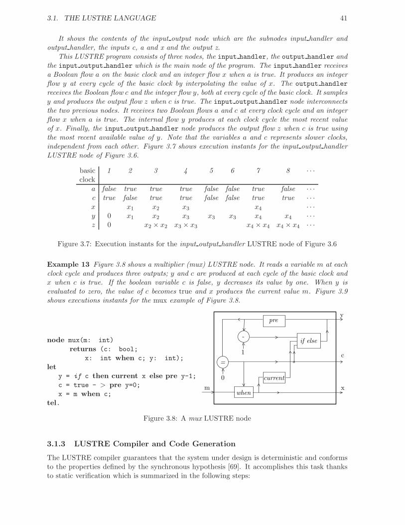
3.1. THE LUSTRE LANGUAGE 41

It shows the contents of the input output node which are the subnodes input handler andoutput handler, the inputs c, a and x and the output z.

This LUSTRE program consists of three nodes, the input handler, the output handler andthe input output handler which is the main node of the program. The input handler receivesa Boolean flow a on the basic clock and an integer flow x when a is true. It produces an integerflow y at every cycle of the basic clock by interpolating the value of x. The output handler

receives the Boolean flow c and the integer flow y, both at every cycle of the basic clock. It samplesy and produces the output flow z when c is true. The input output handler node interconnectsthe two previous nodes. It receives two Boolean flows a and c at every clock cycle and an integerflow x when a is true. The internal flow y produces at each clock cycle the most recent valueof x. Finally, the input output handler node produces the output flow z when c is true usingthe most recent available value of y. Note that the variables a and c represents slower clocks,independent from each other. Figure 3.7 shows execution instants for the input output handlerLUSTRE node of Figure 3.6.

basic 1 2 3 4 5 6 7 8 · · ·clock

a false true true true false false true false · · ·c true false true true false false true true · · ·x x1 x2 x3 x4 · · ·y 0 x1 x2 x3 x3 x3 x4 x4 · · ·z 0 x2 × x2 x3 × x3 x4 × x4 x4 × x4 · · ·

Figure 3.7: Execution instants for the input output handler LUSTRE node of Figure 3.6

Example 13 Figure 3.8 shows a multiplier (mux) LUSTRE node. It reads a variable m at eachclock cycle and produces three outputs; y and c are produced at each cycle of the basic clock andx when c is true. If the boolean variable c is false, y decreases its value by one. When y isevaluated to zero, the value of c becomes true and x produces the current value m. Figure 3.9shows executions instants for the mux example of Figure 3.8.

node mux(m: int)

returns (c: bool;

x: int when c; y: int);

lety = if c then current x else pre y-1;

c = true - > pre y=0;

x = m when c;

tel.

m x

c

y

if else

when

current

-

1

pre

0

=

Figure 3.8: A mux LUSTRE node

3.1.3 LUSTRE Compiler and Code Generation

The LUSTRE compiler guarantees that the system under design is deterministic and conformsto the properties defined by the synchronous hypothesis [69]. It accomplishes this task thanksto static verification which is summarized in the following steps:


basic clock 1 2 3 4 5 6 7 8 · · ·m 5 9 4 3 12 2 3 5 · · ·c true false false false false false true false · · ·

m when c 5 - - - - - 3 - · · ·y 5 4 3 2 1 0 3 2 · · ·

Figure 3.9: Instants of the execution for the mux example

• Definition checking: every local and output variable should have one and only one;

• Clock consistency: every operator is applied to operands on suitable clocks;

• Absence of cycles: any cycle should use at least one pre operator.

LUSTRE compiler provides two methods for generating code. The first method is the codegeneration for a mono-processor and mono-thread implementation. The compiler generatesmonolithic endless single loop C code. The body of this code implements the inputs to out-puts transformations at one clock cycle. The generation of C code is done in two steps:

1. introduce variables for implementing the memory needed by the pre operators and

2. sort the equations in order to respect data-dependencies.

The second method concerns the distributed implementation. LUSTRE programs can bedeployed on a distributed architecture via the object code (OC) automaton-format [31]. Thistechnique is closely related to the Kahn process networks. The distribution of an OC code isbased on the assumption that there exists a set {s1, ...sn} of execution sites (processors) and thateach of these sites is associated with an action of the OC automaton. For a LUSTRE program,each variable of the main node is assigned to an execution site. Propagating this assignmentinside internal nodes provides a site assignment for each variable in the expanded program. Thebasic idea of the method of the distribution for a LUSTRE program contains four steps:

1. The code of the automaton is replicated on each site;

2. On each replication, the instructions that do not concern the considered site are erased;

3. For any pair (si, sj) of sites, the order that si computes its own variables and the orderin which sj uses these variables is known. Thus, statements for communicating valuescomputed by si and used by sj can be introduced without introducing deadlocks;

4. Auxiliary “dummy” communications are added for synchronization.

3.2 SIGNAL

SIGNAL is a declarative synchronous language for real time programming [18, 51]. It relieson constructs which can be combined using a composition operator. These constructs describeprocesses and involve signals. A signal is an infinite typed sequence of data. The status of asignal can be either present or absent (denoted by ⊥). The data of a signal can be of a standardtype like boolean, real and integer or of a specific type like event type. An event signal x, withsyntax event x, is true if and only if x is present, otherwise is equal to ⊥.

3.2. SIGNAL 43

Each signal has an associated clock. Signals that are present simultaneously have the sameclock. Signals and clocks are related through equations. Equations are built on operators.Operators can be of two types, single-clocked and multi-clocked. Single-clocked operators involvesignals which have the same clock. Operators that involve signals with different clocks are multi-clocked operators. A process is defined by an equation or a composition of equations. Parallelcomposition of processes relates signals and their corresponding activation clocks.

The following sections present the basic relations on clocks and the SIGNAL operators.

3.2.1 Clock Relations

SIGNAL defines operations on clocks of signals. For signals x, y, some operations on clocks arepresented below:

• Clock of a signal: h := ∧x ≡ if x = ⊥ then ⊥ else true

• Clock selection: when b, it returns the clock that represents the implicit set of instants atwhich the signal b is true. It is denoted by [b].

• Synchronization: x ∧ = y, it means that the signals x and y have the same clock such that(|x ∧ = y|) = (|h := (∧x = ∧y)|)

• Clock product: x ∧∗y specifies the clock intersection of signals x and y such that (|x∧∗y|) =(|∧x when ∧y|)

• Clock union: x ∧ + y specifies the clock union of x and y iff x or y is present such that(|x ∧ + y|) = (|∧x default ∧y|)

• Clock order restriction: x ∧ < y specifies the restriction of x not to be more frequent thany such that (|x∧ < y|) = (|x∧ = x ∧ ∗ y|) =∧ x when event ∧y.

3.2.2 Single-clocked operators

Combinatorial

A combinatorial operator can be a classical arithmetic (+, -, /, *, ...) or logical (and, not,

<, >, ...) operator. It produces an output signal z computed on two input signals x and y. Acombinatorial operator, with syntax

z = x op y

defines a process such that zt 6= ⊥ ⇔ xt 6= ⊥ ⇔ yt 6= ⊥. The behavior of an operator, forinstance the + operator such that z = x + y is illustrated on the following table:

x : 2 5 1 0 4 1 3 7 · · ·y : 0 4 3 6 6 7 1 0 · · ·z : 2 9 4 6 10 8 4 0 · · ·

Delay

The delay operator defines a signal y whose tth element is the (t-1)th element of its input x. Atthe first instant, it takes an initialization value c. The delay operator, with syntax

y := x$1 init c

defines a process such that yt 6= ⊥ ⇔ xt 6= ⊥, ∀t > 0 : yt = xt−1, yo = c. The behavior of thedelay operator with initial condition c = 0 is illustrated in the following table:


x : 2 5 1 0 4 1 3 7 · · ·y : 0 2 5 1 0 4 1 3 · · ·

3.2.3 Multi-clocked operators

Under-sampling

The under-sampling operator delivers a signal y whenever the data input signal x and theboolean input signal b are present and b is true. The under-sampling, with syntax

y := x when b

defines a process such that yt = xt if bt = true else yt = ⊥. The behavior of the under-samplingoperator is illustrated in the following table:

x : 1 2 ⊥ 3 4 ⊥ 5 6 · · ·y : true false true false true false ⊥ false · · ·z : 1 ⊥ ⊥ ⊥ 4 ⊥ ⊥ ⊥ · · ·

Deterministic merging

The deterministic merging operator defines a signal z by merging two signals x and y withpriority to x when both processes are present simultaneously. The deterministic merging, withsyntax

z := x default y

defines a process such that zt = xt, if xt 6= ⊥, else zt = yt, if yt 6= ⊥. The behavior of thedefault operator is illustrated in the following table:

x : 1 2 ⊥ 3 4 ⊥ 5 ⊥ · · ·y : ⊥ ⊥ 3 4 10 8 9 2 · · ·z : 1 2 3 3 4 8 5 2 · · ·

3.2.4 Parallel Composition

For P and Q two processes, the composition of P and Q, written ( P | Q ), defines a new processwhere common names refer to common signals. Then the processes P and Q communicatethrough their common signals.

3.2.5 An example

The following example illustrates a SIGNAL program.

Example 14 Consider a program that reads an input IN , the value of which is decreased ateach step by one until it becomes ≤ 0. The syntax of this program is shown below:

( X := IN default ZX − 1| ZX := X$1 init 0| B := (ZX ≤ 0)| IN ∧ = when B| H ∧ = B ∧ = X ∧ = ZX)

The first equation says that X is equal to IN , if IN is present, otherwise it is equal toZX − 1. According to the third and fourth equations, IN is present when B, that is, when(ZX ≤ 0). If this condition does not hold, then the value of X is equal to it previous value,decreased by one. The last equations shows equality on the clocks of H,B,X and Z.

3.3. MATLAB/SIMULINK 45

3.3 MATLAB/Simulink

MATLAB/Simulink [2] is a very popular commercial tool for model-based design and simu-lation of dynamic embedded systems. Simulink systems are represented graphically using blocksand communication links for communication between blocks.

Example 15 Figure 3.10 shows a Simulink c© model. This is a model for the anti-lock breakingsystem of a car. It simulates the dynamic behavior of a vehicle under hard braking conditions.Blocks such as Weight, gain, Add, Saturation, Scope and Terminator are atomic Simulink blocksand are dedicated to perform some specific operations. The blocks WheelSpeed and RelativeSleepare subsystems, that is, they are constructed incrementally from atomic blocks and other subsys-tems. Communication links are directed arcs connecting outputs to inputs of different blocks.

Figure 3.10: Anti-Lock Braking (ABS) Simulink c© model

Simulink is widely used by engineers since it provides a wide variety of block libraries forimplementing and testing discrete and continuous system. It is also used for research andeducational purposes. Simulink offers a wide variety of simulation parameters, like simulationtime, solver options, tolerance and step size. In this section we restrict the description ofSimulink on discrete-time models of Simulink which can be simulated using “fixed-step solver insingle tasking mode”.

3.3.1 Signals

Models described in the discrete-time fragment of Simulink operate on discrete-time signals,that are, piecewise-constant functions defined on the time domain R≥0 and with values on anarbitrary data domain (usually, a fixed power set R

k).Simulink models define transformations on discrete-time signals by means of structured block

diagrams. These diagrams are constructed hierarchically from atomic blocks, defining elemen-tary transformations (e.g., delay, sampling, arithmetic, etc.), and dataflow links, expressinginstantaneous data communication.


Every signal s in a discrete-time Simulink model is characterized by its sample time, thatis, the period k > 0 of time at which the signal can change its value. Hence, a signal s canchange its value only at integer multiples1 of k, and remains unchanged within every left-closedright-open interval [n · k, (n + 1) · k[, for n ∈ N.

In Simulink models, the sample time of signals can be either explicitly provided by themodeler e.g., as an annotation to atomic blocks, or left unspecified. In the latter situation, thesample time is inherited, that means, inferred from the sample times of related signals usingSimulink specific inference rules.

3.3.2 Ports and Atomic Blocks

Data ports

Simulink uses inports and outports to define dataflow connection endpoints in subsystems. Theyare used to transfer signals between the subsystems and their environment. The sample time ofthe ports defines the period in which the signal is updated (i.e. read or written). The inportsand outports are graphically represented as shown in Figure 3.11.

Control ports

Simulink uses control ports to produce triggering events (trigger port) or to provide enabling con-ditions (enable port) for the execution of subsystems. Figure 3.11 shows the graphical notationfor the two types of control ports.

port port

In Out

Inport Outport Trigger Enable

Figure 3.11: Data ports and control ports in Simulink

A trigger port produces an event that activates the execution of a triggered subsystem de-pending on some condition on an incoming signal. In Simulink, this condition can be eitherrising, falling or both. For example, in case of rising the activation event is produced when theinput signal rises from a negative or zero value to a positive value.

An enable port defines a condition for the execution of an enabled subsystem depending on anincoming signal. In Simulink, the enabling condition holds as long as the value of the incomingsignal is greater than zero. The enable port specifies one of the two states when it executes afterbeing disabled, held or reset, depending if it holds the previous values of the subsystem or resetsto the initial conditions.

Example 16 Figure 3.12 shows the timing diagram of a signal. A rising trigger signal occursat time steps 2, 4 and 7. An enabling signal occurs between the time steps 4 and 6.

Sources and Sinks

Source blocks produce signals according to some patterns and with a specified or inheritedsample time. Some examples are the Pulse Generator, the Sine Wave, the Constant blocks (seefigure 3.13(a)).

1Simulink allows as well for an offset, however for the sake of simplicity we always consider the offset equal tozero.

3.3. MATLAB/SIMULINK 47

0

0 1 2 3 4 5 6 7

signal level

time

Figure 3.12: Timing diagram of a signal in Simulink

Conversely, sink blocks “consume” signals. Some examples are the Scope block which is usedto display graphically one or more input signals and the simout for writing signal data to theMATLAB workspace (see Figure 3.13(b)).

Combinatorial blocks

Combinatorial blocks combine one or more input signals and produce one (or more) outputsignal(s) as the result of an instantaneous operation. The sample times of all input and outputsignals are equal. Some examples of combinatorial blocks provided by Simulink are usual arith-metic operators, relational operators, Boolean operators, switches, saturation blocks, lookuptables (see Figure 3.13(c)).

Unit delay

A unit-delay block delays the input signal for one period of the (input) sample time. During thefirst period, the unit-delay produces a user-specified constant signal value. This block may alsoperform a sample time change between the input and the output signals as follows: the sampletime of the output can be smaller than (i.e., strict integer divisor of) the sample time of theinput signal (see Figure 3.13(d)).

Zero-order hold

A zero-order hold block acts as a sampler. It holds the output constant for one period ofthe (output) sample time with the latest value of the input. This block may also perform asample time change between input and output signals as follows: the sample time of the outputcan be greater than (i.e., strict integer multiple of) the sample time of the input signal (seeFigure 3.13(d)).

Transfer functions

A transfer function block transforms an input signal according to a given discrete-time transferfunction. The sample time of the input and output signals are equal (see Figure 3.13(e)).

3.3.3 Subsystems

Subsystems are user-defined assemblies constructed recursively from atomic blocks and othersubsystems. They are used to encapsulate some reusable functionality, that can be plugged (i.e.called) in a system model or other subsystems.

The communication between a subsystem and its calling environment is realized throughdata ports. Data ports are inside the subsystem, exported at its interface. They are used to


Constant

3

GeneratorPulse

(a) (d)

HoldZero-Order

Delay

1/z

Scope

(c)

Add

+

+

FunctionTransferz+0.5

(e)

1

(b)

Switch

Figure 3.13: Atomic blocks in Simulink

convey signals, produced outside (resp.inside), towards (resp. outwards) the subsystem.

Simulink does not impose any syntactical restrictions on the inner blocks of the subsystems.However, type checking and sample type checking rules are applied to ensure consistency ofcomputations e.g., the GCD rule for combinatorial operators [70]. The GCD (greatest commondivisor) rule states that the output of a block will have as sample time the GCD of the sampletimes of the inputs. For instance if the two inputs of an Add block have 4 and 9 sample timesrespectively, then the sample time of the output will be 1.

In addition, there exists some support for controlled execution of subsystems. Simulink offerstwo basic mechanisms: trigger conditions, that can be used to activate triggered subsystems forexecution and enabling conditions, that are used to enable/disable the execution of a subsystem.

Triggered Subsystems

Triggered subsystems execute instantaneously only when a trigger event occurs. Trigger eventsare defined as the rising or falling (or both) of a signal defined outside the subsystem.

Triggered subsystems do not have explicit sample time i.e., since their execution is triggeredby data-change events, it is not directly time dependent. Simulink requires that all blocks withintriggered subsystems have inherited sample time. Consequently, triggered subsystems containonly atomic blocks and triggered subsystems (not continuous time subsystems, not enabledsubsystems).

Example 17 Figure 3.14 illustrates a Simulink model which contains a Triggered Subsystem.

Figure 3.14: A Simulink model which contains a triggered subsystems

3.4. DISCUSSION 49

The Triggered Subsystem contains a Unit Delay block, an inport In1 and an outport Out1,it reads inputs from the Sine Wave block and sends outputs to the simout block To Workspace.The subsystem is activated by the “Trigger Signal”. When a trigger events occurs, the subsysteminstantaneously updates its input value In1 and writes its output Out1. The basic blocks SineWave, Trigger Signal and To Workspace have the same sample time TS = 25. The contentblocks of the Triggered Subsystem have inherited sample time.

The subsystem is triggered at the rising edge of the square wave trigger control signal asshown in Figure 3.15. That corresponds to the time units 50, 125,... All blocks outside theSubsystem are executed on the same rate, equal to 25 units of time.

0

time1007562.52512.5 37.5 50 87.5

Start of Executionfor a block

Sine Wave

Trigger Signal

Unit Delay

To Workspace

Figure 3.15: Execution time for blocks of the model 3.14

Enabled Subsystems

Enabled subsystems are time dependent. All the sample times are observed on a unique globaltime defined for the model, that means, execution is synchronized with respect to a global time.

The execution of enabled subsystems is constrained by the actual value of an external signal.That is, the subsystem (i.e. its inner blocks) executes only if the enabling signal has a positivevalue and stays unchanged otherwise.

Example 18 Figure 3.16 shows a Simulink example which contains an enabled Subsystem.Apart from the subsystem, it contains several atomic blocks such as the Sine Wave, the PulseGenerator, the Block A, the Block B and the Signal E that triggers the subsystem. The enabledsubsystem contains the block C, the block D, inports and outports. The block C and block Dinside the subsystem have sample times TS=12.5 and TS=25, respectively.

All blocks outside the “Subsystem” execute independently of the enabling signal E. When the“Signal E” becomes positive, the block C and the block D execute at their assigned sample ratesuntil the Signal E becomes again zero. Figure 3.17 shows the moment of execution for each blockof the model.

3.4 Discussion


Figure 3.16: A Simulink model which contains an enabled subsystem

0

time1007562.52512.5 37.5 50 87.5

Block A

Block B

block C

block DStart of Execution

for a block

Signal E

Figure 3.17: Execution time for blocks of the model 3.16

3.4. DISCUSSION 51

In this chapter we presented the LUSTRE language and the MATLAB/Simulink framework.LUSTRE is a synchronous languages with formal semantics developed at the VERIMAG labo-ratory for the past 25 years. On the top of the language, there is a number of tools, like codegenerator, model checker, tool for simulation of the system on design, etc., that constitute theLUSTRE platform. LUSTRE has been industrialized by Esterel Technologies in the SCADEtool. SCADE has been used from several companies in the area of aeronautics and automotive.It has been recently used for the development of the latest project of Airbus, the A380 carrierairplane.

MATLAB/Simulink is a commercial tool by MathWorks for modeling, simulating and an-alyzing dynamic systems. It offers a graphical interface and a wide variety of libraries thatallow designer to model, simulate and measure performances of its system. Simulink is widelyused in control theory, digital signal processing and Model-Based Design. Coupled with Real-Time Workshop by MathWorks, Simulink can automatically generate C code for given targetexecution platforms. Simulink has multitude of semantics which depend on user options forsimulations.

Later in this document, we will show transformations of LUSTRE and MATLAB/Simulinkto a component based framework dedicated for modeling synchronous systems. We demonstratethe transformations in several examples from LUSTRE and Simulink respectively.

Chapter 4

Modeling synchronous data-flowsystems in BIP

In this chapter we present Synchronous BIP, an extension of the BIP framework [12] for modelingsynchronous data-flow systems. Synchronous BIP components differ from general BIP compo-nents in two aspects. First, all atomic components are strongly synchronized under a globalsynchronization. This synchronization denotes the termination of a synchronous step duringwhich all components perform some computation. Second, the behavior of atomic componentsis specified by a subclass of priority Petri nets.

Figure 4.1 shows three Synchronous BIP components A,B and C which are strongly syn-chronized through the global synchronization gsync.

tick

A

C

B

g3

g4

g5

g1

g2

gtick

gsync

sync

sync

sync

Figure 4.1: A synchronous system described in terms of Synchronous BIP

We consider two models for describing the behavior of atomic components in SynchronousBIP:

• cyclic components: They are based on priority Petri nets extended with an implicit “sync”transition which denotes termination of a synchronous step.

• synchronous components: They are described by modal flow graphs that is, directed acyclicgraphs which represent implicitly the control flow for computation within a synchronousstep.

53

54 CHAPTER 4. MODELING SYNCHRONOUS DATA-FLOW SYSTEMS IN BIP

Cyclic components resulted from the direct translation of synchronous systems into generalBIP components. This model proved to be inappropriate since important safety propertieslike confluence and deadlock-freedom could not be guaranteed. Synchronous components wereintroduced in an attempt to describe the behavior of synchronous systems in BIP in such a waythat these safety properties can be proved at low cost.

This chapter is structured as follows. Cyclic BIP components and their composition arepresented in section 4.1. Section 4.2 presents the Synchronous BIP components defined usingmodal flow graphs. In these two sections, we define the semantics for both cyclic BIP componentsand synchronous BIP components.

Section 4.3 provides sufficient conditions for deadlock-freedom and confluence. The Syn-chronous BIP language is presented in section 4.4 and illustrated with examples. Section 4.5presents related work. We conclude and we present the main applications of Synchronous BIPfor modeling of synchronous systems in section 4.6.

4.1 Cyclic BIP Components

In this section we provide an initial model for describing synchronous systems in BIP, the cyclicBIP components. The behavior of a cyclic component is described by a priority safe-Petri netextended with an implicit sync transition which denotes the termination of a step.

4.1.1 Modeling Cyclic BIP Atomic Components

The transitions of this Petri-net are labeled with elements of a set of ports P and a priorityorder, a strict partial order ≺⊂ P ×P . Furthermore, transitions may be labeled with guards andfunctions representing data transformations. The Petri net has a set of initial and a set of finalplaces. When only no non-final places are marked, a step can terminate by executing the specifictransition labeled by sync. The sync transition is executed synchronously by all components.Termination of a step consists in removing the tokens from final places and putting a token ineach initial place. Implicitly, the priority order requires that sync has lower priority than anyother port to ensure maximal computation in a step. The formal definition for an atomic cyclicBIP component is given below:

Definition 12 (Cyclic BIP Component: Syntax) A cyclic BIP component B is a tuple(X,P,N,�) where:

• X is a set of data variables

• P is a set of ports p, each one labelled with a subset of variables Xp ⊆ X, the ones exportedon interactions through p.

• N = (L, T, F,L0, Lf ) is an extended 1-safe Petri net:

– L is a finite set of places;

– T is a finite set of transitions τ labelled by (pτ , guτ , fτ ) where:

∗ pτ is the port triggered by the transition τ ,

∗ guτ is the guard of τ , that is a predicate on X and

∗ fτ is the update function associated with the transition τ . As already defined in

Chapter 2, fτ = (f(x)τ )x∈X , that is, for every x ∈ X, it provides an arbitrary

expression on X defining the next (updated) value for x. We concretely representfτ as sequential programs operating on data X.

4.1. CYCLIC BIP COMPONENTS 55

– F ⊆ L × T ∪ T × L is the token flow relation,

– L0 ⊆ L is the set of initial places,

– Lf ⊆ L is the set of final places,

• ≺⊆ P × P is a priority order on ports, that is a strict partial order on the set of ports.

Note that the set of initial and final places can intersect, that is Lf ∩ L0 6= ∅.

Example 19 Figure 4.2 shows a cyclic BIP component that produces a tock every P ticks.Initial places are marked with a token; final places are grayed. At every step, it executes thetick transition and then, during the same step, it increases the local variable x by executing theupdate transition. Whenever x reaches the value P , the component can also execute the tocktransition and reset x to 0. In this situation, the tock and update transitions are conflicting,however, the associated priorities enforce the execution of tock before update if both transitionsare possible.

tock

final place

intermediate place

updatex:=x+1

tick[x=P]

x:int

update ≺ tock

tocktick

sync

x:=0initial place

Figure 4.2: The tick-tock cyclic BIP component

Definition 13 (Cyclic BIP Component: Semantics) The operational semantics of a cyclicBIP component B = (X,P,N,≺) with N = (L, T, F,L0, Lf ) is defined as the labelled transitionsystem S = (Q,Σ,−→) where

• Q = M ×DX is the set of states where M = {m : L → N} is the set of 1-safe markingsand DX = {v : X → D} is the set of valuations of variables,

• Σ = {(p, v, v′)} | p ∈ P, v ∈ DXp , v′ ∈ DXp} ∪ {sync} is the set of labels. A label (p, v, v′),as already defined in Chapter 2, marks instantaneous data change through the port p. Thecurrent valuation v is sent and a new valuation v′ is received for the set of variables Xp.We note a label (p, v, v′) as p(v/v′).

• −→⊆ Q × Σ × Q is the set of transitions defined by the rules below:

Rule 1:

control dataτ ∈ T m ∈ M,m′ ∈ M v ∈ DX , v′ ∈ DX

labeled by •τ ≤ m guτ (v) = true (read v) guard(pτ , guτ , fτ ) m′ = m − •τ + τ• v′ = fτ (v) (write v′) action


(m, v)pτ (v/v′)−−−−−→0 (m′, v′)

Rule 2:

control datam ≤ mLf

guard

m′ = mL0v′ = v action

(m, v)sync−−−→0 (m′, v′)

Rule 3:

(m, v)pτ (v/v′)−−−−−→0 (m′, v′)

¬(∃p′.pτ ≺ p′ ∧ (m, v)p′−→0)

(m, v)pτ (v/v′)−−−−−→ (m′, v′)

Rule 4:

(m, v)sync−−−→0 (m′, v′)

¬(∃pτ .(m, v)pτ (v/v′)−−−−−→0)

(m, v)sync−−−→ (m′, v′)

Rule 1 and Rule 2 define moves −→0 of the behavior without priorities. Rule 1 is theusual firing rule of transitions in Petri nets extended with global data. Rule 2 defines synctransitions which denote the end of a step and the beginning of the next one. sync transitionscan be executed whenever the current marking does not contain tokens in non-final places, andtheir effect is to restore the initial marking, while keeping the data unchanged. Rule 3 andRule 4 define the moves −→ of a synchronous component, by restricting −→0 with respect topriorities. Rule 3 is simply the application of the priority rule specified by the priority order≺. Rule 4 ensures that the sync transition is executed only if no other transition can.

Let us note that the rules R1 and R3 correspond to the standard BIP semantics, whereasrule R2 defines the implicit sync step and R4 gives the priority order in case of conflict betweenthe sync and any other transition.

4.1.2 Composition of Cyclic BIP Atomic Components

We define composition parametrized by interactions as an operation of cyclic components. Thisoperation is partial: the result of the composition is defined as a cyclic component only if thepriority order associated to it is acyclic. An interaction is interpreted as in Definition 8 ofChapter 2.

Definition 14 (Composition of Cyclic BIP Components: Semantics) Let a set of cycliccomponents {Bi = (Xi, Pi, Ni,≺i)}i=1,n defined on disjoint sets of variables and ports. Let γ bea set of interactions on ports ∪n

i=1Pi such that each interaction uses at most one port of everycomponent, that is for all a ∈ γ, for all i ∈ 1, n, |a ∩Pi| ≤ 1. The composition γ(B1, ..., Bn) is apartial operation defining the cyclic component B = (X,P,N,≺) where

• the set of variables is X = ∪ni=1Xi,

4.1. CYCLIC BIP COMPONENTS 57

• the set of ports P is the set of interactions γ. Moreover, for each interaction a ∈ γ, andfor Xp the set of exported variables for each port p, the set of its exported variables isXa = ∪p∈aXp,

• the Petri net N = (L, T, F,L0, Lf ) is obtained from the set of the Petri nets {Ni =(Li, Ti, Fi, L0i, Lfi

)}i=1,n as follows:

– the set of places L = ∪ni=1Li,

– the set of transitions T corresponds to sets of interacting transitions

T =

{

〈a, {τi}i∈I〉a ∈ γ, I ⊆ 1, n such that∀i ∈ I.τi ∈ Ti ∧ Pa ={pτi

}i∈I

}

Each transition τ is labeled by (pτ , guτ , fτ ) where:

∗ pτ is the interaction a

∗ guτ = ∧ni=1guτi

∧ Ga is the guard and it is a predicate on the set of variables X.guτi

is the guard of the transition τi and Ga the guard of the interaction a.

∗ fτ = Fa; (⊔ni=1fτi

) is the data transfer function. It consists of the interactionfunction Fa, followed by local functions fτi

in arbitrary order (the order of com-putation is irrelevant as the data of the components are disjoint).

– the token flow relation F of the net is defined as

F = {(l, 〈a, {τi}i∈I〉) | (∃j ∈ I, l ∈ •τj)} ∪{

(〈a, {τi}i∈I〉, l) | (∃j ∈ I, l ∈ τ•j )

}

– the set of initial places L0 is ∪ni=1L0i,

– the set of final places Lf is ∪ni=1Lfi

,

• the relation ≺ is the strict transitive closure of the relation ≺0 defined as the extension ofindividual priority orders ≺i to interactions: a1 ≺0 a2 iff ∃i ∈ 1, n. ∃pi1 ∈ Pa1

∩ Pi. ∃pi2 ∈Pa2

∩ Pi such that pi1 ≺i pi2. The composition is defined only if this relation is a strictpartial order.

Example 20 Composition of two cyclic components is illustrated in Figure 4.3. Two tick-tock components are composed through the interactions γtoT i and γsync. The interaction γtoT i

synchronizes the tock of the left component and the tick2 of the right one. The γsync interactionsynchronizes strongly the sync ports of both components.

The resulting component is shown in Figure 4.4. The transition tock1tock2 corresponds tothe interaction γtoT i. Guards and update functions are inherited from the atomic components.The composed component produces a tock2 every P1 × P2 ticks.

An essential property of synchronous systems is termination of steps, in particular stepsmust be deadlock-free. Another requirement is confluence of computation within a step whichmeans that the overall behavior is deterministic when system states are observed only at theend of each step. For some synchronous languages e.g. Lustre, these properties can be ensuredby checking very simple sufficient conditions [43]. Proving these properties using automata andstandard Petri nets is hard. For that, we define the class of modal flow components wherepriority Petri nets are replaced by modal flow graphs. These graphs correspond to a subclass ofpriority Petri nets where arbitrary control flow is restricted to an acyclic graph of dependenciesbetween ports. For modal flow graphs, deadlock-freedom and confluence can be decided at


x2: int

tick2

syncsync

γsync

tock2tock1

priority: update1 ≺1 tock1 priority: update2 ≺2 tock2

x1: int

tick1

update1

x1:=x1+1

tock1

[x1=P1]x1:=0

tick1

γtoTi

[x2=P2]tock2

x2:=0

update2

tick2

x2:=x2+1

Figure 4.3: Example of composition of cyclic BIP components

x2:=0

update2 ≺ tock2

sync

tock2tick1

x2: int

x1: int

[x2=P2]

priority: update1 ≺ tock1tick2

tick1

update1

[x1 = P ]

x1 := 0

update2

tock1tick2

x2 := x2 + 1x1 := x1 + 1

tock2

Figure 4.4: The resulted components from the composition of the cyclic BIP components ofFigure 4.3

4.2. SYNCHRONOUS BIP COMPONENTS 59

low cost. The causality relation between events is expressed explicitly through three types ofdependencies. These dependencies exhibit a part of all possible combinations between a pairof events. These are the sufficient combinations needed for describing the behavior of somesynchronous formalisms like Lustre.

4.2 Synchronous BIP Components

A Synchronous BIP model consists of synchronous BIP components which are strongly synchro-nized through implicit synchronizations. The behavior of atomic components is described asmodal flow graphs.

For a given set of ports P , a modal flow graph is a directed acyclic graph with nodes P andedges representing the union of three binary relations. Each relation expresses a different kindof causal dependency (modality) between pairs of ports p and q within a step:

• q strongly depends on p if the execution of p must be followed by the execution of q. Thatis, p and q cannot be executed independently, only the sequence pq is possible.

• q weakly depends on p if the execution of p may be followed by q. That is either p can beexecuted alone or the sequence pq.

• q conditionally depends on p if when both p and q are executed, then q must follow p.Conditional dependency requires that if p and q occur together, then only the sequence pqis possible; otherwise or p or q may be independently executed.

Figure 4.5 illustrates the graphical notation used for the three dependencies as well as theirpossible executions in a synchronous step.

q

strong

Dependency Graphical Representation

p q

conditional

weak

ExecutionInterpretation

pq

p, q, pq

p, pqp

p q q never precedes p

q may follow p

q must follow p

Figure 4.5: The three causal dependencies and the possible executions in a synchronous step

4.2.1 Modeling Synchronous BIP Atomic Components

A BIP component that describes the behavior of a synchronous system in terms of modal flowgraphs is called Synchronous BIP components. A formal definition for a Synchronous BIPcomponent is given below.


Definition 15 (Synchronous BIP Component: Syntax) A Synchronous BIP componentBf is defined as a tuple (X,P,D):

• X is a set of data variables,

• P is a set of ports p, each one being associated with a triple (Xp, gup, fp) where

– Xp ⊆ X, the set of variables exported through p,

– gup, the triggering condition of p, that is a predicate defined on X,

– fp, an update function, that is a state transformer function on X. As already men-

tioned, fp = (f(x)p )x∈X , that is, for every x ∈ X, it provides an arbitrary expression on

X defining the next (updated) value for x. We concretely represent fp as sequentialprograms operating on data X.

• D = (Ds,Dw,Dc) is a triple of causal dependency relations between ports. The relationsDs,Dw,Dc ⊆ P ×P denote respectively strong, weak and conditional dependency and aresuch that their union Ds ∪ Dw ∪ Dc is acyclic.

Example 21 Figure 4.6 represents as a Synchronous BIP component, the tick-tock cyclic BIPcomponent of Figure 4.2.

The port tock is weakly dependent on the tick port. Also, the update port is strongly depen-dent on tick and conditionally dependent on tock. Each time that the port update is executed,the value of x is increased by one. The only possible executions within a step are therefore (tickupdate) or (tick tock update) whenever x reaches P .

tickx:=0[x=P]tock

update

tocktick

x

x:=x+1

Figure 4.6: Tick-tock Synchronous BIP component

We use the following notation. For fixed x = s,w, c, we write px q to denote (p, q) ∈ Dx.

We writex

∗ to denote the reflexive and transitive closure ofx . We write p q to denote

(p, q) ∈ Ds ∪ Dw ∪ Dc and ∗ for its reflexive and transitive closure. Two ports p and q are

called independent (noted p♯q) iff neither p ∗ q nor q ∗ p.For fixed x = s,w, c, we denote by minx P the set of minimal ports with respect to Dx, that

is minx P = {q | ¬∃p.px q}. We write min P to denote the set of minimal ports with respect

to Ds ∪ Dw ∪ Dc, that is min P = {q | ¬∃p.p q}.

4.2.2 Well-triggered Modal Flow Graphs

We introduce now the notion of well-triggered modal flow graphs. This notion ensures consis-tency, between the three types of dependencies, defined by the following constraints:


1. each port p has a unique minimal strong cause

|{q ∈ mins P | qs

∗ p}| = 1

2. each port p has exclusively either strong or weak causes.

In a well-triggered modal flow graph, for a port p, we denote its minimal strong cause by root(p).By describing well-triggered modal flow graphs, we provide syntactical restrictions that ex-

clude deadlock situations that may occur within a step. Some examples are illustrated in Fig-ure 4.8. For Figure 4.8(a), if the strong cause q1 is executed but not the strong cause q2, then wewill reach a situation where the execution at p is disabled and the component cannot progressto reach the sync. Similar is the situation in Figure 4.8(b), where the graph reaches a deadlocksituation if port q1 is executed but not q2 and consequently p stays disabled. However, the graphof Figure 4.8(c) will never reach a deadlock situation since a conditional dependency never blocksthe execution. If port q2 is executed but not q1, the conditional dependency allows port p to beexecuted.

For the sequel, we consider only well-triggered modal flow graphs. As we will show in Sec-tion 4.3, for this type of modal flow graphs we provide simple conditions that ensure deadlock-freedom and confluence. Moreover, for some synchronous languages like LUSTRE (see Chap-ter 5), well-triggered modal flow graphs are enough to describe their operators.

Well-triggered modal flow graphs can be decomposed as shown in Figure 4.7.

Figure 4.7: Well-triggered components

The strong dependency relation defines a set of connected subgraphs involving all the portsof the component. Each one of these subgraphs has a single root which is the common causefor its ports. Weak dependencies express triggering of the root of a subgraph by some portof another subgraph. Finally, conditional dependencies may relate ports of different subgraphsprovided the acyclicity property is not violated.

We define the semantics of synchronous components which are well-triggered in terms ofcyclic BIP components.

Definition 16 (Synchronous BIP Component: Semantics) The operational semantics ofa well-triggered synchronous component Bf = (X,P,D) is a cyclic component B = (X,P,N,≺):

• the set of variables is X,

• the set of ports is P ; moreover, for each port p the associated set of exported variables isXp,


(c)

q1 q2

p

q1 q2

p

q1 q2

p

(a) (b)

Figure 4.8: Examples of modal flow graphs, non well-triggered (a) and (b) and well-triggered(c)

• the Petri net N = (L, T, F,L0, Lf ) is defined by:

– the set of places L is isomorphic to the set Ds ∪ Dw ∪ Dc augmented with the set ofminimal ports. That is L = {lxp,q | p

x q} ∪ {lp | p ∈ min P},

– the set of transitions T is isomorphic to the set of ports P , that is T = {τp |p ∈ P}.Moreover, for any transition τp we define the triple (pτ , gτp , fτp), where:

∗ pτ is the associated port

∗ gτp is the guard of τp and it is a predicate on X

∗ fp is the update function. As already defined in Definition 15, fτp = (f(x)τp )x∈X ,

that is, for every x ∈ X, it provides an arbitrary expression on X defining thenext (updated) value for x. We concretely represent fτp as sequential programsoperating on data X,

– the token flow relation F ⊆ L × T ∪ T × L, is constructed as follows:

∗ for each p ∈ min P add (lp, τp) to F ,

∗ for each dependency px q add (τp, l

xp,q), (l

xp,q, τq) to F ,

∗ for each conditional dependency pc q add (lcp,q, τroot(p)) to F . This relation

implies that execution of q disables further execution of the root(p), in the samestep,

– the set of initial places L0 corresponds to minimal ports and conditional dependenciesthat is L0 = {lp | p ∈ minP} ∪ {lcp,q | p

c q},

– the set of final places Lf consists of all places corresponding to all but strong depen-

dencies Lf = L \ {lsp,q | ps q}.

• the priority order ≺= ( ∗)−1 \ Id, that is p ≺ q iff q ∗ p and q 6= p, for all p, q ∈ P .

The Petri nets representing Synchronous BIP components satisfy the following trivial prop-erties: 1) every place has at most one incoming transition, 2) every place lcp,q corresponding toa conditional dependency belongs to a cycle, 3) initially, there is precisely one token in everycycle of the net.

The mapping of modal flow graphs to Petri nets is done by associating with each port atransition of the Petri net and the dependencies transformed as shown in Figure 4.9. ThesePetri nets represent valid execution for one synchronous step. Termination of a step consistsin removing the tokens from final places and putting a token in each initial place. Guards andupdate functions are inherited from ports to the corresponding transitions.

Notice that the above construction rules of the Petri net enforce the three kinds of depen-dencies between ports. Strong and weak dependencies are obviously enforced by the net. An


strong

Dependency Graphical Representation

p q

conditional

weak p

p q

q

Petri Net Representation

τq ≺ τp

[gp]

[gp]

fp

[gq]

fq

fq

fp

[gq][gp]

fp

τp

[gp]fp

τq

τq[gq]fq

τq

[gq]

τp

[gp]

fp

τp

[gp]fp fq

Figure 4.9: The correspondence of causal dependencies in Petri nets

initial empty place lp,q between τp and τq will prevent the execution of τq before τp. Moreover,if the place is not final, the execution of τp will require the execution of τq before the end of the

step. Concerning conditional dependencies pc q, the Petri net ensures that the execution of τq

disables any further execution of τroot(p) and consequently of τp. For the conditional dependencyof Figure 4.9, root(p) = p.

Example 22 The tick-tock synchronous component shown in Figure 4.10 (right), is well-triggered.Its semantics is defined by the tick-tock cyclic component in Figure 4.10 (left). As explained inExample 19), due to initial marking, in one step, transition tick can be executed followed bythe execution of the transition update, increasing x by one. Whenever x reaches P , both transi-tions update and tock can be executed. This conflict is resolved and in the same time, maximalcomputation is ensured using the priority update ≺ tock that enforces execution of tock beforeupdate.

Notice that guards and update functions in ports of the synchronous components are inheritedfrom the transitions of the cyclic component.

The next result gathers some additional properties.

Proposition 1 Priority Petri nets representing modal flow graphs meet the following proper-ties

1. Every reachable marking has at most one token in every cycle of the net.

2. Each transition is executed at most once in every step.

3. Are 1-safe.

Proof.

1. This property is an inductive invariant on the set of reachable markings and holds becauseeach place in a cycle has a unique incoming transition – that is any attempt to put a tokeninto a cycle will first remove a token from the same cycle.


tickx:=0[x=P]tock

update

x:int

tick tock

x:=x+1updatex:=x+1

tick[x=P]

x:int

update ≺ tock

tocktick

sync

x:=0

tock

Figure 4.10: The Tick-tock synchronous component (right) and its semantics (left)

2. Minimal ports p can only be executed at most once since they will remove the token inthe corresponding initial place lp. For any other port p, we consider that all his directpreceding ports q are executed at most once. If q is related to p through a strong or weakdependency, by construction, p is executed at most once. If q is related to p through aconditional dependency, the place lq,p has initially a token and belongs to a cycle of thenet. By executing p, the cycle containing lq,p becomes empty and will remain empty inany further execution of the net;

3. Given the previous result, it follows that every place will receive a token at most once. Soevery place may have at most one token, if it is initially empty, or two tokens, if it containsinitially a token. However, places that contain initially tokens belong to cycles and cyclescontain at most one token globally. So the net is 1-safe.

�

4.2.3 Composition of Synchronous BIP Atomic Components

We lift composition of cyclic BIP components to Synchronous BIP components, as follows.

Definition 17 (Composition of Synchronous BIP Components: Semantics) Let {Bfi =

(Xi, Pi,Di)}i=1,n be a set of synchronous components defined on disjoint sets of variables andports. That is, for variables Xi,Xj and ports Pi, Pj it holds Xi ∩ Xj = ∅ and Pi ∩ Pj = ∅. Letγ be a set of interactions on ports ∪n

i=1Pi such that

• each interaction uses at most one port of every component, that is for all a ∈ γ, for alli ∈ 1, n |a ∩ Pi| ≤ 1,

• each port belongs to at most one interaction, that is for all p ∈ ∪ni=1Pi |{a | p ∈ Pa}| ≤ 1,

We define the composition γ(Bf1 , ..., Bf

n) as the modal flow component Bf = (X,P,D) where

• the set of variables X is ∪ni=1Xi,

• the set of ports P is the set of interactions γ. Moreover, for every interaction a of γ, wedefine the tuple (Xa, ga, fa), where:

– Xa is the set of exported variables such that Xa = ∪p∈PaXp and Xp the set of variablesexported at the port p,


– ga is the guard such that ga = (∧p∈Pagp) ∧ Ga, a predicate on X

– fa is the data transfer function such that fa = Fa; (⊔p∈Pafp). where ⊔ defines parallelcomposition. Figure 4.11 depicts the composition of ports with guards and transferfunctions.

=pk

[gk]

fk...p1

[g1]

f1

Fa

composition [g1 ∧ ... ∧ gk ∧ Ga]

Fa; f1; ...; fk

[Ga]

pkp1 ...

Figure 4.11: Composition of ports

• the set of dependencies D = (Ds,Dw,Dc) are inherited from atomic components, thatis for every x = s,w, c we have Dx = {(a1, a2) | ∃i ∈ 1, n.∃p1 ∈ Pa1

∩ Pi, p2 ∈ Pa2∩

Pi such that (p1, p2) ∈ Dxi}

Notice that composition amounts to merging nodes belonging to the same interaction withoutchanging the dependency relations. Composition is a partial operation because, its result is avalid synchronous component only if the set of derived dependencies is acyclic.

Example 23 The composition of two Synchronous BIP components is illustrated in Figure 4.12.

x2: int

tick1

update1

tock1

x1:=0[x1=P1]

x1:=x1+1

tick2

update2

tock2

x2:=x2+1

tick1 tock1 tock2

[x2=P2]

tick2

x2:=0

gtoctic

sec min

gs2gs1

x1: int

Figure 4.12: Example of composition of Synchronous BIP atomic components

Two tick-tock components sec and min respectively are composed by synchronizing the tockof the first component and the tick of the second one through the control flow interaction γtoT i.

Figure 4.13 illustrates the produced component from the composition of the two atomic com-ponents sec and min. The resulting component produces a tock2 every P2 tock1.

Let us observe that the result from the composition of Synchronous BIP components is notthe same operation as composition of cyclic BIP components. These differ because conditionaldependencies do not have a local interpretation e.g. p

c q implies that execution of transition

q disables further execution root(p). But, the minimal strong cause root(p) of p can denotedifferent actions within the Synchronous BIP component and the composed Synchronous BIPcomponent.

Example 24 This example validates the previous observation. Figure 4.14 (a) shows two Syn-chronous BIP components strongly synchronized through the interaction γ. The interactionconnects the ports q and r and it is associated with the data-transfer function y := x.


update1

tick1tock1tick2

update2

x2: intx1: int

[x1 = P1]x1 := 0

x1 := x1 + 1 x2 := x2 + 1

tock2

x2 := 0[x2 = P2]

tick1 tock2

gs2gs1

Clock

Figure 4.13: The produced component from the synchronization of the composition of atomiccomponents shown in figure 4.12

The resulted composed component is shown in Figure 4.14 (b). Ports q and r are composedto a single port which executes the associated functions each time this port is triggered. Thebehavior of the execution of the composed component is illustrated on the following table:

x : 0 1 2 3 4 5 6 7 · · ·y : − 0 2 4 6 8 10 12 · · ·

This component is transformed to cyclic BIP component as shown in Figure 4.14 (c). Forcomponents of Figures 4.14 (b), (c), the possible executions are in one step either s or p, qr, s.

(b) (c)(a)

s

rx:=x + 1 y:=2 ∗ y

r

x=0

γ, y:=x

sp q

x=0s

x:=x + 1x:=x + 1

qr

x=0

sp s pqr

q

p

qr

p

y:=x

y:=2 ∗ y

y:=x

y:=2 ∗ y

p

qr

s

Figure 4.14: (a)Two Synchronous BIP components strongly synchronized through the interac-tion γ, (b) the component obtained by the composition of the two Synchronous BIP components,(c) the cyclic BIP component corresponding to the composed Synchronous BIP component

Figure 4.15 (a) is the translation of Figure 4.14 (a) into cyclic BIP components. Figure 4.15(b) shows the resulted cyclic BIP component obtained by the composition of the two components

4.3. STRUCTURAL PROPERTIES OF SYNCHRONOUS BIP COMPONENTS 67

of Figure 4.15 (a). A simplification of this component is shown in Figure 4.15 (c). The possibleexecutions are either p, qr, s or s, p, qr.

(b)(a) (c)

qrr

x=0

γ, y:=x

sp q

x=0

x:=x + 1q

p

s

r

p

x:=x + 1

psqr

x=0

s

x:=x + 1y:=2 ∗ y

y:=x

y:=2 ∗ y

s

qr

p

y:=x

y:=2 ∗ y

s

qr

p

Figure 4.15: (a) The cyclic BIP components corresponding to the Synchronous BIP compo-nents of Figure 4.14 strongly synchronized through the interaction γ, (b) the Synchronous BIPcompound component obtained by the composition of the two cyclic BIP components, (c) asimplified form for the Petri net of the compound component

We observe that the executions of the composed cyclic BIP component and the SynchronousBIP component are not identical. The cyclic BIP component produces the execution s, p, qrwhich does not correspond to the desirable behavior. If both s and r appear in the same step thens must be executed before r.

4.3 Structural Properties of Synchronous BIP Components

In this section we will give the main results of the Synchronous BIP components. Syn-chronous BIP components can be proved deadlock-free and confluent (i.e.,deterministic) bychecking syntactic conditions. These conditions are formally stated by theorems below. Westart by giving concrete definitions about deadlock-freedom and confluence.

Definition 18 A modal flow graph is deadlock-free if all tokens have been removed from non-final places or equivalently when the set P0 = {q | ∃p · p

s q and lsp,q has a token} is empty.

Theorem 1 (Deadlock-freedom) A well-triggered Synchronous BIP component Bf = (X,P,D)is deadlock-free if every port p with strong causes has its guard true that means gp = true.

Proof. First situation, if no strong dependencies exist, all places in the Petri net are finaltherefore the sync transition is always enabled. Consequently, no deadlock is possible.

Second situation, if there exist strong dependencies, a deadlock potentially occurs only whenthe sync transition is not enabled. This happens only when there are non-final places containing


tokens or equivalently when the set

P0 = {q | ∃p · ps q and lsp,q has a token} is not empty. Let now define the set P1 to be

P1 = {r | ∃q ∈ P0 · qs

∗ r} the set of ports that are transitively strongly dependent on ports

in P0. Obviously, we have P0 ⊆ P1. Intuitively, the set P1 contains all the ports which havestrong dependencies and which remain to be executed in the current step.

Choose r0 ∈ P1, an arbitrary minimal element of P1. We will show that r0 is enabled andtherefore, the is no deadlock. First, rO is a port with strong dependencies. From the hypothesisof the theorem, we know that its guard is true, therefore whether it is enabled or not dependsonly on the control (i.e., the markings of the net) and not on data. By contradiction, assumethat there are missing tokens in one of the previous places lxu,rO

of r0. Since the component iswell-triggered, we distinguish two cases, depending on the dependency x:

1. x = s, the place lsu,r0comes from a strong dependency. First, if there is no token in lsu,r0

it follows that u has not been executed within a step. Second, since the component iswell-triggered, we have root(u) = root(r0). Third, r0 ∈ P1 implies that root(r0) has beenalready executed within the step. Consequently, we have also u ∈ P1, that is u remains tobe executed in the current step. Since we have u

s r0, this contradicts the minimality of

r0 in P1.

2. x = c, the place lcu,r0comes from a conditional dependency. If there is no token in lcu,r0

,it means that the token has been consumed for the firing of root(u) and not yet produced

by u. Hence u belongs to the set P1 and we have uc r0. Again, this contradicts the

minimality of r0 in P1.

�

A modal flow graph is confluent if it has deterministic behavior. That is, it always has thesame output independently of the order of execution of conflicted ports. A formal definition fora confluent modal flow graph is given below:

Definition 19 A modal flow graph is confluent iff for each state (m, v) such that (m, v) −→∗

(m1, v1) and (m, v) −→∗ (m2, v2) then (m1, v1) = (m2, v2).

Theorem 2 (Confluence) A well-triggered Synchronous BIP component Bf = (X,P,D) isconfluent if for every pair of independent ports p1♯p2, their associated guarded actions are inde-pendent, that is:

• Xp1∩ Xp2

= ∅

• use(gp1) ∩ (Xp2

∪ def(fp2)) = ∅

• use(gp2) ∩ (Xp1

∪ def(fp1)) = ∅

Proof. Whenever there is a choice between executing two ports p1 and p2 after applyingpriorities, it follows that p1 and p2 are independent. That is, by definition, priorities selectenabled ports which are minimal with respect to ∗ to be executed - if two or more suchports exist, it follows that they are incomparable with respect to ∗ and hence independent.Moreover, the hypothesis ensures that execution of such independent ports commute.

We will show that the execution within a whole step is confluent. By contradiction, andwithout loss of generality assume that there exist two distinct terminal states (m1, u1), (m2, u2)reachable from the same initial state (m0, u0). By terminal state we mean either a deadlockconfiguration or a state from which only the sync transition is possible.

4.4. THE SYNCHRONOUS BIP LANGUAGE 69

Consider the graph of all possible executions from (m0, v0) within one step. Let us remarkthat this graph is finite and acyclic – since by construction we know that every port can beexecuted at most once within one step. On this graph, let us define the following subsets ofstates:

X1 = {(m, v) | (m, v) −→∗ (m1, v1) and ¬(m, v) −→∗ (m2, v2)}X2 = {(m, v) | (m, v) −→∗ (m2, v2) and ¬(m, v) −→∗ (m1, v1)}

Intuitively, X1 (resp. X2) contains the states that lead eventually to the terminal state(m1, v1) (resp. (m2, v2)). Obviously, we have X1 ∩X2 = ∅. Moreover, we can prove that X1 andX2 are a partition of all the reachable states from (m0, v0). By contradiction, assume there arestates which are neither in X1 or X2. Among them, we can choose one state (m, v) which hasall successors in X1 union X2 – because we consider that there are precisely two terminal states.Now, if (m, v) has all successors in X1 then it will eventually lead to (m1, v1), so it belongsto X1 – contradiction. The dual reasoning applies when (m, v) has all successors in X2. Theonly remaining possibility is that (m, v) has distinct successors into X1 and X2 respectively. So,

let assume that (m, v)p1−→ (m′

1, v′1) such that (m′

1, v′1) ∈ X1 and (m, v)

p2−→ (m′

2, v′2) such that

(m′2, v

′2) ∈ X2. But, transitions p1 and p2 interleave - hence there exists (m′

12, v′12) such that

(m′1, v

′1)

p2−→ (m′

12, v′12) and (m′

2, v′2)

p1−→ (m′

12, v′12). This implies (m′

12, v′12) belongs to both X1

and X2, which is impossible because X1 ∩ X2 = ∅.Finally, since X1 and X2 define a partition of the reachable states from (m0, v0) in one step,

we obtain the contradiction: the state (m0, v0) belongs to either X1 or X2 so, it cannot lead toboth terminal states (m1, v1) and (m2, v2).

�

4.4 The Synchronous BIP Language

We implement the Synchronous BIP components using the Synchronous BIP language whichis an extension of the BIP language. The Synchronous BIP language (S-BIP) provides constructsfor describing synchronous systems conforming to the formal framework as described up to now.The new constructs that S-BIP adds to the BIP language are described below:

• modal type: It specifies the behavior of an atomic component. For Synchronous BIPcomponents, behavior is described by modal flow graphs (MFGs). MFGs are described byports and dependencies between ports.

• dependency type: It specifies the dependency that relates ports and specify causal orderbetween them. Dependencies can be of the following types: conditional, weak or strong.

A modal type is characterized by its ports and its dependencies. The syntax of a modal typeis given below:

<modal type> ::= modal type <modal name><variable definition><port definition><dependency definition>

endVariables are declared as data objects and they are typed, as in C language. They may have

initial values. Ports are instances of port types, i.e. ports associated with typed variables. Fora dependency, the definition is given below:


<dependency definition> ::= on < port name>(<dependency type> (<port name>)∗)∗

(provided <expression>)? (do <expression>)?

A dependency is defined on a port name following the keyword on. The cause that triggersthis port is given by the port name following the construct <dependency type>. The guard of theport is specified after the provided keyword and the action statement of the port is specifiedfollowing the do.

The syntax for the dependency type is given below:

<dependency type> ::= <= | < − | < −−

Dependency can be of type strong (<=), weak (< −) or conditional (< −−).

Example 25 The S-BIP description of the synchronous component tick-tock of Figure 4.10 isillustrated below:

modal type TickTock

export port DataPort update(x)=update

export port DataPort tock(x)=tock

export port EventPort tick = tick

on tick

on tock <- tick provided x=60

do x=0;

on update <= tick < −− tock

do x=x+1;

end

Ports update, tock and tick are exported at the interface of the component. The order ofexecution of the ports is defined by the dependencies and the associated guards. The executionof the component begins from tick, since its execution is not dependent on any other port.

The composition of two tickTock synchronous atomic components shown in Figure 4.12, isdescribed in S-BIP as follows. The S-BIP description of this compound component is shownbelow:

compound type Clock

component TickTock sec

component TickTock min

connector BroadcastData gtoctic(sec.tock1, min.tick2)

connector SingletonEvent gs1(sec.tick1)

connector SingletonEvent gs2(min.tock2)

export port DataPort tick1 is gs1.tick1

export port DataPort tock2 is gs2.tock2

end

component Clock clk

4.5. RELATED WORK 71

end

The compound component Clock is defined by two instances of component type tickTock, secand min respectively. The components are composed via the connector BroadcastData whichconnects two ports of type EventPort. The singleton connectors singleTick and singleTock exportthe involved ports at the border of the compound component.

4.5 Related Work

The work we presented in this chapter is related to approaches with similar objectives. In the42 framework [55] steps are described by using automata with final states. Another similarityis the distinction between data ports and control ports. Nonetheless, the latter are activatedby controllers which are specific components. The synchronous/reactive domain of the Ptolemysystem-level design framework [38] allows component-based description of synchronous systemswhere synchronous execution is orchestrated by a director. Finally, our work has the samegeneral objectives as [17] which studies a compositional framework for heterogeneous reactivesystems. In contrast to BIP, the framework is denotational and is based on the concept of tagsmarking the events of the signals of a system.

There are several differences between our work and existing results. Our work is based onoperational semantics. It considers synchronous component-based systems as a particular caseof the BIP framework which also encompasses general asynchronous computation. As we willshow in the next chapter, our framework is expressive enough to allow modular translation ofsynchronous languages into BIP by preserving the structure of the source.

Modal flow graphs without data and only strong dependencies are acyclic partial orders onevents. They correspond to acyclic marked graphs which are Petri nets without forward andbackward conflicts.

Modal flow graphs with strong dependencies and their composition operation are also similarto synchronous structures used in a study of the synchronous model of computation [59]. Thismodel has also some similarities with models such as modal automata [50] which distinguishbetween must and may transitions or live sequence charts [35] which distinguish between hotand cold events. Nonetheless, modal flow graphs encompass three independent modalities whichare all necessary for modular description of synchronous systems. Furthermore, for a reasonablygeneral class of modal flow graphs we proposed sufficient conditions for deadlock-freedom andconfluence.

Conditional Dependency Graphs

Conditional Dependency Graphs (CDGs) [51, 39] is a tool that has been developed for compilingand implementing SIGNAL programs on given architectures. CDGs are labelled directed graphsthat express clock inclusion and causality, where:

• Vertices are signals and clock variables

• Edges represent dependence relations. For x1, x2 two signals, the relation x1 → x2 meansthat x2 depends on x1.

• Labels represent the clocks at which the dependence relations are valid. For x1hc−→ x2 with

hc the clock of c, it means that x2 depends on x1 and the c is present.


H-[B]IN

[B]

B

ZXX

H

[B]

Figure 4.16: The conditional dependency graph for the example 14 of Chapter 3

Figure 4.16 shows the conditional dependency graph for the SIGNAL example 14 of Chap-ter 3. This graph can be interpreted as follows. The clock H is independent of any other clock.The possible execution of clocks is then ZX,B, [B], IN . The execution of X is restricted by thelabels [B] and H − [B] on the edges (IN,X) and (ZX,X) respectively. That is, X depends onIN if [B] is present, otherwise, if H − [B] is present, on ZX.

As already mentioned, the BIP framework is used as a unifying semantic model for struc-tural representation of different domain specific languages and programming models. The Syn-chronous BIP model which is a subset of BIP, was created in an attempt to integrate synchronousformalisms within BIP. Synchronous BIP is not a new synchronous formalism but a model fordescribing already existing synchronous formalisms. Currently, two synchronous formalismshave been represented by the Synchronous BIP model, LUSTRE and MATLAB/Simulink. Onthe other hand, SIGNAL is a synchronous programming language for real time systems devel-opment. Proof system, compilation and distributed implementation are some of the features itprovides [22].

An attempt to compare Synchronous BIP and SIGNAL is described in the sequel. In modalflow graphs, vertices are ports or action names, attached with computation on variables (guardsand update functions). Vertices in conditional dependency graphs are signals or typed variablesand clock variables. Edges in modal flow graphs express dependencies between ports that defineorder of execution. There are three types of dependencies, strong, weak and conditional. Inconditional dependency graphs, there exists only one type of edge which expresses dependencerelation between a pair of signals. An edge can be labeled with a clock which restricts the depen-dency according to the presence or not of the clock. Finally, composition of modal flow graphsis defined through interactions between ports. In conditional dependency graphs composition isachieved with communication through common signals.

A represention of modal flow graphs in SIGNAL and conditional dependency graphs is shownin Figure 4.17. Ports p and q are attached with operations opp and opq and associated thoughcausal dependencies. Each dependency is represented by a SIGNAL program and a conditionaldependency graph. Both together, express the control and data dependency between the ports.For strong dependencies, ports p and q operate on the same clock, that is the clocks hp and hq

must be equal. Moreover, the order of the operations on ports is opp followed by opq. For weakdependencies, the clock domain of port p is included in the time domain of q. Moreover, if theclock of q is present there is a data dependency between the operators of p and q such that,first is executed opp and then opq. Finally, for conditional dependencies, ports p and q are notclock related. The only constraint is set when both ports are executed on the same step. Then,because of data dependency, the operation on q proceeds the operation on p.

4.6. CONCLUSION 73

SIGNAL and Conditional Dependency Graphs

p q

p

p q

q

conditional

weak

strong

Dependency Modal Flow Graphs

Control flow Data flow

opqopp

opp opqhp

opp opq

hp∧ ∗ hq

oppopq

opp

opq

opq

opp

( hp∧ = hq

| opp | opq )

| opp | opq )

( hq∧ < hp

( opp | opq )

Figure 4.17: Relation of Modal Flow Graphs with SIGNAL/Conditional Dependency Graphs

From the above description, modal flow graphs can clearly be considered as a subset of theconditional dependency graphs. All three dependencies can be successfully expressed using theSIGNAL syntax and the conditional dependency graphs. Moreover, the syntactic restrictionof modal flow graphs, known as well-triggered, can be captured by the notion of endochronyproposed by SIGNAL. Endochronous SINGAL models have a unique way to compute the clocksof signals, preserving in that way deterministic behavior. However, dependencies in modal flowgraphs are expressed on occurrence of ports and not on their absence. On the other hand,conditional dependency graphs treat in the same way absence and presence of clocks. Finally,modal flow graphs have one to one mapping to Petri nets which is not yet clearly presented forSIGNAL programs.

4.6 Conclusion

In this chapter we presented Synchronous BIP as an extension of the BIP component-basedframework. Synchronous BIP is a formalism for modeling synchronous data flow systems. Be-havior of Synchronous BIP components is described by modal flow graphs. These are a particularclass of Petri nets for which deadlock-freedom and confluence are met by construction providedsome easy-to-check conditions hold.

In the following two chapters, we provide translations of synchronous formalisms into Syn-chronous BIP. The first concerns the translation of the Lustre language and the second thetranslation of MATLAB/Simulink. These translations show the interplay between data flowand control flow and allow understanding how strict synchrony can be weakened to get lesssynchronous computation models.

Chapter 5

Language Factory for SynchronousBIP

This chapter provides two transformations from synchronous formalisms into SynchronousBIP. The first concerns the transformation of the LUSTRE language and the second the transfor-mation of the discrete-time fragment of MATLAB/Simulink. For both methods we present theprinciples of the translations and we give the modal flow graphs that correspond to the LUSTREoperators and to several Simulink blocks respectively. Both translations are fully implementedfor automatic generation of Synchronous BIP code from LUSTRE and Simulink models re-spectively. For LUSTRE we provide theoretical results on the correction of the translation.For MATLAB/Simulink we validate the translation to Synchronous BIP based on experimen-tal results. We conclude this chapter with a discussion concerning the translations of moresynchronous formalisms into Synchronous BIP.

This chapter is structured as follows. Section 5.1 describes the translation from LUSTRE toSynchronous BIP. The translation from MATLAB/Simulink to Synchronous BIP is describedin section 5.2. Section 5.3 draws some conclusions.

5.1 From LUSTRE to Synchronous BIP

For the translation of Lustre programs into Synchronous BIP, we consider statically correctprograms which satisfy the static semantics rules of Lustre [41]. These rules exclude programscontaining cyclic, dependent equations, recursive calls of nodes as well as combinatorial operatorsapplied to expressions having different clocks. We define modular translation for LUSTRE toSynchronous BIP, first for single-clock programs and then for multi-clock programs.

5.1.1 Principles of the Translation for Single-clock LUSTRE Nodes

The single-clock subset of Lustre is generated by using only combinatorial and unit delay oper-ators. All flows are sampled (indexed) by the basic clock.

The translation from the single-clock subset of Lustre to Synchronous BIP is modular. EachLustre node is represented by a well-triggered Synchronous BIP component with two kinds ofports:

1. control port, including a unique act port which is triggered by the basic clock and initiatesthe step of the node.

75

76 CHAPTER 5. LANGUAGE FACTORY FOR SYNCHRONOUS BIP

2. data ports, including in1, ..., ini, out1, ...outj for input events and output events respectively.These data ports carry data input (resp. output) that are read (resp. written) by the node.

Additionally, atomic Synchronous BIP components may contain internal ports and variables,depending on the specific computation carried by the node.

The interface of a Synchronous BIP component associated to a Lustre node is shown inFigure 5.1

.in2

in1 out1MNs

node

returns

Ns (in1, ..., ini)act

(out1, ..., outj)

ini

outj..

...

Figure 5.1: A single-clock LUSTRE node Ns and its associated Synchronous BIP componentMNs

The Synchronous BIP component representing a single-clock Lustre node is obtained bycorresponding to each of its content elements an atomic Synchronous BIP component and bycomposing them using a set of interactions. These two steps are defined below:

• components: For each single-clock operator, we add a Synchronous BIP atomic compo-nent. Moreover for each call of subnode within the equations, we add its correspondingSynchronous BIP component.

• interactions: Interactions are of two types:

1. control flow interaction: it realizes strong synchronization between all the act portsof all components. A Synchronous BIP component representing a single-clock Lustrenode has only one control flow interaction.

2. data flow interaction: it synchronizes one out port to one or more in ports. Theyare used to propagate data from input flow components to expression components,between different expression components and from expression components to outputflow components, according to the syntactic structure of expressions and equations.

5.1.2 Translation of Single-clock LUSTRE Operators

The Synchronous BIP components shown in figure 5.2 correspond to a data flow, a pre operatorand a combinatorial operator respectively.

The flow component whenever activated through the act port, reads a value x through the inport and outputs this value through the out port in the same execution step. The pre componenthas a local variable which is initially set to x0. Whenever it is activated through act, it outputsthe current value x, then it reads and assigns a new value to x to be used in the next step. Thecombinatorial component starts a step when it is triggered through the act port. Then it readsinput values in some arbitrary order, performs its specific computation, and finally produces anoutput value. The corresponding synchronous BIP code is shown in Figure 5.3.

Example 26 An integrator node in LUSTRE (left) and its corresponding network of operators(right) are shown in Figure 5.4.

5.1. FROM LUSTRE TO SYNCHRONOUS BIP 77

x1, x2, y

op

in2in1

act

out

y=

out

act act

flow

in x x

act

in x x

in

out

in

act

out

out

out

act

in1

in2

y

x1

x2 op(x1, x2)

combinatorialpre(·, x0)

x x := x0

Figure 5.2: Single-clock operators

modal type Pre

data int x=0

export port EventPort act=act

export port DataPort in(x)=in

export port DataPort out(x)=out

on act

on out <= act

on in <= out

end

modal type Plus


export port DataPort in1(x1)=in1

export port DataPort in2(x2)=in2

export port DataPort out(y)=out

port EventPort op

on act

on in1 <= act

on in2 <= act

on op <= in1 in2

do y=x1+x2;

on out <= op

end

Figure 5.3: The synchronous BIP code for a pre operator (left) initialized to zero and a plusoperator (right) for adding two integers

node Integrator(i: int)

returns o: int;

let o = i + pre(o,0); tel;

o

pre

+

i

Figure 5.4: An integrator described in LUSTRE

Figure 5.5 illustrates the produced Synchronous BIP for the integrator node shown above, asa composition of atomic components corresponding to elementary operators in LUSTRE.

The atomic components correspond to the pre expression, the combinatorial expression for the+ operator, the input flow i and the output flow o. There is a unique control flow interaction γact

that strongly synchronizes the act ports of all components. There are also data flow interactionsfor data transfer from outputs to inputs and which are the following: 1) g1, from the input flowcomponent to the + component, 2) g2, from the pre component to the + component and 3)


out4

act1

out1

in1iiin1

act1

out1

p

act4

out4

in4ooin4 out4

act4in3a

act3

act3

in3b

z

out3y

xin3a

in3b

out3+

out2

act2

in2

pin2

act2

out2

p := 0

flow i

pre

+flow o

g3

act

gact

g1

g2

p := z, o := z

in1

y := p

x := i

gsin

gsout

Figure 5.5: The integrator node of Figure 5.5 described as a compound synchronous BIP com-ponent

g3, from the + component to the output flow component and back to the pre component. Thecorresponding synchronous BIP code is shown in Figure 5.6

The compound component corresponding to the integrator, is shown in Figure 5.7. All controlports are composed in one port called act1act2act3act4 and which represents all ports participat-ing on the gact connector. Ports involved in the interactions g1, g2, g3 are mapped to a porteach, out1in3a, out2in3b and out3in2in − 4 respectively. Ports in1 and out4 are the points ofcommunication of the component with its environment.

Example 27 Figure 5.8 (left) shows the LUSTRE node for a watchdog device and its corre-sponding synchronous network of operators (right).

Figure 5.9 shows its representation in Synchronous BIP as composition of atomic compo-nents. Each operator is mapped to an atomic synchronous BIP component. The link between theoperators are mapped to connectors g1...g7. All components are strongly synchronized throughthe gact connector. The composite component communicates with its environment through theports exported by the connectors gs1

, gs2, gs3

, gs4and gact. The Synchronous BIP code for the

watchdog device is illustrated in Figure 27.

5.1.3 Principles of the Translation for Multi-clock LUSTRE Nodes

The multi-clock subset of Lustre is generated using two additional operators, the samplingoperator and the interpolation operator.

The translation from the multi-clock subset of Lustre to Synchronous BIP is modular. Eachmulti-clock Lustre node is represented by a well-triggered Synchronous BIP component with twokinds of ports:


modal type IntegratorCompound

component Flow = flow i

component Flow = flow o

component Pre = pre

component Plus =plus

connector RendezVous4Events gact(flow i.act1,

flow o.act4, pre.act2, plus.act3)

connector RendezVousData g1(plus.in3a, flow i.out1)

connector RendezVousData g2(plus.in3b, pre.out2)

connector RendezVous3Data g3(flow o.in4,

pre.in2,plus.out3)

connector SingletonData gsin(flow i.in1)

connector SingletonData gsout(flow o.out4)

export port DataPort in is gsin.in1

export port DataPort out is gsout.out4

export port EventPort act is gact.act

end

Figure 5.6: The synchronous BIP code for the integratorof Figure 5.4

out3in2in4 out4p := 0

in1 i

o out4

in1

z = x + y

x := i y := p

p := z, o := z

+

act

out1in3a out2in3b

act1act2act3act4

Figure 5.7: The integrator synchronous BIP composite component produced as the compositionof atomic Synchronous BIP components

1. control ports, including act, acta, ..., actz ports which are triggered by the basic clock andslower (derived) clocks. Slower (derived) clocks correspond to the LUSTRE expressionwhen b, for b = a, ..., z, where b is a boolean variable.

2. data ports, including in1, ..., ini, out1, ...outj for input events and output events respectively.These data ports carry data input (resp. output) that are read (resp. written) by the node.

Additionally, atomic Synchronous BIP components may contain internal ports and variables,depending on the specific computation carried by the node.

The interface of a Synchronous BIP component associated to a multi-clock Lustre node is


node Watchdog(set, reset, deadline: bool)

returns alarm: bool;

var is set: bool;

letalarm = deadline and is set;

is set = set -> if set then true

else if reset then false

else pre(is set);

tel.

reset

alarm

is setif else

andpre

deadline

set

Figure 5.8: A watchdog in LUSTRE (left) and as a synchronous network of operators (right)

act

gact

if else

g4

act

and

gs4

act

is set

g5

g7g3

g6

act

act

act

act

set

in out

act

g1

g2in

in

in1

in

in2

in

in3

in1

in

in2out

out

out

out

out out

set

pre(is set)

alarm

gs1

reset

deadline

reset

alarm

gs3

gs2

deadline

act

Figure 5.9: A watchdog device described as the composition of Synchronous BIP components

shown in Figure 5.11The method we apply for building Synchronous BIP components for multi-clock nodes is

similar to the one used for single-clock nodes. It consists of two steps, first, correspondingbasic Lustre elements to atomic Synchronous BIP components and second, composing atomiccomponents by using a set of interactions. These steps are described in more details as follow.

• components: First, we add a derived clock component for each clock. The derived clockcomponent corresponds to the Lustre expression when b. Second, we add a sampling(resp. interpolation component for each sampling (resp. interpolation) expression occur-ring within the equations of a Lustre node. All other elements and equations occurring ina Lustre node are translating as in the single-clock case.


modal type Watchdog

component Flow = set

component Flow = reset

component Flow = deadline

component Flow = is set

component Flow = alarm

component Pre = pre

component And = and

component Conditional =if else

connector RendezVous8Events gact(set.act,

reset.act, deadline.act, is set.act

alarm.act, and.act, pre.act, if else.act)

connector RendezVousData g1(if else.in1, set.out)

connector RendezVousData g2(if else.in2, reset.out)

connector RendezVousData g3(is set.in, if else.out)

connector RendezVousData g4(alarm.in, and.out)

connector RendezVousData g5(and.in2, deadline.out)

connector RendezVousData g6(if else.in3, pre.out)

connector RendezVous3Data g7(and.in1,

pre.in, is set.out)

connector SingletonData gs1(set.in)

connector SingletonData gs2(reset.in)

connector SingletonData gs3(deadline.in)

connector SingletonData gs4(alarm.out)

export port DataPort set is gs1.in

export port DataPort reset is gs2.in

export port DataPort deadline is gs3.in

export port DataPort alarm is gs4.out

export port EventPort act is gact.act

end

Figure 5.10: Synchronous BIP code for the watchdog of Figure 5.9

• interactions: The data flow interactions are the same as for the single-clock case, with theaddition that data is also propagated to the input port of the derived clock. Regardingthe control flow interactions, we add one interaction which synchronizes all the act portsof flows and expression sampled on the basic clock. Moreover, for each derived clockcomponent, we add an interaction which synchronizes its clock port with all act ports offlows and expressions sampled under that slower clock.

The following theorem establishes the correctness of the translation from single-clock Lustreto Synchronous BIP. We consider statically correct programs which satisfy the static semanticsrules of Lustre [41]. These rules exclude programs containing cyclic, dependent equations,recursive calls of nodes as well as combinatorial operators applied to expressions having different


.

ini

outj

in2

in1 out1MNm

actanode

(out1, ..., outj when a)returns

act

Nm (in1, in2 when a, ..., ini whenz)actz...

.....

Figure 5.11: A multi-clock LUSTRE node Nm and its associated Synchronous BIP componentMNm

clocks. However, applying the translation to statically incorrect Lustre programs, we obtainSynchronous BIP components which do not satisfy desirable properties of acyclic behavior andwell-triggerdness.

The following theorem is a consequence of modularity of translation and of the followingfacts:

• The modal flow graphs corresponding to the basic constructs of Lustre are well-triggered;

• For statically correct Lustre programs [41], composition of the basic modal flow graphspreserves well-triggerdness.

Theorem 3 Every statically correct single-clock Lustre node N is represented by a well-triggeredS synchronous BIP component Bf

N such that:

1. it has a unique root which is an act port;

2. all its dependencies are strong;

3. it is deadlock-free and confluent;

4. simulates the micro-step Lustre semantics [41] of N .

Proof.

1. Each atomic single-clock component has a unique root, the act port. By composition allact ports are strongly synchronized that leads to a component with a unique root.

2. From definition 17, dependencies are inherited by composition. Since all dependencies inatomic components are strong the conclusion follows.

3. Deadlock-freedom. Following theorem 1, BfN is deadlock-free, if each port with strong

dependencies has its guard true. For each interaction, guards are obtained as conjunctionof guards of sub-components. Given that in atomic components all guards are true, thenthe compound component has all its guards true and therefore is deadlock-free.

Confluence. Following theorem 2, a Synchronous BIP component is confluent, if the resultof the execution of a step is independent of the order of the execution of independent ports.The synchronous BIP component Bf

N is confluent, if for every independent ports p1♯p2,their associated guarded actions are independent. For the independent ports p1, p2 one ofthe following two situations may happen: 1) p1 (resp. p2) is port of the atomic component

Bf1 (resp. Bf

2 ) or 2) both p1 and p2 are ports of the same atomic component Bf .Inboth cases the actions associated to the ports are independent. For the first case, all


actions are defined on disjoint sets of variables. For the second case, p1 and p2 can onlybe in data ports of a combinatorial component and have associated different variables byconstruction.

4. The possible executions of BNf are determined by dependencies and interactions between

atomic components. Initially, all components are triggered by the control act interactionand they all complete a step till the next activation. The order of execution of dataports is constrained by strong dependencies within atomic components and by data in-teractions. The former enforces local constraints e.g., a) flow components update theirvalues, then deliver them, b) pre components deliver their values, then they are updated,c) combinatorial operator components update all their inputs, then compute and deliverthe result. Data flow interactions enforce overall data-flow constraints e.g., a) the resultsof sub-expressions are required to evaluate expressions, b) the right-hand expressions inequations are required to update output flows, etc. These constraints restrict as little aspossible the order of actions while ensuring the correct operation within a synchronousstep.

�

5.1.4 Translation of Multi-clock LUSTRE Operators

In Figure 5.12 we provide two atomic components, the sampling component and the interpolationcomponent which model the sampling and interpolation operation of Lustre respectively and thederived clock component which generates slower clocks corresponding to a boolean flow b. Thecorresponding synchronous BIP code for the last two atomic components is shown in Figure 5.1.4.

x := x0

sampling interpolation derived clock

clock

clock[b]

inin b

act

act

actiacto

acti

in

outxout

in x

acto

actoactiacti

acto

outx

out

in

xin

Figure 5.12: Atomic components for mutli-clock Lustre operators

Both of the first two components have two control ports acti and acto triggering respectivelythe input in and the output out data flow ports. For a sampling component, acto dependsweakly on the acti, and moreover, the output port out depends conditionally on the input portin. Thus an input is always read and whenever required, an output is produced with the mostrecent value of the input. For the interpolation component, we have the opposite: acti dependsweakly on acto but out depends conditionally on in. Thus the input is read on specific instantsbut the output is always produced with the most recent value of the input. The last atomiccomponent is used to initiate all the computations carried on the clock b. Intuitively, it triggersthe clock port only after its base clock act has been triggered and if the value b read throughthe data flow port in is true.


modal type Interpolation

export port EventPort acto=actoexport port EventPort acti=actiexport port DataPort in(x)=in

export port DataPort out(x)=out

on actoon acti <-actoon in <= action out <= acto <-- in

end

modal type Derived clock


export port EventPort clock=clock

export port DataPort in(b)=in

on act

on in <= act

on clock <-in provided b

end

Figure 5.13: The synchronous BIP code for an interpolation operator (left) and a derivedclock (right)

node input handler(a: bool, x: int when a)

returns y: int;

let y = if a then current x else pre(y, 0);

tel ;

node output handler(c: bool, y: int)


var yc: int when c;

let yc = y when c; z = yc * yc ;

tel ;

node input output(a,c: bool, x: int when a)


var y: int;

let y = input handler(a, x);

z = output handler(c, y);

tel;

za

c

output handler

input handlery

x

Figure 5.14: Input/output handler in LUSTRE


Example 28 The input/output handler of Figure 5.14 is a multi-clock LUSTRE node.

The main node is the input/output and uses two other nodes, the input handler and the out-put handler. Figure 5.15 shows the synchronous BIP composite component for the input handlernode. It is the composition of atomic components that correspond to single-clock operators (flowa, flow x,...) and to mutli-clock operators (current x,...).

act

acta

act

a

acta act act

then

if

else

g1

g2

g3

g4

g6

g5

gact

gacta

gs3

act

act

when

current xx

pre(y, 0)

if else

y

clka

acta act

gs2inx

ina

outy

a

yx

gs1

Figure 5.15: The synchronous BIP composite component for the LUSTRE input handler node

The composite component exports at its interface two control ports, act that correspond tothe basic clock and acta that represents a slower clock a. The clock clka is produced by thecomponent when if the value of a is true. The g1, ..., g6 are strong synchronizations betweenports for data transfer between different atomic components. Finally, the components exportsalso data ports at its interface, ina, inx and outy to each of which is assigned a data variablea, x and y respectively.

Example 29 Figure 5.16 shows the synchronous compound component for the input/outputhandler. The input handler component receives the data a and x at the ports ina and inx

respectively. It communicates with the output handler through the port outy propagating thevariable y. The output handler receives also the variable c and produces z at the port outz. Theactivation ports act, acta, and actc correspond respectively to the basic, when a and when cclocks. The synchronous BIP code for the composite compound component input/output handleris shown below:

modal type InOutHandler

component input handler = in handler


component output handler = out handler

connector RendezVous2Events gact(in handler.act,

out handler.act)

connector RendezVousData gio(out handler.iny, in handler.outy)connector SingletonData gs1

(in handler.inc)

connector SingletonData gs2(in handler.ina)

connector SingletonData gs3(in handler.inx)

connector SingletonData gs4(out handler.outz)

connector SingletonEvent gacta(in handler.acta)connector SingletonEvent gactc(out handler.actc)

export port DataPort inc is gs1.inc

export port DataPort ina is gs2.ina

export port DataPort inx is gs3.inx

export port DataPort outz is gs4.outz

export port EventPort act is gact.actexport port EventPort acta is gacta.actaexport port EventPort actc is gactc.actc

end

gacta

outzz

gio

gact gactc

acta act

input handler

act

output handlerx xinxinx

y outyinaa inaa

c

yiny

z

inc

outz

acta

inc c

act

gio

gio

gio

gio

actc

actc

Figure 5.16: Compound component for the input/output handler of Figure 5.14

The synchronous BIP component produced by the composition of the components input handlerand output handler is shown in Figure 5.17. It is decomposed into three subgraphs each of whichis rooted by one of the activation ports act, acta, and actc.

The following theorem that establishes the correctness of the translation from multi-clockLustre to Synchronous BIP. We consider statically correct programs which satisfy the staticsemantics rules of Lustre [41].

Theorem 4 Every statically correct single-clock Lustre node N is represented by a well-triggeredS synchronous BIP component Bf

N such that:

1. it has a unique root which is an act port;


z

inx

a, c : boolx, z, y, yc : int

[a = T ] acta

outz

[c = T ]

yc := yz := yc2

ina

if ay := x

inaa

xinx

inc c

act acta actc

act

outz

actcinc

Figure 5.17: The Synchronous BIP component corresponding to the input/output handler ofFigure 5

2. all its dependencies are strong;

3. it is deadlock-free and confluent;

4. simulates the micro-step Lustre semantics [41] of N .

Proof.

1. Each atomic single-clock component has a unique root, the act port. By composition allact ports are strongly synchronized that leads to a component with a unique root.

2. From definition 17, dependencies are inherited by composition. Since all dependencies inatomic components are strong the conclusion follows.

3. Deadlock-freedom. Following theorem 1, BfN is deadlock-free, if each port with strong

dependencies has its guard true. For each interaction, guards are obtained as conjunctionof guards of sub-components. Given that in atomic components all guards are true, thenthe compound component has all its guards true and therefore is deadlock-free.

Confluence. Following theorem 2, a Synchronous BIP component is confluent, if the resultof the execution of a step is independent of the order of the execution of independent ports.The synchronous BIP component Bf

N is confluent, if for every independent ports p1♯p2,their associated guarded actions are independent. For the independent ports p1, p2 one ofthe following two situations may happen: 1) p1 (resp. p2) is port of the atomic component

Bf1 (resp. Bf

2 ) or 2) both p1 and p2 are ports of the same atomic component Bf .Inboth cases the actions associated to the ports are independent. For the first case, allactions are defined on disjoint sets of variables. For the second case, p1 and p2 can onlybe in data ports of a combinatorial component and have associated different variables byconstruction.

4. The possible executions of BNf are determined by dependencies and interactions between

atomic components. Initially, all components are triggered by the control act interaction


and they all complete a step till the next activation. The order of execution of dataports is constrained by strong dependencies within atomic components and by data in-teractions. The former enforces local constraints e.g., a) flow components update theirvalues, then deliver them, b) pre components deliver their values, then they are updated,c) combinatorial operator components update all their inputs, then compute and deliverthe result. Data flow interactions enforce overall data-flow constraints e.g., a) the resultsof sub-expressions are required to evaluate expressions, b) the right-hand expressions inequations are required to update output flows, etc. These constraints restrict as little aspossible the order of actions while ensuring the correct operation within a synchronousstep.

�

Theorem 5 Every statically correct multi-clock Lustre Node N is represented by a well-triggeredSynchronous BIP component Bf

N which:

1. has multiple (control) root act ports, one for each clock in the Lustre program, and multipledata in/out ports;

2. the subgraphs are defined by strong dependencies and are interconnected through weak de-pendencies forming a tree;

3. is deadlock-free and confluent;

4. simulates the micro-step Lustre semantics [41] of N.

Proof.

1. Each atomic multi-clock component, except the derived clock component, has two roots,the acti port and the acto ports. The clock port of each derived clock component issynchronized with all act ports of components which are sampled by that clock. Bycomposition, that leads to a component with multiple act ports, one for each clock. Eachof these roots define a subgraph where all ports are sampled by the same clock. In addition,the component has multiple data in/out ports which derive from the multiple subgraphsand each of them may be sampled by a different clock.

2. At each atomic single-clock or multi-clock component, data ports are strongly dependenton act ports. The composition by synchronization of act ports, leads to components withsubgraphs rooted by act interactions. By definition 17, chapter 4, the subgraphs inheritthe strong dependencies which are defined between the control ports and the data ports.In addition, the clock port of the derived clock depends weakly on data ports triggered onfaster clocks. Consequently, weak dependencies interconnect the subgraphs, by triggeringroots sampled on slower clocks. That leads to an overall acyclic structure, that is, a setof trees. But, since the act interaction sampled on the basic clock does not have anydependencies, the structure reduces to a unique tree.

3. Similar to theorem 4, point 3.

4. Similar to theorem 4, point 4.

�

5.2. FROM MATLAB/SIMULINK INTO SYNCHRONOUS BIP 89

5.1.5 Implementation of the Translation

The translation from LUSTRE to Synchronous BIP has been implemented in the Lustre2S-BIPtool. It parses LUSTRE files (.lus) and produces Synchronous BIP models (.bip). Thegenerated models reuse a (handwritten) predefined component library of atomic componentsand connectors (lustre.bip). This library contains the Lustre operators (combinatorial, pre,when, current,...) as well as the most useful connectors for data transfer and control activation.Chapter 6 presents LUSTRE node that were translated in Synchronous BIP.

5.2 From MATLAB/Simulink into Synchronous BIP

The modeling of Simulink models in Synchronous BIP is far from being trivial. The underly-ing models of computation are essentially different i.e., synchronous, step-based for Simulink andasynchronous, interaction-based for Synchronous BIP. Simulink uses very particular control exe-cution mechanisms such as the triggering and enabling of sub-systems. It has informal semanticsdefined operationally through a simulation engine. The user can use simulation parameters (e.g.simulation step, solver used, etc) the meaning of which is only partially documented.

The translation from Simulink to synchronous BIP is modular and enjoys the same prop-erties as the translation of Lustre. That is, each “correct” Simulink model is represented bya well-triggered component of Synchronous BIP which is always deadlock-free and confluent.The proposed translation exhibits maximal parallelism, that is, it enforces only the absolutelynecessary dependencies between events needed for correct execution.

In the following paragraphs we present the principles of the translation as well as details forthe translation of basic Simulink blocks and Simulink subsystems. The translation is restrictedto Simulink blocks which are simulated using “fixed-step solver in single tasking mode”.

5.2.1 Principles of the Translation

The translation from Simulink models into Synchronous BIP associates with each Simulink modelB a unique synchronous BIP component MB. Moreover, basic Simulink blocks e.g., operators,are translated into elementary (atomic) synchronous BIP components. Structured Simulinkblocks e.g., subsystems, are translated recursively as composition of the components associatedto their contained blocks. The composition is also translated structurally i.e., dataflow andactivation links used within the subsystem are translated to connectors.

To avoid confusion between control (resp.data) ports of Simulink with control (resp.data)pors of BIP we will refer to the latter as control (resp. data) BIP ports. The interface ofSynchronous BIP components associated to Simulink blocks is shown in Figure 5.18. Suchcomponents involve two categories of BIP ports, control BIP ports and data BIP ports.

• control BIP ports, including actk1, · · · , actkn and trigk1 , · · · , trigkm for activation ports andtriggering events respectively. These BIP ports represent pure input and output controlevents. They are used to coordinate the overall execution of modal flow graph behaviorand correspond to control mechanisms provided by Simulink e.g., sample times, triggeringsignals, enabling conditions, etc.

• data BIP ports, including in1, · · · , ini and out1, · · · , outj for input ports and output portsrespectively. These BIP ports transport data values into and from the component. Theyare used to build the dataflow links provided by Simulink.


.

trigk1 trigkm· · ·

in2

in1 out1

actk1 · · · actkn

MBin2

in1 out1B

inioutjoutj

.... .......

ini

Figure 5.18: A Simulink block B and its associated Synchronous BIP component MB

The synchronous BIP component MB that corresponds to the Simulink model B needs anadditional synchronous component ClkB which generates all activation events actk1, actk2 , · · ·that correspond to periodic sample times k1, k2, · · · used within the model. The final resultof the translation will be the composition of MB and ClkB with synchronization on activationevents.

5.2.2 Translation of Simulink Ports and Simulink Atomic Blocks

Simulink ports and atomic blocks are translated into elementary Synchronous BIP components.Each component has a single activation control BIP port actk and several data BIP portsin1, · · · , inn, out. Computation of functions on the inputs is done on internal BIP ports. Thecontrol BIP port coordinates the execution of the graph and corresponds to the sample time kof the Simulink port/block. At each activation of actk actual data values x1, · · · , xn are receivedon all input events in1, · · · , inn and the output value y is computed and sent on the outputevent out.

act

in

op

out

out

in

act

y outx outin x

in2 x2

x1in1

v :=

out

τ

in2in1

act

act

x x1, x2, y

act act

xin outy

ft()op(v1, v2)

x, y

Figure 5.19: Atomic synchronous BIP components for Simulink data ports (left), combinatorialblocks (middle) and transfer functions (right)

Simulink inports and outports are translated into elementary synchronous BIP components asshown in figure 5.19 (left). These graphs represent a simple identity flow i.e., at each activationof the control BIP port act one value x of data comes in and goes out through the data BIPports in and out respectively.

Combinatorial blocks are translated as shown in figure 5.19 (middle). At each activation ofthe control BIP port act, actual data values x1 and x2 are received on all input data BIP portsin1 and in2 and then the output value y is computed and then sent on the output data BIPport out.


x

outx

out

act

act

in x

x

in

act

act

Figure 5.20: Atomic synchronous BIP components for Simulink source (left) and sink (right)blocks

Transfer functions are translated as shown in figure 5.19 (right). For a given transfer functionb0z0+···+bqz−q

1+a1z−1+···+apz−p the computation is realized by the function ft()as follows:

r[0] := us[0] :=

∑qj=0 bjr[j] −

∑pi=1 ais[i]

r[j] := r[j − 1] for all j = q down to 1s[i] := s[i − 1] for all i = p down to 1

v := s[0]

where s and r are buffers for the input/output values.

Simulink sources and sink blocks are translated into elementary modal flow graphs as shownin figure 5.20. At each activation of the control BIP port act, these graphs produce (respectivelyconsume) one data value y through the output data BIP ports out (respectively input data BIPport) in.

Figure 5.21 shows the synchronous BIP components corresponding to unit-delay and zero-order hold blocks of Simulink respectively.

x := x0

in x

in

out

x

outx

actq

actp

actqactp

in x x out outyin x

in

out

act

act

τ v2 := v1

outin

actp

actq

actp actq

x := x0, y

Figure 5.21: Atomic synchronous BIP components for the unit-delay Simulink block with iden-tical sample times (left), with different sample times (middle) and the zero-order hold withdifferent incoming and outgoing sample times (right)

We remind that these blocks can be used in Simulink to change the sample time of theincoming signal (see Chapter 3). We provide two alternative translations. The first correspondsto identical (unchanged) sample time. In this case, the modal flow graphs are rooted by a uniquecontrol BIP port act which triggers both the input in and the output out data BIP ports. The


second corresponds to different sample times for the incoming and the outgoing signals. In thiscase the input in and the output out data BIP ports are triggered by different control BIP portsactp and actq respectively. Moreover, the two control BIP ports are also weakly dependent insome order, and this dependency enforces the Simulink restriction that unit-delay (resp. zero-order hold) elements can be used to increase (resp. decrease) the sample time of the signal.Furthermore, input and output data BIP ports are conditionally dependent on each other, inorder to represent the expected behavior i.e., unit-delay is delaying any input for at least one(input) sample time period.

The following theorem is a consequence of modularity of the translation and gives importantstructural properties.

Theorem 6 A synchronous BIP component MB obtained by the translation of a Simulink modelB that is built according to the restrictions for simulating in “fixed-step solver in single-taskingmode”, enjoys the following structural properties:

• is well-triggered;

• every data BIP port is strongly dependent on exactly one of the control BIP ports;

• is confluent and deadlock-free.

5.2.3 Translation of Triggered Subsystems

Triggered subsystems are translated into synchronous BIP components with a unique controlBIP port act⊥ and several input {in1, in2, · · · , ini} and output {out1, out2, · · · ,outj} data BIPports, one for every Simulink inport and outport respectively defined within the Simulink model.

The general interfaces of synchronous BIP component that represent triggered subsystem isshown in Figure 5.22.

.in2

in1

act⊥

out1

outjini

...

..

Figure 5.22: The general interface of synchronous BIP component representing triggeredSimulink subsystems

According to Simulink restrictions, all atomic blocks within a triggered subsystem haveinherited sample time. Moreover, a triggered subsystem can only contain basic Simulink blocks,other triggered subsystems but not enabled and continuous time general subsystems. Hencethe only possible connections within a triggered subsystem are dataflow links between differentblocks and ports and triggering links which activate inner triggered subsystems.

The translation of triggered subsystems is structural. The synchronous BIP componentthat represents a Simulink triggered subsystem is obtained by composition of its constituentcomponents. The composition which is performed by the connectors, reflects the dataflow andactivation links used within the triggered subsystem.

More precisely, the translation proceeds as follows:


First, there are generated synchronous BIP components that represent the constituent Simulinkblocks of the triggered subsystem. We distinguish the following three categories:

• Simulink inports and outports are translated as shown in the previous section. BIP com-ponents associated with Simulink blocks play a particular role in the definition of theinterface of the resulting composed synchronous BIP component. The in (resp.out) dataBIP ports associated to BIP components that represent Simulink inports (resp. outports)will not become part of some connector within the subsystem and it will become part ofthe interface.

• Simulink atomic blocks are translated as shown in the previous section. All these blockswill lead to components with a unique activation event act⊥. In particular, this is also thecase for unit-delay and zero-order hold elements since they are activated by the uniquesample time of the subsystem.

• Simulink triggered subsystems are translated recursively, following the same procedure. Wesimply rely on their interface in order to perform composition with other components.

Second, the components are composed by synchronization according to the dataflow and thetriggering links in the Simulink model. The different type of Simulink links within a triggeredsubsystem and their translation in synchronous BIP are illustrated below. The continuous linesillustrate connections between control BIP ports and the dashed lines, connections between dataBIP ports.

We distinguish basically three categories of connectors, presented in the following paragraphs.

Case 1

Dataflow links between blocks operating on the same sample time, e.g., Simulink outport x ofblock A is connected to Simulink inport y of block B as shown in figure 5.23.

yA xB

Simulink Synchronous BIP

MA MBinout

act⊥ act⊥

Figure 5.23: Translation of dataflow links between blocks operating on the same sample timewithin triggered subsystems

In this case, the dataflow link is translated into a strong synchronization between the out dataBIP port of the synchronous BIP component MA and the in data BIP port of the componentMB. Moreover, the control data ports of MA and MB are also strongly synchronized. Note thatMA and MB are the synchronous BIP components that represent the Simulink block A and B.

Case 2

Dataflow links between blocks operating on different sample times e.g., Simulink outport x ofblock A is connected to Simulink inport y of block B which is triggered by some other event, asshown in figure 5.25.


out

out

x

x

acto

acto

acti

in

acti

in x

x, xpre

in x

trig [grising ]

in

trig

τ xpre := x

act

act

Figure 5.24: Additional components for the sample-time-adapter (STA) (left) and the triggergenerator (TG) (right)

In this case, the connection is realized by passing through a sampling-time-adapter (STA)component which is shown in figure 5.24 (left). This component allows the correct transfer ofdata between a producer and a consumer activated by different events. The two control BIPports of the sample-time-adapter component are synchronized with the control BIP ports of MA

and MB respectively.

yAx

BSTAMA

act⊥

MBinout

act⊥

in out

actkoactki


Figure 5.25: Translation of dataflow links between blocks operating on different sample timeswithin triggered subsystems

Case 3

Triggering link i.e., activation of an inner triggered subsystem e.g., Simulink outport x of blockA is used to trigger the block B as shown in figure 5.26. In this case, the connection is realizedby passing through a trigger-generator (TG) component which is shown in figure 5.24 (right).This component produces a triggering event trig whenever some condition on the input signalx holds. In Simulink this condition can be either rising (value changed from a negative to apositive value, grising ≡ vpre ≤ 0, vpre < v, 0 ≤ v), falling (conversely, value changed from apositive to a negative value) or either (rising or falling).

Finally, all the act⊥ control BIP ports which are not explicitly synchronized with a trigcontrol BIP port (i.e., occurring at top level) are synchronized and exported as the act⊥ controlBIP port of the composed synchronous BIP component.

Example 30 The Simulink model of Figure 3.14 is translated in Simulink BIP as shown inFigure 5.27. The Simulink blocks Sine Wave, Trigger Signal, To workspace are translated to thecorresponding synchronous BIP components. Each of these components has a unique activation



...Ax

B

MAout

act⊥

in

act⊥

trig

MB

act⊥

TG

Figure 5.26: Translation of triggering links withing triggered subsystems

control port actTs that corresponds to the sample time Ts of the Simulink blocks. The synchronousBIP composite component that represents the Triggered Subsystem is obtained by composition ofits constituent components. That is, the synchronous BIP components that correspond to the In1

and Out1 Simulink ports and the UnitDelay atomic block. The Trigger Subsystem synchronousBIP component has a unique control port act⊥. The connections between the Triggered Sub-systems, the Sine Wave and the To Workspace is realized through two sampling-time-adapters(STA) respectively. The connection between the Trigger Signal and the Triggered Subsystem isrealized by passing through a trigger-generator (TG) synchronous BIP component. All actTs

ports are strongly synchronized and exported to the composite component.

5.2.4 Translation of Enabled Subsystems

The construction of such a subsystem is structural and incremental, extending the methoddescribed previously for triggered subsystems. As before, first there are collected the componentsfor all the constituent blocks and then there are composed according to dataflow, triggering andenabling links defined in Simulink.

The general interfaces of synchronous BIP component that represent enabled subsystem isshown in Figure 5.28.

The translation of the new categories of Simulink links occurring in the context of an enabledsubsystem is illustrated in Figure 5.29 and 5.30. The continuous lines illustrate connectionsbetween control BIP ports and the dashed lines, connections between data BIP ports.

We distinguish two new categories of connections as shown below.

Case 1

Dataflow links between subsystems having different enabling conditions e.g. Simulink outportx of A connected to Simulink inport y of B as illustrated in Figure 5.29.

In this case the connection in BIP is realized by passing through a sample-time-adapter(STA) component in order to adapt for the possible different activation times for input andoutput events. Only the control BIP ports actko and actki triggering respectively the eventsoutx in MA and iny in MB have to be synchronized with the STA, whereas all other act controlBIP ports remain unconstrained.

Case 2

enabling link i.e., conditional execution of the subsystem depending on some condition e.g.,


act⊥

actTs

TG

STA

Sine Wave

STA

actTs actTsact⊥act⊥act⊥

Triggered

Subsystem

TriggerSignal

actTsactTs

trig

To Workspace

actTs

actTs

act⊥act⊥

act⊥

In1 Out1

UnitDelay

Figure 5.27: Translation of the Simulink model of Figure 3.14.

actkn

ini

in2

in1 out1

outj

actk1 actk2

Figure 5.28: The general interface of synchronous BIP component representing enabled Simulinksubsystem

STAMAB

yAx

actki

MBinout

actko

Synchronous BIPSimulink

outin

actkiactko

Figure 5.29: Translation of dataflow links between subsystems having different enabling condi-tions


outport x of A defines the enabling condition for B as illustrated in figure 5.30.

...

...

EC ...Ax

B

MAout

actko

in

act actk1 actkn

trigkntrigk1

actk1B actkn

B

MB

Synchronous BIPSimulink

Figure 5.30: Translation of enabling links in enabled subsystem

Such a connection requires an additional component called enabling condition (EC) illus-trated in Figure 5.32. Such a component filters out any (periodic) control BIP port actki occur-ring when the input signal x is false or negative. Otherwise it propagates the event correspondingto the control BIP port actki renamed as trigki .

Any other category of connections is handled as for triggered subsystems.Finally, all activation events actki which correspond to the same sample time ki and which

are not explicitly synchronized with a trigki control BIP port, are strongly synchronized andexported as the actki control BIP port on the interface of the composed synchronous BIP com-ponent.

Example 31 The Simulink model of Figure 3.16 is translated in Simulink BIP as shown inFigure 5.31.

The Simulink blocks are translated to the corresponding synchronous BIP components. TheSubsystem is translated recursively to a composite component. The necessary smalling-time-adapters (STA) and the enabling condition (EC) are added for communication between the syn-chronous BIP components. There are produced four different activation ports one for each ofthe different sample times of the Simulink model.

5.2.5 Clock Generator

A clock component ClkB produces the activation events that correspond to the different sampletimes occurring in the model. The activation events of the ClkB component are produced usinga global time reference and obey the corresponding ratio, respectively k1, k2, .... A concreteexample of such a Synchronous BIP component is provided in Figure 5.33. This componentgenerated the activation events for the example of figure 5.31. The same construction can beeasily generalized to any number of sample times.

Example 32 Figure 5.33 shows the Synchronous BIP component that produces different clockevents for every 12.5, 25, 37.5 and 50 units of time.

The component uses a variable c to measure time and has six ports tick, act12.5, act25, act37.5

and act50. The port tick represents a global clock tick. This port is triggered every synchronousstep and increases the value of c by 12.5. A clock event (actk)k=12.5,25,37.5,50 is then producedeach time the period k divides the current time c, denoted by k|c. The port reset is used to resetc every 150 time units, that is, the least common multiple of all the periods. The guards and the


act12.5S

act50 act37.5 act25 act12.5

act37.5 act25

trig25 trig12.5

act12.5

act12.5S act50

act25Sact25act25

Subsystem

act50

Generator

Pulse

Sine Wave

Block B

Block A

Scope

Display

Signal E

STA

STA STA

STA

act25S

EC

act25

act50

act37.5

act50 act50

act25

act12.5S

act12.5Sact25S

act25

act25S

act25S

act25Sact25S

In1 Out1

block C

block D

Out2In2

act12.5S

act12.5Sact12.5

S

Figure 5.31: Translation of the Simulink Subsystem of Figure 3.16.


...

...

trigk1 trigknx

[x]trigkn[x]trigk1xin

in

act actk1 actkn

actknactk1act

Figure 5.32: The enabling condition(EC) component

act25 act37.5 act50

c := 0

act12.5

tick c=c+12.5

act37.5act25

act50

reset

[37.5|c]

[12.5|c]

[50|c]

[25|c]

act12.5

[c = 150]c = 0

tick

Figure 5.33: A clock generator component


causal dependencies ensure that, in every synchronous step, exactly one of the following sequencesis executed: tick, tick · act12.5,tick · act12.5 · act25, tick · act12.5 · act37.5, tick · act12.5 · act25 · act50,tick · act12.5((act25 · act50)|act37.5) · reset (where | denote the shuffling of two sequences).

5.2.6 Translation of a Simulink Model

The complete translation of a Simulink block B is carried out by strongly synchronizing theclock ClkB component with the Synchronous BIP component MB as shown in Figure 5.34.The activation ports of the ClkB component are strongly synchronized with the ports of thecomponent MB that correspond to the same sample time.

actkn

outj

out1

ini

in2

in1

actk1 · · · actkn

trigk1 trigkm· · ·

MB

tick

actk1 · · ·

ClkB

Figure 5.34: Complete translation of a Simulink model

5.2.7 Implementation of the Translation

The translation from MATLAB/Simulink to Synchronous BIP has been implemented in theSimulink2S-BIP tool. It parses MATLAB/Simulink model files (.mdl), and produces Syn-chronous BIP models (.bip). The generated models reuse a (hand-written) predefined compo-nent library of atomic components and connectors (simulink.bip). This library contains themost common atomic blocks (sources, combinatorial operators, memories, transfer functions,etc) as well as the most useful connectors (for in/out data transfer and for control activation).Chapter 6 presents a list with Simulink models that we translated into Synchronous BIP.

5.2.8 Similar Translations

The work in [7] presents a translation for a subset of MATLAB/Simulink and Stateflow intoequivalent hybrid automata. The translation is specified and implemented using a metamodel-based graph transformation tool. The translation allows semantics interoperability between theSimulink’s standard tools and other verification tools.

The work of [65, 70] is probably the closest to our work. These papers present a composi-tional translation for discrete-time Simulink and respectively discrete-time Stateflow models intoLustre programs [43]. This work leverages the use of validation and (certified) code generation

5.3. CONCLUSION 101

techniques available for Lustre to Simulink models. The translation consists of three steps: typeinference, clock inference, and hierarchical bottom-up translation. It has been implemented bythe S2L tool [3].

We can also mention [57] where a restricted subset of MATLAB/Simulink, consisting ofboth discrete and continuous blocks, is translated into the COMDES framework (Component-based Design of Software for Distributed Embedded Systems). However, this work focuses on therelation between control engineering and software engineering related activities.

Finally, [58] presents a tool which automatically translates discrete-time Simulink modelsinto the input language of the NuSMV model checker. This translation allows efficient symbolicverification techniques to Simulink models used in safety-critical systems.

The fragments translated in [7], [57] and [58] are either incomparable or handled differently.For instance, the translation reported in [7] focuses on continuous-time models, and allows for alimited discrete behavior represented using switches. The work [58] covers an important part ofthe discrete-time fragment, and in particular, n-dimension signals and related operators (mux,demux). Nevertheless, it does not consider blocks such as the discrete transfer functions, andmoreover, it seems to be restricted to models with unique sample time. The solution chosen in[57] for handling multiple sample times is also different. Although, the precise translation is notexplained thoroughly in the paper, it is claimed that it relaxes the exact timing constraints ofSimulink, since they are fundamentally impossible to implement and unnecessarily restrictive.

We cover almost the same discrete-time fragment as [70]. Also, we adopt exactly the samesemantics choices. However, we believe that our translation method provides a much understand-able representation, which better illustrates the control and data dependencies in the Simulinkmodel. For example, we are using (generic) explicit components for adaptation of sample timesfor signals going into/coming from subsystems. In the Lustre translation, this adaptation is hard-coded using sampling/interpolation operators and gets mixed with other (functional) equationsof the subsystem. Furthermore, we do not hard-wire the sample time of signals using absoluteclocks. Instead, we merely track all the sample time dependencies (e.g., equalities) within themodel and define them only once, at the upper layer, using a sample-time period generator.

Finally, as a general remark, our models have a graphical representation that is closestto the Simulink models. There is almost an one to one mapping of each Simulink block to aSynchronous BIP component. In that sense, the produced Synchronous BIP model can be easilyunderstood by Simulink users.

5.3 Conclusion

This chapter presented transformations of synchronous formalisms into Synchronous BIP.We proposed transformations of LUSTRE and discrete MATLAB/Simulink into well-triggeredsynchronous systems. The translations are modular and exhibit data-flow connections betweenmodels within heterogeneous BIP designs. Moreover, they enable the application of validationand automatic implementation techniques already available for BIP. Both translations have beenimplemented to tools.

The principles of the above transformations can be applied to other synchronous formalismstoo. Till now, we have been experimented with two more formalism, Scilab [4] and StreamIT [5].

In next chapter, we will generate C code from Synchronous BIP components correspondingto LUSTRE nodes and Simulink models. We will use this code to compare performances withthe C code generated from LUSTRE and Simulink respectively.

Chapter 6

Code Generation for SynchronousBIP

This chapter presents two implementations for generating C code from Synchronous BIPmodels, sequential implementation and distributed implementation. The sequential implemen-tation generates a single endless loop. The distributed implementation transforms modal flowgraphs to a particular class of Petri nets that can be mapped to Kahn process networks.

The chapter is structured as follows. Section 6.1 describes the sequential implementation.It presents the main algorithm for the generation of C code and some experimental resultson LUSTRE and MATLAB/Simulink examples. Section 6.2 describes two methods for thedistributed implementation. Both methods use transformations to Petri nets which can bemapped to Kahn process Networks. Section 6.4 draws some conclusions.

6.1 Sequential Implementation

This section presents the sequential implementation of Synchronous BIP models. The codegenerator takes as input a Synchronous BIP compound component which is the set of atomiccomponents connected through interactions. The code generator produces single endless loopC code. The execution of one loop cycle corresponds to the behavior of the Synchronous BIPmodel in one computational step. The code generator for the sequential implementation has thefollowing algorithm:

1. Static composition of the compound component to an atomic component: Composition ofSynchronous BIP atomic components is defined as a partial internal operation parametrizedby a set of interactions. Given a set of Synchronous BIP atomic components, we get aproduct component by composing their modal flow graphs. The produced component con-sists of a set of ports that correspond to the set of interactions between atomic components.Dependencies between ports are inherited from atomic components (see also Definition 17,Chapter 4). We assume that the produced Synchronous BIP atomic component satisfiestwo important properties. First, it is acyclic, that is, the set of dependencies do not pro-duce a closed walk. Second, it is well-triggered that is ports have exclusively either strongor weak causes. Moreover, for each port there exists a unique minimal strong cause.

2. Find an execution order for all ports of an atomic component: Given the atomic compo-nent produced in the previous step, we determine the order of execution of ports of the

103

104 CHAPTER 6. CODE GENERATION FOR SYNCHRONOUS BIP

component. The order is computed by applying a topological sorting algorithm. Causaldependencies enforce source ports to be executed before the target ports.

3. Generation of the code: The code we generate from a Synchronous BIP component is asingle loop C code. Inside the loop, all ports of the component are executed in the orderdefined by the topological sorting. The execution of a port p, is marked with an associatedboolean variable exec p. A port p is then executed if:

• its assigned guard gp has been evaluated to true;

• all its strong and weak predecessor ports p1, ...pn have already been executed, i.e. theboolean variables exec p1, ..., exec pn are true.

• if conditional predecessors are present, they have already been executed, enforced bythe execution order of the ports.

The following block of code shows the execution of a port p inside the loop of the generatedC code for an atomic Synchronous BIP atomic component. The execution of the port p isfollowed by the computation of its assigned function fp. Moreover, its associated booleanvariable exec p is set to true.

if (gp ∧ (exec p1 ∧ exec p2 ∧ ... ∧ exec pn)){fp;

exec p = true;

}

Example 33 Figure 6.1 (left) shows the generated C code for the Tick-tock example (Figure 6.1(right)).

Boolean variables exec tick, exec tock and exec update are assigned to the ports of thecomponent tick, tock and update. Initially, they are all set to true. Ports are executed in theorder tick, tock, update. Port tick has no predecessors, so execution or not execution of thisport depends on its associated guard which is true. We mark the execution of the tick port byassigning to true the variable exec tick. Port tock can be executed if its associated guard istrue and moreover its predecessor port has been executed, i.e. exec tick is true. Execution oftock is followed by assigning to zero the variable x and to true its associated variable exec tock.Finally, execution of port update depends on its associated guard gupdate which is always trueand on whether its predecessor port has been executed, i.e. exec tick is true. The execution ofupdate is followed by increasing x by one and assigning its boolean value exec update to true.

6.1.1 Experimental Results

The code generator for producing C code from Synchronous BIP models has been implementedto the S-BIP2C tool. It has been implemented in Java and has 5.000 lines of Java code, excludingthe auto generated files. This section presents experimental results on the sequential implemen-tation for Synchronous BIP models. We generate C code for Synchronous BIP components thatcorrespond to LUSTRE and MATLAB/Simulink models using the S-BIP2C tool. We compareperformances with the C code generated from the lustre2C code generator and the Real-TimeWorkshop for MATLAB/Simulink.

6.1. SEQUENTIAL IMPLEMENTATION 105

tickx:=0[x=P]tock

update

tocktick

x

x:=x+1

while(true) {bool exec tick = false;

bool exec tock = false;

bool exec update = false;

/* execution of tickif (true) {exec tick:=true;

}

/* execution of tockif ( (x == P) && exec tick) {x = 0;

exec tock:=true;

}

/* execution of updateif (true && exec tick) {x = x + 1;

exec update:=true;

}}

Figure 6.1: Generated C code (right) for the Tick-tock example (left)

Example #SC #MC tlus ts−bip tbip

watchdog 8 0 1,7 1,5 969,5mux 6 6 1,9 1,4 843,6async 6 3 1,2 1,8 936,1

Figure 6.2: Experimental results for LUSTRE examples

Results on LUSTRE Models

Table 6.2 summarizes experimental results on several LUSTRE models. The table provides in-formation about the complexity of these models. #SC is the number of single-clock componentsand #MC is the number of multi-clock components. For all examples we have produced exe-cutable code using respectively lustre2C code generator, the S-BIP2C code generator and theBIP2C code generator (code generator for BIP models). Table 6.2 reports the execution timesmeasured using the three implementations (i.e. columns tlus for lustre2C, ts−bip for S-BIP2C

and tbip for BIP2C) for 107 iterations. For these examples, the experiments show comparable ex-ecution time between the C code produced by the Synchronous BIP code generator and the flatC code produced by the LUSTRE code generator. Moreover, the C code produced by the BIPgenerator and executed by the BIP engine has a clear overhead 600:1 compared to sequential Ccode produced by the Synchronous BIP. Table 6.2 summarizes experimental results on severalLUSTRE models.


Results on MATLAB/Simulink Models

Table 6.3 summarizes experimental results on several MATLAB/Simulink models.

Ex. #A #P #T #E n trtw ts−bip

64-bit 365 0 60 0 106 3,330s 1,863counter 107 59,283s 25,953sAnti-lock 39 2 0 0 104 0,017s 0,016sbreaking 106 0,317s 1,273sSteering 120 15 1 0 106 1,863s 3,330sWheel 107 7,221s 31,899s

Enabled 24 0 0 2 106 0,382s 0,196sSubsystem 107 3,201s 1,756sThermal 45 3 0 2 106 0,562s 0,751s

model house 107 5,215s 7,565s

Figure 6.3: Experimental results for MATLAB/Simulink examples

We have discretized and translated several demo examples available in MATLAB/Simulinkincluding the Anti-lock Breaking system, the Enabled subsystem demonstration and the Thermalmodel of a house. We have also translated examples provided in [70] like the Steering Wheelapplication. Finally, we have considered several artificial benchmarks like the 64-bit counter.The table provides information about the complexity of these models. #A is the number ofatomic blocks, #P the number of periodic blocks, #T the number of triggered subsystems and#E the number of enabled subsystems. As illustrated in the table, our translation tool actuallycovers a significant number of Simulink concepts.

In all cases, the simulation traces produced respectively by Simulink in simulation modeand by Synchronous BIP are almost identical. We have observed few small differences for someexamples, which are due to a different representation of floating-point numbers in the Simulinkand Synchronous BIP.

Finally, for all examples we have produced executable code using respectively the Real-TimeWorkshop tool of MATLAB for generating C code and the S-BIP2C code generator. Table6.3 reports the execution times measured using the two implementations (i.e., columns trtw forReal-Time Workshop, ts−bip for Synchronous BIP) for different numbers of iterations n. Weobserve that the Synchronous BIP generated code is comparable to the Real-Time Workshop inalmost all the considered examples. The results are measured on a standard PC Linux machine.Nevertheless, they provide only a preliminary and partial comparison since (1) our translationdoes not (yet) cover all the models that can be actually handled by the Real-Time Workshopand (2) the two code generators do not necessarily target the same execution platforms.

6.2 Distributed Implementation

This section presents two methods for generating distributed code for Synchronous BIP compo-nents, the direct method and the cluster-oriented method. Both methods propose a representa-tion of Synchronous BIP components to a particular class of Petri nets which can be mappedto Kahn process networks (KPN) [49].

KPN is a model of computation (MoC) for modeling distributed systems. Kahn processnetworks are directed graphs where nodes represent processes and arcs represent channels ofcommunication between processes. Channels are infinite FIFO queues. Writing to a channel isnon blocking but reading can be blocking. If a process tries to read from an empty input it is

6.2. DISTRIBUTED IMPLEMENTATION 107

suspended until it has enough input data and the execution is switched to another process.Processes of KPN are deterministic. For the same input they always produce exactly the

same output. Moreover, each process of a KPN has a sequential behavior. It consumes datafrom its input FIFO queues and produces tokens to the output queues. Finally each FIFO queuehas one source and one destination. One way to describe the semantics of processes of a KPNis using Petri Nets. Processes are mapped to transitions and FIFO queues to places.

Before presenting the two methods for generating distributed code from Synchronous BIPcomponents, we give the following definitions.

Definition 20 (Cluster) Let M = (X,P,D) a modal flow graph with X the set of variables,P the set of ports and D the set of dependencies such that D = Ds ∪ Dw ∪ Dc. M can bedecomposed in clusters Ci with i ∈ I such that:

• Ci ⊆ P, ∀i ∈ I and⋃

i∈I Ci = P , i.e., the set of ports P forms clusters Ci;

• Ci ∩ Cj = ∅ with i 6= j, i.e., each port belongs to exactly one cluster;

• For p ∈ Ci and q ∈ Cj with ps−→ q then Ci = Cj i.e., strong dependencies are allowed only

within clusters;

The methods we present in this section can be applied to Synchronous BIP componentswhich satisfy the following properties:

1. Each cluster Ci is triggered from at most an other cluster Cj. That is, the root of a clusterCi has at most one weak dependency.

2. Conditional dependencies between two clusters exist if only their predecessors are alsoweakly dependent.

3. For the sake of simplicity, we restrict to clusters that have sequential behavior, that is,every port has precisely one successor port (except for the final one).

Example 34 Figure 6.4 shows a Synchronous BIP component which consists of three clustersC1, C2 and C3 rooted by b, a and f respectively. The component has the properties we describedabove. Each cluster has only strong dependencies between ports. For clusters C1 and C3 there isa unique weak dependency that triggers their root. Moreover, conditional dependent ports havepredecessors which are weakly dependent. Finally, all three clusters have sequential behavior,that is, each port has a unique predecessor and successor.

6.2.1 Direct Method for Distributed Code Generation

The “direct” method for generation of distributed code from Synchronous BIP components wasproposed by Goesller and Smeding [68]. This method consists of two steps:

1. Transformation of modal flow graphs to Petri nets. The procedure of this transformationis the following:

• Each port p of a modal flow graph is mapped to a pair of transitions, a positive tp anda negative tp. For a weak dependency, an additional negative transition tp is added.

For weak dependent ports p and q such that pw−→ q, three are the possible executions:

1) both p and q are executed, mapped to transitions tp and tq respectively, 2) noneof them is executed, mapped to transitions tp and tq respectively and 3) port p isexecuted but port q is not executed, mapped to transitions tp and tq respectively.A global transition tsync is added to denote the termination of the execution of thecomponent.


C2

[c = T ]

C3

[a = T ] b

f

C1

a

d

g

c

i

h

e

Figure 6.4: A Synchronous BIP component formed in clusters C1, C2 and C3

• Dependencies are mapped to places. Each strong and weak dependency is mapped totwo places corresponding to execution or not execution of the cause of the dependency.Conditional dependency is mapped to a unique place since a dependent port can beexecuted even if its cause is not executed.

2. Mapping the constructed Petri nets to Kahn Process Networks. Transitions are mapped toprocesses and places to FIFO communication channels as explained below:

• Each pair or triple of transitions tp, tp and tp, corresponding to a port p, is a processin the KPN

• Places lpq and lpq (if any) as well as places corresponding to the minimal and maxi-mal causes, represent FIFO buffers. These are channels for communication betweeninterconnected processes.

The Petri net transformation of a modal flow graph for the “direct” method is a BIPcomponent which is defined as shown in Definition 21. We remind that minP defines theset of minimal causes, that is, ports with no dependencies. This set is defined formally asminP = {q | ¬∃p.p q}. We define maxP the set of maximal ports, that is ports which donot trigger the execution of any other port. That is, maxP = {q | ¬∃p.p q}.

Definition 21 Let a synchronous BIP component Bf = (X,P,D). We define a BIP component(X,P,N) such that:

• X is the set of variables

• P is the set of ports; moreover for each port p ∈ P the associated set of exported variablesis Xp.


• the Petri net is defined as N = (L, T, F,L0), where:

– the set of places L such that

L = {lpq, lpq | ps,w−−→ q}

⋃

{lpq | pc−→ q}

⋃

{lp | p ∈ minP}⋃

{lq | q ∈ maxP}

– the set of transitions T such that

T = {tq, tq | ps,c−→ q}

⋃

{tq, tq, tq | pw−→ q}

⋃

{tp, tp | p ∈ minP⋃

tsync

– the token flow relation F ⊂ L × T ∪ T × L is defined as follows:

∗ for ps−→ q, add (tp, lpq), (lpq, tq) and (tp, lpq), (lpq, tq) and (tp, lpq), (lpq, tq)

∗ for pw−→ q, add (tp, lpq), (lpq, tq) and (tp, lpq), (lpq, tq) and (lpq, tq), (tp, lpq)

∗ for pc−→ q, add (tp, lpq), (lpq, tq) and (tp, lpq), (lpq, tq) and (tp, lpq), (lpq, tq)

∗ for {q ∈ maxP}, add (tq, lq), (tq, lq), (tq, lq) and (lq, tsync)

∗ for {p ∈ minP}, add (tsync, lp) and (lp, tp), (lp, tp)

– L0 is the set of initially marked places such that L0 ⊂ L and L0 = {p | p ∈ minP}.

Figure 6.5 represents graphically the correspondence of causal dependencies for modal flowgraphs to Petri nets according to the method described below.

Example 35 Figure 6.6 illustrates the representation of the Synchronous BIP component ofFigure 6.4 into Petri nets as described above. Ports are mapped to sets of positive and negativetransitions and interconnected through places. Positive transitions ta, tb, ..., ti correspond to theexecution of the ports a, b, ...i respectively. Negative transitions ta, ..., ta denote that the corre-sponding ports are not executed in the current step. The negative transitions ta correspond toweak transitions and denote not execution of the dependent ports in contrast to its causes. Thecycle of an execution is completed when the tsync transition is executed.

To prove the correctness of the implementation, that is, all executions of the produced Petrinet conform to dependencies enforced by the modal flow graphs, we consider the following facts:

1. Execution steps are explicitly separated using an explicit synchronization, implementedby the “clk” process (corresponding to the tsync transition)

2. The execution of a port is decided and realized by one process.

3. Each dependency is encoded by one FIFO channel. The data sent over the FIFO channelscarry explicit information about execution or not execution of the source port.

4. Each process Pp is executed involving the following three steps:

(a) It reads data from all its input FIFO channels. This data informs the process aboutthe execution status of its proceeding ports;

(b) Based on the information acquired from the FIFO channel and the local guard itdecides about the execution of the port;


Dependency MFG Representation Petri net Representation

p qstrong

weak p q

p qconditional

tp

tqlpq

tq

tq

lpq

tq

tq

tq

lpq

tq

tq

lpq

tq

lp,q

tp

tp

tp

tp

tp

tp

tp

tp

Figure 6.5: The transformation of causal dependencies for modal flow graphs to Petri nets(Direct method)


ta

tg

lcd

ldglbf

lac lac

tc

lcd

lfd

la

ldg

lcb

th

te

lhi

leh

te

lde

leh

titi

th

lhi

lde

te

tsync

li

lgi

tg

tdtd

ta

tc

lcb

tb

lbf

tb tb

tftf

Figure 6.6: The Petri net representation (Direct method) for the Synchronous BIP componentof Figure 6.8


(c) It writes data to all its output FIFO channels. This data informs its dependentprocesses about its execution status.

Based on those observations, it holds that, during each execution step, all the dependenciesbetween ports are explicitly examined. The execution at each step is therefore a valid executionof the modal flow graph as defined by its semantics.

6.2.2 Cluster-oriented Method for Distributed Code Generation

The “cluster-oriented” method for generation of distributed code from Synchronous BIP compo-nents considers modal flow graphs that can be formed in clusters as described in Definition 20.Clusters are formed of ports which have only strong dependencies. Communication betweenclusters is done through conditional and weak dependencies. The “cluster-oriented” methodconsists of two steps:

1. Transformation of the modal flow graphs to Petri nets. The procedure of the transforma-tion is the following:

• Each port of a cluster is mapped to as many transitions as to represent the executionor not of all predecessor weak dependencies.

• Strong dependencies are encoded from as many places as the produced transitions.Weak and conditional transitions are encoded from one place each.

2. Mapping the constructed Petri nets to Kahn process networks. The produced Petri net canbe seen as a set of processes communicating through FIFO channels. Each process is a setof transitions that corresponds to the the ports of each cluster of the modal flow graph.FIFO channels are the places that encode the weak and conditional dependencies.

The Petri net transformation of a modal flow graph for the “cluster-oriented” method is aBIP component which is defined as shown in Definition 22. We give the following notations:

1. For a port p ∈ Ci we define the set Prep of predecessors for a port p such that Pre(p) =

{x ∈ Ci | xs−→

∗q};

2. For each port p′ in the set Pre(p) we define the set of all ports q weakly dependent fromthe ports p as Weak(p) = {q | p′

w−→ q, p′ ∈ Prep}.

Example 36 In Figure 6.4, Pre(a) = {a}, Pre(d) = {a, c, d} and Pre(h) = {e, h}. Moreover,weak(a) = {∅}, Weak(c) = {b} and Weak(g) = {b, e}.

Definition 22 Let a synchronous BIP component Bf = (X,P,D). We define a BIP component(X,P,N) such that:

• X is the set of variables

• P is the set of ports; moreover for each port p ∈ P the associated set of exported variablesis Xp.

• the Petri net is defined as N = (L, T, F,L0), where:

– the set of places L such that

L = {lpq,X | ps−→ q and X ⊆ weak(p)}

{lpq | pw,c−−→ q}


– the set of transitions T such that

T = {tp,X | X ⊆ weak(p)}

– the token flow relation F ⊂ L × T ∪ T × L is defined as follows:

∗ for ps−→ q, add (tp,X, lpq), if (q ∈ X) and (lpq, tq,Y )

∗ for pw−→ q, add (tp,X , lpq), if (q ∈ X) and (lpq, tq, Y )), if (p ∈ Y )

∗ for pc−→ q, add (tp,X, lpq,X) and (lpq,X , tq,Y ), if (p ∈ Y )

– L0 is the set of initially marked places such that L0 ⊂ L and L0 = {p | p ∈ minP}.

The transformation of causal dependencies to Petri nets is represented graphically in Fig-ure 6.7.

p q

p q

Dependency MFG Representation

p qweak

conditional

strong

p, X

p, X

p, X q, Y

q, Y

q, Y

Petri net Representation

lp,q

lp,q

[q ∈ X]

[q ∈ X]

(Y \X) ∧ weak(p) = ∅]

[p ∈ Y ]

[X ⊆ Y ,lp,q,X

Figure 6.7: The transformation of causal dependencies to Petri nets (cluster-oriented method)

Example 37 Figure 6.8 illustrates the Petri net according to the cluster-oriented method for theexample of Figure 6.4. Guards in the transitions enforce deterministic behavior restricting theexecution to exactly one transition when there is the choice between two. Guards are inheritedfrom the weak dependent ports. The produced model reproduces the form of the initial model.Clusters of ports are mapped to clusters of transitions and places and weak and conditionaldependencies are represented by places. This model can be mapped to a Kahn process networkwhere P1, P2 and P3 represent processes and places lcb, lfd, lde and lgh the FIFO queues forcommunication between processes.

To prove the correctness of the implementation, that is, all executions of the produced Petrinet conform to dependencies enforced by the modal flow graphs, we consider the following facts:

1. Each cluster of the modal flow graph is mapped to a process. A process contains thosetransitions that correspond to the ports of a cluster in modal flow graphs;

2. Each weak and conditional dependency is encoded to one FIFO channel. The data sentover the FIFO channel, carry the information that the source port has been executed;

3. Each process is executed involving the following steps:

(a) It waits to be activated. Activation of the process is done when the input FIFOchannel to the initial transition (root of the cluster) has a token. This FIFO channelencodes the weak dependency that triggers the execution of the cluster. A token tothis channel gives the information that the source port of the dependency has beenexecuted and that the guard of the destination port has been evaluated to true.


lac

ta

tgtg,betg,b

ldgldg,beldg,b

lcdlcd,b

td,b td,be td[c][¬c] [¬c] [c]

tc[¬a]

tc,b[a]

tg,e

ti

leh

lhi

th

te

P3

lcb

lfd

lbf

P2

tb

tf

ldg,e

lgh

td,e

lde

P1

Figure 6.8: Cluster-oriented representation for the Synchronous BIP component of Figure 6.4

6.3. RELATED WORK 115

(b) For each transition tp, it reads input FIFO channels, executes the associated updatefunction fp and writes to output FIFO channels. Input FIFO channels correspond toconditional dependencies from other processes that have already been activated frompredecessor ports of p. Output FIFO channels encode either weak dependencies toclusters that wait to be activated or conditional dependencies to processes that havealready been activated from the current process.

Based on these observations, during each execution step, dependencies are implicitly exam-ined. The causal order of dependencies is enforced and the execution of clusters triggered byports which are not enabled is suspended. Therefore, the execution at each step produces avalid execution of the modal flow graph as defined by its semantics.

6.3 Related Work

The work in [19] is devoted to the issues of compositionality for modular code generation indataflow synchronous languages. Causality and scheduling specification are two important fea-tures for the purpose of code generation. This work introduces the notions of endochrony andisochrony for the purposes of distributing synchronous programs on asynchronous architectureswithout loosing semantics properties. The work in [62] extends the previous theory by intro-ducing the notions of weak endochrony and weak isochrony. Weak endochrony allows peocesseswithin a component to run independently if no synchronization is needed. The work in [63]guarantees deterministic execution of synchronous programs in an asynchronous environment.This work defines an execution machine that generalizes the notion of weak endochrony andguarantees deterministic behavior independently of the signal absence in asynchronous environ-ments. The solution we propose for code generation using the cluster-oriented method is closeto this approach. Processes run indenpendently and preserve their deterministic behavior.

Based on the results for endochronous systems, the work in [61] introduces a model forrepresenting asynchronous implementations of synchronous specifications. This model coversimplementations where the notion of global synchronization is preserved and in the same timeglobally asynchronous, locally synchronous (GALS) implementations, where global synchroniza-tion is relaxed by removing the global clock. This work provides theoretical basis that allowto reason about semantics preservation and absence of deadlock in GALS implementation ofsynchronous specification.

A more recent work, that is based on the endochronous design, is presented in [64]. Thiswork introduces the clocked graph, a representation where arcs and nodes are attached with in-formation concerning causality order and time constraints. Efficient implementation is achievedbased on the Kahn principles and the notions of endochrony. The clocked graph has been usedto implement distributed architectures where no global clock is considered.

The work in [30] explains how a centralized synchronous program can be executed in itsenvironment, which is intrinsically asynchronous. For that purpose, it defines a synchronous/asynchronous interface, which links the logical time of the program with the physical time ofthe environment. The work [34] extends a core synchronous data-flow language with a notionof periodic clocks, and designs a relaxed clock calculus (a type system for clocks) to allow nonstrictly synchronous processes to be composed or correlated. The work [54] presents methodsto generate modular code from synchronous block diagrams. That is, for a given block of thediagram, code is generated independently from context. Modular code allows reusability ofblocks without creating dependency cycles.


6.4 Discussion

The previous sections described two methods for distributed implementation of SynchronousBIP models. Both methods consist of two steps. First, transformation of modal flow graphs toparticular classes of Petri nets. Both transformations ensure deterministic behavior and enforcecausality for dependencies between ports. 2) Mapping of produced Petri nets to Kahn processnetworks.

The “direct” method uses a global synchronization, represented by the tsync transition. Theexecution of tsync denotes the end of a step and the beginning of a new one. That is, at eachstep, the computation of the model is completed by executing the process that corresponds tothe tsync transition. This action can be seed as a resynchronization of the model.

Another aspect of the direct method is that there is a continuous exchange of data betweencommunicated processes. FIFO channels send data containing information about the executionstatus of the ports. The network is obliged to keep the communication between processes evenif only negative transitions are executed.

The “cluster-oriented” method preserves the initial clusterized design. This design decom-poses the model to clusters of ports. Clusters wait to be activated from other clusters. Thisdesign shows clearly the different execution times within a model. Communication betweenclusters is done using FIFO channels. Empty input FIFO channels for the initial transitions ofclusters suspend the whole execution of the cluster till a token arrives.

Chapter 7

Representation ofLatency-Insensitive Designs inSynchronous BIP

The theory of latency-insensitive design (LID) proposed by Carloni et al. [29] deals with theproblem of communication latencies between synchronous components.

Synchronous systems assume that computation and communication takes ”no time”. How-ever, in hardware design the situation is not exactly the same. The latest trends want scaledchips to dominate in the world of digital systems. Wire delay increases with scaled chips, thatmeans that signals will need more than one clock cycle to be propagated along wires. Latencyof long wires can be critical for complex systems.

According to the LID theory, synchronous systems can be “desynchronized” as networks ofsynchronous processes that might run with increased frequency. Specific interconnect mecha-nisms are introduced to “resynchronize” the global system. These methodologies, called relaystations and shell wrappers, allow latencies at interconnects between processes.

The theory of latency-insensitive design has been formalized using the tagged-signal model [53].This model provides denotational semantics for describing the computation of synchronous andasynchronous systems.

In this chapter we present an alternative method for representation of latency-insensitivedesigns as Synchronous BIP systems. Section 7.1 describes the methodology of the Latency-Insensitive Design as proposed in [29]. The single-clock Synchronous Design is presented insection 7.2. These are Synchronous BIP components restricted to a single activation port. Forthe sequel, we consider synchronous systems consisting of exclusively single-clock components.Section 7.3 presents the transformation of the Latency-Insensitive Design to Synchronous BIPcomponents. Conclusions are drawn in section 7.4.

7.1 The Methodology

This section presents the basic aspects of the latency-insensitive design (LID). We use thefollowing notations:

• An event is a member of V × T , where V is a set of values and T is a set of timestamps.A signal is a set of events. A subset of N-tuples of signals is a process.

117

118CHAPTER 7. REPRESENTATION OF LATENCY-INSENSITIVE DESIGNS IN SYNCHRONOUS BIP

• An absent event (⊥) is called stalling event. An event which is not stalling is calledinformative event.

• A process is called strict if all informative events precede all stalling events.

• A process is called stallalble if stalling events are inserted synchronously on all input signalsand all output signals.

• A process which tolerates arbitrary distribution of stalling events (delays) among its signalis called patient.

The LID approach proposes a solution, which does not require a costly redesigning of thesystem nor adaptation to the latencies of the systems. An initial model consists of strict syn-chronous processes. The LID design aims to transform every strict process to a patient one byadding a set of auxiliary modules. The procedure is done in two steps:

1. It breaks long delay interconnections into segments such that each of the segments cantransmit signals in one clock cycle. Each segment is implemented by a buffer of capacityat least two, called relay station.

2. It encapsulates synchronous processes by a set of modules called shell wrapper to ensurethe correct synchronization of the in/out data-flow. Each strict process receives and sendsonly valid data (informative events). In order for the system to achieve the expectedbehavior, processes must be stallable, that is, all inputs and all outputs have the samedelays.

Relay Stations

Relay stations are channels which act as media of communication between the synchronousprocesses. They are implemented with buffers in order to store data. A buffer of size two is theminimum capacity buffer for achieving maximal throughput. At each cycle, the stored data istransferred and the current read value is stored, avoiding overwriting or loss of data.

goout and outy

stationRelayinx outy

half

goin and inx

goin and inx

empty

full

goout and outy

goin and goout and

goin goout

inx and outy

Figure 7.1: Relay Station Structure and the corresponding FSM

7.2. THE SINGLE-CLOCK SYNCHRONOUS DESIGN 119

Figure 7.1 shows the interface of a relay station. An input data signal inx is read wheneverthe control signal goin is received. Similarly, an output signal outy is produced if the controlsignal goout is received.

The FSM of Figure 7.1 shows the behavior of a relay station. Initially, the buffer of a relaystation is empty. That is, the relay station can only read input data. At the next step andconsidering that its buffer has a stored value, the relay station can produce this data and/orread a new one. When the buffer is full, it can only produce an output data. In general, a goin

signal is emitted if the buffer has at least one free place to store data, that is, either it is instate empty or half. A goout signal is emitted if the buffer has at least one data stored, that is,either in state half or full. The emission of a control signal (goin/goout) is accompanied by theemission of the corresponding data signal (inx/outy), that is the transfer (in/out) of data.

Wrappers

A set of functional processes are composed together with a synchronous process (strict andstallable) P in order to produce a patient process W , called shell wrapper. The shell wrapperW and the process P produce the same sequence of output data for the same input dataindependently of the delays. The shell wrapper guarantees that outputs are not produced unlessall inputs are valid (informative events).

BP

PCG

ERS

ERS

Figure 7.2: Wrapper Structure - P is a stallable synchronous process which reads three inputsand produces two outputs. It is encapsulated by a clock gate (CG), a back pressure (BP) andtwo extended relay stations (ERS) one for each output of the process P

Each shell wrapper, as shown in Figure 7.2, consists of the following three modules:

• a clock gate, it guarantees that the process P will be activated only when all inputs arereceived. That is, it aligns input flows and generates the activation events that trigger theexecution of the process

• one extended relay station for each output of the synchronous process. It is a two placesbuffer strongly synchronized with the process P . It stores output values produced by thesynchronous process.

• a back pressure, it synchronizes the relay stations with the clock gate such that the processP reads inputs only when the outputs can be consumed, in the same clock cycle, by theextended relay stations.

7.2 The Single-clock Synchronous Design


A Synchronous BIP component is called single-clock if there is a single activation port thattriggers the execution of the component. Moreover the dependencies between ports are restrictedto strong. These components corresponds to LUSTRE nodes, considering only single-clockoperators (see Chapter 4). Figure 7.3 shows an example of a single-clock Synchronous BIPcomponent.

outy2

act

inx1

op

inx2

act

outy1

y2

y1

outy2

x2inx2

x1inx1

outy1

Figure 7.3: A single-clock Synchronous BIP component. At each step, the component is triggeredby the port act, reads the two inputs at the ports inx1 and inx2, performs an operation op andwrites the two output at ports outx1 and outx2 .

The following definition describes formally a single-clock synchronous component.

Definition 23 (Single-clock Synchronous Component) A single-clock synchronous com-ponent, noted Bs satisfies the additional properties:

1. The component has a unique control port act which is the root of the component;

2. The control port act triggers the execution of all data ports {inx1 , ..., inxi , outy1 , ..., outyj};

3. All dependencies are strong.

A single-clock synchronous component satisfies the properties of unique strong cause (prop-erty (2)) and exclusively either strong or weak causes for each port (property (3)), thus it iswell-triggered.

A single-clock synchronous system is realized by the composition of single-clock synchronouscomponents. Composition of single-clock synchronous components is characterized by a strongsynchronization γact involving control ports act of all components. Moreover, data ports aresynchronized through data flow interactions that connect one outy port to one inx port. Theformal definition of a single-clock synchronous system is given below.

Definition 24 (Single-clock Synchronous System) A single-clock synchronous system isthe composition of single-clock synchronous components with the following two types of interac-tions:

• control ports of a synchronous system are strongly synchronized to a unique interactionγact,

• data ports of different strict synchronous systems are communicating through data flowinteractions of type γio = {inx, outy}

7.3. TRANSFORMATION OF SYNCHRONOUS BIP SYSTEMS TO LID 121

7.3 Transformation of Synchronous BIP Systems to LID

This section provides the transformation of single-clock synchronous systems into LID sys-tems. We provide models for relay stations and shell wrappers as synchronous BIP components.

Breaking data flow connectors

The synchronous component that corresponds to a relay station (Figure 7.4) contains a twoplaces buffer B. The component exchanges activation events with its environment through theports {goin and goout}. The goin port is executed if the buffer is not full and triggers theexecution of the data port inx (strong dependency). The inx reads a value from its environmentand adds it to the buffer B. The goout port is executed if the buffer is not empty. It triggersthe execution of the port outy (strong dependency). This port propagates one value of thebuffer at its environment. The control for the current status of the buffer is done before readingnew values or propagating already existing ones. If both activation ports can be triggered inone step, then they are enforced to be executed before any data port is executed (conditionaldependencies).

Definition 25 (Relay Station) A relay station synchronous component Brs is defined by thetuple (X,P,D) where

• X = {B,x, y} is the set of data variables with B a FIFO buffer of two places and x, ydata exported through the ports inx and outy.

• P is the set of control ports {goin, goout} and of data ports {inx, outy}

• D is the set of dependencies as shown in figure 7.4

x

inx B.add(x)x

goin [B notfull]

outy y

buffer B

y=B.get

empty][B notgoout

outyy

gooutgoin

inx

Figure 7.4: A relay station represented by a synchronous BIP component

Relay stations are used to “break” in/out connectors.Figure 7.5 illustrates the functionality of a relay station. On the top of the Figure, processes

A and B are strongly synchronized through the control ports act and through a data connectorbetween the ports in and out respectively. On the bottom of the Figure, the data connectoris replaced by a sequence of interconnected relay stations BRS

1 , BRS2 ,...,BRS

k where (x1, y1),(x2, y2),...(xk, yk) correspond to the buffers B1, B2, ..., Bk respectively.

Initially, all buffers are empty. At the first clock cycle, the component A produces z1. Thisvalue is stored at the relay station BRS

1 . At the second clock cycle, the component A produces anew value z2. The value z1 is then propagated at the relay station BRS

2 and the value z2 is stored


in

act

act

in

in

act

act

in

x2 y2

out

act

act

outz w

A

A

B

Bout

act

act

outz w

BRS2 BRS

k

...

x1 y1B1 B2 Bk xkyk

BRS1

Figure 7.5: Breaking an in/out connector to a sequence of relay stations

at the relay station BRS1 . At the kth cycle, the value z1 will be propagated at the kth buffer.

Finally, at the kth+1 cycle, the value z1, if requested, can be consumed by the component B.An instant of the execution is shown in Figure 7.6. It can be shown that the decomposition

of the in/out connector to relay stations is equivalent with the initial connector. That is, thedata sent from the out port of the component and put on the buffers of the relay stations areeventually read from the component B after a number of steps and in the right order (the orderin which they were sent).

clock cycle 0 1 2 · · · k k+1 k+2 · · ·z ⊥ z1 z2 · · · zk zk+1 zk+2 · · ·

B1(x1, y1) (⊥,⊥) (⊥, z1) (⊥, z2) · · · (⊥, zk) (⊥, zk+1) (⊥, zk+2) · · ·B2(x2, y2) (⊥,⊥) (⊥,⊥) (⊥, z1) · · · (⊥, zk−1) (⊥, zk) (⊥, zk+1) · · ·

... ... ... ... ... ... ... ...Bk(xk, yk) (⊥,⊥) (⊥,⊥) (⊥,⊥) · · · (⊥, z1) (⊥, z2) (⊥, z3) · · ·

w ⊥ ⊥ ⊥ · · · ⊥ z1 z2 · · ·

Figure 7.6: Instants of the execution for the design of Figure 7.5

Wrapping of components

The role of the wrapper is to encapsulate a synchronous process into a patient process, that is, afunctional process insensitive to the delays of the inputs. It consists of three modules, the clockgate, the back pressure and the extended relay stations.

In the sequel, we give some formal definition for these modules described in SynchronousBIP.

Definition 26 (Clock gate) A clock gate synchronous BIP component, denoted as Bcg, is


defined by the tuple (X,P,D) where:

• X = {b1, ..., bn, x1, ..., xn} is the set of Boolean variables b1, ...bn with initial values falseand the variables x1, ..., xn (one for each input/output).

• P is the set of ports, {go, act, goin1 , ..., goinn , inx1 , ..., inxn , outx1 , ..., outxn}. Through thegoin1 , ..., goinn control ports the wrapper gets synchronized with relay stations. Through theinx1, ..., inxi ports the wrapper receives inputs from relay stations. A ready event is receivedfrom the back pressure. An act signal is the clock of the synchronous process and producedif all input data and the ready event are received. Finally, the data ports outx1, ..., outxn

produce the output values that were received via the input ports inx1, ..., inxn .

• D is the set of dependencies as shown in figure 7.7.

act

xn

xi

inx1

goin1 [¬b1]

inxn bn=T

[¬bn]goinn

b1=Tx1

act [b1 ∧ ... ∧ bn]

b1=Fx1...

...

...

ready

bn=Foutxnoutx1outxn

...

outx1

xn

x1inx1

inxn

x1

xn

...

b1, .., bn

goin1 ... goinnready

Figure 7.7: A clock gate represented by a synchronous component

The clock gate aligns a set of inputs and provides them to the synchronous process. Thestrong dependencies between data ports goini and control ports inxi , say that new data may bereceived if the variables bi are set to false. When an inputs xi is read through a port inxi , thecorresponding variable bi becomes true. When all inputs are read and the control port ready isenabled, the control port act is triggered and the outputs xi are sent through the ports outxi .Then, all variables bi are set to false and a new synchronous step is ready to start.

Definition 27 (Extended relay station) An extended relay station in synchronous BIP isa component denoted as Bers and it is defined by the tuple (X,P,D) where:

• the set of data variables X is a FIFO buffer of capacity two

• P is the set of control ports {goin, goout, act} and of data ports {inx, outy}. The controlport goout and the data port inx synchronize the wrapper with a relation station which willreceive an output produced by the wrapper.

• D is the set of dependencies as shown in figure 7.8.


y

[B notfull] empty]

[B not

outy y=B.getyB.add(x)inxx

act

Bbuffer

goin goout

gooutactgoin

inx x outy

Figure 7.8: An extended relay station represented by a synchronous component

The behavior of an extended relay station is similar to this of a relay station. Moreover, anextended relay station has an additional control port, named act for strong synchronization withthe synchronous process.

Definition 28 (Back pressure) A back pressure synchronous component Bbp is defined by thetuple (P,D) where the port go is weakly dependent on the set of ports {readyini}i=1,k as shownin figure 7.9.

readyin1

...readyin1 readyinj

ready

ready

readyinj...

Figure 7.9: A back pressure Synchronous BIP component

This component produces a unique activation event ready if all events readyin1 , ..., readyinj

are received. These are events sent by the extended relay stations to denote their availability forstoring data. The activation event ready of the back pressure is strongly synchronized with theclock gate. When the ready event is generated, the clock gate reads input data.

Figure 7.10 shows a shell wrapper for the single-clock component pre of Figure 7.3.The cyclic BIP component of Figure 7.3 is encapsulated by the components clock gate Bcg,

extended relay stations Bers1 and Bers2 and back pressure Bbp. Atomic components are stronglysynchronized with connections as shown in the Figure. Composing atomic components, weobtain a unique component as shown in Figure 7.11.

The Figure depicts the different modules of the shell wrapper. On the top, back pressure andclock gate, in the middle the single-clock process and white ports correspond to one extendedrelay station. We can remark that inputs and outputs are “desynchronized” since they take


inx2

gact

gready

Bbp

goinx1 goinx2

gin1

gout2

gout1

x2

x1

goouty1

outy1y1

outy2y2

γready1 γready2

Bs

goouty2

Bcg gin2

b1, b2

Bers1

Bers2

B2

B1

inx1

Figure 7.10: Shell wrapper compound component for the single-clock component of Figure 7.3

inx1

goinx1 [¬b1]

b1=T inx2

goinx2

gactinx2

inx1 x2

x2

ready

goouty1 goouty2

outy1

outy2

op

goinx2

gin1 gin2b1=F b2=F

[B2goin1 [B1

gout1 gout2

y1

goinx1

B1.add(x1) B2.add(x2)

not full] not full]goin2

[¬b2]

b2=T

y1=B1.getouty1

not empty]goouty2

not empty]

outy2 y2=B2.get

[b1 ∧ b2]

[B2[B1goouty1

y2

Figure 7.11: Composition of shell wrapper of Figure 7.10


place on different activation ports (goinx and goouty respectively). The function (op) is activatedwhen all inputs are present ([b1 ∧ b2]) and when there is space in all out buffers ([B1 not full]and [B2 not full]).

Comparing the composed component with the initial single-clock component (see Figure 7.3),we observe that the order of execution of ports remains the same. Thus, it can be shown thatthe LID constructions of Synchronous BIP components produces equivalent models.

7.4 Discussion

This chapter described a representation of latency-insensitive designs (LID) in SynchronousBIP. According to the LID theory, synchronous systems can be “desynchronized” as networksof synchronous processes that might run with increased frequency. Relay stations and ShellWrappers are modules introduced by the LID theory in order to “resynchronize” the globalsystem. We show how to map those modules in Synchronous BIP components and the functionalequivalence between the initial and the transformed model.

Chapter 8

Conclusion

Achievements

We have presented a general approach for modeling synchronous component-based systems.These are systems of synchronous components strongly synchronized by a common action sync

that initiates execution steps of each component. Steps are described by priority Petri nets.Priorities are instrumental for enforcing run-to-completion in the execution of a step. Modalflow graphs have been introduced and used to define a particular class of Petri nets for whichdeadlock-freedom and confluence are met by construction provided some easy-to-check condi-tions hold. This result is the generalization of existing results for classes of Petri nets withoutconflicts. It allows more general behavior for components given that the semantics of conditionaldependencies lead to Petri nets with backward conflicts and priorities.

We have applied the construction of Synchronous BIP components to the LUSTRE syn-chronous language. The result is a semantic preserving mapping of LUSTRE into BIP. Thismapping shows the interplay between data flow and control flow and allows understandinghow strict synchrony can be weakened to get less synchronous computation models. We havealso shown a translation from the discrete-time fragment of Simulink into Synchronous BIP.The translation is structural and incremental. The Synchronous BIP components obtained bythe translation of Simulink models have several properties including confluence and deadlock-freedom.

We have provided the Synchronous BIP toolset, an extension of the BIP toolset. Figure 8.1illustrates an overview of the Synchronous BIP toolset. This toolset includes the SynchronousBIP language, Language Factories, Synchronous BIP compiler and code generators. The Syn-chronous BIP language (S-BIP) provides constructs for describing synchronous systems in theSynchronous BIP framework. It reuses constructs of the BIP language and introduces some newones to describe the behavior of modal flow graphs. The Language Factories contain transfor-mations from synchronous formalisms into Synchronous BIP. Currently, the Language Factoriesfor Synchronous BIP contains two tools, the Lustre2-SBIP for translating LUSTRE programsto Synchronous BIP and the Simulink2-SBIP for the translation of Simulink models into Syn-chronous BIP.

We have presented how to generate sequential and distributed code from Synchronous BIPmodels. The sequential implementation produces endless single loop C code. The results ob-tained by measuring performances on LUSTRE and Simulink examples are comparable with theresults produced by code generators of LUSTRE and Simulink respectively. Moreover, we haveobserved clear overhead of the endless loop C code produced by the Synchronous BIP compilerand the C code produced by the BIP compiler. For the distributed implementation, we have

127

128 CHAPTER 8. CONCLUSION

Figure 8.1: The Synchronous BIP toolset

presented two methods, the direct method and the cluster-oriented method. Both methods pro-ceed in two steps. First, they transform modal flow graphs to particular classes of Petri nets.Second, they map these Petri nets to Kahn process networks.

Finally, we have proposed a latency-insensitive design for Synchronous BIP. We have beenbased on the work done by Carloni et.al and we proposed representation of relay stations andshell wrappers as Synchronous BIP components.

Perspectives for Future Work

The main goal of this thesis was only partially achieved. The Synchronous BIP framework weintroduced in this work, allows integration of synchronous systems theory in an all encompassingcomponent framework without losing advantages such as correctness-by-construction and effi-cient code generation. This makes possible modeling mixed synchronous/asynchronous systemswithout artefacts. The definition of synchronous components as a subset of the BIP frameworkallows their combination with other asynchronous languages that can be translated into BIP.However, because of lack of case studies, we were not able to demonstrate a possible integrationof synchronous and asynchronous systems. It remains a very interesting problem to be studiedin the future.

The translation principles for LUSTRE and Simulink can be generalized for other syn-chronous formalisms. We plan to propose more translations of that kind creating a libraryof components from synchronous formalisms into Synchronous BIP.

As far as the translation from Simulink to Synchronous BIP concerns, although we covered

129

a significant part of the discrete-time fragment of Simulink, our translation is not complete andcan be rapidly extended in several directions. On a longer term perspective, we would like toextend the translation from Simulink to Synchronous BIP to the full discrete-time fragment.This must include all of the conditionally executed subsystems, like the triggered and enabledsubsystems, the function-call subsystems as well as user defined functions blocks. We plan todefine a similar translation for discrete-time Stateflow. Finally, we plan to extend the translationfor the continuous-time fragment of Simulink. This last direction needs extension of the BIPmodel to encompass for continuous computation.

The methods we proposed for distributed code generation are in preliminary stages. Weplan to continue the work on that domain by providing full implementations and experimentalresults. Finally, further research is required for the latency-insensitive design of BIP. Formalvalidation and correctness of the transformation will be provided in future work.

130 CHAPTER 8. CONCLUSION

Bibliography

[1] http://www.laas.fr.

[2] http://www.mathworks.com/products:simulink/.

[3] http://www-verimag.imag.fr/ss2lus.html/.

[4] http://www-rocq.inria.fr/scicos//.

[5] http://groups.csail.mit.edu/cag/streamit/index.shtml.

[6] T. Abdellatif, J. Combaz, and J. Sifakis. Model-based implementation of real-time appli-cations. In Proceedings of the tenth ACM international conference on Embedded software,EMSOFT ’10, pages 229–238, New York, NY, USA, 2010. ACM.

[7] A. Agrawal, G. Simon, and G. Karsai. Semantic translation of simulink/stateflow modelsto hybrid automata using graph transformations. In International Workshop on GraphTransformation and Visual Modeling Techniques, page 2004, 2004.

[8] C. Andre. Synccharts: a visual representation of reactive behaviors. Technical Report RR95–52, rev. RR (96–56), I3S, Sophia-Antipolis, France, Rev. April 1996.

[9] A. Basu. Component-based Modeling of Heterogeneous Real-time Systems in BIP. PhDthesis, UJF, 2008.

[10] A. Basu, P. Bidinger, M. Bozga, and J. Sifakis. Distributed semantics and implementationfor systems with interaction and priority. In Proceedings of the 28th IFIP WG 6.1 inter-national conference on Formal Techniques for Networked and Distributed Systems, FORTE’08, pages 116–133, Berlin, Heidelberg, 2008. Springer-Verlag.

[11] A. Basu, M. Bozga, S. Bensalem, B. Caillaud, B. Delahaye, and A. Legay. Statisticalabstraction and model-checking of large heterogeneous systems. In Proc 30th InternationalConference on Formal Techniques for Distributed Systems, Amsterdam, volume 6117 ofLecture Notes in Computer Science, pages 32–46. Springer-verlag, 2010.

[12] A. Basu, M. Bozga, and J. Sifakis. Modeling heterogeneous real-time components in bip.In Proceedings of the Fourth IEEE International Conference on Software Engineering andFormal Methods, pages 3–12, Washington, DC, USA, 2006. IEEE Computer Society.

[13] A. Basu, M. Gallien, C. Lesire, T. Nguyen, S. Bensalem, F. Ingrand, and J. Sifakis. Incre-mental Component-Based Construction and Verification of a Robotic System. In EuropeanConference on Artificial Intelligence ECAI’08 Proceedings, volume 178 of FAIA, pages 631–635. IOS Press, 2008.

131

132 BIBLIOGRAPHY

[14] A. Basu, L. Mounier, M. Poulhies, J. Pulou, and J. Sifakis. Using BIP for Modelingand Verification of Networked Systems – A Case Study on TinyOS-based Networks. InProceedings of NCA’07, pages 257–260, 2007.

[15] S. Bensalem, M. Bozga, T.-H. Nguyen, and J. Sifakis. D-finder: A tool for compositionaldeadlock detection and verification. In Proceedings of the 21st International Conference onComputer Aided Verification, CAV ’09, pages 614–619, Berlin, Heidelberg, 2009. Springer-Verlag.

[16] A. Benveniste and G. Berry. The synchronous approach to reactive and real-time systems.In Proceedings of the IEEE, pages 1270–1282, 1991.

[17] A. Benveniste, B. Caillaud, L. P. Carloni, P. Caspi, and A. L. Sangiovanni-Vincentelli.Composing heterogeneous reactive systems. ACM Trans. Embed. Comput. Syst., 7:43:1–43:36, August 2008.

[18] A. Benveniste, P. Caspi, S. A. Edwards, N. Halbwachs, P. L. Guernic, and R. D. Simone.The synchronous languages twelve years later. In Proceedings of the IEEE, pages 64–83,2003.

[19] A. Benveniste, P. L. Guernic, and P. Aubry. Compositionality in dataflow synchronouslanguages: specification & distributed code generation, 1997.

[20] A. Benveniste, P. Le Guernic, and C. Jacquemot. Synchronous programming with eventsand relations: the signal language and its semantics. Sci. Comput. Program., 16:103–149,September 1991.

[21] G. Berry, P. Couronne, and G. Gonthier. Synchronous programming of reactive systems:an introduction to esterel. In Proceedings of the first Franco-Japanese Symposium on Pro-gramming of future generation computers, pages 35–56, Amsterdam, The Netherlands, TheNetherlands, 1988. Elsevier Science Publishers B. V.

[22] L. Besnard, T. Gautier, P. Le Guernic, and J.-P. Talpin. Compilation of PolychronousData Flow Equations. In Sandeep K. Shukla and Jean-Pierre Talpin, editors, Synthesis ofEmbedded Software, pages 1–40. Springer, 2010.

[23] S. Bliudze and J. Sifakis. The algebra of connectors—structuring interaction in BIP. IEEETransactions on Computers, 57(10):1315–1330, 2008.

[24] B. Bonakdarpour, M. Bozga, M. Jaber, J. Quilbeuf, and J. Sifakis. From high-levelcomponent-based models to distributed implementations. In Proceedings of the tenth ACMinternational conference on Embedded software, EMSOFT ’10, pages 209–218, New York,NY, USA, 2010. ACM.

[25] M. Bozga. Component-based Design of Real-time Systems. PhD thesis, UJF, 2009.

[26] M. Bozga, M. Jaber, and J. Sifakis. Source-to-source architecture transformation for per-formance optimization in bip.

[27] M. Bozga and E. Sifakis. Issues on memory-management for component-based systems. InExploiting Concurrency Efficiently and Correctly, EC 2, 2010.

[28] M. D. Bozga, V. Sfyrla, and J. Sifakis. Modeling synchronous systems in bip. In Proceedingsof the seventh ACM international conference on Embedded software, EMSOFT ’09, pages77–86, New York, NY, USA, 2009. ACM.

BIBLIOGRAPHY 133

[29] L. P. Carloni, S. Member, K. L. Mcmillan, and A. L. Sangiovanni-vincentelli. Theory oflatency-insensitive design. IEEE Transactions on Computer-Aided Design of IntegratedCircuits and Systems, 20:1059–1076, 2001.

[30] P. Caspi and A. Girault. Execution of distributed reactive systems. In Proceedings of theFirst International Euro-Par Conference on Parallel Processing, Euro-Par ’95, pages 15–26,London, UK, 1995. Springer-Verlag.

[31] P. Caspi, A. Girault, and D. Pilaud. Automatic distribution of reactive systems for asyn-chronous networks of processors. Software Engineering, IEEE Transactions on, 25(3):416–427, 1999.

[32] M. Y. Chkouri, A. Robert, M. Bozga, and J. Sifakis. Models in software engineering. chapterTranslating AADL into BIP - Application to the Verification of Real-Time Systems, pages5–19. Springer-Verlag, Berlin, Heidelberg, 2009.

[33] A. Cohen, M. Duranton, C. Eisenbeis, C. Pagetti, F. Plateau, and M. Pouzet. N-synchronous kahn networks: a relaxed model of synchrony for real-time systems. SIGPLANNot., 41:180–193, January 2006.

[34] A. Cohen, M. Duranton, C. Eisenbeis, C. Pagetti, F. Plateau, and M. Pouzet. N-synchronous kahn networks: a relaxed model of synchrony for real-time systems. SIGPLANNot., 41:180–193, January 2006.

[35] P. Combes, D. Harel, and H. Kugler. Modeling and verification of a telecommunicationapplication using live sequence charts and the play-engine tool. In In Proc. ATVA 2005,number 3707 in LNCS, pages 414–428. Springer, 2005.

[36] F. Commoner, A. W. Holt, S. Even, and A. Pnueli. Marked directed graphs. J. Comput.Syst. Sci., 5:511–523, October 1971.

[37] J. Eidson, M. Fischer, and J. White. IEEE 1588 standard for a precision clock synchro-nization protocol for networked measurement and control systems. In 34 th Annual PreciseTime and Time Interval (PTTI) Meeting, pages 243–254, 2002.

[38] J. Eker, J. Janneck, E. A. Lee, J. Liu, X. Liu, J. Ludvig, S. Sachs, and Y. Xiong. Tamingheterogeneity - the ptolemy approach. Proceedings of the IEEE, 91(1):127–144, January2003.

[39] A. Gamatie, T. Gautier, P. L. Guernic, and J.-P. Talpin. Polychronous design of embeddedreal-time applications. ACM Trans. Softw. Eng. Methodol., 16(2), 2007.

[40] G. Gossler and J. Sifakis. Composition for component-based modeling. Sci. Comput.Program., 55:161–183, March 2005.

[41] N. Halbwachs. About synchronous programming and abstract interpretation. SCP,31(1):75–89, 1998.

[42] N. Halbwachs. Synchronous programming of reactive systems, a tutorial and commentedbibliography. In Tenth International Conference on Computer-Aided Verification, CAV’98,Vancouver (B.C.), June 1998. LNCS 1427, Springer Verlag.

[43] N. Halbwachs, P. Caspi, P. Raymond, and D. Pilaud. The synchronous dataflow program-ming language Lustre. Proceedings of IEEE, 79(9):1305–1320, 1991.

134 BIBLIOGRAPHY

[44] N. Halbwachs, P. Caspi, P. Raymond, and D. Pilaud. The synchronous dataflow program-ming language lustre. In Proceedings of the IEEE, pages 1305–1320, 1991.

[45] D. Harel. Statecharts: A visual formalism for complex systems. Sci. Comput. Program.,8:231–274, June 1987.

[46] R. Harper and C. Stone. A type-theoretic interpretation of standard ml. In In Proof,Language and Interaction: Essays in Honour of Robin Milner. MIT Press, 1998.

[47] M. W. Heath, W. P. Burleson, and I. G. Harris. Synchro-tokens: A deterministic galsmethodology for chip-level debug and test. IEEE Transactions on Computers, 54:1532–1546, 2005.

[48] M. Jaber. Centralized and Distributed Implementations of Correct-by-constructionComponent-based Systems by using Source-to-source Transformations in BIP. PhD the-sis, UJF, 2010.

[49] G. Kahn. The semantics of a simple language for parallel programming. In J. L. Rosen-feld, editor, Information processing, pages 471–475, Stockholm, Sweden, Aug 1974. NorthHolland, Amsterdam.

[50] K. G. Larsen, U. Nyman, and A. Wasowski. Modal i/o automata for interface and productline theories. In Proceedings of the 16th European conference on Programming, ESOP’07,pages 64–79, Berlin, Heidelberg, 2007. Springer-Verlag.

[51] P. Le Guernic, T. Gautier, M. Le Borgne, and C. Le Maire. Programming real-time appli-cations with signal. Proceedings of the IEEE, 79(9):1321–1336, September 1991.

[52] E. A. Lee and D. G. Messerschmitt. Synchronous data flow: Describing signal processingalgorithm for parallel computation. In COMPCON, pages 310–315, 1987.

[53] E. A. Lee and A. Sangiovanni-vincentelli. The tagged signal model - a preliminary ver-sion of a denotational framework for comparing models of computation. Technical report,University of California, Berkeley, CA, 1996.

[54] R. Lublinerman and S. Tripakis. Modularity vs. reusability: code generation from syn-chronous block diagrams. In Proceedings of the conference on Design, automation and testin Europe, DATE ’08, pages 1504–1509, New York, NY, USA, 2008. ACM.

[55] F. Maraninchi and T. Bouhadiba. 42: programmable models of computation for acomponent-based approach to heterogeneous embedded systems. In Proceedings of the 6thinternational conference on Generative programming and component engineering, GPCE’07, pages 53–62, New York, NY, USA, 2007. ACM.

[56] F. Maraninchi and Y. Remond. Argos: an automaton-based synchronous language. Com-puter Languages, (27):61–92, 2001.

[57] N. Marian and S. Top. Integration of simulink models with component-based softwaremodels. Advances in Electrical and Computer Engineering, 2008.

[58] B. Meenakshi, A. Bhatnagar, and S. Roy. Tool for translating simulink models into inputlanguage of a model checker. In ICFEM, pages 606–620, 2006.

[59] D. Nowak. Synchronous structures, 1999.

BIBLIOGRAPHY 135

[60] S. B. K. H. J. S. P. Bourgos, A. Basu. Integrating architectural constraints in applicationsoftware by source-to-source transformation in bip. Technical Report TR-2011-1, VerimagResearch Report, 2010.

[61] D. Potop-Butucaru and B. Caillaud. Correct-by-construction asynchronous implementationof modular synchronous specifications. Fundam. Inf., 78:131–159, January 2007.

[62] D. Potop-Butucaru, B. Caillaud, and A. Benveniste. Concurrency in synchronous systems.Form. Methods Syst. Des., 28:111–130, March 2006.

[63] D. Potop-Butucaru, R. de Simone, and Y. Sorel. Necessary and sufficient conditions fordeterministic desynchronization. In Proceedings of the 7th ACM & IEEE internationalconference on Embedded software, EMSOFT ’07, pages 124–133, New York, NY, USA,2007. ACM.

[64] D. Potop-Butucaru, R. de Simone, Y. Sorel, and J.-P. Talpin. Clock-driven distributed real-time implementation of endochronous synchronous programs. In Proceedings of the seventhACM international conference on Embedded software, EMSOFT ’09, pages 147–156, NewYork, NY, USA, 2009. ACM.

[65] N. Scaife, C. Sofronis, P. Caspi, S. Tripakis, and F. Maraninchi. Defining and translatinga ”safe” subset of simulink/stateflow into lustre. In EMSOFT ’04: Proceedings of the 4thACM international conference on Embedded software, pages 259–268, New York, NY, USA,2004. ACM.

[66] V. Sfyrla, G. Tsiligiannis, I. Safaka, M. Bozga, and J. Sifakis. Compositional translation ofsimulink models into synchronous bip. In SIES, pages 217–220, 2010.

[67] J. Sifakis. A framework for component-based construction extended abstract. In Proceedingsof the Third IEEE International Conference on Software Engineering and Formal Methods,pages 293–300, Washington, DC, USA, 2005. IEEE Computer Society.

[68] G. Smeding and G. Goessler. Modal flow graphs to petri nets. Personal Communication.

[69] C. Sofronis. Embedded Code Generation from High-Level Heterogeneous Components. PhDthesis, UJF, 2006.

[70] S. Tripakis, C. Sofronis, P. Caspi, and A. Curic. Translating discrete-time simulink tolustre. ACM Trans. Embed. Comput. Syst., 4(4):779–818, 2005.

Modélisation des systèmes synchrones en BIP

Documents

Transcript of Modélisation des systèmes synchrones en BIP